arX

iv:2

012.

0596

6v2

[ees

s.S

Y]

6 F

eb 2

021

A tuning algorithm for a sliding mode controller of buildings with ATMD ⋆

Antonio Conchaa, Suresh Thenozhib, Ramon J. Betancourtc, S. K. Gadid,∗

aFacultad de Ingenierıa Mecanica y Electrica, Universidad de Colima, Coquimatlan, Colima 28400, MexicobFacultad de Ingenierıa, Universidad Autonoma de Queretaro, Santiago de Queretaro, Queretaro 76010, Mexico

cFacultad de Ingenierıa Electromecanica, Universidad de Colima, Manzanillo, Colima 28860, MexicodFacultad de Ingenierıa Mecanica y Electrica, Universidad Autonoma de Coahuila, Torreon, Coahuila 27276, Mexico

Abstract

This paper proposes an automatic tuning algorithm for a sliding mode controller (SMC) based on theAckermann’s formula, that attenuates the structural vibrations of a seismically excited building equippedwith an Active Tuned Mass Damper (ATMD) mounted on its top floor. The switching gain and slidingsurface of the SMC are designed through the proposed tuning algorithm to suppress the structural vibrationsby minimizing either the top floor displacement or the control force applied to the ATMD. Moreover, thetuning algorithm selects the SMC parameters to guarantee the following closed-loop characteristics: 1) thetransient responses of the structure and the ATMD are sufficiently fast and damped; and 2) the controlforce, as well as the displacements and velocities of the building and ATMD are within acceptable limitsunder the frequency band of the earthquake excitation. The proposed SMC shows robustness against theunmodeled dynamics such as the friction of the damper. Experimental results on a reduced scale structurepermits demonstrating the efficiency of the tuning algorithm for the SMC, which is compared with thetraditional Linear Quadratic Regulator (LQR) and with the Optimal Sliding Mode Controller (OSMC).

Keywords: Active vibration control, Sliding mode controller, Automatic controller tuning, ATMD, Filterdesign.

Highlights

• A tuning algorithm for a sliding mode vibration control of buildings is proposed.

• The tuned controller can minimize the top floor displacement or the control force.

• A desired transient and frequency response of the closed-loop system is guaranteed.

• Experimental results verify the effectiveness of the proposed tuning algorithm.

1. Introduction

Buildings can be subject to external forces such as earthquakes or winds, which can damage them [1, 2].To protect the building against these natural hazards, a passive [3, 4], or semi-active [5, 6], or active [7]device can be added to the structure. A well-established approach is to employ Mass Dampers (MDs). Itspassive version, known as Tuned Mass Damper (TMD), is composed of a moving mass attached to a springand a viscous damper. The active version of the MD is named as Active Mass Damper (AMD), which is

⋆©< 2021 >. This manuscript version is made available under the CC-BY-NC-ND 4.0 licensehttp://creativecommons.org/licenses/by-nc-nd/4.0/. Published version: https://doi.org/10.1016/j.ymssp.2020.107539

∗Corresponding author.Email addresses: aconcha@ucol.mx (Antonio Concha), suresh@uaq.mx (Suresh Thenozhi), rjimenez@ucol.mx (Ramon J.

Betancourt), Research@SKGadi.com (S. K. Gadi)

Accepted manuscript for Mechanical Systems and Signal Processing February 9, 2021

constructed by coupling an actuator to the moving mass. By adding an actuator to the TMD results in ahybrid device, that is called Active Tuned Mass Damper (ATMD) [8]. Active vibration control techniquesusing AMD or ATMD have been of great interest in recent years, due to their ability to provide highervibration attenuation than the TMD.

Linear controllers are by far the most widely applied techniques for active vibration control using AMD orATMD. They include the classical proportional-derivative (PD) or the proportional-integral-derivative (PID)controllers [7, 9]; acceleration feedback regulators [10, 11]; state-feedback with variable gain [12]; full-state-feedback control using displacement, velocity, and acceleration of the structure [13–16]; Linear QuadraticRegulator (LQR) using the knowledge of the seismic excitation [17, 18] or without it [19]; Linear QuadraticGaussian (LQG) [20]; feedforward and feedback optimal tracking controller (FFOTC) [21]; and robustcontrollers like H2, H∞ [22, 23] or H2/H∞ [24]. On the other hand, intelligent techniques have also beenapplied for active control of structures. Yang et al. [25] designed a neural-network for system identificationand vibration control of a structure with AMD. Thenozhi and Yu [26] proposed Fuzzy PD/PID controllersfor structures with friction uncertainty. Genetic algorithms were applied in [27, 28] for optimization ofstructural active control laws.

An alternative to the aforementioned linear and intelligent control techniques is the sliding mode con-troller (SMC). It is widely accepted for structural control and is designed to drive the trajectories of theclosed-loop system to a sliding surface, that is a linear combination of the system state, and it can in-clude nonlinear or fractional terms [29, 30]. Once that the trajectories have reached the sliding surface, theclosed-loop system is robust against disturbances and unmodeled dynamics. Yang et al. [31] presented acontinuous SMC based on a saturation function for seismically excited structures, where the authors showedwith numerical simulations that this controller avoids the undesirable chattering effect. Adhikari et al. [32]designed a SMC based on the theory of compensators to prevent a large response in the building due toits interaction with the ATMD. On the other hand, Wang et al. [33] developed a fuzzy SMC that usesa Mamdani inference method to determine the behavior of the closed-loop system in the sliding mode.Moreover, Li et al. [34] proposed a model reference SMC for a building with an ATMD at its top floor,where the reference model is the structure coupled to the TMD. Soleymani et al. [35] designed a SMC fora building modeled through a second-order reduced model, and they consider time delays in the controlforce applied to an AMD coupled to the structure. In addition, Mamat et al. [36] presented an adaptivenonsingular terminal SMC employed in a three-story building equipped with an ATMD, that was simulatedin Matlab/Simulink. Finally, Khatibinia et al. [37] developed an Optimal SMC, denoted as OSMC, thatwas obtained by transforming the model of a building with ATMD into the regular form.

This article proposes an algorithm to automatically tune the sliding variable and switching gain of a SMCbased on the Ackermann’s formula, that is used for vibration control of a building containing an ATMD onits top floor. Considering that the first mode of the building response is dominant during the earthquake,the structure equipped with the ATMD is modeled as a fourth-order system. It is shown that the closed-loopsystem in the sliding mode is reduced to a third-order system, whose displacement of the dominant mode ofthe structure and that of the ATMD damper, as well as its control force behave as the outputs of dominantsecond-order filters, whose input is the seismic excitation. These filters have the advantage that are easierto design than the fourth-order filters presented in [10]. The aim of the proposed tuning algorithm is todesign these dominant second-order filters to:

• minimize the displacement of the top floor of the structure as much as possible, or to minimize thecontrol force applied to the ATMD while offering a great attenuation of this displacement.

• produce sufficiently fast and damped transient responses of the ATMD and building.

• guarantee that the Root Mean Square (RMS) values of the ATMD control force, displacements andvelocities of both building and damper are within acceptable limits in the frequency band of theearthquake excitation.

Unlike the SMC techniques presented in [31–37], this article proves that the seismic excitation signal isnot a coupled disturbance, whose effect on the controller and on the movements of the ATMD and building is

2

analyzed. Moreover, in contrast to [32], that uses a compensator to filter out undesirable ATMD responses,the present work uses the dominant second-order filters to remove these undesirable responses, which areautomatically designed using the proposed tuning algorithm. Thus, large responses in the building due tothe movements of the ATMD are avoided.

The rest of this paper is organized as follows. Section 2 introduces the mathematical model of a buildingequipped with an ATMD. The SMC designed with the Ackermann’s formula is presented in Section 3.The desired transient and frequency responses of the closed-loop structure are described in Section 4. Theproposed algorithm for tuning the sliding variable and switching gain of the SMC is explained in Section5. Section 6 demonstrates the effectiveness of the proposed tuning algorithm in both simulations andexperiments. Finally, Section 7 gives the conclusions of this article.

2. Mathematical model of a building with an ATMD

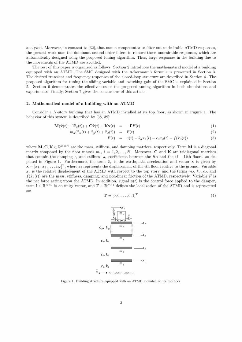
Consider a N -story building that has an ATMD installed at its top floor, as shown in Figure 1. Thebehavior of this system is described by [38, 39]:

M(x(t) + lxg(t)) +Cx(t) +Kx(t) = −ΓF (t) (1)

md(xn(t) + xg(t) + xd(t)) = F (t) (2)

F (t) = u(t)− kdxd(t)− cdxd(t)− f(xd(t)) (3)

where M,C,K ∈ RN×N are the mass, stiffness, and damping matrices, respectively. Term M is a diagonal

matrix composed by the floor masses mi, i = 1, 2, . . . , N . Moreover, C and K are tridiagonal matricesthat contain the damping ci and stiffness ki coefficients between the ith and the (i − 1)th floors, as de-picted in Figure 1. Furthermore, the term xg is the earthquake acceleration and vector x is given byx = [x1, x2, . . . , xN ]T, where xi represents the displacement of the ith floor relative to the ground. Variablexd is the relative displacement of the ATMD with respect to the top story, and the terms md, kd, cd, andf(xd(t)) are the mass, stiffness, damping, and non-linear friction of the ATMD, respectively. Variable F isthe net force acting upon the ATMD. In addition, signal u(t) is the control force applied to the damper,term l ∈ R

N×1 is an unity vector, and Γ ∈ RN×1 defines the localization of the ATMD and is represented

as:Γ = [0, 0, . . . , 0, 1]T (4)

¨1k

2k

u

k NN

xN

x3

x2

x1

m

m

m

m 1

2

3

N

3kc ,3

1

2

c ,

gx

c ,

dmdkd

c ,

������������������������������������������������

c

x

d

Figure 1: Building structure equipped with an ATMD mounted on its top floor.

3

Since the first mode of vibration is dominant during an earthquake, the building model (1) can beapproximated as [13]:

m0x0(t) + c0x0(t) + k0x0(t) = −β0m0xg(t)− F (t)

md(x0(t) + xg(t) + xd(t)) = F (t)(5)

Signal x0 represents the displacement of the dominant mode, which is given by

x0(t) =φ0

TMx(t)

φ0TMφ0

(6)

where φ0 ∈ RN×1 is the the first mode, that is scaled to satisfy

φ0TΓ = 1 (7)

This equality, in turn, produces the approximation [40]

xN (t) ≈ x0(t) (8)

Parameters m0, c0, k0, and β0 are the mass, damping, stiffness, and participation factor of the dominantmode, respectively. They are defined as [38]:

m0 = φ0TMφ0, c0 = φ0

TCφ0, k0 = φ0TKφ0, β0 =

φ0TMl

φ0TMφ0

(9)

Moreover, the natural frequency of the first mode is given by

ω0 =

√k0m0

(10)

Using the approximation (8) and substituting F (t) of (3) into (5) yields:

xd =

(m0 +md

m0md

)(u− cdxd − f(xd)− kdxd) +

k0m0

xN +c0m0

xN + xg(β0 − 1)

xN =−c0m0

xN −k0m0

xN − β0xg +cdm0

xd +f(xd)

m0+kdm0

xd −1

m0u

(11)

where argument t has been omitted in the time dependent signals.Defining the following state variables

z1 = xd, z2 = xN , z3 = xd, z4 = xN (12)

allows rewriting system (11) in the following state-space representation:

z︷ ︸︸ ︷

z1z2z3z4

=

A︷ ︸︸ ︷

0 0 1 00 0 0 1

−kd(m0 +md)

m0md

k0m0

−cd(m0 +md)

m0md

c0m0

kdm0

−k0m0

cdm0

−c0m0

z︷ ︸︸ ︷

z1z2z3z4

+

B︷ ︸︸ ︷

00

(m0 +md)

m0md

−1

m0

(u− f(z3)) +

D︷ ︸︸ ︷

00

β0 − 1−β0

xg

(13)

4

3. Sliding mode control of the structure

This section presents a SMC design based on the Ackermann’s formula for vibration attenuation ofseismically excited buildings. For this purpose, let us first define a full-state feedback controller ua forsystem (13), such that the closed-loop eigenvalues λ1, λ2, λ3, and λ4 are placed in a desired location in thes-plane. The control law ua is defined as

ua = −kTz (14)

According to the Ackermann’s formula [41], the feedback gain vector kT ∈ R1×4 can be computed as

kT = eTP (A) (15)

with

eT =[0, 0, 0, 1][B,AB,A2B,A3B]−1 ∈ R1×4 (16)

P (λ) =(λ− λ1)(λ− λ2)(λ− λ3)(λ − λ4) (17)

In order to design the SMC for the system (13), let us assume the following.

Assumption 1. The eigenvalue λ4 in (17) is real and negative.

Assumption 2. Bounds δ and , corresponding to the earthquake acceleration xg and the non-linearfriction f(z3), respectively, are known and satisfy

|xg| ≤δ (18)

|f(z3)| ≤ (19)

where the bound δ can be determined from the historical records of the ground acceleration in the region wherethe building is located, and the bound can be determined using friction estimation techniques, such as theones based on the Linear Extended State Observer (LESO) or the Least Squares Method (LSM). Throughthe LESO, the friction f(z3) is considered as a new state of a high gain observer that is estimated using theinput u and the displacement z1 of the ATMD [42]. On the other side, with the Least Squares method, thefriction f(z3) is contained in linear regression model, that is identified using the signals u and z1 [43].

The following theorem presents the SMC based on the Ackermann’s formula (15) and analyses thebehavior of the resulting closed-loop system in the sliding mode at the plane σ = ηTz = 0, where ηT ∈ R

1×4

is a constant vector that will be automatically calculated through the proposed methodology outlined inSection 5.

Theorem 1. Let us consider the building structure in (13), that is equipped with an ATMD, whose controlforce u is provided by the following SMC

u = −M0sign(σ) (20)

where σ = ηTz and M0 > 0 are called sliding variable and switching gain, respectively. The vector ηT isgiven by

ηT = [η1, η2, η3, η4] = eTP1(A), P1(λ) = (λ− λ1)(λ− λ2)(λ− λ3) (21)

where λ1, λ2, and λ3 are the desired closed-loop eigenvalues; moreover, parameter M0 satisfies

M0 > + h0 (22)

where h0 is a constant such that|ua + α1xg| ≤ h0 (23)

with ua given in (14) and α1 defined as

α1 = β0(η4 − η3) + η3 (24)

5

Then, the trajectories of closed-loop system reach the plane σ = ηTz = 0 in a finite time tσ, and they areconfined in this plane for t ≥ tσ, where tσ ≤ σ(0)/(M0− [+h0]). Furthermore, when this plane is reached,the fourth-order dynamic system (13) is reduced to the following third-order system

z∗ = A1z∗ +B1xg (25)

where A1 ∈ R3×3 is a matrix containing the eigenvalues λ1, λ2, and λ3; vector z∗ ∈ R

3×1 is given by

z∗ = [z1, z2, z3]T (26)

and

B1 =

00α2

with α2 = (β0 − 1) +

α1(m0 +md)

m0md

(27)

Proof. First, note that vector η in (21) satisfies the following equalities [44]:

ηTB = 1, ηTA∗ = λ4ηT (28)

where A∗ = A−BkT. Adding and subtracting the term Bua to (13) yields

z = (A−BkT)z+B [u− ua − f(z3)] +Dxg (29)

The system (29) is transformed into a new set of equations using the following state transformation

w =

[z∗

σ

]=

T1︷ ︸︸ ︷[I3×3 03×1

ηT

]z = T1z (30)

where T1 is an invertible matrix. The dynamics of the transformed system w = Tz is given by

w =T1

((A−BkT)z+B [u− ua − f(z3)] +Dxg

)

=T1(A−BkT)T−11 w+T1B[u− ua − f(z3)] +TDxg (31)

Using the equalities in (28) allows deducing the following structure of matrices T1(A − BkT)T−11 and

T1B in (31)

T1(A−BkT)T−11 =

[A1 a∗

01×3 λ4

], T1B =

[b∗

1

]with b∗ =

00

(m0 +md)

m0md

(32)

where a∗ ∈ R3×1, and A1 is a matrix whose eigenvalues are equal to the closed-loop eigenvalues λ1, λ2 and

λ3. Finally, vector TD in (31) is given by

TD =

[d1

−α1

]with d1 =

00

β0 − 1

(33)

Substituting equations (32) and (33) into (31) produces

z∗ = A1z∗ + a∗σ + b∗[u − ua − f(z3)] + d1xg (34)

σ = λ4σ + u− ua − f(z3)− α1xg (35)

6

The control law u is designed such that the trajectories of the structural system (13) converge to the

plane σ = 0 in finite time, which is ensured when1

2

d

dtσ2 = σσ < 0. The product σσ is given by

σσ = σ[λ4σ + u− ua − f(z3)− α1xg] = λ4σ2 + σ[u− ua − f(z3)− α1xg] (36)

Since λ4 < 0, the last expression satisfies

σσ ≤ σ[u− ua − f(z3)− α1xg] (37)

Substituting the control law u = −M0sign(σ) into (37) and using the inequalities (19), (22) and (23), weget

σσ ≤ σ [−M0sign(σ) − ua − f(z3)− α1xg] ≤ |σ| [−M0 + + h0] ≤ −|σ|[M0 − ( + h0)] < 0 (38)

Therefore, the trajectories of system (13) reach the surface σ = ηTz = 0 in a finite time tσ, and remainthere for t ≥ tσ, where tσ is computed by integrating (38) and its value is given by

tσ ≤σ(0)

M0 − ( + h0)(39)

Finally, in order to determine the behavior of the closed-loop system in the surface σ = 0, the nextsolution of σ = 0 with respect to u

u = ua + f(z3) + α1xg (40)

is substituted into (34) to produce the sliding motion equation (25).

Remark 1. Since the SMC (20) and the dynamics of the closed-loop system (25) in the sliding mode donot depend of λ4, this parameter can take any negative value, and it is used only for the stability analysis ofthe SMC.

Remark 2. Note that the building and the ATMD are at rest or in equilibrium before an earthquake,therefore, the initial condition zi(0) of variables zi, i = 1, 2, 3, 4 is zero, i.e., z(0) = 0, which implies thatσ(0) = ηTz(0) = 0, and as an consequence tσ = 0.

Remark 3. Parameter h0 in (23) is required to design the SMC. In section 5.2, a methodology is proposedto compute this parameter using the frequency response of the closed-loop system in the sliding mode, andthe knowledge of the bound δ in (18) of the earthquake acceleration xg.

4. Analysis of the closed-loop system at the sliding mode

The closed-loop system dynamics in the sliding mode is described in the Laplace domain as

(sI3×3 −A1)Z∗(s) = B1L[xg(t)] (41)

where L is the Laplace transform operator and Z∗(s) = [Z1(s), Z2(s), Z3(s)]T.

Using (41), the transfer function Z∗(s)/L[xg(t)] can be expressed as

Z∗(s)

L[xg(t)]= (sI3×3 −A1)

−1B1 (42)

The characteristic polynomial P1(s) in (21) corresponding to (42) can be rewritten as

P1(s) = (s− λ1)(s− λ2)(s− λ3) = (s2 + 2ζωns+ ω2n)(s− λ3) (43)

where ζ and ωn are positive constants, which are called damping ratio and undamped natural frequency,respectively.

7

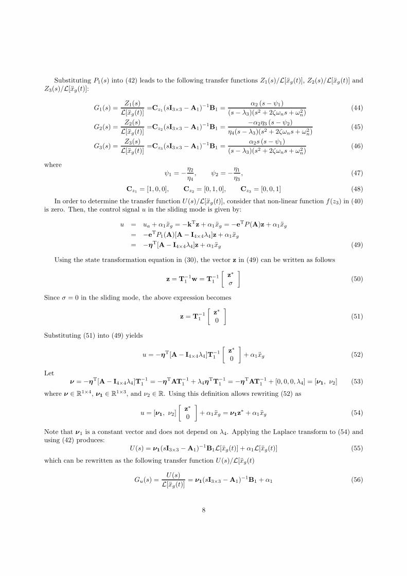
Substituting P1(s) into (42) leads to the following transfer functions Z1(s)/L[xg(t)], Z2(s)/L[xg(t)] andZ3(s)/L[xg(t)]:

G1(s) =Z1(s)

L[xg(t)]=Cz1(sI3×3 −A1)

−1B1 =α2 (s− ψ1)

(s− λ3)(s2 + 2ζωns+ ω2n)

(44)

G2(s) =Z2(s)

L[xg(t)]=Cz2(sI3×3 −A1)

−1B1 =−α2η3 (s− ψ2)

η4(s− λ3)(s2 + 2ζωns+ ω2n)

(45)

G3(s) =Z3(s)

L[xg(t)]=Cz3(sI3×3 −A1)

−1B1 =α2s (s− ψ1)

(s− λ3)(s2 + 2ζωns+ ω2n)

(46)

whereψ1 = −

η2η4, ψ2 = −

η1η3, (47)

Cz1 = [1, 0, 0], Cz2 = [0, 1, 0], Cz3 = [0, 0, 1] (48)

In order to determine the transfer function U(s)/L[xg(t)], consider that non-linear function f(z3) in (40)is zero. Then, the control signal u in the sliding mode is given by:

u = ua + α1xg = −kTz+ α1xg = −eTP (A)z + α1xg

= −eTP1(A)[A− I4×4λ4]z+ α1xg

= −ηT[A− I4×4λ4]z+ α1xg (49)

Using the state transformation equation in (30), the vector z in (49) can be written as follows

z = T−11 w = T−1

1

[z∗

σ

](50)

Since σ = 0 in the sliding mode, the above expression becomes

z = T−11

[z∗

0

](51)

Substituting (51) into (49) yields

u = −ηT[A− I4×4λ4]T−11

[z∗

0

]+ α1xg (52)

Letν = −ηT[A− I4×4λ4]T

−11 = −ηTAT−1

1 + λ4ηTT−1

1 = −ηTAT−11 + [0, 0, 0, λ4] = [ν1, ν2] (53)

where ν ∈ R1×4, ν1 ∈ R

1×3, and ν2 ∈ R. Using this definition allows rewriting (52) as

u = [ν1, ν2]

[z∗

0

]+ α1xg = ν1z

∗ + α1xg (54)

Note that ν1 is a constant vector and does not depend on λ4. Applying the Laplace transform to (54) andusing (42) produces:

U(s) = ν1(sI3×3 −A1)−1B1L[xg(t)] + α1L[xg(t)] (55)

which can be rewritten as the following transfer function U(s)/L[xg(t)

Gu(s) =U(s)

L[xg(t)]= ν1(sI3×3 −A1)

−1B1 + α1 (56)

8

4.1. Transient response for z1(t) and z2(t)

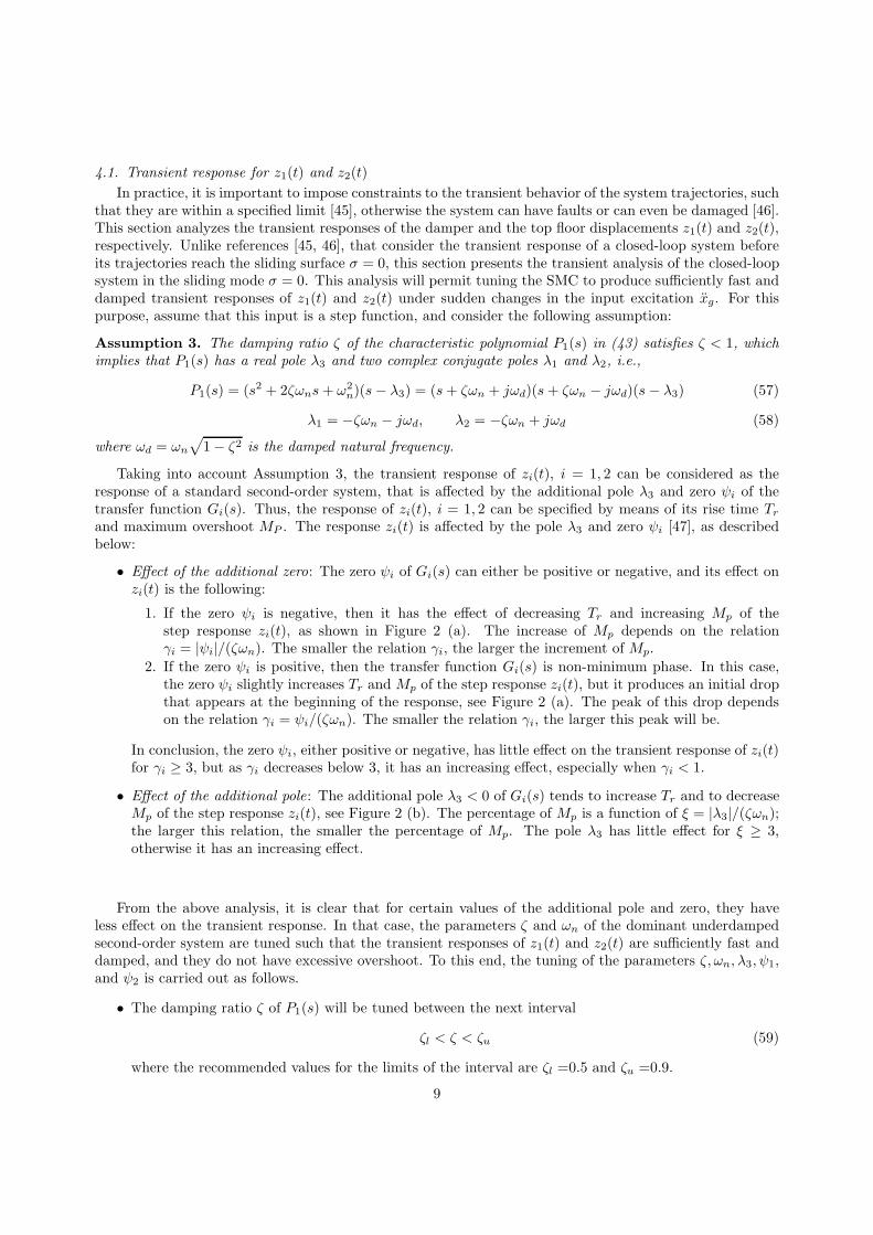
In practice, it is important to impose constraints to the transient behavior of the system trajectories, suchthat they are within a specified limit [45], otherwise the system can have faults or can even be damaged [46].This section analyzes the transient responses of the damper and the top floor displacements z1(t) and z2(t),respectively. Unlike references [45, 46], that consider the transient response of a closed-loop system beforeits trajectories reach the sliding surface σ = 0, this section presents the transient analysis of the closed-loopsystem in the sliding mode σ = 0. This analysis will permit tuning the SMC to produce sufficiently fast anddamped transient responses of z1(t) and z2(t) under sudden changes in the input excitation xg. For thispurpose, assume that this input is a step function, and consider the following assumption:

Assumption 3. The damping ratio ζ of the characteristic polynomial P1(s) in (43) satisfies ζ < 1, whichimplies that P1(s) has a real pole λ3 and two complex conjugate poles λ1 and λ2, i.e.,

P1(s) = (s2 + 2ζωns+ ω2n)(s− λ3) = (s+ ζωn + jωd)(s+ ζωn − jωd)(s− λ3) (57)

λ1 = −ζωn − jωd, λ2 = −ζωn + jωd (58)

where ωd = ωn

√1− ζ2 is the damped natural frequency.

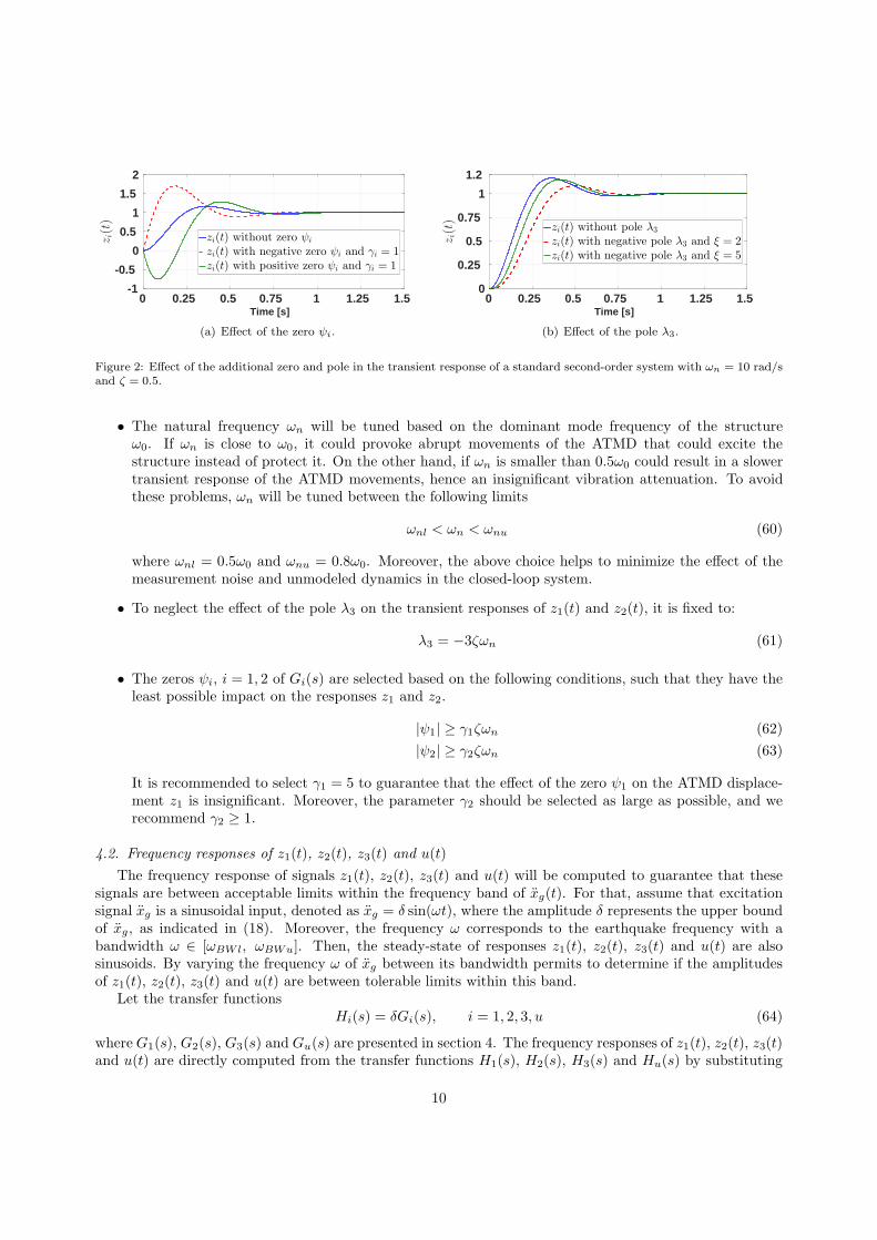
Taking into account Assumption 3, the transient response of zi(t), i = 1, 2 can be considered as theresponse of a standard second-order system, that is affected by the additional pole λ3 and zero ψi of thetransfer function Gi(s). Thus, the response of zi(t), i = 1, 2 can be specified by means of its rise time Trand maximum overshoot MP . The response zi(t) is affected by the pole λ3 and zero ψi [47], as describedbelow:

• Effect of the additional zero: The zero ψi of Gi(s) can either be positive or negative, and its effect onzi(t) is the following:

1. If the zero ψi is negative, then it has the effect of decreasing Tr and increasing Mp of thestep response zi(t), as shown in Figure 2 (a). The increase of Mp depends on the relationγi = |ψi|/(ζωn). The smaller the relation γi, the larger the increment of Mp.

2. If the zero ψi is positive, then the transfer function Gi(s) is non-minimum phase. In this case,the zero ψi slightly increases Tr and Mp of the step response zi(t), but it produces an initial dropthat appears at the beginning of the response, see Figure 2 (a). The peak of this drop dependson the relation γi = ψi/(ζωn). The smaller the relation γi, the larger this peak will be.

In conclusion, the zero ψi, either positive or negative, has little effect on the transient response of zi(t)for γi ≥ 3, but as γi decreases below 3, it has an increasing effect, especially when γi < 1.

• Effect of the additional pole: The additional pole λ3 < 0 of Gi(s) tends to increase Tr and to decreaseMp of the step response zi(t), see Figure 2 (b). The percentage of Mp is a function of ξ = |λ3|/(ζωn);the larger this relation, the smaller the percentage of Mp. The pole λ3 has little effect for ξ ≥ 3,otherwise it has an increasing effect.

From the above analysis, it is clear that for certain values of the additional pole and zero, they haveless effect on the transient response. In that case, the parameters ζ and ωn of the dominant underdampedsecond-order system are tuned such that the transient responses of z1(t) and z2(t) are sufficiently fast anddamped, and they do not have excessive overshoot. To this end, the tuning of the parameters ζ, ωn, λ3, ψ1,and ψ2 is carried out as follows.

• The damping ratio ζ of P1(s) will be tuned between the next interval

ζl < ζ < ζu (59)

where the recommended values for the limits of the interval are ζl =0.5 and ζu =0.9.

9

Time [s]0 0.25 0.5 0.75 1 1.25 1.5

zi(t)

-1

-0.5

0

0.5

1

1.5

2

zi(t) without zero ψi

zi(t) with negative zero ψi and γi = 1zi(t) with positive zero ψi and γi = 1

(a) Effect of the zero ψi.

Time [s]0 0.25 0.5 0.75 1 1.25 1.5

zi(t)

0

0.25

0.5

0.75

1

1.2

zi(t) without pole λ3

zi(t) with negative pole λ3 and ξ = 2zi(t) with negative pole λ3 and ξ = 5

(b) Effect of the pole λ3.

Figure 2: Effect of the additional zero and pole in the transient response of a standard second-order system with ωn = 10 rad/sand ζ = 0.5.

• The natural frequency ωn will be tuned based on the dominant mode frequency of the structureω0. If ωn is close to ω0, it could provoke abrupt movements of the ATMD that could excite thestructure instead of protect it. On the other hand, if ωn is smaller than 0.5ω0 could result in a slowertransient response of the ATMD movements, hence an insignificant vibration attenuation. To avoidthese problems, ωn will be tuned between the following limits

ωnl < ωn < ωnu (60)

where ωnl = 0.5ω0 and ωnu = 0.8ω0. Moreover, the above choice helps to minimize the effect of themeasurement noise and unmodeled dynamics in the closed-loop system.

• To neglect the effect of the pole λ3 on the transient responses of z1(t) and z2(t), it is fixed to:

λ3 = −3ζωn (61)

• The zeros ψi, i = 1, 2 of Gi(s) are selected based on the following conditions, such that they have theleast possible impact on the responses z1 and z2.

|ψ1| ≥ γ1ζωn (62)

|ψ2| ≥ γ2ζωn (63)

It is recommended to select γ1 = 5 to guarantee that the effect of the zero ψ1 on the ATMD displace-ment z1 is insignificant. Moreover, the parameter γ2 should be selected as large as possible, and werecommend γ2 ≥ 1.

4.2. Frequency responses of z1(t), z2(t), z3(t) and u(t)

The frequency response of signals z1(t), z2(t), z3(t) and u(t) will be computed to guarantee that thesesignals are between acceptable limits within the frequency band of xg(t). For that, assume that excitationsignal xg is a sinusoidal input, denoted as xg = δ sin(ωt), where the amplitude δ represents the upper boundof xg, as indicated in (18). Moreover, the frequency ω corresponds to the earthquake frequency with abandwidth ω ∈ [ωBWl, ωBWu]. Then, the steady-state of responses z1(t), z2(t), z3(t) and u(t) are alsosinusoids. By varying the frequency ω of xg between its bandwidth permits to determine if the amplitudesof z1(t), z2(t), z3(t) and u(t) are between tolerable limits within this band.

Let the transfer functionsHi(s) = δGi(s), i = 1, 2, 3, u (64)

whereG1(s), G2(s), G3(s) and Gu(s) are presented in section 4. The frequency responses of z1(t), z2(t), z3(t)and u(t) are directly computed from the transfer functions H1(s), H2(s), H3(s) and Hu(s) by substituting

10

variable s by jω, where ω ∈ [ωBWl, ωBWu]. The root mean square (RMS) value κi of Hi(jω) is alsocalculated in the frequency band of xg(t). This value is defined as

κi = RMS (|Hi(jω)|)ω∈[ωBWl, ωBWu]

, i = 1, 2, 3, u (65)

Since the predominant spectral content of earthquakes is between 1 to 20Hz [48], the parameters ωBWl andωBWu will be set as ωBWl = 2π rad/s and ωBWu = 40π rad/s.

5. Tuning algorithm for the SMC

This section presents the proposed tuning algorithm to compute: 1) the vector η using the transient andfrequency responses of the closed-loop system; and 2) the switching gain M0 by analyzing the frequencyresponse Hu(jω).

5.1. Procedure to compute vector η

According to equation (21), vector η depends on the parameters ζ and ωn of the characteristic polynomialP1(s) in (43). Let us define Υ as the possible set of vectors η, with which the closed-loop system (25) inthe sliding mode satisfies the following three conditions:

1. The limits for ζ in (59) and for ωn in (60), the value λ3 = −3ζωn for the non-dominant pole, as wellas the inequalities in (62) and (63) corresponding to the zeros ψ1 and ψ2, respectively.

2. The next upper limits κi for κi i = 1, 2, 3 in (65) given by

κi ≤ κi, i = 1, 2, 3 (66)

where κi, i = 1, 2, 3 are positive constants, which constrain the maximum value of |Hi(jω)| under thebandwidth ω ∈ [ωBWl, ωBWu], or in time-domain, the maximum permitted values of signals z1, z2and z3 in the bandwidth of xg.

3. The inequalityκu + ≤ κu (67)

deduced from (40), which indicates that the sum of the RMS value κu of frequency response |Hu(jω)|and the bound of the non-linear friction f(z3) should be less than or equal to the specified limit κu.

Then, the vector η ∈ Υ used by the SMC, denoted as η∗, is obtained by minimizing either of the following

two performance indexes (PIs)

Jz2 =minη∈Υ

κ2(η) (68)

Ju =minη∈Υ

κu(η) (69)

where parameters κ2 and κu show their dependency on η. Note that Jz2 and Ju are related to the ability ofthe SMC to minimize the top floor displacement z2 and the control force u, respectively. Hence the slidingvariable σ = ηT

∗z guarantees a minimal of z2 or u, while ensuring that the RMS values of the closed-loop

signals are within acceptable limits and their transient responses are sufficiently fast and damped.

5.2. Procedure to compute the switching gain M0

According to inequality (22), the value of M0 should satisfy M0 > + h0. Among these two terms ofthe sum, only parameter is assumed to be known according to Assumption 2. This section presents amethodology for estimating parameter h0, that is subsequently employed to compute M0. Note that from(23), the parameter h0 must satisfy the condition h0 ≥ |ua + α1xg|, where the frequency response of thesignal ua +α1xg is given by Hu(jω). Define χ as the maximum magnitude of |Hu(jω)| between the interval

11

ω ∈ [ωBWl, ωBWu], where χ is computed using the vector η∗that minimizes either of the performance

indexes (68) and (69), i.e.,χ = max (|Hu(jω,η∗

)|)ω∈[ωBWl, ωBWu]

(70)

Since χ ≥ |ua+α1xg| in the spectrum of xg, we will select h0 = χ. Thus, the switching gain M0 of the SMCis computed as:

M0 = + χ+ ς (71)

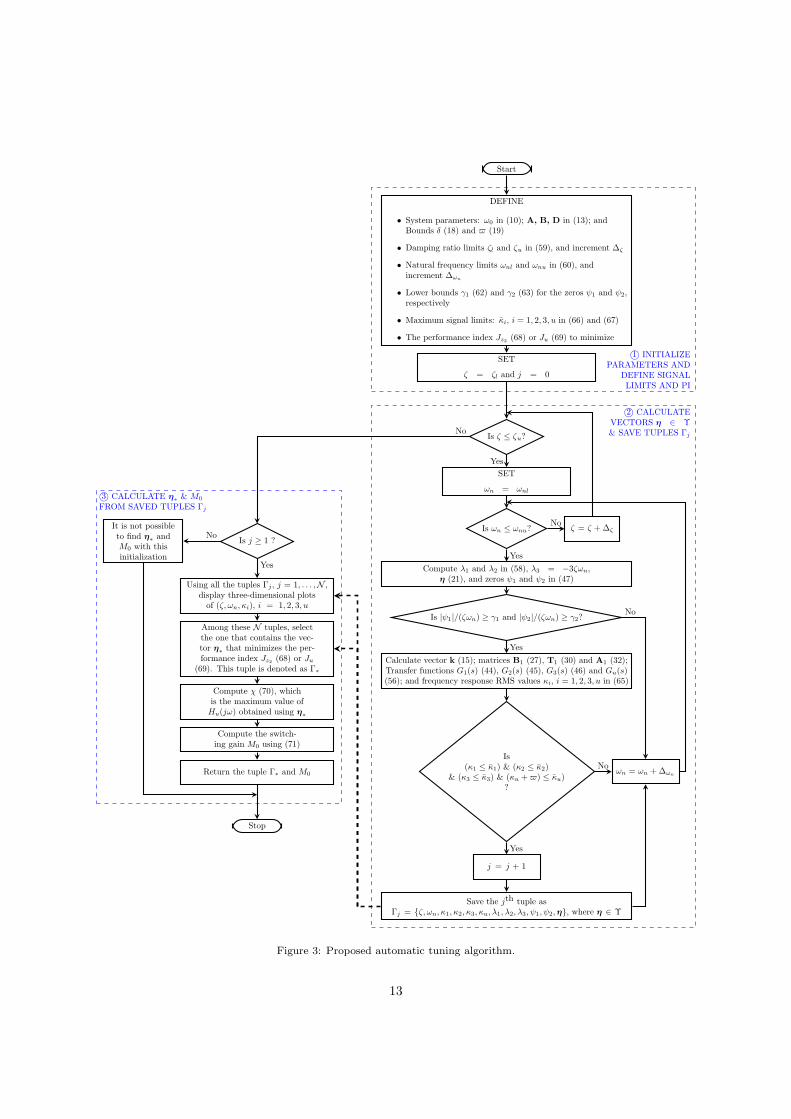
where ς is a small positive constant that guarantees the inequality (22), and that in this work is fixed to 0.5.Finally, Figure 3 shows the proposed tuning algorithm that computes the vector η

∗and gain M0 of the

SMC. This algorithm implements the procedure outlined in the present section, and it is programmed in theMatlab software. It has three main phases: 1) initialization of system parameters, definition of limits forsignals and parameters, and selection of the PI to be minimized; 2) calculation of feasible vectors η for theSMC, which are saved in tuples Γj = {ζ, ωn, κ1, κ2, κ3, κu, λ1, λ2, λ3, ψ1, ψ2,η}, where j = 1, . . . ,N ; and 3)searching in these N tuples to determine the vector η

∗that minimizes the PI Jz2 (68) or Ju (69), and its

corresponding switching gain M0. The terms ∆ζ and ∆ωnin this algorithm represent the increments for ζ

and ωn from their lower to upper limits.

6. Results and discussion

The performance of the proposed tuning algorithm for the SMC, based on the Ackermann’s formula,is evaluated by means of numerical and experimental studies. In both studies the SMC is programed inthe Matlab/Simuink software and the data is sampled at 1ms. The SMC in (20) causes the chatteringeffect, that is a discontinuous force at σ = 0 that cannot be applied to the ATMD in practice. There existsseveral chattering reduction techniques such as the Boundary layer solution [49], Dynamic Terminal SMC[50], Super-twisting SMC [51], and Higher-order SMC [52], just to mention a few. In this paper, we usethe Boundary layer solution, where the sign function of the SMC is approximated by means of followingcontinuous saturation function

u = −M0sign(σ) ≈ −M0sat(σ) =

−M0 if σ > ǫσ/ǫ if − ǫ ≤ σ ≤ ǫM0 if σ < −ǫ

(72)

where ǫ is a positive constant that is fixed to ǫ = 0.05.For the implementation of the proposed scheme, first the parameters of the SMC in (72), i.e., the

vector η∗of the sliding variable and the switching gain M0, that guarantees that the top floor and the

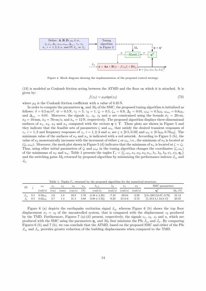
ATMD displacements and velocities remain within some specified limits, are calculated by the proposedtuning algorithm outlined in Section 5. Then, these parameters are used in the SMC (72) to attenuate thevibrations of the seismically excited building (13) via the ATMD. The block diagram representation of thecontrol implementation is presented in Figure 4.

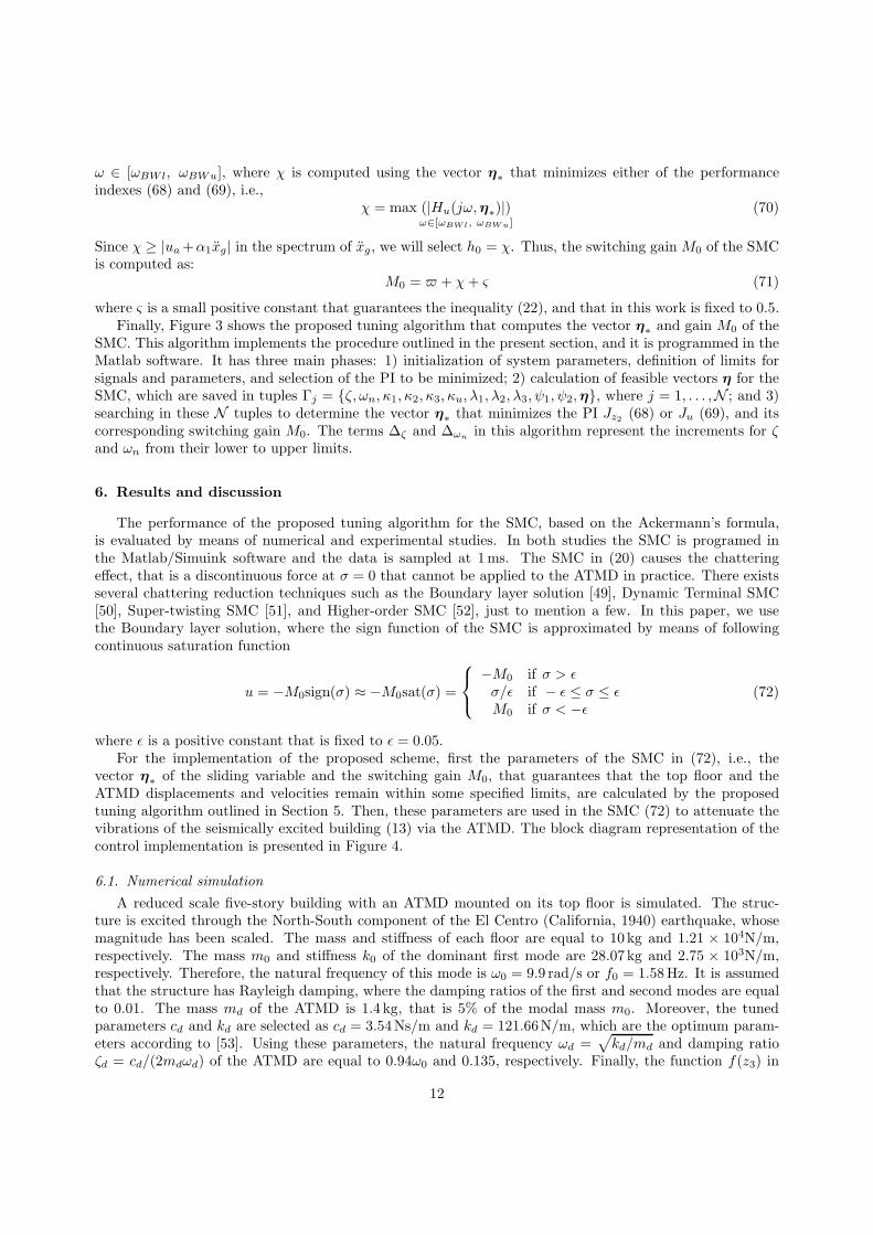
6.1. Numerical simulation

A reduced scale five-story building with an ATMD mounted on its top floor is simulated. The struc-ture is excited through the North-South component of the El Centro (California, 1940) earthquake, whosemagnitude has been scaled. The mass and stiffness of each floor are equal to 10 kg and 1.21 × 104N/m,respectively. The mass m0 and stiffness k0 of the dominant first mode are 28.07kg and 2.75 × 103N/m,respectively. Therefore, the natural frequency of this mode is ω0 = 9.9 rad/s or f0 = 1.58Hz. It is assumedthat the structure has Rayleigh damping, where the damping ratios of the first and second modes are equalto 0.01. The mass md of the ATMD is 1.4 kg, that is 5% of the modal mass m0. Moreover, the tunedparameters cd and kd are selected as cd = 3.54Ns/m and kd = 121.66N/m, which are the optimum param-eters according to [53]. Using these parameters, the natural frequency ωd =

√kd/md and damping ratio

ζd = cd/(2mdωd) of the ATMD are equal to 0.94ω0 and 0.135, respectively. Finally, the function f(z3) in

12

Start

DEFINE

• System parameters: ω0 in (10); A, B, D in (13); andBounds δ (18) and (19)

• Damping ratio limits ζl and ζu in (59), and increment ∆ζ

• Natural frequency limits ωnl and ωnu in (60), andincrement ∆ωn

• Lower bounds γ1 (62) and γ2 (63) for the zeros ψ1 and ψ2,respectively

• Maximum signal limits: κi, i = 1, 2, 3, u in (66) and (67)

• The performance index Jz2 (68) or Ju (69) to minimize

SET

ζ = ζl and j = 0

Is ζ ≤ ζu?

SET

ωn = ωnl

Is ωn ≤ ωnu?

Compute λ1 and λ2 in (58), λ3 = −3ζωn,η (21), and zeros ψ1 and ψ2 in (47)

Is |ψ1|/(ζωn) ≥ γ1 and |ψ2|/(ζωn) ≥ γ2?

Calculate vector k (15); matrices B1 (27), T1 (30) and A1 (32);Transfer functions G1(s) (44), G2(s) (45), G3(s) (46) and Gu(s)(56); and frequency response RMS values κi, i = 1, 2, 3, u in (65)

Is(κ1 ≤ κ1) & (κ2 ≤ κ2)

& (κ3 ≤ κ3) & (κu +) ≤ κu)?

j = j + 1

Save the jth tuple asΓj = {ζ, ωn, κ1, κ2, κ3, κu, λ1, λ2, λ3, ψ1, ψ2,η}, where η ∈ Υ

ωn = ωn +∆ωn

ζ = ζ + ∆ζ

Is j ≥ 1 ?

1○ INITIALIZEPARAMETERS AND

DEFINE SIGNALLIMITS AND PI

2○ CALCULATEVECTORS η ∈ Υ& SAVE TUPLES Γj

3○ CALCULATE η∗& M0

FROM SAVED TUPLES Γj

It is not possibleto find η

∗and

M0 with thisinitialization

Using all the tuples Γj , j = 1, . . . ,N ,display three-dimensional plotsof (ζ, ωn, κi), i = 1, 2, 3, u

Among these N tuples, selectthe one that contains the vec-tor η

∗that minimizes the per-

formance index Jz2 (68) or Ju(69). This tuple is denoted as Γ∗

Compute χ (70), whichis the maximum value ofHu(jω) obtained using η

∗

Compute the switch-ing gain M0 using (71)

Return the tuple Γ∗ and M0

Stop

Yes

Yes

Yes

Yes

No

No

No

No

No

Yes

Figure 3: Proposed automatic tuning algorithm.

13

z = Az+B [u− f(z3)] +Dxg

ηT−M0sat(.)

Tuningalgorithmin Figure 3

Define: A,B,D, ω0, δ,,ζl, ζu,∆ζ , ωnl, ωnu,∆ωn

, γ1, γ2,κi, i = 1, 2, 3, u, and PI Jz2 or Ju.

xg

z = [xd, xN , xd, xN ]T

σu

η = η∗M0

Figure 4: Block diagram showing the implementation of the proposed control strategy.

(13) is modeled as Coulomb friction acting between the ATMD and the floor on which it is attached. It isgiven by:

f(z3) = µdsign(z3) (73)

where µd is the Coulomb friction coefficient with a value of 0.35N.In order to compute the parameters η

∗andM0 of the SMC, the proposed tuning algorithm is initialized as

follows: δ = 0.5m/s2, = 0.5N, γ1 = 5, γ2 = 1, ζl = 0.5, ζu = 0.9, ∆ζ = 0.01, ωnl = 0.5ω0, ωnu = 0.8ω0,and ∆ωn

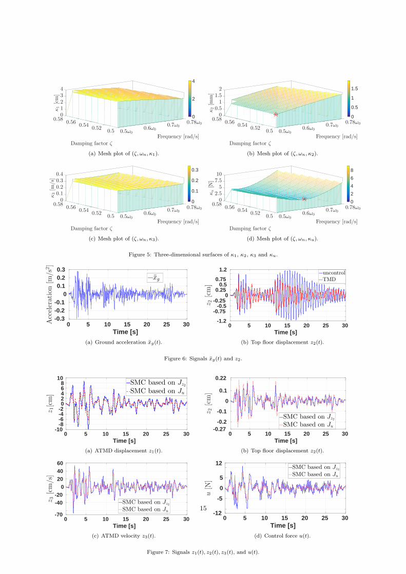
= 0.01. Moreover, the signals z1, z2, z3 and u are constrained using the bounds κ1 = 20 cm,κ2 = 10mm, κ3 = 70 cm/s, and κu = 12N, respectively. The proposed algorithm displays three-dimensionalsurfaces of κ1, κ2, κ3 and κu computed with the vectors η ∈ Υ. These plots are shown in Figure 5 andthey indicate that the feasible sets of parameters ζ and ωn, that satisfy the desired transient responses ofzi, i = 1, 2 and frequency responses of zi, i = 1, 2, 3 and u, are ζ ∈ [0.5, 0.58] and ωn ∈ [0.5ω0, 0.78ω0]. Theminimum value of the surfaces of κ2 and κu is indicated with a red asterisk. According to Figure 5 (b), thevalue of κ2 monotonically increases with the increment of either ζ or ωn, i.e., the minimum of κ2 is located at(ζl, ωnl). Moreover, the mesh plot shown in Figure 5 (d) indicates that the minimum of κu is located at ζ = ζl.Thus, using other initial parameters of ζl and ωnl in the tuning algorithm changes the coordinates (ζ, ωn)of the minimums of κ2 and κu. Table 1 presents the tuples Γ∗ = {ζ, ωn, κ1, κ2, κ3, κu, λ1, λ2, λ3, ψ1, ψ2,η∗

}and the switching gainsM0 returned by proposed algorithm by minimizing the performance indexes Jz2 andJu.

Table 1: Tuples Γ∗ returned by the proposed algorithm for the numerical structure.

PI ζωn κ1 κ2 κ3 κu λ1,2 λ3 ψ1 ψ2 SMC parameters

(rad/s) (cm) (mm) (cm/s) (N) (rad/s) (rad/s) (rad/s) (rad/s) ηT∗

M0 (N)

Jz2 0.5 0.50ω0 4.0 1.0 33.8 5.76 -2.48± 4.29j -7.43 -29.64 -2.99 [2.6,-289.2,0.87,-9.76] 24.13Ju 0.5 0.62ω0 3.7 1.4 31.4 3.68 -3.08± 5.33j -9.23 2114.6 -3.72 [5,-312.3,1.34,0.15] 20.35

Figure 6 (a) depicts the earthquake excitation signal xg, whereas Figure 6 (b) shows the top floordisplacement x5 = z2 of the uncontrolled system, that is compared with the displacement z2 producedby the TMD. Furthermore, Figures 7 (a)-(d) present, respectively, the signals z1, z2, z3 and u, which areproduced with the SMC using the parameters η

∗and M0 that minimize the PIs Jz2 and Ju. By comparing

Figures 6 (b) and 7 (b), we can conclude that the ATMD, based on the proposed SMC and either of the PIsJz2 and Ju, provides greater reduction of the building displacements when compared to the TMD.

14

0.78ω0

Frequency [rad/s]

0.7ω00.6ω00.5ω00.5

Damping factor ζ

0.520.54

0.56

10

432

0.58

κ1[cm]

0

2

4

(a) Mesh plot of (ζ, ωn, κ1).

0.78ω0

Frequency [rad/s]

0.7ω00.6ω00.5ω00.5

Damping factor ζ

0.520.54

0.56

2

00.51

1.5

0.58

κ2[m

m]

0

0.5

1

1.5

(b) Mesh plot of (ζ, ωn, κ2).

0.78ω0

Frequency [rad/s]

0.7ω00.6ω00.5ω00.5

Damping factor ζ

0.520.54

0.56

00.10.20.30.4

0.58

κ3[m

/s]

0

0.1

0.2

0.3

(c) Mesh plot of (ζ, ωn, κ3).

0.78ω0

Frequency [rad/s]

0.7ω00.6ω00.5ω00.5

Damping factor ζ

0.520.54

0.56

02.55

7.510

0.58κu[N

]

0

2

4

6

8

(d) Mesh plot of (ζ, ωn, κu).

Figure 5: Three-dimensional surfaces of κ1, κ2, κ3 and κu.

Time [s]0 5 10 15 20 25 30A

cceleration[m

/s2]

-0.3-0.2-0.1

00.10.20.3

xg

(a) Ground acceleration xg(t).

Time [s]0 5 10 15 20 25 30

z2[cm]

-1.2

-0.75-0.5

-0.250

0.250.5

0.75

1.2uncontrolTMD

(b) Top floor displacement z2(t).

Figure 6: Signals xg(t) and z2.

Time [s]0 5 10 15 20 25 30

z1[cm]

-10-8-6-4-202468

10SMC based on Jz2SMC based on Ju

(a) ATMD displacement z1(t).

Time [s]0 5 10 15 20 25 30

z2[cm]

-0.27-0.2

-0.1

0

0.1

0.22

SMC based on Jz2SMC based on Ju

(b) Top floor displacement z2(t).

Time [s]0 5 10 15 20 25 30

z3[cm/s]

-70

-40-20

0204060

SMC based on Jz2SMC based on Ju

(c) ATMD velocity z3(t).

Time [s]0 5 10 15 20 25 30

u[N

]

-12

-5

0

5

12SMC based on Jz2SMC based on Ju

(d) Control force u(t).

Figure 7: Signals z1(t), z2(t), z3(t), and u(t).

15

Now, let us define zrmsi , urms and zpeaki , upeak as the RMS and peak values of signals zi and u, respectively.

Moreover, let us denote R(zrms2 ) and R(zpeak2 ) as the vibration attenuation percentages of zrms

2 and zpeak2 ,respectively, which are given by:

R(zrms2 ) =

(1−

(zrms2 )controlled

(zrms2 )uncontrolled

)× 100 (74)

R(zpeak2 ) =

(1−

(zpeak2 )controlled

(zpeak2 )uncontrolled

)× 100 (75)

The larger these percentages, the better the attenuation of the signal z2. Table 2 presents these valuescorresponding to the TMD and ATMD during the period of t = 0 to t = 30 s. This table indicatesthat the ATMD allows reducing more than three times the peak value of the floor displacement z2 = x5when compared to the TMD. For both SMCs, the percentages R(zrms

2 ) and R(zpeak2 ) of attenuation forthe displacement z2 are close to 90% and 80%, respectively. Note that the SMC that minimize the PI Jz2(respectively Ju) produce the smallest zrms

2 (respectively urms), as expected. Finally, by comparing Tables1 and 2, it is possible to observe that the values zrms

i , i = 1, 2, 3, u can be considered as an scaled version ofthe parameters κi, since the relation κi/z

rmsi is between 1.5 to 2.65.

Table 2: RMS and peak values of zi, i = 1, 2, 3, 4 and u(t).

Controller PIzrms1 z

peak1 zrms

2 zpeak2 zrms

3 zpeak3 zrms

4 zpeak4 urms upeak R(zrms

2 ) R(zpeak2 )

(cm) (mm) (cm/s) (mm/s) (N) (%)

Uncontrol – – – 4.70 11.79 – – 46.48 118.02 0 0 0 0TMD – 0.33 1.33 2.67 9.33 3.19 13.38 25.8 93.8 0 0 43.19 20.87ATMD Jz2 2.61 9.84 0.48 2.0 14.0 66.9 3.93 17.61 2.78 10.66 89.79 83.04ATMD Ju 1.86 6.74 0.58 2.58 11.81 55.04 5.11 26.49 1.81 7.81 87.66 78.12

6.2. Experimental results

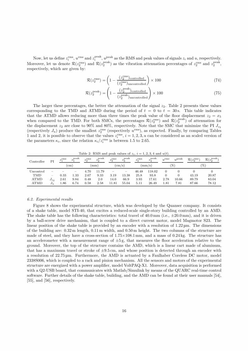
Figure 8 shows the experimental structure, which was developed by the Quanser company. It consistsof a shake table, model STI-40, that excites a reduced-scale single-story building controlled by an AMD.The shake table has the following characteristics: total travel of 40.0mm (i.e., ±20.0mm), and it is drivenby a ball-screw drive mechanism, that is coupled to a direct current motor, model Magmotor S23. Thelinear position of the shake table is provided by an encoder with a resolution of 1.22µm. The dimensionsof the building are: 0.32m length, 0.11m width, and 0.50m height. The two columns of the structure aremade of steel, and they have a cross-section of 1.75×108.1mm, and a mass of 0.24kg. The structure hasan accelerometer with a measurement range of ±5 g, that measures the floor acceleration relative to theground. Moreover, the top of the structure contains the AMD, which is a linear cart made of aluminum,that has a maximum travel or stroke of ±9.5 cm, and whose position is detected through an encoder witha resolution of 22.75µm. Furthermore, the AMD is actuated by a Faulhaber Coreless DC motor, model2338S006, which is coupled to a rack and pinion mechanism. All the sensors and motors of the experimentalstructure are energized with a power amplifier, model VoltPAQ-X1. Moreover, data acquisition is performedwith a Q2-USB board, that communicates with Matlab/Simulink by means of the QUARC real-time controlsoftware. Further details of the shake table, building, and the AMD can be found at their user manuals [54],[55], and [56], respectively.

16

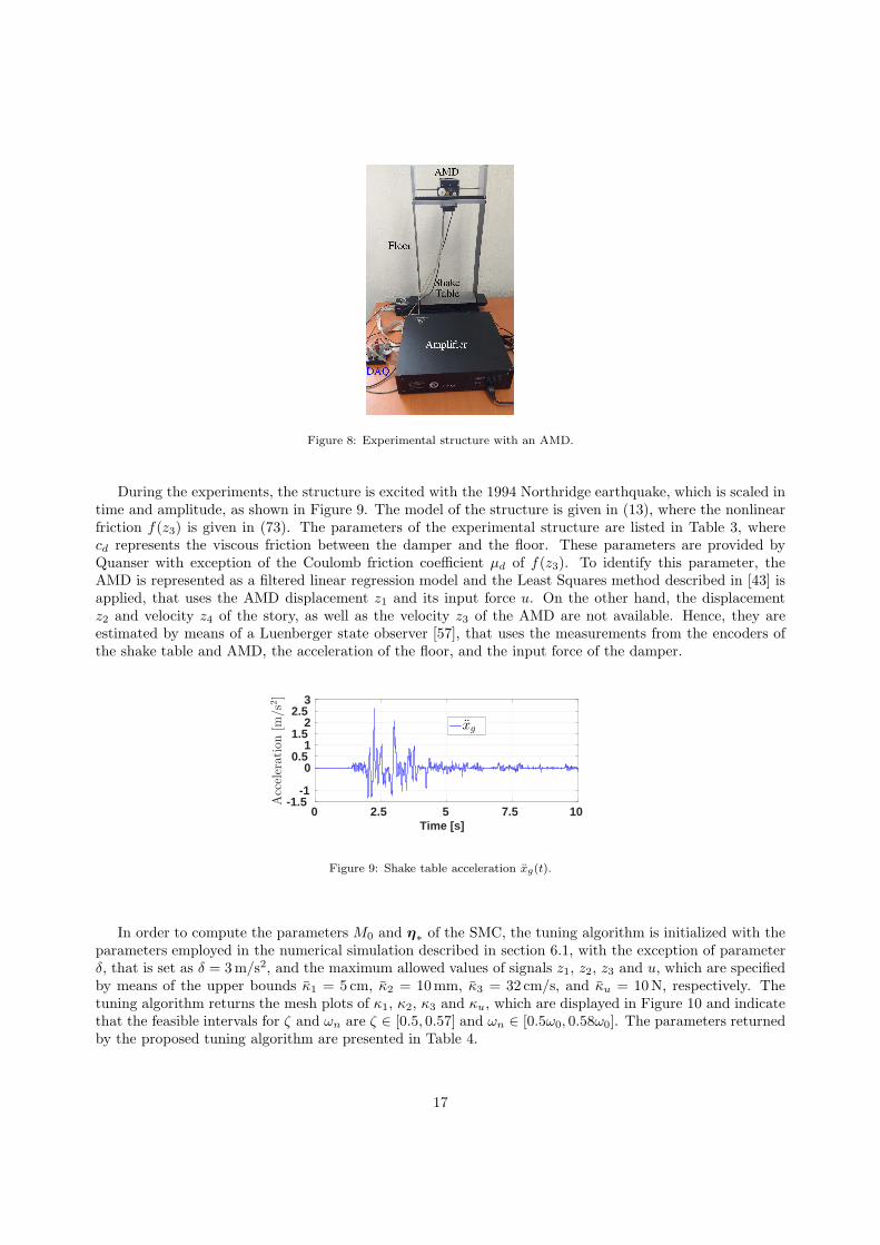
Figure 8: Experimental structure with an AMD.

During the experiments, the structure is excited with the 1994 Northridge earthquake, which is scaled intime and amplitude, as shown in Figure 9. The model of the structure is given in (13), where the nonlinearfriction f(z3) is given in (73). The parameters of the experimental structure are listed in Table 3, wherecd represents the viscous friction between the damper and the floor. These parameters are provided byQuanser with exception of the Coulomb friction coefficient µd of f(z3). To identify this parameter, theAMD is represented as a filtered linear regression model and the Least Squares method described in [43] isapplied, that uses the AMD displacement z1 and its input force u. On the other hand, the displacementz2 and velocity z4 of the story, as well as the velocity z3 of the AMD are not available. Hence, they areestimated by means of a Luenberger state observer [57], that uses the measurements from the encoders ofthe shake table and AMD, the acceleration of the floor, and the input force of the damper.

Time [s]0 2.5 5 7.5 10

Acceleration[m

/s2]

-1.5-1

00.5

11.5

22.5

3

xg

Figure 9: Shake table acceleration xg(t).

In order to compute the parameters M0 and η∗of the SMC, the tuning algorithm is initialized with the

parameters employed in the numerical simulation described in section 6.1, with the exception of parameterδ, that is set as δ = 3m/s2, and the maximum allowed values of signals z1, z2, z3 and u, which are specifiedby means of the upper bounds κ1 = 5 cm, κ2 = 10mm, κ3 = 32 cm/s, and κu = 10N, respectively. Thetuning algorithm returns the mesh plots of κ1, κ2, κ3 and κu, which are displayed in Figure 10 and indicatethat the feasible intervals for ζ and ωn are ζ ∈ [0.5, 0.57] and ωn ∈ [0.5ω0, 0.58ω0]. The parameters returnedby the proposed tuning algorithm are presented in Table 4.

17

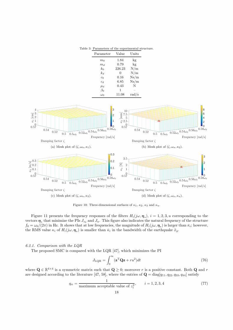
Table 3: Parameters of the experimental structure.

Parameter Value Units

m0 1.84 kg

md 0.79 kg

k0 226.23 N/mkd 0 N/mc0 0.16 Ns/mcd 6.85 Ns/mµd 0.43 N

β0 1 –

ω0 11.08 rad/s

0.58ω0

Frequency [rad/s]

0.56ω00.54ω00.52ω00.5ω00.5

Damping factor ζ

0.520.54

0

4321

0.57

κ1[cm]

0

1

2

3

(a) Mesh plot of (ζ, ωn, κ1).

0.58ω0

Frequency [rad/s]

0.56ω00.54ω00.52ω00.5ω00.5

Damping factor ζ

0.520.54

7.5

02.55

10

0.57

κ2[m

m]

0

2

4

6

8

(b) Mesh plot of (ζ, ωn, κ2).

0.58ω0

Frequency [rad/s]

0.56ω00.54ω00.52ω00.5ω00.5

Damping factor ζ

0.520.54

0

0.1

0.2

0.3

0.57

κ3[m

/s]

0

0.1

0.2

0.3

(c) Mesh plot of (ζ, ωn, κ3).

0.58ω0

Frequency [rad/s]

0.56ω00.54ω00.52ω00.5ω00.5

Damping factor ζ

0.520.54

3.5

0

1

2

0.57

κu[N

]

0

1

2

3

(d) Mesh plot of (ζ, ωn, κu).

Figure 10: Three-dimensional surfaces of κ1, κ2, κ3 and κu.

Figure 11 presents the frequency responses of the filters Hi(jω,η∗), i = 1, 2, 3, u corresponding to the

vectors η∗that minimize the PIs Jz2 and Ju. This figure also indicates the natural frequency of the structure

f0 = ω0/(2π) in Hz. It shows that at low frequencies, the magnitude of Hi(jω,η∗) is larger than κi; however,

the RMS value κi of Hi(jω,η∗) is smaller than κi in the bandwidth of the earthquake xg.

6.2.1. Comparison with the LQR

The proposed SMC is compared with the LQR [47], which minimizes the PI

JLQR =

∫∞

0

(zTQz+ ru2)dt (76)

where Q ∈ R4×4 is a symmetric matrix such that Q ≥ 0; moreover r is a positive constant. Both Q and r

are designed according to the literature [47, 58], where the entries of Q = diag[q11, q22, q33, q44] satisfy

qii =1

maximum acceptable value of z2i, i = 1, 2, 3, 4 (77)

18

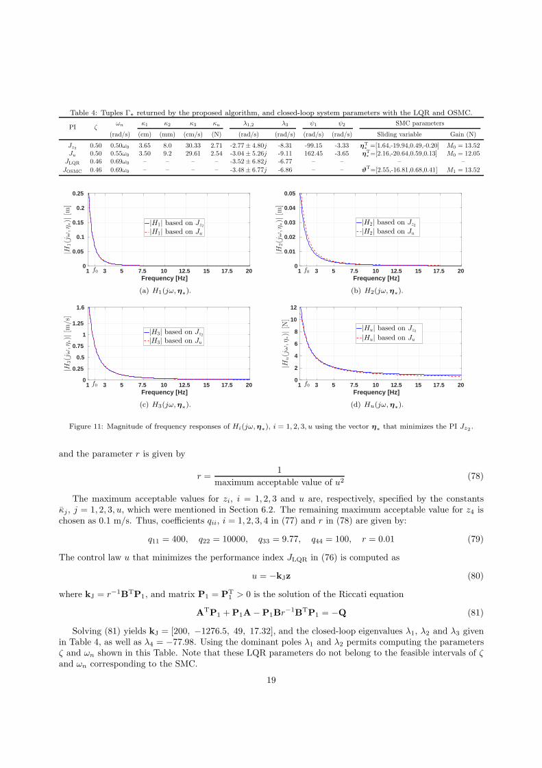
Table 4: Tuples Γ∗ returned by the proposed algorithm, and closed-loop system parameters with the LQR and OSMC.

PI ζωn κ1 κ2 κ3 κu λ1,2 λ3 ψ1 ψ2 SMC parameters

(rad/s) (cm) (mm) (cm/s) (N) (rad/s) (rad/s) (rad/s) (rad/s) Sliding variable Gain (N)

Jz2 0.50 0.50ω0 3.65 8.0 30.33 2.71 -2.77± 4.80j -8.31 -99.15 -3.33 ηT∗=[1.64,-19.94,0.49,-0.20] M0 = 13.52

Ju 0.50 0.55ω0 3.50 9.2 29.61 2.54 -3.04± 5.26j -9.11 162.45 -3.65 ηT∗=[2.16,-20.64,0.59,0.13] M0 = 12.05

JLQR 0.46 0.69ω0 – – – – -3.52± 6.82j -6.77 – – – –

JOSMC 0.46 0.69ω0 – – – – -3.48± 6.77j -6.86 – – ϑT=[2.55,-16.81,0.68,0.41] M1 = 13.52

Frequency [Hz]1 3 5 7.5 10 12.5 15 17.5 20

|H1(jω,η

∗)|[m

]

0

0.05

0.1

0.15

0.2

0.25

|H1| based on Jz2|H1| based on Ju

f0

(a) H1(jω,η∗).

Frequency [Hz]1 3 5 7.5 10 12.5 15 17.5 20

|H2(jω,η

∗)|[m

]

0

0.01

0.02

0.03

0.04

0.05

|H2| based on Jz2|H2| based on Ju

f0

(b) H2(jω,η∗).

Frequency [Hz]1 3 5 7.5 10 12.5 15 17.5 20

|H3(jω,η

∗)|[m

/s]

0

0.25

0.5

0.75

1

1.25

1.6

|H3| based on Jz2|H3| based on Ju

f0

(c) H3(jω,η∗).

Frequency [Hz]1 3 5 7.5 10 12.5 15 17.5 20

|Hu(jω,η

∗)|[N

]

0

2

4

6

8

10

12

|Hu| based on Jz2|Hu| based on Ju

f0

(d) Hu(jω,η∗).

Figure 11: Magnitude of frequency responses of Hi(jω,η∗), i = 1, 2, 3, u using the vector η

∗that minimizes the PI Jz2 .

and the parameter r is given by

r =1

maximum acceptable value of u2(78)

The maximum acceptable values for zi, i = 1, 2, 3 and u are, respectively, specified by the constantsκj, j = 1, 2, 3, u, which were mentioned in Section 6.2. The remaining maximum acceptable value for z4 ischosen as 0.1 m/s. Thus, coefficients qii, i = 1, 2, 3, 4 in (77) and r in (78) are given by:

q11 = 400, q22 = 10000, q33 = 9.77, q44 = 100, r = 0.01 (79)

The control law u that minimizes the performance index JLQR in (76) is computed as

u = −kJz (80)

where kJ = r−1BTP1, and matrix P1 = PT1 > 0 is the solution of the Riccati equation

ATP1 +P1A−P1Br−1BTP1 = −Q (81)

Solving (81) yields kJ = [200, −1276.5, 49, 17.32], and the closed-loop eigenvalues λ1, λ2 and λ3 givenin Table 4, as well as λ4 = −77.98. Using the dominant poles λ1 and λ2 permits computing the parametersζ and ωn shown in this Table. Note that these LQR parameters do not belong to the feasible intervals of ζand ωn corresponding to the SMC.

19

6.2.2. Comparison with the OSMC

The designed SMC is also compared with the OSMC [59], that is based on the minimization of thefollowing PI:

JOSMC =

∫∞

0

zTQzdt (82)

Note that the PI (82) is quite different from the PI (76) corresponding to the LQR, since the former doesnot impose a penalty cost on the control effort u. Meanwhile, both of these PIs use the same matrix Q.

To determine the OSMC, the structure model (13) needs to be written in its regular form [60]. For

that, the vector B of this model is partitioned as B = [B1 B2]T, where B1 = [0, 0, (m0 +md)/m0md]

Tand

B2 = −1/m0. This vector is used in the following non-singular transformation matrix T2, which producesa state transformation from z to v ∈ R

4×1

v =

[v1

v2

]=

T2︷ ︸︸ ︷[I3×3 −B1B

−12

03×1 B−12

]z = T2z (83)

In the new state v, the building model (13) is written in the following regular form:

v1 =A11v1 +A12v2 +D1xg (84)

v2 =A21v1 +A22v2 + (u− f(z3)) +D2xg (85)

where A11 ∈ R3×3, A12 ∈ R

3×1, A21 ∈ R1×3, A22 ∈ R, D1 = [0, 0,−(β0m0 +md)/md]

T, and D2 = β0m0.

For obtaining the control effort u that minimizes (82), it is assumed that D1 = 0 [37]. This assumptionleads to the optimal sliding surface given by

σ = ϑTz, with ϑT = [K, 1]T2 (86)

where

K = −Q−122

(AT

12P2 +Q21

), and

[T−1

2

]TQT−1

2 =

[Q11 Q12

Q21 Q22

](87)

Moreover, the matrix P2 = PT2 > 0 satisfies the following Riccati equation

ATP2 +P2A −P2A12Q−122 A

T12P2 = −Q (88)

withA = A11 −A12Q

−122 Q21, and Q = Q11 −Q12Q

−122 Q21 (89)

Finally, the control law u of the OSMC that minimizes the PI (82) is given by [60]:

u = −(ϑTB

)−1 [ϑTAz +M1sign(σ)

](90)

where the switching gain M1 is selected to satisfy the reachability condition σσ < 0, such that the systemtrajectories reach the sliding surface σ = ϑ

Tz = 0 in finite time. The product σσ satisfies

σσ = σ[−M1sign(σ)− ϑTBf(z3) + ϑTDxg

]≤ −|σ|[M1 − (|ϑTB| + |ϑTD|δ)] < 0 (91)

forM1 > |ϑTB| + |ϑTD|δ (92)

It is worth mentioning that the closed-loop system in the sliding mode σ = 0 is reduced to the followingthird-order system:

v1 = [A11 −A12K]v1 (93)

20

Like in the case of the proposed SMC, the sign term of the OSMC u in (90) is substituted by a saturationfunction in order to apply it to the experimental prototype. Solving the Riccati equation (88) produces thegain K = [2.55, −16.81, 0.68] in (87), and substituting it into (86) yields the vector ϑ shown in Table 4.The switching gain should satisfy M1 > 2.97N, which is fulfilled by selecting M1 = 13.52N, that is equalto the value M0 of the SMC designed with the proposed algorithm by minimizing the PI Jz2 . The OSMCgenerates the closed-loop system (93), whose eigenvalues λ1, λ2 and λ3 are given in Table 4. Note that theparameters ζ and ωn of this system are equal to those obtained with the LQR.

Remark 4. By comparing the tuned SMC based on the Ackermann’s formula and the OSMC, it is possibleto establish the following differences:

1. Tuning the SMC requires the transformation matrix T1 in (30), whereas the design of the OSMC isbased on the matrix T2 in (83) that converts the building model to the regular form.

2. To design the SMC based on the Ackermann’s formula, it is assumed that the matching conditionD ∈ span(B) is not satisfied. Therefore, the proposed tuning algorithm for the SMC considers theeffect of the seismic excitation signal xg on the transient and frequency responses of the structure anddamper. On the other hand, the design of the OSMC assumes that this matching condition is satisfied,since the effect of xg is omitted in equation (84) by considering D1 = 0.

3. The design of the OSMC only considers the minimization of the system states z and does not considerthe control effort u. On the other side, the proposed tuning algorithm can minimize either the controleffort u of the SMC or the top floor displacement z2, ensuring that the displacements and velocities ofthe building and damper are within the specified limits.

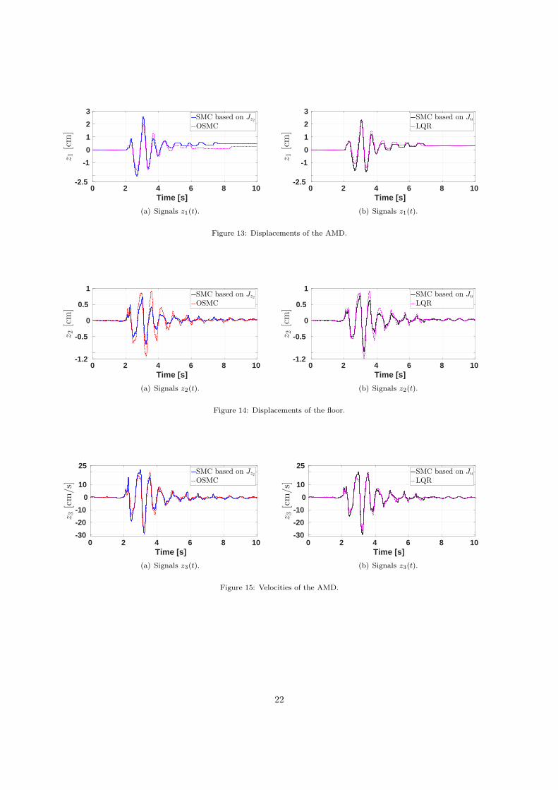
6.2.3. Responses produced by the LQR, OSMC, and the SMC tuned with the proposed algorithm

Figure 12 depicts the uncontrolled response z2(t) of the experimental structure under the earthquakeexcitation, which indicates that its maximum magnitude is approximately 3.5 cm. Figures 13−17 show,respectively, the signals z1(t), z2(t), z3(t), z4(t), and u(t) produced by the LQR, OSMC, and the tunedSMC. From these plots, it is possible to see that the maximum displacement z2(t) corresponding to theSMC, based on either PI Jz2 or Ju, is smaller than that produced by the LQR and OSMC. Moreover, thepeak value of the signals u(t) and z1(t) corresponding to the SMC is slightly larger than those generated bythe LQR and OSMC, but these signals are within the specified limits.

Time [s]0 2 4 6 8 10 12 14 16 18 20

z2[cm]

-3.5

-2-1012

3.5

Figure 12: Uncontrolled response of z2(t).

21

Time [s]0 2 4 6 8 10

z1[cm]

-2.5

-1

0

1

2

3SMC based on Jz2OSMC

(a) Signals z1(t).

Time [s]0 2 4 6 8 10

z1[cm]

-2.5

-1

0

1

2

3SMC based on JuLQR

(b) Signals z1(t).

Figure 13: Displacements of the AMD.

Time [s]0 2 4 6 8 10

z2[cm]

-1.2

-0.5

0

0.5

1SMC based on Jz2OSMC

(a) Signals z2(t).

Time [s]0 2 4 6 8 10

z2[cm]

-1.2

-0.5

0

0.5

1SMC based on JuLQR

(b) Signals z2(t).

Figure 14: Displacements of the floor.

Time [s]0 2 4 6 8 10

z3[cm/s]

-30

-20

-10

0

10

25SMC based on Jz2OSMC

(a) Signals z3(t).

Time [s]0 2 4 6 8 10

z3[cm/s]

-30

-20

-10

0

10

25SMC based on JuLQR

(b) Signals z3(t).

Figure 15: Velocities of the AMD.

22

Time [s]0 2 4 6 8 10

z4[cm/s]

-14

-8

-4

0

4

8SMC based on Jz2OSMC

(a) Signals z4(t).

Time [s]0 2 4 6 8 10

z4[cm/s]

-14

-8

-4

0

4

8SMC based on JuLQR

(b) Signals z4(t).

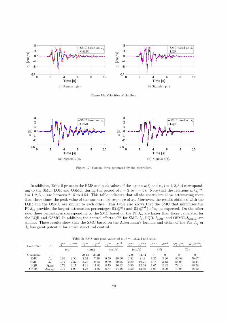
Figure 16: Velocities of the floor.

Time [s]0 2 4 6 8 10

u[N

]

-3.5

-2-10123

SMC based on Jz2OSMC

(a) Signals u(t).

Time [s]0 2 4 6 8 10

u[N

]

-3.5

-2-10123

SMC based on JuLQR

(b) Signals u(t).

Figure 17: Control force generated by the controllers.

In addition, Table 5 presents the RMS and peak values of the signals u(t) and zi, i = 1, 2, 3, 4 correspond-ing to the SMC, LQR and OSMC, during the period of t = 2 to t = 6 s. Note that the relations κi/z

rmsi ,

i = 1, 2, 3, u, are between 2.15 to 4.54. This table indicates that all the controllers allow attenuating morethan three times the peak value of the uncontrolled response of z2. Moreover, the results obtained with theLQR and the OSMC are similar to each other. This table also shows that the SMC that minimizes thePI Jz2 provides the largest attenuation percentages R(zrms

2 ) and R(zpeak2 ) of z2, as expected. On the otherside, these percentages corresponding to the SMC based on the PI Ju, are larger than those calculated forthe LQR and OSMC. In addition, the control efforts urms for SMC-Ju, LQR-JLQR, and OSMC-JOSMC aresimilar. These results show that the SMC based on the Ackermann’s formula and either of the PIs Jz2 orJu has great potential for active structural control.

Table 5: RMS and peak values of zi, i = 1, 2, 3, 4 and u(t).

Controller PIzrms1 z

peak1 zrms

2 zpeak2 zrms

3 zpeak3 zrms

4 zpeak4 urms upeak R(zrms

2 ) R(zpeak2 )

(cm) (mm) (cm/s) (cm/s) (N) (%)

Uncontrol — — — 20.14 35.31 — — 17.90 34.54 0 0 0 0SMC Jz2 0.84 2.56 2.62 7.39 9.59 29.06 2.52 8.49 1.25 3.36 86.99 79.07SMC Ju 0.77 2.32 3.21 9.73 9.39 29.95 2.89 10.71 1.18 3.43 84.06 72.44LQR JLQR 0.74 2.17 4.21 11.80 8.75 26.62 3.50 12.68 1.05 2.92 79.10 66.58OSMC JOSMC 0.72 1.99 4.22 11.22 8.87 24.18 3.50 13.66 1.05 2.90 79.05 68.22

23

7. Conclusions

This paper proposed a tuning algorithm for a SMC designed for attenuating the structural vibration of aseismically excited building equipped with an ATMD on its top floor. The SMC is based on the Ackermann’sformula and its robustness against friction uncertainty was demonstrated. It was proved that the seismicexcitation signal is not a coupled disturbance, and as consequence it cannot be eliminated by the SMC;however, its effect can be minimized by designing the SMC with the proposed tuning algorithm.

It was also shown that the responses of the ATMD and building under the SMC can be describedby means of dominant second-order filters, whose input is the seismic excitation. Their parameters wereautomatically tuned by the proposed algorithm in order to minimize the PI Jz2 or Ju. The PI Jz2 is related tothe minimization of the top floor displacement, while the PI Ju is related to the minimization of the controlforce applied the ATMD while offering a great attenuation of this displacement. The effectiveness of thedesigned SMC was demonstrated in a numerical and an experimental structure. Moreover, the experimentsshowed that the designed SMC has a better vibration attenuation performance than the LQR and OSMC,while ensuring that the structure and the ATMD signals are within the specified limits.

Acknowledgments

The authors thank the Programa para el Desarrollo Profesional Docente (PRODEP-SEP) of Mexico forsupporting this research. The authors also acknowledge the anonymous reviewers for their helpful comments.

References

[1] O. Avci, O. Abdeljaber, S. Kiranyaz, M. Hussein, M. Gabbouj, D. J. Inman, A review of vibration-based damage detectionin civil structures: From traditional methods to machine learning and deep learning applications, Mechanical Systems andSignal Processing 147 (2021) 107077.

[2] J. Chen, Y. Chen, Y. Peng, S. Zhu, M. Beer, L. Comerford, Stochastic harmonic function based wind field simulation andwind-induced reliability of super high-rise buildings, Mechanical Systems and Signal Processing 133 (2019) 106264.

[3] S.-Y. Kim, C.-H. Lee, Peak response of frictional tuned mass dampers optimally designed to white noise base acceleration,Mechanical Systems and Signal Processing 117 (2019) 319–332.

[4] D. K. Pandey, M. K. Sharma, S. K. Mishra, A compliant tuned liquid damper for controlling seismic vibration of shortperiod structures, Mechanical Systems and Signal Processing 132 (2019) 405–428.

[5] M. Amjadian, A. K. Agrawal, Seismic response control of multi-story base-isolated buildings using a smart electromagneticfriction damper with smooth hysteretic behavior, Mechanical Systems and Signal Processing 130 (2019) 409–432.

[6] X. B. Nguyen, T. Komatsuzaki, Y. Iwata, H. Asanuma, Modeling and semi-active fuzzy control of magnetorheologicalelastomer-based isolator for seismic response reduction, Mechanical Systems and Signal Processing 101 (2018) 449–466.

[7] S. Paul, W. Yu, A method for bidirectional active control of structures, Journal of Vibration and Control 24 (15) (2018)3400–3417.

[8] S. Chesne, G. Inquiete, P. Cranga, F. Legrand, B. Petitjean, Innovative hybrid mass damper for dual-loop controller,Mechanical Systems and Signal Processing 115 (2019) 514–523.

[9] A. E. Kayabekir, G. Bekdas, S. M. Nigdeli, Z. W. Geem, Optimum design of pid controlled active tuned mass damper viamodified harmony search, Applied Sciences 10 (8) (2020) 2976.

[10] D.-H. Yang, J.-H. Shin, H. Lee, S.-K. Kim, M. K. Kwak, Active vibration control of structure by active mass damper andmulti-modal negative acceleration feedback control algorithm, Journal of Sound and Vibration 392 (2017) 18–30.

[11] E. Talib, J.-H. Shin, M. K. Kwak, Designing multi-input multi-output modal-space negative acceleration feedback controlfor vibration suppression of structures using active mass dampers, Journal of Sound and Vibration 439 (2019) 77–98.

[12] A. Younespour, H. Ghaffarzadeh, Structural active vibration control using active mass damper by block pulse functions,Journal of Vibration and Control 21 (14) (2015) 2787–2795.

[13] C. Chang, H. T. Yang, Control of buildings using active tuned mass dampers, Journal of engineering mechanics 121 (3)(1995) 355–366.

[14] S. Ankireddi, H. T. Y. Yang, Simple atmd control methodology for tall buildings subject to wind loads, Journal ofStructural Engineering 122 (1) (1996) 83–91.

[15] Y. Xu, H. Hua, J. Han, Modeling and controller design of a shaking table in an active structural control system, MechanicalSystems and Signal Processing 22 (8) (2008) 1917–1923.

[16] C. Li, J. Li, Y. Qu, An optimum design methodology of active tuned mass damper for asymmetric structures, MechanicalSystems and Signal Processing 24 (3) (2010) 746–765.

[17] F. Ricciardelli, A. D. Pizzimenti, M. Mattei, Passive and active mass damper control of the response of tall buildings towind gustiness, Engineering structures 25 (9) (2003) 1199–1209.

24

[18] Z.-H. Li, C.-J. Chen, J. Teng, A multi-time-delay compensation controller using a Takagi–Sugeno fuzzy neural networkmethod for high-rise buildings with an active mass damper/driver system, The Structural Design of Tall and SpecialBuildings 28 (13) (2019) e1631.

[19] Y. Lei, J. Lu, J. Huang, S. Chen, A general synthesis of identification and vibration control of building structures underunknown excitations, Mechanical Systems and Signal Processing 143 (2020) 106803.

[20] S. Allaoua, L. Guenfaf, LQG vibration control effectiveness of an electric active mass damper considering soil–structureinteraction, International Journal of Dynamics and Control 7 (1) (2019) 185–200.

[21] B.-L. Zhang, Y.-J. Liu, Q.-L. Han, G.-Y. Tang, Optimal tracking control with feedforward compensation for offshore steeljacket platforms with active mass damper mechanisms, Journal of Vibration and Control 22 (3) (2016) 695–709.

[22] B. Spencer Jr, J. Suhardjo, M. Sain, Frequency domain optimal control strategies for aseismic protection, Journal ofEngineering Mechanics 120 (1) (1994) 135–158.

[23] R. B. Santos, D. D. Bueno, C. R. Marqui, V. Lopes Jr, Active vibration control of a two-floors building model based onH2 and H∞ methodologies using linear matrix inequalities (lmis)., in: International Modal Analysis Conference–XXVIMAC, Orlando, EUA, 2007, pp. 1–13.

[24] L. Xu, Y. Yu, Y. Cui, Active vibration control for seismic excited building structures under actuator saturation, measure-ment stochastic noise and quantisation, Engineering Structures 156 (2018) 1–11.

[25] S.-M. Yang, C.-J. Chen, W. Huang, Structural vibration suppression by a neural-network controller with a mass-damperactuator, Journal of Vibration and Control 12 (5) (2006) 495–508.

[26] S. Thenozhi, W. Yu, Active vibration control of building structures using fuzzy proportional-derivative/proportional-integral-derivative control, Journal of Vibration and Control 21 (12) (2015) 2340–2359.

[27] Q. Li, D. Liu, J. Fang, C. Tam, Multi-level optimal design of buildings with active control under winds using geneticalgorithms, Journal of Wind Engineering and Industrial Aerodynamics 86 (1) (2000) 65–86.

[28] A. Banaei, J. Alamatian, New genetic algorithm for structural active control by considering the effect of time delay,Journal of Vibration and Control (2020) 1077546320933467.

[29] J. Fei, Y. Chen, Fuzzy double hidden layer recurrent neural terminal sliding mode control of single-phase active powerfilter, IEEE Transactions on Fuzzy Systems.

[30] J. Fei, H. Wang, Experimental investigation of recurrent neural network fractional-order sliding mode control of activepower filter, IEEE Transactions on Circuits and Systems II: Express Briefs.

[31] J. Yang, J. Wu, A. Agrawal, Sliding mode control for seismically excited linear structures, Journal of engineering mechanics121 (12) (1995) 1386–1390.

[32] R. Adhikari, H. Yamaguchi, Sliding mode control of buildings with ATMD, Earthquake Engineering & Structural Dynamics26 (4) (1997) 409–422.

[33] A.-P. Wang, Y.-H. Lin, Vibration control of a tall building subjected to earthquake excitation, Journal of Sound andVibration 299 (4-5) (2007) 757–773.

[34] L. Li, N. Wang, H. Qin, Adaptive model reference sliding mode control of structural nonlinear vibration, Shock andVibration 2019.

[35] M. Soleymani, A. H. Abolmasoumi, H. Bahrami, A. Khalatbari-S, E. Khoshbin, S. Sayahi, Modified sliding mode controlof a seismic active mass damper system considering model uncertainties and input time delay, Journal of Vibration andControl 24 (6) (2018) 1051–1064.

[36] N. Mamat, F. Yakub, S. A. Z. Shaikh Salim, M. S. Mat Ali, Seismic vibration suppression of a building with an adaptivenonsingular terminal sliding mode control, Journal of Vibration and Control (2020) 1077546320915324.

[37] M. Khatibinia, M. Mahmoudi, H. Eliasi, Optimal sliding mode control for seismic control of buildings equipped with atmd,Iran University of Science & Technology 10 (1) (2020) 1–15.

[38] A. K. Chopra, Dynamics of Structures: theory and applications to earthquake engineering, Prentice Hall, EnglewoodCliffs, NJ, 2001.

[39] W. Yu, S. Thenozhi, Active structural control with stable fuzzy PID techniques, Springer, 2016.[40] J. Wu, J. Yang, W. Schmitendorf, Reduced-order H∞ and LQR control for wind-excited tall buildings, Engineering

Structures 20 (3) (1998) 222–236.[41] J. Ackermann, Sampled-Data Control Systems, Springer-Verlag, Berlin, Germany, 1985.[42] L. Wang, Q. Li, R. Jiao, Y. Yin, Y. Feng, Y. Liu, Tracking of stribeck friction based on second-order linear extended state

observer, in: 2016 Chinese Control and Decision Conference (CCDC), IEEE, 2016, pp. 4334–4337.[43] R. Garrido, A. Concha, Inertia and friction estimation of a velocity-controlled servo using position measurements, IEEE

Transactions on industrial electronics 61 (9) (2013) 4759–4770.[44] J. Ackermann, V. Utkin, Sliding mode control design based on Ackermann’s formula, IEEE Transactions on Automatic

Control 43 (2) (1998) 234–237.[45] J. Song, Y. Niu, Y. Zou, Finite-time stabilization via sliding mode control, IEEE Transactions on Automatic Control

62 (3) (2016) 1478–1483.[46] J. Song, Y. Niu, Y. Zou, A parameter-dependent sliding mode approach for finite-time bounded control of uncertain

stochastic systems with randomly varying actuator faults and its application to a parallel active suspension system, IEEETransactions on Industrial Electronics 65 (10) (2018) 8124–8132.

[47] G. F. Franklin, J. D. Powell, A. Emami-Naeini, J. D. Powell, Feedback control of dynamic systems, 7th Edition, Pearson,Upper Saddle River, NJ, 2015.

[48] J. Kayal, Microearthquake seismology and seismotectonics of South Asia, Springer Science & Business Media, 2008.[49] J. E. Slotine, W. Li, Applied Nonlinear Control, Prentice Hall, 2002.[50] J. Fei, Y. Chen, Dynamic terminal sliding-mode control for single-phase active power filter using new feedback recurrent

25

neural network, IEEE Transactions on Power Electronics 35 (9) (2020) 9906–9924.[51] J. Fei, Z. Feng, Fractional-order finite-time super-twisting sliding mode control of micro gyroscope based on double-loop

fuzzy neural network, IEEE Transactions on Systems, Man, and Cybernetics: Systems.[52] A. Levant, Higher-order sliding modes, differentiation and output-feedback control, International journal of Control 76 (9-

10) (2003) 924–941.[53] R. Rana, T. Soong, Parametric study and simplified design of tuned mass dampers, Engineering structures 20 (3) (1998)

193–204.[54] Quanser Inc., Shake Table I-40 User manual (2012).[55] Quanser Inc., Active Mass Damper - One Floor (AMD-1) (2012).[56] Quanser Inc., Linear Motion Servo Plants: IP01 or IP02 (2012).[57] K. Ogata, Modern control engineering, Prentice Hall, Upper Saddle River, NJ, 2002.[58] A. E. Bryson, Y. C. Ho, Applied Optimal Control, Taylor & Francis, Madison Avenue, NY, 1975.[59] V. I. Utkin, Sliding modes in control and optimization, Springer Science & Business Media, 2013.[60] H. Alwi, C. Edwards, C. P. Tan, Fault detection and fault-tolerant control using sliding modes, Springer Science & Business

Media, 2011.

26