ARTICLE IN PRESS

Control Engineering Practice 16 (2008) 1275– 1284

Contents lists available at ScienceDirect

Control Engineering Practice

0967-06

doi:10.1

� Corr

E-m

journal homepage: www.elsevier.com/locate/conengprac

Adaptive sliding mode control of electro-hydraulic system with nonlinearunknown parameters

Cheng Guan �, Shuangxia Pan

Mechanical Design Institute, Zhejiang University, Hangzhou, Zhejiang 310027, China

a r t i c l e i n f o

Article history:

Received 25 May 2006

Accepted 22 February 2008Available online 18 April 2008

Keywords:

Adaptive control

Electro-hydraulic system

Lyapunov stability

Sliding mode control

Nonlinear unknown parameter

61/$ - see front matter & 2008 Elsevier Ltd. A

016/j.conengprac.2008.02.002

esponding author.

ail address: gchzju@hotmail.com (C. Guan).

a b s t r a c t

In this paper, an adaptive sliding control method is presented for an electro-hydraulic system with

nonlinear unknown parameters, which enter the system equations in a nonlinear way. Previous

adaptive control methods of hydraulic system always assume that the original control volumes are

certain and known, which can guarantee that all system unknown parameters occur linearly. But in

practical hydraulic systems, the original control volumes are unknown or change; as a result some

unknown parameters appear nonlinearly. The proposed control method in this paper is to present a

nonlinear adaptive controller with adaptation laws to compensate for the nonlinear uncertain

parameters caused by the varieties of the original control volumes. The main feature of the scheme is

that by combining sliding mode control method, a novel-type Lyapunov function is developed to

construct an asymptotically stable adaptive controller and adaptation laws, which can compensate for

the system uncertain nonlinearities, linear uncertain parameters, and especially for the nonlinear

uncertain parameters caused by the various of the original control volumes. The experimental results

show that the nonlinear control algorithm, together with the adaptation scheme, gives a good

performance for the specified tracking task in the presence of nonlinear unknown parameters.

& 2008 Elsevier Ltd. All rights reserved.

1. Introduction

Electro-hydraulic systems have been widely used in industrialapplications because of their high power-to-weight ratio, highstiffness, high payload capability, etc. For example, they have beenused in robot manipulators (Li & Khajepour, 2005; Raade &Kazerooni, 2005), anti-lock braking system (Wu & Shih, 2003),hydraulic excavator (Lee & Chang, 2002), plate hot rollings (Kim &Lee, 2006), etc. However, the dynamic behavior of hydraulicsystems is highly nonlinear due to the phenomena such asnonlinear servo valve flow-pressure characteristics, variations incontrol volumes and associated stiffness, etc., which, in turn,cause difficulties in the control of such systems. Apart from thenonlinear nature of hydraulic dynamics, hydraulic systems alsohave a large extent of model uncertainties due to parametricuncertainties and uncertain nonlinearities.

In order to obtain higher performance, more and moreresearchers used nonlinear control methods to compensate forthe nonlinear feature of electro-hydraulic system. Firstly, thefeedback linearization technique was used in some researchworks (Re & Isidori, 1995; Shol & Bobrow, 1999; Vossoughi &

ll rights reserved.

Donath, 1995), but this control method did not account for systemuncertainties. So several kinds of sliding mode variable structurecontrol (SMVSC) methods are adopted in electro-hydraulic controlsystems by some researchers (Bonchis, Corke, Rye, & Ha, 2001;Hisseine, 2005; Hong, Kil, Tae, & Yeong, 2003; Li & Khajepour,2005; Liu & Handroos, 1999; Wu & Shih, 2003). However, thecontroller designed by using SMVSC contains discontinuousfunction, which can cause chattering phenomena, so the perfor-mance of the control system is affected.

Adaptive control is a valid method to overcome systemuncertainties, especially uncertainties derived from uncertainparameters; hence several kinds of nonlinear adaptive controlschemes have been proposed in hydraulic control systems such asfeedback linearization adaptive control (Garagic & Srinivasan,2004), sliding mode adaptive control (Guan & Zhu, 2004), andnonlinear adaptive control based on backstepping techniques(Alleyne & Liu, 2000; Liu & Alleyne, 2000; Yao, Bu, & Chiu, 1998;Yao, Bu, Reedy, & Chiu, 2000). For example, Alleyne and Liu (2000)and Liu and Alleyne (2000) applied the nonlinear adaptive controlbased on the backstepping method to the force control of electro-hydraulic system, B. Yao et al. (1998, 2000) applied nonlinearadaptive robust control in double-rod and single-rod cylinderhydraulic system based on backstepping techniques to compen-sate for the uncertainties from both parametric uncertainties anduncertain nonlinearities. Recently, some novel nonlinear adaptive

ARTICLE IN PRESS

Fig. 1. Schematic diagram of the hydraulic system.

C. Guan, S. Pan / Control Engineering Practice 16 (2008) 1275–12841276

control methods have been presented for the hydraulic system (Bu& Yao, 2001; Duraiswamy & Chiu, 2003; Liu & Yao, 2003; Shi, Gu,Lennox, & Ball, 2005; Zhu & Piedboeuf, 2005). These nonlinearadaptive control laws not only solved the control problem comingfrom uncertain nonlinear system successfully in some conditionsbut also demonstrated that nonlinear control schemes can achievebetter performance than conventional linear controllers.

However, one of the assumptions in these adaptive schemes isthat the original total control volume between a servo valve and acylinder including volume of the servo valve, pipelines andcylinder chambers is certain and known. This assumption makesthe system; all uncertain parameters occur linearly. But in arealistic electro-hydraulic control system, the original totalcontrol volume is uncertain. The volume of the servo valve canbe neglected since it is smaller correspondingly. But in manycases, the volume of pipelines is too large to be neglected;moreover, it significantly affects the performance of a hydrauliccontrol system. Nevertheless, the exact volume of pipelines is verydifficul to obtain, the length of pipelines may be variable indifferent environments for the same control system, and differentoriginal positions of cylinder piston can also change the originaltotal control volume; as a result, the original total control volume(mainly including pipelines and a cylinder chamber) is uncertainbut important. Hence, in practical hydraulic systems, nonlinearunknown parameters, which enter the system state-equations in anonlinear way, are common, and previous adaptive schemes of anelectro-hydraulic system cannot solve the problem from thenonlinear unknown parameters. Therefore, it is a challengingproject to propose a nonlinear adaptive control method that canbe used in the electro-hydraulic systems with nonlinear unknownparameters due to the variations of the original total controlvolume.

In this paper, by utilizing a practical property of the double-rod cylinder hydraulic system, a special novel-type Lyapunovfunction is developed to construct a Lyapunov-based controllerand nonlinear parameters update laws for the system withnonlinear unknown parameters. The sliding mode controlmethod is not only simple but also can be applied to a nonlinearsystem; hence by combining the sliding mode control method, thewhole system controller and all unknown parameters updatelaws are developed. Moreover, in order to avoid the discontinuousfunction, which can cause chattering phenomena during thecontrol process, inside the controller designed with the vari-able structure control (VSC) method, a simple robust controlmethod is used to solve the problem derived from unmodeleduncertainties.

To test the proposed advanced nonlinear adaptive slidingcontrol strategy, an experiment is performed. Experimentalresults have been obtained for the position tracking control ofthe hydraulic cylinder, and the results verify the higher perfor-mance nature of the proposed nonlinear adaptive sliding controlapproach in comparison to the proposed control but withoutusing adaptation laws.

This paper is organized as follows. In Section 2, problemformulation and the detailed nonlinear model are presented. InSection 3, the proposed adaptive sliding control for the electro-hydraulic system with nonlinear unknown parameters strategy isgiven. In Section 4, the experiment is set up and results arediscussed, In Section 5, conclusions are presented.

2. Problem formulation and dynamic models

The hydraulic system shown in Fig. 1 comprises a double-rodcylinder, a 4/3 way servo valve, and a load force. The goal is tohave the load track any specified motion trajectory as closely as

possible. In the following, the nonlinear dynamic model willbe given.

The dynamics of the forces balance can be described by

ðP1 � P2ÞA ¼ m€xþ Kxþ FlðtÞ, (1)

where x is the displacement of the load, m is the mass of the load,P1 and P2 are the pressures inside the two chambers of thecylinder, A is the ram area of the two chambers, K is the effectivebulk modulus of the spring, and Fl(t) is lumped uncertainnonlinearity due to external disturbances, the unmodeled frictionforces, damping viscous friction forces on the load, and thecylinder rod and other hard-to-model terms.

For a double-rod cylinder hydraulic control system, someresearches assume that the original control volumes of the twochambers V1 and V2 are the same so that the dynamic oil flow ofthe two chambers can be combined into a single equation withload flow and load pressure to guarantee that system parametersoccur linearly. However, in a realistic hydraulic system, it isdifficult to satisfy the assumption, hence V1 and V2 are treated astwo different parameters in this paper. In addition, with thedevelopment of seal techniques, the external leakage flow isalmost zero; hence the external leakage of the cylinder isneglected here. Therefore, the dynamics of cylinder oil flow canbe written as follows (Merritt, 1967):

A_xþ CtðP1 � P2Þ þV1 þ Ax

be

_P1 ¼ Q1

A_xþ CtðP1 � P2Þ ¼V2 � Ax

be

_P2 þ Q2

(2)

where Ct is the coefficient of the internal leakage of the cylinder, be

is the effective bulk modulus of the hydraulic fluid in thecontainer. V1 and V2 are the original total control volume of thetwo cylinder chambers, respectively (including the volume ofservo valve, pipelines and cylinder chambers).

Q1 is the supplied flow rate to the forward chamber, Q2 is thereturn flow rate of the return chamber. Q1 and Q2 are given as(Merritt, 1967)

Q1 ¼ kq1xv sðxvÞffiffiffiffiffiffiffiffiffiffiffiffiffiffiffiffiPs � P1

pþ

hsð�xvÞ

ffiffiffiffiffiffiffiffiffiffiffiffiffiffiffiffiP1 � Pr

p iQ2 ¼ kq2xv sðxvÞ

ffiffiffiffiffiffiffiffiffiffiffiffiffiffiffiffiP2 � Pr

pþ sð�xvÞ

ffiffiffiffiffiffiffiffiffiffiffiffiffiffiffiffiPs � P2

p ih (3)

Define function as (Tazafoli, de Silva, & Lawrence, 1998)

sðnÞ ¼1 if nX0

0 if no0

((4)

kq1 ¼ Cdw1

ffiffiffi2

r

s; kq2 ¼ Cdw2

ffiffiffi2

r

s

where Ps is the supplied pressure, Pr is the return line pressure, xv

is the spool displacement of the servo valve, Cd is the dischargecoefficient, w is the spool valve area gradient, and r is the fluiddensity.

ARTICLE IN PRESS

C. Guan, S. Pan / Control Engineering Practice 16 (2008) 1275–1284 1277

The effects of servo valve dynamics have been included insome literatures (Alleyne & Liu, 2000; Liu & Alleyne, 2000), butthis requires an additional sensor to obtain the spool position andonly minimal performance improvement is achieved for positiontracking, so other researchers neglect servo valve dynamicsaccording to practice status, (Garagic & Srinivasan, 2004; Liu &Handroos, 1999). Since a high-response servo valve is used here, itis assumed that the control applied to the spool valve is directlyproportional to the spool position, then the following equation isgiven by xv ¼ lu, where l is a positive constant, u is input voltage.Thus from (4), s(xv) ¼ s(u) is obtained.

Therefore (3) can be transformed to

Q1 ¼ g1u sðuÞffiffiffiffiffiffiffiffiffiffiffiffiffiffiffiffiPs � P1

pþ sð�uÞ

ffiffiffiffiffiffiffiffiffiffiffiffiffiffiffiffiP1 � Pr

ph iQ2 ¼ g2u sðuÞ

ffiffiffiffiffiffiffiffiffiffiffiffiffiffiffiffiP2 � Pr

pþ sð�uÞ

ffiffiffiffiffiffiffiffiffiffiffiffiffiffiffiffiPs � P2

ph i (5)

where g1 ¼ kq1l, g2 ¼ kq2lDefine the state variables as x ¼ ½x1 x2; x3�

T¼D½x; _x; €x�T.

The entire system including Eqs. (1), (2) and (5) can be expressedin a state-space form as follows:

_x1 ¼ x2

_x2 ¼ x3

_x3 ¼Abe

mðV1 þ Ax1Þ�Ax2 �

Ct

Aðmx3 þ Kx1 þ FlÞ þ g1uR1

� �

�Abe

mðV2 � Ax1ÞAx2 þ

Ct

Aðmx3 þ Kx1 þ FlÞ � g2uR2

� �

�K

mx2 �

_Fl

m, (6)

where

R1 ¼ sðuÞffiffiffiffiffiffiffiffiffiffiffiffiffiffiffiffiPs � P1

pþ sð�uÞ

ffiffiffiffiffiffiffiffiffiffiffiffiffiffiffiffiP1 � Pr

p(7)

R2 ¼ sðuÞffiffiffiffiffiffiffiffiffiffiffiffiffiffiffiffiP2 � Pr

pþ sð�uÞ

ffiffiffiffiffiffiffiffiffiffiffiffiffiffiffiffiPs � P2

p(8)

Given the desired motion trajectory xd(t), the objective of thispaper is to design a bounded control input u so that the output x1

tracks as closely as possible to the desired motion trajectory xd(t)in spite of various model uncertainties including nonlinearunknown parameters. Based on the realistic hydraulic system,the following practical assumption is given.

Assumption 1. The desired position xd(t), its velocity_xdðtÞ, accel-eration€xdðtÞ, and

_ _ _

xdðtÞ are all bounded.

Remark 1. The state variables of this hydraulic system dynamicmodel includeðx; _x; P1; P2Þ, but it is necessary to control variablesðx; _x; P1 � P2Þ. Therefore, from (1), it is known that it is sufficientto control states ðx; _x; €xÞ, so in this paper, states ðx; _x; €xÞ are usedto replace ðx; _x; P1 � P2Þ. In addition, in a practical hydraulicsystem under normal working condition, P1 and PB2B are bothbounded, in fact, 0oProP1oPs, 0oProP2oPs, so it is feasible touse a third-order model of using the states ðx; _x; €xÞ to represent adynamic model in the variables ðx; _x; P1 � P2Þ.

3. Adaptive sliding control for the electro-hydraulic systemwith nonlinear unknown parameters

3.1. Design model and issues to be addressed

In order to simplify the state-space equation, first, define theparameters set � ¼ ½�1; �2; �3; �4; �5; �6�

T as e1 ¼ Abe/m, �2 ¼

beCt=A, �3 ¼ KbeCt=Am�4 ¼ beg1=m, �5 ¼ beg2=m, e6 ¼ K/m; andparameters set b ¼ [b1, b2]T as b1 ¼ V1/A, b2 ¼ V2/A, andd1ðtÞ ¼ ðCtbe=AmÞFlðtÞ, 2ðtÞ ¼ _FlðtÞ=m. Thus the state-space Eq. (6)

is transformed to

_x1 ¼ x2

_x2 ¼ x3

_x3 ¼1

b1 þ x1½��1x2 � �2x3 � �3x1 � d1ðtÞ þ �4uR1�

�1

b2 � x1½�1x2 þ �2x3 þ �3x1 þ d1ðtÞ � �5uR2�

� �6x2 � d2ðtÞ (9)

Then define parameter set y ¼ y1; y2; y3; y4; y5; y6; y7;½

y8; y9�T as y1 ¼ e3(b1+b2), y2 ¼ e1(b1+b2)+e6b1b2, y3 ¼ e2(b1+b2),

y4 ¼ e6(b2�b1), y5 ¼ e6, y6 ¼ e4b2, y7 ¼ e5b1, y8 ¼ e5, y9 ¼ e4 andj ¼ [j1 j2]T as j1 ¼ b1b2, j2 ¼ b2�b1.

Substituting the above parameters y and j into (9), the state-space Eq. (9) is converted into

_x1 ¼ x2

_x2 ¼ x3

_x3 ¼1

j1 þ j2x1 � x21

f�y1x1 � y2x2 � y3x3 � y4x1x2

þ y5x21x2 � ðb1 þ b2Þd1ðtÞ � ðj1 þ j2x1 � x2

1Þd2ðtÞ

þ ½y6R1 þ y7R2 þ y8R2x1 � y9R1x1�ug (10)

From Eqs. (9) and (10), it is shown that the hydraulic system is anonlinear system. Moreover, parameters Ct, be, and Cd are variablesin the whole work process due to different temperature,environments, etc; hence these parameters are uncertain. Accu-rate spool valve area gradient w is difficult to be obtained and rmay be variable in different conditions, so g1 and g2 are alsouncertain. Sometimes load mass m is variable, so m is alsouncertain. Thus in Eqs. (9) and (10), parameters � ¼ ½�1; �2;

�3; �4; �5; �6�T and y ¼ ½y1; y2; y3; y4; y5; y6; y7; y8; y9�

T, whichappear linearly, are all uncertain. In addition, d1(t), d2(t) in (9)and the items related to d1(t) and d2(t) in (10) are clearly uncertainnonlinearities.

Especially, it is clear that in nonlinear state-space equations (9)and (10), the parameters b1 and b2, or j1 and j2, occurnonlinearly. In most previous papers, researchers always treatedb1 and b2 or j1 and j2 as known certain parameters. However, in arealistic hydraulic system, the values of the original controlvolume V1 and V2 including the volume of pipelines, servo valve,cylinder chambers, etc. are very difficult to obtain precisely andmay change as is discussed in the introduction. b1 ¼ V1/A andb2 ¼ V2/A, so parameters b1 and b2 are really uncertain, thenj1 ¼ b1b2 and j2 ¼ b2�b1 are certainly uncertain, i.e., the non-linear unknown parameters do exist in the electro-hydraulicsystem.

Therefore, the uncertainties of the nonlinear electro-hydraulicsystem derive from the nonlinear uncertain parameters set b, thelinear uncertain parameters set e, and the uncertain nonlinearitiesd1(t) and d2(t) of Eq. (9), or nonlinear uncertain parameters set j,linear uncertain parameters set y, and uncertain nonlinearitiesitems related to d1(t) and d2(t) of Eq. (10).

The existing Lyapunov-based adaptive control, in whichLyapunov function is in a conventional quadratic form, is invalidto the nonlinear uncertain parameters b1 and b2, or j1 and j2;therefore most previous researches assumed that V1 and V2, i.e., b1

and b2, are certain and known, and took into account only linearuncertain parameters e (Alleyne & Liu, 2000; Liu & Alleyne, 2000),or both linear uncertain parameter e and uncertain nonlinearitiesd1(t) and d2(t) (Yao et al., 1998; Yao et al., 2000). Therefore, it is achallenging project to propose an adaptive control method thatcan be used in the electro-hydraulic system with nonlinearunknown parameters b1 and b2.

ARTICLE IN PRESS

C. Guan, S. Pan / Control Engineering Practice 16 (2008) 1275–12841278

In the following, by defining a special-type Lyapunov function,a nonlinear adaptive control and parameter adaptation schemewill be proposed to overcome the difficult problem from thenonlinear unknown parameters like b1 and b2. Moreover, theadaptive sliding control and adaptation laws for the whole system(10) compensating for all uncertain parameters and uncertainnonlinearities are presented by combining the sliding modecontrol and a simple robust control method.

Though b1 and b2 are uncertain, in a practical hydraulic systemthey are both bounded and positive. In addition, y, d1(t) and d2(t)are also bounded. Thus the following practical assumptionsare made.

Assumption 2. yi 2 Oyi¼D½yimin yi max�; jd1ðtÞjpD1; jd2ðtÞjpD2 and

L1pb1pB1; L2pb2pB2 where L1, L2, B1, B2, and D1, D2 are allpositive constants. In fact, L1 is larger than the possible maximalabsolute value of the negative displacement of the load, and L2 islarger than the possible maximal positive displacement.

From Assumption 2, the following inequations are given

jj1jpB1B2; jj2jomaxðB1;B2Þ (11)

And, since x1 is the displacement of the load, it is clear that

b1 þ x140; b2 � x140

Thus

ðb1 þ x1Þðb2 � x1Þ ¼ j1 þ j2x1 � x2140 (12)

From Section 3.1, it is seen that y6 ¼ e4b2, y7 ¼ e5b1, y8 ¼ e5,y9 ¼ e4, and e4 ¼ beg1/m, e5 ¼ beg2/m. Moreover, in the practicalhydraulic system be, m, g1 and g2 are all positive, so e4 and e5 arepositive. In addition, from (7) and (8), it is obtained thatR140; R240. Hence, if yi 2 Oyi (i ¼ 6,7,8,9), the following resultalways holds:

y6R1 þ y7R2 þ ðy8R2 � y9R1Þx1

¼ �5R2ðb1 þ x1Þ þ �4R1ðb2 � x1Þ40

3.2. Adaptive control of a class of a nonlinear system with nonlinear

unknown parameters

Firstly, consider the following classical first-order nonlinearsystem with nonlinear parameterization like system (10):

_y ¼sT

1f l1ðyÞ þ sT2f l2ðyÞu

sT3f n0ðyÞ

(13)

where yAR is the system state, uAR is the control input,f l1ðyÞ 2 Rn1 , f l2ðyÞ 2 Rn2 , and f n0ðyÞ 2 Rn3 are all continuous func-tions sets. s1 2 Rn1 , s2 2 Rn2 , and s3 2 Rn3 are all uncertainparameters sets, in which parameters s3 are clearly nonlinearlike j of system (10).

The control objective is to make y track a desired trajectory yd

asymptotically.

Assumption 3. yd and _yd are both bounded.

Assumption 4. si 2 Osi¼D½si min si max�, i ¼ 1,2,3,4 and sT

2f l2ðyÞa0,8s2 2 Os2

; sT3f n0ðyÞa08s3 2 Os3

Let si denote the estimate of si, and ~si denote the estimation

errors, ~si ¼ s� si, i ¼ 1,2,3.

Let tracking error e ¼ y�yd.In order to construct the controller and adaptation law for

system (13) with nonlinear parameterization, a different special-type Lyapunov function is developed to replace the most widelyused Lyapunov function, which is in a conventional quadratic

form. This Lyapunov function is designed as follows:

V0 ¼12s

T3f n0ðyÞZðyÞe

2, (14)

where the function Z(y)AR and is satisfied as follows:

(1)

Z(y) is differentiable, (2) ensure that sT

3f n0ðyÞZðyÞ40.

Thus V0 is a positive definite function with respect to thetracking error e. In the following, based on the Lyapunov functionV0, a controller is proposed to guarantee _V0p0 to achieveasymptotic tracking control.

The time derivative of the tracking error e along system (13) isobtained as

_e ¼ _y� _yd ¼sT

1f l1ðyÞ þ sT2f l2ðyÞu

sT3f n0ðyÞ

� _yd (15)

Taking into account (14) and (15), the time derivative of V0 isobtained as

_V0 ¼1

2sT

3e2 d½f n0ðyÞZðyÞ�dt

þ sT3f n0ðyÞZðyÞe_e

¼1

2sT

3e2 d½f n0ðyÞ�

dtZðyÞ þ f n0ðyÞ

d½ZðyÞ�dt

� �þ ZðyÞe sT

1f l1ðyÞ þ sT2f l2ðyÞu� sT

3f n0ðyÞ_yd

� �(16)

It is clear that the above equation does not include non-linear uncertain parameters, that is, all uncertain parameters arelinear. So by defining the novel-type Lyapunov function (14),the problem of solving nonlinear unknown parameters isconverted to solving the problem of linear unknown parameters;subsequently, the conventional method can be used to design thecontroller and adaptation law. Therefore, the following results canbe obtained.

The controller is designed as

u ¼1

sT2f l2ðyÞ

�sT1f l1ðyÞ þ sT

3f n0ðyÞ_yd �1

ZðyÞke

�

�1

2ZðyÞsT

3ef ðyÞ

�(17)

with

f ðyÞ ¼d½f n0ðyÞ�

dtZðyÞ þ f n0ðyÞ

d½ZðyÞ�dt

.

Substituting controller (17) into (16), the following equation isobtained:

_V0 ¼ � ke2 þ1

2~sT

3e2f ðyÞ

þ ZðyÞe½ ~sT1f l1ðyÞ þ ~sT

2f l2ðyÞu� ~sT3f n0ðyÞ_yd� (18)

In order to obtain the update laws of parameters, the followingLyapunov function is defined as

Vd ¼ V0 þ1

2

X3

i¼1

~sTi T�1

i ~si (19)

where T1, T2, and T3 are positive definite constant diagonalmatrices.

Taking into account (18), the time derivative of Vd is

_Vd ¼_V0 � ~s

T1T�1

1_s1 � ~s

T2T�1

2_s2 � ~sT

3T�13_s3

¼ � ke2 þ ~sT1½ZðyÞef l1ðyÞ � T�1

1_s1�

þ ~sT2½ZðyÞef l2ðyÞu� T�1

2_s2�

þ1

2~sT

3e ef ðyÞ � 2ZðyÞf n0ðyÞ_yd

h i� ~sT

3T�13_s3 (20)

ARTICLE IN PRESS

C. Guan, S. Pan / Control Engineering Practice 16 (2008) 1275–1284 1279

To make sure that _Vdp0, and to guarantee that sT2f l2ðyÞa0, the

adaptation law is chosen as

_s1 ¼ T1ZðyÞef l1ðyÞ

_s2 ¼ Projs2T2ZðyÞef l2ðyÞu

_s3 ¼12T3e f ðyÞe� 2ZðyÞf n0ðyÞ_yd

h i(21)

The function Projs2fng is chosen to make sure that

ð1Þ sT2f l2ðyÞa0

ð2Þ ~sT2 ZðyÞef l2ðyÞu� T�1

2_s2

h ip0 (22)

Here, the simple function Projs2fng is chosen as follows:

Projs2fng ¼

0 if s2 ¼ s2 max and n40

0 if s2 ¼ s2 min and no0

n otherwise

8><>: (23)

Fact 1. If the function Projs2fng is chosen as (23), conditions (22) will

be satisfied.

For proof see Appendix A.Therefore, substituting the above adaptation law (21) into (20),

_Vdp� ke2p0 is obtained, and since Vd(t)X0, thus Vd(t)pVd(0),8t40, and

R t0 ke2ðtÞdtpVdð0Þ � VdðtÞpVdð0Þo1. Therefore eAL2 is

obtained. From (14) and (19), it is seen that V0(t), e and s1, s2, s3

are all bounded. Since sT2f l2ðyÞa0, the control input u is also

bounded. It follows from (15) that _e is bounded. Because e 2

L2 \ L1 and _e 2 L1, according to Barbalat’s lemma (Popov, 1973),the conclusion that lim

t!1eðtÞ ¼ 0 asymptotically is reached. Hence

the following theorem can be obtained.

Theorem 1. For the nonlinear system (13) consisting of nonlinear

uncertain parameters and satisfying Assumptions 3 and 4, under the

controller (17) and adaptive laws (21), the estimated parameters s1,s2, and s3 are bounded, and the closed-loop system is globally stable

and asymptotic tracking is achieved, i.e., limt!1 yðtÞ ¼ ydðtÞ.

Remark 2. It has been shown that the choice of the novel-typeLyapunov function (14) plays an important role in the controllerdesign, with which the problem of nonlinear unknown para-meters can be converted into that of linear unknown parameters.Moreover, it is worth noting that for a given system a differentfunction Z(y) can be found to construct a different Lyapunovfunction V0. Hence, the resulting controller is not unique, and thecontrol performance is also affected by a different choice offunction Z(y); hence it is important to choose an appropriate Z(y)based on the controlled system.

3.3. Adaptive sliding controller design for the hydraulic system with

nonlinear unknown parameters

In the following, for system (10) with nonlinear uncertainparameters j1 and j2, the above-mentioned method and thesliding mode control method are combined to derive the con-troller and update laws of uncertain parameters (includingnonlinear and linear uncertain parameters) to make sure thatthe tracking error converges to zero or as small as possible.

Let the tracking error be epðtÞ ¼ x1ðtÞ � xdðtÞ

In order to reduce the static tracking error, an integral-typesliding surface is defined as follows:

zðtÞ ¼d

dtþ l

� �3 Z t

0epðtÞdt

¼ €epðtÞ þ 3l_epðtÞ þ 3l2epðtÞ þ l3Z t

0epðtÞdt (24)

where l is a positive constant.

Firstly, cousider a lemma as follows

Lemma 1. For the sliding surface as (24), if jzðtÞjpM, then the

tracking error will be given by jepðtÞjp2M=l2, at t-N. M is a

positive constant.

For proof see Appendix B.In the following, a bounded control input is designed to force

z(t) converge to zero or make its absolute value smaller.From (24), the time derivative of z(t) along system (10) is

given as

_z ¼

_ _ _

ep þ 3l€ep þ 3l2 _ep þ l3ep

¼ ð_x3 �

_ _ _

xdÞ þ 3lðx3 � €xdÞ þ 3l2ðx2 � _xdÞ þ l3

ðx1 � xdÞ

¼1

j1 þ j2x1 � x21

�y1x1f � y2x2 � y3x3 � y4x1x2

þ y5x21x2 � ðb1 þ b2Þd1ðtÞ � ðj1 þ j2x1 � x2

1Þd2ðtÞ

þ y6R1 þ y7R2 þ y8R2x1 � y9R1x1½ �u

þ 3lx3 þ 3l2x2 þ l3x1 �

_ _ _

xd � 3l€xd

� 3l2 _xd � l3xd (25)

From (12), it is known that jþ j2x1 � x2140, so choose simply

as Z(x) ¼ 1. By adopting the method of Section 3.2, the Lyapunovfunction is defined as

Vz ¼12ðj1 þ j2x1 � x2

1Þz2

The time derivative of Vz along system (8) is given by

_Vz ¼12j2x2z2 � x1x2z2 þ zðj1 þ j2x1 � x2

1Þ_z

¼ 12j2x2z2 � x1x2z2 þ z �y1x½ 1 � y2x2 � y3x3 � y4x1x2

þ y5x21x2 � ðb1 þ b2Þd1ðtÞ � ðj1 þ j2x1 � x2

1Þd2ðtÞ�

þ z y6R1 þ y7R2 þ y8R2x1 � y9R1x1½ �u

þ zðj1 þ j2x1 � x21Þa (26)

where a ¼ 3lx3 þ 3l2x2 þ l3x1 �_ _ _

xd � 3l€xd � 3l2 _xd � l3xd

Thus the controller is designed as

u ¼u1 þ u2 þ u3

y6R1 þ y7R2 þ ðy8R2 � y9R1Þx1

(27)

u1 ¼ x1x2zþ x21a

u2 ¼ y1x1 þ y2x2 þ y3x3 þ y4x1x2 � y5x21x2

� j1a�12j2ðx2zþ 2x1aÞ

where yi denotes the estimate of yi, i ¼ 1,2,y,9, and jj denotes theestimate of jj, j ¼ 1,2. u1 is used to compensate for certain knownitems; u2 is an adaptive controller, which is used to overcome theproblem from uncertain parameters.

In the following, a robust controller u3 is designed tocompensate for the unknown items related to d1(t) and d2(t).Usually, the VSC method is used to solve this kind of problem.However, the VSC controller contains discontinuous functions,that can cause chattering phenomena; as a result, the perfor-mance of the control system will be affected. Therefore, here,according to the practical status of the electro-hydraulic system, asimple robust controller is designed to solve this problem. Takinginto account (11), (12), and Assumption 2, the robust controller u3

is designed

u3 ¼ � hz� D1ðB1 þ B2Þz

d

� D2z

d½B1B2 þmaxðB1;B2Þ �maxðL1; L2Þ�

where h and d are both positive constants.

ARTICLE IN PRESS

C. Guan, S. Pan / Control Engineering Practice 16 (2008) 1275–12841280

The adaptation law is given similar that of (21) as

_ya ¼ Projyj�G1z½x1; x2; x3; x1x2;�x2

1x2�T

j ¼ 1; . . . ;5 (28)

_yb ¼ ProjyiG2zu½R1;R2;R2x1;�R1x1�

T

; i ¼ 6;7;8;9 (29)

_j ¼ ProjjlG3z a;

1

2ðx2zþ 2x1aÞ

� �T( )

l ¼ 1;2 (30)

where ya ¼ ½y1; y2; y3; y4; y5�T, yb ¼ ½y6; y7; y8; y9�

T, and ya and yb

denote the estimate of ya and yb respectively. G1, G2, and G3 arepositive definite constant adaptation rate diagonal matrices.

Theorem 2. For the nonlinear electro-hydraulic system (10) with

Assumptions 1 and 2 being satisfied, if controller (27) is adopted, and

the adaptation law shown by Eqs. (28)–(30) is used, the following

will be given:

(1)

In general, the tracking error ep(t) ¼ x(t)�xd(t) and the sliding

surface z, the estimated parameters j ¼ ½j1; j2�T and ya ¼

½y1; y2; y3; y4; y5�T, yb ¼ ½y6; y7; y8; y9�

T are all bounded.

(2) The absolute value of the tracking error ep(t) converges to be

within bound 2d/l2 at t-N, that is, limt!1jepðtÞjp2d=l2.

For proof see Appendix C.

Remark 3. It is seen that the value of the system tracking error isrelated to controller parameter d and l, which can be chosenarbitrarily. The smaller the d, the bigger the l, and the smaller thetracking error will be. But, on the other hand, when d is smallerand l is bigger, the performance of the control system will beaffected, such as the chatting phenomena will happen, the valueof control input may be increased, etc. Therefore it is important toselect an appropriate d and l according to the controlled system.

4. Experimental results

To test the proposed nonlinear adaptive sliding control strategyand to study the fundamental problems associated with thecontrol of electro-hydraulic systems, in Fig. 2 the experimentalsystem installation of the model is presented. In this installation,the servo valve used is the HRV-type servo solenoid valve made byBosch Co., of which the control input voltage is [�10 10] V.Dimensions of the cylinder are 40 mm/22 mm/300 mm. The pumpused is a gear pump, again made by Bosch Co., whose displace-ment is 20 cm3/rev. The supplied pressure Ps is set at 60 bar by arelief valve.

Fig. 2. Experimental setup.

The system states including the load position x, the velocity x2,the acceleration x3, and the pressures in two cylinder chambers P1

and P2 are directly measured by position, velocity, acceleration,and pressure transducers, respectively. The digital control of thesystem is implemented with a PC computer in real time. Inaddition, in order to improve the precision of the control system,the supplied pressure Ps and the return line pressure Pr are alsodirectly measured by pressure transducers, respectively. And allthe analog measurement signals (the cylinder position x1, thevelocity xB2, the acceleration xB3 and pressure P1, P2 and Ps, Pr) arefed back to the PC through a plugged-in 12-bit A/D and D/A board.To attenuate the influence of noise, all measured signals areprocessed through a low-pass filter.

The estimated system parameters that are used as the originalvalues of the proposed nonlinear adaptive sliding controller areset as follows: the effective bulk modulus of spring K ¼ 7000 N/m,load mass m ¼ 100 kg, the effective bulk modulus of the hydraulicfluid be ¼ 700 Mpa, the coefficient of internal leakage of thecylinder Ct ¼ 10�15

ðm3 s=PaÞ, g1 ¼ g2 ¼ 3:5� 10�8 m3 s=ðVffiffiffiffiffiPa

pÞ.

The original position of the piston is set to be at the middle ofthe cylinder, at which the original total control volume of the twocylinder chambers are V1 ¼ 2.2�10�4 m3 and V2 ¼ 2.5�10�4 m3.

The controller parameters are designed as

D1 ¼ 0:05; D2 ¼ 0:01; d ¼ 0:01,

L1 ¼ L2 ¼ 0:2; B1 ¼ B2 ¼ 0:7; l ¼ 6,

h ¼ 20; G1 ¼ diagf40; 103; 0:01; 103; 103g,

G2 ¼ diagf104; 103;0:15; 0:15g; G3 ¼ diagf10;10g,

½y1 min; y1 max� ¼ ½0:015; 0:233�,

½y2 min; y2 max� ¼ ½2200; 4700�,

½y3 min; y3 max� ¼ ½5:7� 10�4; 2:1� 10�3�,

½y4min; y4max� ¼ ½1:6; 3:4�; ½y5 min; y5 max� ¼ ½47; 100�,

½y6 min; y6 max� ¼ ½1000; 5000�; ½y7 min; y7 max� ¼ ½1000; 5000�,

½y8 min; y8 max� ¼ ½3960; 6360�; ½y9 min; y9 max� ¼ ½3960; 6360�,

½j1 min;j1 max� ¼ ½0:01; 0:49�; and ½j2 min; j2 max� ¼ ½�0:6; 0:6�.

Here, in order to show the influence of the uncertainparameters, especially nonlinear uncertain parameters, and totest the performance of the proposed control scheme, twocontrollers are used and compared, among which one is the justproposed nonlinear adaptive sliding control and the other isthe same control law as the proposed control but without usingparameter adaptation, that is, let G1 ¼ diagf0; 0; 0; 0; 0g,G2 ¼ diagf0; 0; 0; 0g, and G3 ¼ diag{0,0}.

The two controllers track the desired motion trajectory of a0.5 Hz sinusoidal motion xd ¼ 0:1 sinðptÞm. Fig. 3 shows thetracking errors when systems nonlinear parameters b1 and b2 arenot changed. As seen, the two controllers can obtain better controlperformance. But the maximal error is about 0.03 mm larger whenadaptation laws are not used, since the values of other parameterssuch as the effective bulk modulus of the hydraulic fluid be, thecoefficient of internal leakage of the cylinder Ct, and the dischargecoefficient Cd, etc. may be different from their original values usedin the controller, or may change in the control process due tovarious temperatures. This illustrates the effectiveness of usingparameter adaptation.

To test the influence of variations of nonlinear parameters b1

and b2 on the performance of the control system, and to verify therobustness of the proposed adaptive sliding control method, thevalues of the original total control volumes V1 and V2 are changedby changing the length of pipelines between the servo valve andthe cylinder from 0.8 to 1.7 m so as to change the values of b1 andb2. The tracking errors are shown in Fig. 4, from which it is clearthat the value of the tracking error obtained by the proposedcontroller almost does not change. But when the adaptation laws

ARTICLE IN PRESS

0 2 4 6 8 10 12-0.1

-0.05

0

0.05

0.1

Time (s)

Err

or (m

m)

0 2 4 6 8 10 12-0.1

-0.05

0

0.05

0.1

Time (s)

Err

or (m

m)

Fig. 3. Tracking errors with no change: (a) without parameter adaptations, (b) the

proposed control.

0 2 4 6 8 10 12-3

-2

-1

0

1

2

3

Time (s)

Err

or (m

m)

0 2 4 6 8 10 12-0.1

-0.05

0

0.05

0.1

Time (s)

Err

or (m

m)

Fig. 4. Tracking errors with V1 and V2 changes: (a) without parameter adaptations,

(b) the proposed control.

0 2 4 6 8 10 120

10

20

30

40

Time (s)

Pre

ssur

e (b

ar)

0 2 4 6 8 10 120

10

20

30

40

Time (s)

Pre

ssur

e (b

ar)

Fig. 5. Pressures in two cylinder chambers with V1 and V2 changes.

0 2 4 6 8 10 12-6

-4

-2

0

2

4

6

Time (s)

Con

trol i

nput

(V)

Fig. 6. Control input with V1 and V2 changes.

C. Guan, S. Pan / Control Engineering Practice 16 (2008) 1275–1284 1281

are not used, due to the change of the values of b1 and b2, themaximal absolute value of the tracking error increases greatly,from about 0.08 mm up to over 2 mm. It is illustrated that thevalues of the original total control volumes, that is, the nonlinearparameters b1 and b2, can affect significantly the performance ofthe hydraulic control system, and the proposed adaptive slidingcontrol strategy can eliminate the effects through the adaptationlaw for the nonlinear parameters, which shows that the objectiveof this paper is achieved.

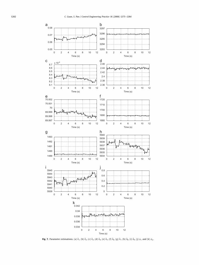
The transient pressures P1 and P2 are shown in Fig. 5, and thecontrol input is shown in Fig. 6. It is seen that they are all boundedand in the permissible capacity scope. Moreover, the control inputis smooth except for in the very short beginning time. All theestimations of parameters are shown in Fig. 7, it is seen thatthough they may not be converged to their true values, they arebounded, and it is their updating during the control process thatmakes the performance of the hydraulic system improve.

ARTICLE IN PRESS

0 2 4 6 8 10 120.05

0.06

0.07

0.08

Time (s)0 2 4 6 8 10 12

3293

3294

3295

3296

3297

Time (s)

0 2 4 6 8 10 128.18.28.38.48.58.68.7

x 10-4

Time (s)0 2 4 6 8 10 12

2.36

2.38

2.4

2.42

2.44

2.46

Time (s)

0 2 4 6 8 10 1269.997

69.998

69.999

70

70.001

70.002

Time (s)0 2 4 6 8 10 12

1680

1690

1700

1710

1720

Time (s)

0 2 4 6 8 10 121489

1490

1491

1492

1493

Time (s)0 2 4 6 8 10 12

5934593559365937593859395940

Time (s)

0 2 4 6 8 10 125939594059415942594359445945

Time (s)0 2 4 6 8 10 12

0

0.2

0.4

0.6

0.8

Time (s)

0 2 4 6 8 10 120.034

0.036

0.038

0.04

0.042

Time (s)

Fig. 7. Parameter estimations. (a) y1, (b) y2, (c) y3, (d) y4, (e) y5, (f) y6, (g) y7, (h) y8, (i) y9, (j) j1 and (k) j2.

C. Guan, S. Pan / Control Engineering Practice 16 (2008) 1275–12841282

ARTICLE IN PRESS

C. Guan, S. Pan / Control Engineering Practice 16 (2008) 1275–1284 1283

5. Conclusion

An adaptive sliding controller has been presented for anelectro-hydraulic system driven by a double-rod actuator withnonlinear uncertain parameters. Both the control structure andthe parameters tuning algorithms are developed for a class ofsystem with nonlinear unknown parameters through the newlychosen Lyapunov function. By combining the sliding mode controland a simple robust method, the adaptive sliding control of theelectro-hydraulic system is presented. The proposed controlmethod can compensate for all system uncertainties from thenonlinear unknown parameters, the linear unknown parameters,and uncertain nonlinearities. The experimental results show thatthe proposed control method and adaptation schemes can obtaina good performance when the position signal trajectories aretracked even if the nonlinear uncertain parameters caused by thevarieties of the original control volumes also exist.

Acknowledgments

This work was supported in part by the China PostdoctoralScience Foundation under Grant 20060401038, the Key Technol-ogies R&D Program of China 2007BAF13B04, and the KeyTechnologies R&D Program of Zhejiang Province, China2006C11148.

Appendix A

Proof of Fact 1. According to (21) and (23), it is clear thats2 2 Os2

¼D½s2mins2max�, thus from Assumption 4, it is known that

sT2f l2ðyÞa0 is guaranteed.

From (23) and adaptation law (21), it is shown that if s2 ¼ s2max

and T2ZðyÞef l2ðyÞ u40, then _s2 ¼ 0 and ~s2 ¼ s2 � s2 ¼ s2�

s2maxp0, thus ~sT2½ZðyÞef l2ðyÞu� T�1

2_s2�p0 is obtained; if s2 ¼

s2min and t2ZðyÞef l2ðyÞuo0, then _s2 ¼ 0 and ~s2 ¼ s2 � s2 ¼

s2 � s2minX0, so ~sT2½ZðyÞef l2ðyÞu� T�1

2_s2�p0 is obtained; in the

other case, it is known that _s2 ¼ T2ZðyÞef l2ðyÞu, so ~sT2½ZðyÞ

ef l2ðyÞu� T�12_s2� ¼ 0, therefore ~sT

2½ZðyÞef l2ðyÞu� T�12_s2�p0 is

always obtained. Hence, conditions (22) are satisfied. &

Appendix B

Proof of Lemma 1. From (24), the time derivative of z(t) is givenas

_zðtÞ ¼

_ _ _

epðtÞ þ 3l€epðtÞ þ 3l2 _epðtÞ þ l3epðtÞ

Define a function (Bouri & Thomasset, 2001) as xðtÞ ¼ epðtÞelt ,then the following equation is obtained:

_ _ _

xðtÞ ¼ _ _ _

epðtÞ þ 3l€epðtÞ þ 3l2 _epðtÞ þ l3epðtÞh i

elt ¼ _zelt (B.1)

Integrating Eq. (B.1), as the following equation is obtained:

€xðtÞ � €xð0Þ ¼ zelt t0� l

Z t

0zelt dt

¼ zðtÞelt � zð0Þ � lZ t

0zelt dt

pMelt þ lM

Z t

0elt dt� zð0Þ

¼ 2Melt � zð0Þ �M

Thus we obtain

€xðtÞp2Melt þ c1 (B.2)

where c1 ¼€xð0Þ � zð0Þ �M.

Similarly, we obtaine

€xðtÞX� 2Melt þ c1 (B.3)

where c1 ¼€xð0Þ � zð0Þ þM.

Integrating (B.2), we obtaine

_xðtÞp2M

lelt þ c1t þ c2

where c2 ¼_xð0Þ � ð2M=lÞ.

Integrating the above inequality, we get

xðtÞp2M

l2elt þ

1

2c1t2 þ c2t þ c3

where c3 ¼ xð0Þ � ð2M=l2Þ.

So

epðtÞ ¼ xðtÞe�ltp2M

l2þ

1

2c1t2 þ c2t þ c3

� �e�lt

Thus, we obtain

limt!1

epðtÞp2M

l2þ lim

t!1

1

2c1t2 þ c2t þ c3

� �e�lt ¼

2M

l2

Similarly, from (B.3), it can be derived that limt!1 epðtÞX

�2M=l2. Therefore, limt!1 jepðtÞjp2M=l2, that is, at t!1,jepðtÞjp2M=l2. &

Appendix C

Proof of Theorem 2. From the adaptation law (28)–(30), and

(23), it is known that j ¼ ½j1; j2�T, ya ¼ ½y1; y2; y3; y4; y5�

T,

and yb ¼ ½y6; y7; y8; y9�T are all bounded.

By substituting controller (27) into (26), the following equationis obtained:

_Vz ¼ � hz2 � z ~y1x1

�þ ~y2x2 þ

~y3x3 þ~y4x1x2 �

~y5x21x2

�þ z ~y6R1 þ

~y7R2 þ~y8R2x1 �

~y9R1x1

� �u

þ z ~j1aþ12z ~j2ðx2zþ 2x1aÞ

� D1ðB1 þ B2Þz2

d� ðb1 þ b2Þd1ðtÞz

� Dz2

d½B1B2 þmaxðB1;B2Þ �maxðL1; L2Þ�

� ðj1 þ j2x1 � x21Þd2ðtÞz (C.1)

where ~yi ¼ yi � yi, i ¼ 1;2; . . . ;9; ~jj ¼ jj � jj, j ¼ 1,2.Define Lyapunov function as

V ¼ Vz þ12~y

T

aG�11~ya þ

12~y

T

bG�12~yb þ

12 ~j

TG�13 ~j

where ~ya ¼ ya � ya, ~yb ¼ yb � yb, and ~j ¼ j� jThe time derivative of V is

_V ¼ _Vz �~y

T

aG�11_ya �

~yT

bG�12_yb � ~jTG�1

3_j (C.2)

Substitute (C.1), the adaptation law (28)–(30) into the aboveEq. (C.2), and from Section 3.2, the following inequation

ARTICLE IN PRESS

C. Guan, S. Pan / Control Engineering Practice 16 (2008) 1275–12841284

is obtained:

_Vp� hz2 � D1ðB1 þ B2Þz2

d� ðb1 þ b2Þd1ðtÞz

� D2z2

d½B1B2 þmaxðB1;B2Þ �maxðL1; L2Þ�

� ðj1 þ j2x1 � x21Þd2ðtÞz (C.3)

Let D ¼ D2½B1B2 þmaxðB1;B2Þ �maxðL1; L2Þ�.From (11) and (12) and Assumption 2, it is clear that if jzjXd,

then �D1ðB1 þ B2Þðz2=dÞ � ðb1 þ b2Þd1ðtÞzp0 and �ðDz2=dÞ � ðj1þ

j2x1 � x21Þd2ðtÞzp0. So is _Vp� hz2p0, then jzj converges to be

within bounded d, that is, jzjpd, in finite time. Hence, fromLemma 1, it can be obtained that jepðtÞjp2d=l2, at t-N. &

References

Alleyne, A., & Liu, R. (2000). A simplified approach to force control for electro-hydraulic systems. Control Engineering Practice, 8, 1347–1356.

Bonchis, A., Corke, P. I., Rye, D. C., & Ha, Q. P. (2001). Variable structure methods inhydraulic servo systems control. Automatica, 37, 589–595.

Bouri, M., & Thomasset, D. (2001). Sliding control of an electropneumatic actuatorusing an integral switching surface. IEEE Transactions on Control SystemsTechnology, 9(2), 368–375.

Bu, F., & Yao, B. (2001). Desired compensation adaptive robust control of single-rodelectro-hydraulic actuator. In Proceedings of the American control conference,Arlington, pp. 3927–3931.

Duraiswamy, S., & Chiu, G.T.-C. (2003). Nonlinear adaptive nonsmooth dynamicsurface control of electro-hydraulic systems. In Proceedings of the Americancontrol conference, Denver, Colorado, pp. 3287–3292.

Garagic, D., & Srinivasan, K. (2004). Application of nonlinear adaptive controltechniques to an electrohydraulic velocity servomechanism. IEEE Transactionson Control Systems Technology, 12(2), 303–314.

Guan, C., & Zhu, S. (2004). Adaptive time-varying sliding mode control forhydraulic servo system. In International conference on control, automation,robotics and vision, China, pp. 1774–1779.

Merritt, H. E. (1967). Hydraulic control systems. New York: Wiley.Hisseine, D. (2005). Robust tracking control for a hydraulic actuation system. In

IEEE conference on control applications, Canada, pp. 422–427.Hong, L., Kil, T. C., Tae, S. N., & Yeong, Y. S. (2003). Vehicle longitudinal brake control

using variable parameter sliding control. Control Engineering Practice, 11(4),403–411.

Lee, S. U., & Chang, P. H. (2002). Control of a heavy-duty robotic excavator usingtime delay control with integral sliding surface. Control Engineering Practice, 10,697–711.

Li, G., & Khajepour, A. (2005). Robust control of a hydraulically driven flexible armusing backstepping technique. Journal of Sound and Vibration, 280, 759–775.

Liu, R., & Alleyne, A. (2000). Nonlinear force/pressure tracking of an electro-hydraulic actuator. ASME Journal of Dynamic Systems, Measurement and Control,122, 232–237.

Liu, S., & Yao, B. (2003). Indirect adaptive robust control of electro-hydraulicsystems driven by single-rod hydraulic actuator. In Proceedings of the IEEE/ASME international conference on advanced intelligent MeChalroniCS (AIM ZW3),pp. 296–301.

Liu, Y., & Handroos, H. (1999). Technical note sliding mode control for a class ofhydraulic position servo. Mechatronics, 9(1), 111–123.

Kim, M. Y., & Lee, C.-O. (2006). An experimental study on the optimization ofcontroller gains for an electro-hydraulic servo system using evolutionstrategies. Control Engineering Practice, 14(2), 137–147.

Popov, M. V. (1973). Hyperstability of control systems. New York: Springer.Raade, J. W., & Kazerooni, H. (2005). Analysis and design of a novel hydraulic power

source for mobile robots. IEEE Transactions on Automation Science andEngineering, 2(3), 226–232.

Re, L. D., & Isidori, A. (1995). Performance enhancement of nonlinear drives byfeedback linearization of linear–bilinear cascade models. IEEE Transactions onControl Systems Technology, 3(2), 299–308.

Shol, G. A., & Bobrow, J. E. (1999). Experimental and simulations on the nonlinearcontrol of a hydraulic servo system. IEEE Transactions on Control SystemsTechnology, 7(1), 238–247.

Tazafoli, S., de Silva, C. W., & Lawrence, P. D. (1998). Tracking control of anelectrohydraulic manipulator in the presence of friction. IEEE Transactions onControl Systems Technology, 6(3), 401–411.

Vossoughi, R., & Donath, M. (1995). Dynamic feedback linearization for electro-hydraulically actuated control systems. ASME Journal of Dynamic Systems,Measurement and Control, 117(4), 468–477.

Wu, M. C., & Shih, M. C. (2003). Simulated and experimental study of hydraulicanti-lock braking system using sliding-mode PWM control. Mechatronics, 13,331–351.

Yao, B., Bu, F., & Chiu, G. T. C. (1998). Nonlinear adaptive robust control of electro-hydraulic servo systems with discontinuous projections. Proceedings of the IEEEConference on Decision and Control, 2265–2270.

Yao, B., Bu, F., Reedy, J., & Chiu, G. T. C. (2000). Adaptive robust motion control ofsingle-rod hydraulic actuators: Theory and experiments. IEEE/ASME Transac-tions on Mechatronics, 5(1), 79–91.

Shi, Z., Gu, F., Lennox, B., & Ball, A. D. (2005). The development of an adaptivethreshold for model-based fault detection of a nonlinear electro-hydraulicsystem. Control Engineering Practice, 13(11), 1357–1367.

Zhu, W. H., & Piedboeuf, J. C. (2005). Adaptive output force tracking control ofhydraulic cylinders with applications to robot manipulators. ASME Journal ofDynamic Systems, Measurement and Control, 127, 206–217.