Advanced fractal approach for unsupervised classification of SAR images

$: Advanced fractal approach for unsupervised classification of SAR images$
Available online at www.sciencedirect.com

www.elsevier.com/locate/asr

Advances in Space Research 45 (2010) 1338–1349

Advanced fractal approach for unsupervised classificationof SAR images

Triloki Pant a, Dharmendra Singh b,*, Tanuja Srivastava a

a Department of Mathematics, Indian Institute of Technology Roorkee, Indiab Department of Electronics and Computer Engineering, Indian Institute of Technology Roorkee, India

Received 10 December 2008; received in revised form 30 November 2009; accepted 7 January 2010

Abstract

Unsupervised classification of Synthetic Aperture Radar (SAR) images is the alternative approach when no or minimum apriori infor-mation about the image is available. Therefore, an attempt has been made to develop an unsupervised classification scheme for SARimages based on textural information in present paper. For extraction of textural features two properties are used viz. fractal dimensionD and Moran’s I. Using these indices an algorithm is proposed for contextual classification of SAR images. The novelty of the algorithmis that it implements the textural information available in SAR image with the help of two texture measures viz. D and I. For estimationof D, the Two Dimensional Variation Method (2DVM) has been revised and implemented whose performance is compared with anothermethod, i.e., Triangular Prism Surface Area Method (TPSAM). It is also necessary to check the classification accuracy for various win-dow sizes and optimize the window size for best classification. This exercise has been carried out to know the effect of window size onclassification accuracy. The algorithm is applied on four SAR images of Hardwar region, India and classification accuracy has been com-puted. A comparison of the proposed algorithm using both fractal dimension estimation methods with the K-Means algorithm is dis-cussed. The maximum overall classification accuracy with K-Means comes to be 53.26% whereas overall classification accuracy withproposed algorithm is 66.16% for TPSAM and 61.26% for 2DVM.� 2010 COSPAR. Published by Elsevier Ltd. All rights reserved.

Keywords: Fractal dimension; Moran’s I; SAR image classification; Unsupervised classification

1. Introduction

Classification of satellite images is an essential process toidentify different land classes. Different land classes havedifferent properties based on which they may be identifiedand hence classified, e.g., water, agricultural area, urbanarea, forest etc. All these classes can be identified accordingto their spectral properties, which vary with the imagerysystem, i.e., the spectral properties for aerial photographare different than thermal image, which are again differentin microwave imagery. SAR images are the preferred satel-lite images for analysis purposes due to their all weather

0273-1177/$36.00 � 2010 COSPAR. Published by Elsevier Ltd. All rights rese

doi:10.1016/j.asr.2010.01.008

* Corresponding author.E-mail address: [email protected] (D. Singh).

and all time availability (Acqua and Gamba, 2003; Lille-sand and Kiefer, 2002; Oliver, 2000; Rajesh et al., 2001).

1.1. SAR image analysis

The spectral property for SAR images is determined bythe backscattered signal that is simply the back reflectedpart of the microwaves scattered from the land cover. Sincethe backscattered signal is very weak, it is very difficult todistinguish different land classes in SAR images. Radarbackscatter is affected by different surface properties andusing Rayleigh criterion of scattering, surfaces can be con-sidered as rough or smooth (Lillesand and Kiefer, 2002).The roughness of surface causes a variation in backscatter-ing and hence variation in image texture. The inverse mod-eling, i.e., variation of texture can be used to categorize the

rved.

http://dx.doi.org/10.1016/j.asr.2010.01.008

mailto:[email protected]

T. Pant et al. / Advances in Space Research 45 (2010) 1338–1349 1339

surface roughness and hence to classify the SAR images.However, the problems with single band and single polar-ization SAR images also exist. The first one is the singleband information, which makes the SAR images to bespectrally poor, i.e., the single band of SAR does not pro-vide much visual information as it shows only gray tones(Chamundeeswari et al., 2007; Lillesand and Kiefer, 2002;Wu and Linders, 1999). Thus for single band SAR image,it is customary to estimate other features from the imageitself. For example, local statistics, texture information,shape of the objects can be used for feature generation(Davidson et al., 2006; Wu and Linders, 1999). The secondproblem is the inherent speckle noise, which plays a vitalrole in information extraction from SAR images (Hender-son and Lewis, 1998; Lillesand and Kiefer, 2002; Ulabyet al., 1986).

Classification of SAR images can be performed in eitherof the two approaches, viz. Supervised and Unsupervisedclassification (Lillesand and Kiefer, 2002). The single bandinformation again comes into the picture as most of theclassification algorithms are based on multiband imagesand for single band SAR images they lack the number offeatures. As obvious, speckle noise plays a dominant rolein classification too. Due to speckle noise, it is difficult toclassify the SAR image based on the pixel values sincespeckle makes various pixels to be mixed and hence pro-vides an ambiguous classification (Henderson and Lewis,1998). Although speckle noise makes it a tedious task toextract the information from SAR images, it makes themrich in texture and this textural information can beobtained in various ways from SAR images (Chamundees-wari et al., 2007; Lillesand and Kiefer, 2002; Rajesh et al.,2001; Ulaby et al., 1986). In order to utilize the texturalinformation due to speckle, we have directly worked onspeckled images. Further, texture is a context dependentproperty (Wu and Linders, 1999) and texture based classi-fication is the contextual classification rather than per pixelclassification (Lillesand and Kiefer, 2002; Petrou and Sevil-la, 2006). The richness of texture in SAR images is highlyappreciated by many researchers because texture informa-tion is relevant to characterize various regions, e.g., waterbodies, vegetation, built up area (Rajesh et al., 2001; Ulabyet al., 1986).

Textural analysis of SAR images can be performed by anumber of parameters according to the application orusers’ requirements. Commonly used parameters are Co-occurrence Matrix, Fourier Spectrum, Fractals, Autocorre-lation function, Gabor Function, Run Length Measure etc.(Petrou and Sevilla, 2006; Rajesh et al., 2001; Sun et al.,2006; Wu and Linders, 1999), where each parameter hasits own advantages and limitations. For example, Co-occurrence Matrix corresponds to joint pdf used to charac-terize the image statistics, Fourier Spectrum deals with thespatial frequency. Fractals are used to model the imagesand measure their roughness and the Autocorrelation func-tion can be used either as a signature or to characterize tex-ture by inferring the periodicity of the texture. Gabor

functions use the spatial frequency for textural analysisof images, for this purpose Fourier transform is used andthe frequency space is tessellated into rectangular bands.Among these parameters we have used Fractal and SpatialAutocorrelation for texture analysis of SAR images. Thefractal approach directly deals with roughness of the sur-face and it measures the roughness with the renowned mea-sure, i.e., fractal dimension. The fractal dimension forsurfaces varies between 2.0 and 3.0 showing the roughnessincrement with its increasing values, i.e., the surface withfractal dimension 2.0 is ideally smooth whereas with 3.0is highly complex (Pentland, 1984; Sun et al., 2006).Another measure of texture considering spatial statisticsis spatial autocorrelation index, i.e., Moran’s I, which mapsthe pixel association in the range �1 to +1. An unsuper-vised clustering algorithm proposed by Tasoulis andVrahatis (2006) utilizes the fractal dimension for movementand enlargement of the cluster window as well as for merg-ing of the windows. In their approach the fractal dimensionis the distinguishing factor to generate various clusterswhereas in present approach fractal dimension along withMoran’s I has been analyzed and used for classificationof various land covers in SAR images. Since it is difficultto differentiate various land classes using fractal dimensionalone, another contextual feature viz. spatial autocorrela-tion index (Moran’s I) has been used to aid fractal dimen-sion for classification. Still D and I used for SAR imageclassification is not very much reported in the literature.Therefore in this paper we have attempted to critically ana-lyze the effect of D and I on SAR image classification.

The paper is organized in seven sections. Section 2describes the fractal approach for SAR image analysis.The importance of fractal dimension for image analysis isdiscussed and two methods of fractal dimension estimationare depicted in modified form. The issues related to fractaldimension and its estimation techniques are also distin-guished. Section 3 covers the spatial autocorrelation indexviz. Moran’s I for textural classification of SAR images.The methodology for estimation of Moran’s I and therelated issues are also discussed. The details of data usedare given in Section 4 and the proposed methodology forcontextual classification is described in Section 5. Section6 contains the results and discussion and finally the paperis concluded in Section 7.

2. Fractal approach for SAR image analysis

It is widely known that fractals are best suited for natu-ral surface modeling (De Jong and Burrough, 1995; Fal-coner, 2003; Keller et al., 1987; Lee et al., 2005;Mandelbrot, 1982; Pentland, 1984; Sun et al., 2006). Natu-ral objects and surfaces are so complex that the traditionalEuclidean objects viz. lines, circles, cones etc. are not ableto represent them (De Cola, 1989; Emerson et al., 2005;Mandelbrot, 1982; Pentland, 1984). This lack was filledby introduction of fractal geometry. In fact the more inter-est behind fractal surfaces and modeling of natural surfaces

1340 T. Pant et al. / Advances in Space Research 45 (2010) 1338–1349

with fractal approach is evolved after introduction of frac-tal geometry. Particularly in satellite imagery fractalapproach is taking more attention and it is helpful in var-ious applications (De Cola, 1989; De Jong and Burrough,1995; Pentland, 1984; Read and Lam, 2002; Sun et al.,2006). In order to apply fractal geometry to natural imageanalysis, Pentland (1984) had proposed that natural sur-faces can be modeled with the fractional Brownian motion(fBm) function (Pentland, 1984). The image intensity I(x,

y) follows the condition of fBm, given by

PrIðxþ Dx; yÞ � Iðx; yÞ

kDxkH < z

" #¼ F ðzÞ ð1Þ

where F(z) is the cdf and 0 < H < 1 is the Hurst parameter.In fact the height difference, i.e., I(x + h, y + k) � I(x, y)

follows the normal distribution with zero mean and vari-ance (h2 + k2)H and hence the fractional Brownian surfacesare defined (Falconer, 2003) as

P ðIðxþ h; y þ kÞ � Iðx; yÞ � zÞ

¼ 1ffiffiffiffiffiffi2pp ffiffiffiffiffiffiffiffiffiffiffiffiffiffiffiffiffiffiffiffiffi

ðh2 þ k2ÞHq Z z

�1exp

�r2

2ðh2 þ k2ÞH

!dr ð2Þ

The term fractal, coined by B.B. Mandelbrot, is definedto be a mathematical set having two basic characteristics,viz. self-similarity and fractal dimension (Mandelbrot,1982). Self-similarity, also called scale independence (Pent-land, 1984), means any part of the fractal is exactly similarto the whole at any magnification or reduction level. Onemajor fact about self-similarity of natural scenes is thatthey are not true self-similar rather they are statisticallyself-similar. This point is obvious because natural scenesare similar to another at some extent but they are notexactly same. Again, it was pointed out by Mandelbrot thatnatural objects show the self-similar behavior up to fourthor fifth level (Mandelbrot, 1982). But in present study wehave not exercised with scaling behavior of the image.

The second property of fractals, i.e., fractal dimension isthe measure of complexity of the fractal, however, now it iswidely accepted that the exact definition of the fractaldimension does not exist (Falconer, 2003). Nevertheless,the self-similarity dimension is considered as the fractaldimension, which is defined by Mandelbrot (Mandelbrot,1982) as

D ¼ logðNrÞlog 1

r

� � ð3Þ

where Nr represents the number of similar parts of an ob-ject scaled down by the ratio r.

Fractal dimension is of more interest for image analysisin terms of roughness estimation. The basic thing is thatfractal dimension gives an idea of roughness and usinglocal fractal dimension, we can get the value of roughnessat local level. As it is very common to say rough, veryrough, highly rough and so on for various land classes; thisterminology ends with D values which map these terms into

a range between 2.0 and 3.0 for two dimensional images(Pentland, 1984; Sun et al., 2006). In fact local variationsin computed D values can be used as texture measure tosegment images. The basic idea is that various land covertypes may have their characteristic texture and their rough-ness could be described by the D values. D could be consid-ered as the fractal signature of the land cover types if therewere a one to one relation between the land cover textureand a unique D value (Peleg et al., 1984; Sun et al.,2006). However, this fact is only hypothetical because frac-tal dimension is not a unique feature, i.e., it can notuniquely identify different fractals (Falconer, 2003; Man-delbrot, 1982; Sun et al., 2006).

The local fractal map provides a textured image of theoriginal image which is dependent on the size of local win-dow. Using various window sizes, different types of tex-tures are obtained. It is useful for our study in comparingdifferent textures based on local window size. Some ofthe features are highlighted for a particular window size.It is interesting to find out such features and hence theappropriate window size. It is important to note that thisevent is not useful for overall classification but used foridentification of some particular area or point in the imagebased on its neighboring pixel arrangements. For ourexperiment this property is used to identify the canal area.

In order to estimate the fractal dimension of surfaces anumber of methods exist, viz. Box counting method (Kelleret al., 1989; Pentland, 1984), Triangular Prism SurfaceArea Method (TPSAM) (Clarke, 1986; De Jong and Bur-rough, 1995; Emerson et al., 2005; Jaggi et al., 1993; Readand Lam, 2002; Sun, 2006; Sun et al., 2006), Variogrammethod (Berizzi et al., 2006; De Jong and Burrough,1995; Jaggi et al., 1993; Sun et al., 2006), Isarithm method(Berizzi et al., 2006; Jaggi et al., 1993), Fourier spectrummethod (Pentland, 1984), Two Dimensional variationmethod (2DVM) (Berizzi et al., 2006). Among these meth-ods, the most famous and widely used method is TPSAM,which has been modified by a number of researchers(Emerson et al., 2005; Sun, 2006; Sun et al., 2006). Besidesthis method, we have chosen 2DVM for our analysis. It isrecently developed method for fractal dimension estima-tion. The advantages of the chosen methods for presentstudy over other methods are their feasibility and simplicitysince the methods are easy to implement (Berizzi et al.,2006; Clarke, 1986; Sun et al., 2006).

2.1. Triangular prism surface area method (TPSAM)

It is the most widely known method for estimating frac-tal dimension which was proposed by K.C. Clarke (Clarke,1986; De Jong and Burrough, 1995; Emerson et al., 2005;Jaggi et al., 1993; Read and Lam, 2002; Sun, 2006; Sunet al., 2006). The image pixels are considered as columnshaving heights equal to their digital number value. Thepixel columns are considered for generating the prism in3D space with four pixels at four corners and their averageas the central pixel. These five points generate four triangu-


lar prisms in 3D space, whose upper surface areas are esti-mated and added to obtain the whole surface area. There-after the surface area is estimated for different basesgenerated by corner pixels values, which keeps track withthe resolution of base of triangular prism area. For differ-ent values of base resolution, total surface area is estimatedand plotted against the base area in a log–log scale. The

oscKeðn;mÞ ¼ supjn0j�Ke

jm0j�Ke

½zðnþ n0;mþ m0Þ� � infjn0j�Ke

jm0j�Ke

½zðnþ n0;mþ m0Þ�;

Ke � n � Nx � Ke; Ke � m � Ny � Ke

oscKeðn;mÞ ¼ oscKeðKe;KeÞ; 1 � n < Ke; 1 � m < Ke

oscKeðn;mÞ ¼ oscKeðKe;mÞ; 1 � n < Ke; Ke � m � Ny � Ke

oscKeðn;mÞ ¼ oscKeðn;KeÞ; Ke � n � Nx � Ke; 1 � m < Ke

oscKeðn;mÞ ¼ oscKeðNx � Ke;mÞ; N x � Ke < n � Nx; Ke � m � N y � Ke

oscKeðn;mÞ ¼ oscKeðn;Ny � KeÞ; Ke � n � Nx � Ke; Ny � Ke < m � N y

oscKeðn;mÞ ¼ oscKeðNx � Ke;Ny � KeÞ; N x � Ke < n � Nx; N y � Ke < m � Ny

377777777777777777775

ð5Þ

R1 R2 R3

(1,1)

Kε

Kε

Ny-Kε

Nx-Kε

slope of the least square fit line is subtracted from 2.0 tocalculate the fractal dimension, i.e.

D ¼ 2:0� Slope ð4Þ

The total surface area decreases as the base resolutionincreases (Clarke, 1986; Emerson et al., 2005), the slopecomes to be negative in general and hence the value of D

becomes greater than 2.0. The base resolution is increasedin power of 2 in original method, i.e., 1, 2, 4, 16, and soon. However, the method has been modified by consideringall base resolutions, i.e., 1, 2, 3, and so on for better cover-age of all pixels (Emerson et al., 2005; Sun et al., 2006). Forour study, we have considered the modified TPSA methodand used the term TPSAL for the method. The method isbased on the variation of pixel values in 3D space in termsof the surface area showing the distribution of image points.The pixel values showing low variation correspond tosmooth surface and thus give high value of slope and conse-quently low fractal dimension. Using local moving windowapproach, the fractal dimension is estimated for local neigh-borhoods with TPSAL method. The corresponding fractalmaps are also generated, which are used for classification.

R4 R5 R6

R7 R8 R9

(Nx,Ny)

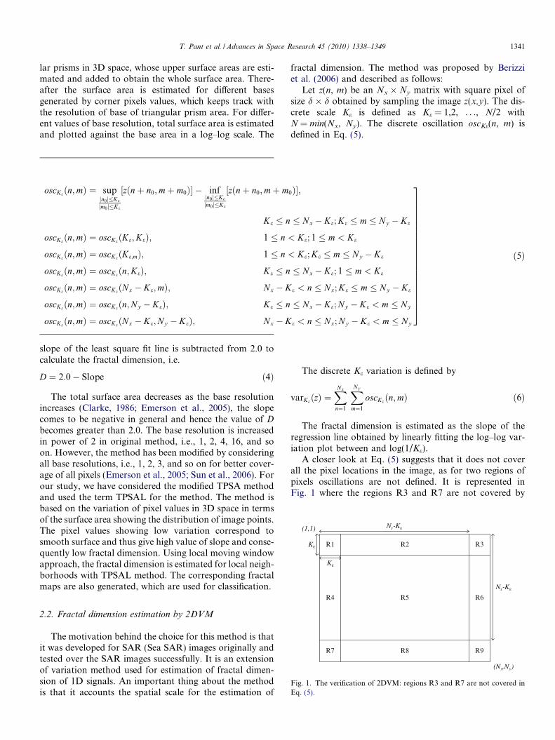
Fig. 1. The verification of 2DVM: regions R3 and R7 are not covered inEq. (5).

2.2. Fractal dimension estimation by 2DVM

The motivation behind the choice for this method is thatit was developed for SAR (Sea SAR) images originally andtested over the SAR images successfully. It is an extensionof variation method used for estimation of fractal dimen-sion of 1D signals. An important thing about the methodis that it accounts the spatial scale for the estimation of

fractal dimension. The method was proposed by Berizziet al. (2006) and described as follows:

Let z(n, m) be an Nx � Ny matrix with square pixel ofsize d � d obtained by sampling the image z(x,y). The dis-crete scale Ke is defined as Ke = 1,2, . . ., N/2 withN = min(Nx, Ny). The discrete oscillation oscKe(n, m) isdefined in Eq. (5).

The discrete Ke variation is defined by

varKeðzÞ ¼XNx

n¼1

XNy

m¼1

oscKeðn;mÞ ð6Þ

The fractal dimension is estimated as the slope of theregression line obtained by linearly fitting the log–log var-iation plot between and log(1/Ke).

A closer look at Eq. (5) suggests that it does not coverall the pixel locations in the image, as for two regions ofpixels oscillations are not defined. It is represented inFig. 1 where the regions R3 and R7 are not covered by


the Eq. (5). We have therefore added the two remainingequations in the oscillation Eq. (5) which are as following:

oscKe ðn;mÞ¼ oscKeðKe;N y�KeÞ;1� n<Ke;N y�Ke<m�N y

oscKe ðn;mÞ¼ oscKeðN x�Ke;KeÞ;N x�Ke< n�N x;1�m<K e

�ð7Þ

Thus, the complete oscillation equations are given byEqs. (5) and (7). Using moving window approach, the localfractal dimension is estimated with 2DVM and corre-sponding fractal maps are used for classification purpose.

2.3. Issues related to fractal dimension and its estimation

methods

There are few major issues related to fractal dimensionand the dimension estimation methods which are faced inpresent study. The first issue about fractal dimension is thatit is not unique for all the fractals, i.e., two or more differ-ent fractals may have same value of fractal dimension. Thefractals differ in their construction property as well as inorientation, yet may have same value of fractal dimension,e.g. the well known Koch’s snowflake generated by its clas-sical generation rule and random fractal generation rule aretwo different fractals by orientation, however their fractaldimension is same (Falconer, 2003; Mandelbrot, 1982). Insuch cases, the fractal dimension is used for measuringthe complexity of the fractals and does not create the prob-lem, however, for classification or identification purposes,direct use of fractal dimension is not preferred; rather, localfractal dimension is used.

Another issue is related to the methods used for fractaldimension estimation. There are a number of methods forestimation of fractal dimension of images. All the methodsuse the spatial coordinates for the scaling purpose and thepixel values for estimation of fractal dimension. However,different methods estimate different values of fractal dimen-sion of same surface as observed by a number of research-ers (De Jong and Burrough, 1995; Emerson et al., 2005;Jaggi et al., 1993; Pentland, 1984).

The TPSAM is sensitive to contrast stretching (Emer-son et al., 2005; Sun, 2006) as well as to scale used. Themodified method (Emerson et al., 2005; Sun et al., 2006)used as TPSAL in present study is a better approachtoward the problem of scale used. The method considersall the step values, i.e., 1, 2, 3 and so on for estimation tocover all scales but it consumes extra time incomputation.

Finally, the theoretical value of D lies in the range 2.0–3.0, however, its practical values flow away from the spec-ified range, i.e., for some images, the value of D is calcu-lated to be less than 2.0 while for some images it comesto be greater than 3.0. The out of bound values are dueto the least square estimation of the slope in log–log scaleas used in D estimation methods. These outflowing valuesapprove the fact that satellite images are not true fractals;however they resemble to the fractals. The out of boundvalues, however, do not affect much the fractal analysisof the images (Sun et al., 2006).

3. Spatial autocorrelation (Moran’s I) for contextual

information

The fractal dimension alone is not enough for clusteringin land cover classification; therefore another measure oftexture accounting the spatial association is introduced toaid fractal dimension. The spatial association of pixels isan important issue for contextual information, which canbe measured with the help of spatial autocorrelation index.Spatial autocorrelation index maps the pixel clusteringproperties in a fixed range and based on that range, theassociation can be explained. As obvious, a number of spa-tial autocorrelation indices are in vogue, viz. Moran’s I,Geary’s C (Emerson et al., 2005; Lloyd, 2007; Myint,2003; Read and Lam, 2002), yet Moran’s I is the dominantone. Moran’s I is defined by following formula:

I ¼nPn

i¼1

Pnj¼1wijðzi � �zÞðzj � �zÞPn

i¼1

Pnj¼1wij

Pni¼1ðzi � �zÞ2

ð8Þ

where n is the number of pixels in the image, i.e., numberof pixels in local neighborhood, w is spatial proximitymatrix whose weights wij are determined using neighbor-hood properties. We have used Queen’s case for determin-ing the values, which considers the 8-neighbor connectivityof pixels. Further, z is the pixel intensity and �z is the meanof all pixel values. The single suffixed z, i.e., zi representsthe pixel values considered in a linear row wise fashionso that for each pixel other image pixels are tested for 8-neighbor connectivity.

Moran’s I can be estimated either globally or locallyaccording to the application requirement (Lloyd, 2007).The global value of I represents mutual association of allthe pixels in image, which is not of much interest for clas-sification purposes. As the image size grows, global I

becomes less important. On the other hand, local I givesthe information about the association of pixels in smallerneighborhoods which is important for image classification.Again, local I depends on the size of neighborhood as wellas on the selection of neighboring pixels, e.g., m-neighbor-hood. In order to decide the neighborhood type differentcases are to be considered, e.g., Rook’s case, Bishop’s caseand Queen’s case which implement 4-neighborhood, diago-nal neighborhood (d-neighborhood) and 8-neighborhoodrespectively. It is obvious that selection of neighborhoodand hence the connectivity case is important and affectsthe value of I.

The value of I lies between �1 and +1 such that thepositive value shows higher association of neighboring pix-els and negative value shows opposite association of thepixels. The value 0 indicates no association, i.e., a randomsequence of pixels (Emerson et al., 2005; Lloyd, 2007; Readand Lam, 2002). However, selection of connectivity doesnot affect the range of I and for each case it lies betweenthe specified range. The use of Moran’s I is motivated asit gives this contextual association in a fixed range, i.e.,�1 to +1 and thus provides a scale for measuring the affil-


iation of pixels. However, the index is image dependentbecause an image having high variation of pixel values willshow a random sequence of I values, while an image havingfine textural structure will show a better grouping in termsof I. If the values of I vary randomly, it is difficult to con-clude something significant at on go.

3.1. Importance of Moran’s I for classification

As discussed earlier, Moran’s I is the measure of contex-tual association of pixels and this association is representedin the range [�1, +1]. The positive value of I representsgood association of pixels, i.e., the pixels with higher valueof I belong to same class, while the pixels with negative val-ues of I represent opposite association. Here the term pixelsrepresents the local neighborhood of pixels instead of indi-vidual pixels. The importance of I for classification lies inthe fact that the pixels having higher positive values of Ibelong to same class and hence this fact is useful for iden-tifying various clusters based on I values. Although, thepixels showing higher value of I belong to same class, itis not necessary that the class is unique one, i.e., the samevalue of I may indicate the pixels of two different classes.This fact is similar to that of fractal dimension, where thepixels showing same fractal dimension may belong to dif-ferent classes. Using the values of I clustering is performed,where the cluster centers are generated by choosing I valuesand then clusters are labeled by the classes identified fromground truth data. Further, I values are combined withpixel values as well as with D values for generating com-bined textural maps. The combined texture images aremore informative than the SAR image as well as individualtextural images.

4. Data used

For the current study we have used three ERS-2 SARimages and one ALOS PALSAR image of Hardwar (Utta-rakhand, India) and surrounding area. All the ERS-2images are C band (5.3 GHz) images taken with VV polar-ization having the spatial resolution 12.5 m. The slope ofthe terrain in less than 4�, therefore DEM correction isnot carried out. The three images are of dates July 2001,

Fig. 2. The data set used: (a) the SAR Image

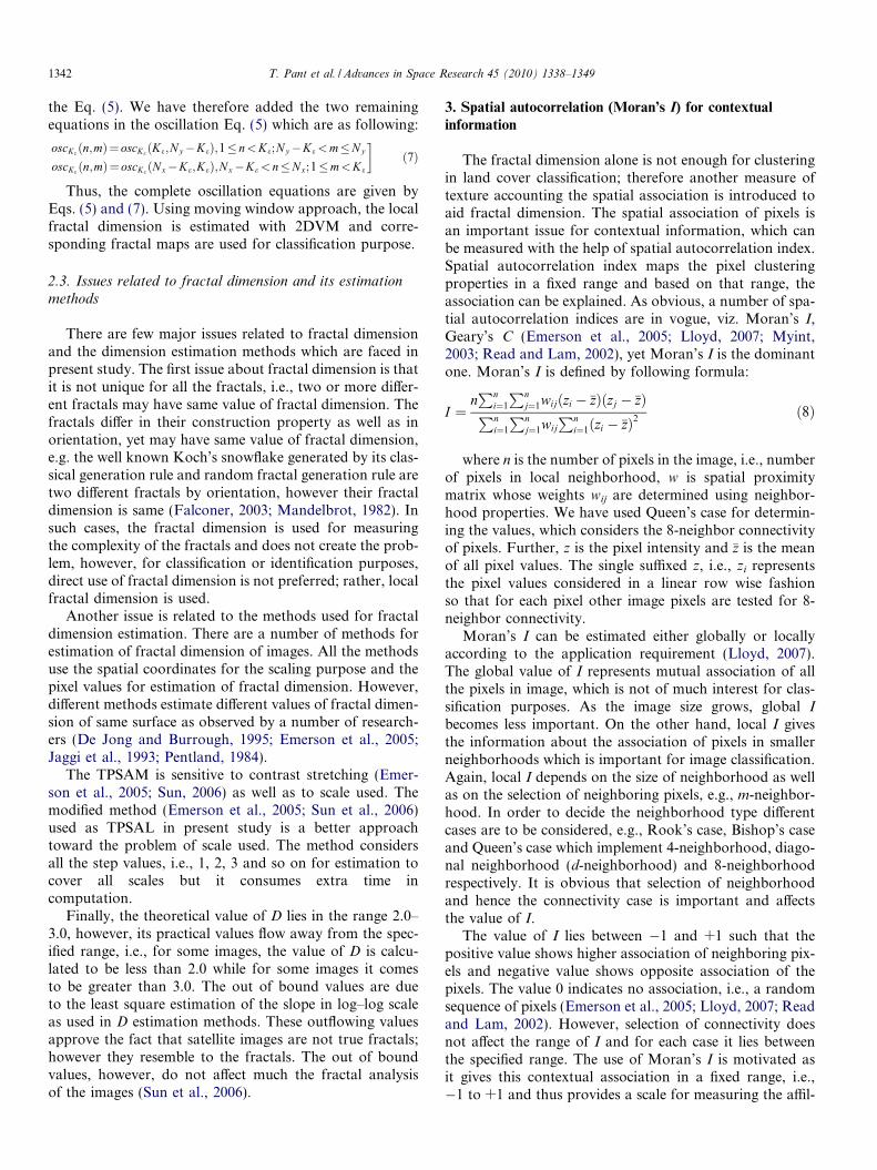
July 2003 and March 2004. Further, we have considereda subset of the images covering the city Roorkee (Uttarak-hand, India) and surrounding area with 303 � 379 pixelsfor the study. We name three subimages SImage1, SIm-age2, and SImage3, which represent the images of year2001, 2003, and 2004, respectively. The images lie betweenlongitudes 77.807�E and 77.901�E and latitudes 29.890�Nand 29.850�N. The PALSAR image is full polarimetric, Lband (1.27 GHz) image having spatial resolution of 25 m.The image is of year 2007 and named as SImage4. Theimage subset between longitudes 77.862�E and 77.918�Eand latitudes 29.896�N and 29.845�N is used for the study.Finally, for classification accuracy assessment purposes, wehave used the topographic map of the same region. Theimages SImage1 and corresponding reference topographicmap are shown in Fig. 2.

5. Proposed methodology for contextual classification

Many of the researchers have used fractal dimension (D)for classification of satellite images in a supervised manner– De Cola (1989), De Jong and Burrough (1995), Read andLam (2002) etc. are among them. As their results show, D

had been estimated for known classes and used as a feature(De Cola, 1989; De Jong and Burrough, 1995; Emersonet al., 2005). De Jong and Burrough (1995) made a signif-icant effort, who estimated the local fractal dimension ofdifferent known classes, i.e., in a supervised approach (DeJong and Burrough, 1995). Further, De Cola (1989) hadused it as post classification matching (De Cola, 1989),where the classification results are further refined usingfractal dimension information. The noticeable thing inthese classification strategies is their classification accuracy,which is significant in such supervised approaches. Anunsupervised scheme, on the other hand, requires one ormore features e.g., the pixel intensity, to identify differentobjects in the image uniquely without having any aprioriinformation. We have applied local fractal dimension onimages and then made an attempt to identify various clas-ses on the basis of D values, i.e., D is considered as theidentifying feature. For this purpose, K-Means classifieris used where the identifying feature is D rather than tradi-tional pixel values. This attempt is important one because it

and (b) the reference topographic map.


is widely known that the fractal dimension is not a uniquevalue to identify the fractals (Falconer, 2003; Mandelbrot,1982), which is also verified by our results. We also turnour attention toward spatial autocorrelation along withfractal dimension. In order to estimate the spatial autocor-relation, we are using Moran’s I as the autocorrelationindex. It is important to note that Moran’s I itself is notenough to classify remotely sensed data, which is mainlydue to its non-uniqueness. Still use of Moran’s I for classi-fication is of interest for our problem, the reasons are �first, the contextual information and second the I-map,i.e., an image having all the values in the range [�1, +1]representing the pixels’ association value.

The proposed methodology is as following:First step requires selection of local window size. We

have chosen the local window to be of odd size, i.e.,5 � 5, 7 � 7, and so on till 15 � 15 (De Jong and Burrough,1995).

In second step local fractal dimension and local Moran’sI are estimated for these window sizes and correspondingD-map and I-map are generated, which are shown inFig. 3. For each D-map, clustering is performed for fourdifferent classes using D values and then these classes arelabeled using reference map, which are Water, Urban,Agriculture and Others; the class Others includes rest ofthe land classes. The next step used as the sub-step of pre-vious one considers the I-map for clustering. Based on I

values, the clusters are generated using K-Meansalgorithm.

In third step, the D values are combined with the imageand the combination of these two features, i.e., pixel valuesand D values are used for clustering. For the compatibilityof sizes, the original image is resized to be equal to that offractal map. The image comprising the pixel values andfractal dimension values highlight some features clearly.For example, the linear objects like canal area are easilyidentified with its edges because fractal dimension is sensi-tive to sharp changes in land features. By addition of frac-tal dimension to the pixel values, both the originalinformation and the textural information are availablefor land feature identification. Thus, the clustering basedon pixel values combined with D values is better than thatof individual D values. The next sub-step includes the com-bination of pixel values with I values. In this step the addi-

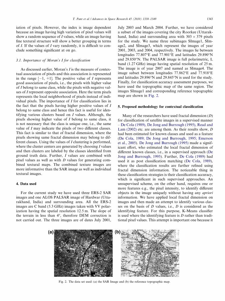
Fig. 3. D-Map (a) with TPSAL, (b) with 2DVM

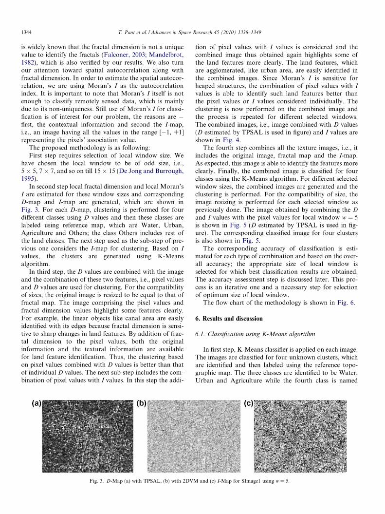
tion of pixel values with I values is considered and thecombined image thus obtained again highlights some ofthe land features more clearly. The land features, whichare agglomerated, like urban area, are easily identified inthe combined images. Since Moran’s I is sensitive forheaped structures, the combination of pixel values with Ivalues is able to identify such land features better thanthe pixel values or I values considered individually. Theclustering is now performed on the combined image andthe process is repeated for different selected windows.The combined images, i.e., image combined with D values(D estimated by TPSAL is used in figure) and I values areshown in Fig. 4.

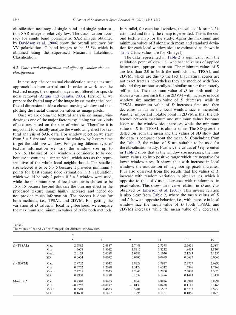
The fourth step combines all the texture images, i.e., itincludes the original image, fractal map and the I-map.As expected, this image is able to identify the features moreclearly. Finally, the combined image is classified for fourclasses using the K-Means algorithm. For different selectedwindow sizes, the combined images are generated and theclustering is performed. For the compatibility of size, theimage resizing is performed for each selected window aspreviously done. The image obtained by combining the Dand I values with the pixel values for local window w = 5is shown in Fig. 5 (D estimated by TPSAL is used in fig-ure). The corresponding classified image for four clustersis also shown in Fig. 5.

The corresponding accuracy of classification is esti-mated for each type of combination and based on the over-all accuracy; the appropriate size of local window isselected for which best classification results are obtained.The accuracy assessment step is discussed later. This pro-cess is an iterative one and a necessary step for selectionof optimum size of local window.

The flow chart of the methodology is shown in Fig. 6.

6. Results and discussion

6.1. Classification using K-Means algorithm

In first step, K-Means classifier is applied on each image.The images are classified for four unknown clusters, whichare identified and then labeled using the reference topo-graphic map. The three classes are identified to be Water,Urban and Agriculture while the fourth class is named

and (c) I-Map for SImage1 using w = 5.

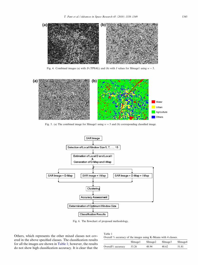
Fig. 4. Combined images (a) with D (TPSAL) and (b) with I values for SImage1 using w = 5.

Fig. 5. (a) The combined image for SImage1 using w = 5 and (b) corresponding classified image.

Fig. 6. The flowchart of proposed methodology.

Table 1Overall % accuracy of the images using K-Means with 4 classes.

SImage1 SImage2 SImage3 SImage4

Overall% accuracy 53.26 48.94 48.62 51.81


Others, which represents the other mixed classes not cov-ered in the above specified classes. The classification resultsfor all the images are shown in Table 1; however, the resultsdo not show high classification accuracy. It is clear that the


classification accuracy of single band and single polariza-tion SAR image is relatively low. The classification accu-racy for single band polarimetric SAR images obtainedby Davidson et al. (2006) show the overall accuracy forVV polarization, C band images to be 55.8% which isobtained using the supervised Maximum LikelihoodClassification.

6.2. Contextual classification and effect of window size onclassification

In next step, the contextual classification using a texturalapproach has been carried out. In order to work over thetextured image, the original image is not filtered for specklenoise removal (Acqua and Gamba, 2003). First of all weprepare the fractal map of the image by estimating the localfractal dimension inside a chosen moving window and thenplotting the fractal dimension values as image pixels.

Once we are doing the textural analysis on image, win-dowing is one of the major factors explaining various kindsof textures based on the size of window. Therefore it isimportant to critically analyze the windowing effect for tex-tural analysis of SAR data. For window selection we startfrom 5 � 5 size and increment the window by 2 every timeto get the odd size window. For getting different type oftexture information we vary the window size up to15 � 15. The size of local window is considered to be oddbecause it contains a center pixel, which acts as the repre-sentative of the whole local neighborhood. The smallestsize selected is to be 5 � 5 because it provides minimum 4points for least square slope estimation in D calculation,which would be only 2 points if 3 � 3 window were used,while the maximum size of local window is chosen to be15 � 15 because beyond this size the blurring effect in theprocessed texture image highly increases and hence donot provide much information. The process is done forboth methods, i.e., TPSAL and 2DVM. For getting thevariation of D values in local neighborhood, we comparethe maximum and minimum values of D for both methods.

Table 2The values of D and I (For SImage1) for different window size.

w

5 7

D (TPSAL) Max 2.6892 2.6887Min 1.7668 1.8012Mean 2.0129 2.0588SD 0.0634 0.0692

D (2DVM) Max 2.9702 2.8642Min 0.5762 1.2089Mean 2.2235 2.2633SD 0.2930 0.1988

Moran’s I Max 0.7310 0.8403Min �0.2267 �0.0897Mean 0.3518 0.4623SD 0.1600 0.1457

In parallel, for each local window, the value of Moran’s I isestimated and finally the I-map is generated. This is the sec-ond texture map for the study. Again the maximum andminimum values of I along with mean and standard devia-tion for each local window size are estimated as shown inTable 2 (the values are for SImage1).

The data represented in Table 2 is significant from thevalidation point of view, i.e., whether the values of appliedfeatures are appropriate or not. The minimum values of D

are less than 2.0 in both the methods, i.e., TPSAL and2DVM, which are due to the fact that natural scenes arenot exact fractals nevertheless they are modeled with frac-tals and they are statistically self-similar rather than exactlyself-similar. The maximum value of D for both methodsshows a variation such that in 2DVM with increase in localwindow size maximum value of D decreases, while inTPSAL maximum value of D increases first and thendecreases as far as the local window size is increased.Another important notable point in 2DVM is that the dif-ference between maximum and minimum values becomeslesser as the window size increases while the minimumvalue of D for TPSAL is almost same. The SD gives thedeflection from the mean and the values of SD show thatthe data is compact about the mean D. Concluding fromthe Table 2, the values of D are suitable to be used forthe classification study. Further, the values of I representedin Table 2 show that as the window size increases, the min-imum values go into positive range which are negative forlower window sizes. It shows that with increase in localwindow, the association of neighboring pixels increases.It is also observed from the results that the values of D

increase with random variation in pixel values, which isopposite to that of I as it decreases with randomness inpixel values. This shows an inverse relation in D and I asobserved by Emerson et al. (2005). This inverse relationis also clear from Table 2, where the mean values of D

and I show an opposite behavior, i.e., with increase in localwindow size the mean value of D (both TPSAL and2DVM) increases while the mean value of I decreases.

9 11 13 15

2.7448 2.7378 2.6631 2.58841.8315 1.8232 1.8433 1.83042.0783 2.1030 2.1293 2.12350.0705 0.0699 0.0687 0.0667

2.8229 2.7917 2.7757 2.68951.5128 1.6242 1.6946 1.71622.2842 2.2960 2.3030 2.30700.1639 0.1496 0.1443 0.1434

0.8842 0.8816 0.8910 0.8894�0.0138 0.0428 0.1111 0.1465

0.5201 0.5552 0.5787 0.59580.1295 0.1161 0.1056 0.0973

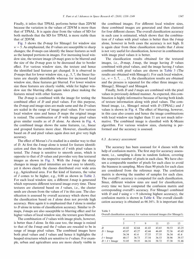
Table 3Overall classification accuracy for various textured images (for SImage1).

w

5 7 9 11 13 15

D 41.02 42.64 41.43 43.65 50.53 43.25D + Image 45.07 45.27 42.44 46.69 52.36 43.45I 36.34 41.4 37.55 37.35 36.34 41.4I + Image 40.17 36.73 37.54 36.53 38.96 39.57D + I + Image 51.05 59.35 66.16 58.72 57.38 51.46


Finally, it infers that TPSAL performs better than 2DVMbecause the variation in the values of 2DVM is more thanthat of TPSAL. It is again clear from the values of SD forboth methods that the SD for TPSAL is more stable thanthat of 2DVM.

Fig. 3 shows the D-map for SImage1 for window sizew = 5. As emphasized, the D values are susceptible to sharpchanges; the D-maps can identify the linear features as wellas the lumped portions in images. For increasing local win-dow size, the texture image (D-map) goes to be blurred andthe size of the D-map goes to be decreased due to bordereffect. For various window sizes, the texture and hencethe identified land features get changed. It is observed inD-maps that for lower window size, e.g., 5, 7, the linear fea-tures are sharply identifiable whereas for increased localwindow size, these features get blurred. For lower windowsize these features are clearly visible, while for higher win-dow size the blurring effect again takes place making thefeatures mixed with other features.

The D-map is combined with the image for testing thecombined effect of D and pixel values. For this purpose,the D-map and image sizes are made same and the D valuesare scaled in the range of image pixel values. For variouslocal window sizes and hence D maps the original imageis resized. The combination of D with image pixel valuesgives similar results as of D alone. As shown in Fig. 4,the combined image shows the same features, i.e., linearand grouped features more clear. However, classificationbased on D and pixel values again does not give very highaccuracy.

The effect of Moran’s I is studied in a similar way to thatof D. At first the I-map alone is tested for feature identifi-cation and then the combination of I with pixel values istested. The I-map is sensitive to smooth areas, which isopposite to that of D values and provides very fine texturedimages as shown in Fig. 3. With the I-map the sharpchanges in image pixel intensities are not easy to identify,yet it shows clearly the classes distributed over wide areae.g., Agricultural area. For flat kind of features, the valueof I comes to be higher, e.g., 0.88 as shown in Table 2.For each local window size, a different I-map is generatedwhich represents different textured image every time. Thesetextures are clustered based on I values, i.e., the clusterseeds are chosen from the values of I in this case. The clas-sification is assessed by overall accuracy which shows thatthe classification based on I alone does not provide highaccuracy. Here again it is emphasized that I alone is similarto D alone in terms of classification accuracy. Similar to D-maps, I-maps are also susceptible to blurring effect and forhigher values of local window size, the texture goes blurred.

The combination of I values with image pixels, however,is better than I alone. In this case too, the image is resizedto that of the I-map and the I values are rescaled to be inrange of image pixel values. The combined images haveboth pixel values and I values and hence it highlights theheaped structures which are sensitive to I values. For exam-ple, urban and agriculture area are more clearly visible in

the combined images. For different local window sizes,these combined images are generated and then clusteredfor four different classes. The overall classification accuracyin each case is estimated, which shows that the combina-tion of I values with pixel values is better than the I-mapalone, however in both cases the accuracy is not high. Itis again clear from these classification results that I aloneis not very useful for classification, however in combinationwith image pixel values it is better.

The classification results obtained for the texturedimages, i.e., D-map, I-map, the image having D valuescombined with pixel values, and the image having I valuescombined with pixel values are shown in Table 3 (Theresults are obtained with SImage1). For each local window,i.e., w = 5, 7, . . ., 15, the classification results are obtainedand the process is repeated for the other three images viz.SImage2, SImage3 and SImage4.

Finally, both D and I maps are combined with the pixelvalues in previously defined manner. As expected, this com-bination is highly informative because of having both kindsof texture information along with pixel values. The com-bined image, i.e., SImage1 mixed with D (TPSAL) and Ivalues is shown in Fig. 4. The effect of blurring, however,in this case also counts and hence the image combinationswith local window size higher than 11 are not much infor-mative. The combined image is classified with K-Meansalgorithm. For various window sizes, clustering is per-formed and the accuracy is assessed.

6.3. Accuracy assessment

The accuracy has been assessed for 4 classes with thehelp of confusion matrix. The first step for accuracy assess-ment, i.e., sampling is done in random fashion, coveringthe respective number of pixels in each class. We have cho-sen a comparable number of pixels for each class to avoidthe biasness in sampling. More than 90 pixels for each classare considered from the reference map. The confusionmatrix is showing the number of samples for each class.The overall% accuracy is computed for each classification.Since, different window sizes are used for classification,every time we have computed the confusion matrix andcorresponding overall% accuracy. For SImage1 combinedwith D and I using w = 9 (showing highest accuracy), theconfusion matrix is shown in Table 4. The overall classifi-cation accuracy is obtained as 66.16%. It is important that

Table 4The confusion matrix for combined Image classified with local windowsize 9 � 9.

Ground truth (pixels)

Class Water Urban Agriculture Others Total

Class 1 70 1 5 12 88Class 2 0 128 2 24 154Class 3 23 27 165 55 270Class 4 0 27 24 28 79

Total 93 183 196 119 591

Overall accuracy = (391/591) 66.16%

Error of commission and error of omission

Class Commission(%)

Omission(%)

Commission(pixels)

Omission(pixels)

Class 1 20.45 24.73 18/88 23/93Class 2 16.88 30.05 26/154 55/183Class 3 38.89 15.82 105/270 31/196Class 4 64.56 76.47 51/79 91/119

Users and producers accuracy

Class Producersaccuracy(%)

Usersaccuracy(%)

Producersaccuracy(pixels)

Usersaccuracy(pixels)

Class 1 75.27 79.55 70/93 70/88Class 2 69.95 83.12 128/183 128/154Class 3 84.18 61.11 165/196 165/270Class 4 23.53 35.44 28/119 28/79


the class named Others is also used in the confusion matrix.The result of clustering provides four classes, from whichthree are well defined and fourth class includes rest of theland classes.

The classification results for all images combined with D

and I values are shown in Tables 5 and 6. The D valuesused in Table 5 are obtained by TPSAL. Same process is

Table 5Overall% accuracy for combined D (TPSAL) and I values with pixelvalues for different window sizes.

w

5 7 9 11 13 15

SImage1 51.05 59.35 66.16 58.72 57.38 51.46SImage2 54.74 57.98 64.29 56.17 57.14 43.41SImage3 53.80 55.77 63.50 56.43 54.88 49.34SImage4 55.39 58.04 62.83 60.33 57.07 56.25

Table 6Overall% accuracy for combined D (2DVM) and I values with pixel valuesfor different window sizes.

w

5 7 9 11 13 15

SImage1 53.71 58.02 61.26 60.44 57.18 57.08SImage2 57.22 59.91 60.39 60.10 58.24 55.82SImage3 54.37 58.13 59.07 60.21 59.11 56.04SImage4 55.80 57.43 60.18 58.09 57.22 54.87

done for 2DVM method separately; however, it gives theresults having less accuracy than those of TPSAL as shownin Table 6. Based on the accuracy results, the optimum sizeof local window comes to be 9, i.e., for w = 9, highest clas-sification accuracy (66.16%) is obtained for current SARimages. Also, for w = 9 the 2DVM too gives highest accu-racy, which is 61.26%. The window size is based on the per-formance of present methodology and is not a global valuefor all images. Myint (2003) has used fractal dimension andspatial autocorrelation indexes with local statistics for clas-sification of multispectral ATLAS image. The overall accu-racy obtained for this image was 40–62% while that forusing Moran’s I varies between 53% and 78%. SimilarlyEmerson et al. (2005) have applied the local variance, frac-tal dimension and Moran’s I for classification of multispec-tral image and got accuracy near to 77% with fractaldimension and 70% with Moran’s I. They have used super-vised approach on multiband images whereas in this paperwe have applied an unsupervised approach for classifica-tion of single band SAR data and obtained results are quiteencouraging.

7. Conclusion

An unsupervised classification of single band and singlepolarization SAR image based on contextual informationis performed in this paper. A classification based onrenowned K-Means classifier is done in which the overallclassification accuracy using four different classes comes tobe around 50%. Further, a fractal based classification isperformed in which the identifying feature is fractaldimension. The local fractal dimension is estimated usingthe moving window approach. For various local windowsizes the fractal map is generated and with the help of thismap, classification is performed. Although, the texturefeatures are highlighted in the method, the classificationusing fractal map alone does not give very high accuracy.Here we emphasize on the fact that fractal dimensionalone is not sufficient for classification of satellite images,particularly single band and single polarization SARimages.

In order to aid the fractal dimension, Moran’s I of spa-tial autocorrelation index is used for classification.Although, Moran’s I alone is similar to fractal dimensionas it does not give high classification accuracy, it is suitableto be used with fractal dimension. Both fractal dimensionand Moran’s I jointly have been used as features for classi-fication and the classification results thus obtained are bet-ter than those of using these measures individually as wellas those obtained by using K-Means classifier. The overallaccuracy obtained for the D and I combination is at most66.16% for local window 9 � 9, which is better than that ofK-Means, i.e., 53.26%. Thus, the optimum size of localwindow for current study comes to be 9. Again, two meth-ods of fractal dimension estimation, i.e., TPSAL and2DVM are used in present study from which TPSALperforms better. The values of D estimated by TPSAL


are more stable and compact than those of 2DVM and theclassification accuracy with D and I combination usingTPSAL, i.e., 66.16%, is also more than that using2DVM, i.e., 61.26%.

Acknowledgment

The authors would like to thank the Physical ResearchLaboratory, Ahmedabad, India for providing the fund tosupport the work. Mr. Triloki Pant is thankful to Prof.S.M. de Jong for providing the necessary study materialand suggestive guidelines.

References

Acqua, F.D., Gamba, P. Texture-based characterization of urbanenvironments on satellite SAR images. IEEE Trans. Geosci. RemoteSens. 41 (1), 153–159, 2003.

Berizzi, F., Bertini, G., Martorella, M., Bertacca, M. Two-dimensionalvariation algorithm for fractal analysis of sea SAR images. IEEETrans. Geosci. Remote Sens. 44 (9), 2361–2373, 2006.

Chamundeeswari, V.V., Singh, D., Singh, K. An adaptive method withintegration of multi-wavelet based features for unsupervised classifi-cation of SAR images. J. Geophys. Eng. 4, 384–393, 2007.

Clarke, K.C. Computation of the fractal dimension of topographicsurfaces using the triangular prism surface area method. Comput.Geosci. 12 (5), 713–722, 1986.

Davidson, G., Ouchi, K., Saito, G., Ishitsuka, N., Mohri, K., Uratsuka, S.Single-look classification accuracy for polarimetric SAR. Int. J.Remote Sens. 27 (22), 5073–5080, 2006.

De Cola, L. Fractal analysis of a classified landsat scene. Photogramm.Eng. Remote Sens. 55 (5), 601–610, 1989.

De Jong, S.M., Burrough, P.A. A fractal approach to the classification ofMediterranean vegetation types in remotely sensed images. Photo-gramm. Eng. Remote Sens. 61 (8), 1041–1053, 1995.

Emerson, C.W., Lam, N.S.-N., Quattrochi, D.A. A comparison of localvariance, fractal dimension, and Moran’s I as aids to multispectralimage classification. Int. J. Remote Sens. 26 (8), 1575–1588, 2005.

Falconer, K. Fractal Geometry: Mathematical Foundations and Appli-cations. John Wiley and Sons Ltd., England, 2003.

Henderson, F.M., Lewis, A.J. (Eds.), Principles and Applications ofImaging Radar, Manual of Remote Sensing, vol. 2. John Wiley andSons, 1998.

Jaggi, S., Quattrochi, D.A., Lam, N.S.-N. Implementation and operationof three fractal measurement algorithms for analysis of remote sensingdata. Comput. Geosci. 19, 745–767, 1993.

Keller, J.M., Chen, S., Crownover, R.M. Textural description andsegmentation through fractal geometry. Comput. Vis., Graph. ImageProcess. 45, 150–166, 1989.

Keller, J.M., Crownover, R.M., Chen, S. Characteristics of natural scenesrelated to the fractal dimension. IEEE Trans. Pattern Anal. Mach.Intell. PAMI-9(5), 621–627, 1987.

Lee, W.L., Chen, Y.C., Chen, Y.C., Hsieh, K.S. Unsupervised segmen-tation of ultrasonic liver images by multiresolution fractal featurevector. Informat. Sci. 175, 177–199, 2005.

Lillesand, T.M., Kiefer, R.W. Remote Sensing and Image Interpretation.John Wiley and Sons, Inc., Singapore, 2002.

Lloyd, C.D. Local Models for Spatial Analysis. CRC Press, London, 2007.Mandelbrot, B.B. The Fractal Geometry of Nature. WH Freeman and

Co., New York, 1982.Myint, S.W. Fractal approaches in texture analysis and classification of

remotely sensed data: comparisons with spatial autocorrelationtechniques and simple descriptive statistics. Int. J. Remote Sens. 24(9), 1925–1947, 2003.

Oliver, C.J. Rain forest classification based on SAR texture. IEEE Trans.Geosci. Remote Sens. 38 (2), 1095–1104, 2000.

Peleg, S.., Naor, J., Hartley, R., Avnir, D. Multiple resolution textureanalysis and classification. IEEE Trans. Pattern Anal. Mach. Intell.PAMI-6(4), 518–523, 1984.

Pentland, A.P. Fractal-based description of natural scenes. IEEE Trans.Pattern Anal. Mach. Intell. PAMI-6(6), 661–674, 1984.

Petrou, M., Sevilla, P.G. Image Processing Dealing with Texture. JohnWiley and Sons, Ltd., England, 2006.

Rajesh, K., Jawahar, C.V., Sengupta, S., Sinha, S. Performance analysis oftextural features for characterization and classification of SAR images.Int. J.Remote Sens. 22 (8), 1555–1569, 2001.

Read, J.M., Lam, N.S.-N. Spatial methods for characterising land coverdetection land-cover changes for the tropics. Int. J. Remote Sens. 23(12), 2457–2474, 2002.

Sun, W. Three new implementations of the triangular prism method forcomputing the fractal dimension of remote sensing images. Photo-gramm. Eng. Remote Sens. 72 (4), 373–382, 2006.

Sun, W., Xu, G., Gong, P., Liang, S. Fractal analysis of remotely sensedimages: a review of methods and applications. Int. J. Remote Sens. 27(21-22), 4963–4990, 2006.

Tasoulis, D.K., Vrahatis, M.N. Unsupervised clustering using fractaldimension. Int. J. Bifurcat. Chaos. 16 (7), 2073–2079, 2006.

Ulaby, F.T., Kouyate, F., Brisco, B. Williams, Williams, T.H.Lee.Textural information in SAR images. IEEE Trans. Geosci. RemoteSens. GE-24(2), 235–245, 1986.

Wu, D., Linders, J. A new texture approach to discrimination of forestclearcut, canopy, and burned area using airborne C-band SAR. IEEETrans. Geosci. Remote Sens. 37 (1), 555–563, 1999.

Advanced fractal approach for unsupervised classification of SAR images

Documents

Transcript of Advanced fractal approach for unsupervised classification of SAR images