HAL Id: tel-02938554https://hal.archives-ouvertes.fr/tel-02938554

Submitted on 23 Sep 2020

HAL is a multi-disciplinary open accessarchive for the deposit and dissemination of sci-entific research documents, whether they are pub-lished or not. The documents may come fromteaching and research institutions in France orabroad, or from public or private research centers.

L’archive ouverte pluridisciplinaire HAL, estdestinée au dépôt et à la diffusion de documentsscientifiques de niveau recherche, publiés ou non,émanant des établissements d’enseignement et derecherche français ou étrangers, des laboratoirespublics ou privés.

Unsupervised cross-lingual representation modeling forvariable length phrases

Jingshu Liu

To cite this version:Jingshu Liu. Unsupervised cross-lingual representation modeling for variable length phrases. Compu-tation and Language [cs.CL]. Université de Nantes, 2020. English. �tel-02938554�

THÈSE DE DOCTORAT DE

L’UNIVERSITE DE NANTESCOMUE UNIVERSITE BRETAGNE LOIRE

Ecole Doctorale N°601Mathèmatique et Sciences et Technologiesde l’Information et de la CommunicationSpécialité : Informatique

Par

« Jingshu LIU »« Unsupervised cross-lingual representation modeling for variable length

phrases »Thèse présentée et soutenue à NANTES , le 29 Janvier, 2020Unité de recherche : LS2NThèse N° :

Rapporteurs avant soutenance :Pierre Zweigenbaum, Directeur de recherche, CNRS - Université de Paris Saclay

Laurent Besacier, Professeur des universités, Université de Grenoble Alpes

Composition du jury :Attention, en cas d’absence d’un des membres du Jury le jour de la soutenance, la composition ne comprend que lesmembres présents

Président : Someone SomeoneExaminateurs : Emmanuel Morin, Professeur des universités, Université de Nantes

Sebastián Peña Saldarriaga, Docteur en informatique, Easiware

Pierre Zweigenbaum, Directeur de recherche, CNRS - Université de Paris Saclay

Laurent Besacier, Professeur des universités, Université de Grenoble Alpes

Olivier Ferret, Ingénieur chercheur, CEA LIST

Dir. de thèse : Emmanuel Morin, Professeur des universités, Université de Nantes

ACKNOWLEDGEMENT

First and foremost, I would like to express my sincere gratitude to my supervisor EmmanuelMorin and my co-supervisor Sebastián Peña Saldarriaga for the continuous support of my Ph.D.study during these three years. I also appreciate their contributions of time, their patience, theirsupport and inspiring advice which allow this Ph.D. bring innovative advance to both academicfield and practical real-life application.

My sincere thanks go to Pierre Zweigenbaum, Laurent Besacier and Olivier Ferret for tak-ing part of my thesis committee and for for their interest in my research, patient reading andinsightful comments. I also thank them for their questions during the Ph.D. defense whichincented me to widen my research from various perspectives.

I am more than grateful to all members of the TALN team and Dictanova with whom I havehad the pleasure to work. It truly has been very good time in the lab and the company thanksto these outstanding and lovely people. A special thank to Joseph Lark for the effort for mypaperwork and the basketball sessions after work.

Last but not the least, I would like to thank my family for all their unconditional love andendless encouragement. I also express my gratitude to all my friends for their presence, theirhelp and their emotional support. Finally I thank my girlfriend Jia who always stood by my sidethrough these years.

TABLE OF CONTENTS

1 Introduction 101.1 Bilingual phrase alignment . . . . . . . . . . . . . . . . . . . . . . . . . . . . 10

1.2 Industrial context . . . . . . . . . . . . . . . . . . . . . . . . . . . . . . . . . 12

1.3 Phrase definition . . . . . . . . . . . . . . . . . . . . . . . . . . . . . . . . . 14

1.4 Unified phrase representation . . . . . . . . . . . . . . . . . . . . . . . . . . . 14

1.5 Bilingual unified phrase alignment . . . . . . . . . . . . . . . . . . . . . . . . 15

1.6 Unsupervised alignment . . . . . . . . . . . . . . . . . . . . . . . . . . . . . 16

1.7 Outline of the manuscript . . . . . . . . . . . . . . . . . . . . . . . . . . . . . 16

2 Word level representation 192.1 Distributional representation . . . . . . . . . . . . . . . . . . . . . . . . . . . 19

2.1.1 Explicit vector space: word co-occurrence . . . . . . . . . . . . . . . 20

2.1.2 Association measures . . . . . . . . . . . . . . . . . . . . . . . . . . 21

2.2 Distributed representation . . . . . . . . . . . . . . . . . . . . . . . . . . . . . 26

2.2.1 Neural Network: sparse to dense vector space . . . . . . . . . . . . . . 26

2.2.2 CBOW . . . . . . . . . . . . . . . . . . . . . . . . . . . . . . . . . . 32

2.2.3 Skip-gram . . . . . . . . . . . . . . . . . . . . . . . . . . . . . . . . . 36

2.2.4 Other popular word embeddings . . . . . . . . . . . . . . . . . . . . . 38

2.3 Data selection for modest corpora with distributional representation . . . . . . 43

2.4 Contribution: Data selection with distributed representation . . . . . . . . . . . 47

2.5 Synthesis . . . . . . . . . . . . . . . . . . . . . . . . . . . . . . . . . . . . . 49

3 Multi-word level representation : phrase modeling 513.1 Approaches without learnable parameters . . . . . . . . . . . . . . . . . . . . 51

3.1.1 Compositional stack . . . . . . . . . . . . . . . . . . . . . . . . . . . 52

3.1.2 Addition based approach . . . . . . . . . . . . . . . . . . . . . . . . . 53

3.1.3 Concatenation . . . . . . . . . . . . . . . . . . . . . . . . . . . . . . 54

3.2 Phrase embeddings with CBOW or Skip-gram . . . . . . . . . . . . . . . . . . 55

3.2.1 One single token processing for non-compositional phrases . . . . . . . 55

3

TABLE OF CONTENTS

3.2.2 Extended skip-gram with negative sampling . . . . . . . . . . . . . . . 56

3.3 Traditional neural networks for sequential inputs . . . . . . . . . . . . . . . . 57

3.3.1 Convolutional Neural Network . . . . . . . . . . . . . . . . . . . . . . 57

3.3.2 Recurrent Neural Network . . . . . . . . . . . . . . . . . . . . . . . . 62

3.3.3 LSTM and GRU . . . . . . . . . . . . . . . . . . . . . . . . . . . . . 67

3.3.4 Recent applications: ELMo . . . . . . . . . . . . . . . . . . . . . . . 71

3.4 Transformers: Multi-Head Attention . . . . . . . . . . . . . . . . . . . . . . . 74

3.4.1 Attention mechanism . . . . . . . . . . . . . . . . . . . . . . . . . . . 74

3.4.2 One head: Scaled Dot-Product Attention . . . . . . . . . . . . . . . . 76

3.4.3 Multi-Head for multiple semantic aspects . . . . . . . . . . . . . . . . 78

3.4.4 Positional encodings for order distinction . . . . . . . . . . . . . . . . 78

3.4.5 Recent applications: Transformer, Opengpt, BERT, XLNet . . . . . . . 79

3.5 Contribution : a new dataset for monolingual phrase synonymy . . . . . . . . . 82

3.6 Contribution : Tree-free recursive neural network . . . . . . . . . . . . . . . . 82

3.6.1 Background: recursive neural network (RNN) . . . . . . . . . . . . . . 83

3.6.2 Tree-free recursive neural network (TF-RNN) . . . . . . . . . . . . . . 85

3.6.3 Evaluation . . . . . . . . . . . . . . . . . . . . . . . . . . . . . . . . 87

3.7 Synthesis . . . . . . . . . . . . . . . . . . . . . . . . . . . . . . . . . . . . . 93

4 Unsupervised training 954.1 Siamese networks . . . . . . . . . . . . . . . . . . . . . . . . . . . . . . . . . 95

4.1.1 Pseudo-Siamese network . . . . . . . . . . . . . . . . . . . . . . . . . 96

4.2 Encoder-decoder architecture . . . . . . . . . . . . . . . . . . . . . . . . . . . 97

4.3 Training objectives . . . . . . . . . . . . . . . . . . . . . . . . . . . . . . . . 99

4.3.1 Autoregression: Next word prediction . . . . . . . . . . . . . . . . . . 99

4.3.2 Denoising: Reconstructing input and Masked language modeling . . . 100

4.4 After the pre-training: feature based vs fine tuning . . . . . . . . . . . . . . . . 101

4.5 Contribution : Wrapped context modeling . . . . . . . . . . . . . . . . . . . . 102

4.6 Synthesis . . . . . . . . . . . . . . . . . . . . . . . . . . . . . . . . . . . . . 106

5 Bilingual word alignment 1075.1 Distributional representation based approach . . . . . . . . . . . . . . . . . . . 107

5.1.1 Standard approach . . . . . . . . . . . . . . . . . . . . . . . . . . . . 107

5.1.2 Standard approach with data selection . . . . . . . . . . . . . . . . . . 109

5.2 Contribution: Standard approach with DSC and WPMI . . . . . . . . . . . . . 110

4

TABLE OF CONTENTS

5.2.1 DSC: distance sensitive co-occurrence . . . . . . . . . . . . . . . . . . 110

5.2.2 WPMI: weighted point-wise mutual information . . . . . . . . . . . . 110

5.2.3 Evaluation . . . . . . . . . . . . . . . . . . . . . . . . . . . . . . . . 111

5.3 Bilingual word embedding . . . . . . . . . . . . . . . . . . . . . . . . . . . . 112

5.3.1 Language space mapping via a linear transformation matrix . . . . . . 113

5.3.2 Improvements . . . . . . . . . . . . . . . . . . . . . . . . . . . . . . . 115

5.4 Contribution: Bilingual word embeddings with re-normalisation and data selec-tion . . . . . . . . . . . . . . . . . . . . . . . . . . . . . . . . . . . . . . . . 120

5.5 Synthesis . . . . . . . . . . . . . . . . . . . . . . . . . . . . . . . . . . . . . 123

6 Bilingual phrase alignment 1256.1 Supervised bilingual phrase alignment with dictionary look-up: compositional

approach . . . . . . . . . . . . . . . . . . . . . . . . . . . . . . . . . . . . . . 125

6.2 (Semi-) supervised bilingual phrase alignment with distributional representation 127

6.2.1 Compositionnal method with context based projection (CMCBP) . . . 127

6.2.2 CMCBP with data selection . . . . . . . . . . . . . . . . . . . . . . . 130

6.3 Contribution : Compositionnal method with word embedding projection (CMWEP)130

6.4 Unsupervised neural machine translation with pre-trained cross-lingual embed-dings . . . . . . . . . . . . . . . . . . . . . . . . . . . . . . . . . . . . . . . . 134

6.4.1 Back translation . . . . . . . . . . . . . . . . . . . . . . . . . . . . . 134

6.4.2 Extract-Edit, an alternative to back translation . . . . . . . . . . . . . . 135

6.5 Contribution : a new dataset for bilingual phrase alignment . . . . . . . . . . . 138

6.6 Contribution for the unsupervised bilingual phrase alignment . . . . . . . . . . 139

6.6.1 Semi tree-free recursive neural network . . . . . . . . . . . . . . . . . 139

6.6.2 Pseudo back translation . . . . . . . . . . . . . . . . . . . . . . . . . . 140

6.6.3 System overview . . . . . . . . . . . . . . . . . . . . . . . . . . . . . 141

6.6.4 Evaluation . . . . . . . . . . . . . . . . . . . . . . . . . . . . . . . . 142

6.7 Synthesis . . . . . . . . . . . . . . . . . . . . . . . . . . . . . . . . . . . . . 147

7 Conclusion and perspective 1497.1 Conclusion . . . . . . . . . . . . . . . . . . . . . . . . . . . . . . . . . . . . 149

7.2 Operational contributions . . . . . . . . . . . . . . . . . . . . . . . . . . . . . 150

7.2.1 Industrialized implementation . . . . . . . . . . . . . . . . . . . . . . 151

7.2.2 Contribution to the JVM based deep learning framework . . . . . . . . 151

7.3 Future work . . . . . . . . . . . . . . . . . . . . . . . . . . . . . . . . . . . . 151

5

TABLE OF CONTENTS

7.3.1 Data selection refinement . . . . . . . . . . . . . . . . . . . . . . . . . 1517.3.2 Synthetic multi-word generation . . . . . . . . . . . . . . . . . . . . . 1527.3.3 Contextualized cross-lingual input . . . . . . . . . . . . . . . . . . . . 1537.3.4 Applications beyond phrase alignment . . . . . . . . . . . . . . . . . . 1537.3.5 Model deployment in industrial context . . . . . . . . . . . . . . . . . 153

A Resource and data 155A.1 Corpora in specialized domain . . . . . . . . . . . . . . . . . . . . . . . . . . 155

A.1.1 Breast cancer (BC) . . . . . . . . . . . . . . . . . . . . . . . . . . . . 155A.1.2 Wind energy (WE) . . . . . . . . . . . . . . . . . . . . . . . . . . . . 155

A.2 Corpora in general domain . . . . . . . . . . . . . . . . . . . . . . . . . . . . 156A.2.1 New commentary (NC) . . . . . . . . . . . . . . . . . . . . . . . . . . 156A.2.2 Semeval 2017 . . . . . . . . . . . . . . . . . . . . . . . . . . . . . . . 156

A.3 Gold standard and candidate list . . . . . . . . . . . . . . . . . . . . . . . . . 156A.3.1 Phrase synonymy . . . . . . . . . . . . . . . . . . . . . . . . . . . . . 156A.3.2 Phrase similarity . . . . . . . . . . . . . . . . . . . . . . . . . . . . . 156A.3.3 Phrase alignment . . . . . . . . . . . . . . . . . . . . . . . . . . . . . 157

A.4 Bilingual dictionaries . . . . . . . . . . . . . . . . . . . . . . . . . . . . . . . 157A.5 Pre-trained models . . . . . . . . . . . . . . . . . . . . . . . . . . . . . . . . 158

A.5.1 Word embeddings . . . . . . . . . . . . . . . . . . . . . . . . . . . . 158A.5.2 Language models . . . . . . . . . . . . . . . . . . . . . . . . . . . . . 158

B Experiment settings 159B.1 Implementation tools . . . . . . . . . . . . . . . . . . . . . . . . . . . . . . . 159B.2 Distributional representation setting . . . . . . . . . . . . . . . . . . . . . . . 159B.3 Encoder-decoder network setting . . . . . . . . . . . . . . . . . . . . . . . . . 160

Bibliography 161

6

LIST OF FIGURES

1.1 A use case of the Dictanova semantic analysis. . . . . . . . . . . . . . . . . . . 12

2.1 Illustration of the co-occurrence matrix of the example sentence. . . . . . . . . 20

2.2 Comparison between DOR and PMI. . . . . . . . . . . . . . . . . . . . . . . . 25

2.3 Comparison of three different activation functions. . . . . . . . . . . . . . . . 27

2.4 An illustration of a neural network with multiple fully connected layers. . . . . 28

2.5 Comparison of five different power functions. . . . . . . . . . . . . . . . . . . 39

2.6 Weight function in GloVe. . . . . . . . . . . . . . . . . . . . . . . . . . . . . 41

2.7 GSA co-occurrence matrix. . . . . . . . . . . . . . . . . . . . . . . . . . . . . 44

2.8 SSA merging process. . . . . . . . . . . . . . . . . . . . . . . . . . . . . . . . 45

2.9 Comparison between SA, GSA and SSA. . . . . . . . . . . . . . . . . . . . . 46

3.1 Compositional stack. . . . . . . . . . . . . . . . . . . . . . . . . . . . . . . . 52

3.2 1-d convolution. . . . . . . . . . . . . . . . . . . . . . . . . . . . . . . . . . . 58

3.3 2-d convolution. . . . . . . . . . . . . . . . . . . . . . . . . . . . . . . . . . . 59

3.4 An example of max pooling. . . . . . . . . . . . . . . . . . . . . . . . . . . . 61

3.5 LeNet-5 architecture. . . . . . . . . . . . . . . . . . . . . . . . . . . . . . . . 61

3.6 A basic cell of RctNN. . . . . . . . . . . . . . . . . . . . . . . . . . . . . . . 63

3.7 Unfolded RctNN . . . . . . . . . . . . . . . . . . . . . . . . . . . . . . . . . 63

3.8 Diagram of BPTT. . . . . . . . . . . . . . . . . . . . . . . . . . . . . . . . . 66

3.9 Diagram of LSTM. . . . . . . . . . . . . . . . . . . . . . . . . . . . . . . . . 68

3.10 Diagram of GRU. . . . . . . . . . . . . . . . . . . . . . . . . . . . . . . . . . 70

3.11 ELMo ablation test-1. . . . . . . . . . . . . . . . . . . . . . . . . . . . . . . . 72

3.12 ELMo ablation test-2. . . . . . . . . . . . . . . . . . . . . . . . . . . . . . . . 73

3.13 ELMo results. . . . . . . . . . . . . . . . . . . . . . . . . . . . . . . . . . . . 73

3.14 Global vs local attention. . . . . . . . . . . . . . . . . . . . . . . . . . . . . . 76

3.15 Comparison between a fully-connected layer and a self-attention layer. . . . . . 77

3.16 One head vs multi-head attention. . . . . . . . . . . . . . . . . . . . . . . . . 78

3.17 Transformer model architecture. . . . . . . . . . . . . . . . . . . . . . . . . . 80

7

LIST OF FIGURES

3.18 BERT training. . . . . . . . . . . . . . . . . . . . . . . . . . . . . . . . . . . 803.19 BERT results. . . . . . . . . . . . . . . . . . . . . . . . . . . . . . . . . . . . 813.20 Diagram of a recursive neural network. . . . . . . . . . . . . . . . . . . . . . . 833.21 RctNN and CNN. . . . . . . . . . . . . . . . . . . . . . . . . . . . . . . . . . 843.22 Diagram of the tree-free recursive neural network (TF-RNN). . . . . . . . . . . 86

4.1 A Siamese network. . . . . . . . . . . . . . . . . . . . . . . . . . . . . . . . . 964.2 Diagram of a general encoder-decoder architecture. . . . . . . . . . . . . . . . 974.3 Diagram of a stacked bidirectional encoder architecture. . . . . . . . . . . . . 984.4 Wrapped context prediction. . . . . . . . . . . . . . . . . . . . . . . . . . . . 103

5.1 An example of projecting a source word vector to the target language space. . . 1085.2 Concatenated word embeddings. . . . . . . . . . . . . . . . . . . . . . . . . . 122

6.1 Diagram of CMCBP. . . . . . . . . . . . . . . . . . . . . . . . . . . . . . . . 1296.2 An example diagram of CMCBP. . . . . . . . . . . . . . . . . . . . . . . . . . 1326.3 Extract-edit approach based NMT architecture. . . . . . . . . . . . . . . . . . 1376.4 Diagram of the semi tree-free recursive neural network (STF-RNN). . . . . . . 1406.5 Overview of the cross-lingual alignment training architecture. . . . . . . . . . 142

8

LIST OF TABLES

2.1 Word synonynmy results. . . . . . . . . . . . . . . . . . . . . . . . . . . . . . 48

3.1 Comparison of complexity . . . . . . . . . . . . . . . . . . . . . . . . . . . . 873.2 Phrase synonymy. . . . . . . . . . . . . . . . . . . . . . . . . . . . . . . . . . 893.3 Phrase similarity. . . . . . . . . . . . . . . . . . . . . . . . . . . . . . . . . . 903.4 Phrase analogy. . . . . . . . . . . . . . . . . . . . . . . . . . . . . . . . . . . 92

4.1 Comparison between different training objectives. . . . . . . . . . . . . . . . . 1044.2 Encoder-decoder vs pseudo-siamese network. . . . . . . . . . . . . . . . . . . 1044.3 Comparison between different input embeddings. . . . . . . . . . . . . . . . . 105

5.1 Comparison between SA and SSA on BC and WE datasets. . . . . . . . . . . . 1105.2 Results with distributional approach. . . . . . . . . . . . . . . . . . . . . . . . 1125.3 Bilingual alignment results (accuracy) on EN-IT. . . . . . . . . . . . . . . . . 1195.4 Results with re-normalisation. . . . . . . . . . . . . . . . . . . . . . . . . . . 1215.5 Bilingual word embedding results on BC and WE datasets. . . . . . . . . . . . 122

6.1 Results of CMWEP. . . . . . . . . . . . . . . . . . . . . . . . . . . . . . . . . 1336.2 Results for unsupervised bilingual phrase alignment. . . . . . . . . . . . . . . 1446.3 Results for single-word alignment only. . . . . . . . . . . . . . . . . . . . . . 1456.4 Alignment examples within top 2 candidates. . . . . . . . . . . . . . . . . . . 146

9

CHAPTER 1

INTRODUCTION

As more and more text data of different languages are collected via millions of websites, itis in tremendous researchers’ and enterprises’ interests to leverage this data. Among variousattractive applications (terminology extraction, opinion mining, machine translation, questionanswering, etc), bilingual phrase alignment is what this thesis studies. With recent advances inMachine Learning and Natural Language Processing, our work proposes a new unified bilingualphrase alignment framework in an unsupervised manner.

In the beginning section of this introductory chapter, we briefly discuss the two axes forbilingual phrase alignment which are the guidelines of this work. The second section presentsthe industrial context of our work. In the next section we give and clarify our phrase definition.Then from the fourth section to the sixth section we progressively describe several key fea-tures that help us achieve our final objective: unsupervised unified bilingual phrase alignment.Finally, the manuscript structure will be given at the end of the chapter.

1.1 Bilingual phrase alignment

Bilingual phrase alignment is an essential task for various NLP applications, ranging fromphrase synonymy and phrase similarity to machine translation. Besides, projecting phrases intoa common space can be an attractive feature when integrated in some industrial software. Theobjective consists in, given a phrase in source language, extracting the best translation phrasefrom the target language corpus.

The task requires two main technology axes: the phrase representation modeling and thebilingual phrase mapping with the properly learned representations.

The first axe is considered to be the prerequisite of the latter. For many years human hasbeen trying to understand how the semantics of language sequence are captured. Traditionally,two complementary principles addressed this problem:

• Compositional principle. Compositionality is defined as the property where “the mean-

10

Introduction

ing of the whole is a function of the meaning of the parts” (Keenan and Faltz, 1985). InSzabó (2017), the authors state that “The meaning of a complex expression is determinedby its structure and the meanings of its constituents”. For example, a frying pan is indeed

a pan used for frying (Morin and Daille, 2012).

• Syntactical principle. The compositional principle would fail when encountering id-iomatic expressions such as a pain in the neck (refers to something or somebody that isannoying or difficult to deal with according to Cambridge dictionary 1) or pomme de terre

(lit. apple of earth, meaning: potato) in French. The syntactical principle would like tocomplement the compositionality by analysing the sentence sequence which can be di-vided into clauses, and clauses can be further divided into phrases. Consequently theseless compositional expressions are treated as a whole unit in a syntactical structure, e.g.a parsing tree.

For the first axis of this thesis, the phrase representation learning, we follow these twomajor principles as we desire to propose a unified framework to represent all types of phraseswithout length or linguistic constraints. Both compositional and idiomatic phrases are goingto be handled in the same framework with respect to the compositionality and the syntacticalstructure.

The second axe is in between the Information Retrieval and the Machine Translation do-mains. While the task objective is to extract the most likely translation phrase by ranking allthe candidates, it is not a task of generating the most likely translation sequence as in Machine

Translation. Nonetheless, there are still a substantial amount of common points with Machine

Translation. One might actually view the translation task as a sequential/conditional top 1 can-didate selection process, in other words, the translator ranks all the candidate tokens and selectsthe best at each time step t with regard to all the previously generated tokens at time steps[1, t− 1]. To sum up, the translation objective is to maximise the conditional probability:

arg maxy

Ty

Πt=1P (yt|x, y1, y2, ..., yt−1) (1.1)

where yt means the selected best token at step t and x means the initial information. Thefactorial part in 1.1 can be also written as:

P (y1, y2, ..., yt|x) = P (y1|x)P (y2|x, y1), ..., P (yt|x, y1, y2, ..., yt−1) (1.2)

1https://dictionary.cambridge.org

11

Introduction

It is worth noting that there is one extreme case where the translation task is equivalent to thealignment task: when the target sequence length T equals to 1. Some call the word alignmenttask bilingual word lexicon induction. Therefore we estimate that the phrase alignment taskis a non sequential translation task in terms of the candidate generative side and a sequenceinformation retrieval task considering the comparison and selection aspect.

1.2 Industrial context

The thesis is carried out in an industrial context with the CIFRE2 (Convention Industrielle de

Formation par la REcherche, lit. Industrial Conventions Training by Research) convention.The CIFRE subsidizes any company that hires a PhD student to collaborate with a public labo-ratory. In our scenario, the collaboration was originally between the company Dictanova 3 andLaboratoire de Sciences du Numérique de Nantes (LS2N) 4.

Dictanova was a french start-up enterprise as a software editor in SaaS (Software as aService) mode who provided semantic analysis for the Customer Relationship Management

(CRM). Created in 2011 by several young researchers from the historical Nantes AtlantiqueComputer Science Laboratory (LINA) which later composed LS2N with other laboratories, thecompany received a financial aid from the National Competition of the newly founded inno-vative technology companies in 2012 and then in 2013 it was awarded by the Forum of theEuropean Language Technologies Industry. The company was imbued with a strong academicscientific culture, particularly in the field of natural language processing. A use case of itssoftware is illustrated in the figure below.

Figure 1.1 – A use case of the Dictanova semantic analysis.

2http://www.anrt.asso.fr/en/cifre-78433https://apps.dictanova.com/4https://www.ls2n.fr/

12

Introduction

The main function was to provide aspect based sentiment analysis 5 (ABSA), as shown inthe Figure 1.1, the sentence in the left block is annotated with key phrases (bold), positive sen-timent (green) and negative sentiment (red). Since the company supported several languagesand the clients were also from different countries (France, Germany, Spain, etc), it was com-pelling for the company to develop a cross-lingual phrase alignment system. There are twomajor benefits:

• Facilitation of the transition from one language to another. Developing or maintaining amultilingual platform can be smoothed.

• Projection of the terms of different languages in a common space so that an internationalclient has a better view of what is happening across all regions.

Moreover, recall the first axis of the thesis, the monolingual phrase representation model-ing, which was also very interesting for the company as it enabled more subtle functions ormanipulations over the phrases such as the automatic thematic clustering or synonym phraseaggregation.

In 2019, Dictanova was acquired by Easiware 6, who develops a multi-channel applicationprocessing software to enhance customer support service. As pointed out by the co-founderof Easiware, Brendan Natral, the perspective is to integrate the technology of Dictanova onthe machine learning and the semantic analysis 7. Concerning the thesis, since Easiware hasalso an international vision, our objective remains uninterrupted. We are able to continue ourpre-acquisition work without major impact.

However, our industrial context also brings us some practical limits:

• The corpora are noisier compared to the academic ones and they are usually in veryspecialised domains. Besides, the size is often modest.

• Start-up enterprises are more product driven, and the less resource the system demands,the more practical it is for the enterprise to apply. With this perception, we would like topropose a system that requires as less calculation resources as possible.

• Syntactical information such as the parsing tree are not trivial information as not all thesupported languages have a commercialised parser and in addition, the parsing process

5 https://en.wikipedia.org/wiki/Sentiment_analysis#Feature/aspect-based6https://www.easiware.com/7https://www.easiware.com/blog/easiware-acquisition-startup-dictanova

13

Introduction

could cause an excessive pre-processing burden for the relatively light product. Hence asystem without requiring syntactical information becomes our leading choice.

• Parallel data are difficult to obtain for our specialised domain, and the cost of annotatingparallel data is certainly expensive. However, we dispose naturally of comparable corporaas the clients speak usually of the same topics for a given customer. (The delivery is too

slow. vs Je suis déçu de la livraison. (lit. I am disappointed with the delivery.)) Our finalframework should be unsupervised or quasi unsupervised.

1.3 Phrase definition

Linguistically, the definition of a phrase is “is a group of words (or possibly a single word)that functions as a constituent in the syntax of a sentence, a single unit within a grammaticalhierarchy”8. However, some argue that a phrase should contain at least two words (Finch,2000). In our case, we apply the first definition where a phrase is simply a group of words or asingle-word.

Sobin (2010) proposes to use tree structures to represent phrases, which provide schematicsof how the words in a sentence are grouped and relate to each other. Any word combination thatcorresponds to a complete subtree can be seen as a phrase. This is in line with the compositionalprinciple mentioned in 1.1.

Kroeger (2005) states that the meaning of a phrase is often determined by the syntacticalhead. For example, blue shoe, very happy and watch TV. This suggests that we should takethe syntactical structure into account when associating phrase components as discussed in thesyntactical principle in 1.1.

1.4 Unified phrase representation

We would like to propose a unified phrase representation for phrases of all syntactical types ofvariable length. For instance, this may be observed by a few classes of semantically synony-mous phrase pairs:

• Length related

– Single-word synonym pair, as in energy - power.

8https://en.wikipedia.org/wiki/Phrase

14

Introduction

– Same length multi-word synonym pair, as in to carry on - to keep going.

– Fertile synonym pair, as in wind generator - aerogenerator.

• POS (part of speech) related

– Same POS synonym pair, as in attitude - morale.

– Different POS synonym pair, as in buy a car - purchase of a car.

With these possible features taken into account, the unified phrase representation shouldbe versatile and generic enough to allow that semantically close phrases are more similar toeach other no matter how different they may appear on the superficial level, or close in therepresentation space, for instance the Euclidean vector space if we represent the phrases withvectors.

1.5 Bilingual unified phrase alignment

Once we have the unified monolingual phrase representation, the bilingual unified phrase align-ment can be concluded by what has been mentioned in 1.1 plus the features in 1.4.

• Length related

– Single-word to single-word alignment (sw2sw), as in bag - sac.

– Same multi-word length alignment (n2n), as in wind turbine - turbine éolien.

– Fertile alignment (p2q), as in airflow - flux d’air.

• POS (part of speech) related

– Same POS alignment, as in car - voiture.

– Different POS alignment, as in buy a car - achat d’une voiture.

Because we do not have the POS information during the alignment most of the time, wefocus more on the length criterion when analysing our systems. As for the POS related feature,we consider that it is automatically included and no further special processing is required foraligning different POS phrases.

15

Introduction

1.6 Unsupervised alignment

Not only because of the limits mentioned in 1.2, but also the fact that even outside of theindustrial context, parallel data is always costly to build as it requires specialised expertise.Besides such data is unfortunately often nonexistent for low-resource languages and specialiseddomains (Lample, Conneau, et al., 2018). Therefore it is preferred that the alignment systemoperates in an unsupervised manner.

More concretely, unsupervised means, in our scenario, that we do not have any access tocross-lingual information about phrases which in many cases is equal to a phrase mapping table.In our unsupervised proposal, we tackle this problem by incorporating pre-trained bilingualword embeddings (BWE) (Mikolov, Quoc V. Le, et al., 2013) and a back-translation mechanism(Sennrich et al., 2016a). The general idea is to exploit the shared vector space of the bilingualword embedding in a wider context where a sequence of words can also be projected into thesame shared space.

1.7 Outline of the manuscript

This introductory chapter explains the motivation and the background of our work, which willbe further detailed following the two axes (See 1.1) in a single-word and multi-word perspective.

From Chapter 2 to Chapter 3 we discuss the first axis concerning the phrase representation.Chapter 2 revises the traditional and neural network based approaches for word-level represen-tation, in the most common case, it is in the form of word vectors (bag-of-words and wordembeddings) in Euclidean vector space. We also review an effective method for improving theword vectors (bag-of-words and word embeddings) for corpora in specialised domain. Basedon all these state-of-the art works, we propose our modifications which later improve our resultson bilingual word alignment task. Chapter 3 generalises a substantial body of previous workson modeling multi-words. Finally, we propose a new structure for homogeneously modelingsingle-word and multi-word phrases, which fits better our scenario and allows a unified phraserepresentation.

Chapter 4 is focused on the training systems. From the regression based to the predictionbased training system, we discover a new training strategy potentially powerful for many NLPtasks.

Then from Chapter 5 to Chapter 6, we dive into the second axis which seeks to align single-words or multi-words of different languages. Chapter 5 presents the word-level alignment. This

16

Introduction

task is widely studied over the past years, we mainly cover the distributional based and theword embedding based approach as we mentioned in 2. Chapter 6 generalises the word-levelalignment to multi-word level by incorporating a few techniques of the traditional compositionalmethod and the Machine Translation field, reaching the best results for our task.

Chapter 7 concludes the thesis and opens perspectives for future works.

17

CHAPTER 2

WORD LEVEL REPRESENTATION

The compositionality of phrases necessitates meaningful word level representations in order tocompose multi-word representations. In this chapter we first study word representation mod-eling with two widely applied approaches, the distributional approach and the distributed ap-proach. Both represent words in n-dimensional Euclidean space Rn. The first one is a moretraditional approach where the word vectors are high dimensional sparse vectors with word co-occurrence, while the second one is a more recent approach where the word vectors are lowdimensional dense vectors with learned parameters. Following the introduction of the two ap-proaches, we explore how we can improve these approaches in our scenario where the domain-specific corpus size is quite modest. As these statistical approaches will often achieve betterperformance when larger training data is available, the mindset of the improvement is on howto efficiently add external data to reinforce the system. Then at the end of this chapter weexplain an application of this improvement on dense word vectors.

2.1 Distributional representation

The distributional representation has been extensively studied in the NLP literature (Dagan etal., 1994; Lin, 1998; Kotlerman et al., 2010; P. D. Turney and Pantel, 2010; Baroni and Lenci,2010) (and the references therein). This approach associates each word in a corpus vocabularyto a high dimensional (equal to the vocabulary size) vector space. A dimension in this spacemeans a word-context co-occurrence, thus, naturally this kind of word vectors can be directlyextracted from a word co-occurrence matrix. Suppose that each row of the matrix represents aword vector, then each column is a context to this particular word. We will give more detailsin the following section. Moreover, most works using the distributional approach apply anassociation measure to the word context vectors in order to smooth the vector values. In thesecond section 2.1.2, we review some most popular association measures and discuss theiradvantages and disadvantages.

19

Part , Chapter 2

2.1.1 Explicit vector space: word co-occurrence

The very first step towards the distributional approach is to construct a word co-occurrencematrix. For instance, each cell represents a word-context co-occurrence and the matrix is sym-metric. To build such a matrix, we need to decide a window size within which we considerthe proximity of words to be relevant. Typically this hyper parameter varies between one up toten. The larger the window size is, the more features it will collect for the central word but alsomore likely to collect noisy features, while the smaller the window size is, the less noise it willretrieve but also the more discriminant information it will miss. For example, considering thefollowing sentence:

It is the first vehicle in the world in which passengers pay for their rideupon entering it.

With the vocabulary size d, the co-occurrence matrix will be in Nd∗d. Each word vectorbelongs to Nd. The co-occurrence matrix corresponding to the sentence above will be in N16∗16.

It

is

......

entering.

It is ... ... entering

.

Figure 2.1 – Illustration of the co-occurrence matrix of the example sentence.

If the current central word is passengers, then within a window size of 3 and 5 we havefollowing data where vpassengers

i means the word vector of passengers at each dimension i.

It is the first vehicle in the world in which passengers pay for their rideupon entering it.

window size = 3

20

2.1. Distributional representation

vpassengersi =

1, i ∈ {world, in, which, pay, for, their}

0, otherwise

It is the first vehicle in the world in which passengers pay for their rideupon entering it.

window size = 5

vpassengersi =

2, i = in

1, i ∈ {the, world, which, pay, for, their, ride, upon}

0, otherwise

Note that within a window size of 5 we are able to associate the word ride to passengers whichseems semantically relevant. Finally, the obtained word vectors have these properties:

1. High-dimensional. Obviously, as the co-occurrence matrix is in Rd∗d, each word vectorhas d dimensions. More concretely, if we look at some famous training corpora such asWiki1, Gigaword2, Common Crawl3 or Europarl4 , the vocabulary size is usually between100,000 to 500,000 even after some filtering.

2. Sparse. Most non functional words only co-occur with a limited number of other nonfunctional words. Therefore the word vectors are highly sparse.

3. Explicit. The compelling point of the distributional representation is the explicitness ofeach dimension. One can simply understand the semantics behind each dimension andapply linguistic analysis.

2.1.2 Association measures

The raw word co-occurrence is often biased by the frequency of words in the training corpus,especially for the function words. Imagine that the word in appears 1000 times in an articleand co-occurs 10 times with the word passengers, and the word ride appears only 5 times but

1dumps.wikimedia.org/2www.ldc.upenn.edu3commoncrawl.org/4www.statmt.org

21

Part , Chapter 2

all these occurrences are within the window of passengers. From the pure word co-occurrencematrix, the word vector of passengers has a value of 100 at the dimension of in which is farmore important than 5, the value at the dimension of ride. This phenomenon misleads us to aconclusion that the word passengers is semantically more related to in rather than ride. As aconsequence, people introduce association measures to normalise the co-occurrence value withregard to the probability of having the relative word-context pair. The association measuresstudied are Pointwise Mutual Information (Fano, 1961), Log-likelihood (Dunning, 1993), andthe Discounted Odds-Ratio (Evert, 2005).

Pointwise Mutual Information (PMI). Mutual Information reflects the mutual dependencebetween two random variables. For two discrete variables X and Y whose joint probabilitydistribution is P (x, y), and P (x) , P (y) the marginal distributions, the mutual informationbetween them, denoted I(X, Y ), is given by Shannon and Weaver (1949):

I(x, y) =∑x

∑y

P (x, y) log P (x, y)P (x)P (y) (2.1)

The application of Pointwise Mutual information dates back to Fano (1961), he states that“if two points (words), x and y, have probabilities P(x) and P(y), then their mutual information,MI(x,y), is defined to be:”

PMI(x, y) = log P (x, y)P (x)P (y) (2.2)

Many NLP tasks exploited this variant to construct word vectors (Church and Hanks, 1990;Dagan et al., 1994; P. Turney, 2001). Intuitively, PMI(x, y) approaches +∞ if there is a strongrelation between x and y, and −∞ if x and y are independent. In practice, word probabilitiesP (x) and P (y) are estimated by simply counting the number of observations of x and y in thetraining corpus and normalizing by N , the size of the corpus. Similarly, joint probabilities,P (x, y), are estimated by counting how many times x co-occurs with y in the pre-set window,divided by the corpus size N . So if we take the previous example, let a be the occurrence of theword passengers:

PMI(passengers, in) = log10N

aN

1000N

= log N

100a

PMI(passengers, ride) = log5NaN

5N

= log Na

PMI(passengers, ride) > (passengers, in)

(2.3)

With PMI the value for the word context pair (passengers, ride) becomes higher than (pas-

22

2.1. Distributional representation

sengers, in), which seems more logical compared to the raw co-occurrence. However, sincethe value of P (x,y)

P (x)P (y) is almost always greater than 1, a problem with this measure is that thelogarithm would overestimate low counts and underestimate high counts (Hazem and Morin,2016).

Log Likelihood (LL). Likelihood function expresses how likely the parameters (θ) of astatistical model are while having a certain data (D), it is denoted by L(θ|D). In a real lifescenario, we do not know the parameters θ, it is what we want to learn. If D is a set of discretevariables, then we have:

L(θ|D) = P (D|θ) (2.4)

SinceD is observable, we can estimate θ by maximizing the probability P (D|θ). Pertainingto our work, we consider that a word-context pair (x, y) is actually a data observation-parameterpair. In this way P (x|y) = P (x,y)

P (y) , finally the log likelihood is not very different from PMI:

logL(y|x) = logP (x|y) = log P (x, y)P (y) (2.5)

Once again if we take our example with passengers, this time the value ofLL(passengers|in) = log 1

100 and LL(passengers|ride) = log 1, reaching the maximum in our scenario. Com-pared to PMI, LL’s values range from negative to zero and it ignores the marginal occurrence ofthe central word. In addition, with the negative input of the logarithm function, the small countswould be quickly underestimated.

Discounted Odds-Ratio (DOR). The (logarithmic) odds-ratio can be interpreted by:

odds-ratio(x, y) = log o11o22

o12o21(2.6)

where o11 means the co-occurrence of the word x and the context y, o12 the times when y occurswithout x, o12 the times when x occurs without y and o22 the total occurrence (words) withoutx and y:

o11 = o(x, y)

o12 = o(y)− o11

o21 = o(x)− o11

o22 = N − o12 − o21 − o11

(2.7)

As always, pertaining to the previous example, there is now a problem: the value of o12 iszero because all the five occurrences of ride co-occurs with passengers. This is also reported by

23

Part , Chapter 2

Evert (2005), indicating the odds-ratio “assumes an infinite value whenever any of the observedfrequencies is zero (−∞ for o11 = 0 or o22 = 0, +∞ for o12 = 0 or o21 = 0).” Thus a lot of worksapply a discounted version named discounted odds-ratio which avoids the infinitive value byadding a constant 1

2 :

odds-ratiodisc(x, y) = log(o11 + 1

2)(o22 + 12)

(o12 + 12)(o21 + 1

2) (2.8)

Actually we find that OR is nearly equivalent to PMI in pragmatical view:

PMI = log P (x, y)P (x)P (y)

= logo(x,y)N

o(x)N

o(y)N

= log o(x, y)No(x)o(y)

(2.9)

odds-ratio = log o11o22

o12o21

= log o(x, y)(N − (o(y)− o(x, y))− (o(x)− o(x, y))− o(x, y))(o(y)− o(x, y))(o(x)− o(x, y))

= log o(x, y)N + o(x, y)(o(x, y)− o(x)− o(y))o(x)o(y) + o(x, y)(o(x, y)− o(x)− o(y))

let o(x, y)(o(x, y)− o(x)− o(y)) be c:

= log o(x, y)N + c

o(x)o(y) + c

(2.10)

Note that DOR only applies a smoothing on OR so the proportion does not change for non zerovalues. We can see that the final forms in 2.9 and 2.10 are quite close, normally the absolutevalue of c is much smaller than o(x, y)N and o(x)o(y), therefore DOR and PMI tend to be closein most cases. Our analysis coincides with the comparison experiments between DOR and PMIon the bilingual word alignment task conducted by Hazem and Morin (2016).

The results in Figure 2.2 show that DOR and PMI have extremely similar performancewhich confirms our intuition. Considering most works exploit PMI and it is theoretically moresteady than LL, we choose to use PMI in our frameworks as the association measure of thedistributional approach. After the association process, the co-occurrence matrix becomes a realmatrix Rd∗d.

24

2.1. Distributional representation

BC+EP

BC+CC

BC+UN

VG+EP

VG+CC

VG+UN

WE+EP

WE+CC

WE+UN

50

55

60

65

70

75

80

85

corpus

MA

P(%

)

PMIDOR

Figure 2.2 – Comparison between DOR and PMI on experiments of Hazem and Morin (2016).BC (breast cancer), VG (volcanology) and WE (wind energy) are corpora in specialized domainwith roughly 500k, 400k and 300k tokens. Europarl (EP), common crawl (CC) and unitednations (UN) are general domain corpora with roughly 60M, 85M and 380M tokens. For corpusmerging method, we will further explain it in Section 2.3.

25

Part , Chapter 2

2.2 Distributed representation

Despite the simpleness and the effectiveness of the explicit word vectors, it can always betremendously time and space consuming to train a model, especially when the corpus size be-comes as big as the wiki corpus which is a rather common one for training many NLP models.Another way of constructing word vectors is by using neural network based approaches, thegenerated word vectors are low-dimensional, dense, and the dimensions features are highly gen-eralised. We call this kind of word vectors word embeddings. In this section we first cover thebasic component of these approaches: the Neural Network. Then we will explain the two mostwidely exploited systems: CBOW and Skip-gram (Mikolov, Sutskever, et al., 2013; Mikolov,K. Chen, et al., 2013), and quickly discuss some other popular word vectors like Glove (Pen-nington et al., 2014) and fastText (Bojanowski et al., 2017).

2.2.1 Neural Network: sparse to dense vector space

McCulloch and Pitts (1943) proposed to simulate the behaviour of human neurons using amathematical model, opening an era of artificial neural network research. However it was notuntil the great progress of the machine computing power that the artificial neural network cameto dominate a wide range of machine learning tasks. Thanks to the parallel processing abilityof the GPUs, neural networks or deep neural networks are successfully addressed in reasonabletime. A neural network can take an input vector of any dimension, so sparse high-dimensionalvectors can be transformed to dense low-dimensional vectors.

The basic component of a neural work, like in neuroscience, consists in a neuron. A neuroncan be considered as a perceptron unit (Rosenblatt, 1958) (in other words, a perceptron is asingle neuron). A neuron is called activated or excited when the received information passesthe threshold:

z = wTx+ b

a = f(z)(2.11)

x ∈ Rn is the input vector, w is a weight matrix in Rn∗d with d the output dimension. f is asigmoid function (S-shaped curve) in order to imitate the human neuron. We call it ActivationFunction in artifical neural network models. The most popular sigmoid functions are logistic(σ), tanh, and rectified linear unit (relu) function:

σ(x) = 11 + e−x

(2.12)

26

2.2. Distributed representation

−3 −2 −1 0 1 2 3−1

−0.5

0

0.5

1

x

f(x

)σ(x)

tanh(x)relu(x)

Figure 2.3 – Comparison of three different activation functions.

tanh(x) = ex − e−x

ex + e−x(2.13)

relu(x) = max(0, x) (2.14)

We can plot these functions in a single space to compare them in Figure 2.3. The tanh functionis actually a zoomed and translated version of σ as tanh(x) = 2σ(2x)− 1. The rectified linear

unit is supposed to be more similar to human neurons as it creates sparse representations withtrue zeros, which seem remarkably suitable for naturally sparse data (Glorot et al., 2011).

A deep neural network is usually composed of multiple layers where each layer takes theoutput of the last layer and generates a new output. Eventually, each layer is connected bysequentially passing the information. The most common neural network layer is the Fully-connected layer. A multi-layer fully connected neural network has shown impressive perfor-mance in transforming information into a more generalized feature space.

As shown in Figure 2.4, a neural network with L fully-connected layers has following keyproperties:

• nl. The dimension size at layer l.

• fl. The activation function at layer l.

• W l ∈ Rnl∗nl−1 . The weight matrix for transforming the information from the layer l − 1to l.

27

Part , Chapter 2

Figure 2.4 – An illustration of a neural network with multiple fully connected layers.

• bl ∈ Rnl . The bias for the l-th layer.

• zl ∈ Rnl . The state for the neurons in the l-th layer.

• al ∈ Rnl . The activation for the neurons in the l-th layer.

The network transfers information layer by layer following the equation 2.11. Final outputy equals to aL. With a training set sample (x(i), y(i)), 1 6 i 6 N , the objective function of thenetwork is:

J(W, b) =N∑i=1

J(W, b;x(i), y(i)) (2.15)

Our objective is to minimize J(W, b;x(i), y(i)), with gradient descent, we can update the net-work’s parameters:

W l = W l − αN∑i=1

(∂J(W, b;x(i), y(i))∂W l

)

bl = bl − αN∑i=1

(∂J(W, b;x(i), y(i))∂bl

)(2.16)

where α is the learning rate. Note that W and b are all the weight matrices and bias vectors ineach layer which can also be denoted by (W 1,W 2, ...,WL) and (b1, b2, ..., bL). The questionconsists in how we calculate the partial differentials. For instance, by the chain rule, the partialdifferential for the weight matrix W can be written as:

∂J(W, b;x(i), y(i))∂W l

i,j

= (∂J(W, b;x(i), y(i))∂zl

)T ∂zl

∂W li,j

(2.17)

28

2.2. Distributed representation

For the layer l, we let δl = ∂J(W,b;x(i),y(i))∂zl ∈ Rnl to represent the partial differential of the final

output about zl. In addition, since zl = W lal−1 + bl, we have:

∂zl

∂W li,j

= ∂(W lal−1 + bl)∂W l

i,j

=

0.

.

al−1j

.

.

0

= al−1

j (2.18)

The equation 2.17 can then be written as:

∂J(W, b;x(i), y(i))∂W l

i,j

= (δl)T ∂zl

∂W li,j

=(δl0 . . δli . . δlnl

)

0.

.

al−1j

.

.

0

= δlia

l−1j

(2.19)

Therefore we have:∂J(W, b;x(i), y(i))

∂W l= δl(al−1)T (2.20)

In the same way:∂J(W, b;x(i), y(i))

∂bl= δl (2.21)

Now let’s look at the calculation of δl:

δl = ∂J(W, b;x(i), y(i))∂zl

= ∂al

∂zl∂zl+1

∂al∂J(W, b;x(i), y(i))

∂zl+1

(2.22)

29

Part , Chapter 2

For each of the three parts, we have:

∂al

∂zl= ∂fl(zl)

∂zl

= diag(f ′l (zl)) Because every activation fl is an element-wise function.

(2.23)

∂zl+1

∂al= ∂W l+1al + bl+1

∂al= (W l+1)T (2.24)

∂J(W, b;x(i), y(i))∂zl+1 = δl+1 (2.25)

With 2.23, 2.24 and 2.25, the equation 2.22 is equivalent to :

δl = ∂J(W, b;x(i), y(i))∂zl

= f ′l (zl)� (W l+1)T δl+1(2.26)

We can see that δ of the layer l can be calculated by the δ of the next layer l + 1. It can beconsidered as a product of the gradient of the current activation function and the weighted δ ofthe next layer using the weight matrix of the next layer. Therefore in order to calculate the δ oflayer l, we have to begin with obtaining the δ of the previous layer. Recursively, we should startfrom the very last layer. This procedure is basically the famous Back propagation algorithm:

Sometimes the Back propagation algorithm will have a gradient vanishing problem withsigmoid activation functions when there are a lot of layers. Since the differential is always infe-rior to 1, after several layers the product by a series of value below 1 would become ignorable.One possible solution is to use the relu as the activation function.

In implementation, it can take a tremendous time to calculate all the differentials in a net-work graph. Most machine learning libraries use auto-differentiation to solve the gradients 5.The idea is to convert all functions into several derivative-known mathematical operations suchas +,−,×, /, log, exp, cos, sin, xa, etc. And then apply the chain rule on the computationalgraph where each node represents a basic mathematical operation and each leaf an input vari-

5Theano, Tensorflow, Chainer, PyTorch and Deeplearning4j (beta version). Note that Theano and Tensor-flow use static computational graph which is highly parallelizable but cannot be changed after compilation, whileChainer and Pytorch use dynamic computational graph which is more space consuming but highly flexible.

30

2.2. Distributed representation

Algorithm 1: Back propagation algorithm.Data: (x(i), y(i)), 1 6 i 6 N (N training samples)Result: W, b (the network parameters)Random initialization of W and b ;while current epoch 6 max epoch or early stop condition not met do

for i = 1, ..., N doForward pass of the entire network to get all z and a of each layer;Backward pass step 1 : calculate δ for every layer using 2.26;Backward pass step 2 : calculate the differentials for W and b of each layer :

∂J(W, b;x(i), y(i))∂W l

= δl(al−1)T

∂J(W, b;x(i), y(i))∂bl

= δl

Update W and b of each layer with gradient descent:

W l = W l − αN∑i=1

(∂J(W, b;x(i), y(i))∂W l

)

bl = bl − αN∑i=1

(∂J(W, b;x(i), y(i))∂bl

)

endend

31

Part , Chapter 2

able or tensor. The final differential can be obtained by simply multiplying the known derivativeof each operation. In case of multiple paths, we sum all the derivatives.

Based on the derivative calculation order, we can do the auto-differentiation in a forwardmode or backward mode. In the forward mode, the derivative is calculated in the same orderas in the computation graph, while in the backward mode, the order is reversed by first calcu-lating the derivative of the last operation. The backward mode is essentially equivalent to backpropagation.

2.2.2 CBOW

The most successful neural network based word vectors were introduced by Mikolov, Sutskever,et al. (2013). Two models were presented: Continuous Bag-of-Words (CBOW) and Skip-gram.We first discuss the CBOW model in this section.

The Continuous Bag-of-Words Model is composed of two fully connected neural networklayers without bias (“biases are not used in the neural network, as no significant improvementof performance was observed”) and one softmax layer at the end in order to obtain a probabilitydistribution on the vocabulary with the size of V . The input are one hot vectors x ∈ NV .Representing a word by a one hot vector means that the value at only the dimension of the wordequals to 1, at other dimensions the values are always 0. A word w is represented by x:

xi, i ∈ [0, V ] =

1 i is the index of w.

0 otherwise(2.27)

Let’s begin with the simplest case where we consider only one context word wI , we notethe first layer the hidden layer and the second layer the output layer. The weight matrix in thehidden layer is W1 ∈ RV ∗N and the weight matrix in the output layer is W2 ∈ RN∗V . The inputone hot vector x of the input word wI is transformed to the hidden dense vector h by:

h = W T1 x = W T

1 [k, :] = vTwI(2.28)

Since x is a one hot vector, the output vector vwIis actually one row of the matrix W1. Then

from the hidden layer to the output layer, each word in the vocabulary is associated with a score

32

2.2. Distributed representation

which is stored in the vector u, and each value uj can be obtained by a scalar product:

u = W T2 h

uj = W2[:, j]Th = sTwjh

(2.29)

swjis the j-th column of the matrix W2. Finally, a softmax function is applied to the output

vector to get a probability distribution:

P (wj|wI) = yj = exp(uj)∑Vj′=1 exp(uj′)

(2.30)

The probability of predicting the word wj given the input word wI is also denoted by yj .According to 2.28 and 2.29, 2.30 can be written as:

P (wj|wI) = yj =exp(sTwj

vTwI)∑V

j′=1 exp(sTw′jvTwI

) (2.31)

The training objective is to maximize the conditional probability of observing the actualoutput word wO (let j be the corresponding index in the vocabulary) given the input contextword wI with regard to the network parameters (weight matrices).

arg maxW1,W2

P (wO|wI) = arg maxW1,W2

yj

= arg maxW1,W2

log yj

= arg maxW1,W2

uj − logV∑j′=1

exp(uj′)

= arg minW1,W2

logV∑j′=1

exp(uj′)− uj

E = logV∑j′=1

exp(uj′)− uj

(2.32)

Finally the objective is equivalent to minimize E, in order to update W1 and W2, we use theback propagation explained in 1. First we should calculate the derivative of E with regard to

33

Part , Chapter 2

the output vector where uj is the j-th element.

∂E

∂uj=∂ log∑V

j′=1 exp(uj′)− uj∂uj

if j 6= j, by chain rule :

=∂ log∑V

j′=1 exp(uj′)∂∑Vj′=1 exp(uj′)

∂∑Vj′=1 exp(uj′)∂exp(uj)

∂exp(uj)∂uj

− 0

= 1∑Vj′=1 exp(uj′)

1 exp(uj)

= yj

similarly, if j = j :∂E

∂uj= yj − 1

(2.33)

Next we calculate the derivative of the loss on W2 to obtain the gradient for W2 whosefunction is to transform the hidden vectors to the network’s output layer:

∂E

∂W2[i, j] = ∂E

∂uj

∂uj∂W2[i, j]

=

(yj − 1)hi if j = j

yjhi otherwise= ejhi(ej denotes the 1 part)

(2.34)

So the update function for W2 is:

W t+12 [i, j] = W t

2[i, j]− ηejhiOr :

st+1wj

= stwj− ηejh

(2.35)

where t means the t-th iteration and η the learning rate. swjis the j-th column of the matrix W2.

34

2.2. Distributed representation

As for the W1, the gradient is calculated by the derivative of the loss E on W1:

∂E

∂W1[k, i] = ∂E

∂hi

∂hi∂W1[k, i]

=V∑j=1

∂E

∂uj

∂uj∂hi

∂∑Vk=1W1[k, i]xk∂W1[k, i]

=V∑j=1

ejW2[i, j] xk

= EHixk (EH is an N -dim vector denotingV∑j=1

ejW2[i, j])

(2.36)

Note that Equation 2.36 follows Equation 2.26 and Equation 2.20, the first part is essentiallythe δ and the second part is the layer input. Vector EH can be intuitively interpreted as theweight sum of output vectors of all words in vocabulary with regard to their prediction errorej . Finally the gradient for the weight matrix W1 in the hidden layer can be obtained fromEquation 2.36:

∂E

∂W1= xEHT ∈ RV ∗N (2.37)

The update function for W1 is:

W t+11 = W t

1 − ηxEHT

Or :

vt+1wI

= vtwI− ηEHT

(2.38)

where vwIis one row in W1, the row index is determined by the non-zero element index in x as

x is a one-hot vector. So basically for each update of W1, there is only one row that is updated.

The real input of CBOW model is built on multiple context words, this is not very differentfrom what we have seen. Instead of taking one single input vector x, the multi-word contextmodel takes the average of C input vectors [x1, x2, ...xC ], so the only change point is the hidden

35

Part , Chapter 2

vector h:

h = W T1

∑Cc=1 x

c

C

=∑Cc=1 v

Twc

C

(2.39)

The loss function the same as in 2.32, and the update function for the weight matrix in theoutput layer (W2) is also the same as in 2.35. The update function for the weight matrix in thehidden layer (W1) is:

W t+11 = W t

1 − η∑Cc=1 x

c

CEHT

Or :

vt+1wI,c

= vtwI,c− 1CηEHT , for c ∈ [1, C]

(2.40)

where xc is one input context word one-hot vector, vwI,cis one row of W1 of the c-th word

in the input context. This time for each update there will be C updated rows.

2.2.3 Skip-gram

Skip-gram (Mikolov, Sutskever, et al., 2013) is the reversed architecture of CBOW. In place oftaking several context words and predicting the central word, the models takes the central wordas input and predicts its C context words. As a consequence the input to hidden transformationis the same as in Equation 2.28.

On the output layer, instead of outputting one single vector representing the multinomialdistribution, the Skip-gram model outputs C same vectors:

uc = W T2 h

uc,j = uj = W2[:, j]Th = sTwjh, c ∈ [1, C]

(2.41)

where uc is one output vector and uc,j is the j-th value of uc. swjis the j-th column of the

hidden-to-output matrix W2, swjalso represents the word wj in the vocabulary before the soft-

max process. Next with the softmax function we obtain a probability distribution:

P (wc,j|wI) = yc,j = exp(uc,j)∑Vj′=1 exp(uj′)

(2.42)

The training objective is yet again very close to what we have seen in Equation 2.32, thistime we want to maximize the probability of predicting all the actual c output context words

36

2.2. Distributed representation

wO,1, wO,2, ..., wO,C given the input central word wI :

arg maxW1,W2

P (wO,1, wO,2, ..., wO,C |wI) = arg minW1,W2

− logP (wO,1, wO,2, ..., wO,C |wI)

= arg minW1,W2

− logC∏c=1

exp(uc,jc)∑Vj′=1 exp(uj′)

= arg minW1,W2

CV∑j′=1

log exp(uj′)−C∑c=1

uc,jc

= arg minW1,W2

CV∑j′=1

log exp(uj′)−C∑c=1

ujc

E = CV∑j′=1

log exp(uj′)−C∑c=1

ujc

(2.43)

where jc is the index of the actual c-th context word in the vocabulary. With the loss functionE, we can calculate the derivative of E on every output vector uc,j following the same logic asin Equation 2.33:

∂E

∂uc,j= yc,j − 1(j) = ec,j (2.44)

where 1 = 1 when j = jc. We define a V -dimensional vector EI as the sum of predictionerrors over all actual context words:

EIj =C∑c=1

ec,j , j ∈ [1, V ] (2.45)

The derivative of the loss E with regard to W2 can be then obtained:

∂E

∂W2[i, j] =C∑c=1

∂E

∂uc,j

∂uc,j∂W2[i, j]

=C∑c=1

ec,jhi

= EIjhi

(2.46)

Then the update function for W2 is:

W t+12 [i, j] = W t

2[i, j]− ηEIjhiOr :

St+1wj

= Stwj− ηEIjh

(2.47)

37

Part , Chapter 2

The derivative of the lossE with regard toW1 is the same as in Equation 2.36, only this timeEH is the sum of all the c output vectors’ prediction errors or in other words, ej in Equation2.36 is replaced by EIj :

∂E

∂W1= xEHT ∈ RV ∗N

EHi =V∑j=1

EIjW2[i, j], , i ∈ [1, N ](2.48)

Finally the update function for W1 is the same as in Equation 2.38.

2.2.4 Other popular word embeddings

There are a bunch of other word embeddings (Deerwester et al., 1990; Lebret and Collobert,2014; Mnih and Kavukcuoglu, 2013; Mikolov, K. Chen, et al., 2013; Mikolov, Sutskever, et al.,2013; Pennington et al., 2014; Bojanowski et al., 2017) which have been widely applied as theinput of many NLP frameworks. In this section we will review three notable models becausethey are the more relevant to our work. The first one is rather a variant or an improvement of thework of Mikolov, Sutskever, et al. (2013), Negative Sampling, proposed by Mikolov, Sutskever,et al. (2013) themselves. The second one is GloVe (Pennington et al., 2014) which is a min leastsquares model with global learning (vs on-line learning in CBOW and Skip-gram). Finally thethird model, FastText6, is essentially a skip-N-gram model where each word is represented as abag of character n-grams.

CBOW and Skip-gram with Negative SamplingThe negative sampling was originally proposed to optimize the computation for both CBOW

and Skip-gram. By observing Equation 2.35 and 2.47, we can tell that updating the hidden-to-ouput weight matrixW2 requires iterating through every word wj in the vocabulary and runningthe whole network with them. One possible solution is to reduce the number of words to gothrough.

The actual output word (i.e., positive sample) should not be dropped, so the column in W2

for the positive sample is always going to be updated. In addition, a few negative samples (theauthors state that selecting 5-20 words works well for smaller datasets, and 2-5 words for largedatasets) are randomly selected in order to update other weights in W2. The selection could

6https://fasttext.cc/

38

2.2. Distributed representation

be any probabilistic distribution by empirical tuning. The authors have exploited a unigramdistribution raised to the 3

4 power for the word counts, where more frequent words are morelikely to be selected as negative samples.

P (wi) = #(wi)34∑V

j=1 #(wj)34

(2.49)

where #(wi) means the count of the word wi in the training corpus. If we look at Figure2.5, the intent of this distribution is to decrease the probability of more frequent words (e.g.,grammatical words) compared to lexical words.

2 4 6 8 10

5

10

15

20

x1/2x3/4

x

x4/3

x3/2

x

xa

Figure 2.5 – Comparison of five different power functions.

With the set of negative samples Wneg, the authors argue that a simplified loss functionenables the model to produce high-quality embeddings, which is further elaborated in Goldbergand O. Levy (2014):

E = − log σ(sTwOh)−

∑wk∈Wneg

log σ(−sTwkh) (2.50)

where swOis the column in W2 corresponding to the actual output word (positive sample) wO

and h is the output of the hidden layer which is 1C

∑c=1Cvwc in the CBOW model and vwI

inthe Skip-gram model.

We first want to obtain the update equation for W2 which is also swjfor wj ∈ wO ∪Wneg .

39

Part , Chapter 2

The derivative of E with regard to swjis :

∂E

∂swj

= ∂E

∂sTwjh

∂sTwjh

swj

= (σ(sTwjh)− 1(wj))h

1(wj) =

1 , if wj = wO

0 , if wj ∈ Wneg

(2.51)

Hence the update function for W2 is :

st+1wj

= stwj− η(σ(sTwj

h)− 1(wj))h (2.52)

This new update function makes the model consider only a subset of the entire vocabulary,wj ∈ wO ∪ Wneg, with a much smaller size of 1 + #(Wneg) compared to V . This equationcan be used for both CBOW and the Skip-gram model. For the skip-gram model, we apply thisequation for one actual context word (wO) at a time.

Next to obtain the update function for W1 we need to calculate the derivative of E withregard to h :

∂E

∂h=

∑wj∈wO∪Wneg

∂E

∂sTwjh

∂sTwjh

h

=∑

wj∈wO∪Wneg

(σ(sTwjh)− 1(wj))swj

In Skip-gram :

=∑

wO∈Wpos

∑wj∈wO∪Wneg

(σ(sTwjh)− 1(wj))swj

(2.53)

This equation is EH in Equation 2.36 and 2.48. Finally for the update function for W1 inCBOW, we simply replace EH with this new equation, and as for Skip-gram, we calculate thesum of this equation for each actual context word (positive sample) wO and replace EH with it.

Since the authors of Mikolov, Sutskever, et al. (2013) declare that Skip-gram with negativesampling has empirically better results, in our work we exploit primarily Skip-gram with nega-tive sampling as our word embedding vectors.

GloVe: Global vectors

40

2.2. Distributed representation

Unlike CBOW and Skip-gram, Pennington et al. (2014) argue that these “shallow window-based methods suffer from the disadvantage that they do not operate directly on the co-occurrencestatistics of the corpus. ” They propose to learn word vectors based on the co-ocurrence ofwords of the entire training corpus.

The first step consists in constructing a word co-occurrence matrixX . Let∑kX[i, k] denote

the number of times any word appears in the context of word i. The training is achieved byaddressing a weighted least squares regression problem with a weight function f :

E =V∑i,j

f(X[i, j])(wTi wj + bi + bj − log(X[i, j]))2 (2.54)

where wi is a word vector for word i and wj is a word vector for a word in the context windowof word i. bi and bj are scalar bias for the corresponding word. And the weight function f ismanually defined by the authors:

f(x) =

(x/xmax)α if x < xmax

1 otherwise(2.55)

where the authors have empirically set xmax to 100 for their huge training corpus (>6B tokens),and a power α of 3

4 is reported to obtain the best results, which is an interesting coincidence withthe power in negative sampling technique of Mikolov, Sutskever, et al., 2013. The objective ofthis function is to assign a relatively small weight for frequent co-occurrences and a linearweight for co-occurrences that are below the threshold xmax, as shown in the figure below.

Figure 2.6 – Weight function in GloVe.

41

Part , Chapter 2

The gradients are fairly easy to calculate, for instance for wi:

dEdwTi

= ∂f(X[i, j])(wTi wj + bi + bj − log(X[i, j]))2

∂wTi

let y = (wTi wj + bi + bj − log(X[i, j]))2 :

= ∂f(X[i, j])y2

∂y2∂y2

∂y

∂y

∂wTi

= f(X[i, j]) · 2y · wTj

(2.56)

Following the same logic, we have:

dEdwj

= f(X[i, j]) · 2y · wi (2.57)

dEdbi

= dEdbj

= f(X[i, j]) · 2y (2.58)

Pertaining to our work, we are particularly inspired by the weight function introduced inGloVe as it is closely related to what we want achieve by penalizing frequent co-occurrences,we will discuss the details later.

FastText: word embeddings with subword information

Bojanowski et al. (2017) propose to incorporate character-level information into word em-beddings. Character-level or subword n-gram information is not original in word representationlearning, Lazaridou, Marelli, et al. (2013), Botha and Blunsom (2014), Qiu et al. (2014), andWieting et al. (2016) exploit these morphological information with supervised training setting(they have paraphrase pairs), while Kim et al. (2016), Sennrich et al. (2016b), and Luong andChristopher D. Manning (2016) model language with subword information with only corpustexts.

The authors of FastText build their model based on Skip-gram with negative sampling, theystate that the Skip-gram model ignores the internal structure of words using a distinct vectorrepresentation for each word. They represent each word as a bag of character n-gram. They alsoinclude the whole word sequence in the n-gram list and two special n-grams at the beginningand end of words (begin = <, end = >). For example, the word “where” will have the followingtri-gram representation:

<wh, whe, her, ere, re>, where

42

2.3. Data selection for modest corpora with distributional representation

In practice, they extract all the n-grams for n greater or equal to 3 and smaller or equal to6. In the vector space, for instance, we have a vocabulary of all n-grams G, the vocabulary ofn-grams for a given word w is denoted by Gw. The word vector of w is the sum of the n-gramvectors in Gw. Therefore, the scalar product of sTwO

h in 2.50 becomes:

sTwOh =

∑g∈GwO

sTg h (2.59)

In our experiments, our input word embedding vectors are primarily obtained by FastText asit is has shown the state-of-the art performance compared to Skip-gram with negative samplingon word similarity and analogy tasks.

2.3 Data selection for modest corpora with distributional rep-resentation

All the word vector models mentioned above will work very well on large corpus in opendomain. Nevertheless, in our real life scenario, most of our corpora have a modest size onspecialised domains. This would yield an unreliability of word co-occurrences. Consideringthat the statistics of word co-occurrences in a corpus is the primary source of information avail-able to all unsupervised methods for learning word representations, both the distributional anddistributed approach may possibly deteriorate with these unreliable counts. In this section, wepresent a popular solution to improve the reliability of word co-occurrences counts for buildinga distributional model.

The basic idea of the solution is to add data from other corpora in general domain becausesuch corpora are easier to get, which has already been successfully employed in machine trans-

lation (MT) especially with statistical machine translation (SMT) (Moore and Lewis, 2010;Axelrod et al., 2011; Longyue Wang et al., 2014). This approach is also known as data selec-

tion, which improves the quality of the language and translation models, and hence, increasesthe performance of SMT systems. Hazem and Morin (2016) propose to apply this approachto bilingual lexicon extraction from specialized comparable corpora which is closely related toour work as the corpora we dispose are naturally specialized comparable corpora as discussedin 1.2. Their hypothesis is that word co-occurrences learned from a general-domain corpusfor general words (as opposed to the terms of the domain) improve the characterization of thespecific vocabulary of the corpus (the terms of the domain).

43

Part , Chapter 2

In the work of Hazem and Morin (2016), two data selection techniques have been proposedto enhance the performance of bilingual lexicon extraction:

The first one is called Global Standard approach which merges the whole external datainto the domain-specific corpus and then constructs the word co-occurrence matrix. It is worthmentioning that by using this technique, we potentially increase quadratically the word co-occurrence matrix in memory space. For instance, we note Vs and Vg the vocabulary size for thedomain-specific and open-domain corpora respectively. The size of word co-occurrence matrixis illustrated in Figure 2.7.

Vs

Vg\(g∩s)

Vs Vg\(g∩s)

Figure 2.7 – GSA co-occurrence matrix.

where Vg\g∩s means the vocabulary size of all the words that appear in the open-domaincorpus but not in the specialized-domain corpus. The original word co-occurrence matrix isbuilt exclusively on the specialized-domain corpus, its size is Vs ∗ Vs. The merged matrix basedon the merged corpus has a size of (Vg\g∩s + Vs) ∗ (Vg\g∩s + Vs), the number of elements storedin the matrix is boosted to the square of the increase of the vocabulary. Moreover, normally,Vg\g∩s >> Vs, the matrix obtained by GSA is far more space consuming than the originalmatrix.

The second approach named Selective Standard Approach, is more space efficient, since itenlarges only linearly the word co-occurrence matrix. The first step is to build independentlythe word co-occurrence matrix of the two corpora (specialized and general). The second step

44

2.3. Data selection for modest corpora with distributional representation

is composed of merging co-occurrence counts for each word that appears in the two corpora,which allows to filter open domain words that are not part of the specialized corpus and rendersthe selective standard approach much less time consuming than the global standard approach.The process can be formally concluded as:

∀w ∈ S ∩G,∀c ∈ S ∪G, cooc(w, c) = coocS(w, c) + coocG(w, c) (2.60)

where S and G represents the specialized and open-domain corpus. cooc(w, c) is the word-context co-occurrence between the word w and the context c. An example of the diagram ofthis approach is shown in Figure 2.8.

merge

Ms ∈ N3∗3

Mg ∈ N9∗9

MSSA ∈ N3∗9 The right part re-tains the same values as in Mg,the left part stores the summedvalues.

a

b

c

a

b

c

d

e

fg

h

i

a

b

c

a b c d e f g h i

Figure 2.8 – SSA merging process.

Note that the merging process is carried out before applying the association measure men-tioned in 2.1.2. The final matrix is of size 3 ∗ 9, compared to 9 ∗ 9 which will be the size usingGSA. In this case, SSA is 6 (Vg\g∩s) times more efficient. Since Vg\g∩s is generally much greaterthan Vs, this approach could save potentially a huge amount of memory.

The authors evaluate the GSA and SSA approaches on bilingual lexicon extraction task. Wereport their results in Figure 2.9.

First, the results confirm the effectiveness of the data selection approaches as they obtainsignificant improvements. In addition, since GSA and SSA have very similar performances, andin many cases SSA shows stronger results, we decide to apply the SSA merging technique whenwe want to exploit external data to enhance our data taking the space complexity into account.

45

Part , Chapter 2

BC+EP

BC+CC

BC+UN

VG+EP

VG+CC

VG+UN

WE+EP

WE+CC

WE+UN

50

55

60

65

70

75

80

Corpus

MA

P(%

)

SAGSASSA

Figure 2.9 – Comparison between only external data (SA), Global data merging (GSA) andselective data merging (SSA) approach on bilingual lexicon extraction task with distributionalword vectors using PMI as association measure. The x-axis labels represent the training corpora,the left left part represents the specialized-domain corpus and the right part the open-domainone. In case of the only external data setting (SA), only the open-domain corpus is used forconstructing distributional word vectors. BC (breast cancer), VG (volcanology) and WE (windenergy) are corpora in specialized domain with roughly 500k, 400k and 300k tokens. Europarl(EP), common crawl (CC) and united nations (UN) are general domain corpora with roughly60M, 85M and 380M tokens.

46

2.4. Contribution: Data selection with distributed representation

2.4 Contribution: Data selection with distributed represen-tation

We have seen an efficient solution for training word co-occurrence count based word vectors.One would imagine how external data could be leveraged for distributed word vectors, or rather,word embeddings. In this section, we present our proposal of leveraging external data fordistributed word vectors.

First, some of the distributed word vectors can directly apply the existing data selection

approaches mentioned in the previous section. For example, GloVe can be easily constructedfrom a merged word co-occurrence matrix. While on-line learning models such as CBOW orSkip-gram which are built on iterating the entire corpus, the overall word co-occurrence do notplay any role in the training. Our proposal concerns essentially these models, the objective isto reinforce the word embeddings trained on specialized domain corpora with external open-domain data.

Word embedding systems usually need a large amount of data in order to obtain reliableword vectors. However the size of domain-specialized comparable corpora is generally verymodest (fewer than one million words for our real life corpora). The word embedding modelstrained on our small size specialized corpora are not capable of generalizing meaningful fea-tures. To overcome this problem, the idea exploited by Hazem and Morin (2016) using externalopen-domain data to enrich the training phase could be useful, but it occasionally makes thespecialized word representation biased by the open-domain corpus. This is especially the casewhen the specialized corpus contains some infrequent or ambiguous words that have differentmeanings in different corpora. Considering these factors, we propose to use a concatenatedvector of the one trained on the specialized corpora and on the open-domain corpora as our newword vector. More specifically, we want to concatenate a relatively small size word vector fromthe specialized corpora and a relatively large size one from the open-domain corpora. The con-catenated vector will have a dimension size of dims+dimg, where dims and dimg represent thedimension size of the word embedding vectors trained on the specialized and general domaincorpus. In our experiments, the word vector size for the word embedding model trained on thespecialized corpus is empirically set to be 100 and the size for the model trained on the generalcorpus is set to be 300. Hence we preserve the specialized corpus features albeit with less cor-responding weight features in the transformation matrix. Consequently the new concatenatedword vector carries self-contained information from both corpora. Another advantage is that bydoing the concatenation, it is not necessary to retrain our word embedding models over large

47

Part , Chapter 2

corpora because we can use existing pre-trained models available. This could save a great dealof time in practice while improving efficiency.

We evaluate our approach on the word synonymy task which is closely related to our real-life demands. To this end, we first train our own Skip-gram word embedding model on thespecialized corpora we dispose of (WE-en, WE-fr, BC-en) 7. The negative sampling size is set to15. After 20 epochs we obtain our 100-dimensional word embeddings carrying specific domain-related information. Then we concatenate these vectors to the pre-trained 300-dimensionalFastText embeddings, forming our final word embeddings of 400 dimensions. The results areshown in Table:

Dataset word embeddingsS G S _ G

WE-fr 4.61 4.95 5.48WE-en 9.02 8.43 22.93BC-en 23.63 25.02 34.03

Table 2.1 – Word synonynmy results (MAP%) on three datasets of two different languages.S and G mean that the word embeddings are seperately trained from the specialized and thegeneral domain corpus. S _ G means that word embeddings are obtained from concatenatingthe seperately trained embeddings.

Across all the results, the concatenated embeddings reach the best performances. In parallel,when comparing the results of the first two columns, we find that it is not always guaranteedthat the embeddings trained on the specialized domain corpus or on the open domain corpusleads to the better performance. Because it depends on the specificity of the words in the testlist, for example, rotor is more domain related than machine in most situations, it may be moredifficult for the open-domain model to find a closer relation for these two words. However,when concatenating the two models, we mitigate this problem by “pulling” the domain-relatedwords together. Additionally, the vectors trained on a much larger corpus will carry relativelyreliable statistics to our concatenated vectors, making them more resilient to the bias due to thesmall size of the specialized domain corpus size.

7Details of our data can be found in Appendix A.1.1 and A.1.2

48

2.5. Synthesis

2.5 Synthesis

In this chapter, we started by reviewing the word co-occurrence count based approach, alsoknown as distributional approach for generating word vector representations. In summary, thevectors obtained from this approach are high-dimensional, sparse and explicit.

The integer word vectors are then normalized by an association measure which turns theco-occurrence matrix into a real matrix (the word vectors are thus real vectors), and mean-while adjust the co-occurrence values with respect to the total occurrences of the central andthe context word. We have presented three popular association measures: Pointwise MutualInformation (PMI), Log Likelihood (LL) and Discounted Odds-Ratio (DOR). In our work,we choose to use PMI because it is more stable than LL and theoretically similar to DOR butmore efficient.

Then we have covered the distributed approaches which, on the contrary to the distribu-tional approach, generate low-dimensional, generalized and dense word vectors, also knownas word embeddings. We have particulary focused on the neural network based word embed-dings because nowadays they hold most of the state-of-the-art results.

After revising the prerequisites for learning the parameters of a neural network, the mostwidely exploited word embeddings, CBOW and Skip-gram are explained so that we clearlyunderstand how these embeddings are learned and what each hyper-parameter means exactly.This will be very useful when we want to train and fine-tune our own models.

Apart from the CBOW and Skip-gram, we have also included several other word embeddingmodels which are interestingly related to our work. For instance, we would like to incorporatethe negative sampling in order to accelerate our distributed model training, the weight functionof GloVe to improve the performance of the distributional approach and FastText vectors totake sub-word information into account.

The final part of this chapter addresses the problem of generating relevant word vectorsfrom modest corpora. We first introduced the data selection proposal which seeks external datato help training the model. Then at last we propose a new approach of data selection for wordembeddings which has shown strong empirical results in our monolingual word synonymy task.

49

CHAPTER 3

MULTI-WORD LEVEL REPRESENTATION :PHRASE MODELING

Having studied the word level representation, we now move on to the multi-word level repre-sentation. Recall that the definition of phrase in Section 1.3 is no more than a group of words(or one single-word), which is basically equivalent to multi-word. Learning multi-word repre-sentations is a key step towards our final goal. The single-word representation discussed in theprevious chapter plays actually an important role for building multi-word representations be-cause most multi-word frameworks either use single-word tokens as input or even more simply,treat multi-words as single-word tokens. This chapter begins with approaches that do not de-pend on learnable parameters. Thanks to their simplicity and fast applicability, these approachesare often considered as the baseline approaches. Thereafter, we investigate the approaches thatare based on the same architecture as in the word embedding work of Mikolov, Sutskever, etal., 2013. In the next section, we review some neural networks which can encode a sequentialinput. Note that all these networks use the same back-propagation algorithm to calculate thegradients for updating the whole network (See 2.2.1). The following section introduces somerecent models for sequence modeling. These models have become the latest state-of-the-artapproaches in 2019 in general natural language understanding tasks 1. Finally, we present ourcontributions which are composed of a new dataset for the monolingual phrase synonymy taskand a new neural network architecture dedicated to encoding phrases (short sequences).

3.1 Approaches without learnable parameters

If we agree with “Everything should be made as simple as possible, but not simpler” (AlbertEinstein), we would like to study the simplest approaches which often have already satisfyingperformance. We choose three simple approaches. The first one consists in the traditional

1https://gluebenchmark.com/leaderboard/

51

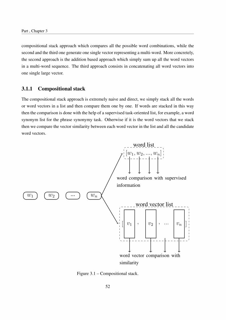
Part , Chapter 3

compositional stack approach which compares all the possible word combinations, while thesecond and the third one generate one single vector representing a multi-word. More concretely,the second approach is the addition based approach which simply sum up all the word vectorsin a multi-word sequence. The third approach consists in concatenating all word vectors intoone single large vector.

3.1.1 Compositional stack

The compositional stack approach is extremely naive and direct, we simply stack all the wordsor word vectors in a list and then compare them one by one. If words are stacked in this waythen the comparison is done with the help of a supervised task-oriented list, for example, a wordsynonym list for the phrase synonymy task. Otherwise if it is the word vectors that we stackthen we compare the vector similarity between each word vector in the list and all the candidateword vectors.

w1 w2 ... wn

[w1, w2, ..., wn]

[ v1 , v2 , ... vn ]

word list

word vector list

word comparison with supervisedinformation

word vector comparison withsimilarity

Figure 3.1 – Compositional stack.

52

3.1. Approaches without learnable parameters

For a given multi-word sequence w1, w2, ..., wn with n words, the word comparison looks ateach of the words and replace it with a word of the given supervised list, e.g., a synonym. Theword vector comparison replace each word with their corresponding word vector and map eachtoken to the most similar word according to the vector similarity.

This simple approach may bring decent results if we have exhaustive task-oriented informa-tion such as a synonym word pair list. Nevertheless, it has several major drawbacks :

• Highly dependent on the task-oriented supervised information. If we do not possess suchdata, then the word comparison is inaccessible.

• Length sensitive. Even with the word vector comparison, this approach cannot deal withthe fertility problem. We cannot obtain unified representation with this approach.

• Word inner relation ignored. This approach treats separately each word of a multi-wordsequence, thus the inner relation between them is completely ignored. However we esti-mate that many multi-word expressions’ meaning is deeply related to the association ofwords. This phenomenon is especially obvious when it comes to the idiomatic expres-sions or the homographs. For example, “a piece of cake” means in general a job, task or

other activity that is easy, which is no more a part of cake. In “full magazine”, the word“magazine” stands for a store for arms or ammunition, while in “fashion magazine” itmeans a periodical publication.

3.1.2 Addition based approach

One may argue that the most common baseline approach is the addition based approach. It isapplicable when we use vector representations. For a given multi-word sequence w1, w2, ..., wn

with n words, and their corresponding word vectors v1, v2, ..., vn, the addition based approachsimply use the sum as the vector representing the whole sequence :

vmw =n∑i=1

vi (3.1)

where vmw is the vector for representing the whole multi-word. FastText (Bojanowski et al.,2017) uses the same idea to obtain the word vectors with subword tokens. Some specify thatthis vector should be averaged by the sequence length n:

vmw =

n∑i=1

vi

n

(3.2)

53

Part , Chapter 3

In practice, if we use the cosine similarity, for any two non-averaged vector x and y, theywill have the same similarity as for their averaged version x and y:

cos(x, y) =

d∑i=1

xi

ayi

b√d∑i=1

(xi

a)2

√d∑i=1

(yi

b)2

=

d∑i=1

xiyi

ab√d∑

i=1xi

2

√d∑

i=1y2

i

√a2√b2

=

d∑i=1

xiyi√d∑i=1

x2i

√d∑i=1

y2i

= cos(x, y)

(3.3)

where d is the word vector dimension size, a and b are the sequence length for the two multi-words.

The addition based approach has shown very strong results on sequence classification andsimilarity tasks (Mikolov, Sutskever, et al., 2013; Del et al., 2018; Liu et al., 2018). However,it has still two issues :

• Order ignored. For example, “service department” and “department service” will havethe same representation while they do not have the same semantics.

• Word inner relation ignored. As described in Section 3.1.1.

3.1.3 Concatenation

The concatenation approach (Garten et al., 2015; Goikoetxea et al., 2016) consists in concate-nating all the word vectors of a multi-word into one single high dimensional vector. If eachword vector is of size d and the length of the multi-word is n, the concatenated vector will havea dimension size of nd.

The concatenation method does register word order but variable length phrases are no longersemantically comparable with the cosine similarity even if we pad them. For example the cosinesimilarity between “sneaker shoe” and “sneaker”, denoted by cos(v(sneaker, shoe), v(sneaker)) will

54

3.2. Phrase embeddings with CBOW or Skip-gram

be 12 if we pad “sneaker” with zeros. This similarity will be probably lower than :

cos(v(sneaker, shoe), v(sneaker, shop))

However, it is obvious that “sneaker shoe” is semantically synonym of “sneaker”. With thisbeing said, we think the concatenation approach is not suitable for generating unified sequencerepresentation even if it generates one single vector.

3.2 Phrase embeddings with CBOW or Skip-gram

Concerning the models with learnable parameters, many would wonder if it is possible thatwe simply train a word embedding model using CBOW or Skip-gram if we treat the n-gramsas a single token. The answer is yes, we can indeed train a word embedding model just likewhat we do for all the n-grams. However, it ignores compositionality and inner word rela-tions. Another way of training embedding model for multi-words is the extended Skip-gramintroduced Artetxe, Labaka and Agirre (2018b). which is a generalized skip-gram that learnsn-gram embeddings on-the-fly while keeping the desirable property of unigram invariance tohandle compositional phrases but it still suffers from the sparsity and memory problem. In thissection we will go through these two strategies for training a multi-word embedding model.

3.2.1 One single token processing for non-compositional phrases

Treating n-grams as a single token in a pre-processing step has been explored in the very inspir-ing work of Mikolov, Sutskever, et al. (2013). But they mainly focused on the phrases whosemeaning is not a simple composition of the meanings of its individual words, such as New York

Times and Toronto Maple Leafs. They proposed to extract some n-grams based on a thresholdscore which is defined as :

score(wi, wj) = n(wi, wj)δn(wi)n(wj)

(3.4)

where n(w) is the count for the word w and δ is used as a discounting coefficient and preventstoo many phrases consisting of very infrequent words to be formed. The bigrams with scoreabove the chosen threshold score are extracted and after 2-4 passes over the training data withdecreasing threshold value, they build recursively n-grams longer than 2 tokens.

Clearly, this approach works relatively well on more idiomatic phrases, whereas in ourscenario, most of the phrases are freely combined multi-words. In addition, this approach can

55

Part , Chapter 3

only handle phrases that have been passed into the model during the training. A new phrase,even if it is idiomatic, can never have its phrase vector through this approach.

3.2.2 Extended skip-gram with negative sampling

Apart from the more idiomatic phrases extracted by the score of Equation 3.4, to learn the em-beddings for other n-grams which are generally more compositional phrases, one could simplymerge all n-grams but this would greatly increase the vocabulary size, making the model timeand space too complex. This idea has shown very poor performance in the preliminary exper-iments of Artetxe, Labaka and Agirre (2018b) while they tried to randomly generate multipleconsistent segmentations for each sentence.

In order to produce relevant phrase embeddings with Skip-gram, Artetxe, Labaka and Agirre(2018b) propose to extend the Skip-gram with negative sampling model. Recall the loss functionof this model in Equation 2.50, for the ease of the reading, we copy it here :

E = − log σ(sTwOh)−

∑wk∈Wneg

log σ(−sTwkh) (3.5)

where h is the output of the hidden layer for the input word tokenw, s is the output of the hiddenlayer for the context c ∈ wO∪Wneg. This can be seen as a logistic regression to predict whetherthe word-context pair really co-occurs in the on-line sampled sentence, or the context is one ofthe negative samples inWneg. Updating the hidden weight matrix W2 is equal to updating theword vector w and context vectors c.

In the extended Skip-gram with negative sampling, in addition to the updates based on thesingle-word pairs (update the vector of w and all the vectors of c), they also extract all thepossible n-grams phrases, p, within a max length and update all the vectors of p while using thesame context unigrams c.

The positive and negative context vectors in W2 are only updated for single-word pairs (w,c). The update function is the same as in Equation 2.52 because the positive and negative con-texts are always unigrams. For each n-gram p, the corresponding embedding vector is directlyupdated in W1 using the n-gram and context single-word pairs (except that the vectors in W2

are not updated this time). According to the authors, this allows to naturally learn n-gram em-beddings based on their co-occurrence patterns as modeled by Skip-gram, without introducingsubtle interactions that affect its fundamental behavior.

In conclusion, this approach learns all the n-grams in a corpus including the compositionalphrases. But it still cannot generate a phrase embedding for phrases that do not appear in the

56

3.3. Traditional neural networks for sequential inputs

training corpus.

3.3 Traditional neural networks for sequential inputs

We have seen the “simple approaches” for modeling multi-word representations. All theseapproaches ignore the inner structure of multi-words. In this section we discuss some morecomplex approaches using neural networks for sequential inputs. We will first go through threetypes of these neural networks : the Convolutional Neural Network (CNN), the Recurrent Neu-

ral Network (RctNN) and its variants such as Long short-term memory (LSTM) and Gated

Recurrent Unit (GRU). Finally, we present the latest application: Embeddings from Language

Models (ELMo) using the bidirectional LSTM as basic unit.

3.3.1 Convolutional Neural Network

The Convolutional Neural Network (CNN) is also a feed forward neural network. Inspiredby the Receptive Field theory in neural science (Hubel and Wiesel, 1968), Fukushima (1980)introduced the basic layer using the convolution operation.

Convolution is a mathematical operation, denoted by ~, here we only consider the discretecase. Let f and g be two functions defined on the integers, the 1-d discrete convolution of f andg is :

(f ~ g)[n] =inf∑

m=−inff [m]g[n−m] (3.6)

and the 2-d discrete convolution:

(f ~ g)[i, j] =inf∑

k=−inf

inf∑t=−inf

f [k, t]g[k − i, t− j] (3.7)

In practice, we let our input distribution as one function defined on indices (discrete values),and a kernel (or filter, containing some weights) as the other function. The idea is to repeatedlyapply the kernel on all the outputs. The convolution output is also called feature map becausethe convolution can be seen as a feature extraction process. Usually, the definition domain ofthe kernel is much narrower. For the 1-d convolution, we can note the input xi with i ∈ [1, n],the kernel function fi with i ∈ [1,m] where m << n. The output sequence yi is :

yi =m∑k=1

fkxi−k+1 (3.8)

57

Part , Chapter 3

Figure 3.2 shows an example of the 1-d convolution.

Kernel 3 2 1

Input 1 2 3 4 5 6 7

Output 10 16 22 28 34

Figure 3.2 – 1-d convolution with kernel length m = 3 for an input sequence with length n = 7.The output sequence length is n−m+ 1.

As for the 2-d convolution which is widely applied in the computer vision domain, we notethe input graph xi,j with i ∈ [1, n], j ∈ [1, q], the kernel fi,j with i ∈ [1,m], j ∈ [1, p] wherem << n and p << q. The output graph yi.j is then :

yi,j =m∑u=1

p∑v=1

fu,vxi−u+1,j−v+1 (3.9)

Figure 3.3 shows an example of the 2-d convolution.

In fact, we can move the kernel by a larger stride, in the illustrated examples the stride isalways 1, the output size after the convolution is n− f + 1 where n is the input size and f thekernel size at the corresponding dimension. Apart from stride, we can also zero-pad the input.With the stride and zero-padding into account, the output size is n−f+2padding

stride+ 1. Note that if

the result is not an integer, then the current convolution does not fit, we should always makesure that the convolution process can be successfully completed.

Compared to the fully connected neural network, a convolutional neural network canbe considered as a partially connected neural network. In the fully connected network, nl isthe dimension size at layer l, the weight matrix between layer l − 1 and l will have nl × nl−1

parameters. Each neuron in layer l− 1 is connected to nl weights, whereas in the convolutionalnetwork, each neuron in layer l − 1 is only connected to a window of weights. The passagefunction between layer l − 1 and l for 1-d convolution is :

al = f(wl ~ al−1 + bl) (3.10)

where wl ∈ Rm is the kernel. We only need m weight parameters for this layer. However,

58

3.3. Traditional neural networks for sequential inputs

Kernel

3 2 1

1 0 1

0 1 2

Input

1 2 3

4 5 6

7 8 9

Output

46

Figure 3.3 – 2-d convolution with a 3× 3 kernel graph and for a 7× 7 input graph. The outputsequence length is (7 − 3 + 1) × (7 − 3 + 1). We only show one output value, the rest can becalculated by sliding the kernel on the input graph.

59

Part , Chapter 3

unlike the fully connected layer, the output neuron number of each layer is not configurable. Itis determined by the kernel size m :

nl = nl−1 −m+ 2paddingstride

+ 1 (3.11)

Similarly, for the 2-d convolution, the graphX l−1 in layer l−1 is transformed toX l in layerl following :

X l = f(W l ~X l−1 +Bl) (3.12)

where W l ∈ Ru∗v is the kernel, X l ∈ Rwl∗hl and X l−1 ∈ Rwl−1∗hl−1 are the graph in layer l andl − 1. The size of graph X l is :

wl = wl−1 − u+ 2paddingstride

+ 1

hl = hl−1 − u+ 2paddingstride

+ 1(3.13)

In order to learn multiple aspects from the input, we can apply several different kernels,the number of kernels is called depth. Usually, we add a pooling or subsampling layer afterobtaining the outputs of each kernel to reduce the final output dimension and thus avoid theoverfitting problem. Pooling layers downsample each feature map independently, reducing theheight and width, keeping the depth intact.

Contrary to the convolution operation, pooling has no weight parameters. We only haveto set the stride and window hyper-parameters. The most common type of pooling is the max

pooling and the average pooling:

poolmax(Rk) =∑i∈Rk

max(ai)

poolavg(Rk) = 1|Rk|

∑i∈Rk

ai(3.14)

where Rk is the pooling window and ai the feature map value at position i. Figure 3.4 shows anexample of a max pooling with a stride of 1 and a 2× 2 pooling layer.

We also show an illustration of the famous LeNet-5 for handwritten number recognitionwhich is built on some convolutional layers (Lecun et al., 1998) with a depth column in eachlayer (with multiple kernels) :

The gradients calculation is fairly straightforward with the formula given in 2.26. For theδ(l,i) which is the error in the layer l for the i-th value of the feature map, if the pooling layer is

60

3.3. Traditional neural networks for sequential inputs

Feature mapmax pooling

5 4 8

2 0 3

6 1 7

5 8

6 7

Figure 3.4 – An example of max pooling.

Figure 3.5 – LeNet-5 architecture. Original illustration from Lecun et al. (1998).

the l + 1-th layer, then we have :

δ(l,i) = ∂L(Y, Y )∂Z(l,i)

= ∂X(l,i)

∂Z(l,i)∂Z(l+1,i)

∂X(l,i)∂L(Y, Y )∂Z(l+1,i)

= f ′l (Z(l,i))� up (δ(l+1,i))

(3.15)

where Y and Y are respectively the output and real label of the network. X l is the final output ofthe layer l after activation or the input of the layer l+ 1, Z l is the output of the layer l before theactivation. Since the l + 1-th layer is a pooling layer, Z l+1 is the output of the pooling with theinput X l. The up (upsampling) is the reverse function of the subsampling, for instance, for themax pooling, up(δ(l+1,i)) will simply associate every value to the maximum value of the featuremap in the previous layer. The rest positions will be 0. While for the average pooling, thevalues in δ(l+1,i) will be equally distributed to every position of the feature map in the previouslayer.

Similarly, if the pooling layer is the l-th layer and the l+ 1-th layer is a convolutional layer,

61

Part , Chapter 3

the i-th feature map for layer l + 1, Z(l+1,i) is :

Z(l+1,i) =D∑d=1

W (l+1,i,d) ~X(l,d) + b(l+1,i) (3.16)

where D is the convolution depth. Then the d-th error in the l-th layer δ(l,d) is :

δ(l,d) = ∂L(Y, Y )∂Z(l,d)

= ∂X(l,d)

∂Z(l,d)∂L(Y, Y )∂X(l,d)

= f ′l (Z l)�∑i

(rot180(W (l+1,i,d)) ~ ∂L(Y, Y )∂Z(l+1,i) )

= f ′l (Z l)�∑i

(rot180(W (l+1,i,d)) ~ δ(l+1,i))

(3.17)

where rot180 is a rotation of 180 degrees. The detail of the derivative calculation for the con-volution operation is omitted here.

In our work, we use 1-d convolution with zero-padding to encode our phrases as one of thebaseline approaches.

3.3.2 Recurrent Neural Network

In the feedforward network, the information is transferred in a uni-directional way. The layeroutput depends only on the input, this grants the network a quick learning of the parameters butin many actual tasks, one neuron’s output also depends on the “memory” or previous outputs.Recurrent neural network (RctNN) is in line with this need, it is capable of memorizing a shortperiod by taking not only the current input but also the previous output of itself.

Figure 3.6 shows the basic idea of RctNN, for a sequence xt, t ∈ [1, T ], the RctNN transfersthe information by the following formula :

ht = f(ht−1, xt)

yt = g(ht)(3.18)

where ht is the current hidden state and yt is the output at the current time step t. f and g aretwo non-linear functions, i.e., a feedforward network.

The simple recurrent neural network (SRNN) (Elman, 1990) is a basic recurrent neural

62

3.3. Traditional neural networks for sequential inputs

f

xt

g

yt

ht

Figure 3.6 – A basic cell of RctNN.

network architecture with only one hidden layer. Each net input zt2 at time step t of the hiddenlayer is calculated based on the current network input xt :

zt = Uht−1 +Wxt + b

ht = f(zt)(3.19)

where U and W are weight matrices and b the bias vector. If we consider that each time stepis a single layer, then RctNN is actually a multiple layer network with shared weights. We canunfold in Figure 3.6 :

x1 x2 x3 x4 ... xT

h1 h2 h3 h4 ... hT

y1 y2 y3 y4 ... yT

Figure 3.7 – Unfolded RctNN

Now we look at the parameter learning with gradient descent, the loss function at time step

2We refer net input or net activation to the layer output before the activation function

63

Part , Chapter 3

t is :

Lt = L(yt, g(ht)) (3.20)

The loss function for all time steps is :

L =T∑t=1Lt (3.21)

The gradient for U :∂L∂U

=T∑t=1

∂Lt∂U

(3.22)

Since U is the weight matrix related to the previous hidden state, the gradient calculation isdifferent from the feedforward networks. Typically, we can use the Back propagation through

time (BPTT) (Werbos, 1990) to obtain gradients in a RctNN.

The BPTT treats the RctNN as an unfolded multi-layer feedforward network as shown inFigure 3.7. In this unfolded multi-layer network, all the layers share the same parameters, so thegradients are the sum of the gradients in each layer. We begin with the derivative in Equation3.22. Because the derivative at time step t is related to all the previous net inputs zk, withk ∈ [1, t], we have:

∂Lt∂ui,j

=t∑

k=1

∂zk(U)∂ui,j

∂Ltzk

(3.23)

Since zk = Uhk−1 + Wxk + b, the direct derivative of zk with regard to ui,j , denoted byzk(U) which means that we consider zk as a function on U with hk−1 as a constant :

∂zk(U)∂ui,j

= Ii(hk−1[j]) (3.24)

where Ii(hk−1[j]) means a vector with the same size as hk−1 with all values set to zero exceptfor the i-th dimension whose value is equal to hk−1[j].

For the second part in 3.23, again we can define an error δt,k = ∂Lt

∂zkwhich is the derivative

64

3.3. Traditional neural networks for sequential inputs

of the network loss at time step t with regard to the net input at time step k.

δt,k = ∂Lt∂zk

= ∂hk∂zk

∂zk+1

∂hk

∂Lt∂zk+1

= diag(f ′(zk))UT δt,k+1

(3.25)

So the formula in 3.23 can be written as:

∂Lt∂ui,j

=t∑

k=1δt,k[i]hk−1[j]

∂Lt∂U

=t∑

k=1δt,kh

Tk−1

(3.26)

So with substitution in 3.22, the gradient for the total loss with regard to U is:

∂L∂U

=T∑t=1

t∑k=1

δt,khTk−1 (3.27)

For the same reason, the gradients for other parameters are:

∂L∂W

=T∑t=1

t∑k=1

δt,kxTk (3.28)

∂L∂b

=T∑t=1

t∑k=1

δt,k (3.29)

Figure 3.8 gives an illustration of BPTT.

Another way of calculating the gradients is real-time recurrent learning or RTRL (Williamsand Zipser, 1995) which is a forward procedure similar to the forward mode in auto-differentiation(See 2.2.1). RTRL follows the same gradient calculation except we calculate each δ in the sameorder as the time sequence and update each parameter right after obtaining the correspondinggradient.

The hidden state at time step t+ 1, ht+1 is:

ht+1 = f(zt+1) = f(Uht +Wxt+1 + b) (3.30)

65

Part , Chapter 3

xt−2 xt−1 xt

ht−2 ht−1 ht

yt−2 yt−1 yt

yt−2 yt−1 yt

Lt−2 Lt−1 Lt

δt−2,t−2

δt,tδt,t−1δt,t−2δt−1,t−1δt−1,t−2

Figure 3.8 – Diagram of BPTT. Black lines are the forward pass and dashed lines are the localbackward pass. Gradients are accumulated through time.

The derivative of ht+1 with regard to ui,j is:

∂ht+1

∂ui,j= ∂zt+1

∂ui,j

∂f(zt+1)∂zt+1

∂zt+1

∂ui,j= ∂Uht

∂ui,j, and because

∂f(x)g(x)∂x

= f ′(x)g(x) + g′(x)f(x), above line equals to

= ( ∂U∂ui,j

ht + ∂ht∂ui,j

UT ) ∂f(zt+1)∂zt+1

= (Ii(ht[j]) + ∂ht∂ui,j

UT )diag(f ′(zt+1))

= (Ii(ht[j]) + ∂ht∂ui,j

UT )� (f ′(zt+1))T

(3.31)

We use Equation 3.31 to calculate ∂h1∂ui,j

, ∂h2∂ui,j

, ∂h3∂ui,j

, ... in a forward order and at each timestep t, the gradient can be obtained simultaneously with the current loss Lt:

∂Lt∂ui,j

= ∂ht∂ui,j

∂Lt∂ht

(3.32)

Note that in RTRL we will update the parameters right after obtaining the gradient at eachstep. The update for W and b follows the same way.

In general, as we usually use sigmoid functions as the activation function and its derivative is

66

3.3. Traditional neural networks for sequential inputs

inferior to 1, the sequence product of multiple derivatives of sigmoids functions would approach0, causing the gradient vanishing problem for Lt

∂hkwhere t − k is relatively high3. In other

words, the hidden states hk which are far from the current step t would merely influence thecurrent gradient Lt

∂U, the RctNN can only memorize short distance dependencies.

Concerning our work, we also implement RctNN as a baseline approach for phrase repre-sentation modeling.

3.3.3 LSTM and GRU

To overcome the gradient vanishing problem for long distance dependencies, we could addlinear relation between each time step so there will be both linear and non-linear relations andit would be less possible for the gradient to vanish. However, there are still problems such asgradient explosion and limited memory capacity4. In order to solve these problems, someRctNN variants are proposed with a gate mechanism. We will cover the two most successfulgated RctNN: Long Short-Term Memory (LSTM) (Hochreiter and Schmidhuber, 1997; Gerset al., 2000) and Gated Recurrent Unit (GRU) (Cho et al., 2014; Chung et al., 2014).

Long Short-Term MemoryIn addition to the hidden state or external state ht in the RctNN, LSTM introduces an inter-

nal state or cell state ct (with a candidate cell ct) and three gates whose range is [0, 1] in orderto indicate how much information should pass the “gate”:

• Forget gate ft decides how much information in the previous cell ct−1 should drop:

ft = σ(Wfxt + Ufht−1 + bf ) (3.33)

• Input gate it decides how much information in the current candidate cell ct should bepassed:

it = σ(Wixt + Uiht−1 + bi) (3.34)

• Output gate ot decides how much information in the current cell ct should be passed tothe current hidden ht:

ot = σ(Woxt + Uoht−1 + bo) (3.35)

3Similarly, if the derivative is superior to 1, it will cause the gradient explosion problem.4ht would converge with information accumulated through time. The memory of ht is limited.

67

Part , Chapter 3

We can see that the three gates are all functions about the current input xt and the previoushidden state vector ht−1, with a logistic function to obtain values between [0, 1] in order tocontrol the information passing proportion.

Basically, one LSTM layer passes information with the hidden and cell state:

ct = ft � ct−1 + it � ctht = ot � tanh (ct)

(3.36)

where the candidate cell ct is:

ct = tanh (Wcxt + Ucht−1 + bc) (3.37)

The LSTM architecture is shown in Figure 3.9 in a computational graph form, we can con-sider an LSTM unit as a special RctNN unit, with two input and output states c and h.

xt−1 xt xt+1

ct−2 ct−1 ct ct+1

ht−2 ht−1 ht ht+1

xt

ht−1

ct−1

cat

σ σ tanh σ

ft it ct ot

�

� + ct

tanh

�

ht

Figure 3.9 – Diagram of LSTM.

68

3.3. Traditional neural networks for sequential inputs

In practice, we can concatenate the input xt ∈ Ra and the previous hidden ht−1 ∈ Rd, sowe can write one single weight matrix for the matrices in Equation 3.33, 3.34, 3.35 and 3.37:W ∈ Rd∗(a+d). We usually set relatively high initial values for the parameters in the forget gatesince otherwise most of the previous information would be dropped5.

The network can also be learned by gradient descent and the gradient calculation is not verydifferent from what we have seen in RctNN. We will not go through all the details for LSTMand all the advanced network architecture in later sections.

There are also many variants of LSTM, the work of Greff et al. (2017) and Jozefowicz et al.(2015) has compared a good deal of popular variants and concluded that they are essentially thesame architecture and have similar experimental performance.

In a neural network, long-term memory consists in the network parameters, which coversall the training period and are updated gradually. In a LSTM network, the cell state c is capableof storing and transferring information for a short period yet still longer than the hidden state h,that is why we call the network Long short-term memory.

We will also include LSTM in our work as a baseline approach for encoding phrases.Gated Recurrent UnitGated recurrent unit (GRU) is simpler than LSTM, it does not introduce a new state like the

cell state in LSTM. Still, GRU uses several “gates”: an update gate which is a combination ofthe forget and input gates in LSTM and a reset gate which determines the dependency on theprevious hidden state ht−1.

• Update gate zt. It decides how much information should be kept from the previoushidden ht−1 and meanwhile, how much information should be passed from the currentcandidate state ht.

zt = σ(Wzxt + Uzht−1 + bz) (3.38)

• Reset gate rt. It decides the degree of the dependency on the previous hidden ht−1 forthe current candidate state ht.

rt = σ(Wrxt + Urht−1 + br) (3.39)

The current candidate hidden state ht is defined as :

ht = tanh(Whxt + Uh(rt � ht−1) + bh) (3.40)

5Generally speaking, the initial values for the parameters in a neural network are quite small, here in LSTM,we would like to set a high value for the bias vector in the forget gate, for instance bf = 1

69

Part , Chapter 3

Then the information in the GRU network is passed with the hidden state ht :

ht = zt � ht−1 + (1− zt)� ht (3.41)

From 3.41 we can see that when zt = 1, the current hidden state ht is linearly related tothe previous hidden state ht−1, and when zt = 0, ht is related to ht−1 in a non-linear manneras ht is obtained from a sigmoid function tanh. From 3.40 we can see that when rt = 1, thecurrent candidate hidden state ht depends on both the current input xt and the previous hiddenstate ht−1, and when rt = 0, ht depends on only xt. Combining these observations, whenzt = 0, rt = 1, the GRU network is basically a recurrent neural network. Furthermore, whenzt = 0, rt = 0, the current hidden ht is only related to the current input xt, which is similar toone separated fully connected layer. Figure 3.10 illustrates how GRU passes information.

xt−1 xt xt+1

ht−2 ht−1 ht ht+1

xt

ht−1

catσ σ

cat

tanh

rt zt ht

�

�

1−

+

ht

�

Figure 3.10 – Diagram of GRU.

Since GRU has very similar performance with LSTM, we will not include GRU in ourframeworks, one can refer to LSTM to get an approximate performance of GRU.

70

3.3. Traditional neural networks for sequential inputs

3.3.4 Recent applications: ELMo

There are many great works incorporating a recurrent neural network or its variants. Quiterecently, embedding from language models (ELMo) (Peters et al., 2018) has been proposedwhich is built on a deep bidirectional LSTM network (BiLSTM) with subword informationencoded by a character convolutional network. The network is first trained on non-supervisedbidirectional language modeling, then the pre-trained model can be applied to some supervisedNLP tasks by adding some other layers on top while freezing the weights in the pre-trainedmodel6.

Bidirectional language model with LSTMsSimilarly to the translation objective in Equation 1.1, given a sequence of T tokens, xk, k ∈

[1, T ], a forward language model computes the probability of the sequence by modeling theprobability of the current token xk given all the previous tokens (x1, x2, ...xk−1):

P (x1, x2, ..., xT ) =T

Πk=1

P (xk|x1, x2, ..., xk−1) (3.42)

Analogously, a backward language model is a reversed version of the forward one :

P (x1, x2, ..., xT ) =T

Πk=1

P (xk|xT , xT−1, ..., xk+1) (3.43)

Each token is represented by a vector vk (input embedding), and it is passed to L stackedlayers of forward and backward LSTMs, obtaining

−→hk,j and

←−hk,j where j ∈ [1, L] means the j-th

LSTM layer. The top LSTM layer’s outputs−−→hk,L and

←−−hk,L are used to predict the next token

xt+1 with a softmax function.

−→hk,j = −−−−→LSTMj(vk,

−−−→hk−1,j)

←−hk,j =←−−−−LSTMj(vk,

←−−−hk+1,j)

(3.44)

A bidirectional language model (biLM) maximizes the log likelihood:

T∑k=1

(logP (xk|x1, x2, ..., xk−1;−→θ ) + logP (xk|xT , xT−1, ..., xk+1;←−θ )) (3.45)

where θ means the network parameters.Linear combination of biLMFor each token xk, we can conclude that a L-layer biLM contains a set of 2L + 1 vector

6We can conclude this manner as a feature extraction, further discussion can be found in the next chapter.

71

Part , Chapter 3

Figure 3.11 – Development set performance for SQuAD, SNLI and SRL when including ELMoat different locations in the supervised model. Extracted from the original paper of Peters et al.(2018). The data set details can be found in the original paper.

representations:Rk = {vk,

−→hk,j,←−hk,j|j ∈ [1, L]}

= {vk,←→hk,j|j ∈ [1, L]}

(3.46)

where←→hk,j means the concatenated vector of [−→hk,j;

←−hk,j].

In ELMo, the outputs in each layer are collapsed into a single vector ELMok = E(Rk; θ).For a specific task, ELMo computes different weights for each layer:

ELMotaskk = E(Rk; θtask) = γtaskL∑j=0

staskj

←→hk,j (3.47)

where staskj are softmax-normalized weights in terms of layer and task, and γtask is a scalarparameter which allows the model to scale the ELMo vector. Equation 3.47 can also be seen asa linear combination of each BiLM layer.

Integration of ELMo

ELMo vectors can be incorporated into other supervised NLP models. Basically, the authorstate that ELMo vector can substitute static word embedding vectors such as CBOW, Skip-gram or GloVe. For instance, to integrate ELMo into a task-specific RctNN model, we canfirst freeze the weights of the BiLM and then pass the concatenated vector [vk;ELMotaskk ]obtained from ELMo vector ELMotaskk and the input vector vk into the RctNN. For some tasks,authors find that it is beneficial to integrate ELMo vectors at the output layer of a RctNN whichmeans replacing the hidden state hk with [hk;ELMotaskk ]. Or sometimes, we can make thesemodifications at the same time, changing the input and the output of a RctNN. In the ablationtests, authors have shown some interesting results about different application locations of ELMovectors.

Besides, in addition to using all the layers, we can use one particular layer of the biLM.

72

3.3. Traditional neural networks for sequential inputs

Figure 3.12 – Development set performance for SQuAD, SNLI and SRL comparing using alllayers of the biLM (with different choices of regularization strength λ) to just the top layer.Extracted from the original paper of Peters et al. (2018). The data set details can be found inthe original paper.

Figure 3.13 – Test set comparison of ELMo enhanced neural models with state-of-the-art singlemodel baselines across six benchmark NLP tasks. The performance metric varies across tasks– accuracy for SNLI and SST-5; F1 for SQuAD, SRL and NER; average F1 for Coref. The“increase” column lists both the absolute and relative improvements over the baseline. Extractedfrom the original paper of Peters et al. (2018). The data set details can be found in the originalpaper.

In Figure 3.12, ablation tests conducted by authors show that using all the layers does help themodel to encode different types of syntactic and semantic information.

Conclusion

We report the main results of ELMo vector in Figure 3.13.

In general, ELMo has strong generalization ability of modeling language, this has beenproven by large improvements when applying ELMo to a broad range of NLP tasks. Therefore,we would like to not only include ELMo for a comparison with our systems but also make oursystems capable of integrating ELMo as an input layer.

73

Part , Chapter 3

3.4 Transformers: Multi-Head Attention

The neural networks for processing sequential inputs must have a large memory capacity inorder to stock more information, which requires enlarging the network’s complexity. In thissection, we begin with presenting the attention mechanism which manages to focus on certainaspects of the input information, reducing the network’s input size. Then we study a recentattention architecture called multi-head attention (Vaswani et al., 2017) which has constructedthe Transformer architecture, achieving strong empirical results, many new state-of-the-artarchitectures are derived from the Transformer.

3.4.1 Attention mechanism

In the past few years, attention mechanisms have brought effective progression to many NLPtasks. Basically they can be considered as a data/task-driven weighting process for the inputinformation. For each input in a sequence, the attention applies a weight indicating how much“attention” we should pay to the input. Bahdanau et al. (2014) use an attention-based modelfor neural machine translation with an encoder-decoder architecture, Xu et al. (2015) generalizeattention into soft and hard attention while Luong, Pham, et al. (2015b) further develop theminto global attention and local attention. Ling et al. (2015) employ attention to obtain betterword representations with respect to word contexts.

Generally speaking, attention mechanisms can be split into two steps, the first one consistsin calculating the attention distribution and the second step calculates the weighted mean.

Attention distributionGiven a sequence of input vector vi, i ∈ [1, N ], the attention distribution is obtained by

applying the softmax function on a score on the input and a query vector q.

αi = softmax(s(vi, q))

= exp(s(vi, q))∑Nj exp(s(vi, q))

(3.48)

where αi is the attention distribution for the i-th input vector and s is a score function whichcan be obtained by one of the following formulas:

• Addition.

s(vi, q) = sT tanh(Wvi + Uq) (3.49)

74

3.4. Transformers: Multi-Head Attention

• Dot-product.

s(vi, q) = vTi q (3.50)

• Scaled dot-product.

s(vi, q) = vTi q√d

(3.51)

• General.

s(vi, q) = vTi Wq (3.52)

where W,U, s are learnable parameters, d is the dimension size of the input vector vi.

Weighted mean

The final attention is actually a weighted mean with the attention distribution αi as theweight for the i-th vector:

attention(V, q) =N∑i=1

αivi (3.53)

Equation 3.53 is also called the soft attention or global attention. The soft attention calcu-lates its value depending on all the input vectors. In addition to the soft attention, hard attention

also calculates the attention depending only on one input at one step (Xu et al., 2015).

attention(V, q) = vj (3.54)

where we copy one input vj with j the index of the element with the highest probability,Nargmaxi=1

αi in the first formular of 3.48. The soft attention is smooth and differentiable but

can be very expensive when the input is large. The hard attention is less complex at the infer-ence time but is non-differentiable and requires more complicated techniques such as variancereduction or reinforcement learning to train (Luong, Pham, et al., 2015b). Figure 3.14 showsthe comparison between the global and the local attention of Luong, Pham, et al. (2015b).

We can see that the global attention calculates the weights using all the input vectors (h)while in the right part of the figure, the local attention calculates the weights with only a windowof input vectors plus a position information for the current step pt.

75

Part , Chapter 3

Figure 3.14 – Global vs local attention. (source: Luong et al. (2015). ) Note h in this figure isthe input for the attention layer which is v in our manuscript.

3.4.2 One head: Scaled Dot-Product Attention

In fact we can generalize attention with key-value pairs, given a sequence a key-value pairs(ki, vi), i ∈ [1, N ], the attention is:

attention((K,V ), q) =N∑i=1

αivi =N∑i=1

softmax(s(ki, q))vi

=N∑i=1

exp(s(ki, q))∑j exp(s(kj, q))

vi

(3.55)

where s is the score function. If K = V , this equals to Equation 3.53 with Equation 3.48.Based on this idea, Vaswani et al. (2017) introduce a scaled dot-product based key-value self-attention.

Given an input sequence X = [x1, x2, ...xN ] ∈ RN∗dinput and the output dimension doutput,the query Q, key K and value V matrices are first obtained by three linear transformations withdifferent learnable parameters WQ, WK and Qv:

Q = XWQ ∈ RN∗dm

K = XWK ∈ RN∗dm

V = XWV ∈ RN∗doutput

(3.56)

76

3.4. Transformers: Multi-Head Attention

where WQ ∈ Rdinput∗dm , WK ∈ Rdinput∗dm and Qv ∈ Rdinput∗doutput . dm is the intermediatedimension size for queries and keys. The final attention has a scaled dot-product as the scorefunction:

attention(Q,K, V ) = softmax(QKT

√dm

)V ∈ RN∗doutput (3.57)

where softmax is a column-wise function.

Intuitively, this self-attention can be considered as a fully-connected network with dynamicweight matrices. Both have the capability of memorizing long dependencies (Compared toRctNN and CNN). In a fully-connected layer, all inputs are connected to each output withlearnable weights. One input xi is connected or contributes to one output yj, j ∈ [1, J ] withWi,jxi + bj where Wi,j reveals actually the transformation direction. The input xi is connectedto the output yj by a weight Wi,j . Once we have set the output size J we can no longer modifyit. In the self-attention, one input xi is first connected to all other inputs xj with i, j ∈ [1, N ],by QKT , and then multiplied by V to obtain the output whose length is always the same asthe input length N . Thus we consider that the process is “dynamic” and the self-attention canhandle variable length input. This is illustrated in Figure 3.15.

x1 x2 x3 x4

y1 y2 y3 y4

(a) Fully-connected layer connectionx1 x2 x3 x4

q1 q2 q3 q4k1 k2 k3 k4v1 v2 v3 v4

y1 y2 y3 y4

(b) Self-attention layer connection

Figure 3.15 – Comparison between a fully-connected layer and a self-attention layer of Vaswaniet al. (2017). The solid lines represent a linear transformation with learnable parameters andthe dashed lines mean a dot-product which does not require any parameters. We can see thatthe self-attention’s is more dymanic since for any input with length N , the network use alwaysthe same parameters to generate a sequence of length N , while in a fully-connected layer, if wechange the input size we will have to change the weight matrix.

In the work of Vaswani et al. (2017), one such attention as in Equation 3.57 is called “onehead” which can be used as an alternative of a recurrent or convolutional neural network in anyarchitecture.

77

Part , Chapter 3

3.4.3 Multi-Head for multiple semantic aspects

Like in a convolutional neural network, Vaswani et al., 2017 propose to add some “depth” to theattention layer to capture different aspect information: instead of performing a single attentionfunction with one set of keys, values and queries, they linearly project the queries, keys andvalues h times with different, learned linear projections to dm, dm and doutput dimensions, re-spectively. Then, they perform the attention function(3.57) in parallel on each of these projectedversions of queries, keys and values, yielding hdoutput dimensional values in total:

MultiHeadAtt(Q,K, V ) = concat(head1, head2, ..., headh)WO ∈ RN∗dfo (3.58)

where the i-th head, headi = attention(QWQi , KW

Ki , V W

Vi ) with i ∈ [1, h]. WQ

i ∈ Rdinput∗dm ,WKi ∈ Rdinput∗dm and W V

i ∈ Rdinput∗doutput are the weight matrices in the i-th head. WO ∈Rhdoutput∗dfo where doutput is the output dimension for one head and dfo is the final outputdimension for the multi-head attention.

The relation of one head and multi-head attention is shown in Figure 3.16.

Figure 3.16 – The relation between one head (left) and multi-head attention (right). (Source:Vaswani et al. (2017))

3.4.4 Positional encodings for order distinction

Since the weight for one input xi in the self-attention Equation 3.57 depends only on the lineartransformation of qi and ki, ignoring completely the position of xi in the input sequence, incase of using only self-attention layers, we usually add some order information via positional

78

3.4. Transformers: Multi-Head Attention

encodings. For instance, we can use sine and cosine functions of different frequencies:

PE(pos, 2i) = sin( pos

100002i/do)

PE(pos, 2i+ 1) = cos( pos

100002i/do)

(3.59)

where do is the dimension size of the input vector embeddings, for example, do = dinput inour manuscript. pos represents the input position in the sequence. i is the dimension indexof the positional encoding. Here, each dimension corresponds to a sinusoid. The periodicityallows the model to easily learn to attend by relative positions because for any fixed offset k,PE(pos+ k) can be represented as a linear function of PE(pos).

3.4.5 Recent applications: Transformer, Opengpt, BERT, XLNet

Since 2017, the multi-head attention has been integrated in many general sequence modelingworks which have advanced the state-of-the-art results (Vaswani et al., 2017; Devlin et al., 2018;Radford et al., 2019; Zhilin Yang et al., 2019).

The very first application is the transformer which is proposed in Vaswani et al. (2017)right after introducing the multi-head attention. The encoder contains 6 layers of multi-headattentions which combines 8 different heads and output 512 dimensional attention vectors. Andthey set dm equal to doutput. Then it is followed by a normalization of (x + MultiHeadAtt(x))where x is the input, and finally passed to a fully-connected layer with a second normalizationof (x + Dense(x)) where x is the previous output of the multi-head attention layer. The de-coder uses the similar architecture except that it inserts another multi-head attention sublayer toconnect the encoder’s output and masks the first multi-head attention layer. (See Figure 3.17)

Shortly after, it is extended by Z. Dai et al. (2019), proposing transformer-XL to removethe fixed-length context limit during the training of language models. In the same line, Rad-ford et al. (2019) propose their language model GPT-2 pre-trained with an objective of simplypredicting the next word given the previous sequence with transformer units.

All these works train the model with whether unidirection or bidirection but in a separatedmanner, Devlin et al. (2018) introduce a pre-trained generic model for a wide range of NLPtasks with joint bidirection training, Bidirectional Encoder Representations from Transformers

(BERT). A brief comparison between the training of these models is given in Figure 3.18.Concerning the training objective, apart from the next sentence prediction in many general

language models, they also add a masked language model (masked LM) training objectivewhich predicts only some randomly masked tokens. This process is very similar to the denoising

79

Part , Chapter 3

Figure 3.17 – Transformer model architecture. (Source: Vaswani et al. (2017))

Figure 3.18 – Differences in pre-training model architectures. BERT uses a jointly-linked bidi-rectional Transformer. GPT uses a left-to-right Transformer. ELMo uses the concatenationof independently trained left-to-right and right-to-left LSTM. models. (Source: Devlin et al.(2018))

80

3.4. Transformers: Multi-Head Attention

(Vincent et al., 2008) which will be discussed later, only in masked LM the prediction is onlyon the masked words rather than the entire input sequence. The authors state that by doing thisthe deep joint bidirectional model can be learned without allowing each word to indirectly “seeitself” in a multi-layer context.

Compared to the previous models, BERT has achieved new state-of-the-art results on mul-tiple GLUE tasks7:

Figure 3.19 – Glue test results. Note that BERTBASE and OpenGPT have comparable parameternumber while BERTLARGE is not yet publicly available. (Source: Devlin et al. (2018)) The dataset details can be found in the original paper or the Glue official website.

Later, in June 2019, Zhilin Yang et al. (2019) argue that the denoising based training inBERT neglects dependency between the masked positions and suffers from a pretrain-finetunediscrepancy. Based on the pros and cons of BERT and transformer-XL, they propose a gen-eralized autoregressive pretraining method, XLNET, which is a autoregressive model whose

objective is to maximize the conditional probabilityT

Πk=1

P (xk|x1, x2, ..., xk−1) just like ELMoor transformer-XL. In addition, they maximize the probability of all possible permutations ofthe factorization order, the idea is to simulate a joint bidirectional model to capture informationfrom bidirectional contexts like BERT but without introducing noising-denoising processing.Let Zt be the set of all possible permutations of the T -length input sequence, zt and z<t thet-th element and the first t − 1 elements of a permutation z ∈ Zt, the training objective is tomaximize the following averaged log likelihood:

Ez∼Zt(T∑t=1

logP (xz<t |xz<t)) (3.60)

In our work, due to the heavy computation capacity requirement we have only chosen BERTas a baseline and an alternative input to the static embedding for our framework.

7https://gluebenchmark.com/leaderboard/

81

Part , Chapter 3

3.5 Contribution : a new dataset for monolingual phrase syn-onymy

For the phrase synonymy task, in addition to the dataset of Hazem and Morin (2017), we build anew dataset on the Breast cancer English corpus (BC-en). To extract the corpus, we crawl froma scientific website 8 by filtering all the publicly accessible articles and then search the keywords“breast cancer” for English articles. The final English corpus results from concatenating 168articles and contains 26,716 sentences and 874,595 tokens. Our corpus crawler script is opensource 9.

Concerning the the gold standard, we manually look for the most frequent terms of thecorpus and then see if they have synonyms which exist simultaneously in the corpus and theMeSH 2018 thesaurus10. Finally the gold standard contains 108 synonymy phrase pairs.

3.6 Contribution : Tree-free recursive neural network

In previous sections, we have seen simple approaches which ignore the inner structure of tokensin a sequence. Regarding neural network based sequence modeling, there are various neuralnetwork architectures for inputs of variable length: convolutional, recurrent and self-attention.However, these architectures are proposed to encode natural sentence sequences which are of-ten composed of more than 10 tokens, while our objective is to encode short sequences whichare phrases of less than 10 tokens. Besides, RctNN can encode multiple tokens into one singlevector (e.g., the hidden state for the last token) but this vector is biased by the last several wordsin a sequence due to the architecture property, and the self-attention only propose to encode asequence to a sequence of the same length. Even if we can still choose the last or first tokento represent the whole sequence, this vector is much biased by the last token as it is based onthe linear combination of the key and query of the last step alone(See Figure 3.15). Althoughthe experimental results in previous works are quite promising with this approach, the tasks aresentence-level classifications and the results are obtained by a supervised task-specific transferlearning process which differs from our scenario. With this being said, we propose a new ar-chitecture called Tree-free recursive neural network (TF-RNN) which is dedicated to encodingshort sequences such as phrases. In this section, we first review the original recursive neural

8https://www.sciencedirect.com9https://bitbucket.org/stevall/data-crawler.git

10https://meshb.nlm.nih.gov/search

82

3.6. Contribution : Tree-free recursive neural network

network and then present our architecture model. Finally, we conduct a series of experiments onphrase synonymy and similarity, our results show that our proposal outperforms state-of-the-artresults, and on the general domain corpora, the TF-RNN achieved even stronger results whenintegrating ELMo or BERT as an alternative input to the static word embedding.

3.6.1 Background: recursive neural network (RNN)

Recursive neural network (RNN) (Goller and Küchler, 1996) is a generalized version of therecurrent neural network (Elman, 1990) which always applies a left binary tree, where the firsttwo leaves are combined to form a node, then the node is combined to the next leaf to form thenext level node, etc. The recursive neural network encodes a sequence of word vectors along atree structure, e.g. a parse tree, by recursively applying the weight matrices to each node asso-ciation. This architecture has been successfully exploited in a variety of tasks, Socher, Bauer, etal. (2013) use an untied weight RNN for the constituent parsing where they use different weightmatrices depending on the constituent syntactic category, P. Le and Zuidema (2014) collect thecontext information by adding an outer representation for each node. Their system is used ina dependency parsing task. Besides, various works (Socher, Perelygin, et al., 2013; Irsoy andCardie, 2014; Paulus et al., 2014) apply the RNN to generate sentence level representation forsentiment analysis using some labelled data.

Wl Wr

Wl

Wr

Wl

Wr

leaf vectors

intermediate node vectors

root vector

v1 v2 v3 v4Figure 3.20 – Diagram of a recursive neural network.

Figure 3.20 shows an example of a sequence of length four. Suppose we have a parse tree,each input is a word vector vi ∈ Rd. The network applies a linear function with a weight matrixWl ∈ Rd∗d for each left node child and a weight matrix Wr ∈ Rd∗d for each right node child in

83

Part , Chapter 3

the given tree. So for each non-leaf node η, the corresponding vector xη is calculated as follows:

xη = Wlvl(η) +Wrvr(η) + b (3.61)

where vl(η) and vr(η) mean respectively the left and the right child vector of the node η.

The RNN is particularly interesting for us because short sequences or phrase associationcan be traced with the parse tree. By nature, the network distributes association weights foreach element in a phrase. Therefore a phrase representation is not always biased by the lasttoken like in the RctNN. However, the disadvantage of RNN in our scenario is the need of a treestructure because not only it is not always available in all languages, but it is also not possibleto retrieve the context sentence for the parsing if we meet a new freely combined phrase thathas never occurred in the corpus. The recurrent neural network or the LSTM does not need atree structure but applies a universal left binary tree to all sequences, while the convolutionalneural network with a kernel size of 2 can be considered as a specialised RNN where it adoptselement-wise multiplication rather than matrix multiplication with only one layer by a poolingoperation.

Wxh,Whh Wxh

Whh

Wxh

Whh

Wxh

v1 v2 v3 v4

pooling

vl vrvl vrvl vr

v1 v2 v3 v4

Figure 3.21 – Diagram of recurrent neural network (left) and 2 kernel sized convolutional neuralnetwork (right). For the purpose of clarity, we omit the output layer in the recurrent neuralnetwork.

Figure 3.21 shows how the recurrent and a 2 kernel sized convolutional neural networkmodel for a sequence of 4 tokens. Wxh ∈ Rh∗d and Whh ∈ Rh∗h are the parameters in atypical recurrent neural network where h is the hidden dimension, and for the convolutionalnetwork with a kernel size of 2, we can consider the convolution operation as two element-wisemultiplications (dashed line in Figure 3.21) with a left multiplier vl ∈ Rd and a right multipliervr ∈ Rd. Stacking vl and vr forms the actual convolution kernel. The final vector is obtained bya pooling operation such as max or average. Note that the addition based approach (Liu et al.,2018) can be viewed as a specialised version of CNN where the values in vl and vr are fixed to

84

3.6. Contribution : Tree-free recursive neural network

be one and the pooling is an averaging process.

3.6.2 Tree-free recursive neural network (TF-RNN)

In order to encode phrases of variable length without tree structures into a single fixed-lengthvector, we propose a new network called tree-free recursive neural network (TF-RNN). Weconsider it as a variant of the original recursive neural network because the basic idea is stillto associate each token following a bottom-up structure. This structure is required as inputof the original recursive neural network while in the TF-RNN, we eliminate this requirementby recursively splitting each node into a left and a right semantic part, then associating theleft part with its right neighbour and the right part with its left neighbour. This is motivatedby our hypothesis that the semantics of a pair of words could be retrieved by combining theirmeaning with some position-specific weights, and consequently the semantics of a sequence ofwords could be retrieved by recursively combining the semantics of each word pair. In fact, bydoing this we create a pseudo binary tree structure where we associate each adjacent node pairwithout parsing it twice. This kind of structure can be seen as an approximation of a generalizedsentence syntax as each language unit is directly associated with its adjacent neighbours andhierarchically associated with other units eventually yielding the overall semantics of all theunits.

Let [v01, v

02, v

03, ..., v

0n] with v0

i ∈ Rd be the input word vector sequence with n words, theTF-RNN outputs a single fixed-length vector vo ∈ Rp by following steps:

vji,l = tanh(Wlv

ji + bl

)vji−1,r = tanh

(Wrv

ji−1 + br

)vj+1i = tanh

(vji,l + vji−1,r

)...

vo = tanh(Uvn0 + b)

(3.62)

where j indicates the pseudo-tree structure layer level. A phrase with n word components willhave n levels in such a structure. Wl ∈ Rd∗d and Wr ∈ Rd∗d respectively represent the left andright weight matrices for the extraction of the word semantics; bl ∈ Rd and br ∈ Rd are thecorresponding bias vectors. A node vector in the level j + 1, vj+1

i is calculated in terms of apair of adjacent node vectors from the previous level j. Once we reach the final level n, thefinal output vector vo can be calculated by a linear layer on top with U ∈ Rp∗d and b ∈ Rp as

85

Part , Chapter 3

its parameters. A non-linear activation function is applied after each operation. An example ofa sequence of three words (n = 3) is illustrated in Figure 3.22.

Wl Wr Wl Wr Wl Wr

add add

Wl Wr Wl Wr

add

v1 v2 v3

vo

Figure 3.22 – Diagram of the tree-free recursive neural network (TF-RNN).

Clarification about the boundaryWith a sequence of n words, each layer 0 <= j < n will have n − j vectors. At layer j,

the leftmost Wl matrix (resp. rightmost Wr matrix) is not included in the calculation for levelj + 1. For single words we apply zero-padding to the left and right, so single-words’ output isactually the sum of the left and right matrices.

ComplexityWe compare the complexity of different neural network layers which can encode sequences

of variable length, the RctNN and self-attention encode the input sequence to another sequenceof equal length while our proposal TF-RNN and CNN with padding and pooling (right part ofFigure 3.21) encode to one fixed-length vector.

We compare mainly two criteria for one layer of each architecture, the first is the compu-tational complexity which represents how many weight parameters are involved in the lineartransformation; the second is the maximum dependency length which is the length of the pathsforward and backward signals have to traverse in the network. This is critical for learning long-range dependencies in many sequence transduction tasks. We show the complexity comparisonin Table 3.1.

For the computational complexity, the RctNN has n times linear transformations with ma-trices in Rd∗d, while the CNN is more expensive than RctNN by a factor of the kernel width kwhich can be seen as having k times the weight matrices in a RctNN. The self-attention is fasterfor most of cases since usually n < d. Our proposal seems to be the most expensive since the

86

3.6. Contribution : Tree-free recursive neural network

RctNN CNN Self-Att TF-RNN

Computational complexity O(n · d2) O(k · n · d2) O(n2 · d) O(n(n−1)2 · d2)

Dependency length O(n) O(nk) O(1) O(n2 )

Table 3.1 – Comparison of complexity. n is the input sequence length, d means the modeldimension where we assume d = dinput = dhidden = doutput for simplifying the comparison. kis the kernel width for CNN.

complexity is quadratic in terms of input length and model dimension, however, keep in mindthat our objective is to encode phrases which are most of the time n-gram with n ∈ [1, 5]. Forunigrams and bigrams our encoder is less complex than RctNN and CNN. Besides, our encoderis a one-layer architecture compared to the self-attention which has a “depth” of 8 heads in theTransformer-base architecture.

The shorter the dependency length is, the easier the model memorizes long dependencies.Because the self-attention is a dynamic fully-connected layer, it traces each input position withone linear transformation. As for our proposal, we can see that it is linearly related to theinput length, yet again since our inputs are mostly short sequences, this is not considered asproblematic in our scenario.

3.6.3 Evaluation

We have conducted a set of experiments on the phrase synonymy and similarity tasks. Base-lines approaches are pre-trained models and context means that we train the correspondingphrase encoder with an encoder-decoder architecture which will be detailed in the next chapter.The BERT and ELMo inputs can be categorized as contextualized embeddings consideringtheir context training properties. Static means either the 400 dimensional static word embed-ding vectors obtained from concatenating the pre-trained fastText11 vectors and vectors trainedon small specialised domain corpora for the phrase synonymy task (See Section 2.4 for moredetails), or the 64-dimensional static word embedding vectors provided by the Semeval 201712 dataset for the phrase similarity task. Skip-gram-ext is the extended Skip-gram presentedin Section 3.2.2 (Artetxe, Labaka and Agirre, 2018b). Finally, we have three types of inputembedding:

• Skip-gram-ext. 300 dimensional embeddings trained on the specialized domain corpora

11https://fasttext.cc/12http://alt.qcri.org/semeval2017/task2/index.php?id=data-and-tools

87

Part , Chapter 3

where N-gram phrases are considered as one single unit in the embedding look up table.

• Static. The 400 dimensional static word embedding vectors obtained from concatenatingthe pre-trained fastText vectors and vectors trained on small specialized domain corpora.

• BERT or ELMo. Pre-trained contextualized embeddings with feature-based usage set-ting.

In addition, we have explored three different methods to pool a single vector representationfrom a vector sequence:

• mean. The addition based approach can be applied to both the static and the contextual-ized input embeddings.

• reduce. Use an output at one specific step of a sequence to represent the whole inputsequence for the contextualized embeddings. For ELMo we use the last step as in manystandard sequence model while for BERT we use the first step which is the special token“[CLS]” as it has been used for the classification tasks in Devlin et al. (2018).

• ELMo-Peters et al. (2018). The original pooling method proposed in the work of ELMo.It concatenates the first and the last step token embeddings to represent a sequence. Notethat for single-words, we simply duplicate the only embedding and concatenate the twoidentical vectors.

To compare our proposed TF-RNN encoder with other architectures, we also implementedseveral neural networks which do not structured input: RecurrentNN, CNN and Transformercell. To conclude, we have four types of phrase encoder:

• CNN (0.4M parameters). The CNN has a kernel size of 2 and a zero-padding to the leftand right of one phrase so that even single-word phrases can be encoded.

• RctNN (0.5M parameters). A regular recurrent neural network which always applies aleft binary tree to generate the final vector.

• Transformer. (5M parameters). In order to be comparable with other architectures inparameter number, we use a small Transformer encoder with 4 layers and 4 heads, thehidden dimension size is 2 times the model dimension.

• TF-RNN (0.5M parameters). Our proposed phrase encoder presented above.

88

3.6. Contribution : Tree-free recursive neural network

Phrase synonymyEach dataset of the phrase synonymy task contains phrases of variable lengths and for each

phrase, the reference phrase can be different in length, for example, “wind turbine” and “wind-mill”. The results are shown in Table 3.2.

Method Synonymy datasetWE-fr WE-en BC-en

Baselines

Skip-gram-ext <0.5 <0.5 23.30Static-mean 5.29 12.19 39.65BERT-reduce 4.07 10.44 26.04BERT-mean 4.49 16.59 36.58ELMo-reduce 1.54 4.09 26.23ELMo-mean 7.37 5.20 29.27ELMo-Peters et al. (2018) 8.97 9.60 28.28

Context

Static-CNN 7.42 15.71 35.75Static-RctNN 12.89 20.53 42.60Static-Transformer 4.62 15.82 35.90Static-TF-RNN 15.06 33.47 44.84

Table 3.2 – Overall MAP comparison for the phrase synonymy task. We have introduced thedata set for BC-en in Section 3.5. Details for the WE corpus can be found in Appendix A.1.2and the gold standard for WE is in Appendix A.3.1.

Phrase similarityThe phrase similarity task dataset also contains phrase comparison pairs of variable lengths

such as “Harry Potter” and “wizard”, “window blind” and “curtain”. The results are shown inTable 3.3.

DiscussionOur approach with concatenated static word embeddings and the TF-RNN as phrase encoder

has the best results in phrase synonymy task. While the Transformer encoder has achievedthe best result for Semeval2013 and the second best result for Semeval2017 phrase similaritytask. The TF-RNN has managed to obtain the third best result for the phrase similarity taskon Semeval2017. Given that the Semeval2013 dataset does not provide any textual data andthe model is trained on the textual corpus of Semeval2017, the results on Semeval2013 for thecontext prediction approaches are biased by the data availability. Moreover, even comparedto the approaches with contextualized embedding input, for the most of the time the contextprediction approaches (last four lines) have better results on the datasets that provide a textual

89

Part , Chapter 3

Method Similarity datasetSemeval2013† Semeval2017

Baselines

Skip-gram-ext 0.378 76.827Static-mean 26.910 38.843BERT-reduce 0.754 12.735BERT-mean 19.482 36.378ELMo-reduce 35.112 37.968ELMo-mean 37.991 36.207ELMo-Peters et al. (2018) 36.233 31.420

Context

Static-CNN (29.890) 42.245Static-RctNN (21.720) 42.961Static-Transformer (39.524) 49.324Static-TF-RNN (22.003) 44.382

Table 3.3 – Overall comparison of correlation score for the similarity task. The Semeval cor-relation score is the harmonic mean of Pearson and Spearman scores. A † indicates that thecorresponding corpus for training a neural network is not available. In the case of the contextbased approaches, we use the network trained on the Semeval2017 corpus, as it is also a generaldomain corpus. Details of the data set can be found in Appendix A.2.2 and A.3.2

.

corpus to train the model. Although the contextualized embedding models capture the innerrelation between each component word in a phrase, it cannot exploit the context informationof the phrase during the test phase or if the phrase is out of the training corpus, while theencoder-decoder training based approach memorizes and generalizes the context information ofdifferent phrases in the training corpus (See the next chapter). This confirms again the hypoth-esis of Harris (1954) and that the context information of a phrase is meaningful for learningthe phrase representation. Moreover, if we compare different phrase encoders, our proposedTF-RNN outperforms the existing neural networks (even the Transformer encoder with signifi-cantly more parameters) on the synonymy task on every dataset and obtains comparable resultson the similarity tasks. Therefore we believe that carefully representing the phrase following arelevant syntactical structure can generate better vector representations.

Among the non encoder-decoder training based approaches (the first seven lines), first theextended Skip-gram works very poorly for the phrase synonymy task. This is because manyphrases during the inference are freely combined so they may not appear in the training cor-pus. As a consequence, these phrases do not have any representation in the look-up table. Thisphenomenon can also be observed on Semeval2013 similarity task. However, it performs sur-

90

3.6. Contribution : Tree-free recursive neural network

prisingly well for the similarity task on Semeval2017. The reason probably lies in the fact thatSemeval2017 has a large training corpus and all the phrases in our test are presented in thetraining corpus. We also notice that the contextualized embeddings (from the second to thefifth lines) are not better than the static embeddings for short sequence tasks. In fact the staticembeddings hold the best results on the BC dataset. For the contextualized embedding models,it seems that the mean of each output vector works better for BERT and each of the three pool-ing method has its own advantage for ELMo. When comparing the BERT and ELMo modelswith mean representation, we can see that the BERT model has relatively decent results on theEnglish synonymy datasets while the ELMo model is more effective on the French dataset andthe similarity task. Our explanation is that, as the BERT model is a multilingual model mixedwith 104 languages, it is not surprising that the model is biased by the English training corpus.By contrast, the ELMo French model is a separate model trained only on French data. Forthe similarity task, the ELMo model largely outperforms the BERT model on the Semeval2013

dataset although the two models have similar results on the Semeval2017 dataset.

In addition, we provide a qualitative evaluation on the phrase analogy task using the stacticword embeddings. The phrase analogy task is identical to the word analogy task, we onlyreplace words by longer linguistic units. We try to address the question a to a’ is like b to

?, formally written as a : a′ :: b : b′, as in the famous example of “man to woman is likeking to queen”, and “king - man + woman” results in a vector very close to “queen” (Mikolov,Sutskever, et al., 2013). Since we have no available phrase analogy reference, we show 3representative samples found in the WE corpus to illustrate the properties of the proposed modelcompared to the state-of-the-art approaches by exploratory analysis.

The results are shown in Table 3.4. Clearly, our proposed model achieve better results com-pared to addition based representations. Moreover, our model manages to reduce the penaltyinherited from the word embedding problem reported in other works that b− a+ a′ results ba-sically in a vector close to b or a′ (Schluter, 2018). This phenomenon can been observed moreeasily from the results of the addition based approach, the results are always phrases similar to bor a′. However our model shows relatively strong relatedness to all the three inputs. If we lookat the results from the additive approach, “wind power tank - wind power capacity + hydrogenstorage” basically leads to a vector close to “hydrogen storage”, thus missing the storage devicemeaning that our model is able to retrieve. The same happens to “marine animal - marine mam-mal + marine epifauna” which leads to “epifauna” while we are able to retrieve “marine fish”.We also observe that the model is able to capture the key information in the phrases which isnot always the syntactic head, for example it is “safety” not “glass” that should appear in the

91

Part , Chapter 3

TF-RNN ADDITION

wind power capacity : hydrogen storage :: wind power tank : ?

hydrogen storage device storage of hydrogengas storage tank hydrogen storage systemhydrogen storage system hydrogen storage devicehydrogen system gas storage tankhydrogen solution hydrogen

marine mammal : marine epifauna :: marine animal : ?

marine fish epifaunamarine environment marinemarine site non marineconservation of marine biodiversity marine fishmarine zone marine environment

safety equipment : safety standard :: safety glass : ?

safety concept glass fibresafety requirement make of glasscarbon glass carbon glassmake of glass safetyglass fibre occupational safety

Table 3.4 – Top 5 phrases similar to b− a+ a′

92

3.7. Synthesis

phrase close to “safety glass - safety equipment + safety standard”, the addition model vectoris clearly overwhelmed by the meaning of “glass”. Overall, phrase representation of TF-RNNimproves the rank for highly related phrases for each analogy.

3.7 Synthesis

Modeling sequence representation has been a challenging task. In this chapter we first studythe relatively simple approaches which do not require parameter training. Despite of thesimplicity, the addition approach has always a fairly acceptable performance on many NLPtasks including our synonymy and similarity tasks. One drawback of these approaches is thatthey all ignore the inner relation between phrase components.

Another simple approach to obtain sequence representation is to treat the sequence as onesingle token. By doing this we can easily apply single-word representation learning approachessuch as CBOW or Skip-gram. In this line, the work of Artetxe, Labaka and Agirre (2018b)proposes an extended skip-gram in order to encode phrases. Typically, this approach cannothandle freely combined phrases that have not been “seen” during training.

In order to take the inner relation of phrase components into account while still being ableto generate a representation for freely combined phrases, we can rely on models that distributedifferent weights to each token with regard to their position and association manner of thephrase. This can be achieved by several neural networks such as the recurrent neural network(RctNN), the convolutional neural network (CNN) and the popular variants of the recurrentneural network, e.g, Long short-term memory (LSTM) and gated recurrent unit (GRU).One of the successful applications is the embedding from language models (ELMo) whichcan be seen as a substitution of the static word embeddings such as CBOW and Skip-gram.

More recently, multi-head attention unit based architectures have made significant progresson a wide range of general NLP tasks. As nearly all of these models incorporate the Trans-former (Vaswani et al., 2017) layer which contains several multi-head attention layers, wecategorize them as transformers, including the original Transformer, BERT, Open-gpt andXLNET which is the latest application to date (June 2019). Note that these models encodesequences of variable lengths into sequences of the same length, while we would like to encodesequences of variable lengths into one single fixed-length vector. Although we can use the rep-resentation at one particular step, we assume it is biased by the input at that step by analysingthe computation.

Finally, we propose a new architecture based on the Recursive neural network (RNN)

93

Part , Chapter 3

which is often used for constituent parsing with a tree structure, and remove the dependencyof a tree structure since it is not a trivial resource for us. We call it the Tree-free recursiveneural network (TF-RNN). The architecture fits quite well our objective of encoding phraseswhich are actually short sequences. Our experimental results on specialized-domain corporahave outperformed state-of-the-art systems. Moreover, this architecture with BERT or ELMoas input layer has shown promising results on our experiments on general-domain corpora.

94

CHAPTER 4

UNSUPERVISED TRAINING

In the previous chapter, we presented plenty of neural networks for encoding sequences. But wehave not seen how these networks can be trained without supervised information. Recall that inour scenario, we would like to learn phrase representations using only textual information. Inthis chapter we will cover two classes of unsupervised training strategies: the Siamese networkand the encoder-decoder language modeling. Next we discuss how we can exploit the pre-trained models which can be split in two kinds: the feature extraction based approach and fine-tuning based approach. Finally we propose a new unsupervised training objective for learningphrase representations. On the phrase synonymy and similarity tasks, the results on comparisonof different training objectives show the effectiveness of our proposal.

4.1 Siamese networks

Siamese networks were introduced by Bromley et al. (1993) and consists of two identical net-works joined at their output with shared parameters θ. This kind of network can be learned byback-propagating the distance between the two outputs. The training objective is to minimizethe encoding distance of the two branch networks or maximize the similarity, e.g., the cosinesimilarity.

argminθ||BN(x1|θ)− BN(x2|θ)||

argmaxθ

cos(BN(x1|θ),BN(x2|θ))(4.1)

where BN means one branch network forward pass. This regression model can train a networkto capture common features of similar inputs. It has been successfully applied to many computervision works (Koch et al., 2015; Zagoruyko and Komodakis, 2015; Liwei Wang et al., 2016;Martin et al., 2017). In NLP, Kenter et al. (2016) exploit it in the CBOW model (Mikolov,Sutskever, et al., 2013) to get word embeddings which have better performance for sentencerepresentations, while Das et al. (2016) use a deep convolutional Siamese network to retrievesimilar questions. This kind of network is widely used in the computer vision domain. The

95

Part , Chapter 4

basic idea is shown in Figure 4.1:

input 1 input 2

branchnetw

ork1

branchnetw

ork2

distance loss

θ

Figure 4.1 – A Siamese network.

4.1.1 Pseudo-Siamese network

A pseudo-Siamese network is a network with two branches that don’t share the same parameters(Zagoruyko and Komodakis, 2015; Liwei Wang et al., 2016). Our baseline model with thepseudo-Siamese network tries to learn the phrase representation by minimizing the distancebetween the phrase and the context (the sentence containing the phrase), this is also inspired bythe distributional hypothesis (Harris, 1954), i.e., words in similar contexts tend to have similar

meanings. In Figure 4.1, each branch has its own parameters, denoted by θ1 and θ2.

argminθ1,θ2

||BN1(x1|θ1)− BN2(x2|θ2)||

argmaxθ1,θ2

cos(BN1(x1|θ1),BN2(x2|θ2))(4.2)

In regard to our work, it seems quite suitable to apply a pseudo-Siamese network to trainour phrase encoder. Following the distributional hypothesis, it is logical to assume that a phraserepresentation is close to its surrounding contexts. Therefore we use a phrase encoder as abranch network and a context encoder as the other branch in our pseudo-Siamese network. Wewill present the results later in this chapter.

96

4.2. Encoder-decoder architecture

4.2 Encoder-decoder architecture

The encoder-decoder architecture, also known as seq2seq, is a model that aims to map a fixedlength input with a fixed length output where the length of the input and output may differ.Introduced by Sutskever et al. (2014), the encoder-decoder architecture has been successfullyapplied to an extensive range of fields such as automatic summary and question anwsering. Andin NLP, it is mainly used in neural machine translation, where the encoder network encodes asource language sentence and the decoder network decodes it into a target language sentencewith a potentially different length. The overview of this architecture is shown in Figure 4.2.

x1 x2 x3 x4

encoder (RctNN)

encoding

decoder (RctNN)

y1 y2 y3

Figure 4.2 – Diagram of a general encoder-decoder architecture. A common framework usesRctNN or its variants as the encoder and the decoder.

Recall that the attention mechanism described in Section 3.4.1 can be optionally integratedfor the encoder in order to tackle long dependency problems (Bahdanau et al., 2014; Luong,Pham, et al., 2015b).

As for the encoder and the decoder, the most common architecture is the RctNN and itsvariants such as the LSTM and the GRU. Usually, we stack multiple layers in order to capturemore complex relations and use bidirectional layers for the encoder so that both left-to-right andright-to-left language dependencies affect the sequence encoding, as presented in Figure 4.3.

The stacked RctNN can be concluded as:

hlt = f(U lhlt−1 +W lhl−1t + bl) (4.3)

where l means the l-th layer and t is the time step. The hidden states for the first layer h0t equals

to the input xt. Concerning the bidirectional RctNN, the hidden states of each direction are

97

Part , Chapter 4

x1 x2 x3 x4

l1 l1 l1 l1

h11 h1

2 h13 h1

4

l2 l2 l2 l2

h21 h2

2 h23 h2

4

h1,21 h1,2

2 h1,23 h1,2

4

l3 l3 l3 l3

h31 h3

2 h33 h3

4

l4 l4 l4 l4

h41 h4

2 h43 h4

4

h3,41 h3,4

2 h3,43 h3,4

4

First biRctNN

Second biRctNN

Figure 4.3 – Diagram of a stacked bidirectional encoder architecture. Solid lines represent thelinear transformation and dash-dotted lines the concatenation.

98

4.3. Training objectives

concatenated to generate a new double-dimensional hidden vector. There are two sub-layers inone bidirectional RctNN layer, suppose that the first sub-layer is a left-to-right layer and thesecond sub-layer is a right-to-left layer, then for one bidirectional layer we have:

h1t = f(U1h1

t−1 +W 1xt + bl)

h2t = f(U2h2

t+1 +W 2xt + b2)

h1,2t = h1

t ⊕ h2t

(4.4)

where ⊕ means the concatenation and h1,2t implies the concatenated vector of h1

t and h2t , xt is

the current input at time step t. Note that in a stacked bidirectional RctNN scenario, xt = ht.

4.3 Training objectives

In this section, we discuss the training objectives to train a sequence model. These trainingobjectives are mainly used in an encoder-decoder or autoencoder architecture which can beseen as a special case of an encoder-decoder architecture where the output has the same lengthand is in the same space as the input.

4.3.1 Autoregression: Next word prediction

The most common way of training a sequence model in an unsupervised manner is to use anautoregressive training objective (A. M. Dai and Quoc V Le, 2015; Peters et al., 2018; Radfordet al., 2019): distributing the probability for the next or previous word given a sequence of words[x1, x2, ...xT ]. The training objective is to maximize the product of the conditional probabilitiesat each time step t:

arg maxx

T

Πk=1

P (xk|x1, x2, ..., xk−1) In a forward model

arg maxy

T

Πk=1

P (xk|xT , xT−1, ..., xk+1) In a backward model(4.5)

This objective allows us to train a sequence model without supervised downstream task data.All it needs is the text. The decoder, at the inference time, can have two different predictionbehaviours. Let’s see this a little bit more in detail.

Greedy SearchGreedy search is fairly straightforward: at each step of the prediction output, the model

99

Part , Chapter 4

selects the best candidate according to the current probability distribution. In other words, forthe i-th output, the candidate with the highest probability, yi, will be stacked in the outputsequence [y1, y2, ..., yi−1, yi].

Beam SearchThe output sequence of the greedy search algorithm is remarkably impacted if a bad can-

didate is selected at the earlier positions, because once the candidate is selected, it is fixed inthe output sequence and all the next tokens are predicted according to the previous predictionswhich contain a false one. The common solution to this problem, instead of considering onlyone candidate sequence at each step, considers several alternative sequences that equals to thebeam width, b. Note that these sequences should have the top b probabilities. Consequently, forthe step i, we need to stock b sequences:

[y11, y

21, ..., y

i−11 , yi1], [y1

2, y22, ..., y

i−12 , yi2], ..., [y1

b , y2b , ..., y

i−1b , yib]

where yik is the prediction for the i-th step of the k-th candidate sequence. Apparently, thegreedy search is a special case of the beam search where the beam width equals to 1. Usually,beam search improves the prediction quality but also leads to an increase of the time and spacecomplexity.

In practice, since the sequence length is often very long, the factorization of each probabilitytends towards zero, leading to calculation instability. Instead of calculating the factorizationof the probabilities, we use the sum of the logarithm of each probability. This sum is thennormalized by the sequence length:

1Tα

T∑k=1

logP (xk|x1, x2, ..., xk−1) (4.6)

where α is a hyper parameter between 0 and 1 which determines the penalty for long sequences.

4.3.2 Denoising: Reconstructing input and Masked language modeling

Aside from the estimative training objective which predicts a probability distribution, anotherpopular unsupervised training strategy is to reconstruct the input text from its noised or cor-rupted version. We call this kind of training objective denoising.

Undoubtedly, There are quite a lot of different ways to noise an input text. We present thestate-of-the-art method which is applied in BERT (Devlin et al., 2018). Given an input textsequence, by the training data generator, a certain portion of tokens (0.15×0.8) are replaced by

100

4.4. After the pre-training: feature based vs fine tuning

a special symbol [MASK] and some other tokens (0.15× 0.1) are replaced by a random token,and then the model is trained to recover the original text from the noised version.

Since an autoregressive language model is trained to encode a uni-directional context (eitherforward or backward), it is not effective at modeling deep bidirectional contexts. Because theinput inevitably contains the gold tokens in a bidirectional context, the model will be biasedsince it has the gold information at each step. The denoising approach, however, can be appliedin an bidirectional architecture as the input does not contain the masked tokens.

The noising approach is also popular in preparing the data for cross-lingual tasks followingthe idea of denoising autoencoders (Vincent et al., 2008), in order to truly learn the composi-tionality of the input text in a language independent manner, Artetxe, Labaka, Agirre and Cho(2018) alter the word order of the input sentence in a dual training system inspired by He et al.(2016). The denoising training objective, which only leverages the monolingual information, isto reconstruct the original version of the input sentence.

4.4 After the pre-training: feature based vs fine tuning

When the training of a model is finished, there are two ways of exploiting the pre-trained model.The first one, which is fairly straightforward, is simply to run the pre-trained model with theinput and extract the output of some layers to form the features of the input. The second wayconsists in fine tuning the pre-trained model with a downstream task such as sequence labelingor classification. In this section we explain briefly these two strategies.

Feature based approachThe feature based strategy has a long history since the 1990s. The traditional co-occurrence

count based method (Church and Hanks, 1990; Dagan et al., 1994; Niwa and Nitta, 1994; Bul-linaria and J. P. Levy, 2007; P. D. Turney and Pantel, 2010) represents a word by a sparseco-occurrence vector and often applies the pointwise mutual information to associate the wordand its context. Neural network based methods Mikolov, Sutskever, et al. (2013) and Penning-ton et al. (2014) represent a word by a dense embedding vector which has led to significantimprovements in major NLP tasks. These word-level static vectors can be incorporated intoother systems as the basic input units to generate higher level representations.

Fine tuning approachContextualized models (Peters et al., 2018; Devlin et al., 2018; Radford et al., 2019) are

sequence-level representations with word-level granularity. In fact, they all exploit word-levelrepresentations as the basic input and output units. Once pre-trained, we can use these models

101

Part , Chapter 4

in a specific task by stacking for instance some top layers on them. The difference between thefeature based and the fine-tuning based approach lies in whether we freeze the parameters ofthese pre-trained models or not when we incorporate them in a task-specific training framework.

DiscussionThe feature based approach extracts the output of the pre-tained model and uses this output

as static features of the input by omitting the gradients of the parameters, while the fine-tuningbased approach updates its parameters during the back-propagation of the training. The ad-vantage of the fine-tuning based approach is that the whole system can be readjusted to thetask-specific training corpus but it is much more time and space consuming compared to thefeature based approach. Moreover, according to Devlin et al. (2018), similar performance canbe obtained (with -0.3 points in F1 CoNLL-2003 NER) using the same BERT model in thefeature and the fine-tuning based settings. This is particularly interesting because fine tuninga large model with millions of parameters can be exceedingly long while updating only a fewlayers is much more efficient.

Pertaining to our work, we choose to apply the feature based approach for the efficiency andrelatively comparable performance.

4.5 Contribution : Wrapped context modeling

In order to learn our phrase encoder in an unsupervised manner, we propose to exploit theencoder-decoder architecture with a wrapped context prediction training objective.

Similar to the masked language modeling, the wrapped context prediction is a denoisingapproach, however, instead of reconstructing the original input text, our proposal aims to pre-dict the context of the input phrase. This seems to be similar to the continuous bag-of-words

(CBOW) algorithm but CBOW does not take word order into account, while the decoder outputseach prediction based on previous predictions which is a sequential process.

Still, one disadvantage of predicting only the context is that the syntax of the output se-quence is misguided by the missing phrase. Since most of the phrases are either nominal orverbal, we decide to use a single universal random vector to wrap all the tokens of a phrase tohelp the generator reconstruct a syntactically complete context during the system training.

As shown in the Figure 4.4, the wrapped context prediction training objective can be seenas a specialized version of a “conditional CBOW” or “context masked language modeling”. Onone hand, each prediction is obtained by a conditional probability given the previous predic-tions. On the other hand, the input text is composed of only the phrase span, which means that

102

4.5. Contribution : Wrapped context modeling

w1 w2 w3 w4 w5 w6 w7 w8

Feature extraction

Phrase encoder

Phrase vector

Decoder

w1 w2 wrap w6 w7 w8

Figure 4.4 – Overview of the proposed framework, wi is the i-th word in a sentence, wrap is thetoken represented by the randomly generated vector for filling the phrase blank when generatingthe context. In the example [w3, w4, w5] is the phrase sequence.

the context is completely omitted.

Evaluation

For the sake of comparison, we have conducted the same monolingual experiments as inSection 3.6.3 with different training objective settings. The results are shown in Table 4.1. Inorder to prove the effectiveness of the proposed training objective, we evaluate two more modelsusing two different training objectives with exactly the same experimental settings. The firstone predicts all the sentence tokens, represented by “plain”. The second one predicts only thecontext tokens around the phrase without the wrapped phrase token, represented by “context”.

We can clearly see that the wrapped context training objective obtains consistently the bestresults compared to other possible objectives in our scenario. Although the context predictionstrategy is fairly close, adding a wrapped token to replace the phrase allows the system to learnfrom a syntactically more complete sequence. Predicting all the tokens including the phraseis worse than the context prediction objective even if it predicts a syntactically complete se-quence. The reason for this is possibly that predicting the phrase tokens makes the encoder overrelated to the specific phrase components rather than the generalized features across differentbut similar phrases, eventually it is difficult for the encoder to generate close vectors for thesephrases.

103

Part , Chapter 4

Task Training objectivesPlain Context Wrapped

WE-fr 9.40 13.35 15.06WE-en 30.08 32.85 33.47BC-en 39.48 41.49 44.84

Semeval2013† 16.759 21.376 22.003Semeval2017 39.223 43.079 44.382

Table 4.1 – Results of our system with the TF-RNN encoder and static embeddings with dif-ferent training objectives. The BC-en data set is introduced in Section 3.5. The WE data setinformation can be found in Appendix A.1.2 and A.3.1. The Semeval data set information ispresented in Appendix A.2.2 and A.3.2.

In addition to the encoder-decoder architecture, we have also evaluated the pseudo-siamesenetwork. Table 4.2 shows the results.

Task Architecturepseudo-siamese encoder-decoder

WE-fr 3.84 15.06WE-en 11.71 33.47BC-en 32.18 44.84

Semeval2013† 0.345 22.003Semeval2017 4.164 44.382

Table 4.2 – Comparison of the encoder-decoder framework with a pseudo-siamese network. Thetwo systems use the TF-RNN as phrase encoder. The WE data set information can be found inAppendix A.1.2 and A.3.1. The Semeval data set information is presented in Appendix A.2.2and A.3.2.

We can see that the pseudo-siamese network performs very poorly on all datasets, withextremely large drops on the similarity. It is somewhat unexpected for us because it seems thatboth frameworks follow the same distributional hypothesis (Harris, 1954). This may be due tothe nature of the comparison tasks or the small size of our training samples. It perhaps explainswhy the encoder-decoder systems are becoming more popular in recent studies compared toothers.

Given the fact that the siamese network perform poorly in our monolingual experiments, weonly exploit encoder-decoder network in our cross-lingual framework.

Finally, we have also incorporated the pre trained general purpose language models such

104

4.5. Contribution : Wrapped context modeling

as ELMo and BERT as the input of the network. Note that to be fully comparable, we freezethe pre trained BERT model so that it can be viewed as an alternative to the static embeddings.We call these embeddings contextualized considering a word can have different correspondingrepresentation vector based on its context. We show the results in Table 4.3.

Task EmbeddingsELMo BERT Static

WE-fr 9.57 6.47 15.06WE-en 21.39 26.66 33.47BC-en 23.61 26.01 44.84

Semeval2013† 24.279 3.262 22.003Semeval2017 47.703 29.078 44.382

Table 4.3 – Results of our system with the TF-RNN encoder and wrapped context objective withdifferent embeddings. The pre trained models are presented in Appendix A.5. The WE data setinformation can be found in Appendix A.1.2 and A.3.1. The Semeval data set information ispresented in Appendix A.2.2 and A.3.2.

Recall that the static embeddings for the synonymy task are open domain pre-trained vectorsreinforced with specialized domain embeddings, trained on small specialized domain corpora.This solution has been exploited to generate meaningful embedding vectors on specialized do-main corpora for bilingual lexicon extraction (Liu et al., 2018; Hazem and Morin, 2017).

The static embeddings concatenated with specialized domain information achieve clearlybetter results on the specialized domain datasets (WE and BC). On the contrary, the ELMomodel holds the best results for general domain corpora. This gives us the intuition that theavailability of domain specific information outweighs the choice of a particular word embeddingarchitecture. For a specialized domain corpus, it is more effective to exploit domain informationto improve the model rather than using more advanced complicated embeddings.

Results with the BERT model are the worst on the French and the Semeval datasets. Yet,it outperforms the ELMo model on English synonymy datasets. This reveals that the model isless effective on non-English datasets. As for the similarity task, we assume that increasing thetraining size (e.g., 831 phrases in Semeval2017 vs 8,923 in WE-en) would improve the systembecause the BERT model use a subword tokenizer that tokenizes often a word into multipleunits. This could make it more difficult to generalize meaningful parameter weights duringtraining.

105

Part , Chapter 4

4.6 Synthesis

This chapter completes the the previous chapter on how to train a phrase encoder. We beginwith explaining two popular unsupervised training frameworks, the siamese network and theencoder-decoder architecture.

The second part of this chapter focuses on the training objectives for the encoder-decoderarchitecture as there is a wide variety of suitable training objectives. We present the two mostpopular objectives: the autoregression and the denoising approach. To sum up, the autoregres-sion approach predicts the next token according to the previous text tokens, while the denoisingapproach reconstructs the original input tokens given a corrupted version.

Once we have trained our encoder, we can apply it to our task with two exploitation strate-gies: the feature based and the fine tuning approach. Since the two approaches have compa-rable performance according to the ablation tests presented in Devlin et al. (2018), and the finetuning approach is much more time and space expensive, we decide to use the feature extractionapproach.

Finally, we introduce our proposition, wrapped context prediction, which is a new un-supervised training method. The proposed training objective fits well our scenario where wewould like to train a phrase encoder with only text information while retaining the syntacticcompleteness of the original input sentence. Our evaluation experiments have confirmed thisintuition. Indeed, results on general and specialized domain exhibit a reasonable performancefor the phrase synonymy and similarity tasks.

106

CHAPTER 5

BILINGUAL WORD ALIGNMENT

In order to align multi-word phrases of different languages, we have to study word-level align-ment first. Word-level alignment can be classified into two categories according to the wordrepresentation method. As presented in Chapter 2, we will first look at the word alignmentusing the distributional representation which is followed by the presentation of our contribu-tions to the distributional approach for the bilingual word alignment. Then we address thedistributed representation based word alignment. Finally, we present our proposals to improvethe distributed representation based approach on both general and specialized domains.

5.1 Distributional representation based approach

Distributional word representations obtained from a word co-occurrence matrix have been ap-plied to word alignment since the 1990s (Fung, 1995; Rapp, 1999). This section introducesword alignment based on the distributional representation whose detail can be found in section2.1. This approach to word alignment is often called the standard approach.

5.1.1 Standard approach

The historical context-based projection approach, also known as the standard approach (SA)has been studied in a variety of works (Fung, 1995; Rapp, 1999; Chiao and Zweigenbaum,2002; Bouamor et al., 2013; Hazem and Morin, 2016; Jakubina and Langlais, 2017). The firststep consists in building the distributional word representation for each language (see Section2.1 for details).

Next we do the essential step of the standard approach: project the word vector of the sourcelanguage to the target language space by translating each context via a bilingual lexicon. Letuw be the word vector for the source word w, and vw the projected word vector for the source

107

Part , Chapter 5

word w in the target language space. The process can be written as:

vwi =∑

k∈trans(i)

1Dk

uwk (5.1)

where i is an index of the distribution word vector, which is actually a target word. k representsa source word which can be translated by i. Since one target word i can be the translationof multiple source words, the value for i in the projected vector v should be the sum of eachpossible translation uk. Moreover, each translation’s value is normalized by the total number oftranslations, Dk. Let’s see the example in Figure 5.1:

people

in

pay

ride

ticket

peuple

dans

payer

monter

tour

10

20

10

5

3

10

20

10

2.5

2.5

source word vector upassenger projected vector vpassenger

Figure 5.1 – An example of projecting a source word vector to the target language space.

Here in the example, suppose we project an English word vector to the French vector space,and we have a vector upassenger for the source word “passenger”. The word “passenger” co-occurs with 5 words (“ticket”, “ride”, “pay”, “in” and “people”) within the predefined windowin the training corpus. According to the bilingual lexicon we align each non zero value to itscorresponding translations. For instance, vpassengerpeuple = upassengerpeople = 10, and since “ride” has two

108

5.1. Distributional representation based approach

translations that are also in the target corpus, we have vpassengertour = vpassengermonter = 12u

passengerride =

2.5. It should be pointed out that the translations of “ticket” do not occur in the target corpus,so it will be ignored in the target space vector.

The final step is a comparison process where we compare the projected word vector withall the candidate vectors, which most of the time are the word vectors for all the words in thetarget corpus vocabulary. Therefore we can rank the candidate words and eventually choosethe target word with the highest score as the translation word. In our work, we have chosenthe cosine similarity as our comparison score because it is the most widely used score andeasy to parallelize because the comparison process with cosine can be calculated by a matrixmultiplication between normalized vectors.

To conclude the procedure, we list the steps to implement the standard approach:

1. Construct and normalize the word-context co-occurrence matrix for both the source andtarget languages. (See Section 2.1 for more details.)

2. Map the source co-occurrence matrix to the target language space via a bilingual lexicon.(See Section 5.1.1 for more details.)

3. Calculate and rank the similarity between mapped source word vectors and target wordvectors.

5.1.2 Standard approach with data selection

The standard approach can also be extended by exploiting external data as discussed in Section2.3, where motivation and detailed steps are explained. The difference between the standardapproach and the standard approach with external data lies in the word representation construc-tion. Once the word vectors for the source and the target language are built, we follow the sameprocess as in the standard approach.

In our work, we have chosen the SSA (selective standard approach) since it has comparableperformance with GSA (global standard approach) and is much more time and space efficient(Hazem and Morin, 2016). In order to validate the effectiveness of SSA, we have evaluated SAand SSA on two corpora, the results are shown in Table 5.1. It is obvious that using externaldata greatly improves the standard approach for word alignment task.

109

Part , Chapter 5

SA SSA

BC 25.9 56.5WE 15.6 44.4

Table 5.1 – Comparison (MAP%) between SA and SSA on BC and WE corpus. Details of thecorpora can be found in Appendix A.1.1 and A.1.2. The gold standard are the same as in thework of Hazem and Morin (2016) whose details are presented in Appendix A.3.3. We use thenews commentary corpus presented in Appendix A.2.1 as the external data for SSA.

5.2 Contribution: Standard approach with DSC and WPMI

The key step for word alignment is the word vector representation. We propose two improve-ments for word co-occurrence vectors. The first addresses the problem of long contexts and thesecond twist is supposed to fix the over- and under-estimation problem of mutual information.

5.2.1 DSC: distance sensitive co-occurrence

In the standard approach, we note that some context words in the window are not effectivelyrelated to the central word. Usually the further the latter is away from a context word, the lessthey are semantically related. This effect is more obvious especially after stop word filtering.A word originally far from the central word can appear in the context window. This makes thecontext vector less relevant as a representation for the central word. To reduce this effect, wepropose a weighted co-occurrence depending on the distance between the two words, denotedby Distance-Sensitive Co-occurrence (DSC).

DSC(w, c) = g(c|w)× cooc(w, c) where g(c|w) = ∆(w, c)−λ, λ ∈ [0, 1] (5.2)

where w and c respectively denote the central word and the context word, g(c|w) the weightthat is distributed to c as the context of w, ∆ is the distance between the two words and λ ahyper-parameter that determines the degree of penalization for distant word pairs. Note that λ= 0 is equivalent to a uniform distribution.

5.2.2 WPMI: weighted point-wise mutual information

Another limitation in the standard approach is that MI overestimates low counts and underesti-mates high counts (Hazem and Morin, 2016). In order to overcome this drawback, we proposethe weighted mutual information (WMI) inspired by the work of Pennington et al. (2014) where

110

5.2. Contribution: Standard approach with DSC and WPMI

they introduce a function to smooth word co-occurrences. The original function is a weightfunction which prevents the overestimation of word co-occurrences. We also use it as a weightfunction for MI:

WMI(w, c) = f(cooc(w, c))×MI(w, c)

f(x) =

(x/xmax)α, α = 3/4, xmax = 20, if x < xmax

1 otherwise

(5.3)

We have kept the same value for the hyper-parameter α which is 3/4. Concerning thexmax, since our corpora size is much smaller than the one in their work, we decide to makeit correspondingly smaller (20). By adding the weight function, the output value for low co-occurrence counts is in fact reduced and the high co-occurrence counts are not impacted becausetheir weight coefficient is always 1.

5.2.3 Evaluation

We have applied our improvements on both the standard approach (SA) and its variant, theselective standard approach (SSA). The experiments are always carried out on the same corpora(BC: breast cancer and WE: wind energy) which have been used for monolingual experiments.The goal is to verify that our proposals improve the word alignment performance with wordvector projection based approaches with distributional word representation. Our results areshown in Table 5.2.

We observe in Table 5.2 that WMI alone improves the results compared to those obtained byHazem and Morin (2016) with MI but also compared to those when using the Discounted Odds

Ratio (Evert, 2005) as the normalization method, where the MAP is 0.270 for BC and 19.4 forWE (in Figure 2.2). This shows the interest of penalizing small occurrences to compensate theoverestimation of the original MI. The second observation is that DSC alone also improves theresults. This confirms our intuition that the further a context word is from its central word, theless relevant it is. Finally, we see that combining both enhancements gives the best result. Sowe could consider that the two enhancements are not mutually exclusive. Another observationis that the improvement of DSC for WE is indeed smaller than for BC, but the tendency isalways improving. So we think our hypothesis above holds true for the WE data. Again we cansee the same tendency when combining WMI. Note that, despite the difference in improvementbetween the two datasets, the enhancement that our approach offers is still relevant.

The results in Table 5.2b shows that WMI is less efficient when the data is enriched because

111

Part , Chapter 5

Standard Approach BC WE

Hazem and Morin (2016)† 25.9 15.6SA + WMI 28.9 21.4SA + DSC 27.4 15.8SA + WMI + DSC 29.5 21.8

(a) Result (MAP%) of standard approaches forbilingual word alignment

Selective Standard Approach BC WE

Hazem and Morin (2016)† 56.5 44.4SSA + WMI 55.0 33.9SSA + DSC 57.3 45.3SSA + WMI + DSC 55.8 35.7

(b) Result (MAP%) of selective standard approacheswith NC corpus as the external data for bilingual wordalignment

Table 5.2 – Results of the word vector projection based approaches with distributional wordrepresentation on bilingual word alignment. † indicates results obtained by our implementationof the approach. Details of the corpora can be found in Appendix A.1.1 and A.1.2. The goldstandard are the same as in the work of Hazem and Morin (2016) whose details are presentedin Appendix A.3.3. We use the news commentary corpus (NC) presented in in Appendix A.2.1as the external data for SSA.

the overestimation of small occurrences is smoothed by the addition of the enlarged overall dataas discussed in Hazem and Morin (2016). Moreover, since some words to be translated are quiteinfrequent or even non-existent in the general corpus, it is possible that penalizing all the smalloccurrences reduces discriminative features in the general corpus. Besides, although the resultsof SSA are different the two corpora share again the same tendency: they both reach their bestwhen using DSC without WMI. However DSC always improves the results whether it is appliedalone or combined with WMI. As a consequence, it shows that the two enhancements are notmutually exclusive with external data.

5.3 Bilingual word embedding

Word alignment with distributed representations or word embeddings has attracted a lot of at-tention recently with respect to distributional representations. We name word alignment withword embeddings bilingual word embedding. Recall that compared to the distributional wordvectors, word embeddings are much lower in dimension. This allows some mathematical oper-ations scalable such as the singular value decomposition which is an essential operation for themost popular bilingual word embedding approach. The first part of this section introduces thisapproach, then we present several improvements.

112

5.3. Bilingual word embedding

5.3.1 Language space mapping via a linear transformation matrix

There exists two groups of bilingual word embeddings, the first one relies on some cross-lingualsignals such as document-aligned or label-aligned comparable corpora (Søgaard et al., 2015;Vulic and Moens, 2016; Mogadala and Rettinger, 2016), or parallel corpora (Gouws et al., 2015;Luong, Pham, et al., 2015a). We would like to mention that very recently, Lample and Conneau(2019) proposed pre-trained cross-lingual Transformer-based language models using masked

language modeling like Devlin et al. (2018) and a translation language modeling training ob-jective with parallel data to further improve the quality of pre-trained cross-lingual embeddingsfor languages that share the same alphabet. This is an interesting advancement however themodels are not fully released, we will keep an eye on it for our future work.

The second one, however, leverages monolingual corpora to learn separately word repre-sentations for each language, and then map the word representations into a common space by alinear transformation with the help of a small bilingual seed lexicon. This approach is pioneeredby Mikolov, Quoc V. Le, et al. (2013). A large number of works tried since then to improve thelinear transformation method (Lazaridou, Dinu, et al., 2015; Artetxe, Labaka and Agirre, 2016;Liu et al., 2018). Artetxe, Labaka and Agirre (2018a) compiled a substantial amount of similarworks (Mikolov, Quoc V. Le, et al., 2013; Faruqui and Dyer, 2014; Xing et al., 2015; Shigetoet al., 2015; Y. Zhang et al., 2016; Artetxe, Labaka and Agirre, 2016; Smith et al., 2017) into amulti-step bilingual word embedding framework. Since the work of Artetxe, Labaka and Agirre(2018a) is more versatile and expressive while reaching the state-of-the-art results, we chooseto apply it in our word alignment system. We call it a linear transformation approach.

Data preparation

To implement the linear transformation approach, the first step is to build the word embed-ding model for both the source and the target language. Then we extract a subset of each modelto build two matrices according to a bilingual seed lexicon, X and Z where each row Xi or Zicorresponds to a word embedding vector. Let v and d be the size of the bilingual lexicon and dthe dimension size of the word embedding, X,Z ∈ Rv∗d.

Training objective

The original training objective of Mikolov, Quoc V. Le, et al. (2013) is a linear least squareproblem:

arg minW

∑i

‖XiW − Zi‖2(5.4)

where W is the transformation matrix which allows the product of XiW to be close to Zi.Each pair (Xi, Zi) corresponds to the vectors of a translation pair in the bilingual lexicon. In

113

Part , Chapter 5

the work of Mikolov, Quoc V. Le, et al. (2013) authors use the gradient descent to obtainthe transformation matrix. However, by mathematical analysis, we know that the matrix thatminimize the problem is:

W = (XTX)−1XTZ (5.5)

Later, Xing et al. (2015) introduced an orthogonal mapping to reduce inconsistencies inthe previous training objective. Artetxe, Labaka and Agirre (2018a) motivated orthogonalityas a way to preserve monolingual invariance, preventing the degradation in monolingual tasksobserved for other techniques. And Smith et al. (2017) underlined the fact that the orthogonalityis necessary for the mapping to be self-consistent.

By constraining the transformation matrix W to be orthogonal, Equation 5.4 can be writtenas:

arg minW

∑i

(‖XiW‖2 − ‖Zi‖2 − 2XiWZTi )

= arg maxW

∑i

XiWZTi , ‖Xi‖ and ‖Zi‖ are constant and ‖W‖ = I because of the orthogonality.

= arg maxW

Tr(XWZT )

= arg maxW

Tr(ZTXW ) , because Tr(AB) = Tr(BA)(5.6)

Analytical transformation matrix learning

The optimal solution of Equation 5.6 can be solved analytically if we decompose ZTX withsinglar value decomposition (SVD):

SVD(ZTX) = UΣV T (5.7)

whereU , Σ and V T are intermediate matrices of SVD, and they are all in Rd∗d. Then Tr(ZTXW )in Equation 5.6 can be written as:

Tr(ZTXW ) = Tr(UΣV TW ) = Tr(ΣV TWU) (5.8)

Since ZTX is a real matrix, U and V are thus orthogonal matrices by the properties ofSVD. Besides, W is also an orthogonal matrix by our constraint. Therefore V TWU is alsoorthogonal.

Meanwhile, as Σ is a non-negative real diagonal matrix by the nature of SVD, Tr(ΣV TWU)will be maximized only if the values in Σ are preserved. This is because each row or column

114

5.3. Bilingual word embedding

in the orthogonal matrix V TWU is a normalized vector by the properties of orthogonality. Theproduct of a non-negative value and a value of a normalized vector is always inferior or equal toits original value. Given what we have discussed, the matrix W that maximizes Tr(ΣV TWU)is the matrix that makes V TWU equal to I . Consequently, we have:

V TWU = I

V V TWUUT = V IUT

W = V UT

(5.9)

where V and U can be obtained by applying SVD on ZTX which is the product of our inputword embeddings of each language.

After obtaining the tranformation matrix W , we can project any source word embedding esto the target space, obtaining the mapped vector es−>t simply by multiplying it:

es−>t = esW (5.10)

5.3.2 Improvements

There are a substantial body of modifications proposed to improve the linear transformationapproach. We summarize several of them.

Length normalization and mean centering

Word embeddings should be normalized to guarantee that each training instance contributeequally to the learning process of the transformation matrix. Xing et al. (2015) introduce thelength normalization motivated by the consistency between the Euclidean distance training ob-jective and the vector comparison score which is the cosine similarity. Artetxe, Labaka andAgirre (2016) indicate that when constraining the orthogonality and unit length, maximizingthe cosine similarity and minimizing the Euclidean distance are the same training objective.Naturally the length normalization should be applied before the training.

Another modification to the input word embeddings before the training is the mean center-ing. A centering matrix Cn is a square matrix in Rn∗n:

Cn = In −1n

1n (5.11)

where 1n is an all one matrix in Rn∗n. Suppose we have a matrix X ∈ Rm∗n, the centering

115

Part , Chapter 5

matrix can be used to subtract the means of rows or columns for X:

CmX = X broadcast minus(mc1 mc2 ... mcn

)= X −

mc1 mc2 ... mcn

mc1 mc2 ... mcn

...

mc1 mc2 ... mcn

XCn = X broadcast minus

mr1

mr2

...

mrn

= X −

mr1 mr1 ... mr1

mr2 mr2 ... mr2

...

mrn mrn ... mcn

(5.12)

where mci represents the mean for the i-th column and mri the mean for the i-th row of X .

For the linear transformation approach, the goal of the mean centering is to subtract themean of each column of X , because two randomly selected word embeddings (rows) are notsimilar in any dimension.

Whitening

Matrix whitening is a linear transformation, after which, the covariance matrix of the whitenedmatrix is supposed to be identity if the original matrix is mean centered, which means that eachfeature is uncorrelated. Let X ∈ Rv∗d be the matrix that we want to whiten which has al-ready been mean centered by column means, recall that in our case each row represents a wordembedding and each column a feature. The covariance of two columns is:

COV(fp, fq) = E(fpfq)− E(fp)E(fq) (5.13)

where fp and fq are two feature vectors (columns of the matrixX) for any two feature dimensionp and q. Since X is mean centered, E(fp) and E(fq) equals to 0:

COV(fp, fq) = E(fpfq) (5.14)

116

5.3. Bilingual word embedding

Therefore the covariance equals to the correlation. Then we have:

VAR(X) = COV(X,X) =

COV(f1, f1) COV(f1, f2) ... COV(f1, fd)COV(f2, f1) COV(f2, f2) ... COV(f2, fd)

...

COV(fd, f1) COV(fd, f2) ... COV(fd, fd)

= E(XTX)− E(XT )E(X)

= XTX

(5.15)

For the whitening, by definition, let M be the whitening matrix for X , it satisfies:

VAR(XM) = (XM)TXM = I (5.16)

This also means that the features are uncorrelated and each feature’s variance is 1. Certainlythere exists a bunch of matrices that satisfy this condition, we can simply apply the commonlyused Mahalanobis or ZCA whitening, where M = (XTX)− 1

2 . This whitening matrix can becalculated using SVD on X:

M = (XTX)− 12 = ((USV T )TUSV T )− 1

2

= (V (US)TUSV T )− 12

= (V STUTUSV T )− 12

= (V S2V T )− 12

= V S−1V T

(5.17)

where U , S and V are the intermediate matrices of SVD onX . Since S is a rectangular diagonalreal matrix, S−1 is simply obtained by applying the inverse on each value on the diagonal. Inaddition, it is fairly easy to prove Equation 5.16 with M = V S−1V T :

(XM)TXM = (USV TV S−1V T )T (USV TV S−1V T )

= (UV T )TUV T

= V UTUV T = I

(5.18)

Concerning the bilingual word embedding, we apply the whitening transformation on each

117

Part , Chapter 5

language word embedding matrices after the length normalisation and mean centering:

Xwhitened = XMws

Zwhitened = ZMwt

(5.19)

where X and Z are word embedding matrices of the source and the target language, Mws andMwt are respectively the whitening matrix for the source and the target language.

Re-weightingRe-weighting is applied after the orthogonal mapping, where we map the two word em-

bedding matrices to a common space:

Xmapped = XwhitenedV

Zmapped = ZwhitenedU(5.20)

where U and V are obtained from SVD(ZTwhitenedXwhitened) = USV T . Note that this is a little

different from Equation 5.6, where we used one single matrix W = V UT to apply on ZTX . Infact, Equation 5.20 represents the same logic because:

Xmapped = XwhitenedW = XwhitenedV UT = Zwhitened

XwhitenedV = ZwhitenedU(5.21)

In addition, when whitening is applied, the cross-covariance is equivalent to the cross-correlation and corresponds to the singular values in S.

The re-weighting transformation distributes some weights to each component where theweights correspond to the cross-correlation (S), increasing the relevance of those that bestmatch across languages (Artetxe, Labaka and Agirre, 2018a). The re-weighting can be appliedto the source word embeddings or the target word embeddings.

Xreweighted = XmappedS if applied to source word embeddings.

Zreweighted = ZmappedS if applied to target word embeddings.(5.22)

In implementation, we choose to apply the re-weighting to the target word embeddings since itbrings better experimental results.

De-whiteningThe de-whitening transformation restores the original variances of a word embedding matrix

for each feature, this can be done with respect to the original variances in the same language or

118

5.3. Bilingual word embedding

to those in the other language since the two matrices are mapped in a common space after themapping transformation. In practice, we choose to de-whiten the source word embeddings withrespect to the source language and vice versa. The de-whitening transformation happens afterre-weighting and can be implemented as:

Xdewhitened = XreweightedVTM−1

ws V

Zdewhitened = zreweightedUTM−1

wTU(5.23)

If we put aside the re-weighting which can be seen as a broadcast multiplication with a weightvector, the above equation is equivalent to:

XMwsV VTM−1

ws V = XV

ZMwtUUTM−1

wt U = ZU(5.24)

Dimension ReductionDimension reduction is applied after de-whitening. It keeps the first n features ofXdewhitened

and Zdewhitened. This can be done by multiplying by 0d + In which is a d ∗ d matrix with anidentity sub matrix in n ∗ n. This can also be seen as a special re-weighting because the matrix0d + In is basically a weight matrix where the weights for the first n features are 1 and 0 for therest.

EvaluationWe have tested several combinations of these modifications on the widely used bilingual

word alignment dataset between English and Italian1. We report our results in Table 5.3.

whitening re-weighting de-whitening dimension reduction accuracy

no no no no 39.27yes no yes no 39.47yes yes yes no 43.80yes yes yes 150 43.33yes yes yes 200 44.07

Table 5.3 – Bilingual alignment results (accuracy) on EN-IT.

We can see that combining all the modifications does bring significant improvements. Notethat the word embeddings are pre-trained 300 dimensional vectors, so we tried several differentparameter settings for the dimension reduction. We only list the best two settings in the table.

1http://clic.cimec.unitn.it/~georgiana.dinu/down/

119

Part , Chapter 5

We find that the dimension reduction is only beneficial for the task if it is carefully tuned withthe most appropriate parameter. Furthermore, we have different input word vectors in our otherexperiments which could lead to some inconsistency of the optimal dimension reduction pa-rameter. Meanwhile, the gain is quite marginal if we compare lines 3 and 6 (43.80 vs 44.07).As a consequence, we decide to drop the dimension reduction for our own datasets. Finally, inour system the pipeline is composed of the following steps:

1. Train separately the word embeddings for both the source and target languages. (SeeSection 2.2.3 for more details.)

2. Length normalisation, mean centering and re-normalisation for the word embedding ma-trix of each language.

3. Whitening on the word embedding matrices of each language.

4. Orthogonal mapping on the sub-matrices where each row corresponds to a word embed-ding in the bilingual lexicon.

5. Re-weighting on the word embedding matrices of each language.

6. De-whitening on the word embedding matrices of each language.

7. Calculate and rank the similarity between mapped source word vectors and target wordvectors.

5.4 Contribution: Bilingual word embeddings withre-normalisation and data selection

In the original implementation of Artetxe, Labaka and Agirre (2016), we find that after meancentering, word embeddings are no longer in unit length. In order to keep the embeddings lengthnormalized before the mapping, we add a re-normalisation process after the mean centering.Interestingly, in a subsequent work, Artetxe, Labaka and Agirre (2018a) also re-normalize theword embeddings right after mean centering. The effectiveness of the re-normalisation is shownin Table 5.4.

In addition to re-normalisation, following the same idea as in the data selection for thedistributional representation, we also would like to exploit external data to enrich our wordembeddings. Word embedding systems usually need a large amount of data in order to obtain

120

5.4. Contribution: Bilingual word embeddings with re-normalisation and data selection

Bilingual Word Embedding Approach Accuracy

Mikolov, Quoc V. Le, et al. (2013) † 34.93Artetxe, Labaka and Agirre (2016) † 39.27+ Renorm. 39.60

Table 5.4 – Bilingual alignment results (accuracy) on EN-IT with comparison to other ap-proaches. † indicates that the results are obtained from our our implementation of the originalwork.

reliable word vectors. However the size of domain-specialized comparable corpora is generallyvery modest (fewer than one million words).

In most of our scenarios, we only have some specialized corpora in small size, which areoften not enough for a neural network to generalize meaningful features. The proposal of Hazemand Morin (2016) seeks external general data and learns distributional representations fromthe sum of all the data. However it occasionally makes the specialized word representationbiased by the general corpus. This is especially the case when the specialized corpus containssome infrequent or ambiguous words that have different meanings in different corpora. Forinstance, the word “farm” in the WE corpus means a site for wind energy production while itis more like to be related to an agricultural site in other domains. Considering these factors,we propose to use a concatenated vector of the one trained on the specialized corpora andon the general corpora as our new word vector. More specifically, we want to concatenate arelatively small size word vector from the specialized corpora and a relatively large size onefrom the general corpora. In our experiments, the word vector size for the word embeddingmodel trained on the specialized corpus is empirically set to be 100 and the size for the modeltrained on the general corpus is set to be 300. Hence we preserve the specialized corpus featuresalbeit with less corresponding weight features in the transformation matrix. Consequently thenew concatenated word vector carries self-contained information from both corpora (see Figure5.2). Another advantage is that by doing the concatenation, it is not necessary to retrain ourword embedding models over large corpora because we can use existing pre-trained modelsavailable. This could save a great deal of time in practice while improving efficiency.

We have evaluated our data selection approach on our own datasets with specialized BC andWE English corpora. We have also tested the re-normalisation on these specialized corpora.The results are shown in Table 5.5.

It is clearly shown that the data selection improve dramatically the performance. In addi-tion to that, we confirm again the effectiveness of the re-normalisation by comparing the last

121

Part , Chapter 5

dimg dims

source vector

transformation matrix

dims

dimg

specialized corpora related features in output target vector

Figure 5.2 – Concatenated word embeddings. Let dimg be the dimension size of the word vectorfrom general corpora, and dims the size from specialized corpora. The transformation matrixwill have a total number of (dimg+dims)2 weight features. Among these, dimg×(dimg+dims)will be source or target general corpora related features and only dims× (dimg + dims) sourceor target specialized corpora related ones.

Bilingual Word Embedding Approaches BC WE

BWE 27.4 21.8Hazem and Morin (2017) ‡ 82.3 -BWE + data selection 82.4 83.1BWE + data selection + Renorm. 83.2 83.1

Table 5.5 – Result (MAP%) of bilingual word embedding approaches on BC and WE. BWEmeans our own implementation of bilingual word embedding with the length normalisationand mean centering mentioned in Section 5.3.2. ‡ means that the results are reported from theimplementation of the authors, unfortunately it is not publicly available. Details of the corporacan be found in Appendix A.1.1 and A.1.2. The gold standard are the same as in the work ofHazem and Morin (2016) whose details are presented in Appendix A.3.3.

122

5.5. Synthesis

two lines. Our final results in bilingual word alignment on specialized corpora outperform theprevious state-of-the-art results in Hazem and Morin (2017). Including the results in Table 5.4where the corpora is in general domain, we draw the conclusion that re-normalisation improveshomogeneously bilingual word embedding with linear transformation approaches. Moreover,combining the re-normalisation and data selection can further improve the performance.

5.5 Synthesis

In this chapter, we reviewed the two major approaches for bilingual word alignment. The ap-proaches of the first class are based on the distributional representation while the approachesbelonging to the second class exploit the distributed representation.

The distributional representation based approach is often called the standard approach(SA). To obtain better results in our experiments, we propose the distance sensitive co-occurrence(DSC) during the construction of the word-context co-occurrence matrix to make the word-context co-occurrence vectors sensitive to the distance between a central word and one of itscontexts. Then we also propose the weighted point-wise mutual information (WMI) in or-der to rectify the over- and underestimation problem of the original mutual information. Ourempirical results prove the effectiveness of these improvements over the SA.

The distributed based approach is also called bilingual word embedding (BWE) as wordrepresentations are the embeddings. Among different distributed based approaches, we chooseto use the linear transformation approach which is introduced by Mikolov, Quoc V. Le, et al.(2013) because it is more flexible and can be more easily extended with out-of-domain data.We also implement several improvements for BWE which are summarized in Artetxe, Labakaand Agirre (2018a).

In line with the data selection approach for the distributional approach, we also propose toenrich the word embeddings by exploiting external data. More concretely, we first separatelytrain two word embedding models, next we concatenate word embeddings trained on a corpus ingeneral domain to word embeddings trained on a corpus in specialized domain. The embeddingsizes are for instance empirically set. Besides, the re-normalisation originally proposed toimprove Artetxe, Labaka and Agirre (2016), which is also implemented in Artetxe, Labaka andAgirre (2018a), has proven to be beneficial for the word alignment and it works harmoniouslywith the data selection.

Our experimental results show that the bilingual word embedding approach surpasses theresults obtained by the standard approach. In addition, as for the bilingual word embedding

123

Part , Chapter 5

approach, the data selection significantly improves the performance: +55 points in MAP for theBC corpus and +61 points for the WE corpus. Matrix re-normalization brings an extra minorimprovement (on average 0.4 points in MAP). However, it is directly applicable because it doesnot require any external data.

124

CHAPTER 6

BILINGUAL PHRASE ALIGNMENT

In previous chapters we have covered the word representations, and word-level alignment withthese representations. Besides, we have also introduced the approaches for phrase representa-tion modeling. With all these prerequisites, we can now proceed to address the bilingual phrasealignment (BPA). The simplest way to align phrases is by using a bilingual dictionary, however,this supervised approach eminently depends on the quality of the dictionary. The distributionalrepresentation based aligning approach can optimize the dictionary based approach by lever-aging the monolingual corpora so that out-of-vocabulary component words can be aligned to atarget word and contribute to the phrase alignment. Finally, the unsupervised neural machinetranslation techniques can be potentially applied to our task so that even without a bilingualdictionary, we can still align phrases of different languages. Besides, with a unified phraserepresentation, we can then achieve our final objective of aligning phrases of variable length.

6.1 Supervised bilingual phrase alignment with dictionarylook-up: compositional approach

The dictionary look-up approach is also called the compositional approach (CA) (Grefenstette,1999; Tanaka, 2002; Robitaille et al., 2006), it is a simple and direct approach that consists intranslating each element of a multi-word via a dictionary and generating all possible combina-tions and permutations. The ranking of the candidates is done by their frequency in the targetcorpus.

To align a phrase X of length l in the source language to one candidate phrase Y in the tar-get language with N candidate phrases, given a dictionary d where one word x can be mappedto a set of k words {x1, x2, ..., xk}, CA can be implemented by the Algorithm 2. To be clear,Xi,k means the k-th possible translation for the i-th component of the phrase X , the total pos-sible translation number ki depends on both the dictionary entry and the target corpus (all kitranslations must be in the dictionary and the target corpus at the same time).

125

Part , Chapter 6

Algorithm 2: Compositional approachData: X, Y (i), 1 6 i 6 N

d : x 7−→ {x1, x2, ..., xk}, bilingual dictionaryResult: YInitialize a placeholder for the list of possible translations for each component of X ,lcomponents;

for i = 1, ..., l doTranslate the i-th component of X , Xi by d, obtaining a list of possible translationsfiltering those not in the target corpus [Xi,1, Xi,2, ..., Xi,ki

];Stack the list into the list of possible translations for each component lcomponents ;

endGenerate all possible combinations from lcomponents, obtaining c possible combinations ;Generate all possible permutations from c, obtaining p;Rank all the permutations by their frequency in the target corpus;Y equals to the permutation with the highest frequency;

Note that in Algorithm 2, every possible combination c equals to the product of all possibletranslations:

c =l∏i

|trans(Xi)| (6.1)

where trans(Xi) represents the possible translations for the component Xi.

Moreover, every possible permutation p factorizes again c in terms of the phrase length l:

p = c× P(l, l) = c× l!

=l∏i

|trans(Xi)| × l!(6.2)

As we can see, the time and space complexity of CA is O(ll!) during the alignment. It istherefore ll! times as complex as a unified representation based approach. And for the permuta-tion generation phase, the time complexity is O(l2l!), which is also far more complex than theneural unified representations in Table 3.1. Considering these facts, the compositional approachis not optimized for calculation efficiency.

The compositional approach can only align phrases of the same length. So for instance,“airflow” in English can never be aligned with “flux d’air” in French, which is what we expectin our alignment.

Another remark is that the out-of-vocabulary (OOV) words are not handled by the compo-sitional approach. When a phrase contains at least one OOV word, it is automatically rejected.

126

6.2. (Semi-) supervised bilingual phrase alignment with distributional representation

Overall, the compositional approach is a simple and quick-to-apply approach with somerestraints which prevents us from achieving our final goal in an efficient way. We implement itas a baseline approach.

6.2 (Semi-) supervised bilingual phrase alignment with dis-tributional representation

The main limit of the traditional compositional approach is the inability to translate a term whenone of its composing words is not in the dictionary. To solve this problem, Morin and Daille(2012) propose the compositional approach with context-based projection (CMCBP), wherethe objective is to combine the advantages of the standard and compositional approaches bysubstituting OOV words with their context vectors obtained by the standard approach. Thisapproach allows us to align a phrase having one or even each of its components not in thedictionary. Consequently, the strict need for a fairly complete dictionary is alleviated. We canconsider it as a semi-supervised approach with distributional representation.

6.2.1 Compositionnal method with context based projection (CMCBP)

CMCBP begins by building the co-occurrence matrix as in the standard approach. Then it ap-plies a direct translation reinforced by context alignment. If a word of a phrase to be translatedis not present in the dictionary, it uses the context vector obtained by the standard approach andprojects it into the target language, otherwise it takes the context vector of the target languagedirectly. The next step is the generation of all combinations of possible translation representa-tions for a source language phrase. Finally, the candidate phrases are ranked according to theirsimilarity with phrases of the same length in the target language, and the final score for eachpossible translation is defined by the arithmetic or geometric mean of each similarity score.

The detailed algorithm of CMCBP is given in Algorithm 3, and an alignment example is il-lustrated in Figure 6.1. The goal of the example is to calculate the similarity between the Frenchphrase “antécédent familial” as the source phrase and the English phrase “family history” as thetarget phrase.

In the example, the source component word “antécédent” is not in the given dictionary.We apply SA to obtain its context vector in the target language space V ′s1. The other sourcecomponent word “familial” has two possible translations according to the dictionary, “familial”and “family”. We can extract directly the corresponding context vector V ′s21 and V ′s22 from the

127

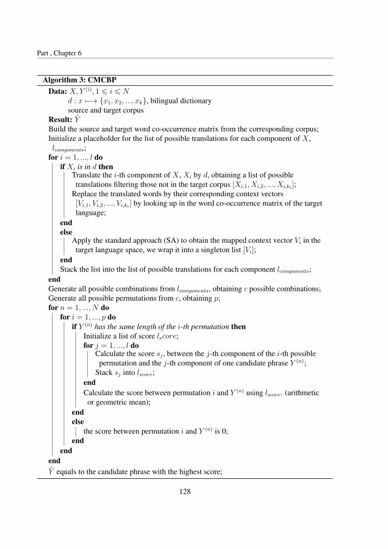
Part , Chapter 6

Algorithm 3: CMCBPData: X, Y (i), 1 6 i 6 N

d : x 7−→ {x1, x2, ..., xk}, bilingual dictionarysource and target corpus

Result: YBuild the source and target word co-occurrence matrix from the corresponding corpus;Initialize a placeholder for the list of possible translations for each component of X ,lcomponents;

for i = 1, ..., l doif Xi is in d then

Translate the i-th component of X , Xi by d, obtaining a list of possibletranslations filtering those not in the target corpus [Xi,1, Xi,2, ..., Xi,ki

];Replace the translated words by their corresponding context vectors[Vi,1, Vi,2, ..., Vi,ki

] by looking up in the word co-occurrence matrix of the targetlanguage;

endelse

Apply the standard approach (SA) to obtain the mapped context vector Vi in thetarget language space, we wrap it into a singleton list [Vi];

endStack the list into the list of possible translations for each component lcomponents;

endGenerate all possible combinations from lcomponents, obtaining c possible combinations;Generate all possible permutations from c, obtaining p;for n = 1, ..., N do

for i = 1, ..., p doif Y (n) has the same length of the i-th permutation then

Initialize a list of score lscore;for j = 1, ..., l do

Calculate the score sj , between the j-th component of the i-th possiblepermutation and the j-th component of one candidate phrase Y (n);

Stack sj into lscore;endCalculate the score between permutation i and Y (n) using lscore. (arithmeticor geometric mean);

endelse

the score between permutation i and Y (n) is 0;end

endendY equals to the candidate phrase with the highest score;

128

6.2. (Semi-) supervised bilingual phrase alignment with distributional representation

Figure 6.1 – An example diagram of CMCBP. (Source: Morin and Daille (2012))

129

Part , Chapter 6

target word co-occurrence matrix. Finally, we have 4 possible permutations for “antécédentfamilial” for the similarity calculation.

6.2.2 CMCBP with data selection

The main contribution of CMCBP is the capability of mapping out-of-vocabulary words, how-ever, this requires that the pre-constructed word co-occurrence matrices are complete and reli-able. In general, such word co-occurrences are difficult to obtain from a modest size corpus inspecialized domain. We can exploit the same data selection strategy as in the selective standardapproach (SSA). To do this, we can build the word co-occurrence matrices with external data asin SSA. Then in CMCBP, when a component is not found in the dictionary, we apply SSA withthe merged matrices in place of SA. The next steps are the same as in the original CMCBP.

6.3 Contribution : Compositionnal method with word em-bedding projection (CMWEP)

Following the idea of CMCBP, we propose a to exploit the word embeddings in a compositionalapproach. The idea is to substitute the word co-occurrence vectors with the word embeddingsin CMCBP. We call it compositional approach with word embedding projection (CMWEP).

With the word embeddings, we can no longer apply the standard approach to map a sourcevector to one in the target language space. Nevertheless, we bridge the gap by the linear trans-formation approach presented in Section 5.3. This requires that we learn the transformationmatrix before the phrase alignment.

Besides, one major limit of CMCBP is that it aligns only the phrases of the same length. Inorder to represent phrases of variable length in a single vector, first we generate all the possiblecombinations and save their word embeddings. Next we apply the addition to finally retrievea single vector representing the phrase for one possible combination. Moreover, the additiongreatly reduce the complexity of the original CMCBP because we do not have to calculate all thepossible permutations. Note that this modification can also be applied to the original CMCBP.We will apply it for our experiments as a good amount of our test samples are pairs of phrasesof variable length.

CMWEP can be implemented by Algorithm 4 where we follow the same notation as inAlgorithm 3.

130

6.3. Contribution : Compositionnal method with word embedding projection (CMWEP)

Algorithm 4: CMWEPData: X, Y (i), 1 6 i 6 N

d : x 7−→ {x1, x2, ..., xk}, bilingual dictionarysource and target corpus

Result: YBuild the source and target word embedding matrix from the corresponding corpus;Learn the transformation matrix M using the linear transformation approach introducedin Section 5.3;

Initialize a placeholder for the list of possible translations for each component of X ,lcomponents;

Build the candidate matrix C with addition, where each row is a phrase vector;for i = 1, ..., l do

if Xi is in d thenTranslate the i-th component of X , Xi by d, obtaining a list of possibletranslations filtering those not in the target corpus [Xi,1, Xi,2, ..., Xi,ki

];Replace the translated words by their corresponding word embeddings[Ei,1, Ei,2, ..., Ei,ki

] by looking up in the word embedding matrix of the targetlanguage;

endelse

Calculate the mapped embedding by BWE, Ei = Es,iM , and wrap it into asingleton list [Ei].;

endStack the list into the list of possible translations for each component lcomponents. ;

endGenerate all possible combinations from lcomponents, obtaining c possible combinations;Initialize a placeholder for embeddings of all possible combinations, A ∈ Rc∗d;for i = 1, ..., c do

Calculate the phrase vector by addition;Put the phrase vector in the i-th row of A;

endCalculate the similarity score matrix, S, S = ACT ;Y equals to the candidate phrase with the highest value in S where the column indexrepresents candidate phrases;

131

Part , Chapter 6

An example of generating phrase vectors in CMWEP is illustrated in Figure 6.2. Supposewe have the English phrase “onshore wind farm” to align to French. The word “onshore” isnot in the given dictionary or the translations are not found in the training corpus. The words“wind” and “farm” have respectively one and three possible translations found. To generate thephrase vectors, we apply BWE on “onshore” and extract the corresponding word embedding foreach possible translation of “wind” and “farm”. So each component word vector is mapped tothe target language space. By addition, finally we have 3 phrase vectors representing the inputphrase.

onshore wind farm

ferme

cultiver

exploiteréolien

BWE(onshore)

translations not foundtranslations

translations

NA éolien ferme

NA éolien cultiver

NA éolien exploiter

translation1

translation2

translation3

BWE(onshore)+vec(eolien)+vec(ferme)3

BWE(onshore)+vec(eolien)+vec(cultiver)3

BWE(onshore)+vec(eolien)+vec(exploiter)3

Figure 6.2 – An example diagram of CMCBP.

EvaluationWe include the original compositional approach (CA) and compositional method with con-

text based projection (CMCBP) in our evaluation on the WE corpus. In addition, we also testif the data selection and the techniques presented in Sections 5.2 and 5.3.2 always improvethe performance for CMCBP and CMWEP. The results are shown in Table 6.1. Note that we

132

6.3. Contribution : Compositionnal method with word embedding projection (CMWEP)

sum all the possible combinations for CMCBP and CMWEP to obtain one single vector so thatphrases of variable length can be aligned.

Model Accuracy MAP

CA 59.0 61.5

CMCBP 49.3 61.4CMCBP + WMI + DSC 46.6 63.2CMCBP + Data selection 50.7 66.0CMCBP + Data selection + WMI + DSC 53.4 66.3

CMWEP 52.1 67.8CMWEP + Data selection 61.6 73.3CMWEP + Data selection + Re-normalisation 61.6 73.4

Table 6.1 – Accuracy (p@1) and MAP % of different approaches on the WE corpus. Details ofthe WE-en-fr corpus and its gold standard can be found in Appendix A.1.2 and A.3.3.

First it is to our surprise that the compositional approach (CA) has better accuracy thanCMCBP This is because the candidates are ranked by their frequency in the target languagecorpus while the candidates in CMCBP are ranked by the similarity measure, so theoreticallythose translated by CA are also translated by CMCBP but with the same similarity score (1.0).Therefore, the final rank in CMCBP is to some degree randomized as multiple top candidateshave the same score. However, when using external data, the MAP is considerably improved byCMCBP, this shows that the CMCBP can effectively find many out-of-vocabulary translationsthat can not be found by CA.

The same problem also exists in CMWEP (randomized rank for the candidates with thesame score). Another remarkable point is that unlike the single word bilingual extraction whereWMI degrades the results when using external data, combining WMI and DSC improves theresults in MAP with or without external data.

Our word embedding methods (CMWEP) notably improve the results when using informa-tion carried by external data by almost 12 points in MAP and 2.6 points in accuracy. Com-bining the usage of external data and the re-normalization gives the best accuracy and MAP.The characteristics of the WE corpus determine the fact that for most phrases, each componentword are included in the dictionary. So CA already provides a high result especially for theaccuracy, if we took a less academic or less cleaned corpus for example the Amazon reviews

where there are more out-of-vocabulary words because of spelling mistakes and internet lan-guages, we expect the result of CA to be much lower while the result of other approaches would

133

Part , Chapter 6

be less impacted. This is also why the re-normalization improves the result very slightly, sincemost of the translations are found by a dictionary look-up process.

6.4 Unsupervised neural machine translation with pre-trainedcross-lingual embeddings

All the previous approaches require a relatively complete dictionary during the alignment, whilesuch dictionaries are not publicly available and sometimes scarce between certain languages.This is especially the case when treating corpora in specialized domain. In order to alignphrases with minimal cross-lingual information, we probe a series of unsupervised neural ma-chine translation systems. Although our objective is not a translation task, we can exploit theunsupervised neural machine translation architecture to train our phrase encoder. Then afterthe training, we can calculate the similarity scores using the phrase vectors generated by theencoder.

6.4.1 Back translation

Neural Machine Translation (NMT) has achieved tremendous progress and recently become thedominant paradigm in machine translation. However, most successful NMT systems are pro-posed in a supervised or semi supervised context. When no parallel data exists between sourceand target languages, several works proposed the use of a pivot language (Firat et al., 2016;Saha et al., 2016; Y. Chen et al., 2017) acting as a bridge between source and target. Followingthe same idea, Johnson et al. (2017) proposed a multilingual neural machine translation modelwhich creates an implicit bridge between language pairs for which no parallel data is used fortraining. Whether explicitly or implicitly, all these works still require the use of parallel corporabetween the pivot language and other languages.

A more recent line of works has completely removed the need of parallel corpora (Lample,Conneau, et al., 2018; Artetxe, Labaka, Agirre and Cho, 2018; Zhen Yang et al., 2018), relyingon pre-trained cross-lingual word embeddings presented in Section 5.3 and language modelspresented in Section 4.3.1 built from monolingual corpora. The loss of the denoising processis:

Ldenoising(θenc, θdec) = −Ex∈DlH(x, dec→l(enc(N (x)))) (6.3)

where θenc and θdec respectively means the parameters in the encoder and the decoder, x ∈ Dl

134

6.4. Unsupervised neural machine translation with pre-trained cross-lingual embeddings

is a sampled sequence from the monolingual data and dec→l(enc(N (x))) represents a recon-structed sequence from the noised version of the original sequence x. Apart from the denoising,they all incorporate a back translation structure to build pseudo-translations between the sourceand target language.

Back translation (Sennrich et al., 2016a; J. Zhang and Zong, 2016) has been dominantlyused prior to unsupervised NMT systems. It couples the source-to-target translation model witha backward target-to-source model and trains the whole system with a reconstruction loss. Inan unsupervised NMT system, the back-translation is activated after a first pass of denoisingautoencoding. The gradients for updating the encoder and decoder are calculated by alterna-tively applying the source-to-target model to source sentences to generate inputs for training thetarget-to-source model (and vice versa):

Lbacktranslation(θenc, θdec) = −Ex∈Dl1H(x, dec→l1(enc(y))),

with y = transl(x) = dec→l2(enc(x))(6.4)

where Dl1 and Dl2 are the two language corpora, dec→l1 means that the decoder will decoderthe sequence in l1 language (or l2 resp.). Suppose y is the translation of x ∈ Dl1 by applyingthe decoder of language l2, dec→l2(enc(x)). Then dec→l1(enc(y)) represents the reconstructedsource sentence from the synthetic translation. The goal is to generate pseudo parallel sentencepairs to train the models with a reconstruction loss. Overall, the system is composed of a sharedencoder thanks to the pre-trained cross-lingual word embeddings, two specific decoders for thesource and the target language and back translation mechanism.

6.4.2 Extract-Edit, an alternative to back translation

Lately, Wu et al. (2019) argue that the popular back translation suffers from the low-qualitypseudo language pairs. Since the generated pseudo sentence pairs are usually of low quality,the errors during the back translation training could probably accumulate, leading to a deviationof the learned target language distribution from the real target distribution.

ExtractRather than using synthetic translations, the authors propose an alternative strategy which

extracts potential parallel sentences from comparable monolingual corpora. This is done bysimply comparing the sentence encoding generated by the shared encoder. Specifically, fora given source sentence s, the top-k real sentences from the target language space would beextracted based on the L2 distance. The set of k potential parallel sentences for s is denoted by

135

Part , Chapter 6

M :

M = {t|min1,...,k

(||es − et||), t ∈ T } (6.5)

where t is a sentence among all the target language sentences T , es and et are sentence en-codings generated by the shared encoder. In fact, the extract can be considered as an alignmentprocess in our definition.

EditThe objective of the extract is to provide some pivot sentences for the system training,

however, it is not always guaranteed there the parallel sentence exists in the target corpus. Theedit operation aims to revise the extracted sentences M in terms of the source sentence s. First,the operation applies a maxpooling layer to reserve the more significant features between thesource sentence embedding es and the extracted sentence embedding et for t ∈ T . Then thetarget language decoder will decode it into a new sentence t′, forming a new pivot sentence setM ′:

M ′ = {t′|t′ ∈ dec(maxpooling(es, et)), t ∈M} (6.6)

Evaluation networkThere is another component which consists in an evaluation network R. After a fully con-

nected layer which takes the source and translated sentence encoding es and et as input, itapplies a softmax distibution on the similarity between the source s and all the extract-editedtarget sentences t plus the translated sentence t generated by decoding the source sentence en-coding, dec(enc(s)).

P (t|s,M ′) =exp

(λ cos

(s, t))

∑t∗∈M ′∪t

exp(λ cos((s, t∗))) (6.7)

where λ is an inversed temperature of the softmax function.

Training objectiveIn addition to the denoising loss, there are several other losses we want to minimize during

the training. First the distance of the translated sentence t to the source sentence s compared tothe top-k extract-edited sentences M ′ by a comparative loss.

Lcom(θenc|θR) = E(− logP (t|(s,M ′))) (6.8)

where θenc and θR are the parameters of the encoder and evaluation network. Combined with

136

6.4. Unsupervised neural machine translation with pre-trained cross-lingual embeddings

the denoising loss, the overall loss for updating the encoder and decoder is given in Equation6.9

Ls→t(θenc, θdec|θR) = wdenoisingLdenoising + wcomLcom (6.9)

where wdenoising and wcom are the hyper-parameters weighing the importance of the denoisingand the comparative learning. They are both set to 1 in the work of Wu et al. (2019). Besides,the evaluation network is learned by maximizing the score between the extract-edited sentencesM ′ and the source sentence s. This can be viewed as a “discriminator” in an adversarial trainingnetwork (Goodfellow et al., 2014), while the decoder-encoder is served as a “generator” whichgenerates a translated sentence t with a higher score than the sentences in M ′.

LR(θR|θenc, θdec) = Et′∈M ′(− logP (t′|(s,M ′))) (6.10)

Merging Equations 6.9 and 6.10, the final training objective is:

arg minθenc,θdec

arg maxθR

L(θenc, θdec, θR) = −LR(θR|θenc, θdec) + Ls→t(θenc, θdec|θR) (6.11)

The whole system is learned by alternatively updating first the evaluation network and then thetranslation network (encoder-decoder network). Figure 6.3 shows an overview of the wholeextract-edit system architecture. Since the work is very recently published and the source code

Figure 6.3 – The overview of the extract-edit approach based NMT architecture. (Source: Wuet al. (2019))

is not yet available, we did not include it in our final system. However, the idea of using acomparative model to guide the unsupervised training opens an interesting line of future work.

137

Part , Chapter 6

6.5 Contribution : a new dataset for bilingual phrase align-ment

For the bilingual phrase alignment task, we use the same Wind Energy (WE) comparable corpusas in the monolingual tasks. This time we evaluate on the English, French, Spanish and Chi-nese corpora. Besides, we build a new publicly available Breast Cancer (BC) English-Spanishcomparable corpus by crawling from a scientific website 1. More specifically, we filter all thepublicly accessible articles and then search the keywords “breast cancer” for English articlesand “cáncer de mama” for Spanish articles. The final English corpus results from concatenating168 articles and the Spanish corpus 141 articles. The data crawler script is publicly available2. The gold standard is built on the same 108 English phrases as in the monolingual phrasesimilarity task and the mapping Spanish phrases are manually selected from the target corpus.

The English BC corpus has 26,716 sentences and the Spanish one has 62,804 sentences.For the WE corpus, Hazem and Morin (2016) proposed a reference list consisting of 139 singlewords for the English-French corpus, while Liu et al. (2018) provided a gold standard with 73multi-word phrases for the same corpus. Based on the reference list of Liu et al. (2018), wepropose a new gold standard including also single words. Moreover, we extended this goldstandard to other languages while ensuring that all reference lists share the same 90 Englishphrases to be aligned. Finally, alignment reference lists were obtained for three languagespairs: English-French, English-Spanish and English-Chinese. For the sake of comparability,we also report results on the datasets of Liu et al. (2018) and Hazem and Morin (2016).

For the preprocessing and phrase extraction, we also use the IXA pipes library to tokenizeand lemmatize French and Spanish corpora. It is worth noting that the WE Chinese corpus isalready pre-segmented. We use the Stanford CoreNLP library3 pos-tagger for all languages,then for the phrase extraction we use the same PKE tool as mentioned in monolingual tasks.After hapax filtering, each corpus contains roughly 6,000 phrases of maximal length 7.

1https://www.sciencedirect.com2https://bitbucket.org/stevall/data-crawler.git3https://stanfordnlp.github.io/

138

6.6. Contribution for the unsupervised bilingual phrase alignment

6.6 Contribution for the unsupervised bilingual phrase align-ment

In this section, we present our architecture for unsupervised bilingual phrase alignment whichcombines the previous techniques. Concretely, the system is an encoder-decoder network witha context prediction training objective. The encoder is a semi tree-free recursive neural networkbased on the TF-RNN introduced in Section 3.6. We train the network using a pseudo backtranslation mechanism which grants the ability of being fully unsupervised.

6.6.1 Semi tree-free recursive neural network

To encode phrases of variable length in one single vector, we could have applied the tree-free

recursive neural network (TF-RNN) introduced in Section 3.6. However, the surprising fact isthat in our preliminary experiments, it did not meet our expectation as the synthetic translationsare sometimes of low quality and the accumulated translation errors affect more radically withthe recursivity (Wu et al., 2019). The same phenomenon also occurs in other similar networkssuch as the recurrent or LSTM network.

On the other hand, the additive approach (Liu et al., 2018) always successes to hold a decentperformance, therefore we decide to adapt the tree-free recursive neural network to the cross-lingual context by levelling the network. Consequently the network has more additive featureswhile being able to distinguish the word order and distribute different weights. More concretely,there are three layers in the adapted version, in the first we operate the same processing as inTF-RNN which consists in splitting the semantics of each word by a linear transformation intotwo parts: the right side and the left side. Thus the first layer remains a recursive layer. Then weassociate these nodes by concatenation, the left side is supposed to be associated with the rightside of the previous token and vice versa. The second layer is composed of a fully connectedlayer that maps the input vectors to output vectors in a specified dimension. Finally the thirdlayer is an addition based pool layer which sums all intermediate level nodes and outputtinga single fixed-length vector. The sum operation is motivated by the additive characteristicsmentioned in Mikolov, Sutskever, et al. (2013) as the additive approach has showed interestingresults in our preliminary experiments. We name it semi tree-free recursive neural network.Figure 6.4 shows the schema of the proposed network which is clearly a flat version of theTF-RNN presented in 3.6.

In our scenario we use pre-trained cross-lingual embeddings as the input vector sequence

139

Part , Chapter 6

∑

Wl Wr Wl Wr Wl Wr

concat concat

fully connected layer

v1 v2 v3

vo

Figure 6.4 – Diagram of the semi tree-free recursive neural network (STF-RNN).

[v1, v2, v3, ..., vn] with vi ∈ Rd, the output vector vo ∈ Rp is calculated as follows:

vi,l = tanh(Wlvi + bl)

vi−1,r = tanh(Wrvi−1 + br)

vinter,i = tanh(U [vi−1,r; vi,l] + b)

vo =n∑i=1

vinter,i

(6.12)

where Wl ∈ Rd∗d and Wr ∈ Rd∗d denote respectively the left and the right weight matrices inthe linear transformation of the semantic association, bl ∈ Rd and br ∈ Rd are the correspondingbias vectors, U ∈ Rp∗d and b ∈ Rp are the parameters in the fully connected layer with d theinput dimension and p the output vector dimension.

6.6.2 Pseudo back translation

Since we do not have cross-lingual data, a direct link between a phrase in language l1 and onein language l2 is not feasible. However, synthetic translations of single words can be easilyobtained using bilingual word embeddings (BWE). By using translated single-word phrases

140

6.6. Contribution for the unsupervised bilingual phrase alignment

to train our model, we create stronger links between the two languages. This can be viewedas pseudo back-translation as we generate synthetic translations by BWE while in NMT sys-tems the translation is generated by the corresponding decoder (Sennrich et al., 2016a; Artetxe,Labaka, Agirre and Cho, 2018; Lample, Conneau, et al., 2018; Wu et al., 2019). Concerningthe training objective, recall the context prediction loss introduced in Section 4.5. Because theencoder never conditions on the context information and the decoder predicts these never seencontexts, we can harmlessly exploit the bidirectional phrase encoders such as PTF-RNN, CNNor Transformer without provoking the redundancy problem mentioned in Devlin et al. (2018).Therefore, the system potentially has four objective loss functions when we alternatively iterateall phrases in the two languages l1 and l2:

Lcp l1→l1(θenc, θdec→l1) = −Ex∈Dl1H(ws(x), dec→l1(enc(x))), (6.13)

Lcp l2→l1(θenc, θdec→l1) = −Ex∈Dl1H(ws(x), dec→l1(enc(BWE(x)))), (6.14)

Lcp l2→l2(θenc, θdec→l2) = −Ex∈Dl2H(ws(x), dec→l2(enc(x))), (6.15)

Lcp l1→l2(θenc, θdec→l2) = −Ex∈Dl2H(ws(x), dec→l2(enc(BWE(x)))) (6.16)

where Lcp lp→lq means the context prediction loss from an encoded phrase in language lp tothe context of language lq, dec→l(enc(x)) is the reconstructed version of the wrapped sentence,ws(x) denotes the real wrapped sentence containing the phrase x and BWE(x) is the translatedsingle-word phrase for x using bilingual word embedding.

6.6.3 System overview

The general encoder-decoder architecture of our method is shown in Figure 6.5. Since the inputsequence is always a phrase, usually much shorter than a sentence, we did not use attentionwhich is intended to capture long-range dependencies. The LSTM decoders predict the contextsurrounding the input phrase from its encoded vector.

As illustrated in Figure 6.5, in addition to our phrase encoder, we incorporate a pseudoback-translation mechanism for single words based on bilingual word embeddings (Artetxe,Labaka and Agirre, 2018a; Liu et al., 2018). The decoder consists of a single layer LSTMand a fully connected layer on top of it. The goal of the decoder is to reconstruct the wrapped

141

Part , Chapter 6

pre-trained cross-lingual embeddings,x ∈ Dl1

phrase encoder

encoded output voLSTMs

reconstructed wrapped sentence

LSTMs

reconstructed wrapped sentencex is single-word

synthetic translationyes

BWE(x) ∈ Dl2shared encoder for l1 and l2

context decoder for l1

context decoder for l2

Figure 6.5 – Overview of the cross-lingual alignment training architecture. For a phrase x inlanguage Dl1, we first use the shared tree-free phrase encoder, then the system can be trainedin two subnetworks: the first one is the encoder-decoder system given the original phrase xw.r.t Dl1, and if x is a single-word phrase, we apply a second encoder-decoder system giventhe translated phrase BWE(x) also w.r.t Dl1. We alternatively iterate through all phrases in thetwo languages. The objective of the decoder is to reconstruct a wrapped sentence containing x

sentence which contains the current input phrase. The idea of learning phrase representationsbased on the context is also studied in Del et al. (2018): instead of an end-to-end system, theyfirst learn all the phrase embeddings by Skip-gram considering them as a single word, and thenlearn the composition function by a regression model which predicts the pre-trained phraseembeddings from its composing word embeddings. However they limit the phrase length to2, while we would like to propose a unified end-to-end framework which is able to learn thephrase composition of variable length and the mapping simultaneously.

The detailed training procedure is described in Algorithm 5. Note that in order to keep thetraining unbiased by the distribution of the number of training phrases in different languages,we build a merged phrase list x with identical phrase number of both the source and the targetlanguage. The phrases of the source language are at even indices while the phrases of the targetlanguage are at odd indices. We set an early stop condition of three consecutive loss increases.

6.6.4 Evaluation

We evaluate our proposed system on the WE and BC with three different language pairs:English-French, English-Spanish and English-Chinese. The overall results of all test phrasesare shown in Table 6.2. We also apply two baseline approaches: the mean vector approachand the distributional word representation based approach, CMCBP. Since the distributional ap-

142

6.6. Contribution for the unsupervised bilingual phrase alignment

Algorithm 5: Training process of the proposed unsupervised cross-lingual phrase encoder.Data: pre-trained transformation matrices for BWE.

source and target corpus.merged source and target phrase list x.

while early stop condition not met and max epoch number not reached dofor xi ∈ x do

if xi is in l1 thenupdate the system by Equation 6.13θ ← arg minLcpl1→l1(θ)if xi is single-word then

update the system by Equation 6.14θ ← arg minLcpl2→l1(θ)

endendelse

update the system by Equation 6.15θ ← arg minLcpl2→l2(θ)if xi is single-word then

update the system by Equation 6.16θ ← arg minLcpl1→l2(θ)

endend

endend

143

Part , Chapter 6

proach (Morin and Daille, 2012) does not include the alignment of variable length phrases, weignore the corresponding results in the table.

Dataset MethodCorpus Phrases CMCBP Mean RecurrentNN CNN LSTM Proposal

sw (72) 35.72 47.46 46.71 45.12 46.25 47.76BC n2n (21) 68.73 81.10 28.52 62.10 50.05 86.11

en-es p2q (15) - 42.18 1.11 10.65 7.04 49.11all (108) - 52.85 36.78 43.04 43.72 55.40

sw (15) 65.56 78.25 77.22 78.33 79.36 79.44WE n2n (61) 42.09 57.37 6.16 40.84 18.64 62.19en-fr p2q (14) - 15.83 <0.5 10.07 9.09 37.95

all (90) - 55.77 17.25 43.33 27.42 62.10

sw (15) 63.35 77.92 88.89 75.78 87.18 87.62WE n2n (61) 35.94 62.68 7.31 40.33 23.07 61.35en-es p2q (14) - 43.28 <0.5 28.57 17.86 46.21

all (90) - 62.20 19.77 44.41 32.94 63.38

sw (17) - 53.43 70.26 76.47 71.43 66.50WE n2n (47) - 23.34 17.53 16.55 25.24 23.01

en-zh p2q (26) - 4.97 5.13 7.60 2.37 12.32all (90) - 22.67 23.91 25.28 27.36 28.13

WE n2n (40) 67.32 78.36 46.07 68.51 44.82 88.01en-fr p2q (33) - 34.38 2.38 20.01 7.93 41.83

Liu et al. (2018) all (73) - 58.48 26.06 46.59 28.13 67.13

Table 6.2 – Overall MAP % for all phrase alignment. sw, n2n and p2q respectively mean single-word to single-word, same length multi-word and variable length phrase alignment. We do notpresent the results of the distributional approach on the English-Chinese corpus because we donot have enough resources to build the co-occurrence matrix as in the other language pairs con-sidering the distributional approach requires a high coverage bilingual dictionary, furthermore ifthe dictionary does not use the same Chinese word segmentation approach as in the WE corpus,it is even harder to find words in it. Details of the WE-en-fr corpus can be found in AppendixA.1.2. For the gold standard, we use the ours presented in Section 6.5 except the last line whichapplies the gold standard in Appendix A.3.3.

It is clearly shown that the proposed method has a better overall performance. Especiallywhen it comes to different length phrase alignment, the new approach improves significantlythe MAP with an average score of 8.8 points. This proves that the proposed method is ableto produce high-quality alignment for phrases of variable length. Keep in mind that the differ-

144

6.6. Contribution for the unsupervised bilingual phrase alignment

ent length distribution represents a small proportion of all test phrases except for the English-Chinese corpus, so the overall score would be furthermore improved if we have uniform distri-bution over all kinds of alignment. The second best method on overall results is the additionapproach, previously reported to obtain decent results (Mikolov, Sutskever, et al., 2013; Delet al., 2018). Besides, in an unsupervised context, the CMWEP 6.3 is actually equivalent to theaddition-based approach. The CNN has some interesting results in same length alignment andthe LSTM is powerful at short phrase alignment but unlike in Del et al. (2018), it falls muchbehind on other types. This difference may be explained by the fact that they limit the alignmentto two-word phrases.

The relatively poor results on the English-Chinese corpus may be due to the segmentationof Chinese words. More concretely, as the input vectors for the Chinese sequences are in word-level, many words in our gold standard are not segmented in the same way as in the givencorpus which is already pre-segmented. We would like to replace the word-level embeddingsby character-level ones or incorporate sub word tokenizer in our future works.

Concerning the single-word alignment on BC, 25 among the 72 single words are in factacronyms which are particularly difficult to align. This would explain why the single-wordalignment has much poorer results than other distributions. Besides, the proposed method ob-tains strong results for single-word alignment, we believe this happens because the system seesmore single-word alignment samples generated by the pseudo back-translation during training.

In order to show that the proposed method can still hold a reasonable performance on singlewords, we present in Table 6.3 the results for single words compared to state-of-the-art workon bilingual word embedding (Artetxe, Labaka and Agirre, 2018a), including the 139 English-French single word dataset of Hazem and Morin (2016) (suffixed -HM in the Table 6.3). To becomparable, we only test on single-word phrases and the candidate list is limited to all singlewords in the corpus vocabulary. On our datasets, the source English words are the 15 same asin the sw line of Table 6.2.

BC WEMethod en-es en-fr en-es en-zh en-fr-HM

(Mikolov, Quoc V. Le, et al., 2013) † 39.96 91.33 87.27 45.88 79.47

(Artetxe, Labaka and Agirre, 2018a) † 49.13 95.56 90.39 73.52 84.01

Our method 45.96 89.44 88.89 58.75 82.23

Table 6.3 – MAP % for single-word phrase alignment. † indicates that the results are obtainedfrom our our implementation of the original work.

145

Part , Chapter 6

We can see that in general, compared to Artetxe, Labaka and Agirre (2018a), the proposedapproach does not degrade much the results except for the English-Chinese words. In additionto that, we succeed to hold a better result with regard to the original transformation matrixmethod (Mikolov, Quoc V. Le, et al., 2013) with only one exception on the English-Frenchwind energy dataset. This shows that our approach is not biased by the compositionality of themulti-word expressions.

For a better understanding of how the proposed method succeeds or fails to align differenttypes of phrases, we analyzed some of the alignments proposed by our system.

Dataset Source Addition Our method

BC breast cancer cáncer mamario cáncer de mamaen-es cell death muerte celular muerte

WE blade tip angle des pales côté supérieur de la paleen-fr Darrieus rotor rotor tripale rotor vertical

WE airflow freno aerodinámico flujo de aireen-es wind power plant electricidad del viento planta eólica

WE wind vane 偏航 电机 风向标en-zh electricity power 电力 电力

Table 6.4 – Alignment examples within top 2 candidates ( “ ” is the segmentation point forChinese words)

Table 6.4 shows examples extracted from top 2 nearest candidates to the source phrase incolumn 2. Again we see that the proposed method is capable of generating better results overdifferent types of alignment. In the first example, with the proposed approach, the source phrasebreast cancer is aligned to cáncer de mama (lit. “cancer of breast”) which is the expected phrasein Spanish and is far more idiomatic than cáncer mamario (lit. “cancer mammary”) obtained bythe addition approach. In line 7 we see that the perfect translation for wind vane is found by ourproposal: 风向标, while the additive approach finds偏航 电机 (lit. “yaw electric machine”).Besides, examples in lines 3, 5, 6, 7 and 8 are all composed of phrases of variable length, thecorresponding reference phrase can be found in the fourth column. Interestingly, we find thatthe proposed system find paraphrases referring to fairly domain-specific phrases like blade tip

which is aligned to côté supérieur de la pale (lit. “side top of the blade”). This is also the casefor Darrieus rotor aligned to rotor vertical, which is remarkable since the Darrieus rotor is akind of vertical rotor.

Though the proposed method performs generally well on phrases, we observe that it em-

146

6.7. Synthesis

phasizes occasionally too much the syntactic head in a multi-word phrase. For instance, in thesecond example, cell death is aligned to muerte (“death”), while the addition based approachsucceeds to align it to muerte celular (lit. “death cellular”) which is the reference phrase inSpanish. Undoubtedly, death is the syntactic head for the noun phrase cell death, it is clearthat the proposed method puts more weight on the syntactic information rather than the com-positional property for this phrase. This also explains why we do not obtain better results onequal-length phrase alignment on the English-Spanish and English-Chinese wind energy cor-pora (Table 6.2). This bias could be due to the increased amount of single-word phrase samplesof the pseudo back-translation reinforced learning. This suggests that we could possibly im-prove the system by adding synthetic translations for multi-word phrases during the training.

6.7 Synthesis

Unsupervised bilingual alignment of variable length phrase, which is also our main goal, is fi-nally addressed in this chapter. Following the same line of the supervised baseline approach,compositional approach (CA), Morin and Daille (2012) propose to remove the constraint ofaligning only in-vocabulary words by exploiting the distributional word representation. Theapproach is an extended version of CA hence it is called compositional method with contextbased projection (CMCBP). With the distributional word representations, CMCBP turns intoa semi-supervised approach. Although it is a step forward towards unsupervised phrase align-ment, it is not when it comes to the unified phrase alignment because it can only align phrasesof same length.

To align phrases of variable length, we can simply sum all the component word vectors ofa phrase. As discussed in Section 3.1, the addition based approach is a simple yet effectiveway to encode multiple word vectors into one single vector, allowing comparisons betweenphrases of variable length without introducing any further parameters. Therefore, we applythe addition approach in CMCBP to make it compatible with all phrases. In addition, we alsopropose to substitute the distributional word vectors with word embeddings, which is namedcompositional method with word embedding projection. In our experiments we find thatincorporating word embeddings improves the phrase alignment performance by about 7 pointsin MAP.

It’s worth mentioning CMWEP in an unsupervised context is identical to a simple similaritycomparison task with addition encoding. In Section 3.3 we point out that the addition approachignores the inner structure of multi-words, and the proposed TF-RNN (see Section 3.6) can

147

Part , Chapter 6

encode phrases according to a certain learned structure without introducing any supervised in-formation such as the parsing tree. Therefore, we would like to improve the performance byexploiting the TF-RNN with the context prediction training objective (see Section 4.5). Nowthe only barrier which keeps us from reaching our final goal lies in the parallel data. Thanksto the unsupervised machine translation technique, back translation (Sennrich et al., 2016a;J. Zhang and Zong, 2016), we can create some synthetic parallel text during the training pro-cess. Combining all these, we build an encoder-decoder network with TF-RNN as the phraseencoder, an LSTM layer as the decoder and a back-translation-like mechanism where the syn-thetic translation is generated by the bilingual word embedding instead of the decoder in anNMT system. The preliminary experiments have shown very poor results because the trainingis biased by the single words and the accumulated translation errors affect more radically withthe recursivity (Wu et al., 2019). We introduce a flatten version of TF-RNN to replace the fullyrecursive version because we notice that the additive approach always successes to hold a decentperformance. The idea is to reduce the recursivity of the phrase encoder so the errors producedby BWE are not propagated to every node.

Finally, our system outperforms the addition approach across all our datasets. And our pro-posed phrase encoder obtains better results compared to other state-of-the-art architectures suchas CNN and LSTM. The gain is especially significant for the different length phrase alignmentwith improvements from about +10 to +40 in MAP.

148

CHAPTER 7

CONCLUSION AND PERSPECTIVE

In this final chapter, we first give an overview of what has been studied and proposed. Then weopen up perspectives for the future work based on the observation of our experiments.

7.1 Conclusion

Significant advances have been achieved in bilingual word-level alignment from comparablecorpora, yet the challenge remains for phrase-level alignment. Traditional methods of phrasealignment can only handle phrases of equal length, while word embedding based approacheslearn phrase embeddings as individual vocabulary entries suffer from a data sparsity problemand cannot handle out of vocabulary phrases. Our objective in this thesis is the unsupervisedbilingual phrase alignment which is a comparative task where a unified phrase representationplays a key role.

In order to learn unified phrase representations for variable length phrases, we have stud-ied the approaches for unified phrase modeling and cross-lingual phrase alignment, rangingfrom co-occurrence based models to most recent neural state-of-the-art approaches. Besides,since our training corpora in specialized domain are modestly sized, we exploit external generaldomain data in our framework. After our survey on existing approaches, we propose a new ar-chitecture called tree-free recursive neural network (TF-RNN) for modeling phrases of variablelength which, combined with a wrapped context prediction training objective, outperforms therecent state-of-the-art approaches on monolingual phrase synonymy task with only plain texttraining information. We attribute the high performance to several points:

• Compositional. Like the addition approach, TF-RNN is also a compositional approachwhere component token vectors are associated to form the final phrase vector. Further-more, by recursively applying weight matrices for each combination pair, the final phrasevector takes word inner relation into account.

• Sequential. Like RecurrentNN, TF-RNN is also a sequential approach where unlike the

149

addition approach, component order counts. However, it is best suited to short sequencessuch as phrases. Instead of depending more on the latest parsed words in RecurrentNN,the final output vector of TF-RNN depends more on the higher level representations ofthe phrase, which we think coherent because humans process natural language followinga syntactical tree and the latest words they see are not always those who have the largestweights.

• Tree-free. Like RNN, TF-RNN also generates the phrase vector following a tree struc-ture, however, it removes the need of an input tree structure by systematically building arecursive binary tree.

• Context-aware. Like the extended word embedding approach, we train our TF-RNN byleveraging the phrase context in order to learn from the information outside the compo-nents. While the extended word embedding approach considers phrases as one single unitand suffers from the data sparsity and out-of-vocabulary problems, TF-RNN can still beapplied to new freely combined phrases thanks to its compositional properties.

As for the Transformer based encoder, its low performance in our phrase synonymy experimentsare indeed surprising to us. We assume that the multi-head attention is probably more suitablefor long sequence tasks as the advantage of the attention based models lies in the caption oflong range dependencies.

For the alignment part, we have reviewed supervised and unsupervised training frameworkswith the traditional compositional approaches and the recent neural machine translation sys-tems. Finally we propose to incorporate an architecture called Tree-free semi recursive neural

network (TF-SRNN) derived from TF-RNN in an encoder-decoder model with a pseudo backtranslation mechanism inspired by works on unsupervised neural machine translation. The sys-tem can be trained without cross-lingual phrase table and different length phrases are encodedand represented in a homogeneous way. Empirically, our proposition improves significantlybilingual alignment for phrases of different lengths while achieving state-of-the-art results onsingle-word and same length multi-word phrase alignments.

7.2 Operational contributions

During this thesis, our implementations has been partially industrialized as a component of thecompany’s software. In the meantime, we have tightly followed the development and road map

150

of the framework deeplearning4j. We have made a contribution to this project which added anew neural network class.

7.2.1 Industrialized implementation

A first part of our work has already been integrated in the product which involves the topic mod-eling task. More specifically, we exploit the addition based phrase representation of componentword embeddings (Section 3.1.2) along with the concatenation based data selection (Section2.4). Then, principal component analysis (PCA) can be applied to retrieve the most discrim-inant features of the mean centered phrase vectors. Finally, the phrases are unsupervisedlyclassified into several topics using k-means clustering. These functions are implemented withthe JVM mathematical library Nd4j.

7.2.2 Contribution to the JVM based deep learning framework

We have paid close attention to the roadmap of deeplearning4j which was a first choice forJVM deep learning. However, when we began with this framework with the previous versions(<= 0.91), it did not support the popular auto-differentiation so each time we want to makesome custom neural network layer we have to implement it manually. The implementationincludes the initialization of the parameters, the forward pass and the backward pass where thegradients are manually calculated. We have implemented an element-wise multiplication layerand contributed it to the project.1

7.3 Future work

This work opens exciting opportunities for future research, as we mentioned through the manuscriptthat there are still several aspects with substantial room for improvement. Particularly, we iden-tify the following future works.

7.3.1 Data selection refinement

We exploit external data to reinforce our word-level representations due to the word co-occurrenceinconsistency caused by the modest size of the training corpora. We show that the best resultis obtained by the concatenated word embeddings. In our experiments, we empirically set the

1 https://github.com/eclipse/deeplearning4j/pull/4255

151

dimension for the word embeddings trained from the general and specialized domain corpora.Although it is true that the training of a neural network can adjust the weights associated toeach word embedding dimension, we still believe that a smarter way of leveraging the externaldata would bring further improvement. For instance, some polysemy words have a differentmeaning in a specialized domain corpus compared to its most common meaning in a generaldomain corpus. If we set the dimension of the general domain embedding higher than the spe-cialized domain embedding, then we probably will only capture its most common interpretationwhich does not correspond to its real meaning for tasks in specialized domain. Otherwise, if thespecialized domain embedding is too important, it will be even worse since most words keeptheir most common interpretation in a specialized domain corpus and the embeddings trainedon large size general domain corpus are more reliable and coherent.

Two strategies could be more deeply explored for future work: pre-training corpus mergeand post-training embedding merge. Note that the latter is actually applied in this thesis. Thefirst strategy investigates the nature and the quality of the corpora and trains the word em-beddings with one finely merged corpus. The second one trains separately word embeddingsfrom the general and specialized domain corpora, and then merges these word embeddings withsome operations such as the concatenation incorporated in this thesis. Interestingly, Schusteret al. (2019) introduced embeddings anchor which exploited contextualized word embeddingssuch as the pre-trained ELMo. The goal of the embedding anchor is to generate a context-independent word embedding from the contextualized models so that the richer informationcan be exploited for word alignment and polysemy words can be linked to its different mean-ings. We would like to study the behavior of using different merging approaches such as theapproach of Schuster et al. (2019), a specific layer related to the merge or multi-task learningfor both separated embeddings.

7.3.2 Synthetic multi-word generation

As a means to train the phrase alignment system, we choose to incorporate back translation inour framework. The idea is to generate synthetic translations for single-word phrases since thepre-trained bilingual word-level embedding model produces more accurate word translations.We could have the decoder generate synthetic translations for multi-word phrases but it wouldlargely degrade the performance because of the size and the comparability of our training cor-pora. Nevertheless, the translation errors produced by the bilingual word embedding processare propagated and hence accumulated through the training samples. Consequently the systemperformance is still somewhat distorted by these errors.

152

Concerning future works, we would like to further study a recent alternative approach toback translation, extract-edit (Wu et al., 2019). Based on a similar idea, we could use extractedand potentially edited phrases as the synthetic translations which would avoid the misleadingcaused by the poor generated synthetic translations and fill the blank of synthetic multi-wordtranslations.

7.3.3 Contextualized cross-lingual input

With the release of the deep contextualized pre-trained cross-lingual language model(Lampleand Conneau, 2019), apart from the pre-trained static cross-lingual embedding, we can alsoapply the contextualized cross-lingual embedding as our input. Furthermore, since the contex-tualized embedding are basically sequential model, we can use it as a shared encoder and finetune the whole network. However, this means that all the parameters in the language modelneed to be calculated during the backward pass. The training process would take much morespace and time than the feature extraction scenario plus a small network such as the TF-RNN.

7.3.4 Applications beyond phrase alignment

The output of our work can be viewed as a phrase mapping table. Since such resource is crucialto SMT systems, we hope to leverage our output in an SMT system or other down stream tasksbeyond the phrase synonymy and similarity tasks, with or even without adaptation. Comparingthe performance between our phrase table based SMT system and an unsupervised NMT systemwould yield more insight on unsupervised or low-resource training studies.

7.3.5 Model deployment in industrial context

Since our objective is to provide reliable mono- and cross-lingual phrase representations forreal world scenarios, it is once the model is deployed to production that our objective is fullyachieved.

We mentioned above that a part of our work has been incorporated in the product. However,because our models are initially designed for an experimental usage, two essential functions arelacking to obtain an ideal machine learning solution:

• On-the-fly inference optimization. For most cases, the model in production should beoptimized for an on-the-fly inference, which includes the interaction with the database,user request design, etc.

153

• Continuous self-learning pipeline with client feedback. User feedback is a precious re-source for improving the machine learning model as it builds a task-specific superviseddata set without too much extra cost. A pipeline allowing to leverage the feedback isbeneficial to both the service provider and the user.

This line of future work involves a thorough design of the machine learning architecture andco-working with others. We hope to wrap our models in a continuous self-learning machinelearning pipeline in the future.

154

APPENDIX A

RESOURCE AND DATA

A.1 Corpora in specialized domain

In this section, we present specialized domain corpora which existed prior to this thesis, andthat were used by several past studies.

A.1.1 Breast cancer (BC)

This corpus is composed of documents collected from the Elsevier website1. The documentswere taken from the medical domain within the subdomain of breast cancer. There are Englishand French comparable corpora where the English corpus has 525,934 tokens and the French521,262 tokens.

A.1.2 Wind energy (WE)

This corpus has been released by the TTC project. The corpus has been crawled using theBabouk crawler (Groc, 2011) based on several keywords such as “wind", “energy", “rotor" inEnglish and their translations in French.2 The whole data set has 6 languages, we only usethe English, French, Spanish and Chinese corpora. They respectively have 313,943, 314,549,453,953 and 487,286 tokens.

1http://www.elsevier.com2http://www.lina.univ-nantes.fr/?Reference-Term-Lists-of-TTC.html

155

A.2 Corpora in general domain

A.2.1 New commentary (NC)

This corpus consists of political and economic commentaries crawled from the web3. We usethis corpus as the external data for the distributional approaches in English and French. TheEnglish and French corpora have respectively 5.7M and 4.7M tokens.

A.2.2 Semeval 2017

This English corpus is only used for Semeval 2017 task24, it is extracted from Wikipedia andhas 1.7 B tokens. Note in practice we only use a subset of the corpus where each sentencecontains at least one phrase in the test list.

A.3 Gold standard and candidate list

A.3.1 Phrase synonymy

A list of phrases is extracted using the open source tool PKE5 for the the three phrase synonymydatasets: WE-English, WE-French and BC-English. Each corresponding candidate list has8,923, 6,412 and 8,989 phrases. PKE is a symbolic terminology extraction system which gener-ally extracts three times as many multi-words as single-words in the vocabulary. The terms areextracted following some pre-defined syntactic patterns, for example the pattern NOUN NOUN

could lead to the extraction of shop assistant. As for WE-English and WE-French, we use thesame gold standard as in Hazem and Daille (2018) with respectively 49 and 14 phrases. Thesmall gold standard size problem is also mentioned in the original work. For the BC corpus, wehave presented it in Section 3.5.

A.3.2 Phrase similarity

The phrase similarity gold standard is directly obtained from the official website of the Semevaltasks6. Since most phrase pairs of the gold standard of Semeval 2017 task2 are single-word

3http://opus.lingfil.uu.se4alt.qcri.org/semeval2017/task2/index.php?id=data-and-tools5github.com/boudinfl/pke6alt.qcri.org/semeval

156

pairs, we have filtered the list to obtain a gold standard where each phrase pair contains at leastone multi-word phrase. Finally there are 95 of such phrase pairs. The Semeval 2013 task5 goldstandard was originally a binary reference where 7,814 phrase pairs are tagged with “positive”or “negative” for the similarity. We adapted it to a similarity list with 1 for positive and 0 fornegative.

A.3.3 Phrase alignment

Apart from the new reference list that we have built, the reference lists for single-word phrasealignment for BC and WE corpora are the same as used in Hazem and Morin (2016) which con-sist of 248 word pairs for BC and 139 for WE. The reference list for unified multi-word phrasein WE is built based on the term list provided by the project site. Finally this list contains73 phrase pairs but each pair has multiple variant translations and in our settings, we considerthem to be also the gold translations7. The list is built based on 277 one-to-one mapping pairs,but if we use directly this list the results would be biased by those who have multiple transla-tions, therefore we factorized these pairs and finally obtained a list of 73 one-to-many mappingpairs. The reference list for the Italian/English task is the same as in Artetxe, Labaka and Agirre(2016) which contains 1,500 entries.

The candidate list is also extracted from PKE following the same pipeline as in the mono-lingual tasks. Therefore the WE-English and WE-French corpus has always 8,923 and 6,412phrases as for the phrase synonymy task. The WE-Spanish and WE-Chinese corpus have re-spectively 8,323 and 5,747 phrases.

A.4 Bilingual dictionaries

For our French/English experiments, we use the French/English dictionary ELRA-M003378

(243,539 entries). From this dictionary we select a subset of 3,007 entries from the BC corporaand a subset of 2,745 entries from the WE corpora based on a word frequency threshold of 5.These two subsets are used as the training data in our word embedding mapping experiments.For our Italian/English experiments, we only use the same seed lexicon9 as used in Artetxe,Labaka and Agirre (2016) where 5,000 entries are manually selected.

7The reference list and evaluation software are available here: https://github.com/Dictanova/term-eval

8http://catalog.elra.info/product_info.php?products_id=6669https://github.com/artetxem/vecmap

157

A.5 Pre-trained models

A.5.1 Word embeddings

We have used pre trained word embeddings in English, French, Spanish and Chinese. Theyare all 300-dimensional Fasttext vectors10 pre trained on wiki dump. Regarding the embeddingmodels of the domain specialized corpora, we use deeplearning4j11 to train domain-specific100-dimensional word embeddings using the Skip-gram model, with 15 negative samples anda window size of 5.

A.5.2 Language models

We have incorporated the implementation of BERT12 and ELMo13 because they both have pre-trained models on multiple languages. The BERT implementation has a multilingual modelwhich contains 104 languages while the ELMo implementation has 44 separate language mod-els. All these models are pre-trained on wikidump plus common crawl corpora (1B words forELMo and 3.3B for BERT).

10http://github.com/facebookresearch/fastText/blob/master/pretrained-vectors.md

11deeplearning4j.org12github.com/huggingface/pytorch-pretrained-BERT13github.com/HIT-SCIR/ELMoForManyLangs

158

APPENDIX B

EXPERIMENT SETTINGS

B.1 Implementation tools

Through our experiments, we have used two major frameworks.

• Deeplearning4j-beta1. The deeplearning4j framework is a JVM based machine learn-ing tool which has implemented some of the most popular models such as word2vec andprovides a numpy-like tensor library Nd4j in native JVM environment. In our early exper-iments, we used this framework to learn monolingual and cross-lingual word embeddingsand build the distributional representation based approaches.

• Pytorch-1.22. Pytorch is a dynamic computation graph based neural machine learningframework in Python. Unlike tensorflow 1.0 or deeplearning4j where we define compu-tation graphs statically before a model can run (discussed at the end of Section 2.2.1),Pytorch uses dynamic computational graphs where each run of the graph can be different.More specifically, for some models we may wish to perform different computations foreach data point. For a dynamic computational graph this can be done using imperativeflow control while in a static graph we have to declare different paths at the graph buildstep.

B.2 Distributional representation setting

In the standard approach, the window size is 3 (a total of 7 words are considered), which is thesame as in Hazem and Morin (2016). The distance weight parameter λ in distance-sensitiveco-occurrence is empirically set to be 0.25. For the weighted mutual information, we havekept the same value for the hyper-parameter α = 3

4 as in the work of Pennington et al. (2014).

1https://deeplearning4j.org/2https://pytorch.org/

159

Concerning xmax, since our corpora size is much smaller than the one in the original work, wedecide to make it correspondingly smaller (20).

B.3 Encoder-decoder network setting

Our models are trained for a maximum of 200 epochs with an early-stop condition of threeconsecutive loss increases. We use the Adam algorithm with AMSGrad3 to update the models.The initial learning rate is 1e−4. One model with static word embeddings takes roughly 2 daysto train on a single Geforce 1080 Ti GPU with Pytorch 1.0 and Cuda 10 on Ubuntu 16.04, whiletraining with contextualized embeddings (ELMo/BERT) takes about 4 days with the featurebased strategy.

We pad the special token [CLS] to the beginning of every sentence for the models withBERT. To extract the features from the BERT model, we sum the output vector of the last fourhidden layers (Devlin et al., 2018), this has shown to be the second best method, with only 0.2F-score point behind concatenating the last four layers which is 4 times less space efficient.The generated phrase vectors are compared by cosine similarity. For the synonymy task wesimply calculate the cosine of all pre-extracted phrase candidates. We use the evaluation scriptprovided with the Semeval2017 dataset for the similarity task, and the MAP score (ChristoperD. Manning et al., 2008) to evaluate the synonymy task:

MAP = 1|W |

|W |∑1

1Ranki

(B.1)

where |W | corresponds to the size of the evaluation list, and Ranki corresponds to the rankingof a correct synonym candidate i. Besides it is also worth noting that the baseline for this task(Camacho-Collados et al., 2016) uses additional data like a concept net and a different pre-trained word embedding model, so it is not comparable with systems which only use providedtext data.

3https://openreview.net/forum?id=ryQu7f-RZ

160

BIBLIOGRAPHY

Artetxe, Mikel, Gorka Labaka and Eneko Agirre (2016), “Learning principled bilingual map-pings of word embeddings while preserving monolingual invariance”, in: Proceedings of

the 2016 Conference on Empirical Methods in Natural Language Processing (EMNLP’16),Austin, TX, USA, pp. 2289–2294, URL: https://aclweb.org/anthology/D16-1250.

— (2018a), “Generalizing and Improving Bilingual Word Embedding Mappings with a Multi-Step Framework of Linear Transformations”, in: Proceedings of the 32nd AAAI Conference

on Artificial Intelligence (AAAI’18), New Orleans, LA, USA, pp. 5012–5019.— (2018b), “Unsupervised Statistical Machine Translation”, in: Proceedings of the 2018 Con-

ference on Empirical Methods in Natural Language Processing (EMNLP’18), Brussels, Bel-gium, pp. 3632–3642.

Artetxe, Mikel, Gorka Labaka, Eneko Agirre and Kyunghyun Cho (2018), “Unsupervised Neu-ral Machine Translation”, in: Proceedings of the 6th International Conference on Learning

Representations (ICLR’18), Vancouver, Canada.Axelrod, Amittai, Xiaodong He and Jianfeng Gao (2011), “Domain Adaptation via Pseudo In-

Domain Data Selection”, in: Proceedings of the 2011 Conference on Empirical Methods in

Natural Language Processing (EMNLP’11), Edinburgh, Scotland, UK., pp. 355–362, URL:https://www.aclweb.org/anthology/D11-1033.

Bahdanau, Dzmitry, Kyunghyun Cho and Yoshua Bengio (2014), Neural Machine Translation

by Jointly Learning to Align and Translate, arXiv: 1409.0473 [cs.CL].Baroni, Marco and Alessandro Lenci (2010), “Distributional Memory: A General Framework

for Corpus-Based Semantics”, in: Computational Linguistics 36.4, pp. 673–721, URL: https://www.aclweb.org/anthology/J10-4006.

Bojanowski, Piotr, Edouard Grave, Armand Joulin and Tomas Mikolov (2017), “EnrichingWord Vectors with Subword Information”, in: Transactions of the Association for Com-

putational Linguistics 5, pp. 135–146, ISSN: 2307-387X.Botha, Jan and Phil Blunsom (2014), “Compositional Morphology for Word Representations

and Language Modelling”, in: Proceedings of the 31st International Conference on Machine

161

Learning (ICML’14), vol. 32, 2, pp. 1899–1907, URL: http://proceedings.mlr.press/v32/botha14.html.

Bouamor, Dhouha, Nasredine Semmar and Pierre Zweigenbaum (2013), “Context Vector Dis-ambiguation for Bilingual Lexicon Extraction from Comparable Corpora”, in: Proceedings

of the 51st Annual Meeting of the Association for Computational Linguistics (ACL’13),Sofia, Bulgaria, pp. 759–764, URL: http://www.aclweb.org/anthology/P13-2133.

Bromley, Jane, Isabelle Guyon, Yann LeCun, Eduard Säckinger and Roopak Shah (1993), “Sig-nature Verification using a ”Siames” Time Delay Neural Network”, in: International Journal

of Pattern Recognition and Artificial Intelligence 7.4, pp. 669–688.Bullinaria, John A. and Joseph P. Levy (2007), “Extracting semantic representations from word

co-occurrence statistics: A computational study”, in: Behavior Research Methods 39.3,pp. 510–526.

Camacho-Collados, José, Mohammad Taher Pilehvar and Roberto Navigli (2016), “NASARI:Integrating explicit knowledge and corpus statistics for a multilingual representation of con-cepts and entities”, in: Artificial Intelligence 240, pp. 36–64, ISSN: 0004-3702, URL: http://www.sciencedirect.com/science/article/pii/S0004370216300820.

Chen, Yun, Yang Liu, Yong Cheng and Victor O.K. Li (2017), “A Teacher-Student Frame-work for Zero-Resource Neural Machine Translation”, in: Proceedings of the 55th Annual

Meeting of the Association for Computational Linguistics (ACL’17), Vancouver, Canada,pp. 1925–1935, DOI: 10.18653/v1/P17-1176, URL: http://aclweb.org/anthology/P17-1176.

Chiao, Yun-Chuang and Pierre Zweigenbaum (2002), “Looking for Candidate TranslationalEquivalents in Specialized, Comparable Corpora”, in: Proceedings of the 19th International

Conference on Computational Linguistics (COLING’02), Stroudsburg, PA, USA, pp. 1–5, DOI: 10.3115/1071884.1071904, URL: https://doi.org/10.3115/1071884.1071904.

Cho, Kyunghyun, Bart van Merrienboer, Caglar Gulcehre, Dzmitry Bahdanau, Fethi Bougares,Holger Schwenk and Yoshua Bengio (2014), “Learning Phrase Representations using RNNEncoder–Decoder for Statistical Machine Translation”, in: Proceedings of the 2014 Con-

ference on Empirical Methods in Natural Language Processing (EMNLP’14), Doha, Qatar,pp. 1724–1734, DOI: 10.3115/v1/D14- 1179, URL: http://aclweb.org/anthology/D14-1179.

162

Chung, Junyoung, Caglar Gulcehre, KyungHyun Cho and Yoshua Bengio (2014), Empirical

Evaluation of Gated Recurrent Neural Networks on Sequence Modeling, arXiv: 1412.3555 [cs.NE].

Church, Kenneth Ward and Patrick Hanks (1990), “Word Association Norms, Mutual Informa-tion, and Lexicography”, in: Computational Linguistics 16.1, pp. 22–29, ISSN: 0891-2017,URL: http://dl.acm.org/citation.cfm?id=89086.89095.

Dagan, Ido, Fernando Pereira and Lillian Lee (1994), “Similarity-based Estimation of WordCooccurrence Probabilities”, in: Proceedings of the 32nd Annual Meeting on Association

for Computational Linguistics (ACL ’94), Las Cruces, New Mexico, pp. 272–278, DOI: 10.3115/981732.981770, URL: https://doi.org/10.3115/981732.981770.

Dai, Andrew M and Quoc V Le (2015), “Semi-supervised Sequence Learning”, in: Advances

in Neural Information Processing Systems 28 (NIPS’15), pp. 3079–3087, URL: http://papers.nips.cc/paper/5949-semi-supervised-sequence-learning.

pdf.Dai, Zihang, Zhilin Yang, Yiming Yang, Jaime Carbonell, Quoc V. Le and Ruslan Salakhutdi-

nov (2019), Transformer-XL: Attentive Language Models Beyond a Fixed-Length Context,arXiv: 1901.02860 [cs.LG].

Das, Arpita, Harish Yenala, Manoj Chinnakotla and Manish Shrivastava (2016), “Together westand: Siamese Networks for Similar Question Retrieval”, in: Proceedings of the 54th An-

nual Meeting of the Association for Computational Linguistics (ACL’16), Berlin, Germany,pp. 378–387, DOI: 10.18653/v1/P16- 1036, URL: http://aclweb.org/anthology/P16-1036.

Deerwester, Scott, Susan T. Dumais, George W. Furnas, Thomas K. Landauer and RichardHarshman (1990), “Indexing by latent semantic analysis”, in: Journal of the Association for

Information Science and Technology 41.6, pp. 391–407.Del, Maksym, Andre Tättar and Mark Fishel (2018), “Phrase-based Unsupervised Machine

Translation with Compositional Phrase Embeddings”, in: Proceedings of the Third Confer-

ence on Machine Translation: Shared Task Papers, Belgium, Brussels: Association for Com-putational Linguistics, pp. 361–367, URL: https://www.aclweb.org/anthology/W18-6407.

Devlin, Jacob, Ming-Wei Chang, Kenton Lee and Kristina Toutanova (2018), BERT: Pre-training

of Deep Bidirectional Transformers for Language Understanding, arXiv: 1810.04805[cs.CL].

163

Dunning, Ted (1993), “Accurate Methods for the Statistics of Surprise and Coincidence”, in:Computational Linguistics 19.1, pp. 61–74, URL: https : / / www . aclweb . org /anthology/J93-1003.

Elman, Jeffrey L. (1990), “Finding Structure in Time”, in: Cognitive Science 14.2, pp. 179–211.Evert, Stefan (2005), “The Statistics of Word Cooccurrences: Word Pairs and Collocations”,

PhD thesis, Universität Stuttgart.Fano, Robert M. (1961), Transmission of Information: A Statistical Theory of Communications,

Cambridge, MA, USA: MIT Press.Faruqui, Manaal and Chris Dyer (2014), “Improving Vector Space Word Representations Using

Multilingual Correlation”, in: Proceedings of the 14th Conference of the European Chapter

of the Association for Computational Linguistics (EACL’14), Gothenburg, Sweden, pp. 462–471, URL: http://www.aclweb.org/anthology/E14-1049.

Finch, Geoffrey (2000), Linguistic Terms and Concepts, London: Macmillan Education UK,ISBN: 978-1-349-27748-3, DOI: 10.1007/978-1-349-27748-3_5, URL: https://doi.org/10.1007/978-1-349-27748-3_5.

Firat, Orhan, Baskaran Sankaran, Yaser Al-Onaizan, Fatos T. Yarman Vural and KyunghyunCho (2016), “Zero-Resource Translation with Multi-Lingual Neural Machine Translation”,in: Proceedings of the 2016 Conference on Empirical Methods in Natural Language Pro-

cessing (EMNLP’16), Austin, TeX, USA, pp. 268–277, DOI: 10.18653/v1/D16-1026,URL: http://aclweb.org/anthology/D16-1026.

Fukushima, Kunihiko (1980), “Neocognitron: A self-organizing neural network model for amechanism of pattern recognition unaffected by shift in position”, in: Biological Cybernetics

36.4, pp. 193–202, DOI: 10.1007/BF00344251, URL: https://doi.org/10.1007/BF00344251.

Fung, Pascale (1995), “Compiling Bilingual Lexicon Entries From a non-Parallel English-Chinese Corpus”, in: Proceedings of the 3rd Annual Workshop on Very Large Corpora

(VLC’95), Cambridge, MA, USA, pp. 173–183.Garten, Justin, Kenji Sagae, Volkan Ustun and Morteza Dehghani (2015), “Combining Dis-

tributed Vector Representations for Words”, in: Proceedings of the 1st Workshop on Vector

Space Modeling for Natural Language Processing, Denver, CO, USA, pp. 95–101, DOI:10.3115/v1/W15-1513, URL: https://www.aclweb.org/anthology/W15-1513.

Gers, Felix A., Jürgen A. Schmidhuber and Fred A. Cummins (2000), “Learning to Forget:Continual Prediction with LSTM”, in: Neural Computation 12.10, pp. 2451–2471, ISSN:

164

0899-7667, DOI: 10.1162/089976600300015015, URL: http://dx.doi.org/10.1162/089976600300015015.

Glorot, Xavier, Antoine Bordes and Yoshua Bengio (2011), “Deep Sparse Rectifier Neural Net-works”, in: Proceedings of the Fourteenth International Conference on Artificial Intelli-

gence and Statistics (AISTATS’11), ed. by Geoffrey Gordon, David Dunson and MiroslavDudík, vol. 15, Proceedings of Machine Learning Research, Fort Lauderdale, FL, USA:PMLR, pp. 315–323, URL: http://proceedings.mlr.press/v15/glorot11a.html.

Goikoetxea, Josu, Eneko Agirre and Aitor Soroa (2016), “Single or Multiple? Combining WordRepresentations Independently Learned from Text and WordNet”, in: Proceedings of the

Thirtieth AAAI Conference on Artificial Intelligence (AAAI’16), Phoenix, AZ, USA, pp. 2608–2614, URL: http://dl.acm.org/citation.cfm?id=3016100.3016266.

Goldberg, Yoav and Omer Levy (2014), word2vec Explained: deriving Mikolov et al.’s negative-

sampling word-embedding method, arXiv: 1402.3722 [cs.CL].Goller, C. and A. Küchler (1996), “Learning Task-Dependent Distributed Representations by

Backpropagation Through Structure”, in: Proceedings of International Conference on Neu-

ral Networks (ICNN’96), Washington, DC, USA, pp. 347–352, URL: https://ieeexplore.ieee.org/document/548916.

Goodfellow, Ian J., Jean Pouget-Abadie, Mehdi Mirza, Bing Xu, David Warde-Farley, SherjilOzair, Aaron Courville and Yoshua Bengio (2014), “Generative Adversarial Nets”, in: Ad-

vances in Neural Information Processing Systems 27 (NIPS’14), vol. 2, Montreal, Canada,pp. 2672–2680, URL: http://dl.acm.org/citation.cfm?id=2969033.2969125.

Gouws, Stephan, Yoshua Bengio and Greg Corrado (2015), “BilBOWA: Fast Bilingual Dis-tributed Representations Without Word Alignments”, in: Proceedings of the 32nd Inter-

national Conference on International Conference on Machine Learning (ICML’15), Lille,France, pp. 748–756, URL: http://dl.acm.org/citation.cfm?id=3045118.3045199.

Grefenstette, Gregory (1999), “The World Wide Web as a Resource for Example-Based Ma-chine Translation Tasks”, in: Proceedings of the ASLIB Conference on Translating and the

Computer 21, London, UK.Greff, Klaus, Rupesh K. Srivastava, Jan Koutnik, Bas R. Steunebrink and Jurgen Schmidhu-

ber (2017), “LSTM: A Search Space Odyssey”, in: IEEE Transactions on Neural Net-

works and Learning Systems 28.10, pp. 2222–2232, ISSN: 2162-2388, DOI: 10.1109/

165

tnnls.2016.2582924, URL: http://dx.doi.org/10.1109/TNNLS.2016.2582924.

Groc, Clément De (2011), “Babouk: Focused Web Crawling for Corpus Compilation and Au-tomatic Terminology Extraction”, in: 2011 IEEE/WIC/ACM International Conferences on

Web Intelligence and Intelligent Agent Technology, vol. 1, pp. 497–498, DOI: 10.1109/WI-IAT.2011.253.

Harris, Zellig (1954), “Distributional Structure”, in: Word 10.2–3, pp. 146–162.Hazem, Amir and Béatrice Daille (2018), “Word Embedding Approach for Synonym Extraction

of Multi-Word Terms”, in: Proceedings of the 11th edition of the Language Resources and

Evaluation Conference (LREC’18), Miyazaki, Japan, pp. 297–303, URL: http://www.lrec-conf.org/proceedings/lrec2018/pdf/36.pdf.

Hazem, Amir and Emmanuel Morin (2016), “Efficient Data Selection for Bilingual Terminol-ogy Extraction from Comparable Corpora”, in: Proceedings of the 26th International Con-

ference on Computational Linguistics (COLING’16), Osaka, Japan, pp. 3401–3411, URL:http://aclweb.org/anthology/C16-1321.

— (2017), “Bilingual Word Embeddings for Bilingual Terminology Extraction from Special-ized Comparable Corpora”, in: Proceedings of the 8th International Joint Conference on

Natural Language Processing (IJCNLP’17), Taipei, Taiwan, pp. 685–693, URL: http://aclweb.org/anthology/I17-1069.

He, Di, Yingce Xia, Tao Qin, Liwei Wang, Nenghai Yu, Tie-Yan Liu and Wei-Ying Ma (2016),“Dual Learning for Machine Translation”, in: Advances in Neural Information Processing

Systems 29 (NIPS’16), pp. 820–828, URL: http://papers.nips.cc/paper/6469-dual-learning-for-machine-translation.pdf.

Hochreiter, Sepp and Jürgen Schmidhuber (1997), “Long Short-Term Memory”, in: Neural

Computation 9.8, pp. 1735–1780, ISSN: 0899-7667, DOI: 10.1162/neco.1997.9.8.1735, URL: http://dx.doi.org/10.1162/neco.1997.9.8.1735.

Hubel, David H. and Torsten Nils Wiesel (1968), “Receptive fields and functional architectureof monkey striate cortex”, in: The Journal of Physiology 195.1, pp. 215–243.

Irsoy, Ozan and Claire Cardie (2014), “Deep Recursive Neural Networks for Composition-ality in Language”, in: Advances in Neural Information Processing Systems 27 (NIPS’14),pp. 2096–2104, URL: http://papers.nips.cc/paper/5551-deep-recursive-neural-networks-for-compositionality-in-language.pdf.

Jakubina, Laurent and Phillippe Langlais (2017), “Reranking Translation Candidates Producedby Several Bilingual Word Similarity Sources”, in: Proceedings of the 15th Conference of

166

the European Chapter of the Association for Computational Linguistics (EACL’17), Valen-cia, Spain, pp. 605–611, URL: http://www.aclweb.org/anthology/E17-2096.

Johnson, Melvin et al. (2017), “Google’s Multilingual Neural Machine Translation System:Enabling Zero-Shot Translation”, in: Transactions of the Association for Computational

Linguistics 5, pp. 339–351, URL: http://aclweb.org/anthology/Q17-1024.Jozefowicz, Rafal, Wojciech Zaremba and Ilya Sutskever (2015), “An Empirical Exploration of

Recurrent Network Architectures”, in: Proceedings of the 32nd International Conference on

International Conference on Machine Learning (ICML’15), vol. 37, Lille, France, pp. 2342–2350, URL: http://dl.acm.org/citation.cfm?id=3045118.3045367.

Keenan, Edward L. and Leonard M. Faltz (1985), Boolean Semantics for Natural Language, D.Reidel Publishing Company.

Kenter, Tom, Alexey Borisov and Maarten de Rijke (2016), “Siamese CBOW: Optimizing WordEmbeddings for Sentence Representations”, in: Proceedings of the 54th Annual Meeting of

the Association for Computational Linguistics (ACL’16), Berlin, Germany, pp. 941–951,DOI: 10.18653/v1/P16-1089, URL: http://aclweb.org/anthology/P16-1089.

Kim, Yoon, Yacine Jernite, David Sontag and Alexander M. Rush (2016), “Character-awareNeural Language Models”, in: Proceedings of the Thirtieth AAAI Conference on Artificial

Intelligence (AAAI’16), Phoenix, Arizona, pp. 2741–2749, URL: http://dl.acm.org/citation.cfm?id=3016100.3016285.

Koch, Gregory, Richard Zemel and Ruslan Salakhutdinov (2015), “Siamese Neural Networksfor One-shot Image Recognition”, in: Proceedings of the 32nd International Conference on

Machine Learning (ICML’15), Lille, France.Kotlerman, Lili, Ido Dagan, Idan Szpektor and Maayan Zhitomirsky-Geffet (2010), “Directional

Distributional Similarity for Lexical Inference”, in: Natural Language Engineering 16.4,pp. 359–389, ISSN: 1351-3249, DOI: 10.1017/S1351324910000124, URL: http://dx.doi.org/10.1017/S1351324910000124.

Kroeger, P.R. (2005), Analyzing Grammar: An Introduction, Cambridge University Press, ISBN:9781139443517, URL: https://books.google.fr/books?id=rSglHbBaNyAC.

Lample, Guillaume and Alexis Conneau (2019), Cross-lingual Language Model Pretraining,arXiv: 1901.07291 [cs.CL].

Lample, Guillaume, Alexis Conneau, Ludovic Denoyer and Marc’Aurelio Ranzato (2018),“Unsupervised Machine Translation Using Monolingual Corpora Only”, in: Proceedings

167

of the 6th International Conference on Learning Representations (ICLR’18), Vancouver,Canada.

Lazaridou, Angeliki, Georgiana Dinu and Marco Baroni (2015), “Hubness and Pollution: Delv-ing into Cross-Space Mapping for Zero-Shot Learning”, in: Proceedings of the 53rd Annual

Meeting of the Association for Computational Linguistics and the 7th International Joint

Conference on Natural Language Processing (ACL-IJCNLP’15), Beijing, China, pp. 270–280, DOI: 10.3115/v1/P15-1027, URL: http://aclweb.org/anthology/P15-1027.

Lazaridou, Angeliki, Marco Marelli, Roberto Zamparelli and Marco Baroni (2013), “Compo-sitionally Derived Representations of Morphologically Complex Words in DistributionalSemantics”, in: Proceedings of the 51st Annual Meeting of the Association for Computa-

tional Linguistics (ACL’13), vol. 1, Sofia, Bulgaria, pp. 1517–1526, URL: https://www.aclweb.org/anthology/P13-1149.

Le, Phong and Willem Zuidema (2014), “The Inside-Outside Recursive Neural Network modelfor Dependency Parsing”, in: Proceedings of the 2014 Conference on Empirical Methods in

Natural Language Processing (EMNLP’14), Doha, Qatar, pp. 729–739, DOI: 10.3115/v1/D14-1081, URL: http://aclweb.org/anthology/D14-1081.

Lebret, Rémi and Ronan Collobert (2014), “Word Embeddings through Hellinger PCA”, in:Proceedings of the 14th Conference of the European Chapter of the Association for Compu-

tational Linguistics (EACL’14), Gothenburg, Sweden, pp. 482–490, DOI: 10.3115/v1/E14-1051, URL: https://www.aclweb.org/anthology/E14-1051.

Lecun, Yann, Léon Bottou, Yoshua Bengio and Patrick Haffner (1998), “Gradient-based learn-ing applied to document recognition”, in: Proceedings of the IEEE 86.11, pp. 2278–2324.

Lin, Dekang (1998), “Automatic Retrieval and Clustering of Similar Words”, in: Proceedings

of the 36th Annual Meeting of the Association for Computational Linguistics and 17th In-

ternational Conference on Computational Linguistics (ACL-COLING ’98), vol. 2, Mon-treal, Quebec, Canada, pp. 768–774, DOI: 10.3115/980691.980696, URL: https://doi.org/10.3115/980691.980696.

Ling, Wang, Yulia Tsvetkov, Silvio Amir, Ramon Fermandez, Chris Dyer, Alan W Black, IsabelTrancoso and Chu-Cheng Lin (2015), “Not All Contexts Are Created Equal: Better WordRepresentations with Variable Attention”, in: Proceedings of the 2015 Conference on Em-

pirical Methods in Natural Language Processing (EMNLP’15), Lisbon, Portugal, pp. 1367–1372, DOI: 10.18653/v1/D15-1161, URL: http://aclweb.org/anthology/D15-1161.

168

Liu, Jingshu, Emmanuel Morin and Sebastián Peña Saldarriaga (2018), “Towards a unifiedframework for bilingual terminology extraction of single-word and multi-word terms”, in:Proceedings of the 27th International Conference on Computational Linguistics (COL-

ING’18), Santa Fe, NM, USA, pp. 2855–2866, URL: http://aclweb.org/anthology/C18-1242.

Luong, Minh-Thang and Christopher D. Manning (2016), “Achieving Open Vocabulary NeuralMachine Translation with Hybrid Word-Character Models”, in: Proceedings of the 54th

Annual Meeting of the Association for Computational Linguistics (ACL’16), vol. 1, Berlin,Germany, pp. 1054–1063, DOI: 10.18653/v1/P16-1100, URL: https://www.aclweb.org/anthology/P16-1100.

Luong, Minh-Thang, Hieu Pham and Christopher D. Manning (2015a), “Bilingual Word Rep-resentations with Monolingual Quality in Mind”, in: Proceedings of the 1st Workshop on

Vector Space Modeling for Natural Language Processing, Denver, Colorado: Associationfor Computational Linguistics, pp. 151–159, DOI: 10.3115/v1/W15- 1521, URL:https://www.aclweb.org/anthology/W15-1521.

— (2015b), “Effective Approaches to Attention-based Neural Machine Translation”, in: Pro-

ceedings of the 2015 Conference on Empirical Methods in Natural Language Processing

(EMNLP’15), Lisbon, Portugal, pp. 1412–1421, DOI: 10.18653/v1/D15-1166, URL:http://aclweb.org/anthology/D15-1166.

Manning, Christoper D., Prabhakar Raghavan and Hinrich Schütze (2008), An Introduction to

Information Retrieval, Cambridge University Press, DOI: 10.1017/CBO9780511809071.Martin, Kyle, Nirmalie Wiratunga, Sadiq Sani, Stewart Massie and Jérémie Clos (2017), “A

Convolutional Siamese Network for Developing Similarity Knowledge in the SelfBACKDataset”, in: In Proceedings of the Case-Based Reasoning and Deep Learning Workshop

(CBRDL’17), Trondheim, Norway, pp. 85–94, URL: http://ceur-ws.org/Vol-2028/paper8.pdf.

McCulloch, Warren S. and Walter Pitts (1943), “A logical calculus of the ideas immanent in ner-vous activity”, in: The bulletin of Mathematical Biophysics 5.4, pp. 115–133, URL: https://doi.org/10.1007/BF02478259.

Mikolov, Tomas, Kai Chen, Greg Corrado and Jeffrey Dean (2013), Efficient Estimation of Word

Representations in Vector Space, arXiv: 1301.3781 [cs.CL].Mikolov, Tomas, Quoc V. Le and Ilya Sutskever (2013), Exploiting Similarities among Lan-

guages for Machine Translation, arXiv: 1309.4168 [cs.CL].

169

Mikolov, Tomas, Ilya Sutskever, Kai Chen, Greg S Corrado and Jeff Dean (2013), “DistributedRepresentations of Words and Phrases and their Compositionality”, in: Advances Neural

Information Processing Systems 26 (NIPS’13), pp. 3111–3119, URL: http://papers.nips.cc/paper/5021-distributed-representations-of-words-and-

phrases-and-their-compositionality.pdf.Mnih, Andriy and Koray Kavukcuoglu (2013), “Learning Word Embeddings Efficiently with

Noise-contrastive Estimation”, in: Advances Neural Information Processing Systems 26

(NIPS’13), vol. 2, Lake Tahoe, Nevada, pp. 2265–2273, URL: http://dl.acm.org/citation.cfm?id=2999792.2999865.

Mogadala, Aditya and Achim Rettinger (2016), “Bilingual Word Embeddings from Parallel andNon-parallel Corpora for Cross-Language Text Classification”, in: Proceedings of the 2016

Conference of the North American Chapter of the Association for Computational Linguis-

tics: Human Language Technologies (NAACL’16), San Diego, California, pp. 692–702, DOI:10.18653/v1/N16-1083, URL: https://www.aclweb.org/anthology/N16-1083.

Moore, Robert C. and William Lewis (2010), “Intelligent Selection of Language Model TrainingData”, in: Proceedings of the ACL 2010 Conference Short Papers, pp. 220–224.

Morin, Emmanuel and Béatrice Daille (2012), “Revising the Compositional Method for Termi-nology Acquisition from Comparable Corpora”, in: Proceedings of the 24rd International

Conference on Computational Linguistics (COLING’12), Mumbai, India, pp. 1797–1810,URL: http://www.aclweb.org/anthology/C12-1110.

Niwa, Yoshiki and Yoshihiko Nitta (1994), “Co-occurrence Vectors from Corpora vs. DistanceVectors from Dictionaries”, in: Proceedings of the 15th Conference on Computational Lin-

guistics (COLING’94), Kyoto, Japan, pp. 304–309, DOI: 10.3115/991886.991938,URL: https://doi.org/10.3115/991886.991938.

Paulus, Romain, Richard Socher and Christopher D Manning (2014), “Global Belief RecursiveNeural Networks”, in: Advances in Neural Information Processing Systems 27 (NIPS’14),pp. 2888–2896, URL: http : / / papers . nips . cc / paper / 5275 - global -belief-recursive-neural-networks.pdf.

Pennington, Jeffrey, Richard Socher and Christopher Manning (2014), “GloVe: Global Vectorsfor Word Representation”, in: Proceedings of the 2014 Conference on Empirical Methods

in Natural Language Processing (EMNLP’14), Doha, Qatar, pp. 1532–1543.Peters, Matthew, Mark Neumann, Mohit Iyyer, Matt Gardner, Christopher Clark, Kenton Lee

and Luke Zettlemoyer (2018), “Deep Contextualized Word Representations”, in: Proceed-

170

ings of the 2018 Conference of the North American Chapter of the Association for Compu-

tational Linguistics: Human Language Technologies (NAACL’18), New Orleans, LA, USA,pp. 2227–2237, DOI: 10.18653/v1/N18-1202, URL: http://aclweb.org/anthology/N18-1202.

Qiu, Siyu, Qing Cui, Jiang Bian, Bin Gao and Tie-Yan Liu (2014), “Co-learning of Word Rep-resentations and Morpheme Representations”, in: Proceedings the 25th International Con-

ference on Computational Linguistics: Technical Papers (COLING’14), Dublin, Ireland,pp. 141–150, URL: https://www.aclweb.org/anthology/C14-1015.

Radford, Alec, Jeff Wu, Rewon Child, David Luan, Dario Amodei and Ilya Sutskever (2019),Language Models are Unsupervised Multitask Learners, https://github.com/openai/gpt-2, URL: https://d4mucfpksywv.cloudfront.net/better-language-models/language-models.pdf.

Rapp, Reinhard (1999), “Automatic Identification of Word Translations from Unrelated En-glish and German Corpora”, in: Proceedings of the 37th Annual Meeting of the Association

for Computational Linguistics (ACL’99), College Park, Maryland, USA, pp. 519–526, DOI:10.3115/1034678.1034756, URL: http://www.aclweb.org/anthology/P99-1067.

Robitaille, Xavier, Yasuhiro Sasaki, Masatsugu Tonoike, Satoshi Sato and Takehito Utsuro(2006), “Compiling French-Japanese Terminologies from the Web”, in: Proceedings of the

11th Conference of the European Chapter of the Association for Computational Linguistics

(EACL’06), Trento, Italy, pp. 225–232, URL: http://aclweb.org/anthology/E06-1029.

Rosenblatt, F. (1958), “The Perceptron: A Probabilistic Model for Information Storage andOrganization in The Brain”, in: Psychological Review 65.6, pp. 386–408.

Saha, Amrita, Mitesh M. Khapra, Sarath Chandar, Janarthanan Rajendran and Kyunghyun Cho(2016), “A Correlational Encoder Decoder Architecture for Pivot Based Sequence Gener-ation”, in: Proceedings of the 26th International Conference on Computational Linguistics

(COLING’16), Osaka, Japan, pp. 109–118, URL: http://aclweb.org/anthology/C16-1011.

Schluter, Natalie (2018), “The Word Analogy Testing Caveat”, in: Proceedings of the 2018

Conference of the North American Chapter of the Association for Computational Linguis-

tics: Human Language Technologies (NAACL’18), New Orleans, LA, USA, pp. 242–246,DOI: 10.18653/v1/N18-2039, URL: http://aclweb.org/anthology/N18-2039.

171

Schuster, Tal, Ori Ram, Regina Barzilay and Amir Globerson (2019), “Cross-Lingual Align-ment of Contextual Word Embeddings, with Applications to Zero-shot Dependency Pars-ing”, in: Proceedings of the 2019 Conference of the North American Chapter of the As-

sociation for Computational Linguistics: Human Language Technologies, Volume 1 (Long

and Short Papers), Minneapolis, Minnesota: Association for Computational Linguistics,pp. 1599–1613, URL: https://www.aclweb.org/anthology/N19-1162.

Sennrich, Rico, Barry Haddow and Alexandra Birch (2016a), “Improving Neural MachineTranslation Models with Monolingual Data”, in: Proceedings of the 54th Annual Meeting of

the Association for Computational Linguistics (ACL’16), Berlin, Germany, pp. 86–96, DOI:10.18653/v1/P16-1009, URL: http://aclweb.org/anthology/P16-1009.

— (2016b), “Neural Machine Translation of Rare Words with Subword Units”, in: Proceedings

of the 54th Annual Meeting of the Association for Computational Linguistics (ACL’16),Berlin, Germany, pp. 1715–1725, DOI: 10.18653/v1/P16- 1162, URL: https://www.aclweb.org/anthology/P16-1162.

Shannon, Claude E and Warren Weaver (1949), The mathematical theory of communication,Urbana, Illinois, USA: University of Illinois Press.

Shigeto, Yutaro, Ikumi Suzuki, Kazuo Hara, Masashi Shimbo and Yuji Matsumoto (2015),“Ridge Regression, Hubness, and Zero-Shot Learning”, in: Proceedings of the Joint Eu-

ropean Conference on Machine Learning and Knowledge Discovery in Databases (ECML-

PKDD’15), ed. by Annalisa Appice, Pedro Pereira Rodrigues, Vítor Santos Costa, CarlosSoares, João Gama and Alípio Jorge, Porto, Portugal, pp. 135–151.

Smith, Samuel L., David H. P. Turban, Steven Hamblin and Nils Y. Hammerla (2017), “Offlinebilingual word vectors, orthogonal transformations and the inverted softmax”, in: Proceed-

ings of the 5th International Conference on Learning Representations (ICLR’17), Toulon,France.

Sobin, N. (2010), Syntactic Analysis: The Basics, Wiley, ISBN: 9781444390704, URL: https://books.google.fr/books?id=X0lSCdzzJOsC.

Socher, Richard, John Bauer, Christopher D. Manning and Ng Andrew Y. (2013), “Parsingwith Compositional Vector Grammars”, in: Proceedings of the 51st Annual Meeting of the

Association for Computational Linguistics (ACL’13), Sofia, Bulgaria, pp. 455–465, URL:http://aclweb.org/anthology/P13-1045.

Socher, Richard, Alex Perelygin, Jean Wu, Jason Chuang, Christopher D. Manning, AndrewNg and Christopher Potts (2013), “Recursive Deep Models for Semantic Compositionality

172

Over a Sentiment Treebank”, in: Proceedings of the 2013 Conference on Empirical Methods

in Natural Language Processing (EMNLP’13), Seattle, WA, USA, pp. 1631–1642, URL:http://aclweb.org/anthology/D13-1170.

Søgaard, Anders, Željko Agic, Héctor Martínez Alonso, Barbara Plank, Bernd Bohnet and An-ders Johannsen (2015), “Inverted indexing for cross-lingual NLP”, in: Proceedings of the

53rd Annual Meeting of the Association for Computational Linguistics and the 7th Inter-

national Joint Conference on Natural Language Processing (ACL-IJCNLP’15), vol. 1, Bei-jing, China, pp. 1713–1722, DOI: 10.3115/v1/P15-1165, URL: https://www.aclweb.org/anthology/P15-1165.

Sutskever, Ilya, Oriol Vinyals and Quoc V Le (2014), “Sequence to Sequence Learning withNeural Networks”, in: Advances in Neural Information Processing Systems 27 (NIPS’14),pp. 3104–3112, URL: http://papers.nips.cc/paper/5346-sequence-to-sequence-learning-with-neural-networks.pdf.

Szabó, Zoltán Gendler (2017), “Compositionality”, in: The Stanford Encyclopedia of Philoso-

phy, ed. by Edward N. Zalta, Summer 2017, Metaphysics Research Lab, Stanford Univer-sity.

Tanaka, Takaaki (2002), “Measuring the Similarity Between Compound Nouns in DifferentLanguages Using Non-parallel Corpora”, in: Proceedings of the 19th International Confer-

ence on Computational Linguistics (COLING’02), Taipei, Taiwan, pp. 1–7, URL: https://doi.org/10.3115/1072228.1072293.

Turney, Peter (2001), “Mining the web for synonyms: PMI-IR versus LSA on TOEFL”, in: Pro-

ceedings of the Twelfth European Conference on Machine Learning (ECML’01), pp. 491–502, DOI: 10.1007/3-540-44795-4_42.

Turney, Peter D. and Patrick Pantel (2010), “From Frequency to Meaning: Vector Space Modelsof Semantics”, in: Journal of Artificial Intelligence Research 37.1, pp. 141–188, ISSN: 1076-9757, URL: http://dl.acm.org/citation.cfm?id=1861751.1861756.

Vaswani, Ashish, Noam Shazeer, Niki Parmar, Jakob Uszkoreit, Llion Jones, Aidan N Gomez,Łukasz Kaiser and Illia Polosukhin (2017), “Attention is All you Need”, in: Advances in

Neural Information Processing Systems 30 (NIPS’17), pp. 5998–6008, URL: http://papers.nips.cc/paper/7181-attention-is-all-you-need.pdf.

Vincent, Pascal, Hugo Larochelle, Yoshua Bengio and Pierre-Antoine Manzagol (2008), “Ex-tracting and Composing Robust Features with Denoising Autoencoders”, in: Proceedings

of the 25th International Conference on Machine Learning (ICML’08), Helsinki, Finland,

173

pp. 1096–1103, ISBN: 978-1-60558-205-4, DOI: 10.1145/1390156.1390294, URL:http://doi.acm.org/10.1145/1390156.1390294.

Vulic, Ivan and Marie-Francine Moens (2016), “Bilingual Distributed Word Representationsfrom Document-aligned Comparable Data”, in: Journal of Artificial Intelligence Research

55.1, pp. 953–994, ISSN: 1076-9757, URL: http://dl.acm.org/citation.cfm?id=3013558.3013583.

Wang, Liwei, Yin Li and Svetlana Lazebnik (2016), “Learning Deep Structure-Preserving Image-Text Embeddings”, in: Proceedings of the 2016 IEEE Conference on Computer Vision and

Pattern Recognition (CVPR’16), Las Vegas, NV, USA, pp. 5005–5013, DOI: 10.1109/CVPR.2016.541.

Wang, Longyue, Derek F. Wong, Lidia S. Chao, Yi Lu and Junwen Xing (2014), “A SystematicComparison of Data Selection Criteria for SMT Domain Adaptation”, in: The Scientific

World Journal 2014, p. 10, DOI: 10.1155/2014/745485.Werbos, Paul J (1990), “Backpropagation through time: what it does and how to do it”, in:

Proceedings of the IEEE 78.10, pp. 1550–1560, DOI: 10.1109/5.58337.Wieting, John, Mohit Bansal, Kevin Gimpel and Karen Livescu (2016), “Charagram: Embed-

ding Words and Sentences via Character n-grams”, in: Proceedings of the 2016 Confer-

ence on Empirical Methods in Natural Language Processing (EMNLP’16), Austin, Texas,pp. 1504–1515, DOI: 10.18653/v1/D16-1157, URL: https://www.aclweb.org/anthology/D16-1157.

Williams, Ronald J. and David Zipser (1995), “Backpropagation: Theory, architectures, and ap-plications”, in: ed. by Yves Chauvin and David E. Rumelhart, Hillsdale, NJ, USA: LawrenceErlbaum Associates, Inc, chap. Gradient-Based Learning Algorithms for Recurrent Net-works and Their Computational Complexity, pp. 433–486.

Wu, Jiawei, Xin Wang and William Yang Wang (2019), “Extract and Edit: An Alternative toBack-Translation for Unsupervised Neural Machine Translation”, in: Proceedings of the

2019 Conference of the North American Chapter of the Association for Computational Lin-

guistics: Human Language Technologies (NAACL’19), Minneapolis, Minnesota, pp. 1173–1183, URL: https://www.aclweb.org/anthology/N19-1120.

Xing, Chao, Dong Wang, Chao Liu and Yiye Lin (2015), “Normalized Word Embedding andOrthogonal Transform for Bilingual Word Translation”, in: Proceedings of the 2015 Confer-

ence of the North American Chapter of the Association for Computational Linguistics: Hu-

man Language Technologies (NAACL’15), Denver, CO, USA, pp. 1006–1011, URL: http://www.aclweb.org/anthology/N15-1104.

174

Xu, Kelvin, Jimmy Ba, Ryan Kiros, Kyunghyun Cho, Aaron Courville, Ruslan Salakhudinov,Rich Zemel and Yoshua Bengio (2015), “Show, Attend and Tell: Neural Image CaptionGeneration with Visual Attention”, in: Proceedings of the 32nd International Conference

on Machine Learning (ICML’15), vol. 37, Lille, France, pp. 2048–2057, URL: http://proceedings.mlr.press/v37/xuc15.html.

Yang, Zhen, Wei Chen, Feng Wang and Bo Xu (2018), “Unsupervised Neural Machine Trans-lation with Weight Sharing”, in: Proceedings of the 56th Annual Meeting of the Association

for Computational Linguistics (ACL’18), Melbourne, Australia, pp. 46–55, URL: http://aclweb.org/anthology/P18-1005.

Yang, Zhilin, Zihang Dai, Yiming Yang, Jaime Carbonell, Ruslan Salakhutdinov and Quoc V.Le (2019), XLNet: Generalized Autoregressive Pretraining for Language Understanding,arXiv: 1906.08237 [cs.CL].

Zagoruyko, Sergey and Nikos Komodakis (2015), “Learning to Compare Image Patches viaConvolutional Neural Networks”, in: Proceedings of the 2015 IEEE Conference on Com-

puter Vision and Pattern Recognition (CVPR’15), Boston, MA, USA, pp. 885–894, DOI:10.1109/CVPR.2015.7299064, URL: https://hal.archives-ouvertes.fr/hal-01246261.

Zhang, Jiajun and Chengqing Zong (2016), “Exploiting Source-side Monolingual Data in Neu-ral Machine Translation”, in: Proceedings of the 2016 Conference on Empirical Methods

in Natural Language Processing (EMNLP’16), Austin, TX, USA, pp. 1535–1545, DOI:10.18653/v1/D16-1160, URL: http://aclweb.org/anthology/D16-1160.

Zhang, Yuan, David Gaddy, Regina Barzilay and Tommi Jaakkola (2016), “Ten Pairs to Tag –Multilingual POS Tagging via Coarse Mapping between Embeddings”, in: Proceedings of

the 2016 Conference of the North American Chapter of the Association for Computational

Linguistics: Human Language Technologies (NAACL’16), San Diego, CA, USA, pp. 1307–1317, DOI: 10.18653/v1/N16-1156, URL: http://aclweb.org/anthology/N16-1156.

175

Titre: Apprentissage de représentations cross-lingue d’expressions de longueur variable

Mot clés : plongement lexical bilingue, alignement d’expressions, apprentissage non-supervisé

Resumé : L’étude de l’extraction de lex-iques bilingues à partir de corpus compara-bles a été souvent circonscrite aux mots sim-ples. Les méthodes classiques ne peuventgérer les expressions complexes que si ellessont de longueur identique, tandis que lesméthodes de plongements de mots modélisentles expressions comme une seule unité. Cesdernières nécessitent beaucoup de données, etne peuvent pas gérer les expressions hors vo-cabulaire. Dans cette thèse, nous nous in-téressons à la modélisation d’expressions delongueur variable par co-occurrences et parles méthodes neuronales état de l’art. Nousétudions aussi l’apprentissage de représenta-tion d’expressions supervisé et non-supervisé.Nous proposons deux contributions majeures.

Premièrement, une nouvelle architecture ap-pelée tree-free recursive neural network (TF-RNN) pour la modélisation d’expressions in-dépendamment de leur longueur. En apprenantà prédire le contexte de l’expression à partirde son vecteur encodé, nous surpassons lessystèmes état de l’art de synonymie mono-lingue en utilisant seulement le texte brut pourl’entraînement. Deuxièmement, pour la mod-élisation cross-lingue, nous incorporons unearchitecture dérivée de TF-RNN dans un mod-èle encodeur-décodeur avec un mécanisme depseudo contre-traduction inspiré de travauxsur la traduction automatique neurale non-supervisée. Notre système améliore significa-tivement l’alignement bilingue des expressionsde longueurs différentes.

Title: Unsupervised cross-lingual representation modeling for variable length phrases

Keywords: bilingual word embedding, bilingual phrase alignment, unsupervised learning

Abstract: Significant advances have beenachieved in bilingual word-level alignmentfrom comparable corpora, yet the challenge re-mains for phrase-level alignment. Traditionalmethods to phrase alignment can only handlephrase of equal length, while word embed-ding based approaches learn phrase embed-dings as individual vocabulary entries sufferfrom the data sparsity and cannot handle outof vocabulary phrases. Since bilingual align-ment is a vector comparison task, phrase rep-resentation plays a key role. In this thesis, westudy the approaches for unified phrase model-ing and cross-lingual phrase alignment, rang-ing from co-occurrence models to most re-cent neural state-of-the-art approaches. We re-view supervised and unsupervised frameworks

for modeling cross-lingual phrase representa-tions. Two contributions are proposed in thiswork. First, a new architecture called tree-freerecursive neural network (TF-RNN) for mod-eling phrases of variable length which, com-bined with a wrapped context prediction train-ing objective, outperforms the state-of-the-artapproaches on monolingual phrase synonymytask with only plain text training data. Sec-ond, for cross-lingual modeling, we proposeto incorporate an architecture derived fromTF-RNN in an encoder-decoder model with apseudo back translation mechanism inspiredby unsupervised neural machine translation.Our proposition improves significantly bilin-gual alignment of different length phrases.