A Comparative Evaluation of Unsupervised Anomaly Detection ...
Upload
khangminh22Category
view
3download
0
Unsupervised Learningof Lexical Information
for Language Processing Systems
Graham Neubig

Abstract
Natural language processing systems such as speech recognition and ma-chine translation conventionally treat words as their fundamental unit ofprocessing. However, in many cases the definition of a “word” is not obvious,such as in languages without explicit white space delimiters, in agglutinativelanguages, or in streams of continuous speech.
This thesis attempts to answer the question of which lexical units shouldbe used for these applications by acquiring them through unsupervised learn-ing. This has the potential to lead to improvements in accuracy, as it canchoose lexical units flexibly, using longer units when justified by the data, orfalling back to shorter units when faced with data sparsity. In addition, thisapproach allows us to re-examine our assumptions of what units we shouldbe using to recognize speech or translate text, which will provide insights tothe designers of supervised systems. Furthermore, as the methods requireno annotated data, they have the potential to remove the annotation bot-tleneck, allowing for the processing of under-resourced languages for whichno human annotations or analysis tools are available.
Chapter 1 provides an overview of the general topics of word segmen-tation and morphological analysis, as well as previous research on learninglexical units from raw text. It goes on to discuss the problems with theexisting approaches, and lays out the general motivation for and techniquesused in the work presented in the following chapters.
Chapter 2 describes the overall learning framework adopted in this the-sis, which consists of models created using non-parametric Bayesian statis-tics, and inference procedures for the models using Gibbs sampling. Non-parametric Bayesian statistics are useful because they allow for automat-ically discovering the appropriate balance between model complexity andexpressive power. We adopt Gibbs sampling as an inference procedure be-cause it is a principled, yet flexible learning method that can be used with awide variety of models. Within this framework, this thesis presents modelsfor lexical learning for speech recognition and machine translation.
With regards to speech recognition, Chapter 3 presents a method that
i

ABSTRACT ii
can learn a language model and lexicon directly from continuous speechwith no text. This is performed using the hierarchical Pitman-Yor languagemodel, a non-parametric Bayesian formulation of standard language mod-eling techniques based on the Pitman-Yor process, which allows for princi-pled and effective modeling and inference. With regards to modeling, thenon-parametric formulation allows for learning of appropriately sized lex-ical units that are long enough to be useful, but not so long as to causesparsity problems. Inference is performed using Gibbs sampling with dy-namic programming over weighted finite states transducers (WFSTs). Thismakes it straight-forward to learn over lattices, allowing for language modellearning in the face of acoustic uncertainty. Experiments demonstrate thatthe proposed method is able to reduce the phoneme error rate on a speechrecognition task, and is also able to learn a number of intuitively reasonablelexical units.
In the work on machine translation, Chapter 4 presents a model that,given a parallel corpus of sentences in two languages, aligns words or multi-word phrases in each sentence for use in machine translation. The modelis hierarchical, allowing for the inclusion of overlapping phrases of multiplegranularities, which is essential for achieving high accuracy when using thephrases in translation. Inference is performed using Gibbs sampling overtrees expressed using inversion transduction grammars (ITGs), a particularform of synchronous context-free grammar that allows for the expression ofreordering between languages and polynomial-time alignment through theprocess of biparsing. Experiments show that this model is able to achievetranslation accuracy that is competitive with the process used in traditionalsystems while reducing the model to a fraction of its original size.
Chapter 5 extends this model to perform alignment over multi-charactersubstrings, learning a model that directly translates character strings fromone language to another. In order to do so, two changes are made to im-prove alignment. The first improvement is based on aggregating substringco-occurrence statistics over the entire corpus and using these to seed theprobabilities of the ITG model. The second improvement is based on intro-ducing a look-ahead score similar to that of A* search to the ITG biparsingalgorithm, which allows for more effective pruning of the search space. Anexperimental evaluation finds that character-based translation with auto-matically learned units is able to provide comparable results to word-basedtranslation while handling linguistic phenomena such as productive mor-phology, proper names, and unsegmented text.
Chapter 6 concludes the thesis with an overview of the task of lexicallearning for practical applications and directions for future research.
Acknowledgements
First and foremost, thank you to Professor Tatsuya Kawahara for wel-coming me into his lab, and for showing me by example what it takes tobe both an excellent researcher and teacher. I am so grateful for everythinghe has taught me, whether it is about technical topics such as WFSTs andspeech recognition, or about the basics of being a researcher such as the at-tention to detail needed to write a top-class paper or give a good academicpresentation.
I would also like to thank Professor Shinsuke Mori, from whom I havelearned a large amount of my knowledge about both natural language pro-cessing, and about language in general. I am grateful for not only his lessonsand discussions, but also particularly for the experiences that he providedby encouraging me to create open source tools and getting other people touse them.
Thank you to Professor Sadao Kurohashi and Professor Toshiyuki Tanakafor agreeing to serve as members of my doctoral committee, and for carefullychecking this thesis and providing advice during my presentation.
Dr. Taro Watanabe was in a way the second advisor for most of mythesis work, and I am not only grateful for all his advice, but eternallyimpressed by his depth and breadth of knowledge about all things related tomachine translation. In addition, I would like to thank Dr. Eiichiro Sumitafor allowing me to visit NICT, as well as Dr. Andrew Finch, Dr. MichaelPaul, Dr. Masao Utiyama, and all of the members at NICT for the helpfuladvice and discussions that I received there.
I would also like to thank Dr. David Talbot for welcoming me as an internat Google, and for many enlightening discussions about not only machinetranslation, but also language in general. The internship was a preciousexperience, and I am also particularly indebted to Mr. Colin Young, Mr.Jan Pfeifer, Mr. Hiroshi Ichikawa, Mr. Jason Katz-Brown, Dr. AshishVenugopal, Dr. Hideto Kazawa, Dr. Taku Kudo, and countless others forall the help and advice they gave me while I was there.
iii
ABSTRACT iv
Of course my time as a graduate student would not have been completewith the members of the Kawahara lab. Thank you for all your help, all youradvice, and all the lunchtime banter over mini-karaage (or just the table inthe student room).
There are so many others that have helped me along my way that itwould be impossible to name them all, but there are a few people thatdeserve special mention. I would like to thank Dr. Shinji Watanabe, Dr.Mamoru Komachi, and Dr. Hisami Suzuki for giving me an opportunity topresent my work at NTT and MSR. Thank you to Dr. Daichi Mochihashi,Dr. Yugo Murawaki, Dr. Fabien Cromieres, Dr. Phil Blunsom, and Dr.Sharon Goldwater for taking the time to answer my questions. Thank youto all the members of the ANPI_NLP project for doing what we could tohelp after that great Eastern Japan earthquake, and to Dr. Koji Murakami,Dr. Masato Hagiwara, Dr. Yuichiroh Matsubayashi, Professor Atsushi Fu-jita, and Professor Taiichi Hashimoto for helping to spread the word of thisproject to the rest of the world.
Mom, Dad, Maia, and all of the rest of the family have been endlesslyencouraging and understanding, even when I decided to study so far awayfrom home. And finally, thank you Yuko, for always being there with meand reminding me about the things that are really important in life.
Contents
Abstract i
Acknowledgements iii
1 Introduction 11.1 Supervised Lexical Processing Systems . . . . . . . . . . . . . 11.2 Unsupervised Learning of Lexical Units and Morphology . . . 31.3 Problems . . . . . . . . . . . . . . . . . . . . . . . . . . . . . 4
1.3.1 The Data Bottleneck . . . . . . . . . . . . . . . . . . . 41.3.2 The Problem with Standards . . . . . . . . . . . . . . 4
1.4 Lexical Learning for Language Processing Systems . . . . . . 6
2 Modeling and Inference using Non-Parametric Bayesian Statis-tics 82.1 Statistical Modeling for Discrete Distributions . . . . . . . . . 8
2.1.1 Maximum Likelihood Estimation . . . . . . . . . . . . 92.1.2 Bayesian Estimation . . . . . . . . . . . . . . . . . . . 10
2.2 Conjugate Priors and Stochastic Processes . . . . . . . . . . . 112.2.1 The Dirichlet Distribution . . . . . . . . . . . . . . . . 122.2.2 The Dirichlet Process . . . . . . . . . . . . . . . . . . 142.2.3 The Chinese Restaurant Process . . . . . . . . . . . . 152.2.4 The Pitman-Yor Process . . . . . . . . . . . . . . . . . 17
2.3 Gibbs Sampling . . . . . . . . . . . . . . . . . . . . . . . . . . 192.3.1 Latent Variable Models . . . . . . . . . . . . . . . . . 192.3.2 Basic Gibbs Sampling . . . . . . . . . . . . . . . . . . 212.3.3 Gibbs Sampling for Word Segmentation . . . . . . . . 222.3.4 Blocked Gibbs Sampling . . . . . . . . . . . . . . . . . 232.3.5 Gibbs Sampling as Stochastic Search . . . . . . . . . . 25
v
CONTENTS vi
3 Learning a Language Model from Continuous Speech 283.1 Speech Recognition and Language Modeling . . . . . . . . . . 30
3.1.1 Speech Recognition . . . . . . . . . . . . . . . . . . . . 303.1.2 Language Modeling . . . . . . . . . . . . . . . . . . . 313.1.3 Bayesian Language Modeling . . . . . . . . . . . . . . 333.1.4 Weighted Finite State ASR . . . . . . . . . . . . . . . 36
3.2 Learning LMs from Unsegmented Text . . . . . . . . . . . . . 373.2.1 Unsupervised WS Modeling . . . . . . . . . . . . . . . 383.2.2 Inference for Unsupervised WS . . . . . . . . . . . . . 393.2.3 Calculating Predictive Probabilities . . . . . . . . . . 41
3.3 WFST-based Sampling of Word Sequences . . . . . . . . . . . 413.3.1 A WFST Formulation for Word Segmentation . . . . . 423.3.2 Sampling over WFSTs . . . . . . . . . . . . . . . . . . 443.3.3 Extension to Continuous Speech Input . . . . . . . . . 46
3.4 Experimental Evaluation . . . . . . . . . . . . . . . . . . . . . 473.4.1 Experimental Setup . . . . . . . . . . . . . . . . . . . 473.4.2 Effect of n-gram Context Dependency . . . . . . . . . 483.4.3 Effect of Joint and Bayesian Estimation . . . . . . . . 493.4.4 Effect of Lattice Processing . . . . . . . . . . . . . . . 503.4.5 Lexical Acquisition Results . . . . . . . . . . . . . . . 53
3.5 Conclusion . . . . . . . . . . . . . . . . . . . . . . . . . . . . 53
4 Phrase Alignment for Statistical Machine Translation 564.1 Phrase-Based Statistical Machine Translation . . . . . . . . . 574.2 Inversion Transduction Grammars (ITGs) . . . . . . . . . . . 59
4.2.1 ITG Structure and Alignment . . . . . . . . . . . . . . 594.2.2 Probabilistic ITGs . . . . . . . . . . . . . . . . . . . . 62
4.3 Bayesian Modeling for Inversion Transduction Grammars . . 634.3.1 Base Measure . . . . . . . . . . . . . . . . . . . . . . . 64
4.4 Hierarchical ITG Model . . . . . . . . . . . . . . . . . . . . . 664.4.1 Length-based Parameter Tuning . . . . . . . . . . . . 674.4.2 Implementation . . . . . . . . . . . . . . . . . . . . . . 71
4.5 Phrase Extraction . . . . . . . . . . . . . . . . . . . . . . . . 724.5.1 Heuristic Phrase Extraction . . . . . . . . . . . . . . . 724.5.2 Model-Based Phrase Extraction . . . . . . . . . . . . . 744.5.3 Sample Combination . . . . . . . . . . . . . . . . . . . 75
4.6 Related Work . . . . . . . . . . . . . . . . . . . . . . . . . . . 754.7 Experimental Evaluation . . . . . . . . . . . . . . . . . . . . . 76
4.7.1 Experimental Setup . . . . . . . . . . . . . . . . . . . 764.7.2 Experimental Results . . . . . . . . . . . . . . . . . . 78
CONTENTS vii
4.7.3 Acquired Phrases . . . . . . . . . . . . . . . . . . . . . 804.8 Conclusion . . . . . . . . . . . . . . . . . . . . . . . . . . . . 84
5 Lexical Acquisition for Machine Translation 855.1 Related Work on Lexical Processing in SMT . . . . . . . . . . 875.2 Look-Ahead Biparsing . . . . . . . . . . . . . . . . . . . . . . 885.3 Substring Prior Probabilities . . . . . . . . . . . . . . . . . . 925.4 Experiments . . . . . . . . . . . . . . . . . . . . . . . . . . . . 94
5.4.1 Experimental Setup . . . . . . . . . . . . . . . . . . . 945.4.2 Quantitative Evaluation . . . . . . . . . . . . . . . . . 965.4.3 Effect of Alignment Method . . . . . . . . . . . . . . . 985.4.4 Qualitative Evaluation . . . . . . . . . . . . . . . . . . 985.4.5 Phrases Used in Translation . . . . . . . . . . . . . . . 99
5.5 Conclusion . . . . . . . . . . . . . . . . . . . . . . . . . . . . 103
6 Conclusion 1046.1 Future Work . . . . . . . . . . . . . . . . . . . . . . . . . . . 105
6.1.1 Use of Prosodic or Textual Boundaries . . . . . . . . . 1056.1.2 Learning Morphological Patterns . . . . . . . . . . . . 1066.1.3 Learning on Large Scale . . . . . . . . . . . . . . . . . 106
Bibliography 108
A Commonly Used Symbols 122
Authored Works 124

Chapter 1
Introduction
This thesis is concerned with the most fundamental, and the most im-portant unit in natural language processing: the word. In many cases, theword is taken for granted. Previous works on machine translation usuallystart with assumption that we will be turning sequences of words from onelanguage to another, while previous works on speech recognition assume thatwe are handling the task of accurately transcribing the words that someonespeaks.
But what is a word anyway? In English, the answer may be simple,the previous sentence has six words, each of which is separated by a whitespace. But let us ask the same question in Japanese: “単語とは一体なんでしょう?” Suddenly things become more complicated, as there are noexplicit boundaries between the words. And if we ask in Korean, we findwe are somewhere in the middle: “단어란 도대체 무엇일까요?” Thereare white spaces, but much less frequently than in English, with conceptsthat would require multiple white-space separated segments in English beingpacked into a single segment.
Despite these conceptual difficulties, before we begin to build systemsthat can process language, it is necessary to decide what unit we will treatas the fundamental element for our further analysis, and finding a properanswer to this question is paramount to the creation of effective languageprocessing systems.
1.1 Supervised Lexical Processing SystemsOne answer to the question of how we define lexical units for Japanese
can be found in the annotation standard for the Balanced Corpus of Con-
1
CHAPTER 1. INTRODUCTION 2
temporary Written Japanese (Ogura et al., 2011), a 359-page effort detailingstandards of segmentation and tag annotation that was the result of carefulconsideration by professional linguists. With this standard in hand, we pro-ceed to create automatic systems for word segmentation or morphologicalanalysis, which are able to analyze new, unsegmented text.
As word segmentation and morphological analysis are fundamental prob-lems in natural language processing, there has been a significant amount ofresearch into methodologies to perform these tasks. These methodologies fallinto two general categories: those based on dictionaries or pattern matching,and those using boundary prediction.
The first examples of word segmentation and morphological analysis sys-tems were dictionary-based methods that represent each sentence as a se-quence of words (or morphemes) in a dictionary, and try to decide whichsequence is most appropriate. This can be done using anything from simpletechniques that match the dictionary units of maximal length (Yoshimura etal., 1983), or other methods with more finely hand-tuned scores (Kurohashiet al., 1994). There are also data-driven methods for dictionary predictionusing n-gram models (Nagata, 1994; Sproat et al., 1996), HMMs (Changand Chen, 1993; Takeuchi and Matsumoto, 1995), or discriminative meth-ods such as conditional random fields (CRFs) (Kudo et al., 2004).
In addition, there have also been methods proposed to perform segmen-tation by simply predicting whether each character lies on a word boundaryor not. This is done by predicting the presence or absence of word boundariesbetween each pair of characters in the input sentence as a binary classifi-cation problem (Sassano, 2002; Neubig et al., 2011), or treating word seg-mentation as a chunking problem using a “left-middle-right” tagging scheme(Xue and Shen, 2003; Peng et al., 2004). Finally, there has also been signifi-cant research on combining dictionary-based and boundary-based predictionmethods for increased accuracy (Nakagawa, 2004; Kruengkrai et al., 2009).
The previously introduced works all concern themselves with the segmen-tation of languages such as Japanese or Chinese, which are written withoutexplicit boundaries between words or morphemes. In addition, there hasalso been work on morphological analysis for segmented, but morphologi-cally productive languages such as Finnish and Arabic (Koskenniemi, 1984;Beesley, 1996). Unlike word segmentation, which simply splits the textstream into words, these systems do more complicated pattern matchingand base form recovery, which cannot be achieved by simple segmentationof the input text.

CHAPTER 1. INTRODUCTION 3
1.2 Unsupervised Learning of Lexical Units andMorphology
In contrast to supervised methods for morphology and analysis, therehas also been a large amount of work on the unsupervised acquisition oflexicons and morphological patterns (Harris, 1954; de Marcken, 1996; Brent,1999; Goldwater et al., 2009; Mochihashi et al., 2009; Räsänen, 2011). Firstconsidering the problem of learning lexical units from unsegmented textwithout the concept of morphological patterns, there are two problems thatmust be solved. The first is a problem of modeling: how do we create amodel that assigns a high score to units that are of appropriate length?This problem is difficult because it requires a balance between models thatassign longer units but may be prone to over-fit the training data, andmodels that assign shorter units but lack the expressiveness to accuratelymodel the phenomena that we are interested in. The second is a problemof inference: given our model, how do we find a segmentation of maximalscore? This is also difficult in that the number of possible segmentationsgrows exponentially in the length of the corpus.
One of the first works to handle both of these issues in a formal proba-bilistic framework is (de Marcken, 1996), who handles the modeling problemusing the principle of minimum description length (MDL), which attemptsto maximize likelihood but also penalizes overly complex models. Inferenceis performed using a hill-climbing technique, merging and separating lexicalunits based on their contribution to description length.
Another method that has received much attention recently is the Bayesianword segmentation approach of (Goldwater et al., 2009). Modeling is per-formed using Bayesian techniques, which help to prevent over-fitting, whileinference is performed using Gibbs sampling, both of which are describedin detail in Chapter 2. (Mochihashi et al., 2009) describes how to train thismodel more efficiently using dynamic programming.
There has also been work on learning morphology for languages thathave spaces between words, but with productive morphology that combinesmultiple morphemes into single words. Some models deal with concatena-tive morphology, which is similar to word segmentation as it assumes thateach word is a simple concatenations of its component parts (Creutz andLagus, 2007; Snyder and Barzilay, 2008; Poon et al., 2009), an assumptionalso made in this thesis. Others concern themselves with non-concatenativemorphology, learning conjugation patterns or even irregular constructionssuch as “take/took” through the use of string similarity, clustering, and syn-tactic information (Yarowsky and Wicentowski, 2000; Schone and Jurafsky,
CHAPTER 1. INTRODUCTION 4
2001; Naradowsky and Goldwater, 2009; Dreyer and Eisner, 2011).
1.3 ProblemsThere are two major problems concerning the choice of lexical units with
these existing frameworks: how are we able to get data to train supervisedclassifiers, and how do we know that the lexical units we have chosen areactually proper for the task at hand?
1.3.1 The Data BottleneckWithin the framework of supervised segmentation, the move to data-
driven methods has brought improvements in the accuracy, flexibility, andcoverage of word segmentation and morphological analysis systems. How-ever, it has also exchanged the difficulty of creating and tuning rules for thedifficulty of creating training data. It is a well known fact that if we do nothave enough in-domain data, either in the form of dictionaries or trainingcorpora, supervised analysis systems will perform poorly, particularly whenencountering unknown words (Neubig and Mori, 2010).
There has been significant work on efficient creation of data through ac-tive learning for lexical analysis. Methods have been proposed for creatingdata both from scratch (Sassano, 2002), and in the context of domain adap-tation, where there exists an annotated corpus of text in a certain domain(such as newspaper text), but not in the domain of the text that we wouldlike to analyze (such as medical text) (Neubig and Mori, 2010; Neubig et al.,2011). Even with these techniques, however, there is still a need to spend afixed amount of effort for each domain of concern.
There has also been work on semi-supervised learning (Xu et al., 2008;Wang et al., 2011), which can use unsegmented text to improve the accu-racy of segmenters originally trained on manually annotated data. This isa promising approach as it requires no human effort to improve the systemaccuracy, but it does require seed data created according to some segmen-tation standard. This has its own potential pitfalls, as the following sectionexplains.
1.3.2 The Problem with StandardsAll of the previously mentioned works are performed and evaluated based
on a single premise: that we have some “correct” annotation for our corpusof interest, and our goal is to develop a system that is able to accurately

CHAPTER 1. INTRODUCTION 5
recover this correct annotation. But the question of what is correct is no-toriously hard to answer for human annotators. For example, when nativespeakers of Chinese were asked to segment text into “words” with no ad-ditional instruction, the agreement between annotators was a mere 87.6%(Xia et al., 2000). This is a problem of linguistic annotation in general,with more difficult tasks such as word sense disambiguation and semanticstructure annotation seeing agreements as low as 50-60% (Ng et al., 1999;Passonneau et al., 2006).
In order to reduce some of this inconsistency, linguists create detailedand voluminous annotation standards when attempting to annotate newlinguistic data. However, while these standards do provide a level of internalconsistency to the annotations, they have turned out to not necessarily beideal for practical applications such as speech recognition (Hirsimäki et al.,2006) and machine translation (Carpuat and Wu, 2005; Chang et al., 2008).
Let us take the example of choosing a segmentation of the English word“uninspiring” do we treat this as a single unit, do we separate it into “uninspir ing,” or do we separate only the inflectional prefix and keep togetherthe derivational suffix leaving us with “un inspiring?” Do we normalize“inspir” into “inspire?”
In the context of machine translation, if we assume the longest unit“uninspiring” does not appear in our training corpus, the machine transla-tion system will not be able to generate a translation in the target language,leaving the word as-is. On the other hand, if we choose to process all themorphemes separately, there is a possibility that “inspir ing” will be mis-interpreted as the present progressive form of the verb “inspire,” insteadof being interpreted as the adjective that it actually is, resulting in a mis-translation
Similarly, for speech recognition, most modern speech recognition sys-tems are only able to recognize in-vocabulary words, so if “uninspiring”(with the correct corresponding pronunciation) does not exist in the lexi-con, we will not be able to recognize it. On the other hand, if we segment toofinely and introduce very short units into the lexicon, there is a good chancethat this will confuse the recognizer, causing mistakes such as between themorphological prefix “un” and the filler “um.”
What is interesting to note here is that “un,” which simply turns a verbor adjective into the negative form, may be relatively easy to handle formachine translation. However, as it is acoustically confusable with “um,”it can be expected to cause problems for speech recognition. Thus, we cansee that the lexical units that provide the highest accuracy depend both onthe application and the amount of data we have available, indicating that
CHAPTER 1. INTRODUCTION 6
no single segmentation standard, no matter how well thought out, will bethe answer to all of our lexical processing needs.
1.4 Lexical Learning for Language Processing Sys-tems
This thesis presents techniques that perform unsupervised lexical learn-ing with the specific purpose of learning units that are able to improve theaccuracy of practical applications such as speech recognition and machinetranslation. This helps resolve the data bottleneck, as unsupervised learn-ing techniques function directly on unlabeled data, which can be gatheredin large quantities from the internet for many of the world’s languages. Thisalso has the potential to resolve the problem of which units we use in ourlanguage processing systems by learning them automatically from the textaccording to an objective function that is correlated with system perfor-mance.
The objective function that is used throughout this thesis is likelihoodaccording to models rooted in non-parametric Bayesian statistics. As men-tioned previously, non-parametric Bayesian models have been shown effec-tive for lexical learning tasks, and thus are a natural choice for application-driven lexical learning models as well. Chapter 2 provides an overview ofnon-parametric Bayesian statistics, focusing on models for discrete variables,and describing how to perform both modeling and inference.
Chapter 3 describes a model for learning lexical information and rudi-mentary contextual information in the form of an n-gram language model foruse in automatic speech recognition. The proposed technique builds uponthe language-model-based word segmentation work of (Mochihashi et al.,2009), formalizing the model using finite state machines, which allows forthe use of noisy input such as speech in the learning process. As this workuses no transcribed text data, it offers a solution to the data bottleneck,allowing learning from raw speech in languages or domains with no text re-sources. It is also able to automatically adjust the length of the lexical unitsused in language modeling. More interestingly, it is able to learn pronun-ciations directly from speech, allowing for the discovery of non-traditionalpronunciations that do not exist in human-created lexicons.
In the context of machine translation, this thesis presents a methodto learn the appropriate lexical units for a translation model directly frombilingual data without referencing explicit word boundaries or human tok-enization standards. This is done through a bi-text alignment method based

CHAPTER 1. INTRODUCTION 7
on Inversion Transduction Grammars (ITGs), which is described fully inChapter 4. This model is inspired by the previous work of (de Marcken,1996), but is extensively modified by replacing MDL with Bayesian statis-tics, replacing hill-climbing with sampling, and porting the model to allowfor bilingual phrases. An experimental evaluation demonstrates that thistechnique is able to learn a compact translation model using a fully proba-bilistic approach, with none of the heuristics used in previous research.
Chapter 5 then applies this model to learning lexical units for machinetranslation. Specifically, the model is used to learn alignments not overstrings of words, but over strings of characters, and modified with two im-provements that allow for effective alignment of character strings. This offersa solution to the data bottleneck, allowing for the automatic acquisition oflexical units with no annotated resources. In addition, as the units usedin translation are automatically learned, the model is able to choose unitlengths that are appropriate for the translation task.
Finally, Chapter 6 discusses overall findings, and points out future di-rections for research in the area of lexical learning for practical applications.
Chapter 2
Modeling and Inferenceusing Non-ParametricBayesian Statistics
This chapter introduces the preliminaries of non-parametric Bayesianstatistics that are used as a learning framework throughout this thesis. Inparticular, it focuses on distributions over discrete variables modeled usingthe Pitman-Yor process, and techniques to approximate this distributionusing Gibbs sampling. As the focus of the thesis is on the use of this frame-work to model language, this chapter provides an introduction to the generalproperties of the models and learning framework, but leaves more rigorousmathematical discussion to the references. In addition, the focus will be puton discrete distributions, which are useful for modeling language, as opposedto non-parametric techniques for continuous or relational data (Rasmussen,2004; Roy and Teh, 2009).
2.1 Statistical Modeling for Discrete DistributionsAssume we have training data X = {x1, . . . , xI}, which is a collection of
discrete samples, the values of which we assume to be generated indepen-dently from some distribution (in other words, the values are independentand identically distributed, i.i.d.). For the purpose of demonstration, assumethere is an example sequence with the following values
X = {1, 2, 4, 5, 2, 1, 4, 4, 1, 4} (2.1)
8
CHAPTER 2. NON-PARAMETRIC BAYESIAN STATISTICS 9
which we assume were i.i.d. according to some distribution over the naturalnumbers from 1 to 5.
The question that modeling and inference must solve is, how do weestimate the underlying distribution that generated this data for the purposeof modeling new phenomena that are not included in the training data? Inother words, let us assume that we have a collection of variables G thatparameterizes the underlying distribution, and element gk represents thetrue probability of generating the value k according to this distribution:
gk = P (x = k|G). (2.2)
We will attempt to estimate G given the data X .
2.1.1 Maximum Likelihood EstimationThe most straight-forward way of estimating G is maximum likelihood
estimation, which chooses G to maximize the likelihood over the trainingdata. In order to do so, as each element of X is a discrete sample, wefirst define a count variable cX ,k, where k is an arbitrary value that may begenerated by the underlying distribution, and cX ,k is the number of samplesin X that took the value k. We will omit the first subscript indicating thecollection of samples that we are counting over (in this case, X ) when it isobvious from context.
Given the data shown in Equation (2.1), we are able to acquire countsas follows:
C = {c1, . . . , c5} = {3, 2, 0, 4, 1}. (2.3)
Given these counts, the parameterization that maximizes the likelihood ofX can be estimated as follows
gk =ck∑k ck
. (2.4)
In the running example, this gives us a multinomial distribution over thediscrete variables as follows:
G = {g1, . . . , g5} = {0.3, 0.2, 0.0, 0.4, 0.1}. (2.5)
There are two fundamental problems with maximum likelihood estima-tion. The first is that pure maximum likelihood estimation has no constraintto prevent it from reaching degenerate parameter configurations that assignunreasonably low probabilities to events not observed in the training data,

CHAPTER 2. NON-PARAMETRIC BAYESIAN STATISTICS 10
or unreasonably high probabilities to events that are observed in the data.An example of this can be seen in the fact that the zero count of c3 resultsin a probability of g3 = 0 in Equation (2.5). Given this probability, anynew input that happens to contain an instance of xi = 3 will be given aprobability of 0.
The second problem is that maximum likelihood estimation chooses asingle unique solution for G, even though we are not actually certain of G’sactual value.
2.1.2 Bayesian EstimationBayesian statistics alleviate these two problems by working with not
a single value of G, but instead considering the entire distribution overthe parameters given the data P (G|X ). In turn, the expectation of thisdistribution can be used as our predictive distribution for new values of x
P (x = k|X ) = E[gk] =∫
gkP (G|X )dG. (2.6)
Given this definition, the next question becomes: how do we estimatethe parameters G in this framework given that we have no direct definitionof P (G|X )? The answer comes in the form of Bayes’s law (Bayes and Price,1763), which allows us to decompose the probability P (G|X ) as follows
P (G|X ) = P (X|G)P (G)
P (X ). (2.7)
Here, P (X|G) is the likelihood, which can be calculated trivially accord-ing to the parameters of the multinomial distribution
P (X|G) =∏
x=k∈XP (x = k|G) (2.8)
=∏
x=k∈Xgk (2.9)
which can be simplified using the counts ck into
P (X|G) =
K∏k=1
gckk . (2.10)
P (G) is the prior probability over the parameters, which can be specifiedaccording to our prior belief about which parameter configurations are likely.
CHAPTER 2. NON-PARAMETRIC BAYESIAN STATISTICS 11
P (G) is particularly useful in solving the problem of degenerate parameterconfigurations, as we can define a prior that assigns low probabilities todegenerate configurations, and high probabilities to configurations that arelikely according to our prior knowledge about the distribution we are tryingto model.
For example, if we know the data X that we are modeling represents thefrequency of words, we will want to define a prior that assigns at least someprobability to all possible words (i.e. all sequences of one or more letters),as we don’t have any a priori knowledge of which words will appear in ourtraining data. We may also want to define the prior so that it gives a lowprobability to words that we know are highly unlikely, such as extremelylong words. Finally, we may want to define a prior that prefers distributionswhere the most common words are given most of the probability, but witha long tail spreading small amounts of probability over many less commonwords in accordance to the power-law distribution, as this is a commoncharacteristic of linguistic data (Zipf, 1949; Manning and Schütze, 1999).
Finally, we have the evidence, or normalization term P (X ), which is thelikelihood of the data given all possible parameter settings
P (X ) =∫
P (X|G)P (G)dG. (2.11)
Calculating the normalization term is generally the bottleneck in findingP (G|X ), as calculating integrals over arbitrary distributions is computa-tionally intractable. Fortunately, there are special cases where this integralcan be calculated efficiently, as described in the following section.
2.2 Conjugate Priors and Stochastic ProcessesOne tractable way of allowing for calculation of the normalization term
is through the use of conjugate priors for the distribution that we wouldlike to model. Priors that are conjugate have the favorable property thatthe product of the prior probability and the likelihood takes the same formas the prior itself. Because the product of these two takes a known form,the normalization term can be calculated analytically without complicatedintegration. Most common probability distributions have a conjugate priorthat can be used in Bayesian inference (Fink, 1997). The multinomial dis-tribution is no exception, using a conjugate prior defined by the Dirichletdistribution, which is explained in more detail in the following section.

CHAPTER 2. NON-PARAMETRIC BAYESIAN STATISTICS 12
2.2.1 The Dirichlet DistributionThe conjugate prior for the K dimensional multinomial distribution is
the K dimensional Dirichlet distribution. The Dirichlet distribution is de-fined over the space of parameters G = {g1, . . . , gK} that form legal multi-nomial distributions. Specifically, the elements of G must all be legal prob-abilities
∀gk∈G(0 ≤ gk ≤ 1) (2.12)and the probabilities must sum to one∑
gk∈Ggk = 1. (2.13)
The Dirichlet distribution takes the form:
P (G;A) =1
Z
K∏k=1
gαk−1k . (2.14)
The parameters A = {α1, . . . , αK} are proportional to the expected prob-ability of elements of G. The normalization term Z can be calculated inclosed form as follows (Ferguson, 1973):
Z =
∏Kk=1 Γ(αk)
Γ(∑K
k=1 αk)(2.15)
where Γ() is the gamma function, an extension of the factorial function thatcan be applied to all real numbers instead of only integers.
The fact that the Dirichlet distribution is conjugate to likelihoods gener-ated by the multinomial distribution can be easily confirmed by multiplyingthe likelihood in Equation (2.10) with the Dirichlet distribution:
K∏k=1
gckk ∗1
Z
K∏k=1
gαk−1k =
1
Z
K∏k=1
gck+αk−1k (2.16)
∝ 1
Znew
K∏k=1
gck+αk−1k . (2.17)
It can be seen that the product of the two is proportional to a new Dirichletdistribution with the counts ck in the likelihood added to αk parameters ofthe prior distribution. This can be normalized appropriately by substitutingin a new normalization constant Znew for the old constant Z
Znew =
∏Kk=1 Γ(αk + ck)
Γ(∑K
k=1 αk + ck). (2.18)
CHAPTER 2. NON-PARAMETRIC BAYESIAN STATISTICS 13
Another important feature of a distribution over parameters of the multi-nomial distribution is that we should be able to predict the probability ofthe value of a new data point xnew using the expectation of the parameters
P (xnew = k;A) =
∫GgkP (G;A)dG (2.19)
= E[gk]. (2.20)
In order to calculate this expectation, we first introduce the sum α0 =∑Kk=1 αk, which can be used to find the expectation according to the follow-
ing equation (a detailed derivation of this expectation is given in (Gelman,1995))
P (xnew = k;A) =αk
α0. (2.21)
Equation (2.21) indicates that the expected value of gk is proportionalto αk. From a modeling point of view, this means that we can adjust αk
according to our prior knowledge of which gk is likely to be higher. If wehave no prior knowledge, we can set all αk to equal values, which will resultin the expectations of gk forming a uniform distribution over the space ofpossible values k. If we believe that a certain value of k is more likely thanothers, we can set its corresponding αk to a higher value than the othersaccordingly.
If we instead want to find the posterior expectation of gk given theobserved data and the Dirichlet prior, we can use the fact that the posteriorin Equation (2.16) is also in the form of a Dirichlet distribution, which givesus an expectation as follows:
P (xnew = k|X ;A) = ck + αk∑Kk=1
ck + α0
. (2.22)
It should be noted that this use of the predictive probability of a multinomialdistribution with a Dirichlet prior is identical to the widely used heuristictechnique of additive smoothing, where a fixed pseudo-count is added to ob-servation counts before calculating probabilities (Mackay and Petoy, 1995),with the parameter of αk functioning as the pseudo-count for element k.
Again, taking a look from the modeling perspective, the sum α0 hasimportant connotations for the value of this posterior probability. If wechoose a small value of α0, our posterior expectation will be easily influencedby even small amounts of data, with the extreme value α0 = 0 reducing tomaximum likelihood estimation. On the other hand, if α0 is large, we willneed to see large amounts of data before there is a significant effect on theposterior expectations.

CHAPTER 2. NON-PARAMETRIC BAYESIAN STATISTICS 14
2.2.2 The Dirichlet ProcessThe previous section described the properties of theK-dimensional Dirich-
let distribution, which can be used to define prior probabilities over K-dimensional multinomial distributions. However, it is possible to think ofcases where K is essentially infinite. For example, when attempting to de-fine a probability distribution over words in a language, there are an infinitenumber of combinations of letters that could form a word. In order to createa robust model that can properly handle unknown words, we would like toassign at least a small amount of probability to every possible word that wemay see in the future. Models that are formulated in this way are referredto as non-parametric, which is somewhat of a misnomer, as the models donot have no parameters, but a potentially infinite number of parameters asK is not explicitly set in advance.
The Dirichlet process is a framework that allows us to model these non-parametric distributions. The main practical difference between the Dirich-let process and the standard Dirichlet distribution is how they are param-eterized. While the Dirichlet distribution has a fixed set of parametersα1, . . . , αK , the Dirichlet process replaces these with a single parameter α0
and the base measure Pbase
αk = α0Pbase(x = k). (2.23)
It can be seen that Pbase is equal to the expectation as shown in Equation(2.21).
This may seem like a superficial change, but it is actually quite importantin practice, as it allows us to easily define Dirichlet priors over elements ofany space that can be given a probability according to a distribution Pbase,including infinite discrete spaces, or even continuous spaces. For example,let us consider a model for which Pbase is generated according to the Poissondistribution parameterized by λ
Pbase(k;λ) =(λ− 1)k−1
(k − 1)!e−(λ−1). (2.24)
In this model the base measure will give some probability to all naturalnumbers, resulting in a multinomial distribution with an expected valueequal to the Poisson base measure, but instead of using an infinite numberof hyper-parameters to represent each natural number, we have only twohyper-parameters α0 and λ.
CHAPTER 2. NON-PARAMETRIC BAYESIAN STATISTICS 15
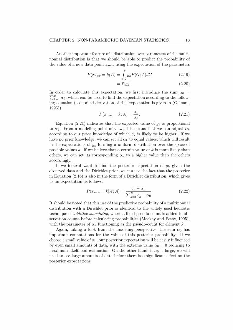
Figure 2.1: An example of a configuration of the Chinese restaurant process.Circles represent tables, labeled with the food (value k) that they generate.Squares represent customers, labeled with their index in X . Each value ofX is also marked with whether it was generated as a new table from α, oras an existing table from the cache c.
2.2.3 The Chinese Restaurant ProcessOne other way of looking at the posterior probability of the Dirichlet
process (or other stochastic process) is based on a representation schemecalled the Chinese Restaurant Process (CRP) (Pitman, 1995). This repre-sentation is useful for a number of reasons, in that it allows us to calculatethe marginal probability of the observed data X given the parameters α0
and Pbase, and also allows for intuitive representation of more complex mod-els during the process of Gibbs sampling. In order to describe this process,Figure 2.1 shows an example of one configuration for the Chinese restaurantprocess for X = {1, 2, 4, 5, 2, 1, 4, 4, 1, 4}.
The basic concept of the Chinese restaurant process is that there is aChinese restaurant with a potentially unlimited number of tables. Each timea customer enters the restaurant, he or she will, according to some probabil-ity, choose to sit either at any of the existing tables in T = {t1, . . . , tJ} thatalready has at least one customer, or at a new table tJ+1. For the Dirichletprocess, these probabilities are:
P (tj) =ctj
α0 +∑J
j=1 ctj(2.25)
P (tJ+1) =α0
α0 +∑J
j=1 ctj(2.26)
where ctj is the number of customers sitting at table tj . If the customer sitsat a new table, we decide which type of food will be served at that tableaccording to the base measure Pbase, which the customer will then proceed

CHAPTER 2. NON-PARAMETRIC BAYESIAN STATISTICS 16
to eat. If the customer decides to sit at an existing table, the customer willproceed to eat the food that is already being served at the table. Here, thenumber of customers eating a particular food k is equal to ck.
While it may be difficult to tell the relation between Chinese restaurantsand Dirichlet processes at first glance, there is a very clear connection be-tween this process and the calculation of the marginal probability of the dataP (X ;α0, Pbase) after we have marginalized out the multinomial distributionparameters G. First, note that the probability of X can be decomposed intothe product of the conditional probabilities using the chain rule
P (X ;α0, Pbase) =
I∏i=1
P (xi|xi−11 ;α0, Pbase) (2.27)
where xi−11 is used as short hand for {x1, . . . , xi−1}. We then substitute in
the posterior probability of Equation (2.16)
P (X ;α0, Pbase) =
I∏i=1
cxi−11 ,xi
+ α0Pbase(xi)
i− 1 + α0(2.28)
=I∏
i=1
( cxi−11 ,xi
i− 1 + α0+
α0Pbase(xi)
i− 1 + α0
). (2.29)
Note that here we are using counts cxi−11 ,xi
not over all of X , but overthe previously generated elements xi−1
1 , as we are conditioning on only thepreviously generated elements as shown in Equation (2.27).
After this transformation, the correspondence between the first of thetwo elements of Equation (2.29) and Equation (2.25) is clear. In addition, itcan be seen that the second of the two elements in Equation (2.29) is equalto the probability of choosing a new table in Equation (2.26) multiplied bythe base measure probability Pbase, with which we choose which food mustbe served at that table.
While this equivalence is interesting, it still does not make clear themotivation for the Chinese restaurant process. The true power of the Chi-nese restaurant process lies in the fact that it allows us to keep track ofthe number of times that a particular value of x = k was generated by thecontribution of the base distribution α0Pbase, as opposed to the counts (orcache) ck. This is done by keeping track of the number of tables for whichx = k, which will be represented using the function tk. These table counts,while not important for the simple Dirichlet process, are essential for accu-rately calculating the probabilities of other models such as the Pitman-Yor

CHAPTER 2. NON-PARAMETRIC BAYESIAN STATISTICS 17
process explained in the next section, or the hierarchical models describedin the rest of this thesis.
One other important thing to notice about the Chinese restaurant pro-cess is that the joint probability in Equation (2.29) is the same regardlessof the order in which we add the customers or tables. The denominatordepends only on the total number of customers, while the numerator de-pends only on the number of customers sitting at tables serving a particulardish (as well as the number of tables for the Pitman-Yor process describedin Section 2.2.4). This property of probabilities being agnostic to order iscalled exchangeability, and is useful for learning using Gibbs sampling asdescribed in Section 2.3.
2.2.4 The Pitman-Yor ProcessThe Pitman-Yor process is a generalization of the Dirichlet process that
allows for more expressive modeling (Pitman and Yor, 1997; Ishwaran andJames, 2001). The Pitman-Yor process has three parameters: a discount d,strength s, and base measure Pbase. Given these parameters, observed dataX , and the table distribution according to the Chinese restaurant process,the posterior probability of x given a Pitman-Yor process prior is
P (x|X , T ; d, s, Pbase) =cx − d ∗ tx + (s+ d
∑x tx)Pbase(x)∑
x cx + s. (2.30)
When compared to the posterior of the multinomial distribution with aDirichlet prior (Equation (2.16)) we can see that the Pitman-Yor s directlycorresponds with α0, and the only difference is the addition of the discountd, which is subtracted once for every table that corresponds to x.
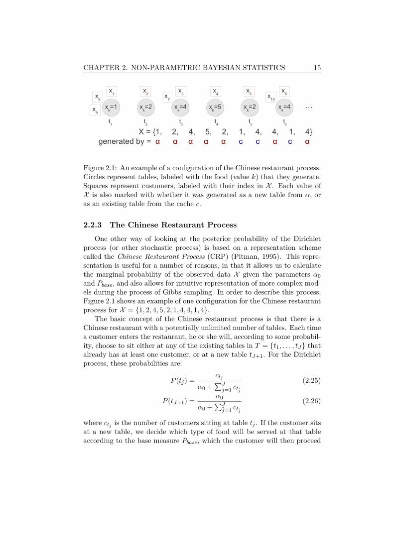
However, this discount is extremely important for modeling language(Kneser and Ney, 1995; Teh, 2006; Durrett and Klein, 2011). Figure 2.2gives an intuition of why this is true. The figure details an experimentwhere a large corpus of text was divided exactly into two, one training setand one testing set, so that each set contains C words. The words aresorted into buckets based on their frequency in the training set ctrain, andctest measures the actual average frequency of the words in each bucket usingthe testing set. The correspondence between the training and the testingfrequency gives us an idea of how much probability we should give to eachword in the predictive distribution given its count in the training data.
In the case of the Dirichlet prior, our estimate for the testing set fre-
CHAPTER 2. NON-PARAMETRIC BAYESIAN STATISTICS 18
Figure 2.2: The actual (solid line) and estimated (dashed line) number oftimes a word occurred in the test corpus based on how many times it oc-curred in the training corpus fitted (a) without a discount (Dirichlet prior),and (b) with a discount (Pitman-Yor prior).
quency ctest is as follows:
ctest,x = Ptrain(x)C (2.31)
=ctrain,x + α0Pbase(x))
C + α0C (2.32)
= (ctrain,x + α0Pbase(x))C
C + α0(2.33)
If we ignore the contribution of the base measure probability1 we cansee that the estimated test set frequency is simply the training set frequencymultiplied by a constant C
C+α0. This sort of discounting allows us to fit the
frequencies using estimates similar to Figure 2.2 (a), with a straight linethat passes through the origin, with the value of the constant modifyingthe slope of this line. However, it can be seen that this does not provide agood fit for the actual testing counts, overestimating the frequency of lessfrequent words, and underestimating the frequency of more frequent words.
In contrast, when we examine the same frequency with the additional1When C � α0, which is true in most cases, the counts contributed by the base measure
are generally significantly smaller than those contributed by the cache counts.

CHAPTER 2. NON-PARAMETRIC BAYESIAN STATISTICS 19
discount allowed by the Pitman-Yor prior
ctest(x) = (ctrain,x − d ∗ ttrain(x) + sPbase(x))C
C + s, (2.34)
and assume for simplicity that ttrain(x) = 1, we are able to create discountsthat correspond to any straight line that either travels through the origin,or anywhere below it. As can be seen in Figure 2.2 (b), this provides amuch better fit for word frequencies. This discount allows for modeling ofdistributions with a few common instances and many uncommon instances(power-law distributions). Power-law distributions are known to be goodmodels of not only word counts (Zipf, 1949), but also parts of speech (Gold-water and Griffiths, 2007), syntactic structures (Johnson et al., 2007b), andother aspects of natural language.
2.3 Gibbs SamplingThe previous section described how to calculate probabilities for Bayesian
probabilistic models given an observed data set X . However, for most mod-els of interest, in addition to our observed variables, we also have a set oflatent variables Y. Given that the goal of Bayesian learning is to discoverthe distribution over the parameters P (G|X ), introducing additional hid-den variables indicates that we will have to take the integral over possibleconfigurations of these hidden variables
P (G|X ) =∫
P (G|Y,X )P (Y|X )dY. (2.35)
Unfortunately, these integrals are often intractable and need to be approx-imated. There are two main techniques for approximating these integrals,variational Bayes (Beal, 2003) and Gibbs sampling (Geman and Geman,1984). This thesis focuses on the latter, as it allows for relatively straight-forward implementation of the more complex models introduced therein.
2.3.1 Latent Variable ModelsIn order to demonstrate the basics of Gibbs sampling, we can take an
example from unsupervised word segmentation, which will be a recurringtheme throughout the rest of this thesis. In unsupervised word segmenta-tion, we assume we have an observed corpus of unsegmented text X thatwas generated as a word sequence specified by latent variables Y from some
CHAPTER 2. NON-PARAMETRIC BAYESIAN STATISTICS 20
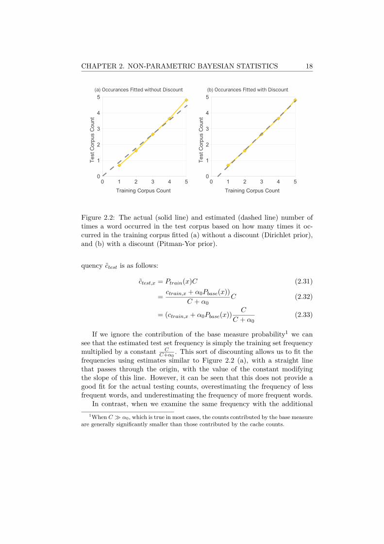
Figure 2.3: Word segmentation with a probabilistic model with charactersX , word boundary indicators Y, words W , and likelihood P (X ,Y|G).
word-based generative model with parameters G. Figure 2.3 shows an ex-ample of a sentence within this framework, which we will assume is partof a larger corpus. Here, the observed variables X ∈ X indicate charactersof a single sentence and hidden variables Y ∈ Y indicate whether a wordboundary exists between the corresponding characters. Finally, for conve-nience, we define a set of variables W ∈ W that represent the sequence ofwords that will be created when X is segmented according to Y . The pair〈X,Y 〉 and the words W uniquely determine each other, so they can be usedinterchangeably.
As the likelihood for this model we use a multinomial distribution overwords and assume that each word is generated independently, giving us thefollowing likelihood of the entire training data:
P (X ,Y|G) = P (W|G) (2.36)
=∏w∈W
gw. (2.37)
In order to calculate the posterior distribution of the parameters giventhe observed data P (G|X), we can perform the familiar transformation usingBayes’s law:
P (G|X ) = P (X|G)P (G)
P (X )(2.38)
and introduce the likelihood term P (X ,Y|G) by marginalizing over Y
P (G|X ) =∫
P (X ,Y|G)P (G)
P (X )dY. (2.39)
However, here we run into a problem. As changes in the value of Y willaffect the distribution over all G and changes in the value of G will affect
CHAPTER 2. NON-PARAMETRIC BAYESIAN STATISTICS 21
the distribution over Y, it becomes impossible to calculate this integral inclosed form. Instead, we turn to methods that can approximate this integralin a computationally tractable fashion.
2.3.2 Basic Gibbs SamplingThe most widely used method for approximating this integral over Y
is Gibbs sampling. The basic premise of sampling is based on the law oflarge numbers: if we make enough observations of a random variable that isgenerated according to some distribution, the distribution over observationswill eventually approach the true distribution. This means that insteadof analytically solving the integral in Equation (2.39), if we can generatesamples of Y, we can instead approximate this integral with the averageover each sample {Y1, . . . ,YN}:
P (G|X ) ≈ 1
N
N∑n=1
P (X ,Yn|G)P (G)
P (X )(2.40)
However, while it is easy to generate each sample Yn from simple distribu-tions such as the multinomial, it is often not possible to directly sample frommultivariate distributions with complex interactions between the componentvariables, as in the previous word segmentation example.
Gibbs sampling is a technique that allows for the sampling from mul-tivariate distributions, relying on the fact that if we sample one variableat a time conditioned on all the other variables, we can simulate the truedistribution (Geman and Geman, 1984). The intuition behind this is basedon the fact that if we assume that all variables in Y except y (denoted Y\y)are already distributed according to the true joint distribution, and sampley according to its conditional distribution given Y\y, we will recover thetrue distribution over all variables in Y
P (y|Y\y)P (Y\y) = P (Y). (2.41)
This indicates the distribution is invariant, which is one of the conditionsfor convergence of Gibbs sampling.
Even if we cannot assume the current Y\y was distributed correctlyaccording to P (Y\y), each time we draw a new sample, we will get slightlycloser to the true distribution, and will approach the true distribution inthe limit as long as the distribution is ergodic. Ergodicity is the propertythat every configuration of Y is reachable from every other configuration ofY with non-zero probability. A sufficient (but not necessary) condition for

CHAPTER 2. NON-PARAMETRIC BAYESIAN STATISTICS 22
ergodicity in the Gibbs sampling framework is that each time we sample avalue for y, all of its possible values are given a non-zero probability. If thisis the case, any configuration Y can be reached with non-zero probabilityby sampling the values of each of its corresponding y one-by-one.
In addition, the property of exchangeability mentioned in Section 2.2.3is particularly useful for Gibbs sampling. The reason for this is that everytime we sample a new value for y, if the values of Y are exchangeable wecan assume that current y of interest was the last value generated from thedistribution. For example, for multinomials with Dirichlet process priors,this makes calculating the probability P (y|Y\y) as simple as calculating theprobability of generating one more value from the posterior in Equation(2.16). On the other hand, if exchangeability does not hold, it may benecessary consider the probability of y itself, along with the effect that yhas upon all following values in Y, a much more computationally intensivetask.
2.3.3 Gibbs Sampling for Word SegmentationTo further illustrate the sampling process, let us take word segmentation
as an example and imagine the situation where we want to sample y5, whichdetermines whether there is a boundary between “e” and “a” in “meat” (or“me at”). To find the probability that the boundary exists, we first removethe effect that this word boundary has on the model by subtracting all ofthe counts that are influenced by the choice of y5. In this case, y5 lies withinthe word “meat” so we subtract one from its count:
cW\w,“meat” ← cW,“meat” − 1. (2.42)
Next, we calculate the probability of whether this new boundary existsaccording to the posterior probability of the Dirichlet process
P (y5 = 0) ∝cW\w,“meat” + α0Pbase(w = “meat”)∑
w cW\w,w + α0(2.43)
P (y5 = 1) ∝cW\w,“me” + α0Pbase(w = “me”)∑
w cW\w,w + α0
∗cW\w,“at” + α0Pbase(w = “at”)∑
w cW\w,w + α0 + 1. (2.44)
Note that if y5 = 0, we have generated a single word “meat” from thedistribution, while in the case of y5 = 1 we have generated two words,“me” and “at”. It should also be noted that we are adding a count of 1
CHAPTER 2. NON-PARAMETRIC BAYESIAN STATISTICS 23
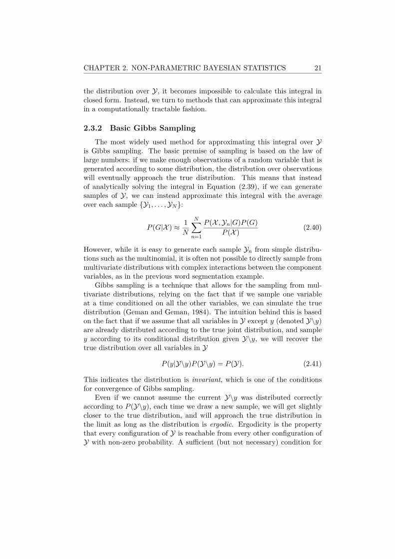
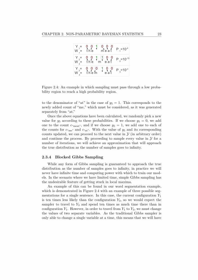
Figure 2.4: An example in which sampling must pass through a low proba-bility region to reach a high probability region.
to the denominator of “at” in the case of y5 = 1. This corresponds to thenewly added count of “me,” which must be considered, as it was generatedseparately from “at.”
Once the above equations have been calculated, we randomly pick a newvalue for y5 according to these probabilities. If we choose y5 = 0, we addone to the count c“meat”, and if we choose y5 = 1, we add one to each ofthe counts for c“me” and c“at”. With the value of y5 and its correspondingcounts updated, we can proceed to the next value in Y (in arbitrary order)and continue the process. By proceeding to sample every value in Y for anumber of iterations, we will achieve an approximation that will approachthe true distribution as the number of samples goes to infinity.
2.3.4 Blocked Gibbs SamplingWhile any form of Gibbs sampling is guaranteed to approach the true
distribution as the number of samples goes to infinity, in practice we willnever have infinite time and computing power with which to train our mod-els. In the scenario where we have limited time, simple Gibbs sampling hasthe undesirable feature of getting stuck in local maxima.
An example of this can be found in our word segmentation example,which is demonstrated in Figure 2.4 with an example of three possible seg-mentations for a single sentence. In this case, the current configuration Y1is ten times less likely than the configuration Y3, so we would expect thesampler to travel to Y3 and spend ten times as much time there than inconfiguration Y1. However, in order to travel from Y1 to Y3, we must changethe values of two separate variables. As the traditional Gibbs sampler isonly able to change a single variable at a time, this means that we will have

CHAPTER 2. NON-PARAMETRIC BAYESIAN STATISTICS 24
to choose each of these two changes independently. If the intermediate hy-potheses such as Y2 are highly unlikely, this means that it may take a largenumber of samples to make one of the two required changes. In the caseof the example, the probability of Y2 is 10−6 less than Y1 (which is not analtogether unreasonable number in most models of unsupervised learning),and thus it would require an average of one million iterations to escape fromthe local maximum.
There have been several solutions proposed to this problem (Hukushimaand Nemoto, 1996; Liang et al., 2010), but here we focus on blocked sampling(Jensen et al., 1995; Ishwaran and James, 2001; Scott, 2002), which is usedextensively in this thesis. Blocked Gibbs sampling is based on the idea thatwhile it is generally not possible to acquire a sample for all variables inY simultaneously, it is often possible to acquire a sample for some subsetY ⊂ Y according to the true distribution where |Y | > 1. One example wouldbe that Y describes the word boundaries for an entire corpus of observeddata, while Y describes the word boundaries for a single sentence within thiscorpus. If we are able to explicitly sample over all possible configurations ofY , the problem of intermediate states disappears, allowing us to jump fromY1 to Y3 or vice-versa in a single step.
In the case of word segmentation, we can acquire a sample of Y for asingle sentence by recasting the problem as the task of finding W , assumingindependence between each w ∈W , and performing dynamic programmingto allow for efficient calculation. This process is described fully in Section3.3, but the important point to note is the independence assumption betweenwords in W , which results in a sample from the proposal distribution:
Pprop(W |W\W ) =∏w∈W
cW\W,w + α0Pbase(w)∑w cW\W,w + α0
(2.45)
where W\W and cW\W respectively indicate the corpus and counts withsentence W removed.
While this particular proposal distribution is a close approximation tothe actual probability of the word segmentation, it is not exact. As notedpreviously in Equation (2.44), we must actually add the counts of eachword to the denominator before generating the next word to achieve thetrue marginal probabilities of the multinomial distribution with a Dirichletprior. In addition, if a particular word w is generated more than once in asentence, we must add the additional counts to the cw term in the numeratoras well. In order to express this, we define uniq(W ) as the collection of allunique words in W , and get the following true conditional probability for

CHAPTER 2. NON-PARAMETRIC BAYESIAN STATISTICS 25
W given W\W :
Ptrue(W |W\W ) =
(∏x∈uniq(W )
∏cW,x−1i=0 cW\W,x + i+ α0Pbase(x)
)(∏|W |−1
j=0 |W\W |+ j) . (2.46)
The numerator here takes into account words that are generated more thanone time in W , and the denominator takes into account the fact that thenumber of words in W increases as we generate each word in W .
It can be seen that there is a small gap between the proposal distri-bution Pprop and the true distribution Ptrue. Fortunately, there exists amethod called Metropolis-Hastings sampling that allows us to close this gapand ensure that we are sampling from the correct distribution (Hastings,1970; Johnson et al., 2007b). This technique is based on rejection samplingwhere we choose a sample from the proposal distribution, then decide toaccept or reject it based on an acceptance probability A. In the case ofMetropolis-Hastings sampling, this acceptance probability is defined usingthe probabilities Pprop and Ptrue for the old and new values of W , which arelabeled Wold and Wnew respectively2
A(Wold,Wnew) = min(Ptrue(Wnew)
Ptrue(Wold)
Pprop(Wold)
Pprop(Wnew), 1
). (2.47)
Mathematical details of this result can be found in the references (Hastings,1970), but the basic intuition lies in the comparison between the ratios ofthe Ptrue and Pprop. When the probability ratio of Wnew to Wold is higherfor Pprop than it is for Ptrue, we will be acquiring more samples of Wnew
than are justified by Ptrue. The Metropolis-Hastings method adjusts forthis fact by reducing the acceptance probability accordingly, so we rejectsome of these over-produced samples, allowing us to remain faithful to thetrue distribution. If this method is properly applied, we can be guaranteedto be sampling from the proper distribution, as the distribution will sat-isfy the property of detailed balance, which is a sufficient condition for thedistribution being invariant (Bishop, 2006).
2.3.5 Gibbs Sampling as Stochastic SearchUp until this point we have presented Gibbs sampling as a method for
approximating Equation (2.39)’s integral over Y to estimate the posterior2Simple Gibbs sampling is actually a specific case of Metropolis-Hastings sampling
where Pprop = Ptrue.
CHAPTER 2. NON-PARAMETRIC BAYESIAN STATISTICS 26
probability of G. However, in many cases (perhaps the majority in naturallanguage processing), we are more interested in the actual values of Y thanthe distribution over G. In our running word segmentation example, thiswould indicate that we are interested in the word sequence W of our corpusmore than the word probabilities G, a perfectly reasonable proposition if thiscorpus is to be used, for example, as data for training of machine translationor speech recognition systems. This indicates that Gibbs sampling can beused as a method not for approximating the integral over Y, but instead asa stochastic search method to find some value for the latent variables Y thatlies in a high-probability section of the space over all possible Y.
Within this context, it is often better to focus on implementation mo-tivated considerations, even at the cost of some degree of mathematicalcorrectness, when and only when they are justified. For example, whenestimating the parameters G using sampling, it is technically necessary toaverage over values obtained at each sample to obtain the true distribution.In the speech recognition experiments of Section 3.4, this provides signifi-cant gains in accuracy, so practical concerns suggest that we adopt a methodto take this sample averaging into account. However, Section 4.7 finds thatfor machine translation, this can lead to larger models without providingsignificant gains in down-stream accuracy, so we are justified by practicalconsiderations in using only a single sample.
In addition, in the case of block sampling where the most efficientlycomputable proposal distributions differ significantly from the true distri-bution (such as the ITG-based sampling model proposed in Chapter 4), wemay be faced with prohibitively high rejection rates when performing theMetropolis-Hastings step. This can hurt learning, particularly in the earlystages, as in most cases rejected samples of Wnew are still generally higherin probability than Wold according to both Pprop and Ptrue, but rejectedbecause of mismatches between the two.
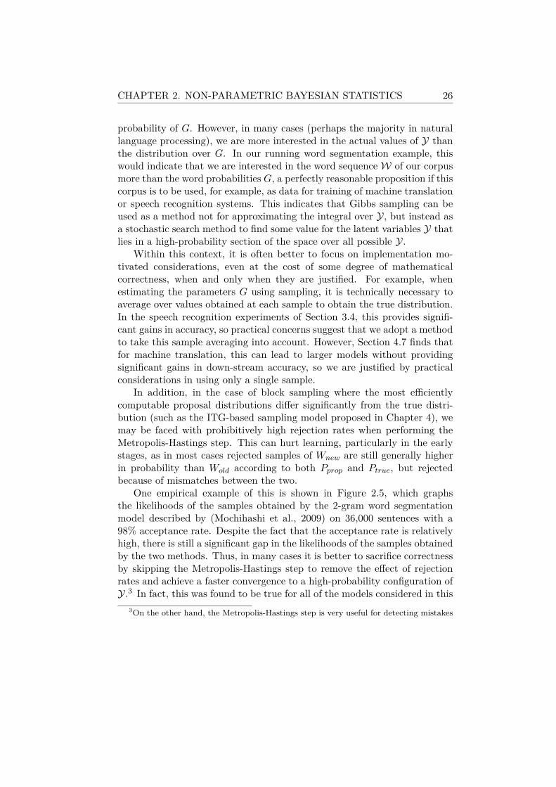
One empirical example of this is shown in Figure 2.5, which graphsthe likelihoods of the samples obtained by the 2-gram word segmentationmodel described by (Mochihashi et al., 2009) on 36,000 sentences with a98% acceptance rate. Despite the fact that the acceptance rate is relativelyhigh, there is still a significant gap in the likelihoods of the samples obtainedby the two methods. Thus, in many cases it is better to sacrifice correctnessby skipping the Metropolis-Hastings step to remove the effect of rejectionrates and achieve a faster convergence to a high-probability configuration ofY.3 In fact, this was found to be true for all of the models considered in this
3On the other hand, the Metropolis-Hastings step is very useful for detecting mistakes

CHAPTER 2. NON-PARAMETRIC BAYESIAN STATISTICS 27
Figure 2.5: Likelihoods with and without Metropolis-Hastings sampling.
thesis, so the Metropolis-Hastings rejection step is never used, even when itis necessary for strict mathematical correctness.
This thesis mainly uses Gibbs sampling as a tool for stochastic search,and will be making these sort of approximations when they are motivated.
in the implementation of sampling algorithms. In general, the calculation of Pprop andPtrue must be performed separately, and mistakes in the implementation of either willlead to unrealistically high rejection rates, which are easy to notice and debug.
Chapter 3
Learning a Language Modelfrom Continuous Speech
A language model (LM) is an essential part of automatic speech recog-nition (ASR) systems, providing linguistic constraints on the recognizer andhelping to resolve the ambiguity inherent in the acoustic signal. Tradition-ally, these LMs are learned from digitized text, preferably text that is similarin style and content to the speech that is to be recognized. In addition, thistext is generally annotated with word or morpheme boundaries using thesupervised techniques introduced in Section 1.1, and a dictionary mappingthe surface form of words to their pronunciations must be prepared.
This chapter proposes a new paradigm for LM learning, using not digi-tized text but audio data of continuous speech. The proposition of learningan LM from continuous speech is motivated from a number of viewpoints.First, the properties of written and spoken language are very different (Tan-nen, 1982), and LMs learned from continuous speech can be expected tonaturally model spoken language. In contrast, when language models arelearned from written text, it is often necessary to manually transcribe speechor compensate for these differences by transforming written-style text intospoken-style text when creating an LM for ASR (Vergyri and Kirchhoff,2004; Akita and Kawahara, 2010). Second, learning lexical units and theircontext from speech can allow for out-of-vocabulary word detection and ac-quisition, which has been shown to be useful in creating more adaptableand robust ASR or dialog systems (Bazzi and Glass, 2001; Hirsimäki et al.,2006). Learning LMs from speech can also provide a powerful tool in ef-forts for technology-based language preservation (Abney and Bird, 2010),particularly for languages that have a rich oral, but not written tradition.
28

CHAPTER 3. LM LEARNING FROM SPEECH 29
Finally, as human children learn language from speech, not text, computa-tional models for learning from speech are of great interest in the field ofcognitive science (Roy and Pentland, 2002).
For all of the previous reasons, there has been a significant amount ofwork on learning lexical units from speech data. These include statisticalmodels based on the minimum description length or maximum likelihoodframeworks, which have been trained on one-best phoneme recognition re-sults (de Marcken, 1995; Deligne and Bimbot, 1997; Gorin et al., 1999)or recognition lattices (Driesen and Hamme, 2008). There have also been anumber of works that use acoustic matching methods combined with heuris-tic cutoffs that may be adjusted to determine the granularity of the unitsthat need to be acquired (ten Bosch and Cranen, 2007; Park and Glass,2008; Jansen et al., 2010). Finally, many works, inspired by the multi-modal learning of human children, use visual and audio information (orat least abstractions of such) to learn lexical units without text (Roy andPentland, 2002; Iwahashi, 2003; Yu and Ballard, 2004).
The work presented in this chapter is different from these other ap-proaches in that it is the first model that is able to learn a full n-gramlanguage model from raw audio, and demonstrate that this model can beused to reduce the phoneme error rate of speech in an ASR system. Thefirst step in learning an LM from continuous speech is to generate lattices ofphonemes without any linguistic constraints using a standard ASR acous-tic model. To learn an LM from this data, this chapter builds on recentwork in unsupervised word segmentation of text (Mochihashi et al., 2009),proposing a novel inference procedure that allows for models to be learnedover lattice input. For LM learning, the proposed technique uses the hi-erarchical Pitman-Yor LM (HPYLM) (Teh, 2006), a variety of LM that isbased on non-parametric Bayesian statistics. As mentioned in Chapter 2,non-parametric Bayesian statistics are well suited to this learning problem,as they allow for automatically balancing model complexity and expressive-ness, and have a principled framework for learning through the use of Gibbssampling.
To perform sampling over phoneme lattices, all models are representedusing weighted finite state transducers (WFSTs), which allow for simpleand efficient combination of the phoneme lattices with the LM. Using thiscombined lattice, we can use a variant of the forward-backward algorithmto efficiently sample a phoneme string and word segmentation accordingto the model probabilities. By performing this procedure on each of theutterances in the corpus for several iterations, it is possible to effectivelydiscover phoneme strings and lexical units appropriate for LM learning,
CHAPTER 3. LM LEARNING FROM SPEECH 30
even in the face of acoustic uncertainty.Finally, experiments are performed to test the feasibility of learning an
LM from only audio files of fluent adult-directed meeting speech with no ac-companying text. The results of the experiment show that, despite the lackof any text data, the proposed model is able to both decrease the phonemerecognition error rate over a separate test set and acquire a lexicon withmany intuitively reasonable lexical entries. Moreover, the proposed lat-tice processing approach proves effective for overcoming acoustic ambiguitypresent during the training process.
Section 3.1 briefly overviews the process of speech recognition, includinglanguage modeling and representation of ASR models in the WFST frame-work. Section 3.2 describes previous research on LM-based unsupervisedword segmentation in more detail. Section 3.3 proposes a method for for-mulating LM-based unsupervised word segmentation using a combinationof WFSTs and Gibbs sampling. The description concludes in Section 3.3.3by showing that the WFST-based formulation allows for LM learning di-rectly from speech, even in the presence of acoustic uncertainty. Section3.4 describes the results of an experimental evaluation demonstrating theeffectiveness of the proposed method, and Section 3.5 concludes the chapterand discusses future directions.
3.1 Speech Recognition and Language ModelingThis section provides an overview of ASR and language modeling and
provides definitions that will be used in the rest of the chapter.
3.1.1 Speech RecognitionASR can be formalized as the task of finding a series of words W given
acoustic features U of a speech signal containing these words. Most ASRsystems use statistical methods, creating a model for the posterior proba-bility of the words given the acoustic features, and searching for the wordsequence that maximizes this probability
W = argmaxW
P (W |U). (3.1)
As this posterior probability is difficult to model directly, Bayes’s law is
CHAPTER 3. LM LEARNING FROM SPEECH 31
used to decompose the probability
W = argmaxW
P (U |W )P (W )
P (U)(3.2)
= argmaxW
P (U |W )P (W ). (3.3)
Here, P (U |W ) is computed by the acoustic model (AM), which makesa probabilistic connection between words and their acoustic features. How-ever, directly modeling the acoustic features of the thousands to millions ofwords in large-vocabulary ASR systems is not realistic due to data sparsityissues. Instead, AMs are trained to recognize sequences of phonemes X,which are then mapped into the word sequence W . Phonemes are definedas the smallest perceptible linguistic unit of speech. Thus, the entire ASRprocess can be described as finding the optimal word sequence according tothe following formula
W = argmaxW
∑X
P (U |X)P (X|W )P (W ). (3.4)
This is usually further approximated by choosing the single most likelyphoneme sequence to allow for efficient search:
W = argmaxW,X
P (U |X)P (X|W )P (W ). (3.5)
Here, P (U |X) indicates the AM probability and P (X|W ) is a lexicon proba-bility that maps between words and their pronunciations. P (W ) is computedby the LM, which will be described in more detail in the following section.It should be noted that in many cases a scaling factor α is used
W = argmaxW,X
P (U |X)P (X|W )P (W )α. (3.6)
This allows for the adjustment of the relative weight put on the LM probabil-ity, with a higher weight indicating that the LM will have a large influence onthe recognition results, preferring to generate well-formed sentences, while alower weight will indicate that the acoustic model will have a large influence,resulting in sentences that closely match the acoustic features.
3.1.2 Language ModelingThe goal of the LM probability P (W ) is to provide a preference towards
“good” word sequences, assigning high probability to word sequences that
CHAPTER 3. LM LEARNING FROM SPEECH 32
the speaker is likely to say, and low probability to word sequences that thespeaker is unlikely to say. By doing so, this allows the ASR system toselect linguistically proper sequences when purely acoustic information isnot enough to correctly recognize the input.
The most popular form of LM is the n-gram, which is notable for itssimplicity, computational efficiency, and surprising power (Goodman, 2001).n-gram LMs are based on the fact that it is possible to calculate the jointprobability of W = wI
1 sequentially by conditioning on all previous words inthe sequence using the chain rule
P (W ) =I∏
i=1
P (wi|wi−11 ). (3.7)
Conditioning on previous words in the sequence allows for the consider-ation of contextual information in the probabilistic model. However, as fewsentences will contain exactly the same words as any other, conditioning onall previous words in the sentence quickly leads to data sparseness issues.n-gram models resolve this problem by only conditioning on the previous(n− 1) words when choosing the next word in the sequence
P (W ) ≈I∏
i=1
P (wi|wi−1i−n+1). (3.8)
The conditional probabilities are generally trained from a large corpus ofword sequencesW. FromW we can calculate the counts of each subsequenceof n words wi
i−n+1 (an “n-gram”). From these counts, it is possible tocompute conditional probabilities using maximum likelihood estimation
Pml(wi|wi−1i−n+1) =
cwii−n+1
cwi−1i−n+1
. (3.9)
However, even if we set n to a relatively small value, we will never have acorpus large enough to exhaustively cover all possible n-grams. In order todeal with this data sparsity issue, it is common to use a framework that ref-erences higher order n-gram probabilities when they are available, and fallsback to lower order n-gram probabilities according to a fallback probabilityP (FB|wi−1
i−n+1):
P (wi|wi−1i−n+1) = {
Ps(wi|wi−1i−n+1) if cwi
i−n+1> 0,
P (FB|wi−1i−n+1)P (wi|wi−1
i−n+2) otherwise.

CHAPTER 3. LM LEARNING FROM SPEECH 33
By combining more accurate but sparse higher-order n-grams with lessaccurate but more reliable lower-order n-grams, it is possible to createLMs that are both accurate and robust. To reserve some probability forP (FB|wi−1
i−n+1), we replace Pml with the smoothed probability distributionPs. Ps can be defined according to a number of smoothing methods, whichare described thoroughly in (Chen and Goodman, 1996).
3.1.3 Bayesian Language ModelingWhile traditional methods for LM smoothing are based on heuristics (of-
ten theoretically motivated), it is also possible to motivate language mod-eling from the perspective of Bayesian statistics (Mackay and Petoy, 1995;Teh, 2006). In order to perform smoothing in the Bayesian framework, wefirst define a variable gwi|wi−1
i−m+1that specifies n-gram probabilities
gwi|wi−1i−m+1
= P (wi|wi−1i−m+1) (3.10)
where 0 ≤ m ≤ n− 1 is the length of the context being considered.As we are not sure of the actual values of the n-gram probabilities due
to data sparseness, the standard practice of Bayesian statistics suggests wetreat all probabilities as random variables G that we can learn from thetraining data W. Formally, this learning problem consists of estimating theposterior probability P (G|W). This can be calculated in a Bayesian fashionby placing a prior probability P (G) over G and combining this with thelikelihood P (W|G) and the evidence P (W)
P (G|W) =P (W|G)P (G)
P (W)(3.11)
∝ P (W|G)P (G) (3.12)
=
( ∏W∈W
P (W |G)
)P (G). (3.13)
We can generally ignore the evidence probability, as the training data isfixed throughout the entire training process, and we assume that each of thesentences in the corpus was generated independently from the probabilitydistribution specified by G.
It should be noted that LMs are a collection of multinomial distribu-tions Gwi−1
i−m+1= {gwi=1|wi−1
i−m+1, . . . , gwi=N |wi−1
i−m+1} where N is the number of
words in the vocabulary. There is one multinomial for each history wi−1i−m+1,
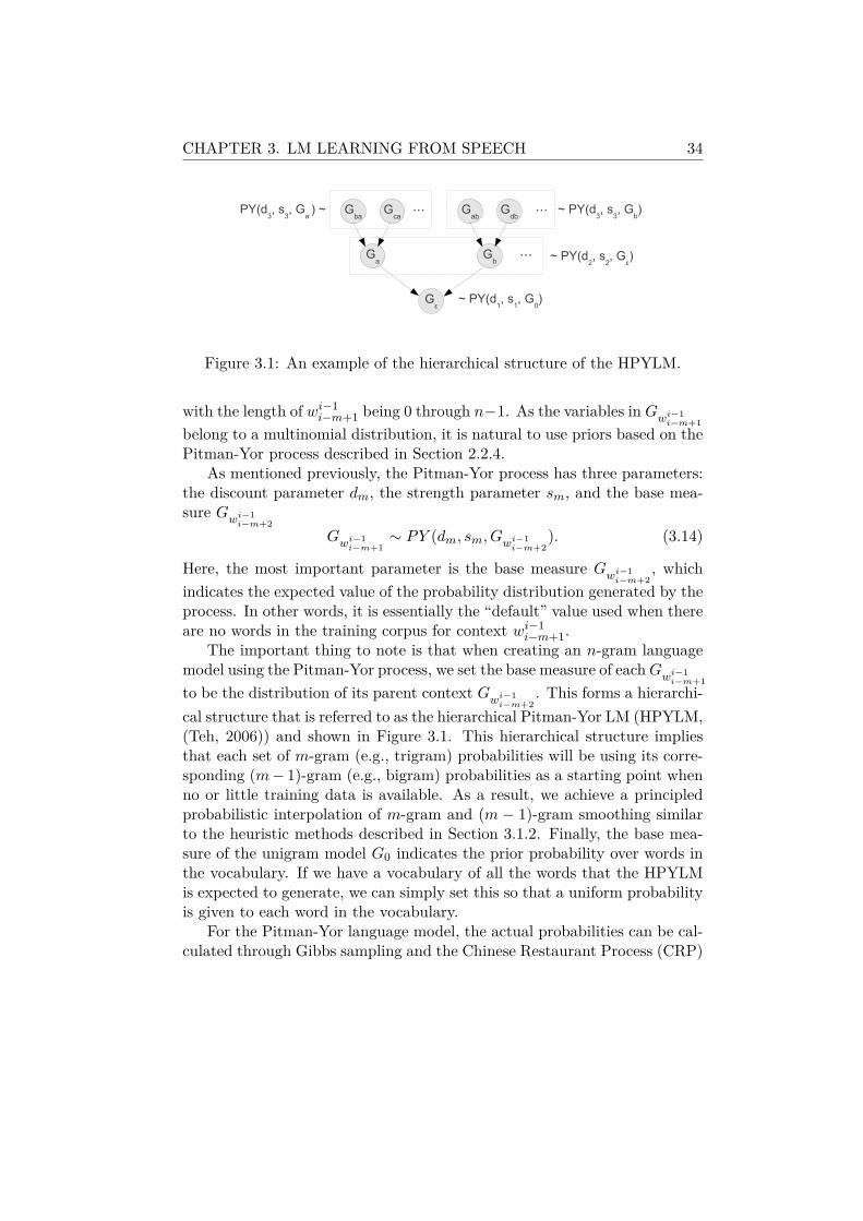
CHAPTER 3. LM LEARNING FROM SPEECH 34
Figure 3.1: An example of the hierarchical structure of the HPYLM.
with the length of wi−1i−m+1 being 0 through n−1. As the variables in Gwi−1
i−m+1
belong to a multinomial distribution, it is natural to use priors based on thePitman-Yor process described in Section 2.2.4.
As mentioned previously, the Pitman-Yor process has three parameters:the discount parameter dm, the strength parameter sm, and the base mea-sure Gwi−1
i−m+2
Gwi−1i−m+1
∼ PY (dm, sm, Gwi−1i−m+2
). (3.14)
Here, the most important parameter is the base measure Gwi−1i−m+2
, whichindicates the expected value of the probability distribution generated by theprocess. In other words, it is essentially the “default” value used when thereare no words in the training corpus for context wi−1
i−m+1.The important thing to note is that when creating an n-gram language
model using the Pitman-Yor process, we set the base measure of eachGwi−1i−m+1
to be the distribution of its parent context Gwi−1i−m+2
. This forms a hierarchi-cal structure that is referred to as the hierarchical Pitman-Yor LM (HPYLM,(Teh, 2006)) and shown in Figure 3.1. This hierarchical structure impliesthat each set of m-gram (e.g., trigram) probabilities will be using its corre-sponding (m− 1)-gram (e.g., bigram) probabilities as a starting point whenno or little training data is available. As a result, we achieve a principledprobabilistic interpolation of m-gram and (m − 1)-gram smoothing similarto the heuristic methods described in Section 3.1.2. Finally, the base mea-sure of the unigram model G0 indicates the prior probability over words inthe vocabulary. If we have a vocabulary of all the words that the HPYLMis expected to generate, we can simply set this so that a uniform probabilityis given to each word in the vocabulary.
For the Pitman-Yor language model, the actual probabilities can be cal-culated through Gibbs sampling and the Chinese Restaurant Process (CRP)
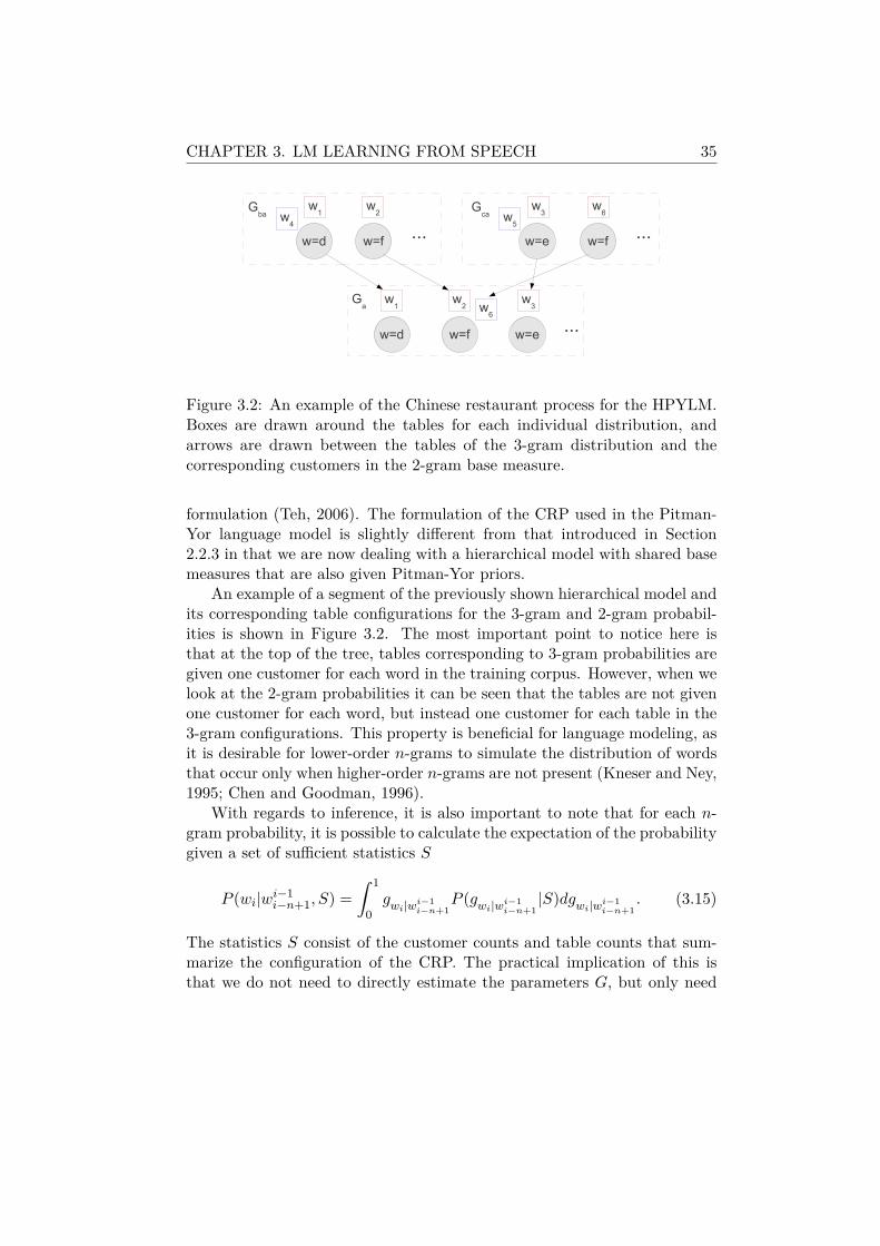
CHAPTER 3. LM LEARNING FROM SPEECH 35
Figure 3.2: An example of the Chinese restaurant process for the HPYLM.Boxes are drawn around the tables for each individual distribution, andarrows are drawn between the tables of the 3-gram distribution and thecorresponding customers in the 2-gram base measure.
formulation (Teh, 2006). The formulation of the CRP used in the Pitman-Yor language model is slightly different from that introduced in Section2.2.3 in that we are now dealing with a hierarchical model with shared basemeasures that are also given Pitman-Yor priors.
An example of a segment of the previously shown hierarchical model andits corresponding table configurations for the 3-gram and 2-gram probabil-ities is shown in Figure 3.2. The most important point to notice here isthat at the top of the tree, tables corresponding to 3-gram probabilities aregiven one customer for each word in the training corpus. However, when welook at the 2-gram probabilities it can be seen that the tables are not givenone customer for each word, but instead one customer for each table in the3-gram configurations. This property is beneficial for language modeling, asit is desirable for lower-order n-grams to simulate the distribution of wordsthat occur only when higher-order n-grams are not present (Kneser and Ney,1995; Chen and Goodman, 1996).
With regards to inference, it is also important to note that for each n-gram probability, it is possible to calculate the expectation of the probabilitygiven a set of sufficient statistics S
P (wi|wi−1i−n+1, S) =
∫ 1
0gwi|wi−1
i−n+1P (gwi|wi−1
i−n+1|S)dgwi|wi−1
i−n+1. (3.15)
The statistics S consist of the customer counts and table counts that sum-marize the configuration of the CRP. The practical implication of this isthat we do not need to directly estimate the parameters G, but only need
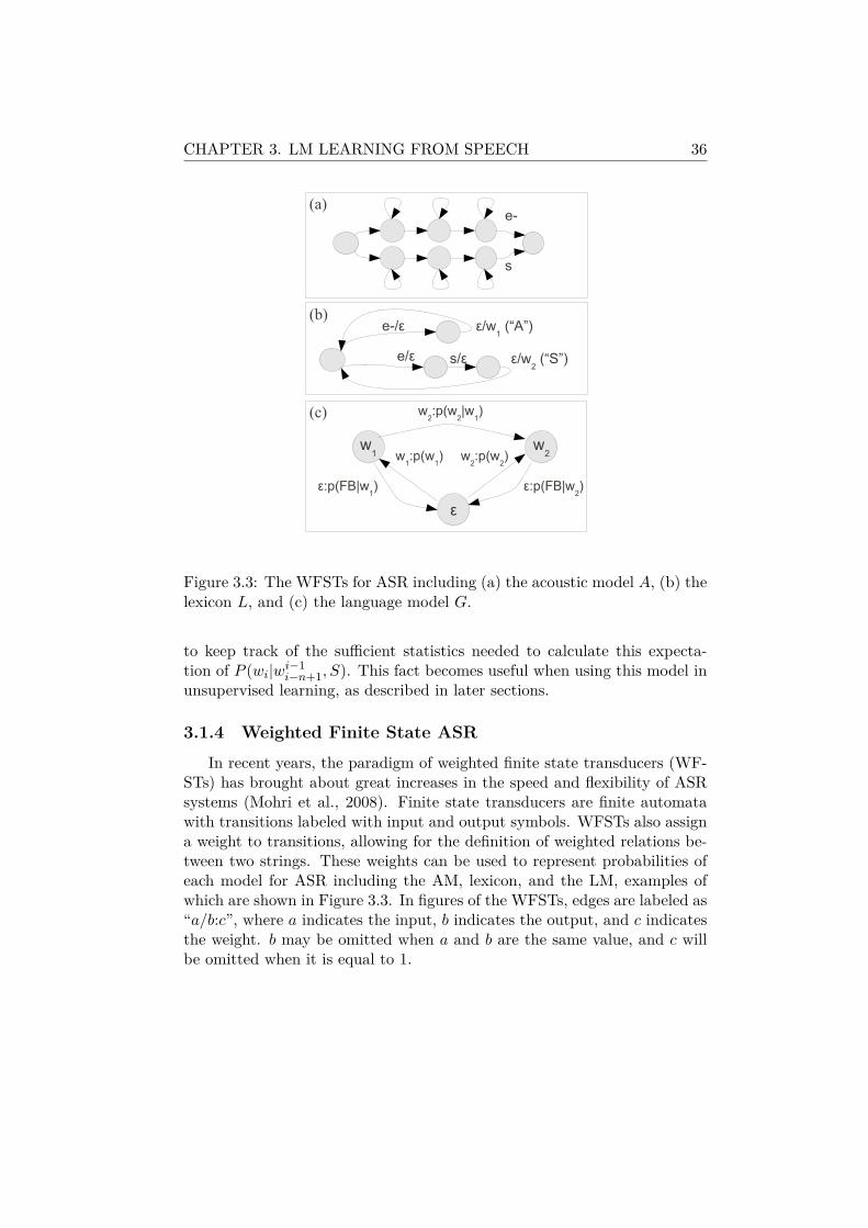
CHAPTER 3. LM LEARNING FROM SPEECH 36
Figure 3.3: The WFSTs for ASR including (a) the acoustic model A, (b) thelexicon L, and (c) the language model G.
to keep track of the sufficient statistics needed to calculate this expecta-tion of P (wi|wi−1
i−n+1, S). This fact becomes useful when using this model inunsupervised learning, as described in later sections.
3.1.4 Weighted Finite State ASRIn recent years, the paradigm of weighted finite state transducers (WF-
STs) has brought about great increases in the speed and flexibility of ASRsystems (Mohri et al., 2008). Finite state transducers are finite automatawith transitions labeled with input and output symbols. WFSTs also assigna weight to transitions, allowing for the definition of weighted relations be-tween two strings. These weights can be used to represent probabilities ofeach model for ASR including the AM, lexicon, and the LM, examples ofwhich are shown in Figure 3.3. In figures of the WFSTs, edges are labeled as“a/b:c”, where a indicates the input, b indicates the output, and c indicatesthe weight. b may be omitted when a and b are the same value, and c willbe omitted when it is equal to 1.

CHAPTER 3. LM LEARNING FROM SPEECH 37
The standard AM for P (U |X) in most ASR systems is based on a Hid-den Markov Model (HMM), and its WFST representation, which will becalled A. A simplified example of this model is shown in Figure 3.3 (a).As input, this takes acoustic features, and after several steps through theHMM outputs a single phoneme such as “e-” or “s.” The transition and emis-sion probabilities are identical to the standard HMM used in ASR acousticmodels, but they are omitted from the figure for simplicity.
The WFST formulation for the lexicon L, shown in Figure 3.3 (b), takesphonemes as input and outputs words along with their corresponding lexiconprobability P (X|W ). Excluding the case of homographs (words with thesame spelling but different pronunciations), the probability of transitions inthe lexicon will be 1.
Finally, the LM probability P (W ) can also be represented in the WFSTformat. Figure 3.3 (c) shows an example of a bigram LM with only two wordsw1 and w2 in the vocabulary. Each node represents a unique n-gram contextwi−1i−m+1, and the outgoing edges from the node represent the probability of
symbols given this context P (wi|wi−1i−m+1). In order to handle the fallback
to lower-order contexts as described in Section 3.1.2, edges that transitionfrom wi−1
i−m+1 to wi−1i−m+2 are added, weighted with the fallback probability
(marked with “FB” in the figure). The label ε on these edges indicates theempty string, which means they can be followed at any time, regardless ofthe input symbol.
The main advantage of using WFSTs to describe the ASR problem isthe existence of efficient algorithms for operations such as composition, in-tersection, determinization, and minimization. In particular, composition(designated with the ◦ operator) allows the combination of two WFSTs insequence, so if we compose A ◦L ◦G together, we can create a single WFSTthat takes acoustic features as input and outputs weighted strings of wordsentailed by the acoustic features. This property of WFSTs will be usefullater to facilitate the implementation of learning of LMs from continuousspeech.
3.2 Learning LMs from Unsegmented TextWhile Sections 3.1.2 and 3.1.3 described how to learn LMs when we
are given a corpus of word sequences W, there are some cases when theword sequence is not obvious. For example, when human babies learn wordsthey do so from continuous speech, even though there often are not explicitboundaries between words in the phoneme stream. In addition, as mentioned

CHAPTER 3. LM LEARNING FROM SPEECH 38
previously, many languages such as Japanese, Chinese, and Thai are writtenwithout boundaries between words, and thus the definition of words is notuniquely fixed. This section describes formally and in detail a method forjointly learning lexical units and a language model from unsegmented text.
3.2.1 Unsupervised WS ModelingThis work follows (Mochihashi et al., 2009) in taking an LM-based ap-
proach to unsupervised WS, learning a word-based LM G from a corpusof unsegmented phoneme strings X . The LM-based approach is attractivefor the task of learning from speech, as LMs are an integral part of speechrecognition systems, and the resulting LM can thus be plugged directly backin to ASR for use on text that is not included in our training data.
The problem of learning an LM from unsegmented phoneme strings canbe specified as finding a model according to the posterior probability of theLM P (G|X ), which can be decomposed using Bayes’s law
P (G|X ) ∝ P (X|G)P (G). (3.16)
However, as G is a word-based LM, we also assume that there are hiddenword sequences W, and model the probability given these sequences
P (G|X ) ∝∑W
P (X|W)P (W|G)P (G). (3.17)
Here, P (X|W) indicates that the words inW must correspond to the phonemesin X , and will be 1 if and only if X can be recovered by concatenating thewords in W together. P (W|G) is the likelihood given the LM probabilities,and is identical to that described in Equation (3.8).
P (G) can be set using the previously described HPYLM, with one ad-justment. With the model described in Section 3.1.3, it was necessary toknow the full vocabulary in advance so that we could set the base measureG0 to a uniform distribution over all the words in the vocabulary. However,when learning an LM from unsegmented text, W is not known in advance,and thus it is impossible to define a closed vocabulary before training starts.As a result, it is necessary to find an alternative method of defining G0 thatallows the model to flexibly decide which words to include in the vocabularyas training progresses.
In order to do so, (Mochihashi et al., 2009) use a “spelling model” H,which assigns prior probabilities over words by using an LM specified overphonemes. If we have a word wi that consists of phonemes, x1, . . . , xJ , we
CHAPTER 3. LM LEARNING FROM SPEECH 39
define the spelling model probability of wi according to the n-gram proba-bilities of H:
G0(wi) = P (wi = x1, . . . , xJ |H) =
J∏j=1
hxj |xj−1
j−n+1(3.18)
We assume that H is also distributed according to the HPYLM, and thatthe set of phonemes is closed and thus we are able to define a uniformdistribution over phonemes H0. The probabilities of H can be calculatedfrom the set of phoneme sequences of words generated from the spellingmodel, much like the probabilities of G can be calculated from the set ofword sequences contained in the corpus.
This gives us a full generative model for the corpus X that first generatesthe LM probabilities
H ∼ HPY LM(dH , sH ,H0) (3.19)G ∼ HPY LM(dG, sG, P (w|H)) (3.20)
then generates each word sequence W ∈ W and concatenates it into aphoneme sequence
W ∼ P (W |G) (3.21)X ← concat(W ). (3.22)
This generative story is important in that it allows for the creation ofLMs that are both highly expressive and compact (and thus have high gen-eralization capacity). The HPYLM priors for H and G have a preference forsimple models, and thus will tend to induce compact models, while the like-lihoods for W bias towards larger and more expressive models that describethe data well. It should be noted that in contrast, if maximum likelihoodestimation is used without a prior that biases against degenerate solutions,the model will have a tendency to maximize the likelihood by over-fittingthe training data, memorizing each training sentence as a single word.
3.2.2 Inference for Unsupervised WSThe main difficulty in learning LM G from the phoneme string X is
solving Equation (3.17). Here, it is necessary to sum over all possible con-figurations ofW, which represent all possible segmentations of X . However,for all but the smallest of corpora, the number of possible segmentations is
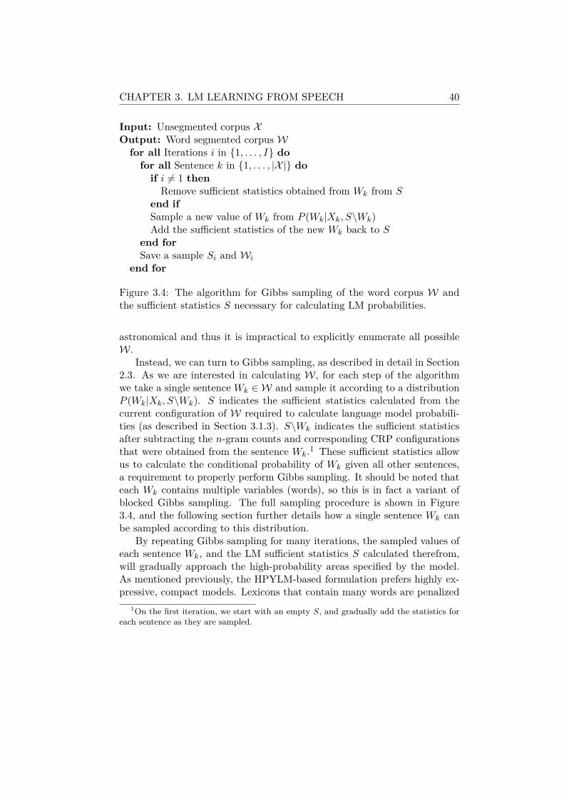
CHAPTER 3. LM LEARNING FROM SPEECH 40
Input: Unsegmented corpus XOutput: Word segmented corpus W
for all Iterations i in {1, . . . , I} dofor all Sentence k in {1, . . . , |X |} do
if i 6= 1 thenRemove sufficient statistics obtained from Wk from S
end ifSample a new value of Wk from P (Wk|Xk, S\Wk)Add the sufficient statistics of the new Wk back to S
end forSave a sample Si and Wi
end for
Figure 3.4: The algorithm for Gibbs sampling of the word corpus W andthe sufficient statistics S necessary for calculating LM probabilities.
astronomical and thus it is impractical to explicitly enumerate all possibleW.
Instead, we can turn to Gibbs sampling, as described in detail in Section2.3. As we are interested in calculating W, for each step of the algorithmwe take a single sentence Wk ∈ W and sample it according to a distributionP (Wk|Xk, S\Wk). S indicates the sufficient statistics calculated from thecurrent configuration of W required to calculate language model probabili-ties (as described in Section 3.1.3). S\Wk indicates the sufficient statisticsafter subtracting the n-gram counts and corresponding CRP configurationsthat were obtained from the sentence Wk.1 These sufficient statistics allowus to calculate the conditional probability of Wk given all other sentences,a requirement to properly perform Gibbs sampling. It should be noted thateach Wk contains multiple variables (words), so this is in fact a variant ofblocked Gibbs sampling. The full sampling procedure is shown in Figure3.4, and the following section further details how a single sentence Wk canbe sampled according to this distribution.
By repeating Gibbs sampling for many iterations, the sampled values ofeach sentence Wk, and the LM sufficient statistics S calculated therefrom,will gradually approach the high-probability areas specified by the model.As mentioned previously, the HPYLM-based formulation prefers highly ex-pressive, compact models. Lexicons that contain many words are penalized
1On the first iteration, we start with an empty S, and gradually add the statistics foreach sentence as they are sampled.
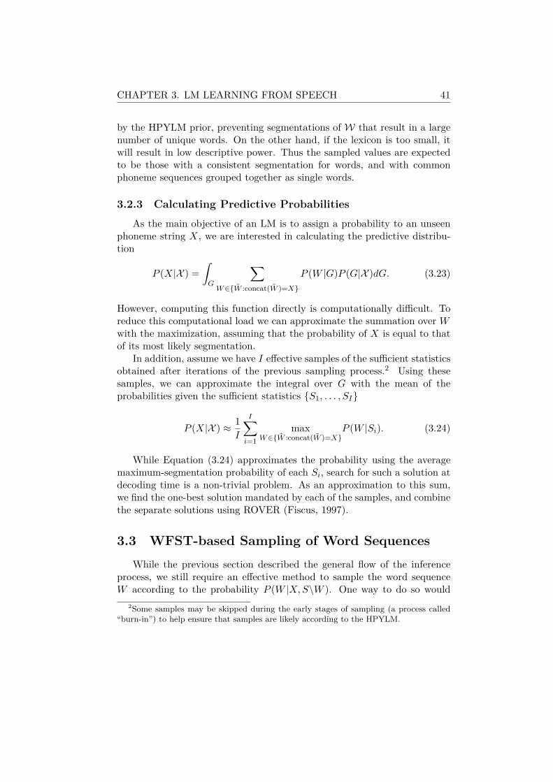
CHAPTER 3. LM LEARNING FROM SPEECH 41
by the HPYLM prior, preventing segmentations of W that result in a largenumber of unique words. On the other hand, if the lexicon is too small, itwill result in low descriptive power. Thus the sampled values are expectedto be those with a consistent segmentation for words, and with commonphoneme sequences grouped together as single words.
3.2.3 Calculating Predictive ProbabilitiesAs the main objective of an LM is to assign a probability to an unseen
phoneme string X, we are interested in calculating the predictive distribu-tion
P (X|X ) =∫G
∑W∈{W :concat(W )=X}
P (W |G)P (G|X )dG. (3.23)
However, computing this function directly is computationally difficult. Toreduce this computational load we can approximate the summation over Wwith the maximization, assuming that the probability of X is equal to thatof its most likely segmentation.
In addition, assume we have I effective samples of the sufficient statisticsobtained after iterations of the previous sampling process.2 Using thesesamples, we can approximate the integral over G with the mean of theprobabilities given the sufficient statistics {S1, . . . , SI}
P (X|X ) ≈ 1
I
I∑i=1
maxW∈{W :concat(W )=X}
P (W |Si). (3.24)
While Equation (3.24) approximates the probability using the averagemaximum-segmentation probability of each Si, search for such a solution atdecoding time is a non-trivial problem. As an approximation to this sum,we find the one-best solution mandated by each of the samples, and combinethe separate solutions using ROVER (Fiscus, 1997).
3.3 WFST-based Sampling of Word SequencesWhile the previous section described the general flow of the inference
process, we still require an effective method to sample the word sequenceW according to the probability P (W |X,S\W ). One way to do so would
2Some samples may be skipped during the early stages of sampling (a process called“burn-in”) to help ensure that samples are likely according to the HPYLM.
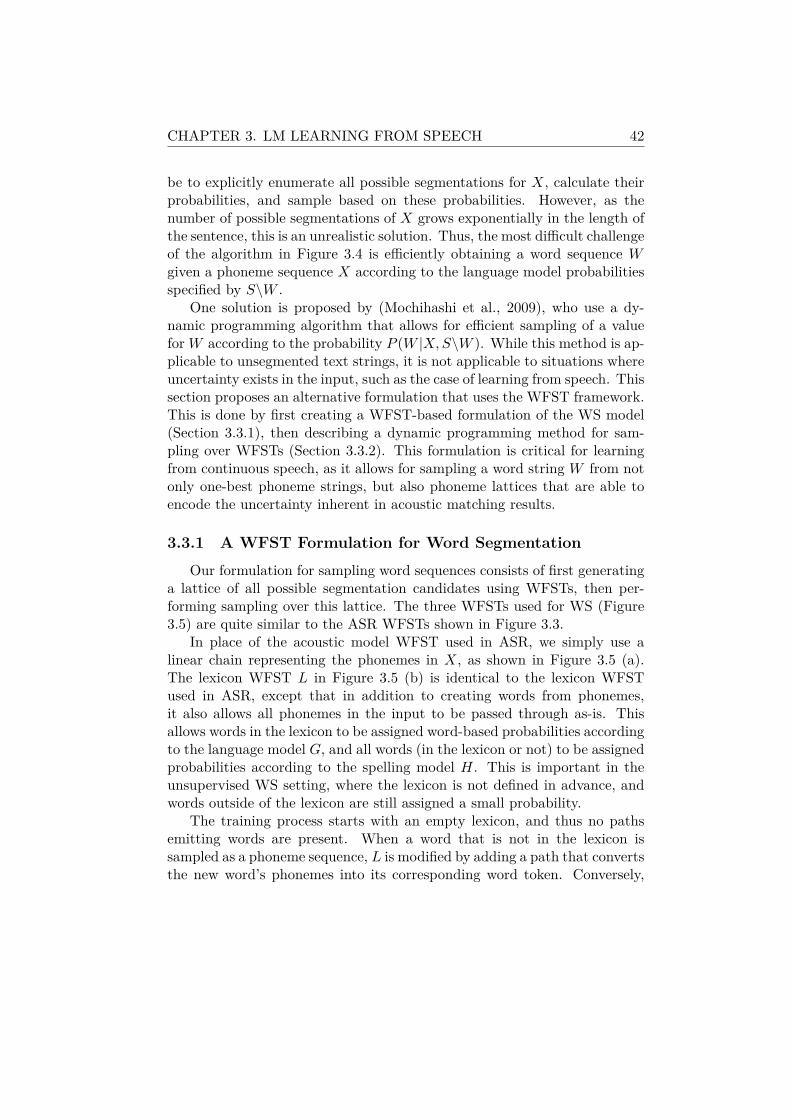
CHAPTER 3. LM LEARNING FROM SPEECH 42
be to explicitly enumerate all possible segmentations for X, calculate theirprobabilities, and sample based on these probabilities. However, as thenumber of possible segmentations of X grows exponentially in the length ofthe sentence, this is an unrealistic solution. Thus, the most difficult challengeof the algorithm in Figure 3.4 is efficiently obtaining a word sequence Wgiven a phoneme sequence X according to the language model probabilitiesspecified by S\W .
One solution is proposed by (Mochihashi et al., 2009), who use a dy-namic programming algorithm that allows for efficient sampling of a valuefor W according to the probability P (W |X,S\W ). While this method is ap-plicable to unsegmented text strings, it is not applicable to situations whereuncertainty exists in the input, such as the case of learning from speech. Thissection proposes an alternative formulation that uses the WFST framework.This is done by first creating a WFST-based formulation of the WS model(Section 3.3.1), then describing a dynamic programming method for sam-pling over WFSTs (Section 3.3.2). This formulation is critical for learningfrom continuous speech, as it allows for sampling a word string W from notonly one-best phoneme strings, but also phoneme lattices that are able toencode the uncertainty inherent in acoustic matching results.
3.3.1 A WFST Formulation for Word SegmentationOur formulation for sampling word sequences consists of first generating
a lattice of all possible segmentation candidates using WFSTs, then per-forming sampling over this lattice. The three WFSTs used for WS (Figure3.5) are quite similar to the ASR WFSTs shown in Figure 3.3.
In place of the acoustic model WFST used in ASR, we simply use alinear chain representing the phonemes in X, as shown in Figure 3.5 (a).The lexicon WFST L in Figure 3.5 (b) is identical to the lexicon WFSTused in ASR, except that in addition to creating words from phonemes,it also allows all phonemes in the input to be passed through as-is. Thisallows words in the lexicon to be assigned word-based probabilities accordingto the language model G, and all words (in the lexicon or not) to be assignedprobabilities according to the spelling model H. This is important in theunsupervised WS setting, where the lexicon is not defined in advance, andwords outside of the lexicon are still assigned a small probability.
The training process starts with an empty lexicon, and thus no pathsemitting words are present. When a word that is not in the lexicon issampled as a phoneme sequence, L is modified by adding a path that convertsthe new word’s phonemes into its corresponding word token. Conversely,
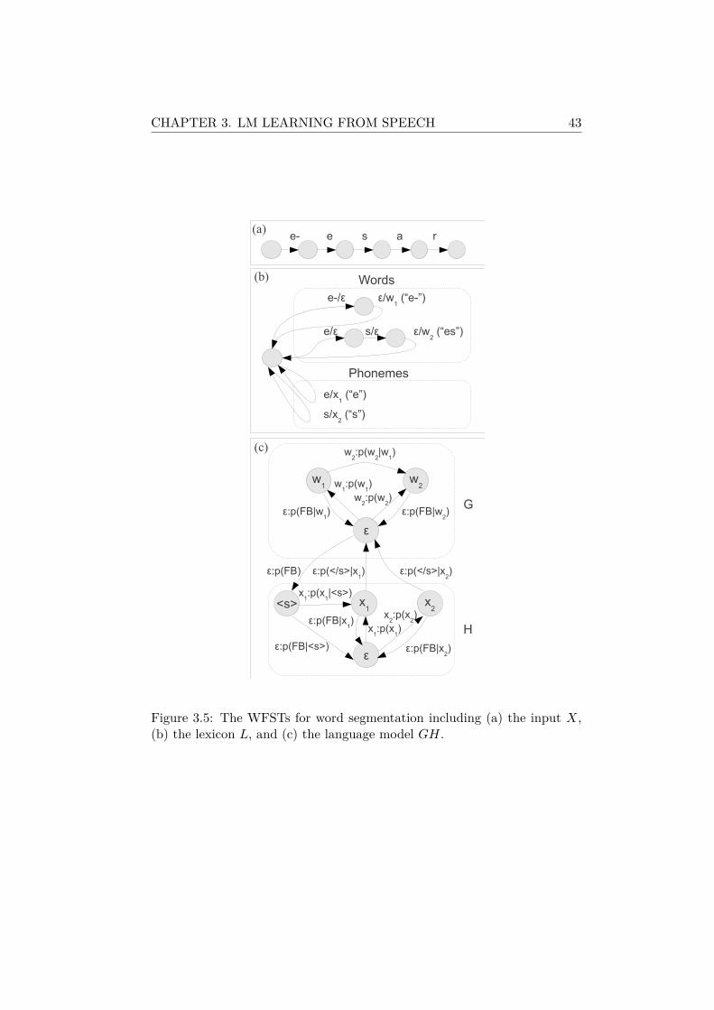
CHAPTER 3. LM LEARNING FROM SPEECH 43
Figure 3.5: The WFSTs for word segmentation including (a) the input X,(b) the lexicon L, and (c) the language model GH.

CHAPTER 3. LM LEARNING FROM SPEECH 44
when the last sample containing a word in the lexicon is subtracted fromthe distribution and the word’s count becomes zero, its corresponding path isremoved from L. It should be noted that here we are making the assumptionthat each word can be mapped onto a single spelling, so P (X|W ) will alwaysbe 1.3
More major changes are made to the LM WFST, which is shown in Fig-ure 3.5 (c). Unlike the case in ASR, where we are generally only concernedwith words that exist in the vocabulary, it is necessary to model unknownwords that are not included in the vocabulary. The key to the representa-tion is that the word-based LM G and the phoneme-based spelling model Hare represented in a single WFST, which we will call GH. GH has weightededges falling back from the base state of G to H, and edges accepting theterminal symbol for unknown words and transitioning from H to the basestate of G. This allows for the WFST to transition as necessary betweenthe known word model and the spelling model.
By composing together these three WFSTs as X◦L◦GH, it is possible tocreate a WFST representing a lattice of segmentation candidates weightedwith probabilities according to the LM.
3.3.2 Sampling over WFSTsOnce we have a WFST lattice representing the model probabilities, we
can sample a single path through the WFST according to the probabili-ties assigned to each edge. This is done using forward-filtering/backward-sampling, a technique similar to that of the forward-backward algorithm forhidden Markov models (HMM). This algorithm can be used to sample asingle path from all probabilistically weighted, acyclic WFSTs defined by aset of states S and a set of edges E.
The first step of the algorithm consists of choosing an ordering for thestates in S, which will be written s1, . . . , sI . This ordering must be chosenso that all states included in paths that travel to state si should be processedbefore si itself. Each edge in E is defined as ek = 〈si, sj , wk〉 traveling fromsi to sj and weighted by wk. Assuming the graph is acyclic, we can choosethe ordering so that for all edges in E, i < j. Given this ordering, if allstates are processed in ascending order, we can be ensured that all stateswill be processed after their predecessors.
Next, we perform the forward filtering step, identical to the forward3This work assumes that all words are represented by their phonetic spelling, not
considering the graphemic representation used in usual text. For example, the word“ASR” will be transcribed as “e-esar” in the learned model.
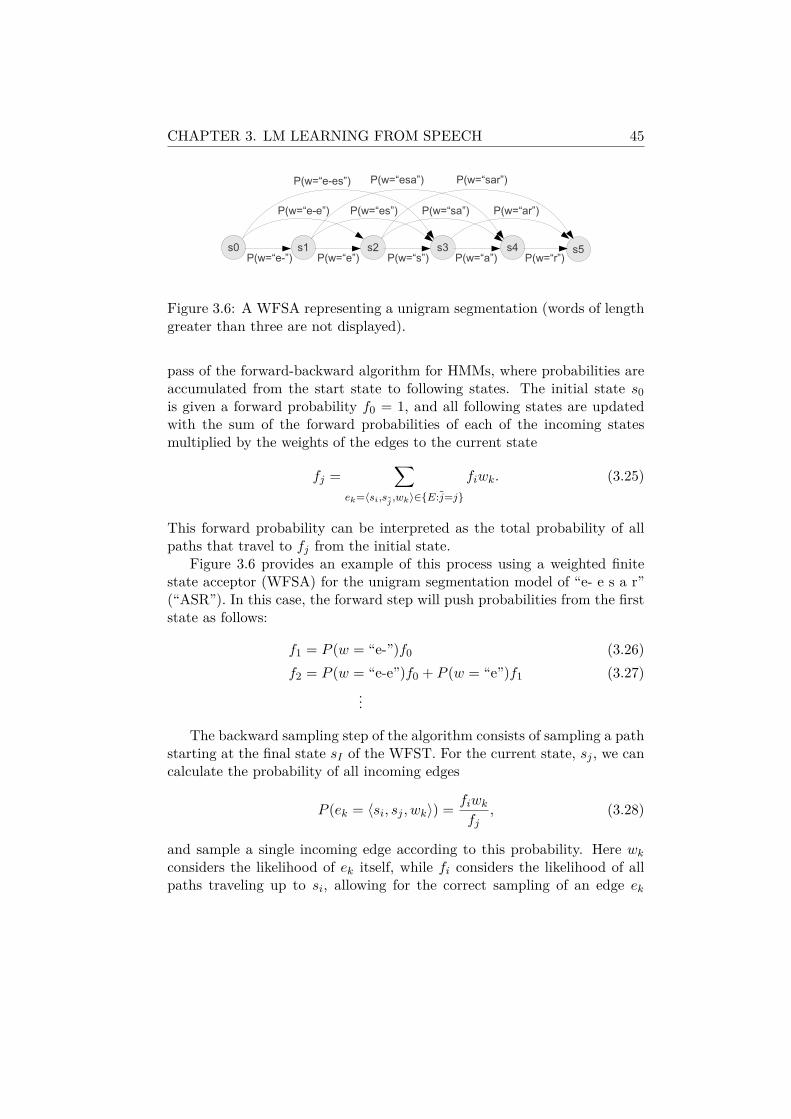
CHAPTER 3. LM LEARNING FROM SPEECH 45
Figure 3.6: A WFSA representing a unigram segmentation (words of lengthgreater than three are not displayed).
pass of the forward-backward algorithm for HMMs, where probabilities areaccumulated from the start state to following states. The initial state s0is given a forward probability f0 = 1, and all following states are updatedwith the sum of the forward probabilities of each of the incoming statesmultiplied by the weights of the edges to the current state
fj =∑
ek=〈si,sj ,wk〉∈{E:j=j}
fiwk. (3.25)
This forward probability can be interpreted as the total probability of allpaths that travel to fj from the initial state.
Figure 3.6 provides an example of this process using a weighted finitestate acceptor (WFSA) for the unigram segmentation model of “e- e s a r”(“ASR”). In this case, the forward step will push probabilities from the firststate as follows:
f1 = P (w = “e-”)f0 (3.26)f2 = P (w = “e-e”)f0 + P (w = “e”)f1 (3.27)
...
The backward sampling step of the algorithm consists of sampling a pathstarting at the final state sI of the WFST. For the current state, sj , we cancalculate the probability of all incoming edges
P (ek = 〈si, sj , wk〉) =fiwk
fj, (3.28)
and sample a single incoming edge according to this probability. Here wk
considers the likelihood of ek itself, while fi considers the likelihood of allpaths traveling up to si, allowing for the correct sampling of an edge ek
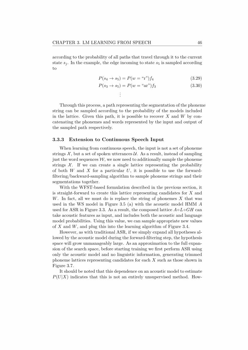
CHAPTER 3. LM LEARNING FROM SPEECH 46
according to the probability of all paths that travel through it to the currentstate sj . In the example, the edge incoming to state s5 is sampled accordingto
P (s4 → s5) = P (w = “r”)f4 (3.29)P (s3 → s5) = P (w = “ar”)f3 (3.30)
...
Through this process, a path representing the segmentation of the phonemestring can be sampled according to the probability of the models includedin the lattice. Given this path, it is possible to recover X and W by con-catenating the phonemes and words represented by the input and output ofthe sampled path respectively.
3.3.3 Extension to Continuous Speech InputWhen learning from continuous speech, the input is not a set of phoneme
strings X , but a set of spoken utterances U . As a result, instead of samplingjust the word sequencesW, we now need to additionally sample the phonemestrings X . If we can create a single lattice representing the probabilityof both W and X for a particular U , it is possible to use the forward-filtering/backward-sampling algorithm to sample phoneme strings and theirsegmentations together.
With the WFST-based formulation described in the previous section, itis straight-forward to create this lattice representing candidates for X andW . In fact, all we must do is replace the string of phonemes X that wasused in the WS model in Figure 3.5 (a) with the acoustic model HMM Aused for ASR in Figure 3.3. As a result, the composed lattice A◦L◦GH cantake acoustic features as input, and includes both the acoustic and languagemodel probabilities. Using this value, we can sample appropriate new valuesof X and W , and plug this into the learning algorithm of Figure 3.4.
However, as with traditional ASR, if we simply expand all hypotheses al-lowed by the acoustic model during the forward-filtering step, the hypothesisspace will grow unmanageably large. As an approximation to the full expan-sion of the search space, before starting training we first perform ASR usingonly the acoustic model and no linguistic information, generating trimmedphoneme lattices representing candidates for each X such as those shown inFigure 3.7.
It should be noted that this dependence on an acoustic model to estimateP (U |X) indicates that this is not an entirely unsupervised method. How-
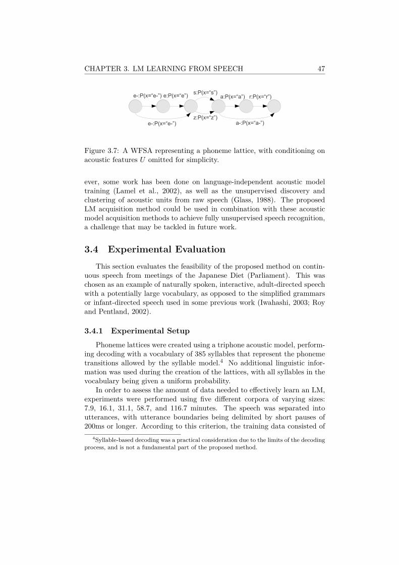
CHAPTER 3. LM LEARNING FROM SPEECH 47
Figure 3.7: A WFSA representing a phoneme lattice, with conditioning onacoustic features U omitted for simplicity.
ever, some work has been done on language-independent acoustic modeltraining (Lamel et al., 2002), as well as the unsupervised discovery andclustering of acoustic units from raw speech (Glass, 1988). The proposedLM acquisition method could be used in combination with these acousticmodel acquisition methods to achieve fully unsupervised speech recognition,a challenge that may be tackled in future work.
3.4 Experimental EvaluationThis section evaluates the feasibility of the proposed method on contin-
uous speech from meetings of the Japanese Diet (Parliament). This waschosen as an example of naturally spoken, interactive, adult-directed speechwith a potentially large vocabulary, as opposed to the simplified grammarsor infant-directed speech used in some previous work (Iwahashi, 2003; Royand Pentland, 2002).
3.4.1 Experimental SetupPhoneme lattices were created using a triphone acoustic model, perform-
ing decoding with a vocabulary of 385 syllables that represent the phonemetransitions allowed by the syllable model.4 No additional linguistic infor-mation was used during the creation of the lattices, with all syllables in thevocabulary being given a uniform probability.
In order to assess the amount of data needed to effectively learn an LM,experiments were performed using five different corpora of varying sizes:7.9, 16.1, 31.1, 58.7, and 116.7 minutes. The speech was separated intoutterances, with utterance boundaries being delimited by short pauses of200ms or longer. According to this criterion, the training data consisted of
4Syllable-based decoding was a practical consideration due to the limits of the decodingprocess, and is not a fundamental part of the proposed method.
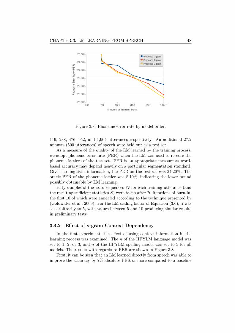
CHAPTER 3. LM LEARNING FROM SPEECH 48
Figure 3.8: Phoneme error rate by model order.
119, 238, 476, 952, and 1,904 utterances respectively. An additional 27.2minutes (500 utterances) of speech were held out as a test set.
As a measure of the quality of the LM learned by the training process,we adopt phoneme error rate (PER) when the LM was used to rescore thephoneme lattices of the test set. PER is an appropriate measure as word-based accuracy may depend heavily on a particular segmentation standard.Given no linguistic information, the PER on the test set was 34.20%. Theoracle PER of the phoneme lattice was 8.10%, indicating the lower boundpossibly obtainable by LM learning.
Fifty samples of the word sequences W for each training utterance (andthe resulting sufficient statistics S) were taken after 20 iterations of burn-in,the first 10 of which were annealed according to the technique presented by(Goldwater et al., 2009). For the LM scaling factor of Equation (3.6), α wasset arbitrarily to 5, with values between 5 and 10 producing similar resultsin preliminary tests.
3.4.2 Effect of n-gram Context DependencyIn the first experiment, the effect of using context information in the
learning process was examined. The n of the HPYLM language model wasset to 1, 2, or 3, and n of the HPYLM spelling model was set to 3 for allmodels. The results with regards to PER are shown in Figure 3.8.
First, it can be seen that an LM learned directly from speech was able toimprove the accuracy by 7% absolute PER or more compared to a baseline
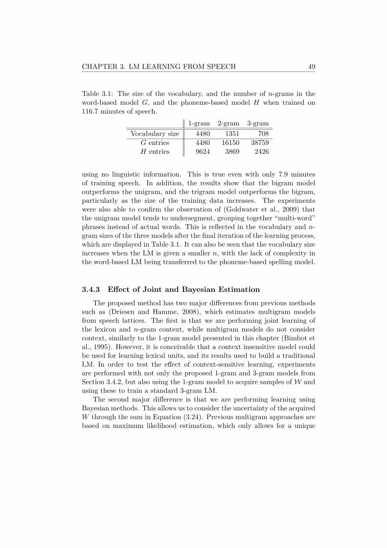
CHAPTER 3. LM LEARNING FROM SPEECH 49
Table 3.1: The size of the vocabulary, and the number of n-grams in theword-based model G, and the phoneme-based model H when trained on116.7 minutes of speech.
1-gram 2-gram 3-gramVocabulary size 4480 1351 708
G entries 4480 16150 38759H entries 9624 3869 2426
using no linguistic information. This is true even with only 7.9 minutesof training speech. In addition, the results show that the bigram modeloutperforms the unigram, and the trigram model outperforms the bigram,particularly as the size of the training data increases. The experimentswere also able to confirm the observation of (Goldwater et al., 2009) thatthe unigram model tends to undersegment, grouping together “multi-word”phrases instead of actual words. This is reflected in the vocabulary and n-gram sizes of the three models after the final iteration of the learning process,which are displayed in Table 3.1. It can also be seen that the vocabulary sizeincreases when the LM is given a smaller n, with the lack of complexity inthe word-based LM being transferred to the phoneme-based spelling model.
3.4.3 Effect of Joint and Bayesian EstimationThe proposed method has two major differences from previous methods
such as (Driesen and Hamme, 2008), which estimates multigram modelsfrom speech lattices. The first is that we are performing joint learning ofthe lexicon and n-gram context, while multigram models do not considercontext, similarly to the 1-gram model presented in this chapter (Bimbot etal., 1995). However, it is conceivable that a context insensitive model couldbe used for learning lexical units, and its results used to build a traditionalLM. In order to test the effect of context-sensitive learning, experimentsare performed with not only the proposed 1-gram and 3-gram models fromSection 3.4.2, but also using the 1-gram model to acquire samples of W andusing these to train a standard 3-gram LM.
The second major difference is that we are performing learning usingBayesian methods. This allows us to consider the uncertainty of the acquiredW through the sum in Equation (3.24). Previous multigram approaches arebased on maximum likelihood estimation, which only allows for a unique
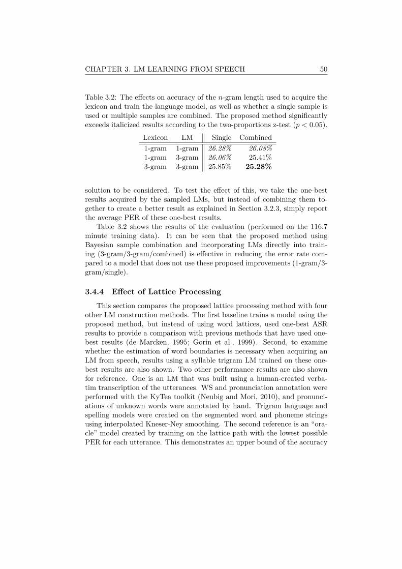
CHAPTER 3. LM LEARNING FROM SPEECH 50
Table 3.2: The effects on accuracy of the n-gram length used to acquire thelexicon and train the language model, as well as whether a single sample isused or multiple samples are combined. The proposed method significantlyexceeds italicized results according to the two-proportions z-test (p < 0.05).
Lexicon LM Single Combined1-gram 1-gram 26.28% 26.08%1-gram 3-gram 26.06% 25.41%3-gram 3-gram 25.85% 25.28%
solution to be considered. To test the effect of this, we take the one-bestresults acquired by the sampled LMs, but instead of combining them to-gether to create a better result as explained in Section 3.2.3, simply reportthe average PER of these one-best results.
Table 3.2 shows the results of the evaluation (performed on the 116.7minute training data). It can be seen that the proposed method usingBayesian sample combination and incorporating LMs directly into train-ing (3-gram/3-gram/combined) is effective in reducing the error rate com-pared to a model that does not use these proposed improvements (1-gram/3-gram/single).
3.4.4 Effect of Lattice ProcessingThis section compares the proposed lattice processing method with four
other LM construction methods. The first baseline trains a model using theproposed method, but instead of using word lattices, used one-best ASRresults to provide a comparison with previous methods that have used one-best results (de Marcken, 1995; Gorin et al., 1999). Second, to examinewhether the estimation of word boundaries is necessary when acquiring anLM from speech, results using a syllable trigram LM trained on these one-best results are also shown. Two other performance results are also shownfor reference. One is an LM that was built using a human-created verba-tim transcription of the utterances. WS and pronunciation annotation wereperformed with the KyTea toolkit (Neubig and Mori, 2010), and pronunci-ations of unknown words were annotated by hand. Trigram language andspelling models were created on the segmented word and phoneme stringsusing interpolated Kneser-Ney smoothing. The second reference is an “ora-cle” model created by training on the lattice path with the lowest possiblePER for each utterance. This demonstrates an upper bound of the accuracy
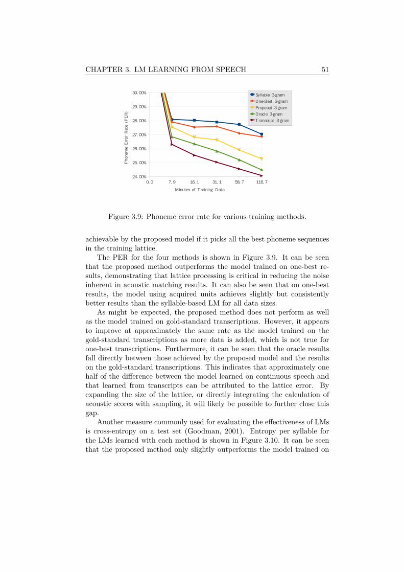
CHAPTER 3. LM LEARNING FROM SPEECH 51
Figure 3.9: Phoneme error rate for various training methods.
achievable by the proposed model if it picks all the best phoneme sequencesin the training lattice.
The PER for the four methods is shown in Figure 3.9. It can be seenthat the proposed method outperforms the model trained on one-best re-sults, demonstrating that lattice processing is critical in reducing the noiseinherent in acoustic matching results. It can also be seen that on one-bestresults, the model using acquired units achieves slightly but consistentlybetter results than the syllable-based LM for all data sizes.
As might be expected, the proposed method does not perform as wellas the model trained on gold-standard transcriptions. However, it appearsto improve at approximately the same rate as the model trained on thegold-standard transcriptions as more data is added, which is not true forone-best transcriptions. Furthermore, it can be seen that the oracle resultsfall directly between those achieved by the proposed model and the resultson the gold-standard transcriptions. This indicates that approximately onehalf of the difference between the model learned on continuous speech andthat learned from transcripts can be attributed to the lattice error. Byexpanding the size of the lattice, or directly integrating the calculation ofacoustic scores with sampling, it will likely be possible to further close thisgap.
Another measure commonly used for evaluating the effectiveness of LMsis cross-entropy on a test set (Goodman, 2001). Entropy per syllable forthe LMs learned with each method is shown in Figure 3.10. It can be seenthat the proposed method only slightly outperforms the model trained on
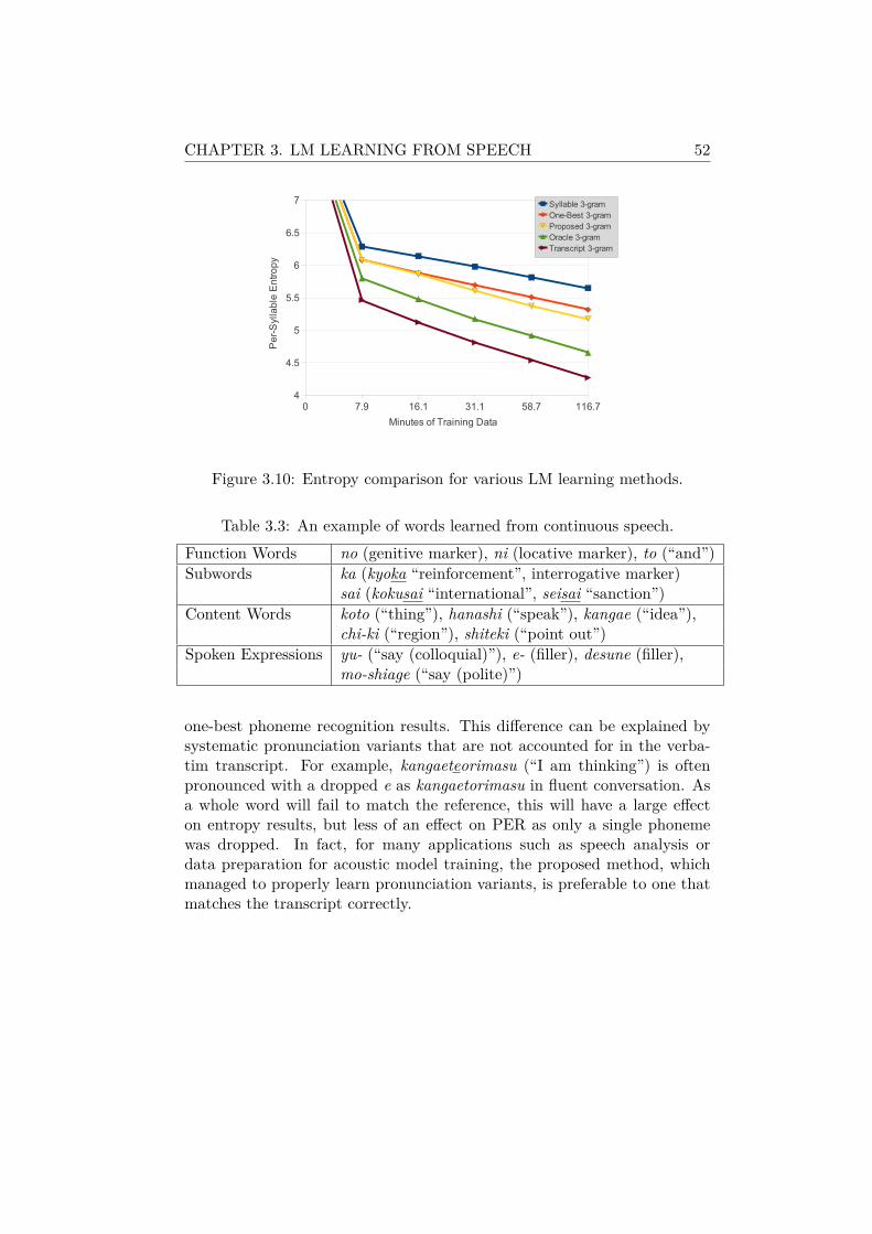
CHAPTER 3. LM LEARNING FROM SPEECH 52
Figure 3.10: Entropy comparison for various LM learning methods.
Table 3.3: An example of words learned from continuous speech.Function Words no (genitive marker), ni (locative marker), to (“and”)Subwords ka (kyoka “reinforcement”, interrogative marker)
sai (kokusai “international”, seisai “sanction”)Content Words koto (“thing”), hanashi (“speak”), kangae (“idea”),
chi-ki (“region”), shiteki (“point out”)Spoken Expressions yu- (“say (colloquial)”), e- (filler), desune (filler),
mo-shiage (“say (polite)”)
one-best phoneme recognition results. This difference can be explained bysystematic pronunciation variants that are not accounted for in the verba-tim transcript. For example, kangaeteorimasu (“I am thinking”) is oftenpronounced with a dropped e as kangaetorimasu in fluent conversation. Asa whole word will fail to match the reference, this will have a large effecton entropy results, but less of an effect on PER as only a single phonemewas dropped. In fact, for many applications such as speech analysis ordata preparation for acoustic model training, the proposed method, whichmanaged to properly learn pronunciation variants, is preferable to one thatmatches the transcript correctly.

CHAPTER 3. LM LEARNING FROM SPEECH 53
3.4.5 Lexical Acquisition ResultsFinally, this section presents a qualitative evaluation of the lexical ac-
quisition results. Typical examples of the words that were acquired in theprocess of LM learning are shown in Table 3.3. These are split into fourcategories: function words, subwords, content words, spoken language ex-pressions.
In the resulting vocabulary, function words were the most common of theacquired words, which is reasonable as function words make the majority ofthe actual spoken utterances. Subwords are the second most frequent cate-gory, and generally occur when less frequent content words share a commonstem.
An example of the content words discovered by the learning methodshows a trend towards the content of discussions made in meetings of theDiet. In particular, chi-ki (“region”) and shiteki (“point out”) are goodexamples of words that are characteristic of Diet speech and acquired bythe proposed model. While this result is not surprising, it is significantin that it shows that the proposed method is able to acquire words thatmatch the content of the utterances on which it was trained. In additionto learning the content of the utterances, the proposed model also learneda number of stylistic characteristics of the speech in the form of fillers andcolloquial expressions. This is also significant in that these expressions arenot included in the official verbatim records in the Diet archives, and thuswould not be included in an LM that was simply trained on these texts.
3.5 ConclusionThis chapter presented a method for unsupervised learning of an LM
given only speech and an acoustic model. Specifically, a Bayesian modelfor word segmentation and LM learning was adapted so that it could beapplied to speech input. This was achieved by formulating all elements ofLM learning as WFSTs, which allows for lattices to be used as input to thelearning algorithm, and then formulating a Gibbs sampling algorithm thatallows for learning over composed lattices that represent acoustic and LMprobabilities.
An experimental evaluation showed that LMs acquired from continuousspeech with no accompanying transcriptions were able to significantly reducethe error rates of ASR over when no such models were used. It also showedthat the proposed technique of joint Bayesian learning of lexical units andan LM over lattices significantly contributes to this improvement.
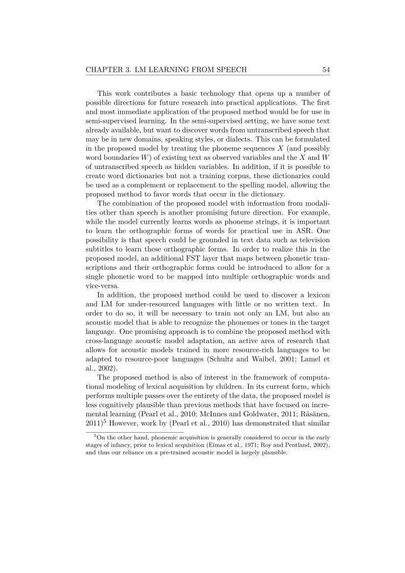
CHAPTER 3. LM LEARNING FROM SPEECH 54
This work contributes a basic technology that opens up a number ofpossible directions for future research into practical applications. The firstand most immediate application of the proposed method would be for use insemi-supervised learning. In the semi-supervised setting, we have some textalready available, but want to discover words from untranscribed speech thatmay be in new domains, speaking styles, or dialects. This can be formulatedin the proposed model by treating the phoneme sequences X (and possiblyword boundaries W ) of existing text as observed variables and the X and Wof untranscribed speech as hidden variables. In addition, if it is possible tocreate word dictionaries but not a training corpus, these dictionaries couldbe used as a complement or replacement to the spelling model, allowing theproposed method to favor words that occur in the dictionary.
The combination of the proposed model with information from modali-ties other than speech is another promising future direction. For example,while the model currently learns words as phoneme strings, it is importantto learn the orthographic forms of words for practical use in ASR. Onepossibility is that speech could be grounded in text data such as televisionsubtitles to learn these orthographic forms. In order to realize this in theproposed model, an additional FST layer that maps between phonetic tran-scriptions and their orthographic forms could be introduced to allow for asingle phonetic word to be mapped into multiple orthographic words andvice-versa.
In addition, the proposed method could be used to discover a lexiconand LM for under-resourced languages with little or no written text. Inorder to do so, it will be necessary to train not only an LM, but also anacoustic model that is able to recognize the phonemes or tones in the targetlanguage. One promising approach is to combine the proposed method withcross-language acoustic model adaptation, an active area of research thatallows for acoustic models trained in more resource-rich languages to beadapted to resource-poor languages (Schultz and Waibel, 2001; Lamel etal., 2002).
The proposed method is also of interest in the framework of computa-tional modeling of lexical acquisition by children. In its current form, whichperforms multiple passes over the entirety of the data, the proposed model isless cognitively plausible than previous methods that have focused on incre-mental learning (Pearl et al., 2010; McInnes and Goldwater, 2011; Räsänen,2011)5 However, work by (Pearl et al., 2010) has demonstrated that similar
5On the other hand, phonemic acquisition is generally considered to occur in the earlystages of infancy, prior to lexical acquisition (Eimas et al., 1971; Roy and Pentland, 2002),and thus our reliance on a pre-trained acoustic model is largely plausible.

CHAPTER 3. LM LEARNING FROM SPEECH 55
Bayesian methods (which were evaluated on raw text, not acoustic input)can be adapted to an incremental learning framework. This sort of incre-mental learning algorithm is compatible with the proposed method as well,and may be combined to form a more cognitively plausible model.

Chapter 4
Phrase Alignment forStatistical MachineTranslation
Statistical machine translation (SMT) has seen great improvements overthe past decade thanks largely to the introduction of phrase-based transla-tion, which helps resolve lexical ambiguity and short-distance reordering bytranslating multi-word phrases as single chunks. The most important ele-ment of phrase-based SMT systems is the “phrase table,” a list of bilingualphrase pairs that are translations of each other, each annotated with featurefunctions indicating certain properties of the phrase. This phrase table isgenerated from a parallel corpus of translated sentences that are aligned atthe sentence level, but not at the word or phrase level.
Traditional systems construct phrase tables by going through a two-step pipeline. The first step consists of finding alignments between wordsor minimal phrases in both sentences, while the second step extracts anexpanded phrase table from these alignments through heuristic combinationof words or minimal phrases into longer units. The ability to use bothshort single-word units and longer phrases is one of the major reasons whyphrase-based translation achieves superior results to word-based methods.However, it has been shown in previous research (DeNero and Klein, 2010)that this two step approach results in word alignments that are not optimalfor the final task of generating phrase tables that are used in translation. Inaddition, exhaustively extracted phrase tables are often unnecessarily large,which results in an increase in the amount of time and memory required torun machine translation systems.
56
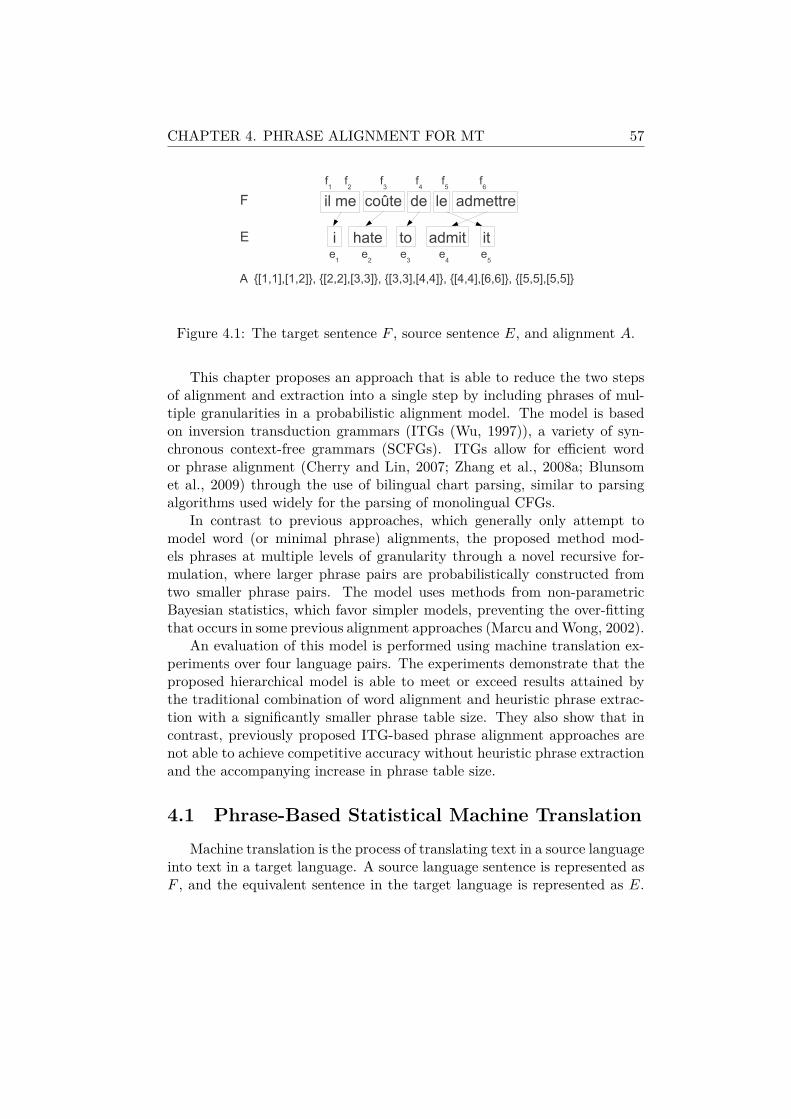
CHAPTER 4. PHRASE ALIGNMENT FOR MT 57
Figure 4.1: The target sentence F , source sentence E, and alignment A.
This chapter proposes an approach that is able to reduce the two stepsof alignment and extraction into a single step by including phrases of mul-tiple granularities in a probabilistic alignment model. The model is basedon inversion transduction grammars (ITGs (Wu, 1997)), a variety of syn-chronous context-free grammars (SCFGs). ITGs allow for efficient wordor phrase alignment (Cherry and Lin, 2007; Zhang et al., 2008a; Blunsomet al., 2009) through the use of bilingual chart parsing, similar to parsingalgorithms used widely for the parsing of monolingual CFGs.
In contrast to previous approaches, which generally only attempt tomodel word (or minimal phrase) alignments, the proposed method mod-els phrases at multiple levels of granularity through a novel recursive for-mulation, where larger phrase pairs are probabilistically constructed fromtwo smaller phrase pairs. The model uses methods from non-parametricBayesian statistics, which favor simpler models, preventing the over-fittingthat occurs in some previous alignment approaches (Marcu andWong, 2002).
An evaluation of this model is performed using machine translation ex-periments over four language pairs. The experiments demonstrate that theproposed hierarchical model is able to meet or exceed results attained bythe traditional combination of word alignment and heuristic phrase extrac-tion with a significantly smaller phrase table size. They also show that incontrast, previously proposed ITG-based phrase alignment approaches arenot able to achieve competitive accuracy without heuristic phrase extractionand the accompanying increase in phrase table size.
4.1 Phrase-Based Statistical Machine TranslationMachine translation is the process of translating text in a source language
into text in a target language. A source language sentence is represented asF , and the equivalent sentence in the target language is represented as E.
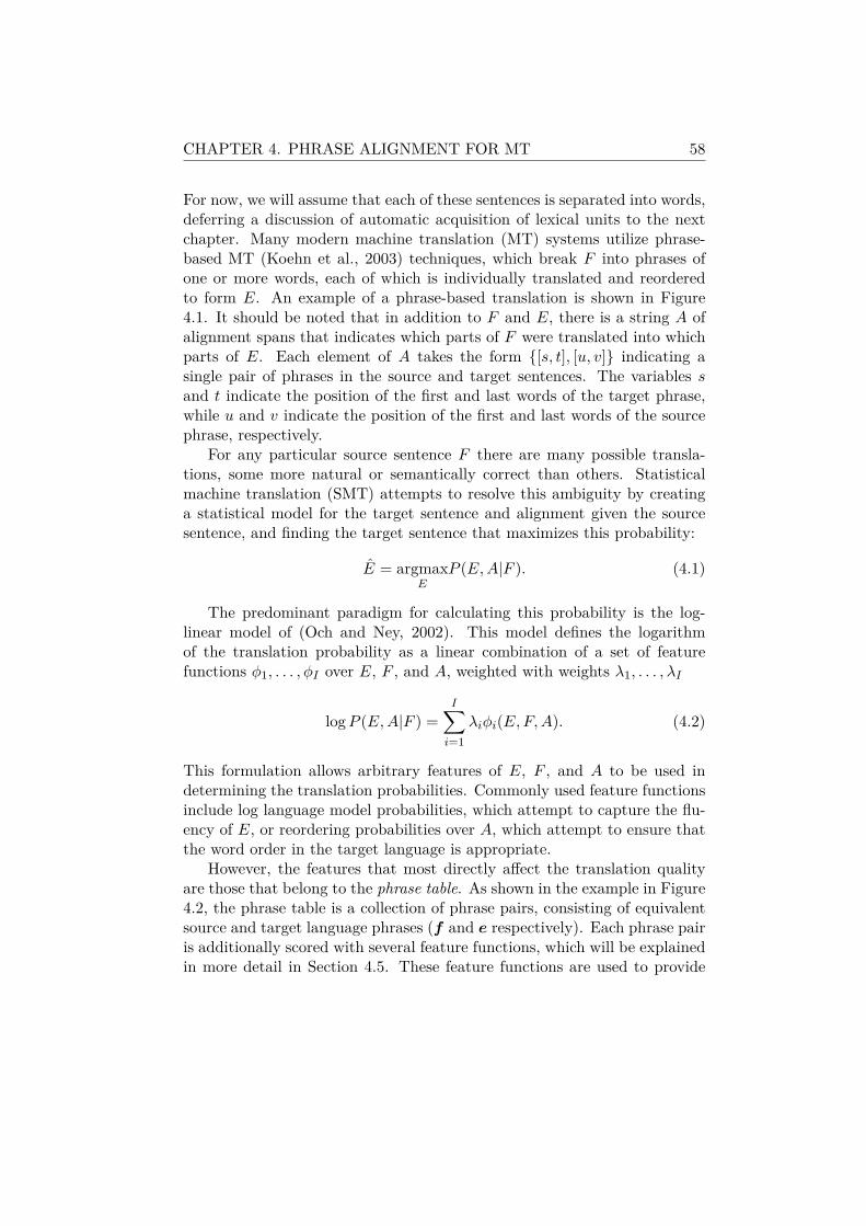
CHAPTER 4. PHRASE ALIGNMENT FOR MT 58
For now, we will assume that each of these sentences is separated into words,deferring a discussion of automatic acquisition of lexical units to the nextchapter. Many modern machine translation (MT) systems utilize phrase-based MT (Koehn et al., 2003) techniques, which break F into phrases ofone or more words, each of which is individually translated and reorderedto form E. An example of a phrase-based translation is shown in Figure4.1. It should be noted that in addition to F and E, there is a string A ofalignment spans that indicates which parts of F were translated into whichparts of E. Each element of A takes the form {[s, t], [u, v]} indicating asingle pair of phrases in the source and target sentences. The variables sand t indicate the position of the first and last words of the target phrase,while u and v indicate the position of the first and last words of the sourcephrase, respectively.
For any particular source sentence F there are many possible transla-tions, some more natural or semantically correct than others. Statisticalmachine translation (SMT) attempts to resolve this ambiguity by creatinga statistical model for the target sentence and alignment given the sourcesentence, and finding the target sentence that maximizes this probability:
E = argmaxE
P (E,A|F ). (4.1)
The predominant paradigm for calculating this probability is the log-linear model of (Och and Ney, 2002). This model defines the logarithmof the translation probability as a linear combination of a set of featurefunctions φ1, . . . , φI over E, F , and A, weighted with weights λ1, . . . , λI
logP (E,A|F ) =
I∑i=1
λiφi(E,F,A). (4.2)
This formulation allows arbitrary features of E, F , and A to be used indetermining the translation probabilities. Commonly used feature functionsinclude log language model probabilities, which attempt to capture the flu-ency of E, or reordering probabilities over A, which attempt to ensure thatthe word order in the target language is appropriate.
However, the features that most directly affect the translation qualityare those that belong to the phrase table. As shown in the example in Figure4.2, the phrase table is a collection of phrase pairs, consisting of equivalentsource and target language phrases (f and e respectively). Each phrase pairis additionally scored with several feature functions, which will be explainedin more detail in Section 4.5. These feature functions are used to provide
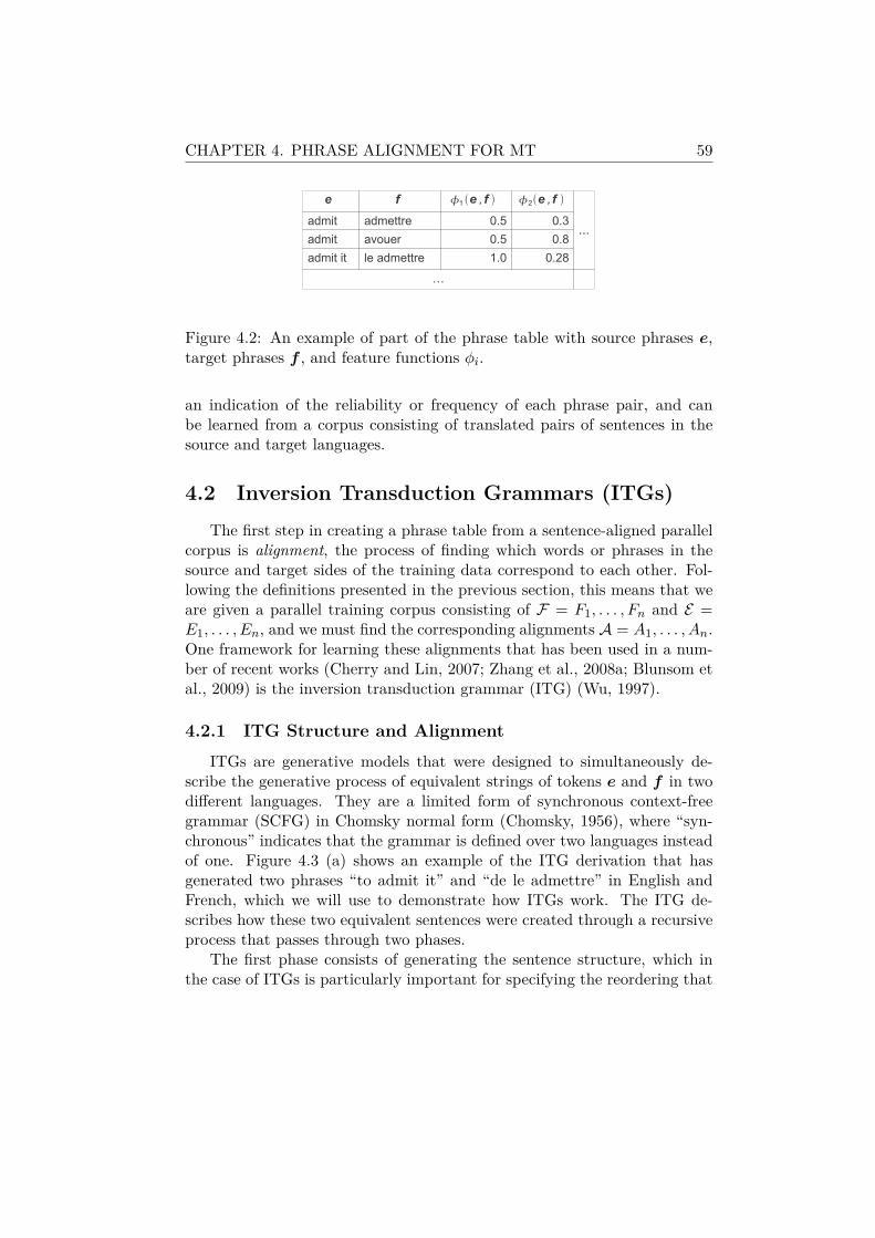
CHAPTER 4. PHRASE ALIGNMENT FOR MT 59
Figure 4.2: An example of part of the phrase table with source phrases e,target phrases f , and feature functions φi.
an indication of the reliability or frequency of each phrase pair, and canbe learned from a corpus consisting of translated pairs of sentences in thesource and target languages.
4.2 Inversion Transduction Grammars (ITGs)The first step in creating a phrase table from a sentence-aligned parallel
corpus is alignment, the process of finding which words or phrases in thesource and target sides of the training data correspond to each other. Fol-lowing the definitions presented in the previous section, this means that weare given a parallel training corpus consisting of F = F1, . . . , Fn and E =E1, . . . , En, and we must find the corresponding alignments A = A1, . . . , An.One framework for learning these alignments that has been used in a num-ber of recent works (Cherry and Lin, 2007; Zhang et al., 2008a; Blunsom etal., 2009) is the inversion transduction grammar (ITG) (Wu, 1997).
4.2.1 ITG Structure and AlignmentITGs are generative models that were designed to simultaneously de-
scribe the generative process of equivalent strings of tokens e and f in twodifferent languages. They are a limited form of synchronous context-freegrammar (SCFG) in Chomsky normal form (Chomsky, 1956), where “syn-chronous” indicates that the grammar is defined over two languages insteadof one. Figure 4.3 (a) shows an example of the ITG derivation that hasgenerated two phrases “to admit it” and “de le admettre” in English andFrench, which we will use to demonstrate how ITGs work. The ITG de-scribes how these two equivalent sentences were created through a recursiveprocess that passes through two phases.
The first phase consists of generating the sentence structure, which inthe case of ITGs is particularly important for specifying the reordering that
CHAPTER 4. PHRASE ALIGNMENT FOR MT 60
Figure 4.3: An example of (a) an inversion transduction grammar (ITG)derivation tree, (b) its corresponding alignment matrix.
occurs between the sentences in the two languages. It can be seen thatfrom the reordering matrix in Figure 4.3 (b) that for some phrase pairs theword order is the same in both languages (“to” precedes “admit it,” and“de” precedes “le admettre”). On the other hand, there are also some placeswhere the order is inverted (“admit” precedes “it” while “admettre” succeeds“le”). ITGs represent this reordering structure as a binary tree, with eachinternal node labeled as straight (str) or inverted (inv), where each of thesenode types represents the case where the order is the same or inverted inboth languages, respectively.1 Much like standard CFGs, each leaf node islabeled with the pre-terminal (term) to indicate that we have finished thefirst step of generating the sentence structure.
This method of expressing reordering through an underlying derivationis both intuitive and flexible. Figures 4.4 (a-d) demonstrate a number ofITG derivations and their corresponding alignments. On the other hand,it should be noted that there are some patterns that are not able to beexpressed in this framework. Some examples of these include the pinwheelpattern shown in Figure 4.4 (e), and patterns where a single word in onelanguage is aligned to multiple discontiguous words in the other language
1Here we are specifically referring to a special case of ITGs with only a single symboleach for straight and inverted productions, which is also known as the bracketing ITG.ITGs with multiple straight and inverted terminals are also conceivable, but are generallynot used in alignment as they significantly increase the computational burden of learningthe ITG.
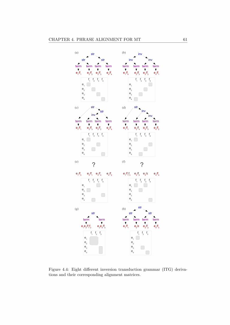
CHAPTER 4. PHRASE ALIGNMENT FOR MT 61
Figure 4.4: Eight different inversion transduction grammar (ITG) deriva-tions and their corresponding alignment matrices.

CHAPTER 4. PHRASE ALIGNMENT FOR MT 62
shown in Figure 4.4 (f). However, these are known to be relatively rare,with ITGs being reported to cover 98.8-100% of the reordering patterns inactual parallel corpora (Wu, 1997; Haghighi et al., 2009).
The second phase takes place after generating the pre-terminal symbol,and consists of generating short parallel phrases. While these are generallyword pairs such as “to/de,” “admit/admettre,” and “it/le,” they can also beone-to-many or many-to-many alignments such as “admit it/le admettre,” orone-to-zero or many-to-zero alignments, where words in one language haveno translation in the other language. These allow for the representation ofalignments that are not strictly one-to-one such as those shown in Figures4.4 (g-h).
4.2.2 Probabilistic ITGsBy assigning a probability to each of the ITG productions, it is possible
to create a generative model for parallel phrase pairs. The traditional ITGgenerative probability for a particular phrase pair Pflat(〈e,f〉; θx, θt) is pa-rameterized by θt, which defines a distribution over terminal phrase pairs(the minimal phrase pairs that are generated after the pre-terminal symbol),and θx, which specifies a probability distribution over the non-terminal andpre-terminal symbols that define the derivation structure. A number ofsmall variations of this traditional ITG model have been proposed in theliterature, but the following generative story can be used as a representativeof previously proposed models.
1. Generate symbol x from the multinomial distribution Px(x; θx). x cantake the values term, str, or inv.
2. According to the value of x, take the following actions.
(a) If x = term, the pre-terminal, generate a phrase pair from theterminal phrase distribution Pt(〈e,f〉; θt).
(b) If x = str, a straight ITG non-terminal, generate phrase pairs〈e1,f1〉 and 〈e2,f2〉 from Pflat, and concatenate them into asingle phrase pair 〈e1e2,f1f2〉.
(c) If x = inv, an inverted ITG non-terminal, follow the same processas (b), but concatenate f1 and f2 in reverse order 〈e1e2,f2f1〉.
The result of this generative process is a bilingual phrase pair, alongwith its corresponding generative probability. Hereafter, this model will bereferred to as flat.

CHAPTER 4. PHRASE ALIGNMENT FOR MT 63
ITG-based models can be used to find alignments for words in parallelsentences through the process of biparsing (Wu, 1997). Within the previ-ously described ITG framework, a sentence pair 〈E,F 〉 can be defined asthe phrase pair that is generated by the node at the top of the derivationtree. Biparsing for ITGs finds the most likely derivation for this sentencepair given the ITG probabilities. Once we have this most likely derivation,we treat all phrase pairs that were generated from the same terminal sym-bols as aligned (for example, in Figure 4.3: “to/de,” “admit/admettre,” and“it/le”).
4.3 Bayesian Modeling for Inversion TransductionGrammars
The probabilities of ITG models can be calculated in the same manner astraditional unsupervised PCFGs using the expectation-maximization algo-rithm and maximum likelihood estimation. However, as noted by (DeNeroet al., 2006), when many-to-many alignments are allowed, the solution thatmaximizes the likelihood is often to simply memorize every sentence as a sin-gle phrase pair, a degenerate solution that defeats the purpose of performingalignment. (Zhang et al., 2008a) and others propose dealing with this prob-lem by putting a prior probability P (θx, θt) on the parameters, which allowsus to bias towards compact models and prevent this degenerate solution.
Priors based on the Bayesian statistics introduced in Chapter 2 haveproven useful for controlling model complexity in previous work, and a sim-ilar approach will be adopted here. The symbol distribution parameters θxspecify a multinomial distribution over three elements. Because of this itis natural to use a Dirichlet distribution as a prior for θx, as the Dirichletdistribution is the conjugate prior of the multinomial distribution.
θx ∼ Dirichlet(α). (4.3)
α is the concentration hyper-parameter controlling the sparsity of the distri-bution, but this has little empirical effect on the results, so we can arbitrarilyset α = 1.
The phrase table parameters θt specify a multinomial distribution overan undetermined number of elements (every possible phrase pair). Previouswork on both word alignment (Zhang et al., 2008a; Blunsom et al., 2009) andother natural language processing tasks has used non-parametric Bayesiantechniques to specify priors over these sort of infinite multinomial distribu-tions. In particular we use a prior based on the non-parametric Pitman-Yor

CHAPTER 4. PHRASE ALIGNMENT FOR MT 64
process described in Section 2.2.4. Remember that the prior is expressed as
θt ∼PY (d, s, Pbase), (4.4)
where d is the discount parameter, s is the strength parameter, and Pbase
is the base measure. The most important element of this distribution forthe task at hand is how we define the base measure Pbase, which assignsthe prior probability of generating a particular phrase pair. The followingsection describes this in more detail.
Non-parametric priors are appropriate for modeling the phrase distribu-tion because every time a phrase is generated by the model, it is “memo-rized” and given a higher probability. Within the framework of the ITGmodel, this indicates that phrase pairs that are generated by Pt many timesare more likely to be reused (the rich-get-richer effect), which results inthe induction of phrase tables with fewer, but more helpful phrases. Inthe flat model, non-terminal nodes are first generated from Px, reducingthe sentence to manageable chunks, followed by the generation of the pre-terminal from Px, then the generation of a minimal phrase pair from Pt. AsPt will only generate a phrase pair at the end of the generative process, onlyphrase pairs of the smallest level of granularity will be memorized and givena higher probability by the model.
As previous works had used the Dirichlet process to specify the phrasedistribution (DeNero et al., 2008), we performed preliminary experiments(using the data described in Section 4.7) to test whether the Pitman-Yorprocess was actually necessary. The results of these experiments confirmedthat the Pitman-Yor process with automatically adjusted parameters resultsin superior alignment results, outperforming the sparse Dirichlet processpriors used in previous research.2 The average gain across all data sets wasapproximately 0.8 BLEU points.
4.3.1 Base MeasurePbase in Equation (4.4) is the base measure, the prior probability of
phrase pairs according to the model. By choosing this probability appropri-ately, we can incorporate prior knowledge of what phrases tend to be alignedto each other. In particular, there are three pieces of prior knowledge that
2Following (Teh, 2006), we put priors on s (Gamma(α = 2, β = 1)) and d (Beta(α =2, β = 2)) for the Pitman-Yor process, and sample their values. These priors do notprovide a strong bias towards any particular value of s or d, allowing the model freedomto choose values that maximize the likelihood of the training data. For the Dirichletprocess α was set to 10−10.

CHAPTER 4. PHRASE ALIGNMENT FOR MT 65
we would like to provide through the base measure. First, we would like tominimize the number of phrases that are not aligned to any phrase in theother language, as we can assume that most of the phrases will have somecorresponding translation. Second, we would like to bias against overly longphrases, as these are likely to cause sparsity and hurt generalization per-formance when the model is tested on new data. Finally, when aligningmulti-word phrases, it makes sense to align phrases that are composed ofwords that are good translations of each other.
This section adopts a formulation similar to that of (DeNero et al., 2008)that is able to satisfy all of these desiderata. Pbase is first calculated bychoosing whether to generate an unaligned phrase pair (where |e| = 0 or|f | = 0) according to a fixed probability pu. pu should generally be a smallvalue to minimize the number of unaligned phrases.3 Based on this choice,we next generate an aligned phrase pair from Pba, or an unaligned phrasepair from Pbu
For Pba, we use the following probability:
Pba(〈e,f〉) =M0(〈e,f〉)Ppois(|e|;λ)Ppois(|f |;λ) (4.5)
M0(〈e,f〉) =(Pm1(f |e)Puni(e)Pm1(e|f)Puni(f))12 . (4.6)
Ppois is the Poisson distribution with the average length parameter λ,where k represents the phrase length |f | or |e|.
Ppois(k|λ) =(λ− 1)k−1
(k − 1)!e−(λ−1). (4.7)
λ was set to a relatively small value, which allows us to bias against overlylong phrases.4
Puni is the unigram probability of a particular phrase, and Pm1 is theword-based Model 1 (Brown et al., 1993) probability of one phrase given theother. Model 1 probabilities are word-based translation probabilities thathelp to indicate whether the words in each phrase are good translations ofeach other. The phrase-based Model 1 probability is calculated accordingto the following equation:
Pm1(e|f) =|e|∏i=1
1
|f |
|f |∑j=1
Pm1(ei|fj) (4.8)
3One of the three values 10−2, 10−3, or 10−10 was chosen based on which value gavethe best translation accuracy on the development set.
4We tune λ to 1, 0.1, or 0.01 based on which value gives the best translation accuracyon the development set.

CHAPTER 4. PHRASE ALIGNMENT FOR MT 66
where ei and fj are the i-th and j-th words in phrases e and f respectively.The word-based probabilities Pm1(ei|fj) and Pm1(fj |ei) are parameters ofthe model, and can be calculated efficiently using the expectation maximiza-tion algorithm (Brown et al., 1993) before starting phrase alignment.
Following (Liang et al., 2006), we combine the Model 1 probabilitiesin both directions using the geometric mean. It should be noted that theprobabilities of the geometric mean do not add to one, and are thus not,strictly speaking, proper probabilities. However empirically, even when leftunnormalized, they provided much better results than the model using thearithmetic mean, which is mathematically correct. This is because takingthe geometric mean favors alignments that are supported by both models,and alignments for which both models agree are generally highly reliable. Onthe other hand, the arithmetic mean favors alignments that are supportedby either of the two models, which indicates that the less reliable alignmentswhere the two models disagree will still receive a relatively high probabil-ity, weakening the ability of the base measure to penalize bad alignmentcandidates.
For Pbu, in the case of |f | = 0, we calculate the probability as follows:
Pbu(〈e,f〉) = Puni(e)Ppois(|e|;λ)/2. (4.9)
The probability can be calculated similarly when |e| = 0. Note that Pbu
is divided by 2 as the probability is considering null alignments in bothdirections.
4.4 Hierarchical ITG ModelWhile in flat only minimal phrases were memorized by the model, as
(DeNero et al., 2008) note and the experiments in Section 4.7 confirm, usingonly minimal phrases leads to inferior results for phrase-based translation.Because of this, previous research has combined flat with heuristic phraseextraction, which exhaustively combines all adjacent phrases permitted bythe word alignments (Och et al., 1999). This section proposes an alternative,fully statistical approach that directly models phrases at multiple granular-ities, which will be referred to as hier. By doing so, we are able to doaway with heuristic phrase extraction, creating a phrase table that is ableto achieve competitive accuracy in a single step through a fully probabilisticprocess.
Similarly to flat, hier assigns a probability Phier(〈e,f〉; θx, θt) to phrasepairs, and is parameterized by a phrase table θt and a symbol distribution

CHAPTER 4. PHRASE ALIGNMENT FOR MT 67
θx. The main difference between the two models is that non/pre-terminalsymbols and phrase pairs are generated in reverse order. While flat firstgenerates branches of the derivation tree using Px, then generates leavesusing the phrase distribution Pt, hier first attempts to generate the fullsentence as a single phrase pair from Pt, then falls back to ITG-style deriva-tions to cope with sparsity. The proposed model accounts for this withinthe Bayesian ITG context by defining a new base measure Pdac (“divide-and-conquer”) to replace Pbase in Equation (4.4), resulting in the followingdistribution for θt.
θt ∼ PY (d, s, Pdac) (4.10)
Pdac essentially generates a single longer phrase through two generationsand a combination of shorter phrases, allowing even long phrase pairs tobe given significant amounts of probability when justified. The generativeprocess of Pdac, similar to that of Pflat from the previous section, is asfollows:
1. Generate symbol x from Px(x; θx). x can take the values base, str,or inv.
2. According to x, take the following actions.
(a) If x = base, generate a new phrase pair directly from Pbase ofSection 4.3.1.
(b) If x = str, generate 〈e1,f1〉 and 〈e2,f2〉 from Phier, and con-catenate them into a single phrase pair 〈e1e2,f1f2〉.
(c) If x = inv, follow the same process as (b), but concatenate f1
and f2 in reverse order 〈e1e2,f2f1〉.
A comparison of derivation trees for flat and hier is shown in Figure4.5. As previously described, flat first generates from the symbol distri-bution Px, then from the phrase distribution Pt. On the other hand, hiergenerates directly from Pt, which falls back to divide-and-conquer based onPx when necessary. The minimal and non-minimal phrase pairs that aregenerated by Pt are surrounded by solid and dotted lines respectively. Itcan be seen that while Pt in flat only generates minimal phrases, Pt inhier generates (and thus memorizes) phrases at all levels of granularity.
4.4.1 Length-based Parameter TuningThere are still two problems with hier, one theoretical, and one practi-
cal. Theoretically, hier contains itself as its base measure, and stochastic

CHAPTER 4. PHRASE ALIGNMENT FOR MT 68
Figure 4.5: A word alignment (a), and its derivation according to flat(b), and hier (c). Solid and dotted lines indicate minimal and non-minimalpairs respectively, and phrases memorized by the model are written in quotesunder their corresponding instance of Pt. The pair hate/coûte is generateddue to the contribution Pbase.
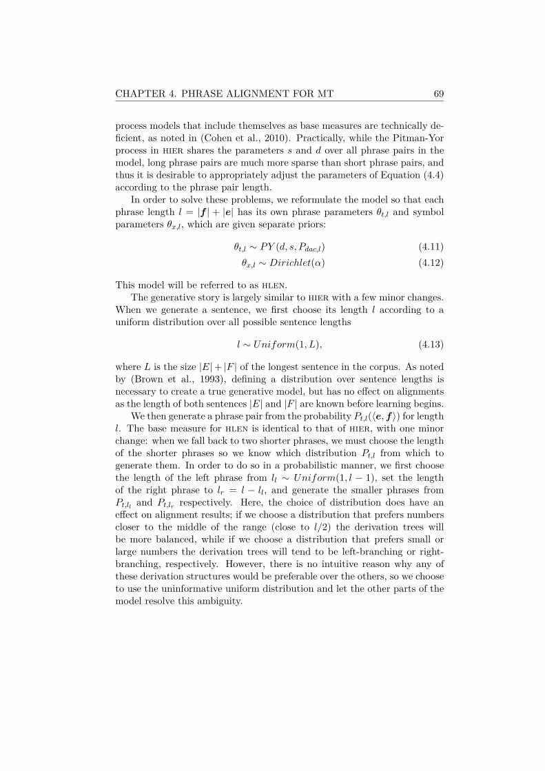
CHAPTER 4. PHRASE ALIGNMENT FOR MT 69
process models that include themselves as base measures are technically de-ficient, as noted in (Cohen et al., 2010). Practically, while the Pitman-Yorprocess in hier shares the parameters s and d over all phrase pairs in themodel, long phrase pairs are much more sparse than short phrase pairs, andthus it is desirable to appropriately adjust the parameters of Equation (4.4)according to the phrase pair length.
In order to solve these problems, we reformulate the model so that eachphrase length l = |f | + |e| has its own phrase parameters θt,l and symbolparameters θx,l, which are given separate priors:
θt,l ∼ PY (d, s, Pdac,l) (4.11)θx,l ∼ Dirichlet(α) (4.12)
This model will be referred to as hlen.The generative story is largely similar to hier with a few minor changes.
When we generate a sentence, we first choose its length l according to auniform distribution over all possible sentence lengths
l ∼ Uniform(1, L), (4.13)
where L is the size |E|+ |F | of the longest sentence in the corpus. As notedby (Brown et al., 1993), defining a distribution over sentence lengths isnecessary to create a true generative model, but has no effect on alignmentsas the length of both sentences |E| and |F | are known before learning begins.
We then generate a phrase pair from the probability Pt,l(〈e,f〉) for lengthl. The base measure for hlen is identical to that of hier, with one minorchange: when we fall back to two shorter phrases, we must choose the lengthof the shorter phrases so we know which distribution Pt,l from which togenerate them. In order to do so in a probabilistic manner, we first choosethe length of the left phrase from ll ∼ Uniform(1, l − 1), set the lengthof the right phrase to lr = l − ll, and generate the smaller phrases fromPt,ll and Pt,lr respectively. Here, the choice of distribution does have aneffect on alignment results; if we choose a distribution that prefers numberscloser to the middle of the range (close to l/2) the derivation trees willbe more balanced, while if we choose a distribution that prefers small orlarge numbers the derivation trees will tend to be left-branching or right-branching, respectively. However, there is no intuitive reason why any ofthese derivation structures would be preferable over the others, so we chooseto use the uninformative uniform distribution and let the other parts of themodel resolve this ambiguity.
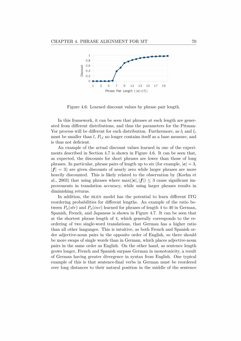
CHAPTER 4. PHRASE ALIGNMENT FOR MT 70
Figure 4.6: Learned discount values by phrase pair length.
In this framework, it can be seen that phrases at each length are gener-ated from different distributions, and thus the parameters for the Pitman-Yor process will be different for each distribution. Furthermore, as ll and lrmust be smaller than l, Pt,l no longer contains itself as a base measure, andis thus not deficient.
An example of the actual discount values learned in one of the experi-ments described in Section 4.7 is shown in Figure 4.6. It can be seen that,as expected, the discounts for short phrases are lower than those of longphrases. In particular, phrase pairs of length up to six (for example, |e| = 3,|f | = 3) are given discounts of nearly zero while larger phrases are moreheavily discounted. This is likely related to the observation by (Koehn etal., 2003) that using phrases where max(|e|, |f |) ≤ 3 cause significant im-provements in translation accuracy, while using larger phrases results indiminishing returns.
In addition, the hlen model has the potential to learn different ITGreordering probabilities for different lengths. An example of the ratio be-tween Px(str) and Px(inv) learned for phrases of length 4 to 40 in German,Spanish, French, and Japanese is shown in Figure 4.7. It can be seen thatat the shortest phrase length of 4, which generally corresponds to the re-ordering of two single-word translations, that German has a higher ratiothan all other languages. This is intuitive, as both French and Spanish or-der adjective-noun pairs in the opposite order of English, so there shouldbe more swaps of single words than in German, which places adjective-nounpairs in the same order as English. On the other hand, as sentence lengthgrows longer, French and Spanish surpass German in monotonicity, a resultof German having greater divergence in syntax from English. One typicalexample of this is that sentence-final verbs in German must be reorderedover long distances to their natural position in the middle of the sentence

CHAPTER 4. PHRASE ALIGNMENT FOR MT 71
Figure 4.7: The ratio of Px(str) to Px(inv) by length. Higher values indicatemore monotonic alignments.
for English. Finally, Japanese has significantly lower monotonicity than allof the European languages at almost all phrase pair lengths, a result of thevast differences in sentence structure between Japanese and English. Incontrast, hier can only learn a single value for Px(str) and Px(inv). ForGerman, Spanish, French, and Japanese, the values of Px(str)/Px(inv) were4.83, 5.81, 4.99, and 1.83 respectively, showing that the overall preferencefor monotonicity or non-monotonicity can be learned, although not in thefine-grained manner allowed by hlen.
4.4.2 ImplementationPrevious research has used a variety of methods to learn Bayesian phrase
based alignment models, all of which have used Gibbs sampling as their cen-tral learning algorithm (DeNero et al., 2008; Blunsom et al., 2009; Blunsomand Cohn, 2010). All of these techniques are applicable to the proposedmodel, but the sentence-based blocked sampling proposed by (Blunsom andCohn, 2010) has desirable convergence properties compared to sampling sin-gle alignments, and is what we will use here. In this method, the majority ofcomputation in the sampling process takes place in the parsing step whereprobabilities for each possibly aligned bilingual span are calculated to allowfor proper sampling of an ITG parse tree for each sentence.
Exhaustive parsing of ITGs can be performed in O(n6), but this is too
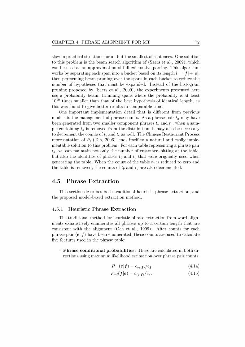
CHAPTER 4. PHRASE ALIGNMENT FOR MT 72
slow in practical situations for all but the smallest of sentences. One solutionto this problem is the beam search algorithm of (Saers et al., 2009), whichcan be used as an approximation of full exhaustive parsing. This algorithmworks by separating each span into a bucket based on its length l = |f |+ |e|,then performing beam pruning over the spans in each bucket to reduce thenumber of hypotheses that must be expanded. Instead of the histogrampruning proposed by (Saers et al., 2009), the experiments presented hereuse a probability beam, trimming spans where the probability is at least1010 times smaller than that of the best hypothesis of identical length, asthis was found to give better results in comparable time.
One important implementation detail that is different from previousmodels is the management of phrase counts. As a phrase pair ta may havebeen generated from two smaller component phrases tb and tc, when a sam-ple containing ta is removed from the distribution, it may also be necessaryto decrement the counts of tb and tc as well. The Chinese Restaurant Processrepresentation of Pt (Teh, 2006) lends itself to a natural and easily imple-mentable solution to this problem. For each table representing a phrase pairta, we can maintain not only the number of customers sitting at the table,but also the identities of phrases tb and tc that were originally used whengenerating the table. When the count of the table ta is reduced to zero andthe table is removed, the counts of tb and tc are also decremented.
4.5 Phrase ExtractionThis section describes both traditional heuristic phrase extraction, and
the proposed model-based extraction method.
4.5.1 Heuristic Phrase ExtractionThe traditional method for heuristic phrase extraction from word align-
ments exhaustively enumerates all phrases up to a certain length that areconsistent with the alignment (Och et al., 1999). After counts for eachphrase pair 〈e,f〉 have been enumerated, these counts are used to calculatefive features used in the phrase table:
• Phrase conditional probabilities: These are calculated in both di-rections using maximum likelihood estimation over phrase pair counts:
Pml(e|f) = c〈e,f〉/cf (4.14)Pml(f |e) = c〈e,f〉/ce. (4.15)
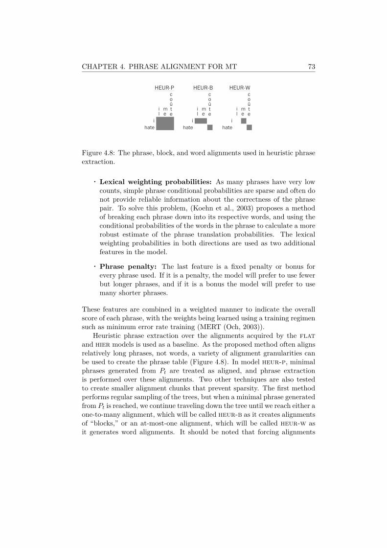
CHAPTER 4. PHRASE ALIGNMENT FOR MT 73
Figure 4.8: The phrase, block, and word alignments used in heuristic phraseextraction.
• Lexical weighting probabilities: As many phrases have very lowcounts, simple phrase conditional probabilities are sparse and often donot provide reliable information about the correctness of the phrasepair. To solve this problem, (Koehn et al., 2003) proposes a methodof breaking each phrase down into its respective words, and using theconditional probabilities of the words in the phrase to calculate a morerobust estimate of the phrase translation probabilities. The lexicalweighting probabilities in both directions are used as two additionalfeatures in the model.
• Phrase penalty: The last feature is a fixed penalty or bonus forevery phrase used. If it is a penalty, the model will prefer to use fewerbut longer phrases, and if it is a bonus the model will prefer to usemany shorter phrases.
These features are combined in a weighted manner to indicate the overallscore of each phrase, with the weights being learned using a training regimensuch as minimum error rate training (MERT (Och, 2003)).
Heuristic phrase extraction over the alignments acquired by the flatand hier models is used as a baseline. As the proposed method often alignsrelatively long phrases, not words, a variety of alignment granularities canbe used to create the phrase table (Figure 4.8). In model heur-p, minimalphrases generated from Pt are treated as aligned, and phrase extractionis performed over these alignments. Two other techniques are also testedto create smaller alignment chunks that prevent sparsity. The first methodperforms regular sampling of the trees, but when a minimal phrase generatedfrom Pt is reached, we continue traveling down the tree until we reach either aone-to-many alignment, which will be called heur-b as it creates alignmentsof “blocks,” or an at-most-one alignment, which will be called heur-w asit generates word alignments. It should be noted that forcing alignments

CHAPTER 4. PHRASE ALIGNMENT FOR MT 74
smaller than the model suggests is only used for generating alignments foruse in heuristic extraction, and does not affect the training process.
4.5.2 Model-Based Phrase ExtractionFor our proposed model, we are also able to perform phrase table ex-
traction that directly utilizes the phrase probabilities Pt(〈e,f〉). Similarlyto the heuristic phrase tables, we use conditional probabilities Pt(f |e) andPt(e|f), lexical weighting probabilities, and a phrase penalty. Here, insteadof using maximum likelihood, we calculate conditional probabilities directlyfrom Pt probabilities:
Pt(f |e) = Pt(〈e,f〉)/∑
{f :c〈e,f〉≥1}
Pt(〈e, f〉) (4.16)
Pt(e|f) = Pt(〈e,f〉)/∑
{e:c〈e,f〉≥1}
Pt(〈e,f〉). (4.17)
To limit phrase table size, we include only phrase pairs that are aligned atleast once in the sample.
Two more features are also added:
• Model joint probability: As the proposed method assigns a prob-ability Pt(〈e,f〉) to all phrase pairs, we can use this as an additionalfeature.
• Span generative probability: Use the average generative probabil-ity of each span that generated 〈e,f〉 as computed by the chart parserduring training. This is similar to the joint probability, but is morereliable for low-frequency phrases, where the model probability tendsto over-estimate the actual probability. The generative probabilitywill be high for common phrase pairs that are generated directly fromthe model, and also for phrases that, while not directly included in themodel, are composed of two high-probability child phrases and thuscan be assumed to be more reliable.
It should be noted that while for flat and hier Pt can be used directly,as hlen learns separate models for each length, we must combine theseprobabilities into a single value. We can do this by setting
Pt(〈e,f〉) = Pt,l(〈e,f〉)cl/L∑l=1
cl (4.18)

CHAPTER 4. PHRASE ALIGNMENT FOR MT 75
for every phrase pair, where l = |e|+ |f | and cl is the number of phrases oflength l in the sample.
This model-based extraction method is referred to as mod.
4.5.3 Sample CombinationAs has been noted in previous works, (Koehn et al., 2003; DeNero et
al., 2006) exhaustive phrase extraction tends to outperform approaches thatuse syntax or generative models to limit phrase boundaries. (DeNero etal., 2006) states that this is because generative models choose only a singlephrase segmentation, and thus throw away many good phrase pairs that arein conflict with this segmentation.
Fortunately, in the Bayesian framework it is simple to overcome thisproblem by combining phrase tables from multiple samples. In mod, wedo this by taking the average of the joint probability and span probabilityfeatures, and recalculating the conditional probabilities from the averagedjoint probabilities.
4.6 Related WorkWhile ITGs have been growing in popularity in recent years, they are by
no means the only method for word or phrase alignment. In fact, the seminalIBM models presented in (Brown et al., 1993) and the implementation pro-vided by the open-source software giza++5 (Och and Ney, 2003) are stillused for word alignment in a large number of systems. The IBM models,while quite powerful, are fundamentally different from the models previouslydescribed in this chapter in that they are not able to handle many-to-manyalignments. As a result, it is necessary to find one-to-many word alignmentsin both directions, which allows for the capturing of multi-word units onboth the source and target sides. These one-to-many alignments can thenbe combined using heuristics into a many-to-many alignment (Koehn et al.,2003). Finally, using this alignment, heuristic phrase extraction enumeratesall possible phrases that do not conflict with the word alignments (Och etal., 1999). In the next section, we present experimental results compar-ing alignments acquired using the IBM models with those acquired usingITG-based alignment methods.
In addition to the previously mentioned alignment techniques, there hasalso been a significant body of work on improving phrase extraction methods
5http://code.google.com/p/giza-pp/
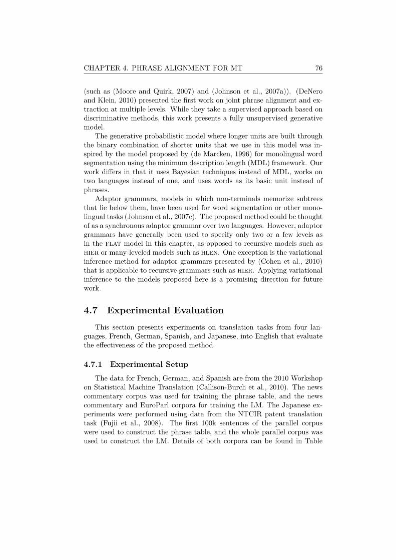
CHAPTER 4. PHRASE ALIGNMENT FOR MT 76
(such as (Moore and Quirk, 2007) and (Johnson et al., 2007a)). (DeNeroand Klein, 2010) presented the first work on joint phrase alignment and ex-traction at multiple levels. While they take a supervised approach based ondiscriminative methods, this work presents a fully unsupervised generativemodel.
The generative probabilistic model where longer units are built throughthe binary combination of shorter units that we use in this model was in-spired by the model proposed by (de Marcken, 1996) for monolingual wordsegmentation using the minimum description length (MDL) framework. Ourwork differs in that it uses Bayesian techniques instead of MDL, works ontwo languages instead of one, and uses words as its basic unit instead ofphrases.
Adaptor grammars, models in which non-terminals memorize subtreesthat lie below them, have been used for word segmentation or other mono-lingual tasks (Johnson et al., 2007c). The proposed method could be thoughtof as a synchronous adaptor grammar over two languages. However, adaptorgrammars have generally been used to specify only two or a few levels asin the flat model in this chapter, as opposed to recursive models such ashier or many-leveled models such as hlen. One exception is the variationalinference method for adaptor grammars presented by (Cohen et al., 2010)that is applicable to recursive grammars such as hier. Applying variationalinference to the models proposed here is a promising direction for futurework.
4.7 Experimental EvaluationThis section presents experiments on translation tasks from four lan-
guages, French, German, Spanish, and Japanese, into English that evaluatethe effectiveness of the proposed method.
4.7.1 Experimental SetupThe data for French, German, and Spanish are from the 2010 Workshop
on Statistical Machine Translation (Callison-Burch et al., 2010). The newscommentary corpus was used for training the phrase table, and the newscommentary and EuroParl corpora for training the LM. The Japanese ex-periments were performed using data from the NTCIR patent translationtask (Fujii et al., 2008). The first 100k sentences of the parallel corpuswere used to construct the phrase table, and the whole parallel corpus wasused to construct the LM. Details of both corpora can be found in Table

CHAPTER 4. PHRASE ALIGNMENT FOR MT 77
Table 4.1: The number of words in each corpus for phrase table (PT) andLM training, tuning, and testing.
de-en es-en fr-en ja-enPT (en) 1.80M 1.62M 1.35M 2.38MPT (other) 1.85M 1.82M 1.56M 2.78MLM (en) 52.7M 52.7M 52.7M 44.7MTune (en) 49.8k 49.8k 49.8k 68.9kTune (other) 47.2k 52.6k 55.4k 80.4kTest (en) 65.6k 65.6k 65.6k 40.4kTest (other) 62.7k 68.1k 72.6k 48.7k
4.1. Corpora are tokenized, lower-cased, and sentences of over 40 words oneither side are removed for phrase table training. For both tasks, weighttuning and testing were performed on specified development and test sets.Case-insensitive BLEU score is used as an evaluation measure (Papineni etal., 2002), a widely used evaluation metric for machine translation.
Next, the accuracy of our proposed method of joint phrase alignmentand extraction using the flat, hier and hlen models is compared witha baseline of using word alignments from giza++ (Och and Ney, 2003)and heuristic phrase extraction. Translation is performed using the Mosesphrase-based machine translation decoder (Koehn and others, 2007) usingthe phrase tables learned by each method under consideration. Phrase re-ordering probabilities are calculated using Moses’s standard lexicalized re-ordering model (Koehn et al., 2005) for all experimental settings. The max-imum phrase length is limited to 7 in all models, and the LM is createdusing an interpolated Kneser-Ney 5-gram model.
giza++ is trained using the standard training regimen up to Model 4,and the resulting alignments are combined with the grow-diag-final-andheuristic (Koehn et al., 2005). The proposed models were allowed to run 100iterations, with the final sample acquired at the end of the training processbeing used to construct the translation model in experiments using a singlesample.6 In addition, results are presented for averaging the phrase tablesfrom the last ten samples as described in Section 4.5.3.
6For most models, while likelihood continued to increase gradually for all 100 iterations,BLEU score gains plateaued after 5-10 iterations, likely due to the strong prior informationprovided by Pbase. As iterations took 1.3 hours on a single processor, good translationresults can be achieved in approximately 13 hours, which could be further reduced usingdistributed sampling (Newman et al., 2009; Blunsom et al., 2009).

CHAPTER 4. PHRASE ALIGNMENT FOR MT 78
Table 4.2: BLEU score and phrase table size by alignment method andsamples combined. Bold numbers are not significantly different from thebest result according to the sign test (p < 0.05). giza uses heur-w forphrase extraction and all other models use mod.
de-en es-en fr-en ja-enAlign Samp BLEU Size BLEU Size BLEU Size BLEU Sizegiza 1 16.62 4.91M 22.00 4.30M 21.35 4.01M 23.20 4.22Mflat 1 13.48 136k 19.15 125k 17.97 117k 16.10 89.7khier 1 16.58 1.02M 21.79 859k 21.50 751k 23.23 723khlen 1 16.49 1.17M 21.57 930k 21.31 860k 23.19 820khier 10 16.53 3.44M 21.84 2.56M 21.57 2.63M 23.12 2.21Mhlen 10 16.51 3.74M 21.69 3.00M 21.53 3.09M 23.20 2.70M
4.7.2 Experimental ResultsThe results for these experiments can be found in Table 4.2. From these
results it can be seen that when using a single sample, the combination ofusing hier and model probabilities achieves results approximately equal togiza++ and heuristic phrase extraction. This is the first reported resultin which an unsupervised phrase alignment model has built a phrase ta-ble directly from model probabilities and achieved results that compare toheuristic phrase extraction. It can also be seen that the phrase table cre-ated by the proposed method is approximately 5 times smaller than thatobtained by the traditional pipeline.
In addition, hier significantly outperforms flat when using the modelprobabilities. This confirms that phrase tables containing only minimalphrases are not able to achieve results that compete with phrase tables ofmultiple granularities.
Somewhat surprisingly, hlen consistently slightly underperforms hier.This indicates potential gains to be provided by length-based parametertuning were outweighed by losses due to the increased complexity of themodel. In particular, as examined further in Section 4.7.3, dividing phrasesof each length between different models provides an implicit bias to spreadphrases evenly across all of the models, even when this is not justified bythe data.
It can also be seen that combining phrase tables from multiple samplesimproved the BLEU score for hlen, but not for hier. This suggests that forhier, most of the useful phrase pairs discovered by the model are includedin every iteration, and the increased recall obtained by combining multiple
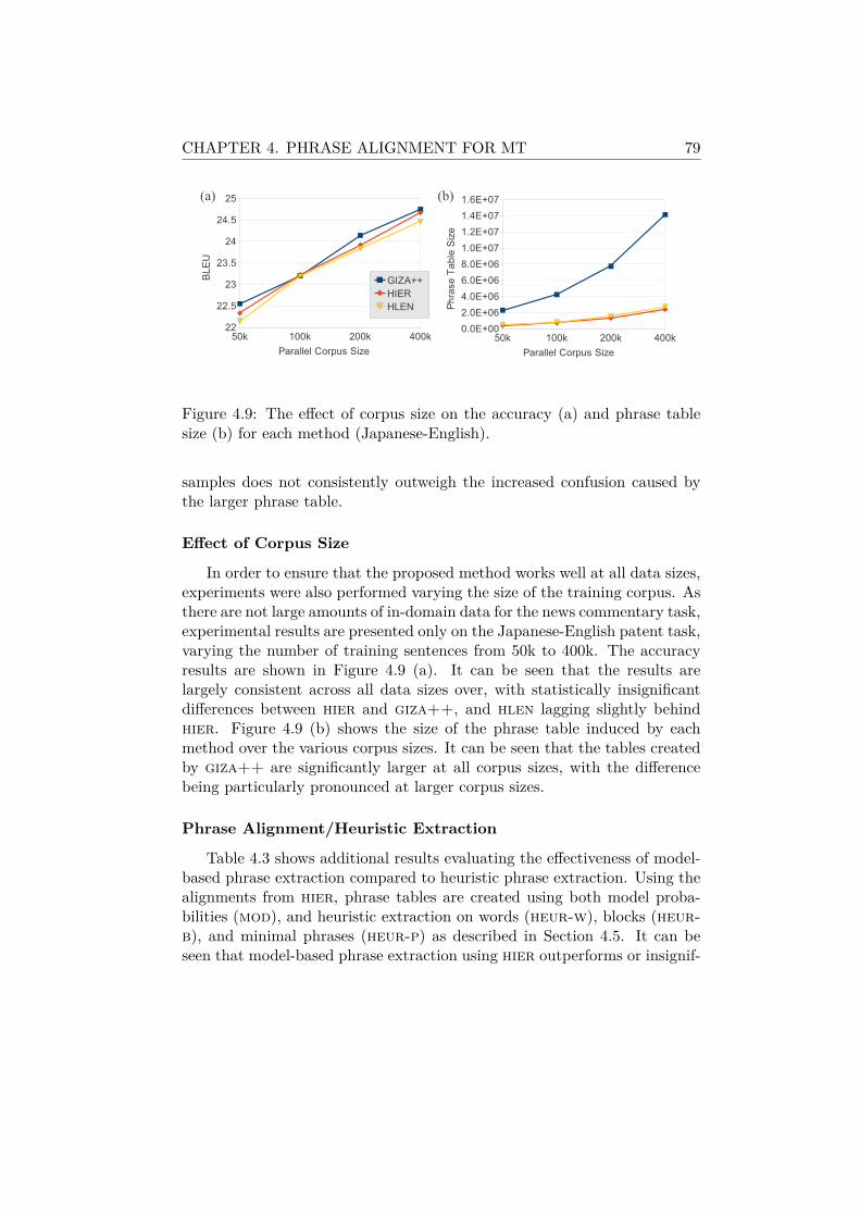
CHAPTER 4. PHRASE ALIGNMENT FOR MT 79
Figure 4.9: The effect of corpus size on the accuracy (a) and phrase tablesize (b) for each method (Japanese-English).
samples does not consistently outweigh the increased confusion caused bythe larger phrase table.
Effect of Corpus Size
In order to ensure that the proposed method works well at all data sizes,experiments were also performed varying the size of the training corpus. Asthere are not large amounts of in-domain data for the news commentary task,experimental results are presented only on the Japanese-English patent task,varying the number of training sentences from 50k to 400k. The accuracyresults are shown in Figure 4.9 (a). It can be seen that the results arelargely consistent across all data sizes over, with statistically insignificantdifferences between hier and giza++, and hlen lagging slightly behindhier. Figure 4.9 (b) shows the size of the phrase table induced by eachmethod over the various corpus sizes. It can be seen that the tables createdby giza++ are significantly larger at all corpus sizes, with the differencebeing particularly pronounced at larger corpus sizes.
Phrase Alignment/Heuristic Extraction
Table 4.3 shows additional results evaluating the effectiveness of model-based phrase extraction compared to heuristic phrase extraction. Using thealignments from hier, phrase tables are created using both model proba-bilities (mod), and heuristic extraction on words (heur-w), blocks (heur-b), and minimal phrases (heur-p) as described in Section 4.5. It can beseen that model-based phrase extraction using hier outperforms or insignif-

CHAPTER 4. PHRASE ALIGNMENT FOR MT 80
Table 4.3: Translation results and phrase table size for various phrase ex-traction techniques (French-English).
flat hiermod 17.97 117k 21.50 751k
heur-w 21.52 5.65M 21.68 5.39Mheur-b 21.45 4.93M 21.41 2.61Mheur-p 21.56 4.88M 21.47 1.62M
Table 4.4: Overlap of phrase tables. The numbers indicate the percentageof the phrase table in the column that is also included in the phrase tablein the row.
giza flat hier hlengiza - 40.46% 47.94% 41.54%flat 1.68% - 14.84% 12.51%hier 9.24% 68.72% - 31.61%hlen 9.59% 69.40% 37.89% -
icantly underperforms heuristic phrase extraction over all experimental set-tings, while keeping the phrase table to a fraction of the size of most heuristicextraction methods.
4.7.3 Acquired PhrasesThis section presents a quantitative and qualitative analysis of the phrase
tables acquired using giza, flat, hier, and hlen for the French-Englishtask. Phrase extraction was performed with heur-w for giza and mod forall other alignment methods.
First, Table 4.4 shows the results of an analysis of how much overlap therewas between the extracted phrase tables. Interestingly, the giza phrasetable only covers approximately 40-50% of the acquired phrases in eachof the ITG models, despite being much larger. To help understand thedifference between giza and the ITG-based methods, Table 4.5 shows asample of the phrases that occurred in only the giza phrase table, as wellas the phrases that occurred in all of the other phrase tables, but not thegiza phrase table. For phrases found by all of the ITG models but notgiza, the majority were rare single-word translations that were mis-alignedby giza due to the “garbage-collecting” phenomenon, where rare words arealigned to too many words, and thus not extracted properly. Among theshorter phrases that were found by none of the ITG models, but found by
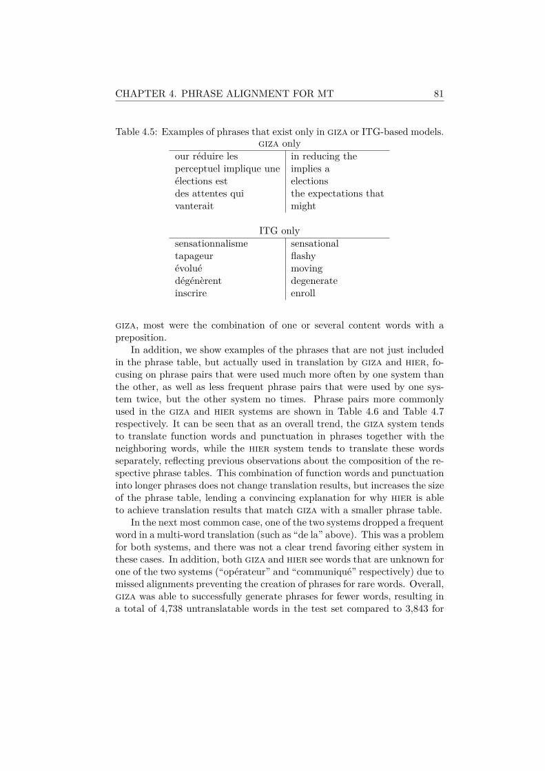
CHAPTER 4. PHRASE ALIGNMENT FOR MT 81
Table 4.5: Examples of phrases that exist only in giza or ITG-based models.giza only
our réduire les in reducing theperceptuel implique une implies aélections est electionsdes attentes qui the expectations thatvanterait might
ITG onlysensationnalisme sensationaltapageur flashyévolué movingdégénèrent degenerateinscrire enroll
giza, most were the combination of one or several content words with apreposition.
In addition, we show examples of the phrases that are not just includedin the phrase table, but actually used in translation by giza and hier, fo-cusing on phrase pairs that were used much more often by one system thanthe other, as well as less frequent phrase pairs that were used by one sys-tem twice, but the other system no times. Phrase pairs more commonlyused in the giza and hier systems are shown in Table 4.6 and Table 4.7respectively. It can be seen that as an overall trend, the giza system tendsto translate function words and punctuation in phrases together with theneighboring words, while the hier system tends to translate these wordsseparately, reflecting previous observations about the composition of the re-spective phrase tables. This combination of function words and punctuationinto longer phrases does not change translation results, but increases the sizeof the phrase table, lending a convincing explanation for why hier is ableto achieve translation results that match giza with a smaller phrase table.
In the next most common case, one of the two systems dropped a frequentword in a multi-word translation (such as “de la” above). This was a problemfor both systems, and there was not a clear trend favoring either system inthese cases. In addition, both giza and hier see words that are unknown forone of the two systems (“opérateur” and “communiqué” respectively) due tomissed alignments preventing the creation of phrases for rare words. Overall,giza was able to successfully generate phrases for fewer words, resulting ina total of 4,738 untranslatable words in the test set compared to 3,843 for

CHAPTER 4. PHRASE ALIGNMENT FOR MT 82
Table 4.6: Phrase pairs that are used more often by giza than hier. #gizaand #hier are the number of times the phrase was used by each system.Source Target #giza #hier hier Phrase
les the 529 475 with nounqu’ that 74 38 with verb: ” : ” 33 0 separatec’ est it is 32 0 separateopérateur opérateur 32 0 operatorde la the 33 2 of2010 . 2010 . 2 0 separate, ou alors , or 2 0 separatequi sont who are 2 0 separateil nous we 2 0 with commatravaillait ” 2 0 depravity (correct: “was working”)
Table 4.7: Phrase pairs that are used more often by hier than giza.Source Target #giza #hier giza Phrase
, , 2061 2833 with wordde of 685 1366 with noun. . 1443 2002 with wordla the 495 820 with nounle the 574 795 with noundéfinitif final 0 2 done, meanscommuniqué communiqué 0 2 declaration, communicatedfréquente frequent 0 2 frequentlyconnaissant surplus 0 2 moreover (correct: “knowing”)moment où moment when 0 2 with “the”
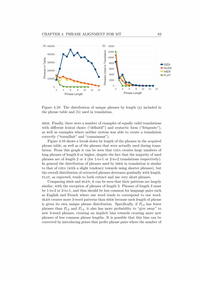
CHAPTER 4. PHRASE ALIGNMENT FOR MT 83
Figure 4.10: The distribution of unique phrases by length (a) included inthe phrase table and (b) used in translation.
hier. Finally, there were a number of examples of equally valid translationswith different lexical choice (“définitif”) and syntactic form (“fréquente”),as well as examples where neither system was able to create a translationcorrectly (“travaillait” and “connaissant”).
Figure 4.10 shows a break-down by length of the phrases in the acquiredphrase table, as well as of the phrases that were actually used during trans-lation. From this graph it can be seen that giza creates large numbers oflong phrases of length 6 or higher, despite the fact that the majority of usedphrases are of length 2 or 4 (for 1-to-1 or 2-to-2 translations respectively).In general the distribution of phrases used by hier in translation is similarto that of giza (with a slight tendency towards using shorter phrases), butthe overall distribution of extracted phrases decreases gradually with length.flat, as expected, tends to both extract and use very short phrases.
Comparing hier and hlen, it can be seen that their patterns are largelysimilar, with the exception of phrases of length 3. Phrases of length 3 mustbe 1-to-2 or 2-to-1, and thus should be less common for language pairs suchas English and French where one word tends to correspond to one word.hlen creates more 3-word patterns than hier because each length of phraseis given its own unique phrase distribution. Specifically, if Pt,3 has fewerphrases than Pt,2 and Pt,4, it also has more probability to “give away” tonew 3-word phrases, creating an implicit bias towards creating more newphrases of less common phrase lengths. It is possible that this bias can becorrected by introducing priors that prefer phrase pairs where the number of

CHAPTER 4. PHRASE ALIGNMENT FOR MT 84
words is roughly equal on both sides. However, this will require significantexpansions to the current generative story, which does not explicitly keeptrack of the number of words on each side, and thus we leave this to futurework.
4.8 ConclusionThis chapter presented a novel approach to joint phrase alignment and
extraction through a hierarchical model using non-parametric Bayesian meth-ods and inversion transduction grammars (ITGs). Unlike previous work,this hierarchical model directly includes phrases of multiple granularities,which allows for the effective use of model probabilities in phrase table con-struction. Machine translation systems using phrase tables learned by theproposed model were able to achieve accuracy competitive with the tradi-tional pipeline of word alignment and heuristic phrase extraction, the firstsuch result for an unsupervised model.
One of the advantages of the proposed model is that it lends itself to rel-atively simple extension, allowing for further gains in accuracy through theintroduction of more sophisticated alignment models. One promising futuredirection is the introduction of more intelligent prior knowledge throughthe base measure Pbase. For example, Pbase could be adjusted to take intoaccount spelling similarities, parts of speech, phrase-based translation dic-tionaries, or bilingually acquired classes such as those proposed by (Och,1999). It may also be possible to refine hlen to use a more appropriatemodel of phrase length than the uniform distribution, particularly by at-tempting to bias against phrase pairs where one of the two phrases is muchlonger than the other.
In addition, it is worth testing the use of the proposed model with otherforms of translation than simple phrase-based translation. These could in-clude examining the applicability of the proposed model in the context ofhierarchical phrases (Chiang, 2007), or in alignment using syntactic struc-ture (Galley et al., 2006). It is also worth examining the plausibility ofvariational inference as proposed by (Cohen et al., 2010) in the alignmentcontext.
Chapter 5
Lexical Acquisition forMachine Translation
In the previous chapter, we treated statistical machine translation (SMT)as the task of translating a source language sentence F to a target languagesentence E, where each element of F and E is assumed to be a word in thesource and target languages. However, as noted in Chapter 1, the definitionof a “word” is often problematic. In unsegmented languages such as Chinese,Japanese, or Thai, it has been noted that the segmentation standard has alarge effect on translation accuracy (Chang et al., 2008). Even for languageswith explicit word boundaries, all machine translation systems perform atleast some precursory form of tokenization, splitting punctuation and wordsto prevent the sparsity that would occur if punctuated and non-punctuatedwords were treated as different entities. Sparsity also manifests itself ina number of other forms, with an extremely large number of rare wordsexisting due to morphological productivity, word compounding, numbers,and proper names. A myriad of methods have been proposed to handleeach of these phenomena individually in the context of machine translation,including morphological analysis, stemming, compound breaking, numberregularization, optimizing word segmentation, and transliteration, which areoutlined in more detail in Section 5.1.
These difficulties stem from the basic premise that we are translatingsequences of words as our basic unit. On the other hand, (Vilar et al., 2007)examine the possibilities of eschewing the concept of words, treating eachsentence as sequences of characters to be translated. This method is at-tractive, as it is theoretically able to handle all sparsity phenomena in asingle unified framework, but has only proven feasible between similar lan-
85

CHAPTER 5. LEXICAL ACQUISITION FOR MT 86
guage pairs such as Spanish-Catalan (Vilar et al., 2007), Swedish-Norwegian(Tiedemann, 2009), and Thai-Lao (Sornlertlamvanich et al., 2008), whichhave a large number of cognates and a strong co-occurrence between singlecharacters. As (Vilar et al., 2007) and (Xu et al., 2004) state and as isfurther confirmed here, accurate translations cannot be achieved when ap-plying traditional translation techniques to character-based translation forless similar language pairs.
This chapter proposes improvements to the alignment process tailored tocharacter-based machine translation, and demonstrate that it is, in fact, pos-sible to achieve competitive translation accuracy for distant language pairsusing only character strings. This is achieved by adapting the phrase-basedalignment method of the previous chapter, applying it not to word strings,but to character strings. As the many-to-many units learned may be at thecharacter, subword, word, or multi-word phrase level, this can be expectedto allow for better character alignments than one-to-many alignment tech-niques, and will also allow for better translation of uncommon words thantraditional word-based models by breaking down words into their componentparts.
In order to make character-based alignment feasible, two improvementsare proposed to the alignment model. The first proposed improvement in-creases the efficiency of the beam-search technique of (Saers et al., 2009) byaugmenting it with look-ahead probabilities in the spirit of A* search. Thisis important because in the inversion transduction grammar (ITG) frame-work (Wu, 1997) used in the previous chapter, search is cumbersome forlonger sentences, a problem that is further exacerbated when using charac-ters instead of words as the basic unit. The second proposed improvementseeds the search process using counts of all substring pairs in the corpusto bias the phrase alignment model. This is done by defining prior prob-abilities based on these substring counts within the Bayesian phrasal ITGframework.
The proposed method for character-based translation is evaluated onfour language pairs with differing morphological properties. The evaluationshows that for distant language pairs, character-based SMT can achievetranslation accuracy that is comparable to word-based systems. In addi-tion, ablation studies show that these results were not possible without theproposed enhancements to the model. Finally, a qualitative analysis showsthat the character-based method is able to translate unsegmented text, con-jugated words, and proper names in a unified framework with no additionalprocessing.

CHAPTER 5. LEXICAL ACQUISITION FOR MT 87
5.1 Related Work on Lexical Processing in SMTAs traditional SMT systems treat all words as single tokens without con-
sidering their internal structure, major problems of data sparsity occur forless frequent tokens. In fact, it has been shown that there is a direct negativecorrelation between vocabulary size (and thus sparsity) of a language andtranslation accuracy (Koehn, 2005). Rare words causes trouble for align-ment models, both in the form of incorrect alignments, and in the form ofgarbage collection, where rare words in one language are incorrectly alignedto large segments of the sentence in the other language (Och and Ney, 2003).Unknown words are also a problem during the translation process, and thedefault approach is to map them as-is into the translated sentence.
This is a major problem in morphologically rich languages such as Finnishand Korean, as well as highly compounding languages such as Dutch andGerman. Many previous works have attempted to handle morphology,decompounding and regularization through lemmatization, morphologicalanalysis, or unsupervised techniques (Nießen and Ney, 2000; Brown, 2002;Lee, 2004; Goldwater and McClosky, 2005; Talbot and Osborne, 2006;Macherey et al., 2011). Other research has noted that it is more difficultto translate into morphologically rich languages with word-based systems,and methods for modeling target-side morphology have attracted interestin recent years (Bojar, 2007; Subotin, 2011). It is also notable that mor-phology and compounding remain problematic regardless of the size of thetraining data, with systems trained on hundreds of millions of words stillseeing significant gains in accuracy due to lexical processing (Macherey etal., 2011).
Another major source of rare words in all languages is proper names,which have been handled by using cognates or transliteration to improvetranslation (Knight and Graehl, 1998; Kondrak et al., 2003; Finch andSumita, 2007). More sophisticated methods for named entity translationthat combine translation and transliteration have also been proposed (Al-Onaizan and Knight, 2002).
Choosing word units is also essential for creating good translation re-sults for languages that do not explicitly mark word boundaries, such asChinese, Japanese, and Thai. A number of works have addressed this wordsegmentation problem in translation, mainly focusing on Chinese-to-Englishtranslation (Bai et al., 2008; Chang et al., 2008; Zhang et al., 2008b; Chungand Gildea, 2009; Nguyen et al., 2010; Wang et al., 2010), although theseworks generally assume that a word segmentation exists in one language(English) and attempt to optimize the word segmentation in the other lan-
CHAPTER 5. LEXICAL ACQUISITION FOR MT 88
guage (Chinese).This enumeration of related works demonstrates the myriad of problems
caused by rare words and the large number of proposed solutions to theseproblems. Character-based translation has the potential to handle all of thephenomena in the previously mentioned research in a single unified frame-work, requiring no language specific tools such as morphological analyzersor word segmenters. However, while the approach is attractive conceptually,previous research has only been shown effective for closely related languagepairs (Vilar et al., 2007; Tiedemann, 2009; Sornlertlamvanich et al., 2008).This work proposes effective alignment and decoding techniques that allowcharacter-based translation to achieve accurate translation results for bothclose and distant language pairs.
5.2 Look-Ahead BiparsingIn order to perform many-to-many alignment, we represent our target
and source sentences as E and F . ei and fj represent single elements ofthe target and source sentences, respectively. These may be words in word-based alignment models or single characters in character-based alignmentmodels.1 We define our alignment as A, where each element is a span ak =〈s, t, u, v〉 indicating that the target string ets = es, . . . , et and source stringfvu = fu, . . . , fv are alignments of each other.These alignments can be acquired using the alignment method presented
in the previous chapter. As this method has been shown to achieve compet-itive accuracy with a much smaller phrase table than traditional methods,it is particularly well suited for character-based translation as we wouldlike to use phrases that contain large numbers of characters without creat-ing a phrase table so large that it cannot be used in actual decoding. Inthis framework, blocked sampling is performed by processing sentences ina corpus one-by-one, acquiring a sample for each sentence by first perform-ing bottom-up biparsing to create a chart of probabilities, then performingtop-down sampling of a new tree based on the probabilities in this chart.
We define a chart as a data structure with a single cell for each align-ment as,t,u,v spanning ets and fv
u. Each cell has an accompanying “inside”probability I(as,t,u,v). This probability is the combination of the genera-tive probability of each phrase pair Pt(e
ts,f
vu) as well as the sum of the
1Some previous work has also performed alignment using morphological analyzers tonormalize or split the sentence into morpheme streams (Corston-Oliver and Gamon, 2004).
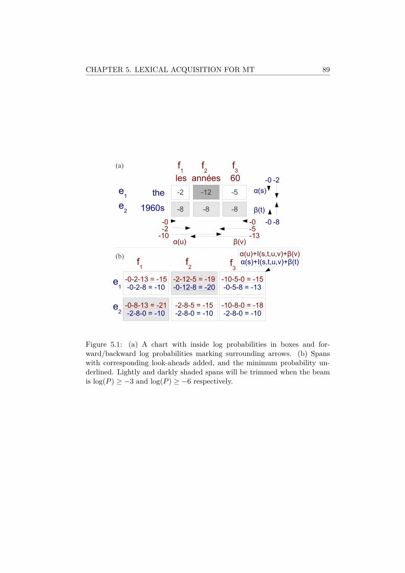
CHAPTER 5. LEXICAL ACQUISITION FOR MT 89
Figure 5.1: (a) A chart with inside log probabilities in boxes and for-ward/backward log probabilities marking surrounding arrows. (b) Spanswith corresponding look-aheads added, and the minimum probability un-derlined. Lightly and darkly shaded spans will be trimmed when the beamis log(P ) ≥ −3 and log(P ) ≥ −6 respectively.

CHAPTER 5. LEXICAL ACQUISITION FOR MT 90
Figure 5.2: An example of the first three queues used in ITG parsing alongwith their inside probabilities. The hypotheses that would be processed ifthe beam is set to c = 1e− 1 are surrounded by boxes.
probabilities over all shorter spans in straight and inverted order
I(as,t,u,v) =Pt(ets, f
vu)
+∑
s≤S≤t
∑u≤U≤v
Px(x = str)I(as,S,u,U )I(aS,t,U,v)
+∑
s≤S≤t
∑u≤U≤v
Px(x = inv)I(as,S,U,v)I(aS,t,u,U ) (5.1)
where Px(x = str) and Px(x = inv) are the probability of straight andinverted ITG productions. An example of part of the chart used in thisbottom-up parsing can be found in Figure 5.1 (a), where we show the cellsthat have one-to-one alignments.
The exact calculation of these probabilities can be performed in O(n6)time, where n = max(I, J) is the length of the longer of eI1 and fJ
1 (Wu,1997). This calculation is performed using a dynamic programming algo-rithm that separates each of the spans into queues based on their lengthl = t − s + u − v, and queues are processed in ascending order of l. Anexample of the queues for the first three lengths is shown in Figure 5.2.
The motivation behind this algorithm is that when calculating a particu-lar span’s inside probability I(as,t,u,v) according to Equation (5.1), all of theother inside spans that we reference on the right-hand side of the equationare shorter than as,t,u,v itself. Thus, if we process all spans in ascendingorder, it is simple to calculate these sums for every span in the chart. The

CHAPTER 5. LEXICAL ACQUISITION FOR MT 91
computational complexity of the algorithm is O(n6) because Equation (5.1)must be calculated for all of the O(n4) spans in the sentence, and there areO(n2) elements in each calculation of the sum.
However, exact computation of these probabilities in O(n6) time is im-practical for all but the shortest sentences. Thus it is necessary to usemethods to reduce the search space such as beam-search-based chart pars-ing (Saers et al., 2009) or slice sampling (Blunsom and Cohn, 2010).
(Saers et al., 2009) note that in order to increase the efficiency of pro-cessing, queues can be trimmed based on a fixed histogram beam, only pro-cessing the b hypotheses with the highest probability for each queue. Here,we instead utilize a probability beam, expanding only hypotheses that aremore than c times as likely as the best hypothesis a. In other words, wehave a queue discipline based on the inside probability, and all spans akwhere I(ak) < cI(a) are pruned. c is a constant between 0 and 1 describingthe width of the beam, and a smaller constant probability will indicate awider beam. Figure 5.2 shows an example of this, with boxes surroundingpart of each queue showing the hypotheses that fall within the beam whenc = 10−1.
While this pruning increases the speed of alignment significantly, thismethod is insensitive to the existence of competing hypotheses when per-forming pruning. Figure 5.1 (a) provides an example of what a competinghypothesis is, and why it is unwise to ignore them during pruning. Partic-ularly, the alignments “les/1960s” and “les/the” both share the word “les,”and thus cannot both exist in a single derivation according to the ITG frame-work. We will call hypotheses that are mutually exclusive in this mannercompeting hypotheses. As the probability of “les/1960s” is much lower thanits competing hypothesis “les/the,” it is intuitively unlikely, and thus a goodcandidate for pruning. However its inside probability is the same as that of“années/1960s,” which has no competing hypotheses and thus should not beremoved from consideration. This section proposes the use of a look-aheadprobability to increase the efficiency of this chart parsing by consideringcompeting hypotheses.
In order to take into account competing hypotheses, we can use for ourqueue discipline not only the inside probability I(ak), but also the outsideprobability O(ak), the probability of generating all spans other than ak, asin A* search for CFGs (Klein and Manning, 2003), and tic-tac-toe pruningfor word-based ITGs (Zhang and Gildea, 2005). As the calculation of theactual outside probability O(ak) is just as expensive as parsing itself, itis necessary to approximate this with heuristic function O∗ that can becalculated efficiently.
CHAPTER 5. LEXICAL ACQUISITION FOR MT 92
This section proposes a heuristic function that is designed specifically forphrasal ITGs and is computable with worst-case complexity of n2, comparedwith the n3 amortized time of the tic-tac-toe pruning algorithm describedby (Zhang et al., 2008a). During the calculation of the phrase generationprobabilities Pt, we save the best probability O∗ for each monolingual span.
O∗e(s, t) = max
{a=〈s,t,u,v〉;s=s,t=t}Pt(a) (5.2)
O∗f (u, v) = max
{a=〈s,t,u,v〉;u=u,v=v}Pt(a) (5.3)
For each language independently, we calculate forward probabilities α andbackward probabilities β. For example, αe(s) is the maximum probability ofthe span (0, s) of e that can be created by concatenating together consecutivevalues of O∗
e :
αe(s) = max{S1,...,Sx}
O∗e(0, S1)O
∗e(S1, S2) . . . O
∗e(Sx, s). (5.4)
Backwards probabilities and probabilities over f can be defined similarly.These probabilities are calculated for e and f independently, and can becalculated in n2 time by processing each α in ascending order, and each β indescending order in a fashion similar to that of the forward-backward algo-rithm. Finally, for any span, we define the outside heuristic as the minimumof the two independent look-ahead probabilities over each language
O∗(as,t,u,v) = min(αe(s) ∗ βe(t), αf (u) ∗ βf (v)). (5.5)
Taking a look again at the example in 5.1 (b), it can be seen that the rel-ative probability difference between the highest probability span “les/the”and the spans “années/1960s” and “60/1960s” decreases, allowing for tighterbeam pruning without losing these good hypotheses. In contrast, the rela-tive probability of “les/1960s” remains low as it is in conflict with a high-probability alignment, allowing it to be discarded.
5.3 Substring Prior ProbabilitiesWhile the Bayesian ITG framework uses the previously mentioned phrase
distribution Pt during search, it also allows for definition of a phrase pairprior probability Pbase(e
ts,f
vu) through the base measure. This can help
efficiently seed the search process with a bias towards phrase pairs thatsatisfy certain properties.
CHAPTER 5. LEXICAL ACQUISITION FOR MT 93
As noted in Section 4.3.1 this can be achieved by using the IBM Model1 probabilities, which can be efficiently calculated using the dynamic pro-gramming algorithm described by (Brown et al., 1993). However, for rea-sons previously stated, these methods are less satisfactory when performingcharacter-based alignment, as the amount of information contained in acharacter does not allow for proper alignment.
Instead, this work proposes a method for using raw substring co-occurrencestatistics to bias alignments towards substrings that often co-occur in theentire training corpus. This is similar to the method of (Cromieres, 2006),but instead of using these co-occurrence statistics as a heuristic alignmentcriterion, they are incorporated as a prior probability in a statistical modelthat can take into account mutual exclusivity of overlapping substrings in asentence.
We define this prior probability using three counts over substrings ce,cf , and c〈e,f〉. ce and cf count the total number of sentences in which thesubstrings e and f occur, respectively. c〈e,f〉 is a count of the total numberof sentences in which the substring e occurs on the target side, and f occurson the source side. We can perform the calculation of these statistics usingenhanced suffix arrays, a data structure that can efficiently calculate allsubstrings in a corpus (Abouelhoda et al., 2004).2
While suffix arrays allow for efficient calculation of these statistics, stor-ing all co-occurrence counts c〈e,f〉 is an unrealistic memory burden for largercorpora. In order to reduce the amount of memory used, each count is dis-counted fixed value d, which is set to 5. This has a dual effect of reducingthe amount of memory needed to hold co-occurrence counts by removingvalues for which c〈e,f〉 < d, as well as helping to prevent over-fitting thetraining data. In addition, we can heuristically prune values for which theconditional probabilities P (e|f) or P (f |e) are less than some fixed value,which is set to 0.1 for the reported experiments.
Preliminary experiments designed to determine how to combine ce, cf ,and c〈e,f〉 into prior probabilities tested a number of methods proposed byprevious research including plain co-occurrence counts, the Dice coefficient,and Chi-squared statistics (Cromieres, 2006), as well as a new method ofdefining substring pair probabilities to be proportional to bi-directional con-
2Using the open-source implementation esaxx http://code.google.com/p/esaxx/
CHAPTER 5. LEXICAL ACQUISITION FOR MT 94
ditional probabilities
Pcooc(e,f) = Pcooc(e|f)Pcooc(f |e)/Z (5.6)
=
(c〈e,f〉 − d
cf − d
)(c〈e,f〉 − d
ce − d
)/Z (5.7)
for all substring pairs where c〈e,f〉 > d and where Z is a normalization termequal to
Z =∑
{e,f ;c〈e,f〉>d}
Pcooc(e|f)Pcooc(f |e). (5.8)
The motivation for combining the probabilities in this fashion is similar tothat of the base measure in Equation (4.6), finding highly reliable align-ments that are supported by both models. The preliminary experimentsshowed that the bi-directional conditional probability method gave signifi-cantly better results than all other methods, so this method will be adoptedfor the remainder of the experiments.
It should be noted that as we are using discounting, many substringpairs will be given zero probability according to Pcooc. As the prior is onlysupposed to bias the model towards good solutions and not explicitly ruleout any possibilities, we can instead linearly interpolate the co-occurrenceprobability with the one-to-many Model 1 probability, which will give atleast some probability mass to all substring pairs
Pbase(e,f) = λPcooc(e,f) + (1− λ)Pm1(e,f). (5.9)
In order to find an appropriate value, we put a Beta prior (α = 1, β = 1)on the interpolation coefficient λ and learn it during training.
5.4 ExperimentsThis section describes experiments over a variety of language pairs de-
signed to test the effectiveness of character-based translation.
5.4.1 Experimental SetupEvaluation was performed on a combination of four languages with En-
glish, using freely available data. The first three languages, French-English,German-English, and Finnish-English, used data from EuroParl (Koehn,2005), with development and test sets designated for the 2005 ACL shared

CHAPTER 5. LEXICAL ACQUISITION FOR MT 95
Table 5.1: The number of words in each corpus for TM and LM training,tuning, and testing.
de-en fi-en fr-en ja-enTM (en) 2.80M 3.10M 2.77M 2.13MTM (other) 2.56M 2.23M 3.05M 2.34MLM (en) 16.0M 15.5M 13.8M 11.5MLM (other) 15.3M 11.3M 15.6M 11.9MTune (en) 58.7k 58.7k 58.7k 30.8kTune (other) 55.1k 42.0k 67.3k 34.4kTest (en) 58.0k 58.0k 58.0k 26.6kTest (other) 54.3k 41.4k 66.2k 28.5k
task on machine translation.3 Experiments were also performed with Japanese-English Wikipedia articles from the Kyoto Free Translation Task4 using thedesignated training and tuning sets, and reporting results on the test set.These languages were chosen as they have a variety of interesting character-istics. French has some level of inflection, but among the test languages hasthe strongest one-to-one correspondence with English, and is generally con-sidered easy to translate. German has many compound words, which mustbe broken apart to translate properly into English. Finnish is an agglutina-tive language with extremely rich morphology, resulting in long words andthe largest vocabulary of the languages in EuroParl. Japanese does not haveany clear word boundaries, and uses logographic characters, which containmore information than phonetic characters.
With regards to data preparation, the EuroParl data was pre-tokenized,so the experiments simply used the tokenized data as-is for the training andevaluation of all models. For word-based translation in the Kyoto task, train-ing was performed using the provided tokenization scripts. For character-based translation, no tokenization was performed, using the original text forboth training and decoding. For both tasks, all sentences for which bothsource and target were 100 characters or less were selected as training data,the total size of which is shown in Table 5.1. In character-based translation,white spaces between words were treated as any other character and notgiven any special treatment. Evaluation was performed on tokenized andlower-cased data.
For alignment, GIZA++ was used as an implementation of one-to-many3http://www.statmt.org/wpt05/mt-shared-task/.4http://www.phontron.com/kftt/.
CHAPTER 5. LEXICAL ACQUISITION FOR MT 96
alignment and pialign was used as an implementation of the ITG models5
modified with the proposed improvements. For GIZA++, the default set-tings were used for word-based alignment, but the HMM model was used forcharacter-based alignment to allow for alignment of longer sentences. Forpialign, default settings were used except for character-based ITG align-ment, which used a probability beam of 10−4 instead 10−10. Decoding wasperformed with the Moses decoder,6 with the default settings except forthe stack size, which was set to 1000 instead of 200. Minimum error ratetraining was performed to maximize word-based BLEU score for all sys-tems.7 For language models, word-based translation used a word 5-grammodel, and character-based translation used a character 12-gram model,both smoothed using interpolated Kneser-Ney smoothing.
5.4.2 Quantitative EvaluationThis section presents a quantitative analysis of the translation results
for each of the proposed methods. As previous research has shown thatit is more difficult to translate into morphologically rich languages thaninto English (Koehn, 2005), experiments are performed to test the accuracytranslating in both directions for all language pairs. Translation quality isevaluated using BLEU score (Papineni et al., 2002), both on the word andcharacter level, as well as METEOR (Denkowski and Lavie, 2011) on theword level.
Table 5.2 shows the results of the evaluation. It can be seen that ingeneral, character-based translation with all of the proposed alignment im-provements greatly exceeds character-based translation using the IBM mod-els, confirming the hypothesis that substring-based information is necessaryfor accurate alignments. In general, the accuracy of character-based transla-tion is comparable or slightly inferior to that of word-based translation. Theevaluation of character-based BLEU shows that character-based translationis superior, comparable, or inferior based on the language pair, word-basedMETEOR shows that character-based translation is comparable or inferior,and word-based BLEU shows that character-based translation is inferior.
For translation into English, character-based translation achieves higherrelative accuracy compared to word-based translation on Japanese and Finnish
5http://phontron.com/pialign/6http://statmt.org/moses/7This setup was chosen to minimize the effect of tuning criterion on the comparison
between the baseline and the proposed system, although it does indicate that we musthave access to tokenized data for the development set.
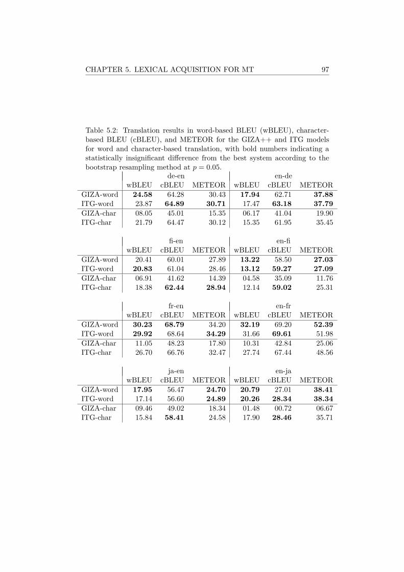
CHAPTER 5. LEXICAL ACQUISITION FOR MT 97
Table 5.2: Translation results in word-based BLEU (wBLEU), character-based BLEU (cBLEU), and METEOR for the GIZA++ and ITG modelsfor word and character-based translation, with bold numbers indicating astatistically insignificant difference from the best system according to thebootstrap resampling method at p = 0.05.
de-en en-dewBLEU cBLEU METEOR wBLEU cBLEU METEOR
GIZA-word 24.58 64.28 30.43 17.94 62.71 37.88ITG-word 23.87 64.89 30.71 17.47 63.18 37.79GIZA-char 08.05 45.01 15.35 06.17 41.04 19.90ITG-char 21.79 64.47 30.12 15.35 61.95 35.45
fi-en en-fiwBLEU cBLEU METEOR wBLEU cBLEU METEOR
GIZA-word 20.41 60.01 27.89 13.22 58.50 27.03ITG-word 20.83 61.04 28.46 13.12 59.27 27.09GIZA-char 06.91 41.62 14.39 04.58 35.09 11.76ITG-char 18.38 62.44 28.94 12.14 59.02 25.31
fr-en en-frwBLEU cBLEU METEOR wBLEU cBLEU METEOR
GIZA-word 30.23 68.79 34.20 32.19 69.20 52.39ITG-word 29.92 68.64 34.29 31.66 69.61 51.98GIZA-char 11.05 48.23 17.80 10.31 42.84 25.06ITG-char 26.70 66.76 32.47 27.74 67.44 48.56
ja-en en-jawBLEU cBLEU METEOR wBLEU cBLEU METEOR
GIZA-word 17.95 56.47 24.70 20.79 27.01 38.41ITG-word 17.14 56.60 24.89 20.26 28.34 38.34GIZA-char 09.46 49.02 18.34 01.48 00.72 06.67ITG-char 15.84 58.41 24.58 17.90 28.46 35.71
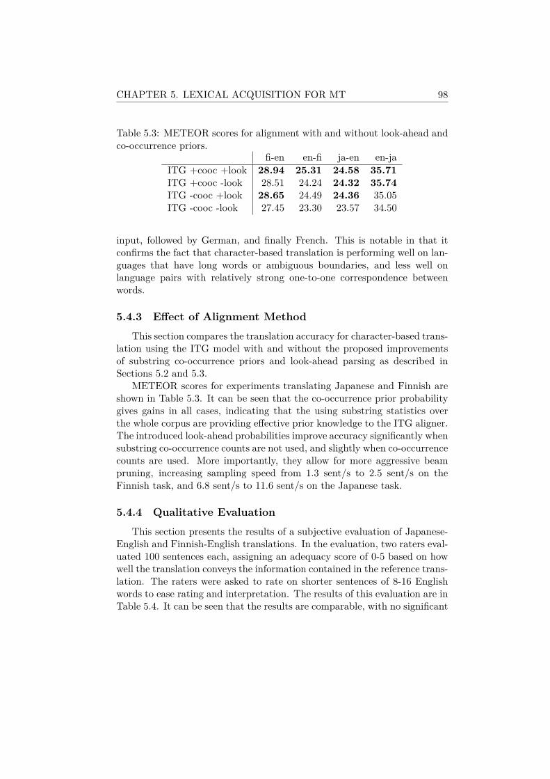
CHAPTER 5. LEXICAL ACQUISITION FOR MT 98
Table 5.3: METEOR scores for alignment with and without look-ahead andco-occurrence priors.
fi-en en-fi ja-en en-jaITG +cooc +look 28.94 25.31 24.58 35.71ITG +cooc -look 28.51 24.24 24.32 35.74ITG -cooc +look 28.65 24.49 24.36 35.05ITG -cooc -look 27.45 23.30 23.57 34.50
input, followed by German, and finally French. This is notable in that itconfirms the fact that character-based translation is performing well on lan-guages that have long words or ambiguous boundaries, and less well onlanguage pairs with relatively strong one-to-one correspondence betweenwords.
5.4.3 Effect of Alignment MethodThis section compares the translation accuracy for character-based trans-
lation using the ITG model with and without the proposed improvementsof substring co-occurrence priors and look-ahead parsing as described inSections 5.2 and 5.3.
METEOR scores for experiments translating Japanese and Finnish areshown in Table 5.3. It can be seen that the co-occurrence prior probabilitygives gains in all cases, indicating that the using substring statistics overthe whole corpus are providing effective prior knowledge to the ITG aligner.The introduced look-ahead probabilities improve accuracy significantly whensubstring co-occurrence counts are not used, and slightly when co-occurrencecounts are used. More importantly, they allow for more aggressive beampruning, increasing sampling speed from 1.3 sent/s to 2.5 sent/s on theFinnish task, and 6.8 sent/s to 11.6 sent/s on the Japanese task.
5.4.4 Qualitative EvaluationThis section presents the results of a subjective evaluation of Japanese-
English and Finnish-English translations. In the evaluation, two raters eval-uated 100 sentences each, assigning an adequacy score of 0-5 based on howwell the translation conveys the information contained in the reference trans-lation. The raters were asked to rate on shorter sentences of 8-16 Englishwords to ease rating and interpretation. The results of this evaluation are inTable 5.4. It can be seen that the results are comparable, with no significant
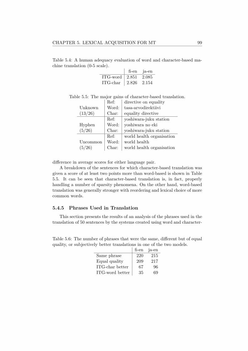
CHAPTER 5. LEXICAL ACQUISITION FOR MT 99
Table 5.4: A human adequacy evaluation of word and character-based ma-chine translation (0-5 scale).
fi-en ja-enITG-word 2.851 2.085ITG-char 2.826 2.154
Table 5.5: The major gains of character-based translation.Ref: directive on equality
Unknown Word: tasa-arvodirektiivi(13/26) Char: equality directive
Ref: yoshiwara-juku stationHyphen Word: yoshiwara no eki(5/26) Char: yoshiwara-juku station
Ref: world health organisationUncommon Word: world health(5/26) Char: world health organisation
difference in average scores for either language pair.A breakdown of the sentences for which character-based translation was
given a score of at least two points more than word-based is shown in Table5.5. It can be seen that character-based translation is, in fact, properlyhandling a number of sparsity phenomena. On the other hand, word-basedtranslation was generally stronger with reordering and lexical choice of morecommon words.
5.4.5 Phrases Used in TranslationThis section presents the results of an analysis of the phrases used in the
translation of 50 sentences by the systems created using word and character-
Table 5.6: The number of phrases that were the same, different but of equalquality, or subjectively better translations in one of the two models.
fi-en ja-enSame phrase 220 215Equal quality 209 217ITG-char better 67 96ITG-word better 35 69
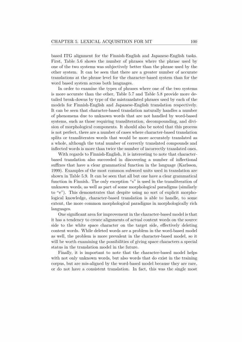
CHAPTER 5. LEXICAL ACQUISITION FOR MT 100
based ITG alignment for the Finnish-English and Japanese-English tasks.First, Table 5.6 shows the number of phrases where the phrase used byone of the two systems was subjectively better than the phrase used by theother system. It can be seen that there are a greater number of accuratetranslations at the phrase level for the character-based system than for theword based system across both languages.
In order to examine the types of phrases where one of the two systemsis more accurate than the other, Table 5.7 and Table 5.8 provide more de-tailed break-downs by type of the mistranslated phrases used by each of themodels for Finnish-English and Japanese-English translation respectively.It can be seen that character-based translation naturally handles a numberof phenomena due to unknown words that are not handled by word-basedsystems, such as those requiring transliteration, decompounding, and divi-sion of morphological components. It should also be noted that this processis not perfect, there are a number of cases where character-based translationsplits or transliterates words that would be more accurately translated asa whole, although the total number of correctly translated compounds andinflected words is more than twice the number of incorrectly translated ones.
With regards to Finnish-English, it is interesting to note that character-based translation also succeeded in discovering a number of inflectionalsuffixes that have a clear grammatical function in the language (Karlsson,1999). Examples of the most common subword units used in translation areshown in Table 5.9. It can be seen that all but one have a clear grammaticalfunction in Finnish. The only exception “s” is used in the transliteration ofunknown words, as well as part of some morphological paradigms (similarlyto “e”). This demonstrates that despite using no sort of explicit morpho-logical knowledge, character-based translation is able to handle, to someextent, the more common morphological paradigms in morphologically richlanguages.
One significant area for improvement in the character-based model is thatit has a tendency to create alignments of actual content words on the sourceside to the white space character on the target side, effectively deletingcontent words. While deleted words are a problem in the word-based modelas well, the problem is more prevalent in the character-based model, so itwill be worth examining the possibilities of giving space characters a specialstatus in the translation model in the future.
Finally, it is important to note that the character-based model helpswith not only unknown words, but also words that do exist in the trainingcorpus, but are mis-aligned by the word-based model because they are rare,or do not have a consistent translation. In fact, this was the single most
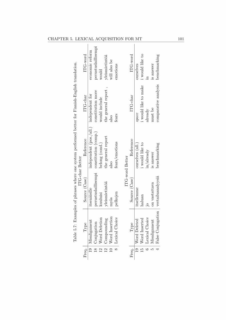
CHAPTER 5. LEXICAL ACQUISITION FOR MT 101
Table5.7:
Exam
ples
ofph
raseswhere
onesystem
perfo
rmed
better
forFinn
ish-E
nglishtran
slatio
n.IT
G-cha
rBe
tter
Freq.
Type
Source
(Case)
Reference
ITG-cha
rIT
G-w
ord
19Misa
lignm
ent
itsenäisille
indepe
ndent(pos./all.)
indepe
ndentfor
econ
omic
reform
18Con
jugatio
npe
rustuslaillise
mpi
constit
ution(com
p.)
constit
utionmore
perustuslaillise
mpi
12WordDeletion
kuuluisi
belong
(con
d.)
wouldinclud
ewo
uld
12Com
poun
ding
yleism
ietin
töä
thegeneralr
eport
thegeneralr
eport,
yleism
ietin
töä
10WordInsertion
myös
also
also
will
also
be8
LexicalC
hoice
pelkojen
fears/em
otions
fears
emotions
ITG-w
ordBe
tter
Freq.
Type
Source
(Case)
Reference
ITG-cha
rIT
G-w
ord
19WordDeleted
itsellemme
ourselves(all.)
spac
eou
rselves
15WordInserted
haluan
iwou
ldlik
eto
iwou
ldlik
eto
mak
eiw
ould
liketo
6Le
xicalC
hoice
join/alre
ady
alread
yin
5Misa
lignm
ent
onvastattava
isan
swer
mustbe
isan
swer
4Fa
lseCon
jugatio
nvertailuan
alyy
siäbe
nchm
arking
compa
rativ
ean
alysis
benchm
arking

CHAPTER 5. LEXICAL ACQUISITION FOR MT 102
Table5.8:
Exam
ples
ofph
raseswhere
onesystem
perfo
rmed
better
forJa
panese-E
nglishtran
slatio
n.IT
G-cha
rBe
tter
Freq.
Type
Source
Reference
ITG-cha
rIT
G-w
ord
38Tr
ansliteratio
n希玄
kigen
kigen
希玄
19WordInsertion
半年間
sixmon
ths
halfyear
sixmon
thsbe
tween
19WordDeletion
病のため
dueto
illness
dueto
hisillness
illness
17Misa
lignm
ent
を求めて
seeking
seeking
the
2Le
xicalC
hoice
俗lay/
common
lycalled
lay
common
lycalled
2Com
poun
d顔洗い
face
washing
face
washing
顔洗い
ITG-w
ordBe
tter
Freq.
Type
Source
Reference
ITG-cha
rIT
G-w
ord
28WordDeletion
も用いた。
wasalso
used
..
wasalso
used
.11
WordInsertion
招請
invited
invitedcont
invited
11Fa
lseTr
anslitertaion
無常
vanity
mujo
vanity
10Misa
lignm
ent
書かれた
writ
ten
the
writ
ten
5Pa
rtialT
ransliteration大佛
osaragi
ososarag
i2
LexicalC
hoice
でin/and
and
in
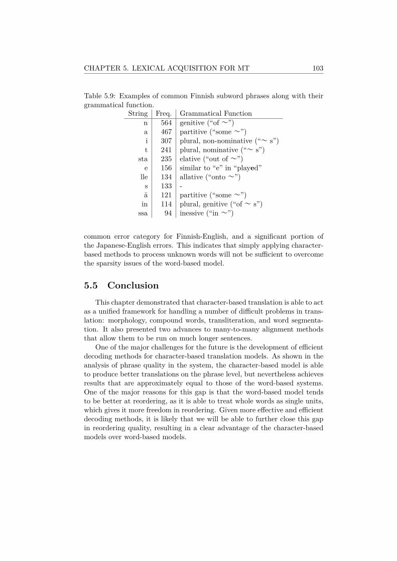
CHAPTER 5. LEXICAL ACQUISITION FOR MT 103
Table 5.9: Examples of common Finnish subword phrases along with theirgrammatical function.
String Freq. Grammatical Functionn 564 genitive (“of 〜”)a 467 partitive (“some 〜”)i 307 plural, non-nominative (“〜 s”)t 241 plural, nominative (“〜 s”)
sta 235 elative (“out of 〜”)e 156 similar to “e” in “played”
lle 134 allative (“onto 〜”)s 133 -ä 121 partitive (“some 〜”)in 114 plural, genitive (“of 〜 s”)ssa 94 inessive (“in 〜”)
common error category for Finnish-English, and a significant portion ofthe Japanese-English errors. This indicates that simply applying character-based methods to process unknown words will not be sufficient to overcomethe sparsity issues of the word-based model.
5.5 ConclusionThis chapter demonstrated that character-based translation is able to act
as a unified framework for handling a number of difficult problems in trans-lation: morphology, compound words, transliteration, and word segmenta-tion. It also presented two advances to many-to-many alignment methodsthat allow them to be run on much longer sentences.
One of the major challenges for the future is the development of efficientdecoding methods for character-based translation models. As shown in theanalysis of phrase quality in the system, the character-based model is ableto produce better translations on the phrase level, but nevertheless achievesresults that are approximately equal to those of the word-based systems.One of the major reasons for this gap is that the word-based model tendsto be better at reordering, as it is able to treat whole words as single units,which gives it more freedom in reordering. Given more effective and efficientdecoding methods, it is likely that we will be able to further close this gapin reordering quality, resulting in a clear advantage of the character-basedmodels over word-based models.
Chapter 6
Conclusion
This thesis has concerned itself with the fundamental problem of learninglexical units for practical tasks. The results presented here give new toolsand new motivation for further studies of the role of the lexicon in languageprocessing systems.
The new tools come in the form of models for lexical learning and theinference algorithms that are used to learn these models. For speech recog-nition, this is a model of statistical word segmentation, with the accompany-ing finite-state representation and inference algorithm for use on continuousspeech. For machine translation, this is a hierarchical model of many-to-many alignment with its accompanying inference algorithm using efficientsearch over inversion transduction grammar (ITG) parses, which can alsobe applied to learning lexical units.
The new motivation comes from experimental results demonstrating thatfully unsupervised lexical learning is not only possible, but also useful whenmeasured by extrinsic measures over the tasks at hand. In particular, theworks here have shown that unsupervised learning has the potential to pro-vide one solution to the data bottleneck and the problem of choosing seg-mentation standards appropriate for the task at hand.
With regards to the data bottleneck, the work on speech recognitionshowed that language model learning is possible without text, removingthe necessity to prepare text resources for language model learning. Thework on machine translation demonstrated that it is possible to performtranslation using only characters, allowing the handling of unsegmented ormorphologically rich languages without preparing manually segmented ormorphologically analyzed data.
In addition, for both machine translation and speech recognition, exper-iments demonstrate that unsupervised learning is able to find units that are
104
CHAPTER 6. CONCLUSION 105
useful for practical applications, often matching or surpassing those used bysupervised systems. This is due to the fact that unsupervised methods areable to automatically adjust the length of the unit used, using longer unitsconsisting of multiple words when there is enough data to allow for the ro-bust estimation of the corresponding statistics, and shorter units consistingof characters or subwords for less common words that suffer from problemsof data sparsity. It is also significant that lexical learning in such a man-ner affords new insights into the basic units that we are using for languageprocessing systems such as speech recognition and machine translation, andthese insights can potentially be integrated into more traditional supervisedlexical processing systems.
6.1 Future WorkEach chapter of this thesis has provided a brief look at extensions to the
individual techniques presented therein. This section wraps up the thesiswith a look at the broad, over-reaching challenges that still remain in thearea.
6.1.1 Use of Prosodic or Textual BoundariesAll of the works presented here concern themselves with learning lexi-
cons from strings of symbols, either phonemes in speech, or characters intext. However, speech is not simply a string of phonemes, and while textmay generally be considered as strings of characters, all characters do notnecessarily merit the same treatment.
In addition to its phonemic content, speech is also rich in social andcontextual signals that may be able to help learning which lexical units touse in recognition in a more robust and generalizable fashion. For example,studies on human language acquisition have shown that while children areheavily influenced by the statistical regularities in the phoneme stream thatare used in this work (Saffran et al., 1996), changes in tone, stress, and otherprosodic factors also play an important role in lexical learning (Jusczyk etal., 1999).
With regards to learning lexical units from text, while the methods pre-sented here were agnostic to explicit word boundaries delimited by spaces,these spaces certainly provide clues about the boundaries of meaningfulunits that can be exploited in the translation and alignment processes. Inaddition, it has been shown that for languages such as Chinese, which do

CHAPTER 6. CONCLUSION 106
not contain specific boundaries, punctuation can provide a strong indicatorin their place (Li and Sun, 2009).
While this thesis has shown that these indicators are not explicitly neces-sary to achieve some degree of lexical learning, a promising future directionis to explore the middle ground between affording them blind trust andignoring them completely.
6.1.2 Learning Morphological PatternsThis thesis has handled the problem of lexical acquisition as a task of
separating the character string into appropriate word units. However, formost languages in the world there are significant morphological regularities.Going back to the example of the word “uninspiring” provided in the intro-duction, we can see that the word stem “inspir” has possible conjugations“e,” “ing,” and “ed,” among others. This common property is shared by anynumber of other words such as “invite,” “relate,” and “abide.”
As mentioned in Section 1.2, the automatic discovery of such morpho-logical patterns has received some treatment in the fields of psychology andcomputational linguistics. There has also been some research on learning thesegmentation of morphemes across languages (Snyder and Barzilay, 2008;Naradowsky and Toutanova, 2011), and even some work on learning thesplitting of compound words for machine translation using morphologicaloperations such as deletion and replacement (Garera and Yarowsky, 2008;Macherey et al., 2011), but there is still no systematic treatment of morecomplex operations such as learning conjugation paradigms for verbs. Thisis also true for language modeling for speech recognition, with some effortbeing made to segment text in morphologically rich languages with bothsupervised (Afify et al., 2006) and unsupervised methods (Hirsimäki et al.,2006), but little to cluster or utilize patterns to improve segmentation re-sults.
6.1.3 Learning on Large ScaleOne final challenge for the future is the scaling of learning to larger data,
which has been shown repeatedly to provide superior results with no changein algorithms (Halevy et al., 2009). While each of the chapters did speak tospeed improvements in their current methods, the overall process of blockedGibbs sampling is still relatively slow compared to other simpler methods(Li and Sun, 2009; Zhikov et al., 2010).
Fortunately, with the proliferation of computing clusters, parallel pro-cessing has allowed for large-scale learning, even for more complicated struc-

CHAPTER 6. CONCLUSION 107
tured models such as the ones presented in this thesis (McDonald et al.,2010). While Gibbs sampling is not trivially parallelizable, there are a num-ber of reports that parallelizing learning can afford great increases in speedwith little to no sacrifice in accuracy (Newman et al., 2007; Asuncion et al.,2008). Using these techniques to scale up to web scale data will likely affordmore robust, more accurate acquisition of a wider variety of lexical phenom-ena, allowing for improvements in system accuracy and a more completeinsight into the nature of lexical knowledge that must be used therein.
Bibliography
Steven Abney and Steven Bird. 2010. The human language project: Build-ing a universal corpus of the world’s languages. In Proceedings of the48th Annual Meeting of the Association for Computational Linguistics(ACL).
Mohamed I. Abouelhoda, Stefan Kurtz, and Enno Ohlebusch. 2004. Re-placing suffix trees with enhanced suffix arrays. Journal of DiscreteAlgorithms, 2(1).
Mohamed Afify, Ruhi Sarikaya, Hong-Kwang Jeff Kuo, Laurent Besacier,and Yuqing Gao. 2006. On the use of morphological analysis for dialectalarabic speech recognition. In Ninth International Conference on SpokenLanguage Processing.
Yuya Akita and Tatsuya Kawahara. 2010. Statistical transformation oflanguage and pronunciation models for spontaneous speech recognition.IEEE Transactions on Audio, Speech, and Language Processing, 18(6).
Yaser Al-Onaizan and Kevin Knight. 2002. Translating named entities usingmonolingual and bilingual resources. In Proceedings of the 40th AnnualMeeting of the Association for Computational Linguistics (ACL).
Arthur Asuncion, Padhraic Smyth, and Max Welling. 2008. Asynchronousdistributed learning of topic models. In Proceedings of the 22nd AnnualConference on Neural Information Processing Systems (NIPS).
Ming-Hong Bai, Keh-Jiann Chen, and Jason S. Chang. 2008. Improvingword alignment by adjusting Chinese word segmentation. In Proceedingsof the 3rd International Joint Conference on Natural Language Process-ing (IJCNLP).
Thomas Bayes and Richard Price. 1763. An essay towards solving a problemin the doctrine of chances. Philosophical Transactions, 53:370.
Issam Bazzi and James Glass. 2001. Learning units for domain-independentout-of-vocabulary word modelling. In Proceedings of the 7th EuropeanConference on Speech Communication and Technology (EuroSpeech).
108
BIBLIOGRAPHY 109
Matthew J. Beal. 2003. Variational algorithms for approximate Bayesianinference. Ph.D. thesis, University College London.
Kenneth R. Beesley. 1996. Arabic finite-state morphological analysis andgeneration. In Proceedings of the 21th International Conference on Com-putational Linguistics (COLING).
Frédéric Bimbot, Roberto Pieraccini, Esther Levin, and Bishnu Atal. 1995.Variable-length sequence modeling: Multigrams. Signal Processing Let-ters, IEEE, 2(6).
Christopher M. Bishop. 2006. Pattern recognition and machine learning.Springer New York.
Phil Blunsom and Trevor Cohn. 2010. Inducing synchronous grammarswith slice sampling. In Proceedings of the Human Language Technol-ogy: The 11th Annual Conference of the North American Chapter of theAssociation for Computational Linguistics (NAACL).
Phil Blunsom, Trevor Cohn, Chris Dyer, and Miles Osborne. 2009. A Gibbssampler for phrasal synchronous grammar induction. In Proceedings ofthe 47th Annual Meeting of the Association for Computational Linguistics(ACL).
Ondrej Bojar. 2007. English-to-Czech factored machine translation. In Pro-ceedings of the 2nd Workshop on Statistical Machine Translation (WMT).
Michael R. Brent. 1999. An efficient, probabilistically sound algorithm forsegmentation and word discovery. Machine Learning, 34.
Peter F. Brown, Vincent J.Della Pietra, Stephen A. Della Pietra, andRobert L. Mercer. 1993. The mathematics of statistical machine trans-lation: Parameter estimation. Computational Linguistics, 19.
Ralf D. Brown. 2002. Corpus-driven splitting of compound words. In Proc.TMI.
Chris Callison-Burch, Philipp Koehn, Christof Monz, Kay Peterson, MarkPrzybocki, and Omar F. Zaidan. 2010. Findings of the 2010 joint work-shop on statistical machine translation and metrics for machine transla-tion. In Proceedings of the Joint 5th Workshop on Statistical MachineTranslation (WMT) and MetricsMATR.
Marine Carpuat and Dekai Wu. 2005. Word sense disambiguation vs. sta-tistical machine translation. In Proceedings of the 43rd Annual Meetingof the Association for Computational Linguistics (ACL).
Chao-Huang Chang and Cheng-Dur Chen. 1993. Hmm-based part-of-speechtagging for Chinese corpora. In Proceedings of the Workshop on VeryLarge Corpora, pages 40–47.
BIBLIOGRAPHY 110
Pi-Chuan Chang, Michel Galley, and Christopher D. Manning. 2008. Opti-mizing Chinese word segmentation for machine translation performance.In Proceedings of the 3rd Workshop on Statistical Machine Translation(WMT).
Stanley F. Chen and Joshua Goodman. 1996. An empirical study of smooth-ing techniques for language modeling. In Proceedings of the 34th AnnualMeeting of the Association for Computational Linguistics (ACL).
Colin Cherry and Dekang Lin. 2007. Inversion transduction grammar forjoint phrasal translation modeling.
David Chiang. 2007. Hierarchical phrase-based translation. ComputationalLinguistics, 33(2).
Noam Chomsky. 1956. Three models for the description of language. IRETransactions on Information Theory, 2(3).
Tagyoung Chung and Daniel Gildea. 2009. Unsupervised tokenization formachine translation. In Proceedings of the Conference on EmpiricalMethods in Natural Language Processing (EMNLP).
Shay B. Cohen, David M. Blei, and Noah A. Smith. 2010. Variationalinference for adaptor grammars. In Proceedings of the Human LanguageTechnology: The 11th Annual Conference of the North American Chapterof the Association for Computational Linguistics (NAACL).
Simon Corston-Oliver and Michael Gamon. 2004. Normalizing German andEnglish inflectional morphology to improve statistical word alignment.Machine Translation: From Real Users to Research.
Mathias Creutz and Krista Lagus. 2007. Unsupervised models for mor-pheme segmentation and morphology learning. ACM Transactions onSpeech and Language Processing, 4(1):3.
Fabien Cromieres. 2006. Sub-sentential alignment using substring co-occurrence counts. In Proc. COLING/ACL 2006 Student ResearchWorkshop.
Carl de Marcken. 1995. The unsupervised acquisition of a lexicon from con-tinuous speech. Technical report, Massachusetts Institute of Technology,Cambridge, MA, USA.
Carl de Marcken. 1996. Unsupervised Language Acquisition. Ph.D. thesis,Massachusetts Institute of Technology.
Sabine Deligne and Frédéric Bimbot. 1997. Inference of variable-lengthlinguistic and acoustic units by multigrams. Speech Communication,23(3).

BIBLIOGRAPHY 111
John DeNero and Dan Klein. 2010. Discriminative modeling of extractionsets for machine translation. In Proceedings of the 48th Annual Meetingof the Association for Computational Linguistics (ACL).
John DeNero, Dan Gillick, James Zhang, and Dan Klein. 2006. Why gener-ative phrase models underperform surface heuristics. In Proceedings ofthe 1st Workshop on Statistical Machine Translation (WMT).
John DeNero, Alex Bouchard-Côté, and Dan Klein. 2008. Sampling align-ment structure under a Bayesian translation model. In Proceedings ofthe Conference on Empirical Methods in Natural Language Processing(EMNLP).
Michael Denkowski and Alon Lavie. 2011. Meteor 1.3: Automatic Metric forReliable Optimization and Evaluation of Machine Translation Systems.In Proceedings of the 6th Workshop on Statistical Machine Translation(WMT).
Markus Dreyer and Jason Eisner. 2011. Discovering morphologicalparadigms from plain text using a dirichlet process mixture model. InProceedings of the Conference on Empirical Methods in Natural LanguageProcessing (EMNLP).
Joris Driesen and Hugo Van Hamme. 2008. Improving the Multigram Al-gorithm by using Lattices as Input. In Proceedings of the 9th AnnualConference of the International Speech Communication Association (In-terSpeech).
Greg Durrett and Dan Klein. 2011. An empirical investigation of discount-ing in cross-domain language models. In Proceedings of the 49th AnnualMeeting of the Association for Computational Linguistics (ACL).
Peter D. Eimas, Einar R. Siqueland, Ppeter Jusczyk, and James Vigorito.1971. Speech perception in infants. Science, 171(3968).
Thomas S. Ferguson. 1973. A bayesian analysis of some nonparametricproblems. The annals of statistics, pages 209–230.
Andrew Finch and Eiichiro Sumita. 2007. Phrase-based machine transliter-ation. In Proc. TCAST.
Daniel Fink. 1997. A compendium of conjugate priors. Technical report,Montana State University.
Jonathan G. Fiscus. 1997. A post-processing system to yield reduced worderror rates: Recognizer output voting error reduction (ROVER). InProceedings of the 1997 IEEE Automatic Speech Recognition and Under-standing Workshop (ASRU).

BIBLIOGRAPHY 112
Atsushi Fujii, Masao Utiyama, Mikio Yamamoto, and Takehito Utsuro.2008. Overview of the patent translation task at the NTCIR-7 workshop.In Proceedings of the 7th NTCIR Workshop Meeting on Evaluation ofInformation Access Technologies.
Michel Galley, Jonathan Graehl, Kevin Knight, Daniel Marcu, Steve De-Neefe, Wei Wang, and Ignacio Thayer. 2006. Scalable inference andtraining of context-rich syntactic translation models. In Proceedings ofthe 44th Annual Meeting of the Association for Computational Linguis-tics (ACL).
Nikesh Garera and David Yarowsky. 2008. Translating compounds by learn-ing component gloss translation models via multiple languages. In Pro-ceedings of the 3rd International Joint Conference on Natural LanguageProcessing (IJCNLP).
Andrew Gelman. 1995. Bayesian data analysis. CRC press.Stuart Geman and Donald Geman. 1984. Stochastic relaxation, Gibbs
distributions and the Bayesian restoration of images. IEEE Transactionson Pattern Analysis and Machine Intelligence, 6(6).
James R. Glass. 1988. Finding acoustic regularities in speech: Applica-tion to phonetic recognition. Ph.D. thesis, Massachusetts Institute ofTechnology, Cambridge, MA, USA.
Sharon Goldwater and Thomas Griffiths. 2007. A fully bayesian approach tounsupervised part-of-speech tagging. In Proceedings of the 45th AnnualMeeting of the Association for Computational Linguistics (ACL).
Sharon Goldwater and David McClosky. 2005. Improving statistical MTthrough morphological analysis. In Proceedings of Human LanguageTechnology Conference and Conference on Empirical Methods in Natu-ral Language Processing.
Sharon Goldwater, Thomas L. Griffiths, and Mark Johnson. 2009. ABayesian framework for word segmentation: Exploring the effects of con-text. Cognition, 112(1).
Joshua T. Goodman. 2001. A bit of progress in language modeling. Com-puter Speech & Language, 15(4).
Allen L. Gorin, Dijana Petrovska-Delacretaz, Giuseppe Riccardi, andJeremy H. Wright. 1999. Learning spoken language without transcrip-tions. In Proceedings of the 1999 IEEE Automatic Speech Recognitionand Understanding Workshop (ASRU).
Aria Haghighi, John Blitzer, John DeNero, and Dan Klein. 2009. Betterword alignments with supervised itg models. In Proceedings of the 47thAnnual Meeting of the Association for Computational Linguistics (ACL).

BIBLIOGRAPHY 113
Alon Halevy, Peter Norvig, and Fernando Pereira. 2009. The unreasonableeffectiveness of data. Intelligent Systems, IEEE, 24(2):8–12.
Zellig S. Harris. 1954. Distributional structure. Word.W. Keith Hastings. 1970. Monte Carlo sampling methods using Markov
chains and their applications. Biometrika, 57(1).Teemu Hirsimäki, Mathias Creutz, Vesa Siivola, Mikko Kurimo, Sami Virpi-
oja, and Janne Pylkkönen. 2006. Unlimited vocabulary speech recogni-tion with morph language models applied to Finnish. Computer Speech& Language, 20(4).
Koji Hukushima and Koji Nemoto. 1996. Exchange Monte Carlo methodand application to spin glass simulations. Journal of the Physical Societyof Japan, 65(6):1604–1608.
Hemant Ishwaran and Lancelot F. James. 2001. Gibbs sampling methodsfor stick-breaking priors. Journal of the American Statistical Association,96(453):161–173.
Naoto Iwahashi. 2003. Language acquisition through a human-robot inter-face by combining speech, visual, and behavioral information. Informa-tion Sciences, 156(1-2).
Aren Jansen, Kenneth Church, and Hynek Hermansky. 2010. Towardsspoken term discovery at scale with zero resources. In Proceedings ofthe 11th Annual Conference of the International Speech CommunicationAssociation (InterSpeech).
Claus S. Jensen, Uffe Kjærulff, and Augustine Kong. 1995. Blocking Gibbssampling in very large probabilistic expert systems. International Jour-nal of Human Computer Studies, 42(6).
J. Howard Johnson, Joel Martin, George Foster, and Roland Kuhn. 2007a.Improving translation quality by discarding most of the phrasetable. InProceedings of the Conference on Empirical Methods in Natural LanguageProcessing (EMNLP).
Mark Johnson, Thomas Griffiths, and Sharon Goldwater. 2007b. Bayesianinference for PCFGs via Markov chain Monte Carlo. In Proceedingsof the Human Language Technologies: The Annual Conference of theNorth American Chapter of the Association for Computational Linguis-tics (NAACL).
Mark Johnson, Thomas L. Griffiths, and Sharon Goldwater. 2007c. Adap-tor grammars: A framework for specifying compositional nonparametricBayesian models. Advances in Neural Information Processing Systems,19.
BIBLIOGRAPHY 114
Peter W. Jusczyk, Derek M. Houston, and Mary Newsome. 1999. Thebeginnings of word segmentation in english-learning infants. CognitivePsychology, 39(3-4):159–207.
Fred Karlsson. 1999. Finnish: An Essential Grammar. Psychology Press.Dan Klein and Christopher D. Manning. 2003. A* parsing: fast exact
viterbi parse selection. In Proceedings of the Human Language Technol-ogy Conference (HLT-NAACL).
Reinhard Kneser and Hermann Ney. 1995. Improved backing-off for m-gram language modeling. Proceedings of the International Conferenceon Acoustics, Speech, and Signal Processing (ICASSP).
Kevin Knight and Jonathan Graehl. 1998. Machine transliteration. Com-putational Linguistics, 24(4).
Philipp Koehn et al. 2007. Moses: Open source toolkit for statistical ma-chine translation. In Proceedings of the 45th Annual Meeting of theAssociation for Computational Linguistics (ACL).
Phillip Koehn, Franz Josef Och, and Daniel Marcu. 2003. Statistical phrase-based translation. In Proceedings of the Human Language TechnologyConference (HLT-NAACL).
Philipp Koehn, Amittai Axelrod, Alexandra Birch Mayne, Chris Callison-Burch, Miles Osborne, and David Talbot. 2005. Edinburgh systemdescription for the 2005 IWSLT speech translation evaluation. In Pro-ceedings of the International Workshop on Spoken Language Translation(IWSLT).
Philipp Koehn. 2005. Europarl: A parallel corpus for statistical machinetranslation. In MT Summit.
Grzegorz Kondrak, Daniel Marcu, and Kevin Knight. 2003. Cognates canimprove statistical translation models. In Proceedings of the HumanLanguage Technology Conference (HLT-NAACL).
Kimmo Koskenniemi. 1984. A general computational model for word-formrecognition and production. In Proceedings of the 10th InternationalConference on Computational Linguistics (COLING), pages 178–181.Association for Computational Linguistics.
Canasai Kruengkrai, Kiyotaka Uchimoto, Jun’ichi Kazama, Yiou Wang,Kentaro Torisawa, and Hitoshi Isahara. 2009. An error-driven word-character hybrid model for joint Chinese word segmentation and POStagging. In Proceedings of the 47th Annual Meeting of the Associationfor Computational Linguistics (ACL).
BIBLIOGRAPHY 115
Taku Kudo, Kaoru Yamamoto, and Yuji Matsumoto. 2004. Applying condi-tional random fields to Japanese morphological analysis. In Proceedingsof the Conference on Empirical Methods in Natural Language Processing(EMNLP).
Sadao Kurohashi, Toshihisa Nakamura, Yuji Matsumoto, and Makoto Na-gao. 1994. Improvements of Japanese morphological analyzer JUMAN.In Proceedings of The International Workshop on Sharable Natural Lan-guage.
Lori Lamel, Jean-Luc Gauvain, and Gilles Adda. 2002. Lightly supervisedand unsupervised acoustic model training. Computer Speech and Lan-guage.
Young-Suk Lee. 2004. Morphological analysis for statistical machine trans-lation. In Proceedings of the Human Language Technology Conference /North American Chapter of the Association for Computational Linguis-tics (NAACL) Meeting (HLT/NAACL).
Zhongguo Li and Maosong Sun. 2009. Punctuation as implicit an-notations for chinese word segmentation. Computational Linguistics,35(4):505–512.
Percy Liang, Ben Taskar, and Dan Klein. 2006. Alignment by agree-ment. In Proceedings of the Human Language Technology Conference- North American Chapter of the Association for Computational Lin-guistics (NAACL) Annual Meeting (HLT-NAACL).
Percy Liang, Michael I. Jordan, and Dan Klein. 2010. Type-based MCMC.In Proceedings of the Human Language Technology: The 11th AnnualConference of the North American Chapter of the Association for Com-putational Linguistics (NAACL).
Klaus Macherey, Andrew Dai, David Talbot, Ashok Popat, and Franz Och.2011. Language-independent compound splitting with morphological op-erations. In Proceedings of the 49th Annual Meeting of the Associationfor Computational Linguistics (ACL).
David J.C. Mackay and Linda C. Bauman Petoy. 1995. A hierarchicalDirichlet language model. Natural Language Engineering, 1.
Christopher D. Manning and Hinrich Schütze. 1999. Foundations of statis-tical natural language processing, volume 59. MIT Press.
Daniel Marcu and William Wong. 2002. A phrase-based, joint probabilitymodel for statistical machine translation. In Proceedings of the Confer-ence on Empirical Methods in Natural Language Processing (EMNLP).
BIBLIOGRAPHY 116
Ryan McDonald, Keith Hall, and Gideon Mann. 2010. Distributed trainingstrategies for the structured perceptron. In Proceedings of the HumanLanguage Technology: The 11th Annual Conference of the North Ameri-can Chapter of the Association for Computational Linguistics (NAACL).
Fergus R. McInnes and Sharon Goldwater. 2011. Unsupervised extractionof recurring words from infant-directed speech. In Proceedings of the33rd Annual Conference of the Cognitive Science Society.
Daichi Mochihashi, Takeshi Yamada, and Naonori Ueda. 2009. Bayesianunsupervised word segmentation with nested Pitman-Yor modeling. InProceedings of the 47th Annual Meeting of the Association for Compu-tational Linguistics (ACL).
Mehryar Mohri, Fernando Pereira, and Michael Riley. 2008. Speech recog-nition with weighted finite-state transducers. Handbook on speech pro-cessing and speech communication, Part E: Speech recognition.
Robert C. Moore and Chris Quirk. 2007. An iteratively-trainedsegmentation-free phrase translation model for statistical machine trans-lation. In Proceedings of the 2nd Workshop on Statistical Machine Trans-lation (WMT).
Masaaki Nagata. 1994. A stochastic Japanese morphological analyzer usinga forward-DP backward-A∗ N-best search algorithm. In Proceedings ofthe 15th International Conference on Computational Linguistics (COL-ING).
Tetsuji Nakagawa. 2004. Chinese and Japanese word segmentation usingword-level and character-level information. In Proceedings of the 20thInternational Conference on Computational Linguistics (COLING).
Jason Naradowsky and Sharon Goldwater. 2009. Improving morphology in-duction by learning spelling rules. In UCAI 2009, Proceedings of the 21st,International Joint Conference on Artificial Intelligence, pages 11–17.
Jason Naradowsky and Kristina Toutanova. 2011. Unsupervised bilingualmorpheme segmentation and alignment with context-rich hidden semi-markov models. In Proceedings of the 49th Annual Meeting of the Asso-ciation for Computational Linguistics (ACL).
Graham Neubig and Shinsuke Mori. 2010. Word-based partial annota-tion for efficient corpus construction. In Proceedings of the 7th Inter-national Conference on Language Resources and Evaluation (LREC),pages 1495–1498, Valetta, Malta, May.
Graham Neubig, Yosuke Nakata, and Shinsuke Mori. 2011. Pointwise pre-diction for robust, adaptable Japanese morphological analysis. In Pro-
BIBLIOGRAPHY 117
ceedings of the 49th Annual Meeting of the Association for ComputationalLinguistics (ACL), pages 529–533, Portland, USA, June.
David Newman, Arthur Asuncion, Padhraic Smyth, and Max Welling.2007. Distributed inference for latent dirichlet allocation. Proceedings ofthe 21st Annual Conference on Neural Information Processing Systems(NIPS), 20(1081-1088).
David Newman, Arthur Asuncion, Padhraic Smyth, and Max Welling. 2009.Distributed algorithms for topic models. Journal of Machine LearningResearch, 10.
Hwee Tou Ng, Chung Yong Lim, and Shou King Foo. 1999. A case studyon inter-annotator agreement for word sense disambiguation. In Proc.of SIGLEX99: Standardizing Lexical Resources.
ThuyLinh Nguyen, Stephan Vogel, and Noah A. Smith. 2010. Nonpara-metric word segmentation for machine translation. In Proceedings of the23rd International Conference on Computational Linguistics (COLING).
Sonja Nießen and Hermann Ney. 2000. Improving SMT quality withmorpho-syntactic analysis. In Proceedings of the 18th International Con-ference on Computational Linguistics (COLING).
Franz Josef Och and Hermann Ney. 2002. Discriminative training and max-imum entropy models for statistical machine translation. In Proceedingsof the 40th Annual Meeting of the Association for Computational Lin-guistics (ACL).
Franz Josef Och and Hermann Ney. 2003. A systematic comparisonof various statistical alignment models. Computational Linguistics,29(1):19–51.
Franz Josef Och, Christoph Tillmann, and Hermann Ney. 1999. Improvedalignment models for statistical machine translation. In Proceedings ofthe 4th Conference on Empirical Methods in Natural Language Processing(EMNLP).
Franz Josef Och. 1999. An efficient method for determining bilingual wordclasses. In Proceedings of the 9th European Chapter of the Associationfor Computational Linguistics (EACL).
Franz Josef Och. 2003. Minimum error rate training in statistical machinetranslation. In Proceedings of the 41st Annual Meeting of the Associationfor Computational Linguistics (ACL).
Hideki Ogura, Hanae Koiso, Yumi Fujiike, Sayaka Miyauchi, Hikaru Kon-ishi, and Yutaka Hara. 2011. Balanced corpus of contemporarywritten Japanese, morphological information standard (4th edition, in
BIBLIOGRAPHY 118
Japanese). Technical report, National Institute for the Japanese Lan-guage and Linguistics.
Kishore Papineni, Salim Roukos, Todd Ward, and Wei-Jing Zhu. 2002.BLEU: a method for automatic evaluation of machine translation. InProceedings of the 19th International Conference on Computational Lin-guistics (COLING).
Alex S. Park and James R. Glass. 2008. Unsupervised pattern discovery inspeech. IEEE Transactions on Audio Speech and Language Processing,16(1).
Rebecca Passonneau, Nizar Habash, and Owen Rambow. 2006. Inter-annotator agreement on a multilingual semantic annotation task. InProceedings of the 5th International Conference on Language Resourcesand Evaluation (LREC).
Lisa Pearl, Sharon Goldwater, and Mark Steyvers. 2010. How ideal are we?incorporating human limitations into Bayesian models of word segmen-tation. In Proceedings of the 34th annual Boston University Conferenceon Child Language Development, Somerville, MA. Cascadilla Press.
Fuchun Peng, Fangfang Feng, and Andrew McCallum. 2004. Chinese seg-mentation and new word detection using conditional random fields. InProceedings of the 20th International Conference on Computational Lin-guistics (COLING).
Jim Pitman and Marc Yor. 1997. The two-parameter Poisson-Dirichlet dis-tribution derived from a stable subordinator. The Annals of Probability,25(2).
Jim Pitman. 1995. Exchangeable and partially exchangeable random par-titions. Probability Theory and Related Fields, 102(2):145–158.
Hoifung Poon, Colin Cherry, and Kristina Toutanova. 2009. Unsupervisedmorphological segmentation with log-linear models. In Proceedings ofthe North American Chapter of the Association for Computational Lin-guistics (NAACL) - Human Language Technology (NAACL HLT).
Okko Räsänen. 2011. A computational model of word segmentation fromcontinuous speech using transitional probabilities of atomic acousticevents. Cognition, 120(2).
Carl E. Rasmussen. 2004. Gaussian processes in machine learning. Ad-vanced Lectures on Machine Learning, pages 63–71.
Deb K. Roy and Alex P. Pentland. 2002. Learning words from sights andsounds: A computational model. Cognitive Science, 26(1).
BIBLIOGRAPHY 119
Daniel M. Roy and Yee Whye Teh. 2009. The mondrian process. In Proceed-ings of the 23rd Annual Conference on Neural Information ProcessingSystems (NIPS).
Markus Saers, Joakim Nivre, and Dekai Wu. 2009. Learning stochasticbracketing inversion transduction grammars with a cubic time biparsingalgorithm. In Proceedings of the The 11th International Workshop onParsing Technologies (IWPT).
Jenny R. Saffran, Richard N. Aslin, and Elissa L. Newport. 1996. Statisticallearning by eight-month-old infants. Science, 274(5294).
Manabu Sassano. 2002. An empirical study of active learning with supportvector machines for Japanese word segmentation. In Proceedings of the40th Annual Meeting of the Association for Computational Linguistics(ACL).
Patrick Schone and Daniel Jurafsky. 2001. Knowledge-free induction ofinflectional morphologies. In Proceedings of the Second Meeting of theNorth American Chapter of the Association for Computational Linguis-tics (NAACL).
Tanja Schultz and Alex Waibel. 2001. Language-independent and language-adaptive acoustic modeling for speech recognition. Speech Communica-tion, 35(1).
Steven L. Scott. 2002. Bayesian methods for hidden Markov models: Recur-sive computing in the 21st century. Journal of the American StatisticalAssociation, 97(457).
Benjamin Snyder and Regina Barzilay. 2008. Unsupervised multilinguallearning for morphological segmentation. Proceedings of the 46th AnnualMeeting of the Association for Computational Linguistics (ACL).
Virach Sornlertlamvanich, Chumpol Mokarat, and Hitoshi Isahara. 2008.Thai-lao machine translation based on phoneme transfer. In Proceedingsof the 14th Annual Meeting of the Association for Natural LanguageProcessing (NLP).
Richard Sproat, Chilin Shih, William Gale, and Nancy Chang. 1996. Astochastic finite-state word-segmentation algorithm for chinese. Compu-tational Linguistics, 22.
Michael Subotin. 2011. An exponential translation model for target lan-guage morphology. In Proceedings of the 49th Annual Meeting of theAssociation for Computational Linguistics (ACL).
Koichi Takeuchi and Yuji Matsumoto. 1995. Hmm parameter learning forJapanese morphological analyzer. In Proc. of the 10th Pacific Asia Con-
BIBLIOGRAPHY 120
ference on Language, Information and Computation (PACLING), pages163–172.
David Talbot and Miles Osborne. 2006. Modelling lexical redundancy formachine translation. In Proceedings of the 44th Annual Meeting of theAssociation for Computational Linguistics (ACL).
Deborah Tannen. 1982. Spoken and Written Language: Exploring Oralityand Literacy. ABLEX.
Yee Whye Teh. 2006. A Bayesian interpretation of interpolated Kneser-Ney.Technical report, School of Computing, National Univ. of Singapore.
Louis ten Bosch and Bert Cranen. 2007. A computational model for unsu-pervised word discovery. In Proceedings of the 8th Annual Conferenceof the International Speech Communication Association (InterSpeech).
Jörg Tiedemann. 2009. Character-based PSMT for closely related lan-guages. In Proceedings of the 13th Annual Conference of the EuropeanAssociation for Machine Translation.
Dimitra Vergyri and Katrin Kirchhoff. 2004. Automatic diacritization ofarabic for acoustic modeling in speech recognition. In Proceedings of the20th International Conference on Computational Linguistics (COLING).
David Vilar, Jan-T. Peter, and Hermann Ney. 2007. Can we translate let-ters. In Proceedings of the 2nd Workshop on Statistical Machine Trans-lation (WMT).
Yiou Wang, Kiyotaka Uchimoto, Jun’ichi Kazama, Canasai Kruengkrai,and Kentaro Torisawa. 2010. Adapting Chinese word segmentation formachine translation based on short units. In Proceedings of the 7th In-ternational Conference on Language Resources and Evaluation (LREC).
Yiou Wang, Jun’ichi Kazama, Yoshimasa Tsuruoka, Wenliang Chen, YujieZhang, and Kentaro Torisawa. 2011. Improving chinese word segmen-tation and pos tagging with semi-supervised methods using large auto-analyzed data. In Proceedings of the 5th International Joint Conferenceon Natural Language Processing (IJCNLP).
Dekai Wu. 1997. Stochastic inversion transduction grammars and bilingualparsing of parallel corpora. Computational Linguistics, 23(3).
Fei Xia, Martha Palmer, Nianwen Xue, Mary Ellen Okurowski, John Ko-varik, Fu-Dong Chiou, Shizhe Huang, Tony Kroch, and Mitch Marcus.2000. Developing guidelines and ensuring consistency for chinese textannotation. In Proceedings of the 2nd International Conference on Lan-guage Resources and Evaluation (LREC).

BIBLIOGRAPHY 121
Jia Xu, Richard Zens, and Hermann Ney. 2004. Do we need Chinese wordsegmentation for statistical machine translation? In Proceedings of the3rd SIGHAN workshop on Chinese language processing.
Jia Xu, Jianfeng Gao, Kristina Toutanova, and Hermann Ney. 2008.Bayesian semi-supervised chinese word segmentation for statistical ma-chine translation. In Proceedings of the 22th International Conferenceon Computational Linguistics (COLING).
Nianwen Xue and Libin Shen. 2003. Chinese word segmentation as LMRtagging. In Proceedings of the 2nd SIGHAN workshop on Chinese lan-guage processing.
David Yarowsky and Richard Wicentowski. 2000. Minimally supervisedmorphological analysis by multimodal alignment. In Proceedings of the38th Annual Meeting of the Association for Computational Linguistics(ACL).
Kenji Yoshimura, Tooru Hitaka, and Sho Yoshida. 1983. Morphologicalanalysis of non-marked-off Japanese sentences by the least bunsetsu’snumber method. Transactions of Information Processing Society ofJapan, 24(1):40–46.
Chen Yu and Dana H. Ballard. 2004. A multimodal learning interface forgrounding spoken language in sensory perceptions. ACM Transactionson Applied Perception, 1.
Hao Zhang and Daniel Gildea. 2005. Stochastic lexicalized inversion trans-duction grammar for alignment. In Proceedings of the 43rd Annual Meet-ing of the Association for Computational Linguistics (ACL).
Hao Zhang, Chris Quirk, Robert C. Moore, and Daniel Gildea. 2008a.Bayesian learning of non-compositional phrases with synchronous pars-ing. Proceedings of the 46th Annual Meeting of the Association forComputational Linguistics (ACL).
Ruiqiang Zhang, Keiji Yasuda, and Eiichiro Sumita. 2008b. Improvedstatistical machine translation by multiple Chinese word segmentation.In Proceedings of the 3rd Workshop on Statistical Machine Translation(WMT).
Valentin Zhikov, Hiroya Takamura, and Manabu Okumura. 2010. An effi-cient algorithm for unsupervised word segmentation with branching en-tropy and MDL. In Proceedings of the Conference on Empirical Methodsin Natural Language Processing (EMNLP).
George Kingsley Zipf. 1949. Human behavior and the principle of leasteffort. Addison-Wesley Press.
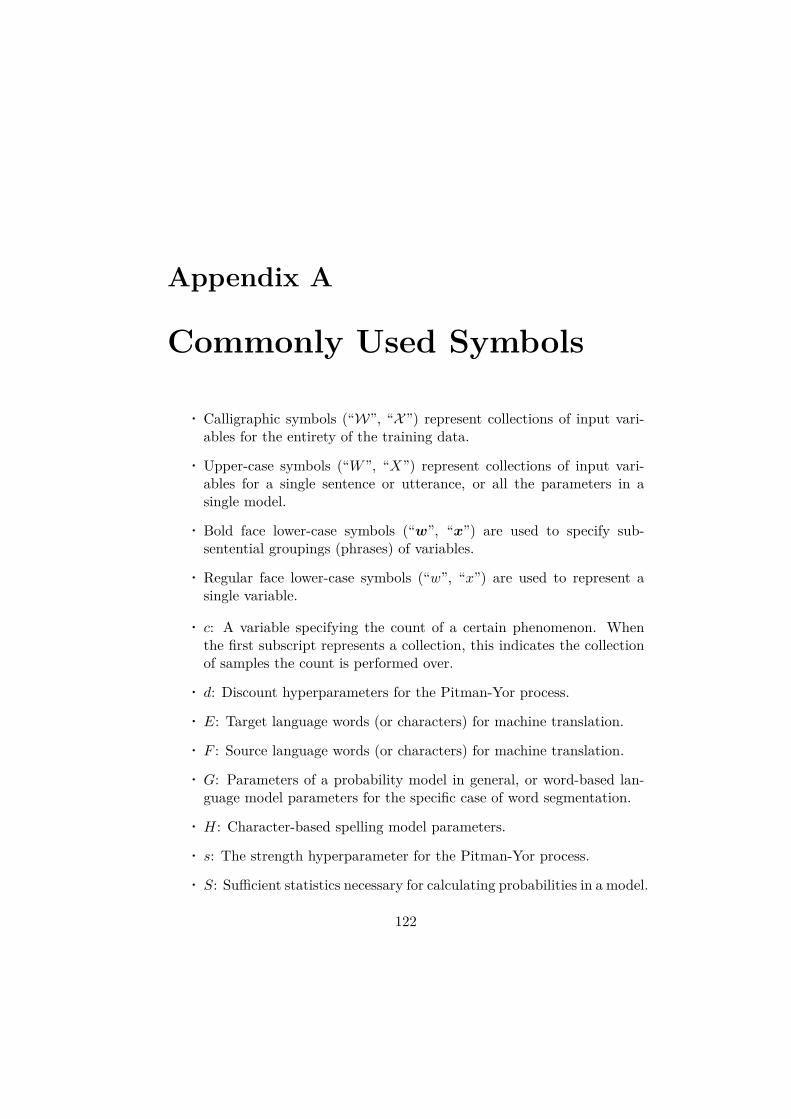
Appendix A
Commonly Used Symbols
• Calligraphic symbols (“W”, “X ”) represent collections of input vari-ables for the entirety of the training data.
• Upper-case symbols (“W”, “X”) represent collections of input vari-ables for a single sentence or utterance, or all the parameters in asingle model.
• Bold face lower-case symbols (“w”, “x”) are used to specify sub-sentential groupings (phrases) of variables.
• Regular face lower-case symbols (“w”, “x”) are used to represent asingle variable.
• c: A variable specifying the count of a certain phenomenon. Whenthe first subscript represents a collection, this indicates the collectionof samples the count is performed over.
• d: Discount hyperparameters for the Pitman-Yor process.
• E: Target language words (or characters) for machine translation.
• F : Source language words (or characters) for machine translation.
• G: Parameters of a probability model in general, or word-based lan-guage model parameters for the specific case of word segmentation.
• H: Character-based spelling model parameters.
• s: The strength hyperparameter for the Pitman-Yor process.
• S: Sufficient statistics necessary for calculating probabilities in a model.
122
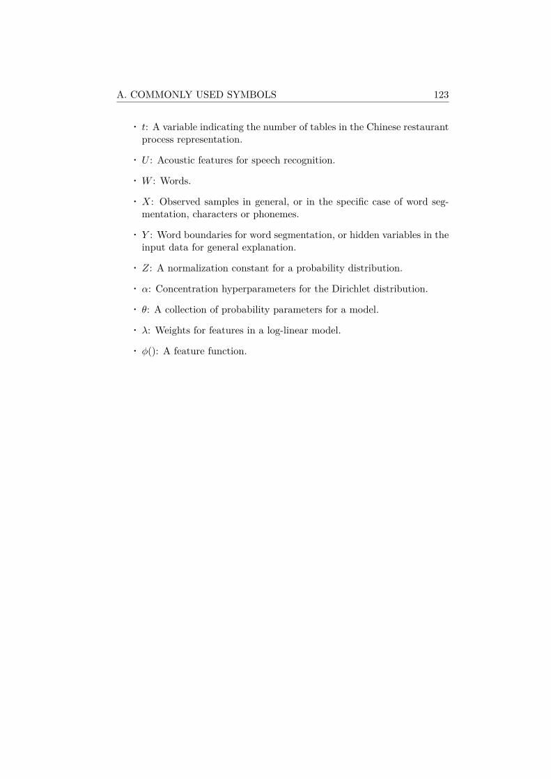
A. COMMONLY USED SYMBOLS 123
• t: A variable indicating the number of tables in the Chinese restaurantprocess representation.
• U : Acoustic features for speech recognition.
• W : Words.
• X: Observed samples in general, or in the specific case of word seg-mentation, characters or phonemes.
• Y : Word boundaries for word segmentation, or hidden variables in theinput data for general explanation.
• Z: A normalization constant for a probability distribution.
• α: Concentration hyperparameters for the Dirichlet distribution.
• θ: A collection of probability parameters for a model.
• λ: Weights for features in a log-linear model.
• φ(): A feature function.
Authored Works
Chapter 3
Refereed Works[1] Graham Neubig, Masato Mimura, Shinsuke Mori, and Tatsuya Kawa-
hara. Learning a language model from continuous speech. In Proceed-ings of the 11th Annual Conference of the International Speech Commu-nication Association (InterSpeech), pages 1495–1498, Makuhari, Japan,September 2010.
[2] Graham Neubig, Masato Mimura, Shinsuke Mori, and Tatsuya Kawa-hara. Bayesian learning of a language model from continuous speech.IEICE Transactions on Information and Systems, E95-D(2), pages614–625, Februrary 2012.
Unrefereed Works
[1] Graham Neubig, Masato Mimura, Shinsuke Mori, and Tatsuya Kawa-hara. Learning a language model from continuous speech using Bayesianinference. In Information Processing Society of Japan SIG Technical Re-port (SLP-82), Sendai, Japan, July 2010.
Chapter 4
Refereed Works
[1] Graham Neubig, Taro Watanabe, Eiichiro Sumita, Shinsuke Mori, andTatsuya Kawahara. An unsupervised model for joint phrase alignment
124
AUTHORED WORKS 125
and extraction. In Proceedings of the 49th Annual Meeting of the Asso-ciation for Computational Linguistics (ACL), pages 632–641, Portland,USA, June 2011.
[2] Graham Neubig, Taro Watanabe, Eiichiro Sumita, Shinsuke Mori, andTatsuya Kawahara. Joint phrase alignment and extraction for statisticalmachine translation. Journal of Information Processing, 2(20), April2012 (To Appear).
Unrefereed Works
[1] Graham Neubig, Taro Watanabe, Eiichiro Sumita, Shinsuke Mori, andTatsuya Kawahara. Phrase alignment for machine translation with ahierarchical model. In Proceedings of the 17th Annual Meeting of theAssociation for Natural Language Processing (NLP), Toyohashi, Japan,March 2011.
Chapter 5
Refereed Works
[1] Graham Neubig, Taro Watanabe, Shinsuke Mori, and Tatsuya Kawa-hara. Machine translation without words through substring alignment.In Proceedings of the 50th Annual Meeting of the Association for Com-putational Linguistics (ACL), Jeju, Korea, July 2012 (In Submission).
Unrefereed Works
[1] Graham Neubig, Taro Watanabe, Shinsuke Mori, and Tatsuya Kawahara.Substring-based machine translation In Proceedings of the 18th AnnualMeeting of the Association for Natural Language Processing (NLP), Hi-roshima, Japan, March 2012 (To Appear).
Other
Refereed Works
[1] Graham Neubig, Shinsuke Mori, and Tatsuya Kawahara. A WFST-basedlog-linear framework for speaking-style transformation. In Proceedings of
AUTHORED WORKS 126
the 10th Annual Conference of the International Speech CommunicationAssociation (InterSpeech), pages 1495–1498, Brighton, UK, September2009.
[2] Graham Neubig, Yuya Akita, Shinsuke Mori, and Tatsuya Kawahara.Improved statistical models for SMT-based speaking style transforma-tion. In Proceedings of the International Conference on Acoustics,Speech, and Signal Processing (ICASSP), pages 5206–5209, Dallas, USA,March 2010.
[3] Graham Neubig and Shinsuke Mori. Word-based partial annotationfor efficient corpus construction. In Proceedings of the 7th Interna-tional Conference on Language Resources and Evaluation (LREC), pages1495–1498, Valetta, Malta, May 2010.
[4] Yuya Akita, Masato Mimura, Graham Neubig, and Tatsuya Kawa-hara. Semi-automated update of automatic transcription system for theJapanese national congress. In 11th Annual Conference of the Inter-national Speech Communication Association (InterSpeech 2010), pages1495–1498, Makuhari, Japan, September 2010.
[5] Mijit Ablimit, Graham Neubig, Masato Mimura, Shinsuke Mori, TatsuyaKawahara, and Askar Hamdulla. Uyghur morpheme-based languagemodels and ASR. In IEEE 10th International Conference on SignalProcessing (ICSP), pages 581–584, Beijing, China, October 2010.
[6] Graham Neubig, Yosuke Nakata, and Shinsuke Mori. Pointwise predic-tion for robust, adaptable Japanese morphological analysis. In Proceed-ings of the 49th Annual Meeting of the Association for ComputationalLinguistics (ACL), pages 529–533, Portland, USA, June 2011.
[7] Shinsuke Mori, Tetsuro Sasada, and Graham Neubig. Language modelestimation from a stochastically tagged corpus. Journal of Natural Lan-guage Processing, 18(2):71–87, June 2011.
[8] Shinsuke Mori and Graham Neubig. A pointwise approach to pronun-ciation estimation for a TTS front-end. In 12th Annual Conference ofthe International Speech Communication Association (InterSpeech 2011),pages 2181–2184, Florence, Italy, August 2011.
[9] Masao Utiyama, Graham Neubig, Takeshi Onishi, and Eiichiro Sumita.Searching translation memories for paraphrases. In Proceedings of theMachine Translation Summit XIII, pages 325–331, Xiamen, China,September 2011.
[10] Shinsuke Mori, Yosuke Nakata, Graham Neubig, and Tatsuya Kawa-hara. Morphological analysis with pointwise predictors. Journal of Nat-ural Language Processing, 18(4):367–381, September 2011.

AUTHORED WORKS 127
[11] Shinsuke Mori, Graham Neubig, and Yuta Tsuboi. A pointwise ap-proach to automatic word segmentation. Journal of Natural LanguageProcessing, 52(10):2944–2952, September 2011.
[12] Graham Neubig, Yuichiroh Matsubayashi, Masato Hagiwara, and KojiMurakami. Safety information mining - what can NLP do in a disaster-. In Proceedings of the 5th International Joint Conference on NaturalLanguage Processing (IJCNLP), pages 965–973, Chiang Mai, Thailand,November 2011.
[13] Daniel Flannery, Yusuke Miyao, Graham Neubig, and Shinsuke Mori.Training dependency parsers from partially annotated corpora. In Pro-ceedings of the 5th International Joint Conference on Natural LanguageProcessing (IJCNLP), pages 776–784, Chiang Mai, Thailand, November2011.
[14] Andrew Finch, Chooi ling Goh, Graham Neubig, and Eiichiro Sumita.The NICT translation system for IWSLT 2011. In Proceedings of the In-ternational Workshop on Spoken Language Translation 2011, San Fran-cisco, USA, December 2011.
[15] Graham Neubig, Yuya Akita, Shinsuke Mori, and Tatsuya Kawahara.A monotonic statistical machine translation approach to speaking styletransformation. Computer Speech and Language, 2012 (To Appear).
Unrefereed Works
[1] Graham Neubig, Shinsuke Mori, and Tatsuya Kawahara. Japanese char-acter error correction using WFSTs. In Proceedings of the 15th An-nual Meeting of the Association for Natural Language Processing (NLP),pages 332–335, Tottori, Japan, March 2009.
[2] Graham Neubig, Shinsuke Mori, and Tatsuya Kawahara. Log-linearspeaking-style transformation using weighted finite state transducers. InInformation Processing Society of Japan SIG Technical Report (SLP-77),Fukushima, Japan, July 2009.
[3] Graham Neubig, Yuya Akita, Shinsuke Mori, and Tatsuya Kawahara.Context-sensitive statistical models for speaking-style transformation.In Information Processing Society of Japan SIG Technical Report (SLP-79), Tokyo, Japan, December 2009.
[4] Graham Neubig, Yosuke Nakata, and Shinsuke Mori. Domain adaptationof automatic word segmentation using pointwise prediction and activelearning. In Proceedings of the 16th Annual Meeting of the Associationfor Natural Language Processing (NLP), Tokyo, Japan, March 2010.
AUTHORED WORKS 128
[5] Graham Neubig, Yuya Akita, Shinsuke Mori, and Tatsuya Kawahara.Speaking style transformation using statistical machine translation. InProceedings of the 16th Annual Meeting of the Association for NaturalLanguage Processing (NLP), Tokyo, Japan, March 2010.
[6] Shinsuke Mori and Graham Neubig. Automatic improvement of the nat-ural language processing accuracy through the use of kana-kanji conver-sion logs. In Proceedings of the 16th Annual Meeting of the Associationfor Natural Language Processing (NLP), Tokyo, Japan, March 2010.
[7] Shinsuke Mori, Tetsuro Sasada, and Graham Neubig. Language modelestimation from a stochastically tagged corpus. In Information Pro-cessing Society of Japan SIG Technical Report (NL-196), pages 71–87,Tokyo, Japan, May 2010.
[8] Yosuke Nakata, Graham Neubig, Shinsuke Mori, and Tatsuya Kawahara.Morphological analysis with pointwise predictors. In Information Pro-cessing Society of Japan SIG Technical Report (NL-198), Tokyo, Japan,September 2010.
[9] Yosuke Nakata, Graham Neubig, Shinsuke Mori, and Tatsuya Kawahara.Improving part-of-speech tagging by combining pointwise and sequence-based predictors. In Information Processing Society of Japan SIG Tech-nical Report (NL-200), Tokyo, Japan, January 2011.
[10] Yuya Akita, Masato Mimura, Graham Neubig, and Tatsuya Kawa-hara. Semi-automated update of automatic transcription system for theJapanese national congress. In Information Processing Society of JapanSIG Technical Report (SLP-84), Tokyo, Japan, December 2010.
[11] Shinsuke Mori, Daniel Flannery, Yusuke Miyao, and Graham Neubig.Training MST parsers from partially annotated corpora. In InformationProcessing Society of Japan SIG Technical Report (NL-201), Tokyo,Japan, May 2011.
[12] Graham Neubig and Shinsuke Mori. Efficient information filteringthrough active learning. In Proceedings of the 18th Annual Meetingof the Association for Natural Language Processing (NLP), Hiroshima,Japan, March 2012 (To Appear).
[13] Daniel Flannery, Yusuke Miyao, Graham Neubig, and Shinsuke Mori.Word-based Japanese dependency parsing. In Proceedings of the 18thAnnual Meeting of the Association for Natural Language Processing(NLP), Hiroshima, Japan, March 2012 (To Appear).
Copyright © 2022 FDOKUMEN