A Context-Sensitive Technique for Unsupervised Change ...

778 IEEE TRANSACTIONS ON GEOSCIENCE AND REMOTE SENSING, VOL. 45, NO. 3, MARCH 2007

A Context-Sensitive Technique for UnsupervisedChange Detection Based on Hopfield-Type

Neural NetworksSusmita Ghosh, Lorenzo Bruzzone, Senior Member, IEEE, Swarnajyoti Patra,

Francesca Bovolo, Member, IEEE, and Ashish Ghosh

Abstract—In this paper, we propose a context-sensitive tech-nique for unsupervised change detection in multitemporal remotesensing images. This technique is based on a modified Hopfieldneural network architecture designed to model spatial correlationbetween neighboring pixels of the difference image produced bycomparing images acquired on the same area at different times.Each spatial position in the considered scene is represented bya neuron in the Hopfield network that is connected only to itsneighboring units. These connections model the spatial correlationbetween neighboring pixels and are associated with a context-sensitive energy function that represents the overall status ofthe network. Change detection maps are obtained by iterativelyupdating the output status of the neurons until a minimum ofthe energy function is reached and the network assumes a sta-ble state. A simple heuristic thresholding procedure is presentedand adopted for initializing the network. The proposed changedetection technique is unsupervised and distribution free. Experi-mental results carried out on two multispectral and multitemporalremote sensing images confirm the effectiveness of the proposedtechnique.

Index Terms—Change detection, context-sensitive image analy-sis, Hopfield neural network, multitemporal images, remote sens-ing, thresholding.

I. INTRODUCTION

IN REMOTE sensing applications, change detection is theprocess aimed at identifying differences in the state of a

land cover by analyzing a pair of images acquired on thesame geographical area at different times [1], [2]. Such aproblem plays an important role in many different domainslike studies on land use/land cover dynamic [3], monitoringshifting cultivations [4], burned areas identification [5], analysisof deforestation processes [6], [7], assessment of vegetationchanges [8], and monitoring of urban growth [9]. Since all ofthese applications usually require an analysis of large areas,development of completely automatic and unsupervised changedetection techniques is of high relevance to reduce the time

Manuscript received April 7, 2006; revised October 6, 2006.S. Ghosh and S. Patra are with the Department of Computer Science and

Engineering, Jadavpur University, Kolkata 700032, India (e-mail: [email protected]).

L. Bruzzone and F. Bovolo are with the Department of Information andCommunication Technology, University of Trento, 38050 Trento, Italy (e-mail:[email protected]).

A. Ghosh is with the Machine Intelligence Unit and Center for Soft Com-puting Research, Indian Statistical Institute, Kolkata 700108, India (e-mail:[email protected]).

Digital Object Identifier 10.1109/TGRS.2006.888861

effort required by manual image analysis and to produce ob-jective change detection maps.

In the literature, the most widely used unsupervised changedetection techniques are based on a three-step procedure [1],namely 1) preprocessing, 2) pixel-by-pixel comparison of twomultitemporal images, and 3) image analysis. The aim ofthe preprocessing step is to make the considered images ascomparable as possible and includes operations like coreg-istration, radiometric and geometric corrections, and noisereduction. The comparison step aims at producing a furtherimage, where differences between the two considered acqui-sitions are highlighted. Different mathematical operators canbe adopted to perform image comparison. When dealing withoptical images, the most widely used operator is the differ-ence. This operator can be applied to: 1) a single spectralband (univariate image differencing) [1], [10], [11]; 2) multiplespectral bands [change vector analysis (CVA)] [1], [12]; and3) vegetation indexes (vegetation index differencing) [1], [13]or other linear (e.g., tasseled cap transformation [10]) or nonlin-ear combinations of spectral bands. Each choice gives rise to adifferent technique. Among these, the most popular is the CVAthat computes the difference image as the magnitude of spectralchange vectors obtained for each pair of corresponding pixelsby vector subtraction. Once image comparison is performed,the change detection process can be carried out adopting eithercontext-insensitive or context-sensitive procedures. The mostwidely used context-insensitive analysis techniques are basedon image thresholding. The decision threshold can be selectedeither with a manual trial-and-error procedure (according to adesired tradeoff between false and missed alarms) or with auto-matic techniques (e.g., by analyzing the statistical distributionof the image obtained after comparison, by fixing the desiredfalse alarm probability, or following a Bayesian minimum errordecision rule [12]). The mentioned thresholding procedures donot take into account the spatial correlation between neighbor-ing pixels in the decision process, i.e., they implicitly assumethat the image has an impulsive autocorrelation function. Toovercome this limitation of neglecting the interpixel class de-pendence, a context-sensitive change detection procedure basedon Markov random field (MRF) has been proposed in [12].

The aforementioned context-sensitive and context-insensitive automatic approaches to change detection requirethe selection of a proper model for the statistical distributionsof changed and unchanged pixels. To obtain an unsupervisedestimation of the parameters of the statistical modelsdescribing the class distributions, techniques based on theExpectation–Maximization (EM) algorithm can be used [14].

0196-2892/$25.00 © 2007 IEEE

GHOSH et al.: CONTEXT-SENSITIVE TECHNIQUE FOR UNSUPERVISED CHANGE DETECTION 779

In change detection problems of remote sensing images, theEM algorithm has been formulated under different assumptionsfor class distributions, i.e., Gaussian [12], generalized Gaussian[15], and mixture of Gaussians [16].

To overcome the limitations imposed by the need of selectinga statistical model for change and no-change class distributions,in this paper, we propose an unsupervised and context-sensitivechange detection technique, which is distribution free. Thepresented algorithm automatically detects the changes in thedifference image using the collective computational ability ofa Hopfield-type neural network [17]. The specific architectureof the Hopfield network used in this paper considers contextualinformation from the neighborhood of each pixel to generate anaccurate change detection map. In the presented architecture,each neuron corresponds to a pixel of the difference image andis connected to all the neurons in the neighborhood. Given aninitial state, the status of each neuron is modified iteratively.When the network reaches a stable state (local minimum ofits energy function), the difference image is classified intotwo classes (neurons having ON (+1) status represent thechanged pixels and those having OFF (−1) status representthe unchanged pixels). The major advantages of the proposedtechnique are listed as follows: 1) it is distribution free (both theproposed initialization strategy of the network and the energyfunction adopted are not based on any specific parametricmodel for the distributions of classes); 2) it properly exploitsthe spatiocontextual information making the change detectionprocess robust to isolated noisy patterns (the procedure forupdating the status of the neurons is regularized by the informa-tion included in the neighborhood); 3) it is completely unsuper-vised (the proposed initialization strategy does not require anya priori information); and 4) unlike the technique proposed in[12], it does not require manual setting of any input parameter.

To assess the effectiveness of the presented technique, weconsidered two real multitemporal remote sensing data sets andcompared the results provided by the proposed technique withthose obtained by reference methods published in the literature.

This paper is organized as follows: Section II provides abrief description of the Hopfield neural network. Section IIIdescribes the proposed change detection technique. The datasets used in the experiments and the obtained results aredescribed in Section IV. Finally, in Section V, conclusionsare drawn.

II. BACKGROUND: HOPFIELD NEURAL NETWORKS

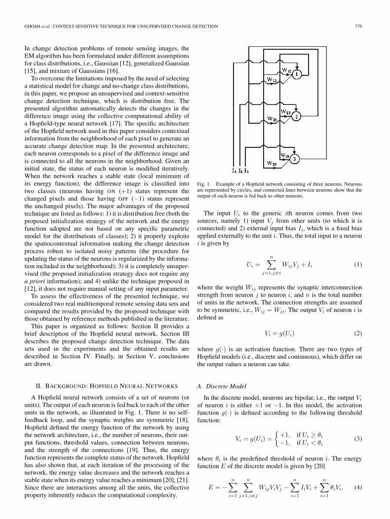
A Hopfield neural network consists of a set of neurons (orunits). The output of each neuron is fed back to each of the otherunits in the network, as illustrated in Fig. 1. There is no self-feedback loop, and the synaptic weights are symmetric [18].Hopfield defined the energy function of the network by usingthe network architecture, i.e., the number of neurons, their out-put functions, threshold values, connection between neurons,and the strength of the connections [19]. Thus, the energyfunction represents the complete status of the network. Hopfieldhas also shown that, at each iteration of the processing of thenetwork, the energy value decreases and the network reaches astable state when its energy value reaches a minimum [20], [21].Since there are interactions among all the units, the collectiveproperty inherently reduces the computational complexity.

Fig. 1. Example of a Hopfield network consisting of three neurons. Neuronsare represented by circles, and connected lines between neurons show that theoutput of each neuron is fed back to other neurons.

The input Ui to the generic ith neuron comes from twosources, namely 1) input Vj from other units (to which it isconnected) and 2) external input bias Ii, which is a fixed biasapplied externally to the unit i. Thus, the total input to a neuroni is given by

Ui =n∑

j=1,j �=i

WijVj + Ii (1)

where the weight Wij represents the synaptic interconnectionstrength from neuron j to neuron i, and n is the total numberof units in the network. The connection strengths are assumedto be symmetric, i.e., Wij = Wji. The output Vi of neuron i isdefined as

Vi = g(Ui) (2)

where g(·) is an activation function. There are two types ofHopfield models (i.e., discrete and continuous), which differ onthe output values a neuron can take.

A. Discrete Model

In the discrete model, neurons are bipolar, i.e., the output Vi

of neuron i is either +1 or −1. In this model, the activationfunction g(·) is defined according to the following thresholdfunction:

Vi = g(Ui) ={

+1, if Ui ≥ θi

−1, if Ui < θi(3)

where θi is the predefined threshold of neuron i. The energyfunction E of the discrete model is given by [20]

E = −n∑

i=1

n∑j=1,i �=j

WijViVj −n∑

i=1

IiVi +n∑

i=1

θiVi. (4)


The change of energy ∆E due to a change of output state of theneuron i equal to ∆Vi is

∆E = − n∑

j=1,i �=j

WijVj + Ii − θi

∆Vi = −[Ui − θi]∆Vi.

(5)

If ∆Vi is positive (i.e., the state of the neuron i is changedfrom −1 to +1), then from (3) we can see that the bracketedquantity in (5) is also positive, making ∆E negative. When ∆Vi

is negative (i.e., the state of the neuron i is changed from +1 to−1), then from (3) we can see that the bracketed quantity in(5) is also negative. Thus, any change in E according to (3) isnegative. Since E is bounded, the time required by the systemto reach convergence is associated to a motion in the state spacethat seeks out minima of E and stops at such points.

B. Continuous Model

In this model, the output of a neuron is continuous [21] andcan assume any real value between [−1,+1]. In the continuousmodel, the activation function g(·) must satisfy the followingconditions: 1) it is a monotonic nondecreasing function and2) g−1(·) exists.

A typical choice of the function g(·) is

g(Ui) =2

1 + e−φi(Ui−τ)− 1 (6)

where the parameter τ controls the shifting of the sigmoidalfunction g(·) along the abscissa, and φi determines the steep-ness (gain) of neuron i. The value of g(Ui) lies in [−1,+1] andis equal to 0 at Ui = τ . The energy function E of the continuousmodel is given by [21]

E=−n∑

i=1

n∑j=1,i �=j

WijViVj−n∑

i=1

IiVi+n∑

i=1

1Ri

Vi∫0

g−1(Vi)dV.

(7)

The function E is a Lyapunov function, and Ri is the totalinput impedance of the amplifier realizing a neuron i. It canbe shown that when neurons are updated according to (6), anychange in E is negative. The last term in (7) is the energy lossterm, which becomes zero at the high gain region. If the gain ofthe function becomes infinitely large (i.e., the sigmoidal non-linearity approaches the idealized hard-limiting form), the lastterm will become negligibly small. In the limiting case, whenφi = ∞ for all i, the maxima and minima of the continuousmodel become identical to those of the corresponding discreteHopfield model. In this case, the energy function is simplydefined by

E = −n∑

i=1

n∑j=1,i �=j

WijViVj −n∑

i=1

IiVi (8)

where the output state of each neuron is ±1. Therefore, the onlystable points of the very high-gain continuous deterministic

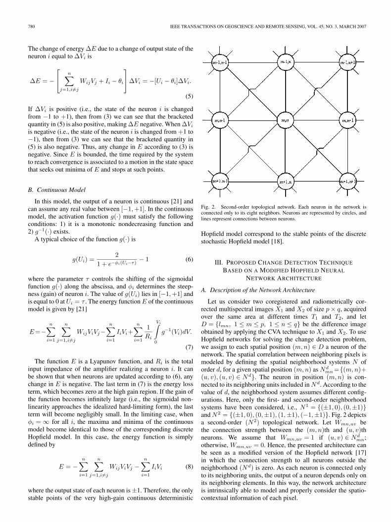
Fig. 2. Second-order topological network. Each neuron in the network isconnected only to its eight neighbors. Neurons are represented by circles, andlines represent connections between neurons.

Hopfield model correspond to the stable points of the discretestochastic Hopfield model [18].

III. PROPOSED CHANGE DETECTION TECHNIQUE

BASED ON A MODIFIED HOPFIELD NEURAL

NETWORK ARCHITECTURE

A. Description of the Network Architecture

Let us consider two coregistered and radiometrically cor-rected multispectral images X1 and X2 of size p× q, acquiredover the same area at different times T1 and T2, and letD = {lmn, 1 ≤ m ≤ p, 1 ≤ n ≤ q} be the difference imageobtained by applying the CVA technique to X1 and X2. To useHopfield networks for solving the change detection problem,we assign to each spatial position (m,n) ∈ D a neuron of thenetwork. The spatial correlation between neighboring pixels ismodeled by defining the spatial neighborhood systems N oforder d, for a given spatial position (m,n) as Nd

mn ={(m,n)+(u, v), (u, v) ∈ Nd}. The neuron in position (m,n) is con-nected to its neighboring units included in Nd. According to thevalue of d, the neighborhood system assumes different config-urations. Here, only the first- and second-order neighborhoodsystems have been considered, i.e., N1 = {(±1, 0), (0,±1)}and N2 = {(±1, 0), (0,±1), (1,±1), (−1,±1)}. Fig. 2 depictsa second-order (N2) topological network. Let Wmn,uv bethe connection strength between the (m,n)th and (u, v)thneurons. We assume that Wmn,uv = 1 if (u, v) ∈ Nd

mn;otherwise, Wmn,uv = 0. Hence, the presented architecture canbe seen as a modified version of the Hopfield network [17]in which the connection strength to all neurons outside theneighborhood (Nd) is zero. As each neuron is connected onlyto its neighboring units, the output of a neuron depends only onits neighboring elements. In this way, the network architectureis intrinsically able to model and properly consider the spatio-contextual information of each pixel.


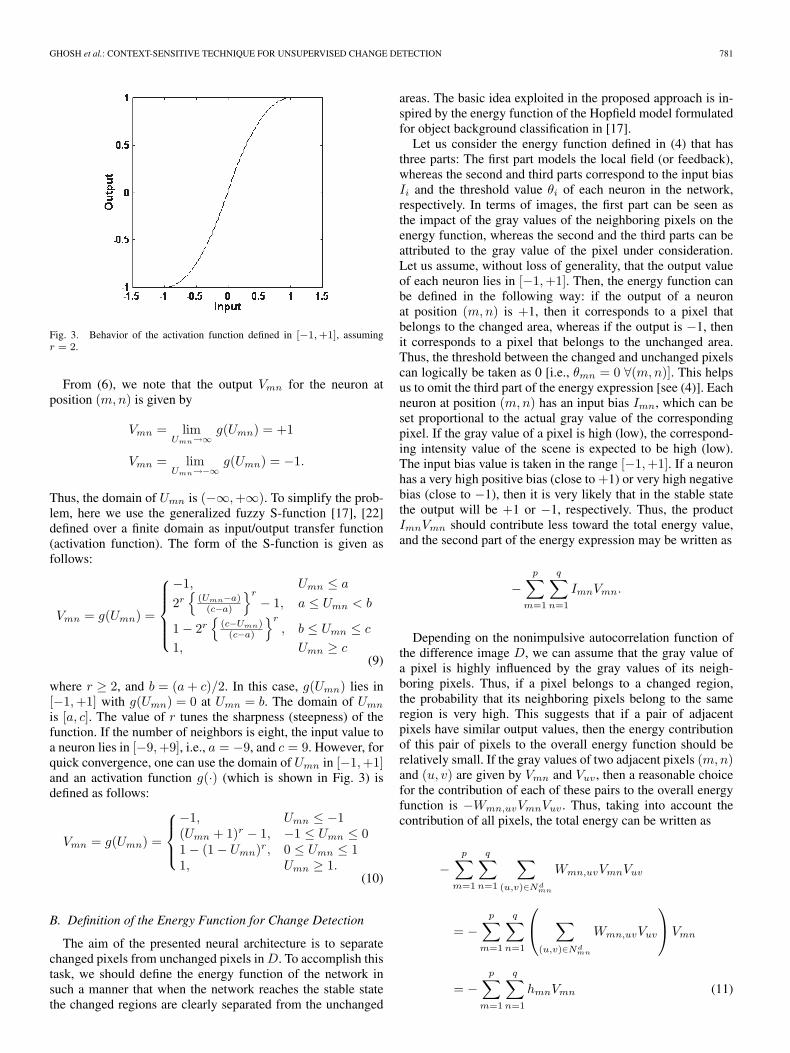
Fig. 3. Behavior of the activation function defined in [−1, +1], assumingr = 2.

From (6), we note that the output Vmn for the neuron atposition (m,n) is given by

Vmn = limUmn→∞

g(Umn) = +1

Vmn = limUmn→−∞

g(Umn) = −1.

Thus, the domain of Umn is (−∞,+∞). To simplify the prob-lem, here we use the generalized fuzzy S-function [17], [22]defined over a finite domain as input/output transfer function(activation function). The form of the S-function is given asfollows:

Vmn = g(Umn) =

−1, Umn ≤ a

2r{

(Umn−a)(c−a)

}r

− 1, a ≤ Umn < b

1 − 2r{

(c−Umn)(c−a)

}r

, b ≤ Umn ≤ c

1, Umn ≥ c(9)

where r ≥ 2, and b = (a + c)/2. In this case, g(Umn) lies in[−1,+1] with g(Umn) = 0 at Umn = b. The domain of Umn

is [a, c]. The value of r tunes the sharpness (steepness) of thefunction. If the number of neighbors is eight, the input value toa neuron lies in [−9,+9], i.e., a = −9, and c = 9. However, forquick convergence, one can use the domain of Umn in [−1,+1]and an activation function g(·) (which is shown in Fig. 3) isdefined as follows:

Vmn = g(Umn) =

−1, Umn ≤ −1(Umn + 1)r − 1, −1 ≤ Umn ≤ 01 − (1 − Umn)r, 0 ≤ Umn ≤ 11, Umn ≥ 1.

(10)

B. Definition of the Energy Function for Change Detection

The aim of the presented neural architecture is to separatechanged pixels from unchanged pixels in D. To accomplish thistask, we should define the energy function of the network insuch a manner that when the network reaches the stable statethe changed regions are clearly separated from the unchanged

areas. The basic idea exploited in the proposed approach is in-spired by the energy function of the Hopfield model formulatedfor object background classification in [17].

Let us consider the energy function defined in (4) that hasthree parts: The first part models the local field (or feedback),whereas the second and third parts correspond to the input biasIi and the threshold value θi of each neuron in the network,respectively. In terms of images, the first part can be seen asthe impact of the gray values of the neighboring pixels on theenergy function, whereas the second and the third parts can beattributed to the gray value of the pixel under consideration.Let us assume, without loss of generality, that the output valueof each neuron lies in [−1,+1]. Then, the energy function canbe defined in the following way: if the output of a neuronat position (m,n) is +1, then it corresponds to a pixel thatbelongs to the changed area, whereas if the output is −1, thenit corresponds to a pixel that belongs to the unchanged area.Thus, the threshold between the changed and unchanged pixelscan logically be taken as 0 [i.e., θmn = 0 ∀(m,n)]. This helpsus to omit the third part of the energy expression [see (4)]. Eachneuron at position (m,n) has an input bias Imn, which can beset proportional to the actual gray value of the correspondingpixel. If the gray value of a pixel is high (low), the correspond-ing intensity value of the scene is expected to be high (low).The input bias value is taken in the range [−1,+1]. If a neuronhas a very high positive bias (close to +1) or very high negativebias (close to −1), then it is very likely that in the stable statethe output will be +1 or −1, respectively. Thus, the productImnVmn should contribute less toward the total energy value,and the second part of the energy expression may be written as

−p∑

m=1

q∑n=1

ImnVmn.

Depending on the nonimpulsive autocorrelation function ofthe difference image D, we can assume that the gray value ofa pixel is highly influenced by the gray values of its neigh-boring pixels. Thus, if a pixel belongs to a changed region,the probability that its neighboring pixels belong to the sameregion is very high. This suggests that if a pair of adjacentpixels have similar output values, then the energy contributionof this pair of pixels to the overall energy function should berelatively small. If the gray values of two adjacent pixels (m,n)and (u, v) are given by Vmn and Vuv , then a reasonable choicefor the contribution of each of these pairs to the overall energyfunction is −Wmn,uvVmnVuv . Thus, taking into account thecontribution of all pixels, the total energy can be written as

−p∑

m=1

q∑n=1

∑(u,v)∈Nd

mn

Wmn,uvVmnVuv

= −p∑

m=1

q∑n=1

∑

(u,v)∈Ndmn

Wmn,uvVuv

Vmn

= −p∑

m=1

q∑n=1

hmnVmn (11)


where hmn is termed as the local field and models the neigh-borhood information of each pixel of D in the energy function.On the basis of the aforementioned analysis, the expression ofthe energy function can be written as

E=−p∑

m=1

q∑n=1

∑(u,v)∈Nd

mn

Wmn,uvVmnVuv−p∑

m=1

q∑n=1

ImnVmn.

(12)

The minimization of (12) results in a stable state of thenetwork in which changed areas are separated from unchangedones. The energy function in (12) can be minimized by both thediscrete and the continuous models.

In the case of the discrete model, both the initial externalinput bias Imn and the input Umn to a neuron are taken as +1if the gray value of the corresponding pixel of D is greater thana specific global initialization threshold value t; otherwise, theyhave a value of −1. As the threshold t is used to set the initialvalue of each neuron, we call it initialization threshold (notethat this initialization threshold t and the threshold θi defined inSection II-A are different). Here, the status updating rule is thesame as in (3) with the threshold value θmn = 0 ∀(m,n).

In the case of the continuous model, both the initial exter-nal input bias and the input to a neuron at position (m,n)are proportional to (lmn/t) − 1 (if (lmn/t) − 1 > 1 then thevalue +1 is used for initializing the corresponding neuron).The activation function defined in (10) is used to update thestatus of the network iteratively, until the network reachesthe stable state. When the network reaches the stable state,we consider the value of the gain parameter r = ∞ (i.e., thesigmoidal nonlinearity approaches the idealized hard-limitingform) and update the network. This makes the continuousmodel behave like a discrete model; thus, at the stable state,the energy value of the network can be expressed accordingto (12).

For both the discrete and the continuous models, at eachiteration itr, the external input bias Imn(itr) of the neuron atposition (m,n) updates its value by taking the output valueVmn(itr − 1) of the previous iteration. When the networkbegins to update its state, the energy value is gradually reduceduntil the minimum (stable state) is reached. Convergence isreached when (dVmn)/dt = 0 ∀(m,n) [21], i.e., if for eachneuron it holds that ∆Vmn = Vmn(itr − 1) − Vmn(itr) = 0.

C. Proposed Technique for a Proper Initializationof the Network

In the literature [17], the initialization of the neurons ofa Hopfield network is usually carried out in a very simpleway, i.e., if L is the maximum gray value of the consideredimage, the global initialization threshold t is fixed to L/2. Inthe discrete case, the neurons are initialized to +1 if the grayvalue of the corresponding pixel is greater than the initializationthreshold value (L/2); otherwise, the neurons take the valueof −1. In the continuous case, a linear transform functionlike 2(lmn/L) − 1 is used to initialize the units in the range[−1,+1]. In our change detection problem, this is not a validapproach because there is no direct relation between the optimalinitialization threshold value t0 (which should be related to the

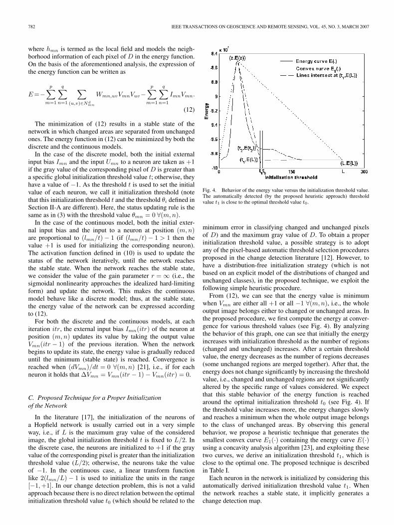
Fig. 4. Behavior of the energy value versus the initialization threshold value.The automatically detected (by the proposed heuristic approach) thresholdvalue t1 is close to the optimal threshold value t0.

minimum error in classifying changed and unchanged pixelsof D) and the maximum gray value of D. To obtain a properinitialization threshold value, a possible strategy is to adoptany of the pixel-based automatic threshold selection proceduresproposed in the change detection literature [12]. However, tohave a distribution-free initialization strategy (which is notbased on an explicit model of the distributions of changed andunchanged classes), in the proposed technique, we exploit thefollowing simple heuristic procedure.

From (12), we can see that the energy value is minimumwhen Vmn are either all +1 or all −1 ∀(m,n), i.e., the wholeoutput image belongs either to changed or unchanged areas. Inthe proposed procedure, we first compute the energy at conver-gence for various threshold values (see Fig. 4). By analyzingthe behavior of this graph, one can see that initially the energyincreases with initialization threshold as the number of regions(changed and unchanged) increases. After a certain thresholdvalue, the energy decreases as the number of regions decreases(some unchanged regions are merged together). After that, theenergy does not change significantly by increasing the thresholdvalue, i.e., changed and unchanged regions are not significantlyaltered by the specific range of values considered. We expectthat this stable behavior of the energy function is reachedaround the optimal initialization threshold t0 (see Fig. 4). Ifthe threshold value increases more, the energy changes slowlyand reaches a minimum when the whole output image belongsto the class of unchanged areas. By observing this generalbehavior, we propose a heuristic technique that generates thesmallest convex curve E1(·) containing the energy curve E(·)using a concavity analysis algorithm [23], and exploiting thesetwo curves, we derive an initialization threshold t1, which isclose to the optimal one. The proposed technique is describedin Table I.

Each neuron in the network is initialized by considering thisautomatically derived initialization threshold value t1. Whenthe network reaches a stable state, it implicitly generates achange detection map.


TABLE IALGORITHM FOR AUTOMATICALLY DERIVING

THE INITIALIZATION THRESHOLD

IV. EXPERIMENTAL RESULTS

A. Description of the Experiments

In our experiments, we used two different data sets related totwo areas in Mexico and Italy. Four change detection maps weregenerated for each data set by using four different Hopfieldnetwork models (i.e., the maps were produced by the discreteand continuous Hopfield models considering first- and second-order neighborhoods). In the continuous model, the activationfunction defined in (10) was used for updating the status ofthe network setting r = 2 to have a moderate steepness. It isworth noting that the change detection process is less sensitiveto variations of r. On the basis of these results, two differentexperiments were carried out to test the validity of the proposedtechnique.

The first experiment aims at evaluating the effectivenessof both the proposed technique and the related initializationalgorithm (see Section III-C). To this end, the optimal initial-ization threshold value t0 was computed by a manual trial-and-error procedure, i.e., generating the change detection mapby initializing the network with different threshold values andcomputing the corresponding overall change detection error byusing the available reference map. The optimal initializationthreshold value t0 corresponds to the minimum overall error.This value and the related error were compared with the valueof the initialization threshold t1 obtained automatically bythe proposed approach and the corresponding overall changedetection error, respectively.

The second experiment compares the results provided by theproposed technique with the best possible accuracies obtainedboth manually and with a context-sensitive change detectiontechnique published in the literature [12]. This experimentis aimed at assessing the effectiveness of the proposed tech-nique in terms of change detection error by comparing it with

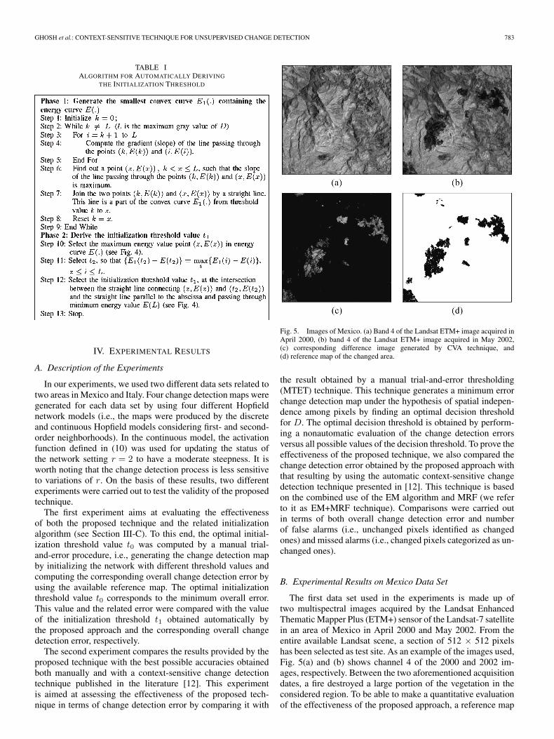
Fig. 5. Images of Mexico. (a) Band 4 of the Landsat ETM+ image acquired inApril 2000, (b) band 4 of the Landsat ETM+ image acquired in May 2002,(c) corresponding difference image generated by CVA technique, and(d) reference map of the changed area.

the result obtained by a manual trial-and-error thresholding(MTET) technique. This technique generates a minimum errorchange detection map under the hypothesis of spatial indepen-dence among pixels by finding an optimal decision thresholdfor D. The optimal decision threshold is obtained by perform-ing a nonautomatic evaluation of the change detection errorsversus all possible values of the decision threshold. To prove theeffectiveness of the proposed technique, we also compared thechange detection error obtained by the proposed approach withthat resulting by using the automatic context-sensitive changedetection technique presented in [12]. This technique is basedon the combined use of the EM algorithm and MRF (we referto it as EM+MRF technique). Comparisons were carried outin terms of both overall change detection error and numberof false alarms (i.e., unchanged pixels identified as changedones) and missed alarms (i.e., changed pixels categorized as un-changed ones).

B. Experimental Results on Mexico Data Set

The first data set used in the experiments is made up oftwo multispectral images acquired by the Landsat EnhancedThematic Mapper Plus (ETM+) sensor of the Landsat-7 satellitein an area of Mexico in April 2000 and May 2002. From theentire available Landsat scene, a section of 512 × 512 pixelshas been selected as test site. As an example of the images used,Fig. 5(a) and (b) shows channel 4 of the 2000 and 2002 im-ages, respectively. Between the two aforementioned acquisitiondates, a fire destroyed a large portion of the vegetation in theconsidered region. To be able to make a quantitative evaluationof the effectiveness of the proposed approach, a reference map


TABLE IICHANGE DETECTION RESULTS OBTAINED BY THE PROPOSED

APPROACH (CONSIDERING FOUR DIFFERENT NETWORK MODELS)INITIALIZED BY THE OPTIMAL INITIALIZATION THRESHOLD t0

AND THE AUTOMATICALLY DERIVED INITIALIZATION

THRESHOLD t1 (BAND 4, MEXICO DATA SET)

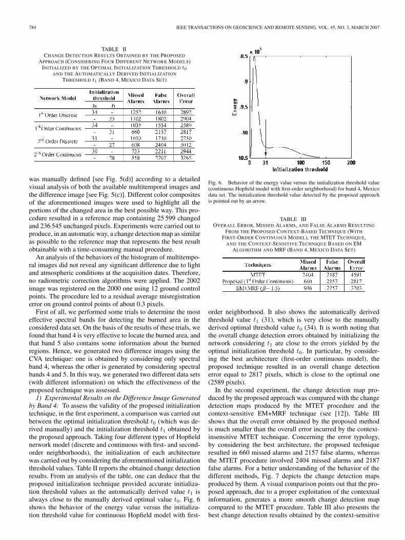
was manually defined [see Fig. 5(d)] according to a detailedvisual analysis of both the available multitemporal images andthe difference image [see Fig. 5(c)]. Different color compositesof the aforementioned images were used to highlight all theportions of the changed area in the best possible way. This pro-cedure resulted in a reference map containing 25 599 changedand 236 545 unchanged pixels. Experiments were carried out toproduce, in an automatic way, a change detection map as similaras possible to the reference map that represents the best resultobtainable with a time-consuming manual procedure.

An analysis of the behaviors of the histogram of multitempo-ral images did not reveal any significant difference due to lightand atmospheric conditions at the acquisition dates. Therefore,no radiometric correction algorithms were applied. The 2002image was registered on the 2000 one using 12 ground controlpoints. The procedure led to a residual average misregistrationerror on ground control points of about 0.3 pixels.

First of all, we performed some trials to determine the mosteffective spectral bands for detecting the burned area in theconsidered data set. On the basis of the results of these trials, wefound that band 4 is very effective to locate the burned area, andthat band 5 also contains some information about the burnedregions. Hence, we generated two difference images using theCVA technique: one is obtained by considering only spectralband 4, whereas the other is generated by considering spectralbands 4 and 5. In this way, we generated two different data sets(with different information) on which the effectiveness of theproposed technique was assessed.1) Experimental Results on the Difference Image Generated

by Band 4: To assess the validity of the proposed initializationtechnique, in the first experiment, a comparison was carried outbetween the optimal initialization threshold t0 (which was de-rived manually) and the initialization threshold t1 obtained bythe proposed approach. Taking four different types of Hopfieldnetwork model (discrete and continuous with first- and second-order neighborhoods), the initialization of each architecturewas carried out by considering the aforementioned initializationthreshold values. Table II reports the obtained change detectionresults. From an analysis of the table, one can deduce that theproposed initialization technique provided accurate initializa-tion threshold values as the automatically derived value t1 isalways close to the manually derived optimal value t0. Fig. 6shows the behavior of the energy value versus the initializa-tion threshold value for continuous Hopfield model with first-

Fig. 6. Behavior of the energy value versus the initialization threshold value(continuous Hopfield model with first-order neighborhood) for band 4, Mexicodata set. The initialization threshold value detected by the proposed approachis pointed out by an arrow.

TABLE IIIOVERALL ERROR, MISSED ALARMS, AND FALSE ALARMS RESULTING

FROM THE PROPOSED CONTEXT-BASED TECHNIQUE (WITH

FIRST-ORDER CONTINUOUS MODEL), THE MTET TECHNIQUE,AND THE CONTEXT-SENSITIVE TECHNIQUE BASED ON EM

ALGORITHM AND MRF (BAND 4, MEXICO DATA SET)

order neighborhood. It also shows the automatically derivedthreshold value t1 (31), which is very close to the manuallyderived optimal threshold value t0 (34). It is worth noting thatthe overall change detection errors obtained by initializing thenetwork considering t1 are close to the errors yielded by theoptimal initialization threshold t0. In particular, by consider-ing the best architecture (first-order continuous model), theproposed technique resulted in an overall change detectionerror equal to 2817 pixels, which is close to the optimal one(2589 pixels).

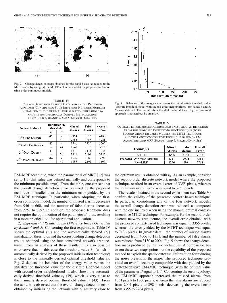
In the second experiment, the change detection map pro-duced by the proposed approach was compared with the changedetection maps produced by the MTET procedure and thecontext-sensitive EM+MRF technique (see [12]). Table IIIshows that the overall error obtained by the proposed methodis much smaller than the overall error incurred by the context-insensitive MTET technique. Concerning the error typology,by considering the best architecture, the proposed techniqueresulted in 660 missed alarms and 2157 false alarms, whereasthe MTET procedure involved 2404 missed alarms and 2187false alarms. For a better understanding of the behavior of thedifferent methods, Fig. 7 depicts the change detection mapsproduced by them. A visual comparison points out that the pro-posed approach, due to a proper exploitation of the contextualinformation, generates a more smooth change detection mapcompared to the MTET procedure. Table III also presents thebest change detection results obtained by the context-sensitive


Fig. 7. Change detection maps obtained for the band 4 data set related to theMexico area by using (a) the MTET technique and (b) the proposed technique(first-order continuous model).

TABLE IVCHANGE DETECTION RESULTS OBTAINED BY THE PROPOSED



THRESHOLD t1 (BANDS 4 AND 5, MEXICO DATA SET)

EM+MRF technique, when the parameter β of MRF [12] wasset to 1.5 (this value was defined manually and corresponds tothe minimum possible error). From the table, one can see thatthe overall change detection error obtained by the proposedtechnique is smaller than the minimum error yielded by theEM+MRF technique. In particular, when adopting the first-order continuous model, the number of missed alarms decreasesfrom 946 to 660, and the number of false alarms decreasesfrom 2257 to 2157. In addition, the proposed technique doesnot require the optimization of the parameter β, thus, resultingin a more practical tool for operational applications.2) Experimental Results on the Difference Image Generated

by Bands 4 and 5: Concerning the first experiment, Table IVshows the optimal (t0) and the automatically derived (t1)initialization thresholds and the corresponding change detectionresults obtained using the four considered network architec-tures. From an analysis of these results, it is also possibleto observe that in this case the threshold value t1 (which isautomatically derived by the proposed initialization technique)is close to the manually derived optimal threshold value t0.Fig. 8 depicts the behavior of the energy value versus theinitialization threshold value for the discrete Hopfield modelwith second-order neighborhood [it also shows the automati-cally derived threshold value t1 (39), which is very close tothe manually derived optimal threshold value t0 (43)]. Fromthe table, it is observed that the overall change detection errorsobtained by initializing the network with t1 are very close to

Fig. 8. Behavior of the energy value versus the initialization threshold value(discrete Hopfield model with second-order neighborhood) for bands 4 and 5,Mexico data set. The initialization threshold value detected by the proposedapproach is pointed out by an arrow.

TABLE VOVERALL ERROR, MISSED ALARMS, AND FALSE ALARMS RESULTING


SECOND-ORDER DISCRETE MODEL), THE MTET TECHNIQUE,AND THE CONTEXT-SENSITIVE TECHNIQUE BASED ON EM

ALGORITHM AND MRF (BANDS 4 AND 5, MEXICO DATA SET)

the optimum results obtained with t0. As an example, considerthe second-order discrete network model where the proposedtechnique resulted in an overall error of 3355 pixels, whereasthe minimum overall error was equal to 3253 pixels.

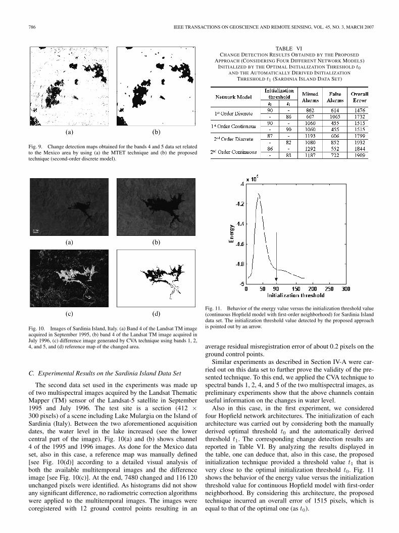
The results obtained in the second experiment (see Table V)confirm the validity of the presented context-based technique.In particular, considering any of the four network models,the overall change detection error was reduced, as comparedwith the one incurred when using the manual optimal context-insensitive MTET technique. For example, for the second-orderdiscrete network architecture, the overall error obtained withthe proposed context-based technique was equal to 3355 pixels,whereas the error yielded by the MTET technique was equalto 7136 pixels. In greater detail, the number of missed alarmsdecreased from 4006 to 1351, and the number of false alarmswas reduced from 3130 to 2004. Fig. 9 shows the change detec-tion maps produced by the two techniques. A comparison be-tween these two maps points out the capability of the proposedmethod to exploit the spatiocontextual information for reducingthe noise present in the maps. The proposed technique pro-vided an overall accuracy comparable with that yielded by thecontext-sensitive EM+MRF technique (with the optimal valueof the parameter β equal to 1.1). Concerning the error typology,the EM+MRF approach increased the missed alarms from1351 pixels to 1866 pixels, whereas the false alarms are reducedfrom 2004 pixels to 898 pixels, decreasing the overall errorfrom 3355 to 2764 pixels.


Fig. 9. Change detection maps obtained for the bands 4 and 5 data set relatedto the Mexico area by using (a) the MTET technique and (b) the proposedtechnique (second-order discrete model).

Fig. 10. Images of Sardinia Island, Italy. (a) Band 4 of the Landsat TM imageacquired in September 1995, (b) band 4 of the Landsat TM image acquired inJuly 1996, (c) difference image generated by CVA technique using bands 1, 2,4, and 5, and (d) reference map of the changed area.

C. Experimental Results on the Sardinia Island Data Set

The second data set used in the experiments was made upof two multispectral images acquired by the Landsat ThematicMapper (TM) sensor of the Landsat-5 satellite in September1995 and July 1996. The test site is a section (412 ×300 pixels) of a scene including Lake Mulargia on the Island ofSardinia (Italy). Between the two aforementioned acquisitiondates, the water level in the lake increased (see the lowercentral part of the image). Fig. 10(a) and (b) shows channel4 of the 1995 and 1996 images. As done for the Mexico dataset, also in this case, a reference map was manually defined[see Fig. 10(d)] according to a detailed visual analysis ofboth the available multitemporal images and the differenceimage [see Fig. 10(c)]. At the end, 7480 changed and 116 120unchanged pixels were identified. As histograms did not showany significant difference, no radiometric correction algorithmswere applied to the multitemporal images. The images werecoregistered with 12 ground control points resulting in an

TABLE VICHANGE DETECTION RESULTS OBTAINED BY THE PROPOSED



THRESHOLD t1 (SARDINIA ISLAND DATA SET)

Fig. 11. Behavior of the energy value versus the initialization threshold value(continuous Hopfield model with first-order neighborhood) for Sardinia Islanddata set. The initialization threshold value detected by the proposed approachis pointed out by an arrow.

average residual misregistration error of about 0.2 pixels on theground control points.

Similar experiments as described in Section IV-A were car-ried out on this data set to further prove the validity of the pre-sented technique. To this end, we applied the CVA technique tospectral bands 1, 2, 4, and 5 of the two multispectral images, aspreliminary experiments show that the above channels containuseful information on the changes in water level.

Also in this case, in the first experiment, we consideredfour Hopfield network architectures. The initialization of eacharchitecture was carried out by considering both the manuallyderived optimal threshold t0 and the automatically derivedthreshold t1. The corresponding change detection results arereported in Table VI. By analyzing the results displayed inthe table, one can deduce that, also in this case, the proposedinitialization technique provided a threshold value t1 that isvery close to the optimal initialization threshold t0. Fig. 11shows the behavior of the energy value versus the initializationthreshold value for continuous Hopfield model with first-orderneighborhood. By considering this architecture, the proposedtechnique incurred an overall error of 1515 pixels, which isequal to that of the optimal one (as t0).


TABLE VIIOVERALL ERROR, MISSED ALARMS, AND FALSE ALARMS RESULTING


FIRST-ORDER CONTINUOUS MODEL), THE MTET TECHNIQUE,AND THE CONTEXT-SENSITIVE TECHNIQUE BASED ON EM

ALGORITHM AND MRF (SARDINIA ISLAND DATA SET)

Fig. 12. Change detection maps obtained for the Sardinia Island data setby using (a) the MTET technique and (b) the proposed technique (first-ordercontinuous model).

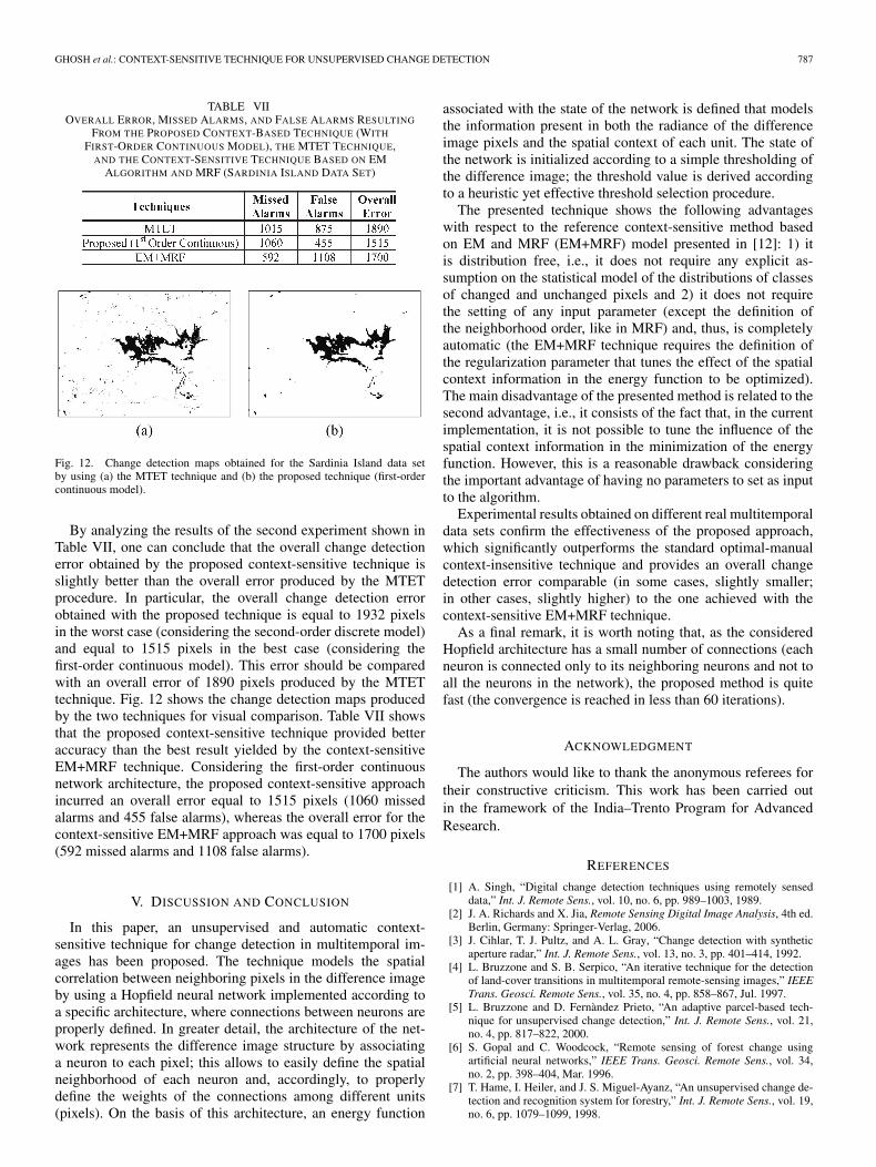
By analyzing the results of the second experiment shown inTable VII, one can conclude that the overall change detectionerror obtained by the proposed context-sensitive technique isslightly better than the overall error produced by the MTETprocedure. In particular, the overall change detection errorobtained with the proposed technique is equal to 1932 pixelsin the worst case (considering the second-order discrete model)and equal to 1515 pixels in the best case (considering thefirst-order continuous model). This error should be comparedwith an overall error of 1890 pixels produced by the MTETtechnique. Fig. 12 shows the change detection maps producedby the two techniques for visual comparison. Table VII showsthat the proposed context-sensitive technique provided betteraccuracy than the best result yielded by the context-sensitiveEM+MRF technique. Considering the first-order continuousnetwork architecture, the proposed context-sensitive approachincurred an overall error equal to 1515 pixels (1060 missedalarms and 455 false alarms), whereas the overall error for thecontext-sensitive EM+MRF approach was equal to 1700 pixels(592 missed alarms and 1108 false alarms).

V. DISCUSSION AND CONCLUSION

In this paper, an unsupervised and automatic context-sensitive technique for change detection in multitemporal im-ages has been proposed. The technique models the spatialcorrelation between neighboring pixels in the difference imageby using a Hopfield neural network implemented according toa specific architecture, where connections between neurons areproperly defined. In greater detail, the architecture of the net-work represents the difference image structure by associatinga neuron to each pixel; this allows to easily define the spatialneighborhood of each neuron and, accordingly, to properlydefine the weights of the connections among different units(pixels). On the basis of this architecture, an energy function

associated with the state of the network is defined that modelsthe information present in both the radiance of the differenceimage pixels and the spatial context of each unit. The state ofthe network is initialized according to a simple thresholding ofthe difference image; the threshold value is derived accordingto a heuristic yet effective threshold selection procedure.

The presented technique shows the following advantageswith respect to the reference context-sensitive method basedon EM and MRF (EM+MRF) model presented in [12]: 1) itis distribution free, i.e., it does not require any explicit as-sumption on the statistical model of the distributions of classesof changed and unchanged pixels and 2) it does not requirethe setting of any input parameter (except the definition ofthe neighborhood order, like in MRF) and, thus, is completelyautomatic (the EM+MRF technique requires the definition ofthe regularization parameter that tunes the effect of the spatialcontext information in the energy function to be optimized).The main disadvantage of the presented method is related to thesecond advantage, i.e., it consists of the fact that, in the currentimplementation, it is not possible to tune the influence of thespatial context information in the minimization of the energyfunction. However, this is a reasonable drawback consideringthe important advantage of having no parameters to set as inputto the algorithm.

Experimental results obtained on different real multitemporaldata sets confirm the effectiveness of the proposed approach,which significantly outperforms the standard optimal-manualcontext-insensitive technique and provides an overall changedetection error comparable (in some cases, slightly smaller;in other cases, slightly higher) to the one achieved with thecontext-sensitive EM+MRF technique.

As a final remark, it is worth noting that, as the consideredHopfield architecture has a small number of connections (eachneuron is connected only to its neighboring neurons and not toall the neurons in the network), the proposed method is quitefast (the convergence is reached in less than 60 iterations).

ACKNOWLEDGMENT

The authors would like to thank the anonymous referees fortheir constructive criticism. This work has been carried outin the framework of the India–Trento Program for AdvancedResearch.

REFERENCES

[1] A. Singh, “Digital change detection techniques using remotely senseddata,” Int. J. Remote Sens., vol. 10, no. 6, pp. 989–1003, 1989.

[2] J. A. Richards and X. Jia, Remote Sensing Digital Image Analysis, 4th ed.Berlin, Germany: Springer-Verlag, 2006.

[3] J. Cihlar, T. J. Pultz, and A. L. Gray, “Change detection with syntheticaperture radar,” Int. J. Remote Sens., vol. 13, no. 3, pp. 401–414, 1992.

[4] L. Bruzzone and S. B. Serpico, “An iterative technique for the detectionof land-cover transitions in multitemporal remote-sensing images,” IEEETrans. Geosci. Remote Sens., vol. 35, no. 4, pp. 858–867, Jul. 1997.

[5] L. Bruzzone and D. Fernàndez Prieto, “An adaptive parcel-based tech-nique for unsupervised change detection,” Int. J. Remote Sens., vol. 21,no. 4, pp. 817–822, 2000.

[6] S. Gopal and C. Woodcock, “Remote sensing of forest change usingartificial neural networks,” IEEE Trans. Geosci. Remote Sens., vol. 34,no. 2, pp. 398–404, Mar. 1996.

[7] T. Hame, I. Heiler, and J. S. Miguel-Ayanz, “An unsupervised change de-tection and recognition system for forestry,” Int. J. Remote Sens., vol. 19,no. 6, pp. 1079–1099, 1998.


[8] P. S. Chavez, Jr. and D. J. MacKinnon, “Automatic detection of vegetationchanges in the southwestern United States using remotely sensed images,”Photogramm. Eng. Remote Sens., vol. 60, no. 5, pp. 1285–1294, 1994.

[9] K. R. Merril and L. Jiajun, “A comparison of four algorithms for changedetection in an urban environment,” Remote Sens. Environ., vol. 63, no. 2,pp. 95–100, 1998.

[10] T. Fung, “An assessment of TM imagery for land-cover change detection,”IEEE Trans. Geosci. Remote Sens., vol. 28, no. 4, pp. 681–684, Jul. 1990.

[11] D. M. Muchoney and B. N. Haack, “Change detection for monitoringforest defoliation,” Photogramm. Eng. Remote Sens., vol. 60, no. 10,pp. 1243–1251, 1994.

[12] L. Bruzzone and D. Fernàndez Prieto, “Automatic analysis of the dif-ference image for unsupervised change detection,” IEEE Trans. Geosci.Remote Sens., vol. 38, no. 3, pp. 1171–1182, May 2000.

[13] J. R. G. Townshend and C. O. Justice, “Spatial variability of images andthe monitoring of changes in the normalized difference vegetation index,”Int. J. Remote Sens., vol. 16, no. 12, pp. 2187–2195, 1995.

[14] A. P. Dempster, N. M. Laird, and D. B. Rubin, “Maximum likelihoodfrom incomplete data via the EM algorithm,” J.R. Stat. Soc., vol. 39, no. 1,pp. 1–38, 1977.

[15] Y. Bazi, L. Bruzzone, and F. Melgani, “An unsupervised approach basedon the generalized Gaussian model to automatic change detection inmultitemporal SAR images,” IEEE Trans. Geosci. Remote Sens., vol. 43,no. 4, pp. 874–887, Apr. 2005.

[16] L. Bruzzone and D. Fernàndez Prieto, “An adaptive semiparametric andcontext-based approach to unsupervised change detection in multitempo-ral remote-sensing images,” IEEE Trans. Image Process., vol. 11, no. 4,pp. 452–466, Apr. 2002.

[17] A. Ghosh, N. R. Pal, and S. K. Pal, “Object background classificationusing Hopfield type neural network,” Int. J. Pattern Recognit. Artif. Intell.,vol. 6, no. 5, pp. 989–1008, 1992.

[18] S. Haykin, Neural Networks: A Comprehensive Foundation. Singapore:Pearson Education, 2003. Fourth Indian Reprint.

[19] S. V. B. Aiyer, M. Niranjan, and F. Fallside, “A theoretical investigationinto the performance of the Hopfield model,” IEEE Trans. Neural Netw.,vol. 1, no. 2, pp. 204–215, Jun. 1990.

[20] J. J. Hopfield, “Neural networks and physical systems with emergentcollective computational abilities,” Proc. Nat. Acad. Sci., U.S.A., vol. 79,no. 8, pp. 2554–2558, Apr. 1982.

[21] ——, “Neurons with graded response have collective computational prop-erties like those of two state neurons,” Proc. Nat. Acad. Sci., U.S.A.,vol. 81, no. 10, pp. 3088–3092, May 1984.

[22] S. K. Pal and D. Dutta Majumdar, Fuzzy Mathematical Approach toPattern Recognition. New York: Halsted, 1986.

[23] A. Rosenfeld and P. De La Torre, “Histogram concavity analysis as an aidin threshold selection,” IEEE Trans. Syst., Man, Cybern., vol. SMC-13,no. 3, pp. 231–235, Mar. 1983.

Susmita Ghosh received the B.Sc. degree (withhonors) in physics and the B.Tech. degree in com-puter science and engineering from the University ofCalcutta, Kolkata, India, in 1988 and 1991, respec-tively, the M.Tech. degree in computer science andengineering from the Indian Institute of Technology,Bombay, in 1993, and the Ph.D. degree in engineer-ing from Jadavpur University, Kolkata, in 2004.

In May 1999, she was with the Institute of Au-tomation, Chinese Academy of Sciences, Beijing,with a CIMPA (France) fellowship. She has also

visited various universities/academic institutes for collaborative research anddelivered lectures in different countries, including Australia, Italy, and Japan.She was a Lecturer with the Department of Computer Science and Engineering,Jadavpur University, during 1997–2002. She is currently a Reader at the samedepartment. Her research interests include genetic algorithms, neural networks,image processing, pattern recognition, soft computing, and remotely sensedimage analysis.

Lorenzo Bruzzone (S’95–M’98–SM’03) receivedthe Laurea Specialistica (M.S.) degree (summa cumlaude) in electronic engineering and the Ph.D. de-gree in telecommunications from the University ofGenoa, Genoa, Italy, in 1993 and 1998, respectively.

From 1998 to 2000, he was a Postdoctoral Re-searcher with the University of Genoa. From 2000to 2001, he was an Assistant Professor with theUniversity of Trento, Trento, Italy, where he was anAssociate Professor from 2001 to 2005. Since March2005, he has been a Full Professor of telecommu-

nications with the University of Trento, where he currently teaches remotesensing, pattern recognition, and electrical communications. He is currently theHead of the Remote Sensing Laboratory, Department of Information and Com-munication Technology, University of Trento. He is the author (or coauthor) ofmore than 150 scientific publications, including journals, book chapters, andconference proceedings. His current research interests are in the area of remotesensing image processing and recognition (analysis of multitemporal data,feature selection, classification, regression, data fusion, and machine learning).He conducts and supervises research on these topics within the frameworks ofseveral national and international projects. Since 1999, he has been appointedEvaluator of project proposals for the European Commission. He is a Refereefor many international journals and has served on the scientific committees ofseveral international conferences.

Dr. Bruzzone ranked first place in the Student Prize Paper Competitionof the 1998 IEEE International Geoscience and Remote Sensing Symposium(Seattle, July 1998). He received recognition of the IEEE TRANSACTIONS

ON GEOSCIENCE AND REMOTE SENSING Best Reviewers in 1999 and was aGuest Editor of a Special Issue of the IEEE TRANSACTIONS ON GEOSCIENCE

AND REMOTE SENSING on the subject of the analysis of multitemporal remotesensing images (November 2003). He was the General Chair and Cochair ofthe First and Second IEEE International Workshop on the Analysis of Multi-temporal Remote Sensing Images. Since 2003, he has been the Chair of theSPIE Conference on Image and Signal Processing for Remote Sensing. He is anAssociate Editor of the IEEE TRANSACTIONS ON GEOSCIENCE AND REMOTE

SENSING. He is a member of the Scientific Committee of the India–ItalyCenter for Advanced Research. He is also a member of the InternationalAssociation for Pattern Recognition and of the Italian Association for RemoteSensing (AIT).

Swarnajyoti Patra received the B.Sc. degree incomputer science and the M.C.A. degree fromVidyasagar University, Midnapore, India, in 1999and 2003, respectively.

He is currently a Research Scholar under theIndia–Trento Program for Advanced Research—Telecommunications project with the Department ofComputer Science and Engineering, Jadavpur Uni-versity, Kolkata, India. His research interests in-clude pattern recognition, evolutionary computation,neural networks, and remote sensing image analysis.


Francesca Bovolo (S’05–M’07) received theLaurea (B.S.) and Laurea Specialistica (M.S.)degrees in telecommunication engineering (summacum laude) and the Ph.D. degree in communicationand information technologies from the Universityof Trento, Trento, Italy, in 2001, 2003, and 2006,respectively.

She currently holds a postdoctoral position at thePattern Recognition and Remote Sensing Group,Department of Information and CommunicationTechnologies, University of Trento. Her main re-

search activity is in the area of remote-sensing image processing; in particular,her interests are related to the analysis of multitemporal data and to change de-tection in multispectral and SAR images. She conducts research on these topicswithin the frameworks of several national and international projects. She is areferee for the International Journal of Remote Sensing, the PhotogrammetricEngineering and Remote Sensing, and the Remote Sensing of Environment.

Dr. Bovolo served on the Scientific Committee of the SPIE Interna-tional Conference on “Signal and Image Processing for Remote Sensing XI”(Stockholm, Sweden, September 2006) and is a member of the ScientificCommittee of the IEEE Fourth International Workshop on the Analysis ofMulti-Temporal Remote Sensing Images (MultiTemp 2007). She is a refereefor the IEEE TRANSACTIONS ON GEOSCIENCE AND REMOTE SENSING.She ranked First Place in the Student Prize Paper Competition of the 2006IEEE International Geoscience and Remote Sensing Symposium (Denver,August 2006).

Ashish Ghosh received the B.E. degree in elec-tronics and telecommunications from Jadavpur Uni-versity, Kolkata, India, in 1987, and the M.Tech.and Ph.D. degrees in computer science from theIndian Statistical Institute, Kolkata, in 1989 and1993, respectively.

He is currently a Professor with the MachineIntelligence Unit, Indian Statistical Institute, and isa member of the founding team that established aNational Center for Soft Computing Research atthe Indian Statistical Institute in 2004 with fund-

ing from the Department of Science and Technology, Government of India.He has been selected as an Associate of the Indian Academy of Sciences,Bangalore, in 1997. From October 1995 to March 1997, he visited the Os-aka Prefecture University, Sakai, Japan, with a postdoctoral fellowship. Healso visited Hannan University, Matsubara, Japan, during September–October1997 and September–October 2004 as a Visiting Faculty and again duringFebruary–April 2005 as a Visiting Professor with a fellowship from the JapanSociety for Promotion of Sciences. In May 1999, he was with the Institute ofAutomation, Chinese Academy of Sciences, Beijing, with a CIMPA (France)fellowship. During January–April 2000, he was with the German NationalResearch Center for Information Technology, Sankt Augustin, with a GermanGovernment (DFG) fellowship. During October–December 2003, he was aVisiting Professor with the University of California, Los Angeles. His visits tothe University of Trento, Trento, Italy, and the University of Palermo, Palermo,Italy, during May–June 2004 and March–April 2006 were in connectionwith collaborative international projects. He has also visited various universi-ties/academic institutes and delivered lectures in different countries, includingSouth Korea, Poland, and The Netherlands. He has already published about100 research papers in internationally reputed journals and referred conferencesand has edited six books. His research interests include pattern recognitionand machine learning, data mining, image analysis, remotely sensed imageanalysis, soft computing, fuzzy sets and uncertainty analysis, neural networks,evolutionary computation, and bioinformatics. He is a Guest Editor for variousinternational journals.

Dr. Ghosh received the prestigious and most coveted Young Scientists Awardin engineering sciences from the Indian National Science Academy in 1995 andYoung Scientists Award in computer science from the Indian Science CongressAssociation in 1992.

A Context-Sensitive Technique for Unsupervised Change ...

Documents

Transcript of A Context-Sensitive Technique for Unsupervised Change ...