A Computational Framework For Unsupervised Analysisof Everyday Human Activities

A ThesisPresented to

The Academic Faculty

by

Muhammad Hamid

In Partial Fulfillmentof the Requirements for the Degree

Doctor of Philosophy

College of ComputingGeorgia Institute of Technology

August 2008

A Computational Framework For Unsupervised Analysisof Everyday Human Activities

Approved by:

Dr. Aaron Bobick, AdvisorCollege of ComputingGeorgia Institute of Technology

Dr. Irfan EssaCollege of ComputingGeorgia Institute of Technology

Dr. James RehgCollege of ComputingGeorgia Institute of Technology

Dr. David HoggSchool of ComputingUniversity of Leeds, U.K.

Dr. Charles IsbellCollege of ComputingGeorgia Institute of Technology

Date Approved: 18 June 2008

To my family.

TABLE OF CONTENTS

LIST OF FIGURES . . . . . . . . . . . . . . . . . . . . . . . . . . . . . . . . . . ix

SUMMARY . . . . . . . . . . . . . . . . . . . . . . . . . . . . . . . . . . . . . . xiii

I INTRODUCTION . . . . . . . . . . . . . . . . . . . . . . . . . . . . . . . . 1

1.1 General Characteristics of Everyday Human Activities . . . . . . . . . . . 2

1.1.1 Intentional Versus Perceptual Aspects . . . . . . . . . . . . . . . 2

1.1.2 Reducible & Hierarchical . . . . . . . . . . . . . . . . . . . . . . 3

1.1.3 Constraint Based & Partially Ordered . . . . . . . . . . . . . . . 4

1.2 Characterizing Everyday Human Activities . . . . . . . . . . . . . . . . . 5

1.2.1 Activities From Direct Perceptual Inputs . . . . . . . . . . . . . . 5

1.2.2 Activities Using Activity Descriptors . . . . . . . . . . . . . . . . 6

1.2.3 Activities As a Function of Intention . . . . . . . . . . . . . . . . 6

1.3 Defining Elements of Human Activity Dynamics . . . . . . . . . . . . . . 7

1.4 Thesis Statement . . . . . . . . . . . . . . . . . . . . . . . . . . . . . . . 9

1.5 Main Contributions . . . . . . . . . . . . . . . . . . . . . . . . . . . . . 10

1.5.1 Activity Representation . . . . . . . . . . . . . . . . . . . . . . . 10

1.5.2 Activity Class Discovery . . . . . . . . . . . . . . . . . . . . . . 11

1.5.3 Activity Class Characterization . . . . . . . . . . . . . . . . . . . 11

1.5.4 Activity Classification & Anomalous Activity Detection: . . . . . 12

1.6 Motivation & Broader Impact . . . . . . . . . . . . . . . . . . . . . . . . 12

II RELATED WORK . . . . . . . . . . . . . . . . . . . . . . . . . . . . . . . . 14

2.1 Activity Modeling . . . . . . . . . . . . . . . . . . . . . . . . . . . . . . 14

2.1.1 Representations Using Motion Fields . . . . . . . . . . . . . . . . 14

2.1.2 Finite State Machines . . . . . . . . . . . . . . . . . . . . . . . . 15

2.1.3 Hidden Markov Models . . . . . . . . . . . . . . . . . . . . . . . 15

2.1.4 Bayesian Networks . . . . . . . . . . . . . . . . . . . . . . . . . 16

2.1.5 Dynamic Bayesian Networks . . . . . . . . . . . . . . . . . . . . 17

iv

2.1.6 Stochastic Context Free Grammars . . . . . . . . . . . . . . . . . 18

2.1.7 Stochastic Petri Nets . . . . . . . . . . . . . . . . . . . . . . . . 18

2.1.8 Symbolic Network Approach . . . . . . . . . . . . . . . . . . . . 19

2.2 Activity-Class Discovery . . . . . . . . . . . . . . . . . . . . . . . . . . 20

2.3 Concept Characterization . . . . . . . . . . . . . . . . . . . . . . . . . . 22

2.3.1 The Classical View . . . . . . . . . . . . . . . . . . . . . . . . . 22

2.3.2 The Probabilistic View: Featural Approach . . . . . . . . . . . . 22

2.3.3 The Probabilistic View: Dimensional Approach . . . . . . . . . . 23

2.3.4 The Probabilistic View: Holistic Approach . . . . . . . . . . . . . 23

2.3.5 The Exemplar View . . . . . . . . . . . . . . . . . . . . . . . . . 23

2.4 Anomaly Detection . . . . . . . . . . . . . . . . . . . . . . . . . . . . . 24

2.4.1 Parametric Approaches . . . . . . . . . . . . . . . . . . . . . . . 24

2.4.2 Non-Parametric Approaches . . . . . . . . . . . . . . . . . . . . 25

2.4.3 Clustering Based Approaches . . . . . . . . . . . . . . . . . . . . 26

2.5 Summary . . . . . . . . . . . . . . . . . . . . . . . . . . . . . . . . . . . 26

III REPRESENTING ACTIVITIES AS BAGS OF EVENT N-GRAMS . . . . 28

3.1 Activity Structure From Event Statistics . . . . . . . . . . . . . . . . . . 28

3.2 Bags of Event n-grams . . . . . . . . . . . . . . . . . . . . . . . . . . . . 29

3.3 Unsupervised Activity-Class Discovery . . . . . . . . . . . . . . . . . . . 30

3.3.1 A Desired Notion of Activity Similarity . . . . . . . . . . . . . . 30

3.3.2 An Activity Similarity Metric . . . . . . . . . . . . . . . . . . . . 31

3.3.3 Activity-Class Discovery . . . . . . . . . . . . . . . . . . . . . . 32

3.3.4 Finding Dominant Sets Using Replicator Dynamics . . . . . . . . 35

3.3.5 Activity Classification . . . . . . . . . . . . . . . . . . . . . . . . 36

3.4 Results: Activity Class Discovery & Classification . . . . . . . . . . . . . 37

3.4.1 Loading Dock Environment . . . . . . . . . . . . . . . . . . . . . 37

3.4.2 Residential House Environment . . . . . . . . . . . . . . . . . . . 40

3.4.3 Noise Analysis of n-grams in Loading Dock Environment . . . . . 43

3.4.4 Automatic Event Detection . . . . . . . . . . . . . . . . . . . . . 45

v

3.5 Summary . . . . . . . . . . . . . . . . . . . . . . . . . . . . . . . . . . . 45

IV REPRESENTING ACTIVITIES USING SUFFIX TREES . . . . . . . . . . 47

4.1 Motivation . . . . . . . . . . . . . . . . . . . . . . . . . . . . . . . . . . 47

4.1.1 Limitations Of Fixed-Length Event n-grams . . . . . . . . . . . . 47

4.1.2 Significance of Capturing Variable-Length Event Dependence . . 48

4.2 Representing Human Activities Using Variable-Length Event Subsequences 49

4.2.1 Basis Event Subsequences . . . . . . . . . . . . . . . . . . . . . 51

4.2.2 Significance of Removing Redundancies Using Basis Event Sub-sequences . . . . . . . . . . . . . . . . . . . . . . . . . . . . . . 51

4.2.3 Basis Event Subsequences Using Suffix Trees . . . . . . . . . . . 52

4.2.4 Representational Scope of Suffix Trees . . . . . . . . . . . . . . . 53

4.3 Empirical Analyses of Suffix Trees . . . . . . . . . . . . . . . . . . . . . 54

4.3.1 Discriminative Prowess of Suffix Trees . . . . . . . . . . . . . . . 55

4.3.2 Noise Sensitivity Analysis . . . . . . . . . . . . . . . . . . . . . 55

4.4 Experimental Setup - Kitchen Environment . . . . . . . . . . . . . . . . . 56

4.4.1 Activity Stages . . . . . . . . . . . . . . . . . . . . . . . . . . . 57

4.4.2 Constraints on Activity Dynamics . . . . . . . . . . . . . . . . . 58

4.4.3 Automatic Event Detection . . . . . . . . . . . . . . . . . . . . . 61

4.5 Results: Activity Class Discovery & Classification . . . . . . . . . . . . . 61

4.5.1 Performance Analysis for a Single Subject . . . . . . . . . . . . . 61

4.5.2 Comparison of Suffix Trees with Smoothed n-grams . . . . . . . . 65

4.5.3 Performance Analysis for Multiple Subjects . . . . . . . . . . . . 66

4.6 Automatic Sequence Parsing Using Suffix Trees . . . . . . . . . . . . . . 70

4.6.1 Extracting Key-Features . . . . . . . . . . . . . . . . . . . . . . 71

4.6.2 Holistic Parsing Using Key-Features . . . . . . . . . . . . . . . . 71

4.6.3 Performance of Holistic Parsing Algorithm . . . . . . . . . . . . 74

4.6.4 Analysis of Holistic Parsing Results . . . . . . . . . . . . . . . . 75

4.6.5 By-Parts Parsing Using Key-Features . . . . . . . . . . . . . . . . 76

4.7 Summary . . . . . . . . . . . . . . . . . . . . . . . . . . . . . . . . . . . 81

vi

V ACTIVITY CLASS CHARACTERIZATION . . . . . . . . . . . . . . . . . 83

5.1 Motivation for Concept Characterization . . . . . . . . . . . . . . . . . . 83

5.2 Characterization of Activity Classes . . . . . . . . . . . . . . . . . . . . . 84

5.3 Class Characterization at a Holistic Level . . . . . . . . . . . . . . . . . . 85

5.3.1 A Method for Finding Typical Members of An Activity Class . . . 86

5.4 Class Characterization at a By-Parts Level . . . . . . . . . . . . . . . . . 87

5.4.1 Defining Event Motifs . . . . . . . . . . . . . . . . . . . . . . . . 87

5.4.2 Formulation of Objective Function . . . . . . . . . . . . . . . . . 88

5.4.3 Objective Function Optimization . . . . . . . . . . . . . . . . . . 89

5.4.4 Results: Discovered Event Motifs . . . . . . . . . . . . . . . . . 90

5.4.5 Subjective Assessment of Discovered Motifs . . . . . . . . . . . . 90

5.5 Summary . . . . . . . . . . . . . . . . . . . . . . . . . . . . . . . . . . . 93

VI ANOMALOUS ACTIVITY DETECTION . . . . . . . . . . . . . . . . . . . 95

6.1 On The Notion Of Anomaly . . . . . . . . . . . . . . . . . . . . . . . . . 95

6.2 Detecting Anomalous Activities . . . . . . . . . . . . . . . . . . . . . . . 96

6.3 Anomaly Detection At a Holistic Level . . . . . . . . . . . . . . . . . . . 97

6.4 Anomaly Detection At a By-Parts Level . . . . . . . . . . . . . . . . . . 105

6.4.1 Defining Anomalies at a Local Level . . . . . . . . . . . . . . . . 106

6.4.2 Anomalies Using Match Statistics . . . . . . . . . . . . . . . . . 107

6.4.3 Anomaly Detection Performance in Kitchen Environment . . . . . 108

6.5 Summary . . . . . . . . . . . . . . . . . . . . . . . . . . . . . . . . . . . 110

VII CONCLUSIONS & FUTURE WORK . . . . . . . . . . . . . . . . . . . . . 112

7.1 Thesis Conclusions . . . . . . . . . . . . . . . . . . . . . . . . . . . . . 113

7.1.1 Learning Global Activity Structure Using Local Event Statistics . 113

7.1.2 Importance of Capturing Variable-Length Event Dependence . . . 114

7.1.3 Specificity versus Sensitivity of Sequential Representations . . . . 114

7.1.4 Importance of Finding Predominant Mode of Temporal Dependence115

7.1.5 Behavior Discovery Using Feature Based View of Activity-Classes 115

vii

7.1.6 A Detection Based Approach To Finding Anomalous Behaviors . 116

7.2 Current Limitations & Future Research Directions . . . . . . . . . . . . . 116

7.2.1 Incorporating Temporal Information of Events . . . . . . . . . . . 117

7.2.2 Selective Usage of Extracted Sequential Features . . . . . . . . . 117

7.2.3 Improving Noise Sensitivity of Suffix Trees . . . . . . . . . . . . 118

7.2.4 Event Detection Using Multiple Sensor Modalities . . . . . . . . 119

7.2.5 Analyzing Group Activities . . . . . . . . . . . . . . . . . . . . . 120

7.2.6 Human Activity Analysis in an Active Learning Paradigm . . . . . 120

7.3 General Applicability of Our Proposed Framework . . . . . . . . . . . . . 121

7.4 Choosing An Appropriate Event Vocabulary . . . . . . . . . . . . . . . . 122

7.5 Concluding Remarks . . . . . . . . . . . . . . . . . . . . . . . . . . . . 125

REFERENCES . . . . . . . . . . . . . . . . . . . . . . . . . . . . . . . . . . . . . 137

viii

LIST OF FIGURES

Figure 1 Different Descriptions of an Example Activity of Walking - (a) Theactivity of walking is considered in terms of the very basic perceptualcues. (b) Walking activity is considered in terms of mid-level activity de-scriptors that follow certain temporal and causal constraints such repeti-tively placing one foot in front of the other. (c) The activity of walkingbeing considered as a function of the person’s intent of walking througha door. . . . . . . . . . . . . . . . . . . . . . . . . . . . . . . . . . . . 5

Figure 2 Illustration of an Example Event - A person shown washing somedishes in the sink of a kitchen. . . . . . . . . . . . . . . . . . . . . . . . 8

Figure 3 General Framework - 1- Starting with a corpus of activities, we extracttheir contiguous subsequences using some activity representation. 2-Based on the frequential information of these subsequences, we define anotion of activity similarity and use it to automatically discover differentactivity classes. 3- We characterize the discovered classes both at holisticand by-parts levels. 4- We classify a test activity to one of the discoveredclasses, and compare it to the previous members of its membership class. 10

Figure 4 Illustration of n-grams - Transformation of an example activity fromsequence of events to histogram of event n-grams. Here the value of n isshown to be equal to 3. . . . . . . . . . . . . . . . . . . . . . . . . . . . 29

Figure 5 Transformation of Activity Corpus Into Activity Graph - we can con-sider a corpus of K activities as an undirected edge-weighted graph withK activity-nodes. Here each node represents the n-grams of one of the Kactivities. The weight of an edge is found according to Equation 1. . . . . 32

Figure 6 Illustration of Activity Class Discovery - Activity-instances are rep-resented as a completed connected, edge-weighted activity graphs G.The edge-weight wp,q between nodes p and q is computed using Equa-tion 1. Maximal cliques of activity-nodes are iteratively found and re-moved from the activity-graph, until there remain no non-trivial maximalcliques. Each of these maximal cliques correspond to an activity-class. . 34

Figure 7 Schematic Diagram of the Camera Setup at The Loading Dock Area- The figure shows overlapping fields of view of the two static camerasused. Representative images as taken from both the Camera 1 and Cam-era 2 are also being shown. Other than that, the main parts of the envi-ronment being shown are the A and B loading docks, the side entrance,and the warehouse entrance. . . . . . . . . . . . . . . . . . . . . . . . . 38

ix

Figure 8 Key Frames of Example Events - The figure shows an example deliveryactivity in a loading dock environment. Only Camera 1 is being shownhere. The key-objects whose interactions define these events are shownin different colored blocks. . . . . . . . . . . . . . . . . . . . . . . . . . 39

Figure 9 Similarity Matrix Before & After Activity Class Discover - Each rowrepresents the similarity of a particular activity with the entire activitytraining set. White implies identical similarity while black representscomplete dissimilarity. The activities ordered after the red cross linein the clustered similarity matrix were dissimilar enough from all otheractivities as to not be included in any non-trivial clique. . . . . . . . . . 39

Figure 10 A Schematic Diagram of the Pressure-Sensors in the ResidentialHouse Environment - The red dots represents the positions of thepressure-sensors. These sensors registered the time when the resident ofthe house walked over them, and this is considered as an events in ourevent vocabulary. . . . . . . . . . . . . . . . . . . . . . . . . . . . . . . 41

Figure 11 Visualization of Similarity Matrices of Residential House Environ-ment - The figure shows the similarity matrices of the training data be-fore and after the procedure of class discovery. White implies identicalsimilarity while black represents complete dissimilarity. The activitiesordered after the red cross line in the clustered similarity matrix weredissimilar enough from all other activities as to not be included in anynon-trivial clique. . . . . . . . . . . . . . . . . . . . . . . . . . . . . . . 42

Figure 12 Performance Analysis Loading Dock Environment - Each graphshows system-performance under synthetically generated noise usingdifferent generative noise models. . . . . . . . . . . . . . . . . . . . . . 44

Figure 13 Length-Sorted Subsequence Contribution to Activity Similarity -The average percentage similarity contribution of basis subsequences ofdifferent lengths for all test points and their respective nearest neighbors. 49

Figure 14 Significance of Linear Cardinality Feature Set - Average percentageclassification difference using basis sub-sequences versus all n-grams. . . 52

Figure 15 Activity Representation - (a) Suffix Tree T for activity a, showing thetrajectory of a person in a kitchen. (b) Activity a represented by countsof basis event subsequences of a, generated by traversing through theSuffix Tree T . . . . . . . . . . . . . . . . . . . . . . . . . . . . . . . . . 53

Figure 16 Feature Space Induced by Suffix Trees vs n-grams - For an exam-ple sequence = {a,b,b,a,c}, the figure shows the feature space inducedby Suffix Trees. This feature space strictly embeds in itself the featurespace generated by n = 1→ 5-grams, showing that for any fixed n, therepresentational power of Suffix Trees is greater than n-grams. . . . . . . 54

x

Figure 17 Discriminative Prowess - Classification accuracy of Suffix Tree repre-sentation as a function of class-overlap. . . . . . . . . . . . . . . . . . . 55

Figure 18 Noise Sensitivity- Classification for various representations relative totheir noise free performance. . . . . . . . . . . . . . . . . . . . . . . . . 56

Figure 19 Activity Stages - Preparation, cooking and finishing stages of an activityare figuratively shown. Notice that in preparation stage, there is temporalorder only within the individual preparatory items. Cooking stage on theother hand follows a more strict temporal constraints. The finishing stagedoes not follow any temporal constraint in particular. . . . . . . . . . . . 59

Figure 20 Positions of Key-Objects and Ingredients - The different key-objectsalong with the various ingredients used are shown. . . . . . . . . . . . . 60

Figure 21 Illustration For Holistic Sequence Parsing - The figure shows the fea-ture counts for two activity classes along with the key-features for bothof them. The ground truth of an example test stream is shown, followedby the varous steps which our proposed mechanism takes to automat-ically parse this stream. For simplicity, here we are only showing thecase for non-overlapping features. . . . . . . . . . . . . . . . . . . . . . 72

Figure 22 Activity Parsing Results - The figure shows an illustration of the pars-ing results obtained for 5 of the 10 trials conducted using a leave-one-outtechnique for learning the key-features for various classes and construct-ing the test streams. The blue-colored graph represents the ground-truthdata, while the red colored shows the parsed output of the system. Foreach of the ground-truth graphs, the uninteresting parts of the stream arerepresented by 0, while activities from different classes are shown byplots of different heights and labeled by numbers 1 2 and 3 respectively.The x-axis in each of the graph shows the symbol-lengths of the inputstreams. . . . . . . . . . . . . . . . . . . . . . . . . . . . . . . . . . . . 73

Figure 23 Illustration of By-Parts Sequence Parsing Setup - The figure showsthe list of event motifs for two example activity classes. For the trainingdata, the activity instances for each class are constructed by conjoiningthe event motifs of respective classes. For testing event stream, the eventmotifs of different activity classes can be interleaved, however the motifsthemselves stay intact. . . . . . . . . . . . . . . . . . . . . . . . . . . . 76

Figure 24 By-Parts Parsing Performance As Function of Maximum MotifLength for Different Amounts of Insertion Noise . . . . . . . . . . . . 78

Figure 25 By-Parts Parsing Performance As Function of Vocabulary Size . . . . 80

Figure 26 By-Parts Parsing Performance As Function of Motif Intersplicing . . 80

xi

Figure 27 ROC Curve For Loading Dock Environment - The figure shows theROC curve obtained for the Loading Dock Environment. The X-axisshows the False Acceptance Rate, while the Y-axis represents the rateof True Positives. Points on this graph give us the expected rate of truepositives and false acceptance rate for corresponding values of threshold.The area under the obtained ROC is 0.94, which indicates a confidenceof 94% in our detection metric. . . . . . . . . . . . . . . . . . . . . . . 99

Figure 28 Anomalous Activities - (a) shows a delivery vehicle leaving the loadingdock with its back door still open. (b) shows an unusual number ofpeople unloading a delivery vehicle. (c) shows a person cleaning theloading dock floor. . . . . . . . . . . . . . . . . . . . . . . . . . . . . . 101

Figure 29 Illustration of Anomaly Explanation - Five simulated activity se-quences are shown to illustrate the different concepts introduced foranomaly explanation. α1 has low value of Pc, its entropy Hc is low andtherefore its predictability is high. α4 has medium Pc, its entropy Hcis also low and its predictability is high. Finally α8 has high Pc, butits entropy Hc is high which makes its predictability low. α1 could beuseful in explaining the extraneous features in an anomaly, while α4could be useful in explaining the features that were deficient in it. . . . . 103

Figure 30 Anomaly Explanation - explanations generated by the system for thedetected anomalies shown in Figure 28. . . . . . . . . . . . . . . . . . . 105

Figure 31 Notion of anomaly - Detection of anomalous subsequences using matchand reverse match statistics. The figure shows an example test activitythat has been classified to a class containing only one training activ-ity. The subsequence bu in the test sequence never appears in trainingsequence and is therefore flagged as anomalous. Subsequence abc how-ever is considered regular since it appears both in the test and the trainingsequences. . . . . . . . . . . . . . . . . . . . . . . . . . . . . . . . . . 107

Figure 32 General Applicability of Proposed Framework in Everyday Environments 121

Figure 33 Illustration of Algorithm 3 - We begin by constructing a complete treeof depth d. P and Q are selected from leaf-set S . Edge probabilitiesof VMMC-1 are sampled from N (0,1). VMMC-2 is constructed byperturbing edge-probabilities of VMMC-1. . . . . . . . . . . . . . . . . 128

xii

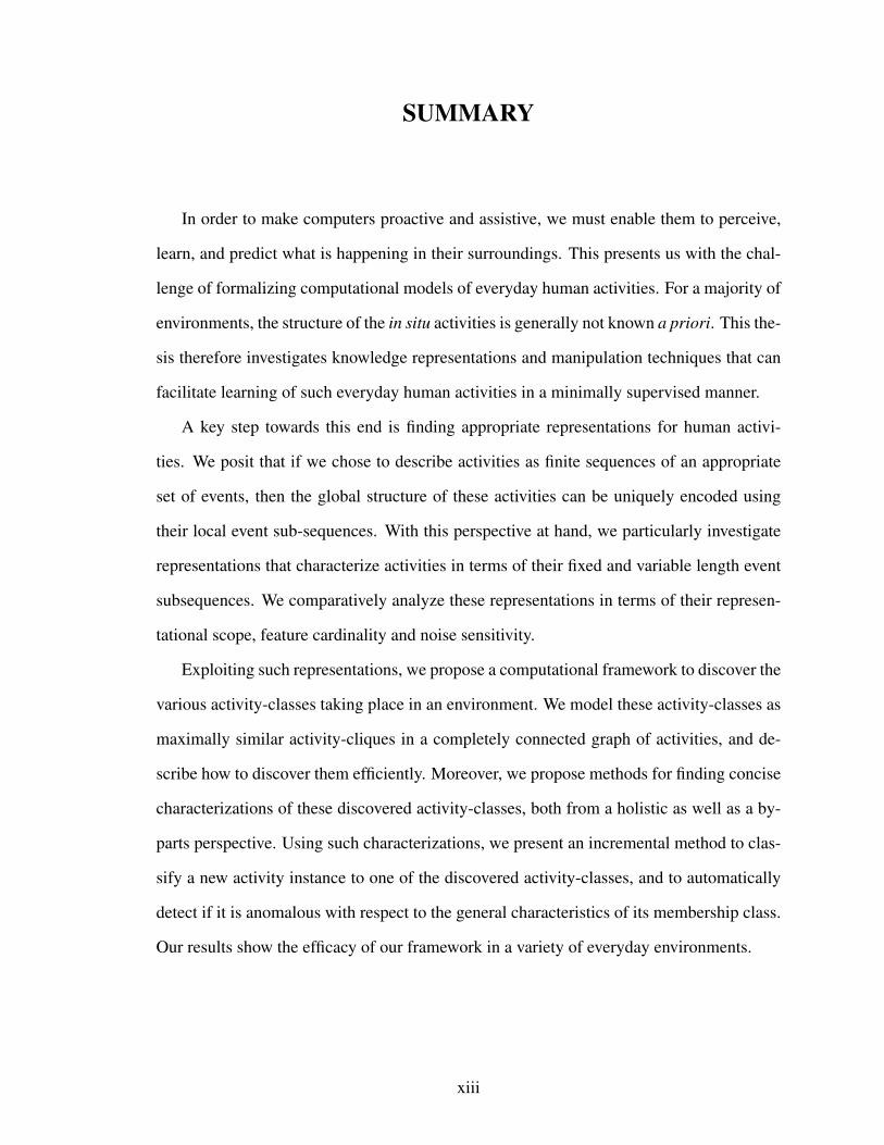
SUMMARY

In order to make computers proactive and assistive, we must enable them to perceive,

learn, and predict what is happening in their surroundings. This presents us with the chal-

lenge of formalizing computational models of everyday human activities. For a majority of

environments, the structure of the in situ activities is generally not known a priori. This the-

sis therefore investigates knowledge representations and manipulation techniques that can

facilitate learning of such everyday human activities in a minimally supervised manner.

A key step towards this end is finding appropriate representations for human activi-

ties. We posit that if we chose to describe activities as finite sequences of an appropriate

set of events, then the global structure of these activities can be uniquely encoded using

their local event sub-sequences. With this perspective at hand, we particularly investigate

representations that characterize activities in terms of their fixed and variable length event

subsequences. We comparatively analyze these representations in terms of their represen-

tational scope, feature cardinality and noise sensitivity.

Exploiting such representations, we propose a computational framework to discover the

various activity-classes taking place in an environment. We model these activity-classes as

maximally similar activity-cliques in a completely connected graph of activities, and de-

scribe how to discover them efficiently. Moreover, we propose methods for finding concise

characterizations of these discovered activity-classes, both from a holistic as well as a by-

parts perspective. Using such characterizations, we present an incremental method to clas-

sify a new activity instance to one of the discovered activity-classes, and to automatically

detect if it is anomalous with respect to the general characteristics of its membership class.

Our results show the efficacy of our framework in a variety of everyday environments.

xiii

CHAPTER I

INTRODUCTION

The measurement and usage of visual motion is one of the fundamental abilities of bi-

ological systems, serving many essential functions. For instance, a sudden movement in

the scene might indicate an approaching predator, or a desirable prey. The rapid expan-

sion of features in the visual fields can signal an object about to collide with the observer.

Similarly, relative movement can be used to infer the 3-dimensional structure of a scene,

allowing efficient movement through the environment.

In more complex organisms such as ourselves, perception of such basic visual motion

gives rise to more involved actions and activities. These actions and activities abound our

daily lives. Simply look around yourself, and you might for instance see someone reading

a book, or talking on the phone, or driving a car etc. This seemingly banal observation

highlights our remarkable ability to understand everyday human activities so effortlessly,

which is in fact crucial for both our physical as well as our social survival.

If we choose to take a reductionist view towards human beings, as biological systems

that can perceive stimuli from their surroundings and can manipulate this information in

a useful way, then we can argue that artificial computational systems might also be able

to do the same tasks with a similar level of competence. In this thesis we explore some

of the computational aspects of building such systems that can analyze the various human

activities in everyday environments.

1

There are many different types of activities that can take place in an environment. Con-

sider for instance a household kitchen, and you can imagine the wide variety of recipes that

can be cooked there. Moreover, each one of these different recipes can be performed in

many different ways. To build systems that can be proactive and assistive in such everyday

environments, it is not plausible to manually model each and every one of these activities,

and to learn these models in a completely supervised manner. We are therefore interested

in knowledge representations and manipulation techniques that can allow computational

systems to analyze human activities with minimal supervision.

The importance of these systems that can learn our everyday activities can be moti-

vated by the vast variety of practical applications that they promise to offer. For instance,

they have the potential to help us in monitoring peoples health as they age, as well as in

fighting crime through improved surveillance. They have tremendous medical applications

in terms of helping surgeons perform better by identifying and evaluating crucial parts of

the surgical procedures, and providing them useful feedback. Similarly, they can help us

improve our productivity in office environments by detecting various interesting and im-

portant events around us to enhance our involvement in various tasks.

1.1 General Characteristics of Everyday Human Activities

While everyday human activities can have a diverse set of characteristics, following is one

way in which these characteristics may be grouped:

1.1.1 Intentional Versus Perceptual Aspects

Human activities generally have some underlying intent. This intent may be implicit or

explicit depending on the nature and scope of the activity [99]. For instance, an activity

such as making an omelet in a household kitchen is performed by a person with an explicit

intent of making something edible. On the other hand, the intent of a person’s activity of

walking is implicit in the context in which it is being performed, i.e. whether someone

2

is walking to get some water, or to go to one’s car, depends on the particular contextual

setting in which the activity of walking is being performed. Intent of an activity may be

thought of describing what an activity is.

At the same time, human activities have a certain perceptual signature associated to

them, i.e., what an activity generally looks like. For example, during the activity of walking,

human body generally moves in a particular pattern through the 3-dimensional space over

a certain duration of time [55]. This spatio-temporal signature of the trajectory of different

body parts as a person moves makes the activity of walking distinguishable from other

activities, such as sitting down, or standing up etc.

While intent is a usually a defining characteristic of human activities, inferring the

intent of an activity can be quite difficult. The challenge for perceptual systems lies in

inferring this goal or outcome using perceptual data. In other words we can only try to

model what an activity looks like, and not necessarily what an activity is. Our hope is

that the differences in the appearance of different activities would be enough to correctly

disambiguate between them.

1.1.2 Reducible & Hierarchical

Human activities often require completion of multiple intermediate tasks for their success-

ful execution. These constituent tasks might be thought of as being arranged in some

hierarchical order [83]. For instance, the activity of making an omelet can be reduced to

being composed of tasks such as beating some eggs, heating some oil, and frying the eggs

etc. The task of beating eggs might still be thought of being composed other constituent

tasks such as fetching some eggs, getting a bowl, getting a beater etc. Such intermediate

constituent tasks of human activities can be usually arranged in a hierarchical manner. It is

generally the case that the more complex an activity is, the more involved is its hierarchy

of composition [31].

3

1.1.3 Constraint Based & Partially Ordered

Successful execution of a variety of human activities depends upon whether certain con-

straints are met or not [73]. These constraints might for instance be:

1- Causal, e.g. pushing the accelerator of a car to cause it to move faster

2- Logical, e.g. opening an oven’s door to get a baked turkey because it was placed in the

oven to be cooked some time ago, or

3- Physical, e.g crossing a river in a boat, since humans themselves cannot walk on water.

The various temporal, logical and causal constrains on the way one can execute activities in

an environment make them partially ordered in nature. In a household kitchen for instance,

if a recipe uses chopped potatoes, then the steps of washing the potatoes, getting a knife

and chopping the potatoes must be performed before using the stove for cooking them.

However, if a recipe uses chopped potatoes and sliced onions, then the set of events needed

to perform these two tasks may very well be interchanged. Capturing this partially ordered

nature of activities is particularly important in distinguishing between different types of

activities. In a loading dock environment for instance, the activities of delivery versus

pickup of packages may both have mostly the same types of events. However the order in

which these events take place in these two types of activities is different, and can be used

to distinguish them from each other.

Characteristics such as the ones mentioned above make everyday human activities an im-

portant class of temporal processes, the perception of which enables us to maintain a better

awareness of the continually changing world around us. These characteristics are in some

sense the concepts according to which we tend to reason about the various human behav-

iors [45], and can therefore be used while designing a computational system for recognition

of such everyday human activities.

4

iiiiiii

iiiii

iiiiii

iiiiii

h

h

hh

Right LegLeft ArmRigh

t Arm

Left L

eg

h

Person

Door

(a) (b) (c)

Figure 1: Different Descriptions of an Example Activity of Walking - (a) The activityof walking is considered in terms of the very basic perceptual cues. (b) Walking activityis considered in terms of mid-level activity descriptors that follow certain temporal andcausal constraints such repetitively placing one foot in front of the other. (c) The activityof walking being considered as a function of the person’s intent of walking through a door.

1.2 Characterizing Everyday Human Activities

Human activities can be considered at various levels of abstraction [114]. The three clas-

sical ways in which scientists have viewed the characterization of human activities are in

terms of (i) direct perceptual inputs, (ii) using a notion of causality amongst some quali-

tative activity descriptors, and (iii) using a notion of context-sensitive intent that dictates

the way in which an activity is carried out. These views facilitate different types of char-

acterizations of human activities, the usefulness of which depends on the dynamics and

complexity of the activities being considered. We present here a brief outline of these

views on human activities with the help of a motivating example.

1.2.1 Activities From Direct Perceptual Inputs

Consider the activity of a person walking in a room. One way of interpreting this activity

may be using the motion properties of the scene detected directly through the raw percep-

tual cues (see Figure 1-a) [89]. In this characterization of walking, there is no notion of

time, physical states, or causality, and the activity is coded strictly in terms of low level sen-

sory stimuli. It is argued that human beings perceive a set of our everyday activities purely

on the basis of direct perceptual inputs. The classic demonstration of activity detection by

5

humans using direct perceptual information was done by the “Moving Lights Display” ex-

periment [55] where human subjects were able to distinguish between actions of walking,

running or stair climbing simply from the intensity patterns of the lights attached to the

joints of actors. Not utilizing any semantic information, this characterizations of human

activities is generally limited to the class of activities that are quite basic in nature.

1.2.2 Activities Using Activity Descriptors

Another way to look at our example activity of walking may be in terms of certain se-

mantically meaningful activity-descriptors [104], such as repetitively putting one foot in

front of another while keeping the other foot on the ground (see Figure 1-b). Such activity-

descriptors follow basic rules of causality, e.g. the movement of one foot is caused by the

other foot having placed on the ground. Similarly, these activity-descriptors must follow a

set of physical constraints, e.g. both feet cannot be apart from each other beyond a certain

distance which is a function of the person’s physical frame. This characterization of human

activities is also context sensitive, i.e. the interpretation requires some notion of a person’s

feet, the difference between left and right, and some notion of the ground [70].

1.2.3 Activities As a Function of Intention

Another way of interpreting human activities involves inferring the goal of the actor exe-

cuting that activity, and organizing the actions into a plan structure [99]. For instance, the

activity of walking may be interpreted as a manifestation of an actor’s intent of moving

through an open door by repeatedly putting one foot in front of another in the direction of

the door (see Figure 1-c). This teleological view represents activities as triplets of contexts,

behaviors, and states [22]. In our example activity of walking, the context is a room, the

behavior is horizontal movement of a person through some intermediate repetitive actions,

and the final state is whether the person has moved through the door or not. While this

interpretation allows understanding of a large variety of complex human activities, it does

assume a substantive amount of contextual semantic knowledge.

6

One of the key challenges in building perceptual systems that can recognize human activ-

ities is the big gap that exists between the low level perceptual inputs such as pixel values

or microphone voltages, and some of the higher level inferences such as what dish is be-

ing prepared in a household kitchen, or whether the cook forgot to add in salt etc. This

semantic void is one of the main reasons for information uncertainty, which in turn results

in poor inference accuracy. A natural way to bridge this gap is to have a set of intermediate

characterizations that would appropriately channel the low-level perceptual information all

the way to higher level inference stage.

The granularity at which these intermediate characterizations should be defined

presents a trade-off between how expressive the characterizations are, versus the robust-

ness with which they can be detected through low-level sensor data. There are no hard and

fast rules according to which the granularity of these intermediate characterizations should

be defined. In general this granularity is carefully chosen according to the dynamics of an

environment and the types of activities being performed. In the following, we define a set

of such intermediate characterizations that we shall use throughout this thesis.

1.3 Defining Elements of Human Activity Dynamics

One way of looking at everyday environments is in terms of a set of perceptually detectable

key-objects [60], which may be defined as:

Key-object: An object present in an environment that provides functionalities that may be

required for the execution of activities of interest in that environment.

We assume that a list of key-objects for an environment is known. An illustrative figure

showing a list of key-objects in a kitchen environment is shown in Figure 2. These objects

pose a certain set of spatial and temporal constraints on the way we generally execute our

activities. For instance, one has to open a fridge before one can get milk out of it. Similarly,

one must turn a stove on before one can use it to fry eggs, etc. Our hypothesis is that these

7

Person

Sink

Fridge

Enter/Exit

Stove Table

Washer

Shelf 1

Shelf 2 Shelf 3

Figure 2: Illustration of an Example Event - A person shown washing some dishes inthe sink of a kitchen.

constraints can be used to define a certain set of perceptually detectable activity-descriptors.

We call these descriptors Events which are defined as:

Event: A particular interaction among a subset of key-objects over a finite duration of time.

A figure showing a key-frame of an example event of a person washing some dishes in a

sink of a kitchen is shown in Figure 2.

Event Vocabulary: The set of interesting events that can take place in an environment.

The event vocabulary for an environment such as a household kitchen may consist of events

like person opens the fridge door, person turns the stove on, person turns the faucet on, etc.

We assume that such an event vocabulary is known a priori.

Activity: A finite sequence of events.

To illustrate the notion of activities in an everyday environment, an example activity of

making scrambled eggs is described below:

Make Scrambled Eggs = Enter Kitchen→ Turn Stove On→ Get Eggs

→ Fry Eggs→ Turn Stove Off→ Leave Kitchen

We assume that the start and end events of activities are known a priori. Moreover, we

assume that every activity must be finished before another is started, i.e. the question of

8

overlapping activities is not included in our problem domain. In the later part of this thesis

we will describe ways to relax some of these constraints.

1.4 Thesis Statement

We want to efficiently learn everyday human activities using some activity representation

that does not require us to manually encode the structural information of these activities

in a completely supervised manner. By structural information of an activity, we mean the

various events constituting that activity, and the temporal order in which these constituent

events are arranged. Our approach to this challenge is based on our hypothesis that we can

learn the global structure of activities simply by using their local event subsequences. In

particular, our thesis states:

Thesis Statement: “The structure of activities can be encoded using a subset of their

contiguous event subsequences, and this encoding is sufficient for activity discovery and

recognition”.

At the heart of our thesis is the question whether we can have an appropriately descrip-

tive yet robustly detectable event vocabulary to describe human activities in a variety of

everyday environments. Such intermediate sets of characterizations have been previously

shown to exist for representing other temporal processes including speech [91], text docu-

ments [97], and protein sequences [7].

We argue that everyday environments pose a certain set of spatial and temporal con-

straints on the way we generally execute our activities [60]. We believe that these con-

straints can be used to construct a set of robustly detectable events that can appropriately

describe the various activities taking place in an environment. These events can channel

the low-level information detected from the sensors, in a manner that facilitates making

useful higher-level inferences. The idea of learning the structural information of activities

simply by looking at the statistics of their local event subsequences is essential to allow us

9

a1

a2

aN

i gRepresentation

p

up

u

p

u

a1

a2

aN

i

Class Discovery&

Characterization

C1

C2

C3 Classification &Anomaly Detectiongg

Figure 3: General Framework - 1- Starting with a corpus of activities, we extract theircontiguous subsequences using some activity representation. 2- Based on the frequentialinformation of these subsequences, we define a notion of activity similarity and use it toautomatically discover different activity classes. 3- We characterize the discovered classesboth at holistic and by-parts levels. 4- We classify a test activity to one of the discoveredclasses, and compare it to the previous members of its membership class.

to move away from the traditional grammar driven approaches for activity modeling, and

adopt a more data-driven learning based perspective. We further elaborate on the question

of selecting an appropriate event vocabulary to describe everyday activities in Chapter 7.

1.5 Main Contributions

We consider this data-driven view of analyzing human activities in four principled ways:

1- Representing activities in terms of their local event subsequences

2- Discovery of the various activity classes in an environment

3- Characterization of the discovered activity classes, and

4- Detection of activities that deviate from general characteristics of discovered classes.

A general overview of the way these steps are undertaken during activity analysis is shown

in figure 3. A brief description of these main contributions follows:

1.5.1 Activity Representation

We propose sequence representations that consider human activities in terms of their con-

tiguous event subsequences of fixed, or variable lengths. In particular, we first consider

activities as histograms of their event n-grams, where an n-gram is a contiguous activity

subsequence of length n. Event n-grams however can only capture activity structure up

to a fixed temporal scale. Events in human activities on the other hand usually depend

10

on their preceding events over variable lengths of time. While entering an unlit room for

instance, a person generally turns the light on after opening the door. In other words the

event of turning the light on is dependent on the immediately previous event of opening

the door. However, while washing dishes in a household kitchen, the event of turning the

faucet on, is usually followed by rinsing the dishes, followed by turning the faucet off. In

other words, the event of turning the faucet off is dependent of the previous two events. In

order to model human activities more accurately, it is important to efficiently represent this

variable length event dependencies. To this end, we explore the usage of Suffix Trees as

an activity representation that allows efficient encoding of activities in terms of their con-

tiguous subsequences of variable lengths. We compare these two representations in terms

of their representational scope, feature cardinality and noise sensitivity.

1.5.2 Activity Class Discovery

Exploiting such representations, we propose a computational framework to discover the

various activity-classes taking place in an environment in an unsupervised manner. We

model these activity-classes as maximally similar activity-cliques in a completely con-

nected graph of activities, and show how to discover them efficiently.

1.5.3 Activity Class Characterization

Finding characterizations of the discovered activity-classes is imperative for online activity

classification as well as anomaly detection. In this regard, we propose methods for finding

concise characterizations of these discovered activity-classes, both from a holistic as well

as a by-parts perspective. From a holistic view, we formalize the problem as finding typical

members of activity-classes that, to some measure, best represent all the members of the

activity-class. On a by-parts level, we consider this problem as that of finding recurrent

event subsequences in the member activities of an activity class. We call these recurrent

event subsequences event motifs, and find them in a why such that they are maximally

mutually exclusive amongst the various activity-classes.

11

1.5.4 Activity Classification & Anomalous Activity Detection:

Using such characterizations, we present a method to classify a new activity instance to

one of the discovered activity-classes, and to automatically detect if it is anomalous with

respect to the general characteristics of its membership class. We consider the notion of

anomaly detection both at a global as well as at a local level. We also present an information

theoretic method to explain the detected anomalies in a maximally informative manner.

1.6 Motivation & Broader Impact

Temporal processes are ubiquitous in nature [3]. Solar cycles, weather patterns, and pan-

demic spreads etc., are all examples of processes that can be modeled using temporal se-

quences. Everyday human activities are an important class of such processes whose analy-

sis requires an understanding of human perception, cognition, and behavior [100]. We are

interested in designing computational systems that can learn to automatically analyze the

various human activities performed in everyday environments [30].

Over the years, computers have continued to become more powerful. This has lead

to new opportunities to have systems that can potentially recognize increasingly complex

activities. While the earlier work on this problem was mostly focused on specific well-

structured activities performed in constrained situations [77], there has been a recent focus

on more complex everyday human activities performed in relatively large-scale uncon-

strained environments [20]. Our work is another step in this direction. Any progress to

this end would influence such fields as robotics [111], ubiquitous computing [101], and

computational sociology [19], just to name a few.

Exploring the problem of unsupervised analysis of human activities may be motivated

both from theoretical as well as practical imperatives. From a more practical perspective,

systems that can perform unsupervised activity analysis can help verify an expert’s intuition

about a domain, find behaviors in a new domain that was previously unexplored, or help

detect irregular patterns not obvious to an expert. They may also be applied to find useful

12

summarizations of large sets of activities, and for learning typical or predictable behav-

iors crucial in understanding the dynamics of an environment. The principles that govern

such perceptual systems can be applied for a wide variety of sensor modalities making

them extremely general-purpose and potentially very effective. In particular, the various

types of data that could be exploited by such systems include EEG signals [17], text docu-

ments [122], on-body sensory signals [74], and identification data such as RFIDs [120].

From a more theoretical perspective, the problem at hand raises a fundamental question

regarding the notion of meaningful representations for intelligent systems. In other words,

in what ways should the perceptual bias of an expert be reflected in the knowledge rep-

resentations and manipulation mechanisms used by an intelligent system. The futility of

bias free learning dictates that there is no escape from some rudimentary bias that must be

incorporated, for how else could a system be evaluated [116]. However finding the optimal

amount and the nature of this bias is anything but trivial.

We view this challenge of finding the right perceptual bias from a learning-based per-

spective. Unlike traditional knowledge-based approaches, we are interested in minimally

supervised mechanisms that allow a system to use its sensory data to learn characterizations

that best inform its inference [21]. Such a data-driven approach focuses more on the detec-

tion and learnability of concept-characterizations, rather than their human interpretability.

It therefore facilitates the acquisition of detectable, robust, and adaptable characterizations

that can be used to learn concepts of increasing complexity. This work is an exploration of

methods that may allow intelligent systems to discover meaningful and relatively indige-

nous concepts - a longstanding goal in A.I.

13

CHAPTER II

RELATED WORK

Our work mostly builds on progress made in the areas of Activity Modeling, Activity-Class

Discovery, Concept Characterization, and Anomaly Detection. This chapter provides an

overview of the related previous work in these areas.

2.1 Activity Modeling

The problem of modeling everyday human activities has been studied in various con-

texts, including computational perception [10], ubiquitous computing [24], as well as

robotics [108]. Much has been written about activity decomposition and the role of knowl-

edge in the perception of motion [8], where scientists have worked on understanding the

psychological [112] as well as computational basis of how motion is perceived [124] [114].

One of the key problems in this regard is finding representations that are robust and

efficiently computable. Most of the previous approaches towards this end assume that

the structure of activities being modeled is known a priori (see e.g. [51] [75] [103] [77]

[12] [67] and the references therein). However, such prior knowledge about activity struc-

ture is generally not at hand. These grammar driven modeling approaches are therefore

limited to representing activities performed in relatively small-scale constrained environ-

ments, underscoring the motivation of our thesis. We can broadly group these previous

modeling approaches into following classes:

2.1.1 Representations Using Motion Fields

The key idea behind such representations is to map a spatio-temporal pattern of a person’s

motion to a static spatial pattern, which can thereon be used for recognition. One such

14

method, proposed in [9] uses the notion of Motion Energy Image (MEI), and Motion His-

tory Images (MHI), to encode the motion patterns of various objects into a single static

image. Work done in [29] uses representations based on motion fields for videos particu-

larly of small size and poor quality.

Such representations are fast to compute and robust to sensor noise, however they are

best applicable for simple settings with usually a single object. The reason for this limita-

tion is that these representations focus on the low-level image-signals to encode the activity

structure without using any mid-level activity-characterizations that can potentially get at

the underlying activity structure in a more explicit way.

2.1.2 Finite State Machines

A finite state machine (FSM) is composed of a set of nodes with probabilistic directed

links amongst them. Usually the topology of the machine is specified by an expert while

the transition probabilities of the links are learned from some training set [96]. FSMs are

useful in describing a single stream of processes in a comprehensible manner. Each node

has some semantic meaning in the high level description, which depends on the attributes

of a segment of lower level observations. The gap between the actual observation features

and the semantic meaning of nodes is usually bridged in some ad-hoc manner.

While FSMs are reasonably competent in modeling activities whose structure is ex-

plicitly known a priori, their applicability is limited to a set of relatively simple activities.

Moreover, they need labeled training data in order to learn the various transition proba-

bilities, which limits their applicability to activities in large-scale everyday environments

where such labeled data is usually not available.

2.1.3 Hidden Markov Models

Hidden Markov Models (HMMs) are a well-known generative framework to model and

classify dynamic behaviors. This framework offers automatic dynamic time warping, ef-

ficient training and inference algorithms, and clear Bayesian semantics. HMMs have so

15

far seen the most application for activity modeling, largely because of their success for

the problem of speech recognition [91]. In particular, HMMs have been used to recognize

fairly complex American Sign Language actions [106], gesture recognition [118] and to

model multi-agent activities [12], just to name a few.

Theoretically, an HMM is a probabilistic finite-state machine. Its major difference

with a normal FSM is how it is constructed. Usually, FSM is designed by first having the

topology and the meaning of nodes, followed by the individual training of the node for

the observation model. HMMs on the other hand usually start with no definite semantic

meaning of the nodes and a loosely defined topology. The semantic meaning of the nodes

can be understood in retrospect once the training is completed.

The reason why HMMs do not need an explicit encoding of their topology is because

they assume a flat topological-structure with a first order Markov assumption for transition

amongst their various states. While this allows them to be implemented readily without

having to manually script out their topology, this feature of HMMs can also play as one

of their limitations to model activities where event dependence is more than first order

Markovian. Moreover, like FSMs, they mostly need to be trained in a supervised framework

using labeled data, which may not be available in largely unconstrained environments.

2.1.4 Bayesian Networks

Bayesian Networks (BNs) are a well defined probabilistic reasoning tool. The nodes of

a Bayesian Network usually have semantic meaning and its links are derived from causal

relationships, making it a very powerful and direct tool to describe the real world [28].

Furthermore, inference on BNs can be carried out using the junction tree algorithm [80] in

polynomial time, making them suitable for a large variety of modeling problems.

Besides the challenges of having to know the exact structure of the problem, as well as

learning the parameters of this model in a supervised manner, BNs do not have a notion

of a temporally evolving process. Rather the process is modeled using some hand-picked

16

instants. While researchers have suggested extensions to this end, such as using specialized

temporal nodes [49], or incorporating the temporal aspect of using leaf nodes [15], the BN

framework is naturally not geared for this type of temporal modeling. This makes BNs

difficult to apply for activities that can evolve over variable durations of time.

2.1.5 Dynamic Bayesian Networks

Dynamic Bayesian Networks (DBNs) are derived from Bayesian Networks to incorporate

the temporal aspect of a process in a more effective way [28]. DBNs are generally used

to model stationary Markov processes. At each time step, this process has a set of hidden

nodes and evidence nodes. Since in stationary markov processes only the variables in

the previous time step influence the current variables, this ensures the hidden variable in

previous time step D-separate the future from the past [80]. The inference in DBNs can

therefore be completed iteratively with only two sets of variables - one representing the

beliefs at the previous time step, and the other representing beliefs at the current time step.

DBNs have been used to model human activities in various scenario. For instance, work

done in [62] attempts to recognize the traffic patterns by a handcrafted DBNs. Similarly,

the work in [76] uses DBNs to model activities for surveillance systems. Work done in [54]

proposes to use an Adaboost training infrastructure to learn the transition and observation

probabilities of DBNs.

A fundamental challenge for DBNs is learning the topology of the network. Due to

this challenge, a majority of the previous work done in this regard has used hand-crafted

topologies of the network, whose parameters are learned in a supervised manner. Learning

the topology of DBNs using some training data is an ongoing research problem, and any

step towards this end will really increase the applicability of DBNs for modeling activities

in unconstrained everyday environments.

17

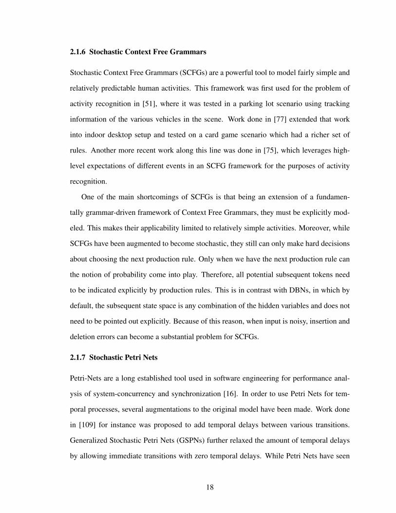
2.1.6 Stochastic Context Free Grammars

Stochastic Context Free Grammars (SCFGs) are a powerful tool to model fairly simple and

relatively predictable human activities. This framework was first used for the problem of

activity recognition in [51], where it was tested in a parking lot scenario using tracking

information of the various vehicles in the scene. Work done in [77] extended that work

into indoor desktop setup and tested on a card game scenario which had a richer set of

rules. Another more recent work along this line was done in [75], which leverages high-

level expectations of different events in an SCFG framework for the purposes of activity

recognition.

One of the main shortcomings of SCFGs is that being an extension of a fundamen-

tally grammar-driven framework of Context Free Grammars, they must be explicitly mod-

eled. This makes their applicability limited to relatively simple activities. Moreover, while

SCFGs have been augmented to become stochastic, they still can only make hard decisions

about choosing the next production rule. Only when we have the next production rule can

the notion of probability come into play. Therefore, all potential subsequent tokens need

to be indicated explicitly by production rules. This is in contrast with DBNs, in which by

default, the subsequent state space is any combination of the hidden variables and does not

need to be pointed out explicitly. Because of this reason, when input is noisy, insertion and

deletion errors can become a substantial problem for SCFGs.

2.1.7 Stochastic Petri Nets

Petri-Nets are a long established tool used in software engineering for performance anal-

ysis of system-concurrency and synchronization [16]. In order to use Petri Nets for tem-

poral processes, several augmentations to the original model have been made. Work done

in [109] for instance was proposed to add temporal delays between various transitions.

Generalized Stochastic Petri Nets (GSPNs) further relaxed the amount of temporal delays

by allowing immediate transitions with zero temporal delays. While Petri Nets have seen

18

some usage in modeling human activities [34], their sensitivity to sensor-noise has for the

most part inhibited their application in modeling a large variety of relatively complex hu-

man activities.

2.1.8 Symbolic Network Approach

Representations that use Symbolic Network Approach usually filter the low-level percep-

tual inputs to generate symbolic values. The temporal and logical constraints amongst these

symbolic values can be encoded deterministically in various ways. Here we review two of

such methods.

(b) Past-Now-Future Networks: The intuition behind Past-Now-Future (PNF) Networks

comes from Allen’s Albegra [2], i.e. a small number of temporal relations are sufficient

to encode the structure of temporal sequences. PNF Networks, first introduced in [88] in

fact propose that in most situations, only the trinary information about the past, present and

future events for a time interval is sufficient to encode the structure of activities. Being

deterministic in nature, PNF networks are prone to sensor noise, and are generally not used

for unconstrained situations.

(a) Frame Based Method: The Frame Based Method introduced in [115] models activities

using a language consisting of (i) actors, (ii) constraints that encode the temporal and log-

ical operators, and (iii) scenarios that consist of actors and constraints. Such an approach

has great expressive power, and can be used to encode a wide variety of activity structures.

On the other hand, like any purely deterministic symbolic approach, it suffers from high

sensitivity to sensor-noise.

Summary of Previous Activity Modeling Approaches

Notice that a vast majority of the aforementioned activity representations all assume prior

knowledge of the structure of the activities that they are being used to model. However,

for largely unconstrained everyday environments, such activity structure is generally not

19

completely known a priori. It is therefore imperative to find representations that facili-

tate learning of this structure with minimal supervision. To this end we have focused on

representations that model activities in terms of their fixed and variable-length sequential

features. The intuition behind using such representations is that the global structure of ac-

tivities can be encoded using the local events subsequences of activities, which can in turn

allow us to learn activity structure in everyday environments with minimal supervision.

2.2 Activity-Class Discovery

In order to perform activity analysis in large-scale everyday environments, it is imperative

to know what are the different types of activities that take place there, so that the general

characteristics of these types of activities might be used to infer some of the properties

of a new test activity. For a large variety of everyday environments however, the number

of different types of activities that can take place there is not always known beforehand.

We are therefore interested in discovering various activity-classes in an environment in an

unsupervised manner. To this end we need some notion of similarity between activities,

based on which we can discovery cohesive activity-clusters.

There are various ways in which these clusters can be discovered. One such way to

this end is the pairwise data clustering techniques (see e.g. [46] [102] [33]). A classical

approach to pairwise clustering uses concepts and algorithms from graph theory [26] [52].

It is indeed natural to map the data to be clustered to the nodes of a weighted graph (the so-

called similarity graph), with edge weights representing similarity relations. These meth-

ods are of significant interest since they frame clustering as purely graph-theoretic prob-

lems for which a solid theory and powerful algorithms have been developed. As pointed

out in [26], these methods can produce highly intricate clusters, but they rarely optimize

an easily specified global cost function. Graph-theoretic algorithms basically consist of

searching for certain combinatorial structures in the similarity graph, such as minimum

20

cut [121]. Amongst these methods is a well-known approach, called the complete-link al-

gorithm [52] that searches for the combinatorial structure of a complete subgraph, namely

a clique. Some authors [5] [92] have even argued that the maximal clique is in fact the

strictest definition of a cluster.

While techniques like minimum spanning tree and the minimum cut (with variations

thereof) are notions that are explicitly defined on edge-weighted graphs, the concept of a

maximal clique is defined on un-weighted graphs, and it has not been clear how to gener-

alize it to the case where a graph can have continuous real-number weights. As a conse-

quence, maximal-clique based clustering algorithms typically work on un-weighted graphs

derived from the similarity graph by means of some direct thresholding operation [52] [5].

Although such thresholding operations can be used to generate a hierarchy of clusters dis-

played to a user in the form of a dendogram [52], in tasks involving a large number of data

items, such an approach is infeasible.

One potential solution to this challenge is the framework of Dominant Sets proposed

in [87] that attempts to find maximal-cliques without having some direct thresholding on

edge weights. In the framework of Dominant Sets, the thresholding is rather done on a

more global function of edge weights of the members of a clique. This allows Dominant

Sets to incorporate the global structural properties of a graph that are not just limited to the

relation of nodes only to their immediate neighbors. This approach allows finding cohesive

clusters even in noisy data where the clusters are not necessarily very well-behaved.

Making use of this framework, we model an activity-class as a maximal clique of ac-

tivity instances in an edge-weighted activity-graph. Each node in this graph represents an

activity instance, while the weight on an edge represents some notion of similarity between

its activity-nodes. We use the discovered maximal-cliques of activity-nodes as cohesive

activity-classes for further analysis, involving activity classification and anomalous activ-

ity detection.

21

2.3 Concept Characterization

Finding general, tractable and concise characterizations for activity-classes is crucial for

their further analysis. These characterizations encode the various commonalities amongst

the members of the different classes or categories. Such commonalities may, for instance,

be appearance based, temporal or purely logical. These common aspects dictate the nature

of analysis that might be undertaken for the different categories. Some of the ways in which

one could model a category are summarized below [105]:

2.3.1 The Classical View

The Classical View for concept characterization models an entire class in terms of some

summary description or features [14]. These features are singly necessary and jointly suf-

ficient to define the concept [58]. Moreover, the features defining a concept A, which is a

part of larger concept B, are contained in the feature-set defining B. Generally, this view

can characterize relatively simple concepts, such as geometric shapes e.g. a square, or a

rectangle etc. Moreover, the classical view cannot characterize disjunctive concepts [32].

Finally, finding the defining features for a large set of more complex concepts is not feasi-

ble [119]. This is because there is enough variability amongst the various members of the

concept for them to share any single set of defining properties.

2.3.2 The Probabilistic View: Featural Approach

Unlike the classical view, the featural approach to the probabilistic view of characterizing

concepts is not restricted to a set of necessary and sufficient conditions. Rather, the char-

acterization is some sort of a measure of central tendency of the instances’ properties [81].

A major shortcoming of this approach is that just listing features does not go far enough in

specifying the knowledge represented in a concept. There almost always is some relation

amongst the features, which also needs to be represented. Secondly, the featural approach

fails to provide constraints on what features may be posited.

22

2.3.3 The Probabilistic View: Dimensional Approach

The dimensional approach to the probabilistic view of characterizing concepts augments

the featural approach by adding two constraints on the nature of the features and the values

that they can acquire. Firstly, any feature used to represent a concept must be a salient

one in terms of having a substantial probability of occurring in instances of the concept.

Secondly, the value of any feature represented in a concept is the average of the values of

that feature for the concept’s subsets. Like the featural approach, the dimensional approach

does not necessarily encode the various relations between a concept’s properties.

2.3.4 The Probabilistic View: Holistic Approach

This approach represents a probabilistic concept in terms of a single holistic property. One

instantiation of such a property is a template. The fact that the appearance of templates

is very similar to the concepts they represent, allows this approach to implicitly encode

the various relations between the features of the represented concept. Perhaps the single

biggest problem with the template approach lies in the notion of template itself. The heart

of this notion is that the representation is isomorphic to the class of entities it represents.

However, there are many superordinate concepts, e.g. furniture, and clothing etc. that do

not have enough perceptual properties to make isomorphic representations a reasonable

property [94].

2.3.5 The Exemplar View

As the name suggests, this view holds that concepts are represented by their exemplars

rather than by an abstract summary. This view is at the heart of finding typical or best

representative exemplars of a category [61]. The notion of typicality is closely related to

the idea of how similar an exemplar is to the other members of the concept. One approach

for this is to represent all the examples of a class as nodes in an edge-weighted graph, and

find the “centroid” of the graph [25]. Another way is to find the maximum in-degree of

23

every node in this graph, labeling the node with maximum in-degree as the typical class

member [25]. While dealing with sequences in particular, the exemplar view has resulted in

attempts to represent the sequences in terms of the their repetitive constituent subsequences

(see e.g. [82] [7] [18] [117] [93]). In Chapter 5, we show how this way of sequence-

class characterization can be useful to model human activities for the purposes of efficient

classification as well as anomaly detection.

While facilitating succinct and efficiently computable characterization of a concept, the

exemplar view does not allow the representation of disjunctive concepts. Moreover, it does

not facilitate the learning of summary information of categories.

2.4 Anomaly Detection

Crucial for identifying irregular or unknown data, Anomaly Detection finds a multitude of

applications including fault detection [23], radar target detection [13], detection of masses

in mammograms [65], hand-written digit detection [27], and e-commerce [68] to name a

few. There are a variety of approaches that have been taken towards the problem of anomaly

detection, some of which are summarized below:

2.4.1 Parametric Approaches

These approaches assume that the observed data is generated from some distribution whose

parametric form is known e.g. Gaussian, or Mixture Models [69] etc. The decision about

whether a data point is regular or anomalous is made based on the likelihood of it being

generated from the assumed probabilistic model.

In real-world scenarios however, the exact form of the underlying distribution is gener-

ally unknown, making such approaches only approximate at best. Moreover, of particular

importance is the trade-off between the recognition rate and the proportion of data rejected

as anomalous [44]. Approaches such as using a Receiver operating characteristic (ROC)

for this usually require labeled anomalous data, which is generally hard to obtain.

24

2.4.2 Non-Parametric Approaches

Non-Parametric approaches towards anomaly detection do not make any assumptions on

the global statistical properties of data. Rather they locally estimate the density in a data

driven way. Nearest Neighbor [37], Parzen Window [123], and String Matching are a few

examples of these approaches. Although for such non-parametric approaches the amount

of training data required could be very large and hence testing unknown patterns on the

model may become slow, the advantage of this type of approaches is that essentially no

training is required. Provided that sufficient data are available, the nonparametric approach

can model arbitrary distributions. Moreover, nonparametric models can easily be adapted

under situations with time-varying data distributions, something that can be of much use

specially in detecting anomalies in dynamically changing environments.

Note that both the parametric as well as the non-parametric approaches towards anomaly

detection consider each data-point as either a regular member of a class, an anomalous

member, or a non-member. The reason this view towards anomalies can be limiting for

the human activity analysis is that it only considers activities holistically, binning activities

distinctly as either a regular member, or an anomalous member of a class. However, there

are many activities that may fall somewhere in the middle of this continuum of being ei-

ther a regular or an anomalous activity. Furthermore, both parametric and non-parametric

approaches towards anomaly detection assume prior availability of regular members of the

various classes, which is not necessarily true for the various categories of human behaviors

taking place in large-scale unconstrained environments. As a potential solution to some

of these challenges, researchers have looked at clustering based approaches for finding

anomalies, that take more of a discovery based perspective rather than a purely detection

based view of the problem at hand.

25

2.4.3 Clustering Based Approaches

Clustering Based Approaches towards anomaly detection attempt to partition the data into

disjunctive clusters [125], and label data points that are significantly different from the

majority data-members of these clusters as anomalous. The main benefit of using a clus-

tering based approach towards anomaly detection is that it does not require a prior model

for regular behaviors in an environment - an assumption that most of the previous vision-

based solutions to tackle this problem make [47] [48]. Such traditional approaches view

the problem of finding anomalous activities from a recognition based perspective, where a

particular type of activity is pre-defined as being anomalous, is modeled in an explicit way,

followed by learning the parameters of the model in a supervised manner. For reasonably

unconstrained situations however, anomalies are hard to completely define a priori, and the

fact that they do not occur as frequently makes learning the parameters of their models all

the more challenging.

To this end, there have been recent efforts to use clustering based approaches to detect

anomalies with minimal supervision. Using such an approach, a new data-point can be

assigned some degree of membership to each of the discovered clusters, and can thereon

be analyzed with respect to the general properties of its membership class [6] [107]. Not

assuming any particular functional form of the underlying activity-classes, as well as being

efficiently computable, these approaches seem to provide a good trade-off between the

advantages of parametric versus the non-parametric approaches. In Chapter 3 and 6 we

explain two methods of using clustering based approach towards anomaly detection to find

anomalies both from a holistic perspective as well as from a by-parts view.

2.5 Summary

Our framework for analyzing everyday human activities is different from previously pro-

posed approaches in certain key ways. Most significant of these are regarding activity

representation, activity-class discovery, and anomaly detection.

26

A vast majority of previously proposed activity representations assume prior knowl-

edge about the structure of activities they are being used to model. However, for a majority

of everyday environments such activity structure is generally not completely known a pri-

ori. To this end we have focused on activity representations that model activities in terms

of their fixed and variable-length sequential features. This idea of using statistics of var-

ious sequential features of activities to extract their global structure is crucial to move us

away from the traditional grammar-driven approaches towards activity modeling, and have

a more data-driven view towards this problem.

We use such sequential representations in order to automatically discover the various

categories of human behaviors taking place in an environment. Such a discovery based

approach towards activity analysis is very different from the traditional purely recognition

based views, and has the potential to be readily used in a variety of unconstrained everyday

environments where not much is know a priori about the dynamics of the environment

under consideration.

Previous approaches towards the problem of finding anomalous activities have also

mostly adopted a recognition based perspective where a particular activity is pre-defined as

being anomalous, modeled in some explicit way, followed by the learning of this model in

a supervised manner. In contrast, we have approached this problem from a detection rather

than a recognition based view. As the notion of anomaly is closely related to what is meant

by regular, we have modeled anomalies as activities that deviate from behaviors perceived

as regular in an environment. Using the discovered activity-classes to learn the concept of

regularity, we try to detect anomalies that deviate from such regular behaviors.

In the rest of this thesis we elaborate in detail on the aforementioned key differences

between our framework and the various previous approaches that summarized here.

27

CHAPTER III

REPRESENTING ACTIVITIES AS BAGS OF EVENT

N-GRAMS

In this chapter1, we present a novel representation of everyday human activities as his-

tograms of their fixed-length event subsequences that we call event n-grams. Using this

representation we present a method for unsupervised analysis of human activities.

3.1 Activity Structure From Event Statistics

Since models of activity structure for relatively unconstrained environments are generally

not available a priori [20], representations that can encode this structure with minimal

supervision are needed. Considering an activity as a sequence of discrete events2, two

important properties emerge:

1- Content - which events are constituting an activity, and

2- Order - the temporal arrangement of the constituent events.

We want to learn the content and order of activities using an activity representation that does

not require us to manually encode this information in a completely supervised manner.

Recall that the underlying hypothesis of our thesis is that if we chose to describe human

activities in terms of a set of appropriate events, then only a subset of these event subse-

quences is sufficient to uniquely encode the content and order information of activities. We

claim that it is plausible to have such an appropriate set of events that are in fact perceptu-

ally detectable for a large variety of everyday environments. This idea of learning global

structure of activities simply by looking at the statistics of their local event subsequences

1This work has previously appeared in [39] and [41].2Recall that we have defined an activity as a finite sequence of discrete events.

28

2 1 2 3 2 1 2

n-gramgf

n-grams = { 212, 123, 232, 321, 212 } 0

1

2

212

123

232

321

g

g

Figure 4: Illustration of n-grams - Transformation of an example activity from sequenceof events to histogram of event n-grams. Here the value of n is shown to be equal to 3.

is essential to allow us to move away from the traditional grammar driven approaches of

activity modeling, and adopt a more data-driven, learning based perspective. This idea of

representing a temporal process as a conjunction of its sequential features has previously

been used in numerous research fields including speech [91], text documents [97], and

protein sequences [7].

3.2 Bags of Event n-grams

In order to learn activity structure with minimal supervision, we consider activities in terms

of histograms of event n-grams where an n-gram is a contiguous subsequence of an activity.

Each event n-gram is of a fixed size n. By sliding a window of length n over an activity, we

can find all the event n-grams contained in it. We can then represent that activity as counts

of these extracted n-grams. For the illustrative example shown in Figure 4, the value of n

is set equal to 3.

It is evident that higher values of n capture higher order temporal information of events

more precisely, and form a more discriminative representation. However, as n increases,

the dimensionality of the histogram space grows exponentially. For instance, given an event

vocabulary of k events, n-grams with n = 5 would span an activity space with k5 dimensions.

For even moderate values of k, density estimation in such a space can be challenging. This

highlights the importance of selecting a reasonable value of n which sufficiently captures

event dependence in an environment, and yet induces a representational space that can

be estimated from the reasonable amounts of data. Discovering the optimal value of n is

29

non-trivial, and we shall return to this problem later on in this thesis.

3.3 Unsupervised Activity-Class Discovery

We want to use the activity representation of event n-grams to automatically discover the

various categories of human behaviors taking place in an everyday environment. We as-

sume that members of an activity-class generally share a set of common properties that

make them perceptually similar to each other, while making them different from members

of other activity-classes. In order to discover such internally cohesive and externally dis-

junctive activity-classes, we first need to define some notion of activity similarity based on

which we could formalize a method for activity-class discovery.

3.3.1 A Desired Notion of Activity Similarity

We argue that the various key-objects in an everyday environment pose a certain set of

spatial and temporal constraints on the way we generally execute our activities in that envi-

ronment [60]. In a household kitchen for instance, in order to get milk out of a refrigerator,

one must first go to a refrigerator and open its door. Similarly, if a recipe uses chopped

potatoes, then the events of washing the potatoes, getting a knife and chopping the potatoes

must be performed before using the stove for cooking them. These type of spatial and tem-

poral constraints force human activities to be partially ordered sequences of events. Our

desired notion of similarity between activities should consider this partially ordered nature

of activities, and we want to use the representation of event n-grams as a means to this end.

Bags of event n-grams capture both the content and partial ordered nature of activities

up to some fixed temporal scale n. While n-grams capture the content information of activi-

ties independent of the value of n, how rigidly do these n-grams encode the partially ordered

nature of activities is a function of the value of n. Our claim is that for a suitable value of

n, our activity representation of event n-grams would be able to capture activity similarity

to a sufficient extent to allow us to discover cohesive and disjunctive activity-classes taking

30

place in an environment. We therefore chose to use the frequencies of constituent event

n-grams of activities to formalize a notion of similarity between them.

3.3.2 An Activity Similarity Metric

Our view of distance or dissimilarity between a pair of activities particularly consists of

two factors:

1- The structural differences, and

2- The frequential differences

The structural differences relate to the distinct n-grams that occurred in either one of the

activities in an activity-pair, but not in both. For such differences, the number of mutually

exclusive n-grams is of fundamental interest. On the other hand, if a particular n-gram

is present in both the sequences, the only discrimination that can be drawn between the

sequence-pair is purely based on the frequency of the occurrence of that n-gram.

This intuition can be formalized as follows. Let A and B denote two activities, and let

their corresponding histograms of event n-grams be denoted by HA and HB. Let Y and Z be

the sets of indices of n-grams with counts greater than zero in HA and HB respectively. Let

αi denote different n-grams, and f (αi|HA) and f (αi|HB) denote the counts of αi in A and

B respectively. We define similarity between two activities as:

sim(A,B) = 1−κ ∑i∈Y,Z

| f (αi|HA) − f (αi|HB)|f (αi|HA) + f (αi|HB)

(1)

where κ = 1/(|Y |+ |Z|) is the normalizing factor, and | · | computes the cardinality of a

set. While our proposed similarity metric conforms to: (1) the property of Identity of

indiscernibles, (2) is commutative, and (3) is positive semi-definite, it does not however

follow the triangular inequality, making it a divergence rather than a true distance metric.

We must mention here that sequence analysis is a well-studied problem and there is a

variety of sequence similarity metrics that have been proposed [36]. Since the aforedefined

activity similarity metric is fundamentally a function of the frequencies of event n-grams,

31

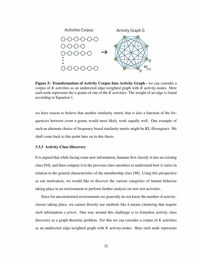
g

Activity Graph G

p

qw p q

Activities Corpus

Figure 5: Transformation of Activity Corpus Into Activity Graph - we can consider acorpus of K activities as an undirected edge-weighted graph with K activity-nodes. Hereeach node represents the n-grams of one of the K activities. The weight of an edge is foundaccording to Equation 1.

we have reason to believe that another similarity metric that is also a function of the fre-

quencies between event n-grams would most likely work equally well. One example of

such an alternate choice of frequency based similarity metric might be KL-Divergence. We

shall come back to this point later on in this thesis.

3.3.3 Activity-Class Discovery

It is argued that while facing some new information, humans first classify it into an existing

class [94], and then compare it to the previous class members to understand how it varies in

relation to the general characteristics of the membership class [98]. Using this perspective

as our motivation, we would like to discover the various categories of human behavior

taking place in an environment to perform further analysis on new test activities.

Since for unconstrained environments we generally do not know the number of activity-

classes taking place, we cannot directly use methods like k-means clustering that require

such information a priori. One way around this challenge is to formalize activity class

discovery as a graph theoretic problem. For this we can consider a corpus of K activities

as an undirected edge-weighted graph with K activity-nodes. Here each node represents

32

the n-gram histogram of one of the K activities. The weight of an edge can be found by

computing the pair-wise similarity between the activity-nodes of that edge according to

Equation 1. This transformation from a corpus of activities to an activity graph is figura-

tively illustrated in Figure 5.

Activity-Class as Maximal Clique

We want to efficiently find large clusters of activity nodes in the activity graph that are

mutually cohesive while being different from the rest of the activity-nodes. This raises the

inherent trade-off between the cohesiveness and cardinality of a discovered cluster. One

way of striking a balance between these two opposing factors is to formalize this prob-

lem as searching for edge-weighted maximal cliques3in this activity graph of K activity-

instances [5]. We begin by finding the first maximal clique in the activity-graph, followed

by removing that set of nodes from the graph, and iteratively repeating this process with the

remaining set of nodes, until there remain no maximal cliques in the graph. The leftover

nodes after the removal of maximal cliques are dissimilar from most of the regular nodes,

and are considered as being anomalous. This process is figuratively illustrated in Figure 6.

Maximal Cliques using Dominant Sets

As combinatorially searching for maximal cliques in an edge-weighted undirected graph is

computationally hard, numerous approximations to the solution of this problem have been

proposed [92]. For our purposes, we adopt the approximate approach of iteratively find-

ing dominant sets of maximally similar nodes in a graph (equivalent to finding maximal

cliques) as proposed in [87]. Besides providing an efficient approximation to finding maxi-

mal cliques, the framework of dominant sets provides a principled measure of cohesiveness

of a class as well as a measure of node participation.

Let the data to be clustered be represented by an undirected edge-weighted graph with

no self-loops G = (V,E,ϑ) where V is the vertex set V = {1,2, ...K}, E⊆V ×V is the edge

3Recall that a subset of nodes is a clique if all its nodes are mutually adjacent; a maximal clique is notcontained in any larger clique; a maximum clique has largest cardinality.

33

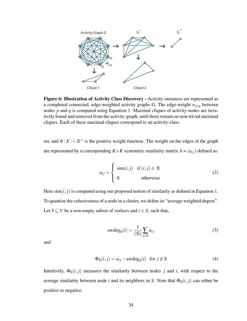
g g

Activity Graph G G

g

g

'

Clique 1 Clique 2

G ''

p

qw p q

Figure 6: Illustration of Activity Class Discovery - Activity-instances are represented asa completed connected, edge-weighted activity graphs G. The edge-weight wp,q betweennodes p and q is computed using Equation 1. Maximal cliques of activity-nodes are itera-tively found and removed from the activity-graph, until there remain no non-trivial maximalcliques. Each of these maximal cliques correspond to an activity-class.

set, and ϑ : E → R+ is the positive weight function. The weight on the edges of the graph

are represented by a corresponding K×K symmetric similarity matrix A = (ai j) defined as:

ai j =

sim(i, j) if (i, j) ∈ E

0 otherwise(2)

Here sim(i, j) is computed using our proposed notion of similarity as defined in Equation 1.

To quantize the cohesiveness of a node in a cluster, we define its “average weighted degree”.

Let S ⊆ V be a non-empty subset of vertices and i ∈ S, such that,

awdegS(i) =1||S||∑j∈S

ai j (3)

and

ΦS(i, j) = ai j− awdegS(i) for j /∈ S (4)

Intuitively, ΦS(i, j) measures the similarity between nodes j and i, with respect to the

average similarity between node i and its neighbors in S. Note that ΦS(i, j) can either be

positive or negative.

34

We now consider how weights are assigned to individual nodes. Let S ⊆ V be a non-

empty subset of vertices and i ∈ S. The weight of i with respect to S is given as:

wS(i) =

1 if ||S|| = 1

∑j∈S\{i}

ΦS\{i}( j, i)wS\{i}( j) otherwise(5)

Moreover, the total weight of S is defined as

W (S) = ∑i∈S

wS(i) (6)

Intuitively, wS(i) gives a measure of the overall similarity between vertex i and the vertices

of S\{i} with respect to the overall similarity among the vertices in S\{i}. We are now in

a position to define dominant sets. A non-empty sub-set of vertices S⊆V such that W (T )

> 0 for any non-empty T⊆S, is said to be dominant if:

• wS(i) > 0, ∀ i ∈ S, i.e. internal homogeneity

• wS∪{i}(i) < 0 ∀ i /∈ S, i.e. external inhomogeneity.

Effectively, we can state that the dominant set in an edge-weighted graph is equivalent to

a cluster of vertices in that graph. As solving Equation 5 combinatorially is infeasible, we

use a continuous optimization technique of replicator dynamics as proposed in [87]).

3.3.4 Finding Dominant Sets Using Replicator Dynamics

We now turn our attention to finding a dominant set in an edge-weighted graph with ad-

jacency matrix A. For this purpose, consider the following quadratic program which is a

generalization of Motzkin-Straus program [79]:

maximize f (x) =12

xT Ax (7)

subject to x ∈ ∆. where

∆ = x ∈ Rn :n

∑i=1

xi = 1 and xi ≥ 0,∀i (8)

35

is the standard simplex in Rn. If S is a dominant sub-set of vertices, then its weighted

characteristics vector xS, defined as:

wi(S) =

w(i, j)W (S) i f |S| ∈ S

0 otherwise(9)

is a strict local maximizer of f in ∆. Conversely, if x∗ is a strict local maximizer of f in ∆

then its support σ = σ(x∗) = {i ∈ V : x∗i 6= 0 }is a dominant set. By the virtue of the

above result, we can find a dominant set by first localizing a solution of Equation 7 with an

appropriate continuous optimization technique, and then picking up the support set of the

solution found. The clustering algorithm we use basically consists of iteratively finding a

dominant set in that graph by solving Equation 7 and finding its support, then removing the

support from the graph, until all the vertices have been clustered.

Because solving Equation 5 combinatorially is infeasible, we use a continuous opti-

mization technique proposed in [87] which solves Equation 5 applying replicator dynam-

ics. Let W = (wi j) be a non-negative real-valued n × n matrix. The discrete time version

of the replicator equation can be given as [79]:

xi(t +1) = xi(t)(Wx(t))i

x(t)TWx(t)(10)

According to the fundamental theorem of natural selection [38], if W = W T , then the func-

tion F(x) = xTWx is strictly increasing along any non-constant trajectory of the replicator

dynamics of equation 10. In other words, ∀ t > 0, F(x(t + 1)) > F(x(t)). Finally, let

W = A, the adjacency matrix, then the replicator system, starting from any arbitrary initial

state will eventually converge to a maximizer of function given in Equation 7. This will

correspond to a dominant set in the graph and hence to a cluster of nodes.

3.3.5 Activity Classification

Given ||C|| discovered activity-classes, we are interested in finding to which of the discov-

ered classes does a new activity instance belong. Each member j of an activity-class c has

36

some weight wc( j), that indicates the participation of j in c. We compute the similarity be-

tween a new activity-instance τ and previous members of each class by defining a function

Ac(τ) as:

Ac(τ) = ∑j

sim(τ, j)wc( j) ∀ j ∈ c (11)

Here wc( j) is the same as defined in Equation 5. Ac represents the average weighted sim-

ilarity between the new activity-instance τ and any one of the discovered classes c. The

selected membership class c∗ is found as:

c∗ = argmax∀c

Ac(τ) (12)

3.4 Results: Activity Class Discovery & Classification

To test the competence of our proposed framework, experiments on extensive data-sets

collected from two everyday environments of a Loading Dock area and a Residential House

environment were performed. For both experimental setups, the value of n for the n-grams

was set equal to 3.

3.4.1 Loading Dock Environment

We collected video data at the Loading Dock area of a retail bookstore. To visually span the

area of loading dock, we installed two cameras with partially overlapping fields of view. A

schematic diagram with sample views from the two cameras is shown in Figure 7. Daily

activities from 9 a.m. to 5 p.m., 5 days a week, for over one month were recorded, during

which 200 instances of activities were collected. Based on our observations of the activities

taking place in this environment, an event vocabulary of 61 events was constructed. A list

of these events along with their description is given in Appendix .5. Every activity has a

known starting event, i.e. Delivery Vehicle Enters the Loading Dock and a known ending

event, i.e. Delivery Vehicle Leaves the Loading Dock.

We must mention here that these events are just one choice of event vocabulary that is

being used to describe the various activities taking place in the loading dock environment.

37

Figure 7: Schematic Diagram of the Camera Setup at The Loading Dock Area - Thefigure shows overlapping fields of view of the two static cameras used. Representativeimages as taken from both the Camera 1 and Camera 2 are also being shown. Other thanthat, the main parts of the environment being shown are the A and B loading docks, theside entrance, and the warehouse entrance.

We chose these events after carefully observing the activities in this environment, as to us

they were the most natural way of describing the different activities, while being simple

enough to be potentially detected using low-level perceptual data. It is quite possible to

have a better set of events that could describe the various activities in the loading dock area

in a more expressive manner, while being even more robustly detectable. In this thesis we

have not focused on the problem of learning the best event vocabulary for an environment,

and leave this question as an open problem for future work.

We used 150 of the collected instances of activities, that were manually annotated using

our defined event-vocabulary of 61 events. The 10 key objects whose various interactions

constituted these 61 events were: Person, Cart, Delivery Vehicle(D.V.), Left Door of D.V.,

38

Delivery Vehicle Enters Loading Dock

Person Removes Package from Backdoor of Vehicle

Person Closes Backdoor of Vechicle

Delivery Vehicle Exists Loading Docka) b) c) d)

g g g

Figure 8: Key Frames of Example Events - The figure shows an example delivery activityin a loading dock environment. Only Camera 1 is being shown here. The key-objects whoseinteractions define these events are shown in different colored blocks.

Right Door of D.V., Back Door of D.V., Package, Doorbell, Front Door of Building, Side

Door of Building. To get the reader better situated in this environment, some events from

one of the delivery activities that was captured are shown in Figure 8.

Discovered Activity Classes - Loading Dock Environment

Of the 150 training activities, we found 7 classes (maximal cliques), with 106 activities as

part of any one of the discovered classes, while 44 activities being different enough to be

Visualization of Discovered Activity ClassesIn Loading Dock Environment

Un-Clustered Similarity Matrix Clustered Similarity Matrix

i

i

Activit

y Clus

ters

Figure 9: Similarity Matrix Before & After Activity Class Discover - Each row rep-resents the similarity of a particular activity with the entire activity training set. Whiteimplies identical similarity while black represents complete dissimilarity. The activitiesordered after the red cross line in the clustered similarity matrix were dissimilar enoughfrom all other activities as to not be included in any non-trivial clique.

39

not included into any non-trivial maximal clique. In this chapter, we focus on the analysis

of the 7 discovered clusters. We shall go over a detail analysis of the 44 activities that could

not be clustered in Chapter 6. The visual representation for the similarity matrices of the

original 150 activities and the re-arranged activities in 7 clusters is shown in Figure 9.

Analysis of Discovered Activity Classes In Loading Dock Environment:

Analysis of the discovered activity classes in the Loading Dock Environment reveals a

strong structural similarity amongst the class members. For instance, the most cohesive of

the discovered class that our system was able to find was the one where all the UPS deliv-

eries were clustered. It must be pointed out that there was no explicit information about

the company-labels of the delivery vehicles in our vocabulary. The reason we were able

to discover all UPS deliveries as a cohesive activity-class is because the activity-structure

induced by a UPS delivery by the virtue of where the truck docks, how many packages

are delivered, in what manner are they delivered etc., is reflected in our similarity met-

ric, and is picked up by our discovery algorithm. This anecdotal evidence is an indication

that the perceptual bias introduced by us in terms of the event-vocabulary, is successfully

transported to the higher-level discovery algorithm. A brief description of the discovered

activity-classes is given in Table 1.

3.4.2 Residential House Environment

To test our proposed algorithms on the daily activities of a person in a Residential House

environment, we deployed 16 pressure-sensors at different locations in a house, each with

a unique identification code. These transducers register the time when the resident of the

house walk over them. The data was collected daily for almost 5 months (151 days -

each day being considered as an individual activity). Whenever the person passed near a

transducer at a particular location, it was considered as the occurrence of a unique event.

Thus our event vocabulary in this environment consists of 16 events. Figure 10 shows a

schematic top-down view of this environment.

40

Table 1: Description for the Discovered Classes in Loading Dock.: A brief descriptionof the various discovered classes in the Loading Dock Environment are given in terms ofthe different distinguishing features.

Class Index Class DescriptionClass 1 UPSr delivery-vehicles that picked up multiple packages

using hand carts.Class 2 Pickup trucks and vans that dropped off a few packages

without needing a hand cart.Class 3 Delivery trucks that dropped off multiple packages, with

multiple people using hand-carts.Class 4 A mixture of car, van, and truck delivery vehicles that

dropped off one or two packages without needing a handcart.

Class 5 Delivery-vehicles that picked up and dropped-off multiplepackages using a motorized hand cart and multiple people.

Class 6 Van delivery-vehicles that dropped off one or two packageswithout needing a hand cart.

Class 7 Delivery trucks dropped off multiple packages using handcarts.

Garage

Formal DiningRoom

Kitchen Den

EnterenceHall Front Room

Stairway

Office

Sunroom

10

168 7

9

146

2 4

3

5

11

13

12

151

Figure 10: A Schematic Diagram of the Pressure-Sensors in the Residential HouseEnvironment - The red dots represents the positions of the pressure-sensors. These sensorsregistered the time when the resident of the house walked over them, and this is consideredas an events in our event vocabulary.

41

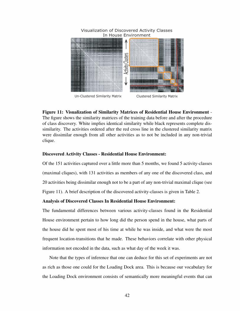
Visualization of Discovered Activity ClassesIn House Environment

i

i

Un-Clustered Similarity Matrix Clustered Similarity Matrix

Activit

y Clus

ters

Figure 11: Visualization of Similarity Matrices of Residential House Environment -The figure shows the similarity matrices of the training data before and after the procedureof class discovery. White implies identical similarity while black represents complete dis-similarity. The activities ordered after the red cross line in the clustered similarity matrixwere dissimilar enough from all other activities as to not be included in any non-trivialclique.

Discovered Activity Classes - Residential House Environment:

Of the 151 activities captured over a little more than 5 months, we found 5 activity-classes

(maximal cliques), with 131 activities as members of any one of the discovered class, and

20 activities being dissimilar enough not to be a part of any non-trivial maximal clique (see

Figure 11). A brief description of the discovered activity-classes is given in Table 2.

Analysis of Discovered Classes In Residential House Environment:

The fundamental differences between various activity-classes found in the Residential

House environment pertain to how long did the person spend in the house, what parts of

the house did he spent most of his time at while he was inside, and what were the most

frequent location-transitions that he made. These behaviors correlate with other physical

information not encoded in the data, such as what day of the week it was.

Note that the types of inference that one can deduce for this set of experiments are not

as rich as those one could for the Loading Dock area. This is because our vocabulary for

the Loading Dock environment consists of semantically more meaningful events that can

42

Table 2: Description for the Discovered Classes in Residential House Environment: Abrief description of the various discovered classes in the Residential House Environment aregiven in terms of the different distinguishing features. he fundamental differences betweenvarious activity-classes found in the Residential House environment pertain to how longdid the person spend in the house, what parts of the house did he spent most of his time atwhile he was inside, and what were the most frequent location-transitions that he made.

Class Index Class DescriptionClass 1 Activities lasting for the entire length of days where the per-

son’s trajectory spans the entire house space. Most of thetime was spent in the area around the Kitchen and the Din-ing Table.

Class 2 The person moves from from kitchen to the stairway moreoften. Further more, as opposed to cluster 1, the person doesnot go from the Office to the Sum Room area.

Class 3 The person spends more time in the areas of Den and theliving-room. Moreover, he visits the Sun-room more often.

Class 4 The person spends most of the day in Kitchen and DiningRoom. The duration for which she stays in the house issmaller for this class.

Class 5 The person moves from Dining Room to the Sun Roommore often. The duration for which she stays in the houseis significantly smaller than any other activity-class.

encode the underlying activity structure more completely. At the same time their detec-

tion cannot directly be made from sensor-readings without some additional low-level event

detectors. For the House environment however, the events are simply the locations of a

person directly detected from sensor readings, and therefore the kinds of inference one can

perform for this setup is more general and high-level.

3.4.3 Noise Analysis of n-grams in Loading Dock Environment

The results presented thus far were generated using activities with hand-labeled events.

However, using low-level vision sensors to detect these events will generate noise. This

invites the question as to how well would the proposed system perform over noisy data.

In the following, the noise analysis to check the stability and robustness of the proposed

framework is presented; allowing one to make some predictions about its performance on

43

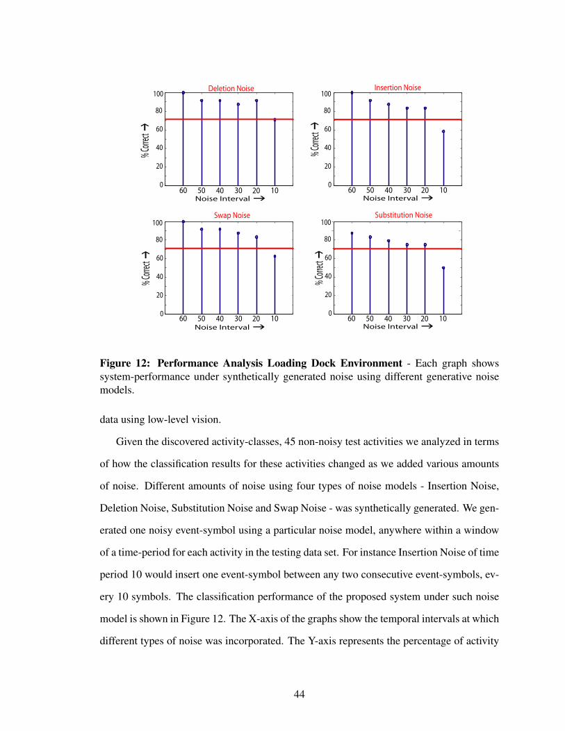
0

20

40

60

80

100

4060 203050 10 4060 203050 10

4060 203050 10 4060 203050 10

0

20

40

60

80

100

0

20

40

60

80

100

0

20

40

60

80

100

Insertion NoiseDeletion Noise

Swap Noise Substitution Noise

Noise Intervalg Noise Intervalg

Noise Intervalg Noise Intervalg

% Corr

ectg

% Corr

ectg

% Corr

ectg

% Corr

ectg

Figure 12: Performance Analysis Loading Dock Environment - Each graph showssystem-performance under synthetically generated noise using different generative noisemodels.

data using low-level vision.

Given the discovered activity-classes, 45 non-noisy test activities we analyzed in terms

of how the classification results for these activities changed as we added various amounts

of noise. Different amounts of noise using four types of noise models - Insertion Noise,

Deletion Noise, Substitution Noise and Swap Noise - was synthetically generated. We gen-

erated one noisy event-symbol using a particular noise model, anywhere within a window

of a time-period for each activity in the testing data set. For instance Insertion Noise of time

period 10 would insert one event-symbol between any two consecutive event-symbols, ev-

ery 10 symbols. The classification performance of the proposed system under such noise

model is shown in Figure 12. The X-axis of the graphs show the temporal intervals at which

different types of noise was incorporated. The Y-axis represents the percentage of activity

44

instances that maintained their assignment to their original when no noise was incorporate

versus when a certain amount of noise was introduced. As can be seen from the graphs, the

system performs quite robustly in the face of noise and degrades gracefully as the amount

of noise increases.

3.4.4 Automatic Event Detection

To move one step closer towards using low-level vision, we created a feature-labeling soft-

ware that a user uses only to label the various objects of interest in the scene such as the

doors of the loading dock, the delivery vehicles and its doors, people, packages and carts.

We assign each object a unique ID during labeling. The ID numbers and object locations

are stored in an XML format on a per-frame basis. We then wrote event detectors that

parsed the XML data files to compute the distances between these objects for the 45 test

activities. Based on the locations and velocities of these objects, the detectors performed

automatic event detection. The horizontal line in Figure 12 shows classification rate of the

45 test activities using aforementioned automatic event generation mechanism, i.e. 70.8%.

3.5 Summary

A vast majority of traditional activity representations assume prior knowledge of the struc-

ture of activities they are being used to model. However, for unconstrained everyday envi-

ronments, such activity structure is generally not completely known a priori. In this chap-

ter, we have explored the activity representation of event n-grams that facilitate learning of

this structure with minimal supervision. The intuition behind using such a representation

is that if we chose to describe everyday activities in terms of an appropriate set of events,

then the global structure of such activities can be sufficiently encoded by simply using their

local event subsequences.

Using our proposed activity representation of event n-grams, we have formalized the

problem of automatically discovering the different categories of human behaviors taking

45

place in an environment. In particular, we have represented a corpus of activities as a com-

pletely connected edge-weighted activity graph, and defined activity classes as maximally

similar cliques of nodes in this activity graph. We have used the framework of Dominant

Sets to efficiently discover the various maximal cliques present in the activity graph, where

each of these maximal cliques corresponds to a classes of activities in that environment.

So far we have presented results of our framework in two everyday environments, i.e.

a Loading Dock area, and a Residential House setting. For both of these settings how-

ever, there is no well-defined notion of activity-classes that exists. It could be argued that

given some data, any discovery framework would come up with a set of cohesive activ-

ity classes, regardless of the usefulness or meaningfulness of the discovered classes. This

poses a fundamental challenge about determining the success of an activity analysis system

that follows an unsupervised discovery paradigm. While by simply observing the types of

activity classes that our system was able to discover, it seems that the discovered activity

classes were in fact semantically meaningful and structurally coherent, however, there is a

need to strengthen this argument by providing more convincing experimental evidence.

Furthermore, while n-grams capture both the content and order information of events

in activities, a natural question this approach raises is what value of n should be chosen.

Moreover, should n only have one fixed value or should it range over a particular range

of values, in order to capture the various variable-length event dependencies that may be

present in an environment.

In the next chapter, we attempt to address some of the representational limitations of

event n-grams, as well as provide a more convincing set of experiments that show the

plausibility of our framework.

46

CHAPTER IV

REPRESENTING ACTIVITIES USING SUFFIX TREES

Recall that our thesis states that the structural information for a large set of everyday human

activities can be uniquely encoded using their local event subsequences. So far in this

thesis, the types of event subsequences (event n-grams) we have used to encode this activity

structure are of fixed length. In this chapter1 we provide an alternate activity representation

of Suffix Trees that uses variable length event subsequences for modeling activities.

4.1 Motivation

We first list some of the limitations of using fixed length event n-grams, followed by high-

lighting the importance of capturing variable length event dependencies in activities.

4.1.1 Limitations Of Fixed-Length Event n-grams

While considering activities in terms of their fixed length event n-grams, it is evident that

higher values of n capture temporal order information of activities more explicitly [35].

However, such explicit structural information comes at the cost of higher data dimension-

ality and therefore greater data sparsity. This naturally raises the question as to what value

should n have.

Moreover, the competence of n-grams is limited by their ability to capture activity

structure only up to some fixed temporal resolution. It is a matter of common observa-

tion however that events in everyday human activities can have strong dependence on their

preceding events over variable lengths of time [83]. While entering an unlit room for in-

stance, a person generally turns the light on after opening the door, i.e. the event of turning

1This work has previously appeared in [40].

47

the light on is dependent on the immediately previous event of opening the door. However,

while washing dishes in a household kitchen, the event of turning the faucet on, is usually

followed by rinsing the dishes, followed by turning the faucet off. In other words, the event

of turning the faucet off is dependent of the previous two events. In order to model human

activities more accurately, it is important to efficiently represent this variable length event

dependence.

4.1.2 Significance of Capturing Variable-Length Event Dependence

One way of demonstrating the significance of capturing the variable-length event depen-

dence is to analyze the degree to which sequential features of various lengths contribute

to the similarity metric. To this end, here we consider a simulation experiment with ac-

tivities from 2 activity classes. The exact details of how we undertook the generation of

our simulation data can be found in Appendix .1. For a symbol vocabulary ||Σ|| = 5, we

generated sequences for 2 classes with % class-overlap decreasing from complete overlap

to complete non-overlap with increments of 10%. For each of these 10 trials, we generated

75 sequences each of length 100, randomly selecting two-thirds for the training data and

the rest for the testing.

For each test sequence t, we classify it to any one of the two activity-classes based on

the nearest neighbor classifier. We are interested in understanding the extent to which the

various subsequences of different lengths contribute to the similarity S of a test sequence t

to its nearest neighbor n in its membership class. In order to do this, we first sort the con-

stituent subsequences of t according to their lengths. We then compute the fraction of the

similarity S due to the length-sorted constituent subsequences of t and its nearest neighbor

n. Figure 13 shows the average similarity contribution over varying lengths between all the

test sequences and their corresponding nearest neighbors in their membership classes.

It can be seen from Figure 13 that the graph is almost bell-shaped, with smaller and

larger length subsequences being not so contributive, while medium length subsequences

48

Subsequence Lengths

Ave

rag

e %

-Sim

ilari

ty C

on

trib

uti

on

2 4 6 8 10 12 14

35

30

25

20

15

10

5

0

Figure 13: Length-Sorted Subsequence Contribution to Activity Similarity - The av-erage percentage similarity contribution of basis subsequences of different lengths for alltest points and their respective nearest neighbors.

being the most contributive towards activity similarity. Note that the predominant length

of symbol dependence in our simulation data was set equal to 3, which is the length of

the most contributive subsequences. While it is clear that longer length subsequences do

not contribute much to activity similarity, the wide range of lengths contributive towards

similarity highlights the importance of incorporating multi-length sequential features for

representing activity sequences.

4.2 Representing Human Activities Using Variable-LengthEvent Subsequences

One naive way of capturing variable-length event dependencies in human activities is to

represent the activity in terms of all of its variable-length constituent event subsequences.

Consider for instance the example activity:

a = {1,2,3,1,2} (13)

49

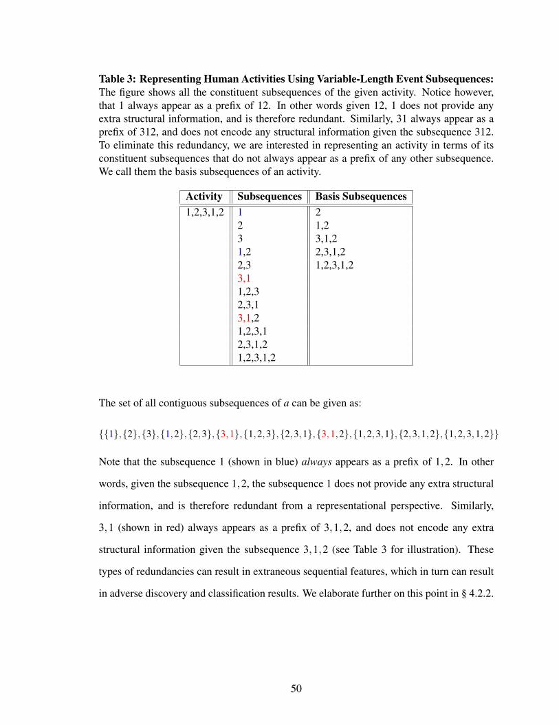
Table 3: Representing Human Activities Using Variable-Length Event Subsequences:The figure shows all the constituent subsequences of the given activity. Notice however,that 1 always appear as a prefix of 12. In other words given 12, 1 does not provide anyextra structural information, and is therefore redundant. Similarly, 31 always appear as aprefix of 312, and does not encode any structural information given the subsequence 312.To eliminate this redundancy, we are interested in representing an activity in terms of itsconstituent subsequences that do not always appear as a prefix of any other subsequence.We call them the basis subsequences of an activity.

Activity Subsequences Basis Subsequences1,2,3,1,2 1 2

2 1,23 3,1,21,2 2,3,1,22,3 1,2,3,1,23,11,2,32,3,13,1,21,2,3,12,3,1,21,2,3,1,2

The set of all contiguous subsequences of a can be given as:

{{1},{2},{3},{1,2},{2,3},{3,1},{1,2,3},{2,3,1},{3,1,2},{1,2,3,1},{2,3,1,2},{1,2,3,1,2}}

Note that the subsequence 1 (shown in blue) always appears as a prefix of 1,2. In other

words, given the subsequence 1,2, the subsequence 1 does not provide any extra structural

information, and is therefore redundant from a representational perspective. Similarly,

3,1 (shown in red) always appears as a prefix of 3,1,2, and does not encode any extra

structural information given the subsequence 3,1,2 (see Table 3 for illustration). These

types of redundancies can result in extraneous sequential features, which in turn can result

in adverse discovery and classification results. We elaborate further on this point in § 4.2.2.

50

4.2.1 Basis Event Subsequences

To eliminate such redundancies, we are interested in representing an activity in terms of its

constituent subsequences that do not always appear as a prefix of any other subsequence.

More formally, we represent a, in terms of a subset B of its set of all contiguous subse-

quences U, where ∀ w ∈U, ∃ b ∈ B , such that:

• fa(w) = fa(b)

• w is a subsequence of b

where fa(w) stands for frequency of w in a. Any set B , satisfying these properties is called

a set of “Basis Event Subsequences” of a. The aforementioned properties of B imply that

∀ w ∈U \B ,fa(w) = max

b∈ψ

fa(b) (14)

where ψ ⊆ B such that w is a subsequence of every member of ψ. Given B , any subse-

quence w ∈U \B , does not provide any extra information about a, and is thus redundant.

Such basis event subsequences encode the structural signature of an activity [43], and can

therefore be used as discriminative features [66].

4.2.2 Significance of Removing Redundancies Using Basis Event Subsequences

As mentioned earlier, a naive way of incorporating multi-length features might be to con-

join the feature spaces induced by n-grams for all values of n. Besides being computation-

ally inefficient, such highly over-complete feature space contains extraneous information

that may reflect in relatively poor classification performance. Suffix Trees on the other hand

efficiently generate a multi-length feature set that is linear in the length of input sequence

to encode sequence structure, naturally filtering out extraneous information [117]. For data

generated as described in Appendix .1, Figure 14 shows this in terms of the average classi-

fication gain while using Suffix Trees over n-grams for all values of n = [1 : N].

51

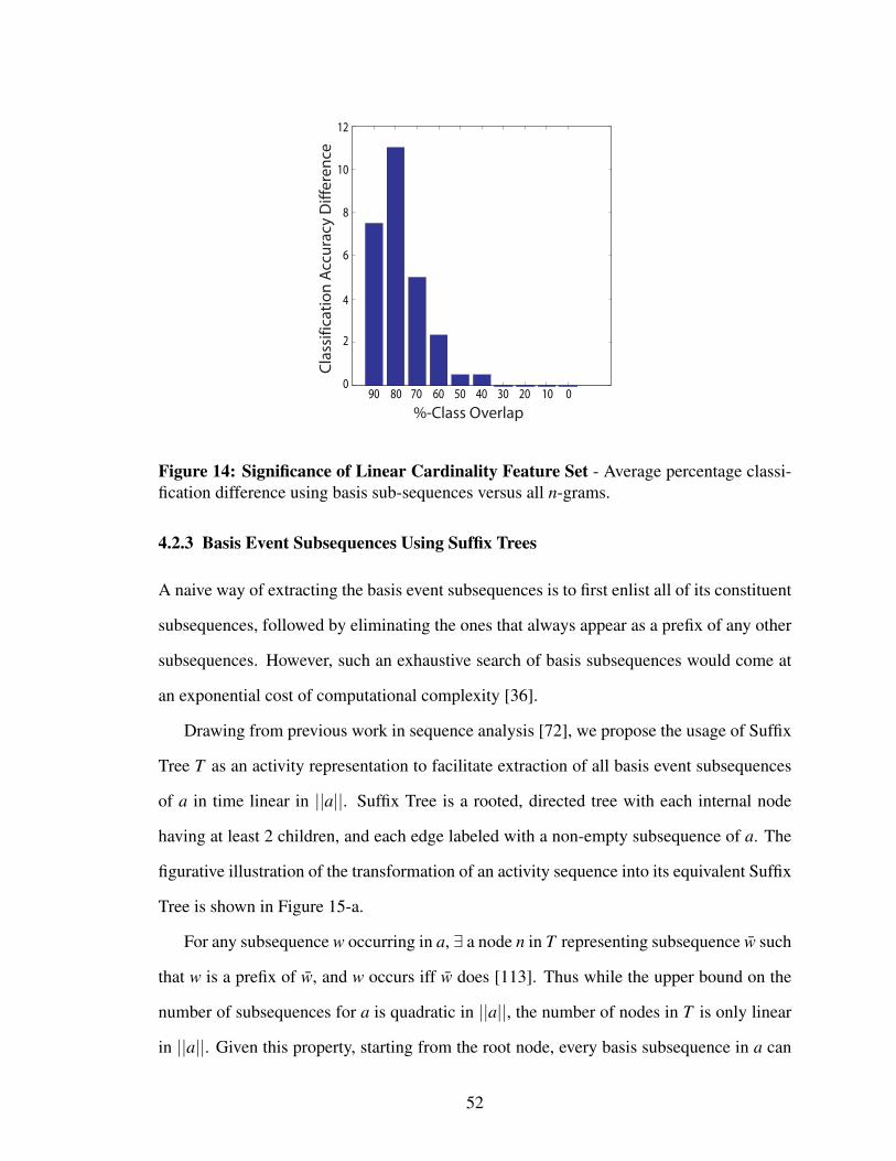
%-Class Overlap

Cla

ssifi

cati

on

Acc

ura

cy D

iffer

ence

90 80 70 60 50 40 30 20 10 0

2

4

6

8

10

12

0

Figure 14: Significance of Linear Cardinality Feature Set - Average percentage classi-fication difference using basis sub-sequences versus all n-grams.

4.2.3 Basis Event Subsequences Using Suffix Trees

A naive way of extracting the basis event subsequences is to first enlist all of its constituent

subsequences, followed by eliminating the ones that always appear as a prefix of any other

subsequences. However, such an exhaustive search of basis subsequences would come at

an exponential cost of computational complexity [36].

Drawing from previous work in sequence analysis [72], we propose the usage of Suffix

Tree T as an activity representation to facilitate extraction of all basis event subsequences

of a in time linear in ||a||. Suffix Tree is a rooted, directed tree with each internal node

having at least 2 children, and each edge labeled with a non-empty subsequence of a. The

figurative illustration of the transformation of an activity sequence into its equivalent Suffix

Tree is shown in Figure 15-a.

For any subsequence w occurring in a, ∃ a node n in T representing subsequence w̄ such

that w is a prefix of w̄, and w occurs iff w̄ does [113]. Thus while the upper bound on the

number of subsequences for a is quadratic in ||a||, the number of nodes in T is only linear

in ||a||. Given this property, starting from the root node, every basis subsequence in a can

52

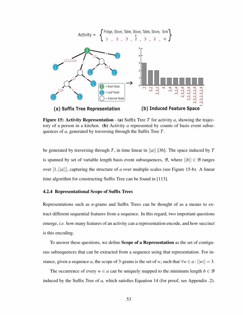
1,2,3,2,3,2,4 2

3,2

3,2,4 4

4

3,2

4 3,2,4

4

Fridge, Stove, Table, Stove, Table, Stove, Sink

1 2 3 2 3 2 4, , , , ,,Activity = { }

R

L

L L

L

L L

L

Rg

g

Root Node

Leaf Node

g Internal Node

RL

h

0

1

2

3

4

5

2

3,2

2,3,

2 4

2,4

3,2,

4

2,3,

2,4

3,2,

3,2,

4

2,3,

2,3,

2,4

1,2,

3,2,

3,2,

4

g

(a) Suffix Tree Representation (b) Induced Feature Space

Figure 15: Activity Representation - (a) Suffix Tree T for activity a, showing the trajec-tory of a person in a kitchen. (b) Activity a represented by counts of basis event subse-quences of a, generated by traversing through the Suffix Tree T .

be generated by traversing through T , in time linear in ||a|| [36]. The space induced by T

is spanned by set of variable length basis event subsequences, B , where ||b|| ∈ B ranges

over [1, ||a||], capturing the structure of a over multiple scales (see Figure 15-b). A linear

time algorithm for constructing Suffix Tree can be found in [113].

4.2.4 Representational Scope of Suffix Trees

Representations such as n-grams and Suffix Trees can be thought of as a means to ex-

tract different sequential features from a sequence. In this regard, two important questions

emerge, i.e. how many features of an activity can a representation encode, and how succinct

is this encoding.

To answer these questions, we define Scope of a Representation as the set of contigu-

ous subsequences that can be extracted from a sequence using that representation. For in-

stance, given a sequence a, the scope of 3-grams is the set of w, such that ∀w∈ a : ||w||= 3.

The occurrence of every w ∈ a can be uniquely mapped to the minimum length b ∈ B

induced by the Suffix Tree of a, which satisfies Equation 14 (for proof, see Appendix .2).

53

The space of all contiguous subsequences of a is spanned by n-grams where n ranges over

[1 : ||a||]. Therefore, scope of Suffix Trees is equivalent to n-grams for all values of n, and

greater than n-grams for a specific value of n (see Figure 16). Furthermore, the number of

nodes in T , and hence the cardinality of B is only linear in ||a|| [113].

u

u

a b c ac bac

bbac

abba

c

1

2

u

u

a b c

1

2

u

u

ac ba bb ab

1

2

u

uab

b

bba

bac

1

2

u

u

abba

bbac

1

2

u

u

abba

c

1

2

u u u

u

u u

u u u

Sequence = { a, b, b, a, c }

uu u

u

n=1-gram n=2-gram n=3-gram n=4-gram n=5-gram

Suffi

x Tr

ee F

eatu

re S

pace

Figure 16: Feature Space Induced by Suffix Trees vs n-grams - For an example sequence= {a,b,b,a,c}, the figure shows the feature space induced by Suffix Trees. This featurespace strictly embeds in itself the feature space generated by n = 1→ 5-grams, showingthat for any fixed n, the representational power of Suffix Trees is greater than n-grams.

4.3 Empirical Analyses of Suffix Trees

We now present a set of empirical analyses for the representational competence of Suffix

Trees using synthetic data. The details of how this data was generated can be found in Ap-

pendix .1. We analyze the discriminative power and noise sensitivity of Suffix Trees, com-

paring them with some of the previously proposed approaches (e.g. VSM [97], HMM’s [90]

& n-grams [71]).

54

% Class Disjunction

Cla

ssifi

cati

on

Acc

ura

cy

Figure 17: Discriminative Prowess - Classification accuracy of Suffix Tree representationas a function of class-overlap.

4.3.1 Discriminative Prowess of Suffix Trees

Using the similarity metric defined in Equation 1, the nearest neighbor classification results

are given in Figure 17. It is evident that for substantive class overlap, higher values of n

seem to capture activity structure more rigidly, entailing a more discriminative represen-

tation. However, since accurate density estimation for higher value n-grams require expo-

nentially greater amount of data, Vector Space Model seems to outperform 3- and 5-grams

in cases where the 2 classes are more disjunctive. Nevertheless, compared to different

representations, Suffix Trees offer greater competence for any amount of class overlap.

4.3.2 Noise Sensitivity Analysis

We now analyze noise sensitivity of Suffix Trees as a function of % noise added as Inser-

tion, Deletion, Transposition and Substitution of symbols. For data generated as described

in Appendix .1, we cumulatively added all four types of noises with a uniform prior on

each, and noise likelihood ranging monotonically from 0 to 30%. Using noisy data, the

classification results for different representations relative to their noise free performance is

55

1 5 10 20 300

% Noise Added

Rel

ativ

e C

lass

ifica

tio

n A

ccu

racy

Figure 18: Noise Sensitivity- Classification for various representations relative to theirnoise free performance.

given in Figure 18.

It is evident that representations that capture event order information more rigidly, are

more sensitive to sensor noise, making 1-grams most robust to noise perturbations. At noise

levels > 10%, Suffix Trees outperform both 3- and 5-grams. This is because while n-grams

capture sequence structure only at a fixed temporal resolution, the scale at which Suffix

Trees encode this structure varies inversely with sequence entropy [110]. Since entropy is

a function of noise, at higher noise levels, Suffix Trees emulate the 1-grams more closely,

making them more robust to noise than n-grams.

4.4 Experimental Setup - Kitchen Environment

We now present a set of experiments conducted in a house kitchen environment, to analyze

the discovery and classification results of our proposed framework using Suffix Trees ac-

tivity representation. We also compare these results to some previously proposed sequence

representations such as fixed length n-grams for different values of n, and HMMs.

It is argued that we organize our surroundings to optimize the execution of different

56

activities [60]. This is particularly true for settings such as a household kitchen, where

different key-objects provide a set of functionalities, instrumental for the completion

of various activities [86]. With this perspective at hand, we deployed a static camera

in a kitchen ceiling to record a users interactions with different key-objects known a

priori. The user enacted 10 activity-classes each constituting of 10 activity instances.

The directions and recipes for preparing dishes of different classes were taken from

http://www.recipeland.com/, and are listed in Appendix .6.

These directions impose a set of temporal constraints, which require different events to

be partially ordered in a particular manner. For instance, if a recipe uses chopped potatoes,

then the events of washing the potatoes, getting a knife and chopping the potatoes must

be executed before using the stove for cooking them. However, if a recipe uses chopped

potatoes and onions, then the set of events needed to perform these two tasks may very well

be interchanged.

4.4.1 Activity Stages

For the purposes of our experiments, we divide the activity of cooking a dish into three

stages. These are summarized below:

1- Preparation Stage

We call the first stage as the preparation stage, which involves getting the various items

needed for a dish ready. For instance, in order to make Potato Curry, its recipe may require

having items such as chopped potatoes, and cut onions. The preparation stage for cook-

ing Potato Curry would involve getting these items ready. While the actions involved in

chopping potatoes or cutting onions must follow rather strict temporal structure, the items

themselves could nonetheless be interchanged.

2- Cooking Stage

Once all the required items have been prepared, they can be combined together based on

the recipe-directions. We call this process as the cooking stage. These steps must follow

57

the partial temporal order dictated by the recipe-directions and the physical constraints of

the environment. For instance, if the directions require frying chopped potatoes, then this

can only be done after the stove has been lit.

3- Finishing-up Stage

Once the dish has been prepared, all the utensils and the ingredients used during the prepa-

ration and the cooking stage need to be either placed back to their original locations, or put

in the sink. We call this stage as the clean-up stage. Since these ingredients can be replaced

in any order, the finishing-up stage does not necessarily follow a strict temporal structure.

The aforementioned three stages are illustrated in Figure 19. As shown, the preparation

stage consists of various items. Each individual item consists of well-defined sequence

of actions, however the individual items themselves can be performed in any particular

temporal order. Once all the items of preparation stage are finished, the different recipe-

steps of the cooking stage can be executed. In this stage, there exists a well defined temporal

structure in the actions needed to be performed in each step, as well as among the different

steps. Finally, once all the steps of the cooking stage have been performed, the various

steps of the finishing stage can be performed. Notice that there exists no temporal order in

which these individual steps need to be performed.

4.4.2 Constraints on Activity Dynamics

We now explain some of the details according to which the different items for the activity-

stages are performed. A schematic figure showing the different ingredients used in our

cooking experiments along with their spatial location in the kitchen and the key objects is

shown in Figure 20.

During the Preparation Stage, the ingredients for each of the individual items are first

brought to the table, and then processed. For instance, for the preparation of item “chopped

potatoes”, the user would:

Wash potatoes→ Bring washed potatoes to the table→ Get the chopping slab→ Bring it

58

P1 P2 PN

C1 C2 CK

1- Preparation Stage

2- Cooking Stage

3- Finishing Stage

F1 F2 F3 FM

Figure 19: Activity Stages - Preparation, cooking and finishing stages of an activity arefiguratively shown. Notice that in preparation stage, there is temporal order only within theindividual preparatory items. Cooking stage on the other hand follows a more strict tem-poral constraints. The finishing stage does not follow any temporal constraint in particular.

to the table→ Get the knife→ Bring it to the table→ Get a bowl→ Bring it to the table

→ Chop potatoes.

There are mainly two reasons for adding the constraint of first bringing each ingredient

to the table and then processing it. Firstly, the events that we are dealing with are mainly

concerned with the proximity of the person with the key-objects. We are presently do not

consider what exactly is being performed at those key-locations. Addition of this constraint

can allow our system to distinguish between the event of simply fetching something, as

opposed to the event of fetching something followed by somehow processing it. Secondly,

this constraint is added to reduce the variation in which a particular activity is allowed to

be performed in an environment. This allows us to have a more meaningful analysis of

the structure of activities using limited amount of data. Note that these constraints were

only used for single subject experiments, and were not incorporated for the experiments

involving multiple human subjects, as explained in § 4.5.3.

59

2

0

1

34

5678

9

Kitc

hen

Layo

ut

1- P

aper

Tow

el1-

Tom

atoe

s2-

Pot

atoe

s3-

Par

sley

4- G

reen

Oni

ons

5- B

ell P

eppe

rs

1- B

ay L

eave

s2-

Oni

ons

3- W

alnu

ts

1- S

ink

1- S

ilver

2- P

ans/

Slab

s3-

Gra

ter

4- B

eate

r5-

Woo

den

Spoo

n6-

Pla

tes

7- B

owls

1- S

tove

1- O

il2-

Gin

ger

3- G

arlic

4- C

hilli

Pow

der

5- S

alt

6- B

asen

7- P

eppe

r8-

Cha

t Mas

ala

9- G

lass

es10

- Flo

ur11

- Cin

nam

on12

- Sug

ar13

- Yea

st14

- Vin

egar

15- C

erea

l16

- Soy

Sau

ce

1- Y

ogar

t2-

But

ter

3- C

hees

e4-

Milk

5- E

ggs

6- P

each

es7-

Str

awbe

rrie

s8-

Bea

ns

9- G

rape

s10

- Lem

on11

- Blu

eber

ries

12- C

ream

Che

ese

13- C

ream

14- M

usta

rd15

- Let

tuce

16- C

hick

en1-

Ent

er/E

xit

1- D

inin

g Ta

ble

Figu

re20

:Pos

ition

sofK

ey-O

bjec

tsan

dIn

gred

ient

s-T

hedi

ffer

entk

ey-o

bjec

tsal

ong

with

the

vari

ous

ingr

edie

nts

used

are

show

n.

60

4.4.3 Automatic Event Detection

We assume the proximity of person with a particular key-object implies an interaction

between the person and the object. Any interaction longer than a particular duration is

registered as an event of person interacting with a certain key-object. For this work, we

implemented the tracking framework proposed in [50]. For extracting the person from

background image, we learned Gaussian Mixture Models for the chromatic contents of the

background, used for computing the likelihood for the presence of the person in the image

space. Given such likelihoods, we used a particle filter framework to search through image

space for computing the maximum a posteriori position of the person. This MAP estimate

in one frame is propagated to the next as the initial state of the filter for next iteration.

4.5 Results: Activity Class Discovery & Classification

For the purposes of analysis, we considered two different set of experiments with different

number of subjects involved. In the first set, only one person enacted a set of activities. In

the other set, we considered 3 different subjects who enacted activities in a less constrained

manner. The purpose of the first experimental set was to assess the efficacy of using Suffix

Trees as activity representation in our proposed framework, and compare it to various other

previously proposed activity representations. The purpose of second set of experiments

was to see how the performance of our framework varies across different subjects who may

cook the same recipe in different ways.

4.5.1 Performance Analysis for a Single Subject

For this set, one person enacted 10 activity-classes each constituting of 10 activity in-

stances. For every class that our framework discovered, the final class-label is assigned

based on the labels of the majority of the class-members. Moreover, any two classes with

the same class labels are merged. Following [42], we considered two metrics for analyzing

61

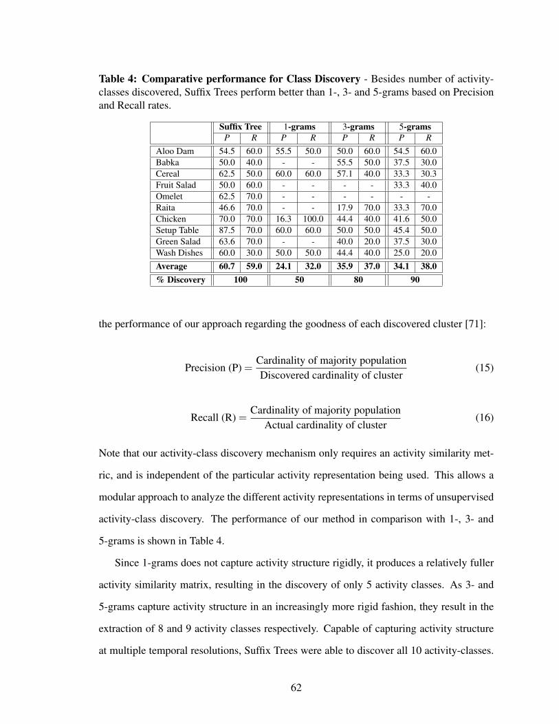
Table 4: Comparative performance for Class Discovery - Besides number of activity-classes discovered, Suffix Trees perform better than 1-, 3- and 5-grams based on Precisionand Recall rates.

Suffix Tree 1-grams 3-grams 5-gramsP R P R P R P R

Aloo Dam 54.5 60.0 55.5 50.0 50.0 60.0 54.5 60.0Babka 50.0 40.0 - - 55.5 50.0 37.5 30.0Cereal 62.5 50.0 60.0 60.0 57.1 40.0 33.3 30.3Fruit Salad 50.0 60.0 - - - - 33.3 40.0Omelet 62.5 70.0 - - - - - -Raita 46.6 70.0 - - 17.9 70.0 33.3 70.0Chicken 70.0 70.0 16.3 100.0 44.4 40.0 41.6 50.0Setup Table 87.5 70.0 60.0 60.0 50.0 50.0 45.4 50.0Green Salad 63.6 70.0 - - 40.0 20.0 37.5 30.0Wash Dishes 60.0 30.0 50.0 50.0 44.4 40.0 25.0 20.0Average 60.7 59.0 24.1 32.0 35.9 37.0 34.1 38.0% Discovery 100 50 80 90

the performance of our approach regarding the goodness of each discovered cluster [71]:

Precision (P) =Cardinality of majority populationDiscovered cardinality of cluster

(15)

Recall (R) =Cardinality of majority population

Actual cardinality of cluster(16)

Note that our activity-class discovery mechanism only requires an activity similarity met-

ric, and is independent of the particular activity representation being used. This allows a

modular approach to analyze the different activity representations in terms of unsupervised

activity-class discovery. The performance of our method in comparison with 1-, 3- and

5-grams is shown in Table 4.

Since 1-grams does not capture activity structure rigidly, it produces a relatively fuller

activity similarity matrix, resulting in the discovery of only 5 activity classes. As 3- and

5-grams capture activity structure in an increasingly more rigid fashion, they result in the

extraction of 8 and 9 activity classes respectively. Capable of capturing activity structure

at multiple temporal resolutions, Suffix Trees were able to discover all 10 activity-classes.

62

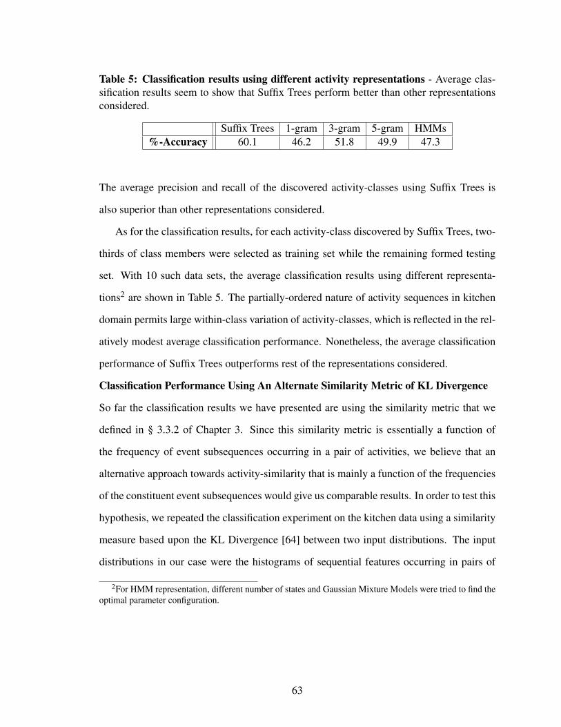
Table 5: Classification results using different activity representations - Average clas-sification results seem to show that Suffix Trees perform better than other representationsconsidered.

Suffix Trees 1-gram 3-gram 5-gram HMMs%-Accuracy 60.1 46.2 51.8 49.9 47.3

The average precision and recall of the discovered activity-classes using Suffix Trees is

also superior than other representations considered.

As for the classification results, for each activity-class discovered by Suffix Trees, two-

thirds of class members were selected as training set while the remaining formed testing

set. With 10 such data sets, the average classification results using different representa-

tions2 are shown in Table 5. The partially-ordered nature of activity sequences in kitchen

domain permits large within-class variation of activity-classes, which is reflected in the rel-

atively modest average classification performance. Nonetheless, the average classification

performance of Suffix Trees outperforms rest of the representations considered.

Classification Performance Using An Alternate Similarity Metric of KL Divergence

So far the classification results we have presented are using the similarity metric that we

defined in § 3.3.2 of Chapter 3. Since this similarity metric is essentially a function of

the frequency of event subsequences occurring in a pair of activities, we believe that an

alternative approach towards activity-similarity that is mainly a function of the frequencies

of the constituent event subsequences would give us comparable results. In order to test this

hypothesis, we repeated the classification experiment on the kitchen data using a similarity

measure based upon the KL Divergence [64] between two input distributions. The input

distributions in our case were the histograms of sequential features occurring in pairs of

2For HMM representation, different number of states and Gaussian Mixture Models were tried to find theoptimal parameter configuration.

63

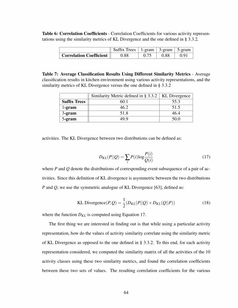
Table 6: Correlation Coefficients - Correlation Coefficients for various activity represen-tations using the similarity metrics of KL Divergence and the one defined in § 3.3.2.

Suffix Trees 1-gram 3-gram 5-gramCorrelation Coefficient 0.88 0.75 0.88 0.91

Table 7: Average Classification Results Using Different Similarity Metrics - Averageclassification results in kitchen environment using various activity representations, and thesimilarity metrics of KL Divergence versus the one defined in § 3.3.2

Similarity Metric defined in § 3.3.2 KL DivergenceSuffix Trees 60.1 55.31-gram 46.2 51.53-gram 51.8 46.45-gram 49.9 50.0

activities. The KL Divergence between two distributions can be defined as:

DKL(P||Q) = ∑i

P(i)logP(i)Q(i)

(17)

where P and Q denote the distributions of corresponding event subsequence of a pair of ac-

tivities. Since this definition of KL divergence is asymmetric between the two distributions

P and Q, we use the symmetric analogue of KL Divergence [63], defined as:

KL Divergence(P,Q) =12(DKL(P||Q)+DKL(Q||P)) (18)

where the function DKL is computed using Equation 17.

The first thing we are interested in finding out is that while using a particular activity

representation, how do the values of activity similarity correlate using the similarity metric

of KL Divergence as opposed to the one defined in § 3.3.2. To this end, for each activity

representation considered, we computed the similarity matrix of all the activities of the 10

activity classes using these two similarity metrics, and found the correlation coefficients

between these two sets of values. The resulting correlation coefficients for the various

64

activity representations considered are given in Table 6. The average correlation coeffi-

cients between all the considered representations is 0.855, indicating the strong similarity

in which these two notions of activity similarity behave.

To further test the effect of using KL Divergence as our activity similarity metric on

our classification results, we repeated our classification experiments. The results, along

with those obtained using our notion of similarity as defined in § 3.3.2 are given in Ta-

ble 7. The difference in the classification accuracy averaged over all the 4 representations

considered is 3.9. This shows that the performance of our framework using our proposed

similarity metric as defined in Equation 1 versus the one using similarity metric based on

KL Divergence are indeed very similar to each other.

4.5.2 Comparison of Suffix Trees with Smoothed n-grams

So far, we have compared the performance of Suffix Trees in comparison to fixed-length n-

grams. However, given limited amounts of data, there are several n-grams distributions that

cannot be estimated well. This is particularly a challenge in the field of Natural Language

Processing, where the problem usually involves very large vocabularies and extremely large

corpus of data. In order to deal with such situations, researchers have proposed certain

smoothing methods that use the densities of well-estimated n-grams to achieve a better

inference on the densities of correlated n-grams that are presently poorly estimated.

There are numerous smoothing methods proposed to improve the density estimation of

n-grams (see e.g., Laplace Smoothing [71], Good Turing Discounting [84], Linear Interpo-

lation [95] etc). Here we implement the Backoff smoothing method proposed in [59]. For a

particular value of n in an n-gram model, this method finds the probabilities of all n-grams

with frequencies equal to zero using the recursive backoff rule:

p(w|h) = α(h)p(w|h′) (19)

where w is a particular event, h is the subsequence of events preceding w in a particular

n-gram, and h′

is the truncated h by one event. To make this notation clear, consider an

65

Table 8: Classification results using different activity representations - Average clas-sification results seem to show that Suffix Trees perform better than other representationsconsidered.

ST 1-gram 3-grams Smthd 3-grams 5-grams Smthd 5-grams HMMs%-Accuracy 60.1 46.2 51.8 54.2 49.9 53.2 47.3

4-gram of say 3215. Then, w = 5, h = 324, and h′= 24. Moreover, α(h) is the backoff

weight associated with the history h such that ∑w p(w|h) = 1.

Since we are more interested in joint probabilities of n-grams as opposed to the condi-

tionals, Equation 19 can be re-written as:

p(h,w) =p(h

′,w).p(h)

∑w p(h′,w)(20)

Using this formulation for smoothed n-grams, we repeated the classification experiment in

the kitchen environment. The results obtained are given in Table 8. While the backoff based

smoothing method improves the classification performance of both 3-grams and 5-grams,

Suffix Trees still seem to outperform the rest of the representations considered.

4.5.3 Performance Analysis for Multiple Subjects

One of the key assumptions behind our proposed framework is that the world around us

imposes a certain set of spatial and temporal constraints on the way we generally execute

our activities. Our hypothesis is that these constraints can be used to define a certain set of

perceptually detectable events, the subsequences of which are sufficient to uniquely encode

the structure of different activities. If this hypothesis holds true for an environment, then

our idea of treating activities as counts of their variable-length event subsequences must

sufficiently extract the underlying activity-structure independent of the different structural

variations brought about by different subjects. In other words, the activity-representation

of Suffix Trees must be able to generalize well across multiple subjects.

In order to test the veracity of this hypothesis, we performed a set of experiments for

cooking data collected from 3 different subjects, each performing 12 instances of each one

66

of 3 different recipes. The exact instructions given to each subject are described in Ap-

pendix .4. The results of these experiments are given in the following. We draw the general

conclusions from these experiments in Section 4.5.3.

Experiment 1 - Within-Subject Generlizability

The first experiment we want to undertake is whether our framework generalizes to dif-

ferent subjects when both the testing and the training data are considered from the same

subject. The purpose of this test is to see if the framework is in fact latching on to the

basic underlying structural information induced by the spatio-temporal constraints of the

recipes, and not just to the style in which these recipes are being performed by any particu-

lar user. The results of this test are presented in Table 9 which are averaged over 500 trials

of random splits of the entire data with 6 training activity instance and remaining 6 testing

activity instances for each of the 3 recipes.

As can be observed from Table 9, our framework performs consistently well for all

the three subjects. This indicates that the system is not latching on to the execution style

of a particular subject, but that it is indeed able to learn the underlying structure of the

activity-classes being performed. The reason we are seeing a difference in the quality of

performance amongst the 3 subjects is due to the fact that some of the subjects followed the

recipe directions extremely closely, while others brought about more variations in the way

they cooked a recipe. Since it is harder to capture higher variation with limited data, our

system naturally performed better for subjects that followed recipe directions more closely

than those that brought about more variation in the way they cooked a recipe. Nonetheless,

for all 3 subjects the systems consistently performed more or less equally well, with average

variance in classification performance equal to 6.867%.

Experiment 2 - Across-Subject Generlizability

The second experiment we undertake is whether our framework generalizes to different

67

subjects when testing and training data are considered from different subjects. Test 2 is

however more stringent than test 1 as here the chance of the system to latch on the style of

any particular subject is minimal since different subjects are being considered for testing

and training. The average results over 500 trials of this test are presented in Table 10. As

in experiment 1, we constructed random training sets using leave 6 out schemes. Note

however the testing data in for this set of tests is always of 12 activity instances.

As in Experiment 1, here again our framework performs consistently well for all the var-

ious combinations of different subjects considered for the testing and training data. Notice

however, that the corresponding classification results for different subjects in Experiment

2 as compared to the ones obtained in Experiment 1 are slightly less. The reason for this

slight decrease in accuracy is due to the additional variance between the testing and training

data brought about by the unique styles of different subjects being considered for training

and testing. Nevertheless, for all 6 combinations of the 3 subjects being considered for test

or training data, the systems consistently performed more or less equally well, with average

variance in classification performance equal to 3.867%.

Experiment 3 - Across-Subject Generlizability for Multiple Training Subjects

The third experiment we want to undertake is to analyze what impact does adding variation

in the training data have on the classification performance of our framework. We also want

to see if some general rules of thumb can be deduced to predict how the framework will

behave in terms of its classification accuracy as the training data from multiple subjects

Table 9: Average classification results for multiple subjects with 6 training instance and 6testing instances for each of the 3 recipes, where the training and the testing data are fromthe same subjects.

Class 1 Class 2 Class 3 AverageSubject 1 84.23 93.06 89.96 89.0Subject 2 99.23 99.40 99.40 99.3Subject 3 93.03 99.20 84.63 92.2

68

increases. Note that test 3 is most stringent of all the three tests as here the chance of the

system to latch on the style of any particular subject is the smallest. The average results

of this test are presented in Table 11. As in experiment 1 and 2, we constructed random

training sets using leave 6 out schemes from two different subjects. As in test 2, the testing

data is always of 12 activity instances from the third remaining subject.

Like in Experiment 1 and 2, here again we see the system performing consistently well

for all three combinations of training and testing data coming from different subjects. The

average variance in classification performance in Experiment 3 is equal to 4.8%.

General Observations from Multiple-Subject Experiments

Following are some key-observations one might make while looking at the results of the

multiple-subject experiments:

• Suffix Trees generalize well to multiple subjects both for within-subject as well as

across-subject cases. This can be seen from the average classification performance

for each of these cases given in Tables 9, 10, and 11 respectively.

• The performance of Suffix Trees is expected to be better when the testing data comes

Table 10: Average classification results for multiple subjects with different subjects beingused for testing and training data. Here we have 6 instance for the training subject and 12instances for testing subject for each of the 3 recipes.

Training Testing Class 1 Class 2 Class 3 AverageSubject 2 Subject 1 89.3 91.6 86.6 89.2Subject 3 Subject 1 89.9 91.8 61.5 81.1

85.1Subject 1 Subject 2 99.6 99.4 81.1 93.3Subject 3 Subject 2 99.0 87.7 78.8 88.5

90.9Subject 2 Subject 3 80.2 99.9 73.4 84.5Subject 1 Subject 3 76.6 100.0 87.2 87.9

86.2

69

Table 11: Average classification results for multiple subjects as training and a differenttesting subject. Here we have 6 instance for each of the training subject and 12 instancesfor testing subject for each of the 3 classes.

Training Testing Class 1 Class 2 Class 3 AverageSubject 2 + Subject 3 Subject 1 86.5 92.5 79.9 86.3Subject 1 + Subject 3 Subject 2 99.9 96.0 84.6 93.5Subject 2 + Subject 1 Subject 3 73.2 100.0 92.7 88.6

from the same subject as the training data. This can be observed from the average

classification results of Tables 9 and 10. This indicates the higher coherence for the

within-subject style of cooking as opposed to across-subject cooking styles.

• For the across-subject case, Suffix Trees are expected to perform better with an in-

crease in the number of different subjects considered for training data. This can be

seen from the average classification results of Tables 10, and 11.

4.6 Automatic Sequence Parsing Using Suffix Trees

While for a variety of environments the start and end of activity sequences are explicitly

known a priori, there are still environments where such explicit demarcations of the start

and end of activities might not be available. Therefore there is a need to infer these bound-

aries automatically in an event-stream.

Here we consider two situations in which unsegmented activities might occur in a

stream of detected events. In one of these schemes, we assume that activities appear holis-

tically in unsegmented event streams. In the second scheme, we consider activities in a

by-parts way, particularly as temporal conjunctions of different variable lengths event sub-

sequences called the event motifs.

For both of these cases, we propose online detection methods using sequential features

that are best representative of activity-classes while being most discriminative amongst

them. Localizing such key-features could be used as approximate demarcations in a stream

70

of events for inferring which activity-class is being performed during a particular interval

of time in the event stream. While there have been various methods proposed to find such

key-features (see e.g. [39] and [41]), here we take a purely frequential perspective towards

them, and define them as

Key Features: “Basis event-subsequences with high frequencies in one activity-class and

low frequencies in other activity-classes”.

The aforementioned intuition can be mathematically formalized as follows.

4.6.1 Extracting Key-Features

Suppose we are given a set of presegmented training activity sequences of M activity-

classes. Let the set of basis subsequences for each of these M classes is given by B = {bm}.

We define two thresholds Rm and DM\m for the representativeness and discriminability of

a feature α ∈ B , such that any α ∈ B would be a key-feature γm of class m, if its frequency

of occurrence in the activity-class m is > Rm while being < DM\m, i.e.,

γm = {α ∈ B : f (α) > Rm, & f (α) < DM\m} (21)

Here f (α) represents the frequency of the feature α. We consider the frequency of γm as

our confidence in the representativeness of γm for activity class c.

We also propose to define the confedence c for the representativeness of the key-feature

γm as its frequency, i.e. f (γm). We intend to use this confidence measure for feature or class

association in terms of overlapping features belonging to same or different activity-classes.

4.6.2 Holistic Parsing Using Key-Features

Given this mechanism for extracting sets of key-features for different activity-classes, let

us now assume that we are given a test event-stream of length L which may consist of

holistically appearing activity instances from different classes, and are interspersed with

subsequences of noisy uninteresting events between pairs of activity instances. To parse the

different activities that are present in this event-stream, we begin by locating the different

71

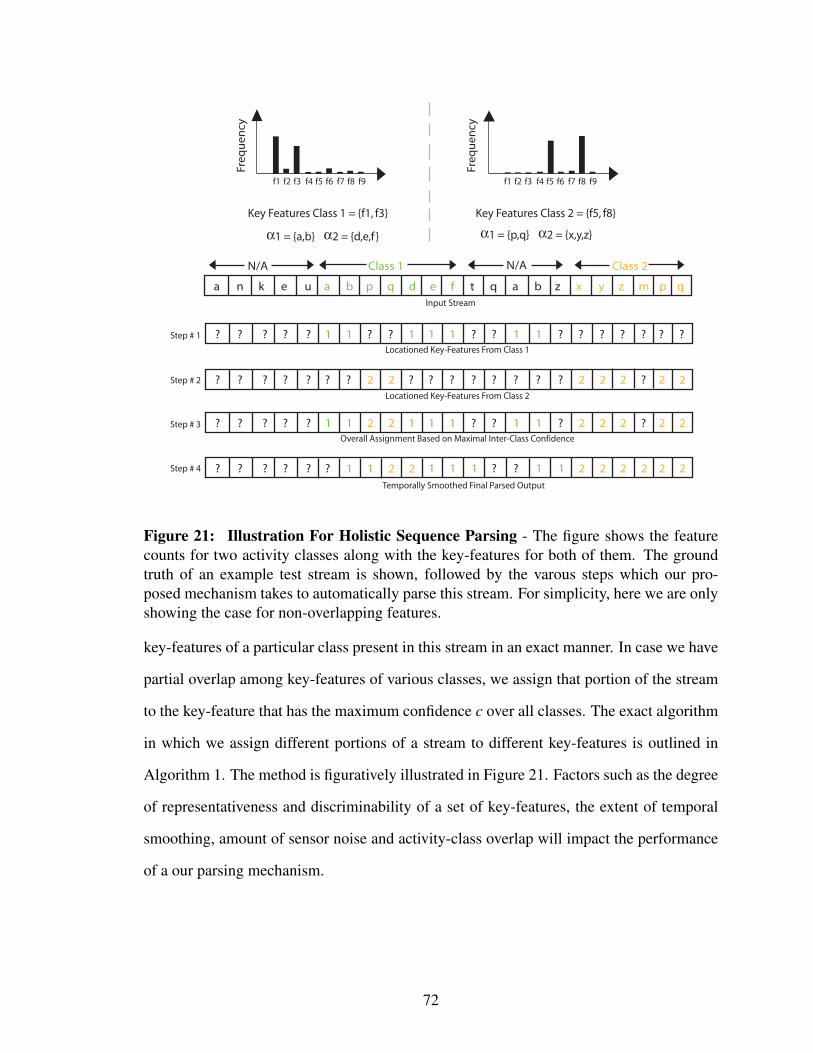
p

uFreq

uen

cy

f1 f2 f3 f4 f5 f6 f7 f8 f9

p

uFreq

uen

cy

f1 f2 f3 f4 f5 f6 f7 f8 f9

Key Features Class 1 = {f1, f3} Key Features Class 2 = {f5, f8}

a n k e u a b p d e fq t q a b z x y z m p q

u u u u

u u u u

N/A Class 1 Class 2

1 = {a,b} 2 = {d,e,f } 1 = {p,q} 2 = {x,y,z}

N/A

????? 1 1 ? ? 1 1 1 ? ? 1 1 ? ? ? ? ? ? ?

????? ? ? 2 2 ? ? ? ? ? ? ? ? 2 2 2 ? 2 2

????? 1 1 2 2 1 1 1 ? ? 1 1 ? 2 2 2 ? 2 2

????? ? 1 2 2 1 1 1 ? ? 1 1 2 2 2 2 2 21

Input Stream

Locationed Key-Features From Class 1

Locationed Key-Features From Class 2

Overall Assignment Based on Maximal Inter-Class Confidence

Temporally Smoothed Final Parsed Output

Step # 1

Step # 2

Step # 3

Step # 4

α α α α

Figure 21: Illustration For Holistic Sequence Parsing - The figure shows the featurecounts for two activity classes along with the key-features for both of them. The groundtruth of an example test stream is shown, followed by the varous steps which our pro-posed mechanism takes to automatically parse this stream. For simplicity, here we are onlyshowing the case for non-overlapping features.

key-features of a particular class present in this stream in an exact manner. In case we have

partial overlap among key-features of various classes, we assign that portion of the stream

to the key-feature that has the maximum confidence c over all classes. The exact algorithm

in which we assign different portions of a stream to different key-features is outlined in

Algorithm 1. The method is figuratively illustrated in Figure 21. Factors such as the degree

of representativeness and discriminability of a set of key-features, the extent of temporal

smoothing, amount of sensor noise and activity-class overlap will impact the performance

of a our parsing mechanism.

72

Subject 1 Subject 2 Subject 3

01

00

20

00

10

02

00

01

00

20

00

10

02

00

01

00

20

0

01

00

20

00

10

02

00

01

00

20

00

10

02

00

01

00

20

0

01

00

20

00

10

02

00

01

00

20

00

10

02

00

01

00

20

0

Tria

l 1Tr

ial 2

Tria

l 3Tr

ial 4

Tria

l 5

12

3

12

3

12

3

12

3

12

3

12

3

12

3

12

3

00

00

00

00

00

00

00

00

00

00

00

00

00

00

00

00

12

3

00

00

12

3

00

00

12

3

00

00

12

3

00

00

12

3

00

00

12

3

00

00

12

3

00

00

Figu

re22

:A

ctiv

ityPa

rsin

gR

esul

ts-T

hefig

ure

show

san

illus

trat

ion

ofth

epa

rsin

gre

sults

obta

ined

for

5of

the

10tr

ials

cond

ucte

dus

ing

ale

ave-

one-

out

tech

niqu

efo

rle

arni

ngth

eke

y-fe

atur

esfo

rva

riou

scl

asse

san

dco

nstr

uctin

gth

ete

stst

ream

s.T

hebl

ue-c

olor

edgr

aph

repr

esen

tsth

egr

ound

-tru

thda

ta,w

hile

the

red

colo

red

show

sth

epa

rsed

outp

utof

the

syst

em.F

orea

chof

the

grou

nd-t

ruth

grap

hs,

the

unin

tere

stin

gpa

rts

ofth

est

ream

are

repr

esen

ted

by0,

whi

leac

tiviti

esfr

omdi

ffer

entc

lass

esar

esh

own

bypl

ots

ofdi

ffer

enth

eigh

tsan

dla

bele

dby

num

bers

12

and

3re

spec

tivel

y.T

hex-

axis

inea

chof

the

grap

hsh

ows

the

sym

bol-

leng

ths

ofth

ein

puts

trea

ms.

73

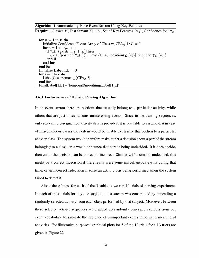
Algorithm 1 Automatically Parse Event Stream Using Key-FeaturesRequire: Classes M, Test Stream T [1 : L], Set of Key Features {γm}, Confidence for {γm}

for m = 1 to M doInitialize Confidence Factor Array of Class m, CFAm[1 : L] = 0for n = 1 to ||γm|| do

if γm(n) exists in T [1 : L] thenCFAm[position(γm(n))] = max{CFAm[position(γm(n))], frequency(γm(n))}

end ifend for

end forInitialize Label[1:L] = 0for l = 1 to L do

Label(l) = argmax∀m(CFAm[l])end forFinalLabel[1:L] = TemporalSmoothing(Label[1:L])

4.6.3 Performance of Holistic Parsing Algorithm

In an event-stream there are portions that actually belong to a particular activity, while

others that are just miscellaneous uninteresting events. Since in the training sequences,

only relevant pre-segmented activity data is provided, it is plausible to assume that in case

of miscellaneous events the system would be unable to classify that portion to a particular

activity class. The system would therefore make either a decision about a part of the stream

belonging to a class, or it would announce that part as being undecided. If it does decide,

then either the decision can be correct or incorrect. Similarly, if it remains undecided, this

might be a correct indecision if there really were some miscellaneous events during that

time, or an incorrect indecision if some an activity was being performed when the system

failed to detect it.

Along these lines, for each of the 3 subjects we ran 10 trials of parsing experiment.

In each of these trials for any one subject, a test stream was constructed by appending a

randomly selected activity from each class performed by that subject. Moroever, between

these selected activity sequences were added 20 randomly generated symbols from our

event vocabulary to simulate the presence of unimportant events in between meaningful

activities. For illustrative purposes, graphical plots for 5 of the 10 trials for all 3 users are

given in Figure 22.

74

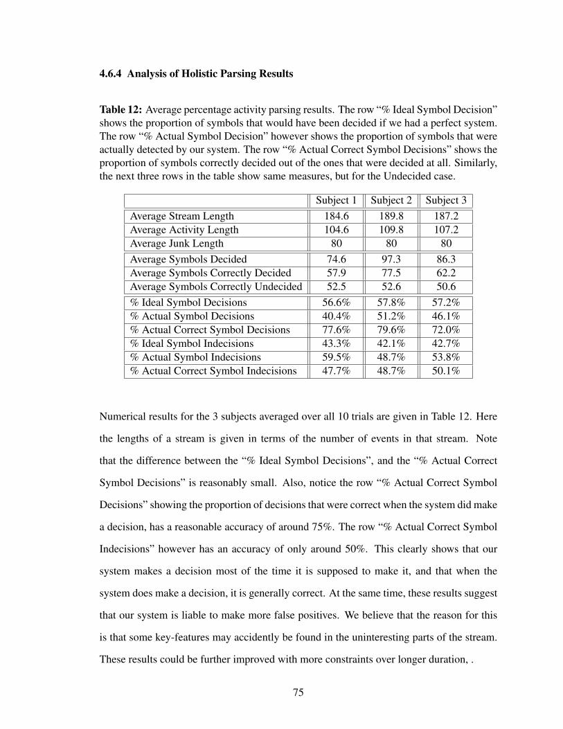
4.6.4 Analysis of Holistic Parsing Results

Table 12: Average percentage activity parsing results. The row “% Ideal Symbol Decision”shows the proportion of symbols that would have been decided if we had a perfect system.The row “% Actual Symbol Decision” however shows the proportion of symbols that wereactually detected by our system. The row “% Actual Correct Symbol Decisions” shows theproportion of symbols correctly decided out of the ones that were decided at all. Similarly,the next three rows in the table show same measures, but for the Undecided case.

Subject 1 Subject 2 Subject 3Average Stream Length 184.6 189.8 187.2Average Activity Length 104.6 109.8 107.2Average Junk Length 80 80 80Average Symbols Decided 74.6 97.3 86.3Average Symbols Correctly Decided 57.9 77.5 62.2Average Symbols Correctly Undecided 52.5 52.6 50.6% Ideal Symbol Decisions 56.6% 57.8% 57.2%% Actual Symbol Decisions 40.4% 51.2% 46.1%% Actual Correct Symbol Decisions 77.6% 79.6% 72.0%% Ideal Symbol Indecisions 43.3% 42.1% 42.7%% Actual Symbol Indecisions 59.5% 48.7% 53.8%% Actual Correct Symbol Indecisions 47.7% 48.7% 50.1%

Numerical results for the 3 subjects averaged over all 10 trials are given in Table 12. Here

the lengths of a stream is given in terms of the number of events in that stream. Note

that the difference between the “% Ideal Symbol Decisions”, and the “% Actual Correct

Symbol Decisions” is reasonably small. Also, notice the row “% Actual Correct Symbol

Decisions” showing the proportion of decisions that were correct when the system did make

a decision, has a reasonable accuracy of around 75%. The row “% Actual Correct Symbol

Indecisions” however has an accuracy of only around 50%. This clearly shows that our

system makes a decision most of the time it is supposed to make it, and that when the

system does make a decision, it is generally correct. At the same time, these results suggest

that our system is liable to make more false positives. We believe that the reason for this

is that some key-features may accidently be found in the uninteresting parts of the stream.

These results could be further improved with more constraints over longer duration, .

75

a b c d r b c s f e dq a b c d p q r s t u c

Input Test Stream

Motifs Class Aa,b,c,dd,b,e,f,a,cf,e,d

Motifs Class Bp,q,r,s,t,u,cr,b,c,s,qd,c,f,s

a b c d f e d a c d db b e f a c f e d f e d

Training Activity - Class A

p q r s t u c a c f sd r b c s q d c f s

Training Activity - Class B

Figure 23: Illustration of By-Parts Sequence Parsing Setup - The figure shows thelist of event motifs for two example activity classes. For the training data, the activityinstances for each class are constructed by conjoining the event motifs of respective classes.For testing event stream, the event motifs of different activity classes can be interleaved,however the motifs themselves stay intact.

4.6.5 By-Parts Parsing Using Key-Features

Note that we previously assumed that activities in a stream of events appear holistically

while there may be uninterested events between different activities in the event stream. In

a majority of everyday environments however, such an assumption might not be followed

very strictly. Consider for instance the environment of a household kitchen, where someone

might be making an omelet and tea simultaneously. One might execute a particular part of

making an omelet before switching to performing a particular part of making tea. In other

words, while event subsequences of these activities might be interleaved, this interleaving

is not completely random, and usually follows certain constraints.

To model such dynamics, we assume that an activity class has a certain set of event

subsequences that are temporally conjoined in a partially ordered manner for successfully

executing activity instances of that activity class. We call these set of constituent event

subsequences as the event motifs of an activity class. We assume that while in an event

stream event motifs of different activity classes can be interleaved, however the motifs

themselves stay intact. This setup is illustrated in Figure 23.

76

Details of Simulation Data: For this setup we generated some simulated data in which we

considered 5 activity classes, each with a set of 5 event motifs. We generated 50 activity

instances for each of these 5 classes, such that each activity instance was constructed by

randomly selecting 10 event motifs from their respective classes. The testing activity in-

stances were constructed by conjoining 10 event motifs from any of the 2 activity classes

with 50% of the motifs selected from each of the 2 considered activity classes. In the

following we present the results of our parsing algorithm as we varied the size of event

vocabulary considered, the minimum/maximum lengths of event motifs, and the amount of

intersplicing that could take place in the test activity instances.

To evaluate the performance of our parsing mechanism while using motif-based by-

parts model, we conducted 3 different experiments using the aforementioned simulation

data. The details of these experiments and their results are given in the following.

By-Parts Parsing Performance - Experiment 1: In the first experiment, one of the trends

we wanted to observe was the rate at which the parsing accuracy of our mechanism varies

as we change the maximum allowable length of the constituent motifs in the simulation

data. For this experiment, we considered a fixed vocabulary size of 10 symbols, and varied

the motif length-range from [3→ 5] symbols to [3→ 13] symbols. The average accuracy

of the parsing mechanism as a function of changing length-range of motifs is shown with

the blue graph in Figure 24.

We also wanted to observe the trend at which the parsing accuracy with varying lengths

would vary as we add different amounts of insertion noise in the data. To this end, we

performed two separate tests. In the first test we added a certain amount of insertion noise

in both training and testing data. The results of this test for different amounts of insertion

noise are shown with red color. In the second test we only added noise in the testing stream

and used non-noisy training data. The results of this test for different amounts of insertion

noise are shown with green color.

There are four important observations to be made in Figure 24.

77

5 7 9 11 130

10

20

30

40

50

60

70

80

90

100

P ure T raining & T esting Data

T raining & T esting Data 10% Noise

P ure T raining Data, T esting Data 10% Noise

T raining & T esting Data 20% Noise

P ure T raining Data, T esting Data 20% Noise

T raining & T esting Data 30% Noise

P ure T raining Data, T esting Data 30% Noise

Maximum Motif Length

Ave

rag

e Pe

rcen

t A

ccu

racy

Vocabulary Size = 10

Minimum Motif Length = 3

Figure 24: By-Parts Parsing Performance As Function of Maximum Motif Length forDifferent Amounts of Insertion Noise

1. The accuracy of the mechanism increases with the increase in the maximum allow-

able motif length. This is because the activities become more well-structured as the

allowed motif-length increases. This in turn increases the lengths of the discovered

key-features increasing the overall accuracy of our parsing mechanism.

2. The accuracy of the parsing mechanism falls down monotonically as we increase the

amounts of insertion noise both in the testing and training data. This can be noted by

observing the heights of the three red graphs in Figure 24. Moreover, compared to

the blue graph, a shallower rate of increase of accuracy is observed with the increase

in maximum allowable motif length. This is because in the presence of noise, longer

motifs do not appear as often, and therefore do not matter as much.

3. If noise is added only to the testing data and not to the training data, the performance

of the parsing mechanism is worse than the case when noise is added to both testing

and training data. This is because when both training and testing data are noisy, the

78

types of mutations that take place in the testing data have be previously seen in the

noisy training data. Such mutations in testing data are not observed in the noise free

training data, which results in its relatively worse performance.

4. If noise is only added to the testing data and not to the training data, the performance

of the parsing mechanism falls down with the increase in motif-length. This is be-

cause in the absence of noise, the lengths of discovered key-features increases with

an increase in allowed motif-length. However, these longer key-features cannot be

exactly matched in the testing data since the insertion noise brakes down longer mo-

tifs in the testing stream. Since our testing stream is constructed by concatenating

different motifs, with an increase in allowed motif-length, the length of the testing

stream increases. This results in decrease in parsing accuracy beyond a certain value

of the maximum allowed motif-lengths.

By-Parts Parsing Performance - Experiment 2: In the second experiment, we wanted to

observe the rate at which the parsing accuracy of our mechanism varies as we change the

size of the vocabulary using which the constituent motifs are generated. For this experi-

ment, we considered a range of vocabulary size from 10→ 37 symbols with increments of

5 symbols. For all these trials we considered a motif-length range of 3→ 7. The average

accuracy of the parsing mechanism as a function of changing size of symbol vocabulary

is shown in Figure 25. The accuracy of the mechanism increases with the increase in the

size of symbol vocabulary since that in turn increases the overlap between the activity

classes. Due to this increased class-overlap, the system is able to find more discriminative

key-features, which result in better parsing performance.

By-Parts Parsing Performance - Experiment 3:In the third experiment, we wanted to

observe the rate at which our parsing accuracy falls when the motifs in the testing stream do

not appear intact, and rather have some amount of intersplicing. For instance, instead of two

example motifs of a,b,c,d and e,f,g,h occurring as a whole side by side, i.e. a,b,c,d,e,f,g,h,

79

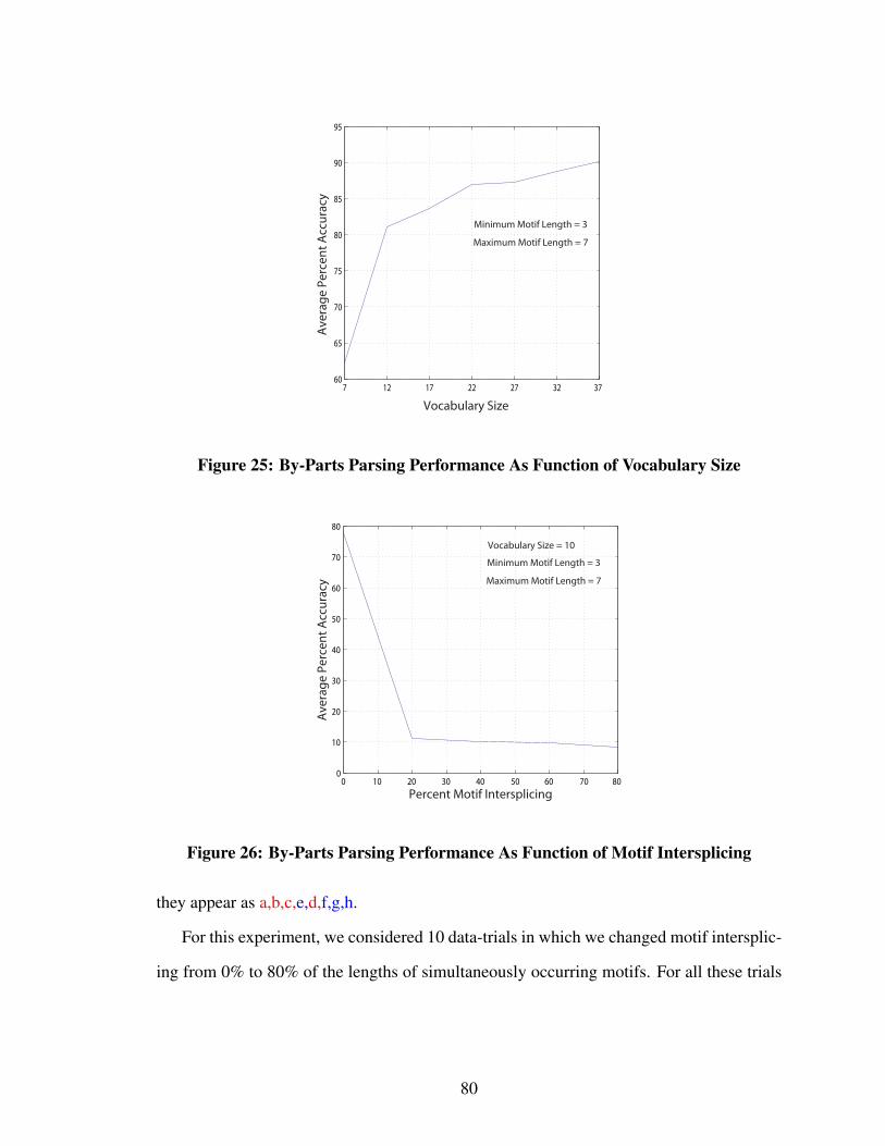
7 12 17 22 27 32 3760

65

70

75

80

85

90

95

Vocabulary Size

Ave

rag

e Pe

rcen

t A

ccu

racy

Minimum Motif Length = 3

Maximum Motif Length = 7

Figure 25: By-Parts Parsing Performance As Function of Vocabulary Size

0 10 20 30 40 50 60 70 800

10

20

30

40

50

60

70

80

Percent Motif Intersplicing

Ave

rag

e Pe

rcen

t A

ccu

racy

Vocabulary Size = 10

Minimum Motif Length = 3

Maximum Motif Length = 7

Figure 26: By-Parts Parsing Performance As Function of Motif Intersplicing

they appear as a,b,c,e,d,f,g,h.

For this experiment, we considered 10 data-trials in which we changed motif intersplic-

ing from 0% to 80% of the lengths of simultaneously occurring motifs. For all these trials

80

we considered a vocabulary of 10 symbols. The average accuracy of the parsing mecha-

nism as a function of motif intersplicing is shown in Figure 26. Note that the knee of the

curve is very evident at 20% at which the performance of the system falls down signifi-

cantly. This is because as there are no motif splicing in the training data, and we are using

an exact matching mechanism to find these motifs, none of the discovered key-features are

able to register with any part of the test stream. This challenge might be avoided by hav-

ing a training data where similar types of motif intersplicing have been observed. Another

potential way around this challenge might be by using a partial matching mechanism of

finding key-features in the test stream, as opposed to the currently used exact matching.

4.7 Summary

Recall that the key hypothesis behind our thesis is that there is sufficient structural signature

at a local temporal scale of activities, that can entail a reasonably disjunctive partitioning

of the activity space. This requires some notion of the range of temporal scales at which

events in activities mostly depend on each other. Capturing this event dependence in terms

of longer constituent event subsequences would result in more discriminative characteriza-

tions, however such characterizations would be more prone to sensor noise. On the other

hand, using smaller length event subsequences to capture activity structure would lead to

representations more robust to sensor-noise, but with less discriminative power. Since for

everyday environments, the predominant temporal scale at which events depend on each

other is generally not known a priori, the question is how does one decide to choose the

lengths of constituent event subsequences that should be used to extract the global structural

information of activities.

In this chapter we presented the activity representation of Suffix Trees that allows ef-

ficient modeling of this variable-length event dependence over a range of temporal scales.

This facilitates automatic learning of the predominant scales of event dependence in an en-

vironment. The fact that the complexity of this representation is only linear in the length of

81

the activity sequence, makes the usage of Suffix Trees all the more appropriate.

We have investigated the competence of Suffix Trees as an activity representation in

terms of their representational scope, discriminative power, noise sensitivity, and ability to

capture the underlying activity structure independent of an actor’s particular style. We have

also shown how the framework of Suffix Trees can be used to parse activities in a stream

of detected events. In Chapter 6, we shall present an efficient algorithm using Suffix Tree

activity representation, to detect local structural anomalies in test activities.

One of the main challenges of using Suffix Trees as human activity representation is

their sensitivity to sensor noise. This shortcoming becomes particularly significant for en-

vironments where events depend on previous events over shorter lengths of time, and the

events detectors are not quite robust. In such situations, fixed length event n-grams with

small values of n would be able to capture the activity structure sufficiently, while being

more robust than Suffix Trees. One way to alleviate the brittleness of Suffix Trees is by se-

lectively using their extracted sequential features only up to a certain length. Another way

to improve their noise sensitivity is to have some partial feature matching mechanism be-

tween different activities, instead of the exact feature matching mechanism being currently

used. This partial feature matching may be based on the edit-distance between activity fea-

tures, and would help map the noisy features of an activity to their closest matches in terms

of edit-distance. We return to these two points in Chapter 7.

82

CHAPTER V

ACTIVITY CLASS CHARACTERIZATION

So far, we have presented activity representations that use fixed and variable-length event

subsequences of activities to automatically discover the various activity classes taking place

in an everyday environment. In this chapter1, we present novel methods to characterize

such discovered activity classes. We show how an activity class can be characterized both

at a holistic as well as at a by-parts level. Such characterizations can be used to detect

various anomalous activities, and explaining in what ways do such anomalies vary from

the various regular behaviors taking place in an environment. We shall elaborate further on

this point in Chapter 6

5.1 Motivation for Concept Characterization

Finding general, tractable and concise characterizations for concepts and categories is cru-

cial for making sense of the world around us [105]. Without such characterizations any

system could be overwhelmed by the sheer diversity of information in its surrounding.

These characterizations encode the various commonalities amongst the members of

the different categories. Such commonalities may e.g. be appearance based, temporal or

logical. These common attributes dictate the nature of analysis that might be undertaken for

the members of the different categories. A concise and efficiently learnable characterization

of a concept can be used to many an end, including the following:

• One may want to use such characterizations to summarize a typical notion of a cate-

gory. This can be particularly useful when dealing with very large quantities of data

where a general or canonical signature of the data may be useful.

1This work has previously appeared in [39] and [41]

83

• Similarly, these characterization could be used to efficiently learn about new pieces

of information that a system may acquire over time. This is true both for classifying

a new piece of information, as well as updating an already learned set of concepts in

a dynamically changing setting.

• These characterizations could be used for the purposes of prediction of the events

that may transpire in a setting. This ability to predict is crucial to have a notion of

expectation, confidence, as well as surprise that a perceptual system needs in order

to function well.

• Finally, such characterizations can enable a system to reason about irregular pieces

of information that are in some sense alarming or anomalous.

There exists a variety of ways to define some characterization of a class. These include

the classical view which considers an entire class in terms of some summary description or

features [14]. The probabilistic view of concept characterization quantifies some measure

of central tendency of instances of a concept [81]. Another perspective on concept char-

acterization is the exemplar view that argues for representing a category by its exemplars

rather than an abstract summary of the general attributes of its members.

Regardless of whichever perspective towards concept categorization one chooses to

take, a crucial factor for the usefulness of a categorization is the granularity at which it

abstracts information about the concept. This point will be of our particular interest dur-

ing the remaining part of this chapter where we look at the problem of finding efficient

characterizations of the various activity classes taking place in everyday environments.

5.2 Characterization of Activity Classes

Considering activity classes as conjunctions of various activity instances in an activity

space, there are two ways in which we want to characterize them:

84

• Class Characterization at a Holistic Level

• Class Characterization at a By-Parts Level

The purpose of having a holistic-level characterization for an activity class is to find the

most “typical member” of the class that best represents the general characteristics of the

other members of that class. This view is particularly useful for the types of analyses that

require considering each activity as a single data point with emphasis on the more global

properties of activities. In Chapter 6, we shall make use of this view on class characteriza-

tion to explain the various anomalous activities taking place in an environment.

Human activities are not monolithic entities, and their constituent events can them-

selves have semantic connotations. It is therefore important to have some characterization

of activity classes that can reflect an activity class at a more local level. The by-parts per-

spective on activity class characterization is particularly useful for the types of analyses

that focus on local event dependencies in the member-activities of an activity class. Such

local event dependencies could be used for efficient on-line activity classification, activity

summarization, and detecting local atypicalities in activities.

5.3 Class Characterization at a Holistic Level

Considering an activity class at a holistic level, a natural way to characterize it might be

in terms of a “typical” member of the class that in some sense best represents all the other

members of that class. The question of typicality is closely related to the idea of how

similar an activity is to the other members of its class [57].

There are many ways in which this idea of the similarity of an activity with respect to

other activities of a class might be used to find the typical member. The classic graph theo-

retic literature provides a potential answer to this problem in terms of finding the “centroid”

of the cluster, i.e. finding the member which minimizes the maximum distance between

the rest of the members and itself (also known as the min-max algorithm) [25]. While this

85

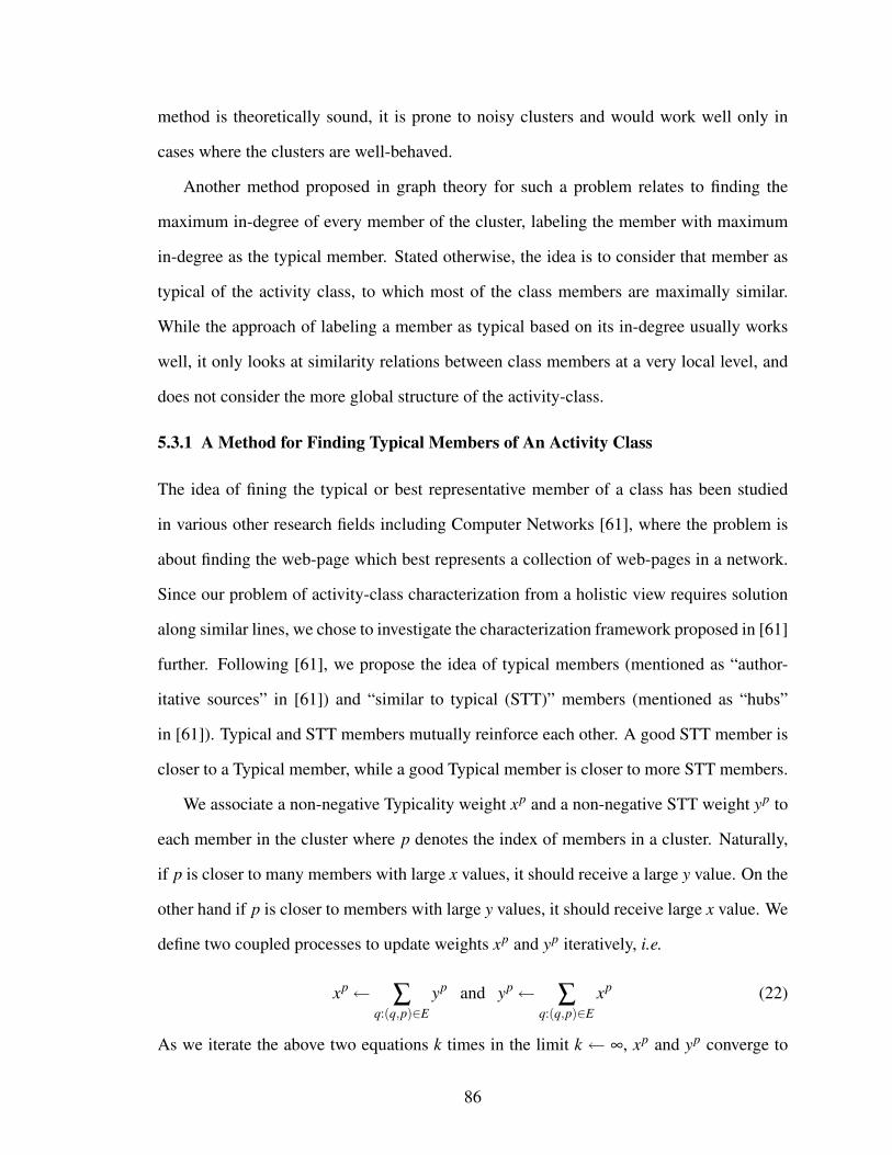
method is theoretically sound, it is prone to noisy clusters and would work well only in

cases where the clusters are well-behaved.

Another method proposed in graph theory for such a problem relates to finding the

maximum in-degree of every member of the cluster, labeling the member with maximum

in-degree as the typical member. Stated otherwise, the idea is to consider that member as

typical of the activity class, to which most of the class members are maximally similar.

While the approach of labeling a member as typical based on its in-degree usually works

well, it only looks at similarity relations between class members at a very local level, and

does not consider the more global structure of the activity-class.

5.3.1 A Method for Finding Typical Members of An Activity Class

The idea of fining the typical or best representative member of a class has been studied

in various other research fields including Computer Networks [61], where the problem is

about finding the web-page which best represents a collection of web-pages in a network.

Since our problem of activity-class characterization from a holistic view requires solution

along similar lines, we chose to investigate the characterization framework proposed in [61]

further. Following [61], we propose the idea of typical members (mentioned as “author-

itative sources” in [61]) and “similar to typical (STT)” members (mentioned as “hubs”

in [61]). Typical and STT members mutually reinforce each other. A good STT member is

closer to a Typical member, while a good Typical member is closer to more STT members.

We associate a non-negative Typicality weight xp and a non-negative STT weight yp to

each member in the cluster where p denotes the index of members in a cluster. Naturally,

if p is closer to many members with large x values, it should receive a large y value. On the

other hand if p is closer to members with large y values, it should receive large x value. We

define two coupled processes to update weights xp and yp iteratively, i.e.

xp← ∑q:(q,p)∈E

yp and yp← ∑q:(q,p)∈E

xp (22)

As we iterate the above two equations k times in the limit k ← ∞, xp and yp converge to

86

stable values, x∗ and y∗. The node which has the largest component in the converged vector

x∗ would correspond to the member which has the greatest Typical weight and hence is the

best representative of the nodes of a cluster. x∗ can be computed from the Eigen Analysis

of the matrix AT A where A is the symmetric similarity matrix of all the nodes of the cluster.

x∗ is the principal eigenvector of AT A, the largest component of which corresponds to the

Typical Node of the cluster (for the proof, see [61]). In Chapter 6, we shall make use of

typical members of activity classes to explain the various anomalous activities taking place

in an environment.

5.4 Class Characterization at a By-Parts Level

Since human activities are not monolithic entities, and their constituent events can them-

selves have semantic connotations, it is important to have some characterization of activity

classes that can reflect their characteristics at a more local level. One way of looking at this

problem is to find recurrent subsequences of events in members of an activity class that have

high predictive power regarding what event may follow them. We call such repetitive and

predictive patterns as event motifs, and are interested in discovering them efficiently. We

argue that such event motifs could be used for predicting future events that may transpire

in an environment. This ability to predict events is crucial to have a notion of expectation,

confidence, as well as surprise that a perceptual system needs in order to detect unexpected

or anomalous events.

5.4.1 Defining Event Motifs

We are interested in frequently occurring event subsequences that are useful in predicting

future events in activities. Following [117], we assume that a class of activity sequences

can be modeled as a variable-memory Markov chain (VMMC). We define an event-motif

for an activity-class as one of the variable-memory elements of its VMMC. We cast the

problem of finding the optimal length of the memory element of a VMMC as a function

87

optimization problem and propose our objective function in the following.

5.4.2 Formulation of Objective Function

Let Y be the set of events, A be the set of activity-instances, and C be the set of discovered

activity-classes. Let function U(a) map an activity a∈A to its membership class c∈C. Let

the set of activities belonging to a particular class c∈C be defined as Ac = {a∈A : U(a) =

c}. For a = (y1,y2, ...,yn) ∈ A where y1,y2, ...yn ∈ Y , let p(c|a) denote the probability that

activity a belongs to class c. Then,

p(c|a) =p(a|c)p(c)

p(a)∝

n

∏i=1

p(yi|yi−1,yi−2, ...,y1,c) (23)

where we have assumed that all activities and classes are equally likely. We approximate

Eq 23 by a VMMC, Mc as:n

∏i=1

p(yi|yi−1, ...,y1,c) =n

∏i=1

p(yi|yi−1, ...,yi−mi,c) (24)

where mi ≤ i− 1 ∀ i. For any 1 ≤ i ≤ n, the sequence (yi−1,yi−2, ...,yi−mi) is called the

context of yi in Mc( [117]), denoted by SMc(yi). We want to find the sub-sequences which

can efficiently characterize a particular class, while having minimal representation in other

classes. We therefore define our objective function as:

Q (Mc|Ac) = γ−λ (25)

where

γ = ∏a∈Ac

p(c|a) and λ = ∑c′∈C\{c}

∏a∈Ac′

p(c′|a) (26)

Intuitively, γ represents how well a set of event-motifs can characterize a class in terms of

correctly classifying the activities belonging to that class. On the other hand, λ denotes to

what extent a set of motifs of a class represent activities belonging to other classes. It is

clear that maximizing γ while minimizing λ would result in the optimization of Q (Mc|Ac).

Note that our motif finding algorithm leverages our activity-class discovery framework

by using the availability of the discovered activity-classes to find the maximally mutually

exclusive motifs.

88

5.4.3 Objective Function Optimization

We now explain how we optimize our proposed objective function. [117] describe a

technique to compare different VMMC models that balances the predictive power of a

model with its complexity. Let s be a context in Mc, where s = yn−1,yn−2, ...,y1, and

yn−1,yn−2, ...,y1 ∈ Y . Let us define the suffix of s as suffix(s) = yn−1,yn−1, ...y2. For

each y ∈ Y , let NA′(y,s) be the number of occurrences of event y in activity-sequences

contained in A′ ⊆ A where s precedes y, and let NA′(s) be the number of occurances of s in

activity-sequences in A′. We define the function ∆A′(s) as

∆A′(s) = ∑y∈Y

N(s,y)log(

p̂(y|s)p̂(y|suffix(s))

)(27)

where p̂(y|s) = NA′(s,y)/NA′(s) is the maximum likelihood estimator of p(y|s). Intuitively,

∆A′(s) represents the number of bits that would be saved if the events following s in A′,

were encoded using s as a context, versus having suffix(s) as a context. In other words, it

represents how much better the model could predict the events following s by including the

last event in s as part of context of these events.

We now define the function Ψc(s) (bit gain of s) as

Ψc(s) = ∆Ac(s)− ∑c′∈C\{c}

∆Ac′ (s) (28)

Note that higher values of ∆Ac(s) imply greater probability that an activity in Ac is assigned

to c, given that s is used as a motif. In particular, higher the value of ∆Ac(s), higher will be

the value of γ. Similarly, higher the value of ∑c′∈C\{c}∆Ac′ (s), higher the value of λ.

We include a sequence s as a context in the model Mc iff

Ψc(s) > K× log(`) (29)

where ` is the total length of all the activities in A, while K is a user defined parameter. The

term K× log(`) represents added complexity of the model Mc, by using s as opposed to

suffix(s) as a context, which is shorter in length and occurs at least as often as s. The higher

the value of K the more parsimonious the model will be.

89

Equation 29 selects sequences that both appear regularly and have good classification

and predictive power - and hence can be thought of as event-motifs. Work in [93] shows

how the motifs in a VMMC can be represented as a tree. Work done in [4] presents a linear

time algorithm that constructs such a tree by first constructing a data structure called a

Suffix Tree to represent all sub-sequences in the training data A, and then by pruning this

tree to leave only the sequences representing motifs in the VMMC for some activity-class.

We follow this approach by using Equation 29 as our pruning criterion.

5.4.4 Results: Discovered Event Motifs

We now present the results of motifs we obtained using our method for the previously

discovered activity-classes in Loading Dock and House environments.

The highest big-gain event-motifs found for the 7 discovered activity-classes in the

Loading Dock domain are given in Table 13. The discovered motifs of activity-classes

seem to characterize these classes efficiently. Note that the discovered motifs for activity-

classes where package delivery occurred, have events like Person Places Package In The

Back Door Of Delivery Vehicle and Person Pushes Cart In The Front Door of Building→

Cart is Full. On the other hand event-motifs for activity-classes where package pick-up

occurred, have events such as Person Removes Package From Back-Door Of Delivery Ve-

hicle and Person Places Package Into Cart. The highest big-gain event-motifs found for the

5 discovered activity-classes in the residential house domain are given in Table 14. The

motifs for the House environment capture the position where the person spends most of his

time and the order in which he visits the different places in the house. Such local event

subsequences seem to capture the discriminating elements of various activity classes, and

can therefore be used to online activity classification as well as anomaly detection.

5.4.5 Subjective Assessment of Discovered Motifs

Given some data, our proposed discovery method would by construction find some motifs

for the discovered activity-classes. This raises the question about the correctness of our

90

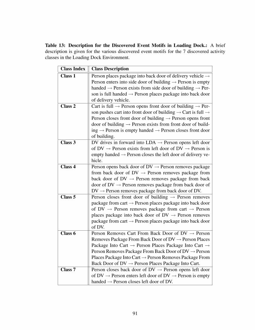
Table 13: Description for the Discovered Event Motifs in Loading Dock.: A briefdescription is given for the various discovered event motifs for the 7 discovered activityclasses in the Loading Dock Environment.

Class Index Class DescriptionClass 1 Person places package into back door of delivery vehicle→

Person enters into side door of building→ Person is emptyhanded→ Person exists from side door of building→ Per-son is full handed→ Person places package into back doorof delivery vehicle.

Class 2 Cart is full → Person opens front door of building → Per-son pushes cart into front door of building→ Cart is full→Person closes front door of building→ Person opens frontdoor of building→ Person exists from front door of build-ing→ Person is empty handed→ Person closes front doorof building.

Class 3 DV drives in forward into LDA → Person opens left doorof DV → Person exists from left door of DV → Person isempty handed→ Person closes the left door of delivery ve-hicle.

Class 4 Person opens back door of DV→ Person removes packagefrom back door of DV → Person removes package fromback door of DV → Person removes package from backdoor of DV→ Person removes package from back door ofDV→ Person removes package from back door of DV.

Class 5 Person closes front door of building → Person removespackage from cart→ Person places package into back doorof DV → Person removes package from cart → Personplaces package into back door of DV → Person removespackage from cart→ Person places package into back doorof DV.

Class 6 Person Removes Cart From Back Door of DV → PersonRemoves Package From Back Door of DV→ Person PlacesPackage Into Cart → Person Places Package Into Cart →Person Removes Package From Back Door of DV→ PersonPlaces Package Into Cart→ Person Removes Package FromBack Door of DV→ Person Places Package Into Cart.

Class 7 Person closes back door of DV → Person opens left doorof DV→ Person enters left door of DV→ Person is emptyhanded→ Person closes left door of DV.

91

Table 14: Description for the Discovered Event Motifs in Residential House Domain.:A brief description is given for the various discovered event motifs for the 5 discoveredactivity classes in the Residential House Environment.

Class Index Class DescriptionClass 1 Alarm → Kitchen entrance → Fridge → Sink → Garage

door (inside).Class 2 Stairway→ Fridge→ Sink→ Cupboard→ Sink.Class 3 Stairway→ Dining Table→ Den→ Living-room Door→

Sun-room→ Living-room door→ Den.Class 4 Den → Living-room door → Den → Kitchen Entrance →

Stairway.Class 5 Fridge → Dining Table → Kitchen Entrance → Fridge →

Sink.

discovered results. Since our final goal is to design a system that would be able to discover

and characterize human-interpretable activity-classes, we performed a limited user test in-

volving 7 participants, to subjectively assess the performance of our system. For each

participant, 2 of the 7 discovered activity classes were selected from the Loading Dock en-

vironment. Each participant was shown 6 example activities, 3 from each of the 2 selected

activity-classes. The participants were then shown the video frames of 6 motifs, 3 for each

of the 2 classes, and were asked to associate each motif to the class that it best belonged

to. Their answers agreed with our systems 83% of the time, i.e., on average a participant

agreed with our system on 5 out of 6 motifs. The probability of agreement on 5 out of 6

motifs by random guessing2 is only 9.3%.

This result shows that the discovered event motifs seem to be able to capture the struc-

tural signature of the various activity-classes in a way that is also semantically meaningful

to human observers. This anecdotal study is an initial indication showing that the percep-

tual bias induced by us in the system in terms of the event-vocabulary and the notion of

2According to binomial distribution the chance of randomly agreeing 5 out of 6 motifs is C65(0.5)1(0.5)5.

92

activity similarity, successfully reflects the underlying activity structure of the various ac-

tivities, and is being manipulated in a way that is semantically meaningful. While these

discovered event motifs on their own do not have to be human interpretable so long as they

can be used for some other task such as classification or anomaly detection, their inter-

pretability can nevertheless be useful for explaining the results for the final task they are

being used for.

5.5 Summary

Finding general, tractable and concise characterizations for activity classes is crucial for

making sense of the various types of activities taking place in an environment. These

characterizations may be used for such tasks as class summarization, reasoning in dynamic

settings, and prediction of future events to learn some notion of expectation and surprise.

We have particularly focused on finding characterizations of the various activity-classes

taking place in an environment both at a holistic as well as at a by-parts level. We model

a holistic-level characterization for as the most “typical member” of that class which best

represents the general characteristics of the other members of that class. We have looked at

the notion of typicality of a class member as a function of how similar it is to other members

of the class. This view on class characterization is particularly useful for the types of anal-

yses that require considering each activity as a single data point with emphasis on the more

global properties of activities. We shall make use of this view on class characterization to

explain detected anomalies in Chapter 6.

From a by-parts perspective on characterization of activity classes, we have looked at

finding recurrent event motifs in member activities of a class that have high predictive

power in terms of what event may follow them in the immediate future. Our anecdotal

user-study of such discovered event motifs seems to corroborate their usefulness for the

task of online activity classification. This gives us reason to believe that such event motifs

may also be used to find unexpected or surprising subsequences of events. So far we have

93

discovered these motifs in a completely unsupervised manner. However, some of these

motifs are more informative than others. Learning what makes a motif more interesting

than others, using an expert’s feedback remains an open question. Moreover, the type of

event motifs we are currently finding are designed to have high predictive power for the

events in the immediate future. However, for many problems longer term event predictions

with relatively high confidence are required. Discovering event motifs using our current

framework, that have such longer term event predictions remains another open question.

94

CHAPTER VI

ANOMALOUS ACTIVITY DETECTION

In this chapter, we explore some of the ways in which we can use the discovered activity

classes in an everyday environment to detect anomalous or irregular activities.

6.1 On The Notion Of Anomaly

If we look up the word anomaly in a dictionary, we would find descriptions such as “de-

viation from common or regular”, or “something alarming” [53]. These descriptions of

anomaly require a notion of what is meant by regular, common, or typical in an envi-

ronment. There are two key challenges in considering anomalies as a function of being

different from what is meant by regular or typical.

Firstly, for a lot of everyday environments, it is not known a priori what are the different

regular behaviors that can take place in that environment. Consider for instance the envi-

ronment of a household kitchen, and you can imagine the large number of different recipes

that can be cooked there. A list of such regular activities in an everyday environment is

usually not known to us a priori.

Secondly, even if we assume prior knowledge about the different types of regular or ac-

ceptable human behaviors being performed in an environment, it is very hard to accurately

model such behaviors. Consider for instance the activity of making an omelet in a house-

hold kitchen, and you can imagine the large number of different ways in which one can

execute this activity in a perfectly acceptable way. Modeling these variations to an extent

where a system can distinguish a true anomaly from an unusual or an outlier instance of

that activity is indeed challenging.

The difference between a truly alarming anomaly versus an outlier is not necessarily

95

embedded in the statistics of its directly observable features - rather it is dependent on the

goal or the outcome of the activity. The challenge for a perceptual system lies in inferring

this goal or outcome using perceptual data. Making use of this perceptual data, we can only

try to model what an activity looks like, and not necessarily what an activity is. The reason

the problem of detecting anomalous activities is particularly challenging is the fact that

while anomalies appear very similar to the regular members of an activity class, they do

not achieve the desired activity goal in an acceptable way. Our hope is that the differences

in the appearance of regular versus the anomalous activities would be enough to correctly

disambiguate between them.

This raises a question about the plausibility of a perceptual system such as ours that

attempts to detect anomalous activities in an unsupervised manner. We must state here

that our proposed framework looks at anomalous activities more from a discovery rather

than a purely detection based perspective. In other words, our framework first attempts to

discover some notion of regularity or typicality in an environment, and then based on this

notion it tries to find what are the activities that do not follow these general regular patterns.

Moreover, our framework is fit to detect only those anomalies where the perceptual differ-

ences between the regular versus anomalous are sufficient to be distinguished using a set of

computational mechanisms. While our approach is not intended for completely automatic

systems, it can however be very useful for large scale unconstrained environments for dis-

tinguishing between activities that can confidently be labeled as regular versus those that

are not. The final decision about calling an activity anomalous can be left to the discretion

of a human expert, requiring him to only analyze those activities that are more likely to be

deemed truly anomalous or alarming.

6.2 Detecting Anomalous Activities

Consider our example activity of making an omelet in a household kitchen. An instance of

this activity may be anomalous because of the fact that the entire activity was performed

96

in a wrong way, and that it failed to achieve the activity-goal of making an omelet. On the

other hand, one can have an instance of making an omelet where although the final goal

of making an omelet was achieved, some intermediate steps required to achieve this goal

were not executed properly. We therefore look at the problem of detecting anomalies in

everyday environments in two ways:

1- Anomaly Detection At a Holistic Level

2- Anomaly Detection At a By-Parts Level

From a holistic perspective, we considered each activity as an individual instance of an

activity class. If this activity member of a class shares the general characteristics of the

various other activity members of that class, then it is considered as a regular member of

that class. Otherwise, it is considered as an anomalous member. From a by-parts view, we

are more interested in detecting local irregularities in an activity instance, such as insertion

of some extraneous events or deletion of some important events from the activity. In the

following we present the details of these two views on anomaly detection.

6.3 Anomaly Detection At a Holistic Level

Recall that given a set of say K activity instances, we consider this set as a completely

connected edge-weighted activity graph and posed the problem of discovering the various

activity-classes in this activity data as that of finding the various maximal cliques present in

the corresponding activity-graph (§ 3.3.3). Given ||C|| such discovered activity-classes, we

are now interested in finding to which of these activity-classes does a test activity belong,

and whether it is is a regular or an anomalous member of its membership class.

Also recall that each member j of an activity-class c has some weight wc( j), that in-

dicates the participation of j in c (Equation 5). We compute the similarity between a new

activity-instance τ and previous members of each class by defining a function Ac(τ) as:

Ac(τ) = ∑j

sim(τ, j)wc( j) ∀ j ∈ c (30)

97

Here Ac represents the average weighted similarity between the new activity-instance τ and

any one of the discovered classes c. The selected membership class c∗ is found as:

c∗ = argmax∀c

Ac(τ) (31)

Once the membership decision of a new test activity has been made, we now focus our

attention on deciding whether the new class member is regular or anomalous. Intuitively,

we want to decide the normality of a new instance based on its closeness to the previous

members of its membership activity-class. This can be done with respect to the average

closeness between all the previous members of its membership class. Let Γ(τ) be:

Γ(τ) = ∑j∈c∗

Φc∗( j,τ)wc∗( j) (32)

where Φ is defined by Equation 4. We define a new class member τ as regular if Γ(τ) is

greater than a particular threshold. The threshold on Γ(τ) is learned by mapping all the

anomalous activity instances detected in the training activity-set to their closest activity-

class (using Equation 30 and 31), and computing the value of Γ for both regular and

anomalous activity instances. We can now observe the variation in false acceptance rate

and true positives as a function of the threshold Γ. This gives a “Receiver Operating Char-

acteristic” (ROC) curve. The area under ROC is indicative of the confidence in our de-

tection metric Γ(τ) [56]. Based on our tolerance for true and false positive rates, we can

choose an appropriate threshold.

Results: Anomaly Detection in Loading Dock Environment

Recall that in the loading dock environment described in § 3.4.1, of the 150 training activi-

ties we found 7 classes, with 106 activities as part of any one of the discovered class, while

44 activities being different enough to be not included into any of the discovered activity-

classes. We first classified the anomalous activities into one of the 7 activity-classes, and

then using Equation 32 computed the value of Γ for all the regular and anomalous mem-

bers of the 7 classes. The resulting ROC that was obtained is shown in Figure 27. The

98

True

Pos

itive

s - H

ITS

Decision Threshold

1

0.9

0.8

0.7

0.6

0.5

0.4

0.3

0.2

0.1

0 0.2 0.4 0.6 0.8 1.0

Area Under The ROC = 0.9403

False Acceptance Rate - FAR

Figure 27: ROC Curve For Loading Dock Environment - The figure shows the ROCcurve obtained for the Loading Dock Environment. The X-axis shows the False AcceptanceRate, while the Y-axis represents the rate of True Positives. Points on this graph give usthe expected rate of true positives and false acceptance rate for corresponding values ofthreshold. The area under the obtained ROC is 0.94, which indicates a confidence of 94%in our detection metric.

area under the obtained ROC was 0.94, which indicates a confidence of 94% in our de-

tection metric [56]. We then used another 45 test activities to be classified to any of the 7

discovered activity-classes. The decision about whether these test activities were regular

or anomalous members of their membership class was made based on their distance from

their membership class, and the threshold Γ.

We now describe how semantically meaningful these detected anomalies were from a

human stand-point, as well as what explanations did we get for the detected anomalous

activities based on some of the selected key-features of the activity-classes.

Analysis of Detected Anomalies

Analyzing the detected anomalous activities reveals that there are essentially two kinds of

activities that are being detected as anomalous, (1) those that are truly alarming, where

someone must be notified, and (2) those that are simply unusual delivery activities with

respect to the other regular activities. Key-frames for three of the truly alarming anomalous

activities are shown in Figure 28. Figure 28-a shows a truck driving out without closing

99

it’s back door. Not shown in the key-frame is the sequence of events where a loading-

dock personnel runs after the delivery vehicle to tell the driver of his mistake. Figure 28-b

shows a delivery activity where a more than usual number of people unload the delivery

vehicle. Usually only one or two people unload a delivery vehicle, however as can be seen

from Figure 28-b, in this case there were five people involved in the process of unloading.

Finally, Figure 28-c shows the unusual activity of a person cleaning the dock-floor.

User Study For Detected Anomalies

To analyze how intuitive the detected anomalies are to humans, a user test involving 7

users was performed. Firstly, 8 regular activities for a subject were selected so she could

understand the notion of a regular activity in the environment. 10 more activities were

selected, 5 of which were labeled as regular by the system while the rest of the 5 were

detected as anomalies. Each of the 7 users were shown these 10 activities and asked to

label every one of them as a regular instance or an anomaly based on the regular activities

previously shown. Each of the 10 activities were given labels based on what the majority

agreed upon. 8 out of 10 activities labeled by the users, corresponded with the labels of

the system. The probability of the system choosing the correct label 8 out of 10 times by

chance is 4.4% 1. This highlights the interesting fact that the anomalies detected by the

proposed system fairly match the natural intuition of human observers.

Anomalous Activity Explanation

Explanation of the activities detected as anomalous in an environment may be thought

of as a function of the general properties of an activity class. We can explain such detected

anomalies at a global level using a typical member of an activity class. Recall that we have

described one way of finding a typical member of an activity class in § 5.3.1. Our general

idea is to find the features of a typical member that can be used to explain an anomalous

activity in a maximally-informative manner.

1Given that the probability of correctly choosing the true label by simply guessing is 0.5, the binomialprobability states that chance of an 8/10 success is C10

8 (0.5)8(0.5)2 ≈ .0439

100

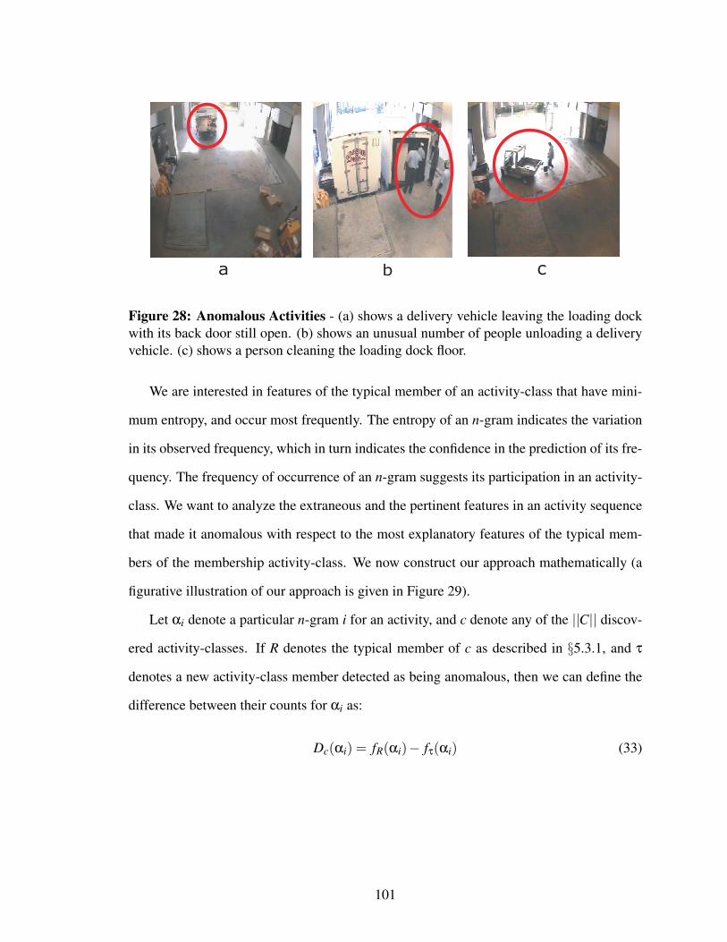
a b c

Figure 28: Anomalous Activities - (a) shows a delivery vehicle leaving the loading dockwith its back door still open. (b) shows an unusual number of people unloading a deliveryvehicle. (c) shows a person cleaning the loading dock floor.

We are interested in features of the typical member of an activity-class that have mini-

mum entropy, and occur most frequently. The entropy of an n-gram indicates the variation

in its observed frequency, which in turn indicates the confidence in the prediction of its fre-

quency. The frequency of occurrence of an n-gram suggests its participation in an activity-

class. We want to analyze the extraneous and the pertinent features in an activity sequence

that made it anomalous with respect to the most explanatory features of the typical mem-

bers of the membership activity-class. We now construct our approach mathematically (a

figurative illustration of our approach is given in Figure 29).

Let αi denote a particular n-gram i for an activity, and c denote any of the ||C|| discov-

ered activity-classes. If R denotes the typical member of c as described in §5.3.1, and τ

denotes a new activity-class member detected as being anomalous, then we can define the

difference between their counts for αi as:

Dc(αi) = fR(αi)− fτ(αi) (33)

101

where f (αi) denotes the count of a n-gram αi. Let us define the distribution of the proba-

bility of occurrence of αi in c as:

Pc(αi) =∑

k∈cfk(αi)

M∑

i=1∑

k∈cfk(αi)

(34)

where M represents all the non-zero n-grams in all the members of activity-class c. Let us

define multi-set χic as:

χic = { fk(αi)|k ∈ c} (35)

We can now define probability Qc(x) of occurrence of a particular member x ∈ χic for αi in

c as:

Qc(x) = ψ ∑j∈c

1 i f f (αi) = x

0 otherwise(36)

where ψ is the normalization factor. Let us define Shannon’s Entropy of a n-gram i for an

activity-class c by Hc(αi) as:

Hc(αi) = ∑x∈χi

c

Qc(x)ln(Qc(x)) (37)

We can now define the notion of predictability, PRDc(αi), of the values of n-gram αi of

cluster c as:

PRDc(αi) = 1− Hc(αi)M∑

i=1Hc(αi)

(38)

It is evident from this definition, that αi with high entropy Hc(αi) would have high vari-

ability, and therefore would have low predictability.

We define the explainability of an n-gram αi ∈ c that was frequently and consistently

present in the regular activity-class as:

ξPc (αi) = PRDc(αi)Pc(αi) (39)

Intuitively, ξPc indicates how much an αi is instrumental in representing an activity-class c.

102

Figure 29: Illustration of Anomaly Explanation - Five simulated activity sequences areshown to illustrate the different concepts introduced for anomaly explanation. α1 has lowvalue of Pc, its entropy Hc is low and therefore its predictability is high. α4 has mediumPc, its entropy Hc is also low and its predictability is high. Finally α8 has high Pc, but itsentropy Hc is high which makes its predictability low. α1 could be useful in explaining theextraneous features in an anomaly, while α4 could be useful in explaining the features thatwere deficient in it.

Similarly, we can define the explainability of αi ∈ c in terms of how consistently was it

absent in representing c.

ξAc (αi) = PRDc(αi)(Pmax

c (αi)−Pc(αi)) (40)

where Pmaxc (αi) is the maximum probability of occurrence of any αi in c.

The first term in both Equation 39 and 40 indicates how consistent αi is in its frequency

over the different members of a class. The second term in Equation 39 and 40 dictates how

representative or non-representative αi is for c respectively.

Given an anomalous member of an activity-class, we can now find the features that

were frequently and consistently present in its regular members, but were deficient in the

103

anomaly τ. To this end, we define the function Deficient(τ) as:

Deficient(τ) = argmaxαi

[ξPc (αi)Dc(αi)] (41)

Similarly, we can find the most explanatory features that were consistently absent in the

regular members of the membership activity-class but were extraneous in the anomaly. We

define the function Extraneous(τ) as:

Extraneous(τ) = argminαi

[ξAc (αi)Dc(αi)] (42)

We can explain anomalies based on these features in two ways. Firstly, we can consider

features that were deficient from an anomaly but were frequently and consistently present

in the regular members. Secondly, we can consider features that were extraneous in the

anomaly but were consistently absent from the regular members of the activity-class.

Results: Explanation of Anomalies in Loading Dock Environment

Figure 30 shows the explanation generated by the aforementioned approach for three

of the detected anomalous activities in loading dock environment (shown in Figure 28).

The anomaly shown in Figure 28- (a) was classified to an activity-class where people

frequently carry packages through the front door of the building. There was only one

person in this anomaly who delivers the package through the side door. This is evident

by looking at the extraneous features of the anomaly (Figure 30-b) where the tri-gram

Person Full Handed → Person Exits from Side Door of Building

→ Person Empty Handed captures this difference. The second tri-gram of Fig-

ure 30-b, Person Full Handed → Person Exits from Back Door →

Person Full Handed shows the fact that there was another person who went out of

the garage to tell the driver of the vehicle that his back door was open.

The membership activity-class of anomaly in Figure 28-b has people frequently carrying

packages through the front door of the building. In this anomaly, all of the workers

go to the side door of the building. Moreover, majority of events in this anomaly were

related to carts that is not one of the general characteristic of its membership activity-class.

104

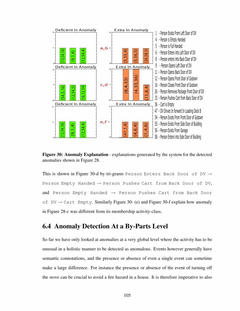
0

0

2

0

2Deficient In Anomaly

1 - Person Exists From Left Door of DV 4 - Person is Empty Handed 5 - Person is Full Handed 6 - Person Enters into Left Door of DV 8 - Person enters into Back Door of DV 9 - Person Opens Left Door of DV11 - Person Opens Back Door of DV12 - Person Opens Front Door of Godown16 - Person Closes Front Door of Godown26 - Person Removes Package Front Door of DV33 - Person Pushes Cart from Back Door of DV36 - Cart is Empty47 - DV Drives In forward In Loading Dock B54 - Person Exists From Front Door of Godown55 - Person Exists From Side Door of Building56 - Person Exists From Garage58 - Person Enters into Side Door of Building0

2 2

0

(12,

54,1

6)

(9,1

,4)

(12,

54,4

)

(12,

54,1

6)

(9,1

,4)

(12,

54,4

)

(5,5

5,4)

(5,5

6,5)

(26,

58,5

)

(47,

1,4)

(4,6

,4)

(1,4

,6)

E xtra In Anomaly

Deficient In Anomaly E xtra In Anomaly0

1

2

0

1

2

(54,

5,16

)

(12,

54,5

)

(16,

12,5

4)

(8,4

,33

)

(4,3

3,3

6)

(11

,8,4

)

Deficient In Anomaly E xtra In Anomaly

1 1

1 1

a,b

c,d

e,f

Figure 30: Anomaly Explanation - explanations generated by the system for the detectedanomalies shown in Figure 28.

This is shown in Figure 30-d by tri-grams Person Enters Back Door of DV →

Person Empty Handed → Person Pushes Cart from Back Door of DV,

and Person Empty Handed → Person Pushes Cart from Back Door

of DV→ Cart Empty. Similarly Figure 30- (e) and Figure 30-f explain how anomaly

in Figure 28-c was different from its membership activity-class.

6.4 Anomaly Detection At a By-Parts Level

So far we have only looked at anomalies at a very global level where the activity has to be

unusual in a holistic manner to be detected as anomalous. Events however generally have

semantic connotations, and the presence or absence of even a single event can sometime

make a large difference. For instance the presence or absence of the event of turning off

the stove can be crucial to avoid a fire hazard in a house. It is therefore imperative to also

105

find irregularities in activities at a more local temporal scale.

Using Suffix Trees for activity representation offers an interesting perspective on

anomaly detection which, unlike previous approaches, calls for detecting event subse-

quences of an activity that have previously been unobserved in the membership class of

that activity. This view is backed by the argument that as an activity can be executed in

multiple regular ways, its regularity is independent of the number of times it is performed

in one of such ways.

Consider for example, the activity of making coffee. Assuming that a majority of people

take coffee with cream, does not make this particular way of taking coffee any more regular

than taking coffee without cream. With this perspective at hand, we argue that given a class

of legitimate activity sequences A, any subsequence of events in a test sequence a classified

as an instance of A, is regular so long as it occurred in A. Conversely, any subsequence of

a is anomalous if it never appears in any of the previously observed members of A.

This approach exacts a more prudent use of training data, resulting in fewer false neg-

atives. While the approach does not necessarily capture different semantic connotations of

an anomaly, it is nevertheless useful in highlighting points of interest in an event-stream,

leaving the final decision to the judgment of a human observer.

6.4.1 Defining Anomalies at a Local Level

Given a test activity sequence a, classified as an instance of activity class A, let S be the set

of all subsequences belonging to A. Then subsequence s ∈ a is said to be anomalous iff:

1. s /∈ S, and

2. @ s′, such that s

′ ⊂ s and s′/∈ S

Intuitively, we are interested in finding minimal length subsequences of an activity a that

do not appear in any other previously observed activities in the membership class of a.

Since an exhaustive search for such previously unobserved minimal length anomalous

subsequences is exponentially hard, we exploit the notion of Match Statistics of an activity

106

Training Sequence (x):

Test Sequence (y):

a b c d u fg g g g g

b a b c fg g g g}

u g

i=3 ms(i)=3 j=6

}

i=1 ms(i)=1 j=2

Figure 31: Notion of anomaly - Detection of anomalous subsequences using match andreverse match statistics. The figure shows an example test activity that has been classifiedto a class containing only one training activity. The subsequence bu in the test sequencenever appears in training sequence and is therefore flagged as anomalous. Subsequence abchowever is considered regular since it appears both in the test and the training sequences.

a (explained below), to detect anomalous event subsequences of a in time linear in ||a|| [36].

6.4.2 Anomalies Using Match Statistics

Let A and S be defined as before. Then following [36] we define the two measurements:

Match Statistics: ms(t) of a is the length of the longest subsequence in S that is a prefix

of a[t : ||a||].

Reverse Match Statistic: ms(t) of a is the length of the longest subsequence in S that is a

suffix of a[1 : t].

In other words, a[t : (t +ms(t)−1)] is the longest subsequence in a starting at index t that

is contained in S. Similarly, a[(t−ms(t)+ 1) : t] is the longest subsequence in a ending

at index t that is contained in S. We now attempt to form the bridge between the match

statistics and reverse match statistics of a to the anomalous subsequences of a.

Theorem 1: Let s = a[i, j] for 1≤ i < j ≤ ||a||. Then s is anomalous iff: (1) ms(i) = j− i

and, (2) ms( j) = j− i (for proof, see Appendix .3).

Here ||s||= j− i+1. Intuitively, a minimal length subsequence is not contained in training

data if: (a) it is itself not contained in training set, (b) all its prefixes and (c) suffixes

107

Algorithm 2 Find anomalous subsequences in activity aLet anomalyList(0) = { /0}for i = 1 to ||a|| do

Let j = i+ms(i)if ms( j) = j− i then

Add (i, j) to anomalyList(i)end if

end forreturn anomalyList

are present in training set. First condition of Theorem 1 implies criteria (a) and (b) are

satisfied, while second condition guarantees criteria (b) and (c) are met. An algorithm to

find anomalous event-subsequences is given in Algorithm 2.

The match and reverse match statistics in Algorithm 2 can be computed in O(||a||) given a

Suffix Tree for the activity sequences of the membership class A [36].

Example Case: A figurative illustration of the notion of anomaly is shown in Figure 31.

For i = 1, the longest subsequences in x that is a prefix of y[1 : ||y||] is b. Therefore ms(i = 1)

of y is 1. Moreover, since the checking condition of Theorem 1 defines j = ms(i)+ i, thus

for i = 1, j = 2. As the longest subsequence in x that is a suffix of y[1 : j = 2] is u, ms( j = 2)

of y is 1. Since ms(i = 1) = ms( j = 2) = j− i = 1, according to Algorithm 2, at i = 1,

anomalyList(1) = {bu}. Similarly, anomalyList(2) = {bu,ua}.

Now consider the case for i = 3. As the longest subsequences in x that is a prefix of

y[3 : ||y||] is a,b,c, therefore ms(i = 3) of y is 3. Similarly, ms( j = 6) of y is 1. Since

ms(i = 3) 6= ms( j = 6) 6= j− i, therefore, at i = 3, anomalyList(2) = anomalyList(3) =

{bu,ua}.

6.4.3 Anomaly Detection Performance in Kitchen Environment

We now present a some experimental results testing the plausibility of this local perspec-

tive on anomaly detection on an environment such as a household kitchen. The details of

the experimental setup and the data collected are give in Chapter 4§ 4.4. A set of anoma-

lous activities with access to ground-truth about the number of anomalies in each activity

108

Table 15: Anomaly Detection Performance - Column 2 shows ground-truth informationabout number of anomalies added per-class. Column 3 represents total number of anoma-lies per-class detected. Number of true anomalies detected are given in column 4. % trueand false positive rates are listed in column 5 and 6.

Class Added Total Correctly % %Labels Anomalies Detected Detected True + False +

C1 15 25 13 86.6 48.0C2 7 18 6 85.7 66.6C3 10 16 9 90.0 43.7C4 16 27 13 81.2 51.8C5 12 14 8 66.6 42.8C6 20 15 12 60.0 20.0C7 16 24 13 81.2 45.8C8 5 12 5 100.0 58.3C9 11 25 11 100.0 56.0C10 17 26 15 88.2 42.3

Average - - - 83.9 % 47.5 %

sequence and their respective locations, was constructed by randomly selecting 5 of the

10 activities for each of the 10 activity-classes, and modifying some of the steps of their

recipes. Using this ground-truth information, the performance rates of our anomaly detec-

tion framework are given in Table 15. Being strict towards the notion of regularity, our

framework is able to correctly extract 84% of the true anomalies. This naturally comes at

the cost of relatively high false positive rate of 47%, which can be addressed by using event

detectors more robust to sensor noise.

An analysis of detected anomalies reveals that anomalies involving key-objects that

serve a unique purpose are detected almost perfectly, while those involving objects with

overloaded affordances can be missed by our approach. For instance, the key-objects sink

and stove each offer only one function. Therefore anomalies where the person forgets to

wash something before cutting it, or pre-heating the stove at the beginning of cooking, are

always detected. However, the anomaly of forgetting to add salt for example, kept in shelf

3 might be missed if the person went to shelf 3 earlier to get some other condiment. This

underscores the importance to define events at a level sufficient to describe different types

of anomalies that can occur in an environment.

109

6.5 Summary

In this chapter we have looked at the problem of detecting and explaining anomalous ac-

tivities taking place in everyday environments. Finding behaviors that are in some sense

anomalous is crucial for the purposes of monitoring and surveillance. Since anomalies are

rare occurrences with large variations amongst them, traditional approaches that attempt to

learn explicitly defined models of anomalies do not generalize well.

We approach the problem of finding anomalous behaviors from a detection rather than a

recognition based perspective. As the notion of anomaly is closely related to what is meant

by being regular, we have modeled anomalies as activities that deviate from behaviors

perceived as regular in an environment. Using the discovered activity classes to learn the

concept of regularity in an environment, we have tried to detect anomalies that deviate

from regular behaviors. In particular, we have tried to find these deviations from regular

behaviors both at a holistic as well as at a by-parts level.

From a holistic perspective, we first classify a test activity to any of the discovered ac-

tivity classes, and then based on its distance from the previous members of the membership

class decide whether the new class member is a regular or an anomalous member. If the

newly classified test activity is an anomalous member of its membership class, we attempt

to explain it in terms of the sequential features that were either too deficient or extraneous

in the test activity. From a by-parts perspective, we have tried to detect minimal length

subsequences in a test activity that have never been observed in the previous members of

its membership class. Since an exhaustive search of such minimal length anomalous subse-

quences is computationally expensive, we have used properties of Suffix Trees to find them

in time linear in the length of the input test activity.

A main challenge in tackling the problem of anomaly detection is the subtle difference

between a truly alarming anomaly versus an outlier. This difference is not necessarily em-

bedded in the statistics of its directly observable features - rather it is dependent on the goal

or the outcome of the activity. The reason the problem of anomaly detection is particularly

110

challenging is the fact that while anomalies appear very similar to the regular members of

an activity class, they fail to achieve the activity goal in an acceptable way. Since we can

only model what an activity looks like as opposed to what an activity is, taking a purely

detection-based perspective towards finding anomalies can in fact be too general. One

way of striking a balance between the brittleness of an exclusively recognition-based per-

spective and the generality of a purely detection-based view towards anomalies, is to learn

certain domain specific constraints on what makes various irregularities truly alarming.

How these constraints should be modeled and learned for different environments remains

an open question.

111

CHAPTER VII

CONCLUSIONS & FUTURE WORK

This thesis explores the problem of learning human activities in everyday environments.

Traditional approaches to this end assume that the structure of activities being modeled is

known a priori. However, for a majority of everyday environments, the structure of such

activities is generally not available. The main contribution of this thesis is an investigation

of knowledge representations and manipulation techniques that can facilitate learning of

everyday human activities in a minimally supervised manner.

A key step towards this end is finding appropriate representations for human activities.

We posit that if we choose to describe everyday activities in term of an appropriate set of

events, then the structural information of these activities can be uniquely encoded using

their local event subsequences. With this perspective at hand, we particularly investigate

representations of event n-grams and Suffix Trees that characterize activities in terms of

their fixed and variable length event subsequences respectively. We compare these repre-

sentations in terms of their representational scope, feature cardinality and noise sensitivity.

Exploiting such representations, we propose a computational framework to discover the

various activity-classes taking place in an environment. We model these activity-classes

as maximally similar activity-cliques in a completely connected graph of activities, and

describe how to discover them efficiently. Moreover, we propose methods for finding con-

cise characterizations of these discovered activity-classes, both from a holistic as well as a

by-parts perspective. Using such characterizations, we present an incremental method to

classify a new activity instance to any one of the discovered activity-classes, and to auto-

matically detect whether it is anomalous with respect to the general characteristics of its

112

membership class. Our results show the efficacy of our framework in a variety of every-

day environments, including a Loading Dock area, a Household Kitchen, and a Residential

House environment.

7.1 Thesis Conclusions

In the following we describe the main conclusions of our thesis.

7.1.1 Learning Global Activity Structure Using Local Event Statistics

The key conclusion of this thesis is that if we describe everyday human activities in terms

of an appropriate set of events, then the structural information of these activities can be

uniquely encoded using the statistics their local event subsequences.

At the heart of this idea of learning activity structure using event statistics is the ques-

tion whether we can have such an appropriately expressive yet robustly detectable event

vocabulary to describe human activities in a variety of everyday environments. There ex-

ists an inherent tradeoff between the expressiveness of events and the robustness with which

they can be detected using low-level perceptual information. The way we strike a balance

between these two opposing factors will impact the kinds of analysis we can perform on the

activities taking place in an environment. For instance our event vocabulary in the loading

dock environment was more expressive than the one in the residential house environment,

which allowed us to perform a more detailed analysis of activities taking place in the load-

ing dock than for those taking place in the residential house environment. At the same time,

detecting events in the loading dock were much more challenging than detecting events tak-

ing place in the residential house environment. There does not exist a set of hard and fast

rules according to which the granularity of events in an environment should be defined -

rather this granularity should be a function of the dynamics of the environment, and the

types of sensor modalities that are available to perceive the various in situ activities.

113

7.1.2 Importance of Capturing Variable-Length Event Dependence

Events in everyday human activities can depend on preceding events over a variable du-

ration of time. In a household kitchen for instance, a persons turns the kitchen lights on

upon entering the kitchen. In other words the event of turning the lights on is dependent on

the immediately previous event of entering the kitchen. On the other hand, while washing

utensils in a kitchen sink, a person generally turns the faucet on followed by rinsing the

utensils, and then turning the faucet off. In other words the event of turning the faucet

off is dependent on the previous two events of rinsing the utensils and turning the faucet

on. In order to capture the activity structure more specifically, it is important to encode

such variable length event dependencies. While representation of n-grams can only cap-

ture event dependence up to some fixed temporal scale, the representation of Suffix Trees

is able capture this variable length event dependence over the entire continuum of an ac-

tivity’s temporal scale. We saw the usefulness of this ability of Suffix Trees to efficiently

capture variable-length event dependence in the kitchen environment where they outper-

formed fixed-length n-grams for different values of n, both for the task of activity-class

discovery as well as activity classification.

7.1.3 Specificity versus Sensitivity of Sequential Representations

Another tradeoff that we have come across over the course of this thesis is the one between

the specificity to which a representation captures the structure of a sequential process, and

its sensitivity to sensor noise. While representations such as n-grams only encode activity

structure up to a fixed temporal scale, and are therefore less exact and more lossy, they are

at the same time more robust to various perturbations brought about by the sensor noise. On

the other hand, representations like Suffix Trees are able to capture sequence structure over

the entire continuum of its temporal scale encode this information more exactly. However,

their greater specificity results in their higher sensitivity to sensor noise. We saw this

trend in the simulation experiments of § 4.3, where the classification performance of Suffix

114

Trees deteriorated faster with increase in the amount of noise as compared to n-grams with

smaller values of n.

7.1.4 Importance of Finding Predominant Mode of Temporal Dependence

We saw in the simulation experiments of § 4.1.2, that event dependencies only up to a

certain value of temporal scale matter. For everyday environments however, this range of

important temporal scales is not known a priori. One way around this problem is to use

Suffix Trees to discover the predominant mode of temporal dependence amongst events

in an environment. Moreover, we can use this discovered predominant modal information

to set the value of n for n-gram representation. This can allow us to capture the majority

of important temporal dependencies, without having to incur the additional sensitivity to

sensor noise that would be there if we arbitrarily chose the value of n to be larger than what

is required.

7.1.5 Behavior Discovery Using Feature Based View of Activity-Classes

In this thesis, we have taken on the problem of unsupervised discovery of human behaviors

with a feature-based view of activity classes. This view posits that members of an activity-

class generally share a set of common properties that make them perceptually similar to

each other. For instance, activities of frying omelets look similar to each other as they

mostly require events such as beating eggs followed by frying them. We believe that our

representation of modeling activities as conjunctions of their sequential features supports

a notion of their perceptual similarity that can be used for the unsupervised discovery and

characterization of various human behaviors. We have shown that posing this question

of activity-class discovery as a graph partitioning problem by modeling activity-classes as

maximally similar cliques of nodes in activity-graphs is a plausible way of solving this

problem. Moreover, we have shown that using the framework of Dominant Sets is an

efficient means to this end.

115

7.1.6 A Detection Based Approach To Finding Anomalous Behaviors

One application of the computational framework that we have proposed in this thesis is au-

tomatically finding activities that are in some sense irregular or anomalous. As anomalies

are rare occurrences with large variation amongst them, traditional approaches that attempt

to learn explicitly defined models of anomalies do not generalize well. In this thesis, we

have approached the problem of finding anomalous behaviors from a detection rather than a

recognition based perspective. As the notion of anomaly is closely related to what is meant

by regular, we have modeled anomalies as activities that deviate from behaviors perceived

as regular in an environment. Using discovered activity-classes to learn the notion of regu-

larity in an environment, we try to detect anomalies that deviate from regular behaviors.

Our research findings demonstrate the importance of formalizing differences of anoma-

lous activities from regular behaviors at multiple temporal scales. Moreover, since all de-

viations from regular behaviors are not necessarily interesting, we conclude that taking a

purely detection-based perspective towards finding anomalies can in fact be too general.

One way of striking a balance between the brittleness of an exclusively recognition-based

perspective and the generality of a purely detection-based view towards anomalies, is to

learn certain domain specific constraints on what makes various irregularities truly alarm-

ing. How these constraints should be modeled and learned for different environments re-

mains an open question.

7.2 Current Limitations & Future Research Directions

At present, there are several limitations of our framework that might be used as avenues for

future research. In the following, we start by mentioning some of the more immediate of

these potential directions, leaving the ones with relatively bigger research-scope for later.

116

7.2.1 Incorporating Temporal Information of Events

In everyday environments, any particular event may take variable time to finish. In a house-

hold kitchen for instance, the event of taking something out of the refrigerator may take

longer or shorter time depending on how many items are being taken out. This duration

over which an event takes place can be an important discriminating factor to distinguish

amongst various activity-classes. Furthermore, the event duration can be an important in-

dicator about whether the event was performed correctly or not. At present, we are not

incorporating any information regarding the duration that the various events take to be ex-

ecuted. A potential future direction of our work might be to investigate the extent to which

considering such temporal information of events is useful for activity analysis.

One naive way of incorporating such information might be to discretize the temporal

duration of event execution into a fixed number of bins, registering to which of these dura-

tional bins does each execution of an event belong. A potential drawback of this approach

might be an increase in the size of event vocabulary by a constant factor, which would

result in further increase in the dimensionality of space. A slightly better solution to this

problem may be to discretize the temporal duration of event execution into variable number

of bins, where this number would be different for each event, and would depend on how

long does a particular event usually take to be executed. We leave further investigation of

this question as an open problem for future work.

7.2.2 Selective Usage of Extracted Sequential Features

Both n-grams and Suffix Tree representations can be thought of as feature extraction meth-

ods that extract sequential features from activity sequences. While the representational

scope of the features extracted by Suffix Trees is provably better than those extracted by

n-grams for any fixed value of n, it is not quite clear in general how useful is this extra

representational power in terms of discriminability.

One way of investigating this question is to use a boosting-based feature selection

117

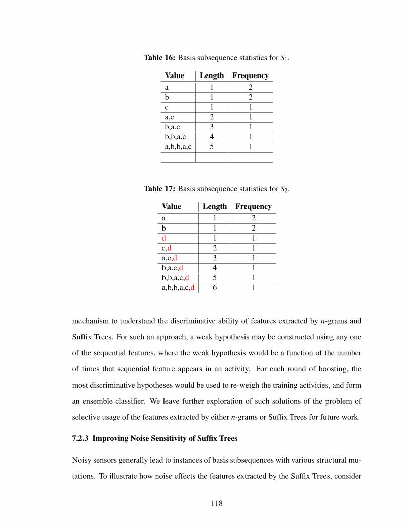
Table 16: Basis subsequence statistics for S1.

Value Length Frequencya 1 2b 1 2c 1 1a,c 2 1b,a,c 3 1b,b,a,c 4 1a,b,b,a,c 5 1

Table 17: Basis subsequence statistics for S2.

Value Length Frequencya 1 2b 1 2d 1 1c,d 2 1a,c,d 3 1b,a,c,d 4 1b,b,a,c,d 5 1a,b,b,a,c,d 6 1

mechanism to understand the discriminative ability of features extracted by n-grams and

Suffix Trees. For such an approach, a weak hypothesis may be constructed using any one

of the sequential features, where the weak hypothesis would be a function of the number

of times that sequential feature appears in an activity. For each round of boosting, the

most discriminative hypotheses would be used to re-weigh the training activities, and form

an ensemble classifier. We leave further exploration of such solutions of the problem of

selective usage of the features extracted by either n-grams or Suffix Trees for future work.

7.2.3 Improving Noise Sensitivity of Suffix Trees

Noisy sensors generally lead to instances of basis subsequences with various structural mu-

tations. To illustrate how noise effects the features extracted by the Suffix Trees, consider

118

the sequence S1 = {a,b,b,a,c}. A list of the basis sub-sequences of S1, their lengths and

respective frequencies are given in Table 16. Now assume a noisy symbol added to the end

of S1, given as S2 = {a,b,b,a,c,d}. A list of the basis sub-sequences of S2, their lengths

and frequencies is given in Table 17. As can be observed, adding just one noisy element d

at the end of this activity changes the basis feature set by a substantive amount.

One potential solution to this problem is to use a partial feature matching mechanism

between features of different activities, as opposed to the exact feature matching method

that is being currently used by our framework. This partial feature matching might be

based on the edit-distance between activity features, and would help map the noisy fea-

tures to their closest matches in terms of edit-distance, hence reducing the brittleness of

longer sequential features. We leave further exploration of such solutions of the problem

of alleviating noise sensitivity of Suffix Trees for future work.

7.2.4 Event Detection Using Multiple Sensor Modalities

Note that currently we are only using one sensor modality in an environment at a time.

A potential direction for improving our proposed computational framework is to combine

information from multiple sensors simultaneously. This can provide us with a more expres-

sive set of event vocabulary for an environment. Recall that in our example environment

of a household kitchen, currently the events are being registered simply based on the prox-

imity of a person with a key-object. However, what exactly does the person do during the

interaction remains undetected. By simply adding multiple sensors in this environment,

we can know certain things such as whether a refrigerator door was opened or closed, or

whether the stove was turned on or off when the person interacted with it, etc. Such infor-

mation would allow us to discover a larger set of human activities, as well as will play a

key role in finding interesting anomalies.

Another related direction is that of fusing the data simultaneously detected through mul-

tiple sensors. This can help us detect the various events in an environment more robustly.

119

All too often one information channel can fail due to poor environmental conditions, how-

ever if our detection mechanisms incorporate information from multiple sources, they can

detect events more robustly so that these poor environmental conditions would not impact

our detection rates too adversely.

7.2.5 Analyzing Group Activities

The aforementioned sensor-level and event-level data fusion can be extremely useful when

the observations are being made at some location X to infer something also about location

X. However, for a variety of everyday environments equipped with sensors at different

locations, inference at X can be improved by also using information at another location Y.

For instance a system which detects if a meeting is taking place in a meeting room can

use information not only from the meeting-room itself, but also by detecting whether the

meeting participants left their cubicles shortly before the scheduled time. An interesting

question to be explored is what type of sequence representations would be suitable to model

these mutually dependent streams of events to infer something more global about the group-

activities taking place in an environment.

7.2.6 Human Activity Analysis in an Active Learning Paradigm

So far, we have explored incorporating some amount of perceptual bias in the system at the

start of the learning process mainly in terms of the key-objects in an environment, some

notion of activity similarity, and the event vocabulary. However the dynamics of the envi-

ronments for which these systems are supposed to be used change over time. In a loading

dock for instance, a new type of delivery activity may start to take place, or in the kitchen

someone may change the position of where they place all the condiments. Therefore, there

is a need to design these systems such that this perceptual bias can be interactively added

to the system. Such mechanisms could for instance incorporate an experts assistance to

dynamically cluster new behaviors in an environment, modify an existing notion of anoma-

lous behaviors, and model certain attributes of an environment that may change over time.

120

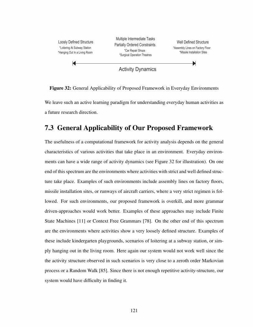
uu

Well Defined Structure*Assembly Lines on Factory Floor

*Missile Installation Sites

Loosly Defined Structure*Loitering At Subway Station

*Hanging Out In a Living Room

Partially Ordered Constraints*Car Repair Shops

*Surgical Operation Theatres

Multiple Intermediate Tasks

Activity Dynamics

Figure 32: General Applicability of Proposed Framework in Everyday Environments

We leave such an active learning paradigm for understanding everyday human activities as

a future research direction.

7.3 General Applicability of Our Proposed Framework

The usefulness of a computational framework for activity analysis depends on the general

characteristics of various activities that take place in an environment. Everyday environ-

ments can have a wide range of activity dynamics (see Figure 32 for illustration). On one

end of this spectrum are the environments where activities with strict and well defined struc-

ture take place. Examples of such environments include assembly lines on factory floors,

missile installation sites, or runways of aircraft carriers, where a very strict regimen is fol-

lowed. For such environments, our proposed framework is overkill, and more grammar

driven-approaches would work better. Examples of these approaches may include Finite

State Machines [11] or Context Free Grammars [78]. On the other end of this spectrum

are the environments where activities show a very loosely defined structure. Examples of

these include kindergarten playgrounds, scenarios of loitering at a subway station, or sim-

ply hanging out in the living room. Here again our system would not work well since the

the activity structure observed in such scenarios is very close to a zeroth order Markovian

process or a Random Walk [85]. Since there is not enough repetitive activity-structure, our

system would have difficulty in finding it.

121

Somewhere between these two ends is the set of environments where the activity struc-

ture is neither too strict, nor too loosely defined. Our proposed framework is geared towards

this class of environments. Some of the general characteristics of such environments are

listed in the following:

1. Many different types of activities can take place in the environment, and the number

of possible in situ activities is not necessarily known a priori.

2. There exists enough variance amongst the instances of different types of activities

so that it is not feasible to write an explicit grammar-based model for the different

activity classes.

3. Instances belonging to each type of activity require execution of multiple intermedi-

ate tasks (i.e. events) for their successful completion.

4. All instances belonging to the various activity types taking place in an environment

can be described in terms of a shared set of events.

5. There exists a mostly common set of partially ordered constraints amongst the con-

stituent events of any particular activity type. Constituent events of different activity

types mostly adhere to sets of different partially ordered constraints.

Some of the example environments that generally have the aforementioned properties in-

clude car repair shops, surgical operation theaters [1], or building construction sites.

7.4 Choosing An Appropriate Event Vocabulary

There can be multiple sets of events with different levels of granularity, that could be used

to describe activities in an environment. The choice of a particular set of events to describe

the in situ activities would determine how strictly or loosely defined the structure of these

activities might be. In the following we enlist some of the criteria for selecting an event

vocabulary suitable for a computational system such as ours.

122

1. Events in an event vocabulary should be of finite duration and temporally local, i.e.

events should have a finite duration between their start and end points, and this range

should in general be reasonably smaller than the duration of an entire activity.

2. Events should not be temporally overlapping. In other words, each event must end

before another event starts. In situations where multiple events are being simulta-

neously performed by different agents, there must exist a mapping between which

event is being performed by which agent.

3. Events in an event vocabulary should not occur spuriously and there needs to be a

strict correlation between the action of an agent which causes the occurrence of a

particular event.

4. Events should have temporal atomicity, i.e., if there are two events in a vocabulary

that cannot happen without being temporally adjacent to each other, then they should

be merged to one, provided that the merged event can still be robustly detected. This

condition supports a minimal sized event vocabulary which would result in reduced

computational complexity. Furthermore, favoring a fewer set of robustly detectable

events over a larger set of less robustly detectable events would benefit sequence

representations like Suffix Trees which are inherently sensitive to sensor noise.

5. An event vocabulary should have a null event, which would represent an environment

when nothing takes place in it. This is particularly important in environments where

there might be long gaps between the execution of an activity instance.

One of the key factors to consider while choosing the event vocabulary for an environment

is the inherent tradeoff that exists between how well does a set of events capture the under-

lying structure of activities, versus how robustly these events can be detected using some

low-level perceptual information. Consider for instance the activity of a person making an

omelet in a household kitchen. Captured through a video camera, one way of describing

123

this activity may be using the motion of various color-blobs in the scene, detected directly

through the raw pixel-data. While these color-blobs are not very expressive on their own,

they can be detected relatively robustly using the low-level data.

Another way to describe our example activity of making an omelet might be in terms of

semantically meaningful intermediate tasks, such as beating some eggs, heating oil, frying

the eggs, etc. While these intermediate tasks are quite expressive on their own, their robust

detection using low-level pixel data can be quite challenging.

There does not exist a set of hard and fast rule according to which the granularity of

constituent events should be selected, however in general this choice should be carefully

made depending on the dynamics of an environment, and the available sensor modalities.

One way of going about finding an appropriate event vocabulary is to realize that the

types of activities that can be performed in an environment usually depends on the various

objects present in that environment. Note that the example environments of car repair

shops or surgical operation theaters where our proposed framework can be used have a

very natural notion of different key-objects that are essential for the execution of different

activities that might take place in these environments.

Each of these key-objects can have a set of states which could be changed by performing

a set of operations on the key-object. Identifying the various key-objects in an environment,

their respective states, as well as the operations that could be performed on them to change

their states, can be useful to choose appropriate sensor modalities that would facilitate

robust detection of the states of key-objects.

For instance, in a household kitchen environment one of the key-objects essential for

many cooking activities is the stove. Identifying this key object can help us enlist its various

states, e.g., being on or off, having some utensil on it or being vacant, etc. Different types

of sensor modalities might be useful to detect the different states of the stove, e.g. using

vision based sensor may be useful to detect whether some utensil is on the stove or not. On

the other hand, some binary detector could be used to register whether the stove is turned

124

on or off. These choices regarding the key-objects in an environment, their various states,

and the appropriate sensor modalities for detecting these states, can be used to have an

event vocabulary that is not only sufficiently expressive, but is also robustly detectable.

7.5 Concluding Remarks

This thesis was an effort to enhance the extent to which computers can be proactive and

assistive in our day-to-day lives, by being able to understand everyday human activities. In

this regard, we particularly focused on formalizing computational models of human activi-

ties that can perform well in the face of data uncertainty and complex activity dynamics.

One of the key challenges towards understanding human behaviors in everyday en-

vironments is the sheer diversity of the different types of activities that can take place.

Moreover, each one of these activities can be executed in a variety of different ways. It is

therefore not plausible to manually model each one of these activities, and to learn these

models in a completely supervised manner. Our intent in this thesis was to use appropri-

ate knowledge representations and manipulation techniques that could allow computational

systems to analyze human activities with minimal supervision. Our hope was that such a

data-driven approach towards human activity modeling would enable computers to become

more useful in large-scale unconstrained environments.

The key idea behind our solution to this challenge was that if we choose to describe

human activities in terms of an appropriate set of events, then only a few contiguous sub-

sequences of these events are sufficient to learn the activity-structure for a wide variety

of activities performed in a large set of environments. The main caveat in this idea is

the assumption that such an appropriate set of events is available for a substantial num-

ber of everyday environments. While the idea of modeling a temporal process in terms

of its sequential features has previously been used in such fields as Text Analysis, Speech

Recognition and Bio-Informatics, the notion of the basic information unit is much more

well-defined for those problems. Words, phonemes, and DNA-elements are natural ways

125

to represent text documents, speech, and protein sequences, that can be used to model any

instance of such sequential processes. Coming up with such a universal set of detectable

events is still an open problem.

Having said that, we have tried to show that at least for a particular class of single-

agent, finite-duration, and non-overlapping activities, it is plausible to come up with an

appropriate set of events for a variety of environments that can characterize a reasonably

large set of activities while being perceptually detectable. We believe that adopting this

“first discover then recognize” paradigm towards modeling human activities would enable

computational systems to efficiently learn a much larger set of human behaviors, and will

play a key role in making such systems become more ubiquitous and useful.

126

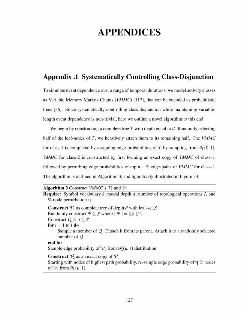
APPENDICES

Appendix .1 Systematically Controlling Class-Disjunction

To simulate event dependence over a range of temporal durations, we model activity classes

as Variable Memory Markov Chains (VMMC) [117], that can be encoded as probabilistic

trees [36]. Since systematically controlling class disjunction while maintaining variable-

length event dependence is non-trivial, here we outline a novel algorithm to this end.

We begin by constructing a complete tree T with depth equal to d. Randomly selecting

half of the leaf-nodes of T , we iteratively attach them to its remaining half. The VMMC

for class-1 is completed by assigning edge-probabilities of T by sampling from N (0,1).

VMMC for class-2 is constructed by first forming an exact copy of VMMC of class-1,

followed by perturbing edge probabilities of top n−% edge-paths of VMMC for class-1.

The algorithm is outlined in Algorithm 3, and figuratively illustrated in Figure 33.

Algorithm 3 Construct VMMC’s V1 and V2Require: Symbol vocabulary k, modal depth d, number of topological operations I, and

% node perturbation η

Construct V1 as complete tree of depth d with leaf-set SRandomly construct P ⊆ S where ||P ||= ||S ||/2Construct Q ≡ S \ Pfor i = 1 to I do

Sample a member of Q . Detach it from its parent. Attach it to a randomly selectedmember of Q .

end forSample edge probability of V1 from N (µ,1) distribution

Construct V2 as an exact copy of V1Starting with nodes of highest path probability, re-sample edge probability of η % nodesof V2 from N (µ,1)

127

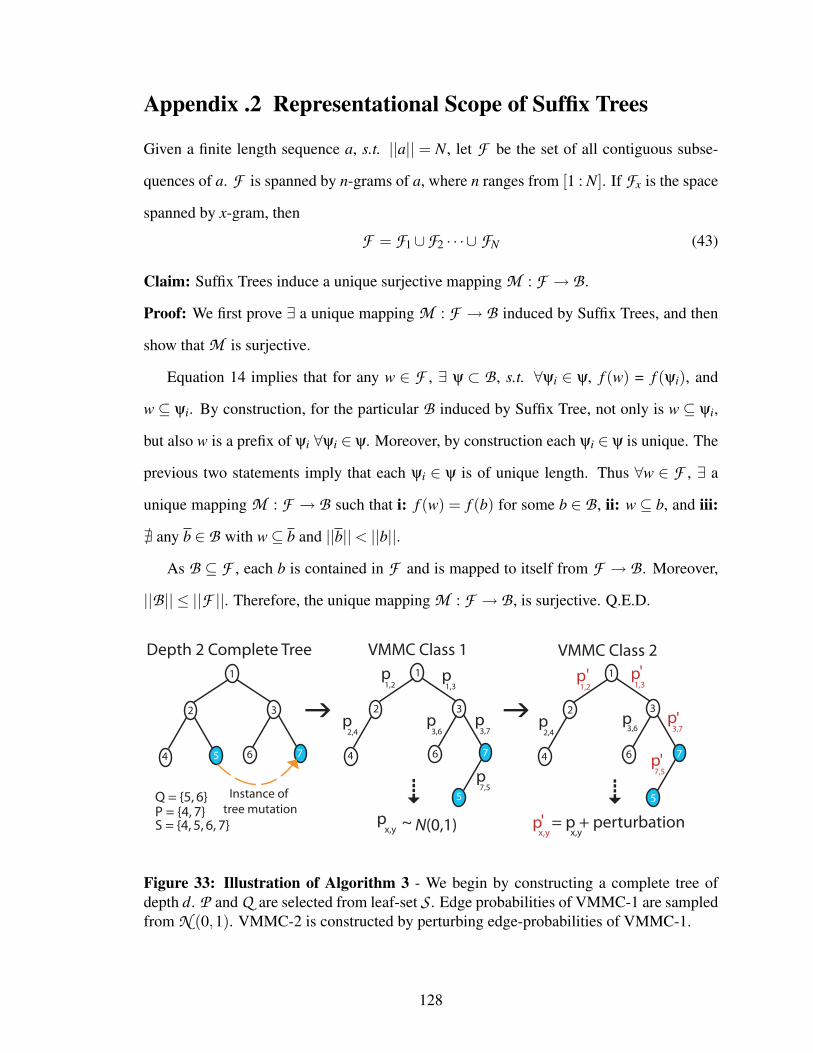
Appendix .2 Representational Scope of Suffix Trees

Given a finite length sequence a, s.t. ||a|| = N, let F be the set of all contiguous subse-

quences of a. F is spanned by n-grams of a, where n ranges from [1 : N]. If Fx is the space

spanned by x-gram, then

F = F1∪F2 · · ·∪ FN (43)

Claim: Suffix Trees induce a unique surjective mapping M : F → B .

Proof: We first prove ∃ a unique mapping M : F → B induced by Suffix Trees, and then

show that M is surjective.

Equation 14 implies that for any w ∈ F , ∃ ψ ⊂ B , s.t. ∀ψi ∈ ψ, f (w) = f (ψi), and

w ⊆ ψi. By construction, for the particular B induced by Suffix Tree, not only is w ⊆ ψi,

but also w is a prefix of ψi ∀ψi ∈ ψ. Moreover, by construction each ψi ∈ ψ is unique. The

previous two statements imply that each ψi ∈ ψ is of unique length. Thus ∀w ∈ F , ∃ a

unique mapping M : F → B such that i: f (w) = f (b) for some b ∈ B , ii: w ⊆ b, and iii:

@ any b ∈ B with w⊆ b and ||b||< ||b||.

As B ⊆ F , each b is contained in F and is mapped to itself from F → B . Moreover,

||B|| ≤ ||F ||. Therefore, the unique mapping M : F → B , is surjective. Q.E.D.

1

2 3

4 5 6 7

1

2 3

4

5

6 7

1

2 3

4

5

6 7

g g

S = {4, 5, 6, 7}P = {4, 7}Q = {5, 6}

x

Instance of tree mutation

p2,4

p1,2

p1,3

p3,6

p3,7

p7,5

p2,4

p1,2

p1,3

p3,6

p3,7

p7,5

'

'

' '

p' = p + perturbation

Depth 2 Complete Tree VMMC Class 1 VMMC Class 2

px,y ~ N(0,1)

6 6x,y x,y

Figure 33: Illustration of Algorithm 3 - We begin by constructing a complete tree ofdepth d. P and Q are selected from leaf-set S . Edge probabilities of VMMC-1 are sampledfrom N (0,1). VMMC-2 is constructed by perturbing edge-probabilities of VMMC-1.

128

Appendix .3 Proof of Theorem 1

(=⇒) Suppose s is an anomalous subsequence, i.e. a[i, j] /∈ S. Then, ms(i) < j − i + 1,

otherwise a[i, j] would be contained in S. Similarly, ms( j) < j − i + 1.

Suppose for a contradiction, that ms(i) < j − i. Since ms(i) < j − i, a[i, i + ms(i)−1] ⊂

a[i, i +( j− i)−1] = a[i, j−1] and by definition, a[i, i + ms(i)−1] is the longest substring

in a starting at i that is contained in S, a[i, j−1] is not contained in S. But since a[i, j] is an

anomalous substring, a[i, j] does not contain any substring that is not in S. This however

contradicts the fact that a[i, j− 1] ⊂ a[i, j] and a[i, j− 1] /∈ S. Hence ms(i) ≥ j− i. Since

we have shown that ms(i) < j− i+1, therefore ms(i) = j− i. Similarly, we can show that

ms( j) = j− i.

(⇐=) Suppose ms(i) = j− i and ms( j) = j− i. We prove a[i, j] satisfies both conditions

of being anomalous:

1. By definition, a[i, i+ms(i)−1] = a[i, i+( j− i)−1] = a[i, j−1] is the longest sub-

sequence of a starting at i that is contained in S. Hence a[i, j] /∈ S.

2. By definition of match statistic, a[i, i + ms(i)− 1] = a[i, i +( j− i)− 1] = a[i, j− 1]

∈ S. Hence all subsequences of a[i, j−1] ∈ S. Similarly, since a[ j−ms( j)+1, j] =

a[ j− ( j− i)+ 1), j] = a[i + 1, j] ∈ S, all subsequences of a[i + 1, j] ∈ S. Since all

subsequences of a[i, j−1] and of a[i+1, j] ∈ S, therefore all proper subsequences of

a[i, j] also ∈ S.

Q.E.D.

129

Appendix .4 Cooking Instructions for Multiple Subjects

You will be asked to cook 3 different dishes in the Aware-Home kitchen. The detailed

recipe instructions and information about the location of the ingredients will be given to

you shortly (Figure 20 in Chapter 4 was provided for ingredient locations). You will cook

each of the 3 recipes 12 different times. The first 2 times, you will actually perform all the

cooking steps for the dish according to its recipe. The reset of the 10 times, you will only

perform some of these steps, and enact the rest. You will be told which step to actually

perform and which step to enact.

I will now explain what I mean by actually performing a step as opposed to just enacting

that step. Suppose one of the steps of the recipe is to wash potatoes. If you were to actually

perform this step, you would carry the potatoes to the washing basin and actually use water

to wash them. On the other hand, if you were to enact this step, you would simply carry

the potatoes to the washing basin and just spend some time there pretending to wash them

without using any water to actually wash them.

The directions for these dishes will be provided to you in terms of three stages, i.e. (i)

the Preparation Stage, (ii) the Cooking Stage, and (iii) the Finishing Stage. I will now tell

you a bit about these three stages:

1- The Preparation Stage: This stage involves getting various items needed for a dish

ready. For instance, to make Potato Curry, we may need chopped potatoes, and sliced

onions. The preparation stage for cooking Potato Curry involve getting these items ready.

2- The Cooking Stage: This stage is about combining all the items prepared in the prepa-

ration stage based on the recipe directions. For instance, if the directions are to fry the

chopped potatoes, then youll have to turn the stove on, get the pan, add oil in the pan, and

then fry the chopped potatoes.

3- The Finishing-Up Stage: In this stage, all the utensils and the ingredients used dur-

ing the preparation and the cooking stage need to be either placed back to their original

locations, or put in the sink.

130

Example Recipe: To illustrate this idea further, the recipes of one of the dishes, Potato

Curry, are given in the following:

1- Preparation Stage: Chop: Onions, Potatoes, Tomatoes. Beat: Yogurt

2- Cooking Stage: Heat oil, add bay-leaf and chopped onions. Fry for 3-4 minutes. Add

ginger and garlic, and fry for another minute. Add mustard and cumin seeds. Add chopped

potatoes and chopped tomatoes. Mix well and cook for 4-5 minutes, stirring well. Add

turmeric, coriander and chili powder. Blend the yogurt into the mixture. Add salt.

3- Finishing-Up Stage: Put all the used pans and dishes in the sink. Replace all the ingre-

dients in their original positions.

During the preparation stage, the ingredients for each of the individual items are first

brought to the table, and then processed. For instance, for the direction “Chop Potatoes”,

you would probably do something like the following:

Get Potatoes→Wash Potatoes→ Place Potatoes on Table→ Get Chopping Slab→ Bring

Chopping Slab on Table→ Get Knife→ Bring Knife to the Table→ Get a Bowl→ Bring

the Bowl to the Table→ Chop Potatoes

You can do any one of these individual tasks in any order that you want to do. For instance,

you can very well get the knife and bring it to the table first, and then wash and chop the

potatoes later.

131

Appendix .5 List of Events in Loading Dock Environment

No. Event Description No. Event Description1 Exit From Left Door of DV 2 Exit From Right Door of DV3 Exit From Back Door of DV 4 Being Empty Handed5 Being Full Handed 6 Enter Left Door of DV7 Enter Right Door of DV 8 Enter Back Door of DV9 Open Left Door of DV 10 Open Right Door of DV11 Open Back Door of DV 12 Close Left Door of DV13 Close Right Door of DV 14 Close Back Door of Bldg.15 Close Back Door of DV 16 Close Front Door of Bldg.17 Take Package From Back Door of DV 18 Take Package From Side Door of DV19 Place Package In Back Door of DV 20 Place Package In Side Door of DV21 Place Package In Side Door of DV 22 Place Cart In Back Door of DV23 Place Package In Cart 24 Take Package From Cart25 Push Cart In Side Door Of Bldg. 26 Remove Package From Back Door of DV27 Push Atmtc. Cart In Backdoor of DV 28 Remove Atmtc. Cart From Backdoor of DV29 Remove Cart From Back Door of DV 30 Remove Package From Cart31 Push Cart In Back Door of Bldg. 32 Remove Cart From Side Door of Bldg.33 Push Cart From Back Door of DV 34 Push Cart From Front Door of Bldg.35 Push Cart From Side Door of Bldg. 36 Cart Is Empty37 Cart Is Full 38 Pull Cart From Back Door of Bldg.39 Pull Cart From Side Door of Bldg. 40 Push Cart Into Back Door of DV41 Push Cart In Front Door of Bldg. 42 Push Cart In Side Door of Bldg.43 Take Something From Another Person 44 Hand Something To Another Person45 Ring Door Bell 46 DV Drive In Forward In LDA47 DV Drive In Forward In LDB 48 DV Drive In Backward In LDA49 DV Drive In Backward In LDB 50 DV Drive Out Forward From LDA51 DV Drive Out Forward From LDB 52 DV Drive Out Backward From LDA53 DV Drive Out Backward From LDB 54 Exit From Front Door of Bldg.55 Exit From Side Door of Bldg. 56 Exit From Garage57 Enter In Front Door of Bldg. 58 Enter In Side Door of Bldg.59 Enter Garage 60 Push Cart In Garage61 Remove Cart From Garage

Table 18: List of Events In Loading Dock Environment - The table shows a list of theevents in the event vocabulary of the loading dock environment.

132

Appendix .6 Directions of Activities In Kitchen Domain

Here we provide the details for the 10 activity classes enacted by one human subject in a

household kitchen environment. 8 out of these 10 activity-classes are of preparing some

recipe. The remaining 2 activity-classes are of setting-up the dining table and washing

dishes. The list of ingredients and directions for the 8 cooking activity-classes were taking

from a 3rd party web-site http://www.recipeland.com/. For the sake of comple-

tion here we write down the ingredients and directions as given on this web-site.

1- Aloo DamIngredients

Vegetable Oil, Bay Leaf, Onions, Ginger, Garlic, Cumin Seeds, Turmeric, Chili Powder,

Plain Yogurt, Salt, Ground Coriander, Potatoes, Tomato, Capsicum.

Directions

Heat oil, add bay leaf and onion. Fry for 3-4 minutes. Add ginger and garlic and fry

for another minute. Add mustard and cumin seeds. The potatoes should be sliced, and the

tomatoes and capsicum cut up. Add these, mix well, and cook for 4-5 minutes, continuously

stirring. Sprinkle with turmeric, coriander and chili powder. Beat the yogurt and blend into

a smooth mixture. Add yogurt and salt. Mix gently, cover and cook for about 10 minutes

on low heat.

2- Basen RaitaIngredients

Basen, Water, Ghee (Clarified Butter), Salt, Black Pepper, Chat Masala, Plain Yogurt, Milk.

Directions

Make a pouring paste of the besan and water. Heat ghee and drop paste in hot ghee through

a slotted spoon to get little drops falling at a time. Remove the drops when golden brown

and dry on a paper towel. Soak the drops in warm water. Add milk, salt, pepper, add chat

133

masala to yogurt. Squeeze water out of the basen drops and add to yogurt.

3- Cheese OmeletIngredients

Parsley, Cheese, Eggs, Salt, Black Pepper, Butter.

Directions

Chop parsley into small bits. Grate the cheese into small shreds. Beat eggs till they get

fluffy. Add salt and pepper into the whisk and beat some more. Heat butter in a pan and fry

the mixture till it gets golden brown. Sprinkle chopped parsley as garnish.

4- Layered Fruit SaladIngredients

Peaches, Blueberries, Strawberries, Grapes, Lemon Juice, Lemon Zest, Cream Cheese,

Whipping Cream, Powdered Sugar, Walnuts.

Directions

In a large glass bowl layer fruit in any order. In a separate bowl mix cream cheese, lemon

juice and lemon rind. In another bowl whip cream just until peaks form; add powdered

sugar and whip to stiff peaks. Fold cream cheese mixture and whipped cream mixture

together. Spread over fruit and sprinkle with walnuts.

5- BabkaIngredients

Yeast, Water, Sugar, Flour, Milk, Unsalted Butter, Eggs, Salt, Cinnamon.

Directions

Prepare the topping by cutting some butter into a bowl, adding sugar, flour and cinnamon

in the bowl, and mixing them well to form a uniform paste. Prepare some powdered sugar

icing by beating the eggs in a bowl, adding sugar in the bowl, and mixing some lemon juice

in it. Make yeast paste by adding hot water in a bowl and mixing some yeast in it to form

134

uniform paste. Heat some milk on a stove and add some butter in it. Mix well till they form

a paste. Add powdered sugar icing in the mixture. Mix well and finally add topping to the

mixture.

6- Green SaladIngredients

Lettuce, Green Onions, Green Bell Pepper, Celery, Apples, Walnuts, Tomatoes, Almonds,

Lemon Juice, Olive Oil, Paprika, Salt, Black Pepper.

Directions

Chop green onions and bell peppers. Cut lettuce into big big pieces. Combine salad ingre-

dients in a large salad bowl. Set aside. Wash tomatoes and cut them into very small cubes.

Chop almonds into small pieces. Combine all these ingredients in a big salad bowl and add

seasoning.

7- Set-Up TableDirections

Get 6 plates and put them in front of the 6 chairs on the dining table. Similarly, get 6 forks,

spoons, knives, and glasses and put them all in front the 6 chairs at the dining table in any

order of choice.

8- Apples and Oat CerealIngredients

Water, Oat Bran, Raisins, Apple, Maple Syrup, Caraway Seeds, Cinnamon, Milk.

Directions

In a saucepan, bring the water and oat bran to a vigorous boil, stirring constantly. Reduce

the heat to low and cook for 2 minutes, stirring frequently, until thick. Remove from heat

and stir in the raisins, apples, maple syrup, and cinnamon. Let it stand for 5 minutes. Spoon

into bowls and serve with the milk.

135

9- Wash DishesDirections

Fetch different utensils from the dining table one at a time, rinse them in the sink, and place

them in the dishwasher. Repeat this process till no utensils are left on the dining table.

10- Szechuan ChickenIngredients

Chicken Breasts, Vinegar, Cornstarch, Sugar, Vegetable Oil, Water, Garlic Cloves, Green

Onions, Soy Sauce, Pepper.

Directions

Cut chicken into cubes. Lightly toss with cornstarch in bag to coat. Heat oil in skillet.

Stir-fry chicken and garlic until lightly browned. Add soy sauce, vinegar, sugar and water.

Cover and cook 3 minutes or until chicken is cooked through. Add green onions and

pepper; cook uncovered about 2 minutes longer.

136

REFERENCES

[1] AHMADI, S., SIELHORST, T., STAUDER, R., HORN, M., FEUSSNER, H., andNAVAB, N., “Recovery of surgical workflow without explicit models,” MICCAI,pp. 420–428, 2006. 7.3

[2] ALLEN, J. F., “Maintaining knowledge about temporal intervals,” Communicationsof the ACM, vol. 26, pp. 832–843, 1983. 2.1.8

[3] ANDRIENKO, G. and ANDRIENKO, N., “Visual exploration of the spatial distri-bution of temporal behaviors,” Proceedings of the 15th annual ACM internationalsymposium on Advances in geographic information systems, 2007. 1.6

[4] APOSTOLICO, A. and BEJERANO, J., “Optimal amnesic probabilistic automata.,”J. of Comp. Biology, vol. 7, pp. 381–393, 2000. 5.4.3

[5] AUGUSTON, J. and MIKER, J., “An analysis of some graph theoretical clusteringtechniques,” J. ACM, vol. 17(4), pp. 571–588, 1970. 2.2, 3.3.3

[6] BAILEY, T. and ELKAN, C., “Fitting a mixture model by expectation maximizationto discover motifs in biopolymers,” in Proc Int. Conf. Intell. Syst. Mol. Biol., pp.28-36, 1994. 2.4.3

[7] BEJERANO, G. and YONA, G., “Modeling protein families using probabilistic suffixtrees,” in In the Proc. of RECOMB, 1999. 1.4, 2.3.5, 3.1

[8] BOBICK, A., “Movement, activity and action: the role of knowledge in the percep-tion of motion,” in Movement, Activity and Action: the Role of Knowledge in thePerception of Motion, Royal Society Workshop on Knowledge-based Vision in Manand Machine., 1997. 2.1

[9] BOBICK, A. and DAVIS, J., “The recognition of human movement using temporaltemplates,” IEEE PAMI, vol. 23, no. 3, 2001. 2.1.1

[10] BOBICK, A., INTILLE, S., DAVIS, J., BAIRD, F., PINHANEZ, C., CAMPBELL, L.,IVANOV, Y., SCHUETTE, A., and WILSON, A., “The kidsroom: A perceptually-based interactive and immersive story environment,” in Vismod, 1996. 2.1

[11] BOOTH, T. L., Sequential Machines and Automata Theory. New York: John Wileyand Sons, 1967. 7.3

[12] BRAND, M., OLIVER, N., and PENTLAND, A., “Coupled hidden markov modelsfor complex action recognition,” in CVPR, 1997. 2.1, 2.1.3

137

[13] CARPENTER, A., RUBIN, M., and STREILEIN, W., “Artmap-fd: familiarity dis-crimination applied to radar targetrecognition,” International Conference on NeuralNetworks, vol. 3, no. 9, pp. 1459 – 1464, 1997. 2.4

[14] CASSIRER, E., Substance and function. New York: Dover, 1923. 2.3.1, 5.1

[15] CHARNIAK, E. and GOLDMAN, R., “A bayesian model of plan recognition,” Artifi-cial Intelligence, vol. 64, p. 5379, 1993. 2.1.4

[16] CHIOLA, G., MARSAN, M., BALBO, G., and CONTE, G., “Generalized stochasticpetri nets: A definition at the net level and its implications,” IEEE Transactions onSoftware Engineering, 1993. 2.1.7

[17] CHIU, B., KEOGH, E., and LONARDI, S., “Probabilistic discovery of time seriesmotifs,” 2003. 1.6

[18] CHIU, B., KEOGH, E., and LONARDI, S., “Probabilistic discovery of time seriesmotifs.,” in SIGKDD, 2003. 2.3.5

[19] CHOUDHURY, T., Sensing and Modeling Human Networks. PhD Thesis, MIT MediaLab., 2003. 1.6

[20] CHOUDHURY, T., PHILIPOSE, M., WYATT, D., and LESTER, J., “Towards activitydatabases: Using sensors and statistical models to summarize people’s lives,” inIEEE Data Engineering Bulletin, 2006. 1.6, 3.1

[21] COHEN, P. and OATES, J., “Robots that learn meanings,” 1.6

[22] CSIBRA, G., “Teleological and referential understanding of action in infancy,”Philosophical Transaction of The Royal Society London, pp. 447–458, 2002. 1.2.3

[23] DASGUPTA, D. and FORREST, S., “Novelty detection in time series data using ideasfrom immunology,” 1996. 2.4

[24] DEY, A., HAMID, R., BECKMANN, C., LI, I., and HSU, D., “a cappella: program-ming by demonstration of context-aware applications,” in SIGCHI, 2004. 2.1

[25] DIESTEL, R., Graph Theory (Graduate Texts in Mathematics). Springer; 2 edition,2000. 2.3.5, 5.3

[26] DUDA, R., HART, P., and STORK., D., Pattern Classification, vol. 2. John Wileyand sons Press. 2.2

[27] DUIN, R., TAX, D., and KITTLER, J., “Combining multiple classifiers by averagingor by multiplying,” Journal of Pattern Recognition, vol. 33(9), 2000. 2.4

[28] E. BAUER, D. K. and SINGER, Y., “Batch and on-line parameter estimation inbayesian networks,” 2.1.4, 2.1.5

138

[29] EFROS, A., BERG, A., MORI, G., and MALIK, J., “Recognizing action at a dis-tance,” IEEE ICCV, 2003. 2.1.1

[30] ESSA, I., “Computers seeing people,” AI Magazine, 1999. 1.6

[31] FINE, S., SINGER, Y., and TISHBY, N., “The hierarchical hidden markov model:Analysis and applications,” Machine Learning, vol. 32, no. 1, pp. 41–62, 1998. 1.1.2

[32] FODOR, A., The Language of Thought. New York: Crowell, 1975. 2.3.1

[33] GDALYAHU, Y., WEINSHALL, D., and WERMAN, M., “Self organization in vi-sion: Stochastic clustering for image segmentation, perceptual grouping, and imagedatabase organization,” IEEE Transactions on Pattern Analysis and Machine Intelli-gence, vol. 23, no. 10, pp. 1053–1074, 2001. 2.2

[34] GHANEM, N., DEMENTHON, D., DOERMANN, D., and DAVIS, L., “Representa-tion and recognition of events in surveillance video using petri nets,” Second IEEEWorkshop on Event Mining, CVPR, 2004. 2.1.7

[35] GRIMSON, W. E., “The combinatorics of local constraints in model-based recogni-tion and localization from sparse data,” Journal of the ACM, vol. 33, no. 4, pp. 658–686, 1986. 4.1.1

[36] GUSFIELD, D., Algorithms on Strings, Trees, and Sequences: Computer Scienceand Computational Biology. Cambridge University Press; 1st edition, 1997. 3.3.2,4.2.3, 6.4.1, 6.4.2, 6.4.2, Appendix .1

[37] GUTTORMSSON, S., MARKS, R., EL-SHARKAWI, M., and KERSZENBAUM, I.,“Elliptical novelty grouping for on-line short-turn detection of excited running ro-tors,” IEEE Transaction on Energy Conversion, vol. 14, no. 1, 1999. 2.4.2

[38] HAFBAUER, J. and SIGMUND, K., Evolutionary Games and Populations Dynamics.Cambridge University Press, Cambridge, UK., 1998. 3.3.4

[39] HAMID, R., JOHNSON, A., BATTA, S., BOBICK, A., ISBELL, C., and COLEMAN,G., “Detection and explanation of anomalous activities: Representing activities asbags of event n-grams,” in IEEE CVPR, 2005. 1, 4.6, 1

[40] HAMID, R., MADDI, S., BOBICK, A., and ESSA, I., “Structure from statistics:Unsupervised activity analysis using suffix trees,” in In proceedings of InternationalConference on Computer Vision 2007, 2007. 1

[41] HAMID, R., MADDI, S., JOHNSON, A., BOBICK, A., ESSA, I., and ISBELL, C.,“Discovery and characterization of activities from event-streams,” in Conference onUncertainty in AI (UAI), 2005. 1, 4.6, 1

[42] HAMID, R., MADDI, S., BOBICK, A., and ESSA, I., “Unsupervised analysis ofactivity sequences using event-motifs,” in VSSN ’06, 2006. 4.5.1

139

[43] HAMMOUDA, M. and KAMEL, M. S., “Efficient phrase-based document indexingfor web document clustering,” IEEE Trans. on KDE, vol. 16, no. 10, pp. 1279–1296,2004. 4.2.1

[44] HANSEN, L., LIISBERG, C., and SALAMON, P., “The error-reject tradeoff,” OpenSystems & Information Dynamics, vol. 4, no. 2, pp. 159–184, 1997. 2.4.1

[45] HILDRETH, E. and KOCH, C., “The analysis of visual motion: From computationaltheory to neuronal mechanisms,” Annual Review of Neuroscience, vol. 10, pp. 477–533, 1987. 1.1.3

[46] HOFMANN, T. and BUHMANN, J., “Pairwise data clustering by deterministic an-nealing,” IEEE Transactions on Pattern Analysis and Machine Intelligence, vol. 19,no. 1, pp. 1–14, 1997. 2.2

[47] HONGENG, S. and NEVATIA, R., “Multi-agent event recognition,” in In Proc. ofIEEE ICCV, 2001. 2.4.3

[48] ILGUN, K., KEMMERER, R., and PORRAS, P., “State transition analysis: A rule-based intrusion detection approach,” IEEE Transaction on software engineering,pp. 188–199, 1995. 2.4.3

[49] INTILLE, S. and BOBICK, A., “Recognizing planned, multiperson action,” Com-puter Vision and Image Understanding, vol. 81, pp. 414–445, 2001. 2.1.4

[50] ISARD, M. and MACCORMICK, J., “Bramble: A bayesian multiple-blob tracker,”in ICCV, 2001. 4.4.3

[51] IVANOV, Y. and BOBICK, A., “Recognition of visual activities and interactions bystochastic parsing,” PAMI, vol. 22, no. 8, pp. 852–872, 2000. 2.1, 2.1.6

[52] JAIN, A. and DUBES, R., Algorithms for Clustering Data. PrenticeHall, 1988. 2.2

[53] JEWELL, E. J., The New Oxford American Dictionary. Oxford University Press,2001. 6.1

[54] JING, Y., PAVLOVIC, V., and REHG, J., “Efficient discriminative learning ofbayesian network classifiers via boosted augmented naive bayes,” in Proceedingsof International Conference on Machine Learning, 2005. 2.1.5

[55] JOHANSSON, G., “Visual perception of biological motion and a model for its anal-ysis.,” Perception and Psychophysics, vol. 14, pp. 201–211, 1973. 1.1.1, 1.2.1

[56] JOHNOSON, A. and BOBICK, A., “Relationship between identification metrics: Ex-pected confusion and area under a roc curve,” in In Proceedings of IEEE Interna-tional Conference on Pattern Recognition, 2002. 6.3

[57] KAHNEMAN, D. and TVERSKY, A., “On the psychology of prediction,” Psycholog-ical Review, vol. 80, pp. 237–251, 1973. 5.3

140

[58] KATZ, J., Semantic Theory. New York: Narper and Row, 1972. 2.3.1

[59] KATZ, S., “Estimation of probabilities from sparse data for the language modelcomponent of a speech recognizer,” IEEE Transactions on Acoustics, Speech, andSignal Processing, pp. 400–401, 1987. 4.5.2

[60] KIRSH, D., “The intelligent use of space,” Journal of Artificial Intelligence, vol. 73,1995. 1.3, 1.4, 3.3.1, 4.4

[61] KLEINBERG, J., “Authoritative sources in a hyperlinked environment,” Journal ofthe ACM, vol. 46, 1999. 2.3.5, 5.3.1, 5.3.1

[62] KOLLER, D., WEBER, J., HUANG, T., MALIK, J., OGASAWARA, G., RAO, B.,and RUSSELL, S., “Towards robust automatic traffic scene analysis in real-time,”pp. 164–170, 1994. 2.1.5

[63] KULLBACK, S., “The kullback-leibler distance,” The American Statistician, vol. 41,pp. 340–341, 1987. 4.5.1

[64] KULLBACK, S. and LEIBLER, R., “On information and sufficiency,” Annals ofMathematical Statistics, vol. 22, pp. 79–86, 1951. 4.5.1

[65] L. TARASSENKO, P. HAYTON, N. C. and BRADY, M., “Novelty detection for theidentification of masses in mammograms,” Fourth Int. Conf. Artif. Neural Networks,1995. 2.4

[66] LARGERON, C., “Prediction suffix trees for supervised classification of sequences,”Pattern Recognition Letters, 2003. 4.2.1

[67] LIAO, L., PATTERSON, D., FOX, D., and KAUTZ., H., “Learning and inferringtransportation routines,” Artificial Intelligence. J., 2007. 2.1

[68] MANIKOPOULOS, C. and PAPAVASSILIOU, S., “Network intrusion and fault detec-tion: a statistical anomaly approach,” IEEE Communications Magazine, vol. 40(10),2002. 2.4

[69] MANIKOPOULOS, C. and PAPAVASSILIOU, S., “Novelty detection: a reviewpart1: statistical approaches,” Signal Processing archive, vol. 83(12), pp. 2481 – 2497,2003. 2.4.1

[70] MANN, R., JEPSON, A., and SISKIND, J., “The computational perception of scenedynamics,” Proceedings of Fourth ECCV, 1996. 1.2.2

[71] MANNING, C. and SCHTZE, H., Foundations of Statistical Natural Language Pro-cessing. 1999. 4.3, 4.5.1, 4.5.2

[72] MCCREIGHT, E., “A space-economical suffix tree construction algorithm,” Journalof the ACM, pp. 262–272, 1976. 4.2.3

141

[73] MEIRI, I., “Combining qualitative and quantitative constraints in temporal reason-ing,” Artificial Intelligence, vol. 87, no. 1, pp. 343–385, 1996. 1.1.3

[74] MINNEN, D., ESSA, I., ISBELL, C., and STARNER, T., “Detecting subdimensionalmotifs: An efficient algorithm for generalized multivariate pattern discovery,” IEEEInt. Conf. on Data Mining (ICDM), 2007. 1.6

[75] MINNEN, D., ESSA, I., and STARNER, T., “Expectation grammars: Leveraginghigh-level expectations for activity recognition,” in IEEE Conference on CVPR.Madison, WI., 2003. 2.1, 2.1.6

[76] MONNE-LOCCOZ, N., BRMOND, F., and THONNAT, M., “Recurrent bayesian net-work for the recognition of human behaviors from video,” in ICVS, 2003. 2.1.5

[77] MOORE, D., ESSA, I., and HAYES, M., “Context management for human activ-ity recognition,” in Proceedings of Audio and Vision-based Person Authentication,1999. 1.6, 2.1, 2.1.6

[78] MOORE, D. and ESSA, I., “Recognizing multitasked activities using stochasticcontext-free grammar,” in Workship on Models versus Exemplars in Computer Vi-sion at CVPR, 2001. 7.3

[79] MOTZKIN, T. and STRAUS, E. G., “Maxima for graphs and an new proof of atheorm of turan.,” Canad. J. Math., vol. 17, pp. 533–540, 1965. 3.3.4, 3.3.4

[80] MURPHY, K., “Dynamic bayesian networks: Representation, inference and learn-ing, phd thesis, uc berkeley, july 2002..” 2.1.4, 2.1.5

[81] NEUMANN, P., An attribute frequency model for the abstraction of prototypes.Memory and Cognition, 1974. 2.3.2, 5.1

[82] OATES, T., “Peruse: An unsupervised algorithm for finding recurring patterns intime series,” in IEEE ICDM, Japan., 2002. 2.3.5

[83] OLIVER, N., HORVITZ, E., and GARG, A., “Layered representations for humanactivity recognition,” in IEEE ICMI, 2002. 1.1.2, 4.1.1

[84] ORLITSKY, A., SANTHANAM, N., and ZHANG, J., “Always good turing: Asymp-totically optimal probability estimation,” Science, vol. 302, pp. 427–431, 2003. 4.5.2

[85] PAPOULIS, A. and UNNIKRISHNA, P., Probability, Random Variables and Stochas-tic Processes. McGraw-Hill Science and Engineering, 2001. 7.3

[86] PARROTT, K., EMMEL, J., and BEAMISH, J., “Someone’s in the kitchen,” in Tech.Report. Center for Real Life and Kitchen Design. Virginia Institute of Technology,2005. 4.4

[87] PAVAN, M. and PELILLO, M., “A new graph-theoretic approach to clustering andsegmentation,” in CVPR, 2003. 2.2, 3.3.3, 3.3.3, 3.3.4

142

[88] PINHANEZ, C. and BOBICK, A., “Human action detection using pnf propagationof temporal constraints,” Proceedings of IEEE Conference on Computer Vision andPattern Recognition, 1998. 2.1.8

[89] POLANA, R. and NELSON, R., “Low level recognition of human motion,” IEEEWorkshop on Non-rigid and Articulated Motion, 1994. 1.2.1

[90] RABINER, L. and JUANG, B.-H., Fundamentals of Speech Recognition. SignalProcessing Series, Prentice Hall, 1993. 4.3

[91] RABINER, L. R., “A tutorial on hidden markov models and selected applications inspeech recognition,” Alex Weibel and Kay-Fu Lee (eds.), Readings in Speech Recog-nition, pp. 267–296, 1990. 1.4, 2.1.3, 3.1

[92] RAGHAVAN, V. and YU, C., “A comparison of the stability characteristics of somegraph theoretic clustering methods.,” IEEE Trans. on PAMI, vol. 3, pp. 393–402,1981. 2.2, 3.3.3

[93] RON, D., SINGER, Y., and TISHBY, N., “The power of amnesia: learning prob-abilistic automata with variable memory length.,” Machine Learning, vol. 25,pp. 117–149, 1996. 2.3.5, 5.4.3

[94] ROSCH, E., C.MERVIS, GRAY, W., JOHNSON, D., and BOYES-BRAEM, P., “Basicobjects in natural categories,” Cognitive Psychology, vol. 8, 1976. 2.3.4, 3.3.3

[95] ROSENFELD, R. and HUANG, X., “Improvements in stochastic language modeling,”Human Language Technology Conference, pp. 107–111, 1992. 4.5.2

[96] S. HONGENG, F. B. and NEVATIA, R., “Bayesian framework for video surveillanceapplication,” pp. 164–170, 2000. 2.1.2

[97] SALTON, G., The SMART Retrieval System - Experiment in Automatic DocumentProcessing. Prentice-Hall, Englewood Cliffs, New Jersey, 1971. 1.4, 3.1, 4.3

[98] SCHANK, R., Dynamic Memory: A Theory of Reminding and Learning in Comput-ers and People. Cambridge University Press, 1983. 3.3.3

[99] SCHMIDT, C., SRIDHARAN, N., and GOODSON, J., “The plan recognition prob-lem: An intersection of psychology and artificial intelligence,” Artificial Intelli-gence, vol. 11, no. 2, pp. 45–83, 1978. 1.1.1, 1.2.3

[100] SHAH, M. and JAIN, R., Motion-Based Recognition. Kluwer Academic Publishers,1997. 1.6

[101] SHAH, M. and JAIN, R., Context-Aware Pervasive Systems: Architectures for a NewBreed of Applications. Auerbach Publishers, 2006. 1.6

[102] SHI, J. and MALIK, J., “Normalized cuts and image segmentation,” in IEEE PatternAnalysis and Machine Intelligence, 22(8): 888-905, 2000. 2.2

143

[103] SHI, Y., HUANG, Y., MINEN, D., BOBICK, A., and ESSA, I., “Propogation net-works for recognizing partially ordered sequential action,” in Proc. of IEEE CVPR,2004. 2.1

[104] SISKIND, J., “Grounding the lexical semantics of verbs in visual perception us-ing force dynamics and event logic,” in Journal of Artificial Intelligence Research,vol. 15, pp. 31–90, 2001. 1.2.2

[105] SMITH, E. E. and MEDIN, D. L., Categories and Concepts, pp-147. Harvard Uni-versity Press, 1981. 2.3, 5.1

[106] STARNER, T., WEAVER, J., and PENTLAND, A., “Real-time american sign lan-guage recognition using desk and wearable computer based video,” PAMI, vol. 20,pp. 1371–1375, 1998. 2.1.3

[107] STAUFFER, C. and GRIMSON, W., “Learning patterns of activity using real-timetracking,” PAMI, vol. 22, no. 8, pp. 747–757, 2000. 2.4.3

[108] SUKTHANKAR, G. and SYCARA, K., “Robust recognition of physical team behav-iors using spatio-temporal models,” in Proceedings of the fifth international jointconference on Autonomous agents and multiagent systems, pp. 638–645, 2006. 2.1

[109] SYMONS, F. J. W., Modeling and Analysis of Communication Protocols Using Nu-merical Petri Nets. PhD thesis, University of Essex, Great Britain, 1978. 2.1.7

[110] SZPANKOWSKI, W., “Unexpected behavior of typical suffix trees,” in Proc. of 3rdACM-SIAM, 1992. 4.3.2

[111] THRUN, S., “Probabilistic algorithms in robotics,” AI Magazine, 2000. 1.6

[112] TSE, P., INTRILIGATOR, J., RIVEST, J., and CAVANAGH, P., “Attention and thesubjective expansion of time,” Perception and Psychophysics, vol. 66, pp. 1171–1189, 2004. 2.1

[113] UKKONEN, E., “Constructing suffix trees on-line in linear time.,” in Proc. Informa-tion Processing 92, Vol. 1, IFIP Transactions A-12 484-492, 1994. 4.2.3, 4.2.4

[114] ULLMAN, S., The Interpretation of Visual Motion. MIT Press, 1979. 1.2, 2.1

[115] VU, V., BREMOND, F., and THONNAT, M., “Video interpretation: human behaviourrepresentation and on-line recognition,” 2002. 2.1.8

[116] WATANABE, S., Pattern recognition: Human and mechanical. New York: Wiley &Sons, 1985. 1.6

[117] WEINBERGER, M., RISSANEN, J., and FEDER, M., “A universal finite memorysource,” in IEEE Trans. Inform. Theory, vol. IT-41, pp. 643–652, 48, 1995. 2.3.5,4.2.2, 5.4.1, 5.4.2, 5.4.3, Appendix .1

144

[118] WILSON, A. and BOBICK, A., “Realtime online adaptive gesture recognition,”ICPR, 2000. 2.1.3

[119] WITTGENSTEIN, L., Philosophical Investigations. Oxford: Blackwell, 1953. 2.3.1

[120] WU, J., OSUNTOGUN, A., CHOUDHURY, T., PHILIPOSE, M., and REHG, J., “Ascalable approach to activity recognition based on object use,” 2007. 1.6

[121] WU, Z. and LEAHY, R., “An optimal graph theoretic approach to data clustering:Theory and its application to image segmentation,” IEEE TPAMI, vol. 15, no. 11,pp. 1101 – 1113, 1993. 2.2

[122] XU, F. and TENENBAUM, J. B., “Word learning as bayesian inference,” 2007. 1.6

[123] YEUNG, D. and CHOW, C., “Parzen-window network intrusion detectors,” in ICPR,vol. 4, pp. 385–388, 2002. 2.4.2

[124] YUILLE, A. and GRZYWACZ, N., “A computational theory for the perception ofcoherent visual motion,” Nature, vol. 333, pp. 71–74, may 1988. 2.1

[125] ZHONG, H., SHI, J., and VISONTAI, M., “Detecting unusual activity in video,” inProc. of IEEE CVPR, 2004. 2.4.3

145