An Image-Guided Computational Framework for Intraoperative Fluorescence Quantification

by

Michael John Daly

A thesis submitted in conformity with the requirements for the degree of Doctor of Philosophy

Institute of Medical Science University of Toronto

© Copyright by Michael John Daly 2018

ii

An Image-Guided Computational Framework for

Intraoperative Fluorescence Quantification

Michael John Daly

Doctor of Philosophy

Institute of Medical Science University of Toronto

2018

Abstract

Fluorescence-guided surgery uses molecular agents that target tumors, lymph nodes, or blood

vessels. Optical devices measure fluorescence light emissions from these functional biomarkers

to help surgeons differentiate diseased and healthy anatomy. Clinical indications for fluorescence

guidance continue to expand, and are being spurred by the rapid development of new agents that

improve biological targeting. To capitalize fully on these advances, there is a corresponding need

to engineer high-resolution imaging systems that provide objective measurements of

fluorescence.

The key innovation in this thesis is the development of a computational framework for image-

guided fluorescence quantification. The underlying principle is to directly incorporate spatial

localization of patient anatomy and optical devices into multi-stage models of fluorescence light

transport. This technique leverages technology for intraoperative cone-beam CT (CBCT)

imaging and surgical navigation to account for tissue deformation and surgical excision. A novel

calibration algorithm enables real-time compensation for fluorescence variations due to

illumination inhomogeneities, tissue topography, and camera response. In endoscopic images of

realistic oral cavity phantoms, navigated light transport modeling not only improved

iii

fluorescence quantification accuracy at the tissue surface, but also reduced tissue

misclassification in a simulated model of surgical decision making (e.g., tumor vs. normal,

perfused vs. necrotic) in comparison to an unguided approach. The image-guidance framework

was also applied to a finite-element implementation of diffuse fluorescence tomography. Camera

and laser tracking enabled adaptive, non-contact acquisition. Sub-surface spatial priors from

CBCT imaging improved the depth-resolved spatial resolution and fluorescence quantification

accuracy in liquid phantom experiments.

These investigations elucidate the deleterious effects of view-dependent illumination

inhomogeneities and depth-dependent diffuse tissue transport on fluorescence quantification

accuracy. Moreover, the direct use of 3D data from a CBCT-guided surgical navigation system

in computational light transport models improves fluorescence quantification and tissue

classification accuracy in pre-clinical experiments. Future clinical translation of these

fluorescence-guided surgery techniques is an essential next step to further assess the potential

impact on intraoperative decision making and cancer patient care.

iv

Acknowledgments

Thank you first to my supervisor Dr. David Jaffray for sharing his vision for precision medicine,

and for the many lessons on imaging physics and scientific communication. To Dr. Jonathan

Irish for his steadfast support of my career, and the opportunities to learn from him in the OR.

And thanks to Dr. Brian Wilson for his precise insights into biophotonics and cancer research.

This work was supported by a Canadian Institutes of Health Research (CIHR) Banting and Best

Doctoral Award and the Harry Barberian Scholarship Fund (Otolaryngology-Head & Neck

Surgery, University of Toronto). Thanks to the entire staff at the Princess Margaret Cancer

Foundation for their continued support for the Guided Therapeutics (GTx) program, with

philanthropic donations from RACH and the Hatch, Strobele, Dorrance and Garron families.

NIH-funded workshops on NIRFAST (Dartmouth College / University of Birmingham) and

IGSTK (Dr. Kevin Cleary, Children’s National) enabled valuable hands-on software training.

Thanks to current and former (I)GTx lab members for the collaboration and encouragement,

including Harley Chan, Robert Weersink, Jimmy Qiu, Daniel Lin, Celeste Merey, Jason

Townson, Hedi Mohseni, Jinzi Zheng, Linyu Fan, Greg Bootsma, Nick Shkumat, Sam Richard

and Jeff Siewerdsen (and those I have missed by negligence not intent). Wilson lab members are

acknowledged for helpful biophotonics pointers, including Jane He, Mira Sibai, Israel Veilleux,

Eduardo Moriyama, Patrick McVeigh, Carolyn Niu, Carl Fisher, Tracy Liu, Laura Burgess and

Margarete Akens. Thank you to Dr. Lothar Lilge for acting as reviewer for my final committee

meeting. Collaborations with GTx surgical fellows, while at times distracting me from thesis

work, helped to motivate clinical applications, with thanks to Drs. Erovic, Dixon, Haerle,

Muhanna, Bernstein, Hasan, Douglas, Sternheim, and Nayak. U of T courses from Drs. Fleet

(Computer Vision) and Levi (Bio-Photonics) provided highly-relevant technical foundations.

To the cancer patients, both past and present, who serve as a constant reminder of the urgent

need for innovative and transformational improvements to cancer care.

To my Mum & Dad and the extended Daly clan (twin sisters Gillian & Laura, brothers-in-law

Reynald & Cam, nephews Jacob & Benjamin, niece Emma), thanks as always for your love and

positive support. And finally to my wife Cristina, for laughter and happiness, for your patience

with my decision to go back to school at the age of <redact>, and for your love my angel.

v

Contributions

Michael Daly (author) solely prepared this thesis. All aspects of this body of work, including the

planning, execution, analysis, and writing of all original research was performed in whole or in

part by the author. In accordance with departmental policy, specific contributions from other

colleagues are formally acknowledged here:

Dr. David Jaffray (Supervisor and Thesis Committee Member) – mentorship; laboratory

resources; guidance and assistance in planning, execution, and analysis of experiments as well as

manuscript/thesis preparation.

Dr. Jonathan Irish (Thesis Committee Member) – mentorship; laboratory resources; manuscript

and thesis feedback; in-person discussions on surgical oncology applications.

Dr. Brian Wilson (Thesis Committee Member) – mentorship; laboratory resources; manuscript

and thesis feedback; in-person discussions on biophotonics methods.

Jane He & Mira Sibai – helped perform measurements of the absorption and scattering properties

of the liquid phantom formulation to validate previously published recipes.

Dr. Andrew Ma, Dr. Harley Chan, Jimmy Qiu, Dr. John de Almeida – the oral cavity phantom

(Chapter 3) was based on a CBCT scan performed during a separate study on trans-oral robotic

surgery that the author collaborated on with the listed colleagues. The author then independently

fabricated the custom optical phantom for use in this thesis.

Jimmy Qiu & Dr. Harley Chan – provided assistance on the use of the lab 3D printer and an

overview of the software tools to convert anatomical segmentations to printable data formats.

Drs. Nidal Muhanna, Jinzi Zhen, Harley Chan & Margarete Akens – the pilot rabbit study

(Chapter 4) was performed on an animal being used for a separate surgical nanoparticle study

that the author collaborated on with the listed colleagues. All aspects of tumor cell injection,

liposome formulation, animal care, and surgical preparation were performed by these

collaborators. All aspects of CBCT scanning, navigated fluorescence imaging, optical

tomography processing, and data interpretation were performed independently by the author.

vi

Table of Contents

Acknowledgments.......................................................................................................................... iv

Contributions....................................................................................................................................v

Table of Contents ........................................................................................................................... vi

List of Tables ...................................................................................................................................x

List of Figures ................................................................................................................................ xi

List of Abbreviations ................................................................................................................... xvi

List of Mathematical Symbols .................................................................................................... xvii

Introduction ..............................................................................................................1

1.1 Challenges in Surgical Oncology.........................................................................................1

1.2 Fluorescence-Guided Surgery ..............................................................................................2

1.2.1 Contrast Mechanisms ...............................................................................................3

1.2.2 Optical Devices ........................................................................................................6

1.2.3 Clinical Applications ...............................................................................................7

1.2.4 Fluorescence Quantification ..................................................................................10

1.3 Background on Light Propagation .....................................................................................11

1.3.1 Radiative Transport Equation ................................................................................11

1.3.2 Diffusion Equation .................................................................................................12

1.3.3 Light Sources and Fluorescence ............................................................................13

1.3.4 Analytical Solutions to Diffusion Equation ...........................................................14

1.3.5 Optical Property Reconstruction ............................................................................16

1.4 Image Guidance .................................................................................................................17

1.4.1 Surgical Navigation ...............................................................................................17

1.4.2 Intraoperative Cone-Beam CT ...............................................................................20

1.4.3 CBCT-Guided Head & Neck Surgery ...................................................................21

vii

1.5 Outline of Thesis ................................................................................................................25

System Design and Optical Modeling for Image-Guided Fluorescence ...............29

2.1 Abstract ..............................................................................................................................29

2.2 Introduction ........................................................................................................................30

2.3 Cone-Beam CT-Guided Surgical Navigation ....................................................................31

2.3.1 Intraoperative Cone-Beam CT Imaging.................................................................31

2.3.2 GTx-Eyes Surgical Navigation Software...............................................................33

2.4 Fluorescence System ..........................................................................................................34

2.5 Camera Geometry ..............................................................................................................38

2.5.1 Camera Model ........................................................................................................38

2.5.2 Calibration Results .................................................................................................40

2.6 Camera Radiometry ...........................................................................................................43

2.6.1 Camera Model ........................................................................................................43

2.6.2 Experimental Results .............................................................................................46

2.7 Fluorescence Phantom Validation .....................................................................................53

2.7.1 Liquid Phantom Components ................................................................................53

2.7.2 Fluorescence Imaging Experiment ........................................................................55

2.8 Discussion and Conclusions ..............................................................................................58

Image-Guided Fluorescence Imaging using a Computational Algorithm for Navigated Illumination..............................................................................................................62

3.1 Abstract ..............................................................................................................................62

3.2 Introduction ........................................................................................................................63

3.3 Methods..............................................................................................................................63

3.3.1 Light Propagation Model .......................................................................................63

3.3.2 Illumination Calibration Algorithm .......................................................................66

3.3.3 Radiometric Software Implementation ..................................................................69

viii

3.3.4 Imaging Hardware Implementation .......................................................................70

3.3.5 Anatomical Phantom Experiments ........................................................................71

3.4 Results ................................................................................................................................75

3.4.1 Illumination Calibration .........................................................................................75

3.4.2 Oral Cavity Phantom..............................................................................................78

3.4.3 Tongue Fluorescence Phantom ..............................................................................82

3.5 Discussion and Conclusions ..............................................................................................86

Image-Guided Fluorescence Tomography using Intraoperative CBCT and Surgical Navigation ...................................................................................................................92

4.1 Abstract ..............................................................................................................................92

4.2 Introduction ........................................................................................................................93

4.3 Methods..............................................................................................................................97

4.3.1 Navigated Optical Instrumentation ........................................................................97

4.3.2 System Calibration .................................................................................................97

4.3.3 Light Propagation Software Platform ..................................................................100

4.3.4 Simulation Studies ...............................................................................................106

4.3.5 Imaging Studies ...................................................................................................107

4.4 Results ..............................................................................................................................111

4.4.1 Simulation Studies ...............................................................................................111

4.4.2 Imaging Studies ...................................................................................................116

4.5 Discussion and Conclusions ............................................................................................127

Conclusions and Future Directions ......................................................................133

5.1 Unifying Discussion.........................................................................................................133

5.2 Conclusions ......................................................................................................................134

5.3 Future Directions .............................................................................................................136

5.3.1 Surgical Fluorescence Phantoms from Intraoperative CBCT ..............................136

ix

5.3.2 Simulations Based on Clinical Data ....................................................................137

5.3.3 Novel Fluorescence Contrast Agent Evaluation ..................................................138

5.3.4 Standardized Models for Fluorescence System Assessment ...............................139

5.3.5 Clinical Translation in Surgical Oncology ..........................................................140

5.3.6 Multi-Modality Surgical Guidance ......................................................................143

References ....................................................................................................................................144

Copyright Acknowledgements.....................................................................................................166

x

List of Tables

Table 2-1. Fluorescence system specifications as provided by manufacturer documentation.

Mathematical symbols are defined for use in the radiometric camera model. ............................. 35

Table 2-2. Intrinsic camera calibration values for camera with sensor resolution 1392×1040

pixels. All parameters are in units of pixels, except for the lens diameter in millimeters. ........... 40

Table 2-3. Hand-eye calibration values (translation vector and Euler rotation angles) and

performance metrics (3D & 2D errors) for the three calibrated camera lenses. SD is standard

deviation. ....................................................................................................................................... 42

Table 2-4. Radiometric model for camera system including an imaging lens, fluorescence filter,

and CCD sensor. ........................................................................................................................... 45

Table 2-5. Optical properties of the ICG fluorescence phantom at both the excitation and

emission wavelengths. Reflectance and fluorescence were computed based on analytical

diffusion theory. ............................................................................................................................ 57

Table 3-1. Geometric illumination parameters for the three calibrated imaging systems. ........... 76

Table 3-2. Radiometric illumination parameters for the three calibrated imaging systems. ........ 77

xi

List of Figures

Figure 1-1. Clinical examples of fluorescence-guided surgery. ..................................................... 7

Figure 1-2. CBCT-guided head and neck surgery. ....................................................................... 21

Figure 1-3. In-house surgical dashboard software during endoscopic skull base surgery............ 24

Figure 1-4. Conceptual overview of the image-guided computational framework for

intraoperative fluorescence quantification. ................................................................................... 25

Figure 1-5. Overview of research chapters. .................................................................................. 26

Figure 2-1. The geometric and radiometric model of an imaging camera. ................................... 30

Figure 2-2. Intraoperative cone-beam CT (CBCT) on a mobile C-arm. ...................................... 32

Figure 2-3. The GTx-Eyes software platform for multi-modality surgical guidance. .................. 34

Figure 2-4. CCD camera with optical tracking fixture for open-field and endoscopic surgical

applications. .................................................................................................................................. 37

Figure 2-5. Camera calibration and camera-to-tracker registration. ............................................. 38

Figure 2-6. Camera lens distortion correction. ............................................................................. 41

Figure 2-7. Camera-to-tracker registration. .................................................................................. 41

Figure 2-8. Camera calibration error in 3D (mm) and 2D (pixels). .............................................. 43

Figure 2-9. Block diagram of radiometric propagation of light through a camera system. .......... 43

Figure 2-10. CCD camera linearity and gain. ............................................................................... 46

Figure 2-11. CCD dark signal, bias, and readout noise experimental validation. ........................ 47

Figure 2-12. CCD noise model over images with variable exposure. .......................................... 48

Figure 2-13. CCD spectral response model. ................................................................................. 49

xii

Figure 2-14. CCD spectral response experimental validation. ..................................................... 50

Figure 2-15. CCD responsivity at four wavelengths compared with model................................. 51

Figure 2-16. Variations in camera signal due to f-number (�#)on a (a) linear and (b) log-log

scale............................................................................................................................................... 52

Figure 2-17. Spectral characteristics of liquid phantom materials. .............................................. 53

Figure 2-18. ICG excitation and emission. ................................................................................... 55

Figure 2-19. Reflectance and fluorescence images of a liquid phantom under planar illumination

for varying ICG concentrations. ................................................................................................... 56

Figure 2-20. Comparisons between measurements and analytical diffusion theory for diffuse

reflectance (a) and fluorescence (b). ............................................................................................. 57

Figure 3-1. Schematic of parameters involved in light propagation between the light source,

tissue surface, and image detector. ............................................................................................... 64

Figure 3-2. Process for camera and light source of an imaging system. ...................................... 67

Figure 3-3. Radiometric light source calibration process. ............................................................ 68

Figure 3-4. Imaging systems for illumination calibration. ........................................................... 70

Figure 3-5. Fabrication process for tissue-simulating oral cavity phantom.................................. 71

Figure 3-6. Surgical dashboard showing a cone-beam CT image of the agar-based oral cavity

phantom......................................................................................................................................... 73

Figure 3-7. Fluorescence tongue phantom. ................................................................................... 74

Figure 3-8. Illumination fitting for decoupled light source and camera. ...................................... 75

Figure 3-9. Image comparison between a 4 mm endoscope calibration measurement and the best-

fit illumination model. .................................................................................................................. 76

Figure 3-10. Parametric fitting results for 4 mm endoscope calibration. ..................................... 77

xiii

Figure 3-11. Position and orientation of tracked endoscope positions corresponding to 30 images

obtained of the oral cavity optical phantom. ................................................................................. 78

Figure 3-12. Light propagation between the imaging system and the tissue surface. .................. 79

Figure 3-13. Factorization of illumination model. ........................................................................ 80

Figure 3-14. Comparison of (a)-(d) image data and (e)-(h) model endoscopic images at varying

positions within oral cavity phantom. ........................................................................................... 81

Figure 3-15. Ratio of measured images to model images. ............................................................ 81

Figure 3-16. Tracked endoscope positions for 8 images of the fluorescence tongue phantom. ... 82

Figure 3-17. Comparison of raw fluorescence image with fluorescence with navigation

compensation. ............................................................................................................................... 83

Figure 3-18. Mean fluorescence optical transport values computed over each corrected image of

ICG tongue phantom. .................................................................................................................... 83

Figure 3-19. Comparison of uncorrected and corrected fluorescence images of tongue phantom.

....................................................................................................................................................... 84

Figure 3-20. Miss rate comparison in tissue segmentation task. .................................................. 85

Figure 4-1. Principle of diffuse optical tomography. .................................................................... 94

Figure 4-2. CBCT-guided surgical navigation approach to fluorescence tomography. ............... 96

Figure 4-3. Navigated non-contact diffuse optical tomography. .................................................. 98

Figure 4-4. Navigated laser calibration. ........................................................................................ 99

Figure 4-5. Schematic overview of software pipeline for non-contact diffuse optical tomography.

..................................................................................................................................................... 101

Figure 4-6. Spatially-resolved reflectance measurements. ......................................................... 108

Figure 4-7. Sub-surface fluorescence tomography experiments. ................................................ 109

xiv

Figure 4-8. Hybrid CBCT/FT implementation during liposome CT/optical contrast agent study.

..................................................................................................................................................... 110

Figure 4-9. Simulated target with varying diameter [2.5, 5, 10, 15 mm] at fixed depth of 2.5 mm

below surface. ............................................................................................................................. 112

Figure 4-10. Fluorescence quantification with simulated target over a range of diameters: ...... 112

Figure 4-11. Simulated 6 mm diameter target at varying depths [2.5−6.5 mm] below surface. 114

Figure 4-12. Fluorescence quantification with simulated target over a range of depths: ........... 114

Figure 4-13. Fluorescence reconstructions with uncertainty in the spatial prior. ....................... 115

Figure 4-14. Comparison of soft-prior fluorescence reconstructions with varying regularization.

..................................................................................................................................................... 116

Figure 4-15. Spatially-resolved diffuse reflectance experimental results. .................................. 117

Figure 4-16. Spatially-resolved fluorescence measurements with ICG tube at different depths.

(a,b) ............................................................................................................................................. 118

Figure 4-17. Conformance of laser navigation in CCD images. ................................................. 119

Figure 4-18. Projected source and detector positions in sequence of CCD images during DOT

acquisition. .................................................................................................................................. 120

Figure 4-19. A 2.4 mm diameter ICG target at different depths. ................................................ 122

Figure 4-20. Fluorescence quantification with sub-surface ICG tube imaged over a range of

depths: ......................................................................................................................................... 122

Figure 4-21. Tetrahedral mesh generation based on intraoperative cone-beam CT imaging of

rabbit model with CT/optical contrast agent. .............................................................................. 123

Figure 4-22. Navigated mapping of fluorescence image onto tissue surface accounting for

camera response and free-space propagation effects. ................................................................. 124

xv

Figure 4-23. Fluorescence tomography reconstructions through buccal VX2 tumor in a rabbit

model containing liposome-encapsulated CT/fluorescence contrast. ......................................... 125

Figure 4-24. Fusion of intraoperative CBCT with soft-prior fluorescence reconstruction......... 126

xvi

List of Abbreviations

ADU Analog-Digital Units

ALA-PpIX Aminolevulinic Acid-Induced Protoporphyrin IX

CBCT Cone-Beam Computed Tomography

CCD Charge-Coupled Device

CT Computed Tomography

DLP Digital Light Projector

DOT Diffuse Optical Tomography

DT Diffusion Equation

FEM Finite Element Method

FI Fluorescence Imaging

FT Fluorescence Tomography

GTx Guided Therapeutics

HP Hard Priors

ICG Indocyanine Green

igFI Image-Guided Fluorescence Imaging

igFT Image-Guided Fluorescence Tomography

IGS Image-Guided Surgery

IGSTK Image-Guided Surgery Toolkit

ITK Insight Segmentation and Registration Toolkit

LD Laser Diode

LED Light Emitting Diode

mPE Mean Percentage Error

MR Magnetic Resonance

NIR Near-Infrared

NP No Priors

OR Operating Room

PET Positron Emission Tomography

rms Root-Mean-Square

ROI Region-Of-Interest

RTE Radiative Transport Equation

SD Standard Deviation

SP Soft Priors

VTK Visualization Toolkit

xvii

List of Mathematical Symbols

Variable Description Nominal Unit � Radiant Power W � Radiant Energy J � Radiant Intensity W/sr � Irradiance W/mm2 Radiant Exposure J/mm2 ��, �̂, �) Radiance W/mm2sr Φ��, �) Fluence Rate W/mm2 ���, �) Flux W/mm2 ���, �) Radial Source W/mm3

�� Absorption coefficient mm-1 �� Scattering coefficient mm-1 � Anisotropy of scattering - � Refractive index - ��� Reduced scattering coefficient mm-1 � Diffusion length mm �� Total attenuation coefficient mm-1

MFP’ Transport mean free path mm �� Point source depth mm �� Extrapolated zero-boundary condition mm �� Effective reflection coefficient - ! Internal reflection parameter - "# Boundary condition parameter - $ Fluorophore quantum yield - ��% Fluorophore absorption coefficient mm-1 $��% Fluorescence yield mm-1 & Wavelength nm

' Subscript denotes excitation wavelength

( Subscript denotes emission wavelength

� Camera focal length �)�, *�) Camera principal point �+,, +-, +.) Radial lens distortion coefficients

xviii

�+/, +0) Tangential lens distortion coefficients 123 Rotation matrix [3x3] from coordinates A to B �23 Translation vector [3x1] from coordinates A to B

4%,' Excitation filter transmittance - 4%,( Emission filter transmittance - �# Lens f-number - 56�' Pixel area mm2 76�' Pixel binning factor - Δ� Camera exposure time ms $99: CCD quantum efficiency e-/photon �6 Photon energy mJ/photon ; Speed of light in a vacuum m/s < Planck’s constant m2kg / s 1= CCD responsivity e-/mJ �99: CCD A/D conversion factor (gain) ADU/e-

�> Irradiance at light source W/mm2 �� Irradiance at tissue surface W/mm2 ?> Light source origin @> Light source direction vector Φ> Light source divergence angle �A> , B> , �>) Illumination transport - A> Angle between illumination ray and light source normal B> Angle between illumination ray and tissue surface normal �> Distance between light source and tissue surface 4 Diffuse optical transport in tissue - C� Flux leaving tissue surface W/mm2 ��), *) Camera signal ADU " Camera gain ADU/(W/mm2sr) D Illumination model system gain ADU E Illumination model angular roll-off - F Illumination model distance dilution -

1

Introduction

This chapter summarizes the clinical challenges in surgical oncology that are driving advances in

intraoperative imaging technology and targeted fluorescence agents. A review of fluorescence-

guided surgery serves to highlight factors that limit objective clinical assessment, with the

mathematical fundamentals of fluorescence light propagation included as background. A review

of image-guided surgery introduces key technology central to this work, including cone-beam

CT imaging and surgical navigation. The backgrounds on fluorescence- and image-guided

surgery are then brought together to introduce the integrated computational framework for

surgical guidance developed in this thesis, and chapters for two-dimensional (2D) fluorescence

imaging and three-dimensional (3D) fluorescence tomography are outlined.

1.1 Challenges in Surgical Oncology

Statistics from the Canadian Cancer Society in 2017 indicate that nearly 1 in 2 Canadians are

expected to be diagnosed with cancer in their lifetime, and 1 in 4 will die from the disease

(Canadian Cancer Statistics Advisory Committee 2017). Globally, one in seven deaths is due to

cancer, more than AIDS, tuberculosis, and malaria combined (American Cancer Society 2012,

Torre et al 2015). While recent overall outcomes show historical improvements, for example

Canadian data has 5-year survival rates increasing from 25% to 60% since the 1940’s, there

exists an unmet clinical need for improvement (Parrish-Novak et al 2015).

For treatment strategies involving surgery, which includes over 50% of cancer patients

(Rosenthal et al 2015a), surgeons are faced with a number of challenges involving the functional

assessment of biological tissue. Firstly, there is the objective of complete tumor resection to

prevent local recurrence and promote overall survival (Upile et al 2007). This goal must be

balanced against the concurrent need to minimize the excision of healthy tissue in order to

reduce the morbidity introduced by the procedure. Surgical oncology procedures also contend

with management of malignant spread through nearby lymphatic vessels. Furthermore, following

2

2

tissue removal, many cases require surgical reconstruction of the resection area to restore post-

operative functionality.

Clinical knowledge combined with visual and palpation clues may not be sufficient for accurate

functional assessment in all cases, and current limitations in the sampling resolution and

processing time of specimen pathology prevent real-time molecular feedback (Rosenthal et al

2015a). These challenges have motivated the development of intraoperative imaging technology

and molecular agents to help inform clinical decisions, as introduced in the next section.

1.2 Fluorescence-Guided Surgery

The role of fluorescence guidance in the operating room is growing rapidly (Vahrmeijer et al

2013, de Boer et al 2015, Pogue et al 2016). This trend is driven by the expansion of surgical

indications for clinically-approved fluorescence agents and devices, and by the pre-clinical

development of agents that may better target tissue function. Intraoperative visualization of

molecular processes delineated by fluorescence contrast agents offers the potential for increased

surgical precision and better patient outcomes (Keereweer et al 2013, Nguyen and Tsien 2013).

The clinical workflow often starts with the intravenous, topical, or internal administration of an

exogenous fluorescence contrast agent (de Boer et al 2015). The clinical intent is to target

specific anatomical structures through the preferential accumulation of fluorescence contrast in

those areas. Alternatively, endogenous fluorescence techniques detect disease-specific alterations

in the intrinsic level of autofluorescence from certain biological structures (Andersson-Engels et

al 1997). For both exogenous and endogenous contrast, visualization of molecular fluorescence

in the operating room commonly makes use of an imaging device with optical components for

light excitation, fluorescence filtering, and light emission collection from the surgical field

(Gioux et al 2010). This instrumentation is specific to fluorophore molecules that absorb light

within a characteristic excitation spectrum, which causes both an increase in the internal energy

of the fluorophore and the remission of light at a longer wavelength. Intraoperative fluorescence

visualization can aid in tumor margin localization, lymphatic tracing, and vascular flow and

blood perfusion assessments. Fluorescence contrast can also serve to facilitate “optics-enabled”

treatments that use localized light interactions to enable photo-chemical, -thermal, or -

mechanical ablative therapies (Wilson et al 2018).

3

3

The combination of molecular contrast agents with optical devices, and the corresponding need

for surgical experience with this imaging technology, involves expertise drawn from a broad

spectrum of specialties including pharmaceutical science, chemistry, biophotonics, medical

physics, biomedical engineering, and surgery. Clinical approval of FGS systems also involves

pharmaceutical vendors, device manufactures, and medical regulators, as well as the increasing

involvement of professional societies and consensus standards bodies (Pogue et al 2018). A brief

overview of this multi-disciplinary field is introduced in the subsequent sections, summarizing

contrast agents, optical devices, clinical applications and fluorescence quantification. This

literature review also serves to narrow the focus onto the objective of this thesis: to develop

computational methods to improve fluorescence quantification, which can serve to complement

existing FGS agents and instrumentation already in use for a wide range of pre-clinical and

clinical applications.

1.2.1 Contrast Mechanisms

Endogenous fluorescence techniques measure the intrinsic contrast between autofluorescence

levels that naturally occur within biological structures such as connective tissue, aromatic amino

acids, and metabolic cofactors (Andersson-Engels et al 1997). Functional assessment of tissue

pathology relies on localized changes in tissue structure (e.g., thickening of the epithelia,

increased vasculature) that cause corresponding variations in autofluorescence. This technique

has been used to screen for pre-malignant changes, differentiate inflamed and cancerous tissue,

and stage cancer, particularly along mucosal surfaces lining the oral cavity and gastrointestinal

tract (De Veld et al 2005, Poh et al 2011). Endogenous contrast has the advantage of not

requiring administration of an external (synthetic) agent, which necessitates drug toxicity

validation and regulatory approval; however, the magnitude of autofluorescence contrast may be

inadequate, or non-existent, in many forms of cancer. Moreover, endogenous contrast in general

provides limited visualization of sub-surface structures, as autofluorescence is most commonly

excited with the use of ultraviolet (UV) or visible (VIS) light (400-700 nm) that has limited

depth penetration in tissue due to high levels of optical absorption from hemoglobin in these

spectral ranges.

4

4

Exogenous fluorescence contrast agents have been developed to help overcome the limitations of

autofluorescence contrast enhancement. Contrast agents with excitation and emission

wavelengths largely in the ultraviolet and/or visible range can provide detailed visualization of

superficial structures, but in general have limited visualization capabilities below the tissue

surface, and are also subject to interference from background autofluorescence. These limitations

can be alleviated through the use of contrast agents in the near-infrared (NIR) spectrum

(~700−900 nm). This improves depth penetration – down to depths beyond a centimeter with

sensitive detection devices – as attenuation due to the dominant absorbers in tissue (hemoglobin,

melanin, water) is reduced compared to UV and VIS (Boas et al 2001). Furthermore,

autofluorescence is also reduced in the NIR, which helps to minimize the background signal

relative to the agent-induced fluorescence (Frangioni 2003).

To date, the number of clinically-approved agents in regular surgical use is quite limited,

consisting primarily of indocyanine green (ICG), aminolevulinic acid-induced protoporphyrin IX

(ALA-PpIX), methylene blue and fluorescein. While these existing agents do not provide

molecular-level targeting of tumor cells, they nonetheless can exploit other characteristics of

tumor biology (e.g., increased blood supply) to provide sufficient functional sensitivity and

specificity for surgical applications spanning anatomical sites including breast, brain, head and

neck, and lung (Orosco et al 2013, Koch and Ntziachristos 2016).

ICG is a NIR fluorescence dye that has been in medical use since the 1950’s for vascular flow

assessment (e.g., cardiac and neurological bypass surgery), retinal angiography, and lymph node

mapping (Schaafsma et al 2011). The predominant surgical use of ICG is as a vascular contrast

agent following intravenous injection, after which ICG rapidly binds to plasma proteins and is

then cleared by the liver with a half-life of ~150-180 seconds (Alander et al 2012). This rapid

clearance, combined with the low-toxicity safety profile of ICG, permits repeated use of

intravenous ICG over the course of surgery in patients who do not have contraindications for this

synthetic dye. A clinical example of ICG imaging during vascular surgery is provided in the

clinical applications sub-section below, along with a second clinical example demonstrating its

utility as a lymphatic tracer. A limited number of studies have investigated ICG imaging for non-

targeted tumor enhancement (Schaafsma et al 2011), based on the enhanced permeability and

retention (EPR) effect due to the dense, leaky vasculature within a solid tumor (Maeda 2012).

5

5

ALA-PpIX is a metabolic biomarker used to localize and treat tissue regions with increased

hemoglobin synthesis, including malignant tumors such as glioma (Krammer and Plaetzer 2008).

Fluorescence contrast is enabled through a two-step process (Kim 2010). First, systemic

administration of the pro-drug aminolevulinic acid (ALA), a precursor in heme biosynthesis,

causes the increased production of the photosensitizer protoporphyrin IX (PpIX) in epithelia and

neoplastic tissues, including malignant gliomas and meningiomas (Vahrmeijer et al 2013).

Second, higher levels of PpIX within areas of increased vascularity, such as certain types of

tumors, are used for fluorescence differentiation. This contrast mechanism can be used not only

for imaging applications, but also to enable light-activated photodynamic therapy (PDT)

approaches (He et al 2017). The dominant excitation peak of PpIX is at 405 nm, which is used in

most clinical devices, but excitation is also feasible (with lower efficiency) at 635 nm for deeper

tissue penetration (Kepshire et al 2008).

Fluorescein was the first fluorescence agent used in the operating room (Moore et al 1948). This

small organic molecule has excitation and emission peaks at 494 and 521 nm, respectively, and

consequently can be visualized either with the naked eye or through an optical device (Pogue et

al 2010a). In either case, one limitation of a visible agent is that it can obscure the natural (white-

light) view of the surgical field, in contrast to a NIR agent with which light collection is typically

performed in a separate spectral band. While appropriate care must be given to mitigate potential

side effects, fluorescein can be used as a blood pooling agent on its own, or in combination with

PpIX using a spectrally-resolved imaging system (Valdes et al 2012).

Finally, methylene blue is a small-molecule dye that has traditionally been used for non-

fluorescence lymph node mapping. This involves dye injections around the periphery of the

tumor in order to visually trace lymphatic drainage to the nearest node (Mondal et al 2014). The

high absorption of the blue dye in the visible range permits direct visualization within the

surgical field. More recently, methylene blue has also been investigated as a NIR fluorescence

contrast agent to localize tumors such as parathyroid adenomas (van der Vorst et al 2014).

While the number of imaging systems and clinical indications for these four clinically-approved

agents continue to expand, the growing interest in fluorescence-guided surgery comes in large

part from the increasing number of novel contrast agents being developed in pre-clinical settings

(Weissleder and Ntziachristos 2003, Te Velde et al 2010), and now entering first in-human

6

6

studies (van Dam et al 2011). The goal is to fabricate high-performance molecular structures that

target cancer with high affinity, while minimizing background uptake and associated drug

toxicity. Developments in the field of nanomedicine are generating new constructs that offer

enhanced capabilities including multi-modality contrast, sustained circulation times, and higher

quantum yields (Kim et al 2010d, Hill and Mohs 2016, Zheng et al 2008, Muhanna et al 2016,

Nguyen et al 2010, Rosenthal et al 2015c). Successful clinical translation of these agents offers

the potential to improve both the sensitivity and specificity of fluoresce contrast accumulation in

cancerous tissue, and to enable advances in surgical efficacy (Rosenthal et al 2015b).

1.2.2 Optical Devices

Despite the limited number of clinically-approved contrast agents available for surgical use, a

growing array of optical imaging devices have been translated to the operating room (DSouza et

al 2016). Devices under regulatory approval have resulted from industrial and/or academic

developments (Frangioni 2003, Troyan et al 2009, Ntziachristos et al 2005, Themelis et al 2009).

To date, the majority of clinical systems are designed for open-field surgical procedures, but

compact laparoscopic and endoscopic devices are now emerging to enable minimally-invasive

surgical approaches (Wang et al 2015). These imaging systems may contain multiple optical

components for white-light and fluorescence illumination, with corresponding filtered detection

of red, green and blue channels within the visible spectrum as well as measurements at the

fluorescence excitation and emission wavelengths (Gioux et al 2010). The equipment used to

visualize fluorescence imaging data depends on the nature of the clinical procedure. For

example, open-field and endoscopy procedures typically employ dedicated monitors beside the

surgical table, while neurosurgery applications often make use of instrumentation to align the

fluorescence within the microscope ocular (Valdes et al 2013). The most widely used robotic

surgery platform (da Vinci, Intuitive Surgical, Sunnyvale, CA) now incorporates NIR optical

instrumentation for ICG imaging shown within the 3D stereoscopic display (Bekeny and Ozer

2016), which has spurred clinical investigations in gynecology, urology, colorectal, and general

surgery (Daskalaki et al 2015). These developments are expanding the clinical applications for

FGS, while also integrating fluorescence visualization technology with other surgical devices.

7

7

1.2.3 Clinical Applications

By way of introduction, Figure 1-1 demonstrates three clinical uses of fluorescence imaging for

surgical guidance: (a) tumor imaging; (b) vascular angiography; and (c) lymph node mapping.

These applications are outlined in subsequent sections.

The first example [Figure 1-1(a)] shows the use of ALA-PpIX for glioma tumor resection

(Stummer et al 2000, Stummer et al 2006). Fluorescence imaging can serve to distinguish

regions of tumor, tissue necrosis, and healthy neurological structures throughout the surgical

procedure. This is used to assess bulk tumor extent prior to resection, as shown in the image, as

well as to identify any residual disease after glioma resection.

The second example [Figure 1-1(b)] illustrates the use of ICG to assess cerebral blood vessel

patency following bypass surgery (Kamp et al 2012). Near-infrared imaging allows visualization

of blood flow in vessels close to the tissue surface (~<1-2 cm). This functionality is most often

used in procedures involving direct manipulation of blood vessels, such as bypass surgery or

free-flap tissue transfer.

The third example [Figure 1-1(c)] shows ICG used to map lymph flow from the site of the tumor

to the surrounding lymphatic system (van der Vorst et al 2013). This information can focus

detailed pathological assessment on the most likely areas of lymphatic spread.

Figure 1-1. Clinical examples of fluorescence-guided surgery. (a) Tumor margin assessment during glioblastoma surgery using ALA-PpIX. Reproduced from (Stummer et al 2000) with permission from the Journal of Neurosurgery. (b) Vascular flow assessment following cerebral blood vessel bypass. Reproduced from (Kamp et al 2012) with permission from Oxford University Press. (c) Sentinel lymph node mapping in the neck following ICG injections around the periphery of an oral cavity tumor. Reproduced from (van der Vorst et al 2013) with permission from Elsevier.

8

8

1.2.3.1 Tumor Imaging

While fluorescence imaging is currently in widespread clinical use for vascular and lymphatic

mapping, primarily using ICG, to date there have only been a limited number of studies focused

on intraoperative tumor assessment using approved agents (Zhang et al 2017). The most mature

fluorophore for tumor imaging is ALA-PpIX. Patient outcomes from a Phase III clinical trial in

PpIX-guided glioblastoma surgery demonstrated significant improvements in 6-month

progression-free survival (Stummer et al 2006). ALA-PpIX is also under investigation to detect

squamous cell carcinoma and melanoma (Betz et al 2002). ICG imaging for hepatobiliary tumor

identification has been explored during liver resection, with uptake based on fluorophore

clearance characteristics (Kokudo and Ishizawa 2012). Recent studies have also begun to

investigate ICG tumor imaging in otolaryngology, for example to differentiate pituitary tumors

(Litvack et al 2012). One challenge found in a number of ICG studies is the high-degree of false

positives (Tummers et al 2015). Clinical translation of contrast agents with increased sensitivity

and specificity offers the potential to increase significantly the number of clinical applications

making use of FGS for tumor assessment.

1.2.3.2 Vascular Angiography

Surgeons performing delicate microsurgical procedures on blood vessels aim to achieve adequate

blood flow in order to minimize post-operative complications (Phillips et al 2016). Many

surgical sub-specialties are faced with this challenge, including neurosurgical aneurysm repair,

cardiac bypass grafting, and peripheral vascular surgery (Schaafsma et al 2011). In surgical

oncology, intraoperative assessment of blood flow and tissue perfusion is performed when

transferring vascularized tissue to repair the site of tumor resection. Vascular assessment is

required first at the anatomical donor site (e.g., anterior lateral thigh, radial forearm, scapula) to

identify sufficiently vascularized tissue, and second following flap transplant to ensure adequate

perfusion (Spiegel and Polat 2007). The properties of ICG lend itself to use as a vascular contrast

agent, as ICG binds to plasma proteins after intravenous injection. ICG fluorescence imaging can

reveal the intensity of blood flow through vessels, particularly for those that have undergone

microsurgical manipulation (Alander et al 2012). Regional variations in tissue perfusion can also

be visualized after ICG injection to identify blood flow issues during free-flap tissue transfer

(Phillips et al 2016).

9

9

1.2.3.3 Lymphatic Mapping

Lymph node involvement is a key prognostic factor in many forms of cancer (Shayan et al

2006). The vast majority of solid tumors have the potential to metastasize through the

surrounding lymphatic system (Barrett et al 2006), thereby the status of lymph node involvement

is central to cancer staging and treatment strategies. Radiological imaging modalities like CT or

MR are able to detect malignancy associated with enlarged nodes, but may miss micro-

metastases that do not present abnormal structure. These limitations in anatomical imaging have

motivated the complementary use of functional modalities for lymphatic imaging (Barrett et al

2006).

Functional imaging approaches commonly make use of a sentinel lymph node (SLN) technique

(Morton et al 1992). The SLN is the first lymph node that drains a tumor. The underlying

hypothesis is that any metastases will first spread through the SLN, prior to transmission through

the remaining lymphatic network. SLN techniques are in regular use for surgical treatments of

breast cancer (Sevick-Muraca et al 2008), melanoma (Gilmore et al 2013) and gynecological

malignancies (Rossi et al 2012). Implementation of SLN imaging in surgery starts with sub-

cutaneous injections of a non-specific functional tracer around the tumor, followed by

monitoring of nearby lymph nodes and vessels. Once the SLN is identified using imaging, this

lymph node undergoes detailed pathological examination to determine its metastatic status,

which can be used to determine if additional lymphatic resection is required.

While the radiocolloid technetium-99m is the most widely used tracer in combination with

devices for gamma ray detection (Barrett et al 2006), ICG fluorescence is also under

investigation for lymph node mapping (van der Vorst et al 2013, Iwai et al 2013). The inherent

limitations in these two tracers (e.g., limited depth penetration for fluorescence, limited spatial

resolution for gamma detection) has also motivated the development of hybrid fluorescence-

radioactive tracers that integrate a radiocolloid with ICG (Vidal-Sicart et al 2015, Brouwer et al

2012) and create new indications for fluorescence imaging in lymphatic mapping.

10

10

1.2.4 Fluorescence Quantification

As illustrated in the clinical examples, fluorescence images are used by surgeons for tissue

classification: Is this tumor or healthy tissue? Is there sufficient blood flow? Is there lymphatic

spread? Objective fluorescence assessment depends on the performance of both the contrast

mechanism and the optical device; the first to enable precise biological targeting and the second

to accurately measure the fluorescence distribution. This thesis focuses specifically on the

second problem, and aims to develop methods that help mitigate factors that can limit

fluorescence quantification accuracy and resolution.

An idealized FGS imaging system would provide high-resolution, quantitative images of the

fluorescence contrast distribution, to serve as a biomarker of tissue function. In practice, the

complex nature of light propagation between the fluorescence contrast and the imaging system

creates measurement uncertainties that can limit objective surgical assessment. These effects can

compromise imaging resolution and reliability at multiple stages in the light propagation process.

First, within the tissue, optical absorption and scattering properties can create nonlinear

variations in fluorescence intensity and degrade spatial resolution. Moreover, these effects

increase with fluorophore depth below the tissue surface. Second, between the tissue surface and

the imaging system, the transmission of excitation and emission light depends on the

illumination distribution, collection optics, tissue topography, and boundary effects including

reflection and refraction. Finally, the conversion of photons incident on the imaging system to

camera counts at the detector depends on device-specific factors including the lens efficiency,

filter transmission, and camera response.

The objective of this thesis is to leverage spatially-localized measurements of 3D anatomical

structures and imaging system instrumentation into computational models of light propagation,

with the goal of reducing measurement uncertainties due to geometric factors. It is shown that

this general approach can help mitigate: i) view-dependent variations due to imaging device

positioning relative to the tissue surface; and ii) depth-dependent variations due to optical

absorption and scattering.

11

11

Before introducing the key components of this image-guided approach, a background on light

propagation modeling in tissue is provided. This includes descriptions of the key analytical and

numerical models that are used for forward simulation and inverse recovery of tissue reflectance

and fluorescence throughout the thesis.

1.3 Background on Light Propagation

The mathematical theory and numerical simulation of light propagation through free-space, air-

tissue boundaries, and biological tissue are well-studied topics in optical physics. This section

summarizes the relevant fundamentals drawn from key review articles: (Durduran et al 2010) for

radiative transport theory and the diffusion approximation; (Jacques and Pogue 2008) for diffuse

transport; and (Dehghani et al 2008) for diffuse optical tomography.

First, the radiative transport equation is introduced to describe the energy transfer of photons in

tissue. The diffusion approximation is then described, which enables a more tractable description

of photon transport. Under simplified conditions (e.g., homogeneous, semi-infinite medium),

analytical solutions to the diffusion differential equation have been derived and validated.

Analytical solutions are used throughout the thesis to compare measurements with theoretical

predictions. To this end, this section summarizes analytical solutions for total and spatially-

resolved reflectance and fluorescence. Finally, for the more general case of arbitrary tissue

geometries, this section also details numerical approaches to the diffusion equation using the

finite element method (FEM). An FEM approach for diffuse optical tomography is central to the

image-guided fluorescence tomography approach developed in Chapter 4.

1.3.1 Radiative Transport Equation

The energy transfer of photons in tissue follows the radiative transport equation (RTE):

1* H��, �̂, �)H� + �̂ ∙ K(�, �̂, �)= −(�� + ��)(�, �̂, �) + �� N (�, �̂, �)�(�̂�, �̂)O�̂�

0P + �(�, �̂, �). (1)

12

12

This differential equation describes radiance (�, �̂, �) [W/mm2sr] travelling along direction

vector �̂ at position � and time � (Durduran et al 2010). The units of radiance are energy flow per

unit normal area per unit solid angle per unit time. Light is treated as photons and ignores wave

effects (e.g., polarization, coherence).

The RTE is derived based on the conservation of energy. Equation (1) balances the temporal and

spatial rate of change in radiance (convective derivative, equation left side) caused by: i) the loss

of photons due to tissue absorption and scattering (right side, term 1); ii) the gain of photons due

to scattering into direction �̂ (right side, term 2); and iii) gains from light sources �(�, �̂, �)

[W/(mm3sr)] in the medium (right side, term 3). The speed of light in the medium is * = ;/�,

where ; is the speed of light in a vacuum and � is the refractive index of the tissue. Photon losses

are defined in terms of the absorption coefficient �� [mm-1] and the scattering coefficient ��

[mm-1]. The inverse of the absorption and scattering coefficients are the typical distances

traveled by photons before they are absorbed or scattered, respectively. The scattering phase

function �(�̂�, �̂) weighs the probability of scattering events from each angle �̂� into direction �̂. In general, solutions to the RTE require complex numerical implementations, in particular due to

angular dependencies in the model, and further approximations are often employed under

suitable conditions to enable efficient approaches (Dehghani et al 2009). An alternative approach

to the RTE is the Monte Carlo technique involving ensembles of simulated photon paths through

tissue. Monte Carlo methods provide accurate solutions, but can be computational intensive

(Wang et al 1995).

1.3.2 Diffusion Equation

The complexity of the RTE is simplified by placing assumptions on the behavior of photon

transport in tissue. A key assumption is that radiance is largely isotropic due to the prevalence of

scattering events over absorption events. Expansion of radiance on a first-order basis set of

spherical harmonics, combined with other requirements including slow temporal flux variations,

isotropic sources, and rotational scattering symmetry (Durduran et al 2010), leads to the

diffusion equation (DE):

1* HΦ(�, �)H� − K ∙ �KΦ(�, �) = −)�Φ(�, �) + �(�, �). (2)

13

13

This time-domain differential equation describes the photon fluence rate Φ(�, �) [W/mm2],

which is the angular integral of radiance: Φ(�, �) = S (�, �̂, �)O�̂0P . The diffusion coefficient is

given by = 1/(3��) [mm], where �� = �� + ��� [mm-1] is the total attenuation coefficient, ��� =(1 − �)�� [mm-1] is the reduced scattering coefficient, and � is the anisotropy of scattering

events. The source term is �(�, �) = S �(�, �̂, �)O�̂0P [W/mm3]. The DE derivation also results in

Fick’s first law of diffusion for light transport relating the flux vector �(�, �) [W/mm2] to the

fluence gradient: �(�, �) = −�∇Φ(�, �) (Durduran et al 2010). In short, diffusion theory

describes photon transport as energy flow from regions of high concentration to low

concentration.

To ensure validity of the diffusion approximation, a widely cited rule of thumb is that the ratio

��� /�� > 10 for scattering to dominate absorption (Jacques and Pogue 2008). The assumption of

nearly isotropic radiance is produced when photons travel greater than one mean-free path

XY�′ = 1/�� [mm], such that their direction is randomized (i.e., no preferential direction of

travel). Under these conditions, diffusion theory is accurate to within a few percent, and finds

application in modeling laser-tissue interactions commonly encountered in photomedicine

(Welch et al 2010).

Closed-form analytical solutions to the DE are solvable for simplified geometries. Solutions for a

homogenous, semi-infinite medium are listed below, for use in validating phantom

measurements. For more complex models, computational approaches such as the finite element

method (Arridge et al 1993, Paulsen and Jiang 1995) or Monte Carlo techniques (Jacques 2010)

are required to solve the diffusion equation. Chapter 4 involves the use of a numerical FEM

approach to model light propagation according to diffusion theory.

1.3.3 Light Sources and Fluorescence

In practice, directional light incident on a tissue surface does not immediately meet the diffusion

theory requirement of an isotropic source. Hence, a widely accepted approach is to generate a

point source “buried” within tissue at depth �� = 1/�� [mm], equivalent to one XY�’, from the

laser-boundary intersection point (Farrell et al 1992, Dehghani et al 2008). Fluence

measurements should ignore regions close to this buried source (e.g., distances <1−2 XY�’) to

satisfy the requirement of a random walk step due to scattering (Jacques and Pogue 2008).

14

14

The diffusion equation models fluence rate Φ [W/mm2], but it is convenient in many cases to

normalize this quantity by the input source power �, resulting in the optical transport 4 = Φ/�.

The units of transport vary depending on the nature of the source (Jacques and Pogue 2008). For

a point source, � has units of W and 4 has units of mm-2. For a planar source, � has units of

W/mm2 and 4 is dimensionless. Imaging experiments in Chapter 2 and Chapter 3 used a planar

light source, while Chapter 4 studies used a projected point source from a laser beam, and so the

units of optical transport vary accordingly.

For fluorescence imaging, photon transport modeling involves a coupled pair of diffusion

equations at the excitation (&') and emission (&() wavelengths. At the excitation wavelength,

the source term �'(�, �) [W/mm3] for use in Eq. (2) is a buried isotropic source due to the light

incident on the tissue surface. Fluorophore molecules in the tissue absorb light within a

characteristic excitation spectrum based on the fluorescence absorption coefficient ��%,' [mm-1].

A portion of the absorbed light is re-emitted at a longer wavelength (i.e., lower energy), and the

remaining residual causes an increase in electronic energy within the fluorophore molecule. The

exact percentage of light that is re-emitted depends on the quantum efficiency $ of the

fluorophore. Fluorescence results in a source term �((�, �) at the emission wavelength that

depends on the efficiency $, absorption ��%,', and the excitation fluence rate Φ\(r, t) at the

fluorophore location, such that �((�, �) = Φ'(�, �)$)�%,'(�) [W/mm3]. The grouping $��%,' is

referred to here as the fluorescence yield. A second diffusion equation is based on these

fluorescence sources, as well as the absorption and scattering coefficients defined at the emission

wavelength, which results in a diffusion model for the fluence rate Φ((�, �).

1.3.4 Analytical Solutions to Diffusion Equation

Analytical diffusion theory is used throughout the thesis for comparison with calibrated phantom

measurements. Steady-state reflectance and fluorescence are computed assuming a homogenous,

semi-infinite medium for both a planar source (total reflectance/fluorescence) and a point source

(spatially-resolved reflectance/fluorescence).

Boundary Condition: Boundary conditions are required to solve the diffusion differential

equation (Haskell et al 1994, Aronson 1995). The escaping flux C� normal to the surface is

15

15

related to the fluence rate Φ = "#C� through the boundary condition "# that accounts for Fresnel

reflections due to refractive index mismatch:

"# = 2! = 2 1 + �� 1 − �� , (3)

where ! = (1 + �� )/(1 − �� ) is the internal reflection parameter and �� = −1.44�a- +0.71�a, + 0.67 + 0.0636� is the effective reflection coefficient for refractive index � (Jacques

and Pogue 2008).

Reflectance: Reflectance models (observable flux) are based on the review (Kim and Wilson

2010).

The total diffuse reflectance 1 in response to a planar source is:

1 = d�1 + 2!(1 − d�) + (1 + 2!/3)e3(1 − d�) , (4)

where d� = ��� /(�� + ��� ) is the reduced albedo and ! is the internal reflection parameter

described above.

The spatially-resolved diffuse reflectance 1(f) is the output flux in response to a unit-power

point source measured at radial distances f [mm] along the surface:

1(f) = 14g h�� i�j%% + 1f,k lamnoopqf,- + (�� + 2��) i�rss + 1f-k lamnoopt

f-- u, (5)

where f,- = ��- + f- and f-- = (�� + 2��)- + f-, �� is the source depth, �� = 2!� is the

extrapolated zero-boundary distance, and �j%% = e��/� [mm-1] is the effective attenuation

coefficient. A related quantity is the effective penetration depth v = 1/�j%% [mm].

Fluorescence: The fluorescence model (Li et al 1996, Diamond et al 2003) is derived in terms

of the fluence (Φ) and total reflectance (1 ) at the excitation and emission wavelengths:

Y = $��%,'�j%%,'- − �j%%,(- w14 Φ(�' + 12 1 ,(�' − i14 Φ'�' + 12 1 ,'�( kx. (6)

16

16

1.3.5 Optical Property Reconstruction

The diffusion equation and corresponding boundary conditions provide a means for generating a

forward problem model of the fluence rate in tissue given the optical properties of the medium

(e.g., absorption, scattering, fluorescence). The inverse problem, involving the recovery of

unknown tissue optical properties from boundary measurements, is typically the more

interesting, but difficult, problem (Welch et al 2010). The interest is due to the fact that

absorption, scattering, and fluorescence can act as biomarkers for tissue classification in medical

imaging. For example, uptake of a fluorescence contrast agent accumulating in a tumor could

potentially help delineate surgical margins. A broad range of recovery methods have been

explored using spatially-, time-, and frequency-resolved measurements (Kim and Wilson 2010).

Direct analytical solutions to the inverse problem are limited. In this thesis (Chapter 4), a

numerical (FEM) approach is applied. Optical property inversion is based on a set of boundary

measurements y related to the fluence rate at the surface (e.g., y = log (})). An optimal solution

minimizes the squared difference between these measurements y and model values y:~ from a

diffusion theory forward simulation:

min��� || y − y:~(���)||- , (7)

where the notation ��� is used to encapsulate the relevant set of optical properties (e.g., ��� =[��, ��� ]).

The nonlinear nature of the diffuse transport model prevents direct matrix-inversion solutions to

this problem in the general case (Jacques and Pogue 2008). This motivates the use of nonlinear

iterative optimization techniques such as gradient descent (Arridge and Schweiger 1998) or

Newton’s method (Dehghani et al 2008). Numerical implementations are challenging due to the

ill-posed, ill-conditioned nature of the inverse problem (Dehghani et al 2008). Recovered optical

properties are sensitive to small changes in boundary data, and appropriate regularization is

required for matrix inversion performed during the iterative optimization process. Furthermore,

the spatial resolution of the optical property reconstruction is limited by the scattering in most

biological tissue.

17

17

These limitations have motivated techniques to incorporate a priori structural information from

anatomical imaging modalities to ease numerical implementation and improve spatial resolution.

These methods often make use of multi-modality techniques to combine fluorescence molecular

imaging with radiological data (e.g., CT, MR) (Chi et al 2014, Pogue et al 2011). This thesis

introduces the use of cone-beam CT imaging and surgical navigation for this purpose. This

image-guidance technology is introduced in the next section.

1.4 Image Guidance

The central innovation in this thesis is the development of an image-guidance computational

framework for fluorescence imaging. This approach leverages two key enabling technologies for

surgical guidance: i) navigation systems for real-time tracking of surgical tools; and ii) flat-panel

cone-beam computed tomography (CBCT) for intraoperative 3D imaging. The integration of

CBCT imaging and surgical navigation permits intraoperative 3D localization of fluorescence

imaging instrumentation, tissue topography, and underlying anatomical structures. Such an

approach allows this 3D geometry to be incorporated into light propagation models describing

photon transport through optical instrumentation, free-space, and biological tissue. This section

provides an overview of surgical navigation and CBCT imaging technology, and includes a

clinical example demonstrating their use in head and neck surgery.

1.4.1 Surgical Navigation

Image-guided surgery (IGS) systems provide a navigational link between surgical tools and 3D

medical images, acting as a so-called “GPS system for the surgeon” (Galloway 2001, Cleary and

Peters 2010). A IGS system typically includes the following components: i) a tracking device to

localize navigation sensors attached to surgical tools; ii) a registration method to align the tracker

coordinate system with the 3D imaging coordinates; and iii) visualization software to present a

virtual representation of the tracked surgical tools superimposed on the imaging data

(Enquobahrie et al 2008). This information is often presented at bedside on a dedicated

navigation monitor, to provide dynamic 3D feedback to the surgeon on the position and

orientation of their surgical tool relative to underlying anatomical structures that may not be

visible at the tissue surface.

18

18

Tracking devices include stereoscopic near-infrared cameras, electromagnetic sensors, and radio-

frequency tags (Peters and Cleary 2008). These devices dynamically localize compatible sensors

(e.g., infrared reflective spheres, electromagnetic sensors) that are attached to surgical

instruments. A corresponding calibration process is then used to relate the rigid transformation

between the navigation sensor and the tip of the surgical tool. This calibration can be achieved in

some cases by rotating the tool around a fixed point or, more generally, with the use of a

calibration jig with known dimensions. To date, most clinical navigation systems are based on

either infrared (IR) or electromagnetic (EM) tracking devices. Each system has inherent tradeoffs

for surgical use. In terms of accuracy, EM tracking may be compromised by conductive or

ferromagnetic materials placed near the electromagnetic field generator (Peters and Linte 2016),

whereas IR navigation provides consistent performance over a large field of view. In terms of

usability, IR systems require direct line-of-sight between the IR camera and the reflective

spheres mounted on surgical tools, which may be intermittent due to occlusion from other

surgical tools, OR equipment, surgeons, or anatomical structures (Glossop 2009). Furthermore,

in the case of invasive, bendable devices (e.g., flexible endoscopes, catheters) it is generally not

feasible to rigidly attach optical markers, in which case the use of wired EM sensors near the

instrument tip may be required (Yaniv et al 2009). Due to these tradeoffs, the choice between IR

and EM tracking technology depends in large part on the specific surgical devices requiring

navigation and the characteristics of the OR environment. In addition to the two dominant

tracking technologies (optical and electromagnetic), alternative navigation methods are being

investigated based on new hardware interfaces (e.g., near-field communications) (Peters and

Linte 2016) and “sensor-less” approaches using machine vision (Mirota et al 2011).

Beginning in the 1980’s, surgical navigation systems have been deployed in a broad range of

clinical applications, including neuro, orthopaedic, spine, head & neck, liver, and cardiac

surgeries (Peters 2006, Bova 2010). Image-guidance has been used to plan surgical incisions

(e.g., cranial exposure), navigate through tubular structures (e.g., colon, bronchus), avoid critical

structures (e.g., nerves, arteries), define tumor boundaries, and guide surgical trajectories to the

target anatomy (e.g., needle biopsy). The most common navigated surgical tool is historically a

dedicated navigation “wand” (e.g., tapered metal rod) for use intermittently throughout surgery.

More recently, tracking sensors have been adapted to the surgical instruments in use throughout

the procedure in order to provide continuous image-guidance. For example, navigation has been

19

19

performed to guide: i) saws performing bone cuts (Cartiaux et al 2010, Sternheim et al 2015); ii)

drills performing delicate resection tasks (Strauss et al 2007, Cho et al 2013); and iii) endoscopes

used for minimally-invasive surgical approaches (Shahidi et al 2002, Wolfsberger et al 2006,

Higgins et al 2008). There is also growing interest in not just tracking the tips of these tools, but

to integrate advanced 3D planning and visualization capabilities into the visualization software

(Peters and Linte 2016, Bharathan et al 2013). For example, pre-defined anatomical

segmentations can be used to create “no fly” zones around key critical structures (e.g., nerves,

arteries), in combination with alerts to inform the surgeon when their tracked instrument is in

close proximity to these areas. Intraoperative alerts may be based on visual (e.g., augmented

reality overlays), auditory, or mechanical (e.g., drill shut off) cues (Cho et al 2013, Black et al

2017, Dixon et al 2014, Strauss et al 2005).

The traditional image-guidance monitor presents a virtual representation of the tracked surgical

tool superimposed on tri-planar views (axial, sagittal, and coronal) through the volumetric

imaging data. With the increasing computational power of graphics hardware and corresponding

rendering methods, tri-planar views can now be combined with 3D surface and/or volume

renderings that more naturally correspond to the surgical view. These virtual reality (VR) views

can make use of enhanced features to promote more intuitive 3D visualization (Li et al 2017),

such as semi-transparent surface renderings and dynamic clipping planes. In addition, tracking of

optical imaging devices (e.g., endoscopes) or the surgeon viewpoint (e.g., eye or head tracking)

permits visualization of 3D rendered data from a perspective that matches the viewing

orientation of the surgical field. An aligned viewpoint also permits the use of augmented reality

(AR) visualization techniques to overlay information from the navigation system directly on top

of the natural view of the surgical field (Bernhardt et al 2017, Guha et al 2017), for example, to

overlay segmentations of critical structures superimposed on an endoscopic image (Daly et al

2010, Shahidi et al 2002). AR views can be presented on the bedside navigation monitor, or

through the use of head mounted displays worn by the surgeon (Deib et al 2018, Gibby et al

2018).

Surgical navigation systems typically provide guidance in the coordinate system of a pre-

operative 3D image (e.g., CT, MR). Reliable navigation is predicated on the assumption that the

pre-operative data continues to accurately represent the intraoperative anatomical morphology.

Hence, the accuracy and applicability of navigation is limited in procedures involving significant

20

20

anatomical deformation or surgical excision. This restriction has motivated the development of

intraoperative imaging systems that can acquire “on-the-table” updates as the surgery proceeds.

Advanced surgical suites that incorporate multiple imaging devices are at the forefront of these

approaches (Tempany et al 2015, Ujiie et al 2017). Navigation based on intraoperative imaging

is now being investigated using in-room MR (Jayender et al 2015, Tempany et al 2015), CT

(Conley et al 2011, Lenski et al 2018), optical surface scanning techniques (e.g., feature

tracking, shape-from-shading, structured illumination) (Maier-Hein et al 2013) and ultrasound

(Solheim et al 2010, Peters and Linte 2016). Central to this thesis is the use of cone-beam CT for

navigation based on intraoperative volumetric imaging data, as introduced in the next section.

1.4.2 Intraoperative Cone-Beam CT

Computed tomography (CT) systems generate three-dimensional (3D) volumes from a set of

two-dimensional (2D) x-ray images obtained from multiple angles around the patient. Traditional

CT imaging employs a narrow “fan-shaped” x-ray beam imaged onto a thin detector that is

rotated about the patient, in combination with translation of the imaging table through the

scanner. As an alternative, CBCT leverages the use of a large-area flat-panel detector in

combination with a “cone-shaped” x-ray beam. Cone-beam acquisition is associated with

increasing amounts of imaging artifacts (e.g., scatter), which in general limits soft-tissue

visualization capabilities in comparison to fan-beam geometries. However, the increased

coverage permits volumetric acquisition without translation of the imaging table – and the

patient – through the scanner. This capability lends itself to streamlined integration into

interventional procedures that often have less flexibility for dynamic patient positioning. In

radiation therapy, daily CBCT is now an accepted approach to help align target patient anatomy

with the radiation treatment device (Jaffray et al 2002b, Jaffray et al 2007). CBCT devices in

interventional radiology are being used for cerebral angiography, hepatic vascular flow and

perfusion imaging (Kagadis et al 2012, Srinivasan et al 2016). Surgical applications include

maxillofacial (Shaye et al 2015), sinus and skull base (Mori et al 2002, Lee et al 2012), otology

(Bloom et al 2009, Cushing et al 2012), spine (Schafer et al 2011), and thoracic (Ujiie et al

2017).

21

21

1.4.3 CBCT-Guided Head & Neck Surgery

An example drawn from an ongoing patient study at our institution is used to illustrate clinical

implementation of surgical navigation and intraoperative cone-beam CT devices (Muhanna et al

2014), as part of a forthcoming publication that the author is part of. The study objectives were

to evaluate the performance of intraoperative CBCT imaging in head and neck cancer surgery,

including assessments of the logistical compatibility with the OR environment, CBCT image

quality under clinical conditions, and the effect of intraoperative imaging data on surgical

decision making. Furthermore, it was also of interest to build up sufficient clinical data to

support the development of imaging protocols that are tailored to specific surgical sub-specialties

and clinical tasks (e.g., optimized dose, acquisition orbit, projection processing, artifact

management, reconstruction parameters). Patient accrual to date is over 50 patients, spanning a

wide range of surgical procedures in otolaryngology including cancer resection and anatomical

reconstruction in the mandible, maxilla, sinuses, skull base, larynx, and temporal bone. The

patient study takes place in the Guided Therapeutics Operating Room (GTx-OR) at the Princess

Margaret Cancer Centre. This 1200 sq. ft. hybrid OR includes equipment for intraoperative

CBCT (Siemens Artis Zeego), dual-source, dual-energy CT (Siemens Flash), high-definition

endoscopy (Olympus), and fluorescence imaging (Novadaq). Image-guided surgery studies in

GTx-OR include research protocols in head & neck, thoracic, orthopaedic, vascular, and cardiac

procedures.

Figure 1-2. CBCT-guided head and neck surgery. (a) DynaCT imaging with a Siemens Artis Zeego in the Guided Therapeutics Operating Room (GTx-OR). (b) Surgical navigation using an optical tracking system during endoscopic skull base surgery.

22

22

Figure 1-2(a) shows intraoperative CBCT imaging being performed by an Artis Zeego (Siemens

Healthcare, Forchheim, Germany) during head and neck surgery. The x-ray tube and 40×30 cm2

flat-panel detector are mounted on a C-arm for rotation around the patient. The nominal 10

second CBCT acquisition consisted of 248 x-ray projections obtained over a 200° rotational orbit

with the x-ray tube passing under the carbon-fiber table. The C-arm is supported by a multi-axis

robotic stand to enable flexible movement of the imaging device for a variety of scanning orbits,

fluoroscopy views, and parked positions. The research protocol was designed to ensure that

intraoperative imaging was performed in a manner that was both safe and effective. First, the

surgical field was covered with a transparent sterile drape during imaging, and the patient

draping was trimmed and taped below table level to allow unobstructed rotation of the C-arm. A

clearance check was then performed prior to imaging to ensure that the C-arm rotation did not

interfere with the standard surgical setup (e.g., anesthesia lines). Finally, surgical tools and

anesthesia lines containing artifact-inducing metal were positioned outside of the imaging field

when feasible. During imaging, the patient was monitored by the x-ray technician and

anesthetist, who were both protected by radiation shielding. In accordance with as-low-as-

reasonably-achievable (ALARA) principles of radiation protection, all other members of the

operating team left the room. The reconstructed 3D CBCT image was available immediately for

review by surgical staff when they returned to the room. The research protocol permits collection

of up to six intraoperative CBCT scans over the course of a single operation; however, in the

majority of cases 2−3 scans were obtained at key clinical milestones. For head and neck

procedures, these milestones include: i) planning cut planes for mandible and/or maxilla bone

resection; ii) guiding sub-cranial and trans-nasal approaches to skull base tumors (e.g., pituitary);

and iii) verifying alignment of maxillofacial anatomical reconstructions (e.g., scapular free-flaps)

(King et al 2013).

Figure 1-2(b) shows the intraoperative setup in the case of surgical guidance for endoscopic skull

base surgery. The stereoscopic infrared tracker (Polaris Spectra, NDI, Waterloo, ON) was

positioned above an endoscopy monitor to provide direct line-of-sight to optical markers

attached to a navigation probe, rigid endoscope, and patient reference. For sinus and skull base

procedures, the patient reference was attached to a navigation head strap (Medtronic) or, for

cases involving neurosurgical access, a carbon-fiber Mayfield skull clamp (Integra). For head

and neck applications, a smaller tracker (Polaris Vicra, NDI) was attached to an overhead boom

23

23

in order to maintain line-of-sight with a custom patient reference consisting of a titanium

mandible clamp. The robotic Zeego scanner is shown in a parked position that minimized

interference with the standard surgical setup and workflow. The 56” bedside monitor presented a

“surgical dashboard” from an in-house software platform (described in 2.3.2) for integrated

visualization of intraoperative CBCT imaging, tracked surgical tools, and endoscopic video.

Figure 1-3 presents a navigation software screenshot obtained during surgery to remove a skull

base mass along the portion of the skull that supports the brain above the sinuses. Surgical access

to the tumor was obtained through the nose with the use of a thin, rigid endoscopic camera for

visualization. Trans-nasal endoscopic approaches such as this can also be employed to resect

nearby neurological structures at the front of the brain (e.g., pituitary), without the need for an

invasive cranial bone resection. The surgical dashboard in Figure 1-3 brings together

intraoperative data from CBCT imaging, optical tool tracking, and endoscopic video. The CBCT

image was acquired after partial resection of the tumor, and the tip of the tracked navigation

probe was at the face of the remaining tumor, as illustrated in the tri-planar CBCT views [(a)

axial; (b) coronal; (c) sagittal]. Superimposed on the tri-planar slices is a segmentation of the

carotid arteries (in red). This was first segmented automatically based on iodine IV contrast

uptake in a pre-surgical CBCT, and then registered to the post-resection scan. Tracker-to-

endoscope calibration permitted visualization of CBCT surface renderings [(e)] from the same

perspective as the real endoscopic view [(d)] (Daly et al 2010). This video-CBCT registration

enables the use of semi-transparent overlays of endoscopic video with CBCT renderings to

reveal the presence of anatomical structures lying behind the visible anatomical surface, as in

this case in which the carotid arteries lie in close proximity to tumor, but are hidden from direct

view with endoscopy. This navigated endoscopy technology has been developed to augment the

clinical expertise of an experienced surgeon, particularly for complex surgical cases involving

irregular anatomical landmarks due to tumor morphology (Daly et al 2010, Prisman et al 2011,

Dixon et al 2014, Haerle et al 2015).

24

24

Figure 1-3. In-house surgical dashboard software during endoscopic skull base surgery. Top row [(a), (b), and (c)] shows CBCT tri-planar slices (axial, coronal, and sagittal) with the position and orientation of a tracked probe shown in cyan. The real endoscopic view, (d), is aligned with an augmented reality view, (e), which reveals the sub-surface location of manually segmented carotid arteries shown in red. Alternatively, the real endoscopic view can be shown side-by-side with a virtual endoscopic view consisting of a semi-transparent surface rendering to reveal the sub-surface presence of the carotid arteries.

This clinical example demonstrates the key aspects of intraoperative CBCT imaging and

endoscopic localization. Real-time optical tracking of the calibrated endoscopic camera enables

the overlay of 2D endoscopic video with 3D imaging data. Such an approach can be readily

applied to localize a fluorescence imaging system (Anayama et al 2015, Wada et al 2015), in

which the goal is similarly to use image-guidance to provide geometric context to the endoscopic

image. This thesis builds on these image-guided endoscopy approaches by leveraging tracking

measurements to account for light transport variations encountered during fluorescence imaging.

25

25

1.5 Outline of Thesis

The main goal of this thesis is to develop an image-guided computational framework to enable

objective measures of intraoperative fluorescence. This approach is motivated by the emergence

of technology for surgical tool tracking and intraoperative CBCT imaging in surgical oncology.

While adding navigation sensors to fluorescence instrumentation is a straightforward task, on its

own this only provides the position and orientation of the imaging device relative to the tissue

surface. To exploit fully the availability of this spatial localization data, this thesis develops

algorithms to incorporate navigation-based geometry directly into computational models of light

propagation. Figure 1-4 presents a conceptual overview of the approach. As a result, variabilities

in measured fluorescence due to dynamic changes in imaging system pose, tissue topography,

and sub-surface anatomical structures can be modeled and compensated for under appropriate

conditions.

Figure 1-4. Conceptual overview of the image-guided computational framework for intraoperative fluorescence quantification. The goal is to quantify the distribution of a fluorescence agent accumulating in a surgical target (e.g., tumor, lymph node, blood vessel). An image-guidance system provides 3D radiological imaging (e.g., from intraoperative cone-beam CT) and real-time tracking data (e.g., from stereoscopic infrared navigation) to drive computational light transport models describing the system optics, free-space propagation, and light diffusion in tissue for 2D imaging and 3D tomography applications. This “spatially-aware” framework is designed to aid objective clinical decision making by mitigating fluorescence quantification uncertainties due to view- and depth-dependent effects (e.g., illumination inhomogeneity, camera response, tissue topography, sub-surface anatomical structures).

26

26

The image-guided framework is applied to two distinct types of fluorescence systems. The first

case considers the most widely used clinical instruments, including open-field cameras and

minimally-invasive endoscopes. These systems typically involve broad-beam illumination from a

light source that is coupled with a camera inside of a common optical housing. The camera

includes optical filters to collect fluorescence emission, possibly with additional channels to

measure the excitation (reflectance) and/or white-light response. The resulting fluorescence

images, which may include fluorescence overlays on top of the white-light images, can be

acquired at video frame rates to permit real-time fluorescence visualization. Here, this general

2D approach is referred to as fluorescence imaging (FI). The second class of imaging systems

involves three-dimensional (3D) tomographic techniques, and is denoted as fluorescence

tomography (FT). While a wide variety of optical tomography approaches exist, here we focus

on image acquisition involving multiple measurements of light emission in response to spatial

variations in input light excitation patterns, in combination with a diffuse model of light

transport. In comparison to FI systems, FT approaches are currently in limited clinical use, due in

part to the additional device and processing complexity, but offer the potential for improved

spatial resolution and quantitative performance. Taken together, the development of image-

guided approaches for both FI and FT demonstrates the general applicability of the

computational framework to enable spatially-resolved compensation for light propagation

variations. An overview of the remaining research chapters is shown in Figure 1-5.

Figure 1-5. Overview of research chapters. (a) Chapter 2 describes an image-guided model of light propagation through a camera system. (b) Chapter 3 develops an image-guided algorithm to compensate for variations due to system positioning and tissue topography in 2D fluorescence imaging. (c) Chapter 4 develops the use of instrument navigation and cone-beam CT as spatial guides for 3D fluorescence tomography.

27

27

Chapter 2 sets the stage by developing an image-guided camera model of geometric and

radiometric light propagation. Light rays entering the imaging system are geometrically localized

within the image-guidance coordinate system using methods for camera calibration and tracker-

to-camera registration. A multi-stage radiometry model converts incident light radiance to digital

camera counts using sub-components for lens efficiency, fluorescence filter transmittance, and

imaging sensor response. Taken together, the geometric and radiometric models permit mapping

of fluorescence images – in arbitrary camera count units – onto measurements of intrinsic

reflectance and fluorescence at a tissue surface.

Chapter 3 builds on the navigated camera model by developing an algorithm for 2D image-

guided fluorescence imaging (igFI). The computational framework leverages real-time surgical

navigation data to compensate for light propagation variations due to illumination

inhomogeneities, tissue topography and camera response. This method is designed to be

applicable to fluorescence instruments for open-field surgery and endoscopic approaches. This

chapter introduces a parametric model of a generic fluorescence imaging system accounting for

the spatial distribution of illumination at the tissue surface, and the corresponding collection of

light intensity within the camera. This approach is demonstrated in custom agar-based oral cavity

phantoms based on 3D images of human anatomy. These experiments not only evaluate the

quantitative agreement between theoretical predictions and algorithm measurements, but also

demonstrate the potential effect on clinical decision making in a simulated experiment of tissue

classification based on fluorescence imaging.

Chapter 4 extends the computational framework to a technique for 3D image-guided

fluorescence tomography (igFT). This chapter builds on well-described methods for diffuse

optical tomography that enable 3D reconstructions of sub-surface fluorescence structures.

Motivated by two recent technical innovations in this field, specifically non-contact acquisition

techniques and spatial-priors approaches, this chapter demonstrates the use of the image-

guidance framework to implement both of these in a manner suitable for surgical use.

Specifically, a calibration algorithm is first developed to map light rays from a non-contact laser

and camera using navigation sensors attached to these devices. Second, cone-beam CT imaging

acts as a structural imaging prior to enable tomographic reconstructions that account for

intraoperative morphological changes and sub-surface anatomical structures. Simulation,

28

28

phantom, and animal model experiments are used to demonstrate the navigated mapping

accuracy and quantification performance of sub-surface fluorescence reconstructions.

Chapter 5 provides a unifying discussion to compare image-guided fluorescence imaging (igFI)

and tomography (igFT) approaches, and emphasizes that these developments provide two

complementary avenues for future research investigation. Key conclusions are summarized in

terms of the benefits of the image-guided computational framework to compensate for view-

dependent and depth-dependent variations in fluorescence transport. Finally, future translational

research directions are outlined with a specific focus on pathways to enable clinical

implementation in surgical oncology applications.

29

29

System Design and Optical Modeling for Image-Guided Fluorescence

2.1 Abstract

An image-guidance framework has been developed and validated for geometric and radiometric

calibration of a fluorescence camera. Image-guidance is performed using a prototype system for

intraoperative cone-beam CT imaging, surgical navigation, and 3D visualization. A fluorescence

imaging system was assembled for indocyanine green (ICG) imaging using a 760 nm laser diode

and a 14-bit near-infrared camera. The geometric model consists of a navigated pinhole camera

with non-linear lens distortion. Conventional camera calibration is combined with a method for

tracker-to-camera registration. Geometric accuracy was evaluated for an open-field camera lens

as well as two endoscopes with diameters of 4 and 10 mm. All three lenses demonstrated mean

3D errors of less than 0.6 mm between projected and real calibration grid corners. A radiometric

model is described to transform electron counts [e-] at the camera sensor to radiance [W/mm2sr]

at the imaging lens. The multi-stage model inverts the effects of lens aperture, fluorescence filter

transmittance, CCD quantum efficiency, photon energy, exposure time, readout offset, and

camera gain. Experimental validation included assessments of signal linearity, detector gain,

dark current, sensor bias, readout noise, and spectral responsivity. The composite camera model

was evaluated in a liquid optical phantom with known absorption, scattering, and ICG

fluorescence properties. Measurements of total reflectance and fluorescence were within 5% of

analytical diffusion theory predictions over a range of ICG concentrations [0–2 µM]. The

generalized mathematical formulation supports future investigations using alternate tracking

devices, camera systems, and fluorophores. This camera model is central to the ongoing

development of fluorescence imaging and tomography approaches based on an image-guided

computational framework.

30

30

2.2 Introduction

This chapter introduces the calibration algorithms and technology components that enable the

collection of fluorescence images within an image-guided surgery framework. This includes key

aspects of CBCT imaging, surgical navigation, and tracking software that form the foundation

for navigated fluorescence imaging. Technical specifications are detailed for the fluorescence

system assembled for open-field and endoscopic imaging applications. A multi-stage model for

light propagation through a camera is described and experimentally validated. System calibration

is partitioned into two components as shown in Figure 2-1: i) geometric calibration involving the

path of light rays; and ii) radiometric calibration involving light intensity effects.

Figure 2-1. The geometric and radiometric model of an imaging camera. (a) The geometric model consists of a pinhole camera with parameters describing the focal length (�) and principal point ()�, *�). Radial and tangential lens distortion effects are also included. This model is used to map points between the 3D camera space (�9) and the detector coordinate system (��). (b) Sub-components of the radiometric model for photon conversion include the lens aperture, fluorescence filter, and sensor parameters for the exposure time, pixel area, spectral sensitivity, camera gain, and sources of noise. This composite model converts the radiance [W/mm2sr] incident on the camera lens to camera counts [ADU] at the imaging detector.

Geometric accuracy was assessed using a checkerboard target commonly used for camera

calibration. The sub-components of the radiometric model were first validated independently,

and then the combined model was evaluated using a flat, homogenous fluorescence phantom

with known optical properties. These experiments set the stage for methods involving more

complex light illumination and tissue topography described in the subsequent chapters.

31

31

2.3 Cone-Beam CT-Guided Surgical Navigation

2.3.1 Intraoperative Cone-Beam CT Imaging

Intraoperative CBCT systems aim to overcome limitations with surgical navigation based on

preoperative images that do not account for tissue deformation and surgical excision. CBCT

systems incorporating a flat-panel x-ray detector on a rotating gantry enable image acquisition in

a single rotation without translation of the patient and table. CBCT imaging was performed using

a prototype mobile C-arm (Figure 2-2) developed in research collaboration with Siemens

Healthcare (Erlangen, Germany) (Siewerdsen et al 2001, Jaffray et al 2002a). This system was

based on a commercial isocentric C-arm unit providing fluoroscopic 2D imaging using an x-ray

image intensifier (Siemens PowerMobil). To enable CBCT acquisition, the image intensifier was

replaced by a flat-panel detector (PaxScan 4030CB, Varian Image Products, Palo Alto CA), in

combination with an expanded x-ray ray field of view and a motorized orbital drive for rotation

of the C-arm gantry. The flat-panel detector is composed of a 2048×1536 (~40×30 cm2) active

matrix of amorphous silicon (a-Si) photodiodes and thin-film transistors with 194 µm pixel

pitch, 70% fill factor, and a 600 µm thick CsI:TI scintillator (Siewerdsen et al 2005).

Nominal CBCT acquisitions consist of 200 x-ray 2D projection images obtained under

continuous rotation of the C-arm around a ~178° orbit. The total scan time is 60 seconds.

Radiation doses for CBCT-guided head and neck surgery have been previously reported (Daly et

al 2006), with a dose − measured at the center of a 16 cm water-equivalent cylinder − of 2.9

mGy (0.10 mSv) for bony detail visualization and 9.6 mGy (0.35 mSv) for soft-tissue contrast.

These doses are sufficiently low to enable collection of multiple (up to ~4−6) CBCT images over

the course of a single surgical procedure with less total radiation dose than a nominal 2 mSv

diagnostic CT scan (Daly et al 2006).

32

32

Figure 2-2. Intraoperative cone-beam CT (CBCT) on a mobile C-arm. The prototype CBCT device is shown in a standard operating room with an anthropomorphic head phantom. The x-ray tube travels in a semi-circular orbit underneath the carbon fiber table section, which minimizes dose to radiosensitive organs (e.g., eyes). This imaging setup was subsequently used for a prospective clinical study in head and neck cancer surgery. Intraoperative imaging was performed by manually moving the mobile C-arm into position around the table at key clinical milestones in the surgical procedure (e.g., pre-operative planning, tumor resection, anatomical reconstruction).

Tomographic reconstruction is performed using a modified algorithm for 3D filtered

backprojection (Feldkamp et al 1984), along with a geometric calibration algorithm to

compensate for orbital non-idealities due to C-arm mechanical flex during rotation (Cho et al

2005). The resulting 3D volumes have a field of view (20×20×15 cm3) that can encompass

relevant surgical sites in the head and neck and other anatomical regions. Nominal volumetric

reconstructions (256×256×192) use isotropic 0.8 mm3 voxels and demonstrate sub-millimeter

spatial resolution, as measured by the full width at half maximum (FWHM) of the point spread

function (Daly et al 2008). Finer reconstructions (0.2−0.4 mm2 voxels) in specific regions of

interest permit visualization of high-resolution anatomical structures (Monteiro et al 2011,

Cushing et al 2012).

33

33

Clinical translation of this CBCT system in a prospective head and neck surgical oncology trial

(15 patients) demonstrated the potential for aiding operations that involve significant bone

ablation and/or complex anatomical reconstruction (King et al 2013). Intraoperative CBCT

images were obtained at key clinical milestones, including surgical planning, tumor resection,

and anatomical reconstruction. The benefits of intraoperative CBCT for improved target

resection, localization accuracy, and critical structure avoidance have also been evaluated in a

broad range of pre-clinical surgical studies including head and neck (Chan et al 2008, Bachar et

al 2010, Ma et al 2017), sinus and skull base (Prisman et al 2011, Dalgorf et al 2011), otology

(Barker et al 2009, Erovic et al 2014), and orthopaedics (Khoury et al 2007, Sternheim et al

2018).

2.3.2 GTx-Eyes Surgical Navigation Software

Surgical navigation was performed using an in-house C++ software platform (“GTx-Eyes”)

developed by our research group (Daly et al 2011). GTx-Eyes (a play on words between x-ray

eyes and excise) was developed based on the open-source software toolkit IGSTK (Image-

Guided Surgery Toolkit; http://www.igstk.org), which provides validated software components

to enable safe and reliable image-guided surgery applications (Enquobahrie et al 2008). IGSTK

has functionalities to input data from common imaging modalities (e.g., CT, MR) and tracking

device vendors (e.g., NDI, Claron). GTx-Eyes also leverages 3D image-processing and

visualization capabilities from other open-source toolkits including VTK (Visualization Toolkit;

http://www.vtk.org) (Schroeder et al 2006), ITK (Insight Segmentation and Registration Toolkit;

http://www.itk.org) (Ibanez et al 2003), and OpenCV (Open Source Computer Vision Library;

https://www.opencv.org) (Bradski and Kaehler 2008).

Figure 2-3 illustrates the use of GTx-Eyes software to create an integrated surgical dashboard for

intraoperative guidance. GTx-Eyes has been deployed in numerous pre-clinical and clinical

studies to enable advanced navigation features including fusion of endoscopic video with CBCT

imaging (Daly et al 2010), critical structure proximity alerts during drill tracking (Erovic et al

2013, Dixon et al 2014, Haerle et al 2015), endoscopy-enhanced radiotherapy planning

(Weersink et al 2011, Qiu et al 2012), bronchoscopy tracking (Wada et al 2015, Anayama et al

2015), and cutting-tool trajectory indicators (Sternheim et al 2015, Bernstein et al 2017,

Sternheim et al 2018).

34

34

Figure 2-3. The GTx-Eyes software platform for multi-modality surgical guidance. Schematic overview of in-house research software architecture based on IGSTK showing intraoperative visualization of data streams from pre-operative and intra-operative radiological imaging, surgical planning contours, optical devices including white-light and fluorescence cameras, and tracking and navigation technology (e.g., infrared, electromagnetic). Taken together, registration of these data streams enables the creation of an integrated “surgical dashboard” for real-time guidance and assessment.

The tracking hardware here consisted of a stereoscopic infrared camera (Polaris Vicra, NDI,

Waterloo, ON, Canada) combined with retro-reflective optical spheres that are rigidly mounted

to surgical instruments. The tracking camera computes the 6D pose (i.e., the 3D position and 3D

rotational alignment) of tracked markers at an update rate of 20 Hz. The communication

interface to the NDI Polaris camera was implemented using IGSTK, which also supports

integration with electromagnetic tracking systems (Weersink et al 2011).

2.4 Fluorescence System

A benchtop system was constructed to facilitate the development and validation of image-guided

fluorescence techniques. The key technical specifications are summarized in Table 2-1. A basic

design was selected to focus on software integration and radiometric modeling with cone-beam

CT and surgical navigation technology. The current state-of-the-art in fluorescence imaging

system design can be found in (DSouza et al 2016).

35

35

Table 2-1. Fluorescence system specifications as provided by manufacturer documentation.

Mathematical symbols are defined for use in the radiometric camera model.

Description Symbol Value

CCD Camera

Model (Manufacturer) Pixelfly USB (PCO)

Spectral Range 290 – 1100 nm

Bit Depth 14 bits

Resolution �� × �� 1392 × 1040

Pixel Area 56�' 6.45 µm × 6.45 µm

Exposure Time Δ� 5 µs – 60 s

Quantum Efficiency $99: 15% @ 760 nm

A/D Conversion Factor �99: 1 ADU/e-

Dark Current �: 1 e-/pixel/s

Readout Noise ��� 5 – 7 e- rms

Full-well Capacity �(�' 16000 e-

Sensor Bias �� 200 e-

ICG Fluorescence Filters

Model (Manufacturer) ICG Filter Set 49030 (Chroma)

Spectral Range, Excitation 750 – 800 nm

Spectral Range, Emission 817.5 – 872.5 nm

Transmittance, Excitation 4%,' 1

Transmittance, Emission 4%,( 0.52

Lens (Open-Field Imaging)

Model (Manufacturer) Model 67715 (Edmund Optics)

Outer Diameter 31 mm

Focal Length � 25 mm

Lens f-number �# 1.4 – 17

Field of View 19.8°

Endoscope (4 mm)

Model (Manufacturer) 27005 AA (Karl Storz)

Outer Diameter 4 mm

Working Length 30 cm

Endoscope (10 mm)

Model (Manufacturer) SC 9100 (Novadaq)

Outer Diameter 10 mm

Working Length 40 cm

36

36

The near-infrared (NIR) optical components were selected for use with indocyanine green (ICG).

ICG rapidly binds to plasma proteins after intravenous injection, and is removed exclusively by

the liver with a half-life of ~150-180 s and low-toxicity (Alander et al 2012). The medical use of

ICG dates since 1957, with applications in cardiac vascular flow and retinal angiography

(Schaafsma et al 2011). Clinical applications in surgical oncology include flap angiography

(Phillips et al 2016, Gurtner et al 2013), lymph node mapping (van der Vorst et al 2013), and

tumor imaging (Holt et al 2015). Optical tomography using a NIR fluorescence agent, such as

ICG (700-900 nm), promotes high tissue penetration and low autofluorescence (Frangioni 2008).

In addition to the extensive clinical use of ICG, the choice of optics specific to ICG was also

motivated by concurrent research developments at our institution. First, there is the ongoing

development of a dual-modality nanoparticle providing liposome co-encapsulation of CT

contrast (iohexol) and ICG (Zheng et al 2015). In addition, there are ongoing clinical studies

involving ICG in head & neck and thoracic surgery. These research activities provide avenues

for future validation of methods introduced in this thesis; however, the imaging algorithms

developed here are readily applicable to other NIR contrast agents.

Reflectance and fluorescence imaging is performed using a 14-bit monochrome charge coupled

device (CCD) camera (Pixelfly USB, PCO AG, Kelheim, Germany). The peak quantum

efficiency over the spectral range 200−1100 nm is 60% at 500 nm. The CCD image sensor is

1392×1040 (1.4 megapixels) with pixel size 6.45µm×6.45µm. The compact camera assembly

(71.5×39×47 mm; 0.25 kg) permits handheld operation. Video streaming into the surgical

navigation software is achieved using manufacturer-specific C++ software (PCO SDK;

http://www.pco.de) integrated with VTK image functionality. Optical filters specific to ICG are

used to separate fluorescence excitation and emission signals (Filter Set 49030, Chroma, Bellows

Falls, VT): i) excitation filter (ET775/50x) with bandpass filter range 750−800 nm; and ii)

emission filter (ET845/55m) with bandpass 817.5−872.5 nm.

Figure 2-4 shows two lens configurations for the CCD camera. For open-field imaging

applications [Figure 2-4(a)], light is collected using a 31 mm diameter VIS-NIR compact fixed

focal length lens (Model 67715, Edmund Optics, Barrington, NJ). The lens has manual dials for

adjusting the aperture (�# = 1.4−17) and in-focus working distance (WD = 100−∞ mm). For

endoscopic applications [Figure 2-4(b)], the CCD camera attaches to a C-mount endoscopic lens

coupler (20200042, Karl Storz, Tuttlingen, Germany) and either a 4 mm diameter endoscope

37

37

(27005 AA, Karl Storz) or a 10 mm diameter endoscope (SC 9100, Novadaq, Mississauga, ON,

Canada). All diameters refer to the dimension of the lens outer housing (e.g., endoscope tube). A

custom 3D printed bracket mounts an optical tracking tool to the NIR fluorescence camera.

Figure 2-4. CCD camera with optical tracking fixture for open-field and endoscopic surgical applications. (a) Open-field imaging setup using a 31 mm diameter lens (Edmund Optics) with variable aperture and focus. (b) Endoscopic imaging with lens coupler between CCD and either a 4 mm (Karl Storz) or 10 mm (Novadaq) telescope.

Illumination light is provided by a 300 mW, 760 nm laser diode operated using current and laser

diode controllers (TED 2000 & LDC 2000, Thor Labs, Newton, NJ). A 200 µm, 0.22 NA multi-

mode optical fiber from the laser diode was connected to optics specific to system developments

in subsequent chapters: Chapter 3 involves laser illumination through an endoscopic light guide;

Chapter 4 involves non-contact raster-scanning of a collimated laser for diffuse optical

tomography. Technical details on the laser source optics are included in those chapters. A digital

light projector (DLP) development kit (LightCrafter, Texas Instruments, Dallas, TX) was also

used for intermediate calibration testing with the use of three wavelengths (red, green, and blue

light-emitting diodes (LEDs)) and programmable light patterns (e.g., cones).

38

38

2.5 Camera Geometry

2.5.1 Camera Model

Navigated camera calibration is performed using images of a planar checkerboard obtained from

a variety of poses as shown in Figure 2-5. The calibration process consists of two stages. First,

conventional camera calibration is performed using open-source software (Camera Calibration

Toolbox for MATLAB) (Bouguet) to estimate the intrinsic and extrinsic parameters of the

camera. Camera calibration is a well-explored topic in computer vision (Zhang 1999, Tsai 1987,

Heikkila and Silven 1997), including applications to medical imaging (Shahidi et al 2002, Mirota

et al 2011). Second, “hand-eye” calibration is performed using custom MATLAB (Mathworks,

Natick, MA) software to relate camera lens coordinates (“eye”) to tracker coordinates on the

camera housing (“hand”) (Daly et al 2010).

Figure 2-5. Camera calibration and camera-to-tracker registration. (a) Camera calibration setup with a rigid endoscope coupled to infrared tracker markers. Synchronized endoscopic images and tracker

coordinates are recorded with the calibration grid positioned at various poses (~10−20). (b) Corresponding schematic of coordinate systems involved in hand-eye calibration to relate tracked tool coordinates to camera position. Reproduced from (Daly et al 2010) with permission from SPIE.

Step 1: Camera Calibration. The calibration toolbox assumes a pinhole camera with non-linear

lens distortion. The intrinsic parameters of the model consist of the focal length, principal point,

and coefficients for radial and tangential lens distortion. A 3D point ?9 = (�9 , �9 , �9) in camera

coordinates first undergoes a perspective transformation into normalized coordinates ?# L��#, �#, �#) L ��9 �9⁄ , �9 �9⁄ ,1�. Lens distortion effects are introduced through a

transformation to distorted coordinates ? L �� , � , 1� defined by:

39

39

� L �1 + +,�- + +-�0 + +.����# + 2+/�#�# + +0��- + 2�#-�, and

� L �1 + +,�- + +-�0 + +.����# + +/��- + 2�#-� + 2+0�#�#,

(8)

where �- L �#- + �#- is the radial distance, (+,, +-, +.) are the radial distortion coefficients, and

(+/, +0) are the tangential distortion coefficients. The distorted point ? is then projected into 2D

pixel coordinates �� L �), *, 1� as �6 L ���(? , where the camera matrix is:

���( L �� 0 )�0 � *�0 0 1 �, (9)

where � is the focal length and �)�, *�� is the principal point (optical center) for image sensor

dimension [��, ��]. The extrinsic parameters for each image are the 3×3 rotation matrix ��9 and

3D translation vector ��9 describing the mapping between grid (I) and camera (C) coordinates.

Step 2: Hand-Eye Calibration. The objective of hand-eye calibration is to determine the best-fit

rigid transformation between tracker (4) and camera (") coordinates shown in Figure 2-5(b).

First, tracker tool and camera poses are brought into the common coordinate system of the grid

image (�). The extrinsic parameters from camera calibration provide the pose of the camera

within grid coordinates. Tracker tool poses are transformed to grid coordinates via rotation �~�

and translation �~� found by composing tracker-to-world and world-to-image transformations.

The tracking system reports the rotation �~� and translation �~� between tracker tool and tracker

world (�) coordinates. World-to-image registration is achieved using paired-point registration

(Horn et al 1988) on 4 outer checkerboard corners identified with a tracked pointer, yielding ���

and ��� . In image coordinates, tracker and camera poses (3D position and rotation) define a

paired set of points for rigid registration in terms of rotation �9~ and translation �9~ . This

calibration transform is the applied to the tracker tool measurements to enable real-time tracking

of the camera pose.

40

40

2.5.2 Calibration Results

Geometric camera calibration was performed for the Pixelfly CCD attached to three lenses: a 31

mm diameter open-field lens (Edmund Optics); a 10 mm endoscope (Novadaq); and a 4 mm

endoscope (Karl Storz). All camera-lens combinations were calibrated with a 9×5 checkerboard

printed on paper. The square checker size was 5×5 mm2 for the open-field lens and 10×10 mm2

for the lower-magnification endoscopes. Nominal camera calibrations consist of ~10-20 images;

here, a total of 14, 14, and 18 images were obtained for the 31 mm, 10 mm, and 4 mm lenses,

respectively. For each image, the position and orientation of the tracked tool attached to the

camera was recorded.

Step 1: Camera Calibration. Table 2-2 summarizes the intrinsic parameters determined for the

three lenses. The focal length for the open-field lens was larger (>4×) than the endoscopic lenses,

as was expected, since endoscopy is typically performed with much smaller working distances.

The principal point of the 10 mm endoscope demonstrated the largest shift relative to the

coordinate center of the 1392×1040 CCD sensor, which for comparison is [��� M 1�/2, ��� M1�/2] = [695.5, 519.5]. The open-field lens had negligible lens distortion; hence, distortion

estimation was disabled as recommended by the Calibration Toolbox. The 10 mm scope had

larger radial distortion factors than to the 4 mm scope, which agreed with qualitative observation.

Table 2-2. Intrinsic camera calibration values for camera with sensor resolution 1392×1040 pixels. All parameters are in units of pixels, except for the lens diameter in millimeters.

Lens Diameter

Imaging Mode

Focal Length

(�� Principal Point

()�, *�� Radial Distortion �+,, +-, +.� Tangential Distortion �+/, +0� 31 mm Open-Field 4279.0 (739.3,510.2) (0,0,0) (0,0)

10 mm Endoscopy 949.1 (780.4,465.9) (-0.4709,0.3153,-0.134) (1.4,1.4)x10-3

4 mm Endoscopy 713.2 (700.0,511.3) -(0.3098,0.1109,0.0244) (-0.05,-1.8)x10-3

Figure 2-6 compares 4 mm endoscopic images before and after distortion correction. The

original image demonstrated characteristic “barrel distortion” with increased curvature at larger

radial distance from the lens center. The corrected image recovered the rectilinear pattern of the

checkerboard, with some residual non-linearity evident at the periphery of the image, as

quantified below. Lens distortion maps were first computed in MATLAB based on the estimated

radial and tangential distortion coefficients, and then applied during video streaming within

GTx-Eyes using generic geometric transformation filters implemented in OpenCV.

41

41

Figure 2-6. Camera lens distortion correction. (a) Original image of calibration checkerboard illustrating “barrel effect” lens distortion in the 4 mm rigid endoscope. (b) Calibrated image following lens distortion correction. The checkerboard squares were 10×10 mm2.

Step 2: Hand-Eye Calibration. For the case of the 4 mm endoscope, Figure 2-7 plots

coordinate axes of the tracker and camera provided by the camera calibration and tracking

system, respectively. The best-fit rigid transformation between camera and tracker coordinates

was then determined based on this data.

Figure 2-7. Camera-to-tracker registration. The position and orientation of the camera and tracker 3D axes are shown in the coordinate system of the calibration grid (G). The correspondence between camera and tracker positions for each image is shown as a dotted green line. Registration involves optimizing for the best-fit rigid transformation (rotation and translation) between the camera and tracker coordinates.

Table 2-3 lists the calibration transforms − translation and rotation − determined for the three

lenses. The distance between the tracker tool and the camera, as described by the magnitude of

the translation vector, was 58, 560, and 420 mm, for the 31, 10, and 4 mm lenses, respectively.

42

42

Table 2-3. Hand-eye calibration values (translation vector and Euler rotation angles) and performance metrics (3D & 2D errors) for the three calibrated camera lenses. SD is standard deviation.

Lens Diameter

Imaging Mode

Translation Vector [mm]

Euler Angles

[°]

3D Error: Mean (SD)

[mm]

2D Error: Mean (SD)

[pixels]

31 mm Open-Field (-34.9,15.1,-44.1) (89.7,0.4,-173.8) 0.17 (0.09) 2.77 (1.37)

10 mm Endoscopy (-91.4,550.1,-47.7) (-90.3,0.6,6.2) 0.55 (0.29) 5.04 (2.58)

4 mm Endoscopy (-74.5,410.7,-44.4) (-89.5,0.1,6.0) 0.51 (0.34) 3.73 (2.31)

Calibration performance was assessed based on deviations in predicated and true grid corner

positions. The 9×5 checkerboard includes 60 (10×6) corners for analysis. Error metrics were

computed in 3D grid coordinates [mm] and 2D camera coordinates [pixels]. Figure 2-8(a)

illustrates grid corners identified in camera space and projected from the camera pinhole onto the

calibration grid plane (� L 0). A 3D error metric was computed as the distance between the

projected points and the true grid corner positions. Figure 2-8(b) shows the reverse process,

comparing corner detection coordinates with points projected into camera space from tracker

coordinates. The 2D error metric was the distance between projected and true corners in pixel

units.

Table 2-3 presents 2D and 3D errors for the three calibrated lenses. The mean 3D error for all

camera lenses was <0.6 mm, which is comparable to the nominal 3D voxel size in CBCT

imaging (typically 0.5−0.8 mm). Compared to the open-field lens, the endoscope errors had a

higher means and standard deviations (SD). This was due primarily to two effects: i) the

presence of slight residual barrel-distortion in corrected endoscopic images; and ii) the increase

in tracking error with distance between the tracker tool and the camera lens (West and Maurer

2004). The 10 mm endoscope has the largest radial distortion and tracker-to-camera distance

(560 mm), as well as the largest error metrics.

43

43

Figure 2-8. Camera calibration error in 3D (mm) and 2D (pixels). (a) Grid corners in 3D coordinates projected from tracked camera. (b) Detected grid corners compared to projected corners based on the tracker-camera registration. The checkerboard squares were 10×10 mm2.

2.6 Camera Radiometry

2.6.1 Camera Model

Signal: Forward propagation of light through a generic camera proceeds as shown in Figure 2-9.

The linear camera model is composed of a lens, fluorescence filter, and CCD sensor. Radiance,

[W/mm2sr], at the lens surface is converted to counts, � [ADU], at the sensor by accounting for

the effects of lens efficiency, filter transmission, exposure time, pixel size, sensor efficiency,

photon energy, and camera gain. Radiance units include steradian, [sr], the SI unit for solid

angles. Radiometry definitions follow the notation of (Welch and Van Gemert 2010).

Figure 2-9. Block diagram of radiometric propagation of light through a camera system. This is composed of a lens, fluorescence emission filter, and CCD detector (last 3 blocks).

Here, lens efficiency depends on the lens f-number, �#, resulting in an irradiance of �% Lg/4��#�a- [W/mm2] at the filter input (Okatani and Deguchi 1997). Light passes through the

44

44

fluorescence filter with a transmittance factor 4%, resulting in irradiance �� L �%4%at the CCD

sensor. This irradiance is first integrated over the exposure time, Δ�[�], to produce radiant

exposure � L �%Δ� [J/mm2], and then integrated over the pixel area, 56�' [mm2], to produce

radiant energy, �� L �56�' [J]. The number of photons, Np, resulting from this incident energy

depends on the photon energy, �6 L ;ℎ/& [J/photon], where & is the wavelength, ; is the speed

of light, and ℎ is Planck’s constant, yielding �6 L ��/�6 [photons]. The conversion of optical

photons to electrons, �j, is determined by the wavelength-dependent quantum efficiency of the

CCD sensor, $99: [e-/photons], resulting in �j L �6$99: [e-]. The analog-to-digital (A/D)

conversion factor, �99: [ADU/e-], produces signal � L �99:�j in analog-digital units [ADU].

Hence, the inverse model to convert counts � [ADU] to irradiance [W/mm2sr] is:

L � g/4��#�a-4%Δ�56�'�6a,$99:�99:¡a,. (10)

Noise: The camera model is subject to noise from three independent sources: shot noise, thermal

noise, and readout noise (Wang et al 1998). Shot noise − due to the Poisson distribution of light

emission − has a standard deviation equal to the square root of the measured signal: ��¢�� Le�j [e-]. Electronic dark current, �: [e-/s], generates signal �: L �:Δ� with noise ��¢ L e�:Δ� [e-]. Detector readout noise is specified by ��� [e-]. The dark current and readout noise are

parameters specific to the image sensor. The noise sources add in quadrature to generate the total

noise � L e��¢��- + ��¢- + ���- and signal-to-noise ratio ��1 L �j/e�j + �:Δ� + ���- .

Dynamic Range: The dynamic range of the sensor is a key determinant of imaging performance,

particularly for low-light fluorescence (tomography) applications. The dynamic range is the

usable signal capacity divided by the readout noise, and is given by �1 L ��£¤\ M ���/���,

where �(�' [e-] is the full-well capacity and �� [e-] is the sensor bias. Full-well capacity is the

charge an individual pixel can hold before it reaches saturation, and sensor bias is the camera

signal with an exposure time of zero.

45

45

Table 2-4 shows the composite model including signal and noise propagation.

Table 2-4. Radiometric model for camera system including an imaging lens, fluorescence filter, and CCD sensor. The model includes factors for the lens f-number (�#), fluorescence emission filter transmittance (4%,(), exposure time (Δ�), pixel area (56�'�, sensor quantum efficiency ($99:), A/D conversion factor

(�99:), dark current (�:), readout noise (����, full-well capacity (�(�'), and sensor bias (��). Description Units Formula

Lens Radiance [W/mm2sr]

Irradiance, Filter [W/mm2] �% L g 4⁄ ��#�a- Irradiance, Sensor [W/mm2] �� L �%4%

Radiant Exposure [J/mm2] � L ��� Radiant Energy [J] �� L �56�'

Energy per Photon [J] �6 L ;ℎ &⁄

Number of Photons [photons] �6 L �� �6⁄

Number of Electrons [e-] �j L �6$99:

Camera Signal [ADU] � L �j�99:

Shot Noise [e-] ��¢�� L e�j Thermal Noise [e-] ��¢ L e�:Δ� Readout Noise [e-] ���

Total Noise [e-] � L ¥��¢��- +��¢- + ���-

Signal-to-Noise Ratio [−] ��1 L �j/e�j + �:Δ� + ���-

Dynamic Range [−] �1 L ��(�' M ���/���

46

46

2.6.2 Experimental Results

2.6.2.1 Signal Linearity

Camera linearity was evaluated with 17 CCD images of a static scene − a black cloth − over a

range of exposure values (5 µs − 900 ms) using the open-field lens. Exposure was increased until

measurements reached the digital saturation level of 16383 (2,0 M 1) for the 14-bit CCD. Square

11×11 pixel regions-of-interest (ROI) were used to compute mean and standard deviations of the

camera measurements � [ADU]. First, mean and standard deviation were computed over a single

central ROI. Figure 2-10(a) shows mean signal as a function of exposure with error bars

corresponding to ±2 standard deviations. A linear fit to the non-saturated data points yielded a

coefficient of determination, 1-, of 0.9996 and a nonlinearity, �, of 2.52%, where � L100%⋅�|+Δ(�'| + | M Δ(�'|�/�(�' is defined in terms of the maximum positive (+Δ(�') and

negative (MΔ(�') deviations from fit. An estimate of the sensor A/D conversion factor, �99:

[ADU/e-], was also determined from this data. After digital conversion to units of ADU, the

camera signal is �99:�j, with corresponding shot noise �99:e�j. For these measurements, shot

noise dominated (see Section 2.6.2.3), in which case the ratio of signal variance (shot noise

squared) over the mean signal cancels electron counts and isolates �99:. Signal variance was

computed in each of 5 ROIs over the detector, and the mean and standard deviation of these 5

values was computed. Figure 2-10(b) plots mean variance as a function of mean signal with a

linear-fit slope of 1.08. The manufacturer specification is 1.0 [ADU/e-].

Figure 2-10. CCD camera linearity and gain. (a) Camera signal [e-] plotted as a function of the exposure time provided a measure of camera linearity over non-saturated pixels. (b) Signal variance as a function of mean signal. The slope of the linear fit yielded an estimate of 1.08 [ADU/e-] for the A/D conversion factor.

47

47

2.6.2.2 Dark Signal

To assess camera dark response, a lens cap was attached to the C-mount lens adapter of the CCD

to block exterior light. Measurements were acquired at room temperature (~21°C). At each of 9

exposures (5 µs − 10 s), 10 CCD images were acquired. Digital measurements �[ADU] were

converted to analog electron counts, �j L �/�99: [e-], using an A/D conversion factor of

�99: L 1.0 [ADU/e-]. For each image, the mean signal count, �j§§§��� [e-], was computed over the

full-resolution image. For each exposure, mean and standard deviation (SD) values were

computed over the set of 10 measurements �j§§§���. Figure 2-11(a) displays these results as a

function of exposure, with error bars corresponding to ±2 standard deviations. A linear fit was

performed yielding 1- L 0.999 and � L 0.16%. The slope of the fit (1.1 [e-/s]) corresponds to

the dark current �:, and the intercept (200.3 [e-]) corresponds to the sensor bias ��. Figure

2-11(b) displays the difference of two images at the lowest exposure (5 µs). The root-mean-

square (rms) signal (i.e., ��/√2�computed over the entire image yielded an estimate of 5.6 [e-

rms] for the readout noise ���. For comparison, manufacturer-provided values for the PCO

Pixelfly USB CCD are �: L1 [e-/s] and ��� L 5−7 [e- rms]. The corresponding dynamic range

determined from experimental values was �1 = 2821, or 69 dB (20×log10(DR)).

Figure 2-11. CCD dark signal, bias, and readout noise experimental validation. (a) Mean and standard

deviation camera signal measurements obtained over 10 frames at exposures ranging 5 µs − 10 s. A linear fit to the data yielded estimates of 1.1 [e-/s] for the dark current (slope) and 200.3 [e-] for the sensor bias (intercept). (b) The difference of two images at the lowest exposure (5 µs) yielded an estimate of 5.6 [e- rms] for the readout noise.

48

48

2.6.2.3 Noise Model

The image data from Section 2.6.2.1 and experimental values from Section 2.6.2.2 were used

together to assess the noise model accuracy. Camera counts [e-] were first processed to subtract

the dark current (�:� [e-]) and sensor bias (�� [e-]) contributions from the input signal �j [e-].

The shot noise (��¢�� L e�j) and thermal noise (��¢ L e�:Δ�) were computed based on the

signal measurements and corresponding exposure values. Figure 2-12(a) plots shot noise,

thermal noise, readout noise (���), as well as the total noise (� L e��¢��- + ��¢- + ���- ). For the

acquisition parameters used in this experiment, the total noise was dominated by shot noise, with

negligible difference between the two except at the smallest exposure values where readout noise

becomes comparable in scale. Figure 2-12(b) compares the predicted total noise against

measured noise given by the standard deviation of camera counts. Error bars correspond to ±2

standard deviations of measured noise estimates over 5 ROIs. The curve varied as the square root

of signal due the dominance of shot noise.

Figure 2-12. CCD noise model over images with variable exposure. (a) Comparison of predicted models for three noise sources: shot noise, thermal noise, and readout noise, as well as the resulting composite total noise. (b) Comparison of total noise model with measured noise values.

49

49

2.6.2.4 Spectral Responsivity

Camera spectral responsivity characterizes the electrical output (e-) per input optical energy (mJ)

as a function of wavelength. Here, it is defined as the ratio of the CCD quantum efficiency ($99:

[e-/photon]) and the photon energy (�6 L ;ℎ/& [mJ/photon]):

R= L $99:/�6. (11)

Figure 2-13 presents model values describing spectral responsivity. Figure 2-13(a) shows

quantum efficiency based on manufacturer specifications for the standard operating mode of the

PCO Pixelfly CCD. The quantum efficiency at the laser diode excitation wavelength (760 nm)

for ICG imaging is 15%. An “infrared boost” mode, not explored in this work, increases the NIR

sensitivity (30%) at the expense of increased blooming artifacts. Figure 2-13(b) is photon energy

and Figure 2-13(c) is responsivity. The responsivity peak is shifted slightly relative to quantum

efficiency due to the increased number of photons produced at higher wavelengths.

Figure 2-13. CCD spectral response model. (a) CCD quantum efficiency based on manufacturer specifications. (b) Photon energy based on analytical model. (c) CCD spectral responsivity.

Experimental validation was performed using measurement data collected at four wavelengths

using two light sources. First, the 760 nm laser diode (LD) was collimated and projected directly

onto the CCD sensor with no lens. Second, the LightCrafter DLP was used to evaluate the

response at three additional wavelengths using the red, green, and blue LEDs with nominal

center wavelengths 468 nm, 540 nm, 630 nm and bandwidths 25 nm, 80 nm, 20 nm, respectively.

The DLP projected a small circular spot, comparable in size to the laser diode (<2 mm diameter),

directly onto the CCD sensor. For each wavelength, images were acquired over a range of light

source drive current, and for each current setting the laser power (�(j��) at the input to the CCD

housing was measured using a handheld power meter (LaserCheck, Coherent, Palo Alto, CA).

50

50

The predicted power (�(� j«) was computed from the measurements � [ADU] by inverting the

camera model (Equation 10; no lens or filter) using the spectral responsivity 1= at the

measurement wavelength to yield �(� j« L ∑�(j���Δ� ∙ 1= ∙ �99:�a, [mW], where the power

integration was performed over the illuminated spot by selecting pixels with measured signal

�(j�� greater than 25% of the maximum. Figure 2-14(a) compares the measured and model over

six images with increasing laser drive current [mA] using the 760 nm laser diode. The laser

source power response was non-linear at this low-level current, but linear for higher wavelengths

(>~300 mA, not shown). Figure 2-14(b) compares measured and predicted power for each LED

over a range of currents (140 – 630 mA). The measurement error bars correspond to the

manufacturer specification on the power-meter accuracy (±8%).

Figure 2-14. CCD spectral response experimental validation. Comparison of power measurements and model for (a) 760 nm laser diode and (b) red, green and blue LEDs of Digital Light Projector. For both graphs error bars correspond to the manufacturer specification on the power-meter accuracy (±8%) used to determine the input power at the face of the imaging system.

51

51

Experimental responsivity was computed as 1=­ L �j/�(j�� [e-/mJ], where the electron rate �j L∑�(j���Δ� ∙ �99:�a, [e-/s], for comparison with the model curve based on the ratio of the

quantum efficiency and photon energy, as shown above in Figure 2-13(c). The mean and

standard deviation of 1=­ values computed at each current are shown in Figure 2-15 for the laser

diode and three DLP wavelengths.

Figure 2-15. CCD responsivity at four wavelengths compared with model. The theoretical spectral responsivity (1=� [e-/mJ] is based on the ratio of the quantum efficiency of the CCD sensor ($99:) and the photon energy (�6� at the operating wavelength of the light source. The four data points correspond to a

760 nm laser diode and three LEDs (blue, green, red) of a digital light projector with nominal central wavelengths of 468 nm, 540 nm, 630 nm and bandwidths 25 nm, 80 nm, 20 nm, respectively.

52

52

2.6.2.5 Lens Aperture

The open-field lens includes a manual dial for aperture adjustment. Using this lens, images of a

uniformly illuminated static scene consisting of white paper were acquired with 9 lens apertures

corresponding to f-numbers (�#) over the range 1.4 − 16. A 101×101 pixel region-of-interest was

used within the CCD image to compute mean and standard deviations of the measured camera

signal. Figure 2-16 plots the mean signal as a function of lens aperture on both a linear and log-

log scale. Error bars correspond to ±2 standard deviations. The lens efficiency was modeled as a

function of �#: g/4��#�a-. The model values were normalized to the signal at the largest

aperture (�# L 1.4). The mean percentage error (mPE) over the set of 9 images was 21.1%

(SD=10.7%). The data exceeded the model for all measurements, corresponding to an

underestimate of the lens efficiency term.

Throughout this thesis, the largest aperture (�#=1.4) was used to maximize collection of

typically low-intensity fluorescence signals. Effective modeling of smaller apertures (higher �#)

may necessitate more complex lens models. For example, a least-squares optimization was

performed to estimate the exponent E in a model g/4��#�a®. The optimum value E = 1.88

reduced the mPE to 9.4% (SD=5.3%). All calculations throughout this thesis were performed

with the original nominal value of E L 2.

Figure 2-16. Variations in camera signal due to f-number (�#�on a (a) linear and (b) log-log scale. The �# was varied with manual adjustments of the lens aperture. The model consistently underestimated the data over the range of values.

53

53

2.7 Fluorescence Phantom Validation

This section first summarizes the materials used to fabricate liquid phantoms. The phantom

recipe includes agents for optical absorption, scattering, and ICG fluorescence. A number of

imaging experiments in this thesis make use of this recipe, although the specific material

quantities and resulting optical properties vary as detailed in subsequent chapters. The second

sub-section describes ICG liquid phantom experiments that compared the composite radiometry

model to predictions from analytical diffusion theory.

2.7.1 Liquid Phantom Components

Liquid optical phantoms were prepared with a mixture of double-distilled water, India ink for

absorption, and Intralipid 20% (Fresenius-Kabi, Bad Homburg, Germany) for scattering. The

refractive index was � L 1.33. As shown in Figure 2-17(a), absorption coefficients, ��, were

based on in-house measurements of India ink from a spectrophotometer (Cary 300, Varian, Palo

Alto, CA), combined with published values for water absorption (see digitized compendium

http://omlc.org/spectra/water/abs/index.html) (Hale and Querry 1973). In stock solution, India

ink absorption is 4 orders of magnitude higher than water; however, the proportion of water to

ink in the NIR phantoms under investigation resulted in comparable absorption from both

sources. Reduced scattering coefficients, ��� , for Intralipid were computed analytically based on a

power-law model (van Staveren et al 1991), as shown in Figure 2-17(b).

Figure 2-17. Spectral characteristics of liquid phantom materials. (a) Absorption coefficients (��) for India ink stock solution (1%) [left axis] and water [right axis]. (b) Scattering coefficient (��� ) for 20% Intralipid.

54

54

ICG powder (IR-125, Acros Organics, Geel, Belgium) was used for fluorescence contrast. The

fluorescence absorption coefficient is given by ��% L ¯[�"°], where ¯is the molar extinction

coefficient and [�"°] is the molar concentration of ICG. The absorption properties of ICG are

known to vary with concentration and solute (Desmettre et al 2000, Haritoglou et al 2003). To

illustrate, Figure 2-18(a) shows normalized ICG absorption curves for 6.5 µM ICG solutions

mixed with water (¯)̅ and plasma (¯6̅«��(�), respectively (Landsman et al 1976). ICG molecules

bind to blood plasma proteins after intravenous injection, which shifts the absorption spectrum to

higher wavelengths and reduces photodegradation effects. Furthermore, at higher concentrations

(e.g., >15 µg/mL in plasma), ICG molecules aggregate, with the effect that absorption is no

longer linear with concentration (Landsman et al 1976). For the Intralipid-based phantoms used

throughout this thesis, the molar extinction coefficient was based on measurements of ICG in

Intralipid at nominal wavelengths for fluorescence excitation (&') and emission (&() (Yuan et al

2004). Specifically, for ICG concentrations in the range 0−2 µM: ¯²³� L 3.43 × 100 mm-1/M at

&' L 780nm and ¯³/� L 7.5 × 10/ mm-1/M at &( L 830nm. To yield a value for the 760 nm

excitation used here, ¯²³� was scaled by a ratio of the normalized absorption values for water:

¯²�� L ¯²³� × ¯²̅��/¯²̅³�, to yield ¯²�� L 2.54 × 100 mm-1/M.

The amount of fluorescence generated also depends on the quantum yield, $, such that the

fluorescence yield is $��%. A range of values for the quantum yield of ICG have been cited

(0.3−4.3%) (Davis et al 2008, Philip et al 1996, Tan and Jiang 2008, Okawa et al 2013); here, a

value of $ L 4% was used based on measurements of ICG in albumin (Philip et al 1996). Figure

2-18(b) shows the ICG emission spectrum measured in 0.8% Intralipid from (Okawa et al 2013),

superimposed on the emission filter response (Chroma ET845/55m). Based on this spectral

overlap, the emission filter transmittance was computed to be 4%,( = 0.52.

55

55

Figure 2-18. ICG excitation and emission. (a) Absorption spectrum in water and plasma from (Landsman et al 1976) (b) ICG emission spectrum from (Okawa et al 2013) and fluorescence emission filter response for the Chroma ET845/55m.

2.7.2 Fluorescence Imaging Experiment

A liquid phantom was used to compare the radiometric camera model with analytical predictions

of diffuse reflectance and fluorescence under planar illumination. Specific values for the

absorption coefficient ��,' L 0.0026 mm-1 and the reduced scattering coefficient ��,'� L 0.89

mm-1 were selected at the excitation wavelength (&' L 760 nm). At the emission wavelength

(&( L 830 nm), the corresponding optical properties were ��,( L 0.0029 mm-1 and ��,(� L0.81 mm-1. The mixed solution was poured into a clear plastic petri dish (9 cm diameter, 2 cm

height) for imaging. The 760 nm laser diode was coupled to a 50° circular diffuser (ED1-C50-

MD, Thor Labs, Newton, NJ) and positioned such that the entire phantom surface was

illuminated with irradiance �� = 1.4 µW/mm2, except for a hotspot at the center of the diffuser

that contributed to a slight non-uniformity in the images. The navigated open-field camera was

positioned to acquire a field of view encompassing the phantom. The focal plane of the lens was

at the liquid surface. A 500 µg/mL stock solution of ICG powder in distilled water was prepared,

and incremental amounts were mixed into the liquid background to yield fluorescence

concentrations of [0, 0.4, 0.8, 1.2, 1.6, 2.0] µg/mL. Molar concentrations were computed using

the molar mass of ICG (776 g/mL) to yield values of [0, 0.5, 1.0, 1.5, 2.1, 2.6] µM. As shown in

Figure 2-19, images were acquired at each concentration with the excitation filter (reflectance)

and then the emission filter (fluorescence) in front of the camera lens.

56

56

Figure 2-19. Reflectance and fluorescence images of a liquid phantom under planar illumination for varying ICG concentrations.

The inverse camera model [Eq. (10)] was applied to convert detector counts � [ADU] to incident

camera radiance � [W/mm2sr]. Assuming Lambertian emission, the flux at the phantom surface

is C� L 9/�1/g� [W/mm2]. Finally, surface flux was normalized by the input irradiance �� to

yield experimental values for total reflectance 1 and fluorescence Y . A 51x51 pixel ROI near

the phantom center was used to compute means and standard deviations.

Experimental values were compared to analytical diffusion theory models described in Section

1.3.4 for reflectance [Eq. (4)] and fluorescence [Eq. (6)], computed based on the known

background optical properties and fluorophore characteristics.

Table 2-5 summarizes the absorption, scattering, and fluorescence properties of the liquid

phantom across the range of ICG concentrations. The total absorption coefficients rose due to the

additional absorption of ICG: ��,' and ��,( increased by 26- and 6-fold, respectively.

Consequently, 1 dropped from 0.77 at 0 µg/mL to 0.34 at 2.0 µg/mL, while Y reached a

maximum of 0.025 at 2.0 µg/mL.

57

57

Table 2-5. Optical properties of the ICG fluorescence phantom at both the excitation and emission wavelengths. Reflectance and fluorescence were computed based on analytical diffusion theory. The increase in fluorescence absorption (��%,', ��%,() contributes to the increase in the total absorption

(��,' , ��,(� and corresponding decrease in the total reflectance (1 ).

Concentration Excitation Properties Emission Properties Reflectance Fluorescence

[ICG] [µg/mL]

[ICG] [µM]

��,'

[mm-1]

��,'�

[mm-1]

��%,'

[mm-1]

��,(

[mm-1]

��,(�

[mm-1]

��%,(

[mm-1]

1 [%]

Y [%]

0 0 0.0026 0.89 0 0.0029 0.81 0 0.77 0

0.4 0.5 0.016 0.89 0.013 0.0068 0.81 0.0039 0.56 0.019

0.8 1.0 0.029 0.89 0.026 0.011 0.81 0.0077 0.47 0.022

1.2 1.5 0.042 0.89 0.039 0.015 0.81 0.012 0.41 0.023

1.6 2.1 0.055 0.89 0.052 0.018 0.81 0.016 0.37 0.024

2.0 2.6 0.068 0.89 0.065 0.022 0.81 0.019 0.34 0.025

Analytical predictions and experimental measurements for reflectance 1 and fluorescence Y

are presented in Figure 2-20. Over the 6 concentrations, the mean (± 1 standard deviation) of the

percentage errors between the model and experiments were 2.0 ± 1.5% (range -0.3 − +3.8) and

3.8 ± 3.2% (range -0.5 − +8.6) for reflectance and fluorescence, respectively.

Figure 2-20. Comparisons between measurements and analytical diffusion theory for diffuse reflectance (a) and fluorescence (b).

58

58

2.8 Discussion and Conclusions

This chapter validates a combined geometric and radiometric model for light propagation

through a camera system. The system design and computational model are central to

fluorescence imaging techniques introduced in subsequent chapters. Optical tracking technology

is used to relate camera geometry to imaging coordinates in a surgical navigation system. Spatial

localization of optical imaging equipment using surgical navigation is an active area of research,

and surgical applications under investigation include trans-nasal endoscopy (Dixon et al 2011,

Schulze et al 2010), bronchoscopy (Higgins et al 2008, Soper et al 2010) and laparoscopy

(Shekhar et al 2010). In general, the objective is to place 2D optical images in the geometric

context of a 3D radiological image, which requires a geometric camera calibration process. A

number of intraoperative visualization techniques can be used for intraoperative display,

including: i) augmented reality, with anatomical data from 3D imaging superimposed on the

optical video (see Figure 1-3); and ii) virtual reality, with 3D rendered data viewed from the

perspective of the tracked camera. Virtual reality views may aim to provide realistic

representations of the surgical scene, but, in general, the objective is to enhance surgical

visualization, rather than serve as imaging data for numerical assessment of optical properties.

To this end, this chapter combines a geometric camera model with a radiometric model

composed of well-known descriptions of photon transport in imaging system hardware (Alander

et al 2012, Wang et al 1998).

The overall accuracy of geometric camera calibration is subject to sources of errors introduced

during the two stages of: i) conventional camera calibration; and ii) hand-eye calibration. For the

first stage, camera calibration was performed based on the model of a pinhole camera combined

with non-linear radial and tangential distortion, a common approach in endoscopic modelling

(Mirota et al 2011). As illustrated in Figure 2-6, residual calibration errors were evident at the

periphery of the image, consistent with uncertainties in the radial lens distortion model. Further

improvements may require the use of a more sophisticated model specific to wide-angle lenses

like endoscopes (e.g., “fish-eye lens”) (Kannala and Brandt 2006). The performance of the

second calibration stage (hand-eye) depends on the inherent accuracy of the tracking system and

the paired-point registration process between the tracking camera and calibration grid, detailed

models of these sources of error being described in the literature (Fitzpatrick et al 1998, Wiles et

al 2004). The numerical results presented in Table 2-3 demonstrated 3D calibration accuracy

59

59

<0.6 mm for all lenses, comparable in scale to high-resolution (CB)CT voxel dimensions.

Additional numerical evaluation could make use of distinct sets of training and testing images,

rather than re-using the same images for both calibration and assessment. A limitation of the

calibration process is that it does not account for dynamic changes in magnification or camera

rotation (e.g., with angled endoscopes).

The camera radiometry experiments served to validate individual components in the full model

and, as expected, measurements were in general agreement with model predictions. Specifically,

model values were within experimental error (±2 standard deviations) for measurements of

camera linearity, gain, dark current, sensor bias, and readout noise. Spectral responsivity

validation showed larger deviations (~8%) for two of the DLP wavelengths, which may have

been the result of uncertainty in the spectral shape of the LED sources. Measurement-model

disparities increased with the use of smaller apertures (mPE = 21.1%), and motivates further

investigation into alternate lens models. One potential source of error is that the lens aperture

blades only approximate a circular opening. Throughout this work the largest lens aperture (�# L1.4) was used to maximize light collection.

The composite radiometry model was evaluated here in a liquid phantom with calibrated

absorption and scattering and varying amounts of ICG. Future measurements in a calibrated

phantom incorporating blood plasma would provide validation of ICG properties in this scenario.

Furthermore, an optical phantom incorporating absorption due to blood would also be of interest,

and initial validation is underway using spectral measurements of methemoglobin (Zijlstra and

Buursma 1997). One source of uncertainty in the fluorescence phantom data was that the

analytical model relied on published values for fluorescence absorption and quantum yield. The

fluorescence absorption coefficients were based on measurements of ICG [0–2 µM] in Intralipid,

which matched the current phantom formulation (Yuan et al 2004). Likely a larger source of

uncertainty involved the choice of quantum efficiency, with available values based on

background mediums other than Intralipid (e.g., water, albumin). The use of a separate

measurement device to independently validate the ICG phantom formulation would be beneficial

in future. Finally, the known variations in ICG behavior due to background solute and

concentration introduces additional uncertainties, which points to further experimental validation

in models representing specific in vivo scenarios.

60

60

The fluorescence imaging system was assembled to enable experimental validation of

navigation-driven computational models of light propagation. ICG fluorescence was selected

based on the wide availability of NIR imaging hardware, established pre-clinical and clinical

surgical applications, and the emergence of multi-modality nanoparticles incorporating ICG. The

system design was based on off-the-shelf components suitable for initial benchtop testing and

potential proof-of-principle patient studies. As a result of the focus on computational methods,

the system hardware does not include a number of state-of-the-art design features that are

recognized to optimize fluorescence detection and clinical workflow efficiency. For example,

many fluorescence-guided surgery systems provide real-time overlays of fluorescence images on

top of white-light or reflectance images for improved surgical context. These approaches require

the use of multiple cameras with dichroic filters, or specialized spectral sensors, to separate light

emissions bands (Frangioni 2003). Corresponding data visualization techniques are also under

development to optimize surgeon perception of fluorescence overlays (Elliott et al 2015). Here,

reflectance and fluorescence images of static scenes were acquired sequentially with manual

exchange of fluorescence filters, which served the current purpose, but is clearly cumbersome.

Imaging sensor sensitivity and dynamic range are also key design characteristics that influence

the ability to resolve low-level fluorescence. The CCD specifications described in Table 2-1

(e.g., 14-bit depth, 2667:1 dynamic range, 15% quantum efficiency at 760 nm) appear to be

comparable to many clinical imaging systems (Zhu and Sevick-Muraca 2015). Use of a cooled,

intensified or electron-multiplied CCD or scientific CMOS (complementary metal–oxide–

semiconductor) sensor would be advantageous to reduce the noise level and extend the dynamic

range (DSouza et al 2016, Jermyn et al 2015a). An additional design consideration is the

excitation wavelength for ICG imaging. Imaging experiments in this work, primarily in water-

based phantoms, were performed using a 760 nm laser diode. In blood plasma, the absorption

spectrum shifts to a peak around 800 nm (Figure 2-18), which could suggest the use of higher

wavelength source, but this would need to be considered along with the optical filter design to

minimize the spectral overlap between light excitation and fluorescence emission.

The geometric camera calibration here was implemented and validated using a stereoscopic

optical tracking system, but the mathematical formulation does not depend on the specific

navigation technology. The calibration algorithm simply requires the 3D position and 3D

rotation of a navigation sensor at frame rates sufficient to capture the dynamics of camera

61

61

motion. An optical tracker was selected for intended clinical applications in head and neck

surgery involving either open-field imaging or rigid endoscopy for trans-nasal and trans-oral

approaches. In these cases, it is feasible to mount optical trackers to imaging hardware that

remains outside the patient. Optical navigation provides reliable accuracy over a large field of

view, but requires direct line-of-sight between the tracking camera and navigation tools (Glossop

2009). Clinical applications involving invasive, bendable devices (e.g., flexible endoscopes,

catheters) typically require the use of electromagnetic tracking with small, wired sensors

attached near the instrument tip (Yaniv et al 2009). Electromagnetic tracking obviates the need

for line-of-sight, but measurement accuracy may be compromised by nearby conductive and

ferromagnetic materials (Peters and Linte 2016). Due to these inherent tradeoffs, the choice of

navigation technology depends on the specific clinical requirements and operating room

environment (Cleary and Peters 2010).

62

62

Image-Guided Fluorescence Imaging using a Computational Algorithm for Navigated Illumination

3.1 Abstract

An image-guided framework has been developed to compensate for measurement uncertainties

encountered during fluorescence imaging. The computational algorithm leverages surgical

navigation to model light propagation variations due to illumination structure, tissue topography

and camera response. Image guidance is performed using an intraoperative cone-beam CT

(CBCT) C-Arm and optical tracker, where tracker-to-camera registration enables fusion of

fluorescence imaging with CBCT. The navigated illumination model includes terms for angular

variation, surface foreshortening, and inverse quadratic attenuation. Illumination calibration

made use of a flat polyurethane surface with known optical properties. The light transport model

uses CBCT imaging to generate a triangular surface mesh representation of the surgical field

topography. Next, a ray-triangle intersection algorithm is applied, providing dynamic mapping of

light rays between the tracked fluorescence system and the surface mesh. Finally, the radiometric

algorithm converts arbitrary camera counts to measurements of optical transport on the tissue

surface. Algorithm performance was assessed in two custom oral cavity phantoms based on

CBCT images of a cadaveric specimen. Surgical tissue classification (e.g., tumor vs. normal,

perfused vs. necrotic) was simulated using normalized contour lines. In oral cavity phantom

experiments, the computational framework quantified the effects of illumination inhomogeneity

and surface topography, demonstrating up to 4-fold variation in endoscopic images. Moreover,

segmentations of fluorescence intensity with and without image-guided compensation resulted in

miss rates of up to 6% and 28%, respectively. These results suggest a potential role for this novel

technology in enabling more objective clinical decision making in surgical applications.

63

63

3.2 Introduction

The previous chapter concluded with a fluorescence experiment involving a flat, homogenous

phantom imaged under uniform illumination with known power. These measurements provided

validation on the isolated camera model in terms of the accuracy with which detector counts can

be converted to surface fluorescence. In practical surgical scenarios, however, the amount of

illumination light at the tissue surface depends on the pose of the imaging device relative to

complex surface topography. As a result, variations in input illumination across the surgical field

can cause corresponding changes in the measured fluorescence in the camera. This process

introduces uncertainty into the image assessment process, as in many fluorescence-guided

surgery applications the image intensity is used to help classify tissue (e.g., tumor vs. normal,

perfused vs. necrotic). In this chapter, an endoscopic illumination model is developed, and, in

combination with the camera model from Chapter 2, an algorithm to compensate for free-space

propagation between the tissue surface and imaging system is developed and validated.

Light transport models have been developed with increasing complexity to account for free-

space propagation between a diffuse tissue surface and an optical imaging system (Ripoll et al

2003, Chen et al 2009, Chen et al 2010b, Chen et al 2010a, Guggenheim et al 2013b). These

studies focused on optical tomography applications involving only a narrow laser beam, and did

not consider broad-beam illumination sources (e.g., and endoscope). A comprehensive

mathematical model of endoscopic image formation has been described previously (Wang et al

1998), but this is valid only for a normal angle of incidence relative to the tissue surface, and

moreover relied on manual measurements of tissue-to-endoscope distance. In the closest

approach to the current work (Rai and Higgins 2008), a radiometric model of an endoscope

camera and light source was developed; however, camera counts were not directly related to

absolute measures of optical transport at the tissue surface, and furthermore experimental

validation was limited to flat paper sheets. In this chapter, a model relating measured CCD

counts to fluorescence optical transport at the tissue surface is evaluated in two oral cavity

phantoms based on human anatomy.

3.3 Methods

3.3.1 Light Propagation Model

Figure 3-1 provides an overview of the light propagation model used for illumination calibration.

64

64

Figure 3-1. Schematic of parameters involved in light propagation between the light source, tissue surface, and image detector.

The light source is modeled as a right circular cone with origin?>, direction@>, and divergence

angle Φ> corresponding to a solid angle of Ω> L 2g�1 M ;¸�Φ>�. A point ?¹on the tissue

surface is assumed to intersect one incident illumination ray º> L ?¹ M ?>. For a finite-sized

light source with irradiance �> [W/mm2], the corresponding irradiance �¹ [W/mm2] at ?¹ due to

illumination is: �¹�?¹� L �>�A> , B> , �>�, (12)

where the illumination transport [dimensionless] models position-dependent variations in

surface illumination:

65

65

�A> , B> , �>� L �cosA>�® cos B>�1 + F�>�- . (13)

The factors in this illumination model are as follows:

• �A>� L �;¸�A>�® models non-uniform angular irradiance, where A> is the angle

between the illumination ray º> and the light source normal @>, and |A>| ≤ Φ>.

• �B>) L ;¸�B> models foreshortening at the tissue surface, where B> is the angle between

the illumination ray º> and the tissue surface normal @¹.

• ��>) L 1 �1 + F�>-�⁄ models inverse quadratic attenuation from a finite-sized light

source, where �> L ‖º>‖- is the distance between the light source and the tissue surface.

Light propagation in tissue is modeled by the diffuse optical transport 4�?¹� [dimensionless] for

a planar source (Jacques and Pogue 2008). The tissue transport describes either reflectance

imaging at the excitation wavelength or fluorescence imaging at the emission wavelength. The

surface flux C¹�?¹� [W/mm2] leaving the tissue surface is given by:

C¹�?¹� L 4�?¹��¹�?¹�. (14)

The imaging detector is modeled as a pinhole camera located at ?9 with non-linear lens

distortion. A perspective projection applied to a 3D point ? L ��9 , �9 , �9� in camera coordinates

yields the 2D point � L �), *� in pixel coordinates, where ) L ����/��) + )�, * = �(��/��) +*�, � is the camera focal length and ()�, *�) is the camera principal point. The effects of non-

linear lens distortion are modeled by a 6th-order polynomial accounting for radial and tangential

distortion (Brown 1971). Assuming Lambertian emission from the tissue surface point ?¹, the

camera signal ��), *) measured in analog-to-digital units [ADU] is:

��), *) L 1g C��?¹�". (15)

where " [ADU/(W/mm2sr)] encapsulates the camera parameters. The linear model for " from

Section 2.6.1 accounts for tunable system parameters and wavelength-dependent effects (e.g.,

excitation and emission during fluorescence imaging):

" L g4 i 1�#k- 4%,(Δ�56�'76�'- �6a,$99:�99: (16)

66

66

which includes terms for lens efficiency (g/4(�#)a- [sr]) based on the lens f-number (�#)

(Okatani and Deguchi 1997), fluorescence emission filter transmittance (4%,(), as well as camera

factors for pixel area (56�' [mm2]), image binning (76�'), exposure time (Δ� [s]), photon energy

(�6 [mJ/photon]), quantum efficiency ($99: [e-/photon]) and A/D conversion gain (�99:

[ADU/e-]). The photon energy is �6 = ;ℎ/&, where ; is the speed of light, ℎ is Planck's constant,

and & is the photon wavelength.

With substitution of Eq. (12) and Eq. (14), the camera signal in Eq. (15) can be written as:

�(), *) L D4�?¹)�A> , B> , �>), (17)

where the system gain D [ADU] is a constant that encapsulates the light source power and

camera parameters:

D L 1g "�> . (18)

The calibration process introduced here estimates D and the parametrized model �A> , B> , �>� based on images of a calibration phantom with known optical transport 4�?¹�. 3.3.2 Illumination Calibration Algorithm

Figure 3-2 presents the experimental setup used to calibrate the camera and light source of a

fluorescence imaging system. As illustrated in Figure 3-2(a), calibration is performed by taking

multiple images of two calibration phantoms with synchronized collection of navigation data.

This process is first performed using a standard checkerboard grid to calibrate the camera [Figure

3-2(b)], as described in Section 2.5, and then with a planar phantom with known optical

properties to calibrate the illumination source [Figure 3-2(c)].

67

67

Figure 3-2. Process for camera and light source of an imaging system. (a) Schematic of coordinate systems involved in the calibration process. (b) Geometric calibration is performed with a standard checkerboard pattern. (c) Radiometric calibration is performed with a flat reflectance phantom.

The multi-step process for light source calibration is performed using images of a planar optical

phantom with known reflectance properties. Experimental validation was performed using a

solid rectangular (11×11×6 cm3) phantom (BioMimic PB0317, INO, Quebec City, QC)

composed of optical-grade polyurethane with titanium dioxide as a scattering agent and carbon

black as an absorbing agent. The absorption coefficient (�� L 0.005 mm-1) and the reduced

scattering coefficient (��� L 0.89 mm-1) were characterized at 780 nm by a time-domain

transmittance calibration setup with a precision of 7% (Bouchard et al 2010). The phantom

refractive index is � = 1.52. These optical properties were used for experiments at 760 nm, as the

absorption and scattering properties display minimal variation in this spectral range. The total

diffuse reflectance (1 = 0.65) of the phantom was computed analytically from diffusion theory

using the approximation of a semi-infinite medium in Eq. (4) (Kim and Wilson 2010).

Figure 3-3 presents an overview of the calibration pipeline implemented in MATLAB

(Mathworks, Natick, MA). Illumination calibration is performed on images already corrected for

lens distortion. Figure 3-3(a) shows a sample reflectance image of the calibration phantom.

Images are first smoothed with a 4×4 median filter to reduce noise. The active region of

68

68

illumination is defined as pixels �), *)�����jwith measured values � À �(�#+Á��(�' M �(�#), where S(�# and �(�' are the minimum and maximum values over the image, respectively. A

nominal value of Á L 5% is used for the binary threshold. The subset of pixels �), *)���#

forming the boundary edge of the active region is found through image erosion and image

subtraction operations.

Figure 3-3(b) demonstrates projection of 2D pixels onto the calibration phantom surface. For

each calibrated camera image, the registered tracking system reports the rotation matrix �9� and

translation vector �9� that define the 3D transformation from camera (") to image (�) coordinates.

Camera pixel rays originate at the tracked camera pinhole position in 3D image coordinates

given by ?9 L �9� . The ray direction for pixel � L �), *) is ? L ��) M )�)/�, �* M *�)/�,1� in

camera coordinates, and º9 L �9� ? in 3D image coordinates. The intersection of camera pixel

rays (?9 + �º9 , for � À 0) with the calibration surface (�� L 0) is solved analytically to generate

surface points ?¹ in image coordinates.

Figure 3-3(c) shows surface points ?¹ transformed into light source coordinates (L) defined by �>� and �>� . Active pixels �), *)�����j transform to points ?�����j= �>� ��?¹ M �>� ) with measured

signal ������j [ADU] shown as texture-mapped elliptical surfaces in 3D. The subset of boundary

pixels �), *)���# transform to conical section points ?���# shown as red ellipses. The

calibration method supports two modes of operation: i) is the coordinate system of a second

tracker tool attached to the light source (decoupled from the camera); or ii) a single tracker

attaches to the imaging system and is defined to coincide with the camera system ". In either

case, the cone position ?� and orientation @� relative to coordinates are unknown parameters.

Figure 3-3. Radiometric light source calibration process. (a) Active areas of illumination are segmented in an endoscopic image; (b) Camera pixels are projected onto the phantom surface within the reference coordinate system; (c) Projected surface points are transformed into the light coordinate system.

69

69

Two unconstrained nonlinear minimization routines are performed to estimate the multi-

dimensional parameters of the light source.

Optimization 1: Geometric Parameters of Illumination. First, the parameters (?�, @�, Φ>) are

optimized over the set of conical section points ?���# :

min?Ã,@Ã,ÄÅ ‖�?���# M ?�) ∙ @� M |?���# M ?�||@�| cosΦ>‖-. (19)

This optimization provides calibration factors to define the position ?> L �>� ?� + �>� and

orientation @> L �>� @� of the light source in 3D image coordinates, from which the geometric

factors (A> , B> , �>) of the illumination model in Eq. (13) can be computed.

Optimization 2: Radiometric Parameters of Illumination. The radiometric parameters

(E, F, D) are then optimized over the set of active pixel values ������j [ADU]:

min®,Æ,Ç ‖������j M D �cosA>)® cos B>�1 + F�>�- 1 ‖-, (20)

where the total diffuse reflectance 1 of the optical calibration phantom is used as the tissue

transport 4�?¹� from Eq. (17).

3.3.3 Radiometric Software Implementation

The calibration procedure provides compensation factors to convert camera images into surface

measurements of intrinsic tissue transport. First, a triangular surface mesh is generated from

volumetric imaging data (e.g., CBCT) using a VTK isosurface rendering at the air-tissue

boundary. The triangular mesh consists of a set of 3D nodes, and groupings of adjacent nodes

into triangular faces. Camera pixel rays (?9 + �º9, for � À 0) are projected onto the surface

mesh using a vectorized MATLAB algorithm for ray-triangle intersection (Möller and Trumbore

1997). As a result, each pixel (), *) is associated with a surface point ?¹ and face normal @¹, and

corresponding illumination transport from Eq. (13). A forward simulation of the camera image ��), *) consists of computing Eq. (17) with a value for tissue transport 4�?¹) assigned to each

surface face. An inverse simulation produces an image of the estimated optical transport 4È by

compensating for the system gain D and illumination transport :

4È L ��), *)D�A> , B> , �>). (21)

70

70

3.3.4 Imaging Hardware Implementation

Section 2.4 details the system components for fluorescence imaging including CCD sensor, ICG

fluorescence filters, imaging lenses, and fiber-coupled laser diode. This chapter involves

calibration of wide-field illumination sources. Two optical configurations were evaluated as

shown in Figure 3-4. First, for open-field imaging, a tracking tool was attached to the

LightCrafter DLP. A well-defined, uniform circular cone was projected with the 625 nm DLP

LED, and calibration images were captured with the open-field lens attached to the CCD.

Second, for endoscopic applications, the endoscopes in Table 2-1 were attached to the Pixelfly

CCD and a 4.8-mm diameter fiber-optic light guide cable (C3278, Conmed, Utica, NY). The 760

nm laser excitation from the 200 µm multi-mode optical fiber was coupled to a custom module

to align the laser collimator output with the input to the endoscopic light guide cable.

Figure 3-4. Imaging systems for illumination calibration. (a) A tracked DLP projects a conical illumination pattern with the red LED. Reflectance images are acquired with the open-field imaging lens attached to the tracked CCD. (b) Endoscopy calibration setup with endoscopic lens coupler attached to the CCD and a 10 mm diameter scope (an Olympus model, shown for illustration only). Inset picture shows the optical coupling assembly used to transmit the fiber-coupled 760 nm laser diode to the endoscopic light guide cable.

71

71

3.3.5 Anatomical Phantom Experiments

Two tissue-simulating oral cavity phantoms were designed and fabricated for validation of the

illumination calibration method. Agar-based phantom recipes with calibrated optical properties

(e.g., absorption, scattering, fluorescence) enables quantitative performance assessment (Pogue

and Patterson 2006). Anatomically-realistic molds for agar mixtures were fabricated using 3D

printing (Chan et al 2015). Both phantoms had homogenous optical property distributions. While

not realistic, this design was intentionally selected as this allows for a qualitative and quantitative

evaluation of the illumination transport model. Specifically, images of the phantoms collected

using different device positions and orientations above the tissue surfaces serve to highlight

spatial variations due to illumination inhomogeneities, as well as tissue diffusion, rather than

absorption and scattering effects. As a result, the measured variations serve to quantify the

magnitude of these spatial effects in models that present realistic human tissue topography.

3.3.5.1 Oral Cavity Reflectance Phantom

As outlined in Figure 3-5, a tissue-simulating oral cavity phantom was created using a multi-step

fabrication process. The anatomical model was based on a fresh-frozen cadaveric specimen

obtained from the University of Toronto Surgical Skills Centre, as part of an image-guided trans-

oral robotic surgery study (Ma et al 2017). The use of dexterous robotic instrumentation enables

minimally-invasive approaches to resect oropharyngeal tumors, with no need to split the

mandible for surgical access (Weinstein et al 2012). An intraoperative CBCT scan of the

specimen was acquired with a radiolucent oral retractor in place to replicate the surgical position.

Figure 3-5. Fabrication process for tissue-simulating oral cavity phantom. (a) 3D segmentation in intraoperative CBCT image of cadaveric specimen; (b) 3D printed ABS plastic model; (c) negative silicone mold of air cavity; (d) final agar-based optical phantom with realistic absorption and scattering properties.

As illustrated in Figure 3-5(a), a 3D segmentation of the intraoral tissue surface in CBCT was

generated using ITK-SNAP (http://www.itksnap.org) (Yushkevich et al 2006). A fused

72

72

deposition modeling 3D printer (Dimension 1200es, Stratasys, Eden Prairie, MN) was used to

convert the stereolithographic (STL) tissue segmentation into a physical model composed of the

thermoplastic polymer ABS (acrylonitrile butadiene styrene) [Figure 3-5(b)]. Small 3D print

striations were smoothed with a brushed coating of XCT-3D (Smooth-On, Macungie, PA). The

3D printed model was then used to generate a negative mold by filling the air space within the

oral cavity with platinum-based silicone (Kit P-4, Eager Plastics, Chicago, IL). The poured

silicone was first degassed in a vacuum chamber to remove air bubbles and then cured overnight

at room temperature before being slid out of the 3D printed model as one piece [Figure 3-5(c)].

The final optical phantom comprised a mixture of agarose (BioShop, Burlington, ON), Intralipid

20% (Fresenius-Kabi, Bad Homburg, Germany) as a scatterer (Di Ninni et al 2011), and India

ink as an absorber (Di Ninni et al 2010). Using a validated phantom recipe (Cubeddu et al 1997),

agarose powder (2% weight/volume) was dissolved in distilled water and heated to boiling, and

then appropriate concentrations of Intralipid and India ink were added under continuous stirring.

The phantom recipe was selected such that µa = 0.003 mm-1 and µs’ = 0.89 mm-1 at 760 nm,

corresponding to a total diffuse reflectance of 1 = 0.8 for ��j« = 1.33. The heated agar mixture

was poured into a plastic cylindrical jar, and then the silicone negative mold was suspended into

the liquid with the posterior surface flush with the top of the mixture. Following agar

solidification (~1-2 hours at 4°C), the silicone mold was slid out of the jar, leaving behind the

tissue-simulating oral cavity phantom [Figure 3-5(d)].

Standard fiducial markers (IZI Medical Products, Owings Mills, MD) were placed on the

exterior of the cylindrical phantom to enable paired-point registration of the tracking system with

CBCT imaging. Thirty navigated reflectance images of oral cavity anatomical structures (e.g.,

oropharynx, tonsils, tongue) were obtained using the 4 mm endoscope. Figure 3-6 demonstrates

navigated endoscopy in the CBCT-guided surgical dashboard software.

73

73

Figure 3-6. Surgical dashboard showing a cone-beam CT image of the agar-based oral cavity phantom. The real-time position and orientation of the navigated endoscope (magenta) is shown in the tri-planar views (top row) and the virtual endoscopic view (bottom right view).

3.3.5.2 Tongue Fluorescence Phantom

A fluorescence tissue phantom was created based on an anterior-lateral segment of a cadaveric

tongue. A CBCT scan of the specimen was segmented using ITK-SNAP and converted into a

negative mold for 3D printing using the open-source software OpenScan (Tabanfar et al 2017).

The mold was filled with an agar-based mixture (µa = 0.005 mm-1 and µs’ = 0.89 mm-1 at 760

nm), with the addition of 1 µg/mL ICG (IR-125, Acros Organics, Geel, Belgium) for

fluorescence contrast (Pleijhuis et al 2014). The corresponding total diffuse fluorescence (Y L0.02) was computed from diffusion theory using Eq. (6) (Diamond et al 2003), based on the

properties of ICG described in Section 2.7.1.

Imaging experiments were performed immediately after solidification of the phantom (<30

minutes at 4°C). The phantom was placed on a white poster board affixed with plastic divot

markers for paired-point registration of the tracking system with CBCT imaging. Figure 3-7(a)

shows the tongue phantom during fluorescence endoscopic imaging, and Figure 3-7(b) presents a

comparable virtual view of the scene from the CBCT-guided surgical navigation software. Eight

navigated fluorescence images were obtained from a variety of poses above the phantom surface

74

74

using the 10 mm endoscope. The ICG phantom was under continuous illumination for ~15

minutes during endoscopic positioning and image acquisition.

Figure 3-7. Fluorescence tongue phantom. (a) photograph of experimental setup; (b) CBCT-based endoscopic navigation system showing triangular mesh isosurface of agar phantom and tracked position and orientation of endoscope.

75

75

3.4 Results

3.4.1 Illumination Calibration

Illumination calibration was performed for three optical systems: i) a 31 mm open-field lens

(Edmund Optics) and a decoupled 625 nm LED (DLP); ii) a 10 mm endoscope (Novadaq); and

iii) a 4 mm endoscope (Storz). Both endoscopes were coupled to a 760 nm laser diode as

described in Section 3.3.4. Nominal illumination calibrations consist of ~5−20 images; here a

total of 6, 7, and 12 images were obtained for the 31 mm, 10 mm, and 4 mm lens systems,

respectively.

Optimization 1: Geometric Parameters. The first step of the illumination calibration optimized

the position, orientation, and divergence angle of the light sources based on Eq. (19). Figure 3-8

demonstrates this process for the case of the imaging system comprised of the open-field lens

and decoupled LED. Figure 3-8(a) shows camera pixel rays projected onto the calibration

surface, and Figure 3-8(b) superimposes the conical sections from each calibration image with

the optimized conical fit.

Figure 3-8. Illumination fitting for decoupled light source and camera. (a) Illuminated pixels are projected from calibrated camera coordinates onto the surface of the optical calibration phantom. (b) For each image, the set of projected surface points are transformed to the coordinate system of the tracker attached to the DLP light source. The resulting conical sections (elliptical surfaces) are used to identify the best-fit right circular cone describing the shape of the illumination pattern.

76

76

Table 3-1 summarizes the geometric parameters for the three illumination systems. The small

translation vectors (?�) for the endoscopes indicates that the light sources are coincident with the

calibrated camera positions, while the open-field LED is decoupled from the imaging lens and

offset from the tracker. The source direction vectors (@�) demonstrate slight (<10°) angulation

relative to the tracker z-axis. The divergence angle (Φ>) for the two endoscopes in effect describe

the imaging field of view. Optimization performance was assessed using the mean residual error �‖�?���# M ?�) ∙ @� M |?���# M ?�||@�| cosΦ>‖-) from Eq. (19) over the set of boundary

pixels (?���# ). The two endoscopes demonstrated higher residual error (3×) in comparison to

the DLP LED, as the endoscopic light profiles were not perfectly circular.

Table 3-1. Geometric illumination parameters for the three calibrated imaging systems. Optimization for the conical source parameters generates translation ?�, direction @�, and diverence angle Φ>. The mean residual quantifies the goodness of fit betwen the conical fit and boundary points.

Lens Diameter Imaging Mode ?� [mm] @� Φ> [°] Mean Residual

31 mm Open-Field (-28.1,-30.5,57.7) (-0.15,-0.07,0.986) 5.7 0.021

10 mm Endoscopy (7.4,7.2,-0.9)×10-3 (-0.104,0.108,0.989) 35.0 0.076

4 mm Endoscopy (-1.9,10.5,3.8)×10-3 (0.016,-0.026,0.999) 34.5 0.063

Optimization 2: Radiometric Parameters. After conical fitting, radiometric optimization was

performed according to Eq. (20). Figure 3-9 shows representative results for the 4 mm

endoscope. The measured image �(j�� [Figure 3-9(a)] is compared to the best-fit model image �(� j« [Figure 3-9(b)] computed using Eq. (17). Figure 3-9(c) shows the ratio of images, where ������ L �(j�� �(� j«⁄ . Calibration performance was assessed using the mean and standard

deviation of the ratio images ������ analyzed over all calibration images.

Figure 3-9. Image comparison between a 4 mm endoscope calibration measurement and the best-fit illumination model. (a) Measured image, �(j�� [ADU], of the optical calibration phantom. (b) Best-fit model image, �(� j« [ADU], based on illumination calibration. (c) Ratio image, ������ L �(j��/�(� j« .

77

77

Figure 3-10 summarizes the fitting results graphically for the case of the 4 mm endoscope. The

best-fit illumination transport (� j« was computed using Eq. (13) for each calibration image.

For comparison, an illumination factor (j�� L �(j��/�D4) was computed from the measured

camera image according to Eq. (17). Figure 3-10(a) shows illumination data (j�� from four

representative acquisitions shown as texture-mapped elliptical surfaces in the coordinate system

of the tracked tool attached to the light source. Fitting results are compared as a function of

lateral distance (�) across the image [Figure 3-10(b)] and radial distance (�) [Figure 3-10(c)].

Figure 3-10. Parametric fitting results for 4 mm endoscope calibration. (a) Illumination transport for four calibration images shown within the light source coordinate system. (b) Variation in illumination transport across the projected surface. (c) Variation in illumination transport with distance from the source.

Table 3-2 summarizes radiometric parameters for the three illumination systems. The 4 mm

scope demonstrated larger angular roll-off (E)with A> , and larger distance dilution (F) with �> , compared to the 10 mm scope. The system gain (D) factors were specific to the acquisition

parameters used for calibration (e.g., exposure time, source power). The mean ratios (0.99, 0.96,

1.01) were all <4% from the ideal (100%). Calibration variability, as measured by the ratio

standard deviation, was higher (~3.5×) for the endoscopes due to the effects of specular

reflection (model underestimation at the image center) and light profile non-idealities

(overestimation near the image periphery), which are both evident in Figure 3-9(c).

Table 3-2. Radiometric illumination parameters for the three calibrated imaging systems. Optimization generates the angular roll-off exponenent E, inverse quadratric dilution factor F and system gain D. Fitting performance is the mean (standard deviation) of image ratios (�(j��/�(� j«) over all calibration images.

Lens Diameter Imaging Mode α F D [ADU] Ratio: Mean (SD)

31 mm Open-Field 1.3 0.02 3.62×107 0.99 (0.06)

10 mm Endoscopy 6.9 0.12 18.9×107 0.96 (0.21)

4 mm Endoscopy 8.2 0.46 7.42×107 1.01 (0.22)

78

78

3.4.2 Oral Cavity Phantom

Figure 3-11 renders a surface mesh (30998 nodes; 62188 triangular faces with average area 0.4

mm2) generated from a CBCT image of the oral cavity phantom. The positions and orientations

of all 30 tracked endoscopic views acquired in the oral cavity are shown as coordinate axes.

Figure 3-11. Position and orientation of tracked endoscope positions corresponding to 30 images obtained of the oral cavity optical phantom.

79

79

Figure 3-12 demonstrates the software pipeline to propagate light between an endoscope position

and the tissue surface. Figure 3-12(a) shows the tracked endoscope at the back of the mouth.

Light rays were projected from the endoscope onto the surface mesh [Figure 3-12(b)], with only

a subset of rays (1/20th) shown to facilitate visualization of individual lines. For illustration,

Figure 3-12(c) shows the illumination transport computed at each visible face centroid.

Illumination varied (4×) over the anatomical surface, ranging from ~4×10-3 at the posterior

tongue, ~3×10-3 at the left tonsil, ~2×10-3 at the uvula, and falling to <1×10-3 at the right side of

the oropharynx.

Figure 3-12. Light propagation between the imaging system and the tissue surface. (a) Triangular surface mesh of oral cavity phantom and tracked position and orientation of endoscope; (b) Ray-triangle intersection between camera pixel rays and tissue surface; (c) Illumination model computed at each surface face.

Figure 3-13 demonstrates factorization of the illumination model described in Eq. (13). Each

binned pixel (76�'=10) consists of computed at tissue surface points that intersect with camera

pixel rays. The illumination transport is composed of factors that model the non-uniform

angular intensity of the light source [�A), Figure 3-13(a)], foreshortening at the tissue surface

[�B), Figure 3-13(b)], and light dilution with distance from the source [��), Figure 3-13(c)].

The composite illumination model �A, B, �) L �A)�B)��) is shown in Figure 3-13(d).

80

80

Figure 3-13. Factorization of illumination model. (a) Angular variation in light source output; (b) surface foreshortening; (c) inverse quadratic attenuation with distance from light source; and (d) combined illumination model.

Figure 3-14 compares measured images �(j��[(a)-(d)] with model predictions �(� j« [(e)-(h)]

for four endoscope positions within the oral cavity phantom. The forward simulation of camera

images set the tissue transport 4�?¹) at each mesh face equal to the total diffuse reflectance of

the phantom recipe (1 = 0.8). All binned images (76�'=10) are shown on an 8-bit scale. The

overall image brightness increased from left (a) to right (d) as the endoscope moved closer to the

phantom surface. The mean (standard deviation) of ratio images (������ L �(j�� �(� j«⁄ )

analyzed over all segmented pixels (N=55,119 over 30 images) was 1.03 (SD=0.38). From Eq.

(21), this corresponds to an estimated optical transport (4È) of 0.83 (SD=0.30).

81

81

Figure 3-14. Comparison of (a)-(d) image data and (e)-(h) model endoscopic images at varying positions within oral cavity phantom. An 8-bit [0-255] grayscale color map is used for all images.

Ratio images for the Figure 3-14 image pairs are shown below in Figure 3-15. These ratios

demonstrate the overall accuracy, but also serve to highlight specific limitations. The tissue

transport model is simply the total diffuse reflectance for a semi-infinite medium and, as such, it

was expected that model values would not always match measurements for this high-curvature

phantom. Specular reflections were underestimated (������>1) in the diffusion model images

[Figure 3-14(a)]. Regions of model underestimation also resulted from more complex light

interactions, including multi-surface reflections and tissue transport near complex surface

topography [Figure 3-14(b)]. Surface points close to the endoscope tip (�><10 mm) were

associated with model overestimation (������<1) [Figure 3-14(c)]. Model overestimation was

evident at narrow surface edges with large foreshortening angles (B>>75°), due to light diffusion

from adjacent flat regions [Figure 3-14(d)].

Figure 3-15. Ratio of measured images to model images. Each ratio image is ������ L �(j��/�(� j« for image pairs shown in Figure 3-14. Image-specific mean (standard deviation) ������ values are shown in the bottom-left corner of the images.

82

82

3.4.3 Tongue Fluorescence Phantom

Figure 3-11 renders a surface mesh (4074 nodes; 8144 triangular faces with 0.2 mm2 average

area) generated from a CBCT image of the tongue phantom. The positions and orientations of all

8 tracked endoscopic views acquired above the phantom are shown as coordinate axes.

Figure 3-16. Tracked endoscope positions for 8 images of the fluorescence tongue phantom.

A fluorescence image (Position 2) of the tongue phantom is shown in Figure 3-17(a). Despite the

phantom’s homogenous ICG concentration, the camera signal (�) displayed variability: peak

values (~9 x104 ADU) in the anterior tongue to darker regions (<30% of peak) posterior.

Implementation of the navigated illumination model [Figure 3-17(b)] revealed illumination

transport () variation (3×) over the phantom surface, with values highest at the anterior tongue

due to the proximity and angulation of the endoscope. The fluorescence optical transport (4) was

computed using this illumination model [Eq. (21)], as shown in Figure 3-17(c).

83

83

Figure 3-17. Comparison of raw fluorescence image with fluorescence with navigation compensation. (a) Raw fluorescence image of a homogeneous ICG tongue phantom. (b) Illumination model applied to tracked endoscope position demonstrating higher light intensity on the anterior region. (c) Fluorescence image after compensation for non-uniform illumination. The fluorescence images were cropped and

rotated by 90° for illustration.

Optical transport images [Figure 3-17(c)] provide an estimate of fluorescence transport after

compensating for the effects of: i) non-uniform illumination on the tissue surface; and ii) light

propagation through the imaging system. The optical transport for the phantom recipe, as

computed by the total diffuse fluorescence, was Y L 0.020. The mean (standard deviation) of

estimated optical transport (4È) over all segmented pixels (N=16,771 over 8 images) was 0.015

(SD=0.0058). Figure 3-18 shows mean estimated transport values for each fluorescence image.

The decreasing trend in measured fluorescence as a function of image number is consistent with

ICG photobleaching (i.e., up to 50% degradation over 15 minutes (Haj-Hosseini et al 2014)).

Figure 3-18. Mean fluorescence optical transport values computed over each corrected image of ICG tongue phantom. Error bars are ±2 standard deviations. The total diffuse fluorescence computed from analytical diffusion theory is shown for comparison.

84

84

Figure 3-19 compares three raw fluorescence images with corresponding illumination-

compensated images. Each image is superimposed with a contour line to segment all pixels

within 40% of the peak value over the image. This contouring process is intended to mimic

fluorescence-guided segmentation of the image into regions of healthy and diseased tissue (e.g.,

tumor vs. normal, perfused vs. necrotic). These images correspond to a phantom with a

homogenous ICG; however, the contours on the raw fluorescence images [top row] encircle

varying amounts of the tongue phantom: 74%, 92%, and 72% for images (a), (b), and (c),

respectively. In contrast, after applying the inverse illumination and camera transport models, the

corrected fluorescence images [bottom row] encircle 97%, 94%, and 99% in (d), (e), and (f).

Figure 3-19. Comparison of uncorrected and corrected fluorescence images of tongue phantom. Top row (a)-(c) demonstrates variability in measured image signal with variations in endoscope position relative to homogenous ICG phantom. Bottom row (d)-(f) is relative light output after compensation for non-uniform illumination. Segmented regions are 40% contour lines.

Segmentation results for all images are shown graphically in Figure 3-20. The metric reported is

the “miss rate”: 100% less the percentage of pixels falling below the selected contour threshold.

Fluorescence pixels were defined as those with mean signal >5% of the peak fluorescence value.

In some cases (#3, 4, 5, and 8), as in the second column pair in Figure 3-19, the differences

between the image pairs were <5%. In the others pairs (#1, 2, 6, and 7) the differences were

15−30%, attributable to more pronounced variations in illumination across the tissue surface as

illustrated in Figure 3-17. In all cases the navigated illumination image had the smaller miss rate.

85

85

Figure 3-20. Miss rate comparison in tissue segmentation task. The percentage of fluorescence pixels falling below a threshold (40%) of the peak value for both the uncorrected raw fluorescence images and the images corrected using navigated illumination.

86

86

3.5 Discussion and Conclusions

This chapter describes an optical transport model and computational algorithm to compensate for

the effects of free-space propagation and camera sensitivity on measured fluorescence. The light

model and calibration technique were designed to permit use with existing fluorescence imaging

instrumentation in regular intraoperative use. In particular, system validation was performed with

an open-field system, as well as two endoscopes suitable for minimally-invasive imaging. The

anatomical phantom experiments demonstrated that illumination inhomogeneities and camera

light transport effects were in large part compensated for using this framework, and furthermore,

this approach reduced uncertainties in tissue classification using contour level sets in a manner

consistent with clinical implementation.

The calibration images demonstrated overall agreement with measured images. Specifically,

mean (standard deviation) ratios of measured to model pixel values over all calibration images

were 0.99 (0.06), 0.96 (0.21), and 1.01 (0.22) for the open-field lens, 10 mm endoscope, and 4

mm endoscope, respectively. As highlighted in Figure 3-15, the light model did not completely

capture the illumination structure, and these effects were more pronounced for the two

endoscopic systems. A number of factors may contribute to these residual errors. The endoscopic

illumination light originates from optical fibers located around the lens, but the spatial

distribution of fibers is not uniform. This is most noticeable in the case of the 4 mm endoscope,

which consists of a crescent-shaped distribution, rather than a symmetric annulus around the

lens. Variations in fiber transmission efficiency may also contribute to this angular non-

uniformity. The illumination transport (Eq. 13) includes parametric models for variations along

radial distance (�) and lateral angle (A), but is symmetric about the central axis, which may not

be sufficient to capture rotational non-uniformities. Further investigations into these error

sources would benefit from testing with a broader range of endoscopes, including flexible

endoscopes that differ in their arrangement of cameras and light sources. While the focus of this

study has been on endoscopes, it is also noted that implementation for open-field systems with

rectangular collimation would necessitate the use of a pyramid parameterization, rather than a

right circular cone.

Two tissue-simulating phantoms were fabricated based on CBCT scans of human oral cavity

anatomy. The intention was to perform algorithm assessment on a set of images with complex

87

87

variations in surface topography, and in this case the specific endoscopic views did not

necessarily correspond to a particular surgical task. Agar-based phantoms are subject to water

evaporation over time when left unexposed at room-temperature (Cubeddu et al 1997), and so

the phantoms were refrigerated in a sealed container and used for imaging experiments within 24

hours of fabrication. The homogeneity of absorption, scattering and fluorescence additives in the

final phantoms was not assessed, and is one potential source of experimental error. Reference

optical property values were assumed based on the liquid formulation described in Section 2.7.1,

which may also introduce uncertainty. Following the imaging experiments, it is noted that the

oral cavity model appeared to maintain its shape over a period of ~3−4 weeks, as assessed

qualitatively using a navigated probe in reference to the original CBCT, but precise

quantification of geometric and optical stability requires further study.

The oral cavity results demonstrated that camera intensity variations were in large part

compensated for using a navigated light transport model. The comparison of measured images

and forward model predictions (Figure 3-14) showed qualitative agreement over a realistic range

of endoscope distances and angles from the tissue surface. A numerical comparison using image

ratios (Figure 3-15) revealed specific sources of error in the radiometric model. First, specular

reflections were apparent in these reflectance images, but the use of an emission filter during

fluorescence imaging would all but eliminate reflections at the excitation wavelength. The

illumination model also overestimated light output at distances close to the endoscope (<10 mm).

This is likely attributable in part to the circular arrangement of illumination fibers around the

camera lens, which results in a darker central region in the near-field (Ashdown 1993), and

additional calibration images at distances in this range (~5−20 mm) would serve to evaluate this

further. The most noticeable discrepancies in the oral cavity data were the result of diffuse light

transport through the phantom. This limitation is consistent with the use of a linear model [Eq.

(17)] for light propagation in terms of the optical transport 4�?�) at the tissue surface. Chapter 4

provides background on diffuse optical tomography approaches that aim to account for non-

linear diffuse light transport throughout the 3D tissue, but in general these approaches require

more sophisticated optical instrumentation and numerical calculations. The simplification to a

linear model in this chapter was to enable a real-time algorithm to mitigate sources of uncertainty

in free-space propagation during endoscopic imaging. This topic is discussed in fuller detail in

Section 5.1, which compares model assumptions used in Chapter 3 and Chapter 4.

88

88

The agar-based tongue phantom experiment demonstrated that changes in endoscope position

induced variations in measured fluorescence (30−100% of peak intensity). The navigated light

transport model predicted surface illuminations with a similar range of variability (3×), which

forms the basis for a computational approach to compensate for light transport effects between

the tissue surface and camera system. Surface fluorescence transport estimates were compared to

the total diffuse fluorescence computed based on the phantom recipe. This introduced one source

of error, as boundary effects were not considered in the analytical calculation due the use of a

semi-infinite medium assumption, and therefore comparison with a numerical approach (e.g.,

FEM) would provide for a more direct comparison. An additional limitation of the numerical

assessment was the effect of photobleaching encountered during the experiment, and future

measurements should minimize laser exposure when not recording data, while the temporal

dynamics of ICG photobleaching in a clinical setting with continuous imaging requires further

consideration. Future measurements would also benefit from a finer sampling of position

variations (e.g., 30−50 images) to provide additional validation and further elucidate potential

limitations in the model. An additional consideration is the choice of surrounding material, as for

these measurements the agar model was placed on white paper, which may introduce light

reflections. To this end, fabrication of a composite phantom with a fluorescence inclusion

embedded in the oral cavity phantom would provide a more realistic surgical scenario.

Normalized contour lines based on fluorescence images (Figure 3-19) are a common

visualization technique for flap perfusion assessment (Gurtner et al 2013, Phillips et al 2016,

Newman et al 2013) and tumor margin delineation (Holt et al 2015). As these cited studies

discuss, variabilities in patient physiology, agent administration timing and tissue properties all

present obstacles to objective assessment. A recent consensus document on translational

pathways for fluorescence-guidance in oncology surgery emphasizes the need for standardized

ratiometric thresholds based on clinical data (Rosenthal et al 2015b). In this context, the

fluorescence phantom results highlight one source of uncertainty − illumination variations with

endoscope position − and demonstrate the use of a navigation-based approach to reduce these

effects. The specific use of a 40% contour line was somewhat arbitrary, but based in part on a

recent study suggesting a threshold between flap necrosis and viability falling in the range

27−59% (Monahan et al 2014). In the context of tumor imaging, a 40% threshold corresponds to

a tumor-to-background ratio of 2.5. A single threshold served to mimic a binary classification

89

89

task, but it is emphasized that the need for reliable ratiometric thresholds is a fundamental goal

across fluorescence-guidance research, and effective validation will likely require considerable

clinical data.

A limitation of the current implementation is that the fluorescence transport estimate is subject to

non-linear attenuation due to tissue absorption and scattering (Bradley and Thorniley 2006). A

number of inverse methods are under development and in clinical evaluation to disentangle the

distorting effects of background optical properties from fluorescence measurements (Muller et al

2001, Kim et al 2010a, Kim et al 2010c, Leblond et al 2011, Kolste et al 2015). For two-

dimensional imaging applications, dual-band optical systems have been developed using the

measured reflectance as a correction factor for fluorescence images (Upadhyay et al 2007,

Themelis et al 2009, Qu and Hua 2001, Qu et al 2000). In these cases, the reflectance image acts

as a compensation factor for both tissue optical property attenuation as well as illumination

variations. What the current work provides is a technique to decouple the effect of illumination

from estimates of intrinsic optical transport, as was demonstrated in the case of reflectance

images in the oral cavity. Further investigation with the use of phantoms with a heterogeneous

distribution of absorption and scattering properties would allow for a comparison between

fluorescence-correction based on the raw reflectance and an approach based on illumination-

corrected reflectance. Streamlined experimental validation could be performed in a modified

prototype imaging system providing concurrent acquisition of fluorescence and reflectance

images, or with the use of an existing dual-band system.

The light propagation model depends on the topography of the tissue surface. The radiometric

software implementation was based on a triangular-mesh representation of the air-tissue

boundary. In the anatomical phantom experiments, mesh generation was based on an isosurface

computed from CBCT imaging, which in clinical use can capture intraoperative changes due to

deformation and excision. The mathematical formulation, however, is not specific to any

particular imaging modality. For example, the widespread use of surgical navigation based on

pre-operative 3D data (e.g., CT) would lend itself to this approach, notwithstanding the potential

limitations in comparison to intraoperative CBCT. Intraoperative surface scanning techniques –

such as multi-view feature tracking or high-resolution structured light – are also potential sources

of tissue morphology (Maier-Hein et al 2013). Regardless of the choice of 3D surface data, a key

technical consideration is the spatial resolution and smoothness of the resulting mesh. Here,

90

90

CBCT volumes with isotropic 0.8 mm3 voxels were used to generate triangular meshes with

average area 0.4 mm2 (oral cavity phantom) and 0.2 mm2 (tongue phantom). The effect of mesh

resolution on algorithm performance is a topic for further investigation. The free-space light

propagation model effectively assumes that the focal plane of the camera is coincident with the

tissue surface, but could be generalized to support more sophisticated models (Ripoll and

Ntziachristos 2004, Chen et al 2010a, Guggenheim et al 2013b). Finally, the accuracy of a

topography representation is subject to errors due to soft-tissue deformations introduced after

surface acquisition. Future in vivo studies involving repeat intraoperative CBCT scans could help

assess such effects in a given surgical approach (e.g., trans-oral surgery).

The calibration algorithm requires the use of a surface with known optical properties. A

polyurethane-based slab phantom was used for this purpose, as the absorption and scattering

coefficients had been measured independently. A few limitations were found in this choice. First,

the limited surface area (11×11 cm2) did not permit image collection for large projected

illumination profiles resulting from large distance separations and/or wide divergence angles.

Also, the assumption of a semi-infinite geometry did not account for boundary effects at the

phantom edges, based on the optical penetration depth (v L 8.6 mm) relative to the slab width

(Wilson and Jacques 1990). Finally, specular reflections from the smooth phantom surface

introduced residual errors into the calibration process. These limitations suggest the use of a

large-area surface with high diffuse reflectance, for example Spectralon, which demonstrates

Lambertian emission with 1 > 99% (Springsteen 1999). An additional future consideration is

to identify a material suitable for intraoperative use following sterilization, with respect to issues

of infection control as well as structural and optical stability.

Further streamlining of the radiometric software implementation is required to enable real-time

visualization. Synchronized recordings of tracking coordinates and optical images were obtained

using the GTx-Eyes C++ software (Section 2.3.2), while the forward [Eq. (17)] and reverse [Eq.

(21)] free-space propagation models were implemented in MATLAB based on surface meshes

generated from CBCT imaging. Real-time implementation in GTx-Eyes could proceed in two

steps. First, implementation of the illumination transport [Eq. (13)] is currently supported in

GTx-Eyes with the choice of 5 L F-, Ê L 2F, and " L 1 in the particular form of the inverse

quadratic [1/(5�- + � + ")] used in the VTK lighting module (Schroeder et al 2006). Second,

implementation of the reverse model − to generate optical transport measurements at the tissue

91

91

surface − could be incorporated into image processing computations used to undistort endoscopic

video at frame rates suitable for dynamic scene visualization (~20 Hz). Such an implementation

would permit future investigations in clinical applications including trans-oral and trans-nasal

endoscopy.

92

92

Image-Guided Fluorescence Tomography using Intraoperative CBCT and Surgical Navigation

4.1 Abstract

A hybrid system for intraoperative cone-beam CT (CBCT) imaging and fluorescence

tomography (FT) has been developed using an image-guidance framework. Intraoperative CBCT

images with sub-millimeter spatial resolution are acquired with a flat-panel C-Arm. Tetrahedral

meshes are generated from CBCT for finite element method implementation of diffuse optical

tomography. Structural data from CBCT is incorporated directly into the optical reconstruction

process using Laplacian-type regularization (“soft spatial priors”). Experiments were performed

using an in-house optical system designed for indocyanine green (ICG) fluorescence. A dynamic

non-contact geometry was achieved using a stereoscopic optical tracker for real-time localization

of a laser diode and CCD camera. Source and detector positions were projected onto the

boundary elements of the tissue mesh using algorithms for ray-triangle intersection and camera

lens calibration. Surface flux was converted from CCD counts using a free-space radiometry

model and camera transport calibrations. The multi-stage camera model accounts for lens

aperture settings, fluorescence filter transmittance, photodetector quantum efficiency, photon

energy, exposure time, readout offset and camera gain. Simulation studies showed the

capabilities of a soft-prior approach, even in the presence of segmentation uncertainties.

Experiments with ICG targets embedded in liquid phantoms determined the improvements in

quantification of fluorescence yield, with errors of 85% and <20% for no priors and spatial

priors, respectively. A proof-of-principle animal study was performed in a VX2-tumor rabbit

model using liposomal nanoparticles co-encapsulating contrast for CT (iohexol) and fluorescence

(ICG) imaging. Fusion of CBCT and FT reconstructions demonstrated concurrent anatomical

and functional delineations of contrast enhancement around the periphery of the buccal tumor.

These developments motivate future clinical translation of the FT system into an ongoing CBCT-

guided head and neck surgery trial.

93

93

4.2 Introduction

The previous chapter described a navigation-based algorithm to mitigate system geometry-

dependent uncertainties encountered during fluorescence endoscopy. This was motivated by the

wide-spread clinical use of endoscopic imaging systems for fluorescence-guided surgery. A two-

dimensional endoscopy system on its own, however, does not provide accurate localization and

quantification of the three-dimensional distribution of fluorescence throughout tissue. For sub-

surface fluorescence targets (e.g., tumors, lymph nodes, blood vessels), the amount of

fluorescence light reaching the surface depends on the effects of absorption and scattering in the

surrounding tissue. While 2D imaging in many cases still provides valuable surgical guidance,

the ability to objectively measure the 3D spread of fluorescence buried in tissue is limited.

Fluorescence tomography approaches have been developed to account for these effects in the

process of generating a map of underlying fluorescence concentration.

The dominant absorbers in tissue (hemoglobin, melanin, water) display relatively low absorption

in the near-infrared (NIR) range of 650−900 nm, which motivates the use of NIR light to probe

deeper depths (up to centimeters) of tissue (Boas et al 2001). Intrinsic levels of autofluorescence

are also lower in the NIR range, which improves the target-to-background ratio (Frangioni

2003). The high scattering in this spectral range lends itself to a diffuse optics treatment of light

transport (Section 1.3.2), and thereby diffuse optical tomography (DOT) approaches to recover

the 3D distribution of tissue optical properties (absorption, scattering, fluorescence). Image

acquisition involves multiple measurements of light emission in response to variations in input

light excitation patterns, in combination with a diffuse model of light transport, as illustrated in

Figure 4-1.

Imaging systems for DOT can involve a wide range of optical instrumentation, imaging

geometries, modeling approaches, and numerical implementations (Arridge 1999, Pogue et al

1999, Gibson et al 2005, Gibson and Dehghani 2009, Hoshi and Yamada 2016). Instrumentation

options include the use of multiple optical fibers in direct contact with tissue, or non-contact

approaches involving projected light and wide-field cameras (Ripoll et al 2003, Schulz et al

2004, Favicchio et al 2016). Light sources, typically from a diode laser, can be continuous-wave

(constant intensity), time-pulsed, frequency-modulated intensity waves, or, most recently,

spatial-frequency modulated patterns (Cuccia et al 2009). Single-wavelength measurements can

94

94

recover absorption and scattering properties, while multi-wavelength techniques permit

reconstruction of dominant chromophores including oxy- and deoxy-hemoglobin concentrations

and water content (Dehghani et al 2009). Fluorescence approaches reconstruct distributions of

contrast agents including PpIX (Kepshire et al 2008, Kepshire et al 2007) and ICG (Corlu et al

2007, Milstein et al 2003, Ntziachristos and Weissleder 2001). DOT systems have been

implemented in pre-clinical research (Schulz et al 2010, Kepshire et al 2009) and various clinical

applications have been implemented including breast cancer management (Tromberg et al 2008),

functional brain mapping (Eggebrecht et al 2014), and joint imaging (Yuan et al 2008).

Figure 4-1. Principle of diffuse optical tomography. (a) Light source (red arrow) at air-tissue boundary causes light fluence rate distribution (log scale) within tissue according to diffusion theory. Measurements are acquired at each detector position (blue arrows). This process is repeated as the source position varies across the tissue surface, with measurements obtained at the remaining positions. (b),(c) show the sensitivity of the measured data to changes in optical properties (e.g., absorption, fluorescence) at each position within the tissue for the given source-detector pair. (b) shows shallow sensitivity for a closely spaced source and detector, while (c) shows sensitivity to deeper regions for larger spacing. The variations in volumetric sensitivity permit tomographic reconstruction of optical properties within tissue.

95

95

In general, the inverse problem in diffuse optical tomography is ill-posed as the number of

unknowns (optical property values within tissue) exceeds the number of measurements. Also, the

highly scattering nature of photon transport in tissue limits the resulting spatial resolution,

particularly at deeper depths below the surface. These challenges have motivated the

development of techniques to incorporate information from anatomical imaging modalities (e.g.,

CT, MR) into the optical reconstruction process in the form of a priori information (Pogue et al

2011). Hybrid DOT systems have been designed to integrate such spatial priors from MRI for

breast and brain imaging (Brooksby et al 2005, Davis et al 2007) and from CT for pre-clinical

biological research (Ale et al 2012, Barber et al 2010). These studies demonstrate that the

combination of data from high-resolution structural imaging with low-resolution optical

measurements enables not only concurrent anatomical and functional assessment, but moreover

improves the spatial resolution and numerical stability of the optical reconstruction process.

While implementation of intraoperative CT and MR scanning during surgery is feasible, both

imaging modalities create logistical challenges in the OR (e.g., patient transport, metal

interference). Alternatively, as described in the introductory chapter, cone-beam CT imaging

systems on mobile gantries are now available for streamlined integration into hybrid surgical

suites. The emerging availability of this intraoperative imaging technology has directly

motivated this chapter, which introduces the use of CBCT imaging data to act as a spatial prior

for DOT-based fluorescence.

This chapter describes a hybrid system for non-contact DOT and CBCT-based surgical guidance.

A schematic overview of the approach is shown in Figure 4-2. A non-contact approach is

described for surgical applications using a stereoscopic optical camera to track the position and

orientation of laser and camera devices. This method converts non-contact camera images to

spatially-resolved measurements at the tissue surface by accounting for free-space light

propagation and camera response. Simulation studies were used to benchmark the impact of

spatial priors as a function of target depth and diameter, and also investigate the effect of

uncertainties in these priors. Experimental validation was performed with a benchtop system

designed for indocyanine green (ICG) fluorescence imaging using both liquid phantoms with

simulated targets, and an in vivo tumor model. Future clinical applications are discussed,

involving the use of CBCT spatial priors for sub-surface anatomical structures (e.g., tumors,

lymph nodes, blood vessels). Initial development of this chapter appeared in an conference

96

96

proceedings (Daly et al 2014) and SPIE gives authors shared copyrights to permit reproduction

in this thesis.

Figure 4-2. CBCT-guided surgical navigation approach to fluorescence tomography. Volumetric meshes are generated from intraoperative CBCT images. Laser source and camera detector positions relative to the tissue surface are obtained in real-time from a stereoscopic optical tracking system. Registered fluorescence CCD images are used in a diffuse optics transport-model to generate 3D reconstructions of sub-surface fluorescent targets (e.g., tumors, lymph nodes, blood vessels).

97

97

4.3 Methods

4.3.1 Navigated Optical Instrumentation

Instrumentation for non-contact optical tomography is based on the multi-modality image-

guidance system described in Section 2.3. Intraoperative CBCT was used for semi-automatic

segmentation of tissue surface topography and sub-surface anatomical structures. Geometric and

radiometric calibration of an optically-tracked CCD was used for free-space propagation of

camera measurements onto the 3D tissue surface. Technical details on the CBCT imaging

system, surgical navigation software, and camera calibration are described in Chapter 2. Here,

tomography imaging was performed with a fast open-field lens (�#=1.4) to maximize light

collection efficiency. Key specifications of the optical imaging components (CCD, fluorescence

filters, imaging lens, laser diode) are summarized in Table 2-1.

Non-contact laser excitation on the tissue surface was performed using an adjustable collimator

(F230SMA-B, Thor Labs, Newton, NJ) coupled to the 760 nm continuous-wave laser diode

through a 200 µm multi-mode optical fiber. Laser beam power �� was measured with a handheld

power meter (LaserCheck, Coherent, Palo Alto, CA). All imaging experiments were performed

with �� ≤ 110 mW. A thin plastic tube (~15 cm length, ~1 cm diameter) extended from the

collimator to cover the stainless steel protective tubing wrapped around the optical fiber. The

tube acted as a handle for free-hand use or for attachment to articulated support arms. The

projected laser spot (~1−2 mm diameter) was mechanically scanned across the surface for DOT

implementation. Phantom and animal imaging experiments consisted of a linear scan of laser

spots along a one-dimensional trajectory.

4.3.2 System Calibration

The coordinate systems involved in navigated non-contact imaging are shown in Figure 4-5.

Real-time tracking of the NIR laser and CCD camera is achieved by mounting optical tracking

tools containing infrared-reflecting spheres. Intraoperative CBCT imaging permits delineation of

the tissue surface and sub-surface anatomical structures.

98

98

Figure 4-3. Navigated non-contact diffuse optical tomography. Tracking tools attach to the camera and laser. The position and orientation of each tracker tool is measured in real-time by the world tracker infrared stereoscopic camera. System calibration determines the rigid transformation between each tracker coordinate system (T) and the corresponding coordinates of the camera (C) or laser (L), allowing dynamic, non-contact mapping of light rays between the optical devices and the tissue surface as the system geometry varies.

4.3.2.1 Tracker-to-Image Registration

The tracking system continuously reports 3×3 rotation matrices �~� and 3×1 translation vectors �~� that define the transformations between tracker-tool (4) and world-tracker (�) coordinates.

Registration of world tracker and 3D imaging (�) coordinates was performed using paired-point

matching of identifiable features (e.g., phantom corners) localized using a tracked pointer, to

yield rotation ��� and translation ��� . The tracker-to-image transformation was applied to world-

tracker measurements to yield rotation �~� and translation �~� . This transformation defines tracker

tool positions and orientations within imaging coordinates. The next two sub-sections describe

the calibration methods used to determine the rigid transformation between the camera (") and

laser () coordinates and their corresponding tracker tool (4), in order to localize these optical

devices within imaging coordinates.

99

99

4.3.2.2 Camera Calibration

As described in Section 2.5, navigated camera calibration was performed using images of a

planar checkerboard obtained from a variety of poses. At the end of this process, paired-point

registration of tracker and camera coordinate axes resulted in the calibration rotation matrix �9~

and translation vector �9~ . This calibration transform was applied to tracker tool measurements to

yield the position ?� and orientation �� of the camera in 3D image coordinates. Measurements in

this chapter were performed with the open-field camera lens, which demonstrated a mean

(standard deviation) 3D projection error of 0.17 (0.09) mm in accuracy measurements performed

using a standard checkerboard (Table 2-3).

4.3.2.3 Laser Calibration

Figure 4-4 summarizes the calibration procedure to track the pose of the laser. An optical

tracking tool with retro-reflective spheres is mounted on the laser collimator assembly. The

surgical navigation system continuously reports the rotation matrix �~� and translation vector �~�

that define the 3D transformation from tracker (4) to image (�) coordinates. Figure 4-4(a) shows

the laser projected onto the tracked surface of a polyurethane reflectance phantom (BioMimic

PB0317, INO, Quebec City, QC). A set of CCD images (~5−10) are obtained with the phantom

surface at a range of distances (~5−30 cm) from the laser.

Figure 4-4. Navigated laser calibration. (a) Projection of the diode laser onto the tracked calibration phantom surface: red laser-beam line is superimposed for illustration. (b) A set of 3D points, ��6�� , at the

intersection of the laser beam and the phantom surface transformed into laser tracker-tool coordinates. A linear fit to the points defines the laser direction, ��. An arbitrary point on the collimator face, �%��j, is

localized with a navigation pointer, and then projected onto the line to define the laser origin, ��.

100

100

The calibration process to relate camera pixels to laser tracker coordinates shares aspects of the

workflow introduced in Section 3.3.2 for broad-beam illumination calibration, except in this case

the active illumination region consists of a single point. Here, the implementation corresponds to

the case of a second tracker tool used to navigate the decoupled light source, rather than a shared

tracker on an integrated imaging system (e.g., endoscope). The relevant coordinate transforms,

shown in Figure 3-3, are briefly summarized here. Firstly, camera images are smoothed with a

4×4 median filter, and the centroid of all pixels above 90% of the maximum intensity yields a

pixel coordinate �), *)�6�� for each image. Secondly, 2D pixel coordinates are projected onto the

phantom by tracing pixel rays through the navigated camera lens model, yielding laser points ?¹

in image coordinates. Third, points ?¹ are transformed into the coordinates of the laser tracking

tool defined by �~� and �~� , yielding 3D points ?�6��. As shown in Figure 4-4(b), the points ?�6�� are used to generate a 3D eigendecomposition linear

fit, minimizing the mean-square orthogonal distance, resulting in an infinite line with direction

vector @�. To find the position of the laser diode along this line, the tip of a navigation pointer is

first touched at an arbitrary point on the front face of the laser collimator to define ?%��j, and

then the projection of this 3D point onto the fitted line is used as the laser position ?�. Together,

the fitted direction vector @� and projected point ?� provide calibration factors to define the

position ?> L �~� ?� + �~� and orientation @> L �~� @� of the laser in 3D image coordinates.

4.3.3 Light Propagation Software Platform

A software pipeline for light transport is described that incorporates CBCT volumetric data and

optical tracking localization to enable structural priors for fluorescence tomography

reconstruction (Daly et al 2014). Propagation of near-infrared light in tissue was modeled using

diffusion theory and implemented using NIRFAST (http://www.dartmouth.edu/~nir/nirfast/), an

open-source finite element method (FEM) software package for diffuse optical tomography

(Dehghani et al 2008). NIRFAST provides a model-based numerical approach to generate

forward simulations of sensor data based on tissue optical absorption, scattering and the

fluorescence. Inverse reconstructions of the optical properties from calibrated sensor data are

supported for a variety of numerical optimization techniques. Imaging applications under

investigation using NIRFAST include MRI-guided breast spectroscopy (Dehghani et al 2003),

brain activation imaging (Davis et al 2010), and molecular luminescence imaging (Guggenheim

101

101

et al 2013a). NIRFAST also includes tools for medical image segmentation and volumetric mesh

creation (Jermyn et al 2013). The MATLAB-based meshing and light modeling tools in

NIRFAST have recently been integrated with a customized version of the open-source 3D Slicer

platform (https://www.slicer.org/). The new program, NIRFAST-Slicer, leverages the 3D image

processing and visualization capabilities available within the VTK-based 3D Slicer user interface

(Kikinis et al 2014, Fedorov et al 2012).

FEM software implementation in NIRFAST requires: i) a tetrahedral mesh representation of the

3D volumetric image; ii) positions of sources and detectors; iii) calibrated measurement data;

and iv) initial estimates of optical properties. The following sub-sections detail how data from

CBCT-guided surgical navigation is leveraged to generate these required inputs, as outlined in

Figure 4-5. Graphical examples of each processing step are included in the descriptions of

imaging experiments that follow.

Figure 4-5. Schematic overview of software pipeline for non-contact diffuse optical tomography. The NIRFAST toolkit for optical tomography is driven by data from the CBCT-guided surgical navigation system.

4.3.3.1 Mesh Generation

For FEM implementation, tetrahedral meshes are obtained from CBCT volumetric images. Mesh

generation is performed based on semi-automatic segmentations delineated using either ITK-

SNAP (Yushkevich et al 2006) or NIRFAST-Slicer (Dehghani et al 2008, Jermyn et al 2013).

Manual painting and editing of contours is available in both programs. For semi-automation,

ITK-SNAP provides active contour methods using elastic snakes initialized by manually-selected

points. NIRFAST-Slicer automation functionalities include thresholding, local level tracing,

region growing, and morphological contour interpolation. Both programs generate label map

files (.mhd) with each region assigned an individual integer value (e.g., 0, 1, 2 ...). Nominal

CBCT images are reconstructed using isotropic voxels with edge length 0.8 mm unless otherwise

102

102

noted, and resulting label files are of the same resolution. Cropping of the CBCT image prior to

segmentation and meshing can reduce computational complexity by isolating tissue regions close

to the incident laser excitation.

Label map files were converted to tetrahedral meshes using NIRFAST (image2mesh) (Jermyn et

al 2013). The custom meshing algorithm is based on Delaunay triangulation tools available in

CGAL (Computational Geometry Algorithms Library; http://www.cgal.org). In this study,

nominal parameters to control mesh quality were fixed for surface facet angle (25°), surface facet

distance (3 mm) and tetrahedral quality (3.0) (Jermyn et al 2013). Tetrahedral and surface facet

sizes were based on the input image resolution and were both set to twice the voxel edge length

(i.e., 2×0.8 mm).

The resulting tetrahedral meshes consist of 3D nodes and 4D elements (i.e., groups of 4 nodes

forming each tetrahedral element) for optical transport calculations. Mesh nodes have associated

region labels and the structural boundaries between non-overlapping segmented regions are

preserved during the meshing process. To enable free-space propagation calculations between

the optical imaging system and the tissue surface, a triangular mesh is extracted from the

tetrahedral mesh by identifying the boundary faces (i.e., those with normals not lying within a

tetrahedral element). Finally, the FEM approach requires the creation of a reconstruction mesh

for intermediate processing at coarser resolution relative to the forward mesh.

4.3.3.2 Source-Detector Positions

Source positions are determined from the intersection of the tracked laser beam with the

triangular mesh. For each image, the tracking system reports the position ?> and orientation @>

of the laser diode. The laser beam, ?> + �@> for � À 0, is projected onto the mesh surface using a

vectorized MATLAB algorithm for ray-triangle intersection (Möller and Trumbore 1997). This

process generates a set of �� source positions ?� along the surface, referred to as “virtual

sources” to distinguish them from DOT techniques involving fibers in direct contact with tissue

(Kepshire et al 2007). For each source position, virtual detectors are positioned at the non-active

source positions; active source positions are excluded as detectors to ensure that photons travel

sufficiently far to adhere to the diffusion approximation. Here, source positions were acquired

along a linear 1D trajectory. Additional virtual detectors were also interspersed between source

positions, using linear interpolation by an upsampling factor of 2−4 for experimental

103

103

measurements. Virtual detectors <3 mm from an active source were excluded to avoid overlap

with the finite spot size of the laser beam (~2−3 mm).

Projection of surface point ?� to pixel �6(), *) is found using the camera model described in

Section 2.5.1. First, given the rotation matrix �9� and translation vector �9� from the tracked

camera, source points in image coordinates are transformed to points ?9 L ��9 , �9 , �9) in camera

coordinates as ?9 L �9� ′�?� M �9� ). Second, pixels coordinates (already corrected for distortion)

are found as �?�), *) L ���(?#, for ?@ L ��9 �9⁄ , �9 �9⁄ , 1). 4.3.3.3 Surface Boundary Data

The camera detector signal � [ADU] is averaged over each virtual detector region of interest.

The inverse camera model in Eq. (10) is applied to convert � [ADU] to incident camera radiance � [W/mm2sr] by accounting for the effects of lens aperture, fluorescence filter transmittance,

exposure time, pixel area, photon energy, and CCD quantum efficiency and analog-to-digital

gain. Assuming Lambertian emission, the flux at the mesh surface is C� L 9/�1/g) [W/mm2].

As detailed in Section 1.3.4, boundary conditions are applied to the flux to yield the fluence rate

ΦË = C�/"# [W/mm2] at the tissue surface. Finally, the fluence is normalized by the input laser

power �� to generate boundary data for inverse reconstruction: � = ΦË/�� [1/mm2].

4.3.3.4 Optical Reconstruction

NIRFAST is based on a Newton’s method numerical approach for nonlinear iterative

optimization of Eq. (7), which minimizes the squared difference between boundary

measurements y and forward model values y:~ over the set of tissue optical properties ���. A

Newton’s method step involves a Taylor series expansion about the current estimate, resulting in

the update equation:

Δ��� L ��~� + �)a,�~ y M y:~����)¡, (22)

where � is the Jacobian, or sensitivity matrix, and R is a regularization matrix used to help

overcome the ill-posed nature of the inverse problem (Dehghani et al 2008). The Jacobian is

formed from the derivatives of modeled data with respect to the optical properties:

� L Hy:~H��� . (23)

104

104

The dimension of � is M×N, where M is the number of measurements and N is the number of

mesh nodes. Due to the ill-posed nature of the inverse problem, the condition number of the

Hessian matrix �~� is typically low, and the regularization term � is added ensure that the

minimum eigenvalues are sufficiently large for numerically-stable matrix inversion.

Standard regularization (with no spatial priors) involves the use of a diagonal matrix:

� L &′Ì, (24)

with &′ L &, where is the maximum diagonal element of the Hessian matrix. DOT studies

typically choose a nominal value of & L 10 empirically (Dehghani et al 2008); hence, this

setting was used unless noted otherwise. Iterative steps were performed to a maximum of 40

iterations, or until the percentage change in the sum of residual squared error between iterations

was less than 2%. Fluorescence reconstructions were performed based on the prescribed

absorption and scattering coefficients.

4.3.3.5 Structural Priors

In addition to providing a means for handling complex geometries and heterogeneous regions, a

numerical approach to optical reconstruction facilitates the introduction of a priori information

from adjunct structural imaging modalities. Structural priors can be incorporated directly into the

optical reconstruction process. Structural data is typically provided in the form of labelled

regions defining groupings of functional tissue types (e.g., fat, muscle, etc.). Region

segmentation in this work is based on CBCT imaging as described in Section 4.3.3.1. Two

approaches to incorporate this data are supported in NIRFAST.

The first approach, “soft priors”, incorporates structural data into the regularization matrix:

� = &′Í~Í, (25)

where the elements of Í are:

Î,Ï LÐM1/�, 1� L 1Ñ1, � L Ò0, 1� Ó 1Ñ , � Ó Ò (26)

and � is the number of nodes in region �. This links all nodes of the same region, such that a

second-order differential (Laplacian-type) operator is approximated within each region.

105

105

Effectively, this is similar to a total-variation minimization approach that reduces the intra-region

variability while still allowing sharp boundaries between regions (Dehghani et al 2008).

The second approach, “hard priors”, assumes homogenous optical properties within each region.

This constraint is enforced by introducing a new Jacobian matrix through multiplication by a

region classifier:

�Ô L �Õ, (27)

where elements of Õ [N×R] are defined such that +�,Ñ L 1 if node � is a member of region Ò and

+�,Ñ L 0 otherwise, for a set of R regions (Dehghani et al 2009). This grouping of regions

produces a modified M×R Jacobian �Ô with each column composed of the sum of columns of �

over each region. This greatly reduces the number of unknowns in the inverse problem, as

regions are typically restricted to a few types of bulk tissue (e.g., fat, muscle). The parameter

reduction improves the numerical stability of the solution, and regularization [Eq. (24)] is only

required to overcome sensor noise. The limitation of this approach is that only bulk homogenous

properties are found in each region. Also, the inverse solution depends on the accuracy of the

region segmentations and uncertainties in this process can lead to unstable inversions.

Simulation and imaging studies directly compared three techniques for optical reconstruction and

made use of the following acronyms: i) NP, for no priors using standard regularization; ii) SP,

for soft priors; and iii) HP, for hard priors.

106

106

4.3.4 Simulation Studies

A series of simulation studies were performed to: i) benchmark the performance of three types of

fluorescence tomography reconstruction (NP, SP, HP) as a function of target depth and diameter;

ii) identify specific conditions under which spatial priors are most beneficial; and iii) evaluate the

effect of soft-prior regularization on image recovery under region segmentation uncertainty. A

2D 50×30 mm2 rectangular mesh was generated using 7,504 nodes and 14,652 triangular

elements with an average edge length of 0.5 mm for forward model calculations. A second mesh

was used for inverse reconstruction with coarser resolution (1,848 nodes, 3,520 elements, 1.0

mm average edge length). A set of 16 source positions were defined across the top surface of the

mesh, with spacing 2.5 mm and total linear range 37.5 mm. For each source, measurement data

were collected at detectors positioned at the remaining 15 positions, yielding 240 measurements

following raster-scan acquisition. Gaussian-distributed random noise with maximum absolute

amplitude of 1% was added to the fluorescence signals, based on typical noise levels present in

clinical DOT systems (Dehghani et al 2008). The background optical properties were �� =0.032 mm-1 and ��� = 1 mm-1 at both the excitation and emission wavelengths and the refractive

index was � = 1.33. The background fluorescence properties consisted of quantum yield $ =4% and fluorescence absorption coefficient ��% = 0.003 mm-1. A fluorescence target was placed

within the homogeneous background volume, with varying properties as detailed below. This

had $ = 4% and ��% = 0.03 mm-1, corresponding to a 10:1 target-to-background fluorescence

contrast ratio. Hence, the fluorescence yield of the target, defined here as the product $��%, was

1.2×10-3 mm-1.

4.3.4.1 Varying Target Diameter and Depth

The first simulation study characterized fluorescence reconstruction performance across a range

of target depths and diameters. The depth was defined as the distance from the 2D tissue surface

to the top of the circular target, and the target centroid metric was the distance to its center. The

fluorescence target was first simulated at a fixed depth of 2.5 mm with diameters of 2.5, 5, 10,

and 15 mm. A 6 mm diameter fluorescence target was then generated at depths 2.5−6.5 mm in

increments of 1 mm. Spatial-prior reconstructions were based on the known geometric properties

of the fluorescence target in the forward model.

107

107

4.3.4.2 Soft-Prior Mismatch and Regularization

The second simulation study used a forward model consisting of an annulus target with outer

diameter 15 mm and inner diameter 13 mm (i.e., a 2 mm thick “hollow” ring) placed at a depth

2.5 mm. This structure was motivated by the characteristics of the rabbit tumor model described

in Section 4.3.5.3, which shows ICG contrast enhancement around the periphery. Furthermore,

this simulation study also investigated the performance of spatial-priors in the presence of

geometric uncertainty in the region segmentation. To this end, spatial-prior reconstructions were

based on a “mismatched” geometric model consisting of a 15 mm diameter “full” circle, without

prior knowledge of the hollow interior in the true forward target. Fluorescence reconstructions

for NP and HP techniques were performed using the nominal regularization parameter & = 10 to

scale a diagonal matrix. Soft-prior reconstructions were performed with a range & =[10a/,10a,,10,,10/], as a way to vary the degree of regional smoothness introduced by the

second-order differential operator described in Eq. (25).

4.3.5 Imaging Studies

4.3.5.1 Reflectance Phantoms

Two optical phantoms were used to compare measurements of spatially-resolved reflectance to

forward model calculations. The first was a solid polyurethane-based slab (11×11×6 cm3) formed

with carbon black for absorption and titanium dioxide for scattering (BioMimic PB0317, INO,

Quebec City, QC). The absorption coefficient, �� = 0.005 mm-1, and the reduced scattering

coefficient, ��� = 0.89 mm-1, were characterized at 780 nm by a time-domain transmittance

calibration setup with a precision of 7% (Bouchard et al 2010). These parameters were used for

experiments at 760 nm, as the absorption and scattering properties display minimal variation in

this spectral range. The phantom refractive index is � = 1.52. The second phantom was a liquid

with the same absorption and scattering properties contained in a plastic cylindrical vessel (8.2

cm diameter, 6.1 cm height).

Experimental measurements of spatially-resolved diffuse reflectance were performed with the

laser beam of power �� [mW] projected onto the phantom surface. The camera was coaxial with

the phantom surface normal, and the laser beam was slightly inclined 10−15° off-normal to avoid

detecting specular reflections. Figure 4-6(a) shows a CCD image of the slab phantom illustrating

the profile along which detector counts � [ADU] were collected as a function of radial distance

108

108

in pixels, which was converted to physical distance f [mm] at the phantom surface using the

tracked imaging geometry. Detector counts were converted to boundary measurements of

normalized surface flux C�/�� [mm-2] to yield the spatially-resolved reflectance values1�f). Reflectance measurements were compared to 2 light diffusion models: i) analytical using Eq. (5);

and ii) numerical FEM using NIRFAST. Line profiles were computed at distance intervals of

Δf = 0.5 mm. The tetrahedral meshes for FEM implementation consisted of: i) 68,609 nodes

corresponding to 391,073 tetrahedral elements for the polyurethane slab; and ii) 30,873 nodes

and 173,960 elements for the liquid cylinder. Both meshes had an average edge length of 2.7

mm. Figure 4-6(b) demonstrates the case of the BioMimic phantom.

Figure 4-6. Spatially-resolved reflectance measurements. (a) Camera image showing the horizontal line used to measure the spatially-resolved reflectance as a function of distance from the projected laser spot. Camera measurements [ADU] were converted to absolute reflectance [1/mm2] using the radiometric camera model. (b) 3D visualization of tracked laser projection onto the flat phantom surface, with resulting diffuse reflectance shown as a color wash on the tetrahedral mesh.

4.3.5.2 Fluorescence Phantoms

A phantom for sub-surface fluorescence tomography was constructed by submerging a tubular

target into a liquid phantom comprising double-distilled water, India ink for absorption,

Intralipid for scattering, and ICG for fluorescence contrast, as described in Section 2.7.1. The

optical properties of the background liquid phantom were �� = 0.032 mm-1 and ��� = 1 mm-1.

The material was poured into a cylindrical petri dish (9 cm diameter, 2 cm height) for imaging.

Sub-surface fluorescent targets lying parallel to the phantom surface were introduced using

fluorinated ethylene propylene (FEP) extruded tubing (Zeus Inc., Orangeburg, SC) with >95%

109

109

NIR optical transmittance (Chen et al 2016). The 2.4 mm inner diameter tubing (0.3 mm wall

thickness) contained the same background material plus 1 µg/mL ICG.

The phantom and experimental setup are shown in Figure 4-7(a). The tube position was varied

using a 3-axis translation stage, which was simultaneously tracked by the navigation system. The

depth of the tube was varied over the range 2.7–6.7 mm and for each tube position the tracked

laser was slid along an aluminum support arm above the phantom surface in increments of ~5

mm over a range ~35 mm. Figure 4-7(b) shows the tracked camera and laser positions relative to

the surface mesh.

Figure 4-7. Sub-surface fluorescence tomography experiments. (a) Experimental setup showing tracked laser and camera positioned above the liquid phantom with a 2.4 mm diameter tube containing ICG at variable depths below the surface. The laser is manually slid along an aluminum support arm to enable linear scan acquisitions. The projected laser line is drawn for illustration only. (b) Light rays projected from the tracked laser (single spot) and tracked camera (pixel rays: subset shown for illustration) onto the faces of a tetrahedral mesh corresponding to the liquid phantom geometry. For illustration, a color wash of simulated fluorescence yield is shown on the boundary faces.

110

110

4.3.5.3 VX2-Tumor Rabbit Model

A pilot study was performed in a VX2-tumor rabbit model as used in other experiments (Zheng

et al 2015) with institutional approval (University Health Network, #2931). Briefly, all

procedures were performed under general inhalation anesthesia (1.5−3% isoflurane in oxygen

(2L/min)). A VX-2 carcinoma cell suspension was injected into the buccinator (cheek) muscle of

a 2.5 kg New Zealand white rabbit (Charles River, Wilmington, MA). Following tumor growth

at the injection site, 20 mL of a liposome-based CT/fluorescence contrast agent (CF800)

developed at this institution (Zheng et al 2015) was injected intravenously as a bolus over 60

seconds. CF800 liposomes are diameter 90.7 nm with 54.1 mg/mL of iodine (Omnipaque350,

GE Healthcare, Milwaukee, WI) and 0.11 mg/mL of ICG (IR-125, Acros Organics, Geel,

Belgium). The liposomal agent provides prolonged circulation in vivo (64 h plasma half-life)

compared with free ICG (Zheng et al 2009). In vivo imaging was performed 7 days post-

liposome injection to maximize the tumor-to-blood signal ratio, based on previous studies that

demonstrated preferential CF800 accumulation in the dense, leaky vasculature within VX2

tumors (Zheng et al 2015).

Figure 4-8. Hybrid CBCT/FT implementation during liposome CT/optical contrast agent study. (a) Experimental setup for CBCT-guided fluorescence tomography in a rabbit buccal VX2 tumor model with a liposome-based CT/optical contrast agent. The rabbit was positioned on its side, with the buccal region shaved in preparation for surgery. (b) Surgical navigation software view of CBCT surface and tracked positions of fluorescence camera and projected laser scan pattern, from a similar perspective to (a).

Figure 4-8 shows the experimental setup. The anesthetized rabbit was shaved prior to surgery

and placed in a plastic tray affixed with navigation fiducials for paired-point registration with

CBCT imaging. NIRFAST-Slicer software was used to segment soft-tissue anatomy and iodine

contrast delineating the periphery of the tumor.

111

111

4.4 Results

4.4.1 Simulation Studies

4.4.1.1 Varying Target Diameter and Depth

Figure 4-9 presents the forward model of fluorescence targets with varying diameter generated at

depth 2.5 mm, compared to the three reconstruction techniques. The reconstructed images of

fluorescence yield demonstrate that, without spatial priors, the top surface of the fluorescence

target was correctly localized, but both the fluorescence yield and target size incorrectly varied

with the target diameter.

Figure 4-10 shows corresponding graphical results for peak fluorescence yield and target

centroid locations based on 1D depth profiles, for both the true (input) distribution and the three

reconstructions. Figure 4-10(a) plots the peak fluorescence yield over the 1D depth profile. The

overall trend was for the NP reconstructions to underestimate the fluorescence at small diameters

(-68% error at 2.5 mm) and overestimate it at large diameters (+108% error at 15 mm). At 2.5

mm diameter, the reconstructed target is a larger and blurred version of the forward model, with

fluorescence yield spread over this region with lower peak value. At 15 mm diameter, the reverse

is evident with the deeper sections of the target effectively missing, and instead all the recovered

fluorescence is at the top surface of the target. These two results – the blurring of small diameter

objects and the loss of depth sensitivity – are both consistent with the contrast-detail performance

of DOT (Davis et al 2005). First, blurring results from the spatial resolution limits of DOT when

reconstructing detailed (e.g., small diameter) objects within a highly scattering medium. Second,

DOT sensitivity decreases non-linearly with increasing depth below the tissue surface, which

produces reconstructions that are biased towards image recovery at shallower depths. By

contrast, the fluorescence yield estimates for both SP and HP had <5% error for all diameters,

except for the soft-priors reconstruction at 2.5 mm (-32% error) that showed blurring.

112

112

Figure 4-9. Simulated target with varying diameter [2.5, 5, 10, 15 mm] at fixed depth of 2.5 mm below surface. Each image shows fluorescence yield: the first column shows the 2D forward model (ground truth) and the remaining columns show NP, SP, and HP reconstructions. The true target fluorescence yield was 1.2x10-3 mm-1. All images are shown with the same false-color map.

Figure 4-10. Fluorescence quantification with simulated target over a range of diameters: (a) fluorescence yield; and (b) target centroid location.

113

113

Figure 4-10(b) plots the target centroid location, which for reconstructed images was the mean of

all depths with fluorescence yield within 50% of the peak (i.e., center of full width at half

maximum region). With no spatial priors, the overall size of the fluorescence target was

underestimated at larger diameters, corresponding to increased error in the target centroid

position estimates (-33% error at 15 mm). By contrast, both SP and HP reconstructions had

centroid estimates <11% from the true location. This spatial error resulted from the slight

inherent mismatch in resolution between the forward and reconstruction meshes.

Figure 4-11 compares the forward model for a 6 mm target at varying depths with three

fluorescence reconstruction techniques, and the corresponding graphical results are shown in

Figure 4-12. The choice of a 6 mm diameter target was based on Figure 4-10(a), in which a

simple linear fit between data points indicates small errors in fluorescence yield for diameters in

this range. In this case, and as confirmed in Figure 4-12(a), the reconstruction with no spatial

priors at depth 2.5 mm had negligible error (<0.5%), but increasingly underestimated

fluorescence yield as the depth varies up to 6.5 mm (up to -60% error). As in the case of the

variable-diameter study, these cases of fluorescence underestimation were associated with

blurred reconstructed targets that spread the fluorescence over a larger area, and are again

consistent with the loss of DOT contrast and spatial resolution with increased depth below the

surface (Davis et al 2005). The absolute errors in fluorescence yield for SP and HP

reconstructions were all <9% and <1%, respectively.

114

114

Figure 4-11. Simulated 6 mm diameter target at varying depths [2.5−6.5 mm] below surface. Each image shows fluorescence yield: the first column shows the 2D forward model (ground truth) and the remaining columns show NP, SP, and HP reconstructions. The true target fluorescence yield was 1.2x10-3 mm-1. All images are shown with the same false-color map.

Figure 4-12. Fluorescence quantification with simulated target over a range of depths: (a) fluorescence yield; and (b) target centroid location.

115

115

Reconstructions without priors again recovered the top surface of the fluorescence target, but

underestimated the corresponding centroid location with errors >10% increasing with depth

(20% at 6.5 mm). Soft- and hard-prior reconstructions had <7.5% absolute error in centroid

location across all depths. The limitation of NP reconstructions at larger depths is consistent with

previous sub-surface fluorescence tomography results (Kepshire et al 2007), which demonstrated

accurate depth localization (up to ~10 mm), but with nonlinear fluorescence signal recovery. The

specific depth-dependent variations in localization accuracy depend on several factors, including

the effective penetration depth of the model and the spacing of sources and detectors. In these

simulations, the relatively low penetration depth (v = 3.1 mm) at the fluorescence-activation

wavelength resulted in larger centroid errors at the largest depth of 6.5 mm. The SP and HP

results demonstrate that a spatial-priors implementation provides two key advantages: i) higher

spatial resolution in the recovered fluorescence images, in particular for smaller diameter targets,

which helps overcome blurring limitations due to diffuse scatter; and ii) enhanced depth

sensitivity, which can help recover regions beyond limits imposed by the effective penetration

depth.

4.4.1.2 Soft-Prior Mismatch and Regularization

Figure 4-13(a) shows the forward model for a 15 mm diameter annulus with a 2 mm thick

border. Figure 4-13(b) is the fluorescence reconstruction performed without the use of spatial

priors, which only recovered the top of the annulus and displays absolute errors >53% for both

peak fluorescence and target centroid. Figure 4-13(c) is the regional segmentation used for both

SP and HP reconstructions consisting of a filled-in circular target. Figure 4-13(d) is the

mismatched hard-prior reconstruction that underestimated the fluorescence yield by 61% and

distributed the fluorescence homogeneously over a filled-in circle corresponding to the region

prior in (c).

Figure 4-13. Fluorescence reconstructions with uncertainty in the spatial prior. (a) Forward model of 15 mm diameter annular target with a 2 mm thick boundary and fluorescence yield 1.2x10-3 mm-1. (b) Fluorescence reconstruction with no spatial priors. (c) Regional labels for spatial-priors implementation. (d) Corresponding hard-priors reconstruction. All images are shown with the same color map, except for (c).

116

116

Figure 4-14 shows soft-prior reconstructions obtained with the same mismatched geometric prior

over a range of regularization parameters &. As described in Section 4.3.3.5, a soft-prior

approach incorporates structural data directly into the regularization process by an amount

proportional to &. Decreasing & resulted in the recovery of higher-frequency structure within the

target region, as evident in image (d) with a hollow interior that was not encoded in the spatial

prior. The corresponding peak fluorescence estimates had errors of [-60%, -59%, -48%, -19%]

for & = [10/,10,,10a,,10a/]. Decreasing regularization came with the associated tradeoff of

increasing imaging artifacts elsewhere in the image, as can be seen near source positions at the

tissue surface for & = 10a/.

Figure 4-14. Comparison of soft-prior fluorescence reconstructions with varying regularization. The regularization parameter & weighed the contribution of the spatial prior. The simulated forward model consisted of a 15 diameter annular target with 2 mm thick boundary and fluorescence yield 1.2x10-3 mm-1, and the regional prior was a full 15 diameter circle.

4.4.2 Imaging Studies

4.4.2.1 Laser Calibration

Laser calibration was based on 6 projected laser points. The average orthogonal distance of the

line fit was 0.20 [mm]. Following calibration, an additional 14 images were collected with the

laser at a range of distances from the calibration surface (~10−20 cm) for accuracy assessment.

Calibration performance was assessed as deviations in predicated and true laser spot positions.

The true spot positions were identified using the centroid detection technique described for laser

calibration to yield points �), *)�6��. Error metrics were computed in both 3D grid coordinates

[mm] and 2D camera image coordinates [pixels], using laser centroids, rather than grid corners

as in the case of camera calibration. The mean (standard deviation) of the 3D and 2D errors were

0.92 (0.50) mm and 13.73 (7.47) pixels, respectively.

117

117

4.4.2.2 Reflectance Phantom Experiments

Figure 4-15 compares spatially-resolved diffuse reflectance measurements with forward-model

calculations from analytical diffusion theory and a NIRFAST numerical implementation. Since

diffusion theory has known limitations at regions close to the laser source (Jacques and Pogue

2008), measurements are shown for f > 2 mm for this phantom with a transport mean free path

XY�� = 1.1 mm. Over the range f = 2 − 25 mm, the calibrated reference phantom (a) and the

in-house liquid phantom (b) demonstrated similar levels of agreement between measured and

model values. For f > 25 mm, larger deviations were observed as the measured signal

approached the camera noise floor of the 14-bit CCD. A technique to generate absolute,

spatially-resolved diffuse reflectance has been previously demonstrated (Kienle et al 1996) but

the system geometry (e.g., camera-to-surface distance) was required to map camera

measurements onto the tissue surface, whereas here the dynamic calibration is provided by

navigated measurements of laser and camera position.

Figure 4-15. Spatially-resolved diffuse reflectance experimental results. (a) Spatially-resolved diffuse reflectance in INO BioMimic phantom (��=0.005 mm-1 and ��� =0.89 mm-1) determined from measurements, analytical diffusion theory, and FEM computations. (b) Spatially-resolved diffuse reflectance comparison in liquid phantom with the same optical properties as (a). The analytical model was generated using diffusion theory models for a semi-infinite medium, and the finite element method (FEM) predictions were from a NIRFAST simulation using a tetrahedral mesh geometry matching each phantom geometry(slab and cylinder, respectively).

118

118

4.4.2.3 Fluorescence Phantom Experiments

As a validation step prior to evaluating the performance of fluorescence reconstruction,

measurements of spatially-resolved fluorescence were compared with forward-model values to

assess the conversion accuracy of camera detector counts [ADU] to calibrated data [1/mm2]. As

shown in Figure 4-16, the laser beam was projected to a fixed lateral distance � = 5 mm from the

sub-surface ICG tube and fluorescence images were acquired with the tube at depths 2.5−6.4

mm. Comparisons were made at two surface points were compared with model values, one point

being directly above the ICG tube (y = 0) and the second offset laterally (y = 10 mm). Figure

4-16(c) shows the results as a function of target depth. The model is in general agreement with

measurements (within 2 standard deviations), except for shallow depths at the close detector,

which may be the result of comparing measurements from a finite diameter tube (2.5 mm) to an

analytical diffusion theory model based on a point source.

Figure 4-16. Spatially-resolved fluorescence measurements with ICG tube at different depths. (a,b) CCD images with tube at depths of 2.4 mm (a) and 6.4 mm (b), together with the position of projected laser spot. Two square ROIs are indicated directly above and 10 mm lateral to the tube. (c) Camera measurements [ADU] converted to absolute spatially-resolved fluorescence [mm-2] and compared with analytical diffusion theory across depths 2.5-6.4 mm. Error bars indicate 2 standard deviations for ease of visualization.

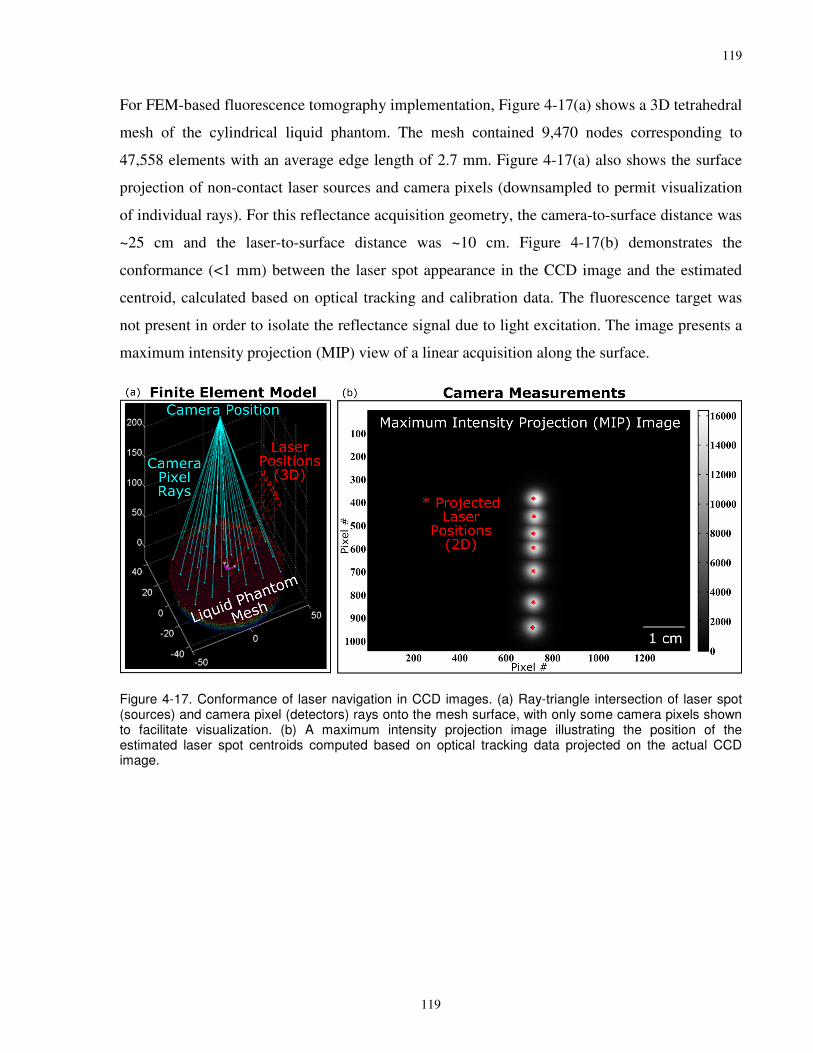
119

119

For FEM-based fluorescence tomography implementation, Figure 4-17(a) shows a 3D tetrahedral

mesh of the cylindrical liquid phantom. The mesh contained 9,470 nodes corresponding to

47,558 elements with an average edge length of 2.7 mm. Figure 4-17(a) also shows the surface

projection of non-contact laser sources and camera pixels (downsampled to permit visualization

of individual rays). For this reflectance acquisition geometry, the camera-to-surface distance was

~25 cm and the laser-to-surface distance was ~10 cm. Figure 4-17(b) demonstrates the

conformance (<1 mm) between the laser spot appearance in the CCD image and the estimated

centroid, calculated based on optical tracking and calibration data. The fluorescence target was

not present in order to isolate the reflectance signal due to light excitation. The image presents a

maximum intensity projection (MIP) view of a linear acquisition along the surface.

Figure 4-17. Conformance of laser navigation in CCD images. (a) Ray-triangle intersection of laser spot (sources) and camera pixel (detectors) rays onto the mesh surface, with only some camera pixels shown to facilitate visualization. (b) A maximum intensity projection image illustrating the position of the estimated laser spot centroids computed based on optical tracking data projected on the actual CCD image.

120

120

Figure 4-18 shows a subset of fluorescence images obtained during linear raster scan imaging of

the sub-surface tube partially filled with a mixture of ICG and the background liquid solution.

The four images correspond to four different projected laser beam positions and a fixed ICG tube

depth of 2.5 mm. Detector measurements are mean detector counts [ADU] computed over each

of the square ROIs superimposed on the fluorescence camera images. The size of each ROI

corresponds to a surface area of 1 mm2. The image sequence shares a common color map in units

of camera detector counts [ADU], and illustrates the increased fluorescence emission as the laser

source moved closer to the sub-surface ICG tube. Data calibration for fluorescence initialization

and emission filter leakage were performed as described in (Kepshire et al 2007).

Figure 4-18. Projected source and detector positions in sequence of CCD images during DOT acquisition. A subset of fluorescence images used for optical tomography reconstruction. Red stars indicate positions of laser sources and remaining cyan squares correspond to virtual detectors within the camera. A common color map in units of camera detector counts [ADU] is used for all images.

121

121

Figure 4-19 shows fluorescence reconstructions as a function of the ICG tube depth for the three

regularization techniques (NP, SP, and HP). Fluorescence reconstructions were performed over a

2D 90×20 mm2 rectangular mesh in-line with the source-detector trajectory, using 5,249 nodes

and 10,080 triangular elements with an average edge length of 0.6 mm for forward model

calculations. A second mesh was used for inverse reconstruction with coarser resolution (1,260

nodes, 2,313 elements, 1.2 mm average edge length). Figure 4-20 plots the corresponding

measures of peak fluorescence yield and target centroid based on 1D line profiles through the

target. Figure 4-20(a) shows that the NP reconstructions underestimated the fluorescence yield

with average error of 85% over the 5 ICG tube depths, and the associated reconstruction images

were larger in diameter than the true model. The corresponding average absolute errors for SP

and HP reconstructions were 18% and 16%, respectively. Figure 4-20(b) shows the centroid-

localization accuracy, with NP accurate to <11% absolute error in all cases, but degrading at

greater depths consistent with the simulations. SP & HP reconstructions had average absolute

errors in centroid localization of 1.8% and 1.2%, respectively, over all depths.

Experimental measurements with tube depths greater than ~7 mm provided limited resolvable

fluorescence signal at larger source-detector distances (e.g., >20−25 mm). As shown in Section

4.3.5.1, the 14-bit dynamic range of the uncooled CCD camera is subject to noise limitations at

the source-detector separations required to provide accurate tomography reconstruction at larger

depths.

122

122

Figure 4-19. A 2.4 mm diameter ICG target at different depths. Each image shows fluorescence yield: the first column shows the 2D forward model (ground truth) and the remaining columns show NP, SP, and HP reconstructions. The true target fluorescence yield was 1.2x10-3 mm-1. All images are shown with the same false-color map.

Figure 4-20. Fluorescence quantification with sub-surface ICG tube imaged over a range of depths: (a) fluorescence yield, (b) target centroid location.

123

123

4.4.2.4 VX2-Tumor Rabbit Model

Figure 4-21 shows the image processing workflow converting rabbit model CBCT images to a

tetrahedral mesh for numerical fluorescence reconstruction. A transverse CBCT slice through the

buccal region containing the VX2 tumor is shown in Figure 4-21(a). Enhanced CT contrast at the

periphery of the tumor was evident. Previous studies have demonstrated that the liposomal

nanoagent preferentially accumulates in the dense, leaky vasculature within VX2 tumors (Zheng

et al 2015, Zheng et al 2010). The putative cause of contrast enhancement is the enhanced

permeability and retention (EPR) effect (Maeda 2012).

Two regions were segmented as shown in Figure 4-21(b): i) a background region delineated

using a global threshold at the air-tissue boundary; and ii) a target region encapsulated by the

ring of CT contrast enhancement as segmented using local level tracing and manual refinement.

The target region volume (1.7 cm3) was approximately spherical with a diameter of ~1.5 cm. On

CBCT, the contrast ring was ~1-2 mm thick and at least ~2-3 mm below the tissue surface. The

target segmentation includes both the peripheral contrast enhancement as well as the interior

region of the tumor visible on CBCT.

Figure 4-21(c) shows conversion of the two-region label map to a tetrahedral mesh with 5,174

nodes and 25,383 elements with an average edge length of 2.1 mm.

Figure 4-21. Tetrahedral mesh generation based on intraoperative cone-beam CT imaging of rabbit model with CT/optical contrast agent. (a) CBCT lateral slice through rabbit buccal region (nose to the right) showing a ring of enhanced CT contrast. (b) Corresponding label map slice of background and target region segmentations. (c) Tetrahedral mesh generated from label map, showing boundary faces of each region.

124

124

Figure 4-22 demonstrates the process of projecting fluorescence images onto the mesh surface. A

fluorescence image in units of camera detector counts [ADU] is shown in Figure 4-22(a),

corresponding to the tracked laser and camera positions shown in Figure 4-22(b). The projected

laser spot was adjacent to the surface bulge encapsulating the buccal tumor, and fluorescence

emission was visible over a portion of the tissue surface. Detector counts [ADU] were converted

to surface flux C� [mW/mm2] based on the radiometric camera model and the mesh surface

topography from CBCT imaging. Geometric mapping of the light rays from the camera into 3D

imaging space was provided by the camera calibration process described in Chapter 2. Projection

of the laser source onto to the tissue was performed using the laser calibration process described

in this chapter. This process of camera and laser mapping was repeated for all source positions.

Figure 4-22. Navigated mapping of fluorescence image onto tissue surface accounting for camera response and free-space propagation effects. The fluorescence image measured in detector counts [ADU]. (b) Fluorescence mapped to surface flux [mW/mm2] using the geometric and radiometric camera model. The laser beam and camera pixel rays were projected onto the mesh using a method for ray-triangle intersection.

Figure 4-23 compares NP, HP, and SP fluorescence reconstructions. The NP and HP

reconstructions used a regularization parameter of & L 10, while SP used & = 10a- in order to

resolve higher-frequency structures within the segmented regions, as described in Section

4.3.4.2. The true in vivo fluorescence concentration and background optical properties were

unknown for this animal model. Background properties of ��� = 1 [mm-1] and �� = 0.001 [mm-

1] were assumed based on a homogeneous fitting algorithm (McBride 2001) performed on

spatially-resolved data in a region of normal tissue adjacent to the buccal tumour. The enhanced

iodine contrast on CBCT corresponded to the periphery of the hard-prior reconstruction as

125

125

shown in Figure 4-23(b). The 3D fluorescence reconstructions are superimposed on an oblique

CBCT slice in line with the projected laser scan trajectory and passing through the buccal tumor.

Fluorescence values below $��% = 2 ´ 10a²mm-1 were made transparent in this image in order

to visualize the CBCT slice. The NP reconstruction recovers limited fluorescence at depths

beyond ~5 mm due to the limited depth penetration of excitation light. The HP approach maps

fluorescence over the entire segmented target prior, but does not directly correspond to the

peripheral iodine enhancement on CBCT, which is assumed to coincide with the liposome co-

encapsulated ICG. As a result, the reconstructed fluorescence yield is taken to be an

underestimate of the true value based on the effects described in Section 4.3.4.2, in which hard-

prior reconstructions based on enlarged target region areas produced low fluorescence yield

estimates. Finally, the SP recovered an annular shape, with an average border thickness of ~5-6

mm. In this case, the soft-prior reconstruction is seen to offer a balance between the information

contained in the measurement data and the prior segmentation.

Figure 4-23. Fluorescence tomography reconstructions through buccal VX2 tumor in a rabbit model containing liposome-encapsulated CT/fluorescence contrast. Oblique slice through 3D fluorescence reconstruction using (a) no priors (b) hard priors and (c) soft priors. All images are shown on equivalent color scale for both the CBCT oblique slice (grayscale) and the fluorescence yield reconstruction (green, with color bar as shown).

Figure 4-24(a) shows the soft-prior fluorescence reconstruction overlaid on a larger CBCT slice

including the buccal region and anterior sinuses of the rabbit. A corresponding 3D rendering is

shown in Figure 4-24(b) including surface renderings of bone (opaque) and soft-tissue (wire

mesh) anatomy, a transverse CBCT slice, and a 3D volume rendering of the soft-prior

fluorescence reconstruction. These images demonstrate the ability to present co-registered

anatomical (CBCT) and functional (fluorescence) 3D imaging data acquired at the time of

surgery. Furthermore, the fluorescence reconstruction in this case of a soft-priors approach made

direct use of CBCT anatomical segmentations in the inverse optical problem.

126

126

Figure 4-24. Fusion of intraoperative CBCT with soft-prior fluorescence reconstruction. (a) Axial CBCT slice through rabbit sinuses and buccal region, with overlay of fluorescence yield. (b) 3D renderings of bone (white) and soft-tissue (pink) surfaces computed from CBCT volume, and 3D fluorescence reconstruction (green). The 3D anatomical (CBCT) and functional (fluorescence) images were both obtained intraoperatively, just prior to tumor resection.

127

127

4.5 Discussion and Conclusions

This chapter describes a hybrid system for intraoperative cone-beam CT and fluorescence

tomography that leverages a navigation-based model of free-space light propagation. Building on

previous studies that demonstrate the use of spatial priors from radiological imaging modalities

(e.g., MR, CT), this study uniquely makes use of intraoperative CBCT imaging data as a

structural prior for 3D fluorescence reconstruction. Furthermore, the development of a non-

contact imaging approach using a surgical tracking framework also adds to the existing literature

on system architectures for DOT implementation. Simulation, phantom and animal studies

demonstrate improvements in fluorescence quantification and target localization using a spatial-

priors approach in comparison to standard tomography reconstruction without the use of a

structural prior.

System calibration for camera and laser tracking yielded mean target registration errors of 0.17

mm and 0.92 mm, respectively. The finite spot size (~2−3 mm) of the laser − due to the

collimator − contributed to the calibration errors. The surface flux mapping procedure assumed

that the focal plane of the camera coincided with the tissue surface, but this approach could be

generalized to support more sophisticated models accounting for out-of-focus effects (Ripoll and

Ntziachristos 2004, Chen et al 2010a, Guggenheim et al 2013b). The system calibration accuracy

also depends on the resolution of the mesh surface. Here, intraoperative CBCT provided high-

resolution 3D imaging data with isotropic voxels in the range 0.2−0.8 mm3. Taken together,

these system metrics enabled navigated surface flux mapping with sub-millimeter accuracy,

which is consistent with the use of high-resolution structural imaging to complement low-

resolution diffuse optical transport data (Pogue et al 2011).

Simulation and imaging studies assessed the benefits of spatial-priors (SP & HP) in contrast to

standard regularization (NP) for fluorescence localization and quantification. For the specific

optical properties used in these experiments (�� L 0.032 mm-1, ��� = 1 mm-1, 10:1 fluorescence

contrast), standard regularization had two key limitations in comparison to spatial priors as

validated in simulations. First, limited spatial resolution for smaller targets resulted in blurred NP

reconstructions and corresponding fluorescence yield underestimation (e.g., -68% error for 2.5

mm diameter target at 2.5 mm depth). Second, limited depth sensitivity resulted in larger errors

at greater depths (e.g., -60% error for 6 mm diameter target at 6.5 mm depth), as well as for

128

128

larger diameter targets extending deeper into the tissue (e.g., +108% error for 15 mm diameter

target at 2.5 mm depth). Under these simulated conditions, both soft- and hard-prior techniques

had fluorescence quantification errors <10%, except for the specific case of a small target (2.5

mm diameter) using SP reconstruction. In experimental measurements using a tube of ICG

embedded in a liquid background, there was an overall reduction in the accuracy of all

techniques compared to simulations, but a comparable improvement in quantifying the

fluorescence yield quantification, with spatial priors reducing the errors in estimating $��%, from

85% with NP to an average of 18% for SP and 16% for HP. Several experimental factors may

have contributed to the remaining errors, including residual light leakage into the emission

bandwidth and background signal. These factors most likely affected measurements with large

source-detector distances, with associated low fluorescence signal, leading to uncertainties in the

reconstruction process.

The simulation and imaging studies also assessed the spatial localization accuracy of each of the

three reconstruction techniques. The NP reconstructions demonstrated accurate recovery of the

top surface of the fluorescence target up to depths related to the optical penetration depth of the

tissue, with a corresponding reduction in fluorescence quantification accuracy. The potential role

for FEM-based tomography for sub-surface localization in this manner has been described

previously (Kepshire et al 2007). The current work extends these results by providing a side-by-

side comparison with spatial priors. The simulation and experimental results demonstrated that

spatial-prior reconstructions localized not only the top surface of the target, but also reduced

errors in estimates of target size (e.g., NP errors of -33% for centroid position of a 15 mm

diameter target), which directly contributed to uncertainty in the estimates of fluorescence yield.

Analytical approaches based on diffusion theory models with the use of multiple excitation

wavelengths (Kim et al 2010c) or emission wavelengths (Leblond et al 2011) have been

developed to recover the nearest topographic surface of a fluorescence target. Moreover,

extensions of these analytical approaches using FEM-based techniques have permitted recovery

of fluorescence intensity along the top surface, and are being explored to identify residual tumor

cells in a number of surgical applications including glioblastoma resection (Kolste et al 2015,

Jermyn et al 2015b). In contrast, the current work recovers a tomographic image consistent with

a DOT framework. The direct comparison of capabilities between optical-based topographic

approaches and a spatial-prior DOT method driven by CBCT is not necessarily a fair one, as

129

129

clearly the need for intraoperative anatomical imaging is a key tradeoff for clinical consideration.

Rather, the results in this chapter serve to benchmark expected imaging performance with the use

of structural priors, and motivate further clinical investigations in specific applications that

already make use of CBCT for surgical guidance.

The pilot VX2-tumor rabbit model data provided the opportunity to demonstrate CBCT-guided

fluorescence tomography capabilities in vivo, but lack of independent measurements of tissue

fluorescence prevented an objective assessment of overall accuracy. Liposome co-encapsulation

of the CT contrast (iodine) with the fluorescence contrast (ICG) permitted the use of the

intraoperative CBCT volume for geometric comparison with the 3D fluorescence

reconstructions. This pilot study was focused on the imaging physics of CBCT-guided

tomography implementation, while the biological and surgical assessment of liposome

distribution in comparison to tumor anatomy is part of ongoing studies by other investigators

(Zheng et al 2015). The specific distribution of iodine contrast on CBCT, consisting of a ring as

thin as 1 mm, presented a challenging case for optical reconstruction. One limitation of the study

data was the relatively sparse source-detector sampling across the tissue surface, consisting of 9

source positions over a range of ~35 mm corresponding to an average source spacing of ~4 mm,

in comparison to an intra-source spacing of ~2.5 mm suggested by previous optimization studies

(Kepshire et al 2006). As a result of limitations in the current hardware system, as discussed

further below, homogenous background properties were assumed based on a simple fitting

procedure, and consequently the fluorescence reconstructions are subject to errors due to

heterogeneous absorption and scattering. The 3D reconstructions must also be interpreted within

the context of the linear acquisition geometry, as the Jacobian matrix [Eq. (23)] in these cases

displays limited sensitivity to measurement data for tissue regions far from the sources. Hence,

image reconstructions were only compared for oblique slices near the source trajectory as shown

in Figure 4-23. The use of a CBCT spatial prior, resulting in either a modified Jacobian (hard

priors) or spatially-regularized Jacobian (soft priors) does permit recovery of fluorescence in

regions that do not necessarily have high optical sensitivity, permitting the 3D visualization as

demonstrated in Figure 4-24.

Both the simulation studies and the rabbit experiment investigated the performance of a soft-

prior implementation with errors in the structural prior. Motivated by the specific distribution of

liposome accumulation in the rabbit model, the simulation studies made use of a forward model

130

130

consisting of an annulus, while the soft-prior reconstruction employed a filled-in circle.

Similarly, the rabbit study soft-prior reconstruction made use of a segmentation consisting of the

entire region encapsulated by the ring of visible iodine contrast enhancement. Clearly, the ideal

choice of structural prior in this case would be to delineate only the outer ring of contrast, and

exclude the interior in order to match the CBCT imaging data. Enforcing the use of a

“mismatched” prior here, while somewhat artificial, was intended to explore the performance of

structural priors in the face of model uncertainty as may be the case in real clinical applications.

While the direct application of structural priors to DOT imaging have been widely described for

other imaging modalities, evaluations including model uncertainty have received less attention.

Both the simulation and rabbit data results demonstrated that a soft-prior approach using reduced

regularization (& = 10a/ − 10a-) helped recover higher-frequency variations corresponding to

the annular model. Effectively, the reduction in regularization permitted larger variations within

each region. The tradeoff with the use of a lower regularization parameter is that it may

introduce larger variabilities elsewhere in the image, such as the slight imaging artifacts evident

near source positions at the tissue surface in both simulation and experimental reconstructions.

This initial investigation demonstrated the ability of a soft-prior reconstruction to recover

fluorescence structure in the face of model uncertainty. Further experimental studies are required

to provide insight into the optimal regularization parameter under a wider range of conditions.

The navigated instrumentation for non-contact imaging was based on manual movement of a

laser diode across the tissue surface. This was achieved by sliding the laser handle along an

aluminum support arm suspended above the phantom, or by manual adjustment of a mechanical

support arm. The integration times required for fluorescence imaging prevented free-hand

operation. Further investment in the optical hardware setup would provide a streamlined

acquisition system more suitable for clinical implementation. For example, non-contact DOT

imaging systems often use a dual-axis galvanometer to raster scan across the tissue surface

(Kepshire et al 2007). Alternatively, a structured light projector can be used that provides

programmable point source inputs (Guggenheim et al 2013b). There is growing interest in using

these projectors to perform DOT by generating wide-field illumination patterns, which has the

potential to improve image acquisition efficiency, and furthermore, to reduce uncertainties

within the tissue light transport model (Cuccia et al 2009, Gioux et al 2009). In all of these cases,

the challenges introduced by complex tissue structure and variable imaging system position are

131

131

still relevant, and motivate further research in combining CBCT-guided navigation with

advanced instrumentation for diffuse optical tomography.

Image acquisitions were limited to linear raster scans. This was due in part to the limitations in

the laser hardware, in order to simplify the experimental setup, but the computational framework

is directly extendable to planar source scanning in reflectance geometry. The choice of linear

acquisition was also driven by considerations of the intended application in surgical guidance.

Processing times for measurement acquisition, mesh generation, and inverse reconstruction

would need to accommodate the intraoperative clinical workflow, which can differ from a

diagnostic imaging situation. In this case, a B-mode approach may alleviate some of these

challenges, as other research studies for sub-surface scanning have considered (Kepshire et al

2007), by facilitating 2D reconstructions along a sub-surface plane in-line with the scanning

trajectory Direct comparisons between linear acquisitions, as subsets of larger planar

acquisitions, would be required to assess these tradeoffs in more sophisticated surgical models,

including computational comparisons between 2D and 3D reconstruction (Schweiger and

Arridge 1998). Furthermore, the fundamental imaging task can differ between a diagnostic

application and surgery, in which there is presumed clinical knowledge on the target anatomical

location that may help to localize the problem and reduce mesh dimensions. Computational FEM

processing times were not explicitly measured in this work, but are consistent (~5-10 minutes)

with previous studies using the same underlying volume segmentation and mesh processing

software (Jermyn et al 2013). The effect of mesh size on imaging performance was not

considered in this study, but the high spatial resolution of CBCT images (i.e., nominal 0.8 mm2

voxels; high-resolution sub-volumes with 0.2 mm2) and navigation accuracy of laser and camera

surface mapping (<1 mm) are consistent with the use of high-resolution spatial priors in contrast

to low-resolution optical data resulting from diffuse transport.

A key limitation in the current system implementation is that background optical properties for

absorption and scattering were assumed to be known. This assumption permitted the use of

simplified imaging hardware for initial laboratory investigations. A widely used approach to

recover optical properties is to first perform DOT at the excitation wavelength, and quite often

the emission wavelength also, before fluorescence data collection (Davis et al 2008, Tan and

Jiang 2008, Lin et al 2010). This requires the use of frequency-domain instrumentation involving

a modulated laser source as well as amplitude and phase measurements to decouple the effects of

132

132

absorption and scattering. Also, future studies could investigate a wider range of background

optical properties. The specific coefficients for absorption (�� = 0.032 mm-1) and reduced

scattering (��� = 1 mm-1) used in simulation and phantom studies were selected somewhat

arbitrarily, but do fall within typical in vivo values, for example breast at 760 nm (Sandell and

Zhu 2011). While the general trends in DOT imaging performance as a function of target size

and depth would still hold, the choice of different absorption and scattering coefficients would

alter the specific numerical results (e.g., depth resolution). A further limitation of this study is

that the fluorescence phantom did not contain any ICG in the background liquid, whereas the

simulations had 10:1 target-to-background ratio, and further experiments with lower contrast

ratios (e.g., 5:1 or 2:1) would help to validate system performance. It is hypothesized that as the

optical tomography problem becomes more challenging at lower contrast ratios there may in fact

be more benefits in the use of spatial priors, but this requires further assessment. An additional

limitation of the fluorescence phantom model was that the background region was homogenous,

whereas layered tissue architectures and/or multiple fluorescence inclusions would present more

challenging conditions (Pogue et al 1999).

The hybrid fluorescence tomography approach is predicated on the availability of intraoperative

CBCT to provide anatomical priors, for the bulk tissue topography as well as sub-surface

regions. The ability to leverage sub-surface anatomical segmentations for a spatial-priors

implementation will in large part be dictated by the specific clinical application under

investigation and the corresponding image quality of CBCT in delineating relevant anatomical

structures. Looking forward, three specific clinical challenges in surgical oncology introduced in

Section 1.1 suggest avenues for future investigation: i) intraoperative CBCT imaging to delineate

tumor morphology; ii) spatial-priors segmentations of lymph nodes readily visible on CT

imaging; iii) CBCT vascular angiography capabilities to provide priors for blood flow

assessment. An in-house CBCT data set from over 50 head and neck cancer patients is available

to support these future efforts (King et al 2013, Muhanna et al 2014), as described further in

Chapter 5.

133

133

Conclusions and Future Directions

5.1 Unifying Discussion

The underlying approach foundational to both Chapter 3 and Chapter 4 is to directly incorporate

navigation-based measurements into computational models of light transport. While both image-

guided techniques are designed to reduce fluorescence uncertainty due to spatial variations, they

are fundamentally different problems: Chapter 3 involves 2D image-guided fluorescence

imaging (igFI) and Chapter 4 involves 3D image-guided fluorescence tomography (igFT). This

section compares and contrasts these two approaches.

Commercially-available fluorescence instruments for 2D imaging are in widespread clinical use.

The igFI technique was designed to integrate with these existing devices. Streamlined software

implementation would permit real-time igFI to correct for variations in fluorescence intensity

due to illumination inhomogeneities and camera response. As demonstrated in Chapter 3, such

an approach reduced uncertainties in simulated fluorescence-guided tissue classification. The key

limitation of any 2D imaging system, however, is the susceptibility to volumetric effects and

regional inhomogeneity.

These 2D limitations have led to the development of 3D fluorescence tomography systems. The

igFT technique was designed to leverage spatial priors from intraoperative CBCT and surgical

navigation. As demonstrated in Chapter 4, a navigated spatial-priors approach improved

quantification accuracy in depth-resolved fluorescence reconstruction. In contrast to 2D imaging,

tomography involves more advanced optical instrumentation and intensive computational

requirements.

It is emphasized that igFT does not necessarily supersede igFI, rather, future investigations will

be driven by clinical requirements (e.g., analogous to 2D x-rays vs. 3D CT). Going forward,

there are potential translational pathways for both approaches, as outlined in subsequent sections.

134

134

5.2 Conclusions

The key innovation in this thesis is the development of a computational framework for image-

guided fluorescence quantification. The underlying principle is to directly incorporate spatial

localization of patient anatomy and optical devices into models of light transport. This approach

leverages technology for intraoperative cone-beam CT (CBCT) imaging and surgical navigation

to permit clinical use for surgical oncology applications including tumor imaging, lymph node

mapping, and vascular angiography. The geometric and computational framework is designed to

reduce measurement uncertainties in fluorescence images and enable more objective clinical

decision making based on fluorescence.

A central achievement was to convert fluorescence images in arbitrary camera units to estimates

of intrinsic fluorescence transport for use as a functional biomarker, both at the tissue surface and

in sub-surface simulated targets. This was performed using a multi-stage model for light

propagation based on data from intraoperative CBCT and surgical navigation, in combination

with mathematical descriptions of optical system transport, free-space light propagation, and

diffuse tissue optics. Experimental validation was performed to assess the geometric and

radiometric accuracy of the model, including assessments of camera sensitivity, tracker-to-

camera registration, illumination patterns, and fluorescence quantification. The general

framework was applied to develop two new image-guidance approaches: 2D fluorescence

imaging (igFI) [Chapter 3], and 3D fluorescence tomography (igFT) [Chapter 4].

In the first implementation (igFI), a novel calibration algorithm for navigated fluorescence

imaging was developed and assessed. This approach is designed to overcome variabilities

introduced into fluorescence images due to illumination inhomogeneities, tissue topography, and

camera response. Experiments in realistic oral cavity models validated that changes in device

positioning can induce fluorescence intensity variations (up to a factor of 4) during minimally-

invasive endoscopic approaches. Furthermore, a fluorescence segmentation task using

normalized contour lines demonstrated that image-guided compensation of illumination

inhomogeneities resulted in reduced rates of tissue misclassification. These results motivate

future clinical investigation for fluoresce-guided tissue assessment during tumor resection (tumor

vs. normal) and anatomical reconstruction (perfused vs. necrotic).

135

135

In the second implementation (igFT), spatial data from a CBCT-guided surgical navigation

system was integrated into a finite element method for fluorescence tomography. Two features

not previously described in the literature were introduced: i) a non-contact geometry for diffuse

optical tomography driven by optical tracker localizations of a calibrated camera; ii) a spatial-

priors approach for fluorescence reconstruction directed by intraoperative CBCT imaging. These

developments enable an adaptive method for fluorescence tomography to account for

intraoperative changes due to tissue deformation and surgical excision. Simulation and

experimental results showed that spatial priors improved quantification, with error reductions of

up to 65% in depth-resolved estimates of fluorescence yield. Proof-of-principle evaluation in a

surgical animal model showed co-registered visualization of concurrent anatomical (CBCT) and

functional (fluorescence) details to reveal contrast enhancement from a liposomal CT/optical

nanoparticle at the periphery of a buccal tumor.

Together, experimental assessments of these two algorithms elucidate the deleterious effects of

view-dependent illumination inhomogeneities and depth-dependent diffuse tissue transport on

fluorescence quantification accuracy. More importantly, the direct use of 3D data from a CBCT-

guided surgical navigation system was shown to provide improvements in fluorescence

quantification and tissue classification accuracy in pre-clinical models. Future research directions

to advance methods developed in this thesis are outlined below, with a specific focus on a

translational pathway to bring these fluorescence-guided surgery techniques into the operating

room for use in cancer surgery.

136

136

5.3 Future Directions

5.3.1 Surgical Fluorescence Phantoms from Intraoperative CBCT

Realistic tissue-simulating phantoms enable imaging system optimization and performance

validation under known geometric and optical conditions prior to clinical translation (Pogue and

Patterson 2006). For example, imaging studies in Chapter 3 made use of two custom oral cavity

phantoms based on CBCT images obtained during cadaveric surgical studies. CBCT data was

converted into 3D printed scaffolds for an agar-based solution with tunable properties for

absorption, scattering and fluorescence. Going forward, a wider range of surgical phantoms

incorporating sub-surface anatomical structures (e.g., tumors, lymph nodes, blood vessels) could

serve to further assess image-guided fluorescence imaging and tomography approaches.

To generate additional anatomical models of surgical anatomy, one potential source of imaging

data is a research database from more than 50 head and neck patients, as part of an ongoing

research study (Muhanna et al 2014). Each case involved the acquisition of 1−5 CBCT images

for initial surgical planning, tumor resection evaluation, and post-reconstruction assessment.

With appropriate REB amendments to support retrospective analysis, this dataset could serve to

generate fluorescence models, with a particular focus on clinical scenarios in which pre-

operative or post-operative diagnostic imaging does not accurately portray the intraoperative

morphology. Specific scenarios of interest include: i) cervical lymph node anatomy during neck

dissection; ii) blood vessel structure during free-flap tissue transfer and microsurgical

anastomosis; iii) trans-nasal access to anterior skull base structures (e.g., pituitary).

Two key methods enable fabrication of patient-specific fluorescence phantoms. First, 3D

printing provides a means to convert CBCT imaging data into geometric models, based on the

rapid emergence of low-cost, high-resolution 3D printers suitable for medical applications (Chan

et al 2015, Martelli et al 2016). Second, recipes for tissue-simulating phantoms are available for

a wide array of materials with tunable optical and mechanical properties (Pogue and Patterson

2006). For future research, one possible phantom design involves the use of gelatin-based

fluorescence inclusions placed within an agar-based background. This technique has been

demonstrated in the case of a pourable breast mold (Pleijhuis et al 2014), and could be adapted to

the more complex structure of the 3D printed oral cavity molds used in this study. Furthermore,

hydrogel-based models (i.e., agar, gelatin) provide elastic properties comparable to human soft-

137

137

tissue, which permits surgical manipulation using standard clinical tools (e.g., scalpel) (Pleijhuis

et al 2011, Samkoe et al 2017). This functionality enables fluorescence imaging studies to model

a wider range of conditions, such as depth variation of a fluorescence inclusion through the

sequential resection of layers of overlapping hydrogel-based material. While clearly such

anatomical phantoms still present limitations in comparison to in vivo scenarios, which in general

have more complex optical heterogeneity and mechanical properties, the key benefit of a

phantom formulation is that it provides known fluorescence distributions and concentrations for

comparison with imaging system measurements.

5.3.2 Simulations Based on Clinical Data

The surgical CBCT database could also serve to drive simulation studies to optimize and assess

image-guided software workflows. This would be consistent with previous computational studies

that combined clinical imaging data (e.g., breast MRI) with simulated optical tomography data in

NIRFAST (Dehghani et al 2008, Jermyn et al 2013). For igFT, the workflow includes

anatomical segmentation of tissue topography and sub-surface anatomical structures, tetrahedral

mesh generation, and inverse reconstruction based on simulated measurement data. To further

streamline these processing steps, two approaches are considered: i) a hardware approach using a

GPU (graphic processing unit) to enable a massively-parallel implementation of the forward and

reverse FEM models (Jermyn et al 2013); and ii) an algorithmic approach to leverage machine

learning techniques developed for automated image segmentation in CBCT-guided radiation

therapy (McIntosh et al 2017). For igFI, intraoperative tissue-surface segmentations from clinical

CBCT data sets could also support computational investigations of navigated illumination

techniques. Simulated measurement data would consist of “virtual” endoscope positions,

combined with simulations of light propagation between the illumination source, tissue surface,

and camera sensor. Light source and camera models could be based on calibration measurements

performed on clinical fluorescence imaging devices. As in the case of phantom experiments,

simulations are no substitute for clinical implementation and in vivo measurement data, but they

do provide a mechanism to realistically assess the software workflow, as well as serve to identify

specific surgical scenarios best suited for clinical translation.

138

138

5.3.3 Novel Fluorescence Contrast Agent Evaluation

While the number of clinically-approved fluorescence probes is currently limited, a growing

number of novel contrast agents are being developed and evaluated in animal models (Nagaya et

al 2017). Pre-clinical molecular imaging studies now have access to an armamentarium of

dedicated small-animal imaging devices for radiologic (e.g., CT, MR, PET) and optical (e.g.,

fluorescence, bioluminescence) assessment (Pogue 2015, Leblond et al 2010). These systems

often make use of animal holders that help to minimize anatomical deformations encountered

during transport, and serve to enable accurate co-registration between imaging modalities. As

new molecular agents proceed through regulatory approvals and into early phase clinical trials,

there is a corresponding interest to provide high-resolution intraoperative imaging to visualize

and measure in vivo fluorescence distributions (Pogue 2015). The emergence of agents with

multi-modality capabilities motivates the development of imaging systems that provide both

radiological and optical detection, as part of a comprehensive strategy for surgical evaluation

(Zhang et al 2017). To this end, the CBCT imaging, surgical navigation, and fluorescence

imaging systems described here are all suitable for not only pre-clinical implementation, but

clinical use also.

Section 4.3.5.3 demonstrated dual-modality imaging of a liposome-encapsulated CT/optical

agent in a pre-clinical rabbit model. This nanoagent is currently passing through the final stages

of pre-clinical validation and into early phase clinical trials in head and neck and lung cancer

surgery (Zheng et al 2015). This translational pathway provides future opportunities to assess the

computational methods developed in this thesis, in collaboration with colleagues in surgical

oncology, pharmaceutical science, and medical physics.

Beyond the use of contrast agents based on ICG, one direction for future research is to evaluate

image-guided fluorescence methods with the cyanine fluorophore IRDye800CW (IR-800CW;

Li-COR Lincoln, Nebraska, USA) used in conjugation with monoclonal antibodies (e.g., anti-

epidermal growth factor receptor) (Rosenthal et al 2015c). In contrast to ICG (without liposome

encapsulation), this fluorophore offers increased quantum yield, improved photostability, and

decreased aggregation (Marshall et al 2010). The specific absorption (778 nm) and emission

(794 nm) peaks of IRDye800CW would permit imaging using the optical hardware assembled

139

139

for this thesis, with further improvements possible with modified fluorescence filtering (Heath et

al 2012).

In addition to fluorescence agents for diagnostic uses, molecular imaging research is also

yielding multi-functional agents that provide both imaging and therapeutic capabilities. For

example, ALA-PpIX is being used clinically for fluorescence-guidance (as shown in Figure 1-1)

as well as local therapy in the form of light-activated photodynamic therapy (PDT) (He et al

2017). One clear path for further investigation involves a pophyrin-based nanoparticle developed

at our institution (Muhanna et al 2015), which combines NIR contrast with capabilities for PDT

and photothermal (PTT) ablation. Using this nanoparticle, future extensions to this thesis could

include: i) an igFT spatial-priors framework to provide 3D monitoring of fluorescence

concentration variations over the course of treatment; ii) surgical navigation of the therapeutic

light delivery systems (e.g., optical fibers) within an FEM model of ablative light transport; and

iii) integration of image-guidance with photoacoustic imaging physics.

5.3.4 Standardized Models for Fluorescence System Assessment

Recent review articles and consensus documents in the field of fluorescence-guided surgery

point to the emerging need for device quality assurance (QA), performance verification, and

standardized methods for fluorescence quantification (Pogue et al 2016, Snoeks et al 2014,

Rosenthal et al 2015b). Reliable QA techniques are required not only to confirm valid operation

of a particular device, but also to provide objective metrics to compare the performance of

different imaging systems (Hoogstins et al 2018). It has also been emphasized that system

models must extend beyond camera-centric metrics (e.g., sensitivity, resolution) to include

uncertainties introduced during clinical use (e.g., tissue optical properties, light illumination

homogeneity) (Keereweer et al 2013, Snoeks et al 2014). The limited availability of standardized

phantoms for reflectance and fluorescence assessment, in contrast to radiological imaging, also

contributes to uncertainties in clinical system evaluation (Pogue et al 2016). Objective

ratiometric thresholds for tissue classification are considered an essential feature to not only

reduce uncertainties for surgical decision making, but to also demonstrate to regulatory agencies

the performance of a given combination of biological agent and imaging device (Rosenthal et al

2015b). In this context, this thesis contributes to the broader effort to develop objective methods

for fluorescence assessment.

140

140

To this end, Chapters 2 and 3 developed light models for the camera and light source of a

fluorescence imaging system, respectively. Taken together, these models enabled a calibration

algorithm to determine the composite parameters of a generic imaging device. Notwithstanding

considerations of the calibration phantom material for sterilization, this approach could be

readily implemented as part of the OR preparation at the start of a surgical case.

Future research directions for fluorescence system assessment include: i) to perform system

calibration (e.g., illumination source distributions) on commonly used commercial fluorescence

devices; ii) to investigate optical phantom designs suitable for intraoperative calibration (e.g.,

sterilizable reflectance phantom); iii) to assess normalized contours based on illumination

compensation as a form of ratiometric quantification; iv) to develop computational models of

imaging uncertainty.

5.3.5 Clinical Translation in Surgical Oncology

As summarized in Section 1.1, cancer surgery aims to meet a number of concurrent objectives

including: i) complete tumor removal; ii) preservation of healthy tissue including proximate

critical structures; iii) management of potential tumor spread to the lymphatic system; and iv)

assessment of vascular flow and blood perfusion during anatomical reconstruction. In this

section, potential clinical applications of igFI and igFT methods in otolaryngology – head and

neck surgery are discussed. The focus on this particular surgical oncology sub-specialty is based

on two key factors. First, the specific CBCT-guided navigation system underpinning data in this

thesis has been previously deployed in a wide range of otolaryngology applications as cited in

previous sections. Hence, clinical translation issues related to CBCT image quality, radiation

dose, surgical instrument trackers, registration accuracy, and clinical workflow have already

been explored, which allows future surgical studies to focus on image-guided fluorescence

implementation. Second, and more importantly, the anatomical complexity in the head and neck

is challenging, even for the experienced surgeon, involving invasive soft-tissue tumor

morphology, close proximity to critical structures (e.g., carotid arteries, jugular vein, optic

nerve), and tortuous vascular and lymphatic pathways. These clinical challenges have directly

motivated this thesis, and lead to the following three clinical areas for future investigation.

141

141

5.3.5.1 Vascular Assessment

Several technologies have been used for intraoperative blood flow imaging (e.g., ICG

fluorescence, Doppler ultrasound, CT angiography), with definitive indications for surgical use

still under investigation (Gurtner et al 2013). ICG fluorescence following intravenous injection

has been investigated in head and neck surgery using free-flaps (Betz et al 2013, Sacks et al

2012) and pedicled flaps (Geltzeiler et al 2018). A common challenge cited in these studies is the

lack of objective measures of fluorescence intensity. Experiments in this thesis demonstrated

specific sources of fluorescence uncertainty (e.g., illumination variation, depth-dependent

tomographic effects) and validated corresponding algorithms for compensation. Two future

implementations are envisioned to assess these image-guided fluorescence techniques further.

First, an igFI implementation using a navigated illumination model obtained for two

fluorescence imaging systems (open-field: SPY; endoscopic: PINPOINT; Novadaq, Mississauga,

ON). Navigated images obtained for a variety of distances and angles would serve to assess

geometric effects on fluorescence intensity. It is hypothesized that these effects would be more

pronounced during endoscopy with larger relative variations in surface topography.

Second, an igFT implementation using CBCT spatial priors based on sub-surface vessel

segmentations. An ongoing surgical study using contrast-enhanced intraoperative CBCT has

demonstrated the ability to segment blood vessels with diameter <1 mm in regions of the anterior

skull base, neck, and oral cavity (Muhanna et al 2014). Moreover, rotational angiography

techniques using digital subtraction of fill and mask volumes offer the potential to enable

automated segmentation of vessel anatomy (Leng et al 2013). Initial testing of this computational

workflow is underway using an anthropomorphic head phantom and a Zeego intraoperative

scanner.

In support of vascular imaging applications, initial work has also begun on a pre-clinical animal

model to investigate biological, surgical, and imaging physics questions associated with a

fluorescence assessment of flap viability. In collaboration with Dr. Margarete Akens (TECHNA

Institute, University Health Network), a preliminary non-survival experiment under an Animal

Use Protocol was performed in an established rat model for epigastric flap surgery to validate its

suitability for future experiments (Giunta et al 2005, Mucke et al 2017).

142

142

5.3.5.2 Lymphatic Mapping

One future research direction is to explore the use of CBCT-guided spatial priors for

fluorescence imaging of lymphatic structures during head and neck surgery. Such an approach

would leverage the ability of contrast-enhanced CT to provide high-resolution structural imaging

of cervical lymph node anatomy (Eisenmenger and Wiggins 2015). Future imaging studies

would focus on evaluating the resolution and efficiency of sub-surface lymph node

segmentations based on intraoperative CBCT. As demonstrated in 4.3.5, the use of spatial priors

can provide improved depth-resolved fluorescence quantification in comparison to standard

tomography or imaging techniques. An additional potential research question is to explore the

capabilities of a soft-priors approach to handle uncertainties in lymphatic spatial segmentation

(e.g., to account for non-uniform fluorescence distributions throughout a lymph node).

5.3.5.3 Tumor Delineation

The improved patient outcomes in a Phase III clinical study using ALA-PpIX fluorescence

guidance for glioma resection has helped drive research efforts into quantitative PpIX

fluorescence methods. Additional information from spectrally- and/or spatially-resolved optical

measurements, combined with appropriate computational models of light transport, enables

point-based (Kim et al 2010b, Valdes et al 2011), topographic (Kim et al 2010c, Leblond et al

2011), and tomographic (Jermyn et al 2015b, Kolste et al 2015) fluorescence quantification. This

thesis can be seen as a complementary development, in that here additional geometric

information is leveraged from surgical navigation and intraoperative imaging measurements.

Two future research directions could investigate the integration of this thesis with the latest

efforts for PpIX quantification. First, as instrumentation for spectrally- and spatially-resolved

PpIX fluorescence have typically been integrated into a neurosurgical microscope for wide-field

imaging, one research direction is to consider an endoscopic implementation that includes a

navigated illumination and detection model. Second, the effects of deformation and excision in

neurosurgery may limit computational methods that require accurate FEM meshes, and further

investigation could consider the benefits of an intraoperative CBCT-guided diffuse optical

tomography approach. This could extend the studies performed in Chapter 4 by taking advantage

of measurements performed at multiple wavelengths. In addition, spatial modulation using a

digital light projector is enabling rapid tomographic imaging capabilities, and such an approach

could be investigated with the benefit of spatial priors from CBCT.

143

143

5.3.6 Multi-Modality Surgical Guidance

Fluorescence devices are increasingly used as components within multi-modality approaches for

surgical guidance (Chi et al 2014). Such an approach can present surgeons with data from a wide

range of sources, including pre-operative radiographic imaging (e.g., CT, MR), intraoperative

imaging (e.g., CBCT, ultrasound), surgical navigation (e.g., optical, electromagnetic), robotic

instrumentation, and optical spectroscopy (e.g., white-light endoscopy, fluorescence imaging).

Furthermore, advances in low-cost commercial devices for augmented reality (AR) and virtual

reality (VR) are changing how guidance information is presented in the OR (Bernhardt et al

2017, Li et al 2017). Computational frameworks, such as this thesis, offer the potential to not

only integrate data streams from these systems, but to exploit synergies in the information. For

example, the synergistic use of spatial segmentations from radiographic images can improve

optical property quantification accuracy (Pogue et al 2010b), as has been demonstrated in this

thesis using spatial data from CBCT imaging and surgical navigation. In order to further explore

a multi-modal computational framework under more realistic clinical conditions, it is therefore

of interest to implement image-guided fluorescence techniques using commercially-available

devices, rather than prototypes, in collaboration with potential industry partners. Such a step is

essential to move this research from prototype pre-clinical testing into a development pathway

that includes considerations of regulatory approval and commercial viability (Wilson et al 2018),

and towards the ultimate goal of improving surgical care for cancer patients.

144

144

References

Alander J T, Kaartinen I, Laakso A, Patila T, Spillmann T, Tuchin V V, Venermo M and Valisuo P 2012 A review of indocyanine green fluorescent imaging in surgery Int J Biomed Imaging 2012 940585

Ale A, Ermolayev V, Herzog E, Cohrs C, de Angelis M H and Ntziachristos V 2012 FMT-XCT: in vivo animal studies with hybrid fluorescence molecular tomography-X-ray computed tomography Nat Methods 9 615-20

American Cancer Society Global Cancer Facts & Figures (3rd Edition): https://www.cancer.org/content/dam/cancer-org/research/cancer-facts-and-statistics/global-cancer-facts-and-figures/global-cancer-facts-and-figures-3rd-edition.pdf)

Anayama T, Qiu J, Chan H, Nakajima T, Weersink R, Daly M, McConnell J, Waddell T, Keshavjee S, Jaffray D, Irish J C, Hirohashi K, Wada H, Orihashi K and Yasufuku K 2015 Localization of pulmonary nodules using navigation bronchoscope and a near-infrared fluorescence thoracoscope Ann Thorac Surg 99 224-30

Andersson-Engels S, af Klinteberg C, Svanberg K and Svanberg S 1997 In vivo fluorescence imaging for tissue diagnostics Phys Med Biol 42 815

Aronson R 1995 Boundary conditions for diffusion of light J Opt Soc Am A Opt Image Sci Vis 12 2532-9

Arridge S R 1999 Optical tomography in medical imaging Inverse Problems 15 R41-R93

Arridge S R and Schweiger M 1998 A gradient-based optimisation scheme for optical tomography Opt Express 2 213-26

Arridge S R, Schweiger M, Hiraoka M and Delpy D T 1993 A finite element approach for modeling photon transport in tissue Med Phys 20 299-309

Ashdown I 1993 Near-field photometry: Measuring and modeling complex 3-D light sources ACM SIGGRAPH Course 22 Notes

Bachar G, Barker E, Chan H, Daly M J, Nithiananthan S, Vescan A, Irish J C and Siewerdsen J H 2010 Visualization of anterior skull base defects with intraoperative cone-beam CT Head Neck 32 504-12

Barber W C, Lin Y, Nalcioglu O, Iwanczyk J S, Hartsough N E and Gulsen G 2010 Combined fluorescence and X-Ray tomography for quantitative in vivo detection of fluorophore Technol

Cancer Res Treat 9 45-52

Barker E, Trimble K, Chan H, Ramsden J, Nithiananthan S, James A, Bachar G, Daly M, Irish J and Siewerdsen J 2009 Intraoperative use of cone-beam computed tomography in a cadaveric ossified cochlea model Otolaryngol Head Neck Surg 140 697-702

145

145

Barrett T, Choyke P L and Kobayashi H 2006 Imaging of the lymphatic system: new horizons Contrast Media Mol Imaging 1 230-45

Bekeny J R and Ozer E 2016 Transoral robotic surgery frontiers World J Otorhinolaryngology-

Head and Neck Surgery 2 130-5

Bernhardt S, Nicolau S A, Soler L and Doignon C 2017 The status of augmented reality in laparoscopic surgery as of 2016 Med Image Anal 37 66-90

Bernstein J M, Daly M J, Chan H, Qiu J, Goldstein D, Muhanna N, de Almeida J R and Irish J C 2017 Accuracy and reproducibility of virtual cutting guides and 3D-navigation for osteotomies of the mandible and maxilla PLoS One 12 e0173111

Betz C S, Stepp H, Janda P, Arbogast S, Grevers G, Baumgartner R and Leunig A 2002 A comparative study of normal inspection, autofluorescence and 5-ALA-induced PPIX fluorescence for oral cancer diagnosis Int J Cancer 97 245-52

Betz C S, Zhorzel S, Schachenmayr H, Stepp H, Matthias C, Hopper C and Harreus U 2013 Endoscopic assessment of free flap perfusion in the upper aerodigestive tract using indocyanine green: a pilot study J Plast Reconstr Aesthet Surg 66 667-74

Bharathan R, Aggarwal R and Darzi A 2013 Operating room of the future Best Pract Res Clin

Obstet Gynaecol 27 311-22

Black D, Hettig J, Luz M, Hansen C, Kikinis R and Hahn H 2017 Auditory feedback to support image-guided medical needle placement Int J Comput Assist Radiol Surg 1-9

Bloom J D, Rizzi M D and Germiller J A 2009 Real-time intraoperative computed tomography to assist cochlear implant placement in the malformed inner ear Otol Neurotol 30 23-6

Boas D A, Brooks D H, Miller E L, DiMarzio C A, Kilmer M, Gaudette R J and Zhang Q 2001 Imaging the body with diffuse optical tomography IEEE Sig Proc Mag 18 57-75

Bouchard J P, Veilleux I, Jedidi R, Noiseux I, Fortin M and Mermut O 2010 Reference optical phantoms for diffuse optical spectroscopy. Part 1--Error analysis of a time resolved transmittance characterization method Opt Express 18 11495-507

Bouguet J Y Camera Calibration Toolbox for Matlab (Computational Vision at the California Institute of Technology: http://www.vision.caltech.edu/bouguetj/calib_doc/)

Bova F 2010 Computer based guidance in the modern operating room: a historical perspective IEEE Rev Biomed Eng 3 209-22

Bradley R S and Thorniley M S 2006 A review of attenuation correction techniques for tissue fluorescence J R Soc Interface 3 1-13

Bradski G and Kaehler A 2008 Learning OpenCV: Computer Vision with the OpenCV Library (Sebastopol: O'Reilly)

146

146

Brooksby B A, Jiang S, Dehghani H, Pogue B W, Paulsen K D, Weaver J B, Kogel C and Poplack S P 2005 Combining near-infrared tomography and magnetic resonance imaging to study in vivo breast tissue: implementation of a Laplacian-type regularization to incorporate magnetic resonance structure J Biomed Opt 10 10

Brouwer O R, Klop W M, Buckle T, Vermeeren L, van den Brekel M W, Balm A J, Nieweg O E, Valdes Olmos R A and van Leeuwen F W 2012 Feasibility of sentinel node biopsy in head and neck melanoma using a hybrid radioactive and fluorescent tracer Ann Surg Oncol 19 1988-94

Brown D C 1971 Close-range camera calibration Photogramm Eng 37 855-66

Canadian Cancer Statistics Advisory Committee Canadian Cancer Statistics 2017: www.cancer.ca/Canadian-Cancer-Statistics-2017-EN.pdf )

Cartiaux O, Paul L, Docquier P L, Raucent B, Dombre E and Banse X 2010 Computer-assisted and robot-assisted technologies to improve bone-cutting accuracy when integrated with a freehand process using an oscillating saw J Bone Joint Surg Am 92 2076-82

Chan H H, Siewerdsen J H, Vescan A, Daly M J, Prisman E and Irish J C 2015 3D Rapid Prototyping for Otolaryngology-Head and Neck Surgery: Applications in Image-Guidance, Surgical Simulation and Patient-Specific Modeling PLoS One 10 e0136370

Chan Y, Siewerdsen J H, Rafferty M A, Moseley D J, Jaffray D A and Irish J C 2008 Cone-beam computed tomography on a mobile C-arm: novel intraoperative imaging technology for guidance of head and neck surgery J Otolaryngol Head Neck Surg 37 81-90

Chen S F, Chen B L, Huang C Q, Jiang X D, Fang Y and Luo X 2016 An antireflection method for a fluorinated ethylene propylene (FEP) film as short pulse laser debris shields RSC Advances 6 89387-90

Chen X, Gao X, Chen D, Ma X, Zhao X, Shen M, Li X, Qu X, Liang J, Ripoll J and Tian J 2010a 3D reconstruction of light flux distribution on arbitrary surfaces from 2D multi-photographic images Opt Express 18 19876-93

Chen X, Gao X, Qu X, Chen D, Ma X, Liang J and Tian J 2010b Generalized free-space diffuse photon transport model based on the influence analysis of a camera lens diaphragm Appl Opt 49 5654-64

Chen X, Gao X, Qu X, Liang J, Wang L, Yang D, Garofalakis A, Ripoll J and Tian J 2009 A study of photon propagation in free-space based on hybrid radiosity-radiance theorem Opt

Express 17 16266-80

Chi C, Du Y, Ye J, Kou D, Qiu J, Wang J, Tian J and Chen X 2014 Intraoperative imaging-guided cancer surgery: from current fluorescence molecular imaging methods to future multi-modality imaging technology Theranostics 4 1072-84

147

147

Cho B, Oka M, Matsumoto N, Ouchida R, Hong J and Hashizume M 2013 Warning navigation system using real-time safe region monitoring for otologic surgery Int J Comput Assist Radiol

Surg 8 395-405

Cho Y, Moseley D J, Siewerdsen J H and Jaffray D A 2005 Accurate technique for complete geometric calibration of cone-beam computed tomography systems Med Phys 32 968

Cleary K and Peters T M 2010 Image-guided interventions: technology review and clinical applications Annu Rev Biomed Eng 12 119-42

Conley D B, Tan B, Bendok B R, Batjer H H, Chandra R, Sidle D, Rahme R J, Adel J G and Fishman A J 2011 Comparison of Intraoperative Portable CT Scanners in Skull Base and Endoscopic Sinus Surgery: Single Center Case Series Skull Base 21 261-70

Corlu A, Choe R, Durduran T, Rosen M A, Schweiger M, Arridge S R, Schnall M D and Yodh A G 2007 Three-dimensional in vivo fluorescence diffuse optical tomography of breast cancer in humans Opt Express 15 6696-716

Cubeddu R, Pifferi A, Taroni P, Torricelli A and Valentini G 1997 A solid tissue phantom for photon migration studies Phys Med Biol 42 1971-9

Cuccia D J, Bevilacqua F, Durkin A J, Ayers F R and Tromberg B J 2009 Quantitation and mapping of tissue optical properties using modulated imaging J Biomed Opt 14 024012

Cushing S L, Daly M J, Treaba C G, Chan H, Irish J C, Blaser S, Gordon K A and Papsin B C 2012 High-resolution cone-beam computed tomography: a potential tool to improve atraumatic electrode design and position Acta Otolaryngol 132 361-8

Dalgorf D, Daly M, Chan H, Siewerdsen J and Irish J 2011 Accuracy and reproducibility of automatic versus manual registration using a cone-beam CT image guidance system J

Otolaryngol Head Neck Surg 40 75-80

Daly M J, Chan H, Nithiananthan S, Qiu J, Barker E, Bachar G, Dixon B J, Irish J C and Siewerdsen J H 2011 Clinical implementation of intraoperative cone-beam CT in head and neck surgery Proc. SPIE 7964 796426-8

Daly M J, Chan H, Prisman E, Vescan A, Nithiananthan S, Qiu J, Weersink R, Irish J C and Siewerdsen J H 2010 Fusion of intraoperative cone-beam CT and endoscopic video for image-guided procedures Proc. SPIE 7625 762503

Daly M J, Muhanna N, Chan H, Wilson B C, Irish J C and Jaffray D A 2014 A surgical navigation system for non-contact diffuse optical tomography and intraoperative cone-beam CT Proc. SPIE 8937 893703

Daly M J, Siewerdsen J H, Cho Y B, Jaffray D A and Irish J C 2008 Geometric calibration of a mobile C-arm for intraoperative cone-beam CT Med Phys 35 2124

148

148

Daly M J, Siewerdsen J H, Moseley D J, Jaffray D A and Irish J C 2006 Intraoperative cone-beam CT for guidance of head and neck surgery: Assessment of dose and image quality using a C-arm prototype Med Phys 33 3767

Daskalaki D, Aguilera F, Patton K and Giulianotti P C 2015 Fluorescence in robotic surgery J

Surg Oncol 112 250-6

Davis S C, Dehghani H, Wang J, Jiang S, Pogue B W and Paulsen K D 2007 Image-guided diffuse optical fluorescence tomography implemented with Laplacian-type regularization Opt

Express 15 4066-82

Davis S C, Pogue B W, Dehghani H and Paulsen K D 2005 Contrast-detail analysis characterizing diffuse optical fluorescence tomography image reconstruction J Biomed Opt 10 050501

Davis S C, Pogue B W, Springett R, Leussler C, Mazurkewitz P, Tuttle S B, Gibbs-Strauss S L, Jiang S S, Dehghani H and Paulsen K D 2008 Magnetic resonance-coupled fluorescence tomography scanner for molecular imaging of tissue Rev Sci Instrum 79 064302

Davis S C, Samkoe K S, O'Hara J A, Gibbs-Strauss S L, Paulsen K D and Pogue B W 2010 Comparing implementations of magnetic-resonance-guided fluorescence molecular tomography for diagnostic classification of brain tumors J Biomed Opt 15 051602

de Boer E, Harlaar N J, Taruttis A, Nagengast W B, Rosenthal E L, Ntziachristos V and van Dam G M 2015 Optical innovations in surgery Br J Surg 102 e56-72

De Veld D C, Witjes M J, Sterenborg H J and Roodenburg J L 2005 The status of in vivo autofluorescence spectroscopy and imaging for oral oncology Oral Oncol 41 117-31

Dehghani H, Eames M E, Yalavarthy P K, Davis S C, Srinivasan S, Carpenter C M, Pogue B W and Paulsen K D 2008 Near infrared optical tomography using NIRFAST: Algorithm for numerical model and image reconstruction Commun Numer Methods Eng 25 711-32

Dehghani H, Pogue B W, Poplack S P and Paulsen K D 2003 Multiwavelength three-dimensional near-infrared tomography of the breast: initial simulation, phantom, and clinical results Appl Opt 42 135-45

Dehghani H, Srinivasan S, Pogue B W and Gibson A 2009 Numerical modelling and image reconstruction in diffuse optical tomography Philos Trans A Math Phys Eng Sci 367 3073-93

Deib G, Johnson A, Unberath M, Yu K, Andress S, Qian L, Osgood G, Navab N, Hui F and Gailloud P 2018 Image guided percutaneous spine procedures using an optical see-through head mounted display: proof of concept and rationale J Neurointerv Surg

Desmettre T, Devoisselle J M and Mordon S 2000 Fluorescence properties and metabolic features of indocyanine green (ICG) as related to angiography Surv Ophthalmol 45 15-27

Di Ninni P, Martelli F and Zaccanti G 2010 The use of India ink in tissue-simulating phantoms Opt Express 18 26854-65

149

149

Di Ninni P, Martelli F and Zaccanti G 2011 Intralipid: towards a diffusive reference standard for optical tissue phantoms Phys Med Biol 56 N21-8

Diamond K R, Farrell T J and Patterson M S 2003 Measurement of fluorophore concentrations and fluorescence quantum yield in tissue-simulating phantoms using three diffusion models of steady-state spatially resolved fluorescence Phys Med Biol 48 4135-49

Dixon B J, Daly M J, Chan H, Vescan A, Witterick I J and Irish J C 2011 Augmented image guidance improves skull base navigation and reduces task workload in trainees: a preclinical trial Laryngoscope 121 2060-4

Dixon B J, Daly M J, Chan H, Vescan A, Witterick I J and Irish J C 2014 Augmented real-time navigation with critical structure proximity alerts for endoscopic skull base surgery Laryngoscope 124 853-9

DSouza A V, Lin H, Henderson E R, Samkoe K S and Pogue B W 2016 Review of fluorescence guided surgery systems: identification of key performance capabilities beyond indocyanine green imaging J Biomed Opt 21 80901

Durduran T, Choe R, Baker W B and Yodh A G 2010 Diffuse Optics for Tissue Monitoring and Tomography Rep Prog Phys 73

Eggebrecht A T, Ferradal S L, Robichaux-Viehoever A, Hassanpour M S, Dehghani H, Snyder A Z, Hershey T and Culver J P 2014 Mapping distributed brain function and networks with diffuse optical tomography Nat Photonics 8 448-54

Eisenmenger L B and Wiggins R H, 3rd 2015 Imaging of head and neck lymph nodes Radiol

Clin North Am 53 115-32

Elliott J T, Dsouza A V, Davis S C, Olson J D, Paulsen K D, Roberts D W and Pogue B W 2015 Review of fluorescence guided surgery visualization and overlay techniques Biomed Opt Express 6 3765-82

Enquobahrie A, Gobbi D, Turek M, Cheng P, Yaniv Z, Lindseth F and Cleary K 2008 Designing Tracking Software for Image-Guided Surgery Applications: IGSTK Experience Int J Comput

Assist Radiol Surg 3 395-403

Erovic B M, Chan H H, Daly M J, Pothier D D, Yu E, Coulson C, Lai P and Irish J C 2014 Intraoperative cone-beam computed tomography and multi-slice computed tomography in temporal bone imaging for surgical treatment Otolaryngol Head Neck Surg 150 107-14

Erovic B M, Daly M J, Chan H H, James A L, Papsin B C, Pothier D D, Dixon B and Irish J C 2013 Evaluation of intraoperative cone beam computed tomography and optical drill tracking in temporal bone surgery Laryngoscope 123 2823-8

Farrell T J, Patterson M S and Wilson B 1992 A diffusion theory model of spatially resolved, steady-state diffuse reflectance for the noninvasive determination of tissue optical properties in vivo Med Phys 19 879-88

150

150

Favicchio R, Psycharakis S, Schonig K, Bartsch D, Mamalaki C, Papamatheakis J, Ripoll J and Zacharakis G 2016 Quantitative performance characterization of three-dimensional noncontact fluorescence molecular tomography J Biomed Opt 21 26009

Fedorov A, Beichel R, Kalpathy-Cramer J, Finet J, Fillion-Robin J C, Pujol S, Bauer C, Jennings D, Fennessy F, Sonka M, Buatti J, Aylward S, Miller J V, Pieper S and Kikinis R 2012 3D Slicer as an image computing platform for the Quantitative Imaging Network Magn Reson Imaging 30 1323-41

Feldkamp L A, Davis L C and Kress J W 1984 Practical cone-beam algorithm J Opt Soc Am A

Opt Image Sci Vis 1 612-9

Fitzpatrick J M, West J B and Maurer C R, Jr. 1998 Predicting error in rigid-body point-based registration IEEE Trans Med Imaging 17 694-702

Frangioni J 2003 In vivo near-infrared fluorescence imaging Curr Opin Chem Biol 7 626-34

Frangioni J V 2008 New technologies for human cancer imaging J Clin Oncol 26 4012-21

Galloway R L, Jr. 2001 The process and development of image-guided procedures Annu Rev

Biomed Eng 3 83-108

Geltzeiler M, Nakassa A C I, Turner M, Setty P, Zenonos G, Hebert A, Wang E, Fernandez-Miranda J, Snyderman C and Gardner P 2018 Evaluation of Intranasal Flap Perfusion by Intraoperative Indocyanine Green Fluorescence Angiography Oper Neurosurg

Gibby J T, Swenson S A, Cvetko S, Rao R and Javan R 2018 Head-mounted display augmented reality to guide pedicle screw placement utilizing computed tomography Int J Comput Assist

Radiol Surg

Gibson A and Dehghani H 2009 Diffuse optical imaging Philos Trans A Math Phys Eng Sci 367 3055-72

Gibson A P, Hebden J C and Arridge S R 2005 Recent advances in diffuse optical imaging Phys

Med Biol 50 R1-R43

Gilmore D M, Khullar O V, Gioux S, Stockdale A, Frangioni J V, Colson Y L and Russell S E 2013 Effective low-dose escalation of indocyanine green for near-infrared fluorescent sentinel lymph node mapping in melanoma Ann Surg Oncol 20 2357-63

Gioux S, Choi H S and Frangioni J V 2010 Image-guided surgery using invisible near-infrared light: fundamentals of clinical translation Mol Imaging 9 237-55

Gioux S, Mazhar A, Cuccia D J, Durkin A J, Tromberg B J and Frangioni J V 2009 Three-dimensional surface profile intensity correction for spatially modulated imaging J Biomed Opt 14 034045

Giunta R E, Holzbach T, Taskov C, Holm P S, Brill T, Busch R, Gansbacher B and Biemer E 2005 Prediction of flap necrosis with laser induced indocyanine green fluorescence in a rat model Br J Plast Surg 58 695-701

151

151

Glossop N D 2009 Advantages of Optical Compared with Electromagnetic Tracking J Bone

Joint Surg Am 91 23-8

Guggenheim J A, Basevi H R, Frampton J, Styles I B and Dehghani H 2013a Multi-modal molecular diffuse optical tomography system for small animal imaging Meas Sci Technol 24 105405

Guggenheim J A, Basevi H R, Styles I B, Frampton J and Dehghani H 2013b Quantitative surface radiance mapping using multiview images of light-emitting turbid media J Opt Soc Am A

Opt Image Sci Vis 30 2572-84

Guha D, Alotaibi N M, Nguyen N, Gupta S, McFaul C and Yang V X D 2017 Augmented Reality in Neurosurgery: A Review of Current Concepts and Emerging Applications Can J

Neurological Sci 44 235-45

Gurtner G C, Jones G E, Neligan P C, Newman M I, Phillips B T, Sacks J M and Zenn M R 2013 Intraoperative laser angiography using the SPY system: review of the literature and recommendations for use Ann Surg Innov Res 7 1

Haerle S K, Daly M J, Chan H, Vescan A, Witterick I, Gentili F, Zadeh G, Kucharczyk W and Irish J C 2015 Localized intraoperative virtual endoscopy (LIVE) for surgical guidance in 16 skull base patients Otolaryngol Head Neck Surg 152 165-71

Haj-Hosseini N, Behm P, Shabo I and Wårdell K 2014 Fluorescence spectroscopy using indocyanine green for lymph node mapping Proc. SPIE 8935 893504

Hale G M and Querry M R 1973 Optical Constants of Water in the 200-nm to 200-µm Wavelength Region Appl Opt 12 555-63

Haritoglou C, Gandorfer A, Schaumberger M, Tadayoni R, Gandorfer A and Kampik A 2003 Light-Absorbing Properties and Osmolarity of Indocyanine-Green Depending on Concentration and Solvent Medium Invest Opthalmology & Visual Sci 44 2722

Haskell R C, Svaasand L O, Tsay T-T, Feng T-C, Tromberg B J and McAdams M S 1994 Boundary conditions for the diffusion equation in radiative transfer J Opt Soc Am A Opt Image

Sci Vis 11 2727-41

He J, Yang L, Yi W, Fan W, Wen Y, Miao X and Xiong L 2017 Combination of Fluorescence-Guided Surgery With Photodynamic Therapy for the Treatment of Cancer Mol Imaging 16 1536012117722911

Heath C H, Deep N L, Sweeny L, Zinn K R and Rosenthal E L 2012 Use of panitumumab-IRDye800 to image microscopic head and neck cancer in an orthotopic surgical model Ann Surg

Oncol 19 3879-87

Heikkila J and Silven O 1997 A four-step camera calibration procedure with implicit image correction Comp Vis Pattern Recogn 1106-12

152

152

Higgins W E, Helferty J P, Lu K, Merritt S A, Rai L and Yu K C 2008 3D CT-video fusion for image-guided bronchoscopy Comput Med Imaging Graph 32 159-73

Hill T K and Mohs A M 2016 Image-guided tumor surgery: will there be a role for fluorescent nanoparticles? Wiley Interdiscip Rev Nanomed Nanobiotechnol 8 498-511

Holt D, Parthasarathy A B, Okusanya O, Keating J, Venegas O, Deshpande C, Karakousis G, Madajewski B, Durham A, Nie S, Yodh A G and Singhal S 2015 Intraoperative near-infrared fluorescence imaging and spectroscopy identifies residual tumor cells in wounds J Biomed Opt 20 76002

Hoogstins C, Burggraaf J J, Koller M, Handgraaf H, Boogerd L, van Dam G, Vahrmeijer A and Burggraaf J 2018 Setting Standards for Reporting and Quantification in Fluorescence-Guided Surgery Mol Imaging Biol

Horn B K P, Hilden H M and Negahdaripour S 1988 Closed-form solution of absolute orientation using orthonormal matrices J Opt Soc Am A 5 1127-35

Hoshi Y and Yamada Y 2016 Overview of diffuse optical tomography and its clinical applications J Biomed Opt 21 091312

Ibanez L, Schroeder W, Ng L and Cates J 2003 The ITK software guide: the insight segmentation

and registration toolkit (Clifton Park: Kitware)

Iwai T, Maegawa J, Hirota M and Tohnai I 2013 Sentinel lymph node biopsy using a new indocyanine green fluorescence imaging system with a colour charged couple device camera for oral cancer Br J Oral Maxillofac Surg 51 e26-8

Jacques S L 2010 Optical-Thermal Response of Laser-Irradiated Tissue, ed A J Welch and M J C Van Gemert (New York: Springer) pp 109-44

Jacques S L and Pogue B W 2008 Tutorial on diffuse light transport J Biomed Opt 13 041302

Jaffray D, Kupelian P, Djemil T and Macklis R M 2007 Review of image-guided radiation therapy Expert Rev Anticancer Ther 7 89-103

Jaffray D A, Siewerdsen J H, Edmundson G K, Wong J W and Martinez A 2002a Flat-panel cone-beam CT on a mobile isocentric C-arm for image-guided brachytherapy Proc. SPIE 4682

209-17

Jaffray D A, Siewerdsen J H, Wong J W and Martinez A A 2002b Flat-panel cone-beam computed tomography for image-guided radiation therapy Int J Radiat Oncol Biol Phys 53 1337-49

Jayender J, Lee T C and Ruan D T 2015 Real-Time Localization of Parathyroid Adenoma during Parathyroidectomy N Engl J Med 373 96-8

Jermyn M, Ghadyani H, Mastanduno M A, Turner W, Davis S C, Dehghani H and Pogue B W 2013 Fast segmentation and high-quality three-dimensional volume mesh creation from medical images for diffuse optical tomography J Biomed Opt 18 86007

153

153

Jermyn M, Gosselin Y, Valdes P A, Sibai M, Kolste K, Mercier J, Angulo L, Roberts D W, Paulsen K D, Petrecca K, Daigle O, Wilson B C and Leblond F 2015a Improved sensitivity to fluorescence for cancer detection in wide-field image-guided neurosurgery Biomed Opt Express 6 5063-74

Jermyn M, Kolste K, Pichette J, Sheehy G, Angulo-Rodriguez L, Paulsen K D, Roberts D W, Wilson B C, Petrecca K and Leblond F 2015b Macroscopic-imaging technique for subsurface quantification of near-infrared markers during surgery J Biomed Opt 20 036014

Kagadis G C, Katsanos K, Karnabatidis D, Loudos G, Nikiforidis G C and Hendee W R 2012 Emerging technologies for image guidance and device navigation in interventional radiology Med Phys 39 5768-81

Kamp M A, Slotty P, Turowski B, Etminan N, Steiger H J, Hanggi D and Stummer W 2012 Microscope-integrated quantitative analysis of intraoperative indocyanine green fluorescence angiography for blood flow assessment: first experience in 30 patients Neurosurgery 70 65-73; discussion -4

Kannala J and Brandt S S 2006 A generic camera model and calibration method for conventional, wide-angle, and fish-eye lenses IEEE Trans Pattern Anal Mach Intell 28 1335-40

Keereweer S, Van Driel P B, Snoeks T J, Kerrebijn J D, Baatenburg de Jong R J, Vahrmeijer A L, Sterenborg H J and Lowik C W 2013 Optical image-guided cancer surgery: challenges and limitations Clin Cancer Res 19 3745-54

Kepshire D, Davis S C, Dehghani H, Paulsen K D and Pogue B W 2008 Fluorescence tomography characterization for sub-surface imaging with protoporphyrin IX Opt Express 16 8581-93

Kepshire D, Gibbs S, Davis S, Dehghani H, Paulsen K D and Pogue B W 2006 Sub-surface fluorescence imaging of Protoporphyrin IX with B-Scan mode tomography Proc. SPIE 6139 61391F

Kepshire D, Mincu N, Hutchins M, Gruber J, Dehghani H, Hypnarowski J, Leblond F, Khayat M and Pogue B W 2009 A microcomputed tomography guided fluorescence tomography system for small animal molecular imaging Rev Sci Instrum 80 043701

Kepshire D S, Davis S C, Dehghani H, Paulsen K D and Pogue B W 2007 Subsurface diffuse optical tomography can localize absorber and fluorescent objects but recovered image sensitivity is nonlinear with depth Appl Opt 46 1669-78

Khoury A, Whyne C M, Daly M, Moseley D, Bootsma G, Skrinskas T, Siewerdsen J and Jaffray D 2007 Intraoperative cone-beam CT for correction of periaxial malrotation of the femoral shaft: A surface-matching approach Med Phys 34 1380

Kienle A, Lilge L, Patterson M S, Hibst R, Steiner R and Wilson B C 1996 Spatially resolved absolute diffuse reflectance measurements for noninvasive determination of the optical scattering and absorption coefficients of biological tissue Appl Opt 35 2304-14

154

154

Kikinis R, Pieper S D and Vosburgh K G 2014 Intraoperative Imaging and Image-Guided

Therapy, ed F A Jolesz (New York: Springer) pp 277-89

Kim A 2010 Quantitative and depth-resolved fluorescence guidance for the resection of glioma. Univeristy of Toronto)

Kim A, Khurana M, Moriyama Y and Wilson B C 2010a Quantification of in vivo fluorescence decoupled from the effects of tissue optical properties using fiber-optic spectroscopy measurements J Biomed Opt 15 067006

Kim A, Roy M, Dadani F and Wilson B C 2010b A fiberoptic reflectance probe with multiple source-collector separations to increase the dynamic range of derived tissue optical absorption and scattering coefficients Opt Lett 18 5580-94

Kim A, Roy M, Dadani F N and Wilson B C 2010c Topographic mapping of subsurface fluorescent structures in tissue using multiwavelength excitation J Biomed Opt 15 066026

Kim A and Wilson B C 2010 Optical-Thermal Response of Laser-Irradiated Tissue, ed A J Welch and M J C Van Gemert (New York: Springer)

Kim B Y, Rutka J T and Chan W C 2010d Nanomedicine N Engl J Med 363 2434-43

King E, Daly M J, Chan H, Bachar G, Dixon B J, Siewerdsen J H and Irish J C 2013 Intraoperative cone-beam CT for head and neck surgery: feasibility of clinical implementation using a prototype mobile C-arm Head Neck 35 959-67

Koch M and Ntziachristos V 2016 Advancing Surgical Vision with Fluorescence Imaging Annu

Rev Med 67 153-64

Kokudo N and Ishizawa T 2012 Clinical application of fluorescence imaging of liver cancer using indocyanine green Liver Cancer 1 15-21

Kolste K K, Kanick S C, Valdes P A, Jermyn M, Wilson B C, Roberts D W, Paulsen K D and Leblond F 2015 Macroscopic optical imaging technique for wide-field estimation of fluorescence depth in optically turbid media for application in brain tumor surgical guidance J

Biomed Opt 20 26002

Krammer B and Plaetzer K 2008 ALA and its clinical impact, from bench to bedside Photochem

Photobiol Sci 7 283-9

Landsman M L, Kwant G, Mook G A and Zijlstra W G 1976 Light-absorbing properties, stability, and spectral stabilization of indocyanine green J Appl Physiol 40 575-83

Leblond F, Davis S C, Valdes P A and Pogue B W 2010 Pre-clinical whole-body fluorescence imaging: Review of instruments, methods and applications J Photochem Photobiol B 98 77-94

Leblond F, Ovanesyan Z, Davis S C, Valdes P A, Kim A, Hartov A, Wilson B C, Pogue B W, Paulsen K D and Roberts D W 2011 Analytic expression of fluorescence ratio detection correlates with depth in multi-spectral sub-surface imaging Phys Med Biol 56 6823-37

155

155

Lee S, Gallia G L, Reh D D, Schafer S, Uneri A, Mirota D J, Nithiananthan S, Otake Y, Stayman J W, Zbijewski W and Siewerdsen J H 2012 Intraoperative C-arm cone-beam computed tomography: quantitative analysis of surgical performance in skull base surgery Laryngoscope 122 1925-32

Leng L Z, Rubin D G, Patsalides A and Riina H A 2013 Fusion of intraoperative three-dimensional rotational angiography and flat-panel detector computed tomography for cerebrovascular neuronavigation World Neurosurg 79 504-9

Lenski M, Hofereiter J, Terpolilli N, Sandner T, Zausinger S, Tonn J-C, Kreth F-W and Schichor C 2018 Dual-room CT with a sliding gantry for intraoperative imaging: feasibility and workflow analysis of an interdisciplinary concept Int J Comput Assist Radiol Surg

Li L, Yu F, Shi D, Shi J, Tian Z, Yang J, Wang X and Jiang Q 2017 Application of virtual reality technology in clinical medicine Am J Transl Res 9 3867-80

Li X, O'leary M, Boas D, Chance B and Yodh A 1996 Fluorescent diffuse photon density waves in homogeneous and heterogeneous turbid media: analytic solutions and applications Appl Opt 35 3746-58

Lin Y, Barber W C, Iwanczyk J S, Roeck W, Nalcioglu O and Gulsen G 2010 Quantitative fluorescence tomography using a combined tri-modality FT/DOT/XCT system Opt Express 18 7835-50

Litvack Z N, Zada G and Laws E R 2012 Indocyanine green fluorescence endoscopy for visual differentiation of pituitary tumor from surrounding structures J Neurosurg 116 935-41

Ma A K, Daly M, Qiu J, Chan H H L, Goldstein D P, Irish J C and de Almeida J R 2017 Intraoperative image guidance in transoral robotic surgery: A pilot study Head Neck 39 1976-83

Maeda H 2012 Macromolecular therapeutics in cancer treatment: The EPR effect and beyond J

Controlled Release 164 138-44

Maier-Hein L, Mountney P, Bartoli A, Elhawary H, Elson D, Groch A, Kolb A, Rodrigues M, Sorger J, Speidel S and Stoyanov D 2013 Optical techniques for 3D surface reconstruction in computer-assisted laparoscopic surgery Med Image Anal 17 974-96

Marshall M V, Draney D, Sevick-Muraca E M and Olive D M 2010 Single-dose intravenous toxicity study of IRDye 800CW in Sprague-Dawley rats Mol Imaging Biol 12 583-94

Martelli N, Serrano C, van den Brink H, Pineau J, Prognon P, Borget I and El Batti S 2016 Advantages and disadvantages of 3-dimensional printing in surgery: A systematic review Surgery

McBride T 2001 Spectroscopic Reconstructed Near Infrared Tomographic Imaging for Breast Cancer Diagnosis. Dartmouth College)

156

156

McIntosh C, Welch M L, McNiven, A., Jaffray D A and Purdie T G 2017 Fully automated treatment planning for head and neck radiotherapy using a voxel-based dose prediction and dose mimicking method Phys Med Biol 62 5926

Milstein A B, Oh S, Webb K J, Bouman C A, Zhang Q, Boas D A and Millane R P 2003 Fluorescence optical diffusion tomography Appl Opt 42 3081-94

Mirota D J, Ishii M and Hager G D 2011 Vision-based navigation in image-guided interventions Annu Rev Biomed Eng 13 297-319

Möller T and Trumbore B 1997 Fast, minimum storage ray-triangle intersection J Graph Tools 2 21-8

Monahan J, Hwang B H, Kennedy J M, Chen W, Nguyen G K, Schooler W G and Wong A K 2014 Determination of a perfusion threshold in experimental perforator flap surgery using indocyanine green angiography Ann Plast Surg 73 602-6

Mondal S B, Gao S, Zhu N, Liang R, Gruev V and Achilefu S 2014 Real-time fluorescence image-guided oncologic surgery Adv Cancer Res 124 171-211

Monteiro E, Das P, Daly M, Chan H, Irish J and James A 2011 Usefulness of cone-beam computed tomography in determining the position of ossicular prostheses: a cadaveric model Otol Neurotol 32 1358-63

Moore G E, Peyton W T, French L A and Walke r W W 1948 The Clinical Use of Fluorescein in Neurosurgery J Neurosurg 5 392-8

Mori K, Deguchi D, Sugiyama J, Suenaga Y, Toriwaki J-i, Maurer C, Takabatake H and Natori H 2002 Tracking of a bronchoscope using epipolar geometry analysis and intensity-based image registration of real and virtual endoscopic images Med Image Anal 6 321-36

Morton D L, Wen D, Wong J H and et al. 1992 Technical details of intraoperative lymphatic mapping for early stage melanoma Arch Surg 127 392-9

Mucke T, Fichter A M, Schmidt L H, Mitchell D A, Wolff K D and Ritschl L M 2017 Indocyanine green videoangiography-assisted prediction of flap necrosis in the rat epigastric flap using the flow(R) 800 tool Microsurgery 37 235-42

Muhanna N, Cui L, Chan H, Burgess L, Jin C S, MacDonald T D, Huynh E, Wang F, Chen J, Irish J C and Zheng G 2016 Multimodal Image-Guided Surgical and Photodynamic Interventions in Head and Neck Cancer: From Primary Tumor to Metastatic Drainage Clin Cancer Res 22 961-70

Muhanna N, Daly M J, Chan H, Weersink R, Qiu J, Goldstein D, De Almeida J R, Gilbert R W, Kucharczyk W, Jaffray D A and Irish J C 2014 Intraoperative cone-beam CT imaging for head & neck cancer surgery 5th World Congress of International Federation of Head & Neck Oncologic

Societies

157

157

Muhanna N, Jin C S, Huynh E, Chan H, Qiu Y, Jiang W, Cui L, Burgess L, Akens M K, Chen J, Irish J C and Zheng G 2015 Phototheranostic Porphyrin Nanoparticles Enable Visualization and Targeted Treatment of Head and Neck Cancer in Clinically Relevant Models Theranostics 5 1428-43

Muller M G, Georgakoudi I, Zhang Q, Wu J and Feld M S 2001 Intrinsic fluorescence spectroscopy in turbid media: disentangling effects of scattering and absorption Appl Opt 40 4633-46

Nagaya T, Nakamura Y A, Choyke P L and Kobayashi H 2017 Fluorescence-Guided Surgery Front Oncol 7 314

Newman M I, Jack M C and Samson M C 2013 SPY-Q analysis toolkit values potentially predict mastectomy flap necrosis Ann Plast Surg 70 595-8

Nguyen Q T, Olson E S, Aguilera T A, Jiang T, Scadeng M, Ellies L G and Tsien R Y 2010 Surgery with molecular fluorescence imaging using activatable cell-penetrating peptides decreases residual cancer and improves survival Proc Natl Acad Sci U S A 107 4317-22

Nguyen Q T and Tsien R Y 2013 Fluorescence-guided surgery with live molecular navigation — a new cutting edge Nat Rev Cancer 13 653-62

Ntziachristos V, Turner G, Dunham J, Windsor S, Soubret A, Ripoll J and Shih H A 2005 Planar fluorescence imaging using normalized data J Biomed Opt 10 064007

Ntziachristos V and Weissleder R 2001 Experimental three-dimensional fluorescence reconstruction of diffuse media by use of a normalized Born approximation Opt Lett 26 893-5

Okatani T and Deguchi K 1997 Shape Reconstruction from an Endoscope Image by Shape from Shading Technique for a Point Light Source at the Projection Center Comput Vis Image Underst 66 119-31

Okawa S, Yano A, Uchida K, Mitsui Y, Yoshida M, Takekoshi M, Marjono A, Gao F, Hoshi Y, Kida I, Masamoto K and Yamada Y 2013 Phantom and mouse experiments of time-domain fluorescence tomography using total light approach Biomed Opt Express 4 635-51

Orosco R K, Tsien R Y and Nguyen Q T 2013 Fluorescence imaging in surgery IEEE Rev

Biomed Eng 6 178-87

Parrish-Novak J, Holland E C and Olson J M 2015 Image-Guided Tumor Resection Cancer J 21 206-12

Paulsen K D and Jiang H 1995 Spatially varying optical property reconstruction using a finite element diffusion equation approximation Med Phys 22 691-701

Peters T and Cleary K eds 2008 Image-guided interventions: Technology and applications (New York: Springer)

Peters T M 2006 Image-guidance for surgical procedures Phys Med Biol 51 R505-40

158

158

Peters T M and Linte C A 2016 Image-guided interventions and computer-integrated therapy: Quo vadis? Med Image Anal 33 56-63

Philip R, Penzkofer A, Bäumler W, Szeimies R M and Abels C 1996 Absorption and fluorescence spectroscopic investigation of indocyanine green J Photochem Photobiol A 96 137-48

Phillips B T, Munabi N C, Roeder R A, Ascherman J A, Guo L and Zenn M R 2016 The Role of Intraoperative Perfusion Assessment: What Is the Current State and How Can I Use It in My Practice? Plast Reconstr Surg 137 731-41

Pleijhuis R, Timmermans A, De Jong J, De Boer E, Ntziachristos V and Van Dam G 2014 Tissue-simulating phantoms for assessing potential near-infrared fluorescence imaging applications in breast cancer surgery J Vis Exp 51776

Pleijhuis R G, Langhout G C, Helfrich W, Themelis G, Sarantopoulos A, Crane L M, Harlaar N J, de Jong J S, Ntziachristos V and van Dam G M 2011 Near-infrared fluorescence (NIRF) imaging in breast-conserving surgery: assessing intraoperative techniques in tissue-simulating breast phantoms Eur J Surg Oncol 37 32-9

Pogue B, McBride T, Osterberg U and Paulsen K 1999 Comparison of imaging geometries for diffuse optical tomography of tissue Opt Express 4 270-86

Pogue B W 2015 Optics in the molecular imaging race Opt Photonics News 26 24-31

Pogue B W, Davis S C, Leblond F, Mastanduno M A, Dehghani H and Paulsen K D 2011 Implicit and explicit prior information in near-infrared spectral imaging: accuracy, quantification and diagnostic value Philos Trans A Math Phys Eng Sci 369 4531-57

Pogue B W, Gibbs-Strauss S, Valdes P A, Samkoe K, Roberts D W and Paulsen K D 2010a Review of Neurosurgical Fluorescence Imaging Methodologies IEEE J Sel Top Quantum

Electron 16 493-505

Pogue B W, Leblond F, Krishnaswamy V and Paulsen K D 2010b Radiologic and near-infrared/optical spectroscopic imaging: where is the synergy? AJR Am J Roentgenol 195 321-32

Pogue B W and Patterson M S 2006 Review of tissue simulating phantoms for optical spectroscopy, imaging and dosimetry J Biomed Opt 11 041102

Pogue B W, Paulsen K D, Samkoe K S, Elliott J T, Hasan T, Strong T V, Draney D R and Feldwisch J 2016 Vision 20/20: Molecular-guided surgical oncology based upon tumor metabolism or immunologic phenotype: Technological pathways for point of care imaging and intervention Med Phys 43 3143-56

Pogue B W, Zhu T C, Ntziachristos V, Paulsen K D, Wilson B C, Pfefer J, Nordstrom R J, Litorja M, Wabnitz H, Chen Y, Gioux S, Tromberg B J and Yodh A G 2018 Fluorescence-guided surgery and intervention — An AAPM emerging technology blue paper Med Phys 45 2681-8

159

159

Poh C F, Durham J S, Brasher P M, Anderson D W, Berean K W, MacAulay C E, Lee J J and Rosin M P 2011 Canadian Optically-guided approach for Oral Lesions Surgical (COOLS) trial: study protocol for a randomized controlled trial BMC Cancer 11 462

Prisman E, Daly M J, Chan H, Siewerdsen J H, Vescan A and Irish J C 2011 Real-time tracking and virtual endoscopy in cone-beam CT-guided surgery of the sinuses and skull base in a cadaver model Int Forum Allergy Rhinol 1 70-7

Qiu J, Hope A J, Cho B C, Sharpe M B, Dickie C I, DaCosta R S, Jaffray D A and Weersink R A 2012 Displaying 3D radiation dose on endoscopic video for therapeutic assessment and surgical guidance Phys Med Biol 57 6601-14

Qu J Y and Hua J 2001 Calibrated fluorescence imaging of tissue in vivo Appl Physics Letters 78 4040

Qu J Y, Huang Z and Hua J 2000 Excitation-and-collection geometry insensitive fluorescence imaging of tissue-simulating turbid media Appl Opt 39 3344-56

Rai L and Higgins W E 2008 Method for radiometric calibration of an endoscope's camera and light source Proc. SPIE 6918 691813

Ripoll J and Ntziachristos V 2004 Imaging scattering media from a distance: theory and applications of noncontact optical tomography Modern Physics Letters B 18 1403-31

Ripoll J, Schulz R B and Ntziachristos V 2003 Free-space propagation of diffuse light: theory and experiments Phys Rev Lett 91 103901

Rosenthal E L, Warram J M, Bland K I and Zinn K R 2015a The status of contemporary image-guided modalities in oncologic surgery Ann Surg 261 46-55

Rosenthal E L, Warram J M, de Boer E, Basilion J P, Biel M A, Bogyo M, Bouvet M, Brigman B E, Colson Y L, DeMeester S R, Gurtner G C, Ishizawa T, Jacobs P M, Keereweer S, Liao J C, Nguyen Q T, Olson J M, Paulsen K D, Rieves D, Sumer B D, Tweedle M F, Vahrmeijer A L, Weichert J P, Wilson B C, Zenn M R, Zinn K R and van Dam G M 2015b Successful Translation of Fluorescence Navigation During Oncologic Surgery: A Consensus Report J Nucl Med 57 144-50

Rosenthal E L, Warram J M, de Boer E, Chung T K, Korb M L, Brandwein-Gensler M, Strong T V, Schmalbach C E, Morlandt A B, Agarwal G, Hartman Y E, Carroll W R, Richman J S, Clemons L K, Nabell L M and Zinn K R 2015c Safety and Tumor Specificity of Cetuximab-IRDye800 for Surgical Navigation in Head and Neck Cancer Clin Cancer Res 21 3658-66

Rossi E C, Ivanova A and Boggess J F 2012 Robotically assisted fluorescence-guided lymph node mapping with ICG for gynecologic malignancies: a feasibility study Gynecol Oncol 124 78-82

Sacks J M, Nguyen A T, Broyles J M, Yu P, Valerio I L and Baumann D P 2012 Near-infrared laser-assisted indocyanine green imaging for optimizing the design of the anterolateral thigh flap Eplasty 12 e30

160

160

Samkoe K S, Bates B D, Tselepidakis N N, AV D S, Gunn J R, Ramkumar D B, Paulsen K D, Pogue B W and Henderson E R 2017 Development and evaluation of a connective tissue phantom model for subsurface visualization of cancers requiring wide local excision J Biomed

Opt 22 1-12

Sandell J L and Zhu T C 2011 A review of in-vivo optical properties of human tissues and its impact on PDT J Biophotonics 4 773-87

Schaafsma B E, Mieog J S, Hutteman M, van der Vorst J R, Kuppen P J, Lowik C W, Frangioni J V, van de Velde C J and Vahrmeijer A L 2011 The clinical use of indocyanine green as a near-infrared fluorescent contrast agent for image-guided oncologic surgery J Surg Oncol 104 323-32

Schafer S, Nithiananthan S, Mirota D J, Uneri A, Stayman J W, Zbijewski W, Schmidgunst C, Kleinszig G, Khanna A J and Siewerdsen J H 2011 Mobile C-arm cone-beam CT for guidance of spine surgery: Image quality, radiation dose, and integration with interventional guidance Med

Phys 38 4563-74

Schroeder W, Martin K and Lorenson B 2006 The Visualization Toolkit: An Object-Oriented

Approach to 3D Graphics (Clifton Park: Kitware)

Schulz R B, Ale A, Sarantopoulos A, Freyer M, Soehngen E, Zientkowska M and Ntziachristos V 2010 Hybrid system for simultaneous fluorescence and x-ray computed tomography IEEE

Trans Med Imaging 29 465-73

Schulz R B, Ripoll J and Ntziachristos V 2004 Experimental fluorescence tomography of tissues with noncontact measurements IEEE Trans Med Imaging 23 492-500

Schulze F, Buhler K, Neubauer A, Kanitsar A, Holton L and Wolfsberger S 2010 Intra-operative virtual endoscopy for image guided endonasal transsphenoidal pituitary surgery Int J Comput

Assist Radiol Surg 5 143-54

Schweiger M and Arridge S R 1998 Comparison of two- and three-dimensional reconstruction methods in optical tomography Appl Opt 37 7419-28

Sevick-Muraca E M, Sharma R, Rasmussen J C, Marshall M V, Wendt J A, Pham H Q, Bonefas E, Houston J P, Sampath L, Adams K E, Blanchard D K, Fisher R E, Chiang S B, Elledge R and Mawad M E 2008 Imaging of lymph flow in breast cancer patients after microdose administration of a near-infrared fluorophore: feasibility study Radiology 246 734-41

Shahidi R, Bax M R, Maurer C R, Jr., Johnson J A, Wilkinson E P, Wang B, West J B, Citardi M J, Manwaring K H and Khadem R 2002 Implementation, calibration and accuracy testing of an image-enhanced endoscopy system IEEE Trans Med Imaging 21 1524-35

Shayan R, Achen M G and Stacker S A 2006 Lymphatic vessels in cancer metastasis: bridging the gaps Carcinogenesis 27 1729-38

Shaye D A, Tollefson T T and Strong E B 2015 Use of intraoperative computed tomography for maxillofacial reconstructive surgery JAMA Facial Plast Surg 17 113-9

161

161

Shekhar R, Dandekar O, Bhat V, Philip M, Lei P, Godinez C, Sutton E, George I, Kavic S, Mezrich R and Park A 2010 Live augmented reality: a new visualization method for laparoscopic surgery using continuous volumetric computed tomography Surg Endosc 24 1976-85

Siewerdsen J H, Jaffray D A, Edmundson G K, Sanders W P, Wong J W and Martinez A A 2001 Flat-panel cone-beam CT: a novel imaging technology for image-guided procedures Proc. SPIE 4319 435-44

Siewerdsen J H, Moseley D J, Burch S, Bisland S K, Bogaards A, Wilson B C and Jaffray D A 2005 Volume CT with a flat-panel detector on a mobile, isocentric C-arm: Pre-clinical investigation in guidance of minimally invasive surgery Med Phys 32 241

Snoeks T J, van Driel P B, Keereweer S, Aime S, Brindle K M, van Dam G M, Lowik C W, Ntziachristos V and Vahrmeijer A L 2014 Towards a successful clinical implementation of fluorescence-guided surgery Mol Imaging Biol 16 147-51

Solheim O, Selbekk T, Lovstakken L, Tangen G A, Solberg O V, Johansen T F, Cappelen J and Unsgard G 2010 Intrasellar ultrasound in transsphenoidal surgery: a novel technique Neurosurgery 66 173-85; discussion 85-6

Soper T D, Haynor D R, Glenny R W and Seibel E J 2010 In vivo validation of a hybrid tracking system for navigation of an ultrathin bronchoscope within peripheral airways IEEE Trans

Biomed Eng 57 736-45

Spiegel J H and Polat J K 2007 Microvascular flap reconstruction by otolaryngologists: prevalence, postoperative care, and monitoring techniques Laryngoscope 117 485-90

Springsteen A 1999 Standards for the measurement of diffuse reflectance – an overview of available materials and measurement laboratories Analytica Chimica Acta 380 379-90

Srinivasan V M, Schafer S, Ghali M G, Arthur A and Duckworth E A 2016 Cone-beam CT angiography (Dyna CT) for intraoperative localization of cerebral arteriovenous malformations J

Neurointerv Surg 8 69-74

Sternheim A, Daly M, Qiu J, Weersink R, Chan H, Jaffray D, Irish J C, Ferguson P C and Wunder J S 2015 Navigated pelvic osteotomy and tumor resection: a study assessing the accuracy and reproducibility of resection planes in Sawbones and cadavers J Bone Joint Surg Am 97 40-6

Sternheim A, Kashigar A, Daly M, Chan H, Qiu J, Weersink R, Jaffray D, Irish J C, Ferguson P C and Wunder J S 2018 Cone-Beam Computed Tomography-Guided Navigation in Complex Osteotomies Improves Accuracy at All Competence Levels: A Study Assessing Accuracy and Reproducibility of Joint-Sparing Bone Cuts J Bone Joint Surg Am 100 e67

Strauss G, Koulechov K, Hofer M, Dittrich E, Grunert R, Moeckel H, Muller E, Korb W, Trantakis C, Schulz T, Meixensberger J, Dietz A and Lueth T 2007 The navigation-controlled drill in temporal bone surgery: a feasibility study Laryngoscope 117 434-41

162

162

Strauss G, Koulechov K, Richter R, Dietz A, Trantakis C and Lueth T 2005 Navigated control in functional endoscopic sinus surgery Int J Med Robot 01 31

Stummer W, Novotny A, Stepp H, Goetz C, Bise K and Reulen H J 2000 Fluorescence-guided resection of glioblastoma multiforme by using 5-aminolevulinic acid-induced porphyrins: a prospective study in 52 consecutive patients J Neurosurg 93 1003-13

Stummer W, Pichlmeier U, Meinel T, Wiestler O D, Zanella F and Reulen H-J 2006 Fluorescence-guided surgery with 5-aminolevulinic acid for resection of malignant glioma: a randomised controlled multicentre phase III trial Lancet Oncol 7 392-401

Tabanfar R, Qiu J, Chan H, Aflatouni N, Weersink R, Hasan W and Irish J C 2017 Real-time continuous image-guided surgery: Preclinical investigation in glossectomy Laryngoscope 127 E347-E53

Tan Y and Jiang H 2008 DOT guided fluorescence molecular tomography of arbitrarily shaped objects Med Phys 35 5703

Te Velde E A, Veerman T, Subramaniam V and Ruers T 2010 The use of fluorescent dyes and probes in surgical oncology Eur J Surg Oncol 36 6-15

Tempany C M, Jayender J, Kapur T, Bueno R, Golby A, Agar N and Jolesz F A 2015 Multimodal imaging for improved diagnosis and treatment of cancers Cancer 121 817-27

Themelis G, Yoo J S, Soh K S, Schulz R and Ntziachristos V 2009 Real-time intraoperative fluorescence imaging system using light-absorption correction J Biomed Opt 14 064012

Torre L A, Bray F, Siegel R L, Ferlay J, Lortet-Tieulent J and Jemal A 2015 Global cancer statistics, 2012 CA: A Cancer Journal for Clinicians 65 87-108

Tromberg B J, Pogue B W, Paulsen K D, Yodh A G, Boas D A and Cerussi A E 2008 Assessing the future of diffuse optical imaging technologies for breast cancer management Med Phys 35 2443-51

Troyan S L, Kianzad V, Gibbs-Strauss S L, Gioux S, Matsui A, Oketokoun R, Ngo L, Khamene A, Azar F and Frangioni J V 2009 The FLARE intraoperative near-infrared fluorescence imaging system: a first-in-human clinical trial in breast cancer sentinel lymph node mapping Ann Surg

Oncol 16 2943-52

Tsai R 1987 A versatile camera calibration technique for high-accuracy 3D machine vision metrology using off-the-shelf TV cameras and lenses IEEE J Robotics Automation 3 323-44

Tummers Q R J G, Hoogstins C E S, Peters A A W, de Kroon C D, Trimbos J B M Z, van de Velde C J H, Frangioni J V, Vahrmeijer A L and Gaarenstroom K N 2015 The Value of Intraoperative Near-Infrared Fluorescence Imaging Based on Enhanced Permeability and Retention of Indocyanine Green: Feasibility and False-Positives in Ovarian Cancer PLoS One 10 e0129766

163

163

Ujiie H, Effat A and Yasufuku K 2017 Image-guided thoracic surgery in the hybrid operation room J Vis Surg 3 148-

Upadhyay R, Sheth R A, Weissleder R and Mahmood U 2007 Quantitative real-time catheter-based fluorescence molecular imaging in mice Radiology 245 523-31

Upile T, Fisher C, Jerjes W, El Maaytah M, Searle A, Archer D, Michaels L, Rhys-Evans P, Hopper C, Howard D and Wright A 2007 The uncertainty of the surgical margin in the treatment of head and neck cancer Oral Oncol 43 321-6

Vahrmeijer A L, Hutteman M, van der Vorst J R, van de Velde C J and Frangioni J V 2013 Image-guided cancer surgery using near-infrared fluorescence Nat Rev Clin Oncol 10 507-18

Valdes P A, Jacobs V L, Wilson B C, Leblond F, Roberts D W and Paulsen K D 2013 System and methods for wide-field quantitative fluorescence imaging during neurosurgery Opt Lett 38 2786-8

Valdes P A, Leblond F, Jacobs V L, Wilson B C, Paulsen K D and Roberts D W 2012 Quantitative, spectrally-resolved intraoperative fluorescence imaging Sci Rep 2 798

Valdes P A, Leblond F, Kim A, Harris B T, Wilson B C, Fan X, Tosteson T D, Hartov A, Ji S, Erkmen K, Simmons N E, Paulsen K D and Roberts D W 2011 Quantitative fluorescence in intracranial tumor: implications for ALA-induced PpIX as an intraoperative biomarker J

Neurosurg 115 11-7

van Dam G M, Themelis G, Crane L M, Harlaar N J, Pleijhuis R G, Kelder W, Sarantopoulos A, de Jong J S, Arts H J, van der Zee A G, Bart J, Low P S and Ntziachristos V 2011 Intraoperative tumor-specific fluorescence imaging in ovarian cancer by folate receptor-alpha targeting: first in-human results Nat Med 17 1315-9

van der Vorst J R, Schaafsma B E, Verbeek F P, Keereweer S, Jansen J C, van der Velden L A, Langeveld A P, Hutteman M, Lowik C W, van de Velde C J, Frangioni J V and Vahrmeijer A L 2013 Near-infrared fluorescence sentinel lymph node mapping of the oral cavity in head and neck cancer patients Oral Oncol 49 15-9

van der Vorst J R, Schaafsma B E, Verbeek F P, Swijnenburg R J, Tummers Q R, Hutteman M, Hamming J F, Kievit J, Frangioni J V, van de Velde C J and Vahrmeijer A L 2014 Intraoperative near-infrared fluorescence imaging of parathyroid adenomas with use of low-dose methylene blue Head Neck 36 853-8

van Staveren H J, Moes C J, van Marie J, Prahl S A and van Gemert M J 1991 Light scattering in Intralipid-10% in the wavelength range of 400-1100 nm Appl Opt 30 4507-14

Vidal-Sicart S, van Leeuwen F W B, van den Berg N S and Valdés Olmos R A 2015 Fluorescent radiocolloids: are hybrid tracers the future for lymphatic mapping? Eur J NuclMed Mol Imaging 42 1627-30

Wada H, Hirohashi K, Anayama T, Nakajima T, Kato T, Chan H H, Qiu J, Daly M, Weersink R, Jaffray D A, Irish J C, Waddell T K, Keshavjee S, Yoshino I and Yasufuku K 2015 Minimally

164

164

invasive electro-magnetic navigational bronchoscopy-integrated near-infrared-guided sentinel lymph node mapping in the porcine lung PLoS One 10 e0126945

Wang K, Chi C, Hu Z, Liu M, Hui H, Shang W, Peng D, Zhang S, Ye J, Liu H and Tian J 2015 Optical Molecular Imaging Frontiers in Oncology: The Pursuit of Accuracy and Sensitivity Engineering 1 309-23

Wang L, Jacques S L and Zheng L 1995 MCML—Monte Carlo modeling of light transport in multi-layered tissues Comp Meth Prog Biomed 47 131-46

Wang T D, Janes G S, Wang Y, Itzkan I, Van Dam J and Feld M S 1998 Mathematical model of fluorescence endoscopic image formation Appl Opt 37 8103-11

Weersink R A, Qiu J, Hope A J, Daly M J, Cho B C, Dacosta R S, Sharpe M B, Breen S L, Chan H and Jaffray D A 2011 Improving superficial target delineation in radiation therapy with endoscopic tracking and registration Med Phys 38 6458-68

Weinstein G S, O'Malley B W, Magnuson J S, Carroll W R, Olsen K D, Daio L, Moore E J and Holsinger F C 2012 Transoral robotic surgery: A multicenter study to assess feasibility, safety, and surgical margins Laryngoscope 122 1701-7

Weissleder R and Ntziachristos V 2003 Shedding light onto live molecular targets Nat Med 9 123-8

Welch A J and Van Gemert M J C eds 2010 Optical-Thermal Response of Laser-Irradiated

Tissue (New York: Springer)

Welch A J, van Gemert M J C and Star W M 2010 Optical-Thermal Response of Laser-

Irradiated Tissue, ed A J Welch and M J C Van Gemert (New York: Springer) pp 27-64

West J B and Maurer C R, Jr. 2004 Designing optically tracked instruments for image-guided surgery IEEE Trans Med Imaging 23 533-45

Wiles A D, Thompson D G and Frantz D D 2004 Accuracy assessment and interpretation for optical tracking systems Proc. SPIE 5367 421-32

Wilson B C and Jacques S L 1990 Optical reflectance and transmittance of tissues: principles and applications IEEE J Quantum Electronics 26 2186-99

Wilson B C, Jermyn M and Leblond F 2018 Challenges and opportunities in clinical translation of biomedical optical spectroscopy and imaging J Biomed Opt 23 1-13

Wolfsberger S, Neubauer A, Buhler K, Wegenkittl R, Czech T, Gentzsch S, Bocher-Schwarz H G and Knosp E 2006 Advanced virtual endoscopy for endoscopic transsphenoidal pituitary surgery Neurosurgery 59 1001-9; discussion 9-10

Yaniv Z, Wilson E, Lindisch D and Cleary K 2009 Electromagnetic tracking in the clinical environment Med Phys 36 876-92

165

165

Yuan B, Chen N and Zhu Q 2004 Emission and absorption properties of indocyanine green in Intralipid solution J Biomed Opt 9 497-503

Yuan Z, Zhang Q, Sobel E S and Jiang H 2008 Tomographic x-ray-guided three-dimensional diffuse optical tomography of osteoarthritis in the finger joints J Biomed Opt 13 044006

Yushkevich P A, Piven J, Hazlett H C, Smith R G, Ho S, Gee J C and Gerig G 2006 User-guided 3D active contour segmentation of anatomical structures: significantly improved efficiency and reliability Neuroimage 31 1116-28

Zhang R R, Schroeder A B, Grudzinski J J, Rosenthal E L, Warram J M, Pinchuk A N, Eliceiri K W, Kuo J S and Weichert J P 2017 Beyond the margins: real-time detection of cancer using targeted fluorophores Nat Rev Clin Oncol 14 347-64

Zhang Z 1999 Flexible camera calibration by viewing a plane from unknown orientations International Conference on Computer Vision (ICCV) 1 666-73

Zheng J, Allen C, Serra S, Vines D, Charron M and Jaffray D A 2010 Liposome contrast agent for CT-based detection and localization of neoplastic and inflammatory lesions in rabbits: validation with FDG-PET and histology Contrast Media Mol Imaging 5 147-54

Zheng J, Jaffray D and Allen C 2009 Quantitative CT imaging of the spatial and temporal distribution of liposomes in a rabbit tumor model Mol Pharm 6 571-80

Zheng J, Jaffray D A and Allen C 2008 Multifunctional Pharmaceutical Nanocarriers, (New York: Springer) pp 409-30

Zheng J, Muhanna N, De Souza R, Wada H, Chan H, Akens M K, Anayama T, Yasufuku K, Serra S, Irish J, Allen C and Jaffray D 2015 A multimodal nano agent for image-guided cancer surgery Biomaterials 67 160-8

Zhu B and Sevick-Muraca E M 2015 A review of performance of near-infrared fluorescence imaging devices used in clinical studies Br J Radiol 88 20140547

Zijlstra W and Buursma A 1997 Spectrophotometry of hemoglobin: absorption spectra of bovine oxyhemoglobin, deoxyhemoglobin, carboxyhemoglobin, and methemoglobin Comp Biochem

Physiol 118 743-9

166

166

Copyright Acknowledgements

The image shown in Figure 1-1(a) is reprinted with permission from the Journal of

Neurosurgery, who published the original image in Figure 1 of the paper:

W. Stummer, A. Novotny, H. Stepp, C. Goetz, K. Bise and H. J. Reulen, "Fluorescence-guided resection of glioblastoma multiforme by using 5-aminolevulinic acid-induced porphyrins: a prospective study in 52 consecutive patients," J Neurosurg, 93, 1003-1013, (2000).

The image shown in Figure 1-1(b) is reprinted with permission from Oxford University Press,

who published the original image in Figure 1 of the paper:

M. A. Kamp, P. Slotty, B. Turowski, N. Etminan, H. J. Steiger, D. Hanggi and W. Stummer, "Microscope-integrated quantitative analysis of intraoperative indocyanine green fluorescence angiography for blood flow assessment: first experience in 30 patients," Neurosurgery, 70, 65-73; discussion 73-64, (2012).

The image shown in Figure 1-1(c) is reprinted with permission from Elsevier, who published the

original image in Figure 2 of the paper:

J. R. van der Vorst, B. E. Schaafsma, F. P. Verbeek, S. Keereweer, J. C. Jansen, L. A. van der Velden, A. P. Langeveld, M. Hutteman, C. W. Lowik, C. J. van de Velde, J. V. Frangioni and A. L. Vahrmeijer, "Near-infrared fluorescence sentinel lymph node mapping of the oral cavity in head and neck cancer patients," Oral Oncol, 49, 15-19, (2013).

Permission to reproduce work presented in a conference proceeding, describing the initial

development of CBCT-guided fluorescence tomography (Chapter 4), is granted by SPIE to the

author who retains copyrights from:

M. J. Daly, N. Muhanna, H. Chan, B. C. Wilson, J. C. Irish and D. A. Jaffray, "A surgical navigation system for non-contact diffuse optical tomography and intraoperative cone-beam CT," in Multimodal Biomedical Imaging IX, Fred S. Azar; Xavier Intes, Editors, Proceedings of SPIE Vol. 8937, 893703 (2014).

Similarly, SPIE provides permission to reproduce the images in Figure 2-5 that appeared in:

M. J. Daly, H. Chan, E. Prisman, A. Vescan, S. Nithiananthan, J. Qiu, R. Weersink, J. C. Irish and J. H. Siewerdsen, "Fusion of intraoperative cone-beam CT and endoscopic video for image-guided procedures," , in Medical Imaging 2010: Visualization, Image-Guided Procedures, and Modeling, Michael I. Miga; Kenneth H. Wong, Editors, Proceedings of SPIE Vol. 7625, 762503 (2010).

An invention disclosure has been submitted to the Technology Development &

Commercialization office at the University Health Network on the computational algorithms for

image-guided fluorescence imaging developed in this thesis.

Chapters 2, 3, and 4 will be submitted as three separate papers, pending intellectual property

considerations related to the invention disclosure.