Unsupervised learning of probabilistic grammars - School of ...

Unsupervised learning of probabilistic grammars

by

Kewei Tu

A dissertation submitted to the graduate faculty

in partial fulfillment of the requirements for the degree of

DOCTOR OF PHILOSOPHY

Major: Computer Science

Program of Study Committee:

Vasant Honavar, Major Professor

Drena Dobbs

Jack Lutz

Giora Slutzki

Jin Tian

Iowa State University

Ames, Iowa

2012

Copyright c© Kewei Tu, 2012. All rights reserved.

ii

DEDICATION

I would like to dedicate this thesis to my parents and beloved wife.

iii

TABLE OF CONTENTS

LIST OF TABLES . . . . . . . . . . . . . . . . . . . . . . . . . . . . . . . . . . . . vi

LIST OF FIGURES . . . . . . . . . . . . . . . . . . . . . . . . . . . . . . . . . . . vii

ACKNOWLEDGEMENTS . . . . . . . . . . . . . . . . . . . . . . . . . . . . . . . ix

ABSTRACT . . . . . . . . . . . . . . . . . . . . . . . . . . . . . . . . . . . . . . . . xi

CHAPTER 1. Introduction . . . . . . . . . . . . . . . . . . . . . . . . . . . . . . 1

1.1 Three Types of Approaches to Unsupervised Learning of Probabilistic Grammars 2

1.2 Related Work . . . . . . . . . . . . . . . . . . . . . . . . . . . . . . . . . . . . . 3

1.2.1 Unsupervised Grammar Learning . . . . . . . . . . . . . . . . . . . . . . 3

1.2.2 Supervised Grammar Learning . . . . . . . . . . . . . . . . . . . . . . . 6

1.2.3 Theoretical Studies of Grammar Induction . . . . . . . . . . . . . . . . 7

1.2.4 Other Related Areas . . . . . . . . . . . . . . . . . . . . . . . . . . . . . 7

1.3 Thesis Overview . . . . . . . . . . . . . . . . . . . . . . . . . . . . . . . . . . . 8

CHAPTER 2. Preliminaries . . . . . . . . . . . . . . . . . . . . . . . . . . . . . . 10

2.1 Probabilistic Grammar . . . . . . . . . . . . . . . . . . . . . . . . . . . . . . . . 10

2.2 Unsupervised Learning of Probabilistic Grammars . . . . . . . . . . . . . . . . 13

CHAPTER 3. A Structure Search Approach Based on Iterative Biclustering 15

3.1 Introduction . . . . . . . . . . . . . . . . . . . . . . . . . . . . . . . . . . . . . . 15

3.2 Grammar Representation . . . . . . . . . . . . . . . . . . . . . . . . . . . . . . 16

3.3 Main Ideas . . . . . . . . . . . . . . . . . . . . . . . . . . . . . . . . . . . . . . 17

3.3.1 Learning a New AND-OR Group by Biclustering . . . . . . . . . . . . . 18

3.3.2 Attaching a New AND Symbol under Existing OR Symbols . . . . . . . 22

iv

3.3.3 Postprocessing . . . . . . . . . . . . . . . . . . . . . . . . . . . . . . . . 25

3.4 Algorithm and Implementation . . . . . . . . . . . . . . . . . . . . . . . . . . . 25

3.4.1 Implementation Issues . . . . . . . . . . . . . . . . . . . . . . . . . . . . 27

3.4.2 Grammar Selection and Averaging . . . . . . . . . . . . . . . . . . . . . 27

3.5 Experiments . . . . . . . . . . . . . . . . . . . . . . . . . . . . . . . . . . . . . . 28

3.5.1 Experiments on Real World Data . . . . . . . . . . . . . . . . . . . . . . 30

3.6 Conclusion and Discussion . . . . . . . . . . . . . . . . . . . . . . . . . . . . . . 30

3.6.1 Related Work . . . . . . . . . . . . . . . . . . . . . . . . . . . . . . . . . 30

3.6.2 Conclusion . . . . . . . . . . . . . . . . . . . . . . . . . . . . . . . . . . 31

CHAPTER 4. A Parameter Learning Approach with Unambiguity Regu-

larization . . . . . . . . . . . . . . . . . . . . . . . . . . . . . . . . . . . . . . . . 32

4.1 Introduction . . . . . . . . . . . . . . . . . . . . . . . . . . . . . . . . . . . . . . 33

4.2 The (Un)ambiguity of Natural Language Grammars . . . . . . . . . . . . . . . 34

4.3 Unambiguity Regularization . . . . . . . . . . . . . . . . . . . . . . . . . . . . . 37

4.3.1 Annealing the Strength of Regularization . . . . . . . . . . . . . . . . . 42

4.3.2 Unambiguity Regularization with Mean-field Variational Inference . . . 42

4.4 Experiments . . . . . . . . . . . . . . . . . . . . . . . . . . . . . . . . . . . . . . 43

4.4.1 Results with Different Values of σ . . . . . . . . . . . . . . . . . . . . . 44

4.4.2 Results with Annealing and Prior . . . . . . . . . . . . . . . . . . . . . . 44


4.5.1 Related Work . . . . . . . . . . . . . . . . . . . . . . . . . . . . . . . . . 46

4.5.2 Conclusion and Future Work . . . . . . . . . . . . . . . . . . . . . . . . 46

CHAPTER 5. An Incremental Learning Approach by Using Curricula . . . . 48

5.1 Introduction . . . . . . . . . . . . . . . . . . . . . . . . . . . . . . . . . . . . . . 48

5.2 Curriculum Learning . . . . . . . . . . . . . . . . . . . . . . . . . . . . . . . . . 49

5.3 The Incremental Construction Hypothesis of Curriculum Learning . . . . . . . 50

5.3.1 Guidelines for Curriculum Design and Algorithm Design . . . . . . . . . 53

5.4 Experiments on Synthetic Data . . . . . . . . . . . . . . . . . . . . . . . . . . . 54

v

5.5 Experiments on Real Data . . . . . . . . . . . . . . . . . . . . . . . . . . . . . . 57

5.5.1 Analysis of Length-based Curriculum . . . . . . . . . . . . . . . . . . . 57

5.5.2 Learning Results . . . . . . . . . . . . . . . . . . . . . . . . . . . . . . . 60


5.6.1 Related Work . . . . . . . . . . . . . . . . . . . . . . . . . . . . . . . . . 63

5.6.2 Conclusion . . . . . . . . . . . . . . . . . . . . . . . . . . . . . . . . . . 63

CHAPTER 6. Conclusions . . . . . . . . . . . . . . . . . . . . . . . . . . . . . . . 65

6.1 Summary . . . . . . . . . . . . . . . . . . . . . . . . . . . . . . . . . . . . . . . 65

6.2 Contributions . . . . . . . . . . . . . . . . . . . . . . . . . . . . . . . . . . . . . 67

6.3 Future Work . . . . . . . . . . . . . . . . . . . . . . . . . . . . . . . . . . . . . 67

APPENDIX A. Derivations for the Structure Search Approach Based on

Iterative Biclustering . . . . . . . . . . . . . . . . . . . . . . . . . . . . . . . . 70

A.1 Learning a New AND-OR Group by Biclustering . . . . . . . . . . . . . . . . . 71

A.2 Attaching the New AND Symbol under Existing OR Symbols . . . . . . . . . . 74

APPENDIX B. Proofs for the Parameter Learning Approach with Unambi-

guity Regularization . . . . . . . . . . . . . . . . . . . . . . . . . . . . . . . . . 78

B.1 Theorem Proofs in Case 2: 0 < σ < 1. . . . . . . . . . . . . . . . . . . . . . . . 78

B.2 Theorem Proofs in Case 4: σ > 1. . . . . . . . . . . . . . . . . . . . . . . . . . . 79

APPENDIX C. Supplementary Material for the Incremental Learning Ap-

proach by Using Curricula . . . . . . . . . . . . . . . . . . . . . . . . . . . . . 81

C.1 Proofs of Theorems . . . . . . . . . . . . . . . . . . . . . . . . . . . . . . . . . . 81

C.2 Experiments . . . . . . . . . . . . . . . . . . . . . . . . . . . . . . . . . . . . . . 85

BIBLIOGRAPHY . . . . . . . . . . . . . . . . . . . . . . . . . . . . . . . . . . . . 87

vi

LIST OF TABLES

Table 3.1 The CFGs used in the evaluation. . . . . . . . . . . . . . . . . . . . . . 28

Table 3.2 Experimental results. The training corpus sizes are indicated in the

parentheses after the grammar names. P=Precision, R=Recall, F=F-

score. The numbers in the table denote the performance estimates av-

eraged over 50 trials, with the standard deviations in parentheses. . . . 29

Table 4.1 The dependency accuracies of grammars learned by our algorithm with

different values of σ. . . . . . . . . . . . . . . . . . . . . . . . . . . . . 44

Table 4.2 The dependency accuracies of grammars learned by our algorithm (de-

noted by “UR”) with annealing and prior, compared with previous pub-

lished results. . . . . . . . . . . . . . . . . . . . . . . . . . . . . . . . . 45

Table 5.1 Average correlations of three types of curricula with the Ideal curricula.

Two types of rank correlation, Kendall’s and Spearman’s correlation, are

shown. . . . . . . . . . . . . . . . . . . . . . . . . . . . . . . . . . . . . 57

vii

LIST OF FIGURES

Figure 2.1 A natural language sentence and its grammatical structure generated

by a PCFG. The whole tree structure is the grammatical structure, and

the leaf nodes constitute the sentence. . . . . . . . . . . . . . . . . . . 11

Figure 2.2 The grammatical structure generated by a dependency grammar. . . . 12

Figure 3.1 Example: a bicluster and its expression-context matrix . . . . . . . . . 19

Figure 3.2 An example of adding a new rule that attaches a new AND under an

existing OR. Here the new AND is attached under one of its own OR

symbols, forming a self-recursion. . . . . . . . . . . . . . . . . . . . . . 24

Figure 4.1 The probabilities and log probabilities of the 100 best parses of the

sample sentence. . . . . . . . . . . . . . . . . . . . . . . . . . . . . . . . 35

Figure 4.2 The probabilities of the 100 best parses of the sample sentence produced

by a random grammar and a maximum-likelihood grammar learned by

the EM algorithm. . . . . . . . . . . . . . . . . . . . . . . . . . . . . . 36

Figure 5.1 Comparison of the PARSEVAL F-scores of plain EM and learning with

seven types of curricula. For each of the six types of curricula that

involve nondeterministic construction, ten different curricula were con-

structed and tested and the mean F-score and standard deviation is

shown. . . . . . . . . . . . . . . . . . . . . . . . . . . . . . . . . . . . . 56

Figure 5.2 Analysis of the length-based curriculum in WSJ30 . . . . . . . . . . . . 58

viii

Figure 5.3 The change of F-scores with the EM iterations. “len” denotes length-

based curriculum; “lh” denotes likelihood-based curriculum; “0/1” de-

notes that weights are set to be either zero or one; “cont” denotes that

a continuous-valued weighting function is used in the weighting schemes. 62

Figure 5.4 The change of probabilities of VBD-headed rules with the stages of the

length-based curriculum during learning (best viewed in color). Rules

with probabilities always below 0.025 are omitted. . . . . . . . . . . . . 62

ix

ACKNOWLEDGEMENTS

I would like to take this opportunity to express my gratitude to a lot of people without

whose support and help I would not have been able to complete this thesis.

First of all, I would like to thank my major professor, Dr. Vasant Honavar, for the advising

and support throughout the years of my PhD studies. I want to thank him for giving me the

freedom to choose the research topics that I am most interested in while keeping me going in the

right direction, and for the guidance on developing my research methodology and career. I also

would like to thank my PhD committee members, Drs. Jin Tian, Giora Slutzki, Drena Dobbs

and Jack Lutz, for all their help and advice. A special thanks to Dr. Tian for introducing me

to probabilistic graphical models and for the seminars and discussions on learning graphical

models. I would also like to thank Dr. Alexander Stoytchev for his courses and discussions in

my first year of PhD studies, which greatly broadened my views of AI researches and partly

motivated my current work.

I would like to thank the former and current students in the AI lab for the helpful discussions

and friendship. Thanks to Adrian Silvescu for his thesis work and discussions that partly

motivated my current research, to Jie Bao and Feihong Wu for their help during my first

few years in the lab, to Oksana Yakhnenko and Cornelia Caragea for the discussions and

collaborations in the research of common interest, and to Yasser El-Manzalawy, Rafael Jordan,

Fadi Towfic, Neeraj Koul, Li Xue, Jia Tao, Harris Lin, Sangchack Lee, Ngot Bui, Rasna Walia

and many others. I also would like to thank fellow graduate students in the department for

their friendship and help. A special thanks to Ru He and Yetian Chen for discussions and

collaborations in the research of learning graphical models.

I would like to thank my colleagues during my two internships at Microsoft Research Asia,

especially Chenxi Lin, Long Zhu and Yuanhao Chen, for their research and discussions with

me that partly motivated my work in grammar learning. I would like to thank Prof. Yong Yu,

x

Dingyi Han, Xixiu Ouyang, Bingkai Lin in the Apex lab of Shanghai Jiaotong University for

research collaborations and support.

I also would like to thank all my friends that I made before and during my stay at Ames.

I would especially thank Bojian Xu and Song Sun for their tremendous help, support and

friendship in my life during the past several years.

Finally, my deepest thanks to my family for the unconditional love and support: thank you

for understanding and supporting my choice of pursuing PhD abroad, and for tolerating my

staying in school for so long: I am graduating at last :)

During my PhD studies I was supported in part by research assistantships funded by Na-

tional Science Foundation (IIS 0711356) and the Iowa State University Center for Computa-

tional Intelligence, Learning and Discovery, and in part by teaching assistantships in Computer

Science Department.

xi

ABSTRACT

Probabilistic grammars define joint probability distributions over sentences and their gram-

matical structures. They have been used in many areas, such as natural language processing,

bioinformatics and pattern recognition, mainly for the purpose of deriving grammatical struc-

tures from data (sentences). Unsupervised approaches to learning probabilistic grammars in-

duce a grammar from unannotated sentences, which eliminates the need for manual annotation

of grammatical structures that can be laborious and error-prone. In this thesis we study un-

supervised learning of probabilistic context-free grammars and probabilistic dependency gram-

mars, both of which are expressive enough for many real-world languages but remain tractable

in inference. We investigate three different approaches.

The first approach is a structure search approach for learning probabilistic context-free

grammars. It acquires rules of an unknown probabilistic context-free grammar through iterative

coherent biclustering of the bigrams in the training corpus. A greedy procedure is used in our

approach to add rules from biclusters such that each set of rules being added into the grammar

results in the largest increase in the posterior of the grammar given the training corpus. Our

experiments on several benchmark datasets show that this approach is competitive with existing

methods for unsupervised learning of context-free grammars.

The second approach is a parameter learning approach for learning natural language gram-

mars based on the idea of unambiguity regularization. We make the observation that natural

language is remarkably unambiguous in the sense that each natural language sentence has a

large number of possible parses but only a few of the parses are syntactically valid. We incor-

porate this prior information into parameter learning by means of posterior regularization. The

resulting algorithm family contains classic EM and Viterbi EM, as well as a novel softmax-EM

algorithm that can be implemented with a simple and efficient extension to classic EM. Our ex-

periments show that unambiguity regularization improves natural language grammar learning,

xii

and when combined with other techniques our approach achieves the state-of-the-art grammar

learning results.

The third approach is grammar learning with a curriculum. A curriculum is a means of

presenting training samples in a meaningful order. We introduce the incremental construction

hypothesis that explains the benefits of a curriculum in learning grammars and offers some

useful insights into the design of curricula as well as learning algorithms. We present results of

experiments with (a) carefully crafted synthetic data that provide support for our hypothesis

and (b) natural language corpus that demonstrate the utility of curricula in unsupervised

learning of real-world probabilistic grammars.

1

CHAPTER 1. Introduction

A grammar is a set of rules that specifies the set of valid sentences of a language as well

as the grammatical structures (i.e., parses) of such sentences. The grammar can be used to

generate any valid sentence of the language. It can also be used to recognize whether a given

sentence is valid, and to derive the grammatical structure of any valid sentence. Aside from

their original use in natural language, grammars have been applied in many other areas like

programming languages, bioinformatics, and pattern recognition, for the purpose of deriving

hidden structures (parses) from data (sentences). For example, in bioinformatics, context-

free grammars have been used in predicting RNA secondary structures [Durbin et al. (1998)],

where the RNA sequences are the sentences and their secondary structures are the parses.

As another example, in pattern recognition, context-sensitive grammars have been applied for

object recognition and parsing [Zhu and Mumford (2006)], where the input images are the

sentences and the compositional structures of the objects in the images are the parses.

In many real-world application scenarios of grammars, uncertainty is ubiquitous which may

arise from the intrinsic ambiguity of the grammars and/or the incompleteness of the observed

data. Therefore, probabilistic grammars, which associate probabilities with grammar rules,

have been developed to deal with such uncertainty. More formally, a probabilistic grammar

defines a joint probability of a sentence and its grammatical structure. By using probabilistic

inference, we can recover the grammatical structures from the sentences in a more robust way

when uncertainty is present.

Manually constructing a probabilistic grammar for a real-world application usually requires

substantial human effort. Machine learning offers a potentially powerful approach to automati-

cally inducing unknown grammars from data (a training corpus). A supervised learning method

requires all the sentences in the training corpus to be manually annotated with their grammat-

2

ical structures. However, such manual annotation process is both laborious and error-prone,

and therefore the availability, quality, size and diversity of the annotated training corpora is

quite limited. On the other hand, an unsupervised learning method requires only unannotated

sentences, making it a more desirable way for learning grammars when annotated corpus is

scarce. In this thesis we focus on unsupervised learning of probabilistic grammars.

There are many different types of probabilistic grammars, which can be organized into a

hierarchy. At the bottom of the hierarchy, we have Markov models and probabilistic regular

grammars (aka. hidden Markov models), which are relatively easy to learn and to do infer-

ence with, but have limited expressive power. Higher in the hierarchy, we have probabilistic

context-sensitive grammars, which are very expressive and powerful but lead to intractable

inference and learning. In this thesis we study two related types of grammars that are in the

middle of the hierarchy: probabilistic context-free grammars (PCFG) and probabilistic depen-

dency grammars (DG). They are expressive enough to model complicated languages such as (a

significant subset of) natural languages, but remain tractable in inference. There has been a

significant amount of work in studying unsupervised learning of these two types of grammars,

but there remains much room for improvement.

1.1 Three Types of Approaches to Unsupervised Learning of Probabilistic

Grammars

The learning of a probabilistic grammar includes two parts: the learning of the grammar

rules (i.e., the structure of the grammar) and the learning of the rule probabilities (i.e., the

parameters of the grammar). We can divide existing approaches to unsupervised learning of

probabilistic grammars into the following three types.

1. The structure search approaches try to find the optimal set of grammar rules. Most of

these approaches perform local search with operations on grammar rules, e.g., adding,

removing or changing grammar rules. To assign probabilities to the learned grammar

rules, some of these approaches make use of a parameter learning approach while others

assign the probabilities in a heuristic way.

3

2. The parameter learning approaches assume a fixed set of grammar rules and try to learn

their probabilities. Some parameter learning approaches, especially those encouraging

parameter sparsity, can also be used to refine the set of grammar rules by removing rules

with very small probabilities.

3. The incremental learning approaches are meta-algorithms that specify a series of in-

termediate learning targets which culminate in the actual learning target. These meta-

algorithms can utilize either structure search approaches or parameter learning approaches

as the subroutine.

The structure search approaches try to solve unsupervised grammar learning as a discrete

optimization problem. Because of the difficulty in searching in the super-exponentially large

structure space, many structure search approaches rely on heuristics and approximations. In

contrast, the parameter learning approaches try to solve unsupervised grammar learning as a

continuous optimization problem, which is in general much easier than discrete optimization.

Even though a complete search in the parameter space is still infeasible, many well-established

approximation techniques can be used to efficiently find a suboptimal solution. As a result, most

of the state-of-the-art approaches for unsupervised grammar learning in real-world applications

are based on parameter learning. The incremental learning approaches try to set up a series

of optimization goals related to the actual optimization goal in order to ease the learning.

For some very complicated real-world grammars (e.g., natural language grammars), they may

provide a better learning result than the direct application of the structure search or parameter

learning approaches.

1.2 Related Work

1.2.1 Unsupervised Grammar Learning

In this section we review previous work related to unsupervised learning of context-free

grammars and dependency grammars. There is also a large body of work on learning other

types of grammars, e.g., learning regular grammars [de la Higuera (2005); Baum et al. (1970);

Teh et al. (2006); Hsu et al. (2009)] and learning more expressive grammars like tree-substitution

4

grammars [Bod (2006); Johnson et al. (2006); Cohn et al. (2009)], which we will not cover here.

We divide our discussion of previous work based on the three types of approaches mentioned

earlier.

1.2.1.1 Structure Search Approaches

Some of the previous structure search approaches do not assume the training corpus to be

strictly i.i.d. sampled and try to learn a non-probabilistic grammar. EMILE [Adriaans et al.

(2000)] constructs from the training corpus a binary table of expressions vs. contexts, and per-

forms biclustering on the table to induce grammar rules that produce strings of terminals; after

that, EMILE uses the substitutability heuristic to find high-level grammar rules. ABL [van

Zaanen (2000)] employs the substitutability heuristic to group possible constituents to nonter-

minals, while the approach proposed by Clark (2007) uses the “substitution-graph” heuristic or

distributional clustering [Clark (2001)] to induce new nonterminals and grammar rules. Both

of these two approaches rely on some heuristic criterion to filter out non-constituents. ADIOS

[Solan et al. (2005)] iteratively applies a probabilistic criterion to learn “patterns” (composi-

tions of symbols) and the substitutability heuristic to learn “equivalence classes” (groupings of

symbols). GRIDS [Langley and Stromsten (2000)] utilizes two similar operations but relies on

beam search to optimize the total description length of the learned grammar and the corpus.

There are also a few structure search approaches that adopt a probabilistic framework.

Stolcke and Omohundro (1994) tried to maximize the posterior of the learned grammar by

local search with the operations of merging (of existing nonterminals) and chunking (to create

new nonterminals from the composition of existing nonterminals). Chen (1995) also tried to

find the maximum a posteriori grammar by local search, with two types of operations that both

add new rules between existing nonterminals into the grammar. Kurihara and Sato (2006) used

the free energy of variational inference as the objective function for local search, with three

operations of merging nonterminals, splitting nonterminals and deleting rules.

5

1.2.1.2 Parameter Learning Approaches

The inside-outside algorithm [Baker (1979); Lari and Young (1990)] is one of the earliest

algorithms for learning the parameters of probabilistic context-free grammars. It is a special

case of the expectation-maximization (EM) algorithm, which tries to maximize the likelihood

of the grammar, making it very likely to overfit the training corpus. Klein and Manning (2004)

also used the EM algorithm in learning the dependency grammar, but their approach utilizes a

sophisticated initialization grammar which significantly mitigates the local minimum problem

of EM. Spitkovsky et al. (2010b) discovered that Viterbi EM, which is a degraded version of

EM, can achieve better results in learning natural language grammars. More recent work has

adopted the Bayesian framework and introduced various priors into learning. Kurihara and

Sato (2004) used a Dirichlet prior over rule probabilities and derived a variational method for

learning. Johnson et al. (2007) also used a Dirichlet prior (with less-than-one hyperparameters

to encourage parameter sparsity), and they proposed two Markov Chain Monte Carlo methods

for learning. Finkel et al. (2007) and Liang et al. (2007) proposed the use of the hierarchical

Dirichlet process prior which encourages a smaller grammar size without assuming a fixed

number of nonterminals. Cohen et al. (2008) and Cohen and Smith (2009) employed the

logistic normal prior to model the correlations between grammar symbols.

Techniques other than probabilistic inference have also been used in parameter learning.

Headden et al. (2009) applied linear-interpolation smoothing in learning lexicalized dependency

grammars. Gillenwater et al. (2010) incorporated the structural sparsity bias into grammar

learning by means of posterior regularization. Daume (2009) adapted a supervised structured

prediction approach for unsupervised use and applied it to unsupervised dependency grammar

learning.

1.2.1.3 Incremental Learning Approaches

There exist only a few incremental learning approaches for unsupervised grammar learning.

Structural annealing [Smith and Eisner (2006)] gradually decreases the strength of two types of

structural bias to guide the iterative learning of dependency grammars. Baby-step [Spitkovsky

6

et al. (2010a)] starts learning with a training corpus consisting of only length-one sentences,

and then adds increasingly longer sentences into the training corpus.

1.2.1.4 Limitations

In spite of the large body of existing work, the performance of unsupervised grammar

learning still lags far behind the performance of supervised approaches, especially on real-world

data like natural languages, which implies much room for improvement. Moreover, on natural

language data, unsupervised learning of context-free grammars (CFG) is much less studied than

unsupervised learning of dependency grammars, even though some best-performance natural

language parsers are based on CFG (learned in a (semi-)supervised way, e.g., [Petrov et al.

(2006)]). This is most likely because a CFG typically contains much more parameters and

produces much more possible parses of a sentence than a dependency grammar, which makes

CFG much more difficult to learn. A third observation is that almost all the unsupervised

learning approaches of dependency grammars only learn unlabeled dependencies, although

dependency labels can be very useful in applications like information extraction [Poon and

Domingos (2009)]. One possible reason is that adding labels to dependencies dramatically

increases the number of parameters as well as the number of possible parses of a sentence,

making the learning task much harder.

1.2.2 Supervised Grammar Learning

Supervised grammar learning induces a grammar from a treebank, which is a corpus where

each sentence is manually parsed by linguists. One can simply count the number of times

a production rule is used in the treebank to construct a probabilistic grammar. In natural

language parsing, however, a grammar learned in this way (e.g., from the Penn Treebank

[Marcus et al. (1993)]) achieves a parsing accuracy well below the current state-of-the-art

[Charniak (1996); Petrov et al. (2006)]. The main reason is that while a rule probability

is solely conditioned on the left-hand side nonterminal of the rule, the nonterminals used in

manual parsing usually do not convey enough information to distinguish different conditions.

Therefore many approaches have been developed to augment the treebank grammar, e.g., parent

7

annotation [Johnson (1998)], nonterminal splitting [Klein and Manning (2003); Petrov et al.

(2006); Liang et al. (2007)], lexicalization [Collins (1999); Charniak (1997)].

1.2.3 Theoretical Studies of Grammar Induction

There has been a significant amount of work in the theoretical studies of grammar induction,

but the main focus in that field is on regular grammars. For context-free grammars (CFG),

it has been shown that CFG is not identifiable in the limit [Gold (1967)]. However, positive

results have also been obtained with easier and more realistic settings on some subclasses of

CFG (for example, [Clark et al. (2008)]). See [de la Higuera (2005)] for a comprehensive survey.

1.2.4 Other Related Areas

Unsupervised grammar learning is also related to the following research areas.

Structured prediction studies the prediction problem in which the output variables are mu-

tually dependent. Grammar learning can be seen as a special case of structured prediction.

Supervised and semi-supervised structured prediction has received substantial attention

in recent years and has been applied to grammar learning. On the other hand, unsuper-

vised structured prediction (e.g., [Daume (2009)]) has received much less attention.

Deep learning tries to construct a deep network consisting of a hierarchy of high level fea-

tures on top of the inputs. Such deep structures have been found to perform better

than traditional shallow learners. Some types of grammars, e.g., probabilistic context-

free grammars, can also derive deep structures from their input, in which the variables

contain high level information, e.g., syntactic roles of a phrase. Such grammars may be

extended for general deep learning (see, for example, [Poon and Domingos (2011)]). Un-

supervised learning is essential for deep learning because the deep structure is generally

not observable to the learner.

Graphical model structure learning is related to probabilistic grammar learning because

probabilistic grammars can be seen as special dynamic graphical models. More specifi-

cally, unsupervised learning of a probabilistic grammar can be seen as learning the struc-

8

ture (and parameters) of a certain type of dynamic graphical models with hidden vari-

ables. Indeed, some existing grammar learning algorithms are special cases of graphical

model structure learning algorithms.

The cognitive research of first language acquisition studies how human learn their na-

tive languages (including the grammars of the languages). Note that human children

learn their native language in a largely unsupervised way, in the sense that they learn

the language mostly from the speaking of adults, which does not explicitly reveal the

underlying grammatical structures.

1.3 Thesis Overview

In this thesis we propose three novel approaches for unsupervised learning of probabilistic

grammars.

The first approach is a structure search approach for learning probabilistic context-free

grammars [Tu and Honavar (2008)]. It acquires rules of an unknown probabilistic context-free

grammar through iterative coherent biclustering of the bigrams in the training corpus. A greedy

procedure is used in our approach to add rules from biclusters such that each set of rules being

added into the grammar results in the largest increase in the posterior of the grammar given

the training corpus. Our experiments on several benchmark datasets show that this approach

is competitive with existing methods for unsupervised learning of context-free grammars.

Structure search approaches, however, cannot scale up well to real-world data that is sparse

and noisy, e.g., natural language data. In comparison, parameter learning approaches are

more scalable, and therefore most of the state-of-the-art algorithms for unsupervised learning

of natural language grammars are parameter learning approaches. Our second approach is

a parameter learning approach for learning natural language grammars based on the idea of

unambiguity regularization [Tu and Honavar (2012)]. We make the observation that natural

language is remarkably unambiguous in the sense that each natural language sentence has a

large number of possible parses but only a few of the parses are syntactically valid. We in-

corporate this prior information into parameter learning by means of posterior regularization

9

[Ganchev et al. (2010)]. The resulting algorithm family contains classic EM and Viterbi EM, as

well as a novel softmax-EM algorithm that can be implemented with a simple and efficient ex-

tension to classic EM. Our experiments show that unambiguity regularization improves natural

language grammar learning, and when combined with other techniques our approach achieves

the state-of-the-art grammar learning results.

For some very complicated real-world grammars (e.g., natural language grammars), incre-

mental approaches can provide a better learning result than both structure search approaches

and parameter learning approaches. So our third approach is an incremental learning approach,

namely learning with a curriculum [Tu and Honavar (2011)]. A curriculum is a means of pre-

senting training samples in a meaningful order. We introduce the incremental construction

hypothesis that explains the benefits of a curriculum in learning grammars and offers some

useful insights into the design of curricula as well as learning algorithms. We present results

of experiments with (a) carefully crafted synthetic data that provide support for our hypoth-

esis and (b) natural language corpus that demonstrate the utility of curricula in unsupervised

learning of real-world probabilistic grammars.

The rest of the thesis is organized as follows.

• In chapter 2, we introduce preliminary concepts and problem definitions.

• In chapter 3, we present our structure search approach for learning probabilistic context-

free grammars based on iterative biclustering.

• In chapter 4, we describe our parameter learning approach for learning natural language

grammars based on the idea of unambiguity regularization.

• In chapter 5, we study the incremental learning approach that uses curricula.

• In chapter 6, we conclude the thesis with a summary of contributions and directions for

future research.

10

CHAPTER 2. Preliminaries

In this chapter we define the basic concepts and formalize the the problem of unsupervised

learning of probabilistic grammars.

2.1 Probabilistic Grammar

A formal grammar is a 4-tuple 〈Σ, N, S,R〉

• Σ is a set of terminal symbols, i.e., the vocabulary of a language

• N is a set of nonterminal symbols (disjoint from Σ)

• S ∈ N is a start symbol

• R is a set of production rules. Each rule specifies how a string of terminals and/or

nonterminals can be rewritten into another string of terminals and/or nonterminals.

A grammar defines valid generative processes of strings in a language, that is, starting from a

string containing only the start symbol S and recursively applying the rules in R to rewrite the

string until it contains only terminals. This string is called the sentence, and the generative

process is its grammatical structure.

A probabilistic grammar is a grammar with a probability associated to each rule, such

that the probabilities of rules with the same left-hand side sum up to 1. In other words, the

probability of a grammar rule α→ β is the conditional probability of producing the right-hand

side β given the left-hand side α. A probabilistic grammar defines a joint probability of a

sentence x and its grammatical structure y:

P (x, y|G) =∏r∈R

θrfr(x,y)

11

SS

NP VP

VBG VBZ JJNP

JJ NNS

Learning probabilistic grammars is hard

Figure 2.1 A natural language sentence and its grammatical structure generated by a PCFG.

The whole tree structure is the grammatical structure, and the leaf nodes constitute

the sentence.

where G is the probabilistic grammar, θr is the probability of rule r in G, and fr(x, y) is the

number of times rule r is used in the generative process of x as specified by y.

In this thesis we will focus on two types of probabilistic grammars: probabilistic context-free

grammars and probabilistic dependency grammars. Both of these two types of probabilistic

grammars are expressive enough to represent many real world structures such as natural lan-

guages, while still remain computationally tractable in inference and learning.

A probabilistic context-free grammar (PCFG) is a probabilistic grammar such that for any

of its grammar rules, the left-hand side of the rule is a single nonterminal. In other words,

every rule in a PCFG must take the form of A→ γ, where A is a nonterminal and γ is a string

of terminals and/or nonterminals. It is easy to see that the grammatical structure generated by

a PCFG is a tree. Figure 2.1 shows an example English sentence and its grammatical structure

specified by a PCFG.

A (probabilistic) dependency grammar is a (probabilistic) grammar that requires its gram-

mar rules to take the form of ROOT → A, A → AB, A → BA or A → a, where ROOT

is the start symbol, A and B are nonterminals, and a is a terminal. So dependency gram-

mars are a subclass of context-free grammars. Figure 2.2(a) shows the grammatical structure

of the example sentence specified by a dependency grammar. Equivalently, we can represent

the grammatical structure specified by a dependency grammar using a set of dependencies, as

shown in Figure 2.2(b). Each dependency is a directed arc between two nonterminals.

12

ROOT

VBZ

ROOT

VBG VBZ

VBG VBZ JJNNS

JJ NNS


(a) The parse tree representation

ROOTROOT

VBG JJ NNS VBZ JJ


(b) The dependency representation

Figure 2.2 The grammatical structure generated by a dependency grammar.

There are several variants of dependency grammars. In this thesis we use a variant named

dependency model with valence (DMV) [Klein and Manning (2004)]. DMV extends dependency

grammars by introducing an additional set of rules that determine whether a new dependency

should be generated from a nonterminal, conditioned on the nonterminal symbol, the direction

of the dependency (i.e., left vs. right) and the adjacency (whether a dependency has already

been generated from the nonterminal in that direction). So take the sentence in Figure 2.2

for example, with a probabilistic DMV the probability of VBZ generating VBG and JJ in the

dependency structure is

P (¬stop|VBZ, direction = left, adjacency = false) P (VBG|VBZ, direction = left)

×P (stop|VBZ, direction = left, adjacency = true)

×P (¬stop|VBZ, direction = right, adjacency = false) P (JJ|VBZ, direction = right)

×P (stop|VBZ, direction = right, adjacency = true)

Klein and Manning (2004) have shown that adding this set of grammar rules leads to better

models of natural language and therefore better learning results in natural language grammar

learning. It is easy to see that DMV is still a subclass of context-free grammars.

Most of the state-of-the-art approaches in unsupervised natural language grammar learning

try to learn a DMV or extensions of DMV. This is probably because compared with PCFG,

DMV contains less nonterminals and much less valid grammar rules, which makes it much easier

13

to learn. On the other hand, as can be seen in Figure 2.1 and 2.2, the grammatical structure

generated by a PCFG does provide more information than the grammatical structure generated

by a dependency grammar, i.e., a PCFG uses a different set of nonterminals for non-leaf nodes

in the parse tree which can be used to convey additional linguistic information (e.g., the type

of phrase). In addition, since dependency grammars are a subclass of context-free grammars,

there may exist linguistic phenomena that can be modeled by a PCFG but not by a dependency

grammar. Therefore, some state-of-the-art natural language parsers are based on PCFG (e.g.,

the Berkeley parser [Petrov et al. (2006)], which is learned in a supervised way).

2.2 Unsupervised Learning of Probabilistic Grammars

Unsupervised grammar learning tries to learn a grammar from a set of unannotated sen-

tences (i.e., with no information of the grammatical structures). These sentences are usually

assumed to be generated independently from the same probabilistic grammar (the i.i.d. as-

sumption). Formally, given a set of sentences D = {xi}, we want to find

G∗ = arg maxG

P (G|D)

Unsupervised grammar learning saves the substantial cost incurred by manually annotating

the grammatical structures of the training sentences. It also avoids potential limitations of the

annotations, e.g., the size and coverage of the annotated corpus, and the errors and biases of

the annotations. On the other hand, with the grammatical structures of the training sentences

hidden from the learner, it becomes very difficult to learn an accurate grammar.

Note that this type of learning is called “unsupervised” in the sense that we want to use the

grammar to derive the grammatical structures of sentences while the structure information is

not available in the training data. If, on the other hand, the goal is to distinguish grammatical

sentences from ungrammatical ones, then this learning scenario can be seen as a one-class

classification problem [Tax (2001)], because only grammatical sentences are presented in the

training set.

As introduced in Chapter 1, the approaches to unsupervised learning of probabilistic gram-

mars can be divided into three types: structure search, parameter learning and incremental

14

learning. Here we give a more formal definition of these three types of approaches.

Note that a probabilistic grammar G can be represented by two variables: the set of gram-

mar rules R (i.e., the grammar structure) and the rule probabilities Θ (i.e., the grammar pa-

rameters). Structure search approaches learn the grammar structure along with the grammar

parameters.

G∗ = arg max(R,Θ)

P (R,Θ|D)

Parameter learning approaches assume a fixed grammar structure R0 (which is usually assumed

to include all possible grammar rules), and try to learn the grammar parameters.

G∗ =

(R0, arg max

ΘP (Θ|D,R0)

)

Incremental approaches specify a series of intermediate learning targets 〈G1, G2, . . . , Gn〉

which culminate in the actual learning target G∗. The intermediate learning targets are usually

specified implicitly by modifying the objective function, e.g., imposing additional constraints,

changing the hyperparameters of the priors, or weighting the training sentences. Typically

we require that each intermediate target is closer to the final target G∗ than any previous

intermediate target:

∀i < j, d(Gi, G∗) ≥ d(Gj , G

∗)

where d is some kind of distance measure. The learner iteratively pursues each intermediate

target based on the result of pursuing the previous intermediate target, until the final target

G∗ is presented to the learner.

15

CHAPTER 3. A Structure Search Approach Based on Iterative

Biclustering

The structure search approaches for learning probabilistic grammars try to find the optimal

set of grammar rules. Most of these approaches use local search with operations on grammar

rules, e.g., adding, removing or changing grammar rules. To assign the grammar rule probabil-

ities, some of these approaches make use of a parameter learning approach while others assign

the probabilities in a heuristic way.

This chapter presents a structure search approach named PCFG-BCL for unsupervised

learning of probabilistic context-free grammars (PCFG). The algorithm acquires rules of an

unknown PCFG through iterative biclustering of bigrams in the training corpus. Our analysis

shows that this procedure uses a greedy approach to adding rules such that each set of rules

that is added to the grammar results in the largest increase in the posterior of the grammar

given the training corpus. Results of our experiments on several benchmark datasets show that

PCFG-BCL is competitive with existing methods for unsupervised CFG learning.

3.1 Introduction

In this chapter we propose PCFG-BCL, a new structure search algorithm for unsupervised

learning of probabilistic context-free grammars (PCFG). The proposed algorithm uses (distri-

butional) biclustering to group symbols into non-terminals. This is a more natural and robust

alternative to the more widely used substitutability heuristic or distributional clustering, espe-

cially in the presence of ambiguity, e.g., when a symbol can be reduced to different nonterminals

in different contexts, or when a context can contain symbols of different nonterminals, as illus-

trated in [Adriaans et al. (2000)]. PCFG-BCL can be understood within a Bayesian structure

16

search framework. Specifically, it uses a greedy approach to adding rules to a partially con-

structed grammar, choosing at each step a set of rules that yields the largest possible increase

in the posterior of the grammar given the training corpus. The Bayesian framework also sup-

ports an ensemble approach to PCFG learning by effectively combining multiple candidate

grammars. Results of our experiments on several benchmark datasets show that the proposed

algorithm is competitive with other methods for learning CFG from positive samples.

The rest of the chapter is organized as follows. Section 3.2 introduces the representation

of PCFG used in PCFG-BCL. Section 3.3 describes the key ideas behind PCFG-BCL. Section

3.4 presents the complete algorithm and some implementation details. Section 3.5 presents the

results of experiments. Section 3.6 concludes with a summary and a brief discussion of related

work.

3.2 Grammar Representation

It is well-known that any CFG can be transformed into the Chomsky normal form (CNF),

which only has two types of rules: A→ BC or A→ a. Because a PCFG is simply a CFG with

a probability associated with each rule, it is easy to transform a PCFG into a probabilistic

version of CNF.

To simplify the explanation of our algorithm, we make use of the fact that a CNF grammar

can be represented in an AND-OR form containing three types of symbols, i.e., AND, OR, and

terminals. An AND symbol appears on the left-hand side of exactly one grammar rule, and on

the right-hand side of that rule there are exactly two OR symbols. An OR symbol appears on

the left-hand side of one or more rules, each of which has only one symbol on the right-hand

side, either an AND symbol or a terminal. A multinomial distribution can be assigned to the

set of rules of an OR symbol, defining the probability of each rule being chosen. An example

is shown below (with rules probabilities in the parentheses).

17

CNF The AND-OR Form

S → a (0.4) | AB (0.6) ORS → a (0.4) | ANDAB (0.6)

A→ a (1.0) ANDAB → ORAORB

B → b1 (0.2) | b2 (0.5) | b3 (0.3) ORA → a (1.0)

ORB → b1 (0.2) | b2 (0.5) | b3 (0.3)

It is easy to show that a CNF grammar in the AND-OR form can be divided into a set of

AND-OR groups plus the start rules (rules with the start symbol on the left-hand side). Each

AND-OR group contains an AND symbol N , two OR symbols A and B such that N → AB, and

all the grammar rules that have one of these three symbols on the left-hand side. In the above

example, there is one such AND-OR group, i.e., ANDAB, ORA, ORB and the corresponding

rules (the last three lines). Note that there is a bijection between the AND symbols and the

groups; but an OR symbol may appear in multiple groups. We may simply make identical

copies of such OR symbols to eliminate overlap between groups.

3.3 Main Ideas

PCFG-BCL is designed to learn a PCFG using its CNF representation in the AND-OR

form. Sentences in the training corpus are assumed to be sampled from an unknown PCFG

under the i.i.d. (independent and identically distributed) assumption.

Starting from only terminals, PCFG-BCL iteratively adds new symbols and rules to the

grammar. At each iteration, it first learns a new AND-OR group by biclustering, as explained

in Section 3.3.1. Once a group is learned, it tries to find rules that attach the newly learned

AND symbol to existing OR symbols, as discussed in Section 3.3.2. This second step is needed

because the first step alone is not sufficient for learning such rules. In both steps, once a

new set of rules are learned, the corpus is reduced using the new rules, so that subsequent

learning can be carried out on top of the existing learning result. These two steps are repeated

until no further rule can be learned. Then start rules are added to the learned grammar in a

postprocessing step (Section 3.3.3). Since any CNF grammar can be represented in the form

of a set of AND-OR groups and a set of start rules, these three steps are capable, in principle,

of constructing any CNF grammar.

18

We will show later that the first two steps of PCFG-BCL outlined above attempt to find

rules that yield the greatest increase in the posterior probability of the grammar given the

training corpus. Thus, PCFG-BCL performs a local search over the space of grammars using

the posterior as the objective function.

3.3.1 Learning a New AND-OR Group by Biclustering

3.3.1.1 Intuition.

In order to show what it means to learn a new AND-OR group, it is helpful to construct a

table T , where each row or column represents a symbol appearing in the corpus, and the cell

at row x and column y records the number of times the pair xy appears in the corpus. Because

the corpus might have been partially reduced in previous iterations, a row or column in T may

represent either a terminal or a nonterminal.

Since we assume the corpus is generated by a CNF grammar, there must be some symbol

pairs in the corpus that are generated from AND symbols of the target grammar. Let N be

such an AND symbol, and let A, B be the two OR symbols such that N → AB. The set

{x|A→ x} corresponds to a set of rows in the table T , and the set {y|B → y} corresponds to

a set of columns in T . Therefore, the AND-OR group that contains N , A and B is represented

by a bicluster [Madeira and Oliveira (2004)] (i.e., a submatrix) in T , and each pair xy in this

bicluster can be reduced to N . See Fig.3.1 (a), (b) for an example, where the AND-OR group

shown in Fig.3.1(a) corresponds to the bicluster shown in Fig.3.1(b).

Further, since we assume the target grammar is a PCFG, we have two multinomial distri-

butions defined on A and B respectively that independently determine the symbols generated

from A and B. Because the corpus is assumed to be generated by this PCFG, it is easy to prove

that the resulting bicluster must be multiplicatively coherent [Madeira and Oliveira (2004)], i.e.,

it satisfies the following condition:

aikajk

=ailajl

for any two rows i, j and two columns k, l (3.1)

where axy is the cell value at row x (x = i, j) and column y (y = k, l).

19

ANDNP → ORDetORN

ORDet → the(0.67) | a(0.33)ORN → circle(0.2)| triangle(0.3) | square(0.5)

(a) An AND-OR group(with rule probabilities inthe parentheses)

is circle triangle square the …below 8

above 10

the 24 36 60

a 12 18 30

circle 4triangle 6

…

(b) A part of the table T and the bicluster thatrepresents the AND-OR group. Zero cells areleft blank.

… covers(.)

… touches(.)

… isabove (.)

… isbelow (.)

(.)rolls.

(.)bounces.

…

(a,circle) 1 2 1 1 0 0(a,triangle) 1 2 1 3 2 1(a,square) 3 4 2 4 4 1(the,circle) 2 3 1 3 2 1(the,triangle) 3 5 2 5 4 2(the,square) 5 8 4 8 7 3

…

(c) A part of the expression-context matrix of the bicluster

Figure 3.1 Example: a bicluster and its expression-context matrix

Given a bicluster in T , we can construct an expression-context matrix, in which the rows

represent the set of symbol pairs (expressions) in the bicluster, the columns represent all the

contexts in which these symbol pairs appear, and the value in each cell denotes the number of

times the corresponding expression-context combination appears in the corpus (see Fig.3.1(c)

for an example). Because the target grammar is context-free, if a bicluster represents an AND-

OR group of the target grammar, then the choice of the symbol pair is independent of its context

and thus the resulting expression-context matrix should also be multiplicatively coherent, i.e.,

it must satisfy Eq.3.1.

The preceding discussion suggests an intuitive approach to learning a new AND-OR group:

first find a bicluster of T that is multiplicatively coherent and has a multiplicatively coherent

expression-context matrix, and then construct an AND-OR group from it. The probabilities

associated with the grammar rules can be estimated from the statistics of the bicluster. For

example, if we find that the bicluster shown in Fig.3.1(b) and its expression-context matrix

shown in Fig.3.1(c) are both multiplicatively coherent, we can learn an AND-OR group as

shown in Fig.3.1(a).

20

3.3.1.2 Probabilistic Analysis.

We now present an analysis of the intuitive idea outlined above within a probabilistic

framework. Consider a trivial initial grammar where the start symbol directly generates each

sentence of the corpus with equal probability. We can calculate how the likelihood of the corpus

given the grammar is changed by extracting a bicluster and learning a new AND-OR group as

described above.

Suppose we extract a bicluster BC and add to the grammar an AND-OR group with an

AND symbol N and two OR symbols A and B. Suppose there is a sentence d containing a

symbol pair xy that is in BC. First, since xy is reduced to N after this learning process, the

likelihood of d is reduced by a factor of P (N → xy|N) = P (A→ x|A)×P (B → y|B). Second,

the reduction may make some other sentences in the corpus become identical to d, resulting in

a corresponding increase in the likelihood. Suppose the sentence d is represented by row p and

column q in the expression-context matrix of BC, then this second factor is exactly the ratio of

the sum of column q to the value of cell pq, because before the reduction only those sentences

represented by cell pq are equivalent to d, and after the reduction the sentences in the entire

column become equivalent (the same context plus the same expression N).

Let LG(BC) be the likelihood gain resulting from extraction of BC; let Gk and Gk+1 be

the grammars before and after extraction of BC, D be the training corpus; in the bicluster

BC, let A denote the set of rows, B the set of columns, rx the sum of entries in row x, cy the

sum of entries in column y, s the sum over all the entries in BC, and axy the value of cell xy;

in the expression-context matrix of BC, let EC-row denote the set of rows, EC-col the set of

columns, r′p the sum of entries in row p, c′q the sum of entries in column q, s′ the sum of all the

entries in the matrix, and EC(p, q) or a′pq the value of cell pq. With a little abuse of notation

we denote the context of a symbol pair xy in a sentence d by d−“xy”. We can now calculate

the likelihood gain as follows:

LG(BC) =P (D|Gk+1)

P (D|Gk)=∏d∈D

P (d|Gk+1)

P (d|Gk)

=∏

x∈A, y∈B, xy appears in d∈DP (x|A)P (y|B)

∑p∈EC-rowEC(p, d− “xy”)

EC(“xy”, d− “xy”)

21

=∏x∈A

P (x|A)rx∏y∈B

P (y|B)cy∏q∈EC-col c

′qc′q∏

p∈EC-rowq∈EC-col

a′pqa′pq

It can be shown that, the likelihood gain is maximized by setting:

P (x|A) =rxs

P (y|B) =cys

Substituting this into the likelihood gain formula, we get

maxPr

LG(BC) =∏x∈A

(rxs

)rx ∏y∈B

(cys

)cy ∏q∈EC-col c

′qc′q∏


a′pqa′pq

=

∏x∈A rx

rx∏y∈B cy

cy

s2s×

∏q∈EC-col c

′qc′q∏


a′pqa′pq

where Pr represents the set of grammar rule probabilities. Notice that s = s′ and axy = r′p

(where row p of the expression-context matrix represents the symbol pair xy). Thus we have

maxPr

LG(BC) =

∏x∈A rx

rx∏y∈B cy

cy

ss∏

x∈Ay∈B

axyaxy×∏p∈EC-row r

′pr′p∏q∈EC-col c

′qc′q

s′s′∏


a′pqa′pq

The two factors in the righthand side are of the same form, one for the bicluster and one

for the expression-context matrix. This form of formula actually measures the multiplicative

coherence of the underlying matrix (in a slightly different way from Eq.18 of [Madeira and

Oliveira (2004)]), which is maximized when the matrix is perfectly coherent. Therefore, we see

that when extracting a bicluster (with the new grammar rule probabilities set to the optimal

values), the likelihood gain is the product of the multiplicative coherence of the bicluster and

its expression-context matrix, and that the maximal gain in likelihood is obtained when both

the bicluster and its expression-context matrix are perfectly multiplicatively coherent. This

validates the intuitive approach in the previous subsection. More derivation details can be

found in Appendix A.

It must be noted however, in learning from data, simply maximizing the likelihood can result

in a learned model that overfits the training data and hence generalizes poorly on data unseen

during training. In our setting, maximizing the likelihood is equivalent to finding the most

coherent biclusters. This can result in a proliferation of small biclusters and hence grammar

rules that encode highly specific patterns appearing in the training corpus. Hence learning

22

algorithms typically have to trade off the complexity of the model against the quality of fit

on the training data. We achieve this by choosing the prior P (G) = 2−DL(G) over the set of

candidate grammars, where DL(G) is the description length of the grammar G. This prior

penalizes more complex grammars, as complex grammars are more likely to overfit the training

corpus.

Formally, the logarithm of the gain in posterior as a result of extracting an AND-OR group

from a bicluster and updating the grammar from Gk to Gk+1 (assuming the probabilities

associated with the grammar rules are set to their optimal values) is given by:

maxPr

LPG(BC) = maxPr

logP (Gk+1|D)

P (Gk|D)

=

∑x∈A

rx log rx +∑y∈B

cy log cy − s log s−∑

x∈A,y∈Baxy log axy

+

∑p∈EC-row

r′p log r′p +∑

q∈EC-col

c′q log c′q − s′ log s′ −∑


a′pq log a′pq

+ α

4∑

x∈A,y∈Baxy − 2|A| − 2|B| − 8

(3.2)

where LPG(BC) denotes the logarithmic posterior gain resulting from extraction of the bi-

cluster BC; α is a parameter in the prior that specifies how much the prior favors compact

grammars, and hence it controls the tradeoff between the complexity of the learned grammar

and the quality of fit on the training corpus. Note that the first two terms in this formula

correspond to the gain in log likelihood (as shown earlier). The third term is the logarithmic

prior gain, biasing the algorithm to favor large biclusters and hence compact grammars (see

Appendix A for details).

3.3.2 Attaching a New AND Symbol under Existing OR Symbols

3.3.2.1 Intuition.

For a new AND symbol N learned in the first step, there may exist one or more OR symbols

in the current partially learned grammar, such that for each of them (denoted by O), there is a

rule O → N in the target grammar. Such rules cannot be acquired by extracting biclusters as

23

described above: When O is introduced into the grammar, N simply does not exist in the table

T , and when N is introduced, it only appears in a rule of the form N → AB. Hence, we need a

strategy for discovering such OR symbols and adding the corresponding rules to the grammar.

Note that, if there are recursive rules in the grammar, they are learned in this step. This is

because the first step establishes a partial order among the symbols, and only by this step can

we connect nonterminals to form cycles and thus introduce recursions into the grammar.

Consider an OR symbol O that was introduced into the grammar as part of an AND-OR

group obtained by extracting a bicluster BC. Let M be the AND symbol and P the other

OR symbol in the group, such that M → OP . So O corresponds to the set of rows and P

corresponds to the set of columns of BC.

If O → N , and if we add to BC a new row for N , where each cell records the number of

appearances of Nx (for all x s.t. P → x) in the corpus, then the expanded bicluster should

be multiplicatively coherent, for the same reason that BC was multiplicatively coherent. The

new row N in BC results in a set of new rows in the expression-context matrix. This expanded

expression-context matrix should be multiplicatively coherent for the same reason that the

expression-context matrix of BC was multiplicatively coherent. The situation is similar when

we have M → PO instead of M → OP (thus a new column is added to BC when adding the

rule O → N). An example is shown in Fig.3.2.

Thus, if we can find an OR symbolO such that the expanded bicluster and the corresponding

expanded expression-context matrix are both multiplicatively coherent, we should add the rule

O → N to the grammar.

3.3.2.2 Probabilistic Analysis.

The effect of attaching a new AND symbol under existing OR symbols can be understood

within a probabilistic framework. Let BC be a derived bicluster, which has the same rows and

columns as BC, but the values in its cells correspond to the expected numbers of appearances

of the symbol pairs when applying the current grammar to expand the current partially reduced

corpus. BC can be constructed by traversing all the AND symbols that M can be directly or

indirectly reduced to in the current grammar. BC is close to BC if for all the AND symbols

24

AND→ OR1OR2

OR1 → big (0.6) | old (0.4)OR2 → dog (0.6) | cat (0.4)New rule: OR2 → AND

(a) An existing AND-ORgroup and a proposed new rule

dog cat ANDbig 27 18 15old 18 12 10

(b) The bicluster and its expan-sion (a new column)

the (.)slept.

the big(.)slept.

the old(.)slept.

the oldbig (.)slept.

… heardthe (.)

… heardthe old(.)

…

(old, dog) 6 1 1 0 3 1(big, dog) 9 2 1 1 4 1(old, cat) 4 1 0 0 2 1(big, cat) 6 1 1 0 4 1

(old, AND) 3 1 0 0 2 1(big, AND) 5 1 1 0 2 1

…

…

(c) The expression-context matrix and its expansion

Figure 3.2 An example of adding a new rule that attaches a new AND under an existing

OR. Here the new AND is attached under one of its own OR symbols, forming a

self-recursion.

involved in the construction, their corresponding biclusters and expression-context matrices are

approximately multiplicatively coherent, a condition that is ensured in our algorithm. Let BC′

be the expanded derived bicluster that contains both BC and the new row or column for N . It

can be shown that the likelihood gain of adding O → N is approximately the likelihood gain of

extracting BC′, which, as shown in Section 3.3.1, is equal to the product of the multiplicative

coherence of BC′

and its expression-context matrix (when the optimal new rule probabilities

are assigned that maximize the likelihood gain). Thus it validates the intuitive approach in the

previous subsection. See Appendix A for details.

As before, we need to incorporate the effect of the prior into the above analysis. So we

search for existing OR symbols that result in maximal posterior gains exceeding a user-specified

threshold. The maximal posterior gain is approximated by the following formula.

maxPr

logP (Gk+1|D)

P (Gk|D)≈ max

PrLPG(BC

′)−max

PrLPG(BC) (3.3)

where Pr is the set of new grammar rule probabilities, Gk and Gk+1 is the grammar before

and after adding the new rule, D is the training corpus, LPG() is defined in Eq.3.2. Please see

Appendix A for the details.

25

3.3.3 Postprocessing

The two steps described above are repeated until no further rule can be learned. Since

we reduce the corpus after each step, in an ideal scenario, upon termination of this process

the corpus is fully reduced, i.e., each sentence is represented by a single symbol, either an

AND symbol or a terminal. However, in practice there may still exist sentences in the corpus

containing more than one symbol, either because we have applied the wrong grammar rules

to reduce them, or because we have failed to learn the correct rules that are needed to reduce

them.

At this stage, the learned grammar is almost complete, and we only need to add the start

symbol S (which is an OR symbol) and start rules. We traverse the whole corpus: In the case

of a fully reduced sentence that is reduced to a symbol x, we add S → x to the grammar if such

a rule is not already in the grammar (the probability associated with the rule can be estimated

by the fraction of sentences in the corpus that are reduced to x). In the case of a sentence that

is not fully reduced, we can re-parse it using the learned grammar and attempt to fully reduce

it, or we can simply discard it as if it was the result of noise in the training corpus.

3.4 Algorithm and Implementation

The complete algorithm is presented in Algorithm 1, and the three steps are shown in

Algorithm 2 to 4 respectively. Algorithm 2 describes the “learning by biclustering” step (Section

3.3.1). Algorithm 3 describes the “attaching” step (Section 3.3.2), where we use a greedy

solution, i.e., whenever we find a good enough OR symbol, we learn the corresponding new

rule. In both Algorithm 2 and 3, a valid bicluster refers to a bicluster where the multiplicative

coherence of the bicluster and that of its expression-context matrix both exceed a threshold

δ. This corresponds to the heuristic discussed in the “intuition” subsections in Section 3.3,

and it is used here as an additional constraint in the posterior-guided search. Algorithm 4

describes the postprocessing step (Section 3.3.3), wherein to keep things simple, sentences not

fully reduced are discarded.

26

Algorithm 1 PCFG-BCL: PCFG Learning by Iterative Biclustering

Input: a corpus C

Output: a CNF grammar in the AND-OR form

1: create an empty grammar G

2: create a table T of the number of appearances of each symbol pair in C

3: repeat

4: G, C, T , N ⇐ LearningByBiclustering(G, C, T )

5: G, C, T ⇐ Attaching(N , G, C, T )

6: until no further rule can be learned

7: G ⇐ Postprocessing(G, C)

8: return G

Algorithm 2 LearningByBiclustering(G, C, T )

Input: the grammar G, the corpus C, the table T

Output: the updated G, C, T ; the new AND symbol N

1: find the valid bicluster Bc in T that leads to the maximal posterior gain (Eq.3.2)

2: create an AND symbol N and two OR symbols A, B

3: for all row x of Bc do

4: add A→ x to G, with the row sum as the rule weight

5: for all column y of Bc do

6: add B → y to G, with the column sum as the rule weight

7: add N → AB to G

8: in C, reduce all the appearances of all the symbol pairs in Bc to N

9: update T according to the reduction

10: return G, C, T , N

Algorithm 3 Attaching(N , G, C, T )

Input: an AND symbol N , the grammar G, the corpus C, the table T

Output: the updated G, C, T

1: for each OR symbol O in G do

2: if O leads to a valid expanded bicluster as well as a posterior gain (Eq.3.3) larger than

a threshold then

3: add O → N to G

4: maximally reduce all the related sentences in C

5: update T according to the reduction

6: return G, C, T

27

Algorithm 4 Postprocessing(G, C)

Input: the grammar G, the corpus C

Output: the updated G

1: create an OR symbol S

2: for each sentence s in C do

3: if s is fully reduced to a single symbol x then

4: add S → x to G, or if the rule already exists, increase its weight by 1

5: return G

3.4.1 Implementation Issues

In the “learning by biclustering” step we need to find the bicluster in T that leads to the

maximal posterior gain. However, finding the optimal bicluster is computationally intractable

[Madeira and Oliveira (2004)]. In our current implementation, we use stochastic hill-climbing

to find only a fixed number of biclusters, from which the one with the highest posterior gain

is chosen. This method is not guaranteed to find the optimal bicluster when there are more

biclusters in the table than the fixed number of biclusters considered. In practice, however, we

find that if there are many biclusters, often it is the case that several of them are more or less

equally optimal and our implementation is very likely to find one of them.

Constructing the expression-context matrix becomes time-consuming when the average con-

text length is long. Moreover, when the training corpus is not large enough, long contexts often

result in rather sparse expression-context matrices. Hence, in our implementation we only check

context of a fixed size (by default, only the immediate left and immediate right neighbors). It

can be shown that this choice leads to a matrix whose coherence is no lower than that of the

true expression-context matrix, and hence may overestimate the posterior gain.

3.4.2 Grammar Selection and Averaging

Because we use stochastic hill-climbing with random start points to do biclustering, our

current implementation can produce different grammars in different runs. Since we calculate

the posterior gain in each step of the algorithm, for each learned grammar an overall posterior

gain can be obtained, which is proportional to the actual posterior. We can use the posterior

gain to evaluate different grammars and perform model selection or model averaging, which

28

Grammar Name Size (in CNF) Recursion Source

Baseline 12 Terminals, 9 Nonterminals, 17 Rules No Boogie [Stolcke (1993)]

Num-agr 19 Terminals, 15 Nonterminals, 30 Rules No Boogie [Stolcke (1993)]

Langley1 9 Terminals, 9 Nonterminals, 18 Rules Yes Boogie [Stolcke (1993)]

Langley2 8 Terminals, 9 Nonterminals, 14 Rules Yes Boogie [Stolcke (1993)]

Emile2k 29 Terminals, 15 Nonterminals, 42 Rules Yes EMILE [Adriaans et al. (2000)]

TA1 47 Terminals, 66 Nonterminals, 113 Rules Yes ADIOS [Solan et al. (2005)]

Table 3.1 The CFGs used in the evaluation.

usually leads to better performance than using a single grammar.

To perform model selection, we run the algorithm multiple times and return the grammar

that has the largest posterior gain. To perform model averaging, we run the algorithm multiple

times and obtain a set of learned grammars. Given a sentence to be parsed, in the spirit of

Bayesian model averaging, we parse the sentence using each of the grammars and use a weighted

vote to accept or reject it, where the weight of each grammar is its posterior gain. To generate

a new sentence, we select a grammar in the set with the probability proportional to its weight,

and generate a sentence using that grammar; then we parse the sentence as described above,

and output it if it’s accepted, or start over if it is rejected.

3.5 Experiments

A set of PCFGs obtained from available synthetic, English-like CFGs were used in our

evaluation, as listed in Table 3.1. The CFGs were converted into CNF with uniform probabil-

ities assigned to the grammar rules. Training corpora were then generated from the resulting

grammars. We compared PCFG-BCL with EMILE [Adriaans et al. (2000)] and ADIOS [Solan

et al. (2005)]. Both EMILE and ADIOS produce a CFG from a training corpus, so we again

assigned uniform distributions to the rules of the learned CFG in order to evaluate them.

We evaluated our algorithm by comparing the learned grammar with the target grammar on

the basis of weak generative capacity. That is, we compare the language of the learned grammar

with that of the target grammar in terms of precision (the percentage of sentences generated

by the learned grammar that are accepted by the target grammar), recall (the percentage of

sentences generated by the target grammar that are accepted by the learned grammar), and

F-score (the harmonic mean of precision and recall). To estimate precision and recall, 200

29

GrammarName

PCFG-BCL EMILE ADIOSP R F P R F P R F

Baseline (100) 100 (0) 100 (0) 100 (0) 100 (0) 100 (0) 100 (0) 100 (0) 99 (2) 99 (1)

Num-agr (100) 100 (0) 100 (0) 100 (0) 50 (4) 100 (0) 67 (3) 100 (0) 92 (6) 96 (3)

Langley1 (100) 100 (0) 100 (0) 100 (0) 100 (0) 99 (1) 99 (1) 99 (3) 94 (4) 96 (2)

Langley2 (100) 98 (2) 100 (0) 99 (1) 96 (3) 39 (7) 55 (7) 76 (21) 78 (14) 75 (14)

Emile2k (200) 85 (3) 90 (2) 87 (2) 75 (12) 68 (4) 71 (6) 80 (0) 65 (4) 71 (3)

Emile2k (1000) 100 (0) 100 (0) 100 (0) 76 (7) 85 (8) 80 (6) 75 (3) 98 (3) 85 (3)

TA1 (200) 82 (7) 73 (5) 77 (5) 77 (3) 14 (3) 23 (4) 77 (24) 55 (12) 62 (14)

TA1 (2000) 95 (6) 100 (1) 97 (3) 98 (5) 48 (4) 64 (4) 50 (22) 92 (4) 62 (17)

Table 3.2 Experimental results. The training corpus sizes are indicated in the parentheses

after the grammar names. P=Precision, R=Recall, F=F-score. The numbers in the

table denote the performance estimates averaged over 50 trials, with the standard

deviations in parentheses.

sentences were generated using either the learned grammar or the target grammar (as the case

may be), and then parsed by the other grammar.

To ensure a fair comparison, we tuned the parameters of PCFG-BCL, EMILE and ADIOS on

a separate dataset before running the evaluation experiments. Table 3.2 shows the experimental

results. Each table cell shows the mean and standard deviation of performance estimates from

50 independent runs. In each run, each algorithm produced a single grammar as the output.

The results summarized in Table 3.2 show that PCFG-BCL outperformed both EMILE

and ADIOS, on each of the test grammars, and by substantial margins on several of them.

Moreover, in a majority of the tests, the standard deviations of the performance estimates

of PCFG-BCL were lower than those of EMILE and ADIOS, suggesting that PCFG-BCL is

more stable than the other two methods. It should be noted however, that neither EMILE nor

ADIOS assume the training corpus to be generated from a PCFG, and thus they do not make

full use of the distributional information in the training corpus. This might explain in part the

superior performance of PCFG-BCL relative to EMILE and ADIOS.

We also examined the effect of grammar selection and grammar averaging (see Section

3.4.2), on the four datasets where PCFG-BCL did not achieve a perfect F-score on its own. In

each case, we ran the algorithm for 10 times and then used the resulting grammars to perform

grammar selection or grammar averaging as described in Section 3.4.2. The results (data not

shown) show that grammar selection improved the F-score by 1.5% on average, and the largest

increase of 4.4% was obtained on the TA1-200 data; grammar averaging improved the F-score

30

by 3.2% on average, and the largest increase of 9.3% was obtained also on the TA1-200 data.

In addition, both grammar selection and averaging reduced the standard deviations of the

performance estimates.

3.5.1 Experiments on Real World Data

We have also tested PCFG-BCL on a real-world natural language corpus, the Wall Street

Journal corpus from the Penn Treebank, and evaluated the learned grammar on the basis of

strong generative capacity (the PARSEVAL metric [Manning and Schutze (1999)]). The result-

ing score is worse than that of the right-branching baseline (i.e., assigning a right-branching

parse tree to any sentence), even if the algorithm is enhanced with beam search. This bad

performance is likely due to the combination of two factors: 1) the real-world natural language

corpus is very sparse and noisy, so the statistics is very unreliable, which leads to erroneous

grammar rule learning, and 2) the algorithm does not have the ability to reverse its rule learning

and sentence parsing, so earlier errors can lead to more errors in later learning.

Note that other structure search approaches, like EMILE and ADIOS, have also been found

to perform bad in learning real-world natural language grammars [Cramer (2007)]. This high-

lights a more fundamental limitation of structure search approaches: to solve the discrete

optimization problem of structure search, they often resort to suboptimal methods that cannot

scale up to real-world data that is sparse and noisy.

3.6 Conclusion and Discussion

3.6.1 Related Work

EMILE [Adriaans et al. (2000)] uses a simpler form of biclustering to create new nontermi-

nals. It performs biclustering on an initial table constructed from the unreduced corpus, finding

rules with only terminals on the right-hand side; and then it turns to the substitutability heuris-

tic to find high-level rules. In contrast, PCFG-BCL performs iterative biclustering that finds

both kinds of rules. ABL [van Zaanen (2000)] employs the substitutability heuristic to group

possible constituents to nonterminals. Clark (2007) uses the “substitution-graph” heuristic or

31

distributional clustering [Clark (2001)] to induce new nonterminals and rules. These techniques

could be less robust than the biclustering method, especially in the presence of ambiguity as

discussed in Section 3.1 and also in [Adriaans et al. (2000)]. Both ABL and Clark’s method

rely on some heuristic criterion to filter non-constituents, whereas PCFG-BCL automatically

identifies constituents as a byproduct of learning new rules from biclusters that maximize the

posterior gain. ADIOS [Solan et al. (2005)] uses a probabilistic criterion to learn “patterns”

(AND symbols) and the substitutability heuristic to learn “equivalence classes” (OR symbols).

In comparison, our algorithm learns the two kinds of symbols simultaneously in a more unified

manner.

The inside-outside algorithm [Baker (1979); Lari and Young (1990)], one of the earliest

algorithms for learning PCFG, assumes a fixed, usually fully connected grammar structure and

tries to maximize the likelihood, making it very likely to overfit the training corpus. Subsequent

work has adopted the Bayesian framework to maximize the posterior of the learned grammar

given the corpus [Chen (1995); Kurihara and Sato (2004)], and has incorporated grammar

structure search [Chen (1995); Kurihara and Sato (2006)]. Our choice of prior over the set

of candidate grammars is inspired by [Chen (1995)]. However, compared with the approach

used in [Chen (1995)], PCFG-BCL adds more grammar rules at each step without sacrificing

completeness (the ability to find any CFG); and the posterior re-estimation in PCFG-BCL is

more straightforward and efficient (by using Eq.3.2 and 3.3).

3.6.2 Conclusion

We have presented PCFG-BCL, an unsupervised algorithm that learns a probabilistic

context-free grammar (PCFG) from positive samples. The algorithm acquires rules of an un-

known PCFG through iterative biclustering of bigrams in the training corpus. Results of our

experiments on several synthetic benchmark datasets show that PCFG-BCL is competitive

with the state-of-the-art structure search methods for learning CFG from positive samples.

32

CHAPTER 4. A Parameter Learning Approach with Unambiguity

Regularization

The parameter learning approaches for learning probabilistic grammars assume a fixed set

of grammar rules and try to learn their probabilities. Some parameter learning approaches,

especially those encouraging parameter sparsity, can also be used to refine the set of grammar

rules by removing rules with very small probabilities. The parameter learning approaches are

typically more scalable than the structure search approaches, because parameter learning is

a continuous optimization problem which is in general easier than the discrete optimization

problem that the structure search approaches try to solve. Therefore, most of the state-of-the-

art algorithms for unsupervised learning of natural language grammars belong to the parameter

learning approaches.

In this chapter we introduce a novel parameter learning approach for learning natural lan-

guage grammars based on the idea of unambiguity regularization. We first make the observation

that natural language is remarkably unambiguous in the sense that each natural language sen-

tence has a large number of possible parses but only a few of the parses are syntactically valid.

We then incorporate this prior information of grammar unambiguity into parameter learning

by means of posterior regularization [Ganchev et al. (2010)]. The resulting algorithm family

contains classic EM and Viterbi EM, as well as a novel softmax-EM algorithm that can be

implemented with a simple and efficient extension to classic EM. Our experiments show that

unambiguity regularization improves natural language grammar learning, and when combined

with other techniques our approach achieves the state-of-the-art grammar learning results.

33

4.1 Introduction

The simplest parameter learning approaches for unsupervised grammar learning optimize

the likelihood of the grammar rule probabilities given the training data, typically by means

of expectation-maximization (EM) [Baker (1979); Lari and Young (1990); Klein and Manning

(2004)]. However, on real-world problems like natural language grammar learning, the training

data is usually very sparse, so the maximum-likelihood grammar is very likely to overfit the

training data. To avoid this problem, many of the more recent approaches incorporate prior

information of the target grammar into learning. A Dirichlet prior over rule probabilities was

used by Kurihara and Sato (2004) to smooth the probabilities, and was used by Johnson et al.

(2007) (with less-than-one hyperparameters) to encourage sparsity of grammar rules. Finkel

et al. (2007) and Liang et al. (2007) proposed the use of the hierarchical Dirichlet process prior

which encourages a smaller grammar size without assuming a fixed number of nonterminals.

Cohen et al. (2008) and Cohen and Smith (2009) employed the logistic normal prior to model the

correlations between grammar symbols. Gillenwater et al. (2010) incorporated the structural

sparsity bias into grammar learning by means of posterior regularization.

Recently, however, it was found that when Viterbi EM (also called hard EM) is used in-

stead of classic EM, unsupervised learning of natural language grammars can be significantly

improved even without using any prior information [Spitkovsky et al. (2010b)]. A similar ob-

servation was made in [Poon and Domingos (2011)] where a grammar-like model is learned

from image data. This finding is somewhat surprising because Viterbi EM is a degeneration of

classic EM and is therefore considered to be less effective in finding the optimum. Spitkovsky

et al. (2010b) speculate that the observed advantage of Viterbi EM over classic EM is partly

because classic EM reserves too much probability mass to spurious parses in the E-step, but it

remains unclear why Viterbi EM is more likely to find the correct parses than classic EM.

In this chapter we propose to use a novel kind of prior information for natural language

grammar learning, namely the syntactic unambiguity of natural language. It has been widely

acknowledged that syntactic ambiguities (i.e., multiple syntactic parses exist for a single sen-

tence) are ubiquitous in natural languages. However, the number of high-probability parses of

34

a typical natural language sentence is rather small, in comparison with the number of all pos-

sible parses which can be tremendous even for short sentences. In this sense, natural language

grammars are impressively unambiguous. We incorporate this prior information into grammar

learning by using the posterior regularization framework [Ganchev et al. (2010)]. The resulting

algorithm family contains a novel softmax-EM algorithm which falls between classic EM and

Viterbi EM. The softmax-EM algorithm can be implemented with a simple and efficient ex-

tension to classic EM. In addition, we show that Viterbi EM is a special case of our algorithm

family, which gives an explanation of the good performance of Viterbi EM observed in previous

work: it is because Viterbi EM implicitly utilizes unambiguity regularization. Our experiments

on real-world natural language data show that unambiguity regularization improves natural

language grammar learning, and when combined with other techniques our approach achieves

the state-of-the-art grammar learning results.

The rest of this chapter is organized as follows. In section 4.2 we analyze the unambiguity

of natural language grammars. In section 4.3 we formulate the unambiguity regularization for

grammar learning and derive the algorithms. We show the experimental results in section 4.4

and conclude the chapter in section 4.5.

4.2 The (Un)ambiguity of Natural Language Grammars

A grammar is said to be ambiguous on a sentence if the sentence can be parsed in more

than one way by the grammar. It is widely acknowledged that ambiguities are ubiquitous in

natural languages, i.e., natural language grammars are ambiguous on a significant proportion

of natural language sentences. For example, in [Manning and Schutze (1999), Chapter 12] the

authors randomly choose a Wall Street Journal article and parse the first sentence:

The post office will hold out discounts and service concessions as incentives.

They point out that even this randomly selected sentence has at least five plausible syntactic

parses.

We parsed the same sentence using one of the stat-of-the-art English parser, the Berkeley

parser [Petrov et al. (2006)]. In the parsing result we found the parses given in [Manning and

35

0 20 40 60 80 1000

0.05

0.1

0.15

0.2

0.25

100 Best Parses

Pro

babi

lity

(a)

0 20 40 60 80 100−50

−40

−30

−20

−10

0

100 Best Parses

Log

Pro

babi

lity

(b)

Figure 4.1 The probabilities and log probabilities of the 100 best parses of the sample sentence.

Schutze (1999)] as well as many other alternative parses. Indeed, since the Berkeley parser uses

a probabilistic context-free grammar, we estimate that the total number of possible parses1 of

the above sentence is 9×1040. However, only a few of these parses have significant probabilities.

Figure 4.1(a) shows the probabilities of the 100 parses of the sample sentence with the highest

probabilities, and we can see that most of the parse probabilities are negligible compared to

the probability of the best parse. Figure 4.1(b) shows the log probabilities of the same 100 best

parses, and it can be seen that there is a roughly exponential decrease in the probabilities from

the best parses to the less likely parses. We repeatedly parsed many other natural language

sentences and observed very similar results. This observation suggests that natural language

grammars are indeed remarkably unambiguous on natural language sentences, in the sense that

for a typical natural language sentence, the probability mass of the parses is concentrated in a

tiny portion of all possible parses (a few parses out of 9× 1040 parses for our sample sentence).

This is not surprising considering that the main purpose of natural language is communication

and the evolutionary pressure for more efficient communication has certainly minimized the

ambiguity in natural language over the tens of thousands of years since the origin of natural

language.

1Given a sentence of length m and a Chomsky normal form grammar with n nonterminals, the number ofall possible parses is Cm−1 × nm−1, where Cm−1 is the (m − 1)-th Catalan number. This number is furtherincreased if there are unary rules in the grammar.

36

0 20 40 60 80 1000

1

2

3

4

5

6

x 10−24

100 Best Parses

Pro

babi

lity

(a)

0 20 40 60 80 1000

0.5

1

1.5

2

2.5

3x 10

−3

100 Best Parses

Pro

babi

lity

(b)

Figure 4.2 The probabilities of the 100 best parses of the sample sentence produced by a ran-

dom grammar and a maximum-likelihood grammar learned by the EM algorithm.

To highlight the unambiguity of natural language grammars, here we compare the parse

probabilities shown in Figure 4.1(a) with the parse probabilities produced by two other proba-

bilistic context-free grammars. In figure 4.2(a) we show the probabilities of the 100 best parses

of the sample sentence produced by a random grammar. The random grammar has a similar

number of nonterminals as in the Berkeley parser, and its grammar rule probabilities are sam-

pled from a uniform distribution and then normalized. It can be seen that unlike the natural

language grammar, the random grammar produces a very uniform probability distribution.

Figure 4.2(b) shows the probabilities of the 100 best parses of the sample sentence produced

by a maximum-likelihood grammar learned from the unannotated Wall Street Journal corpus

of the Penn Treebank using the EM algorithm. An exponential decrease can be observed in

the probabilities, but the probability mass is still much less concentrated than in the case of

the natural language grammar. Again, we repeated the experiments on other natural language

sentences and observed similar results. This suggests that both the random grammar and the

maximum-likelihood grammar are far more ambiguous on natural language sentences than the

true natural language grammars.

37

4.3 Unambiguity Regularization

In order to learn a grammar that is unambiguous on natural language sentences, we need

to incorporate this inductive bias into the learning process. To achieve this, we first need to

formulate the ambiguity of a grammar on a sentence. Assume a grammar with a fixed set

of grammar rules and let θ be the rule probabilities. Let x represent a sentence and let z

represent its parse. Then one natural measurement of the ambiguity is the information entropy

of z conditioned on x and θ:

H(z|x, θ) = −∑z

pθ(z|x) log pθ(z|x)

The lower the entropy is, the less ambiguity there is in sentence x given the grammar. When

the entropy reaches 0, the grammar is strictly unambiguous on sentence x, i.e., only one parse

of the sentence has non-zero probability.

Now we need to modify the objective function of grammar learning to encourage low am-

biguity of the learned grammar in parsing natural langauge sentences. One approach is to use

a prior distribution that prefers a grammar with low ambiguity on the sentences it generates.

Since the likelihood term in the objective function assures that the grammar has high prob-

ability to generate natural language sentences, combining the likelihood and the prior would

encourage low ambiguity of the grammar on natural language sentences. Unfortunately, adding

this prior distribution to the objective function leads to intractable inference. So here we adopt

a different approach that uses the posterior regularization framework [Ganchev et al. (2010)].

Posterior regularization biases the learning towards the desired behavior by constraining the

posterior probability on unlabeled data. In our case, we use the constraint that the posterior

distributions on the parses of the training sentences must have low entropy, which is equivalent

to requiring the learned grammar to have low ambiguity on the training sentences.

Let X = {x1, x2, . . . , xn} denote the set of training sentences, Z = {z1, z2, . . . , zn} denote

the set of parses of the training sentences, and θ denote the rule probabilities of the grammar.

We use the slack-penalized version of the posterior regularization objective function:

J(θ) = log p(θ|X)−minq,ξ

(KL(q(Z)||pθ(Z|X)) + σ

∑i

ξi

)

38

s.t. ∀i,H(zi) = −∑zi

q(zi) log q(zi) ≤ ξi

where σ is a nonnegative constant that controls the strength of the regularization term; q is an

auxiliary distribution such that q(Z) =∏i q(zi). The first term in the objective function is the

log posterior probability of the grammar parameters given the training corpus, and the second

term minimizes the KL-divergence between the posterior distribution on Z and the auxiliary

distribution q while constrains q to have low entropy. We can incorporate the constraint into

the objective function, so we get

J(θ) = log p(θ|X)−minq


∑i

H(zi)

)

To optimize this objective function, we can perform coordinate ascent on a two-variable

function:

F (θ, q) = log p(θ|X)−(

KL(q(Z)||pθ(Z|X)) + σ∑i

H(zi)

)(4.1)

We can also rewrite F (θ, q) as

F (θ, q) =∑Z

q(Z) log(pθ(X)p(θ)) + const−∑Z

q(Z) logq(Z)

pθ(Z|X)− σ

∑i

H(zi)

=∑Z

q(Z) log(pθ(X,Z)p(θ)) + const−∑Z

q(Z) log q(Z)− σ∑i

H(zi) (4.2)

There are two steps in each coordinate ascent iteration. In the first step, we fix q and optimize

θ (based on Eq.4.2).

θ∗ = arg maxθF (θ, q) = arg max

θEq[log(pθ(X,Z)p(θ))]

This is equivalent to the M-step in the EM algorithm. The second step fixes θ and optimizes

q (based on Eq.4.1).

q∗ = arg maxqF (θ, q) = arg min

q


∑i

H(zi)

)

It is different from the E-step of the EM algorithm in that it contains an additional regulariza-

tion term σ∑iH(zi). Ganchev et al. (2010) propose to use the projected subgradient method

to solve the optimization problem in this step in the general case of posterior regularization.

In our case, however, an analytical solution can be derived as shown below.

39

First, note that the optimization objective of this step can be rewritten as sum over functions

of individual training sentences.

KL(q(Z)||pθ(Z|X)) + σ∑i

H(zi) =∑i

fi(q)

where

fi(q) = KL(q(zi)||pθ(zi|xi)) + σH(zi)

=∑zi

(q(zi) log

q(zi)

pθ(zi|xi)− σq(zi) log q(zi)

)

=∑zi

(q(zi) log

q(zi)1−σ

pθ(zi|xi)

)

So we can optimize fi(q) for each training sentence xi. The optimum of fi(q) depends on the

value of the constant σ.

Case 1: σ = 0.

fi(q) contains only the KL-divergence term, so the second step in the coordinate ascent

iteration becomes the standard E-step of the EM algorithm.

q∗(zi) = pθ(zi|xi)

Case 2: 0 < σ < 1.

The space of valid assignments of the distribution q(zi) is a unit m-simplex, where m is the

total number of valid parses of sentence xi. Denote this space by ∆. We have the following

theorem, the proof of which can be found in Appendix B.

Theorem 4.1. fi(q) is strictly convex on the unit simplex ∆.

By applying the Lagrange multiplier, we get the stationary point of fi(q) on the unit simplex

∆:

q∗(zi) = αipθ(zi|xi)1

1−σ (4.3)

where αi is the normalization factor

αi =1∑

zi pθ(zi|xi)1

1−σ

40

Because fi(q) is strictly convex on the unit simplex ∆, this stationary point is the global

minimum.

Note that because 11−σ > 1, q∗(zi) can be seen as the result of applying a version of softmax

function on pθ(zi|xi). To compute q∗, note that pθ(zi|xi) is the product of a set of grammar

rule probabilities, so we can raise all the rule probabilities of the grammar to the power of 11−σ

and then run the normal E-step of the EM algorithm. The normalization of q∗ is included in

the normal E-step.

With q∗, the objective function becomes

F (θ, q∗) = log p(θ|X)−∑i

∑zi

q(zi) log

(αipθ(zi|xi)

11−σ)1−σ

pθ(zi|xi)

=

∑i

(log p(xi|θ)− (1− σ) logαi) + log p(θ)− log p(X)

=∑i

((1− σ) log p(xi|θ)

11−σ + (1− σ) log

∑zi

pθ(zi|xi)1

1−σ

)+ log p(θ)− log p(X)

= (1− σ)∑i

log∑zi

p(zi, xi|θ)1

1−σ + log p(θ)− log p(X)

The first term is proportional to the log “likelihood” of the corpus computed with the ex-

ponentiated rule probabilities. So we can use a parsing algorithm to efficiently compute the

value of the objective function (on the training corpus or on a separate development corpus)

to determine when the iterative coordinate ascent shall be terminated.

Case 3: σ = 1

We need to minimize

fi(q) = −∑zi

(q(zi) log pθ(zi|xi))

Because log pθ(zi|xi) ≤ 0 for any zi, the minimum of fi(q) is reached at

q∗(zi) =

1 if zi = arg maxzi pθ(zi|xi)

0 otherwise

Case 4: σ > 1

We have the following theorem. The proof can be found in Appendix B.

41

Theorem 4.2. The minimum of fi(q) is attained at a vertex of the unit simplex ∆.

Now we need to find out at which of the vertices of the unit simplex ∆ the minimum of

fi(q) is attained. At the vertex where the probability mass is concentrated at the assignment

z, the value of fi(q) is − log pθ(z|xi). So the minimum is attained at

q∗(zi) =

1 if zi = arg maxzi pθ(zi|xi)

0 otherwise

It can be seen that the minimum in the case of σ > 1 is attained at the same point as in

the case of σ = 1, where all the probability mass is assigned to the best parse of the training

sentence. So q∗ can be computed using the E-step of the Viterbi EM algorithm. Denote the

best parse by z∗i . With q∗, the objective function becomes

F (θ, q∗) = log p(θ|X) +∑i

log p(z∗i |xi, θ)

=∑i

(log p(xi|θ) + log p(z∗i |xi, θ)) + log p(θ)− log p(X)

=∑i

log p(z∗i , xi|θ) + log p(θ)− log p(X)

The first term is the sum of the log probabilities of the best parses of the corpus. So again we

can use a parsing algorithm to efficiently compute it for the purpose of termination judgment.

Summary

Our learning algorithm with unambiguity regularization is an extension of the EM algo-

rithm. The behavior of our algorithm is controlled by the value of the nonnegative constant σ.

A larger value of σ induces a stronger bias towards an unambiguous grammar. When σ = 0,

our algorithm is exactly the classic EM algorithm. When σ ≥ 1, our algorithm is exactly the

Viterbi EM algorithm, which considers only the best parses of the training sentences in the

E-step. When 0 < σ < 1, our algorithm falls between classic EM and Viterbi EM: it applies a

softmax function (Eq.4.3) to the parsing distributions of the training sentences in the E-step.

The softmax function can be computed by simply exponentiating the grammar rule probabili-

ties at the beginning of the classic E-step, which does not increase the time complexity of the

E-step. We call our algorithm in the case of 0 < σ < 1 the softmax-EM algorithm.

42

4.3.1 Annealing the Strength of Regularization

In unsupervised probabilistic grammar learning, the initial grammar is typically very am-

biguous (e.g., a random grammar or uniform grammar). So we need a value of the contant σ

that is large enough to induce unambiguity in learning. On the other hand, natural language

grammars do contain some degree of ambiguity, so if the value of σ is too large, then the in-

duced grammar might be over-unambiguous and thus not a good model of natural languages.

Therefore, it can be difficult to choose a proper value of σ.

One way to avoid choosing a fixed value of σ is to anneal its value. In the early stage of

learning, the learner is typically in a “bad” region of the grammar space that contains highly

ambiguous grammars, so we set a very large value of σ (e.g., σ = 1) to strongly push the learner

towards the region of less ambiguous grammars. In the later stage of learning, we reduce the

value of σ to avoid inducing too much unambiguity in the learned grammar. In fact, when the

learner is already in a region of highly unambiguous grammars, it would be safe to reduce the

value of σ to 0 (i.e., switching to classic EM).

4.3.2 Unambiguity Regularization with Mean-field Variational Inference

Variational inference approximates the posterior of the model given the training data. It

typically leads to more accurate predictions than the MAP estimation. In addition, for certain

types of prior distributions (e.g., a Dirichlet prior with less-than-one hyperparameters), the

MAP estimation may not exist, while variational inference does not have this problem. Here

we incorporate unambiguity regularization into mean-field variational inference.

The objective function with unambiguity regularization for mean-field variational inference

is:

F (q(θ), q(Z)) = log p(X)−(

KL(q(θ)q(Z)||p(θ,Z|X)) + σ∑i

H(zi)

)where ∀i,H(zi) = −

∑zi

q(zi) log q(zi)

We can perform coordinate ascent that alternately optimizes q(θ) and q(Z). Since the regular-

ization term does not contain q(θ), the optimization of q(θ) is exactly the same as in the classic

43

mean-field variational inference. To optimize q(Z), we have

q∗(Z) = arg minq(Z)

(KL(q(Z)||p(X,Z)) + σ

∑i

H(zi)

)

where p(X,Z) is defined as

log p(X,Z) = Eq(θ)[log p(θ,Z,X)] + const

Now we can follow the same derivation as in the MAP estimation with unambiguity regular-

ization, and the result is also the same except that pθ(zi|xi) is replaced with p(xi, zi) in the

four cases.

Note that if Dirichlet priors are used over grammar rule probabilities θ, then in mean-field

variational inference p(xi, zi) can be represented as the product of a set of weights Kurihara

and Sato (2004). Therefore in order to compute q∗(zi), in the case of 0 < σ < 1, we simply

need to raise all the weights to the power of 11−σ before running the normal step of computing

q∗(zi) in classic mean-field variational inference; and in the case of σ ≥ 1, we can simply use

the weights to find the best parse of the training sentence and assign probability 1 to it.

4.4 Experiments

We tested the effectiveness of unambiguity regularization in unsupervised learning of a

type of dependency grammar called the dependency model with valence (DMV) [Klein and

Manning (2004)]. We used section 2-21 of the Wall Street Journal corpus of the Penn Treebank

for training, and section 23 of the same corpus for testing. We trained the learner on the

unannotated sentences of length ≤ 10 with punctuation stripped in the training corpus. We

started our algorithm with the informed initialization proposed in [Klein and Manning (2004)],

and terminated the algorithm when the increase in the value of the objective function fell below

a threshold of 0.01%. To evaluate the learned grammars, we used each grammar to parse the

testing corpus and the resulting dependency parses were compared against the gold standard

parses. The percentage of the dependencies that were correctly matched was output as the

dependency accuracy (DA) of the grammar. We report the dependency accuracy on sentences

of length ≤ 10, ≤ 20 and all sentences.

44

Testing Accuracyσ ≤ 10 ≤ 20 All

0 (classic EM) 46.6 40.3 35.50.25 53.9 44.8 40.30.5 52.0 42.9 38.80.75 51.5 43.1 38.81 (Viterbi EM) 58.3 45.4 39.5

Table 4.1 The dependency accuracies of grammars learned by our algorithm with different values of σ.

4.4.1 Results with Different Values of σ

We compared the performance of our algorithm with five different values of the constant

σ: 0 (i.e., classic EM), 0.25, 0.5, 0.75, 1 (i.e., Viterbi EM). Table 4.1 shows the experimental

results. It can be seen that learning with unambiguity regularization (i.e., with σ > 0) con-

sistently outperforms learning without unambiguity regularization (i.e., σ = 0). The grammar

learned by Viterbi EM has significantly higher dependency accuracy in parsing short sentences.

We speculate that this is because short sentences are less ambiguous and therefore a strong

unambiguity regularization is especially helpful in learning the grammatical structures of short

sentences. In parsing sentences of all lengths, σ = 0.25 achieves the best dependency accu-

racy, which suggests that explicitly controlling the strength of unambiguity regularization can

improve learning.

4.4.2 Results with Annealing and Prior

We annealed the value of σ from 1 to 0 when running our algorithm. Since it takes about 30

iterations for classic EM to converge on the training set, we reduce the value of σ at a constant

speed such that it reaches 0 at iteration 30. We also tested other choices of the annealing

speed and found that the algorithm is insensitive to it. The first row in Table 4.2 shows the

experimental result. It can be seen that annealing the value of σ not only circumvents the

problem of choosing a proper value of σ, but also significantly improves the learning result

than using any fixed value of σ.

Dirichlet priors with less-than-one hyperparameters are often used to induce parameter

sparsity. We added Dirichlet priors over grammar rule probabilities and ran the variational

45

Testing Accuracy≤ 10 ≤ 20 All

UR with Annealing 62.9 52.4 47.3UR with Annealing&Prior 64.2 55.5 50.2PR-S 62.1 53.8 49.1LN Families 59.3 45.1 39.0SLN TieV&N 61.3 47.4 41.4

Table 4.2 The dependency accuracies of grammars learned by our algorithm (denoted by “UR”) withannealing and prior, compared with previous published results.

inference version of our algorithm. We experimented with different values of the hyperparameter

α and found that 0.25 is the best value, which is consistent with the result from previous work

[Cohen et al. (2008); Gillenwater et al. (2010)]. When tested with different values of σ, adding

Dirichlet priors with α = 0.25 consistently boosted the dependency accuracy of the learned

grammar by 1–2. When the value of σ was annealed during variational inference with Dirichlet

priors, the dependency accuracy was further improved, as shown in the second row of Table

4.2.

Table 4.2 also compares our results with the best results that have been published in the

literature for unsupervised learning of DMV with the same training set. PR-S is a posterior reg-

ularization approach that encourages sparsity in dependency types [Gillenwater et al. (2010)].

LN Families is learning with logistic normal priors with manual initialization of the covariance

matrices [Cohen et al. (2008)]. SLN TieV&N is a version of learning with shared logistic normal

priors [Cohen and Smith (2009)]. It can be seen that our best result (unambiguity regulariza-

tion with annealing and prior) clearly outperforms previous results. In addition, we expect our

algorithm to be more efficient than the other approaches, because our algorithm only inserts

an additional parameter exponentiation step into each iteration of classic EM or variational

inference, while all the other approaches involve additional optimization steps (using gradient

descent) in each iteration.

46


4.5.1 Related Work

Our work is motivated by the discovery of the advantage of Viterbi EM over classic EM

in learning grammars from natural language data [Spitkovsky et al. (2010b)] and image data

[Poon and Domingos (2011)]. As we have shown in this chapter, Viterbi EM implicitly employs

the unambiguity regularization in learning, which gives an explanation of its good performance.

The sparsity bias, which encourages sparsity of grammar rules, has been widely used in

unsupervised grammar learning (e.g., Chen (1995); Johnson et al. (2007); Gillenwater et al.

(2010)). The sparsity bias is related to the unambiguity bias in the sense that a sparser

grammar is in general less ambiguous. However, sparsity and unambiguity are conceptually

different and lead to different mathematical formulations. Also, for natural language grammars,

their sparsity and unambiguity might be the results of different evolutionary pressures.

4.5.2 Conclusion and Future Work

We have introduced a novel inductive bias for learning natural language grammars called

unambiguity regularization. It is based on the fact that natural language grammars are re-

markably unambiguous, i.e., in parsing natural language sentences they tend to concentrate

the probability mass to a very small portion of all possible parses. We incorporate this in-

ductive bias into learning by using posterior regularization. The resulting algorithm family

contains classic EM and Viterbi EM, as well as a novel softmax-EM algorithm which falls

between classic EM and Viterbi EM. The softmax-EM algorithm can be implemented with a

simple and efficient extension to classic EM. Our experiments on real-world natural language

data show that unambiguity regularization improves natural language grammar learning, and

by incorporating regularization strength annealing and sparsity priors our approach achieves

the state-of-the-art grammar learning result.

For future work, it is interesting to try other formulations of unambiguity regularization.

One may try measurements of ambiguity other than the entropy. One may also try applying

a nonlinear loss function to the ambiguity of the grammar in order to allow some degree of

47

ambiguity as observed in natural language.

48

CHAPTER 5. An Incremental Learning Approach by Using Curricula

The incremental learning approaches for learning probabilistic grammars are meta-algorithms

that specify a series of intermediate learning targets which culminate in the actual learning tar-

get. These meta-algorithms can utilize either structure search approaches or parameter learning

approaches as the subroutine. For some very complicated real-world grammars (e.g., natural

language grammars), incremental approaches can provide a better learning result than the

direct application of structure search or parameter learning approaches.

In this chapter, we study a particular type of incremental learning, namely learning with a

curriculum (a means of presenting training samples in a meaningful order). We introduce the

incremental construction hypothesis that explains the benefits of a curriculum in learning gram-

mars and offers some useful insights into the design of curricula as well as learning algorithms.

We present results of experiments with (a) carefully crafted synthetic data that provide support

for our hypothesis and (b) natural language corpus that demonstrate the utility of curricula in

unsupervised learning of probabilistic grammars.

5.1 Introduction

Much of the existing work on unsupervised grammar learning (e.g., [Lari and Young (1990);

Klein and Manning (2004); Cohen et al. (2008)]) starts with all the sentences of a training corpus

and tries to learn the whole grammar. In contrast, there is a substantial body of evidence that

humans and animals learn much better when the data are not randomly presented but organized

into a curriculum that helps expose the learner to progressively more complex concepts or

grammatical structures. Such a learning strategy has been termed curriculum learning by

Bengio et al. (2009). There has been some effect to apply curriculum learning to unsupervised

49

grammar learning. The results of a seminal experimental study by Elman (1993) suggested

that grammar induction using recurrent neural networks can benefit from starting small, i.e.,

starting with restrictions on the data or on the capacity of the learner, and gradually relaxing

the restrictions. However, the experiments of Rohde and Plaut (1999) called into question the

benefits of starting small in language acquisition. A more recent study by Spitkovsky et al.

(2010a) offered evidence that is suggestive of the benefits of curricula in probabilistic grammar

induction. To explain the benefits of curricula, Bengio et al. (2009) hypothesized that a well-

designed curriculum corresponds to learning starting with a smoothed objective function and

gradually reducing the degree of smoothing over successive stages of the curriculum, thus

guiding the learning to better local minima of a non-convex objective function. The precise

conditions on the curriculum or the learner that lead to improved learning outcomes are far

from well-understood.

Against this background, we explore an alternative explanation of the benefits of curricula,

especially in the context of unsupervised learning of probabilistic grammars. Our explanation

is based on the incremental construction hypothesis (ICH) which asserts that when the target of

learning is a structure (in our case, a probabilistic grammar) that can be decomposed into a set

of sub-structures (in our case, grammar rules), an ideal curriculum gradually emphasizes data

samples that help the learner to successively discover new sub-structures. This hypothesis, if

true, can help guide the design of curricula as well as learning algorithms. We present results

of experiments on synthetic data that provide support for ICH; and we demonstrate the utility

of curricula in unsupervised learning of grammars from a real-world natural language corpus.

5.2 Curriculum Learning

As noted by Bengio et al. (2009), at an abstract level a curriculum can be seen as a sequence

of training criteria. Each training criterion in the sequence is associated with a different set of

weights on the training samples, or more generally, with a re-weighting of the training distribu-

tion. Thus, we can model a curriculum as a sequence of weighting schemes 〈W1,W2, . . . ,Wn〉.

The first weighting scheme W1 assigns larger weights to “easier” samples, and each subsequent

weighting scheme increases the weights assigned to “harder” samples, until the last weighting

50

scheme Wn that assigns uniform weights to the training samples. The measure of “hardness” of

training samples depends on the learning problem and learning algorithm. Ideally, the informa-

tion entropy of the weighting schemes increases monotonically, i.e., ∀i < j,H(Wi) < H(Wj).

Given a curriculum, learning proceeds in an iterative fashion: at iteration i, the learner is

initialized with the model fi−1 learned from the previous iteration, and is provided with the

training data weighted by the weighting scheme Wi, based on which it generates a new model fi.

The final output of curriculum learning is fn, the model produced by the last (n-th) iteration.

The baby-step algorithm [Spitkovsky et al. (2010a)] for unsupervised grammar learning

can be seen as an instance of learning with a curriculum. The training data consist of a set

of unannotated sentences. The hardness of a sentence is measured by its length (number of

words). The i-th weighting scheme Wi assigns a weight of one to each sentence that consists of

no more than i words and a weight of zero to any of the other sentences (thus specifying a subset

of training sentences). At iteration i of learning, the expectation-maximization algorithm [Lari

and Young (1990)] is run to convergence on the subset of training data specified by Wi, and

the resulting grammar Gi is then used to initialize iteration i+ 1. This curriculum introduces

increasingly longer sentences into the training data seen by the learner, with the entire training

corpus being provided to the learner at the last iteration, which produces the final output

grammar.

5.3 The Incremental Construction Hypothesis of Curriculum Learning

We explore the incremental construction hypothesis (ICH) as a possible explanation of

curriculum learning, in the context of learning probabilistic grammars. The hypothesis asserts

that an ideal curriculum gradually emphasizes data samples that help the learner to successively

discover new sub-structures (i.e., grammar rules) of the target grammar, which facilitates the

learning. Formally, we define an ideal curriculum for grammar learning suggested in ICH as

follows.

Definition 5.1. A curriculum 〈W1,W2, . . . ,Wn〉 for learning a probabilistic grammar G of a

pre-specified class of grammars C is said to satisfy incremental construction if the following

51

three conditions are met.

1. for any weighting scheme Wi, the weighted training data corresponds to a sentence dis-

tribution defined by a probabilistic grammar Gi ∈ C;

2. if Ri and Rj denote the sets of rules of the probabilistic grammars Gi and Gj respectively,

then for any i, j s.t. 1 ≤ i < j ≤ n, we have Ri ⊆ Rj;

3. for any i, j s.t. 1 ≤ i, j ≤ n, and for any two grammar rules r1, r2 with the same rule

condition (left-hand side) that appear in both Gi and Gj, we have

P (r1|Gi)P (r2|Gi)

=P (r1|Gj)P (r2|Gj)

In order words, an ideal curriculum that satisfies incremental construction specifies a se-

quence of intermediate target grammars 〈G1, G2, . . . , Gn〉, and each intermediate grammar Gi

is a sub-grammar of the next intermediate grammar Gi+1. Note that curriculum learning re-

quires the last weighting scheme Wn to be uniform, so given enough training data, the last

grammar Gn in the sequence should be weakly equivalent to the target grammar G, i.e., they

define the same distribution of sentences.

The third of the three conditions in Definition 5.1 implies that for a grammar rule that

appears in two consecutive grammars, its probability either remains unchanged or, if one or

more new rules that share the same left-hand side of the rule are introduced in the second

grammar, is renormalized to a smaller value that preserves the probability ratios of this rule

to other rules that share the same left-hand side. However, since the training data is usually

sparse and sometimes noisy in practice, it would be almost impossible to find a curriculum that

exactly satisfies the third condition. Therefore we can relax this condition as follows.

3b. for any i, j s.t. 1 ≤ i < j ≤ n, and for any grammar rule r that appears in both Gi and

Gj, we have P (r|Gi) ≥ P (r|Gj)

In order to be able to meaningfully assess the benefits of curricula in grammar learning, we

need some measures of distance between two probabilistic grammars. There are two commonly

used measures. The first is the distance between the parameter vectors (i.e., the vectors of rule

52

probabilities) of the two grammars. For each rule condition p in grammar Gi, the probabilities

of the grammar rules with condition p constitute a multinomial vector (in the case that Gi

contains no such rule, we add a dummy rule p→ ε with probability 1). Let the parameter

vector θi of a grammar Gi be the concatenation of the multinomial vectors of all the rule

conditions. To make the parameter vectors of different grammars comparable, the elements

of different parameter vectors are aligned such that a given rule occupies the same position

in the parameter vector of each of the grammars G1 . . . Gn. The second distance measure is

the distance between the distributions of grammatical structures (parses) defined by the two

grammars. We can use the total variation distance of two distributions (defined as one half of

the L1 distance between them) for this purpose.

Now we can express the advantages of an ICH-based ideal curriculum (Definition 5.1) in

the form of the following theorem.

Theorem 5.1. If a curriculum 〈W1,W2, . . . ,Wn〉 satisfies incremental construction (with ei-

ther condition 3 or 3b), then for any i, j, k s.t. 1 ≤ i < j < k ≤ n, we have

d1(θi, θk) ≥ d1(θj , θk)

dTV (Gi, Gk) ≥ dTV (Gj , Gk)

where d1(·, ·) denotes the L1 distance; dTV (Gi, Gj) represents the total variation distance be-

tween the two distributions of grammatical structures defined by Gi and Gj.

The proof of the theorem exploits the fact that both the L1 norm of the parameter vector

and the sum of probabilities over all grammatical structures are constant regardless of the

values of i, j and k. We give the detailed proof in Appendix C. This theorem shows that for

any i < j < k, Gj is a better approximation of Gk than Gi. Therefore, it follows that each

stage of curriculum learning tries to induce a grammar that provides a better initialization for

the next stage of learning than any of the previous grammars, and the sequence of grammars

〈G1, G2, . . . , Gn〉 offers a guided sequence of intermediate learning targets culminating in Gn.

In the case of some curricula that have been used in practice (e.g., the length-based cur-

riculum in [Spitkovsky et al. (2010a)]), condition 3b appears to be still too strong. As will

53

be shown in Section 5.5, a curriculum may gradually introduce a new grammar rule to the

learner across multiple stages. In this case, the probability of the new rule in the sequence of

intermediate target grammars does not instantly jump from 0 to its actual value, but instead

increases from 0 to its actual value through a series of small changes over several stages. We

can prove a theorem similar to Theorem 5.1 in this setting:

Theorem 5.2. If a curriculum 〈W1,W2, . . . ,Wn〉 satisfies the first two conditions in Definition

5.1 as well as a further relaxed version of the third condition:

3c. for any grammar rules r, P (r|Gi) first monotonically increases with i and then monoton-

ically decreases with i.

then for any i, j, k s.t. 1 ≤ i < j < k ≤ n, we have


The proof is similar to that of Theorem 5.1 and is given in Appendix C. However, under

condition 3c, the second inequality for the total variation distance of grammars in Theorem 5.1

no longer holds.

5.3.1 Guidelines for Curriculum Design and Algorithm Design

ICH offers some guidance on how to design effective curricula. First, an effective curriculum

should approximately satisfy the three conditions discussed above. Second, it should effectively

break down the target grammar to be learned into as many chunks as possible, so that at each

stage of learning the set of new rules introduced by the curriculum can be small and hence easy

to learn. Quantitatively, this makes the distance between any two consecutive grammars Gi

and Gi+1 in the sequence G1 . . . Gn as small as possible. Third, at each iteration an effective

curriculum should introduce the new rule that results in the largest number of new sentences

being added into the training data seen by the learner. This ensures that the learner has as

many training sentences as possible for learning the new rule. From a theoretical perspective,

since each new rule introduced into a grammar leads to some new grammatical structures that

were previously invalid (i.e., had zero probabilities in the absence of the new rule), ideally at

54

each iteration the curriculum should introduce the rule that leads to a set of new grammatical

structures with the highest sum of probabilities. The third guideline entails two special cases.

First, if there are dependencies between rules (i.e., one rule is required for the other rule to be

used), then the curriculum should conform to the the partial order defined by the dependencies.

Second, among rules that share the same left-hand side, the curriculum should introduce rules

in the descending order of their probabilities in the target grammar.

ICH also offers some guidance on designing learning algorithms. Because the learning target

at each stage of the curriculum is a partial grammar, it is especially important for the learning

algorithm to avoid the over-fitting to this partial grammar that hinders the acquisition of new

grammar rules in later stages. Indeed, from our experiments (see the next two sections), we

find that if adequate care is not exercised to minimize over-fitting, the results of learning with

a curriculum can be worse than the results of learning without curriculum.

5.4 Experiments on Synthetic Data

To explore the validity of ICH, we designed a set of experiments using synthetic data

generated from a known target grammar. With the target grammar known, we were able to

construct the ideal curricula suggested by ICH. The grammar formalism that we used is the

dependency model with valence (DMV) ([Klein and Manning (2004)], see Chapter 2), which

has been shown to be amenable to unsupervised learning. We used the dependency treebank

grammar of WSJ30 (the set of sentences no longer than 30 in the Wall Street Journal corpus of

the Penn Treebank) as our target grammar, and generated a corpus of 500 sentences using this

grammar. Expectation-maximization (EM) was used as the base learning algorithm. To deal

with the problem of over-fitting mentioned in Section 5.3.1, we used a dynamic smoothing factor

that is set to a large value initially when the effective training set seen by the learner is small;

and is decreased as the learner is exposed to more training data. Five-fold cross-validation was

used for evaluation: each time 100 sentences were used for training and the rest were used for

evaluation. The results reported correspond to averages over the 5 cross-validation runs. Since

we knew the correct parses of all the sentences, we used the standard PARSEVAL measures

[Manning and Schutze (1999)] to evaluate the learned grammars.

55

We compared the performance of the learning algorithm when trained with seven different

types of curricula as well as without a curriculum. In each curriculum, we used weights of

either zero or one in the weighting schemes, which is tantamount to selecting a subset of the

training corpus at each stage of the curriculum.

Ideal Curricula that satisfy all the ICH-based guidelines of curriculum design. We construct

a curriculum as follows. Given the target grammar and the training set, at each stage

of the curriculum we add to the partial grammar the smallest number of new rules of

the target grammar that lead to the largest number of new sentences being added to the

training set seen by the learner. We assign weight one to each of the training sentences

that can be generated by the partial grammar. When there is a tie between two sets of

new rules, we randomly select one.

Sub-Ideal Curricula that satisfy the first two guidelines of curriculum design. At each stage,

we randomly add a new rule to the partial grammar and assign weight one to each of the

sentences in the training corpus that can be generated by the partial grammar.

Random Curricula that add new training sentences at random to the training set at each

stage of the curricula. We set the number of stages to be the same as that of Ideal

Curricula to ensure a fair comparison.

Ideal10, Sub-Ideal10 and Random10 curricula that are variants of Ideal, Sub-Ideal

and Random curricula respectively except that each stage in the curricula introduces

at least 10 new training sentences. Therefore these curricula contain fewer stages.

Length-based Curriculum that introduces new training sentences ordered by their lengths,

such that the learner is exposed to shorter sentences before it encounters longer sentences,

as described in Section 5.2.

Figure 5.1 shows the mean PARSEVAL F-score from cross-validation for each type of curric-

ula as well as learning without curriculum (labeled as PlainEM). The construction procedure

of the first six types of curricula is nondeterministic, so we present the mean F-score and

standard deviation obtained from experiments with ten curricula of each type.

56

56

58

54

56

58

%)

50

52

54

56

58

score (%

)

46

48

50

52

54

56

58

F‐score (%

)

44

46

48

50

52

54

56

58

F‐score (%

)

44

46

48

50

52

54

56

58

F‐score (%

)

44

46

48

50

52

54

56

58

F‐score (%

)

44

46

48

50

52

54

56

58

F‐score (%

)

Figure 5.1 Comparison of the PARSEVAL F-scores of plain EM and learning with seven types

of curricula. For each of the six types of curricula that involve nondeterministic

construction, ten different curricula were constructed and tested and the mean

F-score and standard deviation is shown.

The results of these experiments show that learning with any of the seven types of curricula,

including the random ones, leads to better performance than learning without a curriculum.

A possible explanation for the observed gains from the two types of random curricula could

be that the target grammar used in this experiment tends to use a rather different set of rules

to generate each sentence in the corpus, which would imply that with a small training corpus

like ours, even a random partition of the sentences is likely to yield a curriculum that satisfies

incremental construction to some extent. The results obtained using the four types of ideal

and sub-ideal curricula are significantly better than those obtained using the random curricula.

This is consistent with ICH (i.e., the first guideline of curriculum design). Each of the two types

of ideal curricula has a slightly better mean F-score and a smaller standard deviation than the

corresponding sub-ideal curricula, which suggests that the third guideline of curriculum design

also helps facilitate learning. However, to the contrary of the second guideline, Ideal and Sub-

Ideal have slightly worse performance than Ideal10 and Sub-Ideal10. We speculate that it

is because curricula with more stages are more prone to the over-fitting problem discussed in

Section 5.3.1.

Interestingly, Length-based Curriculum shows performance that is comparable to the

57

Length-based vsIdeal

Sub-Ideal vs Ideal Random vs Ideal

Kendall 0.7641 0.4125 0.0306Spearman 0.9055 0.5672 0.0442

Table 5.1 Average correlations of three types of curricula with the Ideal curricula. Two types of rankcorrelation, Kendall’s and Spearman’s correlation, are shown.

four types of ideal and sub-ideal curricula. To explore why this might be the case, we measured

how similar the Length-based curriculum is to the Ideal curricula. Since in this set of ex-

periments, each curriculum corresponds to an ordering of the sentences in the training corpus,

we can compute the correlation between the orderings to measure the similarity of different

curricula. We used two types of rank correlation, Kendall’s correlation and Spearman’s corre-

lation, for this purpose. Table 5.1 shows the correlation between Length-based and Ideal,

along with the correlations of Sub-Ideal and Random with Ideal for comparison. Because

our experiments used ten different Ideal, Sub-Ideal and Random curricula, we report the

average values of the correlations between curricula of different types. It can be seen that the

Length-based curriculum is very similar to the Ideal curricula in the case of the training

corpus and target grammar used in this experiment.

5.5 Experiments on Real Data

5.5.1 Analysis of Length-based Curriculum

In practice, since little is known about the target grammar when doing unsupervised learn-

ing, it is very difficult, if not impossible, to construct an ideal curriculum suggested by ICH.

Hence, curricula that can be constructed without knowledge of the target grammar are pre-

ferred. The length-based curriculum offers an example of such curricula. In Section 5.4, we

have shown that on the synthetic data generated from a real-world treebank grammar, the

length-based curriculum is a good approximation of an ideal curriculum. In this subsection,

we offer some evidence that this may still be true in the case of a real-world natural language

corpus.

We use the WSJ30 corpus (the set of sentences no longer than 30 in the Wall Street Journal

58

0 5 10 15 20 25 300

50

100

150

lr

Fre

quen

cy

0 5 10 15 20 25 3010

0

101

102

103

104

105

Rul

e U

sage

(a) The bar graph shows the histogram of lr(the length of the shortest sentence in the setof sentences that use rule r). Each point in theoverlay corresponds a grammar rule r (with x-coordinate being lr and y-coordinate being thenumber of times rule r is used in the whole cor-pus).

0 10 20 300

2

4

6

8

10

12

Mean

Sta

ndar

d D

evia

tion

1E+1

1E+2

1E+3

1E+4

(b) Each point in the plot corresponds to agrammar rule r, with its x-coordinate being themean length of sentences in Sr (the set of sen-tences in which rule r is used), y-coordinate be-ing the corresponding standard deviation, andcolor indicating the number of times r is usedin the whole corpus (with hotter colors denotinggreater frequency of usage).

0.25

mar VBD‐>RB

0.2

0.25

nk Grammar VBD‐>RB

VBD‐>VBN

VBD‐>JJ

0.15

0.2

0.25

Treebn

k Grammar VBD‐>RB

VBD‐>VBN

VBD‐>JJ

VBD‐>VB

VBD‐>NNS

0.1

0.15

0.2

0.25

ability in

Treeb


VBD‐>VBN

VBD‐>JJ

VBD‐>VB

VBD‐>NNS

VBD‐>PRP

VBD‐>CD

0.05

0.1

0.15

0.2

0.25

ule Prob

ability in

Treeb


VBD‐>VBN

VBD‐>JJ

VBD‐>VB

VBD‐>NNS

VBD‐>PRP

VBD‐>CD

VBD‐>NN

VBD‐>TO

0

0.05

0.1

0.15

0.2

0.25

0 2 4 6 8 10 12 14 16 18 20 22 24 26 28 30

Rule Probability in Treeb


VBD‐>VBN

VBD‐>JJ

VBD‐>VB

VBD‐>NNS

VBD‐>PRP

VBD‐>CD

VBD‐>NN

VBD‐>TO

VBD‐>IN

VBD‐>VBD

0

0.05

0.1

0.15

0.2

0.25

0 2 4 6 8 10 12 14 16 18 20 22 24 26 28 30


nk Grammar

Curriculum Stage

VBD‐>RB

VBD‐>VBN

VBD‐>JJ

VBD‐>VB

VBD‐>NNS

VBD‐>PRP

VBD‐>CD

VBD‐>NN

VBD‐>TO

VBD‐>IN

VBD‐>VBD

0

0.05

0.1

0.15

0.2

0.25

0 2 4 6 8 10 12 14 16 18 20 22 24 26 28 30


nk Grammar

Curriculum Stage

VBD‐>RB

VBD‐>VBN

VBD‐>JJ

VBD‐>VB

VBD‐>NNS

VBD‐>PRP

VBD‐>CD

VBD‐>NN

VBD‐>TO

VBD‐>IN

VBD‐>VBD

(c) The change of probabilities of VBD-headed rules with the stages of the length-based curriculum in the treebank grammars (best viewed in color). Rules withprobabilities always below 0.025 are omitted.

Figure 5.2 Analysis of the length-based curriculum in WSJ30

59

corpus of the Penn Treebank) to learn a DMV grammar. Since we know the correct parse

of each sentence in WSJ30, we can find the grammar rules that are used in generating each

sentence. For a grammar rule r, let Sr be the set of sentences in which r is used, and let

lr be the length of the shortest sentence in Sr. Some statistics of grammar rule usage in

WSJ30 are shown in Figure 5.2(a) and 5.2(b). The histogram in Figure 5.2(a) in fact shows

the distribution of the stages at which the grammar rules are introduced in the length-based

curriculum. It can be seen that the introduction of grammar rules is spread throughout the

entire curriculum, as required by ICH (although more rules are introduced in the early stages).

From the overlay plot in Figure 5.2(a) we can also see that rules that are used more frequently

tend to be introduced earlier in the curriculum, which is consistent with the third guideline of

curriculum design in Section 5.3.1. In Figure 5.2(b), most rules fall within a continuum that

ranges from intermediate mean and high standard deviation to high mean and low standard

deviation. This suggests that for any grammar rule r, in most cases, the lengths of the sentences

in Sr distribute relatively evenly in the interval of [lr, 30] (where 30 is the length of the longest

sentence in WSJ30). So in the length-based curriculum, rules learned in earlier stages can help

parse the sentences introduced in later stages of the curriculum, thus facilitating the acquisition

of new rules in later stages. This is also consistent with the third guideline of curriculum design.

With the correct parses being known for all the sentences in WSJ30, we can further construct

the treebank grammar, in which the rule probabilities are computed from the number of times

each rule is used in the parsed corpus. Since each stage of the length-based curriculum specifies

a subset of the training sentences, we can construct a sequence of such treebank grammars,

one for each stage in the curriculum. Each such grammar is the maximal likelihood grammar

of the correct parses of the corresponding sub-corpus, so we can assume that condition 1 in

Definition 5.1 is satisfied. Since each stage of the length-based curriculum adds new sentences

to the sub-corpus that is available to the learner, it is easy to see that in this sequence of

treebank grammars, once a rule is learned its probability can never drop to zero. This ensures

that condition 2 in Definition 5.1 is also satisfied. How about condition 3? Figure 5.2(c)

shows, for grammar rules that are conditioned on the VBD (past tense verb) head and the

right dependency, how the rule probabilities change over the sequence of treebank grammars.

60

We note that most rule probabilities shown in the figure first increase over multiple stages

(implying that the rules are being gradually introduced), and then monotonically decrease

(due to renormalization of the probabilities as other rules are being introduced). We find that

other grammar rules also behave similarly in relation to the sequence of treebank grammars.

Therefore, the original condition 3 in Definition 5.1 is clearly violated, but its relaxed version,

condition 3c in Theorem 5.2, is approximately satisfied. Therefore, the theoretical guarantee

of Theorem 5.2 is likely to hold for the length-based curriculum for the WSJ30 corpus.

Furthermore, from Figure 5.2(c) we can see that rules are introduced in a specific order.

Among the first rules to be introduced are those that produce RB, VBN, JJ and VB (as

adverbials, predicatives, etc.); followed by rules that produce NNS, PRP and CD (as objects,

etc.); followed by rules that produce NN (as objects) and TO (to head preposition phrases);

and ending with rules that produce IN, VBD and VBG (for preposition phrases and clauses).

This confirms that rules are introduced incrementally in the length-based curriculum.

5.5.2 Learning Results

We tested curriculum learning of DMV grammars from the unannotated WSJ30 corpus. Fol-

lowing the standard procedure for evaluating natural language parsers, section 2-21 of WSJ30

were used for training, section 22 was used for development, and section 23 was used for testing.

We used expectation-maximization (EM) as the base learning algorithm, with an initialization

of the grammar as described in [Klein and Manning (2004)]. To minimize the over-fitting prob-

lem discussed in Section 5.3.1, at each stage of the curriculum we terminated training when the

likelihood of the development set stopped increasing. In addition, we set the maximal number

of iterations at each stage (except the last stage) of the curriculum to a relatively small value,

which further alleviates over-fitting while also speeding up the algorithm.

In addition to plain EM and the length-based curriculum, we tested a novel curriculum

based on the likelihood of sentences. Because the use of EM as the base learning algorithm

guarantees that at any time of the learning we have a complete grammar, we can use the

negative log likelihood of a sentence given this grammar as a measure of the relative hardness of

the sentence. With this likelihood-based hardness measure, we can construct a new curriculum

61

similar to the length-based curriculum, i.e., sentences with higher likelihood receive larger

weights at earlier stages in the curriculum. However, because the grammar used to estimate

the hardness of a sentence is continuously updated as a result of learning, so is the hardness

measure, making the resulting curriculum an “active” curriculum. We repeated the analysis

described in Section 5.5.1 on this new curriculum, and found the results similar to those reported

for the length-based curriculum (data not shown).

In the curricula discussed in Section 5.4, the weights are set to either zero or one in the

weighting schemes, and the set of sentences with weight one expands over successive stages of

the curriculum. Here we also tested a different method: a continuous-valued weighting function

is used to assign greater weights to easier sentences and less weights to harder sentences, and

the weighting function becomes increasingly uniform over successive stages of the curriculum.

We evaluated all the intermediate grammars produced in the course of learning as well as

the grammars that was output at the end, using the PARSEVAL metric [Manning and Schutze

(1999)]. Figure 5.3 shows how the F-score changes with the EM iterations when learning with

each of four different curricula as well as in the no-curriculum baseline. It can be seen that

learning with a curriculum consistently converges to a grammar with a better F-score than the

no-curriculum baseline. Also, during the early stages of learning, the use of curricula results in

faster improvements in F-score as compared to the no-curriculum baseline. The four curricula

behave similarly, with the length-based curriculum using zero/one weights performing slightly

better than the others.

We also plotted the change of rule probabilities during learning with a curriculum. Figure

5.4 shows the plot for VBD-headed grammar rules in learning with the length-based curriculum.

The overall trends are very similar to those seen in Figure 5.2(c): the probability of each rule

first rises and then drops, and rules are learned in a specific order. However, we can also see

that some rules behave differently than specified by the curriculum, which is due to the errors

or alternative parses made by the unsupervised learner. For example, the unsupervised learner

learns to assign DT (determiner) as the head of a noun phrase, so in Figure 5.4 we see a curve

for the rule VBD→DT, which is not present in Figure 5.2(c).

62

46

48

44

46

48

42

44

46

48

ore (%

)No Curriculum

38

40

42

44

46

48

F‐score (%

)No Curriculum

len + 0/1

len + cont

36

38

40

42

44

46

48

F‐score (%

)No Curriculum

len + 0/1

len + cont

lh + 0/1

lh + cont34

36

38

40

42

44

46

48

0 20 40 60 80 100

F‐score (%

)No Curriculum

len + 0/1

len + cont

lh + 0/1

lh + cont34

36

38

40

42

44

46

48

0 20 40 60 80 100

F‐score (%

)

EM Iteration

No Curriculum

len + 0/1

len + cont

lh + 0/1

lh + cont34

36

38

40

42

44

46

48

0 20 40 60 80 100

F‐score (%

)

EM Iteration

No Curriculum

len + 0/1

len + cont

lh + 0/1

lh + cont

Figure 5.3 The change of F-scores with the EM iterations. “len” denotes length-based cur-

riculum; “lh” denotes likelihood-based curriculum; “0/1” denotes that weights are

set to be either zero or one; “cont” denotes that a continuous-valued weighting

function is used in the weighting schemes.

0.35

ar

VBD‐>CD

VBD‐>DT

0.25

0.3

0.35

d Grammar

VBD‐>CD

VBD‐>DT

VBD‐>IN

VBD‐>JJ

VBD >MD

0.2

0.25

0.3

0.35

Learne

d Grammar

VBD‐>CD

VBD‐>DT

VBD‐>IN

VBD‐>JJ

VBD‐>MD

VBD‐>NN

VBD NNP

0.15

0.2

0.25

0.3

0.35

bability in Learned

Grammar

VBD‐>CD

VBD‐>DT

VBD‐>IN

VBD‐>JJ

VBD‐>MD

VBD‐>NN

VBD‐>NNP

VBD‐>NNS

VBD‐>PRP

0.05

0.1

0.15

0.2

0.25

0.3

0.35

Rule Probability in Learned

Grammar

VBD‐>CD

VBD‐>DT

VBD‐>IN

VBD‐>JJ

VBD‐>MD

VBD‐>NN

VBD‐>NNP

VBD‐>NNS

VBD‐>PRP

VBD‐>RB

VBD‐>TO

0

0.05

0.1

0.15

0.2

0.25

0.3

0.35

0 5 10 15 20 25 30


Grammar

VBD‐>CD

VBD‐>DT

VBD‐>IN

VBD‐>JJ

VBD‐>MD

VBD‐>NN

VBD‐>NNP

VBD‐>NNS

VBD‐>PRP

VBD‐>RB

VBD‐>TO

VBD‐>VBD

VBD‐>VBG0

0.05

0.1

0.15

0.2

0.25

0.3

0.35

0 5 10 15 20 25 30


Grammar

Curriculum Stage

VBD‐>CD

VBD‐>DT

VBD‐>IN

VBD‐>JJ

VBD‐>MD

VBD‐>NN

VBD‐>NNP

VBD‐>NNS

VBD‐>PRP

VBD‐>RB

VBD‐>TO

VBD‐>VBD

VBD‐>VBG

VBD‐>VBN

VBD‐>VBZ

0

0.05

0.1

0.15

0.2

0.25

0.3

0.35

0 5 10 15 20 25 30


Grammar

Curriculum Stage

VBD‐>CD

VBD‐>DT

VBD‐>IN

VBD‐>JJ

VBD‐>MD

VBD‐>NN

VBD‐>NNP

VBD‐>NNS

VBD‐>PRP

VBD‐>RB

VBD‐>TO

VBD‐>VBD

VBD‐>VBG

VBD‐>VBN

VBD‐>VBZ

Figure 5.4 The change of probabilities of VBD-headed rules with the stages of the length-

-based curriculum during learning (best viewed in color). Rules with probabilities

always below 0.025 are omitted.

63


5.6.1 Related Work

Our work is motivated by the general curriculum learning framework proposed by Bengio

et al. (2009) and the empirical work of applying curriculum learning to unsupervised grammar

learning by Spitkovsky et al. (2010a). Kumar et al. (2010) proposed a special type of curriculum

learning named self-paced learning, in which whether a training sample is included for training

depends on the likelihood or risk of the sample given the learned parameters. Our likelihood-

based curriculum with zero-or-one weights proposed in Section 5.5.2 can be seen as a special

case of self-paced learning.

Curriculum learning is related to boosting algorithms in that both approaches learn from a

weighted training set in a iterative fashion, with the weights being evolved from one iteration to

the next. However, there are a few important differences between the two. First, boosting starts

with a uniform weighting scheme and modifies the weights based on the learner’s performance

on the training data, whereas curriculum learning starts with a weighting scheme that favors

easy samples and ends with a uniform weighting scheme. The easiness measure of training

samples in curriculum learning is usually based on some external knowledge (e.g., the prior

knowledge that shorter sentences are easier), which therefore introduces additional information

into learning. In addition, in boosting we learn a set of base learners and then combine them

by weighted voting, while in curriculum learning we continuously update a single learner.

Our likelihood-based curriculum learning is related to active learning, in that the choice

of new training samples is based on the grammar that has been learned. The likelihood-

based curriculum learning also resembles some self-training approaches, in that it re-weights

training samples based on the probabilities of the samples given the learned grammar and such

probabilities reflect the confidence of the learner in parsing the training samples.

5.6.2 Conclusion

We have provided an explanation of the benefits of curricula in the context of unsupervised

learning of probabilistic grammars. Our explanation is based on the incremental construction

64

hypothesis which asserts that an ideal curriculum gradually emphasizes data samples that help

the learner to successively discover new sub-structures of the target grammar. The hypothesis

offers some guidance on the design of curricula as well as learning algorithms. We have presented

results of experiments on synthetic data that provide support for the incremental construction

hypothesis; we have further demonstrated the utility of curricula in unsupervised learning of

grammars from a real-world natural language corpus.

65

CHAPTER 6. Conclusions

6.1 Summary

A grammar consists of a set of rules that specifies valid sentences of a language as well as

the grammatical structures of such sentences. A probabilistic grammar augments the grammar

rules with conditional probabilities and therefore defines a joint probability of a valid sentence

and its grammatical structure. Probabilistic grammars have been used in many areas like

natural language processing, bioinformatics, and pattern recognition, mainly for the purpose

of deriving hidden grammatical structures from data (sentences).

Manually constructing a probabilistic grammar for a real-world application usually requires

substantial human effort. Machine learning offers a potentially powerful approach to automati-

cally inducing unknown grammars from data (a training corpus). Supervised grammar learning

requires manual annotation of the grammatical structures of all the training sentences, which

can be laborious and error-prone. Therefore, there is substantial interest in unsupervised gram-

mar learning, which induces a grammar from unannotated sentences.

The existing approaches to unsupervised learning of probabilistic grammars can be divided

into three categories. The first is structure search approaches, which try to find the optimal

set of grammar rules along with the rule probabilities. The second is parameter learning

approaches, which assume a fixed set of grammar rules and try to learn their probabilities.

The third is incremental learning approaches, which specify a series of intermediate learning

targets that culminate in the actual target grammar.

In this thesis we have focused on unsupervised learning of probabilistic context-free gram-

mars and probabilistic dependency grammars. These two types of grammars are expressive

enough to model many complicated real-world languages but remain tractable in inference. We

66

have presented three learning approaches, one in each of the three categories.

• The first approach is a structure search approach for learning probabilistic context-free

grammars. It acquires rules of an unknown probabilistic context-free grammar through

iterative coherent biclustering of the bigrams in the training corpus. A greedy procedure

is used in our approach to add rules from biclusters such that each set of rules being added

into the grammar results in the largest increase in the posterior of the grammar given the

training corpus. Our experiments on several benchmark datasets have shown that this

approach is competitive with existing methods for unsupervised learning of context-free

grammars.

• The second approach is a parameter learning approach for learning natural language

grammars based on the idea of unambiguity regularization. We made the observation

that natural language is remarkably unambiguous in the sense that each natural language

sentence has a large number of possible parses but only a few of the parses are syntac-

tically valid. We incorporated this prior information into parameter learning by means

of posterior regularization. The resulting algorithm is an extension of the expectation-

maximization (EM) algorithm that is efficient and easy to implement. Both classic EM

and Viterbi EM can be seen as a special case of our algorithm. Our experiments on

real-world natural language data have shown that our algorithm has better performance

than both classic EM and Viterbi EM.

• The third approach is learning with a curriculum, which is an incremental learning ap-

proach. A curriculum is a means of presenting training samples in a meaningful order.

We introduced the incremental construction hypothesis that explains the benefits of a

curriculum in learning grammars and offers some useful insights into the design of cur-

ricula as well as learning algorithms. We have presented results of experiments with (a)

carefully crafted synthetic data that provide support for our hypothesis and (b) natu-

ral language corpus that demonstrate the utility of curricula in unsupervised learning of

real-world probabilistic grammars.

67

6.2 Contributions

The main contributions of this thesis include:

• We provided a categorization of existing approaches to unsupervised learning of proba-

bilistic grammars, and discussed the relations between these categories. In particular, we

pointed out that parameter learning approaches are in general more scalable than struc-

ture search approaches, and that incremental approaches can potentially produce better

results than the other two types of approaches in learning very complicated grammars.

• We proposed a novel structure search approach based on iterative biclustering. Our ap-

proach combines the advantages of heuristic structure search approaches and probabilistic

structure search approaches. It is more rigorous and robust than previous heuristic ap-

proaches, and it is more efficient than previous probabilistic approaches.

• We introduced a novel regularization approach, the unambiguity regularization, for pa-

rameter learning of probabilistic natural language grammars. The resulting algorithm

is efficient and easy to implement, and has good learning performance. The algorithm

has both classic EM and Viterbi EM as its special cases, which also gives an explanation

of the previously observed advantage of Viterbi EM in grammar learning. In addition

to natural language grammar learning, the proposed unambiguity regularization may be

useful in many other learning problems.

• We proposed the incremental construction hypothesis to explain the benefits of grammar

learning with a curriculum. We gave both theoretical analysis and empirical evidence (on

synthetic and real data) to support the hypothesis. Based on the hypothesis we offers

some useful guidance on the design of curricula as well as learning algorithms. We also

proposed a few novel curricula for learning probabilistic grammars.

6.3 Future Work

Some interesting directions for future work include:

68

• Although in Chapter 3 we have shown that our structure search approach based on

iterative biclustering cannot scale up to real-world natural language data, there are a few

directions to improve the approach. For example, since biclustering becomes unreliable

on sparse and noisy data, we can learn grammar rules from multiple candidate biclusters

instead of the best bicluster; and instead of greedily reducing training sentences with the

new rules derived from the best bicluster, we can keep track of multiple candidate parses

of each training sentence as a result of having multiple sets of candidate rules.

• As discussed in Chapter 4, one future research direction for our unambiguity regular-

ization approach is to try other formulations of the ambiguity measurement and the

regularization term. Another direction is to study how unambiguity regularization can

be combined with other priors and regularizations for grammar learning. It would also

be interesting to try unambiguity regularization on problems other than unsupervised

natural language grammar learning.

• Structure search approaches are less scalable than parameter learning approaches, while

parameter learning approaches have to assume a fixed grammar structure and can only

remove grammar rules in learning (if parameter sparsity is encouraged). So a future

direction is to combine these two types of approaches. Many existing structure search

approaches do include a parameter learning component, but the purpose is merely to

assign probabilities to grammar rules. One may employ the parameter learning compo-

nent in structure search approaches to also refine the grammar structure, and only use

the structure-changing operations for adding grammar rules or making large structure

changes.

• We have experimented with a few different curricula in Chapter 5. There are some other

curricula that are interesting to try. In particular, we may design a curriculum based

on the real-world curriculum used by human parents and educators to teach languages

to babies and children. For example, we can construct a curriculum that progressively

includes sentences from children’s readings of increasing age groups.

69

• In Chapter 5 we used the EM algorithm as the base learner in learning with a curriculum.

We may employ other approaches, including those introduced in Chapter 3 and 4, as the

base learner.

• The incremental learning approaches are relatively new and it is interesting to investigate

approaches other than learning with a curriculum. For example, we can anneal the

hyperparameters (of priors or regularization terms) in the objective function of parameter

learning approaches to mimic the psychological development of children during language

learning.

• In this thesis we have only tested our grammar learning approaches on language data.

Considering the wide applications of probabilistic grammars, it is reasonable to test our

approaches on other types of data, e.g., DNA/RNA sequence data and image data. Such

data have different characteristics than the language data and therefore may demand

additional changes to our approaches.

70

APPENDIX A. Derivations for the Structure Search Approach Based on

Iterative Biclustering

In chapter 3 we have introduced a structure search approach based on iterative biclustering.

In this appendix, we formulate how the learning process in the approach changes the posterior

probability of the learned grammar given the training corpus.

The prior is defined as follows.

P (G) = 2−DL(G)

where DL(G) is the description length of the grammar G. In our algorithm we simply assume

the same bit length for any symbol and use the length of the direct representation of the

grammar as the description length, but other coding methods can also be used. This prior

assigns higher probabilities to smaller grammars (the Occam’s Razor principle). Since large,

complex grammars are more likely to overfit the training corpus, we use this prior to prevent

overfitting. This prior was also used in some previous Bayesian grammar learning algorithms

Chen (1995).

To start with, we define a trivial initial grammar where the start symbol directly generates

all the sentences in the training corpus. For each sentence si =< w1, w2, . . . , wn > in the

training corpus, where each wj (1 ≤ j ≤ n) is a terminal, the initial grammar contains the

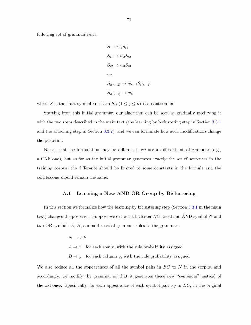
71

following set of grammar rules.

S → w1Si1

Si1 → w2Si2

Si2 → w3Si3

· · ·

Si(n−2) → wn−1Si(n−1)

Si(n−1) → wn

where S is the start symbol and each Sij (1 ≤ j ≤ n) is a nonterminal.

Starting from this initial grammar, our algorithm can be seen as gradually modifying it

with the two steps described in the main text (the learning by biclustering step in Section 3.3.1

and the attaching step in Section 3.3.2), and we can formulate how such modifications change

the posterior.

Notice that the formulation may be different if we use a different initial grammar (e.g.,

a CNF one), but as far as the initial grammar generates exactly the set of sentences in the

training corpus, the difference should be limited to some constants in the formula and the

conclusions should remain the same.

A.1 Learning a New AND-OR Group by Biclustering

In this section we formalize how the learning by biclustering step (Section 3.3.1 in the main

text) changes the posterior. Suppose we extract a bicluster BC, create an AND symbol N and

two OR symbols A, B, and add a set of grammar rules to the grammar:

N → AB

A→ x for each row x, with the rule probability assigned

B → y for each column y, with the rule probability assigned

We also reduce all the appearances of all the symbol pairs in BC to N in the corpus, and

accordingly, we modify the grammar so that it generates these new “sentences” instead of

the old ones. Specifically, for each appearance of each symbol pair xy in BC, in the original

72

grammar there are two rules

Sij → xSi(j+1)

Si(j+1) → ySi(j+2)

which are now combined into

Sij → NSi(j+2)

First, let’s look at how the likelihood is changed. For each sentence that’s involved in

the reduction, its likelihood is changed by two factors. First, the original derivation that

generates xy now generates N instead, and then N generates xy with the probability P (A →

x|A) × P (B → y|B); so the likelihood of this sentence is reduced by a factor equal to this

probability. Second, the reduction may make some other sentences in the corpus become the

same as this sentence, so the likelihood is increased by a factor equal to how many times the

number of such equivalent sentences increases. Suppose this sentence is represented by row

p and column q in the expression-context matrix, then this second factor is exactly the ratio

of the sum of column q to the value of cell (p, q), because before the reduction only those

sentences represented by that cell are equivalent, and after the reduction the sentences in the

whole column become equivalent (the same context plus the same expression N). To sum up,

we can formalize the likelihood gain resulted from the grammar modification as follows.

Denote the likelihood gain of extracting BC by LG(BC). Let D be the set of sentences

in the training corpus, and let Gk and Gk+1 be the grammar before and after extracting the

bicluster. By abuse of notation we denote the set of rows of BC by A, and the set of columns

by B, and denote the context of a symbol pair xy in a sentence d by d−“xy”. For the bicluster

BC, denote the sum of row x by rx, the sum of column y by cy. For the expression-context

matrix, denote its value at row i and column j by EC(i, j), its set of rows by EC-row, its set

of columns by EC-col, and the sum of column q by c′q.

LG(BC) =P (D|Gk+1)

P (D|Gk)=∏d∈D

P (d|Gk+1)

P (d|Gk)

=∏

x∈A, y∈B, xy appears in d∈DP (x|A)P (y|B)

∑p∈EC-rowEC(p, d− “xy”)

EC(“xy”, d− “xy”)

=∏x∈A

P (x|A)rx∏y∈B

P (y|B)cy∏q∈EC-col c

′qc′q∏


EC(p, q)EC(p,q)(A.1)

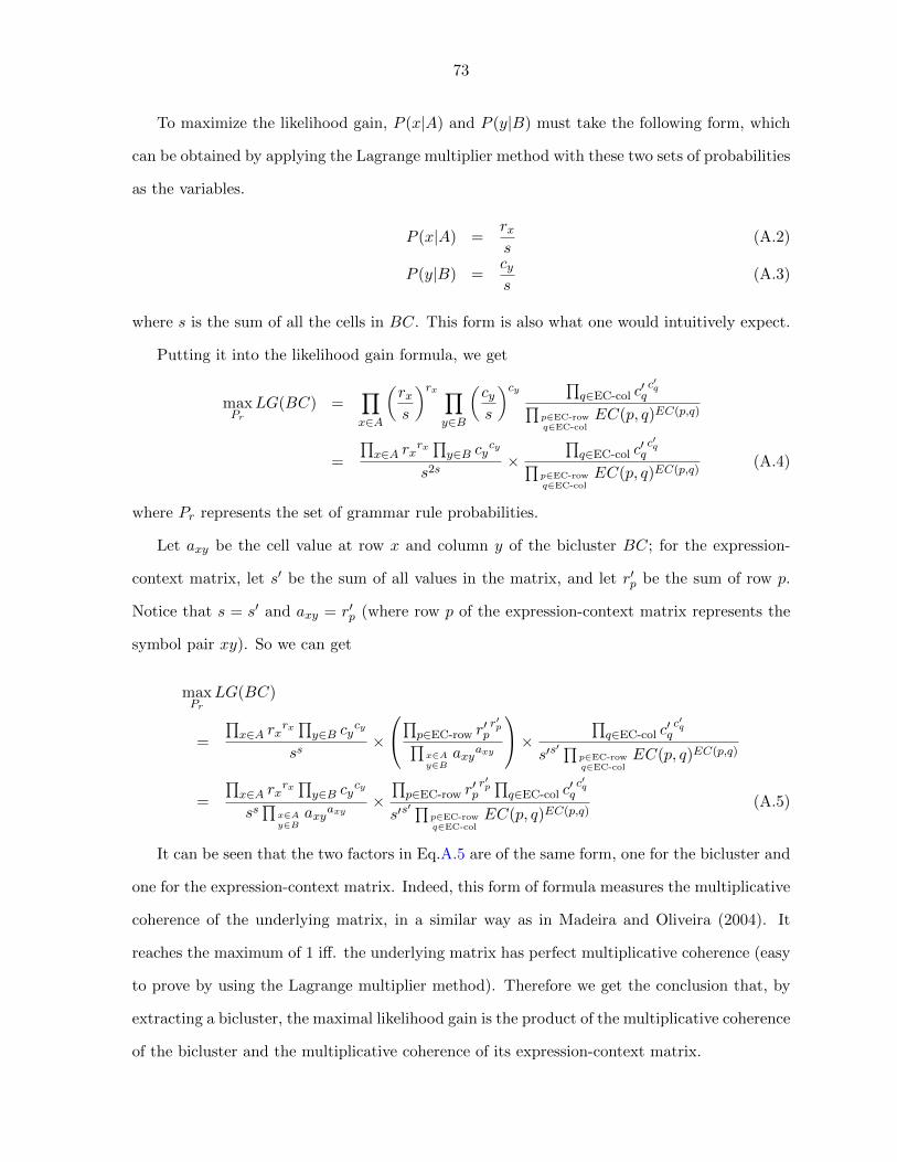
73

To maximize the likelihood gain, P (x|A) and P (y|B) must take the following form, which

can be obtained by applying the Lagrange multiplier method with these two sets of probabilities

as the variables.

P (x|A) =rxs

(A.2)

P (y|B) =cys

(A.3)

where s is the sum of all the cells in BC. This form is also what one would intuitively expect.

Putting it into the likelihood gain formula, we get

maxPr

LG(BC) =∏x∈A

(rxs

)rx ∏y∈B

(cys

)cy ∏q∈EC-col c

′qc′q∏


EC(p, q)EC(p,q)

=

∏x∈A rx

rx∏y∈B cy

cy

s2s×

∏q∈EC-col c

′qc′q∏



where Pr represents the set of grammar rule probabilities.

Let axy be the cell value at row x and column y of the bicluster BC; for the expression-

context matrix, let s′ be the sum of all values in the matrix, and let r′p be the sum of row p.

Notice that s = s′ and axy = r′p (where row p of the expression-context matrix represents the

symbol pair xy). So we can get

maxPr

LG(BC)

=

∏x∈A rx

rx∏y∈B cy

cy

ss×

∏p∈EC-row r′pr′p∏

x∈Ay∈B

axyaxy

× ∏q∈EC-col c

′qc′q

s′s′∏


EC(p, q)EC(p,q)

=

∏x∈A rx

rx∏y∈B cy

cy

ss∏

x∈Ay∈B

axyaxy×∏p∈EC-row r

′pr′p∏q∈EC-col c

′qc′q

s′s′∏



It can be seen that the two factors in Eq.A.5 are of the same form, one for the bicluster and

one for the expression-context matrix. Indeed, this form of formula measures the multiplicative

coherence of the underlying matrix, in a similar way as in Madeira and Oliveira (2004). It

reaches the maximum of 1 iff. the underlying matrix has perfect multiplicative coherence (easy

to prove by using the Lagrange multiplier method). Therefore we get the conclusion that, by

extracting a bicluster, the maximal likelihood gain is the product of the multiplicative coherence

of the bicluster and the multiplicative coherence of its expression-context matrix.

74

Notice that in the above formalization, we don’t consider the possibility that some sentences

containing xy (x ∈ A, y ∈ B) may have been reduced before we learn this AND-OR group.

In that case, when this new AND-OR group is learned, we may get new ways of parsing such

sentences, thus increasing their likelihood. So when there’s significant ambiguity in the target

grammar, the above formulas may not give an accurate estimation of the real likelihood gain.

Now let’s turn to the prior, which is solely determined by the grammar size. By extracting

a bicluster, a set of new rules are added into the grammar, which has 4 + (2 + 2|A|) + (2 + 2|B|)

symbols. On the other hand, each reduction (of xy to N) decreases the grammar size by 4

symbols, and there are s =∑x∈A,y∈B axy number of such reductions. So overall,

P (Gk+1)

P (Gk)=

2−(DL(GK)+(4+(2+2|A|)+(2+2|B|))α−4sα)

2−DL(Gk)= 2α(4s−2|A|−2|B|−8) (A.6)

where α is the number of bits needed to represent a symbol.

Combining Eq.A.5 and Eq.A.6, we can get the posterior gain formula when extracting a

bicluster (with the optimal grammar rule probabilities assigned), as shown in Eq.3.2 in the

main text. Notice that Eq.A.2 and A.3 still hold for maximizing the posterior gain, because

the values of P (x|A) and P (y|B) don’t have any effect on the prior gain.

A.2 Attaching the New AND Symbol under Existing OR Symbols

In this section we try to formalize how the attaching step (Section 3.3.2 in the main text)

changes the posterior. Suppose we add a new rule O → N into the grammar Gk, and do

a maximal reduction on the involved sentences, resulting in a new grammar Gk+1. Suppose

O was learned by extracting the bicluster BC, together with M and P s.t. M → OP (the

following derivation can also be applied to M → PO). So O corresponds to the set of rows of

BC and P corresponds to the set of columns. By adding the rule O → N , we expand BC by

adding a new row, which records the appearance number of Ny in the corpus for each y ∈ P .

Let EC be the expression-context matrix of BC, and EC-row and EC-col be the set of rows

and columns of EC. With the new rule O → N , EC is also expanded with a set of new rows

for the new expressions containing N , and we use EC(“Ny”, q) to represent the value at the

new row Ny and column q in the expanded expression-context matrix. Because we may change

75

the rule probabilities after adding the new rule, denote the original rule probabilities by P ()

and the new rule probabilities by P ′().

The likelihood is changed in the following way. First, for the sentences involved in the new

row for N , each appearance of Ny (y ∈ P ) is reduced to M , leading to a likelihood change

just as discussed in the previous section. Second, for the sentences involved in BC, since we

change the probabilities of rules related to BC, and the reduction of Ny to M results in more

equivalent sentences, their likelihood is changed accordingly.

P (D|Gk+1)

P (D|Gk)

=∏

y∈P, Ny appears in d∈D

(P ′(N |O)P ′(y|P )

col(d− “Ny”)

EC(“Ny”, d− “Ny”)

)

×∏

x∈O, y∈P, xy appears in d∈D

P ′(x|O)P ′(y|P )

P (x|O)P (y|P )× col(d− “xy”)∑

p∈EC-rowEC(p, d− “xy”)

(A.7)

where col() is defined as

col(cont) =∑

p∈EC-row

EC(p, cont) +∑z∈P

EC(“Nz”, cont) (A.8)

EC(p, q) represents the value of cell pq in the derived expression-context matrix, which is the

expected appearance number of the combination of expression p and context q when the current

learned grammar Gk is applied to expand the current partially reduced corpus. To construct

EC, we have to enumerate all the AND symbols that M may be directly or indirectly reduced

to, and traverse their appearances in the partially reduced corpus. Based on the definition of

EC, it’s obvious that it is perfectly multiplicatively coherent.

Let EC′

be the expanded derived expression-context matrix containing both EC and the

new rows for Ny (y ∈ P ). So col(q) is the sum of column q in EC′. Let EC-row′ and EC-col′

be the set of rows and columns of EC′. Let EC ′ be the actual expanded expression-context

matrix containing both EC and the new rows. Let col(q) be the sum of column q in EC ′.

Let BC be the derived bicluster that records the expected appearance number of each

symbol pair xy (x ∈ O, y ∈ P ) when applying the current learned grammar Gk to expand the

76

current partially reduced corpus. So EC is its expression-context matrix. It can be proved

that, when recursive rules are not involved in generating symbol pairs in BC, it has the same

row sums, column sums and total sum as BC, but its cell values may be different, which makes

it perfectly multiplicatively coherent. When recursive rules are involved, however, BC and BC

might be quite different. Let rx be the sum of row x and cy be the sum of column y in BC.

Let BC′be the expanded derived bicluster that contains both BC and the new row for N . Let

rN be the sum of the new row for N , and aNy be the cell value at column y in the new row.

Since P (x|O)P (y|P )∑p∈EC-row EC(p, d−“xy”) = EC(“xy”, d−“xy”), we may further reduce

Eq.A.7 as follows.

P (D|Gk+1)

P (D|Gk)=

∏x∈O∪{N}

P ′(x|O)rx∏y∈P

P ′(y|P )cy+aNy

∏q∈EC-col′

col(q)col(q)

∏p∈EC-row′q∈EC-col′

EC′(p, q)EC′(p,q)

(A.9)

It can be proved that, if for every AND-OR group involved in calculating EC, the bicluster

and its expression-context matrix are both perfectly multiplicatively coherent, and if no recur-

sive rules are involved, then EC = EC. Since we learn new rules only when Eq.3.2 or Eq.3.3

is large enough, we expect that the likelihood gain of each step in the algorithm is close to the

maximum of 1 and thus the biclusters and their expression-context matrixes are approximately

multiplicatively coherent. So we use EC to approximate EC and use col(q) to approximate

col(q), and therefore according to Eq.A.1 we get

P (D|Gk+1)

P (D|Gk)≈ LG(BC

′) (A.10)

Again it can be shown that for the new set of rule probabilities Pr, Eq.A.2 and A.3 hold

when the likelihood gain is maximized. In addition we know both BC and EC are perfectly

multiplicatively coherent. So we get

maxPr

P (D|Gk+1)

P (D|Gk)≈ max

PrLG(BC

′)

=f(rN )×

∏y∈P f(cy + aNy)× f(s)2 ×

∏q∈EC-col f

(c′q +

∑y∈P EC(“Ny”, q)

)∏y∈P f(cy)× f(s+ rN )2 ×

∏y∈P

q∈EC-colf(EC(“Ny”, q))×

∏q∈EC-col f(c′q)

(A.11)

77

where f(x) = xx; s is the total sum of BC; c′q is the sum of column q of EC.

Notice that there might be a third part in the likelihood change in addition to the two

discussed above: after Ny is reduced to M , it may be further reduced, leading to a series of

likelihood changes. However, it can be proved that if 1) Eq.A.11 reaches its maximum of 1, i.e.,

BC′

and its expression-context matrix are perfectly multiplicatively coherent, and 2) for every

AND-OR group involved in calculating EC, the bicluster and its expression-context matrix are

both perfectly multiplicatively coherent, then the likelihood gain caused by this part is 1, i.e.,

the likelihood is not changed. Since we learn new rules only when Eq.3.2 or Eq.3.3 is large

enough, we expect that both conditions are approximately satisfied and the likelihood change

caused by this part is small. Besides, we have to do maximal reduction to calculate the effect

of this part, which would be too time-consuming if we do it for every candidate new rule. So

we choose to omit this part.

Now let’s turn to the prior. There are two changes of the grammar length. First, a new rule

O → N is added into the grammar. Second, we reduce Ny (y ∈ P ) to M , so in the grammar,

for each appearance of Ny, the two rules that generate N and y are now combined to one that

generates M . Therefore the prior gain is

P (Gk+1)

P (Gk)=

2−(DL(GK)+2α−4rNα)

2−DL(Gk)= 2α(4rN−2) (A.12)

where rN is the sum of the new row for N in BC′. Again, here we omit the changes caused by

possible further reductions after Ny is reduced to M .

Putting Eq.A.11 and A.12 together, we get the approximate posterior gain when learning

a new rule in the attaching step (with the optimal grammar rule probabilities assigned). It’s

easy to see that the result is equal to the ratio of the maximal posterior gain by extracting BC′

to the maximal posterior gain by extracting BC, as shown in Eq.3.3 of the main text.

78

APPENDIX B. Proofs for the Parameter Learning Approach with

Unambiguity Regularization

B.1 Theorem Proofs in Case 2: 0 < σ < 1.

To prove Theorem 4.1, we first prove the following lemma.

Lemma B.1. x log x is strictly convex on the interval [0,1], where 0 log 0 is defined to be 0.

Proof. On the interval (0,1], x log x is twice differentiable and we have

∂2x log x

∂x2=

1

x> 0

So x log x is strictly convex on the interval (0,1]. Now note that

∀x ∈ (0, 1], ∀t ∈ (0, 1), (0t+ (1− t)x) log(0t+ (1− t)x) = (1− t)x log(1− t)x

< (1− t)x log x = t× 0 log 0 + (1− t)x log x

Therefore x log x is also strictly convex with 0 included in the interval.

Now we prove Theorem 4.1.

Theorem 4.1. fi(q) is strictly convex on the unit simplex ∆.

Proof. For any t ∈ (0, 1), for any two points q1 and q2 in the unit simplex ∆, we need to prove

that fi(tq1 + (1− t)q2) < tfi(q1) + (1− t)fi(q2). The left-hand side is

fi(tq1 + (1− t)q2) =∑zi

[(tq1(zi) + (1− t)q2(zi)) log

(tq1(zi) + (1− t)q2(zi))1−σ

pθ(zi|xi)

]=

∑zi

[(1− σ) (tq1(zi) + (1− t)q2(zi)) log (tq1(zi) + (1− t)q2(zi))

− (tq1(zi) + (1− t)q2(zi)) log pθ(zi|xi)]

79

The right-hand side is

tfi(q1) + (1− t)fi(q2) =∑zi

[tq1(zi) log

q1(zi)1−σ

pθ(zi|xi)+ (1− t)q2(zi) log

q2(zi)1−σ

pθ(zi|xi)

]=

∑zi

[(1− σ)tq1(zi) log q1(zi) + (1− σ)(1− t)q2(zi) log q2(zi)

− (tq1(zi) + (1− t)q2(zi)) log pθ(zi|xi)]

So the right-hand side minus the left-hand side is

tfi(q1) + (1− t)fi(q2)− fi(tq1 + (1− t)q2)

= (1− σ)∑zi

[tq1(zi) log q1(zi) + (1− t)q2(zi) log q2(zi)

− (tq1(zi) + (1− t)q2(zi)) log (tq1(zi) + (1− t)q2(zi))]

Because ∀zi, 0 ≤ q1(zi), q2(zi) ≤ 1, Lemma B.1 implies that

tq1(zi) log q1(zi) + (1− t)q2(zi) log q2(zi) > (tq1(zi) + (1− t)q2(zi)) log (tq1(zi) + (1− t)q2(zi))

So we have

tfi(q1) + (1− t)fi(q2)− fi(tq1 + (1− t)q2) > 0

B.2 Theorem Proofs in Case 4: σ > 1.

We first introduce the following theorem.

Theorem B.1. fi(q) is strictly concave on the unit simplex ∆.

The proof is the same as that of theorem 4.1, except that 1 − σ is now negative which

reverses the direction of the last inequality in the proof.

Now we can prove Theorem 4.2.

Theorem 4.2. The minimum of fi(q) is attained at a vertex of the unit simplex ∆.

Proof. Assume the minimum of fi(q) is attained at q∗ that is not a vertex of the unit simplex ∆,

so there are at least two assignments of zi, say z1 and z2, such that q∗(z1) and q∗(z2) are nonzero.

Let q′ be the same distribution as q∗ except that q′(z1) = 0 and q′(z2) = q∗(z1)+q∗(z2). Let q′′

80

be the same distribution as q∗ except that q′′(z1) = q∗(z1) + q∗(z2) and q′′(z2) = 0. Obviously,

both q′ and q′′ are in the unit simplex ∆ and q′ 6= q′′. Let t = q∗(z2)q∗(z1)+q∗(z2)

, and obviously we

have 0 < t < 1. So we get q∗ = tq′ + (1 − t)q′′. According to Theorem B.1, fi(q) is strictly

concave on the unit simplex ∆, so we have fi(q∗) > tfi(q

′) + (1 − t)fi(q′′). Without loss of

generality, suppose fi(q′) ≥ fi(q

′′). So we have tfi(q′) + (1 − t)fi(q′′) ≥ fi(q

′′) and therefore

fi(q∗) > fi(q

′′), which means fi(q) does not attain the minimum at q∗. This contradicts the

assumption.

81

APPENDIX C. Supplementary Material for the Incremental Learning

Approach by Using Curricula

Section C.1 provides the proofs of the theorems in section 5.3. Section C.2 gives more

details of the experimental settings in section 5.4 and 5.5.

C.1 Proofs of Theorems

We first prove Theorem 5.1.

Theorem 5.1. If a curriculum 〈W1,W2, . . . ,Wn〉 satisfies incremental construction (with ei-

ther condition 3 or 3b), then for any i, j, k s.t. 1 ≤ i < j < k ≤ n, we have



where d1(·, ·) denotes the L1 distance; dTV (Gi, Gj) represents the total variation distance be-

tween the two distributions of grammatical structures defined by Gi and Gj.

Proof. Here we assume condition 3b because it is more general than condition 3. There are

two inequalities in the conclusion of the theorem. We first give the proof of the inequality

with the L1 distance of parameter vectors. As defined in Section 5.3, a parameter vector is

the concatenation of a set of multinomial vectors, each of which is the vector of probabilities

of grammar rules with a specific rule condition (left-hand side) of the target grammar. Denote

θi,p as the multinomial vector of rule condition p in grammar Gi, and denote θi,p→q as the

probability of rule p→q in grammar Gi. Note that

d1(θi, θj) =∑p

d1(θi,p, θj,p)

82

So to prove the first inequality, it is sufficient to prove that

∀p, d1(θi,p, θk,p) ≥ d1(θj,p, θk,p)

Because the L1 norm of a multinomial vector is always 1, for any rule condition p we have

d1(θi,p, θj,p) =∑

q:θi,p→q>θj,p→q

(θi,p→q − θj,p→q) +∑

q:θi,p→q≤θj,p→q

(θj,p→q − θi,p→q)

=

1−∑


θi,p→q

−1−

∑q:θi,p→q≤θj,p→q

θj,p→q

+

∑q:θi,p→q≤θj,p→q


= 2×∑



= 2×∑q

(θj,p→q − θi,p→q)fi,j,p(q) (C.1)

where fi,j,p(q) is defined as

fi,j,p(q) =

1 if θi,p→q ≤ θj,p→q

0 if θi,p→q > θj,p→q

According to Definition 5.1 (with condition 3b), for any grammar rule p → q in the target

grammar, with the increase of i, its probability θi,p→q first remains 0, then shifts to a non-zero

value in a certain intermediate grammar, and after that decreases monotonically. So for any

i < j < k, there are three possibilities, which we consider in turn.

1. If θi,p→q = θj,p→q = 0 and θk,p→q ≥ 0, then we have

(θk,p→q − θi,p→q)fi,k,p(q) = (θk,p→q − θj,p→q)fj,k,p(q)

2. If θi,p→q = 0 and θj,p→q ≥ θk,p→q > 0, then we have

(θk,p→q − θi,p→q)fi,k,p(q) > 0 = (θk,p→q − θj,p→q)fj,k,p(q)

3. If θi,p→q ≥ θj,p→q ≥ θk,p→q > 0, then we have

(θk,p→q − θi,p→q)fi,k,p(q) = (θk,p→q − θj,p→q)fj,k,p(q) = 0

83

Therefore, we get

∑q

(θk,p→q − θi,p→q)fi,k,p(q) ≥∑q

(θk,p→q − θj,p→q)fj,k,p(q)

where equality holds if there exists no assignment of q that satisfies the second possibility.

According to Eq.C.1, we have

d1(θi,p, θk,p) ≥ d1(θj,p, θk,p)

Therefore we have proved the first inequality.

Now we turn to the second inequality in the conclusion of the theorem and prove it in a

similar fashion. Because the sum of probabilities over all grammatical structures is always 1,

we have

dTV (Gi, Gj) =1

2

∑s

|P (s|Gi)− P (s|Gj)|

=∑s

(P (s|Gj)− P (s|Gi))fi,j(s) (C.2)

where fi,j(s) is defined as

fi,j(s) =

1 if P (s|Gi) ≤ P (s|Gj)

0 if P (s|Gi) > P (s|Gj)

The first equality of Eq.C.2 is the definition of total variation, and the second equality can be

derived in a similar way as in Eq.C.1. According to Definition 5.1 (with condition 3b), for any

grammatical structure s that can be generated by the target grammar, with the increase of i,

the probability P (s|Gi) first remains 0 (when at least one grammar rule used in deriving s is

absent from Gi), then shifts to a non-zero value (when all the grammar rules needed to derive s

have non-zero probabilities), and after that decreases monotonically (because the probabilities

of all the grammar rules used in deriving s are decreasing). Just as in the proof of the first

inequality, for any i < j < k there are three possibilities, and by analyzing the three possibilities

in turn we can get

∑s

(P (s|Gk)− P (s|Gi))fi,k(s) ≥∑s

(P (s|Gk)− P (s|Gj))fj,k(s)

84

So according to Eq.C.2, we have


Therefore we have proved the second inequality.

Now we give a proof sketch of Theorem 5.2.

Theorem 5.2. If a curriculum 〈W1,W2, . . . ,Wn〉 satisfies the first two conditions in Definition

5.1 as well as a further relaxed version of the third condition:

3c. for any grammar rules r, P (r|Gi) first monotonically increases with i and then monoton-

ically decreases with i.

then for any i, j, k s.t. 1 ≤ i < j < k ≤ n, we have


Proof Sketch. The proof is the same as the proof of the first inequality of Theorem 5.1, except

that the three possibilities are changed because of condition 3c. According to condition 3c,

with the increase of i, the probability of a grammar rule θi,p→q first increases monotonically

and then decreases monotonically. So for any i < j < k, we have three new possibilities.

1. If θi,p→q ≤ θj,p→q ≤ θk,p→q, then we have

(θk,p→q − θi,p→q)fi,k,p(q) ≥ (θk,p→q − θj,p→q)fj,k,p(q)

2. If θi,p→q ≤ θj,p→q and θj,p→q ≥ θk,p→q, then we have

(θk,p→q − θi,p→q)fi,k,p(q) ≥ 0 = (θk,p→q − θj,p→q)fj,k,p(q)

3. If θi,p→q ≥ θj,p→q ≥ θk,p→q, then we have

(θk,p→q − θi,p→q)fi,k,p(q) = (θk,p→q − θj,p→q)fj,k,p(q) = 0

So we can still get

∑q

(θk,p→q − θi,p→q)fi,k,p(q) ≥∑q

(θk,p→q − θj,p→q)fj,k,p(q)

and the rest of the proof is exactly the same as in the proof of the first inequality of Theorem

5.1.

85

C.2 Experiments

In this section we provide more details of the experiments presented in section 5.4 and 5.5.

We adapted the DAGEEM software1 to implement the expectation-maximization algo-

rithm of the DMV grammar. We then implemented curriculum learning by using expectation-

maximization as the base learner. In the experiments on synthetic data, expectation-maximization

was initialized with a trivial grammar in which rules with the same left-hand side have equal

probabilities; in the experiments on real data, we used an initial grammar provided in the

DAGEEM software which is created according to the heuristic approach described in Klein

and Manning (2004). As mentioned in section 5.4, we used a dynamic smoothing factor in the

experiments on synthetic data to alleviate the overfitting problem discussed in Section 5.3.1.

The dynamic smoothing factor is computed from the size of the partial corpus that is hidden

from the learner during curriculum learning. More specifically, for each training sentence that

is hidden, we assume it is sampled from a uniform distribution over all possible sentences that

have the same length as the hidden sentence, and we also assume a uniform grammar in which

rules with the same left-hand side have equal probabilities, so we can easily compute the ex-

pected counts of each grammar rule r being used in parsing this sentence; then the dynamic

smoothing factor for grammar rule r is the sum of the expected counts over all the training

sentences that are hidden. We found that dynamic smoothing often improves the learning

result in the experiments on synthetic data; however, in the experiments on real data, dynamic

smoothing usually hurts learning.

We used the WSJ30 corpus (the set of sentences no longer than 30 in the Wall Street

Journal corpus of the Penn Treebank) in our experiments. Because we used the DMV grammar

formalism in our experiments, which is a type of dependency grammar, we converted the phrase

structure annotations in the Penn Treebank to the dependency annotations by running the

“ptbconv” software2. When generating the synthetic data, we found the dependency treebank

grammar of WSJ30 tends to generate sentences much longer than the actual sentences in

WSJ30, so we decreased by 30% the probabilities of grammar rules that determine if a new

1http://www.ark.cs.cmu.edu/DAGEEM/2Available at http://www.jaist.ac.jp/~h-yamada/

http://www.ark.cs.cmu.edu/DAGEEM/

http://www.jaist.ac.jp/~h-yamada/

86

dependency should be generated under a certain condition.

We tested different values of the smoothing factor in the experiments on both synthetic

data and real data. We found that although the value of the smoothing factor did affect the

learning performance, the advantage of curriculum learning over the baseline was consistently

observed.

87

BIBLIOGRAPHY

Adriaans, P., Trautwein, M., and Vervoort, M. (2000). Towards high speed grammar induction

on large text corpora. In SOFSEM 2000, LNCS 1963.

Baker, J. K. (1979). Trainable grammars for speech recognition. In Speech Communication

Papers for the 97th Meeting of the Acoustical Society of America.

Baum, L. E., Petrie, T., Soules, G., and Weiss, N. (1970). A maximization technique occurring

in the statistical analysis of probabilistic functions of markov chains. Ann. Math. Statist.,

41(1):164C171.

Bengio, Y., Louradour, J., Collobert, R., and Weston, J. (2009). Curriculum learning. In

ICML, page 6.

Bod, R. (2006). An all-subtrees approach to unsupervised parsing. In Proceedings of ACL.

Charniak, E. (1996). Tree-bank grammars. In AAAI/IAAI, Vol. 2, pages 1031–1036.

Charniak, E. (1997). Statistical parsing with a context-free grammar and word statistics. In

AAAI/IAAI, pages 598–603.

Chen, S. F. (1995). Bayesian grammar induction for language modeling. In Proceedings of the

33rd annual meeting on Association for Computational Linguistics.

Clark, A. (2001). Unsupervised induction of stochastic context-free grammars using distribu-

tional clustering. In Proceedings of CoNLL.

Clark, A. (2007). Learning deterministic context free grammars: The omphalos competition.

Machine Learning, 66.

88

Clark, A., Eyraud, R., and Habrard, A. (2008). A polynomial algorithm for the inference of

context free languages. In ICGI, pages 29–42.

Cohen, S. B., Gimpel, K., and Smith, N. A. (2008). Logistic normal priors for unsupervised

probabilistic grammar induction. In NIPS, pages 321–328.

Cohen, S. B. and Smith, N. A. (2009). Shared logistic normal distributions for soft parameter

tying in unsupervised grammar induction. In HLT-NAACL, pages 74–82.

Cohn, T., Goldwater, S., and Blunsom, P. (2009). Inducing compact but accurate treesubsti-

tution grammars. In In Proc. NAACL.

Collins, M. J. (1999). Head-driven statistical models for natural language parsing. PhD thesis,

Philadelphia, PA, USA. Supervisor-Marcus, Mitchell P.

Cramer, B. (2007). Limitations of current grammar induction algorithms. In Proceedings of

the 45th Annual Meeting of the ACL: Student Research Workshop, ACL ’07, pages 43–48,

Stroudsburg, PA, USA. Association for Computational Linguistics.

Daume, III, H. (2009). Unsupervised search-based structured prediction. In ICML, page 27.

de la Higuera, C. (2005). A bibliographical study of grammatical inference. Pattern Recogn.,

38(9):1332–1348.

Durbin, R., Eddy, S. R., Krogh, A., and Mitchison, G. J. (1998). Biological Sequence Analysis:

Probabilistic Models of Proteins and Nucleic Acids. Cambridge University Press.

Elman, J. L. (1993). Learning and development in neural networks: The importance of starting

small. Cognition, 48:71–99.

Finkel, J. R., Grenager, T., and Manning, C. D. (2007). The infinite tree. In Proceedings of

the 45th Annual Meeting of the Association of Computational Linguistics, pages 272–279.

Association for Computational Linguistics.

Ganchev, K., Graca, J., Gillenwater, J., and Taskar, B. (2010). Posterior regularization for

structured latent variable models. Journal of Machine Learning Research, 11:2001–2049.

89

Gillenwater, J., Ganchev, K., Graca, Jo a., Pereira, F., and Taskar, B. (2010). Sparsity in

dependency grammar induction. In ACL ’10: Proceedings of the ACL 2010 Conference Short

Papers, pages 194–199, Morristown, NJ, USA. Association for Computational Linguistics.

Gold, E. M. (1967). Language identification in the limit. Information and Control, 10(5):447–

474.

Headden, III, W. P., Johnson, M., and McClosky, D. (2009). Improving unsupervised depen-

dency parsing with richer contexts and smoothing. In HLT-NAACL, pages 101–109.

Hsu, D., Kakade, S. M., and Zhang, T. (2009). A spectral algorithm for learning hidden markov

models. In COLT.

Johnson, M. (1998). Pcfg models of linguistic tree representations. Comput. Linguist.,

24(4):613–632.

Johnson, M., Griffiths, T. L., and Goldwater, S. (2006). Adaptor grammars: A framework for

specifying compositional nonparametric bayesian models. In NIPS, pages 641–648.

Johnson, M., Griffiths, T. L., and Goldwater, S. (2007). Bayesian inference for pcfgs via markov

chain monte carlo. In HLT-NAACL, pages 139–146.

Klein, D. and Manning, C. D. (2003). Accurate unlexicalized parsing. In ACL ’03: Proceedings

of the 41st Annual Meeting on Association for Computational Linguistics, pages 423–430,

Morristown, NJ, USA. Association for Computational Linguistics.

Klein, D. and Manning, C. D. (2004). Corpus-based induction of syntactic structure: Models

of dependency and constituency. In Proceedings of ACL.

Kumar, M. P., Packer, B., and Koller, D. (2010). Self-paced learning for latent variable models.

In Lafferty, J., Williams, C. K. I., Shawe-Taylor, J., Zemel, R., and Culotta, A., editors,

Advances in Neural Information Processing Systems 23, pages 1189–1197.

Kurihara, K. and Sato, T. (2004). An application of the variational Bayesian approach to

probabilistic contextfree grammars. In IJCNLP-04 Workshop beyond shallow analyses.

90

Kurihara, K. and Sato, T. (2006). Variational Bayesian grammar induction for natural lan-

guage. In ICGI 2006, volume 4201 of LNAI, pages 84–96.

Langley, P. and Stromsten, S. (2000). Learning context-free grammars with a simplicity bias.

In ECML, pages 220–228.

Lari, K. and Young, S. (1990). The estimation of stochastic context-free grammars using the

inside-outside algorithm. Computer Speech and Language, 4:35–36.

Liang, P., Petrov, S., Jordan, M. I., and Klein, D. (2007). The infinite pcfg using hierarchical

Dirichlet processes. In Proceedings of EMNLP-CoNLL, pages 688–697.

Madeira, S. C. and Oliveira, A. L. (2004). Biclustering algorithms for biological data analysis:

A survey. IEEE/ACM Trans. on Comp. Biol. and Bioinformatics, 1(1):24–45.

Manning, C. D. and Schutze, H. (1999). Foundations of statistical natural language processing.

MIT Press, Cambridge, MA, USA.

Marcus, M. P., Santorini, B., and Marcinkiewicz, M. A. (1993). Building a large annotated

corpus of english: The penn treebank. COMPUTATIONAL LINGUISTICS, 19(2):313–330.

Petrov, S., Barrett, L., Thibaux, R., and Klein, D. (2006). Learning accurate, compact, and

interpretable tree annotation. In ACL-44: Proceedings of the 21st International Conference

on Computational Linguistics and the 44th annual meeting of the Association for Compu-

tational Linguistics, pages 433–440, Morristown, NJ, USA. Association for Computational

Linguistics.

Poon, H. and Domingos, P. (2009). Unsupervised semantic parsing. In EMNLP, pages 1–10.

Poon, H. and Domingos, P. (2011). Sum-product networks : A new deep architecture. In Pro-

ceedings of the Twenty-Seventh Conference on Uncertainty in Artificial Intelligence (UAI).

Rohde, D. and Plaut, D. (1999). Language acquisition in the absence of explicit negative

evidence: How important is starting small? Cognition, 72:67–109.

91

Smith, N. A. and Eisner, J. (2006). Annealing structural bias in multilingual weighted grammar

induction. In ACL.

Solan, Z., Horn, D., Ruppin, E., and Edelman, S. (2005). Unsupervised learning of natural

languages. Proc. Natl. Acad. Sci., 102(33):11629–11634.

Spitkovsky, V. I., Alshawi, H., and Jurafsky, D. (2010a). From baby steps to leapfrog: How

“less is more” in unsupervised dependency parsing. In NAACL.

Spitkovsky, V. I., Alshawi, H., Jurafsky, D., and Manning, C. D. (2010b). Viterbi training

improves unsupervised dependency parsing. In Proceedings of the Fourteenth Conference on

Computational Natural Language Learning, CoNLL ’10, pages 9–17, Stroudsburg, PA, USA.

Association for Computational Linguistics.

Stolcke, A. (1993). Boogie. ftp://ftp.icsi.berkeley.edu/pub/ai/stolcke/software/

boogie.shar.Z.

Stolcke, A. and Omohundro, S. M. (1994). Inducing probabilistic grammars by Bayesian model

merging. In ICGI, pages 106–118.

Tax, D. M. J. (2001). One-class classification: Concept-learning in the absence of counter-

examples. PhD thesis, Delft University of Technology.

Teh, Y. W., Jordan, M. I., Beal, M. J., and Blei, D. M. (2006). Hierarchical Dirichlet processes.

Journal of the American Statistical Association, 101(476):1566–1581.

Tu, K. and Honavar, V. (2008). Unsupervised learning of probabilistic context-free grammar

using iterative biclustering. In Proceedings of 9th International Colloquium on Grammatical

Inference (ICGI 2008), LNCS 5278.

Tu, K. and Honavar, V. (2011). On the utility of curricula in unsupervised learning of prob-

abilistic grammars. In Proceedings of the Twenty-second International Joint Conference on

Artificial Intelligence (IJCAI 2011).

Tu, K. and Honavar, V. (2012). Unambiguity regularization for unsupervised learning of prob-

abilistic grammars (under review).

ftp://ftp.icsi.berkeley.edu/pub/ai/stolcke/software/boogie.shar.Z

ftp://ftp.icsi.berkeley.edu/pub/ai/stolcke/software/boogie.shar.Z

92

van Zaanen, M. (2000). ABL: Alignment-based learning. In COLING.

Zhu, S.-C. and Mumford, D. (2006). A stochastic grammar of images. Found. Trends. Comput.

Graph. Vis., 2(4):259–362.

Unsupervised learning of probabilistic grammars - School of ...

Documents

Transcript of Unsupervised learning of probabilistic grammars - School of ...