ACOUSTIC EMISSION TECHNIQUES FOR THE DAMAGE

ASSESSMENT OF REINFORCED CONCRETE STRUCTURES

NORAZURA MUHAMAD BUNNORI

Ph.D. MARCH 2008

UMI Number: U585022

All rights reserved

INFORMATION TO ALL USERS The quality of this reproduction is dependent upon the quality of the copy submitted.

In the unlikely event that the author did not send a complete manuscript and there are missing pages, these will be noted. Also, if material had to be removed,

a note will indicate the deletion.

Dissertation Publishing

UMI U585022Published by ProQuest LLC 2013. Copyright in the Dissertation held by the Author.

Microform Edition © ProQuest LLC.All rights reserved. This work is protected against

unauthorized copying under Title 17, United States Code.

ProQuest LLC 789 East Eisenhower Parkway

P.O. Box 1346 Ann Arbor, Ml 48106-1346

DECLARATION

This work has not previously been accepted in substance for any degree and

not being concurrently submitted in candidature for any degree.

Singed •____________________ (candidate)

Date W j o i ! * Q 0 9 _______________

STATEMENT 1

This thesis is the result of my own investigations, except where otherwise

stated.

Other sources are acknowledged by explicit references.

Singed J \ ____________________ (candidate)

Date____________ W/o'i.jo.oo-8________________

STATEMENT 2

I hereby give consent for my thesis, if accepted, to be available for photocopying and the inter-library loan, and for the title and summary to be

made available to outside organizations.

Singed _________________•_________________ (candidate)

Date I ________________

ACOUSTIC EMISSION TECHNIQUES FOR THE DAMAGE ASSESSMENT OF REINFORCED

CONCRETE STRUCTURES

PhD Thesis

Norazura Muhamad Bunnori (BEng (Hons), MSc)

School of Engineering

Cardiff University, Cardiff UK

March 2008

Prifysgol Caerdydd SUMMARY OF THESIS Cardiff University

Candidate’s Surname: Muhamad Bunnori Candidate’s Forenames: Norazura

Candidate for the Degree of: PhDInstitution at which study pursued: Cardiff University, Wales, UK

Full Title of Thesis: Acoustic Emission Techniques for the Damage

Assessment of Reinforced Concrete Structures

Summary:

This thesis examines the role of Acoustic Emission (AE) techniques as a non­destructive testing (NDT) technique for reinforced concrete structures. The work focuses on the development of experimental techniques and data analysis methods for the detection, location and assessment of AE from the reinforced concrete specimens. Three key topics are investigated:

1. Method of analysis for laboratory-based pre-corroded and post­corroded reinforced concrete specimens tested in flexure.

Experimental results from a series of laboratory studies are presented. The work investigates the changing behaviour of the reinforced concrete beams due to chloride-induced reinforcement corrosion by using a parameter-based approach to detect, locate and follow the progression of cracks. The use of AE absolute energy as an indication of concrete cracking is also explored.

2. A practical investigation into acoustic wave propagation in reinforced concrete structures.

Experimental results from acoustic wave propagation of two source modes (parallel and normal to sensor face) are presented. The work investigates the wave velocity in concrete structures over a variety of source-to-sensor distances with the influence of pre-set threshold levels. Specimen geometry, specimen conditions and source orientation is explained. The application of modal behaviour on the AE from both artificial and real sources is examined. Experimental data describing signal attenuation is also presented.

3. The detection of damage within an in-service concrete crosshead.

Further analysis of a commercial bridge inspection is given. A comparison of results from both clustered and non-clustered events, with laboratory based results is made. Apart from being interested with clustered events, non­clustered events are also an important contribution to damage detection in structural monitoring.

Key Words: Acoustic Emission, Corrosion, Reinforced Concrete, Concrete Cracks, Source Location, Wave Propagation, Damage Assessment, Bridge Monitoring.

ACKNOWLEDGEMENTS

I take this opportunity to express my great debt of gratitude to Professor R. J.

Lark and Professor K. M. Holford for their excellent guidance, support and

invaluable patience throughout this work. I thank Dr. Rhys Pullin (Cardiff

University), Tim Bradshaw (PAL) and Jon Watson (PAL) for three years

provided great support and technical assistance.

I would like to thank to Universiti Sains Malaysia (USM) and Ministry of Higher

Education, Malaysia for giving me an opportunity in pursuing a PhD study. My

thanks also to the technical staff of the Cardiff University School of Engineering, particularly to Carl Wadsworth, Brian Hooper, Des Sanford, Len

Czekaj and Andrew Sweeney.

Finally I would like to thank my family, especially my parents Muhamad

Bunnori Kardi and Sadiah Jamali and my husband Mohamed Johari Hashim

for their emotional and financial support and prayer.

GLOSSARY OF TERMS FOR AE TESTING

Acoustic Emission (AE): Elastic waves generated by the rapid release of

energy from sources within a material.

Absolute Energy: This is a true energy measure of an AE hit whose units

are measured in attoJoule (aJ). Absolute energy is derived from the integral of

the squared voltage signal divided by the reference resistance over the

duration of the AE waveform packet.

AE Count: The number of times the signal amplitude exceeds the pre-set

reference threshold.

Array: A group of sensors used for source location.

Attenuation: Loss of amplitude with distance as the wave travels through the

test structures.

Broad Band Sensors: High sensitivity over a wide frequency range.

Burst Emission: A qualitative term applied to AE when bursts are observed.

Channel: A single sensor and the related instrumentation for transmitting,

conditioning, detection and measuring a signal.

Cluster Location: An area of predefined size on a structure that contains an

AE source of such significance that it crosses predefined signal thresholds.

This allows ranking of sources found using location monitoring.

Continuous Emission: A qualitative term applied to AE when bursts or pulses are not discernible.

Couplant: A substance providing an acoustic link between the propagation

medium and sensor.

Duration: The interval between the first and last time the threshold has been

exceeded by the signal.

Energy (MARSE): MARSE (Measured Area under the Rectified Signal

Envelope) energy is relative value proportional to the true energy of the

source event.

Event: A single AE source produces a transient mechanical wave that

propagates in all directions in a medium. The AE wave is detected in the form

of hits on one or more channels. An event therefore, is the group of AE hits

that was received from a single source.

Felicity Ratio: The measurement of the felicity effect. Defined as the ratio

between the applied load at which the AE appears during the next application

of loading and the previous maximum applied load.

Global Monitoring: Large scale monitoring of a structure when no specific

flaws are known.

Hit: A hit is the term used to indicate that a given AE channel has detected

and processed an AE transient.

H-N Source: Also known as Hsu-Neilson or lead break; the industry standard

calibration method, which involves fracturing a 0.5 diameter, 3mm long, 2h

propelling pencil lead at 30° orientation.

Kaiser Effect: The absence of detectable AE until the previous maximum

applied stress level has been exceeded.

Lamb Wave: In a medium bounded by two surfaces, i.e. a plate, at distances

greater than a few centimetres from AE source surface waves can couple to

produce Lamb waves.

Location Group: An array of AE sensors (based on known placement

between one another) for the purpose of determining the general or exact location of an event occurring near or within the detection area.

Local Monitoring: A source location examination of a known flaw.

Location Plot: Representation of sources of AE computed using an array of

sensors.

Lockout Time: The minimum time following the detection of an event before

the analysis software resumes event processing within a location group. This

is typically set to the period of time taken for an AE signal to propagate from

one sensor in a group to the most distant sensor in the given group. Use of lockout time is intended to prevent reflections from a single source event being incorrectly identified as new events by the source location algorithm.

Measure Amplitude Ratio (MAR): MAR expressed as a percentage that is

the ratio of the first wave peak amplitude to the second wave peak amplitude.

Noise: The signal obtained in the absence of any AE, the signal has electrical and mechanical background.

Parametric Inputs: Environmental variables (e.g. load, pressure,

temperature) that can be measured and stored as part of the signal description.

Peak Amplitude: Maximum signal amplitude within the duration of the signal.

Pencil Source: An artificial source using the fracture of a brittle graphite lead

in a suitable fitting to simulate an AE event (also known as an Hsu-Neilsonsource).

Rayleigh Wave: Rayleigh waves are longitudinal and transverse waves which

propagate in the bulk of the material combine in the region dose to the

surface.

Reference Threshold: A pre-set voltage level that has to be exceeded before

an AE signal is detected and processed.

Resonant Sensor: A sensor that uses the mechanical amplification due to a

resonant frequency to give high sensitivity in a narrow band.

Rise-time: The interval between the first threshold crossing and the maximum

amplitude of the signal.

Sensor: A device that converts the physical parameters of a wave into an

electrical signal.

Signal Features: Measurable characteristic of AE signal, such as amplitude,

AE energy, duration, counts, rise-time, that can be stored as a part of AE hitdecription.

Source: The place where an event takes place.

Source Location: The computed origin of AE signal.

Velocity: The speed at which an AE wave propagates from one sensor to

another.

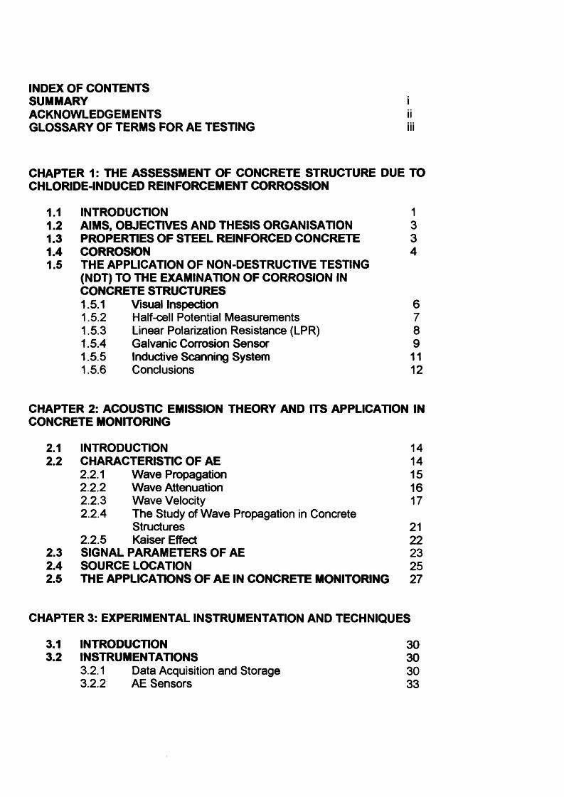
INDEX OF CONTENTSSUMMARY iACKNOWLEDGEMENTS iiGLOSSARY OF TERMS FOR AE TESTING iii

CHAPTER 1: THE ASSESSMENT OF CONCRETE STRUCTURE DUE TO CHLORIDE-INDUCED REINFORCEMENT CORROSSION

1.1 INTRODUCTION 11.2 AIMS, OBJECTIVES AND THESIS ORGANISATION 31.3 PROPERTIES OF STEEL REINFORCED CONCRETE 31.4 CORROSION 41.5 THE APPLICATION OF NON-DESTRUCTIVE TESTING

(NDT) TO THE EXAMINATION OF CORROSION IN CONCRETE STRUCTURES1.5.1 Visual Inspection 61.5.2 Half-cell Potential Measurements 71.5.3 Linear Polarization Resistance (LPR) 81.5.4 Galvanic Corrosion Sensor 91.5.5 Inductive Scanning System 111.5.6 Conclusions 12

CHAPTER 2: ACOUSTIC EMISSION THEORY AND ITS APPLICATION IN CONCRETE MONITORING

2.1 INTRODUCTION 142.2 CHARACTERISTIC OF AE 14

2.2.1 Wave Propagation 152.2.2 Wave Attenuation 162.2.3 Wave Velocity 172.2.4 The Study of Wave Propagation in Concrete

Structures 212.2.5 Kaiser Effect 22

2.3 SIGNAL PARAMETERS OF AE 232.4 SOURCE LOCATION 252.5 THE APPLICATIONS OF AE IN CONCRETE MONITORING 27

CHAPTER 3: EXPERIMENTAL INSTRUMENTATION AND TECHNIQUES

3.1 INTRODUCTION 303.2 INSTRUMENTATIONS 30

3.2.1 Data Acquisition and Storage 303.2.2 AE Sensors 33

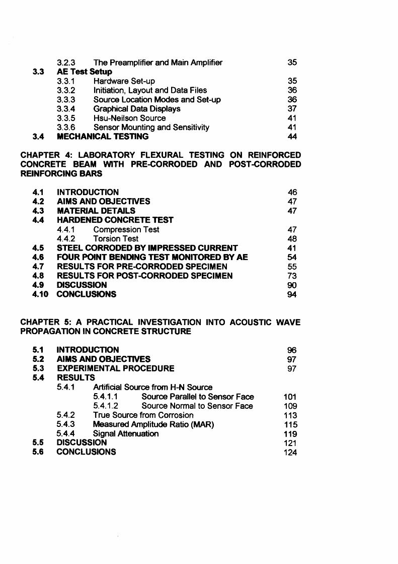
3.2.3 The Preamplifier and Main Amplifier 35AE Test Setup3.3.1 Hardware Set-up 353.3.2 Initiation, Layout and Data Files 363.3.3 Source Location Modes and Set-up 363.3.4 Graphical Data Displays 373.3.5 Hsu-Neilson Source 413.3.6 Sensor Mounting and Sensitivity 41MECHANICAL TESTING 44

CHAPTER 4: LABORATORY FLEXURAL TESTING ON REINFORCED CONCRETE BEAM WITH PRE-CORRODED AND POST-CORRODED REINFORCING BARS

4.1 INTRODUCTION 464.2 AIMS AND OBJECTIVES 474.3 MATERIAL DETAILS 474.4 HARDENED CONCRETE TEST

4.4.1 Compression Test 474.4.2 Torsion Test 48

4.5 STEEL CORRODED BY IMPRESSED CURRENT 414.6 FOUR POINT BENDING TEST MONITORED BY AE 544.7 RESULTS FOR PRE-CORRODED SPECIMEN 554.8 RESULTS FOR POST-CORRODED SPECIMEN 734.9 DISCUSSION 904.10 CONCLUSIONS 94

CHAPTER 5: A PRACTICAL INVESTIGATION INTO ACOUSTIC WAVE PROPAGATION IN CONCRETE STRUCTURE

5.1 INTRODUCTION 965.2 AIMS AND OBJECTIVES 975.3 EXPERIMENTAL PROCEDURE 975.4 RESULTS

5.4.1 Artificial Source from H-N Source5.4.1.1 Source Parallel to Sensor Face 1015.4.1.2 Source Normal to Sensor Face 109

5.4.2 True Source from Corrosion 1135.4.3 Measured Amplitude Ratio (MAR) 1155.4.4 Signal Attenuation 119

5.5 DISCUSSION 1215.6 CONCLUSIONS 124

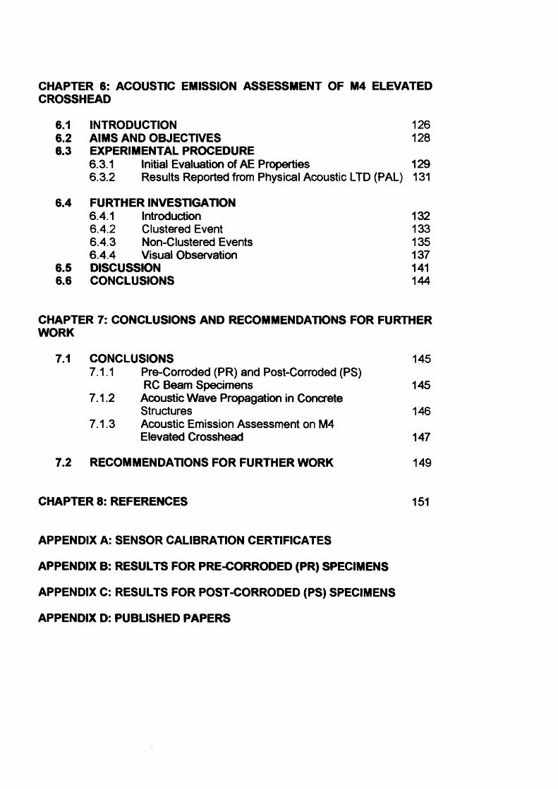
CHAPTER 6: ACOUSTIC EMISSION ASSESSMENT OF M4 ELEVATED CROSSHEAD

6.1 INTRODUCTION 1266.2 AIMS AND OBJECTIVES 1286.3 EXPERIMENTAL PROCEDURE

6.3.1 Initial Evaluation of AE Properties 1296.3.2 Results Reported from Physical Acoustic LTD (PAL) 131

6.4 FURTHER INVESTIGATION6.4.1 Introduction 1326.4.2 Clustered Event 1336.4.3 Non-Clustered Events 1356.4.4 Visual Observation 137

6.5 DISCUSSION 1416.6 CONCLUSIONS 144

CHAPTER 7: CONCLUSIONS AND RECOMMENDATIONS FOR FURTHER WORK

7.1 CONCLUSIONS 1457.1.1 Pre-Corroded (PR) and Post-Corroded (PS)

RC Beam Specimens 1457.1.2 Acoustic Wave Propagation in Concrete

Structures 1467.1.3 Acoustic Emission Assessment on M4

Elevated Crosshead 147

7.2 RECOMMENDATIONS FOR FURTHER WORK 149

CHAPTER 8: REFERENCES 151

APPENDIX A: SENSOR CALIBRATION CERTIFICATES

APPENDIX B: RESULTS FOR PRE-CORRODED (PR) SPECIMENS

APPENDIX C: RESULTS FOR POST-CORRODED (PS) SPECIMENS

APPENDIX D: PUBLISHED PAPERS

CHAPTER 1: THE ASSESSMENT OF THE DETERIORATION CONCRETE

STRUCTURES DUE TO CHLORIDE-INDUCED REINFORCEMENT

CORROSION

1.1 INTRODUCTIONThe aim of this chapter is to investigate the use of structural health monitoring

to assess the deterioration of concrete structures due to chloride-induced

reinforcement corrosion. Non-Destructive Testing (NDT) methods for doing

this are reviewed and the influence of the corrosion process within concrete

structures on these techniques is considered.Deterioration of concrete bridges and other concrete structures caused

by environmental exposure is a severe global problem. One of the most

serious matters with major economic implications is the degradation due to

chloride-induced reinforcement corrosion. Serious deterioration of the civil

engineering infrastructure has encouraged structural monitoring of the

integrity of structural systems.Monitoring the structural health condition at regular intervals can:

i. Enable the detection and location of damage or degradation of

structural components and provide this information to the operatorsand users of the structure quickly and comprehensibly.

ii. Allow structural degradation to be identified early prior to local failure.

iii. Prevent system failure.

iv. Help reduce maintenance costs.Park (2002) suggests that an ideal structural health monitoring system should

be capable of:i. detecting existing damage,

ii. locating the damage,

iii. sizing the damage, andiv. determining the impact of the damage on the performance of the

structure.

1

A recent example of where structural health monitoring of a structure is now

required is as a result of problems that have been identified in 2004 with the

Lumpur Middle Ring Road 2, known as the MRR2 in Malaysia. The

government carried out investigations of a 1.7km flyover, which forms part of

the MRR2, and it was reported as being faulty because 31 of the 33 pillars

supporting the flyover were identified as having active cracks. As a result the

flyover was closed to traffic and only reopened with traffic restricted to 4 out of

6 lanes. To ensure that the MRR2 flyover does not become a threat to public

safety less than two years after its completion and to identify what remedial action needs to be undertaken to end the daily hardship and inconvenience to

tens of thousands of commuters an NDT method is needed to monitor the

whole structure. Early detection of the growth of this damage prior to local

failure is needed to prevent disastrous failures of the whole system.As well as detecting and locating corrosion damage in structures,

further investigation is required by observing the behaviour of concrete

structures which have been affected by chloride induced reinforcement

corrosion. This can be considered as an early warning sign indicating that

deterioration has occurred inside the structure. Steel corrosion in reinforced

concrete (RC) leads to cracking, reduction of bond strength and steel cross

section, loss of concrete cover and, in extreme cases, a loss of structural

integrity. The effects of these phenomena on the changing behaviour of RC

structures, for example as caused by de-icing chemicals, must detected early

and studied in detail.It is possible to use the acoustic emission (AE) signal resulting from

damage, to clarify the location of such damage. Experiments have been

performed on steel-reinforced concrete specimens to determine the feasibility

of using AE monitoring to detect the effect of corrosion on the behaviour of

RC structures. The evaluation on the performance of AE, with regards to the

structural effects of corrosion-damage, is highly significant in order to help

monitor large structures.

2

1.2 AIMS, OBJECTIVES AND THESIS ORGANISATION

The aims of this study are to investigate the AE technique further for use in

global structural monitoring; study the effect and changing behaviour caused

by chloride-induced reinforcement corrosion in concrete bridges and provide a

practical technique for the non-destructive testing of concrete bridges. Regarding smart bridges, this study conveys the effect of corrosion on RC

structures and the AE output in order to develop a tool that could be used to

determine damage and/or deterioration in generic RC structures.

The objectives are to evaluate and enhance existing assessment methods using AE in order to monitor the behaviour of RC bridges due to

corrosion and to improve traditional methods of source location. Studies will include:

i. Laboratory based stepwise static loading tests monitored using AE of corroded and uncorroded RC beams.

ii. Source location trials of AE to determine deterioration/crack location.iii. Investigation into acoustic wave propagation in concrete structures.

iv. Further investigation of bridge monitoring data.

Chapters 1 and 2 present and critically review background research

and reference works. Chapter 3 details the instrumentation and experimental

techniques common to all conducted experimental work. Chapters 4, 5 and 6

report all the experimental and analytical work undertaken. Each chapter

examines the results and discussion relevant to each group of experiments

with conclusions presented separately at the end of each chapter. Chapter 7

draws together all chapters with recommendations for future work. All references are presented in Chapter 8.

1.3 PROPERTIES OF STEEL REINFORCED CONCRETE (RC)

Generally, RC is a composite material made up of concrete and some form of reinforcement such as steel rods, bars or wires; these materials combine to

provide a versatile construction material.

3

Concrete has a high compressive but a low tensile strength. Steel, on the

other hand, has a very high tensile and compressive strength. Due to the high

cost of steel, it is cost effective to combine steel and concrete into a

composite material, making use of both, the high strength of steel and the

relatively low-cost compressive strength of concrete.Corrosion of the reinforcement is a major durability problem. This

largely due to when the rebar in the concrete is exposed to chlorides, either

from the concrete’s ingredients or from the surrounding chloride-bearing

environment. Carbonation of concrete and the penetration of acidic gases into

concrete are other causes of reinforcement corrosion. Others effects that

influence reinforcement corrosion are the water to cement ratio, cement content, impurities in the concrete’s ingredients, the presence of surface crack

and the external environment. Environmental and climate conditions appear

to be a main cause contributing to the deterioration process.

The deterioration process occurs when the severity of the environment

is compounded by poor durability performance of the concrete or faulty design

and construction practices. Deterioration grows rapidly and it cannot easily be

stopped. As a result, large numbers of existing structures are deteriorating

globally.

1.4 CORROSIONCorrosion is an electrochemical reaction. The important factor affecting a

corroded cell is the difference in the potential of the metal. Steel reinforcement in concrete and concrete-like materials are, generally, well protected from

corrosion by the alkaline nature of the cementitious matrix surrounding it. As

long as it is protected, the steel inside concrete structures should not corrode. However, this alkaline environment deteriorates in real structures and

reinforcing and pre-stressing steels are subject to corrosion due to

carbonation and chloride ion attack. Corrosion of steel reinforcement is one of

the major causes affecting the long-term performance of RC structures.

4

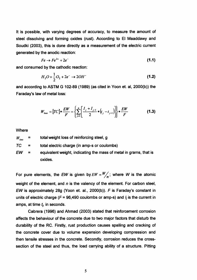
It is possible, with varying degrees of accuracy, to measure the amount of

steel dissolving and forming oxides (rust). According to El Maaddawy and

Soudki (2003), this is done directly as a measurement of the electric current

generated by the anodic reaction:

Fe->Fe2++ 2e~ (1.1)

and consumed by the cathodic reaction:

H 20 + ̂ 0 2 +2e~ -> 2OH- (1.2)

and according to ASTM G 102-89 (1989) (as cited in Yoon et. al, 2000(b)) the

Faraday’s law of metal loss:

I J+ I H ♦ ̂ (1.3)

Where

Wloss = total weight loss of reinforcing steel, g

TC = total electric charge (in amp-s or coulombs)EW = equivalent weight, indicating the mass of metal in grams, that is

oxides.

For pure elements, the EW is given by EW = w/ \ where W is the atomic

weight of the element, and n is the valency of the element. For carbon steel,

EW is approximately 28g (Yoon et. al., 2000(b)). F is Faraday’s constant in

units of electric charge (F = 96,490 coulombs or amp-s) and /y is the current in

amps, at time tj, in seconds.

Cabrera (1996) and Ahmad (2003) stated that reinforcement corrosion

affects the behaviour of the concrete due to two major factors that disturb the

durability of the RC. Firstly, rust production causes spalling and cracking of

the concrete cover due to volume expansion developing compression and

then tensile stresses in the concrete. Secondly, corrosion reduces the cross-

section of the steel and thus, the load carrying ability of a structure. Pitting

5

corrosion of the rebar is more risky than uniform corrosion because it

progressively reduces the cross-sectional area of rebar to a point where the

rebar can no longer withstand the applied load leading to a disastrous failure

of the structure.

1.5 THE APPLICATION OF NON-DESTRUCTIVE TESTING (NDT) TO

THE EXAMINATION OF CORROSION IN CONCRETE

STRUCTURESDue to continuous deterioration and increasing maintenance and repair costs

for civil infrastructure systems bridge managers/owners must make decisions

in an uncertain environment. The introduction of health monitoring techniques

using NDT are beneficial as they improve the confidence with which structural

performance is assessed and predicted; hence optimise resources used for

bridge inspection, maintenance and repair. Widespread corrosion problems of

reinforcing steel in concrete structures have triggered a concerted demand for

the development of NDT techniques to enable accurate assessment of RC

structures.

1.5.1 Visual InspectionVisual inspection is the customary inspection method. The appearance and

colour of a corroded area often provides valuable insight to the cause and

extent of corrosion. Moreover, the location of longitudinal cracks due to

corrosion attack can be drawn as a crack map with lengths and widths

recorded from their first visual observation which enables a global overview of

the damage of the RC structures to be obtained (Poupard et. al., 2006).

Special tools, such as magnifying glasses, may also be used to closelyinspect the subject area. However, such a technique is limited in its

effectiveness to detect surface discontinuities which are often masked by

corroded products and internal discontinuities which are not detectable using

this method.

6

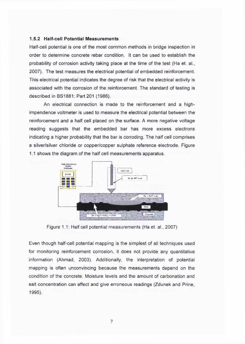
1.5.2 Half-cell Potential MeasurementsHalf-cell potential is one of the most common methods in bridge inspection in

order to determine concrete rebar condition. It can be used to establish the

probability of corrosion activity taking place at the time of the test (Ha et. al.,

2007). The test measures the electrical potential of embedded reinforcement.

This electrical potential indicates the degree of risk that the electrical activity is

associated with the corrosion of the reinforcement. The standard of testing is

described in BS1881: Part 201 (1986).

An electrical connection is made to the reinforcement and a high-

impendence voltmeter is used to measure the electrical potential between the

reinforcement and a half cell placed on the surface. A more negative voltage

reading suggests that the embedded bar has more excess electrons

indicating a higher probability that the bar is corroding. The half cell comprises

a silver/silver chloride or copper/copper sulphate reference electrode. Figure

1.1 shows the diagram of the half cell measurements apparatus.

H *lt C+V

Figure 1.1: Half cell potential measurements (Ha et. al., 2007)

Even though half-cell potential mapping is the simplest of all techniques used

for monitoring reinforcement corrosion, it does not provide any quantitative

information (Ahmad, 2003). Additionally, the interpretation of potential

mapping is often unconvincing because the measurements depend on the

condition of the concrete. Moisture levels and the amount of carbonation and

salt concentration can affect and give erroneous readings (Zdunek and Prine,

1995).

7

1.5.3 Linear Polarization Resistance (LPR)The measurement of half ceil potential is a qualitative way in assessing the

corrosion state of reinforcing steel and in locating the steel area which

presents high corrosion probability. However, to characterize the corrosion

activity on the surface of reinforcing steel in a qualitative way, it is essential toevaluate the corrosion rate. The corrosion rate is deduced from thepolarization resistance (Rp) measurements from the linear polarization

resistance (LPR) method. In this method the corrosion rate is defined as,

l c,„ = (1-4)Kp

where B is constant, Icorr is the corrosion rate and Rp is the polarization

resistance.

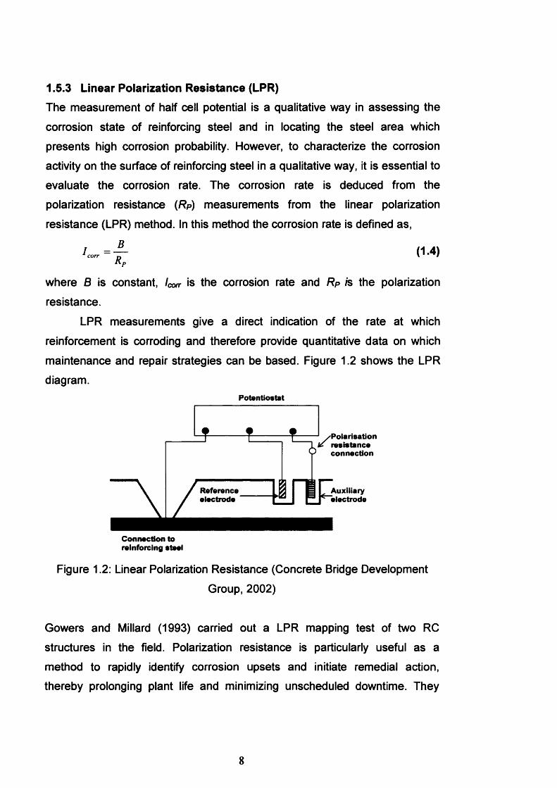
LPR measurements give a direct indication of the rate at which

reinforcement is corroding and therefore provide quantitative data on which

maintenance and repair strategies can be based. Figure 1.2 shows the LPR

diagram.Potentiostat

Referenceelectrode

Connection to reinforcing steel

/Polarisation / resistance

connection

Auxiliaryelectrode

Figure 1.2: Linear Polarization Resistance (Concrete Bridge Development

Group, 2002)

Gowers and Millard (1993) carried out a LPR mapping test of two RC

structures in the field. Polarization resistance is particularly useful as a

method to rapidly identify corrosion upsets and initiate remedial action, thereby prolonging plant life and minimizing unscheduled downtime. They

8

identified regions of the structures, which may have been particularly

susceptible to corrosion, by mapping technique of the corrosion rate. Even

though LPR can provide a more quantitative assessment of corrosion rate,

mapping techniques are time consuming and limited to specific areas. In other

words, LPR can be applied to a location where potential and resistivity

indicate active corrosion is most likely.

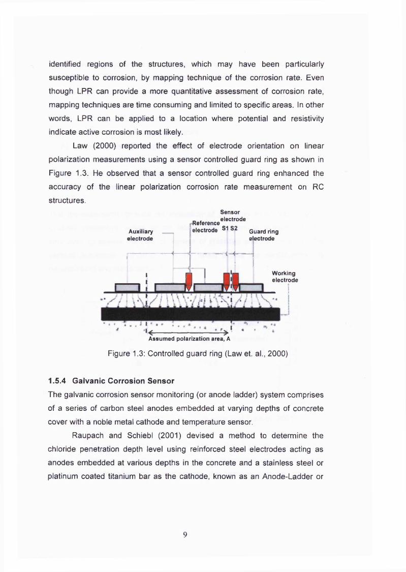
Law (2000) reported the effect of electrode orientation on linear

polarization measurements using a sensor controlled guard ring as shown in

Figure 1.3. He observed that a sensor controlled guard ring enhanced the

accuracy of the linear polarization corrosion rate measurement on RC

structures.

Auxiliaryelectrode

Sensor_ . electrode Referenceelectrode S1 S2 Guard ring

e ectrode

f l

Workingelectrode

Assumed polarization area, A

Figure 1.3: Controlled guard ring (Law et. al., 2000)

1.5.4 Galvanic Corrosion SensorThe galvanic corrosion sensor monitoring (or anode ladder) system comprises

of a series of carbon steel anodes embedded at varying depths of concrete

cover with a noble metal cathode and temperature sensor.

Raupach and Schiebl (2001) devised a method to determine the

chloride penetration depth level using reinforced steel electrodes acting as

anodes embedded at various depths in the concrete and a stainless steel or

platinum coated titanium bar as the cathode, known as an Anode-Ladder or

9

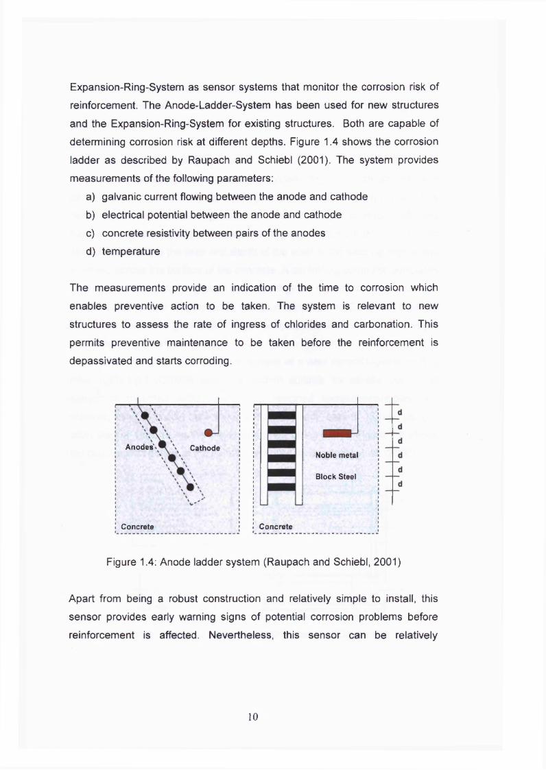
Expansion-Ring-System as sensor systems that monitor the corrosion risk of

reinforcement. The Anode-Ladder-System has been used for new structures

and the Expansion-Ring-System for existing structures. Both are capable of

determining corrosion risk at different depths. Figure 1.4 shows the corrosion

ladder as described by Raupach and Schiebl (2001). The system provides

measurements of the following parameters:

a) galvanic current flowing between the anode and cathode

b) electrical potential between the anode and cathode

c) concrete resistivity between pairs of the anodes

d) temperature

The measurements provide an indication of the time to corrosion which

enables preventive action to be taken. The system is relevant to new

structures to assess the rate of ingress of chlorides and carbonation. This

permits preventive maintenance to be taken before the reinforcement is

depassivated and starts corroding.

Anodes' CathodeNoble metal

Block Steel

ConcreteConcrete

Figure 1.4: Anode ladder system (Raupach and Schiebl, 2001)

Apart from being a robust construction and relatively simple to install, this

sensor provides early warning signs of potential corrosion problems before

reinforcement is affected. Nevertheless, this sensor can be relatively

10

expensive and therefore only appropriate for larger structures or sites in

severe environments. It can only be fitted to new structures or during major

repair or re-construction projects in this form.

1.5.5 Inductive Scanning SystemA laboratory-based motorized scanning system, together with an inductive

sensor, was developed and reported by Gaydecki and Burdekin (1994). This

sensor system is capable of generating computer images of steel reinforcing

bars and cables embedded in concrete. Signal response from an inductive

sensor is related to the area and depth of the steel in the sensing region and

scanned across the surface of the concrete. A controlling computer generates

an image of the underlying steel by converting the signal that responds from

the inductive sensor to grey-scale values mapped to the Cartesian location.

The intensities of the grey-scale images are proportional to the signal strength

produced by the sensor.

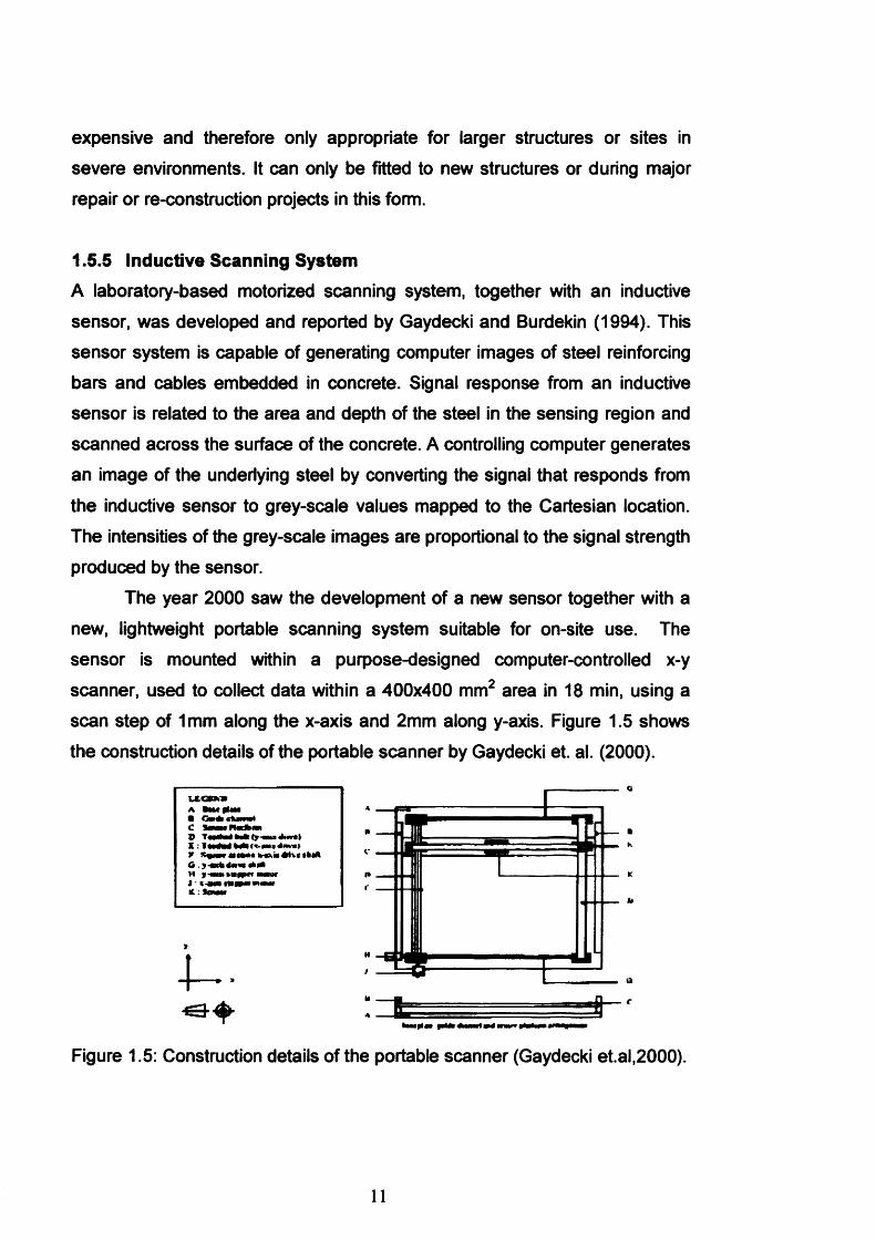
The year 2000 saw the development of a new sensor together with a

new, lightweight portable scanning system suitable for on-site use. The

sensor is mounted within a purpose-designed computer-controlled x-y

scanner, used to collect data within a 400x400 mm2 area in 18 min, using a

scan step of 1mm along the x-axis and 2mm along y-axis. Figure 1.5 shows

the construction details of the portable scanner by Gaydecki et. al. (2000).

Figure 1.5: Construction details of the portable scanner (Gaydecki et.al,2000).

A B M cp laM• O r t t r t — I C S M M P ta d b m X>K : ImM Mld-Pii

G . Jr-Ot*4«aa «k*NMJ ' l - W * : Sowar

It

a

11

1.5.6 ConclusionTable 1.1 shows a summary of the NDT techniques that have been applied to

the examination of corrosion in RC structures. The majority of these methods

are still under research and have potential in relation to the assessment of

corrosion and the condition of RC structures. Choice of the most appropriate

method is usually based on a combination of factors such as a cost, speed, reliability and accuracy of the given method. Each method has certain

advantages and disadvantages and by adopting several testing methods and

combining the results usually yields the best results (Idrissi and Liman, 2003). The significance of these methods is that they identify the presence of

corrosion in concrete structures at discrete locations which can assist and

benefit numerous groups in monitoring large scale structures. Unfortunately,

in a global structural monitoring context, there is still not enough research into

the application of non-destructive techniques. This also applies to monitoring

the effect and the changing behaviour due to chloride-induced reinforcement corrosion in concrete structures, especially bridges.

12

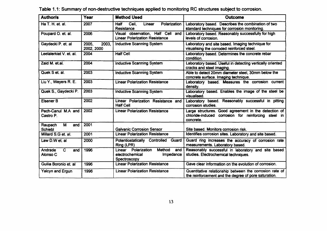
Table 1.1: Summary of non-destructive techniques applied to monitoring RC structures subject to corrosion.

Author/s Year Method Used OutcomeHa T. H. et. al. 2007 Half Cell, Linear Polarization

ResistanceLaboratory based. Describes the combination of two standard techniques for corrosion monitoring.

Poupard 0 . et. al. 2006 Visual observation, Half Cell and Linear Polarization Resistance

Laboratory based. Reasonably successfully for high levels of corrosion.

Gaydecki P. et. al 2005, 2003, 2002, 2000

Inductive Scanning System Laboratory and site based. Imaging technique for visualising the corroded reinforced steel.

Leelalerkiet V. et. al. 2004 Half Cell Laboratory based. Determines the concrete rebar condition.

Zaid M. et.al. 2004 Inductive Scanning System Laboratory based. Useful in detecting vertically oriented cracks and steel imaging.

Quek S et. al. 2003 Inductive Scanning System Able to detect 20mm diameter steel, 30mm below the concrete surface. Imaging technique.

Liu Y., Weyers R. E. 2003 Linear Polarization Resistance Laboratory based. Measures the corrosion current density.

Quek S., Gaydecki P. 2003 Inductive Scanning System Laboratory based. Enables the image of the steel be visualised.

Elsener B 2002 Linear Polarization Resistance and Half Cell

Laboratory based. Reasonably successful in pitting corrosion studies.

Pech-Canul M.A and Castro P.

2002 Linear Polarization Resistance Large structures. Good agreement in the detection of chloride-induced corrosion for reinforcing steel in concrete.

Raupach M and Schiebl

2001Galvanic Corrosion Sensor Site based. Monitors corrosion risk.

Millard S.G et. al. 2001 Linear Polarization Resistance Identifies corrosion sites. Laboratory and site based.

Law D.W et. al 2000 Potentiostatically Controlled Guard Ring (LPR)

Guard ring increases the accuracy of corrosion rate measurements. Laboratory based.

Andrade C and Alonso C

1996 Linear Polarization Method and electrochemical Impedance Spectroscopy

Reasonably successful in laboratory and site based studies. Electrochemical techniques.

Guilia Boronio et. al 1996 Linear Polarization Resistance Gave clear information on the evolution of corrosion.

Yalcyn and Ergun 1996 Linear Polarization Resistance Quantitative relationship between the corrosion rate of the reinforcement and the degree of pore saturation.

13

CHAPTER 2: ACOUSTIC EMISSION THEORY AND ITS APPLICATION IN

CONCRETE MONITORING

2.1 INTRODUCTION

Acoustic Emission (AE) is the phenomenon whereby transient elastic waves

are generated by the rapid release of energy from localized sources within a

material. All materials produce AE during both the generation and propagation

of cracks. The elastic waves travel through the structure to the surface, where

they are detected by sensors. These sensors are transducers that convert the

mechanical waves into electrical signals; information about the existence and

location of possible damage sources can be obtained. Among structural non­destructive tests, the AE monitoring technique is the only one able to detect a

damage process at the same time as it occurs.

Pollock (1989) and Esward et. al. (2002), state that AE differs from

other non-destructive testing techniques in two main respects; firstly, the

energy is released from within the test object itself and secondly, AE is

capable of detecting the dynamic processes associated with the degradation

of structures.Grosse (2003) highlighted that one of the advantages, compared with

other non-destructive evaluation techniques, is the possibility of observing the

damage process during the entire load history without disturbing the

specimen.

2.2 CHARACTERISTICS OF AE

AE testing is based on the fact that solid materials emit elastic waves or AE

when they are mechanically or thermally stressed to the point where

deformation or fracture occurs. A number of characteristics of the elastic wave

need to be investigated including wave propagation, wave attenuation, wave

velocity and the Kaiser effect.

14

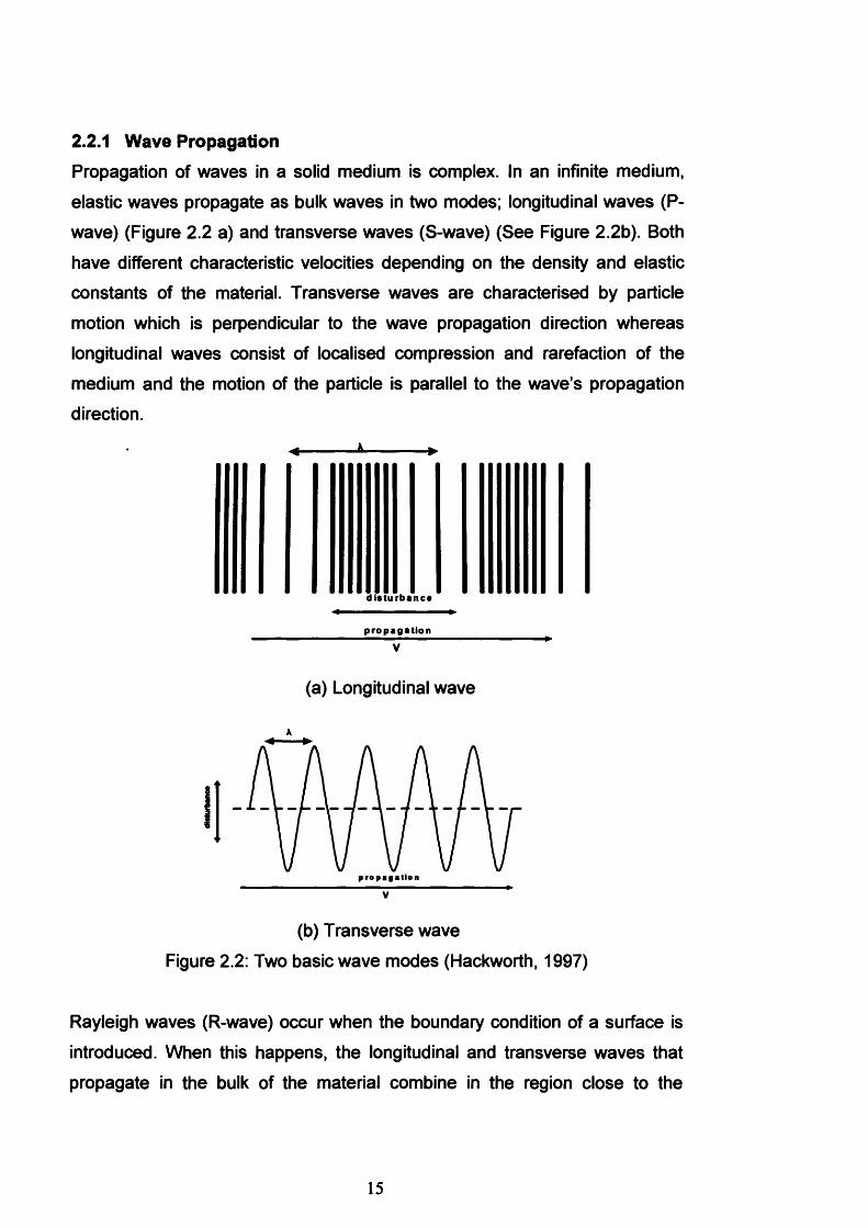
2.2.1 Wave PropagationPropagation of waves in a solid medium is complex. In an infinite medium,

elastic waves propagate as bulk waves in two modes; longitudinal waves CP- wave) (Figure 2.2 a) and transverse waves (S-wave) (See Figure 2.2b). Both

have different characteristic velocities depending on the density and elastic

constants of the material. Transverse waves are characterised by particle

motion which is perpendicular to the wave propagation direction whereas

longitudinal waves consist of localised compression and rarefaction of the

medium and the motion of the particle is parallel to the wave’s propagation

direction.

« A ►

disturbance

propagation

V

(a) Longitudinal wave

A

p r o p a g a t io n

V

(b) Transverse wave

Figure 2.2: Two basic wave modes (Hackworth, 1997)

Rayleigh waves (R-wave) occur when the boundary condition of a surface is

introduced. When this happens, the longitudinal and transverse waves that

propagate in the bulk of the material combine in the region close to the

15

surface and a compression produces a transverse displacement of the

material. Considering the impact of Poisson’s ratio, the overall particle motion

is neither purely longitudinal nor transverse. This is known as a Rayleigh or a

surface wave.In a medium bounded by two surfaces (plates), at distances greater

than a few centimetres from an AE source, surface waves can couple to

produce more complex propagation modes called Lamb waves. Lamb wave

behaviour is complex and characterised by dispersion, depending on the

thickness of the plate and the frequency of the wave.

2.2.2 WAVE ATTENUATION

In real media, waves change in amplitude as they propagate through the

solid. The decrease in amplitude that occurs as a wave travels through a

medium is known as wave attenuation. There are several mechanisms

responsible for this:i. Geometric spreading.

ii. Internal friction.iii. Dissipation of the wave into adjacent media.

iv. Velocity dispersion

When a wave is generated by a localized source, the disturbance propagates

outwards in all directions from the source. The energy in the wave front

remains constant but is spread over a larger spherical surface. The radius of this sphere (geometric) is equal to the distance the wave travelled from the

source. In order for the energy to remain constant, the amplitude of the wave

must decrease with increasing distance from the source.

When waves propagate through media with complex boundaries and

discontinuities, scattering and dispersion occur, e.g. from aggregate grains in

concrete. These phenomena can lead to a decrease in the amplitude of the

waves and can cause wave attenuation.

Dissipation attenuation can be caused by in homogeneities in the propagation

medium which scatter the sound wave in the same material, e.g. grain

16

structure in metals. However, it is most common in specimens in contact with

an adjacent liquid, e.g. tanks and pipes. Liquids draw energy from the wave

travelling in the metal and causes additional attenuation in the near field.

Attenuation due to velocity dispersion happens because the different frequency components of broadband Lamb wave travel at different velocities

and the resulting spreading in time causes a loss in amplitude. The magnitude

of amplitude loss depends on the slope of the dispersion curves and

bandwidth of the signal.

2.2.3 WAVE VELOCITY

The measured velocity describes the speed at which an AE event travels

between two fixed points in a propagation medium; this wave velocity is

determined by characteristics of the material.Theoretically, from the physics of elastic wave propagation, the wave

velocity in a solid media is proportional to the square root of the elastic

modulus and inversely proportional to the square root of the mass density of

the media. As a result, the wave velocity is constant when the wave

propagates through a media. However, in practice, the methods or techniques

that had been used to measure the wave velocity found that the wave

velocities were changing with distance. In this case, the terms ‘apparent’ wave

velocity is used instead of wave velocity.

Homogenous materials, such as steel, have well-defined velocities

whereas with non-homogeneous materials, such as concrete, the wave

velocity is more difficult to predict. Consequently, the measured wave velocity

may restrict the development of widely applicable tools as a constant wave

velocity is required for most of the application. Additionally, due to the

complex composition of most civil engineering structures, determination of the

wave velocity is difficult because of the non-homogeneous of the material.

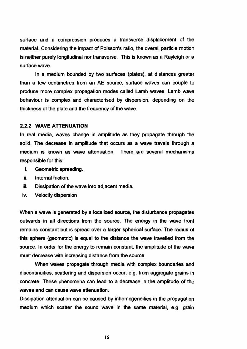
In order to calculate the wave velocity using AE, the determination of the initial P-wave arrival time is essential. The time of the first arrival of a

P-wave can be identified from the first rise in amplitude of the signal as shown

in Figure 2.3. Source location in AE is based on the arrival times of the direct

17

body waves (P-waves). This is because the P-wave is the first signal to arrive

which will not be interfered with by any signal reflections in the later phases

(Schechniger and Vogel, 2007).

In AE, the most common method of estimating the arrival time (as used

in many commercial systems is the threshold method) whereby the arrival

time is recorded when the signal amplitude first crosses a pre-set threshold.

This method is used by Holford and Carter (1999) and Ding et al. (2004) when

calculating the AE wave velocity in a structure.1200

1000

800

600

400

r 200

-200

-600Initial P-wave arrival time-800

-1000

-1200

600pT im * ( S V C )

Figure 2.3: Initial P-wave determination from the recorded AE

waveform

The wave velocity can be calculated using at least two sensors separated by

a known distance and aligned in a straight line with the source point. The

sensors were mounted on the same concrete surface to receive the waveform

of the displacement generated by the arrival of waves as shown in Figure

2.4(a).

From the recorded signals, the time of arrival of the first P-wave to

these two sensors can be identified by using a synchronous setting. This is

when the first hit channel triggers all other synchronised channels and the

arrival hit-time between different channels can be determined. The P-wave

velocity can be calculated as:

18

D is the distance between sensors and At is the time lapse between their arrivals.

As well as AE methods, there are several other methods which can be

used to calculate the P-wave velocity of concrete structures. Brief descriptions

of the most well-known methods are given below.

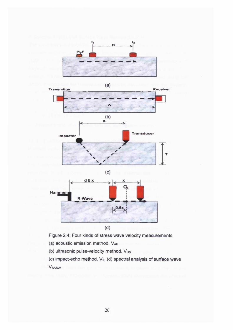
Ultrasonic Pulse Velocity MethodAs described in BS EN 12504-4 (2004), an ultrasonic pulse is created by a

pulse generator and transmitted through the surface of concrete to a receiver. This pulses travel through the specimen with some spreading and attenuation

and will be reflected or scattered at any surface or discontinuity, such as a

crack, within a specimen. The time taken by the generated pulse to travel

through the concrete is accurately measured by the receiver transducer

attached to other side of the concrete surface. A setup of this test is shown

schematically in Figure 2.4(b). The wave velocity can be calculated similar to

Equation 2.1.

Impact-Echo Method

As described in ASTM C1383-04 (2002), this test is based on the principle

that stress waves (P-wave) passing through concrete are reflected at internal

flaws and external surfaces. The P-wave is generated by an impact at the

surface of the concrete. The reflected wave is then measured at the surface of the concrete by a receiving transducer and analysis of the results can indicate

the presence of defects such as cracks, delaminations, voids and debonding. The impact-echo method is illustrated in Figure 2.4(c).

Transmitter(a)

Receiver

w '■w

■

Impactor

(C)

HammerR-Wave

(d)Figure 2.4: Four kinds of stress wave velocity measurements

(a) acoustic emission method, Vae

(b) ultrasonic pulse-velocity method, Vus

(c) impact-echo method, V ie (d) spectral analysis of surface wave

V sasw.

20

A Spectral Analysis of Surface Wave Method (SASW)The applicability of the SASW method for determining the P-wave velocity in a

concrete structure was assessed for nondestructive testing by Kim et al. (2006). The SASW method is based on the dispersive characteristics of

Rayleigh waves in the layered media as illustrated in Figure 2.4(d). The

average Rayleigh wave velocity of concrete can be determined using the

SASW method and the P-wave velocity can be calculated from the Rayleigh

wave velocity with the Poisson’s ratio of the concrete by using the following

equation:

v= Poisson’s ratio, Vp- P-wave velocity, VR= R-wave velocity

2.2.4 The Study of the Wave Propagation in Concrete Structures

In recent years, there has been adequate research regarding wave velocities

in ultrasonic studies on concrete but less material relating specifically to AE.

The fundamental difference between AE and Ultrasonics is that the energy

converted to AE signals comes from the material itself. However, in

Ultrasonics the acoustic wave is generated by an external source and

introduced into the material (Beattie, 1983). As a result, the AE technique is

sensitive to growing defects. Since the AE signals from defects radiate

throughout the structure, relatively few AE sensors can detect and qualify

defects over a large area.Depending on various characteristics, Ultrasonic studies commonly use

non-destructive testing methods to measure the wave velocities. These may

include the ultrasonic pulse-velocity method (Wu et. al., 2000, Philippidis and

Anggelis, 2005), the impact-echo method (Gassman and Tawheed, 2004, Kim

et al., 2006) and a spectral analysis of surface wave method (SASW) (Cho,

2003). Most of these methods use a transmitter and receiver transducer.

There have been few studies in Ultrasonic in determining the P-wave

velocity. One study, Philippidis and Aggelis (2005) investigated the effect of

(2.2)

21

the water to cement ratio on wave velocity in concrete, where for a range of

water to cement ratios between 0.375 and 0.45, the P-wave velocity varied

between 3500m/s and 4700m/s. As the water to cement ratio decreased, the

velocity of the P-wave increased. In addition, the authors found that at a

sensor distance of 150mm, the apparent wave velocity of P-waves in concrete

range from 4100m/s to 4700m/s using a signal from a 15 kHz tone burst.Gassman and Tawheed (2004) analysed the variation in propagation

wave velocity of the slab using an Impact-echo test. The authors discovered

that the wave velocity in concrete, with a distance of 300mm between the two

transducers, varied from 4191 m/s to 4233m/s. They also found that for slab

areas that exhibit no visual surface and with a distance of 210mm, the wave

velocity varied from 4278m/s to 4452m/s. After the load test, a reduction of P-

wave velocity ranging from 2 to 6% was observed as a result of crack

propagation throughout the slab. The authors agreed that the appearance of cracks will reduce the P-wave velocity through the concrete media.

However, no previous study in AE has investigated the relationship

between wave velocities with sensor distances from the source.

2.2.5 Kaiser EffectThe Kaiser effect (defined by Joseph Kaiser in 1950) is one of the important

characteristics of AE. Once a given load has been applied and the AE from

that stress has stopped, an additional AE will not occur until the original stress

level has been exceeded.

The Kaiser effect has been used by many researchers for assessing

the deterioration of concrete structures. Yuyama et al. (1999) performed a

series of studies to evaluate the structural integrity of Reinforced Concrete

(RC) beams and the results demonstrated that the breakdown in the Kaiser effect was directly related to the deterioration of the concrete specimen. Ohtsu

et al. (2002) described a damage assessment method for RC beams

associated with the Kaiser effect, comparing the Load Ratio (load at the onset

of AE activity in a subsequent loading cycle/the previous load) with the

22

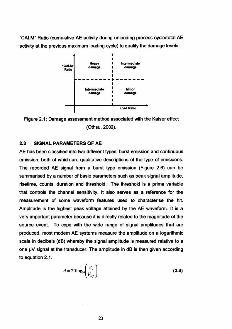
“CALM” Ratio (cumulative AE activity during unloading process cycle/total AE

activity at the previous maximum loading cycle) to qualify the damage levels.

“CALM’Ratio

Heavydamage

Intermediatedamage

Intermediatedamage

Minordamage

Load Ratio

Figure 2.1: Damage assessment method associated with the Kaiser effect(Othsu, 2002).

2.3 SIGNAL PARAMETERS OF AE

AE has been classified into two different types; burst emission and continuous

emission, both of which are qualitative descriptions of the type of emissions. The recorded AE signal from a burst type emission (Figure 2.6) can be

summarised by a number of basic parameters such as peak signal amplitude,

risetime, counts, duration and threshold. The threshold is a prime variable

that controls the channel sensitivity. It also serves as a reference for the

measurement of some waveform features used to characterise the hit. Amplitude is the highest peak voltage attained by the AE waveform. It is a

very important parameter because it is directly related to the magnitude of the

source event. To cope with the wide range of signal amplitudes that are

produced, most modem AE systems measure the amplitude on a logarithmic

scale in decibels (dB) whereby the signal amplitude is measured relative to a

one pV signal at the transducer. The amplitude in dB is then given according

to equation 2.1.

(2.4)

23

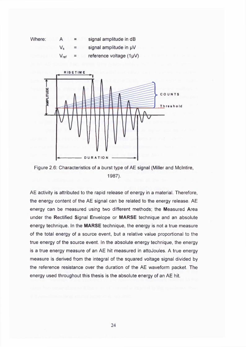
Where: A = signal amplitude in dB

Vs = signal amplitude in pV

Vref = reference voltage (1pV)

R IS ETI M E

C O U N T S

T h re s h o Id

D U R A T I O N

Figure 2.6: Characteristics of a burst type of AE signal (Miller and Mclntire

1987).

AE activity is attributed to the rapid release of energy in a material. Therefore,

the energy content of the AE signal can be related to the energy release. AE

energy can be measured using two different methods; the Measured Area

under the Rectified Signal Envelope or MARSE technique and an absolute

energy technique. In the MARSE technique, the energy is not a true measure

of the total energy of a source event, but a relative value proportional to the

true energy of the source event. In the absolute energy technique, the energy

is a true energy measure of an AE hit measured in attoJoules. A true energy

measure is derived from the integral of the squared voltage signal divided by

the reference resistance over the duration of the AE waveform packet. The

energy used throughout this thesis is the absolute energy of an AE hit.

24

2.4 SOURCE LOCATIONLocalisation of AE sources is important to assess the regions of active

damage. Location can be defined as the determination of the spatial position

of an AE source from arrival time measurement using an array of sensors

(Miller and Mclntire, 1987). The location calculation can be carried out in real­

time and the results can be displayed immediately. Source location is usually

based on the arrival times of transient signals. The predominant method of

source location is based on a measurement of the time difference between

the arrivals of individual AE events at different sensors known as the Time of Arrival (TOA) method. This method enables the location of the damage from

the arrival time of the event at two or more sensors to be determined.One of the main fields for AE research is signal source location

applied. This helps to determine the defects’ position and their orientation in

the material (Shah and Li, 1994). An excellent explanation of location in one, two and three dimensions is presented by Miller and Mclntire (1987). One

dimensional source location is known as linear location. If a source is known

to be somewhere along a straight line between a pair of transducers on the

beam, a difference in the measured arrival time at the two transducers

uniquely determines the source location. Pullin (2001) describes a method

which determines the location of an event in one dimension between two

sensors where the velocity of the signal and the time of arrival at the sensors

is known.

For a plate like structure, it is possible to determine the location of the

source by analyzing the time difference between arrivals to three or more

sensors (Carlos, 2003). This method locates a source in two dimensions. It is

possible to calculate the distance between the source and each sensor by

travel times and the speed of the wave arriving at each sensor. By knowing

the distance, a circle can be drawn centred at the sensors and the intersection

of the three circles drawn from the three sensors should be the focus of the

source. However, if the thickness of the specimen is significant relative to the

other two dimensions or if the area of interest is internal to the specimen, then

a three-dimensional source location is required.

25

Source location is an extremely powerful tool in AE analysis and can be used

in a global monitoring strategy to monitor a relatively large structure with a

minimum number of sensors. This is a tremendous advantage in the case of

monitoring large structures such as bridges as little access is needed for the

placement of AE sensors to determine the structural integrity of a bridge. In

global monitoring, when regions of emission are expected, source location

attempts to identify a particular area of structure that is experiencing damage. This area is then locally monitored to locate the crack and provide quantitative

information about the waveforms emitted (Holford, 2001). Moreover, a

reasonable sensor arrangement is of great importance for the localisation

capability. However, in local monitoring, source location may be used to try

and locate the crack and crack tip, especially if the crack is sub-surface or

unable to locate by visual methods.The precision of source location is dependent on the wave velocity

calculation, time difference measurements and the accuracy of the sensor positions (Beck, 2004). There is a need to have reliable automatic picking

tools. Manually, it would be difficult to manage the enormous amount of data

recorded in the experiments. A widely used method for arrival time

determination is by fixed thresholds that have already been implemented in

the acquisition system. This method was used by Holford and Carter (1999)

Ding et al. (2004) and Schechniger and Vogel (2007) to determine the arrival time for the calculations of AE wave velocity in structures for source location

studies.

There are two types of error common to locating discrete AE sources.

These errors are due to processing and/or due to natural phenomena such as

attenuation, reflection, differing wave modes, refraction or dispersion.

Processing errors is controllable by dictating the number and spacing of

sensors relying on more than three hits and so forth. Errors caused by natural

phenomena are not controllable and not totally manageable (Miller and

Mclntire, 1987). One of the largest sources of error is the corrected

determination of wave velocity.

26

The computational process for location assumes a known and constant wave

velocity. However, non-homogeneous materials such as concrete, the wave

velocity is more difficult to predict. This makes the use of a single wave

velocity, as required in the TOA method, very difficult due to the variety of

wave velocities obtained. In addition, if the source cannot generate signals of adequate strength for detection by the required number of sensors, it will not be possible to calculate the location of the source.

2.5 THE APPLICATION OF AE IN CONCRETE MONITORING

The evaluation of the safety and reliability of reinforced concrete structures

such as bridges, viaducts and buildings, is complex. Therefore, diagnosis and

monitoring techniques are of increasing importance in the evaluation of

structural conditions and reliability. AE is used as a health monitoring tool to

detect, identify, locate and quantify a variety of damage mechanisms (Holford,

2000). In addition, the AE technique does not interfere with the users of the

structure such as traffic and pedestrians.

Miller and Mclntire (1987) and Droulilard (1996) have written a brief history of AE, including its applications and pioneers. The technology of AE

traditionally began in the 1950s with the work of Joseph Kaiser. In the late

1950s and 1960s, researchers explored the fundamentals of AE, developed

instrumentation specifically for AE and characterized its behaviour with many

materials. The most important applications of AE to structural concrete

elements started in the late 1970s when the original technology, developed for metals, was modified to suit heterogeneous materials.

In recent years, advanced signal-based AE techniques for concrete

structures have gained importance. Some fundamental studies with small-

scale specimens have shown that, in principle, AE analysis is an effective

method for damage assessment (Li and Shah, 1994, Zdunek and Prine, 1995,

Othsu and Watanabe, 2001, Suzuki and Othsu, 2004). Research on various

laboratory loading tests up to full scale models of real structural components

has endeavoured to relate observed AE characteristics to failure mechanisms

in reinforced or pre-stressed concrete (Yoon, 2000, Othsu, 2002, Carpinteri

27

et. al., 2007). Nevertheless, only a few applications to real civil engineering

structures like concrete buildings (Sagaidak and Elizarov, 2004, Carpinteri et

al., 2007) and concrete bridges exist that evaluate the structural integrity,

load carrying capacity or eventual failure (Shigeshi et al., 2001, Golaski et. al., 2002). Continuous monitoring of a whole structure is also possible, e.g. the

failures of high-strength steel tendons in pre-stressed concrete bridge

(Yuyama et al., 2007)At Cardiff University, extensive studies of damage assessment in

concrete structures using Acoustic Emission have been carried out. This has

been primarily reported by Beck (2004). These studies included identifying the

most suitable sensor and method of attachment for optimum sensitivity for

concrete structures, analysing laboratory-based concrete specimens using a

Moment Tensor Analysis, source location of AE from fatigue cracks and the

detection of damage within an in-service concrete hinge joint.Yuyama et al. (1999) and Othsu et al (2002) studied the damage

assessment associated with the Kaiser effect of reinforced concrete beams

inspected with AE. The damage levels of the structures are classified based

on two ratios; the “Load” ratio and the “CALM” ratio which are defined from

the Kaiser effect of AE. A further example of this method was published in

2005 by Colombo et al. in association with the Japanese Society for

Nondestructive Inspections (JSNDI). In this study, it was proposed that a

newly developed type of AE data analysis should be used, which utilises a

newly defined parameter, named the “Relaxation” ratio. This is based on the

principle that the presence of AE energy during the unloading phase of an AE

test is an indication of structural damage of the material and/or structure

under study. This is a relatively similar description to the “CALM” ratio which

had been used formerly by Yuyama et al. (1999) and Othsu et al. (2002). The

values of the relaxation ratio appeared to relate to the percentage of failure

load reached in a specific cycle and therefore related to the degree of damage

of the beam.

28

A series of researchers have been interested in using AE to detect corrosion

activities earlier than conventional methods such as half-cell and galvanic

current measurement (Li et al, 1998, Zdunek and Prine, 1995). The

experiments indicated that AE monitoring can detect the onset of rebar

corrosion earlier than other methods. Idrissi and Liman (2003) carried out a

similar study using AE combined with electrochemical techniques. The

electrochemical techniques managed to evaluate the corrosive character of the medium used whilst the AE showed an activity characteristic of the

corrosion initiation phase and the corrosion propagation phase. In addition, Yoon (2000a) carried out a test focused on assessing the AE response of

corroded concrete under cyclic loading and unloading to determine the

applicability of AE as a potential method of differentiating the level of

corrosion in a reinforced concrete structure. This can give a further

understanding on the behaviour of concrete structures affected by chloride

induced reinforcement corrosion and may be considered as an earlier warning

sign indicating that deterioration has occured inside the structure.Moment Tensor Analysis (MTA) is an AE post-test analysis method

used to identify the crack kinematics (crack type and crack orientation) from

the recorded AE waveforms. The procedure developed for MTA was

discovered by Othsu (1991) and is called SIGMA (Simplified Greens function

for Moment tensor Analysis). A moment tensor analysis based on the

measurement of P-wave amplitudes of detected AE waveforms is useful for

quantitative evaluation of fractures in terms of crack orientation, direction of

crack motions and crack type (Yuyama, 2005). Grosse et al. (1997) have

developed a relative MTA method using a cluster analysis technique. A

localization of the AE sources in concrete is carried out by using the first

arrival times of the P-waves of the emitted signals. However, Beck (2004) concluded that any inaccuracy in determining the P-wave arrival times and

amplitudes of the waveforms of an event will greatly affect the crack

kinematics and location.

29

CHAPTER 3: EXPERIMENTAL INSTRUMENTATION AND TECHNIQUES

3.1 INTRODUCTIONThis chapter explores the aspects of Acoustic Emission (AE) equipment and

describes some important terms including, principles, basic procedures and

data used throughout this thesis.

3.2 INSTRUMENTATION

AE instrumentation typically consists of transducers (sensors), preamplifiers, filters, amplifiers and analysis software. The following sections introduce AE

instrumentation including data storage, sensor and preamplifiers that were

used during this study.

3.2.1 Data Acquisition and Storage

Throughout the AE test programme, the DiSP (Digital SPARTAN) was used. DiSP is a Physical Acoustic Corporation (PAC) product based on integrating

one or more PCI-DSP cards into a computer or a multi channel chassis. The

Digital Signal Processor (DSP) resides on the PCI-DSP card. A DSP is a

special purpose microprocessor that is specifically made for high speed

processing, data manipulation and mathematics relating to the processing of

digital signals. The PCI (Peripheral Component Interconnect) is a high speed

PC computer which offers 32 bit wide data paths and up to 132

Mbytes/second data transfer speed. Each PCI-DSP board provides four AE

channels.

30

PCI* M M (with 4 Par«m*|rte»]

r r r r *

I CH *0-

OH *»©■

CH « « ■

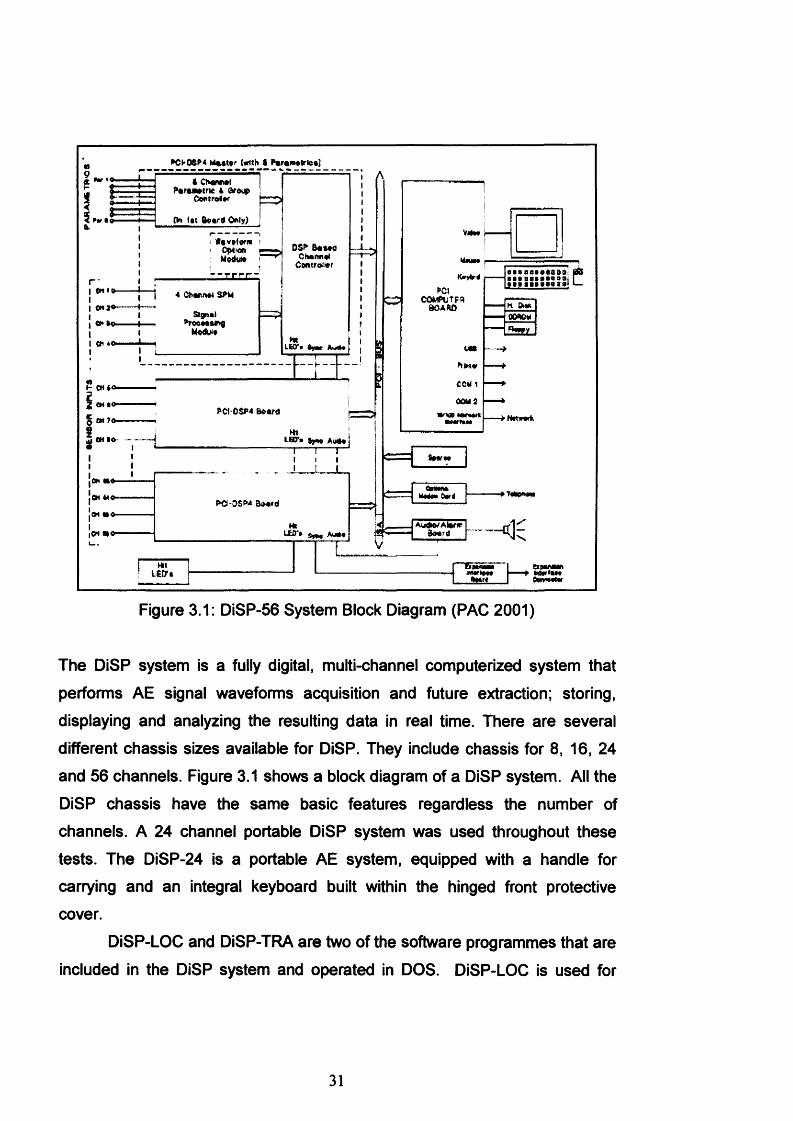
Figure 3.1: DiSP-56 System Block Diagram (PAC 2001)

The DiSP system is a fully digital, multi-channel computerized system that

performs AE signal waveforms acquisition and future extraction; storing, displaying and analyzing the resulting data in real time. There are several

different chassis sizes available for DiSP. They include chassis for 8, 16, 24

and 56 channels. Figure 3.1 shows a block diagram of a DiSP system. All the

DiSP chassis have the same basic features regardless the number of channels. A 24 channel portable DiSP system was used throughout these

tests. The DiSP-24 is a portable AE system, equipped with a handle for carrying and an integral keyboard built within the hinged front protective

cover.

DiSP-LOC and DiSP-TRA are two of the software programmes that are

included in the DiSP system and operated in DOS. DiSP-LOC is used for

31

source location and for providing AE feature data (representing measurable

characteristics of AE signals such as amplitude, AE signal energy, duration,

counts and rise time) for a statistical analysis of the detected AE signals. The

time-based information can also include parametric data from two channels. A

parametric input is an external voltage proportional to a test parameter such

as load, strain and deflection, which can assist in the analysis of the AE data.

Standalone software, DiSP-TRA, is the transient recorder analyzer software

that operates and controls the DiSP hardware to collect, transfer, display,

process and store complete waveforms detected from each AE channel in the

system. DiSP-TRA, enables AE signal waveforms to be recorded both

independently on all channels or synchronized. In synchronized mode, the

first hit channel triggers all other synchonised channels and the arrival hit-time

between different channels can be determined. The speed at which the

sensors are energized is negligible compared to the speed of the signal because they actually recording continuously.

AE WIN is additional software programmes that can be used in DiSP

based products and operated in WINDOWS. The AE WIN program runs

under the WINDOW 2000/XP operating systems. The software has all the

acquisition, graphing and analysis capabilities that are expected in an AE

system. Some of the AE WIN capabilities include multiple copies can be run

at once, a framework for easily adding graphs is provided, has various tools

bars that can be selected and many enhanced features are built in including

graph zooming, panning and a setup icon toolbar. Additionally, 2D and 3D

graphing are possible in AE WIN. AE Win consists of AE mode and TRA

mode. AE mode is used for source location and for providing AE feature data

for a statistical analysis of the detected AE signals Switching AE mode to TRA

mode enables data collection options that were available in the PAC TRA

programs. The most notable is the ability to collect waveform data using a

synchronized and/or external trigger. The TRA mode is only a waveform

collection mode.

32

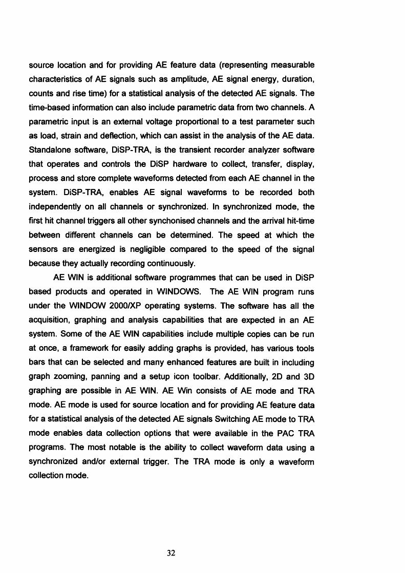
3.2.2 AE SensorsThe main function of AE sensors is to convert the mechanical wave into an

electrical AE signal. The schematic diagram of a typical AE sensor mounted

on a test object is shown in Figure 3.2. The sensor is attached to the surface

of the test object and a thin intervening layer of couplant is usually used. Peizoelectric sensors are principally used due to their high sensitivity,

robustness, ease of use and wide range of response characteristics at a

relatively low cost. The element is usually a special ceramic such as lead

zirconate titanate (PZT) (Mclntire and Miller 1987).An AE sensor normally consists of several components. The wear plate

protects the inside element known as the piezoelectric ceramic. The

piezoelectric ceramic is the active element with electrodes on each face. One

electrode is connected to earth and the other is connected to the signal lead.The active element is surrounded by a damping material which is

usually made by curing an epoxy containing high density particles. The

material is designed so that acoustic waves can propagate easily with minor

reflection back to the active element.The typical AE sensor also has a case with a connector for a signal

cable attachment. The case provides an integrated mechanical package for the sensor components and may also serve as a shield to minimize

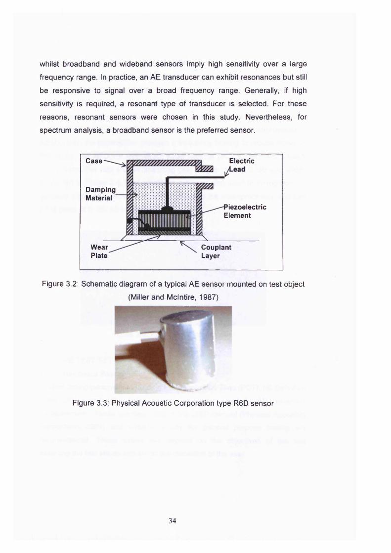
electromagnetic interference.Throughout this laboratory test, the only sensor used is a Physical

Acoustic Corporation (PAC) type R6D (Figure 3.3) with an operating

frequency range of 35-100 kHz and resonant frequency at 60 kHz. This

sensor is chosen based on a study by Beck (2004) of the optimum selection

of AE sensors which suggested that the 7 kHz, 15 kHz, 30 kHz and 60 kHz

resonant frequency sensors were suitable for concrete monitoring. The

highest frequency was chosen in order to optimize the signal to noise ratio

and because the signal attenuates quickly in concrete (Beck, 2004).As well as resonant sensors, broadband sensors can also be used in

AE. Resonant sensor implies high sensitivity over a narrow frequency range

33

whilst broadband and wideband sensors imply high sensitivity over a large

frequency range. In practice, an AE transducer can exhibit resonances but still

be responsive to signal over a broad frequency range. Generally, if high

sensitivity is required, a resonant type of transducer is selected. For these

reasons, resonant sensors were chosen in this study. Nevertheless, for

spectrum analysis, a broadband sensor is the preferred sensor.

iezoelectric

DampingMaterial

Element

WearPlate

CouplantLayer

Case Electric

Figure 3.2: Schematic diagram of a typical AE sensor mounted on test object

(Miller and Mclntire, 1987)

Figure 3.3: Physical Acoustic Corporation type R6D sensor

34

3.2.3 The Preamplifier and Main AmplifierAccording to Beattie (1983), when a cable is connected to an amplifier via a

long coaxial cable, there will be a loss in sensor sensitivity. The common way

to minimize interference is to place a preamplifier close to the transducer;

furthermore, many transducers today are equipped with integrated

preamplifiers and a variable gain amplifier in the main instrumentation.

Additionally, the preamplifier provides a frequency filtering to reduce noise. In

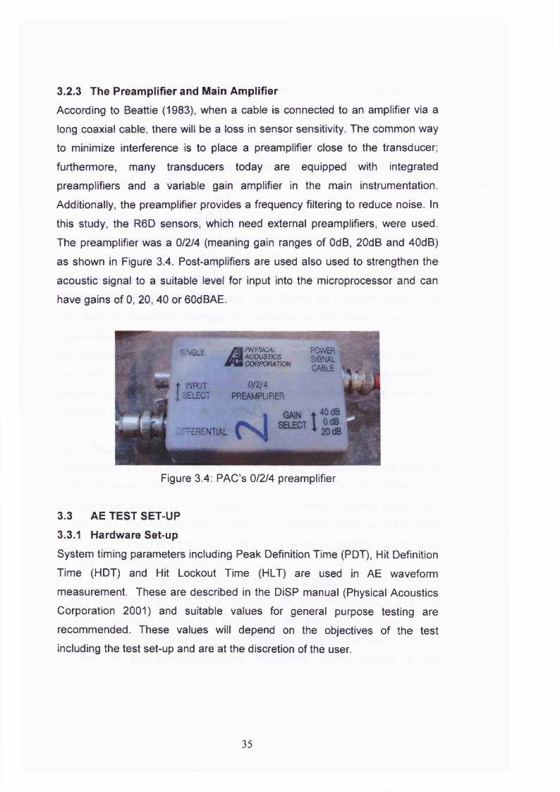
this study, the R6D sensors, which need external preamplifiers, were used.

The preamplifier was a 0/2/4 (meaning gain ranges of OdB, 20dB and 40dB)

as shown in Figure 3.4. Post-amplifiers are used also used to strengthen the

acoustic signal to a suitable level for input into the microprocessor and can

have gains of 0, 20, 40 or 60dBAE.

PHYSICALACOUSTICSCORPORATION

POWERSIGNAL

SINGLE

CABLE

0/2/4PREAMPLIFIER

t INPUT I SELECT

INFERENTIAL

Figure 3.4: PAC’s 0/2/4 preamplifier

3.3 AE TEST SET-UP3.3.1 Hardware Set-upSystem timing parameters including Peak Definition Time (PDT), Hit Definition

Time (HDT) and Hit Lockout Time (HLT) are used in AE waveform

measurement. These are described in the DiSP manual (Physical Acoustics

Corporation 2001) and suitable values for general purpose testing are

recommended. These values will depend on the objectives of the test

including the test set-up and are at the discretion of the user.

35

The hit data set (the set of numbers representing signal features and other

information, stored as result of a hit) allows selection of the measured

parameters to be included in the description of each AE hit; including the

waveforms that are to be collected. In the parametric set-up, hit allows a

scaling of the voltage measured so that load and displacement values can be

displayed in the units (kN, mm) respectively.

3.3.2 Initiation, Layout and Data FilesThe most important files in the AE WIN and DiSP-LOC software are the Setup

Files which are called Layout files in AE WIN and Initiation files in DiSP-LOC

and distinguished by the suffix .LAY and .INI respectively. AE Test Data Files

are identified by a filename extension .DTA. These are the same Setup Files

but due to extensive changes in migrating to Windows, many extra

capabilities have been added to the set up of the system. Therefore, the .INI

file can only be used with the DOS software (DiSP-LOC) while the .LAY file

can only be used with AEWIN software. However, there is compatibility

between the data file structures and AE.DTA data files can be read and

displayed by either the DOS or the AE WIN software.

3.3.3 Source Location Modes and Set-upOne ideal for an NDT technique for structure health monitoring is the ability to

locate damage. The ability to locate sources of AE is one of the most important functions of the multi-channel instrumentation systems used in test

applications. The AE wave can be detected in the form of hits on one or more

channels. An event is a group of hits that is received on multiple sensors from

a single signal source occurrence.

In DiSP-LOC and AE WIN there are several types of source locations - zonal, linear, arbitrary and added extras in AE WIN such as 2D planar, 3D

location, cylindrical, conical and spherical. In this study linear, 2D planar and

3D location modes will be used. These modes represent the source location

in one, two and three dimensions respectively. Linear location is very

36

functional in the investigation of AE wave propagation in concrete structures

and in monitoring crack propagations when the position of the source is

known to be somewhere along a straight line between a pair of transducers

attached to the beam. A three dimensional approach is required when

monitoring large structures, such as bridges, to identify the exact location of

the damage.

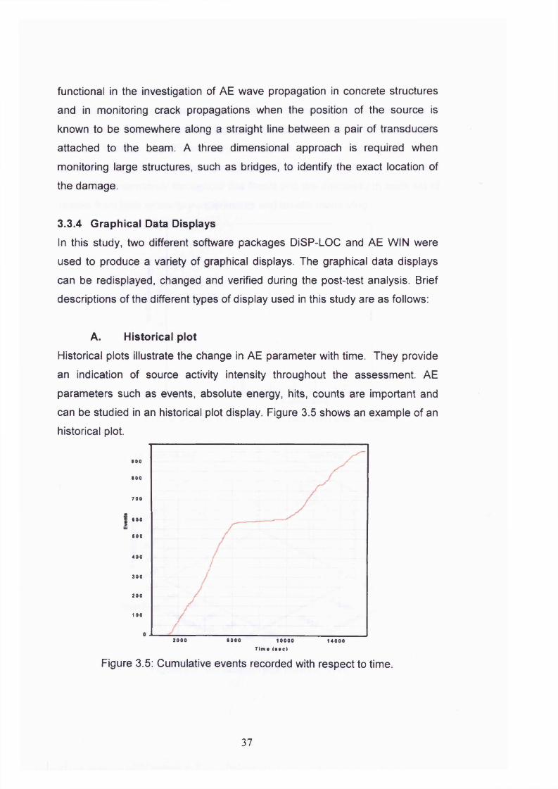
3.3.4 Graphical Data DisplaysIn this study, two different software packages DiSP-LOC and AE WIN were

used to produce a variety of graphical displays. The graphical data displays

can be redisplayed, changed and verified during the post-test analysis. Brief

descriptions of the different types of display used in this study are as follows:

A. Historical plotHistorical plots illustrate the change in AE parameter with time. They provide

an indication of source activity intensity throughout the assessment. AE

parameters such as events, absolute energy, hits, counts are important and

can be studied in an historical plot display. Figure 3.5 shows an example of an

historical plot.

too

too

7 0 0

000lli

soo

4 0 0

3 0 0

200

100

2000 0000 10000 1 4 0 0 0

T i m * ( » * c )

Figure 3.5: Cumulative events recorded with respect to time.

37

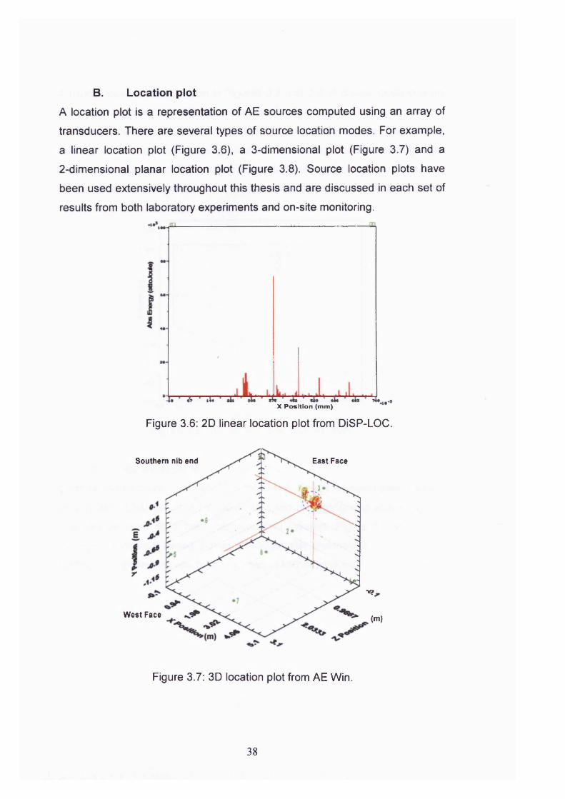
B. Location plotA location plot is a representation of AE sources computed using an array of

transducers. There are several types of source location modes. For example,

a linear location plot (Figure 3.6), a 3-dimensional plot (Figure 3.7) and a

2-dimensional planar location plot (Figure 3.8). Source location plots have

been used extensively throughout this thesis and are discussed in each set of

results from both laboratory experiments and on-site monitoring.

X Position (m m)

Figure 3.6: 2D linear location plot from DiSP-LOC.

Southern nib end East Face

X?

West Face (m)

Figure 3.7: 3D location plot from AE Win.

38

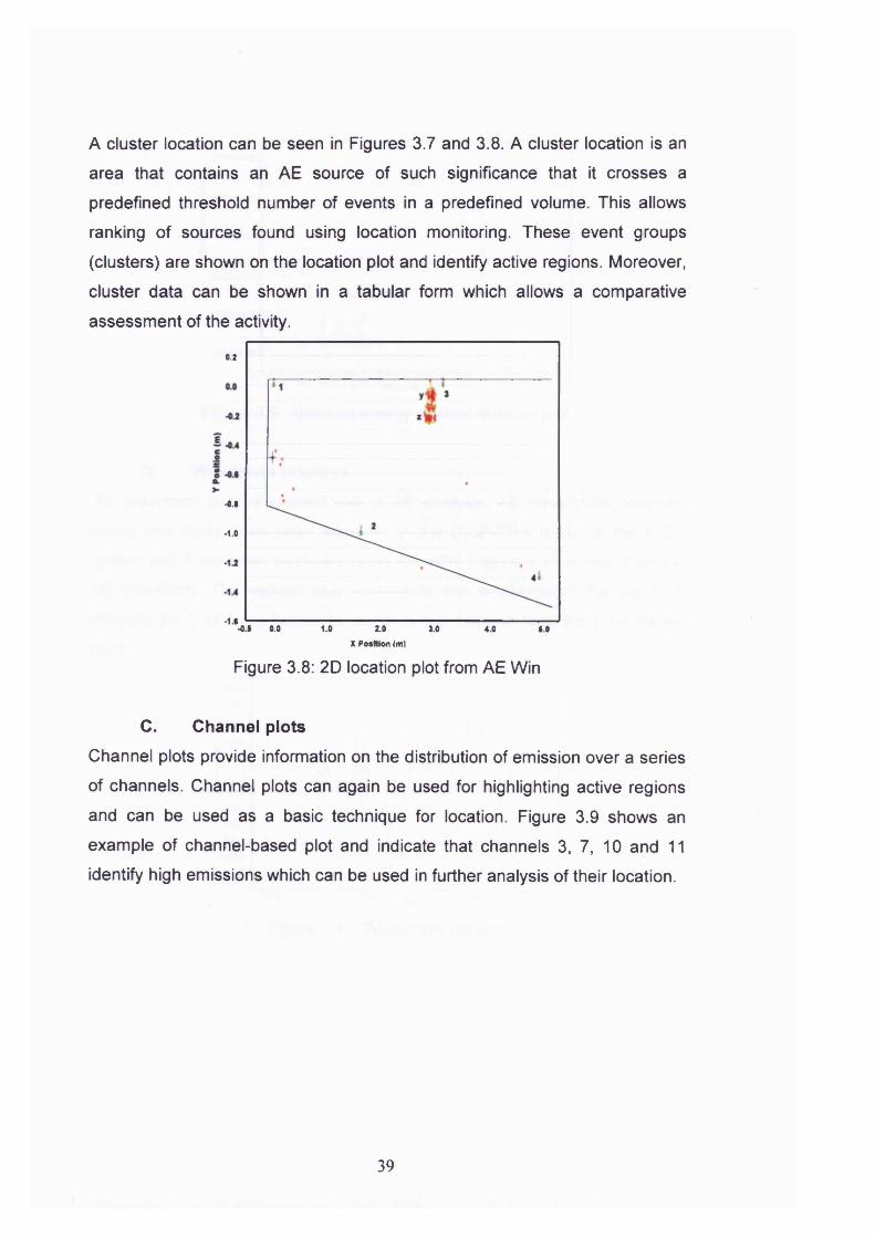
A cluster location can be seen in Figures 3.7 and 3.8. A cluster location is an

area that contains an AE source of such significance that it crosses a

predefined threshold number of events in a predefined volume. This allows

ranking of sources found using location monitoring. These event groups

(clusters) are shown on the location plot and identify active regions. Moreover,

cluster data can be shown in a tabular form which allows a comparative

assessment of the activity.

0.2

-0.1

- 1.0

-1.0•OS 0.0 1.0 2.0 3.0 4.0 S.0

X P osition (m l

Figure 3.8: 2D location plot from AE Win

C. Channel plotsChannel plots provide information on the distribution of emission over a series

of channels. Channel plots can again be used for highlighting active regions

and can be used as a basic technique for location. Figure 3.9 shows an

example of channel-based plot and indicate that channels 3, 7, 10 and 11

identify high emissions which can be used in further analysis of their location.

39

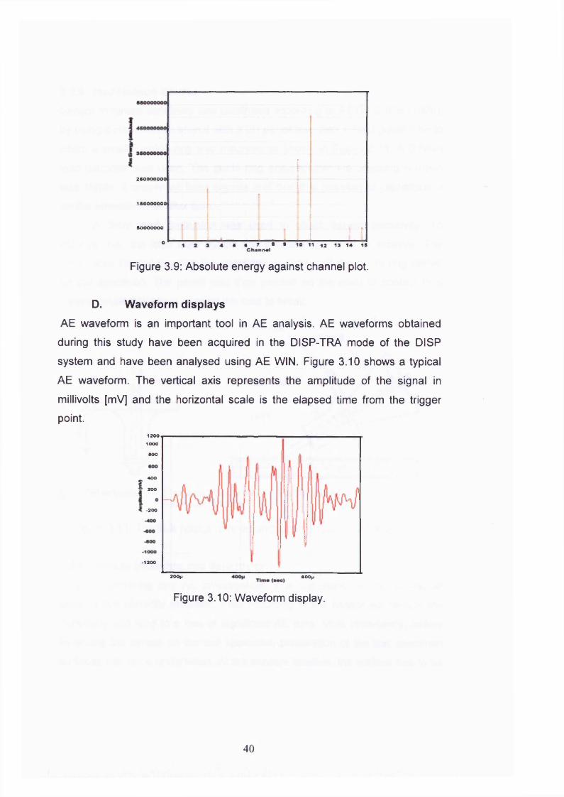
2 60000000

160000000

60000000

0I I

6 6 7 • • 10 11 1 2 19 14 16C h a n n e l

Figure 3.9: Absolute energy against channel plot.

D. Waveform displaysAE waveform is an important tool in AE analysis. AE waveforms obtained

during this study have been acquired in the DISP-TRA mode of the DISP

system and have been analysed using AE WIN. Figure 3.10 shows a typical

AE waveform. The vertical axis represents the amplitude of the signal in

millivolts [mV] and the horizontal scale is the elapsed time from the trigger

point.1200

1000

800

400

200

-200

-1200

200|i 600p

Figure 3.10: Waveform display.

40

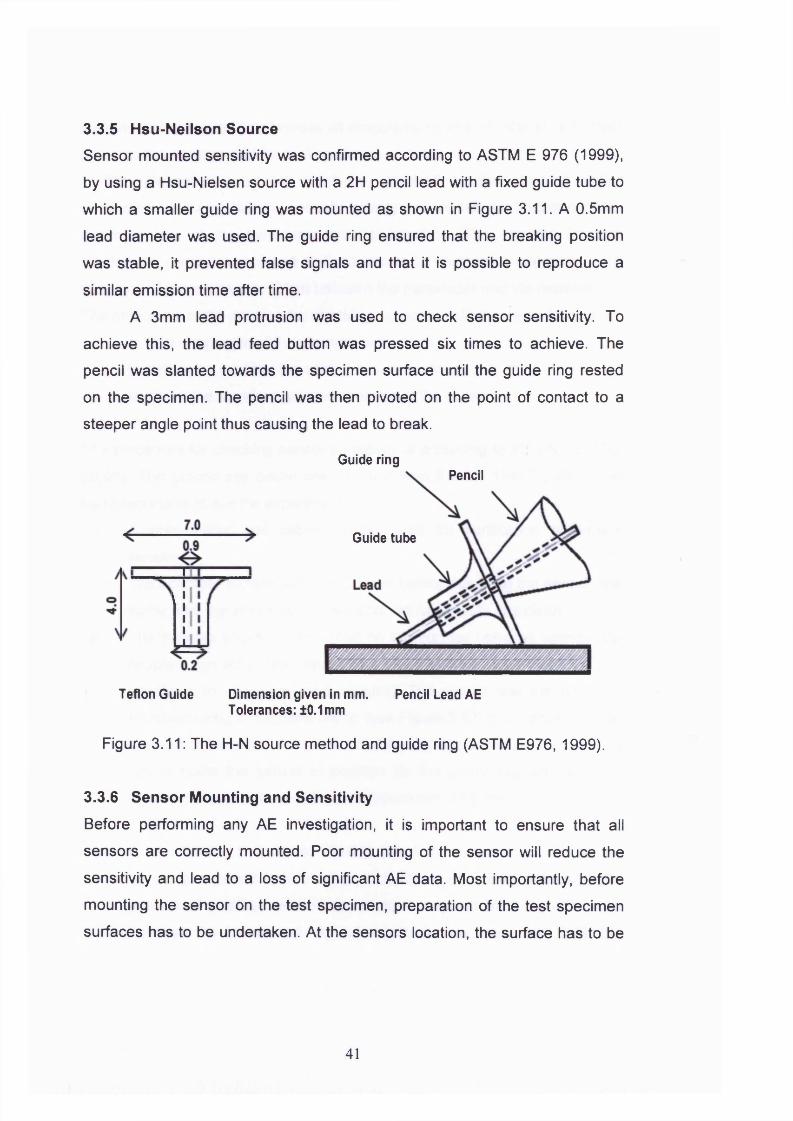
3.3.5 Hsu-Neilson SourceSensor mounted sensitivity was confirmed according to ASTM E 976 (1999),

by using a Hsu-Nielsen source with a 2H pencil lead with a fixed guide tube to

which a smaller guide ring was mounted as shown in Figure 3.11. A 0.5mm

lead diameter was used. The guide ring ensured that the breaking position

was stable, it prevented false signals and that it is possible to reproduce a

similar emission time after time.

A 3mm lead protrusion was used to check sensor sensitivity. To

achieve this, the lead feed button was pressed six times to achieve. The

pencil was slanted towards the specimen surface until the guide ring rested

on the specimen. The pencil was then pivoted on the point of contact to a

steeper angle point thus causing the lead to break.

Teflon Guide Dimension given in mm. Pencil Lead AE Tolerances: ±0.1 mm

Figure 3.11: The H-N source method and guide ring (ASTM E976, 1999).

3.3.6 Sensor Mounting and Sensitivity

Before performing any AE investigation, it is important to ensure that all

sensors are correctly mounted. Poor mounting of the sensor will reduce the

sensitivity and lead to a loss of significant AE data. Most importantly, before

mounting the sensor on the test specimen, preparation of the test specimen

surfaces has to be undertaken. At the sensors location, the surface has to be

Guide ringPencil

Guide tube

41

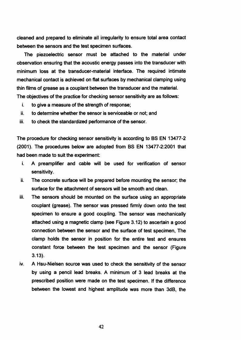
cleaned and prepared to eliminate all irregularity to ensure total area contact

between the sensors and the test specimen surfaces.The piezoelectric sensor must be attached to the material under

observation ensuring that the acoustic energy passes into the transducer with

minimum loss at the transducer-material interface. The required intimate

mechanical contact is achieved on flat surfaces by mechanical clamping using

thin films of grease as a couplant between the transducer and the material.

The objectives of the practice for checking sensor sensitivity are as follows:

i. to give a measure of the strength of response;ii. to determine whether the sensor is serviceable or not; and

iii. to check the standardized performance of the sensor.

The procedure for checking sensor sensitivity is according to BS EN 13477-2

(2001). The procedures below are adopted from BS EN 13477-2:2001 that

had been made to suit the experiment:i. A preamplifier and cable will be used for verification of sensor

sensitivity.ii. The concrete surface will be prepared before mounting the sensor; the

surface for the attachment of sensors will be smooth and clean.

iii. The sensors should be mounted on the surface using an appropriatecouplant (grease). The sensor was pressed firmly down onto the test specimen to ensure a good coupling. The sensor was mechanically

attached using a magnetic clamp (see Figure 3.12) to ascertain a good

connection between the sensor and the surface of test specimen, The

clamp holds the sensor in position for the entire test and ensures

constant force between the test specimen and the sensor (Figure

3.13).

iv. A Hsu-Nielsen source was used to check the sensitivity of the sensor

by using a pencil lead breaks. A minimum of 3 lead breaks at the

prescribed position were made on the test specimen. If the difference

between the lowest and highest amplitude was more than 3dB, the

42

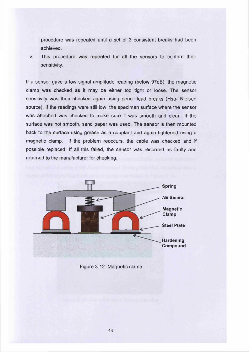
procedure was repeated until a set of 3 consistent breaks had been

achieved.

v. This procedure was repeated for all the sensors to confirm their

sensitivity.

If a sensor gave a low signal amplitude reading (below 97dB), the magnetic

clamp was checked as it may be either too tight or loose. The sensor

sensitivity was then checked again using pencil lead breaks (Hsu- Nielsen

source). If the readings were still low, the specimen surface where the sensor

was attached was checked to make sure it was smooth and clean. If the

surface was not smooth, sand paper was used. The sensor is then mounted

back to the surface using grease as a couplant and again tightened using a

magnetic clamp. If the problem reoccurs, the cable was checked and if

possible replaced. If all this failed, the sensor was recorded as faulty and

returned to the manufacturer for checking.

Spring

AE Sensor

MagneticClamp

Steel Plate

Hardening Compound

Figure 3.12: Magnetic clamp

43

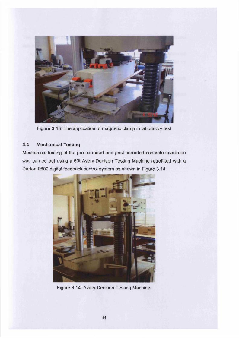
Figure 3.13: The application of magnetic clamp in laboratory test

3.4 Mechanical TestingMechanical testing of the pre-corroded and post-corroded concrete specimen

was carried out using a 60t Avery-Denison Testing Machine retrofitted with a

Dartec-9600 digital feedback control system as shown in Figure 3.14.

Figure 3.14: Avery-Denison Testing Machine.

44

The precautions that were taken before and during testing the concrete

specimen with AE were as follows:

a) A layer of rubber was placed between the loading point and concrete

specimen to minimise any unwanted noise that might be recorded by

the AE sensors.b) A very low load (1kN) was applied for 2 minutes to ensure that no noise

was recorded from the testing machine.

c) At least 2 minutes was allowed between each loading step and before

pausing the DiSP system in order to check for visible damage.d) Visible damage was recorded by digital camera and sketches of the

damage were produced.

45

CHAPTER 4: LABORATORY FLEXURAL TESTING ON REINFORCED

CONCRETE BEAM WITH PRE AND POST CORRODED REINFORCING

BAR

4.1 INTRODUCTIONThis chapter contains a detailed description of the experimental work carried

out and highlights the procedures followed during the laboratory stage of the

project. This section covers the materials, the initial casting and preparation of

the specimens and finally the four-point bending test monitored using Acoustic

Emission (AE) sensor system. As well as this, the problems encountered, possible sources of error and the precautions taken have been included.

A parameter-based approach was used in the analysis of data acquired

by the AE instrumentation. The parameter-based approach evaluates relative

AE activities based on the measurement of parameters such as hits, amplitudes, absolute energy, etc. This method of analysis has been shown to

be sensitive to the initiation and the growth of cracks within materials and

structures. Moreover, the application of Time of Arrival (TOA) method has

been used to determine the location of the damage area in linear location

between sensors.Two types of test specimen have been used in this laboratory work:

pre-corroded (PR) specimen and post-corroded (PS) specimen. The corroded

reinforcement exhibited a reduction of the bar section and also degradation of

the composite bond between steel rebar and concrete. Pre-corroded

reinforcement was cleaned before being cast in the concrete but for post­

corroded reinforcement, the corrosion product was developed inside the

beam, while experiencing an impressed current to accelerate the corrosion.

46

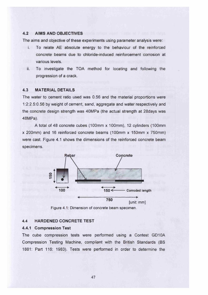
4.2 AIMS AND OBJECTIVESThe aims and objective of these experiments using parameter analysis were:

i. To relate AE absolute energy to the behaviour of the reinforced

concrete beams due to chloride-induced reinforcement corrosion at

various levels.

ii. To investigate the TOA method for locating and following the

progression of a crack.

4.3 MATERIAL DETAILSThe water to cement ratio used was 0.56 and the material proportions were

1:2:2.5:0.56 by weight of cement, sand, aggregate and water respectively and

the concrete design strength was 40MPa (the actual strength at 28days was

48MPa).

A total of 48 concrete cubes (100mm x 100mm), 12 cylinders (100mm

x 200mm) and 16 reinforced concrete beams (100mm x 150mm x 750mm)

were cast. Figure 4.1 shows the dimensions of the reinforced concrete beam

specimens.

Rebar Concrete

oto

<■100 150<- Corroded length

[unit: mm]Figure 4.1: Dimension of concrete beam specimen.

4.4 HARDENED CONCRETE TEST4.4.1 Compression TestThe cube compression tests were performed using a Contest GD10A

Compression Testing Machine, compliant with the British Standards (BS

1881: Part 116: 1983). Tests were performed in order to determine the

47

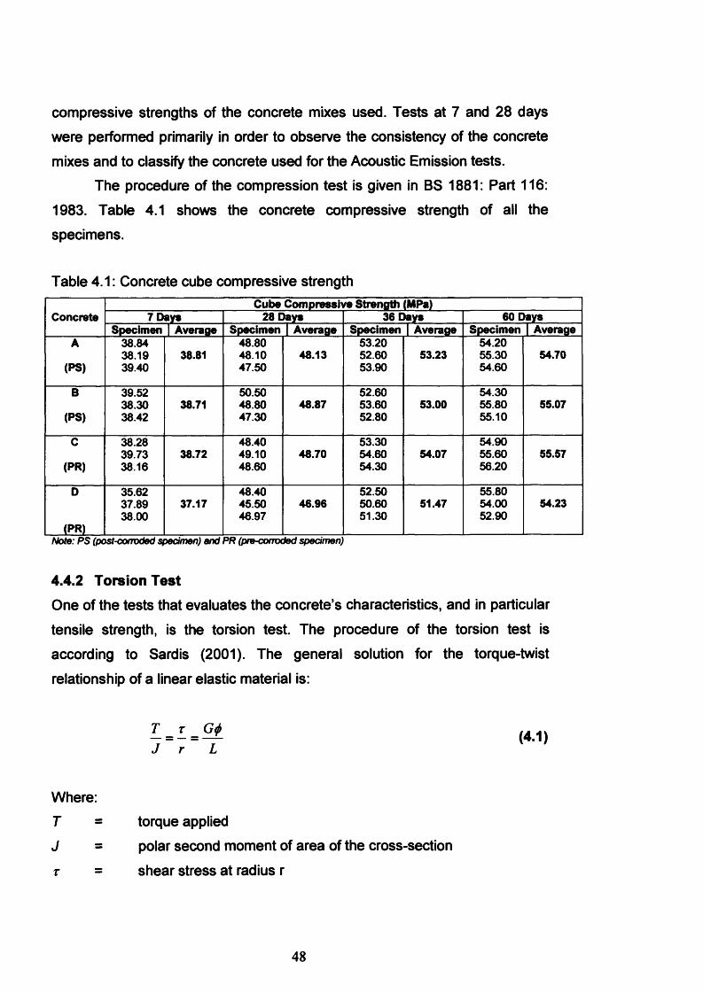
compressive strengths of the concrete mixes used. Tests at 7 and 28 days

were performed primarily in order to observe the consistency of the concrete

mixes and to classify the concrete used for the Acoustic Emission tests.The procedure of the compression test is given in BS 1881: Part 116:

1983. Table 4.1 shows the concrete compressive strength of all the

specimens.

Table 4.1: Concrete cube compressive strength

ConcreteCube Compressive Strength (MPa)

7 Days 28 Days 36 Days 60 DaysSpecimen Average Specimen Average Specimen Average Specimen Average

A 38.84 48.80 53.20 54.2038.19 38.81 48.10 48.13 52.60 53.23 55.30 54.70

(PS) 39.40 47.50 53.90 54.60

B 39.52 50.50 52.60 54.3038.30 38.71 48.80 48.87 53.60 53.00 55.80 55.07

(PS) 38.42 47.30 52.80 55.10

c 38.28 48.40 53.30 54.9039.73 38.72 49.10 48.70 54.60 54.07 55.60 55.57

(PR) 38.16 48.60 54.30 56.20

D

(PR)

35.6237.8938.00

37.1748.4045.5046.97

46.9652.5050.6051.30

51.4755.8054.0052.90

54.23

Note: PS (post-corroded specimen) end PR (pre-corroded specimen)

4.4.2 Torsion TestOne of the tests that evaluates the concrete’s characteristics, and in particular tensile strength, is the torsion test. The procedure of the torsion test is

according to Sardis (2001). The general solution for the torque-twist

relationship of a linear elastic material is:

Where:T

J

T =

l = L = 2 l (4.1)J r L

torque appliedpolar second moment of area of the cross-section

shear stress at radius r

48

r

G

L

an average radius

shearing moduluslength over which rotation <t> is measured

The equation can be rearranged in order to determine the shear stress and

shearing modulus respectively:

" 7 <“ >

P

For a brittle material, which is weak in tension, failure in a torsion test is

expected to happen by tensile fracture at 45° to the longitudinal axis of the

core. According to Norris et. al. 1990 (as cited in Sardis, 2001), the maximum

elastic shear stress fsmax at the surface of the specimen approaches a limiting

value equal to 0.85 times the uniaxial tensile strength of the material ft.

/ . « = 0-85/, (4-4)

The torsion test method used in this work was developed from Norris et.

al.,1990 (as cited in Sardis M., 2001). In this test, torsion rings are used to

apply equal and opposite couples to each end of the test specimen. Two

supports provide upward reactions; and a load is applied to the free end.

Corresponding reactions are generated at the two supports. The load is

transferred from the rig into the concrete core by a set of split collars, attached

to either end of the test specimen using a small amount of adhesive, and

drawn together around the core by hand tightening pairs of nuts.

The system of load and reaction points has been designed such that

the distance between the pairs of loads on the collars is fixed at 250mm. Thus

the applied torque can be expressed as:

T = 0.25P (4.5)

49

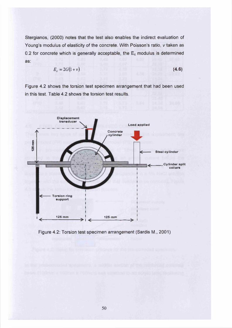
Stergianos, (2000) notes that the test also enables the indirect evaluation of

Young’s modulus of elasticity of the concrete. With Poisson’s ratio, v taken as

0.2 for concrete which is generally acceptable, the Ec modulus is determined

as:

E c = 2G (l + v) (4.6)

Figure 4.2 shows the torsion test specimen arrangement that had been used

in this test. Table 4.2 shows the torsion test results.

Displacementtransducer

Load applied

Concretecylinder

----[

Torsion ring support

125 mm 125 mm

Steel cylinder

Cylinder split collars

Figure 4.2: Torsion test specimen arrangement (Sardis M., 2001)

50

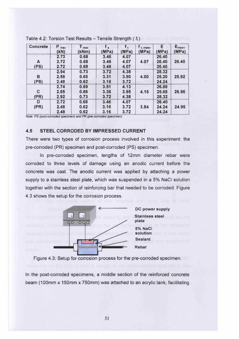
Table 4.2: Torsion Test Results - Tensile Strength ( ft)

Concrete P max(kN)

T max(kNm)

f ,(MPa)

f t(MPa)

f t, mean(MPa)

E(MPa)

Emean(MPa)

2.73 0.68 3.46 4.07 26.40A 2.72 0.68 3.46 4.07 4.07 26.40 26.40

(PS) 2.72 0.68 3.46 4.07 26.402.94 0.73 3.72 4.38 28.32

B 2.58 0.65 3.31 3.90 4.00 25.20 25.92(PS) 2.48 0.62 3.16 3.72 24.24

2.74 0.69 3.51 4.13 26.88c 2.65 0.66 3.36 3.95 4.15 25.68 26.96

(PR) 2.92 0.73 3.72 4.38 28.32D 2.72 0.68 3.46 4.07 26.40

(PR) 2.48 0.62 3.16 3.72 3.84 24.24 24.962.48 0.62 3.16 3.72 24.24

Note: PS (post-corroded specimen) and PR (pre-corroded specimen)

4.5 STEEL CORRODED BY IMPRESSED CURRENTThere were two types of corrosion process involved in this experiment: the

pre-corroded (PR) specimen and post-corroded (PS) specimen.

In pre-corroded specimen, lengths of 12mm diameter rebar were

corroded to three levels of damage using an anodic current before the

concrete was cast. The anodic current was applied by attaching a power

supply to a stainless steel plate, which was suspended in a 5% NaCI solution

together with the section of reinforcing bar that needed to be corroded. Figure

4.3 shows the setup for the corrosion process.

ED QDC power supply

Stainless steel plate

5% NaCI solutionSealant

Rebar

Figure 4.3: Setup for corrosion process for the pre-corroded specimen.

In the post-corroded specimens, a middle section of the reinforced concrete

beam (100mm x 150mm x 750mm) was attached to an acrylic tank, facilitating

51

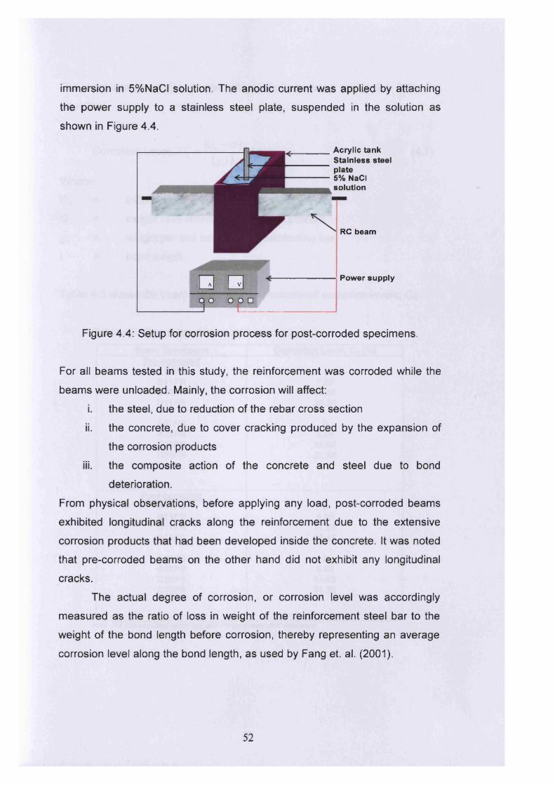
immersion in 5%NaCI solution. The anodic current was applied by attaching

the power supply to a stainless steel plate, suspended in the solution as

shown in Figure 4.4.

H

P V P B P I> S H M R P

□Q ° o o □

Acrylic tank Stainless steel plate 5% NaCI solution

RC beam

Power supply

Figure 4.4: Setup for corrosion process for post-corroded specimens.

For all beams tested in this study, the reinforcement was corroded while the

beams were unloaded. Mainly, the corrosion will affect:

i. the steel, due to reduction of the rebar cross section

ii. the concrete, due to cover cracking produced by the expansion of

the corrosion products

iii. the composite action of the concrete and steel due to bond

deterioration.

From physical observations, before applying any load, post-corroded beams

exhibited longitudinal cracks along the reinforcement due to the extensive

corrosion products that had been developed inside the concrete. It was noted

that pre-corroded beams on the other hand did not exhibit any longitudinal

cracks.

The actual degree of corrosion, or corrosion level was accordingly

measured as the ratio of loss in weight of the reinforcement steel bar to the

weight of the bond length before corrosion, thereby representing an average

corrosion level along the bond length, as used by Fang et. al. (2001).

52

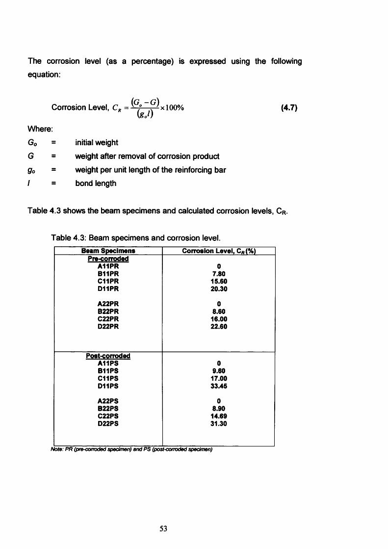
The corrosion level (as a percentage) is expressed using the following

equation:

Corrosion Level, CR = ^ f—^ x l0 0 % (4.7)\g0l)

Where:

G0 = initial weight

G = weight after removal of corrosion product

g0 = weight per unit length of the reinforcing barI = bond length

Table 4.3 shows the beam specimens and calculated corrosion levels, C r .

Table 4.3: Beam specimens and corrosion level.Beam Specimens Corrosion Level, CR(%)

Pre-corrodedA11PR 0B11PR 7.80C11PR 15.60D11PR 20.30

A22PR 0B22PR 8.60C22PR 16.00D22PR 22.60

Post-corrodedA11PS 0B11PS 9.60C11PS 17.00D11PS 33.45

A22PS 0B22PS 8.90C22PS 14.69D22PS 31.30

Note: PR (pre-corroded specimen) and PS (post-corroded specimen)

53

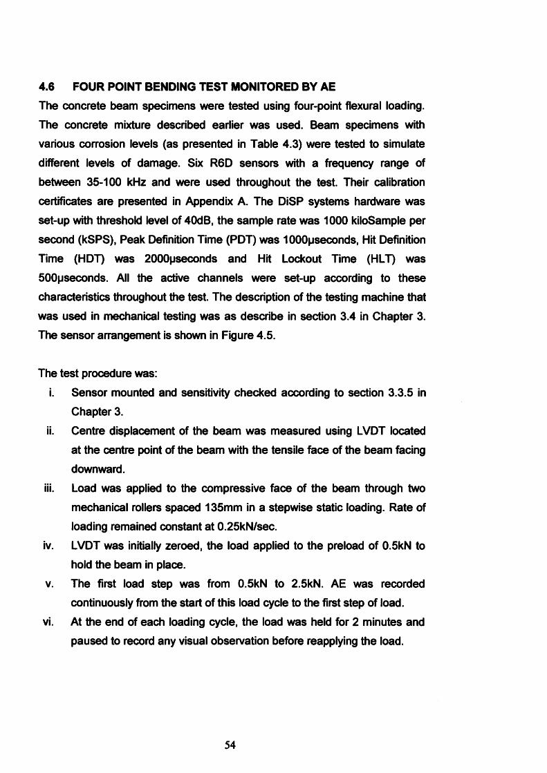
4.6 FOUR POINT BENDING TEST MONITORED BY AEThe concrete beam specimens were tested using four-point flexural loading.

The concrete mixture described earlier was used. Beam specimens with

various corrosion levels (as presented in Table 4.3) were tested to simulate

different levels of damage. Six R6D sensors with a frequency range of

between 35-100 kHz and were used throughout the test. Their calibration

certificates are presented in Appendix A. The DiSP systems hardware was

set-up with threshold level of 40dB, the sample rate was 1000 kiloSample per

second (kSPS), Peak Definition Time (PDT) was 1000pseconds, Hit Definition

Time (HDT) was 2000pseconds and Hit Lockout Time (HLT) was

500pseconds. All the active channels were set-up according to these

characteristics throughout the test. The description of the testing machine that

was used in mechanical testing was as describe in section 3.4 in Chapter 3. The sensor arrangement is shown in Figure 4.5.

The test procedure was:

i. Sensor mounted and sensitivity checked according to section 3.3.5 in

Chapter 3.

ii. Centre displacement of the beam was measured using LVDT located

at the centre point of the beam with the tensile face of the beam facing

downward.

iii. Load was applied to the compressive face of the beam through two

mechanical rollers spaced 135mm in a stepwise static loading. Rate of loading remained constant at 0.25kN/sec.

iv. LVDT was initially zeroed, the load applied to the preload of 0.5kN to

hold the beam in place.

v. The first load step was from 0.5kN to 2.5kN. AE was recorded

continuously from the start of this load cycle to the first step of load.vi. At the end of each loading cycle, the load was held for 2 minutes and

paused to record any visual observation before reapplying the load.

54

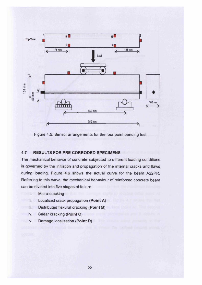
Top View g,0 *

< □ 5P 175 mm ^

I

Load

^ 185 mm ^

i

t650 mm

750 mm

100 mm

K »l

Figure 4.5: Sensor arrangements for the four point bending test.

4.7 RESULTS FOR PRE-CORRODED SPECIMENSThe mechanical behavior of concrete subjected to different loading conditions

is governed by the initiation and propagation of the internal cracks and flaws

during loading. Figure 4.6 shows the actual curve for the beam A22PR.

Referring to this curve, the mechanical behaviour of reinforced concrete beam

can be divided into five stages of failure:

Micro-cracking

Localized crack propagation (Point A)Distributed flexural cracking (Point B)

iv. Shear cracking (Point C)

v. Damage localization (Point D)

55

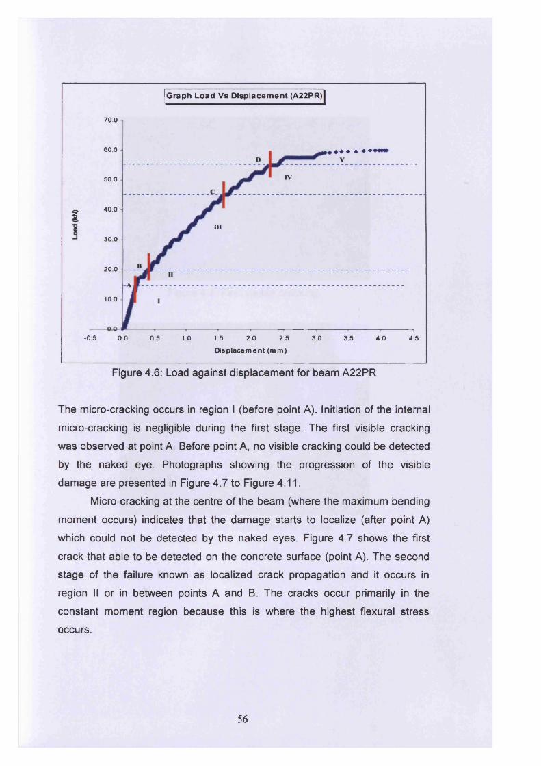
Graph Load Vs Displacement (A22PR)

70.0

60.0

IV50.0

40.0f

III

30.0

20.0 - -

A10.0

-0.5 0.0 0.5 1.0 1.5 2.0 2.5 3.0 3.5 4.0 4.5

Displacement (mm )

Figure 4.6: Load against displacement for beam A22PR

The micro-cracking occurs in region I (before point A). Initiation of the internal

micro-cracking is negligible during the first stage. The first visible cracking

was observed at point A. Before point A, no visible cracking could be detected

by the naked eye. Photographs showing the progression of the visible

damage are presented in Figure 4.7 to Figure 4.11.

Micro-cracking at the centre of the beam (where the maximum bending

moment occurs) indicates that the damage starts to localize (after point A)

which could not be detected by the naked eyes. Figure 4.7 shows the first

crack that able to be detected on the concrete surface (point A). The second

stage of the failure known as localized crack propagation and it occurs in

region II or in between points A and B. The cracks occur primarily in the

constant moment region because this is where the highest flexural stress

occurs.

56

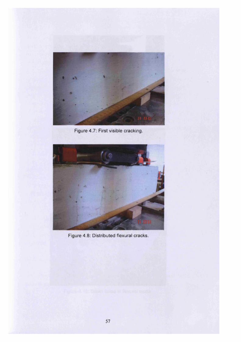
Figure 4.7: First visible cracking.

Figure 4.8: Distributed flexural cracks.

57

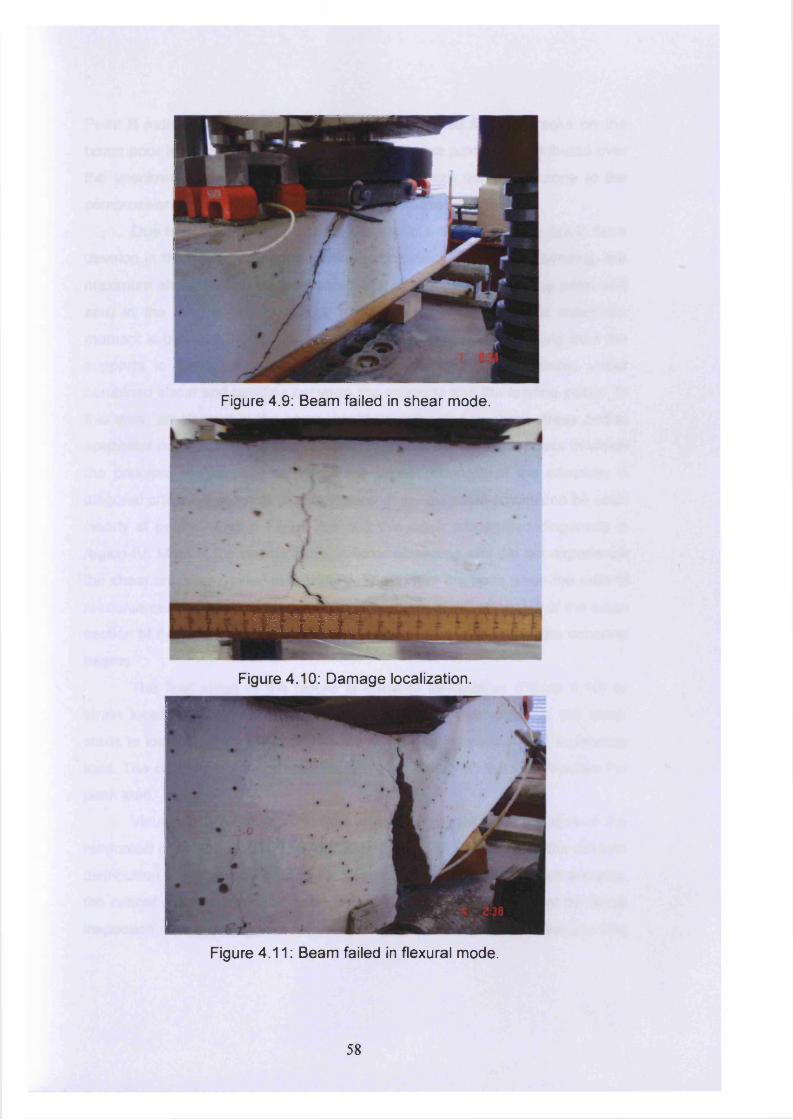
Figure 4.9: Beam failed in shear mode.

m m m m

Figure 4.10: Damage localization.

Figure 4.11: Beam failed in flexural mode.

58

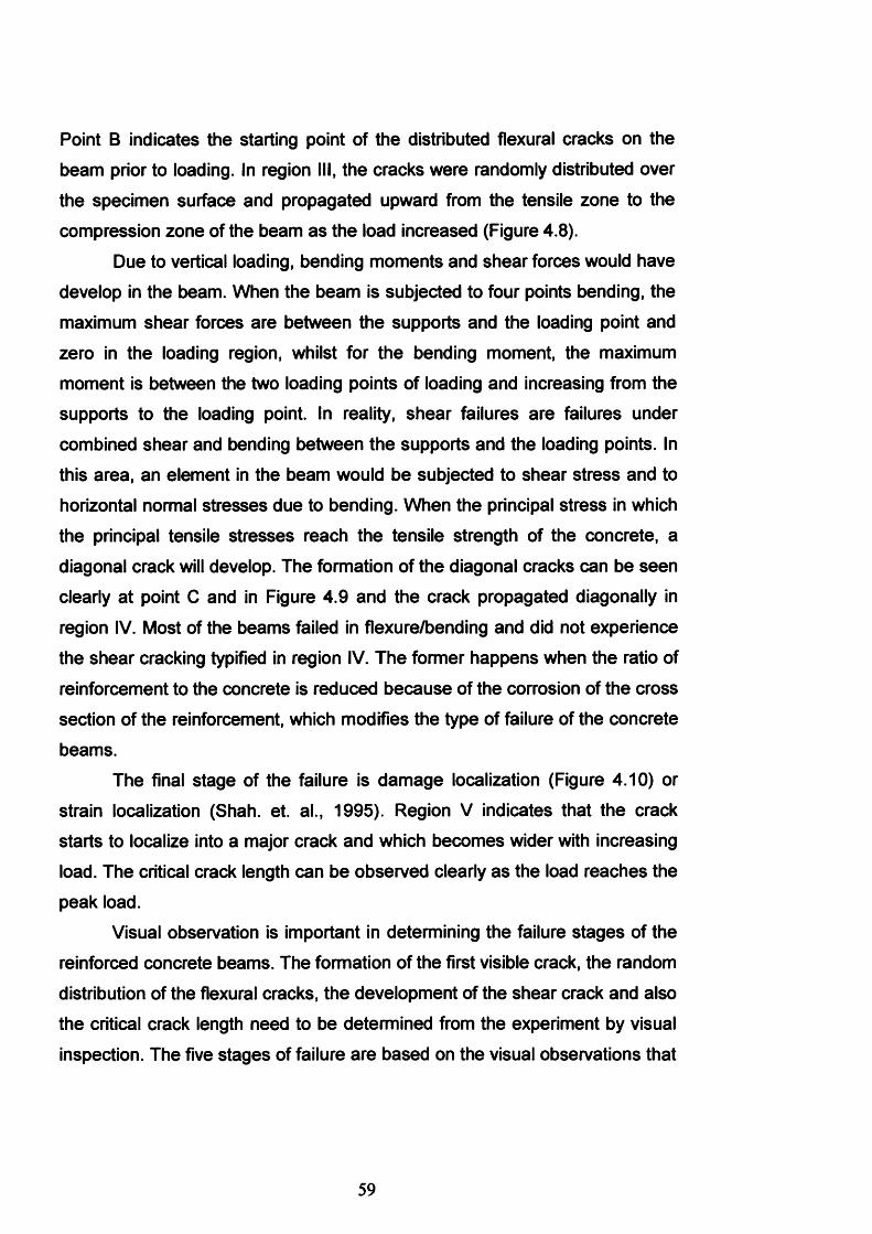
Point B indicates the starting point of the distributed flexural cracks on the

beam prior to loading. In region III, the cracks were randomly distributed over

the specimen surface and propagated upward from the tensile zone to the

compression zone of the beam as the load increased (Figure 4.8).

Due to vertical loading, bending moments and shear forces would have

develop in the beam. When the beam is subjected to four points bending, the

maximum shear forces are between the supports and the loading point and

zero in the loading region, whilst for the bending moment, the maximum

moment is between the two loading points of loading and increasing from the

supports to the loading point. In reality, shear failures are failures under

combined shear and bending between the supports and the loading points. In

this area, an element in the beam would be subjected to shear stress and to

horizontal normal stresses due to bending. When the principal stress in which

the principal tensile stresses reach the tensile strength of the concrete, a

diagonal crack will develop. The formation of the diagonal cracks can be seen

clearly at point C and in Figure 4.9 and the crack propagated diagonally in

region IV. Most of the beams failed in flexure/bending and did not experience

the shear cracking typified in region IV. The former happens when the ratio of

reinforcement to the concrete is reduced because of the corrosion of the cross

section of the reinforcement, which modifies the type of failure of the concrete

beams.The final stage of the failure is damage localization (Figure 4.10) or

strain localization (Shah. et. al., 1995). Region V indicates that the crack

starts to localize into a major crack and which becomes wider with increasing

load. The critical crack length can be observed clearly as the load reaches the

peak load.Visual observation is important in determining the failure stages of the

reinforced concrete beams. The formation of the first visible crack, the random

distribution of the flexural cracks, the development of the shear crack and also

the critical crack length need to be determined from the experiment by visual

inspection. The five stages of failure are based on the visual observations that

59

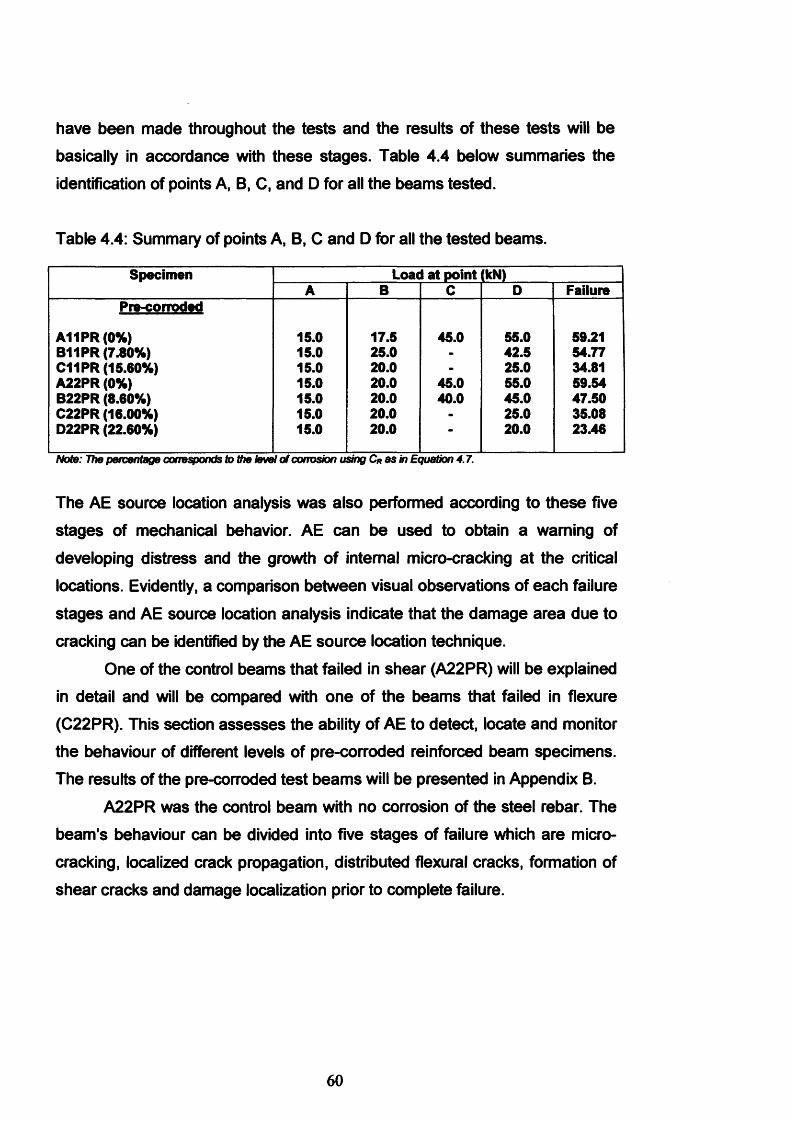
have been made throughout the tests and the results of these tests will be

basically in accordance with these stages. Table 4.4 below summaries the

identification of points A, B, C, and D for all the beams tested.

Table 4.4: Summary of points A, B, C and D for all the tested beams.

Specimen Load at point (kN)A B C D Failure

Pre-corroded

A11PR (0%) 15.0 17.5 45.0 55.0 59.21B11PR (7.80%) 15.0 25.0 - 42.5 54.77C11PR (15.60%) 15.0 20.0 - 25.0 34.81A22PR (0%) 15.0 20.0 45.0 55.0 59.54B22PR (8.60%) 15.0 20.0 40.0 45.0 47.50C22PR (16.00%) 15.0 20.0 - 25.0 35.08D22PR (22.60%) 15.0 20.0 “ 20.0 23.46

Note: The percentage corresponds to die level of corrosion using CRasin Equation 4.7.

The AE source location analysis was also performed according to these five

stages of mechanical behavior. AE can be used to obtain a warning of

developing distress and the growth of internal micro-cracking at the critical locations. Evidently, a comparison between visual observations of each failure

stages and AE source location analysis indicate that the damage area due to

cracking can be identified by the AE source location technique.

One of the control beams that failed in shear (A22PR) will be explained

in detail and will be compared with one of the beams that failed in flexure

(C22PR). This section assesses the ability of AE to detect, locate and monitor the behaviour of different levels of pre-corroded reinforced beam specimens. The results of the pre-corroded test beams will be presented in Appendix B.

A22PR was the control beam with no corrosion of the steel rebar. The

beam’s behaviour can be divided into five stages of failure which are micro­cracking, localized crack propagation, distributed flexural cracks, formation of

shear cracks and damage localization prior to complete failure.

60

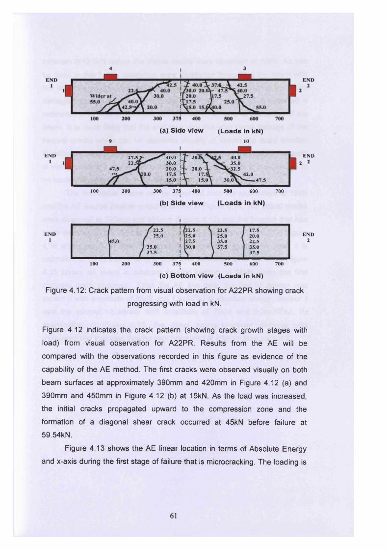
END

(a) Side view (Loads in kN)10

30J27.522.5]

40.030.020.0 17.5 15.0

40.035.0 32.5

147.5 20.0

10.0 i7.a15.0

42.030.0 47.5

100 200 300 375 400 500 600 700

(b) Side view (Loads in kN)

END

END1

22.525.0

22.525.0h7.5bo.o

22.525.035.037.5

17.5 20.022.5 35.037.5

5.035.037.5

100 200 300 375 400 500 600 700

END2

(c) Bottom view (Loads in kN)

Figure 4.12: Crack pattern from visual observation for A22PR showing crack

progressing with load in kN.

Figure 4.12 indicates the crack pattern (showing crack growth stages with

load) from visual observation for A22PR. Results from the AE will be

compared with the observations recorded in this figure as evidence of the

capability of the AE method. The first cracks were observed visually on both

beam surfaces at approximately 390mm and 420mm in Figure 4.12 (a) and

390mm and 450mm in Figure 4.12 (b) at 15kN. As the load was increased,

the initial cracks propagated upward to the compression zone and the

formation of a diagonal shear crack occurred at 45kN before failure at

59.54kN.

Figure 4.13 shows the AE linear location in terms of Absolute Energy

and x-axis during the first stage of failure that is microcracking. The loading is

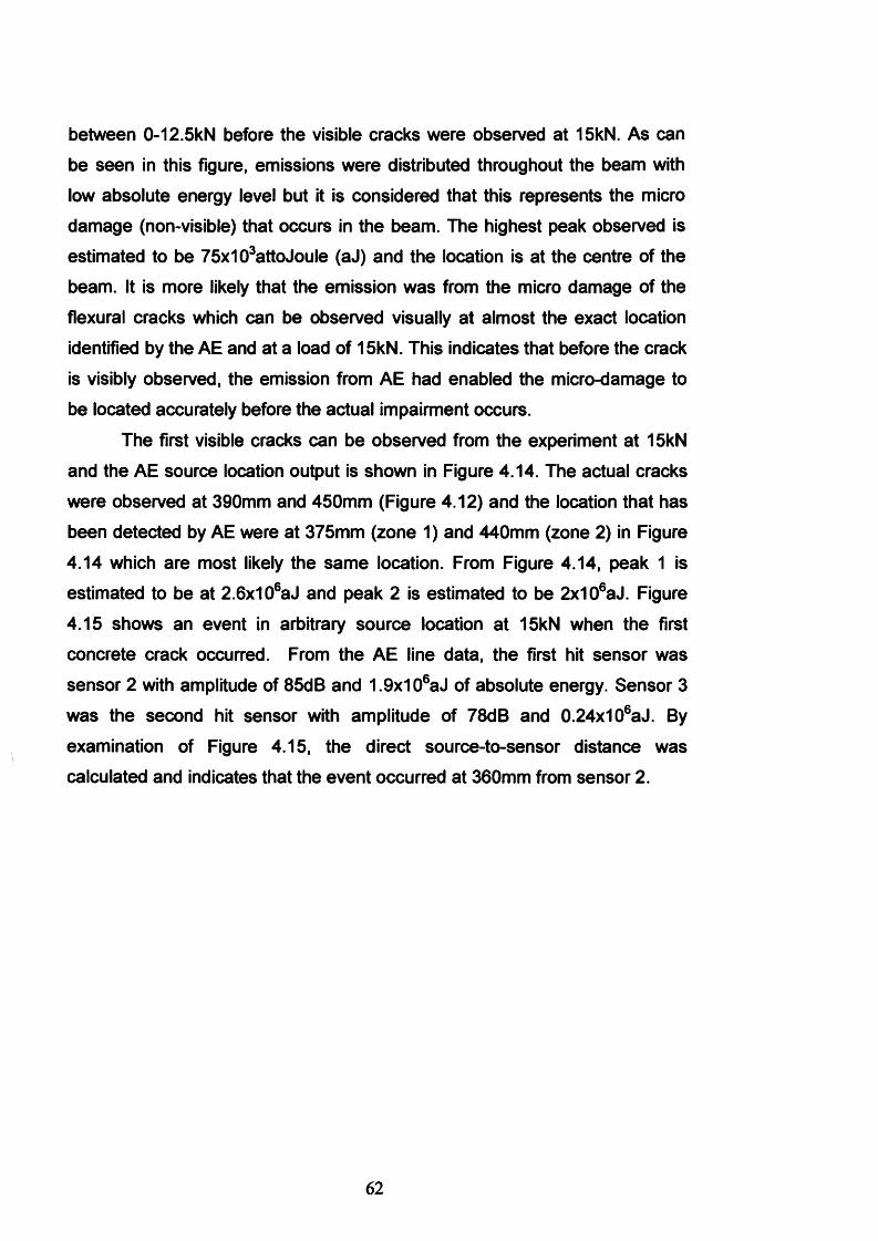
between 0-12.5kN before the visible cracks were observed at 15kN. As can

be seen in this figure, emissions were distributed throughout the beam with

low absolute energy level but it is considered that this represents the micro

damage (non-visible) that occurs in the beam. The highest peak observed is

estimated to be 75x103attoJoule (aJ) and the location is at the centre of the

beam. It is more likely that the emission was from the micro damage of the

flexural cracks which can be observed visually at almost the exact location

identified by the AE and at a load of 15kN. This indicates that before the crack

is visibly observed, the emission from AE had enabled the micro-damage to

be located accurately before the actual impairment occurs.

The first visible cracks can be observed from the experiment at 15kN

and the AE source location output is shown in Figure 4.14. The actual cracks

were observed at 390mm and 450mm (Figure 4.12) and the location that has

been detected by AE were at 375mm (zone 1) and 440mm (zone 2) in Figure

4.14 which are most likely the same location. From Figure 4.14, peak 1 is

estimated to be at 2.6x106aJ and peak 2 is estimated to be 2x106aJ. Figure

4.15 shows an event in arbitrary source location at 15kN when the first concrete crack occurred. From the AE line data, the first hit sensor was

sensor 2 with amplitude of 85dB and 1.9x106aJ of absolute energy. Sensor 3

was the second hit sensor with amplitude of 78dB and 0.24x106aJ. By

examination of Figure 4.15, the direct source-to-sensor distance was

calculated and indicates that the event occurred at 360mm from sensor 2.

62

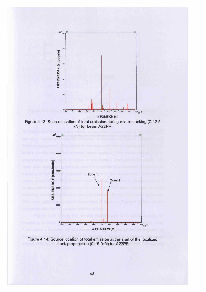
>■ O a:LUin *♦ COm<

. r i■ i i1 >-I* 4? 144 22} 2M S}« r *L,sr r 11 a," >X POSITION (m|

Figure 4.13: Source location of total emission during micro-cracking (0-12.5kN) for beam A22PR

Zone 1\ Zone 2

/

a r a , 1 1 ' 'a.X POSITION (m)

Figure 4.14: Source location of total emission at the start of the localized crack propagation (0-15.0kN) for A22PR

63

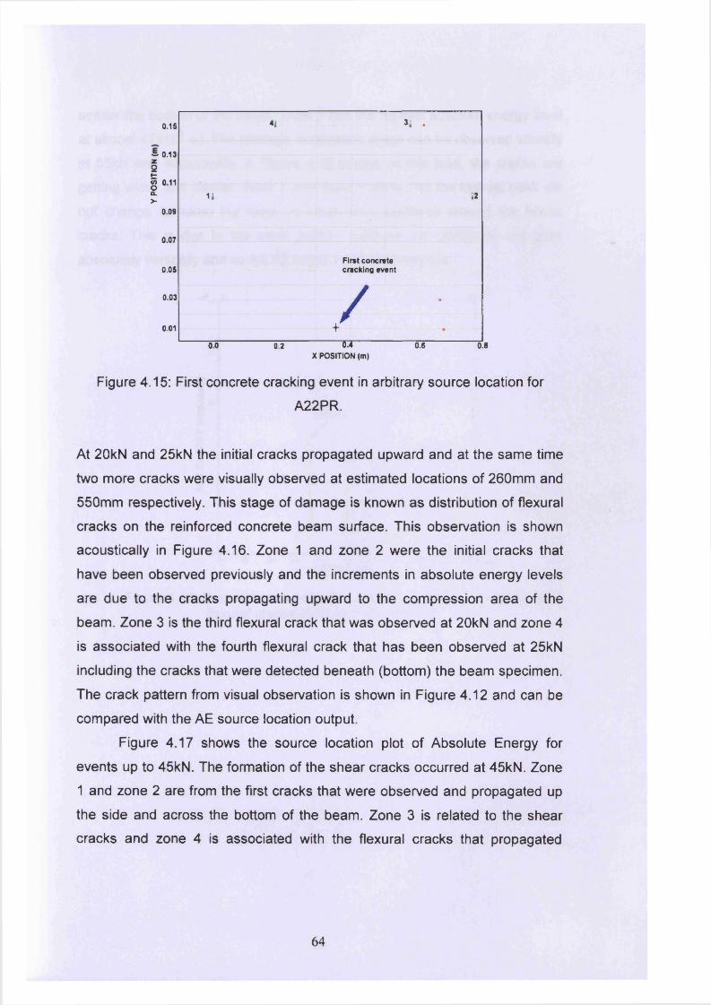
0.15 4 i h .

~ 0.13 z9| 011 a.> 11 a

0.09

0.07

0.05First concrete cracking event

0.03 /0.01 /

(To 0.2 53 03 0.8X POSITION (m)

Figure 4.15: First concrete cracking event in arbitrary source location for

A22PR.

At 20kN and 25kN the initial cracks propagated upward and at the same time

two more cracks were visually observed at estimated locations of 260mm and

550mm respectively. This stage of damage is known as distribution of flexural

cracks on the reinforced concrete beam surface. This observation is shown

acoustically in Figure 4.16. Zone 1 and zone 2 were the initial cracks that

have been observed previously and the increments in absolute energy levels

are due to the cracks propagating upward to the compression area of the

beam. Zone 3 is the third flexural crack that was observed at 20kN and zone 4

is associated with the fourth flexural crack that has been observed at 25kN

including the cracks that were detected beneath (bottom) the beam specimen.

The crack pattern from visual observation is shown in Figure 4.12 and can be

compared with the AE source location output.

Figure 4.17 shows the source location plot of Absolute Energy for

events up to 45kN. The formation of the shear cracks occurred at 45kN. Zone

1 and zone 2 are from the first cracks that were observed and propagated up

the side and across the bottom of the beam. Zone 3 is related to the shear

cracks and zone 4 is associated with the flexural cracks that propagated

64

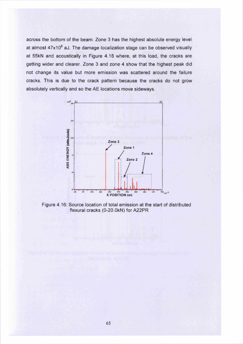
across the bottom of the beam. Zone 3 has the highest absolute energy level

at almost 47x106 aJ. The damage localization stage can be observed visually

at 55kN and acoustically in Figure 4.18 where, at this load, the cracks are

getting wider and clearer. Zone 3 and zone 4 show that the highest peak did

not change its value but more emission was scattered around the failure

cracks. This is due to the crack pattern because the cracks do not grow

absolutely vertically and so the AE locations move sideways.

oa.iu |zUJtoCQ<

Zone 3

Zone 1

Zone 4

Zone 2

X POSITION (m)•I* '

Figure 4.16: Source location of total emission at the start of distributed flexural cracks (0-20.OkN) for A22PR

65

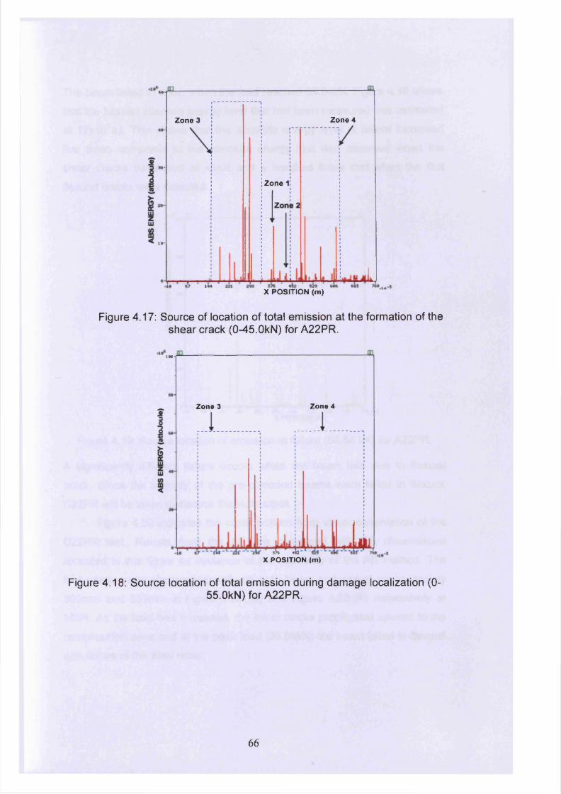
M

Zone 4Zone 3

»Zone 1

it

»-X POSITION (m)

Figure 4.17: Source of location of total emission at the formation of the shear crack (0-45.0kN) for A22PR.

IM-

Zone 4Zone 3

575 4b L ' ~X POSITION (m)

Figure 4.18: Source location of total emission during damage localization (0-55.0kN) for A22PR.

66

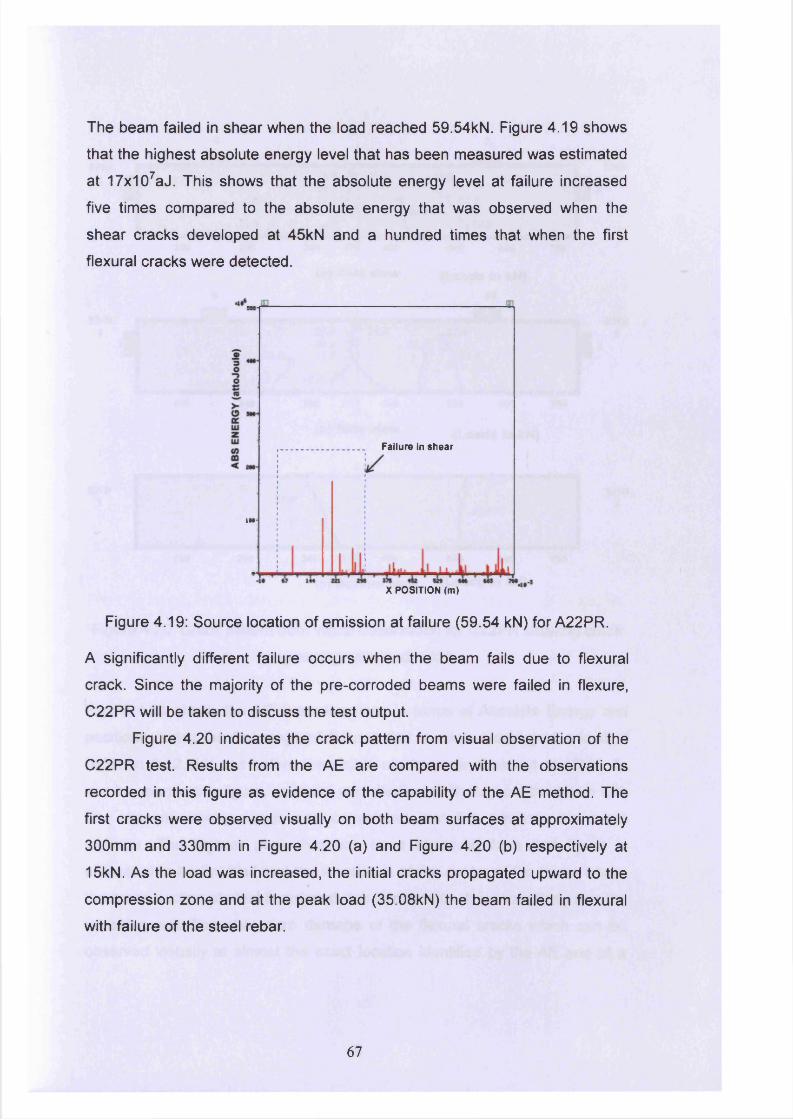
The beam failed in shear when the load reached 59.54kN. Figure 4.19 shows

that the highest absolute energy level that has been measured was estimated

at 17x107aJ. This shows that the absolute energy level at failure increased

five times compared to the absolute energy that was observed when the

shear cracks developed at 45kN and a hundred times that when the first

flexural cracks were detected.

Failure in shear

IM-

X POSITION (m)

Figure 4.19: Source location of emission at failure (59.54 kN) for A22PR.

A significantly different failure occurs when the beam fails due to flexural

crack. Since the majority of the pre-corroded beams were failed in flexure,

C22PR will be taken to discuss the test output.

Figure 4.20 indicates the crack pattern from visual observation of the

C22PR test. Results from the AE are compared with the observations

recorded in this figure as evidence of the capability of the AE method. The

first cracks were observed visually on both beam surfaces at approximately

300mm and 330mm in Figure 4.20 (a) and Figure 4.20 (b) respectively at

15kN. As the load was increased, the initial cracks propagated upward to the

compression zone and at the peak load (35.08kN) the beam failed in flexural

with failure of the steel rebar.

67

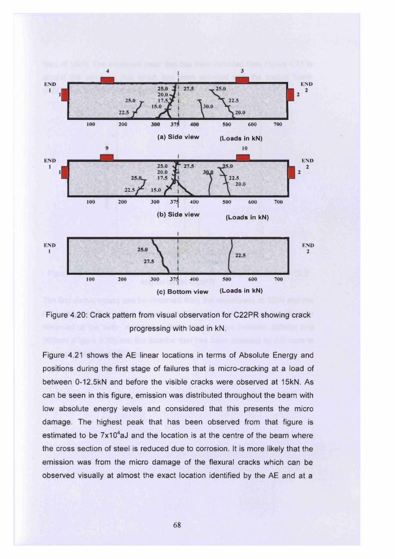
END1 25.0

20.017.5,25.0 22.5

15.0 30.022.5 20.0

100 200 500 600 700

END1

(a) Side view (Loads in kN)10

END

25.0 »/*■ 27.520.0 *1 17.5 OJ

:5.o

22.520.0

22.5 15.0

300 37!100 200 400 500 600 700

(b) Side view (Loads in kN)

END

END1

100 200

END2

300 3 7 ? 400 500 600 700

(c) Bottom view (Loads in kN)

Figure 4.20: Crack pattern from visual observation for C22PR showing crack

progressing with load in kN.

Figure 4.21 shows the AE linear locations in terms of Absolute Energy and

positions during the first stage of failures that is micro-cracking at a load of

between 0-12.5kN and before the visible cracks were observed at 15kN. As

can be seen in this figure, emission was distributed throughout the beam with

low absolute energy levels and considered that this presents the micro

damage. The highest peak that has been observed from that figure is

estimated to be 7x104aJ and the location is at the centre of the beam where

the cross section of steel is reduced due to corrosion. It is more likely that the

emission was from the micro damage of the flexural cracks which can be

observed visually at almost the exact location identified by the AE and at a

68

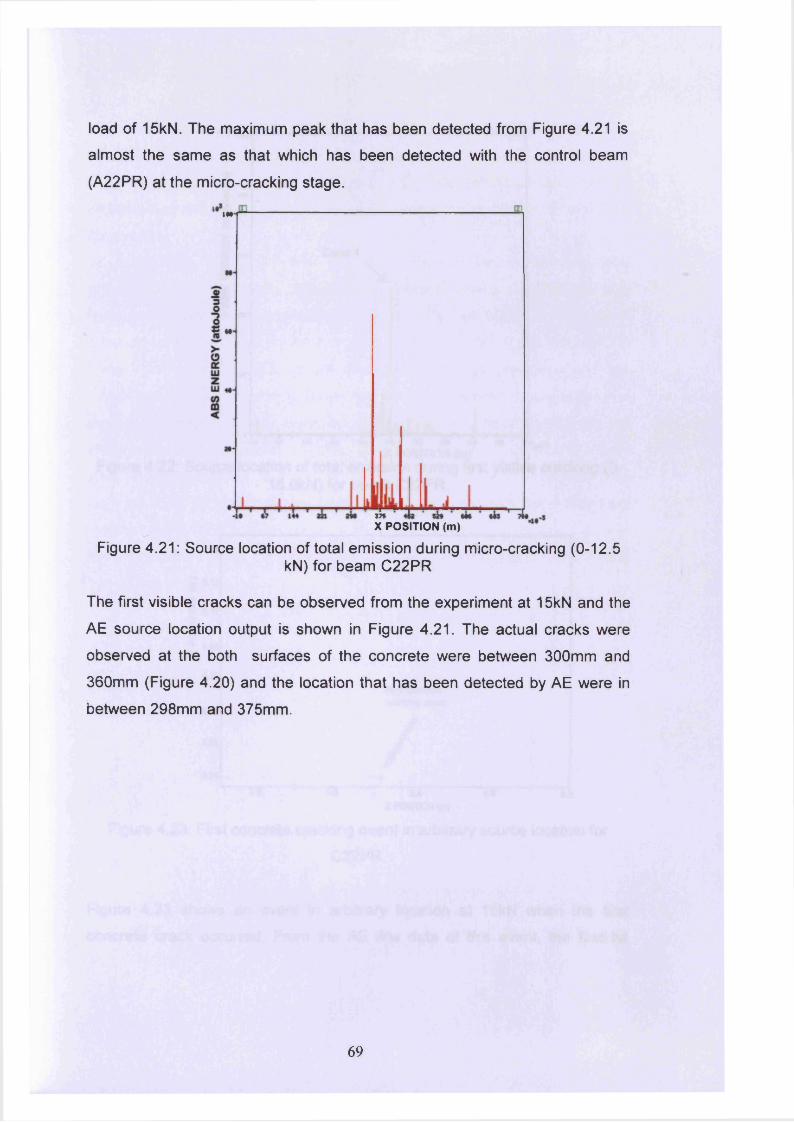
load of 15kN. The maximum peak that has been detected from Figure 4.21 is

almost the same as that which has been detected with the control beam

(A22PR) at the micro-cracking stage.

1M

171

X POSITION (m)

Figure 4.21: Source location of total emission during micro-cracking (0-12.5kN) for beam C22PR

The first visible cracks can be observed from the experiment at 15kN and the

AE source location output is shown in Figure 4.21. The actual cracks were

observed at the both surfaces of the concrete were between 300mm and

360mm (Figure 4.20) and the location that has been detected by AE were in

between 298mm and 375mm.

69

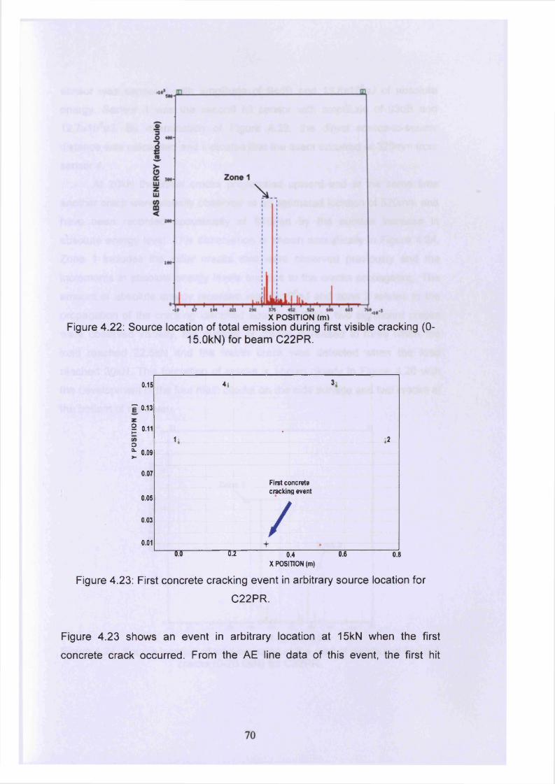
X POSITION (m)Figure 4.22: Source location of total emission during first visible cracking (0-

15.0kN) for beam C22PR.

0.15 41

£ 0.13

| 0.11

o£ 0.09

1i•

42

0.07First concrete

0.05cracking event

0.03 /0.01

r+

IHI 53 (M U 078X POSITION (m)

Figure 4.23: First concrete cracking event in arbitrary source location for

C22PR.

Figure 4.23 shows an event in arbitrary location at 15kN when the first

concrete crack occurred. From the AE line data of this event, the first hit

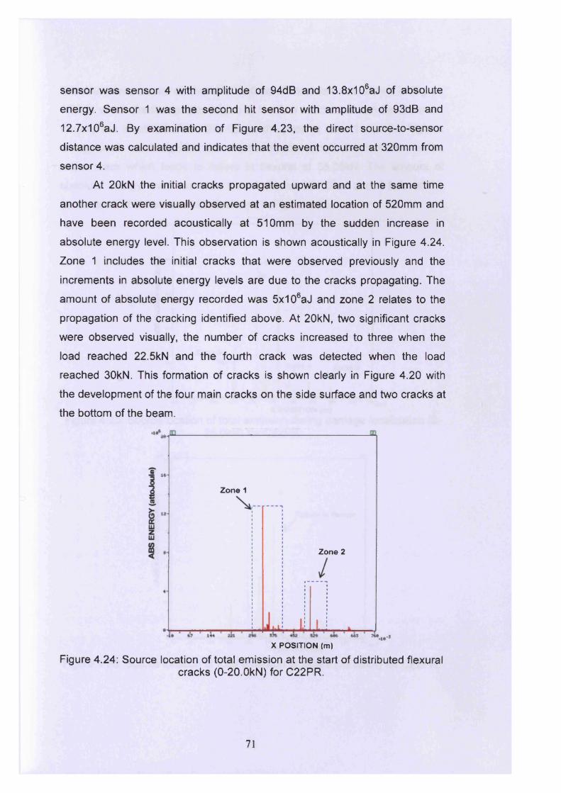
sensor was sensor 4 with amplitude of 94dB and 13.8x106aJ of absolute

energy. Sensor 1 was the second hit sensor with amplitude of 93dB and

12.7x106aJ. By examination of Figure 4.23, the direct source-to-sensor

distance was calculated and indicates that the event occurred at 320mm from

sensor 4.

At 20kN the initial cracks propagated upward and at the same time

another crack were visually observed at an estimated location of 520mm and

have been recorded acoustically at 510mm by the sudden increase in

absolute energy level. This observation is shown acoustically in Figure 4.24.

Zone 1 includes the initial cracks that were observed previously and the

increments in absolute energy levels are due to the cracks propagating. The

amount of absolute energy recorded was 5x106aJ and zone 2 relates to the

propagation of the cracking identified above. At 20kN, two significant cracks

were observed visually, the number of cracks increased to three when the

load reached 22.5kN and the fourth crack was detected when the load

reached 30kN. This formation of cracks is shown clearly in Figure 4.20 with

the development of the four main cracks on the side surface and two cracks at

the bottom of the beam.

X POSITION (m)

Figure 4.24: Source location of total emission at the start of distributed flexuralcracks (0-20.0kN) for C22PR.

<DZone 1

Zone 2

71

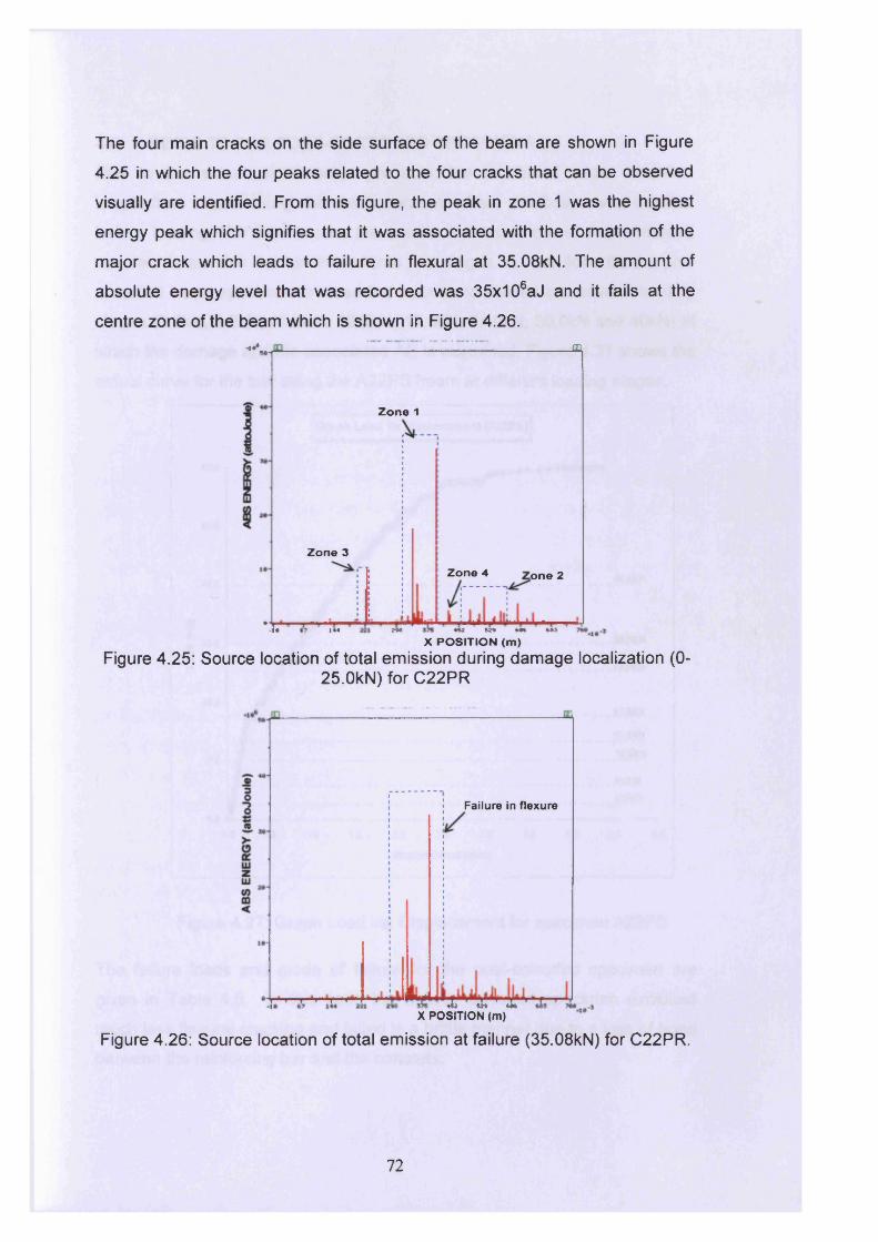
The four main cracks on the side surface of the beam are shown in Figure

4.25 in which the four peaks related to the four cracks that can be observed

visually are identified. From this figure, the peak in zone 1 was the highest

energy peak which signifies that it was associated with the formation of the

major crack which leads to failure in flexural at 35.08kN. The amount of

absolute energy level that was recorded was 35x106aJ and it fails at the

centre zone of the beam which is shown in Figure 4.26.i**.. J2,

Zone 3

Zone 1

Zone 4 one 2

rG *? 144 m 4S i S i * 4 *4 4»3

X POSITION (m)Figure 4.25: Source location of total emission during damage localization (0-

25.0kN) for C22PR

Failure in flexure

3a si* ' «k X POSITION (m)

Figure 4.26: Source location of total emission at failure (35.08kN) for C22PR.

72

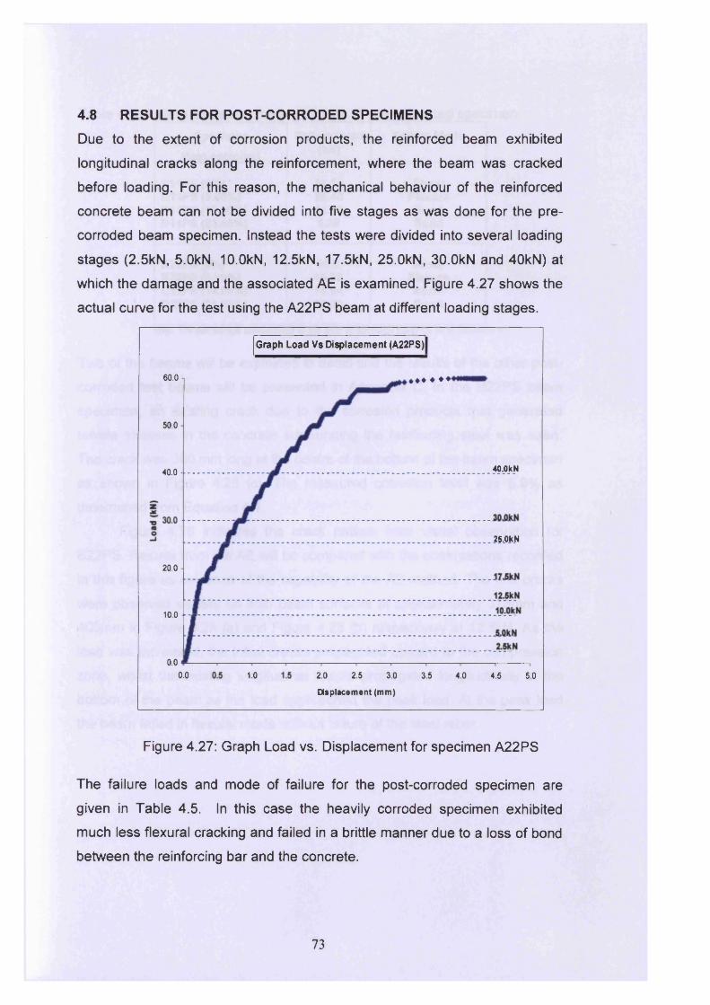
4.8 RESULTS FOR POST-CORRODED SPECIMENSDue to the extent of corrosion products, the reinforced beam exhibited

longitudinal cracks along the reinforcement, where the beam was cracked

before loading. For this reason, the mechanical behaviour of the reinforced

concrete beam can not be divided into five stages as was done for the pre­

corroded beam specimen. Instead the tests were divided into several loading

stages (2.5kN, 5.0kN, 10.0kN, 12.5kN, 17.5kN, 25.0kN, 30.0kN and 40kN) at

which the damage and the associated AE is examined. Figure 4.27 shows the

actual curve for the test using the A22PS beam at different loading stages.

Graph Load Vs Displacement (A22PS)

60.0

50.0

40.0kN40.0 -

25.0kN

20.0

10.0

0.00.0 1.0 2.0 2.5 3.0

Displacement (mm)

3.5 4.0 4.5 5.0

Figure 4.27: Graph Load vs. Displacement for specimen A22PS

The failure loads and mode of failure for the post-corroded specimen are

given in Table 4.5. In this case the heavily corroded specimen exhibited

much less flexural cracking and failed in a brittle manner due to a loss of bond

between the reinforcing bar and the concrete.

73

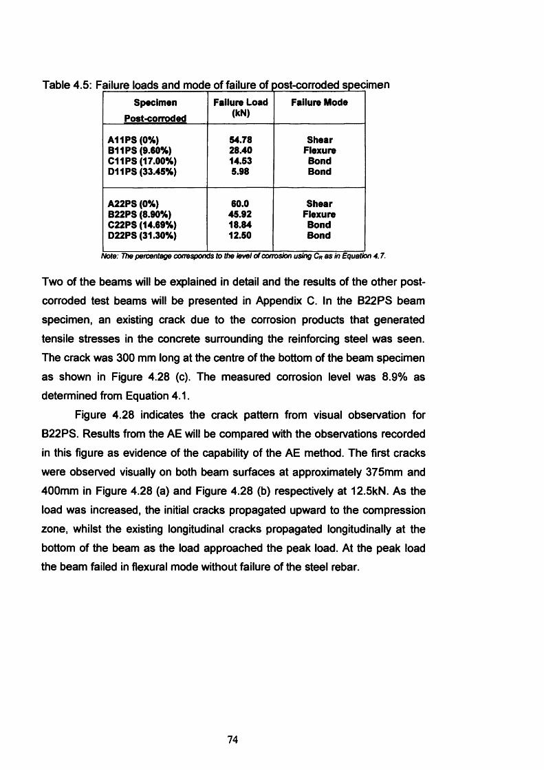
Table 4.5: Failure loads and mode of failure of post-corroded specimenSpecimen

Post-corrodedFailure Load

(kN)Failure Mode

A11PS (0%) 54.78 ShearB11PS (9.60%) 28.40 FlexureC11PS (17.00%) 14.53 BondD11PS (33.45%) 5.98 Bond

A22PS (0%) 60.0 ShearB22PS (8.90%) 45.92 FlexureC22PS (14.69%) 18.84 BondD22PS (31.30%) 12.50 Bond

Note: The percentage corresponds to the level of corrosion using CR as in Equation 4.7.

Two of the beams will be explained in detail and the results of the other post­corroded test beams will be presented in Appendix C. In the B22PS beam

specimen, an existing crack due to the corrosion products that generated

tensile stresses in the concrete surrounding the reinforcing steel was seen.

The crack was 300 mm long at the centre of the bottom of the beam specimen

as shown in Figure 4.28 (c). The measured corrosion level was 8.9% as

determined from Equation 4.1.

Figure 4.28 indicates the crack pattern from visual observation for

B22PS. Results from the AE will be compared with the observations recorded

in this figure as evidence of the capability of the AE method. The first cracks

were observed visually on both beam surfaces at approximately 375mm and

400mm in Figure 4.28 (a) and Figure 4.28 (b) respectively at 12.5kN. As the

load was increased, the initial cracks propagated upward to the compression

zone, whilst the existing longitudinal cracks propagated longitudinally at the

bottom of the beam as the load approached the peak load. At the peak load

the beam failed in flexural mode without failure of the steel rebar.

74

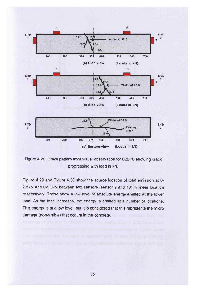
END20.0

Wider at 37.5130.0. 15.0

12.5

100 200 500 600 700

END

END

(a) Side view (Loads in kN)10

10.01

Wider at 37.5

,27.5

100 200 300 400

(b) Side view

500 600 700

(Loads in kN)

END

END1

V s__ - ■ Existings crack

300 37$ 400 500 600 700

(c) Bottom view (Loads in kN)

END2

Figure 4.28: Crack pattern from visual observation for B22PS showing crack

progressing with load in kN.

Figure 4.29 and Figure 4.30 show the source location of total emission at 0-

2.5kN and 0-5.0kN between two sensors (sensor 9 and 10) in linear location

respectively. These show a low level of absolute energy emitted at the lower

load. As the load increases, the energy is emitted at a number of locations.

This energy is at a low level, but it is considered that this represents the micro

damage (non-visible) that occurs in the concrete.

75

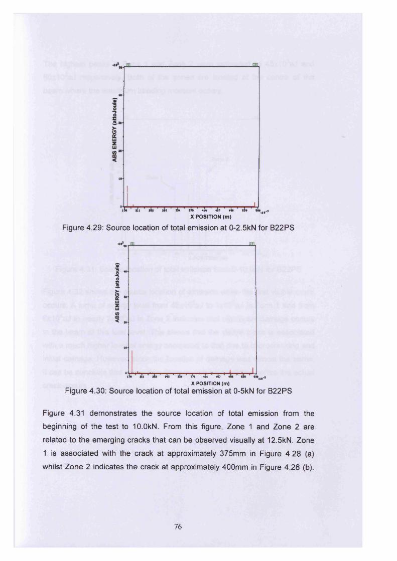
til ' *k ' t ij ' *1* ' *$* ’ *1* ' *47 ' *W ' *J* ' iW.jj-JX POSITION (m)

Figure 4.29: Source location of total emission at 0-2.5kN for B22PS

* 4 * ' » 4 j ' ' j!>* ' 41* ' *4?

X POSITION (m)

Figure 4.30: Source location of total emission at 0-5kN for B22PS

Figure 4.31 demonstrates the source location of total emission from the

beginning of the test to 10.0kN. From this figure, Zone 1 and Zone 2 are

related to the emerging cracks that can be observed visually at 12.5kN. Zone

1 is associated with the crack at approximately 375mm in Figure 4.28 (a)

whilst Zone 2 indicates the crack at approximately 400mm in Figure 4.28 (b).

76

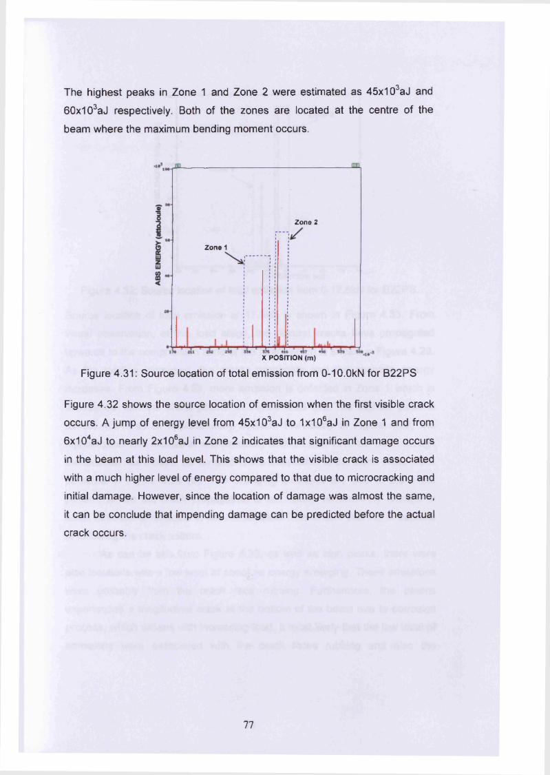
The highest peaks in Zone 1 and Zone 2 were estimated as 45x103aJ and

60x103aJ respectively. Both of the zones are located at the centre of the

beam where the maximum bending moment occurs.

Zone 1

Zone 2

X POSITION (m)

Figure 4.31: Source location of total emission from 0-10.0kN for B22PS

Figure 4.32 shows the source location of emission when the first visible crack

occurs. A jump of energy level from 45x103aJ to 1x106aJ in Zone 1 and from

6x104aJ to nearly 2x106aJ in Zone 2 indicates that significant damage occurs

in the beam at this load level. This shows that the visible crack is associated

with a much higher level of energy compared to that due to microcracking and

initial damage. However, since the location of damage was almost the same,

it can be conclude that impending damage can be predicted before the actual

crack occurs.

77

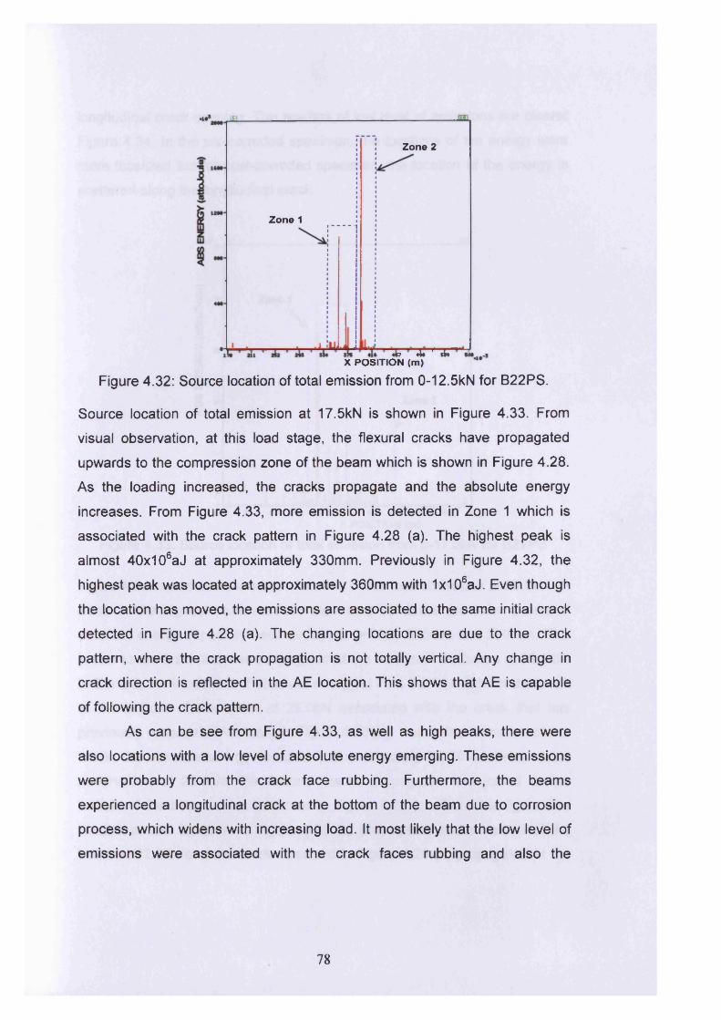
nr

Zone 2o

Zone 1

w «4» ' *J* X POSITION (m)

Figure 4.32: Source location of total emission from 0-12.5kN for B22PS.

Source location of total emission at 17.5kN is shown in Figure 4.33. From

visual observation, at this load stage, the flexural cracks have propagated

upwards to the compression zone of the beam which is shown in Figure 4.28.

As the loading increased, the cracks propagate and the absolute energy

increases. From Figure 4.33, more emission is detected in Zone 1 which is

associated with the crack pattern in Figure 4.28 (a). The highest peak is

almost 40x106aJ at approximately 330mm. Previously in Figure 4.32, the

highest peak was located at approximately 360mm with 1x106aJ. Even though

the location has moved, the emissions are associated to the same initial crack

detected in Figure 4.28 (a). The changing locations are due to the crack

pattern, where the crack propagation is not totally vertical. Any change in

crack direction is reflected in the AE location. This shows that AE is capable

of following the crack pattern.

As can be see from Figure 4.33, as well as high peaks, there were

also locations with a low level of absolute energy emerging. These emissions

were probably from the crack face rubbing. Furthermore, the beams

experienced a longitudinal crack at the bottom of the beam due to corrosion

process, which widens with increasing load. It most likely that the low level of

emissions were associated with the crack faces rubbing and also the

78

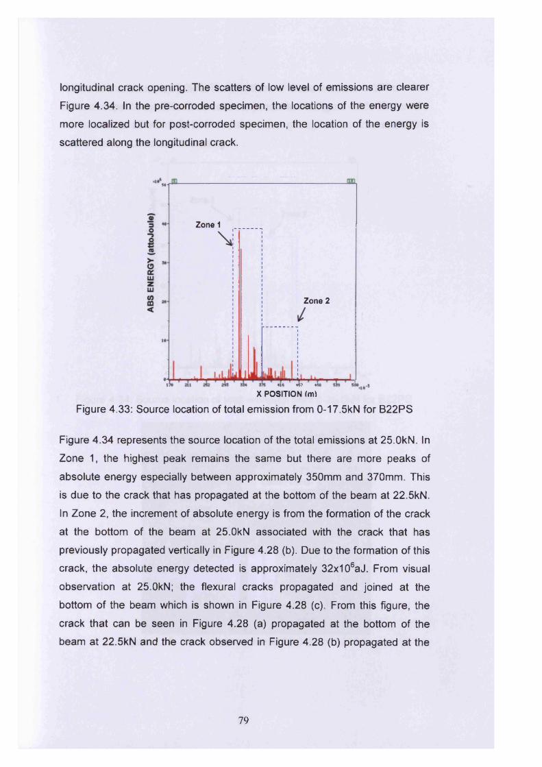
longitudinal crack opening. The scatters of low level of emissions are clearer

Figure 4.34. In the pre-corroded specimen, the locations of the energy were

more localized but for post-corroded specimen, the location of the energy is

scattered along the longitudinal crack.

s*T

Zone 1

Zone 2

4S? «X POSITION Im)

Figure 4.33: Source location of total emission from 0-17.5kN for B22PS

Figure 4.34 represents the source location of the total emissions at 25.0kN. In

Zone 1, the highest peak remains the same but there are more peaks of

absolute energy especially between approximately 350mm and 370mm. This

is due to the crack that has propagated at the bottom of the beam at 22.5kN.

In Zone 2, the increment of absolute energy is from the formation of the crack

at the bottom of the beam at 25.0kN associated with the crack that has

previously propagated vertically in Figure 4.28 (b). Due to the formation of this

crack, the absolute energy detected is approximately 32x106aJ. From visual

observation at 25.0kN; the flexural cracks propagated and joined at the

bottom of the beam which is shown in Figure 4.28 (c). From this figure, the

crack that can be seen in Figure 4.28 (a) propagated at the bottom of the

beam at 22.5kN and the crack observed in Figure 4.28 (b) propagated at the

79

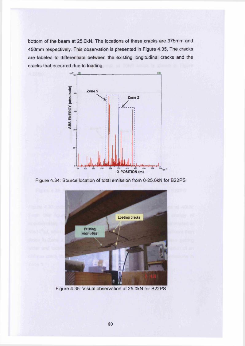
bottom of the beam at 25.0kN. The locations of these cracks are 375mm and

450mm respectively. This observation is presented in Figure 4.35. The cracks

are labeled to differentiate between the existing longitudinal cracks and the

cracks that occurred due to loading.

Zone 1

Zone 2

17*

X POSITION (m)

Figure 4.34: Source location of total emission from 0-25.OkN for B22PS

Loading cracks

Existinglongitudinal

Figure 4.35: Visual observation at 25.OkN for B22PS

80

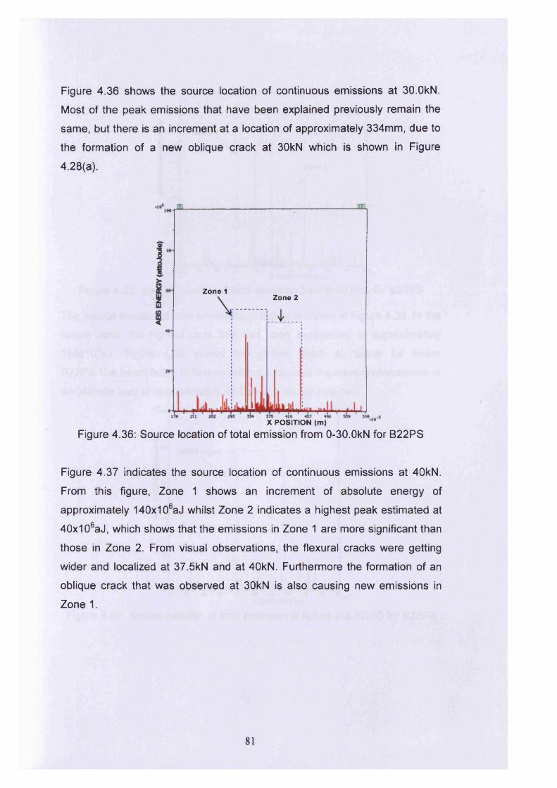
Figure 4.36 shows the source location of continuous emissions at 30.OkN.

Most of the peak emissions that have been explained previously remain the

same, but there is an increment at a location of approximately 334mm, due to

the formation of a new oblique crack at 30kN which is shown in Figure

4.28(a).

Zone 1Zone 2

w>211X POSITION (m)

Figure 4.36: Source location of total emission from 0-30.OkN for B22PS

Figure 4.37 indicates the source location of continuous emissions at 40kN.

From this figure, Zone 1 shows an increment of absolute energy of

approximately 140x106aJ whilst Zone 2 indicates a highest peak estimated at

40x106aJ, which shows that the emissions in Zone 1 are more significant than

those in Zone 2. From visual observations, the flexural cracks were getting

wider and localized at 37.5kN and at 40kN. Furthermore the formation of an

oblique crack that was observed at 30kN is also causing new emissions in

Zone 1.

81

.»•*

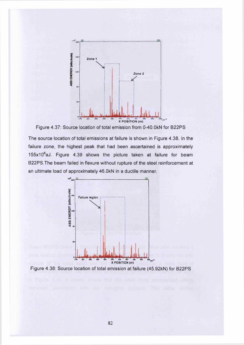
Zone 1

Zone 2

J W 4 6 4 5 7 4

X POSITION (m)

Figure 4.37: Source location of total emission from 0-40.OkN for B22PS

The source location of total emissions at failure is shown in Figure 4.38. In the

failure zone, the highest peak that had been ascertained is approximately

155x106aJ. Figure 4.39 shows the picture taken at failure for beam

B22PS.The beam failed in flexure without rupture of the steel reinforcement at

an ultimate load of approximately 46.OkN in a ductile manner.

O IM-Failure region

< M-

X POSITION (m)

Figure 4.38: Source location of total emission at failure (45.92kN) for B22PS

82

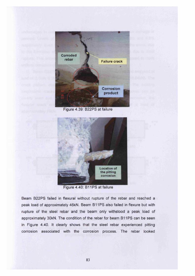
Corrodedrebar Failure crack

Corrosionproduct

Figure 4.39: B22PS at failure

Location of the pitting corrosion

Figure 4.40: B11 PS at failure

Beam B22PS failed in flexural without rupture of the rebar and reached a

peak load of approximately 46kN. Beam B11PS also failed in flexure but with

rupture of the steel rebar and the beam only withstood a peak load of

approximately 30kN. The condition of the rebar for beam B11PS can be seen

in Figure 4.40. It clearly shows that the steel rebar experienced pitting

corrosion associated with the corrosion process. The rebar looked

83

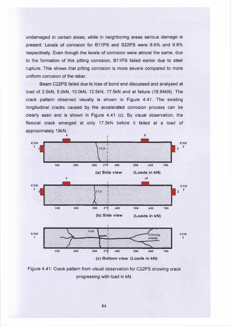
undamaged in certain areas, while in neighboring areas serious damage is

present. Levels of corrosion for B11PS and B22PS were 8.9% and 9.8%

respectively. Even though the levels of corrosion were almost the same, due

to the formation of this pitting corrosion, B11PS failed earlier due to steel

rupture. This shows that pitting corrosion is more severe compared to more

uniform corrosion of the rebar.

Beam C22PS failed due to loss of bond and discussed and analysed at

load of 2.5kN, 5.0kN, 10.0kN, 12.5kN, 17.5kN and at failure (18.84kN). The

crack pattern observed visually is shown in Figure 4.41. The existing

longitudinal cracks caused by the accelerated corrosion process can be

clearly seen and is shown in Figure 4.41 (c). By visual observation, the

flexural crack emerged at only 17.5kN before it failed at a load of

approximately 19kN.

END

I

END

I

END1

T !

100 200 300 374 400 500 600 700

9

(a) Side view

i

(Loads in kN) 10

m

/

17.5 ! 1i

^ i100 200 300 37^ 400 500 600 700

(b) Side view

i

(Loads in kN)

Fail

L IExisting

/ I 1 ^ ---------f V i

JEND

2

IEND

2

END2

100 200 300 375 400 500 600 700

(c) Bottom view (Loads in kN)

Figure 4.41: Crack pattern from visual observation for C22PS showing crack

progressing with load in kN.

84

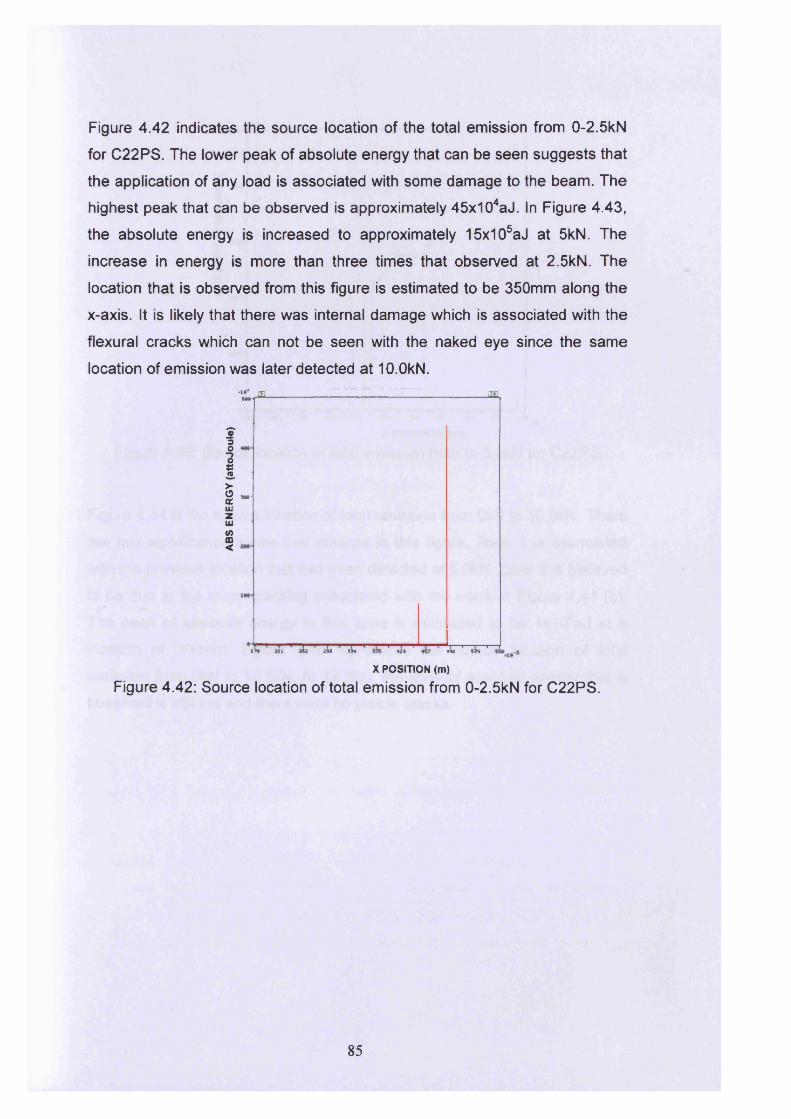
Figure 4.42 indicates the source location of the total emission from 0-2.5kN

for C22PS. The lower peak of absolute energy that can be seen suggests that

the application of any load is associated with some damage to the beam. The

highest peak that can be observed is approximately 45x104aJ. In Figure 4.43,

the absolute energy is increased to approximately 15x105aJ at 5kN. The

increase in energy is more than three times that observed at 2.5kN. The

location that is observed from this figure is estimated to be 350mm along the

x-axis. It is likely that there was internal damage which is associated with the

flexural cracks which can not be seen with the naked eye since the same

location of emission was later detected at 10.0kN.«!•» m tm*•*-

5 “30

1 ■>-0 m . 0£HIzHI<0m<

1L ’ «li ' ai* ' & ' »U ' ' <U ^ 1 M* 1X POSITION (m)

Figure 4.42: Source location of total emission from 0-2.5kN for C22PS.

85

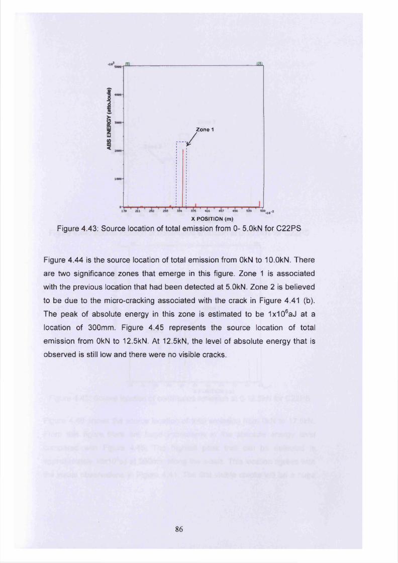
JHL

UJ r /Zone 1

X POSITION (m)

Figure 4.43: Source location of total emission from 0- 5.OkN for C22PS

Figure 4.44 is the source location of total emission from OkN to 10.OkN. There

are two significance zones that emerge in this figure. Zone 1 is associated

with the previous location that had been detected at 5.OkN. Zone 2 is believed

to be due to the micro-cracking associated with the crack in Figure 4.41 (b).

The peak of absolute energy in this zone is estimated to be 1x106aJ at a

location of 300mm. Figure 4.45 represents the source location of total

emission from OkN to 12.5kN. At 12.5kN, the level of absolute energy that is

observed is still low and there were no visible cracks.

86

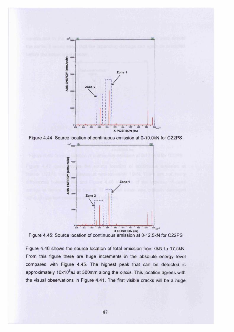
Zone 1

Zone 2

X POSITION (m)

Figure 4.44: Source location of continuous emission at 0-10.OkN for C22PS

Figure 4.45: Source location of continuous emission at 0-12.5kN for C22PS

Figure 4.46 shows the source location of total emission from OkN to 17.5kN.

From this figure there are huge increments in the absolute energy level

compared with Figure 4.45. The highest peak that can be detected is

approximately 16x106aJ at 300mm along the x-axis. This location agrees with

the visual observations in Figure 4.41. The first visible cracks will be a huge

JZL

O —

>

X POSITION (m)

87

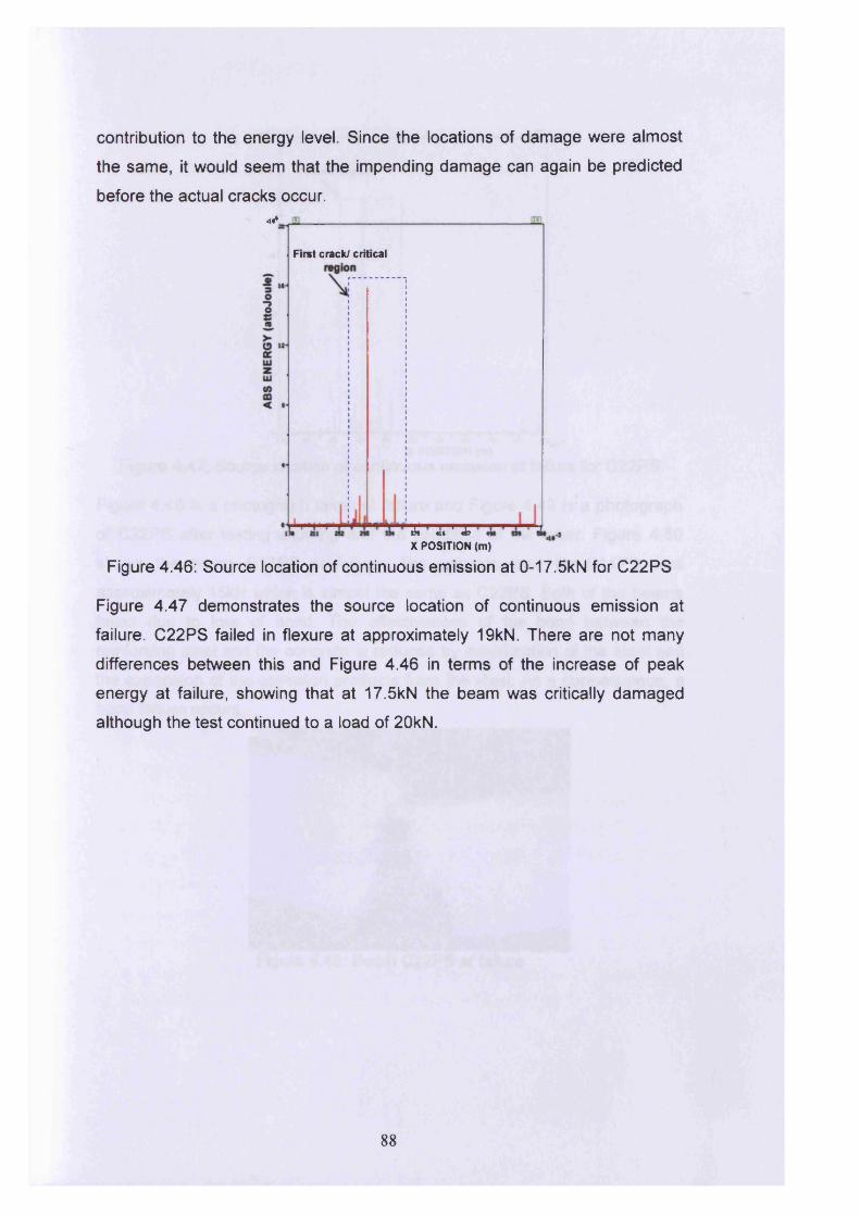
contribution to the energy level. Since the locations of damage were almost

the same, it would seem that the impending damage can again be predicted

before the actual cracks occur.■i**

First crack/ critical

i$» «* ' «bX POSITION (m)

Figure 4.46: Source location of continuous emission at 0-17.5kN for C22PS

Figure 4.47 demonstrates the source location of continuous emission at

failure. C22PS failed in flexure at approximately 19kN. There are not many

differences between this and Figure 4.46 in terms of the increase of peak

energy at failure, showing that at 17.5kN the beam was critically damaged

although the test continued to a load of 20kN.

88

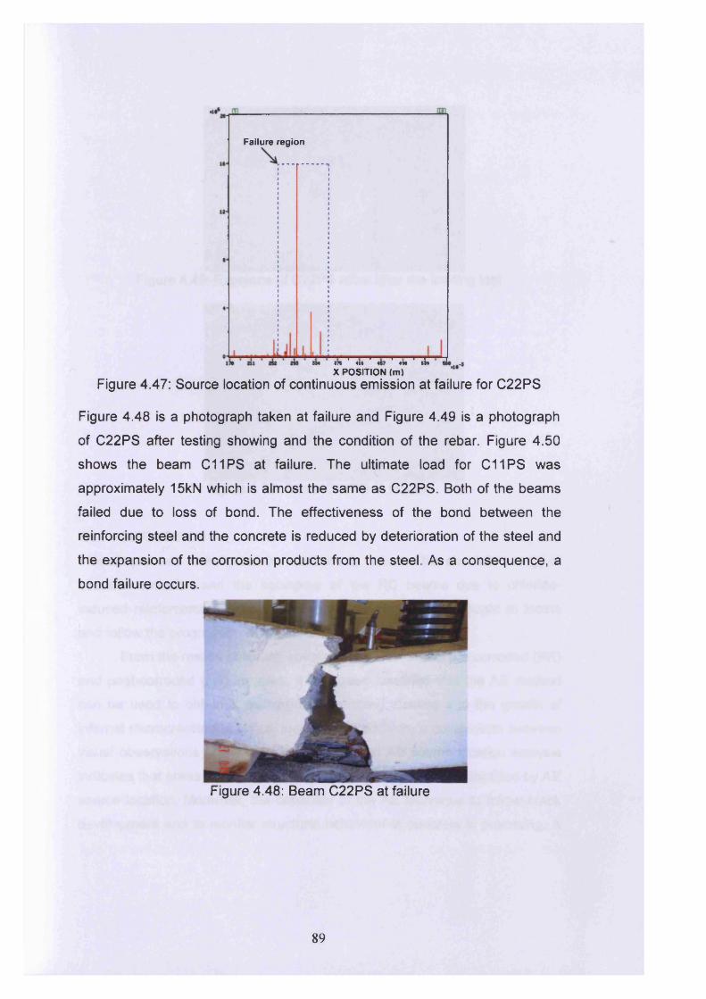
Failure region

m m ' «* ' ' 4« ' titX POSITION (m)

Figure 4.47: Source location of continuous emission at failure for C22PS

Figure 4.48 is a photograph taken at failure and Figure 4.49 is a photograph

of C22PS after testing showing and the condition of the rebar. Figure 4.50

shows the beam C11PS at failure. The ultimate load for C11PS was

approximately 15kN which is almost the same as C22PS. Both of the beams

failed due to loss of bond. The effectiveness of the bond between the

reinforcing steel and the concrete is reduced by deterioration of the steel and

the expansion of the corrosion products from the steel. As a consequence, a

bond failure occurs.

Figure 4.48: Beam C22PS at failure

89

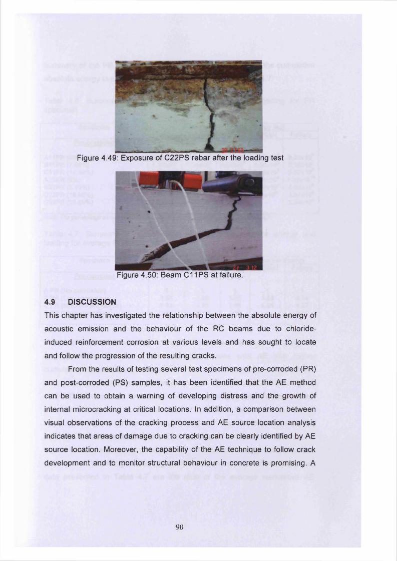
Figure 4.50: Beam C11 PS at failure

Figure 4.49: Exposure of C22PS rebar after the loading test

4.9 DISCUSSIONThis chapter has investigated the relationship between the absolute energy of

acoustic emission and the behaviour of the RC beams due to chloride-

induced reinforcement corrosion at various levels and has sought to locate

and follow the progression of the resulting cracks.

From the results of testing several test specimens of pre-corroded (PR)

and post-corroded (PS) samples, it has been identified that the AE method

can be used to obtain a warning of developing distress and the growth of

internal microcracking at critical locations. In addition, a comparison between

visual observations of the cracking process and AE source location analysis

indicates that areas of damage due to cracking can be clearly identified by AE

source location. Moreover, the capability of the AE technique to follow crack

development and to monitor structural behaviour in concrete is promising. A

90

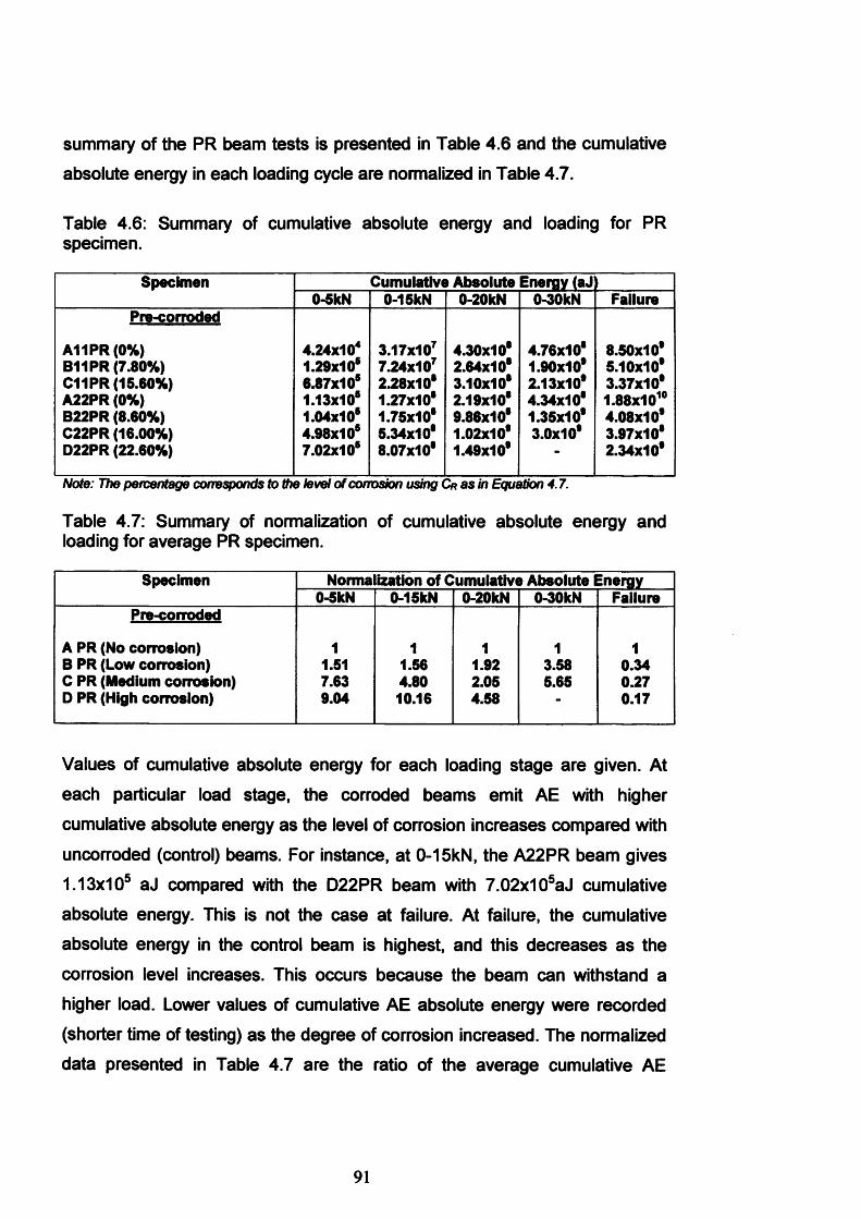
summary of the PR beam tests is presented in Table 4.6 and the cumulative

absolute energy in each loading cycle are normalized in Table 4.7.

Table 4.6: Summary of cumulative absolute energy and loading for PR specimen.

Specimen Cumulative Absolute Energy (aJ0-5kN 0-15kN 0-20kN 0-30kN Failure

Pre-corroded

A11PR (0%)B11PR (7.80%)C11PR (15.60%)A22PR (0%)B22PR (8.60%)C22PR (16.00%)D22PR (22.60%)

4.24x104 1.29x10s 6.87x10s 1.13x10s 1.04x10s 4.98x10s 7.02x10s

3.17x107 7.24x107 2.28x10s 1.27x10s 1.75x10s 5.34x10s 8.07x10s

4.30x10s2.64x10s3.10x10s2.19x10s9.86x10s1.02x10s1.49x10s

4.76x10s1.90x10s2.13x10s4.34x10s1.35x10s3.0x10s

8.50x10s5.10x10s3.37x10s1.88x101°4.08x10s3.97x10s2.34x10s

Note: The percentage corresponds to the level of corrosion using Cr as in Equation 4.7.

Table 4.7: Summary of normalization of cumulative absolute energy and loading for average PR specimen.

Specimen Norma ization of Cumulative Absolute Energy0-5kN 0-15kN 0-20kN 0-30kN Failure

Pre-corroded

A PR (No corrosion) 1 1 1 1 1B PR (Low corrosion) 1.51 1.56 1.92 3.58 0.34C PR (Medium corrosion) 7.63 4.80 2.05 5.65 0.27D PR (High corrosion) 9.04 10.16 4.58 " 0.17

Values of cumulative absolute energy for each loading stage are given. At

each particular load stage, the corroded beams emit AE with higher cumulative absolute energy as the level of corrosion increases compared with

uncorroded (control) beams. For instance, at 0-15kN, the A22PR beam gives

1.13x10s aJ compared with the D22PR beam with 7.02x105aJ cumulative

absolute energy. This is not the case at failure. At failure, the cumulative

absolute energy in the control beam is highest, and this decreases as the

corrosion level increases. This occurs because the beam can withstand a

higher load. Lower values of cumulative AE absolute energy were recorded

(shorter time of testing) as the degree of corrosion increased. The normalized

data presented in Table 4.7 are the ratio of the average cumulative AE

91

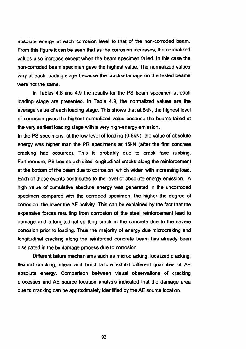
absolute energy at each corrosion level to that of the non-corroded beam. From this figure it can be seen that as the corrosion increases, the normalized

values also increase except when the beam specimen failed. In this case the

non-corroded beam specimen gave the highest value. The normalized values

vary at each loading stage because the cracks/damage on the tested beams

were not the same.In Tables 4.8 and 4.9 the results for the PS beam specimen at each

loading stage are presented. In Table 4.9, the normalized values are the

average value of each loading stage. This shows that at 5kN, the highest level of corrosion gives the highest normalized value because the beams failed at the very earliest loading stage with a very high-energy emission.In the PS specimens, at the low level of loading (0-5kN), the value of absolute

energy was higher than the PR specimens at 15kN (after the first concrete

cracking had occurred). This is probably due to crack face rubbing. Furthermore, PS beams exhibited longitudinal cracks along the reinforcement at the bottom of the beam due to corrosion, which widen with increasing load.

Each of these events contributes to the level of absolute energy emission. A

high value of cumulative absolute energy was generated in the uncorroded

specimen compared with the corroded specimen; the higher the degree of corrosion, the lower the AE activity. This can be explained by the fact that the

expansive forces resulting from corrosion of the steel reinforcement lead to

damage and a longitudinal splitting crack in the concrete due to the severe

corrosion prior to loading. Thus the majority of energy due microcraking and

longitudinal cracking along the reinforced concrete beam has already been

dissipated in the by damage process due to corrosion.Different failure mechanisms such as microcracking, localized cracking,

flexural cracking, shear and bond failure exhibit different quantities of AE

absolute energy. Comparison between visual observations of cracking

processes and AE source location analysis indicated that the damage area

due to cracking can be approximately identified by the AE source location.

92

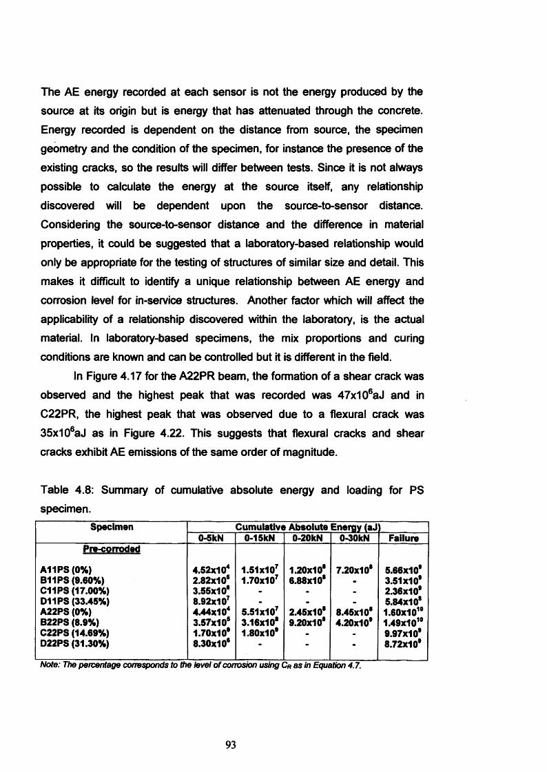
The AE energy recorded at each sensor is not the energy produced by the

source at its origin but is energy that has attenuated through the concrete. Energy recorded is dependent on the distance from source, the specimen

geometry and the condition of the specimen, for instance the presence of the

existing cracks, so the results will differ between tests. Since it is not always

possible to calculate the energy at the source itself, any relationship

discovered will be dependent upon the source-to-sensor distance. Considering the source-to-sensor distance and the difference in material properties, it could be suggested that a laboratory-based relationship would

only be appropriate for the testing of structures of similar size and detail. This

makes it difficult to identify a unique relationship between AE energy and

corrosion level for in-service structures. Another factor which will affect the

applicability of a relationship discovered within the laboratory, is the actual material. In laboratory-based specimens, the mix proportions and curing

conditions are known and can be controlled but it is different in the field.

In Figure 4.17 for the A22PR beam, the formation of a shear crack was

observed and the highest peak that was recorded was 47x106aJ and in

C22PR, the highest peak that was observed due to a flexural crack was

35x106aJ as in Figure 4.22. This suggests that flexural cracks and shear cracks exhibit AE emissions of the same order of magnitude.

Table 4.8: Summary of cumulative absolute energy and loading for PS

specimen.Specimen Cumulative Absolute Energy (aJ

0-5kN 0-15kN 0-20kN 0-30kN FailurePre-corroded

A11PS (0%) 4.52x104 1.51x107 1.20x10s 7.20x10s 5.66x10sB11PS (9.60%) 2.82x10s 1.70x107 6.88x10s - 3.51x10sC11PS (17.00%) 3.55x10s - - - 2.36x10sD11PS (33.45%) 8.92x107 - - - 5.84x10sA22PS (0%) 4.44x104 5.51 x107 2.45x10s 8.45x10s 1.60x101°B22PS (8.9%) 3.57x10s 3.16x10s 9.20x10s 4.20x10s 1.49X1010C22PS (14.69%) 1.70x10s 1.80x10s - - 9.97x10sD22PS (31.30%) 8.30x10s • - 8.72x10s

Note: The percentage corresponds to the level of corrosion using Cr as in Equation 4.7.

93

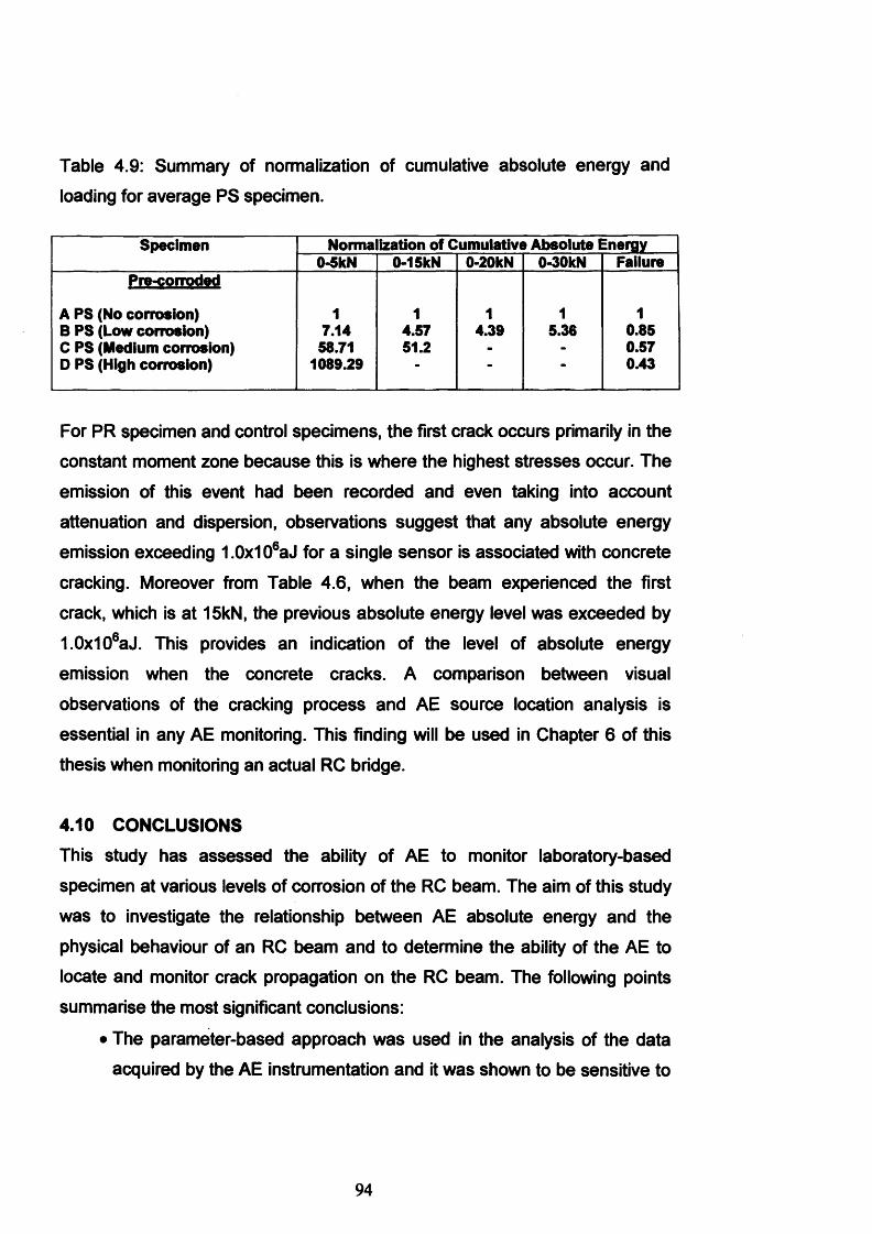
Table 4.9: Summary of normalization of cumulative absolute energy and

loading for average PS specimen.

Specimen Norma ization of Cumulative Absolute Energy0-5kN 0-15kN 0-20kN 0-30kN Failure

Pre-corroded

A PS (No corrosion) 1 1 1 1 1B PS (Low corrosion) 7.14 4.57 4.39 5.38 0.85C PS (Medium corrosion) 58.71 51.2 - - 0.57D PS (High corrosion) 1089.29 • • • 0.43

For PR specimen and control specimens, the first crack occurs primarily in the

constant moment zone because this is where the highest stresses occur. The

emission of this event had been recorded and even taking into account attenuation and dispersion, observations suggest that any absolute energy

emission exceeding 1.0x106aJ for a single sensor is associated with concrete

cracking. Moreover from Table 4.6, when the beam experienced the first

crack, which is at 15kN, the previous absolute energy level was exceeded by

1.0x106aJ. This provides an indication of the level of absolute energy

emission when the concrete cracks. A comparison between visual

observations of the cracking process and AE source location analysis is

essential in any AE monitoring. This finding will be used in Chapter 6 of this

thesis when monitoring an actual RC bridge.

4.10 CONCLUSIONSThis study has assessed the ability of AE to monitor laboratory-based

specimen at various levels of corrosion of the RC beam. The aim of this study

was to investigate the relationship between AE absolute energy and the

physical behaviour of an RC beam and to determine the ability of the AE to

locate and monitor crack propagation on the RC beam. The following points

summarise the most significant conclusions:

• The parameter-based approach was used in the analysis of the data

acquired by the AE instrumentation and it was shown to be sensitive to

94

the initiation and the growth of cracks within the specimens. The

application of the TOA method was used to determine the location of the damage area using linear location between sensors and the results

were promising. In addition, TOA location could be used to indicate

internal crack growth before the crack could be observed visually and

enabled the micro damage to be located accurately before the actual

impairment occured.

• In pre-corroded specimens, five different stages of mechanical failure

were identified; microcraking, localized cracking propagation, distributed flexural cracking, shear cracking and damage localization.

However, in post-corroded (PS) specimen these five stages were not identified since the specimens exhibited longitudinal cracks along the

reinforcement, such that the beam was cracked before loading.

• The AE energy recorded at each sensor is not the energy produced by

the source at its origin but an energy that has attenuated through the

concrete. Therefore, the energy is dependent on the distance from the

source, the specimen geometry and the condition of the specimen.

However, it was observed in the PR specimens that the energy due to

first concrete cracking exceeded 1.0x106aJ in arbitrary source location

for a single sensor. Thus it is proposed that absolute energy in excees

of 1.0x106aJ can be used to indicate the onset of cracking.

• At a particular loading stage, it was observed that the cumulative

absolute energy was higher with increased corrosion level. PS

specimens gave higher emissions because of the existing longitudinal cracks, which widen and cause concrete face rubbing as the load

increases. In the PR specimens, the AE level was related to the loss of

cross section of reinforcing steel. However, this is not true at failure, where the cumulative energy released was lower with increasing

corrosion level due to the load at which the reinforcing bar fails.

CHAPTER 5: A PRACTICAL INVESTIGATION INTO ACOUSTIC WAVE

PROPAGATION IN CONCRETE STRUCTURES

5.1 INTRODUCTION

This chapter details experiments using the AE waveform or transient record to

analyse the synchronous signals from artificial and true sources by exploring

wave propagation in concrete structures over a variety of source-to-sensor

distances. Experiments were performed on a reinforced concrete (RC) beam

and an RC slab using a Hsu-Nelsen (H-N) Source (ASTM, 1999) as an

artificial source. A further investigation examined concrete cracking resulting

from the corrosion process as a true source. A detailed description of the

experimental work is presented highlighting the procedures followed during

the laboratory stage of this study and an analysis of the results is given.

Source location is normally based on the arrival times of transient signals. The

simplest method is known as the Time of Arrival (TOA) method, where the

location of the damage can be determined from the arrival time of the event at

two or more sensors. When using this method, the wave velocity of the

signals that propagate through the material needs to be determined.

Homogenous materials, such as steel, have well-defined velocities, but it is

more difficult to predict the wave velocity in non-homogeneous materials such

as concrete. This makes the use of a single wave velocity, as required in the

TOA method, very difficult especially for large structures. It is therefore

essential to gain an understanding of the factors that may affect the ability to

obtain an accurate value of wave velocity.

The heterogeneous nature of concrete (e.g. aggregates, cracks, reinforcing bars and tendons) influences the wave propagation by scattering.

Reflections and mode conversions at the interfaces and specimen boundaries

cause a very complex wave field. It is often difficult to detect waves other than

the P-wave which is why the arrival times of the P-waves are only considered

for the quantitative analysis.

96

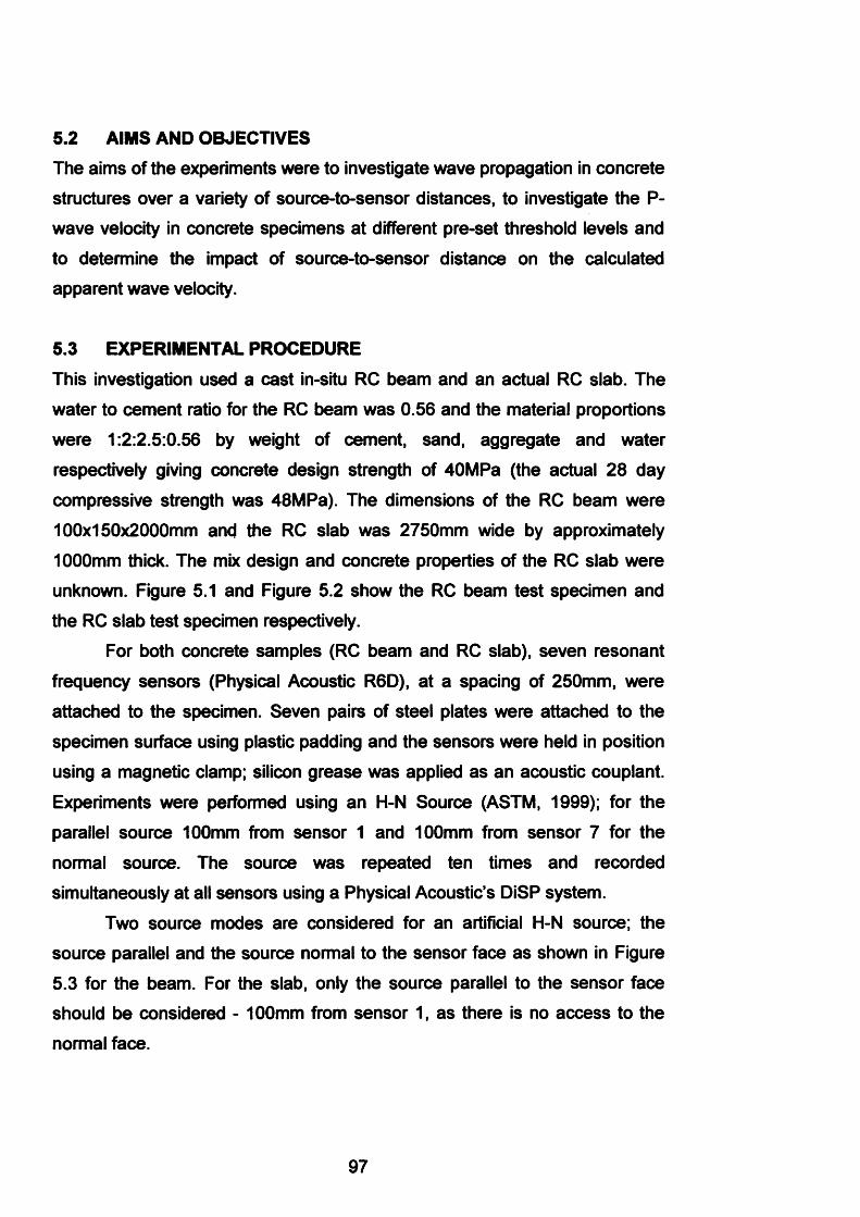
5.2 AIMS AND OBJECTIVESThe aims of the experiments were to investigate wave propagation in concrete

structures over a variety of source-to-sensor distances, to investigate the P- wave velocity in concrete specimens at different pre-set threshold levels and

to determine the impact of source-to-sensor distance on the calculated

apparent wave velocity.

5.3 EXPERIMENTAL PROCEDURE

This investigation used a cast in-situ RC beam and an actual RC slab. The

water to cement ratio for the RC beam was 0.56 and the material proportions

were 1:2:2.5:0.56 by weight of cement, sand, aggregate and water

respectively giving concrete design strength of 40MPa (the actual 28 day

compressive strength was 48MPa). The dimensions of the RC beam were

100x150x2000mm and the RC slab was 2750mm wide by approximately

1000mm thick. The mix design and concrete properties of the RC slab were

unknown. Figure 5.1 and Figure 5.2 show the RC beam test specimen and

the RC slab test specimen respectively.For both concrete samples (RC beam and RC slab), seven resonant

frequency sensors (Physical Acoustic R6D), at a spacing of 250mm, were

attached to the specimen. Seven pairs of steel plates were attached to the

specimen surface using plastic padding and the sensors were held in position

using a magnetic clamp; silicon grease was applied as an acoustic couplant.

Experiments were performed using an H-N Source (ASTM, 1999); for the

parallel source 100mm from sensor 1 and 100mm from sensor 7 for the

normal source. The source was repeated ten times and recorded

simultaneously at all sensors using a Physical Acoustic’s DiSP system.Two source modes are considered for an artificial H-N source; the

source parallel and the source normal to the sensor face as shown in Figure

5.3 for the beam. For the slab, only the source parallel to the sensor face

should be considered - 100mm from sensor 1, as there is no access to the

normal face.

97

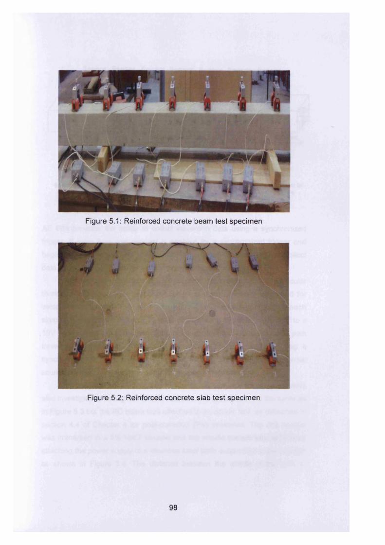
Figure 5.1: Reinforced concrete beam test specimen

Figure 5.2: Reinforced concrete slab test specimen

98

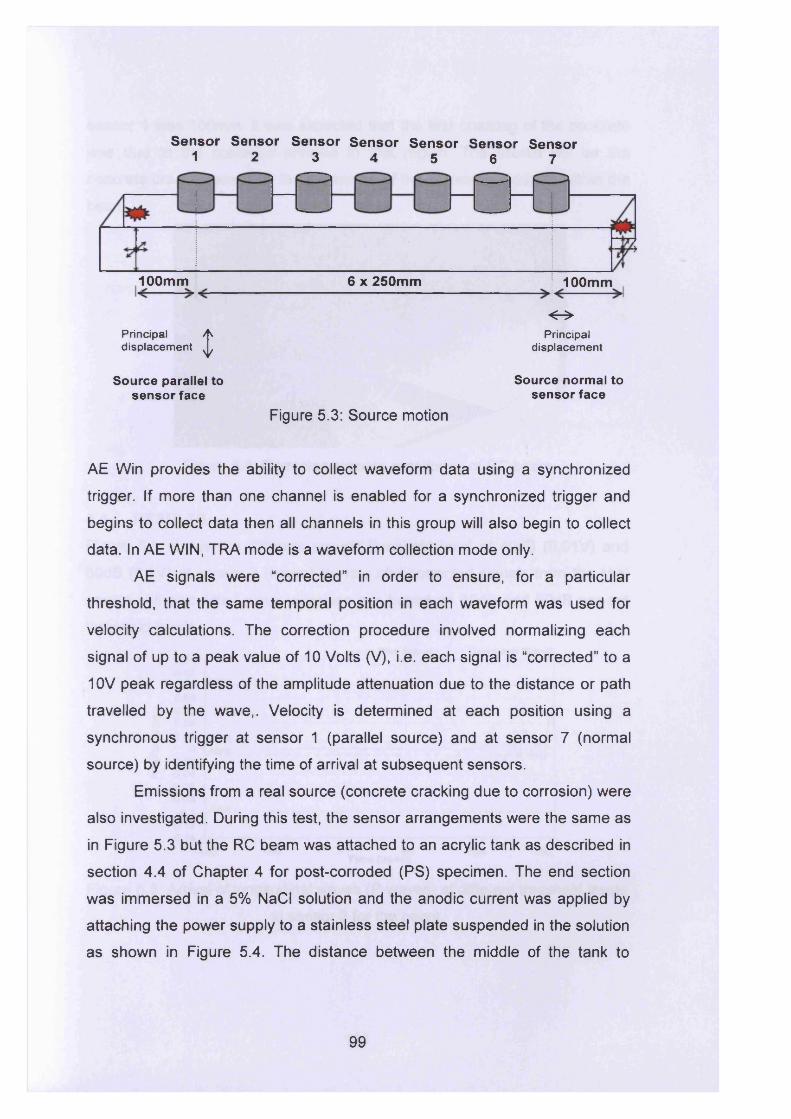
Sensor Sensor Sensor Sensor Sensor Sensor Sensor1 2 3 4 5 6 7

100mm 6 x 250mm 100mm

Principaldisplacement t

<->Principal

displacement

Source parallel to sensor face

Figure 5.3: Source motion

Source normal to sensor face

AE Win provides the ability to collect waveform data using a synchronized

trigger. If more than one channel is enabled for a synchronized trigger and

begins to collect data then all channels in this group will also begin to collect

data. In AE WIN, TRA mode is a waveform collection mode only.

AE signals were “corrected” in order to ensure, for a particular

threshold, that the same temporal position in each waveform was used for

velocity calculations. The correction procedure involved normalizing each

signal of up to a peak value of 10 Volts (V), i.e. each signal is “corrected” to a

10V peak regardless of the amplitude attenuation due to the distance or path

travelled by the wave,. Velocity is determined at each position using a

synchronous trigger at sensor 1 (parallel source) and at sensor 7 (normal

source) by identifying the time of arrival at subsequent sensors.

Emissions from a real source (concrete cracking due to corrosion) were

also investigated. During this test, the sensor arrangements were the same as

in Figure 5.3 but the RC beam was attached to an acrylic tank as described in

section 4.4 of Chapter 4 for post-corroded (PS) specimen. The end section

was immersed in a 5% NaCI solution and the anodic current was applied by

attaching the power supply to a stainless steel plate suspended in the solution

as shown in Figure 5.4. The distance between the middle of the tank to

99

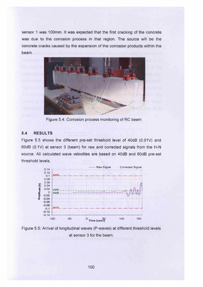
sensor 1 was 100mm. It was expected that the first cracking of the concrete

was due to the corrosion process in that region. The source will be the

concrete cracks caused by the expansion of the corrosion products within the

beam.

Figure 5.4: Corrosion process monitoring of RC beam.

5.4 RESULTSFigure 5.5 shows the different pre-set threshold level of 40dB (0.01V) and

60dB (0.1V) at sensor 3 (beam) for raw and corrected signals from the H-N

source. All calculated wave velocities are based on 40dB and 60dB pre-set

threshold levels. Raw Signal Corrected Signal

0.14 0.12

0.1 0.08 0.06

E 0.04 ■8 0.02 J 0

- 0.1

-0.14

- fj

-4QSJB. _ __ __ I \ t *

• : 4 •;

_ S M 8 _ ...............................................................“ .... ............1----------1----LJ------ 1----- 1---1-----------Li*

T 1 ' i----------------------- 1-----------------------1—

-100 -50Time [usecf

100 150

Figure 5.5: Arrival of longitudinal waves (P-waves) at different threshold levels

at sensor 3 for the beam.

1 0 0

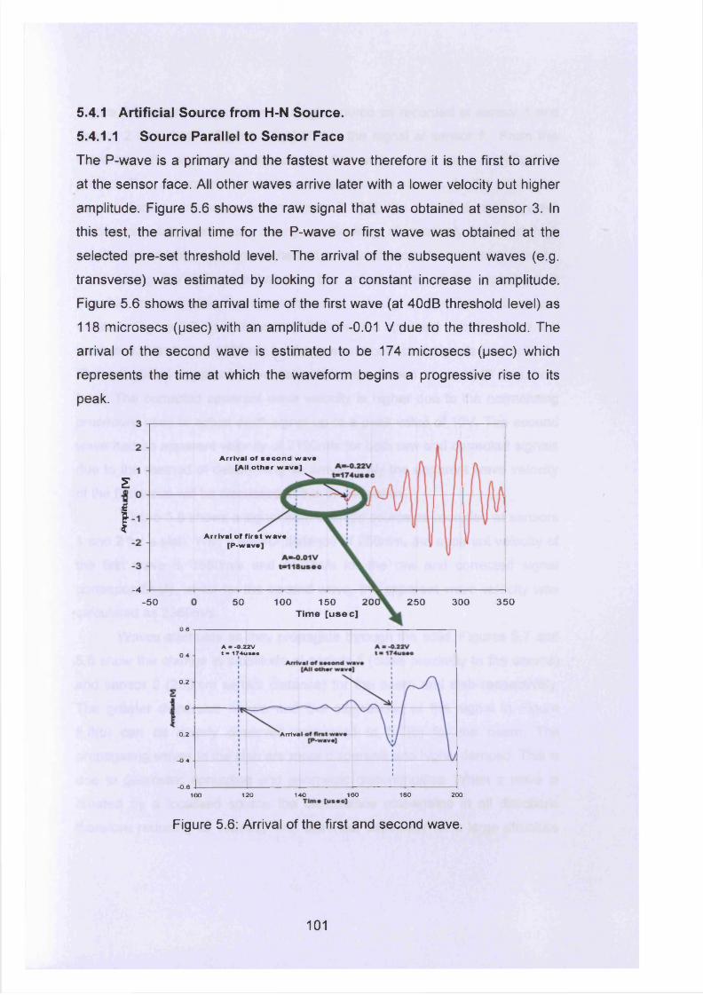
5.4.1 Artificial Source from H-N Source.5.4.1.1 Source Parallel to Sensor FaceThe P-wave is a primary and the fastest wave therefore it is the first to arrive

at the sensor face. All other waves arrive later with a lower velocity but higher

amplitude. Figure 5.6 shows the raw signal that was obtained at sensor 3. In

this test, the arrival time for the P-wave or first wave was obtained at the

selected pre-set threshold level. The arrival of the subsequent waves (e.g.

transverse) was estimated by looking for a constant increase in amplitude.

Figure 5.6 shows the arrival time of the first wave (at 40dB threshold level) as

118 microsecs (psec) with an amplitude of -0.01 V due to the threshold. The

arrival of the second wave is estimated to be 174 microsecs (psec) which

represents the time at which the waveform begins a progressive rise to its

peak.

A rriva l o f s ao ond w av# [A ll o th a r w a v # ]

E

fA rriv a l o f f lra t w av#

[P -w av# ]

-4-50 50 100 150

Time [usee]200 250 300 350

o.aA - -0.22V t ■ 174us#o0.4

0.2

"Arrivi-0.2

-0.4

- 0.8160 180 200120 140100

Figure 5.6: Arrival of the first and second wave.

101

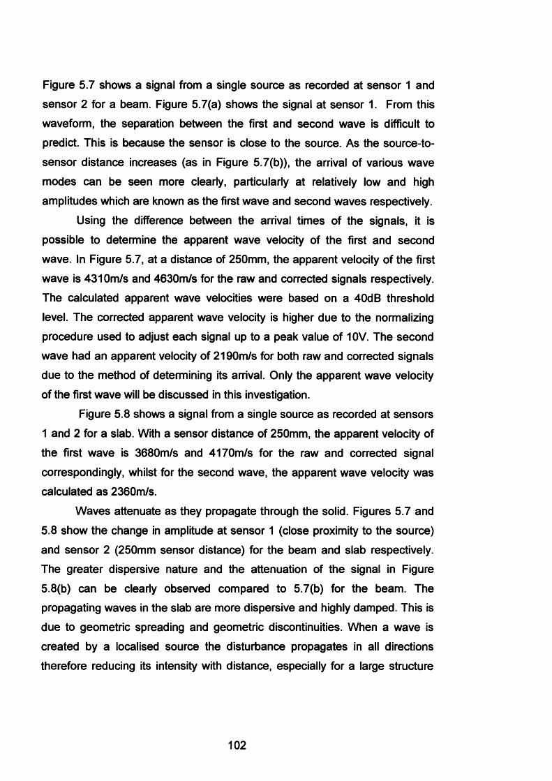
Figure 5.7 shows a signal from a single source as recorded at sensor 1 and

sensor 2 for a beam. Figure 5.7(a) shows the signal at sensor 1. From this

waveform, the separation between the first and second wave is difficult to

predict. This is because the sensor is close to the source. As the source-to-

sensor distance increases (as in Figure 5.7(b)), the arrival of various wave

modes can be seen more clearly, particularly at relatively low and high

amplitudes which are known as the first wave and second waves respectively.

Using the difference between the arrival times of the signals, it is

possible to determine the apparent wave velocity of the first and second

wave. In Figure 5.7, at a distance of 250mm, the apparent velocity of the first

wave is 4310m/s and 4630m/s for the raw and corrected signals respectively. The calculated apparent wave velocities were based on a 40dB threshold

level. The corrected apparent wave velocity is higher due to the normalizing

procedure used to adjust each signal up to a peak value of 10V. The second

wave had an apparent velocity of 2190m/s for both raw and corrected signals

due to the method of determining its arrival. Only the apparent wave velocity

of the first wave will be discussed in this investigation.

Figure 5.8 shows a signal from a single source as recorded at sensors

1 and 2 for a slab. With a sensor distance of 250mm, the apparent velocity of

the first wave is 3680m/s and 4170m/s for the raw and corrected signal

correspondingly, whilst for the second wave, the apparent wave velocity was

calculated as 2360m/s.

Waves attenuate as they propagate through the solid. Figures 5.7 and

5.8 show the change in amplitude at sensor 1 (close proximity to the source)

and sensor 2 (250mm sensor distance) for the beam and slab respectively. The greater dispersive nature and the attenuation of the signal in Figure

5.8(b) can be clearly observed compared to 5.7(b) for the beam. The

propagating waves in the slab are more dispersive and highly damped. This is

due to geometric spreading and geometric discontinuities. When a wave is

created by a localised source the disturbance propagates in all directions

therefore reducing its intensity with distance, especially for a large structure

102

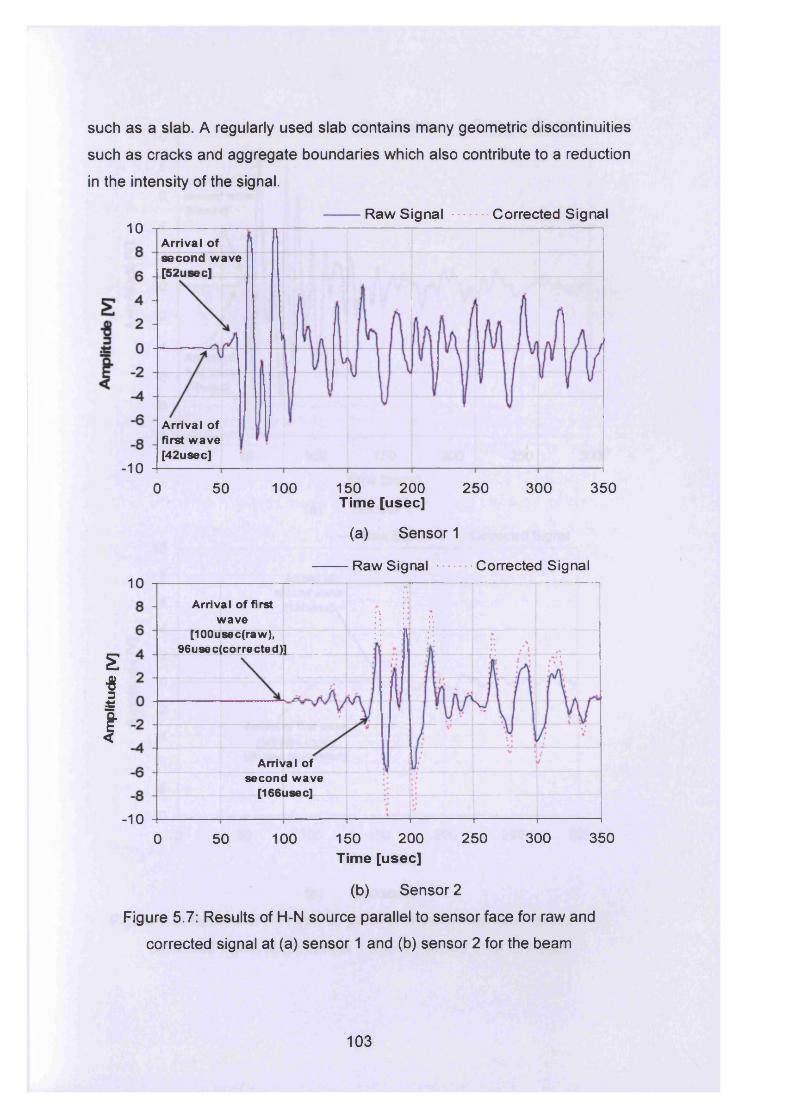
such as a slab. A regularly used slab contains many geometric discontinuities

such as cracks and aggregate boundaries which also contribute to a reduction

in the intensity of the signal.

Raw Signal Corrected Signal10

A rriva l of second w ave [52usec]

A rrival o f first w ave [42usec]

-10150 200 2 5 0 3 0 0 3 5 00 50 100Time [usee]

(a) Sensor 1

Raw Signal Corrected Signal10

Arrival of first w ave

[100usec(raw), 96usec(corrected)]

S*i

!Arrival of

second w ave [166usec]

-10200 2 5 0 300 350100 1500 50

Time [usee]

(b) Sensor 2

Figure 5.7: Results of H-N source parallel to sensor face for raw and

corrected signal at (a) sensor 1 and (b) sensor 2 for the beam

103

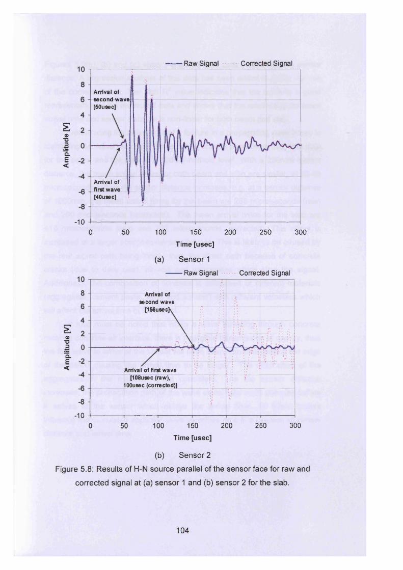
Am

plitu

de

[V]

Am

plitu

de

[V]

Raw Signal Corrected Signal

Arrival of second wave [50usec]

Arrival of first wave [40usec]

-100 50 100 150 200 250 300

Time [usee]

(a) Sensor 1

Raw Signal Corrected Signal

Arrival of second wave

[156usecK

Arrival of first wave [108usec (raw),

100usec (corrected)]

-10250 3000 50 100 150 200

Time [usee]

(b) Sensor 2

Figure 5.8: Results of H-N source parallel of the sensor face for raw and

corrected signal at (a) sensor 1 and (b) sensor 2 for the slab.

104

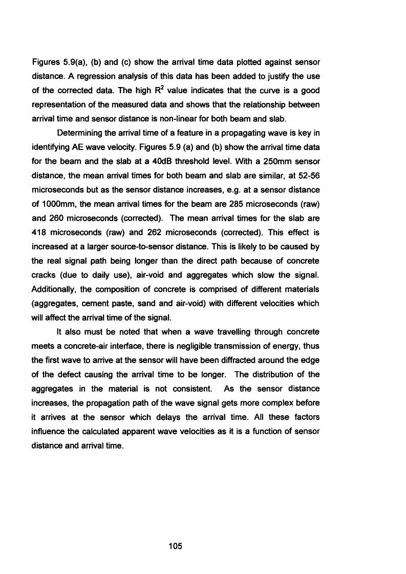
Figures 5.9(a), (b) and (c) show the arrival time data plotted against sensor distance. A regression analysis of this data has been added to justify the use

of the corrected data. The high R2 value indicates that the curve is a good

representation of the measured data and shows that the relationship between

arrival time and sensor distance is non-linear for both beam and slab.Determining the arrival time of a feature in a propagating wave is key in

identifying AE wave velocity. Figures 5.9 (a) and (b) show the arrival time data

for the beam and the slab at a 40dB threshold level. With a 250mm sensor

distance, the mean arrival times for both beam and slab are similar, at 52-56

microseconds but as the sensor distance increases, e.g. at a sensor distance

of 1000mm, the mean arrival times for the beam are 285 microseconds (raw)

and 260 microseconds (corrected). The mean arrival times for the slab are

418 microseconds (raw) and 262 microseconds (corrected). This effect is

increased at a larger source-to-sensor distance. This is likely to be caused by

the real signal path being longer than the direct path because of concrete

cracks (due to daily use), air-void and aggregates which slow the signal.

Additionally, the composition of concrete is comprised of different materials

(aggregates, cement paste, sand and air-void) with different velocities which

will affect the arrival time of the signal.It also must be noted that when a wave travelling through concrete

meets a concrete-air interface, there is negligible transmission of energy, thus

the first wave to arrive at the sensor will have been diffracted around the edge

of the defect causing the arrival time to be longer. The distribution of the

aggregates in the material is not consistent. As the sensor distance

increases, the propagation path of the wave signal gets more complex before

it arrives at the sensor which delays the arrival time. All these factors

influence the calculated apparent wave velocities as it is a function of sensor

distance and arrival time.

105

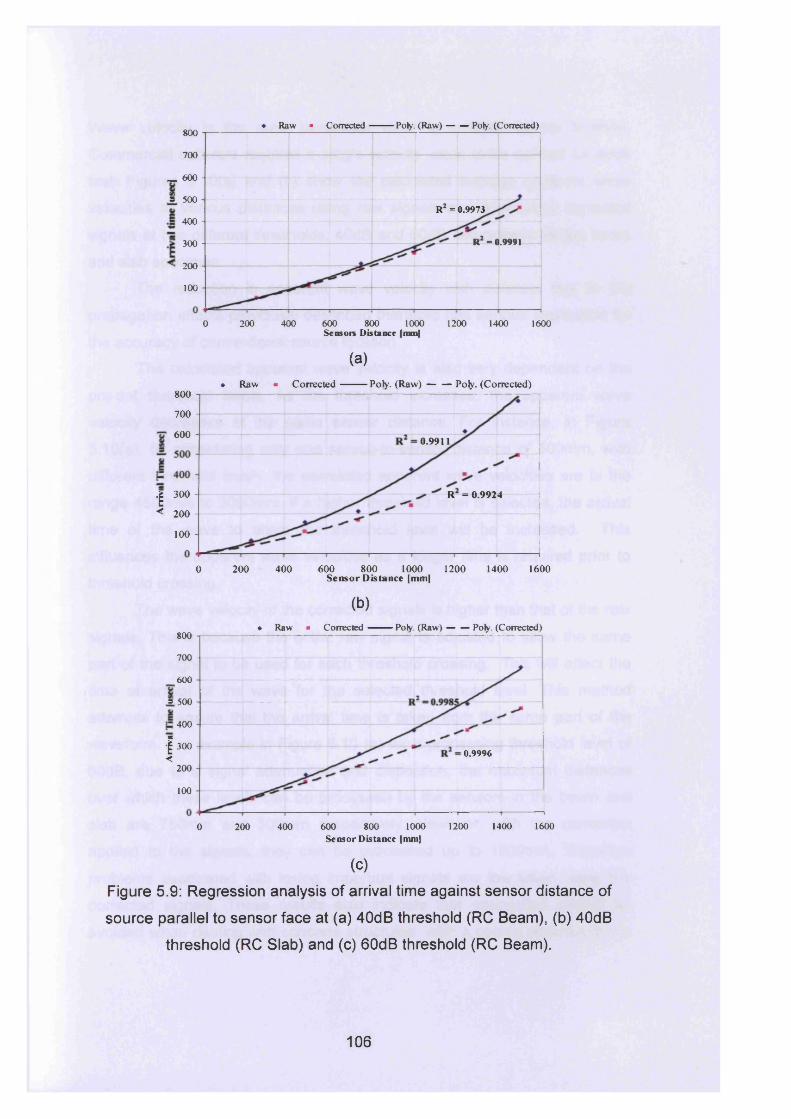
♦ Raw ■ Corrected Poly. (Raw) Poly. (Corrected)800

700 -

_ 600 -

= 500R = 0.9973

400 -

R = 0.9991300 -

200100

800 12000 200 400 600 1000 1400 1600Sensors Distance (mm)

(a)♦ Raw ■ C orrected Poly. (R aw ) Poly. (Corrected)

800

700 -

6000.9911

| 300 -

< 200 -R = 0.9924

100 -

800 1200 16000 200 400 600 1000 1400Sensor Distance |mm]

(b)♦ Raw ■ Corrected Poly. (Raw) Poly. (Corrected)

800

700 -

600

=. 500

400

| 300 - <200

0.9996

100

1000 1200 1400 1600400 600 8000 200Sensor Distance |mm|

(C)

Figure 5.9: Regression analysis of arrival time against sensor distance of

source parallel to sensor face at (a) 40dB threshold (RC Beam), (b) 40dB

threshold (RC Slab) and (c) 60dB threshold (RC Beam).

1 0 6

Wave velocity is the main parameter used to analyse source location.

Commercial software requires a single velocity value to be defined for each

test. Figures 5.10(a) and (b) show the calculated average apparent wave

velocities at various distances using raw signals and attenuation corrected

signals at two different thresholds; 40dB and 60dB respectively for the beam

and slab specimen.

The reduction in apparent wave velocity with distance due to the

propagation effects previously described therefore has serious implication for

the accuracy of conventional source location.The calculated apparent wave velocity is also very dependent on the

pre-set threshold levels. As the threshold increases, the apparent wave

velocity decreases at the same sensor distance. For instance, in Figure

5.10(a), by considering only one source-to-sensor distance of 500mm, with

different threshold levels, the calculated apparent wave velocities are in the

range 4500m/s to 3000m/s. If a higher threshold level is selected, the arrival

time of the wave to attain the threshold level will be increased. This

influences the apparent wave velocities as a longer time is required prior to

threshold crossing.

The wave velocity of the corrected signals is higher than that of the raw

signals. This is because the entire raw signal is adjusted to allow the same

part of the signal to be used for each threshold crossing. This will affect the

time of arrival of the wave for the selected threshold level. This method

attempts to ensure that the arrival time is taken from the same part of the

waveform. For example in Figure 5.10 (b) for a processing threshold level of

60dB, due to a signal attenuation and dispersion; the maximum distances

over which these levels can be processed by the sensors in the beam and

slab are 750mm and 500mm respectively. However, with the correction

applied to the signals, they can be processed up to 1500mm. Therefore

problems associated with losing important signals are low when using the

corrected signals. These results also indicate that attenuation cannot be

avoided when dealing with concrete structures. With a sensor distance of 1.5

107

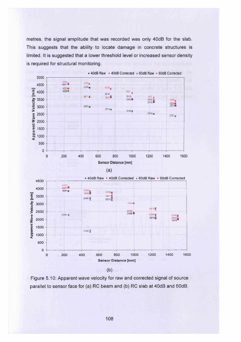
metres, the signal amplitude that was recorded was only 40dB for the slab.

This suggests that the ability to locate damage in concrete structures is

limited. It is suggested that a lower threshold level or increased sensor density

is required for structural monitoring.

♦ 40dB Raw • 40dB Corrected * 60dB Raw • 60dB Corrected5000

4500

| 4000

~ 3500

| 3000

* 2500

5 2000

£ 1500CO

£ 1000 <500

0

4598. 4547 ■ 45K, _______________

4253* - X

4290* 4208 j

_________392J-_______________;_______________3678

3671 £ ^•

3515 3607* 3483* 3432 *

3001*

331 6*3363,

r3070*

2819*2696X

2 51 6*2351*

200 400 1200 1400 1600

4500

600 800 1000

Sensor Distance [mm]

(a)♦ 40dB Raw * 40dB Corrected a 60dB Raw • 60dB Corrected

i*3

4000 -

| 3500

3000 -

> 2500 -Q| 2000

| 1500 -

a 1000 - <500 -

0

41074 0 4 7 *3841*

3683$3601 r ___________

3345 1 3312|

3042|

2439

C

26i7 5 I

2 2 9 6 * 23881 2268 £ 2 2 0 8 * 2079£ 2 0 4 4 *

197 8*

1238 J

200 400 600 800 1000Sensor Distance [mm]

1200 1400 1600

(b)Figure 5.10: Apparent wave velocity for raw and corrected signal of source

parallel to sensor face for (a) RC beam and (b) RC slab at 40dB and 60dB.

108

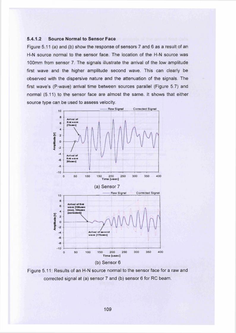
5.4.1.2 Source Normal to Sensor FaceFigure 5.11 (a) and (b) show the response of sensors 7 and 6 as a result of an

H-N source normal to the sensor face. The location of the H-N source was

100mm from sensor 7. The signals illustrate the arrival of the low amplitude

first wave and the higher amplitude second wave. This can clearly be

observed with the dispersive nature and the attenuation of the signals. The

first wave’s (P-wave) arrival time between sources parallel (Figure 5.7) and

normal (5.11) to the sensor face are almost the same. It shows that either

source type can be used to assess velocity.Raw Signal Corrected Signal10

Arrival of firat wav* [70uaac]

E

-2<-4 Arrival of

flrat wava [SOuaao]

-8-10

150 200 250 300 350 40050 1000Tim e [usee]

(a) Sensor 7Raw Signal Corrected Signal10

E

Arrival of aacond wava [170uaac]

-10300 350 400200 25050 100 1500

T im e [usee]

(b) Sensor 6

Figure 5.11: Results of an H-N source normal to the sensor face for a raw and

corrected signal at (a) sensor 7 and (b) sensor 6 for RC beam.

109

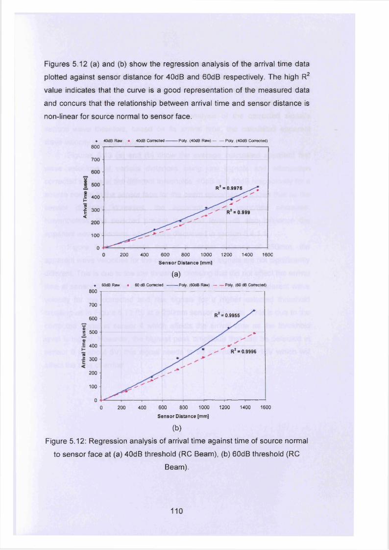
Figures 5.12 (a) and (b) show the regression analysis of the arrival time data

plotted against sensor distance for 40dB and 60dB respectively. The high R2

value indicates that the curve is a good representation of the measured data

and concurs that the relationship between arrival time and sensor distance is

non-linear for source normal to sensor face.

♦ 40dB Raw a 40dB Corrected Poly. (40dB Raw) Poly. (40dB Corrected)800

700

£ 400 H| 300 <

100

0

R2 = 0.9975 ^

j*

R2 = 0.999

, _______ ------------------ 3 * **"[

200 400 600 800 1000 1200 1400 160CSensor Distance [mm]

(a)♦

800

700

60077a.0)(/)a. 500

1 4001-«•§ 300<

200

100

0

« 60dB Raw a 60 dB Corrected Poly. (60dB R a w ) Poly. (60 dB Corrected)

R2 = 0.9955

> >

R2 = 0.9996

**w

0 200 400 600 800 1000 1200 1400 1600Sensor Distance [mm]

(b)Figure 5.12: Regression analysis of arrival time against time of source normal

to sensor face at (a) 40dB threshold (RC Beam), (b) 60dB threshold (RC

Beam).

1 1 0

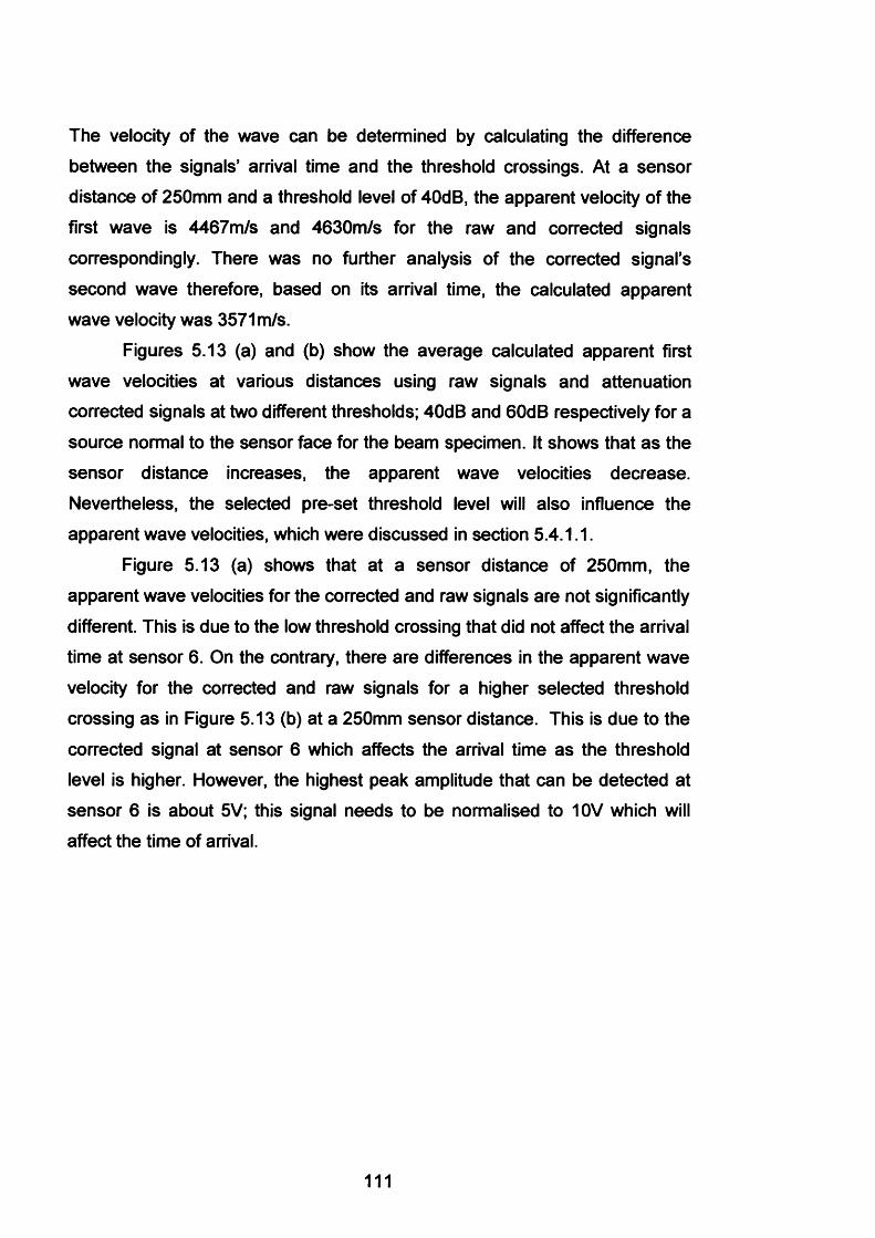
The velocity of the wave can be determined by calculating the difference

between the signals’ arrival time and the threshold crossings. At a sensor

distance of 250mm and a threshold level of 40dB, the apparent velocity of the

first wave is 4467m/s and 4630m/s for the raw and corrected signals

correspondingly. There was no further analysis of the corrected signal’s

second wave therefore, based on its arrival time, the calculated apparent wave velocity was 3571 m/s.

Figures 5.13 (a) and (b) show the average calculated apparent first wave velocities at various distances using raw signals and attenuation

corrected signals at two different thresholds; 40dB and 60dB respectively for a

source normal to the sensor face for the beam specimen. It shows that as the

sensor distance increases, the apparent wave velocities decrease. Nevertheless, the selected pre-set threshold level will also influence the

apparent wave velocities, which were discussed in section 5.4.1.1.

Figure 5.13 (a) shows that at a sensor distance of 250mm, the

apparent wave velocities for the corrected and raw signals are not significantly

different. This is due to the low threshold crossing that did not affect the arrival time at sensor 6. On the contrary, there are differences in the apparent wave

velocity for the corrected and raw signals for a higher selected threshold

crossing as in Figure 5.13 (b) at a 250mm sensor distance. This is due to the

corrected signal at sensor 6 which affects the arrival time as the threshold

level is higher. However, the highest peak amplitude that can be detected at sensor 6 is about 5V; this signal needs to be normalised to 10V which will

affect the time of arrival.

111

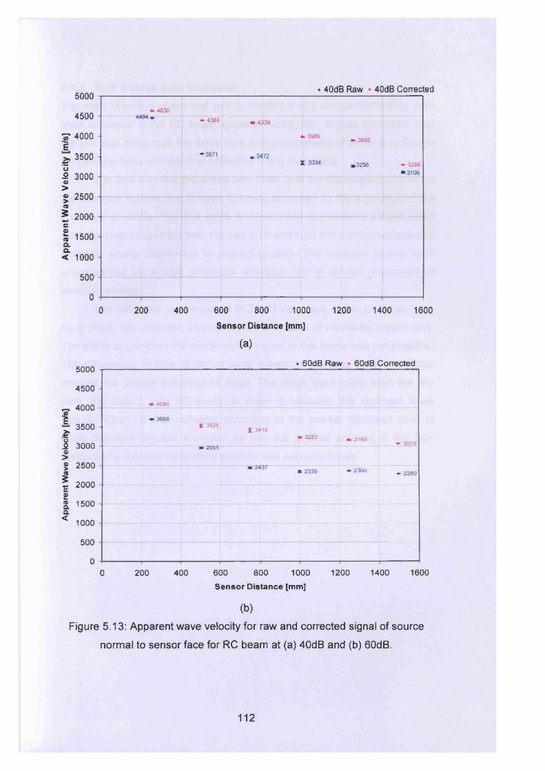
App

aren

t W

ave

Velo

city

[m

/s]

Ap

par

ent

Wav

e V

eloc

ity

[m/s

]

♦ 40dB Raw ■ 40dB Corrected5000

4500

4000

3500

3000

2500

2000

1500

1000

500

00 200 400 600 800 1000 1200 1400 1600

Sensor Distance [mm]

(a)♦ 60dB Raw • 60dB Corrected

5000

4500

4000

3500

3000

2500

2000

1500

1000

500

00 200 400 600 800 1000 1200 1400 1600

Sensor D istance [mm]

(b)Figure 5.13: Apparent wave velocity for raw and corrected signal of source

normal to sensor face for RC beam at (a) 40dB and (b) 60dB.

4086

3699r 3525

I 3416* 3223 3160

30592955

at 2437 ♦ 2360x 2339 ♦ 2280

46304464 * 4 3 8 9 4339

* 39893895

♦3 5 7 1 3472I 3334 *3 2 5 6 * 3286

* 3 1 0 6

1 1 2

5.4.2 True Source from CorrosionThe main objective of this test was to monitor a true source of cracking from

steel corrosion in the RC beam specimen using AE. Figure 5.4 shows how

the test was setup with the same type and arrangement of sensors as for the

H-N source tests with the only difference being the source.The test was first monitored with DiSP until the first crack occurred on

the concrete surface due to cover cracking produced by the expansion of the

corrosion products. The first crack was recorded approximately eight hours

from the beginning of the test. Figures 5.14 and 5.15 show the amplitude and

absolute energy distribution in respect to time. The concrete cracks were

accompanied by a high amplitude emission and a sudden increment of absolute energy.

The AE mode (as explained in 3.2.1) was used in this corrosion test. As a result, the collected waveform was a function of waveform parameters.

The ability to generate the synchronous trigger in this mode was not possible.

The differences in time of arrival were based on the time when the signal crossed the pre-set threshold of 40dB. The times were taken from the line

data, the output from AE mode, in order to calculate the apparent wave

velocity. Each hit was collected according to the pre-set threshold level of

40dB therefore detailed analyses, as with the artificial sources of the type

conducted previously for artificial sources was not undertaken.

113

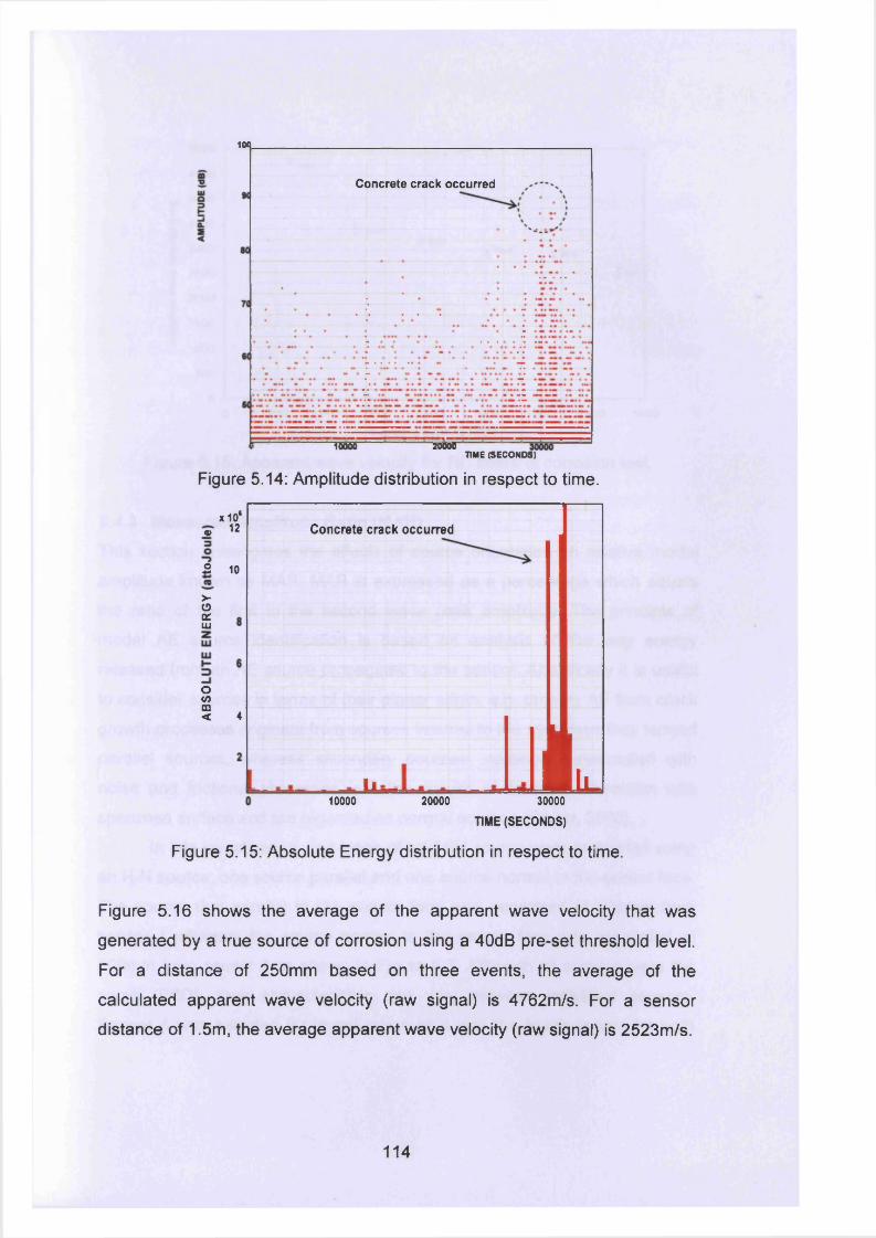
100

Concrete crack occurred

w 20600TIME (SECONDS)

Figure 5.14: Amplitude distribution in respect to time.

x 10* • 12

2 10

>-oQZLU

oCO

5 4

Concrete crack occurred

lA10000

H J20000 30000

TIME (SECONDS)

Figure 5.15: Absolute Energy distribution in respect to time.

Figure 5.16 shows the average of the apparent wave velocity that was

generated by a true source of corrosion using a 40dB pre-set threshold level.

For a distance of 250mm based on three events, the average of the

calculated apparent wave velocity (raw signal) is 4762m/s. For a sensor

distance of 1.5m, the average apparent wave velocity (raw signal) is 2523m/s.

114

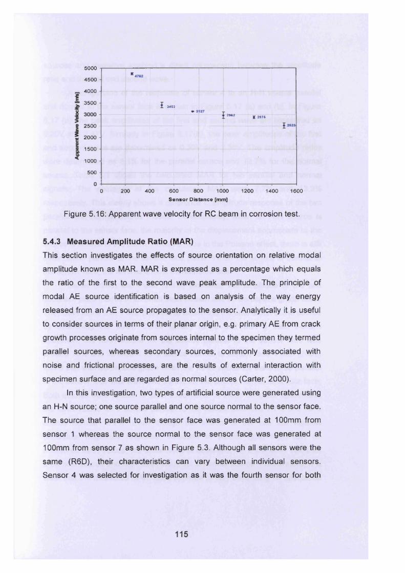
5000

4500

_ 4000

35003403

2962 £ 2876

2500 -

2000

1500

1000

500

8000 200 400 600 1000 1200 1400 1600S ensor D istance [mm]

Figure 5.16: Apparent wave velocity for RC beam in corrosion test.

5.4.3 Measured Amplitude Ratio (MAR)This section investigates the effects of source orientation on relative modal

amplitude known as MAR. MAR is expressed as a percentage which equals

the ratio of the first to the second wave peak amplitude. The principle of

modal AE source identification is based on analysis of the way energy

released from an AE source propagates to the sensor. Analytically it is useful

to consider sources in terms of their planar origin, e.g. primary AE from crack

growth processes originate from sources internal to the specimen they termed

parallel sources, whereas secondary sources, commonly associated with

noise and frictional processes, are the results of external interaction with

specimen surface and are regarded as normal sources (Carter, 2000).

In this investigation, two types of artificial source were generated using

an H-N source; one source parallel and one source normal to the sensor face.

The source that parallel to the sensor face was generated at 100mm from

sensor 1 whereas the source normal to the sensor face was generated at

100mm from sensor 7 as shown in Figure 5.3. Although all sensors were the

same (R6D), their characteristics can vary between individual sensors.

Sensor 4 was selected for investigation as it was the fourth sensor for both

sources and therefore enabled a direct comparison between the amplitude

ratio and the first and second wave.

A comparison of the response of sensor 4 to an H-N source parallel and normal to the sensor face is shown in Figure 5.17 (a) and (b). In Figure

5.17 (a), the peak amplitudes of the first and second wave are measured as0.20V and 2.47V. Similarly in Figure 5.17(b), the peak amplitudes of the first

and second wave are determined as 0.30V and 2.36V. The amplitude ratios

were determined as 8.1% for the parallel source and 12.7% for the normal

source. Table 5.1 shows the calculated MAR for ten parallel and normal

signals. The averages of the calculated MAR were 7.7% and 13.2%

respectively. This clearly shows a difference in amplitude response of the two

parallel and normal source modes. Consequently, when an H-N source is

parallel to the sensor face, the majority of the displacement appropriate to the

source is normal to the beam. However, due to the Poisson effect, there is still

deformation parallel to the sensor face plane. When the source is normal to

the sensor face, the reverse should therefore be true

Carter (2000) and Pullin (2005) examined the amplitude of the two

dominant plate modes in an 8mm steel I-beam and an aerospace grade steel.

They both found that it was possible to determine the orientation of the source

by examining the MAR. Carter (2000) found that with a steel I-beam

specimen, the MAR values for the source parallel to the sensor face was

around 10% and 30%-60% for a source normal to sensor face. Pullin (2005)

found that with aerospace grade steel, the MAR values for the source parallel

to the sensor face was 9.9% and 29.0% for the source normal to sensor face.

Both studies were related to steel specimens. In these concrete specimens, the MAR values for a source parallel to the sensor face was 7.7% and for a

source normal 13.2%. Even though the effects of the test are variable

(individual frequency response, selection of sensor type, materials) on

measured MAR values, the same trend is observed, i.e. a low MAR value for a parallel source and high MAR value for a normal source. Furthermore, it is

clear that the measured MAR value appears to vary depending on orientation

116

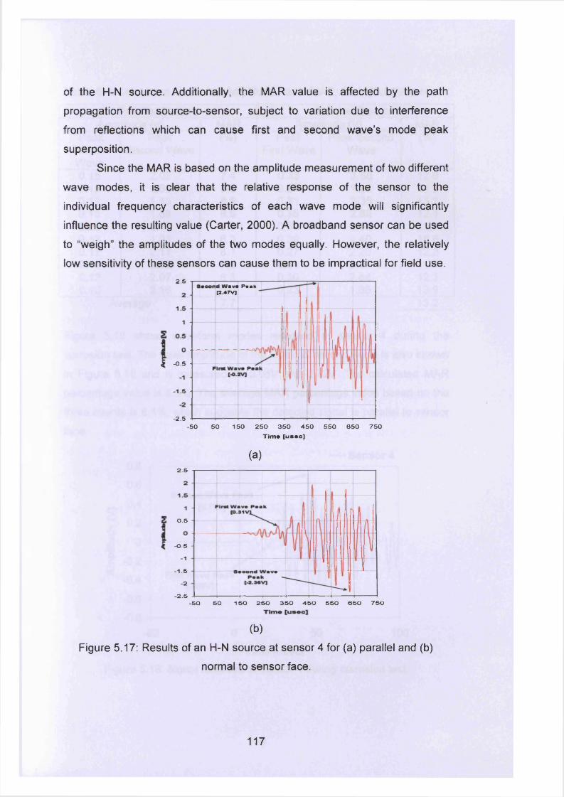
of the H-N source. Additionally, the MAR value is affected by the path

propagation from source-to-sensor, subject to variation due to interference

from reflections which can cause first and second wave’s mode peak

superposition.

Since the MAR is based on the amplitude measurement of two different

wave modes, it is clear that the relative response of the sensor to the

individual frequency characteristics of each wave mode will significantly

influence the resulting value (Carter, 2000). A broadband sensor can be used

to “weigh” the amplitudes of the two modes equally. However, the relatively

low sensitivity of these sensors can cause them to be impractical for field use.2.5

id W a v * P * a k [2.47V]

-0 .5 -

- 1.5 -

- 2.5-50 50 150 250 350 450 550 650 750

T im * [u s e e ]

(a)2.5

0.5

- 0.5 -

-1- 1.5

-2- 2.5

150 250 350 450 550 650 750-50 50

(b)

Figure 5.17: Results of an H-N source at sensor 4 for (a) parallel and (b)

normal to sensor face.

117

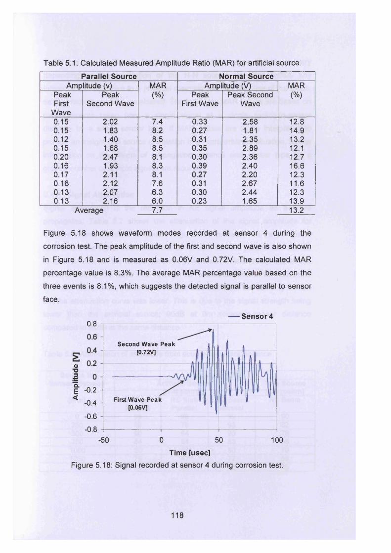
Table 5.1: Calculated Measured Amplitude Ratio (MAR) for artificial source.

Parallel Source Normal SourceAmp itude (v) MAR Amp itude (V) MAR

PeakFirst

Wave

Peak Second Wave

(%) Peak First Wave

Peak Second Wave

(%)

0.15 2.02 7.4 0.33 2.58 12.80.15 1.83 8.2 0.27 1.81 14.90.12 1.40 8.5 0.31 2.35 13.20.15 1.68 8.5 0.35 2.89 12.10.20 2.47 8.1 0.30 2.36 12.70.16 1.93 8.3 0.39 2.40 16.60.17 2.11 8.1 0.27 2.20 12.30.16 2.12 7.6 0.31 2.67 11.60.13 2.07 6.3 0.30 2.44 12.30.13 2.16 6.0 0.23 1.65 13.9

Average 7.7 13.2

Figure 5.18 shows waveform modes recorded at sensor 4 during the

corrosion test. The peak amplitude of the first and second wave is also shown

in Figure 5.18 and is measured as 0.06V and 0.72V. The calculated MAR

percentage value is 8.3%. The average MAR percentage value based on the

three events is 8.1%, which suggests the detected signal is parallel to sensor

face.

— Sensor 40.8

Second Wave Peak [0.72V]

o3

| -0.2 -

< -0.4 First Wave Peak [0.06V]

- 0.6- 0.8

-50 0 50 100Time [usee]

Figure 5.18: Signal recorded at sensor 4 during corrosion test.

118

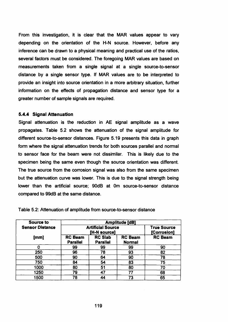
From this investigation, it is clear that the MAR values appear to vary

depending on the orientation of the H-N source. However, before any

inference can be drawn to a physical meaning and practical use of the ratios, several factors must be considered. The foregoing MAR values are based on

measurements taken from a single signal at a single source-to-sensor

distance by a single sensor type. If MAR values are to be interpreted to

provide an insight into source orientation in a more arbitrary situation, further information on the effects of propagation distance and sensor type for a

greater number of sample signals are required.

5.4.4 Signal Attenuation

Signal attenuation is the reduction in AE signal amplitude as a wave

propagates. Table 5.2 shows the attenuation of the signal amplitude for

different source-to-sensor distances. Figure 5.19 presents this data in graph

form where the signal attenuation trends for both sources parallel and normal to sensor face for the beam were not dissimilar. This is likely due to the

specimen being the same even though the source orientation was different.

The true source from the corrosion signal was also from the same specimen

but the attenuation curve was lower. This is due to the signal strength being

lower than the artificial source; 90dB at Om source-to-sensor distance

compared to 99dB at the same distance.

Table 5.2: Attenuation of amplitude from source-to-sensor distance

Source to Sensor Distance

[mm]

Amplitude [dB]Artificial Source

[H-N source]True Source [Corrosion]

RC Beam Parallel

RC Slab Parallel

RC Beam Normal

RC Beam

0 99 99 99 90250 96 78 93 82500 90 64 90 78750 84 54 83 751000 80 51 80 701250 79 47 77 681500 78 44 73 65

119

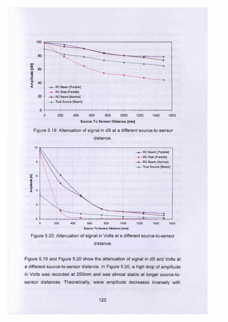
100

CD5

£aE< RC Beam [Parallel]

RC Slab [Parallel] RC Beam [Normal] True Source [Beam]

0 200 400 600 800 1000 1200 1400 1600

Source To Sensor Distance [mm]

Figure 5.19: Attenuation of signal in dB at a different source-to-sensor

distance.

10RC Beam [Parallel] RC Slab [Parallel] RC Beam [Normal] True Source [Beam]

8

6

4

2

00 200 600 800 1000 1200400 1400 1600

Source To Sensor Distance [mm]

Figure 5.20: Attenuation of signal in Volts at a different source-to-sensor

distance.

Figure 5.19 and Figure 5.20 show the attenuation of signal in dB and Volts at

a different source-to-sensor distance. In Figure 5.20, a high drop of amplitude

in Volts was recorded at 250mm and was almost stable at longer source-to-

sensor distances. Theoretically, wave amplitude decreases inversely with

1 2 0

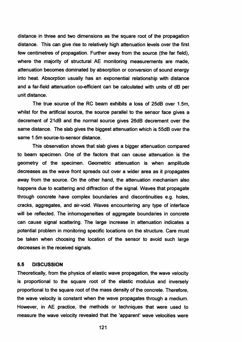
distance in three and two dimensions as the square root of the propagation

distance. This can give rise to relatively high attenuation levels over the first few centimetres of propagation. Further away from the source (the far field),

where the majority of structural AE monitoring measurements are made, attenuation becomes dominated by absorption or conversion of sound energy

into heat. Absorption usually has an exponential relationship with distance

and a far-field attenuation co-efficient can be calculated with units of dB per unit distance.

The true source of the RC beam exhibits a loss of 25dB over 1.5m, whilst for the artificial source, the source parallel to the sensor face gives a

decrement of 21 dB and the normal source gives 26dB decrement over the

same distance. The slab gives the biggest attenuation which is 55dB over the

same 1.5m source-to-sensor distance.

This observation shows that slab gives a bigger attenuation compared

to beam specimen. One of the factors that can cause attenuation is the

geometry of the specimen. Geometric attenuation is when amplitude

decreases as the wave front spreads out over a wider area as it propagates

away from the source. On the other hand, the attenuation mechanism also

happens due to scattering and diffraction of the signal. Waves that propagate

through concrete have complex boundaries and discontinuities e.g. holes,

cracks, aggregates, and air-void. Waves encountering any type of interface

will be reflected. The in homogeneities of aggregate boundaries in concrete

can cause signal scattering. The large increase in attenuation indicates a

potential problem in monitoring specific locations on the structure. Care must be taken when choosing the location of the sensor to avoid such large

decreases in the received signals.

5.5 DISCUSSION

Theoretically, from the physics of elastic wave propagation, the wave velocity

is proportional to the square root of the elastic modulus and inversely

proportional to the square root of the mass density of the concrete. Therefore, the wave velocity is constant when the wave propagates through a medium.

However, in AE practice, the methods or techniques that were used to

measure the wave velocity revealed that the ‘apparent’ wave velocities were

121

not constant when the wave propagates through a medium. This ambiguous

velocity leads to difficulty in the techniques used to locate the source of AE

events.

On the whole, this work has investigated signal attenuation and wave

in concrete structures over a variety of source-to-sensor distances. It has

been shown that apparent wave velocities decrease as the sensor distance

increases. Acoustic waves are modified as they propagate through the

material due to scattering, absorption, attenuation and retransmission through

different materials such as aggregates, cement paste, reinforcement, air-void

due to cracks etc which will affect the wave propagation (Miller and Mclntire,

1987).

The presence of steel reinforcement in the RC specimen will affect the

calculated apparent wave velocity. Since the wave velocity through steel is

greater than concrete the wave signal may be refracted into the bars and

transmitted to the receiver at the wave velocity of the steel. The apparent velocity through the member will be greater than the actual velocity through

the concrete.The measured apparent wave velocity may also be affected by the

presence of cracks or voids along the propagation path from source-to-

sensors. The wave signal may be diffracted around the discontinuities thus

increasing the travel path and travel time. Consequently, the apparent wave

velocity will be measured incorrectly through time of arrival techniques.Apart from investigating the wave propagation in concrete structures

over a variety of source-to-sensor distances; a selected threshold level also

has an impact on the measured apparent wave velocities. As the selected

threshold level increases, the arrival times increase hence causing a

decrease in the apparent wave velocities. For a source-to-sensor distance of 1.5m, the signal amplitude recorded was only 40dB, whereas for 60dB, the

maximum source to distance was 0.5m. Consequently, the ability to locate

damage in concrete structures is limited to a higher threshold level.

There have been few studies in determining the P-wave velocity in

Ultrasonics. Philippidis and Aggelis (2005) investigated the effect of the water

to cement ratio on wave velocity in concrete, where for a range of water to

cement ratios between 0.375 and 0.45, the P-wave velocity varied between

122

3500m/s and 4700m/s. As the water to cement ratio decreased, the velocity of

the P-wave increased. Additionally, the authors found that using a signal from

a 15 kHz tone burst at a sensor distance of 150mm, the apparent wave

velocity of P-waves in concrete ranged from 4100m/s to 4700m/s. This

suggests that, as well as steel reinforcement, aggregates, air-void, cracks and

path propagation, the moisture content of the specimen is an important factor

in influencing the calculated apparent wave velocities. Gassman and

Tawheed (2004) and Chang et al. (2006) discovered that the wave velocity in

concrete varies from 3500m/s to 4000m/s depending on concrete

composition, age and condition.

These factors must be taken into consideration with regards to the

reduction in velocity; the increase in distance is an important result as AE

users often take a velocity measurement at one distance and use it in location

studies over a range of distances. Furthermore the source location will be

greatly affected when considering the inaccuracy in determining the P-wave

arrival times. Source location is of prime interest for modem AE analysis as it

can be used to evaluate damage localization and crack propagation.

Additionally, accurate source location is essential for quantitative AE analysis

using moment tensor analysis (Li, 1996).

There is a similarity in measuring wave velocity techniques between

Ultrasonics and AE. Both techniques define wave velocity as a distance from

the source-to-sensors over the time travelled from the source-to-sensor. The

method that was used in this investigation is similar to indirect transmission in

determining pulse velocity in Ultrasonics. However, from the regression

analysis, the results show that this experimental programme does not concur with the hypothesis proposed in BS EN 12504-4 (2004) for the testing of

concrete using Ultrasonics. In this standard, the determination of the

Ultrasonic pulse velocity is obtained by assuming that the relationship

between the arrival time data and sensor distance is linear. The slope of the

best-fit straight line is drawn through the measured arrival time data over

sensor distance and the slope is taken as the mean wave velocity along the

concrete surface. On the other hand, the best fit lines through the data for

both specimens using the AE data shows that the relationship between the

arrival time and sensor distance is non linear. Consequently, the apparent

123

wave velocity decreases as the sensor distance increases as the wave

propagates through the medium.Signal attenuation involves the measurement of wave amplitudes as a

function of propagation distance. There are two basic mechanisms by which a

wave is attenuated: (1) geometric attenuation; (2) material attenuation.

Geometric attenuation is the phenomena by which the amplitude of the wave

decreases as the wave front spreads out over a wider area as it propagates

away from the source. Material attenuation can be by either absorption or

scattering. Due to attenuation, the monitoring of large structures e.g. concrete

bridges, requires the use of many sensors placed sufficiently close together to

ensure that an event emanating from any point on the structure will not be

attenuated sufficiently to escape detection.The MAR value was determined to investigate the effect of source

orientation as to the viability of modal AE in structural monitoring applications. It was discovered that a source parallel to sensor face exhibited lower MAR

values than a source normal to sensor face. However, if the MAR is to be

viable as a practical discriminant, further quantitative information on factors

that influence its absolute value for a specific source or a sensor position is

required.Several factors can complicate the use of MAR value as a source

identification discriminant in structural monitoring. If conclusions on source

orientation are to be drawn from MAR measurement, consideration on how

the sensor mounting position and orientation relative to other elements

influences its response to sources in various regions of the beam is required. This becomes complex if the precise source position is unknown, as is the

case with global AE inspection. Furthermore, with an unknown source

position, peak superposition and source depth, it is clear that the use of a

single value MAR discriminant in a large area is unlikely to be practically

viable.

5.6 CONCLUSION

In this study, it can be concluded that:

• RC concrete is a non-homogeneous material which consists of several

materials (reinforced steel, aggregates, cement paste, sand and air

124

voids). Therefore an apparent wave velocity was used as the wave

velocity was not constant during propagation through the RC concrete. The apparent wave velocities were reduced due to attenuation and

dispersion of the wave signal which affected the length of time in

reaching the subsequent sensor.

• A practical investigation of two concrete structures shows that as the

source-to-sensor distance increases, the calculated wave velocity

decreases.

• The apparent wave velocities are between 4800m/s to 3100m/s for the

beam specimen and 3841 m/s to 2000m/s for the slab specimen for a

source-to-sensor distance from 250mm to 1500mm with a 40dB pre-set

threshold. This shows that the apparent wave velocity is not constant as the wave propagates through the concrete. Additionally, the

apparent wave velocities varied between one specimen and another.

• The apparent wave velocity used in automatic TOA should be carefully

selected considering both the distance at which measurements will be

taken and the threshold used. A low threshold level is recommended in

order to locate damage in large concrete structures.

• There is a tendency of a low MAR value for a parallel source and a

high MAR value for a normal source on the relative distribution of

values rather than absolute value measured. The MAR value of a

signal from a given source is dependent on sensor frequency response

characteristics and mounting orientation relative to the source. Additionally, the MAR value measurement is subject to variation due to

interference from reflections which can cause first and second wave

mode peak superposition.

• Propagation of the elastic waves in concrete is affected by the

geometry of the sample, the path taken from the source-to-sensor and

the concrete composition and condition. These need to be taken into

consideration when determining the RC concrete’s apparent wave

velocity.

125

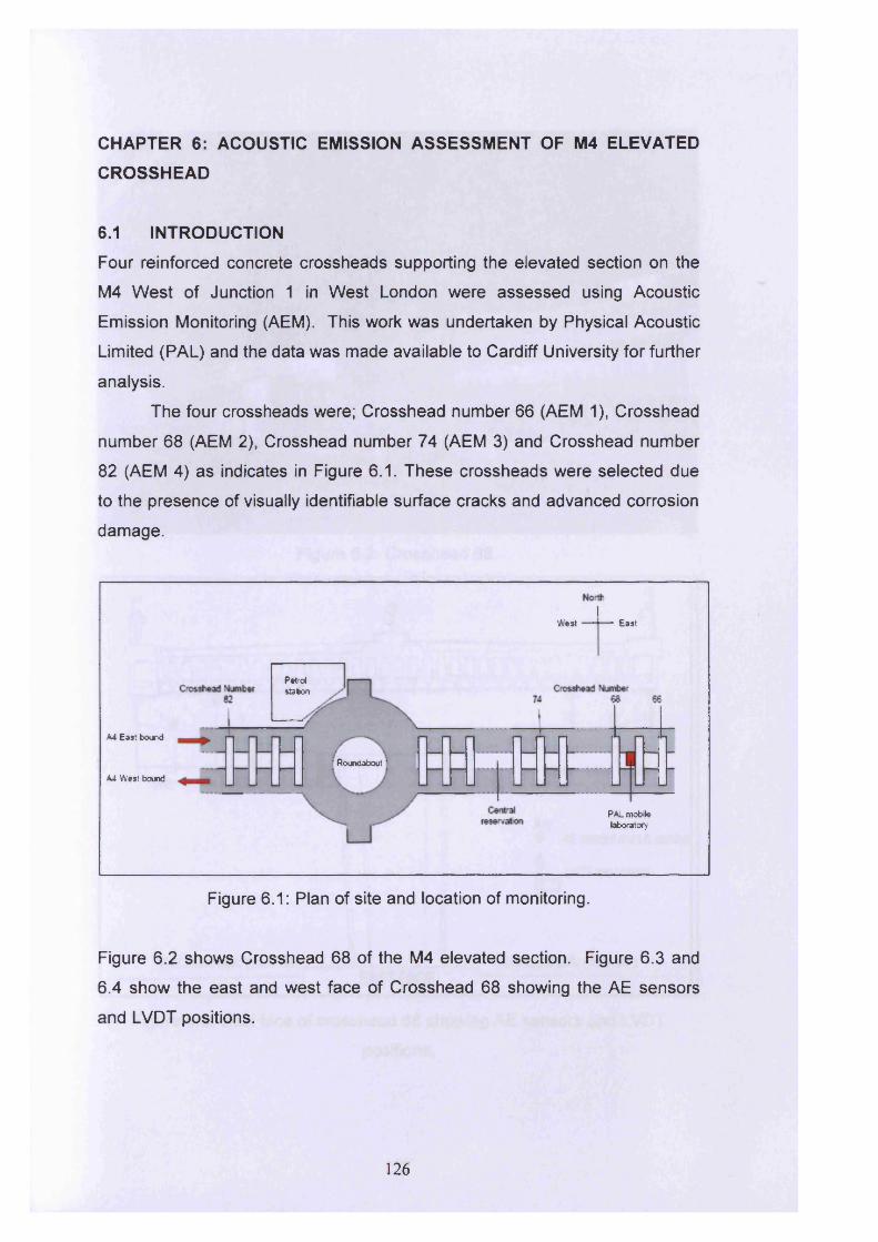
CHAPTER 6: ACOUSTIC EMISSION ASSESSMENT OF M4 ELEVATED

CROSSHEAD

6.1 INTRODUCTIONFour reinforced concrete crossheads supporting the elevated section on the

M4 West of Junction 1 in West London were assessed using Acoustic

Emission Monitoring (AEM). This work was undertaken by Physical Acoustic

Limited (PAL) and the data was made available to Cardiff University for further

analysis.

The four crossheads were; Crosshead number 66 (AEM 1), Crosshead

number 68 (AEM 2), Crosshead number 74 (AEM 3) and Crosshead number

82 (AEM 4) as indicates in Figure 6.1. These crossheads were selected due

to the presence of visually identifiable surface cracks and advanced corrosion

damage.

West East

Petrolstation

A4 East bound

Roundabout

A4 West bound

PAL moble laboratory

Figure 6.1: Plan of site and location of monitoring.

Figure 6.2 shows Crosshead 68 of the M4 elevated section. Figure 6.3 and

6.4 show the east and west face of Crosshead 68 showing the AE sensors

and LVDT positions.

126

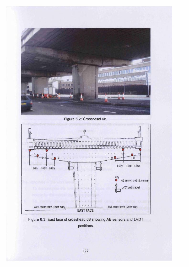
Figure 6.2: Crosshead 68

1.66m 1.66m 1.66m1 66m 166m 1.66m

• ' AE sensors and Ld. number

LVDT and bracket

East bound traffic (North side)West bound traffic (South side) rEAST FACE

Figure 6.3: East face of crosshead 68 showing AE sensors and LVDT

positions.

127

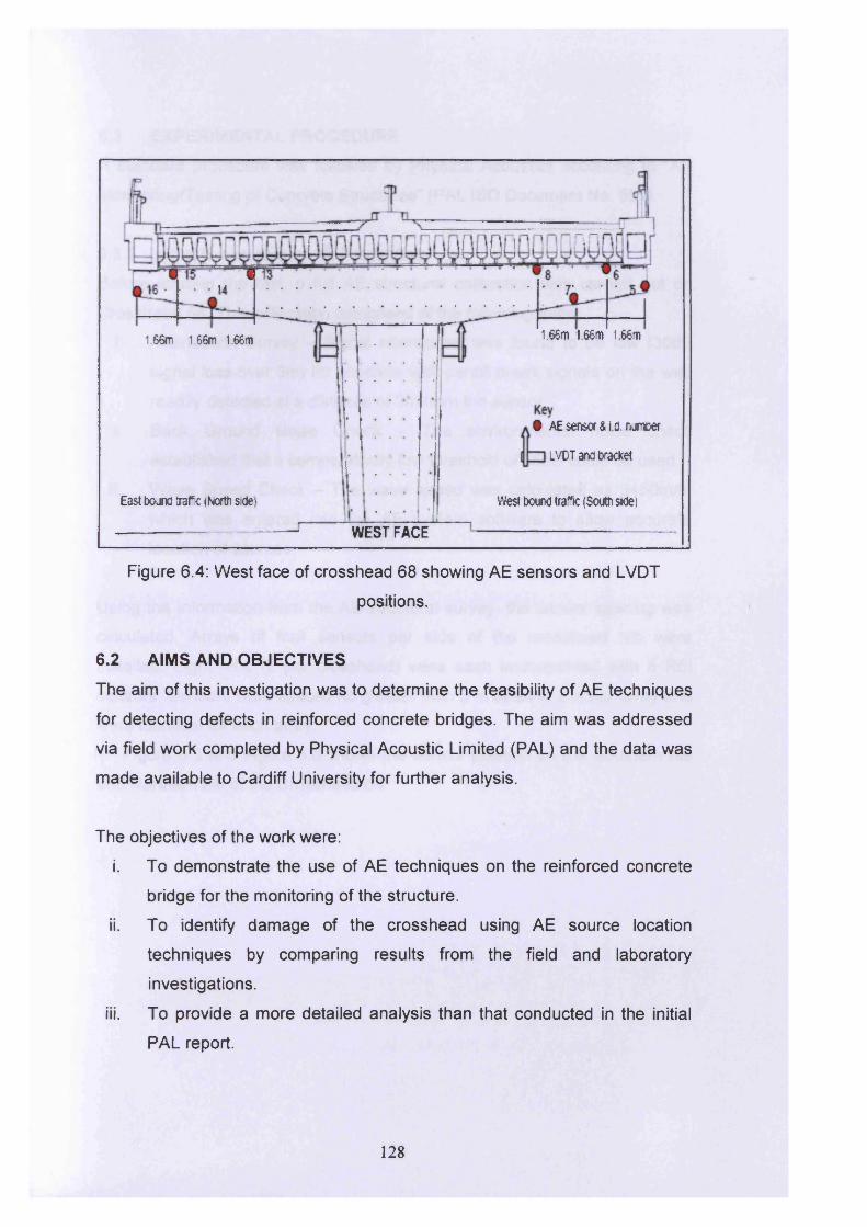
nn

1.66m 1.66m 1.66m1.66m 1.66m 1.66m

§ AE sensor & i a. number

LVDT and bracket

East bound traffic (North side) West bound traffic (South side)

WEST FACE

Figure 6.4: West face of crosshead 68 showing AE sensors and LVDT

positions.

6.2 AIMS AND OBJECTIVESThe aim of this investigation was to determine the feasibility of AE techniques

for detecting defects in reinforced concrete bridges. The aim was addressed

via field work completed by Physical Acoustic Limited (PAL) and the data was

made available to Cardiff University for further analysis.

The objectives of the work were:

i. To demonstrate the use of AE techniques on the reinforced concrete

bridge for the monitoring of the structure.

ii. To identify damage of the crosshead using AE source location

techniques by comparing results from the field and laboratory

investigations.

iii. To provide a more detailed analysis than that conducted in the initial

PAL report.

128

6.3 EXPERIMENTAL PROCEDUREA standard procedure was followed by Physical Acoustics according to “AE

Monitoring/Testing of Concrete Structures” (PAL ISO Document No. 551).

6.3.1 Initial Evaluation of AE Properties

Before starting the test, a full AE structural calibration was carried out on

Crosshead 68. This calibration comprised of the following tests:

i. Attenuation Survey - Signal attenuation was found to be low (30dB

signal loss over 3m) for concrete with pencil break signals on the web

readily detected at a distance of 3m from the sensor.ii. Back Ground Noise Check - The environmental noise check

established that a comparatively low threshold of 35dB could be used.

iii. Wave Speed Check - The wave speed was calculated as 3450m/s,which was entered into the AE system software to allow accurate

location of sources.

Using the information from the AE structural survey, the sensor spacing was

calculated. Arrays of four sensors per side of the crosshead nib were

installed. Eight nibs (2 per crosshead) were each instrumented with 8 R6I

sensors. Sensors were spaced no greater than 3 m apart in a linear array and

were identical for each array.Figure 6.5 and Figure 6.6 shows the sensor position on the Southern nib

and Northern nib of the Crosshead 68.

129

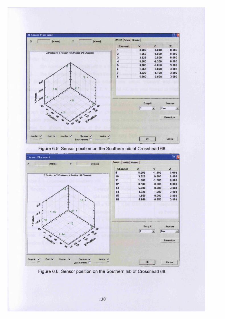
AE Sensor Placement

[Meters] v r [Meters] Sensors Welds, Nozzles

Z Poston vs Y Position vs X Position <AIChemeis>

Channel X Y z1 0.000 0.000 0.0002 1.660 -1.000 0.0003 3.320 0.000 0.0004 5.000 -1.300 0.0005 0.000 -0.850 3.0006 1.660 0.000 3.0007 3.320 -1.100 3.000• 5.000 0.000 3.000

Group I Structure

v | Free

Dimensions

Graphic v> Grid i* Nozzles V Sensors ^ Welds VLock Sensors V l~ OK Cancel

.E Sensor Placement

Figure 6.5: Sensor position on the Southern nib of Crosshead 68.

Sensors Welds Nozzles[Meters] [Meters]

Channel

Z Poston vs Y Poston vs X Poston <AI Channels)

10 •

• 15

♦ 13r

• 14

X Y z5.000 -1.300 0.0003.320 0.000 0.0001.660 -1.000 0.0000.000 0.000 0.0005.000 0.000 3.0003.320 -1.000 3.0001.660 0.000 3.0000.000 -0.850 3.000

Group It Structure

3 F*®«

Dimensions

Graphic V Grid VX'View r

Nozzles v Sensors 9 Welds vLock Sensors f~ F~ OK Cancel

Figure 6.6: Sensor position on the Southern nib of Crosshead 68.

130

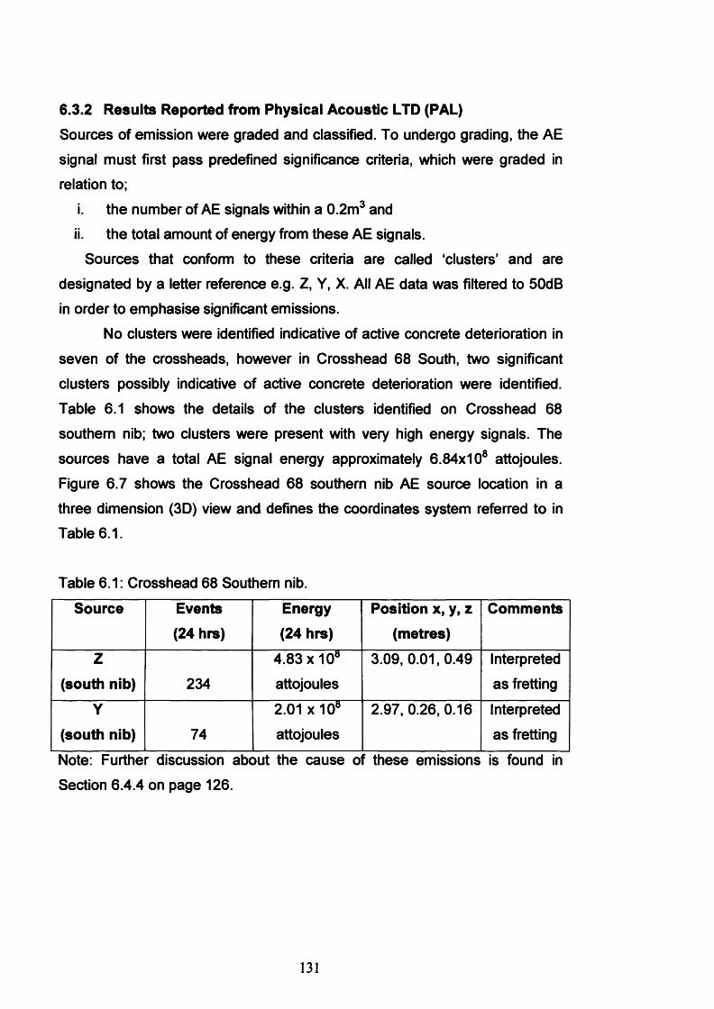
6.3.2 Results Reported from Physical Acoustic LTD (PAL)

Sources of emission were graded and classified. To undergo grading, the AE

signal must first pass predefined significance criteria, which were graded in

relation to;

i. the number of AE signals within a 0.2m3 andii. the total amount of energy from these AE signals.

Sources that conform to these criteria are called ‘clusters’ and are

designated by a letter reference e.g. Z, Y, X. All AE data was filtered to 50dB

in order to emphasise significant emissions.No clusters were identified indicative of active concrete deterioration in

seven of the crossheads, however in Crosshead 68 South, two significant

clusters possibly indicative of active concrete deterioration were identified.

Table 6.1 shows the details of the clusters identified on Crosshead 68

southern nib; two clusters were present with very high energy signals. The

sources have a total AE signal energy approximately 6.84x108 attojoules. Figure 6.7 shows the Crosshead 68 southern nib AE source location in a

three dimension (3D) view and defines the coordinates system referred to in

Table 6.1.

Table 6.1: Crosshead 68 Southern nib.

Source Events

(24 hrs)Energy

(24 hrs)Position x, y, z

(metres)

Comments

Z

(south nib) 2344.83 x 10"

attojoules3.09, 0.01,0.49 Interpreted

as fretting

Y

(south nib) 742.01 x 10“ attojoules

2.97, 0.26, 0.16 Interpreted

as fretting

Note: Further discussion about the cause ol these emissions is found inSection 6.4.4 on page 126.

131

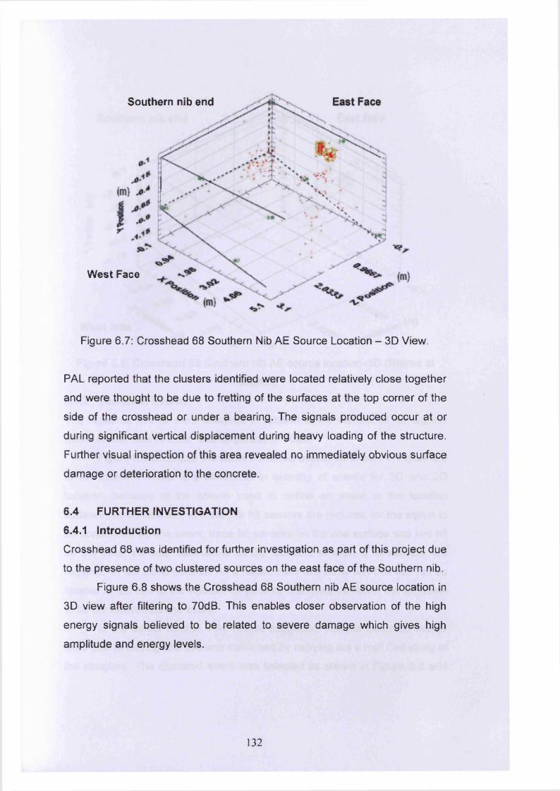
Southern nib end

West Face

Figure 6.7: Crosshead 68 Southern Nib AE Source Location - 3D View.

PAL reported that the clusters identified were located relatively close together

and were thought to be due to fretting of the surfaces at the top corner of the

side of the crosshead or under a bearing. The signals produced occur at or

during significant vertical displacement during heavy loading of the structure.

Further visual inspection of this area revealed no immediately obvious surface

damage or deterioration to the concrete.

6.4 FURTHER INVESTIGATION6.4.1 IntroductionCrosshead 68 was identified for further investigation as part of this project due

to the presence of two clustered sources on the east face of the Southern nib.

Figure 6.8 shows the Crosshead 68 Southern nib AE source location in

3D view after filtering to 70dB. This enables closer observation of the high

energy signals believed to be related to severe damage which gives high

amplitude and energy levels.

132

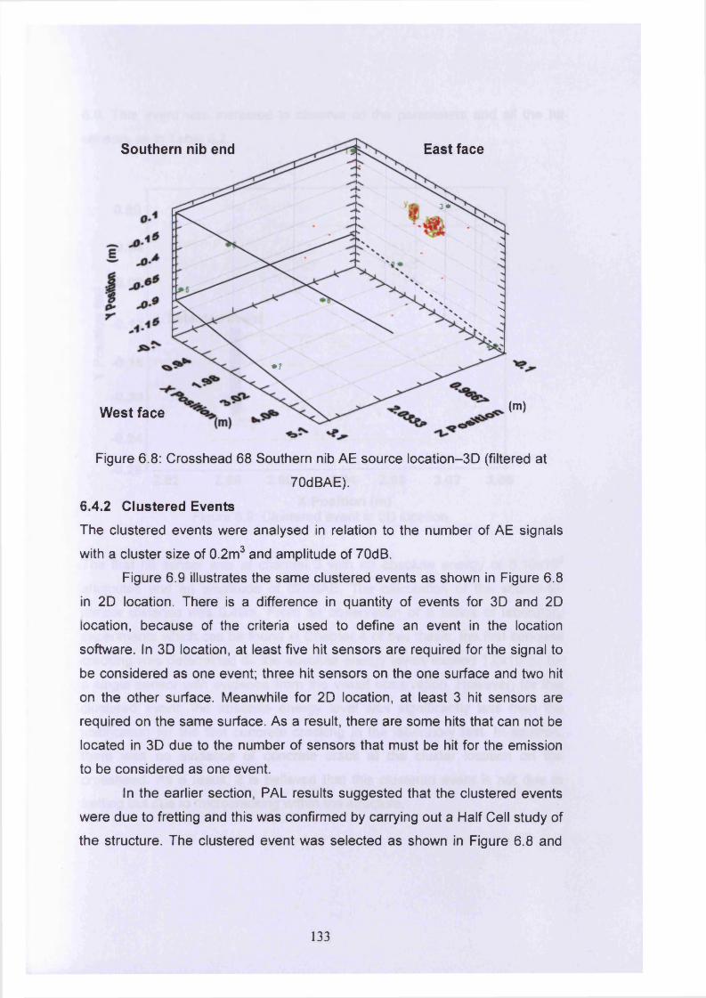
Southern nib end East face

3*

•N

s

• 7

(m)West face

Figure 6.8: Crosshead 68 Southern nib AE source location-3D (filtered at

70dBAE).

6.4.2 Clustered EventsThe clustered events were analysed in relation to the number of AE signals

with a cluster size of 0.2m3 and amplitude of 70dB.

Figure 6.9 illustrates the same clustered events as shown in Figure 6.8

in 2D location. There is a difference in quantity of events for 3D and 2D

location, because of the criteria used to define an event in the location

software. In 3D location, at least five hit sensors are required for the signal to

be considered as one event; three hit sensors on the one surface and two hit

on the other surface. Meanwhile for 2D location, at least 3 hit sensors are

required on the same surface. As a result, there are some hits that can not be

located in 3D due to the number of sensors that must be hit for the emission

to be considered as one event.

In the earlier section, PAL results suggested that the clustered events

were due to fretting and this was confirmed by carrying out a Half Cell study of

the structure. The clustered event was selected as shown in Figure 6.8 and

133

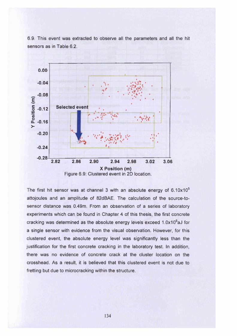
6.9. This event was extracted to observe all the parameters and all the hit

sensors as in Table 6.2.

0.00

-0.04

-0.081

o -0.12g'5>S. -0.16>-

- 0.20

-0.24

-0.282.82 2.86 2.90 2.94 2.98 3.02 3.06

X Position (m)Figure 6.9: Clustered event in 2D location.

The first hit sensor was at channel 3 with an absolute energy of 6.10x105

attojoules and an amplitude of 82dBAE. The calculation of the source-to-

sensor distance was 0.49m. From an observation of a series of laboratory

experiments which can be found in Chapter 4 of this thesis, the first concrete

cracking was determined as the absolute energy levels exceed 1.0x106aJ for

a single sensor with evidence from the visual observation. However, for this

clustered event, the absolute energy level was significantly less than the

justification for the first concrete cracking in the laboratory test. In addition,

there was no evidence of concrete crack at the cluster location on the

crosshead. As a result, it is believed that this clustered event is not due to

fretting but due to microcracking within the structure.

Selected event

134

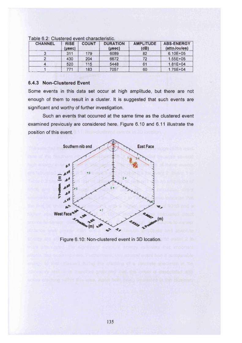
Table 6.2: Clusltered event characteristic.CHANNEL RISE COUNT DURATION AMPLITUDE ABS-ENERGY

(Msec) (psec) (dB) (attojoules)3 311 179 6089 82 6.10E+052 430 204 6672 72 1.55E+054 520 115 5448 61 1.81 E+041 771 183 7057 60 1.76E+04

6.4.3 Non-Clustered EventSome events in this data set occur at high amplitude, but there are not

enough of them to result in a cluster. It is suggested that such events are

significant and worthy of further investigation.

Such an events that occurred at the same time as the clustered event

examined previously are considered here. Figure 6.10 and 6.11 illustrate the

position of this event.

Southern nib end East Face

Figure 6.10: Non-clustered event in 3D location.

135

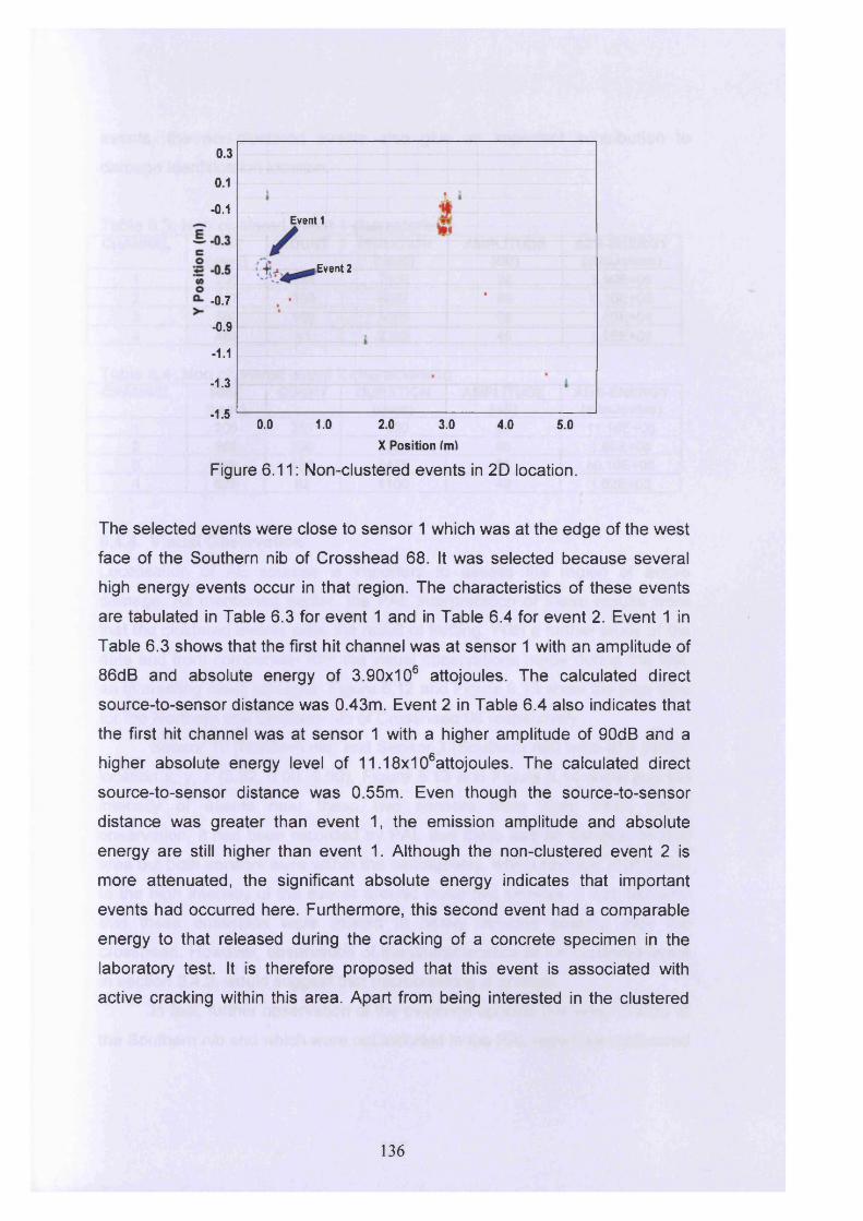
0.3

0.1

- 0.1Event 1

,Event 2

-0.7

-0.9

- 1.1

-1.3

-1.50.0 1.0 2.0 3.0 4.0 5.0

X Position fm)

Figure 6.11: Non-clustered events in 2D location.

The selected events were close to sensor 1 which was at the edge of the west

face of the Southern nib of Crosshead 68. It was selected because several

high energy events occur in that region. The characteristics of these events

are tabulated in Table 6.3 for event 1 and in Table 6.4 for event 2. Event 1 in

Table 6.3 shows that the first hit channel was at sensor 1 with an amplitude of

86dB and absolute energy of 3.90x106 attojoules. The calculated direct

source-to-sensor distance was 0.43m. Event 2 in Table 6.4 also indicates that

the first hit channel was at sensor 1 with a higher amplitude of 90dB and a

higher absolute energy level of 11.18x106attojoules. The calculated direct

source-to-sensor distance was 0.55m. Even though the source-to-sensor

distance was greater than event 1, the emission amplitude and absolute

energy are still higher than event 1. Although the non-clustered event 2 is

more attenuated, the significant absolute energy indicates that important

events had occurred here. Furthermore, this second event had a comparable

energy to that released during the cracking of a concrete specimen in the

laboratory test. It is therefore proposed that this event is associated with

active cracking within this area. Apart from being interested in the clustered

136

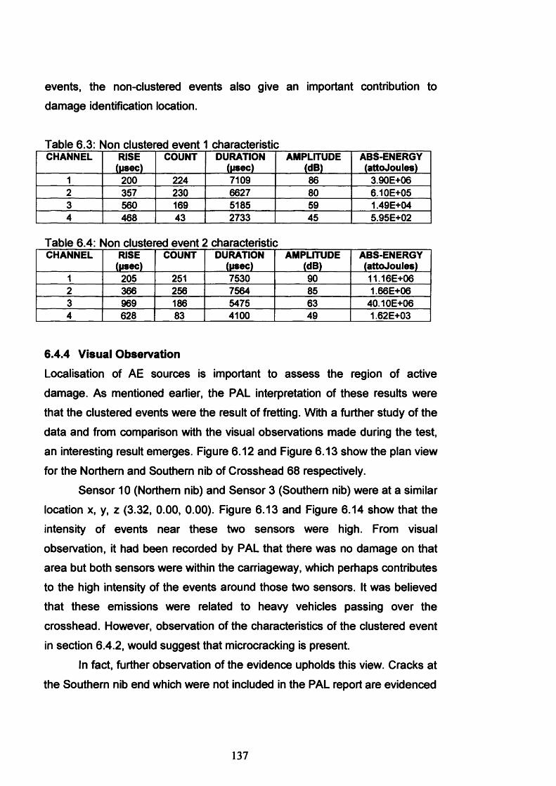
events, the non-clustered events also give an important contribution to

damage identification location.

Table 6.3: Non clustered event characteristicCHANNEL RISE COUNT DURATION AMPLITUDE ABS-ENERGY

(usee) (Msec) (dB) (attojoules)1 200 224 7109 86 3.90E+062 357 230 6627 80 6.10E+053 560 169 5185 59 1.49E+044 468 43 2733 45 5.95E+02

Table 6.4: Non clustered event 2 characteristicCHANNEL RISE

(M«ec)COUNT DURATION

(Msec)AMPLITUDE

(dB)ABS-ENERGY(attojoules)

1 205 251 7530 90 11.16E+062 366 256 7564 85 1.66E+063 969 186 5475 63 40.10E+064 628 83 4100 49 1.62E+03

6.4.4 Visual Observation

Localisation of AE sources is important to assess the region of active

damage. As mentioned earlier, the PAL interpretation of these results were

that the clustered events were the result of fretting. With a further study of the

data and from comparison with the visual observations made during the test, an interesting result emerges. Figure 6.12 and Figure 6.13 show the plan view

for the Northern and Southern nib of Crosshead 68 respectively.Sensor 10 (Northern nib) and Sensor 3 (Southern nib) were at a similar

location x, y, z (3.32, 0.00, 0.00). Figure 6.13 and Figure 6.14 show that the

intensity of events near these two sensors were high. From visual

observation, it had been recorded by PAL that there was no damage on that area but both sensors were within the carriageway, which perhaps contributes

to the high intensity of the events around those two sensors. It was believed

that these emissions were related to heavy vehicles passing over the

crosshead. However, observation of the characteristics of the clustered event

in section 6.4.2, would suggest that microcracking is present.

In fact, further observation of the evidence upholds this view. Cracks at

the Southern nib end which were not included in the PAL report are evidenced

137

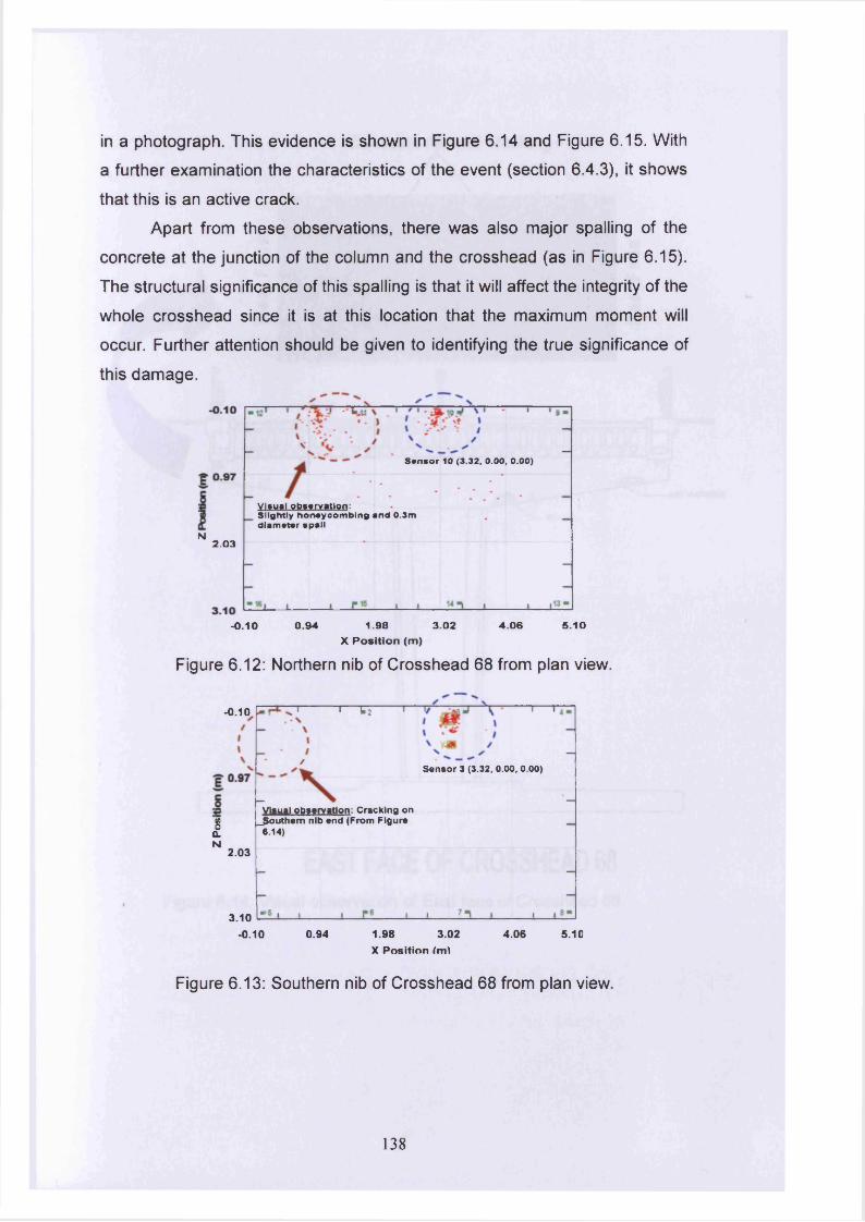
in a photograph. This evidence is shown in Figure 6.14 and Figure 6.15. With

a further examination the characteristics of the event (section 6.4.3), it shows

that this is an active crack.

Apart from these observations, there was also major spalling of the

concrete at the junction of the column and the crosshead (as in Figure 6.15).

The structural significance of this spalling is that it will affect the integrity of the

whole crosshead since it is at this location that the maximum moment will

occur. Further attention should be given to identifying the true significance of

this damage.

Vlf ml 9bSlightly h diameter

Sensor 10 (3.32, 0.00, 0.00)

y i » M » I < ? !? » * r e a l i g n :Slightly honeycom bing and 0.3m diameter spall

N2.0 3

-0 .1 0 0 .9 4 1 .98 3 .0 2 4 .0 6 5 .1 0X P o s itio n (m )

Figure 6.12: Northern nib of Crosshead 68 from plan view.

-0.10 1 C7

/Sensor 3 (3.32, 0.00, 0.00)

Visual observation: Cracking on_Southem nib end (From Figure

6.14)s0.N

2.03

3.10 L. - 0.10 0.94 1.98 3.02

X P o s itio n (m l4.06 S.1G

Figure 6.13: Southern nib of Crosshead 68 from plan view

138

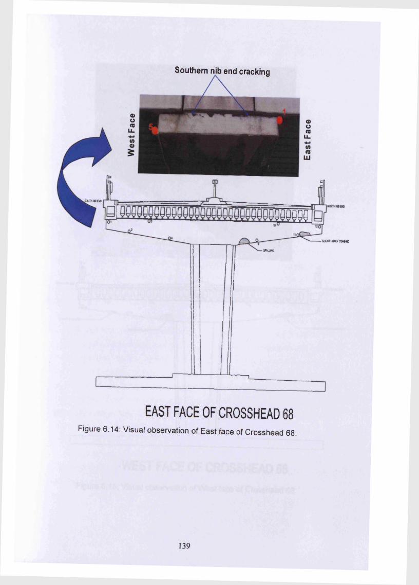
Southern nib end cracking

SOUTH W BO

m m

SMUJNG

SUGHT HONEY C O W *

EAST FACE OF CROSSHEAD 68Figure 6.14: Visual observation of East face of Crosshead 68.

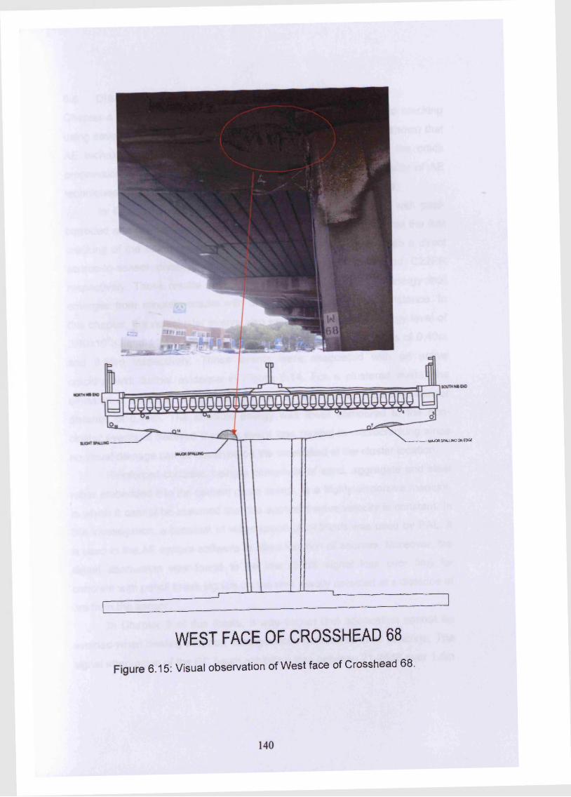
'MAJOR SPALLWG ON EDGE

WEST FACE OF CROSSHEAD 686.15: Visual observation of West face of Crosshead 68.

6.5 DISCUSSIONChapter 4 assessed the ability of AE to detect and locate concrete cracking

using several AE sensors on laboratory-based specimens. It was shown that AE techniques could be used to detect, locate and monitoring the crack

progression until the failure. This chapter has investigated the ability of AE

techniques to detect defects within a real concrete bridge crosshead.

In Chapter 4, a series of laboratory tests was conducted with post- corroded and pre-corroded RC beam specimen. It was observed that the first cracking of the beam emerged at 1.90x106aJ and 13.79x106aJ with a direct source-to-sensor distance of 0.36m and 0.32m for A22PR and C22PR

respectively. These results gave a justification of the absolute energy that emerges from concrete cracks with the direct source-to-sensor distance. In

this chapter, the non-cluster events also emit a high absolute energy level of 3.90x106aJ and 11.18x106aJ with direct source-to-sensor distances of 0.43m

and 0.55m respectively. These events were associated with an active

cracking with further evidence in Figure 6.14. For a clustered event, the

emission of absolute energy was 6.10x105aJ with a direct source-to-sensor distance of 0.49m. The absolute energy was lower compared to the non­

cluster events; it believed that this event was related to microcracking since

no visual damage can be observed on the crosshead at the cluster location.

Reinforced concrete, being a composite of sand, aggregate and steel rebar embedded into the cement paste matrix, is a highly dispersive medium, in which it cannot be assumed that the apparent wave velocity is constant. In

this investigation, a constant of wave speed of 3450m/s was used by PAL. It

is used in the AE system software to allow location of sources. Moreover, the

signal attenuation was found to be low (30dB signal loss over 3m) for

concrete with pencil break signals on the web readily detected at a distance of 3m from the sensor.

In Chapter 5 of this thesis, it was shown that attenuation cannot be

avoided when dealing with non homogeneous material such as concrete. The

signal attenuation of the RC beam exhibits a loss between 21-26dB over 1.5m

141

source-to-sensor distance whilst for a slab specimen, the attenuation signal loss was 55dB over the same distance. For the actual structure (Crosshead

68) a lower threshold level that was used (35dB) as further away from the

source (the far field), where the majority of structural AE monitoring

measurements are made, attenuation becomes dominated by absorption or conversion of sound energy into heat. Due to this reason, with a lower

threshold level is believed that the inspection is capable of locating sources

over a broad area.

It has also been reported earlier that a slab has a slower apparent wave velocity compared to a beam specimen with the same source-to-sensor

distance. This happens because when a wave is generated by a localised

source; the disturbance propagates outwards in all directions from the source.

The wave propagates further for a larger structure with a different and

complicated wave path. Moreover, the real signal path is probably longer than

the direct path due to concrete cracks (due to daily use) and aggregates

which increase the propagation distance to the sensor. In addition, the

components in concrete consist of different materials with different velocities

which will affect the apparent wave velocity as the source-to-sensor distance

increases.A cluster location is an area of predefined size on the structure that

contains AE sources found using location monitoring. Most AE users are

interested in the clustered events because these are associated with damage

localization. However, apart from being interested in the clustered events, the

non-clustered events also give an important contribution to damage detection.

It is important to analyse the non-clustered events as well and compare the

output with visual observation and laboratory-based results, leading to a

viable technique for assessing the integrity of the structure. Nevertheless it is

recommended by PAL that all crossheads be retested within 4 years using AE

to allow assessment of any deterioration and change in condition especially

on Crosshead 68.

142

Visual observation is a predominant inspection method and essential before

proceeding with any NDT techniques. The external appearance of the

crosshead, which was badly stained and heavily spalled, again suggested that

internal corrosion might be expected. There was a major spalling of the

concrete at the junction of the column and the crosshead. Monitoring of this

area is essential since this spalling will affect the integrity of the whole

crosshead since it is at this location that the maximum moment will occur.In monitoring large structures, especially RC, an accurate source location will depend on the calculated wave velocity, time difference measurements, precise and adequate sensors positions and knowledge to interpret the output

with an association to visual observation and laboratory-based results.

However, if the source cannot generate waves of sufficient strength for

detection by the required number of sensors, then it will not be possible to

calculate the location of the source.According to Carter (2000), a successful AE monitoring requires a

thorough understanding of all the factors that govern the AE process. Simply

attaching the AE sensors arbitrarily to the structure and recording the

subsequent data is woefully inadequate. If suitable raw data is to be acquired, the specification and configuration of an AE monitoring system must be

tailored around the detection of sources of interest and the informatics

requirements for source analysis. The following factor is important to take into

consideration in global monitoring:

• AE wave propagation and structural acoustics

• The implication of the structure details

• Identification of the key AE sources of interest

• The properties of these AE sources

• Environmental and structural noise effects

• The capabilities and limitations of the AE equipment and processing

software.

143

6.6 CONCLUSIONSThis chapter has assessed the ability of AE to detect, locate and monitor

damage in an RC bridge using AE sensors. The conclusions are:

• The ability of AE techniques to detect defects within a real RC bridge

crosshead was promising with a detailed investigation.

• Reinforced concrete is a highly dispersive medium, in which wave

velocity cannot be assumed to be constant. The significant effect of

using a constant wave velocity is in source location. Most probably an

error in detecting the exact location of emission can occur because of

this effect. In AE, the commercial software requires a single wave

velocity value to be defined for each test. In reality, the wave velocity will

not be constant as the source-to-sensor distance increases which has

been discussed thoroughly in Chapter 5 of this thesis.

• A lower threshold level (just above the noise level) is required when

monitoring large structures. This is due to the requirement that the

technique has the capability to locate the source within a large area.

• From further analysis of the AE data from Crosshead 68, two

significant clusters possibly indicative of microcracking were identified

and it was confirmed that the emissions were related to heavy vehicles

passing over the crosshead. However, a retest is required in the future

to allow assessment of any deterioration and change in condition

especially on Crosshead 68.

• The non-clustered events are believed to be indicative of active cracking

on the southern end nib of Crosshead 68. A further investigation is

needed to monitor the progress of this cracking.

• A visual inspection is important before deciding where to locate the

sensors. Consideration should be given to the major spalling of concrete

at the crosshead column since this is where the maximum moment occurs and at the Crosshead 68 Southern nib where the active cracking

occurred.

144

CHAPTER 7: CONCLUSIONS AND RECOMMENDATION FOR FUTURE

WORK

7.1 CONCLUSIONS

This thesis has examined the role of acoustic emission in the monitoring

laboratory-based and in-service reinforced concrete specimens and structures. The aim of this research was to further the understanding of AE techniques for use in global and local structural monitoring of concrete damage, in order to

provide a commercial tool for the non-destructive evaluation of reinforced

concrete structures. Three key themes have been investigated; (i) a study of the

capability of the AE technique to follow crack development and to monitor structural behaviour in pre-corroded and post corroded specimen in order to

implement the source location to determine deterioration/crack location, (ii) an

investigation of the nature of wave propagation in concrete structures over a

variety of source to sensor distances and (iii) the use of AE to monitor the

integrity of an in-service concrete bridge crosshead.

7.1.1 Pre-corroded (PR) and Post-corroded (PS) RC Beam Specimens.

AE absolute energy was found to relate to the behaviour of the RC beam and

determined the ability of the AE to locate and monitor crack propagation on the

RC beam. The significant conclusions that can be made from this chapter are:

• The mechanical behaviour of concrete can be related to the emission of absolute energy within the laboratory-based specimens since the loading

conditions are known. However, it is difficult to extrapolate these

relationship to the in service behaviour of a structure due to unknown

loading conditions. Nevertheless, an important criteria was established by

determining the emissions associated with the onset of concrete cracking

and these criteria can be used in field tests. It was found that, whenever

145

the AE absolute energy (single sensor event or cumulative hits) exceeded

1.0x106aJ, concrete cracks had occurred. This was implemented in

Chapter 6 of this thesis and was validated by a visual inspection.

• The ability of the TOA method to detect and monitor the crack propagation

was promising. In addition, it was found that AE could identify the location

of microcraking before the first crack was visually observed. This

demonstrated that the micro damage can be located before the actual impairment occurs.

7.1.2 Acoustic Wave Propagation in Concrete Structures.

This work investigated signal attenuation and wave propagation in concrete

structures over a range of source-to-sensor distances. The attenuation of AE

signals from different signal modes has proven to be an important factor in

deciding the applicability of the technique. It was also observed that the apparent wave velocities were reduced due to attenuation and dispersion of the wave

signal affecting the time to reach the subsequence sensors. In this study it can

be concluded that:

• The determination of a ‘corrected’ signal can be used in order to ensure

that, for a particular threshold, the same temporal position in each

waveform was used for velocity calculations. As a consequence, problems

associated with losing important signals are low when using the corrected

signals. However the determination of the P-wave initial arrival times, amplitudes and normalising of an event was a long and tedious process.

• The source location is of prime interest for modern AE analysis; however it is greatly affected when considering the inaccuracy in determining the P- wave arrival times in calculating the wave velocities. It was shown that the

apparent wave velocity decreases as the sensor distance increases. In

addition, the selected threshold level also has an impact on the measured

wave velocities. In order to detect and locate AE, low threshold levels are

146

needed with sensors pairs in close proximity to each another. However, in

field test, it is not cost-effective because this requires a large number of sensors to be placed closed together in order to detect and locate

damage.

• In this study, the propagation of the elastic waves in concrete was

confirmed to be affected by; the geometry of the sample, the path taken

from the source to sensor and the concrete composition and condition, all of which influences the apparent wave velocity of the RC concrete.

• An attenuation study, showed that a slab suffered the most attenuation

compared to the beam specimen (55dB over 1.5m from the source

compared to 21 dB for the beam over the same source-to-sensor distance). The large increase in attenuation indicates a potential problem

in monitoring specific locations on the structure. Care must be taken when

choosing the location of the sensors to avoid such large decreases in the

received signals.

• Measured Amplitude Ratio (MAR) analysis revealed that a relatively low

MAR value occurs for parallel sources and a higher MAR value for normal sources. However, if conclusions on source orientation are to be drawn

from the MAR measurements, consideration of how the sensor mounting

position and orientation relative to other elements influence its response to

sources in various regions of the beam is required. This becomes complex if the precise source position is unknown, as is the case with global AE

inspection.

7.1.3 Acoustic Emission Assessment on M4 Elevated Crosshead.

The key conclusions from this investigation are:

• Signal attenuation in the concrete bridge was low, permitting H-N source

detection at source-to-sensor distance in excess of 3m.

147

• Emission levels were related to traffic volume and individual vehicle mass.

• Non-clustered events give an important contribution to damage

localization. It is important to analyse the non-clustered events and

compare the output with visual observations and laboratory-based results

in order to obtain a clearer understanding, leading to a viable technique for assessing the integrity of the structure. In complex structures, not all events will reach sufficient sensors to be clustered, but such events can

still be important.

• A visual inspection is important before deciding where to locate the

sensors; important consideration should be given to the major spalling.

To summarise, the most important aspect of AE testing is its ability to

continually monitor entire sections of the structure in-situ. Appropriate methods of AE detection, source location and characterisation are central to this aim. The

most significant challenge of source location is in global monitoring. Most AE

sources can be readily located if data is received on the requisite number of sensors. However in light of the economics constraints, it is desirable to minimise

the number of sensors used to monitor the structure. This limits the hardware

investment and the expense of mounting and maintaining the equipment, it also

reduces the logistic complexity of installing the instrumentation. A reduction in the number of sensors used may be achieved in two ways; by

carefully targeting critical zones of the structure where the flaws of interest are

most likely to concur, or by increasing the sensor spacing. Both methods require

a thorough understanding of the history and behaviour of the structure in

question and all aspects of source detection. Therefore, in global monitoring, sensor configuration is a carefully judged compromise between system sensitivity

and cost. This is not usually the case in local monitoring where the sensors are in

much closer to the source and can be used for source location with a high

degree of confidence.

148

This thesis is part of a significant contribution to the enhancement the concrete

structure knowledge in NDT method specifically in AE technique. It is a vital to

have a NDT method which can detect and locate faults as soon as possible. This

thesis had covered one of the important criteria by determining the emissions

associated with the onset of cracking and had determined that this criterion can

be used in field test. However, looking back to the laboratory test for PR and PS

specimen, it will give more understandable results if all the beams were design to

fail in flexure. Hence the comparison of the data can be done with the same

concrete failure. The calculated apparent velocity gave an important awareness

of source location method and Moment Tensor method whereby the calculated

P-waves were decreases as the sensor distance increases. In this chapter, the

descriptions of the factors that may effect the ability to obtain an accurate value

of wave velocity were stated. The bridge monitoring investigation had discovered

the importance of non-cluster event in damage localization. If permission was

given, it will be appropriate to revisit the structure (Crosshead 68) and to

undertake the area of investigation as a near field. Hence it can be benefit to

obtain a clearer understanding of the emission. Most of all these small important information may be added to the immature nature of concrete structure behaviour associated with AE which will benefit all researchers in concrete area.

7.2 RECOMMENDATIONS FOR FURTHER WORKIn light of the conclusions of this work, the following topics are recommended for further study:

• A detailed investigation into the optimum set-up for the monitoring of reinforced concrete structures. This investigation will need to consider the

lowest possible threshold, optimum sensor spacing and selection of sensors

to enhance the applicability of AE for the monitoring of concrete structures.

• A large of laboratory based corrosion study (Chapter 4) to collect a

database of signals to aid in the evaluation of the behaviour of the RC

149

beams subjected to corrosion levels similar to those found in real bridge

structures.

• A laboratory-based investigation of full size models of RC beam with

varying degrees of damage monitored using the AE technique. This should

include study of wave propagation in damaged and undamaged RC

specimens and mortar specimen to investigate the significance of material influences on the signal behaviour.

• Investigation of the significance of statistical representations of MAR value

data from a range of parallel and normal sources. This will further the

understanding of the role of MAR value in AE source identification. Furthermore, a study of the influence of source-to-sensor distances on

MAR value is appropriate.

• The development of an automated software package to improve the

accuracy and reduce the time taken in the determination of the initial P- wave amplitude and arrival time.

150

CHAPTER 8: REFERENCES

Ahmad, S., 2003, Reinforcement corrosion in concrete structures, it's

monitoring and service life prediction - A review, Cement & Concrete

Composites, Vol. 25, pp 459-471.

Ahmad, S. and Bhattacharjee B., 1995, A simple arrangement and

procedure for in-situ measurement of corrosion rate of rebar embedded in

concrete, Corrosion Science, Vol. 37, No. 5, pp 781-791.

Alonso C., Andrade C., 1996, Corrosion rate monitoring in the laboratory and

on-site, Construction & Building Materials, Vol. 10, No. 5, pp 315-328.

ASTM ,1991, Standard terminology for non-destructive examinations. ASTM.

ASTM Designation: E1316 - 91b.

ASTM C1383-04, 2002, Standard test method for measuring the P-wave

speed and the thickness of concrete plates using the impact-echo method.

ASTM E976, 1999, Standard guide for determining the reproducibility of

Acoustic Emission sensor response, The American Society for Testing and

Materials.

Beattie A. G., 1983, Acoustic emission, principles and instrumentation,

Journal of Acoustic Emission, Vol. 2, Part 1, pp 95-128.

Beck P., 2004, PhD Thesis- Quantitative damage assessment of concrete

structures using acoustic emission, Cardiff School of Engineering, University

of Wales, Cardiff.

151

BS 1881 Testing Concrete. Part 201:1986, Guide to the use of non­

destructive methods of test for hardened concrete.

BS EN 12504-4, 2004, Testing concrete, Part 4: Determination of ultrasonic

pulse velocity, pp. 9 (Annex A).

BS EN 13477-2, 2002, Non-destructive testing-Acoustic Emission-Equipment

characterization, Part 2: Verification of operating characteristic, British

Standard.

Carbera J. G., 1996, Deterioration of concrete due to reinforcement steel

corrosion, Cement & Concrete Composites, Vol. 18, pp 47-59.

Carlos, M. F., 2003, Acoustic Emission: Heading the Warning Sounds from

Materials.<URL:http://wwwastm orQ/SNEWS/OCTOBER 2003/carlos oct.html>

[Accessed 2 February 2004].

Carpinteri A., Lacidogna G., Pugno G., 2007, Structural damage

diagnosis and life-time assessment by acoustic emission monitoring,

Engineering Fracture Mechanics, Vol 74, pp 273-289.

Carter, D. C., 2000, "Acoustic Emission Techniques for the Structural Integrity

Monitoring of Steel Bridges”, PhD Thesis, Cardiff University.

Chaix, J. F., Gamier V., Corneloup. G., 2006, Ultrasonic wave propagation

in heterogeneous solid media: Theoretical analysis and experimental

validation, Ultrasonic, Vol. 44, pp 200-210.

Cho Y. S., 2003, Non-Destructive testing on high strength concrete using

spectral analysis of surface waves, NDT&E International, Vol. 36, pp. 229-

235.

152

Colombo S., Fordo M. C., Main I. G., Shigesgi M., 2005, Predicting the

ultimate bending capacity of concrete beams from the ‘relaxation ratio’

analysis of AE signals, Construction and Building Materials, Vol. 19, pp 746- 754.

Concrete Bridge Development Group, 2002, Technical guide 2- Guide to

testing and monitoring the durability of concrete structure, The Concrete

Society, ISBN 0946691 79 7.

Culshaw B., 1996, Smart structures and Materials. Glasgow ISBN 0-89006-

681-7, Artech House Inc., Boston, London.

Ding Y., Reuben R.L., Steel J. A, 2004, A new method for waveform analysis

for estimating AE arrival times using wavelet decomposition, NDT & E

International, Vol 37, pp. 279-290.

Droullard T. F., 1996, A history of AE, Journal of AE, Vol 14, No 1, pp 1-34.

Dukes R. and culpan E. A., 1984, AE- Its techniques and applications, I EE

Proceedings, Vol. 131, Pt. A, No. 4, pp 241-251.

El Maaddawy T.A, Soudki K.A., 2003, Effectiveness of impressed current

technique to simulate corrosion of steel reinforcement in concrete, Journal of Materials in Civil Engineering/ January/February, pp 41-47.

Elsener, B., 2002, Macrocell corrosion of steel in concrete-implication for

corrosion monitoring, Cement & Concrete Composites, Vol. 24, pp 65-72.

Esward T.J, Theobald P. D., Dowson S.P, Preston R.C., 2002, An

Investigation Into the Establishment and Assessment of a Test Facility for The

Calibration of Acoustic Emission Sensors. Middlesex, National Physical

Laboratory, pp 65.

153

Gaydecki P, Burdekin F. M., 1994, An inductive scanning system for two-

dimensional imaging of reinforcing components in concrete structures,

Measurement Science Technology, Vol. 5, pp 1272-1280.

Gaydecki P., Silva l.y Fernandes B. T., Yu Z. Z., 2000, A portable inductive

scanning system for imaging steel-reinforcing bars embedded within concrete,

Sensors and Actuators, Vol. 84, pp 25-32.

Gaydecki P., Quek S., Miller G.f Fernandes B., Zaid M., 2002, Design and

evaluation of an inductive Q-detection sensor incorporating digital signal

processing for imaging of steel reinforcing bars in concrete, Measurement

Science and technology, Vol 13, pp 1327-1335.

Gaydecki P., Quek S.f Fernandes B. T., Miller G.f 2003, Multiple layer

separation and visualisation of inductively scanned images of reinforcing bars

in concrete using a polynomial-based separation algorithm, NDT & E

International, Vol. 35, pp 233-240.

Gassman S.L. and Tawhed W.F., 2004, Nondestructive assessment of damage in concrete bridge decks, Journal of Performance of Construction

Facilities ASCE, November 2004, pp. 220-231.

Golaski L., Gebski P., Ono K., 2002, Diagnostics of reinforced concrete

bridges by acoustic emission. Journal of Acoustic Emission, Vol. 20, pp 213-

221.

Gowers K. R., Millard S. G., 1993, On-Site linear polarization resistance

mapping of reinforced concrete structures, Corrosion Science, Vol. 35, No. 5,

pp 1593-1600.

154

Gowers K. R. and Millard S. G., 1999, Electrochemical techniques for

corrosion assessment and reinforced concrete structures, Proceedings

Institute of Civil engineers, Structure & Building 134 (Paper No. 11797), pp

129-137.

Grosse C, Reinhardt H, Dahm T, 1997, Localization and classification of

fracture types in concrete with quantitative acoustic emission measurement

techniques, NDT & E International, Vol 34, No 4, pp 223-230

Grosse C. U, Reinhardt H. W., Finck F., 2003, Signal-based Acoustic

Emission techniques in civil engineering, Journal of Materials in Civil

Engineering @ ASCE May / June, pp 274-279.

Guilia Boronio, Berra M.f Bertolini L., Pastore T., 1996, Steel corrosion

monitoring in normal and total-lightweight concretes exposed to chloride and

sulphate solutions. Part II: Polarization resistance measurements, Cement &

Concrete Research Journal, Vol. 26, pp 691-696.

Ha T. H., Muralidran S., Bae J. H., Ha Y. C., Lee H. G., Park K. W., Kim D.

K., 2007, Accelerated short-term techniques to evaluate the corrosion

performance of steel in fly ash blended concrete, Building and Enviroment, Vol. 42, pp 78-85.

Hartmut V, 2002, AE testing fundamentals, equipment, applications, NDT.net

Vol.7, No.9, <URL: http://www.ndt.net/articleA/07n09/05/05.htm> [Accessed

17 November 2005].

Holford K. M., 2000, Acoustic emission - basic principles and future

directions, Strain, Vol 36, No 2, pp 51-54.

Holford K.M., 2001, Damage location in steel bridges by acoustic emission

Journal of Intelligent Material Systems and Structures, Vol 12, pp 567-576.

155

Holford K.M, Carter D.C., 1999, Acoustic emission source location. Key

Engineering Material: Damage Assessment Structure, 167-168, pp. 162-171.

Idrissi H., Liman A., 2003, Study and characterization by acoustic emission

and electrochemical measurements of concrete deterioration caused by

reinforcement steel corrosion, NDT & E International, Vol. 36, pp 563-569.

Jung W. Y. and Sohn Y. M., 2003, Predicting the remaining service life of

land concrete by steel corrosion, Cement & Concrete Composite, Vol. 33, pp

663-677.

Kim D. S., Seo W. S., Lee K. M., 2006, IE-SASW method for non-destructive

evaluation of concrete structure, NDT & E International, Vol. 39, pp 143-154.

Law D.M, Millard S. G., Bungey J.H., 2000, Linear polarization resistance

measurements using a potentiostatically controlled guard ring, NDT & E

International, Vol. 33, pp 15-21.

Leelalerkiet V., Kyung J. W., Ohtsu M., Yokata M., 2004, Analysis of half

cell potential measurement for corrosion of reinforced concrete, Construction

and Building Materials, Vol. 18, pp 155-162.

Li Z., Shah P 1994, Localization of microcracking in concrete under uniaxial

tension. ACI Materials Journal, Vol 91, pp 372-81.

Li Z, Li F, Zdunek A, Landis E, Shah S P, 1998, Application of Acoustic

Emission technique to detection of reinforcing steel corrosion in concrete, ACI

Materials Journal, Vol 1, pp 68-76

Liu Y, Weyers R. E., 2003, Comparison of guarded and unguarded linear

polarization CCD devices with weight loss measurement, Cement & Concrete

Research, Vol. 33, pp 1093-1101.

156

Matsuyama K., Ishibashi A., Ohtsu M., 1993, Field application of acoustic

emission for the diagnosis of structural deterioration of concrete, Journal of Acoustic Emission, Vol. 11, No. 4, pp S65-S73.

Millard S. G., Law D.W, Bungey J.H, Cairns J., 2001, Environmental

influences on linear polarization corrosion rate measurement in reinforced

concrete, NDT & E International, Vol. 34, pp 409-417.

Miller G., Gaydecki P., Quek S., Fernandes B., Zaid M.,2005, A combined

Q and heterodyne sensor incorporating real time DSP for reinforcement

imaging, corrosion detection and material characterisation, Sensor and

Actuators, Vol. A 121, pp 339-346.

Miller R.K, Me Inti re P., 1987, Nondestructive Testing Handbook: Acoustic

Emission Testing, Vol 5, second edition, American Society for Nondestructive

Testing, pp. 151.

Mirmaran A., Philip S., 2000, Comparison of acoustic emission activity in

steel-reinforced and FRP-reinforced concrete beams, Construction and

Building Maintenance, Vol. 14, pp 299-310.

Mix p. E., 1998, Introduction to non-destructive testing- a training guide, John

Willey & Sons, Texas, United State of America.

Othsu M., 1991, Simplified moment tensor analysis and unified

decomposition of AE source: application to in situ Hydrofacturing test, Journal

of Geographical Research, Vol 96, No B4, pp 6211-6221.

Othsu M., Uchida M., Okamoto T., Yuyama S., 2002, Damage assessment

of reinforced concrete beams qualified by Acoustic Emission, ACI Structural

Journal (Technical Paper), July-August, pp 411-417.

157

Othsu M., Watanabe H., 2001, Quantitative damage estimation of concrete

by AE, Construction and Building Materials, Vol. 15, pp 217-224.

Owino, J. O., Jacobs, L. J., (1999), Attenuation measurements in cement-

based materials using laser ultrasonics, Journal of Engineering Mechanics

June: 637-647.

Park S. Y., Kim Y. B., 2002, Non-destructive damage detection in large

structure via vibration monitoring, Electronic Journal of Structural Engineering

2 < URL: http://www.eise.org > [Accessed 20 July 2004], pp 59-75.

Pech-Canul M. A, Castro P., 2002, Corrosion measurements of steel

reinforcement in concrete exposed to a tropical marine atmosphere, Cement & Concrete Research Journal, Vol. 32, pp 491-498.

Philippidis T.P., Aggelis D. G., 2005, Experimental study of wave dispersion

and attenuation in concrete, Ultrasonics, Vol. 43, pp. 584-595.

Physical Acoustic Corporation, 2001, DiSP User Manual, Physical Acoustic

Corporation, Princeton Junction, New Jersey, US.

Physical Acoustic Corporation, 2002, AEWin Software User’s Manual,

Physical Acoustic Corporation, Princeton Junction, New Jersey, US.

Physical Acoustic Limited, 2005, Procedure: AE monitoring of concrete

structures. Document Number 551, Issue No. 2. Physical Acoustic Limited

Company (PAL), Cambridge, UK.

Physical Acoustic Limited, 2005, Acoustic emission of M4 Elevated

Crosshead, Report No. FT03287, Physical Acoustic Limited Company (PAL),

Cambridge, UK.

158

Pollock, A. A., 1989, Acoustic Emission Inspection, Metal Handbook Volume

17, pp 278-294.

Poupard O., L’Hostis V., Catinaud S., Petre-Lazar I., 2006, Corrosion

damage diagnosis of a reinforced concrete beam after 40 years natural exposure in marine environment, Cement and Concrete Research, Vol. 36, pp

504-520.

Pullin, R. ,2001, PhD Thesis- Structural Integrity Monitoring of Steel Bridges

Using Acoustic Emission Techniques. School of Mechanical Engineering.

Cardiff, UK, University of Wales, College of Cardiff.

Quek, S., Gaydecki P., Zaid M.A.M, Miller G, Fernandes B.T., 2003, Three-

dimensional image rendering of steel reinforcing bars using curvilinear models

applied to orthogonal line scans taken by an inductive sensor, NDT & E

International, Vol. 36, pp 7-18.

Raupach M, Schiebl P., 2001, Macrocell sensor systems for monitoring of

corrosion risk of the reinforcement in concrete structures, NDT & E

International, Vol. 34, pp 435-442.

Rochinni G., 1993, Corrosion rate monitoring by linear polarization

resistance, Corrosion Science, Vol. 34, No. 12, pp 2031-2044.

Rochini G., 1999, Some considerations on the polarization resistance

method, Corrosion Science, Vol. 34, No. 12, pp 2353-2367.

Sagaidak A.I., Elizarov S.V., 2004, The relationship of acoustic-emission

signals with the processes of deformation and fracture of building structures,

Russian Journal of Nondestructive Testing, Vol. 40, No. 11, pp 739-745.

159

Sardis M. S., 2001, Msc Thesis- Earthquake resistance design procedure for

High-strength Concrete Structures. School of Civil & Structural Engineering. Cardiff University, Wales, UK.

Sarveswaran V., Roberts M. B., Ward J. A., 2000, Reliability assessment of

deteriorating reinforced concrete beams, Proceedings Institute Civil

Engineers, Structure & Buildings, Vol. 140, pp 239-247.

Schechniger B., Vogel T., 2007, Acoustic emission for monitoring a

reinforced concrete beam subject to four-point-bending, Construction and

Building Materials, Vol. 21, pp 483-490.

Shigeishi M, Colombo C, Broughton K J, Rutledge H, Batchelor A J,

Forde M C, 2001, Acoustic emission to assess and monitor the integrity of

bridges, Construction and Building Materials, Vol 15, pp 35-49

Stern M. and Geary A. L., 1957, A theoretical analysis of the shape of

polarization curves, Journal of the Electrochemical Society, Vol. 104, No. 1,

pp 56-63.

Suzuki T, Othsu M, 2004, Quantitative damage evaluation of structural

concrete by a compression test based on AE rate process analysis,

Construction and Building Materials, Vol 18 ,pp 197-202.

Taylor M. 1997, Msc Thesis- Characterisation of normal and high-strength

plain and fibre-reinforced concretes by means of strength, fracture and

combined fracture/ relaxation test, School of Civil & Structural Engineering,

Cardiff University, Wales, UK.

Tuuti K., 1982, Corrosion of steel in concrete, Swedish Cement and

Concrete, Research Institute, ISSN 0346-6906, pp 469-476.

160

Othsu M., 2003, Detection and identification of concrete cracking in

reinforced concrete by acoustic emission, Proceeding of the AIP Conference,

Vol. 657, Part 1, pp 1455-1462.

Uomoto T. 1987, Application of acoustic emission to the field of concrete

engineering, Journal of Acoustic Emission, Vol. 6, No. 3, pp 137-144.

Wu T. T., Sun J. H., Tong J. H., 2000, On the study of elastic wave scattering

and Rayleigh wave velocity measurement of concrete with steel bar, NDT&E

International, Vol. 33, pp. 401-407.

Yalcyn H, Ergun M., 1996, The prediction of corrosion rates of reinforcing

steels in concrete, Cement & Concrete Research, Vol. 26, No. 10, pp 1593-

1599.

Yoon D. J, Weiss W. J., Shah S. P., 2000a, Assessing damage in corroded

reinforced concrete using acoustic emission, Journal of Engineering

Mechanics(March), pp 273-283.

Yoon D. J., Weiss W. J., Shah S. P., 2000b, Detecting the extent of

corrosion with acoustic emission, Transportation Research Record 1698, Paper No. 00-1425, pp 54-60.

Yoon S., Wang K., Weiss W. J, Shah S.P., 2000, Interaction between

loading, corrosion and serviceability of reinforced concrete, ACI Materials

Journal Vol. 97, No. 6, pp 1-8.

Yuyama S., 2000, Acoustic emission evaluation in concrete, Acoustic

Emission- Beyond the Millenium, Tokyo, Elsevier, pp 187-214.

161

Yuyama S., Okamoto T., Shigeishi M., Othsu M., Kishi T., 1999, Proposed

standard for evaluating structural integrity of reinforced concrete beams by

acoustic emission, ASTM Special Technical Publication, No. 1353, pp 25-40.

Yuyama S., 2005, Acoustic emission for fracture studies using moment tensor analysis, The Journal of Strain Analysis for Engineering Design, Vol. 40, No.

1, pp 33-44.

Yuyama S., Yokoyama K., Niitani K., Ohtsu M., Uomoto T., 2007,

Detection and evaluation of failures in high-strength tendon of prestressed

concrete bridges by acoustic emission, Construction and Building Materials, Vol 21, Pp 491-500.

Zaid M., Gaydecki P., Quek S., Miller G., Fernandes B., 2004, Extracting

dimensional information from steel reinforcing bars in concrete using neural

networks trained on data from an inductive sensor, NDT & E International,

Vol. 37, pp 551-558.

Zdunek A. D, Prine D., 1995, Early detection of steel rebars corrosion by

acoustic emission monitoring, Infrastructure Technology Institute. <URL:

http://www.iti.nwu.edu/publications/technical reports/tr16.html > [Accessed 19

December 2003].

162

APPENDIX A

SENSOR CALIBRATION CERTIFICATES

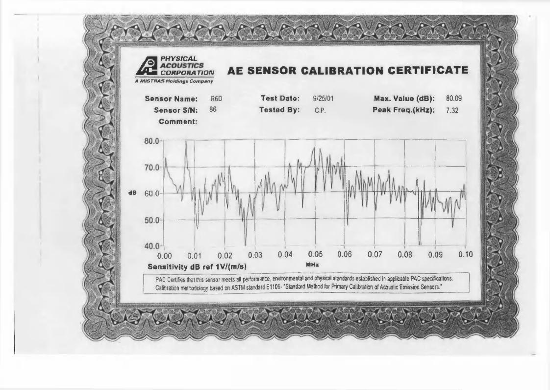
PHYSICALA AE SENSOR CALIBRATION CERTIFICATECORPORATIONA M tSTHAS H oM ing* Company

Test Date: 9 /2 5 /0 1

Tested By: CP.Max. Valuo (dB): 80.09Peak Freq.(kHz): 7.32

Sensor Name: R60 Sensor S/N: 80

Comment:

<■ J^ 60.0

0.00 0.01 0.02 0.03 0.04 0.05 0.06 0.07 0.08 0.09 0.10Sensitivity dB ref 1V/(m/s) MHz

PAC Certffes lhal this sensor meets all performance, erwonrrental and physical standards eslablisfied in applicable PAC speafcalions Calibration melhoddogy based on ASTM standard E11C6- •Standard Melhod to Primary Calibration of Acoustic Emission Sensors.*

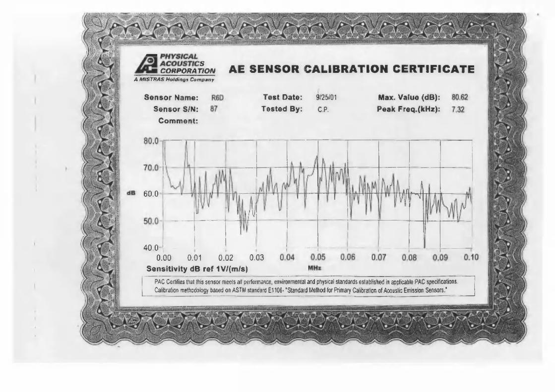
ok:

fe’MfeHl — PHYSICAL

CCm PORA^O N AE SENSOR CALIBRATION CERTIFICATEWxftiS • >! cA MiSTRAS HoUtingi Company

9 /2 5 /0 1

C.P.

Max. Value (dB): Peak Freq.(kHz):

Test Date: Tested By:

Sensor Name: Sensor S/N:

Comment:

m

4m60.0

lA;•> . “<̂ap •

40.0 10.00 0,01 0.02 0.03

Sensitivity dB ref 1V/(m/s)

m %

PAC Certifies nat this sensor mecls aE aerformance, environmental and physical sia.'idards established in applicable PAC sredfcationi Calibration m ettcftlog/ based on ASTM stanch'd E?106- 'Standard M o d for Primary Calibration of Acoustic Emission Sensors.'

ladMflm

PHYSICALA AE SENSOR CALIBRATION CERTIFICATECO RPORATIONA M iSTR AS Holdings Company

Tost Date: 3 /2 5 /0 1

Tested By: C P.

Sensor Name: R 6D

Sensor S/N: 9 2

Comment:

Max. Value (dB): Peak Freq.(kHz):

dB 60.0

40.CH,0.00 0.01 0.02 0.03

Sensitivity dB ref 1V/(m/s)PAC Cenilies that :his sensor meets all performance, environmental and physical standards established in applicable PAC specifications. Calibration meftaaotogy based on ASTM slandard El 106* 'Standard Method fee Primary Calfcralicn of Acousbc Emission Ssnsons."

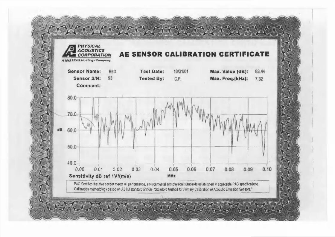
I

'I

I

PHYSICALACOUSTICSCORPORATION AE SENSOR CALIBRATION CERTIFICATE

A 1W S TRA& Hoktitigs Company

Sensor Name Sensor S/N

Comment:

Test Date Tested By:

Max. Value (dB) Max. Freq.(kHa)

40.0 I, !0.00 0.01 0.02 0.03 0.04

Sensitivity d8 ref 1V((m/s)PAC Certifes Ibal tftis sensor mee-.s all periormance. environneol aod physical standards established in applicable PAC specifications. Calibration methDCoagy based on ASTM standard ET106- 'Standard Method tor Pntnary Calibration ol AcojsIk Efrission Senso-s.’

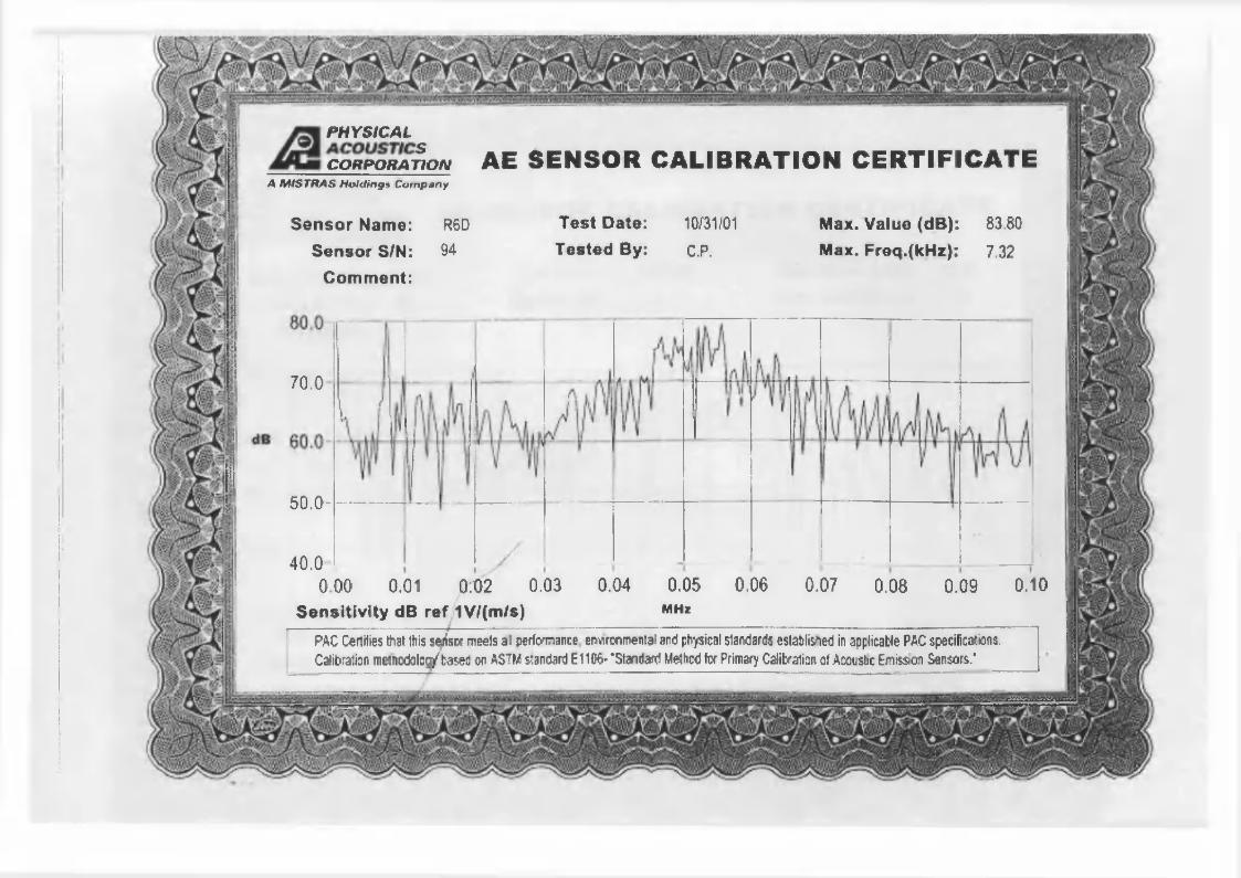
N PHYS/CAi.

COffTOMT̂ O/Vf AE SENSOR CALIBRATION CERTIFICA TEA MfSTfMS Holding* Company

1

Sensor Name: R 6 D

Sensor S/N: 94 Comment:

Test Date: 10/31/01Tested By: C.P.

Max. Value (dB): 83.80Max. Freq.(kHz): 7,32

Sensitivity dB ref 1V/(m/s) MHz

70.0

50.0-

40.00.00 0.01 0:02 0.03 0.04 0.05 0.06 0.07 0.08 0.09 0.10

PAC Certifies t o t this se/isnr mrels a i perfonnance erwronmenlal and physical standards established in applicable PAC specifications. Calibration m«ncdolca/based on A$7M standard E1106*’ Standard Method for Primary Calibration of Acoustic Emission Sensors.'

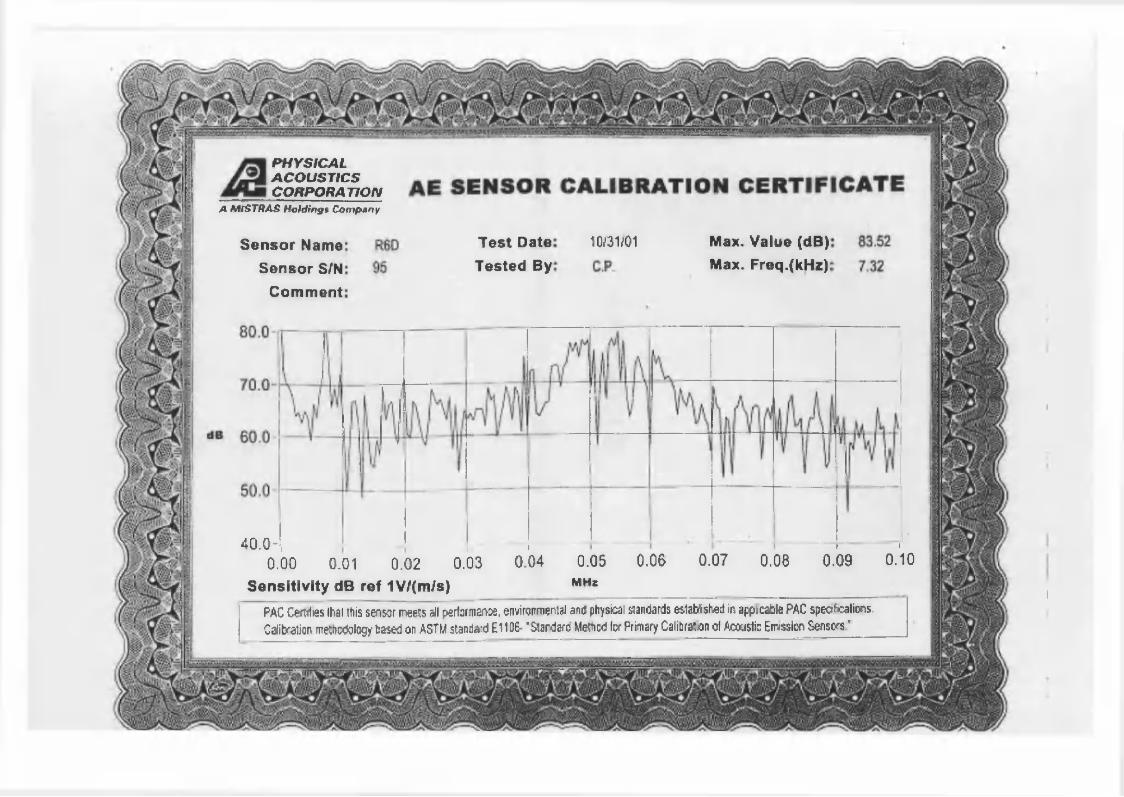
PHYSICALACOUSTICSCORPORATION

A M tSTRAS Holding* Company

Max. Value (dB) Max. Freq.(kHz):

10/31/01Test Date; Tested By

Sonsor Name Sensor S/N

Comment

40.0-, . " \ .......... i0.00 0.01 0.02 0.03 0.04 0.05 0.06 0.07 0.06 0.09 0.10

Sensitivity dB ref 1V/(m/s) WH*PAC CefUles lhai this sensor mee:? all pertorm2n:e. environmenlal and physical standards estaWsted in appicafale PAC spectaalions. Calibration methodology tsased on ASTM standa:d E1136- 'Star-darc Metticd lor Primary Calibragon d Acoustic Emission Sensors * _ _ _ _

»

I

APPENDIX B

RESULTS FOR PRE-CORRODED (PR) SPECIMENS

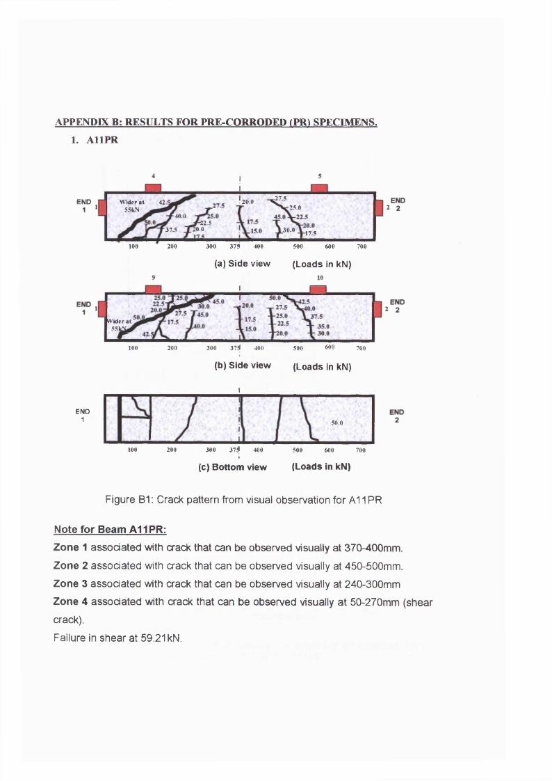
APPENDIX B: RESULTS FOR PRE-CORRODED (PR) SPECIMENS.

1. A11PR

-27.5END ' 20.0W ider a t 55kN

42.!25.0

40.0-22.5

!0.037.5 30.0 17.5

100 200 300 375 400 500 700600

(a) Side view (Loads in kN)

W ider at 55k^100 200 300 37$ 400 500 600 700

I(b) Side view (Loads in kN)

1

END1 50.0

37$100 200 300 400 500 600 700I

(c) Bottom view (Loads in kN)

Figure B1: Crack pattern from visual observation for A11 PR

Note for Beam A11PR:Zone 1 associated with crack that can be observed visually at 370-400mm.

Zone 2 associated with crack that can be observed visually at 450-500mm.

Zone 3 associated with crack that can be observed visually at 240-300mm

Zone 4 associated with crack that can be observed visually at 50-270mm (shear

crack).

Failure in shear at 59.21 kN.

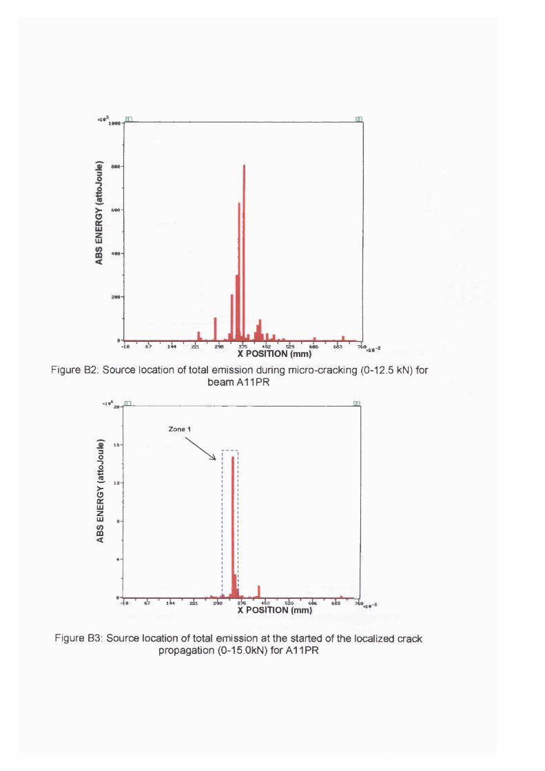
6 0 8 -

Ui

37 5 4 5 2 5 2 9 6

X POSITION (mm)67 221 68 3 760

Figure B2: Source location of total emission during micro-cracking (0-12.5 kN) forbeam A11PR

.I.*

30 “>1 >- 0 O' LU Z LUV>CD<

Zone 1

4 5 2 5 2 9 66 6

X POSITION (mm)

Figure B3: Source location of total emission at the started of the localized crackpropagation (0-15.0kN) for A 11 PR

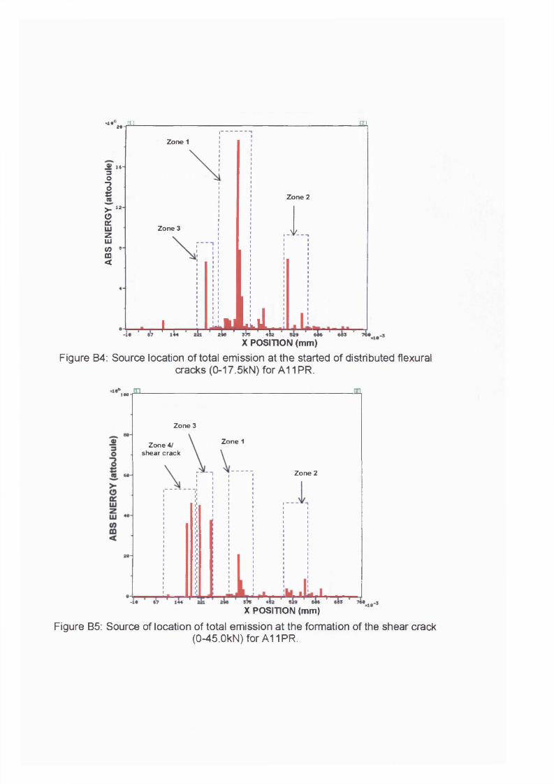
-1. ^ - j r L

® 1 6 - 301(O '

> 12Oa:illzLUCO 8 CD <

m

Zone 1

Zone 3

Zone 2

V

I 4 kak **5? 1 ^ 1 4̂X POSITION (mm)

Figure B4: Source location of total emission at the started of distributed flexuralcracks (0-17.5kN) for A11 PR.

106 “ |

Zone 3

Zone 1Zone 4/ shear crack

Zone 2

X POSITION (mm)

Figure B5: Source of location of total emission at the formation of the shear crack(0-45.OkN) for A11 PR.

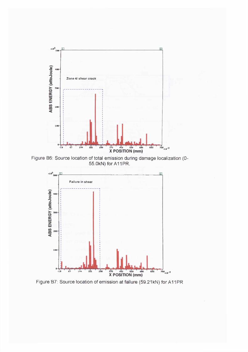
5W-I

Zone 4J shear crack

5M-

UJ

2 W -

67-18 298 375 ♦52

X POSITION (mm)529 «10

Figure B6: Source location of total emission during damage localization (0-55.0kN) for A11PR.

Failure in shear

1M-

67 144

X POSITION (mm)

Figure B7: Source location of emission at failure (59.21 kN) for A11PR

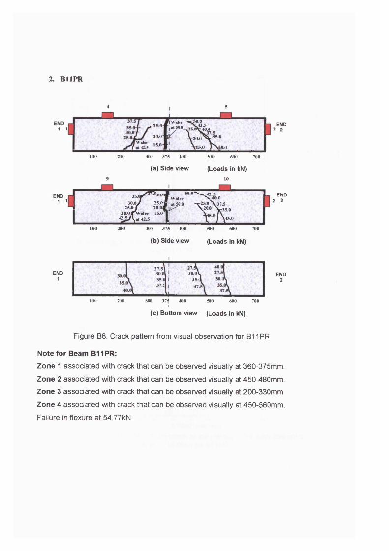
2. B11PR

50.0W ider at 50.0

END.42.525.01 40.0

20.0W iderat 42.5 13 U

35.020.0

5.0 15.0

100 200 300 375 400 500 600 700

(a) Side view (Loads in kN) 10

END I 1 1

| 3 5 .( |^ T7:^O flj5o.<n^ _ 4 2 .5 |

[ l Wider > *4 0 .03 0 .0 / 25.<H1, at 50.0 r 2 5 . 0 \ 37.5

I 2 5 .0 / 2 0 .0 i V 00^ r 3 5 . 020.<HpYider 15.0^i t 5°/V°« £ / l j * 4 2 .5 |L

END2 2

100 200 300 375 400I

(b) Side view

500 600 700

(Loads in kN)

END1

40.127.5 30.0 35. ( 37.£

30.0V3s.a37 .5

30 .1

300 375100 200 400 500 600 700

END2

(c) Bottom view (Loads in kN)

Figure B8: Crack pattern from visual observation for B11PR

Note for Beam B11PR:Zone 1 assodated with crack that can be observed visually at 360-375mm.

Zone 2 assodated with crack that can be observed visually at 450-480mm.

Zone 3 assodated with crack that can be observed visually at 200-330mm

Zone 4 assodated with crack that can be observed visually at 450-560mm.

Failure in flexure at 54.77kN.

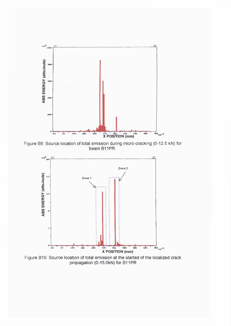
«ie3 rn1008-r -̂

•-r-10

-I— r1—f -529 606375 452

X POSITION (mm)

Figure B9: Source location of total emission during micro-cracking (0-12.5 kN) forbeam B11PR.

Zone 2

16- Zone 1

1 2 -

4-

-10 67 144 221 29« 575 452

X POSITION (mm)-10

Figure B10: Source location of total emission at the started of the localized crackpropagation (0-15.0kN) for B11PR

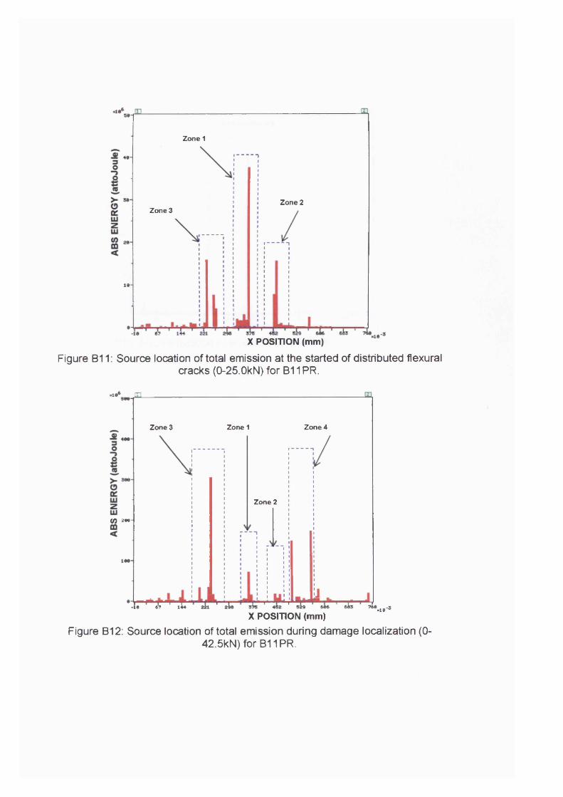
Zone 1

----1

Zone 2Zone 3

X POSITION (mm)

Figure B11: Source location of total emission at the started of distributed flexuralcracks (0-25.0kN) for B11 PR.

m

Zone 1 Zone 4Zone 3

Zone 2

<0 a«-

6? -10X POSITION (mm)

Figure B12: Source location of total emission during damage localization (0-42.5kN) for B11PR.

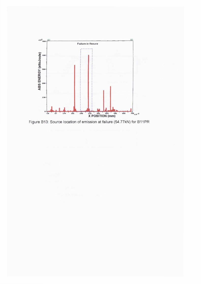
Failure in flexure

198

■49X POSITION (mm)

Figure B13: Source location of emission at failure (54.77kN) for B11PR

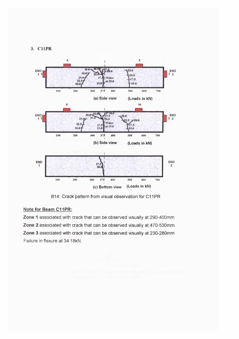
3. C11PR

30.1 15.0END30.

-20.0t-17.51-15.0

253 17.4j Wider

200 300 375 400 500 600 700100

(a) Side view (Loads in kN)10

END2 2

pOTi?7-5

-20.0Wider

fa t 253)

303END253

17.55.020.1 15.1

300 374 400100 200 500 600 700

END2 2

(b) Side view (Loads in kN)

END2

100 200 300 314 400 500 600 700I

(c) Bottom view (Loads in kN)

B14: Crack pattern from visual observation for C11PR

Note for Beam C11PR:Zone 1 associated with crack that can be observed visually at 290-400mm.

Zone 2 associated with crack that can be observed visually at 470-530mm.

Zone 3 associated with crack that can be observed visually at 230-280mm

Failure in flexure at 34.18kN.

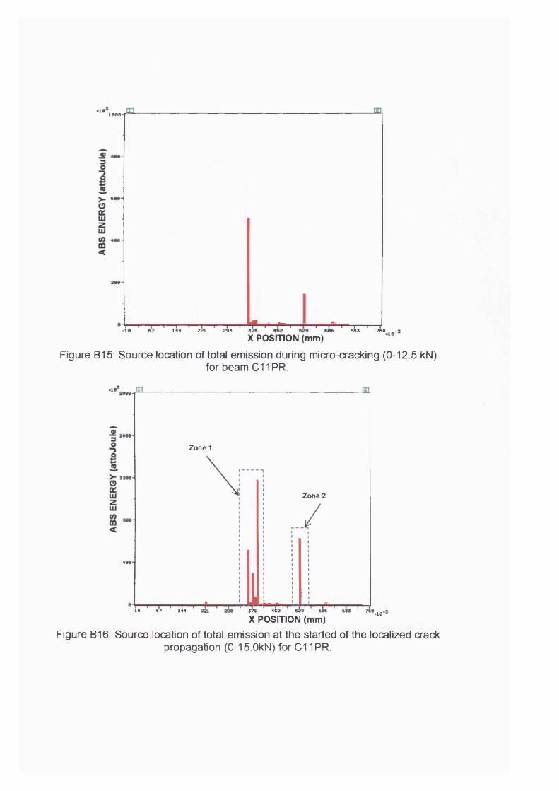
IMS-

144 221 2 9 8

X POSITION (mm)683 760

Figure B15: Source location of total emission during micro-cracking (0-12.5 kN)for beam C11PR.

Zone 1

Zone 2

-is 67 144 221 375 45 2 52 9 606

X POSITION (mm)-1 0

Figure B16: Source location of total emission at the started of the localized crackpropagation (0-15.0kN) for C11PR.

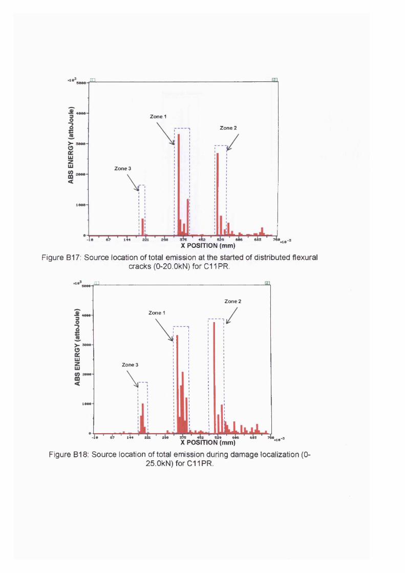
m

Zone 1

Zone 2

111Zone 3

X POSITION (mm)

Figure B17: Source location of total emission at the started of distributed flexuralcracks (0-20.OkN) for C11 PR.

m

Zone 2

Zone 1—i

UiZone 3

6 * 3

X POSITION (mm)

Figure B18: Source location of total emission during damage localization (0-25.0kN) for C11PR.

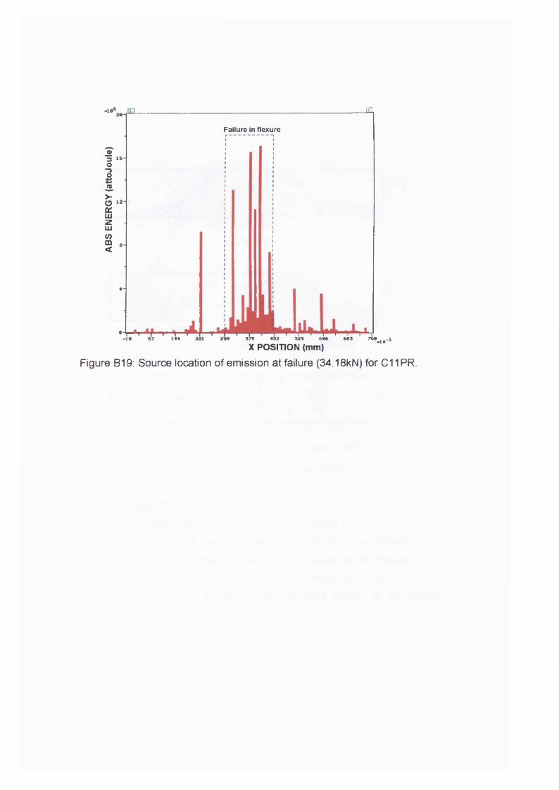
ABS

ENER

GY

(atto

Joul

e)M

Failure in flexure

W \ r-1 4 4 221 2 9 8 3 7 5 4 5 2 5 2 9 6 8 5 6 8 3 7 6 8 l g -3

X POSITION (mm)

Figure B19: Source location of emission at failure (34.18kN) for C11PR.

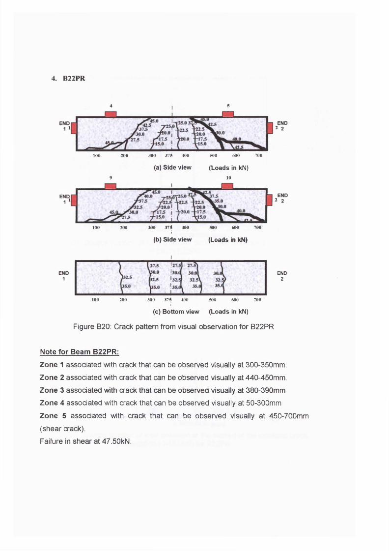
4. B22PR

100 200 300 375 400 500 600 700

(a) Side view (Loads in kN)9 10

100 200 300 375 400 500 600 700I

(b) Side view (Loads in kN)

100 200

END2

300 375 400 500 600 700I

(c) Bottom view (Loads in kN)

Figure B20: Crack pattern from visual observation for B22PR

Note for Beam B22PR:Zone 1 assodated with crack that can be observed visually at 300-350mm.Zone 2 assodated with crack that can be observed visually at 440-450mm.Zone 3 assodated with crack that can be observed visually at 380-390mm

Zone 4 assodated with crack that can be observed visually at 50-300mm

Zone 5 assodated with crack that can be observed visually at 450-700mm

(shear crack).

Failure in shear at 47.50kN.

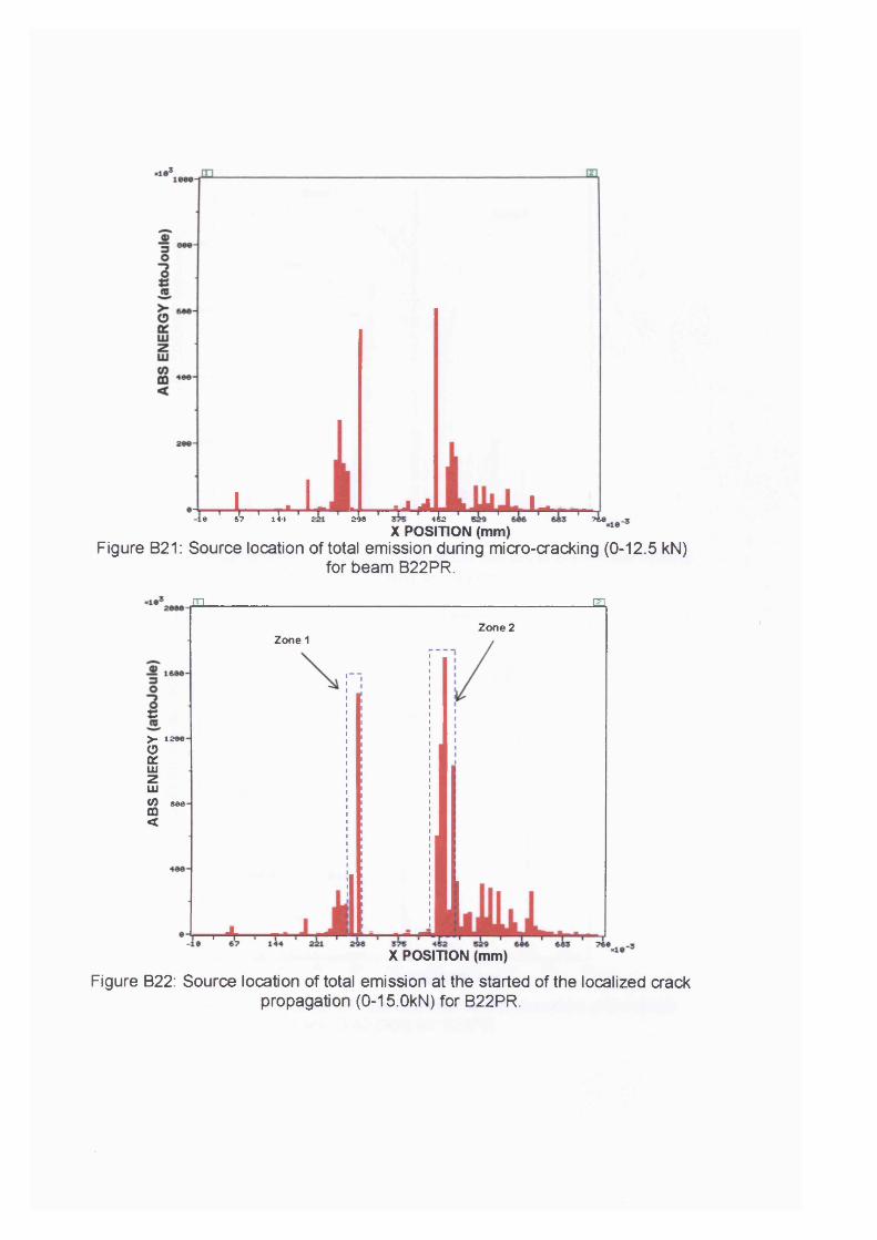
. ■ L ■ ,T.‘ 1 \ 14T J-Jk ̂ TieTX POSITION (mm)

Figure B21: Source location of total emission during micro-cracking (0-12.5 kN)for beam B22PR.

m

8>- iseee>oc.LUzLUCO sea 00 <

mZone 2

Zone 1

T-VX POSITION (mm)

Figure B22: Source location of total emission at the started of the localized crackpropagation (0-15.0kN) for B22PR.

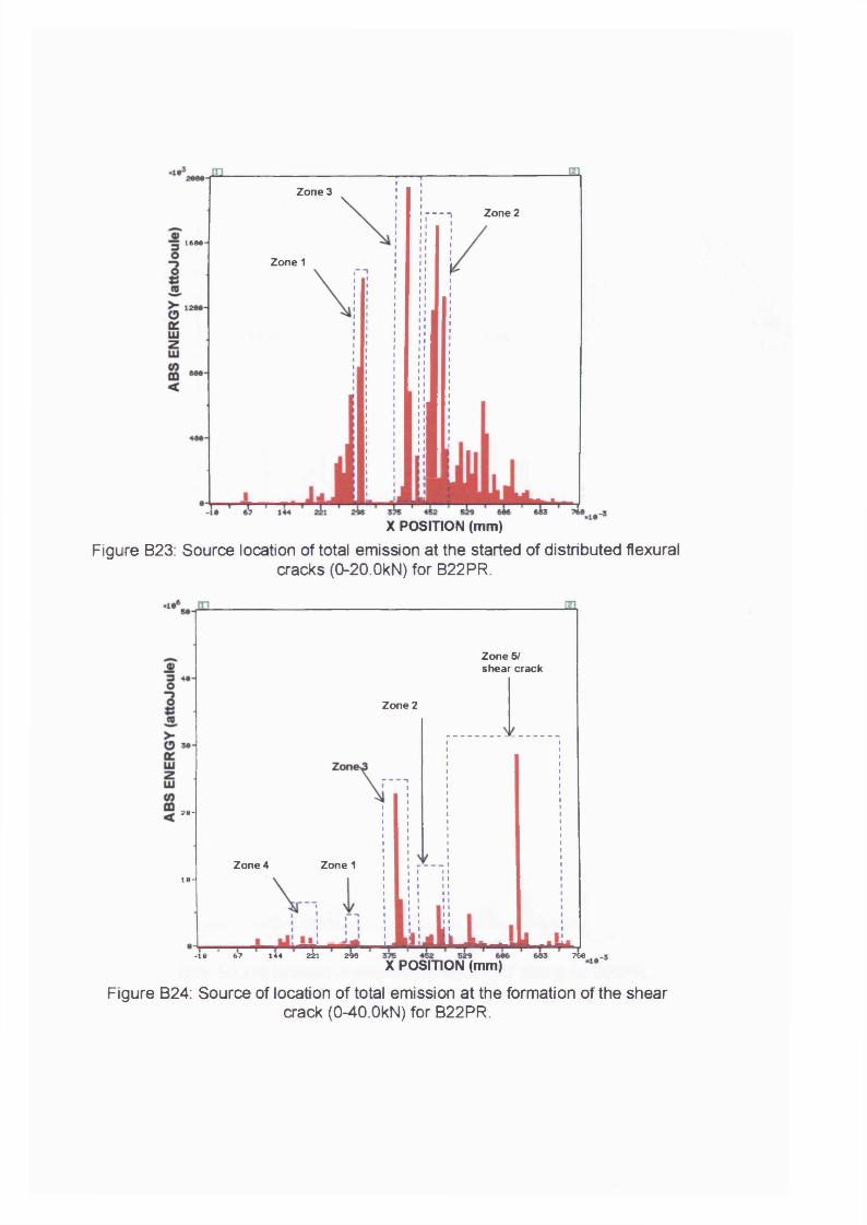
Zone 3

Zone 2----11 6 0 0 -

Zone 1

X POSITION (mm)

Figure B23: Source location of total emission at the started of distributed flexuralcracks (0-20.0kN) for B22PR.

Zone 5/ shear crack

Zone 2

2 9 -

Zone 4 Zone 11 0 -

144 221 298-18 6?X POSITION (mm)

760

Figure B24: Source of location of total emission at the formation of the shearcrack (0-40.0kN) for B22PR.

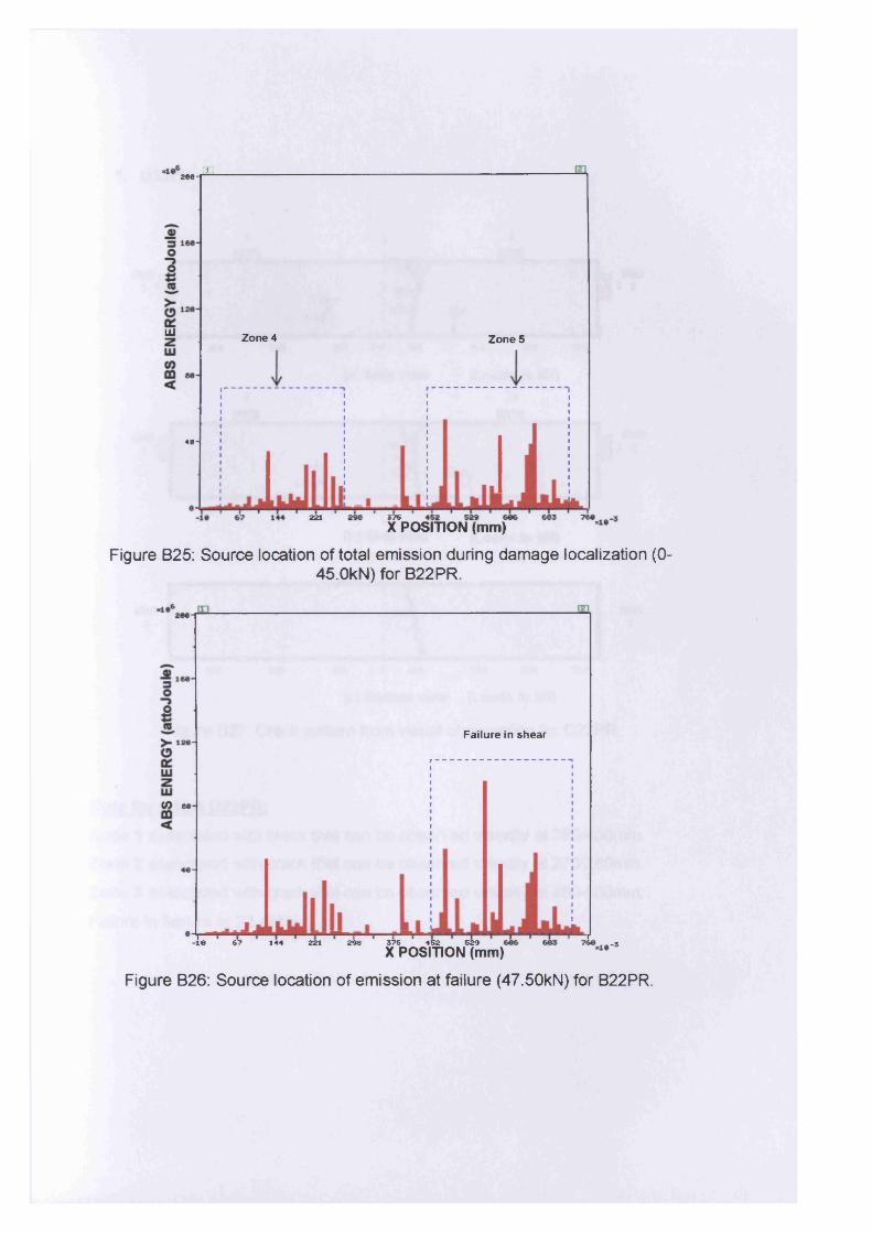
jh200 -

LU Zone 4 Zone 5

4 0 -

221WP OSITION (mm)

Figure B25: Source location of total emission during damage localization (0-45.0kN) for B22PR.

Failure in shear

(0 se

10 67 144 221 298 375 452 529X POSITION (mm) -3

Figure B26: Source location of emission at failure (47.50kN) for B22PR.

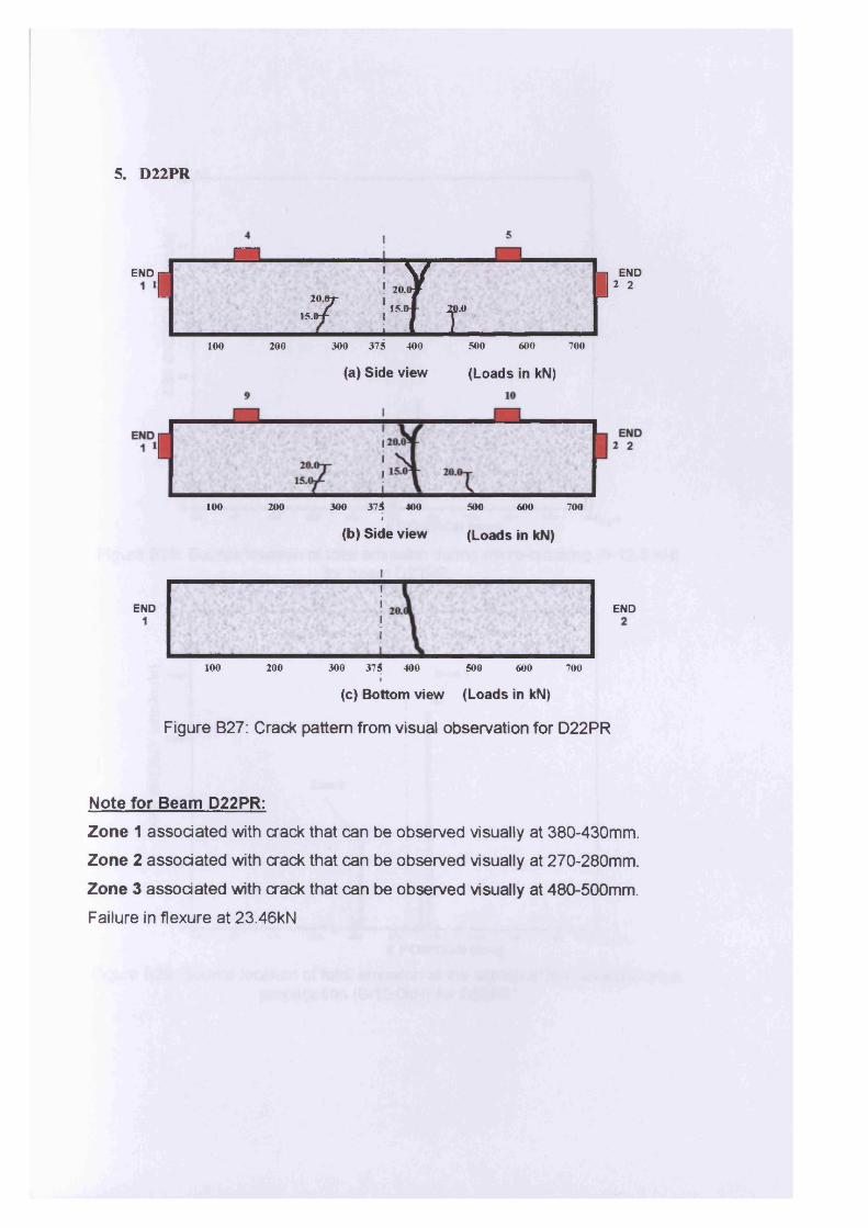
5. D22PR

END m

1 V ....... —20.0#20 .07- fy 15.0-1- 20.0

15.64 - I t

END

100 200

] END2 2

300 375 400

(a) Side view

500 600 700

(Loads in kN)

100 200 300 374 400 500 600 700I

(b) Side view (Loads in kN)

END

100 200 300 374 400 500 600 700

(c) Bottom view (Loads in kN)

Figure B27: Crack pattern from visual observation for D22PR

Note for Beam D22PR:Zone 1 associated with crack that can be observed visually at 380-430mm.

Zone 2 associated with crack that can be observed visually at 270-280mm.

Zone 3 associated with crack that can be observed visually at 480-500mm.

Failure in flexure at 23.46kN

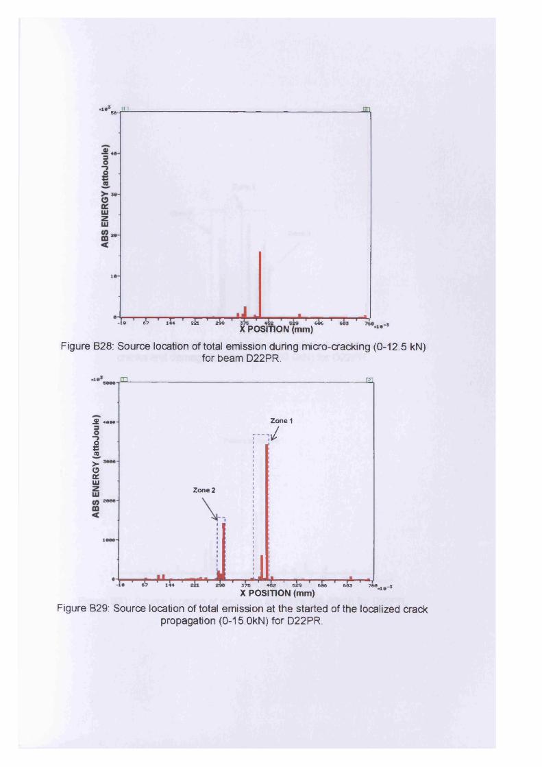
rn50-

6?-10 221 298XPOSiTION (mm)

608

Figure B28: Source location of total emission during micro-cracking (0-12.5 kN)for beam D22PR.

£ 4000-

I>- e> a:LU

m.

Zone 2

-GO.

Zone 1

r - V

I

u T T "529375 452 529 606

X POSITION (mm)683 760 3

Figure B29: Source location of total emission at the started of the localized crackpropagation (0-15.0kN) for D22PR.

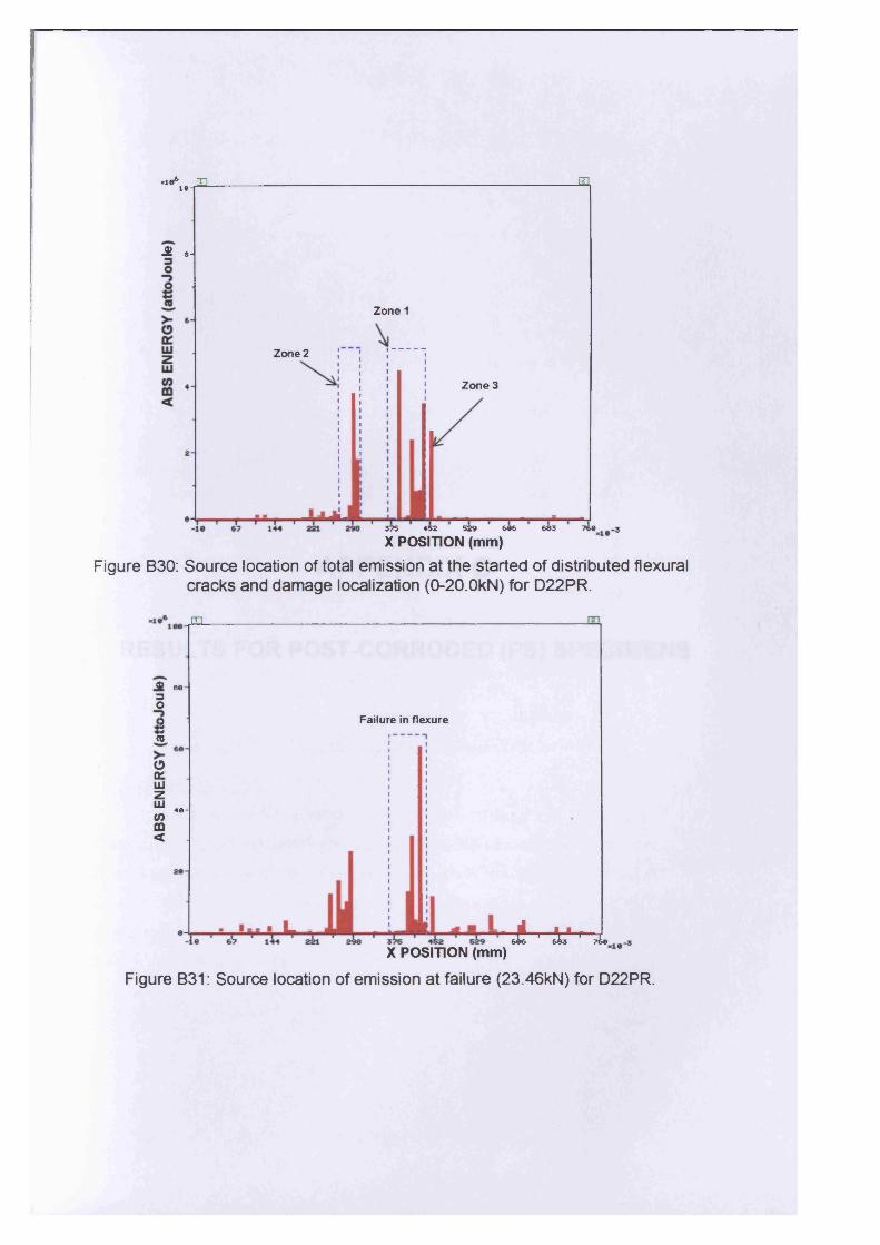
.186 inl*-̂ -L"

A J

m

Zone 1

Zone 3

Zone 2

375 452 529 596

X POSITION (mm)693 769

Figure B30: Source location of total emission at the started of distributed flexural cracks and damage localization (0-20.0kN) for D22PR.

JXL

® 89-|3O2(0

0O'I I Iz* 49-<0 m <

Failure in flexure

J 1 5»'' J.X POSITION (mm)

Figure B31: Source location of emission at failure (23.46kN) for D22PR.

APPENDIX C

RESULTS FOR POST-CORRODED (PS) SPECIMENS

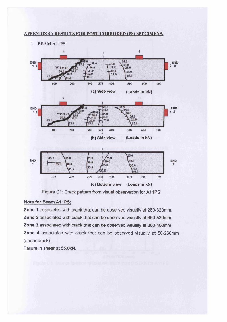
APPENDIX C: RESULTS FOR POST-CORRODED (PS) SPECIMENS.

1. BEAM A1 IPS

END 35.0f30.0-25.0-20.015.0

45.0-42.5

17.51W ider at

-25.045.1

200 300 375 400 500100 600 700

END2 2

(a) Side view (Loads in kN)10

END2 2W ider al

100 200 300 375 400 500 600 700I

(b) Side view (Loads in kN)

i

45.0 !5.0 55.0 /̂ 5.030.015.0

END1

(5.0(7.5 r37-5100 200 300 375 400 500 600 700

(c) Bottom view (Loads in kN)

Figure C1: Crack pattern from visual observation for A11 PS

Note for Beam A11 PS:Zone 1 associated with crack that can be observed visually at 280-320mm.

Zone 2 associated with crack that can be observed visually at 450-530mm.

Zone 3 associated with crack that can be observed visually at 360-400mm

Zone 4 associated with crack that can be observed visually at 50-260mm

(shear crack).

Failure in shear at 55.0kN.

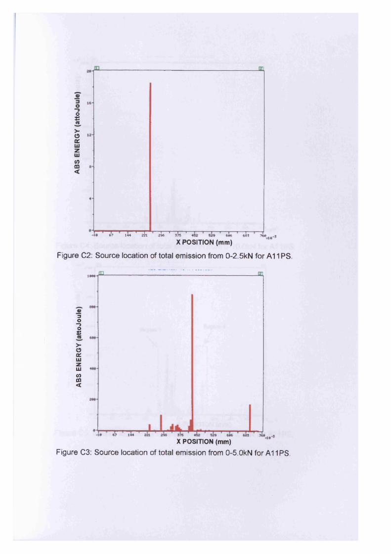
o3Sn>0o'Liiz111COffi<

*'? 144 1 2L *4* ' sk ' ' & * t&s 7M *X POSITION (mm)

Figure C2: Source location of total emission from 0-2.5kN for A11 PS.

. - .A 3-----------------------------

3o“ 5OS>- 0 a:LUzUJ<0CD<

X POSITION (mm)

Figure C3: Source location of total emission from 0-5.OkN for A 11 PS.

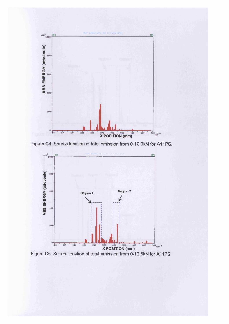
X POSITION (mm)

Figure CA:Source location of total emission from 0-10.0kN for A11 PS.

OC>-oOdi l lzUlCOm<

Region 2Region 1

LX POSITION (mm)

Figure C5: Source location of total emission from 0-12.5kN for A 11 PS.

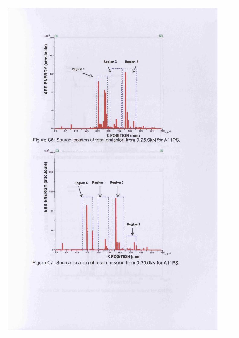
«*•* jn

3Oo l* C>■e>o' **LUzUJCO ffl < *

Region 1

pL 4-

Region 3 Region 2

-1# 0 221-r-M 3SX POSITION (mm)

Figure C6: Source location of total emission from 0-25.0kN for A11 PS.

Region 4 Region 1 Region 3

UJ

UJCO

Region 2

•19 0? 144 221 209 STS 452 $20 &

X POSITION (mm)Figure C7: Source location of total emission from 0-30.0kN for A 11 PS.

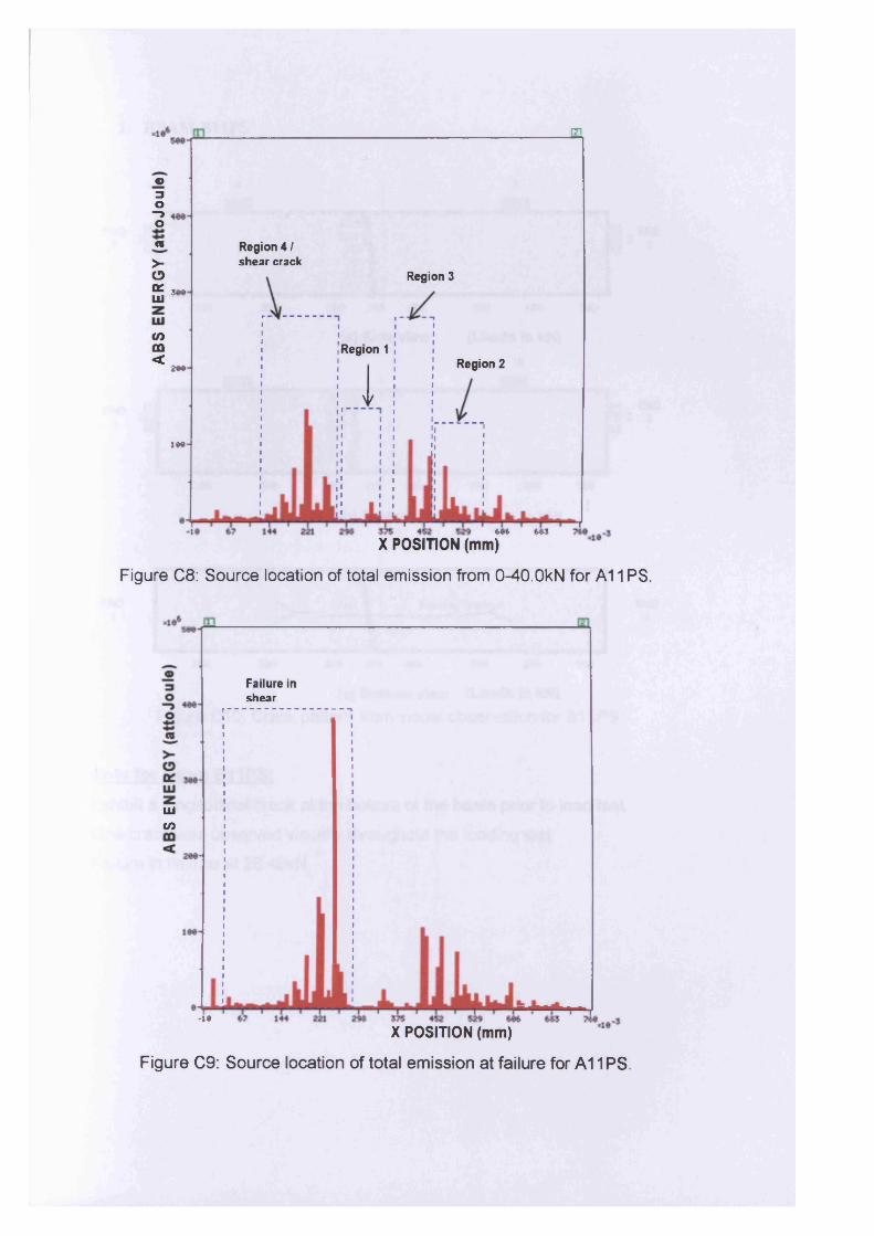
o3O—>ow>-CDa:ui 5M

<0m<

see

1 e a ­

rn

Region 4 / shear crack

Region 3

Region 1Region 2

1

*•* wX POSITION (mm)

Figure C8: Source location of total emission from 0-40.0kN for A11 PS.

Failure in shear

UJin

•teX POSITION (mm)

Figure C9: Source location of total emission at failure for A11 PS.

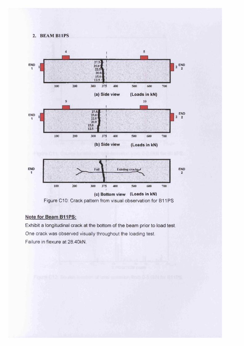
2. BEAM B11PS

END1

27.5-25.0-1

20.015.0

12.5

300 375 400100 200 500 600 700

END1

(a) Side view (Loads in kN)10

25.0 22.520.0

100 200 300 375 400 500 600 700

(b) Side view (Loads in kN)

i

Faal I Existing cracks^

i_______ .100 200 300 375 400 500 600 700

I(c) Bottom view (Loads in kN)

Figure C10: Crack pattern from visual observation for B11 PS

Note for Beam B11 PS:Exhibit a longitudinal crack at the bottom of the beam prior to load test.

One crack was observed visually throughout the loading test.

Failure in flexure at 28.40kN.

END2

END2

END2

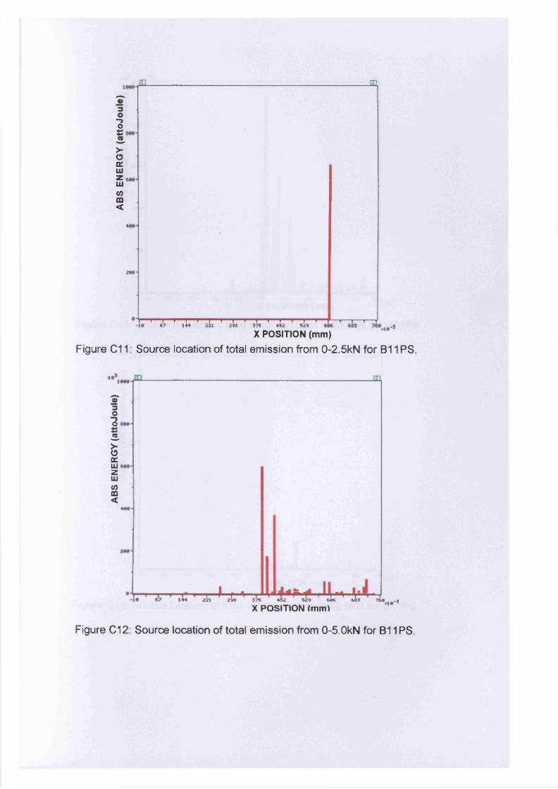
m. m

01>oonUlz111COCD<

M*-

I I I I I I I I I I I I I I I-1* 67 144 221 296 375 452 £29

X POSITION (mm)Figure C11: Source location of total emission from 0-2.5kN for B11 PS.

01OonUJzUJCOCD<

JZX

15T J—r- * p lU -29* 375 452 529 6*4 493 74* 5

X POSITION (mm)

Figure C12: Source location of total emission from 0-5.0kN for B11PS.

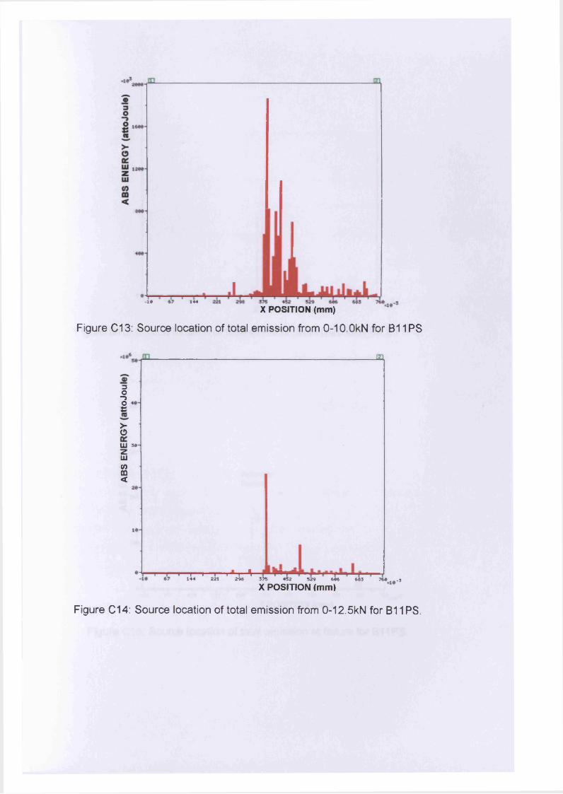
-1* 144

X POSITION (mm)

Figure C13: Source location of total emission from 0-10.0kN for B11 PS

3O“JOe>-oHI 34zUJCO00<

-El

. I . I ■■■ *144 221 241 J75 452 529

X POSITION (mm)646 MS 754 . j

Figure C14: Source location of total emission from 0-12.5kN for B11PS.

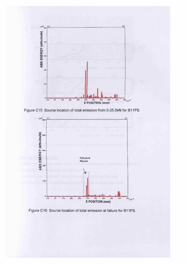
X POSITION (mm*

Figure C15: Source location of total emission from 0-25.0kN for B11 PS.

je____________________________________m

$>- sw O a:UJUJCOm<

Failure in flexure

2*»

Viw

-14 47 144i i *i i fci F1

29* 57» 45* 5 « 694 4*3 74*

X POSITION (mm)

Figure C16: Source location of total emission at failure for B11 PS.

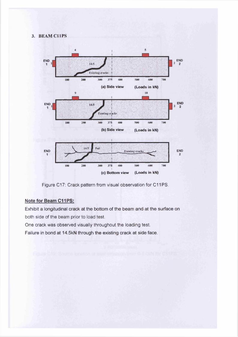
3. BEAM C11PS

END14.5

Existing cracks I

300 375 400 700500 600

END

(a) Side view (Loads in kN)

200 300 375 400

(b) Side view

500 600 700

(Loads in kN)

END2 2

Existing cracks

END1

V u ,JI---------------------1 FailExisting cracks —̂>

----------

100 200 300 375 400 500 600 700

(c) Bottom view (Loads in kN)

END2

Figure C17: Crack pattern from visual observation for C11 PS.

Note for Beam C11PS:Exhibit a longitudinal crack at the bottom of the beam and at the surface on

both side of the beam prior to load test.

One crack was observed visually throughout the loading test.

Failure in bond at 14.5kN through the existing crack at side face.

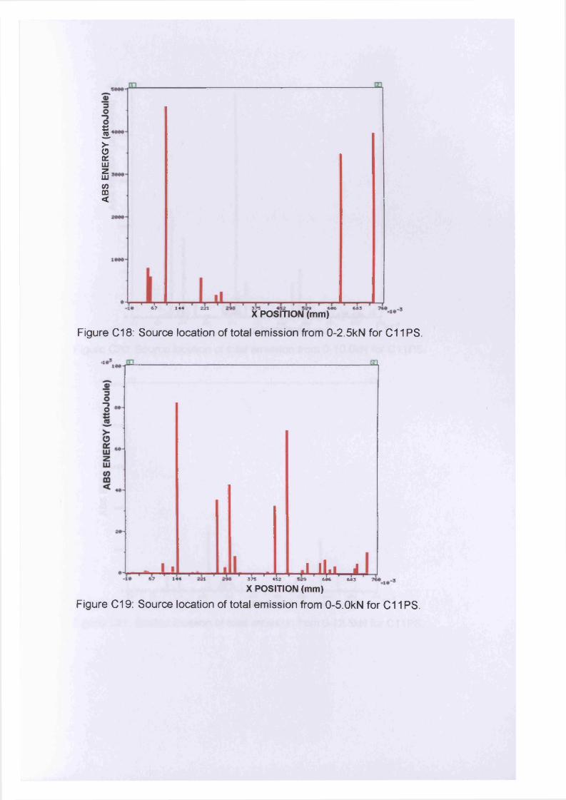
I>-oa:UJzUJV)m<

—i i i• 6? 144 221

I«3FrosftoNTmmr

Figure C18: Source location of total emission from 0-2.5kN for C11 PS.

JLL

i i575 452

u l uI 644 645X POSITION (mm)

Figure C19: Source location of total emission from 0-5.0kN for C 11 PS.

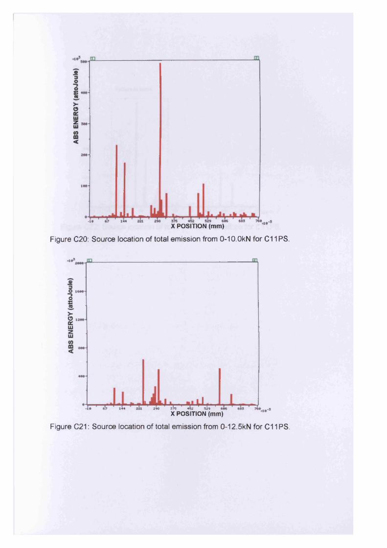
2

•1*X POSITION (mm)

Figure C20: Source location of total emission from 0-10.0kN for C11PS.

1.̂ * I ■■ i 11 I i296 575 452 529

X POSITION (mm)

Figure C21: Source location of total emission from 0-12.5kN for C 11 PS.

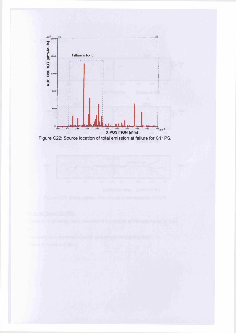
ABS

ENER

GY

(atto

Joul

e)

Failure in bond

sX POSITION (mm)

Figure C22: Source location of total emission at failure for C11 PS.

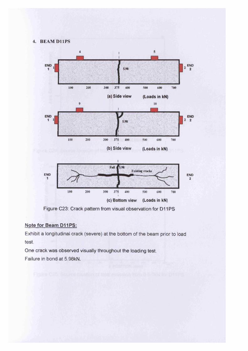
4. BEAM D1 IPS

END

100 200 300 375 400 500 600 700

(a) Side view (Loads in kN)

10

100 200 300 375 400 500 600 700

(b) Side view (Loads in kN)

Existing cracksEND

100 200 300 375 400 500 600 700

(c) Bottom view (Loads in kN)

Figure C23: Crack pattern from visual observation for D11 PS

END2

Note for Beam D11PS:

Exhibit a longitudinal crack (severe) at the bottom of the beam prior to load

test.

One crack was observed visually throughout the loading test.

Failure in bond at 5.98kN.

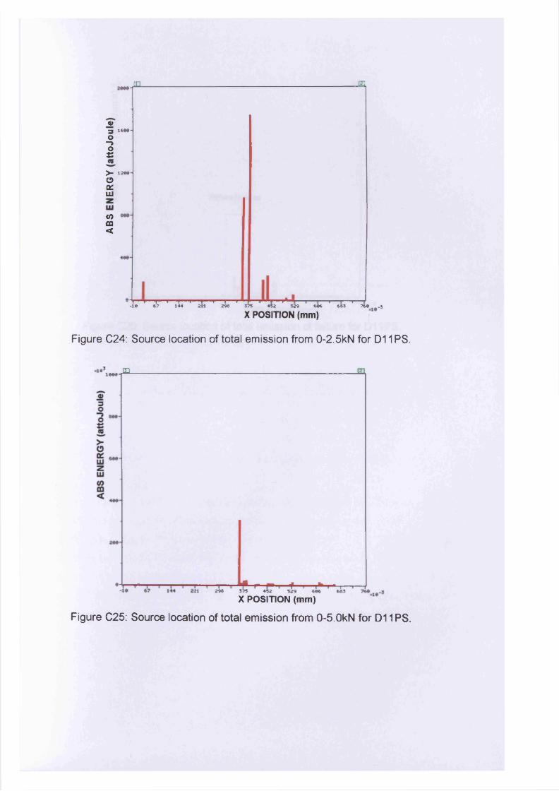
JO- M

«3 1U»-O —> oc>- 12»- o a:Ul

com<

i i i i i i i i i-10 6 ? 144 221 248 375 ' 452 ^'"sM 644 ' 683 ' 764 .3

X POSITION (mm)

Figure C24: Source location of total emission from 0-2.5kN for D11 PS.

•3 m1M« -C~

r ■ i i ■# i ih i * i—.21 248 375 452 529 686 685

X POSITION (mm)

Figure C25: Source location of total emission from 0-5.0kN for D11 PS.

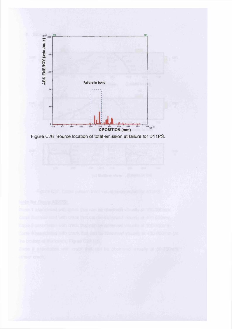
ABS

ENER

GY

(att

oJou

le)

13*

M

X POSITION (mm)

Figure C26: Source location of total emission at failure for D11 PS.

Failure in bond

X POSITION (mm)

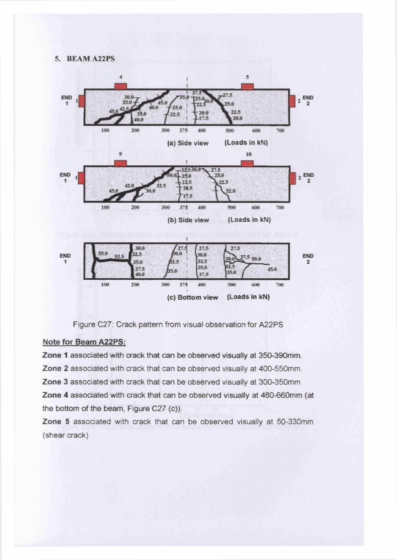
5. BEAM A22PS

(a) Side view (Loads in kN)

(b) Side view (Loads in kN)

100 200 300 375 400 500 600 700I

(c) Bottom view (Loads in kN)

Figure C27: Crack pattern from visual observation for A22PS

Note for Beam A22PS:Zone 1 associated with crack that can be observed visually at 350-390mm.

Zone 2 associated with crack that can be observed visually at 400-550mm.

Zone 3 associated with crack that can be observed visually at 300-350mm

Zone 4 associated with crack that can be observed visually at 480-660mm (at

the bottom of the beam, Figure C27 (c)).

Zone 5 associated with crack that can be observed visually at 50-330mm

(shear crack)

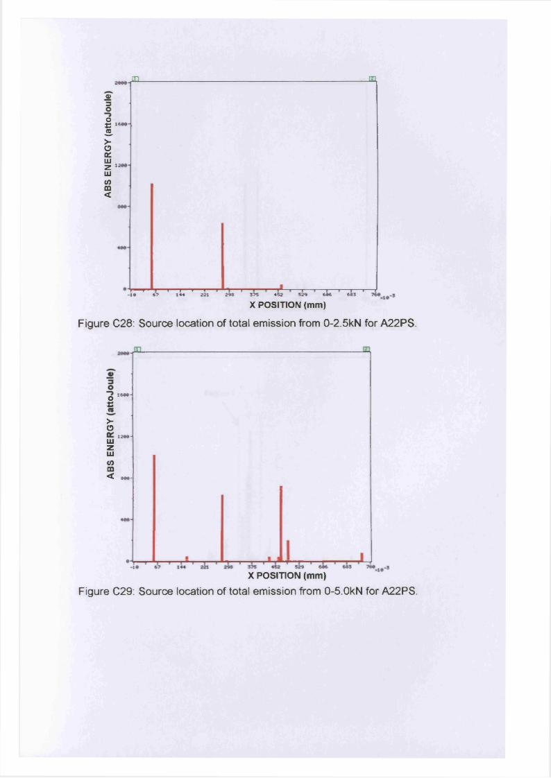
ju­ ju,a>

I">■©O'UJz 1SUJCOffi<

1—1 » 1 I I I-I* 6? 144 221 29? 375 452 « 4 6*6 5*3

X POSITION (mm)

Figure C28: Source location of total emission from 0-2.5kN for A22PS.

— lowoC>-© 12MUJzUJCOm < M

X POSITION (mm)

Figure C29: Source location of total emission from 0-5.OkN for A22PS.

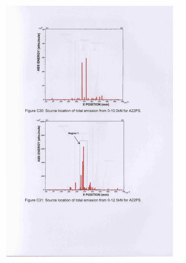
575 4» S»

X POSITION (mm)

Figure C30: Source location of total emission from 0-10.0kN for A22PS.

Region 1

\

n r T 1 *3;X POSITION (mm)

Figure C31: Source location of total emission from 0-12.5kN for A22PS.

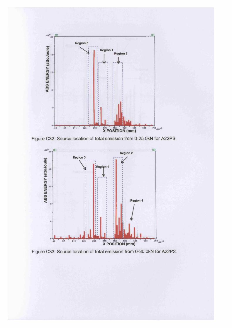
Region 3

N Region 1Region 2o

«-

144

X POSITION (mm)

Figure C32: Source location of total emission from 0-25.0kN for A22PS.

Region 2Region 3

Regi

Region 4

- i t 144

X POSITION (mm)

Figure C33: Source location of total emission from 0-30.0kN for A22PS.

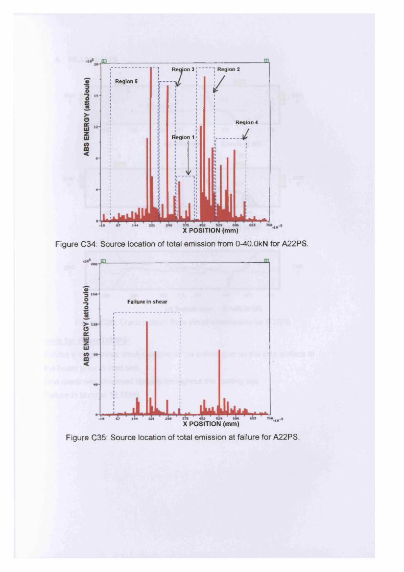
-1 Region 2Region 3

Region 5

»*-

Region 4

Region 1

144

X POSITION (mm)

Figure C34: Source location of total emission from 0-40.0kN for A22PS.

Failure in shear

X POSITION (mm)

Figure C35: Source location of total emission at failure for A22PS.

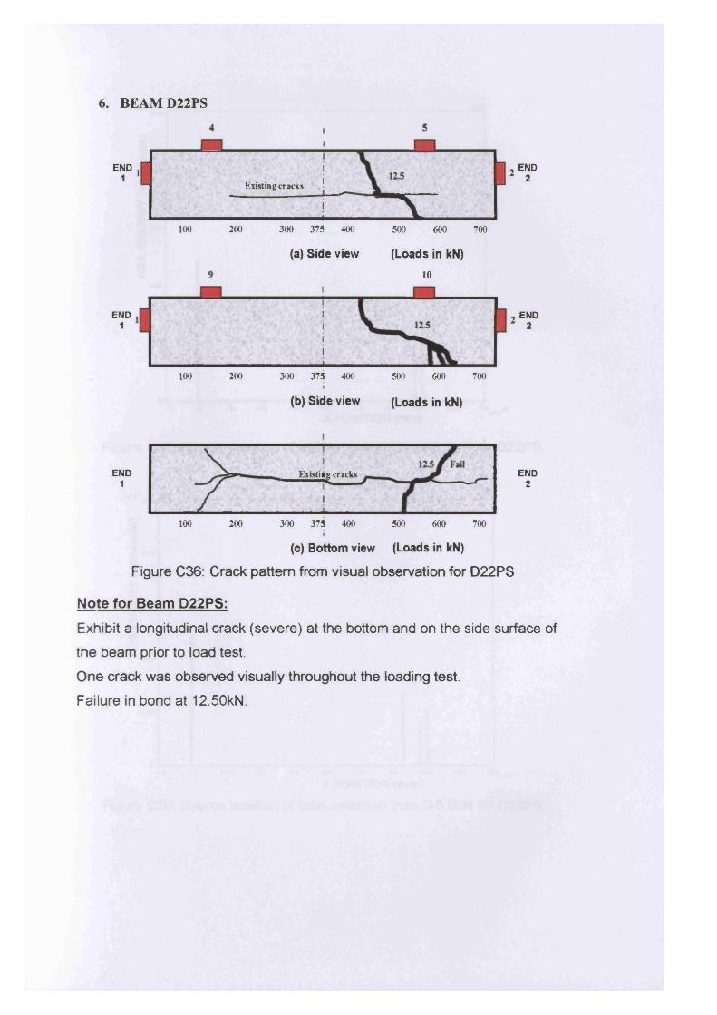
6. BEAM D22PS

END'[

100 200

Existing cracks

. J T y ______________300 373 400

(a) Side view

500 600

(Loads in kN)

10

(b) Side view (Loads in kN)

]END

700

T

200 300 373 400 500 700100 600

END

END1 Esistiig cracks

100 200 300 373 400 500 700600

END2

(c) Bottom view (Loads in kN)

Figure C36: Crack pattern from visual observation for D22PS

Note for Beam D22PS:Exhibit a longitudinal crack (severe) at the bottom and on the side surface of

the beam prior to load test.

One crack was observed visually throughout the loading test.

Failure in bond at 12.50kN.

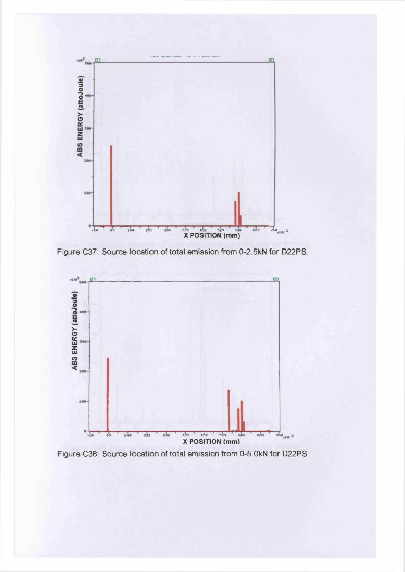
-1* 5? 1«4 *21 2» 575 452 524 545 555 75# .3X POSITION (mm)

Figure C37: Source location of total emission from 0-2.5kN for D22PS.

js

>-oKLUZLUtom<

575 ' «& 1 si»

X POSITION (mm)

Figure C38: Source location of total emission from 0-5.0kN for D22PS.

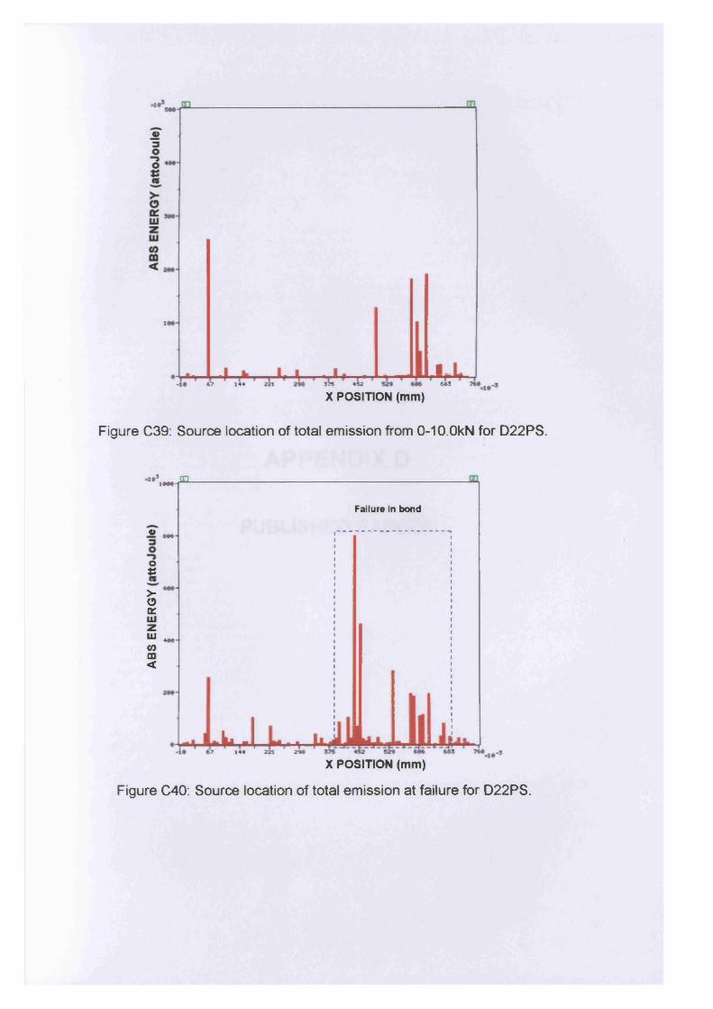
67 221 575

X POSITION (mm)♦52 553144

Figure C39: Source location of total emission from 0-10.0kN for D22PS.

•5 m1444-T̂-

Failure in bond

« « • -

o £>• * oa: uizui 444-(0 CD <

L k J ^>7 144 221 2 *

X POSITION (mm)

Figure C40: Source location of total emission at failure for D22PS.

APPENDIX D

PUBLISHED PAPERS

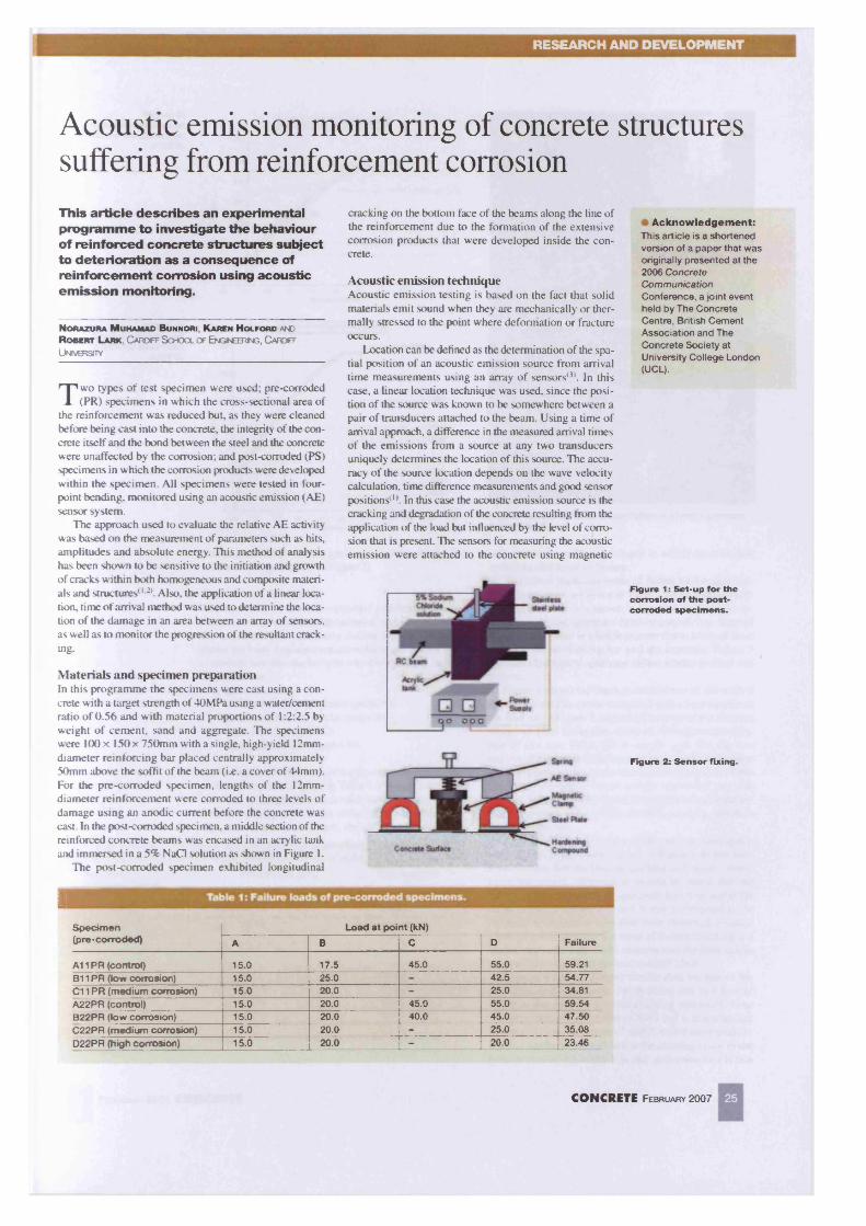
RESEARCH AND DEVELOPMENT

Acoustic emission monitoring of concrete suffering from reinforcement corrosionThis artic le describes an experimental program m e to investigate the behaviour of reinforced concrete structures subject to deterioration as a consequence of reinforcem ent corrosion using acoustic emission monitoring.

N o r a z u r a M u h a m a d B u n n o r i K a r e n W o l f o r d and R o b e r t L a r k , Cardiff Scho ol of En gineering , G w o ff

U ntverstty

T wo types of test specimen were used; pre-corroded (PR) specimens in which the cross-sectional area of

the reinforcement was reduced bu t as they were cleaned before being cast into the concrete, the integrity of the con­crete itself and the bond between the steel and the concrete were unaffected by the corrosion; and post-corroded (PS) specimens in which the corrosion products were developed within the specimen. All specimens were tested in four- point bending, monitored using an acoustic emission (AE) sensor system.

The approach used to evaluate the relative AE activity was based on the measurement of parameters such as hits, amplitudes and absolute energy. This method of analysis has been shown to be sensitive to the initiation and growth of cracks w'ithin both homogeneous and composite materi­als and structures0 -2*. Also, the application of a linear loca­tion, time of arrival method was used to determine the loca­tion of the damage in an area between an array of sensors, as well as to monitor the progression of the resultant crack­ing.

M aterials and specimen preparationIn this programme the specimens were cast using a con­crete with a target strength of 40MPa using a water/cement ratio of 0.56 and with material proportions of 1:2:2.5 by- weight of cement, sand and aggregate. The specimens were 100 x 150 x 750mm with a single, high-yield 12mm- diameter reinforcing bar placed centrally approximately 50mm above the soffit of the beam (i.e. a cover of 44mm). For the pre-corroded specimen, lengths of the 12mm- diameter reinforcement were corroded to three levels of damage using an anodic current before the concrete was cast. In the post-corroded specimen, a middle section of the reinforced concrete beams was encased in an acrylic tank and immersed in a 5% NaCl solution as shown in Figure 1.

The post-corroded specimen exhibited longitudinal

cracking on the bottom face of the beams along the line of the reinforcement due to the formation of the extensive corrosion products that were developed inside the con­crete.

Acoustic emission techniqueAcoustic emission testing is based on the fact that solid materials emit sound when they are mechanically or ther­mally stressed to the point where deformation or fracture occurs.

Location can be defined as the determination of the spa­tial position of an acoustic emission source from arrival time measurements using an array of sensors'3’. In this case, a linear location technique was used, since the posi­tion of the source was known to be somewhere between a pair of transducers attached to the beam. Using a time of arrival approach, a difference in the measured arrival times of the emissions from a source at any two transducers uniquely determines the location of this source. The accu­racy of the source location depends on the wave velocity calculation, time difference measurements and good sensor positions'1*. In this case the acoustic emission source is the cracking and degradation of the concrete resulting from the application of the load but influenced by the level of corro­sion that is present. The sensors for measuring the acoustic emission were attached to the concrete using magnetic

ISpecimen Load at point (kN)(pre-corroded) A B C D Failure

A11 PR (control) 15.0 17.5 45.0 55.0 59.21B11 PR (low corrosion) 15.0 25.0 - 42.5 54.77Cl 1 PR (medium corrosion) 15.0 20.0 - 25.0 34.81A22PR (control) 15.0 20.0 45.0 55.0 59.54B22PR (low corrosion) 15.0 20.0 40.0 45.0 47.50C22PR (medium corrosion) 15.0 20.0 - 25.0 35.08D22PR (high corrosion) 15.0 20.0 - 20.0 23.46

structures

Acknowledgement:This article is a shortened version of a paper that was originally presented at the 2006 Concrete Communication Conference, a joint event held by The Concrete Centre, British Cement Association and The Concrete Society at University College London (UCL).

Figure 1: Set-up for the corrosion of the post- corroded specimens.

Figure 2: Sensor fixing.

CONCRETE Fe bruary 2 0 0 7 2 5

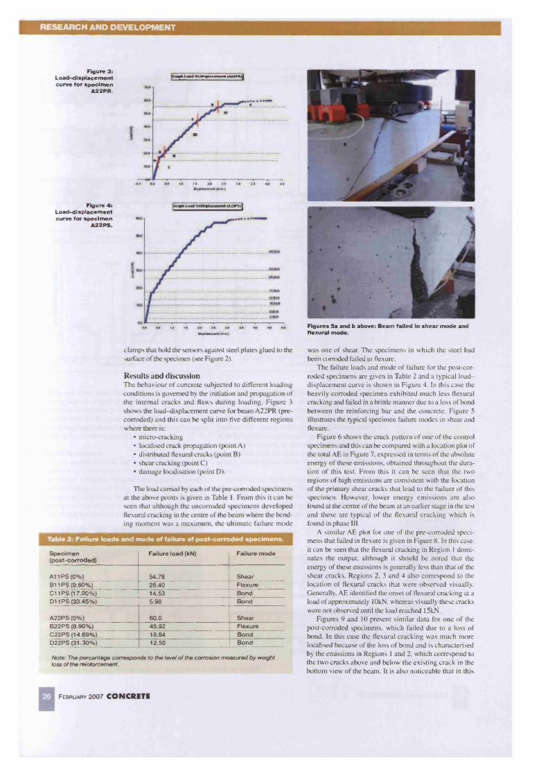
RESEARCH AND DEVELOPMENT

Figure 3: Load-disptacement curve for specimen

A22PR.

i*41 4*

Figure 4: Load-di splac em errt curve for specimen

A22PS.

u a m |

clamps that hold the sensors against steel plates glued to the surface of the specimen (see Figure 2).

Results and discussionThe behaviour of concrete subjected to different loading conditions is governed by the initiation and propagation of the internal cracks and flaws during loading. Figure 3 shows the load-displacement curve for beam A22PR (pre- corroded) and this can be split into five different regions where there is:

• micro-cracking• localised crack propagation (point A)• distributed flexural cracks (point B)• shear cracking (point C)• damage localisation (point D).

The load carried by each of the pre-corroded specimens at the above points is given in Table I. From this it can be seen that although the uncorroded specimens developed flexural cracking in the centre of the beam where the bend­ing moment was a maximum, the ultimate failure mode

Table 2: Failure loads and mode of failure of post-corroded specimens.

Specimen(post-corroded)

Failure load (kN) Failure mode

A11 PS (0%) 54.78 ShearB11 PS (9.60%) 28.40 FlexureCl 1 PS (17.00%) 14.53 BondD11 PS (33.45%) 5.98 Bond

A22PS (0%) 60.0 ShearB22PS (8.90%) 45.92 FlexureC22PS (14.69%) 18.84 BondD22PS (31.30%) 12.50 Bond

Note: The percentage corresponds to the level of the corrosion measured by weightloss of the reinforcement.

F eb r u a r y 2 0 0 7 CONCRETE

was one of shear. The specimens in which the steel had been corroded failed in flexure.

The failure loads and mode of failure for the post-cor­roded specimens are given in Table 2 and a ty pical load- displacement curve is shown in Figure 4. In this case the heavily corroded specimen exhibited much less flexural cracking and failed in a brittle manner due to a loss of bond between the reinforcing bar and the concrete. Figure 5 illustrates the typical specimen failure modes in shear and flexure.

Figure 6 shows the crack pattern of one of the control specimens and this can be compared with a location plot of the total AE in Figure 7. expressed in terms of the absolute energy of these emissions, obtained throughout the dura­tion of this test. From this it can be seen that the two regions of high emissions are consistent with the location of the primary shear cracks that lead to the failure of this specimen. However, lower energy emissions are also found at the centre of the beam at an earlier stage in the test and these are typical of the flexural cracking which is found in phase III.

A similar AE plot for one of the pre-corroded speci­mens that failed in flexure is given in Figure 8. In this case, it can be seen that the flexural cracking in Region 1 domi­nates the output, although it should be noted that the energy of these emissions is generally less than that of the shear cracks. Regions 2, 3 and 4 also correspond to the location of flexural cracks that were observed visually. Generally, AE identified the onset of flexural cracking at a load of approximately lOkN, whereas visually these cracks were not observed until the load reached 15kN.

Figures 9 and 10 present similar data for one of the post-corroded specimens, which failed due to a loss of bond. In this case the flexural cracking was much more localised because of the loss of bond and is characterised by the emissions in Regions 1 and 2, which correspond to the two cracks above and below the existing crack in the bottom view of the beam. It is also noticeable that in this

Figures 5a and b above: Beam failed in shear mode and flexural mode.

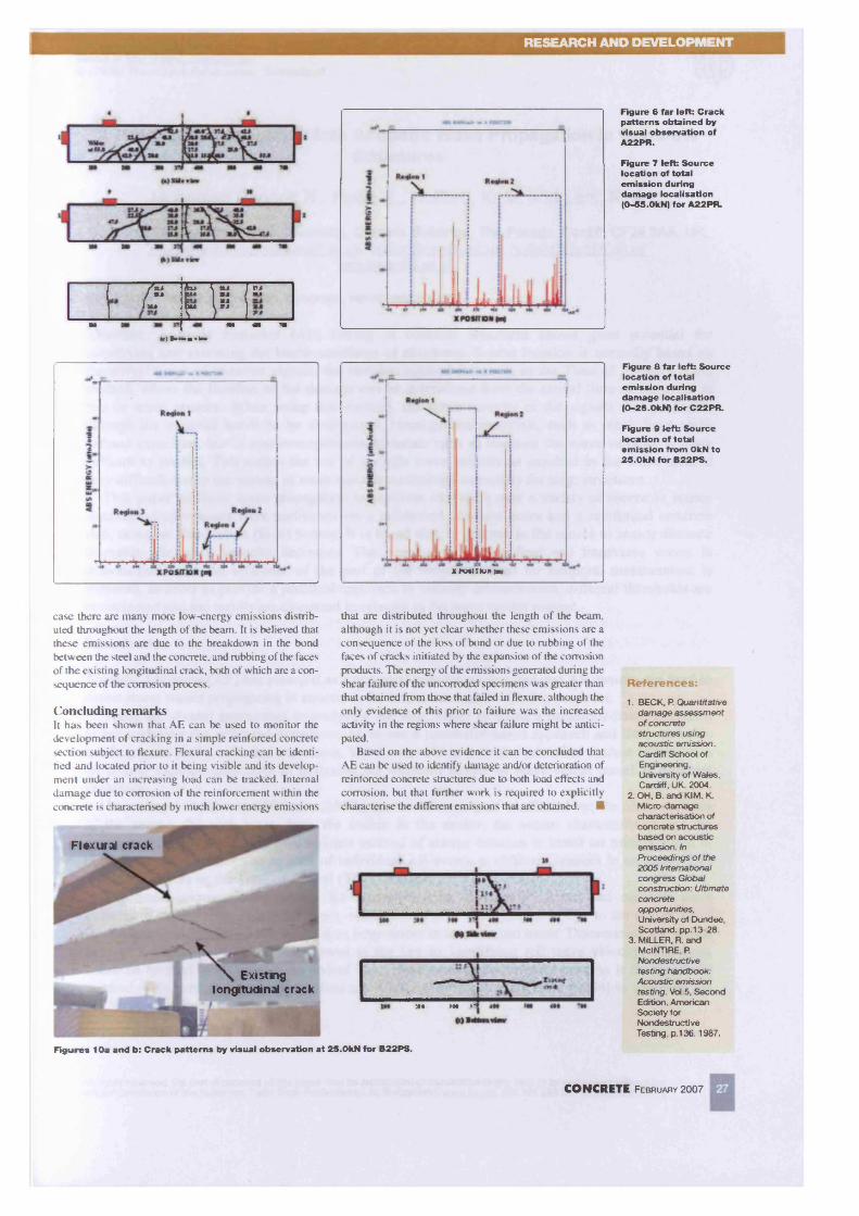
RESEARCH AND DEVELOPMENT

------------------- 7 ^ — k l f t 7 U V S/ w R i | JM » »

I * J s i#* JPS

\ P S

» • m m m

<r) B.,„m ,ym

X POSITION (Ml

Figure 6 tar left; Crack patterns obtained by visual observation of A22PR.

Figure 7 left; Source location of total emission during damage localisation (0 -55 .OkN) for A22PR.

Figure 8 far left; Source location of total emission during damage localisation (0 -25 .OkN) for C22PR.

Figure 9 left: Source location of total emission from OkN to 2 5 .OkN for B22PS.

case there are many more low-energy emissions distrib­uted throughout the length of the beam. It is believed that these emissions are due to the breakdown in the bond between the steel and the concrete, and rubbing of the faces of the existing longitudinal crack, both of which are a con­sequence of the corrosion process.

Concluding rem arksIt has been shown that AE can be used to monitor the development of cracking in a simple reinforced concrete section subject to flexure. Flexural cracking can be identi­fied and located prior to it being visible and its develop­ment under an increasing load can be tracked. Internal damage due to corrosion of the reinforcement within the concrete is characterised by much lower energy emissions

that are distributed throughout the length of the beam, although it is not yet clear whether these emissions are a consequence of the loss of bond or due to rubbing of the faces of cracks initiated by the expansion of the corrosion products. The energy of the emissions generated during the shear failure of the uncorroded specimens was greater than that obtained from those that failed in flexure, although the only evidence of this prior to failure was the increased activity in the regions where shear failure might be antici­pated.

Based on the above evidence it can be concluded that AE can be used to identify damage and/or deterioration of reinforced concrete structures due to both load effects and corrosion, but that further work is required to explicitly characterise the different emissions that are obtained. ■

!» m r

References:1. BECK, P. Quantitative

damage assessment of concrete structures using acoustic emission. Cardiff School of Engineering, University of Wales, Cardiff. UK. 2004.

2. OH, B. and KIM. K Micro-damage characterisation of concrete structures based on acoustic emission. In Proceedings of the 2005 International congress Global construction: Ultimate concrete opportunities, University of Dundee, Scotland, pp. 13-28.

3. MILLER, R. and MclNTIRE, P. Nondestructive testing handbook: Acoustic emission testing. Vol.5, Second Edition, American Society for Nondestructive Testing, p.136.1987.

Figures 10a and b: Crack patterns by visual observation at 2 5 .OkN for B22PS.

Flexural crack

\ Existing longitudinal crack

CONCRETE F e b ru a ry 2 0 0 7 Z

Advanced Materials Research Vols. 13-14 (2006) pp. 205-211 online at http://www.scientific.net © (2006) Trans Tech Publications, Switzerland

A Practical Investigation into Acoustic Wave Propagation in Concrete Structures

Muhamad Bunnori N., Pullin R., Holford, K. M. and Lark, R. J.

School of Engineering, Cardiff University, Queen’s Buildings, The Parade, Cardiff, CF24 3AA, UK,muhamadbunnorin@cardiff:ac.uk. pullinr@cardiff.ac.uk. holford@cardiff.ac.uk

lark@cardiff.ac.uk

Keywords: Acoustic Emission, concrete, wave velocity

Abstract. Acoustic Emission (AE) testing in concrete structures shows great potential for monitoring and assessing the health condition of structures. Source location is normally based on the arrival times of transient signals, the simplest method is known as the Time of Arrival (TOA) method, where the location of the damage can be determined from the arrival time of the event at two or more sensors. When using this method, the wave velocity of the signals that propagate through the material needs to be determined. Homogenous materials, such as steel, have well- defined velocities, but in non-homogeneous materials such as concrete the wave velocity is more difficult to predict. This makes the use of a single wave velocity as required in the TOA method very difficult due to the variety of wave velocities obtained, especially for large structures.

This paper explores wave propagation in concrete structures over a variety of source to sensor distances. Experiments were performed on a reinforced concrete beam and a reinforced concrete slab, using an Hsu-Nelsen (H-N) Source. It is found that, in general, as the source to sensor distance increases, the wave velocity decreases. The presence of longitudinal and transverse waves is demonstrated and the influence of the part of the waveform used for temporal measurement is explored. In order to provide a practical approach to velocity determination, different thresholds are investigated and the results are discussed in relation to the wave modes present.

Introduction

Acoustic Emission (AE) has emerged as a potential non-destructive tool and AE sensors are used to detect stress waves propagating in structures for inspection and monitoring purposes.

There are several approaches to analysing AE data, either by using a parameter-based approach or by analysing the collected waveform. Most use a parameter-based approach and little attention has been paid to the collected waveform. Yet the waveform collected can often contain information on source location especially in analysing the different modes of wave which travel at different velocities.

According to Miller and Mclntire (1987), the waveform signal is affected by; the characteristics of the source, the path taken from the source to the sensor, the sensor characteristics and the measuring system itself. The predominant method of source location is based on measurement of time difference between the arrivals of individual AE events at different sensors in an array. This method is known as the Time of Arrival (TOA) method.

The basic computational process for source location assumes a known and constant wave velocity. If the velocity used is incorrect, either due to poor assumptions or due to the triggering of the system by a different wave mode, then large errors in location can occur. Determining the arrival time of a feature in a propagating wave is the key to identifying AE wave velocity. The most common method of estimating the arrival time, used in many commercial systems is the threshold method. This method is used by Holford and Carter (1999) and Ding et al. (2004) to calculate the AE wave velocity in a structure.

All rights reserved. No part of contents erf this paper may be reproduced or transmitted in any form or by any means without the written permission erf the publisher Trans Tech Publications Ltd, Switzerland, www.ttp.net. (ID: 131.251.0.8-18/04/07,06:35:21)

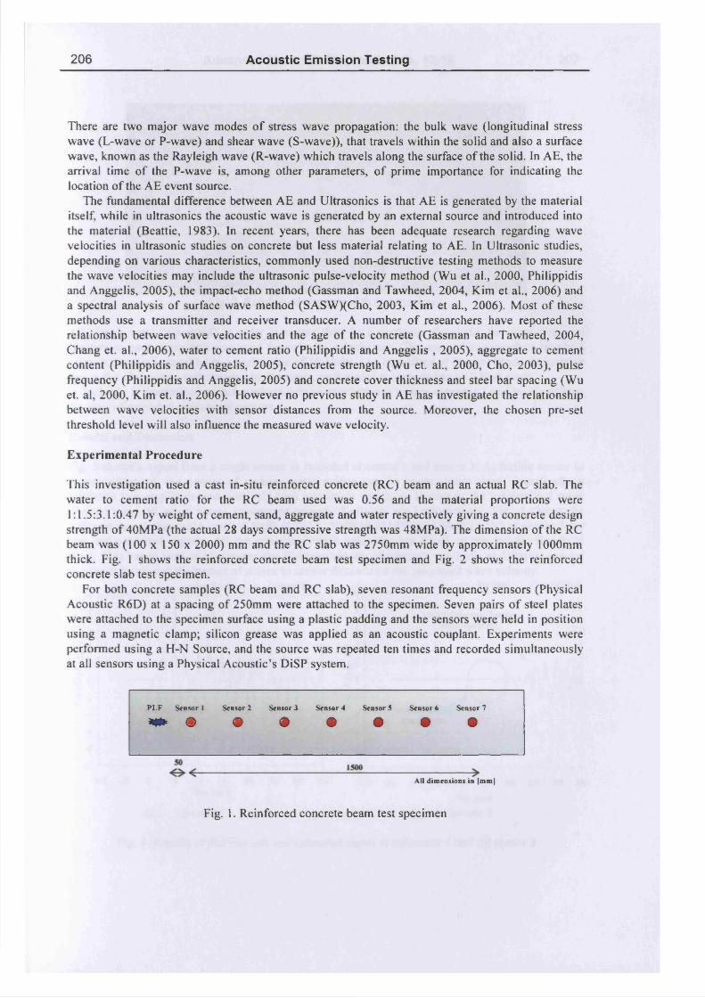
206 Acoustic Emission Testing

There are two major wave modes o f stress wave propagation: the bulk wave (longitudinal stress wave (L-wave or P-wave) and shear wave (S-wave)), that travels within the solid and also a surface wave, known as the Rayleigh wave (R-wave) which travels along the surface o f the solid. In AE, the arrival time o f the P-wave is, among other parameters, o f prime importance for indicating the location o f the AE event source.

The fundamental difference between AE and Ultrasonics is that AE is generated by the material itself, while in ultrasonics the acoustic wave is generated by an external source and introduced into the material (Beattie, 1983). In recent years, there has been adequate research regarding wave velocities in ultrasonic studies on concrete but less material relating to AE. In Ultrasonic studies, depending on various characteristics, commonly used non-destructive testing methods to measure the wave velocities may include the ultrasonic pulse-velocity method (Wu et al., 2000, Philippidis and Anggelis, 2005), the impact-echo method (Gassman and Tawheed, 2004, Kim et al., 2006) and a spectral analysis o f surface wave method (SASWXCho, 2003, Kim et al., 2006). Most o f these methods use a transmitter and receiver transducer. A number o f researchers have reported the relationship between wave velocities and the age o f the concrete (Gassman and Tawheed, 2004, Chang et. al., 2006), water to cement ratio (Philippidis and Anggelis , 2005), aggregate to cement content (Philippidis and Anggelis, 2005), concrete strength (Wu et. al., 2000, Cho, 2003), pulse frequency (Philippidis and Anggelis, 2005) and concrete cover thickness and steel bar spacing (Wu et. al, 2000, Kim et. al., 2006). However no previous study in AE has investigated the relationship between wave velocities with sensor distances from the source. Moreover, the chosen pre-set threshold level w ill also influence the measured wave velocity.

Experimental Procedure

This investigation used a cast in-situ reinforced concrete (RC) beam and an actual RC slab. The water to cement ratio for the RC beam used was 0.56 and the material proportions were 1:1.5:3.1:0.47 by weight o f cement, sand, aggregate and water respectively giving a concrete design strength o f 40MPa (the actual 28 days compressive strength was 48MPa). The dimension o f the RC beam was (100 x 150 x 2000) mm and the RC slab was 2750mm wide by approximately 1000mm thick. Fig. 1 shows the reinforced concrete beam test specimen and Fig. 2 shows the reinforced concrete slab test specimen.

For both concrete samples (RC beam and RC slab), seven resonant frequency sensors (Physical Acoustic R6D) at a spacing o f 250mm were attached to the specimen. Seven pairs o f steel plates were attached to the specimen surface using a plastic padding and the sensors were held in position using a magnetic clamp; silicon grease was applied as an acoustic couplant. Experiments were performed using a H-N Source, and the source was repeated ten times and recorded simultaneously at all sensors using a Physical Acoustic’s DiSP system.

PLF Sensor 1 Sensor 2 Sensor 3 Sensor 4 Sensor S Sensor 6 Sensor 7

* * © Q © © © © O

—All dimensions in |mm]

Fig. 1. Reinforced concrete beam test specimen

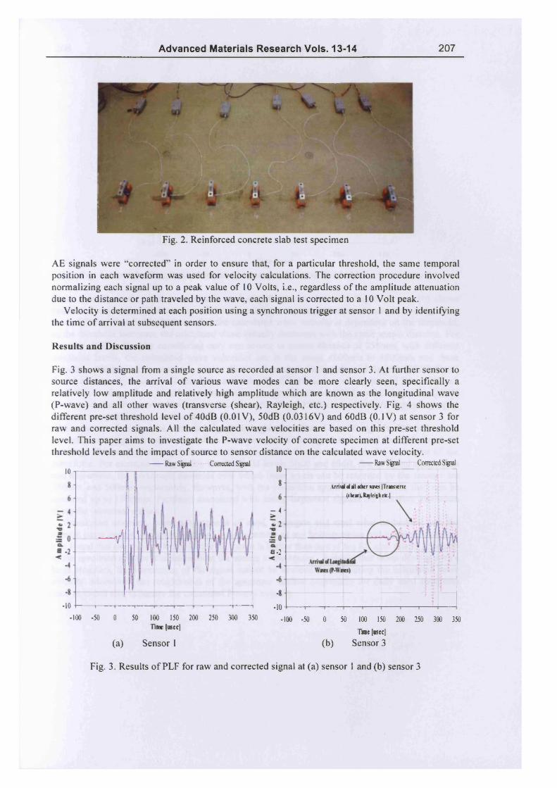
Advanced Materials Research Vols. 13-14 207

Fig. 2. Reinforced concrete slab test specimen

AE signals were “ corrected” in order to ensure that, for a particular threshold, the same temporal position in each waveform was used for velocity calculations. The correction procedure involved normalizing each signal up to a peak value o f 10 Volts, i.e., regardless o f the amplitude attenuation due to the distance or path traveled by the wave, each signal is corrected to a 10 Volt peak.

Velocity is determined at each position using a synchronous trigger at sensor 1 and by identifying the time o f arrival at subsequent sensors.

Results and Discussion

Fig. 3 shows a signal from a single source as recorded at sensor 1 and sensor 3. A t further sensor to source distances, the arrival o f various wave modes can be more clearly seen, specifically a relatively low amplitude and relatively high amplitude which are known as the longitudinal wave (P-wave) and all other waves (transverse (shear), Rayleigh, etc.) respectively. Fig. 4 shows the different pre-set threshold level o f 40dB (0.0IV ), 50dB (0.0316V) and 60dB (0.1V) at sensor 3 for raw and corrected signals. A ll the calculated wave velocities are based on this pre-set threshold level. This paper aims to investigate the P-wave velocity o f concrete specimen at different pre-set threshold levels and the impact o f source to sensor distance on the calculated wave velocity.

Raw Sgnal Corrected Signal10

— y

•10-100 -50 0 50 100 150 200 250 300 350

Time |usec)

(a) Sensor 1

Raw Signal Corrected Signal

Arriwl of ill other «k i [Trnswnt (shears Raleigh efc.|

- 4

B-2 ■

-10-100 -50 0 50 100 150 200 250 300 350

(b)Tune |usec]

Sensor 3

Fig. 3. Results o f PLF for raw and corrected signal at (a) sensor 1 and (b) sensor 3

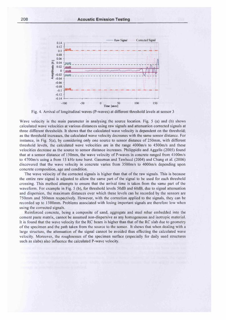
208 Acoustic Emission Testing

0.14 0.12 0.1

0.08 _ 0.06 E 0.04 ■3 0.02 I 0I -0.02< -0.04

-0.06 -0.08

- 0.1 - 0.12 -0.14

-100 -50 0 50 100 150Time [usee]

Fig. 4. Arrival o f longitudinal waves (P-waves) at different threshold levels at sensor 3

Wave velocity is the main parameter in analysing the source location. Fig. 5 (a) and (b) shows calculated wave velocities at various distances using raw signals and attenuation corrected signals at three different thresholds. It shows that the calculated wave velocity is dependent on the threshold; as the threshold increases, the calculated wave velocity decreases with the same sensor distance. For instance, in Fig. 5(a), by considering only one source to sensor distance o f 250mm, with different threshold levels, the calculated wave velocities are in the range 4000m/s to 4500m/s and these velocities decrease as the source to sensor distance increases. Philippidis and Aggelis (2005) found that at a sensor distance o f 150mm, the wave velocity o f P-waves in concrete ranged from 4 lOOm/s to 4700m/s using a from 15 kHz tone burst. Gassman and Tawheed (2004) and Chang et al. (2006) discovered that the wave velocity in concrete varies from 3500m/s to 4000m/s depending upon concrete composition, age and condition.

The wave velocity o f the corrected signals is higher than that o f the raw signals. This is because the entire raw signal is adjusted to allow the same part o f the signal to be used for each threshold crossing. This method attempts to ensure that the arrival time is taken from the same part o f the waveform. For example in Fig. 5 (b), for threshold levels 50dB and 60dB, due to signal attenuation and dispersion, the maximum distances over which these levels can be recorded by the sensors are 750mm and 500mm respectively. However, w ith the correction applied to the signals, they can be recorded up to 1500mm. Problems associated with losing important signals are therefore low when using the corrected signals.

Reinforced concrete, being a composite o f sand, aggregate and steel rebar embedded into the cement paste matrix, cannot be assumed non-dispersive as any homogeneous and isotropic material. It is found that the wave velocity for the RC beam is higher than that o f the RC slab due to geometry o f the specimen and the path taken from the source to the sensor. It shows that when dealing with a large structure, the attenuation o f the signal cannot be avoided thus effecting the calculated wave velocity. Moreover, the roughnesses o f the specimen surface (especially for daily used structures such as slabs) also influence the calculated P-wave velocity.

Raw S ignal Corrected S ignal

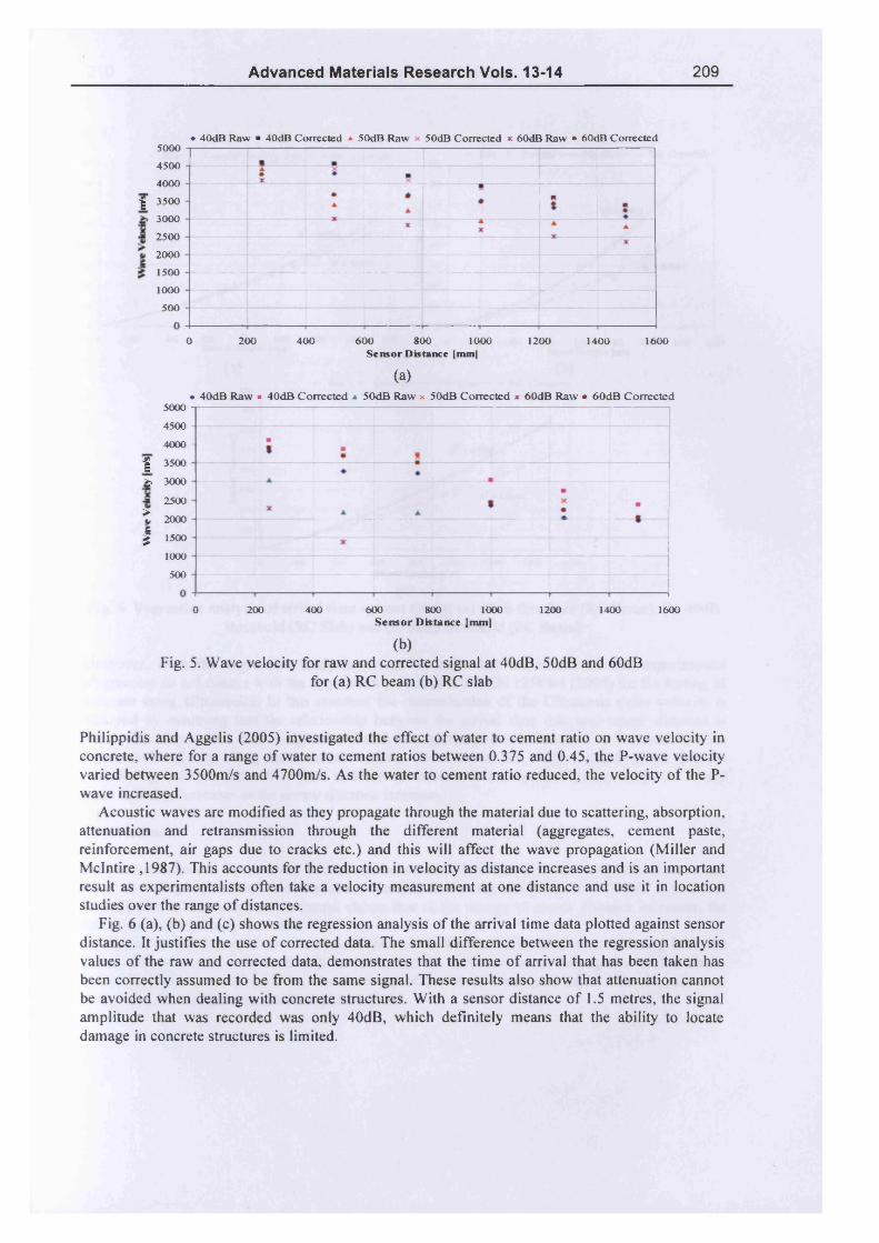
Advanced Materials Research Vols. 13-14 209

♦ 40dB Raw ■ 40dB Corrected * 50dB Raw 50dB Corrected * 60dB Raw • 60dB Corrected5000

4500

4000

| 3500

3000

2500

20001500

1000500

0 200 400 600 800 1000 1200 1400 1600Sensor Distance |mm|

(a)♦ 40dB Raw • 40dB Corrected * 50dB Raw x 50dB Corrected * 60dB Raw • 60dB Corrected

5000

4500 -

4000 -

| 3500

£ 3000

■* 2500

t 2000| 1500

1000500

0 200 400 600 800 1000 1200 1400 1600S en so r Distance [mm]

(b)Fig. 5. Wave velocity for raw and corrected signal at 40dB, 50dB and 60dB

for (a) RC beam (b) RC slab

Philippidis and Aggelis (2005) investigated the effect o f water to cement ratio on wave velocity in concrete, where for a range o f water to cement ratios between 0.375 and 0.45, the P-wave velocity varied between 3500m/s and 4700m/s. As the water to cement ratio reduced, the velocity o f the P- wave increased.

Acoustic waves are modified as they propagate through the material due to scattering, absorption, attenuation and retransmission through the different material (aggregates, cement paste, reinforcement, air gaps due to cracks etc.) and this w ill affect the wave propagation (M ille r and Mclntire ,1987). This accounts for the reduction in velocity as distance increases and is an important result as experimentalists often take a velocity measurement at one distance and use it in location studies over the range o f distances.

Fig. 6 (a), (b) and (c) shows the regression analysis o f the arrival time data plotted against sensor distance. It justifies the use o f corrected data. The small difference between the regression analysis values o f the raw and corrected data, demonstrates that the time o f arrival that has been taken has been correctly assumed to be from the same signal. These results also show that attenuation cannot be avoided when dealing with concrete structures. With a sensor distance o f 1.5 metres, the signal amplitude that was recorded was only 40dB, which definitely means that the ability to locate damage in concrete structures is limited.

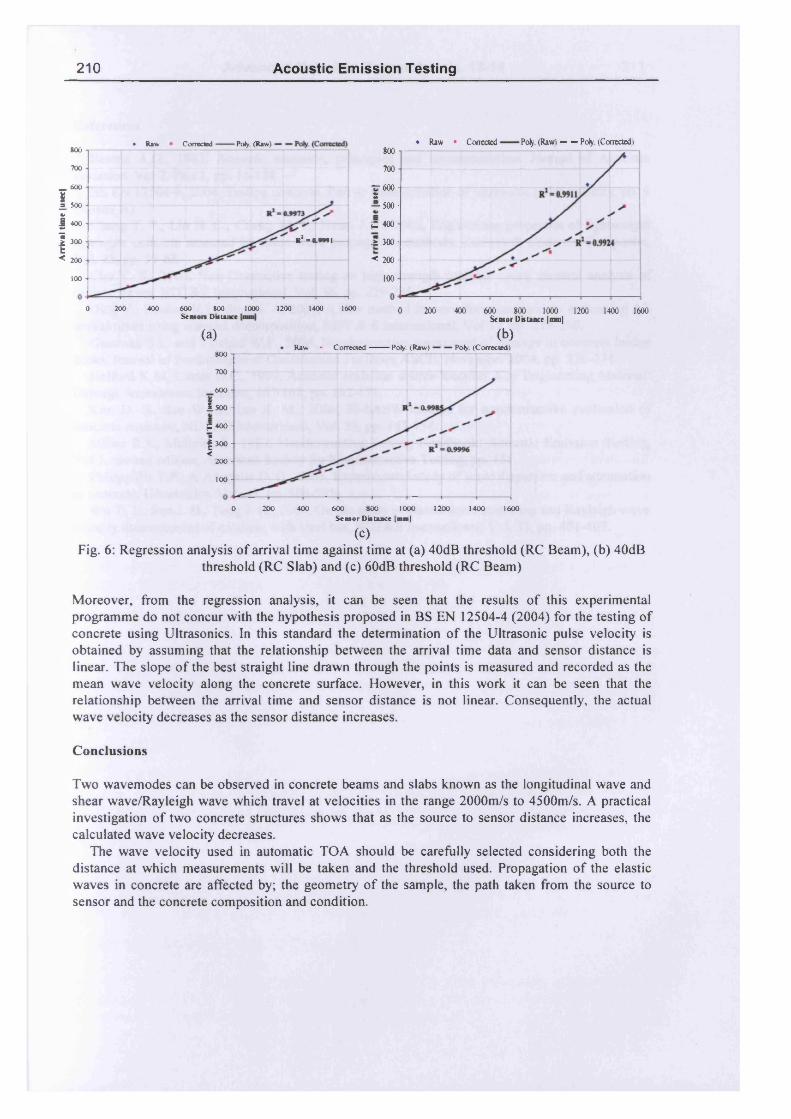
Arr

ival

tim

e |u

*ec|

210 Acoustic Emission Testing

Poly (Raw) Poty (Corrected)♦ Raw • Corrected• Raw Corrected Poty (Raw)800 800

700 700

— 600 ■ s— 500 -

600

500

C 400400

R: =0.9941 ± 300-300

< 200 -200100100

16000 200 400 600Sea

800D ntai

1000 1200 1400 0 200 400 600 800 1000 1200 1400 1600Sensor Distance |mm|

(a) (b)• Raw ■ C orrected Poty (Raw) Poty (Corrected)

800

700 -

600 -

1500 - -O il

P 400 ■ ■| 300 - <200 -

100 -

0 200 400 600 800 1000 1200 1400 1600Sensor D istance [mm]

(C)Fig. 6: Regression analysis o f arrival time against time at (a) 40dB threshold (RC Beam), (b) 40dB

threshold (RC Slab) and (c) 60dB threshold (RC Beam)

Moreover, from the regression analysis, it can be seen that the results o f this experimental programme do not concur with the hypothesis proposed in BS EN 12504-4 (2004) for the testing o f concrete using Ultrasonics. In this standard the determination o f the Ultrasonic pulse velocity is obtained by assuming that the relationship between the arrival time data and sensor distance is linear. The slope o f the best straight line drawn through the points is measured and recorded as the mean wave velocity along the concrete surface. However, in this work it can be seen that the relationship between the arrival time and sensor distance is not linear. Consequently, the actual wave velocity decreases as the sensor distance increases.

Conclusions

Two wavemodes can be observed in concrete beams and slabs known as the longitudinal wave and shear wave/Rayleigh wave which travel at velocities in the range 2000m/s to 4500m/s. A practical investigation o f two concrete structures shows that as the source to sensor distance increases, the calculated wave velocity decreases.

The wave velocity used in automatic TOA should be carefully selected considering both the distance at which measurements w ill be taken and the threshold used. Propagation o f the elastic waves in concrete are affected by; the geometry o f the sample, the path taken from the source to sensor and the concrete composition and condition.

Advanced Materials Research Vols. 13-14 211

References

Beattie A.G., 1983, Acoustic emission, principles and instrumentation. Journal of Acoustic Emission, Vol 2, Part 1, pp. 15-128.

BS EN 12504-4, 2004, Testing concrete, Part 4: Determination of ultrasonic pulse velocity, pp. 9 (Annex A).

Chang T. P., Lin H. C., Chang W. T., Hsiao J. F., 2006, Engineering properties of lightweight aggregate concrete assessed by stress wave propagation methods, Cement & Concrete Composite, Vol. 28, pp. 57-68.

Cho Y. S., 2003, Non-Destructive testing on high strength concrete using spectral analysis ofsurface waves, NDT&E International, Vol. 36, pp. 229-235.

Ding Y., Reuben R.L., Steel J. A, 2004, A new method for waveform analysis for estimating AE arrival times using wavelet decomposition, NDT & E International, Vol 37, pp. 279-290.

Gassman S.L. and Tawhed W.F., 2004, Nondestructive assessment of damage in concrete bridge decks, Journal of Performance of Construction Facilities ASCE, November 2004, pp. 220-231.

Holford K.M, Carter D.C., 1999, Acoustic emission source location. Key Engineering Material: Damage Assessment Structure, 167-168, pp. 162-171.

Kim D. S., Seo W. S., Lee K. M., 2006, IE-SASW method for nondestructive evaluation ofconcrete structure, NDT&E International, Vol. 39, pp. 143-154.

Miller R.K, Mclntire P., 1987, Nondestructive Testing Handbook: Acoustic Emission Testing, Vol 5, second edition, American Society for Nondestructive Testing, pp. 151.

Philippidis T.P., A Anggelis D. G., 2005, Experimental study of wave dispersion and attenuation in concrete, Ultrasonics, Vol. 43, pp. 584-595.

Wu T. T., Sun J. H., Tong J. H., 2000, On the study of elastic wave scattering and Rayleigh wave velocity measurement of concrete with steel bar, NDT&E International, Vol. 33, pp. 401-407.

The AppMcaOon o f Acoustic Emisston Monitoring to the Assessment Concrete Structures Suffering from

Concrete Communication Conference, University CoMege London, 5-9 September2006

THE APPLICATION OF ACOUSTIC EMISSION MONITORING TO THE ASSESSMENT CONCRETE STRUCTURES SUFFERING FROM

REINFORCEMENT CORROSION

N. Muhamad Bunnori, K.M. Holford & R.J. LarkCardiff School of Engineering, Cardiff University

INTRODUCTION

This paper describes an experimental programme to investigate the behaviour of reinforced concrete structures subject to deterioration as a consequence of reinforcement corrosion using acoustic emission monitoring. Two types of test specimen were used: pre-corroded (PR) specimen in which the cross sectional area of the bar was reduced but, as they were cleaned before being cast into the concrete, the integrity of the concrete itself and the bond between the steel and the concrete were unaffected by the corrosion; and post-corroded (PS) specimen in which the corrosion products were developed within the specimen. All specimens were tested in four-point bending monitored using an Acoustic Emission (AE) sensor system.

A parameter-based approach was used to analyse the data. This approach evaluates relative AE activity based on the measurement of parameters such as hits, amplitudes and absolute energy. This method of analysis has been shown to be sensitive to the initiation and growth of cracks within both homogeneous and composite materials and structures (Oh and Kim (2005), Beck P., (2004)). It is also shown that the application of a linear location, Time of Arrival (TOA) method can be used to determine the location of damage in an area between an array of sensors and to monitor the progression of the resultant cracking.

MATERIALS AND SPECIMEN PREPARATION

In this programme the specimen were cast using a concrete mix with a target strength of 40MPa using a water to cement ratio of 0.56 and with material proportions of 1:2:2.5 by weight of cement, sand and aggregate. The specimen were 100mm x 150mm x 750mm with a single, high-yield 12mm diameter reinforcing bar placed at the centre of the width of the section approximately 50mm above the soffit of the beam (i.e. a cover of 44mm).

For the pre-corroded specimen, lengths of the 12mm diameter reinforcement bar were corroded to three levels of damage using an anodic current before the concrete was cast. In the post-corroded specimen, a middle section of the reinforced concrete beams were encased in an acrylic tank. This section was then immersed in a 5% NaCI solution as shown in Figure 1.

The post-corroded specimen exhibited longitudinal cracking on the bottom face of the beams along the line of the reinforcement. This was clearly due to the formation of the extensive corrosion products that were developed inside the concrete.

ACOUSTIC EMISSION (AE) TECHNIQUE

Acoustic emission testing is based on the fact that solid materials emit sound or acoustic emission in the material itself when they are mechanically or thermally stressed to the point where deformation or fracture occurs.

The AppScation o f Acoustic Emission Monitoring to the Assessment Concrete Structures Suffering fromReinforcement Corrosion

Concrete Communication Conference, University CoMogc London, S-9 Snpfnmhnr2006

Location can be defined as the determination of the spatial position of an acoustic emission source from arrival time measurements using an array of sensors (Miller and Mclntire, 1987). In this case a linear location technique was used since the position of the source is known to be somewhere along a straight line between a pair of transducers attached to the beam. Using a time of arrival (TOA) approach, a difference in the measured arrival times of the emissions from a source at any two transducers uniquely determines the location of this source. The accuracy of the source location depends on the wave velocity calculation, time difference measurements and good sensor positions (Beck P., 2004). In this case the acoustic emission source is the cracking and degradation of the concrete resulting from the application of the load but influenced by the level of corrosion that is present The sensors for measuring the acoustic emission were attached to the concrete using magnetic clamps that hold the sensors against steel plates glued to the surface of the specimen (Figure 2).

RESULTS AND DISSCUSSION

The behaviour of concrete subjected to different loading conditions is governed by the initiation and propagation of the internal cracks and flaws during loading. Figure 3 shows the load deflection curve for the beam A22PR (Pre-corroded) and this can be split into five different regions where there is:

I Micro-crackingII Localised crack propagation (Point A)

III Distributed flexural cracks (Point B)IV Shear cracking (Point C)V Damage localization (Point D)

The load carried by each of the pre-corroded specimen at the above points is given in Table 1. From this it can be see that although the un-corroded specimen developed flexural cracking in the centre of the beam where the bending moment was a maximum, the ultimate failure mode was one of shear. The specimens in which the steel had been corroded failed in flexure.

The failure loads and mode of failure for the post-corroded specimen are given in Table 2 and a typical load deflection curve is shown in Figure 4. In this case the heavily corroded specimen exhibited much less flexural cracking and failed in a brittle manner due to a loss of bond between the reinforcing bar and the concrete. Figure 5 illustrates the typical specimen failure modes in shear and flexure.

In Figure 6 the crack pattern of one of the control specimen is given and this can be compared with a location plot of a the total AE in Figure 7, expressed in terms of the absolute energy of these emissions, obtained throughout the duration of this test. From this it can be seen that the two regions of high emissions are consistent with the location of the primary shear cracks that lead to the failure of this specimen. However, lower energy emissions are also found at the centre of the beam at an earlier stage in the test and these are typical of the flexural cracking which is found in phase III. A similar AE plot for one of the pre-corroded specimen that failed in flexure is given in Figure 8. In this case it can be seen that the flexural cracking in region 1 dominates the output, although it should be noted that the energy of these emissions is generally less than that of the shear cracks. Regions 2, 3 and 4 also correspond to the location of flexural cracks that were observed visually. Generally AE identified

The AppBcation o f Acoustic Emission Monitoring to the Assessment Concrete Structures Suffering fromReinforcement Corrosion

Concrete Communication Conference, University CoMogc London, 5-6 September2006

the onset of flexural cracking at a load of approximately 10kN, whereas visually these cracks were not observed until the load reached 15kN.

Figures 9 and 10 present similar data for one of the post-corroded specimen, which failed due to a loss of bond. In this case the flexural cracking was much more localised because of the loss of bond and is characterised by the emissions in regions 1 and 2, which correspond to the two cracks above and below the existing crack in the bottom view of the beam. It is also noticeable that in this case there are many more low energy emissions distributed throughout the length of the beam. It is believed that these emissions are due to the breakdown in the bond between the steel and the concrete and rubbing of the faces of the existing longitudinal crack both of which are a consequence of the corrosion process.

CONCLUSIONS

It has been shown that AE can be used to monitor the development of cracking in a simple reinforced concrete section subject to flexure. Flexural cracking can be identified and located prior to it being visible and its development under an increasing load can be tracked. Internal damage due to corrosion of the reinforcing bar within the concrete is characterised by much lower energy emissions that are distributed throughout the length of the beam, although it is not yet dear whether these emissions are a consequence of the loss of bond or due to rubbing of the faces of cracks initiated by the expansion of the corrosion products. The energy of the emissions generated during the shear failure of the un-corroded spedmens was greater than that obtained from those that failed in flexure, although the only evidence of this prior to failure was the increased activity in the regions where shear failure might be antidpated.

Based on the above evidence it can be conduded that AE can be used to identify damage and/or deterioration of reinforced concrete strudures due to both load effects and corrosion, but that further work is required to explidtly characterise the different emissions that are obtained.

REFERENCES

1. Beck P., 2004. Quantitative Damage Assessment of Concrete Structures Using Acoustic Emission, Cardiff School of Engineering. University of Wales, Cardiff. UK

2. Miller R.K, Mclntire P., 1987. Nondestructive Testing Handbook: Acoustic Emission Testing, Volume 5, Second Edition, American Society for Nondestructive Testing, pp. 136.

3. Oh B. H. and Kim K. S., 2005, Micro-Damage Characterisation of Concrete Structures Based on Acoustic Emission. Proceeding of the International Conference: 2005 International Congress Global Construction: Ultimate Concrete Opportunities, University of Dundee, Scotland, UK, pp. 13-28

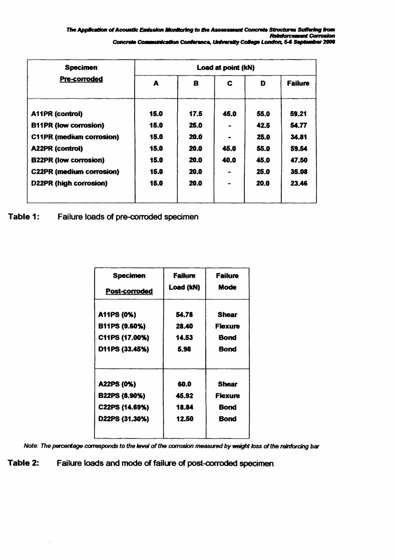
The AppMcaUon o f Acoustic Emission MonUoring to ffte Assessment Concrete Structures Suffering from

Concrete ConmunteaHon Conference, University CoMogo London, 5-6 Soptombor200S

SpecimenPre-corroded

Load at point (kN)

A B C D Failure

A11PR (control) 15.0 17.5 45.0 55.0 59.21B11PR (low corrosion) 15.0 25.0 - 42.5 54.77C11PR (medium corrosion) 15.0 20.0 - 25.0 34.81A22PR (control) 15.0 20.0 45.0 55.0 59.54B22PR (low corrosion) 15.0 20.0 40.0 45.0 47.50C22PR (medium corrosion) 15.0 20.0 - 25.0 35.08D22PR (high corrosion) 15.0 20.0 20.0 23.46

Table 1: Failure loads of pre-corroded specimen

Specimen Failure Failure

Post-corroded Load (kN) Mode

A11PS (0%) 54.78 ShearB11PS (9.60%) 28.40 FlexureC11PS (17.00%) 14.53 BondD11PS (33.45%) 5.98 Bond

A22PS (0%) 60.0 ShearB22PS (8.90%) 45.92 FlexureC22PS (14.69%) 18.84 BondD22PS (31.30%) 12.50 Bond

Note: The percentage corresponds to the level of the corrosion measured by weight loss of the reinforcing bar

Table 2: Failure loads and mode of failure of post-corroded specimen

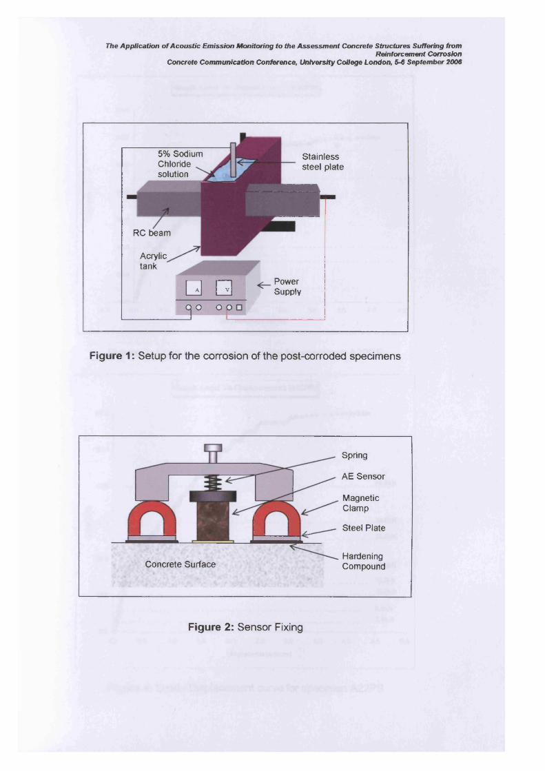
The Application of Acoustic Emission Monitoring to the Assessment Concrete Structures Suffering fromReinforcement Corrosion

Concrete Communication Conference, University College London, 5-6 September 2006

5% Sodium Chloride solution

RC beam

Acrylic tank

Stainless steel plate

Q] Dj o o p

PowerSupply

Figure 1: Setup for the corrosion of the post-corroded specimens

Spring

AE Sensor

MagneticClamp

Steel Plate

HardeningCompoundConcrete Surface

Figure 2: Sensor Fixing

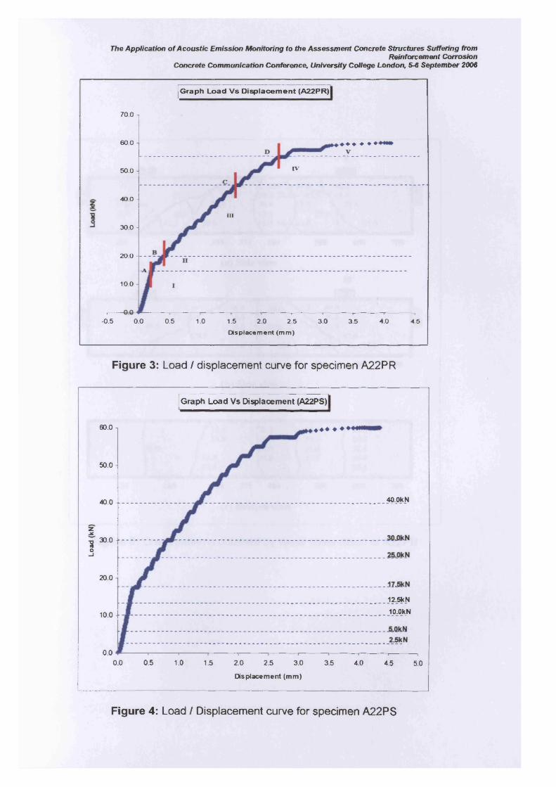
The Application of Acoustic Emission Monitoring to the Assessment Concrete Structures Suffering fromReinforcement Corrosion

Concrete Communication Conference, University College London, 5-6 September 2006

Graph Load Vs Displacement (A22PR)

70.0 -|

60.0

IV50.0

40.0 -

III

30.0

20.0 - - -

-A

10.0

-0.5 0.0 0.5 1.0 1.5 2.0 2.5 3.0 3.5 4.0 4.5

Displacement (mm)

Figure 3: Load / displacement curve for specimen A22PR

Graph Load Vs Displacement (A22PS)

60.0 -

50.0

40. OkN40.0

2-x30.0TJ fI O

-J

20.0

12.5kN

iO.OkN10.0

0.00.0 0.5 1.0 2.0 2.5 3.0 3.5 4.01.5 4.5 5.0

Displacem ent (m m )

Figure 4: Load / Displacement curve for specimen A22PS

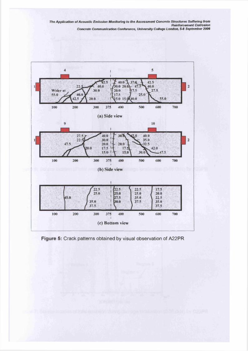
The Application of Acoustic Emission Monitoring to the Assessment Concrete Structures Suffering fromReinforcement Corrosion

Concrete Communication Conference, University College London, 5-6 September 2006

J 2.5 4 0 .0 ^ : 37>O t 42.51 2 2 £ _ 40.0 /3 0 .0 20.0X - 4 7 ^ S 4 0 .0— W id er at / 30.0 T 2 0 .0 U7.5 ^v 27-5

55 .° r 400i T17.5 1 250142 5 / 1 i 20.0 \15 .0 15.0m o .o P V 5 5 . 0

]100 200 300 375 400

(a) Side view

500 600

10

700

40.035.0 -32.5

27.522.5]

40.030.020.0 17.5 15.0

30j

147.5 20.0

17.:o.o 42.030.0 47.5

200 300 375 400 500 600 700100

(b) Side view

22.525.0

22.5 17.5 20.022.5 35.037.5

22.525.035.037.535.0

37.5

100 200 300 375 400 500 700600

(c) Bottom view

Figure 5: Crack patterns obtained by visual observation of A22PR

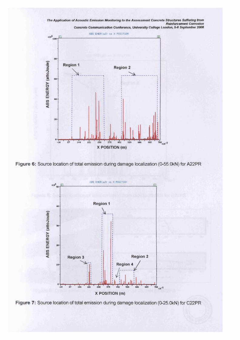
The Application of Acoustic Emission Monitoring to the Assessment Concrete Structures Suffering fromReinforcement Corrosion

Concrete Communication Conference, University College London, 5-6 September 2006

ABS ENER<aJ> vs X POSITION

<V

|OOHUizUiC/5CD<

26-

m

Region 1

\Region 2

-ie - r 1144

■*r221 298

l

.uuLu.LU375 452 529 666 683

X POSITION (m)

Figure 6: Source location of total emission during damage localization (0-55.0kN) for A22PR

ABS ENERCaJ) vs X POSITION

a>o0

1 >- O OH UJzUJCOffl<

m

Region 1

Region 3 Region 2

/Region 4

■id -

X POSITION (m)

Figure 7: Source location of total emission during damage localization (0-25.0kN) for C22PR

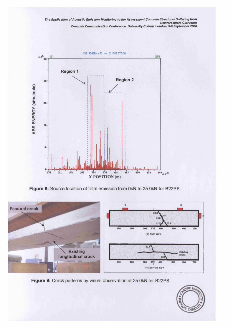
The Application of Acoustic Emission Monitoring to the Assessment Concrete Structures Suffering fromReinforcement Corrosion

Concrete Communication Conference, University College London, 5-6 September 2006

ABS ENER<aJ> vs X POSITION

Region 1

Region 2

3O“ 5O*3<0

O£LUzUJ<0GO<

1 0 -

- r —r-211 252 203 334 375 416

X POSITION (m)457 539 588

*10

Figure 8: Source location of total emission from OkN to 25.0kN for B22PS

Flexural crack

\ Existing longitudinal crack

(c) Bottom view

Figure 9: Crack patterns by visual observation at 25.OkN for B22PS