i

JournalofAcousticEmission,Volume33,2016

Contents

i–iii Contents,JAE,vol.33,2016I–X EWGAE2016,Foreword,Contents,AuthorsIndex

33-S1 StasysV.AUGUTIS,BorisMURAVIN,EdgarasVAŠTAKAS,APPLICATIONOFWAVEGUIDESFORTHECALIBRATIONOFACOUSTICEMISSIONTRANSDUCERS S1-S8

33-S9 IreneuszBARAN,IgorLYASOTA,KrzysztofSKROK,ACOUSTICEMISSIONTESTINGOFUNDERGROUNDPIPELINESOFCRUDEOILOFFUELSTORAGEDEPOTS,S9-S20

33-S21 GabrielBIRCK,IgnacioITURRIOZ,AVERSIONOFTHEDISCRETEELEMENTMETHODINTHESIMULATIONOFTHEACOUSTICEMISSIONTESTING,S21-S30

33-S31 AntoineBONIFACE,ZoubirM.SBARTAÏ,JacquelineSALIBA,NaryRANAIVOMANANA,COMPARISONOFLOCALIZATIONSTRATEGIESOFDAMAGEINCONCRETEBYACOUSTICEMISSION,S31-S39

33-S41 AndreasJ.BRUNNER,CORRELATIONBETWEENACOUSTICEMISSIONSIGNALSANDDELAMINATIONSINCARBONFIBER-REINFORCEDPOLYMER-MATRIXCOMPOSITES:ANEWLOOKATMODEIFRACTURETESTDATA,S41-S49

33-S51 LuigiCALABRESE,MassimilianoGALEANO,EdoardoPROVERBIO,DomenicoDIPIETRO,AngeloDONATO,FilippoCAPPUCCINI,ADVANCEDSIGNALANALYSISAPPLIEDTODISCRIMINATEDIFFERENTCORROSIONFORMSBYACOUSTICEMISSIONDATA,S51-S60

33-S61 LuigiCALABRESE,MassimilianoGALEANO,EdoardoPROVERBIO,DomenicoDIPIETRO,AngeloDONATO,MONITORINGOFHYDROGENASSISTEDSCCONMARTENSITICSTAINLESSSTEELBYACOUSTICEMISSIONTECHNIQUE,S61-S69

33-S71 ManabuENOKI,YukiMUTO,TakayukiSHIRAIWA,EVALUATIONOFDEFORMATIONBEHAVIORINLPSO-MAGNESIUMALLOYSBYAECLUSTERINGANDINVERSEANALYSIS,S71-S76

33-S77 SebastianO.GADE,PhilippPOTSTADA,BenjaminBALACA,MarkusG.R.SAUSE,MEASUREMENTOFELECTROMAGNETICEMISSIONASATOOLTOSTUDYFRACTUREPROCESSESOFCARBONFIBREREINFORCEDPOLYMERS,S77-S86

33-S87 ThomasGUENTHER,AndreasKROLL,LOCALIZATIONOFCOMPRESSEDAIRLEAKSININDUSTRIALENVIRONMENTSUSINGSERVICEROBOTSWITHULTRASONICMICROPHONES,S87-S96

33-S97 MarvinA.HAMSTAD,MODELEDTRANSVERSESURFACEAESIGNALSFROMBURIEDDIPOLESOURCESINAPOLYMERROD,S97-S106

33-S107 DmitryCHERNOV,SergeyELIZAROV,VeraBARAT,IgorVASILYEV,FEATURESOFTHEAETESTINGOFEQUIPMENTONOPERATINGMODE,S107-S116

ii

33-S109 KaitaITO,ManabuENOKI,HIGHSENSITIVITYDETECTIONOFAEEVENTSINNOISYENVIRONMENTUSINGSTREAMRECORDINGANDPARALLELCOMPUTATION,S117-S122

33-S123 DoyunJUNG,YoshihiroMIZUTANI,AkiraTDOROKI,YoshiroSUZUKI,CHANGEINB-VALUEBYAEPROPAGATIONLENGTHINCFRP,S123-S129.

33-S131 YoshikazuKOBAYASHI,TomokiSHIOTANI,TWO-DIMENSIONALQ-VALUEAE-TOMOGRAPHYANDITSVERIFICATIONONNUMERICALINVESITIGATIONS,S131-S140

33-S141 VendulaKRATOCHVILOVA,FrantisekVLASIC,PavelMAZAL,STUDYOFFATIGUEPROCESSESOFSELECTIVELASERMELTINGANDCONVENTIONALPRODUCEDMATERIALS,S141-S148

33-S149 GeraldLACKNER,PeterTSCHELIESNIG,ACOUSTICEMISSIONTESTINGONLPGTANKS–DEFECTDETECTIONCASESTUDIES,S149-S155

33-S157 ZhidongLIU,HongqiangLIAO,YuanLIU,THETIMESEQUENCECHARACTERISTICSANDLOCATIONMETHODOFAESOURCEINDUCEDBYDEBRISCLOUD,S157-S164

33-S165 TomášLOKAJÍČEK,RichardPŘIKRYL,ŠárkaŠACHLOVÁ,AnetaKUCHAŘOVÁ,ALKALISILICAREACTIVITYSTUDYOFACCELERATEDMORTARBARBYMEANSOFACOUSTICEMISSIONANDULTRASONICSOUNDING,S165-S172

33-S173 ShaLUO,AndreaDIAMBRA,ErdinIBRAIM,APPLICATIONOFACOUSTICEMISSIONONCRUSHINGMONITORINGOFINDIVIDUALSOILPARTICLESINUNIAXIALCOMPRESSIONTEST,S173-S181

33-S183 PavelMAZAL,HoussamMAHMOUD,PetrDOSTAL,MichalCERNÝ,MichalSUSTR,JaroslavZACAL,COOPERATIONOFMENDELUNIVERSITYANDBRNOUNIVERSITYOFTECHNOLOGYINTHEFIELDOFBIOLOGICALAPPLICATIONSOFAEMETHOD,S183-S192

33-S193 MarekNOWAK,IgorLYASOTA,IreneuszBARAN,THETESTOFRAILWAYSTEELBRIDGEWITHDEFECTSUSINGACOUSTICEMISSIONMETHOD,S193-S202

33-S203 MaciejPANEK,MarekNOWAK,IreneuszBARAN,KrzysztofJ.KONSZTOWICZ,ACOUSTICEMISSIONDETECTIONOFDAMAGEINITIATIONIN1DCFRPNCFCOMPOSITESSUBJECTEDTOBENDING,S203-S212

33-S213 MatějPETRUŽÁLEK,TomášLOKAJÍČEK,TomášSVITEK,ACOUSTICEMISSIONANDULTRASONICSOUNDINGASATOOLFORMIGMATITEFRACTURING,S213-S222

33-S223 MarkusG.R.SAUSE,ACOUSTICEMISSIONSOURCEIDENTIFICATIONINLARGESCALEFIBREREINFORCEDCOMPOSITES,S223-S232

33-S233 EricSERRIS,AnaCAMEIRAO,FrédéricGRUY,MONITORINGINDUSTRIALCRYSTALLIZATIONUSINGACOUSTICEMISSION,S233-S241

33-S243 TomokiSHIOTANI,TakahiroNISHIDA,HisafumiASAUE,TakuyaMAESHIMA,QUANTIFICATIONOFFATIGUEDAMAGEEVALUATIONINRCSLABSDURINGWHEELLOADINGTESTBYMEANSOF3DAETOMOGRAPHY,S243-252

iii

33-S253 PeterTSCHELIESNIG,AndreasJAGENBREIN,GeraldLACKNER,DETECTINGCORROSIONDURINGINSPECTIONANDMAINTENANCEOFINDUSTRIALSTRUCTURESUSINGACOUSTICEMISSION,S253-S259

33-S261 FabianWILLEMS,JohannesBENZ,ChristianBONTEN,DETECTINGTHECRITICALSTRAINOFFIBERREINFORCEDPLASTICSBYMEANSOFACOUSTICEMISSIONANALYSIS,S261-S270

33-S271 FengmingYU,YojiOKABE,QiWU,NaokiSHIGETA,DAMAGETYPEIDENTIFICATIONBASEDONACOUSTICEMISSIONDETECTIONUSINGAFIBER-OPTICSENSORINCARBONFIBERREINFORCEDPLASTICLAMINATES,S271-S278

33-001 JohannCATTY,ANEWWAYTOEVALUATEACOUSTICEMISSIONINSTRUMENTATION:CATSMETHODOLOGY,1-15

EWGAE 2016

32nd European Conference on Acoustic Emission Testing

Prague, Czech Republic

September 07th - 09th, 2016

Selected Papers from the Proceedings

Czech Society for Non-destructive Testing

in cooperation with

Brno University of Technology

Edited by: Pavel MAZAL and Lubos PAZDERA

Copyright © 2016 Czech Society for NDT

All Rights Reserved

Gerd Manthei, JAE Editor

II 32nd EWGAE

Scientific Committee / Reviewers

Ireneusz Baran Poland chairman Zdenek Prevorovsky Czech Rep. co-chairman Dimitrios Aggelis Greece Masayasu Ohtsu Japan Anastasopoulos Athanasios Greece Kanji Ono USA Petr Benes Czech Rep. Alain Proust France Jürgen Bohse Germany Edoardo Proverbio Italy Andreas Brunner Switzerland Rhys Pullin UK Milan Chlada Czech Rep. Franz Rauscher Austria Crescenzo Di Fratta Italy Bob Reuben UK Sergey Elizarov Russia Markus Sause Germany Antolino Gallego Spain Thomas Schumacher USA Christian Grosse Germany Tomoki Shiotani Japan Janez Grum Slovenia Thomas Thenikl Germany Marvin Hamstad USA Pete Theobald UK Catherine Herve France Peter Tscheliesnig Austria Karen Holford UK Hartmut Vallen Germany Lackner Gerald Austria Shuichi Wakayama Japan Jean-Claude Lenain France Martine Wevers Belgium Gerd Manthei Germany Yoshida Kenichi Japan Marek Nowak Poland

Papers are reviewed by members of Scientific Committee

Local Organising Committee:

• Pavel Mazal chairman • Vaclav Svoboda co-chairman • Luboš Pazdera proceedings • Pavel Turek exhibition • Eva Svobodova member • Vendula Kratochvílová member • Daniela Turkova accommodation

Published by: Czech Society for Non-destructive Testing

in cooperation with Brno University of Technology

ISBN 978-80-214-5386-9 (printed version)

32nd EWGAE III

Scientific Committee / Reviewers

Ireneusz Baran Poland chairman Zdenek Prevorovsky Czech Rep. co-chairman Dimitrios Aggelis Greece Masayasu Ohtsu Japan Anastasopoulos Athanasios Greece Kanji Ono USA Petr Benes Czech Rep. Alain Proust France Jürgen Bohse Germany Edoardo Proverbio Italy Andreas Brunner Switzerland Rhys Pullin UK Milan Chlada Czech Rep. Franz Rauscher Austria Crescenzo Di Fratta Italy Bob Reuben UK Sergey Elizarov Russia Markus Sause Germany Antolino Gallego Spain Thomas Schumacher USA Christian Grosse Germany Tomoki Shiotani Japan Janez Grum Slovenia Thomas Thenikl Germany Marvin Hamstad USA Pete Theobald UK Catherine Herve France Peter Tscheliesnig Austria Karen Holford UK Hartmut Vallen Germany Lackner Gerald Austria Shuichi Wakayama Japan Jean-Claude Lenain France Martine Wevers Belgium Gerd Manthei Germany Yoshida Kenichi Japan Marek Nowak Poland

Papers are reviewed by members of Scientific Committee

Local Organising Committee:

• Pavel Mazal chairman • Vaclav Svoboda co-chairman • Luboš Pazdera proceedings • Pavel Turek exhibition • Eva Svobodova member • Vendula Kratochvílová member • Daniela Turkova accommodation

Published by: Czech Society for Non-destructive Testing

in cooperation with Brno University of Technology

ISBN 978-80-214-5386-9 (printed version)

FOREWORD

This publication contains the papers presented at the 32nd European Conference on Acoustic Emission Testing held in Prague, Czech Republic on September 7th - 9th 2016. This conference was organized by the European Working Group on Acoustic Emission in cooperation with the Czech Society for Non-destructive Testing.

The primary objective of the 32nd European Conference on Acoustic Emission Testing was exchange of information on research and industrial applications of science and technology of Acoustic Emission (AE). The conference brought together the expertise of scientists and engineers in academia and industry and covered activities relevant to effective monitoring of infrastructures and technical systems.

European Working Group on Acoustic Emission (EWGAE) was founded in 1972 by a group of researchers and experts. The primary objective of the EWGAE is exchange of information on acoustic emission method with particular emphasis on scientific and technical development. Secondary objectives are a) Promoting the use of standardised terminology in acoustic emission documentation, b) Providing information about acoustic emission instrumentation, c) Providing information about acoustic emission to interested parties outside the Group, and liaising with other Groups having common interests and d) Development of common standards for acoustic emission practice (see EWGAE Constitution - www.ewgae.eu/).

Czech Society for Non-destructive Testing (CNDT) is a non-profit public organization whose main objective is to promote research, development, practical use and other activities in the field of NDT/NDE of materials and structures in all industrial areas. Through its diversified activity, the Czech NDT Society seeks to assure quality and proficiency in the field of NDT/NDE. The contemporary Czech Society for Non-destructive Testing (founded in 1993) continues a long-time tradition of the antecedent Czechoslovak NDT Society, established already sixty years ago.

Traditionally, CNDT organizes every year the international “NDE for Safety/Defektoskopie” conferences, accompanied by tradeshows and workshops. The society organizes specialized international NDT events, e.g. traditional workshop “NDT in PROGRESS”. Czech Society for NDT was the main organizer of the successful 11th European Conference on NDT 2014 in Prague and 25th EWGAE conference in 2002. More info: www.cndt.cz.

Proceedings are also published in digital form and papers are also presented at www.NDT.net.

32nd EWGAE IV

CONTENTS Contributions can be found in alphabetical order according to the surname of the first author.

ALLEVATO Claudio AET MONITORING OF DAMAGED OR CRACKED CRITICALE QUIPMENT UNTIL REPAIRS OR REPLACEMENT IS POSSIBLE

1

AUGUTIS Stasys V., MURAVIN Boris, VAŠTAKAS Edgaras APPLICATION OF WAVEGUIDES FOR THE CALIBRATION OF ACOUSTIC EMISSION TRANSDUCERS

7

BARAN Ireneusz, LYASOTA Igor, SKROK Krzysztof ACOUSTIC EMISSION TESTING OF UNDERGROUND PIPELINES OF CRUDE OIL OF FUEL STORAGE DEPOTS

15

BASHKOV Oleg, POPKOVA Alexandra, SHARKEEV Yurii, BASHKOVA Tatiana ACOUSTIC EMISSION DURING FATIGUE DAMAGE OF NANOSTRUCTURED TITANIUM

27

BIRCK Gabriel, ITURRIOZ Ignacio A VERSION OF THE DISCRETE ELEMENT METHOD IN THE SIMULATION OF THE ACOUSTIC EMISSION TESTING

35

BONIFACE Antoine, SBARTAÏ Zoubir M., SALIBA Jacqueline, RANAIVOMANANA Nary

COMPARISON OF LOCALIZATION STRATEGIES OF DAMAGE IN CONCRETE BY ACOUSTIC EMISSION

45

BRUNNER Andreas J. CORRELATION BETWEEN ACOUSTIC EMISSION SIGNALS AND DELAMINATIONS IN CARBON FIBER-REINFORCED POLYMER-MATRIX COMPOSITES: A NEW LOOK AT MODE I FRACTURE TEST DATA

55

CALABRESE Luigi, GALEANO Massimiliano, PROVERBIO Edoardo, DI PIETRO Domenico, DONATO Angelo, CAPPUCCINI Filippo

ADVANCED SIGNAL ANALYSIS APPLIED TO DISCRIMINATE DIFFERENT CORROSION FORMS BY ACOUSTIC EMISSION DATA

65

CALABRESE Luigi, GALEANO Massimiliano, PROVERBIO Edoardo, DI PIETRO Domenico, DONATO Angelo

MONITORING OF HYDROGEN ASSISTED SCC ON MARTENSITIC STAINLESS STEEL BY ACOUSTIC EMISSION TECHNIQUE

75

CRESPO Saúl, CARRIÓN Francisco, QUINTANA Juan, SEPÚLVEDA Francisco, HERNÁNDEZ Jorge, GASCA Héctor

AE DEFECT EVALUATION OF THE UPPER ANCHORAGE ELEMENTS OF A STAYED BRIDGE

85

DROUBI Mohamad G., FAISAL Nadimul H., STUART Alan, MOWAT John, NOBEL Craig, EL-SHAIB Mohamed N.

ACOUSTIC EMISSION TESTING OF COMPOSITE-TO-METAL AND METAL-TO-METAL ADHESIVE BOND STRENGTHS

95

V 32nd EWGAE

DUBOV A. A., SEMASHKO N. A., PRIVALOV V. Yu., KOLOKOLNIKOV S. M. RESULTS OF STEEL 20 SPECIMENS TENSILE TESTING USING THE METAL MAGNETIC MEMORY AND ACOUSTIC EMISSION METHODS

105

ELIZAROV Sergey, ALYAKRITSKY Alexander, TROFIMOV Pavel, BUGANKOV Alexey

THE NEW HARDWARE FEATURES OF A-LINE 32D AE SYSTEMS

109

ELIZAROV Sergey, BARAT Vera, BARDAKOV Vladimir, CHERNOV Dmitry, TERENTYEV Denis

FEATURES OF THE AE TESTING OF EQUIPMENT ON OPERATING MODE

115

EL-SHAIB Mohamed, KESHK Omar, SHEHEDA Mohamed MONITORING OF DEEP GROOVE BALL BEARING DEFECTS USING THE ACOUSTIC EMISSION TECHNOLOGY

125

EL-SHAIB Mohamed, RIAD Omar, SHEHEDA Mohamed SEEDED FAULT DETECTION ON SPUR GEARS WITH ACOUSTIC EMISSION

137

ENOKI Manabu, MUTO Yuki, SHIRAIWA Takayuki EVALUATION OF DEFORMATION BEHAVIOR IN LPSOMAGNESIUM ALLOYS BY AE CLUSTERING AND INVERSE ANALYSIS

145

FALLAHI N., NARDONI G., PALAZZETTI R., ZUCCHELLI A. PATTERN RECOGNITION OF ACOUSTIC EMISSION SIGNAL DURING THE MODE I FRACTURE MECHANISMS IN CARBON-EPOXY COMPOSITE

151

GADE Sebastian O., POTSTADA Philipp, ALACA Benjamin B., SAUSE Markus G. R. MEASUREMENT OF ELECTROMAGNETIC EMISSION AS A TOOL TO STUDY FRACTURE PROCESSES OF CARBON FIBRE REINFORCED POLYMERS

163

GUENTHER Thomas, KROLL Andreas LOCALIZATION OF COMPRESSED AIR LEAKS IN INDUSTRIAL ENVIRONMENTS USING SERVICE ROBOTS WITH ULTRASONIC MICROPHONES

173

HAMSTAD Marvin A. MODELED TRANSVERSE SURFACE AE SIGNALS FROM BURIED DIPOLE SOURCES IN A POLYMER ROD

183

HATA Yuto, MIZUTANI Yoshihiro, TODOROKI Akira, SUZUKI Yoshiro DEVELOPMENT OF A METHOD FOR CLASSIFYING CFRP FRACTURE MODES BY AE TESTING

193

CHERNOV Dmitry, ELIZAROV Sergey, BARAT Vera, VASILYEV Igor FEATURES OF THE AE TESTING OF EQUIPMENT ON OPERATING MODE

201

CHLADA Milan, NOHAL Libor, PREVOROVSKY Zdenek CONDITION MONITORING OF THRUST BALL BEARINGS USING CONTINUOUS AE

211

ITO Kaita, ENOKI Manabu HIGH SENSITIVITY DETECTION OF AE EVENTS IN NOISY ENVIRONMENT USING STREAM RECORDING AND PARALLEL COMPUTATION

217

32nd EWGAE VI

JIANG Yu, YANG Zhong, XU Feiyun, XU Bingsheng, GALLEGO Antolino DAMAGE VISUALIZATION AND LOCATION IN METAL STRUCTURE FOR CRANE BY ACOUSTIC EMISSION TOMOGRAPHY

223

JUNG Doyun, MIZUTANI Yoshihiro, TDOROKI Akira, SUZUKI Yoshiro CHANGE IN B-VALUE BY AE PROPAGATION LENGTH IN CFRP

231

JÜNGERT Anne, DUGAN Sandra, UDOH Annett ACOUSTIC EMISSION TESTING UNDER DIFFICULT CONDITIONS

239

KAMYSHEV Arkady, RAZUVAEV Igor, SUCHKOV Eugeny INVESTIGATIONS OF THE AE SIGNAL PROPAGATION IN THE VESSELS AND TANKS IN-OPERATION

247

KOBAYASHI Yoshikazu, SHIOTANI Tomoki TWO-DIMENSIONAL Q-VALUE AE-TOMOGRAPHY AND ITS VERIFICATION ON NUMERICAL INVESITIGATIONS

253

KRATOCHVILOVA Vendula, VLASIC Frantisek, MAZAL Pavel STUDY OF FATIGUE PROCESSES OF SELECTIVE LASER MELTING AND CONVENTIONAL PRODUCED MATERIALS

263

LACKNER Gerald, TSCHELIESNIG Peter ACOUSTIC EMISSION TESTING ON LPG TANKS – DEFECT DETECTION CASE STUDIES

271

LIU Zhidong, LIAO Hongqiang, LIU Yuan THE TIME SEQUENCE CHARACTERISTICS AND LOCATION METHOD OF AE SOURCE INDUCED BY DEBRIS CLOUD

279

LIVITSANOS G., SHETTY N., VERSTRYNGE E., WEVERS M., Van HEMELRIJCK D., AGGELIS D. G.

CHARACTERIZATION OF FRACTURE MODE IN MASONRY BY ACOUSTIC EMISSION

287

LOKAJÍČEK Tomáš, PŘIKRYL Richard, ŠACHLOVÁ Šárka, KUCHAŘOVÁ Aneta

ALKALI SILICA REACTIVITY STUDY OF ACCELERATED MORTAR BAR BY MEANS OF ACOUSTIC EMISSION AND ULTRASONIC SOUNDING

297

LUO Sha, DIAMBRA Andrea, IBRAIM Erdin APPLICATION OF ACOUSTIC EMISSION ON CRUSHING MONITORING OF INDIVIDUAL SOIL PARTICLES IN UNIAXIAL COMPRESSION TEST

305

MAHMOUD Houssam, VLASIC Frantisek, MAZAL Pavel, JANA Miroslav DAMAGE IDENTIFICATION OF PNEUMATIC COMPONENTS BY ACOUSTIC EMISSION

315

MAZAL Pavel, MAHMOUD Houssam, DOSTAL Petr, CERNY Michal, SUSTR Michal, ZACAL Jaroslav

COOPERATION OF MENDEL UNIVERSITY AND BRNO UNIVERSITY OF TECHNOLOGY IN THE FIELD OF BIOLOGICAL APPLICATIONS OF AE METHOD

323

MIZUTANI Yoshihiro, MIKI Takehiro, TODOROKI Akira, SUZUKI Yoshiro MANUAL LAMB WAVE TOMOGRAPHY UTILIZING AE TECHNIQUE

333

DUBOV A. A., SEMASHKO N. A., PRIVALOV V. Yu., KOLOKOLNIKOV S. M.RESULTS OF STEEL 20 SPECIMENS TENSILE TESTING USING THE METALMAGNETIC MEMORY AND ACOUSTIC EMISSION METHODS

105

ELIZAROV Sergey, ALYAKRITSKY Alexander, TROFIMOV Pavel,BUGANKOV Alexey

THE NEW HARDWARE FEATURES OF A-LINE 32D AE SYSTEMS

109

ELIZAROV Sergey, BARAT Vera, BARDAKOV Vladimir, CHERNOV Dmitry,TERENTYEV Denis

FEATURES OF THE AE TESTING OF EQUIPMENT ON OPERATING MODE

115

EL-SHAIB Mohamed, KESHK Omar, SHEHEDA MohamedMONITORING OF DEEP GROOVE BALL BEARING DEFECTS USING THEACOUSTIC EMISSION TECHNOLOGY

125

EL-SHAIB Mohamed, RIAD Omar, SHEHEDA MohamedSEEDED FAULT DETECTION ON SPUR GEARS WITH ACOUSTICEMISSION

137

ENOKI Manabu, MUTO Yuki, SHIRAIWA TakayukiEVALUATION OF DEFORMATION BEHAVIOR IN LPSOMAGNESIUMALLOYS BY AE CLUSTERING AND INVERSE ANALYSIS

145

FALLAHI N., NARDONI G., PALAZZETTI R., ZUCCHELLI A.PATTERN RECOGNITION OF ACOUSTIC EMISSION SIGNAL DURING THEMODE I FRACTURE MECHANISMS IN CARBON-EPOXY COMPOSITE

151

GADE Sebastian O., POTSTADA Philipp, ALACA Benjamin B., SAUSE Markus G. R.MEASUREMENT OF ELECTROMAGNETIC EMISSION AS A TOOL TOSTUDY FRACTURE PROCESSES OF CARBON FIBRE REINFORCEDPOLYMERS

163

GUENTHER Thomas, KROLL AndreasLOCALIZATION OF COMPRESSED AIR LEAKS IN INDUSTRIALENVIRONMENTS USING SERVICE ROBOTS WITH ULTRASONICMICROPHONES

173

HAMSTAD Marvin A.MODELED TRANSVERSE SURFACE AE SIGNALS FROM BURIED DIPOLE SOURCES IN A POLYMER ROD

183

HATA Yuto, MIZUTANI Yoshihiro, TODOROKI Akira, SUZUKI YoshiroDEVELOPMENT OF A METHOD FOR CLASSIFYING CFRP FRACTURE MODES BY AE TESTING

193

CHERNOV Dmitry, ELIZAROV Sergey, BARAT Vera, VASILYEV IgorFEATURES OF THE AE TESTING OF EQUIPMENT ON OPERATING MODE

201

CHLADA Milan, NOHAL Libor, PREVOROVSKY ZdenekCONDITION MONITORING OF THRUST BALL BEARINGS USING CONTINUOUS AE

211

ITO Kaita, ENOKI ManabuHIGH SENSITIVITY DETECTION OF AE EVENTS IN NOISY ENVIRONMENTUSING STREAM RECORDING AND PARALLEL COMPUTATION

217

VII 32nd EWGAE

MURAVIN Boris, GOTTESMAN Tamara ACOUSTIC EMISSION COMPARATIVE STUDY OF CARBON/EPOXY COMPOSITES UNDER LOAD

343

NISHIDA Takahiro, SHIOTANI Tomoki, ASAUE Hisafumi, SAGRADYAN Artur EVALUATION OF INTERNAL DEFECTS OF REINFORCED CONCRETE COLUMNS BY MEANS OF AE TOMOGRAPHY

353

NOWAK Marek, LYASOTA Igor, BARAN Ireneusz THE TEST OF RAILWAY STEEL BRIDGE WITH DEFECTS USING ACOUSTIC EMISSION METHOD

363

OGURA Norihiko, YATSUMOTO Hitoshi, SHIOTANI Tomoki INTERNAL CONCRETE INSPECTION AND EVALUATION METHODS FOR STEEL PLATE-BONDED SLABS BY USING ELASTIC WAVES VIA ANCHOR BOLTS

373

ONGPENG Jason Maximino C., ORETA Andres Winston C., HIROSE Sohichi MONITORING DAMAGE IN REINFORCED CONCRETE STRUCTURE USING SEESAW EFFECT THROUGH ACOUSTIC EMISSION TEST

383

PANEK Maciej, NOWAK Marek, BARAN Ireneusz, KONSZTOWICZ Krzysztof J. ACOUSTIC EMISSION DETECTION OF DAMAGE INITIATION IN 1D CFRP NCF COMPOSITES SUBJECTED TO BENDING

393

PAZDERA Lubos, TOPOLAR Libor, SMUTNY Jaroslav, MIKULASEK Karel, CIKRLE Petr

ACOUSTIC EMISSION METHOD IN CIVIL ENGINEERING APPLIED TO MONITORING THERMAL LOADING CONCRETE SPECIMENS BY A THREE-POINT BENDING TEST

403

PETRUŽÁLEK Matěj, LOKAJÍČEK Tomáš, SVITEK Tomáš ACOUSTIC EMISSION AND ULTRASONIC SOUNDING AS A TOOL FOR MIGMATITE FRACTURING

409

RAVNIK Franc, GRUM Janez IDENTIFICATION OF MACHINE COMPONENTS CRACKING WITH SOUND EMISSION DURING STEEL QUENCHING

419

SAGASTA Francisco, MIZUTANI Yoshihiro, VALVERDE Ignacio, SUAREZ Elisabet, RESCALVO Francisco J., GALLEGO Antolino

INFLUENCE OF ATTENUATION ON THE ACOUSTIC EMISSION B-VALUE FOR DAMAGE EVALUATION OF REINFORCED CONCRETE SPECIMENS

433

SAUSE Markus G. R. ACOUSTIC EMISSION SOURCE IDENTIFICATION IN LARGE SCALE FIBRE REINFORCED COMPOSITES

441

SERRIS Eric, CAMEIRAO Ana, GRUY Frédéric MONITORING INDUSTRIAL CRYSTALLIZATION USING ACOUSTIC EMISSION

451

SHIOTANI Tomoki, NISHIDA Takahiro, ASAUE Hisafumi, MAESHIMA Takuya QUANTIFICATION OF FATIGUE DAMAGE EVALUATION IN RC SLABS DURING WHEEL LOADING TEST BY MEANS OF 3D AE TOMOGRAPHY

461

SVOBODA Václav, ŽEMLIČKA FrantišekCONTINUOUS MONITORING OF STORAGE TANK BY ACOUSTICEMISSION METHOD

471

ŠOFER Michal, CRHA Jan, ZENGERLE HannahFROM NEAR FIELD TO FAR FIELD AND BEYOND

475

TARASENKO Alexander, BOHAC Petr, JASTRABIK LubomirSURFACE ACOUSTIC WAVES IN THE LAYERED SYSTEMS

485

THENIKL Thomas, ALTMANN Daniel, VALLEN HartmutQUANTIFYING LOCATION ERRORS

495

TSCHELIESNIG Peter, JAGENBREIN Andreas, LACKNER GeraldDETECTING CORROSION DURING INSPECTION AND MAINTENANCE OF INDUSTRIAL STRUCTURES USING ACOUSTIC EMISSION

503

VALLEN Hartmut, THENIKL Thomas, TRATTNIG HorstEN13477-2 VERIFICATION OF AE INSTRUMENTATION - STATUS AND PROPOSALS FOR IMPROVEMENT

511

VALLEN Hartmut, THENIKL Thomas, TRATTNIG HorstOBTAINING WAVE-PATH INFORMATION FROM PULSED SENSOR PAIRS

517

WILLEMS Fabian, BENZ Johannes, BONTEN ChristianDETECTING THE CRITICAL STRAIN OF FIBER REINFORCED PLASTICSBY MEANS OF ACOUSTIC EMISSION ANALYSIS

525

YOSHIDA Kenichi, KINOUCHI Hiroyuki, YASUDA TakeshiEXAMINATION OF DYNAMIC BEHAVIOR DUE TO AE METHOD OFMARTENSITIC TRANSFORMATION DURING BENDING DEFORMATION INCU-AL-NI SHAPE MEMORY ALLOY SINGLE CRYSTAL

535

YU Fengming, OKABE Yoji¸ WU Qi, SHIGETA NaokiDAMAGE TYPE IDENTIFICATION BASED ON ACOUSTIC EMISSIONDETECTION USING A FIBER-OPTIC SENSOR IN CARBON FIBERREINFORCED PLASTIC LAMINATES

543

32nd EWGAE VIII

MURAVIN Boris, GOTTESMAN TamaraACOUSTIC EMISSION COMPARATIVE STUDY OF CARBON/EPOXYCOMPOSITES UNDER LOAD

343

NISHIDA Takahiro, SHIOTANI Tomoki, ASAUE Hisafumi, SAGRADYAN ArturEVALUATION OF INTERNAL DEFECTS OF REINFORCED CONCRETE COLUMNS BY MEANS OF AE TOMOGRAPHY

353

NOWAK Marek, LYASOTA Igor, BARAN IreneuszTHE TEST OF RAILWAY STEEL BRIDGE WITH DEFECTS USING ACOUSTICEMISSION METHOD

363

OGURA Norihiko, YATSUMOTO Hitoshi, SHIOTANI TomokiINTERNAL CONCRETE INSPECTION AND EVALUATION METHODS FOR STEEL PLATE-BONDED SLABS BY USING ELASTIC WAVES VIA ANCHOR BOLTS

373

ONGPENG Jason Maximino C., ORETA Andres Winston C., HIROSE SohichiMONITORING DAMAGE IN REINFORCED CONCRETE STRUCTURE USINGSEESAW EFFECT THROUGH ACOUSTIC EMISSION TEST

383

PANEK Maciej, NOWAK Marek, BARAN Ireneusz, KONSZTOWICZ Krzysztof J.ACOUSTIC EMISSION DETECTION OF DAMAGE INITIATION IN 1D CFRPNCF COMPOSITES SUBJECTED TO BENDING

393

PAZDERA Lubos, TOPOLAR Libor, SMUTNY Jaroslav, MIKULASEK Karel, CIKRLE Petr

ACOUSTIC EMISSION METHOD IN CIVIL ENGINEERING APPLIED TOMONITORING THERMAL LOADING CONCRETE SPECIMENS BY A THREE-POINT BENDING TEST

403

PETRUŽÁLEKMatěj, LOKAJÍČEK Tomáš, SVITEK TomášACOUSTIC EMISSION AND ULTRASONIC SOUNDING AS A TOOL FORMIGMATITE FRACTURING

409

RAVNIK Franc, GRUM JanezIDENTIFICATION OF MACHINE COMPONENTS CRACKING WITH SOUNDEMISSION DURING STEEL QUENCHING

419

SAGASTA Francisco, MIZUTANI Yoshihiro, VALVERDE Ignacio, SUAREZ Elisabet, RESCALVO Francisco J., GALLEGO Antolino

INFLUENCE OF ATTENUATION ON THE ACOUSTIC EMISSION B-VALUE FOR DAMAGE EVALUATION OF REINFORCED CONCRETE SPECIMENS

433

SAUSE Markus G. R.ACOUSTIC EMISSION SOURCE IDENTIFICATION IN LARGE SCALE FIBRE REINFORCED COMPOSITES

441

SERRIS Eric, CAMEIRAO Ana, GRUY FrédéricMONITORING INDUSTRIAL CRYSTALLIZATION USING ACOUSTICEMISSION

451

SHIOTANI Tomoki, NISHIDA Takahiro, ASAUE Hisafumi, MAESHIMA TakuyaQUANTIFICATION OF FATIGUE DAMAGE EVALUATION IN RC SLABSDURING WHEEL LOADING TEST BY MEANS OF 3D AE TOMOGRAPHY

461

SVOBODA Václav, ŽEMLIČKA František CONTINUOUS MONITORING OF STORAGE TANK BY ACOUSTIC EMISSION METHOD

471

ŠOFER Michal, CRHA Jan, ZENGERLE Hannah FROM NEAR FIELD TO FAR FIELD AND BEYOND

475

TARASENKO Alexander, BOHAC Petr, JASTRABIK Lubomir SURFACE ACOUSTIC WAVES IN THE LAYERED SYSTEMS

485

THENIKL Thomas, ALTMANN Daniel, VALLEN Hartmut QUANTIFYING LOCATION ERRORS

495

TSCHELIESNIG Peter, JAGENBREIN Andreas, LACKNER Gerald DETECTING CORROSION DURING INSPECTION AND MAINTENANCE OF INDUSTRIAL STRUCTURES USING ACOUSTIC EMISSION

503

VALLEN Hartmut, THENIKL Thomas, TRATTNIG Horst EN13477-2 VERIFICATION OF AE INSTRUMENTATION - STATUS AND PROPOSALS FOR IMPROVEMENT

511

VALLEN Hartmut, THENIKL Thomas, TRATTNIG Horst OBTAINING WAVE-PATH INFORMATION FROM PULSED SENSOR PAIRS

517

WILLEMS Fabian, BENZ Johannes, BONTEN Christian DETECTING THE CRITICAL STRAIN OF FIBER REINFORCED PLASTICS BY MEANS OF ACOUSTIC EMISSION ANALYSIS

525

YOSHIDA Kenichi, KINOUCHI Hiroyuki, YASUDA Takeshi EXAMINATION OF DYNAMIC BEHAVIOR DUE TO AE METHOD OF MARTENSITIC TRANSFORMATION DURING BENDING DEFORMATION IN CU-AL-NI SHAPE MEMORY ALLOY SINGLE CRYSTAL

535

YU Fengming, OKABE Yoji¸ WU Qi, SHIGETA Naoki DAMAGE TYPE IDENTIFICATION BASED ON ACOUSTIC EMISSION DETECTION USING A FIBER-OPTIC SENSOR IN CARBON FIBER REINFORCED PLASTIC LAMINATES

543

IX 32nd EWGAE

INDEX OF AUTHORS

AGGELIS D. G. 287 ALACA Benjamin B. 163 ALLEVATO Claudio 1 ALTMANN Daniel 495 ALYAKRITSKY Alexander 109 ASAUE Hisafumi 353, 461 AUGUTIS Stasys V. 7 BARAN Ireneusz 15, 363, 393 BARAT Vera 115, 201 BARDAKOV Vladimir 115 BASHKOV Oleg 27 BASHKOVA Tatiana 27 BENZ Johannes 525 BIRCK Gabriel 35 BOHAC Petr 485 BONIFACE Antoine 45 BONTEN Christian 525 BRUNNER Andreas J. 55 BUGANKOV Alexey 109 CALABRESE Luigi 65, 75 CAMEIRAO Ana 451 CAPPUCCINI Filippo 65 CARRIÓN Francisco 85 CERNY Michal 323 CIKRLE Petr 403 CRESPO Saúl 85 CRHA Jan 475 DI PIETRO Domenico 65, 75 DIAMBRA Andrea 305 DONATO Angelo 65, 75 DOSTAL Petr 323 DROUBI Mohamad G. 95 DUBOV A. A. 105 DUGAN Sandra 239 ELIZAROV Sergey 109, 115, 201 EL-SHAIB Mohamed N. 95, 125, 137 ENOKI Manabu 145, 217 FAISAL Nadimul H. 95 FALLAHI N. 151 GADE Sebastian O. 163 GALEANO Massimiliano 65, 75 GALLEGO Antolino 223, 433 GASCA Héctor 85 GOTTESMAN Tamara 343 GRUM Janez 419

GRUY Frédéric 451 GUENTHER Thomas 173 HAMSTAD Marvin A. 183 HATA Yuto 193 HERNÁNDEZ Jorge 85 HIROSE Sohichi 383 CHERNOV Dmitry 115, 201 CHLADA Milan 211 IBRAIM Erdin 305 ITO Kaita 217 ITURRIOZ Ignacio 35 JAGENBREIN Andreas 503 JANA Miroslav 315 JASTRABIK Lubomir 485 JIANG Yu 223 JUNG Doyun 231 JÜNGERT Anne 239 KAMYSHEV Arkady 247 KESHK Omar 125 KINOUCHI Hiroyuki 535 KOBAYASHI Yoshikazu 253 KOLOKOLNIKOV S. M. 105 KONSZTOWICZ Krzysztof J. 393 KRATOCHVILOVA Vendula 263 KROLL Andreas 173 KUCHAŘOVÁ Aneta 297 LACKNER Gerald 271, 503 LIAO Hongqiang 279 LIU Yuan 279 LIU Zhidong 279 LIVITSANOS G. 287 LOKAJÍČEK Tomáš 297, 409 LUO Sha 305 LYASOTA Igor 15, 363 MAESHIMA Takuya 461 MAHMOUD Houssam 315, 323 MAZAL Pavel 263, 315, 323 MIKI Takehiro 333 MIKULASEK Karel 403 MIZUTANI Yoshihiro 193, 231, 333,

433 MOWAT John 95 MURAVIN Boris 7, 343 MUTO Yuki 145 NARDONI G. 151

32nd EWGAE X

NISHIDA Takahiro 353, 461 NOBEL Craig 95 NOHAL Libor 211 NOWAK Marek 363, 393 OGURA Norihiko 373 OKABE Yoji 543 ONGPENG Jason Maximino C. 383 ORETA Andres Winston C. 383 PALAZZETTI R. 151 PANEK Maciej 393 PAZDERA Lubos 403 PETRUŽÁLEK Matěj 409 POPKOVA Alexandra 27 POTSTADA Philipp 163 PREVOROVSKY Zdenek 211 PRIVALOV V. Yu. 105 PROVERBIO Edoardo 65, 75 PŘIKRYL Richard 297 QUINTANA Juan 85 RANAIVOMANANA Nary 45 RAVNIK Franc 419 RAZUVAEV Igor 247 RESCALVO Francisco J. 433 RIAD Omar 137 SAGASTA Francisco 433 SAGRADYAN Artur 353 SALIBA Jacqueline 45 SAUSE Markus G. R. 163, 441 SBARTAÏ Zoubir M. 45 SEMASHKO N. A. 105 SEPÚLVEDA Francisco 85 SERRIS Eric 451 SHARKEEV Yurii 27 SHEHEDA Mohamed 125, 137 SHETTY N. 287 SHIGETA Naoki 543 SHIOTANI Tomoki 253, 353, 373,

461 SHIRAIWA Takayuki 145 SKROK Krzysztof 15 SMUTNY Jaroslav 403

STUART Alan 95 SUAREZ Elisabet 433 SUCHKOV Eugeny 247 SUSTR Michal 323 SUZUKI Yoshiro 193, 231, 333 SVITEK Tomáš 409 SVOBODA Václav 471 ŠACHLOVÁ Šárka 297 ŠOFER Michal 475 TARASENKO Alexander 485 TDOROKI Akira 231 TERENTYEV Denis 115 THENIKL Thomas 495, 511, 517 TODOROKI Akira 193, 333 TOPOLAR Libor 403 TRATTNIG Horst 511, 517 TROFIMOV Pavel 109 TSCHELIESNIG Peter 271, 503 UDOH Annett 239 VALLEN Hartmut 495, 511, 517 VALVERDE Ignacio 433 Van HEMELRIJCK D. 287 VASILYEV Igor 201 VAŠTAKAS Edgaras 7 VERSTRYNGE E. 287 VLASIC Frantisek 263, 315 WEVERS M. 287 WILLEMS Fabian 904 WU Qi 543 XU Bingsheng 223 XU Feiyun 223 YANG Zhong 223 YASUDA Takeshi 535 YATSUMOTO Hitoshi 373 YOSHIDA Kenichi 535 YU Fengming 543 ZACAL Jaroslav 323 ZENGERLE Hannah 475 ZUCCHELLI A. 151 ŽEMLIČKA František 471

32nd EWGAE ©CNDT2016 S1

Czech Society for Nondestructive Testing32nd European Conference on Acoustic Emission TestingPrague, Czech Republic, September 07-09, 2016

APPLICATION OF WAVEGUIDES FOR THE CALIBRATION OF ACOUSTIC EMISSION TRANSDUCERS

Stasys V. AUGUTIS1, Boris MURAVIN2, Edgaras VAŠTAKAS3 1 Institute of Metrology, Kaunas University of Technology; Lithuania, Kaunas

Phone: +37067327733, e-mail: vygantas.augutis@ktu.lt 2Integrity Diagnostics Ltd, Israel, e-mail boris@muravin.com, 3

Institute of Metrology, Kaunas University of Technology; Lithuania, Kaunas Phone: +37067343761 e-mail: edgaras.vastakas@gmail.com

Abstract

This work presents new type of acoustic emission transducer (AET) calibration methods based on signal synthesis techniques, applied on different type and shape mechanical waveguides. Based on the results presented in this work a new type of AET calibration system was developed. The system consists of piezoelectric excitation transducer, arbitrary signal generator, and different type of waveguides, capacitive transducer, and data acquisition system and measurement software. Proposed system was calibrated with Polytech interferometer. Mechanical displacements obtained in waveguides were measured and visualized.

Suggested equipment allowed calibration of AET from tens of kilohertz to several hundred kilohertz range. Acquired AET pulse and frequency response measurement examples with suggested equipment in bar type waveguides are presented in work.

Keywords: Acoustic emission transducer calibration

1. IntroductionThe majority of acoustic emission transducers (AET) are of piezoelectric type due to their

simple construction and possibility to perform measurements under complex conditions (high temperature, environmental pollution, dust, etc.), and they are used in many areas as well [1-5]. Transducer time and frequency-based characteristics depend on the properties of piezo ceramics and the construction of the transducer and may vary considerably, depending on the operating conditions [6-7]. Knowlage of these characteristics is usally significant for their application therefore, the calibration of such transducers is necessary.

The calibration of acoustic emission transducers is defined by the standard E1106-86 [8]. In this standard, a method is described, and recommendations for the equipment allowing measurement of the AET impulse and frequency responses are provided.

The AET impulse response is measured during the excitation of the AET, using a mechanical stress of order of microseconds, i.e., impulse, or spike. To prevent the impact of acoustic wave reflections on the measurement of the impulse response, the standard E1106-86 recommends using a metal block. The mechanical effects (nanoscale displacements) are induced by breaking the capillary tube. After its propagation through the metal block, the mechanical stress allows to measure the AET impulse and frequency responses while avoiding the impact of acoustic reflections from the walls of the block on the results of the measurement.

The block size is large in the low frequency range from 20 kHz to 100 kHz, and its mass can reach several tons. Capillary tubes are used to generate the mechanical impact, which leads to a problem associated with the manufacture of such tubes, ensuring repeatability of production parameters, as well as the limited performance of the calibration system. The calibration is performed using a wave of Rayleigh type, regardless of the AET operating conditions. Therefore, the characteristics obtained using existing calibration equipment are

S2 32nd EWGAE

correct when the transducer operating conditions are close to those which were present during calibration. If, during its real-world application the AET measures, the wave of other type that propagates in a material with substantially different acoustic impedance, then the transducer characteristics obtained during calibration are not comprehensive enough. For this reason, a different kind of calibration equipment is necessary, which could provide the possibility to measure the AET characteristics using different types of waves and to evaluate the characteristics of these transducers under different acoustic impedance.

Considering the shortcomings of the existing calibration equipment, a task to create a portable AET calibration equipment of a new type, with a greater measurement performance and allowing the evaluation of AET characteristics using different wave types and waveguides with different acoustic impedances, was formulated.

One of the main problems encountered was the reduction of the calibration equipment size. In the equipment described by the standard, a large metal block is used. Block dimensions are selected so as to reach at least several wavelengths of the propagating wave of minimal frequency. When reducing the size of the calibration equipment, the introduction of such block becomes impossible. For this reason, the bar and plate type constructions of acoustic waveguides with considerably smaller dimensions were offered. The application of these waveguides permits the reduction of the calibration equipment size; however, the acoustic wave dispersion is unavoidable in the waveguides of such type. The systemes impulse response obtained in the dispersive waveguides depends on the geometry of the waveguide (length, diameter, cross section shape, thickness – in plate case), and the properties of the transducer used for the excitation. Because of this reason, it is not possible to obtain displacements of the order of several microseconds when using the conventional methods of excitation in such waveguides. Therefore, deconvolution-based methods of mechanical displacement generation have been proposed and practically implemented (implemented in work method is described in other published work [22]). Based on the results presented in this work, a new type low-frequency AET calibration stands have been suggested.

2 Waveguide geometry selection criteria Calibrations stands waveguides measures are determined by several criteria: wave reflection

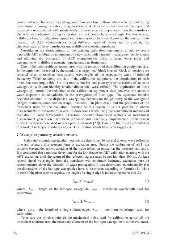
time and arbitrary displacement form in excitation area. During the calibration of AET, the acoustic waveguides allows avoiding of the wave reflection impact on the measurement result. It is considered that a minimal delay time for the low-frequency AET calibration (starting with the AET excitation, until the return of the reflected signal) must be not less than 100 µs. At least several signal wavelengths from the transducer with minimum frequency excitation must be accommodated along the direction of wave propagation. It was determined experimentally that the dimensions of the bar-type waveguides have to be chosen according to formula (1), while in case of the plate-type waveguide, the length of a single edge is found using expression (2).

𝑙𝑙𝑙𝑙𝑏𝑏𝑏𝑏𝑏𝑏𝑏𝑏𝑏𝑏𝑏𝑏 ≥ 3𝜆𝜆𝜆𝜆𝑚𝑚𝑚𝑚𝑏𝑏𝑏𝑏𝑚𝑚𝑚𝑚; (1)

where l bar – length of the bar-type waveguide, λmax – maximum wavelength used for calibration.

𝑙𝑙𝑙𝑙𝑝𝑝𝑝𝑝𝑝𝑝𝑝𝑝𝑏𝑏𝑏𝑏𝑝𝑝𝑝𝑝𝑝𝑝𝑝𝑝 ≥ 6𝜆𝜆𝜆𝜆𝑚𝑚𝑚𝑚𝑏𝑏𝑏𝑏𝑚𝑚𝑚𝑚; (2)

where l plate – the length of a single plates edge , λmax – maximum wavelength used for calibration.

To ensure the synchronicity of the mechanical pulse used for calibration across all the transducer aperture area, the necessary diameter of the bar-type waveguide must be evaluated.

32nd EWGAE S3

It was determined experimentally that this diameter has to be selected according to formula (3).

𝐷𝐷𝐷𝐷𝑏𝑏𝑏𝑏 > 𝜆𝜆𝜆𝜆𝑚𝑚𝑚𝑚𝑚𝑚𝑚𝑚𝑚𝑚𝑚𝑚2

; (3)

where Db – diameter of bar type waveguide, λmin – minimum wavelength used for calibration.

3 Visualisation of generated mechanical displacements in bar and plate type waveguides The excitation signal is calculated using impulse response measured at one point of

the waveguide. Thereafter, the desired arbitrary impact function can be calculated at the measurement point of the impulse response, by using methods of decomposition or time reversal mirror [9-21]. The problem arising independently of the excitation method is related to the continuity of the impulse response on the surface of the waveguide used for AET calibration. This criteria influences AET calibration uncertanty and needs to be evaluated.

When calculating the excitation signal, none of the examined methods estimates that the impulse response function, obtained at the adjacent points of the waveguide, may differ from the one obtained at the impulse response measurement point.

In order to evaluate the influence of non-continuity of the impulse response on the predetermined impact function, the bar and plate type waveguide surface vibration scan was carried out.

The ending of the steel bar-type waveguide with a diameter of 24 mm was scanned. The measurements were accomplished according to the block diagram presented in Figure 1. The excitation signal was calculated for the central point according to the modified deconvolution method presented in previous work [22].

Figure 1. Equipment connection block diagram

The excitation signal frequency band must be selected according to formula (3) (frequency band is related to λmin ). Measurement results presented in Figures 2 and 3 demonstrate importance of the following selection. In Figure 3 frequency band was selected according to equation (3). Another case is demonstrated in Figure (2), where frequency bad is intencionally selected wider than it should be according to equation (3). Measurement results demonstrate frequency bands selection importance for the generation of similar amplitude displacemets in selected area of the bar type waveguide.

S4 32nd EWGAE

a) b) Figure 2. Scanned vibrations of the ending of the steel bar with diameter of 24 mm for the excitation signal

frequency band of 270 kHz: a) surface deformation under maximal vibration amplitude b) surface deformation x-z axis

a) b)

Figure 3. Scanned vibrations of the ending of the steel bar with diameter of 24 mm for the excitation signal frequency band of 150 kHz: a) surface deformation under maximal vibration amplitude; b) surface deformation

x-z axis

AET characteristics usally depends from measured wave type. Therefor generation of arbitrary mechanical pulse waveforms used for AET calibration is necessary not only in bars, but also in plate-type structures. In order to prove that predetermined displacements may be obtained, not only in a certain area of the bar but in plate as well, a surface scan of the 5 mm thick steel plate was carried out.

The excitation signal was calculated using the modified decomposition method [22]. Results are presented in figure 4; here, the 2500 mm2 plate area has been scanned, and the generated displacemnt is shown in different distances from the excitation source.

a) b)

32nd EWGAE S5

c) d)

Figure 4. Scanned plate surface, where the sinusoid period type mechanical displacement is obtained: a) at 320 mm distance from the excitation source; b) at 340 mm distance from the excitation source c) at 350 mm distance

from the excitation source d) pulse in the AET aperture area

Measurement results in bar and plate type waveguides demonstrate possibilities to generate in dispersive waveguides predetermined displacements which can be used for AET calibration.

4 Acoustic emission transducer calibration Block diagrams of acoustic emission calibration stand is presented in Figure 5. The AET

is calibrated using arbitrary mechanical displacements generated according to modified decomposition method [22]. Example of the generated mechanical displacements waveform, measured with capacitive transducer is presented in Figure 6. Calibration stands waveguides geometry is selected according to formulas (1) - (3). Both calibration stands allow to measure AET impulse response, from which AET frequency response is calculated, manucatured transducer characteristics measuremnt example is provided in figure 7.

Figure 5. AET calibration stands block diagram

Acoustic emission transducer frequency response is determined according to formula (4), impulse response is measured with oscilloscope.

𝐾𝐾𝐾𝐾𝐴𝐴𝐴𝐴𝐴𝐴𝐴𝐴𝐴𝐴𝐴𝐴(𝑗𝑗𝑗𝑗𝑗𝑗𝑗𝑗) = 20log 𝑆𝑆𝑆𝑆𝑡𝑡𝑡𝑡(𝑗𝑗𝑗𝑗𝑗𝑗𝑗𝑗)𝑌𝑌𝑌𝑌(𝑗𝑗𝑗𝑗𝑗𝑗𝑗𝑗)

; (4)

Where KAET(jω) – AET frequency response, St (jω) – measured AET impulse response spectrum, Y(jω) – measured waveguides arbitrary type vibration.

S6 32nd EWGAE

a) b) Figure 6. Bar-type waveguides displacement: a) displacement waveform at bar-type waveguides end measured

with capacitive transducer b) calculated frequency response

a) b)

Figure 7. AET characteristics measurement example: a) AET pulse response obtained in stand with bar type waveguide b) calculated frequency response

5. ConclusionsAET calibration stand constructions of a new type are proposed in this paper, offering calibration with different types of waves opportunities and reduced size, compared to existing solutions. These constructions use bar and plate type waveguides. Until now, these constructions haven't been used for AET calibration, because of limited possibilities to generate arbitrary waveform displacements. Offered construction application possibilities for AET calibration are presented by the measurement results.

32nd EWGAE S7

References 1. G.Budenkov, O.Korobeynikova, ‘Application of the rod and torsional waves for

testing the extended objects of oil extracting industry’, ndt for safety, pp.31-38, publisher www.ndt.net , 2007.

2. H.Kwun, Guided wave inspection of nuclear fuel rods, ‘Developments in ultrasonicguided wave inspection’, pp. 1-6, publisher www.ndt.net, 2009.

3. B.Bahr, ‘Automated inspection for aging aircraft, in: International Workshop onInspection and Evaluation of Aging Aircraft’, pp. 18–21, publisher Carnegie Mellon University Pittsburgh ,1992.

4. K.K. Shung, J.M.Cannata, Q.F.Zhou, ‘Piezoelektric materials for high frequencymedical imaging applications: review, journal of Electroceram’, pp. 140-145, springer, 2007.

5. Renaldas Raišutis, Rymantas Kažys, Liudas Mažeika, Egidijus Žukauskas,VykintasSamaitis, Audrius Jankauskas,’Ultrasonic guided wave-based testing technique for inspection of multi-wire rope structures’, journal of NDT&E International, vol 62, pp. 40–49, Elsevier,2014.

6. T.L.Jordan, Z.Ounaies, ‘Piezoelectric Ceramics Characterization, NASA LangleyResearch Center’, NASA/CR-2001-211225, pp 1-22, 2001.

7. ‘Effects of High Static stress on the Piezoelectric properties of transducer materials’,Technical Publications TP-220, pp 1-6, Morgan Electro Ceramics.

8. ‘Standard method for primary calibration of acoustic emission sensors’, ASTMinternational, designation E1106 - 86.

9. Mathias.F,’Time Reversal of Ultrasonics Fields – Part I: Basic Principles’, journalTransactions on Ultrasonics, Ferroelectrics and Frequency Control, vol.39, No.5, pp.555 - 566, IEEE ,September 1992.

10. R. Gangadharan, C.R.L. Murthy, S. Gopalakrishnan, M.R. Bhat.’Time reversaltechnique for health monitoring of metallic structure using Lamb waves’, Journal of ultrasonics,vol 49, pp703-705, Elsevier, 2009.

11. T. Yamasaki, S. Tamai, M. Hirao , ‘Optimum excitation signal for long-rangeinspection of steel wires by longitudinal waves’, journal of NDT&E International, vol 34, pp. 207–212, Elsevier, 2001.

12. S. Bahrami, A. Cheldavi, and A. Abdolali, ‘Moving target tracking using time reversalmethod ‘,journal of Progress In Electromagnetic Research M, Vol. 25, pp. 39-52, EMW Publishing, 2012.

13. W.A.Kuperman, W.S.Hodkiss, T. Akai, S.Kim, G. Edelmann, H.C.Song, ‘Time-reversal acoustics’ , Marine physical laboratory/SIO and SACLANTCEN undersea center, pp. 1 – 6, Acoustics, 2000.

14. M.Fink, C.Prada, ‘Acoustic time-reversal mirrors’, Institute of physics publishing,Topical review, pp.1-38, IOP publishing, 2000.

15. R.Ernst, J. Dual, ‘Acoustic emission localization in beams based on time reverseddispersion’, journal of ultrasonics, Vol. 54, pp. 1522-1533, ELSEVIER, 2014.

16. H.W.Park, S.B.Kim, H.Sohn, ‘Understanding a time reversal process in Lamb wavepropagation’, Journal of Wave motion, Vol. 46, pp. 451 – 467, ELSEVIER, 2009.

S8 32nd EWGAE

17. M.Griffa, B.E.Anderson, R.A.Guyer, T.J.Ulrich, P.A.Johnson, ‘Investigation ofrobustness of time reversal acoustics in solid media through the reconstruction oftemporally symmetric sources’, Journal of physics D:Applied physics, Vol.41, pp. 1-15. IOP publishing, 2008.

18. R.Watkins, R.Jha, ‘A modified time reversal method for Lamb wave based diagnosticsof composite structures’, Journal of mechanical system and signal processing, Vol. 31,pp. 345-354, ELSEVIER, 2012.

19. L.Zeng, J.Lin, ‘Chirp based dispersion precompensation for high resolution Lambwave inspection’, Journal of NDT&E international, Vol 61, pp. 35 – 44, ELSEVIER,2014.

20. V.Augutis, M.Varanauskas, ‘Synthesis of acoustic impulses in a solid waveguide,Ultragarsas’, No. 1(38), Publisher ultragarsas, 2001.

21. A.Benatar, D.Rittel, A.L.Yarin, ‘Theoretical and experimental analysis of longitudinalwave propagation in cylindrical viscoelastic rods’, Journal of the mechanics andphysics of solids, Vol. 51, pp. 1413-1431, Elsevier, 2003.

22. Vygantas, Augutis; Darius Gailius; Edgaras Vaštakas; Pranas Kuzas, ‚Evaluation ofarbitrary waveform acoustic signal generation techniques in dispersive waveguides‘,Journal of Vibroengineering, Vol. 17, no. 7, p. 4047-4056, 2015.

32nd EWGAE ©CNDT2016 S9

Czech Society for Nondestructive Testing32nd European Conference on Acoustic Emission TestingPrague, Czech Republic, September 07-09, 2016

ACOUSTIC EMISSION TESTING OF UNDERGROUND PIPELINES OF CRUDE OIL OF FUEL STORAGE DEPOTS

Ireneusz BARAN 1, Igor LYASOTA 1, Krzysztof SKROK 2 1Cracow University of Technology, Laboratory of Applied Research; Krakow, Poland

Phone: +48 12 628 32 74, Fax: +48 12 628 37 45; e-mail: baran@mech.pk.edu.pl 2PERN S.A., Plock, Poland

Abstract

Considerable quantity of underground in-plant pipelines of crude oil of fuel storage depots and refineries is operated for more than thirty years. Corrosion damages and material degradation are the main causes for structural failures of such underground pipelines. Such failures not detected on time and not monitored in time are potentially the reasons of major breakdowns of the infrastructure of technological underground pipeline installations in-service and finally are the risks of pollution of the environment. The preventive maintenance activities are usually carried out on time driven basis, but evolving defects have to be identified in time to enable appropriate repairs. The primary disadvantages are limited access to pipelines and limited possibilities of testing, due to the necessity for off-line pressure tests of a big part of underground pipeline installation, possible visual inspection and follow-up non-destructive tests (NDT). Based on these facts, we conducted investigations for application of AE testing method of underground pipelines during pressure tests using liquid product transported through pipe. We present the AE investigation on pipeline materials and on real underground pipelines.

Keywords: underground pipelines, AE testing, AE wave propagation in liquid and in pipeline

1. IntroductionA significant part of underground pipelines for transport of petroleum products of the petrochemical industry has been operated for over thirty years. The manufacturing flaws of low carbon steel from the period of pipelines construction resulted in various types of technological defects, structural and chemical heterogeneity, and often, significant contamination of the structure in the form of non-metallic inclusions (mainly sulphur compounds). The long-term operation of such pipelines with hidden defects causes damage development in the material and welded joints in the form of discontinuities, corrosion defects, and structural changes in the matrix material. The development of the defects, in terms of working loads, can lead to their unstable state, the effect of which may be the pipeline leak resulting in the natural environment contamination. The scale of the problem is shown by the statistics [1], according to which the development of corrosion damage in pipelines of the petrochemical industry, despite the use of better and better protective coatings, is at the forefront of reasons for their failure (approx. 30%), and consequently, damage to the natural environment. Accordingly, in the chemical and petrochemical industries, new solutions in the field of diagnostic tests are sough, which allow to precisely assess the technical condition of the underground in-plant pipelines operating for a long time, and to improve their reliability and operational safety. It is worth noting that in case of long underground pipelines, it is hardly efficient to use the standard NDT methods, such as visual testing (VT), ultrasonic testing (UT) or radiographic testing (RT), because their implementation requires the excavation of the entire pipeline.

S10 32nd EWGAE

One of the cheapest and simplest methods of testing the underground pipelines is a visual inspection carried out with the use of the CCTV method (Closed Circuit Television). However, it can only obtain an image of the pipeline interior (internal inspection), and it is necessary to drain the pipeline, which is difficult to implement. There is also no possibility to obtain other relevant information, including, among others, the wall thickness, the condition of its outer surface, or the presence of hidden defects in the material [2]. The tests (In-Line Inspection) implemented by intelligent pigs [3], which use the ultrasonic (UT, Ultrasonic Testing) or electromagnetic method (ET, Electromagnetic Testing) of damage detection, allow to more thoroughly assess the technical condition of underground pipelines. In this case, it is possible to detect, locate and determine the size of corrosion defects (including stress corrosion cracking), both inside and outside the pipeline, and to detect hidden defects in the pipe wall material (various types of discontinuities). A weak point of this technique is the necessity to insert a large-size device to the pipeline inside, which is not always possible to achieve. Therefore, it is mainly used to test the transmission pipelines. In recent times, a long-range ultrasonic method, which is based on the phenomenon of guided waves (Ultrasonic Guided Wave Testing), has been used for testing of the underground pipelines [4, 5]. The test is conducted by generating guided (torsional) waves in the pipe wall, which propagate to a maximum distance of approx. 200 m (depending on the pipe material conditions and operating conditions), and the detection and location of damage are possible by calculating the transit time of reflection of waves from the occurred damage. The disadvantage of this method is a significant decrease in energy of waves propagating on the welds connecting individual elements of the pipeline, as well as a result of the material degradation, especially the corrosion damage, which causes the decrease of the test distance even down to 8 ÷ 10 m. One of the modern NDT methods, which is also used in testing the pipelines is the Acoustic Emission method (AE). However, it is mainly used to test tightness (leak tests) of the pipeline [6-10], and is also used in case of the intelligent pigs. It is generally known that AE is a highly sensitive passive test method, which allows to detect active surface and internal defects in the walls and welds of the tested object under loading. The main advantages of AE method are the possibility of global testing and monitoring of large elements and structures (including those in operational conditions) and above all, the location of AE sources generated by active defects/damage with the possibility to determine the dynamics of their development. Thus, this method is currently considered as appropriate (complementary with other NDT tests) for periodic testing of large equipment, among others, in the petrochemical industry. An additional important advantage of this method is propagation of AE waves through the operating medium (liquid) in the tested object, which enables to use AE for testing large objects, such as above-ground storage tanks. From the above, it can be stated that a prospective solution in the area of diagnostic tests of underground in-plant pipelines would constitute the development of the measurement methodology based on recording of propagation of AE waves through the operating medium that are generated by active defects and damage in the pipeline wall material. One of more important aspects in this case would be the use of the maximum possible distance between AE sensors in order to reduce the amount of excavation (local access to the pipeline) and thus, the costs associated with the test realization. The main components that will constitute the basis for the development of the above mentioned measurement methodology with the use of AE are: • performance of tests related to propagation of AE waves over a length of the underground

pipeline, selection of the optimal measuring equipment and AE recording settings –determination of the propagation range of AE waves by the operating medium (liquid), aswell as by the pipeline wall;

32nd EWGAE S11

• determination of parameters (amplitude, energy/signal strength, duration, frequencydomain of AE signals, etc.) of the recorded AE signals during laboratory tests, and the onesgenerated by actual damage in the wall and especially corrosion damage (concentration ofdeep pitting corrosion) in the pressure testing conditions – loading of the pipeline elementin relation to the conditions of maximum operating pressure, design pressure, proof testand maximum operating pressure;

• verification of the developed measurement methodology in test conditions of in-serviceunderground pipeline.

The basic research and tests to develop the measurement methodology (diagnostic) with the use of AE for testing the underground in-plant pipelines are presented in this publication.

2. AE wave propagation testsIn order to develop a new diagnostic methodology with the use of AE to test long underground parts of the pipelines, it was necessary to determine the maximum distance between the sensors (mounting place of AE sensors), at which the optimal measurement sensitivity and possibility to detect defects as AE sources would be maintained. For this purpose, the tests of propagation of AE waves and measurements of the acoustic background on several sections of the DN600 pipeline filled with crude oil were carried out. The tests were conducted on the pipelines of different lengths with underground (10 ÷ 70 m) and above-ground (100 m and more) sections, and sections with the change of their direction (elbows 90°). Measuring points with the mounted AE sensors were located on the exposed parts of pipelines, and their exemplary layout for one of the tested cases is shown in Figure 1. In order to record AE signals, the AMSY-6 multi-channel measurement system and AE resonant sensors of VS30-SIC/VS30-V (25÷80 kHz) and VS75-V (30÷120 kHz) types of Vallen Systeme, and R1.5 (5÷20 kHz) resonant sensors of Physical Acoustics Corporation were used. As the artificial sources generating AE waves, the following tools were used:

• AE sensors of R1.5, VS30-SIC/VS30-V and VS75-V types connected with the internalgenerator of the AMSY-6 system,

• Hsu-Nielsen 2H/0.50 mm source according to the standard PN-EN 1330-9:2009 [11],• AE sensors of the SE25-P type (DECI company) connected with the Agilent 33220A

function generator.While testing the propagation and attenuation of AE waves, different ranges of frequency filters on the measurement channels (3 ÷ 300 kHz, 6 ÷ 300 kHz and 9 ÷ 300 kHz) were used. It is aimed at checking the difference in attenuation of AE waves, checking the acoustic background and finding the optimum measuring range, which allows to eliminate noise while maintaining adequate measurement sensitivity.

Fig. 1. Scheme of the layout of measurement points over the length of the pipeline while testing the propagation of AE waves (underground part of the pipeline presented by the dotted line)

The amplitude of AE signals for the background did not exceed 30 ÷ 34 dB for the range of filters 3 ÷ 300 kHz. For longer distances (above 20 ÷ 25 m), AE waves propagated only by the medium in the pipeline. It is shown in Figure 2 for tests with AE source in the form of

S12 32nd EWGAE

Hsu-Nielsen 2H/0.5mm. The amplitude of AE signals recorded at the distance of 70 m from the source were respectively 39 dB for R1.5 sensor, 40 dB for VS30-V sensor and 41 dB for VS75-V sensor. In case of the above-ground pipeline segment and the similar test for the distance of 70 m between sensors and source, the amplitude was 58 dB. On the basis of the data collected during testing of the propagation of AE waves, attenuation curves for the underground and above-ground parts of the pipeline were constructed – the curves for VS30-V sensor are presented in Figure 3.

a

b Fig. 2 Propagation of AE waves in the pipeline underground section with a length of 70 m: a – a signal for the

sensor at AE source (HSU 2H/0.5mm source), b – a signal for the second sensor (VS30-V sensors)

Fig. 3. Attenuation curves for AE waves in the underground and above-ground pipelines – for AE sensors of VS30-V

When the distance of the source of AE waves from the sensor is less than 10 ÷ 15 m, AE signals consisted of several modes of waves propagating with variable speed for Hsu-Nielsen 2H/0.5mm source. Figure 4 shows an example of AE signal, where the source was at the distance 5 m from the sensor – AE signals of variable speed are visible: longitudinal wave

AE wave through liquid, 140 cm/ms

32nd EWGAE S13

(535÷540 cm/ms) propagating through the pipe wall, the Lamb longitudinal wave (200÷205 cm/ms) propagating along the pipeline wall and the wave propagating through liquid (140 cm/ms). The modes and parameters of AE waves identified during testing, which propagate in the pipeline filled with liquid, are important and should be taken into account in the future while locating AE sources during diagnostic tests.

Fig. 4 AE signal recorded at the distance of 5 m from the Hsu-Nielsena (HSU/2H/0.50 mm) source – for VS30-SIC sensor

According to the obtained results, it can be concluded that use of lower frequency filters on AE measurement channels and low-frequency sensors allows to increase the range of testing while maintaining the measurement sensitivity – greater range of propagation of AE waves. It was also found that in case of underground pipelines, the maximum distance between the measurement points would be approx. 50 m (Fig. 3). In accordance with the fact that attenuation of AE waves in the exposed pipeline is lower (in relation to attenuation of AE waves in the underground pipeline), the maximum distance between AE sensors in this case could be even more than 120 m (Fig. 3). The data related to attenuation and propagation of AE waves were obtained as a result of the tests, with optimally selected test equipment and recording settings. The results allowed to determine the maximum distance between AE sensors, for which the optimum measurement sensitivity is maintained. The information on the modes of AE waves propagating along the pipe wall and through the operating medium (liquid), will be also useful in the interpretation of the results of AE tests of actual in-plant pipelines.

3. AE laboratory tests on pipeline section and material pipe properties3.1. Mechanical tests of the pipeline steel In the next stage of the research, the tests of properties of the material sections obtained from the pipe of the underground fuel pipeline with the diameter of DN 422÷425 mm (wall thickness 7.5÷8 mm), constructed in 1968, were carried out. The pipeline was operated under the maximum operating pressure conditions at the level of 0.3 ÷ 0.4 MPa. Design pressure was 6.3 MPa and proof test pressure was 9.5 MPa. The tests were aimed at determining the effect of the material degradation on its mechanical properties. A set of material tests, such as: chemical composition analysis, metallographic tests, tensile testing at ambient temperature, were carried out.

Chemical composition testing. The chemical composition was analysed using the emission spectrometry method and to determine precisely the content of sulphur and carbon, the

Longitudinal wave, 535÷540 cm/ms

AE wave through liquid, 140 cm/ms

Longitudinal Lamb wave, 200÷205 cm/ms

S14 32nd EWGAE

infrared absorption method was used after combustion in an induction heating furnace. It was tested for standard specimens. The results of the tests and bibliography data of the 18G2A steel are presented in table 1.

Table 1. Chemical composition of the tested steel and 18G2A steel (PN-EN 10025-1:2007 [12])

Materials Chemical elements, [%] C Si Mn S P Cr Ni Cu

Tested steel 0,17 0,36 1,35 0,040 0,035 0,05 0,05 0,08

18G2A Max 0,20 0,20÷0,55 1,00÷1,50 Max

0,040 Max 0,040

Max 0,30

Max 0,30

Max 0,30

According to the technical documentation, the pipeline, from which the tested sections were taken, is made of steel of the 18G2A (S355) grade, which was also confirmed by the chemical analysis of material cut from the pipes.

Metallographic tests were made with the use of the optical microscopy. The surfaces of unetched and etched (reagent Nital – 4% HNO3 + 96% C2H5OH) polished sections with dimensions of 8×15 mm, cut in the circumferential and axial directions, were tested. The observation of unetched polished sections showed that there are stringers non-metallic inclusions (manganese, sulphides) along the rolling direction, and their amount results from a slightly increased sulphur content (see Table 1). The tests of etched sections demonstrated that the pipe material has a fine-grained ferritic-pearlitic structure (Fig. 5), which is typical for steel of the 18G2A grade, without distinctive features of the secondary structure. No significant changes of the microstructure were observed.

a b Fig. 5. Microstructures of etched polished specimens of the pipeline steel,

a – in the circumferential direction b – in the axial direction, ×500

Tensile testing used the Zwick/Roell Z100 universal testing machine, in accordance with guidelines of the PN-EN ISO 6892-1 standard [13]. The test specimens were cut out in the circumferential and axial directions of pipes. The obtained mechanical properties of tested steel are given in Table 2. The test results of tensile testing at ambient temperature showed that all the strength parameters of the tested pipes are in the range of values given in the pipeline technical documentation.

Table 2. Mechanical properties of steel sections Direction of the sample cutting Rm, MPa Re, MPa A5, % Z, %

Circumferentially 549 371 29.35 49 Axially 552 380 29.78 64

32nd EWGAE S15

3.2. Laboratory pressure tests with AE recording The specimen (Fig. 6) in the form of the pipeline section (from underground pipeline that has been operated for over 40 years), on which the pressure test with recording of AE was carried out. During the pressure test, the specimen was loaded (and unloaded) in stages with the 10 minute load holds and recording of AE. The process of loading the pipeline section lasted until the loss of its stability (break and leak), which occurred at the pressure of approx. 15.8 MPa. There were numerous corrosion damages (including pitting corrosion) of different depths on the outer surface of pipes (1 ÷ 2.6 mm, see Fig. 6 and 7).

Fig. 6 Scheme of the test stand and layout of AE sensors and the map of damage on the coating of the pipeline section (specimen) (1÷6 – VS150-RIC sensors, 29÷34 – VS30-SIC sensors, A ÷ P – inventoried and measured

corrosion damage)

a b c

Fig. 7. General view of the test stand with the pipeline section (a) and example corrosion damage (b, c)

For AE recording were used AMSY-6 system and sensors: VS30-SIC and VS150-RIC with integrated preamplifiers (respectively 46 dB and 34 dB). During the tests on measurement channels and connected AE sensors, the following ranges of the frequency filters were applied: VS30-SIC: 9.3÷300 kHz, VS150-RIC: 95÷850 kHz. The layout of sensors on the tested pipeline section is shown in Figure 6. During the pressure test AE was recorded. AE testing is primarily aimed at collecting the reference AE signals (with correspondingly wide range of the frequency) typical for subsequent stages of development of corrosion damages (including pitting corrosion) in the pipeline wall. The high-amplitude AE signals resulting from corrosion damages appeared at the pressure of 1.6 MPa – location of AE sources was presented in Figure 8. Taking into

S16 32nd EWGAE

account the attenuation curves (Fig. 3), it can be stated that AE waves generated by corrosion damages would be detected for distance of 50 m. In figures 9 ÷ 10 the test results in the form of graphs of changing parameters of AE during the pressure test are shown. The analysis of the obtained results showed a variable nature of generating AE signals in the loading of the tested pipeline section.

Fig. 8. The location of sources of AE signals along the tested part of pipeline – location of active corrosion damage for the load of 1.6 MPa

In Figure 9, it is possible to distinguish three characteristic stages, which correspond to individual stages of the destruction process development of the pipe material:

1. Elastic operation of the pipe (pressure up to 8.5 MPa) was characterised by progressiveincrease in AE activity as the test pressure is increased. It is worth noting that in a givenload range with the use of both types of sensors, comparable numbers of AE wererecorded (Fig. 9). The maximum activity of the located AE signals in this case, wasobserved at the time of transition from the elastic operation to the occurrence of localplastic deformation areas in it. For AE sensors these values respectively reached to:21 hits/sec – VS30-SIC and 23 hits/sec – VS150-RIC (Fig. 9).The high energy AE signals, which were possibly generated by the local plasticdeformation in the area of corrosion damages (in places of the wall local thickness loss– pitting corrosion), were also located. The first such AE signals were detected andsource located at the pressure inside the pipeline at the level of 3.5 MPa, and thegreatest values of the Signal Strength parameter recorded by sensors VS30-SIC.

2. Plastic deformation of the pipe (pressure 8.5 ÷ 13.5 MPa) is characterised bya progressive decrease in AE activity (Fig. 9). At this stage of loading, significantlyfewer AE signals (in relation to the previous stage) and those of a lower amplitude andenergy were recorded (Fig. 10).

3. Strengthening of pipes (pressure from 13.5 MPa) corresponds to a rapid increase of AEactivity. At this stage, a significant increase both in the numbers of AE signals and thevalue of their parameters (Amplitude, Signal Strength) was observed. The difference ofAE activity was visible on particular types of used AE sensors. It is worth noting that inthis case, significantly more signals were recorded with the use of VS150-RIC sensors

32nd EWGAE S17

(Fig. 9, b), however, the signals recorded with the use of VS30-SIC sensors are characterised by higher values of the Signal Strength parameter (Fig. 10). After strengthening the material of pipe, the stage of plastic “flow”, on which AE activity progressive decreases until reaching the moment of failure. The failure of tested pipe section occurred at the area with innermost corrosion damages (F area on Fig. 6, Fig. 7, b). It was located between sensors number 3 and 4 (Fig. 8).

a

b

Fig. 9. AE-activity for sensors: a – VS30-SIC and b – VS 150-RIC

S18 32nd EWGAE

a b Fig. 10. Signal strength of the located AE signals for sensors: a – VS30-SIC and b – VS 150-RIC

4. AE test of real underground pipelines under operating conditionsIn order to verify the results obtained so far and the developed assumptions of the measurement methodology, the tests with AE of underground parts of the in-plant pipelines (DN500), operated for over 40 years, were performed. The maximum operating pressure of pipelines were between 0.3 and 0.6 MPa and the design operating pressure was 2.5 MPa. During AE testing the pipelines filled with crude oil and were subjected to the pressure test and loaded in two cycles, during which the pressure was raised up to 1.0 MPa with holds the load for 30 minutes. In order to record AE, the AMSY-6 multi-channel measurement system and AE low-frequency sensors of VS30-SIC were used. During testing, the filters with the frequency range of 9.3÷300 kHz were used on the measurement channels. AE sensors (maximum distance between the sensors was 40.8 m) were mounted over the length of the tested pipelines – the layout of sensors was shown in Figure 11.

Fig. 11. Scheme of the layout of AE sensors over the length of the tested pipelines

32nd EWGAE S19

As a result of the conducted tests, several AE sources, marked as I ÷ IV, were located (Fig. 12). AE sources I ÷ III were identified as the occurrence of leaks during the test on the valves being close to sensors numbers 10, 16 and 4. Indicated place and marked as IV was AE source with low activity, low amplitude and energy and would be graded to severity 1 (minor source in accordance with PN-EN 14584:2013-07 [14]) – no further actions shall be necessary, included in the report for comparison with subsequent tests.

a

b Fig. 12. Linear location of AE-sources along the tested pipelines

5. Conclusion1. The diagnostic methodology based on tests with AE method of underground sections of in-

plant pipelines designed for transport of petroleum products is developed.2. As a result of the preliminary tests, the data related to attenuation and propagation of AE

waves allowed to determine the maximum distance between AE sensors, with themaintenance of the optimal measurement sensitivity. In case of underground pipelines,the distance between AE sensors is approx. 50 m.

3. It is possible to apply low-frequency sensors for the detection and location of AE sourcesconnected with the corrosion damages in pipe wall (including pitting corrosion) in case ofAE wave propagating through liquid inside pipelines.

4. The analysis of the test results showed a variable nature of generating mechanisms of AEin the loading of the tested pipeline section in laboratory test. Three characteristic stages ofAE activity, which correspond to individual stages of the destruction process development,were identified. It was found that used low-frequency AE sensors are characterised by

S20 32nd EWGAE

increased sensitivity for detection of the local plastic deformation and material degradation due to corrosion, which cause local weakening of the pipeline material. These AE sensors also are suitable for leak testing.

5. It was also found that the high-amplitude AE signals, recorded at the pressure of 1.6 MPa,was generated by local corrosion damage (pitting corrosion), which are located on thepipeline wall. Taking into account the attenuation curves, it can be stated that AE wavesgenerated by corrosion damage would be detected from the distance of 50 m.

6. In order to verify the developed diagnostic methodology, the tests of real undergroundparts of the pipelines (DN500), operated for more than 40 years, were performed.As a result of the tests, several AE sources, identified as the valves leaks, were located.

References [1] Sokólski W. Corrosion Processes Direct Assessment as a Part Of Operational Pipeline Safety’s, VIII National Conference Corrosion Measurements in Electrochemical Protection 16-18. jul 2004 Jurata, Poland. [2] Ming-Der Yang, Tung-Ching Su, Tung-Yen Wu and Kai-Siang Huang, Journal of GeoEngineering, 5 (3) (2010) 99–104. [3] Sunil K. Sinha, Mark A. Knight Intelligent System for Condition Monitoring of Underground Pipelines, Computer-Aided Civil and Infrastructure Eng., 19 (2004) 42–53. [4] Demma A., Alleyne D., Pavlakovic B., Testing of Buried Pipelines Using Guided Waves, Middle East Nondestructive Testing Conference & Exhibition – 27-30 Nov. 2005 Bahrain. [5] Francisco C. R. Marques, Alessandro Demma, Ultrasonic Guided Waves Evaluation of Trials for Pipeline Inspection, 17th World Conference on Nondestructive Testing, 25-28 Oct. 2008, Shanghai, China. [6] Pollock A.A., and Hsu S.-Y.S., Leak Detection Using Acoustic Emission, Journal of Acoustic Emission, 1 (4) 1982 237–243. [7] Shifeng Liu, Luming Li, Jian Cui, Tie Li Acoustic Emission Detection of Underground Pipeline Leakage 15th WCNDT, 2000, Roma, Itally. [8] Anastasopoulos A., Kourousis D., Bollas K., at all. Acoustic Emission Leak Detection of Buried Pipeline, 19th Intl AE Symposium (IAES19), Kyoto, Japan, 8-12 Dec., 2008. [9] Bui Van Hieu, Seunghwan Choi, Young Uk Kim,, Youngsuk Park and Taikyeong Jeong, Wireless Transmission of Acoustic Emission Signals for Real-Time Monitoring of Leakage in Underground Pipes, Journal of Civil Engineering 15 (5) (2011) 805–812. [10] Juliano T. M., Meegoda J. N., Watts D. J. Acoustic Emission Leak Detection on a Metal Pipeline Buried in Sandy Soil, Journal of Pipeline Systems Engineering and Practice, 4(3) (2013) 149-155. [11] PN-EN 1330-9:2009 „Non-destructive testing – Terminology – Part 9: Terms used in acoustic emission testing”. [12] PN-EN 10025-1:2007 „Hot Rolled Products Of Structural Steels – Part 1: General Technical Delivery Conditions”. [13] PN-EN ISO 6892-1 „Metallic materials – Tensile testing – Part 1: Method of test at ambient temperature”. [14] PN-EN 14584:2013-07 „Non-destructive testing – Acoustic Emission Testing – Examination of metallic pressure equipment during proof testing – Planar location of AE sources”.

32nd EWGAE ©CNDT2016 S21

Czech Society for Nondestructive Testing32nd European Conference on Acoustic Emission TestingPrague, Czech Republic, September 07-09, 2016

A VERSION OF THE DISCRETE ELEMENT METHOD IN THE SIMULATION OF THE ACOUSTIC EMISSION TESTING

Gabriel BIRCK1, Ignacio ITURRIOZ1

1 Department of Mechanical Engineering, Federal University of Rio Grande do Sul, Porto Alegre, RS, Brazil. Phone: +55 51 3308 3529; e-mail: gabriel.birck@ufrgs.br, ignacio@mecanica.ufrgs.br

Abstract

In the present work, events of Acoustic Emission testing in quasi-brittle material were simulated by a version of the discrete element method. In this numerical approach the solid is modelled by means of a periodic spatial arrangement of bars with the masses lumped at their ends. The results obtained by numerical approach are evaluated by Acoustic Emission parameters, as b-value, RA value and average frequency, and compared with the moment tensor analysis. The results showed coherent between both forms of evaluation. The numerical approach was able to simulate Acoustic Emission events and provide more information about the damage process.

Keywords: Lattice Discrete Element Method, Damage evaluation, Acoustic Emission, Moment Tensor

1. IntroductionFrom a physical point of view, damage phenomena consist either of surface discontinuities in the form of cracks or of volume discontinuities in the form of cavities [1, 2]. Macroscopically, it’s, therefore, necessary to identify internal variables that reflect the damage level in the material. The most advanced method for a non-destructive quantitative evaluation of damage progression is the Acoustic Emission (AE) technique. Physically, AE is a phenomenon caused by a structural alteration in a solid material in which transient elastic-waves, due to a rapid release of strain energy, are generated. AEs are also known as stress-wave emissions. In the present work a version of the Discrete Element Method built by bars (LDEM) are employed. This approach belongs to the alternative set of computational methods called by Munjiza [3], "Computational Mechanics of Discontinua" introduced during the 1960s, which is characterized by the lack of differential or integral equations to describe the model to study the space domain. In the mentioned approach, the behaviour of the solid is a function of the individual elements, e.g., particles or bars. Here, a notched beam subjected to the three-point bending test is simulated with LDEM. The beam is built in quasi-fragile material. Global stress-strain is evaluated and accelerations in some points of the specimen’s surface are registered. The acceleration registered is interpreted as data provided by a real device EA.

2. Acoustic EmissionOne promisor method for a non-destructive quantitative evaluation of damage progression is the Acoustic Emission (AE) technique. Physically, AE is a phenomenon caused by a structural alteration in a solid material, in which transient elastic-waves, due to a rapid release of strain energy, are generated. AEs are also known as stress-wave emissions. AE waves, whose frequencies typically range from kHz to MHz, propagate through the material towards the surface of the structural element, where they can be detected by sensors which turn the released strain energy packages into electrical signals [4, 5]. Traditionally, in AE testing, a number of parameters are recorded from the signals, such as arrival time, velocity, hits, count, rise time, amplitude, duration and frequency. From these parameters damage conditions and localization of AE sources in the specimens are determined Carpinteri et. al. [6].

S22 32nd EWGAE

2.1. Damage process evolution An effective damage assessment criterion is provided by the statistical analysis of the amplitude distribution of the AE signals generated by growing microcracks. The amplitudes of such signals are distributed according to the Gutenberg-Richter (GR) law [4, 7], N( ≥ A)∝ A-b, where N is the number of AE signals with amplitude ≥A. The exponent b of the GR law, the so-called b-value, changes with the different stages of damage growth. While the initially dominant microcracking generates a large number of low-amplitude AE signals, the subsequent macrocracking generates more signals of higher amplitude. As a result, the b-value progressively decreases when the damage in the specimen advances, as shown in Figure 1. This is the core of the so-called “b-value analysis” used for damage assessment.

Figure 1. The b-value evolution in experimental test [7]

2.2. Crack classification The shape of the AE waveforms characterizes the fracture mode [8]. So, to classify active cracks parameters as Rise Angle (RA) and average frequency are calculated from AE events. The RA value is defined as the ratio between the rise time and the maximum amplitude. The average frequency is obtained from the relation of AE ring-down count and the duration time of the signal, as shown in Figure 2. The AE ring-down count corresponds to the number of threshold crossings within the signal duration time [9]. From these two parameters, cracks are readily classified into tensile and shear cracks as illustrated in Figure 2. The tensile mode of crack (Mode I), which includes opposing movement of the crack sides, results in AE waveforms with short rise time and high frequency. On the other hand, shear type of cracks (Mode II) usually result in longer waveforms, with lower frequency and longer rise time.

(a) (b)

Figure 2. (a) Typical waveforms for tensile and shear events, (b) Relationship between average frequency and RA value

32nd EWGAE S23

2.3. Moment tensor theory By the generalized theory of AE [10], elastic displacement u(x,t) at location x due to the crack displacement in y at the time t is represented as [11],

𝑢𝑢𝑢𝑢𝑖𝑖𝑖𝑖(𝒙𝒙𝒙𝒙, 𝑡𝑡𝑡𝑡) = 𝐺𝐺𝐺𝐺𝑖𝑖𝑖𝑖𝑖𝑖𝑖𝑖,𝑞𝑞𝑞𝑞(𝒙𝒙𝒙𝒙,𝒚𝒚𝒚𝒚, 𝑡𝑡𝑡𝑡)𝑀𝑀𝑀𝑀𝑖𝑖𝑖𝑖𝑞𝑞𝑞𝑞 ∗ 𝑆𝑆𝑆𝑆(𝑡𝑡𝑡𝑡), (1)

where 𝐺𝐺𝐺𝐺𝑖𝑖𝑖𝑖𝑖𝑖𝑖𝑖,𝑞𝑞𝑞𝑞(𝒙𝒙𝒙𝒙,𝒚𝒚𝒚𝒚, 𝑡𝑡𝑡𝑡) represents the spatial derivatives of Green’s functions, S(t) is the kinetic source (time function of crack motion), Mpq is the moment tensor components (kinematics of crack motion) and (*) represents the convolution function. The moment tensor is a symmetric second-rank tensor and is comparable to the elastic stress in elasticity (see Figure 3a), which is expressed as [11-13],

𝑀𝑀𝑀𝑀𝑖𝑖𝑖𝑖𝑞𝑞𝑞𝑞 = 𝐶𝐶𝐶𝐶𝑖𝑖𝑖𝑖𝑞𝑞𝑞𝑞𝑝𝑝𝑝𝑝𝑝𝑝𝑝𝑝𝑙𝑙𝑙𝑙𝑝𝑝𝑝𝑝𝑛𝑛𝑛𝑛𝑝𝑝𝑝𝑝∆𝑉𝑉𝑉𝑉, (2)

where Cpqkl is the constitutive tensor, l is the direction vector of crack motion, n is the normal of the crack surface and ∆V is the crack volume. If only the first motion of the P-wave A(x) is taken into account and assuming that all of the moment tensor components have the same time-dependency, Equation (1) can be simplified as [11-15],

𝐴𝐴𝐴𝐴(𝒙𝒙𝒙𝒙) =𝐶𝐶𝐶𝐶𝑠𝑠𝑠𝑠𝑅𝑅𝑅𝑅𝑒𝑒𝑒𝑒(𝒕𝒕𝒕𝒕,𝒓𝒓𝒓𝒓)

𝑅𝑅𝑅𝑅[𝑟𝑟𝑟𝑟1 𝑟𝑟𝑟𝑟2 𝑟𝑟𝑟𝑟3]

𝑀𝑀𝑀𝑀11 𝑀𝑀𝑀𝑀12 𝑀𝑀𝑀𝑀13𝑀𝑀𝑀𝑀21 𝑀𝑀𝑀𝑀22 𝑀𝑀𝑀𝑀23𝑀𝑀𝑀𝑀31 𝑀𝑀𝑀𝑀32 𝑀𝑀𝑀𝑀33

𝑟𝑟𝑟𝑟1𝑟𝑟𝑟𝑟2𝑟𝑟𝑟𝑟3, (3)

where Cs is the physical coefficient containing the sensor sensitivity, obtained by pencil-lead break test [16]; R is the distance between the crack y and the detection point x, and r1, r2, r3 are its different direction cosines, respectively; Re(t,r) is the reflection coefficient between vector r and the direction t of the sensor (see Figure 3b). In the case where the P-wave arrives vertically to the surface Re(t,r)=2. Equation (3) leads to a series of algebraic equations in which the components of the moment tensor Mpq are unknowns, where there are 6 independent components.

(a) (b) Figure 3. (a) Elements pf the moment tensor, (b) Crack nucleation and AE detection

The source location is determined from the arrival time differences (ti) between the observation xi and xi+1, solving the equations,

𝑅𝑅𝑅𝑅𝑖𝑖𝑖𝑖 − 𝑅𝑅𝑅𝑅𝑖𝑖𝑖𝑖+1 = |𝒙𝒙𝒙𝒙𝒊𝒊𝒊𝒊 − 𝒚𝒚𝒚𝒚| − |𝒙𝒙𝒙𝒙𝒊𝒊𝒊𝒊+𝟏𝟏𝟏𝟏 − 𝒚𝒚𝒚𝒚| = 𝑣𝑣𝑣𝑣𝑖𝑖𝑖𝑖𝑡𝑡𝑡𝑡𝑖𝑖𝑖𝑖 , (4)

where vp is the velocity of P-wave, assumed constant.

S24 32nd EWGAE

By the analysis of eigenvalues and associated eigenvectors of the moment tensor it is possible to classify the crack (failure mode), and obtain the crack motion vector (l) and the crack normal vector (n) [11]. The eigenvalue is decomposed into a shear component X, a deviatoric component Y and a hydrostatic component Z, which, X is the maximum shear contribution, Y is set as the maximum deviatoric tensile component and Z is the maximum isotropic tensile component. Three eigenvalues are normalized and decomposed as follows:

𝑋𝑋𝑋𝑋 + 𝑌𝑌𝑌𝑌 + 𝑍𝑍𝑍𝑍 = 1 = 𝜆𝜆𝜆𝜆1 𝜆𝜆𝜆𝜆1⁄ , 0 − 𝑌𝑌𝑌𝑌 2⁄ + 𝑍𝑍𝑍𝑍 = 𝜆𝜆𝜆𝜆2 𝜆𝜆𝜆𝜆1⁄ , −𝑋𝑋𝑋𝑋 − 𝑌𝑌𝑌𝑌 2⁄ + 𝑍𝑍𝑍𝑍 = 𝜆𝜆𝜆𝜆3 𝜆𝜆𝜆𝜆1⁄ ,

(5)

where λ 1 , λ 2 and λ 3 are maximum, intermediate and minimum eigenvalues, respectively. The cracks are classified, as proposed by Ohtsu [11], into three types of AE sources: X > 60% as shear cracks; X < 40% as tensile cracks, and 40% < X < 60% as mixed-mode cracks.

3. Lattice Discrete Element Method (LDEM)The version of the truss-like Discrete Element Method (DEM) proposed by Riera [17], which is used in this paper, is based on the representation of a solid with a cubic arrangement of elements which is only able to carry axial loads. The cubic module is presented in Figure 4a and Figure 4b. The mass is lumped at the nodes. Each node has three degrees of freedom, corresponding to the nodal displacements in the three orthogonal coordinate directions. The equations that relate the properties of the elements to the elastic constants for an isotropic medium are presented in Equation (6).

𝜂𝜂𝜂𝜂 =9𝜈𝜈𝜈𝜈

4 − 8𝜈𝜈𝜈𝜈,𝐸𝐸𝐸𝐸𝐴𝐴𝐴𝐴𝑛𝑛𝑛𝑛 = 𝐸𝐸𝐸𝐸𝐿𝐿𝐿𝐿𝑐𝑐𝑐𝑐2

(9 + 8𝜂𝜂𝜂𝜂)2(9 + 12𝜂𝜂𝜂𝜂)

,𝐸𝐸𝐸𝐸𝐴𝐴𝐴𝐴𝑑𝑑𝑑𝑑 =2√3

3𝐴𝐴𝐴𝐴𝑛𝑛𝑛𝑛, (6)

where 𝐸𝐸𝐸𝐸 and 𝜈𝜈𝜈𝜈 denote Young’s modulus and Poisson’s ratio, respectively, while 𝐴𝐴𝐴𝐴𝑛𝑛𝑛𝑛 and 𝐴𝐴𝐴𝐴𝑑𝑑𝑑𝑑 are the areas of the normal and the diagonal elements and 𝐿𝐿𝐿𝐿𝑐𝑐𝑐𝑐 is the size of the basic cubic module. The resulting motion equations, obtained with this spatial discretization, can be written in the well-known form presented in Equation (7).

𝐌𝐌𝐌𝐌𝐱𝐱𝐱(𝑡𝑡𝑡𝑡) + 𝐂𝐂𝐂𝐂𝐱𝐱𝐱(𝑡𝑡𝑡𝑡) + 𝐅𝐅𝐅𝐅𝐫𝐫𝐫𝐫(𝑡𝑡𝑡𝑡) − 𝐏𝐏𝐏𝐏(𝑡𝑡𝑡𝑡) = 0, (7)

where 𝑥𝑥𝑥𝑥 is the vector of generalized nodal displacements, 𝑀𝑀𝑀𝑀 is the diagonal mass matrix, 𝐶𝐶𝐶𝐶 is the damping matrix, also assumed diagonal, 𝐅𝐅𝐅𝐅𝐫𝐫𝐫𝐫 is the vector of the internal forces acting on the nodal masses and 𝐏𝐏𝐏𝐏 is the vector of external forces. The operator (•) denotes the time (𝑡𝑡𝑡𝑡) differentiation 𝑑𝑑𝑑𝑑(•)/𝑑𝑑𝑑𝑑𝑡𝑡𝑡𝑡. If 𝑀𝑀𝑀𝑀 and 𝐶𝐶𝐶𝐶 are diagonal, the Equation (7) is not coupled and, therefore, the explicit central finite difference scheme can be used to time domain integration. Since the nodal coordinates are updated for each time step, large displacements can be accounted in a natural and efficient manner. This article adopts a relationship between axial force and axial strain in the uniaxial elements (bar), based on the bilinear law proposed by Hillerborg [18], which is presented in Figure 4c. The specific fracture energy (Gf) is directly proportional to the area below the bilinear constitutive law. Another important feature of this approach is the assumption that Gf is a 3D random field with a Weibull probability distribution. The local strain associated with maximum loading in each bar is called critical strain (𝜀𝜀𝜀𝜀𝑖𝑖𝑖𝑖). This value is also a random variable and its variability, which is measured using the coefficient of variation CV, is related to the Gf parameter by the Equation (8),

𝐶𝐶𝐶𝐶𝑉𝑉𝑉𝑉𝜀𝜀𝜀𝜀𝑝𝑝𝑝𝑝 = 0.5𝐶𝐶𝐶𝐶𝑉𝑉𝑉𝑉𝐺𝐺𝐺𝐺𝑓𝑓𝑓𝑓 . (8)

32nd EWGAE S25

The minimum value of 𝜀𝜀𝜀𝜀𝑖𝑖𝑖𝑖, determined for each specimen bar, is associated with the global strain for which a specimen loses linearity. Mesh perturbation was incorporated to improve the performance when the body is submitted to compression. It is possible to observe in Figure 4c, that the bar failure occurs only when submitted to tensile solicitation. In compression, the bars have linear elasticity behaviour [19]. More exhaustive explanations of this version of the lattice model can be found in Kosteski et al. [20, 21]. Applications of the LDEM in studies involving non-homogeneous materials subjected to fracture, such as concrete and rock, can be found in Riera and Iturrioz [22], Dalguer et al. [23], Miguel et al. [24], Iturrioz et al. [25] and Miguel et al. [26].

(a) (b) (c) Figure 4. LDEM: (a) basic cubic module, (b) generation of a prismatic body, and (c) Bilinear constitutive model

with material damage

3.1. AE tests simulated by LDEM The numerical approach employed in this paper was used to simulate Acoustic Emission tests in others cases, as presented in Iturrioz et al. [27], where comparison between experimental and numerical tests performed. In terms of the distribution of AE event amplitudes in time and frequency, the results were seen to be consistent, as can be seen in Figure 5.

Figure 5. Comparison between numerical and experimental results [27].

4. ApplicationsA plain concrete beam, with pre-notched and depth equal to half the overall height, was simulated to a three-point bending (TPB) with LDEM [28]. Standards results as force and vertical deflection were computed and AE test was performed. The scheme and main geometrical parameters are reported in Figure 6. The material properties are: Young’s modulus 35GPa; Poisson’s ratio 0.25; density 2400 kg/m3, and specific fracture energy (Gf) 70 N/m. The beam was discretized with 168x20x20 basic cubic with length (Lc) equal 5 mm. Twelve sensors were used to EA test, two sensors per side.

S26 32nd EWGAE

Figure 6. Schematic representation of TPB test

The statistical analysis of the amplitude distribution (b-value) for three periods of the time is presented in Figure 7. In Figure 8, the time distribution of instantaneous and accumulated AE events are plotted, also the reaction (force) by the time.

Figure 7. b-value distribution for three periods

Figure 8. Instantaneous and accumulated AE events, and force by the time

The b-value remains low and about constant for the periods analysed, as can be seen in Figure 7, because the AE are mainly emitted from a specific region of the structure (see Figure 9), which is expected since the beam has a notch. By the Figure 8, it’s observed that AE events occur throughout all the period. For the period I, shown in Figure 9, the damage is more widespread than in others, therefore, the b-value is larger.

32nd EWGAE S27

Figure 9. Damage distribution in the three periods of b-value analysis

Crack classification for three AE events were performed by AE parameters and by moment tensor analysis. In Figure 10, crack classification by AE parameters, RA value and Average Frequency was performed by two sensors. These events were chosen because the amplitude of the first motion of the P-wave and the beginning of the event are clearly defined.

Figure 10. Crack classification by AE parameters

In Figure 11, it is represented the position and classification for the AE events analyzed by tensor moment analysis. The arrows represent the crack motion vector (l) and the crack normal vector (n), which are interchangeable [29]. In Table 1, the moment tensor normalized is presented. Through these figures, the classification by AE parameters and moment tensor are coherent, that is, the same classification was obtained. It is noteworthy that using moment tensor analysis it is possible get the orientation and displacement vector of the crack.

Figure 11. AE events representation

S28 32nd EWGAE

Table 1. Normalized moment tensor for each event

Event Normalized moment tensor

A X=10.40%

𝑀𝑀𝑀𝑀𝑖𝑖𝑖𝑖𝑖𝑖𝑖𝑖

max𝑀𝑀𝑀𝑀𝑖𝑖𝑖𝑖𝑖𝑖𝑖𝑖 =

0.02 0.04 0.100.04 0.07 0.370.10 0.37 1.00

B X=32.36%

𝑀𝑀𝑀𝑀𝑖𝑖𝑖𝑖𝑖𝑖𝑖𝑖

max𝑀𝑀𝑀𝑀𝑖𝑖𝑖𝑖𝑖𝑖𝑖𝑖 =

0.00 0.01 0.090.01 1.00 0.320.09 0.32 0.33

C X=57.28%

𝑀𝑀𝑀𝑀𝑖𝑖𝑖𝑖𝑖𝑖𝑖𝑖

max (𝑀𝑀𝑀𝑀𝑖𝑖𝑖𝑖𝑖𝑖𝑖𝑖) =

0.07 0.02 0.130.02 0.90 1.000.13 1.00 0.27

5. ConclusionsThe b-value evolution in the damage process is related with the spatial damage distribution. Furthermore, the classification obtained by the moment tensor analysis showed a demonstrated consistency when compared with the classification by the AE standard parameters. Also the damage orientation obtained by the same methodology showed to be similar with the bar and load orientation. However, Suaris and van Mier [30] point out that the eigenvalues decomposition method to explicitly determine the crack orientation is only valid for cases of traction and pure shear. This study has shown the potential applications of the truss-like DEM not only to simulate AE monitoring analysis, but also to provide a better understanding of the relationships between the basic AE parameters.

Acknowledgements The authors wish to thank the National Council for Scientific and Technological Development (CNPq – Brazil) and Coordination for the Improvement of Higher Education Personnel (CAPES – Brazil) for funding this research.

References 1. Lemaitre, J., and J. L. Chaboche. Mechanics of solid materials. Cambridge University

Press, Cambridge, 1990. 2. Krajcinovic, D. Damage mechanics. volume 41. Elsevier, Amsterdam, 1996.3. Munjiza, A. Special issue on the discrete element method: aspects of recent

developments in computational mechanics of discontinua, Engineering Computations,vol. 26(6), 2009.

4. Shiotani, T.; Fujii, K.; Aoki, T.; Amou, K. Evaluation of progressive failure usingAE sources and improved b-value on slope model tests, Progress in AcousticEmission, vol. 7(7), p. 529–534, 1994.

5. Kurz, J. H.; Finck, F.; Grosse, C. U.; Reinhardt, H.-W. Stress drop and stressredistribution in concrete quantified over time by the b-value analysis, StructuralHealth Monitoring, vol. 5(1), p. 69–81, 2006.

6. Carpinteri, A.; Lacidogna, G.; Niccolini, G. Fractal analysis of damage detected inconcrete structural elements under loading, Chaos, Solitons & Fractals, vol. 42(4),p. 2047–2056, 2009a.

32nd EWGAE S29

7. Carpinteri, A.; Lacidogna, G.; Puzzi, S. From criticality to final collapse: evolution ofthe "b-value"from 1.5 to 1.0, Chaos, Solitons & Fractals, vol. 41(2), p. 843–853,2009c.

8. Aggelis, D. G. Classification of cracking mode in concrete by acoustic emissionparameters, Mechanics Research Communications, vol. 38(3), p. 153–157, 2011.

9. RILEM, T. C. Recommendation of RILEM TC 212-ACD: acoustic emission and relatedNDE techniques for crack detection and damage evaluation in concrete: Test method forclassification of active cracks in concrete structures by acoustic emission. Materialsand Structures, vol. 43(9), p. 1187–1189, 2010b.

10. Aki, K.; Richards, P. Quantitative Seismology. Geology: Seismology. UniversityScience Books, 2nd edition, 2002.

11. Ohtsu, M. Simplified moment tensor analysis and unified decomposition of acousticemission source: application to in situ hydrofracturing test, Journal of GeophysicalResearch, vol. 96(B4), p. 6211–6221, 1991.

12. Ohno, K.; Shimozono, S.; Ohtsu, M. Cracking mechanisms of diagonal-shear failuremonitored and identified by AE-SiGMA analysis, Fract. Mech. Concr. Struct, vol. 2,p. 991–998, 2007.

13. Ohtsu, M. Acoustic Emission Theory for Moment Tensor Analysis, Journal ofResearch in Nondestructive Evaluation, vol. 6(3), p. 169–184, 1995.

14. Ohtsu, M. Moment tensor analysis of AE and SiGMA code. In Acoustic Emission-Beyond the Millennium, pages 19–34. Elsevier, 2000.

15. Grosse, C. U.; Ohtsu, M. Acoustic Emission Testing. Springer Berlin Heidelberg,2008.

16. RILEM, T. C. Recommendation of RILEM TC 212-ACD: acoustic emission and relatedNDE techniques for crack detection and damage evaluation in concrete: Measurementmethod for acoustic emission signals in concrete., Materials and Structures, vol.43(9), p. 1177–1181, 2010a.

17. Riera, J. D. Local effects in impact problems on concrete structures. In Proceedingsof the Conference on Structural Analysis and Design of Nuclear Power Plants, volume3, pages 57–79, Porto Alegre, Brazil, 1984.

18. Hillerborg, A. A model for fracture analysis, Report TVBM-3005, 1978.19. Iturrioz, I.; Lacidogna, G.; Carpinteri, A. Experimental analysis and truss-like discrete

element model simulation of concrete specimens under uniaxial compression,Engineering Fracture Mechanics, vol. 110, p. 81–98, 2013a.

20. Kosteski, L. E.; Iturrioz, I.; Batista, R. G.; Cisilino, A. P. The truss-like discrete elementmethod in fracture and damage mechanics, Engineering Computations, vol. 28(6), p.765–787, 2011.

21. Kosteski, L. E.; D’Ambra, R. B.; Iturrioz, I. Crack propagation in elastic solids usingthe truss-like discrete element method, International Journal of Fracture, vol. 174(2),p. 139–161, 2012.

22. Riera, J. D.; Iturrioz, I. Discrete elements model for evaluating impact and impulsiveresponse of reinforced concrete plates and shells subjected to impulsive loading,Nuclear Engineering and Design, vol. 179(2), p. 135–144, 1998.

23. Dalguer, L.; Irikura, K.; Riera, J. Simulation of tensile crack generation bythreedimensional dynamic shear rupture propagation during an earthquake, Journal ofGeophysical Research: Solid Earth (1978–2012), vol. 108(B3), 2003.

24. Miguel, L. F. F.; Riera, J. D.; Iturrioz, I. Influence of size on the constitutive equationsof concrete or rock dowels, International Journal for Numerical and AnalyticalMethods in Geomechanics, vol. 32(15), p. 1857–1881, 2008.

S30 32nd EWGAE

25. Iturrioz, I.; Miguel, L. F. F.; Riera, J. D. Dynamic fracture analysis of concrete or rockplates by means of the Discrete Element Method, Latin American Journal of Solidsand Structures, vol. 6(3), p. 229–245, 2009.

26. Miguel, L. F. F.; Iturrioz, I.; Riera, J. D. Size effects and mesh independence in dynamicfracture analysis of brittle materials, Computer Modeling in Engineering& Sciences(CMES), vol. 56(1), p. 1–16, 2010.

27. Iturrioz, I.; Lacidogna, G.; Carpinteri, A. Acoustic emission detection in concretespecimens: Experimental analysis and lattice model simulations, International Journalof Damage Mechanics, vol. 23(3), p. 327–358, 2014a.

28. Birck, G. Análise do processo de dano em material quase-frágil através dasimulação de um modelo de barras, Dissertation, Federal University of Rio Grande doSul, Porto Alegre, 2016.

29. Ohtsu, M.; Ohno, K.; Hamstad, M. A. Moment Tensors of In-Plane-Waves Analyzed bySiGMA-2D, Journal of Acoustic Emission, vol. 23, p. 47–63, 2005.

30. Suaris, W.; van Mier, J. Acoustic emission source characterization in concrete underbiaxial loading, Materials and structures, vol. 28(8), p. 444–449, 1995.

32nd EWGAE ©CNDT2016 S31

Czech Society for Nondestructive Testing32nd European Conference on Acoustic Emission TestingPrague, Czech Republic, September 07-09, 2016

COMPARISON OF LOCALIZATION STRATEGIES OF DAMAGE IN CONCRETE BY ACOUSTIC EMISSION

Antoine BONIFACE1, Zoubir M. SBARTAÏ1, Jacqueline SALIBA1, Nary RANAIVOMANANA2

1 I2M laboratory, Civil engineering Department, University of Bordeaux; France; e-mail: antoine.boniface@u-bordeaux.fr, zoubir-mehdi.sbartai@u-bordeaux.fr, jacqueline.saliba@u-bordeaux.fr 2

University of Toulouse ; UPS, INSA ; LMDC ; France; e-mail : ranaivom@insa-toulouse.fr

Abstract

The monitoring of concrete structures by the acoustic emission (AE) technique allows the detection and the localization of damage. The source location is determined by a triangulation algorithm based on the arrival time of AE signals recorded by sensors placed at the surface of the material, and the measured concrete wave velocity. The accuracy of AE source location depends on many assumptions. In this paper, the accuracy related to the choice of the onset detection of AE signals and to the location algorithm is studied. A statistical analysis of AE location maps based on the distribution of AE events is presented. The accuracy of AE events location is also evaluated and compared between the studied criteria. Keywords: acoustic emission, concrete, damage, source location, accuracy.

1. IntroductionThe monitoring of nuclear facilities and concrete structures is a major concern in the field of civil

engineering to ensure safety and durability. A realistic description of cracking allows a better understanding of the degradation problems in concrete. In the case of a quasi-brittle material such as concrete, macro-cracks occurs after the development of a micro-cracked area also called fracture process zone (FPZ) [1-5]. The main objective of this study is to provide further insight in the description of the FPZ evolution in order to prevent the propagation of damage. This is because the accumulation of microcracks causes a local decrease of the mechanical characteristics of the material leading to crack propagation.

Micro-cracking is a phenomenon of localized damage causing the release of mechanical energy. It results from this mechanical event the propagation of an elastic wave in the material. The acoustic emission technique enables the detection of vibration by piezoelectric sensors located on the material surface. The main interest of the AE technique is that it allows the monitoring of damage continuously. It provides also, through the analysis of wave arrival time and triangulation, the localisation of microcracks.

The localization of AE events by the triangulation technique is mastered [6]. Nevertheless, the quality of the results is sensitive to different criteria [7]. An important criterion for performing a good location is the picking of arrival times from the recorded AE signals. Several onset picking techniques have been proposed in the literature: the simple manual picking technique which is very time consuming, the amplitude threshold picker, the STA/LTA picker (Short Term Average / Long Term Average) and the automatic onset detection algorithms based on the Hinckley criterion and Akaike Information Criterion (AIC) [8,9]. To determine the position of AE source, the triangulation method is performed based on the arrival times of AE signals recorded by the sensors. Several iterative algorithms, which consist in generating a sequence of testing and updating of a trial solution based on a linear least-squares algorithm, were applied to obtain the optimal source locations coordinates: grid search, simplex algorithm, Geiger’s method [10], … However, even though the principle of location is still the same, the way in which the minimization problem is resolved affects the final result. The simplex algorithm is the most used for its timeliness. However, this algorithm only allows converging to a local minimum of the minimization problem and may lead, in some cases, to an incorrect solution.

S32 32nd EWGAE

Thus, the objective of the following work is to ensure a reliable location of micro-cracks. To achieve this, an experimental investigation is proposed. Three point bending tests were carried out on notched concrete beams and the monitoring of the damage is assessed by means of the acoustic emission technique. Two evaluation criteria for the onset time of AE signal are presented. Their influence on the overall result of the location is highlighted. Subsequently, three alternative algorithms are also applied for the resolution of the location problem. The advantages and disadvantages of those methods are discussed. The accuracy and the possibility of improving the AE technique are also studied.

2. Experimental details2.1. Materials and Procedures

The dimensions of the tested concrete beams are L x h x l = 500 x 250 x 120 mm. A central notch of 4 mm width is located at the bottom part of the beams and measure 10 mm in height. The composition of the used concrete is shown in Table 1.

Constituents Mass proportions cement CEM I 52.5 CE NF 320 kg.m-3

water 197.5 kg.m-3 sand 0-4 mm 830 kg.m-3

aggregates 4-11 mm 445 kg.m-3 coarse aggregates 8-16 mm

Balloy 550 kg.m-3

Table 1. Concrete composition.

The three-point bending tests were performed using a hydraulic press MTS with a capacity of 100 kN (Figure 1 left). The load was applied with a constant crack mouth opening displacement (CMOD) control with a slow rate of 0.2 mm.min-1. Figure 1 right shows an example of the load-CMOD curves obtained with fracture tests. The load CMOD variations are linear up to 80% of the maximal strength followed by a nonlinear variation up to the peak load and a stable failure in the postpeak region.

Figure 1. General view of the experimental fracture test setup (left). Load/CMOD curve (right).

2.2. Acoustic emission measurements The monitoring of the damage is carried out using a network of 8 piezoelectric sensors R15 of

resonance frequency equal to 150 kHz. The two main faces of the beam were instrumented with 4 sensors so as to perform a 3D localization of acoustic events.

The AE signals were amplified with a 40 dB gain differential amplifier. The signals are converted by a PCI-card 8 and filtered by a low pass filter of 400 kHz and a high pass filter of 100 kHz. The signal

32nd EWGAE S33

detection threshold was set at a value of 35 dB. The signals (or hits) are then grouped by the software AEwin (Mistras Group) into acoustic events based on their arrival time. Thus a set of signals received by the sensors (at least four), in a period of 71 microseconds form an event. This time window corresponds to a propagation distance of 25 cm. The measured wave propagation velocity is equal to 3500 m.s-1. This velocity was measured using the normalized pencil lead break procedure.

3. Principals of source localizationLocation of micro-cracks is based on the following hypothesis: sources are punctual, sources are

temporally spaced apart from each other so that the acoustic activity resulting from the source does not interfere with the acoustic activity of the next source, wave propagation velocity is constant, material is homogeneous and isotropic. According to those hypothesis, the waves travel from a source point to sensors following a straight path with a constant velocity. Figure 2 represents the principal of the AE technique and illustrates the time of arrival approach:

Figure 2. Principal of acoustic emission technique.

As seen in previous parts, the localization process is based on measured arrival time of signals where “i” denote the order of arrival and “j” the sensor indices. In practice only delays between sensors are used: . Considering previous hypothesis, a group of delays between sensors depend on the position of event. The location of micro-cracks is determined by solving an error minimization problem between the received data by the sensors and those from an artificial event with a known position (eq. 1). This artificial event is determined by an algorithm. The retained position corresponds to that of the artificial event for which the error criterion is minimum.

, eq. (1) where “n” is the number of sensors associated to the event. To summarize and considering hypothesis

given above, localization depends on three factors: the velocity of waves, the capability to determine precisely the beginning of AE signals and the algorithm used to solve the minimization problem. Here, the variation of wave velocity is not considered and is kept constant. In the following parts, only the influence of the two others factors is studied and discussed.

4. Influence of the onset picking technique4.1. Fixed threshold versus AIC

The determination of the onset time of AE signals has been identified as a source of error for events location. Indeed, the overall delay measured between the sensors is influenced by the method of determining the onset time of the AE signals. The acquisition of data used in this work has been performed using a fixed threshold which is the simplest form for onset picking. This technique defines the onset time of a signal as the time at which the amplitude received by the sensor exceeds a previously established threshold (35 dB here). The disadvantage of this technique is that it is not adapted to each

S34 32nd EWGAE

signal as small amplitude signals and signal with a high noise level. Figure 3 illustrates this problem; an important delay between the beginning of the signal determined by the fixed threshold method (magenta) and the apparent onset time of the signal is observed. An intuitive way to overcome this problem could be to reduce the gap between threshold and noise. In fact, ambient noise can change during loading due to experimental environment. Thereby this gap must exist to avoid noise record.

The AIC criterion is widely used in the literature. The idea is to compare the difference between standard deviation passed and forthcoming at each point of the signal. Eq. 2 gives the exact form of this criterion.

𝐴𝐴𝐴𝐴𝐼𝐼𝐼𝐼𝐶𝐶𝐶𝐶𝑘𝑘𝑘𝑘 = 𝑘𝑘𝑘𝑘. log[𝑠𝑠𝑠𝑠𝑡𝑡𝑡𝑡𝑑𝑑𝑑𝑑(𝑠𝑠𝑠𝑠(1: 𝑘𝑘𝑘𝑘))] − (𝑁𝑁𝑁𝑁 − 𝑘𝑘𝑘𝑘). log[𝑠𝑠𝑠𝑠𝑡𝑡𝑡𝑡𝑑𝑑𝑑𝑑(𝑠𝑠𝑠𝑠(𝑘𝑘𝑘𝑘: 𝑁𝑁𝑁𝑁))]. eq. (2)

Here “k” is the considered sample and “N” the number of samples on which the computation is done. The orange curve in figure 3 shows the complete form of this function. The minimum of AIC (green) corresponds to the apparent beginning of signal. The advantage of this technique is the independence from subjective parameters like threshold. So there is no a priori about what can be the level of amplitude which correspond to the beginning of the signal. AIC gives the position where there is a modification of the signal which, in our case, corresponds to the onset time of AE signal.

Figure 3. Typical acoustic waveform (blue) and results of two different picking techniques. Fixed threshold (magenta), AIC function (orange) and its minimum (green).

4.2. Results and discussion Figure 4 shows the damage localization maps obtained with the fixed threshold (top) and the AIC (bottom).

Each blue dot represents one of the 14621 events recorded by the acquisition system. The simplex algorithm has been used in both cases for minimisation. Figure 4 shows also the histograms of the density of events in each direction (x, y, and z). The distribution of AE events along the x axis shows that AE events are more concentrated around the cracking zone (above the notch) with the AIC which is closer to the reality.

𝑠𝑠𝑠𝑠 ( 1 : 𝑘𝑘𝑘𝑘 𝑚𝑚𝑚𝑚𝑖𝑖𝑖𝑖𝑛𝑛𝑛𝑛 ) 𝑠𝑠𝑠𝑠 ( 𝑘𝑘𝑘𝑘 𝑚𝑚𝑚𝑚𝑖𝑖𝑖𝑖𝑛𝑛𝑛𝑛 : 𝑁𝑁𝑁𝑁 ) 𝑘𝑘𝑘𝑘 𝑚𝑚𝑚𝑚𝑖𝑖𝑖𝑖𝑛𝑛𝑛𝑛

sensors face 1 (z = 0.12m)

sensors face 2 (z = 0.00m) notch

32nd EWGAE S35

Figure 4. AE events localization maps obtained with fixed threshold (top) and AIC (bottom) with the distribution of AE events along x, y and z axis.

Another way to compare those two techniques is to evaluate the corresponding errors (eq. 1) obtained based on the localization algorithm in each case. Comparing the errors event by event is a hard task. This is why a global analysis of errors is performed. Figure 5 shows the cumulated number of AE events in function of the error.

Figure 5. Proportion of cumulated AE events inside the beam in function of the error. Comparison between two criteria of onset time determination of AE signals: fixed threshold and AIC.

Note here that AE events with an error higher than 5 centimeters have not been represented here. Figure 5 shows that for the same error, AIC allows a greater amount of events located inside the beam. For example: 27% of events are located inside the beam with an error inferior to 2 cm with the use of AIC against 14.9% with fixed threshold.

5. Influence of the type of minimization algorithmsAnalytical solutions do not exist for high order localization. In fact when the number of sensors used

is higher than the unknown location parameters, the system of equations is over-estimated. Computation techniques exist to solve this problem but localization of only one event means hundreds and hundreds of calculations. This is why algorithms based on least-squares methods can be used to perform a large amount of process which lead to a solution. Three different algorithms are considered here with the main goal of finding the position (x, y, z) which leads to the minimum value of error.

maps obtained with fixed threshold (top) and AIC (bottom) with the

S36 32nd EWGAE

5.1. Simplex The simplex algorithm is widely used in the literature for the localization of AE sources. Simplex

algorithm consist in: i. Defining an initial position , ii. Calculating the error criterion for this position and around. The number of positions

depends essentially on the dimension of the problem,iii. The best solution (smaller error criterion) from all the calculated solutions is stored,iv. return to (ii) with the solution of (iii).

The main advantage of this method is its speed. However, it requires a starting position, which can greatly affect the results. There are several local minimum and only one global minimum which correspond to the sought solution. An initial position near local minimum can lead to a wrong final solution. Moreover, in its simplest form (without fixed boundary) the algorithm can converge to a solution corresponding to an event located outside the studied structure.

5.2. Adaptive meshing algorithm (AMA) When using an AMA, the position of an event is not defined from an initial position but from a set of

positions covering the damage referred area. Figure 6 shows an example in 2D of error calculation between a fictional event on the node of the mesh used and the measured data set from an event which one seeks the position. Measured delays (dtmeas) between transducers are compared to delays computed at each node of the mesh (dtmesh). The comparison between those two set of data is made with the error criterion. The final position of AE event is the position of the node with the smallest error.

To increase the accuracy and reduce the cost of calculation time of this technique, three successive meshes are used to determine the position of a single event. Thus, the first mesh covers a large area surrounding the sensors with a coarse mesh (centimeter). A new tighter mesh is then used around the position adopted earlier. This operation is repeated until obtaining a solution in a mesh whose nodes are spaced apart by 2 millimeters. This adaptation of the mesh makes it possible to manipulate matrices of small dimensions in order to make the operation faster.

The main advantage of the adaptive meshing is to avoid local minima problems since many solutions are calculated and compared to retain the one having the lowest error. The disadvantage of this technique is the calculation time required to determine the position of an event. It is between five and ten times higher than for the simplex algorithm. It should be noted that this disadvantage is not so significant in this case since the minimization of errors for the location of the set of events (14621 in this case) is of the order of 1 hour.

Figure 6. Principal of Adaptive Meshing Algorithm (AMA).

32nd EWGAE S37

5.3. Genetic algorithm The different steps of the Genetic algorithms are:

i. a set of random positions is built in the damage area, ii. delays related to those positions are computed and compared to the measured data with the

error criterion (eq. 3), iii. positions with lowest errors are stored, iv. couples of solutions are formed from retained positions. Those couples are called “parents”, v. new couples of solutions called “childrens” are computed from the parents. For example in 1D

a couple of parents (𝑥𝑥𝑥𝑥1, 𝑥𝑥𝑥𝑥2) gives 2 children (𝑥𝑥𝑥𝑥1, ,𝑥𝑥𝑥𝑥2, ) with and ,

vi. return to (ii) with childrens as new starting position if the precision criterion is not reached.

The number of initial solutions, the proportion of solutions retained to build parents, the way that childrens are computed from parents are parameters which can be changed but the global idea of genetic algorithm is to defined new solutions by “mutations”. This kind of algorithm is more time consuming than the two others presented above.

5.4. Results and discussion Figure 7 shows the AE events localization maps of events related to the use of AMA algorithm (top)

and genetic algorithm (bottom). In both cases and in agreement with the results obtained in the previous section (4), the AIC is used to determine the onset time of AE signals. Those maps are qualitatively identical. The maximum amount of events above the notch and the distribution of events along the main axis (x) is similar for the three algorithms (simplex from figure 4, AMA and genetic from figure 7).

Figure 7. AE events localization maps obtained with AMA algorithm (top) and genetic algorithm (bottom) with AIC as onset picking technique.

,

S38 32nd EWGAE

In order to compare the three algorithms, the error of localization was considered as earlier. Figure 8 shows the cumulated number of events inside the beam related to the errors for the three algorithms. For example, when the error is smaller than 8 mm, the simplex algorithm allows a greater proportion of event located than the other algorithms. In another hand, the genetic algorithm gives better results with 32% of event located with an error inferior to 2 cm against 27% for simplex and 26.3% for AMA.

The fact that simplex seems to allow a greatest number of event located with a small error may be explained by the ability of this algorithm to find the exact solution when the initial position is well defined. On the other hand, even if genetic algorithm is able to detect the global minimum of the problem, this algorithm can’t determine the exact position. Final solution of genetic algorithm will always be really near the exact solution but not the real solution. In other words if the real solution is “0”, genetic algorithm will find something like “10−10” but not “0”. Finally AMA is less efficient than the 2 other algorithms for an error less than 2.3 cm. Contrariwise, AMA gives better results than simplex beyond this value. Due to the way that AMA work, the number of possible final solution is finite because it depend on a finite mesh defined by the user. So if the distance between two nodes of the last mesh is about 1mm and the real solution is between those two nods, it will not be possible to find the exact solution. However, it’s possible to make AMA final mesh finer to enhance his accuracy but at the expense of time.

Figure 8. Proportion of cumulated events inside the beam related to error. Comparison between three algorithms of resolution: simplex (blue), AMA (red) and genetic (yellow).

6. ConclusionsThe main objective of the presented research work is to study the accuracy of the location of AE sources

based on different onset picking techniques and minimisation algorithms. The influence of the onset time techniques on the location maps was analysed considering the amplitude threshold based picking technique and the AIC. The results show that the distribution of events around the real fracture is more concentrated with the AIC and consequently the size of the damage area. Furthermore a quantitative comparison between the two criteria shows that the localization errors obtained with the fixed threshold are greater. Three localization algorithms for solving the optimization problem are compared: simplex, AMA and genetic algorithms. This study shows that the choice of an algorithm depends on the desired accuracy and computation time. Each algorithm has its own advantages and disadvantages. Simplex leads to better results for smaller error while genetic algorithm gives a global better solution for error higher than 0.8 mm. Simplex is faster than AMA and event faster than genetic algorithm. To go further a mix of the 3 algorithms could lead to an optimum localization by dealing with the speed and precision of simplex and the global analysis of genetic or AMA techniques. The effect of the variation of the velocity during the damage process on the localization accuracy will be studied in the future. In addition, for a better evaluation of the accuracy of AE event location, reconstructed profiles obtained with the AE technique, based on different criteria, and real crack profile obtained with laser rugosimeter will be compared.

32nd EWGAE S39

7. AcknowledgmentsThis work was conducted as a part of the ANR ENDE national French project. The National Research

Agency is thanked for the financial support and all the partners of ENDE project.

8. Reference[1] Hadjab H., Thimus J.-Fr., « Fracture process zone in notched concrete beams treated by using

acoustic emission », NDT, vol. 12, 2004. [2] Saliba J., Loukili A., Grondin F., Regoin J-P., « Influence of basic creep on cracking of concrete

shown by the Acoustic Emission technique », Materials and Structures, Vol. 45, p. 1389-1401, 2012. [3] Jankowski L. J., « Formation of the fracture process zone in concrete », Enginering fracture

mechanics, vol. 36, n° 2, 1990, p. 245-253. [4] Shah S. P., « Experimental methods for determining fracture process zone and fracture

parameters », Enginering fracture mechanics, vol. 35, n° 1/2/3, p. 3-14, 1990. [5] Sbartaï ZM, Saïdoun K, « Evaluation de l’endommagement mécanique des bétons par émission

acoustique ». Annales du Bâtiment et des Travaux Publics, Janvier-Mars 2014. [6] Ohtsu M., Ono K., « AE source location and orientation determination of tensile cracks from

surface », NDT International, vol. 21, n° 3, 1988. [7] Ohno K., Kimitaka U., Ueno A., Ohtsu M., « Fracture process zone in notched concrete beam

under three-point bending by acoustic emission », Construction and building materials, 2014. [8] Carpinteri A., Xu J., Lacidogna G., Manuello A., « Reliable onset time determination and source

location of acoustic emissions in concrete structures », Cement and concrete composites, 2012. [9] Kurz J. H., Grosse C. U, Reinhardt H-W, Strategies for reliable automatic onset picking of

acoustic emissions and of ultrasound signals in concrete, Ultrasonics, vol. 43, 2005, p. 538-546. [10]Grosse C., Reinhardt H., Dahm, Localization and classification of fracture types in concrete with

quantitative acoustic emission measurement techniques, NDT&E International, vol. 30, n°4, 1997, p. 223-230.

S40 32nd EWGAE

32nd EWGAE ©CNDT2016 S41

Czech Society for Nondestructive Testing32nd European Conference on Acoustic Emission TestingPrague, Czech Republic, September 07-09, 2016

CORRELATION BETWEEN ACOUSTIC EMISSION SIGNALS AND DELAMINATIONS IN CARBON FIBER-REINFORCED

POLYMER-MATRIX COMPOSITES: A NEW LOOK AT MODE I FRACTURE TEST DATA

Andreas J. BRUNNER 1 Empa, Swiss Federal Laboratories for Materials Science and Technology, Laboratory for

Mechanical Systems Engineering; Dübendorf, Switzerland Phone: +41 58 765 44 93, Fax: not available; e-mail: andreas.brunner@empa.ch

Abstract

Recently, a rough correlation between cumulative AE signal amplitude and averaged crack area has been derived from in-situ tensile tests on miniature samples of spruce wood combining AE monitoring and simultaneous synchrotron-based X-ray computed micro-tomography. This indicated that, at least for the chosen experimental set-up and equipment, AE tended to be more sensitive than X-ray imaging in detecting formation and propagation of small cracks. An analogous analysis is now presented for quasi-static mode I (tensile opening) delamination tests performed on carbon-fiber poly-ether-ether-ketone composite laminates with simultaneous insitu AE monitoring and X-ray radiography using an imaging system with video recording. The data are further used for estimating the variation in the correlation factor for a given experimental set-up by comparing different approaches for deriving an estimated value of the correlation factor. Keywords: Carbon fiber-reinforced polymer-matrix composites, mode I tensile-opening fracture, measurement sensitivity, acoustic emission intensity correlation with damage size (crack area or diameter)

1. IntroductionAcoustic Emission (AE) monitoring is a non-destructive method with high sensitivity to microscopic changes caused by, e.g., rapid release of energy from localized sources in materials and structures which makes it different from many other non-destructive test methods (see, e.g., [1,2]). While AE is successfully applied in a wide range of structural health or integrity monitoring using empirical criteria for the evaluation of the AE signals (see, e.g., [3,4]), it has proven more difficult to extract quantitative information on the sources of the AE signals, even though it was recognized a long time ago that the type of source was affecting the recorded AE signals [5]. Recent advances in unsupervised pattern recognition have shown that discrimination between microscopic damage mechanisms in carbon-fiber reinforced polymer-matrix (CFRP) laminates is feasible [6]. The identification of the source mechanism (type and orientation) was achieved by detailed simulations of the whole signal measurement chain from source to signal recording. The main parts of this simulation comprised model sources simulated as dipole or multipoles in different orientations and locations with a range of signal rise times, signal propagation in the material with frequency dependent attenuation and anisotropic wave speeds as well as the frequency-dependent transfer functions of the AE sensors and the signal recording. For CFRP, this procedure identified the source mechanisms of the different clusters resulting from pattern recognition as matrix cracks, fiber-matrix debonding or fiber breaks [7]. However, identification of the type of a localized model AE source does not directly yield quantitative information on the size of the damage created by the respective mechanism, e.g., the area or length of a micro-crack in the matrix polymer.

S42 32nd EWGAE

Combining AE monitoring of load tests on material specimens or structural elements with suitable, complementary non-destructive test methods [8], in principle, can provide an approach for estimating damage size (e.g., crack area or length) for a correlation with the recorded AE signal parameters or their respective source properties. This has been demonstrated by combining in-situ synchrotron X-ray computed micro-tomography with AE monitoring of tensile tests on miniature spruce wood specimens [9]. After detection of significant AE, the tensile loading was stopped and the applied load held constant for performing the X-ray tomography measurement. Consecutive load steps yielded indications of progressive damage, e.g., as growing cracks. Pattern recognition as outlined in [7] essentially yielded two clusters of AE signals for the wood specimens [10,11] that could be associated with slower and faster source mechanisms, i.e., with distinctly different source rise times in the simulations [12]. Tentatively, these were identified as inter-wall cracks between wood cells for the low and with cell wall cracks for the high frequency cluster. Analysing the X-ray tomography image slices and identifying the crack locations, a rough estimate of the crack length increment from one tensile load step to the next could be obtained. This yielded a quantitative, but rough correlation between crack area and AE signal amplitude (measured in mV). Of course, such an estimation depends on the specific set-up (e.g., specimen material and size/shape) and equipment sensitivity (depending mainly on sensor mounting, AE sensor type and data acquisition settings), but holding these constant allows for relative comparison among nominally identical specimens. Comparing the correlation factor indicated that with the chosen signal threshold setting, AE tended to be more sensitive to crack formation than the X-ray computed micro-tomography. This approach is now tried on delamination propagation in CFRP fracture toughness test specimens for an attempt at estimating the micro-crack size due to a single AE signal of given amplitude.

2. Materials and Testing Details2.1 Carbon-fiber reinforced epoxy and delamination growth CFRP composites are increasingly used in many engineering applications, including loadbearing elements. However, their susceptibility to impact damage and subsequent interlaminar delamination growth, or more general, their rather weak strength in the through-thickness direction, have spurred intensive research into the characterization of interlaminar delamination growth under quasi-static and fatigue loads [13]. There are standardized fracture test methods for the so-called mode I (tensile opening) [14] and mode II (in-plane shear) [15] interlaminar fracture toughness or delamination resistance, as well as mixed mode I/II [16], all under constant displacement loading. Analogous test methods for cyclic fatigue delamination propagation are currently under development [17]. The evaluation of the quasistatic mode I fracture toughness according to the standard is using so-called double cantilever beam (DCB) specimens and based on measuring the delamination length increments due to specific applied loads at given crosshead displacements. The measurement of the delamination length increments during the load tests is made by visual observation using a travelling microscope following the propagation of the delamination tip along the edge of the standard test specimen. In research, methods are developed to replace this either by digital image recording and analysis or by back-calculating the delamination length from the change in specimen compliance due to the propagation of the delamination. However, with a required resolution of the crack length around 0.05 mm [14] all these approaches effectively average over many microscopic crack events, both on the length, as well as on the time scale.

The specimens used in the present research were provided by NASA Langley for a round robin performed at several laboratories in Europe, the U.S. and Japan. The details of material preparation and the full range of fracture toughness results are summarized in [18,19]. In the study reported here, only CFRP laminates made from AS4 type carbon fiber and thermoplastic

32nd EWGAE S43

poly-ether-ether-ketone (PEEK) matrix are analysed. The starter crack film insert was a polyimide film. Two different film thicknesses (7 and 13 µm, respectively) were used in the four DCB specimens with an average thickness between about 3.08 and 3.15 mm, an average width between 20.05 and 20.09 mm and a total length of 139.5 mm.

2.2 In-situ AE monitoring and X-ray radiography of interlaminar fracture tests As part of the development of the mode I fracture toughness standard [14] in the framework of the round robin noted above [18,19] delamination tests on the AS4/PEEK CFRP specimens were performed with an equipment that allowed for in-situ X-ray radiography and image recording on video (described in [20]) simultaneously with AE monitoring [21]. For the tests reported here, the loading equipment was set to a displacement speed around 1 mm/min. Load and displacement values were recorded with a separate data acquisition system (not as part of the AE data via external parameter input).

The X-ray radiography used a microfocus X-ray source (focal spot size 5-10 µm at voltages below 40 kV) in projection imaging mode with an imaging system that allowed for video recording of the images (Fig. 1) at a sampling rate (image frequency) of 25 Hz (both from Feinfocus, Germany). X-ray source voltage and current were set constant at 32 kV and 0.116 mA, respectively, for all four tests. Depending on the distance between source and test object compared to that between source and imaging system, image magnifications between a factor of about 2 and 5 are feasible with this set-up. For the tests reported here, the magnification factor was about 2.6. Methylene-di-iodide was used as contrast agent for the X-ray imaging of the delamination growth (Fig. 2) and injected inside the starter crack with a syringe after slightly opening it (displacement of roughly 3 mm).

Figure 1: Photograph of the microfocus X-ray source (right), the DCB-specimen mounted vertically in the loading fixture at the center with the AE sensor near the bottom edge, and the X-ray image intensifier on the left. The video-recording equipment attached the image intensifier is not shown (photograph by Empa).

AE signal parameters from the quasi-static mode I fracture test on the CFRP laminates were recorded with AE equipment type 3000/SPARTAN with one sensor type R-15 (both from Physical Acoustics Corp.) mounted near the bottom end of the specimen (about 1.5 to 2.0 cm from the edge). Data acquisition settings were a preamplifier gain of 40 dB, a threshold 30 dBAE, a hit definition time of 500 µs, and a rearm time of 1000 µs. The AE analysis will use plots of AE activity, i.e., the number of AE signals recorded per unit time, and AE intensity, i.e., maximum AE signal amplitude distributions,

S44 32nd EWGAE

each presented as a function of time (Fig. 3). Video recording of the X-ray images and AE data acquisition were started simultaneously, within roughly 1 second, in order to synchronize the data.

3. Estimating the Sensitivity of AE Monitoring for Microcrack Formation inAS4/PEEK Specimens Loaded under Mode I Tensile Crack Opening Load

3.1 Approach for the sensitivity analysis A detailed study [21] of the AE signals recorded during mode I delamination growth of CFRP DCB specimens has shown that by defining empirical delamination initiation criteria from the observed AE activity and intensity, the critical fracture toughness GIC obtained from these is comparable to that obtained from the analysis procedure outlined in the standard [14]. This confirmed that the AE analysis is capable of capturing the essential features of the mode I DCB delamination tests not only in a qualitative manner, but also yields quantitative results. In the previously published analysis of the sensitivity of AE to yield a measure of the crack length induced by tensile loading of miniature wood specimens [9], the AE signal amplitudes were correlated with the crack area measured from synchrotron-based X-ray computed microtomography. The approach presented here hence first estimates the total fracture surface generated during the test from the the X-ray projection images, and then the average AE signal amplitude and the number of AE signals recorded during the mode I delamination test. It is immediately clear that the correlation between AE signal amplitude and crack area obtained for this test may and likely will significantly differ from that obtained in the tests on the miniature wood specimens. Major effects causing differences are, e.g., the material type (CFRP versus wood) and its specific signal attenuation behaviour, the specimen size (30 mm versus about 140 mm) or more important, the distance between AE signal source and sensor, the different microscopic damage mechanisms (cell wall delamination or cracking versus polymer micro-crack formation) as well as the different AE equipment, sensor types (with different frequency transfer functions) and data acquisition settings used for the AE measurement.

3.2 Estimating the fracture surface area Getting a first estimate of the fracture surface area created during the test is straight-forward. Determining the difference between initial and final delamination length, multiplied by the specimen width yields an approximation which can be considered as a lower bound. The initial delamination length is well defined and straight across the width of the specimen by the tip of the polymer insert film. However, the crack tip during delamination growth (Fig. 2) is not straight and shows small, stochastically distributed protrusions.

Figure 2: X-ray projection radiography image showing the tip of the delamination during delamination growth. The tip is indicated by the contrast agent (dark/black area) and it can be seen that it is not straight across the specimen width. The same holds for the tip defining the final delamination length (photograph by Empa).

32nd EWGAE S45

It has to be noted that the image with the contrast agent may not in all cases show the exact location of the tip of the delamination. First, the wettability of the contrast agent may be limited and may hence not penetrate into the microscopic cracks. Second, there is a minimum amount of contrast agent necessary to yield a detectable contrast difference in the radiography image. Looking at the grey-scale levels of the image pixels along the direction of propagation of the delamination yields (coming from the top of the image) a high level (dark) that is slightly decreasing with increasing length showing some scatter, then a roughly linear decrease and finally a roughly constant, but low value (bright), again with some scatter. From this, it is estimated that the total delamination length can be estimated to within a few mm. This will be further considered in the error estimate for the sensitivity correlation.

Fracture surfaces of CFRP laminates in general show some roughness or corrugation that could vary depending on the scale at which this is analysed. This is also true for the delamination fracture of the CFRP DCB specimens. Deducing roughness from fracture surface images, such as, e.g., SEM micrographs is fairly complex in spite of the apparent obvious corrugation or roughness that can be seen (see, e.g., [23] for details). Assuming some type of fractal surface for the CFRP laminate may be misleading [24]. Even though [24] deals with thermoset epoxy rather than thermoplastic PEEK, the fractal dimension seems questionable for estimating the additional crack or delamination area in the thickness direction of the DCB specimens. In the analysis, this will be considered by simply adding a certain, estimated percentage to the lower bound area and assessing the influence of that on the sensitivity.

One specimen showed unstable delamination growth yielding a tip outside the field of view of the imaging system. The other three DCB specimens yield a lower bound of the delamination area increase of 538, 459, and 432 mm2, respectively, if the change in slope of the grey-scale image is taken as indication of the position of the crack tip. As discussed above, the tip may extend somewhat further and the total fracture surfaces may be larger than the planar rejection due to surface roughens and corrugation. In the analysis, the lower bounds and area values 20% and 40% larger will be used to estimate lower and upper bounds for the sensitivity.

3.3 Estimating the average AE amplitude The AE activity and AE intensity (Fig. 3) typically show significant variation in time. The AE activity first increases roughly exponentially with time, reaches a maximum (close to 1’000 hits per 5 seconds) and then drops. There are three more peaks in AE activity. In the video recording of the delamination growth, these phases of high AE activity correlate with faster delamination growth. The total number of AE signals (“hits”) recorded for the delamination growth period for the three DCB specimens analysed amount to about 35’620, 32’790, and 51’970. It has to be noted that these values are estimates that could vary by as much as 30%. The average amplitudes are estimated to be around 70 to 72 dBAE for all three specimens. From Fig. 3 (left) the upper and lower bound for the average AE signal amplitude are estimated as 80 and 70 dBAE. Converted to µV, the average amplitudes of 70 and 72 dBAE correspond to about 3’160 and 3’980 µV, and the upper and lower bounds are 7’080 and 2’240 µV, respectively. The AE signals below the threshold (30 dBAE) are not recorded and hence do not contribute to both, total number of AE signals and average AE signal amplitude.

The majority of AE signals recorded lies in the amplitude range between about 60 and 80 dBAE (Fig. 3).

S46 32nd EWGAE

Figure 3: AE activity (number of hits per 5 seconds, left) and AE intensity (AE signal amplitude distribution, right) from one of the DCB mode I delamination tests.

3.4 Estimating the average sensitivity of AE analysis With the estimated lower and upper bounds of the delamination area created during the mode I fracture test in the DCB specimens, the average AE signal amplitude and the respective upper and lower bound for the average crack area created per average AE signal (with respect to signal amplitude) can be estimated. The results are compiled in Table 1. Of course, the assumptions made in the determination of the different quantities are essential, and the result could differ significantly, if these assumptions were proven to be questionable. One important aspect is AE signal attenuation, the AE signal amplitudes were used as recorded and no attempt was made at correcting for attenuation. CFRP composites can cause significant attenuation and the recorded AE signals are possibly affected by reflections from the specimen surfaces, since the width and thickness dimensions (nominally 20 and 3 mm) are relatively small.

Table 1: Estimated average and upper and lower bounds for the crack area created in the AS4/PEEK CFRP laminate by an AE signal of average amplitude

Specimen No. Estimated average AE signal amplitude

[µV]

Estimated lower bound delamination area [mm2]

Estimated number of AE

signals [-]

Estimated upper bound for sensitivity per average AE signal [mV/µm2]

1 - - - -

2 3’160 538 35’620 0.00021

3 3’980 459 32’790 0.00028

4 3’160 432 51’970 0.00038

Using the lower bound of the delamination area for the results presented in Table 1 yields an estimated average upper bound of the sensitivity from three specimens of 0.00029 mV/µm2. The individual values for the three DCB specimens are within the range between about 0.0002 and 0.0004 mV/µm2 and hence fairly consistent, considering the rough approximations that were used for the estimates. Assuming fracture areas larger than the lower bound by 20% and 40% respectively, will yield lower average sensitivities of about 0.00024 and 0.00021 (again in units of mV/µm2). Using an upper bound for the average AE signal amplitude of 77 dBAE

32nd EWGAE S47

or 7’080 µV with the lower bound for the fracture area yields about 0.00061 mV/µm2, and the same average amplitude with an area that is higher by 40% (as an estimated upper bound) yields 0.00037 mV/µm2. If the lower bound area is increased by a factor of two. i.e., 100%, the estimated average sensitivity is 0.0003 mV/µm2. This can be compared with the value of 0.0038 mV/µm2 obtained in [9] for testing the miniature tensile specimens made from spruce wood. The higher sensitivity in the latter case can have several causes as discussed above.

4. Summary and ConclusionsCombining AE measurements on mode I DCB fracture tests with CFRP specimens with insitu projection radiography and highlighting the delamination area with a suitable contrast agent, yields a rough estimate of the sensitivity of the AE measurement with respect to microcrack area that can be detected. From the average sensitivity determined for AE monitoring of the CFRP DCB fracture specimens, it can be estimated that the area of a micro-crack that yields an AE signal with an amplitude of 70 dBAE or 3’160 µV is 10’900 µm2. This roughly corresponds (if the crack area is considered to be a square or circular shape) to a crack length of 100 µm. Taking 80 and 60 dBAE as upper and lower AE signal amplitude limit, the crack length range in the test phase with high AE activity and correspondingly fast delamination growth spans roughly 60 to about 190 µm. These values are consistent with an upper bound estimate of a micro-crack size of less than 200 µm from the diameter of the protrusions seen forming stochastically along the crack tip in the X-ray images.

With threshold values of 40 and 30 dBAE, i.e., 100 µV and about 32 µV, the minimal detectable crack length, estimated from the average sensitivity of 0.00029 mV/µm2 amount to about 20 and 10 µm, respectively. With complementary information on the total defect size, e.g., the delamination area or fracture surface from other non-destructive test methods, AE analysis can yield rough quantitative estimates of the damage size caused by the microscopic source mechanism. It is, however, not straight-forward to compare sensitivities estimated in different tests on different materials directly, since the main effects (material type, specimen size/shape, AE sensor location relative to the source, and transfer function of the measurement chain) may have acted in different ways. Nevertheless, this confirms that AE monitoring easily achieves sensitivity to defects on the scale of a few tens of microns in CFRP laminates, at least in laboratory–scale applications.

Acknowledgment The contributions of Mr R Jäggi and of Dr R A Nordstrom for the in-situ AE monitoring and simultaneous radiography measurements and their analysis as well as discussions with members of the committee on acoustic emission of the German Society for Non-Destructive Testing, especially Dr. J Bohse, are gratefully acknowledged.

References 1. C R Ríos-Soberanis, Acoustic Emission Technique, an Overview as a Characterization

Tool in Materials Science, Journal of Applied Research and Technology, Vol:9 No. 3 pp. 367-379, 2011.

2. M E Ibrahim, Nondestructive evaluation of thick-section composites and sandwichstructures: A review, Composites: Part A: Applied Science and Manufacturing, Vol. 64, pp. 36–48, 2014.

S48 32nd EWGAE

3. E Proverbio, Evaluation of deterioration in reinforced concrete structures by AEtechnique, Materials and Corrosion, Vol. 62, No. 2, pp. 161-169, 2011.

4. S C Lovejoy, Acoustic Emission Testing of Beams to Simulate SHM of VintageReinforced Concrete Deck Girder Highway Bridges, Structural Health Monitoring - AnInternational Journal, Vol. 7, No. 4, pp. 329-346, 2008.

5. H N G Wadley, C B Scruby and G Shrimpton, Quantitative acoustic emission sourcecharacterisation during low temperature cleavage and intergranular fracture, ActaMetallurgica, Vol. 29, pp. 399-414, 1981.

6. M G R Sause, A Gribov, A R Unwin and S Horn, Pattern recognition approach to identifynatural clusters of acoustic emission signals. Pattern Recognition Letters, Vol. 33, pp. 17-23, 2012.

7. M G R Sause, T Müller, A Horoschenkoff and S Horn, Quantification of failuremechanisms in mode-I loading of fiber reinforced plastics utilizing acoustic emissionanalysis. Composites Science and Technology, Vol. 72, pp. 167-174, 2012.

8. A J Brunner, E Hack and J Neuenschwander, Nondestructive Testing of Polymers andPolymer-Matrix Composites, Wiley Encyclopedia of Polymer Science & Technology(Ed.Arza Seidel), J. Wiley, pp. 1-39, 2015.

9. F Baensch, M Zauner, S J Sanabria, B R Pinzer, M G R Sause, A J Brunner, M Stampanoni and P Niemz, Damage Evolution in Wood – Synchrotron based microtomography ascomplementary evidence for interpreting acoustic emission behavior, Holzforschung,Vol. 68, No 8, pp 1015-1025, 2015.

10. F Baensch, M G R Sause, A J Brunner and P Niemz, Damage Evolution in Wood – PatternRecognition based on Acoustic Emission Frequency Spectra, Holzforschung, Vol. 69,No. 3, pp. 357-365, 2015.

11. F Baensch, Damage evolution in wood and layered wood composites monitored in situ by acoustic emission, digital image correlation and synchrotron based tomographicmicroscopy, PhD Thesis, ETH Zürich, No. 22372, pp 1-186, 2015.

12. L Vergeynst, M G R Sause, F Ritschel, A J Brunner, P Niemz and K Steppe, Finite element modelling used to support wood failure identification based on acoustic emission signals,Proceedings COST – Timber Bridge Conference (Eds S Franke, B Franke, R Widmann),pp. 141-146, 2014.

13. A J Brunner, B R K Blackman and P Davies, A status report on delamination resistancetesting of polymer-matrix composites, Engineering Fracture Mechanics, Vol. 75, No. 9,pp. 2779-2794, 2008.

14. International Organisation for Standardisation, ISO, Fibre-reinforced plastic composites– determination of mode I interlaminar fracture toughness, GIC, for unidirectionallyreinforced materials, 15024, pp. 1-24, 2001.

15. International Organisation for Standardisation, ISO, Fibre-reinforced plastic composites– Determination of the mode II fracture resistance for unidirectionally reinforced materialsusing the calibrated end-loaded split (C-ELS) test and an effective crack length approach,15114, pp. 1-18, 2014.

16. American Society for Materials and Testing, International, ASTM, Standard Test Method for Mixed Mode I-Mode II Interlaminar Fracture Toughness of Unidirectional FiberReinforced Polymer Matrix Composites, D6671/D6671M-13e1, pp. 1-15, 2013.

32nd EWGAE S49

17. A J Brunner, Fracture mechanics of polymer composites for aerospace applications,Chapter 8 in ‘Polymer Composites in the Aerospace Industry’ (Eds P E Irving, C Soutis),Woodhead Publishing, Series in Composites Science and Engineering: Number 50, pp.191-230, 2015.

18. T K O’Brien and R H Martin, Results of ASTM round robin testing for mode Iinterlaminar fracture toughness of composite materials, NASA Technical Memorandum104222, pp. 1-120, 1992.

19. T K O’Brien and R H Martin, Results of ASTM round robin testing for mode Iinterlaminar fracture toughness of composite materials, Journal of CompositesTechnology and Research, Vol. 15, No. 4, pp. 269-281, 1993.

20. T de Kalbermatten, R Jäggi, P Flüeler, H H Kausch and P Davies, Microfocus radiography studies during mode I interlaminar fracture tests on composites, Journal of MaterialsScience Letters, Vol. 11, pp 543-546, 1992.

21. P Flüeler and A J Brunner, Crack Propagation in Fiber-Reinforced Composite MaterialsAnalysed with In-Situ Microfocal X-Ray Radiography and Simultaneous AcousticEmission Monitoring, Proceedings European Conference on Composites Testing andStandardisation ECCM-CTS, (Eds. P J Hogg, G D Sims, F L Matthews, A R Bunsell andA Massiah), European Association for Composite Materials EACM (ISBN 29506577-1-0), pp 385-394, 1992.

22. J Bohse, T Krietsch, J Chen and A J Brunner, Acoustic Emission Analysis andMicromechanical Interpretation of Mode I Fracture Toughness Tests on CompositeMaterials', Proceedings ESIS Conference on Fracture of Polymers, Composites andAdhesives (Ed. J G Williams and A Pavan), ESIS Publication 27, Elsevier, pp 15-26,2000.

23. L R O Hein, K A Campos, P C R O Caltabiano and K G Kostov, A Brief Discussion About Image Quality and SEM Methods for Quantitative Fractography of Polymer Composites,SCANNING, Vol. 35, pp. 196–204, 2013.

24. K A de Campos, J Augusto, T A Pereira, L R de Oliveira Hein, 3-D reconstruction byextended depth-of-field in failure analysis – Case study II: Fractal analysis of interlaminar fracture in carbon/epoxy composites, Engineering Failure Analysis, Vol. 25, pp. 271–279,2012.

S50 32nd EWGAE

32nd EWGAE ©CNDT2016 S51

Czech Society for Nondestructive Testing32nd European Conference on Acoustic Emission TestingPrague, Czech Republic, September 07-09, 2016

ADVANCED SIGNAL ANALYSIS APPLIED TO DISCRIMINATE DIFFERENT CORROSION FORMS BY ACOUSTIC EMISSION DATA

Luigi CALABRESE 1, Massimiliano GALEANO 1, Edoardo PROVERBIO 1, Domenico DI PIETRO 2, Angelo DONATO 2, Filippo CAPPUCCINI 2

1 Department of Engineering, University of Messina; Messina, Italy Phone: +39 090 3977544, Fax: +39 090 3977471; e-mail: luigi.calabrese@unime.it,

massimiliano.galeano@unime.it, edoardo.proverbio@unime.it 2 GE Oil & Gas; Firenze, Italy; e-mail: domenico.dipietro@ge.com, angelo.donato@ge.com,

filippo.cappuccini@ge.com

Abstract

The analysis of three corrosion phenomena (uniform corrosion, pitting corrosion and stress corrosion cracking) has been carried out through the use of acoustic emission technique. Corrosion attacks have been obtained on three different types of martensitic stainless steel (X12Cr13, X4CrNiMo16-5-1, 17-4 PH) in a FeCl3 solution, using conditions set by the ASTM G48 standard. These alloys are characterized by different mechanical, microstructural and electrochemical properties, for each which lead to develop specific corrosion forms, albeit subject to the same environmental conditions. A multivariate statistical analysis approach, based on PCA (Principal Component Analysis), has been adopted to evaluate AE data and to have highlight damage-sensitive features. Specific clusters of variables related to specific corrosion phenomena have been identified, promoting this approach as a procedure for discriminating onset of specific corrosion mechanism. Keywords: acoustic emission, uniform corrosion, localized corrosion, stress corrosion cracking, principal component analysis

1. IntroductionThe health monitoring of components operating in harsh environments is a very sensitive issue in industrial field. A proper monitoring approach is necessary in order to prevent unexpected failure (e.g. due to stress corrosion cracking mechanism) and, at the same time, to draw up a proper maintenance schedule that may limit the inactivity maintaining periods. Considerable efforts have been done in the last decades to identify an affordable technique of health monitoring of components operating in critical environmental conditions [1]. Corrosion prevention should be achieved by a complex system of monitoring, preventative repairs, and careful use of materials. A significant industrial relevance have the use of technologies able to guaranty in situ real time monitoring of component during service. These systems allow continuous monitoring and control of corrosion mechanisms occurring on sensored component [2]. It is difficult however to have and interpret accurate real-time corrosion information in order to clearly identify and to avoid conditions that cause high corrosion rates. Several efforts have been focused on on-line non-destructive technique (NDT) that should be reliable and able to discriminate different corrosion forms simultaneously occurring on the components during their normal use [3] [4] [5]. The acquisition of the AE signals induced by corrosive processes [6] [7], allows to acquire parameters or values which could be related with specific degradation phenomena that take place on the component [8] [9]. Considering that each corrosion phenomenon generates different peculiar AE patterns, the concomitant presence of several corrosion phenomena involves the superposition of acoustic signals making difficult to discriminate each cause that generate them.

S52 32nd EWGAE

Aim is to give an approach suitable to distinguish the different forms of corrosion that could occur during the metal degradation, in order to identify dangerous condition during component operation. In particular in this work, the corrosion phenomena in three different types of martensitic stainless steels (17-4PH, X4CrNiMo16-5-1 and X12Cr13), were investigated performing corrosion tests in FeCl3 solution according to ASTM G48 standard. These alloys are characterized by different mechanical, microstructural and electrochemical properties, for each which lead to develop specific corrosion forms, albeit subject to the same environmental conditions. AE data were recorded during corrosion tests to define the peculiar characteristics of the three types of corrosive attacks (generalized corrosion, pitting/crevice and stress corrosion cracking). A multivariate statistical analysis approach, by PCA (Principal Component Analysis), was used to have an integrated statistical approach with damage-sensitive features. Clusters of variables related to specific corrosion phenomena were identified, promoting this approach as a suitable procedure for the discrimination between undamaged and damaged conditions of components.

2. Experimental and laboratory practice2.1 Materials

Table 1: Mean mechanical properties of stainless steel alloys Stainless Steel 0.2% Yield strength

(MPa) ultimate tensile strength UTS

(MPa)

Elongation at maximum load

ε (%) 17-4 PH 745 1010 24 X12Cr13 618 760 24 X4CrNiMo16-5-1 615 890 16

Table 2: Nominal chemical composition [wt%] of stainless steel alloys Stainless Steel

17-4 PH X12Cr13 X4CrNiMo16-5-1

Com

posi

tion

[wt%

]

Fe balance Ni 4.43 Cr 15.10 S 0.005 P 0.02 Mn 0.44 Si 0.50 Cu 3.31 Nb 0.22 C 0.042

Fe Balance C 0.13 Mn 0.43 Si 0.29 P 0.020 S 0.001 Cr 12.18 Ni 0.21

Fe balance Ni 4.8 Cr 15.5 S < 0.002 P <0.017 Mn 0.93 Si 0.24 Mo 0.97 C 0.06

Specimens for corrosion tests were made of three different martensitic stainless steel: • 17-4 PH (UNS S17400) stainless steel. 17-4 PH is a precipitated hardening martensitic

stainless steel containing more Cr and Ni than the usual AISI 4xx series, for improvedcorrosion resistance, and additional alloying elements for precipitation hardening.

• X12Cr13 is a martensitic stainless steel. It is very popular in industrial field since itscorrosion resistant and good mechanical properties.

• X4CrNiMo16-5-1 is a martensitic stainless steel with good corrosion and oxidationresistance. This material is tough and strong and it is usually used to produce a variety ofstructural components for the power generation and heat treating industries.

32nd EWGAE S53

In table 1 and table 2 respectively details of mechanical properties and nominal chemical composition of the alloys are reported. Tensile specimens (whose size and shape are displayed in figure 1), were machined by turning with a final surface roughness of 0.3 µm from a forging disk similar to that commonly used for impeller production for oil & gas industry. In detail, specimens were extracted along the circumferential direction at maximum diameter in order to get higher mechanical properties and toughness.

Figure 1. Dog-bone dimensions for the samples

2.2 Corrosion test set-up To guarantee the same conditions concerning signal attenuation and acoustic wave propagation velocity each corrosion test was performed using the same test set-up. All tests were performed, according to ASTM G48 standard, in an aqueous solution containing 10% by weight of FeCl3. Test was carried out at a room temperature (25°C). Test solution was prepared by adding 50 g of reagent to 450 mL of distilled water, so to obtain about 500 mL of solution. The solution was then added into the test cell at test temperature. For the execution of tests a dead weight type machine was employed. The stress applied to the specimens during SCC test was equal to 90% of the 0.2% yield strength of the material. An appropriate cell was produced by using the well-known design of vessel commonly used for SCC test with tensile shape specimens (i.e. NACE TM0177 method A). The cell was composed of a Pyrex ring and two flanges made of Teflon with a central hole for specimen accommodation. This set-up conditions were suitable to obtain the activation of SCC corrosion on 17-4PH, the arise of localized corrosion just like pitting and crevice on X4CrNiMo16-5-1, and finally to get the uniform corrosion on X12Cr13. For each stainless steel three replicas of the test were carried out.

2.3 AE set-up AE signals were recorded by a 10-channel Vallen AMSY-5 measurement system for the full period of the test. The acquisition was performed by using two sensors placed at the two ends of the sample. However, due to cylindrical shape of the samples a particular solution was implemented to accommodate AE sensors that need a contact flat surface. In detail two suitable grips were designed (and produced in 17-4 PH steel) to connect the specimen to the loading machine. The grips have a threaded hole for entering the tensile sample, a hole in the upper part for the connection to the dead weight machine (through a pin) and a large flat surface for the assembly of the AE sensor. The threaded coupling between specimen and grip allows acoustic wave generated within the sample during test to propagate to the sensor without any significant attenuation or interference. A third sensor has been employed as a guard sensor, connected to an independent block and it was used to acquire all the noise signals that were then removed during the data post processing. AE sensors used were piezoelectric transducers with high sensitivity (suitable for metal integrity testing), VS150-M type that worked in 100-450 kHz frequency range with resonance at 150 kHz. In the experimental set-up, the thresholds of amplitude and rise-time parameters were set

S54 32nd EWGAE

respectively at 26.7 dB and 2 µs, the amplification was set at 34 dB with a bandwidth (-3 dB) from 2.5 kHz to 1 MHz.

3. Results and Data analysis3.1 Corrosion phenomena morphology In figure 2 the corroded surface of each different sample after corrosion test are reported. The specimens showed only one predominant type of corrosion for each one of the three types of investigated steel. In particular, the X12Cr13 specimen evidenced very intense generalized corrosion. X4CrNiMo16-5-1 specimen has suffered exclusively pitting and crevice corrosion. The surface evidenced indeed numerous large pits. At the same time in correspondence of the bottom o-ring of the electrochemical cell extended crevice corrosion was observed. While on 17-4PH specimen the stress corrosion cracking occurred with the formation and propagation of a large amount of cracks.

Figure 2. Micrography of all stainless steel alloys after the corrosion test

3.2 Data Analysis Before to perform the statistical analysis of data the recorded AE signals have been properly treated (filtering operations and pre-processing). In particular a three step de-noising approach was used [10]:

1. Spurious events were accurately removed from the population of data. Each acousticalevent identified only by one sensor (and not heard by both sensors) was classified as spurious event, since not attributable to acoustic event due to corrosive phenomena that occur on the specimen, and consequently was removed.

2. Delocalized events were removed from the population of data. At first positionidentification for all AE events was carried out through a process of localization of events. Some events, identified by both sensors, were localised outside the area of interest (outside the wetted area of stainless steel samples). These events cannot be attributed to corrosion phenomena and were removed during the pre-processing of data.

32nd EWGAE S55

3. Removal of environmental noise. All AE events heard by guard sensor were removedfrom the population of data because related to events occurring away from theexperimental set-up thus amenable to environmental noise.

Thus treated signals were subsequently computed to calculate some derived variables, to get a complete and useful description of the system. In table 3 the direct and derived variables of AE data were reported.

Table 3. Variables Data-set

Variable name Variable description Measurements and value limits

Amplitude Value of the maximum peak of the waveform. Indicates magnitude of the waveform. dB

Duration Time between the first and the last overshot of the predefined threshold µs

Risetime Time between the first overshoot of the defined threshold and the peak in the AE burst. µs

Energy Area under the envelope of the AE burst Eu [10-14 V2s]

Counts Number of threshold crossing counts (for a given AE burst). Absolute number

Average Frequency (AVG) Ratio between Duration and Counts kHz

Event Frequency Number of AE events detected in one second s-1

RA Ratio between Risetime and Amplitude Expressed in ms/V, useful to classify the type of cracks.

Crack Index Ratio between AVG and RA Useful to discriminate through shear and tensile crack. KhzV/ms

Time Duration of corrosion test. Time is normalized from 0 to 100 for each three tests.

Cumulative Cumulative value for hits, counts and energy

As is possible to note, a wide variables data-set was defined. These parameters are suitable to describe the characteristics of the waveforms produced during the corrosive phenomena. This data-set identifies a multidimensional system (more than 10 dimensions). So it is nearly impossible to analyse all variables in a comparative way in order to identify a reduced set that could discriminate corrosive phenomena in an easy way. To obtain this issue is necessary to use an advanced data-analysis system that is able to deal with multidimensional data-set in an advantageous way. PCA transform could assist us to operate a feature selection in order to reduce the system dimensionality, and to help us to give a proper significance to the reduced set of variables [11]. Loadings can be computed as coefficients used to obtain the principal components. Each principal component is determined as linear combination of the product of loadings and the respective scaled variables. In Figure 3 the correlation variables matrix is presented. High values (in brown and blue colour) correspond to a significant correlation between the variables, i.e. the two variables are not independent, while values closed to zero indicates that they are mostly independent.

S56 32nd EWGAE

Figure 3. Correlation matrix, referred to the whole variable data-set

Two dependent variables are likely to provide the same informational content, therefore they create redundancy, and they even could lead to mistakes in case of advanced elaboration such data-mining and neural networks. It could be observed that three variables groups could be distinguished. A first group includes all the time-dependent variables, just like time and the cumulative variables. A second group consists of the waveform describers parameters, i.e. Amplitude, Duration, Counts, Average Frequency and Energy. A third group includes variables that are not clearly attributable to the other two groups i.e. Event Frequency, RA and Risetime, Crack Index. Pareto graph, showed in Figure 4, represents the variance contribute by each PC in the total variance observed in the dataset by the principal component analysis. Consequently the relative variance magnitude was obtained from the eigenvalues associated to each principal component (autovector). Since the main PCs usually contributes a major portion of the variance in data, we can compute the most important variables that contribute to these PCs (axes of the multidimensional plane in which the dataset is representable.).

Figure 4. Auto-values for every auto-vector. A total of 85% cumulative value is owned by first three auto-vectors

32nd EWGAE S57

This auto-values graph shows that a great amount of variance relies in the first three auto-vectors (a total of 85% of the total variance is owned by first three auto-vectors), so we can consider that the great part of the dataset information content relies in first three dimensions. An analysis delimited to a 3 dimensional space could lead to an efficient evaluation of the system. A first consideration could be made observing the variables positioning among the space determined by the three auto-vectors (three dimensional space of principal component). In Figure 5 this space is represented with the three projections on the planes identified by the three PC axes. According to autocorrelation matrix, all variables are gather together in three main clusters.

Figure 5. Events distribution in the three dimensional space

First cluster includes all the time related variables (time and all the cumulative ones) displaced in the same direction. This common direction could be named as Time-Axes. It evidently indicates the time evolution of the corrosion phenomena. A second variables group, orthogonal to time axis, includes most part of the waveform descriptors, like Amplitude, Duration, Counts, Average Frequency and Energy. This variable group could be named Waveform-Axis. Finally, variables which remain organized in a non univocal way (RA, R and Crack Index) share the same direction but in opposite way (this direction could be named Event-Axis). Variables data-set identifies three principal axis that could be useful to discriminate the occurring event that actually happens during the corrosive phenomena: Time-Axis, Waveform-Axis, Event-Axis. First axis indicates the time evolution of the phenomena, second axis indicates the shape of acoustic waveform related to the corrosive phenomena, finally third axis is related to the occurring corrosion events. Further information can be obtained analysing the scatter distribution of clustered data in the first three principal components relating the shape of the marker to time variable (Figure 6). Small dot dimension indicates event occurred in the first test stage. Large dot dimension is

S58 32nd EWGAE

associated to AE events occurred during the final stage of the corrosion test. Is it possible to note that events are put in an interesting order in the time axis: all three corrosion type start in the same region (the lower left plane region). This region is characterised by very low magnitude of time and waveform axes variables.

Figure 6. Hit distribution among auto-vectors space. Marker dimension is time-dependent

Then the corrosion phenomena evolution leads SCC and crevice to move forward the direction identified as time axis, where the uniform corrosion events are dominant. This region where the large amount of uniform corrosion event persist was coded as “uniform region”. The combined presence of all corrosion forms in this region could indicate that AE events related to corrosion activation are quite similar for all corrosion forms and they can be related mainly to AE events induced by electrochemical activity of stainless steel surface with FeCl3 electrolyte (uniform-like corrosion characteristics). Then, moving on the time axis direction, the combined presence of SCC and pitting/crevice events can be evidenced (this region was coded as SCC region). This behaviour could be related considering that, for 17-4 PH SS sample, corrosion phenomena induced by activation, nucleation and propagation of pits that during time will evolve in crack [12], could have acoustical waveform quite similar to pitting/crevice events [13] observed on X4CrNiMo16-5-1 stainless steel corrosion test. Finally, crevice evolution stimulates a large amount of AE events clustered in the upper side of the plot (crevice region). This region is populated only by crevice events, and it could be identified as the region of hydrogen evolution bubbling, as the value of Risetime (the higher ones) and values of Duration (the lower ones) suggest us [14]. Furthermore Event-axis could be used to extrapolate more information about the discrimination phenomena. In particular on the right side of the plot a cluster of AE events occurring in 17-4PH- SS corrosion tests were identified. These events are characterised by high amplitude and energy and can be related to crack activation and propagation phenomena (this region was coded SCC crack propagation).

32nd EWGAE S59

These considerations could be confirmed through the analysis of bivariate graphs presented in Figure 7.

Figure 7. Bivariate graphs for most representative variables identified by PCA

Waveforms attributable to uniform corrosion (identified on X12Cr13 stainless steel, blue areas) are characterized by low amplitude and medium duration, while show a high RA compared with other corrosion forms. AE waveforms due to crevice and pitting (predominant in X4CrNiMo16-5-1 stainless steel, green areas) are characterized by high amplitude, energy and cover full RA range. Two clusters related to high and low Duration can be identified respectively related to crevice/pitting activation and hydrogen evolution bubbling. The waveforms attributable to the SCC (observed in 17-4PH corrosion test of, red areas) are mainly characterized by low/medium amplitude, energy and RA. This cluster of data is related to pitting activation. Afterwards few AE hits with very high amplitude, energy and duration are induced by energetically significant SCC crack activation and propagation phenomena. Table 4 summarized synthetically the waveform parameters for each corrosion form.

Table 4. Summarized waveform parameters for each corrosion form

Amplitude Duration Energy RA Uniform Low Medium Low High

Crevice/Pitting High High/Low High Full range

SCC Low/medium Very High

Low/medium High

Low/medium Very High

Medium Very Low

4. ConclusionsIn this study the issue to discriminate among three different corrosive phenomena was dealt. Through the use of a multidimensional data-analysis such PCA, specific variable clusters related to peculiar corrosion phenomena are detected. These clusters are clearly identifiable and well separated each other in a three-dimensional space, modelled by time-related variables, waveform-descriptor variables, event-descriptor variables. Every corrosion event could be identified and assigned to a specific cluster by a triad of variables. Such information could be in the future used in tests in which these corrosive phenomena occur simultaneously, in order to determine a clear discrimination among each corrosion phenomenon and to analyse the contribution of each of them to the specimen damage evolution.

S60 32nd EWGAE

References [1] L. Yang and M. Institute of Materials, Techniques for corrosion monitoring.

Woodhead Pub., 2008. [2] S. Papavinasam and D. Abayarathna, Corrosion control in the oil and gas industry.

Gulf Professional Pub, 2014. [3] M. Ohtsu, Acoustic emission and related non-destructive evaluation techniques in the

fracture mechanics of concrete  : fundamentals and applications. Woodhead Publishing, 2015.

[4] G. Moran and P. Labine, Eds., Corrosion Monitoring in Industrial Plants Using Nondestructive Testing and Electrochemical Methods. 100 Barr Harbor Drive, PO Box C700, West Conshohocken, PA 19428-2959: ASTM International, 1986.

[5] L. Yang and K. T. Chiang, “On-line and real-time corrosion monitoring techniques of metals and alloys in nuclear power plants and laboratories,” in Understanding and Mitigating Ageing in Nuclear Power Plants, 2010, pp. 417–455.

[6] C. U. Grosse and M. Ohtsu, Acoustic Emission Testing. Berlin: Springer, 2008. [7] S. Hewardine, Plant Integrity Assessment by Acoustic Emission Testing,. Warickshire, 1993. [8] J. Kovač, A. Legat, B. Zajec, T. Kosec, and E. Govekar, “Detection and

characterization of stainless steel SCC by the analysis of crack related acoustic emission,” Ultrasonics, vol. 62, pp. 312–322, 2015.

[9] L. Calabrese, G. Campanella, and E. Proverbio, “Identification of corrosion mechanisms by univariate and multivariate statistical analysis during long term acoustic emission monitoring on a pre-stressed concrete beam,” Corros. Sci., vol. 73, pp. 161–171, Aug. 2013.

[10] L. Calabrese, G. Campanella, and E. Proverbio, “Noise removal by cluster analysis after long time AE corrosion monitoring of steel reinforcement in concrete,” Constr. Build. Mater., vol. 34, pp. 362–371, Sep. 2012.

[11] F. S. F. Song, Z. G. Z. Guo, and D. M. D. Mei, “Feature Selection Using Principal Component Analysis,” Syst. Sci. Eng. Des. Manuf. Informatiz. ICSEM 2010 Int. Conf., vol. 1, no. 1, p. 301, 2010.

[12] L. Calabrese, L. Bonaccorsi, M. Galeano, E. Proverbio, D. Di Pietro, and F. Cappuccini, “Identification of damage evolution during SCC on 17-4 PH stainless steel by combining electrochemical noise and acoustic emission techniques,” Corros. Sci., vol. 98, pp. 573–584, 2015.

[13] L. Djeddi, R. Khelif, S. Benmedakhene, and J. Favergeon, “Reliability of acoustic emission as a technique to detect corrosion and stress corrosion cracking on prestressing steel strands,” Int. J. Electrochem. Sci., vol. 8, no. 6, pp. 8356–8370, 2013.

[14] L. Calabrese, L. Bonaccorsi, E. Proverbio, D. Di Pietro, and F. Cappuccini, “SCC damage evolution on martensitic stainless steel by using acoustic emission technique,” Corros. Eng. Sci. Technol., vol. 50, no. 5, pp. 364–371, 2015.

32nd EWGAE ©CNDT2016 S61

Czech Society for Nondestructive Testing32nd European Conference on Acoustic Emission TestingPrague, Czech Republic, September 07-09, 2016

MONITORING OF HYDROGEN ASSISTED SCC ON MARTENSITIC STAINLESS STEEL BY ACOUSTIC EMISSION TECHNIQUE

Luigi CALABRESE 1, Massimiliano GALEANO 1, Edoardo PROVERBIO 1, Domenico DI PIETRO 2, Angelo DONATO 2

1 Department of Engineering, University of Messina; Messina, Italy Phone: +39 090 3977544, Fax: +39 090 3977471; e-mail: luigi.calabrese@unime.it,

massimiliano.galeano@unime.it, edoardo.proverbio@unime.it2 GE Oil & Gas; Firenze, Italy; e-mail: domenico.dipietro@ge.com, angelo.donato@ge.com

Abstract

Aim of the work is to investigate by using acoustic emission technique (AE) the hydrogen assisted Stress Corrosion Cracking (SCC) phenomena, in a martensitic stainless steel. In particular a study based on time domain approach was carried out in order to analyse the corrosion phenomena by using data variables evolution. An appropriate set of variables was presented, some of them directly related to the acoustic phenomena, such as Amplitude, Duration and other descriptors of the AE waveform, while others have been derived from them, such as b-value and Ib-value, that are descriptors about the time domain distribution of the AE event energy. Tests were carried out on a X12Cr13 martensitic stainless steel, according to NACE TM 0177 standard, using a modified sour corrosive environment (5% NaCl, 2.5% Acetic Acid and 10-2M Na2S2O3).

Keywords: acoustic emission, stress corrosion cracking, time domain series, b-value and ib-value

1. IntroductionIn many areas of industrial production, first of all the transport of hydrocarbons and of other dangerous chemicals, it is of primary importance the definition of effective corrosion activation and propagation indices, in order to guarantee efficient corrosion monitoring. It is necessary for the purpose to prevent sudden failures, and to obtain a reduction of infrastructure maintenance costs [1] [2]. Among all the forms of corrosion, Stress Corrosion Cracking (SCC) results to be one of the most critical and dangerous. That is due to its random nature and the lack of a complete comprehension of mechanisms at the basis of the corrosion phenomena [3] [4] [5]. Oil & Gas industry, moreover, deals with more and more aggressive environment. So the use of new corrosion resistant alloys [6] or a better identification of the application limits of already used metal alloys [7] [1] is fundamental. For this issue recently the attention is being focused on martensitic and super-martensitic stainless steel, due to their resistance in moderate aggressive corrosion environments (high CO2, medium to high chlorides and low H2S) and reduced costs. H2S indeed is highly aggressive so an increasing attention is still given to the identification of materials with high corrosion resistance in this environmental condition. Due to the high H2S dangerousness for health, is commonly accepted the use of thiosulphate solution to simulate the sour gas environment [8] [9]. Among all the monitoring methodologies aimed to evaluate the SCC damage phenomena, Acoustic Emission (AE) technique plays a key role. The technique allows to identify the growing faults during the monitoring conditions and is satisfactory used to detect pitting initiation and propagation [10], as well as short and long range crack propagation [11] [12]. The data obtained from the acquired transients can be analysed by different methodology based on uni- and multi-variate approach [13], as well as Principal Component Analysis

S62 32nd EWGAE

(PCA) or Neural network [14]. But these approaches could lead to difficulty in the data interpretation, due to the hidden and complex interaction between the AE variables. AE data analysis could be therefore improved with the use of some additional analysis procedures. In this work the authors coupled to the multidimensional data analysis the so called b and Ib value approach already in use in the geophysics field. The b value analysis is based on the event cumulative frequency-magnitude distribution and was originally applied on seismic science. It was developed to characterize earthquake data populations [15], but it was successfully applied in many other field, such as civil engineering [16][17], geotechnics [18]. It took its theoretical basis on the Gutemberg and Richter empirical formula [19]:

LogN = a – b(AdB /20) (1)

where AdB is the event magnitude, N is the number of events with an amplitude higher than AdB, and b is the so-called b-value. In order to avoid the problem to define amplitude range and number of AE data, the improved b-value (Ib-value) was proposed [20]:

Ib = (log10 N(ω1) – log10 N(ω2) ) / ((α1 + α2)/σ) (2)

where N(ω1) is the cumulative number of AE events with amplitude higher than µ-α1σ, and and N(ω2) is the accumulated number of AE events in which the amplitude is more than µ+α1σ, σ is the standard deviation of the magnitude distribution for each group of events, µ is the mean value of the magnitude distribution for the same group of events, α1 and α2 are constants. These two parameters have a slightly different behaviour: b-value shows the material response to the applied load, i.e. the variation of load as for a stress redistribution [16], while Ib-value shows a better sensitivity to the corresponding fracture processes [2]. Aim of this work is to investigate the hydrogen assisted Stress Corrosion Crack phenomena, in a martensitic stainless steel, by using acoustic emission technique. The different phases of the corrosion phenomena have been investigated using an appropriate set of variables in a time domain approach, furthermore b and Ib values analysis was adopted to better identify critical transients.

2. Experimental part2.1 Materials Tests have been conducted on a martensitic stainless steel X12Cr13. It is one of the most popular alloy in industrial field since is fairly good corrosion resistance and mechanical properties. Chemical composition of the alloy is reported in table 1.

Table 1: Nominal chemical composition [wt%] of X12Cr13 alloy

Fe C Mn Si P S Cr Ni Balance 0.13 0.43 0.29 0.020 0.001 12.18 0.21

Specimens were machined with a surface roughness of 0.3 µm from a forging disk used to obtain compressor impellers used in oil & gas industry. To get the higher mechanical properties and toughness specimens were extracted along the circumferential direction at maximum diameter. After heat treatment the specimens were characterized by an ultimate

32nd EWGAE S63

tensile strength (UTS) of 760MPa, a 0.2% yield strength of 618MPa and an elongation at break of 24%. Specimens were machined in a dog-bone shape, with a reduced diameter of 3.81 mm in the central section (the gauge section with a length of 15 mm), and a diameter of 9 mm in the upper and lower sides having a length of 62.5mm each one (including the junction section).

2.2 SCC test set-up Tests have been carried out in standardized conditions, according to NACE TM 0177. Corrosive environment was a modified sour solution (5% NaCl, 2.5% acetic acid and 10-2M Na2S2O3). Test solution preparation was carried out under nitrogen gas bubbling in order to obtain an oxygen free solution. Test cell was sealed to avoid air inlet for the whole test duration. SCC set-up was composed by a vessel for tensile shape specimen (NACE TM 0177 method A) composed by a Pyrex ring and two Teflon flanges (with a central hole for accommodating the specimen). This SCC vessel was then mounted on a dead weight type machine, to guarantee a constant stress on specimen. Load was set to the 90% of the 0.2% yield strength of the material.

2.3 AE set-up AE signals were recorded by a 8-channel Vallen AMSY-6. It was setted with an amplitude thresholds of 26.7dB, a risetime threshold of 2 µs, and a pre-amplification of 34dB (from 2.5kHz to 1MHz). Recording was active for the full period of the test. Acquisition set-up was then completed by the use of three piezoelectric transducers VS150-M. These sensors have a high sensitivity and works in the 100-450kHz frequency range, with resonance frequency at 150kHz. Two sensors were placed at the two ends of the specimen, while the third one was used as a guard sensor (connecting it to an independent block), its role was to acquire all the external noise signals, useful for a subsequence filtering procedure. Sensors were coupled to the specimen with a proper grease layer, without any significant acoustic attenuation or interference.

3. ResultsTest were repeated 5 times, obtaining always a fracture in a time range from 300 to 400h. Similar results have been obtained by each test showing an appreciable homogeneity in acoustic emission trends. For simplicity and clarity of results each picture, graph and data reported in this paper are related to a single test used as reference.

3.1 Corrosion phenomena morphology The fracture surface of a specimen after SCC test is reported in Figure 1. The specimen showed an irregular fracture surface, with a mix of brittle and ductile propagation modes.

Figure 1. Specimen lateral surface (on the left) and fracture surface (on the right). SEM micrographies.

S64 32nd EWGAE

Several pits with wide eye shape were generated on lateral surface (with a major diameter of about 650 µm and minor diameter of about 420 µm), occasionally smaller rounded pits in proximity of them (diameter of about 150 µm) have been observed. Extended crevice corrosion was observed at the base of the specimen in correspondence to the lower o-ring position.

3.2 Signal De-noising Preliminarily a signal de-noising procedure was applied on raw AE data [21]. In particular spurious events, identified by only one sensor or by the guard sensor, were accurately removed from the population of data. Furthermore, position identification for all AE events was carried out through an event localization procedure. All events located outside the gauge section were removed during data pre-processing. Thus treated signals were subsequently computed to calculate some derived variables, to get a complete and useful description of the system.

3.3 Multidimensional Data Analysis By using the entirely acquired data-set, it is possible to give information concerning corrosion phenomena evolution occurring during time. In Figure 2 the cumulative plot of hits during SCC test is reported.

Figure 2. Cumulative Hits trend

According to cumulative hits plot five regions can be identified and related to specific corrosion damage stages. A first region was identified as the initiation region, in which acoustic events are very limited both in occurrence and in amplitude. A second region was identified as activation region, in which a growing increase in AE occurrence was observed. When the cumulative trend changed its slope a knee can be identified. This region was called pre-quiescence. This region was the prelude of a long time period (about one third of the total duration of the test) during which the amount of acoustic events was very limited and an event frequency was very low. This region event if acoustically silent was however characterized by a high electrochemical activity [22].

32nd EWGAE S65

Then, last region was the re-activation region, in which the acoustic activities re-starts. The localized corrosion grow up with an increase of pit dimension and crack evolution. In this phase cracks propagate in large parts of the specimen, increasing progressively their dimension, until the failure of the sample took place.

Figure 3. a) amplitude (A), b) rise-time (R), c) RA, d) average frequency (AVG) and e) event frequency trends

From the uni-variate trends it is possible to obtain a physical interpretation for each temporal region. The first region was indeed characterized by a low event frequency (point 1 in Figure 3e), at the same time AE hits with low rise-time are not observed (point 1 in Figure 3b). It seems to be a low-significance region, in which the corrosion phenomena could be related to initial adsorption of thiosulphate ions and FeS scale formation. Then, the activation region was characterized by higher waveform frequency (Average Frequency reach 150kHz value, point 2 in Figure 3d). A slight increase of amplitude magnitude can be also identified (point 2 in Figure 3a). This region, predominantly characterized by acoustic events with low and occasionally high intensity events, can be associated to activation of local surface defects such as pits (low intensity events) [23] and sulphide scale build up and cracking (high intensity events) [24]. Afterwards, a pre-quiescence stage can be clearly identified. This region was characterized by events with the absence of low-value rise-time (point 3 in Figure 3b) and with a reduction in magnitude of amplitude (about 40dB, point 3 in Figure 3a). That implies that events with low RA values, under 200 ms/V, disappeared (point 3, Figure 3c). The simultaneous moderate

S66 32nd EWGAE

lower average frequency values, suggest a progressive transition from a different AE source type. The quiescence region shows a substantial absence of acoustic events. The duration of quiescence period in some tests lasted over one third of the full test duration. This phase was mechanically inactive, i.e. characterized by a very low AE activity (point 4, Figure 3e). This behaviour was associated with a change in pit growth mechanisms from thiosulphate promoted accretion to a load assisted anodic dissolution mechanism [13]. Furthermore hydrogen discharge at the pit tip promoted hydrogen diffusion and trapping in the martensitic matrix where high stress caused then microplasicity and transgranular cleavage fracture mechanisms anticipating intergranular brittle fracture. Final phase is the re-activation region, that is the prelude of the final specimen failure. During this phase we can note the re-activation of AE sources. AE hits are characterised mainly by high event frequency (point 5, Figure 3e), with a relative high mean amplitude (but lower maximum magnitude), (point 5, Figure 3a). In particular a significant amount of AE signals evidenced an amplitude with a magnitude in the range 40-60 dB. Average frequency and RA values decreased revealing that the cracking propagation phenomena are shifted firmly in the shear mode [25].

Figure 4. Localization of AE events along specimen length (position is referred from upper specimen side). Blue lines delimit gauge section, green lines delimit fracture region.

Further information can be obtained analysing the AE source colour plot reported in Figure 5. This plot is a bidimensional representation of three variables: amplitude, position and time. It shows the localization during time of each acoustic event. Event marker dimension and colour is proportional to amplitude value of the event. Vertical lines represent the temporal segmentation as identified in Figure 2, while horizontal lines indicate different specimen regions. Failure region is evidenced between green lines. Blue lines identify gauge length. This graph is very useful to visually highlight cluster of events with a higher acoustic significance, identifying their spatial and temporal localization. By carrying out a comparative study of data-set values of events in these clusters [13] it was possible to identify them as hydrogen bubbling, FeS build up and cracking, pit initiation and growth, crack opening and final fracture (Figure 4).

32nd EWGAE S67

3.4 b-value and Ib-value analysis Data analysis based on b-value and Ib-value could help us to identify the transition from a mechanism to another in a more simple and immediate way. The representation, based on amplitude values and their magnitude distribution, could give more information that is not possible to evidence by the conventional amplitude scatter plot. In Figure 5 b and Ib value trends, calculated separately on the different event populations localised on sample length, are shown.

Figure 5. b-value and Ib-value trends for different specimen spatial regions

Black circles identify all b and Ib values that have been computed on small data population (less than 50 events), that corresponded to a not optimal statistical population of data. That leads to consider these points statically not reliable. Plots are related to the different specimen regions: specimen upper side, gauge section above the fracture, fracture area, gauge section below the fracture area, specimen lower side, crevice area. Each location had its own temporal segmentation in order to evidence the b and Ib value trend during corrosion evolution phenomena on the specific specimen regions. Black vertical lines indicate temporal segmentation related to each local segment. A variation in b-value and in Ib-value trends indicates that a change in the corrosion phenomena on the specimen was occurring. Instead, a constant trend indicates that no significant variation on corrosion mechanism took place. Observing the fracture area plot, it is possible to note in particular that quiescence region was longer that in other sample sections. The re-activation started in a subsequent step respect the other regions. Such evidence could indicate that the evolution of plastic zone at crack tips was more intense compared with the other regions. During the reactivation stage the b and Ib trend evidenced a significant variation. Furthermore, the Ib value was always significantly higher than the b. Being the Ib-value more sensitive to the fracture mechanisms [16], it could be considered a valid precursor for the imminent failure. Afterwards, in correspondence of

S68 32nd EWGAE

failure events, a significant drop of b and Ib values occurred as a consequence of the presence of high amplitude value related to failure crack. Furthermore, a significant increase in b and Ib value trends, can be also observed in the zone e and f (lower side regions) during the activation phase. This trend could be attribute to H2 bubble evolution generated in the crevice area (see also Figure 4). These b and Ib peaks can be discriminated from failure crack propagation considering that these trends are not anticipated by a quiescence stage. Consequently, the quiescence region plays an important role to support event discrimination in evolving corrosion phenomena.

4. ConclusionsThe different corrosion mechanisms developing on martensitic stainless steel (X12Cr13) sample during SCC tests in a modified NACE TM0177 solution were evaluated by using acoustic emission technique. Acoustic emission data analysis allowed to reveal the different stages of the corrosion phenomena. The compared analysis between the acoustic waveform parameters and the source localization allowed to differentiate AE sources. The use of b and Ib values trends lead to an immediate and simple recognition of the damage transition on specimen surface. A sudden variation in trend corresponded to a change in corrosion mechanism. A more clear increase in Ib-value than in b-value, anticipated by a quiescent period, indicated the occurrence of a cracking mechanism that lead to the final failure. These outcomes, as confirmed by further investigation on different kind of stainless steel and different test typology, could be of great interest in developing preventative procedure for failure prediction.

References 1. P R Rhodes, 'Environment-assisted Cracking of Corrosion-Resistant Alloys in Oil and

Gas Production Environments: a Review', Corrosion, Vol 57, pp 923-966, 2001.2. I Bertuccio and M V B Moraleda, 'Risk Assessment of Corrosion in Oil and Gas

Pipelines Using Fuzzy Logic' Corros. Eng. Sci. Technol, Vol 47, pp 553-558, 2012.3. R C Newman and C Healey, 'Stability, Validity and Sensitivity to Input Parameters of

the Slip-Dissolution Model for Stress-corrosion Cracking', Corros. Sci, Vol 49, pp 4040-4050, 2007.

4. E M Gutman, 'An Inconsistency in “Film Rupture Model” of Stress CorrosionCracking', Corros. Sci, Vol 49, pp 2289-2302, 2007.

5. M M Hall, 'Critique of the Ford-Andresen Film Rupture model for Acqueous StressCorrosion Cracking', Corros. Sci., Vol 51, pp 1103-1106, 2009.

6. M Ueda, '2006 F.N. Speller Award Lecture: Development of Corrosion-ResistanceAlloys for the Oil and Gas Industry-Based on Spontaneous Passivity Mechanism',Corrosion, Vol 62, pp 856-867, 2006.

7. P R Rhodes, L A Skogsberg and R N Tuttle, 'Pushing the Limits of Metals in CorrosiveOil and Gas Well Environments', Corrosion, Vol 63, pp 63-100, 2007.

8. S Tsujikawa, A Miyasaka, M Ueda, S Ando, T Shibata, T Haruna, M Katahira,Y Yamane, T Aoki and T Yamada, 'Alternative for Evaluating Sour Gas Resistance ofLow-Alloy Steels and Corrosion-Resistant Alloys', Corrosion, Vol 49, pp 409–419,1993.

9. F Zucchi, G Trabanelli and V Grassi, 'Stress Corrosion Cracking of 13% Cr MartensiticSteels in Sodium Chloride Solutions in the Presence of Thiosulphate', Mater. Corros.,Vol 51, pp 207–212, 2000.

32nd EWGAE S69

10. C Jirarungsatian and A Prateepasen, 'Pitting and Uniform Corrosion Source RecognitionUsing Acoustic Emission Parameters', Corros. Sci., Vol 52, pp 187–197, 2010.

11. J Kovac, C Alaux, T J Marrow, E Govekar and A Legat, 'Correlations ofElectrochemical Noise, Acoustic Emission and Complementary Monitoring TechniquesDuring Intergranular Stress-Corrosion Cracking of Austenitic Stainless Steel', Corros.Sci., Vol 52, pp 2015–2025, 2010, 1993.

12. H Shaikh, R Amirthalingam, T Anita, N Sivaibharasi, T Jaykumar, P Manohar, et al.,'Evaluation of Stress Corrosion Cracking Phenomenon in an AISI Type 316LN StainlessSteel Using Acoustic Emission Technique', Corros. Sci., Vol 49, pp 740–765, 2007.

13. L Calabrese, M Galeano, E Proverbio, D Di Pietro, F Cappuccini and A Donato,'Monitoring of 13% Cr Martensitic Stainless Steel Corrosion in Chloride Solution inPresence of Thiosulfate by Acoustic Emission Technique', Corrosion Science, in press,2016.

14. L Calabrese, L Bonaccorsi, E Proverbio, D Di Pietro and F Cappuccini, 'SCC DamageEvolution on Martensitic Stainless Steel by Using Acoustic Emission Technique',Corrosion Enginering Science and Technology, Vol 50, pp 364-371, 2015.

15. S Hainzl and T Fischer, 'Indications for a successively triggered rupture growthunderlying the 2000 earthquake swarm in Vogtland/NW Bohemia', Journal ofGeophysical Research, Vol 107, p 2338, 2002.

16. J H Kurz, F Finck, C U Grosse and H Reinhardt, 'Stress Drop and Stress Redistributionin Concrete Quantified Over Time by the b-value Analysis', Structural HealthMonitoring, Vol 5, pp 69-81, 2006.

17. G Campanella, L Calabrese and E Proverbio, 'Evaluation of Increasing damage Severityin Concrete Structures by Cluster Analysis of Acoustic Emission Signals', CompositesPart B: Engineering, Vol 43, pp 2676-2686, 2012.

18. M V M S Rao and K J Prasanna Lakshimi, 'Analysis of b-value and Improved b-value ofAcoustic Emissions Accompanying Rock Fracture', Current Science, Vol 89, No 9, pp1577-1582, November 2005.

19. B Gutenberg and C Richter, 'Seismicity of the earth and Associated Phenomena',Princeton University Press, 1954.

20. T Shiotani, M Ohtsu and Kenji Ikeda, 'Detection and evaluation of AE waves due torock deformation', Construction and Building Materials, Vol 15, No 5–6, pp 235-246,2001.

21. L Calabrese, G Campanella and E Proverbio, 'Noise Removal by Cluster Analysis AfterLong Time AE Corrosion Monitoring of Steel Reinforced in Concrete', Contruction andBuilding Materials, Vol 34, pp 362-371, 2012.

22. L Calabrese, L Bonaccorsi, M Galeano, E Proverbio, D Di Pietro and F Cappuccini,'Identification of Damage Evolution During SCC on 17-4 PH Stainless Steel byCombining Electrochemical Noise and Acoustic Emission Techniques', CorrosionScience, Vol 98, pp 573-584, 2016.

23. D Nakhaie and M H Moayed, 'Pitting Corrosion of Cold Rolled Solution Treated 17-4PH Stainless Steel', Corros.Sci., Vol 80, pp 290–298, 2014.

24. V Smanio, M Fregonese, J Kittel, T Cassagne, F Ropital and B Normand, 'Contributionof acoustic emission to the understanding of sulfide stress cracking of low alloy steels',Corros. Sci. Vol. 53 pp. 3942–3949, 2011.

25. D G Aggelis, E Z Kordatos and T E Matikas, 'Acoustic Emission for Fatigue DamageCharacterization in Metal Plates', Mech. Res. Commun., Vol 38, pp 106-110, 2011.

S70 32nd EWGAE

32nd EWGAE ©CNDT2016 S71

Czech Society for Nondestructive Testing32nd European Conference on Acoustic Emission TestingPrague, Czech Republic, September 07-09, 2016

EVALUATION OF DEFORMATION BEHAVIOR IN LPSO-MAGNESIUMALLOYS BY AE CLUSTERING AND INVERSE ANALYSIS

Manabu ENOKI1, Yuki MUTO1, Takayuki SHIRAIWA1

1 Department of Materials Engineering, The University of Tokyo; Tokyo, Japan Phone: +81 3 5841 7126, Fax: +81 3 5841 7181;

e-mail: enoki@rme.mm.t.u-tokyo.ac.jp

Abstract Long-period Stacking ordered (LPSO) Mg alloys were attracted attention due to its high properties. The materials used in this study were unidirectional solidification (DS) Mg85Y6Zn9, as-cast Mg97Y1Zn2 and as-cast Mg85Y6Zn9. Compression test and fracture toughness test were conducted with AE measurement. In compression test of DS Mg85Y6Zn9, kink deformation was generated from the early deformation stage. The number of microcrack was increased from about half of yield stress and it was rapidly increased around the yield point. The clustering analysis was applied to the extracted AE events. The AE events were divided into two clusters. The observation results showed that cluster one was considered as the AE events generated by kink deformation and cluster two was considered as the AE events generated by microcrack. The inverse analysis was applied to the extracted AE events. The displacement of height generated by kink deformation was estimated in compression test. It is considered that the dynamic behavior of deformation and fracture in LPSO-Mg alloys was evaluated by AE method.

Keywords: Kink deformation, LPSO-Mg alloys, Clustering, Inverse analysis

1. IntroductionA unique deformation mechanism in synchronizes long-period stacking ordered (LPSO) structures contributes to generate an excellent macroscopic mechanical property [1-6]. Analysis of dynamic deformation mechanism in nanometer scale is expected to develop new materials with better performance. Observation by measurement and analysis equipment such as transmission electron microscope is very useful to understand the deformation mechanism. However, these analyses are usually applicable to only surface of materials and basically give static images. Combination with other techniques will be effective to obtain dynamic mechanism in detail. Acoustic emission (AE) has been used to obtain dynamic information in mechanical deformation which is difficult to be analyzed using other methods.

AE is well known as an elastic wave in materials due to deformation, fracture and so on. Macroscopic mechanical properties of materials such as strength, elongation, fracture toughness, fatigue strength and corrosion characteristics are related to dynamic microscopic behaviors in materials which are mostly sources of AE. One of the advantages of using AE method is to globally monitor the deformation and fracture behaviors in samples with high sensitivity. Many researches have been done to understand the deformation or fracture behaviors in various materials including metals, ceramics, polymers and composites by analysis of AE behaviors. However, electrical or mechanical noises sometime interfere in the effective AE signals related fracture behaviors. Recently our research group has developed a novel AE analysis system with continuous recording function of AE waveforms in order to avoid noises and extract useful information related to deformation behaviors in materials [7]. Our system also includes advanced waveform analysis methods such as wavelet transform with high frequency resolution and accurate location algorithm by Akaike information criteria (AIC) picker.

S72 32nd EWGAE

AE parameters such as amplitude, energy, duration etc. are used to identify AE sources and explain the dynamic evolution of deformation and fracture behaviors in materials. Also clustering by AE parameters gives better understanding of aspect of deformation in material testing. However, it is usually very difficult to identify dislocation movement with continuous type AE signals. Recently novel cluster analysis of AE signals using frequency components has been successfully applied to understand the evolution of plastic deformation in Mg alloys [8-9]. In this paper, mechanical properties of LPSO-Mg alloys with different microstructures were investigated using tensile test, compression test and fracture toughness test. Two materials with different composition, Mg97Zn1Y2 and Mg85Zn6Y9, were used for experiments in this paper. Mg97Zn1Y2 has a volume fraction of α-Mg phase with 75% and 18R LPSO-Mg phase with 25%, and Mg85Zn6Y9 demonstrates a fully18R LPSO-Ma phase. AE signals during tensile, compression and fracture toughness tests were recorded and analyzed. Frequency analysis for each AE event suggested that deformation in α-Mg phase generated a higher frequency signal and deformation in LPSO-Mg phase a generated a lower frequency one. Evolution of deformation mechanism during material tests was also analyzed by clustering techniques using frequency components.

2. Experimental and Analytical Procedures

The materials used in this study were unidirectional solidification (DS) Mg85Y6Zn9, as-cast Mg97Y1Zn2 and as-cast Mg85Y6Zn9. The surfaces of the materials were observed by a scanning electron microscope (SEM, JSM-6510LA, JEOL). The parallel section surface of specimens of unidirectional solidification Mg85Y6Zn9 was shown in Fig. 1(a), vertical section was shown in Fig. 1(b), as-cast Mg97Y1Zn2 was shown in Fig. 1(c) and as-cast Mg85Y6Zn9 was shown in Fig. 1(d). The LPSO phase in DS Mg85Y6Zn9 was grown to the parallel direction to solidification direction. DS Mg85Y6Zn9 and as-cast Mg85Y6Zn9 had LPSO single phase, as-cast Mg97Y1Zn2 had LPSO phase and α-Mg phase. The volume fraction of LPSO phase was about 25% and α-Mg phase was about 75% in as-cast Mg97Y1Zn2. The DS Mg85Y6Zn9 specimens of compression test were prepared. The size of compression test specimen was 5×5×5 mm with cube shape. The as-cast Mg97Y1Zn2 and as-cast Mg85Y6Zn9 specimens of fracture toughness test were prepared.

Figure 1. Surface of specimen. : (a) Mg97Y1Zn2, DS, parallel section, (b) Mg97Y1Zn2, DS, vertical section, (c) Mg97Y1Zn2, as-cast, (d) Mg85Y6Zn9, as-cast.

32nd EWGAE S73

Compression test was conducted at constant crosshead speed of 5×10-4 mm/s by a universal testing machine (AG-5000C, Shimazu Co.) (Fig. 2(a)). The load direction was parallel to solidification direction. The surface observation was conducted by a video microscope (VHX-600, KEYENCE Co.) or high-speed camera (HPV-X2, Shimazu Co., Kirana, Specialised Imaging Ltd., Phantom Miro M110, vision Research Co.) during compression test. The maximum frame rate of high-speed camera was 5 Mfps. The surface observation was performed by SEM and a laser microscope (LEXT, OLYMPUS Co.) after the compression test. The height and size of kink deformation were measured by a laser microscope. Four-point-bending tests were carried out at a constant displacement rate of 8.33×10-3 mm/s with AE measurement. During the tests, the crack path was observed by microscope. The positions of AE sensors were sides of specimens (Fig. 2(b)). AE sensors were AE254SMH177 (Fuji ceramics, Japan). Continuous Waveform Memory (CWM), which was developed by our group, was used to perform AE measurement. The high-pass filter was set at 100 kHz. The RMS voltage was measured with 200 ms time constant.

AE signal was measured by continuous wave memory (CWM) during both tests. The sampling rate was 10 MHz, and the range of measurement was 5 V. Two AE sensors (M304A, Fuji Ceramics Co.) were used in compression test. The AE signal was inputted for the trigger of the high-speed camera in order to observe the generation of kink deformation. The high pass filter of 100 kHz was applied to the AE signal for removing mechanical noise. AE events were extracted from filtered AE wave measured in each tests. The energy spectrum of the AE events was calculated by fast Fourier transform (FFT). The FFT length was 512 samples near the rising point of each AE events. The energy values of each 19.55 kHz were extracted and Savizky-Golay filter was applied to these energy values for smoothing the energy spectrum. The all energy values in the filtered spectrum were divided by the maximum energy values of filtered spectrum in each AE events to reduce the effect of AE amplitude. Normalizing was applied to the all energy values in the spectrum.

Principal component analysis (PCA) was conducted to the all energy values in the spectrum. Clustering analysis was applied by using calculated several principal components of each AE events. K-means method was used for clustering analysis. The value of k in compression test was decided by average silhouette coefficient. Average silhouette coefficient was calculated. High average silhouette coefficient means that the data of same cluster was gathered at short distance and different clusters were far away with each other. The k value at maximum average silhouette coefficient was used for analysis.

Figure 2. Schematic figure of system. : (a) compression test, (b) fracture toughness test.

S74 32nd EWGAE

3. Results and Discussion

The specimens were compressed to eleven different stress levels in compression tests of DS specimens. The part of generation of kink deformation showed low brightness (Fig. 3). Kink deformation fraction at each stress levels was calculated by using this difference of brightness. Kink deformation was started to generate from low stress level and this fraction rapidly increased near the yield point. The specimen surface was divided roughly, and the number of grains introduced kink deformation was calculated. The number of grain introduced kink deformation rapidly increased in low stress levels and stabilized after rapid rise. First kink deformation generated at each grain in early deformation stage represented by white-colored, and further kink deformation generated at each grain already introduced kink deformation in later deformation stage represented by grey-colored.

In the compression tests, the cumulative contribution rate was over 0.7 where the number of principal components was 3. Average silhouette coefficient was calculated at k value from two to seven in this principal components, and it showed maximum value at k = 2. The clustering analysis was applied to the AE events in compression test at k = 2. Fig. 4(a) shows the average energy spectrum of each cluster. The energy of cluster one showed high value at low frequency, and that of cluster two showed high value at high frequency. The cumulative number of AE events in each cluster was calculated (Fig. 4(b)). AE events of cluster one were measured from low stress level and dominant under 100 MPa. On the other hand, AE events of cluster two were increased around 100 MPa, and the specimen was yielded at the time of rapid increase of cluster two.

Figure 3. Surface observation of compression test. : (a) 50 MPa, (b) 100MPa, (c) 200MPa, (d) 200 MPa and 200 s.

32nd EWGAE S75

Figure 4. (a) Energy spectrum of each cluster , and (b) cumulative AE event of each cluster of compression test.

The discussion about the classification of AE sources by clustering analysis is effective for understanding the deformation behavior. The kink fraction behavior coincided well with the AE events behavior of cluster one in early deformation stage, and it did not corresponded with the AE events behavior of cluster one at all in later deformation stage. The kink fraction was rapidly increased and few AE events of cluster one were measured in later deformation stage. On the other hand, the number of grains introduced kink deformation accorded with the AE events behavior of cluster one through the compression test. Our previous papers demonstrated that the first twin deformations in each grains emitted high AE energy, and the twin deformations after the first ones emitted low AE energy in the tensile test of rolled AZ31 [10-15]. As well as twin deformation, it was suggested that the kink deformations in early deformation stage emitted high AE energy and the kink deformations in later deformation stage emitted low AE energy. Therefore, the AE source of cluster one was considered as the kink deformation generated in early deformation stage. The microcrack behavior coincided with the AE events behavior of cluster two. The AE source of cluster two was considered as the microcrack. AE event generated by kink deformation tended to have high energy at high frequency and AE event generated by microcrack tended to have high energy at low frequency.

5. Conclusion

In this study, compression test and fracture toughness test were conducted for the understanding of deformation behavior in DS LPSO-Mg alloys. The following conclusions were drawn. (1) Kink deformation was generated from the early deformation stage. The number of microcrack was increased from about half of yield stress and the rapid increase of microcrack caused the yield in compression test of DS Mg85Y6Zn9. (2) The classification of AE sources by clustering analysis is effective for the evaluation of the dynamic behavior of kink deformation and microcrack.

S76 32nd EWGAE

Acknowledgement

This work was supported by a Grant-in-Aid for Scientific Research on Innovative Areas, "Synchronized Long-Period Stacking Ordered Structure", from the Ministry of Education, Culture, Sports, Science and Technology, Japan (No.23109001). The Mg alloy samples used in the present study were supplied by Kumamoto University and Osaka University.

References 1. Y. Kawamura, K. Hayashi, A. Inoue and T. Masumoto: Mater. Trans., 42 (2001) 1172-

1176. 2. Inoue, M. Matsushita, Y. Kawamura, K. Amiya, K. Hayashi and J. Koike: Mater. Trans.

43 (2002) 580-584.3. T. Itoi, T. Semiya, Y. Kawamura and M. Hirohashi: Scr. Mater. 51 (2004) 107-111.4. E. Abe, Y. Kawamura, K. Hayashi and A. Inoue: Acta Mater. 50 (2002) 3845-3857.5. M. Matsuda, S. Ii, Y. Kawamura, Y. Ikuhara and M. Nishida: Mater. Sci. Eng. A, 393

(2005) 269-274.6. X. H. Shao, Z. Q. Yang and X. L. Ma: Acta Mater. 58 (2010) 4760-4771.7. K. Ito and M. Enoki: Mater. Trans. 48 (2007) 1221-1226.8. E. Pomponi and A. Vinodradov: Mechan. Systems Signal Process. 40 (2013) 791-804.9. A. Vinogradov, D. Orlov, A. Danyuk and Y. Estrin: Mater. Sci. Eng. A 621 (2015) 243-

251. 10. Y.P. Li and M. Enoki: Mater. Trans. 48 (2007) 1215-1220.11. Y.P. Li and M. Enoki: Mater. Trans. 48 (2007) 2343-2348.12. Y.P. Li and M. Enoki: Mater. Trans. 49 (2008) 1800-1805.13. Y.P. Li and M. Enoki: Mater. Sci. Eng. A 536 (2012) 8-13.14. T. Yasutomi and M. Enoki: Mater. Trans. 53(2012) 1611-1616.15. Y. Muto, K. Matsumoto, T. Shiraiwa and M. Enoki: J. Japan Inst. Metals, 78 (2014) 381-

387.

32nd EWGAE ©CNDT2016 S77

Czech Society for Nondestructive Testing32nd European Conference on Acoustic Emission TestingPrague, Czech Republic, September 07-09, 2016

MEASUREMENT OF ELECTROMAGNETIC EMISSION AS A TOOL TO STUDY FRACTURE PROCESSES OF CARBON FIBRE

REINFORCED POLYMERS

Sebastian O. GADE, Philipp POTSTADA, Benjamin B ALACA, Markus G. R. SAUSE Experimental Physics II, University of Augsburg; Augsburg, Germany

Phone: +49 821 598 3407; e-mail: sebastian.gade@physik.uni-augsburg.de

Abstract In addition to acoustic emission (AE), fracture of solid materials is often accompanied by electromagnetic emission (EME). These electromagnetic fields arise due to the separation, displacement or movement of charges and their temporal characteristics and spatial distributions are closely connected to the dynamics of the fracture processes and the material’s physical properties. The measurement of EME provides a method to directly access information of microscopic failure, such as crack velocity, crack duration, crack wall vibration frequencies or crack orientation. The use of capacitive sensors to detect EME offers a linear transfer function for the frequency range of interest. Measurements of EME and AE were performed during interlaminar crack growth of unidirectional carbon fibre reinforced polymers (CFRP) under mode I and mode II load as well as during fracture of cross-plied CFRP specimens under flexural and tensile loading. Different EME signals are observed and attempts are being made to attribute certain EME signal characteristics to specific fracture processes.

Keywords: electromagnetic emission, acoustic emission, fibre reinforced polymers, fracture mechanics

1. IntroductionCarbon fibre reinforced polymers (CFRP) offer a variety of unique physical properties which make these materials favourable for various applications. Especially their mechanical properties make these materials attractive for engineering purposes. Besides their wide range of application, e.g. in aerospace industry, CFRP materials are still subject of research. Due to their complex microstructure and anisotropic properties their failure behaviour is complicated and their ultimate limits are hard to predict. One possible method to study the fracture processes is the acquisition and analysis of signals generated during these processes. These signals can be acoustic emission (AE) signals, measured as transient displacements at the surface of the material, and electromagnetic emission (EME) signals, measured in the vicinity of the fracture. Both types of signals contain information about their sources, i.e. the fracture processes. The study of AE generated by fracture is a well-established method but is nevertheless still subject to current research. On the other hand, the study of EME generated by fracture of composites, though there has been some research in the past [1-3], has not been progressed this far. EME has been reported for various materials and failure modes [2,4-7] and numerous theories for the origin of these electromagnetic fields were proposed [8-10]. The source mechanisms may well be completely different for different materials and failure modes, but on a fundamental basis electromagnetic fields are generated by charges and their dynamics. Electromagnetic emission, as referred to in this text, is described in terms of electric fields in the frequency range of kHz to MHz, since these are directly measured as voltage signals by our capacitive sensors [11]. The different components of CFRP and their fracture processes are likely to generate different kinds of EME signals (in fact, different EME signal characteristics for the individual components have already been reported [1,12]). Furthermore, in contrast to the emitted

S78 32nd EWGAE

acoustic signals, the EME signals can be measured almost undisturbed, i.e. are not influenced by the specimen’s material and geometry. This advantage of EME over AE may prove to be particularly beneficial in highly anisotropic composite materials. In the context of a recent research project, we studied EME generation of CFRP materials and its components. In this study we present EME signals generated by interlaminar crack growth of unidirectional CFRP under mode I and mode II load as well as EME signals generated by fracture of cross-ply CFRP specimens under flexural and tensile loading. A discussion of the acquired EME signals is made with respect to the differences when comparing signals generated by different fracture processes and when comparing the EME signals to the accompanying AE signals.

2. Experimental set-up and results2.1 Testing and acquisition set-ups In order to detect EME signals generated by different failure modes in CFRP a variety of different testing procedures were conducted to induce CFRP fracture under various loading conditions. CFRP specimens of different ply stacking sequences were fabricated from unidirectional Sigrafil CE1250-230-39 carbon/epoxy prepreg laminate. Most of the applied test fixtures, with the exception of the tensile test fixture presented in section 2.2.4, were manufactured from non-conductive materials to reduce interfering influences of conductive materials on the EME acquisition. PMMA was used for most parts while supports were made from PVC and bolts were made from POM. The mechanical load is introduced using a tube of pultruded glass-fibre reinforced plastic (GFRP). Two different types of acoustic emission sensors were used, a KRBBN-PC point contact sensor and a multi resonant, “wideband differential” (WD) sensor (Physical Acoustics). The point contact sensor offers an almost linear transfer function and a greater band width but suffers from a weaker sensitivity when compared to the WD sensor. For the DCB and ENF tests measurable EME signals could only be detected for macroscopic crack propagation. Thus, the KRBBN-PC sensor was chosen to measure the accompanying, high amplitude acoustic emission signals. During fracture of CFRP specimens during flexure and tensile testing EME signals with a wide range of amplitudes could be measured. Therefore, in order to measure the accompanying AE signals, the more sensitive WD sensor was chosen. For both AE sensor types the AE signals were amplified by a 2/4/6 pre-amplifier without use of an internal bandpass filter. For distinguishability AE signals recorded with the KRBBN-PC sensor are plotted in blue throughout this text while AE signals recorded with the WD sensor are plotted in pink. For the EME signal detection two amplification stages were used. The first preamplifier, which is located inside the shielding enclosure, is a junction field effect transistor (n-channel JFET 2SK932-22) in a common source circuit with a 10 MΩ input resistor, with a total amplification of 20 dB. This preamplifier is directly connected to the wire forming the capacitive sensor. The voltage signal then is further amplified by a commercially available low frequency amplifier (UBBV-NF35, Aaronia AG). The total gain was adjustable with a potential divider between the two amplifiers. A PCI-2 acquisition card (Mistras corporation, software: AEwin) was used to record the signals. For flexural an tensile testing, AE and EME signals were acquired in synchronized mode, while for mode I and mode II testing, AE and EME signals were triggered independently following the settings of Table 1. Since the field distributions of the EME generated by fracture have been shown to exhibit pronounced directional characteristics [7,9,13] the positions of the EME sensors were chosen accordingly.

32nd EWGAE S79

All set-ups were electrically shielded by a grounded metallic shielding enclosure. A detailed description of this acquisition circuit and the shielding measures can be found in [12]. Table 1 summarizes all acquisition parameters used.

Table. 1. Parameters used for EME and AE acquisition

Set-up DCB ENF Flexural Tensile Amplif. AE [dB] 20 20 40 40 Amplif. EME [dB] 40 40 40 46 Threshold AE [dBAE] 40 40 30 35 Threshold EME [dBAE] 28 27 35 38 Sample rate AE [MS/s] 10 10 10 10 Sample rate EME [MS/s] 5 2 10 10 Band pass* [kHz] 1-3000 1-3000 1-3000 1-3000 PDT AE [µs] 10 10 synchronized synchronized HDT AE [µs] 80 80 synchronized synchronized HLT AE [µs] 300 300 300 300 PDT EME [µs] 20 20 synchronized synchronized HDT EME [µs] 1200 1200 synchronized synchronized HLT EME [µs] 200 200 300 300 ( * band pass of acquisition board, AE sensors exhibit smaller band widths)

2.2. Mode I - DCB test 2.2.1 Set-up Figure 1 shows the DCB test set-up which was manufactured to conform with the requirements of ASTM D5528. CFRP specimens with a [07]sym ply stacking sequence and dimensions of 155 mm x 25 mm x 3 mm were used. As crack initiation side an ETFE insert of 60 mm length was embedded at the centre of the laminate plies. PMMA loading blocks were added using an adhesive. For the detection of the acoustic emission signals, a point contact sensor is mounted on top of the specimen. A copper wire attached to the upper face of the specimen is used as EME sensor.

Fig. 1. Schematic of DCB test set-up.

The load was applied displacement controlled by an universal testing machine (Zwick ZT 5.0) with a constant cross head velocity of 2 mm/min and is measured by a 5 kN Xforce HP load cell. The tests were conducted in two stages. The first stage was carried out to induce a precrack to the specimen, starting from the ETFE insert. In the second stage the precrack then serves as a natural crack starter, when the crack slowly propagates along the midplane of the specimen.

S80 32nd EWGAE

2.2.2 Results Figure 2 shows exemplary EME and AE signals generated during the first testing stage, i.e. during the initiation and propagation of the first crack starting at the ETFE insert. The obtained AE and EME signals show some variation in amplitude and characteristic which is attributed to variations in crack length and crack propagation. The EME signals all start with a fast rise in amplitude which then slowly decreases, superimposed by oscillations. The rise is attributed to the crack propagation where charges are separated while the characteristic decrease results from the 1kHz high pass filter of the used acquisition board. The oscillations are attributed to vibrations of the electrified crack surfaces and the dynamics of the specimen and EME sensor during and after crack propagation. Applying a 4kHz high pass filter (6th order Butterworth) removes most of the low frequency signal components attributed to the charges resulting from crack extension, leaving only the oscillations attributed to crack wall vibration and specimen movement (see figure 2). A comparison to the corresponding AE signals reveals some similarities between EME and AE signals like similar rise times, frequencies and signal duration.

Fig. 2. AE and EME signals recorded during precracking stage of DCB testing.

In the second stage, starting at the precrack, the crack slowly begins to propagate within the specimen. During this phase various EME signals could be measured. Three basic EME signal characteristics were observed. The first kind of EME signal consists of a very fast rise and a slow decay representing the high pass filter of the acquisition board. This signal shape is the response function of our acquisition set-up to a step-function as input voltage. Figure 3 (left) shows an exemplary EME signal that consists of several signals of this type occurring in rapid succession. EME signals with these characteristics are also observed during fracture of carbon fibres [1,12] where the fast signal rise is attributed to the very short crack length (<10 µm) and therefore very short crack propagation times (order of nanoseconds [14]). The point contact AE sensor (with 20dB amplification) did not detect any AE signals that correlate to this type of EME signals. Only by the more sensitive WD AE sensor with 40 dB amplification corresponding AE signals were detected (see figure 3, left).

Fig. 3. AE and EME signals recorded during crack propagation stage of DCB testing.

32nd EWGAE S81

A second type of EME signal is shown in figure 3 (middle). It resembles the precrack signals with superimposed oscillations, but exhibits smaller amplitudes for both, EME and AE signals. Figure 3 (right) shows a third kind of observed EME signal which exhibits a slower rise than signal type one. No superimposed oscillations are measured with this type of signal. For the remaining EME signals the shape could be considered as combinations of these three base types.

2.3 Mode II - ENF tests 2.3.1 Set-up The ENF test set-up was manufactured according to ASTM D7905. A schematic of the set-up is shown in figure 4. CFRP specimens with a [08]sym ply stacking sequence and dimensions of 180 mm x 25 mm x 3.5 mm were used. As crack initiation side, an ETFE insert of 45 mm length was embedded at one side of the specimens. A point contact sensor was placed at the surface of the specimens to detect the AE signals. A pair of copper wires is placed near the crack tip, consisting of a "detecting" wire (attached to the acquisition chain) and a grounded wire, thus forming a capacitor type EME sensor.

Fig. 4. Schematic of ENF test set-up.

As for the DCB tests, the ENF tests are carried out in two stages, with the load applied displacement controlled with a cross head velocity of 2 mm/min. The first stage only induces a precrack while in the second stage the crack propagation occurs. Here, between the two stages, the specimen position is adjusted to account for the new crack tip position and to match with the position of the EME sensor.

2.3.2 Results The EME signals recorded during the precracking stages of the DCB and ENF tests are comparable in terms of signal characteristics and rise times. As for the mode I tests, the first rise of the EME signals are considered to contain information about the crack propagation. When the crack stops its propagation, no new charges are generated and the signal amplitude starts to decrease. Superimposed oscillations are attributed to microscopic and macroscopic movement of the charged crack surfaces. Exemplary EME signals are shown in figure 5.

Fig. 5. EME signals recorded during precracking stage of ENF testing.

In contrast to the DCB tests, the crack propagation in the second stage is not entirely stable. Here, starting at the precrack, the crack initially propagates slowly before unstable crack

S82 32nd EWGAE

propagation occurs. This unstable crack growth generates strong EME signals which are comparable to the ones recorded during the first, precracking stage. Figure 6 (left) exemplarily shows an EME signal of this kind. Another kind, which was also observed during the DCB tests, is shown in figure 6 (middle). Signals recorded after this unstable crack propagation are considered to be generated by secondary processes since the macroscopic crack tip already is out of the detection range of the EME sensor. An example of such EME signals is shown in figure 6 (right). The kind of EME signal with the step-function like rise in amplitude was not observed during the ENF tests. In contrast to the distinct and repeatable EME signal types seen in testing of polymers [13] or carbon fibres [12] the EME signals of composite failure tend to cover a broad spectrum of different signatures reflecting the complexity of the fracture process seen in composite materials.

Fig. 6. EME signals recorded during crack propagation stage of ENF testing.

2.4 Flexure test 2.4.1 Set-up On the basis of DIN EN ISO 14125 a three point bending test set-up was manufactured to induce fracture of cross-ply CFRP specimens. These tests were conducted on specimens with different ply stacking sequences to obtain a variety of failure modes and crack surface orientations. Stacking sequences of [02,903]sym, [0,902,0,90]sym and [02,90,0,90]sym were chosen. The specimens’ dimensions are 95 mm x 15 mm x 2.2 mm. The acoustic emission signals were detected at the specimen surface by an attached WD sensor. A pair of copper wires, placed near the region of the load nose, serves as EME sensor. The load was applied displacement controlled, with a cross head velocity of 1mm/min.

Fig. 7. Schematic of flexure test set-up. 2.4.2 Results The fracture of the CFRP specimens during the flexure test progresses in multiple steps. Initial failure occurs in the upmost layer of the specimens directly beneath the load nose. Here, compressive failure of the 0°-layer occurs. During this first phase of specimen failure multiple EME signals could be measured. Figure 8 (left) shows an exemplary EME and AE signal pair of this initial failure.

32nd EWGAE S83

Fig. 8. AE and EME signals recorded during flexure tests. Left: Signals from initial failure of first layer. Middle and right: Signals from final failure (Middle: signal exceeding detection range of amplifier results in signal saturation).

Figures 8 (middle and right) show AE and EME signals recorded during the final failure of the specimens. The stronger signals (figure 8, middle) may be attributed to the occurrence of larger cracks, e.g. inter-ply delamination. Other signals, as exemplarily shown in figure 8 (right), exhibit smaller amplitudes for both, AE and EME, signals and therefore are attributed to weaker source mechanisms. All measured EME signals recorded during the flexure tests exhibit a similar characteristic shape. An initial rise in amplitude is followed by a slower decrease. The time constant of the decrease is caused by the 1 kHz high pass filter of our acquisition board. However, the rise times are assumed to correlate with crack propagation times, which are measured in the order of 10-6 s to 10-4 s.

2.5 Tensile tests 2.5.1 Set-up The tensile tests were conducted in accordance with DIN EN ISO 527-4. The tests were performed in a universal testing machine Zwick 250 with hydraulic grips. The load is applied displacement controlled with a velocity of 1 mm/min. Here, a test fixture made from non-conductive materials was not feasible to apply. To eliminate influences of the testing machine and the metallic components of the test fixture on the detected EME signals, a small shielding enclosure was chosen instead, to only contain parts of the specimen, the AE and EME sensors and one EME pre-amplifier. CFRP specimens with a [0,90,0,90]sym stacking sequence were used. At both ends the specimens were reinforced with end tabs made of cross ply laminates. The specimens dimensions were 178mm x 15 mm. The specimen thickness was 1 mm at the centre and 4 mm at the reinforced ends. To ensure the induced failure to occur at the specimen centre (where the EME sensor is located) additional notches of 2.5 mm length were added (see figure 9).

Fig. 9. Schematic of tensile test set-up. Left: side view of set-up, with shielding enclosure. Right: front view of specimen.

S84 32nd EWGAE

For the AE detection a WD sensor was attached to the specimen surface. Two loops of copper wire, forming a kind of capacitor, were placed around the specimens near the centre of the specimen as depicted in figure 9.

2.5.2 Results Although the partially conducting CFRP specimens penetrate the shielding enclosure and therefore weaken its shielding effectiveness [12], numerous EME signals could be detected during the fracture tests. Due to the chosen cross-ply stacking sequence different failure modes occur during testing, i.e. fibre fracture, matrix fracture and various types of interfacial failure. Microscopic failure arises long before the final failure of the specimens. Figure 10 shows AE and EME signals generated during the early stage of loading.

Fig. 10. AE and EME signals recorded before final failure of specimens during tensile tests.

When final failure of the specimens occurs, numerous AE and EME signal pairs were detected. These signals exhibit high amplitudes which most of the times exceed the maximum input voltage of the acquisition equipment which results in saturated signals. Figure 11 shows exemplary AE and EME signals recorded during this final failure. As seen from the voltage scale the EME signals are also extraordinary strong, therefore indicating a general relationship between the occurrence of macroscopic damage and strong EME release.

Fig. 11. AE and EME signals recorded during final failure of specimens during tensile tests (partially clipped).

32nd EWGAE S85

3. Summary and ConclusionEME signals could be detected for all tests. Nevertheless, the total amount of detected EME signals was small when compared to the amount of detected AE signals. This discrepancy is mainly attributed to the weaker sensitivity of the EME acquisition set-up which depends on various factors but is in particular limited by the considerable dependence of the EME signal strength on source-sensor-distance. Both methods, AE and EME, are able to detect the formation of microscopic damage in fibre reinforced composites. For EME the similarity in the band width is attributed to the vibrations of newly generated crack surfaces, which also forms the source for acoustic emission. The EME signal components not accessible to AE may offer further applications. Most EME theories assume some kind of electrification of the new crack surfaces, e.g. via charge separation. The build-up of this charge distribution continues as long as the crack propagates. Therefore, the EME signal rise times are assumed to correlate with crack propagation times, which should allow for the derivation of the crack tip position as function of time. For known maximum crack extensions this even allows for the derivation of the time dependent crack propagation velocities. For the acoustic emission signals, the analysis of its frequency components, e.g. by applying pattern recognition techniques, to identify the source mechanisms of the signals in composite materials is a well-established method. Similar techniques should also be applicable to EME signals but will require a higher signal yield. In this regard, a combined approach of AE and EME analysis seems to be the most promising. The evaluation of the amplitudes of EME signals proves to be more difficult since the detected EME amplitude not only depends on the source strength but also substantially depends on source-sensor-distance as well as source-sensor orientation. The applied acquisition set-up also demonstrates the close similarity of information of the AE and EME signals. However, EME acquisition set-ups using capacitive sensors can easily be built to exhibit almost perfectly flat transfer functions. Herein lies a huge advantage of the EME detection, as acoustic wave propagation is shaped by the propagation medium and propagation path.

Acknowledgements This research is funded by the DFG as part of the project ”Relation of electromagnetic and acoustic emission to temporal and spatial crack motion on a microscopic scale in polymers and carbon fibres”.

References 1. C Sklarczyk, S Winkler, B Thielicke, ‚Die elektrische Emission beim Versagen von

Faserverbundwerkstoffen und ihren Komponenten‘ Mat.-wiss. u. Werkstofftech.27 559–66, 1996

2. P Koktavy, ‘Experimental study of electromagnetic emission signals generated bycrack generation in composite materials’ Meas. Sci. Technol. 20 8pp, 2009

3. P Sedlak, M Enoki, T Ogasawara, J Sikula, ‚Electromagnetic and Acoustic Emissionin PEEK/Carbon Nanotube Composites‘ 29th European Conference on AcousticEmission Testing. ,Vienna, 2010

4. I Yamada, K Masuda, H Mizutani, ‚Electromagnetic and acoustic emission associatedwith rock fracture‘ Phys. Earth Planet. Int. 57 157–68, 1989

S86 32nd EWGAE

5. A Misra, R C Prasad, V S Chauhan, B Srilakshmi, ‚A theoretical model for theelectromagnetic radiation emission during plastic deformation and crack propagationin metallic materials‘ Int. J. Fract. 2 99–121, 2007

6. A Rabinovitch, A Shay, R Liraz, V Frid, D Bahat, ‚Electromagnetic radiation emittedduring friction process‘ Int. J. Fract. 2 21–27, 2005

7. A Tsutsumi, N Shirai, ‚Electromagnetic signals associated with stickslip of quartz-freerocks‘ Tectonophysics. 1-4 79–84, 2008

8. V Frid, A Rabinovitch, D Bahat, ‚Fracture induced electromagnetic radiation‘ J. Phys.D: Appl. Phys. 36 1620-8, 2003

9. P Sedlak, J Sikula, T Lokajicek, Y Mori, ‚Acoustic and electromagnetic emission asa tool for crack localization‘ Meas. Sci. Technol. 19 7pp, 2008

10. S G O’Keefe, D V Thiel, ‚A Mechanism for the production of ElectromagneticRadiation during the fracture of Brittle Materials‘ Phys. Earth and Planet. Inter. 89127–35, 1995

11. S Winkler, ‚Tear detector for mechanical loading test sample - uses capacitive sensorcoupled via impedance converter to electronic evaluation circuit‘ patent DE 4004171C2, 1993

12. M G R Sause, ‚In-situ monitoring of fiber-reinforced composites‘ Springer-International, Cham, 2016

13. S O Gade, U Weiss, M A Peter, M G R Sause, ‚Relation of Electromagnetic Emissionand Crack Dynamics in Epoxy Resin Materials‘ J. Nondestruct. Eval. 4 711-23, 2014

14. M G R Sause, S Richler, ‚Finite Element Modelling of Cracks as Acoustic EmissionSources‘ J Nondestruct Eval 34 1-13, 2015

32nd EWGAE ©CNDT2016 S87

Czech Society for Nondestructive Testing32nd European Conference on Acoustic Emission TestingPrague, Czech Republic, September 07-09, 2016

LOCALIZATION OF COMPRESSED AIR LEAKS IN INDUSTRIAL ENVIRONMENTS USING SERVICE ROBOTS WITH ULTRASONIC

MICROPHONES

Thomas GUENTHER 1, Andreas KROLL 1 1 Department of Measurement and Control, University of Kassel; Kassel, Germany

Phone: +49 561 804 2758, Fax: +49 561 804 2847; e-mail: thomas.guenther@mrt.uni-kassel.de, andreas.kroll@mrt.uni-kassel.de

Abstract Compressed air is a widespread but costly energy carrier. Leaks account for 10compressed air consumption in production facilities and their removal offers high potential for cost reduction. The turbulent flow from a leak causes broadband acoustic emissions. These are exploited for leak detection using a narrowband ultrasonic microphone that is insensitive to audible noise. A parabolic mirror or an acoustic horn is utilized to enhance the directivity and the received signal power of the microphone. The microphone is mounted on mobile service robots. In the project Robotair an automated guided vehicle (AGV) and a remotely controlled micro aerial vehicle (MAV) were used for robotized inspection of production facilities. In order to detect leaks, predefined areas are scanned. A leak is detected and localized based on the sensed peak amplitude of the ultrasound signal. The corresponding pose of the sensor facing the leak is determined based on the selflocalization of the robot. Leak localization is carried out by triangulation of two sensor poses. Tests were conducted in an automobile production facility to evaluate the performance of the system. A leak was placed in an assembly line and multiple measurements were taken from two positions with the AGV and the MAV. The leaks were successfully detected and localized. Keywords: air-coupled ultrasound, compressed air, leak detection, leak localization, mobile service robots

1. IntroductionCompressed air is used as an energy carrier in the manufacturing industry. The conversion from primary energy is costly and losses should be avoided. The losses due to leakage range from 10project Robotair [3] was to automate routine inspections and gain access to installations, which are otherwise hard to reach. This paper addresses the use of mobile robotic sensing systems for detecting, localizing and assessing compressed air leaks. An automated guided vehicle (AGV) with a scanning ultrasonic measuring unit is used for autonomous leak detection and localization in predefined areas in order to relieve factory workers of the monotonous task of manual leak search. Prior knowledge of the compressed air system and of common leak positions, such as couplings, fittings, joints, etc. [2], is used to narrow down the inspection targets in order to reduce the time demand for an inspection tour. A micro aerial vehicle (MAV) is used to inspect areas, which are hard or impossible to access by employees or by the AGV. It is operated manually, due to the often complex structure of the indoor airspace in industrial environments, e. g. hanging wires or narrow pipes.

2. Leak detectionCompressed air leaks can be detected manually with various methods. Leak detection spray is used to visualize the escaping air [2]. IR thermography can be used to visualize and detect the temperature gradient between the leaking component, which is cooled down by

S88 32nd EWGAE

the decompression of the air, and its surroundings. References [4], [5] and [6] provide for a more detailed overview on approaches.

Acoustic emissions play a main role in compressed air leak detection [7]. The decompression of the compressed air causes turbulences near the leak. Pressure and density variations emerge from the turbulent flow as broadband acoustic emissions, which can be sensed from a distance using microphones. In industrial environments ultrasonic transducers are widely used to suppress noise in the audible frequency band. Own measurements showed little ultrasonic noise for most machinery except for presses, air blowers and active ultrasonic devices. For manual detection hand-held devices are used for leak detection [8].

In the recent years sensor arrays have been used for the detection of acoustic emissions of compressed air leaks. With microphone arrays the angle of arrival of a signal can be estimated without sensor movement. Signal processing techniques can also be used to separate the signal of the leak from interfering signals of other sources and additive noise. A handheld device with three ultrasonic microphones was used to estimate the direction of arrival using the time difference of arrival [9]. Simulations for an array with 32 randomly placed ultrasonic microphones were conducted in a scenario with multiple leaks [10]. An acoustic camera, a combination of a microphone array and a camera, was used to localize and visualize compressed air leaks [11].

Compressed air leak detection with mobile robots is rarely addressed in literature. A similar leak detection system using an AGV and a single directed sensor for remote gas detection and localization was addressed in [6, 12]. In [6] a scanning method (“dynamic raster scan”) is used to optimize scanning time and coverage of the scanned area. In [12] a combination of triangulation and maximum method is used to reposition the AGV to improve the accuracy and precision of the estimated leak position. The intelligent automatic measuring system used for the tests in this paper was investigated under laboratory conditions in [13]. Methods for quick scanning, leak detection and estimation of the direction of the leak were introduced. The paper showed the feasibility of using the system and discussed boundary conditions, which influence the accuracy of the methods.

3. Robotic systemThe robotic system consists of an AGV, a MAV (Figure 1) and a movable control station. All subsystems communicate using 5 GHz WLAN. They are controlled using the ROS (Robot Operating System) framework.

3.1 Automated guided vehicle The AGV is a vehicle custom made by S-Elektronik GmbH & Co. KG in cooperation with Fraunhofer Institute for Communication, Information Processing and Ergonomics. It is maneuvered by two diagonal center pivot plate drives. 2D mapping and self-localization are realized by diagonally mounted laser scanners SICK S300. On top of the rear side of the AGV is a landing platform for the MAV. A stereo camera system on a pan-tilt-unit (PTU) Schunk PW 70, which is used to track the position of the MAV, is mounted in the middle top side of the AGV. An intelligent measuring system is mounted in the front of the AGV (Figure 2, left). It consists of a measurement device carrier with several sensors, a PTU and a computer. The sensor of interest in this contribution is a piezoelectric microphone with a parabolic mirror produced by SONOTEC Ultraschallsensorik Halle GmbH to focus the incoming ultrasonic wave towards the sensor. This results in an increased range and a higher directivity of the sensor. The microphone operates in a narrow frequency band with a resonance frequency of 40 kHz. The ultrasonic signal is converted to an audible signal by a frequency

32nd EWGAE S89

mixer, which is recorded with 44100 samples per second and 16 bit resolution using an uncalibrated sound card. The recorded signal is proportional to the incoming sound pressure.

A camera is mounted behind the parabolic mirror for documentation purposes. The sensors are placed on the measurement device carrier, which is mounted on a PTU Schunk PW 90. Its two axes have a positioning reproducibility of 0.004°. The PTU enables scanning target areas and directing the sensors independent of the AGV. The geometric transformations between the local coordinate systems of the AGV, the PTU and the sensor result directly from the technical design of the devices and the mechanical assembly, and were calibrated manually.

Figure 1. Robotic system consisting of AGV with intelligent measuring system (front) and tracking system (middle), and MAV with ultrasound measuring module (top back)

Figure 2. Intelligent measuring system for the AGV (left); MAV with payload for leak detection (right)

S90 32nd EWGAE

3.2 Micro aerial vehicle

The MAV is an Aibot X6 multicopter (Figure 2, right) made by Aibotix GmbH. The MAV was equipped with six colored LED markers for tracking with the stereo camera system of the AGV. The payload for compressed air leak detection consists of an ultrasound microphone, a camera and a light-weight computer. Since turbulence originating from the MAV's rotors is emitting noise similar to compressed air leaks, an acoustic horn is used to shield the microphone, a model similar to the one used on the AGV, against this noise. The sensor is placed on the rim of the frame facing away from the rotor turbulence to reduce the influence of the noise further. The signal acquisition is similar to the one used for the AGV. The camera points to the same the measuring direction as the microphone. The sensor pose was measured manually with respect to the pose of the MAV.

4. Leak Detection and Localization4.1 Automated inspection with AGV For the AGV an automated leak localization method was developed. In the beginning the inspection route is taught-in manually using the inspector’s knowledge of the compressed air network and of fixed and temporary obstacles in the inspection area. Measurement positions are chosen and a measurement area is defined using spherical coordinates with the PTU as origin. The route is automatically planned and optimized for short, collision-free paths. The inspection area is scanned line by line from each specified measurement point. The level of the ultrasonic signal is recorded as a function of the PTU pan angle and the maximum is calculated for each line. If the detection criterion, a sufficient ratio between the maximum and the offset of the signal, is met a vertical scan is performed that crosses the found maxima. More details on the scanning method and the detection criterion are given in [13]. If a leak is detected the sensor is directed towards the leak and its pose is saved for localization. A picture of the leak augmented by the measurement direction and the ultrasound level of the leak is saved for documentation.

Figure 3. 2D map of the inspection area with the sensor poses of two successful detections (green arrows) and the estimated leak position (green sphere)

When a leak was detected from multiple positions, the leak localization is performed. The leak location is calculated using triangulation. Two sensor poses are interpreted as rays in the three-dimensional space, with their intersection representing the position of the leak. Due to

32nd EWGAE S91

estimation errors regarding the position of the AGV and the pose of the PTU a direct intersection of both rays is unlikely. Therefore, the points on both rays that have the smallest distance from each other are determined. The point in the center of the line segment between those two points is the estimated leak position. When the origins of two sensor poses are close to each other or their directions are nearly parallel, no localization will be attempted, to avoid scenarios which are prone to large estimation errors. An example of a successful leak localization from two measurement positions is shown in Figure 3 in a 2D map.

4.2 Piloted inspection with MAV The MAV is operated manually. Due to the continuous movement of the MAV, a complete scan of an inspection area analog to section 4.1 is not possible. Therefore, the operator manually directs the MAV close towards the target and the potential leak positions. To support the operator several assistance functions are provided. The audio signal of the leak is transmitted to headphones, such that the operator can perform an aural inspection analog to scanning methods using hand-held devices. Also a live video broadcast can be streamed to smart glasses or to a monitor, enabling the operator to align the sensor more precisely based on the visual cues. To account for smaller variations in the MAV pose and the transmission delay of the audio/video data, a short recording can be triggered while aiming at a potential leak. When the recording is finished the sound level maximum is automatically searched within the recording. The corresponding picture and the sensor pose are documented. The leak localization is performed analogous to the previous section.

5. Industrial case study set-upAn assembly line for car transmissions was used for the case study. Since there were no real leaks present due to recent maintenance, a steel pipe, 21 mm in diameter, with a round drilling of 1 mm diameter was used as an artificial leak. The pipe was mounted on top of a machine in the assembly line (Figure 4) and connected to the common compressed air supply with a pressure of approximately 8 bar.

Figure 4. Picture of a detected leak using the MAV with marked leak position and estimated ultrasound level of the leak (lower left corner)

S92 32nd EWGAE

The world coordinate system for leak localization is a right hand Cartesian coordinate system based on the 2D map recorded beforehand by the AGV. The position of the leak was approximated by measuring the distance from landmarks in the 2D map and the height of the leak. Small errors resulting from self-localization, tracking of the MAV, and geometric calibration of the sensors are likely to produce biased results for the estimated leak locations. Therefore, the focus of the tests lies on the repeatability, i. e. the standard deviation, of the estimates. The results of the detections were validated manually by a visual inspection of the result pictures with the estimated leak position (Figure 4).

The AGV was positioned in front of the leak at two different positions (Figure 5). 30 scans were conducted from each position without moving the AGV between the scans to reduce stochastic errors from the self-localization. For each scan the sensor pose, the pan angle ϕ and the tilt angle θ are recorded. For both angles the mean and the standard deviation are calculated. As a measure of overall precision of the estimated direction the combined standard deviation sϕ,θ of the angle pairs (1) is calculated [13]. N is the number of successful detections and i is the index of the detections.

(1)

The results for the estimated leak positions are treated likewise. The mean and standard deviation of the three Cartesian coordinates x, y and z are calculated and the combined standard deviation sx,y,z is calculated:

(2)

NP is the number of estimated positions and k is the index of the positions.

Figure 5. Inspection positions (green numbered circles) and angular scan range of the AGV (green circle segments) and approximate position of leak (red circle) in the 2D map

The MAV was operated manually to face the leak from some distance (Figure 6). Using the on-board camera and the visual aid, the operator initiated multiple detection attempts from random positions in front of the leak. The copter poses and the pictures of the leak were saved. Two data

32nd EWGAE S93

sets were used to calculate the results. On the one hand all detections were used. On the other hand only detections where the leak was placed within the marking in the result picture were used. The combined standard deviation sx,y,z (2) calculated analogous to the AGV-based tests.

Figure 6. MAV searching for compressed air leaks in factory environment

6. ResultsIn case of the AGV, for both positions all detections were successful and passed the visual inspection (N = 30). The results of the direction estimation are shown in Table 1. The combined standard deviation sϕ ,θ is in the same range as in a similar scenario in a laboratory environment [13]. The standard deviation of the tilt angle θ is about twice the size than the one for the pan angle ϕ .

Using all pairs of sensor poses from the detections 30×30 locations (NP = 900) were estimated (Table 2). The spatial distribution of the positions is visualized in Figure 7.

Table 1. Results of leak direction estimation from two positions Data set N ϕ in ° sϕ in ° θ in ° sθ in ° sϕ ,θ in ° Position 1 30 -16.95 0.12 -17.36 0.26 0.29 Position 2 30 -3.70 0.13 -13.95 0.24 0.27

Table 2. Results of leak position estimation for the AGV Data set NP x in m sx in m y in m sy in m z in m sz in m sx,y,z in m full 900 18.64 0.01 20.63 0.02 2.35 0.02 0.03

S94 32nd EWGAE

Figure 7. Spatial distribution of estimated leak positions using the AGV

In case of the MAV, nine detection attempts by the MAV were successfully carried out and recorded. Three of the detections were rejected after the visual inspection. Due to their random nature not every pair of sensor poses was suited for a successful localization. The results of the measurements are summarized in Table 3. The spatial distribution of the estimated leak positions is visualized in Figure 8. Outliers can be seen in the visualization of both data sets.

Table 3. Results of leak position estimation for the MAV

Data set NP x in m sx in m y in m sy in m z in m sz in m sx,y,z in m full 18 18.87 0.80 21.03 1.15 2.29 0.17 1.45 corrected 6 19.36 1.15 20.51 1.64 2.40 0.25 2.21

Figure 8. Spatial distribution of estimated leak positions using the MAV: raw data (left), corrected data (right)

A comparison of the approximated leak position and the estimated leak positions for all data sets is shown in Table 4. The Euclidean distance d is calculated in respect to the approximated leak position.

32nd EWGAE S95

Table 4. Comparison of approximated leak position and the mean of the estimated leak positions

Data set x in m y in m z in m d in m approximation 19.02 20.77 2.20 0.00 AGV - full 18.64 20.63 2.35 0.43 MAV - full 18.87 21.03 2.29 0.31 MAV - corrected 19.36 20.51 2.40 0.47

7. DiscussionThe results for leak localization with the AGV look very promising. The standard deviation of both the direction estimation (sϕ ,θ < 0.3°) and the location estimation (sx,y,z<= 0.03 m) are very low. In comparison, the location estimates of the leak using the MAV have a much higher standard deviation (sx,y,z > 1 m) although most result pictures suggest that the sensor poses point towards the leak. On the one hand the data sample from the MAV is much smaller, such that single outliers carry a much larger weight on the result. On the other hand the estimation of the sensor pose is less precise due to an additional error source: The position estimation using the AGV is mainly influenced by the self-localization of the AGV while staying stationary, the geometric calibration of the sensor, and the precision of PTU and ultrasonic sensor. The first two bias the leak position and only the latter influence the standard deviation. The MAV is tracked while moving and so another influence on the standard deviation is added. A more precise method to localize the MAV is expected to greatly improve the leak localization results. The difference of the standard deviations of the estimated PTU angles can be a result of the geometry of the parabolic mirror, which is not rotationally symmetric. Since the vertical detection is based on the angle of the horizontal detection the stochastic error of the second part of the detection can increase. Although, calculating the standard deviation of the angles from the data of the laboratory experiments [13] for comparison cannot support either hypothesis. The vertical structures in Figure 7 are a result of using each direction estimate multiple times. Therefore, the location estimates using all direction estimates from one position and a single directions estimate from the other position will form such a distribution located along the ray from the latter direction estimate. The results for the leak localization using the MAV do not improve by manually discarding incorrect detections. As seen in Figure 8 both distributions have a similar spread. Since the corrected data set is much smaller than the original one, the influence of the spread on the standard deviation is larger.

8. Summary and outlookIn the paper it was shown that mobile service robots can be successfully used for localization of compressed air leaks in industrial environments. Due to the high precision the AGV is suited for autonomous leak inspection, where the estimated leak position can be integrated into a 3D map of the inspection area. In addition to automatically triggered maintenance the data can be analyzed for maintenance scheduling. The MAV can be used as a leak detection tool for areas that are hard to access by foot, but offer a sufficient flight corridor. A rough estimate of the sensor pose and the picture of the leak suffice for manual maintenance. Since improvements in indoor self-localization and autonomous flight are under way, it can be expected that a MAV can be used for autonomous leak inspection with a high maneuverability in the future.

S96 32nd EWGAE

Acknowledgements The authors would like to thank the Federal Ministry of Education and Research (BMBF) for supporting the project Robotair (reference 01IM12007F) under which this work has been carried out. The contents of this publication are the sole responsibility of the authors.

References

1. P Radgen and E Blaustein, 'Compressed Air Systems in the European Union', Stuttgart:LOG_X Verlag, 2001.

2. C Galitsky and E Worrell, 'Energy Efficiency Improvement and Cost SavingOpportunities for the Vehicle Assembly Industry', in LBNL-50939-Revision, March2008.

3. J Hegenberg, R Herrmann, D Ziegner, L Schmidt, T Guenther, A O Müller, A Kroll, TBarz and D Schulz, 'Forschungsprojekt RobotAir: Praxistaugliches Boden-LuftServicerobotersystem für die Inspektion industrieller Druckluftversorgung und dieVerbesserung der Arbeitsumgebungsfaktoren', in Technische Sicherheit, Vol 5, No 5,pp. 16-22, May 2015.

4. A Kroll, W Baetz and D Peretzki, 'On autonomous detection of pressured air and gasleaks using passive IR-thermography for mobile robot application', in IEEEInternational Conference on Robotics and Automation (ICRA 2009), pp. 921-926, Kobe,Japan, May 2009.

5. W Baetz, A Kroll and S Soldan, 'On gas leak detection of pressurised components byusing thermograms and pattern recognition algorithms', in 8th Int. Conf. on NDE inRelation to Structural Integrity for Nuclear and Pressurised Components, pp. 503-512,Berlin, Germany: European Commission, Joint Research Center, Institute for Energy,29. September - 1. Oktober 2010.

6. W Baetz, A Kroll and G Bonow, 'Mobile Robots with Active IR-Optical Sensing forRemote Gas Detection and Source Localization', in IEEE International Conference onRobotics and Automation (ICRA 2009), pp. 2773-2778, Kobe, Japan, 2009.

7. A Pollock and S-Y Hsu, 'Leak detection using acoustic emission', Journal of AcousticEmission, vol. 1, pp. 237-243, 1982.

8. Compressed Air Leak Survey Handbook. Brussel: SDT International, 2009.9. X Li, H Liu and X Yang, 'Sound source localization for mobile robot based on time

difference feature and space grid matching', in IEEE/RSJ International Conference onIntelligent Robots and Systems, pp. 2879-2886, San Francisco, CA, September 2011.

10. J Steckel and H Peremans, 'Ultrasound-based air leak detection using a randommicrophone array and sparse representations', in IEEE SENSORS 2014, pp. 1026-1029,Valencia, Spain, November 2014.

11. P Eret and C Meskell, 'Microphone arrays as a leakage detection tool in industrialcompressed air systems', Advances in Acoustics and Vibration, pp. 1-10, 2012.

12. G Bonow and A Kroll, 'Gas leak localization in industrial environments using aTDLAS-based remote gas sensor and autonomous mobile robot with the Tri-Maxmethod', in IEEE International Conference on Robotics and Automation (ICRA),Karlsruhe, Germany, 2013.

13. T Guenther and A Kroll, 'Automated detection of compressed air leaks using a scanningultrasonic sensor system', in 2016 IEEE Sensors Applications Symposium (SAS), pp.116-121, Catania, Italy, April 2016.

32nd EWGAE ©CNDT2016 S97

Czech Society for Nondestructive Testing32nd European Conference on Acoustic Emission TestingPrague, Czech Republic, September 07-09, 2016

MODELED TRANSVERSE SURFACE AE SIGNALS FROM BURIED DIPOLE SOURCES IN A POLYMER ROD

Marvin A. HAMSTAD Dept. of Mechanical and Materials Engineering, University of Denver; Denver, CO, USA

Phone: +1 303 8713191, Fax: +1 303 4450; email: mhamstad@du.edu

Abstract

Finite element modeling (FEM) was used to study the AE type signals generated from internal dipole sources in a 600 mm long by 8.5 mm polyvinyl chloride (PVC) rod. A pencil lead break on a rod end was used to demonstrate the accuracy of the FEM results. Out-of-plane AE signals (ur) versus time were obtained from 16 pseudo sensors equally spaced around the circumference at 90 mm and also at 120 mm from the sources. Group velocity curves were calculated. Filtering was applied to correspond to expected results from experiments. Along with the signals, fast Fourier transform and Choi-Williams distribution results were obtained for radially-oriented dipoles. Three dominant modes in the ur signals were identified: L(0,1) symmetric, F(1,1) antisymmetric and F(2,1) antisymmetric. The relative dominance of these modes changed significantly with the angles to the sensors. The multiple sensors defined the modal displacement patterns of the circumference along with the significant changes in amplitude as a function the angles. Also, the dependence of the signal amplitudes of the modes were determined as a function of the source distance from the axis of the rod.

Keywords: Finite element modeling, dipoles, PVC rod, many sensors, modes

1. IntroductionIn the past, extensive finite element modeling (FEM) of wave propagation signals has been done (by the author and co-authors) using dipole sources (to simulate acoustic emission sources), for example in steel [1] and aluminum [2] plates. These studies examined the effects of variables such as source orientation, source location through the thickness, rise time and type of source (using more than one dipole). The results focused on waveforms, fast Fourier transforms (FFT), and frequency/time analysis (with superimposed group velocity curves) of the signals. This author is not aware of such comprehensive studies on rods. This work represents the initiation of FEM studies with buried dipole sources of the wave propagation signals in an isotropic rod.

2. Material, Rod Geometry, Group Velocities and Pencil Lead BreaksTo allow use of a current desktop computer, a polymer rod was selected for this initial study. This decision was made since higher frequencies would experience substantial material-based attenuation. Thus, very short source rise times and an extremely small mesh size were not required to be able to model a long rod (so end reflections would not arrive during the major direct signal arrival). Hence, a polyvinyl chloride (PVC) rod was selected with diameter of 8.5 mm and length of 600 mm. The rod properties, except for the density (measured at 1500 kg/m3 [3]), were taken from published values [4] that reported bulk longitudinal and shear velocities of 2330 m/s and 1070 m/s respectively. Due to the guided wave propagation, group velocities were calculated after modifying a code developed by Seco and Jimenez [5]. Figure 1 shows the results for the longitudinal modes as well as some flexural modes. In referring to these modes, the notation put forward by Rose

S98 32nd EWGAE

[6] has been adopted. Later it will be established, for the selected signal filtering, that the relevant modes observed were the fundamental longitudinal and flexural modes L(0,1) and F(1,1) respectively and a higher flexural mode F(2,1).

Figure 1. Group velocities for a 8.5 mm diameter PVC rod, red rectangles indicate the modes observed, velocity (m/s) on vertical scale and frequency 0 to 0.5 MHz horizontal scale.

To examine the appropriateness of the selected properties and to examine the accuracy of the FEM results, axial pencil lead breaks (PLBs) were modeled and experimentally applied to the end of a 1 m long actual PVC rod with the same diameter. For this experiment, conical-design broadband sensors (model KRNBB-PC) were placed on the rod circumference at 120 mm from the end PLBs.

3. Sensor Locations, Description of Dipoles, FEM Code and Mesh StructureIn the case of the buried dipole sources, two rings of 16 point-contact “pseudo” sensors were equally spaced around the rod circumference (spaced at 22.5⁰ increments) at 90 mm and 120 mm from the plane of the centers of the dipole sources. These “sensors” provided the out-of-plane displacement (ur) from mesh points versus time for runs of 280 µs. Initially four dipole source types were examined. These included single dipole sources aligned in the axial, radial and tangential directions as well as three simultaneous mutually perpendicular dipoles in these three directions. Since the radial and tangential dipoles results were found to be similar and included an additional mode not present in the other two dipole cases, it was decided to focus on radial dipoles with their centers located at a series of distances from the rod axis.

The FEM code used was that developed by Gary [7, 8]. It was validated in the past on metal samples both by comparison with analytical results as well as by experimental results using PLBs with an absolutely calibrated National Institute of Standards and Technology (NIST) secondary standard sensor. The FEM mesh structure is shown in figure 2(a) as well as the directions of the reference angles to the sensors from 0⁰ to 360⁰. The figure also shows the radius at 90⁰ where the dipole sources as well as the PLBs were centered. The mesh structure in the axial z-direction repeated that shown in the figure by a series of slabs of 0.2 mm thickness. The maximum variable cell size in the r, θ plane was 0.209 mm. The repetition of the mesh structure in the z-direction resulted in a very efficient FEM code. Each slab had

Flexural n = 3

0

200

400

600

800

1000

1200

1400

1600

1800

2000

0 0.05 0.1 0.15 0.2 0.25 0.3 0.35 0.4 0.45 0.5

Vel

ocit

y, m

/s

Frequency, MHz

L(0,1)

L(0,2)

L(0,3)

L(0,4)

Longitudinal

0100200300400500600700800900

1,0001,1001,200

0 0.05 0.1 0.15 0.2 0.25 0.3 0.35 0.4 0.45 0.5

Vel

ocit

y, m

/s

Frequency, MHz

F(1,1)

F(1,2)

F(1,3)

F(1,4)

Flexural n = 1

0100200300400500600700800900

100011001200

0 0.05 0.1 0.15 0.2 0.25 0.3 0.35 0.4 0.45 0.5

Vel

ocit

y m

/s

Frequency, MHz

F(2,1)

F(2,2)

F(2,3)

F(2,4)

Flexural n = 2

32nd EWGAE S99

3072 cells and the total number of cells was 9.2 x 106 for the rod. For the dipole sources and the PLBs, the rise time was 2 µs with a cosine-bell time dependency [8]. The time step used was 0.0429 µs, and the FEM displacement signals were resampled to a time step of 0.1 µs for the data analysis.

Figure 2. (a) Mesh structure and definitions of angles to the sensors and source locations. (b) Geometry of a radial dipole source in the numbered mesh. Resultants of body forces in blue

cells as well as the center of the dipole (x). Green cells without body force.

The dipole sources were made up of two monopoles (cells with body forces) separated by two cells without body forces. As shown in figure 2(b), the monopoles, with net force of 1 N, were two cells wide to preserve symmetry about the radius from the rod axis to the 90⁰ direction. For the dipoles oriented in the other directions, the same two cells without body forces were separated by the appropriate monopoles. The centers of the dipoles (relative to the rod axis) were taken to be located at the mid-points of a line from the center of each of the monopole cells.

4. Results PLB versus FEMFigure 3(a) demonstrates a comparison between the FEM calculation and the experimental signal for a PLB (monopole) located on the rod end at 1 mm from the rod axis. For both the FEM model and PLB experiment the sensor was located on the rod circumference in the 90⁰ direction. The signal is in mV and the FEM result is in nm, since no absolute calibration is available for the broadband sensor on a polymer. Since the real sensor does not respond down to 0 Hz, the FEM signal was high-pass filtered (Butterworth) at 6 kHz (5 pole). It was also low-passed at 100 kHz (8 pole) to approximate the material-based attenuation of higher frequencies in the polymer rod. No filtering was done on the broadband sensor experimental signal. Given the limitations of the comparison (unknown material damping as a function of frequency, material bulk velocities not measured and lack of absolution calibration of the sensor), the results indicate a reasonable accuracy of the FEM model versus the experimental axial PLB result for the two fundamental modes that are present. Figure 3(b) schematically shows the dipole source plane and the sensor planes.

0°

90°

270°

180°

Sources at locations on this radius

45°135°

225°315°

(a)

S100 32nd EWGAE

Figure 3. (a) Comparison of results PLB experiment (voltage) and FEM (ur); both scaled by flex peak at about 190 µs for a propagation distance of 120 mm. (b) Geometry of source and

sensor positions, dimensions in mm, not to scale.

Figure 4. (a) Preliminary filtered result and (b) final filtered result of ur for radial dipole at 1 mm from rod axis at the angles to the sensors for a propagation distance of 90 mm.

5. Filtering for FEM-Based Dipole ResultsSince surface PLBs are known to generate larger flexural modes compared to the case of buried dipole sources, it was necessary to establish a different filtering scheme for the dipole-based results. For the initial filtering a high-pass 8 kHz (6 pole) filter was selected so as to represent what might be obtained with a near flat with frequency sensor that went down to near 8 kHz. This high-pass filter was followed by a 120 kHz (8 pole) low-pass filter, but as figure 4(a) illustrates this selection resulted in a dominance of what will be shown later to be the F(2,1) mode at 100 kHz. Since it is expected that a dominance at 100 kHz would not be present in the polymer material (due to material-based attenuation), a low-pass filter at 80 kHz (8 pole) was selected to reduce the 100 kHz dominance, as illustrated in figure 4(b). This filter allowed all three modes to be observed in a more amplitude-balanced way for the radial dipole.

-697

0

697

Am

plitu

de, m

V

-10.7

0

10.7

Am

plitu

de, n

m

0 40 80 120 160 200 240Time, µs

ExperimentFEM

60090

120 250230

8.5

Source plane; dipolesSensor set

Sensor set

(a)

(b)

0°

22.5°

45°

67.5°

90°

0

0

0

0

0

0 50 100 150 200 250Time, µs

Am

plitu

de, p

m

(a) 8 kHz HP followed by 120 kHz LP

Am

plitu

de, p

m

0

0

0

0

0

0 50 100 150 200 250Time, µs

0°

22.5°

45°

67.5°

90°

(b) 8 kHz HP followed by 80 kHz LP

32nd EWGAE S101

Figure 5. Focus on initial arrival region of ur for radial dipole at 1 mm above rod axis at a propagation distance of 90 mm.

Figure 6. (a) Displacement signal, ur, at 0⁰ and 90 mm propagation for source 1 mm off axis. (b) CWD with superimposed L(0,1) mode. Orange line shows correspondence of initial

arrival of signal (a) and group velocity (b).

6. Analysis of Initial Arrival ModeTo allow determination of key aspects of the initial arrival region of the ur signals, the signals shown in figure 5 at 90 mm from a radial dipole located at 1 mm above the axis were examined. First as illustrated in part (a), up to about 92 µs, the amplitudes and phase of ur are identical at all angles to the sensors. Examining the signals at the vertical lines labeled A and B in figure 5(b), it is clear that as the wave passes the sensors the rod circumference is uniformly vibrating in and out from the static diameter of the rod at a frequency of about 66 kHz (based on the 7.6 µs spacing of lines A and B). Thus, the large number of sensors allowed a direct determination of the full modal shape of the AE wave. Figure 6 (a) shows the ur signal for the above radial dipole for the sensor at 0⁰ and propagation distance of 90 mm, and (b) demonstrates the Choi-Williams distribution (CWD) ([9] parameters default values) for the signal. Due to the match with the group velocity curve for the L(0,1) mode in part (b), it is clear that the initial arrival mode is the L(0,1) mode. Also, the CWD results show the signal has peak intensity of 61 kHz at 75 µs. Additional runs made as the distance from rod axis to the center of the radial dipole source varied from 0.2 mm to 3.2 mm demonstrated only a small decrease (about 1.7 dB) in the ur peak amplitude of this mode from a source near

Am

plitu

de, p

m

Time, µs

0°

180°

90°

270°

92 µs(a)

-18.4

28.6

-18.4

28.6

-18.4

28.6

-18.4

28.6

0 40 80 120 160 200 240 280

45°

315°

225°

135°

A B, after ½ cycle

Am

plitu

de, p

m

Time, µs

(b)

-24.0

28.6

-24.0

28.6

-24.0

28.6

-24.0

28.6

0 20 40 60 80 100 120 140

-25-20-15-10-505

10152025

Am

plitu

de,p

m

0 50 100 150 200 250Time, µs

(a) (b)

S102 32nd EWGAE

the axis to one far from the axis. The small difference may be related to the small change in geometry (figure 2(a)) of the source cells as the sources were moved further from the axis.

Figure 7. Focus on radial displacement from later arrival low frequency mode for a radial dipole 1 mm off axis and 90 mm propagation.

7. Analysis of Low Frequency Later Arrival ModeFigure 7(a) shows (in the first quadrant) for a radial dipole (off-axis 1 mm and propagation distance of 90 mm) at a fixed time (see green vertical line) the amplitude of this mode varies significantly with the angle to the sensors. Clearly, the amplitude is essentially zero at 0⁰ and it is a maximum at 90⁰. In figure 7(b), by examining the signal at the vertical lines A and B, it is clear that the phase of this mode in the upper half of the rod (45⁰ and 90⁰ sensors) is opposite to that in the lower half (270⁰ and 315⁰ sensors). Further, the out-of-phase amplitudes are essentially of the same absolute magnitude for the pair at 45⁰ and 315⁰ as well as the pair at 90⁰ and 270⁰. These out-of-phase pairs are at the same absolute angle difference from the 0⁰ to 180⁰ line where the amplitude is zero. Also, the time difference of 45 µs from A to B implies a frequency of about 11 kHz.

In figure 8(a), a rough end-view sketch is shown of the vibration from A to B of this mode relative to the static circumference of the rod. The 0⁰ to 180⁰ line represents what is called the neutral axis in static bending. As might be expected, figure 8(b) demonstrates for the ur signal at 0⁰ and 90 mm and it’s CWD with superimposed group velocity that this mode is the fundamental anti-symmetric mode F(1,1). Based on this CWD result the peak frequency is about 12 kHz with arrival at about 177 µs. When the distance of the center of this radial dipole from the rod axis was varied as before, the peak amplitude (pm) at the 90⁰ sensor depended linearly on the source distance (mm) from the rod axis with a slope of 39 pm/mm. Further, when the angular dependence of the normalized peak amplitude (normalized by the 90⁰ value) was examined from 0⁰ to 90⁰, it was determined to vary as the sine of the angle to the sensor locations (from the radius to 0⁰). The character of these two amplitude aspects was the same in the other quadrants with adjustments per the illustrated modal vibration shape.

-420

42

Am

plitu

de, p

m

-420

42

-420

42

-420

42

-420

42

0 56 112 168 224 280Time, µs

A B (after ½ cycle)

90°

45°

0°

315°

270°

Upper half

Lower half

(b)

Am

plitu

de, p

m

Time, µs

Max.

-18.4

28.6

-18.4

28.6

-18.4

28.6

-18.4

28.6

-18.4

28.6

0 40 80 120 160 200 240 280

0°

22.5°

45°

67.5°

90°

(a)

32nd EWGAE S103

Figure 8. (a) End view sketch of radial vibration of later arrival low frequency mode relative to dashed static circumference. Red at time A and black at time B in fig. 7(b). (b) Signal and

CWD for ur at 90° and 90 mm propagation distance for radial dipole 1 mm off axis. Peak frequency 12 kHz at 177 µs (orange line).

Figure 9. Radial displacement ur signals for later arrival high frequency signal. Radial source at 1 mm of axis and 90 mm propagation.

8. Analysis of Later Arrival High Frequency ModeThe high frequency region has an interesting behavior with respect to its modal shape. Figure 9(a) for angles in the first quadrant demonstrates (use vertical black line to compare) that ur has the same phase at 0⁰ and 22.5⁰, no amplitude at 45⁰ and opposite phase at 67.5⁰ and 90⁰. For another set of angles to the sensor, figure 9(b) shows (use vertical lines A and B) the phase is the same at 0⁰ and 180⁰ and opposite at both 90⁰ and 270⁰. The time gap of about 5 µs between lines A and B indicates an approximate frequency of about 100 kHz for this mode. By use of the above observations and similar observations for the other quadrants, the modal shape (end view) of the vibration at the sensors is roughly sketched in figure 10(a) for the motion relative to the static circumference at the two times A and B. This figure shows that ur for this mode remains zero at the sensors angles of 45⁰, 135⁰, 225⁰ and 315⁰.

0°

90°

45°

180°

270°

··

Neutral surface

-42

0

42

Am

plitu

de, p

m

0 50 100 150 200 250Time, µsTime, µs

(a) (b)

-400

40

Am

plitu

de, p

m -400

40

-400

40

-400

40

-400

40

0 40 80 120 160 200 240 280Time, µs

0°

90°

45°

22.5°

67.5°

A B (after ½ cycle)0°

90°

180°270°

-14

0

14

Am

plitu

de, p

m

-40

0

40

-14

0

14

-40

0

40

150 176 202 228 254 280Time, µs

(a) (b)

S104 32nd EWGAE

Figure 10. (a) Sketch of end view of radial vibration of later arrival high frequency mode relative to dashed static circumference. Red at time A and black at time B in fig. 9(b). (b)

Signal and CWD for high frequency arrival ur at 0° and 90 mm distance, radial dipole 1 mm off axis and CWD peak frequency 101 kHz at 231 µs (green line) for F(2,1) mode.

Additional modeling, examining ur at interior diameters verified that the radii to these four angles have zero radial displacement for this modal vibration. Figure 10(b) which shows the signal at the 0⁰ sensor and the corresponding CWD result with superimposed group velocity demonstrates that this high frequency mode is F(2,1). Also, it is apparent that the frequency corresponds to the cut-off frequency (see figure 1) of this mode at about 101 kHz. Figure 10(b) shows the amplitude slowly increases with increasing time out to the modeled signal length of 280 µs. When the peak-to-peak amplitude at the 0⁰ sensor of this mode was examined as a function of the source distance from the rod axis at a fixed propagation time, it was determined that the amplitude was largest when the source was nearer the axis, and it decreased in a non-linear fashion as the distance from the axis increased. It was found without an explanation, that this amplitude increased nearly linearly with the horizontal distance (parallel to the 0⁰ to 180⁰ line) from the source centers (along the 90⁰ radius) to the circumference of the rod. To examine the angular dependence of this mode a special FEM run was done with nine sensors equally spaced from 0⁰ to 45⁰. As a function of the angle to these sensors the normalized (by the 0⁰ sensor magnitude) amplitude decreased directly with the cosine of two times the angle to the sensor.

10. Analysis Results from Other Dipole CasesThe ur results for the three single dipoles cases (radial, axial and tangential) and the three simultaneous dipoles (dilatation) (with source positions on the axis to 90⁰ line) are best demonstrated in figure 11 using the CWD results for first quadrant signals (at 90 mm) with all the source centers off axis at 1 mm. These results illustrate that the radial and tangential dipoles have very similar intensities of all three modes as the angle locating the sensors changes. On the other hand, the axial dipole and the dilatation case are similar but only show intensity of the two fundamental modes. For all four source cases the fundamental modes change in a similar fashion as the angle to the sensors changes.

(a) (b)

0°

90°

45°

180°

270°

135°

225° 315°

·

·

·

·

-29

0

29

Am

plitu

de, p

m

0 50 100 150 200 250Time, µsTime, µsTime, µs

32nd EWGAE S105

Figure 11. CWD results for ur for first quadrant of four different source cases showing modes and the variation of the intensity as the angle to the sensors changes. All at 1 mm off axis.

11. ConclusionsBased on use of flat-with-frequency pseudo sensors on the circumference of a 8.5 mm PVC rod; long enough that end reflections do not appear in the ur filtered signals (HP 8 kHz followed by LP 80 kHz):

• For the radial dipole cases, three modes for ur are significantly excited• Modal shapes of the signals for the radial sources vary:

o L(0,1) uniform radial vibration about static circumferenceo F(1,1) normalized vibration varies in amplitude in sinusoidal fashion as the

angles to the sensors changes from 0⁰ to 90⁰ (or 180⁰ to 90⁰) and it hasopposite phase above and below the 0⁰ to 180⁰ line

o F(2,1) vibration has nodes at lines from 45⁰ to 225⁰ and 135⁰ to 315⁰.The normalizes vibration varies in amplitude with cosine of two times theangle to the sensors.

• Amplitudes as radial source center moves further from the rod axis:o L(0,1) no significant changeo F(1,1) increases linearly with distance increaseo F(2,1) decreases with distance increase

• Different source cases:o Radial and tangential sources similar behavior for all three modeso Axial and three dipole source similar, only fundamental modes

• Except for signs, the first quadrant provides examples that translate to other quadrantsThe inexpensive use of 16 sensors from FEM modeling and group velocity curves results in easy mode identification and verification of modal shapes on the circumference. Also, the results demonstrate that the signals obtained depend strongly on the location of the sensors relative to the source location in the rod.

Tangential Axial DilatationRadial

Freq

uenc

y (0

to 1

50),

kHz

0°

22.5°

45°

67.5°

90°

F(1,1) mode

L(0,1) modeF(2,1) mode

S106 32nd EWGAE

Acknowledgements

John Gary (NIST Boulder, retired) is acknowledged for the finite element runs, Manuela Zelenyak (University of Augsburg) for the group velocity curves and Lidewei Vergeynst (University of Ghent) for the PLBs.

References 1. M. A. Hamstad, ‘Lamb Modal Regions with Significant AE Energy in a Thick Steel

Plate,’ Advances in Acoustic Emission – 2007, Proceedings of The Sixth InternationalConference on Acoustic Emission, Edited by Kanji Ono, pp. 247 -252, 2007.

2. M. A. Hamstad, A. O’Gallagher and J. Gary, ‘Examination of the Application ofa Wavelet Transform to Acoustic Emission Signals: Part 2. Source Location,’ J. ofAcoustic Emission, Vol. 20, pp.62-82, 2002.

3. Personal communication, L. Vergeynst, University of Ghent, Belgium, 2014.4. Kaye & Laby, Tables of Physical and Chemical Constants, National Physical

Laboratory and Online, 2005http://www.kayelaby.npl.co.uk/general_physics/2_4/2_4_1.html

5. Fernando Seco and Antonio R. Jiménez, Modelling the Generation and Propagation ofUltrasonic Signals in Cylindrical Waveguides, Ultrasonic Waves, A. Santos (ed.),InTech, doi: 10.5772/29804. 2012.

6. J. L. Rose, Ultrasonic Waves in Solid Media, Cambridge: Cambridge UniversityPress, 2004.

7. John Gary and Marvin Hamstad, ‘On the Far-field Structure of Waves Generated bya Pencil Break on a Thin Plate,’ J. Acoustic Emission, Vol. 12, Nos. 3-4, pp. 157-170,1994.

8. M. A. Hamstad, A. O’Gallagher and J. Gary, ‘Modeling of Buried Acoustic EmissionMonopole and Dipole Sources With a Finite Element Technique,’ Journal of AcousticEmission, Vol. 17, No. 3/4, pp. 97-110, 1999.

9. J. Vallen, ‘AGU-Vallen Wavelet Transform Software Version R2010.0202,’ Vallen-Systeme GmbH, Münich, Germany, 2009, Available athttp://www.vallen.de/wavelet/index.html.

32nd EWGAE ©CNDT2016 S107

Czech Society for Nondestructive Testing32nd European Conference on Acoustic Emission TestingPrague, Czech Republic, September 07-09, 2016

FEATURES OF THE AE TESTING OF EQUIPMENT ON OPERATING MODE

Dmitry CHERNOV 1, Sergey ELIZAROV 1, Vera BARAT 1, Igor VASILYEV 2 1INTERUNIS-IT LLC, Moscow, Russia; Phone: +7 495 3617673; e-mail: chernovdv@interunis-it.ru

2Blagonravov Institute of Machine Science, Russian Academy of Sciences, Moscow, Russia

Abstract

Composite materials are very widespread in aerospace, reinfinery and chemical industries. The wide application may be explained by the improved mechanical properties -ultimate tensile strength, flexural modulus and small specific density. The nondesctructive evaluation of the composite materials is an actual and complicate problem. Traditional ultrasonic, thermal and electromagnetic NDT methods have a limited application which is explained by anisopropic properties of the composite materials. This study focuses on the problems of acoustic emission arrising during the composite materials testing. In the case of the composite materials AE testing has a set of specific features, for example, high AE activity even at the beginning of the structure loading, diversity of AE signals waveforms and spectra from the different AE source (fiber breakage, matrix cracking, destruction of the adhesive layer). Novel AE data registration method adapted for composite materials was offered in this sudy. This method takes into account the multiform and multiscale character of AE data. It allows to separate AE impulses from the different sources – fiber and matrix and as result - estimate the intensity of destruction for each component of the composite material separetelly. Authors also proposed improved criteria and improved location algorithm for the composite materials.

Keywords: AE,

Introduction From year to year, composite materials find expanding applications in a different

industries - aerospace, oil, machine building, and in medicine and construction. The main advantages of composites are high rigidity, specific strength and low weight. Despite all the advantages, composite materials have some drawbacks – the lack of methods for the nondestructive estimation and the low level of maintainability. Thus it is an urgent problem to ensure accident free operation of dangerous industrial objects made of composite materials, and its solution will allow an improvement of the reliability level of devices in service.

One of effective NDT methods within the limits of which such systems are implemented is the acoustic emission (AE) method. This method is highly sensitive and does not require surface scanning. Also, the AE method is quite universal and can be used to test both metal and non-metal objects. Furthermore, multilayer and complex structure of the test material has an effect on the diagnostic results to a lesser degree as compared with an ultrasonic or thermal testing method.

Destruction of Composite Materials The initial step in solving this problem is study of destruction mechanisms in composite

materials. The behavior of composites under loading is influenced not only by the presence of defects, but also by the characteristics of matrix and dispersed phase, the state of dispersed phase (fibrous or granular), the content of this phase in the composite, the direction of applied force, etc.

Methods of composites manufacture may also have a significant influence. The sizes and distribution of voids and inclusions, the degree of nonuniformity of fibers distribution, the state of adhesion between the levels are dependent on these methods [3,4].

S108 32nd EWGAE

Based on achievements of modern science in the field of AE testing of composite materials, it is necessary to identify the main types of acoustic signal sources occurring in the course of applying load of the specific kind. For example, Ono et al. [6] demonstrate the potentially possible AE sources occurring during destruction of a fiber-reinforced composite.

When the composite stretches in longitudinal direction, a damage accumulation model includes the stages of matrix destruction, adhesion layer destruction and fiber destruction. In the initial stages of loading the occurrence of AE sources is associated with brittle destruction of matrix. The process of matrix destruction is characterized by appearance of acoustic signals with characteristic high-frequency spectral components (up to 700 kHz) and large amplitudes, which reach values in excess of 55 dB [7]. The AE signals which appear with further increase in load can be associated with the adhesion layer destruction. Such sources are characterized by signals with amplitude from 60 to 80 dB. Further loading of composite will lead to the fiber destruction. The process of fiber destruction is characterized by acoustic signals, whose amplitudes can reach 100 dB or more [7, 8].

During application of shear loads, the following stages of composite destruction should be identified, i.e. matrix destruction and delamination. The initial stage of composite destruction during application of shear loads is the matrix cracking. AE sources occurring in the course of matrix destruction both at shear and at tensile loadings are characterized by acoustic signals with similar values of standard parameters. Further increase in loading leads to composite delamination. During delamination the sources of acoustic signals occur with amplitudes corresponding to the range from 50 to 70 dB. It should be noted that these signals are low-frequency, with a resonant frequency of about 100 kHz [7, 9]. Thus, based on the values of standard AE parameters and the known type of applied load it is possible to identify the stages of composite destruction and to create new criteria parameters for estimating the state of structures made of composite materials.

Results of Laboratory Research To investigate the process of composite material destruction and to specify the diagnostic

model, a series of experiments was carried out which involved compression and stretching of composite material reinforced with carbon fibers.

The first stage of research is study of destruction model using the AE method in the course of stretching (Fig. 1) of the composite specimen (Fig.2). Fig. 2 shows the specimen of polymer composite material (PCM) brought to failure using the AE method. The system A-Line 32D by the company "INTERUNIS" was used as equipment for recording acoustic signals.

Fig. 1 Stretching - tensile machine “INSTRON-250" Fig. 2 Test specimen of PCM

32nd EWGAE S109

In the experiment AE sensor GT200 were used with a resonance frequency of 165 kHz, as well as preamplifiers by the company "INTERUNIS" with a frequency bands of 25-500 kHz and a gain of 26 dB. Tests were performed according to a specially designed loading diagram (Fig. 3).

Fig. 3 Loading diagram of PCM specimen

Fig. 4 Values of standard AE parameters recorded during specimen stretching -(a) time dependence of average amplitude, (b) time dependence of duration, (c) time dependence of AE activity, with superimposed load curve

S110 32nd EWGAE

Fig. 3 shows the loading diagram, involving execution of four stages when the level of tensile stress increases up to 20, 60, 90 and 120 kN. Duration of force delays at constant load was determined by activity of AE signals recording – till termination of generation of AE impulses. At the last stage the load was increased until the specimen lost its bearing capacity.

Fig. 4 shows the results of AE testing of the PCM specimen which were recorded during specimen testing – the time dependences of average amplitude, duration and activity. On this basis, one can determine three characteristic time regions: I - from 130 to 410 seconds, II - from 410 to 530 seconds, III - from 530 to 600 seconds. At the initial stage of loading the AE signals duration is not longer than 5,500 mcs (Fig. 4b, region I), in this case the average amplitude (Fig. 4a, region II) of such signals varies from 40 to 70 dB. This process according to the models discussed earlier can be assigned to the process of brittle destruction of matrix. With further increase in the load there is an increment of AE activity from 100 to 350 impulses per second (Fig. 4b, region II). Also in the region of load increase up to 123 kN an occurrence of rising trend of the time dependence of amplitude average values (Fig. 4b, area II) is observed. This process according to the previously discussed models can be assigned tothe process of adhesion layer destruction. At the final stage, there is an increase in all the above parameters - average amplitude (Fig.4a), duration (Fig.4b) and activity (Fig.4c). This process can be assigned to the process of fiber destruction.

Fig. 5 Specimen of PCM installed between units of compression machine

The second stage of research is study of the AE signal parameters when the PCM specimen is exposed to compressive load (Fig. 5). Fig. 5 shows the specimen brought to failure by compressive load. The system A-Line 32D was also used as the data recording equipment. In the experiment the same transducers and preamplifiers were used as in stretching composite specimens. Tests were performed according to a loading diagram (Fig. 6) which included regions of delay and increase of the compression force level. Fig. 7 shows the results of AE testing of the PCM specimen, recorded during applying compressive load

32nd EWGAE S111

Fig. 6 Loading diagram of PCM specimen

Fig. 7 Values of standard AE parameters recorded during specimen stretching – (a) time dependence of average amplitude, (b) time dependence of duration, (c) time dependence of AE activity, with superimposed load curve

S112 32nd EWGAE

Fig. 7 shows the time dependences of standard AE parameters. On this basis one can determine three characteristic time intervals: stage 0 – from 0 to 84 seconds, stage I - from 84 to 392 seconds, stage II - from 392 to 916 seconds and stage III - from 916 to 1,138 seconds. The stage 0 corresponds to pre-loading of the object under test, which is loading by small action wherein alignment of grips and the specimen is checked. At the initial stage - from 20 to 120 kN - acoustic signals of short duration are recorded (Fig. 7b, region I.), in so doing, the amplitude average value does not exceed 50 dB (Fig. 7c, region I). According to the models accepted, such parameters of AE data correspond to the process of matrix destruction. Further increase in the load leads to the AE activity increase from 50 to 180 signals per second (Fig. 7c, region II.), and also there is an increment of values both of the average amplitude parameter - up to 90 dB, and of the duration parameter - up to 20,000 mcs. Such process can be associated with the adhesion layer destruction. At the final stage there is an increment of all above parameters – average amplitude (Fig. 7a, region III.), duration (Fig. 7b, region III.) and activity (Fig. 7b, region III.), that may be typical for the fiber destruction. As a result of experimental AE data analysis the key stages of composite material destruction were identified [1,2].

Data Analysis During data processing two typical forms of AE signals were determined (Figs. 8 a,b).

The first type signals (Fig. 8a) were recorded from the beginning of internal pressure buildup and to complete destruction of the object. By the standard parameters values and by the form, the first type signals correspond to the process of matrix destruction. The second type signals (Fig.8b ) were recorded at the later stages of destruction. By the standard parameters values and by the form, such signals belong to the process of fibers destruction.

Fig. 8 Form and spectrogram of AE signal corresponding a. to matrix destruction b. to fiber destruction

Both types of signals can be described by invariants of form. The first invariant of form (4) is the ratio of decay time 𝑡𝑡𝑡𝑡𝑑𝑑𝑑𝑑𝑑𝑑𝑑𝑑𝑑𝑑𝑑𝑑𝑑𝑑𝑑𝑑𝑑𝑑𝑑𝑑 to rise time 𝑡𝑡𝑡𝑡𝑟𝑟𝑟𝑟𝑟𝑟𝑟𝑟𝑟𝑟𝑟𝑟𝑑𝑑𝑑𝑑. On its basis, it is possible to detect acoustic signals of long duration, which correspond to the process of delamination and destruction of fibers.

32nd EWGAE S113

𝐶𝐶𝐶𝐶𝐶𝐶𝐶𝐶𝐶𝐶𝐶𝐶𝑡𝑡𝑡𝑡𝐶𝐶𝐶𝐶𝐶𝐶𝐶𝐶𝐶𝐶𝐶𝐶𝑎𝑎𝑎𝑎1 = 𝑡𝑡𝑡𝑡𝑑𝑑𝑑𝑑𝑑𝑑𝑑𝑑𝑑𝑑𝑑𝑑𝑑𝑑𝑑𝑑𝑑𝑑𝑑𝑑/𝑡𝑡𝑡𝑡𝑟𝑟𝑟𝑟𝑟𝑟𝑟𝑟𝑟𝑟𝑟𝑟𝑑𝑑𝑑𝑑 (4)

𝐶𝐶𝐶𝐶𝐶𝐶𝐶𝐶𝐶𝐶𝐶𝐶𝑡𝑡𝑡𝑡𝐶𝐶𝐶𝐶𝐶𝐶𝐶𝐶𝐶𝐶𝐶𝐶𝑎𝑎𝑎𝑎2 = 𝐴𝐴𝐴𝐴 ∙ 𝑡𝑡𝑡𝑡𝑑𝑑𝑑𝑑𝑑𝑑𝑑𝑑𝑑𝑑𝑑𝑑𝑑𝑑𝑑𝑑𝑑𝑑𝑑𝑑 (5)

The second invariant of form (5) is a product of the AE signal amplitude A and the value of decay time 𝑡𝑡𝑡𝑡𝑑𝑑𝑑𝑑𝑑𝑑𝑑𝑑𝑑𝑑𝑑𝑑𝑑𝑑𝑑𝑑𝑑𝑑𝑑𝑑. These parameters can be used for filtering noise signals and selecting AE pulses with a sharp front and a short duration, which belong to the process of matrix brittle destruction.

AE diagnostics of high-pressure metal composite vessel To evaluate the efficiency of developed criterial estimations, they were put to an

evaluation test during the object testing to destruction [5, 8]. As the object under test, the metal composite vessel was used which composed of titanium liner and composite shell (Fig. 9), brought to destruction through stepwise increment of load (Fig. 10).

Fig. 9 Metal composite vessel located in protective bunker 1 – points of TAEs installation

Fig. 10 Loading diagram of object under test

Fig. 10 shows the loading diagram consisting of sections of pressure buildup and delays, base values of which correspond to 50, 80, 110, 130, 150, 180, 200, 300 kgf/cm2. Further pressure buildup resulted in the object complete destruction (330 kgf/cm2).

During the tests, the AE data were recorded both by the industrial system A-Line32D and by the continuous recording unit L-Card. In the experiment AE sensors GT200 were used having resonance frequency of 165 kHz, as well as preamplifiers of the company LLC "INTERUNIS" characterized by a bandpass of 25-500 kHz and gain of 26 dB.

Processing of AE data obtained during tests Destruction of the object under test consists of two stages – deformation of titanium liner

and destruction of composite shell. Titanium liner strain begins at the load of 1 kgf/cm2 and continues till vessel destruction. Titanium would be fully subject to plastic strain when pressure value is 30 kgf/cm2. Once pressure value reaches 30 kgf/cm2 strain intensity

0255075

100125150175200225250275300325350

0 20 40 60 80 100

120

140

160

180

Pres

sure

, kgf

/cm

2

Time, min

S114 32nd EWGAE

decreases, as titanium turns into plastic mass. The composite material destruction starts at pressure value about 50 kgf/cm2.

The first stage of research is matching of the stages of metal composite vessel destruction with AE data. The main goal of study is identification of characteristic dependences corresponding to the destruction stages determined earlier.

At the initial stage of pressure buildup there is an intensive straining of titanium liner. The process of active strain in the form of reduction in the shell thickness occurs in the area of poles, from pole to equator the material elongates with the cross-section loss. The process of liner plastic strain is characterized by continuous emission, which is an additional difficulty in data interpretation (Fig. 11). The main difference of such signal from noise flux is a spectrogram form, which allows for revealing the plastic strain against the background noise.

Fig. 11 Oscillogram of liner plastic strain process

With further increase in load the beginning of composite shell straining is observed. The composite straining begins with the processes of matrix cracking and delamination. These processes are characterized by specific trend of amplitudes growth (Fig. 12).

Fig. 12 Time dependence of AE-pulse amplitude under loading up to 110 kgf/cm2 with the superimposed load curve

Fig. 12 shows the amplitude dependence with a characteristic increasing trend. The increasing amplitude trend characterizes the process of damage accumulation in the composite material matrix, as well as the transition to the next stage of object deformation.

32nd EWGAE S115

Fig. 13 Separation of signals by two types using the developed criteria (a) criterial plane when loaded to 120 kgf/cm2, (b) criterion plane when loaded to destruction

Drawing of a criterion plane on the basis of invariants of acoustic waveform will also permit to separate the stages of composite material destruction. And on the activity calculation of each of signal types it is possible to assess the intensity of damage accumulation.

Fig. 13 shows the result of AE signals separation by two types at different load levels. Under loading to 120 kgf/cm2 (Fig. 13a), the point density raises only in the first cluster that includes AE signals occurring during the matrix destruction. With further increase in load (Fig. 13b) the activity of acoustic signals increases in the second cluster, which can be assigned to the process of fibers destruction.

To evaluate the intensity of damage accumulation, the activity assessment algorithm was used for each of determined types of AE pulses. The algorithm is an approximation of total account of the specific type signals (Fig. 14).

Fig. 14 Approximation of total account function - (a) the first type signals, (b) the second type signals

Fig. 14 shows the total account functions of signals of the first (Fig. 14a) and second (Fig. 14b) type. For the numerical evaluation of damage accumulation intensity the calculation of k-factor was performed after piecewise-linear approximation by function 𝑦𝑦𝑦𝑦 =𝑘𝑘𝑘𝑘𝑘𝑘𝑘𝑘 + 𝑏𝑏𝑏𝑏. The higher the k-factor value, the higher the damage accumulation intensity. Thus, within the framework of assigned task it has been possible using the developed criteria to separate the stages of metal composite object destruction, as well as to evaluate the damage accumulation intensity.

S116 32nd EWGAE

Conclusion As part of the study a large amount of work was carried out. Initially the main stages of

composite material destruction which occur at different types of loading were studied. To solve the problem of evaluating states of composites and matching the destruction stages and the AE signal parameters, laboratory tests were carried out, which included destruction of specimens using compressive and tensile loads. Upon experiments performance, the most informative parameters of AE signal were determined, on the basis of which the criteria parameters were developed. Criteria for evaluating the composite destruction stage, as well as the intensity of damage accumulation were developed.

To check the efficiency of developed method, destructive tests of metal composite vessel were performed. Application of the developed criteria also allowed for separating the stages of object destruction.

Referencies 1. Ivanov V.I., Vlasov I.E. Acoustic emission testing method. Nondestructive testing:

Handbook; volume 7, editor Kluev V.V..: Mashinostroenie. 2005, – 340 pp. (in Russian)2. PB 03-593-03. Rules of organizing and conducting acoustic emission testing of vessels,

vehicles, boilers and process piping, 2003 (in Russian)3. Fracture Mechanics of Composite Materials. Moscow, Mir 1982, 232 p.(in Russian)4. Cherepanov GP Fracture mechanics of composite materials. - M .: Science, Home edition

of Physical and Mathematical Literature, 1983. - 296 p. (in Russian)5. D.V. Chernov, V.A. Barat and I.E. Vasiliev The development of methodology for

assessing the stages of destruction of multilayer composite materials according to theparameters of acoustic emission signals, Electronics, Electrical Engineering and Energy:Twenty-first int. scientific and engineering. Conf. undergraduate and graduate students,Moscow: Tez.dokl. Publishing House MEI (in Russian)

6. H. Suzuki, M. Takemoto and K. Ono «A Study of Fracture Dynamics in a ModelComposite by Acoustic Emission Signal Processing», Journal of Acoustic Emission, vol.11, 1, 1993, pp.117-128

7. K. Ono and A. Gallego, «Research and Application of AE on Advanced Composites»,Journal of Acoustic Emission, vol. 30, 2012, pp.180-229

8. K. Ono, H. Cho and T. Matsuo, “Experimental transfer functions of acoustic emissionsensors”, Journal of Acoustic Emission, vol. 26, 2008, pp. 72-90.

9. W.H. Prosser, “Advanced AE techniques in composite materials research”, J. AcousticEmission, vol. 14, 1996, pp. S1-S11.

32nd EWGAE ©CNDT2016 S117

Czech Society for Nondestructive Testing32nd European Conference on Acoustic Emission TestingPrague, Czech Republic, September 07-09, 2016

HIGH SENSITIVITY DETECTION OF AE EVENTS IN NOISY ENVIRONMENT USING STREAM RECORDING AND PARALLEL

COMPUTATION

Kaita ITO 1, Manabu ENOKI 11 Department of Materials Engineering, The University of Tokyo; Tokyo, Japan

Phone: +81 3 5841 7129, Fax: +81 3 5841 7181; e-mail: ito@rme.mm.t.u-tokyo.ac.jp, enoki@rme.mm.t.u-tokyo.ac.jp

Abstract

Conventional event-by-event recording of AE with fixed threshold voltage is often not effective in noisy environment such as monitoring of material processing. In such cases, stream recording i.e. continuous recording of AE waveforms during the whole experimental period is effective because it enables flexible and high efficient noise reduction and event detection by software. However, analysis of multi-channel AE stream often becomes a very heavy task even for modern CPU because of its extremely huge data amount. In this study, two types of processors for parallel computation i.e. CPU and GPGPU (General-Purpose computing in Graphic Processing Unit) are compared in noise reduction process in frequency domain and hit detection with multiple threshold voltages of AE streams. Optimum usage of heterogeneous multi-core processor showed high performance for analysis of AE streams. This method shows great advantage of defects monitoring during noisy environment such as dynamic material processes e.g. thermal spraying.

Keywords: Signal Processing, Continuous Waveform, Noise Filtering, Multiple Thresholds, Parallel Computing

1. IntroductionAcoustic emission method is one of the few real-time non-destructive evaluation methods for detection of many types of dynamic phenomenon in solid materials and structures e.g. micro-crack initiation and propagation, dislocation movement, friction and leakage. Conventionally in AE measurement, a threshold voltage has to be set preliminarily. An AE hit is detected when the voltage signal from AE sensor and amplifier exceeds this preset threshold voltage. This simple thresholding method needs small calculation load for AE measurement equipment. However, optimal configuration of noise filter and threshold voltage is very difficult under measurement environments with high noise level or frequent AE hits.

Therefore, AE stream recording i.e. continuous recording of AE waveform is a reliable method for successful monitoring in such environments. To this end, an AE measurement and analysis system called “Continuous Wave Memory” (CWM) has been developed [1, 2]. This CWM system includes powerful hardware e.g. computational processor and large scale storage device for continuous recording of AE streams for several days. CWM system has been also equipped powerful software for flexible real-time and post analyses of waveforms which includes frequency domain noise filter and multiple threshold voltages for event detection [3]. However, continuous recording and analyzing of multi-channel AE waveforms will induce huge data rate which is too heavy even for multi-core CPU (Central Processing Unit) for personal computers. For example, real-time processing is difficult when the data and calculation amount are huge such as noise reduction in frequency domain. GPGPU (General Purpose computing on Graphics Processing Units) is a highly attracted solution for this problem [4]. Historically, GPU is a specialized processor for rendering of

S118 32nd EWGAE

three dimensional graphics. However, modern GPU has been evolved as SIMD (single instruction multiple data) processor with hundreds or thousands of calculation cores and it is not specialized for graphics computing. The total performance of one GPU has been reached to TFLOPS (Tera FLoating-point Operations Per Second) order meanwhile CPU still remains in hundred GFLOPS (Giga-FLOPS) order. Software platform for GPGPU also has been substantiated. CUDA (Compute Unified Device Architecture) of NVIDIA® Corporation is the most widely used platform for their Tesla® and GeForce® series of processors. The OpenCL (Open Computing Language) which is an open framework for programing on heterogeneous platform also supports GPGPU. Now, GPGPU has been widely used for scientific calculations. The latest (June 2016) world-wide TOP500 list of supercomputers includes at least 66 systems with GPU acceleration [5]. Thousands units of commercial GPUs easily enables PFLOPS (Peta-FLOPS) class supercomputers with much lower cost than the originally developed many-core CPU for supercomputers. However, GPU calculation has some limitations which are not existed in the conventional CPU calculation. At first, calculation in GPU should be independent each other for better parallelization. If the calculation is sequential i.e. one calculation depends on the result of the previous calculation, these calculations cannot be parallelized. In such case, conventional CPU with small number of high performance calculation core still superior to GPU. Actually, some of TOP500 supercomputers equip only CPUs and many-core CPU accelerator units like Xeon® Phi™ from Intel® Corporation. Ultimately, adaptive heterogeneous computing with CPU and GPU is important for optimal correspondence to many types of problems.

There are some of reports which utilize GPU for processing of AE waveforms. Riha et al. used GPU to accelerate many individual functions of waveform analysis e.g. event detection, location of AE events, envelope calculation [6]. However, there are few examples about processing of AE streams and our previous study is one of the earliest reports [7]. In this study, CWM has been improved to enable real-time processing of multi-channel AE streams by using heterogeneous multi-threaded programming with CPU and GPU.

2. Experimental Procedure2.1 Specifications of AE Measurement System CWM system equipped Intel® Core™ i7-4770S CPU and a NVIDIA® GeForce® GT640 GPU or NVIDIA® Tesla® C2050 GPU. Specifications of these processors are shown in table 1. Hyper-threading technology was disabled in CPU for precise estimation of performance.Intel® C++ Compiler 2013, GNU C compiler version 4.6 and NVIDIA® CUDA® version 5.5 were used for building the software. In case of GPU calculation, data on the main memory which is attached to CPU have to be transferred to the GPU memory in advance. Furthermore, the data have to be transferred again to the main memory after processing in GPU. CWM system also equipped two of Interface® PCI-3525 dual channel ADC (Analog-to-Digital Converter) boards and totally four channels of AE waveforms were continuously recorded with 10 MHz sampling frequency, 12 bits of resolution and -5 V to +5 V range. The size of one sampled data was 16 bits and the high-order 4 bits were always zero. Then, the total data rate was 80 MB/s (8 × 107 bytes/s). At first, sampled data was stored in the 64 MB of first ring buffer on ADC boards, then it was sequentially transferred to the 512 MB of second ring buffer on the CPU memory by direct memory access feature of ADC boards and CPU was not used for this memory transaction. All of signal processing was done on this second ring buffer. Finally, the data was recorded to the RAID-0 storage device i.e. parallelized HDD (hard disk drives). In normal condition, two of Hitachi® 0S03361 type 7200 rpm 4 TB HDD was combined as one RAID-0 device. The read / write speed was about

32nd EWGAE S119

250 MB/s maximum and 120 MB/s minimum. It was sufficient speed to record AE streams in real-time. However, in this study continuous AE waveform for signal processing was recorded in advance and read from the storage device. It is because the read/write speed of the storage device not to become the bottle neck on benchmarking of CPU and GPUs processing. The continuous AE waveform for testing was extracted from the waveform during plasma spraying process under very noisy condition [2]. Four of Crucial™ CT500MX200SSD1 type 500 GB SSD (Solid State Drive) was combined to be one RAID-0 device and the maximum reading speed was about 2.0 GB/s.

2.2 Procedure of Signal Processing Figure 1 is the schematic diagram of signal processing in CWM. Performance of CPU and GPU was compared both in the noise filtering part and hit detection parts. Before and after the noise filtering, STFT (Short Time Fourier Transform) and inverse STFT processes were needed to enable a frequency domain filter i.e. arithmetic operations on time-frequency-magnitude data. FFT (Fast Fourier Transform) length in this STFT / i-STFT processing was 1,024 (210) samples. Here, STFT / i-STFT of continuous AE waveform could be parallelized i.e. one result of FFT / i-FFT does not affect to the next FFT / i-FFT. Then, the continuous AE waveform simply could be separated and assigned to each calculation thread. In this study, the length of one section was 262,144 (218) samples. Furthermore, 256 FFT / i-FFT calculation in one section was automatically parallelized in GPU by a function in CUDA. Therefore, more number of calculation threads than the number of cores in CPU and GPU could be prepared in STFT / i-STFT processing.

Meanwhile, in the hit detection part, thresholding of continuous AE waveform is difficult to be parallelized. When an AE count i.e. threshold crossing was detected, it depended on the previous result whether this count could be detected as start of an AE hit or not. Therefore, the number of calculation threads in the hit detection part was limited to (AE channels) × (the number of threshold voltages). The number of thresholds is theoretically unlimited in CWM, however, 2 dB-pitch is empirically sufficient to detect AE hits regardless of noise and signal levels of continuous AE waveform [3]. Therefore, 32 thresholds are enough to cover the whole dynamic range of AE waveform. Consequently, the number of calculation threads in the hit detection part was limited less than 128 in this study. It was much more than the number of cores in CPU but much less than GPUs.

Table 1. Specifications of CPU and GPUs CPU

Core™ i7-4770S GPU #1

GeForce® GT640 GPU #2

Tesla® C2050 Cores 4 384 448

Frequency / GHz 3.90 (boost) 0.90 1.15 Operations / clock 16 1 1

Theoretical performance / GFLOPS 250 345 515

Memory transfer / GB/s - 4 (Half-duplex) 8 (Full-duplex)

STFT Filtering Multiple-Thresholding

Continuouswaveform

Frequency domain noise filter Hit Detection

ResultInverse STFT

Figure 1. Schematic diagram of signal processing in CWM.

S120 32nd EWGAE

3. ResultsFigure 2 shows the total throughput of CPU and GPUs in the noise filtering part with different number of calculation threads. As previously mentioned, much more parallelization was automatically enabled in GPU calculation. Calculation amount of the filtering itself was much smaller and ignorable than STFT and i-STFT. Both in case of CPU and GPU calculation, the total throughputs were improved as increasing of the number of calculation threads. However, they were eventually saturated in all cases. The maximum throughput of CPU, GPU #1 and GPU #2 were about 70, 260 and 980 MSPS (Mega samples per second), respectively.

Tota

l Thr

ough

put /

MSP

S

Number of calculation threads

0

200

400

600

800

1000

4 8 16 32 64 128

CPU GPU #1 GPU #2

Figure 2. Relationship between the throughput and the number of threads in the noise filter part of the processing of continuous AE waveforms.

Figure 3 shows the total throughput of CPU and GPUs in the hit detection part with different number of thresholds. CPU was much faster than GPU when the number of thresholds was small. However, the throughput of CPU was in inverse proportion to the number of thresholds whereas the throughputs of GPUs were not so diminished. GPUs showed higher throughputs than CPU when the number of thresholds was 64 or more.

Tota

l Thr

ough

put /

MSP

S

Number of thresholds

0100200300400500600700800

4 8 16 32 64 128

CPU GPU #1 GPU #2

Figure 3. Relationship between the throughput and the number of thresholds in the AE hit detection part of the processing of continuous AE waveforms.

32nd EWGAE S121

4. DiscussionThe throughput of noise filtering process of 4 ch × 10 MHz sampling streams could be done in real-time both by CPU and GPU. In our previous study, a previous generation CPU (Intel® Core i7-3770K, maximum 3.90 GHz, 4 cores) showed only about 40 MSPS of throughput i.e. only 60 % of current study. This significant performance improvement may be an effect of AVX2 (Advanced Vector Extension 2) new instructions of current CPU and its support by Intel® C++ compiler 2013. If AVX2 was disabled or used older generation of FFT library on compiling, the throughput was about 40 – 50 MSPS with current CPU. Meanwhile, GPU showed a significant improvement of throughputs than CPU. It is because that AE streams could be separated in many parts and processed by hundreds of calculation cores in GPU in parallel. It can be said that, STFT extracted the merit of large scale parallel computing by GPU. The bottle neck of STFT / i-STFT calculation in GPU was memory bandwidth between CPU and GPU [7]. It was only several gigabytes per second, but GPU #2 has four times of bandwidth than GPU #1 and their throughputs been proportional to their bandwidth.

The throughput of AE hit detection showed a different tendency. Thresholding of AE stream was very simple processing but could not be expected to parallelize in GPU because of its sequential processing i.e. one result affects to the next calculation. Therefore, the performance of one calculation core decided the total throughput when the number of threshold was small. In such cases, CPU had an advantage. However, when the number of threshold became large, each CPU core processed multiple thresholding simultaneously and finally GPU showed the better throughput. In this type of calculation, memory transaction between CPU and GPU was small and memory bandwidth between CPU and GPU did not be the bottle neck of calculation in GPU.

5. ConclusionAnalysis of multi-channel AE stream often becomes a very heavy task even for modern CPU because of its extremely huge data and calculation amount. In this study, two types of processors for parallel computation i.e. CPU and GPU were compared in two types of signal processing on continuously recorded AE waveforms. In general, GPU calculation showed better performance than CPU especially in case of large scale calculation for high sensitivity and automatic AE event detection in noisy environment i.e. noise filtering in frequency domain and automatic AE hit detection with many threshold voltages. Meanwhile, CPU showed sufficient performance for sequential processing. Ultimately, proper use of CPU and GPU showed the highest performance for analysis of AE streams.

Acknowledgement We are particularly grateful for the assistance given by Mr. Dai Miyashita and Mr. Tadayoshi Okuma about development of software, and this work is supported by MEXT/JSPS KAKENHI Grant #26820302 and research subsidizing program by Moritani Scholarship Foundation.

References 1. K. Ito and M. Enoki, “Acquisition and Analysis of Continuous Acoustic Emission

Waveform for Classification of Damage Sources in Ceramic Fiber Mat”, Materials Transactions. 48 (2007) 1221-1226.

2. K. Ito, H. Kuriki, H. Araki, S. Kuroda and M. Enoki, “Detection of Segmentation Cracks inthe Top Coat of Thermal Barrier Coatings during Plasma Spraying by Non-Contact Acoustic Emission Method”, Science and Technology of Advanced Materials, 15 (2014) 035007.

S122 32nd EWGAE

3. K. Ito, H. Kuriki, H. Araki, S. Kuroda and M. Enoki, “Noise-Resistant Method of AEEvents Detection with Multiple Thresholds and Its Application to Plasma SprayingProcess”, Progress in Acoustic Emission, XVI (2012) 55-60.

4. (For example) D. Luebke, M. Harris, N. Govindaraju, A. Lefohn et al., “GPGPU: general-purpose computation on graphics hardware”, Proceedings of the 2006 ACM/IEEEconference on Supercomputing, 208.

5. Official website of TOP500, http://www.top500.org/list/2016/06/ .6. L. Riha, R. Smid, H. El-Sayed and A. Docekal, “GPU Acceleration of AE Signal

Processing Algorithms, Progress in Acoustic Emission, XV (2010) 25-30.7. K. Ito and M. Enoki, “Real-time Noise Reduction of Continuously Recorded AE

Waveforms using GPU Based Parallel Computing Technique”, Progress in AcousticEmission, XVII (2014) 215-220.

32nd EWGAE ©CNDT2016 S123

Czech Society for Nondestructive Testing32nd European Conference on Acoustic Emission TestingPrague, Czech Republic, September 07-09, 2016

CHANGE IN B-VALUE BY AE PROPAGATION LENGTH IN CFRP

Doyun JUNG 1, Yoshihiro MIZUTANI 1, Akira TDOROKI 1, Yoshiro SUZUKI 1 1 Tokyo Institute of Technology; 2-12-1, Ookayama, Meguro-ku, Tokyo, Japan

Phone: +81 3 5734 3178, Fax: +81 3 5734 3178; e-mail: jdoyeon@ginza.mes.titech.ac.jp, ymizutan@mes.titech.ac.jp, atodorok@ginza.mes.titech.ac.jp, ysuzuki@ginza.mes.titech.ac.jp

Abstract

In this study, changes in b-values with several fracture modes (matrix cracking, de-bonding and fiber breakage) of FRPs were investigated. When AE sources contain single fracture mode, b-value does not change by propagation length. On the other hand, when AE sources contain several fracture modes, b-value changes with propagation length. The change in b-value for multiple fracture modes may occur by change in the proportion of each frequency components after the propagation due to frequency dependence of the attenuation.

Keywords: b-value, Carbon Fiber Reinforced Plastic (FRP), Frequency dependence of Attenuation.

1. IntroductionAcoustic Emission Testing (AT) is one of the non-destructive testing methods which detect damages in mechanical structures by using AE signals caused from damages. Severity of damages can be estimated by evaluating AE parameters of detected AE signals. Amplitude distributions of AE signals are characterized by b-value and the value is also used for the severity evaluation. Shiotani et. al. [1] and Sammonds et.al.[2] showed that the b-value for evaluating damages of ground slopes and rocks. b-value is now widely used in the fields of civil engineering. On the other hands, Carbon fiber reinforced plastic (CFRP) is a hybrid material that contains carbon fiber as reinforcements and epoxy resin as matrixes, and is widely used in the chemical and mechanical industries. It is known that FRP (fiber reinforced plastic) have several fracture modes (Matrix cracking, De-bonding and Fiber breakage) and each mode cause AE with different frequency range (see Figure 1). It is also known that attenuation of AE changes with the frequency of AE. In this study effects of propagation length and frequency of AE on b-value are discussed.

Figure 1 Schematic image of defects caused in FRP

S124 32nd EWGAE

2. b-value analysisThe b-value is usually calculated using the cumulative frequency-magnitude distribution data and applying the Gutenberg-Richter relationship, which is widely used in earthquake seismology [3]. The relationship can be expressed by a following empirical equation (2)

N(M) = ∫ 𝑛𝑛𝑛𝑛(𝑀𝑀𝑀𝑀)∞𝑀𝑀𝑀𝑀 ........................................................................................................... (1)

𝑙𝑙𝑙𝑙𝑙𝑙𝑙𝑙𝑙𝑙𝑙𝑙10𝑁𝑁𝑁𝑁(𝑀𝑀𝑀𝑀) = 𝑎𝑎𝑎𝑎 − 𝑏𝑏𝑏𝑏𝑀𝑀𝑀𝑀 ................................................................................................... (2)

Where M = earthquake magnitude, n(M) = number of the earthquake of magnitude M, N(M) = total number greater than magnitude M, a and b = empirical constants. As shown in equation (2), the magnitude is proportional to the logarithm of the maximum amplitude log10N(M). Magnitudes of earthquakes are changed with distance from the source to sensor due to attenuation, although, b-value is constant when seismic wave contain single frequency or attenuation has no frequency dependence. From the equation (2), the b-value is the negative gradient of the log-linear AE hits-magnitude plot and therefore it represents the slope of the amplitude distribution (see Figure 2). In terms of AE technique, the Gutenberg-Ritcher formula can be modified as following equation.

𝑙𝑙𝑙𝑙𝑙𝑙𝑙𝑙𝑙𝑙𝑙𝑙10𝑁𝑁𝑁𝑁 = 𝑎𝑎𝑎𝑎 − 𝑏𝑏𝑏𝑏(𝑑𝑑𝑑𝑑𝐵𝐵𝐵𝐵𝐴𝐴𝐴𝐴𝐴𝐴𝐴𝐴20

) ................................................................................................... (3)

Both the frequency and amplitude distribution of AE signals generated from source are changed by characteristics of fractures. For example, micro-cracks generate a large number of small AE. On the other hand, macro-cracks generate small number of large AE. Though, micro-cracks lead b-value for high value and macro-cracks for relatively low value. When damage level of structures reaches close to final fracture, fracture behaviour is changed from micro-crack to macro-crack and then b-value becomes small. This is the reason why b-value is used to evaluate damage severity of structures.

Figure 2 Definition of b-value

3. AE testing of CFRP plates with Center HollThe specimens used in the experiments are CFRP laminates made from unidirectional prepreg sheet (Mitsubishi Rayon Japan, PYROFIL#380). The stacking sequences are [0]8 , [10]16, [90]16 and cross-ply[0/90]8. Plates of 250 mm length and 150 mm width were made using an autoclave. The pre-cure condition was 85˚C × 2 hours, and the main curing condition was 135˚C × 3 hours under 0.7 MPa pressure. From these CFRP plates, rectangular plate specimens of 200 mm length as shown in Figure 3 and table 1 were prepared. The GFRP-tabs

32nd EWGAE S125

with 2mm in thickness were attached to the specimens of both ends for the tensile test to avoid causing any damage by a jig. Three AE sensors (Physical Acoustics, Type: PICO) were mounted on the specimen with different distance from the holes (S1-S3 in Fig. 3). The cross head speed of tensile tester was controlled as 0.1mm/min. Due to the stress concentration, the specimens broke at near the center hole (See lower of Fig. 3). Fracture strain and stress are shown in Table 1. Matrix cracking was dominant for the [90]16 specimen, both the matrix cracking and de-bonding were observed for [10]16 specimen. All fracture modes shown in Fig. 1 were observed for [0]16 and [0/90]8 specimens. During the test, AE signals larger than 35dB were detected.

# 1 [90]16

#2 [10]16

#3 [0]8

#4 cross-ply[0/90]8

Figure 3 Dimensions of tensile test specimen and location of AE sensor (upper) and specimens after the tensile tests (lower)

Table 1 Specifications of test specimen

Test Layer Width (mm)

Length (mm)

C (mm)

0l(mm)

failureσ(MPa)

failureε(%)

# 1 [90]16 16 20 200 4 100 11 0.35 # 2 [10]16 16 20 200 4 100 18 0.58 # 3 [0]8 8 16 200 6 100 805 4.1 # 4 [0/90]8 8 16 200 6 100 840 4

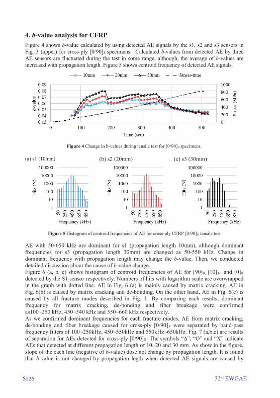
S126 32nd EWGAE

4. b-value analysis for CFRPFigure 4 shows b-value calculated by using detected AE signals by the s1, s2 and s3 sensors in Fig. 3 (upper) for cross-ply [0/90]8 specimens. Calculated b-values from detected AE by three AE sensors are fluctuated during the test in some range, although, the average of b-values are increased with propagation length. Figure 5 shows centroid frequency of detected AE signals.

Figure 4 Change in b-values during tensile test for [0/90]8 specimens.

(a) s1 (10mm) (b) s2 (20mm) (c) s3 (30mm)

Figure 5 Histogram of centroid frequencies of AE for cross-ply CFRP [0/90]8 tensile test.

AE with 50-650 kHz are dominant for s1 (propagation length 10mm), although dominant frequencies for s3 (propagation length 30mm) are changed as 50-550 kHz. Change in dominant frequency with propagation length may change the b-value. Then, we conducted detailed discussion about the cause of b-value change. Figure 6 (a, b, c) shows histogram of centroid frequencies of AE for [90]8, [10]16 and [0]8 detected by the S1 sensor respectively. Numbers of hits with logarithm scale are overwrapped in the graph with dotted line. AE in Fig. 6 (a) is mainly caused by matrix cracking. AE in Fig. 6(b) is caused by matrix cracking and de-bonding. On the other hand, AE in Fig. 6(c) is caused by all fracture modes described in Fig. 1. By comparing each results, dominant frequency for matrix cracking, de-bonding and fiber breakage were confirmed as100~250 kHz, 450~540 kHz and 550~660 kHz respectively. As we confirmed dominant frequencies for each fracture modes, AE from matrix cracking, de-bonding and fiber breakage caused for cross-ply [0/90]8 were separated by band-pass frequency filters of 100~250kHz, 450~550kHz and 550kHz~650kHz. Fig. 7 (a,b,c) are results of separation for AEs detected for cross-ply [0/90]8. The symbols “∆”, “O” and “X” indicate AEs that detected at different propagation length of 10, 20 and 30 mm. As show in the figure, slope of the each line (negative of b-value) dose not change by propagation length. It is found that b-value is not changed by propagation legth when detected AE signals are caused by

32nd EWGAE S127

certain fracture mode (When frequency range of detected AE signals is narrow) as not like Fig. 4. In order to discuss about the cause of changing b-value by propagation length in Fig. 4, the cumulative amplitude distributions of each frequency component according to fracture modes were investigated.

Figure 8 shows cumulative amplitude distribution for each fracture modes (:matrix cracking, :de-bonding, × : fiber breakage) with different AE propagation length ((a):10 mm, (b):20mm, (c):30mm). AE distribution for total of each fracture modes is also shown in the graph (symbol ). Slope of the distribution of all AE sources () which propagation length

(a) [90]16 (b) [10]16 (c) [0]8

Figure 6 Histogram of centroid frequencies of AE for [90]8, [10]16 and [0]8. Hits with logarithm scale are overwrapped in the graph with dotted line.

(a) 100~250kHz (b) 450~550kHz (c) 550~650kHz

Figure 7 Cumulative amplitude distributions of each frequency component according to fracture modes (100~250kHz = matrix cracking, 450~550kHz = de-bonding, 550~650kHz = fiber failure).

(a) 10mm (b) 20mm (c) 30mm

Figure 8 Cumulative amplitude distribution for each fracture modes with different AE propagation length.

S128 32nd EWGAE

10mm (Fig. (a)) is composed with all frequency components of 100~250kHz, 450~550kHz and 550kHz~650kHz. The negative slope of the line (b-value) becomes 0.06 and the value is different from that of each frequency sorce (100-250kHz: 0.05, 450-550kHz: 0.07 and 550-650kHz: 0.049). On the other hands, due to the frequency dependence of attenuation (high attenuation factor for high frequency components) , number of high frequency AE due to fiber breakage (550-650kHz) is drastically reduced for the results of 20 and 30 mm propagation lentgh (Fig. (b) and (c)). Though, slope of the distribution of all AE sources () which propagation length 20 and 30 mm are almost decided by 100-250 kHz component (matrix cracking) and 450-550 kHz (de-bonding) components only. From these result, the change in b-value may be caused by change in the proportion of each frequency components after the propagation due to frequency dependence of the AE attenuation.

5. Failure mechanism of CFRP estimated by b-value analysisAs propagation length affects b-value for CFRP, we focused on certain propagation length of 10mm and discussed about failure mechanism of CFRP based on b-value analysis. Figure 9 is time-series data of b-value of total AE (O: 50kHz~650kHz) during tensile test (Extracted symbol data from Fig. 4). Change in b-value for each frequency components (each fracture modes) are overwrapped in the graph (matrix cracking (◊: 100~250kHz), de-bonding (∆: 450~550kHz), fiber breakage (X: 550kHz~650kHz)). Dotted points indicate the stress during the test. Both matrix cracking and de-bonding are dominant fracture modes until 270sec., although, fiber breakage is added after 270sec.. When damage level of CFRP specimens reaches close to final fracture, fracture behaviour is changed from matrix cracking and de-bonding to fiber breakage and then each b-value changes drastically (matrix cracking: 0.003, de-bonding: 0.058, fiber breakage: 0.041 and all AE source: 0.048).

Figure 9 Relations between all AE source (50~650kHz), and each AE source according to fracture mode (100~250kHz, 450~550kHz and 550kHz~650kHz).

32nd EWGAE S129

6. ConclusionsIn this study, changes in b-values with fractures of FRPs were investigated. We conducted the tensile test with AE analysis for [0]8, [10]16, [90]16 and cross-ply[0/90]8 tensile specimens. Dominant fracture modes (matrix cracking, de-bonding and fiber breakage) are changed with stacking sequence of CFRP. The AE signals due to each fracture modes can be separated by using frequency filter of 100~250kHz (matrix cracking), 450~550kHz (de-bonding) and 550kHz~650kHz (fiber breakage). When AE sources contain single fracture mode, b-value does not chang by propagation length. On the other hand, when AE sources contain several fracture modes (AEs with different frequency range), b-value changes with propagation length. The change in b-value for multiple fracture modes may occur by change in the proportion of each frequency components after the propagation due to frequency dependence of the attenuation. Additionally, it was found that when damage level of cross-ply[0/90]8 specimens reaches close to final fracture, fracture behaviour is changed from matrix cracking and de-bonding to fiber breakage and then b-value for total AE is changed.

Acknowledgement This work was supported by JSPS KAKENHI Grant Number 16J12078.

References 1. Shiotani, T., Fujii, K., Aoki, T., and Amou, K., “Evaluation of progressive failure using

AE sourced and improved b-value on slope model tests.”, Prog. Acoustic Emission. VII, 7, pp.529-534, 1994.

2. Colombo, Ing S., I. G. Main, and M. C. Forde. "Assessing damage of reinforced concretebeam using “b-value” analysis of acoustic emission signals." Journal of materials in civil engineering 15.3, pp 280-286, 2003.

3. Gutenberg, Beno, and Charles Francis Richter. "Magnitude and energy of earthquakes."Annals of Geophysics 9.1, 1-15, 1956.

S130 32nd EWGAE

32nd EWGAE ©CNDT2016 S131

Czech Society for Nondestructive Testing32nd European Conference on Acoustic Emission TestingPrague, Czech Republic, September 07-09, 2016

TWO-DIMENSIONAL Q-VALUE AE-TOMOGRAPHY AND ITS VERIFICATION ON NUMERICAL INVESITIGATIONS

Yoshikazu KOBAYASHI 1,3, Tomoki SHIOTANI 21 College of Science and Technology, Nihon University; Tokyo, Japan

Phone: +81 3 3259 0575, Fax: +81 3 3259 0575; e-mail: kobayashi.yoshikazu@nihon-u.ac.jp 2 Faculty of Engineering, Kyoto University; Kyoto, Japan; e-mail: shiotani.tomoki.2v@kyoto-u.ac.jp

3 C-PIER, Kyoto University; Kyoto, Japan Abstract AE-Tomography is a technique that identifies source locations of AE events and elastic wave velocity distribution in objects of interest for evaluation of integrity of structures on the basis of the nature in which elastic wave velocity correlates with deterioration of materials. However, sensitivity of elastic wave velocity is insufficient to reveal the deterioration on its early stage, and further, elastic wave velocity depends on frequency of elastic wave due to dispersion. Thus, Shiotani et al. proposed a method in which Q-Value is adopted as index of the deterioration to detect the deterioration adequately, and the authors have introduced a tomographic technique that identifies elastic wave velocity and Q-Value distributions on the basis of the method to visualize distribution of the deterioration. Thus, in this study, the authors propose a new algorithm of AE-Tomography that estimates source locations of AE events, elastic wave velocity and Q Value distributions simultaneously by using arrival time of AE and gradient of logarithmic frequency response ratio at receivers on the basis of the tomographic technique. The proposed technique is verified by performing a series of numerical investigations and its characteristic is discussed in this study. Keywords: AE-Tomography, Q-Value distribution, Elastic wave velocity distribution, Source location technique, System identification, Kalman filter

1. IntroductionJapan experienced the period of high economy growth in the 60’s, and many of social infrastructures constructed during the period, and the structures are playing significant roles in the society since the time. However, decades have passed since the constructions, and the structures aged over time. According to the whitepaper of land, infrastructure, transport and tourism in Japan, it was reported that more than 60 percent of bridge decks will be older than 50 years old in 2032 [1]. For keeping serviceability of the structures, i.e. it immediately supports social activity, maintenance of the structures is an important task, and evaluation of structural integrity is necessary for the maintenance. The authors have studied on tomographic techniques, e.g. elastic wave velocity tomography for the evaluations, and the techniques have been applied for investigations of existing aged structures [2]. Among the studies, the authors recently proposed AE-Tomography (Acoustic Emission Tomography) in which elastic wave velocity distributions and AE source locations are identified by using arrival times of AE at receivers. AE-Tomography has been applied for the evaluation as well as elastic wave velocity tomography and successfully visualized deterioration of the structure. Nevertheless, AE-Tomography adopts elastic wave velocity as an index of damage of materials, and it is empirically known that sensitivity of the velocity to early stage of material damage is low, and further, in particular cases, its dispersion would cause problems on the evaluation because the damage level has to be determined by the velocity although it would change by not only damage of the material but also its frequency. For overcoming the difficulty, one of the authors proposed a technique that identifies Q-Value on two- or three- dimensional objects as an index of material deterioration of the objects [3]. Although the proposed technique assumes that Q-Value and elastic wave velocity is homogeneous on the objects, the authors proposed an algorithm of Q-Value tomography that identifies Q-Value distribution as well as elastic wave velocity distribution with consideration of heterogeneity of the distributions on the basis of tomographic

S132 32nd EWGAE

algorithm [4]. Because the proposed Q-Value tomography is on the basis of conventional tomographic technique, source information, i.e. signal emission time and location of excitation, are required, and consequently it leads limitation of application of the algorithm. Thus, in this study, a new algorithm of AE-Tomography that identifies Q-Value distribution, elastic wave velocity distribution and the AE source locations based on the ray-trace algorithm is introduced.

2. Two-dimensional Q-Value AE-TomographyAE-Tomography is a technique that identifies elastic wave velocity distribution and AE source locations by using arrival times of AE at receivers, and two-dimensional Q-Value AE-Tomography is structured on the basis of the conventional algorithm of the two-dimensional AE-Tomography. Figure 1 shows a conceptual flow diagram of Q-Value AE-Tomography. On Q-Value AE-Tomography, firstly area of interest is meshed as illustrated in Figure 2. This mesh consists of triangle and quadrilateral cells, and relay points [5] are installed on the cells to raise accuracy of the identified AE source locations. It is assumed that elastic wave velocity and Q-Value are constant in individual cells, and initial elastic wave velocity and Q-Value distributions are given as initial conditions of the analysis. On the initial conditions, AE source locations are identified, and then, elastic wave velocity and Q-Value distributions are updated by using the identified AE source locations on the basis of the tomographic algorithm. If the updated distributions fulfil a criteria of convergence, the distributions are adopted as resultant distributions. Otherwise, the procedure in a red square in Figure 1 is conducted on the updated distributions. Thus, the procedure in the red square is iteratively performed until the criteria is fulfilled. In following subsections, individual parts in the entire algorithm are introduced.

2.1 Identification of AE source locations The identification of AE source locations is performed on the basis of ray-trace technique that considers heterogeneity of elastic wave velocity distribution [6]. In a source location technique that is adopted here, firstly ray-trace is conducted from the location of a receiver that is assigned at a nodal or relay points to all of the other nodal and relay points on the mesh for obtaining first travel times from the receiver to the other points on the mesh. Because arrival times of AE

Figure 1 Flow diagram of Q-Value AE-Tomography

Figure 2 A mesh on a cross section

32nd EWGAE S133

are known at the receivers, potential emission times of AE at the other points are computed by subtracting the travel time from the arrival time. Hence, the potential emission time implies that AE is observed at the arrival time at the receiver if the AE is emitted at the potential emission time at the point. Thus, every nodal and relay points have a potential emission time for each receiver on an AE event, and consequently, each nodal and relay points have n potential emission times on the AE event if n receivers are installed on the area. If the representation of the elastic wave velocity distribution and ray-paths from the source to receivers are identical to the real ones, the potential emission times should be the same at a source location of the AE event. However, a point at which variance of the potential emission times is minimum is adopted as the source location since the representation is generally not identical to the real ones. Additionally, an emission time of an AE is approximated as an average of the potential emission times at the source location.

2.2 Observation equation for identification of elastic wave velocity and Q-Value distributionsSince the source location and emission time of AE are already identified, elastic wave velocity and Q-Value distributions are identified in the method of Q-Value tomography that was proposed by the authors [4]. As demonstrated in the conventional elastic wave velocity tomography, observation equation for first travel time is shown as follows in general on, for example, a ray-path that is illustrated in Figure 3.

(1)

In which, is arrival time of AE of event at receiver , is the estimated emission time of AE of event , is slowness, reciprocal of elastic wave velocity, of cell , and is length of a ray-path from source of AE event to receiver in cell . Thus, the ray-path does not across cell , is identical to zero. Since the elastic wave velocity distribution is generally heterogeneous on real structures because damage or insufficient quality of materials cause decreasing of the elastic wave velocity. If the elastic wave velocity distribution is heterogeneous, the ray-paths bend because of reflation and diffraction of the elastic wave. This influence is considered in this study by performing ray-trace on the mesh to obtain the ray-paths. This is a shortest path problem, and Dijkstra method is used to solve the problem here. For the

Figure 3 Example of ray-path and its travel time

S134 32nd EWGAE

identification of Q-Value distribution, another observation equation is necessary. The authors proposed an observation equation for the identification of Q-Value distribution in an algorithm of Q-Value Tomography on the basis of a technique that evaluates integrity of materials by using Q-Value proposed by Shiotani et. al [3]. In the technique, it is assumed that AE is observed at receivers on an observation system that is illustrated in Figure 4. The observation system is described as follows in frequency domain.

(2)

In which, is acceleration of AE event at receiver , is acceleration of AE event at its source location, is transfer function of cell on the ray-path from source location of AE event to receiver . It should be noted that is not taken account if cell is not on the ray-path. Further, and are transfer functions of receiver and data acquisition system, respectively. Thus, if AE event is observed at two receivers, namely receiver and , for example as shown in Figure 5, ratio of accelerations between the two receivers in frequency domain are described as follows in general.

∏ ∏

∏ ∏

(3)

In Equation 3, it is assumed that and are identical to simply the computational procedure. Q-Value is a parameter that relates with dissipation of kinetic energy while propagation of elastic wave in media. Q-Value is defined as

(4)

where and are energy of the elastic wave and dissipation of the energy during a cycle. A transfer function of elastic wave between two points of which distance is is given as follows on the basis of Equation 4 on homogeneous materials.

(5)

In which, , , are frequency of the elastic wave, elastic wave velocity and Q-Value of the material, respectively. By applying Equation 5 to compute the transfer functions of individual cells on the ray-paths, the transfer function of cell is obtained as follows.

Figure 4 Observation in frequency domain

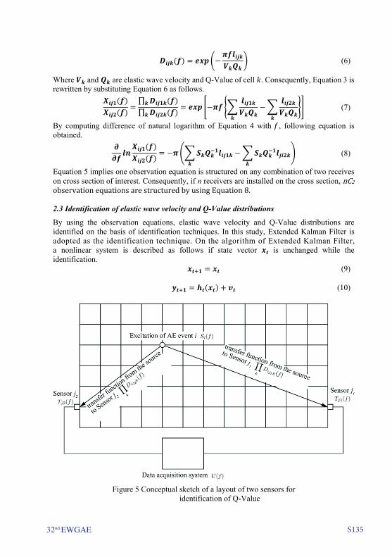
32nd EWGAE S135

(6)

Where and are elastic wave velocity and Q-Value of cell . Consequently, Equation 3 is rewritten by substituting Equation 6 as follows.

∏ ∏

(7)

By computing difference of natural logarithm of Equation 4 with , following equation is obtained.

(8)

Equation 5 implies one observation equation is structured on any combination of two receives on cross section of interest. Consequently, if n receivers are installed on the cross section, nC2observationequationsarestructuredbyusingEquation8. 2.3 Identification of elastic wave velocity and Q-Value distributions

By using the observation equations, elastic wave velocity and Q-Value distributions are identified on the basis of identification techniques. In this study, Extended Kalman Filter is adopted as the identification technique. On the algorithm of Extended Kalman Filter, a nonlinear system is described as follows if state vector is unchanged while the identification.

(9)

(10)

Figure 5 Conceptual sketch of a layout of two sensors for identification of Q-Value

S136 32nd EWGAE

in which, , and are observation vector, mapping function from to and noise of the observation, respectively. On this system, elastic wave velocity and Q-Value on individual cells are used as state values in the state vector. The mapping function is formed by combining Equations 1 and 7. It should be noted that Equation 9 demonstrates that the elastic wave velocity and Q-Value of the cells are unchanged while the process of the identification in this study. Thus, this technique is only applicable for the materials which state is unchanged while the observations. This implies that AE events that are used as the observation on this technique should be the secondary AE because occurrence of primary AE indicates fracture is progressing, and it consequently demonstrates state of the material is changing. On the basis of Equations 9 and 10, Extended Kalman Filter is structured as follows.

(11)

(12)

in which, and are identified state vector at on the basis of the information at and , respectively. is a Kalman gain as shown in following equations.

(13)

(14)

(15)

where and are estimated error covariance matrices of the state vector at on the basis of the information at and , respectively, is an error covariance matrix of the observation vector at . These matrices indicate reliability of initial state value and observations, these matrices should be given appropriately on the basis of accuracy of the initial distributions and observations. It should be noted that non-diagonal term of R and P are set to zero in this study. Further, it is assumed that is constant while the identification. This implies that elastic wave velocity and Q-Value on the individual cells are independent each other. However, if the correlations are demanded, it can be specified by giving appropriate quantities. is an observation vector that is described as follows.

(11)

By applying Equations 11 and 12 iteratively, the state vector is appropriately identified.

3. VerificationsThe introduced algorithm of Q-Value AE-Tomography is verified by performing a series of numerical investigations. Figure 6 shows a cross section that is used for the verifications. The cross section is a square with a side length of 15m and receivers are installed at the apexes of the cross section. Thus, there are 4 receivers on the cross section in the verification. The cross section consists of two types of regions. Regions of one of the types are coloured with white and regions of the another type are coloured with grey, and the white and grey regions are supposed intact and damaged area, respectively. For these verifications, two models that are described in Table 1 are adopted in this study. As shown in Table 1, elastic wave velocity and Q-Value are set to 4000m/s and 50 on the white region, and 3000m/s and 20 on the grey region in Case 1. This case assumes that the degradation of the grey region is severe, and both of elastic wave velocity and Q-Value are relatively low due to the degradation. On Case 2, the elastic

32nd EWGAE S137

wave velocity on the grey region is raised to 4000 m/s in comparison with Case1. This case assumes the degradation is still on its early stage and elastic wave velocity is keeping its quantity in intact condition. Since the observations are necessary for the numerical investigations, 100 artificial AE events are generated randomly on the cross section, and the observations are computed by performing the ray-trace from the generated artificial sources to the receivers for the arrival time and using Equation 1 on resultant ray-path of the ray-trace, and assuming straight ray-paths from the AE source to the receives and using Equation 8 on the straight ray-paths for gradient of logarithmic frequency response ratio. Thus, total number of the observation equations is 400 for the arrival time, and 600 for the gradient of logarithmic frequency response. Consequently, there are 1000 observation equations in this investigation. As the initial distributions, homogeneous elastic wave velocity distribution of 4000 m/s, and homogeneous Q-Value distribution of 50 are given. Figures 7 and 8 show identified elastic wave velocity distribution and Q-Value distribution in Case 1 at 5th iteration and the end of the identification. On the figures, the white circles are identified source locations and the black circles are real source locations that are generated artificially. According to the Figures 7 and 8, the identified distributions qualitatively reproduce the original distributions. On the identified Q-Value distribution, there are high Q-Value area from left side to center on the band of 5.5m to 10 m in y coordinate of the cross section. The low Q-Value areas exist on the upper and lower parts of the cross section and this results shows the same tendency with the original model that is illustrated in Figure 6. However, the low Q-Value area penetrates from the upper part to the lower part on the right side of the cross section. On the identified elastic wave velocity distributions, it shows the same tendency with the original model as well. There are low velocity areas exists on the upper and lower part of the cross section as well. The penetration of the low Q-Value area is caused by the resolution of the source location technique and limitation of the identification technique. Since resolution of source locations is density of relay and nodal points in this source location technique, and further, because the resultant elastic wave velocity is not identical to the original one, there are errors on the source locations. Under this situation, relative error of the source locations becomes large if the source location and receiver is close, and consequently, resultant Q-Value distribution is affected by the error. Moreover, since Equation 9 is defined as products of Q-Value and elastic wave velocity, the equation is fulfilled if the products is identical to the

Figure 6 Numerical model for the verification

Table 1 Conditions Case 1 Case 2

V(grey zone) 3000m/s 4000m/s

Q(grey zone) 20 20

V(white zone) 4000m/s 4000m/s

Q(white zone) 50 50

Num. Events 100 100

Num. Iteration 200 200

Initial V 4000/s 4000m/s

Initial Q 50 50

S138 32nd EWGAE

original value. Thus, in the right side on the band of y=5.5m to 10m, the elastic wave velocity is overestimated, and consequently, Q-Value would be underestimated. Further, the identified source locations moved between the middle and the end of the identification. This is because the elastic wave velocity distribution is updated while the identification, and the source locations identified more closely to the real source locations due to the update of the elastic wave velocity distribution. Figures 9 and 10 show identified elastic wave velocity and Q-Value distributions in Case 2 at 5th iteration and the end of identification. Since the elastic wave velocity distribution is the homogeneous one of 4000 m/s in the original model in this case, change of elastic wave velocity distribution while the identification is suppressed and the identified elastic wave velocity distribution is consequently very close to the original elastic wave velocity distribution. In contrast, although Q-Value distribution largely changes from the initial distribution, the identified Q-Value distribution reproduces the original distribution very well. This is because the accuracy of the identified source locations is high because of the identified elastic wave velocity distribution is almost identical to the real one. Due to the highly accurate source locations and elastic wave velocity distributions, actual number of degree of freedom is drastically reduced since the variables that actually identified is only Q-Value distribution.

Figure 7 Identified Q-Value distribution in Case 1 (Left: after 5 iterations, right: after 200 iterations)

Figure 8 Identified elastic wave velocity distribution in Case 1 (Left: after 5 iterations, right: after 200 iterations)

32nd EWGAE S139

Consequently, the Q-Value distribution is identified with sufficient number of observations and it was identified more accurately. These results suggest that the introduced technique identifies Q-Value and elastic wave velocity distributions more accurately on the early stage of degradation. Because it is known the sensitivity of Q-Value is higher than the elastic wave velocity to the damage, and it is supposed that the elastic wave velocity is still close the velocity in intact condition nevertheless Q-Value is already low because of the damage. This characteristic of the proposed method is an advantage of the policy of the proactive maintenance since finding of the damage on the early stage is demanded on the policy.

3. Conclusions

In this study, a new algorithm of Two-dimensional Q-Value AE-Tomography that identifies Q-Value and elastic wave velocity distribution and source locations of AE events by using only observed AE data at receivers is introduced. The introduced techniques are verified by performing a series of numerical investigations, and following conclusions are drawn.

Figure 9 Identified Q-Value distribution in Case 2 (Left: after 5 iterations, right: after 200 iterations)

Figure 9 Identified Q-Value distribution in Case 2 (Left: after 5 iterations, right: after 200 iterations)

S140 32nd EWGAE

1. The introduced algorithm was verified on a model that has deteriorated regions in whichboth of elastic wave velocity and Q-Value is low as a case that the regions damagedheavily. The results show that the proposed method identifies Q-Value and elastic wavevelocity distributions adequately.

2. The introduced algorithm was verified on a model that has deteriorated regions in whichOnly Q-Value is low as a case that the regions damaged slightly. In this case, the identifieddistributions are consistent with the original distributions as well. Especially, theidentified Q-Value distribution is more accurate than the heavily damaged case and thischaracteristic suggested the proposed technique would be efficient for the evaluation ofstructural integrity for proactive maintenance.

Acknowledgement

This study is supported by JSPS KAKENHI Grant Number JPNumber 15K06193 Grant-in-Aid for Scientific Research (C), Japan Society for the Promotion of Science(JSPS)

References

1. Ministry of Land, Infrastructure, Transport and Tourism, 'White paper of land,infrastructure, transport and tourism in Japan 2013', Ministry of Land, Infrastructure,Transport and Tourism website: http://www.mlit.go.jp/en/statistics/white-paper-mlit-2013.html, 2013

2. S., Momoki, T. Shiotani, H. K. Chai, D. G. Aggelis, Y. Kobayashi, ‘Large-scaleevaluation of concrete repair by three-dimensional elastic-wave based visualizationtechnique’, Structural Health Monitoring, Volume 12, No 3, pp 241–252, 2013

3. T., Shiotani, Y. Takada, T. Watanabe, H. Ohtsu, ‘Damage evaluation of heterogeneousmaterials by Q-value analysis of AE waveforms’, JSNDI, Progress in Acoustic EmissionXV, 1-6, 2012.

4. Y. Kobayashi, T. Shiotani, ‘Two-dimensional Q-Value Tomography and its verificationbased on numerical investigations’, Proceedings of Structural Faults and Repair 2016,May 2016

5. Y. Kobayashi, ‘Mesh-independent ray-trace algorithm for concrete structures’,Constructions and Building Materials, Volume 48, pp. 1309–1317, 2013

6. Y. Kobayashi, T. Shiotani, ‘Seismic Tomography with Estimation of Source Location forConcrete Structures’, Proceedings of Structural Faults and Repair 2012, July 2012

32nd EWGAE ©CNDT2016 S141

Czech Society for Nondestructive Testing32nd European Conference on Acoustic Emission TestingPrague, Czech Republic, September 07-09, 2016

STUDY OF FATIGUE PROCESSES OF SELECTIVE LASER MELTING AND CONVENTIONAL PRODUCED MATERIALS

Vendula KRATOCHVILOVA1a, Frantisek VLASIC1b, Pavel MAZAL1c

1 Brno University of Technology, Faculty of Mechanical Engineering; Technicka 2896/2, 616 69 Brno, Czech Republic

Phone: +420 54114 3240; e-mail: a xkrato04@vutbr.cz, b vlasic@fme.vutbr.cz, c mazal@fme.vutbr.cz

Abstract

The main aim of the study is to compare fatigue processes and its acoustic emission (AE) signal of conventional produced material and material produced by selective laser melting (SLM) technology. The SLM offers the same benefits as the rest of the rapid prototyping technologies, the most important is big range of produced shapes, but without expensive moulds, cores or huge material waste. However the mechanical properties of these materials are currently worse than those of conventionally produced materials. AE method was used to get new information about fatigue damage of SLM materials. This study summarizes results from bending fatigue tests of reference Al alloy AW-2618A (AlCu2Mg1,5Ni) and SLM material with comparable chemical composition. Acquired AE and fatigue data from both materials were compared. The fractographic and metallographic analysis were also conducted as complement. Internal defects and inhomogenities in SLM materials cause different fracture behaviour than we can see at conventional materials. Differences in fatigue behaviour of SLM materials are strongly reflected in AE signal. The results may be used to improve the production of SLM materials in order to get better material characteristics. AE data helps to understand the fatigue behaviour of SLM materials in order to predict crack initiation.

Keywords: selective laser melting, acoustic emission method, fatigue, crack, Al alloy

1. IntroductionRapid prototyping (RP) technologies, especially those that enable to produce metal parts are nowadays under intensive studies. Selective laser melting (SLM) technology produces parts by adding thin material layers, which are connected by melting by focused laser beam (Fig. 1a) [1]. This allows producing parts with complicated shapes without huge material waste or expensive moulds and cores. As the SLM technology is still under research, achieved mechanical characteristics, especially fatigue, are not as good as in case of conventional produced materials. Current studies were aimed mainly on titanium alloy and steel, aluminium alloys have been overlooked. For titanium alloy Ti-6Al-4V was possible to get better fatigue life than is usual in cast material and equivalent to the cast material with heat treatment [2]. For stainless steel SS 316L and 15-5PH was possible to get only 20-25 % lesser fatigue life than has conventionally produced materials and fatigue life was strongly effected by surface quality [3]. This is mainly connected with internal defects, which could be more or less similar as casting or welding defects – porosity, lack of material, but we can also see typical SLM defects for example unmelted powder in cavities [2, 4]. Those defects could be eliminate by optimizing of process parameter, which are scanning speed [5], laser power [6], powder grain size and quality [7], building strategy [8], hatch spacing [9] and layer thickness [10]. Acoustic emission (AE) is one of the standard non-destructive (NDT) methods. It allows to detect, localize and evaluate defects during their formation, so it is suitable for fatigue process

S142 32nd EWGAE

monitoring [11]. There is possible not only to detect and characterization fatigue damage growth [12], but also to distinguish various stages of fatigue phases, to predict the rate of crack propagation [13] and to identify sources of AE in metals fatigue specimens and relate them to damage mechanisms [14, 15].

2. Material and methodsTesting material is aluminium alloy. The results from fatigue testing and AE data of SLM material were compared with results of reference conventionally produced (extruded) material from Al alloy AlCu2Mg1,5Ni (2618A) with T6 heat treatment, chemical composition of SLM material is similar. Chemical composition of both materials is shown in Table 1.

Table 1. Chemical composition (%) of reference and SLM material

Element Si Fe Cu Mg Ni Ti Reference material 0,24 1,1 2,5 1,5 1,2 0,04 SLM powder 0,15 1,0 2,66 1,39 1,22 0,2

SLM samples were produced by SLM 180 HL machine. At the beginning there were tried different process parameters. Quality of produced samples were evaluated on the basis of relative density, the best result was 0,35 %. The final optimal parameters were: laser power 200 W, laser speed 100 mm/s, hatch distance 110 µm and beam diameter 82 µm. Scanning strategy were meander and it is shown in the Fig. 1b) [17].

a) b) Figure 1. SLM technology principle (a) [16] and meander scanning strategy (b) [17]

A set of 26 specimens was made from reference material, 13 pieces of this set were subjected to heat treatment (T6). 3 sets of 4 pieces were made from SLM material. Two sets were made from new powder; the difference was in the distribution of samples on the plate. Samples from 1st set (identified as 2015) were made one by one, but pieces from 2nd set (identified as 2016) were produced together. 3rd set was made from recycled powder. On the metallographic samples (Fig. 2) we can clearly see layer borders and a lot of defects near them (red arrows in the Fig. 2). This kind of internal structure has bad influence on fatigue life. The bending fatigue tests were carried out by electro-resonance RUMUL Cractronic 8204 testing machine. The fatigue cycle was sinusoidal in stress ratio R = -1, test were conducted in high-cycle region in room temperature. Approximate loading frequency was about 52 Hz.

32nd EWGAE S143

Figure 2. Microstructure of SLM material in the longitudinal (left) and transverse (right) direction

AE signal was detected by a DAKEL-XEDO and also by IPL system using two piezoelectric DAKEL IDK-09 sensors with 35 dB preamplifiers. The sensors were clamped on each end of the specimen by Loctite glue in order to create a two channel linear location system. Advanced IPL continuous data storage system was used to record all the incoming signals sampled by 2MHz. This system covers the frequency bandwidth of approximately 20 – 800 kHz with a total system gain of 80 dB. The threshold detection of the AE hits was frequently applied in post processing.

3. ResultsAll specimens were machined to the shape in the Fig. 3 and fatigue tested in same conditions at different stress level. The results were compared using standard S-N curves (Fig. 4). SLM material has significantly worse fatigue resistance than reference extruded material. Extruded material with T6 treatment has slightly better results than material without treatment. The results of SLM material fatigue show that the quality of produced material is strongly depend not only on process parameters, but also on the quality of the used metal powder. Specimens made from recycled powder have significantly worse fatigue resistance than specimens from new powder.

Figure 3. Fatigue testing specimen

The AE measurements were carried only at several stress levels. In order to get an overview of the AE activity, the number of counts and cumulative number of events was observed, at the beginning in the reference material (Fig. 5). The beginning of loading (pre-initiation stage) is characterized by high AE activity caused by changes in material microstructure, interaction and glide of dislocations and persistent slip band formation. This stage is followed by low and

S144 32nd EWGAE

constant AE activity, which takes about 1/3 of the lifetime; micro-cracks start to propagate here (initiation stage). AE activity significantly increases in the last stage, where the long crack is growing (post-initiation stage).

Figure 4. S-N diagrams of extruded and SLM materials

The same three stages were observed in the SLM material, but the AE activity is significantly different (see Fig. 5b). The main differences are in count rate, ratio and duration of the stages. First two stages, pre-initiation and initiation stages, takes about half of the total fatigue lifetime, especially the initiation stage is much shorter than in reference material. This behaviour is probably cause by large amount of production defects (pores and shrinkages).

a) b) Figure 5. AE counts and loading frequency vs. noramlized fatigue cycles of AlCu2Mg1,5Ni at stress amplitude

level of 229 MPa (a), SLM at stress amplitude level of 122 MPa (b)

Significant differences were also observed in the AE amplitude values and duration in different phases of fatigue process (comparing the initial phase is given in Fig. 6). In the pre-initiation stage of the reference material was observed a lot of events with big scatter of amplitude value and its duration, most events from the 1st stage of SLM material have amplitude between 45 and 48 dBAE with low duration. Reference material initiation stage is characterized by signal with low amplitude and duration, which are coming from the micro-crack initiation, the same stage of SLM material is characterized by higher amplitude with low duration.

32nd EWGAE S145

a) b) Figure 6. Linear regression of AE events in the initiation stage of AlCu2Mg1,5Ni (a) and same stage of SLM material (b)

a) b)

Figure 7. Distribution of signal energy in different stages of fatigue (a) AlCu2Mg1,5Ni, (b) SLM

Percentage of the overall signal energy in the different stages of fatigue process for reference material and SLM material is given in Fig. 7. The crack initiation phase (“ini” in the graph) normally spans the minority of the considered life-cycle in reference material while the pre-initiation phase (“pre-“ in the graph) usually covers almost the entire life-cycle. Unfortunately, this study did not confirm the relationship between phase duration and bending amplitude. More convincing and consistent results come from SLM material. Here is clear, despite the inhomogeneous structure of SLM, the crack propagation phase (“post-“ in Fig. 7b) spans more than 2/3 life-cycle in all cases of amplitude level. This is caused by manufacturing defects cause early crack initiation and growth due to cyclic loading. Therefore the initiation phase as well as pre-initiation phase is very short here. This is also seen in Fig. 5b where the loading frequency is going down very soon and AE hits change its parameters. The fatigue and AE measurements were supplemented by fractographic study, see Fig. 8 and Fig. 9. There is clearly visible a production defects in the Fig. 8 (red ring), the unmelted powder particles (yellow arrows) shows, that the defect was created during production.

S146 32nd EWGAE

Figure 8. The fractography of SLM material with marked defect

The red rings in the Fig. 9 and 10 mark the crack origins, which are located in the production defects. There are the unmelted powder particles in the cavities, so those defects were also created during the manufacturing process.

Figure 9: The fractographic of SLM material with marked crack origins, stress amplitude level 122 MPa

32nd EWGAE S147

Figure 10. The fractographic of SLM material with marked crack origins, stress amplitude level 61 MPa

4. ConclusionThe results from fatigue testing of aluminium alloy AlCu2Mg1,5Ni and SLM material with similar chemical composition supplemented by AE measurement and fractographic were presented in the paper. The results from both material were compared and many differences, but also some similar behaviour were observed. All 3 batches of SLM material have significantly worse fatigue life than conventionally produced (extruded) material. The AE signal showed the same three stages in both materials, pre-initiation, initiation and post-initiation stage. The ratio of the stages, AE amplitude and duration is significantly different in SLM and reference material. The fractographic study of SLM samples showed that the crack origins are located in the surface defects, which were created during the production. The production parameters for production of cyclical loaded parts from material AlCu2Mg1,5Ni is not optimized yet and further research is needed.

5. AcknowledgementsThe authors would like to thank the Czech Science Foundation (GACR) for the funding of the project GA15-23274S “Design of advanced materials using selective laser melting”. The project is also supported by NETME Centre (New Technologies for Mechanical Engineering), Reg. No. CZ.1.05/2.1.00/01.0002 and, in the follow-up sustainability stage, supported through NETME CENTRE PLUS (LO1202) by financial means from the Ministry of Education, Youth and Sports under the „National Sustainability Programme I“ and by the project No. FSI-S-14-2329 “Vibro-isolation system of cosmic carrier payload” of the Faculty of Mechanical Engineering.

References 1. J.P. Kruth, P. Mercelis, J. Van Vaerenbergh, L. Froyen and M. Rombouts, 'Binding

mechanisms in selective laser sintering and selective laser melting', Rapid Prototyping Journal, Vol 11, No 1, pp 26-36, 2005.

2. Q. Liu, J. Elambasseril, S. Sun, M. Learz, M. Brandt and P.H. Sharp, The Effect ofManufacturing Defects in The Fatigue Behaviour of Ti-6Al-4V Specimens Fabricated Using Selective Laser Melting', International Fatigue Congress, PTS 1 and 2. Melbourne, Australia 2014, pp 1519-1524, 2014.

S148 32nd EWGAE

3. A.B. Spierings, T.L. Starrand K. Wegener, 'Fatigue performance of additivemanufactured metallic parts', Rapid Prototyping Journal, Vol 19, No 2, pp 88-94,2013.

4. H. Gong, K. Rafi, H. Gu, G.D. Janaki Ram, T. Starr and B. Stucker, 'Influence ofdefects on mechanical properties of Ti–6Al–4V components produced by selectivelaser melting and electron beam melting', Materials and Design, Vol 86, pp 545-554,2015.

5. K. Rafi, H. Khalid, T. L. Starr and B. E. Stucker, 'A comparison of the tensile,fatigue, and fracture behaviour of Ti–6Al–4V and 15-5 PH stainless steel parts madeby selective laser melting', International Journal of Advanced ManufacturingTechnology, Vol 69, No 5-8, pp 1299-1309, 2013.

6. B. Song, S. Dong, S. Deng, H. Liao and C. Coddet, , 'Microstructure nad tensileproperties of iron parts fabricated by selective laser melting', Optics and LaserTechnology, Vol 53, No 3, pp 451-460, 2014

7. D. Bourell, A.B. Spierings, N. Herres and G. Levy, 'Influence of the particle sizedistribution on surface quality and mechanical properties in AM steel parts', RapidPrototyping Journal, Vol 17, No 3, pp 195-202, 2011.

8. P. Mercelis and J.P. Kruth, 'Residual stresses in selective lasesr sintering andselective laser melting', Rapid Prototyping Journal, Vol 12, No 5, pp 254-265, 2006.

9. B. Vandenbroucke and J.P. Kruth, 'Selective laser melting of biocompatible metalsfor rapid manufacturing medical parts', Rapid Prototyping Journal, Vol 13, No 4, pp196-203, 2007.

10. K. ABD-Elghany and D.L. Bourel, 'Property evaluation of 304L stainless steelfabricated by selective laser melting', Rapid Prototyping Journal, Vol 18, No 5, pp420-428, 2012.

11. A. Shanyavskiy nad B. Mukharbiy, 'Fatigue cracking and acoustic emissionregularitires in Metals: Crack origination and growth', Key Engineering Materials,Vol 592, No 5, pp 735-740, 2013.

12. I.M. Daniel, J.J. Luo, C.G. Sifniotopoulos and H.J. Chun, 'Acoustic emissionmonitoring of fatigue damage in metals', Nondestructive Testing and Evaluation,Vol 14, pp 71-87, 1998.

13. Z. Han, H. Luo, C. Sun, J. Li, M. Papealias and C. Davis, 'Acoustic emission studyof fatigue crack propadation in extruded AZ31 magnesium alloy', Materials Scienceand Engineering A, Vol 597, pp 270-278, 2014.

14. K. Shrama, A. Clarke, R. Pullin and S.L. Evans, 'Detection of cracking in mild steelfatigue specimens using acoustic emission and digital image correlation', KexEngineering Materials, Vol 592, pp 735-740, 2013.

15. L. Nohál, F. Hort, J. Dovřáček and P. Mazal, 'An experimental investigation ofrolling contact fatigue of steels using acoustic emission method', Insight, Vol 55, No12, pp 665-669, 2013.

16. 3D Printing Processes: The Free Beginner’s Guide. 3D Printing Industry [online].2013. Available on: http://3dprintingindustry.com/3d-printing-basics-free-beginners-guide/processes/

17. O. Koukal, D. Koutný, D. Paloušek, R. Vrána, T. Zikmund and L. Pantělejev,'Research about the influence of process parameters of selective laser malting onmaterial EN AW 2618', Euro PM2015 Proceedings, Reim, France, pp 1-6, 2009.

32nd EWGAE ©CNDT2016 S149

Czech Society for Nondestructive Testing32nd European Conference on Acoustic Emission TestingPrague, Czech Republic, September 07-09, 2016

ACOUSTIC EMISSION TESTING ON LPG TANKS - DEFECT DETECTION CASE STUDIES

Gerald LACKNER 1, Peter TSCHELIESNIG 21 TÜV AUSTRIA, Deutschstrasse 10, 1230 Vienna, Austria; e-mail: gerald.lackner@tuv.at

2 AT – Consult e.U., Planckhgasse 21, 3400 Klosterneuburg, Austria; e-mail: office@at-consult.at

Abstract

One main practical application of acoustic emission is testing of metallic pressure vessels at site of installation in the field. Beginning with the qualification of the employed testing technique and then throughout the whole period of field testing, people want to know what the intervention on the test object is good for. It is in the very interest of the stakeholders (manufacturers, owners, operators, authorities as well as testing and inspection organisations) to verify its capabilities. Practical examples of detected defects taken from qualification tests as well as from routine tests are able to demonstrate the main advantages and thus support the acceptance of the testing technique by all parties concerned. This contribution describes by means of case studies a few tests on LPG tanks where severe defects were found.

Keywords: liquefied petroleum gas (LPG) tank, pressure vessel, field testing, integrity testing, corrosion detection, leakage detection, crack detection

1. IntroductionThe requalification of a pressure equipment after a certain period of service requires usually a set of inspections/tests in order to assess the structural integrity. Depending on the legal environment given in the country of installation, the set of inspections/tests to be performed may consist of external inspection, pressure test, leak test, internal inspection and the like. Acoustic emission testing (AT) may be employed in the course of the requalification either alone or in combinations with other tests. It provides information regarding the structural integrity of the item under test at the same level of safety achieved by conventional inspections/tests. The following list highlights the most important drivers for its application:

• Internal inspection is considered to be a high risk activity. Entry into a confined spaceneeds thorough preparation and execution. Serious situations in the course of internal inspections are reported every year. Acoustic emission testing on LPG tanks makes internal inspection unnecessary.

• Water used for hydrostatic testing is considered to be a hazardous waste and has to bedisposed at specialised facilities. Furthermore, residual humidity may induce or promote internal corrosion. Acoustic emission testing does not require to empty or to clean the tank. In most cases it is performed with the LPG of the tank under test. After completion of the test, the tank is immediately available for the consumer.

• In the event of an already severely damaged tank, monitoring of the pressurisation withacoustic emission provides on-line information regarding the actual condition of the tank and thus enables the test operator to suspend or even to terminate the test in a safe way in order to prevent a serious situation to evolve.

Starting from 1993, when the first testing campaign in Austria with more than 1000 tank tests had been completed, TÜV AUSTRIA and its cooperation partners have been testing successfully several thousands of LPG tanks in Austria and other European countries till

S150 32nd EWGAE

today. The core part of the developed procedure consists of the testing technique including the Cluster Evaluation Factor (CEF) based on measuring equipment from Vallen Systeme and the mobile testing laboratory. The on-board pressurisation unit utilizes for evaporation some part of the liquid phase of the LPG tank under test and feeds back the resulting gas phase at a higher pressure, thus being independent from other pressurisation media like nitrogen. The applied testing technique is described in detail in several publications [1, 2]. This contribution focuses on the discussion of test results obtained from different qualification, demonstration or testing activities at different sites.

2. Case study for crack detection on an above ground tankA serious incident occurred in Austria in 2009, where a LPG tank failed during a filling operation inside a gas facility. One head of the tank detached from the cylinder and it was sent about 100 m away where it hit the ground luckily without causing major damage, neither at the gas facility nor at the neighbouring facility as shown in figure 1. However, this incident triggered a follow-up investigation and it was found that both circumferential welds (joggle joints) were affected by stress corrosion cracking (SCC) due to unspecified maintenance works performed on the tank using a corrosive medium. At the other joggle joint a crack with a length of approximately 1 m centred at the 6 o’clock position had been detected. It had to be shown to the authority that in case of further tanks with similar history, such kind of defect will be detected by AT while performing the pressurisation. For this purpose a new head was welded onto the tank. It was intended to pressurise the tank till to burst for obtaining the burst pressure of the already severely damaged tank. The pressurisation was monitored with AT during the pressure test section and the results were analysed and described in reference [3]. It could be shown that the degradation was indicated by AT well before the failure of the tank. The sensor positions and the measuring results are given in figure 1 and figure 2 respectively. On the other hand side, the tank passed the hydrostatic test (test pressure equal to 1,5 times the design pressure) without any finding of plastic deformation or leakage.

Figure 1. Set-up of an above ground LPG tank (2700 litre) for crack detection, photo on the top left shows the tested tank with new head welded onto the tank near sensor XD 1, photo on top right shows the affected

circumferential weld near to the tank leg after the previous failure of the tank head, graph below indicates the incident with the head sent about 100 m away, over the neighbouring road right into another facility.

32nd EWGAE S151

Figure 2. Qualification test on an above ground LPG tank (2700 litre), tank was loaded up to 1 MPa (10 bar) before the test, graphs show CEF and pressure vs. time (1st row left), CEF of located events vs. position along the cylinder lengths (1st row right), maximum amplitude and energy accumulation of located events vs. time

(2nd row left), waveform and frequency content of an event located near to sensor XD 2 (2nd row right)

One may easily take from figure 2 that the activated degradation process lead to rather high values of CEF at an early stage. The test operator had to be alarmed already at about 1,1 MPa (11 bar with value of CEF equal to 2,6) and the test was to stop at the latest at 1,3 MPa (13 bar with value of CEF equal to 2,9). And it is obvious that the obtained location results based on the linear location using sensors XD 1 and XD 2 (both VS150-RIC, Vallen Systeme) near to the circumferential welds are in good agreement with the location of the SCC affected weld near to sensor XD 2. The performed test and the gained results were another proof of competence towards the Austrian Accreditation Body, where TÜV AUSTRIA SERVICES GMBH is accredited as ISO 17025 testing laboratory with the scope of accreditation comprising the European standards EN 12817 and EN 12819 (requalification of LPG tanks up to 13 m3 and greater than 13 m3, respectively).

3. Case study for corrosion detection on an underground tankLPG companies usually perform a service provider assessment prior to awarding a long term frame contract for performing AT on their tank population. The purpose of this measure is to demonstrate the quality and the effectiveness of the proposed testing service. In many cases this includes a demonstration on real structures, where tanks with or without defects are to be tested and evaluated.

At the site of a gas storage facility we were invited to test an underground tank, which was buried according to figure 3. The linear sensor setup consisted of sensors XD 1 at the circumferential weld near to the valve chamber, XD 3 in the area of the valve chamber and XD 4 at the other circumferential head of the tank. All three sensors were of type VS75-SIC. The pressurisation was done by a nitrogen blanket on top of a liquid product. The only information we received from the tank owner regarding the tank condition was, that the tank

S152 32nd EWGAE

had been tested previously by another testing organisation. Therefore we asked to pressurise the tank up to 1,1 times the design pressure, which was near to 2 MPa (20 bar). In this way we obtained the maximum amount of information still achievable by AT and at the same time we kept rather close to the design limits due to risk considerations. All three sensors were mounted on the 12 o’clock position after removing the soil at their defined location.

Figure 3. Set-up of an underground LPG tank (5000 litre) for detection of degradation, photo on the top shows the buried tank with the valve chamber box in green and sensors XD 1, XD 3 and XD 4 (VS75-SIC) used for

linear location, photo on bottom right shows some corrosion effects in the area below the valve chamber, photo on the bottom left shows the close-up of the maximum affected area.

Figure 4 indicates that the given active sources lead to a value of CEF above 2,4 at about 1,7 MPa (17 bar) and then increased at about 1,9 MPa (19 bar) to a value of CEF above 2,8. The tank owner was satisfied with this result and after a final presentation no further information regarding the technical background was requested. All questions were answered in sufficient detail and finally we won a frame contract for a three years duration. In order to fulfil the required number of tested tanks per year we had to produce additional mobile testing laboratories and we had to train local test operators. Both tasks were handled for the subsidiary TÜV AUSTRIA TURK by the acoustic emission unit of TÜV AUSTRIA based in Vienna.

32nd EWGAE S153

Figure 4. Qualification test on an underground LPG tank (5000 litre), tank loaded before the test till to at least 1,4 MPa (14 bar) , graphs show CEF and pressure vs. time (1st row left), CEF of located events vs. position

along the cylinder lengths (1st row right), maximum amplitude and energy accumulation of located events vs. time (2nd row left), waveform and frequency content of an event located near to sensor XD 1 (2nd row right)

4. Case study for leak detection on an above ground tankDuring a regular field testing route on the Iberian Peninsula, the test operator of QTEC – the Portuguese subsidiary of TÜV AUSTRIA group - came to an above ground tank as shown in figure 5. He applied the usual test set-up procedure and then started with the pressurisation by feeding LPG liquid phase from the tank under test to the mobile laboratory, where it was evaporated in the heat exchanger and fed through the filling valve back to the gas phase.

Figure 5. Field test on an above ground LPG tank (2300 litre), photo of the tested tank

S154 32nd EWGAE

He saw that the value of CEF increased rather quickly as shown in figure 6 and was alarmed. Additionally he realised that the background noise (given by the measuring parameter RMS-status) was rising with increasing load (see figure 7). This led him to the conclusion that there might be a leakage at the tank fittings. A leakage was confirmed at the first pressure hold where after closing the gas flow to the tank the RMS-status did not reduce, as it is supposed to do in case the increase of noise is caused by the gas flow to the tank from the pressurisation unit.

Figure 6. Evaluation of a field test on an above ground LPG tank (2300 litre), graphs show CEF and pressure vs. time (1st row left), CEF of located events vs. position along the cylinder lengths (1st row right), maximum

amplitude and energy accumulation of located events vs. time (2nd row left), waveform and frequency content of an event located near to sensor XD 1 (2nd row right)

He continued the test till to 1,75 MPa (17,5 bar) and performed the final pressure hold phase. The tank was graded preliminary by class C (value of CEF greater 2,8 red light, the tank will finally most likely fail the test). Then the follow-up was done to clarify the found indications. For this reason soapy water was applied to check the fittings for leakage. Unexpectedly the nozzles and valves did not show any indication for loss of gas phase. Suddenly the test operator saw that bubbles indicating a leak showed up not at the tank fittings but below at some vertical distance. The photos given in figure 7 document these findings. The owner/operator was informed immediately.

Figure 7. Leak indication at an above ground LPG tank (2300 litre), graph left shows RMS-status (red for XD 1 and green for XD 2) and pressure (blue) vs. time, photo on the right shows two leak indications (bubbles of

soapy water) within parent metal of LPG tank

32nd EWGAE S155

The tank was taken out of service and replaced by a new one. It was the first time that such kind of defect has been seen in the field and the test result prevented an unsafe situation, which most likely would have evolved in time.

5. Conclusion and OutlookThe described case studies for crack detection, corrosion detection and leak detection strongly support to use AT in the course of the LPG tank requalification process. It is evident that the level of safety is at least the same compared to the conventional approach consisting of, as applicable and as required, a hydrostatic test and other tests connected to the internal or the external inspections. The experience gained by TÜV AUSTRIA group within a period of time exceeding 20 years and after testing more than 100000 tanks installed all over Europe highlight the contribution of AT to raise the level of safety in LPG tank operation. It proofs that AT is the standard test method in many European countries.

The testing technology is applicable to very large tanks with several hundred cubic meters. In this regard a reference has been set by TÜV AUSTRIA in Italy. The largest cylindrical LPG tank tested in 2014 was a mounded cylindrical tank with a capacity of 2000 m3 using an innovative methodology to access the tank shell developed by Blu Solutions [4].

Enquiries from all over the world indicate that our testing service is considered to be beneficial for our clients of the LPG industry.

References 1. P. Tscheliesnig and G. Schauritsch, ‘Inspection of LPG vessels with AE examination’,

Journal of Acoustic Emission, Vol. 18, pp 138 – 143, 2000.2. P. Tscheliesnig, ‘Periodic inspection of LPG vessels within Europe’, Proceedings of 28th

European Conference on Acoustic Emission Testing – EWGAE 2008 Cracow, pp 49 – 52,2008

3. G. Schauritsch, ‘Schallemissionsprüfung an einem rissbehafteten Flüssiggaslagerbehälter –Ergebnisse zum Nachweis der Verfahrenseignung’, Proceedings of 18. KolloquiumSchallemission, Vortrag #03, 2011.

4. C. Di Fratta, A. Ferraro, P. Tscheliesnig, G. Lackner, V. Correggia and N. Altamura, ‘ATon Buried LPG Tanks Over 13m3 – an Innovative and Practical Solution’, Proceedings of31st Conference of the European Working Group on Acoustic Emission (EWGAE),Contribution Fr.2.A.2, 2014.

S156 32nd EWGAE

32nd EWGAE ©CNDT2016 S157

Czech Society for Nondestructive Testing32nd European Conference on Acoustic Emission TestingPrague, Czech Republic, September 07-09, 2016

THE TIME SEQUENCE CHARACTERISTICS AND LOCATION METHOD OF AE SOURCE INDUCED BY DEBRIS CLOUD

Zhidong LIU 1, Hongqiang LIAO 1, Yuan LIU 2

1 Institute of System Engineering, China Academy of Engineering Physics, China Phone: +86 013708120572; e-mail: 411liuzd@caep.cn, 411liaohq@caep.cn

2 Harbin Institute of Technology, Harbin, China; E-mail: 330472801@qq.com

Abstract

The increasing of space debris pose a serious threat to the spacecraft. Space debris may penetrate shield structure create debris cloud, debris cloud impact the module wall may cause damage and create a large amount of punctate acoustic emission (PAE) sources, debris cloud AE source is a combinations of these PAE sources. This paper will present a location method based on AE technology for debris cloud impact position. Firstly, the impact sequence of the debris and the propagation characteristics of the signals emitted by PAE sources have been analyzed by introducing the corvonato debris cloud model, the relation of the debris cloud structure characteristics and the debris cloud AE source time sequence characteristics was established, a concept of most fast ring was proposed, and hypervelocity impact (HVI) test was carried out to verify the most fast ring concept. Then, the virtual wave front location method (VFLM) was extended to locate debris cloud AE source; location tests were conducted to verify the feasibility of the location method. The results indicate that: the most fast ring can be used to represent debris cloud AE source, VFLM can locate the impact center and the location error is less than 6.1 mm.

Keywords: Space debris, debris cloud, acoustic emission, source location, HVI

1. IntroductionWith the increase of human space activities, space debris environment has deteriorated[1], pose a serious impact threat to the spacecraft, especially to manned spacecraft[2]. For the purpose of monitoring the impacts in real time, a new onboard monitoring system based on AE technology was assumed to locate the impact position and evaluate the effect of impact[3]. And to reduce the impact threaten, space debris shield structure was deployed onto manned spacecraft[4]. Whipple structure is a typical shield structure[5], single layer plate installed onto the outside of the spacecraft module wall, incoming debris would penetrate the plate, then create debris cloud, the debris cloud would impact the module wall in a certain sequence, create amount of PAE sources. The wave emitted by the PAE sources propagate in the module wall, arrival at AE sensor in a certain sequence, the waveform of debris cloud AE signal is a mixed waveform. The arrival sequence of debris cloud AE signal is related to the impact sequence of the particals and AE signal wave speed, decided the arrival time of the mixed wave, is closely related to the AE source location problem. In order to develop debris cloud AE source location method, it’s necessary to study the time sequence characteristic of debris cloud AE source. In this thesis, corvonato debris cloud model was introduced to analyse the impact sequence of the particles, and the propagation characteristics of the signals emitted by PAE sources have been analyzed. Finally, VFLM was extended to locate the impact position of the debris cloud.

2. Time Sequence Characteristic of AE Source Induced by Debris Cloud2.1 Impact Sequence of Debris Cloud When a projectile impacts a plate, a debris cloud emerges from the back surface of the plate. The debris cloud may be comprised of solid fragment, liquid droplets, vapor, or a combination of these

S158 32nd EWGAE

material states. In normal impact case, the debris cloud is axi-simmetric. Debris cloud contains ejecta veil, rear debris, internal structure and external bubble, as shown in Figure 1. The external bubble would firstly impact the module wall, the arrival time of debris cloud AE signal is mainly related to the external bubble. Chi Runqiang studied the debris cloud by numerical simulation, four measurement points are identified in the debris cloud to represent its velocity distribution[6]. In this thesis, two of the four measurement points are used to represent the external bubble velocity distribution. Point 1 is at the front of bubbles which the axial velocity and distance measured normal to the bumper are the largest, point 2 is at the edge of bubbles which the axial velocity and distance measured normal to the debris cloud center line are the largest. V1x represents the normalized axial velocity of point 1, V2x and V2r represent the normalized axial and diametral velocity of point 2, and V2x≈0.6V1x, h is the distance between the bumper and target plate. Assume that: all particals well distributed at bubble surface, the debris velocity is constant and the shape of the debris cloud keeps self-similar.

R

O X

target plate

bump plateh

θ

v2x

v2r

v1x

external bubble

internal structure

rear debrisejecta veil

Figure 1. Schematic of secondary debris cloud structure

Set the intersection point of the bumper and debris cloud center line as original point, the relation of velocity and position of debris inside the bubble shown as equation 1

( )r r

x x

tv vr tgx tv v

θ= = = (1)

Where r is the distance normal to the debris cloud center line, x is the distance normal to the bumpe, vr and vx is the diametral and axial velocity of the debris, θ is the spray angle.

Debris With same axial velocity has unified distance normal to the debris cloud center line and the bumper, form a ring in the space, and impact the target plate at the same time in a ring zone, create amount PAE sources. The bubble would create a series ring with different radius, the formation sequence of the ring related to the velocity distribution of the bubble. Corvonato set up a model to describe debris cloud shape use bernoulli lemniscate, as shown in equation 2[7]

2 22 (2 1) 8 1η ξ ξ= − + + + (2) Where ξ、η are shown in equation 3

max

max

==

x xr r

ξη

(3)

Where xmax is Point 1 distance normal to the bumper, rmax is Point 2 distance normal to the debris cloud center line.

32nd EWGAE S159

It can be derived from equation 1 and equation 3 ,max

,max

x x

r r

v vv v

ξη

= =

(4)

Where vx, vr is the axial and diametral velocity of debris partical, vx,max is v1x,vr,max is v2.

Set the impact time as initial time, the impact time and postion of debris particals shown as

r

impx

imp r

htv

t v

= =

(5)

Where timp is the impact time of the projectile, r is the distance between the impact position and the center of the impact zone.

According to equation 4 and equation 5, the area of the debris cloud impacting zone and the impacting sequence of the debris particals depend on v1x and v2r. As the relative velocity between space debris and spacecraft is between 0~15 km/s, the average velocity is about 10 km/s[1], while the debris cloud velocity is lower than the space debris impacting velocity, thus v1x is less than 15 km/s.

Guan Gongsun[5] and Chi Runqiang [6]studied the shape of the debris cloud produced by projectile penetrate single aluminium sheet, found that: under the condition that the distance between bump and target plate is 100 mm, the debris cloud spray angle would be less than 45°. According to equation 1, it can be derived that

2 2 10.6r x xv v v< ≈ (6)

2.2 Propagation Sequence of AE Signal Emitted by Punctate AE Sources Among the entire PAE sources, there is a single PAE source, the wave emitted by which would firstly arrival at AE sensor. Define the PAE source as most fast PAE Source(MFP). Assume that: a projectile penetrate the bump at time timp, then the extern bubble debris impact the target plate in a certain sequence and create a large amount of PAE sources, the wave emitted from the PAE source at the position of (α, r) propagate in velocity CP to the AE sensor located at (xs, ys), and arrival at the sensor at the time of tP(α, r), shown as figure 2.

Figure 2. Schematic diagram of the propagation of AE signals emitted by the PAE source

S160 32nd EWGAE

Where Cc-s is the AE wave speed along the direction of θc-s, Cp is the AE wave speed along the direction of θp. It can be derived that

( ) ( ), r , r( )

pp imp

p

Lt t

Cα α

θ= + (7)

Where Lp, θp are shown in equation 8 2 2

0

2 2 2

c-s 0

2 2 2

c-s 0

2 cos 0 , 180 180

cos (0 ,0 180 )2

cos (0 , 180 0 )2

p c s c s

p c s

p c s

p

p c s

p c s

L L r rL r r

L L rarc r r

L L

L L rarc r r

L L

α α

θ α

θ

θ α

− −

−

−

−

−

= + − ≤ ≤ − ° ≤ < °

+ −− ≤ ≤ ° ≤ ≤ ° =

+ − + ≤ ≤ − ° < < °

（ ）

(8)

Substitute equation 5 into equation 7

( ) 0( )

, r( )

pp

x r p

Lht tv C

αθ

= + + (9)

Equation 9 established the relationship of impact sequence of the debris and propagation characteristics of the signals emitted by PAE sources. The minimal value of equation 7 corresponds to the arrival time of debris cloud AE signal, its minimal value point correspond to MFP. Equation 9 can be used as a numerical AE source model, simulate debris cloud AE source both in anisotropic or isotropic plate. This thesis will only concentrate on the debris cloud AE source in isotropic plate.

2.3 Distribution Characteristics of Most Fast Point in Aluminium Plate Aluminium plate is an isotropic media, wave velocity is irrelevant to the propagation direction. equation 7 can be simplified as

( ) 0( )

, r t pp

x r

Lhtv C

α = + + (10)

Where c is the wave velocity of the plate.

It can be learned that, when r is unchanged, the minimal value point of equation 10 is α=0. equation 10 can be simplified as

( ) 0( )

r c sp

x r

L h rt tC v C

−= + + − (11)

It can be leaned from equation 11 that, for a given AE sensor array and a given shield structure, the value of tp only depends on the value of r and the impacting sequence characteristic of the debris cloud, which means the MFP position is also only depend on he value of r and the debris cloud impacting sequence characteristic. As the debris cloud is axi-simmetric, the MFP position would also be axi-simmetric.

To sum up, it can be learned that, the MFPs distribute on the same ring, MFP is the junction of the ring and the line defined by the impacting center and AE sensor, shown as figure 3, define the ring as Most Fast AE Source Ring (MFR). It can be learned from figure 3 and equation 11, for a given impacting case, the difference between impact center signal arrival time and the MFP signal arrival time is a fixed value, as shown in equation 12

32nd EWGAE S161

Figure 3. The most fast ring and HVI AE source of debris cloud

mfr

, ,

, ,

mfr, ,

1 ( )

( 0)( 0)

r h h=

m i c i mfr

m i c i mfr

c i m ix x r

t t rt t r

dt t tc v v

= = < > = − + −

(12)

Where tm is measured arrival time of debris cloud signal, that is the arrival time of the MFP signal, tc is the arrival time of the impact center signal, i is the number of AE sensors, dt is time difference between tc and tm.

2.4 Verification Experiment 2.4.1 Experiment setup

To validate the MFR concept, HVI test was conducted, shown in figure 4. During the impact experiment, a bump was placed 100 mm before the target plate in order to obtain debris cloud. A two-stage light gas gun was utilized to speed up the spherical aluminum projectile to impact the bump plate, debris cloud was created by the impact. The debris cloud will keep flying ahead and impact the target plate after a distance of 100 mm. The setting closely simulates the debris cloud caused by HVI of space debris against the shield impacts the module wall. Four ultrasonic transducers were deployed on the back face of target to receive debris cloud AE source, a polyvinylidene fluoride piezoelectric film (PVDF) was deployed in the center of the front face to obtain the impact time of the debris cloud.

99mm

bump plate target plate

1mm 3mm

V

projectile

(a) schematic of panels arrangement (b)schematic of transducers arrangement Figure 4. Experiment setting of debris cloud hypervelocity impact test

S162 32nd EWGAE

Table 1. Debris cloud HVI experiment parameters

item material size

projectile AL 2017 Φ3.2 mm

bump plate AL 6061-T6 500 mm×500 mm×1 mm

target plate AL 5A06 500 mm×500 mm×3 mm

2.4.2 Experimental Result and Analysis During the impact experiment, a projectile was speed up to 1.94km/s, the impact center of the debris cloud is (5mm, -3.5mm). The waveforms of PVDF signal and AE signal are depicted in Figure 5.

0 200 400 600-10

-5

0

5

Time (µs)

Vol

tage

(V

)

270 272 274 276-2

-1

0

1

2

Time (µs)

Vol

tage

(V

)

274.35µs

(a) typical PVDF signal (b) arrival time of PVDF signal

0 200 400 600-20

-10

0

10

20

Time (µs)

Vol

tage

(V

)

285 290 295 300-5

-4

-3

-2

-1

0

1

2

Time (µs)

Vol

tage

(V

)

tc=299.07µs

tm

=293.8µs

(c) typical AE signal (d) arrival time of MFP and impact center signal Figure 5. Waveform of collected signals

The arrival time of PVDF signal correspond to the impact time of the impact center, and the arrival time of the impact center signal shown as

c-s,,

ic i pvdf

Lt t

c= + (13)

Where tc,i is the arrival time of impact center signal, tpvdf is the impact time of the impact center, C is measured wave velocity of the target plate which is 5.5 km/s.

The result shows that the arrival time of impact center signal is later than the arrival time of the debris cloud signal. The detail is described in table 2.

32nd EWGAE S163

Table 2. Comparison between TOA of AE signal from MFP and impact center

item Time

Channel 1 Channel 2 Channel 3 Channel4

tc 299.07 μs 305.11 μs 300.54 μs 313.61 μs

tm 293.80 μs 299.70 μs 295.35 μs 308.55 μs

dt 5.27 μs 5.41 μs 5.19 μs 5.06 μs

It can be learned from Tab2. that, the arrival time of impact center signal is later than debris cloud signal, and the time difference of each channel is close, the tiny deviation is the test error. The result fits equation 12, indicate that the MFR concept is valid.

3. Debris cloud AE source location methodAs discussed above, arrival time interval of the impact center AE signal is equivalent to the

arrival time interval of debris cloud AE signal. It’s anticipated that location methods based on arrival time interval, such as VFLM[8], could be used to locate the debris cloud AE source.

3.1 Experiment setup To validate the source location method, debris cloud impact location experiments were carried out. During the experiments, use the same setting like the previous HVI experiment. The difference is that PVDF is removed and the arrangement of the transducers is changed as shown in figure 6.

500

500

200

200250

250

S1

S2S3

S4

X

Y

Figure 6. Schematic of the arrangement of transducers

3.2 Experimental Result and Analysis The experiment results are shown in table 3, the distance between the impact center and the calculated position was set as location error. the maximum location error is 6.1 mm, which is much smaller than the transducer diameter (~19 mm), indicates that VFLM can be used to locate the debris cloud impact position effectively.

S164 32nd EWGAE

Table 3. AE source location result of debris cloud HVI experiment test number location position impact center location error 1 4.5 mm, -51.7 mm 1.5 mm, -50.0 mm 3.4 mm 2 0.6 mm, -55.2 mm 0.5 mm, -56 mm 0.8 mm 3 -3.2 mm, -7.0 mm -9.0 mm, -9.0 mm 6.1 mm

4 Conclusions This paper take debris cloud AE source as research object, studied the time sequence

characteristic of secondary debris cloud AE source, extended the VFLM to solve the debris cloud AE source location problem, and conducted Verification experiments. The results indicate that:

(1) Presented concepts of MFP, MFR, found in isotropic plate, MFP, debris cloud impact center and AE sensor are collinear;

(2) Based on corvonato debris cloud model, set up a equation which can be used to debris cloud AE source in anisotropic or isotropic plate;

(3) The location error of the method is less than 6.1 mm, which can satisfy the engineering accuracy requirements, VFLM can be extended to debris cloud impact location.

References 1. L Udpa and S S Udpa, 'Neural Networks for the Classification of Non-Destructive

Evaluation Signals', IEE Proceedings-F, Vol 138, No 1, pp 201-205, February 1991.

2. S Q Liu and J Liu, 'Space Environment Support for The SZ-5 Spacecraft', Physics, Vol33, No 5, pp 359-366, 2004.

3. Y Y Li and H R Shen, 'Assessing the Short-Term Hazard of Spacecraft CollisionBreakup Debris', Journal of Astronautics, Vol 31, No 4, pp 1231-1236, 2010.

4. IADC WG3 members, 'Sensor Systems to Detect Impacts on Spacecraft',http://www.iadc-online.org/Documents, 2013.

5. Z Z Gong and Z Y Han, 'A Review of Studies on Protection Against M/OD', SpacecraftEnvironment Engineering, Vol 27, No 1, pp 24-31, 2010.

6. G S Guan, 'Hypervelocity Impact Characteristic Investigation of Spacecraft SpaceDebris Shield Configuration', Harbin Institute of Technology, 2006.

7. R Q Chi, 'Research and Modeling of Debris Cloud Produced by Hypervelocity Impactof Projectile with Thin Plate', Harbin Institute of Technology, 2010.

8. E Corvonato and D Roberto, 'Integral Model for The Description of The Debris CloudStructure and Impact', International Journal of Impact Engineering, Vol 26, pp115-128, 2001.

9. Z D Liu and B J Pang, 'A Method Based on Virtual Wave Front for Acoustic EmissionSource Location in Laminated Plates', Piezoelectrics & Acoustooptics, Vol 32, No 3, pp 493-497, 2010.

32nd EWGAE ©CNDT2016 S165

Czech Society for Nondestructive Testing32nd European Conference on Acoustic Emission TestingPrague, Czech Republic, September 07-09, 2016

ALKALI SILICA REACTIVITY STUDY OF ACCELERATED MORTAR BAR BY MEANS OF ACOUSTIC EMISSION AND ULTRASONIC

SOUNDING

Tomáš LOKAJÍČEK1, Richard PŘIKRYL2, Šárka ŠACHLOVÁ2, Aneta KUCHAŘOVÁ2 1 Institute of Geology, Czech Academy of Sciences, Prague, Czech Republic

e-mail: tl@gli.cas.cz 2 Institute of Geochemistry, Mineralogy and Mineral Resource, Faculty of Science, Charles University in Prague,

Czech Republic; e-mail:prikryl@natur.cuni.cz, astastna@gmail.com, s.sachlova@seznam.cz

Abstract Semi-continuous ultrasonic sounding and acoustic emission were used to study the accelerated alkali silica reactivity (ASTM C1260) of experimental mortar bars with different aggregates. To confirm ultrasonic results, expansion test and SEM/EDS examination of ASR-related damage were carried out. It was found that high reactivity aggregates pronounced by high mortar bar dilatancy result in significant decrease of P-wave velocity and high ultrasonic signal attenuation. Acoustic emission can be used for ASR study mainly during first days of ASTM C1260 study to monitor origin of ASR. Later stage of study is limited by high signal attenuation caused by material deterioration. Ultrasonic sounding and acoustic emission monitoring can be used as an effective supplementary tools for the monitoring of internal structure of expanding mortar bars during laboratory tests for the evaluation of alkali silica potential of aggregates.

Keywords: Alkali silica reactivity; experimental mortar bars; ultrasonic sounding; acoustic emission; swelling reactions

1. IntroductionAlkali silica reaction (ASR) is one of the critical internal swelling reactions that affect stability of concrete structures by cracking (Fournier and Bérubé 2000). Use of non-reactive forms of aggregates seems to be the most effective way how to mitigate this serious problem (Malvar et al. 2002). Direct search for reactive forms of silica by petrographic methods (Sims and Nixon 2003) combined with expansion of experimental mortar bars or concrete prisms subjected to ASR accelerating conditions (Berube et al. 1995, Grattan-Bellew 1997, Thomas and Innis 1999, Rogers 1999, Shon et al. 2002, Haha et al. 2007) presents the most widely employed approach, although analysis of leaching potential of aggregate by chemical tests is also common. Specifically for tests based on expansion measurement, the precise determination of the onset and the progression of ASR are fundamental for further classification of tested aggregate. More recently, the expansion reading of experimental mortar bars or concrete prisms is supplemented with direct observation of crack and/or gels associated with ASR by microscopic observation (Lukschová et al., 2009) or by non-destructive testing (NDT) (Rivard and Saint-Pierre 2009). NDT offers possibility to record change of measured property of test specimen continuously or with high frequency of readings. Recent adoption of non-destructive techniques to cope with ASR phenomena both in laboratory and in situ scales cover several methods such as electric/electromagnetic, seismic and/or acoustic (Stauffer et al. 2005, Saint-Pierre et al. 2007, Chen et al., 2010, Kodjo et al. 2009, Sargolzahi et al. 2010, Schurr et al. 2011, Leśnicki et al., 2013, Omikrine Metalssi et al. 2013). From non-destructive methods used during tests leading to the development of brittle damage related to internal stress, recording of acoustic emission

S166 32nd EWGAE

seems to be most promising as shown on numerous laboratory studies on brittle damage of rock specimens in rock mechanical tests (Přikryl et al., 2003). We have decided to examine possible adoption of NDT during the standard ultra-accelerated mortar bar test. By using aggregates exhibiting wide range of ASR potential, we have focused on the development of test assemblage allowing quasi-continuous recording of acoustic emission (AE) and after-test interpretation of the obtained data. These data were correlated to standard expansion values and to direct microscopic observation of microstructural changes (aggregate damage due to microcracks, pores filled with alkali silica gel) caused by developing ASR.

2. Experimental2.1. Material The experimental study was performed using a set of quartz-rich rocks exhibiting different microstructural and quartz deformation characteristics (Table 1). Two of selected aggregates (Sample Nos. EMB2 and EMB3) are used in the construction industry as filler for both concrete and asphalt mixtures as well as gravel basements. Other two samples were sampled from natural outcrop (Sample No. EMB4) and from the abandoned quarry (Sample No. EMB1). For each of the studied materials, chips and blocks several cm to several dm large were sampled in total amount of 30 – 50 kg.

Table 1. Petrographic and macroscopic descriptions of selected samples.

Sample No. Q9A Q0B Q7C Q3 Sample marking EMB1 EMB2 EMB3 EMB4 Locality Edsele Těchobuz Klövsjö Litohlavy Petrographic classification

quartz from pegmatite quartzite quartz meta-greywacke chert

Quartz content (vol. %) 100 71 74 35

Mean/max. grain size (mm) > 20 0.09/0.46 0.07/0.68 0.01/0.53

2.2. Accelerated experimental mortar bar (EMB) test A complementary set of EMB was prepared by using same aggregates to perform accelerated EMB test according to requirements of ASTM C1260-14 (2014) standard. The mortar was mixed using aggregate fraction of 0.125/5 mm, CEM I 42.5 Portland cement, and distilled water in the ratio of 2.25/1/0.47 (aggregate/cement/water). Four different mortar bar specimens (EMB1 – EMB4) were prepared from each sample. After 24 hours of hardening and 24 hours of tempering, the mortar bars were placed in 1M NaOH solution at 80°C. Expansion of the mortar bar specimens was measured for 14 days through the test period.

2.3. Acoustic emission monitoring (AEM) and ultrasonic sounding in a temperature controlled chamber Experimental mortar bars (EMB) were prepared according to requirements of ASTM C1260-14 (2014) standard. For each sample, two mortar bars were placed in the 1M NaOH test solution at 80°C, i.e. same conditions as for the accelerated mortar bar test following ASTM C1260-14 (2014) standard. Recording of acoustic signals was possible by using a pair of ultrasonic AE sensors, located outside of the heating chamber. Sealed steel 316L waveguides

32nd EWGAE S167

0 2 4 6 8 10 12 14time [day]

0

0.2

0.4

0.6

expa

nsio

n[%

]

EMB1EMB2EMB3EMB4

were used to enable transmission of ultrasonic signals to AE sensors. As a sensors, a pair of wide-band, high-temperature-resistant sensors manufactured by the 3S Sedlak company, was used for each tested bar. AE was monitored by means of Vallen AMSY multichannel automatic recording system, which enables also regular ultrasonic sounding of mortar bars during the test. AE was monitored continuously during the whole test period, reading of propagating ultrasonic signal (P-wave velocity measurement together with determination of true energy and amplitude of transmitted signals during the test) was performed with a 10 minutes interval. Concentration and level of the test solution was controlled during the test; concentration was checked/corrected every second day, level of the solution was monitored automatically.

Figure 1. Technical layout of heating chamber equipped with waveguides and ultrasonic sensors.

3. Results and discussion3.1. Expansion of experimental mortar bars The studied materials show expansion due to ASR from 0.05% to 0.55% after 14 days of testing (Fig. 2). Based on these data, only one material (sample from pegmatite, EMB1) can be considered as non-reactive, whilst the remaining fit to the category of reactive ones. However, their reactivity potential is different as can be seen from expansion values and from supplementary measurements by ultrasonic sounding and acoustic emission monitoring as described below.

Figure 2. Expansion curves of mortar bars EMB with different aggregates.

S168 32nd EWGAE

0 2 4 6 8 10time [day]

0.5

0.6

0.7

0.8

0.9

1

ampl

itude

[ ] EMB1

EMB2EMB3EMB4

0 2 4 6 8 10time [day]

2.8

3.2

3.6

4

4.4

velo

city

[km

/s] EMB1

EMB2EMB3EMB4

0 2 4 6 8 10time [day]

0

0.2

0.4

0.6

0.8

1

AE

hits

rate

[ ]

EMB1EMB2EMB3EMB4

0 2 4 6 8 10time [day]

0

4000

8000

12000

16000

AE

hits

[ ]

EMB1EMB2EMB3EMB4

3.2. EMB Ultrasonic sounding Ultrasonic sounding data are shown in Figure 3. Dependence of P-wave velocity propagation is shown in Fig 3A. It can be observed that samples with different aggregate activity reflect different dependencies. P-wave velocity of “fresh” mortar bars was in the range between 3.3 to 4.1 km/s. Starting from these values we can observe increase of P-wave velocities. After some time (0.8 to 3 days) we can observe continues decrease/stabilisation of P-wave velocity. Samples with higher expansion values show higher decrease of P-wave propagation velocity. Similar behaviour reflects maximum amplitude of transmitted ultrasonic signal – see Fig3 B.

A B Figure 3. Ultrasonic sounding: Changes of P-wave velocity (A) and amplitude of ultrasonic signal (B) for

specimens studied during the first ten days of experiments.

There is observed continues decrease of P-wave amplitude maximum of ultrasonic signal recorded in the course of regular ultrasonic sounding. It can be observed that mortar bars with higher activity aggregates shows higher decrease of recorded maximum ultrasonic signal amplitude.

3.3. Acoustic emission of EMB As concerns the AE activity of studied mortar bars, expressed as number of AE hits numbers (Fig. 4), AE energetic parameters (full cumulative energy and/or AE energy rate – Fig. 5) and

A B Figure 4. Basic AE characteristics of studied mortar bars during first ten days of experiment: cumulative

distribution of AE hits (A) and AE hits rate (B).

32nd EWGAE S169

0 2 4 6 8 10time [day]

0

0.2

0.4

0.6

0.8

1

AE

ener

gy ra

te [

]

EMB1EMB2EMB3EMB4

0 2 4 6 8 10time [day]

0

4000000

8000000

12000000

AE

ener

gy[ ]

EMB1EMB2EMB3EMB4

AE maximum amplitude radiation of individual events (cumulative AE maximum amplitude and/or AE maximum amplitude rate – Fig. 6), the studied samples exhibit different behaviour that can be only partly explained by microstructural changes due to formation of brittle microcracks associated with ASR. Prior to the assembly of the current test procedure, our expectation was that materials that are more susceptible to ASR should provide more AE events due to the development of ASR-related brittle damage. Although this presumption was confirmed by later direct observation of polished sections prepared from mortar bars, the AE activity is more complicated. AE rate data are shown normed to maximum value for each sample and/or data.

A B

Figure 5. Parameters of AE activity of studied mortar bars during first ten days of experiment: cumulative distribution of AE energy (A), AE rate (B).

In case of AE events, one can observe their continuous increase, mainly during the first days of the experiment (Fig. 4). Change in the slope of AE activity during the experiment (cumulative number of AE hits, Fig. 4A) is obvious specifically for the specimen EMB4 exhibiting the highest reactivity (black curve on Fig. 4A) and for non-reactive specimen EMB1 (green line, Fig. 4A). In the case of the most reactive specimen EMB4, AE activity is the most pronounced during first 2 days of the test and then rapidly diminishes during the third day (Fig. 4B), although this specimen follows to expand very rapidly during the next days (Fig. 2). On contrary, non-reactive specimen EMB1 exhibiting very slow quasi-linear expansion (Fig. 2) shows very slow continuous increase of AE events during the first 5 days, followed by non-linear acceleration of AE activity from 5th to 8th day of experiment and very steep linear increase of AE events from then. Higher AE activity of this specimen can be explained due to the development of microstructure due to the ongoing hardening of concrete mixture (Reinhardt & Grosse, 2004). The remaining two samples EMB2 and EMB3 (also reactive), show low to moderate quasi-linear increase of AE events (Fig. 4A). Development of energetic parameters of AE events is even more complicated. The trend of full energy released of AE events (expressed as cumulative number, Fig. 5A) apparently exhibits similar trend as linear expansion does: two most expansive materials EMB3 and EMB 4 possess much higher increase of full energy compared to less expansive EMB2 and non-expansive EMB1 specimens. However, focusing on full energy rate (Fig. 5B), one can see rapid drop of this parameter for the most expansive sample EMB4 (black line, Fig. 5B) although this material continues to expand during the whole test period. On contrary, non-

S170 32nd EWGAE

0 2 4 6 8 10time [day]

0

0.2

0.4

0.6

0.8

1

AE

ampl

itude

rate

[ ]

EMB1EMB2EMB3EMB4

0 2 4 6 8 10time [day]

0

1000000

2000000

3000000

4000000

5000000

AE

ampl

itude

[ ]

EMB1EMB2EMB3EMB4

expansive sample EMB1 (green line, Fig. 5B) exhibits change (initiation of rapid increase) in full energy rate from about 7th day of the test. Similar behaviour can be observed also for the cumulative maximum amplitude release (Fig. 6A) and maximum amplitude rate (Fig. 6B) which rapidly increases for the same sample from the 7th day of the test. However, its value remains very low for the most expansive specimen through the whole test, and rapidly drops from relatively high values to very low one for the second most expansive samples EMB3 (red line, Fig. 6B).

A B

Figure 6. Parameters of AE activity of studied mortar bars during first ten days of experiment: cumulative distribution of AE amplitude (A), AE amplitude rate (B).

3.5. Effect of test assembly and conditions on the quality of recorded data Although the observed behaviour of AE events is linked preferentially to the development of ASR in the studied material, some additional effects can play role as well. As the individual mortar bars expand during the test, there was no chance to secure constant contact conditions between the mortar bar and transducer, resp. wave guide. This fact can have serious impact on the quality of signal transmitted from mortar bar through the wave guide. Development of open brittle fractures, that are filled with test solution or newly formed alkali silica gels during the test can affect the quality of the signal transmission through the mortar bar; in reality can lead to serious attenuation of signals. The current experimental set-up prohibited possibility of constant contact conditions due to the fact that wave guides were fixed to the walls of experimental chamber (in order to prevent leaching off the test solution from it). As the mortar bar change its dimensions during the test, the contact conditions at the mortar bar/wave guide could not be constant. This can be overcome by further development of test heating chamber, which will unify sensors contact conditions. Development of such a test assemblage will be matter of our further research.

4. ConclusionsUltrasonic sounding and acoustic emission monitoring can be used as an effective supplementary tools for the monitoring of internal structure of expanding mortar bars during laboratory tests for the evaluation of alkali silica potential of aggregates. In general, P-wave velocity rapidly increases during the first 2-5 experiment days, but then starts to deteriorate for reactive materials. This can be explained by formation of brittle microcracks, resulting in

32nd EWGAE S171

microstructural mortar bar changes – expansion. More reactive materials exhibit faster P-wave velocity decrease compared with less reactive ones. Similar relationship was observed for the maximum amplitude of ultrasonic signal; the degree of ultrasonic signal attenuation is proportional to the degree of expansion due to ASR. Acoustic emission monitoring can be performed by using same sensors that are used for quasi-continuous (readings each 10 minutes) ultrasonic sounding in the recent experimental set-up. Acoustic emission of materials prone to ASR and of innocuous materials exhibits considerable difference that is qualitatively and quantitatively dependent not only on the brittle damage character of the reaction but also on the formation of reaction products – alkali silica gels. Their presence leads to the significant attenuation of AE signals (specifically diminishes their amplitude and energy); their reading in expanding specimens can be further complicated by expansion of mortar bars and change of the quality of contact between specimen and transducers. All these factors make interpretation of AE more complicated during the later stages (from about 10th day) of mortar bar test. Further development of experimental set-up (improvements of specimen/transducer contact) could contribute to wider adoption of AE monitoring during the ASR testing.

Acknowledgement This study was financially supported through OPPK project CZ.2.16/3.1.00/21516, research project P104/12/0915 with funding provided by the Czech Science Foundation and by the Academy of Sciences of the Czech Republic, project RVO 67985831.

References 1. Bektas F., Topal T., Goncuoglu M.C., Turanli L., 2007. Evaluation of the alkali

reactivity of cherts from Turkey., Construction and Building Materials 22, 1183–1190.2. Bérubé M.A., Duchesne J., Chouinard D., 1995. Why the accelerated mortar bar

method ASTM C 1260 is reliable for evaluating the effectiveness of supplementarycementing materials in suppressing expansion due to alkali-silica reactivity. Cement,Concrete and Aggregates 17(1), 26–34.

3. Chen J., Jayapalan A.R., Kim J.Y., Kurtis K.E., Jacobs L.J., 2010. Rapid evaluation ofalkali–silica reactivity of aggregates using a nonlinear resonance spectroscopytechnique. Cement and Concrete Research 40(6), 914–923.

4. Fournier B., Bérubé M.A., 2000. Alkali-aggregate reaction in concrete: a review ofbasic concepts and engineering implications. Canadian Journal of Civil Engineering27(2), 167–191.

5. Grattan-Bellew P.E., 1997. A critical review of ultra-accelerated tests for alkali-silicareactivity. Cement and Concrete Composites 19(5), 403–414.

6. Haha M.B., Gallucci E., Guidoum A., Scrivener K.L., 2007. Relation of expansion dueto alkali silica reaction to the degree of reaction measured by SEM image analysis.Cement and Concrete Research 37(8), 1206–1214.

7. Kodjo A., Rivard P., Cohen-Tenoudji F., Gallias J.L. (2009, November). Evaluation ofdamages due to alkali-silica reaction with nonlinear acoustics techniques. InProceedings of Meetings on Acoustics (Vol. 7, No. 1, p. 045003). Acoustical Societyof America.

8. Leśnicki K.J., Kim J.Y., Kurtis K.E., Jacobs L.J., 2013. Assessment of alkali–silicareaction damage through quantification of concrete nonlinearity. Materials andStructures 46(3), 497–509.

S172 32nd EWGAE

9. Lukschová, Š., Přikryl, R., & Pertold, Z. (2009). Petrographic identification of alkali–silica reactive aggregates in concrete from 20th century bridges. Construction andbuilding materials, 23(2), 734-741.

10. Omikrine Metalssi O., Godart B., Toutlemonde F., 2013. Effectiveness ofnondestructive methods for the evaluation of structures affected by internal swellingreactions: a review of electric, seismic and acoustic methods based on laboratory andsite experience. Experimental Techniques, DOI: 10.1111/ext.12010

11. Malvar L.J., Cline G.D., Burke D.F., Rollings R., Sherman T.W., Greene J.L., 2002.Alkali-silica reaction mitigation: state of the art and recommendations. ACI MaterialsJournal 99(5), 480–489.

12. Přikryl,R., Lokajíček, T., Li, C. and Rudajev, V., 2003. Acoustic EmissionCharacteristics and Failure of Uniaxially Stressed Granitic Rocks: the Effect of RockFabric, Rock Mech. Rock Engng. 36 (4), 255–270.

13. Reinhardt, H. W., & Grosse, C. U. (2004). Continuous monitoring of setting andhardening of mortar and concrete. Construction and building materials, 18(3), 145-154.

14. Rogers C.A., 1999. Multi-laboratory study of the accelerated mortar bar test (ASTM C1260) for alkali-silica reaction. Cement, Concrete and Aggregates 21(2), 185–194.

15. Saint-Pierre F., Rivard P., Ballivy G., 2007. Measurement of alkali–silica reactionprogression by ultrasonic waves attenuation. Cement and Concrete Research 37(6),948–956.

16. Sargolzahi M., Kodjo S.A., Rivard P., Rhazi J., 2010. Effectiveness of nondestructivetesting for the evaluation of alkali–silica reaction in concrete. Construction andBuilding Materials 24(8), 1398–1403.

17. Schurr D.P., Kim J.Y., Sabra K.G., Jacobs L.J., 2011. Damage detection in concreteusing coda wave interferometry. NDT & E International 44(8), 728–735.

18. Shayan A., Morris H., 2001. A comparison of RTA T363 and ASTM C1260accelerated mortar bar test methods for detecting reactive aggregates. Cement andConcrete Research, 31(4), 655–663.

19. Shon C.S., Zollinger D.G., Sarkar S.L., 2002. Evaluation of modified ASTM C 1260accelerated mortar bar test for alkali–silica reactivity. Cement and Concrete Research32(12), 1981–1987

20. Sims I., Nixon P., 2003. RILEM recommended test method AAR-1: detection ofpotential alkali-reactivity of aggregates—petrographic method. Materials andStructures 36(7), 480–496.

21. Stanchits, S., Mayr, S., Shapiro, S., & Dresen, G. (2011). Fracturing of porous rockinduced by fluid injection. Tectonophysics, 503(1), 129-145.

22. Stauffer J.D., Woodward C.B., White K.R., 2005. Nonlinear ultrasonic testing withresonant and pulse velocity parameters for early damage in concrete. ACI MaterialsJournal 102(2), 118–21.

23. Thomas M.D.A., Innis F.A., 1999. Use of the accelerated mortar bar test forevaluating the efficacy of mineral admixtures for controlling expansion due to alkali-silica reaction. Cement, Concrete and Aggregates 21(2), 157–164.

32nd EWGAE ©CNDT2016 S173

Czech Society for Nondestructive Testing32nd European Conference on Acoustic Emission TestingPrague, Czech Republic, September 07-09, 2016

APPLICATION OF ACOUSTIC EMISSION ON CRUSHING MONITORING OF INDIVIDUAL SOIL PARTICLES IN UNIAXIAL

COMPRESSION TEST

Sha LUO 1, Andrea DIAMBRA 1, Erdin IBRAIM 11 Department of Civil Engineering, University of Bristol, Senate House, Bristol, BS8 1TH, UK,

Phone: +44 117 928 9000; e-mail: sl13796@bristol.ac.uk, Andrea.Diambra@bristol.ac.uk , Erdin.Ibraim@bristol.ac.uk

Abstract

Soil grain breakage has a significant influence on the performance of the geotechnical system. Due to the nature of the underground environment, it is hard to track the soil grain breakage process in both temporal and spatial dimensions. Hence, the use of non-destructive Acoustic Emission (AE) technique to characterise the soil breakage is explored in this work. This study particularly focuses on the individual soil grains, and aims to distinguish the crack formation of the individual silica sand particles with different sizes and shape under uniaxial compression. AE parameters and the signal waveforms at each particle crushing point are analysed. It is found that the AE parameters changing trend match well with the mechanics behaviour in the test, with this, the crack of the silica sand particle could be detected. What is more, in the frequency domain analysis, the difference in the frequency distribution at critical crushing hit within different silica sand test has been found and the possible reason are shown.

Keywords: Acoustic Emission (AE), silica sand particle, crack formation, uniaxial compression, frequency domain analysis

1. IntroductionAcoustic Emission (AE) monitoring technique has been used in various engineering applications mainly for the assessment of damage and failure of brittle materials [1], evaluation of the response of retrofitted reinforced concrete elements [2], detection of the onset and position of failure in fiber reinforced composite materials [3-6], and monitoring of large bridge structures [7]. In geomechanics, pioneering work of Koerner and co-workers [8-11] and more recently [12-15] used the AE technique to assess the stability of soil slopes. Correlations between the characteristics of the acoustic emission in soils subjected to oedometric compression, triaxial testing, cone penetrometer tests, direct shear and deformation properties, including particle crushing have been established by [16-21]. The study of soil breakage phenomena is difficult and complex [22-35]. However, insight into internal mechanisms can firstly be gained through the study of individual soil particles under loading. This study focuses on the use of AE technique for breakage characterisation of discrete silica sand grains under uniaxial compression loading. The discussion of the test results is divided into two parts. In the first part, the observed mechanical response of the silica sand particle during the uniaxial compression test is presented. The relation between the mechanical response and the particle size is also discussed. In the second part, the associated AE parameters which are recorded during the whole uniaxial compression test are analysed. Finally, the statistical analyses of the AE parameters at the crushing point are presented and some correlation between these parameters and the behaviour established.

S174 32nd EWGAE

2. MaterialIn this work, Leighton Buzzard sand [26-29] which contains about 96% of Si02 has been selected. The size of the particles has been defined in terms of the equivalent area diameter da [36] which is the diameter of the circle which has the same area with the projection area of the particle outlet observed in an optical microscope. The equivalent area diameter, da, of the silica particles considered in this study is between 1.47 mm and 2.26 mm. Qic-Pic measurements [37] and optical 2D microscope analysis [38] have been used for shape description. The latter measurement technique has been used in this work. The shape descriptors are measured on 2D particle projections of the real 3D particles. These can only be statistically representative if the 2D projections are obtained from particle orientations that are randomly oriented in space [38]. While recognising that such data is not normally attainable using microscopy, in this study, the shape descriptors and da for an individual particle have been evaluated based on six microscope images of the particle placed in different positions on the microscope set up as shown in figure 1. Then the shape descriptors have been evaluated from these pictures in Matlab, and the average values recorded. The circularity, 𝐶𝐶𝐶𝐶 = (4𝜋𝜋𝜋𝜋𝜋𝜋𝜋𝜋) (𝑃𝑃𝑃𝑃2)⁄ , irregularity, 𝐼𝐼𝐼𝐼𝐼𝐼𝐼𝐼 = 𝑑𝑑𝑑𝑑𝑖𝑖𝑖𝑖𝑖𝑖𝑖𝑖𝑖𝑖𝑖𝑖𝑖𝑖𝑖𝑖 𝑑𝑑𝑑𝑑𝑐𝑐𝑐𝑐𝑖𝑖𝑖𝑖𝑖𝑖𝑖𝑖𝑐𝑐𝑐𝑐⁄ , and aspect ratio,𝜋𝜋𝜋𝜋𝐼𝐼𝐼𝐼 = 𝑑𝑑𝑑𝑑𝑑𝑑𝑑𝑑𝑖𝑖𝑖𝑖𝑖𝑖𝑖𝑖𝑐𝑐𝑐𝑐 𝑑𝑑𝑑𝑑𝑑𝑑𝑑𝑑𝑖𝑖𝑖𝑖𝑖𝑖𝑖𝑖𝑖𝑖𝑖𝑖⁄ , [36] average values for 60 silica particles are given in table 1, where 𝜋𝜋𝜋𝜋 and P (figure 2a) are the area and the perimeter of the particle projection, respectively, dimax

is the diameter of maximum inscribe circle, 𝑑𝑑𝑑𝑑𝑐𝑐𝑐𝑐𝑖𝑖𝑖𝑖𝑖𝑖𝑖𝑖𝑐𝑐𝑐𝑐is the diameter of minimum circumscribe, 𝑑𝑑𝑑𝑑𝑑𝑑𝑑𝑑𝑖𝑖𝑖𝑖𝑖𝑖𝑖𝑖𝑖𝑖𝑖𝑖 is the maximum ferret diameter and 𝑑𝑑𝑑𝑑𝑑𝑑𝑑𝑑𝑖𝑖𝑖𝑖𝑖𝑖𝑖𝑖𝑐𝑐𝑐𝑐 is the minimum ferret diameter (all defined in figure 2b). According to the suggested circularity classification [41], the mean value of circularity among the 60 silica particle is 0.566, which means this group of silica sands has a low circularity.

Figure 1. Photos of one silica sand particle in six positions in microscope

(a) (b) Figure 2. Photos of silica sand in microscope and Matlab

Table 1. Statistical analysis of shape descriptors of 60 silica particles

da (mm) AR IR C Mean 1.889 0.807 0.728 0.566

Variance 0.040 0.006 0.004 0.034 Minimum 1.470 0.560 0.520 0.120

Maximum 2.260 0.960 0.850 0.910

𝜋𝜋𝜋𝜋

𝑃𝑃𝑃𝑃𝑑𝑑𝑑𝑑𝑖𝑖𝑖𝑖𝑖𝑖𝑖𝑖𝑖𝑖𝑖𝑖𝑖𝑖𝑖𝑖

𝑑𝑑𝑑𝑑𝑐𝑐𝑐𝑐𝑖𝑖𝑖𝑖𝑖𝑖𝑖𝑖𝑐𝑐𝑐𝑐

𝑑𝑑𝑑𝑑𝑑𝑑𝑑𝑑𝑖𝑖𝑖𝑖𝑖𝑖𝑖𝑖𝑐𝑐𝑐𝑐

𝑑𝑑𝑑𝑑𝑑𝑑𝑑𝑑𝑖𝑖𝑖𝑖𝑖𝑖𝑖𝑖𝑖𝑖𝑖𝑖

32nd EWGAE S175

3. Test settingThe uniaxial compression test on individual particles uses a displacement controlled electro-mechanical loading frame (figure 3). Each particle was loaded between two rigid steel platens, of which one is fixed to the loading ram that incorporates an LVDT for vertical displacement measurements and a 5 KN-load cell. The lower platen moves upwards with a speed of 0.05 mm/min. During the crushing test, two piezoelectric sensors with a bandwidth between 10 kHz and 1 MHz record the acoustic emission signals. The first AE sensor (AE 1), which links to channel 1 of the AE acquisition system, is fixed within the steel base plate, just below the particle at a depth of about 1 cm by means of a mechanical system that ensures a constant holding force (figure 3). The second AE sensor (AE 2), which links to channel 2, is simply placed on the base plate at a distance of about 4 cm from the particle. For both sensors, silicon grease is also used as a coupler. During the crushing test, the resulting vertical force and vertical displacement are recorded, while the AE system allows the acquisition of the acoustic bursts. The typical AE acquisition system setting parameters are listed in table 2.

Figure.3. Diagram of loading system

Table 2.Typical settings of the AE acquisition system

Sampling rate 5 MSPS Recording length 5 K Preamplifier gain 40 dB

Threshold of detection 40 dB

4. Results & discussions4.1 Uniaxial compression test Although the shape and the size of the silica sand particles are not identical, the observed uniaxial compression crushing response follows a similar pattern. A typical force-displacement response obtained during the compression tests is shown in figure 4. In general, no visible cracks are observed during the uniaxial loading test (although for some particles, local crushings possibly of asperities were observed before the final crush, see figure 8), and at some point the sand particle crushes without any warning in a brittle mode. Several small

S176 32nd EWGAE

fragments are generated and ejected in random directions. The maximum force recorded at the crushing point is defined as critical failure force, Fc. For a particle, the tensile stress, σ , developed is Fc/d2, where d is the particle diameter [32], which in our case, is taken to be da. There is some variation of the critical tensile stress among all the tested silica sand particles but overall the data fits well the results obtained by different authors [26] on similar sand (figure 5) which show a decrease of σ with the increase of the size of the silica sand particles. It has also been observed that for some particles, some slight rotation occurred during the loading, and that may explain the change of the force rate evolution observed in force-displacement curves (figure 4). As discussed by [39], in this case, both the normal and the shear forces contribute to the particle crushing and affects the observed force-displacement response.

Figure 4. Typical force-displacement line of a silica sand particle under uniaxial compression

Figure 5. Critical tension stress versus diameter of the silica sand particles (asterisk) and data from Y. Nakata et al [26] on similar sand (hollow circles).

4.2 AE analysis During the whole uniaxial compression test, the acoustic emission has continuously been recorded by the AE system. We combine the observed mechanical behaviour with the AE parameters during the whole uniaxial compression test. A representation of an AE signal and some associated AE parameters like AE Amplitude, AE Duration, Rise Time, AE Counts and AE Threshold are shown in figure 6. Additional parameters like ASL (Average Signal Level) which is the average of all the amplitudes of the signal can also be deduced. Examples of AE burst signals recorded at the critical crushing point for three particles are shown in figure 7. These three particles have a similar equivalent area diameter, da, and the shape descriptors of two of them, designated as silica particle 27 and silica particle 30, are close to the mean value of the 60 silica sand particles, while the shape descriptors like Aspect Ratio and Irregularity of

0 0.01 0.02 0.03 0.04 0.050

20

40

60

80

100

120

140

160

180

200

Displacement(mm)

For

ce(N

)

da(mm)

0.1 1 2 2.5

Tens

ion

stre

ss (M

Pa)

10

100

500

Y. Nakata et al. [26]

data od this study

Possible rotation of the particle

32nd EWGAE S177

the silica particle 15 are slightly different compared with the averages of the entire sample. The shape descriptors, critical force and tension stress of the three particles are given in table 3.

Figure 6. Typical AE burst signal and some associated AE parameters

(a)

(b)

(c) Figure 7. Original AE burst signal recorded at the critical crushing point for three silica particles: (a) silica 15,

(b) silica 27, (c) silica 30

Time(Microsecond)

0 200 400 600 800 1000 1200

Am

plitu

de(V

olt)

-5

-4

-3

-2

-1

0

1

2

3

4

5

silica 15

Time(Microsecond)

0 200 400 600 800 1000 1200

Am

plitu

de(V

olt)

-5

-4

-3

-2

-1

0

1

2

3

4

5silica 27

Time(Microsecond)

0 200 400 600 800 1000 1200

Am

plitu

de(V

olt)

-5

-4

-3

-2

-1

0

1

2

3

4

5

silica 30

S178 32nd EWGAE

Table 3. Shape descriptors, maximum compression force and corresponding tension stress for the three chosen particles

Particle Name da(mm) AR IR C Fc (N) tension stress (MPa)

15 1.87 0.56 0.52 0.72 100.6 28.91 27 1.71 0.84 0.80 0.67 100.6 34.24 30 1.89 0.81 0.73 0.70 113.1 31.56

In the data recorded by the AE system, the Amplitude of the signals at the critical crushing hit reaches 99 dB (figure 8), while the Average Signal Level (ASL) ranges from 20dB to 75dB. The cumulative ASL of all the hits during the tests (figure 9) shows different evolutions for the three tests. It seems that the Amplitude of the recorded signal is a good parameter that may allow the detection of the crushing point of the silica particle, while the value of the ASL and cumulated ASL at the crushing point do not appear to be related to the particle shape and mechanical response information. But the trend of the cumulated ASL matches well with the trend of the axial force, and a drop in the force is well replicated by the cumulative ASL with a sharp jump. When the axial loading is close to the critical crushing force, the slope of the cumulated ASL-time relation increases rapidly. To some degree, this could be used as a way to detect the occurrence of particle crushing.

Figure 8. Force-time vs. Amplitude-ASL (Average signal level)at critical crushing hit of the three tests

Figure 9. Force-Cumulated Average Signal Level-time diagram of the three tests

Time (s)

0 50 100 150 200 250 300 350 400 450

Forc

e (N

)

0

200

Ampl

itude

/Ave

rage

Sig

nal L

evel

(dB)

0

50

100Force-Time-15

Force-Time-27

Force-Time-30

Amplitude at critical crushing hit-15

Amplitude at critical crushing hit-27

Amplitude at critical crushing hit-30

ASL at critical crushing hit-15

ASL at critical crushing hit-27

ASL at critical crushing hit-30

Time (s)

0 50 100 150 200 250 300 350 400 450

For

ce (

N)

0

50

100

150

Acc

umul

atio

n A

vera

ge S

igna

l Lev

el (

dB)

10 4

0

0.5

1

1.5

2Force-Time-15

Force-Time-27

Force-Time-30

Cumulated ASL-Time-15

Cumulated ASL-Time-27

Cumulated ASL-Time-30

32nd EWGAE S179

4.3 Frequency domain analysis of AE signals The recorded waveforms at the crushing point (figure 7) are also analyzed in the frequency domain which is based on Welch's power spectral density estimate method [40] and was conducted using Matlab software package. The results for the three particles are shown in figure 10. While the maximum amplitudes correspond to different frequencies for all three particles, the succession of the peak frequencies appears to match well, especially for the silica 27 and silica 30. The peak frequencies for silica 15 are displayed differently and that suggests that the shape of the particle may affect the AE specific signature. In a bulk soil formed by an agglomerate of different particles, this may help discriminate between them if crushing occurs.

(a)

(b)

(c) Figure 10. Results of frequency domain analysis: (a) silica sand particle 15, (b) silica sand particle 27, (c) silica

sand particle 30.

KHz

0 50 100 150

dB

10-5

0

0.5

1

1.5

2

2.5

3

silica 15

KHz

0 50 100 150

dB

10-5

0

0.5

1

1.5

2

silica 27

KHz

0 50 100 150

dB

10-4

0

0.5

1

1.5silica 30

S180 32nd EWGAE

5. ConclusionThis study focuses on the behaviour of individual silica particles under uniaxial compression loading. The long term objective is the study of crushing phenomena in granular media and the development of non-destructive detection methods for fracture particle characterisation. This study uses the AE technique alongside with mechanical loading of particles and it shows that some AE parameters derived from the analysis of recorded signals can be useful for tracking of the particle fractures as well as crushing identification. Futhermore, the analysis of the recorded signals in the frequency domain appears to be related to the particle shape. Further work is ongoing to estabilsh other criteria for identification of crushing in assemblies of particles. The study is also extended to a large variaty of particles.

References 1. Dai ST, Labuz JF, ‘Damage and failure analysis of brittle materials by acoustic emission’.

J Mater Civil Eng, Vol. 9(4), pp 200-205, 1997. 2. Yuyama S, Okamoto T, Nagataki S, ‘Acoustic emission evaluation of structural integrity in

repaired reinforced concrete beams’, Material Evaluation, Vol. 52(1), pp 88-90, 1994. 3. Giordano M, Calabro A, Esposito C, D’Amore A, Nicolais L., ‘An acoustic- emission

characterization of the failure modes in polymer–composite materials’, Compos Sci Technol,Vol. 58, pp 1923–1928, 1998.

4. Bohse J., ‘Acoustic emission characteristics of micro-failure processes in polymer blends andcomposites’, Compos Sci Technol, Vol. 60, pp 1213–1226, 2000.

5. Huguet S, Godin N, Gaertner R, Salmon L, Villard D. , ‘Use of acoustic emission to identify damage modes in glass fibre reinforced polyester’, Compos Sci Technol, Vol. 62, pp 1433–1444, 2002.

6. Haselbach W, Lauke B., ‘Acoustic emission of debonding between fibre and matrix to evaluatelocal adhesion’, Composite Science Technology, Vol. 63(15), pp 2155–2162, 2003.

7 Shigeishi, M., Colombo, S., Broughton, K.J., Rutledge, H., Batchelor, A.J., Forde, M.C., ‘Acoustic emission to assess and monitor the integrity of bridges’. Construction and Building Materials, Vol.15, pp 35-49, 2001.

8. Lord, A.E., Koerner, R.M., ‘Acoustic-emission response of dry soils’, Journal of Testing andEvaluation 2, pp 159–162, 1974.

9. Lord, A.E., Koerner, R.M., ‘Acoustic emissions in soils and their use in assessing earth damstability’, Journal of the Acoustical Society of America, Vol57, pp 516–519, 1975.

10. Koerner, R., Lord, A., McCabe, W., Curran, J., ‘Acoustic-emission behavior of granular soils’,Journal of the Geotechnical Engineering Division – ASCE, Vol.103, pp 1460–1461, 1976.

11. Koerner, R.M., Lord, A.E., McCabe, W.M., ‘Acoustic-emission behavior of cohesive soils’,Journal of the Geotechnical Engineering Division – ASCE, Vol.103, pp 837–850, 1977.

12. Chichibu, A., Jo, K., Nakamura, M., Goto, T., Kamata, M., ‘Acoustic emission characteristics of unstable slopes’, Journal of Acoustic Emission, Vol.8, pp 107–111, 1989.

13. Rouse, C., Styles, P., Wilson, S., ‘Microseismic emissions from flow slide-type movements inSouth Wales’, Engineering Geology, Vol.31, pp 91–110, 1991.

14. Dixon, N., Hill, R., Kavanagh, J., ‘Acoustic emission monitoring of slope instability:Development of an active waveguide system’, Proceedings of the ICE: GeotechnicalEngineering, Vol.156, pp 83–95, 2003.

15. Dixon, N., Spriggs, M., ‘Quantification of slope displacement rates using acoustic emissionmonitoring’, Canadian Geotechnical Journal, Vol.44, pp 966–976, 2007.

16. Tanimoto, K., Nakamura, J., ‘Studies of acoustic emission in soil’, Acoustic Emission inGeotechnical Engineering Practice, ASTM STP 750. American Society for Testing andMaterials, pp 164–173, 1981.

17. Fernandes, F., Syahrial, A.I., Valdes, J.R., ‘Monitoring the oedometric compression of sandswith acoustic emissions’, Geotechnical Testing Journal, American Society for Testing andMaterials 33, pp 410–415, 2010.

18. Wang, Y., Ma, C., Yan, W., ‘Characterizing bond breakages in cemented sands using a memsaccelerometer’, Geotechnical Testing Journal, Vol.32, pp 1–10, 2009.

32nd EWGAE S181

19. Karner, S.L., Chester, F.M., Kronenberg, A.K., Chester, J.S., ‘Subcritical compaction andyielding of granular quartz sand’, Tectonophysics Vol.377, pp 357–381, 2003.

20. Villet, W., Mitchell, J., Tringale, P., ‘Acoustic emissions generated during the quasi-static conepenetration of soils’, Acoustic Emission in Geotechnical Engineering Practice, ASTM STP 750,V. P. Drnevich and R.E. Gray, Eds., American Society for Testing and Materials, pp 175–193, 1981.

21. Aslan, H., and Baykal, G., ‘Analysing the crushing of granular materials by sound analysistechnique’, Journal of testing and Evaluation, Vol. 34, No. 6, 1-7, 2006.

22. Hendron, A. J., ‘The behavior of sand in one-dimensional compression’, PhD thesis, Univ. of Illinois, Urbana, Ill., pp 50-89, 1963.

23. Terzaghi, K., ‘Elastic behavior of sand and clay’, Engrg. News-Rec., 95(Dec), pp 987, 1925. 24. Terzaghi, K., and Peck, R. B. ‘Soil mechanics in engineering practice’. 1st Ed., John Wiley

& Sons, Inc., New York, N.Y., pp 61, 1948. 25 Vesic, A., and Clough, G. W. ‘Behavior of granular materials under high stresses.’ J. Soil Mech.

and Found. Engrg. Div., ASCE, 94(3), pp 661-668, 1968. 26. Nakata, Y., Kato, Y., Hyodo, M., Hyde, F.L. A., and Murata, H. ‘One-dimensional compression

behaviour of uniformly graded sand related to single particle crushing strength’. Soil andfoundation. Vol. 41, No. 2. pp, 39-51, 2001.

27. Nakata, Y., ‘Macro and micromechanical behaviour of crushable soil under compression’, Geomechanics: pp 585-599, 2005.

28. Nakata, Y., A. F. L. Hyde, M. Hyodo, and H. Murata, ‘A probabilistic approach to sand particlecrushing in the triaxial test’, Geotechnique 49, No. 5, pp 567–583, 1999.

29 McDowell, G. R. and M. D. Bolton, ‘On the micromechanics of crushable aggregates’, Géotechnique, 48(5), pp 667–679, 1998.

30. McDowell, G. R. and O. Harireche, ‘Discrete modelling of soil particle fracture’ Technical note. Geotechnique 52, No. 2, pp 131–135, 2002.

31. Mullier, M., U. Tuzun, and O. R. Walton, ‘A single-particle friction cell for measuring contactfrictional properties of granular materials’, Powder Technology 65, pp 61–74, 1991.

32. Jaeger, J. C., ‘Failure of rocks under tensile conditions’, International Journal of Rock Mechanics and Mining Sciences 4, pp 219–227, 1967.

33. Griffith, A. A., ‘Theory of rupture’, In Proceedings of the First International Congregation on Applied Mechanics, Delft, pp 55–63, 1924.

34. Hardin, B. O., ‘Crushing of Soil Particles’, Journal of Geotechnical Engineering 111, No. 10, pp 1177–1192, 1985.

35. Nakata, Y., Kato, Y., Hyodo, M., Hyde, A. F. L., & Murata, H., ‘One-dimensional compression behaviour of uniformly graded sand related to single particle crushing strength’, Soil andfoundation. Vol. 41, No. 2, pp 39-51, 2001.

36. ISO, ISO 9276-6:2008(E), ‘Representation of results of particle size analysis — Part 6:Descriptive and quantitative representation of particle shape and morphology’, 2008.

37. Cavarretta, I., O’Sullivan, C., Ibraim, E., Martin Lings, M., Hamlin, S., Muir Wood, D.,‘Characterization of artificial spherical particles for DEM validation studies’. Particuology 10,pp 209– 220, 2012.

38. Cavarretta, I., O’Sullivan, C., & Coop, M., ‘Applying 2D shape analysis techniques to granularmaterials with 3D particle geometries’, In Powders and grains 2009: Proceedings of the 6thinternational conference on micromechanics of granular media Vol. 1145(1), pp 833–836, 2009.

39. O’Sullivan, C., & Cavarretta, I. ‘The mechanics of rigid irregular particles subject to uniaxialcompression’, Géotechnique, 62(8), pp 681–692, 2012.

40. D.Welch, P., 'The use of fast Fourier transform for the estimation of power spectra: a methodbased on time averaging over short', IEEE Transactions on Audio and Electroacoustics, Vol. 15, issue 2, pp 70-73, 1967.

41. Blott, S. J., & Pye, K. ‘Particle shape: A review and new methods of characterization andclassification’. Sedimentology, Vol. 55(1), pp 31–63, 2008.

S182 32nd EWGAE

32nd EWGAE ©CNDT2016 S183

Czech Society for Nondestructive Testing32nd European Conference on Acoustic Emission TestingPrague, Czech Republic, September 07-09, 2016

COOPERATION OF MENDEL UNIVERSITY AND BRNO UNIVERSITY OF TECHNOLOGY IN THE FIELD OF BIOLOGICAL

APPLICATIONS OF AE METHOD

Pavel MAZAL1, Houssam MAHMOUD1, Petr DOSTAL2, Michal CERNÝ2, Michal SUSTR2, Jaroslav ZACAL2

1Brno University of Technology, Czech Republic 2Mendel University in Brno, Czech Republic

mazal@fme.vutbr.cz

Abstract: This paper gives an overview of the common experiments performed in identifying the possible usage of acoustic emission (AE) in selected areas of monitoring life processes of living organisms. The paper accumulates and partially comments the results of experiments where AE method has been applied to evaluation of response of transpiratory flow responses in various species in different parts of day. The second part is focused on deepening knowledge of diagnostics and evaluation of the influence of natural conditions to the growth of maize. The final part of the paper deals with a continuous monitoring of honey bee (Apis mellifera) colony. Overall colony activity was monitored and data was recorded to describe development of the bee colony.

Keywords: acoustic emission, SAP flow, tree, maize, insects, honey

1. IntroductionMendel University in Brno focuses in research work on agricultural and forestry sciences. Brno University of Technology is the second largest technical university in the Czech Republic with several workplaces focused on the non-destructive testing of materials and condition monitoring of structures. Both universities are significantly different in its focus, but some workplaces work closely together. This cooperation exists e.g. between the Laboratory of Acoustic Emission of Faculty of Mechanical Engineering BUT and the Department of Technology and Automobile Transport of Faculty of AgriSciences of Mendel University and focuses not only on application of AE method in various technical applications (welding, corrosion), there are implemented also the measurements which are aimed to verify the possibility of unconventional application of AE method in biological sciences.

2. Measurement and overview of results2.1 Evaluation of transpiration activity of trees The identification of changes in transpiration activity trees is in the centre of interest of scientists since the mid-60s. Introduction of AE into the investigation of plants (begin. of eighties) meant significant progress in identifying sources of AE [1]. Development and application of AE occurred largely in the end of the 20th century, and the results were published in several papers at conferences and in journals [2], [3] and [4]. Our joint research in this area was launched in 2008. We applied the AE method to evaluate acoustic responses of diurnal changes of sap flow rate in maple tree (Acer pseudoplatanus), lime tree (Tilia cordata), Douglas spruce (Pseudotsuga menziesii) etc. Sap flow rate was

S184 32nd EWGAE

measured at breast height by the standard trunk heat balance method for comparison with our results. Measuring channel units of multi-channel AE systems Dakel Xedo© were fitted with piezoceramic sensors of type MTR-15 and magnetic MDK-13. The information from data files was subsequently processed by software DaeShow©, which enables all basic procedures of evaluation – ring down counts, AE burst rate, summation of AE counts, RMS etc. Sensors MTR-15 were fixed on steel blade and magnetic sensors were mounted on the end of waveguides with conical end (see Fig. 1). Conical wave-conductive sensors appeared to be better than blade-form ones.

Steel blade and waveguide with magnetic AE sensor

Position of sensors on the tree: on steel blade and on waveguide

Final situation on the tested tree

Figure 1. Arrangement of AE tests on the trees [5]

Examples of basic results from tested trees are presented in Fig. 2. Simplest records of AE activity changes in several days are shown there. AE counts — the amount of overshoot of signal over a preset threshold levels during any selected portion of a test. Our measurement could record up to 16 levels (Counts) of AE signal. In figures there are plotted only selected energetic levels and RMS value of the AE signal. The change of AE activity roughly corresponds to the day’s cycle. It is evident that the AE signal is more active in the early-evening and partially in the early morning periods. For evaluation of AE signal sources it is necessary to use more detailed analysis of the captured signal. It is possible to evaluate changes of rise-time, duration of AE events, peak amplitude, etc. This could provide another view to estimate the sources of AE signal [5] and [6]. Our results of application of AE for monitoring of changes to the SAP flow showed significant changes of selected parameters of the signal in different daily hours on all monitored trees (maple tree, lime tree and Douglas spruce). The regularity of these changes and a comparison of changes of AE signal parameters with results of the other standard methods suggest that they correspond to the daily life cycle of the trees. [7] and [8]. Records of RMS value and individual events in the frequency analysis in measurements of acoustic emission (AE) have different activities (maximum of records) at regular intervals depending on the natural processes occurring during daily biorhythm hydration xylem vessels. A clear correlation can be found between the records of all the curves obtained from available measurements of temperature fields (Fig. 3). Development of acoustic response activities can be found in the areas of increased temperature of differential thermocouple with inverted value (curve 3), which follows its heating and cooling due to sap flow. The second important activity occurs at the minimum (of the curves 1 and 2) at the differential records both in the vertical and horizontal layout. Minima correspond to the size of the transpiratory current, respectively to dimensional changes of status (change in diameter) in the aboveground part of the trunk.

32nd EWGAE S185

Figure 2. Examples of typical changes of AE records during a day (maple and lime tree) [5]

Figure 3. Comparison of sap flow rate with acoustic emission activity – maple [6]

Interesting information can be expected from a detailed frequency analysis of AE events in selected time intervals [5] and [6]. Simultaneously a development in the area of acoustic wave conduction by changing the shape of the waveguides is taking place. The specific shape of the waveguides affects the signal intensity obtained.

2.2 The maize The aim of second type of experiments was to monitor AE signals generated by plant to describe the plant response to various stimuli - being under both water-stressed and well-watered conditions [9]. The maize has been chosen as a test plant and installed with an AE sensor at position of its stem to acquire AE signals. The results indicated that great amounts of AE signals occurred during the daytime whereas small amounts of AE signals appeared during night. As the results, AE signals generated by tested maize are capable of indicating its

S186 32nd EWGAE

stress condition. Therefore, using of AE method is interestingly modern technique, especially in agricultural field [10].

Figure 4. Schematic plot of test arrangement [10]

a) b) Figure 5. Setting up AE device with plant, AE system connected with plant [10]

To implement the experiment suitably, experiment was operated inside the greenhouse of Mendel University at 9.30 AM from 27th March to 3rd April, 2015. The stress conditions of tested maize were visible using AE device showing the AE signal parameters, which are root mean square and the number of counts values, and environmental factors as following charts.

Similarly to the measurements on trees also the initial measurements in maize indicate a good sensitivity of AE method on changes in plant nutrition process. AE parameters can be used for denoting the stress condition of maize, especially in the number of counts and RMS values. The variation of AE parameter values might occur from the response of transpiration system of plant due to change of environmental parameters.

32nd EWGAE S187

Figure 6. AE parameters (log cnt, RMS) and air temperature, light intensity and relative humidity values versus a period of time [10]

2.3 Acoustic emission and insects Acoustic emissions can also be used to evaluate the incidence, activities and status of certain species of insects. It is quite understandably that in focus are mainly wood-destroying insects. The losses caused by pests of wood used in construction and other industries achieve such high values that the need to develop effective diagnostic methods for detecting of pests continues to grow. There are supplied instruments for identifying wood-destroying insects e.g. termites. Our interest was focused especially on the application of AE for evaluating the condition of useful and economically important insects, e.g. bees.

2.3.1 Wood-destroying insects The experiments with evaluation of longhorn beetle (Hylotrupes bajulus) activities were performed in the laboratories of Mendel University in the past. The preliminary measurements have shown that damage of wood by beetle larvae is accompanied by the emission of acoustic signals in the audible and ultrasonic spectrum. The character of monitored events was measured in relation to the function of the power spectral density (PSD) and the total activity of larvae in both day and night mode. According to the PSD function, it is possible to distinguish two main types of AE signals. The first type or second type consists primarily of frequencies with a maximum of 8 kHz, respectively 30 kHz. Considering the directional

S188 32nd EWGAE

anisotropy of mechanical characteristics (along and perpendicular to the fibres) caused by the construction of wood, can be expected that AE signal emitted by fracture perpendicular to the fibre will have a higher frequency than the signal emitted by fracture along the fibres. It was interesting to monitor the activity of the larvae during the 17 daily measurements (Fig. 7). Although terrarium maintain a constant temperature of between 24-26 ° C and a relative humidity of 90%, the activity of larvae for unknown reasons, changed significantly after the initial slightly elevated stage came a sharp rise and then a significant drop in the number of measured AE events.

Figure 7. AE events sum change during the long-term measurements of beetle larvae activities [11]

During the 24-hour cycle was observed cumulative increase of AE events in order to establish preferential time zone for the actual measurements in the field. During the reporting period, there were no typical pattern of distribution of AE events, it was not possible to identify the "active" hours characterized by increased activity of the larvae, or "inactive time" without tracking events AE [11].

2.3.2 Beneficial insects - honey bee (Apis mellifera) The initial measuring of activity of honeybees was carried out in 2012. One AE sensor was placed on the glass plate, which was stored at the bottom of the hive and the opening of the port. A second sensor was attached to the plate dimensions (30x100 mm), which was inserted between the frames. Measurements began in late March and early April. Fig. 8 shows the colony activity in different phases on two-channel measuring system (glass and metal).

Sensor on a glass plate (Fig. 9 above) - as shown, thus the RMS correlates with temperature, which determines the activity of the colony. Between days when the temperature was unfavorable for the development of colonies is visible low activity on the glass. After warming activity is increased. When the colony had a chance collecting pollen and nectar (5th day) the activity is even at night. The colony processed brought material. The glass plate most reacted at elevated temperatures when the activity of bees performing work outside the hive was the highest. The activity at night is a result of the cleaning instinct, when the space of hive is cleaned and bee corpses are pulled out of the hive environment.

32nd EWGAE S189

a) b) Figure 8. Placement of AE sensors in bee hive [12]

a) AE sensor on steel plate, b) AE sensor on glass plate in the inlet port

Figure 9. RMS of AE signal and temperature curves for sensors on glass and metal plates [12]

Sensor on the metal plate - (Fig. 9 below) the sensor on the plate was not influenced by the outside temperature, because in the hive bees can create enough heat to their thermal comfort. This sensor was influenced by its location, so that it was placed on the penultimate a frame where there is no a large accumulation of bees. In the first phase can be observed that bees respond positively when the foreign object (plate with sensor) was placed in its space. In subsequent phases of measuring the colony pulled together into a tight formation to reduce heat loss and activity, thus declined. When the outside temperature increase the colony responded by loosening of clusters into other aisles, where was placed the sensor with metal sheet. The last phase of activity measurement is high hives sheet metal backing, when the bees fill the entire space of the hive.

S190 32nd EWGAE

The vibroacoustic signals are an important part of communication in the honey bees (Apis mellifera L.). The aim of next study was to observe the acoustic emission that varies in a bee colony during different weather phenomena (strong winds and hailstorms) and to estimate the nature and the extent of the reactions of the colony by the analysis of the obtained data. Example of bee colonies response in very bad weather (storms with hail and wind) is shown in Fig.10 [13].

Figure 10. AE signal (RMS) as result of bee colony reaction on storm [13]

Continuation of these experiments was additional measurements aimed at monitoring the activities of bees exposed to stress factors. There were detected some intensive biological processes, which were deviated from the standard norms. It was the insertion of formic acid into the colony [14]. The method of acoustic emission scans disconcerted colonies in the imminent vicinity. To standard hive assembly was inserted glass plate, on which were placed two sensors. One sensor is placed on top of the glass plate, which intervened to another extension. A second sensor was inserted into the bottom edge of the glass plate that was at the bottom of the first extension. The first part was measured normal activity in the colony and the following day was inserted the carrier Mitegone which wearied the formic acid.

Figure 11. Value of RMS in bee hive with application of intermediate acid [14]

The upset of the colony, which was caused when inserted into the evaporator Mitegon environment hive, when this type of acid reacted more experimental bees in the hive, and it subsequently, increased expression of excitement that was recorded. Exclusively acoustic emission, which was used with a suitable methodology for setting and recorded the activity of colonies on a glass plate. Glass plate impulses transmitted from individual colonies that have shown significant differences between both samples. Total RMS samples are very different from each other on the reaction of acid insertion. General view of the insertion of formic acid in the hive environment is an increased activity of the colony, which manifests enhanced cleaning soil and intensive ventilation, which was recorded in the Fig. 11. Finally, it is an effort to encourage the use of application of formic acid, which, when properly handled is beneficial for the treatment of hives.

32nd EWGAE S191

3. ConclusionPresented examples of the AE method using in biological applications clearly show a positive reaction of AE signal to the processes occurring in living organisms. The problem is the correct interpretation of experimental data. Application of acoustic emission method for evaluation of growth parameters of the trees can significantly extend the knowledge of the nutritional status of trees and the status of forest stands in the future. A similar situation occurs when evaluating agricultural crops - mostly tomatoes, corn etc. Also, this application can be useful for assessing the current status of these crops, or when deciding on the necessary intervention of growers. Identification of the precise resources AE signal, of course, requires further detailed studies. AE method shows its applicability in monitoring the presence or condition of living organisms, particularly insects. Also in this case, the application offers various levels of EA, from the mere registering the presence of wood-destroying insects in design to sophisticated monitoring the status and activity of beneficial insects, which will create optimal living conditions, application of medicaments. Overview of presented results deals with a continuous monitoring of honey bee colony depending on the activity, hive space and in the hive. Overall colony activity was monitored using acoustic emission (AE) method. Data was recorded to describe development of the bee colony. The information gained will be used to represent a more comprehensive view on the life-cycle and behaviour of honey bees (Apis mellifera). AE method allows determining, without the immediate presence of the operator both select plants or insects react to external stimuli. AE method for diagnose the condition of monitored objects can also be used at more distant sites. This can be very beneficial, especially for bee colonies when the AE signal line may describe the flight activity and intensity field bees that provide water and pollen. The method can be used if the colony is located at remote sites or to beekeepers, which is time busy. It is obvious that the main task now is to develop the measurement methodology that allows obtaining comparable results. The collaboration with other professionals is essential to explain the processes that give rise to acoustic emission signals.

ACKNOWLEDGEMENTS The project was supported by NETME Centre (New Technologies for Mechanical Engineering), Reg. No. CZ.1.05/2.1.00/01.0002 and, in the follow-up sustainability stage, supported through NETME CENTRE PLUS (LO1202) by financial means from the Ministry of Education, Youth and Sports under the „National Sustainability Programme I“ and by the project No. FSI-S-14-2329 “Vibro-isolation system of cosmic carrier payload” of the Faculty of Mechanical Engineering.

References 1. M. T. Tyree and M. A. Dixon, "Cavitation events in Thuya occidentalis? Ultrasonic

acoustic emissions from sapwood can be measured". Plant Physiology, Vol. 72, 1094-1099, 1983.

2. M. P. Perks., J. Irvine and J. Grace, "Xylem acoustic signals from mature Pinussylvestris during an extended drought". Ann. For. Sci. 61 (2004) 1–8 1, © INRA, EDPSciences, 2004, DOI: 10.1051/forest:2003079.

3. R. Laschimke, M. Burger, H. Vallen, "Acoustic emissions from transpiring plants – newresults and conclusions" In: EWGAE 2004, DGZfP-Proceedings BB 90-CD, Lecture 12,p.141-148, Berlin, 2004.

S192 32nd EWGAE

4. K. Fukuda, S. Utsuzawa and D. Sakaue, "Correlation between, acoustic emission, waterstatus and xylem embolism in pine wilt disease", Tree Physiology 27, 969–976 © 2007Heron Publishing, Victoria, Canada.

5. P. Mazal, L. Nohal, M. Cerný, J. Cermák, "Measurements of Acoustic Emission inEvaluating of Sap Flow in Trees", Acta Horticulturae, 2012(951), p. 309 - 315. ISSN0567-7572.

6. M. Cerný, P. Mazal, L. Nohal, 'Potencials of sap flow evaluation by means of acousticemission measurements', Acta Universitatis Agriculturae et Silviculturae MendelianaeBrunensis. 2011, 59(6). p. 1 - 6. ISSN 1211-8516.

7. N. Nadezhdina, J. Cermák, "The technique and instrumentation for estimation the sapflow rate in plants" (in Czech). Patent No. 286438 (PV-1587-98), 1998.

8. N. Nadezhdina, J. Cermák, V. Nadezhdin, "Heat field deformation method for sap flowmeasurements". In: Measuring Sap Flow in Intact Plants. Proceedings of 4th InternationalWorkshop, Zidlochovice, Czech Republic, 1998, IUFRO Publications, p. 72-92.

9. R. Okushima, "Application of acoustic emission in plant cultivation". Fresh FoodSystems, Vol. 29; No. 1; p. 44 - 47 (2000), ISSN: 1341-9323,

10. P. Sriwongras, P. Dostal, V. Trojan, "Measurement of Acoustic Emission Signals fromStem of Maize Under Controlled Environment", Acta Univ. Agric. Silvic. Mendel. Brun.,2016, 64, p. 535 - 541 ISSN 1211-8830.

11. D. Varner, M. Varner, "Detekce poškozování dřeva tesaříkem krovovým metodou měření akustické emise", In: Defektoskopie 2008, p. 345 - 352, Brno 2008, ISBN 978-80-214-3759-3.

12. J. Tlacbaba, M. Cerny, A. Pridal, P. Dostal, "Application of the selected physicalmethods in biological research". Acta Univ. Agric. Silvic. Mendel. Brun., 2013. Vol. 61,No. 1, p. 215 - 220. ISSN 1211-8516.

13. J. Tlacbaba, M. Cerny, P. Dostal, A. Pridal, "Acoustic Emission in the Nest of the HoneyBee Depending on the Extreme Weather Conditions", Acta Univ. Agric. Silvic. Mendel.Brun., 2014, Vol. 62, Issue 1, pp. 245-254.

14. J. Tlacbaba, M. Cerny, P. Dostal, "Observing the effect of formic acid on apis mellifera using acoustic emission method", MendelNet, 2013, p. 888 – 892, ISBN: 978-80-7375-908-7.

32nd EWGAE ©CNDT2016 S193

Czech Society for Nondestructive Testing32nd European Conference on Acoustic Emission TestingPrague, Czech Republic, September 07-09, 2016

THE TEST OF RAILWAY STEEL BRIDGE WITH DEFECTS USING ACOUSTIC EMISSION METHOD

Marek NOWAK1, Igor LYASOTA1, Ireneusz BARAN1 1 Laboratory of Applied Research, Cracow University of Technology, 31-864 Krakow, al. Jana Pawla II 37, Poland, nowak@mech.pk.edu.pl

Abstract Currently a significant part of operated railway steel bridges in Poland is exploited from the beginning of XX-th century. Very often the technical condition of them is bad and these objects require the appropriate diagnostics. Mostly the visual diagnostics is used, and in exceptional cases in some places of objects the other non-destructive testing are performed. Therefore the opinion about condition of bridge is non completed and it is necessary to study the effective method, which will enable on more exact diagnostics of steel bridges. The Cracow University of Technology together with PKP Polish Railway Lines realizing the project for the work out of diagnostic method the steel railway bridges with use of acoustic emission method (AE). During project realization, the laboratory tests on material from railway steel bridge for collection data were performed. These measurements were done on standard specimens and on samples with corrosion products. The AE measurements on real object with different crack size were also done. The tests were carried out at a controlled moving train at different speeds and for various weight of railway carriages. The results of acoustic emission tests and analysis with standard and additional parameters are presented. The results of metallography and numerical analysis of bridge and defected element are also presented. Keywords: railway steel bridge, acoustic emission, crack

1. IntroductionAround 250 000 railway engineering structures is used in the European Union member states [1]. In Poland, the main railway infrastructure managing entity is PKP Polish Railway Lines S.A., which manages 3 500 bridge structures with the total length of over 130 000 metres, a considerable part of which, i.e. 37% are structures with steel bays [2]. The bridge structures are exploited in the conditions of varying atmospheric environment, vibrations and varying exploitation stresses caused by the passage of railway units, resulting in the constant degradation of materials. The negative impact of the environment is especially significant for the steel structures. Simultaneously, the multiple years of exploitation of the Polish bridge structures result in a bad technical condition of many of them, because their age nears or exceeds the durability assumed at the designing stage. The danger of defects in the exploitation of bridge structures results in the need to systematise and extend the used assessment procedures related to the progress of new testing methods. Based on the report [3] elaborated and issued in 2008 by the European Commission Join Research Centre, one of the approved testing methods that can be used for assessing the technical conditions of this type of structures is the acoustic emission (AE) method. The incorporation of a new and efficient method based on the system of procedures utilising the AE method and developed for the purpose of monitoring and determining safe exploitation conditions for the load-carrying elements of defected bridges featured the foundation of a consortium comprised of the Cracow University of Technology and the owner of the railway bridges and line – PKP Polish Railway Lines S.A. The consortium is jointly executing a project

S194 32nd EWGAE

within the scope of the Applied Research Programme financed by the National Centre for Research and Development. One of the project’s stages featured the tests presented in this paper.

2. Laboratory testingIn order to conduct the laboratory tests aimed at developing the diagnostics methodology, we have acquired structural elements of a steel bridge exploited since the beginning of the XX century. We carried out the chemical composition test to characterise the aforementioned material (hereinafter referred to as material I). The test was also conducted in the later stage of the project for a section collected from an exploited bridge (material II) constituting the subject of testing on a real structure. The chemical composition of both steels and the bibliography data of the content of elements in the cast steel used at the beginning of the XX century to construct bridge structures are presented in table 1.

Table 1. Chemical composition of the tested materials and bibliography data [4]

Material Chemical elements, [%]

C Mn S P Cu Cr Ni Si I 0,054 0,37 0,029 0,05 0,20 - 0,15 0,002 II 0,05 0,50 0,023 0,04 0,04 0,02 0,05 0,02

Cast steel 0,03- 0,35

0,04- 0,75

0,0040,16 0,0040,16 0,11- 0,14

0,007- 0,014

0,03- 0,04

traces- 0,18

The next stage for the characterisation of the tested materials was to conduct metallographic tests of the material’s structure. Exemplary photographs are presented in figure 1.

Figure 1. The micrustrfucture of steel, zoom 500×: a – material I , b – material II

During the microscopic observations conducted using optical light microscopy it was confirmed that both materials (material I and II) contain a large number of non-metallic inclusions with a globular shape and extended in the direction of the steel section’s rolling. Additional metallographic tests conducted using the SEM have demonstrated that the inclusions are mainly sulphur compounds (MnS, FeS) and silicones. The microstructure of both materials, due to the low content of carbon (approx. 0,05% C), is ferritic with a minor share of perlite, which is distributed mainly on the grain edges (fig. 1). The metallographic tests of materials I and II, conducted using the SEM, have demonstrated ongoing microstructure ageing processes, which consisted in the coagulation of carbides

32nd EWGAE S195

and nitrides inside ferrite grains. In both cases, the ferrite grain edges featured inclusions of cementite Fe3CIII. The chemical composition and structures tests have demonstrated similarities in both materials and affiliation to the group of materials used in the construction of bridge structures at the beginning of the XX century.

3. Laboratory testing on model samplesWe have conducted the acoustic emission measurements in laboratory conditions to determine the emission characteristics of the material acquired from the bridge structure. One of the tests was a static tensile test. The tests were carried out using the Zwick/Roell Z100 tensile testing machine with hydraulic grips. The recording of AE signals was executed using two types of sensors: VS75-V and VS150-M with resonance frequencies of 75kHz and 150 kHz respectively, AEP4 external preamplifiers with a 34dB amplification and the Vallen AMSY6 AE system. The tests were performed on flat samples (fig. 2a and b), which included two sensors of each type, according to the diagram presented in the figure (fig. 2c). The recording of the force and displacement values in the AMSY6 system was executed by using parametric channels connected to output parametric channels of the tensile testing machine. The bridge structures very often feature extensive corrosive defects, which may impact the generation of acoustic emission signals, thus the measurements were conducted on two types of samples: A – base sample with the surface condition required by the standard [5] (material IA), B – cut-out from elements with extensive corrosive defect (material IB). The samples were prepared so that their measurement part included natural corrosive defect including corrosion products (fig. 2b).

Figure 2. View of the samples for static tensile testing of steel using the AE method: a – types IA, b – type IB and c - diagram of the test stand

During the static tensile test we have recorded signals generated by the material and, additionally, during the loading of the samples with corrosive defect we also recorded signals deriving from friction, cracking and loosening of corrosion products. The processes also take place during the loading of the actual structures with this type of defect and lingering corrosion products. Figure 3 presents exemplary tension charts and the activity for both types of AE sensors for the representative IA and IB type samples. We presented the fragments of charts which included the range of displacement up to 2 mm, because the part is the most interesting from the point of

S196 32nd EWGAE

view of the structure’s diagnostics. The eliminated fragment, which characterises the critical stage of the destruction process, exceeds the NDT scope, because the main purpose of these tests is to prevent the loss of stability of the structural element.

Figure 3. Activity of signals and the chart of sample tensile testing for material type IA (a, b) and IB (c, d); a, c – VS 75-V sensors and b, d – VS 150-M sensors

The analysis of the obtained results demonstrated substantial differences in the nature of generating the AE signals during the tensile testing of specific types of samples. The only common feature of the tested samples is the clear peak of the maximum AE activity during the transition between the material’s flexible operation and creation of plastic deformations. During the tensile testing of material IA, we registered the highest activity of the located events (54 hits/sec – VS75-V, 55 hits/sec – VS150-M). In this case, the VS75-V type sensors located approx. 880÷900 signals and the VS150-M type sensors recorded the highest number of AE signals – approx. 1350÷1400. The AE activity during the tensile testing of material IB amounted to 12 hits/sec with a total number of 760÷780 signals located by the VS75-V sensors and 6 hits/sec as well as 200÷220 signals located by the VS150-M sensors. It is worth to note the large differences in the numbers

32nd EWGAE S197

of the signals located for particular materials and the fact that for material IA, the higher number of AE signals was recorded by sensors with the higher frequency range of 150 kHz, whereas during the tensile testing of samples with corrosion products – material IB, we observed an opposite effect, i.e. more signals were recorded by sensors with the resonance frequency of 75 kHz. The probable cause for such phenomenon is the fact that in the tensile testing of material IA samples the AE sources mainly include processes of deformation and destruction of the steel’s microstructure components, whereas in the case of material IB samples we observed additional AE sources, i.e. friction, loosening and cracking of the corrosion products.

4. Bridge structure testing4.1 Structure and testing methodology

One of the bridge structures that was subject to testing using the AE method was the sandwichstructured steel bridge with the length of 13,5 m, operated since 1915. The entire structure included extensive corrosive defect and additionally in one of the stringer occurred a crack of approx. 75% of the I-beam’s cross-section. The structure’s diagram and view with the marked crack spot is presented in figure 4.

Figure 4. The model of bridge structure and crack area of stringer

The tests with AE signal recording were conducted with controlled structure loading by a passage of the Fablok 401Da-466 diesel locomotive with freight cars with varying mass. During the execution of subsequent measurement sessions, according to the developed program, the crack type defect has undergone gradual repairs and activity aimed at stopping the development of the existing crack by executing a stop hole at the tip. We realized measurements for various sizes of defects. The defect marked as A was characterised by a discontinuity encompassing approx. 75% of the frame section’s cross-section, B – discontinuity amounting to approx. 25% of the cross-section, C – discontinuity amounting to approx. 25% of the cross-section finished with a stop hole at the crack’s tip. The fefect, in the form of geometric models of the beam element for the FEM calculations, is presented in figure 5. For each type of defects, a single measurement session embraced an equal number of passages of the train through the structure with various speeds. Several measurement sessions were conducted and the paper presents representative results.

S198 32nd EWGAE

Figure 5. The diagram of defect stringer of bridge for AE test

The testing of the structure was performed using two types of sensors (75kHz and 150kHz) located in the bridge’s structural nodes. For the purpose of further analyses, in the crack zone we mounted additional AE sensors, tensometers for deformation measurements and an extensometer recording the crack’s opening, connected to the AE measuring system, as the parametric channel’s input. During the bridge loading, we also recorded bridge bending at various measurement points using potentiometric sensors of displacements with a 100 mm travel.

4.2 Numerical analysis of the stress field in a defected bridge element

The tensometric measurements, structure bending measurements and the determined material properties were used in the FEM calculations aimed at determining the actual locomotive load at the structure’s crack spot and then determining the stress field in the defected frame section. Fig. 6a presents the loading diagram for the cracked node for the FEM calculations and the locations of the tensometers, whereas fig. 6b specifies the results of the tensometric measurements from a single loading session. The charts illustrate the opposite directions of deformations on the tensometers placed on both sides of the crack, which is a result of existence of shear mechanisms in the given zone.

Figure 6. Defected node diagram and an exemplary tensometer record

For each type of defect (A÷C) we created a calculative 3D model, in which we used tetragonal finite elements of various dimensions. Near the tip crack and stop hole, the element grid has been condensed to increase the accuracy of the calculations in the given zones. Figure 7 presents the exemplary results of the FEM calculations for particular defect types.

32nd EWGAE S199

Figure 7. Stress distribution by Mises in discontinuity area for A, B and C type of defects

For type A defect, we presented the Mises stress distribution in the entire defect zone and an increased area of the crack’s tip (fig. 7a). The maximum values, i.e. the cracks concentrated in the tip in this case, reach the values of approx. 270 MPa. They are similar to the stringer material’s yield strength. The Mises stresses in the type B defect zone are smaller and amount to approx. 200 MPa. The execution of the stop hole in the crack’s tip (type C defect) resulted in a substantial drop in the stress field’s concentration down to approx. 130÷140 MPa. This activity is often used as reparatory and is aimed at preventing defect growth.

4.3 AE testing results

The analysis of the obtained results demonstrated substantial differences in the number of AE signals when loading bridge structures with particular defect types. Figure 8 presents the results for sensors with the frequency of 150kHz.

When loading of the structure with the type A defect (discontinuity of approx. 75% of the stringer’s cross-section), the maximum activity of the located events amounted to 10 events per second. We located approx. 650÷700 AE signals in the crack zone for singular sessions and their largest number was located in the middle part of the defect (fig. 8a). The values of amplitudes of the located signals were within the range of 40÷65dB (max. 75dB) and the energies of these signals – in the range of 20÷10000 eu (max. 100000 eu).

In the case of the type B defect (material discontinuity of approx. 25% of the crosssection), the maximum number of located events did not exceed 5 hits/sec, with a total number of 130÷140 hits for a single loading session. The signals were distributed evenly along the entire defect with an increased number in the crack’s tip (fig. 8b). The amplitude and energy of the recorded signals amounted to 40÷60dB (max. 70dB) and 50÷1600 eu (max. 38500 eu), respectively. The lowest activity and number of located signals were recorded when loading the structure with the type C defect (lack of material continuity of approx. 25% of the cross-section, finished with a stop hole at the crack’s tip). The values for singular sessions and the 150 kHz sensors were as follows: activity – 2 hits/sec and total number of 60÷65 hits (fig. 8c). The amplitude of the recorded signals amounted to 40÷60dB (max. 75dB) and the energy – 500÷2200 eu (max. 29000 eu).

S200 32nd EWGAE

Figure 8. The location, activity and total number of located events for different types of stringer defects

The next step of the analysis of the recorded signals was to separate the signals located in the crack tip zone (fig. 9). In the case of loading of structures with the type A and B defects, the total numbers of located signals for particular sessions were similar and amounted approx. 25÷30 hits per session.

A

B

C

32nd EWGAE S201

They differed however in terms of the values of amplitudes and energies for loading of structures with particular defect types. In the case of the type A defect, where the stress values at the crack tip were higher, the amplitudes of the recorded signals reached the value of 55 dB and the energy - 1000 eu, whereas for the type B defect (lower level of Mises stresses), the values amounted to 50 dB and 260 eu, respectively. It was concluded that the execution of a round hole in the crack’s tip resulted in a substantial decrease of the stress values in the given zone (fig. 7c), which in turn resulted in the lowering of the activity of AE signal generation to the value of approx. 5 hits per session. The locations of signals for particular types of defect in the crack tip zone are presented in figure 9.

Figure 9. Locations of AE signals in the crack tip zone for defect types A, B and C

When conducting the AE method tests, we also realized the measurement of crack edge displacements using a mounted extensometer, placed transversely to the crack, in its middle part. It was also used as an input signal for the parametric channel of the AE measuring system. This enabled correlation of the recorded AE signals with the existing loading of the defect zone. Fig. 10 presents the exemplary chart illustrating the impact of the mass of the passing train (crack size) on the recorded AE signals. The obtained results indicate that in the studied case the load increase caused a decrease in the crack opening dilation value – closure of the opening. Figure 10 also presents the values of amplitudes, energies, signal strength and the Historic Index parameter in correlation with the load size (extent of displacement of the opening edges).

Figure 10. Amplitude (a), Historic Index (b), signal strength (c) and energy (d) for signals located in crack tip during loading of bridge with A type defect

S202 32nd EWGAE

We confirmed a substantial increase in the AE signal parameters (maximum amplitude, signal strength and energy) with an increase in the bridge structure’s loading. The analysis conducted with the use of the Historic Index also confirmed the influence of the load on the recorded AE signals.

5. ConclusionsThe chemical composition testing and the metallographic testing has confirmed that the material obtained for the laboratory testing samples and the stringer of the studied bridge are made from cast steel used for building bridges at the beginning of the XX century. The laboratory tests demonstrated substantial differences in the nature of the recorded AE signals during the tensile testing of the samples without (IA) and with lingering corrosion products (IB). In the case of samples without corrosion defects, most AE signals were recorded using sensors with the resonance frequency of 150 kHz, whereas in the case of samples with corrosion products, most signals were recorded using sensors with lower frequencies. The FEM calculations demonstrated substantial differences in the value of the reduced Mises stresses at the crack’s tip for particular defect types and the stop hole in the crack’s tip has especially allowed reducing the stresses. The type of the bridge frame section’s defect had an impact on the number and parameters of the recorded AE signals. Due to the existence of increased stress values (type A defect), we recorded signals with higher amplitude and energy in comparison to the defect for which the stress values were lower (type B defect). In the case of the type A defect, a large number of signals was generated in the middle part of the crack. The highest values of amplitude and other energy parameters of the signals recorded during the loading of the bridge structure occurred during the most substantial loading. We have confirmed the influence of load on the recorded AE signals.

References [1] M. Maksymowicz, P.J.S. Cruz, J. Bień, Load Capacity Of Damaged RC Slab Spans Of

Railway Bridges, Archives Of Civil And Mechanical Engineering, 11 (4) (2011) 963-968. [2] Szadkowski K.: Raport o stanie technicznym kolejowych obiektów inżynieryjnych PKP

Polskie Linie Kolejowe S.A. według stanu na dzień 31 grudnia 2013 roku, Biuro Dróg Kolejowych PKP Polskie Linie Kolejowe S.A., Warszawa, 2014

[3] Assessment of Existing Steel Structures; Recommmendations for Estimation of Remaining Fatigue Life, European Commission Join Research Centre, 2008.

[4] J. Hołowaty, B. Wichtowski, Properties of Steel in Railway Bridge Constructed in 1887, Roads and Bridges, 14 (4) (2015) 271-283

[5] PN-EN ISO 6892-1:2010 Metale -- Próba rozciągania -- Część 1: Metoda badania w temperaturze pokojowej

32nd EWGAE ©CNDT2016 S203

Czech Society for Nondestructive Testing32nd European Conference on Acoustic Emission TestingPrague, Czech Republic, September 07-09, 2016

ACOUSTIC EMISSION DETECTION OF DAMAGE INITIATION IN 1D CFRP NCF COMPOSITES SUBJECTED TO BENDING

Maciej PANEK1, Marek NOWAK2, Ireneusz BARAN2, Krzysztof J. KONSZTOWICZ3

1 Wroclaw University of Technology, KMMT, 50-372 Wroclaw, Poland 2 Cracow University of Technology, Institute of Production Eng., Krakow, Poland

3 University of Bielsko-Biała, IB WIMBiS, ul.Willowa2, Bielsko-Biala, Poland phone +48 33 827 9114, e-mail: kkonsztowicz@ath.bielsko.pl

Abstract Acoustic Emission was applied to detect microcrack initiation in unidirectional (1D) carbon fiber reinforced composites (CFRP) subjected to 4-point bending. Materials were prepared from polyester (PES) bonded 1D carbon fiber fabric and epoxy resin using the RTM technology. Fiber volume content of composites varied from small (35%) through medium (51%) to high (68%). Samples were cut from 1D composite plates to the size of 120x20x2mm in two orthogonal directions - along fibers [0] and across fibers [90]. Selected samples had part of their tensile surface (in bending) pre-polished to enable microscopic (SEM) observations. Samples were subjected to monotonic and step-loading tests in 4-point bending while Acoustic Emission (AE) sensors attached to samples’ surfaces monitored the damage initiation. The AE Historic Index proved to be the most reliable AE parameter indicating damage initiation, which allowed to interrupt loading sequence before failure. Details of microcracks were observed under the SEM on polished composite tensile surfaces loaded in bending. Fiber debonding and breakage occurred simultaneously and were the first defects to initiate damage in the examined materials. Keywords: acoustic-emission, 4-point bending, step-load, SEM, debonding

1. IntroductionAn important number of damage studies were carried out on unidirectional (UD or 1D) fiber composites over the past half-century, mostly on glass fiber reinforced plastics (GFRP) and carbon fiber reinforced plastics (CFRP) materials [1]. Multitude of direct or indirect NDE methods have been applied in these studies with different degree of success [2, 3]. The majority of NDE techniques are capable of detecting larger defects at the stage of propagation, closer to catastrophic failure, however the initiating flaws are usually too small to be detected by available conventional NDE techniques [4, 5]. As pointed out by Lomov et al.[6], one of fundamental issues in composite damage studies is the definition what “damage initiation” means. Singular fiber breaks may not constitute substantial danger to integrity of material, as composites containing broken fibers are known to sustain long-term fatigue tests [7, 8]. The fiber-matrix debonds also may not be lethal to material as long as they do not coalesce into larger flows [9], whereas the details of the nature of matrix cracks and their relation to matrix cross-linking process are still not quite well recognized [10]. Another difficult issue of damage initiation studies is the accuracy of applied experimental techniques with regard to localization and time of occurrence of initiating defects. In earlier works [11, 12] significant progress was already achieved using visual examination to describe flaws of millimiter order of magnitude. Recently, the high resolution scanning electron microscopy (SEM) and computer tomography (CT) techniques enable flaw detection of micrometer sizes [3] and yet the details of damage initiation are still not fully recognized. Due to specific application requirements, many works related to 1D composites were carried out on multilayer, complex architecture materials and often attempts were made to describe the flaws of very different nature (i.e. matrix cracks, debonding, fiber breakage, fiber pull-out,

S204 32nd EWGAE

delamination) – all in one study [13]. On the other pole, many excellent results were achieved in examining single fiber composites (sfc), single bundle or a layer [14-16]. However, owing to complexity of stress distribution in composite structures, such singular results are hardly transferable to real materials. There still seems to exist the need for systematic studies of damage initiation studies in composite materials of simple fiber architecture, concentrating on particular type of flaw. The aim of this work is to describe the microcrack initiation process in 1D non-crimp fabric (NCF) CFRP composites subjected to 4-point bending tests, based on continuous monitoring of damage initiation in function of time of test with use of Acoustic Emission. To this end, the sensitivity of AE Historic Index to the onset of damage is exploited. Important deformation of fiber reinforced plastic (FRP) composites in bending [17] is turned into advantage, enhancing the possibility of defect localization in the area of highest risk of damage. In the 4-point bending tests it is the area near the center of outer surface, and this was observed under the SEM. This simple methodology was already proven successful in compression studies of CFRP composites [18].

2. Materials and Methods2.1 Sample preparation Carbon fibre/epoxy matrix composite plates of the size 500 x 500 mm were manufactured by LZS ILK TU Dresden1 using the RTM technology, with injection pressure of 6 bars, processing time 8 hrs and resin transfer temperature 600C. The epoxy resin L was used together with EPH 294 hardener2 to form matrix material. The 1D composite plates were made of polyester (PES) bonded Toho Tenax E HTS40 non-crimp fabric (NCF) with carbon fibre strands of 12K filaments and linear density 800 tex. Average tensile strength of single Toho Tenax HTS40 carbon fibres used in this work is equal to 4300 MPa and tensile modulus to 240 GPa [19]. The number of fabric layers and the amount of resin injected during plate moulding were varied to give final products with small, medium and large fibers volume content: 35vol.%, 51% and 68%, respectively. Rectangular composite samples of dimensions 120x20x2mm were water-jet cut from each of large 1D plates with varying fibre volume content, in both principal directions - across [90] and along [0] fiber strands (Fig. 1).

a b Fig. 1. a) 1D CFRP rectangular samples water-jet cut along and across carbon fiber strands

b) carbon fiber strands close-up on the backside of 1D PES bonded CFRP sample

1 Leichtbau-Zentrum Sachsen GmbH, Institut fur Leichtbau und Kunstofftechnik, Technische Universitaet Dresden, Germany 2 both manufactured by R&G Faserverbundwerkstoffe GmbH of Waldenbuch, Germany

32nd EWGAE S205

2.2 Mechanical properties of 1D CFRP Flexural strength of the examined CFRP composite materials was determined in monotonic 4 point bending tests [20, 21], with simultaneous monitoring of their AE response [22]. Experiments were carried out using Zwick Z100 electro-mechanical testing machine, equipped with testXpert v.3.1 software (also by Zwick). The cross-head speed applied in these tests was equal to 2 mm/min. Dimensions used in 4-point bending experimental set-up as well as the positioning of AE sensors on sample’s ends are presented in Fig.2a. Five samples per direction/material were examined.

a b

Fig.2. a) positioning of AE sensors on CFRP sample in monotonic 4-point bending tests b) loading schedule of 4-point bending step-load tests

The cyclic 4-point bending step-load tests [23-28] were performed in similar experimental set-up geometry, using the servo-hydraulic MTS 810 machine, equipped with FlexTest software, version 3.5B 1787 and force sensor MTS model 661 19F-01. Five samples per direction/material were examined. Increasing load was applied following the scheme shown in Fig. 2b, with 10% increasing steps (in relation to rupture stress), followed by 5 min hold. The load was increased with average rate of 0,01 of fracture stress per minute and recorded using force sensor MTS 661 19F-01. Unloading rate was on average 0,1 of fracture stress per minute, down to the level of ~1% of fracture stress, which enabled to avoid testing machine’s instability. Unloading was also followed by hold period of five minutes. This sequence was repeated till final failure of the sample or until interruption of the test by operator.

2.3 Acoustic Emission The AMSY6 acoustic emission system3 was used for damage monitoring during the monotonic 4-point bending examination of CFRP samples in electro-mechanical Zwick100 testing machine. The AMSY-6 was equipped with Vallen software for parametric and transient data acquisition and analysis [29]. Loading data were transferred directly to AMSY-6 system allowing for correlation with acoustic emission signals obtained from examined CFRP samples. The AE signals were registered using two broad-band sensors Fuji AE144A (50-700 kHz) attached to sample’s surface (Fig. 2a) with rubber band and vacuum grease as a coupling agent. The Vallen AEP4 preamplifiers had the gain set to 34dB. System threshold setting varied from 34 to 46 dB (depending on type of sample), and transient files registration TR used 2048 samples per set. Standard signal calibration procedure using the Hsu-Nielsen source preceded the actual measurements [30].

3 manufactured by Vallen Systeme GmbH, 82057 Icking, Germany. http://www.vallen.de/

S206 32nd EWGAE

Damage monitoring during the step-load tests in servo-hydraulic MTS 810 machine was performed using AMS-3 acoustic emission system (also by Vallen Systeme GmbH), equipped with Vallen software for parametric and transient data acquisition and analysis. Signals were collected by Vallen resonant sensors V150-M followed by Vallen AEP3 preamplifiers, with gain set to 34dB. System threshold in most cases was set to 40,7 dB, with 2048 samples per TR set. Standard signal calibration procedure was applied prior to measurements [30].

2.4 Microscopic observations Two of each set of 5 samples per material/direction had central part of their outer surface (between inner supports, Fig.2a) pre-polished for microscopic studies. The SEM observations of damage initiation in these surfaces were performed using high resolution scanning electron microscope Nova NanoSEM 2004. Uncoated samples were observed in secondary electron mode (SE) in low vacuum conditions (60 Pa) and at relatively low voltage (5kV).

3. Results and Discussion3.1 The 4-point bending of 1D CFRP The mechanical response of neat epoxy resin obtained in 4-point bending on same size samples as the examined 1D CFRP composites is presented in Fig. 3a. It is not quite certain that the departure from linearity at higher loads may be related only to viscoelasticity of epoxy resin. It may be also due to described recently microcrack formation similar in nature to that found in crystalline solids [10].

The samples of 1D NCF CFRP composites cut longitudinally [0] and transversely to fibers [90] practically do not show the non-linearity of force-displacement plots (Fig.3b). The longitudinal strength of 1D NCF CFRP increases with fiber volume, while transversal strength does not change with fiber volume (Fig. 3c), as it depends mostly on fiber-matrix interphase [1, 9].

30 35 40 45 50 55 60 65 70

Fiber Volume [%]

σm

[M

Pa]

0

50

100

600

650

700

750

800

850

900

XY

a b c

Fig.3. Force-displacement plots and strength obtained in monotonic 4-point bending: a) neat epoxy resin; b) 1D NCF CFRP of average fib. vol.- 51%, measured in [0] and [90] direction; c) strength of examined 1D NCF CFRP in function of fiber volume (X - dir.[90], Y - dir.[0])

4 FEI Company, Europe NanoPort, Achtseweg Noord 5, 5651 GG Eindhoven, The Netherlands

32nd EWGAE S207

3.2 Acoustic Emission in 4-point bending of 1D CFRP The AE basic parameters registered during monotonic 4-pont bending tests of 1D NCF CFRP composites did not reveal any specific pattern, which would be of interest from the point of view of damage initiation description in these materials. Of all the obtained data, only the AE Frequency results may be more interesting, as they seem to be indicative of the type of damage occurring during loading, similarly to results observed in other published works [31-36].

The histograms of AE Frequency vs # Hits (Fig. 4 a-c) obtained for longitudinally cut 1D NCF CFRP samples point at fiber debonding (~200 kHz) as the dominant damage mechanism. Interestingly, decreasing number of hits related to fibre breaks (300-350 kHz) can be also noticed from these results, following the increase of fiber volume content. This observation may indicate reduced singular fiber damage when more fibers are capable of transferring the load.

Figs. 4 (d-f) present the histograms of AE Frequency vs # Hits obtained for transversely cut samples of 1D NCF CFRP composites. It is interesting to note here the increasing role (relative) of debonding and matrix defects following the increase of fiber volume content (~100kHz and ~200kHz). A few signals ~300 kHz in these histograms may come from incidentally misaligned fibers.

a)38v/o of fib. b) 51v/o c) 68v/o

d) 38v/o e) 51v/o f) 68v/o

Fig.4. The histograms of AE Frequency vs # Hits obtained during monotonic 4-point bending tests of CFRP samples with varying fibre volume content, cut in longitudinal [0] direction (a,b,c), and in transversal [90] direction to fibers (d,e,f).

3.2 Determination of damage initiation using the AE Historic Index The most consistent AE parameter indicating clearly the initiation of micro-damage during both monotonic and step-loading of the examined CFRP composites was the AE Historic Index [23, 37, 38]. Fig.5 shows the variations of Historic Index with time of test in monotonic 4-point bending loading. This parameter is sensitive to settings and Fig.5a proves that its important indications may sometime pass unnoticed in standard AE tests. Fig.5b is the same plot after re-scaling of vertical axis and it gives the evidence of initial damage appearing already in the mid-time of bending test (HI ~2).

S208 32nd EWGAE

At the time of these experiments no significant changes of Historic Index were observed in samples cut transversely to fibers, i.e. in direction [90]. However, the appearance of measuring points at HI values ~1,0 in some of these [90] plots (Fig. 5c) prompted the setting adjustments, which enabled to find significant HI variations even in neat epoxy resin [10].

a b c

Fig.5. The AE Historic Index indications during monotonic 4-point bending for UD NCF CFRP. a) sample cut in longitudinal [0] direction, b) rescaled HI plot for this sample, c) The HI indication in transversal [90] sample.

The increases of HI values with time of test were much more evident in the case of 4-point bending step-load tests. As the examples in Fig.6a-c show, the indications of HI enabled to control the increasing-load process and interrupt the loading sequence before macroscopic failure. The samples were submitted then to SEM observations of microcracks initiation on their tensile surfaces.

a) b) c)

Fig.6. Step-load tests of UD CFRP with 51% fib. vol. in longitudinal [0] direction: a) full test b) interrupted sample; c) sample cut transversely [90]. Corresponding HI plots below.

3.3 Microscopic (SEM) observations of damage initiation in 1D CFRP Fig. 7. shows the advantage of damage initiation analysis on the surface subjected to stress as opposed to standard fracture surface observation, often named “post mortem” analysis [6]. Fig.7a is the SEM micrograph of fracture surface of the sample of examined 1D NCF CFRP composite cut vertically to fibers and cycled to failure in 4-point bending step-load test. Tensile surface of this sample is seen on the left side of the picture, vertical to fracture surface. Not much information concerning the damage initiation phenomena can be obtained from viewing such fracture surface.

32nd EWGAE S209

Fig. 7b is the SEM micrograph of tensile (in bending) surface of 1D NCF CFRP sample cut in [90] direction (vertically to fibers), after the step-loading test was interrupted when the HI increased noticeably. Debonding crack can be clearly seen in the center of this micrograph on tensile surface of the sample which was still mechanically undamaged. A few other debonding cracks were seen on the same surface, and similar observations were made on tensile surfaces of other samples examined in these conditions.

a b

Fig.7. a) fracture surface of CFRP [90] sample failed in 4-point bending step-load test; b) debonding crack on tensile surface after interruption of cyclic step-loading (fibers vertical to stress)

Although Acoustic Emission data indicated the presence of fiber breakages in 1D CFRP samples cut in [0] direction (longitudinally to fibers), it was much more difficult to find the microscopic evidence for this type damage mechanism on tensile surfaces of analyzed materials than in the case of debonding flaws in the [90] samples.

Singular fiber breaks like the one seen in Fig.8a could be rarely found during extensive microscopic observations of tensile surfaces of 1D NCF CFRP composite samples with different fiber volume content. They were definitely not as numerous as observed in 2D plain-weave CFRP composites examined in similar 4-point bending conditions [39], as well as in 3-point bending SBS shear tests [40].

a b

Fig. 8. a) SEM micrograph of broken fibre in a tow parallel to tensile stress, on surface of 1D NCF CFRP sample cut in [0] direction; b) granularity of epoxy matrix in CFRP may the reason for matrix micro-crack formation under stress.

Fracture surface

Tensile surface

<= tensile =>

<= tensile =>

S210 32nd EWGAE

Direct observations of damage initiation in form of epoxy matrix micro-cracks will remain the most difficult feature in direct damage initiation studies in 1D CFRP composites. Due to still not quite well known processes of epoxy resin cross-linking in the presence of carbon fibers, the matrix morphology is not fully glassy. The granularity observed in epoxy matrices, of the type seen in Fig. 8b, may vary with varying carbon fiber content and may be the source of appearance of microcracks in the boundaries of these domains, but this hypothesis requires further detailed studies.

4. Conclusions Acoustic Emission technique is a very sensitive experimental tool for monitoring of

damage initiation in 4-point monotonic and step-load bending tests of unidirectional(1D) non-crimp fabric (NCF) carbon fiber reinforced plastic (CFRP) composites withvarying fiber volume content

Acoustic Emission Frequency may be considered as indicative of the type of damageinitiating in 1D NCF CFRP materials

The Acoustic Emission Historic Index (HI) is a reliable indicator of the time ofoccurrence of damage initiation during the 4-pont bending step-load testing of CFRP

Microscopic (SEM) evidence correlates well with AE monitoring and shows thatfiber-matrix debonding dominates damage initiation in transversely [90] cut samples.Fiber breakages were directly observed in longitudinally cut [0] CFRP compositesbefore final failure, after interruption of step-load tests

Acknowledgements The authors wish to acknowledge the financial support of this work by the National Science Centre (Poland) with grant No NCN 2011/03/B/ST5/03180. Thanks are due to Dr Jerzy Schmidt of ARLAB in Cracow University of Technology, Krakow, Poland for helpful discussions on use of Acoustic Emission technique. Authors also extend their thanks to Dr Magdalena Ziąbka of AGH University of Science and Technology, Krakow, Poland, for excellent microscopic (SEM) work, and to Mr. B. Kotecki of AGH University of Science and Technology, Krakow, Poland, for preparation of samples’ surfaces for microscopic observations.

Reference [1] A. Kelly, C. Zweben, (eds-in-chief), „Polymer Composite Materials”, Elsevier, Oxford, UK, 2001 [2] M.R.P.D. Rao, “Review of nondestructive evaluation techniques for FRP composite structural components”, MSc thesis, University of West Virginia, 2007. [3] M.G.R. Sause, Keynote lecture 6: “Advances in in-situ monitoring of fiber reinforced composites”, ECCM17, Munich, Germany, June 26-30, 2016. [4] L. Lorenzo, H.T. Hahn, Damage Assessment by Acousto-Ultrasonic Technique in Composite, in: W. J.D. (Ed.) Composite Materials Testing and Design, ASTM STP 972, Philadelphia, 1988, pp 380-397. [5] Y.A. Dzenis, J. Qian, Analysis of microdamage evolution histories in composites, International Journal of Solids and Structures, 38 (2001) 1831-1854. [6] S.V. Lomov, D.S. Ivanov, T.C. Truong, et.al., Experimental methodology of study of damage initiation and development in textile composites in uniaxial tensile test, Composites Science and Technology, 68 (2008) 2340-2349.

32nd EWGAE S211

[7] B. Harris (ed.), Fatigue in Composites, CRC Press, Woodhead Publishing Ltd, Cambridge, UK, 2003. [8] A.P. Vassilopoulos, T. Keller, Fatigue of Fiber-reinforced Composites, Springer, 2011. [9] S.L. Gao, E. Mader, S.F. Zhandarov, Carbon fibers and composites with epoxy resins: Topography, fractography and interphases, Carbon, 42 (2004) 515-529. [10] K. Konsztowicz, M. Nowak, I. Baran, M. Ziąbka, C. J., “Detection of micro-crack initiation in epoxy matrix material with use of acoustic emission”, Proceedings of ECCM17, Munich, Germany, June 2016. [11] R.S. Williams, K.L. Reifsnider, Investigation of acoustic-emission during fatigue loading of composite specimens, Journal of Composite Materials, 8 (1974) 340-355. [12] A.L. Highsmith, K.L. Reifsnider, Stiffness-Reduction Mechanisms in Composite Laminates, Damage in Composite Materials, ASTM STP 775, K. L. Reifsnider, Ed., ASTM, Philadelphia, 1982, pp. 103-117. [13] P.F. Liu, J.K. Chu, Y.L. Liu, J.Y. Zheng, A study on the failure mechanisms of carbon fiber/epoxy composite laminates using acoustic emission, Materials & Design, 37 (2012) 228-235. [14] J. Bohse, Acoustic emission characteristics of micro-failure processes in polymer blends and composites, Composites Science and Technology, 60 (2000) 1213-1226. [15] R.P. Reed, J.C. Berg, Measuring effective interfacial shear strength in carbon fiber bundle polymeric composites, Journal of Adhesion Science and Technology, 20 (2006) 1929-1936. [16] Q.Q. Ni, E. Jinen, Fracture behavior and acoustic emission in bending tests on single-fiber composites, Engineering Fracture Mechanics, 56 (1997) 779-796. [17] I. De Baere, W. Van Paepegem, J. Degrieck, Comparison of different setups for fatigue testing of thin composite laminates in bending, International Journal of Fatigue, 31 (2009) 1095-1101. [18] N.V. De Carvalho, S.T. Pinho, P. Robinson, An experimental study of failure initiation and propagation in 2D woven composites under compression, Composites Science and Technology, 71 (2011) 1316-1325. [19] Toho product specification, http://www.tohotenax.com/products/tenax%c2%ae-carbon-fiber/. [20] ASTM D6272-10, Standard Test Method for Flexural Properties of Unreinforced and Reinforced Plastics and Electrical Insulating Materials by Four-Point Bending, ASTM International, West Conshohocken, PA, 2010, www.astm.org. [21] EN ISO 14125: Fibre-reinforced plastic composites -- Determination of flexural properties, 1998. [22] C.J. Hellier, „Handbook of Nondestructive Evaluation”, Chap.10: "Acoustic Emission Testing", McGrow-Hill Co., 2003. [23] ASTM E2478-11, Standard Practice for Determining Damage-Based Design Stress for Glass Fiber Reinforced Plastic (GFRP) Materials Using Acoustic Emission, ASTM International, West Conshohocken, PA, 2011, www.astm.org. [24] J. Gassan, T. Dietz, Load-increasing fatigue test to characterize the interface of composites under fatigue loadings, Journal of Materials Science, 38 (2003) 2755-2760. [25] P. Alander, L.V.J. Lassila, A. Tezvergil, P.K. Vallittu, Acoustic emission analysis of fiber-reinforced composite in flexural testing, Dental Materials, 20 (2004) 305-312. [26] A.R.A. Abraham, K.L. Johnson, C.T. Nichols, R.L. Saulsberry, J.M. Waller, “Use of statistical analysis of acoustic emission data on carbon-epoxy COPV materials-of-construction for enhanced felicity ratio onset determination”, NASA report JSC-CN-26080, pp. 1-15, 2012.

S212 32nd EWGAE

[27] J.M. Waller, C.T. Nichols, D.J. Wentzel, R.L. Saulsberry, Use of modal acoustic emission to monitor damage progression in carbon fiber/epoxy composites, in: 37th Annual Review of Progress in Quantitative Nondestructive Evaluation (QNDE), San Diego, CA, 2010, pp. 919-926. [28] N.B. Mabry, C.Toutanji, H.Seif, M., Acoustic Emission Felicity Ratio Measurements in Carbon Composites Laminates using Fiber Bragg Grating Sensors, in: W. Ecke, K.J. Peters, T.E. Matikas (Eds.) Smart Sensor Phenomena, Technology, Networks, and Systems, 2011, Proceedings of SPIE, 2011. [29] H. Vallen, "AE testing fundamentals, Equipment, Applications", The e-Journal of Non-destructive Testing, www.ndt.net, Vol.7, No9, Sept. 2002. [30] N.N. Hsu, F.R. Breckenridge, Characterization and calibration of acoustic-emission sensors, Materials Evaluation, 39 (1981) 60-68. [31] P.J. deGroot, P.A.M. Wijnen, R.B.F. Janssen, Real-time frequency determination of acoustic emission for different fracture mechanisms in carbon epoxy composites, Composites Science and Technology, 55 (1995) 405-412. [32] J. Bohse, Acoustic emission examination of polymer–matrix composites, in, J. Acoust. Emission, vol. 22, 2004, pp. 208–23. [33] C.R. Ramirez-Jimenez, N. Papadakis, N. Reynolds, T.H. Gan, P. Purnell, M. Pharaoh, Identification of failure modes in glass/polypropylene composites by means of the primary frequency content of the acoustic emission event, Composites Science and Technology, 64 (2004) 1819-1827. [34] R. Gutkin, C.J. Green, S. Vangrattanachai, S.T. Pinho, P. Robinson, P.T. Curtis, On acoustic emission for failure investigation in CFRP: Pattern recognition and peak frequency analyses, Mechanical Systems and Signal Processing, 25 (2011) 1393-1407. [35] L. Li, S.V. Lomov, X. Yan, V. Carvelli, Cluster analysis of acoustic emission signals for 2D and 3D woven glass/epoxy composites, Composite Structures, 116 (2014) 286-299. [36] K. Ono, A. Gallego, “Research and Applications of AE on Advanced Composites”, in, 30th European Conference on Acoustic Emission Testing & 7th International Conference on Acoustic Emission, University of Granada, 12-15 September 2012. [37] N. Ativitavas, “Acoustic emission signature analysis of failure mechanisms in fibre reinforced plastic structures”, in, PhD thesis, University of Texas at Austin, 2002. [38] P.H. Ziehl, T.J. Fowler, Fiber reinforced polymer vessel design with a damage criterion approach, Composite Structures, 61 (2003) 395-411. [39] M. Nowak, M. Panek, I. Baran, K. Konsztowicz, "Acoustic emission detection of damage initiation in plain-weave CFRP loaded in bending", Proceedings of ECCM17, Munich, Germany, June 2016. [40] I.J. Baran, M.B. Nowak, J.P. Chłopek, K.J. Konsztowicz, Acoustic emission detection of microcrack initiation in CFRP under shear stress, 10th Internat’l. Conf. on Comp. Sci. and Technol. ICCST/10, Lisboa, Sept. 2015, paper 23.

32nd EWGAE ©CNDT2016 S213

Czech Society for Nondestructive Testing32nd European Conference on Acoustic Emission TestingPrague, Czech Republic, September 07-09, 2016

ACOUSTIC EMISSION AND ULTRASONIC SOUNDING AS A TOOL FOR MIGMATITE FRACTURING

Matěj PETRUŽÁLEK, Tomáš LOKAJÍČEK, Tomáš SVITEK Institute of Geology, Czech Academy of Sciences, v.v.i., Prague, Czech Republic

Phone: +420- 224 313 520, E-mail: petruzalek@gli.cas.cz, lokajicek@gli.cas.cz, svitek@gli.cas.cz

Abstract

Migmatite from the Skalka region (Czech Republic) was chosen as an experimental rock material. It has a macroscopically visible plane-parallel structure (foliation). The foliation was caused mainly by biotite grain arrangement. Four cylindrical specimens of migmatite with sub-horizontal, sub-vertical and oblique foliation were uniaxially loaded up to failure. A network of 8 broadband sensors was employed for acoustic emission monitoring and ultrasonic sounding. A grid search method with an anisotropic velocity model was used for AE hypocenter localization. The source types of successfully localized events were determined from the average first arrival amplitude. Structural anisotropy of the tested rock material caused the anisotropy of its mechanical properties (peak strength, Young’s modulus) as well as a different fracturing in dependence on the angle between the axial stress and the foliation plane. The combination of tension and shear microcracking together with sliding in biotite basal planes was found to control the failure of specimens with sub-horizontal foliation. Shearing and sliding were dominant in the failure of specimens with oblique foliation. With greater dip of foliation, the role of sliding increased at the expense of shearing. Due to the favorably oriented system of microcracks already present, the shearing and splitting was at the same level during fracturing of specimens with sub-vertical foliation before nucleation began.

Keywords: migmatite, sample filiation, acoustic emission, ultrasonic sounding, uniaxial loading,

1. IntroductionThe process of failure of low-porosity rocks depends on their mechanical properties and actual stress and temperature conditions. At low pressure and low temperature, brittle failure is most common. This is a progressive process requiring the initiation, growth and coalescence of cracks (Lockner, 1993). Stress strain behavior of low-porosity crystalline rocks during laboratory compression experiments is divided into four characteristic stages: crack closure, elastic region, stable crack growth and unstable crack growth which leads to brittle failure, (Brace et al., 1966; Bieniawski, 1967; Lajtai, 1974). The fracturing process of stressed rock begins with crack initiation (σci), which for low-porosity rocks occurs approximately at 40-50% of peak strength (σp) (Cai et al., 2004; Nicksiar and Martin, 2013). After σci, dilatancy begins and stable crack growth follows up to the crack damage threshold (σcd), which is approximately at 80% of σp (Cai et al., 2004). After crossing the crack damage level, there is unstable crack growth accompanied with nucleation of the fault plane (σn) at 97-100% of σp (Rao et al., 2011). The stress drop accompanied with the formation of a macro-scale shear failure plane follows after peak stress is crossed. Throughout stable crack growth, the generation and propagation of tension cracks is supposed to be dominant (Tapponnier and Brace, 1976; Martin and Chandler, 1994). Because the tension cracks are parallel to the maximum compressive stress, they cause a nonlinear increase in lateral strain while the axial strain remains linear with increasing stress. In the plane perpendicular to maximum stress, these tension cracks also decrease elastic wave velocities while increasing elastic wave attenuation, velocity anisotropy and shear wave splitting (Stanchits et al., 2006). After crossing σci, there is an onset in acoustic emission (AE) activity (Eberhardt et al., 1998). When isotropic material is fractured, random space

S214 32nd EWGAE

distribution and dominance of tension source types is characteristic for AE events at this stage of loading Stanchits et al., 2006). The crack damage threshold corresponds to the reversal point in the volumetric stiffness curve (Cai et al., 2004). Unstable crack growth follows after σcd, already existing tension cracks connect with shear ones, which also initiate new tension cracks and after reaching peak strength eventually lead to failure (Lajtai, 1971). There is an exponential increase in AE activity, AE events cluster around the failure plane and the shear type of sources begins to dominate as the nucleation process starts (Lockner, 1993; Stanchits et al., 2006; Eberhardt et al., 1998). The fracturing process is also influenced by grain size (Lei et al., 1992; Eberhardt et al., 1999), presence of predisposed fault planes (Lei et al., 2004; Petruzalek et al., 2013) and the loading regime (Zang et al., 2013). The fracturing process of isotropic rocks is well described, but there are only a few studies of the fracturing of anisotropic low-porosity rocks. Shea and Kronenberg (1993) studied the role of mica concentration and spatial arrangement in rock failure under triaxial loading. Rawling et al. (2002) found that the initiation of cracks is mostly affected by the orientation of the weakest mineral relative to the axial stress. Kwasniewski (2007) described the dilatancy process of foliated schist under true triaxial compression. Hakala et al. (2007) thoroughly investigated the anisotropy of mechanical properties and the fracturing process of migmatic mica gneiss. This paper presents a laboratory study of the fracturing process of foliated migmatite under uniaxial loading and describes a different fracturing behavior depending on the mutual orientation of foliation, microcrack alignment and acting stress.

2. Specimen material and experimental setupMigmatite, a highly anisotropic rock from the Skalka region in the Bohemian - Moravian Uplands was used as the experimental rock material. Mineralogical analyses showed a plane-parallel arrangement of the clusters of individual minerals in the migmatite specimens. These rock-forming minerals were quartz, potassium feldspar, plagioclase, muscovite, biotite and amphibole. The average size of the grains was from 0.5 mm (quartz) to 2 mm (mica). The migmatite had a distinct, macroscopically visible foliation. There was also found a lineation in the foliation plane, caused by elongation of biotite - amphibole aggregates. The combination of the foliation plane and lineation in this plane should correspond to the orthorhombic elastic symmetry of the rock matrix. Detailed P-wave velocity distribution and its changes under hydrostatic pressure loading were measured to determine the elastic anisotropy and primary microcrack orientation (Prikryl et al., 2007). The P-wave velocity was measured on a 50 mm spherical specimen in 132 independent directions (Pros and Podrouzkova, 1975) under hydrostatic pressure up to 200 MPa. At atmospheric pressure, the minimum velocity (4 km/s) direction was perpendicular to the migmatite foliation. The maximum velocity (5.9 km/s) direction lay in the foliation plane in the direction of lineation. The velocity in the foliation plane was within an interval from 5.6 km/s to 5.9 km/s. The orientation of velocity anisotropy did not change during the entire hydrostatic loading experiment up to 200 MPa, where most of the microcracks should be closed. The velocity difference between 200 MPa and atmospheric pressure was caused mainly by the closing of microcracks. The size and nature of the anisotropy of the velocity difference indicated the presence of a microcrack system whose orientation was parallel to the foliation plane. Velocity measurements returned to their original values after unloading. A reversible process of closing the microcrack system parallel to foliation occurred under hydrostatic pressure loading. This experiment confirmed the anticipated orthorhombic symmetry of the rock matrix. The presence of microcracks parallel

32nd EWGAE S215

2550

25

50

13

4

57

8

2

6

with foliation increases the difference between maximum and minimum velocity (magnitude of anisotropy) but does not change the type or orientation of symmetry caused by the rock matrix. Cylindrical specimens of migmatite 50 mm in diameter and 100 mm in height were uniaxially loaded by means of a digitally controlled MTS815 servo-hydraulic loading frame at a constant loading rate (10 N/s) up to failure. Four specimens with different dip of foliation were tested: sub-horizontal (13°), sub-vertical (81°) and oblique (47° and 67°), as is shown in Figure 2. Two axial MTS extensometers and MTS circumferential extensometer were attached to the specimen to evaluate the relative deformations. Eight broadband acoustic emission sensors (WD - Physical Acoustic Corporation, USA) 1.5 cm in diameter were attached to the surface of the specimens (Figure 1) and were used for acoustic emission (AE) monitoring as well as ultrasonic sounding (US).

Fig. 1 Experimental setup showing the location of 8 AE sensors on the cylindrical specimen

A high-voltage sine pulse with a frequency of 200 kHz was used as a source of US. This corresponds to wavelengths of 2 - 3 centimeters for velocities from 4 to 6 km/s. The AE and ultrasonic transmission waveforms were recorded by a multi-channel transient recorder (Vallen System AMSY - 5, Germany). This apparatus was set up in triggered regime, the sampling rate was 10 MHz and the length of recorded waveforms was 2,048 points, each point with 16 bit resolution of the A/D converter.

3. Processing of measured dataFor some specimens, the measured relative axial deformation was not correct due to the contact of axial extensometers with rubber bands which were used to attach the AE sensors. Loading of the dural calibration specimen showed inflection points in the circumferential deformation which should not be present and might lead to misinterpretation of experimental data. From these reasons, the extensometric data were not used in interpretation. The relative axial deformation was evaluated from loading frame displacement using a dural calibration specimen with known elastic properties. Apparent Young modulus was calculated from the linear part of the axial stress-axial strain relation. A two-step AIC picker (Sedlak et al., 2009) was used to identify the onset times in recorded AE and US waveforms. The precision of this technique, verified by comparison with hand-picked travel times, was ± 0.2 μs. The resultant velocity error should have not exceeded 100 m/s. The measured velocity should correspond to the phase velocity considering the size

S216 32nd EWGAE

of transducers, length of trajectories between the sensors and frequency range (Dellinger and Vernik, 1994). The ultrasonic transmission was performed in successive transmission cycles at selected loading levels. Every sensor acted as an ultrasonic wave transmitter while the others acted as receivers in one particular step. A velocity ellipsoid model was calculated as a least square approximation of measured velocities (Petruzalek et al., 2013) for every transmission cycle. A grid search procedure was applied to locate the AE events. Only strong AE events with clear identification of first arrival time were localized. The velocity ellipsoid was used as an anisotropic velocity model. This model showed smaller localization error in comparison with the commonly used isotropic velocity model (Petruzalek et al., 2013). The accuracy of localization of strong AE events was ± 3 mm. That was estimated by the localization of known transmitting sensor position during ultrasonic transmission measurements and by localization of sources generated by the pencil lead breaking. The first arrival amplitude was automatically determined for each recorded waveform of AE and US. The crack initiation stress σci was determined at the point of first decrease in first arrival amplitude of US. The point where the AE cumulative count-axial stress relation changed from linear to exponential was defined as the crack damage stress σcd (Hakala et al., 2007). Source types of AE events were determined based on the average polarity of first arrival (Zang et al., 1998). Only the source types of AE events located in the middle part of the specimen (z coordinate 25-75 mm, see Figure 1) with little error in the localization process (4 us) were interpreted.

4. Experimental results and discussionThe uniaxial strength and apparent Young modulus (Tab. 1) were determined from the stress strain data. The uniaxial strength (σp) showed highest values for specimens with sub-horizontal and sub-vertical foliation, while the specimens with oblique foliation had lower values of σp. Similar anisotropic behavior of peak strength in dependence on foliation angle was described in (Hakala et al., 2007; Nasseri et al, 1997; Nasseri et al, 2003; Cho et al., 2012). The value of apparent Young modulus increased with the foliation angle, which is in accordance with results published by (Rawling et al., 2002; Hakala et al., 2007; Kim et al., 2012).

Tab. 1 Results of uniaxial experiments. Φ – dip of foliation, E – apparent Young modulus, pσ – uniaxial peak strength, ciσ – crack initiation stress in MPa and in percentage of pσ , σcd – crack damage stress in MPa and in percentage of pσ , nσ – nucleation stress in MPa and in percentage of pσ , n – number of AE events detected.

Specimen Φ E σp σci σci σcd σcd σn σn n [ °] [GPa] [MPa] [MPa] [%] [MPa] [%] [MPa] [%] [-]

vv02 13 39.1 114.5 51.5 45 103.1 90 107.6 94 4.1*104 vv23 47 44.2 109.6 76.7 70 98.6 90 104.1 95 2.7*104 vv21 67 50.7 82.8 62.1 75 80.3 97 78.7 95 0.6*104 vv11 81 53.4 125.3 43.9 35 112.8 90 114.0 91 7.3*104

The crack initiation stress (σci) was determined at the first decrease of first arrival amplitude of ultrasonic sounding in the horizontal direction which was most perpendicular to the failure plane (see figures on the left side of Fig. 3). Specimens with oblique foliation showed higher σci in comparison to specimens with sub-horizontal and sub-vertical foliation. The differences were greater when normalized by σp, because of lower σp for specimens with oblique foliation. Cai et al. (2004) summarized previous results of crack initiation stress determined on various types of mostly isotropic rocks. The crack initiation level was found to be 35-60 %

32nd EWGAE S217

of σp. Hakala et al. (2007) determined σci of anisotropic mica gneiss depending on the mutual orientation of the loading axis and foliation. Their results showed only slightly higher σci for specimens with oblique foliation (49% of σp) compared to ones with sub-horizontal and sub-vertical foliation (41% of σp). The crack initiation in isotropic specimens or in specimens with sub-horizontal and sub-vertical foliation is associated with microcracks parallel to the maximum compression stress. In this case, the ultrasonic method used for determining σci is suitable and considering its sensitivity, probably more reliable than other methods based on strain or AE measurements. In tested specimens with oblique foliation, crack initiation was associated mainly with shear-type microcracks, for which the ultrasonic method is not so sensitive due to their smaller aperture. The very high values of σci for specimens with oblique foliation presented in this paper were caused by an unsuitable method for determining σci in this particular case. The crack damage level (σcd) corresponds to the stress at which the unstable microcracking begins. In this paper, σcd was determined at the beginning of exponential increase in AE cumulative count (Fig. 3). The values of σcd were found to be 90-97% of σp, which is in accordance with the values of σcd (91-97% of σp) published in (Hakala et al., 2007).

Fig. 2 Photographs of fractured specimens and corresponding AE hypocenter distribution

Figure 2 shows specimen scale fractures caused by the failure of loaded specimens. Failure planes were determined based on AE localization. In specimens with foliation angles of 47°, 67° and 81°, the failure planes lay in the foliation plane. One failure plane developed in the specimen with a 67° foliation angle. Several parallel failure planes developed in the specimen with a 47° foliation angle. The development of several extension macrocracks parallel to foliation led to the failure of the specimen with sub-vertical foliation. One shear plane cross-cutting the foliation caused the failure of the specimen with sub-horizontal foliation. Even in this case, the foliation predetermined the orientation of the failure plane, both planar structures had the same strike. The described influence of mutual orientation between the

S218 32nd EWGAE

loading axis and foliation on the failure of stressed specimens is in accordance with the works of Nasseri et al. (1997), Niandou (1997) and Cho et al. (2012). The results of ultrasonic sounding, P-wave velocity and amplitude of first arrival reflected the anisotropic behavior of the fracturing process of all tested specimens (Figure 3), which was most pronounced in the specimen with sub-vertical foliation (Figure 3c, d).

Fig. 3 P-wave velocity (red color), first arrival amplitude (blue color) and AE cumulative activity (black color). Figures on the left side correspond to the horizontal direction most perpendicular to the failure plane. Figures on the right side correspond to the horizontal direction most parallel to the failure plane.

The fracturing process of the specimen with sub-horizontal foliation was dominated by tension-type microcracks up to 94% of peak strength. At 94% of σp, the nucleation phase

32nd EWGAE S219

began accompanied by a sharp increase in shear-type microcracks. The domination of shear-type AE events and continued increase of collapse-type AE events were seen as the specimen approached failure (Figure 4a). The specimen with sub-vertical foliation was found to have an equal amount (45%) of tension and shear-type AE events before reaching nucleation phase at 91% of σp, where the percentage of shear-type AE sources sharply increased. After nucleation began, the amount of shear and collapse-type AE sources continuously increased as the specimen approached failure (Figure 4b). The dominance of non-tension-type AE sources was characteristic for the specimens with oblique foliation. Nucleation began at 95% of peak strength and was accompanied with a continuous increase in collapse-type AE sources (Figure 4c, d).

Fig. 4 AE source type versus stress level, tension type- blue color, shear type- green color, collapse type- red color. a) specimen vv02 with foliation angle 13°, b) specimen vv11 with foliation angle 81°, c) specimen vv23 with foliation angle 47° a) specimen vv21 with foliation angle 67°.

The deformation process of migmatite may be explained as a combination of tension microcracking, shear microcracking, pore collapse microcracking and sliding. Sliding occurs on the inclined basal planes of biotite (Shea and Kronenberg, 1993). Because the process of sliding is slow and shear modulus in biotite basal planes is low, it does not cause AE activity. The attenuation of elastic waves is very sensitive to tension microcracking. The anisotropic changes of the attenuation reflect a preferential tension microcracking. Only in the specimen with sub-horizontal foliation did the microfracturing process resemble the microfracturing of isotropic specimens with dominant tension-type microcracks parallel to maximum compressive stress up to the nucleation stress level. The other specimens showed different behavior with an important role being played by non-tension-type microcracking. Based on optical microscopy and SEM, Rawling et al. (2002) reported that tension-type microfractures are dominant in triaxially loaded specimens of biotite gneiss independent of the mutual orientation between maximum compressive stress and foliation. The different behavior of specimens tested in this study might be caused by the absence of confining

S220 32nd EWGAE

pressure and by the presence of relatively large amounts of primary microcracks, most of which were parallel to foliation. In the specimen with sub-horizontal foliation, the tension was active up to nucleation. When the density of extensional microcracks was at the same level as their length, the nucleation process started and shearing dominated. Even if the dip of foliation was small, sliding was also present in biotite and caused the anisotropy of the fracturing process. Based on the results of ultrasonic sounding (Figure 3a, b), the amount of extension microcracks in the direction perpendicular to sliding was higher than in the direction parallel to sliding. The fact that the failure plane had the same strike as the foliation was also induced by sliding in foliation planes. The combination of shearing and sliding led to the failure of specimens with oblique foliation. Because the process of sliding is slow and shear modulus in biotite basal planes is low, it does not cause AE activity. The decrease in AE activity (Tab. 1) with increasing dip of foliation resulted from the increased role of sliding at the expanse of shearing. Before nucleation stress was reached in the specimen with sub-vertical foliation, the combination of shear and extension microcracks was found to dominate the fracturing process. At this stage of fracturing, the relatively high amount of shear-type events was caused by the interactions between favorably oriented primary microcracks already present.

5. ConclusionsThe anisotropy of mechanical properties was determined based on the interpretation of uniaxial loading tests on specimens with different dip of foliation. The specimens with oblique foliation had lowest peak strength. The apparent Young modulus increased with the dip of foliation. A new approach based on the decrease of first arrival amplitude of ultrasonic sounding was used to determine the crack initiation stress. Even if this method is not suitable for specimens with oblique foliation, it should be very sensitive and probably more reliable than methods based on AE and strain measurement in the case of isotropic specimens. Based on the results of ultrasonic sounding, the fracturing process was found to be anisotropic for all tested specimens. The mutual orientation between foliation and maximum compression stress determined the failure mode of tested specimens. The combination of tension, shearing and sliding was found to control the fracturing of the specimen with sub-horizontal foliation. Shearing and sliding were dominant in the fracturing of specimens with oblique foliation. With greater dip of foliation, we found an increasing role of sliding at the expense of shearing. Due to the favorably oriented system of microcracks already present, shearing and splitting was at the same level during fracturing of the specimen with sub-vertical foliation before nucleation began.

6. AcknowledgementsThis work was partially supported by the Grant Agency of the Czech Republic, project No. 16-03950S and by the long-time research development support of the Institute of Geology AS CR, v.v.i. - RVO67985831.

References 1. Bieniawski, Z. T. 1967. Mechanism of brittle fracture of rock: Part II—experimental

studies. International Journal of Rock Mechanics and Mining Sciences andGeomechanics Abstracts. 4 (4): 407-423.

2. Brace, W. F., B. W. Paulding, and C. H. Scholz. 1966. Dilatancy in the fracture ofcrystalline rocks. Journal of Geophysical Research. 71(16): 3939-3953.

32nd EWGAE S221

3. Cai, M., P. K. Kaiser, Y. Tasaka, T. Maejima, H. Morioka, and M. Minami. 2004.Generalized crack initiation and crack damage stress thresholds of brittle rock massesnear underground excavations. International Journal of Rock Mechanics and MiningSciences. 41(5): 833-847.

4. Cho, J. W., H. Kim, S. Jeon, and K. B. Min. 2012. Deformation and strength anisotropyof Asan gneiss, Boryeong shale, and Yeoncheon schist.International Journal of RockMechanics and Mining Sciences. 50, 158-169.

5. Dellinger, J. and L. Vernik. 1994. Do traveltimes in pulse-transmission experimentsyield anisotropic group or phase velocities?. Geophysics. 59(11): 1774-1779.

6. Eberhardt, E., D. Stead, B. Stimpson, and R. S. Read. 1998. Identifying crack initiationand propagation thresholds in brittle rock. Canadian Geotechnical Journal. 35(2): 222-233.

7. Eberhardt, E., B. Stimpson, and D. Stead. 1999. Effects of grain size on the initiation andpropagation thresholds of stress-induced brittle fractures. Rock Mechanics and RockEngineering. 32(2): 81-99.

8. Hakala, M., H. Kuula, and J. A. Hudson. 2007. Estimating the transversely isotropicelastic intact rock properties for in situ stress measurement data reduction: a case studyof the Olkiluoto mica gneiss, Finland. International Journal of Rock Mechanics andMining Sciences. 44(1): 14-46.

9. Kim, H., J. W. Cho, I. Song, and K. B. Min. 2012. Anisotropy of elastic moduli, P-wavevelocities, and thermal conductivities of Asan Gneiss, Boryeong Shale, and YeoncheonSchist in Korea. Engineering Geology. 147, 68-77.

10. Kwasniewski M. 2007. Mechanical behavior of rocks under true triaxial compressionconditions – volumetric strain and dilatancy. Archives of Mining Sciences. 52(3): 409–435.

11. Lajtai, E. Z. 1971. A theoretical and experimental evaluation of the Griffith theory ofbrittle fracture. Tectonophysics. 11(2): 129-156.

12. Lajtai, E. Z. 1974. Brittle fracture in compression. International Journal of Fracture.10(4): 525-536.

13. Lei, X., K. Masuda, O. Nishizawa, L. Jouniaux, L. Liu, W. Ma, ... and K. Kusunose.2004. Detailed analysis of acoustic emission activity during catastrophic fracture offaults in rock. Journal of Structural Geology. 26(2): 247-258.

14. Lei, X., O. Nishizawa, K. Kusunose, and T. Satoh. 1992. Fractal structure of thehypocenter distributions and focal mechanism solutions of acoustic emission in twogranites of different grain sizes. Journal of Physics of the Earth. 40(6): 617-634.

15. Lockner, D. 1993. The role of acoustic emission in the study of rock fracture.International Journal of Rock Mechanics and Mining Sciences and GeomechanicsAbstracts. 30(7): 883-899.

16. Martin, C. D. and N. A. Chandler. 1994. The progressive fracture of Lac du Bonnetgranite. International Journal of Rock Mechanics and Mining Sciences andGeomechanics Abstracts. 31(6): 643-659.

17. Nasseri, M. H. B., K. S. Rao, and T. Ramamurthy. 2003. Anisotropic strength anddeformational behavior of Himalayan schists. International Journal of Rock Mechanicsand Mining Sciences. 40(1): 3-23.

18. Nasseri, M. H., K. S. Rao, and T. Ramamurthy. 1997. Failure mechanism in schistoserocks. International Journal of Rock Mechanics and Mining Sciences. 34(3): 219-e1.

19. Niandou, H., J. F. Shao, J. P. Henry, and D. Fourmaintraux. 1997. Laboratoryinvestigation of the mechanical behaviour of Tournemire shale. International Journal ofRock Mechanics and Mining Sciences. 34(1): 3-16.

S222 32nd EWGAE

20. Nicksiar, M. and C. D. Martin. 2013. Crack initiation stress in low porosity crystallineand sedimentary rocks. Engineering Geology. 154, 64-76.

21. Petružálek, M., J. Vilhelm, V. Rudajev, T. Lokajíček, and T. Svitek. 2013.Determination of the anisotropy of elastic waves monitored by a sparse sensor network.International Journal of Rock Mechanics and Mining Sciences. 60, 208-216.

22. Pros, Z. and Z. Podrouzkova. 1975, July. Apparatus for investigating the elasticanisotropy on spherical rock samples at high pressure: 4F, 7R. ZENTRALINST.PHYSIK DER ERDE, POTSDAM, DDR, N22, 1974, P42–P47. In International Journalof Rock Mechanics and Mining Sciences and Geomechanics Abstracts. (Vol. 12, No. 7,p. 90). Pergamon.

23. Přikryl, R., T. Lokajíček, Z. Pros, and K. Klíma. 2007. Fabric symmetry of lowanisotropic rocks inferred from ultrasonic sounding: Implications for the geomechanicalmodels. Tectonophysics. 431(1): 83-96.

24. Rao, M. V. M. S., K. P. Lakshmi, G. N. Rao, R. Vijayakumar, and S. Udayakumar.2011. Precursory microcracking and brittle failure of Latur basalt and migmatite gneissunder compressive loading. Current Science(Bangalore). 101(8): 1053-1059.

25. Rawling, G. C., P. Baud, and T. F. Wong. 2002. Dilatancy, brittle strength, andanisotropy of foliated rocks: Experimental deformation and micromechanical modeling.Journal of Geophysical Research: Solid Earth (1978–2012). 107(B10): ETG-8.

26. Sedlak, P., Y. Hirose, S. A. Khan, M. Enoki, and J. Sikula. 2009. New automaticlocalization technique of acoustic emission signals in thin metal plates. Ultrasonics.49(2): 254-262.

27. Shea Jr, W. T. and A. K. Kronenberg. 1993. Strength and anisotropy of foliated rockswith varied mica contents. Journal of Structural Geology. 15(9): 1097-1121.

28. Stanchits, S., S. Vinciguerra, and G. Dresen. 2006. Ultrasonic velocities, acousticemission characteristics and crack damage of basalt and granite. pure and appliedgeophysics. 163(5-6): 975-994.

29. Tapponnier, P. and W. F. Brace. 1976. Development of stress-induced microcracks inWesterly granite. International Journal of Rock Mechanics and Mining Sciences andGeomechanics Abstracts. 13(4): 103-112.

30. Zang, A., F. C. Wagner, S. Stanchits, G. Dresen, R. Andresen, and M. A. Haidekker.1998. Source analysis of acoustic emissions in Aue granite cores under symmetric andasymmetric compressive loads. Geophysical Journal International. 135(3): 1113-1130.

31. Zang, A., J. S. Yoon, O. Stephansson, and O. Heidbach. 2013. Fatigue hydraulicfracturing by cyclic reservoir treatment enhances permeability and reduces inducedseismicity. Geophysical Journal International, ggt301.

32nd EWGAE ©CNDT2016 S223

Czech Society for Nondestructive Testing32nd European Conference on Acoustic Emission TestingPrague, Czech Republic, September 07-09, 2016

ACOUSTIC EMISSION SOURCE IDENTIFICATION IN LARGE SCALE FIBRE REINFORCED COMPOSITES

Markus G. R. SAUSE Experimental Physics II, University of Augsburg; Augsburg, Germany

Phone: +49 821 5983238, Fax: +49 821 5983244; e-mail: markus.sause@physik.uni-augsburg.de

Abstract

Within the last decades many approaches have been proposed to perform source identification in fibre reinforced composites. Some of them have been validated using skilled micromechanical experiments or by using reference specimens in combination with imaging methods, leaving strong evidence that these approaches are valid tools to perform source identification tasks. Lately, also numerical methods have been applied to validate the applicability of source identification methods to fibre reinforced composites for reasonably small size specimens as typically used in materials testing. However, the implementation of the same approach for a real composite structure as used in an industrial environment is still challenging. The reasons for this are manifold. To name just a few reasons, the frequency dependent attenuation starts to compromise frequency information with distance of propagation, directivity effects in a composite laminate may cause distinct differences of frequency spectra when detected at different angles to the source and changes in material and thickness will influence the guided wave modes. The aim of this contribution is to present and discuss the current limitations of source identification procedures in large scale composite structures and to highlight the challenges to overcome when attempting to use such approaches. Influence of signal attenuation, directivity effects, laminate stacking and thickness, presence of existent damage, load configurations and component geometry are discussed and recommendations are given how to estimate the applicability of a source identification approach for a specific application.

Keywords: source identification, fibre reinforced composites, acoustic emission

1. IntroductionIn acoustic emission of fibre reinforced composites our ability to identify the underlying source mechanisms by signal characteristics has been substantially extended throughout the last decades. Based on the characteristics of the signals, modern statistically driven approaches such as multivariate data analysis and machine learning are now able to reliably classify groups of similar signals [1]–[6]. Modern numerical methods have added the ability to model particular source mechanisms and to obtain corresponding AE signals [7]–[10]. This allows to validate the origin of particular groups of signals as has been shown for various typical coupon test configurations, such as tensile testing, flexural testing, fracture mechanics testing and similar setups [11]–[13]. Despite of these efforts, the direct transfer of established approaches to larger test pieces made from fibre reinforced polymers is still challenging. For typical structural components several items differ substantially to the aforementioned test coupons. The most obvious difference usually is their size. For AE this is linked to three particular challenges. First, the mean source-sensor distance is likely to increase as the sensor spacing is usually chosen larger. Therefore, the effect of frequency specific attenuation is expected to be larger. Second, the influence of dispersion effects increases as well. Third, the sensors are less likely to be mounted in 1D-like orientation (as being the case for a typical tensile test). This causes AE signals to arrive from many different angles to the sensor as seen in Figure 1. Typically, composite structures also exhibit fairly complex stacking sequences. As with the other effects of wave propagation mentioned above, this may readily be expected to have an

S224 32nd EWGAE

impact on the distinguishability of AE signal groups. Also, the formation of damage within the propagation path of the AE wave is likely to add some disturbance to the amplitude and frequency content of the signal. If any of these factors starts to override the intrinsic characteristics of the AE signals due to their source mechanism, only error-prone source identification will be the result.

Figure 1. Geometric relation between AE source position and AE sensor position for tensile test setup (left) and component test setup (right).

In the following the author’s approach to AE source identification is briefly described and subsequently several factors of influence when applying this to larger structures are elucidated and discussed.

2. Source identification approachesA general prerequisite of source identification procedures is a suitable data reduction of the acquired AE signals. This comprises elimination of obvious noise signals, and a suitable strategy to focus on the AE signals relevant for material failure. One possibility to aid with the latter is to localize AE source positions and analyze only those signals originating from a specific location (e.g. in the tapered area of a tensile specimen). Subsequently, the detected AE signals are reduced to a number of features calculated from the signals. This comprises an elementary step of AE analysis, but requires some specific attention when dealing with larger structures as outlined in section 3.1. A multitude of those extracted features is then used as dataset and is investigated by an unsupervised pattern recognition method to yield groups of similar AE signals, further denoted as “AE signal clusters”. The overall task of the method proposed in [6] is to detect the most significant clusters of the entirety of AE signals with a minimum of initial assumptions on the cluster structure. Therefore, no assumptions are made on the exact number of signal clusters or the number of AE features or the type of AE features. Technically, the proposed method is based on a generalization of the clustering approach introduced by [3] and utilizes a two-stage voting scheme adopted from [14]. Based on a list of preselected frequency features, the algorithm calculates all subset feature combinations. For each feature combination, a clustering algorithm yields the partitions for 2, 3, …, 10 clusters, which are evaluated by cluster validity indices. These statistical measures are used to

AE source

AE source

AE source

AE sensor

Figure 1. Geometric relation between AE source position and AE sensor position for tensile

32nd EWGAE S225

indicate the best partition for the respective feature combination. In the final step, the results of all subset feature combinations are ranked to yield the globally best partition and the respective feature combination (cf. Figure 2). Compared to signal classification methods based on single features, such pattern recognition methods are computationally intense. But single AE features like peak-frequency or signal amplitudes have significant dependency on the type of sensor or the details of the specimen geometry, stacking sequence and material. Therefore, source classification by static AE feature ranges cannot be generalized beyond certain limits. In contrast, pattern recognition techniques are adaptive to the problem investigated and do not rely on static AE feature ranges. However, the algorithm by itself is not able to provide more than groups of similar AE signals. Based on the hypothesis that similar AE signals may originate from similar AE sources, the final step consists of an appropriate labelling of the clusters. This may be achieved by microscopic observations (e.g. relative to hot-spots of clusters at particular locations), by comparison to predicted onsets using failure criteria for composites (cf. [12], [15]) or by comparison to modelling results (cf. [11]–[13], [16]–[19]). The latter approach, although being based on modelling results, seems to form the smartest approach to perform such labelling as it does not come with restrictions of specimen type and geometry (other than microscopy). However, it requires a validated modelling strategy to be meaningful. Then it is feasible to either validated signals one-to-one or to compare the resulting partitions directly as done e.g. in [11]–[13], [16]–[19].

Figure 2. Schematic of pattern recognition approach introduced in [6] including validation procedure using modelling results as proposed in [11], [12].

Regardless how the source identification procedure has been carried out, there is a way to assess the quality of the partition obtained. Based on the corresponding features, an algorithm has been recently proposed to convert the corresponding cluster validity measures into a measure of uncertainty of classification [20]. This is based on the resulting overlap of clusters in their feature space and acts as measure of ambiguity of the cluster labels.

(1) List of AE features

(2) Calculate all subset combinations

(3) Compute partition for each feature combination for clusters

Rank Rank (4) all partitions based on cluster validity metrics

Best feature combination

for global optimum Global optimum of cluster number

feature 2

feature 1

experimental partition

feature 2

feature 1 modeled partition

partition comparison

known source type

S226 32nd EWGAE

3. Factors of influenceIn the following some factors of influence are presented which impact the ability to perform source identification in larger composite structures. In the discussion it is assumed that only transient AE signals are to be interpreted and no noise signals are present in the dataset.

3.1 Extraction of features

One technical difficulty which has seen less attention in the context of source identification so far is the way of feature extraction itself. However, this is of crucial importance and may easily be much more relevant for source identification than the other items listed below. Typical commercial programs either extract features out of the full length of the recorded wave (usually taken as default approach) or allow to extract features from some specific time range (e.g. several µs after first threshold crossing). Considering the dispersive nature of guided wave modes, it may readily be assumed, that the frequency information also changes within the duration of the wave package. Thus it may not be expected to extract similar information at a fixed time window of a wave detected at short distance compared to a wave that has travelled some distance. The signal shown in Figure 3-a is a modeled signals of an inplane dipole source detected at 100 mm distance in a 1 mm Aluminum plate following the approach taken in [21]. The corresponding feature values taken from the first 100 µs after threshold crossing for the features “weighted Peak-Frequency” and “Partial Power 2” are shown as function of the length of the time window used for feature extraction in Figure 3-b. Here, weighted Peak-Frequency is taken as geometric mean of the classical features “Peak-Frequency” and “Frequency Centroid”, while “Partial Power 2” quantifies the fraction of spectral intensity within the range between 150 kHz and 300 kHz (see e.g. [12] for precise definitions). It is clearly seen, that before reaching 30 µs window length, the frequency information appears to be relatively constant. This corresponds to the time window spanning predominantly the range of the detected S0-mode as seen in Figure 3-a. This guided wave mode exhibits higher frequencies in this case, thus turning into higher frequency features (500-600 kHz weighted Peak-Frequency). In contrast, the A0-mode propagates predominantly at lower frequencies. As soon as the extraction time window starts to include a significant portion of that guided wave mode, the frequency features start to be affected as well. With increasing length of the extraction time window this decreases the values and starts to stabilize again for values larger than 75 µs resulting in almost constant feature values. Consequently, the same AE signal could result in fairly different AE features just based on the length of the feature extraction time window.

Figure 3. Modeled signal for in-plane dipole detected at 100 mm distance (a) and corresponding feature extraction using different extraction time windows (b).

32nd EWGAE S227

This finding motivates a first assessment on its relevance to source identification procedures. Figure 4-a present a typical result of the pattern recognition process with accompanying labels derived from numerical modelling results. The dataset itself was collected during four-pointbending of an unidirectional [05]sym T800/913 epoxy prepreg material using two WD sensors as described in more detail in [11], [13]. In Figure 4-a the AE features were computed out of the first 100 µs after signal arrival as determined using the AIC strategy (cf. [22]).

(a)

(b)

(c)

Figure 4. Partition of classified signals using pattern recognition based on 100 µs (a), 50 µs (b) and 25 µs extraction time window (c).

S228 32nd EWGAE

Keeping the labels, the AE features are re-calculated using 50 µs and 25 µs as extraction time window. The resulting partitions are given in Figure 4-b and Figure 4-c, respectively. Obviously, the shortening of the extraction time window results in significant overlap / fusion of the individual clusters. Correspondingly, some of the AE signals move their positions to those of the other clusters (labeling of all data points is kept identical to Figure 4-a). Hence, a different assignment of cluster labels would be expected if the same pattern recognition approach is applied to the AE features seen in Figure 4-b or Figure 4-c. Therefore, a source identification procedure based on AE features always needs to reflect the full frequency information provided by the AE signal, therefore not restricting itself to just the information given by a single guided wave mode. Suitability of these settings may either be derived from accompanying modelling work, or to some extent, may also be based on the separation seen between clusters. For the latter, the uncertainty of classification may act as a guideline to select an appropriate length of the feature extraction time window.

However, for larger structures, this becomes increasingly difficult as a constant extraction time window will not work for the fairly different arrival times of modes as exemplified in Figure 5. Here AE signals from a study using 0.57 m long double cantilever beams (details in [20]) are shown as located in 80 mm distance (Figure 5-a) and in 280 mm distance (Figure 5-b). Whereas 100 µs would have been sufficient for the short distance to cover significant amounts of both guided wave modes, >500 µs would be required for distances >280 mm. Thus adaptive approaches for feature extraction are required for AE signals travelling to the sensor with fairly different distances.

6

4

2

Figure 5. AE signals detected during double cantilever beam tests located at a source-sensor distance of 80 mm (a) and at 280 mm (b).

3.2 Signal attenuation In addition to the guided wave propagation in thin composite shells, the attenuation of polymer based fibre reinforced materials is also of relevance for the identification of AE source mechanisms. Based on the thermoelastic dissipation effect, higher frequencies are subject to stronger losses of amplitude with propagation distance. Thus, the relative frequency content of AE signals is expected to change even at short propagation distances (< 150 mm). This effect is well known and was investigated in its relevance to AE source identification in [20]. It was found that no substantial reduction of AE source discrimination is expected for propagation distances up to 275 mm. For larger source-sensor distances (up to 500 mm) the study also

32nd EWGAE S229

indicates that source discrimination should still be possible given some rise in the uncertainty of classification. In polymer based composites, for such large propagation distances the signal attenuation starts to significantly affect the overall detectability of weak AE sources. Therefore, this allows to speculate if (i) changes to the AE signal frequencies or (ii) the loss of detectability will be the final limit for successful source discrimination in large composite structures.

3.3 Laminate stacking On top of the effect of the source-sensor distance, the intrinsic structure of fibre reinforced composites adds some additional challenges. Previous work has already demonstrated the ability of the proposed pattern recognition method to work for different stacking sequences other than unidirectional materials. In general, the added complexity of cross-ply or quasiisotropic layups can well be covered by pattern recognition approaches [12], [15]. Also, the frequency feature based approach was validated for laminates up to thickness values of 15 mm [12]. Special challenges arise in textile architecture materials such as woven or knitted fabrics. Here the additional level of hierarchy as introduced by warp and wefts adds further ambiguity in the damage mechanisms, as e.g. matrix cracking may occur within the warp/weft, in between the same, but also in between the fabric layers. This causes a less distinct separation of the clusters as compared to Figure 4-a for unidirectional materials, therefore reducing the ability to identify particular failure mechanisms. However, several successful attempts using mixed amplitude and frequency based pattern recognition have been proposed in literature [23], [24].

3.4 Formation of damage During mechanical loading of composite materials, a distinct evolution of damage occurs on several length scales. Therefore, the acoustic properties of the propagation medium will significantly change during the test. In guided wave testing, the change of the signal characteristics is actively monitored to detect the formation of damage within the propagation path between actuator and sensor. In combination with acoustic emission detection this is then usually referred to as acousto-ultrasonics approach [25], [26]. Hence it is easy to conclude, that the characteristics of AE waves propagating through damaged areas will be affected as well. Therefore, a recent study [12] considered this effect by repetitively pulsing an actuator mounted on a tensile specimen. Signals were transmitted throughout the test section of the specimen and were detected with the mounted AE sensors. The result from one measurement using a quasi-isotropic stacking sequence for the Sigrafil CE125-230-39 carbon/epoxy prepreg system is shown in Figure 6. The colour code indicates the clusters identified by pattern recognition methods using the features weighted Peak-Frequency and Partial Power 2. The same feature extraction applied to the signals originating from the pulser (a source that has constant properties during the full test) yields the data points in black surrounded by a black ellipsoid. Choosing a high frequency source for the present case was motivated by the fact that higher frequencies seem to be affect more from damaged areas than the low frequencies [27]. Despite of noticeable changes in the pulser signals detected during the experiment, the extracted feature values stay close together and do not overlap with another cluster. This indicates that the propagation effect itself will not substantially affect the feature values even when massive damage forms within the laminate. This has been confirmed with six typical laminate sequences [12]. Additional evidence is brought in by the fact, that the clusters itself are relatively sharp defined and retain their locations, regardless if only signals from the beginning or the end of the experiment are used (corresponding to almost undamaged and severely damaged specimens).

S230 32nd EWGAE

Figure 6. Pattern recognition result from tensile test with superimposed data from pulser signals during test.

3.5 Directivity effects

Another challenge faced in composite structures when compared to coupons was already described in the introduction section. As seen in Figure 1, the direction of propagation from AE source to AE sensor will substantially differ in large scale composite components when compared to the frequently used 1D-like arrangements in coupon testing. As the direction of wave propagation has tremendous effect on the wave velocities and signal attenuation this comes with additional challenges for valid source identification procedures. As discussed in [12], this may cause a strong overlap of signal clusters belonging to one mechanism, just because of the detection direction. Hence it was proposed to compensate for this effect by calculating the mean AE features for several principal directions [12]. This has been found to work for test sources applied on unidirectional, cross-ply and quasi-isotropic plates. However, so far no attempts have been made to bring this to the level of composite structures as the averaging process requires the AE signals to be detected at the principal angles which is hardly the case in practice. Recently, other research groups also proposed an correction procedure of the AE feature values as function of propagation distance [28], [29]. For the complexity in changes to AE features seen in realistic composite structures it still needs to be investigated, which feature compensation technique will perform best to account for this effect.

4. ConclusionA brief overview on factors of influence to AE source identification as seen in large scale composite structures was given. For some of them, the limits are well established and can be considered in their impact when performing AE testing on this level. Despite of the various challenges it seems possible to apply source identification in large scale composite structures within certain limitations. Apart from cleaned datasets it is necessary to consider the influence of the feature extraction procedure and the directivity effects when judging on the feasibility for a given application. Without further modification to the feature extraction process it does seem only feasible to perform source identification as long as the propagation behaviour stays approximately constant. For general cases, the feature compensation techniques proposed in

32nd EWGAE S231

literature will need to be validated on the structural composite level. If successful, these will form an important contribution to enable reliable AE source identification in large composite structures.

Acknowledgments

Part of this research was funded by the Free State of Bavaria within the joint research program “ComBo”.

References

[1] S. Huguet, N. Godin, R. Gaertner, L. Salmon, and D. Villard, “Use of acoustic emission to identify damage modes in glass fibre reinforced polyester,” Compos. Sci. Technol., vol. 62, pp. 1433–1444, 2002.

[2] A. A. Anastassopoulos, V. N. Nikolaidis, and T. P. Philippidis, “A Comparative Study of Pattern Recognition Algorithms for Classification of Ultrasonic Signals,” Neural Comput. Appl., vol. 8, no. 1, pp. 53–66, 1999.

[3] A. A. Anastassopoulos and T. P. Philippidis, “Clustering Methodology for the Evaluation of Acoustic Emission from Composites,” J. Acoust. Emiss., vol. 13, pp. 11– 21, 1995.

[4] C. R. Ramirez-Jimenez, N. Papadakis, N. Reynolds, T. H. Gan, P. Purnell, and M. Pharaoh, “Identification of failure modes in glass/polypropylene composites by means of the primary frequency content of the acoustic emission event,” Compos. Sci. Technol., vol. 64, pp. 1819–1827, 2004.

[5] V. Kostopoulos, T. Loutas, a Kontsos, G. Sotiriadis, and Y. Pappas, “On the identification of the failure mechanisms in oxide/oxide composites using acoustic emission,” NDT E Int., vol. 36, no. 8, pp. 571–580, 2003.

[6] M. G. R. Sause, A. Gribov, A. R. Unwin, and S. Horn, “Pattern recognition approach to identify natural clusters of acoustic emission signals,” Pattern Recognit. Lett., vol. 33, no. 1, pp. 17–23, 2012.

[7] P. D. Wilcox, C. K. Lee, J. J. Scholey, M. I. Friswell, M. R. Wisnom, and B. W. Drinkwater, “Progress Towards a Forward Model of the Complete Acoustic Emission Process,” Adv. Mater. Res., vol. 13–14, pp. 69–75, 2006.

[8] J. Cuadra, P. A. Vanniamparambil, D. Servansky, I. Bartoli, and A. Kontsos, “Acoustic emission source modeling using a data-driven approach,” J. Sound Vib., vol. 341, pp. 222–236, Apr. 2015.

[9] J. A. Cuadra, K. P. Baxevanakis, M. Mazzotti, I. Bartoli, and A. Kontsos, “Energy dissipation via acoustic emission in ductile crack initiation,” Int. J. Fract., vol. 199, no. 1, pp. 89–104, May 2016.

[10] M. G. R. Sause and S. Richler, “Finite Element Modelling of Cracks as Acoustic Emission Sources,” J. Nondestruct. Eval., vol. 34, no. 4, pp. 1–13, Mar. 2015.

[11] M. Sause, Identification of failure mechanisms in hybrid materials utilizing pattern recognition techniques applied to acoustic emission signals. Berlin: mbv-Verlag, 2010.

[12] M. G. R. Sause, In Situ Monitoring of Fiber-Reinforced Composites, vol. 242. Cham: Springer International Publishing, 2016.

[13] M. G. R. Sause and S. R. Horn, “Influence of Specimen Geometry on Acoustic Emission Signals in Fiber Reinforced Composites: FEM-Simulations and Experiments,” in 29th European Conference on Acoustic Emission Testing, 2010, pp. 1–8.

[14] S. Günter and H. Bunke, “Validation indices for graph clustering,” Pattern Recognit. Lett., vol. 24, no. 8, pp. 1107–1113, May 2003.

S232 32nd EWGAE

[15] M. G. R. Sause and A. Monden, “Comparison of Predicted Onset of Failure Mechanisms By Nonlinear Failure Theory and By Acoustic Emission Measurements,” in 16th European Conference on Composite Materials, 2014.

[16] M. G. R. Sause and S. Horn, “Simulation of acoustic emission in planar carbon fiber reinforced plastic specimens,” J. Nondestruct. Eval., vol. 29, no. 2, pp. 123–142, 2010.

[17] L. L. Vergeynst, M. G. R. Sause, F. Ritschel, A. J. Brunner, P. Niemz, and K. Steppe, “Finite element modelling used to support wood failure identification based on acoustic emission signals,” in COST Timber Bridges Conference 2014, 2014, pp. 141–146.

[18] L. L. Vergeynst, M. G. R. Sause, and K. Steppe, “Acoustic emission signal detection in drought-stressed trees : beyond counting hits,” in 31st Conference of the European Working Group on Acoustic Emission, 2014, pp. 1–8.

[19] M. G. R. Sause, J. Scharringhausen, and S. R. Horn, “Identification of failure mechanisms in thermoplastic composites by acoustic emission measurements,” in 19th International Conference on Composite Materials, 2013.

[20] M. G. R. Sause and S. Horn, “Quantification of the uncertainty of pattern recognition approaches applied to acoustic emission signals,” J. Nondestruct. Eval., vol. 32, no. 3, pp. 242–255, 2013.

[21] M. G. R. Sause, M. A. Hamstad, and S. Horn, “Finite element modeling of lamb wave propagation in anisotropic hybrid materials,” Compos. Part B Eng., vol. 53, pp. 249– 257, 2013.

[22] H. Akaike, “Markovian representation of stochastic process and its application to the analysis of autoregressive moving average processes,” Ann. Inst. Stat. Math., vol. 26, pp. 363–387, 1974.

[23] L. Li, S. V. Lomov, and X. Yan, “Correlation of acoustic emission with optically observed damage in a glass/epoxy woven laminate under tensile loading,” Compos. Struct., vol. 123, pp. 45–53, May 2015.

[24] L. Li, S. V. Lomov, X. Yan, and V. Carvelli, “Cluster analysis of acoustic emission signals for 2D and 3D woven glass/epoxy composites,” Compos. Struct., vol. 116, pp. 286–299, Sep. 2014.

[25] A. Vary, “The Acousto-Ultrasonic Approach,” in Acousto-Ultrasonics, J. C. Duke, Ed. Boston, MA: Springer US, 1988, pp. 1–21.

[26] K. Ono, “Special issue: Acousto-Ultrasonics,” J. Acoust. Emiss., vol. 12, no. 1–2, pp. 1–102, 1994.

[27] M. G. R. Sause, “Acoustic Emission Signal Propagation in Damaged Composite Structures,” J. Acoust. Emiss., vol. 31, pp. 1–18, 2013.

[28] E. Maillet, N. Godin, M. R. Mili, P. Reynaud, and G. Fantozzi, “Lifetime prediction with acoustic emission during static fatigue tests on ceramic matrix composite at intermediate temperature under air,” no. June, pp. 22–26, 2014.

[29] S. K. Al-jumaili, M. Eaton, K. Holford, and R. Pullin, “A Parameter Correction Technique ( PCT ) for Acoustic Emission Characterisation in Large- Scale Composites,” pp. 1–8.

32nd EWGAE ©CNDT2016 S233

Czech Society for Nondestructive Testing32nd European Conference on Acoustic Emission TestingPrague, Czech Republic, September 07-09, 2016

MONITORING INDUSTRIAL CRYSTALLIZATION USING ACOUSTIC EMISSION

Eric SERRIS1, Ana CAMEIRAO1, Frédéric GRUY1 1Mines Saint-Etienne, SPIN EMSE, CNRS UMR 5307, LGF, CS 62362, F-42023 St Etienne, France

Phone: +33 4770290, Fax: +33 4770290 ; e-mail: serris@emse.fr

Abstract

Acoustic emission (AE), which has been successfully applied for monitoring a rather wide variety of solids elaboration processes, was almost never evaluated in the field of industrial crystallization for pharmaceutical or chemical products. Few papers reported that crystallization processes give rise to acoustic emission signals that could be related to the development of the basic crystallization phenomena. This study is intended to demonstrate new perspectives opened up by the possible use of acoustic emission (AE) as a non-intrusive and non destructive sensor for monitoring crystallization with a particular focus being put on real industrial processes. The preliminary results of the study will be reported in this work namely concerning the ability of the EA to follow the crystallization processes under different operating conditions and different types of crystallisation, and the obtained crystals in terms of particle size distribution and agglomeration degree.

Keywords: particle size, crystallisation, monitoring, industrial processes

1. IntroductionWe show that acoustic emission (AE) is a very attractive non-intrusive technique for monitoring crystallization processes. AE has been successfully applied in many fields of material sciences [1] and it was also used in the pharmaceutical industry for monitoring various chemical engineering processes [2] including fluidized bed granulation [3], fluidized bed coating [4], powder compaction [5-6], etc. However, few studies deal with the use of AE to monitoring crystallization processes [7-10]. The objective of this work is to evaluate the potential for using acoustic emission to monitor batch crystallization. The basic concept behind AE monitoring of crystallization processes is that the phase transitions occurring during crystallization in solution induce physicochemical changes in the suspension. Such changes release energy and therefore generate acoustic elastic waves propagating in the liquid medium [11]. Furthermore, as crystal particles are generated, the elastic properties of the dispersed phase also change. The latter changes affect the acoustic emission caused by the particle collision impacts and inter-particles and/or particles-wall frictions. In this present work, -we will only consider particles impacts and the influence of several parameters on it.

2. Materials and Method2.1 Acoustic emission on crystallisation vessel As displayed in Fig.1, a 3 L glass vessel equipped with a jacket was used for the experiments. The jacket is baffled and a centrifugal pump forces the circulation. Stainless –steel baffles and a high efficiency propeller (Mixel TT TM) are used to maintain a good homogeneity of particles in the slurry. The temperature is set at 20°C and the rotating speed of the impeller is 300 rpm.

S234 32nd EWGAE

Figure 1 : Experimental apparatus

During this work, we had recourse to system MISTRAS (Massively Instrumented Sensor Technology for Received Acoustic Signal) developed by Euro Physical Acoustics (EPA) for the acquisition and the treatment of the signals of EA. The system uses the chart of digitalization AEDSP 32/16 which allows digital acquisition high speed and high-resolution of the forms of wave and gives access to the parameters (Fig.2) of acoustic emission such as the number of counts, duration, rise time and amplitude (dB).

Figure 2 : Main characteristics of acoustic emission

The sampling rate is of 4 MHz. Two sensors: a WD and a F15 provided by Mistras whose Eigen frequency are respectively of 450 Khz and 150 Khz are used in this work. They are both connected to a preamplifier of 40 dB and of a filter [20, 1200] Khz. The PDT (peak time definition), HDT (hit time definition), HLT (hit lockout time) are of 100 100 and 200 µs, respectively.

The energy of reference (600 atto Joules) and a threshold of acquisition (30 dB) were given starting from measurements taking of account the electromagnetic environment, the agitation and the flow of coolant on the level of dual envelope.

32nd EWGAE S235

2.2 Powders Two powders we used in this study, adipic acid and also citric acid. Sigma Aldrich provided both powders and the purity is above 99%. In the table 1, the list of the physical properties is given:

Density Solubility D50 Adipic acid 1,36 g.cm3 8 g .L-1 250 µm Citric acid 1,66 g.cm3 2000 g .L-1 500 µm table 1: physic-chemical properties of powders

The solubility is given by the work done by Apelblat et al [12]. The density is obtained by helium pycnometer (accupyc from micrometrics) and the D50 by laser granulometry using the sirocco device of the Mastersizer 2000 (Malvern).

2.3 Experimental procedure We only want to study the influence of several parameters of crystallisation on acoustic emission, that’s why the solutions must be at a saturation state. The first step of experiments is the dissolution of the two products in order to achieve the saturation stage. Sufficient amount of powder is dropped into the water in order to dissolve all particles. We consider that this stage is achieved when no particles are observed in the vessel. This stage is at least three hour for citric acid and two hours for adipic acid. The next step of experiment is to drop a certain amount of powder inside the solution and then change the volume fraction, the rotating speed or the particle size and records the associated acoustic emission.

3. Results and discussionThis work on acoustic emission on monitoring industrial crystallization will only consider the impacts of particles and the sensibility of the AE to several parameters such as volume fraction, rotating speed and also particle size. Previous work [13] shows that crystallization processes like nucleation and growth is also responsible for AE, but this will not be included in this work.

3.1 Acoustic emission during dissolution First we discuss on some acoustic event that occur during the dissolution stage of citric acid and then of adipic acid.

3.1.1. Citric acid The first experiment on citric acid is recorded after dissolving a large amount of powder (2kg) in 1L of pure water. We show the evolution of AE amplitude during three hours after the introduction of 500 g of citric acid in order to reach a supersaturated state. This evolution is plotted in figure 3. Two periods (from 0 to 1000s and from 5000s to 6000s) of acoustic activity is observed. The first one is the dissolution and the particles impacts of the powders. The other one is not obvious. Normally nothing changes during this period of dissolution.

S236 32nd EWGAE

Figure 3 : Amplitude of AE (dB) versus time(s).

In order to have an idea of what may happen during this period, let’s have a look on the evolution of centroid frequency versus time.

Figure 4 : Centroid frequency (kHz) versus time (s)

The centroid frequency of dissolution phenomena is generally under 200 khz but for the second part of ÀE activity the frequency is above 200 khz. In oxalate ammonium crystallisation in Gherras work [13] is generally near 250 khz for nucleation and/or growth of particles. We can consider that, thanking into account the fact that we are above the supersaturation stage, we have a crystallisation of citric acid during this period.

For this reason and also for the strong viscosity of the solution due to the high concentration of citric acid, we change to adipic acid system for the following results.

3.1.2. Adipic acid The first experiment on adipic acid is recorded after dissolving 16g of powder in 2L of pure water. We show the evolution of AE amplitude during three hours after the introduction of 8 g of adipic acid in order to reach a supersaturated state. This evolution is plotted in figure 5.

32nd EWGAE S237

Figure 5: Cumulative counts versus time (s)

In this case, we observe in the vessel that the powder is on the surface of the water; the wettability of the adipic acid is not good. That’s why a large number of AE counts are recorded by 2000s and 3000s when the powder sink into the water and the dissolution occur. The dissolution and particles impacts are responsible of this AE. In order to have a better idea of this AE, the evolution of centroid frequency versus time is plotted in figure 6.

Figure 6: Frequency centroid (khz) versus time (s)

At the beginning the AE frequency is centred around 175 kHz, and then the frequency dropped and is between 100 and 175 kHz. This may be the related frequency of dissolution of adipic acid that is different to the frequency of particle impact. So we can characterize both AE. In the following results we change the experimental procedure by adding surfactant to overcome the poor wettability of adipic acid.

3.2 Influence of volume fraction

We want now know the sensibility of AE to the volume fraction φ of particles inside the vessel. After dissolving 16g of adipic acid with surfactants in 2L of pure water and waiting for total dissolution, we introduce different quantity of powder by adding it with a funnel. After several tests, we decide to introduce from 0,001 up to 0,02 of volume fraction. In table 2, we have the experimental procedure of the different stages of volume fraction, introduced mass of adipic acid versus time.

S238 32nd EWGAE

Time (s) Volume fraction Total introduced mass (g) 0-1800s 0,001 2,72

1800-3600s 0,005 13 3600-5000s 0,01 27,5

table 2: experimental procedure

In figure 7, cumulative counts versus time of this experiment are plotted.

Figure 7: Cumulative counts versus time (s)

First, we notice that around 100000 counts are recorded when we introduce the particle inside the vessel. This is the AE of the sliding particles in the funnel. We only want the AE between those two very emissive events. That’s why we will analyse the AE amplitude versus time of figure 8.

Figure 8: Amplitude of AE (dB) versus time(s).

We have also the AE of the introduction of particles with amplitude up to 80dB. For the first volume fraction, AE is recorded in the beginning then weak AE is detected (may be the background noise).

3.3 Influence of rotating speed We want now know the sensibility of AE to the rotating speed of the impeller. After dissolving 16g of adipic acid with surfactants in 2L of pure water and waiting for total

32nd EWGAE S239

dissolution, we change rotating speed from 300 rpm to 500 rpm. In table 3, we have the experimental procedure of the different steps of rotating speed versus time.

Time (s) Rotating speed 2500-5200 s 300 rpm 5500-7200 s 400 rpm 7200-9000 s 500 rpm

9000-10800 s 400 rpm 10800-12600 s 300 rpm

table 3 : experimental procedure with evolving rotating speed

In figure 9, cumulative counts versus time of this experiment are plotted.

Figure 9: Cumulative counts versus time (s)

We easily notice that the number of counts increases with increasing rotating speed. With higher rotating speed, the velocity inside the vessel is higher and the particle impacts are more numerous and more energetics. The stability of AE is quite good because we can draught straight line of number of counts versus time. The slope of the line may be in relation with the number of particles and the size of particles. This will be discussed in the last part of this work.

3.3 Influence of particle size In this part, we sieve the adipic acid powder into two different granulometrics classes, big particles (250-500 µm) and small particles (50-125 µm). After dissolving 16g of adipic acid with surfactants in 2L of pure water and waiting for total dissolution, we change rotating speed from 300 rpm to 500 rpm with the sieved particles .In figure 10 cumulative counts versus time is shown of the experimental part of 500 rpm in order to have the better differences between the AE of particles. The big particles are represented by the cluster in green dots 2 and the small one by the purples ones 3. We have more counts for big particles and we have also a linear slope for AE counts versus time like in figure 9.

S240 32nd EWGAE

Figure 10: Cumulative counts versus time (s)

The AE is related to the particle size, and we try to assign one AE characteristic by looking at the variation of centroid frequency versus time plotted in figure 11. In this figure, the big particles are represented by the cluster in green dots 2 and the small one by the purples ones 3.

Figure 11: Frequency centroid (kHz) versus time (s)

We notice that the centroid frequency is lower for big particle and the range is broader (175 to 300 kHz) than those for smaller particles. So we can use AE to estimate particle size distribution by using may be several sensors and filters in order to have specific response to precise particle size. In this case, we can monitor crystallisation in order to stop the process when a certain size is reached.

4. ConclusionsIn this study of monitoring industrial crystallization using acoustic emission, several interesting results are obtained. We can notice that we can distinguish different phenomena with different centroid frequencies. The crystallisation can be characterized with frequencies above 200 kHz (figure 4), the dissolution with frequencies down to 100 kHz and for all the particles impacts (figure6). We can detect particles (with this sensor and this experimental procedure) when the volume fraction inside the vessel is above 0,05. Further work must be done in this field to try to detect particle with lower volume fraction. One way can be by increasing rotating speed because the AE is far higher with a speed of 50 rpm for example. To conclude we can distinguish the particle size with AE because the AE signature is changing with particle size.

32nd EWGAE S241

This work must be proceed by further investigation with other products, other sensors and also vessel to better understand all the AE sources and the AE signature.

References 1. A. Marec, J. Thomas, et R. El Guerjouma, “Damage characterization of polymerbased

composite materials: Multivariable analysis and wavelet transform for clusteringacoustic emission data,” Mech. Syst. & Signal Proces., 22, 2008, 1441-64.

2. J. W.R. Boyd et J. Varley, “The uses of passive measurement of acoustic emissionsfrom chemical engineering processes,” Chemical Engineering Science, vol. 56, Mar.2001, p. 1749-1767.

3. E.M. Hansuld, L. Briens, J.A. McCann, et A. Sayani, “Audible acoustics in highshearwet granulation: Application of frequency filtering,” International Journal ofPharmaceutics, vol. 378, Aoû. 2009, p. 37-44.

4. K. Naelapää, P. Veski, J.G. Pedersen, D. Anov, P. Jørgensen, H.G. Kristensen, etP. Bertelsen, “Acoustic monitoring of a fluidized bed coating process,” InternationalJournal of Pharmaceutics, vol. 332, Mar. 2007, p. 90-97.

5. J. Salonen, K. Salmi, A. Hakanen, E. Laine, et K. Linsaari, “Monitoring the acousticactivity of a pharmaceutical powder during roller compaction,” International Journalof Pharmaceutics, vol. 153, Juil. 1997, p. 257-261.

6. E.Serris, L Perier-Camby, G.Thomas, M.Desfontaines, G.Fantozzi, “Acousticemission of pharmaceutical powders during compaction” Powder Technology, vol128(2-3), 2002, 296-299

7. E.L. Lube et A.T. Zlatkin, “In-process monitoring of crystal perfection during meltgrowth,” Journal of Crystal Growth, vol. 98, Déc. 1989, p. 817-826.

8. Sawada et al, 1985. Acoutics Emission from Phase Transition of Some Chemicals.Analytical Chemistry ,57, 1743-1745.

9. Chotard T. J., Smith A., Codet N. , De Baillencourt M. , Fargeot D. and GaultC. 2005. “Effect of malic and citric acid on the crystallisation of gypsum investigatedby coupled acoustic emission and electrical conductivity techniques” J. of MaterialsScience, 41(21), 7210-7217.

10. Betteridge D. et al., 1981, “Acoustic Emissions from Chemical Reactions”. AnalyticalChemistry. 53, 1064-1073.

11. V.A. garten & R.B. head, “Crystalloluminescence,” Nature, vol. 209, 1966, p. 705.12. A. Apelblat, E. Manzurola, 1987. “Solubility of oxalic, malonic, succinic, adipic,

maleic, malic, citric, and tartaric acids in water from 278.15 to 338.15 K”. J. Chem.Thermodyn. 19, 317–320.

13. N. Gherras, E.Serris, G. Fevotte, 2012, “Monitoring Industrial PharmaceuticalCrystallisation Processes Using Acoustic Emission”, International Journal ofPharmaceutics, 439(1-2), 109-119

S242 32nd EWGAE

32nd EWGAE ©CNDT2016 S243

Czech Society for Nondestructive Testing32nd European Conference on Acoustic Emission TestingPrague, Czech Republic, September 07-09, 2016

QUANTIFICATION OF FATIGUE DAMAGE EVALUATION IN RC SLABS DURING WHEEL LOADING TEST BY MEANS OF 3D AE

TOMOGRAPHY

Tomoki SHIOTANI1, Takahiro NISHIDA1, Hisafumi ASAUE1, Takuya MAESHIMA2

1 C3-b4S14-16, Katsura Campus, Kyoto University, Nishikyo-Ku Kyoto 615-8540, Japan Phone: +81 75 383 3494, Fax: +81 383 3495; e-mail: shiotani.tomoki.2v@kyoto-u.ac.jp,

nishida.takahiro.6e@kyoto-u.ac.jp, asaue.hisafumi.7a@kyoto-u.ac.jp 2 1 Nakagawara, Tokusada, Tamuramachi, Nihon University, Koriyama, Fukushima 963-8642,

Japan; E-mail: maeshima@civil.ce.nihon-u.ac.jp

Abstract Among maintenance budget of road structures, remediation and replacement of RC bridge deck conquer the major part in Japan, and intensive studies to expand the service life of the deck are carried out. When implementing proper remediation program of the deck, evaluation of damage progress shall be examined in advance in order to rate the damage. Observations by naked eyes have so far been conducted for this task; however, this way of investigation is a kind of correcting maintenance approach where the repair shall be conducted when the remarkable deterioration was emerged on the surface resulting in taking the huge repair budget. To decrease the amount of road investment, the deterioration/ damage shall be evaluated before reaching to the surface from the view point of life cycle cost, being referred to as proactive maintenance. Accordingly in this study, internal damage of RC deck due to fatigue failure is reproduced by wheel loading testing apparatus, and the damage progress was evaluated by 3D AE tomography analysis. Through the velocity distributions by AE tomography in comparison with visible cracks on the surface by each damage steps, the applicability of 3D AE tomography is discussed. Keywords: AE tomography, fatigue damage, RC decks, wheel loading test

1. IntroductionAlthough a large share has been made by bridge deck replacement among road investment, a principal mechanism of the damage, namely fatigue damage has been discussed when the deterioration became remarkable as to be observed on the surface. Crack characteristics on the direction as well as density on the surface have been employed to determine the grade of the damage during the fatigue failure. This way of investigation was well implemented for the correcting maintenance procedure where the repair shall be conducted when the remarkable deterioration was emerged on the surface; however, to reduce the repair budget, leading to decrease the amount of road investment, the deterioration/ damage shall be evaluated before reaching to the surface from the view point of life cycle cost [1]. Bridge owners have long been possessing a requirement that the investment could be reduced when internal damage could be evaluated with NDT approaches and the damage n reasonably quantified. Beside authors’ works with elastic wave tomography or AE tomography [2][3], X-ray tomography [4] was the only tool to visualize the internal damage; however, as it takes a large cost and time as well as bringing harmful situation against human health, as a result, this has not been well employed.

Acoustic emission measurements were then considered that it is the only solution to trace the damage continuously [5], while as AE monitoring needs multiple numbers of specific sensors, preamplifiers as well as corresponding multi-channel system, this made the application only for the very limited numbers of the important structures only. In addition external environmental situation frequently brought unavoidable noise-signals to record for that long-term monitoring, so that real-time fatigue damage monitoring with AE technique has only conducted for experimental purposes [6].

S244 32nd EWGAE

As different to the AE monitoring, ultrasonic approaches in which signal excitations and their detection is necessarily implemented with at least one pair of excitation and receive sensors, are convenient to explore internal damages. In this ultrasonic technique, the locations of defect can be measured by propagation time under the assumption that there exist unique or spatially homogeneous value of ultrasonic wave velocity, whereas in the case that the wave-propagation length of the media has already been known, overall deterioration can be estimated by the wave-velocity calculated with propagation time. Also it is noted, in order to identify AE sources suggesting damage positions/ areas, wave-velocity is necessarily determined in advance of the test, because the sources are determined based on the arrival time differences among sensors under the unique velocity value e.g., 4000 m/s. AE tomography of which the authors have been developed for more than a decade enables to determine the both of wave-velocity and AE sources even under the condition that the damage is evolving or existed within the materials of interest. Relationship between velocity change and fatigue failure progress is, however, not clarified in the RC deck. In this study, the fatigue failure progress of RC decks is reproduced by wheel loading apparatus,

and elastic wave excitations for 3D AE tomography analysis are executed at proper timings through the test. Finally internal progress of fatigue damage is visualized and quantified by the elastic wave velocity, followed by comparison with resultant surface crack conditions.

2. Wheel loading programTo induce fatigue failure quantitatively, a RC deck specimen was subjected to repeated wheel loading with a steel wheel as shown in Fig. 1. In the apparatus there is a steel wheel of 300 mm in diameter and 400 mm in width and can be applied the load up to 250 kN in the case of dynamic and 534 kN in the case of static load in the vertical direction. Contrary to the conventional wheel loading machine with a movable loading wheel [7], the foundation where the specimen is put, is moved in the longitudinal direction within ±500 to ±1000 mm (±500 mm in this test). The repetition rate can be set between 0.897 - 9.97 rpm/ min (8.97 rpm in this test). The test specimen was 3000 ×2000 ×210 mm in size with steel reinforcement arranged as shown in Fig. 2. Step-wise cyclic loading was performed as show in Fig. 3.

Firstly the load of 98 kN was repeatedly applied for 100k times, followed by elastic wave excitations with 35mm dia. steel hammer for 3D AE tomography. Further load repetitions for 200k cycles were applied with load of 127.4 kN. Elastic wave excitations were subsequently performed after this loading step. Next cyclic loading was conducted for 250k times with 156.8 kN load. The same manner of elastic wave was repeated after this loading step, and the specimen reached fatigue limit at 235k times during the loading step.

Fig. 1 Wheel lading test machine

32nd EWGAE S245

Fig. 2 Configuration of RC deck specimen Fig. 3 Load application program in wheel loading test

(a) Upper surface (unit: mm) (b) Bottom surface (unit: mm) Fig. 4 Arrangement of AE sensors and impact points. Green lines, red rectangle, and blue rectangle denote

wheel load area, static load area, and analysis of interest area, respectively

3 Measurement condition Damage evolution can be visualized when plotting accumulated AE sources through the whole failure process. In in-situ structures, however, as there are few cases installing AE sensors from default condition, cumulative damage interpretation with AE activity cannot be performed, and therefore tomographic approaches using through the thickness elastic waves have been employed. In order to artificial excitations, 32 AE sensors of 60 kHz resonant were placed onto the four planes namely 10 on the top, 18 on the bottom and 2 each on the two sides. Artificial excitations were made by 35 dia. hammer at designated 18 points on the top and 22 points on the bottom surface.

The wheel loads were applied in the longitudinal direction shown by the area surrounded by green lines in Fig. 4. In each phase-suspension of wheel loads, the specimen was subjected to static vertical loads at the central area shown by a red rectangle.

Elastic wave signals due to excitations were amplified at the sensor-integrated pre-amplifier by 40 dB and acquired by AE monitoring system, 48-ch Express 8 of PAC with a 16 bit A/D conversion rate and a 1 MHz sampling rate.

4 Theory of AE tomography As shown above in AE tomography (hereafter referred to as AET), both of source locations and velocity distributions are simultaneously calculated with the following procedure.

S246 32nd EWGAE

Hereafter, the source location algorithms are demonstrated, leaving detailed tomographic procedure to the other literature [8].

The source location technique is based on ray-trace algorithm [9]. This algorithm is characterized by installation of relay points in each cell as illustrated in Fig. 5. As the ray-paths are formed by segments among nodal points in conventional ray-trace algorithm, its resolution depends on the mesh characteristics, implying that high accuracy source location requires fine mesh. This leads to increment of the number of degrees of freedom since slowness, which is a

Fig. 5 Conventional set of relay points Fig. 6 Revised ray path in consideration of proposed relay points

reciprocal of velocity, shall be defined in each cell, and consequently makes the identification procedure more complicated. In this ray-trace algorithm, the relay points between nodes are proposed and a ray-path is formed by segments among nodal, and relay points as shown in Fig. 6.

The resolution of ray-trace is increased without increment of the degrees of freedom by this approach. Besides as role of the relay points is relaying the signals, the relay points shall be distributed uniformly on the surface. However, it is difficult due to the heterogeneous shape of cross section of concrete structures. To solve this problem, the relay points are installed by using iso-parametric mapping that is used in the ray-trace algorithm. Since each cell is mapped into isosceles right triangle, the relay points can be uniformly installed in the mapped cell as shown in Fig. 7. This algorithm does not give exactly uniform distribution of relay points if the shape of the cell is skewed; however, the distribution is improved by avoiding use of strongly skewed cells. The source location is estimated by using this ray-trace algorithm.

The procedure of the estimation of source location is briefly described as in Fig. 8. As for the first step to estimate the source location, the ray-trace is carried out for a receiver as illustrated in Fig. 9. This procedure calculates travel times tij from a receiver i to all nodal and relay points that are numbered as j. Since first travel time Ti at receiver i is observed, the possible emission time of the signal Eij is computed by Eq. 1 at a nodal or relay point j.

𝐸𝐸𝐸𝐸𝑖𝑖𝑖𝑖𝑖𝑖𝑖𝑖 = 𝑇𝑇𝑇𝑇𝑖𝑖𝑖𝑖 − 𝑡𝑡𝑡𝑡𝑖𝑖𝑖𝑖𝑖𝑖𝑖𝑖 (1) The step is applied for all receivers, and then variance of the Eij is computed as follow.

𝜎𝜎𝜎𝜎𝑖𝑖𝑖𝑖 =∑ 𝐸𝐸𝐸𝐸𝑖𝑖𝑖𝑖𝑖𝑖𝑖𝑖 − 𝑚𝑚𝑚𝑚𝑖𝑖𝑖𝑖

2𝑖𝑖𝑖𝑖

𝑁𝑁𝑁𝑁(2)

in which 𝑚𝑚𝑚𝑚𝑖𝑖𝑖𝑖 =

∑ 𝐸𝐸𝐸𝐸𝑖𝑖𝑖𝑖𝑖𝑖𝑖𝑖𝑖𝑖𝑖𝑖

𝑁𝑁𝑁𝑁(3)

32nd EWGAE S247

where N is number of receivers. For the estimation of the source location, the variance σj is evaluated. If the slowness distribution is exactly identical to real slowness distribution, σj must be equal to zero at the source location and m j must be the emission time. Due to the

Fig. 7 Mapping to the global coordinate of set relay points Fig. 8 Procedure to estimate the source locations

Fig. 9 Mapping to the global coordinate of set relay points

Fig. 10 Procedure to estimate the source locations and velocity distributions

discretization error of slowness distribution and insufficient resolution of ray-trace, generally σj is not zero even at the source location while the identification procedure of seismic tomography. However, it is predicted that σj gets minimum at the source location. Hence, in this procedure, the source location is determined as a nodal or relay point of minimum variance σjmin. Additionally mj is used as possible emission time. It is noted that the accuracy of the estimation of source location is controlled by the density of nodal and relay points because the source location is assigned to a nodal or relay point in the proposed algorithm. Furthermore, by applying this technique to the iterative procedure of identification of wave velocity structure, the source locations are updated in every iterative step, improving the accuracy of the source location. This approach can be applied for not only AE signals but also signals that are generated by any excitation point.

Seismic tomography requires source location, emission time and travel time to the receiver. However, the signals having neither emission time nor source location can be used for seismic tomography. It is noteworthy that the source location and emission time can be estimated from travel times to the receivers under the wave velocity distribution determined by the method introduced in previous section. Based on these facts, a procedure of seismic tomography with estimation of source location is introduced. Figure 10 illustrates the procedure of seismic tomography with estimation of source location. In the seismic tomography with estimation of source location, the first step is to estimate the source location and emission time. If the observed travel times can be separated into groups that are respectively associated with individual excitation points, the estimation of source location and emission time are carried out for each observed travel time group. The second step is applying the ray-trace to all estimated source locations. In this step, the ray-trace is carried out for the

S248 32nd EWGAE

all of estimated source locations, and the travel time among the estimated source locations to the other nodal or relay points are figured out. Finally by adding the computed travel time to the estimated emission time, the theoretical travel times at receivers are given by the following equation.

𝑇𝑇𝑇𝑇𝑖𝑖𝑖𝑖′ = 𝑚𝑚𝑚𝑚𝑖𝑖𝑖𝑖 + 𝑡𝑡𝑡𝑡𝑖𝑖𝑖𝑖𝑖𝑖𝑖𝑖 (4)

In the third step, the slowness distribution is updated to eliminate the difference of the theoretical and observed travel time by identification technique.

In order to evolve this 2D AET practically, 3D AET has been proposed [8]. Firstly the element in the 3D AET is expressed in three dimensions different from the one of 2D AET, where the most different point between 2D AET and 3D AET is the ray-trace technique in the algorism. In the developed ray-trace technique, the waves in 3D AET are expressed by Eqs. 5 and 6, which are expanded to three dimensions different from Eq. 7 used in 2D AET.

𝑎𝑎𝑎𝑎1𝑥𝑥𝑥𝑥 + 𝑏𝑏𝑏𝑏1𝑦𝑦𝑦𝑦 + 𝑐𝑐𝑐𝑐1𝑧𝑧𝑧𝑧 + 𝑑𝑑𝑑𝑑1 = 0 (5)

𝑎𝑎𝑎𝑎2𝑥𝑥𝑥𝑥 + 𝑏𝑏𝑏𝑏2𝑦𝑦𝑦𝑦 + 𝑐𝑐𝑐𝑐2𝑧𝑧𝑧𝑧 + 𝑑𝑑𝑑𝑑2 = 0 (6)

𝑎𝑎𝑎𝑎𝑥𝑥𝑥𝑥 + 𝑏𝑏𝑏𝑏𝑦𝑦𝑦𝑦 + 𝑐𝑐𝑐𝑐 = 0 (7)

For the sake of this developed ray-trace technique, it can be possible to verify the AE source location and the deterioration of elastic wave velocity in three-dimensions. This method can carry out the calculation, irrespective of input source which may be AE or elastic wave excitation, and whether input time or position of elastic excitation are known or not. Accordingly, tomography analysis using the above input sources is named as 'AET'.

5 Results of 3D AET In order to estimate velocity distributions after each load phases of 100k, 200k, and 250k, an analysis area was set by a rectangular parallelepiped (blue rectangular in Fig.4) which consisted of 25 (long axis direction) ×11 (short axis direction) ×5 (thickness direction) nodes for 3D AET. Results of 3D AET after each load phases are shown in Figs. 11-13.

As show in the figures of the velocity distributions after the first load phase (Fig. 11a-d), the overall velocity is approximately 3500 m/s or more, and remarkably small velocity distributions could not be estimated in the internal areas of specimen. It is certain from the three-dimensional model (Fig. 11d) that velocity in the right side of specimen tends to show relatively smaller value as 3000-3500 m/s than of the left side.

The results after the load phase of 200k times (Fig. 12a-d) show a characteristic low velocity area, namely smaller than 3000 m/s in the right side on the surfaces. The difference of large and small internal velocity distribution can be more clearly observed in this step than of before one. It could be regarded in this phase that sound and fatigue damage parts were mixed in the deck.

Velocity distributions after 250k times are shown in Fig. 13a-d. The specimen had reached its fatigue limit in this load phase. The velocity under 2500 m/s extensively appears in the whole of specimen. Comparing the results with the velocity distributions after 100k and 200k times, velocity values were dramatically decreased. Particular low velocity zones could be confirmed under the wheel running area from three-dimensional model as shown in Fig.13d.

32nd EWGAE S249

(a) Upper surface (c) Bottom surface

(b) Middle surface (d) Three-dimensional cut-model

Fig. 11 Velocity distributions of RC specimen after load phase of 100k times

(a) Upper surface (c) Bottom surface

(b) Middle surface (d) Three-dimensional cut-model

Fig. 12 Velocity distributions of RC specimen after load phase of 200k times

S250 32nd EWGAE

(b) Middle surface (d) Three-dimensional cut-model Fig. 13 Velocity distributions of RC specimen after load phase of 250k times

6 Discussions The bottom surface cracks overlaid by velocity distributions after the load phases of 100k,

200k, and 250k times are shown in Fig. 14a-c, respectively. After 100k times many cracks grow in the central area. The area of the right side is more densely cracked than of the left side. In addition, it appeared to extend toward the four corners direction. Velocity at this phase shows slightly lower, developing the whole area; however, remarkable difference of the velocity among areas could not be confirmed. Internal velocity showed the same tendency as in the bottom as shown in Fig. 11, so that it can be concluded that the fatigue damage was not so progressed intensively at this stage.

In comparison of crack distributions after 200k times and ones of after 100k times, remarkable dense crack distributions were appeared in the center and right side areas after 200k times. These crack evolution can be confirmed by the velocity distributions as well since smaller velocity areas reveal at these dense areas of crack distributions. Specifically remarkable low velocity zone under 3000 m/s appeared on the right side. It is considered that large scale of fatigue failure might be started around this area.

After 250k times, developed cracks further evolved the overall area of interest, together with extremely small velocity areas under 2700 m/s. The small velocity areas were also confirmed in the internal area from Fig.13. It could be concluded that the specimen reached its fatigue failure limit showed extremely small velocity distribution due to development of micro- to macro-cracks. In addition, as velocity change rate from 200k to 250k times was more rapidly than that from 100k to 200k times, more precise trace of fatigue damage will be possible to implement the AET between 200k and 250k times. It should be noted that the velocity is one of the promising parameter relating to the damage obtained by AET but it is also known that this is not so sensitive to the small damage than e.g., energy parameter [10], and therefore, when one would like to study microscopical behaviour, energy parameters would be preferably employed to visualize the internal damage. Visualization of elastic wave parameters before 100k times as well as the phases between 200k and 250k times would be presented in the follow-up paper with using AET.

(a) Upper surface (c) Bottom surface

32nd EWGAE S251

7 Conclusions The 3D AET has applied to the quantification of fatigue damage progress in RC deck. The damage was reproduced by the wheel loading apparatus and the tomographic approach are conducted in every loading phase. As in the result, internal damage was evaluated by 3D AET using elastic wave velocity distributions. Comparing crack evolutions and the velocity distributions on the bottom surface it can be suggested that the areas showing dense crack distribution shows small elastic wave velocity while ones exhibiting sparse crack distribution show relatively large elastic wave velocity. Thus elastic wave velocities obtained from the 3D AET can contribute to evaluate the inside damage of concrete, which would be difficult to investigate by such conventional technique as external observation. As rapid fatigue damage had progressed between 200k and 250 k times in this study, more detail investigation on the fatigue damage evolution would be possible when implementing AET between 200k and 250k. These results will be presented in the follow-up paper.

(a) 100k times (b) 200k times (c) 250k times (after fatigue limit)

Fig. 14 Overlay map on the bottom surface by velocity distribution and clack situation

Acknowledgment In this study, experimental works were principally conducted in College of Engineering of Nihon University under support of Cross-Ministerial Strategic Innovation Promotion Program (SIP). Special thanks shall be sent to Prof. I. Iwaki and Associate Prof. Y. Koda with Nihon University as well as Associate Prof. Y. Tanaka with The University of Tokyo.

S252 32nd EWGAE

References

1. D. Frangopol, K. Lin and A. Estes, 'Life-Cycle Cost Design of Deteriorating Structures,'ASCE, J. Struct. Eng., 0733-9445(1997)123:10(1390), pp. 1390-1401, 1997.

2. Y. Kobayashi, T. Shiotani and H. Shiojiri, 'Damage identification using seismic travel timetomography on the basis of evolutional wave velocity distribution model,' EngineeringTechnics Press, Proceedings of Structural Faults and Repair 2006, 2006 (CD-ROM).

3. T. Shiotani, S. Osawa, S. Momoki and H. Ohtsu, 'Visualization of damage in RC bridgedeck for bullet trains with AE tomography,' Springer, Advances in Acoustic EmissionTechnology, pp. 357-368, 2014.

4. J. Otani and Y. Obara edts, 'X-ray CT for geomaterials, soils, concrete, rocks,'A.A. Balkema, 2004.

5. U. Grosse and M. Ohtsu edts, 'Acoustic Emission Testing,' Springer, 2008.6. T. Shiotani, D.G. Aggelis and O. Makishima, 'Global monitoring of large concrete

structures using acoustic emission and ultrasonic techniques: case study,' ASCE,J. Bridge Eng., Vol. 14, No. 3, pp. 188-192, 2009.

7. T. Shiotani, H. Ohtsu, S. Momoki, HK. Chai, H. Onishi and T. Kamada, 'Damageevaluation for concrete bridge deck by means of stress wave techniques,' ASCE,J. Bridge Eng., Vol.17, No. 6, pp. 847-856, 2012.

8. T. Shiotani, S. Osawa, Y. Kobayashi and S. Momoki, 'Application of 3D AE tomographyfor triaxial tests of rocky specimens,' Proceedings of 31st conference of the EuropeanWorking Group on Acoustic Emission (EWGAE), 2014 (CD-ROM).

9. F. Schubert, 'Basic principles of acoustic emission tomography,' J. Acoustic Emission,22, pp. 147-158, 2004.

10. T. Shiotani, and D.G. Aggelis, ‘Wave propagation in cementitious material containingartificial distributed damage,’ Springer, Materials and Structures 42, pp. 377-384, 2009.

32nd EWGAE ©CNDT2016 S253

Czech Society for Nondestructive Testing32nd European Conference on Acoustic Emission TestingPrague, Czech Republic, September 07-09, 2016

DETECTING CORROSION DURING INSPECTION AND MAINTENANCE OF INDUSTRIAL STRUCTURES USING

ACOUSTIC EMISSION

Peter TSCHELIESNIG 1, Andreas JAGENBREIN 2, Gerald LACKNER 2 1 AT Consult; Klosterneuburg; Austria

2 TUV AUSTRIA SERVICES GMBH; Vienna; Austria

Abstract

Beside fatigue cracking, corrosion damages are a main cause for structural failures in pressure equipment, storage tanks, pipes, ships, road tankers and railway tank cars. Undetected corrosion will lead to catastrophic failure of structures and consequently to enormous economic losses. The direct costs only for the US were calculated approximately with more than 3% of the gross domestic product. The detection of corrosion on time during the regular inspection and maintenance of the structures is very important, but will cause high effort especially for corrosion attack on hard accessible or coated/insulated surface. Acoustic Emission Testing (AT) is an integral and non-invasive method, which has been used successfully during decades for inspection in various industrial branches. Due to this sensitive tool, AT, active corrosion has been detected / monitored at many different applications. EC funded projects improved the understanding of acoustic emission related to corrosion process and their behaviour with respect to AE. Results, especially their AE signature, will be demonstrated concerning active corrosion and secondary effects of corrosion during loading. Based on described case studies, future possibilities for integration of AE in risk based inspection system will be discussed to demonstrate the abilities of AT making our life safer and protect our environment against any kind of pollution. Keywords: acoustic emission, inspection, maintenance, active corrosion, secondary effects, monitoring

1. IntroductionMost defects in pressure equipment, storage tanks, pipes, ships, road tankers and railway tank cars are caused by fatigue cracking and corrosion. Corrosion at metallic vessels is usually a combination of different processes [1]. The primary process is the randomly occurring chemical reaction anywhere at the structure causing acoustic emission (AE) of low energy and short duration. For a better understanding of AE during corrosion processes and the secondary effects several tests were performed within different EC funded projects. Corrosion processes may happen either at blank metallic surface or at corroded areas, i.e. at brittle scaling layers. Also secondary effects, like peeling off or breaking of corrosion products, can generate acoustic emission with high amplitudes or energies and long durations. As a rule of thumb, a loss in wall thickness of 1 mm caused by corrosion yields to 8 mm thickness of scaling layer. Using measuring data from laboratory tests as well as from field tests, analysis tools based on pattern recognition were developed for data discrimination. Possibilities in corrosion detection and its advantages in the application on maintenance and inspection of industrial facilities will be demonstrated and the future of the methodology will be discussed.

S254 32nd EWGAE

2. Case studiesIn the following paragraphs five representative cases are illustrated: 1) Corrosion testing at flat bottomed storage tanks2) Corrosion in water ballast tanks on ships3) Corrosion under insulation of a pressure vessel4) Corrosion between pipes and pipe supports5) Corrosion at LPG tanks

Acoustic emission testing without pressurization is applied to structures like flat bottomed storage tanks, case 1), and water ballast tanks on ships, case 2). Acoustic waves propagate in case 1) mainly and in case 2) partly through the liquid (liquid storage product, sea water). Typical examples for corrosion detected during pressurization of equipment or components of plants are shown in case 3) and case 4). Here secondary effects resulting from corrosion lead to acoustic emission. Peelingoff or breaking of corrosion products and degradation of the structural integrity due to the loss of wall thickness can be stimulated by pressurisation. The integrity of LGP tanks, case 5), is inspected regarding corrosion and fatigue cracks using acoustic emission testing.

2.1 Corrosion testing at flat bottomed storage tanks

For identification of source mechanisms of located AE-sources at the tank floor, frequencydomain-based pattern recognition [2-5] was developed during the EU-funded project "Inspection of flat-bottomed storage tanks by acoustical methods" (SMT4-CT97-2177). Turbulent leakages as well as active corrosion processes can be monitored during testing, because they generate acoustic emission. Thus, degradation of the tank floor can be found. Typically flat bottomed storage tanks are tested and monitored without pressurization. The AE-sensors are mounted at the outer side of the tank wall and acoustic waves propagate through the liquid product to the sensors. Typical degradation, like corrosion at wear plates, can be indicated very well by acoustic emission testing (Fig. 1).

Fig. 1: AE-source (wear plate) and related indications from acoustic emission testing

Discrimination of acoustic emission data related to leakage and corrosion, respectively, was performed by a classifier developed using reference data from various measurements at tanks. Choosing appropriate features enables maximum discrimination of measuring data with respect

32nd EWGAE S255

to corrosion and leakage (Fig. 2). For verification, the classifier was applied to measuring data (Leak1, Leak2, Corr1 and Corr2). Different types of layer thickness (Fig. 2) could be distinguished by specific classifiers developed additionally.

Fig. 2: Results of the developed classifiers applied to measurement data; left: regarding leakage and corrosion; right: concerning layer thickness

2.2 Corrosion in water ballast tanks on ships

The EU-funded project CORFAT (SCP7-GA-2008-21863) based on the experiences of the EU-funded project "Inspection of flat-bottomed storage tanks by acoustical methods" (SMT4CT97-2177) and its main topics were detection of fatigue cracking and corrosion regarding the detection of degradations (cracks, corrosion) on transport products (ships, railway cars and trucks) by acoustic emission testing. External loads generated by waves during cruising yield to bending and torsion of the structure. Hence, in areas of high stresses can be stimulated fatigue cracking as well as peeling off and cracking of corrosion products. To generate corrosion on ship steel plates, they were applied during laboratory tests to corrosive environment similar to real conditions [6]. Based on measurement data from acoustic waves propagating through the metallic plate, a classifier was created to distinguish between acoustic emission data related to background noise, corrosion and fatigue cracks, respectively. Field tests at real tankers were carried out during cruising [6]. In the compartments of a water ballast tank AE-sensors were mounted for monitoring acoustic emission (Fig. 3).

Fig. 3: Acoustic emission measurement during anchorage - Location 3D inside one compartment, low level background noise, location of real corrosion sources (purple dots: class “corrosion”)

S256 32nd EWGAE

Because of good environment conditions during cruising, bending or torsion of the ship was very low. AE-monitoring indicated in an empty area of the water ballast tank active AEsources with amplitudes up to 65 dBAE approximately 1.5 m to 2.5 m below the sensor setup. Thus, two sensors were replaced from an upper region to the area of the found corrosion for location (Fig. 3). Applying the created classifier to the measurement data of the found AEsources led to a classification of data to the class “corrosion”.

Follow-up inspection of the located areas showed corrosion and corrosion products (Fig. 4). The biggest corrosion area had a length of approximately 23 cm and a maximum depth of 2.7 mm. Found corrosion products were removed and after cleaning new coating layers were painted to the surface.

Fig. 4: View of the area with biggest corrosion damages (length 23 cm, maximum depth 2.7 mm) found by acoustic emission testing

2.3 Corrosion under insulation of a pressure vessel

Testing of pressure vessels with respect to structural degradation caused by fatigue cracking and corrosion is defined by legal regulations and standards. The preferred testing method in many industrial branches is acoustic emission testing. Severe corrosion under insulation was found during pressurization of the demonstrated pressure vessel (Fig. 5).

Fig. 5: Indications (middle) of acoustic emission testing during pressurization of a pressure vessel (left) and examples of found corrosion (right) at indicated locations (middle)

Acoustic emission can be effected by structural degradation due to loss of wall thickness and secondary effects, e.g. peeling off and breaking of corrosion products. The thermal insulation was removed at the regions indicated by acoustic emission and partly severe corrosion was found. Corrosion products were removed and after cleaning new coating layers were painted to the surface and thermal insulation was replaced by new one.

32nd EWGAE S257

2.4 Corrosion between pipes and pipe supports

Acoustic emission testing using linear location usually is performed for inspection of the structural integrity of pipes. This case demonstrate the results of AT during pressurisation of a pipe. Indications from acoustic emission were related to specific pipe supports (Fig. 6).

Fig. 6: Indications (linear location) of acoustic emission during pressurization of a pipe

Acoustic emission originated mainly by corrosion and/or cracking of corrosion products during pressurization is described in the following. Nearly during the whole pressurization (13 bar to 24 bar) the cluster evaluation factor (CEF) showed a constant maximum value (Fig. 7). The values of corrected amplitudes were mainly within a small range (here 50 dBAE and 65 dBAE) for located indications. The values rise to approximately 70 dBAE above a pressure of 21 bar. The event rate for the located events was nearly constant (here from 18 bar to 25 bar).

Fig. 7: Indications (lower part: located events and corrected amplitudes, upper part: CEF) versus pressure of acoustic emission during pressurization of a pipe

Between the pipe and local pipe supports corrosion as well as corrosion products were found (Fig. 8) at positions resulted from acoustic emission testing (Fig. 6). Supports

S258 32nd EWGAE

were demounted and corrosion products were removed. After cleaning new coating layers were painted to the surfaces. For comparison, other pipe supports without indication from acoustic emission were inspected, but no corrosion was found there.

Fig. 8: Found corrosion and corrosion products at the inner side of pipe supports

2.5 Corrosion at LPG tanks

Increasing loss of wall thickness rises degradation of tanks. Hence, inspection of LPG tanks with respect to corrosion is very important. Acoustic emission during pressurization of tanks can originate from crack growth in the base material as well as from peeling off or cracking of corrosion products. Figure 9 shows the corrected amplitudes of acoustic emission measured during pressurization up to a pressure of 13 bar with values in the range of 63 dBAE to 83 dBAE. Indications from acoustic emission testing (Fig. 9) were related to friction and corrosion (Fig.10). Detection of corrosion by acoustic emission testing does not need pressurisation of the tank. Hence, the standard EN 12817 requires for security reasons monitoring of LPG tanks by acoustic emission testing for a period of 5 min before pressurization in order to evaluate any acoustic emission resulting from active corrosion.

Fig. 9: Indications (left: locations at the surface of the tank (blue area: corrosion); right: corrected amplitudes versus pressure) of acoustic emission during pressurization

32nd EWGAE S259

Fig. 10: Real corrosion found in the LPG tank

3. Conclusion and OutlookAs demonstrated by the discussed cases, monitoring by acoustic emission testing can detect active corrosion and peeling off or cracking of corrosion products, respectively. Discrimination of measuring data with respect to related sources can be done with classification tools based on pattern recognition, if relevant reference data will be available. Thus, wave propagation (trough liquid medium or in the metallic plate) has to be taken into account. The knowledge of the origins of acoustic emission can support maintenance and improve optimization of maintenance, repairs and stops in combination with inspection measures, e.g. risk based inspection. Thus, not only the protection of the environment against disasters and pollution will be improved but also the competiveness of the industry will be increased.

References 1. P. J. Van de Loo, D. A. Kronemeijer, 'Acoustic Emission tank testing: How to

discriminate between the onset of corrosion and further stages of degradation?',Proceedings of the European Conference on Acoustic Emission Testing, p174-179, TÜVAustria, Wien, 1998

2. P. Tscheliesnig, G. Lackner, M. Gori, H. Vallen, B. Herrmann, 'Inspection offlatbottomed storage tanks by acoustical methods; classification of corrosion relatedsignals', Journal-AE, Volume 18, 2014

3. G. Lackner, P. Tscheliesnig, 'Field testing of flat bottomed storage tanks with acousticemission – a review on the gained experience', Journal-AE, Volume 22, 2004

4. I. Baran, G. Lackner, 'Analysis of Corrosion processes and Leak in Aboveground Storage Tanks with AE Monitoring', 30th European Conference on Acoustic Emission Testing&7th International Conference on Acoustic Emission, University of Granada, 2012

5. I. Baran, M. Novak, G. Lackner, 'The Acoustic Emission Monitoring System ofAboveground Storage Tanks', 31th Conference of the European Working Group onAcoustic Emission, Germany, Dresden, 2014

6. I. Baran, M. Novak, A. Jagenbrein, H. Buglacky, 'Acoustic Emission Monitoring ofStructural Elements of a Ship for Detection of Fatigue and Corrosion Damages', 30thEuropean Conference on Acoustic Emission Testing &7th International Conference onAcoustic Emission, University of Granada, 2012

S260 32nd EWGAE

32nd EWGAE ©CNDT2016 S261

Czech Society for Nondestructive Testing32nd European Conference on Acoustic Emission TestingPrague, Czech Republic, September 07-09, 2016

DETECTING THE CRITICAL STRAIN OF FIBER REINFORCED PLASTICS BY MEANS OF ACOUSTIC EMISSION ANALYSIS

Fabian WILLEMS 1, Johannes BENZ 1, Christian BONTEN 1 1 Institut für Kunststofftechnik, University of Stuttgart; Stuttgart, Germany

Phone: +49 711 685 62883, Fax: +49 711 685 85335; e-mail: Fabian.Willems@ikt.uni-stuttgart.de, Johannes.Benz@ikt.uni-stuttgart.de, Christian.Bonten@ikt.uni-stuttgart.de

Abstract

Acoustic emission testing is a quasi-non-destructive testing method to detect and record the ignition and propagation of irreversible damage in materials under load. In tensile testing of fiber reinforced plastics, first micro cracks occur as soon as a critical strain is exceeded. They emit a characteristic sound, which can be detected via acoustic emission analysis. By increasing the load, the amount of acoustic emissions rises. Even, if the plastic´s matrix causes a high damping rate, a sudden change in amplitude is indicating the critical strain. Further, the analysis shows signals of the whole frequency range which can be distinguished into three different damage mechanisms (matrix cracking, interfacial failure and fiber breakage) by using pattern recognition techniques. It can be shown that the appearance of micro cracks can be correlated with a specific strain value which is interpreted as the critical strain.

Keywords: critical strain, micro cracks, failure limit, acoustic emission analysis, fiber reinforced plastics

1. IntroductionCompared to conventional materials for structural components, the deformation behavior of plastics depends strongly on many different conditions like time, temperature, load etc. Therefore, all these conditions have to be considered during the design process. Till today, the estimation of the plastics material’s failure limit is more complex than for linear elastic materials like metal. In most cases, as a failure criterion the principal stress under load is compared to the tensile strength. As tensile strength values are often measured uni-directionally and do not consider the different influences mentioned above, various reduction factors for different conditions are used for the valid calculation of plastic parts. Thus, the full potential of the material often cannot be exploited. Alternatively, plastics can be dimensioned by means of the critical strain as failure limit. The critical strain is the strain, at which first micro cracks occur. There are different estimation methods; however, they are all very time-consuming. The use of acoustic emission analysis in a slightly adjusted tensile test is a promising method with the potential to get quick values for the critical strain of a new material. The occurrence and growth of micro cracks lead to an emission of acoustic sound waves, which are detectable by a piezo transducer. With these signals the critical strain can be measured quick and reliable for fiber reinforced plastics

2. State of the ArtThe use of the critical strain as a dimensioning factor was invented in the 1970s by Georg Menges and his group [1, 2]. They found out that an optically detected occurrence of first flow zones εF, for lower loads decreased to lower strains, converging towards an asymptotic value. This is schematically shown in Figure 1. This value was interpreted as the critical strain [1, 3] and its existence could be validated for amorphous transparent and semi crystalline translucent specimens as well. It is remarkable that the value for the critical strain differs

S262 32nd EWGAE

insignificantly for thermoplastics with similar mechanical characteristics [2]. But the most important aspect of the critical strain as a dimensioning factor (the so called “permissible strain limit”) is that it is mostly independent of

kind of stressing (static, cyclic, etc.) [2, 4] stress distribution (uni- or multiaxial) [3] temperature (assumed no changes in material condition taking place), [2, 5] time (short-time, long-term) [1, 3] kind of medium (assumed no change of condition is initiated) [2, 6, 7]

Figure 1. Determination of critical strain/flow zones by means of creep tests [2]

In comparison to stress based dimensioning methods, the critical strain as a permissible strain limit provides several advantages, which are summarized in [8, 9, 10, 11]. One major advantage of the critical strain is its independence of different boundary conditions, which allows for a simplified calculation and design procedure [12]. However, there is a remaining disadvantage, which lies in the measurement of the critical strain being more complex than that of conventional stress limits like the tensile or yield strength. Over the past decades, several different methods were validated to determine the critical strain, of which the most important are listed below.

Visual examination during tensile testing (quick, but only valid for transparent andtranslucent specimen): For amorphous transparent thermoplastics the exceeding of permissible strain leads toa silvery glimmer (crazes), which can be recognized with the naked eye [1, 2, 3]. Forsemi-crystalline as well as amorphous translucent thermoplastics the exceeding ofpermissible strain leads to hazing. With a photo-optical measurement during tensiletesting, the refraction of light can be measured by the changing intensity [13].

Specific fracture energy [13] (time-consuming, valid also for non-transparentspecimen): During cyclic loading of tensile bars up to different load steps (predefined strainvalue), the deformation energy can be calculated for each cycle. The specimen getsunclamped for 24 h between two load cycles to relax stresses. After a minimum offour load cycles, the specific fracture energy can be calculated by the difference of theenergy loss of the first cycle and a mean value of the subsequent energy losses.Occurring damages at a specific load step will lead to specific fracture energy greaterthan zero. The lowest load step where first damages occur can be determined ascritical strain.

time t

stra

in ε

εcrit = critical strain

σ1 > σ2 > σ3

σ3 σ2

σ1 εb at break

εF growth of first flow zones (crazing)

32nd EWGAE S263

Pin/ball impression method according to Porth [14, 15, 16] (time-consuming, valid fornon-transparent specimen): This method compares the reduction of tensile strength of different prepared tensile bars. All tensile bars are prepared with a 3 mm bore hole in the middle. The bore hole of different tensile bars is expanded with a stepwise increased steel pin or ball size. Afterwards a tensile test is performed. A critical damage level is exceeded, when the initial strength is reduced by 5 %. The residual corresponding pin oversize is an indicator for the critical strain.

But common to all is that they are either very time-consuming or at limited to certain materials. A quick, universal and robust determination of the critical strain for a wide variety of materials is not possible with these procedures. In contrast to that the acoustic emission analysis can provide a direct detection of micro cracks. In [11] a method based on the acoustic emission analysis for fiber reinforced epoxy resin is presented. Using a slightly adjusted tensile test, the critical strain can be quickly detected by means of acoustic emission analysis. The occurrence and growth of micro cracks lead to an emission of acoustic sound waves, which are detectable by a piezo transducer. With these signals the critical strain can be estimated for fiber reinforced plastics.

Acoustic emission analysis has also been used since the 1970s for crack characterization of endless fiber reinforced applications, mostly in aerospace [17, 18, 19, 20, 21]. In addition to this, different research for thermoplastics has been performed, likewise for unreinforced thermoplastics [22, 23] and also polymer blends [22, 23] as well as particle and fiber reinforced thermoplastics [24, 25, 26]. Crack initiation and propagation is correlating with the detectable signals of acoustic emission analysis. Thereby, different microscopic failure mechanisms can be distinguished. The signals are analyzed mostly by their amplitude [24, 25, 27]. Recent methods are also using frequency based criteria for determination [21, 28, 29]. Cracks emit higher frequencies with increasing stiffness and decreasing density of the material [22]. Thus, matrix cracks, interfacial failure (fiber pull-out) and fiber breakage can be distinguished by frequency in fiber reinforced plastics [19, 20, 21]. Latest methods are also using pattern recognition techniques to distinguish between different acoustic emission signal types [28, 29, 30].

The determination of the critical strain by means of acoustic emission analysis has also been shown in [25] for short fiber reinforced thermoplastics and particle reinforced thermoplastics. But a quick, universal and robust method to determine the critical strain for many different materials is still missing. Therefore, a method based on the acoustic emission analyses is presented.

3. Experimental Set-up and Procedure3.1. Materials and Specimens A polycarbonate (PC) from Covestro GmbH, Leverkusen, Germany, available with different fiber types and contents was chosen for analysis. The following Table 1 lists the specification of each material.

Table 1. Material specification

Short form Fiber content wt.-% Fiber type Classification PC unreinforced Covestro, Makrolon® 3105 PC-GF20 20 short glass fiber Covestro, Makrolon® 8025 PC-GF30 30 short glass fiber Covestro, Makrolon® 8035 PC-LGF35 35 long glass fiber Covestro, Makrolon® 8345

S264 32nd EWGAE

For all tests, standard tensile bars according to ISO 527-2 [31], type 1A, were produced on an injection molding machine Allrounder 520S 1600-400 of Arburg, Loßburg/Germany. The processing conditions were kept constant, except for a slight variation of mold temperature and injection velocity in order to completely fill the cavities. Before processing, the pellets were predried according to the manufacturer´s processing guidelines.

3.2. Tensile test and acoustic emission analysis All tensile tests were performed on a tensile testing machine UPM 1476 of Zwick Roell, Ulm/Germany, at room temperature 23 °C and a relative humidity of 50 % following ISO 291 [32]. A strain rate of 0.4 mm/min was chosen. The strain is controlled by sensor-arm extensometers with an initial distance of 75 mm. The measured values for force and elongation were steadily transferred to the acoustic emission (AE) system during testing.

For the acoustic emission analysis (AEA) the system PCI-2 AE by MISTRAS, Cambridge/UK, with external amplifiers (40 dB/60 dB) was used. The receiving transducers are wideband differential sensors with a sensitive frequency response ranging from 100 to 900 kHz. The detectable signals were recorded with the software AEWIN, Version E 5.6. The sampling rate was set to 10 MHz and the magnification to 40 dB for the reinforced materials and 60 dB for the unreinforced materials respectively. For the signal acquisition the properties were set to following values: The threshold to 40 dB for the reinforced materials and to 26 dB for the unreinforced materials. All other properties were set equal for all materials: peak definition time PDT = 20 µs, hit definition time HDT = 80 µs and hit lockout time HLT = 300 µs. To raise the signal transmission from the specimens to the sensors, the ultrasound couplant ZG-F from General Electric, Fairfield/USA, was used. The transducers were placed with clamps at the surface of the tensile bar between the sensor arms of the extensometers (Figure 2).

Figure 2. Experimental set-up of the tensile test and simultaneous AEA

3.3. Procedure Before each measurement a sensor response verification test was performed with a pencil lead break source according to Hsu-Nielsen described in ASTM F2174-02:2015 [33]. As clamping the specimens in the tensile testing machine can cause vibrations detectable by the sensors, it has to be made sure that these have faded away when the test begins. Therefore, a waiting

32nd EWGAE S265

period of two minutes was introduced between clamping and testing. Acoustic emissions were recorded while all specimens were stressed with a constant strain rate until failure. Based on this data the permissible strain could be detected by a strong increase of recorded signals, caused by the first micro cracks.

4. ResultsFigure 3 shows the stress-strain-curves of the tested materials. It can be seen that the strain at break decreases dramatically by adding glass fibers to the Polycarbonate. In contrast to that, the Young’s modulus increases at the same time. Adding long fibers leads to a higher tensile strength (about twice as high). This effect can be explained by the ‘theory of the critical fiber length’: only exceeding the critical fiber length can exploit the full reinforcement potential. But, at least for the calculating and design process this diagram offers information about uniaxial tension for the specific testing conditions (for instance: temperature, time, fiber orientation and length distribution within the tensile bars, etc.), only.

Figure 3. Comparison of stress-strain-curves of PC with different fiber contents

The detailed data determined in tensile tests are summarized in Table 2.

Table 2. Structural properties of the used materials

material Young’s modulus in MPa tensile strength in MPa strain at break in % PC 2339 60.62 77.35 PC-GF20 4209 53.91 3.12 PC-GF30 6486 64.45 2.05 PC-LGF35 9730 122.72 2.39

The detected acoustic emissions during continuous testing of a PC-GF20 specimen are shown in Figure 4. Each point in the scatter-plot represents the maximum amplitude of a detected signal occurring at a certain strain value. The shown signals have passed the filters, mentioned in chapter 3.2, only. It can be seen that the first detectable hits are below a threshold of 50 dBAE. When passing a strain value of 0.8 %, the amount as well as the amplitude of the signals increases significantly. This means that beyond this point irreversible damages occur within the specimen and thereby induce acoustic sound waves. Lower amplitudes are

0

20

40

60

80

100

120

140

0 1 2 3 4 5

stress

in M

Pa

5 25 45 65 85strain in %

PC-LGF 35

PC-GF30 PC-GF20 PC

5 25 45 65 85

0 1 2 3 4 5

140

120

100

80

60

40

20

0

stre

ss in

MPa

strain in %

S266 32nd EWGAE

observed at the beginning of the damages. Accordingly, further strain leads to higher amplitudes. But considering the amplitude only is insufficient, because of the high damping rate of plastics. However, the sudden change in amplitude is a strong indication for reaching the critical strain.

Figure 4. Amplitudes of AE during continuous testing of PC-GF20

In comparison to that, damages can be observed for PC-GF30 by far lower strains. The permissible strain that causes an increase in acoustic emissions is reached already at 0.6 %. According to that, the higher glass fiber content decreases the strain at break, which can be seen in Table 2. Results for PC-GF30 are not presented graphically, because they are close to that of the long fiber reinforced polycarbonate (PC-LGF35), which are shown in Figure 5. The increase of acoustic emissions already starts at a strain of 0.5 %, even though the strain at break of the specimen is slightly higher. However, for this material a threshold of ≈ 50 dBAE can be observed as well.

Fiber content and length both influence the conduction of the acoustic waves through the specimen. This results not only to a rise in the total amount of detected acoustic emissions with higher fiber content and length, but also to an increase of noise emissions. For non-reinforced PC, hardly any acoustic signals are detected due to high damping. Therefore, the determination of the critical strain for unfilled PC is not possible with this method.

Figure 5. Amplitudes of AE during continuous testing of PC-LGF35

strain in %0.00 0.50 1.00 1.50 2.00 2.50 3.12

40

50

60

70

80

strain: 0.8 %stress: 31 MPa

ampl

itude

in d

BA

E

strain in %0.00 0.50 1.00 1.50 2.00 2.40

40

50

60

70

80

90

100

strain: 0.5 %stress: 48 MPa

ampl

itude

in d

BA

E

32nd EWGAE S267

In addition, the acoustic emissions that occur are classified by their peak frequency. As stated before, the peak frequency can be assigned to the different failure mechanisms. The use of pattern techniques allows to distinguish between different acoustic emission signals. Figure 6 shows the resulting peak frequencies during a tensile test of PC-GF20.

Figure 6. Peak frequencies during tensile testing of PC-GF20

Frequencies below 200 kHz are attributed to matrix cracks. It has to be noted that noise signals generally have a low frequency and thereby blur with the signals caused by matrix cracks. In Figure 7 this blurring is more obvious since emitted signals are detected during the complete tensile test of the long fiber reinforced polycarbonate (PC-LGF35). Peak frequencies from 200 kHz to 320 kHz are interpreted as interfacial failure due to a high rate of fiber pull-out. This can be confirmed by SEM images which are shown in each diagram. However, the weak fiber-matrix adhesion could only be found in the short fiber reinforced specimens, whereas the fiber-matrix adhesion is significantly higher in the long fiber specimens (PC-LGF35). All peak frequencies higher than 320 kHz are assigned to fiber breakage.

Figure 7. Peak frequencies during tensile testing of PC-LGF35

strain in %

peak

freq

uenc

yin

kH

z

0.00 0.50 1.00 1.50 2.00 2.50 3.100

100

200

300

400

500

600

fiber breakage

interfacial failure

matrix cracks

strain in %

peak

freq

uenc

yin

kH

z

0.00 0.50 1.00 1.50 2.00 2.400

100

200

300

400

500

600

fiber breakagefiber breakage

interfacial failure

matrix cracks

S268 32nd EWGAE

The first fiber breakage is observed at a strain of ε ≈ 0.8 % for PC-GF20 and ε ≈ 0.6 % for PC-LGF35. Finally, these values are correlating with the permissible strain by exceeding a threshold for amplitude.

The difference between the actual beginning of damages and the strain at break for the discontinuous fiber reinforced plastics is compared in Figure 8. It can be stated that first micro cracks appear much earlier than the material fails. In comparison to literature [12], which gives a range of 1–2 % for stiff thermoplastic reinforced materials, the critical strain values found in this work are lower. Moreover, Figure 8 is showing that even within this material group, detectable differences are found.

Figure 8. Comparison of the detected micro cracks by different reinforced materials

5. Conclusion and OutlookThe appearance of micro cracks has been correlated to a specific strain value which is interpreted as the so called critical strain. Tough, the acoustic emission analysis is a fast approach to detect the critical strain of fiber reinforced plastics. The deeper examination of the signal’s amplitude provides a better indication of the critical strain. The use of frequency based criteria allows for a better distinction between the occurring fracture mechanisms within the reinforced materials. Finally, the two methods lead to comparable values for the critical strain. The total amount of detected signals in general increases with the fiber content and fiber length. To validate this method and the determined critical strain values, it has to be verified with different proven methods such as mentioned in Chapter 2. Further investigations on the acoustic emission analysis have to exclude noise signals more reliably. Since non-reinforced thermoplastic’s parts are harder to calculate and design, the method should be extended to be applicable to this group of plastics materials.

6. AcknowledgmentsThe authors would like to thank Covestro, Leverkusen/Germany for providing the testing materials. The findings presented in this work were funded by the German Federal Ministry for Economy and Energy (BMWi) administered by the Federation of Industrial Research Association (AIF).¨

0.8 %0.6 % 0.5 %

3.0 %

2.0 %2.4 %

0,0

0,5

1,0

1,5

2,0

2,5

3,0

3,5

PC-GF20 PC-GF30 PC-LGF35

stra

in in

%

Bruchdehnung Schädigungsbeginnstrain at break first micro cracks

32nd EWGAE S269

References

[1] G. Menges and H. Schmidt, 'Spannungsrisse bei Langzeit-Zugbeanspruchung von Kunststoffen,' Kunststoffe, vol. 57, no. 11, pp. 885–890, (1967).

[2] G. Menges and H. Roskothen, 'Deformation as a new criterion for dimensioning of plastic structures,' Journal of Macromolecular Science, vol. 6, no. 3, pp. 631–640,1972.

[3] G. Menges and H. Schmidt, 'Spannungsrissbildung und elastisch-plastisches Verformungsverhalten von thermoplastischen Kunststoffen bei Langzeitzugbeanspruchung,' Plastverarbeiter, vol. 19, no. 7, pp. 547–551, 1968.

[4] G. Menges and E. Alf, 'Das Verhalten thermoplastischer Kunststoffe unter schwingender Beanspruchung,' Plastverarbeiter, no. 21, pp. VIII-1-VIII6, 1970.

[5] G. Menges and R. Taprogge, 'Denken in Verformungen erleichtert das Dimensionieren von Kunststoffteilen,' VDI-Z, vol. 112, no. 6 , 1970.

[6] G. Menges, R. Riess and H.-J. Schanek, 'Einfluss korrosiver Flüssigkeiten auf mechanisch beanspruchte Thermoplaste,' Kunststoffe, vol. 64, pp. 200–204, 1974.

[7] G. Menges and R. Riess, 'Verarbeitung- und Umgebungseinflüsse auf die kritische Dehnung von Kunststoffen,' Kunststoffe, vol. 64, pp. 87–92, 1974.

[8] G. Menges, E. Haberstroh, W. Michaeli and E. Schmachtenberg, Werkstoffkunde Kunststoffe, 5 ed., G. Menges, Ed., München: Hanser, 2002.

[9] W. Michaeli, T. Brinkmann and V. Lessenich-Henkys, Kunststoff-Bauteile werkstoffgerecht konstruieren, München: Hanser, 1995.

[10] C. Bonten, Kunststofftechnik: Einführung und Grundlagen., München: Hanser, 2014. [11] O. Skrabala and C. Bonten, 'Messtechnik: Kritische Dehnung als Parameter für die

Versagensbestimmung,' Kunststoffe, no. 09, 2012. [12] J. Kunz, 'Ein Plädoyer für die dehnungsbezogene Auslegung,' Kunststoffe, vol. 4, pp.

50–54, 2011.[13] G. Menges, E. Wiegand, D. Pütz and F. Maurer, 'Ermittlung der kritischen Dehnung

teilkristalliner Thermoplaste,' Kunststoffe, vol. 65, no. 6, pp. 368–371, 1975. [14] J. Porth, 'Critical Strain: An Engineer's View of the Energy Balance During

Deformation,' in Polymer Rheology, 1978, pp. 279–305. [15] J. Pohrt, 'Vorgabe und Nachkontrolle kritischer Dehnungen in der Anwendung auf

thermoplastische Bauteile. Teil 1: Theorie der kritischen Dehnung und experimentelle Darstellung,' Gummi, Asbest, Kunststoffe, no. 24, pp. 594–606, 1971.

[16] J. Pohrt, 'Vorgabe und Nachkontrolle kritischer Dehnungen in der Anwendung auf thermoplastische Bauteile. Teil 2: Praxis der Nutzanwendung in Konstruktion und Fertigung,' Gummi, Asbest, Kunststoffe, no. 24, pp. 700–713, 1971.

[17] J. Fitz-Randolph, D. C. Phillips, P. W. R. Beaumont and A. S. Tetelman, 'The fracture energy and acoustic emission of a boron-epoxy composite,' Journal of Materials Science, no. 7, pp. 289–294, 1972.

[18] A. Rotem and J. Baruch, 'Determining the load-time history of fibre composite materials by acoustic emission,' Journal of Materials Science, no. 9, pp. 1789–1796, 1974.

[19] P. J. Groot, P. A. M. Wijnen and R. B. F. Janssen, 'Real-time frequency determination of acoustic emission for different fracture mechanisms in carbon/epoxy composites,' Composites Science and Technology, no. 55, pp. 405–412, 1995.

S270 32nd EWGAE

[20] W. Haselbach and B. Lauke, 'Acoustic emission of debonding between fibre and matrix to evaluate local adhesion,' Composites Science and Technology, no. 63, pp. 2155–2162, 2003.

[21] N.-S. Choi, S.-C. Woo and K.-Y. Rhee, 'Effects of fibre orientation on the acoustic emission and fracture characteristics of composite laminates,' Journal of Materials Science, no. 42, pp. 1162–1168, 2007.

[22] J. Bohse, 'Acoustic emission characteristics of micro-failure processes in polymer blends and composite,' Composites Science and Technology, vol. 60, no. 8, pp. 1213–1226, 2000.

[23] U. Niebergall, J. Bohse, S. Seidler, W. Grellmann and B. L. Schürmann, 'Relationship of fructure behavior and morphology in polyolefin blends,' Polymer Engineering and Science, no. 39, pp. 1109–1118, 1999.

[24] J. Yuan, A. Hiltner and E. Bear, 'Acoustic emission during irreversible deformation in short fibre reinforced Poly(vinyl chloride) composites.,' Polymer Composites, no. 7, pp. 26–35, 1986.

[25] J. Bohse and G. Kroh, 'Micromechanics and acoustic emission analysis of the failure process of thermoplastic composites,' Journal of Materials Science, no. 27, pp. 298–306, 1992.

[26] B. Bühl, Schallemissionsanalyse (SEA) an kurzglasfaserverstärkten Thermoplasten mit Bindenaht, Disssertation: Stuttgart, Universität, Institut für Kunststoffprüfung und Kunststoffkunde, 1994.

[27] J. Karger-Kocsic and T. Czigány, 'Fracture behaviour of glass-fibre mat-reinforced structural nylon RIM composites studied by microscopic and acoustic emissions techniques,' Journal of Materials Science, no. 28, pp. 2438–2448, 1993.

[28] M. Sause and S. Horn, 'Influence of specimen geometry on acoustic emission signals in fibre reinforced composites: FEM-simulations and experiments. 1. Auflage, 2010,' in (European Working Group on Acoustic Emission Wien 8–10. September 2010), Wien, 2010.

[29] R. Gutkin, C. Green, S. Vangrattanachai, S. Pinho, P. Robinson and P. Curtis, 'On acoustic emission for failure investigation in CFRP: Pattern recognition and peak frequency analyses,' Mechanical Systems and Signal Processing, no. 25, pp. 1393–1407, 2011.

[30] N. Godin, S. Huguet, R. Gaertner and L. Salmon, 'Clustering of acoustic emission signals collected during tensile tests on unidirectional glass/polyester composite using supervised and unsupervised classifiers,' NDT & E International, no. 37, pp. 253–264, 2004.

[31] DIN EN ISO 527-2, 'Plastics – Determination of tensile properties – Part 2: Test conditions for moulding and extrusion plastics (ISO/DIS 527-2:2010); German version prEN ISO 527-2:2010'. May 2010.

[32] DIN EN ISO 291, 'Plastics – Standard atmospheres for conditioning and testing (ISO 291:2008); German version EN ISO 291:2008'. August 2008.

[33] ASTM F2174-02:2015, 'Standard Practice for Verifying Acoustic Emission Sensor Response'. 2015.

[34] R. Unnþórsson, 'Hit Detection and Determination in AE Bursts,' in Acoustic Emission -Research and Applications, W. Sikorski, Hrsg., InTech, 2013, pp. 1–19.

32nd EWGAE ©CNDT2016 S271

Czech Society for Nondestructive Testing32nd European Conference on Acoustic Emission TestingPrague, Czech Republic, September 07-09, 2016

DAMAGE TYPE IDENTIFICATION BASED ON ACOUSTIC EMISSION DETECTION USING A FIBER-OPTIC SENSOR IN CARBON FIBER

REINFORCED PLASTIC LAMINATES

Fengming YU1, Yoji OKABE1, Qi WU1, Naoki SHIGETA2 1 Institute of Industrial Science, University of Tokyo, 4-6-1 Komaba, Meguro-ku, Tokyo, 153-8505 Japan; e-mail: houmei@iis.u-tokyo.ac.jp, okabey@iis.u-tokyo.ac.jp, wuqi@iis.u-tokyo.ac.jp 2 IHI Corporation,

Tonogaya 229 Mizuho-cho, Nishitama, Tokyo, 190-1297 Japan; e-mail: naoki_shigeta@ihi.co.jp

Abstract

Recently, the authors have developed a high sensitive fiber-optic ultrasonic sensing system with phase-shifted fiber Bragg grating (PS-FBG) and employed it for AE detection in composite materials. This research proposed a novel method to identify the damage types in carbon fiber reinforced plastic (CFRP) laminates from the AE signals detected by this system. As the PS-FBG sensor was highly sensitive to the normal strain over a broad bandwidth, the physical quantity of AE signals is much clearer than that of conventional AE sensors. Hence, the signals could be analysed based on a Lamb wave theory to quantitatively identify the damage types in the CFRP laminates. The relative amplitude ratio between the two Lamb wave modes of S0 mode and A0 mode included in the AE signal was obtained after the modes were separated by a time-frequency analysis. Especially, we figured out that the peak frequencies of AE signals had a correlation with the modes. And then, from the actual AE signals detected by PS-FBG sensor under three point bending test, the characteristics of the amplitude ratio of the two modes and the peak frequency were clarified for identification of the three types of microscopic damages: transverse crack, delamination and fiber breaking. Hence, we believe that AE detection using PS-FBG has a great potential for evaluating the damage progress in the CFRP laminates based on the theory of Lamb wave. Keywords: Optical Fiber Sensor, Composite Material, Guided Wave

1. IntroductionAcoustic emission (AE) detection is a non-destructive testing (NDT) method for evaluating damage processes in structural composites. Recently, fiber-optic Bragg gratings (FBGs) have been applied to AE detection [1-3]. Because of their good flexibility and durability, immunity to electro-magnetic interference (EMI), and ability to be embedded in composites, FBGs have potential for extending the application of AE detection to the structural health monitoring of composites [4, 5]. In particular, Wu and Okabe [6] used a special type of FBG, phase-shifted FBGs (PS-FBG), for a balanced sensing system. Due to its high sensitivity and broad frequency bandwidth, that sensing system was suitable for AE detection in CFRP laminates [7-9]. In this research, we attempted to find a reliable method to identify damage types in CFRP laminates based on AE detection using the PS-FBG sensor. Because the PS-FBG sensor detects only the axial strain over a broad bandwidth, the detection results possess a high physical reliability. In addition, AE propagates as a Lamb wave in the plate-shaped structure [10, 11]. Hence, the elastic wave theory was applied to studying the detected AEs in this research. F. Yu et al. [9] extracted amplitude ratios of the S0 and A0 modes from AE signals to quantitatively evaluate the occurrence of transverse cracks and delaminations in CFRP

S272 32nd EWGAE

laminates. However, because only one parameter was used, the method was not sufficient to identify damage among the amount of AE events. The aim of the present paper was to improve the identification method by additionally using another parameter with highly physical reliability. As an important characteristic in wave propagation, the peak frequency of AE attracted our attention. This was because the broad bandwidth [6] allows a PS-FBG sensor to examine AEs with different peak frequencies. Utilizing the peak frequency and the amplitude ratio simultaneously could improve the quantitative identification method involving the PS-FBG sensor. A special configuration shown in Figure 1 was applied to improve the identification method. In this configuration, the optical fiber without the PS-FBG was glued onto the structural plate. The segment of optical fiber between the adhesive and the PS-FBG was used as the AE propagation waveguide. The PS-FBG sensor detected the propagating AE in the waveguide. The existing research [3] proposed a similar configuration for a strain-insensitive FBG sensor. In the present paper, we called this special detection configuration a new adhesive method for remote AE measurement (ADRM). The damage identification method proposed in the present paper depends on correct responses to the S0 mode and A0 mode included in AE. However, the ADRM is different from the normal detection configuration. Hence, first, we studied sensing characteristics of PS-FBG sensor in the special configuration. Then, using the ADRM configuration, we clarified the characteristics of Lamb wave modes in the AE signals caused by transverse cracks, delaminations and fiber breaks in CFRP laminates. To evaluate the mode characteristics quantitatively, the amplitude ratio and the peak frequency were extracted from the AE signals. In the section 4, on the basis of the clarified characteristics of Lamb wave modes and peak frequency in the AEs, we identified the three types of damage among a number of AE events detected under a three point bending test. Finally, the identification result was verified by finite element (FE) simulation of AE propagation.

Fig. 1 The sensing configuration of a PS-FBG sensor using the new adhesive method for remote AE measurement (ADRM)

2. Adhesive Method for Remote AE MeasurementCharacteristics of Lamb wave modes included in the AE signals or the ultrasonic waveforms are useful for studying properties of damages in the CFRP laminates. In the normal adhesive method, the PS-FBG sensor was glued directly on the plate surface in order to accurately detect the dynamic strain caused by the AE or ultrasonic wave at the adhesive point. Conversely, in the ADRM configuration, waves propagated through the waveguide of the optical fiber from the adhesive point to the PS-FBG. The wave propagation in the optical fiber could influence the detection of the Lamb wave modes. Hence, the experiment was conducted to investigate the sensing characteristics of PS-FBG sensor in the ADRM configuration. In the experiment, we used piezo actuator-type macro fiber composite (MFC) to generate a three-cycle sinusoidal wave with a hamming window in an aluminum plate. In the ADRM configurations, the adhesive point was located 20 cm away from the MFC, and the PS-FBG

32nd EWGAE S273

sensor was located 40 and 60 cm away from the MFC to detect the ultrasonic wave, resulting in ADRM(40-20) and ADRM(60-20) configurations, respectively. In addition, normal adhesive methods with distances of 20 and 40 cm between the MFC and PS-FBG, respectively, were also used as references. They resulted in AD(20) and AD(40) configurations, respectively. PS-FBG sensors in the different detection configurations were used to receive the input signals with central frequency of 150, 300 and 450 kHz, respectively. The responses of PS-FBG were modulated by the high sensitive balanced sensing system [6]. Figure 2 shows the results. On the basis of the theoretical dispersive curve of arrival time against frequency, the A0 and S0 modes were separated in detection results corresponding to the AD(40) and AD(20) at each frequency. Referring to the results in AD(20), it was observed that wave components having the same characteristics as that of the S0 and A0 modes also appeared in the ADRM(40-20) and ADRM(60-20). The results indicated that the waveforms detected by using the ADRM configuration could reflect the characteristics of the Lamb waves at the adhesive point. In comparing with the results corresponding the ADRM(40-20) and ADRM(60-20), we determined that detected wave components propagated in the waveguide of optical fiber without distortion. Hence, PS-FBG sensor in the ADRM configuration have a feasible remote sensing of the A0 and S0 modes included in the original AE wave propagating from AE source to the adhesive point.

Fig. 2 Comparison between the response of PS-FBG sensor in the common adhesive method (AD(40) and AD(20)) and ADRM configuration (ADRM(40-20) and ADRM(60-20)) to the ultrasonic wave with center frequency of 150 kHz (from (a) to (d)), 300 kHz (from (e) to (h)) and 450 kHz (from (i) to (l)).

S274 32nd EWGAE

3. The Characteristics of AE Signals Due to Different DamagesA three-point bending test was implemented to generate damage in the [902/02]S coupon specimen (L×W×H= 180×20×1.2 mm3). A T700S/2500 (Toray Inc.) system was used in the fabrication of the laminate. We glued the PS-FBG sensor in the ADRM configuration on the plate to detect AEs generated during the bending test. The adhesive point was located 50 mm away from the loading pin. The distance between the PS-FBG and the adhesive point was 200 mm. Furthermore, as a reference to verify that the S0 and A0 mode components were separated from the AE waves detected by the PS-FBG sensor, the two broad bandwidth PZT sensors were glued near the adhesive point but on two opposite surfaces [9]. The threshold of the channel connected with the PS-FBG and with PZT sensors were set to eliminate the noise generated by friction between the loading pin and specimen. During postprocessing, we filtered the AE signals over a frequency range from 150 kHz to 2 MHz to obtain the A0 and S0 modes clearly. As the first step, after each AE event, the cross-sectional surface of the specimen was examined under a microscope to identify the corresponding damage. We detected three types of AE signals and showed them in the Figure 3 (a), (b) and (c). We applied a continuous wavelet transform (CWT) to the AE signals to identify the modes that were included in the received wave.

Fig. 3 Continuous wavelet transformation (CWT) results for waves detected by the PS-FBG sensor in the ADRM configuration: AE generated by (a) transverse crack, (b) delamination and (c) fiber break.

By observing the cross-sectional surface, we identified that the Figure 3 (a) and (b) were generated by transverse crack and delamination, respectively. Based on the dispersive characteristics [9], we qualitatively identified the S0 and A0 modes in them. The separations on the two modes were also verified by adding and subtracting the two AE signals detected by the PZT sensor pair. The amplitude of the A0 mode in Figure 3 (a) was found to be larger than that of the S0 mode. To quantitatively evaluate this wave characteristic, we calculated the ratio of the peak amplitude of the S0 mode to that of the A0 mode. This ratio was defined as the E/F ratio. In this research, the peak amplitudes were obtained from the CWT results. The E/F ratio obtained from Figure 3 (a) was 0.59. In the Figure 3 (b), the AE signal corresponding to the event of delamination also clearly showed the separated wave mode components corresponding to the A0 and S0 modes. Comparing with the Figure 3 (a), Figure 3 (b) indicated that the amplitude of S0 was larger than that of A0 in the AE generated by delamination. The E/F ratio obtained from the result was 1.35. Because of the broad bandwidth of the PS-FBG sensor, it was determined that not only the E/F ratio but also the peak frequency of AE was useful for identifying damage types in the CFRP laminates. The peak frequency corresponding to the AE of the transverse crack was 0.29 MHz, obtained from CWT results shown in Figure 3 (a). In contrast, the AE shown in Figure 3 (b) generated by the delamination had a higher peak frequency of 0.80 MHz.

32nd EWGAE S275

The results also revealed that the peak frequency was directly related to the relative amplitude of A0 and S0 modes in the AEs, i.e., an AE had a lower peak frequency when the A0 mode was larger and an AE had a higher peak frequency when the S0 mode was larger. That was because the A0 mode dominated in the low frequency field of the AE wave, but the S0 mode was present in the relatively high frequency field [9, 10]. For example, the A0 mode was larger than the S0 mode in Figure 3 (a) and the peak frequency belongs to the A0 mode in the AE generated by the transverse crack. In contrast, the peak frequency of the AE caused by delamination belongs to the larger S0 mode in Figure 3 (b). Figure 3 (c) shows one more type of AE detected using the PS-FBG sensor. We also found that the S0 and A0 modes appeared in the corresponding CWT result. However, the amplitude of the S0 mode was much larger than that of the A0 mode. The E/F ratio obtained from Figure 3 (c) was 6.2. Because of the strong S0 mode, the AE signal shown in Figure 3 (c) had a maximum peak frequency of 0.89 MHz. Because of these characteristics, we believe that this AE was generated by another type of damage. Previous research [9] has determined that the S0 mode dominates in AEs caused by sources whose orientation is parallel to a plate surface and located close to the neutral plane in the thickness direction. Only damage in the 0-degree ply of [902/02]S could possibly satisfy those conditions. Hence, we inferred that the AE shown in Figure 3 (c) was generated by a fiber break. In this section, we studied three types of AEs based on Lamb wave theory. The E/F ratio and the peak frequency obtained from CWT were helpful to quantitatively evaluate the characteristics of AE waves. In the next section, we attempt to use both of the parameters simultaneously to develop a reliable damage identification method.

4. Damage Type Identification Based on E/F Ratio and Peak FrequencyWe conducted another three-point bending test for a specimen with the same laminate configuration [902/02]S. As a result, 34 AE events were detected using the PS-FBG sensor in the ADRM configuration. E/F ratios and peak frequencies were calculated from CWT results of the AEs. The E/F ratios and peak frequencies obtained from all of the AE events are shown in Figure 4 (a) and (b), respectively. However, both sets of results indicated that it was difficult to identify the three types of AE using a single parameter. Based on the analysis in section 3, we could identify that an AE with an E/F ratio of over 4.0 in Figure 4 (a) had been generated by fiber breakage. However, the differences between the other E/F ratios were too small to distinguish between AEs generated by a transverse crack or delamination. On the other hand, the peak frequencies in Figure 4 (b) separated into two groups. We identified the AEs with low peak frequencies as being generated by transverse cracks. However, it was still difficult to distinguish a fiber break from a delamination because of their similar peak frequency.

Fig. 4 Damage identification on the basis of a single physical parameter: (a) E/F ratios and (b) peak frequency.

S276 32nd EWGAE

Hence, we utilized the two parameters, E/F ratio and peak frequency, simultaneously to build a new damage identification method. First, every AE event was expressed as a vector consisting of the peak frequency and E/F ratio, which was plotted as one point in a 2-D space. Then, we applied a pattern recognition method—hierarchical clustering—that was based on the minimum distance between all of the points, to classify the AEs. As a result, three clusters of AE events corresponding to three types of damages were clearly determined in Figure 5. On the basis of the AE signal characteristics clarified in section 3, we identified the events in clusters 1, 2 and 3 as having been generated by fiber breaks, delaminations and transverse cracks, respectively.

Fig. 5 Damage identification based on utilizing the E/F ratios and the peak frequency simultaneously.

From the classification result, we were able to obtain a quantitative damage identification standard in the laminates [902/02]S based on AE detection using a PS-FBG sensor in the ADRM configuration. When AE signals were filtered using a band filter from 150 kHz to 2 MHz, AE signals generated by transverse cracks had E/F ratios below 1, in the peak frequency range of 180 kHz to 390 kHz. The AE signals with E/F ratio from 1 to 3, corresponding to delamination events, had a peak frequency between 410 kHz and 900 kHz. The AEs caused by a fiber break had a distinctly large E/F ratio (over 4) in the peak frequency range of 750 kHz to 900 kHz. Quantitative damage identification was made much clearer by combining the E/F ratio and peak frequency, in comparison with using only one of the two physical parameters. In particular, we used a pattern recognition method to classify the signals, so this method also has great potential for identifying damage among a large amount of AE events.

5. Validation by FEMTo show the physical reliability of the identification method, we conducted a 2-D finite element (FE) analysis using LS-DYNA to validate the identification result. In this simulation, we mainly examined the E/F ratio of AEs caused by transverse cracks and delaminations. In this research, the AE sources were simulated as dipole sources of body force with a cosine bell shape and rise time of 0.2 s. As an AE source, the source orientation of a transverse crack is along the in-plane direction. Delamination has a source orientation along the out-ofplane direction. [10] In addition, as shown in Figure 6, it was found by examination of the cross-section that transverse cracks only happened in the 90-degree-ply. Hence, to simulate transverse cracks in the cross-ply laminate with a thickness of 1.2 mm, the three dipole sources in the in-plane direction were located 0.6, 0.5 and 0.4 mm away from the neutral axis of the plate model, respectively. In contrast, delaminations happened after transverse cracks grew to reach the interface between the 90-degree-ply and the 0-degree-ply. Hence, delamination was simulated

32nd EWGAE S277

by locating the out-of-plane dipole source 0.3 mm away from the neutral axis. In the three-point bending test, all of the damage appeared around the loading point in the bottom ply opposite to the loading surface. Hence, we put the adhesive point 50 mm away from the sources in the longitudinal direction. Because the PS-FBG was only sensitive to the normal strain, the outputs were the strain waves along the axial direction in the shell element of the optical fiber model 200 mm away from the adhesive.

Fig. 6 Schematic of the damage (input sources) in Fig. 7 E/F ratio summarized from the numerically the [02/902]S generated during a three-point bending simulated strain wave results. test

Signal processing was applied to the simulated strain wave in the same way as the experimental data. We obtained the E/F ratios from the simulated strain wave to evaluate the characteristics of Lamb wave modes quantitatively. They were showed in Figure 7. This result indicated that source positions close to the neutral axis increased the E/F ratios. In particular, all of the E/F ratios corresponding to the simulated transverse cracks were below 1 and smaller than those obtained from the simulation result for delamination. The results calculated from the physical model were able to validate the difference between the E/F ratios extracted from the AEs caused by transverse cracks and those caused by delaminations.

6. ConclusionsUsing experiment, we verified that ADRM configuration enable us to detect AE wave correctly. Then, AE detection was conducted under three-point bending test. In this research, using quantitative physical parameters, i.e., E/F ratio and peak frequency, obtained from AEs on the basis of Lamb wave theory, we developed a method to identify damage types in a CFRP laminate. The identification method had good physical reliability because the PS-FBG sensor detected the pure normal dynamic strain caused by AE over a broad frequency bandwidth. In addition, because of the ADRM configuration, the characteristics of the Lamb wave modes were clearly observable even in small coupon specimens and were evaluated correctly using the two quantitative identification parameters. The two AE parameters of E/F ratio and peak frequency enable us to apply a machine learning tool to the identification of damage types within a large number of AE signals. Furthermore, owing to the firm physical background of the method, the identification results could also be verified by FE simulation of wave propagation. Hence, we believe that the new method proposed in this research could be used as an NDT method with great physical reliability for identifying and evaluating damage types in composites.

S278 32nd EWGAE

7. AcknowledgmentsThis research was conducted as a part of a collaborative project sponsored by IHI CO., LTD . We extend our thanks to all members involved.

Reference [1] G. Wild, S. Hinckley, Acousto-Ultrasonic Optical Fiber Sensors: Overview and State-ofthe-Art, IEEE Sens. J. 8(7) (2008) 1184-1193. [2] I.M. Perez, H. Cui, E. Udd, Acoustic emission detection using fiber Bragg gratings, SPIE's 8th Annual International Symposium on Smart Structures and Materials, International Society for Optics and Photonics, 2001, pp. 209-215. [3] H. Tsuda, E. Sato, T. Nakajima, H. Nakamura, T. Arakawa, H. Shiono, M. Minato, H. Kurabayashi, A. Sato, Acoustic emission measurement using a strain-insensitive fiber Bragg grating sensor under varying load conditions, Opt. Lett. 34(19) (2009) 2942-2944. [4] T. Fu, Y. Liu, Q. Li, J. Leng, Fiber optic acoustic emission sensor and its applications in the structural health monitoring of CFRP materials, Opt. Laser. Eng. 47(10) (2009) 10561062. [5] H. Guo, G. Xiao, N. Mrad, J. Yao, Fiber optic sensors for structural health monitoring of air platforms, Sensors 11(4) (2011) 3687-3705. [6] Q. Wu, Y. Okabe, High-sensitivity ultrasonic phase-shifted fiber Bragg grating balanced sensing system, Opt. Express 20(27) (2012) 28353-28362. [7] W. Qi, Y. Fengming, O. Yoji, K. Satoshi, Application of a novel optical fiber sensor to detection of acoustic emissions by various damages in CFRP laminates, Smart Mater. Struct. 24(1) (2015) 015011. [8] Q. Wu, F. Yu, Y. Okabe, K. Saito, S. Kobayashi, Acoustic emission detection and position identification of transverse cracks in carbon fiber–reinforced plastic laminates by using a novel optical fiber ultrasonic sensing system, Struct. Health. Monit. (2014) 1475921714560074. [9] F. Yu, Q. Wu, Y. Okabe, S. Kobayashi, K. Saito, The identification of damage types in carbon fiber–reinforced plastic cross-ply laminates using a novel fiber-optic acoustic emission sensor, Struct. Health. Monit. (2016) 1475921715624503. [10] M. Surgeon, M. Wevers, Modal analysis of acoustic emission signals from CFRP laminates, Ndt&e. Int. 32(6) (1999) 311-322. [11] G.N. Morscher, Modal acoustic emission of damage accumulation in a woven SiC/SiC composite, Compos. Sci. Technol. 59(5) (1999) 687-697.

Journal of Acoustic Emission, 33 (2015-16) 1 ©2016 Acoustic Emission Group

A New Way to Evaluate Acoustic Emission Instrumentation: CATS Methodology

Johann Catty

CETIM, 52 avenue Felix Louat, 60300 Senlis, France

Abstract

Acoustic emission (AE) is widely used in order to evaluate the integrity of many types of structures, such as pressure vessels, reactors, storage tanks, concrete structures, aerospace structures. Several regulatory rules exist for AE testing (AT) around the world and allow AE testing based on two operational modes (zonal location and planar source location methods). However, the different regulations have not always produced the same rules and requirements, leading to different results. The method called CATS has been developed by the author, based on knowledge and experience, to be a universal tool that can evaluate any configuration of AT (a structure, an array of sensors, attenuation characteristics, data acquisition characteristics), with a same methodology. This tool/methodology should help all the users of this technique to measure in a numerical scale, the degree of performance of an AE testing, giving a clear view on what we can detect, and where (the degree of coverage of a structure). 1. Introduction

AE is especially useful in the control of integrity of pressure vessels and mechanical structures, enabling global and rapid testing of large structures, significantly reducing maintenance time and shutdown of facilities [1, 7, 8]. Methods have followed several regulatory rules, codes or standards that have been created, defining the general application rules of this technique. For example, in the case of pressure vessels, AT can be applied according to two operational modes (zonal location and planar source location by triangulation or planar method), without any major impact on the analysis criteria of data recorded during the test.

In paper [2], we have highlighted, from simulation calculations, that there are significant differences in performance between the two techniques of location (up to a ratio 5 to 7). The effect of the acquisition threshold has been also quantified. In Part 2 [3], based on a real industrial case, we showed the differences in results of testing applied on the same structure with different configurations, all consistent with current rules. We demonstrated that the result of the diagnosis could drastically change, some active AE sources can be missed, or not well evaluated. Then, the question is raised about the ways to improve the pertinence and reproducibility of the AE results, from one control to another. We still believe that AE has a great potential to detect emissive areas, but some changes in the AE testing rules may improve the performance of AE testing to achieve the requirements of safety regulations.

Following the work presented in papers [2] and [3], the author developped a tool that enables to evaluate any configuration of AE testing. The result of the CATS (Control by Acoustic Technique Universal Scaling) tool is a numerical value between 0 (no detection/location) and 1 (full detection/location). This number represents the capability of detection/location of a reference source in a specific structure, integrating the following factors:

The attenuation curve, the sensors network,

2

the detection threshold, the type of AE source.

2. AE Testing

AE testing is widely used in the industry to evaluate the health state of a structure. This

technique evaluate the structure by detecting the AE waves emitted by this structure. The diagnosis is based on the quantification of all the signals recorded during the test. By using calculation based on the Delta-t (difference of arrival time of the signals on each sensor), we can calculate the origins of the AE waves. Then, we linked them to the conditions for monitoring it. 3. Required data

3.1. Description of an AE testing

An AE testing is generally applied to metallic or composite structures, such as storage tanks, reactors. But the CATS method can also be applied on any AE test, on any type of structure: as long as you have a structure, a sensors network, an acquisition system and their characteristics, you can apply this tool. Figure 1 gives an overview of an AT in this example; the structure is a spherical storage tank. The sensors network is composed of several sensors regularly installed on the surface of the structure. The AE test consists in overpressurizing the tank, in order to activate AE sources linked to potential structural defects; the AE source will generate AE waves that will propagate in the structure and be detected by one or more sensors. All the sensors are connected to an acquisition system that records the signals and returns in real time the information to the operator. 3.2. The structure As AE testing is generally applied to metallic structures, we will explain the method with an example of a spherical storage tank. It is important to know the physical characteristics of the structure (diameter, thickness, position and number of legs, position and number of nozzles), in order to calculate the most effective sensors network. The structure has AE wave attenuation characteristics: When an AE wave is created by a physical phenomenon, it propagates into the structure while losing energy. The original AE wave is attenuated and distorded during this propagation. Will we be able to detect this wave? Answering this crucial question necessitates knowing the attenuation characteristics of the structure: this attenuation depends on the type of material that composes the structure, the thickness, the type of fluid inside/outside the structure, the presence of insulation layer and also, on the frequency band inside which we will measure this wave, i.e., the type of AE sensors we use. To summarize, the CATS method requires:

- Dimensions and drawings of the structure, - AE wave attenuation curve (or attenuation curves if different depending on the place on

the structure, due to, for example, changes in thickness).

3

Fig. 1: Principle of an AE test

3.3. The sensors network The sensors network is defined by the AT engineer, taking into account the characteristics of the structure, the type of sensors used, and mainly depending on the regulation from which the control is required. Then, we can design for a suitable sensors network, for the same structure and same type of sensor. The CATS method requires:

The exact positions of all the sensors installed on the structure (a drawing of the structure with sensor positions). We will then be able to calculate the distances between each sensor and the others.

3.4. The acquisition system An AE testing necessitates to record the signals coming from all the sensors. These signals are only stored when their amplitude is above a specific threshold. Under this threshold, the signals are not recorded and lost. Moreover, an acquisition system is defined by many other characteristics that can influence the data recorded: bandwidth, dynamic range, rearm time, performance in term of Hit/sec, etc. In the CATS tool, we actually do not manage all these parameters, but nevertheless, the dynamic range (minimum and maximum values of the amplitude that can be measured) has a great importance. The CATS method requires:

The acquisition threshold Athr (expressed in dBae) The dynamic range.

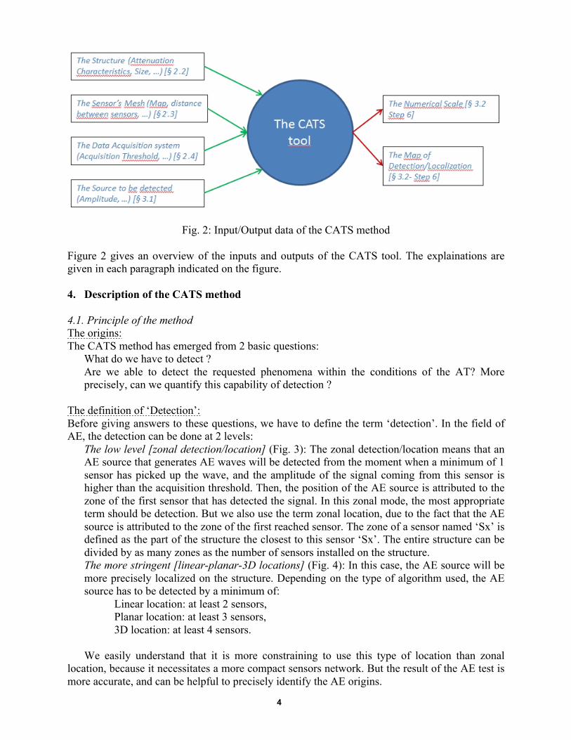
4

Fig. 2: Input/Output data of the CATS method

Figure 2 gives an overview of the inputs and outputs of the CATS tool. The explainations are given in each paragraph indicated on the figure. 4. Description of the CATS method 4.1. Principle of the method The origins: The CATS method has emerged from 2 basic questions:

What do we have to detect ? Are we able to detect the requested phenomena within the conditions of the AT? More precisely, can we quantify this capability of detection ?

The definition of ‘Detection’: Before giving answers to these questions, we have to define the term ‘detection’. In the field of AE, the detection can be done at 2 levels:

The low level [zonal detection/location] (Fig. 3): The zonal detection/location means that an AE source that generates AE waves will be detected from the moment when a minimum of 1 sensor has picked up the wave, and the amplitude of the signal coming from this sensor is higher than the acquisition threshold. Then, the position of the AE source is attributed to the zone of the first sensor that has detected the signal. In this zonal mode, the most appropriate term should be detection. But we also use the term zonal location, due to the fact that the AE source is attributed to the zone of the first reached sensor. The zone of a sensor named ‘Sx’ is defined as the part of the structure the closest to this sensor ‘Sx’. The entire structure can be divided by as many zones as the number of sensors installed on the structure. The more stringent [linear-planar-3D locations] (Fig. 4): In this case, the AE source will be more precisely localized on the structure. Depending on the type of algorithm used, the AE source has to be detected by a minimum of:

Linear location: at least 2 sensors, Planar location: at least 3 sensors, 3D location: at least 4 sensors.

We easily understand that it is more constraining to use this type of location than zonal

location, because it necessitates a more compact sensors network. But the result of the AE test is more accurate, and can be helpful to precisely identify the AE origins.

5

Fig. 3: Principle of zonal detection

Fig. 4: Principle of planar location

6

What do we want to detect? How can we evaluate the capability of an AE system to select from zonal, linear, planar or 3D location? Answering to this question requires, beforehand, to answer to an other fundamental question: What do we want to detect? This fundamental question is at the heart of this technique, and most of the time, people forget that most of the rules of detection actually used are based on an artificial source, called Hsu-Nielsen, from which many criteria has been calculated. This Hsu-Nielsen method consists in generating an artificial AE wave by breaking a pencil lead. This method has been elaborated in the 1970’s [5]. In most of the normative documents, this pencil lead has a diameter of 0.5 mm and a hardness (2H). For specific applications, a diameter of 0.3 mm can be used (for example, in the field of composite structures). But the methodology of the CATS tool could also be applied on different AE type of sources, such as, for example, a laser-generated AE source [6]. In the frame of the CATS tool, we could use any reference source we want, defined by its initial amplitude (related to the released energy); Nevertheless, it is also important to make this tool close to the actual practices. Then (in the following chapters) our reference source will be equivalent as the Hsu-Nielsen (0,5mm-2H) source. When this source is generated in a carbon steel plate, it is characterized by an initial amplitude equal to 98 dBae (+/-2 dBae) when using 100 kHz-300 kHz resonant sensor. This amplitude is the one measured close to a sensor (~10 mm). Now, we have all the data to evaluate the coverage rate of a sensors network on a structure:

The characteristics of the structure itself, the characteristics of the sensors network, the caracteristics of the acquisition system, and the type of source to be detected.

4.2. Steps of calculation integrated in the CATS method The CATS method necessitates to perform the following steps: Step 1: The sensors network Because we have to enter the coordinates of the sensors, this step necessitates knowing exactly the coordinates of all the sensors placed on the structure.

If it is a linear structure, every sensor ‘i’ will have a coordinate [xi]; If it is a planar structure, every sensor ‘i’ will have the coordinates [xi; yi]; If it is a 3D structure, every sensor ‘i’ will have the coordinates [xi; yi; zi].

Figure 5 shows the representations of a sensors network of a planar structure. Each red or white dot represents the position of a sensor. At the left, the coordinates of each sensor are indicated in the table.

7

Fig. 5: Example of planar (2D) Sensors network. Each dot in the graph represents the position of a sensor.

Step 2: The attenuation curve Now, we have to enter the characteristics of the attenuation curve linked to the reference source that has been chosen as seen in Fig. 6: This step necessitates knowing the values of this curve, obtained from a field measurement realized on the structure itself, or coming from previous experience, as long as the characteristics of the structure, environment, type of sensor is very close to the actual case. But we strongly recommend, as required in many normative documents to always confirm the values by doing field measurements. This will only take few minutes! This curve needs to be approximated by calculation (polynomial interpolation, logarithmic interpolation, or any method that will fit the experimental curve). Then, the experimental curve has to be introduced in the mathematical ‘CATS’ tool.

Fig. 6: Example of attenuation curve.

8

Step 3: The type of location In this step, we only need to choose the location to be evaluated is Zonal, Linear, Planar or 3D type; Enter the number of Sensors required:

In the case of Zonal location, the minimum required number of sensors for location is 1, In the case of Linear location, the minimum required number of sensors for location is 2, In the case of Planar location, the minimum required number of sensors for location is 3, In the case of 3D location, the minimum required number of sensors for location is 4.

We can also choose a higher value of minimum required number of sensors. For example, if we consider that the planar location necessitates more than 3 sensors to be more accurate, or to compensate a complex shape that makes the propagation more hazardous, we can enter 4, or 5. Below, we will explain the method for the case of a 2D structure. Step 4: The calculation of distances from each point of the surface to each sensor This step is the first one of the calculations needed to evaluate the coverage rate of a sensors network. For that, we need to measure, for each point of the surface (in the case of a planar configuration), the distances between this point and all the sensors. The objective is to define, for each point of the surface, which is the closest sensor, the 2nd closest sensor, the 3rd closest sensor, … and for each of them, the distance between the point and these sensors. In practice, we have to define a ‘resolution’ of calculation: typically, when we have to evaluate a planar configuration when the distances between the sensors is few meters, we use a step of calculation of 0.05 meter or less, meaning that for a surface of a square meter, we calculate the distance between each of the 441 points of the grid and each sensor. This result is then an array of values giving, for each point of the surface, all the distances between this point and each sensor. An example of grid is shown in Fig. 7, and an example of calculation for a particular point in Fig. 8.

Fig. 7: Graph representing the position of sensors (in red), and the position of each point of the surface for which the distances are calculated (in white). [0.1 m between 2 consecutive points].

9

Fig. 8: Graph representing the position of sensors (in red, and white for the 3 closest sensors), and the position of one particular point of the surface (in green) for which the distances to the 3 closest sensors have been calculated. Once it is possible to represent the surface with these distances, that can help the user to understand where are the easiest areas to be localized or detected, and at the contrary where are the most difficult areas to be localized or detected. Figures 9 and 10 show the representations of the maximum distances, for a same sensors network, but using a zonal detection (1 sensor to be reached – Fig. 9), and a planar location (3 sensors to be reached, Fig. 10). At the right, the color scale represents the distance (Fig. 9, to the nearest sensor; Fig 10, to the 3rd nearest sensor).

Fig. 9: Mapping representing the distance to the 1st closest sensor, (in red, sensor position; maximum distance between sensors = 2.5 m).[2]

10

Fig. 10: Mapping representing the distance to the closest 3rd sensor, (in red, sensor position; maximum distance between sensors = 2.5 m). [2] Step 5: The calculation of minimum detectable amplitudes This step necessitates taking into account:

The acquisition threshold Athr (dBae), as it defines the minimum detectable amplitude, the attenuation curve, and the previous maps of minimum distances calculated in Step 4.

For each point of the surface, we know, from Step 4, the distance to the 1st closest, or 2nd, or 3rd, closest sensor. In the case of zonal location, the distance to the first closest sensor is required. In the case where we need to use planar location, the distance to the third closest sensor is required. Figure 11 explains the calculation of the minimum amplitude that can be processed by planar location algorithm, for a specific point (in green):

The distance to the third nearest sensor is 1.46 m, 1.46 m gives an amplitude of 61 dBae on the attenuation curve, It means that an attenuation of 38 dBae is expected at this distance, If the acquisition threshold is 50 dBae, it means that the minimum amplitude that can be localized is equal to 50 + 38 = 88 dBae.

Then, by calculating for each point of the surface, we can also represent these minimum amplitudes, as we have previously represented the minimum distances. Figures 12 and 13 are the equivalent of Figs. 9 and 10, calculated for an acquisition threshold of 50 dBae. For these calculations, we understand that all the parameters have an influence:

The sensors network, the structure (attenuation curve), and the acquisition system (Acquisition threshold).

11

Fig. 11: Calculation of the equivalent minimum amplitude (planar location algorithm) vs. distance (m).

Fig. 12: Mapping representing the minimum amplitude that can be detected (processed) by zonal location method (maximum distance between sensors = 2.5 m).

12

Fig. 13: Mapping representing the minimum amplitude that can be processed by planar location method (maximum distance between sensors = 2.5 m). At the right-hand side of Figs. 12 and 13, the color scale represents the amplitude (expressed in dBae) . Step 6: The calculation of the rate of detection/location This step necessitates taking into account:

The type of AE reference source to be detected, and the result of Step 5, i.e., the maps of the minimum amplitudes that can be processed by location algorithms.

This calculation is, once again, basic: For each point of the surface, we compare the minimum amplitude calculated in Step 5 with the reference amplitude of the AE source we want to detect/localize. Example: We use a reference amplitude of a Hsu-Nielsen 0.5 mm-2H source (= 98 dBae – That is what we want to detect). From the maps calculated in Step 5, it means that for each point where the minimum amplitude is less than 98 dBae, the reference source will be detected (zonal location) or localized (planar location); If the amplitude is higher than 98 dBae, the reference source will not be detected or localized. Then we can affect a binary value for each point of the surface:

0 = No detection/location ; 1 = Detection/location OK.

Figure 14 shows an example of a map where 0 is black and 1 is white. With this type of picture, it is easy to understand, where are the areas that can lead to difficulties of location/detection (black areas).

13

Fig. 14: Mapping representing the areas where planar location method is efficient (white) and not applicable (black) (sensor’s position in red). From this type of picture, we can now calculate the fraction of surface where the location algorithm is efficient. In the example given in Fig. 14, this is 0.46, i.e., that 46% of the surface satisfies the conditions required to localize a Hsu-Nielsen source. Many examples of this method, and benefits in term of understanding are described in the papers [1,2] and [3]. 4.3. The scale of the CATS method Our goal is finally reached. We can now evaluate the capability of an AE instrumentation (sensors network + Data acquisition Threshold) to detect a defined AE source in a specific structure. It is important to remind the user that this scale is not only one number, between 0 and 1. This scale must specify the type of reference source to be detected/localized, and also the algorithm of detection/location which is the subject of this evaluation. The result should be written as follow (2 examples):

Example 1: Zonal location algorithm (= 1 sensor to be reached) / Hsu-Nielsen 0.5 mm-2H reference source. If the rate is 0.95, we will write the result as follow:

Kcats [1s-Hsu0.5mm] = 0.95 Example 2:

Planar location algorithm (= 3 sensors to be reached) / Hsu-Nielsen 0.5 mm-2H reference source. If the rate is 0.45, we will write the result as follow:

Kcats [3s-Hsu0.5mm] = 0.45

14

We also advise the user of this methodology to complement this result by a drawing of the sensors network, representing the areas where the detection/location is possible or not. It will help each user of the technique to understand more the performances/limitations of the configuration used, and especially the areas where thelocation is not possible. Then, this tool enables to compare the performance of different sensors networks. Let’s describe an example:

For the control of a structure, one service provider says that he will place a sensors network with a distance of 4 m between each sensor, and assures that he will control 100% of the structure by zonal location. For the same structure, another service provider proposes a more compact sensors network (2.5 m between each sensor), saying that it is more efficient, enabling an accurate planar location. What is the difference of efficiency between these 2 proposals?

The CATS method will give, in few minutes, the result given in Table 1:

Table 1: Result of CATS Evaluation for 2 different networks and 2 types of location method

Kcats [1s-Hsu0.5mm] Kcats [3s-Hsu0.5mm] Service Provider 1

(1sensor/4 m) 0.99 0.20

Service Provider 2 (1sensor/2.5 m)

1 1

It clearly means that the service provider 2 is 5 times more efficient (0.2 compare to 1) than the service provider 1 to do a planar location. The customer can now make his choice with a quantitative comparison given by the Kcats factor.

5. Conclusions

The CATS method has emerged from a fundamental question concerning AE testing: Are we able to detect the requested phenomena with the conditions of the AE Testing? More precisely, can we quantify this capability of detection ?

This tool has been described in details, step by step, in order to show that the performance of an AE testing can be easily and quantitatively evaluated. Due to the fact that the required data are most of the time well-known by AE engineers (sensors network + data acquisition threshold, type of AE source to be detected) we believe that this tool will be used and integrated in the ‘good practices’ of this technique. By giving a clear view of the performance of this type of control, all the users of this technique (AT engineers, technicians, customers, regulatory body) will benefit from this tool. We can also imagine that a minimum level of Kcats parameter depending on the criticity of the structure to be controlled could be one day defined and required.

References [1] Non Destructive Testing Handbook, Second Edition, volume 5 – Acoustic Emission Testing, 1987, pp 201-202. [2] J. Catty, “Acoustic Emission Testing – Defining a new standard of acoustic emission testing for pressure vessels Part 1: Quantitative and comparative performance analysis of zonal location and triangulation methods”, Journal of Acoustic Emission, volume 27 (2009), pp 299-313.

15

[3] J. Catty, “Acoustic Emission Testing – Defining a new standard of acoustic emission testing for pressure vessels Part 2: Quantitative and comparative performance analysis of zonal location and triangulation methods”, Journal of Acoustic Emission, volume 28 (2010), pp 11-31. [4] J. Catty, “Acoustic Emission Testing – Defining a new standard of acoustic emission testing for pressure vessels Part 3: Study of current analysis protocols and recommendations for developing a new guide for the application of acoustic emission (to be published). [5] N. Hsu, ‘’US Patent 4,018,084 – Acoustic Emission Simulator’’, April 19, 1977. [6] C.B. Scruby, H.N.G. Wadley, R.J. Dewhurst, D.A. Hutchins, S.B. Palmer, ‘’A Laser-Generated Standard Acoustic Emission Source’’, United Kingdom Atomic Energy Authority Harwell, January 1981. [7] J. Roget, L’émission Acoustique, Mise en oeuvre et applications, 1988. [8] J.D. Leaird, Acoustic Emission Training Guide; Greensland Publishing Co, 1997.