Acoustic emission generation from normal running - CiteSeerX

XML Template (2013) [31.8.2013–12:55pm] [1–23]//blrnas3/cenpro/ApplicationFiles/Journals/SAGE/3B2/PIEJ/Vol00000/130056/APPFile/SG-PIEJ130056.3d (PIE) [PREPRINTER stage]

Original Article

The use of acoustic emission for thecondition assessment of gas turbines:Acoustic emission generation fromnormal running

Mohammad S Nashed, John A Steel and Robert L Reuben

Abstract

Many approaches have been taken to the condition monitoring of gas turbines including performance analysis, vibration

monitoring and lubricant debris monitoring. Acoustic emission monitoring has the potential to provide information

about turbine operation and faults as they occur and has two possible advantages over other techniques. Firstly, because

acoustic emission is sensitive to minor changes which do not necessarily involve whole-body motion, it is potentially able

to reveal faults at an early stage. Secondly, because acoustic emission propagates over the structure from the source(s)

to the sensor(s), it has the capacity to locate the source of any fault signal without intrusion. This paper explores the

nature of the acoustic emission signals generated in a laboratory-scale gas turbine in order to extract and select features

of the signal under normal running conditions and to establish the physical source(s) of this acoustic emission. A series of

tests with the turbine running normally, either idling with the speed being controlled by fuel and air flow, or under load at

fixed fuel and air flow with the speed being controlled by the amount of load applied, provided a range of conditions of

gas flow through the turbine. An ancillary set of simplified tests with the free power turbine impeller jammed or absent

was used to help distinguish between components of the acoustic emission associated with standing waves in various

parts of the turbine and turbulence around the impeller. The results provide the first systematic study of fluid-induced

acoustic emission in turbines and, as such, offer a baseline interpretation for acoustic emission generation in turbines and

fluid machinery generally. Specifically, the findings will be compared with measurements made on the same turbine with

simulated blade faults in a future publication.

Keywords

Acoustic emission, gas turbine, condition monitoring, artificial neural networks, pattern recognition, signal processing

Date received: 3 January 2013; accepted: 16 July 2013

Background

A number of faults that can occur in turbines result inchanges to the gas flow within the machine, so, beforestudying the effect of such faults on the acoustic emis-sion (AE) signal, it is essential to understand whatinfluences the flow-generated AE under ‘normal’ run-ning conditions. Using AE has two possible advan-tages over other on-line monitoring techniques, suchas acceleration monitoring. Firstly, because AE is sen-sitive to minor changes which do not necessarilyinvolve whole-body motion, it is potentially able toreveal faults at an early stage. Secondly, because AEpropagates over the structure from the source(s) tothe sensor(s), it has the capacity to locate the sourceof any fault signal without intrusion.1 However,because of its sensitivity to a number of phenomena,it is necessary to differentiate between AE sources

resulting from gas flow through the turbine andthose resulting from impact, or rolling or sliding con-tact in the ancillary mechanical equipment, such asshafts and bearings. To date, there has been verylittle study of the flow-generated AE in turbines, sothe work presented here forms an essential basis forturbine monitoring using AE.

Most of the research on AE monitoring of turbineshas been related to non-fluid sources of AE, such as

Proc IMechE Part E:

J Process Mechanical Engineering

0(0) 1–23

! IMechE 2013

Reprints and permissions:

sagepub.co.uk/journalsPermissions.nav

DOI: 10.1177/0954408913502167

uk.sagepub.com/jpme

Mechanical Engineering, School of Engineering and Physical Sciences,

Heriot-Watt University, Riccarton, Edinburgh, Scotland, UK

Corresponding author:

Robert L Reuben, Mechanical Engineering, School of Engineering and

Physical Sciences, Heriot-Watt University, Riccarton, Edinburgh EH14

4AS, UK.

Email: [email protected]

at PENNSYLVANIA STATE UNIV on February 21, 2016pie.sagepub.comDownloaded from

http://pie.sagepub.com/


bearing defects,2,3 rubbing damage,4 backgroundnoise determination and AE propagation characteris-tics on off-service engines.5 Board3 was among thefirst to apply AE analysis to such machines, usinginformation from AE sensors at two different pos-itions on a bearing housing to detect roller bearingwear in a large industrial gas turbine. Board observedthat the demodulated AE spectrum at one position ona bearing housing had strong indications at 105.8Hzwhich he identified as the cage rotational frequency ofthe roller bearing thus identifying a defect. Mba andHall2 investigated two faults on the inner and outerraces of a test bearing using a range of AE featuressuch as RMS amplitude, energy and AE counts, andfound that the maximum AE amplitude increasedwith increasing speed, but not with load or defectsize. They also found a correlation between bearingmechanical integrity and AE counts, an observationalso made by Choudhury and Tandon.6

Douglas et al.7 carried out a preliminary study inwhich they attempted to monitor the operating par-ameters of a gas turbine using AE. The experimentwas conducted on the same laboratory-scale gas tur-bine as in the current work, operating under variousconditions, with AE sensors mounted at differentpositions on the rig and turbine surface. In all rec-ords, the blade passing frequency of the monitoredcompressor was observed, suggesting that AE is sen-sitive to fluid-mechanical processes going on in andaround the turbine. Moreover, the frequency analysisof two severities of induced blade fault in the FPTproduced a deviation from the normal spectrum sug-gesting that AE may act as an indicator of individualblade malfunction. Interestingly, these authorsnoted that unstable combustion resulted in AE sig-nals containing sporadic, high-amplitude pulses. In arather different study, Ng et al.8 monitored the flameand the ‘AE’ in the combustor of an industrialgas turbine and found a strong correlation betweenfluctuating light intensities and sound capturedusing a microphone. In particular, an unstable com-bustion mode at 100Hz was locked to an acous-tic mode at the same frequency and this modepersisted over a wide range of operating conditions,whereas stable combustion modes hopped aroundmuch more.

By contrast to the situation where the fluid isentirely gaseous, fluid-generated AE from rotatingand reciprocating machines with liquid–gas mixtureshas been more intensively studied. For example, Neillet al.9 conducted experiments on both laboratory- andindustrial-scale centrifugal pumps to detect incipientcavitation. By applying both RMS and frequencyanalysis to the generated AE, they were able todetect cavitation earlier than its appearance in themeasured dynamic head of the pump, thus demon-strating the feasibility of incipient cavitation detectionusing AE in the face of noise from normal running,although they did suggest that the nearer the sensor is

to the cavitation site the better. Rus et al.10 monitoredboth AE and cavitation (using the optical grey level ofthe liquid) in a model two-blade Kaplan turbine,developing a physical model for the pressure waveintensity as it passes through the two-phase cavitationcloud and then the single-phase liquid. Using thismodel, they were able to explain how, as cavitationintensity increased, the AE went through a maximum,then a local minimum followed by another increase.Using a similar approach, Addali et al.11 havemanaged to isolate some of the AE characteristics oftwo-phase pipe flow.

Sato4 was also interested in applying AE to rotat-ing machines to detect rubbing and other damage inbearings. He mounted AE sensors on two turbinejournal bearing housings in order to detect metalwipes and bearing tilts, and found a correlationbetween the AE pulse shapes and the correspondingdefect. Mba and Hall studied the transmission of AEwaves across very large turbine rotors5 and found thatit was possible to detect AE sources up to 2m fromthe sensor. On this basis, they suggested that the AEtechnique could be viable for detecting seal and bladerubbing in such machines.

The normal statistical approaches to AE analysisare helpful in many cases, but can become unwieldyfor complex pattern recognition cases such as for gen-eric or real-time monitoring requirements involvinglarge amounts of data and adaptability to new situ-ations. Pattern recognition therefore forms the basisof machine intelligence, and AE, with its sensitivity toa wide range of physical phenomena, can clearly playa major role. Because of the high sampling rates andconsequent high time resolution, AE monitoring nor-mally generates a large set of data. To handle thedata, it is therefore helpful to use some form of datareduction to prepare the variables for further statis-tical classification and diagnostic algorithms. Becauseof the complexity and non-linearity of the AE signalsemanating from gas turbines, artificial neural net-works are needed to unravel the way in which thefeatures evolve with operating condition. Artificialneural networks (ANNs), as massively parallel dis-tributed processors made up of simple processingunits (neurons), have a natural propensity for storingexperimental knowledge and making it available foruse.12 A feed-forward-back-propagation network13 isused here since only supervised operation is requiredto map the input features of the AE onto the output(diagnosis).

In summary, whereas the literature indicates thatthe fluid-mechanical processes going on within gasturbines and like machines generate AE, very little isknown about how this AE can be used to providediagnostic information about turbine operation. Thepurpose of this paper is to examine the effect of mod-ifying the fluid mechanical conditions on the AE, witha view to understanding the sources. Ultimately, suchan understanding will form the basis for interpreting

2 Proc IMechE Part E: J Process Mechanical Engineering 0(0)




experiments in which faults in the fluid-loadedsurfaces are simulated.

Experimental set-up and procedure

The gas turbine used was a P.9000 unit manufacturedby Cussons Ltd,14 illustrated schematically inFigure 1. The turbine had two stages: a gas generator(GG) which comprised a compressor and turbinemounted back to back on a short shaft supportedon a journal bearing, and a free power turbine(FPT) which was a single-stage radial turbine operat-ing over the range 170–600 RPS (revolutions persecond) and developing a maximum power ofapproximately 4 kW. The FPT was connected to analternator which generated electricity that could bedissipated through heat lamps or made availablefrom normal plug sockets. The fuel flow rate couldbe adjusted manually and the fuel and air flow rateswere each measured using flow meters. The turbinecontains two rapidly rotating mechanical parts, theGG and the FPT, both of which contain journal bear-ings which are known to generate relatively continu-ous AE. The sensors were placed specifically to avoidrecording the bearing-induced AE, which will mostlybe structure-borne, carried along the shafts to thebearing housings. The gas-borne sources wereexpected to be from flow through relatively confinedspaces and from combustion and combustion instabil-ity, as well as from standing waves within the variouspassages of the turbine.

Two different AE sensors were used, a Micro-80Dsensor (Physical Acoustics, PAC) mounted on a wave-guide welded onto the gas turbine exhaust, and ahigh-temperature AE sensor S9215 (PAC) mounteddirectly onto the gas turbine shroud. A proprietarypreamplifier (PAC 1220A) was used with the Micro-

80D sensor and a different preamplifier (0/2/4, alsofrom PAC) was used with the S9215 sensor. Thetwo types of sensor were chosen deliberately, so thatthe effects of using a lower sensitivity sensor mountedcloser to the potential source(s) against a higher sen-sitivity sensor which has to be stood off from the tur-bine outer surface on a waveguide could beinvestigated. Data were acquired using a NationalInstruments card (type NI 6115) at a sampling rateof 5MHz (over three channels). A tachometer wasused to record shaft speed on the FPT synchronouslywith the AE. The tachometer consisted of a slotteddisc with 34 teeth of circumferential extent 5� andone of extent 15� to obtain a characteristic patternfor every cycle, allowing shaft speed and rotationalposition to be determined alongside the AE.

Separate calibration tests for the two sensors on asteel block at room temperature showed the S9215sensor to be about 100 times less sensitive than theMicro-80D, each being sensitive in a different dynamicrange (50–250 kHz for the S9215 and 100–400 kHz fortheMicro-80D). Calibration with the sensors mountedin their respective places on the turbine before andimmediately after running showed the S9215 to beabout twice as sensitive and the Micro-80D to beabout half as sensitive, with the turbine hot thancold. Finally, the attenuation over the surface of thegas turbine was assessed by introducing an AE source(pencil lead break) at various places along the FPTstarting at the shroud and ending at the exhaust andrecording the energy at both of the sensors. Thesepropagation tests showed the shroud position to beup to 100 times more sensitive to sources on theshroud than on the exhaust and vice versa.15

For the normal running experiments, AE wasacquired over a range of FPT speeds with the machineunder load or idling. The load test involved adding an

Figure 1. Schematic diagram of turbine rig showing AE sensor positions.

AE: acoustic emission

Nashed et al. 3




alternator which generates electricity that could bedissipated through heat lamps. The change in the exci-tation voltage applied to the alternator field coilsallowed the power loading on the alternator (andhence the turbine) to be varied over the required oper-ating range. For the loaded condition, the speed of theGG was kept constant, and the alternator load incre-mentally changed, resulting in a speed change in theFPT. For the no-load (idling) condition, the drive beltbetween the FPT and the alternator was removed andthe turbine speed was changed by changing the fuelflow incrementally which, accordingly, resulted inchanges in both the GG and FPT speeds. The speedof the FPT was also recorded during all experiments,along with other operating parameters such as theGG speed fuel flow, air flow and gas pressure andtemperature of both the compressor and turbine.For each of the two conditions, with and withoutload, the speed was varied between 120 and 380RPS and 20 records of raw AE, each of length0.03 s, acquired at each speed. The speed range wasessentially the widest over which reasonably stableoperation could be achieved. After a change in condi-tions, the turbine settled down quite quickly (typicallywithin 20 s) and measurements were not taken untilthe turbine had settled at the new conditions. Eachexperiment (i.e. range of speeds with or withoutload) was repeated a total of three times to checkfor consistency.

Some simplified experiments were also carried out,in which the impeller of the FPT was either jammedby connecting the turbine belt to a locked alternator,

or entirely removed from the turbine. When theimpeller was removed, it was necessary to replace itwith a dummy, blade-free piece which allowed pas-sage of gas through the shroud but prevented gasleakage from the FPT to the lubrication system.Two, nominally identical tests were run for each ofthe jammed impeller and absent impeller configur-ations. Each test consisted of acquiring data over arange of incrementally increased GG shaft speedsbetween 490 and 1170 RPS achieved by means ofchanging the fuel flow. At each operating condition,fuel flow, air flow and gas pressure and temperature ofboth the compressor and turbine were recorded asthese were not precisely reproducible between tests.At each operating condition, raw AE was recordedfor 0.03 s and 20 records were obtained at eachoperating condition, as was the case for the normaloperating tests.

Analysis and results

Figure 2 shows a typical example of a 0.03 s AErecord from the running turbine, normalized to afixed energy over the whole record in order that thepattern can be seen more clearly across the speedrange. To obtain an overview of the data, two basicmeasures were used for all data. The first measure isthe energy in the time domain which is obtained byintegrating the square of the samples of the measuredsignal over the (fixed) record length. The second meas-ure is a frequency spectrum of the low-pass filteredsignal which is calculated by averaging the measured

0 0.005 0.01 0.015 0.02 0.025 0.03S1

S2

S3

S4

S5

S6

S7

S8

S9

Time (Sec)

No

rmal

ized

Am

plit

ud

e (A

rbitr

ary

un

it)

Figure 2. Typical normalized AE records, showing raw and averaged time series. Exhaust sensor signatures (exhaust) for test

without load. Free power turbine speed increases from bottom to top, with S1 recorded at 140 RPS and S9 recorded at 345 RPS.

FPT: free power turbine; RPS: revolutions per second





signal over a fixed number of points. The effect ofaveraging is such that the low frequency componentsof the spectrum are preserved, while the high fre-quency components are damped (reduced). Figure 2shows the raw squared signal and the averaged signal,using an averaging time of 0.03ms. As can be seen,there are potentially periodic features outside thebandwidth of the raw (carrier) wave which can beinvestigated by the frequency spectrum of the aver-aged signal as described previously.

Simplified experiments

In the experiments carried out with the simplified con-figuration, the impeller and shaft in the FPT do notrotate, so all AE emanating from the turbine will beassociated with gas flow rather than moving mechan-ical parts. The gas flow will also not be conditioned bythe extraction of power at the FPT allowing an assess-ment of the effects of the flow alone with and withoutthe static constriction offered by the impeller. Also,since the impeller does not rotate, the principal experi-mental variable is the GG speed.

Test without impeller. Here, the impeller was replaced bya non-rotating disc which essentially acted as a simplebaffle in the FPT. Figures 3 and 4 show the evolutionof AE energy with GG speed for the exhaust andturbine shroud sensors, respectively. Each point rep-resents the energy content of the record and all20 values are shown at each speed for each of thetwo tests. As can be seen, the AE energy at a givenspeed seems consistent between the records (each ofwhich accounts for typically 15–33 revolutions of the

machine) but there is a marked difference in the levelof energy between the two tests for the exhaust-mounted sensor, not reflected in the record for theshroud-mounted sensor. Notwithstanding this, bothsensors indicate a reasonably monotonic increase inAE energy with speed with an increasing slope, fittedhere using an exponential growth function. It mightalso be noted that the energy recorded on the shroudis a factor of 50–100 lower than that recorded at theexhaust.

Decimated frequency analysis was also applied tothe signals by RMS averaging them over 150 points,making an effective sampling rate of 33.3 kS/s.Transforming the resulting signals into the frequencydomain shows periodic information at frequencies upto 1 kHz and examples of such spectra are shown inFigures 5 and 6 (the spectra have been normalized tohighlight changes in frequency content). The Micro-80D sensor on the turbine exhaust shows a peakwhose frequency increases with the GG speed, varyingfrom 300Hz at 490 RPS to 700Hz at 1170 RPS. Thesefrequencies are absent in the records of the S9215sensor mounted on the turbine shroud.

Test with jammed impeller. The only essential differencebetween this test and the one with the absent impelleris that the flow through the shroud has the additionalimpediment of the (static) impeller. Figures 7 and 8show the evolution of AE energy with GG speed forthe two AE sensors.

The two tests give repeatable results and, as for thetest with the impeller absent, there is a monotonicincrease in energy with GG speed. The level ofenergy is much higher, and that recorded at the two

400 500 600 700 800 900 1000 1100 12000

0.5

1

1.5

2

2.5

3

3.5

4x 10

–9

Gas generator speed (RPS)

E (

V2 .s

)

Test 1Test 2Fit 1Fit 2

Figure 3. Micro-80D (exhaust) sensor AE energy versus gas generator speed for tests without impeller.

GG: gas generator

Nashed et al. 5




locations is much closer in magnitude than for theabsent impeller, indicating a shift in the total energyof the source away from the exhaust towards theshroud, coupled with a significant increase in AEenergy liberated in this area. Also, in contrast to thetest with the impeller absent, the scatter of energy ineach record at a given speed is quite high, suggestingthat the effect of the impeller on the flow is associatedwith unsteady flow effects.

The frequency analysis (Figures 9 and 10) doesnot show any particular peaks in the range up to1500Hz indicating that the low frequency character-istics associated with the flow around the impeller are

broader band than those taking place in the exhaust(Figure 5).

Normal running tests

Figure 11 shows samples of the normalized AE innormal running tests recorded by the shroud sensorfor the same records as shown for the exhaust sensorin Figure 2. The exhaust sensor exhibits some weakpulses which appear to coalesce at higher speeds of theFPT, so that the signal becomes continuous. Theshroud record contains more pronounced pulses,

0 100 200 300 400 500 600 700 800 900 1000S1

S2

S3

S4

S5

S6

S7

S8

S9

S10

S11

S12

S13

S14

S15

S16

S17

Frequency(Hz)

Nor

mal

ized

vol

t (A

rbitr

ary

unit)

Figure 5. Typical AE spectra for test without impeller recorded with exhaust-mounted sensor. GG speed increases from bottom to

top, from 500 RPS (S1) to 1170 RPS (S17).

400 500 600 700 800 900 1000 1100 12000

0.5

1

1.5

2

2.5x 10

–11


E (

V2 .s

)


Figure 4. S9215 (shroud) sensor AE energy versus GG speed for tests without impeller.





but their occurrence, both within a record and as theFPT speed increases, is quite erratic.

Energy analysis. Figures 12 and 13 show the evolutionof the AE energy with FPT speed for each of the twosensors for all three of the repeat tests without load.For the sensor mounted on the exhaust, the generalshape of the curves is similar for each of the three testsbut, for the sensor on the shroud, one of the curves ismarkedly lower than the other two. Also, the generallevel of AE on the shroud is about a factor of twohigher than that measured at the exhaust, despite thefact that the Micro-80D sensor is about 100 timesmore sensitive than the S9215.

Perhaps the most significant observation, though,is that, for both sensors, there is a considerable degree

of increased scatter as the FPT speed increases, alongwith the introduction of what appears to be peaks inthe energy evolution with FPT speed.

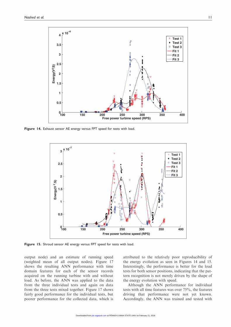
The load test involved adding a loading device, i.e.the alternator, to the FPT and increased load beingreflected in a reduced speed of the FPT. In thisrespect, the signals were expected to be more complex,but also more relevant to real operations. Figures 14and 15 show the variation in AE energy with FPTspeed for the two sensors in the load tests. The moststriking feature of these two curves is that they are upto two orders of magnitude higher than the equivalentidling curves and that the curves are no longer mono-tonic, with peaks in AE energy across the range ofspeed studied, the speeds at which the peaks occurvarying between the three repeat tests. This time,

0 100 200 300 400 500 600 700 800 900 1000S1

S2

S3

S4

S5

S6

S7

S8

S9

S10

S11

S12

S13

S14

S15

S16

S17

Frequency (Hz)

No

rmal

ized

vo

lt (A

rbitr

ary

un

it)

Figure 6. Typical AE spectra for test without impeller recorded with shroud-mounted sensor. GG speed increases from bottom to

top, from 500 RPS (S1) to 1170 RPS (S17).

500 550 600 650 700 750 800 850 9000

1

2

3

4

5

6

7

8x 10

–9


E(V

2 .S)


Figure 7. Micro-80D (exhaust) sensor AE energy versus GG speed for tests with jammed impeller.

Nashed et al. 7




the energy levels recorded at the shroud were gener-ally an order of magnitude lower than those recordedat the exhaust. At first sight, these evolutions appearerratic and rather intractable, but it was noted thatthe peaks in energy (e.g. in Test 1 at about 230 RPS)were associated mainly with modulations of the AE atfrequencies in the range of a few hundred Hertz, andthese were tentatively attributed to instabilities andstanding waves in the combustion and/or gas flow.

Frequency analysis. Inspection of a sample of spectrawith different levels of averaging revealed peaks in

the order of a few hundred Hertz, although with pat-terns that seemed to be very complex. Figure 16 showssome examples of such spectra recorded during theidling tests for the exhaust-mounted sensor (corres-ponding to the evolution shown in Figure 12). Allspectra were normalized to the energy content tofacilitate comparison and averaging and to avoid thecomplication of including the energy or amplitude ofthe signal in a frequency analysis. Many of the aver-aged spectra show a clear peak at the running speed(arrowed in Figure 16), and, less often, the first har-monic of the running speed. However, the running

0 500 1000 1500S1

S2

S3

S4

S5

S6

S7

S8

S9

Frequency (Hz)

No

rmal

ized

vo

lt (A

rbitr

ary

un

it)

Figure 9. Typical AE spectra for test with jammed impeller recorded with exhaust-mounted sensor. GG speed increases from

bottom to top, from 500 RPS (S1) to 850 RPS (S9).

500 550 600 650 700 750 800 850 9000

0.2

0.4

0.6

0.8

1

1.2x 10

–8


E(V

2 .S)


Figure 8. S9215 (shroud) sensor AE energy versus GG speed for tests with jammed impeller.





speed is rarely the dominant peak in the spectrumand, in cases where this peak is weak or absent, theindividual spectra which make up the average oftencontain strong peaks at a very wide range of frequen-cies. Many of the exhaust spectra contain a strongpeak at around 110Hz, sometimes associated withpeaks on either side at around 40 and 165Hz.

Pattern recognition analysis. The picture of the results sofar indicates that the complexity of the AE signalsincreases with the complexity of the fluid mechanics

occurring within the FPT and its exhaust, at its sim-plest with the impeller absent, increasing in complex-ity with the impeller present, but not rotating, with theimpeller rotating, and being at its most complex withthe impeller rotating and loaded. It is also clear thatthe signal changes with operating conditions (speedand load), but in a way that cannot easily be inter-preted by marshalling graphical information. Thus, apattern recognition study was used to try to isolatewhat key features in the time and frequency domainsare significant. Because the requirement is to

0 0.005 0.01 0.015 0.02 0.025 0.03S1

S2

S3

S4

S5

S6

S7

S8

S9

Time (Sec)

No

rmal

ized

Am

plit

ud

e (A

rbitr

ary

un

it)

Figure 11. Typical shroud sensor record for test without load. FPT speed increases from bottom to top, with S1 recorded at

140 RPS and S9 recorded at 345 RPS.

0 500 1000 1500S1

S2

S3

S4

S5

S6

S7

S8

S9

Frequency (Hz)

No

rmal

ized

vo

lt (A

rbitr

ary

un

it)

Figure 10. Typical AE spectra for test with jammed impeller recorded with shroud-mounted sensor. GG speed increases from

bottom to top, from 500 RPS (S1) to 850 RPS (S9).

Nashed et al. 9




understand the changing characteristics of the AEwith normal running operating conditions, the targetof the pattern recognition was taken to be the turbinerunning speed.

For the time series features, it was decided, after aninitial scoping, to use a purely statistical approach, soa range of features, such as energy, maximum ampli-tude, counts, RMS, mean, standard deviation, skewand kurtosis, was generated in the interest of describ-ing the signals as fully as possible. A dynamic neuralnetwork was used because its response at any given

time depends not only on the current input but alsoon the history of the input sequence, i.e. it has amemory. The implementation used consisted ofone log-sigmoid layer with 20 neurons with a feed-forward, back-propagation learning algorithm, withthe output consisting of the running speed, one nodebeing allocated to each speed used. Half of the datasetwas used to train the network to the measured run-ning speed and the other half for test, deliveringweights to the output nodes from which a speed clas-sification could be obtained (most highly weighted

100 150 200 250 300 3500

0.5

1

1.5

2

2.5

3

3.5

4x 10

–8

Free power turbine speed (RPS)

En

egry

(v2

.s)

Test 1Test 2Test 3Fit 1Fit 2Fit 3

Figure 13. S9215 (shroud) sensor AE energy versus FPT speed for tests without load.

100 150 200 250 300 3500

0.2

0.4

0.6

0.8

1

1.2

1.4

1.6

1.8x 10–8


En

egry

(v2 .s

)


Figure 12. Micro-80D (exhaust) sensor AE energy versus FPT speed for tests without load.





output node) and an estimate of running speed(weighted mean of all output nodes). Figure 17shows the resulting ANN performance with timedomain features for each of the sensor recordsacquired on the running turbine with and withoutload. As before, the ANN was applied to the datafrom the three individual tests and again on datafrom the three tests mixed together. Figure 17 showsfairly good performance for the individual tests, butpoorer performance for the collected data, which is

attributed to the relatively poor reproducibility ofthe energy evolution as seen in Figures 14 and 15.Interestingly, the performance is better for the loadtests for both sensor positions, indicating that the pat-tern recognition is not merely driven by the shape ofthe energy evolution with speed.

Although the ANN performance for individualtests with all time features was over 75%, the featuresdriving that performance were not yet known.Accordingly, the ANN was trained and tested with

100 150 200 250 300 350 4000

0.5

1

1.5

2

2.5

3

3.5

4x 10

–6


En

erg

y(V

2 .S)


Figure 14. Exhaust sensor AE energy versus FPT speed for tests with load.

100 150 200 250 300 350 4000

0.5

1

1.5

2

2.5

3x 10

–7


En

erg

y(V

2 .S)


Figure 15. Shroud sensor AE energy versus FPT speed for tests with load.

Nashed et al. 11




each individual time feature in order to identify themost efficient time features in pattern recognition.Analysis of the resulting ANN performance rankedthem into three groups, those features with high dis-criminating power (standard deviation and RMS,1 and 2), those with medium power (maximum

amplitude, counts and energy, 3, 4 and 5) and thosewith low discriminating power (skew, kurtosis andmean 6, 7 and 8). Figures 18 and 19 show the cumu-lative effect on ANN performance of the time fea-tures, sorted in order of strongest discriminatingpower for each sensor in each test. For the individual

0 100 200 300 400 500 600 700 800 900 10000

1

2

3

4

5

6

x 10–3

Frequency(Hz)

Am

plit

ud

e (V

)

FPT speed (308 RPS)

0 100 200 300 400 500 600 700 800 900 10000

2

4

6

8

x 10–3

Frequency (Hz)

Am

plit

ud

e (V

)

FPT speed (323 RPS)

0 200 400 600 800 10000

0.002

0.004

0.006

0.008

0.01

0.012

Frequency (Hz)

Am

plit

ud

e (V

)

FPT speed (340 RPS)

0 100 200 300 400 500 600 700 800 900 10000

0.002

0.004

0.006

0.008

0.01

0.012

Frequency(Hz)

Am

plit

ud

e (V

)

FPT speed (291 RPS)

100 Hz frequency

0 200 400 600 800 10000

0.002

0.004

0.006

0.008

0.01

0.012

Frequency(Hz)

Am

plit

ud

e (V

)

FPT speed (199 RPS)

0 100 200 300 400 500 600 700 800 900 10000

0.002

0.004

0.006

0.008

0.01

Frequency(Hz)

Am

plit

ud

e (V

)

FPT speed (242 RPS)

0 200 400 600 800 10000

0.002

0.004

0.006

0.008

0.01

Frequency(Hz)

Am

plit

ud

e (V

)

FPT speed (260 RPS)

0 100 200 300 400 500 600 700 800 900 10000

0.005

0.01

0.015

Frequency(Hz)

Am

plit

ud

e (V

)

FPT speed (268 RPS)

Running speed

Running speed harmonic

Figure 16. Spectra for idling test recorded by the exhaust sensor at eight different speeds of FPT. (Individual spectra shown as

fainter, solid lines and averaged spectra shown as heavy, dotted lines).





tests, improvement is slow with added features, andsometimes deteriorates. For the collective tests, steadyimprovement is obtained, at least up to six features.

Since the spectra showed a number of characteris-tic frequencies (including the turbine running speed),

it was expected that they would be more likely to pro-duce information indicative of operating conditions ofthe turbine. The features were selected to employ asmuch of the type of information seen in Figure 16 aspossible without the computational burden of using

Test 1 Test 2 Test 3 All Tests0

10

30

50

70

90(a)

AN

N P

erfo

rman

ce(%

)


10

30

50

70

90(b)

AN

N P

erfo

rman

ce(%

)


10

30

50

70

90(c)

AN

N P

erfo

rman

ce(%

)


10

30

50

70

90(d)

AN

N P

erfo

rman

ce(%

)

Figure 17. Artificial neural network (ANN) classification performance using all statistical time features: (a) shroud sensor, idling

tests, (b) exhaust sensor, idling tests, (c) shroud sensor, load tests, (d) exhaust sensor, load tests.

0 1 2 3 4 5 6 7 80

20

40

60

80

100

Added Time Features

AN

N P

erfo

rman

ce (

%)

(a)

Test 1

Test 2

Test 3

All Tests

0 1 2 3 4 5 6 7 80

20

40

60

80

100

Added Time Features

AN

N P

erfo

rman

ce (

%)

(b)

Test 1

Test 2

Test 3

All Tests

Figure 18. Cumulative ANN performance for time features in idling test: (a) shroud sensor, (b) exhaust sensor.

Nashed et al. 13




the entire spectrum as input to the ANN.Across the 20 records at each speed in each experi-ment, the 10 highest amplitude frequencies werefirst identified and the proportion of the total

energy and the frequencies of the five commonestpeaks used as input to the ANN. As before, halfof the dataset was used to train the network to themeasured running speed and the network was then

0 1 2 3 4 5 6 7 80

20

40

60

80

100

Added Time Features

AN

N P

erfo

rman

ce (

%)

(a)

Test 1

Test 2

Test 3

All Tests

0 1 2 3 4 5 6 7 80

20

40

60

80

100

Added Time Features

AN

N P

erfo

rman

ce (

%)

(b)

Test 1

Test 2

Test 3

All Tests

Figure 19. Cumulative ANN performance for time features in load test: (a) shroud sensor, (b) exhaust sensor.


10

30

50

70

90(a)

AN

N P

erfo

rman

ce(%

)


10

30

50

70

90(b)

AN

N P

erfo

rman

ce(%

)


10

30

50

70

90(c)

AN

N P

erfo

rman

ce(%

)


10

30

50

70

90(d)

AN

N P

erfo

rman

ce(%

)

Figure 20. ANN speed classification using frequency features: (a) shroud sensor, idling tests, (b) exhaust sensor, idling tests,

(c) shroud sensor, load tests, (d) exhaust sensor, load tests.





150 200 250 300 3500

1

2

3

4

5x 10

–9

FPT Speed(RPS)

En

erg

y(V

2 .s)

Test 1

150 200 250 300 3500

0.5

1

1.5

2

2.5

x 10–9

FPT Speed(RPS)

En

erg

y(V

2 .s)

Test 2

150 200 250 300 3500

0.5

1

1.5

2x 10

–8

FPT Speed(RPS)

En

erg

y(V

2 .s)

Test 3

150 200 250 300 3500

1

2

3

4

5x 10

–9

FPT Speed(RPS)

En

erg

y(V

2 .s)

All Tests

Test1Test2Test3

Figure 22. Exhaust sensor spectral peak energy removal for idling tests. (Open symbols before peak removal and closed

symbols after).


10

30

50

70

90(a)

AN

N P

erfo

rman

ce (

%)


10

30

50

70

90(b)

AN

N P

erfo

rman

ce (

%)


10

30

50

70

90(c)

AN

N P

erfo

rman

ce (

%)


10

30

50

70

90(d)

AN

N P

erfo

rman

ce (

%)

Figure 21. ANN speed recognition using time and frequency features: (a) shroud sensor idling tests, (b) exhaust sensor idling tests,

(c) shroud sensor load tests, (d) exhaust sensor load tests.

Nashed et al. 15




tested, delivering weights to the output nodes fromwhich a speed classification and an estimate ofrunning speed could be obtained. Figure 20shows the resulting ANN classification performance

to be superior to those using time-based features(Figure 17) with classification being better than90% for all individual tests and over 80% forthe grouped data.

0.02 0.03 0.04 0.05 0.06 0.07 0.08 0.09 0.1 0.11 0.120

0.1

0.2

0.3

0.4

0.5

0.6

0.7

0.8

0.9

1x 10

–6

Gas flow (kg/s)

Ene

rgy(

V2 .s

)Without load 3Without load 2Without load 1Without impeller 2Without impeller 1Jammed impeller 2Jammed impeller 1

Figure 23. Shroud sensor background AE energy for idling, and with impeller jammed or absent.

0.02 0.03 0.04 0.05 0.06 0.07 0.08 0.09 0.1 0.11 0.120

0.5

1

1.5

2

2.5

3x 10

–7

Gas flow (kg/s)

Ene

rgy(

V2 .s

)

Without load 1Without load 2Without load 3Without impeller 1Without impeller 2Jammed impeller 1Jammed impeller 2

Figure 24. Exhaust sensor background AE energy for idling, and with impeller jammed or absent.





Because it relies on the energy of the signal, thestatistical time-based analysis suffers from the draw-back that calibration of the sensors is required onevery application, as the energy will depend on

many factors not related to the running condition,not the least of them being the source–sensor distanceand the quality of the coupling. On the other hand,although the frequency-based analysis can clearly

100 200 300 400 500 600 700 800 900 10000

0.05

0.1

0.15

0.2

0.25

0.3

0.35

0.4

0.45

0.5


En

erg

y(V

2 .s)

With load 1With load 2With load 3Without load 1Without load 2Without load 3

Figure 26. Exhaust sensor background AE energy for idling and load tests.

100 200 300 400 500 600 700 800 900 10000

0.01

0.02

0.03

0.04

0.05

0.06

0.07

0.08


En

erg

y(V

2 .s)

Without load 1Without load 2Without load 3With load 1With load 2With load 3

Figure 25. Shroud sensor background AE energy for idling and load tests.

Nashed et al. 17




identify instabilities in the time evolutions, it is notable to detect the clear (albeit weaker) trends instable regimes. Figure 21 shows the ANN perform-ance for the running turbine with and without loadwhen both the statistical time features and the fre-quency features are used together. As can be seen,the performance is better than either set of featuresused alone, the success for the individual tests improv-ing to almost 100% and the success when the tests aretreated as a group rising to around 90%. The robust-ness of the approach is particularly indicated when all

tests are considered together, indicating that the net-work is now recognizing a particular behaviourreflected in the AE signal rather than training to aparticular curve shape.

Discussion

Given the relative sensitivities of the sensors and thesensor positions, along with the general levels of theAE energy between the two simplified tests, it wouldappear that the increase in energy with the jammed

Figure 27. Shroud sensor energy distribution across the spectral peaks for idling Test 1.

Figure 28. Exhaust sensor energy distribution across the spectral peaks for idling Test 1.





impeller over that with the impeller absent is almostcertainly associated with the flow through the con-fined space between impeller and shroud. Thiswould mean that the spectral peaks and most of theenergy observed in the tests with the impeller absentare coming from the gas setting up standing waveswithin the exhaust.

From the normal running tests, it was seen that thebackground AE energy associated with gas flowbegins to become modulated when the impeller is

rotating and, at higher speeds, there are a numberof spectral peaks in the 20–1000Hz range. These spec-tral peaks disrupt the smooth evolution of energyversus running speed and the peaks in the energycurve, as well as the speed at which certain spectralpeaks appear, are not precisely reproducible in repeattests, suggesting some kind of transient instability.However, as shown by the ANN analysis, the behav-iour of the turbine can be characterized by a combin-ation of the energy within those spectral peaks and the

Figure 29. Shroud sensor energy distribution across the spectral peaks for load Test 1.

Figure 30. Exhaust sensor energy distribution across the spectral peaks for load Test 1.

Nashed et al. 19




overall energy. Potential sources of the spectral peaksare the combustion chamber, the impeller, the exhaustand feedback between the alternator and the impellerunder load. For the same running speed, the AE sig-nature for the loaded and idling conditions is differentand, for the same test, the behaviour recorded at theexhaust- and shroud-mounted sensors is different.

The first stage is to separate the two components ofthe signal in a systematic way. The ‘spectral peakenergy’ in each record, defined as the total energy inthe five highest peaks of the frequency spectrum, wassubtracted from the total energy to leave a back-ground energy. As can be seen in Figure 16, clearpeaks were present in all the individual spectra andthe energy in the top 10 peaks typically accounted for80% of the spectral peak energy. Figure 22 shows oneexample of the spectral peak energy removal for eachof the repeats of one of the normal running tests. Thedotted curves in the first three graphs show the bestexponential fit to the energy after removing the spec-tral peak energy for each repeat and the last graphshows these best fit lines for the repeat tests.

The background AE energy thus obtained from theidling test is compared with the background energyfor the static impeller tests (jammed impeller andimpeller absent) in Figures 23 and 24, re-plottedagainst the combustion gas flow rate through the tur-bine (which is a basis common to both tests). It isclear that the AE energy is mainly correlated withgas flow resistance through the turbine shroud,which is lowest for the tests without an impeller,becomes higher for the jammed impeller tests wherethe gas has to pass through the orifices represented bythe blades and vanes and is at its highest when the gas

flow passes through the rotating blades. In support ofthis suggestion, it might be noted that, for a given gasflow rate, the differences between the AE energiesassociated with the three configurations are largerfor the shroud sensor than for the exhaust sensor.

The background AE energy for the idling test iscompared with the background energy for the loadtest in Figures 25 and 26, in this case plotted againstFPT speed. At a given speed, the load test containsmore background AE energy only for the exhaustsensor; for the shroud sensor the background is, ifanything, higher for the idling test. At a given FPTspeed, this suggests that loading results in a reducedbackground flow noise associated with the blades, andan increased flow noise associated with the exhaust.

Inspection of the five highest energy spectral peaksindicated that their frequencies could be classified intoone of five categories: a band from 20 to 100Hz, aband from 100 to 200Hz, a band around the fre-quency corresponding to the running speed, the firstharmonic of the running speed and a fifth band eitherat the second harmonic of the running speed or at afrequency corresponding to 0.65–0.7 times the GGrunning speed. This last component is the one clearlyvisible in the spectra from the exhaust sensor for thetests without the impeller (Figure 5).

Figures 27 to 30 show the fraction of the total spec-tral peak energy in each category for the shroud andexhaust sensors for one of the idling and load tests,respectively. Generally, it can be seen that none of thefractions changes monotonically with turbine speedand that the energy fraction at the running speed fre-quency is almost always the highest with its first har-monic following a slightly different pattern with

Figure 31. Frequency analysis of idling tests, as fraction of total AE energy within the top five frequency bands. Each bar represents a

separate test (three in total) and the whiskers indicate the range in values, the extremities of the box represent the upper and lower

quartile, and the mean is shown by a symbol (cross or star).





turbine speed. The 20–100 and 100–200Hz bandsoccupy a significant proportion of the total spectralenergy at all turbine speeds, particularly in the idlingtests. The peak related to the GG speed is usually thelowest of the five main peaks for the idling tests, pos-sibly due to instability in the combustion chamber,and is overtaken by the second harmonic of the run-ning speed in the load tests.

Figures 31 and 32 show spectral summaries of allof the idling and load tests, respectively, averagedacross all the turbine speeds examined. Clearly, thefraction of the total energy accounted for by theFPT rotational speed and its harmonics is greaterfor the load tests than for the idling tests. Also, theFPT energy fraction is approximately the same forboth the shroud and exhaust sensors in both theload and idling tests, and, in all cases, the harmonicsaccount for substantially less energy than the preced-ing harmonic in the series. The peak at 60–70% of theGG speed only appears in the top five frequencies inthe idling tests, probably associated with the dimin-ution of the FPT energy (specifically its second har-monic). The fraction of energy in the low frequencyband (20–100 Hz) is higher whilst idling than underload and tends to be greater on the exhaust sensorthan on the shroud sensor in both load andidling tests. On the other hand, the energy in the100–200Hz band is about the same whilst idling orunder load and seems to be greater for the exhaustsensor only in the load tests.

Figure 33 shows a schematic diagram of the turbineexhaust, which consists of two pipes of diameters100 and 300mm and lengths 1.69 and 4.15m, respect-ively. The temperature of the exhaust gases varies

between 400 and 530�C for the load and idling tests,respectively, and the speed of sound, c (m/s), in eachtube can be calculated from

c ¼

ffiffiffiffiffiffiffiffiffiffi�RT

M

rð1Þ

where� is the adiabatic index of the gasR is the molar gas constant (J/molK)T is the absolute temperature (K)M is the molar mass (kg/mol)The frequency, f (Hz), of standing waves in the

tube can be estimated from

f ¼c

2LN ð2Þ

whereN¼ 1, 2, 3, . . .L is the length of the tube (m)

Figure 32. Frequency analysis of load tests, as fraction of total AE energy within the top five frequency bands. Legend as for

Figure 31.

Figure 33. Schematic of gas turbine exhaust system.

Nashed et al. 21




From equation (2), the standing wave frequency inthe smaller diameter pipe can be estimated to bebetween 100 and 200Hz, and, in the larger diameterpipe, between 20 and 100Hz. This suggests that theenergies in the 20–100 and 100–200Hz bands are asso-ciated with standing waves in the exhaust and explainstheir tendency to be expressed more strongly in theexhaust sensor than the shroud sensor for both loadand idling tests. It is not entirely clear why the lowerstanding wave frequency is stronger (in comparisonwith the higher one) in the idling tests than in theload tests, but this may be associated with combustioninstability. The appearance of a frequency locked tothe GG speed in the idling tests would tend to supportthis suggestion.

For the idling tests, the running speed frequencyand its harmonics seem to be more strongly expressedat specific turbine speeds and examination of thesespeeds reveals them to be coincident with the standingwave basic frequency of the small diameter exhaustpipe, suggesting that this frequency is powering therunning speed frequency in the turbine. On theother hand, the higher energy associated with the run-ning speed frequency and its harmonics in the loadtests indicates that the spectral peaks here are domi-nated by feedback between the turbine impeller andalternator.

Conclusions

This work has sought to identify, for the first time, thesources of fluid-generated AE in a running turbine,with a view to obtaining a background descriptionof how operating conditions affect the AE, againstwhich the effects of simulated faults can be assessed.To this end, AE was measured as a function of oper-ating speed in series of tests where the complexity ofthe flow through the turbine was gradually increased.The following conclusions can be drawn.

1. The simplified experiments without an impellerand with the jammed impeller exhibited asmooth evolution of AE energy with GG turbinespeed. Removal of the five highest peaks in thefrequency spectrum showed the load and idlingtests also to exhibit a smooth background evolu-tion of AE energy with speed. The magnitude ofthe evolution between the various tests indicatesthat this component of the AE is associated withthe degree of constriction of the flow at the shroudoffered by the impeller.

2. The experiments with a turbine running both withand without load exhibited a complex evolution ofAE energy against running speed which, particu-larly in the case of the load tests, was not entirelyreproducible in repeat tests. It is clear that thegeneral AE energy level increases with both run-ning speed and load and, by implication, withincreasing gas flow rate and complexity of the

flow in the turbine shroud. However, the AEenergy level does not, in itself, provide an explan-ation for the AE sources, nor is it alone sufficientto identify the turbine operating conditions.

3. The AE records contain further structural infor-mation such as pulses in the time series and infor-mation in the frequency domain, but the patternswith running speed are too complex to be eluci-dated by inspection.

4. The use of ANNs allowed two types of features tobe tested: those based on time-series statistics andthose based on the spectrum at frequencies in theorder of a few hundred Hertz. Both approachesgave identifiably poorer performance when con-sidering the repeat tests as a group rather thanindividually.

5. Combining the statistical time features with thefrequency features gave better performance thaneither set alone and, in particular, gave betterthan 90% speed classification when the testswere considered as a group.

6. Analysis of the five highest decimated spectralpeaks showed a number of other peaks to be pre-sent besides the turbine running speed and its har-monics, although the magnitudes of these peaksdo not show a smooth evolution with increasingrunning speed.

7. Standing waves in the exhaust are thought to bean important source of AE when the turbine isidling, with a much weaker peak, possibly asso-ciated with combustion instability.

8. On the basis of the analysis, two types of AEsource were recognized in the gas turbine. Thefirst is a continuous background associated withgas flow through the turbine which increased inintensity with turbine speed. The second sourceis a pattern of spectral peaks emanating from dif-ferent zones in the gas turbine and identified asstanding waves in the exhaust, and feedbackbetween the impeller and alternator.

9. Together, the results illustrate that the AE ema-nating from a running turbine is influenced byvarious aspects of the dynamic gas flow throughthe turbine. This, in principle, means that defectswhich disrupt the gas flow, such as damagedblades or inefficient combustion, should be detect-able through their effect on the AE perhaps beforethey can be detected by more conventional meth-ods, such as vibration monitoring.

Funding

MS Nashed was funded by the Government of Syria underthe auspices of the British Council.

References

1. Reuben RL. The role of acoustic emission in industrialcondition monitoring. Int J COMADEM 1998; 1(4):35–46.





2. Morhain A and Mba D. Bearing defect diagnosis andacoustic emission. Proc IMechE, Part J: J EngineeringTribology 2003; 217(4): 257–272.

3. Board D. Stress wave analysis of turbine engine faults.IEEE Aerosp Conf Proc 2000; 6: 79–93.

4. Sato I. Rotating machinery diagnosis with acoustic

emission techniques. Electr Eng Jpn 1990; 100(2):115–127.

5. Mba D and Hall LD. The transmission of acoustic

emission across large scale turbine rotors. NDT & EInt 2002; 35(8): 529–539.

6. Choudhury A and Tandon N. Application of acousticemission technique for the detection of defects in rolling

element bearings. Tribol Int 2000; 33: 39–45.7. Douglas M, Beugne S, Jenkins MD, et al. Monitoring

of gas turbine operating parameters using acoustic

emission. In EWGAE, DGZfP-Proceedings BB 90-CD,Deutsche Gesellschaft fur Zerstorungsfreie Prufunge.V., Berlin, September 15–17, 2004, pp.389–396.

8. Ng WB, Clough E, Syed KJ, et al. The combined inves-tigation of the flame dynamics of an industrial gas tur-bine combustor using high-speed imaging and an

optically integrated data collection method. Meas SciTechnol 2004; 15: 2303–2309.

9. Neill GD, Reuben RL, Sandford PM, et al. Detectionof incipient cavitation in pumps using acoustic emis-sion. Proc IMechE, Part E: J Process Mechanical

Engineering 1997; 211(4): 267–277.10. Rus T, Dular M, Sirok B, et al. An investigation of the

relationship between acoustic emission, vibration,

noise, and cavitation structures on a Kaplan turbine.ASME J Fluid Eng 2007; 129: 1112–1121.

11. Addali A, Al-Lababidi S, Yeung H, et al. Acoustic

emission and gas-phase measurements in two-phaseflow. Proc IMechE, Part E: J Process MechanicalEngineering 2010; 224: 281–290.

12. Beale R and Jackson T. Neural computing: An introduc-

tion. 1st ed. Bristol and Philadelphia: CRC Press, 1990.13. Spina PR, Torella G and Venturini M. The use of

expert systems for gas turbine diagnostics and mainte-

nance. American Society of Mechanical Engineers,International Gas Turbine Institute, Turbo Expo(Publication) IGTI, v 2 A, p 127–134, 2002.

14. Cussons Technology Ltd. P9005_8 Two shaft gas tur-bine manual, 2004.

15. Nashed MS. Acoustic emission monitoring of propulsion

systems: A laboratory study on a small gas turbine. PhDThesis, Heriot-Watt University, 2010.

Nashed et al. 23



Acoustic emission generation from normal running - CiteSeerX

Documents

Transcript of Acoustic emission generation from normal running - CiteSeerX