A time domain boundary element method for poroelasticity

INTERNATIONAL JOURNAL FOR NUMERICAL METHODS IN ENGINEERING, VOL. 28, 2423-2449 ( I 989)

A TIME DOMAIN BOUNDARY ELEMENT METHOD FOR POROELASTICITY

G F DARGIJSH* AND P K BANERJEE'

Department of Civil Enyineerrny, State Uniberutk of Neu York at Buffulo, Buffalo, N Y 14260, U S A

SUMMARY

The development of a general boundary element method (BEM) for two- and three-dimensional quasistatic poroelasticity is discussed in detail. The new formulation, for the complete Biot consolidation theory, operates directly in the time domain and requires only boundary discretization. As a result, the dimensionality of the problem is reduced by one and the method becomes quite attractive for geotechnical analyses, particularly those which involve extensive or infinite domains.

The presentation includes the definition of the two key ingredients for the BEM, namely, the fundamental solutions and a reciprocal theorem. Then, once the boundary integral equations are derived, the focus shifts to an ovcrview of the general purpose numerical implementation. This implementation includes higher-order conforming elements, self-adaptive integration and multi-region capability. Finally, several detailed examples are presented to illustrate the accuracy and suitability of this boundary element approach for consolidation analysis.

INTRODUCTION

Although nearly half a century has passed since Biot' developed the general theory of three- dimensional consolidation, only a handful of analytical solutions have been obtained for the coupled set of governing differential equations. For the most part, these solutions are limited to half-spaces or single uniform soil layers subjected to quite specialized loads and boundary conditions. (See, for example, McNamee and Gibson,' Gibson and M ~ N a m e e , ~ Cryer: Gibson et al.' and Cleary,6) However, for the more gcneral situations often encountered in practice, the geotechnical engineer must resort to numerical techniques.

The most popular technique is, of course, the finite element method which was first applied to poroelasticity by Sandhu and Wilson.' Over the years, numerous refinements and extensions have been made, so that today the finite element soil consolidation formulation is not only a textbook example (e.g. Desai and Abel,' Zienkiewic~~). but has been implemented in several general purpose codes (e.g. Gunn and Brittol'). The major drawback is the requirement for discretization of the domain, which for many geotcchnical problems extends indefinitely. While the domain can typically be truncated at some large distance without serious error, mesh preparation remains tedious, particularly in three dimensions, and a very large set of simultaneous algebraic equations results.

*Assistant Professor 'Professor

0029-5981/89/112423-27$05.00 (0 1989 by John Wiley & Sons, Ltd.

Receiaed 8 July 1988 Revised 20 January 1989

2424 G. F. DARGUSH AND P. K. BANERJEE

A more attractive alternative is the boundary element method. As an initial attempt, Banerjee and Butterfield” discuss a staggered procedure for solving the coupled poroelastic equations. The algorithm requires solution of the transient pore fluid flow equation followed by a poroelastic deformation analysis at each time step. This is not a boundary-only formulation, and complete volume discretization is necessary. As an example, the consolidation of a strip foundation was examined. Interestingly, this same scheme was applied by Kuroki et al.’ for two-dimensional consolidation, by Aramaki and YasuharaI3 for axisymmetric consolidation, and, in a recent article, by AramakiI4 for consolidation problems which include thin layers with high permeability.

Another alternative involves casting the problem in the Laplace transform domain. Cheng and Liggett15 took that approach for two-dimensional quasistatic poroelasticity. While this is a boundary-only formulation, the procedure is not, in general, very satisfactory. Transformation to the Laplace domain introduces several serious side effects, including sensitivity to the selection of values for the transform parameter, requirements for numerical inversion of the transform and limitations to strictly linear problems. It should be noted that, in an earlier paper, Cleary6 had discussed some aspects of a similar numerical procedure.

More recently, Nishimura16 developed the first two-dimensional time domain boundary element formulation for regions infiltrated by an incompressible fluid. The fundamental solutions were presented, along with discussions of existing singularities. Numerical results for a simple, one element problem were included. In a subsequent paper, Nishimura et al.” presented two additional problems, hut provided no further correlations with analytical results.

The present effort involves the development of boundary element methods for general two- and three-dimensional Biot’s theory of consolidation. Included is capability to analyse arbitrarily shaped, multi-region bodies subjected to time varying boundary conditions. Furthermore, relationships are developed to accurately determine effective stress in the interior, as well as on the boundary. The resulting BEM time domain formulation and implementation represents the first of its kind for three-dimensional problems. However, even in the two-dimensional case, the present formulation appears to be more attractive than that of Nishimura.

In particular, Nishimura introduces the time integrated total normal mass flow as a primary variable in order to avoid a singularity problem. Unfortunately, this choice is not consistent with the remaining primary variables which are intensive, rather than extensive, in nature. Beyond this, proper boundary conditions for the poroelastic problem are in terms of flux not the total flow. As will be seen, once the fundamental solutions are clearly understood, all of the singularities become manageable, and flux can be used directly as the primary variable.

Additionally, Nishimura omits the term involving thc time rate of change of pore pressure from the flow equation, thus limiting the formulation to completely saturated soils. The more general Biot’s theory, employed in the present work, is also applicable for partially saturated soils, and for fluid-infiltrated rocks for which compressibility of the solid phase becomes important.

Before presenting the detailed development of the new boundary element method, some background information is needed. Consequently, the governing differential equations and fundamental solutions for a poroelastic body are provided in the next two sections.

GOVERNING EQUATIONS

In the absence of inertial effects, application of the conservation of momentum to a poroelastic body yields the familiar equilibrium equations,

REM FOR POROELASTICITY 2425

in which cji represents the total stress tensor. From kinematics, strain--displacement takes the form

& . . = q U . 1.1 2 1.1 . + u . 1,L .) (2) Next, a constitutive relationship for the soil mass must be introduced. Following Biot,' the total stress cij is decomposed into effective stress eli of the soil and pore pressure p of the fluid. That is,

(3) (T.. = (T! .- 6. . / j p 11 V 11

Note that a negative sign appears because, by convention, the stresses uij and eij are positive in tension, whereas positive pore pressure is compressive.

Then the effective stress can be related to the strains via an isotropic, linear elastic constitutive law of the form

= djjE,&,, + 2pEij (4)

The elastic constants, E. and p, appearing in (4) are termed drained moduli. Meanwhile, the dimensionless material parameter in (3) can be defined as

where

is the drained bulk modulus, and Ki is an empirical constant which in certain circumstances equals the bulk modulus of the solid constituents.'*

Substituting (2 ) , (3) and (4) into (1) produces Navier's equations generalized for a poroelastic body. That is,

( ~ + p ) ~ j . i j + ~ u i , j j - b P , i + ~ ~ = O (6a)

Next, the principle of conservation of mass is applied to the fluid. After invoking Darcy's law for an isotropic medium, this can be written

Kp b2 p-/h.il,l+$ = o 'lJ R, - I

where A, is the undraincd Lame modulus which can be expressed in terms of Skcmpton pore pressure parameter B as jl+ [BPK/( l -BP)].

The expressions (6a) and (6b) are the complete set of governing differential equations for poroelasticity. Notice, in particular, the appearance of displacement and pore pressure in both equations. Thus, in poroelasticity not only do pore pressure changes cause deformation, but also deformation produces pore pressure variations.

FUNDAMENTAL SOLUTIONS

Three-dimensional

A key ingredient in a boundary element formulation is the appropriate fundamental solution of the governing differential equations. In particular, for three-dimensional analysis, the infinite

2426 G F. DAKGUSH AND P. K. BANERJEE

space, unit step point force and point source solutions of (6) are required. Nowacki,” working within the context of coupled quasistatic thermoelasticity, appears to be have been the first to develop these solutions or Green’s functions. More recently, Cleary6 in an apparently independent effort, derived the same Green’s functions. Subsequently, Rudnicki” corrected some errors in Cleary’s solution. The resulting corrected Green’s functions are presented below.

Consider, first, the effect of a unit step force in thej-direction acting at the point 5 in an infinite medium. Thus, the forcing function can be written

r , C S , t ) = s(51)S(~2)8(~3)H(t)e, (7)

where S(5,) and H ( t ) are standard Dirac delta and Heaviside step functions, and e, is a unit vector. In the coupled theory, this force produces the following displacement and pore pressure at any point X :

where

y . = x . - ( . 1 1 1

r2 = yiyi

r q=- (c t)’!2

The evolution functions gl(q), g2(q) and g3(q) appearing in equations (8) are

s , (r) = 1 +c, @ 1 ( q ) - M v ) }

in which

11.. - \’

BEM FOR POROELASTICITY 2427

with the error function defined by

erf(z) = ~~ ePx2 dx (13) J- 2s; The functions gl(q), g2(q) and y3(q) allow the fundamental solution, defined in (8), to evolve naturally from undrained to drained response.

The other fundamental solution that is needed is that due to a unit step fluid mass source acting, again, at point ( in an infinite medium. This mass source is, then,

and the corresponding displacement and pore pressure response at point X can be written:

where

g4(q) = erfc (3 +? gs(q)=erfc - (3

The complementary error function, erfc, is expressible as

erfc (z) = 1 - erf (z)

Again, the evolution functions g4(q) and g5(q) provide the transition from undrained to drained response.

Two-dimensional

Many physical problems can be idealized as primarily two-dimensional, within the limits of typical engineering approximation. In such cases, significant computational savings result. For that reason, a two-dimensional plane strain boundary element method will also be developed herein for the poroelastic problem. The required fundamental solutions were derived by Rice and Clearyl' and Rudnicki." However, rather than detailing these solutions here, the final form of the boundary integral kernel functions are included in the Appendix. As was mentioned previously, these are somewhat different from those given by Ni~h i rnu ra . ' ~* '~

BOUNDARY INTEGRAL FORMULATION

A reciprocal theorem generally provides a convenient starting point for a direct boundary element formulation. For the coupled problem at hand, it appears that Ionescu-CazimirZ2 was the first to explicitly state an appropriate reciprocal theorem, although certainly the groundwork was laid earlier by B i ~ t . ~ ~ In the context of Coupled Quasistatic Poroelasticity, that theorem can be written, for a body of volume V and surface S with zero initial conditions, in the following time


domain form:

[ p * 4 2 ) +q“’ * ( 2 ) - .(1)*t!2) - p ( t ) * 4 (21 I d s P Ui 1

+ [ i ( f ) * u j z ) + $ ( I ) * ( 2 ) - . ( l )* f c i2 ,~p( l )*1 /1 (2 ) ]dV= 0 (18)

s, P ui . I;

where t i represents surface tractions and q is the flux normal to S. The superscripts ( 1 ) and (2) denote any two independent statesexisting in the body defined by [ti:’), ;!‘I, p“), q“),f!”, $(‘)I and [u!~), f:’), P(,~), qi2),,f{’), $”)], respectively. The symbol * indicates a Riemann convolution integral, where, for example

It should be mentioned that the form of (18) above will lead to a boundary element formulation with displacement, traction, pore pressure and flux as primary quantities. Other researchers, notably P r e d e l e a n ~ ~ ~ and Sladek and Sladek,25 have written equally valid reciprocal statements that, unfortunately, lead to a much less desirable set of primary variables including, for example, displacement and traction rates.

This reciprocal theorem involves any two independent states existing in the body of interest. Let one of those states, say state (2), be the, as yet, unknown solution to a given boundary value problem. Then the remaining state may be chosen arbitrarily. However, by initially selecting for state (i), the infinite region response to a unit step force in the j-direction acting at < within Yand beginning at time Lero, the volume integrals in the reciprocal theorem can be made to vanish. That is, in equation (18), at any point 2 in V, let the applied forces and sources equal

and represent the response by

u ~ ” ( X , t ) = Gij(X - t, t)ej

p‘”(X, t ) = G,(X - (, t)ej

tj’”x, t ) = F. . (X-& ‘ J f ) e j (20e)

q‘”(X, f) = FPj(x - 5, t)ej

(204

(204

@Of)

In this notation, the subscript p in (20d) and (20f) does not vary, but instead takes the value four for threeAdimcnsiona1 regions, or three for two-dimensional problems. Obviously, equations (20c) and (20d) are the same fundamental solutions that were presented in the previous sections, but now with a different nomenclature. For example, in the three-dimensional case, the function Gij (X - (, f ) is defined by equation (8a), while G,(X - 5, t ) is contained in (8b). On the other hand, the functions F i j ( X - < , t ) and F, , (X- ( , t ) can be obtained from G , and Gp,i through the constitutive relationships. The superposed dots in (20d) and (20f) represent time derivatives which have been introduced for notational convenience. Ultimately, only the kernel functions G,, Gpj, F i j and FPj will be required in explicit form, and these are detailed for both two- and three-dimensional domains in the Appendix.


Next for simplicity, assume that no body forces or fluid mass sources exist in the actual boundary value problem. Thus, for all Z,

p ( z , t ) = 0

Ip(2, t ) = 0

Upon simplifying the volume integral, factoring out the common e j term and dropping the superscript (2), equation (18) can be rewritten

( s i jU i (c ‘ , t ) = G j ( X - t, t ) * t j ( X , t ) + G,,(X - c‘, t ) * q(X, t) 5. - pij(X - 4, t ) * u i (X , t) - p,,(X - (, t - T) * p ( X , t )] dS(X) (22)

This is an integral equation for interior displacement that involves only boundary quantities. Therefore, volume integration has, indeed, been eliminated through the use of an infinite space Green function.

Evidently, equation (22) is the desired expression for the displacement vector at any interior point; however, a similar relationship is also desired for interior pore pressure. To that end, return to the reciprocal theorem (18) and select, instead, for state (1) the infinite space response to a unit pulse fluid mass source, acting at time zero and at point ( within V. That is, let

, jy) (Z, t ) = 0 (23a)

p ( Z , t ) = S(Z-c‘)S(l)

Uj”(X, t ) = G,(X - 4, t )

p‘l’(X, t ) = C,,(X - (, t)

t!”(X, t ) = F,(X - 4, t )

q‘l’(X, t) = FP,(X - c‘, t )

and consequently,

Since this is the solution due to a unit pulse, the functions C,, and G p p are the time derivatives of the unit step Grccn’s functions presented previously. In the end, it will be the kernel functions Gi,, G,,, Fi, and F,, that will be of primary importance, rather than their time derivatives. Consequently, only the former arc detailed in the Appendix, but for both two- and three- dimensional regions.

Now, again, state (2) is chosen to be the actual problem in which body forces and fluid mass sources are absent. The reciprocal theorem, in this case, reduces to

P(c‘, t ) = CGJX - 4 , t ) * t , (X , t ) + GP,(X - t, t) * 4 ( X , t )

(24)

i: - P,,(X- 5, t ) * ~ , (x , t ) - Fp,(X - 4, t ) * P(X, t)l dS(X)

which, of course, is the desired statement for interior pore pressure in terms of boundary quantities.

Equations (22) and (24) can now be combined and rewritten in a more convenient matrix notation as

2430 G. F. DARGUSH A N D P. K. BANERJEE

However, this can even be further compacted by generalizing the displacement and traction vectors to include pore pressure and flux, respectively, as an additional component. Thus, in three dimensions, for example, let

u , = { u , u2 u3 PI' (264

t , = I l l t2 13 dT (26b)

where the Greek index tl, and subsequently p, varies from one to four. Obviously, for the two- dimensional counterpart

Then (25) becomes

Equation (27) can be viewed as a generalized Somigliana's identity for coupled quasistatic poroelasticity, and, as such, is an exact statement for the interior displacements and pore pressure at any point 5 within I/ at any time t. However, to determine those interior quantities, the entire history of boundary values of u, and t , must be known. Unfortunately, in a well-posed boundary value problem only half of that information is given at each instant of time. In order to obtain the missing information, and in essence, solve the problem, the point < must be moved to the boundary.

Owing to the singular nature of the kernel functions, the process of writing (27) for a point on the boundary is not straightforward, and considerable care must be exercised in evaluating the surface integrals. Symbolically, however, the boundary integral equation can be written as

c / J U ( c ) U , ( c > ') = [G,, * t,(X> t ) -F,Q * t)l ds(x) (28) b where c,,(t) is a matrix of constants, dependent only upon the local geometry of the boundary at 5 . For ( on a smooth surface, c,, reduces to 6,,/2.

In principle, at each instant of time progressing from time zero, this equation can be written at every point on the boundary. The collection of the resulting equations could then be solved simultaneously, producing exact values for all the unknown boundary quantities. In reality, of course, discretization is needed to limit this process to a finite number ofequations and unknowns. Techniques useful for the discretization of (28) are the subject of the following section.

NUMERICAL IMPLEMENTATION

Introduction

The boundary integral equation (28), developed in the last section, is an exact statement. No approximations have been introduced other than those used to formulate the boundary value problem described. However, in order to apply (28) for the solution of practical engineering problems. approximations are required in both time and space. In this section, a brief overview of a general-purpose, state-of-the-art numerical implementation is presented. This entire implementation has been accomplished within the GP-BEST (General Purpose Boundary Element Solution Technique) analysis system, which, in addition to poroelasticity, contains a wide

BEM FOR POROELASTICITY 243 1

spectrum of capabilities in linear and non-linear solid and fluid mechanics. As a result, many of the features and techniques were developed previously for elastostatics and elastodynamics (see e.g. Banerjee et al.,z6 Hanerjee and Ahmad,27 Banerjee et a1.28), but are here adapted for poroelastic analysis.

Temporal discretization

Consider, first, the time integrals represented in (28) as convolutions. Clearly, without any loss of precision, the time interval from zero to t can be divided into N equal increments of duration At. At this point, the primary field variables, t , and u,, are assumed constant within each At time increment. For example, let

where the superscript on the generalized tractions, obviously, represents the time increment number. Notice, also, that, within an increment, these primary field variables are now functions of position only. Since the remaining integrands are known in explicit form from the fundamental solutions, the required temporal integration can be performed analytically. The result is the kernel functions, G;,(X - () and F ;,(X - t), and

The summation indicated, with the time increment superscript increasing for the primary variables while decreasing for the kernels, defines the discretized version of a convolution integral.

Spatial discretization

Next, a spatial discretization must be introduced to permit numerical evaluation of the surface integrals appearing in (30). The techniques employed, actually, originated in the finite element literature, but were later applied to boundary elements by Lachat and Watson.29

The process begins by subdividing the entirc surface of the body into individual elements of relatively simple shape. The geometry of each element is, then, completely defined by the co- ordinates of the nodal points and associated interpolation functions.

Next, the same type of representation is used, within the clement, to describe the primary variables. However, the same number of nodes, and consequently shape functions, are not necessarily used to describe both the geometric and functional variations. Specifically, in the present work, the gcomctry is exclusively defined by quadratic shape functions. In two dimensions, this requires the use of three-noded line elements, whilc for three-dimensional bodies, both six- and eight-noded elements arc employed. On the other hand, the variation of the primary quanlitics can be described, within an element, by either quadratic or linear shape functions. In ail cases, the location of any functional node coincides with a geometric node. This provides the basis for a conforming boundary element approach. which ensures, for example, that the displacement, pore pressure. traction and flux fields arc continuous across inter-element boundaries. The significant computational advantages of such an approach have been documcntcd in a recent paper by Manolis and Banerjec3'

Once this spatial discretization has becn accomplished and the body has been subdivided into M elements, the nodal quantities can be brought outside the surface integrals. The positioning of

2432 G. F. DARGUSH AND P. K . BANERJEE

the nodal primary variables outside the integrals is, of course, a key step, since now the integrands contain only known functions. However, before discussing the techniques used to numerically evaluate these integrals, a closer examination of the singularities present in the kernels Gim and F is in order.

Kernel singularities

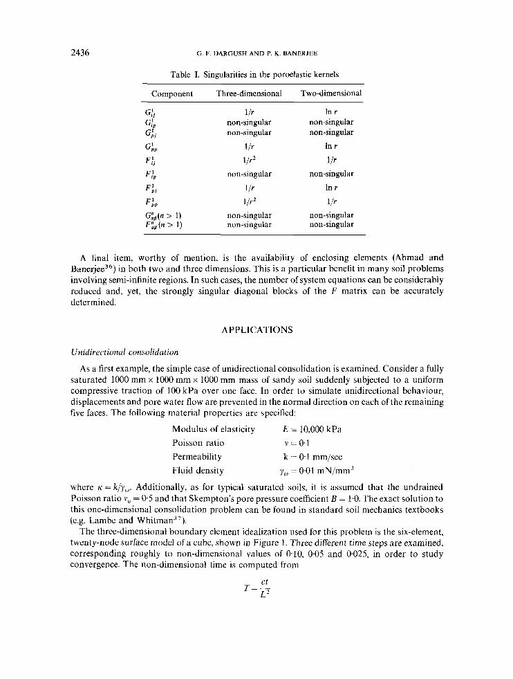
As was mentioned previously, the fundamental solutions to the poroelastic problem contain singularities when the load point and field point coincide, that is, when r = 0. The same is true of G;E and FE,, since these kernels are derived directly from the fundamental solutions. Series expansions of terms present in the evolution functions can be used to deduce the level of singularities existing in the kernels. Results are provided in Table I for both the two- and three- dimensional cases.

A number of observations concerning these results should be emphasized. First, as would be expccted, FiP has a stronger level of singularity than does the corresponding G;,, since an additional derivative is involved in obtaining FbfP from G&. Second, the coupling terms do not have as high a degree of singularity as do the corresponding non-coupling terms. For example, compare G:p and G i j with G:,. Third, all of the kernel functions for the first time step could actually be rewritten as a sum of steady-state and transient component$. That is,

Then, the singularity is completely contained in the steady-state portion. Furthermore, the singularity in Gh and F!j is precisely equal to that for elastostatics, while the G&, and F i p singularities are identical to those for potential flow. This observation is critical in the numerical integration of the Pa, kernel to be discussed in the next subsection. However, from a physical standpoint, this means simply that, at any time 1, the nearer one moves toward the load point, the closer the quasistatic response field corresponds with the fully drained, steady-state field. Eventually, when the sampling and load points coincide, the quasistatic and drained responses are indistinguishable. As a final item, after careful examination of the Appendix, it is evident that the steady-state components in the kernels Gib and F i p , with n > I , vanish. In that case, all that remains is a transient portion that contains no singularities. Thus, all singularities reside in the "Gm, and "FEp components of G$ and F&, respectively.

Numerical integration

Having clarified the potential singularities present in the coupled kernels, it is now possible to consider the evaluation of the integrals. To assist in this endeavour, the following three distinct categories can be identified:

1 . the point < does not lie on the element m; 2. the point t lies on the elemcnt m, but only non-singular or weakly singular integrals are

3. the point 5 lies on the element m, and the integral is strongly singular. involved;

In the above, the definition of strong and weak singularities depends upon not only the degree of the singularity in the inlegrand, but also on the dimensionality of the integration. For three-

EEM FOR POROEI ASTICITY 2433

dimensional problems, surface integrals are termed strongly singular, if the exponent, u, in

is greater than one. Thus, from the previous subsection, for an element containing 4, surface integrals involving F,'j and F,& are strongly singular, whereas those incorporated in Gli, G i p and F;j are only weakly singular. A similar situation arises in two dimensions, except that strong singularities are defined by v greater than zero in (32).

In practical problems involving many elements, it is evident that most of the integration will be of the Category ( 1 ) variety. In this case, the integrand is always non-singular, and standard Gaussian quadrature formulas can be employed. Sophisticated error control routines are needed, however, to minimize the computational effort for a certain level of accuracy. This non-singular integration is the most expensive part of a boundary element analysis, and, consequently, must be optimized to achieve an efficient solution. In the present implementation, error estimates, based upon the work of Stroud and Se~res t ,~ ' are employed to automatically select the proper ordcr of the quadrature rule. Additionally, to improve accuracy in a cost-effective manner, a graded subdivision of the element is incorporated, especially when ( is nearby.

Turning next to Category (2), one finds that again Gaussian quadrature is applicable; however, a somewhat modified scheme must be utilized to evaluate the weakly singular integrals. In this case, for three dimensions, the element is segmented into triangular sub-elements whose sides radiate from 5. A transformation, within each sub-element, to polar co-ordinates removes the singularity, permitting the use of normal Gaussian rules. Circumferential subdivision within the triangular sub-element is included to improve accuracy. The same effect is accomplished with two- dimensional elements via suitable subsegmentation along the length of the element.

Unfortunately, the remaining strongly singular integrals of Category ( 3 ) exist only in the Cauchy principal value sense and cannot, in general, be evaluated numerically, with sufficient precision. It should be noted that this apparent stumbling block is limited to the strongly singular portions, SSFij and " F P P , of the FAa kernel. Howcver, these Category (3) ssFij and s s f ; p p kernels can be accurately determined by employing an extension of the indirect 'rigid body' method originally developed by Cruse3' and Banerjee et ~ 1 . ~ ~

Assembly

Once the discretization in both time and space is complete, a system of algebraic equations can be developed to permit the approximate solution of the original poroelastic problem. This is accomplishcd by systematically writing the boundary integral at each global boundary node. The ensuing nodal collocation process, then, produces a global set of equations of the form

whcre

[ G ' + ' ~ " ] is an unassemblcd matrix of size (d+ l)P x ( d i l)Q, CP" " ] an assembled matrix of size (d+ l)P x (d+ 1)P, with clll included in the diagonal

blocks, M

P the total number of global functional nodes and Q =

A, the number of functional nodes in element m and d the dimensionality of the problem.

A , , m- 1

2434 Ci. F. DARGUSH AND P. K. BANERJEE

In the above, recall that the terms generalized displacement and traction refer to the inclusion of the pore pressure and flux, respectively, as the ( d - t 1) component at any point.

Consider, now, the first time step. Thus, for N = 1, equation (33) becomes

However, at this point, the diagonal block of [ F ' ] has not been completely determined owing to the strongly singular nature of 'SF,, and SSFPP. Following Cruse32 and, later, Banerjee et in eiastodynamics, these diagonal contributions can be calculated indirectly by imposing a uniform 'rigid body' generalized displacement field on the same body, bul under drained conditions. Then, obviously, the generalized tractions must be zero, and

C""Fl(I) = lo) (35) where ( 1 3 is a vector having all (d + l)P components equal to one. Using (35) , the desired diagonal blocks, 'SF,, and " F p P , can be obtained from the summation of the off-diagonal terms of P ' F ] . The remaining transient portion of the diagonal block is non-Fingular, and hence can be evaluated directly to any desired precision. With that step completed, (34) is rewritten as

[ G ' ] { t ' ) - [ F ' ] ( u ' ] = (0 )

In a well-posed problem, at time Ar, the set of global generalized nodal displacements and tractions will contain exactly (d + l)P unknown components. Then, as the final stage in the assembly process, equation (36) can be rearranged to form

[ A ' ] {x'} = [ B ' ] { y ' )

in which

(37)

{x'} are the unknown components of { u ' } and { t ' } , ( y ' } the known components of { u ' } and (t '} and [ A ' ] , [B'] the associated coefficient matrices.

It should be noted that, in the process of organizing the system equation (37) from the original system (36). ii very large amount of housekeeping is necessary. This is probably one of the most complex parts of a BEM code and arises mainly due to the presence of rnultivalued tractions at edges and corners." With the aid of integer matrix identifiers all boundary conditions for these elements are incorporated. Finally, if any corner node still contains unknown multivalued tractions, the corresponding components are equated. This last operation is still quite complex because it almost invariably depends on the type of qpecified boundary conditions at the edge or corner elements. As an alternative. others employ non-conforming (discontinuous) or partially conforming elements; however, this latter approach carries a severe penalty in terms of both accuracy and computational effort3'

Solution

To obtain a solution of (37) for the unknown nodal quantities, a decomposition of matrix [ A ' ] is required. In general, [ A '1 is a densely populated, unsymmetric matrix. 'The out-of-core solver, utilized here, was developed originally for elastostatics from the LINPACK software package (Dongarra e~ and operates on a submatrix level. Additional information on this solver is available in Banerjee et aLZ6

After returning from the solver routines, the entire nodal response vectors, {u' } and ( t ' 1, at time At are known. For solutions at later times, a simple marching algorithm is employed. Thus, for a


general time step N , N - 1

"4'1 {."} = [ B ' ] { y N } - " ~ * ( [ G N + l - n ] { t n } - [ " F N + ' - " I {u"}, n = 1

(39)

in which the summation represents the effect of past events. By systematically storing all of the matrices and nodal response vectors computed during the marching process, surprisingly little computing time is required at each new time step. In fact, for any time step beyond the first, the only major computational task is the integration needed to form [G"] and [ F " ] . Even this process is considerably reduced, since now that all of the kernels are non-singular a less intensive integration can be performed.

It should be emphasized that the entire boundary element method developed in this section has involved surface quantities exclusively. A complete solution to the well-posed linear coupled quasistatic poroelastic problem, with homogeneous properties, can be obtained in terms of the nodal response vectors, without the need for any volume discretization.

In many practical situations, however, additional information, such as the pore pressures at interior locations or the stress at points on the boundary, is required. For any point < strictly in the interior, the generalized displacement can be determined from (30) directly with cPa = hnm. On the other hand, when 5 is on the boundary, the strong singularity in ""F,, prohibits accurate evaluation of the generalized displacement and an alternate approach employing the elemental shape functions is used. In this latter case, neither integration nor the explicit contribution of past events is needed to evaluate generalized boundary displacements.

In much the same manner, an integral equation can be written for interior effective stresses by utilizing the constitutive relations in conjunction with the appropriate derivatives of (30). Since strong kernel singularities appear when this integral equation is written for boundary points, an alternate procedure is needed to determine surface effective stress. This alternate scheme exploits the interrelationships between generalized displacement, traction and stress, and is the straightforward extension of the technique typically used in electrostatic implementations. Complete details are available in Dargush and B a ~ ~ e r j e e . ~ ~

Speciul features

The foregoing poroelastic formulation has been implemented directly in a state-of-thc-art, general-purpose boundary element computer program. Consequently, many additional features, beyond those discussed above, are available for the analysis of complex geotechnical engineering problems.

Perhaps the most significant of these items is the capability to analyse substructured problems. This not only extends the analysis to bodies composed of several different materials, but also often provides computational efficiencies. Consider a body divided into several substructures or generic modelling regions (GMR's). During the integration process, the individual regions remain separate entities. The GMR's are brought together for the first time at the assembly stage, where compatibility relations are enforced on the common boundary between adjacent regions. This multi-GMR assembly process produces block-banded system matrices that can be solved in an efficient manner.

As another convenience, a high degree of flexibility is provided for the specification of boundary conditions. In general, time-dependent values can be defined in either global or local co-ordinates, with or without sliding. Not only can generalized displacements and tractions be specified, but also spring and smearing contact resistance relations are available. Furthermore, a comprehensive symmetry capability is included with provisions for both planar and cyclic symmetry.


Table I. Singularities in the poroelastic kernels

Component Three-dimensional Two-dimensional

l l r non-singular non-singular

l/r I / r2

non-singular l / r l / r2

non-singular non-singular

In r non-singular non-singular

In r

l / r non-singular

In r

l / r non-singular non-singular

A final item, worthy of mention, is the availability of enclosing elements (Ahmad and B a ~ ~ e r j e e ~ ~ ) in both two and three dimensions. This is a particular benefit in many soil problems involving semi-infinite regions. In such cases, the number of system equations can be considerably reduced and, yet, the strongly singular diagonal blocks of the F matrix can be accurately determined.

APPLICATIONS

Unidirectionul consolidalion

As a first example, the simple case of unidirectional consolidation is examined. Consider a fully saturated 1000 mm x 1000 mm x 1000 mm mass of sandy soil suddenly subjected to a uniform compressive traction of 100 kPa over one face. In order to simulate unidirectional behaviour, displacements and pore water flow are prevented in the normal direction on each of the remaining five faces. The following material properties are specified:

Modulus of elasticity Poisson ratio v = o 1 Permeability k = 0 1 mm/sec Fluid density

E = 10,000 kPa

yru = 0.01 mN/mm3

where K = k/y, . Additionally, as for typical saturated soils, it is assumed that the undrained Poisson ratio v, = 0.5 and that Skempton’s pore pressure coefficient B = 1.0. The exact solution to this one-dimensional consolidation problem can be found in standard soil mechanics textbooks (e.g. Lambe and Whitman3’).

The three-dimensional boundary element idealization used for this problem is the six-element, twenty-node surface model of a cube, shown in Figure I . Three different time steps are examined, corresponding roughly to non-dimensional values of 0.10, 0.05 and 0,025, in order to study convergence. The non-dimensional time is computed from

ct T = ~

L2

BEM FOR POROELASTICITY

9 Ccrner nsde

2437

Figure 1. Unidirectional consolidation: boundary element model

10.

a .

- E v

6 . Y

L 0 E W - +-' * 4 . a, (i?

2 .

2 .

- C

__ Fna I y t 3 c a I 0 GP-BEST tAt=1.00) A GP-EEST (ot=0.5a) 0 GP-BEST (&=0.25)

0. 2 . 4. 6 . 8 . 10.

l i m e ( s e c )

Figure 2. Unidirectional consolidation: 3d results

C

/y __ Fna I y t 3 c a I 0 GP-BEST tAt=1.00) A GP-EEST (ot=0.5a) 0 GP-BEST (&=0.25)

2 . 4. 6 . 8 . 10.

T i m e ( s e c )


where c is the coefficient of consolidation or the poroelastic diffusivity. The quantity L is the flow length. GP-BEST settlement and pore pressure results are compared to the exact solution in Figures 2 and 3, respectively. From these graphs, it is evident that the current boundary element formulation can correctly simulate the unidirectional consolidation process. A time step of 0.50 sec provides excellent results. In fact, in the light of the quality of the solution, it is remarkable that only a single quadratic element exists in the flow direction. However, in order to capture very short time behaviour, refinement of both the temporal and spatial discretizations is required. Additionally, refinement is needed for high aspect ratio domains.

2438 G. F. DARGUSH A N D P. K. BANERJEE

1.0

F .I3 3 Df i? 0

a L

0 . 6

a 0 -c 0

N . 4

E - m

z . 2

- FnaIytTcai 0 GP-ZEST (At=l.Q@l

- A GP-BEST (At=0.52> 0 GP-BEST (At=0.25)

t-

-

h -

.a 1 I

T i m e (set)


Consolidation under a strip load

A number of analytical, as well as finite element solutions are available for the consolidation of a single poroelastic stratum beneath a strip load. The geometry for this problem is completely defined in the x-y plane by the depth of the layer H , and the total breadth of the strip load 2a. The lower boundary remains impervious, while free drainage is permitted along the entire upper surface. For convenience, non-dimensional forms of the material parameters are utilized. In particular, let E = 1.0, v = 0.0, IC = 1.0, v,, = 0.5 and B = 1.0. Notice, for this set of properties, that the diffusivity is unity. The forthcoming presentation of results is simplified further by also assuming unit values for both the half-width a and the applied traction.

Analytical solutions for this general problem were developed by Gibson et al.,s although previous work for the special case of infinite H is contained in Schiffman rt The finite element results included in the following graphs are those of Y o ~ s i f . ~ ~

Meanwhile, the boundary element mesh for the particular case of H/u = 5 is depicted in Figure 4. It contains 12 elements, 25 boundarj nodes, and 9 interior points. Symmetry is imposed along x = 0. As in the finite element analysis cited above, the region is truncated at a horizontal dimension of L/a = 10. While theoretically the vertical elements along x = 10 are unnecessary, closilre of the region permits accurate determination of the strongly singular diagonal blocks of the F matrix via rigid body considerations. A recently discovered alternative is the enclosing element concept, which was developed by Ahmad and B a n e ~ - j e e ~ ~ for elastodynamics. With this new technique, the enclosing elements are used only in the calculation of the diagonal blocks of F , and do not produce additional boundary equations.

First, results are presented for H,/u + a. Figure 5 contains the pore pressure time history for a point, on the centreline, a unit depth below the surface. The well-known Mandel Cryer effect, of increasing pore pressure during the early stages of the process, is evident in the graph. Actually, only the final portion of the rising pore prcssure response was captured in the boundary element analysis, since a relatively large time step was selected. Even with this large step, however, the analytical solution is accurately reproduced. In Figure 6, the pore pressure distribution with depth

BEM FOR POROELASTIClTY

.0

2439

I I "---

0 L

3 VI VI

0 i a Iu i 0 a 7J 0 N - - m E L

9

is shown for

I x 1

-5. 1 1 -7. =. t Corner node

0 Midnode X Interior p o i n t

-8. I I I I I I I I I 1

-1. 8. I . 2. 3. 4. 5. 6 . 7 . a. 3 . 1 8 .

Figure 4. Consolidation under a strip load: boundary element model

1.

7 ,

T = 0.1. Obviously, the boundary element solutions are comparable to those obtained by Yousif 39 via finite elements.

Next, Figure 7 displays the degree of consolidation versus time for various H/a ratios. Again, in all cases, excellent agreement with the analytical solution is obtained.

Finally, the effects of partial saturation are explored. For soils, this is accomplished by maintaining the effective stress parameter f i at unity, while reducing Skempton's coefficient B to various levels. Consequently, the undrained Poisson ratio will assume values less than 0.5. Physically, as the degree of saturation is reduced, v, and B decrease, resulting in a larger immediate

2440

a.

-1.

c 4J p. m

71 0 N

-2. a

.- - Id

,E -3. 9

G. F. DARGUSH AND P. K. BANERJEE

- Analytical X FE (60 elements) 0 FE (40 elements) 0 GP-EEST

.OO

Figure 7. Consolidation under a strip load results

settlement and a slower consolidation process. This behaviour is evident in the boundary element results presented in Figures 8 and 9 for the particular case of H/u = 10. Analytical solutions are unavailable for this partially saturated problem.

Consolidation at the Koyna Dam

The next example involves the simulation of a consolidation process beneath the Koyna Dam and reservoir in India. The objective of the analysis is to determine the changes in excess pore

BEM FOR POROELASTlCITY

-P C 4 2.0 - c, c, D Ln 2.5

E" .-

1.0 1

-

-

1.5 L - GP-BEST (B-I. 00) - - GP-BEST (6=0.85) . . . GP-BEST (8-0.701

GP-EEST ( 8-0.50 )

z

. . . .

3.5 i 4.0 1 I I 4

-1.5 -1.0 -. 5 .0

log (T)

Figure 8. Consolidation under a strip load results (H/a = 10)

2441

. 5

Figure 9. Consolidation under a strip load results (Hia = 10)

pressures and effective stresses at various subsurface locations due to impoundment and seasonal variations in reservoir level. All geometric, load and material property definitions were provided by Roel~ffs.'~

As a first approximation, the reservoir is considered a uniformly loaded 40 km by 5 km rectangle resting on a two-layer half-space. Specifically, the subsurface geology is idealized by a 1 km thick zone of basalt, on top of a semi-infinite granite region. The material properties that were adopted for each layer are detailed in Table 11. The reservoir level, and consequently, the load

2442

-5. c i ' x x x x x m

I x x x x x

G . F. DARGUSH AND P. K. BANERJEE

Table TI. Koyna Dam subsurface material properties

E k (GPa) v (kmiyr) v, B

Basalt 75.0 0.25 2.0 x 0.3 0.8 Granite 75.0 0.25 2 . 0 ~ 10- 0.3 0.8

Table 111. Koyna Dam reservoir levels

t h t h (mo.1 (4 (mo.) (4 .-

0 0.0 19 8.9 2 2.3 24 6.5 7 5.0 26 13.3

12 4.8 31 10.4 14 10.3 36 7.2

-15. c 8 Corner node

0 Mianode X Interior point

-28. I -- 4

-25. i ~ I I I -L-.-l-__i - !0 . -5. 0 . 5 . 18. 15. 20. 2 5 . 30.

Figure 10. Consolidation at the Koyna Dam: boundary element model

history, is a function of time, involving the initial filling stage plus typical seasonal variations. Table I11 contains the assumed reservoir levels, h, during the first three years after impoundment. This information is used to determine the boundary conditions on the outer surface. Beneath the reservoir, let

t , = - p = p g h and t , = t , = O

t = t = t = p = o while elsewhere

X Y Z

In the above, p g is the weight density of water.


Owing to the elongated shape of the reservoir, a two-dimensional plane strain analysis, taken in the plane normal to the long axis, is in order. The two-region boundary element mesh is detailed in Figure 10. The basalt layer is modelled with seventeen elements, while only twelve elements are needed to describe the response of the granite. An ample supply of interior nodes is also included to monitor excess pore pressures and effective stresses throughout the area of interest. Results for points A to D are presented in Figure 11. In that diagram, the excess pore pressures at those four locations are traced versus time. Notice that the intensities drop dramatically with depth and that, in some instances, load reversals produce negative pore pressures in the underlying strata. It has been hypothesized by some that consolidation, as considered here, could induce seismic events. However, in all cases, the magnitudes of the pressures and stresses due to this consolidation process are very small, particularly when compared to typical tectonic stresses.

150.

125. m

% 100.

W L 3 : 75.

Y 56. a"

L a

v)

2 5 . U X

W

0.

-25.

I - -

I I I I I I I 0. 6 . 12. 18 . 24. 30. 3 6 .

Time (mu)

Figure 11. Consolidation at the Koyna Dam: plane strain results

Figure 12. Consolidation under a load (b/a = 8): boundary element model

2444 G . F. DARGUSH AND P. K. BANERJEE

0 GP-BEST (Wa-1) 0 CP-BEST (b/a-2) A GP-BEST (b/a-8)

-1. 0. 1.

1Cg (TI’

Figure 13. Consolidation under rectangular loads: results

2 .

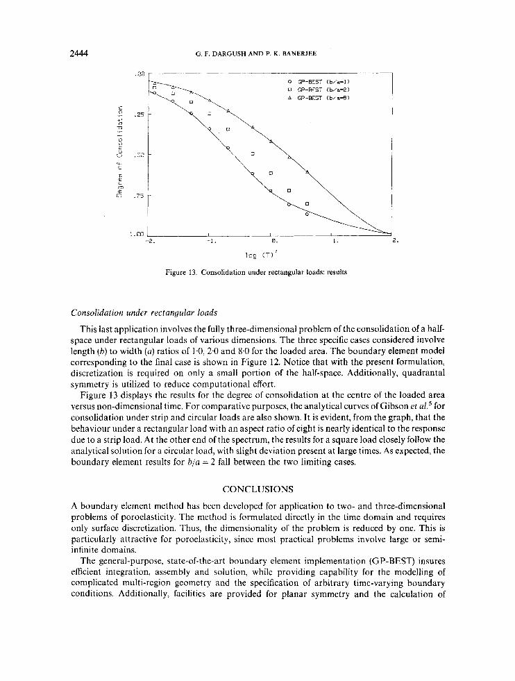
Consolidation under rectangular loads

This last application involves the fully three-dimensional problem of the consolidation of a half- space under rectangular loads of various dimensions. The three specific cases considered involve length (b) to width (a) ratios of 1.0, 2.0 and 8.0 for the loaded area. The boundary element model corresponding to the final case is shown in Figure 12. Notice that with the present formulation, discretization is required on only a small portion of the half-space. Additionally, quadrantal symmetry is utiliz.ed to reduce computational effort.

Figure 13 displays the results for the degree of consolidation at the centre of the loaded area versus non-dimensional time. For comparative purposes, the analytical curves of Gibson et a1.’ for consolidation under strip and circular loads are also shown. It is evident, from the graph, that the behaviour under a rectangular load with an aspect ratio of eight is nearly identical to the response due to a strip load. A t the other end of the spectrum, the results for a square load closely follow the analytical solution for a circular load, with slight deviation present at large times. As expected, the boundary element results for b/a = 2 fall between the two limiting cases.

CONCLUSIONS

A boundary element method has been developed for application to two- and three-dimensional problems of poroelasticity. The method is formulated directly in the time domain and requires only surface discretization. Thus, the dimensionality of the problem is reduced by one. This is particularly attractive for poroelasticity, since most practical problems involve large or semi- infinite domains.

The general-purpose, state-of-the-art boundary element implementation (GP-BEST) insures efficient integration, assembly and solution, while providing capability for the modelling of complicated multi-region geometry and the specification of arbitrary time-varying boundary conditions. Additionally, facilities are provided for planar symmetry and the calculation of


interior and boundary pore pressures and effective stresses. Four detailed numerical examples validate this new formulation and highlight the versatility of the implementation.

APPENDIX: QUASISTATIC POROELASTIC KERNELS

Introduction

This Appendix contains the detailed presentations of all the kernel functions utilized in the poroelastic boundary element formulation. Both three-dimensional and two-dimensional (plane strain) kernels are provided, based upon continuous source and force fundamental solutions. As a result, the following relationships must be used to determine the proper form of the functions required in the boundary element discretization. That is,

Gi,(X - <) = G,,(X- t, nAt)

Gz,(X - <) = G,,(X - 5, nAt) - G,,(X - 5, (n - 1)At)

for n= 1

for n > 1

with similar expressions holding for all the remaining kernels. In the specification of these kernels below, the arguments ( X - 5, t ) are assumed.

Where possible. consistent notation is used for both the three- and two-dimensional presentations. In particular, the indices

i, j , k, 1 a, P P equals d

vary from 1 to d vary from 1 to (d + 1)

where d is the dimensionality of the problem. Additionally,

x, co-ordinates of integration point 5 , co-ordinatcs of field point

2446 Ci. F. DARGUSH A N D P. K. BANERJEE

whereas, for the traction kernel,

REM FOR POROELASTICITY 2447

Two-dimensional kernels

For the displacement kernel,

whereas, for the traction kernel,

In the above,

E , fz) = Jz “t‘ dx


REFERENCES

1. M. A. Biot, ‘General theory of three-dimensional consolidation’, J. Appl. Phys., 12, 155-164 (1941). 2. J. McNamee and R. E. Gibson, ‘Plane strain and axially symmetric problems of the consolidation of a semi-infinite clay

3. R. E. Gibson and J. McNamee, ‘A three-dimensional problem of the consolidation of a semi-infinite clay stratum’,

4. C. W. Cryer, ‘A comparison of the three-dimensional consolidation theories of Biot and Terzaghi’, Quuri. J. Mech.

5. R. E. Gibson, R. L. SchiiTman and S. L. Pu, (1970). ‘Plane strain and axially symmetric consolidation ofa clay layer on a

6. M. P. Cleary, ‘Fundamental solutions for a fluid-saturated porous solid’, Inl. J. Solids Slrucl., 13, 7855806 (1977). 7. R. S. Sandhu and E. L. Wilson, ‘Finite element analysis of seepage in elastic media’, J . Eng. Mech. Din A S C E , 95,

8. C. S. Desai and J. F. Abel, Introduction to the Finite Element Method, Van Nostrand Reinhold, New York, 1972. 9. 0. C. Zienkiewicz, 7Ae Finite Element Method, McGraw-Hill, London, 1977.

10. M. J. Gunn and A. M. Britto, CRiSP User’s and Programmer’s Guide, Engineering Department, Cambridge

I i. P. K. Banerjee and R. Butterfield, Boundary Element Methods in Engiwering Science. McGraw-Hill, London, 1981. 12. ‘T. Kuroki, T. Ito and K. Onishi, ‘Bi)undary element method in Biot’s linear consolidation’, Appl. Math. Modelling, 6,

13. G. Aramaki and K. Yasuhara, ‘Application of the boundary element method for axisymmetric Biot’s consolidation’,

14. (i. Aramaki, ‘Boundary e!emenls for thin layers with high permcability in Biot’s consolidation analysis’, Appl. Mach.

! 5. A. H-D. Cheng and J. A. Ciggctt, ‘Houndary integral cquation mcthod for linear porous-elasticity with applications to

16. N. Nishimura, ‘A BIE formulation for consolidarion prohlems‘, in C. A. Brebbia and C;. Maicr (eds.), Boundary

stratum’, Quart. J. Mech. Appl, .Uuth., XIII, 21&227 (1960).

Quart. J. Mech. Appl. Math., XVI, 115-127 (1963).

Appl. Math., XVI, 401-412 (1963).

smooth impervious base’, Quurt. J. Mech. Appl. Math., 23, 505-520 (1970).

641-651 (1969).

University, 1984.

105-110 (1982).

En!]. Anill.. 2, 184-191 (1Y85).

Modeliiny. 10, 82--86 (19861.

soil consolidation,’ I n r . j . nume(. rnefh(ids eng., 20, 755 278 (1984).

Elements V I I , Proc. 7ih Inf. Con& Springer-Verlag, Berlin, 1985.


17. N. Nishimura, A. Umeda and S. Kobayashi, ‘Analysis of consolidation by boundary integral equation method’, in

18. J. R. Rice and M. P. Cleary, ’Some basic stress diffusion solutions for fluid-saturated elastic porous media with

19. W. Nowacki, ‘Green’s functions for a thermoelastic medium (quasi-static problem)’, Bull. Inst. Polit. Jasi, Sierie noua,

20. J. W. Rudnicki, ‘On ‘Fundamental solutions for a fluid-saturated porous solid’, by M. P. Cleary’, In t . J . Solids Struct.,

21. J. W. Rudnicki, ‘Fluid mass sources and point forces in linear elastic diffusive solids’, Mech. of Mater., 5 , 383-393

22. V. lonescu-Cazimir, ‘Problem of linear coupled thermoelasticity. Theorems on reciprocity for the dynamic problem of

23. M. A. Biot, ‘New thermomechanical reciprocity relations with application to thermal stress analysis’, J . AerolSpace

24. M. Predeleanu, ‘Boundary integral method for porous media’, in C. A. Brebbia (ed.), Boundary Methods, Springer-

25. V. Slbdek and J. Sladek, ‘Boundary integral equation method in two-dimensional thermoelasticity’, Eng. Anal., 1,

26. P. K . Banejeel R. B. Wilson and N. Miller, ‘Development of a large BEM system for three-dimensional inelastic analysis’, in T. A. Cruse et a / . (eds), Advanced Topies in Boundary Element Analysis, AMD-Vol. 72, ASME, New York, 1985.

27. P. K. Banerjee and S. Ahmad, ‘Advanced three-dimensional dynamic analysis by boundary element methods’, in T. A. Cruse et al. (eds), Advanced Topics in Boundary Element Analysis, AMD-Vol. 72, ASME, New York, 1985.

28. P. K . Banerjee, R. R. Wilson and N. Miller, ‘Elastic and inelastic analysis of gas turbine engine structures by BEM’, Int. j . numer. methods eng., 26, 393411 (1985).

29. J . C. Lachat and J. 0. Watson, ‘Effective numerical treatment of boundary integral equations: A formulation for three- dimensional elasto-statics’, Int . j. numer. methods. eng., 10, 991-1005 (1976).

30. G. D. Manolis and P. K. Bancrjee, ‘Conforming versus non-conforming boundary elements in three-dimensional elastostatics’, Int. ,j. numer. methods eng., 23, 1885- 1904 (1986).

31. A. H. Stroud and D. Secrcst, Gaussian Quadrature Formulas, Prentice-Hall, Englewood Cliffs, N.J., 1966. 32. T. A. Cruse, ’An improved boundary integral equation method for three-dimensional elastic stress analysis’, Comp.

33. P. K. Banerjee, S. Ahmad and G. D. Manolis, ‘Transient elastodynamic analysis of three-dimensional problems by

34. J. J. Dongarra et ul., Linpak User’s Guide, SIAM, Philadelphia, 1979. 35. G. F . Dargush and P. K. Banerjee, ‘Boundary element methods for poroelastic and thermoelastic analyses’, in P. K.

Bansrjee and R. B. Wilson (eds.), Deuelopments in Boundary Element Methods-5, Applied Scicncc Publishers, Barking, [J.K., to appear.

36. S. Ahmad and P. K. Banerjee, ‘Multi-domain BEM for two-dimensional problems of elastodynamics’, Int. j . numer methods eng., 26, 891-912 (1988).

37. T. W. Lambe and R. V. Whitman, Soil Mechanics, Wiley, New York, 1969. 38. R. L. Schiffman, A. T-F., Chen and J. C. Jordan, ‘An analysis of consolidation theories’, J . Soil Mech. Found. Div.

39. N. B. Yousif, ‘Finite element analysis of some time indcpcndcnt construction problems in geotechnical engineering,

40. E. Roelolh, Private communication, 1985.

DuQinghua (ed.), Boundary Elements, Proc. I n t . Con&, Beijing, 1986, pp. 119-126.

compressible constituents’, Rev. Geophys. Space Phys. 14, 227-241 (1976).

12, 83-92 (1966).

17, 855-857 (1981).

(1987).

coupled thermoelasticity. I’, Bull. Acad. Polonaise Sci., Series sci. techniques, 12, 473-488 (1964).

Sci., 26, 401 4 0 8 ( 1 959).

Verlag, Berlin. 1981, pp. 325-334.

135-148 (1984).

Stvuct.. 4, 741-754 (1974).

boundary element method‘, Earthquake eng. struet. dyn., 14, 933-949 (1986).

ASCE, 95, 285-312 (1969).

Ph.D. Dissertation, State University of New York at Buffalo, 1984.

A time domain boundary element method for poroelasticity

Documents

Transcript of A time domain boundary element method for poroelasticity