Treatment of hypersingularities in boundary element ...

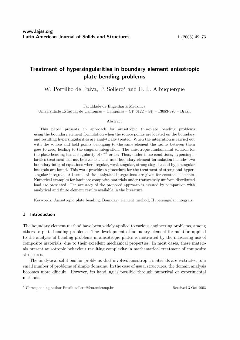
www.lajss.orgLatin American Journal of Solids and Structures 1 (2003) 49–73

Treatment of hypersingularities in boundary element anisotropic

plate bending problems

W. Portilho de Paiva, P. Sollero∗ and E. L. Albuquerque

Faculdade de Engenharia MecanicaUniversidade Estadual de Campinas – Campinas – CP 6122 – SP – 13083-970 – Brazil

Abstract

This paper presents an approach for anisotropic thin-plate bending problemsusing the boundary element formulation when the source points are located on the boundaryand resulting hypersingularities are analytically treated. When the integration is carried outwith the source and field points belonging to the same element the radius between themgoes to zero, leading to the singular integration. The anisotropic fundamental solution forthe plate bending has a singularity of r−2 order. Thus, under these conditions, hypersingu-larities treatment can not be avoided. The used boundary element formulation includes twoboundary integral equations where regular, weak singular, strong singular and hypersingularintegrals are found. This work provides a procedure for the treatment of strong and hyper-singular integrals. All terms of the analytical integrations are given for constant elements.Numerical examples for laminate composite materials under transversely uniform distributedload are presented. The accuracy of the proposed approach is assured by comparison withanalytical and finite element results available in the literature.

Keywords: Anisotropic plate bending, Boundary element method, Hypersingular integrals

1 Introduction

The boundary element method have been widely applied to various engineering problems, amongothers to plate bending problems. The development of boundary element formulation appliedto the analysis of bending problems in anisotropic plates is motivated by the increasing use ofcomposite materials, due to their excellent mechanical properties. In most cases, these materi-als present anisotropic behaviour resulting complexity in mathematical treatment of compositestructures.

The analytical solutions for problems that involves anisotropic materials are restricted to asmall number of problems of simple domains. In the case of usual structures, the domain analysisbecomes more dificult. However, its handling is possible through numerical or experimentalmethods.

∗ Corresponding author Email: [email protected] Received 3 Oct 2003

50 W. Portilho de Paiva, P. Sollero and E. L. Albuquerque

Nomenclaturedi, ei real and imaginary part of complex roots of characteristic equationDij plate flexural rigidities

E1, E2 Modulus of elasticity in tension and compressionG12 Modulus of elasticity in shear

Mn,M∗n bending moment perpendicular no n direction and its fundamental solution

n, nx, ny outward unit normal vector on field point and its componentsn0, n0x , n0y outward unit normal vector on source point and its components

P field pointq transverse load intensityQ source point

r, θ polar coordinatesR curvature radius at a smooth point of the boundary Γ

Rci , wci reaction forces and deflections at ith plate cornerVn, V ∗

n Kirchhoff’s equivalent shear force and its fundamental solutionw, w∗ out-of-plane deflection of a plate and its fundamental solution

x, y rectangular coordinates of field pointx0, y0 rectangular coordinates of source point

Γ boundary of solidµ1, µ2 complex roots of characteristic equation

ν1 Poisson’s ratioδ Dirac delta function

Due to hardware and software evolution, numerical methods have been used for solve awider range of problems. Among the methods that have been outstanding in the treatment ofstructural problems there are the finite element and the boundary element methods.

In the last ten years, the boundary element method has been successfully applied to theanalysis of a large number of anisotropic material problems. Plane elasticity problems wereanalised by Sollero and Aliabadi [24], Deb [8] and Albuquerque et al. [1, 2, 4, 5]; out-of-planeelasticity problems were shown by Zhang [29,30] and tri-dimensional problems were analised byKogl and Gaul [13–15].

Studies of plate bending problems using the boundary element method have been carriedout by many researchers. Bending problems of isotropic plates, for statics as well as dynamics,have been widely studied [6, 9, 11, 12, 19, 20, 23, 25, 27]. On the other hand, it can be noted thatthe number of references in which boundary element method is applied to anisotropic structuresis significantly smaller than those treating isotropic ones. Boundary element formulation hasbeen applied to plate bending anisotropic problems using Kirchhoff’s theory. Shi and Bezine [22]presented a boundary element analysis of plate bending problems, based on Kirchhoff’s plate

Latin American Journal of Solids and Structures 1 (2003)

Hypersingularities in boundary element anisotropic plate problems 51

bending assumptions, using fundamental solutions proposed by Wu and Altiero [28]. Similarprocedure was used by Rajamohan and Raamachandran [21] who presented a formulation foranisotropic plate bending in which the singularities were avoided by placing source points outsidethe domain. An analysis of the fundamental solution for anisotropic thin plates was presentedby Portilho de Paiva et. al. [7] who compared it with isotropic fundamental solution using quasi-isotropic material properties. An analysis of symmetric laminate composites under bending usingthe boundary element method was presented by Albuquerque et. al. [3] who carried out analysisof symmetric cross-ply and angle-ply laminate composites under several boundary conditions.

This paper presents detailed procedures for the treatment of singularities inherent to bound-ary element formulation for anisotropic plate bending. Similar procedure was developed byRashed et. al. [10] for isotropic thick plates. In order to be self-contained, all terms of theanalytical integration for constant element are presented here. Numerical examples for laminatecomposite materials under transversely uniform distributed load are presented. The accuracyof the proposed approach is assured by comparison with analytical and finite element resultsavailable in the literature.

2 Theory of anisotropic thin plate bending

In this work, a plate is understood as a structural element defined by two parallel plane surfaces(Figure 1). The distance between these two surfaces defines the thickness of the plate, which issmall when compared with other plate dimensions. In the theory of anisotropic plate bending,loads are always transversely applied in the surface of the plate.

Depending on its material properties, a plate can be considered eitheranisotropic, with different properties in different directions, or isotropic, with same propertiesin all directions. In this work the Kirchhoff theory will be applied to anisotropic thin plates.

Figure 1: Definition of thin plate.

According to Timoshenko and Woinowsky-Krieger [26] the thin plate bending theory is basedon the following assumptions:

1. The middle plane of the plate does not undergo deformations;



2. Straight sections, which are normal to middle surface when the plate is in the undeformedstate, remain straight and normal to the deformed middle surface, after loading;

3. The normal stress perpendicular to the middle plane can be disregarded.

Consider a plate following these assumptions. The lateral midsurface deflection w satisfiesthe differential equation (Lekhnitskii [17]):

D11∂4w

∂x4+ 4D16

∂4w

∂x3∂y+ 2(D12 + D66)

∂4w

∂x2∂y2+ 4D26

∂4w

∂x∂y3+ D22

∂4w

∂y4= q

(1)

where Dij are the flexural rigidities of the anisotropic plate, q is the transverse load intensity.General solution to w in Equation (1) depends on µk, the roots of characteristic equation

given by:

D22µ4 + 4D26µ

3 + 2(D12 + 2D66)µ2 + 4D16µ + D11 = 0. (2)

Roots of this equation are always complex for homogeneous materials. The complex rootsµk = dk + eki, where k = 1, 2 and does not imply summation, are known as deflection complexparameters. In general, these roots are different complex numbers.

3 Boundary integral equation

Using Rayleigh-Green identity, an integral equation for an anisotropic thin plate under transver-sal load q(p) is obtained. In this equation one has the boundary integral equation given in termsof four basic boundary values, namely, deflection w, normal slope ∂w/∂n, bending moment Mn

and Kirchhoff’s equivalent shear force Vn. Two of these four values should be the unknowns ofthe problem and other two are determined by boundary conditions.

As shown by Shi and Bezine [22] the first boundary integral equation over the boundary Γis:

cw(Q)+∫

ΓV ∗

n (Q,P )w(P )dΓ(P )−∫

ΓM∗

n(Q,P )∂w

∂n(P )dΓ(P ) +

Nc∑

i=1

R∗ci

(Q,P )wci(P ) =

∫

Γw∗(Q,P )Vn(P )dΓ(P )−

∫

Γ

∂w∗

∂n(Q,P )Mn(P )dΓ(P ) +

Nc∑

i=1

w∗ci(Q,P )Rci(P ) (3)



where the constant c is introduced in order to consider that the Dirac delta function can beapplied in the domain, in the boundary, or outside the domain. In the particular case, whenthe point is taken in a smooth part of boundary, c = 1/2. Besides, Nc is the number of cornerpoints on the boundary. Q is the point where the load is applied, so-called source point, and P

is the point where the deflection is observed, so-called field point. Stars indicate the known statefundamental solution. Rci and wci are reaction forces and deflections at the ith plate corner. InEquation (3) the body forces are neglected.

In plate bending problems there are always two unknowns to be determined at any boundarypoint. Thus, the problem solution requires a second boundary integral equation in order to havean equal number of equations and unknown variables. This second equation is obtained bydifferentiating the displacement w(Q) in relation to a Cartesian coordinate system fixed in thesource point, i.e., the point where the Dirac delta of the fundamental state is applied, in thedirection of the outward unit normal vector n0 on source point. It is given by:

c∂w

∂n0(Q)

∫

Γ

∂V ∗n

∂n0(Q,P )w(P )dΓ(P )−

∫

Γ

∂M∗n

∂n0(Q,P )

∂w

∂n(P )dΓ(P ) +

Nc∑

i=1

∂R∗ci

∂n0(Q,P )wci(P ) =

∫

Γ

∂w∗

∂n0(Q,P )Vn(P )dΓ(P )−

∫

Γ

∂2w∗

∂n0∂n(Q,P )Mn(P )dΓ(P ) +

Nc∑

i=1

∂w∗ci

∂n0(Q,P )Rci(P ). (4)

The detailed development of Equations (3) and (4) can be seen in [6,12,22]. It is importantto say that it is possible to use only Equation (3) in a boundary element formulation by usingthe boundary nodes as source points and an equal number of points external to the domain ofthe problem.

4 Anisotropic fundamental solution

The fundamental solutions are the solutions of the differential Equation (1) with the non-homogeneous term equal to a concentrated force given by a Dirac delta function δ(Q, P ), i.e.,

∆∆w∗(Q,P ) = δ(Q,P ) (5)

where ∆∆(.) is the differential operator given by:

∆∆(.) =D11

D22

∂4(.)∂x4

+ 4D16

D22

∂4(.)∂3∂y

+2(D12 + 2D66)

D22

∂4(.)∂x2∂y2

+ 4D26

D22

∂4(.)∂x∂y3

+∂4(.)∂y4

. (6)



As presented by Shi and Bezine [22], the deflection fundamental solution for anisotropic platebending is:

w∗(r, θ) =18π{C1R1(r, θ) + C2R2(r, θ) + C3 [S1(r, θ)− S2(r, θ)]} (7)

where r is the distance between the source point P (x0, y0) and field point Q(x, y),

θ = arctany − yo

x− xo, (8)

C1 =(d1 − d2)2 − (e2

1 − e22)

GHe1, (9)

C2 =(d1 − d2)2 + (e2

1 − e22)

GHe2, (10)

C3 =4(d1 − d2)

GH, (11)

G = (d1 − d2)2 + (e1 + e2)2, (12)

H = (d1 − d2)2 + (e1 − e2)2, (13)

Ri(r, θ) = r2[(cos θ + di sin θ)2 − e2

i sin2 θ]×

{log

[r2

a2

((cos θ + di sin θ)2 + e2

i sin2 θ)]− 3

}−

4r2ei sin θ (cos θ + di sin θ) arctanei sin θ

cos θ + di sin θ(14)

and

Si(r, θ) = r2ei sin θ (cos θ + di sin θ)×{log

[r2

a2


i sin2 θ)]− 3

}+

r2[(cos θ + di sin θ)2 − e2

i sin2 θ]arctan

ei sin θ

cos θ + di sin θ. (15)



The index i of functions Ri(r, θ) and Si(r, θ) given by Equations (14) and (15) does not implysummation and the coefficient a is an arbitrary constant. In this work it is assumed that a = 1.

Other fundamental solutions are given by:

M∗n = −

(f1

∂2w∗

∂x2+ f2

∂2w∗

∂x∂y+ f3

∂2w∗

∂y2

), (16)

R∗ci

= −(

g1∂2w∗

∂x2+ g2

∂2w∗

∂x∂y+ g3

∂2w∗

∂y2

)(17)

and

V ∗n = −

(h1

∂3w∗

∂x3+ h2

∂3w∗

∂x2∂y+ h3

∂3w∗

∂x∂y2+ h4

∂3w∗

∂y3

)−

1R

(h5

∂2w∗

∂x2+ h6

∂2w∗

∂x∂y+ h7

∂2w∗

∂y2

)(18)

where R is the curvature radius at a smooth point of the boundary. Other constants of thefundamental solutions are presented in Appendix A.

The derivatives of deflection fundamental solution can be expressed by linear combinationof derivatives of functions Ri and Si. For example:

∂2w

∂y2=

18π

[C1

∂2R1

∂y2+ C2

∂2R2

∂y2+ C3

(∂2S1

∂y2− ∂2S2

∂y2

)]. (19)

All other derivative terms are obtained in a similar way. The derivatives of Ri and Si arepresented in Appendix B.

As it can be seen in equations presented in Appendix B, derivatives of Ri and Si presentweak (log r), strong (r−1), and hyper (r−2) singularities that will need special attention duringtheir integration in boundary element kernels.

5 Matrix equation

In order to compute the unknown boundary variables, the boundary Γ is discretized in n straightelements Ni (i = 1, 2, ..., n) with a node Ki defined in the middle point of each segment. In thiswork the boundary variables w, ∂w/∂n, Mn, and Vn are supposed to be constant along eachelement Ni, with their values being those taken by variables at the node Ki.

Equations (3) and (4) can be written in the discretized matrix form placing the source pointin a node d as:



12

w(d)

∂w(d)

∂n0

+Ne∑

i=1

([H

(i,d)11 H

(i,d)12

H(i,d)21 H

(i,d)22

]{w(i,d)

∂w(i,d)

∂n

})+

Nc∑

i=1

({K

(i,d)1

K(i,d)2

}w(i,d)

c

)=

Ne∑

i=1

([G

(i,d)11 G

(i,d)12

G(i,d)21 G

(i,d)22

]{V

(i,d)n

M(i,d)n

})+

Nc∑

i=1

({F

(i,d)1

F(i,d)2

}R(i,d)

c

)(20)

where Ne stands for the number of element, Nc stands for the number of corners. Terms ofmatrices and vectors are given by:

H(i,d)11 =

∫

Γi

V ∗n dΓ, H

(i,d)12 = −

∫

Γi

M∗ndΓ, (21)

H(i,d)21 =

∫

Γi

∂V ∗n

∂n0dΓ, H

(i,d)22 = −

∫

Γi

∂M∗n

∂n0dΓ, (22)

G(i,d)11 =

∫

Γi

w∗dΓ, G(i,d)12 = −

∫

Γi

∂w∗

∂ndΓ, (23)

G(i,d)21 =

∫

Γi

∂w∗

∂n0dΓ, G

(i,d)22 = −

∫

Γi

∂2M∗n

∂n0∂ndΓ, (24)

K(i,d)1 = R∗

ci, K2 =

∂R∗ci

∂n0, (25)

F(i,d)1 = w∗ci

, F2 =∂w∗ci

∂n0. (26)

In matrix equation (20) we have two equations and 2Ne +Nc unknowns. In order to obtain asolvable linear system, the source point is placed successively in every boundary node, resulting2Ne equations. Other Nc equations are obtained by writing Equation (3) to every corner node.So one obtains the matrix equation given by:

[H KH′ K′

]{wwc

}=

[G FG′ F′

]{VVc

}(27)

where w contains the deflection and rotation to every boundary node, V contains shearforces and twisting moments to every boundary node, wc contains deflection to every cornerand Vc contains the corner reactions to every corner. Terms H, K, G, and F, are matriceswhich contain the respective terms of Equation (20) written to every boundary node. TermsH′, K′, G′, and F′ are matrices which contain the respective first line terms of Equation (20)written to each corner.

Applying boundary conditions, equation (27) can be rearranged as



Ax = b (28)

which can be solved by standard procedure for linear systems.

6 Treatment of hypersingularities

Equations (3) and (4) present integrals of fundamental solutions where,according to Equation (7) one can see that w∗, the fundamental solution of deflection, andits derivatives ∂w∗/∂n and ∂w∗/∂n0 are regular functions i.e., they do not show singularities.Thus they can be carried out analytically or using Gauss quadrature. According to Equations(7) and (16) one can see that integrals that comprise ∂2w∗/∂n∂n0 and M∗

n are improper inte-grals, i.e., these functions are weak singular. Their integrals can be carried out analytically orusing Gauss logarithmic.

On the other hand, integrals of V ∗n , given in Equation (18), and ∂M∗

n/∂n0, that is thederivative of M∗

n, given in Equation (16), include a jump term and these functions presentstrong singularities, so their integrals must be computed in the Cauchy principal-value sense.Let one analyses the V ∗

n fundamental solution given by Equation (18). Since constant elementshave straight geometry, the second part of Equation (18) vanishes because R tends to infinite.Thus V ∗

n is comprised only of third derivatives of w∗. So,

V ∗n = −

(h1

∂3w∗

∂x3+ h2

∂3w∗

∂x2∂y+ h3

∂3w∗

∂x∂y2+ h4

∂3w∗

∂y3

), (29)

and according to Equation (19) one has:

∂3w∗

∂x3=

18π

[C1

∂3R1

∂x3+ C2

∂3R2

∂x3+ C3

(∂3S1

∂x3− ∂3S2

∂x3

)], (30)

∂3w∗

∂x2∂y=

18π

[C1

∂3R1

∂x2∂y+ C2

∂3R2

∂x2∂y+ C3

(∂3S1

∂x2∂y− ∂3S2

∂x2∂y

)], (31)

∂3w∗

∂x∂y2=

18π

[C1

∂3R1

∂x∂y2+ C2

∂3R2

∂x∂y2+ C3

(∂3S1

∂x∂y2− ∂3S2

∂x∂y2

)], (32)

∂3w∗

∂y3=

18π

[C1

∂3R1

∂y3+ C2

∂3R2

∂y3+ C3

(∂3S1

∂y3− ∂3S2

∂y3

)]. (33)



It can be see in Equations (B.6) to (B.9) and from Equations (B.20) to (B.23) that thirdderivatives of Ri and Si reduce to

∂3Ri

∂x3=

1r

a1i, (34)

∂3Ri

∂x2∂y=

1r

a2i, (35)

∂3Ri

∂x∂y2=

1r

a3i, (36)

∂3Ri

∂y3=

1r

a4i, (37)

∂3Si

∂x3=

1r

b1i, (38)

∂3Si

∂x2∂y=

1r

b2i, (39)

∂3Si

∂x∂y2=

1r

b3i, (40)

∂3Si

∂y3=

1r

b4i. (41)

where aji and bji are given functions of θ. As θ is constant when straight elements are used,aji and bji are constants. The aji constants are given by:

a1i =4 (cos θ + di sin θ)

(cos θ + di sin θ)2 + e2i sin2 θ

, (42)

a2i =4

[di (cos θ + di sin θ) + e2

i sin θ]


, (43)



a3i =4

[(d2

i − e2i

)cos θ +

(d2

i + e2i

)di sin θ

]


, (44)

a4i =4

[di

(d2

i − 3e2i

)cos θ +

(d4

i − e4i

)sin θ

]


, (45)

and bji constants are given by:

b1i = − 2ei sin θ


, (46)

b2i =2ei cos θ


, (47)

b3i =2ei

[2di (cos θ + di sin θ)− (

d2i − e2

i

)sin θ

)


, (48)

b4i =2ei

[(3d2

i − e2i

)cos θ + 2di

(d2

i + e2i

)sin θ

]


. (49)

Substituting Equations (34) and (38) into Equation (30) results:

∂3w∗

∂x3=

18π

[C1

1ra11 + C2

1ra12 + C3

(1rb11 − 1

rb12

)](50)

or

∂3w∗

∂x3=

1rm1. (51)

Similarly, it can be seen that:

∂3w∗

∂x2∂y=

1rm2, (52)

∂3w∗

∂x∂y2=

1rm3, (53)



∂3w∗

∂y3=

1rm4. (54)

where mn are constants given by

mn =18π

[C1an1 + C2an2 + C3 (bn1 − bn2)] . (55)

The substitution of Equations (51) to (54) into Equation (29) results

V ∗n = −

(h1

1rm1 + h2

1rm2 + h3

1rm3 + h4

1rm4

)(56)

or

V ∗n =

1r

M (57)

where M is a constant given by

M = − (h1m1 + h2m2 + h3m3 + h4m4) . (58)

From this it can be seen that H(i,d)11 of Equation (21) can be interpreted in the Cauchy

principal-value sense. It is given by:

∫

Γi

V ∗n dΓ = M −

∫ L

−L

1r

dr = 0 (59)

where L is the half of the element length.Following the same procedure, ∂M∗

n/∂n0 can be obtained. From

∂M∗n

∂n0=

∂M∗n

∂xn0x +

∂M∗n

∂yn0y (60)

and from Equation (16), ∂M∗n/∂x and ∂M∗

n/∂y are obtained:

∂M∗n

∂x= −

(f1

∂3w∗

∂x3+ f2

∂3w∗

∂x2∂y+ f3

∂3w∗

∂x∂y2

), (61)



∂M∗n

∂y= −

(f1

∂3w∗

∂x2∂y+ f2

∂3w∗

∂x∂y2+ f3

∂3w∗

∂y3

). (62)

Then, substituting Equations (51) to (54) into (61) and (62) and after into (60), it can berewritten as:

∂M∗n

∂n0= −

(f1

1rb1 + f2

1rb2 + f3

1rb3

)n0x −

(f1

1rb2 + f2

1rb3 + f3

1rb4

)n0y (63)

or

∂M∗n

∂n0=

1r

N, (64)

where

N = − (f1b1 + f2b2 + f3b3) n0x − (f1b2 + f2b3 + f3b4)n0y . (65)

Thus, H(i,d)22 of Equation (22) can be interpreted in the Cauchy principal-value sense. It

results:

∫

Γi

∂M∗n

∂n0dΓ = N −

∫ L

−L

1r

dr = 0. (66)

Finally, from the fourth derivatives of Ri and Si shown in the Appendix B it can be seenthat the integral of ∂V ∗

n /∂n0 of H(i,d)21 of Equation (22) shows an hypersingularity that must be

interpreted in the Hadamard principal-value sense. From

∂V ∗n

∂n0= −

(∂V ∗

n

∂xn0x +

∂V ∗n

∂yn0y

)(67)

and from Equation (29) one has

∂V ∗n

∂x= −

(h1

∂4w∗

∂x4+ h2

∂4w∗

∂x3∂y+ h3

∂4w∗

∂x2∂y2+ h4

∂4w∗

∂x∂y3

), (68)

∂V ∗n

∂y= −

(h1

∂4w∗

∂x3∂y+ h2

∂4w∗

∂x2∂y2+ h3

∂4w∗

∂x∂y3+ h4

∂4w∗

∂y4

). (69)



Integrating H(i,d)21 of Equation (22) in the Hadamard principal-value sense results:

∫

Γi

∂V ∗n

∂n0dΓ = T =

∫ L

−L

1r2

dr = −T2L

. (70)

Where T is a function of θ.Since all singularities are properly treated, integrals (59), (66) and (70) can be substituted

into matrix equation (27) and the problem can be solved following the traditional BEM proce-dure.

7 Numerical results

In this section, the formulation developed in this work will be applied to the analysis of bendingproblem in anisotropic plates.

7.1 Orthotropic simply-supported square plate

Consider a square plate of side length a = 1 and thickness h = 0.01. The material is orthotropicand its material properties are: E1 = 206.8 · 109, E2 = 13.8 · 109, G12 = 0.6055 · 109 andν1 = 0.3. All values are given in SI units. This problem was analyzed by Wu and Altiero[28] under uniformly distributed load using influence load function and by Shi and Bezine [22]under concentrated and uniformly distributed load using boundary element method and domainintegration to treat the distributed load. Rajamohan and Raamachandran [21] analyzed the sameproblem under concentrated and uniformly distributed load using charge simulation method,which is a boundary element method without singular integrals and the domain integrals weretreated by particular integrals. In this work, the square plate is considered simply supportedon its four edges under uniformly distributed load q = 1 Pa applied along its domain (Figure2). For this case the results obtained by BEM will be compared with the solution obtained byTimoshenko and Woinowski-Krieger [26] which solve this problem using a series solution givenby:

w =16qo

π6

M∑

m=1,3,...

N∑

n=1,3,...

sin mπxa sin nπy

b

mn(

m4

a4 D11 + 2m2n2

a2b2H + n4

b4D22

) , (71)

where

H = D12 + 2D66. (72)

In order to assess convergence, the problem is solved using different meshes and the resultsfor deflections at point A and at point B are compared with series solutions using N = 19



Figure 2: Square plate with simply-supported edges under uniformly distributed load.

and M = 19. This series solution for point A is wse. = 8.1258 · 10−7 and for point B iswse. = 4.5211 · 10−7. Table 1 shows deflections computed by the present BEM technique usingdifferent meshes and their respective errors compared to Timoshenko and Woinowski-Krieger [26]series solutions.

Deflections and errorsNumber of w [m] Error [%] w [m] Error [%]Elements at point A at point A at point B at point B

8 9.2185 10−7 13.45 5.3973 10−7 19.3816 8.0420 10−7 1.03 4.5821 10−7 1.3524 8.0441 10−7 1.01 4.4647 10−7 1.2532 8.0630 10−7 0.77 4.4716 10−7 1.0940 8.0778 10−7 0.59 4.5211 10−7 0.88

Table 1: Accuracy of deflection obtained by BEM for the orthotropic square plate with simplysupported edges under uniformly distributed loads.

As it can be seen in Table 1, results are very poor when 8 elements (2 elements per side)are used. However, they converge quickly to the series solutions if the number of the element isincreased. When 40 boundary elements are used (Figure 3), deflections in both points presenterrors below 1 % if compared with series solutions. The deformed plate is shown in Figure 4.

In order to assess the accuracy of the method with the principal axes of orthotropy notcoinciding with coordinate axes, the plate was rotated 30o around its center as shown in Figure5. The deflection computed to a point in the center of the plate is equal to w = 8.0645 · 10−7.



−0.2 0 0.2 0.4 0.6 0.8 1 1.2−0.2

0

0.2

0.4

0.6

0.8

1

1.2

Figure 3: Boundary element mesh (40 constant boundary elements).

The error in this case is 0.75% if compared with the series solution. This shows how accurate theformulation is even for orthotropic materials with principal axes not coinciding with coordinateaxes.

7.2 Cross-ply laminate graphite/epoxy composite square plate with simply supported edges

The second problem that has been analyzed is a nine-layer ply simply supported laminate[0◦/90◦/0◦/90◦/0◦/90◦/0◦/90◦/0◦] of side length a = 1 under a uniformly distributed load q =6.9 ·103. The properties of each layer of a high modulus graphite-epoxy composite material usedin this analysis are: E11 = 2.07 · 109, E22 = 5.17 · 109, G12 = 3.10 · 109, and ν12 = 0.25. Allvalues are given in SI units. The total thickness of the laminate h is taken as 0.0254mm. Andthe total thickness of the 0◦ and 90◦ laminate are the same.

This problem was analysed by Rajamohan and Raamachandran [21] using charge simulationmethod and by Lakshminarayana and Murthy [16] using finite element method. The centerpoint deflection for such plate are compared in Table 2 with the finite element solution andwith an analytical solution, which is derived by treating the plate as an equivalent single layerorthotropic plate. A mesh of 22 boundary elements per side (Figure 6) was used in order to obtainthe same accuracy of the finite element results published in the literature (Lakshminarayana andMurthy [16]). The analytical solution for deflection in the center of the plate, presented by Noorand Mathers [18], is given by:

wan.E22h3

qa4× 103 = 4.4718 (73)

As shown in Table 2, the same accuracy obtained by FEM was obtained by BEM. Whilein this work it was used 88 constant boundary elements to discretize the entire plate, Laksh-minarayana and Murthy [16] used symmetry considerations and 72 cubic triangular elements



Figure 4: Deflections in a simply supported orthotropic plate (in meters).

Numerical Deflections and errorsMethods wE22h

3/(qa4)× 103 Errors [%]BEM 4.4507 0.47FEM 4.4508 0.47

Table 2: Accuracy of deflection obtained by BEM (88 constant boundary elements) and FEM(72 third order triangular element - discretization of one quarter of the plate) for the cross-plylaminate graphite/epoxy composite square plate with simply supported edges under uniformlydistributed loads

to discretize one quarter of the plate. Of course, if the entire plate was discretized by FEM,it would be necessary larger number of elements to obtain the same accuracy. Furthermore, ifwe consider the number of nodes or degrees of freedom, the boundary element method has lessnodes per element. On the other hand, the matrices in FEM are sparse and symmetric while inBEM are fully populated and non-symmetric.

From all above, comparison between BEM and FEM is not an easy task. Both of them arewell-established numerical methods and both of them have advantages and disadvantages. Inoccasions, the decision to use one or other is due to the experience of the researcher in workingwith one of the formulations.

8 Conclusions

This paper presented an approach for anisotropic thin-plate bending problems using the bound-ary element formulation when the source points are located on the boundary. The treatment ofsingularities inherent of formulation was introduced and all terms of the analytical integration



−0.8 −0.6 −0.4 −0.2 0 0.2 0.4 0.6 0.8−0.8

−0.6

−0.4

−0.2

0

0.2

0.4

0.6

0.8

Figure 5: Rotated boundary element mesh.

for constant elements were presented. Numerical examples for laminate composite materials un-der transversely uniform distributed load was presented. The accuracy of the proposed approachwas assured by comparison with analytical and finite element results available in the literature.

Acknowledgments: The authors are thankful to FAPESP (The State of Sao Paulo Research Foundation)for the financial support of this work.

References

[1] E. L. Albuquerque, P. Sollero, and M. H. Aliabadi. The boundary element method applied totime dependent problems in anisotropic materials. International Journal of Solids and Structures,39:1405–1422, 2002.

[2] E. L. Albuquerque, P. Sollero, and M. H. Aliabadi. Dual boundary element method for anisotropicdynamic fracture mechanics. International Journal for Numerical Methods in Engineering, 2003 (Toappear).

[3] E. L. Albuquerque, P. Sollero, and W. Portilho de Paiva. Bending analysis of symmetric laminatecomposites using the boundary element method. In 15th International Conference on ComputerMethods in Mechanics, pages CD–ROM. Gliwice/Szczyrk, Poland, jun 2003.

[4] E. L. Albuquerque, P. Sollero, and P. Fedelinski. Dual reciprocity boundary element method inlaplace domain applied to anisotropic dynamic crack problems. Computers and Structures, 81:1707–1713, 2003 (To appear).

[5] E. L. Albuquerque, P. Sollero, and P. Fedelinski. Free vibration analysis of anisotropic materialstructures using the boundary element method. Engineering Analysis with Boundary Elements,2003 (To appear).

[6] T. W. Davies and F. A. Moslehy. Modal analysis of plates using the dual reciprocity boundaryelement method. Engineering Analysis with Boundary Elements, 14:357–362, 1994.



−0.2 0 0.2 0.4 0.6 0.8 1 1.2−0.2

0

0.2

0.4

0.6

0.8

1

1.2

Figure 6: Boundary element mesh (22 element per side).

[7] W. Portilho de Paiva, P. Sollero, , and E. L. Albuquerque. Analysis of the fundamental solution foranisotropic thin plates. In 15th ASCE Engineering Mechanics Conference, pages CD–ROM. NewYork, USA, jun 2002.

[8] A. Deb. Boundary elements analysis of anisotropic bodies under thermo mechanical body forceloadings. Computers and Structures, 58:715–726, 1996.

[9] A. El-Zafrany, S. Fadhil, and M. Debbih. An efficient approach for boundary element bendinganalysis of thin and thick plates. Computers & Structures, 56(4):565–576, 1995.

[10] Y. F.Rashed, M. H. Aliabadi, and C. A. Brebbia. Hypersingular boundary element formulation forreissner plates. International Journal of Solids and Structures, 35(18):2229–2249, 1998.

[11] W. J. He. An equivalent boundary integral formulation for bending problems of thin plates. Com-puters & Structures, 74:319–322, 2000.

[12] N. Kamiya and Y. Sawaki. The plate bending analysis by the dual reciprocity boundary elements.Engineering Analysis with Boundary Elements, 5(1):36–40, 1988.

[13] M. Kogl and L. Gaul. A 3-d boundary element method for dynamic analysis of anisotropic elasticsolids. CMES-Comp. Model. in Engn. and Scie., 1:27–43, 2000.

[14] M. Kogl and L. Gaul. A boundary element method for transient piezoelectric analysis. Engn. Anal.with Boundary Elements, 24:591–598, 2000.

[15] M. Kogl and L. Gaul. Free vibration analysis of anisotropic solids with the boundary element method.Engn. Anal. with Boundary Elements, 27:107–114, 2003.

[16] H. V. Lakshminarayana and S. S. Murthy. A shear-flexible triangular finite element model forlaminated composite plates. Int. J. for Numercial Methods in Engineering, 20:591–623, 1984.

[17] S. G. Lekhnitskii. Anisotropic Plates. Gordon and Breach Science Publishers, New York, 2nd edition,1968.



[18] A. K. Noor and M. D. Mathers. Shear flexible finite element models of laminated composite platesand shells. Technical report, NASA, Technical Report TND-8044, Houston/USA, 1975.

[19] J. B. Paiva. Boundary element method formulation for plate bending and its application on structuresengineering. PhD thesis, University of S ao Paulo, Structures Department - Engineering School ofSao Carlos, nov 1987 (In Portuguese).

[20] F. Parıs and S. de Leon. Thin plates by the boundary element method by means of two poissonequations. Engineering Analysis with Boundary Elements, 17:111–122, 1996.

[21] C. Rajamohan and J. Raamachandran. Bending of anisotropic plates by charge simulation method.Advances in Engineering Software, 30:369–373, 1999.

[22] G. Shi and G. Bezine. A general boundary integral formulation for the anisotropic plate bendingproblems. Journal of Composite Materials, 22:694–716, 1988.

[23] N. A. Silva. Aplication of boundary element method to analysis of plates on elastic foundations.Master’s thesis, University of S ao Paulo, Structures Department - Engineering School of Sao Carlos,out 1988 (In Portuguese).

[24] P. Sollero and M. H. Aliabadi. Fracture mechanics analysis of anisotropic plates by the boundaryelement method. International Journal of Fracture, 64:269–284, 1993.

[25] M. Tanaka, T. Matsumoto, and A. Shiozaki. Application of boundary-domain element method tothe free vibration problem of plate structures. Computers & Structures, 66(6):725–735, 1998.

[26] S. Timoshenko and S. Woinowsky-Krieger. Theory of Plates and Shells. McGraw-Hill Book Company,Inc., New York, 1959.

[27] W. S. Venturini. A study of boundary element method and its application on engineering problems.Associate Professor thesis, University of S ao Paulo, Structures Department - Engineering School ofS ao Carlos, dez 1988.

[28] B. C. Wu and N. J. Altiero. A new numerical method for the analysis of anisotropic thin-platebending problems. Computer Methods in Applied Mechanics and Engineering, 25:343–353, 1981.

[29] Ch. Zhang. Transient elastodynamic antiplane crack analysis of anisotropic solids. Int. J. of Solidsand Structures, 37:6107–6130, 2000.

[30] Ch. Zhang and D. Gross. Interaction of anti-plane cracks with elastic waves in transversely isotropicmaterials. Acta Mechanica, 101:231–247, 1993.

Appendix

A Constants of fundamental solutions

The constants of fundamental solutions are defined as:

f1 = D11n2x + 2D16nxny + D12n

2y, (A.1)

f2 = 2(D16n2x + 2D66nxny + D26n

2y), (A.2)

f3 = D12n2x + 2D26nxny + D22n

2y, (A.3)



g1 = (D12 −D11) cos α sin α + D16(cos2 α− sin2 α), (A.4)

g2 = 2(D26 −D16) cos α sin α + 2D66(cos2 α− sin2 α), (A.5)

g3 = (D22 −D12) cos α sin α + D26(cos2 α− sin2 α), (A.6)

h1 = D11nx(1 + n2y) + 2D16n

3y −D12nxn2

y, (A.7)

h2 = 4D16nx + D12ny(1 + n2x) + 4D66n

3y −D11n

2xny − 2D26nxn2

y, (A.8)

h3 = 4D26ny + D12nx(1 + n2y) + 4D66n

3x −D22nxn2

y − 2D16n2xny, (A.9)

h4 = D22ny(1 + n2x) + 2D26n

3x −D12n

2xny, (A.10)

h5 = (D12 −D11) cos 2α− 4D16 sin 2α, (A.11)

h6 = 2(D26 −D16) cos 2α− 4D66 sin 2α, (A.12)

h7 = (D22 −D12) cos 2α− 4D26 sin 2α. (A.13)

B Derivatives of Ri and Si

B.1 First derivatives of Ri

∂Ri

∂x= 2r (cos θ + di sin θ)

{log

[r2

a2


i sin2 θ)]− 2

}−

4rei sin θ arctanei sin θ

cos θ + di sin θ, (B.1)

∂Ri

∂y= 2r

[di (cos θ + di sin θ)− e2

i sin θ]×

{log

[r2

a2


i sin2 θ)]− 2

}−

4rei (cos θ + 2di sin θ) arctanei sin θ

cos θ + di sin θ. (B.2)

B.2 Second derivatives of Ri

∂2Ri

∂x2= 2 log

{r2

a2

[(cos θ + di sin θ)2 + e2

i sin2 θ]}

, (B.3)

∂2Ri

∂x∂y= 2di log

{r2

a2


i sin2 θ]}

−

4ei arctanei sin θ




∂2Ri

∂y2= 2

(d2

i − e2i

)log

{r2

a2


i sin2 θ]}

−

8diei arctanei sin θ


B.3 Third derivatives of Ri

∂3Ri

∂x3=

4 (cos θ + di sin θ)

r[(cos θ + di sin θ)2 + e2

i sin2 θ] , (B.6)

∂3Ri

∂x2∂y=

4[di (cos θ + di sin θ) + e2

i sin θ]


i sin2 θ] , (B.7)

∂3Ri

∂x∂y2=

4[(

d2i − e2

i

)cos θ +

(d2

i + e2i

)di sin θ

]


i sin2 θ] , (B.8)

∂3Ri

∂y3=

4[di

(d2

i − 3e2i

)cos θ +

(d4

i − e4i

)sin θ

]


i sin2 θ] . (B.9)

B.4 Fourth derivatives of Ri

∂4Ri

∂x4= −

4[(cos θ + di sin θ)2 − e2

i sin2 θ]

r2[(cos θ + di sin θ)2 + e2

i sin2 θ]2 , (B.10)

∂4Ri

∂x3∂y= − 4

r2

{di


+

2e2i sin θ cos θ[


]2

, (B.11)

∂4Ri

∂x2∂y2= − 4

r2

(d2

i + e2i

)[(cos θ + di sin θ)2 + e2

i sin2 θ]−

2e2i cos2 θ[


]2

, (B.12)



∂4Ri

∂x∂y3= − 4

r2

di

(d2

i + e2i


i sin2 θ]−

2e2i cos θ

(2di cos θ +

(d2

i + e2i

)sin θ


i sin2 θ]2

, (B.13)

∂4Ri

∂y4= − 4

r2

{ (d4

i − e4i

)


−

2e2i cos θ

[(3d2

i − e2i

)cos θ + 2di

(d2

i + e2i

)sin θ

][(cos θ + di sin θ)2 + e2

i sin2 θ]2

. (B.14)

B.5 First derivatives of Si

∂Si

∂x= rei sin θ

{log

[r2

a2


i sin2 θ)]− 2

}+

2r (cos θ + di sin θ) arctanei sin θ


∂Si

∂y= rei (cos θ + 2di sin θ)

{log

[r2

a2


i sin2 θ)]− 2

}+

2r[di (cos θ + di sin θ)− e2

i sin θ]arctan

ei sin θ


B.6 Second derivatives of Si

∂2Si

∂x2= 2arctan

ei sin θ


∂2Si

∂x∂y= ei log

{r2

a2


i sin2 θ]}

+

2di arctanei sin θ


∂2Si

∂y2= 2diei log

{r2

a2


i sin2 θ]}

+

2(d2

i − e2i

)arctan

ei sin θ




B.7 Third derivatives of Si

∂3Si

∂x3= − 2ei sin θ


i sin2 θ] , (B.20)

∂3Si

∂x2∂y=

2ei cos θ


i sin2 θ] , (B.21)

∂3Si

∂x∂y2=

2ei

[2di (cos θ + di sin θ)− (

d2i − e2

i

)sin θ

)


i sin2 θ] , (B.22)

∂3Si

∂y3=

2ei

[(3d2

i − e2i

)cos θ + 2di

(d2

i + e2i

)sin θ

]

r((cos θ + di sin θ)2 + e2

i sin2 θ] . (B.23)

B.8 Fourth derivatives of Si

∂4Si

∂x4=

4ei sin θ (cos θ + di sin θ)


i sin2 θ]2 , (B.24)

∂4Si

∂x3∂y=

2ei

r2

{1


−

2 cos θ (cos θ + di sin θ)[(cos θ + di sin θ)2 + e2

i sin2 θ]2

, (B.25)

∂4Si

∂x2∂y2= −4ei cos θ

[di (cos θ + di sin θ) + e2

i sin theta]


i sin2 θ]2 , (B.26)

∂4Si

∂x∂y3= −2ei

r2

{ (d2

i + e2i

)


+

2(d2

i + e2i

)cos θ (cos θ + di sin θ)− 4e2

i cos2 θ[(cos θ + di sin θ)2 + e2

i sin2 θ]2

, (B.27)



∂4Si

∂y4= −4ei

r2

{di

(d2

i + e2i

)


+

cos θ[di

(d2

i − 3e2i

)cos θ +

(d4

i − e4i

)sin θ

][(cos θ + di sin θ)2 + e2

i sin2 θ]2

. (B.28)


Treatment of hypersingularities in boundary element ...

Documents

Transcript of Treatment of hypersingularities in boundary element ...