Literature survey on Boundary Element Methods for the Effi ...

www.fl andershydraulicsresearch.be

19_040_1FHR reports

Literature survey on Boundary Element Methods for the Effi cient Simulation of Ship Propellers in CFD Codes

Literature survey on Boundary ElementMethods for the Efficient Simulation of Ship

Propellers in CFD Codes

Van Hoydonck, W.; Eloot, K.; Mostaert, F.

Cover figure © The Government of Flanders, Department of Mobility and Public Works, Flanders Hydraulics Research

Legal notice

Flanders Hydraulics Research is of the opinion that the information and positions in this report are substantiated by the availabledata and knowledge at the time of writing.

The positions taken in this report are those of Flanders Hydraulics Research and do not reflect necessarily the opinion of theGovernment of Flanders or any of its institutions.

Flanders Hydraulics Research nor any person or company acting on behalf of Flanders Hydraulics Research is responsible for anyloss or damage arising from the use of the information in this report.

Copyright and citation

© The Government of Flanders, Department of Mobility and Public Works, Flanders Hydraulics Research, 2020

D/2020/3241/182

This publication should be cited as follows:

(2020). Literature survey on Boundary Element Methods for the Efficient Simulation ofShip Propellers in CFD Codes. Version 2.0. FHR Reports, 19_040_1. Flanders Hydraulics Research: Antwerp

Reproduction of and reference to this publication is authorised provided the source is acknowledged correctly.

Document identification

Customer: Flanders Hydraulics Research Ref.: WL2020R19_040_1

Keywords (3‐5): Boundary Element Method, potential code, ship propeller, literature survey, isogeometric analysis

Knowledge domains: Harbours and Waterways Manoeuvring behaviour Open water Numerical calculations

Text (p.): 24 Appendices (p.): 3

Confidentiality: No Available online

Author(s): Van Hoydonck, W.

Control

Name Signature

Revisor(s): Eloot, K.

Project leader: Van Hoydonck, W.

Approval

Head of division: Mostaert, F.

F‐WL‐PP10‐5 version 23VALID AS FROM: 11/6/2020

Reden: Ik keur dit document goed

Getekend door: Katrien Eloot (Signature)Getekend op: 2020-07-08 08:00:17 +01:00


Getekend door: Wim Van Hoydonck (SignatGetekend op: 2020-07-07 15:30:57 +01:00


Getekend door: Frank Mostaert (Signature)Getekend op: 2020-07-07 15:32:18 +01:00

Literature survey on Boundary Element Methods for the Efficient Simulation of Ship Propellers in CFD Codes

Abstract

The objective of this report is to give an overview of the Boundary Element Method (BEM) for the efficientsimulation of ship propellers in Reynolds‐Averaged Navier Stokes (RANS) Computational Fluid Dynamics (CFD)simulations. In the first chapter, first the background of the BEM is given. This is followed with a short dis‐cussion about methods to determine the correct shape of the vortical propeller wake. Methods to adapt theBEM to include an estimate of viscous effects on the blades are also discussed. After this, the IsogeometricBoundary Element Method (IgBEM) is discussed. The first chapter finishes with an overview of the literaturerelated to coupling BEM with CFD codes. In the second chapter, an overview of existing commercial, researchand open‐source BEM software is given. This report does not pretend to give a complete overview of all lit‐erature available on the subject of panel methods and software that implements the methods, but does tryto list some of the more relevant references. In the third chapter, a summary is given and a discussion is heldabout possibilities for future research.

Final version WL2020R19_040_1 III


Contents

Abstract. . . . . . . . . . . . . . . . . . . . . . . . . . . . . . . . . . . . . . . . . . . . . . . . . . . . . . . . . . . . . . . . . . . . . . . . . . . . . . . . . . . . . . . . . . . . . . . . . . . . . . . . . . . . . . . . . . . III

Nomenclature .. . . . . . . . . . . . . . . . . . . . . . . . . . . . . . . . . . . . . . . . . . . . . . . . . . . . . . . . . . . . . . . . . . . . . . . . . . . . . . . . . . . . . . . . . . . . . . . . . . . . . . . . . . VII

1 Boundary element method background .. . . . . . . . . . . . . . . . . . . . . . . . . . . . . . . . . . . . . . . . . . . . . . . . . . . . . . . . . . . . . . . . . . . . . . . . 11.1 Panel methods .. . . . . . . . . . . . . . . . . . . . . . . . . . . . . . . . . . . . . . . . . . . . . . . . . . . . . . . . . . . . . . . . . . . . . . . . . . . . . . . . . . . . . . . . . . . . . . . . . 11.1.1 Statement of the problem ... . . . . . . . . . . . . . . . . . . . . . . . . . . . . . . . . . . . . . . . . . . . . . . . . . . . . . . . . . . . . . . . . . . . . . . . . . . . . . 11.1.2 Implementation choices .. . . . . . . . . . . . . . . . . . . . . . . . . . . . . . . . . . . . . . . . . . . . . . . . . . . . . . . . . . . . . . . . . . . . . . . . . . . . . . . . . 21.1.3 Boundary conditions .. . . . . . . . . . . . . . . . . . . . . . . . . . . . . . . . . . . . . . . . . . . . . . . . . . . . . . . . . . . . . . . . . . . . . . . . . . . . . . . . . . . . . 21.1.4 Discretisation of the blade geometry .. . . . . . . . . . . . . . . . . . . . . . . . . . . . . . . . . . . . . . . . . . . . . . . . . . . . . . . . . . . . . . . . . . 31.1.5 Discretisation of the singularity distribution .. . . . . . . . . . . . . . . . . . . . . . . . . . . . . . . . . . . . . . . . . . . . . . . . . . . . . . . . . . 4

1.2 Shape of the wake .. . . . . . . . . . . . . . . . . . . . . . . . . . . . . . . . . . . . . . . . . . . . . . . . . . . . . . . . . . . . . . . . . . . . . . . . . . . . . . . . . . . . . . . . . . . . . 41.2.1 Initial wake shape (trim) computation .. . . . . . . . . . . . . . . . . . . . . . . . . . . . . . . . . . . . . . . . . . . . . . . . . . . . . . . . . . . . . . . . . 41.2.2 Time stepping approaches.. . . . . . . . . . . . . . . . . . . . . . . . . . . . . . . . . . . . . . . . . . . . . . . . . . . . . . . . . . . . . . . . . . . . . . . . . . . . . . . 51.2.3 Vortex particle wake methods .. . . . . . . . . . . . . . . . . . . . . . . . . . . . . . . . . . . . . . . . . . . . . . . . . . . . . . . . . . . . . . . . . . . . . . . . . . 5

1.3 Boundary layer methods .. . . . . . . . . . . . . . . . . . . . . . . . . . . . . . . . . . . . . . . . . . . . . . . . . . . . . . . . . . . . . . . . . . . . . . . . . . . . . . . . . . . . . 61.4 Panel methods and Isogeometric Analysis . . . . . . . . . . . . . . . . . . . . . . . . . . . . . . . . . . . . . . . . . . . . . . . . . . . . . . . . . . . . . . . . . . 61.5 Interfacing BEM and CFD .. . . . . . . . . . . . . . . . . . . . . . . . . . . . . . . . . . . . . . . . . . . . . . . . . . . . . . . . . . . . . . . . . . . . . . . . . . . . . . . . . . . . . 71.5.1 Coupling procedure: literature overview .. . . . . . . . . . . . . . . . . . . . . . . . . . . . . . . . . . . . . . . . . . . . . . . . . . . . . . . . . . . . . . 71.5.2 FINE/Marine.. . . . . . . . . . . . . . . . . . . . . . . . . . . . . . . . . . . . . . . . . . . . . . . . . . . . . . . . . . . . . . . . . . . . . . . . . . . . . . . . . . . . . . . . . . . . . . . 8

2 Overview of existing boundary element software .. . . . . . . . . . . . . . . . . . . . . . . . . . . . . . . . . . . . . . . . . . . . . . . . . . . . . . . . . . . . . 92.1 Commercial codes .. . . . . . . . . . . . . . . . . . . . . . . . . . . . . . . . . . . . . . . . . . . . . . . . . . . . . . . . . . . . . . . . . . . . . . . . . . . . . . . . . . . . . . . . . . . . . 92.1.1 ProCAL .. . . . . . . . . . . . . . . . . . . . . . . . . . . . . . . . . . . . . . . . . . . . . . . . . . . . . . . . . . . . . . . . . . . . . . . . . . . . . . . . . . . . . . . . . . . . . . . . . . . . . 92.1.2 VSAERO/USAERO .. . . . . . . . . . . . . . . . . . . . . . . . . . . . . . . . . . . . . . . . . . . . . . . . . . . . . . . . . . . . . . . . . . . . . . . . . . . . . . . . . . . . . . . . . 92.1.3 CMARC .. . . . . . . . . . . . . . . . . . . . . . . . . . . . . . . . . . . . . . . . . . . . . . . . . . . . . . . . . . . . . . . . . . . . . . . . . . . . . . . . . . . . . . . . . . . . . . . . . . . . . 102.1.4 FlightStream... . . . . . . . . . . . . . . . . . . . . . . . . . . . . . . . . . . . . . . . . . . . . . . . . . . . . . . . . . . . . . . . . . . . . . . . . . . . . . . . . . . . . . . . . . . . . . 12

2.2 Research codes .. . . . . . . . . . . . . . . . . . . . . . . . . . . . . . . . . . . . . . . . . . . . . . . . . . . . . . . . . . . . . . . . . . . . . . . . . . . . . . . . . . . . . . . . . . . . . . . . 132.2.1 PMARC .. . . . . . . . . . . . . . . . . . . . . . . . . . . . . . . . . . . . . . . . . . . . . . . . . . . . . . . . . . . . . . . . . . . . . . . . . . . . . . . . . . . . . . . . . . . . . . . . . . . . . 132.2.2 panMARE .. . . . . . . . . . . . . . . . . . . . . . . . . . . . . . . . . . . . . . . . . . . . . . . . . . . . . . . . . . . . . . . . . . . . . . . . . . . . . . . . . . . . . . . . . . . . . . . . . . 13

2.3 Open source codes .. . . . . . . . . . . . . . . . . . . . . . . . . . . . . . . . . . . . . . . . . . . . . . . . . . . . . . . . . . . . . . . . . . . . . . . . . . . . . . . . . . . . . . . . . . . . 132.3.1 PANAIR .. . . . . . . . . . . . . . . . . . . . . . . . . . . . . . . . . . . . . . . . . . . . . . . . . . . . . . . . . . . . . . . . . . . . . . . . . . . . . . . . . . . . . . . . . . . . . . . . . . . . . 132.3.2 Apame .. . . . . . . . . . . . . . . . . . . . . . . . . . . . . . . . . . . . . . . . . . . . . . . . . . . . . . . . . . . . . . . . . . . . . . . . . . . . . . . . . . . . . . . . . . . . . . . . . . . . . 14

3 Summary and discussion .. . . . . . . . . . . . . . . . . . . . . . . . . . . . . . . . . . . . . . . . . . . . . . . . . . . . . . . . . . . . . . . . . . . . . . . . . . . . . . . . . . . . . . . . . . 16

References .. . . . . . . . . . . . . . . . . . . . . . . . . . . . . . . . . . . . . . . . . . . . . . . . . . . . . . . . . . . . . . . . . . . . . . . . . . . . . . . . . . . . . . . . . . . . . . . . . . . . . . . . . . . . . . 18

A1 Descriptions of Commercial Software .. . . . . . . . . . . . . . . . . . . . . . . . . . . . . . . . . . . . . . . . . . . . . . . . . . . . . . . . . . . . . . . . . . . . . . . . . . . A1A1.1 VSAERO .. . . . . . . . . . . . . . . . . . . . . . . . . . . . . . . . . . . . . . . . . . . . . . . . . . . . . . . . . . . . . . . . . . . . . . . . . . . . . . . . . . . . . . . . . . . . . . . . . . . . . . . . . A1A1.2 USAERO.. . . . . . . . . . . . . . . . . . . . . . . . . . . . . . . . . . . . . . . . . . . . . . . . . . . . . . . . . . . . . . . . . . . . . . . . . . . . . . . . . . . . . . . . . . . . . . . . . . . . . . . . . A1A1.3 OMNI3D .. . . . . . . . . . . . . . . . . . . . . . . . . . . . . . . . . . . . . . . . . . . . . . . . . . . . . . . . . . . . . . . . . . . . . . . . . . . . . . . . . . . . . . . . . . . . . . . . . . . . . . . . A2A1.4 SPIN(w) .. . . . . . . . . . . . . . . . . . . . . . . . . . . . . . . . . . . . . . . . . . . . . . . . . . . . . . . . . . . . . . . . . . . . . . . . . . . . . . . . . . . . . . . . . . . . . . . . . . . . . . . . . A3

Final version WL2020R19_040_1 V


List of Figures

Figure 1 Panel arrangement for propeller P4119: conventional grid and grid with hydrodynamic tip. . . . . 3Figure 2 USAERO pressure distribution on a propeller computation in non‐uniform inflow ... . . . . . . . . . . . . . 10Figure 3 Pressure distribution on the P‐51 Mustang computed with CMARC. . . . . . . . . . . . . . . . . . . . . . . . . . . . . . . . . 11Figure 4 Streamlines and pressure distribution around an aerofoil with extended flap.. . . . . . . . . . . . . . . . . . . . . 11Figure 5 F16‐A surface discretisation and vorticity distribution with wake filaments. . . . . . . . . . . . . . . . . . . . . . . . 12Figure 6 Surface pressure visualisations of computations executed with VSAERO... . . . . . . . . . . . . . . . . . . . . . . . . . A1Figure 7 Unsteady simulation of the release of payload from the wings of a jet fighter. . . . . . . . . . . . . . . . . . . . . A2Figure 8 Visualisation of the pressure on the fuselage of a jet trainer with OMNI3D. . . . . . . . . . . . . . . . . . . . . . . . A3Figure 9 Wake preprocessing using SPINw: configuration of wake geometry of a jet engine aircraft. . . . . . A3

VI WL2020R19_040_1 Final version


Nomenclature

Abbreviations

BEM Boundary Element MethodBIE Boundary Integral EquationCAD Computer Aided DesignCCCM Constant Circulation Contour MethodCFD Computational Fluid DynamicsCRS Cooperative Research ShipsCVC Constant Vorticity ContourDWT Digital Wind TunnelFEA Finite Element AnalysisFHR Flanders Hydraulics ResearchFLAG Flow Adapted GridFMM Fast Multipole MethodFV Finite VolumeGPL GNU General Public LicenseIgA Isogeometric AnalysisIgBEM Isogeometric Boundary Element MethodMOL Method of LinesNURBS Non‐Uniform Rational B‐SplineODE Ordinary Differential EquationPANAIR Panel AerodynamicsPDAS Public Domain Aeronautical SoftwarePMARC Panel Method Ames Research CenterProCAL Propeller CalculationPSW Personal Simulation WorksRANS Reynolds‐Averaged Navier StokesVPM Vortex Particle Method

Final version WL2020R19_040_1 VII


1 Boundary element method background

1.1 Panel methods

This section focuses solely on potential panel methods, without placing them in a wider context of otherapproximations of the Navier‐Stokes equations. More information on other approximations of these equa‐tions can be found in Bertin and Cummings (2009), Peerlings (2018) and Wendt (2009) and the referencestherein.

1.1.1 Statement of the problem

The type of problem that can be solved with panel methods is one where the majority of the flow is inviscid,irrotational and incompressible. For incompressible flow, the volume of a fluid element is constant as it movesalong a streamline,

∇V = 0. (1)

For irrotational flow, the fluid element does not rotate as it moves along a streamline. For this flow type, thevelocity can be expressed as the gradient of a scalar velocity potential function 𝜙,

V = ∇𝜙. (2)

The combination of Eqs. 1 and 2 gives Laplace’s equation,

∇ ⋅ ∇𝜙 = ∇2𝜙 = 0. (3)

Viscous and rotational flow is allowed, but it is assumed to be confined to thin surfaces (such as boundarylayers and wakes behind a lifting body).

With an appropriate set of boundary conditions, a boundary value problem can be constructed on the surfaceboundary S. Due to the lack of viscosity, the (no‐slip) tangential velocity on a solid body cannot be prescribed,only the normal velocity can be enforced. The wake surface 𝑆𝑊 has zero thickness, and the normal velocityjump and pressure jump across it are zero, while a jump in the potential is allowed (Kerwin et al., 1987). For alifting surface, the potential jump across the wake surface equals the circulation on the body and is constantin the streamwise direction. At the trailing edge, a Kutta condition is required to fix the circulation to ensurethat the flow leaves the trailing edge smoothly (Kerwin et al., 1987; Wendt, 2009). On the outer surface,the perturbation velocity due to the presence of the (lifting) body vanishes. These boundary conditions arediscussed in more detail in § 1.1.3.

By assuming a fictitious fluid inside the body with an associated perturbation velocity potential 𝜙′ the integralequation can be obtained (Kerwin et al., 1987; Maskew, 1987),

4𝜋𝜙(𝑝) = ∬𝑆𝐵

[(𝜙(𝑞) − 𝜙′(𝑝)) 𝜕𝜕𝑛𝑞

1𝑅(𝑝; 𝑞) − (𝜕𝜙(𝑞)

𝜕𝑛𝑞− 𝜕𝜙′(𝑞)

𝜕𝑛𝑞) 1

𝑅(𝑝; 𝑞)] 𝑑𝑆

+ ∬𝑆𝑊

Δ𝜙(𝑞) 𝜕𝜕𝑛𝑞

1𝑅(𝑝; 𝑞)𝑑𝑆,

(4)

where 𝜙 and 𝜙′ are the perturbation potentials in the real and fictitious domains, 𝑝(𝑥, 𝑦, 𝑧) is a field pointwhere the potential is computed, 𝑞(𝑥, 𝑦, 𝑧) is location of the singularity and 𝑅(𝑝; 𝑞) is the distance betweenthe two points.

Final version WL2020R19_040_1 1


Eq. 4 computes the value of 𝜙(𝑝) in terms of 𝜙 and 𝜕𝜙/𝜕𝑛 on the surface boundaries. The difference betweenthe external and internal potential is defined as a doublet 𝜇 while the difference between the normal derivat‐ives of the external and internal potential is a source 𝜎.By choosing an appropriate value for the fictitious potential 𝜙′ inside the body, different kinds of potentialmethods can be formulated with different sets of singularities. If 𝜙′ = 0, the perturbation potential method isobtained (Kerwin et al., 1987; Maskew, 1987). The total potential method is obtained if the fictitious internalpotential is set to the negative of the inflow velocity potential ∇𝜙∞ = U∞, hence 𝜙′ = −𝜙∞.

By taking the normal derivative w.r.t. the field point 𝑝 of Eq. 4, an alternative integral equation can be con‐structed: with appropriate choices of the internal velocity potential, velocity field formulations can be con‐structed (Kerwin et al., 1987) but these will not be discussed here.

1.1.2 Implementation choices

Different choices must be made when implementing a panel method:

• the type of singularity used to describe lifting and non‐lifting objects and wakes (sources, dipoles, vor‐tices, and combinations thereof);

• the order of the singularity used: constant, linear, quadratic, and/or higher;• direct methods (where the velocity is solved for directly) and indirect methods (where the potential issolved for).

Note that the above distinction between direct and indirect methods is found in literature (Erickson, 1990),although recently, Bertram (2012) and Gaschler (2017) switched the description for the direct and indirectformulation.

The direct method (where the velocity is solved for directly) was first introduced by Hess and Smith (1964)while the indirect method was introduced approximately a decade later by Morino (1974).

The different steps required with all panel methods are:

• discretisation of the geometry (both solid bodies and wake);• discretisation of the singularity distribution;• boundary conditions satisfied at the collocation points of the panels;• a Kutta condition imposed to obtain a correct flow field.

Not all reported panel method implementations seem to perform (or converge) equally well for the simulationof marine propellers (Lee, 1987). Convergence characteristics of multiple implementations of panel methodshave been tested for two‐dimensional test cases (Vaz et al., 2000). The conclusion was that theMorino formu‐lation (based on the disturbance potential) – which is often used for propeller panel implementations – hasconvergence issues with foils with a cusped trailing edge.

1.1.3 Boundary conditions

The external Neumann boundary condition must be satisfied at the solid surface 𝑆 (Maskew, 1987),

n ⋅ ∇𝜙 = −𝑉𝑁 − n ⋅ V𝑆, (5)

where 𝑉𝑁 is the resultant normal velocity component relative to the surface, which is zero for a solid surfacewith no transpiration. V𝑆 is the local velocity of the surface (due to body rotation, for example). For steadyproblems in a body‐fixed coordinate system, V𝑆 is zero and Eq. 5 reduces to

n ⋅ ∇𝜙 = −𝑉𝑁 . (6)

2 WL2020R19_040_1 Final version


Infinitely far away from the body, the disturbance in the flow caused by the presence of the body should vanish,

lim𝑟→∞

∇𝜙 = 0. (7)

The wake is a zero‐thickness surface that carries all shed and trailed vorticity with the local velocity away fromthe body. Two boundary conditions are applied to the wake. The first one states that the wake is carried awaywith the local velocity and the second one states that the pressure on either side of thewake is equal (force‐freecondition). To uniquely define the circulation around the lifting surface, the Kutta condition must be imposedat the trailing edge. The most widely used Kutta condition is the one introduced by Morino (Morino, 1974),which states that dipole strength of the first wake panel equals the difference between the dipole strengthof the two panels adjacent to the trailing edge (Morino, 1974). This method works well for two‐dimensionalcases and cases without a significant cross‐flow component at the trailing edge, but for cases with a significantcross‐flow at the trailing edge, the method contains a fundamental error (Lee, 1987). By requiring that thepotential across the wake equals the total potential of the upper and lower panels at the trailing edge, thecirculation converges to the correct analytical value for two‐dimensional cases. For three‐dimensional caseswith significant cross flow, this modified Kutta condition is not enough. By explicitly requiring that the pressureat the last panels are equal, an iterative pressure Kutta condition is obtained (Kerwin et al., 1987; Lee, 1987).This iterative pressure Kutta condition has been used in more recent (maritime) panel implementations aswell (Baltazar, 2008; Gaschler, 2017; Vaz, 2005).

1.1.4 Discretisation of the blade geometry

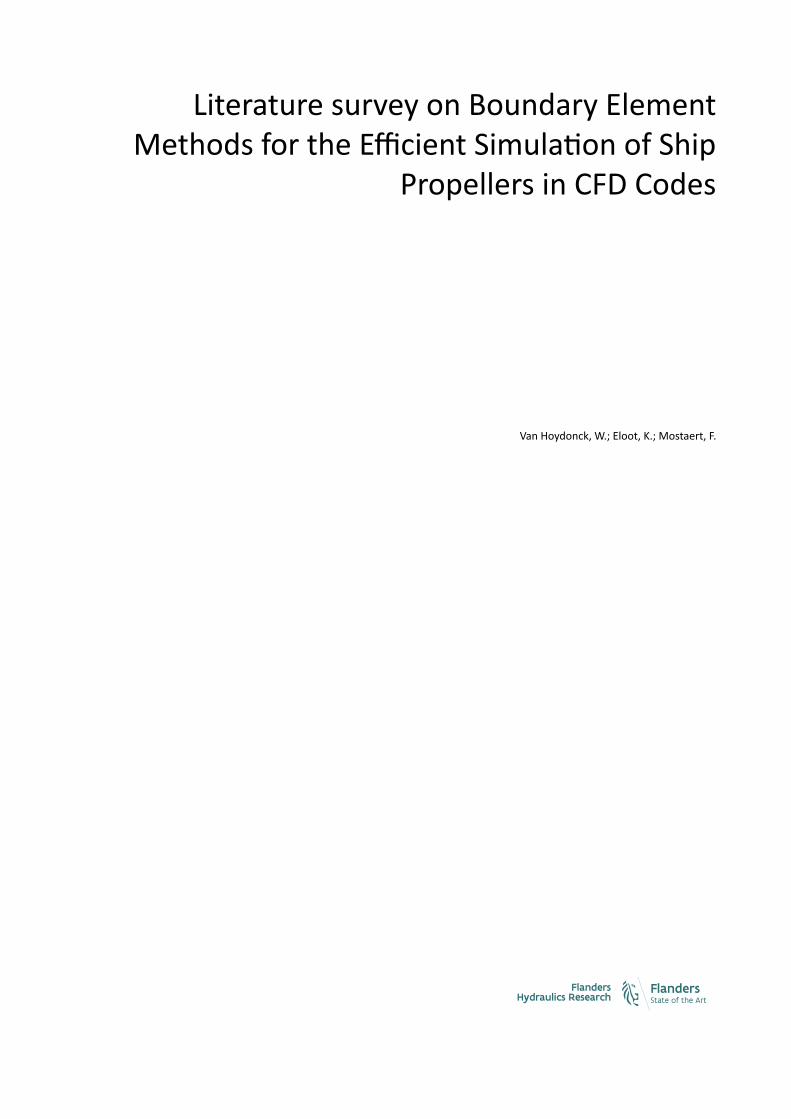
It has been shown that the panel discretisation near the tip of a blade and the associated (and a‐priori determ‐ined) location (and end) of the trailing edge has an impact on convergence of the pressure distribution nearthe tip (Baltazar, 2008; Baltazar et al., 2005; Pyo, 1995). The hydrodynamic tip1 grid (right‐hand side of Fig. 1)as compared to the usual propeller blade discretisation (left‐hand side of Fig. 1) based on the blade geometriccharacteristics (rake, skew, chord length, pitch and blade profile as a function of radial distance) (Baltazar andFalcao de Campos, 2006; Hoshino, 1989; Jennings, 2010) has been shown to improve convergence character‐istics of the iterative scheme to determine the pressure Kutta condition (Baltazar, 2008; Pyo, 1995).

Figure 1 – Blade panel arrangement for propeller P4119:conventional grid (left) and new panel arrangement with hydrodynamic tip (right) (from Baltazar et al. (2005)).

1The hydrodynamic tip is the location on the blade where the wake ends which does not necessarily coincide with the geometrictip (Baltazar, 2008; Baltazar et al., 2005).



Likewise, the use of a Flow Adapted Grid (FLAG), where the blade grid is adapted such that the computationaltip corresponds to the location where the tip vortex detaches from the blade, has been shown to improve theconvergence characteristics of the panel method applied to marine propellers (Pyo, 1995).

This discussion shows that discretizing the blade geometry of a marine propeller is not as straightforward asthe discretisation of an aircraft wing, where the wing tip is clearly defined.

1.1.5 Discretisation of the singularity distribution

Discretisation of the blade andwake geometry in a finite number of panels converts Eq. 4 into a systemof linearequations in the unknown doublet (and source) values on the panels. The order of the singularity distributionover each panel has an influence on the convergence characteristics of the method and the difficulty of theactual implementation. The simplest (and nowadays most‐widely used) methods use constant distributions ofdoublets and sources per panel (Ashby et al., 1991; Baltazar, 2008; Bosschers, 2007; Filkovic, 2008; Gaschler,2017; Hundemer, 2013; Jennings, 2010; Kerwin et al., 1987; Lee, 1987; Martin, 2015; Maskew, 1987; Pyo,1995; Takinaci et al., 2003; Tarafder et al., 2010; Vaz, 2005; Willis et al., 2006; Yari and Ghassemi, 2016; Yiranet al., 2018). Linear and higher‐order potential distributions have been used in the past (Baltazar, 2005; de Kon‐ing Gans, 1994; Hoeijmakers, 1989; Magnus and Epton, 1981; Pease Moore, 2013; Willis, 2006) to (amongstothers) reduce or eliminate issues with leakage of constant strength implementations, and to get more accur‐ate solutions at coarser discretisations. The issue of flow leakage due to the non‐flat nature of propeller paneldiscretisations has been solved by assuming that quadrilateral panels are hyperboloidal in shape: the cornerpoints are connected by straight line segments and the influence coefficients are obtained by a geometric ar‐gument avoiding direct integration (Newman, 1986). In general, higher‐order implementations require morecomputations per panel, but need less panels to get a similar level of accuracy as low‐order methods (Kerwinet al., 1987).

1.2 Shape of the wake

During a time simulation inwhich the boundary conditions vary (such as the angular velocity, the angle of attackof the propeller or the velocity field in which the propeller operates), the loads on the propeller blades willchange and as a consequence, the shed and trailed vorticity in the wake will vary in time. In turn, this changein vorticity in the wake affects the shape of the wake: a higher blade loading will result in stronger trailed (tip)vortices that will have a larger pitch. The tip vortex strength affects the inflow (or induced velocity) in the wakeplane and thus the angle of attack of the propeller blades. In general, the mechanism of feedback betweenthe different parts of the system means that a solution needs to be obtained in an iterative fashion, even fora steady (harmonic) condition where the boundary conditions are fixed in time. Determining the shape of thewake can be split in two parts:

• determination of wake shape for fixed boundary conditions (trim computation2);• evolution in time of wake shape for fixed or variable boundary conditions.

1.2.1 Initial wake shape (trim) computation

Anoverviewof the literature related to the computationof a harmonicwake shapeunder fixedboundary condi‐tions is given in Van Hoydonck (2013). Normally, the problem is written as a set of partial differential equations

2Note that the term trim computation is taken from the aerospace sciences where it refers to the general process of determiningstates and controls of a dynamic system given a set of boundary conditions (Van Hoydonck, 2013), whereas in naval architecture, trimof a vessel is only related to the amount of pitch of a vessel in a certain sailing condition.)



that are discretised using a finite difference scheme and these are solved with a relaxation scheme (Chopraet al., 1997). The process of determining the correct partial differential equation and the subsequent discret‐isation using a finite difference approach can be left alone by looking at the problem from a perspective of thestreamlines that emanate from the propeller blades and that carry the vorticity downstream. By reversing theequation to compute the derivative along a Non‐Uniform Rational B‐Spline (NURBS) curve at a fixed parametricpoint, an interpolation algorithm follows that can reconstruct a streamline given its starting point and deriv‐ative data along the curve (Van Hoydonck, 2013). This method has been shown to be robust (independent ofthe initial wake shape) and to work well for cases where the slipstream of the propeller is blocked by a solidsurface.

1.2.2 Time stepping approaches

Similar to the trim problem described in the previous section, the time stepping problem can be describedby a partial differential equation that is discretised using some finite difference approximation. Another ap‐proach is the use of theMethod of Lines (MOL) for the solution of partial differential equations by reducing thenumber of dependent variables to only one, usually replacing the spatial variable with algebraic approxima‐tions, see Hidalgo (2014) and the references therein. The PDE problem is thus reduced to a system of OrdinaryDifferential Equation (ODE) that can be solved with standard ODE solvers.

1.2.3 Vortex particle wake methods

One of the biggest disadvantages of the standard engineering dipole‐based wake models as used in the ma‐jority of panel methods (Baltazar, 2008; Bosschers, 2007; de Koning Gans, 1994; Gaschler, 2017; Hundemer,2013; Magnus and Epton, 1981; Vaz, 2005; Willemsen, 2013), is that these wake models inherently assumethat the flow is ordered (Hoeijmakers, 1989). The individual Lagrangianmarker points (i.e. the corner points ofa doublet panel, or themarker points of a vortex filament section) are transportedwith the local velocity whichmay mean that as time progresses, the panel becomes severely distorted and the assumption of ordered flowmay no longer hold. Most of the codes do not contain features to adaptively refine panels as they becomelarger or severely distorted because this means that the linear systems that are solved during BEM simulationschange size, which in turn can negatively affect the computing time to advance the system in time. Apart fromengineering corrections to account for viscous diffusion by changing the core sizes as time progresses, thesemethods have no means to account for viscous diffusion in a first principles way. The only method compat‐ible with panel methods that can account for viscous diffusion in the wake and that does not assume thatthe flow is ordered is the Vortex Particle Method (VPM) (Winckelmans, 1989) where the part of the fluid do‐main with non‐zero vorticity (i.e., the shed and trailed vortical wake behind a propeller) is discretised withvortex particles that are periodically redistributed to ensure that the vortex particles overlap (Winckelmans etal., 2005; Winckelmans and Leonard, 1993). Viscous vortex particle methods have been used in combinationwith a Fast Multipole Method (FMM)‐accelerated arbitrarily high‐order panel method (Pease Moore, 2013), amultipole‐accelerated unsteady panel method with quadratic curved panels (Willis, 2006; Willis et al., 2006),and a low order panel method (Martin, 2015). For engineering applications where panel methods are usedwith geometries such as ducted propellers (Kerwin et al., 1987), standard structured doublet latticewakemod‐els may require a lot of tuning and effort to improve the predictions in the gap between the propeller tip andshroud (Baltazar and Falcao de Campos, 2009; Baltazar et al., 2018; Willemsen, 2013).



1.3 Boundary layer methods

Boundary layer methods can use the pressure distribution from the panel code to compute the displacementthickness of the viscous layer around the discretised body. This displacement thickness is then used in thepanel code by either modifying the body shape by adding the incremental thickness to the discretised bodyshape or, by adjusting the source strengths of the individual panels such that each panel ejects or sucks enoughfluid to cause the resulting flow field to be approximately displaced by the displacement thickness that wascomputed in the previous iteration (Drela, 1989; Erickson, 1990; Maskew, 1987).

Simplermethods use the tangential velocity distributionalong a streamline and semi‐empiricalmethods (Moran,1984) to compute the growth of the boundary layer along the aerofoil (Gillebaart, 2018; Gilllebaart and DeBreuker, 2016).

1.4 Panel methods and Isogeometric Analysis

Isogeometric Analysis (IgA) has been introduced as a means to bridge the gap that exists between Finite Ele‐ment Analysis (FEA) and Computer Aided Design (CAD). By utilising the NURBS basis functions used in CAD asa basis for the discretisation of both the geometry and the solution fields in the FEA, the time‐consuming andnon‐trivial task of converting the input geometry to a form that is suitable for the FEA can be reduced signi‐ficantly (Hughes et al., 2005). The use of higher‐order elements and exact geometry representation (whichmeans that refinement of the discretisation can be executed without communicating with the original CADmodel) in IgA have shown to be advantageous for the accuracy of solutions (Cottrell et al., 2009). However,due to the three‐dimensional nature of FEA, one often needs to construct (by hand) a trivariate splinemappingof the geometry, a task that is not always trivial for real‐world geometry (Marussig et al., 2015).

In recent years, the concept of IgA has been applied to BEM problems (Beer et al., 2020; Chen et al., 2019; Dölzet al., 2018; Marussig et al., 2015; Politis et al., 2014). Three‐dimensional BEM problems only require a two‐dimensional discretisation of the boundary surfaces, which means that IgA can be applied in this field moreeasily to real‐world problems asmanyCADapplications (such as Rhino) onlymodel the bounding surfaces of thegeometry. But here also, the need to use trimmed surfaces in geometry poses a challenge for the applicationof IgBEM for which researchers only recently have found a solution (Beer et al., 2015).

In Politis et al. (2014), problem formulations are based on a Boundary Integral Equation (BIE) for the velocitypotential combinedwith a Kutta condition for lifting surfaces. The resulting IgBEMmethod utilises the geomet‐ric NURBS representation also for representing the velocity potential. Compared to a low‐order conventionalpanelmethod, the IgBEMmethodwas shown to require significantly fewer degrees of freedom to reach similaror better levels of accuracy. The general features of BEM formulations also apply to IgBEM implementations:the resulting linear system of equations is dense and the evaluation of the field functions is still an N‐bodyproblem that scales with the square of the number of elements. For this reason, FMM‐type enhancementshave been implemented in IgBEM formulations as well (Chen et al., 2019; Dölz et al., 2018; Marussig et al.,2015).

In (aero)nautical engineering, IgBEM has been used recently for the simulation and shape optimization oflifting flows around hydrofoils (Kostas et al., 2016; Politis et al., 2014), wave scattering problems governed bythe Helmholtz equation (Chen et al., 2019), wave propagation and wave‐structure interaction (Heredia, 2016),wave loading on ships (Kaklis et al., 2017), wave resistance of ships (Wang et al., 2017) the open‐water marinepropeller flow problem (Chouliaras et al., 2017), ship hull shape optimization (Kostas et al., 2015), low‐fidelityaeroelastic analysis and optimization of morphing airfoils (Gilllebaart and De Breuker, 2016) and aerostructuraloptimization of composite aircraft wings (Gillebaart, 2018).

The specific issues that have been discussed previously (such as the location and extend of the trailing edge linewhere the wake forms, and the shape of the wake) also apply to IgBEM implementations. Although the IgBEM



promises a more accurate solution with less variables, the user should make sure that the correct problemis solved accurately (i.e., the wake release point near the propeller blade tip should be located at its correctposition).

1.5 Interfacing BEM and CFD

When a propeller BEMcode is interfacedwith a Finite Volume (FV) CFD code to include the effects of a propellerwithout the disadvantages of completely resolving the viscous flow around the rotating propeller (such asincreased computing times), information must be exchanged between the BEM code and the CFD code. TheBEM code requires a uniform or non‐uniform flow field in order to solve for the non‐penetrating boundaryconditions at the panel control points. With this flow field, the linear systems of equations are solved and thedistribution of pressure on the propeller is determined. This pressure distribution (which can be integrated togive the resultant forces and moments on the propeller) is passed to the CFD code where they are added asbody forces to the governing equations.

In the coupling scheme (Hally, 2015), the propeller influence on the RANS solution is introduced via a forcefield that mimics the propeller action, similar to how an actuator disk model is added in a RANS computation.The influence of the hull on the propeller is introduced by supplying an inflow wake computed from the RANSsolution from which the propeller induction calculated with the BEM has been subtracted. This procedure isrepeated until the effective propeller wake no longer changes.

1.5.1 Coupling procedure: literature overview

The coupling procedure between the RANS flow solver FresCo+ and the potential panel method panMare ispresented inWöckner et al. (2011). Coupling is based on the transfer of inviscid propeller‐induced body forcesto the viscous solver and the transfer of the effective wake velocities to the inviscid solver. Details of the spatialmapping techniques required to exchange data between two grids of significantly different nature are givenas are details on the temporal transfer of information. The viscous velocity distribution is extracted from theRANS solver 0.1D and 0.2D upstream of the propeller. The inviscid pressure values on the individual panels ofthe propeller are distributed to adjacent fluid cell centers and added to the RANS solver as body forces. For thecoupling procedure, the inviscid solver needs the velocity field from the viscous solver, without the influence ofthe induced velocities due to the action of the propeller in the inviscid method. The paper explains the detailsof two coupling modi: an explicit and an implicit procedure. The method is also extended to free‐surfaceflows, where the location of the free surface is accounted for in the inviscid panel method with an inviscid wallboundary. Instead of transferring the actual free surface as determined by the viscous solver to the panel code,Fourier transforms are calculated along two‐dimensional longitudinal sections and these Fourier coefficientsare transferred to the inviscid solver. The latter one uses the Fourier coefficients to reconstruct the free surfaceat arbitrary locations.

Rijpkema et al. (2013) explains the procedure that is used to couple Propeller Calculation (ProCAL) with Re‐Fresco. First, a steady RANS simulation is executed and the wake field at the propeller plane is evaluated. Thisfield is used for the first BEM computation, where the loading distribution on the propeller blades is determ‐ined. The non‐uniform nature of the wake field, means that an unsteady BEM computation is required. Theaverage forces on the camber plane are computed at different positions of the blades, a three‐dimensionaltime‐averaged force distribution is constructed. This time‐averaged BEM propeller loading distribution is usedin the RANS computation as a body force field. The force field is interpolated to the RANS grid. To correct fordeficiencies in the interpolation procedure, the body force field can be scaled to ensure equal thrust in theRANS computation as determined by the BEM. With the propeller body forces included in the RANS computa‐tion, the total wake field can be computed. The effective wake of the propeller is obtained by subtracting the



propeller induced velocities from the total wake field. The averaged propeller induced velocities are determ‐ined in the BEM computation. This procedure is repeated with the new effective wake field until convergence(change in thrust and effective wake velocities) is reached.

Hally (2015) details a procedure where ProCAL is coupled with OpenFOAM. The paper focuses on the correctrepresentation of the propeller blade blockage in the RANS computations by adding source mass terms to theequations of motion. Failure to include the propeller blade blockage in the RANS computation results in anincrease of the axial velocity in the effective wake which increases the advance ratio and reduces the predictedthrust and torque. In a subsequent publication, Hally details the procedure to interpolate the velocity field thatis used in the exchange of information between the ProCAL and RANS procedures (Hally, 2017). The methoduses multiple planes normal to the rotation axis of the propeller which means that axial velocity variations areallowed. This contrasts with simpler methods where the velocity is sampled at a single plane (Anon., 2020;Hally, 2012).

1.5.2 FINE/Marine

FINE/Marine has a predefined interface for adding a Boundary ElementMethod to CFD computations through adynamic Fortran library. The coupling can bemade directly in the dynamic library or this can be kept separately.In the latter case, the communication is handled through system calls and text files.

The interface consists of two parts where information is exchanged between the two programs:

• a velocity field ahead of the propeller is passed to the BEM software for use as boundary condition bythe panel code;

• a body force distribution (pressure) at the propeller blade location used in the CFD code to compute thepropeller forces.

According to the manual of FINE/Marine (Anon., 2020), only the thrust and torque forces are supportedthrough this interface, similar to the functionality of the available actuator disk model. Once the propellercode works and has been validated for simple cases, this assumption could be tested in conditions where a sig‐nificant lateral flow is added. Then it can be verified if the restriction present in FINE/Marine is justified.

The AC&E company in the UK that provides support for the panel methods of AM Inc. in Europe also uses theCFD software of Numeca3. Two‐way coupling, where information is exchanged between both programs hasnot been used, only a one way coupling has been used. In this method, a non‐uniform velocity field directlyupstream of the propeller or in a volume around the propeller is extracted from the CFD computation and usedas input for the panel code.

3http://www.acel.co.uk


http://www.acel.co.uk


2 Overview of existing boundary element soft‐ware

This chapter discusses existing boundary element software that solve the Laplace equation in an infinite do‐main (suitable for low‐speed aero and hydrodynamics), other potential methods (for things such as soundpropagation) are not discussed. In addition, the interface between the BEM and CFD codes is discussed aswell.

2.1 Commercial codes

2.1.1 ProCAL

In 2003, the Cooperative Research Ships (CRS) organisation initiated the development of a panel code for theanalysis and simulation of marine propellers (Bosschers, 2007). A working group was formed consisting of in‐terested parties such as shipyards, a propulsor manufacturer, classification societies, navies and ship researchinstitutes. Within this working group, a panel method (named ProCAL and implemented by MARIN) and agraphical user interface with grid generation capabilities have been developed. The code is available for mem‐bers of the CRS organisation, which has a yearly participation fee of €25 000 (Toxopeus, 2015). One of the cur‐rent ongoing projects is the adaptation the PROCAL program for the simulation of ducted propellers (Moulijnet al., 2019)4. In the recent past, the PROPDEV working group5 aimed at developing a tool based on ProCALfor the design of propulsion including the interaction with the hull and appendages. At TU Delft, ProCAL hasrecently been used in research to simulate flexible marine propellers in an efficient way (Maljaars et al., 2018).Other participants of the CRS have coupled ProCAL with OpenFOAM (Hally, 2017, 2015).

2.1.2 VSAERO/USAERO

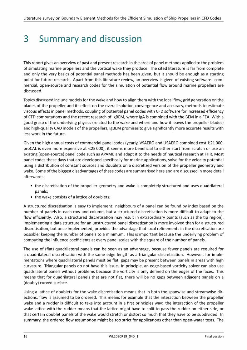
VSAERO(Maskew, 1988, 1987) is a low‐order panel method developed and commercialised by AnalyticalMeth‐ods, Inc. since 1980s. It can be used to compute non‐linear aerodynamic characteristics of arbitrary three‐dimensional configurations in subsonic flow. It contains an iterative wake shape calculation procedure andthe method is coupled with an integral boundary layer solver which means that the effects of viscosity can beaccounted for. Geometries are discretised using quadrilateral panels on which piecewise constant source anddoublet singularities are distributed. Panel source values are determined by the external Neumann boundarycondition that controls the normal component of the local resultant flow while the doublet values are solvedafter imposing the internal Dirichlet boundary condition of zero perturbation potential at the underside of thepanel centres. The original code was written in standard FORTRAN IV and the first version of the code allowedfor the solution of problems with up to 1000 panels. This version was used as a base for the Panel MethodAmes Research Center (PMARC) panel method. As part of this literature survey, a request for information re‐garding the current capabilities of VSAERO and USAEROwas send to AMI Aero, LCC (the successor of AnalyticalMethods, Inc.). Fig. 2 shows the pressure distribution on a propeller in a non‐uniform flow field computedwithUSAERO (Nathman, 2020). Other than that this case required less than 10 minutes on a Linux machine 5 yearsago, no information was provided about it. Although VSAERO and USAERO are capable of computing the po‐tential flow around marine propellers, it seems not much time has been dedicated to thoroughly validate the

4http://www.crships.org/web/Ongoing-Projects/Ducted-Propellers.htm5http://www.crships.org/web/Recent-Projects/Propeller-Design-and-Development.htm


http://www.crships.org/web/Ongoing-Projects/Ducted-Propellers.htm

http://www.crships.org/web/Recent-Projects/Propeller-Design-and-Development.htm


software for this type of problem as has been done more recently with dedicated marine software (Baltazar,2008; Moulijn et al., 2019; Vaz, 2005).

A disadvantage of VSAERO and USAERO is that separate programs are used for unsteady and steady com‐putations, while ideally, this should be possible with a single program. AC&E in the UK6 provides support forVSAERO and USAERO to customers in Europe. Upon inquiry, the programs can be licensed on an annual or per‐manent basis. Typically, a single user floating license price for either VSAERO or USAERO is €10 500 includingSPINW for the wake definition. For postprocessing the output of VSAERO and USAERO, AM Inc. has developedthe interactive 3D data visualisation tool OMNI3D. This has an additional license cost of €4500 per year. Theseprices include annual support and maintenance service. Descriptions of the four programs mentioned in thissection that can be found on the website of aero attack7 are given in Appendix A1.

Figure 2 – USAERO pressure distribution on a propeller computation in non‐uniform inflow (Nathman, 2020).

2.1.3 CMARC

CMARC is an enhanced version of NASA’s PMARC‐12, which in turn is a descendant of an early version ofVSAERO. It is part of AeroLogic’s8 Digital Wind Tunnel (DWT) that can be used to determine longitudinal andlateral static and dynamic stability derivatives, neutral point and elevator deflections required for trim. Thesoftware suite contains a lofting program (Loftsman/P) for designing the outer surface of aeroplanes and boatsand a postprocessing program (Postmarc) for visualisation of the solution. The lofting program can outputthe lofted shapes in IGES and DXF format as well as creating input files for CMARC and VSAERO. The websitecontains analysis examples of general aviation type aircraft and boat hulls generated with the software suite,but lacks examples of propeller analyses. The software is written in ANSI‐C and executables are only providedfor Windows. The yearly licensing costs of the software components are listed on their website and these arerepeated in Table 2.

An example of the panelling andpressure distributionon the fuselage andwings of a P‐51Mustang are shown inFig. 3, while in Fig. 4, the two‐dimensional flow around an aerofoil with extended flap is shown. This exampleseems to include the effects of viscous interaction in the boundary layer, because the pressure around theaerofoil does not seem to decrease in the direction normal to the surface as the distance to the aerofoil is

6http://www.acel.co.uk7http://www.aeroattack.com8http://www.aerologic.com


http://www.acel.co.uk

http://www.aeroattack.com

http://www.aerologic.com


increased.

Table 2 – License cost for the Aerologic software

component price (US dollar)

Personal Simulation Works (PSW) with DWT 3750PSW with CMARC only 3125

CMARC ANSI‐C source code (unix compatible) 625Loftsman/P 1250CMARC 625

DWT (includes CMARC) 1250Postmarc 1250

Figure 3 – Pressure distribution on the P‐51 Mustang computed with CMARC. Retrieved fromhttp://www.aerologic.com/example/p51.html © AeroLogic.

Figure 4 – Streamlines and pressure distribution around an aerofoil with extended flap. Retrieved fromhttp://www.aerologic.com/example/gaw.html, © AeroLogic.


http://www.aerologic.com/example/p51.html

http://www.aerologic.com/example/gaw.html


2.1.4 FlightStream

FlightStream®is a surface vorticity flow solver developed and marketed by Research in Flight9 to allow users todevelop optimized designs for compressible and incompressible subsonic vehicles as well as transonic vehicles.Applications range from modeling UAVs, high‐altitude‐aerostats, high subsonic transport and military aircraft,marine propellers and under‐water vehicles, wind turbines, propellers, store separation and high‐lift com‐ponents. An example of the surface discretisation and vorticity distribution around an F16‐A is shown inFig. 5.

Figure 5 – F16‐A surface discretisation (left) and vorticity distribution (right) with wake filaments (Ahuja, 2013).

The surface vorticity solver uses an unstructured triangular surface discretisation in combination with an un‐structured wake strand model (Ahuja, 2013). The wake filaments originate at nodes that are flagged by thesoftware as trailing edges and the strength of the vorticity trailed at these points is a summation of the strengthof the edges that are connected to these points. A point that is not touched upon in the thesis of Ahuja is(unsteady) time simulation. By the nature of the wake implementation, only steady‐state simulations can beexecuted as vorticity is only trailed in the wake, and not shed. This is a shortcoming that makes the softwareunsuitable for performing propeller simulations with unsteady boundary conditions. The Constant VorticityContour (CVC) wake model has elegantly solved the issue of combining shed and trailed vorticity in a vortexfilament wake model almost 30 years ago by placing the vortex filaments along contours of constant sheetstrength for the sheet of vorticity trailed from each lifting surface (Quackenbush et al., 1991), so there is cer‐tainly a possibility to implement unsteady time simulations in vorticity panel methods that utilize vortex fila‐ment wakes. Recently, this type of wake model was applied to time simulations of wind turbine wakes (Su andBliss, 2019), where it is called the Constant Circulation Contour Method (CCCM).

For use in a marine context, where the trailed wake is (highly) curved, the use of straight line segments toapproximate a curved vortex filament (as is done by Ahuja) is far from optimal because (a) many segments (andhence longer computing times) are required to get a good approximation10 and (b) without corrections for thelocal curvature at a point on a filament where the velocity is computed, fundamental errors are made (Bliss etal., 1987). Hence, in a marine context where vorticity shed from a propeller blade has high curvature, the useof longer curved vortex filaments as compared to shorter straight line segmentsmay prove to be advantageousfor both the accuracy of the results and the reduced computing times.

9www.researchinflight.com10This argument also holds for (low‐order) panel methods where a doublet lattice is used to represent the wake due to the equival‐

ence of a doublet panel and a vortex ring.


www.researchinflight.com


2.2 Research codes

2.2.1 PMARC

PMARC is a low‐order potential panel method developed by NASA Ames Research Center at the end of the1980s (Ashby et al., 1988, 1991) to predict flow fields around complex three‐dimensional geometries. Ex‐perience with panel methods such as Panel Aerodynamics (PANAIR) and VSAERO had shown that low‐ordermethods can provide nearly the same accuracies as higher order methods for many cases. The computingtimes are significantly shorter for a low‐order implementation and at the same time, the implementation of alow‐order method is significantly easier. Furthermore, adjacent panels do not have to match exactly in a low‐order method. The code is based on versions of VSAERO delivered to NASA Ames in the first half of the 1980s.The PMARC low‐order panel method is available through the NASA software website11 for U.S. Government‐authorized use only12.

2.2.2 panMARE

panMARE is a potential panel method developed at the Technical University of Hamburg at the Institute forFluid Dynamics and Ship Theory13. The potential code has been developed with German government fundingand is not available for general use outside Germany (Abdel‐Maksoud, 2015). The implementation of the basicmethod for marine propellers is discussed in Hundemer (2013) (in German) while the addition of a cavitationmodel is detailed in Gaschler (2017).

2.3 Open source codes

2.3.1 PANAIR

PANAIR is an advancedmethod for the solution of linear integral equations of inviscid subsonic and supersonicpotential flow in three dimensions (Magnus and Epton, 1981). The method uses source and doublet panels asboundary surfaces. Complex geometries are split in multiple networks on which panels are laid out in a struc‐tured manner. Higher order (i.e. curved) panel geometries are supported over which linearly varying sourceor quadratically varying doublet singularities are employed. All influence coefficients are computed in closedform. The program has been extensively validated and shows a marked insensitivity to the size, shape andarrangement of panels. For complex configurations, the method has advantages as fewer panels are requiredthan standard first‐order methods. Originally developed for NASA Ames by Boeing in the 1980s, the originalFortran program has been released through the Public Domain Aeronautical Software (PDAS) website14. Thiswebsite also contains a preprocessor (PANIN15) to format the input files for PANAIR.

Evaluation of the code

The source code is contained in a single file with more than 69 × 103 lines of fixed‐format Fortran 77. The the‐ory manual (Magnus and Epton, 1981) mentions that the program is capable of superimposing an incremental

11https://software.nasa.gov/software/ARC-14407-112The research executed at Flanders Hydraulics Research (FHR) does not fall under U.S. Government‐authorized use.13https://www.tuhh.de/panmare/home.html14http://www.pdas.com/panair.html15http://www.pdas.com/panin.html


https://software.nasa.gov/software/ARC-14407-1

https://www.tuhh.de/panmare/home.html

http://www.pdas.com/panair.html

http://www.pdas.com/panin.html


velocity on the freestream to simulate effects such as rotational motion or a propeller slipstream. The place‐ment of the wake (or its alignment with the local velocity) is not discussed in the theory manual. However,the user manual (Sidwell et al., 1990) mentions that PANAIR does not calculate the shape of a wake unlessindirectly as part of a design problem. The user must provide the program with an approximate shape for thewake in the form of panelled surfaces, and the quality of the solution depends on the quality of thewake shapeapproximation.

The above evaluation means that although rotating bodies such as propellers could be simulated, the wakeshape shed by the propeller is part of the input that must be provided by the user: the program cannot alignthe wake with the local velocity. Adapting the PANAIR code to implement this feature may provide a challengegiven the size and dialect of the PANAIR source code.

2.3.2 Apame

Aircraft Panel Method (APAME)16 is a fairly standard low‐order panel method for the analysis of lifting flowaround three‐dimensional bodies in subsonic flow conditions. It is a redesign (in Fortran) of the softwarepackage (written in Matlab) developed by the author for his thesis (Filkovic, 2008). The software is released asopen source (GNU General Public License (GPL)) and contains a solver module and a graphical user interface.The solver supports unstructured meshes consisting of a mix of triangular and quadrilateral panels. It cancompute lift and induced drag over bodies in attached flow conditions. As‐is, the software cannot handlerotating bodies such as propellers. In addition, the wake model is rigid, i.e., it is not aligned with the local flowdirection. From running some of the examples, the solvers seems to work fine, generating lift when a bodyhas an angle of attack. However, validation of code is required to verify that the potential solver has beenimplementation correctly.

Evaluation of the code

This short evaluation will focus on the issues in the current code and the efforts required to adapt it for com‐puting the flow around marine propellers.

The code does not contain functionality to make the object under investigation rotate around an axis whichis required for propellers simulations. The lack of this functionality is however not envisioned as a big issue,implementing this should be fairly straightforward.

More work will be required to implement functionality for aligning the wake with the local flow. In addition, itappears to miss functionality to construct a reasonable prescribed wake as well: all wake geometry panels aredefined directly in the input files. Implementing this is more work, but fortunately the author of this reporthas some experience in this field (Van Hoydonck, 2013).

The source code is implemented in single precision: the keyword double precision is absent from thesource code, and the parametric real facility of modern Fortran is not used. The source code makes callsto (single precision) external functions from LAPACK for solving the linear systems that are typical for potentialflow solvers, which is also an indication of the single precision nature of the program.

The GOTO statement (which is considered harmful by some (Dijkstra, 1968)) appears 105 times in the sourcecode, especially in the module where input files are parsed. The readability of the code can be improvedbecause old‐style logical evaluations are used (such as .ge. and .le.) instead of the easier readable andmore mathematical forms >= and <=. Mathematical constants (such as 𝜋) are not defined in a central locationin the source code and then usedwherever necessary. Instead, the constants are defined at the locationwherethey are needed in the code.

16See http://www.3dpanelmethod.com.


http://www.3dpanelmethod.com


Furthermore, some derived constants, such as 1/(4𝜋) are definedwithout referring to the definition of 𝜋 itself.This makes it difficult and error‐prone to alter the source code if the value of 𝜋 should be changed.

No build system is in place, only the source code is provided along with executables. It should be easy to addconfiguration files for the CMake build system.



3 Summary and discussion

This report gives an overview of past and present research in the area of panel methods applied to the problemof simulating marine propellers and the vortical wake they produce. The cited literature is far from completeand only the very basics of potential panel methods has been given, but it should be enough as a startingpoint for future research. Apart from this literature review, an overview is given of existing software: com‐mercial, open‐source and research codes for the simulation of potential flow around marine propellers arediscussed.

Topics discussed includemodels for the wake and how to align themwith the local flow, grid generation on theblades of the propeller and its effect on the overall solution convergence and accuracy, methods to estimateviscous effects in panel methods, coupling of potential panel codes with CFD software for increased efficiencyof CFD computations and the recent research of IgBEM, where IgA is combined with the BEM in a FEA. With agood grasp of the underlying physics (related to the wake and where and how it leaves the propeller blades)and high‐quality CADmodels of the propellers, IgBEM promises to give significantly more accurate results withless work in the future.

Given the high annual costs of commercial panel codes (yearly, VSAERO and USAERO combined cost €21 000,proCAL is even more expensive at €25 000), it seems more beneficial to either start from scratch or use anexisting (open‐source) panel code such as APAME and adapt it to the needs of nautical research at FHR. Mostpanel codes these days that are developed specifically for marine applications, solve for the velocity potentialusing a distribution of constant sources and doublets on a discretized version of the propeller geometry andwake. Some of the biggest disadvantages of these codes are summarised here and are discussed inmore detailafterwards:

• the discretisation of the propeller geometry and wake is completely structured and uses quadrilateralpanels;

• the wake consists of a lattice of doublets;

A structured discretisation is easy to implement: neighbours of a panel can be found by index based on thenumber of panels in each row and column, but a structured discretisation is more difficult to adapt to theflow efficiently. Also, a structured discretisation may result in extraordinary points (such as the tip region).Implementing a data structure for an unstructured panel discretization is more involved than for a structureddiscretisation, but once implemented, provides the advantage that local refinements in the discretisation arepossible, keeping the number of panels to a minimum. This is important because the underlying problem ofcomputing the influence coefficients at every panel scales with the square of the number of panels.

The use of (flat) quadrilateral panels can be seen as an advantage, because fewer panels are required fora quadrilateral discretisation with the same edge length as a triangular discretisation. However, for imple‐mentations where quadrilateral panels must be flat, gaps may be present between panels in areas with highcurvature. Triangular panels do not have this issue. In principle, an edge‐based vorticity solver can also usequadrilateral panels without problems because the vorticity is only defined on the edges of the faces. Thismeans that for quadrilateral panels that are not flat, there will be no gaps between adjacent panels on a(doubly) curved surface.

Using a lattice of doublets for the wake discretisation means that in both the spanwise and streamwise dir‐ections, flow is assumed to be ordered. This means for example that the interaction between the propellerwake and a rudder is difficult to take into account in a first principles way: the interaction of the propellerwake lattice with the rudder means that the lattice might have to split to pass the rudder on either side, orthat certain doublet panels of the wake would stretch or distort so much that they have to be subdivided. Insummary, the ordered flow assumption might be too strict for applications other than open‐water tests. The



number of panels in the spanwise direction on a blade and on its associated wake are generally kept the same,which means that the number of panels can quickly get very large. By using a buffer layer between the bladetrailing edge and the actual (filament) wake, it is possible to use a lower number of spanwise wake elementsthan the number of spanwise blade elements. However, it seems this is not used in marine research codes. Avortex filament wake model only assumes ordered flow in the streamwise direction which makes interactionwith (lifting) surfaces easier to implement. This type of wake17 is not directly compatible with standard panelmethods that solve for the velocity potential, but it is compatible with surface vorticity panel methods. Thistype of panel method is also compatible with viscous vortex particle methods for cases where the streamwiseordering of the wake as implied by vortex filament wake models is too strict as well.

Marine CFD computations where the turning propeller is taken into account directly generally require a lotof computational resources. Replacing the turning propeller with a potential panel simulation can reduce thecomputational burden significantly by relaxing the time step size requirements and reducing the grid size in theregion of the propeller. This way, it will be possible to execute this type of CFD computations in a reasonableamount of time.

To get there, a choice has to be made between the development (or adaptation) of a low‐order run‐of‐the‐millpanel code with source and doublet singularities, a low‐order vorticity‐based panel method in combinationwith a vortex filament wake method and a method based on IgBEM18. Of these three, the last option is judgedto require most effort to implement a working version. The reward would be high, because the method prom‐ises high quality results with excellent convergence characteristics. One of the requirements for this is that thesurface geometry description must be of high quality as well, which sadly is not always the case in the nauticalsciences. The development effort for the other two options are expected to be lower, with a slight advantagefor a vorticity‐based method due to the use of only one singularity as opposed to the use of two singularitiesfor potential‐based panel methods. Pure vorticity‐based methods are relatively new, which means that thereare more opportunities for innovation as compared to potential‐based panel methods that have been aroundfor more than 50 years. A vorticity‐basedmethodwould also set FHR apart from other maritime research insti‐tutes that have developed in‐house panel codes for the simulation of propellers. Although open for discussion,the author has a preference for a vorticity‐based solver with a vortex filament wake model.

Adapting and extending an existing potential code such as APAME all by oneself is a task that should not beunderestimated, especially given that this is not themain research task of the author. For this reason, a numberof subtasks can be defined that could be executed by students as master thesis assignments once a basicworking version has been developed:

• implementation of a free wake module (either a vortex filament‐based or doublet lattice based) withefficient and robust wake relaxation and time stepping algorithms;

• coupling of the panel method with CFD solvers such as OpenFOAM and FINE/Marine;• implementation of a method to adaptively refine the grid based on the distribution of field variables;• comparisonof the performanceof the direct (velocity‐based) and indirect (potential‐based) panelmethod;• implementation of (or coupling with) a viscous vortex particle method including acceleration methodssuch as the FMM to reduce the computational burden;

• implementation of a method to estimate viscous effects in the boundary layer around the propellergeometry;

• extending the applicability of the method to situations where wake‐piercing objects (such as rudders)are present.

17Possibly implemented using curved vortex filaments laid out along contours of constant vorticity in the wake.18Note that the option of using a commercial code was already discarded.



References

Abdel‐Maksoud,M. (2015). Private communication

Ahuja, V. (2013). Aerodynamic Loads over Arbitrary Bodies by Method of Integrated Circulation. (PhD Thesis).Auburn University: Auburn, Alabama

Anon. (2020). Theory Guide FINE/Marine 8.2

Ashby,D.; Dudley,M.; Iguchi, S. (1988). Development and Validation of an Advanced LowOrder PanelMethod.report, NASA‐TM‐101024. NASA Ames Research Center: Moffett Field, California

Ashby, D.; Dudley,M.; Iguchi, S.; Browne, L.; Katz, J. (1991). Potential flow theory and operation guide for thepanel code PMARC. report, NASA‐TM‐102851. NASA Ames Research Center: Moffett Field, California

Baltazar, J. (2008). On the Modelling of the Potential Flow About Wings andMarine Propellers Using a Bound‐ary Element Method. (PhD Thesis). University of Lisbon: Lisbon, Portugal

Baltazar, J.; Falcao de Campos, J. (2009). On the Modelling of the Flow in Ducted Propellers With a PanelMethod. in: Proceedings of the First International Symposium onMarine Propulsors S:P09. Trondheim, Norway.p. 9

Baltazar, J.; Falcao de Campos, J. (2006). Propeller Unsteady Potential Panel Method. Report, IST‐MARETEC ‐TR ‐ J583 ‐ 14. University of Lisbon: Lisbon, Portugal

Baltazar, J.; J.A.C., F.; Bosschers, J. (2005). A study on the modeling of marine propeller tip flows using BEM.in: Proceedings of the Congreso de Métodos Numéricos en Ingenieria. Granada, 4th–7th July 2005. p. 17

Baltazar, J.; Rijpkema, D.; J.A.C., F.; Bosschers, J. (2018). Prediction of the Open‐Water Performance of DuctedPropellers with a Panel Method. Journal of Marine Science and Engineering 6 (27) (1): 17. DOI: 10.3390/jmse6010027

Baltazar, J. (2005). AHigher order potential basedBEM for three‐dimensional flows. report, POSI‐SFRH/BD/14334/2003.University of Lisbon: Lisbon, Portugal

Beer,G.;Marussig,B.; Duenser, C. (2020). The Isogeometric Boundary ElementMethod. Vol. 90. LectureNotesin Applied and Computational Mechanics. Springer International Publising. ISBN: 978‐3‐030‐23338‐9

Beer, G.; Marussig, B.; Zechner, J. (2015). A simple approach to the numerical simulation with trimmed CADsurfaces. ComputerMethods in AppliedMechanics and Engineering 285. DOI: 10.1016/j.cma.2014.12.010

Bertin, J.; Cummings, R. (Eds.). (2009). Aerodynamics for Engineers. 5th ed. Pearson Education: London, UK.ISBN: 978‐0‐132‐272681

Bertram, V. (2012). Practical Ship Hydrodynamics. 2nd ed. Butterworth‐Heinemann: Oxford, UK. ISBN: 978‐0‐08‐097150‐6

Bliss, D.; Teske,M.; Quackenbush, T. (1987). A NewMethodology for Free Wake Analysis Using Curved VortexFilaments. report, CR‐3958. NASA Ames Research Center: Moffett Field, CA


10.3390/jmse6010027

10.3390/jmse6010027

10.1016/j.cma.2014.12.010


Bosschers, J. (2007). PROCAL beats the panel! online

Chen, L.; Zhao, W.; Liu, C.; Chen, H.; Marburg, S. (2019). Isogeometric Fast Multipole Boundary ElementMethodBasedonBurton‐Miller Formulation for 3DAcoustic Problems.Archives of Acoustics 44 (3). DOI:1024425/aoa.2019.129263

Chopra, I.; Celi, R.; Leishman, J.; Vizzini, A.; Baeder, J.; Werely, N. (1997). Center for Rotorcraft Educationand Research: Progress Report on Army Research Office Contract No. DAAL03‐88‐C‐0002 and DAAHO4‐94‐G‐0074 ”Rotorcraft Center of Excellence” Final Report. Report, DAAHO4‐94‐G‐0074. University of Maryland,Department of Aerospace Engineering: College Park, Maryland

Chouliaras, S.; Kaklas, P.; Ginnis, A.‐A.; Kostas, K.; Politis, C. (2017). An IGA‐BEMMethod for the Open‐WaterMarine Propeller Flow Problem. in: Proceedings of the 4th International Conference on Isogeometric Analysis.Pavia, Italy, 11th–13th September 2017. p. 12

Cottrell, J. A.; Hughes, T.; Bazilevs, Y. (2009). Isogeometric analysis: toward integration of CAD and FEA. 1st ed.John Wiley & Sons Ltd: Chichester, UK. ISBN: 978‐0‐470‐74873‐2

de KoningGans,H. (1994). Numerical TimeDependent Sheet Cavitation Simulations using aHigher Order PanelMethod. (PhD Thesis). Delft University of Technology: Delft, the Netherlands

Dijkstra, E. W. (1968). Go To Statement Considered Harmful. Communications of the ACM 11 (3)

Dölz, J.; Harbrecht, H.; Kurz, S.; S., S.; Wolf, F. (2018). A Fast Isogeometric BEM for the Three DimensionalLaplace‐ and Helmholtz Problems. Computer Methods in Applied Mechanics and Engineering 330. DOI: 10.1016/j.cma.2017.10.020

Drela,M. (1989). XFOIL: An Analysis and Design System for Low Reynolds Number Airfoils. in:Mueller, T. (Ed.).Low Reynolds Number Aerodynamics. Vol. 54. Lecture Notes in Engineering. Springer‐Verlag. ISBN: 978‐3‐540‐51884‐6. p. 14. DOI: 10.1007/978-3-642-84010-4

Erickson, L. (1990). Panel Methods—An Introduction. report, TP‐2995. NASA Ames Research Center: MoffettField, California

Filkovic, D. (2008). Graduate Work. (MSc Thesis). University of Zagreb ‐ Faculty of Mechanical Engineering andNaval Architecture: Zagreb, Croatia

Gaschler,M. (2017). Numerical Modelling and Simulation of Cavitating Marine Propeller Flows. (PhD Thesis).Hamburg University of Technology: Hamburg, Germany

Gillebaart, E. (2018). Towards Geometrically Consistent Aerostructural Optimisation of Composite AircraftWings. (PhD Thesis). Delft University of Technology: Delft, the Netherlands. ISBN: 978‐94‐028‐1081‐3

Gilllebaart, E.; De Breuker, R. (2016). Low‐Fidelity 2D Isogeometric Aeroelastic Analysis and OptimizationMethod with Application to aMorphing Airfoil. Computer Methods in AppliedMechanics and Engineering 305.DOI: 10.1016/j.cma.2016.03.014

Hally, D. (2017). A RANS‐BEM coupling procedure for calculating the effective wakes of ships and submarines.in: Bensow, R. (Ed.). Proceedings of the 5th International Symposium on Marine Propulsion SMP’17. Espoo,Finland. p. 9


1024425/aoa.2019.129263

1024425/aoa.2019.129263

10.1016/j.cma.2017.10.020

10.1016/j.cma.2017.10.020

10.1007/978-3-642-84010-4

10.1016/j.cma.2016.03.014


Hally, D. (2015). Propeller Analysis Using RANS/BEM Coupling Accounting for Blade Blockage. in: Proceedingsof the 4th International Symposium on Marine Propulsors SMP’15. Austin, Texas, USA. p. 9

Hally, D. (2012). Using RANS to Calculate the Flow Past Marine Propellers. in: Proceedings of the Annual Con‐ference of the CFD Society of Canada. Canmore, Canada. p. 7

Heredia, J. M. (2016). Towards the application of the isogeometric boundary element analysis to fluid mech‐anics: non‐linear gravity waves and dynamics of deformable capsules in shear flows. (PhD Thesis). UniversitatRovira i Virgili: Tarragonna, Spain

Hess, J.; Smith, A. M. O. (1964). Calculation of nonlifting potential flow about arbitrary three‐dimensionalbodies. Journal of Ship Research 8: 22–44

Hidalgo, D. (2014). Assessment of a State‐Space Free Wake Model for rotorcraft flight mechanics applications.(MSc Thesis). Delft University of Technology: Delft, the Netherlands

Hoeijmakers, H. (1989). Computational Aerodynamics of Ordered Vortex Flows. (PhD Thesis). Delft Universityof Technology: Delft, Netherlands

Hoshino, T. (1989). Hydrodynamic Analysis of Propellers in Steady Flow Using a Surface Panel Method. Journalof The Society of Naval Architects of Japan 1989 (165). DOI: 10.2534/jjasnaoe1968.1989.55

Hughes, T.; Cottrell, J.; Bazilevs, Y. (2005). Isogeometric analysis: CAD, finite elements, NURBS, exact geometry,and mesh refinement. Computer Methods in Applied Mechanics and Engineering 194 (39‐41). DOI: 10.1016/j.cma.2004.10.008/sym11020196

Hundemer, J. (2013). Development of a procedure for the calculation of the unsteady potential theory pro‐peller flow. (PhD Thesis). Hamburg University of Technology: Hamburg, Germany

Jennings, s. (2010). Creation, Verification and Validation of a Panel Code for the Analysis of Ship Propellers ina Steady, Uniform Wake. (MSc Thesis). University of New Orleans: New Orleans

Kaklis, P.; Politis, C.; Belibassakis, K.; Ginnis, A.; Kostas, K.; Gerostathis, T. (2017). Encyclopedia of Compu‐tational Mechanics. in: Stein, E.; de Borst, R. et al. (Eds.). 2nd ed. Vol. 5. John Wiley & Sons, Ltd. ISBN: 978‐1‐119‐00379‐3. Chap. Chapter XX Boundary‐Element Methods and Wave Loading on Ships. DOI: 10.1002/9781119176817.ecm2115

Kerwin, J.; Kinnas, S.; Lee, J.‐T.; Shih,W.‐Z. (1987). A Surface Panel Method for the Hydrodynamic Analysis ofDucted Propellers. The society of naval architects and marine engineers: 22

Kostas, K.; Ginnis, A.; Politis, C.; Kaklis, P. (2016). Shape‐optimization of 2D hydrofoils using an IsogeometricBEM solver. Computer‐Aided Design 82. DOI: 10.1016/j.cad.2016.07.002

Kostas, K.; Ginnis, A.; Politis, C.; Kaklis, P. (2015). Ship‐hull shape optimization with a T‐spline based BEM‐isogeometric solver. Computer Methods in Applied Mechanics and Engineering 284. DOI: 10.1016/j.cma.2014.10.030

Lee, J.‐T. (1987). A Potential Based Panel Method for the Analysis of Marine Propellers in Steady Flow. Report,87‐13. Massachusetts Institute of Technology: Cambridge, Massachusetts


10.2534/jjasnaoe1968.1989.55

10.1016/j.cma.2004.10.008/sym11020196

10.1016/j.cma.2004.10.008/sym11020196

10.1002/9781119176817.ecm2115

10.1002/9781119176817.ecm2115

10.1016/j.cad.2016.07.002

10.1016/j.cma.2014.10.030

10.1016/j.cma.2014.10.030


Magnus, A.; Epton, M. (1981). PAN AIR – A computer program for predicting subsonic or supersonic linearpotential flows about arbitrary configurations using a higher order panel method. Volume I: Theory document(Version 3.0). report, NASA‐CR‐3251. NASA Ames Research Center: Moffett Field, California

Maljaars, P.; Kaminski,M.; den Besten, H. (2018). Boundary Element Modelling Aspects for the Hydro‐ElasticAnalysis of Flexible Marine Propellers. Journal of Marine Science and Engineering 6 (67): 32. DOI: 10.3390/jmse6020067

Martin, E. (2015). Assessment of Panel and Vortex Particle Methods for the Modelling of Stationary PropellerWake Wash. (MSc Thesis). Memorial University of Newfoundland: St. John’s, Newfoundland

Marussig, B.; Zechner, J.; Beer, G.; Fries, T.‐P. (2015). Fast Isogeometric Boundary Element Method basedon Independent Field Approximation. Computer Methods in Applied Mechanics and Engineering 284. DOI:10.1016/j.cma.2014.09.035

Maskew, B. (1988). Program VSAERO ‐ A Computer Program for Calculating the Non‐linear Aerodynamic Char‐acteristics of Arbitrary Configurations ‐ USER’S MANUAL. report, NASA‐CR‐166476. NASA Ames Research Cen‐ter: Moffett Field, California

Maskew, B. (1987). Program VSAERO Theory Document ‐ A Computer Program for Calculating the Non‐linearAerodynamic Characteristics of Arbitrary Configurations. report, NASA‐CR‐4023. NASA Ames Research Center:Moffett Field, California

Moran, J. (1984). An introduction to theoretical and computational aerodynamics. 1st ed. John Wiley & Sons,Inc.: New York. ISBN: 0‐471‐87491‐4

Morino, L. (1974). A General Theory of Unsteady Compressible Potential Aerodynamics. report, CR‐2464.NASA: Washington, D.C.

Moulijn, J.; Bosschers, J.; Tornros, S.; Schreiber, C.; Grassi, D.; Goedbloed, I.; Bijlard, M. (2019). Validationstudies of a boundary element method for ducted propellers. in: Proceedings of the Sixth International Sym‐posium on Marine Propulsors. Rome, Italy. Institute of Marine Engineering (CNR‐INM). p. 11

Nathman, J. (2020). Private communication

Newman, J. (1986). Distribution of sources and normal dipoles over a quadrilateral panel. Journal of Engineer‐ing Mathematics 20 (2). DOI: 10.1007/BF00042771

Pease Moore, J. (2013). An Arbitrarily High‐Order, Unstructured, Free‐Wake Panel Solver. (MSc Thesis). Mas‐sachusetts Institute of Technology: Cambridge, Massachusetts

Peerlings, B. (2018). A review of aerodynamic flow models, solution methods and solvers – and their applic‐ability to aircraft conceptual design. Literature study report. Delft University of Technology: Delft, Netherlands

Politis, C.; Papgiannopoulos, A.; Belibassakis, K.; Kaklis, P.; Kostas, K.; Ginnis, A.; Gerostathis, T. (2014). Anisogeometric BEM for exterior potential‐flow problems around lifting bodies. in:Onate, E.; Oliver, J. et al. (Eds.).Proceedings of the 11th World Congress on Computational Mechanics (WCCM XI), 5th European Conferenceon Computational Mechanics (ECCM V), 5th European Conference on Computational Fluid Dynamics (ECFD VI).p. 12

Pyo, S. (1995). Numerical Modeling of Propeller Tip Flows with Wake Sheet Roll‐up in Three Dimensions. (PhDThesis). Massachusetts Institute of Technology: Massachusetts, MA


10.3390/jmse6020067

10.3390/jmse6020067

10.1016/j.cma.2014.09.035

10.1007/BF00042771


Quackenbush, T.; Wachspress, D.; Boschitch, A. (1991). Computation of Rotor Aerodynamic Loads with a Con‐stant Vorticity Contour Free Wake Model. in: Proceedings of the AIAA 9th Applied Aerodynamics Meeting.Baltimore, MD, 23rd–25th September 1991

Rijpkema, D.; Starke, B.; Bosschers, J. (2013). Numerical simulation of propeller‐hull interaction and determ‐ination of the effective wake field using a hybrid RANS‐BEM approach. in: Proceedings of the 3rd InternationalSymposium on Marine Propulsors SMP’13. Launceston, Tasmania, Australia. p. 9

Sidwell, K.; Baruah, P.; Bussoletti, J.; Medan, R.; Conner, R.; Purdon,D. (1990). PAN AIR – A computer programfor predicting subsonic or supersonic linear potential flows about arbitrary configurations using a higher orderpanel method. Volume II: User’s Manual (Version 3.0). report, NASA‐CR‐3252. NASA Ames Research Center:Moffett Field, California

Su, K.; Bliss, D. (2019). A Novel Hybrid Free‐Wake Model for Wind Turbine Performance and Wake Evolution.Renewable Energy 131. DOI: 10.1016/j.renene.2018.07.108

Takinaci, A.; Altar, M.; Korkut, E. (2003). A practical surface panel method to predict velocity distributionaround a three‐dimensional hydrofoil including boundary layer effects. Ocean Engineering 30 (2). DOI: 10.1016/S0029-8018(02)00015-X

Tarafder,M.; Saha, G.; Mehedi, S. (2010). Analysis of potential flow around 3‐dimensional hydrofoils by com‐bined source and dipole based panel method. Journal of Marine Science and Technology 18 (3)

Toxopeus, S. (2015). Private communication

Van Hoydonck,W. R. M. (2013). Computation of Rotorcraft Wake Geometry using NURBS. (PhD Thesis). DelftUniversity of Technology: Delft, the Netherlands. ISBN: 9789461917447. DOI: https://doi.org/10.4233/uuid:1d00c8c8-6a69-4fd9-a631-0aedfa063ac3

Vaz, G. (2005). Modelling of Sheet Caviation on Hydrofoils and Marine Propellers using Boundary ElementMethods. (PhD Thesis). University of Lisbon: Lisbon, Portugal

Vaz,G.; Eca, L.; Falcao de Campos, J. (2000). Boundary Elements XXII. in: Brebbia, C.; Power, H. (Eds.). Advancesin Boundary Elements. WITpress: Southampton, UK. ISBN: 978‐1853128240. Chap. A comparison of velocityand potential based boundary element methods for the analysis of steady 2D flow around foils

Wang, X.; Chouliaras, S.; Kaklis, P.; Ginnis, A.‐I.; Politis, C. (2017). Wave‐Resistance Computation via CFD andIGA‐BEM Solvers: A Comparative Study. in: Proceedings of the 27th International Ocean and Polar EngineeringConference. San Fransisco, CA. International Society of Offshore and Polar Engineering. p. 7

Wendt, J. (Ed.). (2009). Computational Fluid Dynamics ‐ An Introduction. 3rd ed. Springer‐Verlag: Berlin Heidel‐berg. ISBN: 978‐3‐540‐85055‐7

Willemsen, J. (2013). Improving Potential Flow Predictions for Ducted Propellers. (MSc Thesis). University ofTwente: Twente, the Netherlands

Willis,D. (2006). An Unsteady, Accelerated, High Order PanelMethodwith Vortex ParticleWakes. (PhD Thesis).Massachusetts Institute of Technology: Cambridge, Massachusetts

Willis, D.; Peraire, J.; White, J. (2006). A combined pFFT‐multipole tree code, unsteady panel method withvortex particle wakes. International Journal for Numerical Methods in Fluids 53 (8). DOI: 10.1002/fld.1240


10.1016/j.renene.2018.07.108

10.1016/S0029-8018(02)00015-X

10.1016/S0029-8018(02)00015-X

https://doi.org/10.4233/uuid:1d00c8c8-6a69-4fd9-a631-0aedfa063ac3

https://doi.org/10.4233/uuid:1d00c8c8-6a69-4fd9-a631-0aedfa063ac3

10.1002/fld.1240


Winckelmans, G. (1989). Topics in Vortex Methods for the Computation of Three‐ and Two‐Dimensional In‐compressible Unsteady Flows. (PhD Thesis). California Institute of Technology: Pasadena, CA

Winckelmans, G.; Cocle, R.; Dufresne, L.; Capart, R. (2005). Vortex methods and their application to trailingwake vortex simulations. Comptes Rendus Physique 6 (4‐5)

Winckelmans,G.; Leonard,A. (1993). Contributions to Vortex ParticleMethods and their application to trailingwake vortex simulations. Journal of Computational Physics 192 (2)

Wöckner, K.; Greve,M.; Scharf,M.; Rung, T.; Abdel‐Maksoud,M. (2011). Unsteady Viscous/Inviscid CouplingApproaches for Propeller Flow Simulations. in: Proceedings of the Second International Symposium on MarinePropulsors smp’11. Hamburg, Germany. p. 8

Yari, E.; Ghassemi, H. (2016). Hydrodynamic analysis of the surface‐piercing propeller in unsteady open waterconditions using boundary element method. International Journal of Naval Architecture and Ocean Engineer‐ing 8 (1). DOI: 10.1016/j.ijnaoe.2015.09.002

Yiran, S.; Kim, S.; Kinnas, S. (2018). Prediction of Propeller‐Induced Hull Pressure Fluctuations via a Potential‐BasedMethod: Study of the Effects of DifferentWake AlignmentMethods and of the Rudder. Journal ofMarineScience and Engineering 6 (52) (2): 14. DOI: 10.3390/jmse6020052


10.1016/j.ijnaoe.2015.09.002

10.3390/jmse6020052


A1 Descriptions of Commercial Software

Due to a lack of description of the different software packages on the website of the developer (AM Inc.), thedescriptions below were taken from the website of aero attack systems19.

A1.1 VSAERO

VSAERO couples integralmethods of potential and boundary layer flows for low runtimes – full configurations inas little as fiveminutes. Compatiblewith structured, unstructured and hybrid surfacemeshes, VSAERO can alsobe expanded to models with 50,000 or more surface panels for extremely complex models. Besides standardsurface calculations (Fig. 6), flowfield properties are computed for off‐body velocity surveys and on/off‐bodystreamlines.

Figure 6 – Surface pressure visualisations of computations executed with VSAERO. Retrieved fromhttps://www.aeroattack.com/vsaero, © Analytical Methods.

A1.2 USAERO

USAERO enables analysis of the aerodynamic effect of relative motion aerodynamic simulations. For exampleit can analyze multi‐store weapons release from a military aircraft.

USAERO is one of the best tools for solving transient calculations. A unique coupling of potential flow andboundary layermethodswith a time‐stepping procedure for arbitrarymotions assures timely and cost effectiveassessments of unsteady surface pressures and loads. As integral potential flow and boundary layer methodsare the basis of this CFD software, the aerodynamics solution is only required on the boundary surfaces foreach time step and requires only surface meshing. Furthermore, while components or bodies may involverelative motions no regridding is required with this solution scheme.

USAERO supports practical engineering solutions for such problems as maneuvering aircraft, formation fly‐ing, aircraft stores carriage (see Fig. 7 for an example of this), gust response, rotor/body interactions, andtrain passing and tunnel entry. Special application modules, FPI and FSP, couple with USAERO to provide,respectively, flight‐path integration calculations with six degrees of freedom and nonlinear free‐surface simu‐lations.

19http://www.aeroattack.com – Design and Development of Military Aircraft and Access Control Systems.

Final version WL2020R19_040_1 A1

https://www.aeroattack.com/vsaero

http://www.aeroattack.com


Figure 7 – Unsteady simulation of the release of payload from the wings of a jet fighter. Retrieved fromhttp://www.aeroattack.com/usaero, © Analytical Methods.

A1.3 OMNI3D

OMNI3D is an interactive, 3D data visualization tool designed for efficient post‐processing of the CFD simulationresults of AMI software.

CFD Data Input

• Accepts data in the VSAERO plot file format, a fully general CFD output format• Reads both formatted (ASCII) and unformatted (binary) data files

2D Displays

• Plots any solution parameter on arbitrary 2D cuts• Plots solution parameters vs. time• Displays streamlines and boundary layer parameters• Computes 2D cuts relative to specific reference frames• Calculates frame loads in a particular axis system

3D Displays

• Displays body and wake geometry using high quality shading or wireframe• Uses sophisticated color mapping to show computed fluid flow and measured experimental data on thegeometry

• Displays wakes as wireframe, ribbons, cross‐sections, or transparent surface• Uses color to show wake strength along wake lines• Displays contours of surface pressure, flow velocity, Mach number, or any other property• Provides real‐time, 3D view manipulation for interactive data investigation• Animation capability for displaying time dependent results with changing surface geometry and severaldifferent reference frames

• Displays on‐body and off‐body streamlines, using color to show streamline and boundary layer proper‐ties

• Mouse‐based techniques for probing geometry and solution data

A2 WL2020R19_040_1 Final version

http://www.aeroattack.com/usaero


Comparison with Experimental Data

• Accepts experimental data from a separate input file• Displays experimental data defined at specific locations on the geometry• Displays experimental data on 2D cuts• Provides specially‐designed visual tools for comparing experimental data with CFD results

Figure 8 – Visualisation of the pressure on the fuselage of a jet trainer with OMNI3D. Retrieved fromhttps://www.aeroattack.com/omni3d, © Analytical Methods.

A1.4 SPIN(w)

SPIN(w) is a wake and data preprocessor for VSAERO. SPIN(w) allows users to generate the wakes graphicallyand provides an interface for VSAERO data input.

Figure 9 – Wake preprocessing using SPINw: configuration of wake geometry of a jet engine aircraft. Retrieved fromhttps://www.aeroattack.com/spinw, © Analytical Methods.

Final version WL2020R19_040_1 A3

https://www.aeroattack.com/omni3d

https://www.aeroattack.com/spinw

DEPARTMENT MOBILITY & PUBLIC WORKSFlanders hydraulics Research

Berchemlei 115, 2140 AntwerpT +32 (0)3 224 60 35F +32 (0)3 224 60 [email protected] www.fl andershydraulicsresearch.be

Literature survey on Boundary Element Methods for the Effi ...

Documents

Transcript of Literature survey on Boundary Element Methods for the Effi ...