Computational Mechanics (1987) 2, 185-196 Computational Mechanics © Springer-Verlag 1987

Dynamic analysis of 3-D structures by a transformed boundary element method

S. Ahmad and G. D. Manolis Department of Civil Engineering, State University of New York, Buffalo, NY 14260, USA

Abstract. In this work, an advanced implementation of the direct boundary element method applicable to periodic (steady- state) and transient dynamic problems involving three-dimensional structures of arbitrary shape and connectivity is presented. Interior, exterior and halfspace type of problems can all be solved by the present method. The discussion first focuses on the formulation of the method, followed by material pertaining to the fundamental singular solutions and to the isoparametric boundary elements used for discretizing the surface of the problem. Subsequently, numerical integration techniques and the solution algorithm are introduced. This methodology has been incorporated in a versatile, general purpose computer program. Finally, the stability and high accuracy of this dynamic analysis technique are established through comparisons with available analytical and numerical results.

1 Introduction

The dynamic analysis of three-dimensional structures by retaining the continuous distribution of mass, is a challenging and difficult proposition. This is especially true if problems involving media of infinite or semi-infinite extent are under consideration. Classical analytical techniques (Graff 1974) are applicable to a small class of highly idealized problems. Experiments are expensive to perform and it is very difficult to scale gravity correctly. Thus, recourse must be made to numerical methods of solution.

There are currently two major categories of numerical techniques for dynamic analyses, namely approximate continuum and discrete (lumped parameter) models. The most widely used approximate continuum method at present is the finite element method (FEM). In principle, it is a very versatile technique because it can handle complex structure geometry, medium inhomogeneities and complicated material behavior in both two and three dimensions. The major deficiency of the FEM is in modelling media of infinite or semi-infinite extent by a mesh of finite size. This situation is remedied by use of transmitting boundaries (Kausel 1975) and of hybrid techniques (Gupta 1982). The finite difference method (FDM) has been used less frequently than the FEM, primarily because of the difficulties associated with handling complicated geometries.

The key idea behind a lumped parameter approach is the determination of values for the mass, stiffness and damping coefficients that essentially represent the problem. Thus, a typical multi degree- of-freedom representation is achieved. These discrete models are particularly useful for soil-structure interaction problems: There, use of frequency dependent coefficients (impedance functions), effectively uncouples the structure from the medium with consideration of the interaction phenomenon. Thus, an efficient analysis of the structure alone is possible. Exact expressions for impedance functions can be obtained for very few cases only (Arnold 1955). In most of the examples, analytic expressions for these functions are obtained under relaxed boundary conditions, i.e., by assuming uncoupling (Veletsos 1971).

In recent years, the boundary element method (BEM) has emerged as a strong candidate for the numerical solution of complicated dynamic problems (Banerjee 1981). This is so because a substantial reduction in the size of the problem can be achieved and the radiation damping condition is automatically satisfied. The following approaches have been used for the general two-dimensional

186 Computational Mechanics 2 (1987)

viscoelastic problem: (i) determination of the harmonic solution followed by reconstitution of the transient response using Fourier synthesis (Banaugh 1963; Kobayashi 1975), (ii) solution of the problem in the Laplace-transform domain by the BEM followed by a numerical inverse transformation to obtain the response in the time domain (Cruse 1968; Manolis 1981) and (iii) time domain formulation and solution in conjunction with step-by-step time integration schemes for the anti-plane strain case by Cole (1978) and the two-dimensional case by Niwa (1980): A comparison of these three approaches appears in Manolis (1983), In the above papers problems such as the unlined and lined circular or square cylindrical cavities under the passage of propagating waves were solved,

Three-dimensional elastodynamic problems were not attempted until recently, primarily because of formidable computing requirements. In order to reduce the computations involved, simplifications of the BEM formulation dictated by the nature of the problem to be solved were developed by a number of workers. In this spirit, the BEM has been used for obtaining dynamic stiffness coefficients for surface and embedded rigid rectangular foundations in the frequency domain (Dominguez 1978) as well as in the time domain (Karabalis 1984; Beskos 1984), More complex problems involving the periodic response of piles and pile groups (Sen 1985a, 1985b; Kaynia 1982) have been attempted by simplifying the boundary integral formulation such that only displacement kernels are involved in the formulation, Some authors (Apse11979; Dravinski 1983) have introduced an indirect BEM involving an 'auxiliary boundary' so that singular integrations can be avoided, As far as the general dynamic analysis is concerned, the BEM was recently implemented for the case of a general, multiregion three- dimensional solid (Wilson 1984; Banerjee and Ahmad 1985): For transformed domain approaches, a somewhat similar implementation has been recently described by Rizzo et al. (1985a), who focus on wave scattering problems and also investigate the problem of fictitious eigenfrequencies in certain exterior problems with homogeneous boundary conditions:

The work described here is a comprehensive attempt to solve the general three-dimensional dynamic problem using the direct transformed BEM. The bulk of the effort went on the development and computer implementation of the method. To the best of the authors' knowledge, the only comparable system for transformed domain analyses by the BEM is the one described in Rizzo et al. (1985a),

2 Formulation

The fundamental equations of elastodynamics, namely equilibrium, the constitutive law, and kinematics, can be combined to give the Navier-Cauchy equations

( c2 - c2)ui, ij + c~ u j, u + bj = uj (1)

where ui(x, t) is the displacement vector at x and at the time t and bj is the body force per unit mass: Furthermore, ca and c2 are the propagation velocities of the pressure and shear waves in the body, respectively. A Cartesian coordinate system is used, Commas and dots indicate space and time differentiation, respectively, and the summation convention is implied for repeated indices, Equation (1) must be accompanied by-the appropriate boundary and initial conditions, -The advantage of constructing an integral equation representation for Eq, (1) and its accompanying conditions in a transformed domain instead of the original time domain stems from the fact that the transformed Navier-Cauchy equations are of the elliptic type, As a result, the transformed domain integral equation representation does not require time convolutions that are necessary in a time domain formulation, Instead, the formulation is parametric in the transformed variable and the resulting algorithm involves the solution of a number of 'quasi-static' type equations.

The Laplace transform f(x , s) of a function f (x , t) with respect to t is defined as

L{f(x, t)} = f (x , s)= ~ f (x , t ) e -S td t , (2) 0

where s is the transform parameter. Application of the Laplace transform to Eq. (1) under zero initial conditions yields

(c 2 2 - 2 - 2- _ (3) --C2)Ui, ij'~-C2Uj, i i - -S u j - -O .

s. Ahmad and G. D. Manolis: Dynamic analysis of 3-D structures 187

Note that the constitutive law, as well as the boundary conditions, have the same form in the Laplace domain as they do in the time domain:

The integral equation formulation can be derived by combining the fundamental point force solution of Eq. (3) with the dynamic extension of Betti's reciprocal theorem (Cruse, 1968)

e,j(z) (z, s) = [8 j(x, z, s) (x, s) - E j (x, z, s) (x, s)] d S(x) . (4) S

In the above equation, z and x are the field and source points, respectively, ~ the transformed tractions, and the body force is assumed to be zero. The value of the discontinuity (or jump) term c~j is defined by the tangent plane at z. For Liapunov smooth surfaces S, c~j= 0:5 8~j, where 6~j is the Kronecker delta. Also, the fundamental solutions G~ and F~s are the displacements and tractions at x, respectively, resulting from a unit harmonic force of the form e- i~,~ at z and are listed in Appendix A. It should be noted that although the functions G~j and ~j become identical to their static counterparts as s tends to zero, it is important to evaluate this limit carefully because of the presence of s in the denominator: As s increases, these functions remain well behaved. Equation (4) is valid for both regular and unbounded regions and can also be used to find interior displacements once the boundary solution is obtained by assigning c~j= 6~j.

Under zero initial conditions, the Laplace-transform becomes identical to the Fourier transform if s is replaced by -ico, co being the circular frequency. Thus, the method that will be subsequently developed is equally valid for the frequency domain as well. Finally, Eq: (4) can be differentiated in accordance with the constitutive law to give an identity for computing the interior stresses in terms of the boundary tractions and displacements (Banerjee and Abroad, 1985): For stresses at the surface, it is best to combine the constitutive law, Cauchys formula for the tractions, and the directional derivatives of the displacement vector because the interior stress formulation tends to break down as the surface is approached:

3 Surface discretization

Equation (4) represents an exact formulation involving integrations over the surface of the problem. Therefore, if grossly simplified assumptions about the spatial variation of the boundary quantities are not made and if accurate inversion algorithm to reconstitute the time domain behavior is used, then the stability problems one encounters in the FDM and the FEM will be absent here: To this purpose we use an isoparametric representation for the geometry and the field variables (boundary displacements and tractions).

The Cartesian coordinates of an arbitrary point p on the surface of a boundary element are given in terms of the nodal coordinates Xi as

x , (p)= , (5)

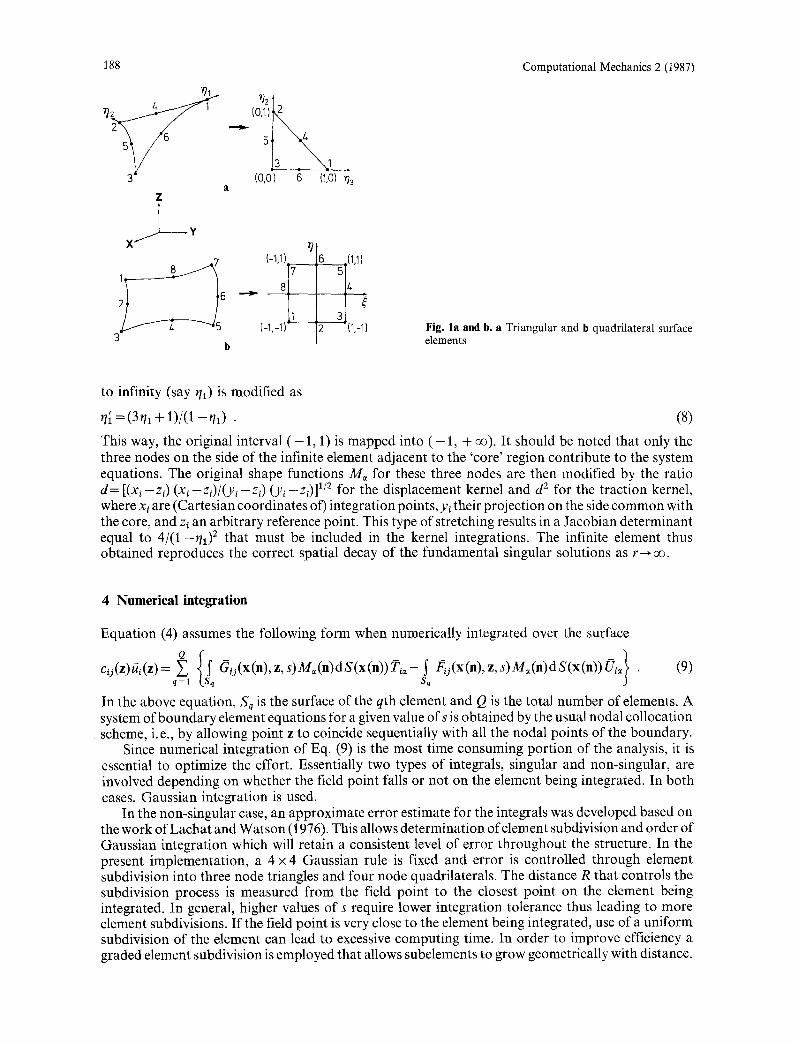
where i= 1,2, 3 and ~ = 1, 2 , . . . , A, with A the number of nodal points necessary to describe the element: Furthermore, M~ are shape functions defined in the local or intrinsic coordinate system (~h, r/z): Two basic quadratic elements are used here: (a) the six node triangular 'patch' and (b) the eight node quadrilateral 'patch'. These two quadratic elements are shown in Fig. I and more information may be found in Appendix B: The Jacobian matrix relating the transformation from the Cartesian coordinate system to the element's intrinsic coordinate system is

Jij = (OM,/~lj) X,~ (6)

where j = 1, 2: The field variables are also represented by the same shape functions, i: e ,

fff (x) = M, (q) U,~ , ~ (x) = M~ (q) ~ , (7)

where O~ and ~ are nodal values of the displacements and tractions, respectively, in the transformed domain:

Infinite elements, which are essential if problems involving half spaces are to be solved, can be constructed by modifying the eight node quadrilateral: The intrinsic coordinate that we want extend

188

Z

Xf,.,.~ [ ...... y

1

3 b

(0,0) 6 (1,0) ~3 3.

(-1,1)_

8[ 71 (-1,-1)-

r L6 _(1,1)

2 -(1,-1)

Computational Mechanics 2 (1987)

Fig. la and b. a Triangular and b quadrilateral surface elements

to infinity (say I/1) is modified as

t/[ = (3 t/1 + 1)/(1 - r h) . (8)

This way, the original interval ( - 1, 1) is mapped into ( - 1, + oo): It should be noted that only the three nodes on the side of the infinite element adjacent to the 'core' region contribute to the system equations: The original shape functions M, for these three nodes are then modified by the ratio d= [(xi-z i) ( x i - z~) / ( y i - z i ) (Yi-z i)] 1/2 for the displacement kernel and d 2 for the traction kernel, where x~ are (Cartesian coordinates of) integration points, y~ their projection on the side common with the core, and z~ an arbitrary reference point. This type of stretching results in a Jacobian determinant equal to 4 / ( 1 - q l ) 2 that must be included in the kernel integrations. The infinite element thus obtained reproduces the correct spatial decay of the fundamental singular solutions as r ~ oe.

4 Numerica l integration

Equation (4) assumes the following form when numerically integrated over the surface

cu(z)~i~(z ) = ~ Gu(x(n), z, s)M~(n)dS(x(n)) 7"i~ - [. ~j(x(n), z, s)M~(n)dS(x(n)) (7i~ . (9) q = 1 Sq

In the above equation, Sq is the surface of the qth element and Q is the total number of elements. A system of boundary element equations for a given value ofs is obtained by the usual nodal collocation scheme, i: e., by allowing point z to coincide sequentially with all the nodal points of the boundary:

Since numerical integration of Eq. (9) is the most time consuming port ion of the analysis, it is essential to optimize the effort: Essentially two types of integrals, singular and non-singular, are involved depending on whether the field point falls or not on the element being integrated. In both cases, Gaussian integration is used.

In the non-singular case, an approximate error estimate for the integrals was developed based on the work of Lachat and Watson (1976): This allows determination of element subdivision and order of Gaussian integration which will retain a consistent level of error throughout the structure: In the present implementation, a 4 x 4 Gaussian rule is fixed and error is controlled through element subdivision into three node triangles and four node quadrilaterals. The distance R that controls the subdivision process is measured from the field point to the closest point on the element being integrated: In general, higher values of s require lower integration tolerance thus leading to more element subdivisions. If the field point is very close to the element being integrated, use of a uniform subdivision of the element can lead to excessive computing time. In order to improve efficiency a graded element subdivision is employed that allows subelements to grow geometrically with distance.

S. Ahmad and G. D. Manolis: Dynamic analysis of 3-D structures 189

Numerical tests of a three-dimensional sphere have demonstrated the accuracy of the non-singular integration process:

In the case of singular integration, the element is first divided into triangular subelements. The integration over each subelement is carried out in a polar coordinate system with origin at the field point: Further subdivision in the angular direction is required to preserve accuracy. This coordinate transformation produces non-singular behavior in all except one of the required integrals. Normal Gauss-rules can then be employed. The integral of the traction kernel times the isoparametric shape function which is still singular at the source point, and cannot be numerically evaluated. Its calculation is then carried out indirectly: Let us concentrate, for illustration purposes, on the singularity that arises in the q--1 element and the ~= 1 node: Then, the corresponding strictly diagonal 3 x 3 block that contains the jump term cij as well as the Cauchy principal value of the traction kernel integral is evaluated as follows. First define

dSJ=cij ~- I F~tM1 dS and c~j=cij+ ~ ~ j M l d S , (10) $1 $1

where d~ t and dij are the strictly diagonal blocks for the static and steady-state systems, respectively. Next, the d~J block is evaluated using the rigid body motion approach: Specifically, if uj= {1} is imposed on the static version of Eq. (9), no tractions result and

) Fi}tM1 d S = - I Fi}tM= dS+ Z Z I Fi} tM=dS • (11) dSj=ciJ+s1 a :2 81 q :2 a : l Sq

Finally, by combining Eqs. (10) and (11),

di j :d~+ ~ ( ~ j - F ~ t ) i l d S • (12) $1

In the above equation, the integral involving ~ j -F i} t is non-singular and can easily be evaluated numerically:

In general, the surface integrals are continuously differentiable and solution accuracy can, therefore, be improved by use of increased integration order: In the case of the exterior and half space problems, the terms 5ij and 0.5 5ij must be substracted from the right-hand side of Eq. (12), respectively: Those terms represent the contribution of the outer surface as its radius approaches infinity.

5 Transformed domain solution

The solution strategy in the transform domain essentially consists of a series of static-like analyses for given values of the transformed parameter s (or co). It should be noted that any internal viscous dissipation of energy can easily be accounted for by replacing the Lame constants 2 and # by their complex counterparts and leaving Poisson's ratio unaltered (Manolis 1981):

Upon numerically integrating Eq: (9) over the surface, the final system equations can be assembled to read as

{x} = [B] (13)

The system matrices A and B are dependent on the transform parameter and are thus complex. Equation (13) is solved for unknowns X in terms of the prescribed boundary quantities vy and for a spectrum of values of the transform parameter. For added accuracy, the system equations are scaled so that all the coefficients of .g, are of the same magnitude. Reduction of A is accomplished using a standard complex block-banded solver: What remains to be done is to invert the solution back to the real time domain. The inverse Laplace transformation is defined as

1 fl+ioo f ( x , t ) = ~ - ~ p_!if(x,s)e~tds , i = V - 1 , (14)

190 Computational Mechanics 2 (1987)

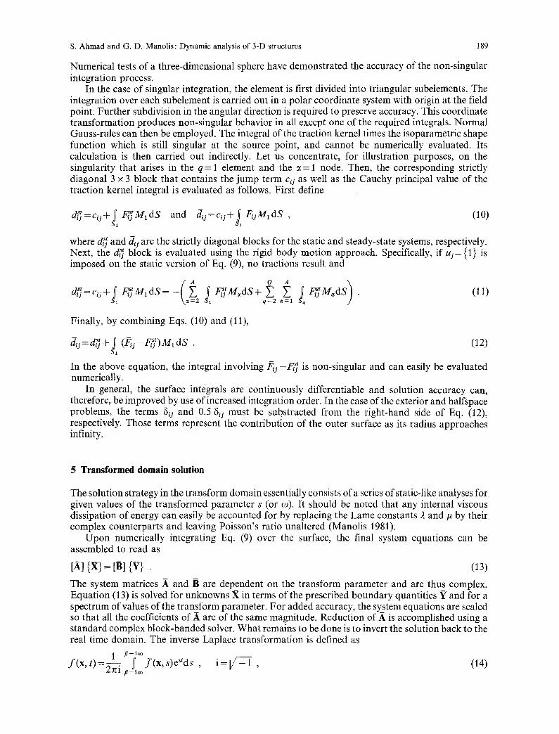
where fl > 0 is arbitrary, but greater than the real part of all the singularities o f f ( s ) , and s is a complex number with Re (s) > 0.

The inverse transformation is done numerically using the inversion algorithm of Durbin (1974)

/ ( t i ) = 2 - Re [f(/~)] + Re (A(n)+iB(n))W J " (15) [.n =o

2~ W = ei2~/N ' where s. =/~ + in ~ - ,

A(n)= 2 Re ~+i(n+lN) , B(n)= ~ Im ~+i(n+lN) / = 0 / = 0

n = 0 , 1 , 2 , . . . , N l = 0 , 1 , 2 , . . . , L . (16)

The numerical values of f(t) are computed for N equidistant points tj=jAt =jT/N, j = 0, 1, 2 , . . . , N - 1 : In this work we have used L = 1, N = 20 and ~ T = 6, al though these values can be adjusted to improve accuracy: The computat ions involved in Eq: (15) are performed by employing the fast Fourier-algorithm of Cooley and Tukey (1965).

Two comments must be made at this point. First, the Laplace transform solution is essentially a superposition of a series of steady state solutions and is therefore applicable only to linear problems. Second, since the Laplace transform casts the entire problem in the complex domain, the storage and computer time requirements are considerably increased.

6 Numerical examples

A number of representative problems were solved in order to test the present methodology. In all cases, SI units are used with meters (m) for length, kilograms (kg) for mass, and seconds (s) for time:

6:1 Prismatic beam

A uniform beam with a rectangular cross-section has a modulus of elasticity E = 1.16 x 107, a Poisson's ratio v = 0:0 and a mass density Q =2.0. Two cases are considered.

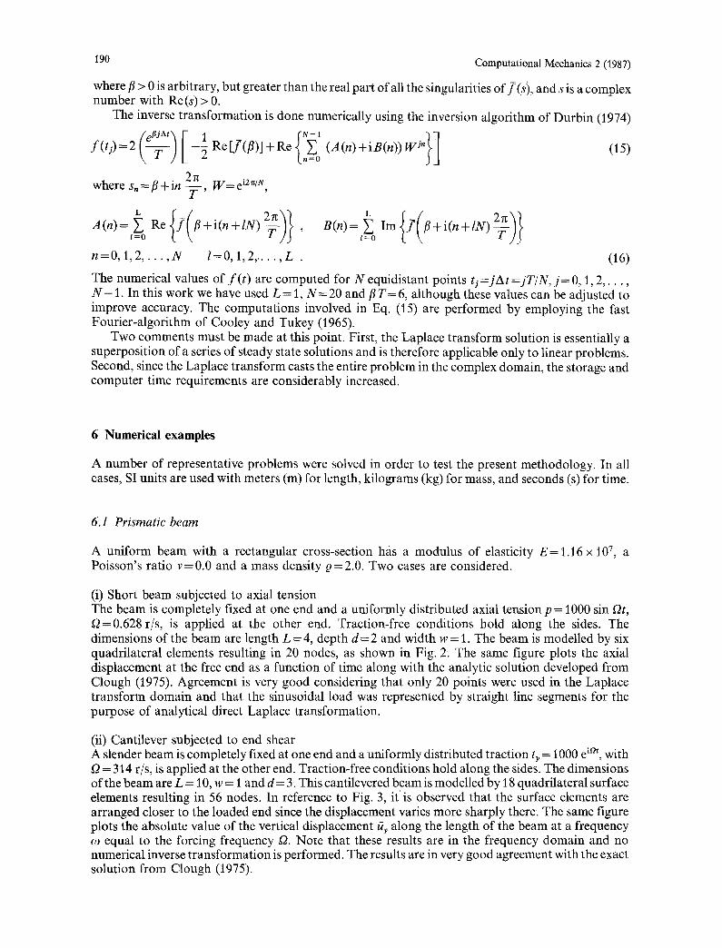
(i) Short beam subjected to axial tension The beam is completely fixed at one end and a uniformly distributed axial tension p = 1000 sin Ot, Q=0.628 r/s, is applied at the other end: Traction-free conditions hold along the sides. The dimensions of the beam are length L = 4, depth d = 2 and width w = 1. The beam is modelled by six quadrilateral elements resulting in 20 nodes, as shown in Fig: 2: The same figure plots the axial displacement at the free end as a function of time along with the analytic solution developed from Clough (1975). Agreement is very good considering that only 20 points were used in the Laplace transform domain and that the sinusoidal load was represented by straight line segments for the purpose of analytical direct Laplace transformation.

(ii) Cantilever subjected to end shear A slender beam is completely fixed at one end and a uniformly distributed traction ty = 1000 e iot, with

= 314 r/s, is applied at the other end. Traction-free conditions hold along the sides. The dimensions of the beam are L = 10, w = 1 and d = 3. This cantilevered beam is modelled by 18 quadrilateral surface elements resulting in 56 nodes. In reference to Fig. 3, it' is observed that the surface elements are arranged closer to the loaded end since the displacement varies more sharply there: The same figure plots the absolute value of the vertical displacement fly along the length of the beam at a frequency o9 equal to the forcing frequency O. Note that these results are in the frequency domain and no numerical inverse transformation is performed: The results are in very good agreement with the exact solution from Clough (1975).

S. Ahmad and G. D. Manolis: Dynamic analysis of 3-D structures

u xl04, 3

m 2

1

0

-1

-2

-3

2

- Ana ly t i ca l • BEN

. . . . .5

191

, J =

x'J

X ¥

IOy I-

0 m

0.002.

0.004.

i= ' i 1

,Z

2 Z, 6 8 10

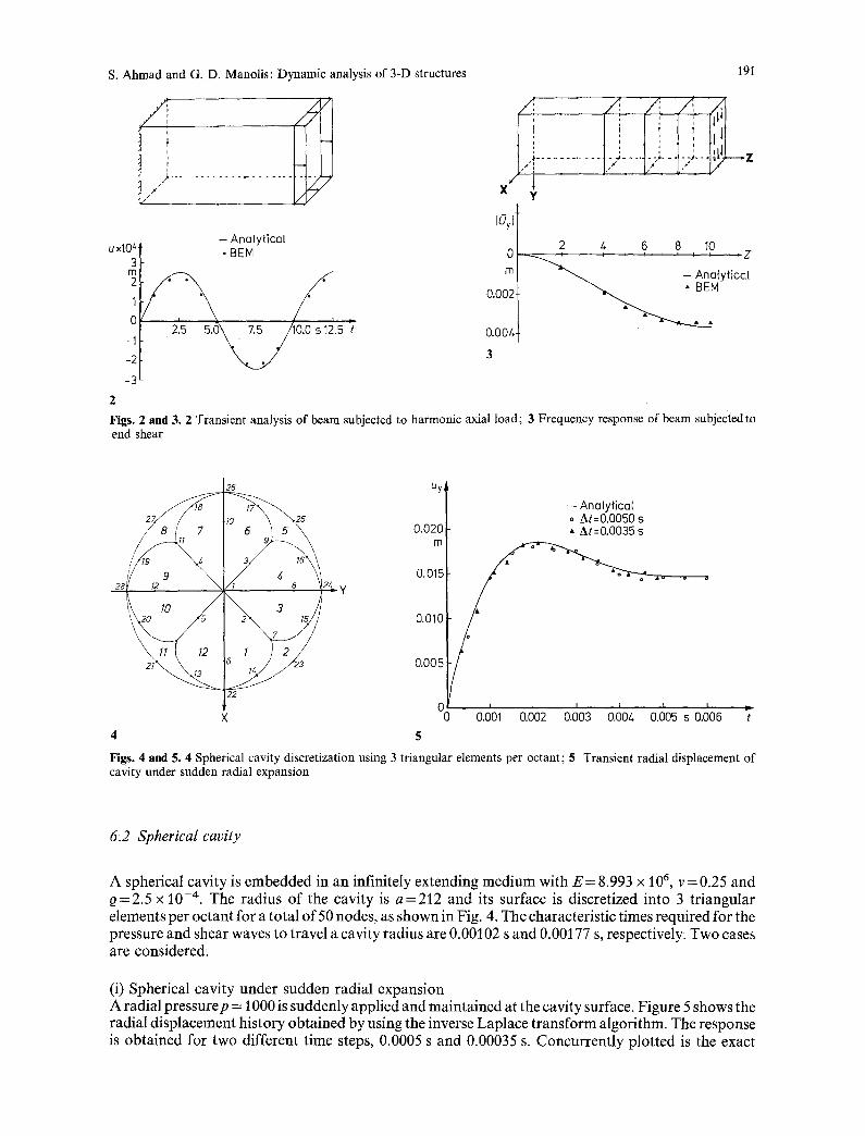
Figs. 2 and 3. 2 Transient analysis of beam subjected to harmonic axial load; 3 Frequency response of beam subjecfedto end shear

uy,

0.020 m

0.015

0.010

0.005

0 0

4 5

- - Ana ly t i ca l o A t : 0 . 0 0 5 0 s • A t :0 .0035 s

I I I I I I I I ,

0.001 0.002 0.003 0.00z, 0.005 s 0.006

Figs. 4 and 5. 4 Spherical cavity discretization using 3 triangular elements per octant; 5 Transient radial displacement of cavity under sudden radial expansion

6:2 Spherical cavity

A spherical cavity is embedded in an infinitely extending medium with E = 8.993 × 106, v = 0.25 and Q=2.5 x 10 -¢. The radius of the cavity is a=212 and its surface is discretized into 3 triangular elements per octant for a total of 50 nodes, as shown in Fig. 4: The characteristic times required for the pressure and shear waves to travel a cavity radius are 0.00102 s and 0.00177 s, respectively. Two cases are considered.

(i) Spherical cavity under sudden radial expansion A radial pressurep = 1000 is suddenly applied and maintained at the cavity surface. Figure 5 shows the radial displacement history obtained by using the inverse Laplace transform algorithm: The response is obtained for two different time steps, 0.0005 s and 0:00035 s. Concurrently plotted is the exact

192

2.0"

1.5"

1.0-

0.5-

- j

O : 9 0

- - A n a l y t i c a [

• , . BEM

- - - - - - - - ~ • . . . 1 0 = 0 o

i I 1 I 2 4 6 8

C o m p u t a t i o n a l M e c h a n i c s 2 (1987)

% , - - Ana ty t i ca l

• BEM 1.0-

0.5- -'---'O = 90°

0 I . . . . I I 2 4 6 8

F i g . 6. T r a n s i e n t s t resses a t c a v i t y s u r f a c e d u e t o

p r o p a g a t i n g p r e s s u r e w a v e

solution from Timoshenko (1970). In general, the numerical results are in good agreement with the analytical solution. There is some oscillation in the results towards the end of the total time interval so that about 85% of the time spectrum obtained is actually plotted.

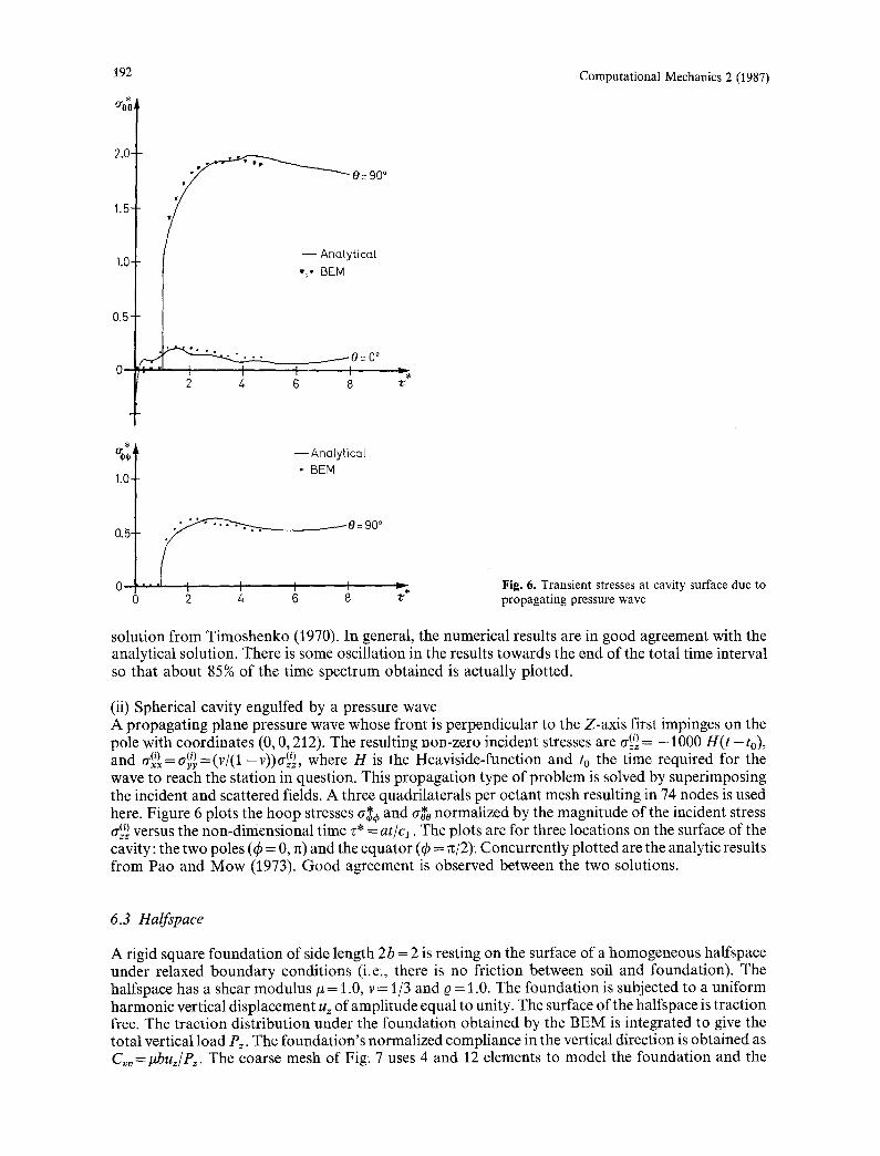
(ii) Spherical cavity engulfed by a pressure wave A propagating plane pressure wave whose front is perpendicular to the Z-axis first impinges on the pole with coordinates (0, 0,212). The resulting non-zero incident stresses are o-(ff~ ) = - 1000 H(t - to), and ~j)~=a(y~=(v/(l-v))a(~'~ ), where H is the Heaviside-function and to the time required for the wave to reach the station in question: This propagation type of problem is solved by superimposing the incident and scattered fields. A three quadrilaterals per octant mesh resulting in 74 nodes is used here. Figure 6 plots the hoop stresses ~ and ~*0 normalized by the magnitude of the incident stress o-~ ) versus the non-dimensional time z* = at/c1. The plots are for three locations on the surface of the cavity: the two poles (~b = 0, n) and the equator (q5 = 7t/2): Concurrently plotted are the analytic results from Pao and Mow (1973): Good agreement is observed between the two solutions:

6.3 Halfspace

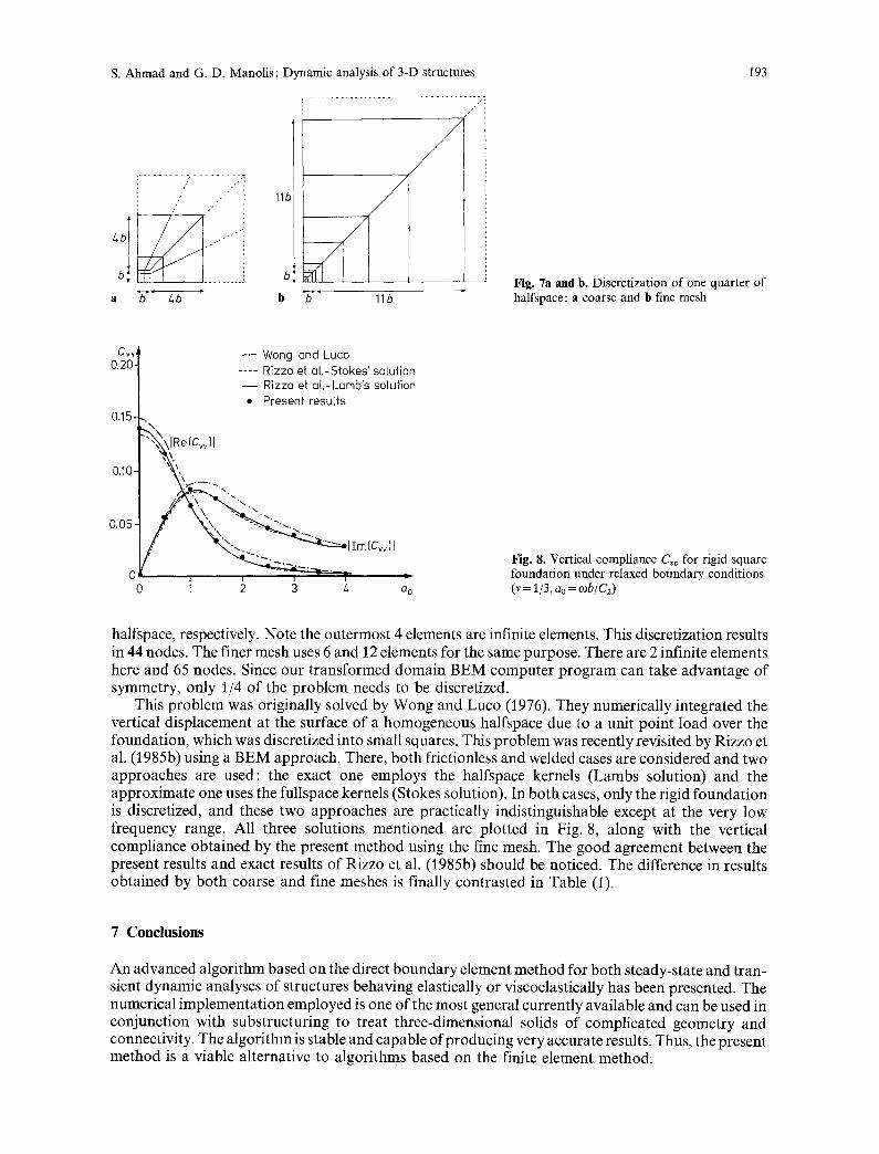
A rigid square foundation of side length 2b = 2 is resting on the surface of a homogeneous halfspace under relaxed boundary conditions (i:e., there is no friction between soil and foundation). The halfspace has a shear modulus # = 1.0, v = 1/3 and Q = 1.0: The foundation is subjected to a uniform harmonic vertical displacement uz of amplitude equal to unity: The surface of the half space is traction free. The traction distribution under the foundation obtained by the BEM is integrated to give the total vertical load P~: The foundation's normalized compliance in the vertical direction is obtained as Cvv=#buz/P~: The coarse mesh of Fig: 7 uses 4 and 12 elements to model the foundation and the

S. Ahmad and G. D. Manolis: Dynamic analysis of 3-D structures

. . . . . . . . . . ., . . . . . . . . ;, /

/ /

a b Lb

11b

, - . . . . . . . . . . , . . . . . . . . . . . . . . . . . . . . . . . . . . / ,

. . . . _,

b b 11b

~93

Fig. 7a and b. Discretization of one quarter of halfspace: a coarse and b fine mesh

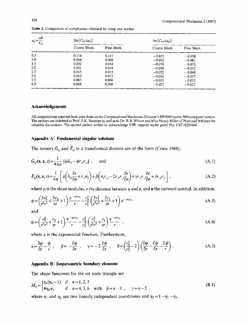
Cvv~ - ' - Wong and Luco 0-201 " . . . . Rizzo et al,-Stokes' solution

/ - - Rizzo et al,-Lumb's solution • Present results

0.15 J '\,\

0 . 1 0 . h e(cVv)l

0.05- ' " -.... ~ Im(Cvv)l

0, o i %

Fig. 8. Vertical compliance Cvv for rigid square foundation under relaxed boundary conditions (v= 1/3, ao =cob~G)

halfspace, respectively. Note the outermost 4 elements are infinite elements. This discretization results in 44 nodes. The finer mesh uses 6 and 12 elements for the same purpose. There are 2 infinite elements here and 65 nodes: Since our transformed domain BEM computer program can take advantage of symmetry, only 1/4 of the problem needs to be discretized.

This problem was originally solved by Wong and Luco (1976). They numerically integrated the vertical displacement at the surface of a homogeneous half space due to a unit point load over the foundation, which was discretized into small squares. This problem was recently revisited by Rizzo et al. (1985b) using a BEM approach: There, both frictionless and welded cases are considered and two approaches are used: the exact one employs the halfspace kernels (Lambs solution) and the approximate one uses the fullspace kernels (Stokes solution): In both cases, only the rigid foundation is discretized, and these two approaches are practically indistinguishable except at the very low frequency range. All three solutions mentioned are plotted in Fig. 8, along with the vertical compliance obtained by the present method using the fine mesh. The good agreement between the present results and exact results of Rizzo et aL (1985b) should be noticed. The difference in results obtained by both coarse and fine meshes is finally contrasted in Table (I):

7 Conclusions

An advanced algorithm based on the direct boundary element method for both steady-state and tran- sient dynamic analyses of structures behaving elastically or viscoelastically has been presented. The numerical implementation employed is one of the most general currently available and can be used in conjunction with substructuring to treat three-dimensional solids of complicated geometry and connectivity: The algorithm is stable and capable of producing very accurate results. Thus, the present method is a viable alternative to algorithms based on the finite element method.

194

Table 1. Comparison of compliances obtained by using two meshes

Computational Mechanics 2 (1987)

cob ao = C~ Re {Cvv(ao)} Im { Cvv(ao) }

Coarse Mesh Fine Mesh Coarse Mesh Fine Mesh

0.5 0:118 0.117 -0:057 -0.058 1.0 0:064 0.069 -0.083 -0.081 1.5 0.032 0.034 -0.076 -0.070 2.0 0:021 0.018 -0.059 -0.052 2:5 0.015 0.015 -0.052 -0.048 3.0 0.010 0.012 -0.036 -0.037 3.5 0.005 0.006 -0:035 -0.032 4.0 0:004 0.004 -0:027 -0:027

Acknowledgements

All computations reported here were done on the Computational Mechanics Division's HP 9000 (series 500) computer system. The authors are indebted to Prof. P:K. Banerjee as well as to Dr. R.B. Wilson and Miss Nancy Miller of Pratt and Whitney for valuable discussions. The second author wishes to acknowledge NSF support under grant No. CEE-8202604.

Appendix A: Fundamental singular solutions

The tensors (~u and iv u in a transformed domain are of the form (Cruse 1968)"

(7ij(x,z,s)=4-~# [¢Su-qarar,j ] , and (A.1)

~j(x,z,s)=~[~(8,J~n+r,,nj)+fl(n,r,,--2r,,r,j~n)+Yr,,r,J-~n+(Sr, jr, i I , (A.2)

where/2 is the shear modulus, r the distance between x and z, and n the outward normal. In addition,

/3~ 3c2 )e -~'sc~ ¢ = t,7;~-~ +7;-r +1 r and

C(--~-~r 2 ' C2 . .'~ e-St/C= 4= -t-~r -t- i ) r

c2 /'3c2 3cl + 1 ) e -s ' l c '

c7 tT-~Y + 7 ; ) (A.3)

<~ / 4 c,'~ e-~'l<' cl t , W + Tr ) - - ; - - ' (A.4)

where e is the exponential function: Furthermore,

80 dp f l = - - - , 2 = - 2 - - - 2 - ~ r r ' ~r 8r ' - \ ~ ~r "

(A.5)

Appendix B: Isoparametric boundary elements

The shape functions for the six node triangle are

~th(th - 1 ) if c~ = 1,2, 3 M,

[4q~t b if 0~=4,5,6 with f l=0~-3 , 7 = 0 ~ - 2 ,

where t/1 and q2 are two linearly independent coordinates and t/a = 1 - t h -t/2.

(B:I)

S. Ahmad and G. D. Manolis : Dynamic analysis of 3-D structures 195

The shape functions for the eight node quadrilateral are

/ 0.25(1 +Go) (1 +t/o) (~o+t/o- l ) if .=1 ,3 ,5 ,7

M=={0.50(I _~2) (i -t/o) if . = 2 , 6 (B.2) / [0.50(1+~o)(1-t/2) if ~=4,8

where {o = ~ and t/o = t/t/=, with { and t/being the two linearly independent coordinates and ({=, t/~) the coordinates of node ~. Two base vectors along the element's intrinsic coordinates are

~x ~x ~v Oz d C j + ~ dCk e2 dt/i+~-~t/dt/j dt/k el = ~ - d ~ i + ~ , =~-~ +~-~ , (/3.3)

where i, j and k are the usual unit vectors: Their cross product is a vector normal to the surface of the element and its magnitude is equal to the value of the determinant of the Jacobian matrix.

References

Apsel, F.J. (1979): Dynamic Green's functions for layered media and applications to boundary-value problems. Ph. D. diss. Uniw of California, San Diego

Arnold, R.N.; Bycroft, G:N: ; Warburton, G.B: (1955): Forced vibrations of a body on an infinite elastic solid. J. Appl. Mech: 22, 391-400

Banaugh, R.P.; Goldsmith (1963): Diffraction of steady elastic waves by surface of arbitrary shape. J. Appl. Mech. 30, 589-597

Banerjee, P:K:; Butterfield, R. (1981): Boundary element methods in engineering sciences. London: McGraw-Hill Banerjee, P.K. ; Abroad, S: (1985): Advanced three-dimensional dynamic analysis by boundary elements: Proc. ASME Conf.

on Advanced Boundary Element Analysis. Cruse, T.A:; Pifko, A.B. ; Armen, H. (eds). AMD 72, 65-81 Beskos, D.E. ; Spyrakos, C:C. (1984): Dynamic response of strip foundations by the time domain BEM-FEM method. Final

Rpt. Part B, NSF Research Grant No. CEE-8024725, Univ. of Minnesota Clough, R.W. ; Penzien, J. (1975): Dynamics of structures. New York: McGraw-Hill Cole, D.M.; Kosloff, D.D.; Minster, J.B. (1978): A numerical boundary integral equation method for elastodynamics I. Bull.

Seismological Soc. Amer. 68, 1331-1357 Cooley, J.W. ; Tukey, J.W. (1965): An algorithm for machine calculation of complex fourier series: Math. Comp. 19, 297-310 Cruse, T.A. (1968): A direct formulation and numerical solution of the general elastodynamic problem IL J. Math. Analy: and

Appl. 22, 341-355 Cruse, T.A:; Rizzo, F.J. (1968): A direct formulation and numerical solution of the general transient elastodynamic problem L J. Math. Analy. and AppL 22, 244-259. Dominguez, J. (1978): Dynamic stiffness of rectangular foundations. Final Rpt., NSF-RANN Grant No. ENV77-18339,

Massachusetts Inst: of Technology, Boston Dravinski, M. (1983): Amplification of P, SV and Rayleigh waves by two alluvial valleys. Int. J. Soil Dynamics and Earthquake

Eng: 2, 65-77 Durbin, F: (1974): Numerical inversion of Laplace transforms: an efficient improvement to Dubner and Abates' method.

Computer J. 17, 371-376 Graff, K.F. (1974): Wave motion in elastic solids. New York: McGraw Hill Gupta, S.; Penzien, J.; Lin, T.W:; Yeh, C.S. (1982): Three-dimensional hybrid modelling of soil-structure interaction.

Earthquake Eng: Struct: Dyn. 10, 69-87 Karabalis, D:L:; Beskos, D.E. (1984): Dynamic response of 3-D rigid surface foundations by time domain boundary element

method. Earthquake Eng. Struct. Dynamics 12, 73-93 Kausel, E. ; Roesset, J.M. ; Waas, G. (1975): Dynamic analysis of footings on layered media. Proc. ASCE, EM5 101,679-693 Kaynia, A.M. ; Kausel, E: (1982): Dynamic behavior of pile groups. Proc. 2nd Int. Conf. on Numer. Meth. in Offshore Piling,

Austin, Texas Kobayashi, Y. ; Fukui, T.; Azuma, N. (1975): An analysis of transient stresses produced around a tunnel by the integral

equation method. Proc: Syrup: Earthquake Eng., Tokyo, Jpn., 631-638 Lachat, J.C. ; Watson, LO. (1976): Effective numerical treatment of boundary integral equations: a formulation for three-

dimensional elastostatics: Int. J. Num. Meth. in Eng. 10, 991-1005 Manolis, G.D:; Beskos, D.E. (1981): Dynamic stress concentration studies by boundary integrals and Laplace transform. Int.

L Num. Meth. Eng. 17, 573-599 Manolis, G.D. (1983): A comparative study on three boundary element method approaches to problems in elastodynamics.

Int. J. Num, Meth. Eng. 19, 71-93 Niwa, Y:; Fukui, T.; Kato, S:; Fujiki, K. (1980): An application of the integral equation method to two-dimensional

elastodynamics. Theor: Appl. Mech., University of Tokyo Press 28, 281-290 Pao, YM:; Mow, C:C. (1973): Diffraction of elastic waves and dynamic stress concentration. New York: Crane Russak

196 Computational Mechanics 2 (1987)

Rizzo, F:J. ; Shippy, D.J. ; Rezayat, M. (1985a): A boundary integral equation method for radiation and scattering of elastic waves in three dimensions: Int. J. Num. Meth. Eng. 21, 115-129

Rizzo, F.J. ; Shippy, D.J. ; Rezayat, M. (1985b): Boundary integral equation analysis for a class of earth-structure interaction problems. Final Rpt. to National Science Foundation, Research Grant CEE-8013461, Dept: of Eng. Mech., University of Kentucky, Lexington

Sen, R. ; Davies, T.G. ; Banerjee, P.K. (1985): Dynamic analysis of piles and pile groups embedded in homogeneous soils. Earthquake Eng. and Struct. Dynamics 13, 53-65

Sen, R. ; Kausel, E. ; Banerjee, P.K. (1985): Dynamic analysis of piles amd pile groups embedded in nonhomogeneous soils. Int. J. Num. Anal. Methods in Geomech. 9, 507-524

Timoshenko, S.P. ; Gere, J.M. (1979): Theory of elasticity. 3rd ed, New York: McGraw-Hill Veletsos, A.S. ; Wei, Y.T. (1971): Lateral and rocking vibration of footings. Proc. ASCE, SM9, 97, 1227-1248 Wilson, R. ; Bak, M.J.; Nakazawa, S:; Banerjee, P:K. (1984): 3-D inelastic analysis methods for hot section components (base

program). First Ann. Status Rpt, NASA Contractor Report 174700, Lewis, Ohio Wong, H.L.; Luco, J.E. (1976): Dynamic response of rigid foundations of arbitrary shape. Earthquake Eng. Strnct.

Dynamics 4, 579-587

Communicated by S. N. Atluri, August 5, 1986