Solution of the NavierStokes equations in velocityvorticity form using a EulerianLagrangian boundary...
24
INTERNATIONAL JOURNAL FOR NUMERICAL METHODS IN FLUIDS Int. J. Numer. Meth. Fluids 2000; 34: 627–650 Solution of the Navier – Stokes equations in velocity – vorticity form using a Eulerian – Lagrangian boundary element method D. L. Young* ,1 , S. K. Yang and T. I. Eldho Department of Ci6il Engineering and Hydrotech Research Institute, National Taiwan Uni6ersity, Taipei, Taiwan, Republic of China SUMMARY This paper describes the Eulerian – Lagrangian boundary element model for the solution of incompress- ible viscous flow problems using velocity – vorticity variables. A Eulerian – Lagrangian boundary element method (ELBEM) is proposed by the combination of the Eulerian – Lagrangian method and the boundary element method (BEM). ELBEM overcomes the limitation of the traditional BEM, which is incapable of dealing with the arbitrary velocity field in advection-dominated flow problems. The present ELBEM model involves the solution of the vorticity transport equation for vorticity whose solenoidal vorticity components are obtained iteratively by solving velocity Poisson equations involving the velocity and vorticity components. The velocity Poisson equations are solved using a boundary integral scheme and the vorticity transport equation is solved using the ELBEM. Here the results of two-dimensional Navier – Stokes problems with low – medium Reynolds numbers in a typical cavity flow are presented and compared with a series solution and other numerical models. The ELBEM model has been found to be feasible and satisfactory. Copyright © 2000 John Wiley & Sons, Ltd. KEY WORDS: boundary element method; Eulerian – Lagrangian method; Navier – Stokes equations; velocity – vorticity formulation 1. INTRODUCTION The velocity – vorticity form of the Navier – Stokes equations pioneered by Fasel [1] has been established as an effective formulation for the solution of incompressible viscous flow problems. In the recent times, many researchers used the velocity – vorticity formulation for the calculations of two- and three-dimensional steady and unsteady flows using various numerical methods, such as the finite difference method (FDM) [2], the finite element method (FEM) [3] * Correspondence to: Department of Civil Engineering, Hydraulic Research Laboratory, National Taiwan University, Taipei 10617, Taiwan, Republic of China. 1 E-mail: [email protected] Copyright © 2000 John Wiley & Sons, Ltd. Recei6ed 13 September 1999 Re6ised 14 February 2000
-
Upload
independent -
Category
Documents
-
view
2 -
download
0
Transcript of Solution of the NavierStokes equations in velocityvorticity form using a EulerianLagrangian boundary...

INTERNATIONAL JOURNAL FOR NUMERICAL METHODS IN FLUIDSInt. J. Numer. Meth. Fluids 2000; 34: 627–650
Solution of the Navier–Stokes equations invelocity–vorticity form using a Eulerian–Lagrangian
boundary element method
D. L. Young*,1, S. K. Yang and T. I. Eldho
Department of Ci6il Engineering and Hydrotech Research Institute, National Taiwan Uni6ersity, Taipei, Taiwan,Republic of China
SUMMARY
This paper describes the Eulerian–Lagrangian boundary element model for the solution of incompress-ible viscous flow problems using velocity–vorticity variables. A Eulerian–Lagrangian boundary elementmethod (ELBEM) is proposed by the combination of the Eulerian–Lagrangian method and theboundary element method (BEM). ELBEM overcomes the limitation of the traditional BEM, which isincapable of dealing with the arbitrary velocity field in advection-dominated flow problems. The presentELBEM model involves the solution of the vorticity transport equation for vorticity whose solenoidalvorticity components are obtained iteratively by solving velocity Poisson equations involving the velocityand vorticity components. The velocity Poisson equations are solved using a boundary integral schemeand the vorticity transport equation is solved using the ELBEM. Here the results of two-dimensionalNavier–Stokes problems with low–medium Reynolds numbers in a typical cavity flow are presented andcompared with a series solution and other numerical models. The ELBEM model has been found to befeasible and satisfactory. Copyright © 2000 John Wiley & Sons, Ltd.
KEY WORDS: boundary element method; Eulerian–Lagrangian method; Navier–Stokes equations;velocity–vorticity formulation
1. INTRODUCTION
The velocity–vorticity form of the Navier–Stokes equations pioneered by Fasel [1] has beenestablished as an effective formulation for the solution of incompressible viscous flowproblems. In the recent times, many researchers used the velocity–vorticity formulation for thecalculations of two- and three-dimensional steady and unsteady flows using various numericalmethods, such as the finite difference method (FDM) [2], the finite element method (FEM) [3]
* Correspondence to: Department of Civil Engineering, Hydraulic Research Laboratory, National Taiwan University,Taipei 10617, Taiwan, Republic of China.1 E-mail: [email protected]
Copyright © 2000 John Wiley & Sons, Ltd.Recei6ed 13 September 1999
Re6ised 14 February 2000
D. L. YOUNG, S. K. YANG AND T. I. ELDHO628
and the boundary element method (BEM) [4]. In most investigations, the governing equationshave been written as a system of parabolic- and Poisson-type equations for the components ofthe vorticity and velocity fields respectively. The main advantage of this formulation includesthe numerical separation of the kinematic and kinetic aspects of the fluid flow from thepressure computation, which is determined afterwards from the known velocity and vorticityfields.
The theoretical potential of the BEM for the solution of Navier–Stokes equations has beenadequately exposed by various researchers [5]. In the solution of the velocity–vorticityformulation of the Navier–Stokes equations, two different types of equations (Poisson-typeand parabolic-type) are to be solved. While the Poisson-type equations can be accuratelysolved with the BEM [6], the method is not so stable in the solution of the parabolic-typetransport equations [7].
While solving the parabolic-type transport equations, the numerical diffusion and dispersionare the two major problems to be concerned with. The popular methods like the upwind FDM[8] and upwind FEM [9] work well only for the problems in which the diffusion effectdominates. In general, the high-order upwind schemes produce numerical oscillations in theresults, while the lower-order upwind schemes cannot avoid the numerical diffusion.
The Eulerian–Lagrangian method is a widely used scheme for the transport modeling. It isa combination of the Eulerian method, in which the equation is solved on a fixed grid in space,and the Lagrangian method, which utilizes either a deforming grid or a fixed grid in deformingco-ordinates. The Eulerian–Lagrangian method (ELM) combines aspects of both approachesso as to merge the simplicity of a fixed Eulerian grid with the computational power of theLagrangian method [10]. In the transport modeling using the ELM, the advection part issolved by the Lagrangian method, which can be computed independently at each time step bythe method of characteristics applied to a grid fixed domain. The remaining diffusion part canbe solved by the FEM [10,11] or by the FDM [12], or by the BEM on a separate grid. Theinfluence of the advection is projected from one grid to another by local interpolation.
In the present study, an accurate Eulerian–Lagrangian boundary element method (ELBEM)is proposed for the first time for the velocity–vorticity formulation of the Navier–Stokesequations. The Poisson-type equations are solved using the general boundary integral tech-nique with domain integration for the source terms and from which the vorticity boundaryconditions are exactly determined. The vorticity transport equation is solved using the ELBEMon a transformed characteristic domain. Based on the concept of the ELM, the formulation ofthe ELBEM and its associated fundamental solution is obtained for vorticity transportequations. By combining the ELM and BEM, the BEM is made easier to handle the variablevelocity field. In this paper, the interpolation procedure for the ELM computation of theconvection part is replaced with the process of the more accurate BEM interior pointevaluation, and hence the interpolation error is avoided.
The application of the ELBEM model to incompressible viscous flow problems has beendemonstrated using the well-known model problem of flow in a driven square cavity. Thecavity flow problem is of continuing interest because it offers a relatively simple model onwhich numerical techniques may be examined and verified with other numerical schemes.Using the ELBEM model, satisfactory results comparable with other models in literature arepresented for Reynolds number of up to 2000.
Copyright © 2000 John Wiley & Sons, Ltd. Int. J. Numer. Meth. Fluids 2000; 34: 627–650
EULERIAN–LAGRANGIAN BOUNDARY ELEMENT MODEL 629
After presenting the governing equations, the numerical formulation using the ELBEM arebriefly described. Then the solution procedure and numerical results for the two-dimensionaldriven cavity flow problem are described, followed by a few concluding remarks.
2. GOVERNING EQUATIONS
The governing equations for mass and linear momentum transport for an incompressibleNewtonian fluid can be written as [13]
(u(t
+ u ·9u= −9p+1
Re92u (1)
9 · u=0 (2)
where u is the velocity vector, p is the pressure, Re is the Reynolds number and t is the time.Equations (1) and (2) represent the Navier–Stokes equations in the velocity–pressureformulation.
The vorticity vector v can be expressed as
v=9× u (3)
By taking the curl of both sides of Equation (1) and using Equations (2) and (3), we can obtainthe vorticity transport equation as follows:
(v
(t+ u ·9v=v ·9u+
1Re
92v (4)
By taking the curl of Equation (3) and using Equation (2) we get
92u= −9×v (5)
which is the vector form of Poisson’s equation for u.Equations (4) and (5), with u and v as velocity and vorticity vectors, are known as the
velocity–vorticity formulation of the Navier–Stokes equations, and can replace Equations (1)and (2) in which u and p are primitive variables.
We seek a solution in the domain V, which satisfies the initial conditions
u= u0, v=9× u0 at t=0 (6)
and the boundary conditions
u= uG, v= (9× u)�G at t]0 (7)
on the boundary G of V.
Copyright © 2000 John Wiley & Sons, Ltd. Int. J. Numer. Meth. Fluids 2000; 34: 627–650
D. L. YOUNG, S. K. YANG AND T. I. ELDHO630
For two-dimensional problems, if (u, 6) are the velocity vectors (u) and v is the associ-ated vorticity, then from Equation (4), the vorticity transport equation can be written as
(v
(t+ u ·9v=
1Re
92v (8)
Equation (5) can be written as
92u= −(v
(y(9)
926=(v
(x(10)
The solution of the vorticity–transport equation (8), in combination with the velocityPoisson equations (9) and (10) with reference to initial and boundary conditions, gives thevelocity and the vorticity distribution all over the domain at the concerned time step.
For the velocity–vorticity formulation, there are certain aspects to be noted [1,14]. Eventhough the continuity equation has been assumed to be satisfied for the derivation ofvelocity Poisson equations (9) and (10), it may not be necessarily guaranteed for theintegral or difference equations based on the velocity–vorticity formulation. In two-dimensional problems, the continuity equation (2) can be described as
D=(u(x
+(6
(y=0 (11)
Differentiating Equations (9) and (10) for x and y respectively and adding the resultingequations, we get
(2
(x2 (D)+(2
(y2 (D)=0 (12)
As explained by Fusegi and Farouk [14], from the ‘maximum principle’ it follows that�D � is maximal on the boundary. It can be concluded that continuity (D=0) is ensured inthe entire integration domain if it is satisfied on the boundary of the problem. Hence, ifcare is taken to satisfy the continuity condition to a high degree of accuracy on theboundaries, mass conservation is ensured to an even higher accuracy in the interior of theintegration domain of the problem. The vorticity definition can be considered in a similarway [1,14]. For the class of problem analyzed in the present investigations, and by theassumption of no-slip walls on the boundaries, the continuity condition is automaticallysatisfied.
Copyright © 2000 John Wiley & Sons, Ltd. Int. J. Numer. Meth. Fluids 2000; 34: 627–650

EULERIAN–LAGRANGIAN BOUNDARY ELEMENT MODEL 631
3. NUMERICAL FORMULATION
As mentioned earlier, in the solution of the velocity–vorticity formulation of Navier–Stokesequations using the present model, the vorticity transport equation (8) is solved using theELBEM and the Poisson-type velocity equations (9) and (10) are solved using the boundaryintegral equation scheme. In this section, the numerical formulation is briefly described.
3.1. BEM formulation of 6elocity Poisson equations
Consider the Poisson-type velocity equation in u and v, say Equation (9)
92u= −(v
(y=b (13)
with velocity boundary conditions as
u=u0 on G1, q0=(u0
(non G2 (14)
where n is the unit outward normal vector. In the present model, an iterative scheme is usedsuch that the vorticity is known in the current iteration and time step from the previous stepby solving the vorticity transport equation (8).
Considering u*= ln(r) as the fundamental solution of the Laplace equation in two dimen-sions, from Green’s theorem, the boundary integral equation for Equation (13) can be writtenas
Ciui=&
Guq* dG−
&G
qu* dG+&
Vbu* dV (15)
where Ci is Green’s constant, q=(u/(n, q*=(u*/(n and r is the distance from the collocationpoint (k) to other field points (i ), defined as
r=(xk−xi)2+ (yk−yi)2 (16)
Considering Equation (13), b= − ((v/(y). In Equation (15), let the domain integral berepresented as
B=&
V−(v
(yu* dV (17)
Now from Green’s theorem, we can write Equation (17) as
B= +&
Vv(u*(y
dV+&
Gvu* dx (18)
Copyright © 2000 John Wiley & Sons, Ltd. Int. J. Numer. Meth. Fluids 2000; 34: 627–650
D. L. YOUNG, S. K. YANG AND T. I. ELDHO632
Now (u*/(y can be found as
( ln(r)(y
=yk−yi
(xk−xi)2+ (yk−yi)2 (19)
Therefore, Equation (18) can be written as
B= +&
Vv
yk−yi
(xk−xi)2+ (yk−yi)2 dV+&
Gvu* dx (20)
Now we can write Equation (15) as
Ciui=&
Guq* dG−
&G
qu* dG+&
Vv
yk−yi
(xk−xi)2+ (yk−yi)2 dV+&
Gvu* dx (21)
In a similar way, the boundary integral equation for Equation (10) can be derived usingGreen’s theorem as
Ci6i=&
G6q* dG−
&G
q %u* dG−&
Vv
xk−xi
(xk−xi)2+ (yk−yi)2 dV+&
Gvu* dy (22)
where q %=(6/(n.In Equations (21) and (22), we have boundary integrals and domain integrals. In the present
model, the domain integration is carried out by sub-dividing the domain into a series ofinternal cells, on each of which a numerical integration is performed. Here linear elements areused for the boundary discretization and two-dimensional isoparametric quadrilateral cells areused for the internal discretization. The details of the element properties, shape functions,co-ordinate transformation and numerical integration used here are described in Brebbia et al.[6], which are not repeated here.
Here, considering Equation (21), if the domain is discretized into L internal cells, then thedomain integral can be written as
Di=&
Vv
yk−yi
(xk−xi)2+ (yk−yi)2 dV= %L
e=1
� %NI
k=1
wk�
vyk−yi
(xk−xi)2+ (yk−yi)2
�k
nVe (23)
where the integral has been approximated by a summation over different cells (e varies from1 to L), wk are the Gauss integration weights, the function needs to be evaluated at integrationpoints k on each cell (k varies from 1 to NI, where NI is the total number of integration pointson each cell) and Ve is the area of cell e. The term Di is the result of the numerical integrationand is different for each position i of the boundary nodes.
Assuming that the boundary of the domain is discretized into NE linear elements with Nnodes, Equation (21) can be discretized and written in matrix form as
Copyright © 2000 John Wiley & Sons, Ltd. Int. J. Numer. Meth. Fluids 2000; 34: 627–650

EULERIAN–LAGRANGIAN BOUNDARY ELEMENT MODEL 633
−Ciui+ %N
j=1
H( ijuj+Di= %N
j=1
(Gijqj−Pijvj) (24)
Combining the effect of the constant term C with the H( matrix, we can write the system ofmatrix as
Hu+D=Gq−Pv (25)
In Equation (25), the boundary conditions are introduced and the known values are taken tothe right-hand side to form a system of linear equations of the form
AX=F (26)
where X is a vector of unknown boundary values of u and q, and F is a known vector.Equation (26) is solved using a Gauss elimination scheme and all the boundary values will bethen known. Once this is done, it is possible to calculate internal values of u or its derivatives.The values of u are calculated at any internal point using Equation (24). Similar procedures areused to calculate the values of 6 at any internal point using Equation (22).
The main advantage of using the BEM in the solution of the velocity Poisson equations isthe exact determination of the vorticity boundary conditions from the velocity flux values thatare obtained by the solution of Equation (25). The vorticity boundary condition that isessential to solve the vorticity transport equation is directly obtained as the velocity normalderivative from the solution of Equations (21) and (22), together with the no-slip boundaryconditions. If other numerical methods like the FDM or the FEM are used in the solution ofvelocity Poisson equations, then the vorticity values are to be separately calculated from thevelocity values. By doing so, computational error for vorticity may be introduced. Besides, theaccuracy of the vorticity boundary conditions is very crucial for the convergence of thevelocity–vorticity formulation.
3.2. ELBEM formulation of 6orticity transport equation
The vorticity transport equation (8) is very similar to the form of unsteady convective diffusionequation for transport phenomena [Young DL, Wang YF, Eldho TI. Solution of the advectiondiffusion equation using the Eulerian–Lagrangian boundary element method. EngineeringAnalysis with Boundary Elements 2000 (in press)]. For the solution of Equation (8), the initialand boundary conditions should be prescribed. The initial condition, usually prescribedvorticity, is described throughout the domain at some initial time as
v=vi(x) in V, t=0 (27)
Two common types of boundary conditions prescribed are
v=v0(t) on Gt, 0B t (28)
Copyright © 2000 John Wiley & Sons, Ltd. Int. J. Numer. Meth. Fluids 2000; 34: 627–650

D. L. YOUNG, S. K. YANG AND T. I. ELDHO634
q= −1
Re(v
(n+ (uv) · n=q0(t) on Gq, 0B t (29)
where q is the normal flux, V is the domain and G= (Gt@Gq) the boundary.Owing to the Eulerian–Lagrangian concept, the computational domain is now chosen along
the characteristic domain, as shown in Figure 1. The vorticity transport equation is rewrittenby a hydrodynamic derivative within this new domain as
Dv
Dt=
1Re
92v in VE (30)
where the hydrodynamic derivative is defined as
Figure 1. Characteristic domain and boundaries.
Copyright © 2000 John Wiley & Sons, Ltd. Int. J. Numer. Meth. Fluids 2000; 34: 627–650
EULERIAN–LAGRANGIAN BOUNDARY ELEMENT MODEL 635
DDt
=(
(t+ u ·9 (31)
The initial and boundary conditions are now defined as
v=vi(x) in VE, t=0 (32)
v=v0(t) on GT, 0B t (33)
q= −1
Re(v
(n=q0(t) on GQ, 0B t (34)
Now using Green’s second identity, the boundary integral equation can be derived on thecharacteristic domain as
a(xi, tn+1)v(xi, tn+1)=& tn+1
t n
&G
q(xi, tn; x, t)v(x, t) dGE dt
−& tn+1
t n
&G
v(xi, tn; x, t)q(x, t) dGE dt+&
VE
v(xi, tn+1; x, tn)v(x, tn) dVE (35)
in which a is the Cauchy principle value, xi is the position vector of base point, x is any fieldpoint, and q and q are the flux terms defined in the following equations:
q(x, t)= −1
Re(v
(n(36)
q(x, t)= −1
Re(v
(n(37)
The associated fundamental solution v satisfies the source varying formally adjoint operatorof the governing equation (30). That is
Dv
Dt−
1Re
92v=d(x− xi)d(t− tn) (38)
Now the fundamental solutions can be easily derived for the one-, two- and three-dimensionalproblems [15]
v(x, t ; xi, tn)=Re
[4p(t− tn)]k/2 exp�
−Rer2
4(t− tn)n
(39)
where r= �x− xi � is the Cartesian distance between the base point and the any field point. Forone-, two- and three-dimensional problems, k is equal to 1, 2 and 3 respectively.
Copyright © 2000 John Wiley & Sons, Ltd. Int. J. Numer. Meth. Fluids 2000; 34: 627–650
D. L. YOUNG, S. K. YANG AND T. I. ELDHO636
The integral equation (35) implies that the boundary conditions and initial condition aretreated as a continuous distribution of the impulse acting on the domain boundary. The thirdterm on the right-hand side of the integral equation (35), which is in the form of a volumeintegral, represents the initial effect of the transport equation. The first and second terms onthe right-hand side, which are in the form of boundary integrals, express the induced effect ofthe Dirichlet and Neumann boundary conditions.
For each time step tn+1, the computational domain VE coincides with the physical domainV only at t= tn+1, and the boundary conditions and initial condition are given on the physicalboundary G, and the physical domain V of time step t= tn. However, the boundary and initialvalues are required to be imposed in integral terms of Equation (35) on the computationalcharacteristics boundary GE (GT@GQ), and the domain VE of time step t= tn. The region ofthe characteristic domain is determined by the method of characteristics as
dxdt
= u (40)
x n= x n+1− u ·dt (41)
The higher-order fractional step technique, or the Runge–Kutta scheme if necessary, could beused to improve the accuracy of the integration with respect to the time domain.
The boundary element approach [6] is used to solve the boundary integral equation (35) andits associated boundary and initial conditions. Constant, or linear or quadratic shape functionscan be used to discretize [6] the temporal and spatial domain respectively, as
v(x, t)=F(t)v(x, tn+1), F(t)=1 at tn5 t5 tn+1 on GT and GQ (42)
q(x, t)=F(t)q(x, tn+1), F(t)=1 at tn5 t5 tk on GT and GQ (43)
v(x, tn+1)= %N
j=1
Sj(x)v(xj, tn+1) at t= tn+1 on GT and GQ (44)
q(x, tn+1)= %N
j=1
Sj(x)q(xj, tn+1) at t= tn+1 on GT and GQ (45)
v(x, t)= %M
i=1
Ti(x)v(xi, t) at tn5 t5 tn+1 on GT and GQ (46)
where N is the number of the boundary nodes and M is the number of nodes of thediscretization of the volume integral and S and T are all the corresponding shape functions forspace. The use of constant elements for the temporal domain allows the analytic integral oftime [6] in Equation (35).
After approaching the base point included in the integral equation (35) to the boundarynodes on VE at t= tn+1, and imposing the boundary conditions and initial conditions, asimultaneous equations system can be written in the matrix form as
Copyright © 2000 John Wiley & Sons, Ltd. Int. J. Numer. Meth. Fluids 2000; 34: 627–650

EULERIAN–LAGRANGIAN BOUNDARY ELEMENT MODEL 637
Figure 2. Profile of u (a) and 6 (b) along the cavity vertical and horizontal centerline of a square cavityfor Re=100.
Copyright © 2000 John Wiley & Sons, Ltd. Int. J. Numer. Meth. Fluids 2000; 34: 627–650
D. L. YOUNG, S. K. YANG AND T. I. ELDHO638
[A ]N×L1{v}L1×1+ [B ]N×L2{q}L2×1={RHS}N×1 (47)
in which L1 and L2 are the unknown values of v and q respectively, and L1+L2=N. If thetime difference is the same, the elements included in the matrices [A ] and [B ] will not bechanged for every time step. Only the right-hand side vector {RHS} should be evaluated foreach time step due to the changes of the time-dependent boundary conditions and the solutionsof the previous time step solutions.
3.3. Determination of streamfunction
The streamfunction distribution of the two-dimensional fluid flow is determined from thefollowing formula:
92c= −v (48)
where c is the streamfunction. Similar to the BEM formulation of velocity Poisson equationsin Section 3.1, the boundary integral equation for Equation (48) can be written as
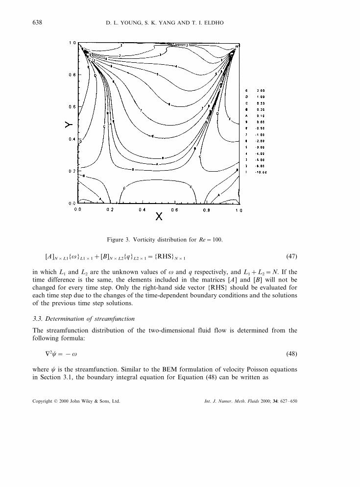
Figure 3. Vorticity distribution for Re=100.
Copyright © 2000 John Wiley & Sons, Ltd. Int. J. Numer. Meth. Fluids 2000; 34: 627–650

EULERIAN–LAGRANGIAN BOUNDARY ELEMENT MODEL 639
Cici=&
Gc( ln(r)(n
dG−&
G
(c
(nln(r) dG−
&V
v ln(r) dV (49)
After the vorticity distribution is determined by solving the vorticity transport equation byintroducing the appropriate boundary conditions, the streamfunction distribution can bedetermined by solving the boundary integral equation (49).
4. SOLUTION PROCEDURE
As mentioned earlier, here an iterative scheme is used in the solution of the velocity–vorticityformulation of Navier–Stokes equations. In most of the incompressible viscous flow problemssolved using Navier–Stokes equations, the most natural boundary condition arises when thevelocity is prescribed all over the boundaries of the problem. The vorticity boundaryconditions are seldom prescribed and hence should be determined iteratively from computa-tions. In the present model, the velocity Poisson equations are initially solved to get thevorticity boundary conditions, which are used in the solution of the vorticity transportequation. The computational procedure adopted here includes the following iterative steps:
Figure 4. Streamfunction distribution for Re=100.
Copyright © 2000 John Wiley & Sons, Ltd. Int. J. Numer. Meth. Fluids 2000; 34: 627–650
D. L. YOUNG, S. K. YANG AND T. I. ELDHO640
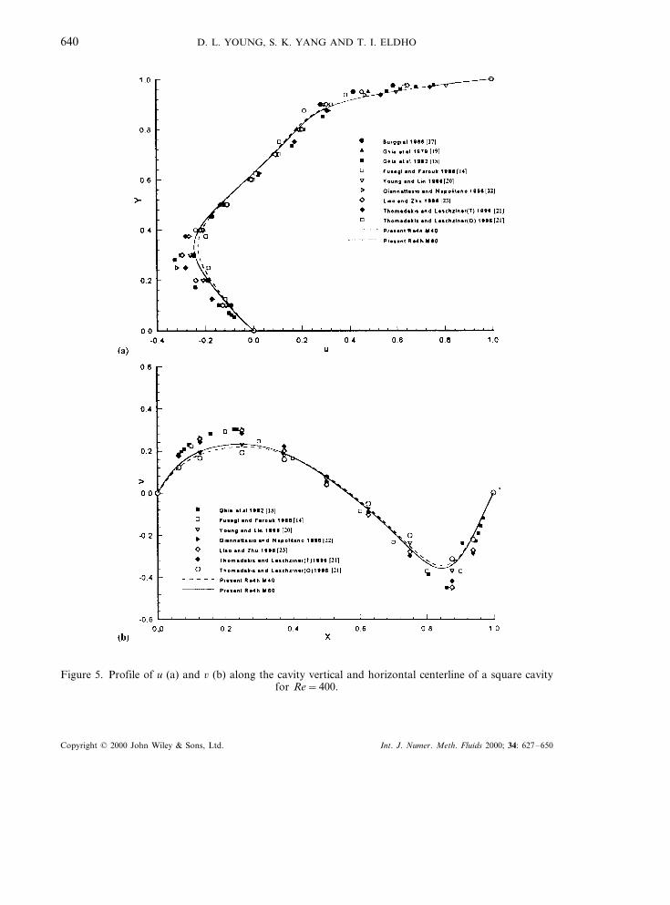
Figure 5. Profile of u (a) and 6 (b) along the cavity vertical and horizontal centerline of a square cavityfor Re=400.
Copyright © 2000 John Wiley & Sons, Ltd. Int. J. Numer. Meth. Fluids 2000; 34: 627–650
EULERIAN–LAGRANGIAN BOUNDARY ELEMENT MODEL 641
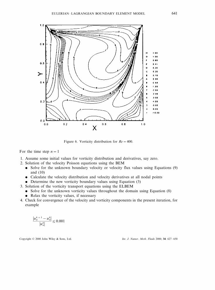
Figure 6. Vorticity distribution for Re=400.
For the time step n=1
1. Assume some initial values for vorticity distribution and derivatives, say zero.2. Solution of the velocity Poisson equations using the BEM
� Solve for the unknown boundary velocity or velocity flux values using Equations (9)and (10)
� Calculate the velocity distribution and velocity derivatives at all nodal points� Determine the new vorticity boundary values using Equation (3)
3. Solution of the vorticity transport equations using the ELBEM� Solve for the unknown vorticity values throughout the domain using Equation (8)� Relax the vorticity values, if necessary
4. Check for convergence of the velocity and vorticity components in the present iteration, forexample
�unk+1−un
k��un
k� 50.001
Copyright © 2000 John Wiley & Sons, Ltd. Int. J. Numer. Meth. Fluids 2000; 34: 627–650
D. L. YOUNG, S. K. YANG AND T. I. ELDHO642
If convergence criterion is satisfied, then stop and proceed to the next time step, otherwisego to step 2.
5. In the successive time step, use the velocity and vorticity components from the previoustime step as initial conditions and use the iterative procedure, steps 2–4. The procedure isrepeated until the prescribed time step is reached.
In order to validate the self-consistency of the present formulation, calculations were madeto ensure the satisfaction of mass balance conditions in the entire domain for all thecomputations. In all the calculations, mass balances were satisfied within 0.1 per cent.
For the unsteady computations, the time step was chosen with variations in Reynoldsnumber and the mesh size, according to the condition given by Liu and Dane [16] as
1Re
Dt� 1
(Dx)2+1
(Dy)2
�5
12
(50)
where Dx and Dy are the mesh size in the x- and y-Cartesian directions.
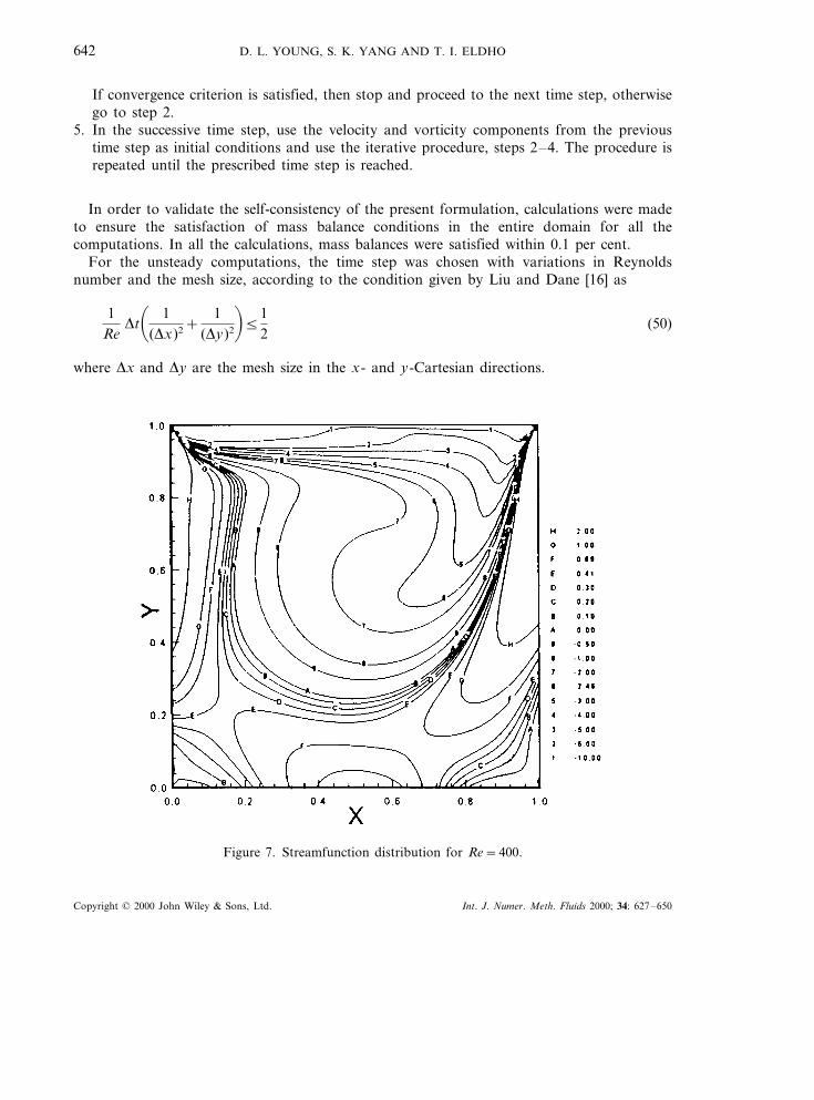
Figure 7. Streamfunction distribution for Re=400.
Copyright © 2000 John Wiley & Sons, Ltd. Int. J. Numer. Meth. Fluids 2000; 34: 627–650
EULERIAN–LAGRANGIAN BOUNDARY ELEMENT MODEL 643
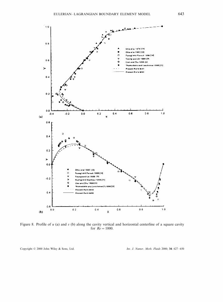
Figure 8. Profile of u (a) and 6 (b) along the cavity vertical and horizontal centerline of a square cavityfor Re=1000.
Copyright © 2000 John Wiley & Sons, Ltd. Int. J. Numer. Meth. Fluids 2000; 34: 627–650

D. L. YOUNG, S. K. YANG AND T. I. ELDHO644
5. MODEL RESULTS AND DISCUSSIONS
The proposed ELBEM model has been applied on a test problem to verify the feasibility of themodel. The test problem is the classical ‘driven flow in a square cavity’, for which manynumerical model results are available in the literature. Present model results are compared withthe results of a series solution and FDM, FEM and BEM models in two dimensions.
The model problem consists of a square cavity with a moving top lid with constant velocity,totally filled with an incompressible viscous fluid. In all the cases, the flow inside the cavitywas initially at rest. No-slip and impermeability conditions were imposed on all walls, with thevelocity at the upper wall set equal to unity. Due to the computational limitations (we used anIBM AIX workstation with 128 MB RAM), the present analysis is limited to a maximumcomputational mesh points of 60×60 (on the boundary as well as internal domain).
Four analyses have been presented here, for Re=100, 400, 1000 and 2000 respectively.Although the computations were carried out in time, only steady state solutions are presentedhere. In all the cases, steady states are reached.
Figure 9. Vorticity distribution for Re=1000.
Copyright © 2000 John Wiley & Sons, Ltd. Int. J. Numer. Meth. Fluids 2000; 34: 627–650

EULERIAN–LAGRANGIAN BOUNDARY ELEMENT MODEL 645
Figure 10. Streamfunction distribution for Re=1000.
Figure 2 shows the u- and 6-velocity profiles along the vertical and centerlines of the cavityfor Re=100. Two different grids of 40×40 and 60×60 uniform quadrilaterals have beenused for the computations. Figure 3 shows the vorticity distribution along the domain andFigure 4 shows the profile of the streamfunction distribution along the domain. The velocityvariations are compared with different models of Burgraff [17], Ghia et al. [18,19], Young andLin [20] and Thomadakis and Leschziner [21]. The results mostly agree with all the modelresults. From Figure 2 it can be seen that for both computational mesh grids, the results arealmost the same.
Figure 5 shows the u- and 6-velocity profiles along the vertical and centerlines of the cavityfor Re=400 with two different grids of 40×40 and 60×60 uniform quadrilaterals. Figures 6and 7 show the vorticity and streamfunction distributions respectively along the domain. Thevelocity variations are compared with different models of Burgraff [17], Ghia et al. [18,19],Fusege and Farouk [14], Young and Lin [20], Giannattasio and Napolitano [22], Liao and Zhu[23], and Thomadakis and Leschziner [21]. The results obtained are closer to the results of theFEM and the finite volume models. As is obvious from the figures, the small difference toother models can be attributed to the mesh size used in the present investigation.
Copyright © 2000 John Wiley & Sons, Ltd. Int. J. Numer. Meth. Fluids 2000; 34: 627–650
D. L. YOUNG, S. K. YANG AND T. I. ELDHO646
As the Reynolds number increases, the sensitivity to the grid density becomes more obvious.For a higher Reynolds number, Re=1000, Figure 8 shows the x-component velocity profile(u) and y-component velocity profile (6) on the vertical and horizontal centerline of the cavity.Figures 9 and 10 show the vorticity and streamfunction distributions respectively along thedomain. Results of the analysis are again compared with the various models [14,18–21,23,24].The present analysis is in good agreement with most of the models, bearing in mind that themaximum mesh density was only 60×60. Further analysis has been carried out for a Reynoldsnumber of 2000 using 60×60 mesh. Figures 11–13 show the vorticity, streamfunction andvelocity distributions respectively along the domain.
The merit of the present model is that it provides the best way to treat the velocity–vorticityformulation for two-dimensional flow by the BEM. In general, the boundary conditions ofvorticity are not known a priori, so that the solution of the vorticity transport equation israther difficult. However, the BEM solution of the velocity Poisson equations together with theno-slip boundary conditions will automatically render the necessary vorticity boundary condi-tions directly as the normal derivatives of velocity, while solving the boundary integralequations. If numerical models like FDM and FEM are used in the solution of velocity
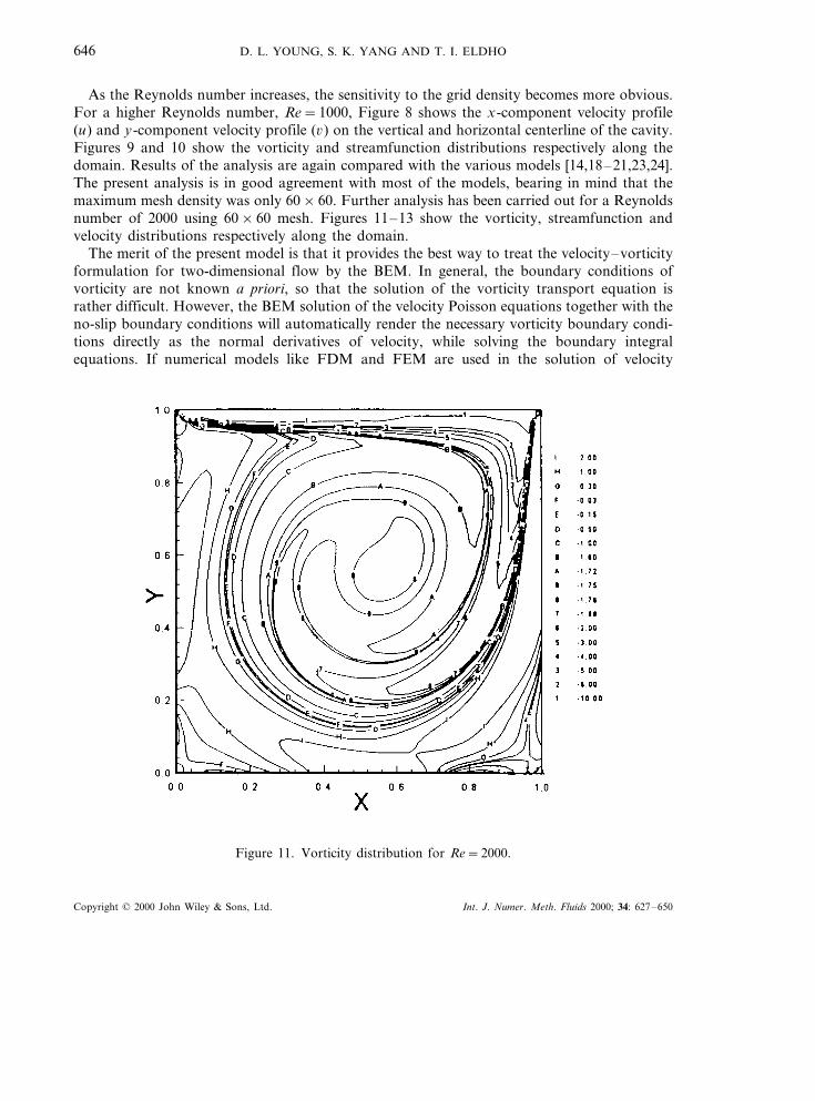
Figure 11. Vorticity distribution for Re=2000.
Copyright © 2000 John Wiley & Sons, Ltd. Int. J. Numer. Meth. Fluids 2000; 34: 627–650

EULERIAN–LAGRANGIAN BOUNDARY ELEMENT MODEL 647
Figure 12. Streamfunction distribution for Re=2000.
Poisson equations, then the boundary vorticity values have to be separately determined fromthe velocity distribution, which may reduce the accuracy in determining the vorticity boundaryconditions for the solution of vorticity transport equation.
As the vorticity transport equation includes convective terms and time-dependent terms, thegeneral BEM solution [5,6] of vorticity transport equation is very difficult. The ELBEM,proposed by combining the Eulerian–Lagrangian method and the BEM, has been proved tobe a feasible method to solve advective–diffusion equations such as the vorticity transportequation [Young et al.]. Hence, the present model in which the velocity Poisson equations aresolved using the BEM and the vorticity transport equation is solved using ELBEM and theiterative scheme combining both models provides the best way to treat the velocity–vorticityformulation for two-dimensional incompressible flow problems. This study demonstrates thateven with a relatively coarse mesh, the solutions are very stable and fairly accurate as shownin the case study with different Reynolds numbers.
The approximate number of iterations required for the convergence at each time step varyfrom 50 to 500 depending on the value of the Reynolds number, time step and grid. Eventhough the CPU time for each calculation has not been separately found out, typical CPU timefor the calculation varies from 1 to 6 h on an IBM AIX workstation for 60×60 mesh.
Copyright © 2000 John Wiley & Sons, Ltd. Int. J. Numer. Meth. Fluids 2000; 34: 627–650

D. L. YOUNG, S. K. YANG AND T. I. ELDHO648
Figure 13. Profile of the flow vectors for Re=2000.
Even though in the present analysis we have carried out the analysis up to a Reynoldsnumber of 2000, the method can be further used for higher Reynolds number with a refinedmesh, smaller time step and vorticity relaxation. The ELBEM has already been successfullyimplemented for three-dimensional diffusion and advection problems [25; Young DL, Her BC,Eldho TI. Boundary integral modeling of three-dimensional circulation and transport instratified estuaries. Journal of Engineering Mechanics, ASCE 2000 (in press)]. Authors alsohave successfully implemented the velocity–vorticity formulation for the Stokes problem [26]and the Navier–Stokes problem [27] in three dimensions by a combined BEM and FEMscheme. Extension of the ELBEM model for three-dimensional Navier–Stokes equations invelocity–vorticity form will be presented in one of our future papers.
6. CONCLUDING REMARKS
An accurate Eulerian–Lagrangian BEM for solving the velocity–vorticity Navier–Stokesequations is proposed for the first time by the combination of the ELM and the BEM. The.
Copyright © 2000 John Wiley & Sons, Ltd. Int. J. Numer. Meth. Fluids 2000; 34: 627–650
EULERIAN–LAGRANGIAN BOUNDARY ELEMENT MODEL 649
Poisson-type velocity equations are solved using the general boundary integral technique withdomain integration for the source terms and the vorticity boundary conditions are exactlydetermined. The vorticity transport equation is solved using the ELBEM on a transformedcharacteristic domain. By the combination of the ELM and the BEM, the BEM is made easierto handle the variable velocity field. Here the results of two-dimensional Navier–Stokesproblems with low–medium Reynolds numbers in a typical square cavity flow are presented.A comparison with other numerical models demonstrates the feasibility of the present ELBEMmodel.
ACKNOWLEDGMENTS
The work reported in this paper was supported by the National Science Council of Taiwan. It is greatlyappreciated.
REFERENCES
1. Fasel H. Investigation of the stability of boundary layers by a finite-difference model of the Navier–Stokesequations. Journal of Fluid Mechanics 1976; 78: 355–383.
2. Dennis SCR, Ingham DB, Cook RN. Finite-difference methods for calculating steady incompressible flows inthree dimensions. Journal of Computational Physics 1979; 33: 325–339.
3. Gunzburger MD, Peterson JS. On finite element approximations of the streamfunction–vorticity and velocity–vorticity equations. International Journal for Numerical Methods in Fluids 1988; 8: 1229–1240.
4. Skerget L, Rek Z. Boundary-domain integral method using a velocity–vorticity formulation. Engineering Analysiswith Boundary Elements 1995; 15: 359–370.
5. Power H, Wrobel LC. Boundary Integral Methods in Fluid Mechanics. Computational Mechanics Publications:Southampton, 1995.
6. Brebbia CA, Telles JCF, Wrobel LC. Boundary Element Techniques—Theory and Applications in Engineering.Springer: Berlin, 1984.
7. Ikeuchi M. Transient solution of convective diffusion problem by boundary element method. Transactions ofIECE Japan 1985; E68(7): 435–440.
8. Sharif MAR, Busnaina AA. Assessment of finite difference approximations for the advection terms in thesimulation of practical flow problems. Journal of Computational Physics 1988; 74: 143–176.
9. Heinrich JC, Huyakorn PS, Zienkiewics OC, Mitchell AR. An upwind finite element scheme for two-dimensionalconvective transport equation. International Journal for Numerical Methods in Engineering 1977; 11: 131–143.
10. Neuman SP. A Eulerian–Lagrangian numerical scheme for the dispersion–convective equation using conjugatespace–time grids. Journal of Computational Physics 1981; 41: 270–294.
11. Neuman SP. Adaptive Eulerian–Lagrangian finite element method for advection–dispersion. International Journalfor Numerical Methods in Engineering 1984; 20: 321–337.
12. Li CW. Advective–dispersion simulation by minimization characteristics and alternate direction-explicit methods.Applied Mathematical Modeling 1991; 15: 616–623.
13. Liggett JA. Fluid Mechanics. McGraw-Hill: New York, 1994.14. Fusegi T, Farouk B. Predictions of fluid and heat transfer programs by the vorticity–velocity formulation of the
Navier –Stokes equations. Journal of Computational Physics 1986; 65: 227–243.15. Carslaw HS, Jaegar JC. Conduction of Heat in Solids (2nd edn). Clarendon Press: Oxford, 1959.16. Liu HH, Dane JH. An interpolation-corrected modified method of characteristics to solve advection–dispersion
equations. Journal of Ad6ances in Water Resources 1996; 19: 359–368.17. Burgraff OR. Analytic and numerical studies of structure of steady separated flows. Journal of Fluid Mechanics
1966; 24: 131–151.18. Ghia U, Ghia KN, Shin CT. High-Re solutions for incompressible flow using the Navier –Stokes equations and
a multi-grid method. Journal of Computational Physics 1982; 48: 387–411.19. Ghia KN, Hamkey Jr WL, Hodge JK. Use of primitive variables in the solution of incompressible Navier–Stokes
equations. AIAA Journal 1979; 17: 298–301.
Copyright © 2000 John Wiley & Sons, Ltd. Int. J. Numer. Meth. Fluids 2000; 34: 627–650

D. L. YOUNG, S. K. YANG AND T. I. ELDHO650
20. Young DL, Lin QH. Application of finite element method to 2D flows. In Proceedings of the Third NationalConference on Hydraulic Engineering, Young DL (ed.). National Taiwan University: Taipei, 1986; 223–242.
21. Thomadakis M, Leschziner M. A pressure-correction method for the solution of incompressible viscous flows onunstructured grids. International Journal for Numerical Methods in Fluids 1996; 22: 581–601.
22. Giannattasio P, Napolitano M. Optimal vorticity conditions for the node-centered finite-difference discretizationof the second-order vorticity–velocity equations. Journal of Computational Physics 1996; 127: 208–217.
23. Liao SJ, Zhu JM. A short-note on high-order streamfunction–vorticity formulations of 2D steady stateNavier–Stokes equations. International Journal for Numerical Methods in Fluids 1996; 22: 1–9.
24. Huang H, Seymour BR. The no-slip boundary condition in finite difference approximations. International Journalof Numerical Methods in Fluids 1996; 22: 713–729.
25. Young DL, Her BC, Wang YF. Three-dimensional mathematical modeling of pollutant transport in stratifiedestuaries. In En6ironmental Hydraulics, Lee JH, Jayawardena AW, Wang ZY (eds). Balkema: Rotterdam, 1999;93–97.
26. Young DL, Liu YH, Eldho TI. Three-dimensional Stokes flow solution using combined boundary element andfinite element methods. Chinese Journal of Mechanics 1999; 15: 169–176.
27. Young DL, Liu YH, Eldho TI. A combined BEM–FEM model for the velocity–vorticity formulation of theNavier–Stokes equations in three-dimensions. Engineering Analysis with Boundary Elements 2000; 24: 307–316.
Copyright © 2000 John Wiley & Sons, Ltd. Int. J. Numer. Meth. Fluids 2000; 34: 627–650