Convolution quadrature method-based symmetric Galerkin boundary element method for 3-d...

Institute ofApplied MechanicsInstitut für Baumechanik

Preprint Series

Institute of Applied Mechanics

Graz University of Technology

Preprint No 1/2008

Convolution Quadrature Method basedsymmetric Galerkin Boundary Element Method

for 3-d elastodynamics

Lars Kielhorn&

Martin SchanzInstitute of Applied Mechanics, Graz University of Technology

Published by: International Journal for Numerical Methods inEngineering

Latest revision: January 21, 2009

AbstractThe boundary integral equations in 3-d elastodynamics contain convolution integrals with

respect to the time. They can be performed analytically or with the convolution quadraturemethod. The latter time stepping procedure’s benefit is the usage of the Laplace transformedfundamental solution. Therefore, it is possible to apply this method also to problems whereanalytical time-dependent fundamental solutions might not be known.

To obtain a symmetric formulation the second boundary integral equation has to be usedwhich, unfortunately, requires special care in the numerical implementation since it in-volves hypersingular kernel functions. Therefore, a regularization for closed surfaces of theLaplace transformed elastodynamic kernel functions is presented which transforms the bi-linear form of the hypersingular integral operator to a weakly singular one. Supplementary,a weakly singular formulation of the Laplace transformed elastodynamic double layer po-tential is presented. This results in a time domain boundary element formulation involvingat least only weakly singular integral kernels.

Finally, numerical studies validate this approach with respect to different spatial and timediscretizations. Further, a comparison to the wider used collocation method is presented. Itis shown numerically that the presented formulation exhibits a good convergence rate and amore stable behavior compared to collocation methods.

This is a preprint of an article published inKielhorn, L.; Schanz, M.: Convolution Quadrature Method based symmetric Galerkin Boundary

Element Method for 3-d elastodynamics. International Journal for Numerical Methods in Engineering,76(11):1724–1746, 2008.

Available online at: http://dx.doi.org/10.1002/nme.2381

http://dx.doi.org/10.1002/nme.2381

Preprint No 1/2008 Institute of Applied Mechanics

1 INTRODUCTION

The Boundary Element Method (BEM) in time domain is known to be well suited to treat wavepropagation problems (for an overview see [3, 4]). A general mathematical background of theunderlying boundary integral equations for time dependent problems may be found in [8]. Addi-tionally, the more particular elastodynamic case is treated in [7]. Nowadays in engineering, thespatial discretization of those time-dependent boundary integral equations is mostly done via thecollocation method (see, e.g. [16]). But also Galerkin type approaches exist which are mostlyused for time independent problems (for an overview see [6]).

Here, the symmetric Galerkin boundary element method (SGBEM) will be applied to solvemixed initial boundary value problems of 3-d elastodynamics. Unfortunately, the drawbackwhen considering mixed problems by symmetric methods is the evaluation of the second bound-ary integral equation which, in fact, contains a non integrable hypersingularity. This kind ofsingularity has to be interpreted as a finite part integral in the sense of Hadamard [23]. Thosesingularities can be either treated numerically [38] or in an analytical way [18]. Here, an an-alytical transformation of the hypersingular integral operator based on integration by parts in3-d elastodynamics will be presented which, finally, will lead to a bilinear form containing onlyweak singularities. The used approach is very similar to a regularization in elastostatics givenby Han [24] since it takes advantage of the similar structure between the elastostatic and theelastodynamic fundamental solutions.

When dealing with singularities in dynamics it is a common practice to subtract and to addthe corresponding static fundamental solution from its elastodynamic counterpart. This is dueto the fact that the singular behavior of the static part coincides with the dynamic one (see,e.g., [5], [25]). Hence, an existing regularization for the static case can be used to regularize alsothe equivalent dynamic integral kernel. Unfortunately, the occurring residual kernel might causenumerical instabilities due to the fact that it involves the difference between the singular dynamicand the singular static kernel. The method presented here does not cause those instabilities sincethe elastodynamic hypersingular integral operator is treated as a whole.

Regularization approaches of non integrable kernel functions based on integration by partshave a long tradition and are well known nowadays. This technique was firstly used in 1949by Maue [33] who applied it to the wave equation in frequency domain. A major enhancementwas then given by Nedelec [34] who introduced regularized hypersingular bilinear forms forthe Laplace equation, the Helmholtz equation as well as for the system of linear elastostatics.Further, regularizations in the field of 3-d time-harmonic elastodynamics were presented byNishimura & Kobayashi [36] and Becache et al. [2]. While these both approaches rely mainlyon the previous work by Nedelec [34], the particular regularizations are nevertheless slightlydifferent. In the first case the hypersingular operator is used within a collocation scheme whilein the other case a Galerkin scheme is formulated. Using the latter discretization scheme isadvantageous since it features less restrictions concerning the choice of shape functions forthe displacement field. Contrary to the collocation approach, the only requirement in Galerkinbased regularizations is the continuity of the displacement field. Another regularization of thehypersingular bilinear form in case of 3-d elastostatics was presented by Han [24] who usedsome basic results from Kupradze [26]. Unlike Nedelec whose regularization is based on avery general approach and, therefore, results in rather complicated formulae, Han restricts his

2


regularization a priori to the isotropic case and discards the possibility of describing also theanisotropic system. Hence, the resulting regularized bilinear form is simpler to deal with andmotivates the use of Han’s proof within the present work. As will be shown the extension of hisproof to the system of 3-d elastodynamics leads to a more convenient formulation with respectto the numerical implementation than the already established regularizations [36, 2].

For the time discretization there exist in principle two approaches. Firstly, if time dependentfundamental solutions are available, the usage of ansatz functions with respect to time yields atime stepping procedure after an analytical time integration within each time step. This techniquehas been proposed by Mansur [32] and is denoted in the following as the classical time domainboundary element formulation. Secondly, the Convolution Quadrature Method (CQM) devel-oped by Lubich [28], [29] can be used to establish the same time stepping procedure as obtainedby a direct time integration [39]. Contrary to the approach from Mansur for this methodologyonly the Laplace domain fundamental solutions have to be used and the time integration is per-formed numerically. Hence, this approach can easily be extended to the viscoelastic case [40]where the fundamental solutions in closed form are only available in Laplace or Fourier domain.Moreover, the regularization process is more advantageous since the fundamental solutions inLaplace domain are simpler to deal with. This is due to the fact that no retarded potentials occurlike in time-dependent fundamental solutions [20].

Here, the CQM based approach will be used in conjunction with a symmetric Galerkin bound-ary element formulation. This is motivated by the positive results of the Galerkin approach inelastostatics [41] as well as for parabolic problems [31] and the Helmholtz equation [30].

Finally, the present formulation will be validated and it will be studied whether the stabilityof the time stepping procedure is improved compared to the collocation based approach.

2 BOUNDARY INTEGRAL EQUATIONS

2.1 Formulation of the problem

Let Ω⊂ R3 be a domain with boundary Γ = ∂Ω and let the final time T ∈ R+ be fixed. A dis-placement of a point x = [x1, x2, x3]

T ∈Ω at the time t lying in the open interval (0,T ) is denotedby u(x; t) = [u1(x; t),u2(x; t),u3(x; t)]T. The displacement field u(x; t) satisfies the equation ofmotion

(L(∂x)+ρ∂2

∂t2 )u = b , (1)

where ρ is the mass density, L(∂x) is the Lamé-Navier operator

L(∂x) =−(λ+µ)∇x∇x ·−µ∆ (2)

and b = b(x; t) is a given force per unit volume. This body force is assumed to be absent inthe following, i.e., b≡ 0 holds. In (2), λ and µ are the Lamé constants and the operator ∇xdenotes the Nabla operator whereas the subscript indicates that the partial derivatives are takenwith respect to the point x. Moreover, ∆ represents the Laplacian.

To consider a mixed initial boundary value problem, first, the boundary Γ is split into twonon-overlapping sets ΓD,i and ΓN,i with respect to the i-th direction such that Γ = ΓD,i ∪ΓN,i

3


holds. By taking into account some component-wise prescribed Dirichlet data gD,i(x; t) on ΓD,i

and Neumann data gN,i(x; t) on ΓN,i, respectively, the system reads as

((L(∂x)+ρ∂2

∂t2 )u)(x; t) = 0 ∀ (x; t) ∈Ω× (0,T )

ui(x; t) = gD,i(x; t) ∀ (x; t) ∈ ΓD,i× (0,T )ti(x; t) = gN,i(x; t) ∀ (x; t) ∈ ΓN,i× (0,T ) .

(3)

In (3), ti(x; t) represents the i-th component of the traction vector t(x; t) = σ(x; t) ·n(x) definedby the product of the Cauchy stress tensor σ(x; t) with the outward unit normal vector n(x).

Moreover, homogeneous initial conditions are assumed such that u(x;0+)= 0 and ∂

∂t u(x;0+)=0 hold for all x ∈Ω.

2.2 Space-time representation formulas and boundary integral equations

To obtain a boundary element formulation of the stated problem, first, an appropriate boundaryintegral representation of the given system of partial differential equations has to be derived.Therefore, the representation formula corresponding to (3) is introduced [13]

u(x; t) =tZ

0

ZΓ

U(y− x; t− τ) · (T (∂y,n(y))u)(y;τ) dsy dτ

−tZ

0

ZΓ

[(T (∂y,n(y))U)(y− x; t− τ)]T ·u(y;τ) dsy dτ ∀ x ∈Ω,y ∈ Γ, t ∈ (0,T )

(4)

containing the function U(y− x; t− τ) which satisfies

TZ0

ZΩ

((L(∂y)+ρ∂2

∂t2 )U)(y− x; t− τ) ·φ(y;τ) dydτ = φ(x; t) ∀ x,y ∈Ω, t,τ ∈ (0,T ) (5)

for any function φ. A function U(y− x; t− τ) with the property (5) is called fundamental solu-tion. In fact, it is the main ingredient of any boundary element formulation.

As it can be seen, (4) contains only spatial integrals over the boundary Γ. Moreover, causalityimplies that all integrations with respect to the time variable must be of Volterra type. Theoccurring operator T (∂y,n(y)) is a trace operator related to the outward normal vector n(y). Inelastodynamics it represents the stress-strain relation based on Hooke’s law. Hence, applyingT (∂y,n(y)) to the displacement field u(y; t) yields the relation

(T (∂y,n(y))u)(y; t) = t(y; t) = σ(y; t) ·n(y) . (6)

Until now, (4) holds only for a point x ∈Ω. Therefore, a limiting process Ω 3 x→ x ∈ Γ has to

4


be performed which finally gives the first boundary integral equation

u(x; t) =12

u(x; t)−tZ

0

ZΓ

[(T (∂y,n(y))U)(y−x; t− τ)]T ·u(y;τ) dsy dτ

+tZ

0

ZΓ

U(y−x; t− τ) · t(y;τ) dsy dτ

(7)

valid for almost all x,y ∈ Γ, all times t ∈ (0,T ), and a sufficiently smooth boundary Γ. In (7),the singular behavior of the kernel functions has to be considered. Hence, the first integral in (7)is weakly while the second one is strongly singular and has to be interpreted in the sense of aCauchy principal value.

The second, or traction boundary integral equation can be derived by the application of theoperator lim

Ω3x→x∈ΓT (∂x,n(x)) to (4)

t(x; t) =12

t(x; t)+tZ

0

ZΓ

(T (∂x,n(x))U)(y−x; t− τ) · t(y;τ) dsy dτ

−tZ

0

limΩ3x→x∈Γ

T (∂x,n(x))ZΓ

[(T (∂y,n(y))U)(y− x; t− τ)]T ·u(y;τ) dsy dτ .

(8)

Note, that the limiting process to obtain (8) is the same as for the first boundary integral equation(7). Due to the singular kernels in (7) the first integral in (8) is strongly singular while the secondone contains a hypersingularity which has to be understand in the sense of a finite part. Thishypersingular kernel will be discussed in detail in section 4.

Now, by introducing the operators

(I ∗w)Γ(x; t) =tZ

0

ZΓ

δ(y−x; t− τ)I ·w(y;τ) dsy dτ

(V ∗w)Γ(x; t) =tZ

0

ZΓ

U(y−x; t− τ) ·w(y;τ) dsy dτ

(K ′ ∗w)Γ(x; t) =tZ

0

ZΓ

(T (∂x,n(x))U)(y−x; t− τ) ·w(y;τ) dsy dτ

(K ∗w)Γ(x; t) =tZ

0

ZΓ

[(T (∂y,n(y))U)(y−x; t− τ)]T ·w(y;τ) dsy dτ

(D ∗w)Γ(x; t) =−tZ

0

limΩ3x→x∈Γ

T (∂x,n(x))ZΓ

[(T (∂y,n(y))U)(y− x; t− τ)]T ·w(y;τ) dsy dτ

(9)

5


for some arbitrary functions w(y;τ) the equations (7) and (8) can be written more compact[( 12 I −K V

D 12 I +K ′

)∗(

ut

)]Γ

(x; t) =(

u(x; t)t(x; t)

). (10)

In (9) and (10), the ∗ abbreviates the convolution integrals in time. Beside the identity given inthe first line of (9) the operators can sequentially be titled as single layer, adjoint double layer,and double layer potential. The last operator is the so-called hypersingular integral operator.

2.3 Symmetric Galerkin formulation

To find the complete Cauchy data [u, t]T the symmetric formulation as proposed in [41, 9] isused. Therefore, the first boundary integral equation (7) is used only on the Dirichlet part ΓD,i

while the second one (8) is used on the Neumann part ΓN,i. Note, because here a vectorial prob-lem has to be solved at each boundary point different types of boundary data in each directioni = 1,2,3 may be prescribed. This yields

(V ∗ t)Γi(x; t)− (K ∗u)Γi(x; t) =12

gD,i(x; t) ∀ x ∈ ΓD,i

(K ′ ∗ t)Γi(x; t)+(D ∗u)Γi(x; t) =12

gN,i(x; t) ∀ x ∈ ΓN,i .

(11)

Now, the displacements ui(y; t) as well as the tractions ti(y; t) are decomposed into

ui = ui + gD,i with ui = 0, gD,i = gD,i ∀ y ∈ ΓD,i

ti = ti + gN,i with ti = 0, gN,i = gN,i ∀ y ∈ ΓN,i(12)

where gD,i and gN,i are arbitrary but fixed extensions of the prescribed boundary data. Note, thatthe extensions ui and gD,i have to be continuous due to regularity requirements [43]. After insert-ing the decompositions (12) into the system of boundary integral equations (11) the symmetricboundary integral formulation

(V ∗ t)ΓD,i(x; t)− (K ∗ u)ΓN,i(x; t) = ((12 I +K )∗ gD)Γi(x; t)− (V ∗ gN)Γi(x; t)

(K ′ ∗ t)ΓD,i(x; t)+(D ∗ u)ΓN,i(x; t) = ((12 I −K ′)∗ gN)Γi(x; t)− (D ∗ gD)Γi(x; t)

(13)

is obtained with the unknown Cauchy data [u, t]T. By using the inner product 〈 f ,g〉Γ =R

Γf (x)g(x) dsx

a variational formulation is introduced to find [u, t]T such that

〈V ∗ t,w〉ΓD,i−〈K ∗ u,w〉ΓD,i = 〈(12 I +K )∗ gD−V ∗ gN ,w〉ΓD,i

〈K ′ ∗ t,v〉ΓN,i + 〈D ∗ u,v〉ΓN,i = 〈(12 I −K ′)∗ gN−D ∗ gD,v〉ΓN,i

(14)

holds for all test-functions w(x),v(x). Note, as the Galerkin scheme is used only for the spatialintegrations the test-functions w(x) and v(x) exhibit no time dependency.

6


3 BOUNDARY ELEMENT FORMULATION

3.1 Time discretization

The CQM as proposed by Lubich [28, 29] is used to approximate the convolution integrals intime. As already stated in section 1, this approach is advantageous due to the fact that the CQMdeals only with the Laplace transformed fundamental solutions, which makes it also attractivefor handling problems where fundamental solutions are only known in Laplace domain or arenot given in closed form in the time domain.

The goal is the computation of the convolution integral

y(t) = f ∗g =tZ

0

f (t− τ) g(τ)dτ . (15)

If the Laplace transform of the function f (t) is known and by dividing the time into M intervalsof equal step size ∆t the integral can be approximated for the time step tm = m∆t by

ym = y(m∆t)≈m

∑k=0

ωm−k( f ,∆t) g(k∆t) (16)

with the integration weights ωn. These integration weights are given by

ωn( f ,∆t) =R−n

2π

2πZ0

f

(γ(Reiϕ

)∆t

)e−inϕ dϕ (17)

and can be approximated by the trapezoidal rule

ωn( f ,∆t) =1L

L−1

∑`=0

f(

γ(ζ`)∆t

)ζ−n` , with ζ` := Rei` 2π

L . (18)

From (18), it is obvious that the integration weights depend only on the Laplace transform ofthe function f denoted by f (s) = L f(s) with the complex Laplace variable s ∈ C. Theparameters R and L depend mainly on the number of time steps M and are chosen as R =10−5/2M and L = M. Moreover, this choice allows the computation of the integration weightsvia a technique similar to the Fast Fourier Transformation. Finally, the term γ(·) represents thecharacteristic function of an underlying multistep method, e.g., a backward differential formulaof order 2 (BDF2) with γ(s) = 3/2−2s+ s2/2. More details about the Convolution QuadratureMethod and the choice of the used parameters can be found in [28], [29], and [39].

Now, the convolution quadrature formula (16) with the definition of the integration weightsgiven in (18) is applied to the variational formulation (14). For example, an entry correspondingto the single layer potential can be computed for tm as

〈(V ∗ t)ΓD,i(x; tm),w(x)〉ΓD,i =tmZ

0

ZΓD,i

w(x) ·Z

ΓD,i

U(y−x; t− τ) · t(y;τ) dsy dsx dτ

≈m

∑k=0

ZΓD,i

w(x) ·Z

ΓD,i

ωm−k(U,∆t) · t(y;k ∆t) dsy dsx

(19)

7


with the integration weights

ωm−k(U,∆t) =1L

L−1

∑`=0

U(y−x;γ(ζ`)

∆t)ζ−(m−k)` . (20)

Finally, inserting (20) into (19) and rearranging yields

〈(V ∗ t)ΓD,i(x; tm),w(x)〉ΓD,i ≈m

∑k=0〈Vm−k tk,w〉ΓD,i (21)

with

Vm−k tk :=L−1

∑`=0

ζ−(m−k)`

L

ZΓD,i

U(y−x;γ(ζ`)

∆t) · t(y;k ∆t) dsy . (22)

Equation (21) indicates that the application of the CQM as a time-stepping procedure to thetime-dependent variational form (14) results in an variational form very similar to a series ofstatic analysis – except that the Laplace transformed fundamental solutions have to be evaluatedfor several complex parameters γ(ζ`)/∆t.

Applying the same technique as for the single layer potential in (21) to all other involvedboundary integral operators yields the following time discretized variational formulation

m

∑k=0

[〈Vm−k tk,w〉ΓD,i−〈Km−kuk,w〉ΓD,i

〈K ′m−k tk,v〉ΓN,i + 〈Dm−kuk,v〉ΓN,i

]=

m

∑k=0

[〈(1

2 I + K )m−kgDk − Vm−kgNk ,w〉ΓD,i

〈(12 I − K ′)m−kgNk − Dm−kgDk ,v〉ΓN,i

]. (23)

The above expression perfectly represents the well known structure of classical boundary inte-gral equations formulated directly in time domain. This structure becomes immediately clearwhen the used subscripts in (23) are considered a bit more detailed. Obviously, they form adiscrete convolution for the times tk. To point out this structure more clearly, the Laplace trans-formed identity operator I is discussed briefly. This operator contains the Laplace transformedDelta distribution L δ(s) which is known to be 1. Therefore, the integration weights ωn candirectly be computed by using (17)

ωn =R−n

2π

2πZ0

e−inϕ dϕ =

1 for n = 00 for n 6= 0

. (24)

This shows that the identity operator in (23) contributes only to the first time step as in classicaltime domain boundary element formulations.

In 3-d calculations, another similarity to the classical time domain formulations is the pos-sibility of introducing a cutoff of the sum ∑

mk=0(· · ·). This cutoff corresponds to the material’s

behavior. In contrast to a viscoelastic material an elastic material has no memory. Until thecompression wave has not arrived at the location x all operators must be zero (causality) andthey must be again zero when the shear wave has passed. Contrary to the classical time depen-dent boundary integral formulations where the cutoff is a consequence of the analytical timeintegration [32], here, one has to be content with an estimate for it [39]

ωn ≈

(rmaxc2∆t

)n

n!e−

32

rmaxc2∆t . (25)

8


In the above equation, rmax is the maximum distance in the discretized body, i.e., the largestdistance the shear wave associated with the velocity c2 has to travel. Moreover, for this estimatea BDF 2 as underlying multistep method is assumed. The use of other multistep methods will, ofcourse, lead to other estimations. Hence, an upper limit n for calculating the integration weightscan be estimated so that for all n > n the integration weights can be neglected in relation to theweights n < n. The use of a cutoff leads to a significant optimization due to the fact that it isdispensable to calculate and, of course, to store the system matrices for the time steps tk,k > n.So, instead of obtaining a system of lower triangular Toeplitz block matrices one ends up witha banded system just by replacing the sums in (23) by ∑

mk=0(· · ·)→ ∑

mk=max(0,m−n)(· · ·). More

information about the cutoff may be found in [39, 21].

3.2 Spatial discretization

After the variational formulation (14) has been discretized in time the remaining step is thespatial discretization of (23). Due to the similarities between (23) and systems occurring instatic analysis this procedure follows the same rules already known for those types of variationalformulations.

First, a triangulation of the boundary Γ = ∪nk=1τk is introduced, i.e., the boundary Γ is the

union of n boundary elements τk. Further, for each boundary element τk the unknown boundarydata belong either to ΓD,i or to ΓN,i in each direction i. With respect to this triangulation thesubspaces

Sα

h,i(ΓD,i) = spanϕα

i,kνik=1

Sβ

h,i(ΓN,i) = spanϕβ

i,kυik=1

(26)

are defined containing νi polynomial shape functions ϕα of order α and υi polynomials ϕβ

of order β. The subspaces’ dimensions νi and υi correspond to the number of unknowns onΓD,i and ΓN,i. Therefore, the unknown Dirichlet data and the unknown Neumann data can beapproximated by

tα

h,i(x; t) =νi

∑k=1

ti,k(t) ϕα

k (x)

uβ

h,i(x; t) =υi

∑k=1

ui,k(t) ϕβ

k (x) .

(27)

In the following, Neumann data are approximated by constant functions and Dirichlet data bylinear functions, i.e., α = 0, th = t0

h and β = 1, uh = u1h. Further, to obtain symmetric system-

matrices the test-functions w(x),v(x) used in the variational formulation (23) are approximatedby polynomials corresponding to the approximations for the Neumann and Dirichlet data, i.e.,w0

h,i ∈ S0h,i and v1

h,i ∈ S1h,i. Finally, the shape functions approximating the geometry are chosen of

the same order as the Dirichlet data, i.e., the geometry is also approximated with linear polyno-mials.

9


3.3 System of linear equations

For a time index m and for the total numbers of degrees of freedom ν = ∑3i=1 νi, υ = ∑

3i=1 υi let

Vm ∈ Rν×ν, Km ∈ Rν×υ, Dm ∈ Rυ×υ (28)

denote the discretized single layer, double layer, and hypersingular operator, respectively. More-over, the unknown Cauchy data for the time step m is represented by the two vectors

tm ∈ Rν, um ∈ Rυ . (29)

Then, together with the stated time and spatial discretizations a system of linear equationsis obtained which represents nicely the structure of the introduced time discretized variationalform (23). This banded system is composed by the already mentioned lower triangular Toeplitzblock matrices and, finally, reads as[

V0 −K0KT

0 D0

]·[

tm

um

]=[

fDm

fNm

](30)

with the given right hand side[fDm

fNm

]=[

fDm

fNm

]−

m−1

∑k=k0

[Vm−k · tk−Km−k ·ukKT

m−k · tk +Dm−k ·uk

]. (31)

In (30) and (31), the usual structure of a BE time stepping technique is observed. The vector[fD

m , fNm ]T is given by[

fDm

fNm

]=[

K0 ·gDm−V0 · gN

mK′0 ·gN

m−D0 · gDm

]+

m−1

∑k=k0

[Km−k ·gD

k −Vm−k · gNk

K′m−k ·gNk −Dm−k · gD

k

]. (32)

and contains the prescribed boundary data of the actual time step m whereas in the last term of(31) all information about the Cauchy data up to the previous time step m−1 is stored.

In (31) and (32), k0 denotes the cutoff and is defined as k0 = max(0,m− n). Moreover, in(32), the diagonal terms of the discrete double layer potential K0 which correspond to the firsttime step are given by K0 = 1

2 I + K0 and, analogously, by K′0 = 12 I−K′0 for the discrete adjoint

double layer potential.From (30), it is obvious that the solution requires only the inversion of the matrix correspond-

ing to the first time step. Therefore, the matrix V0, which is symmetric as a result of the Galerkindiscretization, is decomposed via a Cholesky-factorization. Afterwards, the Schur-Complement-System is computed by

S0 = KT0 V−1

0 K0 +D0 . (33)

Due to the symmetry of V0 and D0 the Schur-Complement S0 is also symmetric and can bedecomposed itself by a Cholesky-factorization.

Hence, the displacement field u and the tractions t can be found by solving

S0um = fNm −KT

0 V−10 fD

m (34)

andtm = V−1

0

(fDm +K0um

)(35)

for every time step m = 0, . . . ,M−1.

10


4 REGULARIZATION OF THE HYPERSINGULAR BILINEAR FORM

Since the fundamental solutions are used in Laplace domain (see section 3.1), only the Laplacetransformed fundamental solutions are considered when speaking about elastodynamics fromnow on. Therefore, also the ( ) denoting the Laplace transformed fundamental solution will beomitted. Moreover, for sake of simplicity the functions’ argument list is skipped whenever themeaning is clear by the functions’ name themselves.

In elastostatics there exists a regularized representation of the hypersingular bilinear formwhich has been deduced by Han [24] who has used some basic results from elasticity given in[26]. His proof leads to a bilinear form of the hypersingular operator containing at least a weaklysingular integral kernel which can be treated numerically by using some appropriate cubaturerules. Here, this technique will be transfered to elastodynamics. Contrary to the regularizationgiven by Becache et. al. [2] this formulation is deduced only for the isotropic case but featuresthe benefit of being more efficient for a numerical treatment since the resulting bilinear formexhibits a much simpler structure.

A comment must be made concerning the topology of the body being under consideration.According to all other mentioned regularizations [24, 34, 36, 2] the body is assumed to be ei-ther closed or to be the unbounded complement of a closed domain. This assumption simplifiesthe application of Stokes theorem, since in this case the surface’s boundary ∂Γ vanishes and∂Γ = /0 holds. Further, bearing in mind that the involved integral kernels fulfill Sommerfeld’sradiation condition [42], the surface’s boundary integrals vanish also in the case of bodies withinfinite expansion, e.g., elastic halfspaces. Therefore, the present regularization holds in prin-ciple also for these special problems. Nevertheless, problems might occur on a discrete level ifa semi-infinite geometry like an elastic halfspace is considered. There, it is a common practiceto model just a truncated part of the infinite geometry. Unfortunately, the emerging truncation’sborderline represents the surface’s boundary such that ∂Γ 6= /0 holds. In the typical case ofprescribed boundary data of Neumann type on ∂Γ, then, the regularization is just incompleteand, therefore, any numerical study will fail. In opposite for prescribed homogeneous Dirichletdata on ∂Γ, like it is common in crack analysis, the regularization will work perfectly since inthis case the boundary part ΓN on which the hypersingular operator has to be evaluated is closed.

Now, to adapt Han’s proof to elastodynamics, first, the similarities between both fundamentalsolutions have to be worked out. These fundamental solutions are well known and go back to theworks of Lord Kelvin (1848) and G. Stokes (1849). For instance, the elastostatic fundamentalsolution may be found in [27] whereas the elastodynamic case is treated in [11, 12].

The elastostatic fundamental solution can be written as

UES =1µ

[∆χ

ESI− λ+µλ+2µ

∇y∇yχES], χ

ES =r

8π. (36)

The respective representation in elastodynamics is

UED =1µ

[∆χ

EDI− λ+µλ+2µ

∇y∇yχED]− 1

µκ

21χ

EDI, χED =

14πr

1κ2

1−κ22

(e−κ1r− e−κ2r) .

(37)

11


For later purpose it is important to state that the scalar functions χES and χED fulfill the partialdifferential equations

∆2χ

ES =−δ(y− x) (38)

(∆−κ21)(∆−κ

22)χ

ED =−δ(y− x) . (39)

In (36) and (37), as well as in the following, r denotes the Euclidean distance between the pointsy ∈ Γ and x ∈ Ω, i.e., r = |y− x| holds. Further, κ1(s) = s

√ρ/λ+2µ, and κ2(s) = s

√ρ/µ denote

the wave numbers corresponding to the compression wave and to the shear wave, respectively.First of all, it can be stated that both fundamental solutions are compositions of some regu-

lar scalar functions χES and χED. The elastodynamic fundamental solution’s (37) first term isweakly singular due to the involved second order derivatives, whereas the last term in (37) isregular. Moreover, having in mind that the hypersingular operator is achieved by applying thetraction operator twice it can be concluded that the term κ2

1/µχEDI will become weakly singular.Hence, no special attention has to be paid to this expression during the regularization process.Further, the terms in brackets in (36) and (37) are the identical operator applied to different func-tions χ. This similar structure motivates a similar treatment of the regularization process. Nowin doing so, a kernel function U(χ) is thought depending on some arbitrary but differentiablefunction χ(r)

U =1µ

[∆χI− λ+µ

λ+2µ∇y∇yχ

]. (40)

Let us consider the double layer potential for some differentiable function u(y)

(K u)(x) :=ZΓ

[T (∂y,n(y))U]T ·u(y) dsy x ∈Ω,y ∈ Γ . (41)

As mentioned in section 2.2 the trace operator T (∂y,n(y)) represents the stress-strain relationbased on Hooke’s law. This matrix differential operator can be defined by using the Günterderivatives (59)

T (∂y,n(y))(·) = 2µM (∂y,n(y))(·)+(λ+2µ)n(y)∇y · (·)−µ(n(y)× curl(·)) . (42)

Inserting (42) into (41) and integrating by parts gives

(K u)(x) = 2µZΓ

U · (M (∂y,n(y))u) dsy−ZΓ

∆χ (M (∂y,n(y))u) dsy +ZΓ

∂∆χ

∂n(y)u dsy . (43)

Equation (43) is very useful with regard to the limiting process Ω 3 x→ x ∈ Γ since the aboveequation will lead to a weakly singular form of the double layer potential. This could be used toavoid the computation of the Cauchy principal value integrals. If χ is substituted by χES from(36) a weakly singular formulation of the elastostatic double layer potential (K ESu)(x) is ob-tained which is already given in [26]. Substituting χ by χED from (37) and subtracting the term

12


κ21/µ

RΓ

[(T (∂y,n(y))χED · I)

]T ·u dsy yields a regularized double layer potential in elastodynam-ics

(K EDu)(x) = 2µZΓ

U(χED) · (M (∂y,n(y))u) dsy−ZΓ

∆χED (M (∂y,n(y))u) dsy +

ZΓ

∂∆χED

∂n(y)u dsy

−ZΓ

dχED

dr

[(κ

22−2κ

21)

∇yr⊗n(y)+κ21n(y)⊗∇yr +κ

21

∂r∂n(y)

I]·u dsy

(44)valid for almost all x,y ∈ Γ. Note that the last term of (44) is regular since a Taylor seriesexpansion of dχED

dr yields

dχED

dr=

18π− κ2

1 +κ1κ2 +κ22

12(κ1 +κ2)πr +O(r2) . (45)

Now, to go ahead with the treatment of the hypersingular kernel, the next step is the applicationof the operator T (∂x,n(x)) to the double layer potential (K u)(x) from (43). This results in

T (∂x,n(x))(K u)(x) =µZΓ

∂∆χ

∂n(y)∂n(x)u dsy

+ZΓ

[M (∂x,n(x))

(4µ2U−3µ∆χI

)]· (M (∂y,n(y))u) dsy

+ψ1 +ψ2

(46)

with

ψ1 := (λ+µ)n(x)ZΓ

[(∇x

∂∆χ

∂n(y)

)·u− (∇x∆χ) · (M (∂y,n(y))u)

]dsy

ψ2 := µZΓ

[(M (∂x,n(x))

∂∆χ

∂n(y)

)·u+

∂∆χ

∂n(x)(M (∂y,n(y))u)

]dsy .

(47)

The above result can be obtained directly by following the proof given by Han [24]. For furthersimplification of (47) the identities (62) and (63) are needed. This yields

ψ1 =−(λ+µ)n(x)ZΓ

n(y) ·u∆2χ dsy

ψ2 =−µZΓ

[M (∂x,n(x))∆χM (∂y,n(y))]T ·u dsy +µM (∂x,n(x))ZΓ

∆χ (M (∂y,n(y))u) dsy

−µZΓ

∆2χ (n(y)⊗n(x)−n(x)⊗n(y)) ·u dsy .

(48)Now it is time to pick up the pieces. Inserting the expressions ψ1 and ψ2 from (48) into (46)

13


and using (61) finally gives

T (∂x,n(x))(K u)(x) = µ3

∑k=1

∂

∂Sk(x)

ZΓ

∆χ∂

∂Sk(∂y,n(y))u dsy

+M (∂x,n(x))ZΓ

(4µ2U−2µ∆χI

)· (M (∂y,n(y))u) dsy

−µZΓ

[M (∂x,n(x))∆χM (∂y,n(y))]T ·u dsy

−ZΓ

∆2χ [λ(n(y) ·u)n(x)+µ(n(x) ·u)n(y)+µ(n(y) ·n(x))u] dsy .

(49)Remember that up to this point the above statement holds only for x /∈ Γ. Therefore, the nextstep will be the limiting process Ω 3 x→ x ∈ Γ. To do so, the partial differential equations (38)and (39) have to be taken into account. As stated at the beginning of this section the functionχ depends on the problem which is under consideration. In the elastodynamic case ∆2χ fulfills(39), i.e.,

∆2χ

ED =(κ

21 +κ

22)

∆χED−κ

21κ

22χ

ED (50)

due to the fact that the point x lies inside the domain and, therefore, δ(r) = 0 holds. SubstitutingU by UED, inserting (50) into (49), and taking the fundamental solution’s last term from (37)into account yields the elastodynamic hypersingular operator

(DEDu)(x) =−

T (∂x,n(x))(K u)(x)− κ21

µT (∂x,n(x))

ZΓ

[T (∂y,n(y))χEDI

]T ·u dsy

.

(51)Note that also the elastostatic hypersingular operator as given by Han [24] can easily be obtainedfrom (49). In this case U has to be substituted with UES. Moreover, ∆2χ fulfills (38) and,therefore, ∆2χES = 0 holds due to the same reasons as mentioned for ∆2χED.

Now, it is almost done. Equation (51) contains no more hypersingular kernel functions. Thus,the limiting process Ω 3 x→ x ∈ Γ can be performed. The hypersingular bilinear form thenfollows by testing (51) with a differentiable function v(x). Afterwards, Stokes theorem is applied

14


a last time and the complete regularized bilinear form is obtained

〈DEDu,v〉=ZΓ

v(x) · limΩ3x→x∈Γ

(DEDu)(x) dsx

= µZΓ

ZΓ

∆χED

(3

∑k=1

∂

∂Sk(∂x,n(x))v · ∂

∂Sk(∂y,n(y))u

)dsy dsx

+µZΓ

ZΓ

(M (∂x,n(x))v)T ·(2∆χ

ED I−4µU(χED))· (M (∂y,n(y))u) dsy dsx

+µZΓ

ZΓ

3

∑j,`,k=1

(M jk(∂x,n(x))v`

)∆χ

ED (M j`(∂y,n(y))uk)

dsy dsx

+µZΓ

ZΓ

n(x) ·v(κ

22−2κ

21)(

3∆χED−κ

22χ

ED) n(y) ·u dsy dsx

+µZΓ

ZΓ

n(x) ·n(y)v ·[κ

21(∇x∇yχ

ED)+∆2χ

EDI]·u+κ

21

∂2χED

∂n(y)∂n(x)u ·v dsy dsx

+µZΓ

ZΓ

v ·[

κ21

(∇x

∂χED

∂n(y)

)+∆

2χ

EDn(y)]

n(x) ·u

+2(κ

22−2κ

21)

v ·(

∇y∂χED

∂n(x)

)n(y) ·u dsy dsx

+µZΓ

ZΓ

κ21v ·n(y)

(∇y

∂χED

∂n(x)

)·u+2

(κ

22−2κ

21)

v ·n(x)(

∇x∂χED

∂n(y)

)·u dsy .

(52)Equation (52) contains only weak singularities due to the fact that all involved second orderderivatives of χED are of order O(r−1). This could be proven by using the chain rule

∇y∇xχED =

(d2

χED

dr2 −1r

dχED

dr

)∇yr⊗∇xr− 1

rdχED

drI =: φ1∇yr⊗∇xr−φ2I . (53)

A series expansion of φ1 and φ2 then yields

φ1 =− 18πr

+O(r)

φ2 =1

8πr− κ2

1 +κ1κ2 +κ22

12π(κ1 +κ2)+O(r) .

(54)

Hence, the representation (52) of the hypersingular bilinear form is obviously suitable for thenumerical treatment. Here, all implementations are done by using cubature rules developed byErichsen and Sauter [15, 37].

15


5 NUMERICAL EXAMPLES

In order to validate the proposed boundary element formulation, a 3-d elastodynamic rod withlength `1 = 3m, width `2 = 1m, and height `3 = 1m is considered as depicted in Fig. 1. The

x1

x3

x2

fixed end

traction free

free end

P

Figure 1: System and loading

rod is fixed on one end and excited by a pressure jump t1 = −1H(t)N/m2 according to a unitstep function H(t) on the other free end. The remaining surfaces are traction free. The materialdata represent steel with Lamé’s constants λ = 0.0 N/m2, µ = 1.05 · 1011 N/m2, and the densityρ = 7850 kg/m3. Note that λ = 0.0 N/m2 is equivalent to an artificial Poisson’s ratio of ν = 0instead of ν = 0.3. The choice of this artificial value is used to be able to compare the resultswith a 1-d analytical solution of longitudinal waves in an elastodynamic column [17].

The Figures 2 & 3 shows a total of four regular meshes for the described model problem.While the first two meshes represents BEM discretizations the two remaining meshes are dis-cretizations being used with the Finite Element Method (FEM). In the following, the BEMmeshes will be referred to as BEM1 which is made up by 112 elements and 58 nodes and BEM2which consists of 700 elements with 352 nodes. Analogously the FEM discretizations are titledas FEM1 made up of 24 elements and 63 nodes and FEM2 being composed of 375 elements and576 nodes. As mentioned in section 3.2, for the BEM formulation the tractions are approximatedwith constant functions whereas the displacements are approximated linear. The FEM studiesare done by using the classical Newmark algorithm (β = 0.25,γ = 0.50) [35]. This time steppingscheme is embedded in displacement-based FEM implementation using trilinear approximationsfor the Dirichlet data.

In order to compare some results for different time and spatial discretizations the dimension-less value

β =c1 ∆t

h(55)

is introduced which can be referred to as the Courant-Friedrichs-Lewy (CFL) number [10].Beside the velocity c1 =

√λ+2µ/ρ of the compression wave the value β depends on the time step

size ∆t and the characteristic mesh size h. In 3-d, the definition of the mesh size h is not uniquesince the elements are 2-dimensional surfaces. Here, the triangles’ cathetus is used for h, i.e.,h = 0.5m for mesh BEM1, and h = 0.2m for mesh BEM2, respectively. The mesh sizes as wellas the time step sizes of the FEM discretizations are in accordance to the BEM discretizations.

16


(a) BEM1: 112 elements, 58nodes

(b) BEM2: 700 elements, 352nodes

Figure 2: Spatial discretizations (BEM) of the considered bar

(a) FEM1: 24 elements, 63nodes

(b) FEM2: 375 elements, 576nodes

Figure 3: Spatial discretizations (FEM) of the considered bar

17


Figure 4 depicts the longitudinal displacements at the point P for mesh BEM1 and meshBEM2 with respect to different time step sizes. As expected, an increasing time step size leadsto a larger numerical damping for both meshes. When considering the results for the finer gridBEM2, the largest CFL number yields almost the same results as the finest time discretization.This observation confirms the experience with CQM based BEM formulations that a more exactspatial discretization yields a more stable time stepping procedure.

Concerning the choice of the CFL number, several numerical studies have shown the existenceof a lower bound for this number. As depicted in Fig. 4, for the present boundary elementformulation the time stepping scheme gets unstable for a CFL number of β ≈ 0.04. For clarityof the pictures, the results for this unstable time step size is shown only in Fig. 4(b). In contrastto that lower bound, there exist no upper bound for β. Even if β is chosen to be larger than onethe results are still stable but the numerical damping increases such that the dynamic solutionapproaches the static solution.

(a) BEM1 (b) BEM2

Figure 4: Longitudinal displacements at the free end versus time: Different ∆t

The traction solutions confirm the already stated observations: This solution is given for apoint at the fixed end opposite to the point P and is shown for both meshes in Fig. 5. For meshBEM1 as well as for mesh BEM2 a CFL number of β = 0.2 leads to the best results.

Two FEM results as depicted in Fig. 6 are given for completeness. Using the same meshsizes for both, the BEM and the FEM meshes, it can be stated that the results of the BEMsolution are very smooth while the FEM solutions are a bit more rough. Especially for thecoarse grid solution depicted in Fig. 6(b) this roughness is very conspicuous. Another differencebetween both numerical methods occurs due to the different time stepping procedures. Whileboth time stepping schemes are very stable, there is some overtone in the Newmark algorithm.This overtone is characteristic for the chosen Newmark algorithm and would become even morevisible if a longer time period would be under consideration. In contrast, the CQM schemeexhibits minor damping.

Finally, a comparison between the CQM based collocation method as proposed in [39] and theactual presented symmetric Galerkin method reflects clearly the advantage of the latter method.In Figs. 7 and 8 long time solutions are depicted with respect to the coarse mesh BEM1. More-over, for both simulations a CFL number of β = 0.2 is chosen. At first, the displacement solution

18


-0.5

0

0.5

1

1.5

2

2.5

trac

tions

t 1 [ N

/m2 ]

0 0.002 0.004 0.006 0.008time t [ s ]

analyticalβ = 0.2β = 0.4β = 0.7

(a) BEM1

-0.5

0

0.5

1

1.5

2

2.5

trac

tions

t 1 [ N

/m2 ]

0 0.002 0.004 0.006 0.008time t [ s ]

analyticalβ = 0.2β = 0.4β = 0.7

(b) BEM2

Figure 5: Normal traction at the fixed end versus time: Different ∆t

(a) BEM2 vs. FEM2 (b) BEM1 vs. FEM1: Long time displ. solution

Figure 6: Comparison of BEM and FEM displacement solutions

19


in Fig. 7 exhibits much more numerical damping effects in the collocation case than it does forthe symmetric Galerkin method. The collocation result has also a phase shift for large timeswhich is not visible for the Galerkin formulation.

-3e-11

-2.5e-11

-2e-11

-1.5e-11

-1e-11

-5e-12

0

disp

lace

men

ts u

1 [ m

]

0 0.01 0.02 0.03 0.04time t [ s ]

analyticalCollocationSGBEM

Figure 7: SGBEM vs. Collocation: Long time displacement solution for mesh BEM1

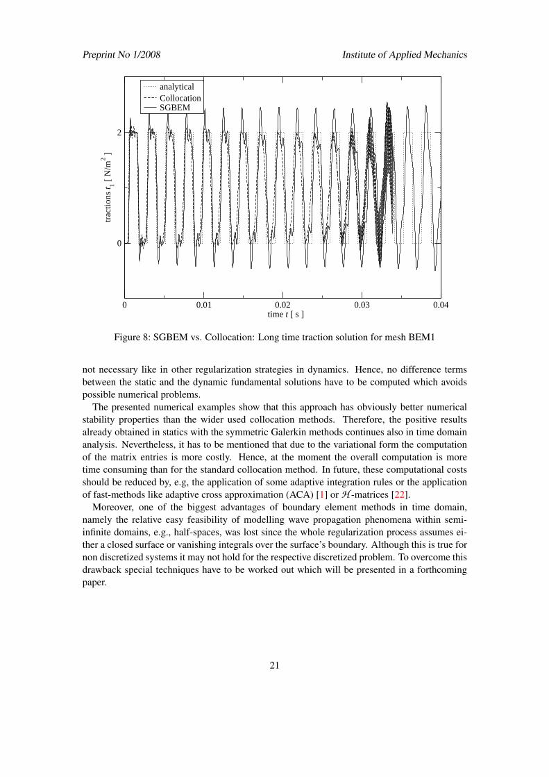
Besides the increasing damping for the displacement solution the collocation method revealsnumerical instabilities with regard to the traction solution (see Fig. 8). This traction solutionbecomes completely instable and is therefore only depicted up to the time t = 0.034s. In contrastto this instability the Galerkin method is still stable during the whole observation time, althoughthe numerical solution’s quality decreases with increasing time.

6 CONCLUSIONS

A boundary element method for elastodynamics based on a Galerkin discretization in space andon the Convolution Quadrature Method in time was presented. To obtain a symmetric, or tobe more precise, a skew-symmetric formulation, also the usage of the second boundary inte-gral equation is required. Since the usage of the second boundary integral equation demandsthe computation of hypersingular kernel functions, a regularization of the elastodynamic hyper-singular integral operator was presented which leads to a weakly singular bilinear form. Theregularization is based mainly on integrations by parts and transfers a proof given for elasto-statics to elastodynamics. This is based on the similar structure of the elastostatic fundamentalsolution compared to the Laplace transformed elastodynamic fundamental solution. Moreover,during the whole regularization process the use of the elastostatic fundamental solutions was

20


0

2

trac

tions

t 1 [ N

/m2 ]

0 0.01 0.02 0.03 0.04time t [ s ]

analyticalCollocationSGBEM

Figure 8: SGBEM vs. Collocation: Long time traction solution for mesh BEM1

not necessary like in other regularization strategies in dynamics. Hence, no difference termsbetween the static and the dynamic fundamental solutions have to be computed which avoidspossible numerical problems.

The presented numerical examples show that this approach has obviously better numericalstability properties than the wider used collocation methods. Therefore, the positive resultsalready obtained in statics with the symmetric Galerkin methods continues also in time domainanalysis. Nevertheless, it has to be mentioned that due to the variational form the computationof the matrix entries is more costly. Hence, at the moment the overall computation is moretime consuming than for the standard collocation method. In future, these computational costsshould be reduced by, e.g, the application of some adaptive integration rules or the applicationof fast-methods like adaptive cross approximation (ACA) [1] or H -matrices [22].

Moreover, one of the biggest advantages of boundary element methods in time domain,namely the relative easy feasibility of modelling wave propagation phenomena within semi-infinite domains, e.g., half-spaces, was lost since the whole regularization process assumes ei-ther a closed surface or vanishing integrals over the surface’s boundary. Although this is true fornon discretized systems it may not hold for the respective discretized problem. To overcome thisdrawback special techniques have to be worked out which will be presented in a forthcomingpaper.

21


A TANGENTIAL SURFACE DERIVATIVES

A.1 Definitions and properties

The whole regularization process presented in section 4 is based on applications of some variantsof Stokes theorem which should be recalled briefly. Let Γ be a surface with the outward unitnormal vector n(y). Further, let ∂Γ denote the surface’s boundary and let p(y) be the unit tangentto ∂Γ. Then, the classical Stokes theorem for some differentiable vector field v(y) reads asZ

Γ

(∇y×v) ·n(y) dsy =Z∂Γ

v ·p(y) dσy . (56)

By introducing the surface curl

∂

∂S(∂y,n(y))= n(y)×∇y (57)

and assuming a closed surface Γ in the following, i.e., ∂Γ = /0, Stokes theorem (56) can bewritten as Z

Γ

∂

∂S(∂y,n(y))·v dsy = 0 . (58)

The introduced surface curl (57) is a so-called tangential differential operator since ∂

∂S(∂y,n(y)) ·n(y) = 0 holds. The operator’s definition is taken from [26]. An analysis of the presented tan-gential differential operators may be also found in [14]. Here, a short review of their propertiesis given from a more engineering point of view. The used notation follows directly [24, 26].Sometimes the surface curl (57) is also denoted by curlΓ [34].

Moreover, the Günter derivatives M (∂y,n(y)) are used during the regularization process.These derivatives form an antisymmetric matrix operator [26, 19] and are defined as

Mi j(∂y,n(y)) = n j(y)∂

∂yi−ni(y)

∂

∂y j=

3

∑k=1

εk ji∂

∂Sk(∂y,n(y)). (59)

Following Stokes theorem it is easy to verify that for a closed surface Γ the Günter derivativesfulfill the following equationZ

Γ

u · (M (∂y,n(y))v) dsy =ZΓ

v · (M (∂y,n(y))u) dsy, u(y) ∈ R3,v(y) ∈ R3 . (60)

Again, (60) holds only for a closed surface ∂Γ.

A.2 Useful equalities

In section 4, the expressions given in (46) and (47) are simplified by making use of the followingidentities. These identities are a more generalized version of identities already given in [24] and

22


can be obtained by some basic calculations

∂2∆χ

∂n(y)∂n(x)=− ∂

∂S(∂y,n(y))· ∂

∂S(∂x,n(x))∆χ

−n(y) ·n(x)∆2χ

(61)

∇x

(∂∆χ

∂n(y)

)= M (∂y,n(y))(∇x∆χ)−n(y)∆

2χ (62)

M (∂x,n(x))(

∂∆χ

∂n(y)

)−M (∂y,n(y))

(∂∆χ

∂n(x)

)=−(n(y)⊗ n(x)−n(x)⊗n(y))∆2

χ

+[M (∂y,n(y))M (∂x,n(x))−M (∂x,n(x))M (∂y,n(y))]∆χ .

(63)

References

[1] M. Bebendorf and S. Rjasanow. Adaptive Low-Rank Approximation of Collocation Ma-trices. Computing, 70:1–24, 2003.

[2] E. Becache, J. C. Nedelec, and N. Nishimura. Regularization in 3D for anisotropic elasto-dynamic crack and obstacle problems. Journal of Elasticity, 31(1):25–46, 1993.

[3] D. E. Beskos. Boundary element methods in dynamic analysis. Applied Mechanics Review,40(1):1–23, 1987.

[4] D. E. Beskos. Boundary element methods in dynamic analysis: Part II (1986-1996). Ap-plied Mechanics Review, 50(3):149–197, 1997.

[5] M. Bonnet and H. D. Bui. Regularization of the Displacement and Traction BIE for 3DElastodynamics Using Indirect Methods. In J. H. Kane, G. Maier, N. Tosaka, and S. N.Atluri, editors, Advances in Boundary Element Techniques, Springer series in computa-tional mechanics, pages 1–29. Springer Verlag Berlin Heidelberg New York, 1993.

[6] M. Bonnet, G. Maier, and C. Polizzotto. Symmetric Galerkin boundary element methods.Applied Mechanics Review, 51(11):669–703, 1998.

[7] I. Chudinovich. Boundary Equations in Dynamic Problems of the Theory of Elasticity.Acta Applicandae Mathematicae, 65:169–183, 2001.

[8] M. Costabel. Time-dependent problems with the boundary integral equation method, vol-ume 1 of Encyclopedia of Computational Mechanics, chapter 25. John Wiley & Sons, NewYork, Chister, Weinheim, 2005.

[9] M. Costabel and E. P. Stephan. Integral equations for transmission problems in linearelasticity. Journal of Integral Equations and Applications, 2:211–223, 1990.

[10] R. Courant, K. Friedrichs, and H. Lewy. Über die partiellen Differenzengleichungen dermathematischen Physik. Mathematische Annalen, 100:32–74, 1928.

23


[11] T. A. Cruse. A Direct Formulation and Numerical Solution of the General Transient Elas-todynamic Problem. II. Journal of Mathematical Analysis and Applications, 22:341–355,1968.

[12] T. A. Cruse and F. J. Rizzo. A Direct Formulation and Numerical Solution of the GeneralTransient Elastodynamic Problem. I. Journal of Mathematical Analysis and Applications,22:244–259, 1968.

[13] J. Domínguez. Boundary Elements in Dynamics. Computational Mechanics Publications,Southampton, Boston, 1993.

[14] R. Duduchava. The Green formula and layer potentials. Integral Equations and OperatorTheory, 41(2):127–178, 2001.

[15] S. Erichsen and S. A. Sauter. Efficient automatic quadrature in 3-d Galerkin BEM. Com-puter Methods in Applied Mechanics and Engineering, 157:215–224, 1998.

[16] L. Gaul, M. Kögl, and M. Wagner. Boundary Element Methods for Engineers and Scien-tists. Springer-Verlag Berlin Heidelberg, 2003.

[17] K. F. Graff. Wave motions in elastic solids. Dover Publications, 1991.

[18] M. Guiggiani. Formulation and numerical treatment of boundary integral equations withhypersingular kernels. In V. Sladek and J. Sladek, editors, Singular Integrals in BoundaryElement Methods, pages 85–124. Computational Mechanics Publications, 1998.

[19] N. M. Günter. Potential theory, and its applications to basic problems of mathematicalphysics. Frederick Ungar Publishing, New York, 1967.

[20] T. Ha-Duong. On Retarded Potential Boundary Integral Equations and their Discretisation.In M. Ainsworth, P. Davies, D. Duncan, P. Martin, and B. Rynne, editors, Topics in Compu-tational Wave Propagation: Direct and Inverse Problems, pages 301–336. Springer-VerlagBerlin, 2003.

[21] W. Hackbusch, W. Kress, and S. Sauter. Sparse Convolution Quadrature for Time DomainBoundary Integral Formulations of the Wave Equation by Cutoff and Panel-Clustering. InM. Schanz and O. Steinbach, editors, Boundary Element Analysis, volume 29 of LectureNotes in Applied and Computational Mechanics, pages 113–134. Springer-Verlag BerlinHeidelberg, 2007.

[22] W. Hackbush. A Sparse Matrix Arithmetic Based on H -Matrices. Part I: Introduction toH -Matrices. Computing, 62:89–108, 1999.

[23] J. Hadamard. Lectures on Cauchy’s problem in linear partial differential equations. DoverPublications, Inc. (reprint), 1952.

[24] H. Han. The boundary integro-differential equations of three-dimensional Neumann prob-lem in linear elasticity. Numerische Mathematik, 68:269–281, 1994.

24


[25] G. Krishnasamy, L. W. Schmerr, T. J. Rudolphi, and F. J. Rizzo. Hypersingular BoundaryIntegral Equations: Some Applications in Acoustic and Elastic Wave Scattering. Journalof Applied Mechanics, 57:404–414, 1990.

[26] V. D. Kupradze, editor. Three-dimensional problems of the mathematical theory of elas-ticity and thermoelasticity, volume 25 of Applied mathematics and mechanics. North Hol-land, Amsterdam, 1979.

[27] A. E. H. Love. A treatise on the mathematical theory of elasticity, volume 1. CambridgeUniversity Press, 1892.

[28] C. Lubich. Convolution quadrature and discretized operational calculus I. NumerischeMathematik, 52:129–145, 1988.

[29] C. Lubich. Convolution quadrature and discretized operational calculus II. NumerischeMathematik, 52:413–425, 1988.

[30] C. Lubich. On the multistep time discretization of linear initial-boundary value problemsand their boundary integral equations. Numerische Mathematik, 67:365–389, 1994.

[31] C. Lubich and R. Schneider. Time discretization of parabolic boundary integral equations.Numerische Mathematik, 63:455–481, 1992.

[32] W. J. Mansur. A Time-Stepping Technique to Solve Wave Propagation Problems Using theBoundary Element Method. PhD thesis, University of Southampton, 1983.

[33] A. W. Maue. Zur Formulierung eines allgemeinen Beugungsproblems durch eine Integral-gleichung. Zeitschrift für Physik, 126(7–9):601–618, 1949.

[34] J.C. Nedelec. Integral equations with non integrable kernels. Integral Equations and Op-erator Theory, 5:563–672, 1982.

[35] N. M. Newmark. A method of computation for structural dynamics. ASCE Journal of theEngineering Mechanics Division, 85:67–93, 1959.

[36] N. Nishimura and S. Kobayashi. A regularized boundary integral equation method forelastodynamic crack problems. Computational Mechanics, 4:319–328, 1989.

[37] S. Sauter and C. Schwab. Randelementmethoden. B.G. Teubner Verlag, Stuttgart LeipzigWiesbaden, 2004.

[38] S. A. Sauter and C. Lage. Transformation of hypersingular integrals and black-box cuba-ture. Mathematics of Computation, 70:223–250, 2001.

[39] M. Schanz. Wave Propagation in Viscoelastic and Poroelastic Continua: A BoundaryElement Approach, volume 2 of Lecture Notes in Applied Mechanics. Springer-VerlagBerlin Heidelberg, 2001.

[40] M. Schanz and H. Antes. A new visco- and elastodynamic time domain Boundary Elementformulation. Computational Mechanics, 20:452–459, 1997.

25


[41] S. Sirtori. General stress analysis method by means of integral equations and boundaryelements. Meccanica, 14:210–218, 1979.

[42] A. Sommerfeld. Partial Differential Equations in Physics. Academic Press, New York,1949.

[43] O. Steinbach. Numerical Approximation Methods for Elliptic Boundary Value Problems.Springer Science+Business Media, LLC, New York, 2008.

26

Convolution quadrature method-based symmetric Galerkin boundary element method for 3-d...

Documents

Transcript of Convolution quadrature method-based symmetric Galerkin boundary element method for 3-d...