Design of Water Distribution Systems-Hardy Cross Method and Equivalent Pipe

Method

Dr. Izharul Haq FarooqiProfessor and Incharge

Environmental Engineering Section, Department of Civil Engineering, Z.H. College of Engineering and Technology

Aligarh Muslim University Aligarh – 202001, India

Introduction

• Distribution system is a network of pipelines that distribute water to the consumers, namely, domestic, industrial, commercial and for fire fighting.

• A good distribution system should satisfy the followings: • Adequate water pressure at the consumer's taps for a specific rate of flow

(i.e, pressures should be great enough to adequately meet consumer needs).

• Pressures should be great enough to adequately meet fire fighting needs.• At the same time, pressures should not be excessive because development

of the pressure head brings important cost consideration and as pressure increases leakages too.

• Pipes can be placed either parallel or in series

Analysis of Distribution Networks

• Following methods are commonly used for the analysis of networks:• Hardy Cross Method• Equivalent Pipe Method• Method of section and circle method • Graphical method • Newton-Rapson method

Basics of Design

• Analysis of water distribution system includes determining quantities of flow and head losses in the various pipe lines, and resulting residual pressures.

• In any pipe network, the following two conditions must be satisfied.• The flow entering in a junction or network must be equal to the flow

leaving the same. • The algebraic sum of the pressure drops around a closed loop must be zero

i.e. there can be no discontinuity in pressure.• When the pipes are connected in series, the total head loss is equal to the

summation of the individual head losses.• When the pipes are laid parallel the head loss through the parallel pipes(or

set of pipes) will be the same.

Pressure in Pipes

• Desirable Pressure in municipal distribution systems ranges from 150-300 kPa in residential districts with structures of three stories or less and 500 kPa in commercial districts.

• For fire hydrants the pressure should not be less than 150 kPa • Moreover, the maximum pressure should be limited to 70 m of water.

Pipe sizes

• Primary feeders form the skeleton of distribution system. They convey water from Pumping station to & from OHR/CWR to various parts of city. They should be provided with Air-Relief & Blow-off Valves. Size is generally 300 mm (12 in to 60 in).

• Secondary feeder carry water from primary feeder to various parts of city to provide normal supplies. Sizes are 200 mm, 250 mm, 300 mm.

• The size of the small distribution mains is seldom less than 150 mm.• Sizes of Domestic Supply Lines are generally 100mm, 80mm

Hardy Cross Method

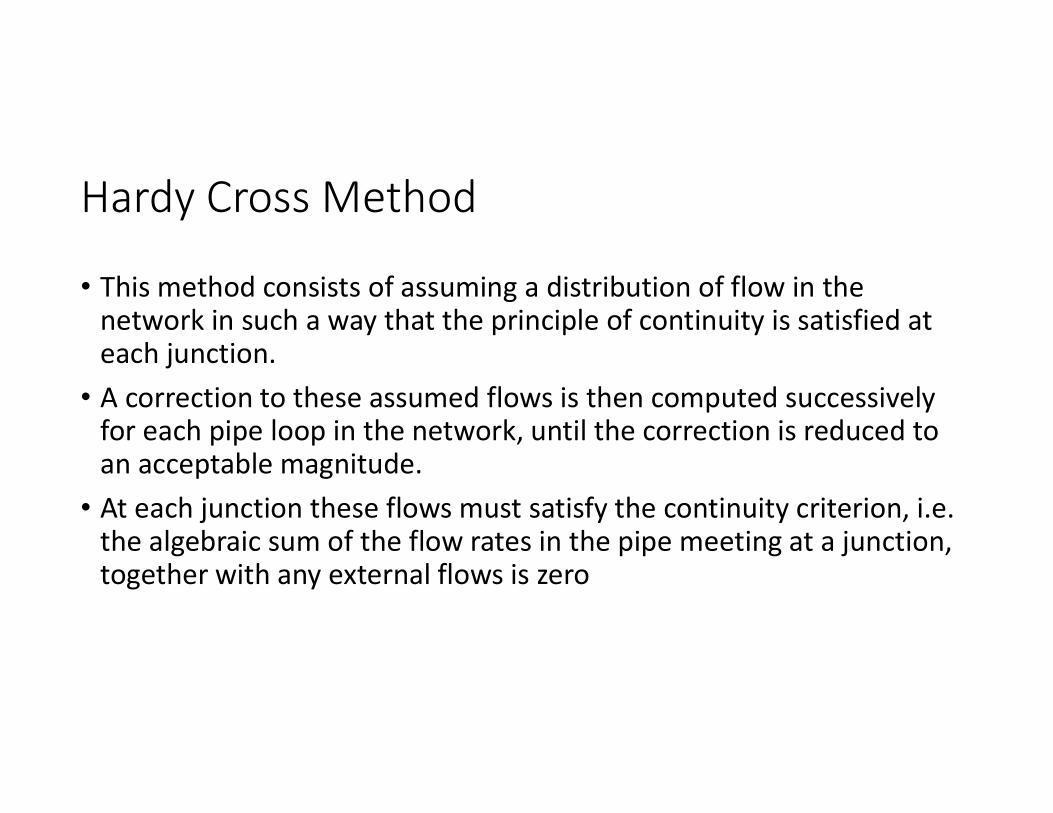
• This method consists of assuming a distribution of flow in the network in such a way that the principle of continuity is satisfied at each junction.

• A correction to these assumed flows is then computed successively for each pipe loop in the network, until the correction is reduced to an acceptable magnitude.

• At each junction these flows must satisfy the continuity criterion, i.e. the algebraic sum of the flow rates in the pipe meeting at a junction, together with any external flows is zero

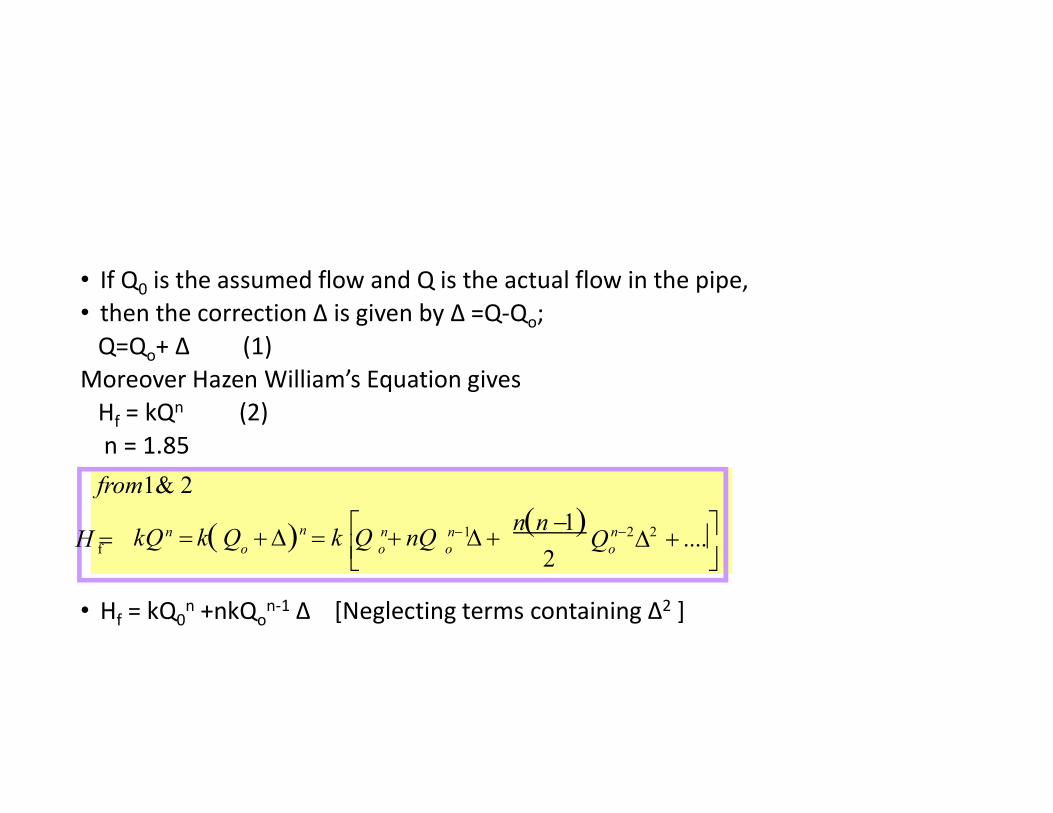
• If Q0 is the assumed flow and Q is the actual flow in the pipe, • then the correction Δ is given by Δ =Q-Qo;

Q=Qo+ Δ (1) Moreover Hazen William’s Equation gives

Hf = kQn (2)n = 1.85

• Hf = kQ0n +nkQo

n-1 Δ [Neglecting terms containing Δ2 ]

+ ....o

n-2 2Q D2oo

of

n(n-1)1n-nnQ +D) = k Q + nQ D +nkQ = k(H =

from1& 2

• For each Loop∑ Hf = ∑ kQn = 0∑ kQn = ∑ kQ0

n + ∑ nkQon-1 Δ = 0

Δ = - ∑ kQ0n / ∑ nkQo

n-1

Δ = - ∑ Hf / n ∑ (Hf/Q)

where Hf is the head loss for assumed flow Qo

Procedure

• The numerator in the above equation is the algebraic sum of the headlosses in the various pipes of the closed loop computed with assumedflow.

• As the direction and magnitude of flow in these pipes is alreadyassumed, their respective head losses with due regard to sign can beeasily calculated after assuming their diameters.

• The absolute sum of respective KQon-1 or HL/Qo is then calculated.

Finally the value of Δ is found out for each loop, and the assumedflows are corrected.

• Repeated adjustments are made until the desired accuracy isobtained

Design Example (Source: NPTEL)

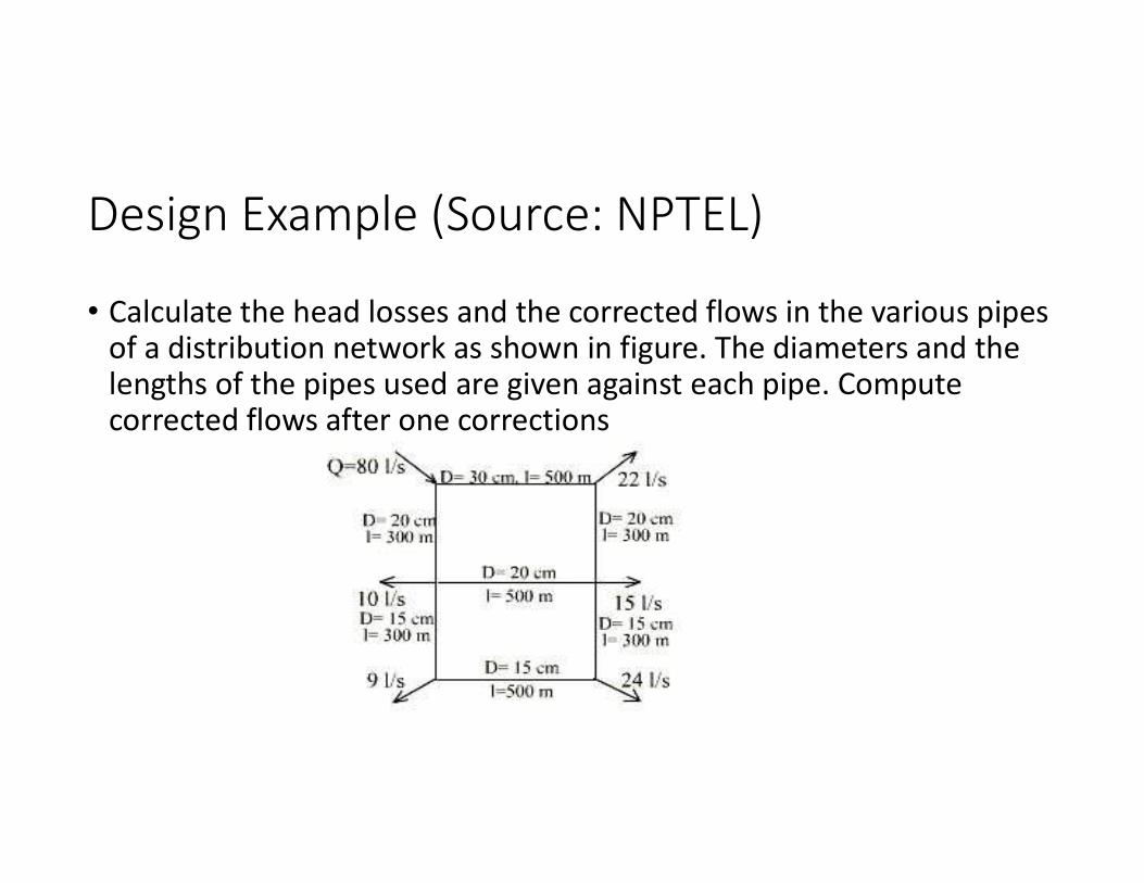
• Calculate the head losses and the corrected flows in the various pipes of a distribution network as shown in figure. The diameters and the lengths of the pipes used are given against each pipe. Compute corrected flows after one corrections

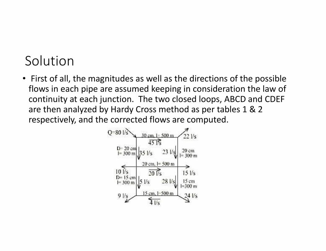
Solution• First of all, the magnitudes as well as the directions of the possible

flows in each pipe are assumed keeping in consideration the law of continuity at each junction. The two closed loops, ABCD and CDEF are then analyzed by Hardy Cross method as per tables 1 & 2 respectively, and the corrected flows are computed.

Pipe Assumed flow Dia of pipe Length of pipe (m)

K= L

470 d4.87

Q 1.85a HL=

K.Q 1.85 alHL/Qal

in l/sec

in cumecs

d in m d4.87

(1) (2) (3) (4) (5) (6) (7) (8) (9) (10)

AB (+) +0.043 0.30 2.85 X10-3 500 373 3 X10-3 +1.12 26

BC 43 +0.023 0.20 3.95 X10-4

3.95 X10-4

3.95 X10-4

300 1615 9.4 X10-4

7.2 X10-4

2 X10-3

+1.52 66

CD (+) -0.020 0.20 500 2690 -1.94 97

23

DA -0.035 0.20 300 1615 -3.23 92

(-) 20

(-) 35

S -2.53 281

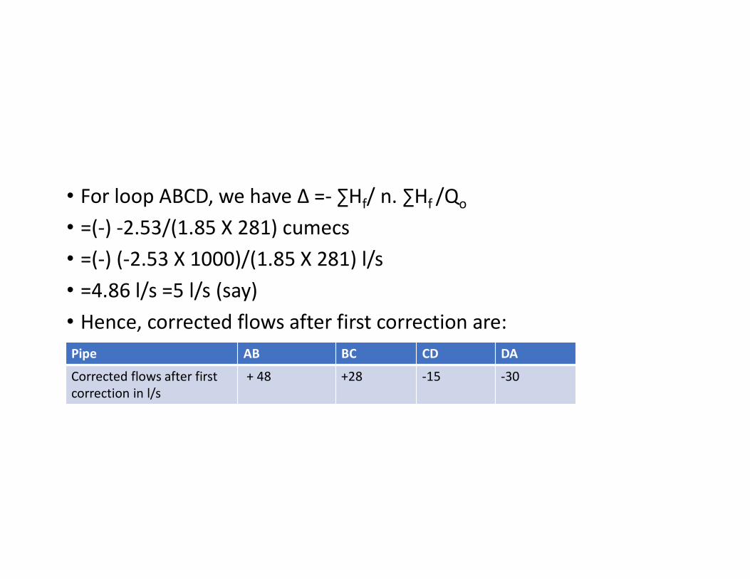
• For loop ABCD, we have Δ =- ∑Hf/ n. ∑Hf /Qo

• =(-) -2.53/(1.85 X 281) cumecs• =(-) (-2.53 X 1000)/(1.85 X 281) l/s• =4.86 l/s =5 l/s (say) • Hence, corrected flows after first correction are:Pipe AB BC CD DA

Corrected flows after first correction in l/s

+ 48 +28 -15 -30

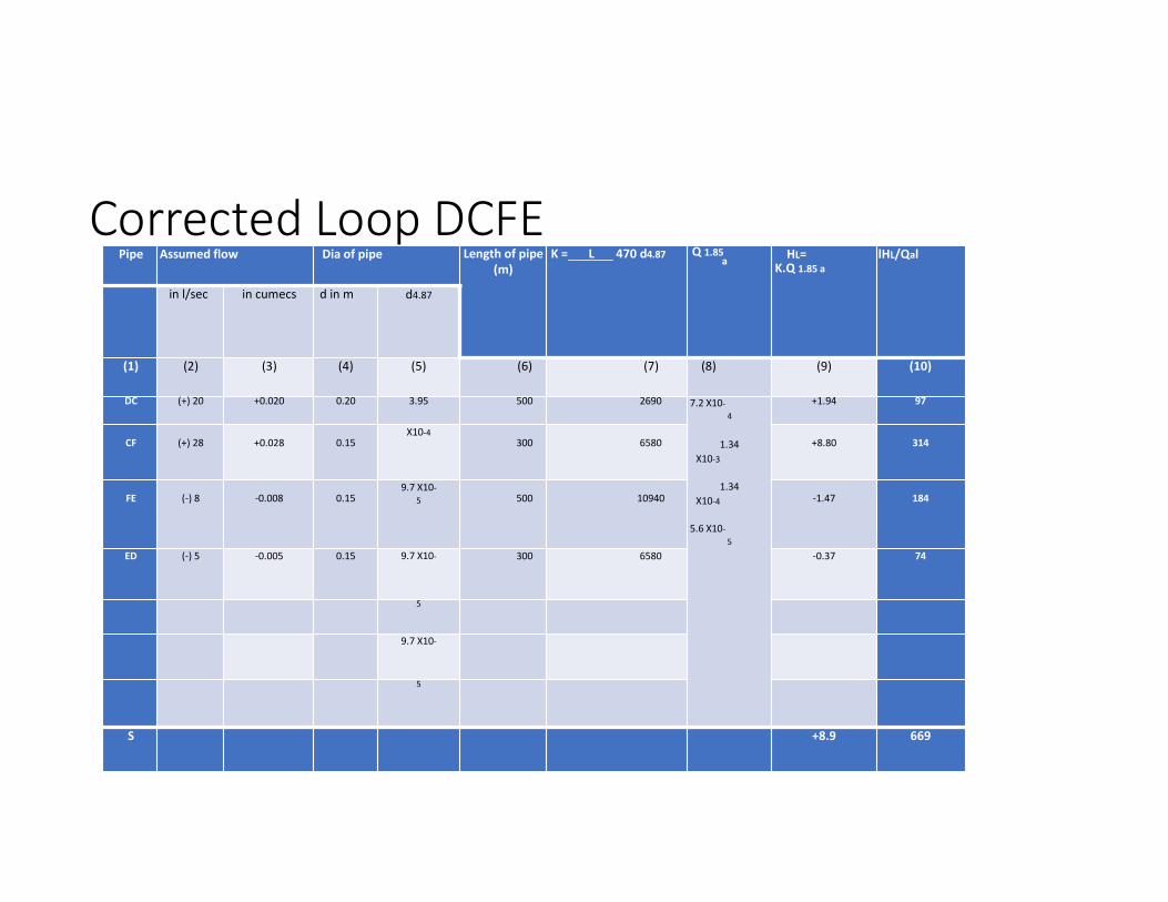
Corrected Loop DCFEPipe Assumed flow Dia of pipe Length of pipe

(m)K = L 470 d4.87 Q 1.85

a HL=K.Q 1.85 a

lHL/Qal

in l/sec in cumecs d in m d4.87

(1) (2) (3) (4) (5) (6) (7) (8) (9) (10)

DC (+) 20 +0.020 0.20 3.95 500 2690 7.2 X10-4

1.34X10-3

1.34X10-4

5.6 X10-5

+1.94 97

CF (+) 28 +0.028 0.15X10-4

300 6580 +8.80 314

FE (-) 8 -0.008 0.159.7 X10-

5 500 10940 -1.47 184

ED (-) 5 -0.005 0.15 9.7 X10- 300 6580 -0.37 74

5

9.7 X10-

5

S +8.9 669

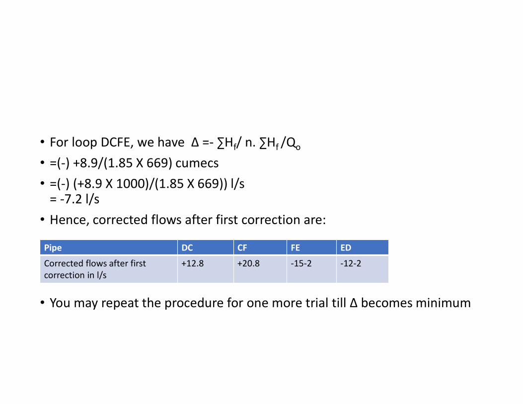
• For loop DCFE, we have Δ =- ∑Hf/ n. ∑Hf /Qo

• =(-) +8.9/(1.85 X 669) cumecs• =(-) (+8.9 X 1000)/(1.85 X 669)) l/s

= -7.2 l/s• Hence, corrected flows after first correction are:

• You may repeat the procedure for one more trial till Δ becomes minimum

Pipe DC CF FE ED

Corrected flows after first correction in l/s

+12.8 +20.8 -15-2 -12-2

Equivalent Pipe Method• Equivalent pipe is a method of reducing a combination of pipes into a

simple pipe system for easier analysis of a pipe network, such as a waterdistribution system.

• An equivalent pipe is an imaginary pipe in which the head loss anddischarge are equivalent to the head loss and discharge for the real pipesystem.

• In this method a complex system of pipes is replaced by single hydraulicallyequivalent pipe.

• Hydraulically equivalent pipe means it will have same capacity.(Q) • It willhave same amount of head loss.(hf)

• When the pipes are connected in series, the total head loss is equal to thesummation of the individual head losses.

• When the pipes are laid parallel the head loss through the parallelpipes(or set of pipes) will be the same.

Example

• Solve the following pipe network using Hazen William’s Equation

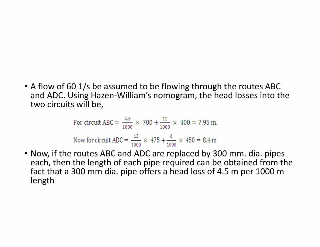
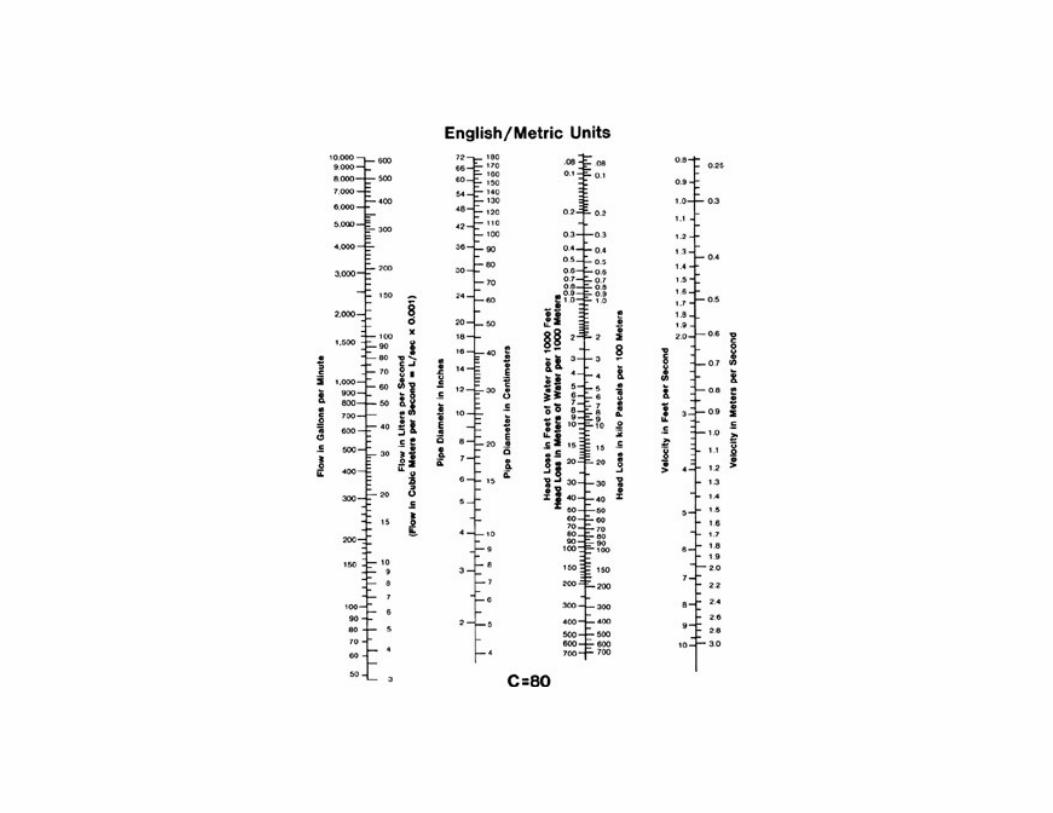
• A flow of 60 1/s be assumed to be flowing through the routes ABC and ADC. Using Hazen-William’s nomogram, the head losses into the two circuits will be,

• Now, if the routes ABC and ADC are replaced by 300 mm. dia. pipes each, then the length of each pipe required can be obtained from the fact that a 300 mm dia. pipe offers a head loss of 4.5 m per 1000 m length

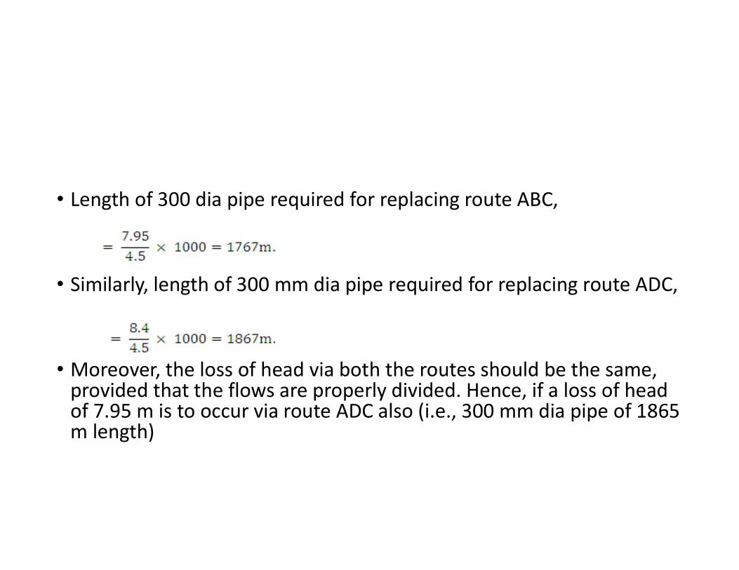
• Length of 300 dia pipe required for replacing route ABC,

• Similarly, length of 300 mm dia pipe required for replacing route ADC,

• Moreover, the loss of head via both the routes should be the same, provided that the flows are properly divided. Hence, if a loss of head of 7.95 m is to occur via route ADC also (i.e., 300 mm dia pipe of 1865 m length)

• The rate of loss of head per 1000 m will be,

• In a 300 mm dia. pipe, such a loss (i.e. 4.25 m per 1000 m) will occur only if the discharge is 56 l/s (from Hazen-William’s monogram). Therefore, the circuits ABC and ADC can be replaced by an equivalent pipe carrying a total discharge of 60 + 56 = 116 l/s.

• Now, for this equivalent pipe having a dia. of300 mm and a discharge of 116 l/s, the rate of loss of head per 1000 m is found from nomogram as 15 m. In order to ensure a head loss of 7.95 m in this equivalent pipe also, the length of this pipe should be,

Hence, the total loop ABCD can thus be replaced by a single equivalent pipe of300 mm dia and 530 m length, irrespective of the flow discharges.

Note: Head Loss in pipes was calculated using Hazen William’s Nomograph, shown on next page