Dr. Mohd Ishtyak - Aligarh Muslim University
57
Mohd. Ishtyak LECTURE NOTES ON ORDINARY DIFFERENTIAL EQUATIONS based on the course-contents of MMB-352 (A course of Mathematics (Main/Subsidiary) prescribed for B. Sc. (Hons.) III Semester) Complied by Dr. Mohd Ishtyak Assistant Professor, Department of Mathematics Aligarh Muslim University, Aligarh-202002, India
-
Upload
khangminh22 -
Category
Documents
-
view
0 -
download
0
Transcript of Dr. Mohd Ishtyak - Aligarh Muslim University
Moh
d.Ish
tyakLECTURE NOTES ON
ORDINARY DIFFERENTIAL EQUATIONS
based on the course-contents of MMB-352
(A course of Mathematics (Main/Subsidiary)
prescribed for B. Sc. (Hons.) III Semester)
Complied by
Dr. Mohd IshtyakAssistant Professor,
Department of Mathematics
Aligarh Muslim University, Aligarh-202002, India
Moh
d.Ish
tyak
Lecture No. 01
Preliminaries(A topic of Unit I)
In this lecture, we shall revise the basic notions regarding to this course, which we
have already discussed in +2 level Mathematics.
Differential Equations: An equation containing the derivatives or differentials of
one or more dependent variables with respect to one or more independent variables is
called a differential equation.
Ordinary Differential Equations: A differential equation in which each involved
dependent variable is a function of a single independent variable is known as an
ordinary differential equation.
Throughout the course, we shall study of different methods for solving ordinary
differential equations. But for the sake of simplicity, we shall use the term ‘differential
equation’ instead of ‘ordinary differential equation’.
Order of a Differential Equation: The order of a differential equation is the order
of highest order derivative appearing in equation.
Degree of a Differential Equation: The degree of a differential equation is the
power of highest order derivative occurring in the equation, when differential coeffi-
cients are made free from radicals and fractions.
eg, the differential equation d3ydx3− 6(dydx
)2 − 4y = 0 is of order 3 and degree 1.
Classification of Differential Equations: Differential equations are classified into
linear and nonlinear differential equations. An nth order differential equation is called
1
Moh
d.Ish
tyak
2
linear if it can be expressed in the form:
P0dny
dxn+ P1
dn−1y
dxn−1+ P2
dn−2y
dxn−2+ ...Pn−1
dy
dx+ Pny = Q
where P0, P1, ..., Pn and Q are either constants or functions of the variable x and
P0 6= 0.
A differential equation, which is not linear is called a nonlinear differential
equation.
Linear differential equations are further classified into homogeneous and nonho-
mogeneous equations according to Q ≡ 0 and Q 6≡ 0, respectively. In this regards,
we shall study deeply later in Unit II.
Formation of a Differential Equation: Usually, differential equations are derived
to eliminate arbitrary constants (parameters) involved in a family of curves. For
illustration, consider the two-parameter family of straight lines
y = mx+ c (1)
having the slop m and passing through the point (0, c). Differentiating Eq. (2), we
getdy
dx= m.
Differentiating again, we getd2y
dx2= 0 (2)
which is a second order differential equation.
Remark 1: To eliminate n arbitrary constants from n-parameter family of curves,
we obtain a differential equation of order n.
Solution of a Differential Equation: A solution (or integral/primitive) of a dif-
ferential equation is an explicit or implicit relation between the variables involved
that does not contain derivatives and satisfies the differential equation.
Naturally, the solution of a differential equation in one dependent variable y and
one independent variable x are of the form y = f(x) (explicit form) or of the form
φ(x, y) = 0 (implicit form). Geometrically speaking, both forms represents the curves
Moh
d.Ish
tyak
3
in xy-plane. Henceforth, the solutions of such a differential equation are also called
‘integral curves’ of the equation.
For example, Eq. (1) forms an integral curve of differential equation (2).
General and Particular Solutions: A solution of a differential equation which
contains a number of arbitrary constants equal to the order of the differential equation
is called the general solution or the complete solution of the differential equation.
For example, y = a cosx+b sinx is the general solution of the differential equation
y′′ + y = 0. Although, y = a cosx and y = b sinx both satisfy the given equation
yet they are not general solutions as each of them contains only one arbitrary constant.
In lieu of the concept of general solution, it can be highlighted that a single
differential equation can possess an infinite number of solutions corresponding to the
unlimited number of choices for the arbitrary constants. A solution of a differential
equation obtained by giving particular values to arbitrary constants in the general
solution is called a particular solution.
Elementary Methods of Solving of Differential Equations of First Order
and First Degree: In class 12, we have studied the techniques of solving the
following three types of differential equations of order one and degree one:
1. Differential Equations with variable separable
2. Homogeneous Differential Equations
3. Linear Differential Equations
As a continuation, we shall discuss several another methods for solving the differential
equations of order one and degree one in our upcoming lectures.
Moh
d.Ish
tyak
Lecture No. 02
Bernoulli Equation(A topic of Unit I)
Recall that the general solution of linear differential equation:
dy
dx+ P (x)y = Q(x)
is
y × I.F. =
∫(Q× I.F.)dx+ c
where c is an arbitrary constant and I.F. = e∫Pdx (called integrating factor).
Sometimes certain nonlinear differential equations can be reduced to linear forms
by making suitable substitutions and hence can be solved easily. Bernoulli equation
is one of such equations. Indeed, an equation of the form
dy
dx+ P (x)y = Q(x)yn (1)
(where n 6= 0 and n 6= 1) is called Bernoulli equation.
Dividing Eq. (1) by yn, we get
y−ndy
dx+ P (x)y−n+1 = Q(x). (2)
Put y−n+1 = u so that (1− n)y−n dydx
= dudx
. Thus, Eq. (2) reduces to
1
1− ndu
dx+ P (x)u = Q(x)
or,du
dx+ (1− n)P (x)u = (1− n)Q(x)
1
Moh
d.Ish
tyak
2
which is a linear differential equation in dependent variable u and independent variable
x. After solving it and then replacing u by y−n+1, we can obtain the general solution
of Eq. (1).
Example 2.24/p.42: Solve (1− x2) dydx
+ xy = xy2.
Solution. Dividing given equation by y2, we get
(1− x2)y−2 dydx
+ xy−1 = x
which can be written as
y−2dy
dx+
x
1− x2y−1 =
x
1− x2.
Put y−1 = u so that −y−2 dydx
= dudx
. Then, above equation reduces to
du
dx− x
1− x2u = − x
1− x2
which is a linear differential equation in dependent variable u and independent variable
x. Its integrating factor is
I.F. = e∫Pdx = e
−∫
x1−x2
dx
= e12
∫ −2x
1−x2dx
= e(1/2) log(1−x2)
= (1− x2)1/2.
Therefore, the solution is
u× I.F. =
∫(Q× I.F.)dx+ c
or,
u(1− x2)1/2 =
∫− x
1− x2(1− x2)1/2dx+ c
=
∫−x(1− x2)−1/2dx+ c
=
∫t−1/2.
1
2dt+ c (put t = 1− x2 so that −2xdx = dt)
=1
2
t1/2
1/2+ c = t1/2 + c
= (1− x2)1/2 + c.
Moh
d.Ish
tyak
3
Putting u = y−1 in above equation, we get
y−1(1− x2)1/2 = (1− x2)1/2 + c
or, √1− x2 = y
√1− x2 + cy
or,
(1− y)√
1− x2 = cy
which is the required solution of given differential equation.
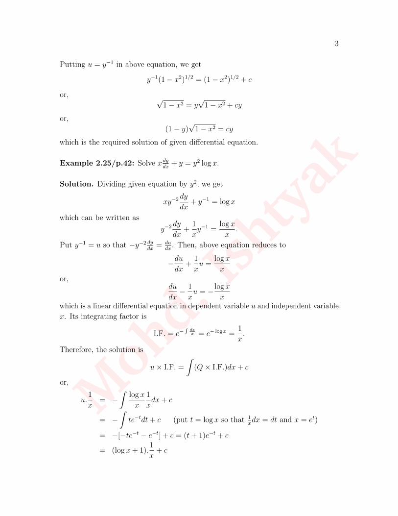
Example 2.25/p.42: Solve x dydx
+ y = y2 log x.
Solution. Dividing given equation by y2, we get
xy−2dy
dx+ y−1 = log x
which can be written as
y−2dy
dx+
1
xy−1 =
log x
x.
Put y−1 = u so that −y−2 dydx
= dudx
. Then, above equation reduces to
−dudx
+1
xu =
log x
x
or,du
dx− 1
xu = − log x
xwhich is a linear differential equation in dependent variable u and independent variable
x. Its integrating factor is
I.F. = e−∫
dxx = e− log x =
1
x.
Therefore, the solution is
u× I.F. =
∫(Q× I.F.)dx+ c
or,
u.1
x= −
∫log x
x
1
xdx+ c
= −∫te−tdt+ c (put t = log x so that 1
xdx = dt and x = et)
= −[−te−t − e−t] + c = (t+ 1)e−t + c
= (log x+ 1).1
x+ c
Moh
d.Ish
tyak
4
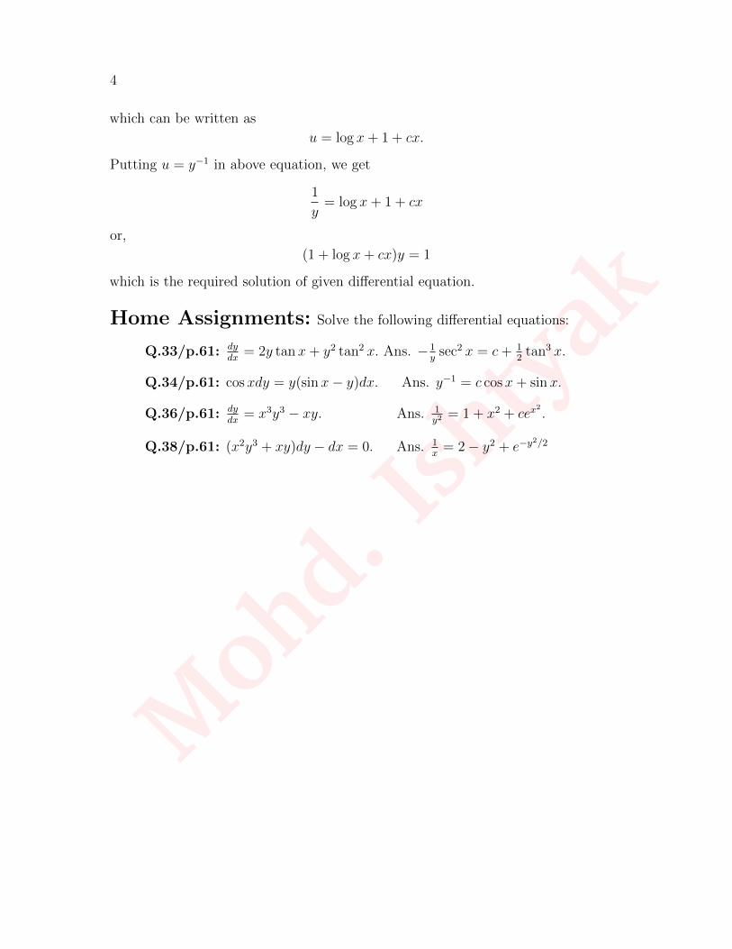
which can be written as
u = log x+ 1 + cx.
Putting u = y−1 in above equation, we get
1
y= log x+ 1 + cx
or,
(1 + log x+ cx)y = 1
which is the required solution of given differential equation.
Home Assignments: Solve the following differential equations:
Q.33/p.61: dydx
= 2y tanx+ y2 tan2 x. Ans. − 1y
sec2 x = c+ 12
tan3 x.
Q.34/p.61: cosxdy = y(sinx− y)dx. Ans. y−1 = c cosx+ sinx.
Q.36/p.61: dydx
= x3y3 − xy. Ans. 1y2
= 1 + x2 + cex2.
Q.38/p.61: (x2y3 + xy)dy − dx = 0. Ans. 1x
= 2− y2 + e−y2/2
Moh
d.Ish
tyak
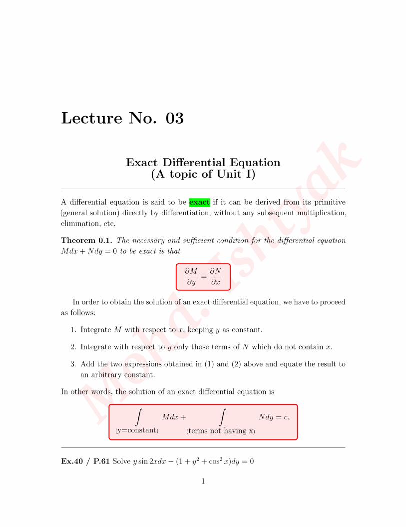
Lecture No. 03
Exact Differential Equation(A topic of Unit I)
A differential equation is said to be exact if it can be derived from its primitive
(general solution) directly by differentiation, without any subsequent multiplication,
elimination, etc.
Theorem 0.1. The necessary and sufficient condition for the differential equation
Mdx+Ndy = 0 to be exact is that
∂M
∂y=∂N
∂x
In order to obtain the solution of an exact differential equation, we have to proceed
as follows:
1. Integrate M with respect to x, keeping y as constant.
2. Integrate with respect to y only those terms of N which do not contain x.
3. Add the two expressions obtained in (1) and (2) above and equate the result to
an arbitrary constant.
In other words, the solution of an exact differential equation is∫(y=constant)
Mdx+
∫(terms not having x)
Ndy = c.
Ex.40 / P.61 Solve y sin 2xdx− (1 + y2 + cos2 x)dy = 0
1
Moh
d.Ish
tyak
2
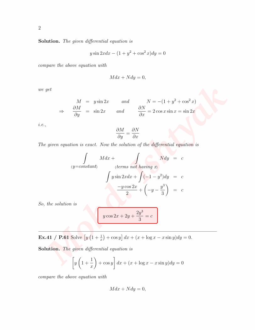
Solution. The given differential equation is
y sin 2xdx− (1 + y2 + cos2 x)dy = 0
compare the above equation with
Mdx+Ndy = 0,
we get
M = y sin 2x and N = −(1 + y2 + cos2 x)
⇒ ∂M
∂y= sin 2x and
∂N
∂x= 2 cos x sinx = sin 2x
i.e.,∂M
∂y=∂N
∂x
The given equation is exact. Now the solution of the differential equation is∫(y=constant)
Mdx+
∫(terms not having x)
Ndy = c
∫y sin 2xdx+
∫(−1− y2)dy = c
−y cos 2x
2+
(−y − y3
3
)= c
So, the solution is
y cos 2x+ 2y +2y3
3= c
Ex.41 / P.61 Solve[y(1 + 1
x
)+ cos y
]dx+ (x+ log x− x sin y)dy = 0.
Solution. The given differential equation is[y
(1 +
1
x
)+ cos y
]dx+ (x+ log x− x sin y)dy = 0
compare the above equation with
Mdx+Ndy = 0,
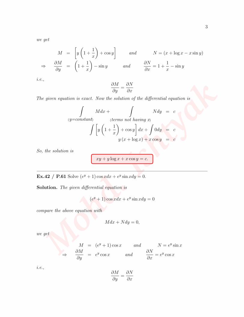
Moh
d.Ish
tyak
3
we get
M =
[y
(1 +
1
x
)+ cos y
]and N = (x+ log x− x sin y)
⇒ ∂M
∂y=
(1 +
1
x
)− sin y and
∂N
∂x= 1 +
1
x− sin y
i.e.,∂M
∂y=∂N
∂x
The given equation is exact. Now the solution of the differential equation is∫(y=constant)
Mdx+
∫(terms not having x)
Ndy = c
∫ [y
(1 +
1
x
)+ cos y
]dx+
∫0dy = c
y (x+ log x) + x cos y = c
So, the solution is
xy + y log x+ x cos y = c.
Ex.42 / P.61 Solve (ey + 1) cosxdx+ ey sinxdy = 0.
Solution. The given differential equation is
(ey + 1) cosxdx+ ey sinxdy = 0
compare the above equation with
Mdx+Ndy = 0,
we get
M = (ey + 1) cosx and N = ey sinx
⇒ ∂M
∂y= ey cosx and
∂N
∂x= ey cosx
i.e.,∂M
∂y=∂N
∂x
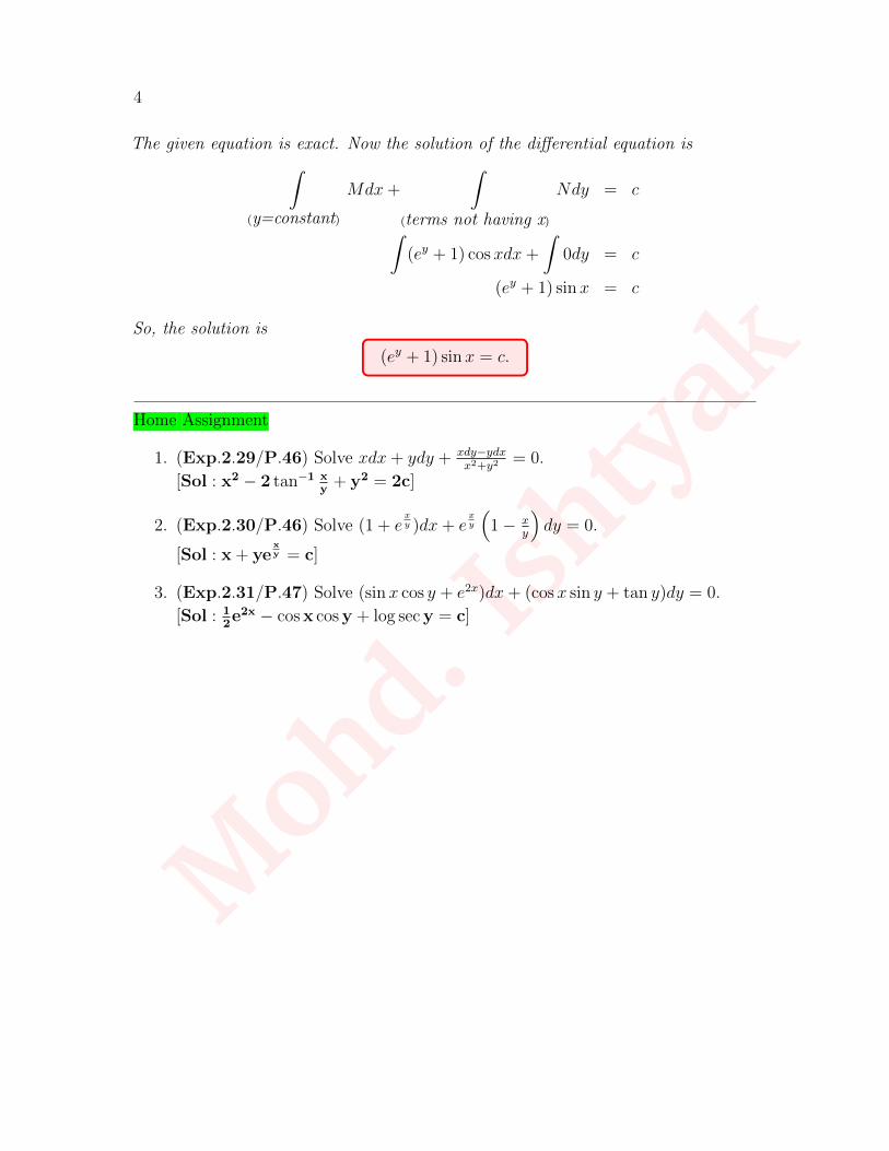
Moh
d.Ish
tyak
4
The given equation is exact. Now the solution of the differential equation is∫(y=constant)
Mdx+
∫(terms not having x)
Ndy = c
∫(ey + 1) cosxdx+
∫0dy = c
(ey + 1) sinx = c
So, the solution is
(ey + 1) sinx = c.
Home Assignment
1. (Exp.2.29/P.46) Solve xdx+ ydy + xdy−ydxx2+y2
= 0.
[Sol : x2 − 2 tan−1 xy
+ y2 = 2c]
2. (Exp.2.30/P.46) Solve (1 + exy )dx+ e
xy
(1− x
y
)dy = 0.
[Sol : x + yexy = c]
3. (Exp.2.31/P.47) Solve (sin x cos y + e2x)dx+ (cosx sin y + tan y)dy = 0.
[Sol : 12e2x − cos x cos y + log sec y = c]
Moh
d.Ish
tyak
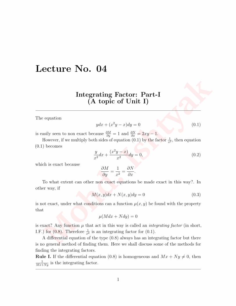
Lecture No. 04
Integrating Factor: Part-I(A topic of Unit I)
The equation
ydx+ (x2y − x)dy = 0 (0.1)
is easily seen to non exact because ∂M∂y
= 1 and ∂N∂x
= 2xy − 1.
However, if we multiply both sides of equation (0.1) by the factor 1x2
, then equation
(0.1) becomesy
x2dx+
(x2y − x)
x2dy = 0, (0.2)
which is exact because∂M
∂y=
1
x2=∂N
∂x.
To what extent can other non exact equations be made exact in this way?. In
other way, if
M(x, y)dx+N(x, y)dy = 0 (0.3)
is not exact, under what conditions can a function µ(x, y) be found with the property
that
µ(Mdx+Ndy) = 0
is exact? Any function µ that act in this way is called an integrating factor (in short,
I.F.) for (0.8). Therefore 1x2
is an integrating factor for (0.1).
A differential equation of the type (0.8) always has an integrating factor but there
is no general method of finding them. Here we shall discuss some of the methods for
finding the integrating factors.
Rule I. If the differential equation (0.8) is homogeneous and Mx + Ny 6= 0, then1
Mx+Nyis the integrating factor.
1
Moh
d.Ish
tyak
2
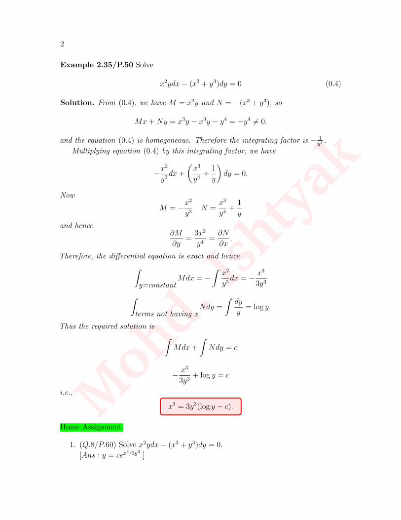
Example 2.35/P.50 Solve
x2ydx− (x3 + y3)dy = 0 (0.4)
Solution. From (0.4), we have M = x2y and N = −(x3 + y3), so
Mx+Ny = x3y − x3y − y4 = −y4 6= 0,
and the equation (0.4) is homogeneous. Therefore the integrating factor is − 1y4
.
Multiplying equation (0.4) by this integrating factor, we have
−x2
y3dx+
(x3
y4+
1
y
)dy = 0.
Now
M = −x2
y3N =
x3
y4+
1
y
and hence∂M
∂y=
3x2
y4=∂N
∂x.
Therefore, the differential equation is exact and hence∫y=constant
Mdx = −∫x2
y3dx = − x3
3y3∫terms not having x
Ndy =
∫dy
y= log y.
Thus the required solution is ∫Mdx+
∫Ndy = c
− x3
3y3+ log y = c
i.e.,
x3 = 3y3(log y − c).
Home Assignment:
1. (Q.8/P.60) Solve x2ydx− (x3 + y3)dy = 0.
[Ans : y = cex3/3y3 .]
Moh
d.Ish
tyak
3
2. (Q.39/P.61) Solve (x2 − 2xy − y2)dx− (x+ y)2dy = 0.
[Ans : x3 − y3 + 3xy(x− y) = C]
Rule II. If in the differential equation (0.8), M = yf1(xy) and N = xf2(xy). Then1
(Mx−Ny) is an integrating factor.
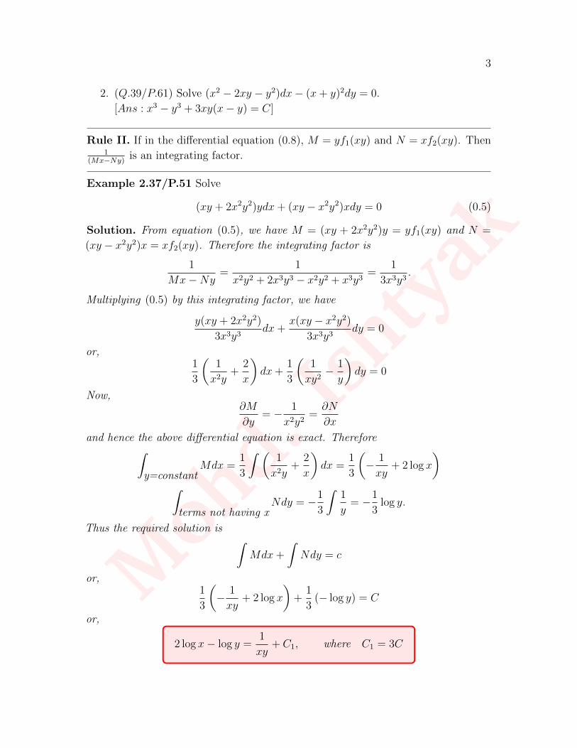
Example 2.37/P.51 Solve
(xy + 2x2y2)ydx+ (xy − x2y2)xdy = 0 (0.5)
Solution. From equation (0.5), we have M = (xy + 2x2y2)y = yf1(xy) and N =
(xy − x2y2)x = xf2(xy). Therefore the integrating factor is
1
Mx−Ny=
1
x2y2 + 2x3y3 − x2y2 + x3y3=
1
3x3y3.
Multiplying (0.5) by this integrating factor, we have
y(xy + 2x2y2)
3x3y3dx+
x(xy − x2y2)3x3y3
dy = 0
or,1
3
(1
x2y+
2
x
)dx+
1
3
(1
xy2− 1
y
)dy = 0
Now,∂M
∂y= − 1
x2y2=∂N
∂x
and hence the above differential equation is exact. Therefore∫y=constant
Mdx =1
3
∫ (1
x2y+
2
x
)dx =
1
3
(− 1
xy+ 2 log x
)∫
terms not having xNdy = −1
3
∫1
y= −1
3log y.
Thus the required solution is ∫Mdx+
∫Ndy = c
or,1
3
(− 1
xy+ 2 log x
)+
1
3(− log y) = C
or,
2 log x− log y =1
xy+ C1, where C1 = 3C
Moh
d.Ish
tyak
4
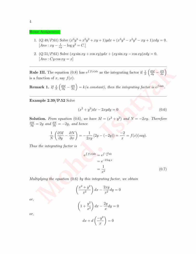
Home Assignment:
1. (Q.48/P.61) Solve (x3y3 + x2y2 + xy + 1)ydx+ (x3y3 − x2y2 − xy + 1)xdy = 0.
[Ans : xy − 1xy− log y2 = C.]
2. (Q.51/P.61) Solve (xy sinxy + cosxy)ydx+ (xy sinxy − cosxy)xdy = 0.
[Ans : Cy cosxy = x]
Rule III. The equation (0.8) has e∫f(x)dx as the integrating factor if 1
N
(∂M∂y− ∂N
∂x
)is a function of x, say f(x).
Remark 1. If 1N
(∂M∂y− ∂N
∂x
)= k(a constant), then the integrating factor is e
∫kdx.
Example 2.39/P.52 Solve
(x2 + y2)dx− 2xydy = 0 (0.6)
Solution. From equation (0.6), we have M = (x2 + y2) and N = −2xy. Therefore∂M∂y
= 2y and ∂N∂x
= −2y, and hence
1
N
(∂M
∂y− ∂N
∂x
)= − 1
2xy(2y − (−2y)) =
−2
x= f(x)(say).
Thus the integrating factor is
e∫f(x)dx = e
∫ −2xdx
= e−2 log x
=1
x2(0.7)
Multiplying the equation (0.6) by this integrating factor, we obtain(x2 + y2
x2
)dx− 2xy
x2dy = 0
or, (1 +
y2
x2
)dx− 2y
xdy = 0
or,
dx+ d
(−y2
x
)= 0
Moh
d.Ish
tyak
5
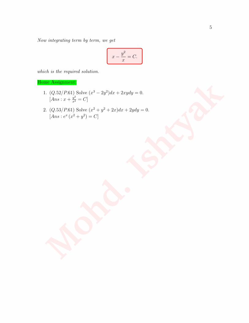
Now integrating term by term, we get
x− y2
x= C.
which is the required solution.
Home Assignment:
1. (Q.52/P.61) Solve (x3 − 2y2)dx+ 2xydy = 0.
[Ans : x+ y2
x2= C]
2. (Q.53/P.61) Solve (x2 + y2 + 2x)dx+ 2ydy = 0.
[Ans : ex (x2 + y2) = C]
Moh
d.Ish
tyak
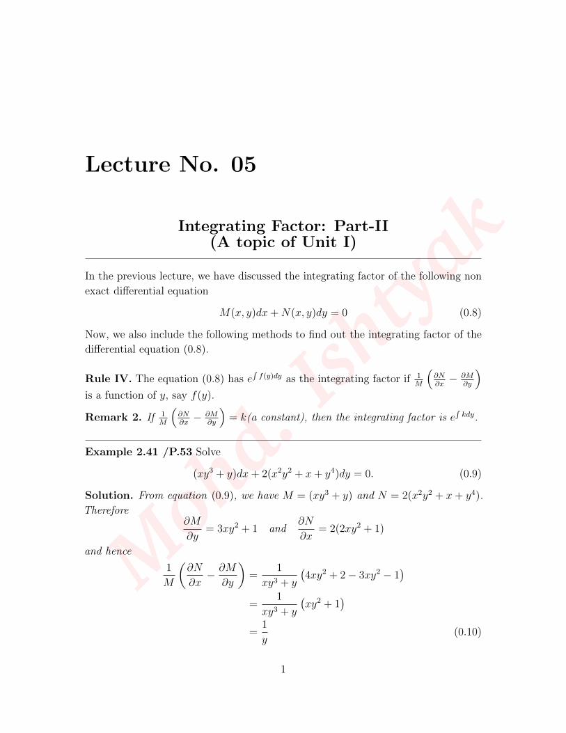
Lecture No. 05
Integrating Factor: Part-II(A topic of Unit I)
In the previous lecture, we have discussed the integrating factor of the following non
exact differential equation
M(x, y)dx+N(x, y)dy = 0 (0.8)
Now, we also include the following methods to find out the integrating factor of the
differential equation (0.8).
Rule IV. The equation (0.8) has e∫f(y)dy as the integrating factor if 1
M
(∂N∂x− ∂M
∂y
)is a function of y, say f(y).
Remark 2. If 1M
(∂N∂x− ∂M
∂y
)= k(a constant), then the integrating factor is e
∫kdy.
Example 2.41 /P.53 Solve
(xy3 + y)dx+ 2(x2y2 + x+ y4)dy = 0. (0.9)
Solution. From equation (0.9), we have M = (xy3 + y) and N = 2(x2y2 + x+ y4).
Therefore∂M
∂y= 3xy2 + 1 and
∂N
∂x= 2(2xy2 + 1)
and hence
1
M
(∂N
∂x− ∂M
∂y
)=
1
xy3 + y
(4xy2 + 2− 3xy2 − 1
)=
1
xy3 + y
(xy2 + 1
)=
1
y(0.10)
1

Moh
d.Ish
tyak
2
Thus the integrating factor is e∫f(y)dy = e
∫1ydy = elog y = y. Multiplying (0.9) by y,
we obtain the following exact differential equation
(xy4 + y2)dx+ 2(x2y3 + xy + y5)dy = 0 (0.11)
Now,
M1 = (xy4 + y2) and N1 = 2(x2y3 + xy + y5)
and hence ∫y=constant
M1dx =1
2xy4 + y2x
and ∫terms not having x
N1dy =2
6y6.
Thus the required solution is
1
2xy4 + y2x+
2
6y6 = C
or,
3xy4 + 6y2x+ 2y6 = 6C.
Home Assignment:
1. (Q.54/P.61) Solve (2x2y − 3y2)dx+ (2x3 − 12xy + log y)dy = 0.
[Ans : 6x3y3 − 27xy4 − 3y3 log y − y3 = C.]
2. (Q.55/P.61) Solve (3x2y4 + 2xy)dx+ (2x3y3 − x2)dy = 0.
[Ans : x3y3 + x2 = Cy]
Rule V. If the differential equation (0.8) is of the form
xayb(mydx+ nxdy) + xcyd(pydx+ qxdy) = 0,
where a, b, c, d, m, n, p and q are constants, then xhyk is the integrating factor
of the given differential equation, where h, k are constants and can be obtained by
applying the condition that after multiplication by xhyk the given equation is exact.
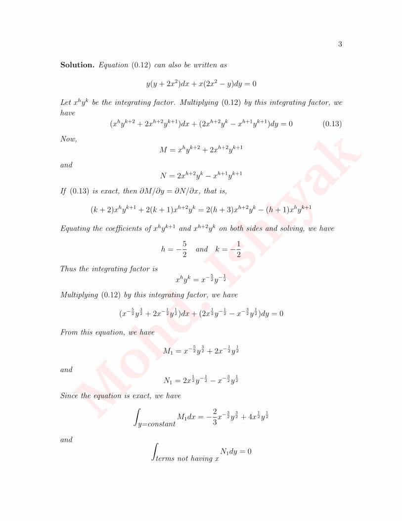
Example 2.43/P.54 Solve
(y2 + 2x2y)dx+ (2x3 − xy)dy = 0. (0.12)
Moh
d.Ish
tyak
3
Solution. Equation (0.12) can also be written as
y(y + 2x2)dx+ x(2x2 − y)dy = 0
Let xhyk be the integrating factor. Multiplying (0.12) by this integrating factor, we
have
(xhyk+2 + 2xh+2yk+1)dx+ (2xh+2yk − xh+1yk+1)dy = 0 (0.13)
Now,
M = xhyk+2 + 2xh+2yk+1
and
N = 2xh+2yk − xh+1yk+1
If (0.13) is exact, then ∂M/∂y = ∂N/∂x, that is,
(k + 2)xhyk+1 + 2(k + 1)xh+2yk = 2(h+ 3)xh+2yk − (h+ 1)xhyk+1
Equating the coefficients of xhyk+1 and xh+2yk on both sides and solving, we have
h = −5
2and k = −1
2
Thus the integrating factor is
xhyk = x−52y−
12
Multiplying (0.12) by this integrating factor, we have
(x−52y
32 + 2x−
12y
12 )dx+ (2x
12y−
12 − x−
32y
12 )dy = 0
From this equation, we have
M1 = x−52y
32 + 2x−
12y
12
and
N1 = 2x12y−
12 − x−
32y
12
Since the equation is exact, we have∫y=constant
M1dx = −2
3x−
32y
32 + 4x
12y
12
and ∫terms not having x
N1dy = 0
Moh
d.Ish
tyak
4
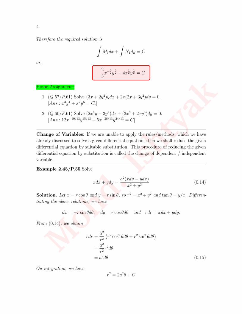
Therefore the required solution is∫M1dx+
∫N1dy = C
or,
−2
3x−
32y
32 + 4x
12y
12 = C
Home Assignment:
1. (Q.57/P.61) Solve (3x+ 2y2)ydx+ 2x(2x+ 3y2)dy = 0.
[Ans : x3y4 + x2y6 = C.]
2. (Q.60/P.61) Solve (2x2y − 3y4)dx+ (3x3 + 2xy3)dy = 0.
[Ans : 12x−10/13y15/13 + 5x−36/13y24/13 = C]
Change of Variables: If we are unable to apply the rules/methods, which we have
already discussed to solve a given differential equation, then we shall reduce the given
differential equation by suitable substitution. This procedure of reducing the given
differential equation by substitution is called the change of dependent / independent
variable.
Example 2.45/P.55 Solve
xdx+ ydy =a2(xdy − ydx)
x2 + y2(0.14)
Solution. Let x = r cos θ and y = r sin θ, so r2 = x2 + y2 and tan θ = y/x. Differen-
tiating the above relations, we have
dx = −r sin θdθ, dy = r cos θdθ and rdr = xdx+ ydy.
From (0.14), we obtain
rdr =a2
r2(r2 cos2 θdθ + r2 sin2 θdθ
)=a2
r2r2dθ
= a2dθ (0.15)
On integration, we have
r2 = 2a2θ + C
Moh
d.Ish
tyak
5
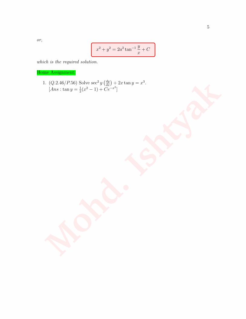
or,
x2 + y2 = 2a2 tan−1y
x+ C
which is the required solution.
Home Assignment:
1. (Q.2.46/P.56) Solve sec2 y(dydx
)+ 2x tan y = x3.
[Ans : tan y = 12(x2 − 1) + Ce−x
2]
Moh
d.Ish
tyak
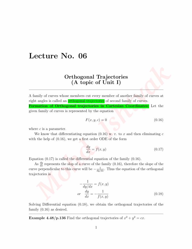
Lecture No. 06
Orthogonal Trajectories(A topic of Unit I)
A family of curves whose members cut every member of another family of curves at
right angles is called an orthogonal trajectories of second family of curves.
Formation of Orthogonal trajectories in Cartesian Coordinates: Let the
given family of curves is represented by the equation
F (x, y, c) = 0 (0.16)
where c is a parameter.
We know that differentiating equation (0.16) w. r. to x and then eliminating c
with the help of (0.16), we get a first order ODE of the form
dy
dx= f(x, y) (0.17)
Equation (0.17) is called the differential equation of the family (0.16).
As dydx
represents the slop of a curve of the family (0.16), therefore the slope of the
curve perpendicular to this curve will be − 1dy/dx
. Thus the equation of the orthogonal
trajectories is
− 1
dy/dx= f(x, y)
ordy
dx= − 1
f(x, y)(0.18)
Solving Differential equation (0.18), we obtain the orthogonal trajectories of the
family (0.16) as desired.
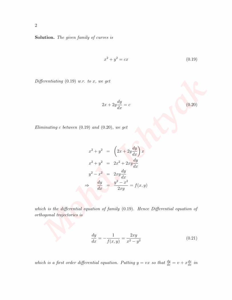
Example 4.48/p.136 Find the orthogonal trajectories of x2 + y2 = cx.
1
Moh
d.Ish
tyak
2
Solution. The given family of curves is
x2 + y2 = cx (0.19)
Differentiating (0.19) w.r. to x, we get
2x+ 2ydy
dx= c (0.20)
Eliminating c between (0.19) and (0.20), we get
x2 + y2 =
(2x+ 2y
dy
dx
)x
x2 + y2 = 2x2 + 2xydy
dx
y2 − x2 = 2xydy
dx
⇒ dy
dx=
y2 − x2
2xy= f(x, y)
which is the differential equation of family (0.19). Hence Differential equation of
orthogonal trajectories is
dy
dx= − 1
f(x, y)=
2xy
x2 − y2(0.21)
which is a first order differential equation. Putting y = vx so that dydx
= v + x dvdx
in
Moh
d.Ish
tyak
3
(0.21), we get
v + xdv
dx=
2x(vx)
x2 − (vx)2
v + xdv
dx=
2v
1− v2
xdv
dx=
2v
1− v2− v
xdv
dx=
2v − v(1− v2)1− v2
=2v − v + v3
1− v2
xdv
dx=
v + v3
1− v2
xdv
dx=
v(1 + v2)
1− v21− v2
v(1 + v2)dv =
dx
x
[(1 + v2)− 2v2]
v(1 + v2)dv =
dx
x
dv
v− 2v
1 + v2dv =
dx
x
On integrating, we get
log v − log(1 + v2) = log x+ log av
1 + v2= ax
Putting v = yx
in above equation, we get
y/x
1 + (y/x)2= ax
⇒ yx
x2 + y2= ax
⇒ x2 + y2 =1
ay
or
x2 + y2 = by,
where 1a
= b, which is the desired orthogonal trajectories.
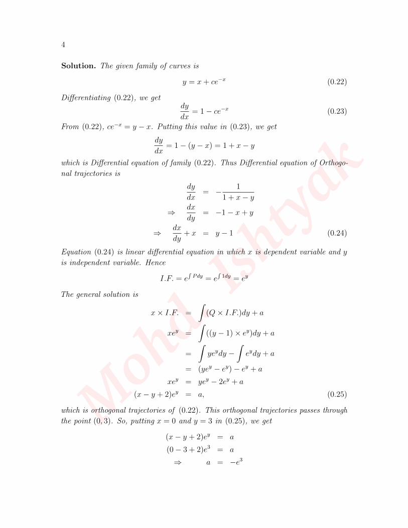
Example 4.49/p.137 Find the orthogonal trajectories of the family y = x+ ce−x
and determine that particular member of each family that passes through (0, 3).
Moh
d.Ish
tyak
4
Solution. The given family of curves is
y = x+ ce−x (0.22)
Differentiating (0.22), we getdy
dx= 1− ce−x (0.23)
From (0.22), ce−x = y − x. Putting this value in (0.23), we get
dy
dx= 1− (y − x) = 1 + x− y
which is Differential equation of family (0.22). Thus Differential equation of Orthogo-
nal trajectories is
dy
dx= − 1
1 + x− y
⇒ dx
dy= −1− x+ y
⇒ dx
dy+ x = y − 1 (0.24)
Equation (0.24) is linear differential equation in which x is dependent variable and y
is independent variable. Hence
I.F. = e∫Pdy = e
∫1dy = ey
The general solution is
x× I.F. =
∫(Q× I.F.)dy + a
xey =
∫((y − 1)× ey)dy + a
=
∫yeydy −
∫eydy + a
= (yey − ey)− ey + a
xey = yey − 2ey + a
(x− y + 2)ey = a, (0.25)
which is orthogonal trajectories of (0.22). This orthogonal trajectories passes through
the point (0, 3). So, putting x = 0 and y = 3 in (0.25), we get
(x− y + 2)ey = a
(0− 3 + 2)e3 = a
⇒ a = −e3
Moh
d.Ish
tyak
5
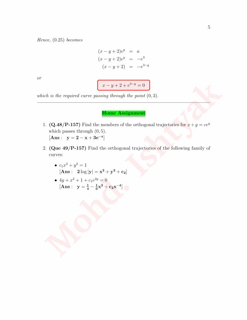
Hence, (0.25) becomes
(x− y + 2)ey = a
(x− y + 2)ey = −e3
(x− y + 2) = −e3−y
or
x− y + 2 + e3−y = 0
which is the required curve passing through the point (0, 3).
Home Assignment
1. (Q.48/P-157) Find the members of the orthogonal trajectories for x+ y = cey
which passes through (0, 5).
[Ans : y = 2− x + 3e−x]
2. (Que 49/P-157) Find the orthogonal trajectories of the following family of
curves:
• c1x2 + y2 = 1
[Ans : 2 log |y| = x2 + y2 + c2]
• 4y + x2 + 1 + c1e2y = 0
[Ans : y = 14− 1
6x2 + c2x
−4]
Moh
d.Ish
tyak
Lecture No. 07
Orthogonal Trajectories in Polar Coordinates(A topic of Unit I)
Consider the equation of the family of curves in polar form:
F (r, θ, c) = 0 (0.26)
where c is a parameter. Differential equation of family (0.26) is of the form:
f
(r, θ,
dr
dθ
)= 0 (0.27)
Replacing drdθ
by −r2 dθdr
in (0.27), we obtain the differential equation of orthogonal
trajectories of the family (0.26) given by
f
(r, θ,−r2dθ
dr
)= 0 (0.28)
On solving (0.28), we get the equation of orthogonal trajectories of (0.26).
Example 4.51/p.138 Find the equation of the orthogonal trajectory of the family
of circles having a polar equation r = f(θ) = 2a cos θ.
Solution. The given family of curves is
r = 2a cos θ (0.29)
Differentiating (0.29) w.r. to θ, we get
dr
dθ= −2a sin θ (0.30)
1
Moh
d.Ish
tyak
2
From (0.29), we have 2a = rcos θ
. Using this, (0.30) becomes
dr
dθ= −2a sin θ
dr
dθ= −
( r
cos θ
)sin θ
dr
dθ= −r tan θ
which is differential equation of family of (0.29).
Hence, differential equation of orthogonal trajectories is
−r2dθdr
= −r tan θ
rdθ
dr= tan θ
⇒ dθ
tan θ=
dr
r
⇒ cos θ
sin θdθ =
dr
r
On integrating, we get∫cos θ
sin θdθ + c′ =
∫dr
r
log sin θ + log 2a = log r, where c′ = log 2a
⇒ r = 2a sin θ
which is the required equation of orthogonal trajectories.
Example 4.52/p.139 Find the orthogonal trajectories of r = c1(1− sin θ).
Solution. The given family of curves is
r = c1(1− sin θ) (0.31)
Differentiating (0.31) w.r. to θ, we get
dr
dθ= −c1 cos θ (0.32)
Dividing (0.32) by (0.31) (to eliminate c), we have
1
r
dr
dθ= − cos θ
1− sin θ
⇒ dr
dθ= − r cos θ
1− sin θ
Moh
d.Ish
tyak
3
which is differential equation of family of (0.31).
Hence, the differential equation of orthogonal trajectories is
−r2dθdr
= − r cos θ
1− sin θ
⇒ rdθ
dr=
cos θ
1− sin θ
⇒ dr
r=
1− sin θ
cos θdθ
⇒ dr
r= (sec θ − tan θ)dθ
On integrating, we get
log r = log(sec θ + tan θ) + log cos θ + log a
log r = log[(sec θ + tan θ) cos θa]
⇒ log r = log[a(1 + sin θ)]
r = a(1 + sin θ)
which is the required equation of orthogonal trajectories of family (0.31).
Home Assignment
Find the orthogonal trajectories of the following family of curves:
1. (Q.) r2 = c sin 2θ
[Ans : r2 = a cos 2θ]
2. (Q.) r = c(sec θ + tan θ)
[Ans : r = ae− sin θ]
Moh
d.Ish
tyak
Lecture No. 08
Nonlinear ODEs solvable for p(A topic of Unit I)
Differential Equations of first order but not of the first degree: The general form of
differential equation of first order and nth(n > 1) degree, is(dy
dx
)n+ a1
(dy
dx
)n−1+ a2
(dy
dx
)n−2+ · · ·+ an−1
(dy
dx
)+ an = 0 (0.33)
or pn + a1pn−1 + a2p
n−2 + · · ·+ an−1p+ an = 0
where, p = dydx
and aa, a2, cdots, an−1 and an are the functions of x and y.
The equation (0.33) can be written as
f(x, y, p) = 0
Solution of the Differential Equation (0.33): We have the following two cases:
1. Differential Equation (0.33) can be written as product of first degree factors.
2. It can not be resolved into factors of first degree.
Case I: Equations solvable for p: In this case, Differential equation (0.33) is of
the form
[p− f1(x, y)][p− f2(x, y)][p− f3(x, y)] · · · [p− fn(x, y)] = 0. (0.34)
Now, equating each factor to zero,
p− fi(x, y) = 0, i = 1, 2, cdots, n
Let the solutions of these factors be
φ(x, y, ci) = 0, i = 1, 2, · · · , n
Taking, c1 = c2 = c3 = · · · = cn = c, hence required solution is
φ1(x, y, c)φ2(x, y, c) · · ·φn(x, y, c) = 0
1
Moh
d.Ish
tyak
2
Remark. Since the differential equation (0.33) is of first order, therefore its solution
contains only one arbitrary constant.
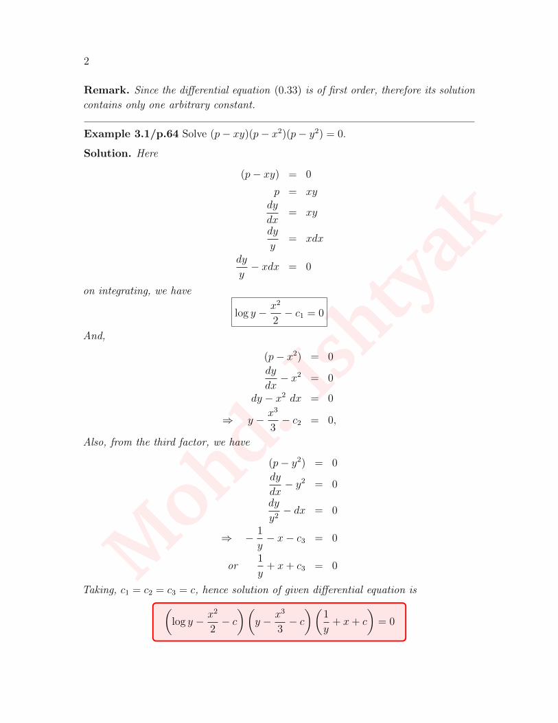
Example 3.1/p.64 Solve (p− xy)(p− x2)(p− y2) = 0.
Solution. Here
(p− xy) = 0
p = xydy
dx= xy
dy
y= xdx
dy
y− xdx = 0
on integrating, we have
log y − x2
2− c1 = 0
And,
(p− x2) = 0
dy
dx− x2 = 0
dy − x2 dx = 0
⇒ y − x3
3− c2 = 0,
Also, from the third factor, we have
(p− y2) = 0
dy
dx− y2 = 0
dy
y2− dx = 0
⇒ − 1
y− x− c3 = 0
or1
y+ x+ c3 = 0
Taking, c1 = c2 = c3 = c, hence solution of given differential equation is(log y − x2
2− c)(
y − x3
3− c)(
1
y+ x+ c
)= 0
Moh
d.Ish
tyak
3
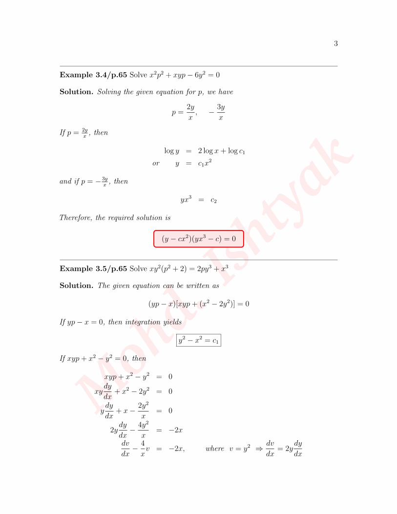
Example 3.4/p.65 Solve x2p2 + xyp− 6y2 = 0
Solution. Solving the given equation for p, we have
p =2y
x, − 3y
x
If p = 2yx
, then
log y = 2 log x+ log c1
or y = c1x2
and if p = −3yx
, then
yx3 = c2
Therefore, the required solution is
(y − cx2)(yx3 − c) = 0
Example 3.5/p.65 Solve xy2(p2 + 2) = 2py3 + x3
Solution. The given equation can be written as
(yp− x)[xyp+ (x2 − 2y2)] = 0
If yp− x = 0, then integration yields
y2 − x2 = c1
If xyp+ x2 − y2 = 0, then
xyp+ x2 − y2 = 0
xydy
dx+ x2 − 2y2 = 0
ydy
dx+ x− 2y2
x= 0
2ydy
dx− 4y2
x= −2x
dv
dx− 4
xv = −2x, where v = y2 ⇒ dv
dx= 2y
dy
dx
Moh
d.Ish
tyak
4
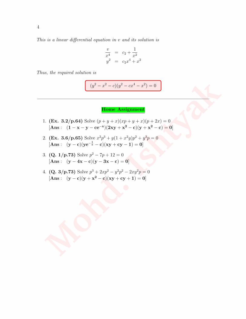
This is a linear differential equation in v and its solution is
v
x4= c2 +
1
x2
y2 = c2x4 + x2
Thus, the required solution is
(y2 − x2 − c)(y2 − cx4 − x2) = 0
Home Assignment
1. (Ex. 3.2/p.64) Solve (p+ y + x)(xp+ y + x)(p+ 2x) = 0
[Ans : (1− x− y − ce−x)(2xy + x2 − c)(y + x2 − c) = 0]
2. (Ex. 3.6/p.65) Solve x2p3 + y(1 + x2y)p2 + y3p = 0
[Ans : (y − c)(ye−1x − c)(xy + cy − 1) = 0]
3. (Q. 1/p.73) Solve p2 − 7p+ 12 = 0
[Ans : (y − 4x− c)(y − 3x− c) = 0]
4. (Q. 3/p.73) Solve p3 + 2xp2 − y2p2 − 2xy2p = 0
[Ans : (y − c)(y + x2 − c)(xy + cy + 1) = 0]
Moh
d.Ish
tyak
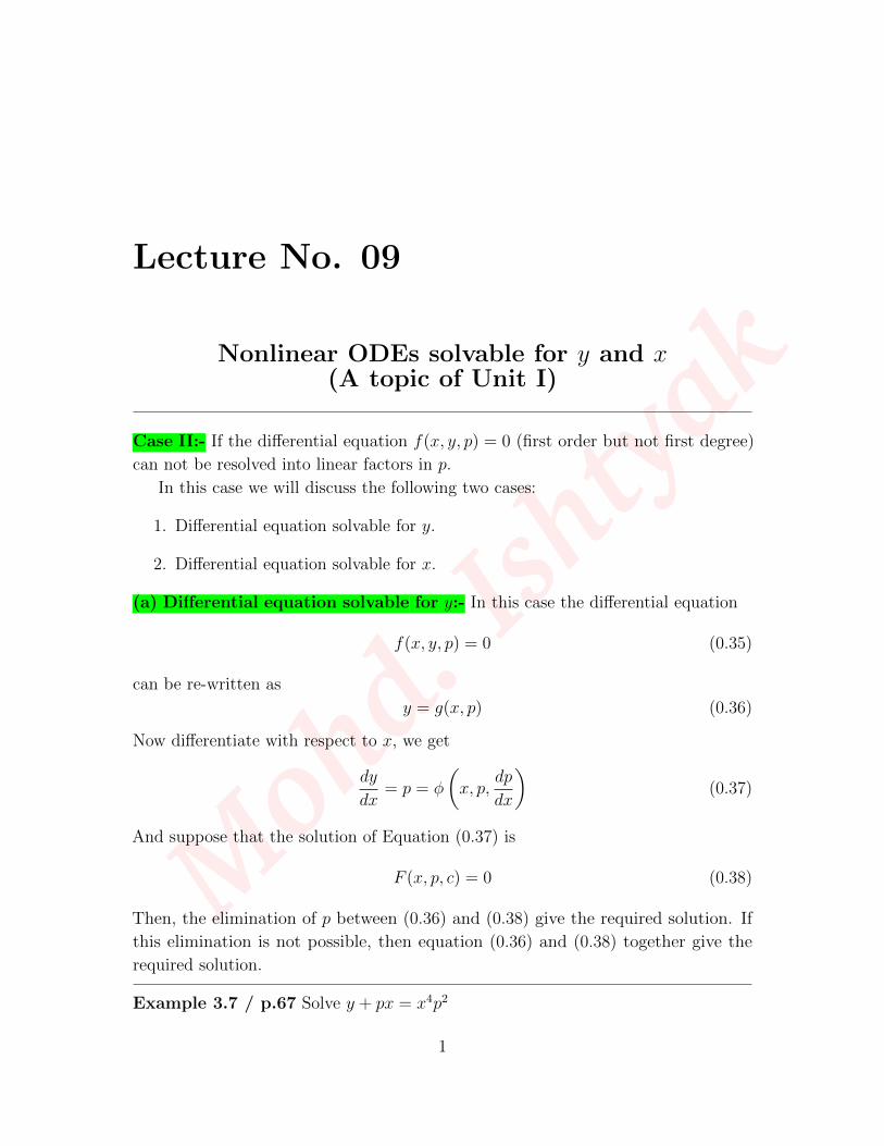
Lecture No. 09
Nonlinear ODEs solvable for y and x(A topic of Unit I)
Case II:- If the differential equation f(x, y, p) = 0 (first order but not first degree)
can not be resolved into linear factors in p.
In this case we will discuss the following two cases:
1. Differential equation solvable for y.
2. Differential equation solvable for x.
(a) Differential equation solvable for y:- In this case the differential equation
f(x, y, p) = 0 (0.35)
can be re-written as
y = g(x, p) (0.36)
Now differentiate with respect to x, we get
dy
dx= p = φ
(x, p,
dp
dx
)(0.37)
And suppose that the solution of Equation (0.37) is
F (x, p, c) = 0 (0.38)
Then, the elimination of p between (0.36) and (0.38) give the required solution. If
this elimination is not possible, then equation (0.36) and (0.38) together give the
required solution.
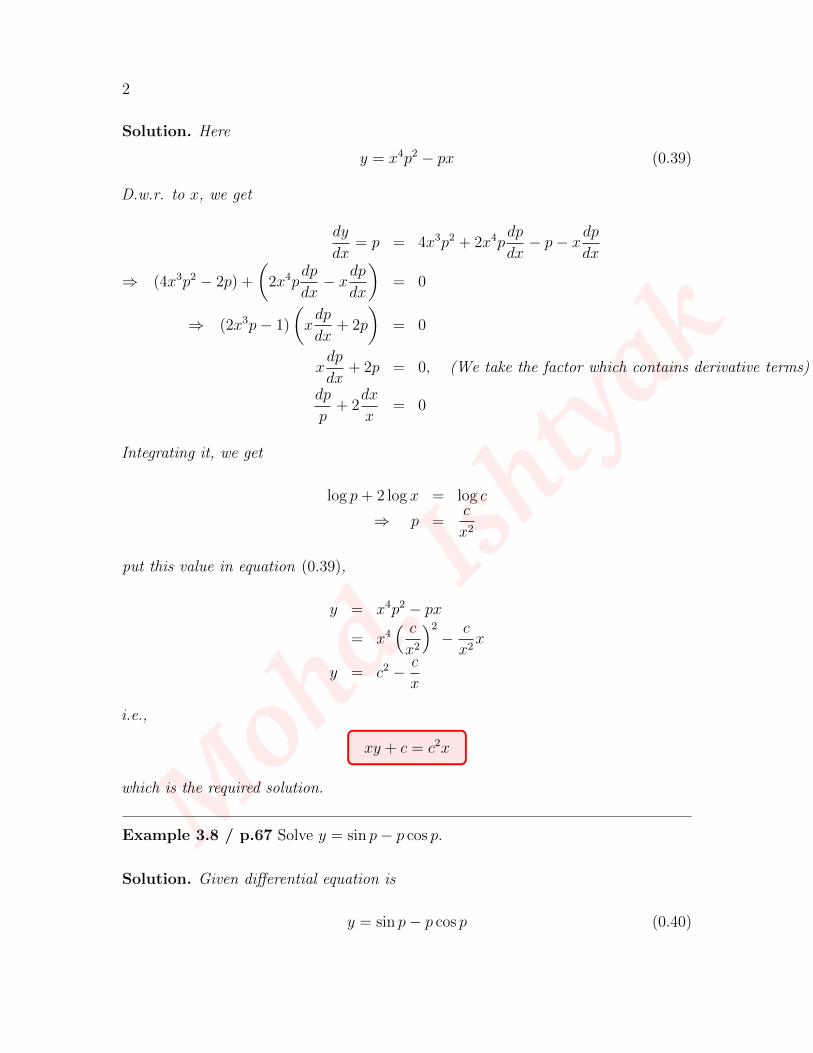
Example 3.7 / p.67 Solve y + px = x4p2
1
Moh
d.Ish
tyak
2
Solution. Here
y = x4p2 − px (0.39)
D.w.r. to x, we get
dy
dx= p = 4x3p2 + 2x4p
dp
dx− p− xdp
dx
⇒ (4x3p2 − 2p) +
(2x4p
dp
dx− xdp
dx
)= 0
⇒ (2x3p− 1)
(xdp
dx+ 2p
)= 0
xdp
dx+ 2p = 0, (We take the factor which contains derivative terms)
dp
p+ 2
dx
x= 0
Integrating it, we get
log p+ 2 log x = log c
⇒ p =c
x2
put this value in equation (0.39),
y = x4p2 − px
= x4( cx2
)2− c
x2x
y = c2 − c
x
i.e.,
xy + c = c2x
which is the required solution.
Example 3.8 / p.67 Solve y = sin p− p cos p.
Solution. Given differential equation is
y = sin p− p cos p (0.40)
Moh
d.Ish
tyak
3
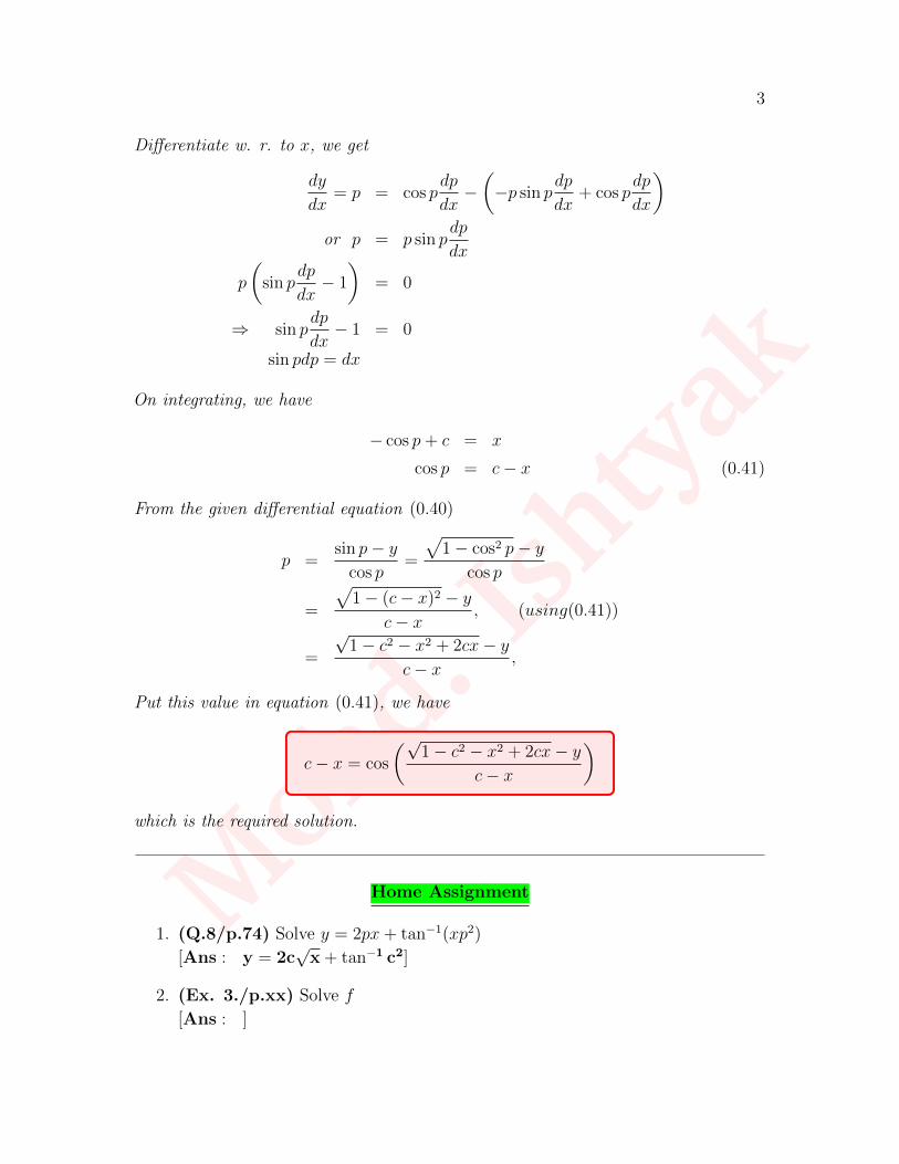
Differentiate w. r. to x, we get
dy
dx= p = cos p
dp
dx−(−p sin p
dp
dx+ cos p
dp
dx
)or p = p sin p
dp
dx
p
(sin p
dp
dx− 1
)= 0
⇒ sin pdp
dx− 1 = 0
sin pdp = dx
On integrating, we have
− cos p+ c = x
cos p = c− x (0.41)
From the given differential equation (0.40)
p =sin p− y
cos p=
√1− cos2 p− y
cos p
=
√1− (c− x)2 − y
c− x, (using(0.41))
=
√1− c2 − x2 + 2cx− y
c− x,
Put this value in equation (0.41), we have
c− x = cos
(√1− c2 − x2 + 2cx− y
c− x
)
which is the required solution.
Home Assignment
1. (Q.8/p.74) Solve y = 2px+ tan−1(xp2)
[Ans : y = 2c√
x + tan−1 c2]
2. (Ex. 3./p.xx) Solve f
[Ans : ]
Moh
d.Ish
tyak
4
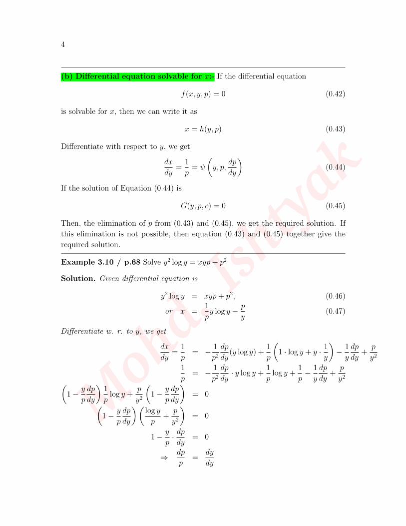
(b) Differential equation solvable for x:- If the differential equation
f(x, y, p) = 0 (0.42)
is solvable for x, then we can write it as
x = h(y, p) (0.43)
Differentiate with respect to y, we get
dx
dy=
1
p= ψ
(y, p,
dp
dy
)(0.44)
If the solution of Equation (0.44) is
G(y, p, c) = 0 (0.45)
Then, the elimination of p from (0.43) and (0.45), we get the required solution. If
this elimination is not possible, then equation (0.43) and (0.45) together give the
required solution.
Example 3.10 / p.68 Solve y2 log y = xyp+ p2
Solution. Given differential equation is
y2 log y = xyp+ p2, (0.46)
or x =1
py log y − p
y(0.47)
Differentiate w. r. to y, we get
dx
dy=
1
p= − 1
p2dp
dy(y log y) +
1
p
(1 · log y + y · 1
y
)− 1
y
dp
dy+
p
y2
1
p= − 1
p2dp
dy· y log y +
1
plog y +
1
p− 1
y
dp
dy+
p
y2(1− y
p
dp
dy
)1
plog y +
p
y2
(1− y
p
dp
dy
)= 0(
1− y
p
dp
dy
)(log y
p+
p
y2
)= 0
1− y
p· dpdy
= 0
⇒ dp
p=
dy
dy
Moh
d.Ish
tyak
5
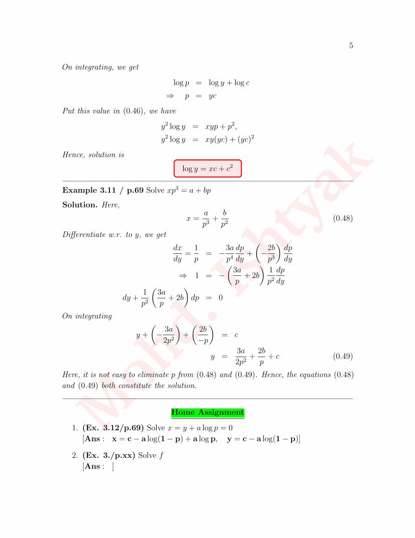
On integrating, we get
log p = log y + log c
⇒ p = yc
Put this value in (0.46), we have
y2 log y = xyp+ p2,
y2 log y = xy(yc) + (yc)2
Hence, solution is
log y = xc+ c2
Example 3.11 / p.69 Solve xp3 = a+ bp
Solution. Here,
x =a
p3+
b
p2(0.48)
Differentiate w.r. to y, we get
dx
dy=
1
p= −3a
p4dp
dy+
(−2b
p3
)dp
dy
⇒ 1 = −(
3a
p+ 2b
)1
p2dp
dy
dy +1
p2
(3a
p+ 2b
)dp = 0
On integrating
y +
(− 3a
2p2
)+
(2b
−p
)= c
y =3a
2p2+
2b
p+ c (0.49)
Here, it is not easy to eliminate p from (0.48) and (0.49). Hence, the equations (0.48)
and (0.49) both constitute the solution.
Home Assignment
1. (Ex. 3.12/p.69) Solve x = y + a log p = 0
[Ans : x = c− a log(1− p) + a log p, y = c− a log(1− p)]
2. (Ex. 3./p.xx) Solve f
[Ans : ]

Moh
d.Ish
tyak
Lecture No. 10
Clairaut and Lagrange Equation(A topic of Unit I)
The most general form of a differential equation of the first order but not of the first
degree (say nth degree) is(dy
dx
)n+ P1
(dy
dx
)n−1+ P2
(dy
dx
)n−2+ · · ·+ Pn−1
(dy
dx
)+ Pn = 0 (0.50)
or pn + P1pn−1 + P2p
n−2 + · · ·+ Pn−1p+ Pn = 0
where p = dydx
and P1, P2, · · · , Pn are functions of x and y. This equation can also be
written as
F (x, y, p) = 0. (0.51)
The above equation however can not be solved in this general form.
The Clairaut Equation
When the given equation (0.51) is of the first degree in x and y, and of the form
y = px+ f(p) (0.52)
Equation (0.52) is known as Clairaut’s equation. To solve it, we differentiate with
respect to x to obtain
p =dy
dx= [x+ f
′(p)]p
′+ p
or [x+ f′(p)]
dp
dx= 0 (0.53)
If dp/dx = 0, then p = c = constant. Eliminating p between this and equation (0.52),
we get
y = cx+ f(c) (0.54)
which is required solution of Clairaut’s equation.
1
Moh
d.Ish
tyak
2
Remark 3. Sometimes by a suitable substitution, an equation can be reduced to
Clairaut’s form.
Example (3.13/P-71) Solve (y − px)(p− 1) = p.
Solution. The given equation can be written as
y = xp+p
p− 1,
which is a Clairaut equation. Hence the solution is
y = xc+c
c− 1,
y =xc(c− 1) + c
(c− 1)
y(c− 1) = xc(c− 1) + c
y(c− 1)− xc(c− 1) = c
i.e., which is the required solution.
Example (3.14/P-71) Solve p = log(px− y)
Solution. The given equation is
y = px− ep.
Which is a Clairaut equation. Hence the solution is
y = cx− ec
ec = cx− y,
i.e.,
c = log(cx− y)
Example (3.17/P-73) Solve (px− y)(py + x) = h2p.
Solution. This equation can be written as
p2xy + px2 − py2 − xy = h2p
p2xy − xy + px2 − py2 − h2p = 0
p2xy − xy + p(x2 − y2 − h2) = 0,
Moh
d.Ish
tyak
3
Putting x2 = u⇒ 2xdx = du and y2 = v ⇒ 2ydy = dv, and p =dy
dx=x
y
dv
duthe given
equation takes the form
p2xy − xy + p(x2 − y2 − h2) = 0(x
y
dv
dv
)2
xy − xy +x
y
dv
du(u− v − h2) = 0
x2
y
(dv
dv
)2
− y +1
y
dv
du(u− v − h2) = 0
x2(dv
dv
)2
− y2 +dv
du(u− v − h2) = 0
u
(dv
dv
)2
− v +dv
du(u− v − h2) = 0
or uP 2 + (u− v − h2)P − v = 0, where P =dv
du
or v = uP − h2P
P + 1
which is of Clairaut‘s form and has the solution as
v = uc− h2c
c+ 1
where u = x2 and v = y2. i.e.,
y2 = x2c− h2c
c+ 1.
Home Assignment
1. (Example 3.18/P-73) Solve y = 2px+ y2p3.
[Ans : y2 = cx + 18c3]
2. (Que 21/P-74) sin px cos y = cos px sin y + p,
[Ans : y = cx− sin−1 c]
3. (Que 22/P-74) xy(y − px) = x+ py,
[Ans : y2 = cx2 + (1 + c)]
4. (Que 24/P-74) Solve x2p2 + yp(2x+ y) + y2 = 0 by reducing it to Clairaut’s
form by using the substitution y = u and xy = v.
[Ans : xy = cy + c]

Moh
d.Ish
tyak
4
[RB1] The Lagrange Equation
An equation of the form
y = xf1(p) + f2(p) (0.55)
is known as Lagrange’s Equation. To solve it, we differentiate with respect to x to
obtain
p =dy
dx= f1(p) + xf
′
1(p)dp
dx+ f
′
2(p)dp
dx
p− f1(p) =dp
dx[xf
′
1(p) + f′
2(p)]
dx
dp=
xf′1(p) + f
′2(p)
p− f1(p)
ordx
dp− f
′1(p)
p− f1(p)x =
f′2(p)
p− f1(p)(0.56)
which is a linear equation in x, and hence can be solved in the form
x = φ(p, c) (0.57)
eliminating p from equations (0.55) and (0.57), we get the required solution. If it is
not possible to eliminate p, then the values of x and y in terms of p can be found
from equations (0.55) and (0.57), and these will constitute the required solution.
Note. The Clairaut Equation is the particular case of the Lagrange Equation.
Example 2/ P.46 Solve the equation y = xp2 − 1p.
Solution. This equation is Lagrange equation. Differentiating it w.r.t. x, we get
dy
dx= p = x
(2pdp
dx
)+ p2(1)−
(− 1
p2
)dp
dx
p− p2 =
[2xp+
1
p2
]dp
dx
dx
dp=
2xp+ 1p2
p− p2dx
dp=
2xp
p− p2+
1
p2(p− p2)
⇒ dx
dp+
2x
p− 1= − 1
p3(p− 1)
Moh
d.Ish
tyak
5
This equation is linear in x [An equation is linear if it is of the form dydx
+ Py = Q].
Therefore
I.F. = e∫
2p−1
dp = elog(p−1)2
= (p− 1)2
On integrating, we get
x.(I.F.) =
∫(I.F.)Qdp
x(p− 1)2 =
∫ {(p− 1)2
(− 1
p3(p− 1)
)}dp
x(p− 1)2 = −∫ (
p− 1
p3
)dp
x(p− 1)2 = −∫ {
1
p2− 1
p3
}dp
x(p− 1)2 = c1 +1
p− 1
2p2
x(p− 1)2 =2c1p
2 + 2p− 1
2p2
x =2c1p
2 + 2p− 1
2p2(p− 1)2
x =cp2 + 2p− 1
2p2(p− 1)2(0.58)
Substituting this value of x in the given equation, we get
y = xp2 − 1
p
y =cp2 + 2p− 1
2(p− 1)2− 1
p(0.59)
Equations (0.58) and (0.59) together give the required solution. Hence,
x =cp2 + 2p− 1
2p2(p− 1)2, y =
cp2 + 2p− 1
2(p− 1)2− 1
p
Example 4 /P.47 Solve the equation y = 2px+ pn.

Moh
d.Ish
tyak
6
Solution. This equation is Lagrange equation. Differentiating it w.r.t. x, we get
dy
dx= p = 2p.(1) + x.
(2dp
dx
)+ npn−1
dp
dx
p = 2p+ (2x+ npn−1)dp
dx
−p = (2x+ npn−1)dp
dxdx
dp=
2x+ npn−1
−p
⇒ dx
dp+
2
px = −npn−2
This equation is linear in x. Therefore
I.F. = e∫(2/p)dp = e2 log p = elog p
2
= p2
On integrating, we get
x.(I.F.) =
∫(I.F.)Qdp
x.p2 =
∫ {p2.(−npn−2)
}dp
x.p2 = −∫npndp
xp2 = − n
n+ 1pn+1 + c
⇒ x =c
p2− n
n+ 1pn−1 (0.60)
Substituting this value of x in the given equation, we get
y = 2px+ pn
y = 2p
[c
p2− n
n+ 1pn−1
]+ pn
y =2c
p− 2n
n+ 1pn + pn
y =2c
p− (n− 1)
(n+ 1)pn (0.61)
Equation (0.60) and (0.61) together give the required solution. Hence,
x =c
p2− n
n+ 1pn−1, y =
2c
p− (n− 1)
(n+ 1)pn
Moh
d.Ish
tyak
7
Home Assignment
1. (Ex 7/ p-48) Solve y = x(1 + p) + p2
[Ans : x = 2(1− p) + ce−p, y = {2(1− p) + ce−p}(1 + p) + p2]
2. (M Ex.8/ p-48) Solve y = xp2 + p
[Ans : x = (log p− p + c)(p− 1)−2, y = xp2 + p]
3. (M Ex.10/ p-48) Solve y = 32xp+ ep
[Ans : x = cp3 − 2ep
(1p− 2
p2 + 2p3
), y = 3c
2p2 − 2ep(1− 3
p+ 3
p2
)]
Moh
d.Ish
tyak
Lecture No. 11
The Singular Solution of a First order ODE1
(A topic of Unit I)
Consider the ordinary differential equation
f(x, y, p) = 0, where p =dy
dx. (0.62)
In Lecture 1, we have already discussed the two types of solution of an ordinary
differential equation namely: general solution and particular solution.
In case of differential equation (0.62), its general solution will contain an arbitrary
constant c, and therefore the general solution of differential equation (0.62) is of the
form
g(x, y, c) = 0. (0.63)
Recall that, any particular solution of equation (0.62) can be obtained from (0.63)
by substituting the suitable values of c.
Besides general solution and particular solution, there is another type of solution
of equation (0.62), which is called Singular solution.
Definition 1. A singular solution of equation (0.62) is a solution, which is free from
arbitrary constants but not a particular solution of the equation.
For example, consider the first order differential equation
y = xp+√
1 + p2.
Here, x2 + y2 = a2 is the singular solution of above equation as it can not be derived
from its general solution y = cx +√
(1 + c2) by assigning values to the arbitrary
constant c.1The Content of this lecture is based on the reference book
”Frank Ayres, Jr: Theory and Problems of Differential Equations (Schaum‘s Outline Series)”
1
Moh
d.Ish
tyak
2
Note. An equation of the first order does not have singular solutions; if it is of the
first degree it can not have singular solutions.
Discriminant Relations:
p-discriminant relation: The p-discriminant relation of the equation (0.62) can be
obtain by eliminating p between equation (0.62) and
∂f
∂p= 0.
c-discriminant relation: The c-discriminant relation of the equation (0.62) can be
obtain by eliminating c between equation (0.63) and
∂g
∂c= 0.
Ex 1/p-70 Find the discriminant relations for each of the following:
1. p3 + px− y = 0,
2. [HA] p3x− 2p2y − 16x2 = 0,
3. y = C(x− C)2
Solution 1. The given equation is
f(x, y, p) = p3 + px− y = 0; (0.64)
and∂f
∂p= 3p2 + x = 0. (0.65)
eliminate p between (0.64) and (0.65) as follows:
Multiply (0.65) with p, we get
3p3 + px = 0 (0.66)
Now, {(0.66)− (0.64)}, we get
(3p3 + px)− (p3 + px− y) = 0
2p3 + y = 0
p =(−y
2
) 13
Moh
d.Ish
tyak
3
substitute the value of p in (0.64), we get
p3 + px− y = 0
−y2
+(−y
2
) 13x− y = 0(
−y2
) 13x− 3
2y = 0(
−y2
) 13x =
3
2y
−y2x3 =
27
8y3
27y3 + 4yx3 = 0
Hence the required p-discriminant relation is
4x3 + 27y2 = 0.
Remark 4. If f(x, y, p) = 0 is of the degree n in p, we eliminate p between nf−p∂f∂p
=
0 and ∂f∂p
= 0.
Solution 2. Do yourself.
Solution 3. The given equation is
g(x, y, c) = cx2 − 2c2x+ c3 − y = 0 (0.67)
and∂g
∂c= x2 − 4cx+ 3c2 = 0 (0.68)
Now we eliminate c from (0.67) and (0.68) as:
Multiply (0.68) with c, we get
cx2 − 4c2x+ 3c3 = 0 (0.69)
Now, {(0.69)− 3× (0.67)}, we get
(cx2 − 4c2x+ 3c3)− 3(cx2 − 2c2x+ c3 − y) = 0
−2cx2 + 2c2x+ 3y = 0 (0.70)
Now, Multiplying {3× (0.70)− 2x× (0.68)} , we have
3(−2cx2 + 2c2x+ 3y)− 2x(x2 − 4cx+ 3c2) = 0
−2cx2 + 2x3 − 9y = 0
⇒ c =2x3 − 9y
2x2
Moh
d.Ish
tyak
4
substitute the value of c in (0.68), we get
x2 − 4cx+ 3c2 = 0
x2 − 4
(2x3 − 9y
2x2
)x+ 3
(2x3 − 9y
2x2
)2
= 0
After simplification, the required c-discriminant relation is
y(4x3 − 27y) = 0.
Extraneous Loci Let h(x, y) = 0 be the singular solution of the differential equation
(0.62). Also suppose that
C(x, y) = 0
and
P (x, y) = 0
are the c-discriminant and p-discriminant relations, respectively of equation (0.62).
Then h(x, y) will be a factor of each of C(x, y) and P (x, y). Thus
C(x, y) = h(x, y)E1(x, y)
and
P (x, y) = h(x, y)E2(x, y).
The relations E1(x, y) = 0 and E2(x, y) = 0 generally do not satisfy the differential
equation (0.62). Such relations are called extraneous. Usually there are three special
types of extraneous loci.
1. Tac Locus
2. Nodal Locus
3. Cusp Locus
Determination of Singular Solutions and extraneous loci: An equation which
posses a singular solution is not considered completely solved until the singular
solution has been found.
Method 1 (Using c-discriminant relation): Whenever we determine the c-
discriminant relation C(x, y) = 0 of equation (0.62) then C(x, y) includes as a factor
(after equating to 0) as follows:
Moh
d.Ish
tyak
5
1. singular solution once.
2. cuspidal locus three times.
3. the nodel locus twice.
Method 2 (Using p-discriminant relation): Whenever we determine the p-
discriminant relation P (x, y) = 0, of the differential equation (0.62); then p-discriminant
P (x, y), includes as a factor (after equating to 0) as follows:
1. singular solution once.
2. the cuspidal locus once.
3. the tac locus twice.
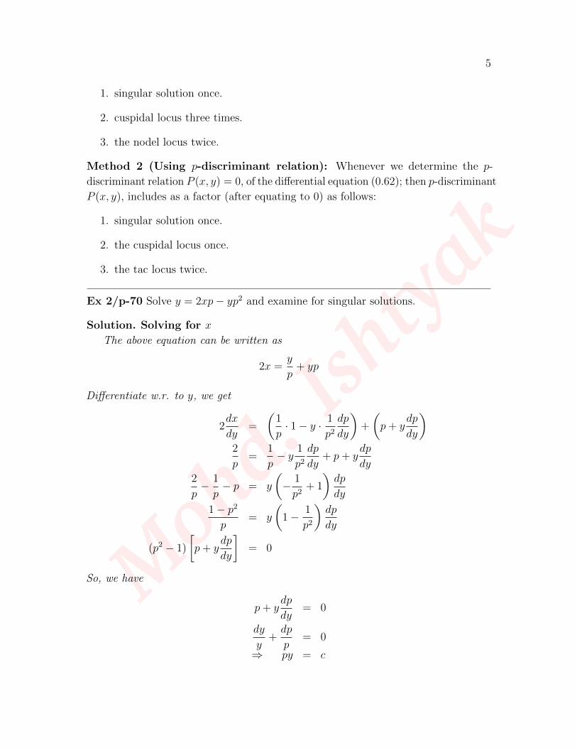
Ex 2/p-70 Solve y = 2xp− yp2 and examine for singular solutions.
Solution. Solving for x
The above equation can be written as
2x =y
p+ yp
Differentiate w.r. to y, we get
2dx
dy=
(1
p· 1− y · 1
p2dp
dy
)+
(p+ y
dp
dy
)2
p=
1
p− y 1
p2dp
dy+ p+ y
dp
dy
2
p− 1
p− p = y
(− 1
p2+ 1
)dp
dy
1− p2
p= y
(1− 1
p2
)dp
dy
(p2 − 1)
[p+ y
dp
dy
]= 0
So, we have
p+ ydp
dy= 0
dy
y+dp
p= 0
⇒ py = c
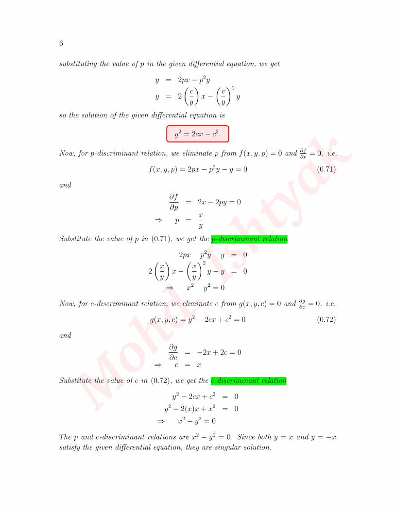
Moh
d.Ish
tyak
6
substituting the value of p in the given differential equation, we get
y = 2px− p2y
y = 2
(c
y
)x−
(c
y
)2
y
so the solution of the given differential equation is
y2 = 2cx− c2.
Now, for p-discriminant relation, we eliminate p from f(x, y, p) = 0 and ∂f∂p
= 0. i.e.
f(x, y, p) = 2px− p2y − y = 0 (0.71)
and
∂f
∂p= 2x− 2py = 0
⇒ p =x
y
Substitute the value of p in (0.71), we get the p-discriminant relation
2px− p2y − y = 0
2
(x
y
)x−
(x
y
)2
y − y = 0
⇒ x2 − y2 = 0
Now, for c-discriminant relation, we eliminate c from g(x, y, c) = 0 and ∂g∂c
= 0. i.e.
g(x, y, c) = y2 − 2cx+ c2 = 0 (0.72)
and
∂g
∂c= −2x+ 2c = 0
⇒ c = x
Substitute the value of c in (0.72), we get the c-discriminant relation
y2 − 2cx+ c2 = 0
y2 − 2(x)x+ x2 = 0
⇒ x2 − y2 = 0
The p and c-discriminant relations are x2 − y2 = 0. Since both y = x and y = −xsatisfy the given differential equation, they are singular solution.
Moh
d.Ish
tyak
7
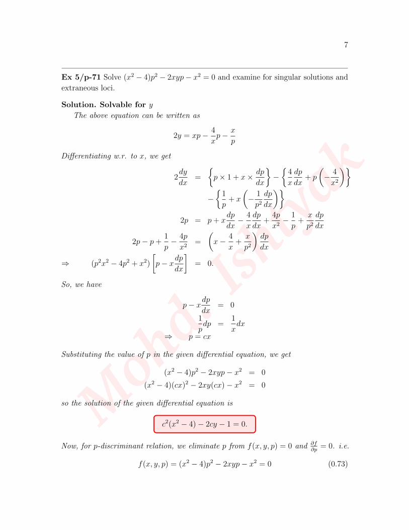
Ex 5/p-71 Solve (x2 − 4)p2 − 2xyp− x2 = 0 and examine for singular solutions and
extraneous loci.
Solution. Solvable for y
The above equation can be written as
2y = xp− 4
xp− x
p
Differentiating w.r. to x, we get
2dy
dx=
{p× 1 + x× dp
dx
}−{
4
x
dp
dx+ p
(− 4
x2
)}−{
1
p+ x
(− 1
p2dp
dx
)}2p = p+ x
dp
dx− 4
x
dp
dx+
4p
x2− 1
p+x
p2dp
dx
2p− p+1
p− 4p
x2=
(x− 4
x+x
p2
)dp
dx
⇒ (p2x2 − 4p2 + x2)
[p− xdp
dx
]= 0.
So, we have
p− xdpdx
= 0
1
pdp =
1
xdx
⇒ p = cx
Substituting the value of p in the given differential equation, we get
(x2 − 4)p2 − 2xyp− x2 = 0
(x2 − 4)(cx)2 − 2xy(cx)− x2 = 0
so the solution of the given differential equation is
c2(x2 − 4)− 2cy − 1 = 0.
Now, for p-discriminant relation, we eliminate p from f(x, y, p) = 0 and ∂f∂p
= 0. i.e.
f(x, y, p) = (x2 − 4)p2 − 2xyp− x2 = 0 (0.73)
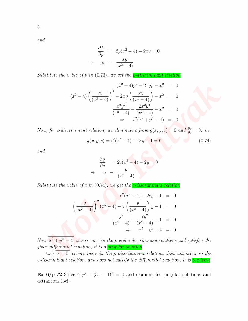
Moh
d.Ish
tyak
8
and
∂f
∂p= 2p(x2 − 4)− 2xy = 0
⇒ p =xy
(x2 − 4)
Substitute the value of p in (0.73), we get the p-discriminant relation
(x2 − 4)p2 − 2xyp− x2 = 0
(x2 − 4)
(xy
(x2 − 4)
)2
− 2xy
(xy
(x2 − 4)
)− x2 = 0
x2y2
(x2 − 4)− 2x2y2
(x2 − 4)− x2 = 0
⇒ x2(x2 + y2 − 4) = 0
Now, for c-discriminant relation, we eliminate c from g(x, y, c) = 0 and ∂g∂c
= 0. i.e.
g(x, y, c) = c2(x2 − 4)− 2cy − 1 = 0 (0.74)
and
∂g
∂c= 2c(x2 − 4)− 2y = 0
⇒ c =y
(x2 − 4)
Substitute the value of c in (0.74), we get the c-discriminant relation
c2(x2 − 4)− 2cy − 1 = 0(y
(x2 − 4)
)2
(x2 − 4)− 2
(y
(x2 − 4)
)y − 1 = 0
y2
(x2 − 4)− 2y2
(x2 − 4)− 1 = 0
⇒ x2 + y2 − 4 = 0
Now x2 + y2 = 4 occurs once in the p and c-discriminant relations and satisfies the
given differential equation, it is a singular solution.
Also x = 0 occurs twice in the p-discriminant relation, does not occur in the
c-discriminant relation, and does not satisfy the differential equation, it is tac locus.
Ex 6/p-72 Solve 4xp2 − (3x − 1)2 = 0 and examine for singular solutions and
extraneous loci.
Moh
d.Ish
tyak
9
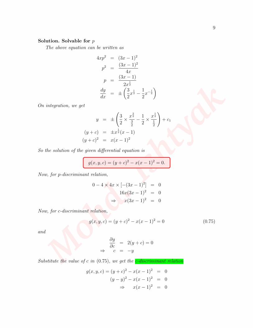
Solution. Solvable for p
The above equation can be written as
4xp2 = (3x− 1)2
p2 =(3x− 1)2
4x
p =(3x− 1)
2x12
dy
dx= ±
(3
2x
12 − 1
2x−
12
)On integration, we get
y = ±
(3
2× x
32
32
− 1
2× x
12
12
)+ c1
(y + c) = ±x12 (x− 1)
(y + c)2 = x(x− 1)2
So the solution of the given differential equation is
g(x, y, c) = (y + c)2 − x(x− 1)2 = 0.
Now, for p-discriminant relation,
0− 4× 4x× [−(3x− 1)2] = 0
16x(3x− 1)2 = 0
⇒ x(3x− 1)2 = 0
Now, for c-discriminant relation,
g(x, y, c) = (y + c)2 − x(x− 1)2 = 0 (0.75)
and
∂g
∂c= 2(y + c) = 0
⇒ c = −y
Substitute the value of c in (0.75), we get the c-discriminant relation
g(x, y, c) = (y + c)2 − x(x− 1)2 = 0
(y − y)2 − x(x− 1)2 = 0
⇒ x(x− 1)2 = 0
Moh
d.Ish
tyak
10
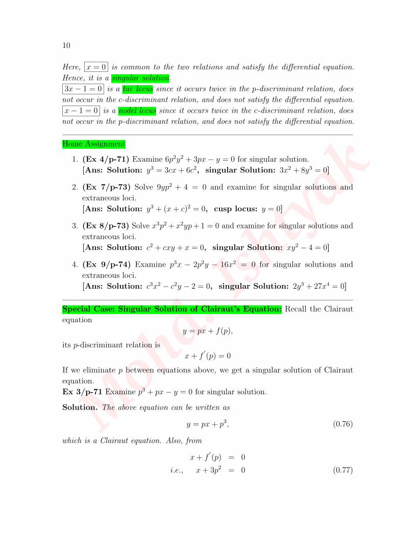
Here, x = 0 is common to the two relations and satisfy the differential equation.
Hence, it is a singular solution.
3x− 1 = 0 is a tac locus since it occurs twice in the p-discriminant relation, does
not occur in the c-discriminant relation, and does not satisfy the differential equation.
x− 1 = 0 is a nodel locus since it occurs twice in the c-discriminant relation, does
not occur in the p-discriminant relation, and does not satisfy the differential equation.
Home Assignment
1. (Ex 4/p-71) Examine 6p2y2 + 3px− y = 0 for singular solution.
[Ans: Solution: y3 = 3cx+ 6c2, singular Solution: 3x2 + 8y3 = 0]
2. (Ex 7/p-73) Solve 9yp2 + 4 = 0 and examine for singular solutions and
extraneous loci.
[Ans: Solution: y3 + (x+ c)2 = 0, cusp locus: y = 0]
3. (Ex 8/p-73) Solve x3p2 + x2yp+ 1 = 0 and examine for singular solutions and
extraneous loci.
[Ans: Solution: c2 + cxy + x = 0, singular Solution: xy2 − 4 = 0]
4. (Ex 9/p-74) Examine p3x − 2p2y − 16x2 = 0 for singular solutions and
extraneous loci.
[Ans: Solution: c3x2 − c2y − 2 = 0, singular Solution: 2y3 + 27x4 = 0]
Special Case: Singular Solution of Clairaut’s Equation: Recall the Clairaut
equation
y = px+ f(p),
its p-discriminant relation is
x+ f′(p) = 0
If we eliminate p between equations above, we get a singular solution of Clairaut
equation.
Ex 3/p-71 Examine p3 + px− y = 0 for singular solution.
Solution. The above equation can be written as
y = px+ p3, (0.76)
which is a Clairaut equation. Also, from
x+ f′(p) = 0
i.e., x+ 3p2 = 0 (0.77)
Moh
d.Ish
tyak
11
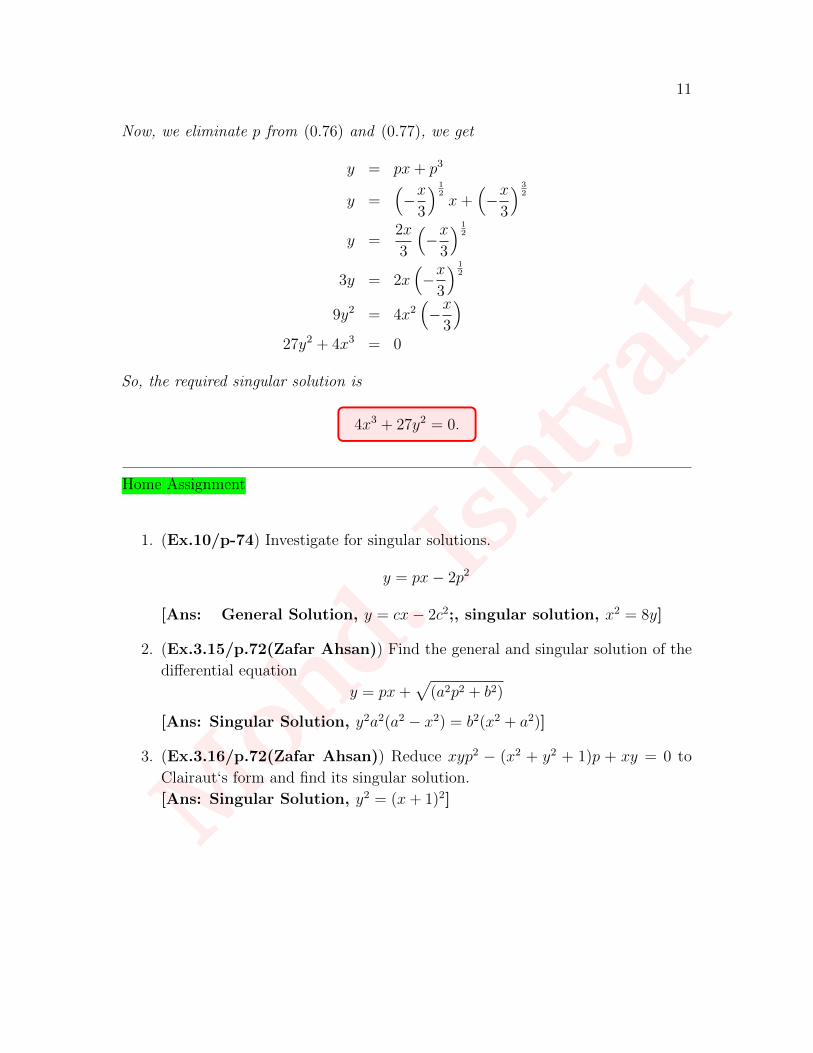
Now, we eliminate p from (0.76) and (0.77), we get
y = px+ p3
y =(−x
3
) 12x+
(−x
3
) 32
y =2x
3
(−x
3
) 12
3y = 2x(−x
3
) 12
9y2 = 4x2(−x
3
)27y2 + 4x3 = 0
So, the required singular solution is
4x3 + 27y2 = 0.
Home Assignment
1. (Ex.10/p-74) Investigate for singular solutions.
y = px− 2p2
[Ans: General Solution, y = cx− 2c2;, singular solution, x2 = 8y]
2. (Ex.3.15/p.72(Zafar Ahsan)) Find the general and singular solution of the
differential equation
y = px+√
(a2p2 + b2)
[Ans: Singular Solution, y2a2(a2 − x2) = b2(x2 + a2)]
3. (Ex.3.16/p.72(Zafar Ahsan)) Reduce xyp2 − (x2 + y2 + 1)p + xy = 0 to
Clairaut‘s form and find its singular solution.
[Ans: Singular Solution, y2 = (x+ 1)2]