Multi-domain BEM for two-dimensional problems of elastodynamics

INTERNATIONAL JOURNAL FOR NUMERICAL METHODS IN ENGINEERING, VOL, 26, 891-91 1 (1988)

MULTI-DOMAIN BEM FOR TWO-DIMENSIONAL PROBLEMS OF ELASTODYNAMICS

SHAHID AHMAD* A N D PRASANTA K. BANERJEEt

Department of Civil Engineering, State University of New York at Buffalo, 240 Engr. West, Buffalo, N . Y. 14260, U.S.A.

SUMMARY

An advanced implementation of the boundary element technique for the periodic and transient dynamic analyses of two-dimensional elastic or visco elastic solids of arbitrary shape and connectivity is presented. For transient dynamic analysis the problem is first solved in the Laplace transform space and then the time domain solutions are obtained by numerical inversion of transformed domain solutions.

The present analysis is capable of treating very large, multi-domain problems by substructuring and satisfying the equilibrium and compatibilities at the interfaces. With the help of this substructuring capability, problems related to the layered media and soil-structure interaction can all be analysed. This paper also introduces a new type of element called 'Enclosing Element', which has been developed and used to model the infinitely extending boundaries of a half-space or a layered medium. A number of numerical examples are presented, and through comparisons with available analytical and numerical results, the accuracy, stability and efficiency of the present analysis are established.

INTRODUCTION

Although the boundary integral formulation for elastodynamics have existed in the classical literature, their applications to the solutions of boundary-value problems only started with the advent of computers in the early sixties with Banaugh and Goldsmith' solving an elastic wave scattering problem. Since then a number of applications primarily involving cylinders and half- space have been presented by many authors, demonstrating that the boundary element formulations can be used for dynamic stress analysis. For example, Cruse and Rizzo' presented numerical results for the two-dimensional problem of the elastic half-space under transient load; Niwa et Kobayashi et ~ 1 . ~ ~ ~ and Manolis and Beskos' solved the problem of transient wave scattering by cavities of arbitrary shape due to the passage of travelling waves; Dominguez and Alarcons applied the boundary element method (BEM) to determine the dynamic stiffness of rigid strip footings; Kobayashi and Nishimurag used the BEM to obtain periodic dynamic responses of a tunnel and a column in a half-space subjected to plane waves of oblique incidence; and Abascal and Dominguezlo*ll studied the influence of a non-rigid soil base on the compliances of a rigid surface footing and response of the rigid surface strip footing to incident waves.

However, most of the above-mentioned work suffers from one or more of the following: lack of generality, crude assumption of constant variation of the field variables, modelling of boundary geometry by using straight line segments, inadequate treatment of singular integrals and unacceptable level of accuracy. The approach of modelling the boundary geometry by straight line

*Assistant Professor +Professor

0029-598 1 /88/O4089 1-21 $10.50 0 1988 by John Wiley & Sons, Ltd.

Received 30 March 1987 Revised 18 June 1987

892 S. AHMAD A N D P. K. BANERJEE

segments and assuming the field variables to be constant within a segment may be used for a very simple problem, but for relatively complex problems and higher frequencies the results are unacceptable and easily lead to ill conditioning of the system matrix. As pointed out by Kobayashi and Nishimura: it is crucial to use higher-order boundary elements for boundary modelling of a steady-state dynamic problem so that it is fine enough to be compatible with the wavy nature of the solution. In addition, it should be noted that none of the above-mentioned algorithms is capable of solving general two-dimensional elastodynamic or viscoelastodynamic problems because they cannot take care of edges and corners which are always present in a real engineering problem.

This paper presents an advanced numerical implementation for accurate dynamic analyses of any general two-dimensional problem involving complicated geometry and boundary conditions. In this implementation, families of isoparametric curvilinear boundary elements are used, and the normal and singular integrals have been evaluated in an accurate and elegant manner by using superior and sophisticated integration techniques. The present analysis is capable of treating very large multizone problems by substructuring and satisfying the equilibrium and compatibilities at the interfaces.

Since the BEM for a Laplace domain transient dynamic problem (for a single Laplace transform parameter) is identical to that for a steady-state dynamic problem, the solution for the transient dynamic problem has been obtained by first solving the problem in the Laplace transform domain for a number of Laplace transform parameters, and then performing the numerical inversion of the Laplace domain solutions.

Finally, a number of examples are described to show the utility of the developed analysis. To the best of the authors’ knowledge a comparable boundary element formulation for the accurate dynamic analysis of two-dimensional problems does not exist in the published literature.

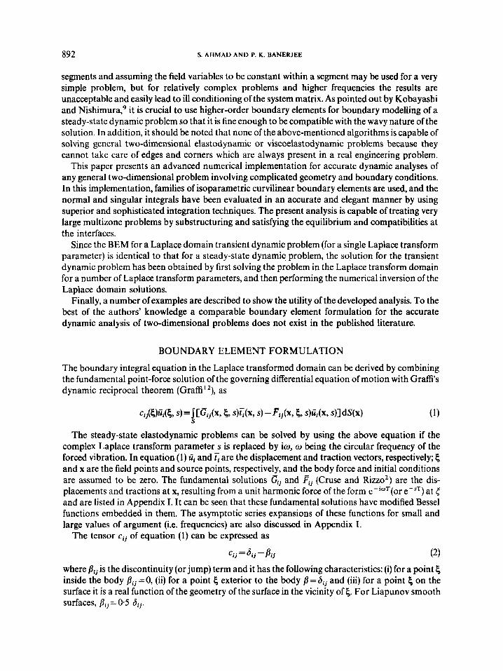
BOUNDARY ELEMENT FORMULATION

The boundary integral equation in the Laplace transformed domain can be derived by combining the fundamental point-force solution of the governing differential equation of motion with Graffi’s dynamic reciprocal theorem (Graffi”), as

The steady-state elastodynamic problems can be solved by using the above equation if the complex Laplace transform parameter s is replaced by io, o being the circular frequency of the forced vibration. In equation (1) Ui and 6 are the displacement and traction vectors, respectively; 6 and x are the field points and source points, respectively, and the body force and initial conditions are assumed to be zero. The fundamental solutions Gij and Fij (Cruse and Rizzo2) are the displacements and tractions at x, resulting from a unit harmonic force of the form e-iwT(or e-sT) at ( and are listed in Appendix I. It can be seen that these fundamental solutions have modified Bessel functions embedded in them. The asymptotic series expansions of these functions for small and large values of argument (i.e. frequencies) are also discussed in Appendix I.

The tensor cij of equation (1) can be expressed as

where Bij is the discontinuity (or jump) term and it has the following characteristics: (i) for a point 6 inside the body Bij=0, (ii) for a point 6 exterior to the body B=6, and (iii) for a point 6 on the surface it is a real function of the geometry of the surface in the vicinity of 6. For Liapunov smooth surfaces, pij = 0.5 d i j .

MULTI-DOMAIN BEM 893

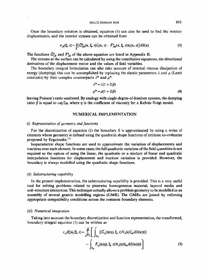
Once the boundary solution is obtained, equation (1) can also be used to find the interior displacements, and the interior stresses can be obtained from

The functions GGk and FGk of the above equation are listed in Appendix 11. The stresses at the surface can be calculated by using the constitutive equations, the directional

derivatives of the displacement vector and the values of field variables. The boundary integral formulation can also take account of internal viscous dissipation of

energy (damping); this can be accomplished by replacing the elastic parameters A and p (Lamk constants) by their complex counterparts A* and p*:

A* = A( 1 + 2ip)

p* = p( 1 + 2ip) (4)

leaving Poisson's ratio unaltered. By analogy with single-degree-of-freedom systems, the damping ratio fl is equal to oq/2p, where q is the coefficient of viscosity for a Kelvin-Voigt model.

NUMERICAL IMPLEMENTATION

(i) Representation of geometry and functions

For the discretization of equation (1) the boundary S is approximated by using a series of elements whose geometry is defined using the quadratic shape functions of intrinsic co-ordinates proposed by Ergatoudi~.'~

Isoparametric shape functions are used to approximate the variation of displacements and tractions over each element. In some cases, the full quadratic variation of the field quantities is not required so the option of using the linear, the quadratic or a mixture of linear and quadratic interpolation functions for displacement and traction variation is provided. However, the boundary is always modelled using the quadratic shape functions.

(ii) Substructuring capability

In the present implementation, the substructuring capability is provided. This is a very useful tool for solving problems related to piecewise homogeneous material, layered media and soil-structure interaction. This technique actually allows a problem geometry to be modelled as an assembly of several generic modelling regions (GMR). The GMRs are joined by enforcing appropriate compatibility conditions across the common boundary elements.

(iii) Numerical integration

boundary integral equation (1) can be written as Taking into account the boundary discretization and function representation, the transformed,

P 1


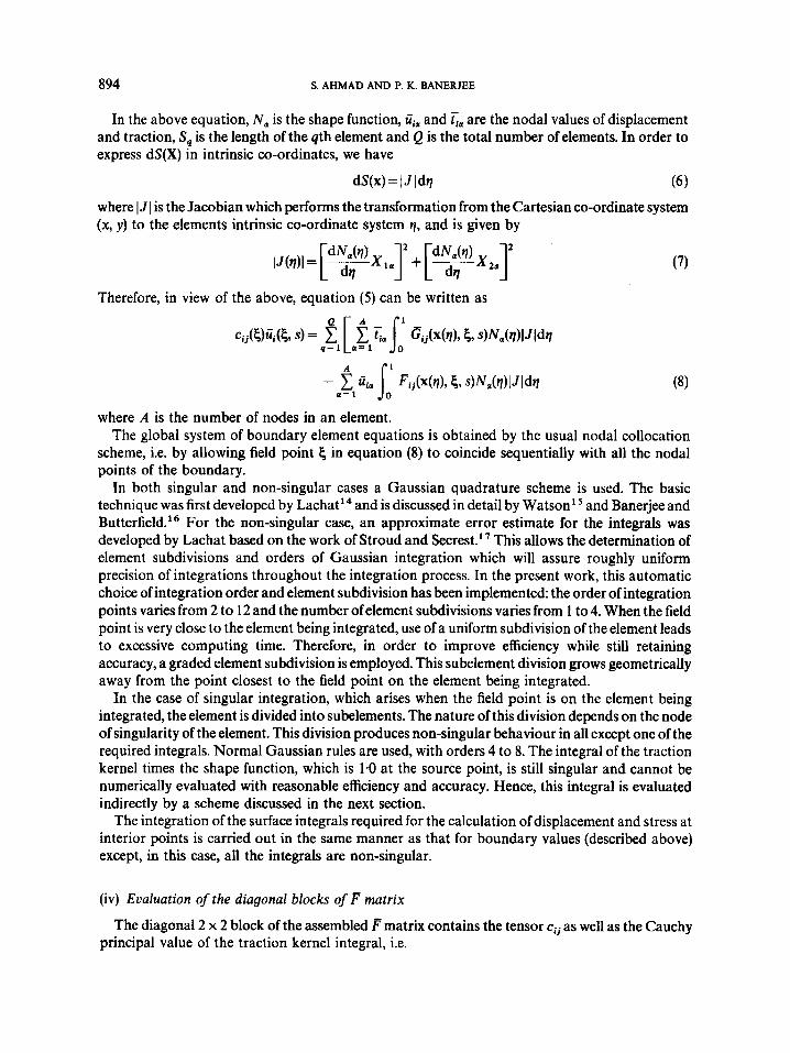
In the above equation, Nu is the shape function, Cia and are the nodal values of displacement and traction, S, is the length of the 9th element and Q is the total number of elements. In order to express dS(X) in intrinsic co-ordinates, we have

dS(x) = IJldq (6 1 where IJI is the Jacobian which performs the transformation from the Cartesian co-ordinate system (x, y) to the elements intrinsic co-ordinate system q, and is given by

Therefore, in view of the above, equation ( 5 ) can be written as

1

- f uia j0 Fij(x(q), ~3 S ) N ~ ( ~ ) I J I ~ ~ (8) a= 1

where A is the number of nodes in an element. The global system of boundary element equations is obtained by the usual nodal collocation

scheme, i.e. by allowing field point 5 in equation (8) to coincide sequentially with all the nodal points of the boundary.

In both singular and non-singular cases a Gaussian quadrature scheme is used. The basic technique was first developed by Lachat14 and is discussed in detail by Watson” and Banerjee and Butterfield.16 For the non-singular case, an approximate error estimate for the integrals was developed by Lachat based on the work of Stroud and Secrest.” This allows the determination of element subdivisions and orders of Gaussian integration which will assure roughly uniform precision of integrations throughout the integration process. In the present work, this automatic choice of integration order and element subdivision has been implemented the order of integration points varies from 2 to 12 and the number ofelement subdivisions varies from 1 to 4. When the field point is very close to the element being integrated, use of a uniform subdivision of the element leads to excessive computing time. Therefore, in order to improve efficiency while still retaining accuracy, a graded element subdivision is employed. This subelement division grows geometrically away from the point closest to the field point on the element being integrated.

In the case of singular integration, which arises when the field point is on the element being integrated, the element is divided into subelements. The nature of this division depends on the node of singularity of the element. This division produces non-singular behaviour in all except one of the required integrals. Normal Gaussian rules are used, with orders 4 to 8. The integral of the traction kernel times the shape function, which is 1.0 at the source point, is still singular and cannot be numerically evaluated with reasonable efficiency and accuracy. Hence, this integral is evaluated indirectly by a scheme discussed in the next section.

The integration of the surface integrals required for the calculation of displacement and stress at interior points is carried out in the same manner as that for boundary values (described above) except, in this case, all the integrals are non-singular.

(iv) Evaluation of the diagonal blocks of F matrix

principal value of the traction kernel integral, i.e. The diagonal 2 x 2 block of the assembled F matrix contains the tensor cij as well as the Cauchy


(9)

where N , is the shape function for the singular node, and S , is the length of the singular element. Similarly for a static problem

r Dzj=cij+ J FijN,dS

s1

where the variables are the static counterpart of those of equation (9). From (9) and (10) we can obtain

dij= D;j+ [sl(Fij-F;)N, dS

In the above equation, the diagonal blocks D t of coefficients of the traction matrix for a static problem of the same geometry can be obtained by using the rigid body motion, i.e.

Djj = cij + J Fzj N, dS SI

In addition, the integral involving the difference (Fij - Fjj) is non-singular, therefore, equation (11) can be used to obtain Dij. Recently, a similar approach has been used by Rizzo et aZ.,’* Ahmad,lg Banerjee and Ahmad” and Banerjee et a1.” for three-dimensional problems.

In almost all of the past two-dimensional analyses, the non-singular integral of equation (1 1) has been neglected. This results in inaccuracy, particularly at high frequencies. For problems having boundaries extending to infinity (such as a layered soil strata) a new scheme outlined below has been developed to calculate the diagonal blocks of F matrix.

(v) Diagonal blocks of F matrix for problems of half-space and infinitely extending layered media

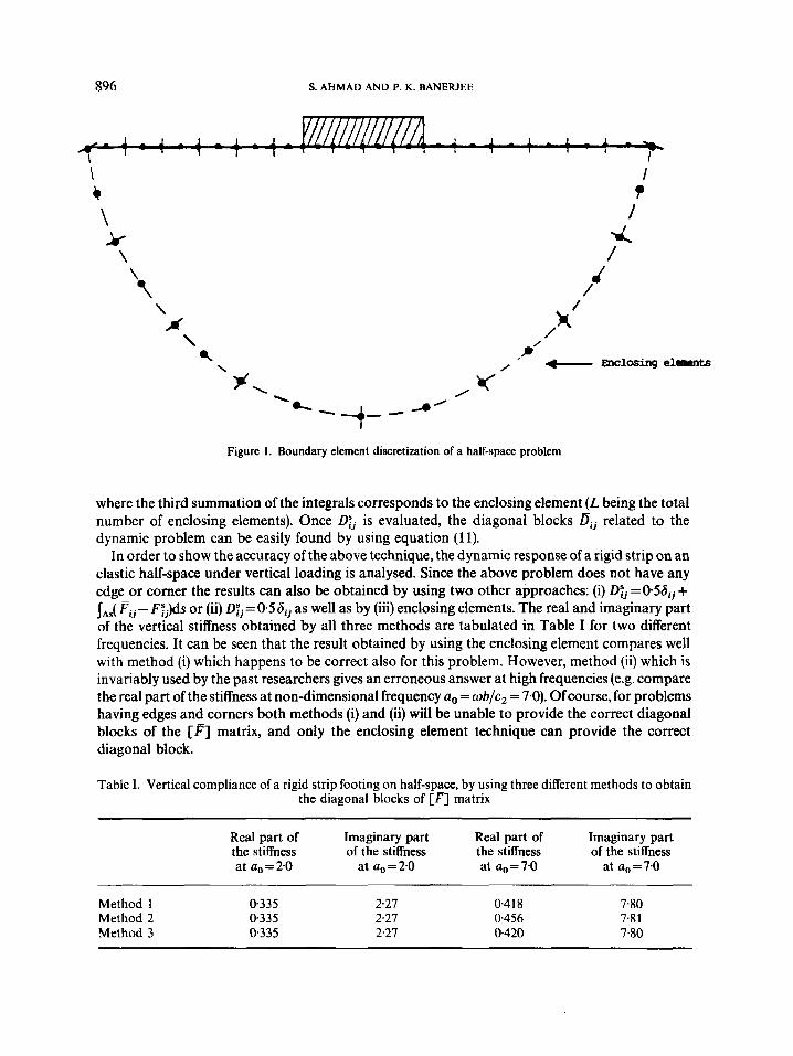
The conventional approach of assuming O%,, as the block diagonal terms of the F matrix (used in all previous work) does not hold true for cases where the geometry of the problem has edges and corners, except for the case where the field variables are assumed to be constant within each element. This assumption is impractical to use for a realistic engineering problem. In the present work, a new technique to calculate dij using ‘enclosing elements’ (see Figure 1) is developed. The basic assumption in this technique is that the dispIacements and tractions at the enclosing elements at a sufficiently distant location have negligible effect on the displacements at any point on the modelled boundary.

Using this scheme, the diagonal blocks D:j of the F matrix are obtained by the summation of non-singular integrations of the static traction kernel over all the elements of the modelled boundary as well as all the enclosing elements, i.e.

896 S. AHMAD AND P. K. BANERJEE

1 1 - 1 - 1 1 - i 1 I 7 I I

\ h

I t

Figure I. Boundary element discretization of a half-space problem

where the third summation of the integrals corresponds to the enclosing element ( L being the total number of enclosing elements). Once D:j is evaluated, the diagonal blocks Dij related to the dynamic problem can be easily found by using equation (1 1).

In order to show the accuracy of the above technique, the dynamic response of a rigid strip on an elastic half-space under vertical loading is analysed. Since the above problem does not have any edge or corner the results can also be obtained by using two other approaches: (i) Ofj =0.56, + Jb( Fij- F;j)ds or (ii) D;j=056 i j as well as by (iii) enclosing elements. The real and imaginary part of the vertical stiffness obtained by all three methods are tabulated in Table I for two different frequencies. It can be seen that the result obtained by using the enclosing element compares well with method (i) which happens to be correct also for this problem. However, method (ii) which is invariably used by the past researchers gives an erroneous answer at high frequencies (e.g. compare the real part of the stiffness at non-dimensional frequency a, = wb/c, = 7.0). Of course, for problems having edges and corners both methods (i) and (ii) will be unable to provide the correct diagonal blocks of the [ F ] matrix, and only the enclosing element technique can provide the correct diagonal block.

Table I. Vertical compliance of a rigid strip footing on half-space, by using three different methods to obtain the diagonal blocks of [ F ] matrix

Real part of Imaginary part Real part of Imaginary part the stiffness of the stiffness the stiffness of the stiffness at a,=2*0 at a, = 2.0 at a, = 7.0 at a,=7.0

Method 1 Method 2 Method 3

0.335 0.335 0.335

2.27 2.27 2.27

0.418 0.456 0.420

7.80 7.81 7.80


(vi) Assembly of system equations

applied we have a set of linear system of matrix equations of the form Once the boundary collocation and integrations are completed, and boundary conditions are

where

{ Y} and (X} are the vectors of known and unknown field quantities, respectively; {u'"} and {u} are the vectors of displacements and stresses at interior points, respectively.

In any substructured (multi-zone) problem, the matrix [A] in (14) contains large blocks of zeros because separate GMRs communicate only through common surface elements. In order to save both storage space and computer time, the matrix [A] is stored in a block basis with zero blocks being ignored. Since interior results in any GMR involve only the boundary values related to that GMR, the matrices in (15) and (16) are also block diagonal. In addition, for added accuracy the system equations are scaled so that all the coefficients of matrix [A] ( and [ B ] ) are of the same magnitudes (for detail, see Banerjee and ButtefieldI6).

(vii) Solution of equations

Since the system equations (14) involve complex numbers it requires a complex solver. In the present work, an out-of-core complex solver is developed using softwares from LINPACK (Dongarra"). In this solver, in order to minimize the time requirements the solution process is carried out using the block form of the matrix. Thus, this block banded solver operates at the submatrix level using software from LINPACK to carry out all operations on submatrices. The system matrix is also stored by submatrices on a direct accessfile. The first operation in the solution process is the decomposition of the system matrix using the block form of it This decomposition process is a Gaussian reduction to upper triangular (submatrix) form. The row operations required during the decomposition are stored in the space originally occupied by the lower triangle of the system matrix. Finally, the calculation of the solution vector is carried out by using the decomposed form of the system matrix from the direct access file.

(viii) Laplace transformed transient dynamic analysis

The numerical solution of the transient dynamic problem in Laplace transformed domain essentially consists of a series of solutions to a steady-state dynamic problem for a number of discrete values of the transformed parameter s. The final solution is, of course, then obtained by a numerical inversion of the transformed domain solutions to the time domain. Thus, the steady- state dynamic boundary element formulation and its numerical implementation presented in previous sections are also valid for Laplace transformed transient dynamic analysis.

A detailed description of the numerical procedure used for the direct Laplace transform of the boundary conditions and inversion of the transform domain solutions can be found in References 19,20 and 23.

898 S. A H M A D A N D P. K . BANERJEE

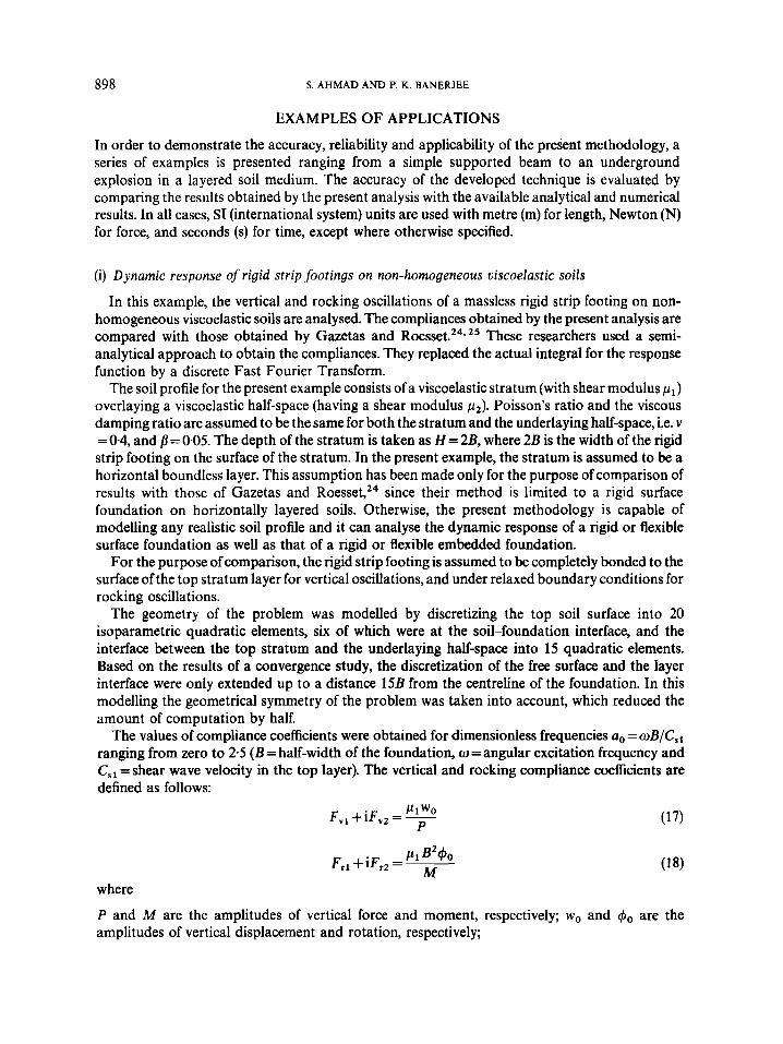
EXAMPLES OF APPLICATIONS

In order to demonstrate the accuracy, reliability and applicability of the present methodology, a series of examples is presented ranging from a simple supported beam to an underground explosion in a layered soil medium. The accuracy of the developed technique is evaluated by comparing the results obtained by the present analysis with the available analytical and numerical results. In all cases, SI (international system) units are used with metre (m) for length, Newton (N) for force, and seconds (s) for time, except where otherwise specified.

(i) Dynamic response of rigid strip footings on non-homogeneous viscoelastic soils

In this example, the vertical and rocking oscillations of a massless rigid strip footing on nonhomogeneous viscoelastic soils are analysed. The compliances obtained by the present analysis are compared with those obtained by Gazetas and R o e s ~ e t . ~ ~ * 25 These researchers used a semi- analytical approach to obtain the compliances. They replaced the actual integral for the response function by a discrete Fast Fourier Transform.

The soil profile for the present example consists of a viscoelastic stratum (with shear modulus p,) overlaying a viscoelastic half-space (having a shear modulus p,). Poisson’s ratio and the viscous damping ratio are assumed to be the same for both the stratum and the underlaying half-space, i.e. v = 0-4, and B = 0.05. The depth of the stratum is taken as H = 2B, where 2B is the width of the rigid strip footing on the surface of the stratum. In the present example, the stratum is assumed to be a horizontal boundless layer. This assumption has been made only for the purpose of comparison of results with those of Gazetas and R o e s ~ e t , ~ ~ since their method is limited to a rigid surface foundation on horizontally layered soils. Otherwise, the present methodology is capable of modelling any realistic soil profile and it can analyse the dynamic response of a rigid or flexible surface foundation as well as that of a rigid or flexible embedded foundation.

For the purpose of comparison, the rigid strip footing is assumed to be completely bonded to the surface of the top stratum layer for vertical oscillations, and under relaxed boundary conditions for rocking oscillations.

The geometry of the problem was modelled by discretizing the top soil surface into 20 isoparametric quadratic elements, six of which were at the soil-foundation interface, and the interface between the top stratum and the underlaying half-space into 15 quadratic elements. Based on the results of a convergence study, the discretization of the free surface and the layer interface were only extended up to a distance 15B from the centreline of the foundation. In this modelling the geometrical symmetry of the problem was taken into account, which reduced the amount of computation by half.

The values of compliance coefficients were obtained for dimensionless frequencies a, = o B / C , ranging from zero to 2.5 (B = half-width of the foundation, o = angular excitation frequency and C,, =shear wave velocity in the top layer). The vertical and rocking compliance coefficients are defined as follows:

P1 wo FV1 + iF,, = - P

Pl BZ40 Frl + iF,, = - M

where

P and M are the amplitudes of vertical force and moment, respectively; wo and 6, are the amplitudes of vertical displacement and rotation, respectively;


F, , and F , , are the real parts of the compliances; and F,, and F,, are the imaginary parts of the compliances.

The real and imaginary parts of the vertical compliance for three values of soil modulus ratio (i.e. p1/p2 = 1*0,0.25 and 0.06) are plotted in Figures 2(a) and 2(b). In general, the agreement between the present and Gazetas-Roe~set~~ results is good, particularly for the imaginary parts of the vertical compliance. In Figure 2(a), the agreement for the half-space case (pi/p2 = 1.0) is very good, whereas for the other two cases, particularly at high frequencies, the agreement between the results is poor. In the present analysis the variation in the field variables (such as contact stresses) over each element is represented by quadratic shape functions, whereas in the Gazetas-Roesset

.6

.4

2 .i? L

.a

I Present analysis ( a / e - 1.0) - Present analysis (p1/p2 5 0.25) - - Present analysis (p1/p2 - 0.06) ......-. Gazetas-Roesset ‘(e1/e2 1.0) Gazetas-Roesset (pl/p2 - 0.25) Gazetas-Roesset (p:/pi I 0.06) 0

I n o

-.t .w .50 1 .88 1.50 2.88 2 . 5 0

a0

(a) Real Part

- -- . . . . . . . .

Present analysis (vl/e2 = 1.0 1 Present analysis (v1/e2 = 0.25) Present analysis (P /u - 0.06)

0 Gazetas-Rcesset ( p 1 / v 2 1.0) A Gazetas-Roesset ( u i / v i = 0.25) 0 @zetas-Roesset (e1/p2 = 0.06) - 4

(Y

lu

.2

.B I I I I I

.88 .50 1.m 1.58 2.00

a0

(b) Imaginary Part

Figure 2. Vertical compliances


.6

N

L

. 4

. 2

.0

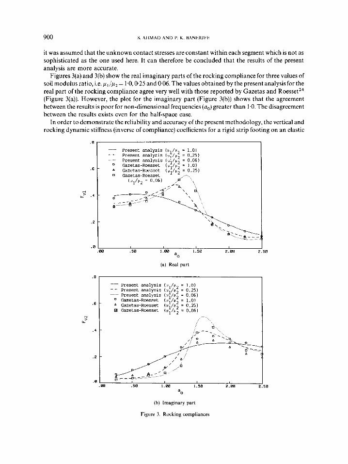
it was assumed that the unknown contact stresses are constant within each segment which is not as sophisticated as the one used here. It can therefore be concluded that the results of the present analysis are more accurate.

Figures 3(a) and 3(b) show the real imaginary parts of the rocking compliance for three values of soil modulus ratio, i.e. pl/p2 = 1.0,0*25 and 0.06. The values obtained by the present analysisfor the real part of the rocking compliance agree very well with those reported by Gazetas and RoessetZ4 (Figure 3(a)). However, the plot for the imaginary part (Figure 3(b)) shows that the agreement between the results is poor for non-dimensional frequencies (a,) greater than 1 .O. The disagreement between the results exists even for the half-space case.

In order to demonstrate the reliability and accuracy of the present methodology, the vertical and rocking dynamic stiffness (inverse of compliance) coefficients for a rigid strip footing on an elastic

- Present analysis ( P / P = 1.0) - - Present analysis (p1/p2 = 0.25) ...."' Present analysis (u1/p2 - 0.06)

Gazetas-Roesset (p1/p2 1.0) A Gazetas-Rcesset (u1/p2 = 0.25)

Gazetas-Roesset (N;/P; = 0.06)

-

..... : .. . ..

d- ... :.' w - - . : , 0'. ,..

' .. -

-

I I I

.m .50 1.m 1.50 2.00 i

.e

.6

4 b' . 4

. 2

- Present analysis ( P / u = 1.0) - - . . . . . . . . present analysis ( p i / p ; = 0.25)

present analysis (pl/p2 = 0.06) 0 Gazetas-Rcesset ( pl/p2 = 1 .O) t. Gazetas-Rcesset (pl/p2 = 0.25) 0 Gazetas-Roesset .. .. ._....

(pl/p2 = 0.06) ,...m. "_.. ,,.+' -4 .,...

/A<...'

. 0 I I I I I

.m . 5 0 1.m 1.50 2 . 0 0 2 aO

(a) Real part

I

50

50

MULTI-DOMAIN BEM 90 1

.7

.6

.5

-4 -4

F .Y

. 4

.3

.2

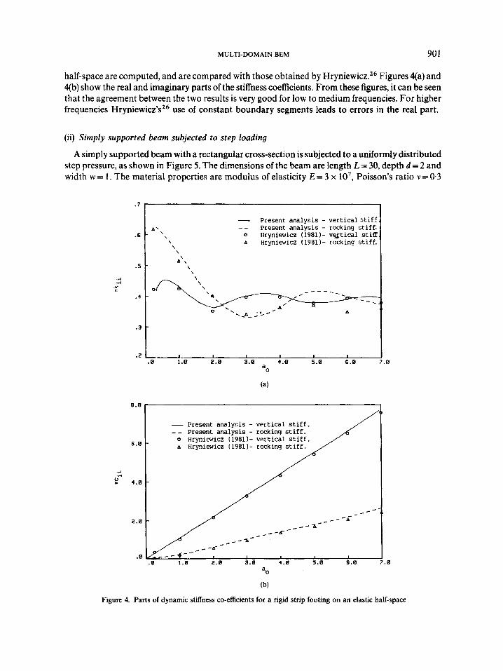
half-space are computed, and are compared with those obtained by Hryniewicz.26 Figures 4(a) and 4(b) show the real and imaginary parts of the stiffness coefficients. From these figures, it can be seen that the agreement between the two results is very good for low to medium frequencies. For higher frequencies Hryniewicz’sZ6 use of constant boundary segments leads to errors in the real part.

- --

Present analysis - vertical stiff. Present analysis - rocking stiff.

0 HKynieWiCZ (1981)- vQtical stiff. A‘\ - , \ A Hryniewicz (1981)- rocking stiff. \ \

A‘, - \ \ \

0 _ - - _ - c - - - x ----7-i A

-

I I I 1 I I

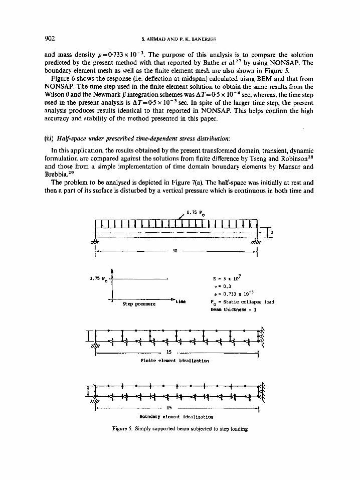
(ii) Simply supported beam subjected to step loading

A simply supported beam with a rectangular cross-section is subjected to a uniformly distributed step pressure, as shown in Figure 5. The dimensions of the beam are length L= 30, depth d = 2 and width w = 1. The material properties are modulus of elasticity E = 3 x lo7, Poisson’s ratio v =0.3

e.0

6 . 0

..+ -4

P 4.0

2.e

.e

- Present analysis - vertical stiff. - - Present analysis - rocking stiff. o Hryniewicz (1981)- vertical stiff. A Hryniewicz (1981)- rocking stiff.

- - -c - a- - ,--c - - -

_,-a’--

- - - / , a 1.0 2 .0 3.0 4.0 , 5.0 , 6.0 , * - - - . 0

a0

(b)

Figure 4. Parts of dynamic stiffness co-efficients for a rigid strip footing on an elastic half-space

902 S. A H M A D A N D P. K. BANERJEE

and mass density p=0.733 x The purpose of this analysis is to compare the solution predicted by the present method with that reported by Bathe et aL2’ by using NONSAP. The boundary element mesh as well as the finite element mesh are also shown in Figure 5 .

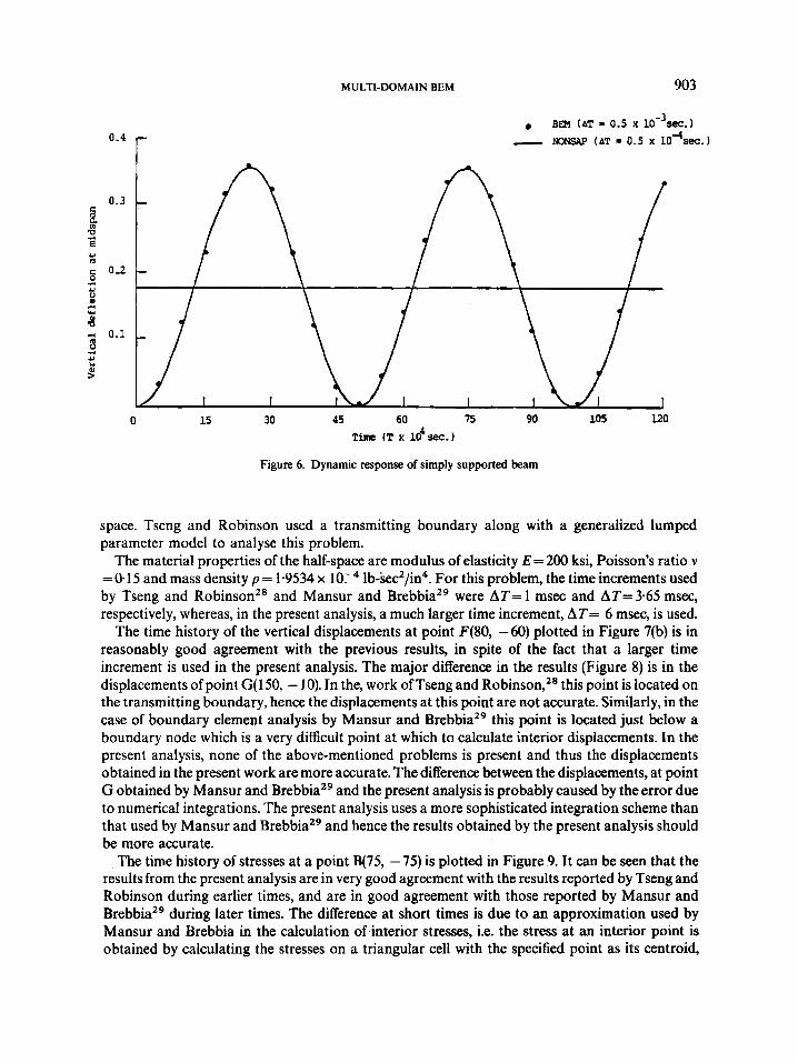
Figure 6 shows the response (i.e. deflection at midspan) calculated uisng BEM and that from NONSAP. The time step used in the finite element solution to obtain the same results from the Wilson 8 and the Newmark B integration schemes was AT=0.5 x sec; whereas, the time step used in the present analysis is AT=05 x lop3 sec. In spite of the larger time step, the present analysis produces results identical to that reported in NONSAP. This helps confirm the high accuracy and stability of the method presented in this paper.

(iii) Half-space under prescribed time-dependent stress distribution:

In this application, the results obtained by the present transformed domain, transient, dynamic formulation are compared against the solutions from finite difference by Tseng and Robinson2’ and those from a simple implementation of time domain boundary elements by Mansur and Brebbia.

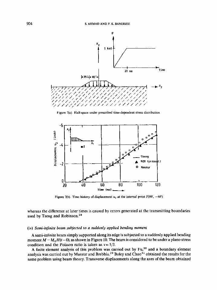
The problem to be analysed is depicted in Figure 7(a). The half-space was initially at rest and then a part of its surface is disturbed by a vertical pressure which is continuous in both time and

0.75 Po t E = 3 x lo7 u = 0.3

= 0.733 x Po = Static collapse load Step pressure _ _ Beam thickness = 1

I Finite element idealization

1 1 5 -- Boundary element idealization

Figure 5. Simply supported beam subjected to step loading


0 - 4 r . BM (AT - 0.5 x

-4 - "SAP (AT 3 0.5 X 10 SeC.1

0 15 30 45 60 75 90 105 UO 4 Time (T X 10 S . 1

Figure 6. Dynamic response of simply supported beam

space. Tseng and Robinson used a transmitting boundary along with a generalized lumped parameter model to analyse this problem.

The material properties of the half-space are modulus of elasticity E = 200 ksi, Poisson's ratio v =0-15 and mass density p = 1-9534 x lb-sec2/in4. For this problem, the time increments used by Tseng and Robinsonz8 and Mansur and Brebbia29 were AT= 1 msec and AT=3-65 msec, respectively, whereas, in the present analysis, a much larger time increment, AT= 6 msec, is used.

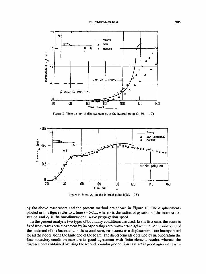
The time history of the vertical displacements at point F(80, -60) plotted in Figure 7(b) is in reasonably good agreement with the previous results, in spite of the fact that a larger time increment is used in the present analysis. The major difference in the results (Figure 8) is in the displacements of point G( 150, - 10). In the, work of Tseng and Robinson,'' this point is located on the transmitting boundary, hence the displacements at this point are not accurate. Similarly, in the case of boundary element analysis by Mansur and Brebbiaz9 this point is located just below a boundary node which is a very difficult point at which to calculate interior displacements. In the present analysis, none of the above-mentioned problems is present and thus the displacements obtained in the present work are more accurate. The difference between the displacements, at point G obtained by Mansur and BrebbiaZ9 and the present analysis is probably caused by the error due to numerical integrations. The present analysis uses a more sophisticated integration scheme than that used by Mansur and BrebbiaZ9 and hence the results obtained by the present analysis should be more accurate.

The time history of stresses at a point B(75, -75) is plotted in Figure 9. It can be seen that the results from the present analysis are in very good agreement with the results reported by Tseng and Robinson during earlier times, and are in good agreement with those reported by Mansur and Brebbiaz9 during later times. The difference at short times is due to an approximation used by Mansur and Brebbia in the calculation of interior stresses, i.e. the stress at an interior point is obtained by calculating the stresses on a triangular cell with the specified point as its centroid,


P

I k S i k 20 ms Tim

Figure 7(a). Half-space under prescribed time-dependent stress distribution

Figure 7(b). Time history of displacement u2 at the internal point F(80, -60’)

whereas the difference at later times is caused by errors generated at the transmitting boundaries used by Tseng and Robinson.28

(iv) Semi-injinite beam subjected to a suddenly applied bending moment

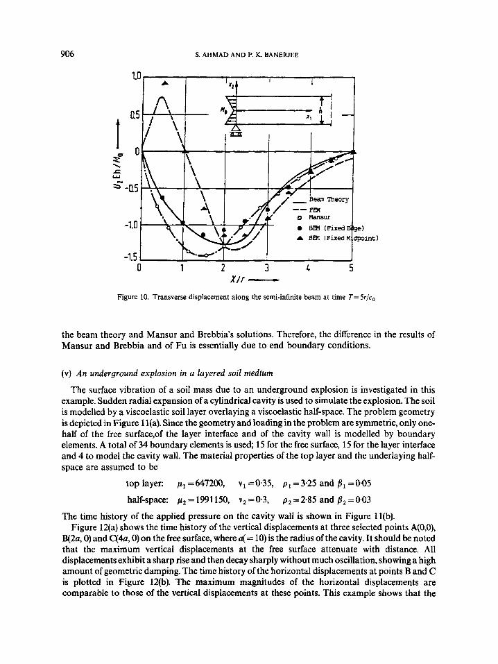
A semi-infinite beam simply supported along its edge is subjected to a suddenly applied bending moment M = M,H(t -O), as shown in Figure 10. The beam is considered to be under a plane-stress condition and the Poisson ratio is taken as v = 1/3.

A finite element analysis of this problem was carried out by Fu,~’ and a boundary element analysis was carried out by Mansur and Brebbia.29 Boley and Chao3I obtained the results for the same problem using beam theory. Transverse displacements along the axes of the beam obtained

MULTI-DOMAIN BEM

- Tseng A BM o Mansuc

X2t

f - n

I

905

Time (mi),-.

Figure 9. Stress uZ2 at the internal point B(75', -75')

by the above researchers and the present method are shown in Figure 10. The displacements plotted in this figure refer to a time t = 5r/c0, where r is the radius of gyration of the beam cross- section and co is the one-dimensional wave propagation speed.

In the present analysis two types of boundary conditions are used. In the first case, the beam is fixed from transverse movement by incorporating zero transverse displacement at the midpoint of the finite end of the beam, and in the second case, zero transverse displacements are incorporated for all the nodes along the finite end of the beam. The displacements obtained by incorporating the first boundary-condition case are in good agreement with finite element results, whereas the displacements obtained by using the second boundary-condition case are in good agreement with

906 S. AHMAD AND P. K. BANERJEE

0 BPI (Fixed

1 2 3 4 5 X/r -

Figure 10. Transverse displacement along the semi-infinite beam at time T = 5r/c,

the beam theory and Mansur and Brebbia’s solutions. Therefore, the difference in the results of Mansur and Brebbia and of Fu is essentially due to end boundary conditions.

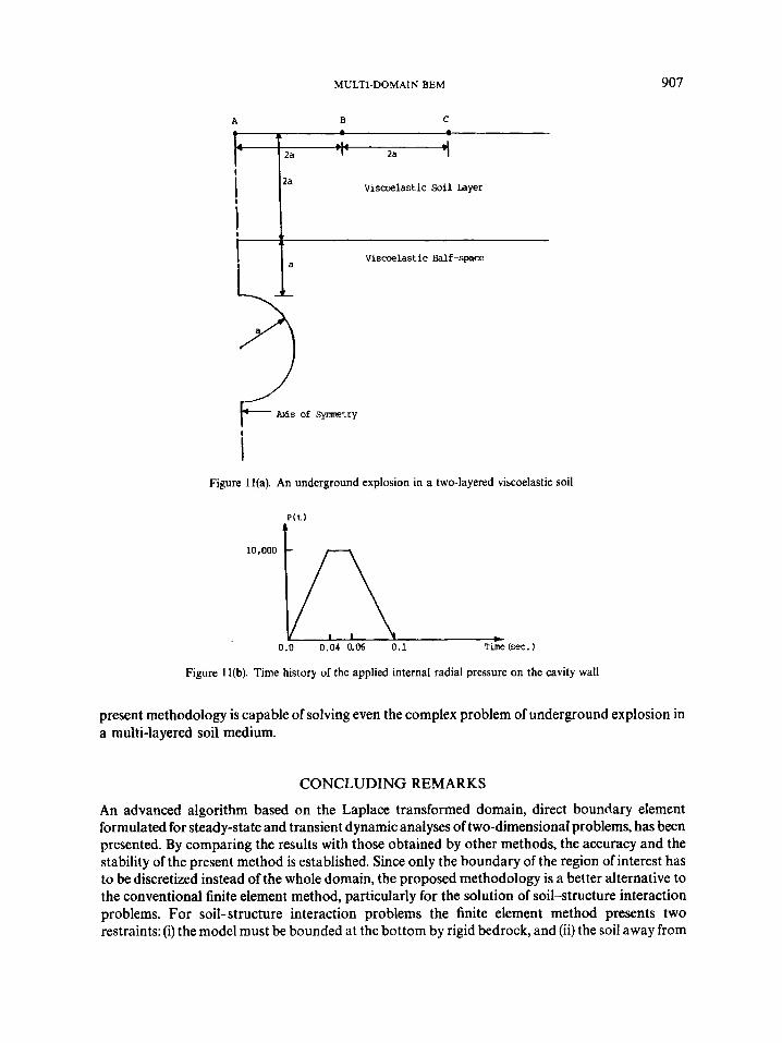
(v) An underground explosion in a layered soil medium

The surface vibration of a soil mass due to an underground explosion is investigated in this example. Sudden radial expansion of a cylindrical cavity is used to simulate the explosion. The soil is modelled by a viscoelastic soil layer overlaying a viscoelastic half-space. The problem geometry is depicted in Figure 1 l(a). Since the geometry and loading in the problem are symmetric, only one- half of the free surface,of the layer interface and of the cavity wall is modelled by boundary elements. A total of 34 boundary elements is used; 15 for the free surface, 15 for the layer interface and 4 to model the cavity wall. The material properties of the top layer and the underlaying half- space are assumed to be

top layer: p, =647200, v 1 =0.35, p1 =3-25 and p1 =0.05

half-space: p2= 1991150, v,=O*3, p,=2-85 and Bz=O-03

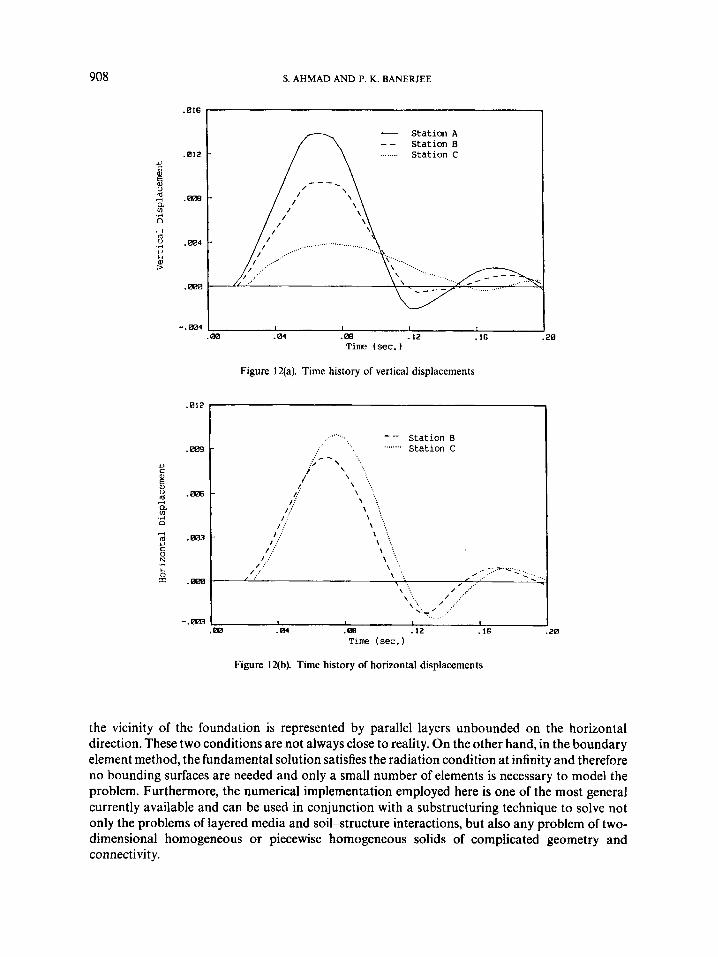
The time history of the applied pressure on the cavity wall is shown in Figure 1 l(b). Figure 12(a) shows the time history of the vertical displacements at three selected points A(O,O),

B(2a, 0) and C(&, 0) on the free surface, where a( = 10) is the radius of the cavity. It should be noted that the maximum vertical displacements at the free surface attenuate with distance. All displacements exhibit a sharp rise and then decay sharply without much oscillation, showing a high amount of geometric damping. The time history of the horizontal displacements at points B and C is plotted in Figure 12(b). The maximum magnitudes of the horizontal displacements are comparable to those of the vertical displacements at these points. This example shows that the


A B C

Viscoelastic Soil Layer 1 J2a

Figure 1 l(a). An underground explosion in a two-layered viscoelastic soil

Figure 1 l(b). Time history of the applied internal radial pressure on the cavity wall

present methodology is capable of solving even the complex problem of underground explosion in a multi-layered soil medium.

CONCLUDING REMARKS

An advanced algorithm based on the Laplace transformed domain, direct boundary element formulated for steady-state and transient dynamic analyses of two-dimensiona1 problems, has been presented. By comparing the results with those obtained by other methods, the accuracy and the stability of the present method is established. Since only the boundary of the region of interest has to be discretized instead of the whole domain, the proposed methodology is a better alternative to the conventional finite element method, particularly for the solution of soil-structure interaction problems. For soil-structure interaction problems the finite element method presents two restraints: (i) the model must be bounded at the bottom by rigid bedrock, and (ii) the soil away from

908

-.ma4

S . AHMAD AND P. K. BANERJEE

I I I 1

.016

.012 I

Station B Station C

..... - _ ,. .. . , . . . . . , . . . . . ,

4 u 0 X

.0a3

.000

.20 Time (sec.)

Figure I2(b). Time history of horizontal displacements

the vicinity of the foundation is represented by parallel layers unbounded on the horizontal direction. These two conditions are not always close to reality. On the other hand, in the boundary element method, the fundamental solution satisfies the radiation condition at infinity and therefore no bounding surfaces are needed and only a small number of elements is necessary to model the problem. Furthermore, the numerical implementation employed here is one of the most general currently available and can be used in conjunction with a substructuring technique to solve not only the problems of layered media and soil-structure interactions, but also any problem of two- dimensional homogeneous or piecewise homogeneous solids of complicated geometry and connectivity.


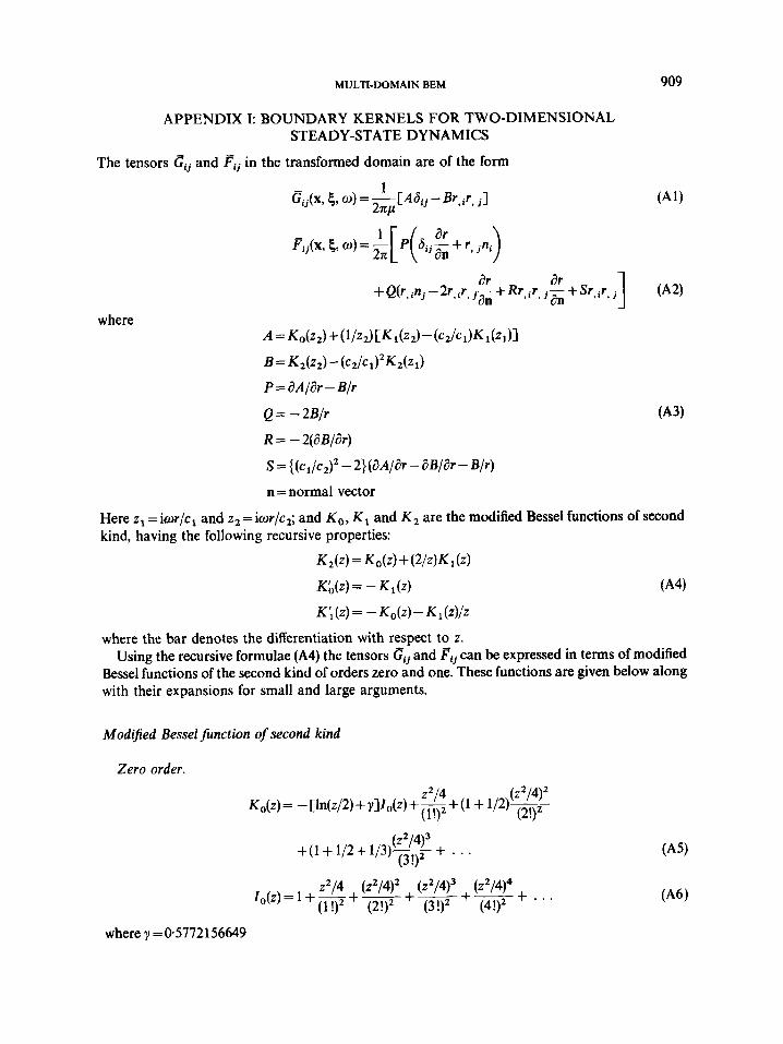
APPENDIX I: BOUNDARY KERNELS FOR TWO-DIMENSIONAL STEADY-STATE DYNAMICS

The tensors Gij and Fij in the transformed domain are of the form

where

1 cij(x, 5, o) = -[A6,, - Br,ir, j]

~ , ~ ( x , 5, o) = -[ 2x .( 6ijdn + r, j n i )

2nCL 1 ar

Here z1 =iwr/c, and z,=iwr/c,; and K O , K, and K, are the modified Bessel functions of second kind, having the following recursive properties:

K2(4 =KO@) + (2/z)K, (4 K ~ ( z ) = -K,(z) 644)

K;(z) = - K ~ ( Z ) - K,(z)/z

where the bar denotes the differentiation with respect to z. Using the recursive formulae (A4) the tensors G, and Fij can be expressed in terms of modified

Bessel functions of the second kind of orders zero and one. These functions are given below along with their expansions for small and large arguments.

Modified Bessel function of second kind

Zero order

z2/4 (z2/4)' (I!)

Ko(z) = - [ln(z/2) + y]Z,(z) +? + (1 + l/2)+-- (2!)2

(z2/4)3 + . + ( I + 1/2+ 1/3)- (3!)2

2214 (z2/4)2 (z2/4)3 Io(z)= 1 + y+ 7 +-

(l!) (2!) (3!)2

. .

+ . . . +- (z2/4)4 (4!)2

where y =05772156649


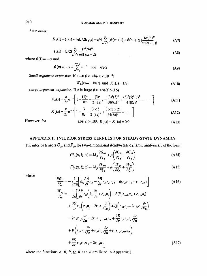
First order.

where $(1)= -7 and

Small argument expansion. If z-0 (i.e. abs(z)< lop8)

Ko(z)= -ln(z) and Kl(z)= l/z)

Large argument expansion. If z is large (i.e. abs(z) > 3.5)

- . . .] + - . . .] 8z 2!(8z)' 3 ! ( 8 ~ ) ~

However, for abs(z) > 100, Ko(z) = K (z) = 0.0

APPENDIX 11: INTERIOR STRESS KERNELS FOR STEADY-ST

where

TE DYI' 4MICS

The interior tensors G i j k and F i j k for two-dimensional steady-state dynamic analysis are ofthe form

1 aA aB - -r,krv i r , - B(r,ir, j k + r, j r , i k )

+ P(Sijr,mknm + r, jkni)

9 'an

ar aR ar -2r,ir , . - -2r , i r , j r ,mknm+-r ,kr , i r .- Ikan ar ' J a n

ar . -+r , i r , jr,ml,nm Jkan

1 as ar + - r ,kr , in , j+Sr , ikn , j

where the functions A, B, P, Q, R and S are listed in Appendix I.

MULTI-DOMAIN BEM 91 1

REFERENCES

1. R. P. Banaugh and E. Goldsmith, ‘Diffraction of steady elastic waves by surface of arbitrary shape’, J . Appl. Mech. 30,

2. T. A. Cruse and F. J. Rizzo, ‘A direct formulation and numerical solution of the general transient elastodynamic problem I’, J . Math. Anal. Appl., 22, 244-259 (1968).

3. Y. Niwa, S. Kobayashi and N., Azuma, ‘An analysis of transient stresses produced around cavities of an arbitrary shape during the passage of travelling wave’, Memo Fac. Eng. Kyo to Unio., 37, 2 8 4 6 (1975).

4. Y. Niwa, S. Kobayashi and T. Fukui, ‘Application of integral equation method to some geomechanical problems’, Proc. 2nd lnt . Con$ Numerical Methods and Geomechanics 1976, pp. 120-131.

5. S. Kobayashi, T. Fukui and N. Azuma, ‘An analysis of transient stresses produced around a tunnel by the integral equation method’, Proc. Symp. Earthquake Engineering Japan, 1975, pp. 631438.

6. S. Kobayashi and N. Nishimura, ‘Transient stress analysis of tunnels and cavities of arbitrary shape due to travelling waves’, in P. K. Banerjee and R. P. Shaw (eds.), Developments in BEM-11. Applied Science Publishers, Barking, England. 1982, Chapt. 7.

7. G. D. Manolis and D. E. Beskos, ‘Dynamic stress concentration studies by boundary integrals and Laplace transform’, Int. j. numer. methods eng., 17, 573-599 (1981).

8. J. Dominguez and E. Alarcon, ‘Elastodynamics’, in C. A. Brebbia (ed.), Progress in Boundary Element Methods, Halstead Press, New York, 1981, Chapt. 7, pp. 213-257.

9. S. Kobayashi and N. Nishimura, ‘Analysis of dynamic soil-structure interaction by boundary integral equation method‘, Proc. 3rd Int. Symp. on Numerical Methods in Engineering, Yo/ 1, Paris, Pluralis Publ., 1983, pp. 353-362.

10. R. Abscal and J. Dominguez, ‘Dynamic behavior of strip footings on nonhomogeneous visco-elastic soils’, in D. E. Beskos (ed.), Proc. Int. Symp. on Dynamic Soil-structure Interaction, Minneapolis, A. A. Balkema, 1984, pp. 25-35.

1 I . R. Abscal and J. Dominguez, ‘Dynamic response of embedded strip foundation subjected to obliquely incident waves’, Proc. Seventh Int. Con$ on Boundary Element Methods, Lake Como, Italy, Springer-Verlag, Berlin, 1985, pp. 6-63 to 6-69.

589-597 ( I 963).

12. D. Graffi. ‘Memorie della Academia Scienze’, Bologna Series 10, 4, 103-109 (1947). 13. J. G. Ergatoudis, ‘Isoparametric finite elements in two and three-dimensional stress analysis’, Ph.D. Thesis, University

of Wales, University College, Swansea, England, 1968. 14. J. C. Lachat, ‘Further developments of the boundary integral technique for elasto-statics’, Ph.D. Thesis, Southampton

University, England, 1975. 15. J. 0. Watson, ‘Advanced implementation of the boundary element method for two and three-dimensional elastostatics’,

in P. K. Benerjee and R. Butterfield (eds.), Developments in BEM-I, Applied Science Publishers, Barking, England, 1979, Chapt. 3.

16. P. K. Banerjee and R. Butterfield, Boundary Element Methods in Engineering Science. McGraw-Hill, London, New York. 1981.

17. A. H. Stroud and D. Secrest, Gaussian Quadrature Formulas. Prentice-Hall, New York, 1966. 18. F. J. Rizzo, D. J. Shippy, and M. Rezayat, ‘Boundary integral equation analysis for a class ofearth-structure interaction

problems’, Final Report to NSF, Grant No. CEE 80-13461, Department of Engineering Mechanics, University of Kentucky, Lexington 1985.

19. S. Ahmad, ‘Linear and nonlinear dynamic analysis by boundary element method’, Ph.D. Thesis, Department of Civil Engineering, State University of New York at Buffalo, 1986.

20. P. K. Banerjee and S. Ahmad,‘Advanced three-dimensional dynamic analysis by boundary element’, A S M E Con$ on Advanced Boundary Element Analysis, Florida, Nov. 1985.

21. P. K. Banerjee, S. Ahmad and G. D. Manolis, ‘Transient elasto-dynamic analysis of 3-D problems by boundary element method, Earthquake eng. struc. dyn. 14,933-949 (1986).

22. J. J. Dongarra, L I N P A C K User’s Guide. SIAM, Philadelphia, PA, 1979. 23. S. Ahmad and G. D. Manolis, ‘Dynamic analysis of 3-D structures by a transformed boundary element method‘, Comp.

24. G. Gazetas and J. M. Roesset, ‘Forced vibrations of strip footings on layerd soils’, Methods Struct. Anal. ASCE, I,

25. G. Gazetas and J. M. Roesset, ‘Vertical vibrations of machine foundation’, J . Geotech. Eng. Diu. ASCE, 105,1435-1454

26. Z . Hryniewicz, ‘Dynamic response of a rigid strip on an elastic half-space’, Cornp. Methods Appl. Mech. Eng. 25,355-364

27. K. L. Bathe, H. Ozdemir and E. L. Wilson, ‘Static and dynamic geometric and material nonlinear analysis’, Report No.

28. M. N. Tseng, and A. R. Robinson, ‘A transmitting boundary for finite difference analysis of wave propagation in solids’,

29. W. J. Mansur, and C. A. Brebbia, ‘Transient Elastodynamics’, in Topics in Boundary Element Research, Vol. 2, Springer-

30. C. C. Fu, ‘A method for the numerical integration of the equations of motion arising from a finite element analysis’, J .

31. B. A. Boley and C. C. Chao, ‘An approximate analysis of Timoshenko Beams under dynamic loads’, J . Appl. Mech.

Mech. Vol. 2, 185-196 (1987).

115-131 (1976).

(1979).

(1981).

U C SESM 74-4. Structural Engineering Laboratory, University of California, Berkeley, CA, 1974.

Project No. NR 064-183, University of Illinois, Urbana, 1975.

Verlag, Berlin, 1985, Chapt. 5.

Appl. Mech. ASME, E37, 599-605 (1970).

ASME, E25, 31-36 (1958).

Multi-domain BEM for two-dimensional problems of elastodynamics

Documents

Transcript of Multi-domain BEM for two-dimensional problems of elastodynamics