Two useful techniques for heat transfer BEM: addressing the corner ...

Two useful techniques for heat transfer

BEM: addressing the corner problem and

use of the FFT for turning domain integrals

into boundary integrals

A.J. Kassab, R.S. Nordlund

Department of Mechanical and Aerospace Engineering,

University of Central Florida, Orlando, Florida 32816-0450,

ABSTRACTTwo numerical problems which feature prominently in the implementation of theboundary element method for the solution of heat conduction problems includedouble-valued heat fluxes at boundary corners and the evaluation of domainintegrals due to distributed energy generation terms. The first problem is dealt withby explicitly treating nodal heat fluxes as double valued prior to assembly of thenodal equations. An additional equation is derived for corner nodes across which thetemperature is prescribed. The additional equation is general, is free of heuristicconstraints, and is applicable through the wide range of acute, shallow, obtuse, andre-entrant angles encountered in practice. The second problem is dealt with bydeveloping a two dimensional Fast Fourier Transform to efficiently implement theuse the Fourier Dual Reciprocity Method for turning domain integrals into contourintegrals. Numerical examples are provided to validate both approaches.

INTRODUCTION

In the implementation of the direct boundary element method for thesolution of the heat conduction equation, the heat flux at a corner is double valueddue to the non-uniqueness of the outward-drawn normal. This fact poses anumerical problem for linear, quadratic, and higher order element formulationswhich have nodes located at these geometric corners. Discontinuous prescription ofboundary conditions poses a numerical problem as well. Improper treatment of thisproblem can severely degrade the solution around the corner region/" Severalschemes have been proposed by researchers to address this problem.^"^ Alarcon etal^ derive two expressions relating the two upstream and downstream fluxes totangential gradients and local geometry and compute the fluxes independent of theBEM solution. Walker and Fenner** divide the two expressions derived by Alarconet al to obtain an additional equation which they use to integrate the heat fluxcomputation directly in the BEM solution of the problem. The method is flexible asit lends itself to a general scheme treating the heat flux at each node as doublevalued, allowing for treatment of discontinuous heat fluxes at corners, and also forthe prescription of discontinuous boundary conditions along smooth boundaries.

Transactions on Modelling and Simulation vol 3, © 1993 WIT Press, www.witpress.com, ISSN 1743-355X

106 Boundary Element Technology

However, the additional equation provided by Walker and Fenner is potentially ill-conditioned for certain geometries and boundary conditions. They modify theirequation by using alternative expressions which are based on heuristic corner turnangle criteria. Instead, we subtract the equations derived by Alarcon et al andobtain an additional equation which is also general, but free of heuristic constraints,and applicable through the wide range of acute, shallow, obtuse, and re-entrantangles encountered in practice.

A second numerical problem featured in heat transfer BEM is theevaluation of the area integral arising from conducting media with generation.Although these area integrals involve no unknowns, their explicit evaluation using afinite element-like domain discretization detracts from the boundary onlydiscretization nature of the BEM. An accurate, yet computationally expensivetechnique for evaluating these are integrals without the need for internaldiscretization is the Fourier Dual Reciprocity Boundary Element Method(FDRBEM) developed by Tang.*'* In this method the generation term is expandedin a two-dimensional Fourier series which is in turn used to transform the areaintegrals into contour integrals. Tang uses the analytical definition of the Fouriercoefficients, and computes these coefficients with area integration over a specifiedrectangular Fourier domain. Although simpler, this task nevertheless requiresdomain discretization, essentially defeating the purpose of the FDRBEM. Here, wedevelop a Fast Fourier Transform^ (FFT) algorithm to efficiently evaluate thecoefficients of the double Fourier series expansion of the generation term. Thecomputational burden is further significantly reduced with harmonic filtering.Numerical examples are presented which demonstrate the accuracy of both thecorner treatment and the FFT-FDRBEM in the BEM solution of heat conductionproblems.

TEE BOUNDARY ELEMENT METHOD FOR STEADY-STATE HEATCONDUCTION

The double-noded BEM formulation for two-dimensional steady-state heatconduction is briefly reviewed. *~^ The steady temperature field in an isotropic,homogeneous medium with distributed generation, u^, is governed by

V-(A VT)+ %y =0 (1)

If the thermal conductivity, Jt, varies with temperature then the Kirchhofftransform can be used to transform the governing heat conduction equation to thePoisson equation in the transform parameter. The solution to this equation issought subject to three types of boundary conditions: Dirichlet, Neumann, and/orRobin conditions. Consequently, results discussed herein are applicable to potentialproblems as well. Using standard BEM methodology, discretizing with linear orquadratic elements, and explicitly treating the double valued normal derivatives ofthe temperature in the formulation, the Poisson equation is recast as

J = 1 J = 1

where, .;,= y «t%do (3)

nThe symbol 0 represents either the temperature in a linear heat conduction problemor the Kirchhoff transform parameter in a nonlinear heat conduction problem. In


Boundary Element Technology 107

(2), N is the number of nodes used to discretize the domain, so that L=N andM-2N for linear elements, and L=N/2 and M-3N/2 for quadratic elements (;Vmust be even in this case).

The components of G— have been separated thereby allowing fordiscontinuous boundary conditions and for explicit treatment of double valuednormal gradients of the temperature at corner nodes. Equation (2) is symbolicallywritten as [H]{ T} = [G] {Q}+ {1} . If the tangent to the boundary possesses adiscontinuity at each node which is common to two elements, the normal gradientwill be doubled valued. Such a node is termed a corner. There are three variables atsuch nodes: the temperature and two normal gradients of the temperature.Boundary conditions provide N of the IN unknowns in (2), except for the case ofDirichlet conditions prescribed across a corner node. In this case an additionalequation must be provided. The treatment of this condition is addressed in detail inthe next section. The FDRBEM can be used to evaluate the integrals in (3). A two-dimensional FFT algorithm is developed following the next section to efficiently andaccurately extract the real Fourier coefficients of the two-dimensional seriesexpansion of the generation term.

TREATMENT OF CORNERS

Referring to Figure 1, Alarcon et al^ express the upstream and downstreamnormal gradients at a corner node with a Dirichlet condition prescribed across thatnode in terms of the tangential gradients of the adjoining element as

(4)

(I)„ - i §)„ - (§)„-!

Figure 1. Corner node with normal and tangential gradients.

Here, 5 is the coordinate tangent to the boundary and 0 is the angle by which thetangent turns at the corner. The subscript U refers to the upstream condition, andthe subscript D refers to the downstream condition. The tangential derivatives arecalculated by differentiating the parametrized temperature with respect to theintrinsic coordinate along the element of interest and (4) and (5) can be used tocompute the normal heat fluxes independently of the BEM analysis. Walker andFenner^ point out that the error incurred in computing the fluxes independently ofthe BEM could be smoothed by incorporating the heat flux calculation in the BEMsolution. They divide (4) by (5) to obtain the nonlinear relationship



U D J U

which they applied to find the temperature distribution in several arbitrarygeometries with good accuracy. However, as the authors point out, equation (6) isill-conditioned when 0 is in the vicinity of 90 ° and indeterminate when bothtangential gradients are zero or nearly zero. Alternative expressions for cases where75°< 0 < 105° and for 0<30°. The above equation requires alternative formulationsfor particular geometries based on heuristic angle criteria.

An alternative and more general expression is obtained by subtracting (5)from (4) yielding

y#n +rgn l^a - n + rm r?\**?/ *\6S) \\ sinO ) \0n ^

U D] D

Here, the positive sign is for concave corner nodes(#<180°) and the negative sign isfor re-entrant corners. Equation (7) relates the difference between the normal heatfluxes while (6) expresses the ratio of the normal heat fluxes. In implementing (6)and (7), expressions relating the tangential gradients to linear combinations of nodaltemperatures for the tangential temperature gradients are readily determined.

Given the boundary conditions, (7) can be substituted for the either theupstream or downstream corresponding flux component of the vector Q at anycorner node for which only the temperature is prescribed. The structure of (7) allowsfor two ways in which to adjust the matrices to accommodate its inclusion:compute the tangential gradients prior to introducing (7) and adjust the G matrixand Q vector appropriately to render the system solvable, or, absorb the coefficientsmultiplying the nodal temperatures in (7) in the H matrix after multiplying by theappropriate G-^ coefficients and adjust the G matrix to leave the unsolved heat fluxas an unknown in Q. In either case, the second of each pair of corner heat fluxes iscalculated after the BEM analysis using (7). Although more complicated, the latterapproach is implemented in our code as it more fully integrates (7) into the BEMsolution. Numerical experiments reveal that this approach yields slightly moreaccurate results. It is noted that (7) requires no special treatment which depends onheuristic turn angle criteria.

TURNING AREA INTO CONTOUR INTEGRALS BY FFT AND TIIE FDRBEM

If the generation term satisfies V^u« = /?%_, where (3 is a non-zero constant,then Green's second identity can be applied to rewrite equation (3) as

(8)

Such functions thus exhibit a reciprocity property. Arbitrary functions do notgenerally satisfy such reciprocity relations. However, the generation term can beexpanded in a series whose terms individually satisfy such a reciprocity relation.Indeed, this is the basis of the Dual Reciprocity Boundary Element Method.^ InTang's method, *^ the generation term u^ is expanded in a Fourier series, and aseach term in the Fourier expansion individually exhibits a reciprocity relation, sowill the expansion. To expand an arbitrary two-dimensional generation function Ugas a Fourier series, a rectangular Fourier domain, Q/-, is first defined that extends ashort distance beyond the domain of u^ and is [2/x2L]. The function is expressed



as a discrete Fourier series as follows

/ v / j 71*' M / j / j 771 rrt ' -* * v / v TlTn rimi i '* __o i __ i i I inii

where, the sub- and superscripted /'s are the trigonometric functions and sub- andsubscripted A''s are the coefficients in the double Fourier series expansion, seeTang or Tolstov.^ The variables n and m represent the wave numbers of theharmonics in the x and y directions, respectively.

Using these results and Green's second identity allows each of the domainintegrals in (30) to be transformed into boundary integrals one-by-one resulting inthe following series of boundary integrals which are the basis of the FDRBEM

2 #+Z Z'p=ln=l

n(nm

The constants /3 are normalized Fourier coefficients. Equation (10) is called thetransformation formula. It is numerically evaluated using the existing boundarydiscretization. Equation (10) transforms the domain integral in (3) into the series ofboundary integrals and it is based on the dual reciprocity properties of the Fourierseries expansion terms in (9). As such, this method is seen to be a Fourier DualReciprocity BEM.

Tang computes the exact Fourier coefficients by means of domainintegration. For an arbitrary generation functions, the integral is evaluatednumerically. This is not a particularly difficult task since the Fourier domain isrectangular. However, when the generation varies markedly within the medium, afinite element-like breakup of the Fourier domain is necessary for accurateextraction of the coefficients. This approach detracts from the aim of a boundaryonly discretization, and the calculations are time-consuming. The coefficients can becalculated much more simply, accurately, and efficiently by employing the two-dimensional FFT without recourse to domain discretization. The one-dimensional N-term Fourier series approximation for a function f(x) defined for x E [a,b] is

N

where N is the number of evenly spaced data points. Essentially, the one-dimensional FFT algorithm uses these N data points f(x ) for k=0,l,2...N-l togenerate the complex Fourier coefficients C: in the series approximation for f(x).These are given as


no

N-l• i>k=0

Boundary Element Technology

and C=a-2b)

where, 2=^ — 1. The real coefficients are readily extracted from the complexcoefficients. The one-dimensional FFT subroutine used in this study is found inKahaner et al. Available two-dimensional FFT's are exclusively written incomplex notation due to the compactness of the notation and due to the naturalsetting for the practical applications of the transform in digital signal processing andimage processing.™ In this notation, the real Fourier coefficients in (9) are related inan implicit and complicated way to the complex coefficients provided by these two-dimensional FFT's and they are explicitly irretrievable. In order to extract thesereal coefficients, we developed a two-dimensional FFT which directly provides themin matrix form. The logic for the algorithm is shown in Figure 3. The basis of themethod is the recognition that the real coefficients can be expressed as

// =l/d (13)

This equation can be evaluated using a sequence of one-dimensional transforms. Theone-dimensional FFT is first used to calculate the terms in the brackets for a giveny-value. Having calculated these, the FFT algorithm is then used to calculate theouter integral in (13). Repeated calls are made to the one-dimensional FFT togenerate the one-dimensional transforms of each row of data of a matrix [F] ofequally spaced data f(xj,,y ) with k=0,l...N-l and £=0,1...M-l. Each row of data isoverwritten with the transform, resulting in a complex matrix [F]. The real andimaginary parts [F] are used along with (12) to retrieve two matrices [G] and [H], asshown in Figure 2. The FFT is then repeatedly called to transform the columns of[G] and [H]. These matrices are overwritten with the transform, resulting in twocomplex matrices [G] and [H]. The real and imaginary parts of [G] and [H] are thenused along with (12) to retrieve four real matrices [A], [B], [C], and [D]. Thecorrespondence between the elements of these matrices and the /i's are readilyestablished.^

l-D FFTon rowsof [F]

N*Mofdat

Comnot

matrix !real 1A CF1 ':

piex ir-x [F]

na1frc

l-D FFT on imatrix CGJ |

Imatrix [A]from Re CGI

trix LG1>n Re CF]

matrix [Efrom Im

UCG]

Imatrix [H]from Im [F]

1-D Ffnatr(%

matrix [C]from ReCH]

natrfrom

•T on5 Of[H]

ix CD!fen CHI

Figure 2. Two-Dimensional FFT algorithm.

In implementing the FFT, a grid of equally spaced sample points is laidover a rectangular region which extends some distance beyond the minimum and



maximum coordinates of the original domain boundary. Generation of this grid is atrivial operation as we are dealing with a distribution of equally spaced points overa rectangular region. However, it is important to extend the region in order toeliminate the deleterious effects of the Gibbs phenomenon in the computation of thetransformation formula. A safe distance is on the order of twice the data pointspacing. The FFT analysis of the generation term is performed prior to the BEMsolution. A concern arises as to the number of coefficients selected in (10). This canbe set arbitrarily high. Once the Fourier coefficients are extracted, they can beconveniently analyzed to eliminate the wavelengths which do not substantiallycontribute to the evaluation of u Jx,y). For example, an amplitude cutoff value canbe established upon examination of the amplitude matrices [A], [B], [C], and [D].Sample points are then tested to check whether this truncation leads to anacceptable approximation to the generation term prior entering the BEiM phase ofthe solution. Two examples are presented next to validate the above discussion.

EXAMPLES

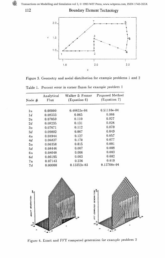
The first problem provides for a direct comparison of Equations (6) and (7)through application of each to the geometry shown in Figure 3. The exacttemperature solution is taken as T(x,y)=ln{[(x+5) +(y+5) ]~ }. This problemposes a severe test of the method as only Dirichlet boundary conditions are imposed,in addition to possessing a high percentage of corner nodes. There are six concaveconcave corners, with turn angles of 20, 45, 80, 90, 107, and 135% and one re-entrantcorner of 117°. Quadratic elements were used to model the temperature and heatflux. The thermal conductivity was set to 1. Results for this problem are given inTable 1. The percent error based on the local nodal flux is presented for the twonormal fluxes at each corner node. It is evident that the proposed equation.Equation (7), yields either equivalent, or in the majority of cases, higher accuracythan does Equation (6) and its variants.

The second example problem tests the proposed FFT-FDRBEM techniquein combination with the proposed corner treatment method. Further, the thermalconductivity is now taken to vary with temperature as A'(T)=T. The geometry andnodal distribution of the first problem is again used. The exact solution in Kirchhoffspace is taken to be <£(x,y) = ln{[(x+5) + (y+5) ]~ }+x -fy and the exacttemperature distribution is computed using the backward transformationT(x,y)={[a*7V/vJ-f[l-f2*a*0(x,y)//vJ }/a/v . In this example, a, 1\,, and K^are all equal to 1. The generation term is also readily found to be u =[6*(j;-f-j/)]//v\,.For the transform, 200 x 100 data points were used in the x and y directions,respectively, with n equal to 30 and m equal to 15. Further, any frequency with anamplitude less than 0.1% of the maximum amplitude was not used. The resultingcomputed generation function in shown in Figure 4. The high accuracy of thetransform is evident. Although the largest error is roughly 4% (occurring near theborder, as expected), the mean error is only % 0.6%. It is worthwhile to note thatfor the cutoff amplitude imposed, 95% of the frequencies are eliminated from thecomputation of the function. The maximum and minimum errors are reduced onlynegligibly if no cutoff is imposed. The important point is to select a high number ofdata points and eliminate afterwards. The high efficiency of the FFT is thus highlyconvenient. The corner flux results are shown in Table 2. Again, excellent accuracyis obtained with a maximum error of % 2.5% and a mean error of % 0.8%. Since thetransform of the generation term can be considered a least squares fit, theintegration of the transform over the Fourier domain has as smoothing effect on theerror. The FDRBEM is thus a forgiving technique in that high local accuracy of thegeneration term is not necessary (i.e. high cutoff amplitudes can be imposed).



Y 1.5

1.0 2.0 3.0

Figure 3. Geometry and nodal distribution for example problems 1 and 2

Table 1. Percent error in corner fluxes for example problem 1

Analytical Walker & Fenner Proposed MethodNode # Flux (Equation 6) (Equation 7)

luId2u2d3%3d4ti4d5u5d6ti6JluId

0.0.0.0.0.0.0,0,000000

00000083330705908235,07671,09802.08944.06837.06350.08446.08048.06195.07143.00000

0.48E0.0.0.0.0.0.0.0.0.0,00

0.13:

J33e-04065110131112067127,170,015,007.006.003.236352e-03

0.51110e-040.0660.0270.0280.0700.0490.0570.0770.0010.0080.0030.0020.019

0.13708e-04

8*1

Figure 4. Exact and FFT computed generation for example problem 2



Table 2. Percent error in corner fluxes for example problem 2

Analytical Proposed MethodNode # Flux (Equation 7)

\uId2u2d3%3d4%4d5u5d6uUluId

033

12.12.12.14.26.27.29.28.12.12.0

.00000

.08333

.0705948235,0767122222,84741,65801,06698,43219,75411,06195,07143.00000

0.18375e-010.4192.3380.6981.0010.7610.9522.5360.0330.1430.0070.0080.559

0.58022e-01

CONCLUSIONS

An extra equation is derived for corner nodes across which Dirichletconditions are prescribed rendering the system of algebraic equations solvable. Theequation, which linearly relates the upstream and downstream tangential derivativesof the field variable at a corner node with the normal fluxes at that node, is easilyintegrated in the BEM, is free of heuristic criteria, and is unrestricted in its use.Numerical examples demonstrate its superior accuracy. An efficient implementationof the FDRBEM using a real 2-D FFT and harmonic filtering is presented. Anumerical example integrating the developed corner equation and the FFT-FDRBEM to the solution of a nonlinear heat conduction problem with generationcorrectly retrieves the generation term and yields accurate flux evaluations.

REFERENCES

1. Brebbia, C.A., The Boundary Element Method for Engineers, Pentech Press,London, 1978.

2. Banerjee, P.K. and Butterfield, R., Boundary Element Methods in EngineeringScience, McGraw-Hill, New York, 1981.

3. Brebbia, C.A., Telles, J.C., and VVrobel, L.C., Boundary Element Techniques.Springer-Verlag, New York, 1984.

4. Symm, G.T., 'Integral equation methods in potential theory-II,' Proceedings ofMe #oya/ .Soczefy, Vol.275(A), 33-46, 1963.

5. Lachat, J. C. and Watson, J. 0., 'Effective numerical treatment of boundaryintegral equations: a formulation for three-dimensional elastostatics,'International Journal for Numerical Methods in Engineering, Vol. 10,991-1005, 1976.

6. Ricardella, P. ' An implementation of the boundary integral techniques forplane problems in elasticity and elasto-plasticity,' Ph. D. Thesis, CarnegieMellon University, Pittsburgh, 1973.

7. Brebbia, C. A. and Dominguez J., 'Boundary element methods for potentialproblems,' Applied Mathematical Modelling, Vol. 1(7), 372-378, 1977.



8. Detournay, C. ' On the Cauchy integral method for potential flow with cornersingularities, Computational Engineering with Boundary Elements, Grilli,S.Cheng A.H., and Brebbia, C.A. eds., Proceeding of the Fifth International onBoundary Element Technology, Newark, Delaware, Computational Mechanics,1990.

9. Alarcon, E., Martin, A., and Paris, F., 'Boundary elements in potential andelasticity theory,' Computers and Structures, Vol. 10, Vol. 1, 351-362, 1979.

10. Paris, F., Martin, A., and Alarcon, E., 'Potential theory,' Chapter 3 inProgress in Boundary Element Methods, Brebbia, C.A., ed., Vol. 1, 45-83, JohnWiley and Sons, New York, 1989.

11. Walker, S. P. and Fenner, R. T., 'Treatment of corners in BIE analysis ofpotential problems,' International Journal for Numerical Methods inEngineering, Vol. 28, 2569-2581, 1989.

12. Patterson, C. and Sheikh, M. A., 'Interelement continuity in the boundaryelement method," Chapter 6 in Topics in Boundary Element Research,Brebbia, C. A., ed., Vol. 1, 123-141, Springer-Verlag, New York, 1984.

13. Manolis, G. D. and Banerjee, P. K., 'Conforming versus non-conformingboundary elements in three-dimensional elastostatics,' International Journal forNumerical Methods in Engineering, Vol.23, 1885-1904, 1986.

14. Tang, W., Transforming Domain into Boundary Integrals in BEM, Springer-Verlag, Berlin, 1989.

15. Cooley, J. W. and Tukey J. W., An Algorithm for the Machine Calculation ofComplex Fourier Series, Mathematics of Computation, Vol. 19 No. 90, 297-301,1965.

16. Azvedo, J. P. S. and Wrobel, L.C., 'Nonlinear heat conduction in compositebodies: a boundary element formulation,' International Journal for NumericalMethods in Engineering, Vol.26, 19-38, 1986.

17. Partridge, P. W., Brebbia, C. A. and Wrobel, L. C., The Dual ReciprocityBoundary Element Method, Computational Mechanics Publications, ElsevierApplied Science, London, 1992.

18. Tolstov, I Fourier Series, Dover, 19.19. Kahaner, D., Moler, C. and Nash, S., Numerical Methods and Software,

Prentice Hall, Englewood Cliffs, New Jersey, 1989.20. Brigham, E. O., The Fast Fourier Transform and Its Applications, Prentice-

Hall, Inc., Englewood Cliffs, New Jersey, 1988.21. Kassab, Alain J. and Nordlund, R. S., 'Efficient Implementation of the Fourier

Dual Reciprocity Boundary Element Method using Two-Dimensional FastFourier Transforms', Engineering Analysis with Boundary Elements (at press).


Two useful techniques for heat transfer BEM: addressing the corner ...

Documents

Transcript of Two useful techniques for heat transfer BEM: addressing the corner ...