MIXED FEM AND BEM COUPLING FORTHE THREE-DIMENSIONAL

MAGNETOSTATIC PROBLEM

Daveau C † and Menad M ‡† Universite d’Orsay,

Laboratoire de Mathematiques,Equipe d’Analyse Numerique,

91405 Orsay, France.‡ Universite de Cergy-Pontoise,Departement de mathematique,

2 avenue Adolphe Chauvin,95000 Cergy-Pontoise, France.

AbstractWe present two new mixed finite element methods coupled with a

boundary method for the three dimensional magnetostatic problem. Suchformulations are obtained by coupling finite element method inside a boundeddomain with a boundary integral method involving either the Calderonequations or the inverse of Dirichlet Neumann operator to treat the ex-terior domain. First, we present the formulations and then prove thatour mixed formulations are well posed and that they lead to a convergentGalerkin method. Finally, we give numerical results for a sphere immersedin a homogeneous (source) field in the two formulations.

1 Introduction

In the past, most formulations of the magnetostatic problem have been based onvector or scalar potential (see e.g. [15],[1]). Then, F. Kikuchi introduced a for-mulation which uses directly the magnetic field and known boundary conditions[14]. Another procedure is obtained by coupling the boundary integral methodand the finite element method. Such coupled procedures have been proposed in[2] and in [9]. In these methods, we split the whole domain into two parts: onebounded part where we use the finite element method to describe the nonlinear-ity and another unbounded part in which the integral method is applied. In [8],

1

we have studied mixed FEM BEM formulations and proved that they are wellposed in the context of Babuska-Brezzi theory, [3]. This method has been alsodevelopped and applied to other interface problems, [12], [13], [6]. The purposeof this paper is to present new FEM BEM formulations for the three-dimensionalmagnetostatic problem.The paper is organized as follows. In section 2, we present the results necessaryto study the model. In section 3, we deal with the first formulation where we de-rive the variational form by coupling a finite element method inside the boundeddomain using the magnetic field as unknown, with an integral method whichyields Calderon equations. We prove that this mixed formulation is well posed.In section 4, we present a second formulation in which the magnetic inductionis the state unknown. It differs from the previous formulation in the integralapproach which uses the inverse of the Dirichlet-Neumann operator. In section5, we discretize the two formulations with conforming finite element method andstudy discrete versions for both continuous problems. In section 6, numericalresults for the case of a sphere are presented.

2 Variational framework

Let Ω be a Lipschitz bounded domain and is supposed to be both connected andsimply connected. We denote by Γ the boundary of Ω which is also connectedand simply connected and by n the outward normal to Γ.

2.1 Some Hilbert spaces and notations

In order to get and study the variational formulations for the magnetostaticproblem, we need some Hilbert spaces of vector functions. We first considerthe Beppo-Levi space, [5], W 1(Ω′) = ψ

(1+r2)1/2 ∈ L2(Ω′); ∂ψ∂xi

∈ L2(Ω′), i =

1, 2, 3 and then the Hilbert spaces on Ω, H(curl ; Ω) = u ∈ (L2(Ω))3; curl u ∈(L2(Ω))3, H(div ; Ω) = u ∈ (L2(Ω))3; div u ∈ L2(Ω). More precisely, in orderto establish the first variational formulation, we also introduce H0(div0 ; Ω) =u ∈ H(div ; IR3); div u = 0 in Ω; u · n = 0 on Γ and H1/2(Γ) the usual tracespace. For the second formulation, we need L2

0(Ω) = u ∈ L2(Ω);∫Ω u(x) dx =

0, and H1/2∗ (Γ) = ϕ ∈ H1/2(Γ), < ϕ, 1 >= 0 where the bracket <,> denotes

the duality pairing between H−1/2(Γ) and H1/2(Γ).Futhermore, we also need following notations. For Hilbert spaces X and Y, letL(X,Y ) denote the vector space of bounded linear mappings from X into Y . Ifx ∈ X and Y ⊂ X, distX(x, Y ) = inf||x− y||X , y ∈ Y denotes the distance ofx to Y . Then, we denote by γτ the trace mapping defined by

γτ ∈ L(H(div; Ω), H−1/2(Γ)), γτ u := (u · n)|Γ

and by γ∗τ ∈ L(H1/2(Γ), (H(div; Ω))′) its dual.

2

2.2 Calderon equations

Now we should like to study the properties of integral operator which will beinvolved in a boundary integral method.Define the single layer potential V , the double layer potential K, its formal adjointK ′ and the hypersingular operator W for x ∈ Γ by:

Ku(x) =∫

Γu(y)

∂

∂ny

E(x, y) dsy, ∀u ∈ H1/2(Γ),

V λ(x) =∫

ΓE(x, y)λ(y) dsy ∀λ ∈ H−1/2(Γ),

Wu(x) = − ∂

∂nx

∫

Γu(y)

∂

∂ny

E(x, y) dsy ∀u ∈ H1/2(Γ),

K ′λ(x) =∫

Γλ(y)

∂

∂nx

E(x, y)dsy ∀λ ∈ H−1/2(Γ)

where E(x, y) = (4π|x−y|)−1 is the fundamental solution for the three-dimensionallaplacian problem and ∂

∂nydenotes the weak normal derivate with respect to the

variable y.We have the following properties about these operators.

Lemma 2.1 The integral operators previously defined:

V : H−1/2(Γ) → H1/2(Γ),

K : H1/2(Γ) → H1/2(Γ),

K ′ : H−1/2(Γ) → H−1/2(Γ),

W : H1/2(Γ) → H−1/2(Γ)

are linear and continuous. V is symmetric, self-adjoint and positive definite andW is symmetric, self-adjoint and positive semidefinite provided that the capacityof Γ is smaller than 1 which is asssumed here.

Proof: See [7].

Lemma 2.2 W is an isomorphism from H1/2∗ (Γ) into H−1/2(Γ).

Proof: Taking into account that ker W = IR (ie., the constant functions) we

deduce from the closed graph theorem that W : H1/2∗ (Γ) → H−1/2(Γ) is an iso-

morphism.

3

Let (ϕ, λ), with λ = ∂ψ∂n

be the Cauchy data of the function ψ ∈ W 1(Ω′) with∆ψ = 0 dans Ω′. We have the Calderon equations on Γ:

ϕ = 1

2ϕ + K ϕ− V λ,

λ = −W ϕ + 12λ−K ′ λ.

Due to Green’s formula, the following representation formula for x ∈ Ω′,

ψ(x) =< K(x, .), ϕ > − < E(x, .), λ >, (1)

is proved for Lipschitz domains.

Now we present several variational formulations for the three dimensionalmagnetostatic problem in which the state unknown is either the magnetic fieldor the magnetic induction. These formulations are obtained by coupling a finiteelement method and a boundary element method.

3 Mixed Formulation with magnetic field

3.1 Variational formulation

Our purpose is to compute the magnetic field in the bounded domain Ω. Weassume that j is a given current density. We suppose that j has a boundedsupport included in Ω′ and satisfies the compatibility condition div j = 0. Themagnetic field h is solution of the following magnetostatic problem model whichis derived from Maxwell’s equations

div µh = 0 in IR3, (2)

curl h = j in IR3. (3)

Here µ is the permeability and is a function of x ∈ IR3 which is strictly positiveand in L∞(IR3). Besides, we assume that outside of domain Ω, µ = µ0 where µ0

is the permeability in vacuum.In order to state the variational formulation, we define the following space:

Z = H(rot ; Ω)×H1/2(Γ)×H−1/2(Γ)

which is endowed with the norm

||(h, ϕ, λ)||Z = (||h||2H(rot ; Ω)

+ ||ϕ||2H1/2(Γ) + ||λ||H−1/2(Γ))1/2.

As in [2] and in [9], we write h = hr + hs where hs is the magnetic field whichremains if we remove Ω and hr is the reaction field due to Ω. The field hs verifies:

div hs = 0 in IR3,

4

curl hs = j in IR3.

Then, we introduce the space

H = u ∈ H(curl ; IR3) ∩H(div ; IR3), curl u = j in IR3, div u = 0 in IR3.

Since div µhr = 0 in IR3, we deduce from the Poincare lemma that there existsv ∈ W 1(IR3) such that µhr = rot v in IR3. We mutiply this equation by h′ andintegrate over IR3. Then, we use Stokes formula and as we assume that the testfunction h′ satisfies the same conditions in Ω′ as above, we obtain

∫

IR3µhr · h′ −

∫

Ωrot h′ · v = −

∫

IR3µhs · h′.

The following result will permit us to represent h in terms of a scalar potentialin Ω′.

Lemma 3.1 Let u ∈ (L2(Ω′))3 such that curl u = 0 in Ω′. Then there exists aunique function p ∈ W 1(Ω′) (up a constant) such that u = grad p in Ω′.

Proof: see [5].We deduce from the last lemma that there exists ψ ∈ W 1(Ω′) such that hr =gradψ in Ω′. Now, we observe that, as hr is also divergence free in Ω′, ψ satisfies:

∆ψ = 0 in Ω′.

Setting h′ = gradψ′ in Ω′ with

∆ψ′ = 0 in Ω′

gives ∫

Ω′µhr · h′ =

∫

Ω′µgrad ψgrad ψ′ = µ0

∫

Γ

∂ψ

∂nψ′.

Then, the coupling method consist of using Calderon equation for the Cauchydata (ψ/Γ, λ) with λ = ∂ψ

∂n. Therefore, we obtain the weak mixed formulation in

which the second equation corresponding to the equation (2) of the initial prob-lem:Problem (A):For a given hs ∈ H, find ((hr, ϕ, λ), v) ∈ Z ×H0(div0 ; Ω) such that:

a((hr, ϕ, λ), (h′, ϕ′, λ′)) + b(h′, v) = f1(h

′, ϕ′, λ′) ∀(h′, ϕ′, λ′) ∈ Z,b(hr, v′) = f2(v

′) ∀v′ ∈ H0(div0 ; Ω).(4)

On Z × Z, the bilinear continuous form a is defined by:

a((h, ϕ, λ), (h′, ϕ′, λ′)) = (µh, h′)(L2(Ω))3 +µ0

4π< V λ, λ′ >

5

−µ0

2< λ′, ϕ > −µ0

4π< λ′, Kϕ >

+µ0

2< λ, ϕ′ > +

µ0

4π< K ′λ, ϕ′ > +

µ0

4π< Wϕ, ϕ′ > .

On Z ×H0(div0 ; Ω), the bilinear continuous form b is defined by:

b(h, v) = (curl h, v)(L2(Ω))3 ,

on Z, f1 is a linear continuous form defined by

f1(h, ϕ, λ) = µ0 < hs · n, ϕ > −(µhs, h)(L2(Ω))3

andon H0(div0 ; Ω), f2 is a linear continuous form defined by

f2(v) = −(curl hs, v)(L2(Ω))3 .

We have the following equivalence theorem.

Theorem 3.1 Let h be the solution of the equations (1)− (2) . Then there existsa scalar potential ϕ such that ((hr

|Ω, ϕ, λ), v) with hr|Ω = h|Ω−hs

|Ω and λ = ∂ψ∂n

whereψ verifies ∆ψ = 0 in Ω′ and ψ = ϕ on Γ is solution of problem (A). Conversely,we suppose that problem (C) has a solution ((hr, ϕ, λ), v). Then, h is the solutionof the equations (1)− (2) with h|Ω = hr + hs

|Ω in Ω and h|Ω′ = gradψ + hs|Ω′ in Ω′

and ψ given by the representation formula (1).

Next, we show that the problem (A) is well posed with the Basbuska-Brezzitheory since the variational formulation is mixed.

3.2 Study of the problem (A)

Let N(b) be the null space of the bilinear form b:

N(b) = (h, ϕ, λ) ∈ Z; b((h, ϕ, λ), v) = 0 ∀v ∈ H0(div0 ; Ω)

= (h, ϕ, λ) ∈ Z; curl h = 0 in Ω.First, we have the statement about the coercivity of the bilinear form a.

Lemma 3.2 Let a( . , . ) be the previous bilinear form. There exists a constantC > 0 such that:

∀ (h, ϕ, λ) ∈ N(b), a((h, ϕ, λ), (h, ϕ, λ)) ≥ C‖(h, ϕ, λ)‖2Z .

6

Proof:

∀(h, ϕ, λ) ∈ Z, a((h, ϕ, λ), (h, ϕ, λ)) = (µh, h)(L2(Ω))3+µ0

4π< V λ, λ > +

µ0

4π< Wϕ, ϕ′ >;

then with lemma (2.1), we have

a((h, ϕ, λ), (h, ϕ, λ)) ≥ ||µh||2(L2(Ω))3 + α||ϕ||2H1/2(Γ) + β||λ||2H−1/2(Γ).

Therefore, one has

a((h, ϕ, λ), (h, ϕ, λ)) ≥ C||(h, ϕ, λ)||2Z with C > 0.

On the other hand, we give the result about the inf-sup condition which is thesecond condition necessary for the existence of a solution to the problem consid-ered.

Lemma 3.3 Let b( . , . ) be the previous bilinear form defined on Z×H0(div0 ; Ω).

Then, there exists a positive constant β such that:

sup(h,ϕ,λ)∈Z\0

b((h, ϕ, λ), v)

‖(h, ϕ, λ)‖Z

≥ β ||v||H0(div0

; Ω), ∀ v ∈ H0(div

0 ; Ω).

Proof: See [8].Therefore, we have the following result.

Theorem 3.2 The problem (A) has a unique solution ((hr, ϕ, λ), v) in Z×H0(div0 ; Ω).

4 Mixed formulations with magnetic induction

4.1 First variational formulation

Now, we establish a weak formulation of the magnetostatic problem to computemagnetic induction in Ω. The magnetic induction b is solution of the problem:

curl νb = j in IR3,

div b = 0 in IR3

where ν = 1µ

is the medium permitivity.

Since rot νb = rot hs in IR3, we deduce from Poincare lemma that there existsp ∈ W 1(IR3) such that νb = grad p + hs in IR3. We mutiply this equation by b′

and integrate on IR3. Then, using Stokes formula and since div b′ = 0 in Ω′ weobtain: ∫

IR3νb · b′ −

∫

Ωdiv b′p = +

∫

IR3hs · b′.

Therefore, we obtain the weak mixed formulation in which the second equationcorresponds to the equation div b = 0 in IR3:

7

Problem (B)Let hs ∈ H, find (b, p) ∈ H0(div ; IR3)× L2

0(Ω) such as:

(νb, b′)(L2(IR3))3 + (div b′, p)L2(Ω) = (hs , b′)(L2(IR3))3 , ∀b′ ∈ H0(div; IR3),(div b, p′)L2(Ω) = 0 ∀p′ ∈ L2

0(Ω).(5)

4.1.1 Study of problem (B)

In [8], we have studied this variational problem. Then, we have:

Lemma 4.1 There exists a constant β > 0 such as:

supb∈H0(div ; IR3)\0

(div b, p)L2(Ω)

||b||H0(div ; IR3)

≥ β ||p||L2(Ω) ∀ p ∈ L20(Ω), β > 0,

Therefore, we have the following statement about the existence and uniquenessof a solution to the considered problem.

Theorem 4.1 The problem (B) has a unique solution in H0(div ; IR3)× L20(Ω).

Proof: See [3], p 53, and lemma (4.1).

In the next section, we want to establish a new mixed formulation only on Ωby applying a boundary integral method.

4.2 Coupling FEM with BEM

In order to get this weak formulation, we first consider the inverse of the Dirichlet-to-Neumann map. It is an integral symmetric operator defined by:

R :∂ψ

∂n→ ψ|Γ

where ψ is solution of the exterior problem:

ψ ∈ W 10 (Ω′), (6)

∆ψ = 0 in Ω′. (7)

On the other hand, we know that this operator is an isometry from H−1/2∗ (Γ)

onto H1/2(Γ).

Now we describe the coupling method. First, we write b = br + bs wherebs = µ0h

s and bs is in the space:

B = u ∈ H(curl ; IR3) ∩H(div ; IR3), curl ν0u = j in IR3, div u = 0 in IR3.

8

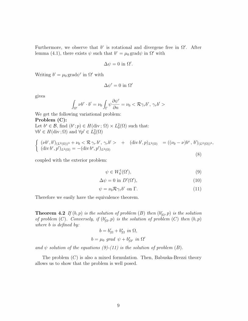
Furthermore, we observe that br is rotational and divergene free in Ω′. Afterlemma (4.1), there exists ψ such that br = µ0 gradψ in Ω′ with

∆ψ = 0 in Ω′.

Writing b′ = µ0 gradψ′ in Ω′ with

∆ψ′ = 0 in Ω′

gives ∫

Ω′νbr · b′ = ν0

∫

Γψ

∂ψ′

∂n= ν0 < Rγτb

r, γτb′ >

We get the following variational problem:Problem (C):Let bs ∈ B, find (br; p) ∈ H(div ; Ω)× L2

0(Ω) such that:∀b′ ∈ H(div ; Ω) and ∀p′ ∈ L2

0(Ω)

(νbr, b′)(L2(Ω))3 + ν0 < R γτ br, γτb

′ > + (div b′, p)L2(Ω) = ((ν0 − ν)bs , b′)(L2(Ω))3 ,(div br, p′)L2(Ω) = −(div bs, p′)L2(Ω)

(8)coupled with the exterior problem:

ψ ∈ W 10 (Ω′), (9)

∆ψ = 0 in D′(Ω′), (10)

ψ = ν0Rγτbr on Γ. (11)

Therefore we easily have the equivalence theorem.

Theorem 4.2 If (b, p) is the solution of problem (B) then (br|Ω, p) is the solution

of problem (C). Conversely, if (br|Ω, p) is the solution of problem (C) then (b, p)

where b is defined by:b = br

|Ω + bs|Ω in Ω,

b = µ0 grad ψ + bs|Ω′ in Ω′

and ψ solution of the equations (9)-(11) is the solution of problem (B).

The problem (C) is also a mixed formulation. Then, Babuska-Brezzi theoryallows us to show that the problem is well posed.

9

4.2.1 Study of problem (C)

We write the problem (C) as follows:let bs ∈ H, find (br, p) ∈ H(div ; Ω)× L2

0(Ω), such that:

a1(b

r, b′) + b1(b′, p) = g1(b

′) ∀b′ ∈ H(div ; Ω),b1(b

r, p′) = g2(p′)L2(Ω) ∀p′ ∈ L2

0(Ω).(12)

On H(div ; Ω)×H(div ; Ω) the bilinear form a1 is defined by:

a1(b, b′) = (νb, b′)(L2(Ω))3 + ν0 < R γτ b, γτ b′ >,

on H(div ; Ω)× L20(Ω), the bilinear continuous form b1 is defined by:

b1(b, p) = (div b, p)L2(Ω).

Moreover, let g1 and g2 be linear continuous forms:

g1(b) = ((ν0 − ν) bs , b)(L2(Ω))3 on H(div ; Ω)

andg2(p) = −(div bs, p)L2(Ω) on L2

0(Ω).

We deduce from the properties of the integral operator R that the bilinear forma1 is continuous on H(div ; Ω)×H(div ; Ω). Now, let N(b1) be the null space ofthe bilinear form b1. It is obvious that:

N(b1) = b ∈ H(div, Ω) div b = 0 in Ω.

We study the existence and uniqueness of the solution for the problem (C).First, we get the following lemma.

Lemma 4.2 Let a1( . , . ) be the previous bilinear form. There exists a positiveconstant α such that:

∀b ∈ N(b1), a1(b, b) ≥ α‖b‖2H(div ; Ω)

where N(b1).

Proof: We deduce from lemma (2.1):

a1(b, b) = ||b||2(L2(Ω))3 + ν0 < R γτ b , γτ b >,

≥ c||b||2H(div ; Ω)

, ∀b ∈ N(b1).

We establish now the statement:

10

Lemma 4.3 Let b1( . , . ) be the previous bilinear form defined on H(div ; Ω) ×L2(Ω). Then, there exists a positive constant β such that:

supb∈H(div,Ω)\0

b1(b, p)

‖b‖H(div ;Ω)

≥ β ||p||L2(Ω) , ∀ p ∈ L20(Ω).

Proof: Let p ∈ L20(Ω) and φ be the solution of the Neumann problem:

∆φ = p in Ω,

∂φ∂n

= 0 in Γ.(13)

Then φ ∈ H1(Ω). We set now b0 = gradφ. Therefore, b0 ∈ H(div ; Ω), and wehave

b1(b0 , p) = ||p||2L2(Ω).

Also, there exists a constant β > 0 such as:

b1(b0 , p) ≥ β||p||L2(Ω)||b0||H(div; Ω).

The previous lemma allows to have the following statement.

Theorem 4.3 The problem (C) has an unique solution (br, p) ∈ H(div ; Ω) ×L2

0(Ω).

In the following section, we concentrate on the study of the numerical analysisfor both mixed formulations (A) and (C).

5 Conforming finite element approximations

5.1 Discretization of problem (A)

In order to define our discrete Galerkin scheme we consider the finite elementapproximation of problem (A) by means of Nedelec edge elements and RaviartThomas face elements with respect to simplicial triangulation of Ω.Let τ 1

h be a regular triangulation of Ω made up of tetrahedra of diameter hK withh = supK∈τ1

hhK. A triangulation τ 2

h of Γ is deducted from τ 1h .

First, we use the standard Nedelec element space to interpolate functions inH(curl, Ω), [16]:

Hh = hh ∈ H(curl, Ω) ; hh|K = α+β×x, ∀K ∈ T 1h , α ∈ (P0)

3, β ∈ (P0)3, x ∈ R3.

We denote by Pk the space of polynomials of degree at most k. We also introduce:

H0h = hh ∈ Hh; hh × n|Γ = 0.

11

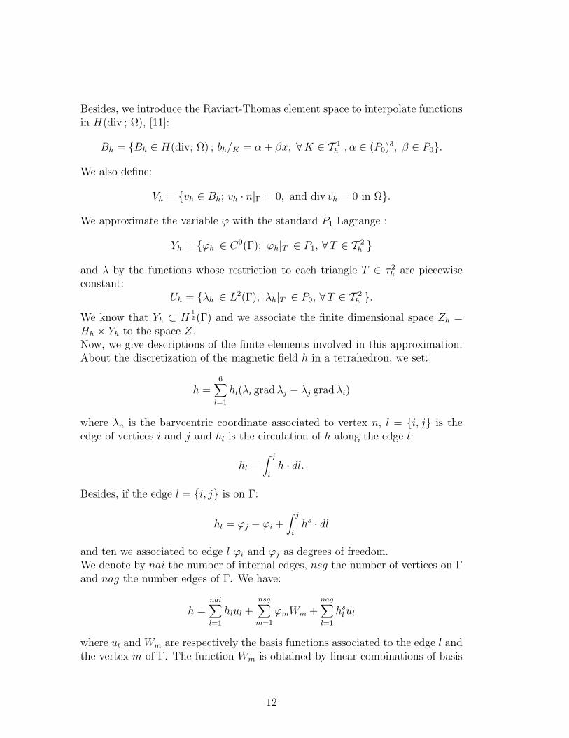
Besides, we introduce the Raviart-Thomas element space to interpolate functionsin H(div ; Ω), [11]:

Bh = Bh ∈ H(div; Ω) ; bh/K = α + βx, ∀K ∈ T 1h , α ∈ (P0)

3, β ∈ P0.

We also define:

Vh = vh ∈ Bh; vh · n|Γ = 0, and div vh = 0 in Ω.

We approximate the variable ϕ with the standard P1 Lagrange :

Yh = ϕh ∈ C0(Γ); ϕh|T ∈ P1, ∀T ∈ T 2h

and λ by the functions whose restriction to each triangle T ∈ τ 2h are piecewise

constant:Uh = λh ∈ L2(Γ); λh|T ∈ P0, ∀T ∈ T 2

h .We know that Yh ⊂ H

12 (Γ) and we associate the finite dimensional space Zh =

Hh × Yh to the space Z.Now, we give descriptions of the finite elements involved in this approximation.About the discretization of the magnetic field h in a tetrahedron, we set:

h =6∑

l=1

hl(λi grad λj − λj grad λi)

where λn is the barycentric coordinate associated to vertex n, l = i, j is theedge of vertices i and j and hl is the circulation of h along the edge l:

hl =∫ j

ih · dl.

Besides, if the edge l = i, j is on Γ:

hl = ϕj − ϕi +∫ j

ihs · dl

and ten we associated to edge l ϕi and ϕj as degrees of freedom.We denote by nai the number of internal edges, nsg the number of vertices on Γand nag the number edges of Γ. We have:

h =nai∑

l=1

hlul +nsg∑

m=1

ϕmWm +nag∑

l=1

hsl ul

where ul and Wm are respectively the basis functions associated to the edge l andthe vertex m of Γ. The function Wm is obtained by linear combinations of basis

12

functions associated to edges on Γ whose m is a vertex.On the other hand, the discretization of vh in tetrahedron is, [2]:

vh =4∑

f=1

vfwf

where vf =∫f v · n ds and if f = l, m, n

wf = 2(λl grad λm × grad λn + λm grad λn × grad λl + λn grad λl × grad λm).

All faces of T 1h have to be endowed with a fixed internal orientation, (as all the

edges).For the variable ϕ, we have

ϕ =3∑

i=1

ϕi λi

where ϕi is the nodal variable associated to vertex i of a triangle of the boundary.Then, in our discrete scheme the degrees of freedom are:

• the circulation of the magnetic field h inside Ω,

• the scalar reaction potential ϕ at the vertices of Γ,

• the flux of potential vector v on all faces inside Ω,

• the value of Lagrange multiplier λ on all faces of Γ.

We are now in position to write the discrete version of problem (A):Problem (Ah):Let hs ∈ H, find ((hr

h, ϕh, λh), vh) in Zh × Vh such that:

a((hrh, ϕh, λh), (h

′h, ϕ

′h, λh)) + b((h′h, ϕ

′h), vh) = f1((h

′h, ϕ

′h, λ

′h)) ∀(h′h, ϕ′h, λ′h) ∈ Zh,

b((hrh, ϕh, λh), v

′h) = f2(v

′h) ∀v′h ∈ Vh.

Now, we study the discrete problem (Ah) via the Babuska-Brezzi theory.

5.1.1 Study of the discrete problem (Ah)

First, we get the lemma.

Lemma 5.1 There exists a positive constant α such that:

∀ (hh, ϕh, λh) ∈ N(b) ∩ Zh, a((hh, ϕh, λh), (hh, ϕh, λh)) ≥ α‖(hh, ϕh, λh)‖2Z .

Now, let us consider the finite elements spaces H0h and Vh. From [16], we have

the following statement.

13

Theorem 5.1 For every vh in Vh , there exists a unique element hh in H0h such

that:curl hh = vh.

Moreover,||hh||H(curl, Ω)

≤ C||vh||(L2(Ω))3 .

On the other hand, we obtain the statement.

Lemma 5.2 There exists a positive constant β such that:

sup(hh,ϕh,λh)∈Zh\0

b((hh, ϕh, λh), vh)

‖(hh, ϕh, λh)‖Z

≥ β ||vh||L2(Ω) , ∀ vh ∈ Vh.

Proof: Let vh ∈ Vh. We consider the vector function hh in H0h such that

curl hh = vh.

Then it is clear that (hh, 0, 0) ∈ Zh and we have

b((hh, 0, 0), vh) = ||hh||H(curl ; Ω)||vh||(L2(Ω))3 .

Finally, we deduce that there exists a constant C > 0 such that:

b((hh, 0, 0), vh) ≥ C||(hh, 0, 0)||Z ||vh||(L2(Ω))3 .

Therefore, we have the result.

Theorem 5.2 The problem (Ah) has a unique solution ((hrh, ϕh, λh), vh) in Zh×

Vh.

Since the triangulations are regular, we can get an error estimate of order 1.

Theorem 5.3 Assume that ((h, ϕ, λ), v) belongs to H2(Ω)×H3/2(Γ)×H1/2(Γ)×H1(Ω), then there exists a constant C independent of h such that:

‖h− hh‖H(curl ;Ω)+ ‖ϕ− ϕh‖H1/2(Γ) + ‖v − vh‖(L2(Ω))3 + ‖λ− λh‖H−1/2(Γ)

≤ C h(|h|(H2(Ω))3 + |v|(H1(Ω))3 + ‖ϕ‖H3/2(Γ)) + ‖λ‖H1/2(Γ))

proof: see [11], [16].

14

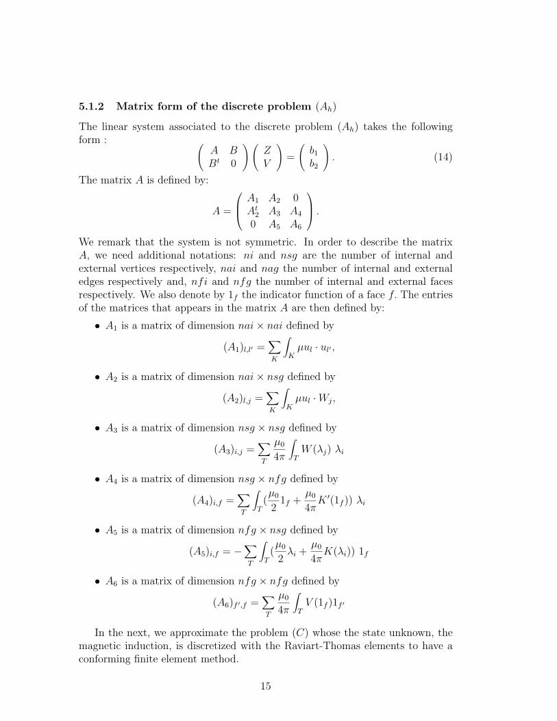
5.1.2 Matrix form of the discrete problem (Ah)

The linear system associated to the discrete problem (Ah) takes the followingform : (

A BBt 0

) (ZV

)=

(b1

b2

). (14)

The matrix A is defined by:

A =

A1 A2 0At

2 A3 A4

0 A5 A6

.

We remark that the system is not symmetric. In order to describe the matrixA, we need additional notations: ni and nsg are the number of internal andexternal vertices respectively, nai and nag the number of internal and externaledges respectively and, nfi and nfg the number of internal and external facesrespectively. We also denote by 1f the indicator function of a face f. The entriesof the matrices that appears in the matrix A are then defined by:

• A1 is a matrix of dimension nai× nai defined by

(A1)l,l′ =∑

K

∫

Kµul · ul′ ,

• A2 is a matrix of dimension nai× nsg defined by

(A2)l,j =∑

K

∫

Kµul ·Wj,

• A3 is a matrix of dimension nsg × nsg defined by

(A3)i,j =∑

T

µ0

4π

∫

TW (λj) λi

• A4 is a matrix of dimension nsg × nfg defined by

(A4)i,f =∑

T

∫

T(µ0

21f +

µ0

4πK ′(1f )) λi

• A5 is a matrix of dimension nfg × nsg defined by

(A5)i,f = −∑

T

∫

T(µ0

2λi +

µ0

4πK(λi)) 1f

• A6 is a matrix of dimension nfg × nfg defined by

(A6)f ′,f =∑

T

µ0

4π

∫

TV (1f )1f ′

In the next, we approximate the problem (C) whose the state unknown, themagnetic induction, is discretized with the Raviart-Thomas elements to have aconforming finite element method.

15

5.2 Discretization of problem (C)

We will seek an approximation of the first unknown b of problem (C) in Bh. Thefinite dimensional space Ph corresponding to the unknown p is given by piecewiseconstant function on the triangulation of Ω:

Ph = ph ∈ L2(Ω); ph|K ∈ P0, ∀K ∈ τ 1h .

We denote by R1 the operator defined by:

R1 = γ∗τRγτ ∈ L(H(div ; Ω), H(div ; Ω)′).

In order to define an approximation of the oprator R1, we consider the canonicalembeddings:

ih : Bh → H(div Ω)

jh : Uh → H−1/2(Γ)

kh : Yh → H1/2(Γ)

with i∗h, j∗h and k∗h their duals.We then define the discrete operator

Rh = i∗hγ∗τ (

I

2+ K)kh(k

∗hWkh)

−1k∗h(I

2+ K ′)γ∗τV γτ ih + i∗hγ

∗τV γτ ih

where I stands for the identity.Define the bilinear form on Bh ×Bh:

a1h(bh, b

′h) = (νbh, b

′h)(L2(Ω))3 + ν0(Rh bh, b′h)Bh

.

Then, we are in position to write the discrete version of problem (C):Problem (Ch):Let bs ∈ H, find (br

h, ph) in Bh × Ph such that:

a1h(br

h, b′h) + b1(b

′h, ph) = g1(b

′h) ∀b′h ∈ Bh,

b1(brh, p

′h) = g2(p

′h) ∀p′h ∈ Ph.

(15)

We are going to show that the discrete problem is well-posed in the context ofthe Babuska-Brezzi theory.

5.2.1 Study of problem (Ch)

First, we get the following statement.

Lemma 5.3 There exists c > 0 such that

(Rh bh, bh)Bh≥ c||γτ ihbh||2H−1/2(Γ), ∀bh ∈ Bh.

16

Proof. The operator W is positive. Then, we have:

(Rh bh, bh)Bh≥ (i∗hγτV γτ ih bh, γτ ih bh)Bh

.

Since V is positive definite, there exists a constant c > 0 such as:

(Rh bh, bh)Bh≥ c||γτ ihbh||2H−1/2(Γ), ∀bh ∈ Bh.

Because of the approximation property of the inverse of Dirichlet-Neumann op-erator and of the discrete spaces, we obtain the coercivity of the bilinear form a1h

and the “inf-sup” condition which are necessary to the existence and uniquenessof the solution of the discrete problem considered.

Theorem 5.4 There exists α > 0 such as:

b1(bh, ph) = 0 ∀ph ∈ Ph, implies a1h(bh, bh) ≥ α||bh||2H(div ;Ω)

and there exists a positive constant β such as:

supbh ∈Zh\0

b1(bh, ph)

||ph||L2(Ω)

≥ β ||ph||L2(Ω) ∀ ph ∈ Ph.

Then the discrete problem (Ch) has a unique solution.

Proof. As Bh ⊂ H(div ; Ω) and with the previous lemma we have the coercivityof a1.Let ph be in Ph, we may associate v ∈ (H1(Ω))3 such that :

div v = ph in Ω,

||v||H1(Ω)3 ≤ C||ph||L2(Ω).

Now we denote by Πh the interpolating operator associated to face element. Now,choosing bh = Πhv, we have:

b1(bh, ph) = b1(v, ph) = ||ph||2L2(Ω).

Then, we have the result.The linear system associated to the problem (Bh) is symmetric and we remarkthat once again we recover exactly the system in the form of (14):

(A1 B1

Bt1 0

) (UT

)=

(b1

b2

).

The unknowns in our discrete Galerkin scheme are:

Σf (Ω) = σf (b) =∫

fb · n dγ, f face of T 1

h ,

Σt(Ω) = σt(p) = pT , T tetrahedra of T 1h ,

The matrices A1 and B1 are easily obtained. In the next, we study the conver-gence of the method.

17

5.2.2 Study of the convergence of the method

In the convergence analysis of the method, we shall use the lemma (5.3) and thesecond crucial point.

Lemma 5.4 There exists a constant c > 0 such that

(Rh bh −R1 b, bh − b′h)Bh≤ c ||bh − b′h||H(div ; Ω)

.( distH1/2(W−1(I/2 + K ′)γτ b, Yh) + ||bh − b||H(div ; Ω)

)

∀ bh, b′h ∈ Bh, ∀ b ∈ B.

Proof. The proof is based on Cea’s estimate applied to W and k∗hWkh andcan be found in [4]. Besides, we use the continuity of γτ from H(div ; Ω) intoH−1/2(Γ).Now, we can state the convergence of the method.

Theorem 5.5 There exists a constant c > 0 such that:

||b− bh||H(div ; Ω)+ ||p− ph||L2(Ω) ≤ c inf

vh∈Z(g2)||b− vh||H(div ; Ω)

+distH1/2 (W−1(I

2+ K ′)γτb, Yh)+ inf

p′h∈Ph

||p− p′h||L2(Ω)

where Z(g2) = bh ∈ Bh, b1(bh, ph) = g2(ph), ∀ph ∈ Ph.Proof. On the first hand, we have

||b− bh||H(div ; Ω)≤ ||b− vh||H(div ; Ω)

+ ||vh − bh||H(div ; Ω), ∀vh ∈ Z(g2).

As bh − vh ∈ N(b1) and that the bilinear form a1his coercive on N(b1) , we can

write

α||bh − vh||H(div ; Ω)≤ sup

wh ∈N(b1)\0

a1h(bh − vh, wh)

‖wh‖L2(Ω)

= supwh ∈N(b1)\0

a1h(bh, wh)− a1h

(vh, wh)

‖wh‖L2(Ω)

.

Besides, we have a1(u, vh) = a1h(uh, vh), if vh ∈ N(b1). This implies:

α||bh − vh|| ≤ supwh ∈N(b1)\0

a1(b, wh)− a1h(vh, wh)

‖wh‖L2(Ω)

= supwh ∈N(b1)\0

ν0(b− vh, wh)L2 + ν0(R1b−Rh vh, wh)Bh

‖wh‖L2(Ω)

.

On the other hand, we can write ∀ qh ∈ Ph:

β||ph − qh||L2(Ω) ≤ supwh ∈Zh\0

b(wh, ph − qh)

‖wh‖H(div ; Ω)

= supwh ∈Zh\0

−a1h(bh, wh) + a1(b, wh)− b1(wh, qh − p)

‖wh‖H(div ; Ω)

.

Consequently, the result is proved.

18

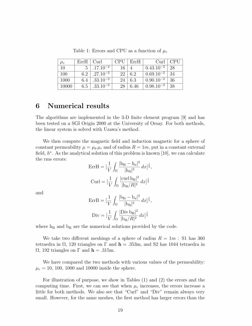
Table 1: Errors and CPU as a function of µr

µr ErrH Curl CPU ErrH Curl CPU10 5 .17.10−2 16 4 0.43.10−2 28100 6.2 .27.10−2 22 6.2 0.69.10−2 341000 6.4 .33.10−2 24 6.3 0.90.10−2 3610000 6.5 .33.10−2 28 6.46 0.98.10−2 38

6 Numerical results

The algorithms are implemented in the 3-D finite element program [9] and hasbeen tested on a SGI Origin 2000 at the University of Orsay. For both methods,the linear system is solved with Uzawa’s method.

We then compute the magnetic field and induction magnetic for a sphere ofconstant permeability µ = µ0 µr and of radius R = 1m, put in a constant externalfield, hs. As the analytical solution of this problem is known [10], we can calculatethe rms errors:

ErrH = [1

V

∫

Ω

|hn − ha|2|ha|2 dx]

12 ,

Curl = [1

V

∫

Ω

|curl hn|2|ha/R|2 dx]

12

and

ErrB = [1

V

∫

Ω

|bn − ba|2|ba|2 dx]

12 ,

Div = [1

V

∫

Ω

|Div bn|2|ba/R|2 dx]

12

where hn and bn are the numerical solutions provided by the code.

We take two different meshings of a sphere of radius R = 1m : S1 has 360tetraedra in Ω, 120 triangles on Γ and h = .353m, and S2 has 1044 tetraedra inΩ, 192 triangles on Γ and h = .315m.

We have compared the two methods with various values of the permeability:µr = 10, 100, 1000 and 10000 inside the sphere.

For illustration of purpose, we show in Tables (1) and (2) the errors and thecomputing time. First, we can see that when µr increases, the errors increase alittle for both methods. We also see that “Curl” and “Div” remain always verysmall. However, for the same meshes, the first method has larger errors than the

19

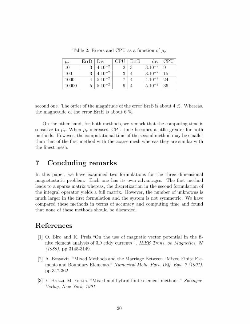
Table 2: Errors and CPU as a function of µr

µr ErrB Div CPU ErrB div CPU10 3 4.10−2 2 3 3.10−2 9100 3 4.10−2 3 4 3.10−2 151000 4 5.10−2 7 4 4.10−2 2410000 5 5.10−2 9 4 5.10−2 36

second one. The order of the magnitude of the error ErrB is about 4 %. Whereas,the magnetude of the error ErrH is about 6 %.

On the other hand, for both methods, we remark that the computing time issensitive to µr. When µr increases, CPU time becomes a litlle greater for bothmethods. However, the computational time of the second method may be smallerthan that of the first method with the coarse mesh whereas they are similar withthe finest mesh.

7 Concluding remarks

In this paper, we have examined two formulations for the three dimensionalmagnetostatic problem. Each one has its own advantages. The first methodleads to a sparse matrix whereas, the discretization in the second formulation ofthe integral operator yields a full matrix. However, the number of unknowns ismuch larger in the first formulation and the system is not symmetric. We havecompared these methods in terms of accuracy and computing time and foundthat none of these methods should be discarded.

References

[1] O. Biro and K. Preis,“On the use of magnetic vector potential in the fi-nite element analysis of 3D eddy currents ”, IEEE Trans. on Magnetics, 25(1989), pp 3145-3149.

[2] A. Bossavit, “Mixed Methods and the Marriage Between “Mixed Finite Ele-ments and Boundary Elements.” Numerical Meth. Part. Diff. Equ, 7 (1991),pp 347-362.

[3] F. Brezzi, M. Fortin, “Mixed and hybrid finite element methods.” Springer-Verlag, New-York, 1991.

20

[4] C. Cartensen,“Interface Problem in Holonomic Elastoplastic”, MathematicalMethods in the Applied Sciences, Vol. 16, (1993), pp 819-835.

[5] M. Cessenat, “Exemples en electromagnetisme et en physique quantique.”Analyse mathematique et calcul numerique pour les sciences et les techniques,Ed by R. Dautray and J.L. Lions, Masson 1988 vol 5, chap IX, pp 235-273.

[6] M. Costabel and Ernst P. Stephan, “Coupling of Finite and Boundary Ele-ment Method For An Elastoplastic Interface Prolem”, Siam, J. Numer. Anal.Vol 27, No 5, oct. 1990, , pp 1212-1226.

[7] M. Costabel, “Boundary Integral operators on Lipschitz domains: Elemen-tary results”, SIAM J. Math. Anal., 19 (1988), pp 613-626.

[8] C. Daveau and J. Laminie, “ Mixed and Hybrid Formulations For TheThree-Dimensional magnetostatic problem”, Num. Meth. Partial Diff. Equ.,2002, pp 85-104.

[9] B. Bandelier, C. Daveau, J. Laminie, M. Mefire and F. Rioux-Damidau ,“Three-Dimensional Magnetostatic Problem”, Int. J. Num. Meth. Engng.,46, 1999, pp 117-130.

[10] E. Durand, “Magnetostatique”, Masson, Paris, Dunod 1968.

[11] V. Girault, P. A. Raviart, “Finite element methods for Navier-Stokes equa-tions.” Springer-Verlag, Berlin - Heidelberg - New York - Tokyo, 1986.

[12] Hsiao G. and Porter J.F.,“The Coupling of BEM and FEM for the Two-Dimensional Viscous Flow Problem”, Applicable Analysis, (1988), Vol. 27,pp 79-108.

[13] Johnson C., Nedelec J. C., “On the Coupling of Boundary Integral and FiniteElement Methods”, Math. Comp., Vol. 35,, pp1063-1079.

[14] F. Kikuchi, “Mixed formulations for finite element analysis of magnetostaticand electrostatic problems, ” Japan J. Appl. Math. 6, 1989, pp 209-221.

[15] T. Nakata and K. Fujiwara,“ Summary on results for Benchmark problem 13(3D Non-linear magnetostatic model)”, COMPEL, 11 (1992), pp 345-369.

[16] J. C. Nedelec : “A New Family of Mixed finite elements in IR3, ”, Numer.Math., 35, 1986, pp 57-80.

[17] R. Stenberg and P. Trouve, “A Mixed Finite Element Method for the Mag-netic Field.” International Symposium on Numerical Methods in Engineer-ing.

21