Master of Science in

Computacional Mechanics

Erasmus Mundos Master Course

INTRODUCTION TO THE FINITE ELEMENT METHOD

Lectures

EUGENIO OÑATE PEDRO DÍEZ

FRANCISCO ZÁRATE ANTONIA LARESE

October 2008

Contents

1 INTRODUCTION TO THE FINITE ELEMENT METHOD 11.1 WHAT IS THE FINITE ELEMENT METHOD? . . . . . . . . 11.2 ANALYTICAL AND NUMERICAL METHODS . . . . . . . . 11.3 WHAT IS A FINITE ELEMENT? . . . . . . . . . . . . . . . . 21.4 STRUCTURAL MODELLING AND FEM ANALYSIS . . . . . 3

1.4.1 Classification of the problem . . . . . . . . . . . . . . . . 31.4.2 Structural model . . . . . . . . . . . . . . . . . . . . . . 31.4.3 Structural analysis by the FEM . . . . . . . . . . . . . . 51.4.4 Verification and validation of FEM results . . . . . . . . 6

1.5 DISCRETE SYSTEMS. BAR STRUCTURES . . . . . . . . . . 91.5.1 Basic concepts of matrix analysis of bar structures . . . . 101.5.2 Analogy with the matrix analysis of other discrete systems 131.5.3 Basic steps for matrix analysis of discrete systems . . . . 15

1.6 DIRECT ASSEMBLY OF THE GLOBAL STIFFNESS MATRIX 171.7 DERIVATION OF THE MATRIX EQUILIBRIUM EQUATI-

ONS FOR THE BAR ELEMENT USING THE PRINCIPLEOF VIRTUAL WORK . . . . . . . . . . . . . . . . . . . . . . . 19

1.8 DERIVATION OF THE BAR EQUILIBRIUM EQUATIONSVIA THE MINIMUM TOTAL POTENTIAL ENERGY PRIN-CIPLE . . . . . . . . . . . . . . . . . . . . . . . . . . . . . . . . 20

1.9 PLANE PIN-JOINTED FRAMEWORKS . . . . . . . . . . . . 221.10 TREATMENT OF PRESCRIBED DISPLACEMENTS AND

COMPUTATION OF REACTIONS . . . . . . . . . . . . . . . . 241.11 INTRODUCTION TO THE FINITE ELEMENT METHOD

FOR ANALYSIS OF CONTINUUM SYSTEMS . . . . . . . . . 27

i

1

Contents

2 FEM ANALYSIS OF 1D PROBLEMS. APPLICATION TOTHE POISSON EQUATION 332.1 INTRODUCTION . . . . . . . . . . . . . . . . . . . . . . . . . 332.2 THE POISSON EQUATION . . . . . . . . . . . . . . . . . . . 342.3 WEIGHTED RESIDUAL METHOD . . . . . . . . . . . . . . . 40

2.3.1 Approximation of the unknown. Weighted Residuals . . 422.3.2 Application of the WRM for the solution of the 1D heat

conduction equation . . . . . . . . . . . . . . . . . . . . 432.3.3 Global definition of the shape functions . . . . . . . . . . 452.3.4 Point Collocation Method . . . . . . . . . . . . . . . . . 482.3.5 Subdomain collocation method . . . . . . . . . . . . . . 512.3.6 Galerkin method . . . . . . . . . . . . . . . . . . . . . . 532.3.7 Least square method . . . . . . . . . . . . . . . . . . . . 55

2.4 GENERAL SOLUTION PROCEDURE . . . . . . . . . . . . . 592.4.1 Conclusions . . . . . . . . . . . . . . . . . . . . . . . . . 61

2.5 INTEGRABILITY CONDITION . . . . . . . . . . . . . . . . . 622.6 WEAK FORM OF THE WEIGHTED RESIDUAL METHOD . 62

2.6.1 Natural boundary condition . . . . . . . . . . . . . . . . 642.6.2 Discretization of the weak form . . . . . . . . . . . . . . 64

2.7 DERIVATION OF THE PRINCIPLE OF VIRTUAL WORKFROM THE WEIGHTED RESIDUAL METHOD . . . . . . . 71

2.8 THE PVW IN POISSON PROBLEMS . . . . . . . . . . . . . . 732.9 THE FEM IN 1D POISSON PROBLEMS . . . . . . 73

2.9.1 Discretization of the problem. Local definition of theshape functions . . . . . . . . . . . . . . . . . . . . . . . 75

2.9.2 Derivation of the algebraic equation systems. Solutionof the 1D Poisson problem using one 2-noded 1D element 77

2.9.3 Solution of the 1D Poisson problem using two 2-nodedelements . . . . . . . . . . . . . . . . . . . . . . . . . . . 81

2.10 GENERALIZATION OF THE SOLUTION FOR A MESH OFTWO-NODED ELEMENTS . . . . . . . . . . . . . . . . . . . . 85

i

2

Contents

3 1D FINITE ELEMENTS FOR AXIALLY LOADED RODS 873.1 INTRODUCTION . . . . . . . . . . . . . . . . . . . . . . . . . . 873.2 AXIALLY LOADED ROD . . . . . . . . . . . . . . . . . . . . . . 873.3 AXIALLY LOADED ROD OF CONSTANT CROSS SECTIONAL

AREA. DISCRETIZATION IN ONE LINEAR ROD ELEMENT . 893.4 DERIVATION OF THE DISCRETIZED EQUATIONS FROM

THE GLOBAL DISPLACEMENT INTERPOLATION FIELD . . 943.5 AXIALLY LOADED ROD OF CONSTANT CROSS

SECTIONAL AREA. DISCRETIZATION IN TWO LINEAR RODELEMENTS . . . . . . . . . . . . . . . . . . . . . . . . . . . . . . 97

3.6 GENERALIZATION OF THE SOLUTION WITH N LINEARROD ELEMENTS . . . . . . . . . . . . . . . . . . . . . . . . . . 102

3.7 EXTRAPOLATION OF THE SOLUTION FROM TWO DIF-FERENT MESHES . . . . . . . . . . . . . . . . . . . . . . . . . . 106

3.8 MATRIX FORMULATION OF THE ELEMENT EQUATIONS . 1083.8.1 Shape function matrix . . . . . . . . . . . . . . . . . . . . 1093.8.2 Strain matrix . . . . . . . . . . . . . . . . . . . . . . . . . 1093.8.3 Constitutive matrix . . . . . . . . . . . . . . . . . . . . . . 1093.8.4 Principle of Virtual Work . . . . . . . . . . . . . . . . . . 1103.8.5 Stiffness matrix and equivalent nodal force vector . . . . . 110

3.9 SUMMARY OF THE STEPS FOR THE ANALYSIS OF A STRUC-TURE USING THE FEM . . . . . . . . . . . . . . . . . . . . . . 112

3.10 ADVANCED ROD ELEMENTS AND REQUIREMENTS FORTHE NUMERICAL SOLUTION . . . . . . . . . . . . . . . . . . 1133.10.1 INTRODUCTION . . . . . . . . . . . . . . . . . . . . . . 113

3.11 ONE DIMENSIONAL Co ELEMENTS. LAGRANGEELEMENTS . . . . . . . . . . . . . . . . . . . . . . . . . . . . . . 114

3.12 ISOPARAMETRIC FORMULATION AND NUMERICAL INTE-GRATION . . . . . . . . . . . . . . . . . . . . . . . . . . . . . . . 1173.12.1 Introduction . . . . . . . . . . . . . . . . . . . . . . . . . . 1173.12.2 The concept of parametric interpolation . . . . . . . . . . 1183.12.3 Isoparametric formulation of the two-noded rod element . 1203.12.4 Isoparametric formulation of the 3-noded quadratic rod el-

ement . . . . . . . . . . . . . . . . . . . . . . . . . . . . . 121

i

3

3.13 NUMERICAL INTEGRATION . . . . . . . . . . . . . . . . . . . 1233.14 STEPS FOR THE COMPUTATION OF MATRICES AND VEC-

TORS FOR AN ISOPARAMETRIC ROD ELEMENT . . . . . . 1253.14.1 Interpolation of the axial displacement . . . . . . . . . . . 1263.14.2 Geometry interpolation . . . . . . . . . . . . . . . . . . . . 1263.14.3 Interpolation of the axial strain . . . . . . . . . . . . . . . 1263.14.4 Computation of the axial force . . . . . . . . . . . . . . . . 1273.14.5 Element stiffness matrix . . . . . . . . . . . . . . . . . . . 1273.14.6 Equivalent nodal force vector . . . . . . . . . . . . . . . . 128

3.15 BASIC ORGANIZATION OF A FINITE ELEMENT PROGRAM 1293.16 SELECTION OF ELEMENT TYPE . . . . . . . . . . . . . . . . 1293.17 REQUIREMENTS FOR CONVERGENCE OF THE SOLUTION 133

3.17.1 Continuity condition . . . . . . . . . . . . . . . . . . . . . 1333.17.2 Derivativity condition . . . . . . . . . . . . . . . . . . . . 1333.17.3 Integrability condition . . . . . . . . . . . . . . . . . . . . 1333.17.4 Rigid body condition . . . . . . . . . . . . . . . . . . . . . 1343.17.5 Constant strain condition . . . . . . . . . . . . . . . . . . 134

3.18 ASSESSMENT OF CONVERGENCE REQUIREMENTS.THE PATCH TEST . . . . . . . . . . . . . . . . . . . . . . . . . 135

3.19 OTHER REQUIREMENTS FOR THE FINITE ELEMENT AP-PROXIMATION . . . . . . . . . . . . . . . . . . . . . . . . . . . 1373.19.1 Compatibility condition . . . . . . . . . . . . . . . . . . . 1373.19.2 Condition of complete polynomial . . . . . . . . . . . . . . 1373.19.3 Stability condition . . . . . . . . . . . . . . . . . . . . . . 1383.19.4 Geometric invariance condition . . . . . . . . . . . . . . . 139

3.20 SOME REMARKS ON THE COMPATIBILITY AND EQUILIB-RIUM OF THE SOLUTION . . . . . . . . . . . . . . . . . . . . . 139

3.21 CONVERGENCE REQUIREMENTS IN ISOPARAMETRIC EL-EMENTS . . . . . . . . . . . . . . . . . . . . . . . . . . . . . . . 141

3.22 ERROR TYPES IN THE FINITE ELEMENT SOLUTION . . . 1423.22.1 Discretization error . . . . . . . . . . . . . . . . . . . . . . 1423.22.2 Error in the geometry approximation . . . . . . . . . . . . 1433.22.3 Error in the computation of the element integrals . . . . . 1443.22.4 Errors in the solution of the global equation system . . . . 1443.22.5 Errors associated with the constitutive equation . . . . . . 146

ii

4

ii CONTENTS

5

Contents

7 SHAPE FUNCTIONS FOR 2D AND 3D ELEMENTS WITHC CONTINUITY 1837.1 INTRODUCTION . . . . . . . . . . . . . . . . . . . . . . . . . 1837.2 DERIVATION OF THE SHAPE FUNCTIONS FOR Co TWO

DIMENSIONAL ELEMENTS . . . . . . . . . . . . . . . . . . . 1837.2.1 Complete polynomials in two dimensions. Pascal’s triangle1837.2.2 Shape functions of Co rectangular elements. Natural

coordinates in two dimensions . . . . . . . . . . . . . . . 1847.3 LAGRANGE RECTANGULAR ELEMENTS . . . . . . . . . . 186

7.3.1 Four-noded Lagrange rectangle . . . . . . . . . . . . . . 1867.3.2 Nine-noded quadratic Lagrange rectangle . . . . . . . . . 1867.3.3 Sixteen-noded cubic Lagrange rectangle . . . . . . . . . . 1907.3.4 Other Lagrange rectangular elements . . . . . . . . . . . 190

7.4 SERENDIPITY RECTANGULAR ELEMENTS . . . . . . . . . 1917.4.1 Eigth-noded quadratic Serendipity rectangle . . . . . . . 1927.4.2 Twelve-noded cubic Serendipity rectangle . . . . . . . . . 1947.4.3 Seventeen-noded quartic Serendipity rectangle . . . . . . 195

7.5 SHAPE FUNCTIONS FOR Co CONTINUOUS TRIANGU-LAR ELEMENTS . . . . . . . . . . . . . . . . . . . . . . . . . 1967.5.1 Area coordinates . . . . . . . . . . . . . . . . . . . . . . 1967.5.2 Derivation of the shape functions for Co continuous tri-

angles . . . . . . . . . . . . . . . . . . . . . . . . . . . . 1987.5.3 Shape functions for the 3-noded linear triangle . . . . . . 1987.5.4 Shape functions for the six-noded quadratic triangle . . . 1997.5.5 Shape functions for the ten-noded cubic triangle . . . . . 2007.5.6 Natural coordinates for triangles . . . . . . . . . . . . . . 201

7.6 ANALYTIC COMPUTATION OF INTEGRALS OVERRECTANGLES AND STRAIGHT SIDE TRIANGLES . . . . . 201

7.7 SHAPE FUNCTIONS FOR 3D ELEMENTS . . . . . . . . . . . 2057.8 RIGHT PRISMS . . . . . . . . . . . . . . . . . . . . . . . . . . 205

7.8.1 Right prisms of the Lagrange family . . . . . . . . . . . 2067.8.2 Serendipity prisms . . . . . . . . . . . . . . . . . . . . . 209

7.9 STRAIGHT EDGED TETRAHEDRA . . . . . . . . . . . . . . 2157.9.1 Shape functions for the 10-noded quadratic tetrahedron . 219

i

6

ii CONTENTS

7.9.2 Shape functions for the 20-noded quadratic tetrahedron . 2207.10 COMPUTATION OF THE ELEMENT INTEGRALS . . . . . . 221

7.10.1 Analytical computation of element integrals . . . . . . . 221

7

Contents

9 2D SOLIDS. LINEAR TRIANGULAR AND RECTANGU-LAR ELEMENTS 2599.1 INTRODUCTION . . . . . . . . . . . . . . . . . . . . . . . . . 2599.2 TWO DIMENSIONAL ELASTICITY THEORY . . . . . . . . . 260

9.2.1 Displacement field . . . . . . . . . . . . . . . . . . . . . 2609.2.2 Strain field . . . . . . . . . . . . . . . . . . . . . . . . . 2619.2.3 Stress field . . . . . . . . . . . . . . . . . . . . . . . . . . 2629.2.4 Stress-strain relationship . . . . . . . . . . . . . . . . . . 2629.2.5 Virtual work expression . . . . . . . . . . . . . . . . . . 270

9.3 FINITE ELEMENT FORMULATION. THREE-NODEDSOLID TRIANGULAR ELEMENT . . . . . . . . . . . . . . . . 2709.3.1 Discretization of the displacement field . . . . . . . . . . 2719.3.2 Discretization of the strain field . . . . . . . . . . . . . . 2739.3.3 Discretization of the stress field . . . . . . . . . . . . . . 2759.3.4 Discretized equilibrium equations . . . . . . . . . . . . . 2759.3.5 Stiffness matrix and equivalent nodal force vectors for

the 3-noded solid triangular element . . . . . . . . . . . 2789.4 THE FOUR NODED SOLID RECTANGULAR ELEMENT . . 282

9.4.1 Basic formulation . . . . . . . . . . . . . . . . . . . . . . 2829.4.2 Some remarks on the behaviour of the 4-noded solid rect-

angle . . . . . . . . . . . . . . . . . . . . . . . . . . . . . 2869.5 PERFORMANCE OF THE 3-NODED SOLID TRIANGLE AND

THE 4-NODED SOLID RECTANGLE . . . . . . . . . . . . . . 2899.6 GENERAL PERFORMANCE OF TRIANGULAR AND

RECTANGULAR ELEMENTS . . . . . . . . . . . . . . . . . . 2919.7 CONCLUDING REMARKS . . . . . . . . . . . . . . . . . . . . 293

10 REFERENCES 295

i

8

Chapter 1

INTRODUCTION TO THE FINITEELEMENT METHOD

1.1 WHAT IS THE FINITE ELEMENT METHOD?The finite element method (FEM) is a procedure for the numerical solution ofthe equations which govern problems found in nature. Usually the behaviour ofnature can be described by equations expressed in differential or integral form.For this reason the FEM is understood in mathematical circles as a numericaltechnique for solving partial differential or integral equations. Generally, theFEM allows to obtain the evolution in space and/or time of one or morevariables representing the behaviour of a physical system.

When referred to the analysis of structures the FEM is a powerful methodfor computing the displacements, stresses and strains in a structure under aset of loads. This is precisely what we aim to study in this book.

1.2 ANALYTICAL AND NUMERICAL METHODSThe conceptual difference between analytical and numerical methods is thatthe former search for the universal mathematical expressions representing thegeneral and “exact” solution of a problem governed typically by mathematicalequations. Unfortunately exact solutions are only possible for a few particularcases which frequently represent coarse simplifications of reality.

On the other hand, numerical methods, such as the FEM aim to providinga solution, in the form of a set of numbers, to the mathematical equationsgoverning a problem. The strategy followed by most numerical methods is totransform the mathematical equations into a set of algebraic equations whichdepend on a finite set of parameters. These equations in the practical caseinvolve many thousands (or even millions) of unknowns and therefore the finalsystem of algebraic equations can only be solved with the help of computers.This explains why even though many numerical methods have been known

1

since the XVIII century, their development and popularity has occurred intandem to the progress of modern computers in the XX century. The termnumerical method is synonym of computational method in this text.

Numerical methods represent, in fact, the return of numbers as the trueprotagonists in the solution of a problem. The loop initiated by Pythagorassome 25 centuries ago has been closed in the last few decades with the evidencethat, with the help of numerical methods, we can find precise answers to anyproblem in science and engineering.

We should keep in mind that numerical methods for structural engineeringare inseparable from mathematics, material modelling and computer science.Nowadays it is unthinkable to attempt the development of a new numericalmethod for the solution of a structural problem without referring to those disci-plines. As an example, any numerical method for solving large scale structuralproblems has to take into account the hardware environment where it will beimplemented (most probably using parallel computing facilities). Also a mod-ern computer program for structural analysis should be able to incorporate thecontinuous advances in the modelling of new materials.

The word which perhaps best synthesizes the immediate future of numer-ical methods is “computational multiphysics”. The solution of problems willnot be attempted from the perspective of a single physical field and it willinvolve all the couplings which characterize the complexity of reality. For in-stance, the design of a structural component for a vehicle (an automobile,an aeroplane, etc.) will take into account the manufacturing process and thefunction which the component will play throughout its life time. Structures incivil engineering will be studied considering the surrounding environment (soil,water, air). Similar examples are found in mechanical, naval and aeronauti-cal engineering and indeed in practically all branches of engineering science.Accounting for the non-deterministic character of data will be essential for esti-mating the probability that the new products and processes conceived by menbehave as planned. The huge computational needs resulting from a “stochasticmultiphysics” viewpoint will demand better numerical methods, new materialmodels and, indeed, faster computers.

It is only through the integration of a deep knowledge of the physical andmathematical basis of a problem and of numerical methods and informatics,that effective solutions will be found for the mega-structural problems of thetwenty-first century.

1.3 WHAT IS A FINITE ELEMENT?A finite element can be visualized as a small portion of a continuum (i.e. astructure). The word “finite” distinguishes such a portion from the “infinites-imal” elements of a differential calculus. The geometry of the continuum isconsidered to be formed by the assembly of a collection of non-overlapping do-mains with simple geometry termed finite elements (i.e. triangles and quadri-

2

laterals in 2D, or tetrahedra and hexahedra in 3D). It is usually said that a“mesh” of finite elements “discretizes” the continuum (Figure 1.1). The spacevariation of the problem parameters (i.e. the displacements in a structure) isexpressed within each element by means of a polynomial expansion. Giventhat the “exact” analytical variation of such parameters is more complex (andgenerally unknown), the FEM only provides an approximation to the exactsolution.

1.4 STRUCTURAL MODELLING AND FEM ANALYSIS

1.4.1 Classification of the problemThe first step in the solution of a problem is the identification of the problemitself. Hence, before we can analyze a structure we must ask ourselfs the fol-lowing questions: Which are the more relevant physical phenomena influencingthe structure? Is the problem of static or dynamic type? Are the kinematicsor the material properties linear or non-linear? Which are the key results re-quested? What is the level of accuracy sought? The answers to these questionsare essential for selecting a structural model and the adequate computationalmethod.

1.4.2 Structural modelComputational methods, such as the FEM, are applied to “models” of a realproblem, and not to the actual problem itself. Even experimental methodsin structural laboratories make use of scale physical models, unless the actualstructure is tested in real size, which rarely occurs. Models can be developedonce the physical nature of a problem is clearly understood. In the derivationof a model we should aim to exclude superfluous details and include all therelevant features of the problem under consideration so that the model candescribe reality with enough accuracy.

A structural model must include three fundamental aspects. The geome-tric description of the actual structure by means of its specific geometricalcomponents (points, lines, surfaces, volumes), the mathematical expression ofthe basic physical laws governing the behaviour of the structure (i.e. force-equilibrium equations) usually written in terms of differential and/or integralequations, and the specification of the properties of the materials in the struc-ture. Note that the same structure can be analyzed using different structuralmodels depending on the accuracy and/or simplicity sought in the analysis.As an example, a beam can be modelled using the more general 3D elasticitytheory, the 2D plane stress theory or the simpler beam theory. Each modelprovides a different set out for the analysis of the actual structure. We shouldbear in mind that the solution taking as its starting point an incorrect struc-tural model, even if obtained with the most accurate numerical method, will

3

Fig. 1.1: Discretization of different solids and structures into finite elements

be a wrong solution, far from correct physical values.

In this book we will study the analysis by the FEM of a number of struc-tural models, each one applicable to one or more practical structural types.The material properties in all cases will be considered to be linear elastic.

4

Furthermore the analysis will be restricted to linear kinematics and to staticloading. The structures are therefore analyzed under linearlinear staticstatic conditionsconditions.Despite their simplicity, these assumptions are applicable to most of the situ-ations found in the everyday practice of structural analysis and design.

The structural models considered in this book are classified as solid models(2D/3D solids and axisymmetric solids), beam and plate models and shell mod-els (faceted shells, axisymmetric shells and curved shells). Figure 1.2 showsthe general features of a typical member of each structural model family. Thestructures that can be analyzed with these models cover the main problemsin structural engineering and include frames, dams, retaining walls, tunnels,bridges, cylindrical tanks, shell roofs, ship hulls, mechanical parts, airplanefuselages, vehicle components, etc.

1.4.3 Structural analysis by the FEM

The geometry of a structure is discretized when it is split into a mesh of finiteelements of a certain accuracy. Clearly the discretization introduces anotherapproximation. With respect to reality we have therefore to account for twoerror sources from the outset: the modelling error and the discretization error.The former can be reduced by improving the structural model which describesthe actual behaviour of the structure, as previously explained. The discretiza-tion error, on the other hand, can be reduced by using a finer mesh (i.e. moreelements), or else by increasing the accuracy of the finite elements chosen us-ing higher order polynomial expansions for approximating the displacementfield within each element. We have to recall that even if we could reduce thediscretization error to zero, we would not be able to reproduce accurately theactual behaviour of the structure, unless the structural model was perfect.

Additionally, the use of computers introduces numerical errors associatedwith the ability of the computer to represent data accurately with numbers offinite precision. The numerical error is usually small, although it can be largein some problems, such as when some parts of the structure have very differentphysical properties. The sum of discretization and numerical errors contributeto the error of the computational method.

Figures 1.3(a) and (b) show schematically the discretization of some geo-metrical models of structures using specific finite elements. Figure 1.4 showsthe actual image of a car panel, the geometrical definition of the panel surfaceby means of NURBS (non-uniform rational b-splines) patches using computer-aided design (CAD) tools, the discretization of the surface by a mesh of 3-nodedshell triangles and some numerical results of the FEM analysis. The differencesbetween the real structure of the panel, the geometrical description and theanalysis mesh can be seen clearly. A similar example of the FEM analysis ofan office building is shown in Figure 1.5.

5

Fig. 1.2: Structural models for some structures

1.4.4 Verification and validation of FEM results

Developers of structural finite element computer codes, analysts who use thecodes and decision makers who rely on the results of the analysis face a criticalquestion: How should confidence in modelling and computation be criticallyassessed? Validation and verification of FEM computations are the primarymethods for building and quantifying this confidence. In essence, validationis the assessment of the accuracy of both the structural and computationalmodels by comparison of the numerical results with experimental data. Ex-periments can be performed in laboratory using scale models of a structure

6

Fig. 1.3: (a) Discretization of structural models into finite elements

or on actual structures. The correct definition of the experimental tests andthe reliability of the experimental results are crucial issues in the validationprocess.

In verification, on the other hand, the relationship between the numericalresults to the real world is not an issue. The verification of FEM computationsis usually made by comparing the numerical results for simple benchmarkproblems with “exact” solutions obtained analytically, or using more accuratenumerical methods.

Figure 1.6 shows a scheme of the validation and verification procedures.

7

Fig. 1.3: (b) Discretization of structural models in one-, two- and three-dimensionalfinite elements

The verification process is typically performed first in order to evaluate and re-duce the possible sources of numerical error (i.e. discretization error, numericalerrors, etc.). These errors can be appraised using error estimation techniques.A more accurate numerical solution can be found with a finer discretizationor by using higher order elements (Chapter 0). The subsequent experimentalvalidation provides insight on the capacity of the overall structural model to

8

Fig. 1.4: (a) Actual geometry of an automotive panel. (b) CAD geometrical de-scription by NURBS patches. (c) Finite element mesh of 3-noded shell trianglesdiscretizing the panel geometry. (d) FEM numerical results of the structural analy-sis showing the equivalent strain distribution (Images by courtesy of Quantech ATZSA, www.quantech.es)

reproduce the behaviour of a real structure with enough precision. Althoughboth the accuracy of the structural model and the computational method areassessed in a validation exercise, a large validation error for an already verifiedcode typically means that the structural model chosen is not adequate andthat a more refined structural model should be used. In summary, verificationserves to check that we are solving structural problems accurately, while vali-dation tell us that we are solving the right problem. The issue of verificationand validation of FEM codes is treated extensively in [].

In the following sections we will revisit the basic concepts of the matrixanalysis of bar structures, considered here as a particular class of the so-called“discrete systems”. Then we will summarize the general steps in the analysis of“continuous” structures by the FEM. The interest of classical matrix structuralanalysis is that it provides a general solution framework which reassembles veryclosely that followed in the FEM.

1.5 DISCRETE SYSTEMS. BAR STRUCTURESThe solution of a many technical problems requires the analysis of a networksystem formed by different “elements”connected by their extremities or joints,and subjected to a set of “loads” which are usually external to the system.Examples of such systems, which we will call discrete systems, are common instructural engineering (pin-jointed bar structures, frames, grillages, etc.) andin many other different engineering problems, e.g.: hydraulic piping networks,

9

Fig. 1.5: FEM analysis of the Agbar tower (Barcelona). Actual structure and dis-cretization into shell and 3D beam elements. Deformed mesh (amplified) under windloads (Images courtesy of Compass Ingenierıa y Sistemas SA, www.compassis.com)

electric networks, transport planning networks, production organization sys-tems (PERT, etc) amongst others. Figure 1.7 shows some of these discretesystems.

Most discrete systems can be studied using matrix analysis procedureswhich have a very close resemblance to the Finite Element Method (FEM). InAppendix I the basic concepts of matrix algebra are summariced. An outlineof the matrix analysis techniques for bar structures and other discrete systemssuch as electric and hydraulic networks is presented in the next section.

1.5.1 Basic concepts of matrix analysis of bar structures

Matrix analysis is the most popular technique for the solution of bar structures[L3], [P14]. Matrix analysis also provides a general methodology for the FEManalysis of other structural problems. A good knowledge of this technique is

10

!

"#$%

&'(

$

)

#*

Fig. 1.6: Schematic view of the verification and validation processes in the FEM

essential for the study of this book.

Fig. 1.7: Some discrete systems

The matrix equations for a bar structure are obtained from the study ofthe “equilibrium” of the different individual bars. We will consider first thecase of an isolated bar, e, of length l(e) subjected to axial end forces R

(e)1 and

R(e)2 only (Figure 1.8). Strength of Materials defines the strain at any point

11

Fig. 1.8: Deformation of a bar subjected to axial forces

along the bar by the relative elongation [T7,10], i.e.

ε =∆l(e)

l(e)=

u(e)2 − u

(e)1

l(e)(1.1)

where u(e)1 and u

(e)2 are the displacements of the end points 1 and 2, respectively.

In Eq.(1.1) and the following the superindex denotes values associated to anindividual bar.

The axial stress σ is related to the strain ε by Hooke’s law [T6,7] as

σ = E(e)ε = E(e)u(e)2 − u

(e)1

l(e)(1.2)

where E(e) is the Young modulus of the material. The axial force N at eachsection is obtained by integrating the stress over the cross sectional area. Theaxial force is transmitted to the adjacent bars through the joints. In the caseof a homogeneous material we have

N = A(e)σ = (EA)(e)u(e)2 − u

(e)1

l(e)(1.3)

The equilibrium equation for the bar of Figure 1.8 is simply

R(e)1 + R

(e)2 = 0 (1.4a)

withR

(e)2 = N = (EA)(e)u

(e)2 − u

(e)1

l(e)= k(e)(u2 − u1) (1.4b)

where k(e) =(

EAl

)(e). Eqs.(1.4) can be written in matrix form as

q(e) =

R

(e)1

R(e)2

= k(e)

[1 −1−1 1

] u

(e)1

u(e)2

= K(e)a(e) (1.5a)

where

K(e) = k(e)[

1 −1−1 1

](1.5b)

12

K(e) is the stiffness matrix of the bar, which depends on the geometry of thebar (l(e), A(e)) and its mechanical properties (E(e)) only; a(e) = [u

(e)1 , u

(e)2 ]T and

q(e) = [R(e)1 , R

(e)2 ]T are the joint displacements and the joint equilibrium force

vectors for the bar, respectively.The effect of a uniformly distributed external axial load of intensity b(e)

can easily be taken into account by adding one half of the total external loadto each axial force at the bar ends. The equilibrium equation now reads

q(e) =

R

(e)1

R(e)2

= k(e)

[1 −1−1 1

] u

(e)1

u(e)2

− (bl)(e)

2

11

= K(e)a(e) − f (e)

(1.6)

where f (e) = (bl)(e)

2

11

is the vector of joint forces due to the distributed

loading.The equilibrium equations for the whole structure are obtained by imposing

the equilibrium of forces at each of the n joints. This condition can be writtenas

ne∑

e=1

R(e)i = Rj , j = 1, n (1.7)

The sum on the left hand side (l.h.s.) of Eq.(1.7) extends over all bars ne

sharing the joint point with global number j and Rextj represents the external

load acting on that joint. The values of the bar end forces R(e)i of Eq.(1.7)

are expressed in terms of the joint displacements using Eq.(1.6). This processleads to the following global equilibrium equation

K11 K12 · · · · · · K1n

K21 K22 · · · · · · K2n......

Kn1 Kn2 · · · · · · Knn

u1

u2......

un

=

f1

f2......

fn

(1.8a)

Ka = f (1.8b)

where K is the global stiffness matrix of the structure and a and f are theglobal joint displacement vector and the global joint force vector respectively.The derivation of Eq.(1.8a) is termed the assembly process. The solution ofEq.(1.8a) yields the displacements at all joint points from which the values ofthe internal axial forces in the bars can be computed.

1.5.2 Analogy with the matrix analysis of other discrete systems

The steps between Eqs.(1.1) and (1.8) are very similar for many discrete sys-tems. For instance, the study of a single resistance element 1-2 in an electricnetwork (Figure 1.9a) yields the following relationship between the currents

13

entering the resistance element and the voltages at the end points (Ohm’s law)

I(e)1 = − I

(e)2 =

1

R(e)(V

(e)1 − V

(e)2 ) = k(e)(V

(e)1 − V

(e)2 ) (1.9)

Fig. 1.9: a) Electrical resistance, b) Fluid carrying pipe. Equations of equilibrium

We note that this equation is identical to Eq.(1.4) for the bar element ifthe current intensities and the voltages are replaced by the joint forces and the

joint displacements, respectively, and 1/R(e) by(

EAl

)(e). Indeed, if uniformly

distributed external currents b(e) are supplied along the length of the element,the force term f (e) of Eq.(1.6) is found. The “assembly rule” is the well knownKirchhoff’s law stating that the sum of all the current intensities arriving at ajoint must be equal to zero, i.e.

ne∑

e=1

I(e)i = Ij , j = 1, n (1.10)

where Ij is the external current intensity entering joint j. Note the analogybetween Eqs.(1.10) and (1.7).

The same analogy can be found in the study of fluid carrying pipe networks.The equilibrium equation relating fluid flow q and hydraulic head h at the endsof a single pipe element can be written as (Figure 1.5b)

q(e)1 = − q

(e)2 = k(e)(h

(e)1 − h

(e)2 ) (1.11)

where k(e) is a parameter which is a function of the pipe roughness and thehydraulic head. This implies that the terms of the stiffness matrix K(e) fora pipe element are known functions of the joint heads h

(e)i . The equilibrium

equation for each pipe element is written in an identical manner to Eq.(1.6)

where u(e)i and R

(e)i are replaced by h

(e)i and q

(e)i , respectively and b(e) represents

the input of a uniformly distributed flow source along the pipe length.

14

The assembly rule simply states that at each of the n pipe joint the sum ofthe flow contributed by the adjacent pipe elements should equal the externalflow source, i.e.

ne∑

e=1

q(e)i = qj , j = 1, n (1.12)

The global equilibrium equations are assembled similarly as for the barelement yielding the system of Eqs.(1.8). In the general problem matrix Kwill be a function of the nodal hydraulic head via the k(e) parameter. Iterativetechniques for the solution of the resulting non-linear system of equations areneeded in this case.

1.5.3 Basic steps for matrix analysis of discrete systemsWhat we have seen thus far leads us to conclude that the analysis of a discretesystem (i.e. a bar structure) involves the following steps:

a) Definition of a network of discrete elements (bars) connected amongthemselves by joints adequately numbered. Each element e has knowngeometrical and mechanical properties. All these characteristics consti-tute the problem data and should be defined in the simplest possible way(preprocessing step).

b) Computation of the stiffness matrix K(e) and the joint force vector f (e)

for each element of the system.

c) Assembly and solution of the resulting global matrix equilibrium equa-tion (Ka = f) to compute the unknown parameters at each joint (i.e.the displacements for the bar system).

d) Computation of other relevant parameters for each element (i.e. theaxial strains and forces) in terms of the joint parameters.

The results of the analysis should be presented in a clear graphical form tofacilitate the assessment of the system’s performance (postprocessing step).

Fig. 1.10: Analysis of a simple three-bar structure under an axial load

15

Example: 1.1 Compute the displacements and axial forces in the three bar structure ofFigure 1.10 subjected to an horizontal force P acting at its right hand end.

- Solution- Solution

The equilibrium equations for each joint are (see Eq.(1.5))

Bar 1

R

(1)1

R(1)2

= k(1)

[1 −1−1 1

]u

(1)1

u(1)2

Bar 2

R

(2)1

R(2)2

= k(2)

[1 −1−1 1

]u

(2)1

u(2)2

Bar 3

R

(3)1

R(3)2

= k(3)

[1 −1−1 1

]u

(3)1

u(3)2

with k(1) = k(2) = EAl and k(3) = 2EA

l .

The compatibility equations between local and global displacements are

u(1)1 = u1 ; u

(1)2 = u3 ; u

(2)1 = u2

u(2)2 = u3 ; u

(3)1 = u3 ; u

(3)2 = u4

Applying the assembly equation (1.7) to each of the four joints we have

joint 1:3∑

e=1

R(e)i = −R1

joint 2:3∑

e=1

R(e)i = −R2

joint 3:3∑

e=1

R(e)i = 0

joint 4:3∑

e=1

R(e)i = P

Substituting the values of R(e)i from the equilibrium equation of each bar, we obtain

joint 1 : k(1)(u(1)1 − u

(1)2 ) = −R1

joint 2 : k(2)(u(2)1 − u

(2)2 ) = −R2

joint 3 : k(1)(−u(1)1 + u

(1)2 ) + k(2)(−u

(2)1 + u

(2)2 ) + k(3)(u(3)

1 + u(3)2 ) = 0

joint 4 : k(3)(−u(3)1 + u

(1)2 ) = P

16

Above equations can be written in matrix form using the displacement compatibilityconditions as

1 2 3 4

1234

k(1) 0 −k(1) 00 k(2) −k(2) 0

−k(1) −k(2) (k(1) + k(2) + k(3)) −k(3)

0 0 −k(3) k(3)

u1

u2

u3

u4

=

−R1

−R2

0P

Substituting the values of k(e) for each bar and imposing the boundary conditionsu1 = u2 = 0, the previous system can be solved to give

u3 =Pl

2EA; u4 =

Pl

EA; R1 = R2 =

P

2

The axial forces in each bar are finally obtained as

Bar 1 : N (1) =EA

l(u3 − u1) =

P

2

Bar 2 : N (2) =EA

l(u3 − u2) =

P

2

Bar 3 : N (3) =2EA

l(u4 − u3) = P

1.6 DIRECT ASSEMBLY OF THE GLOBAL STIFFNESS MA-TRIX

The stiffness contribution of each individual bar can be directly assembledin the global stiffness matrix by the following procedure. Consider a bar econnecting two joints with global numbers i and m. Each term (i,m) of the barstiffness matrix contributes to the same position (i,m) of the global stiffnessmatrix (Figure 1.11). Thus, the global stiffness matrix terms can be directlycomputed by sistematically adding the contributions from the different barsusing information from the nodal numbers. This assembly process can beprogrammed in a simple and general form [H5].

17

Fig. 1.11: Contributions to the global stiffness matrix from an individual bar

Example: 1.2 Obtain the bandwidth of the stiffness matrix of the structure of Figure 1.4with the node numbering indicated below.

- Solution- Solution

Numbering a)

The local numbering of each bar element is always taken from left to right

K(e) =

k(1)11 k

(1)12 0 0

k(1)21 (k(1)

22 + k(2)22 + k

(3)11 ) k

(2)21 k

(3)12

0 k(2)12 k

(2)11 0

0 k(3)21 0 k

(3)22

Numbering b)

18

K(e) =

k(1)11 0 0 k(1)

12

0 k(3)22 0 k(3)

21

0 0 k(2)11 k(2)

12

k(1)21 0 k(2)

21 (k(1)11 + k(2)

22 + k(3)11 )

It is observed that in numbering (a) the bandwidth is 4, whereas in numbering (b)the banded structure is lost and the bandwidth coincides with the number of terms ofthe main diagonal (=6). These differences, although of little relevance in this simpleexample, can be very significant in practical problems.

1.7 DERIVATION OF THE MATRIX EQUILIBRIUM EQUATI-ONS FOR THE BAR ELEMENT USING THE PRINCIPLEOF VIRTUAL WORK

One of the main steps in the matrix analysis of bar structures is the derivationof the matrix equations for the single bar element. These equations expressthe equilibrium between the loads acting at the bar joints and the displace-ments of the joint points (Eq.(1.5)). For the simple axially loaded bar theseequations can be directly obtained using concepts from Strength of Materials.For complex structures more general procedures are needed. Among these,the Principle of Virtual Work (PVW) is the more powerful and widespreadtechnique. This well known principle states that: “A structure is in equilib-rium under a set of external loads if after imposing to the structure arbitrary(virtual) displacements compatible with the boundary conditions, the workperformed by the external loads on the virtual displacements equals the workperformed by the actual stresses on the strains induced by the virtual displace-ments”.

The PVW is a necessary and sufficient condition for the equilibrium of thewhole structure or any of its parts [T7], [Z6]. Next, we will apply this techniqueto the axially loaded bar of Figure 1.2. The PVW in this case is written as

∫ ∫ ∫

V (e)δεσdV = δu

(e)1 R

(e)1 + δu

(e)2 R

(e)2 (1.13)

where δu(e)1 and δu

(e)2 are, respectively, the virtual displacements of ends 1 and

2 of a bar with volume V (e), and δε is the corresponding virtual strain whichcan be obtained in terms of δu

(e)1 and δu

(e)2 as

δε =δu

(e)2 − δu

(e)1

l(e)(1.14)

19

Substituting the values of σ and δε of Eqs.(1.2) and (1.14) into (1.13) andintegrating the stresses over the cross sectional area of the bar gives

∫

l(e)

1

l(e)

[δu

(e)2 − δu

(e)1

](EA)(e) 1

l(e)

[u

(e)2 − u

(e)1

]dx = δu

(e)1 R

(e)1 + δu

(e)2 R

(e)2

(1.15)Integrating over the bar length, assuming the Young modulus E(e) and the

area A(e) to be constant, yields

(EA

l

)(e) [u

(e)1 − u

(e)2

]δu

(e)1 +

(EA

l

)(e) [u

(e)2 − u

(e)1

]δu

(e)2 =

= δu(e)1 R

(e)1 + δu

(e)2 R

(e)2 (1.16)

Since the virtual displacements are arbitrary , the satisfaction of Eq.(1.16)

for any value of δu(e)1 and δu

(e)2 requires that the terms multiplying each virtual

displacement at each side of the equation should be identical. This leads tothe following system of two equations

For δu(e)1 :

(EA

l

)(e) [u

(e)1 − u

(e)2

]= R

(e)1 (1.17a)

For δu(e)2 :

(EA

l

)(e) [u

(e)2 − u

(e)1

]= R

(e)2 (1.17b)

which are the equilibrium equations we are looking for.We can check that these equations, written in matrix form, coincide with

Eqs.(1.5) directly obtained using more physical arguments. The effect of adistributed load can easily be taken into account by adding to the right handside (r.h.s.) of Eq.(1.13) the term

∫l(e) δub dx. Assuming a linear distribution of

the virtual displacements in terms of the end values, the expression of Eq.(1.6)is recovered.

The PVW will be used throughout this book to derive the matrix equilib-rium equations for the different structures studied.

1.8 DERIVATION OF THE BAR EQUILIBRIUM EQUATIONSVIA THE MINIMUM TOTAL POTENTIAL ENERGY PRIN-CIPLE

The equilibrium equations for a structure can also be derived via the prin-ciple of Minimum Total Potential Energy (MTPE). The resulting equationsare identical to those obtained via the PVW. The applications of the MTPEprinciple are generally limited to elastic materials for which simple forms ofthe total potential energy can be derived. The PVW is more general as itis applicable to non linear problems (including both material and geometrical

20

non linearities) and it is usually chosen as the starting variational form forderiving finite element equations.

The total potential energy for a single bar e under point forces R(e)i at the

two ends is

Π(e) =1

2

∫

l(e)εNdx−

2∑

i=1

u(e)i R

(e)i (1.18)

Substituting into Eq.(1.18) the expression for the elongation ε and the axialforces in terms of the end displacements, i.e.

ε =u

(e)2 − u

(e)1

l(e), N = (EA)(e)u

(e)2 − u

(e)1

l(e)(1.19)

gives

Π(e) =1

2

∫

l(e)

u

(e)2 − u

(e)1

l(e)

(EA)(e)

u

(e)2 − u

(e)1

l(e)

dx−

(u

(e)1 R

(e)1 + u

(e)2 R

(e)2

)

(1.20)The MTPE principle states that a structure is in equilibrium for values of

the displacement making Π stationary. The MTPE also holds for the equilib-rium of any part of the structure. The equilibrium condition is written for thesingle bar as

∂Π(e)

∂u(e)i

= 0 i = 1, 2 (1.21)

i.e.∂Π(e)

∂u(e)1

= − 1

l(e)

∫

l(e)(EA)(e)

u

(e)2 − u

(e)1

l(e)

dx−R

(e)1 = 0

∂Π(e)

∂u(e)2

=1

l(e)

∫

l(e)(EA)(e)

u

(e)2 − u

(e)1

l(e)

dx−R

(e)2 = 0

(1.22)

For a linear material, the above equations simplify to

(EA

l

)(e) [u

(e)1 − u

(e)2

]= R

(e)1

(EA

l

)(e) [u

(e)2 − u

(e)1

]= R

(e)2

(1.23)

Note the coincidence between the above end force-displacement equilibriumequations and those obtained via the PVW (Eqs.(1.17)).

Eq.(1.20) can be rewritten as

Π(e) =l

2[a(e)]TK(e)a(e) − [a(e)]Tq(e) (1.24)

where K(e), a(e) and q(e) are respectively the stiffness matrix, the joint dis-placement vector and the joint equilibrium force vector for the single bar (seeEqs.(1.5)).

21

The stationarity of Π(e) with respect to the joint displacements gives

∂Π(e)

∂a(e)= 0 → K(e)a(e) = q(e) (1.25)

Eq.(1.25) is the same matrix equilibrium equation between the forces andthe displacements at the bar joints obtained in the the previous section (seeEq.(1.5a)).

The total potential energy for a bar structure can be written in a formanalogous to Eq.(1.24) as

Π =1

2aTKa− aT f (1.26)

where K, a and f are respectively the stiffness matrix, the joint displacementvector and the external joint force vector for the whole structure. The station-arity of Π with respect to a gives

∂Π

∂a= 0 → Ka = f (1.27)

Eq.(1.27) is the global matrix equilibrium equation relating the displace-ments and the external forces at all the joints of the structure. The globalmatrix equations can be obtained by assembly of the contributions from theindividual bars, as previously explained.

Fig. 1.12: Forces and displacements at the end points of a plane pin-jointed bar

1.9 PLANE PIN-JOINTED FRAMEWORKSWe will briefly treat the case of plane pin-jointed frameworks as an extensionof the concepts previously studied. Each joint has now two degrees of free-dom (d.o.f.) corresponding to the displacements along the two cartesian axes.

22

Eqs.(1.4) relating the joint displacements and the axial forces in local axes stillholds. However, the sum of the joint forces for the different bars sharing ajoint requires the force-displacement relationships to be expressed in a globalcartesian system x, y.

Let us consider a bar 1-2 inclined an angle α with respect to the global axisx, as shown in Figure 1.12. For joint 1 we have

R′(e)1 = R(e)

x1cos α + R(e)

y1sen α

u′(e)1 = u

(e)1 cos α + v

(e)1 sen α

(1.28)

where the primes denote the components in the direction of the local axis x′.In matrix form

R′(e)1 = [cos α, sen α]

Rx1

Ry1

(e)

= L(e)q(e)1

u′(e)1 = [cos α, sen α]

u1

v2

(e)

= L(e)u(e)1

(1.29)

where u(e)1 and q

(e)1 contain the two displacements and the two forces of joint 1

expressed in the global cartesian system x, y, respectively and L(e) = [cos α, sen α].Analogous expressions can be found for node 2 as

R′(e)2 = L(e)q

(e)2 and u

′(e)2 = L(e)u

(e)2 (1.30)

withq

(e)2 =

[R(e)

x2, R(e)

y2

]T

and u(e)2 =

[u

(e)2 , v

(e)2

]T

From Figure 1.6, we deduce

R′(e)1 = −R

′(e)2 = k(e)

[u′(e)1 − u

′(e)2

]with k(e) =

(EA

l

)(e)

(1.31)

Multiplying Eq.(1.31) by [L(e)]T and using Eqs.(1.29) and (1.30) the fol-lowing two equations are obtained

q(e)1 =

[L(e)

]T

k(e)L(e)u(e)1 −

[L(e)

]T

k(e)L(e)u(e)2

q(e)2 = −

[L(e)

]T

k(e)L(e)u(e)1 +

[L(e)

]T

k(e)L(e)u(e)2

(1.32)

In matrix form

q(e)1

q(e)2

=

K

(e)11 K

(e)12

K(e)21 K

(e)22

u(e)1

u(e)2

(1.33a)

where

K(e)11 = K

(e)22 = −K

(e)12 = −K

(e)21 =

[L(e)

]T

k(e)L(e) =

= k(e)

[cos2 α sin α cos α

sin α cos α sin2 α

] (1.33b)

23

The assembly of the contributions of the individual bar members into theglobal stiffness matrix follows precisely the steps explained in Section 1.2. Notethat each joint contributes a 2×2 matrix as shown in Figure 1.13. An exampleof the assembly process is presented in Figure 1.14.

K(e) =

K

(e)11 K

(e)12

K(e)21 K

(e)22

K(e)11 = K(e)

22 = −K(e)12 = −K(e)

21 =(

EA

l

)(e) [cos2 α sinα cos α

sinα cos α sin2α

]

i m

i

m

K(e)11 K

(e)12

K(e)21 K

(e)22

ui

vi

um

vm

=

Rxi

Ryi

Rxm

Rym

Fig. 1.13: Contributions to the global stiffness matrix from a general member of apin-jointed framework

1.10 TREATMENT OF PRESCRIBED DISPLACEMENTS ANDCOMPUTATION OF REACTIONS

In this book we will not enter into the details of techniques for solving thesystem of algebraic equations Ka = f . This is a problem typical of matrixalgebra and many well known solution procedures are available (i.e.: Gaussreduction, Choleski, modified Choleski, Frontal; Profile, etc.) [H4], [P13],[R2]. We will just treat here briefly the problem of prescribed displacementsand the computation of the corresponding reactions, as these are issues ofgeneral interest for the study of this book.

24

1 2

K(1) =

K(1)

11 K(1)12

K(1)21 K(1)

22

1

2

;

2 3

K(2) =

K(2)

11 K(2)12

K(2)21 K(2)

22

2

3

1 2 3

Ka =

1

2

3

K(1)11 K(1)

12 0

K(1)21 K(1)

22 + K(2)11 K(2)

12

0 K(2)21 K(2)

22

a1

−−−a2

−−−a3

=

f(e)1

−−−f(e)2

−−−f(e)3

= f

ai = [ui, vi]T , f

(e)i = [Rxi

, Ryi]T , K

(e)ij as in ec.(1.33b)

Fig. 1.14: Plane pin-jointed framework. Equation of global equilibrium

Let us consider the following system of equations

k11u1 + k12u2 + k13u3 + . . . + k1nun = f1

k21u1 + k22u2 + k23u3 + . . . + k2nun = f2

k31u1 + k32u2 + k33u3 + . . . + k3nun = f3...

......

......

kn1u1 + kn2u2 + kn3u3 + . . . + knnun = fn

(1.34)

where fi are external forces (which can be equal to zero) or reactions in pointswhere the displacement is prescribed.

Let us assume that a displacement, for example u2, is prescribed to the

25

value u2, i.e.u2 = u2 (1.35)

There are two basic procedures to introduce this condition in the abovesystem of equations:

a) The second row and column of Eq.(1.34) are eliminated and the valuesof fi in the right hand side are substituted by fi − ki2u2. That is, thesystem of n equations with n unknowns is reduced in one equation andone unknown as follows

k11u1 + k13u3 + . . . + k1nun = f1 − k12u2

k31u1 + k33u3 + . . . + k3nun = f3 − k32u2...

......

......

kn1u1 + kn3u3 + . . . + knnun = fn − kn2u2

(1.36)

Once the values of u1, u3, . . . , un are obtained, the reaction f2 is com-puted by the following equation (in the case that the external force actingat node 2 is equal to zero)

f2 = k21u1 + k22u2 + k23u3 + . . . + k2nun (1.37)

If u2 is zero, the procedure remains the same, although the values of fi

are not modified and f2 is obtained by Eq.(1.37) with u2 = 0.

b) An alternative procedure which does not require the original system ofequations to be modified substantially, is to add a very large number tothe term of the main diagonal corresponding to the prescribed displace-ments. The force term in the modified row is substituted by the valueof the prescribed displacement multiplied by the large number chosen.Thus, if we have u2 = u2 we substitute k22 by k22+1015k22 (for instance),and f2 by 1015k22 × u2. The final system of equations is

k11u1 + k12u2 + k13u3 + . . . + k1nun = f1

k21u2 + (1 + 1015)k22u2 + k23u3 + . . . + k2nun = 1015k22u2

k31u1 + k32u2 + k33u3 + . . . + k3nun = f3...

......

......

kn1u1 + kn2u2 + kn3u3 + . . . + knnun = fn

(1.38)

In this way, the second equation is equivalent to

1015k22u2 = 1015k22u2 or u2 = u2 (1.39)

which is the prescribed condition. The value of the reaction f2 is com-puted “a posteriori” by Eq.(1.37).

26

1.11 INTRODUCTION TO THE FINITE ELEMENT METHODFOR ANALYSIS OF CONTINUUM SYSTEMS

Most problems in science and engineering are of continuous nature and cannot be naturally modelled by a collection of discrete element. Examples of“continuous” problems in structural analysis are standard in civil, mechanical,aeronautical and naval engineering. Amongst the more common we can list:plates, foundations, roofs, containers, bridges, dams, airplane fuselages, carbodies, ship hulls, mechanical components, etc. (Figure 1.15).

Fig. 1.15: Continuous structures: a) Dam, b) Shell, c) Bridge, d) Plate

Although a continuous system is inherently three-dimensional (3D), itsbehaviour can be accurately described in some cases by one- (1D) or two-dimensional (2D) structural models. This occurs, for instance, in the analysisof plates in bending, where only the deformation of the plate mid-plane isconsidered. Other examples are the case of prismatic bodies analyzed with 2Dor axisymmetric models.

The analytical solution of a “continuous” system is very difficult (generallyimpossible), due to the complexities of the geometry, the boundary conditions,the material properties, the type of loading, etc. This explains the need forcomputational methods to analyse continuous systems.

The FEM is the simpler and more powerful computational procedure for theanalysis of continuous systems with arbitrary geometry and general material

27

properties subjected to any type of loading.The FEM allows one the behaviour of a continuous system with an infinite

number of d.o.f. to be modelled by that of another one with approximatelythe same geometrical and mechanical properties, but with a finite number ofd.o.f. The latter are related to the external forces by a system of algebraicequations expressing the equilibrium of the system. We will find that thebasic finite element methodology is analogous to the matrix analysis techniquesstudied for bar structures. These analogies between matrix analysis can beclearly visualized in the analysis of the bridge shown in Figure 1.16. Withoutentering into too the details, the basic steps in the finite element analysis arethe following:

Fig. 1.16: Analysis of a bridge by the finite element method

Step 1 : Starting with the geometrical description of the bridge, its supportsand the loading, the first step is to select a structural model. For example, we

28

could use a stiffened plate model (Chapter 13), a facet shell model (Chapter10), or a 3D solid model (Chapter 7). The material properties must also bedefined, as well as the scope of the analysis (small or large displacements, staticor dynamic analysis, etc.). As mentioned earlier in this book we will focus onlinear static analysis only.

Step 2 : The structure is subdivided into a mesh of non-intersecting do-mains termed finite elements (discretization process). The problem variables(displacements) are interpolated within each element in terms of their valuesat a known set of points of the element called nodes. The number of nodesdefines the approximation of the solution within each element. Some nodes areplaced at the element boundaries and they can be interpreted as linking pointsbetween adjacent elements. However, nodes in the interior of the elements areneeded for higher-level approximations and, hence, the nodes do not have aphysical meaning as the connecting joints in bar structures. The mesh caninclude elements with different geometries, such as 2D plate elements coupledwith 1D beam elements. The discretization process is an essential part of thepreprocessing step which includes the definition of all the analysis data. Thepreprocessing step typically consumes a considerable amount of human effort.The use of efficient preprocessing tools is therefore essential for the analysis ofpractical structures in competitive times [F2,F,H,G].

Step 3 : The stiffness matrices K(e) and the load vectors f (e) are obtainedfor each element. The computation of K(e) and f (e) is more complex thanfor bar structures and it usually requires the evaluation of integrals over theelement domain.

Step 4 : The element stiffness and the load terms are assembled into theoverall stiffness matrix K and the load vector f for the structure.

Step 5 : The global system of linear simultaneous equations Ka = f is solvedfor the unknown displacement variables a.

Step 6 : Once the displacements a are computed, the strains and the stressesare evaluated within each element. Reactions at the nodes restrained againstmovement are also computed.

Step 7 : Solving steps 3-6 requires a computer implementation of the FEMby means of a standard or specially developed program.

Step 8 : After a successful computer run, the next step is the interpretationand presentation of results. Results are presented graphically to aid their in-terpretation and checking (postprocessing step). The use of specialized graphicsoftware is essential in practice [F2,F,G,H].

29

Step 9 : Having assessed the finite element results, the analyst may con-sider several modifications which may be introduced at various stages of theanalysis. For example, it may be found that the structural model selected isinappropriate and hence it should be adequately modified. Alternatively, thefinite element mesh chosen may turn out to be too coarse to capture the ex-pected stress distributions and must therefore be refined or a different, moreaccurate element used. Round-off problems arising from ill-conditioned equa-tions, the equation solving algorithm and the computer word length employedin the analysis may cause difficulties and can require the use of double-precisionarithmetic or some other techniques. Input data errors which occur quite fre-quently must be also corrected.

All these possible modifications are indicated by the feedback loop shownin Figure 1.17 taken from [H5].

From the structural engineer’s point of view, the FEM can be considered asan extension to continuous systems of the matrix analysis procedures for barstructures. The origins of the FEM go back to the early 1940’s with the firstattempts to solve problems of 2D elasticity using matrix analysis techniquesby subdividing the continuum into bar elements [H11,M6]. In 1946 Courant[C16] introduced for the first time the concept of “continuum element” tosolve 2D elasticity problems using a subdivision into triangular elements withan assumed displacement field. The arrival of digital computers in the 1960’scontributed to the fast development of matrix analysis based techniques, freefrom the limitations imposed by the need to solve large systems of equations.It was during this period what the FEM rapidly establish itself as a powerfulapproach to solve many problems in mathematics and physics. It is interest-ing that the first applications of the FEM were related to structural analysisand, in particular, to aeronautical engineering [A10], [T12]. It is acknowledgedthat Clough first used the name “finite elements” in relation to the solutionof 2D elasticity problems in 1960 [C8]. Since then the FEM had a tremen-dous expansion in its application to many different fields. Supported by thecontinuous upgrading of computers and by the increasing complexity of manyareas in science and technology, today the FEM enjoys a unique position as apowerful technique for solving the most difficult problems in engineering andapplied sciences.

It would be an impossible task to list here all the significant published worksince the origins of the FEM. Only in 2006, scientific publications in this fieldwere estimated to number in excess of 25,000. The reader interested in thehistorical aspects of the FEM should consult the reference list in Zienkiewiczand Taylor [Z15] and the Encyclopedia of Computational Mechanics [].

Within the fields of engineering, applied mathematics and physics the prob-lems to which the FEM is applied are basically the following:

1. Stationary equilibrium problems : those problems where the properties of

30

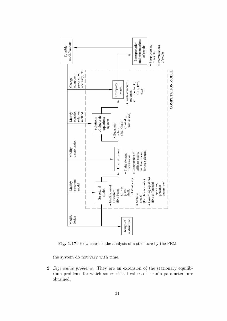
Fig. 1.17: Flow chart of the analysis of a structure by the FEM

the system do not vary with time.

2. Eigenvalue problems. They are an extension of the stationary equilib-rium problems for which some critical values of certain parameters areobtained.

31

Chapter 2

FEM ANALYSIS OF 1D PROBLEMS.APPLICATION TO THE POISSONEQUATION

2.1 INTRODUCTIONThe behaviour of continuum systems can in general be expressed in terms ofdifferential equations with their adequate boundary conditions. The objectiveof this chapter is to present an overview of the solution of one-dimensional(1D) partial differential equations with the FEM.

There are two general procedures for solving a differential equation: a) thedirect integration of the equation, which yields the so called analytical solution(exact method), and the approximate solution using numerical methods.

Numerical solution procedures for partial differential equations (PDE) beclassified as: a) those which are applied on the original PDE (for example,the finite difference method), and b) those which work with an equivalentintegral expression. The FEM belongs to this second class of methods. Thetwo standard approaches of this kind are: a) variational methods, and b)residual formulations.

The variational method is based on the search for the solution to the prob-lem by solving an integral equation which represents a general property ofthe system. A typical example is the integral expression obtained from theminimum energy principle.

The residual formulations are based on Weighted Residual (WR) methodssuch as the Point Collocation method, the Subdomain Collocation method,the Galerkin method, the Minimum Least Squares method, etc.

The FEM can therefore be viewed as a procedure for solving the PDEsgoverning a physical problem via a residual or variational formulation. Typ-ically, residual methods are more general and advantageous than variationalmethods and they will be the focus of this chapter.

This chapter presents different weighted residual techniques for solving a

33

PDE with the FEM. The model problem considered is the Poisson equation in1D.

2.2 THE POISSON EQUATIONThe Poisson equation expresses in mathematical form the behaviour of manyphysical problems. For this reason it has been chosen here as the model prob-lem for introducing the basis of the FEM.

The simplest form of the Poisson equation is as follows:

In 1D: kd2φ

dx2+ Q(x) = 0

In 2D: kd2φ

dx2+ k

d2φ

dy2+ Q(x, y) = 0

In 3D: kd2φ

dx2+ k

d2φ

dy2+ k

d2φ

dz2+ Q(x, y, z) = 0

k∇2φ + Q = 0 (2.1)

where φ is the problem unknown, k is a parameter expressing a physical prop-erty of the system, Q is a source term and ∇2 is the Laplace operator, i.e.∇2 = ∂2

∂x2 + ∂2

∂y2 in 2D. In general the parameter k can be different for each ofthe space directions. The simplest isotropic form is chosen here.

Table 2.1 presents the meaning of the terms in Eq.(2.2) for some physicalproblems.

Unknown, φ k QHeat conditions temperature heat internal heat

conductivity sourceFlow through pressure permeability waterporous media head source1D elasticity displacement Young modulus body force

x AreaPotential flow velocity density –

potentialMagnetostatics magnetic potential reductivity –

Torsion warping function shear modulus –Torsion stress function (shear modulus) -1 twist

Gass diffusion concentration diffusivity –Reynolds film pressure (film thickness)3/ lubricantlubrication viscosity supply

Table 2.1: Meaning of the terms in the Poisson equation for some problems

34

The form of the Poisson equation given in Eq.(2.2) assumes that k is con-stant. In fact k can be a function of the position and even of the problemunknown φ and its derivatives, as it happens in non-linear problems.

We present next examples of the derivation of the Poisson equation forthree specific problems: 1) heat transfer in a bar, 2) bar under axial forces and3) seepage in a porous media.

Figure 2.1: Heat conduction in a bar. Heat flow balance in an infinitesimaldomain.

Example 2.1 Steady state heat conduction in a bar

Solution

Let us consider the bar of Figure 2.1 representing a 1D domain through which heatis transfered via conduction effects in a steady manner. The temperature φ at x = 0is known, i.e.

φ = φ|x=0 (a)

and also the heat flux q at x = lq = q|x=l (b)

The balance of heat flux in a differential domain of the bar in expressed as (Figure2.2b)

(q + dq)︸ ︷︷ ︸out going flux

− q︸︷︷︸in-coming flux

= 0

dq = 0 (c)

The relationship between the heat flux q and the temperature is expressed by Fourier’slaw

q = −kdφ

dx(d)

where k is the thermal conductivity parameter.

35

Figure 2.2: a) Bar under a heat source Q(x); b) Heat balance in an infinitesimaldomain.

Derivation of (d) gives

dq =dq

dxdx = − d

dx

(k

dφ

dx

)dx

Substituting this equation into (c) gives

d

dx

(k

dφ

dx

)= 0 heat balance equation (e)

Note that the mathematical problem is well defined as we know

1. The governing differential equation (e)

2. The boundary conditions (a) and (b)

Let us know assume that the bar is subjected to an external heat source per unitlength Q (Figure 2.2a). A similar heat balance procedure on an infinitesimal domain(Figure 2.2b) leads to the following equations

(q + dq)− q −Qdx = 0 (f)

dq

dx−Q = 0 (g)

Substituting (d) into (g) gives

d

dx

(k

dφ

dx

)+ Q = 0 (h)

Expressions (e) and (h) are two forms of the Poisson equation. The form (e) (withQ = 0) is usually known as the Laplace equation.

Note that for k being constant, the simplified form of the Poisson equation of Eq.(2.1)is obtained.

36

Figure 2.3: Bar under axial forces. Equilibrium of force in an infinitesimaldomain.

The boundary conditions (a) and (b) completing the definition of the problem can besummarized as

Boundary conditions

Prescribed temperature: φ− φ = 0 at x = 0 (i)

Prescribed heat flux

q − q = 0 at x = lor (j)

k dφdx + q = 0 at x = l

Condition (i) are known in mathematics a Dirichlet boundary condition, while condi-tion (j) is known as Neumann boundary condition.

Example 2.2 Bar under axial forces

Solution

Let us consider the clamped bar of Figure 2.3, under an horizontal force x2 acting inthe free end and distributed axial forces b(x).

The governing equations of the problem are obtained following a similar process as inExample 2.1. The equilibrium of axial forces is established in an infinitesimal domain(Figure 2.3b), i.e.

dN

dx+ b(x) = 0 (a)

The stress-strain relationship is expressed by Hooke’s law

σ = Eε = Edu

dx︸︷︷︸ε

(b)

The axial force N is obtained by integrating the stress over the transverse cross-sectionas

N = σA (c)

37

In (a) and (b) σ is the normal stress, E is the Young’s modulus, ε is the axial strain,u the horizontal displacement and A the area of the transverse cross section.

From (b) and (c)

N = σA = EAdu

dx(d)

Substituting (d) into (a) gives

d

dx

(EA

du

dx

)+ b = 0 (e)

The above equation expresses the equilibrium (or balance) of forces at each point ofthe bar. It is therefore named the equilibrium equation for the bar.

The boundary conditions are

Prescribed displacement: u = 0 at x = 0

Prescribed force

N = x2 in x = lo

EAdudx −X2 = 0 in x = l

(f)

Eqs.(e) and (f) define the governing equations of the problem.

Note the analogy of Eq.(e) with Eq.(h) of the previous example. Both are Poissonequations in 1D. The following lines show the analogies between the structural andthermal problems.

Thermal problem – Axially loaded bar

temperature φ ←→u displacementconductivity k ←→EA axial stiffnessheat source Q ←→b distributed forceprescribed heat flow q ←→−X2 point force

The only difference in the analysis between the equation parameters in the thermalproblem and the axially loaded bar is the negative sign in the point force X2. Thisis a consequence of the proportionality between the displacement gradient and thestress in structures, whereas in thermal problems the heat flux goes in the oppositedirection of the gradient, i.e.

N = EA︸︷︷︸k

du

dx= k

du

dx

q = −kdφ

dx

38

Figure 2.4: a) Water flow through a porous bar.; b) Balance of water fluxes inan infinitesimal domain

Example 2.3 Water flow in a porous medium

Solution

The balance of water flow in the infinitesimal doman of Figure 2.4 gives

(q + dq)−Qdx− q = 0

dq

dx−Q = 0 (a)

In (a) q and Q represent the internal water flux and the external source of water perunit length, respectively.

The relationship between the water flow q and the pressure p is expressed by meansof Darcy law

q = −kdp

dx(b)

where k is the permeability of the porous medium.

Note the analogy of above equations with the equivalent ones in the thermal andstructural problems. Substituting (b) into (a) gives

d

dx

(k

dp

dx

)+ Q = 0 (c)

Boundary conditions

Prescribed pressure p− p = 0 at x = 0

Prescribed flux q − q = 0 at x = lor

k dpdx + q = 0 at x = l

(d)

39

There is a perfect analogy between the governing equations in the thermal and porousmedia flow problems, as expressed in the following lines:

Thermal problem – Porous media flow

temperature φ ←→p water pressureconductivity k ←→k permeabilityheat source Q ←→Q water sourceheat flux q ←→q water flux

2.3 WEIGHTED RESIDUAL METHODThe weighted residual method (WRM) is based on transforming the differentialequation which governs the problem in an equivalent integral expressions.

Let A(φ) be the governing differential equation (i.e. the Poisson equation)

A(φ) =d

dx

(kdφ

dx

)+ Q = 0 in Ω (2.2)

where Ω is the analysis domain.

Also, let B(φ) be the equation expressing the boundary conditions

B(φ) :

φ− φ = 0 in Γφ

k dφdx

+ q = 0 in Γq

(2.3)

where Γφ is the Dirichlet boundary where the unknown function is prescribedand Γq is the Neumann boundary where the flux incoming or outgoing thedomain is prescribed. The unknown φ and the parameters k, Q and q haveadequate meanings for each physical problem, as explained in the previoussection.

For instance, for the problem of Figure 2.1, we have

Ω: 0 ≤ x ≤ l (the bar length)Γφ: x = 0 (left hand end point)Γq: x = l (right hand end point)

The integral form equivalent to the governing equations given above isobtained by multiplying the differential expressions A and B by arbitraryweighting functions and integrating over the domain of each equation. Thus

∫

Ω

W (x)A(φ)dΩ +

∮

Γ

W (x)B(φ)dΓ = 0 (2.4)

where W (x) and W (x) are the weighting functions.

40

It is clear that if above integral equation is satisfied for each pair of weight-ing functions W and W , the following conditions must be satisfied

A(φ) = 0 in Ω

B(φ) = 0 in Γ

Conversely, satisfaction of Eq.(2.2) and (2.3) indicates necessarily that theintegral equation (2.4) is satisfied for any weighting function.

This heuristic proof indicates that Eq.(2.4) is a necessary and sufficientcondition for the satisfaction of the governing equations. In other words, func-tion φ satisfying the differential equations (2.2) and (2.3) also satisfies theequivalent integral form (2.4). The solution of the problem via Eq.(2.4) or via(2.2) and (2.3) are the starting point for method such as finite difference orfinite point procedures based on the satisfaction of the differential equationsin a finite set governing of points in the analysis domain. On the other hand,Eq.(2.4) is the basis of the so-called integral methods, such as the finite elementmethod (FEM).

An interesting feature of Eq.(2.4) is the additive property of the integral.This, if the integrals of Eq.(2.4) are computable, the integral from of Eq.(2.4)can be written as

∑e

∫

Ωe

WA(φ)dx +∑

e

∫

Γe

WB(φ)dΓ = 0 (2.5)

where the sum extends over the collection of non-interesting domains (ele-ments) covering the domain Ω and its boundary Γ. Eq.(2.5) is the basis of theassembly process in the FEM.

2.3.1 Approximation of the unknown. Weighted ResidualsThe numerical solution of the problem sought for an approximate value of theunknown φ such that

φ(x) ∼= φ(x) (2.6)

The usual way for expressing the approximate solution is via a linear com-bination of functions as

φ(x) =n∑

i=0

Ni(x)ai (2.7)

where ai are the unknown parameters and Ni(x) are functions of the indepen-dent variable x. Typical choices for Ni, are

1. Monomials (Ni(x) = xi):

φ(x) =n∑

i=0

aixi = a0 +

n∑i=1

aixi (2.8a)

41

2. Fourier series functions (Ni(x) = sin ix, cos ix):

φ(x) =n∑

i=0

ai cos ix +n∑

i=0

βi sin ix = a0 +

p∑i=1

ai cos ix +

p∑i=1

βi sin ix

(2.8b)

3. Exponential functions (Ni(x) = ebix):

φ(x) =n∑0

aiebix (2.8c)

Substituting the approximate function φ into the integral expression (2.4) gives

∫

Ω

WA(φ)dΩ +

∮

Γ

WB(φ)dΓ = 0 (2.9)

The above expression is an approximation of the integral form (2.4) and itis usually called weighed residual expression. This name comes after observingthat A(φ) and B(φ) are the “residuals” of the approximate solution in the do-main and the boundary, respectively. Thus, substituting φ into the governingequations we have

A(φ) = rΩ in Ω

B(φ) = rΓ in Γ

Hence, Eq.(2.9) can be written as

∫

Ω

WrΩdΩ +

∮

Γ

W rΓdΓ = 0 (2.10a)

Obviously, if φ is the exact solution, i.e. of φ = φ, then rΩ = 0 in Ω andrΓ = 0 in Γ.

The value of the residuals rΩ and rΓ indicate the error in the satisfactionof the governing differential equations due to the choice of the approximatefunction φ.

Expressions (2.9) or (2.10a) can be therefore be interpreted as the integralof the residuals of the differential equations weighted by the functions w(x)and w(x). This explains the name of the weighted residual method.

The approximate solution is found by choosing a finite set of weightedfunctions. Thus, by choosing a number of weighting functions equal to theterms of the expansion (3), the following system of equations is obtained

∫

Ω

WiA(∑

j

Njaj)dΩ +

∮

Γ

WiB(∑

j

Njaj)dΓ = 0; i = 1, n (2.11)

42

The above expression can be written in matrix form, after an adequateordering, as

Ka = f (2.12)

where K is a square matrix which elements depend on the geometrical andphysical properties of the problem, a is the vector containing the n unknownparameters and f is a vector depending on the prescribed value of the fluxesand the unknown function in the boundary.

Solution of the algebraic equation system (2.12) yields the value of theunknowns ai. The derivation of Eq.(2.12) for some specific problems will bepresented in the following sections.

2.3.2 Application of the WRM for the solution of the 1D heat conduc-tion equation

The more typical particular cases of the WRM are

1. Point collocation method

2. Subdomain collocation method

3. Galerkin methoed

4. Least square method

Let us consider the solution of the 1D Poisson equation for k = constant,i.e.

A(φ) = kd2φ

dx2+ Q = 0 in Ω (2.13)

More specifically, let us consider the solution of a heat conduction problemin 1D, where k is the heat conductivity, Q is the external heat source per unitlength and φ is the temperature.

In the example to be solved (Figure 2.5) we will take

k = 1

Q :

1 for 0 ≤ x < l/2

0 for l/2 < x ≤ l(2.14)

Boundary conditions

B(φ) :

φ = 0 in x = 0φ = 0 in x = l

(2.15)

The solution process via the WRM follows the steps previously explained,i.e.

43

Figure 2.5: Heat conduction in a bar of length l. Piece-wise distribution of theheat source Q and prescribed temperature at the ends

• We define the governing differential equations of the problem

A(φ) = 0 in the domain Ω

• and the boundary conditions

B(φ) = 0 in the boundary Γ of Ω

The solution process is as follows

1. The unknown φ(x) is approximated by a function φ(x) as

φ ∼= φ =n∑

i=1

Ni(x)ai (2.16)

where Ni(x) is a known “shape functions” and ai i = 1, n are n theunknown parameters. Substituting Eq.(2.16) into Eqs.(2.15) yields theresiduals (errors) in the domain and the boundary, i.e.

A(φ) = rΩ 6= 0 in Ω

B(φ) = rΓ 6= 0 in Γ

2. We impose that the integral of the residuals, weighted with n test func-tions Wi and Wi is zero, i.e.

∫

Ω

Wi(x)A(φ)dΩ +

∫

Γ

Wi(x)B(φ)dΓ = 0 i = 1, 2, . . . , n (2.17)

3. the parameters ai are found by solving the algebraic system of n equa-tions with n unknowns resulting from Eq.(2.17) and written as

Ka = f

44

2.3.3 Global definition of the shape functionsThe shape functions Ni(x) can be defined “globally” over the whole domain Ω,or else “locally” in subdomains Ωi. Next we will consider the global definitionof Ni(x).

For the solution of Eqs.(2.13)–(2.15) we will assume first an approximationof φ using Fourier series

φ(x) ' φ(x) =n∑

i=1

ai sinπxi

l; i = 1, 2, . . . , n (2.18)

Ni(x) = sinπxi

l(2.19)

From the expression of Ni(x) we observe that

• they are continuous over the domain Ω,

• they satisfy the boundary conditions (2.15), i.e.

Ni(0) = sin(0) = 0Ni(l) = sin(iπ) = 0

∀i

Hence

φ(0) =n∑

i=1

aiNi(0) = 0

φ(l) =n∑

i=1

aiNi(l) = 0

This gives

B(φ) = rΓ(x) = 0 in the boundary Γ (x = 0, x = l) (2.20)

Also, from Eqs.(2.13) and (2.18)

A(φ) = A

(n∑

i=1

ai sinπxil

)= k d2

dx2

(n∑

i=1

ai sinπxil

)+ Q =

=n∑

i=1

[−ai

(iπl

)2sin πxi

l

]+ Q

(2.21)

Eq.(2.18) are re-written (for rΓ = 0) as

∫ l

0

Wi(x)

(d2φ

dx2+ Q

)

︸ ︷︷ ︸rΩ

dx = 0; i = 1, 2, . . . , n

45

Substituting Eq.(2.18) into above integral gives

∫ l

0

[n∑1

−(

πj

l

)2

aj sin jπx

l+ Q

]Wi(x)dx = 0; i = 1, 2, . . . , n

n∑j=1

aj

(jπ

l

)2∫ l

0

Wi(x) sin jπx

ldx

︸ ︷︷ ︸Kij

=

∫ l

0

Wi(x)Qdx

︸ ︷︷ ︸fi

, i = 1, 2, . . . , n

(2.22)

In compact form

n∑j=1

Kijaj = fi : i = 1, 2, . . . , n (2.23)

which leads to a system of n linear equation with n unknowns.

For i = 1

a1

(πl

)2∫ l

0

W1 sinπx

ldx + a2

(2π

l

)2 ∫ l

0

W1 sin2πx

ldx + . . .

· · ·+ an

(nπl

)2∫ l

0

W1 sinnπx

ldx =

∫ l

0

W1Qdx

For i = 2

a1

(πl

)2∫ l

0

W2 sinπx

ldx + a2

(2π

l

)2 ∫ l

0

W2 sin2πx

ldx + . . .

· · ·+ an

(nπl

)2∫ l

0

W2 sinnπx

ldx =

∫ l

0

W2Qdx

For i = n

a1

(π

l

)2∫ l

0

Wn sinπx

ldx + a2

(2π

l

)2 ∫ l

0

Wn sin2πx

ldx + . . .

· · ·+ an

(nπ

l

)2∫ l

0

Wn sinnπx

ldx =

∫ l

0

WnQdx

46

The above equations can be written in matrix form as

π2

l2

∫ l

0

W1 sinπx

ldx 4

∫ l

0

W1 sin2πx

ldx . . . n2

∫ l

0

W1 sinnπx

ldx

∫ l

0

W2 sinπx

ldx 4

∫ l

0

W2 sin2πx

ldx . . . n2

∫ l

0

W2 sinnπx

ldx

......

...∫ l

0

Wn sinπx

ldx 4

∫ l

0

Wn sin2πx

ldx . . . n2

∫ l

0

Wn sinnπx

ldx

a1

a2...

an

=

=

∫ l

0

QW1dx∫ l

0

QW2dx

...∫ l

0

QWndx

or

j↓

K11 K12 . . . K1n

K21 K22 . . . K2n

i → ...... Kij

...

Kn1 Kn2 . . . Knn

︸ ︷︷ ︸K

a1

a2

ai

an

︸ ︷︷ ︸a

=

f1

f2

fi

fn

︸ ︷︷ ︸f

(2.24)

Ka = f (2.25)

where a term Kij of K can be expressed as

Kij =

(jπ

l

)2 ∫ l

0

Wi(x) sin jπx

ldx (2.26)

Similarly a term fi of f is

fi =

∫ l

0

Wi(x)Q(x)dx (2.27)

Expressions (2.26) and (2.27) are a generic form of the terms of K and f ,respectively, which favours the programming of all the expressions.

The remaining step is the evaluation of all matrices and vectors after defin-ing the weighted functions Wi. The selection of Wi. yields different forms ofthe Weighted Residual Method.

47

2.3.4 Point Collocation MethodThis method consists in defining n points in the analysis domain and choosingthe Dirac Delta functions as the weighting function. Thus,

Wi(x) = δ(x− xi), i = 1, 2, . . . , n (2.28)

Function δ has the property that for x 6= xi, δi(x) = 0 and satisfies theconditions ∫ ∞

−∞δ(x− xi)dx = 1 (2.29a)

∫ l

0

f(x)δ(x− xi)dx = f(xi) (2.29b)

Thus∫ l

0

Wi(x)A(φ)dx =

∫ l

0

δ(x− xi)A(φ)dx = A(φ)

∣∣∣∣x=xi

= 0, i = 1, 2, . . . , n

(2.30)Choosing the Dirac Delta functions as the weighting function, it is equiva-

lent to making A(φ) equal to zero at each point x = xi (i = 1, . . . , n). Hence,the procedure is equivalent to imposing the vanishing of the residual at eachone of the sampling points chosen. From Eq.(2.30) we deduce that there is noneed to perform an integration for obtaining the system of algebraic equations.

We will solve the previous problem for one and two terms of the Fourierseries expansions (2.18).

Solution with Wi = δi for n = 1

φ = N1(x)a1

We takexi = x1 = l/2

From Eq.(2.28)W1(x) = δ(x− l/2)

From Eq.(2.27)

fi = f1 =

∫ l

0

δ(x− l/2)Q(x)dx = Q

(l

2

)=

1

2

This value is deduced from Figure 2.5. At a point infinitely close to x = l/2from the left Q takes a unit value, where Q = 0 for a point to the right ofx = l/2. This difficulty is overcome by taking Q = l/2 for x = l/2.

On the other hand

K11 =(π

l

)2∫ l

0

δ

(x− l

2

)sin

πx

ldx =

(π

l

)2

sinπ

l

l

2=

(π

l

)2

48

From (2.24)K11a1 = f1

π2

l2a1 =

1

2=⇒ a1 = l2/2π2

The approximate function sought is therefore

φ(x) =l2

2π2︸︷︷︸a1

sinπ

lx

︸ ︷︷ ︸N1(x)

−→ φ = 0, 0507 l2 sinπx

l

We can verify that the residual rΩ vanishes at x1 = l/2

A(φ)

∣∣∣∣x=x1= l

2

=d2φ

dx2+ Q =

d2

dx2

(l2

2π2sin

π

lx

)∣∣∣∣x=l/2

+ Q(x)

∣∣∣∣x=l/2

=

= − l2

2π2

π2

l2sin

π

lx|x=l/2 + Q

(l

2

)= −1

2+

1

2= 0

Solution with Wi = δi for n = 2

φ(x) = N1(x)a1 + N2(x)a2

Taking

x1 = l/4

x2 = 3/4l

W1(x) = δ(x− l/4)

W2(x) = δ(x− 3/4l)

From Eq.(2.23) we obtain

For i = 1

K11a1 + K12a2 = f1

For i = 2K21a1 + K22a2 = f2

The algebraic equation system is

[K11 K12

K21 K22

]a1

a2

=

f1

f2

49

For i = 1

K11 = π2

l2

∫ l

0

W1 sinπx

ldx =

π2

l2

∫ l

0

δ

(x− l

4

)sin

πx

ldx =

π2

l2sin

π

l

l

4=

√2

2

π2

l2

K12 = 4π2

l2

∫ l

0

W1 sin2πx

ldx =

4π2

l2

∫ l

0

δ

(x− l

4

)sin

2πx

ldx =

4π2

l2sin

2π

4ll =

4π2

l2

f1 =

∫ l

0

Q(x)W1(x)dx =

∫ l

0

Qδ

(x− l

4

)dx = Q

(l

4

)= 1

For i = 2

K21 = π2

l2

∫ l

0

W2 sinπx

ldx =

π2

l2

∫ l

0

δ

(x− 3l

4

)sin

πx

ldx =

π2

l2sin

3

4

πl

l=

√2

2

π2

l2

K22 = 4π2

l2

∫ l

0

W2 sin2πx

ldx=

4π2

l2

∫ l

0

δ

(x− 3l

4

)sin

2πx

ldx=

4π2

l2sin

2π

4

3l

l=−4π2

l2

f2 =

∫ l

0

Q(x)W2(x)dx =

∫ l

0

Qδ

(x− 3l

4

)dx = Q

(3l

4

)= 0

Therefore

π2

l2

[√2

24√

22

−4

] a1

a2

=

10

⇒

a1 = l2/

√2π2

a2 = l2/8π2

The approximate solution is

φ(x) =1√2

l2

π2

︸ ︷︷ ︸a1

sinπx

l︸ ︷︷ ︸N1(x)

+l2

8π2︸︷︷︸a2

sin2πx

l︸ ︷︷ ︸N2(x)

We can verify that

A(φ) = 0|x1=l/4

x2=34 l

A(φ) =d2φ

dx2+ Q(x) = −

1√2

l2

π2

π2

l2sin

π

lx +

1

8

l2

π2

4π2

l2sin

2π

lx

+ Q(x)|x1,x2

A(l/4) = −(

1√2

√2

2+

1

21

)+ Q(l/4) = −1 + 1 = 0

A(3/4l) = −(

1√2

√2

2+

1

2(−1)

)+ Q

(3

4l

)= −0 + 0 = 0

50

2.3.5 Subdomain collocation methodThe method consists in subdividing the domain Ω into as many subdomainsas unknown parameters ai. The test functions Wi are then chosen so that theytake a unit value in each subdomain Ωi and zero in the rest. Thus,

Wi(x) = 1 ∀x ∈ Ωi

Wi(x) = 0 ∀x 6∈ Ωi

(2.31)

Applying the WRM gives

∫

Ωi

A(φ)dx = 0, i = 1, 2, . . . , n (2.32)

The previous equation is equivalent to making zero the integral of theresidual in each subdomain Ωi.

As in the previous case we will found φ(x) for one and two terms of theFourier series expansion (2.18)

Solution for n = 1

φ(x) = N1(x)a1

Ωi ≡ Ω

i.e., the subdomain Ωi is taken to coincide with the whole domain Ω : [0, l]

W1 = 1 0 ≤ x ≤ l

From Eq.(2.32) we deduce

K11a1 = f1

where

K11 =π2

l2

∫ l

0

W1 sinπx

ldx =

π2

l2

∫ l

0

sinπx

ldx =

2π

l

f1 =

∫ l

0

W1Q(x)dx =

∫ l

0

Q(x)dx =

∫ l/2

0

Q(x)︸ ︷︷ ︸1

dx +

∫ l

l/2

Q(x)dx = l/2

Therefore

K11︷︸︸︷2π

la1 =

f1︷︸︸︷l

2=⇒ a1 =

l2

4π

51

and

φ(x) =l2

4π︸︷︷︸a1

sinπx

l︸ ︷︷ ︸N1(x)

Solution for n = 2

φ(x) = N1(x)a1 + N2(x)a2

We take as subdomains the two intervals

[0, l/2] and [l/2, l]

hence

W1(x) :

1 0 ≤ x ≤ l/2

0 l/2 < x ≤ l

W2(x) :

0 0 ≤ x ≤ l/2

1 l/2 < x ≤ l

The above is equivalent to imposing that the integral of the residual is zeroin each of the two subdomains chosen.

In Eq.(2.23) we have for n = 2, i = 1, 2

i = 1; K11a1 + K12a2 = f1

i = 2; K21a1 + K22a2 = f2

∣∣∣∣ =⇒[K11 K12

K21 K22

] a1

a2

=

f1

f2

For i = 1

K11 = π2

l2

∫ l

0

W1 sinπx

ldx =

π2

l2

∫ l/2

0

sinπx

ldx =

π

l

K12 = 4π2

l2

∫ l

0

W1 sin2πx

ldx =

4π2

l2

∫ l/2

0

sin2πx

ldx =

4π

l

f1 =

∫ l

0

W1Qdx =

∫ l/2

0

Qdx =l

2

52

For i = 2

K21 = π2

l2

∫ l

0

W2 sinπx

ldx =

π2

l2

∫ l

l/2

sinπx

ldx =

π

l

K22 = 4π2

l2

∫ l

0

W2 sin2πx

ldx =

4π2

l2

∫ l

l/2

sin2πx

ldx = −4π

l

f2 =

∫ l

0

W2Qdx =

∫ l

l/2

Qdx = 0

Henceπ

l

[1 41 −4

]a1

a2

=

l/20

⇒

a1 = l2/4πa2 = l2/16π

The approximate solution is now

φ(x) =l2

4π︸︷︷︸a1

sinπx

l︸ ︷︷ ︸N1(x)

+l2

16π︸︷︷︸a2

sin2πx

l︸ ︷︷ ︸N2(x)

2.3.6 Galerkin methodThis popular method consists in taking as weighting functions the approxima-tion functions Ni, i.e.

Wi(x) ≡ Ni(x) (2.33)

The WRM is written as∫

Ω

NiA(φ)dΩ +

∫

Γ

NiB(φ)dΓ = 0 (2.34)

In the problem we are solving the integral over the boundary Γ is zero. Nextwe will solve the problem by taking one and two terms of the approximation(2.18) as in the previous cases.

Solution for n = 1φ(x) = N1(x)a1

W1(x) = N1(x) = sinπx

l

Hence

K11 =π2

l2

∫ l

0

W1 sinπx

ldx =

π2

l

∫ l

0

sin2 πx

ldx =

π2

2l

f1 =

∫ l

0

W1Qdx =

∫ l/2

0

sinπx

l1dx = l/π

53

Thereforeπ2

2l︸︷︷︸K11

a1 =l

π︸︷︷︸f1

→ a1 =2l2

π3

The final result is

φ(x) =2l2

π3︸︷︷︸a1

sinπx

l︸ ︷︷ ︸N1(x)

Solution for n = 2

φ(x) = N1(x)a1 + N2(x)a2

W1(x) = N1(x) = sinπx

l

W2(x) = N2(x) = sin2πx

lThe terms of the system (2.23) are

For i = 1

K11 = π2

l2

∫ l

0W1dx sin πx

l= π2

l2

∫ l

0

sin2 πx

ldx =

π2

2l

K12 = 4π2

l2

∫ l

0W1 sin 2πx

ldx = 4π2

l2

∫ l

0

sinπx

lsin

2πx

ldx = 0

f1 =∫ l

0W1Qdx =

∫ l/2

0

sinπx

l1dx =

l

π

For i = 2

K21 = π2

l2

∫ l

0

W2 sinπx

ldx =

π2

l2

∫ l

0

sin2πx

lsin

πx

ldx = 0

K22 = 4π2

l2

∫ l

0

W2 sin2πx

ldx =

4π2

l2

∫ l

0

sin2 2πx

ldx = 2

π2

l

f2 =∫ l

0W2Qdx =

∫ l/2

0

sin2πx

l1dx =

l

π

The resulting matrix expression is

π2

l

[1/2 00 2

]a1

a2

=

l/πl/π

⇒

a1 = 2l2/π3

a2 = l2/2π3

The approximate solution is

φ(x) =2l2

π3︸︷︷︸a1

sinπx

l︸ ︷︷ ︸N1(x)

+l2

2π3︸︷︷︸a2

sin2πx

l︸ ︷︷ ︸N2(x)

54

2.3.7 Least square method

The least square (LSQ) method consists in finding the unknown parametersby minimizing the integral of the residual squared in the analysis domain. Theminimization process implies the derivation of the integral with respect to eachunknown. This leads to an algebraic system of n equations with n unknowns,as in the previous methods.

The LSQ method can be interpreted as a particular case of the WRM withW = A(φ) and W = B(φ).

The expression to be minimized is

I =

∫

Ω

[A(φ)]2dΩ +

∫

Γ

[B(φ)]2dΓ (2.35)

Making

δI =∂I

∂a1

δa1 +∂I

∂a2

δa2 + · · ·+ ∂I

∂an

δan = 0 (2.36)

Satisfaction of this equation implies

∂I

∂a1

= 0

∂I

∂a2

= 0

...∂I

∂an

= 0

(2.37)

For the 1D heat conduction problem in hand the minimization process canbe written as

∂

∂ai

∫ l

0

[A(φ)]2dx = 0; i = 1, 2, . . . , n

or

∂

∂ai

∫ l

0

[d2φ

dx2+ Q

]2

dx =

∫ l

0

2

[d2φ

dx2+ Q

]∂

∂ai

[d2φ

dx2

]dx

=

∫ l

0

2∂

∂ai

[d2φ

dx2

]

︸ ︷︷ ︸Wi(x)

[d2φ

dx2+ Q

]

︸ ︷︷ ︸A(φ)

dx

=

∫ l

0

Wi(x)A(φ)dx = 0 i = 1, 2, . . . , n

55

The outcome of the minimization process can be interpreted as a form ofthe WRM with

Wi = 2 ∂∂ai

[d2φdx2

]= 2 ∂

∂ai

[d2

dx2

(n∑1

aj sin jπxl

)]=

= 2 ∂∂ai

[−a1

(πl

)2sin 1πx

l− a2

(2πl

)2sin 2πx

l− . . .

−ai

(iπl

)2sin iπx

l− · · · − an

(nπ

l

)2sin nπx

l

]=

= −2(

iπl

)2sin iπx

l

Solution for n = 1

φ(x) = N1(x)a1

W1 = −2π2

l2sin

πx

l; i = 1

After a little algebra we find

K11 =π2

l2

∫ l

0

W1 sinπx

ldx =

π2

l2

∫ l

0

−2π2

l2sin2 πx

ldx = −π4

l3

f1 =

∫ l

0

W1Qdx =

∫ l/2

0

−2π2

l2sin

πx

ldx = −2π

l

Finally we obtain

−π4

l3a1 = −2

π

l⇒ a1 =

2l2

π3

Hence

φ(x) =2l2

π3︸︷︷︸a1

sinπx

l︸ ︷︷ ︸N1(x)

Solution for n = 2

φ(x) = N1(x)a1 + N2(x)a2

W1 = −2π2

l2sin

πx

l; i = 1

W2 = −8π2

l2sin

2πx

l; i = 2

56

After some algebra we find

For i = 1

K11 = π2

l2

∫ l

0

W1 sinπx

ldx =

π2

l2

∫ l

0

−2π2

l2sin2 πx

ldx = −π4

l3

K12 = 4π2

l2

∫ l

0

W1 sin2πx

ldx =

4π2

l2

∫ l

0

−2π2

l2sin

πx

lsin

2πx

ldx = 0

f1 =

∫ l

0

W1Qdx =

∫ l/2

0

−2π2

l2sin

πx

l1dx = −2π

l

For i = 2

K21 = π2

l2

∫ l

0

W2 sinπx

ldx =

π2

l2

∫ l

0

−8π2

l2sin

2πx

lsin

πx

ldx = 0

K22 = 4π2

l2

∫ l

0

W2 sin2πx

ldx =

4π2

l2

∫ l

0

−8π2

l2sin2 2πx

ldx = −16

π4

l3

f2 =

∫ l

0

W2Qdx =

∫ l/2

0

−8π2

l2sin

2πx

l1dx = −8π

l

The final system of equations is

π4

l3

[−1 00 −16

]a1

a2

=

−2π/l−8π/l

⇒

a1 = 2l2/π3

a2 = l2/2π3

The approximate solution is

φ(x) =2l2

π3sin

πx

l+

l2

2π3sin

2πx

l

Note that the solution coincides with that obtained with the Galerkinmethod. This coincidence is fortuitous and it can not be generalized to otherproblems.

Figures 2.6 and 2.7 show the results obtained with the different WRM pre-sented using one and two terms of the Fourier series used for the approximation(Eq.2.18). Note the best accuracy of the Galerkin method, which explains itspopularity of this method for application with the FEM.

2.4 GENERAL SOLUTION PROCEDURELet is consider the equation

A(φ) =d

dx

(kdφ

dx

)+ Q = 0 en

Ω︷ ︸︸ ︷0 ≤ x ≤ l (2.38)

57

Figure 2.6: Exact and approximate solution using Fourier series (one term) forthe 1D heat conduction problem of Figure 2.4

which governs the heat conduction problem of Figure 2.8 with the boundaryconditions

B(φ)

φ− φ = 0; en x = 0 (Γφ)

k dφdx

+ q = 0; en x = l (Γq)(2.39)

The unknown φ is approximated by

φ ' φ =n∑

i=1

Ni(x)ai (2.40)

58

Figure 2.7: Exact and approximate solution using Fourier series (two terms)for the 1D heat conduction problem of Figure 2.4

Application of the WRM gives

∫ l

0

Wi

[d

dx

(kdφ

dx

)+ Q

]

︸ ︷︷ ︸A(φ)

dx +

Wi

(kdφ

dx+ q

)

︸ ︷︷ ︸B(φ)

x=l

= 0 (i = 1, 2, . . . , n)

(2.41)Note that we have not included in above expression the term in the Dirichlet

boundary Γ(x=0). The reason is that in the following we will choose functions

φ that satisfy the Dirichlet boundary condition.

59

Figure 2.8: The 1D heat conduction problem in a bar

Introducing Eq.(2.40) into (2.41) gives

∫ l

0

Wid

dx

[k

(dN1

dxa1 +

dN2

dxa2 + · · ·+ dNn

dxan

)]dx+

+

[Wik

(dN1

dxa1 +

dN2

dxa2 + · · ·+ dNn

dxan

)+ q

]

x=l

+

+

∫ l

0

WiQdx = 0 (i = 1, 2, . . . , n)

The above equations is a system of n equations with n unknowns that canbe written in matrix form as

K11 K12 . . . K1n

K21 K22 . . . K2n...

Kn1 Kn2 . . . Knn

︸ ︷︷ ︸K

a1

a2...

an

︸ ︷︷ ︸a

=

f1

f2...

fn

︸ ︷︷ ︸f

(2.42)

where

Kij =

∫ l

0

Wid

dxk

(dNj

dx

)dx +

[Wik

dNj

dx

]

x=l

(2.43)

fi = −∫ l

0

WiQdx− [Wiq]x=l

The selection of the test functions Wi leads to the different modalities ofthe WRM. For Wi = Ni we obtain the Galerkin method. Note that in general

Kij 6= Kji

and, therefore, matrix K is non symmetrical.Application of the Galerkin method in the example of previous section lead

to a symmetric expression of K. This a consequence of the particular form ofthe Fourier expansion chosen for the approximation.

60

2.4.1 Conclusions

We point out some key aspects of the solution process explained in the previoussection.

1. The unknown function is approximated by the sum of product of knownfunctions Ni(x) and unknown parameters ai

φ(x) ∼= φ(x) =n∑

i=1

Ni(x)ai (2.44)

2. The governing equations of the problem are written in an integral formvia the WRM as

∫

Ω

WiA(φ)dx +

∫

Γ

WiB(φ)dx = 0 (2.45)

3. Substituting the approximation of the unknown into the previous integralform leads to a system of algebraic equations

Ka = f

Solution of above system gives the value of the parameters ai, which definethe approximate expression of the unknown function φ.

2.5 INTEGRABILITY CONDITION

Integration of the mth-derivative of a function f(x) requires the continuity

of its first m − 1 derivatives. In other words, the integral∫

Ωdmf(x)

dxm dx will be

compatible if the derivative dm−1f(x)dxm−1 is continuous.

This property is clarified in the example of Figure 2.9. The figure shows alinear function f(x). The integral exists in the interval [0, xi +1] and coincideswith the area of the triangular region shown. Figure 2.9b shows the firstderivative f

′(x). Note that this function is discontinuous and its integral is

equal to the sum of the areas of the two rectangular regions shown. Figure2.9c shows f

′′(x). The function is not integrable and this is a consequence

of f′(x) not being continuous, in agreement with the integrability criterium

stated above.

A function is Cm continuous if the function and its m first derivatives arecontinuous. This C1 continuous function implies that both the function and itsfirst derivatives are continuous, C0 continuity indicates that just the functionis continuous. C−1 continuity implies that the function is discontinuous.

61

Figure 2.9: Integral of a linear function and its two first derivative

2.6 WEAK FORM OF THE WEIGHTED RESIDUAL METHODLet us consider once more the 1D Poisson equation

d

dx

(kdφ

dx

)+ Q = 0

with boundary conditions

φ− φ = 0 en x = 0

kdφ

dx+ q = 0 en x = l

The integral form is obtained by multiplying the above equations by testfunctions and integrating over the domain. Thus

∫ l

0

W

[d

dx

(kdφ

dx

)+ Q

]dx +

[W

(kdφ

dx+ q

)]

l

= 0 (2.46)

From this expression we note

• The derivative of φ is of order 2. This requires C1 continuity for φ and,therefore, the shape functions must also be C1 continuous.

• The derivative of k appears in the integral. This requires that is con-tinuous (C0 continuity). This is an obvious inconvenience for problemswhere the analysis domain contains material with different properties.

• No derivative is applied on W . This implies that W can be discontinuous(C−1 continuity). Above requirements are clearly non-symmetrical withrequest to φ and W . Thus, while continuity of the first derivative isrequired for φ, no continuity requirement is demanded for φ. This lack ofsymmetry leads generally to a non symmetric expression of the algebraicequation system resulting from the discretization process.

62

This “problem” can be overcome by an integration by parts of the secondderivative term in the integral expression of the WRM. Recalling the integra-tion by parts rule ∫ l

0

udv = [uv]l0 −∫ l

0

vdu

and applying this rule to the term involving the second derivative of φ in theexpression of the WRM (Eq.(2.46)) gives (for u = W and v = k dφ

dx)

∫ l

0

Wd

dx

(kdφ

dx

)dx =

[Wk

dφ

dx

]l

0

−∫ l

0

dW

dxkdφ

dxdx (2.47a)

Substituting this expression into the WRM gives

−∫ l

0

dW

dxkdφ

dxdx +

∫ l

0

WQdx +

[Wk

dφ

dx

]l

0

+

[W

(kdφ

dx+ q

)]

l

= 0 (2.47b)

Note that the continuity requirements for φ, W and k have changed. Thus,the first derivatives of φ and W are just now involved, which simply requiresC0 continuity for these two functions.

Also, the derivative of the k has disappeared and k can now be a discon-tinuous function. The changes in the continuity requirement are summarizedin Table 2.2.

Continuity requirements

Original integral form Weak integral formφ C C0

W C−1 C0

k C0 C−1

Table 2.2: Continuity requirements for φ, W and k in the original integralform and the weak form

We recall that C−1 continuity means that the function can be discontinuous.Eq.(2.47b) is called the weak integral form (or simple the weak form). This

name comes from the fact that we have restricted the field for selecting thetest functions W . Note that the original integral form we allowed any choicefor W , while the weak form is restricted to functions W which are continuous.

2.6.1 Natural boundary conditionLet us choose for convenience W = −W in the weak form (2.47b). Simplifica-tion and rearranging of terms leads to

∫ l

0

dW

dxkdφ

dxdx =

∫ l

0

WQdx−[Wk

dφ

dx

]

0

− [Wq]l (2.48)

63

Recalling that q = −k dφdx

gives

∫ l

0

dW

dxkdφ

dxdx =

∫ l

0

WQdx + [Wq]0 − [Wq]l (2.49)

We note the following points:

1. The variable φ has disappeared from the Neumann boundary where theheat flux is prescribed ((x = l).

2. If the heat flux at x = l is prescribed to a zero value (q = 0), then allthe Neumann boundary terms disappear from the weak form (2.49). Theconditions of zero prescribed flux at the boundary are typically termednatural boundary condition.

3. q0 is the incoming flux into the domain by the left end (x = 0) where thevalue of φ is prescribed. Thus q0 can be interpreted as an end “reaction”(using a terminology from structural mechanics) corresponding to theprescribed value of the unknown. The value of q0 can be computed “aposteriori”, once the approximate solution for φ has been found.

2.6.2 Discretization of the weak formThe weak form will be in the following the starting expression for deriving thediscretized equation in the FEM. Thus, substituting the approximation for φdefined as

φ ∼= φ =n∑

j=1

Njaj

into the weak form (2.49) and choosing n test functions Wi, i = 1, 2, . . . , ngives

∫ l

0

dWi

dxk

n∑j=1

dNj

dxajdx =

∫ l

0

WiQdx+ [Wiq]x=0 − [Wiq]x=l

i = 1, 2, . . . n

(2.50)

The algebraic system of n equations and n unknowns is obtained by givingvalues to Wi in above expression from i = 1 to n.

For i = 1

∫ l

0

dW1

dxk

(dN1

dxa1 +

dN2

dxa1 + · · ·+ dNn

dxan

)dx =

∫ l

0

W1Qdx+(W1q)0−(W1q)l

(2.51)

64

For i = 2

∫ l

0

dW2

dxk

(dN1

dxa1 +

dN2

dxa2 + · · ·+ dNn

dxan

)dx =

∫ l

0

W2Qdx+(W2q)0−(W2q)l

For i = n

∫ l

0

dWn

dxk

(dN1

dxa1 +

dN2

dxa2 + · · ·+ dNn

dxan

)dx =

∫ l

0

WnQdx+(Wnq)0−(Wnq)l

Above equations can be written in matrix form as

K11 K12 . . . K1n

K21 K22 . . . K2n...

...Kn1 Kn2 . . . Knn

a1

a2...

an

=

f1

f2...

fn

Ka = f

where

Kij =

∫ l

0

dWi

dxkdNj

dxdx

fi =

∫ l

0

WiQdx + (Wiq)0 − (Wiq)l

(2.52)

We are still free to choose an appropriate expression for Wi. Choosing theGalerkin form (Wi = Ni) gives

Kij =

∫ l

0

dNi

dxkdNj

dxdx

fi =

∫ l

0

NiQdx + (Niq)0 − (Niq)l

(2.53)

Note that matrix K is symmetrical, which is advantageous for the compu-tations. This symmetry is one of the key properties of the so-called Galerkinweak form.

We point out again that fi contains the incoming flux q0 at the boundarywhere φ is prescribed. The flux is an unknown that can be computed “aposteriori” once the value of the unknown parameters have been found. Thisprocess is explained in the example given next.

65

Example 2.4 Solution of 1D Poisson equation via the Galerkin weak form and a polyno-mial approximation

Solution

Let us consider the Poisson equation

A(φ) :d2φ

dx2+ 3 = 0 en Ω (a)

The boundary conditions are

B(φ) :

φ− 1 = 0, x = 0 (Γ)φdφdx + 2 = 0, x = l (Γq)

(b)

From (a) and (b) we deduce k = 1, Q = 3, φ = 1 and q = 2.

We define a polynomic approximation of the unknown such that the boundary con-ditions for the temperature prescribed at x = 0 is satisfied, i.e.

φ(x) ∼= φ(x) = 1 +n∑

j=1

ajxj (c)

Note that x = 0, φ = 1.

From (c) we deduce Nj = xj (i = 1, 2, . . . , n).

Let us find now the solution for n = 2

φ(x) = 1 + a1x + a2x2

N1(x) = x, N2(x) = x2 (d)

where a1 and a2 are the unknowns.

The Galerkin weak form leads to an algebraic system with two equations that can beexpressed as [

K11 K12

K21 K22

]a1

a2

=

f1

f2

(e)

where

K11 =∫ l

0

dN1

dx

dN1

dxdx =

∫ l

0

dx = l

K12 =∫ l

0

dN1

dx

dN2

dx=

∫ l

0

2xdx = l2 = K21

K22 =∫ l

0

dN2

dx

dN2

dxdx =

∫ l

0

4x2 =43l3

f1 =∫ l

0

N1Qdx + (N1q)0 − (N1q)l =∫ l

0

3xdx− 2l =32l2 − 2l

f2 =∫ l

0

N2Qdx + (N2q)0 − (N2q)l =∫ l

0

3x2dx− 2l2 = l3 − 2l2

(f)

66

Substituting into (e) gives

[l l2

l2 43 l3

]

︸ ︷︷ ︸K

a1

a2

︸ ︷︷ ︸a

=

3l2

2 − 2ll3 − 2l2

︸ ︷︷ ︸f

(g)

Solution of the system gives a1 = 3l − 2, a2 = −3/2.

The approximate solution is

φ(x) ≡ φ(x) = 1 + (3l − 2)x− 32x2 (h)

Let us find out as an exercise the analytical solution. Integration of the originaldifferential equation gives

dφ

dx= −3x + A

φ = −32x2 + Ax + B

Constants A and B are found by using the boundary conditions

(φ)0 = 1 =⇒ B = 1

(dφ

dx

)|l = − 2 =⇒ −3l + A = −2; A = 3l − 2

The exact solution is therefore

φ = −32x2 + (3l − 2)x + 1 (i)

Note that the approximate solution coincides with the exact one. This is a conse-quence of the quadratic approximation chosen that coincides with the exact one.

The incoming flux q0 is found as

q0 = −kdφ

dx

∣∣∣∣x=0

= −(a1 + 2a2x)∣∣∣∣x=0

= −a1 = 2− 3l

This shows that the flux at the Dirichlet boundary where the unknowns is prescribedcan be computed “a posteriori” in terms of the parameters of the approximation.Note the analogy with the computation of the reaction at the support of a structurefrom the displacements at the joints of the structure.

67

Example 2.5 Solve the 1D heat conduction equation accounting for heat conduction losesvia the Galerkin weak form and a polynomial approximation.

Solution

Let us consider the heat balance equation in a bar where heat is generated due to adistributed source Q and heat is lost along the bar length due to the difference betweenthe temperature of the bar and that of the external medium (heat conduction loss).

The heat balance equation is an infinitesimal element of the bar is written as

q + Qdx− (q + dq)− h(φ− φe)dx = 0

Simplifying and using Fourier’s law(q = −k dφ

dx

), we obtain

d

dx

(k

dφ

dx

)+ Q− h(φ− φe) = 0 (a)

where h is the convection parameter and φe the external temperature.

The third term expresses the heat loss due to convection along the bar.

Let us assume a problem with k = 1, Q = 0, h = 1 and φe = 0, i.e.

A(φ) :d2φ

dx2− φ = 0 in Ω (b)

with the following boundary conditions

B(φ) :

φ = 0; x = 0 (Γφ

dφ

dx− 20 = 0 ; x = l (Γq

(c)

The integral expression of the previous equation is obtained in the usual way as

∫ l

0

Wi

(d2φ

dx2− φ

)dx +

[Wi

(dφ

dx− 20

)]

x=l

= 0 (d)

The weak form is obtained integrating by parts the second derivative term. This

∫ l

0

Wid2φ

dxdx = −

∫ l

0

dWi

dx

dφ

dxdx +

[Wi

dφ

dx

]l

0

(e)

Substituting (e) into (d) and making Wi = −Wi, gives

−∫ l

0

dWi

dx

dφ

dxdx +

[Wi

dφ

dx

]l

0

−∫ l

0

Wiφdx−[Wi

(dφ

dx− 20

)]

l

= 0 (f)

After little algebra we obtain

∫ l

0

(dWi

dx

dφ

dx+ Wiφ

)dx = (Wiq)0 + 20(Wi)l (i = 1, 2, . . . , n) (g)

68

where

q0 = −kdφ

dx

∣∣∣∣0

Note that the effect of convection leads to a new term is the l.h.s. of (g) whichobviously affects the stiffness matrix. Also note that φe 6= 0 introduces and additionalterm in the flux vector.

Let us assume the following expansion

φ ∼= φ =2∑

j=1

ajxj = a1x + a2x

2

N1 = x; N2 = x2

(h)

Substituting Eq.(h) into (g) and applying the Galerkin method (Wi = Ni) gives

∫ l

0

(dNi

dx

dφ

dx+ Niφ

)dx = (Niq)0 + 20(Ni)l; (i = 1, 2) (i)

Substituting the approximation for φ gives

∫ l

0

dNi

dx

2∑

j=1

dNj

dxaj

+ Ni(

2∑

j=1

Njaj)

dx = (Niq)0 + 20(Ni)l; (i = 1, 2) (j)

The expressions for the stiffness matrix and the flux vector are

Kij =∫ l

0

(dNi

dx

dNj

dx+ NiNj

)dx (k)

where dNi

dxdNj

dx is the conduction term and NiNj is the term due to convection.

fi = (Niq)0 + 20(Ni)l (l)

The numerical expressions for Kij and fi are

K11 =∫ 1

0

(1 + x2)dx ⇒ K11 = 4/3

K12 =∫ 1

0

(2x + x3)dx ⇒ K12 = 5/4 = K21

K22 =∫ 1

0

(4x2 + x4)dx ⇒ K22 = 23/15

f1 = (xq)0 + 20x|l = 20f2 = (x2q)0 + 20x2|l = 20

The system of equations is written in matrix form as

[4/3 5/45/4 23/15

]a1

a2

=

2020

69

From above we obtain

4/3a1 + 5/4a2 = 205/4a1 + 23/15a2 = 20 ⇒

a1 = 11, 7579a2 = 3, 4582

The solution is

φ =

a1︷ ︸︸ ︷11, 7579 x +

a2︷ ︸︸ ︷3, 4582 x2

The heat flux q0 at x = 0 is

q0 = −dφ

dx

∣∣∣∣x=0

= −11, 7579

Let us verify the approximation of the flux computed at x = 1 with the exact value

ql = −dφ

dx

∣∣∣∣x=1

= −11, 7579− 2× 3, 4582 = −18, 67

The minus sign denotes that the flux goes out the domain, as expected.

Using a single term in the approximation (h), gives φ = 15 and ql = −15.

We can plot the approximate solution for comparison with the exact solution. Thefollowing tables show the approximate and exact values of φ at x = 0, 5 and x = 1,and of the flux

(dφdx

)at x = 1.

φ φ (exact)

n = 1 n = 2x = 0, 5 7,5 6,7435 6,7540x = 1 15 15,2161 15,2319

dφdx

∣∣∣∣1

dφdx

∣∣∣∣1

(exact)

n = 1 n = 2-15 -18,67 -20

Table 2.3: Comparison of the approximate and exact values for φ y dφdx

∣∣∣∣1

(Example 2.5)

Note that the accuracy for φ is greater than that for the flux at the end point. This isdue to the computation of the flux as the first derivative of the approximate functionφ. Recall that the derivatives of an approximate function introduces an additionalerror. Consequently, the fluxes computed from the numerical solution are an orderless accurate than the values of φ. This conclusion also extends to the FEM.

70

2.7 DERIVATION OF THE PRINCIPLE OF VIRTUAL WORKFROM THE WEIGHTED RESIDUAL METHOD

Let us consider the bar under traction forces of Figure 2.3.The governing equation is

A(u) :d

dx

(EA

du

dx

)+ b = 0 (2.54)

and the boundary conditions

B(u) :

Prescribed displacement u = 0 x = 0

Prescribed forces EAdudx− H = 0 x = l

The equivalent integral form is derived via the WRM

∫ l

0

W

[d

dx

(EA

du

dx

)+ b

]dx +

[W

(EA

du

dx− H

)]

x=l

= 0 (2.55)

The weak form is obtained integrating by parts the term

∫ l

0

W

[d

dx

(EA

du

dx

)]dx = −

∫ l

0

dW

dxEA

du

dxdx +

[WEA

du

dx

]l

0

(2.56)

Substituting above expressions into the WRM and making W = −W , gives

−∫ l

0

dW

dxEA

du

dxdx +

[WEA

du

dx

]l

0

−[W

(EA

du

dx− H

)]

l

+

∫ l

0

Wbdx = 0

(2.57)Let us recall that

N = σA = EεA = EAdu

dx(2.58)

Hence, the weak form can be written as

∫ l

0

dW

dx(EA)

du

dx︸ ︷︷ ︸N

dx =

∫ l

0

Wbdx + (WH)l − (WN)0 (2.59)

Let us denote, for convenience, the arbitrary test functions as virtual dis-placement δu. Hence,

W (x) ≡ δu(x) (2.60)

The term (WN)0 is eliminated by imposing that the virtual displacementδu satisfies the kinematic boundary conditions, i.e.

δu(x)|x=0 = 0 (2.61)

71

Substituting W by δu into the weak form and noting (2.60) leads to

∫ l

0

d(δu)

dxNdx =

∫ l

0

δubdx + (δuH)l (2.62)

The virtual strain is defined as

δε =d(δu)

dx(2.63)

Substituting this expression into the weak form leads finally to

∫ l

0

δεN(x)dx =

∫ l

0

δubdx + δulH (2.64)

The terms δub can be interpreted as the work (per unit length) performedby the distributed force b over the virtual displacement δu. Also, the termδulH is the work of the force H over the virtual displacement of the bar end.Finally the integral of the l.h.s. of Eq.(2.63) represents the work of the axialforces over the virtual strains (elongations) along the bar.

The previous integral expression is known in practice as the Principle ofVirtual Work (PVW). The definition of PVW is a follows:

“A body is in equilibrium if, for any virtual displacement δu that satisfiesthe kinematic boundary conditions, the work performed by the stresses overthe virtual strains equals the work performed by the external forces over thevirtual displacement”.

As the starting point for the derivation of the PVW is the equilibriumequation, the PVW is an equilibrium expression. Also, starting from the PVWand integrating by parts the l.h.s. and taking into account that the virtualdisplacement are arbitrary, we recover the original governing equations. ThePVW is therefore a necessary and sufficient condition for the equilibrium of astructure

The PVW has advantages versus the governing differential equations ex-pressing the equilibrium of a body, as it has a simple physical meaning. ThePVW is the starting point for the solution via FEM of most problems in struc-tural mechanics.

2.8 THE PVW IN POISSON PROBLEMSThe PVW has an analogous expression in Poisson problems. Thus making

W (x) = δφ(x)N = − qd(δφ)

dx= δ

(dφdx

)= δg

b(x) = Q(x)H = − q

72

In above δφ or δg are the virtual variables (i.e. temperature, pressure, etc.)and the virtual gradient, respectively. The PVW is written in this case as,

∫ l

0

δg(−q)dx =

∫ l

0

δφQdx− (δφ)lq

The minus sign in the above expression comes from the fact that the fluxdirection is the opposite to that of the gradient of φ.

x(e)1 , x

(e)2 : abscissae of the coordinates of nodes 1 and 2 of element (e)

Figure 2.10: Discretization of a bar into 1D two-noded finite element

2.9 THE FEM IN 1D POISSON PROBLEMS

We will study next the general solution of 1D Poisson problems with the FEM.

Let us consider a discretization of the analysis domain (the 1D domain)in non-overlapping sub-domains, termed hereafter “finite elements” (Figure2.10).

Among the many choice for approximately the unknown function φ we willchoose the simplest one, using polynomial functions locally defined within eachfinite element as

φ(x) ' φ(x) = ao + a1x + a2x2 + · · ·+ anxn =

n∑i=0

aixi (2.64)

73

where n is the number of points within the element where the value of φ isassumed to be known. Such points are called nodes. Also, ao, a1, . . ., an areconstant parameters depending on the value of φ at the nodes only. The aboveexpression is typically written as

φ(x) = N(e)1 (x)φ

(e)1 + N

(e)2 (x)φ

(e)2 + · · ·+ N (e)

n (x)φ(e)n =

n∑i=1

N(e)i (x)φ

(e)i

(2.65)

where N(e)1 (x), . . ., N

(e)n (x) are the polynomial functions that interpolate φ

within the element domain (they are called shape functions) and φ(e)i is the

value of the approximate function φ at the node i. In the follows for simplicitywe will skip the hat over φ. This means that we will make no distinctionbetween the exact and approximate expressions of the unknown φ.

The shape function N(e)i (x) interpolates within the element the unknown

corresponding to node i only and, therefore, it is called the shape function ofnode i. It is easy to note that N

(e)i (x) takes the unit value at the node and

zero at the other nodes.Substituting the approximate expression from φ(x) for each element into

the integral form of the WRM leads, after simple algebra, to a system ofalgebraic equations expressing the equilibrium of the problem in terms of thenodal values of unknown φ at the nodes of the finite element mesh. Suchequations can be written in matrix form as

K a = f (2.66)

with

K =

K11 K12 . . . K1n...

......

...KN1 KN2 . . . KNN

; a =

φ1

φ2...

φN

; f =

f1

f2...

fN

(2.67)

where N is the total number of nodes in the finite element mesh.By analogy with matrix analysis of structures, K is called the stiffness

matrix of the finite element mesh and a and f are called the nodal unknownvector and the vector of equivalent nodal fluxes, respectively. K and f can beobtained by assembling the individual contributions from each element as inmatrix analysis of bar structures. The solution of the global system of algebraicequations gives the value of φ at the nodes from which the gradient and theflux within each element can be found.

For the sake of clarity we will study in a subsequent section the solutionof the 1D Poisson problem using two meshes of one and two two-noded linearfinite elements, respectively.

74

2.9.1 Discretization of the problem. Local definition of the shape func-tions

Let us define the distribution of the unknown function φ within each element.The bar is discretized into two-noded 1D finite element. Within each ele-ment the unknown function φ(x) is approximated using a linear polynomial as(Figure 2.11)

φ(e)(x) ∼= φ(e)(x) =1∑

i=0

αixi = α0 + α1x (2.68)

Taking into account that at the end node of each element the unknownfunction values coincide with those of the nodal unknowns we can write

φ(e)(x1) = φ(e)1 = α0 + α1x

(e)1

φ(e)(x2) = φ(e)2 = α0 + α1x

(e)2

(2.69)

Solving the above equation system with two unknowns gives

α0 = φ(e)1 − φ

(e)2 −φ

(e)1

x(e)2 −x

(e)1

x(e)1

α1 =φ

(e)2 −φ

(e)1

x(e)2 −x

(e)1

Substituting α0 and α1 into (2.68) gives

φ(e)(x) =

(φ

(e)1 − φ

(e)2 − φ

(e)1

x(e)2 − x

(e)1

x(e)1

)+

(φ

(e)2 − φ

(e)1

x(e)2 − x

(e)1

)x

After some rearranging we obtain

φ(e)(x) =x

(e)2 − x

x(e)2 − x

(e)1︸ ︷︷ ︸

N(e)1 (x)

φ(e)1 +

x− x(e)1

x(e)2 − x

(e)1︸ ︷︷ ︸

N(e)2 (x)

φ(e)2

= N(e)1 (x)φ

(e)1 + N

(e)2 (x)φ

(e)2 =

2∑i=1

N(e)i (x)φ

(e)i

(2.70)

from which the expression of the shape functions N(e)i is deduced as

N(e)1 (x) =

x(e)2 −x

x(e)2 −x

(e)1

=x(e)2 −x

l(e)

N(e)2 (x) =

x−x(e)1

x(e)2 −x

(e)1

=x−x

(e)1

l(e)

(2.71)

75

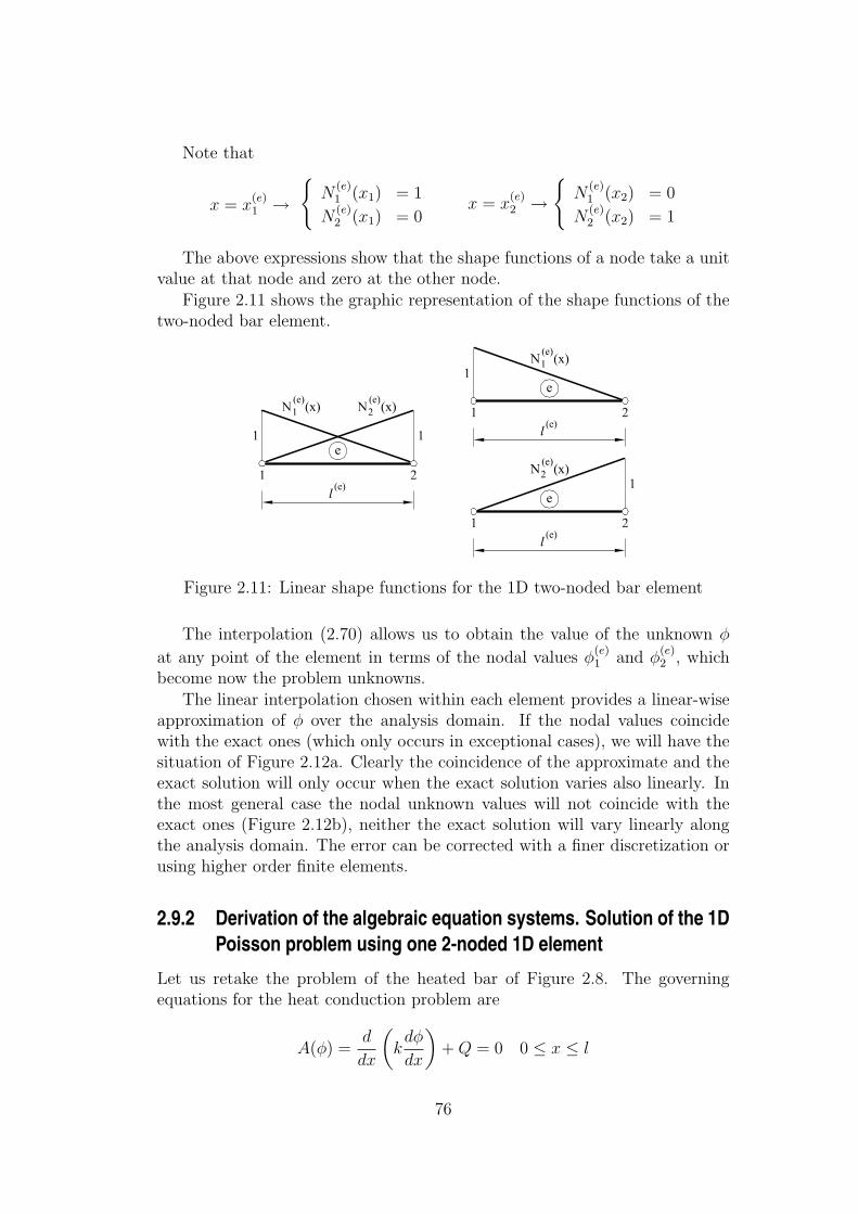
Note that

x = x(e)1 →

N

(e)1 (x1) = 1

N(e)2 (x1) = 0

x = x(e)2 →

N

(e)1 (x2) = 0

N(e)2 (x2) = 1

The above expressions show that the shape functions of a node take a unitvalue at that node and zero at the other node.

Figure 2.11 shows the graphic representation of the shape functions of thetwo-noded bar element.

Figure 2.11: Linear shape functions for the 1D two-noded bar element

The interpolation (2.70) allows us to obtain the value of the unknown φ

at any point of the element in terms of the nodal values φ(e)1 and φ

(e)2 , which

become now the problem unknowns.The linear interpolation chosen within each element provides a linear-wise

approximation of φ over the analysis domain. If the nodal values coincidewith the exact ones (which only occurs in exceptional cases), we will have thesituation of Figure 2.12a. Clearly the coincidence of the approximate and theexact solution will only occur when the exact solution varies also linearly. Inthe most general case the nodal unknown values will not coincide with theexact ones (Figure 2.12b), neither the exact solution will vary linearly alongthe analysis domain. The error can be corrected with a finer discretization orusing higher order finite elements.

2.9.2 Derivation of the algebraic equation systems. Solution of the 1DPoisson problem using one 2-noded 1D element

Let us retake the problem of the heated bar of Figure 2.8. The governingequations for the heat conduction problem are

A(φ) =d

dx

(kdφ

dx

)+ Q = 0 0 ≤ x ≤ l

76

Figure 2.12: Approximation of the solution via linear finite elements. a)Nodaly exact solution; b) Nodally approximate solution

B(φ) :

φ− φ = 0 x = 0

k dφdx

+ q = 0 x = l

The analytical solution of this problem (for k constant) is obtained asfollows:

k dφdx

= −Qx + A

φ = − Q2k

x2 + Axk

+ B

From the boundary conditions we deduce

B = φ

k dφdx

∣∣∣∣l

= −Ql + A

A = −Ql − q

Substituting into the expression for φ gives

φ = −Q

2kx2 + (Ql − q)

x

k+ φ (2.72)

77

Figure 2.13: Solution of the 1D problem of Figure 2.8 using one 2-noded linearelement

The weak form is written as∫ l

0

dWi

dxkdφ

dxdx =

∫ l

0

WiQdx + Wiq

∣∣∣∣x=0

−Wiq

∣∣∣∣x=l

(2.73)

We will now solve the FEM problem with a single 2-noded element (Figure2.13). The temperature φ is approximated within the element as

φ(x) = N1(x)φ1 + N2(x)φ2 (2.74)

where the upper index e has been omitted as we only have one element.Let us recall that φ1 and φ2 are temperatures at nodes 1 and 2, respectively.

Derivating the above expression gives

dφ(x)

dx=

dN1(x)

dxφ1 +

dN2(x)

dxφ2 (2.75)

Substituting (2.74) into the weak form (2.73) and applying the Galerkin WRmethod (Wi = Ni), gives∫ l

0

dNi

dxk

[dN1

dxφ1 +

dN2

dxφ2

]dx =

∫ l

0

Ni(x)Qdx+[Ni(x)q]0−[Ni(x)q]l , i = 1, 2

For i = 1 ∫ l

0

dN1

dxk

[dN1

dxφ1 +

dN2

dxφ2

]dx =

∫ l

0

N1Qdx + q0

as

N1(0) = 1

N1(l) = 0

78

For i = 2

∫ l

0

dN2

dxk

[dN1

dxφ1 +

dN2

dxφ2

]dx =

∫ l

0

N2Qdx− q

as

N2(0) = 0

N2(l) = 1

The above equations define a system of two equations with two unknownsthat can be written as

[K11 K12

K21 K22

]φ1

φ2

=

f1

f2

where the elements of the stiffness matrix are

Kij =

∫ l

0

dNi

dxkdNj

dxdx

Similarly we obtain for the components of the equivalent flux vector

f1 =

∫ l

0

N1Qdx + q0

f2 =

∫ l

0

N2Qdx− q

The above expressions are completely general and applicable to any 1Dheat conduction element. It is easy to particularize the expressions for the2-noded element.

Note thatdN1

dx=−1

l(e),

dN2

dx=

1

l(e)

Thus gives

K(e)11 = K

(e)22 =

k

l

K(e)21 = K

(e)12 =

−k

l

f1 =Ql

2+ q0

f2 =Ql

2− q

The system of algebraic equations to be solved in this simple case is

k

l

[1 −1−1 1

]φ1

φ2

=

Ql2

+ q0Ql2− q

, φ1 = φ (2.76)

79

The approximate solution for the end value φ2 is

φ2 =Ql2

2k− ql

k+ φ (2.77)

Note that the value φ2 coincides with that given by the exact analyticalsolution. This is remarkable as the exact parabolic solution differs from thelinear approximation chosen for the element. This coincidence only occurs forsome special 1D problems.

The end flux “q0” (considered here as a nodal “reaction”) can be obtainedby substituting φ2 into the first equation giving

q0 = q −Ql (2.78)

Note that the end flux satisfies the flux balance equation, i.e.

(q0 + Ql)︸ ︷︷ ︸incoming flux

− q︸︷︷︸outgoing flux

= 0

2.9.3 Solution of the 1D Poisson problem using two 2-noded elementsWe will now solve the problem using a discretization of the bar into two linearelements as shown in Figure 2.14. The approximation of φ over the whole barcan be written as

φ ' φ = N1φ1 + N2φ2 + N3φ3 (2.79)

where Ni are called global shape function. From Figure 2.14 we deduce

N1 = N(1)1

N1 = 0

0 ≤ x ≤ l/2l/2 < x ≤ l

N2 = N(1)2

N2 = N(2)1

0 ≤ x ≤ l/2l/2 < x ≤ l

(2.80)

N3 = 0

N3 = N(2)2

0 ≤ x < l/2l/2 ≤ x ≤ l

We can see that each global shape function Ni coincides with a local shapefunction N

(e)j within each element. Note also that the global shape function of

a node taking a unit value at the node and zero at the other node in the mesh.This means that the “influence domain” of each node in the mesh extends onlyover the element that share the node.

The discretized weak form is written now as

∫ l

0

dNi

dxk

[dN1

dxφ1 +

dN2

dxφ2 +

dN3

dxφ3

]dx =

∫ l

0

NiQdx + [Niq]0 − [Niq]l

i = 1, 2, 3 “global” numbering

(2.81)

80

Figure 2.14: Discretization of a bar with two 1D linear elements. Global shapefunctions

We particularize above expression for different values of i.

For i = 1

∫ l/2

0

dN(1)1

dxk

[dN

(1)1

dxφ1 +

dN(1)2

dxφ2

]dx =

∫ l/2

0

N(1)1 Qdx + [N1q]0 − [N1q]l =

=

∫ l/2

0

N(1)1 Qdx

︸ ︷︷ ︸f(1)1

+q0

(2.82a)

Note that it makes no sense to include dN3

dxφ3 within the bracket term in

the l.h.s., as N3 takes a zero value within the first element (0 ≤ x < l/2).

For the derivation of the r.h.s. of (2.82a) we have used that N1 = 1 atx = 0 and N1 = 0 at x = l.

81

For i = 2

∫ l/2

0

dN(1)2

dxk

[dN

(1)1

dxφ1 +

dN(1)2

dxφ2

]dx +

∫ l

l/2

dN(1)1

dxk

[dN

(2)1

dxφ2 +

dN(2)2

dxφ3

]dx=

=

∫ l/2

0

N(1)2 Qdx

︸ ︷︷ ︸f(1)2

+

∫ l

l/2

N(2)1 Qdx

︸ ︷︷ ︸f(2)1

(2.82b)Note that the boundary terms are zero as N2 = 0 at x = 0 and x = l.

For i = 3

∫ l

l/2

dN(2)2

dxk

[dN

(2)1

dxφ2 +

dN(2)2

dxφ3

]dx =

∫ l

l/2

N(2)2 Qdx+

+[N3q]0 − [N3q]l =

∫ l

l/2

N(2)2 Qdx

︸ ︷︷ ︸f(2)2

−q(2.82c)

The above expressions can be written in matrix form as

K(1)11 K

(1)12 0

K(1)21 K

(1)22 + K

(2)11 K

(2)12

0 K(2)21 K

(2)22

︸ ︷︷ ︸K

φ1 = φ

φ2

φ3

︸ ︷︷ ︸a

=

f(1)1 + q0

f(1)2 + f

(2)1

f(2)2 − q

︸ ︷︷ ︸f

with

K(e)ij =

∫

l(e)

dN(e)i

dxkdN

(e)j

dxdx

f(e)i =

∫

l(e)N

(e)i Qdx

We see that the global stiffness matrix can be obtained by assembling theindividual element matrices K(e), as we did for the assembly of the stiffness ma-trices in bar structures. Also note the banded structure of K. The bandwidthsize depends on the numbering of the nodes in the finite element mesh

The components of the global equivalent nodal flux vector can be alsoobtained by assembling the contributions from each element. Note that at theend nodes 1 and 3 we should add the global flux components q0 and q. As

82

usual the sign of the end flux is positive is heat comes into the body, whereasit is negative for heat fluxes that originate heat loses in the body.

Note again the coincidence of the assembly process for K and f with thatfollowed for the matrix analysis of bar structures.

The expressions of K(e) and f (e) given above are general and applicable toany 1D heat conduction element. We particularize next these expressions forthe 2-noded element. From the expression of the shape function we obtain

dN(e)1 (x)

dx= − 1

l(e)

dN(e)2 (x)

dx= 1

l(e)

Substituting the above expressions into K(e)ij , we obtain

K(e)11 =

∫

l(e)

(− 1

l(e)

)(− 1

l(e)

)kdx =

(k

l

)(e)

= K(e)22

where k has been assumed to be constant within each element. Also

K(e)12 = K

(e)21 =

∫

l(e)

(− 1

l(e)

)k

(1

l(e)

)dx = −

(k

l

)(e)

Assuming a uniform distribution of Q over the bar gives

f(e)1 =

∫

l(e)

x(e)2 − x

l(e)Qdx =

∫

l(e)

x(e)2

l(e)Qdx−

∫

l(e)

x

l(e)Qdx =

= Q[x]l(e)

0 − Q

l(e)

[x2

2

]l(e)

0

=Ql(e)

2

f(e)2 =

∫

l(e)

x− x(e)1

l(e)dx =

Q

l(e)

[x2

2

]l(e)

0

=Ql(e)

2

The global matrix equation is therefore written as

(kl

)(1) (−kl

)(1)0(−k

l

)(1) (kl

)(1)+

(kl

)(2) (−kl

)(2)

0 − (kl

)(2) (kl

)(2)

φ1

φ2

φ3

=

Ql(1)

2+ q0

Ql(1)

2+ Ql(2)

2Ql(2)

2− q

83

For k constant over the bar and an uniform mesh (l(e) = l/2) we obtain

2k

l

1 −1 0−1 2 −10 −1 1

φ1

φ2

φ3

=

Ql4

+ q0Ql2

Ql4− q

, φ1 = φ

The solution of the above system gives

φ3 = Ql2

2k− ql

k+ φ

φ2 = 3Ql2

8k− ql

2k+ φ

φ0 = q −Ql

(2.83)

Note that the solution for φ2 and φ3 coincides again with the exact values(eq. (2.72)). Also, we obtain again q0 = q−Ql which balances the sum of heatfluxes over the bar.

2.10 GENERALIZATION OF THE SOLUTION FOR A MESHOF TWO-NODED ELEMENTS

We summarize next the steps to be followed for solving the 1D Poisson problemwith 2-noded linear elements.

1. Obtain the stiffness matrix K(e) and the equivalent nodal flux vector f (e)

for each element.

For the 2-noded element the expressions are

K(e) =

K(e)11 K

(e)12

K(e)21 K

(e)22

f (e) =

f

(e)1

f(e)2

with

K(e)ij =

∫

l(e)

dN(e)i (x)

dxkdN

(e)j (x)

dxdA = (−1)i+j

(k

l

)(e)

f(e)i =

∫

l(e)N

(e)i Qdx =

(Ql)(e)

2

(e)

(2.84)

Note that K(e) has a many rows and columns as degrees of freedom(d.o.f.) has the element. Recall that for the 1D Poisson problem we justhave a single d.o.f. per node.

84

2. Obtain the global stiffness matrix K and the global equivalent nodal fluxvector f by assembling the contributions for each element. For a meshof n 2-noded elements, the resulting matrix expression can be written as

K(1)11 K

(1)12

K(1)21 K

(1)22 + K

(2)11 K

(2)12 O

K(2)21 K

(2)22 + K

(3)11

O K(n−1)12 + K

(n)11 K

(n)12

K(n)21 K

(n)22

︸ ︷︷ ︸K

φ1

φ2

φ3...

φn

φn+1

︸ ︷︷ ︸a

=

f(1)1 + q0

f(1)2 + f

(2)1

f(2)2 + f

(3)1

...f

(n−1)2 + f

(n)1

f(n)2 − q

︸ ︷︷ ︸f

The assembling process is identical to that followed for assembly theglobal equilibrium equations in the matrix analysis of discrete systems(Chapter 1).

3. Solve the global equations system Ka = f for the values of the nodalunknowns φi. Obtain the gradient of φ and the heat fluxes within eachelement in terms of the nodal unknowns φi.

85

3. Propagation problems. They include all non-stationary problems wherethe evolution of some variables depends on time.

Table I lists different applications of the FEM in different engineering dis-ciplines related to the three types of problems mentioned above.

STATIONARY EIGENVALUE PROPAGATIONDiscipline PROBLEMS PROBLEMS PROBLEMSCivil, Aerospace Static analysis Structural Seismic andand Naval of structures. stability dynamic analysisEngineering Stationary porous problems of structures.

media flow Fluid dynamicsanalysis

Mechanical Stress analysis Modal and Dynamic analysisEngineering of mechanical vibration of mechanical

systems. analysis systems.Stationary heat of mechanical Transient heattransfer components transfer

Geothecnical Stress analysis in Modal and Wave propagationEngineering soils and rocks. vibration in soils

Flow through analysis of and rocksporous media soils

Nuclear Stress and heat Modal and Seismic andEngineering transfer analysis vibration dynamic analysis

in nuclear analysis of nuclear of nuclear structures.structures. structures Transient heatFracture mechanics transfer

Electrical and Stationary analysis Frequency TransientTelecommunication of Maxwell analysis solutionEngineering equations of Maxwell of Maxwell

equations equations

From the practical point of view of the analyst it should never be forgottenthat the FEM is a very powerful technique to obtain approximate solutions forcontinuous problems. In the hands of a careful and expert user the FEM isan indispensable tool for the analysis of complex problems which cannot bestudied otherwise. However, being an approximate method it involves a certainerror in the numerical values and users should always consider FEM resultswith a critical eye. In this course we will try to facilitate the understandingof the theoretical and applied aspects of the FEM for analysis of continuumsystems.

32

Chapter 3

1D FINITE ELEMENTS FOR AXIALLYLOADED RODS

3.1 INTRODUCTIONThe objective of this chapter is to introduce the basic concepts of the FEM inits application to the analysis of simple one-dimensional (1D) axially loaded rodsvia the principle of virtual work (PVW).

The organization of the chapter is as follows. In the first section the analysisof axially loaded rods using 2-noded rod elements is presented. Particular em-phasis is put in the analogies with the solution of the same problem using thestandard matrix analysis techniques studied in the Chapter 1 for bar structures.Here some examples of application are given. Then the chapter the matrix finiteelement formulation which will be adopted throughout this course is presented.In the final part of the chapter the general derivation of the one-dimensional(1D) shape functions is presented. Such functions are very useful for obtainingthe shape functions of two- (2D) and three- (3D) dimensional elements in thenext chapters. The concepts of isoparametric element and numerical integrationare explained. These concepts are essential for the study of high-order 2D and 3Delements. Finally, the requirements for the convergence of the numerical solutionare discussed, together with a description of the more usual solution errors.

3.2 AXIALLY LOADED RODLet us consider a rod of length l subjected to a uniformly distributed axial loadper unit lentgth b(x) and a set of axial point loads Xi acting at p different pointsxi (Figure 3.1). The rod can also have prescribed displacements uj at m points xj.The displacement of the rod points produces the corresponding strains ε(x) = du

dx

and stresses σ in the rod which are related by Hooke’s law, i.e.

σ = Eε = Edu

dx(3.1)

87

Fig. 3.1: Axially loaded rod

where E is the Young modulus of the material.In the equilibrium configuration the stresses and the external forces satisfy

the Principle of Virtual Work (PVW) defined in Section 1.7. The PVW for therod is written as

∫∫∫

V

δε σ dV =

∫ l

0

δu b dx +

p∑i=1

δuiXi (3.2)

where δu and δε are the virtual displacement and the virtual strain of an arbitrarypoint of the rod center line δui is the virtual displacement of the point where thepoint load Xi acts, and V is the rod volume. The left- and right-hand sides ofEq.(3.2) represent the internal and external virtual work carried out by the actualstresses and the external loads, respectively.

Eq.(3.2) can be rewritten after integration over the cross section of area A(note that dV = dA · dx) and using Eq.(3.1) as

∫ l

0

δε EAdu

dx=

∫ l

0

δu b dx +

p∑i=1

δui Xi (3.3)

It can be proved [T7] that the equilibrium solution of the rod problem isreduced to finding a displacement field u(x) satisfying Eq.(3.3) and the displace-ment boundary conditions (kinematic conditions). The approximate solutionusing the FEM is set as follows: find an alternative displacement field u(x) whichapproximates u(x) and which also satisfies Eq.(3.3) and the kinematic conditions.

Among the different options available to express the approximate displacementfield u(x) we will choose the simplest one using polinomials locally defined for eachelement. Thus, after discretization we can write for each element

u(x) ' u(x) = ao + a1x + a2x2 + · · ·+ anxn =

n∑i=1

aixi (3.4)

In Eq.(3.4) n is the number of points of the element where the displacementis assumed to be known. These points are called nodes. The parameters ao, a1,. . ., an depend on the nodal displacements only. In the following we will skip thehat over the approximate solution and write Eq.(3.4) in the form

u(x) = N(e)1 (x)u

(e)1 + N

(e)2 (x)u

(e)2 + · · ·+ N (e)

n (x)u(e)n =

n∑i=1

N(e)i (x)u

(e)i (3.5)

88

where N(e)1 (x), . . ., N

(e)n (x) are the polinomial interpolating functions defined over

the domain of each element e (termed hereafter shape functions) and u(e)i is the

value of the (approximate) displacement of node i. The shape function N(e)i (x)

interpolates within each element the displacements of node i only and for thisreason it is called the shape function of node i. Note from Eq.(3.5) that N

(e)i (x)

is equal to one at node i and equal to zero at all other nodes. These conceptswill be extended in the next section.

Substituting the displacement approximation for each element in the PVWallows us to express the equilibrium equations in terms of the nodal displacementsof the finite element mesh. These algebraic equations can be written in thestandard matrix form

K a = f (3.6)

where, by analogy with bar systems, K is termed the stiffness matrix of thefinite element mesh, and a and f are the vectors of nodal displacements and ofequivalent nodal forces, respectively. Both K and f are obtained by assembling thecontributions from the individual elements as in matrix analysis of bar structures.Solving Eq.(3.6) yields the values of the displacements at all the nodes in the meshfrom which the strains and stresses within each element can be found.

These concepts will be illustrated in the next section for the analysis of anaxially loaded rod with constant cross sectional area using two meshes of one andtwo linear rod elements, respectively.

3.3 AXIALLY LOADED ROD OF CONSTANT CROSS SECTIONALAREA. DISCRETIZATION IN ONE LINEAR ROD ELEMENT

Let us consider the bar in Figure 3.2. The bar is first discretized in a singleelement with two nodes which define a linear interpolation of the displacementfield as

u(x) = ao + a1x (3.7)

Naturally, u(x) must take the values u(1)1 and u

(1)2 at nodes 1 and 2, i.e.

u(x(1)1 ) = u

(1)1 and u(x

(1)2 ) = u

(1)2 (3.8)

where x(1)1 and x

(1)2 are the coordinates of nodes 1 and 2, respectively. The

superindex 1 in Eq.(3.8) denotes that all the parameters refer to the elementnumber one.

From Eqs.(3.8) and (3.7) the following system of equations is obtained

u(1)1 = ao + a1x

(1)1

u(1)2 = ao + a1x

(1)2

(3.9)

89

Fig. 3.2: Axially loaded rod of constant cross section. Discretization in a single 2-noded rod element

from which the parameters ao and a1 are found as

ao =u

(1)1 − u

(1)2

x(1)1 − x

(1)2

and a1 =x

(1)2 u

(1)1 − x

(1)1 u

(1)2

x(1)2 x

(1)1

(3.10)

Substituting Eq.(3.10) into (3.7) allows us to rewrite the latter as

u = N(1)1 (x)u

(1)1 + N

(1)2 (x)u

(1)2 (3.11)

where N(1)1 and N

(1)2 are the shape functions of nodes 1 and 2, respectively given

by

N(1)1 (x) =

x(1)2 − x

l(1); N

(1)2 (x) =

x − x(1)1

l(1)(3.12)

where l(1) = x(1)2 −x

(1)1 is the element length. It is deduced from Eq.(3.12) that the

shape functions N(1)i (i = 1, 2) vary linearly within the element and take the value

one at node i and the value zero at the other node. This is a general propertywhich is a consequence of the local definition of the finite element interpolationchosen. This lets us anticipate in most cases the geometry of the shape functions,as will be frequently seen throughout this book.

Before we proceed any further it is important to clarify the differences betweenlocal and global numbering. Table 3.1 shows an example of both numberings for

90

the nodes, the coordinates and the nodal displacements for the example in Figure3.2.

nodes coordinates displacementElement local global local global local global

1 1 x(1)1 x1 u(1)

1 u1

12 2 x(1)

2 x2 u(1)2 u2

Table 3.1: Local and global parameters for the example in Figure 3.2

Note that since we have taken in this case a single element, the local andglobal numbers coincide.

The derivatives of the shape functions are computed as

dN(1)1

dx= − 1

l(1)and

dN(1)2

dx=

1

l(1)(3.13)

In this way the axial strain can be obtained at each point within the elementas

ε =du

dx=

dN(1)1

dxu

(1)1 +

dN(1)2

dxu

(1)2 = − 1

l(1)u

(1)1 +

1

l(1)u

(1)2 (3.14)

Obviously, the linear shape functions yield a constant strain (and stress) fieldover the element.

The forces between elements are transmited across the nodes only. Theseforces are termed equilibrating nodal forces and can be obtained for each elementusing the PVW. For the single element of Figure 3.2 we can write

∫ x(1)2

x(1)1

δε EA · ε dx =

∫ x(1)2

x(1)1

δu · b dx + δu(1)1 X

(1)1 + δu

(1)2 X

(1)2 (3.15)

where δu(1)1 , δu

(1)2 , X

(1)1 and X

(1)2 are the virtual displacements and the equili-

brating nodal forces of nodes 1 and 2 of the element, respectively. The virtualdisplacement can also be linearly interpolated in terms of the nodal values as

δu = N(1)1 δu

(1)1 + N

(1)2 δu

(1)2 (3.16)

The virtual strain is now expressed in terms of the virtual nodal displacementsas

δε =d

dx(δu) =

dN(1)1

dxδu

(1)1 +

dN(1)2

dxδu

(1)2 (3.17)

91

Eq.(3.15) is rewritten, after substitution of (3.11), (3.16) and (3.17), as

∫ x(1)2

x(1)1

[dN

(1)1

dxδu

(1)1 +

dN(1)2

dxδu

(1)2

](EA)

[dN

(1)1

dxδu

(1)1 +

dN(1)2

dxδu

(1)2

]dx−

−∫ x

(1)2

x(1)1

[N

(1)1 δu

(1)1 + N

(1)2 δu

(1)2

]b dx = δu

(1)1 X

(1)1 + δu

(1)2 X

(1)2 (3.18)

Grouping terms gives

δu(1)1

[∫ x(1)2

x(1)1

(dN

(1)1

dx(EA)

dN(1)1

dxu

(1)1 +

dN(1)1

dx(EA)

dN(1)2

dxu

(1)2

)dx−

−∫ x

(1)2

x(1)1

N(1)1 bdx− X

(1)1

]+ δu

(1)2

[∫ x(1)2

x(1)1

(dN

(1)2

dx(EA)

dN(1)1

dxu

(1)1 +

+dN

(1)2

dx(EA)

dN(1)2

dxu

(1)2

)dx−

∫ x(1)2

x(1)1

N(1)2 bdx−X

(1)2

]= 0 (3.19)

Since the virtual displacements are arbitrary, satisfying of Eq.(3.19) leads tothe following system of two equations

∫ x(1)2

x(1)1

(dN

(1)1

dx(EA)

dN(1)1

dxu

(1)1 +

dN(1)1

dx(EA)

dN(1)2

dxu

(1)2

)dx−

−∫ x

(1)2

x(1)1

N(1)1 bdx−X

(1)1 = 0

(3.20)∫ x

(1)2

x(1)1

(dN

(1)2

dx(EA)

dN(1)1

dxu

(1)1 +

dN(1)2

dx(EA)

dN(1)2

dxu

(1)2

)dx

−∫ x

(1)2

x(1)1

N(1)2 bdx−X

(1)2 = 0

From Eq.(3.20) the values of the equilibrating nodal forces are obtained. Inmatrix form

∫ x(1)2

x(1)1

(dN(1)1

dx(EA)

dN(1)1

dx

) (dN(1)1

dx(EA)

dN(1)2

dx

)

(dN(1)2

dx(EA)

dN(1)1

dx

) (dN(1)2

dx(EA)

dN(1)2

dx

)

dx

u

(1)1

u(1)2

−

−∫ x

(1)2

x(1)1

N

(1)1

N(1)2

bdx =

X

(1)1

X(1)2

(3.21)

orK(1) a(1) − f (1) = q(1) (3.22a)

92

with

K(1)ij =

∫ x(1)2

x(1)1

dNi(1)

dx(EA)

dNj(1)

dxdx (3.22b)

f(1)i =

∫ x(1)2

x(1)1

N(1)i b dx i, j = 1, 2

a(1) = [u(1)1 , u

(1)2 ]

T; q(1) = [X

(1)1 , X

(2)2 ]

T

Eq.(3.22a) expresses the balance between the equilibrating nodal forces q(1),the distributed forces f (1), and the nodal displacements a(1). In Eq.(3.22a) K(1)

is the element stiffness matrix and f (1) is the equivalent nodal force vector for theelement.

If the Young modulus, the cross sectional area and the distributed loading areconstant over the element, the following is obtained

K(1) = (EA

l)(1)

[1 −1

−1 1

]; f (1) =

(bl)(1)

2

11

(3.23)

Note the coincidence between these expressions and those obtained for theaxially loaded bar in Chapter 1. This coincidence could have been anticipated ifwe had observed that in both cases the same linear displacement field is assumed.This obviously leads, via the PVW, to the same expressions for the elementstiffness matrix and the nodal load vector.

The global equilibrium equations are obtained by the same nodal load bal-ancing procedure explained for bar structures in the previous chapter. Thus, foreach of the N nodes in the mesh we have

∑e

X(e)i = Xext

j , j = 1, N (3.24)

where the sum is extended over all the elements sharing the node with globalnumber j, X

(e)i is the equilibrating nodal force contributed by each element, Xext

j

is the external point load acting at the node.For the single element mesh considered, Eq.(3.24) is written as (see Figure

3.2)

node 1 : X(1)1 = R1

node 2 : X(1)2 = P

Substituting the values of the equilibrating nodal forces from Eq.(3.21) andmaking use of Table 3.1 the global equilibrium equations are obtained as

(EA

l)

[1 −1

−1 1

] u1

u2

=

R1 +bl

2

P +bl

2

93

orK a = f (3.25)

where, as usual, K, a and f are, respectively, the global stiffness matrix, the vectorcontaining the displacements of all nodes in the mesh and the global equivalentnodal force vector. Eq.(3.25) is solved after imposing the condition u1 = 0, togive

u2 =l

EA(P +

bl

2) ; R1 = − (P + bl) (3.26)

The axial strain ε and the axial stress N in the element are given by

ε(1) =dN

(1)1

dxu

(1)1 +

dN(1)2

dxu

(1)2 = − u

(1)1

l(1)1

=P + bl

2

EA

N (1) = (EA)(1)ε(1) = P +bl

2(3.27)

The exact solution for this simple problem is [T7]

u =1

EA

[−bx2

2+ (P + bl) x

]

ε =1

EA[P + b(l − x)]

(3.28)

The finite element and the exact solutions are compared in Figure 3.3 forP = 0 and b = 1T/m. Note that the value of the end displacement is theexact solution. This is a coincidence and it should be considered as an exceptionwhich only occurs for a few occasions only.1 Within the rod the single elementapproximation yields a linear displacement field very different from the exactquadratic solution. Also note that the constant axial stress value obtained differssubstantially from the linear exact solution. As expected, the numerical solutionimproves as the mesh is refined and this is shown in Section 3.5 for a mesh of twoelements.

3.4 DERIVATION OF THE DISCRETIZED EQUATIONS FROMTHE GLOBAL DISPLACEMENT INTERPOLATION FIELD

It is interesting that a general expression for the displacement interpolation fieldfor the whole mesh can be obtained by simple superposition of the local ap-proximations for each element. This lets us define global shape functions whichnaturally should coincide with the original local expressions within each element.The use of global shape functions leads to identical results as with the simplerlocal functions. However, its study has an academic interest.

1It has been proved [Z7] that the finite element solution coincides with the exact one for 1Dproblems if the interpolation chosen satisfies exactly the homogeneous form of the differentialequation of equilibrium. This is written for the rod problem as d2u

dx2 = 0, which is obviouslysatisfied by the linear approximation chosen.

94

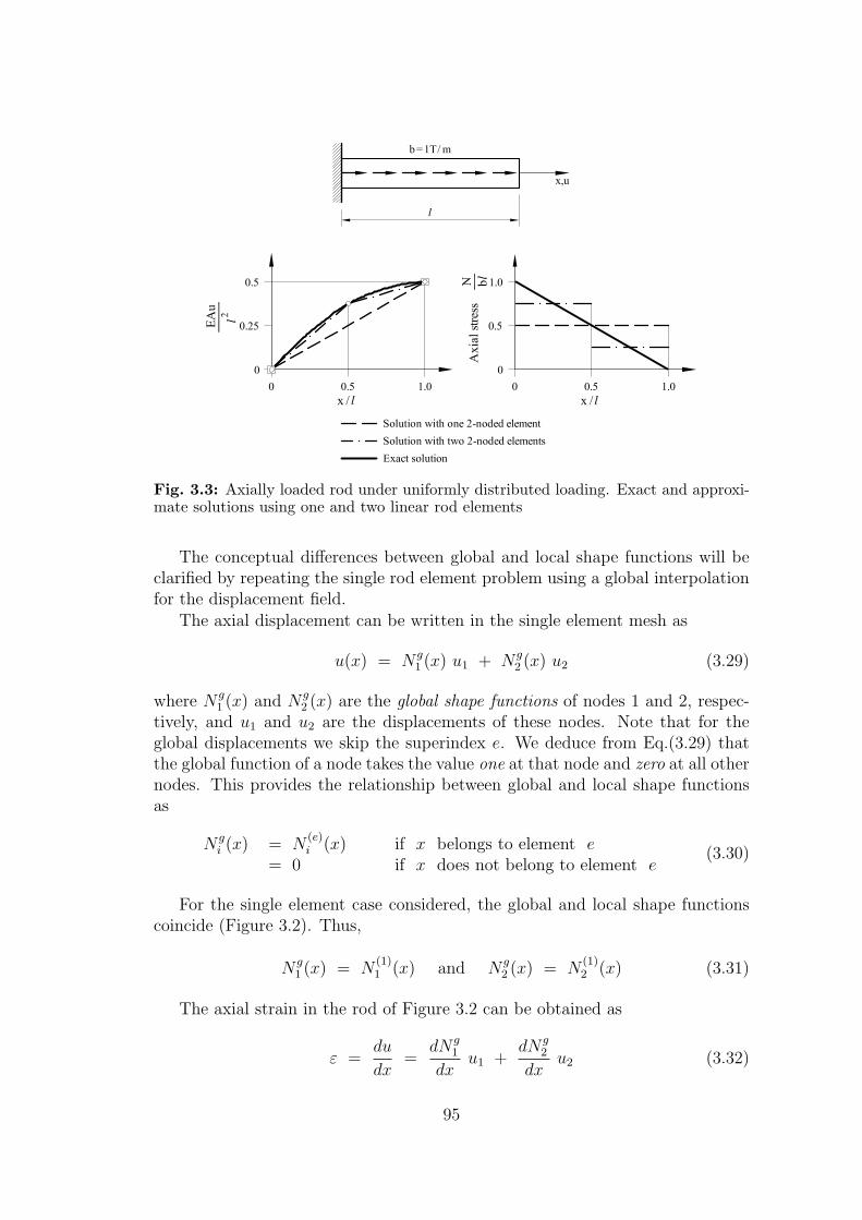
Fig. 3.3: Axially loaded rod under uniformly distributed loading. Exact and approxi-mate solutions using one and two linear rod elements

The conceptual differences between global and local shape functions will beclarified by repeating the single rod element problem using a global interpolationfor the displacement field.

The axial displacement can be written in the single element mesh as

u(x) = N g1 (x) u1 + N g

2 (x) u2 (3.29)

where N g1 (x) and N g

2 (x) are the global shape functions of nodes 1 and 2, respec-tively, and u1 and u2 are the displacements of these nodes. Note that for theglobal displacements we skip the superindex e. We deduce from Eq.(3.29) thatthe global function of a node takes the value one at that node and zero at all othernodes. This provides the relationship between global and local shape functionsas

N gi (x) = N

(e)i (x) if x belongs to element e

= 0 if x does not belong to element e(3.30)

For the single element case considered, the global and local shape functionscoincide (Figure 3.2). Thus,

N g1 (x) = N

(1)1 (x) and N g

2 (x) = N(1)2 (x) (3.31)

The axial strain in the rod of Figure 3.2 can be obtained as

ε =du

dx=

dN g1

dxu1 +

dN g2

dxu2 (3.32)

95

The virtual displacement and the virtual axial strain are expressed as

δu = N g1 δu1 + N g

2 δu2 , δε =dN g

1

dxδu1 +

dN g2

dxδu2 (3.33)

The PVW is written for the rod as

∫ l

0

[dN g

1

dxδu1 +

dN g2

dxδu2

](EA)

[dN g

1

dxu1 +

dN g2

dxu2

]dx −

−∫ l

0

[N g1 δu1 + N g

2 δu2] b dx = δu1R1 + δu2 P (3.34)

After eliminating the virtual displacements, Eq.(3.34) leads to

∫ l

0

dN g1

dx(EA)

dN g1

dx

dN g1

dx(EA)

dN g2

dxdN g

2

dx(EA)

dN g1

dx

dN g2

dx(EA)

dN g2

dx

dx

u1

u2

−

−∫ l

0

N g

1

N g2

b dx =

R1

P

(3.35)

The following relationships are important for the computation of the integralsin Eq.(3.35)

N g1 = N

(1)1

N g2 = N

(1)2

dN g1

dx=

dN(1)1

dx

dN g2

dx=

dN(1)2

dx

0 ≤ x ≤ l (3.36)

Using Eq.(3.36) we obtain

∫ l

0

dN g1

dx

dN g1

dxdx =

∫ l(1)

0

(dN

(1)1

dx

)2

dx =1

l∫ l

0

dN g1

dx

dN g2

dxdx =

∫ l(1)

0

dN(1)1

dx

dN(1)2

dxdx = − 1

l

∫ l

0

dN g2

dx

dN g2

dxdx =

∫ l(1)

0

(dN

(1)2

dx

)2

dx =1

l∫ l

0

N gi dx =

∫ l(1)

0

N(1)1 dx =

∫ l(1)

0

N(1)2 dx =

l

2

(3.37)

Substituting Eq.(3.37) into the PVW expression (3.34) yields the global equi-librium equation (3.25) directly. Recall that in the previous section this equation

96

Fig. 3.4: Axially loaded rod. Discretization in two linear rod elements

was obtained from the assembly of the element contributions. From this pointonwards the solution process is identical to that explained in Eqs.(3.25)-(3.27)and it will not be repeated here.

In the next section the same problem is solved using a mesh of two linearelements.

3.5 AXIALLY LOADED ROD OF CONSTANT CROSSSECTIONAL AREA. DISCRETIZATION IN TWO LINEARROD ELEMENTS

The same rod as for the previous example is discretized now in two linear rodelements as shown in Figure 3.4 where the differences between local and globalshape functions are also shown.

97

The discretized equilibrium equations will be obtained first using the localdescription of the shape functions.

The displacements within each element are interpolated as

Element 1 Element 2

u(x) = N(1)1 (x)u

(1)1 + N

(1)2 (x)u

(1)2

∣∣∣∣ u(x) = N(2)1 (x)u

(2)1 + N

(2)2 (x)u

(2)2

(3.38)

The shape functions and their derivatives are

N(1)1 =

x(1)2 − x

l(1);

dN(1)1

dx= − 1

l(1)

∣∣∣∣∣ N(2)1 =

x(2)2 − x

l(2);

dN(2)1

dx= − 1

l(2)

N(1)2 =

x− x(1)2

l(1);

dN(1)2

dx=

1

l(1)

∣∣∣∣∣ N(2)2 =

x− x(2)1

l(2);

dN(2)2

dx=

1

l(2)

(3.39)

The axial strain in each element is

ε =du

dx=

dN(1)1

dxu

(1)1 +

dN(1)2

dxu

(1)2

∣∣∣∣ ε =du

dx=

dN(2)1

dxu

(2)1 +

dN(2)2

dxu

(2)2

(3.40)The matrix form of the discretized equilibrium equations is obtained using

the PVW as explained in the previous section for the single element case (seeEqs.(3.12)-(3.20)). We find that

q(1) = K(1)a(1) − f (1) ; q(2) = K(2)a(2) − f (2) (3.41a)

where

K(1) =

∫ x(1)2

x(1)1

(EA)

dN(1)1

dx

dN(1)1

dx

dN(1)1

dx

dN(1)2

dx

dN(1)2

dx

dN(1)1

dx

dN(1)2

dx

dN(1)2

dx

dx

f (1) =

∫ x(1)2

x(1)1

[N

(1)1 , N

(1)2

]T

b(1) dx

q(1) =[X

(1)1 , X

(1)2

]T

, a(1) =[u

(1)1 , u

(1)2

]T

K(2) =

∫ x(1)2

x(1)1

EA

dN(2)1

dx

dN(2)1

dx

dN(2)1

dx

dN(2)2

dx

dN(2)2

dx

dN(2)1

dx

dN(2)2

dx

dN(2)2

dx

dx

f (2) =

∫ x(2)2

x(2)1

[N

(2)1 , N

(2)2

]T

b(2) dx

q(2) =[X

(2)1 , X

(2)2

]T

, a(2) =[u

(2)1 , u

(2)2

]T

(3.41b)

98

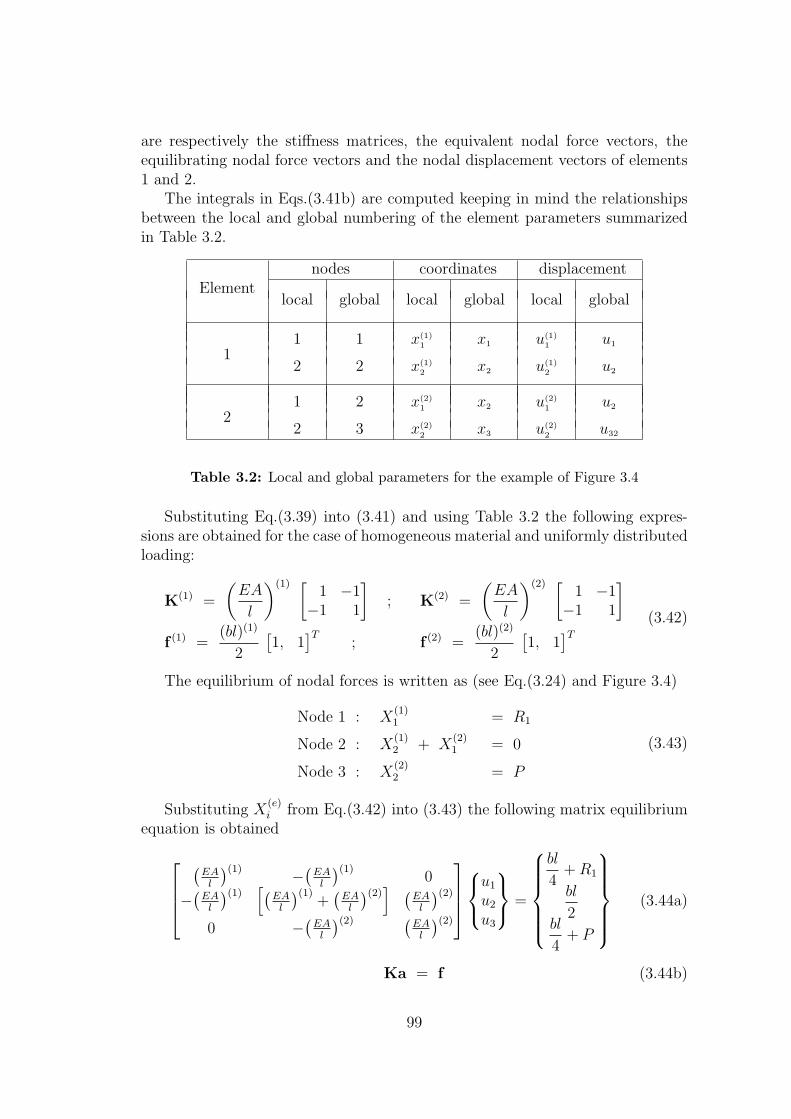
are respectively the stiffness matrices, the equivalent nodal force vectors, theequilibrating nodal force vectors and the nodal displacement vectors of elements1 and 2.

The integrals in Eqs.(3.41b) are computed keeping in mind the relationshipsbetween the local and global numbering of the element parameters summarizedin Table 3.2.

nodes coordinates displacementElement

local global local global local global

1 1 x(1)1 x1 u(1)

1 u1

12 2 x(1)

2 x2 u(1)2 u2

1 2 x(2)1 x2 u(2)

1 u2

22 3 x(2)

2 x3 u(2)2 u32

Table 3.2: Local and global parameters for the example of Figure 3.4

Substituting Eq.(3.39) into (3.41) and using Table 3.2 the following expres-sions are obtained for the case of homogeneous material and uniformly distributedloading:

K(1) =

(EA

l

)(1) [1 −1

−1 1

]; K(2) =

(EA

l

)(2) [1 −1

−1 1

]

f (1) =(bl)(1)

2

[1, 1

]T; f (2) =

(bl)(2)

2

[1, 1

]T

(3.42)

The equilibrium of nodal forces is written as (see Eq.(3.24) and Figure 3.4)

Node 1 : X(1)1 = R1

Node 2 : X(1)2 + X

(2)1 = 0

Node 3 : X(2)2 = P

(3.43)

Substituting X(e)i from Eq.(3.42) into (3.43) the following matrix equilibrium

equation is obtained

(EAl

)(1) −(EAl

)(1)0

−(EAl

)(1)[(

EAl

)(1)+

(EAl

)(2)] (

EAl

)(2)

0 −(EAl

)(2) (EAl

)(2)

u1

u2

u3

=

bl

4+ R1

bl

2bl

4+ P

(3.44a)

Ka = f (3.44b)

99

The element stiffness matrix is deduced from Eqs.(3.42) and (3.44) as

K(e) =

[K

(e)11 K

(e)12

K(e)21 K

(e)22

]=

∫ x(e)2

x(e)1

(EA)(e)

dN(e)1

dx

dN(e)1

dx

dN(e)1

dx

dN(e)2

dxdN

(e)2

dx

dN(e)1

dx

dN(e)2

dx

dN(e)2

dx

dx =

=

(EA

l

)(e) [1 −1

−1 1

](3.45)

Note that the assembly process is identical to that explained in the previouschapter for bar structures.

The same assembly process applies to the global vector of equivalent nodalforces. The elemental expression of this vector is

f (e) =

f

(e)1

f(e)2

=

∫ x(e)2

x(e)1

N

(e)1

N(e)2

b(e) dx =

(bl

2

)(e)

1

1

(3.46)

Substituting(

EAl

)(1)=

(EAl

)(2)= 2EA

linto Eq.(3.44a) and solving the equa-

tion system we find that

u1 = 0 ; u2 =l

2EA

(P +

3bl

4

)

u3 =l

2EA(2P + bl) ; R1 = −(P + bl)

(3.47)

The axial strain and the axial force are constant within each element and areobtained as

Element 1 Element 2

ε(1) =

(du

dx

)(1)

=u2

l(1)=

P + 3bl4

EA

∣∣∣∣∣ ε(2) =

(du

dx

)(2)

=u3 − u2

l(2)=

1

EA

(bl

4+ P

)

N (1) = (EA)(1)ε(1) = P +3bl

4

∣∣∣∣∣ N (2) = (EA)(2)ε(2) =bl

4+ P

(3.48)The distribution within each element of the displacement u and the constant

axial force N is shown in Figure 3.3. Note that for the same reasons explainedin Section 3.3 the nodal displacements coincide with the exact values. Some im-provement in the approximation of the global displacement field is also observed.However, the error in the axial force is still considerable and its reduction requiresa finer discretization and the nodal smoothing of the constant axial forces overeach element. This can be done by simply averaging the nodal forces.

The results obtained for the axial forces (and strains) are more innacuratethan those for the displacement field. This is a general rule which is explainedby the fact that the strains and the stresses are computed from the derivatives of

100

the approximate displacement field. This, naturally, increases the solution errorfor those values.

The same problem is now solved using the global description of the shapefunctions.

The axial displacement can be expressed globally over the two elements meshas (see Figure 3.4)

u(x) = N g1 (x)u1 + N g

2 (x)u2 + N g3 (x)u3 (3.49)

and the axial strain is given by

ε =du

dx=

dN g1

dxu1 +

dN g2

dxu2 +

dN g3

dxu3 (3.50)

The discretized form of the PVW is written using above equations as

∫ l

0

(dN g

1

dxδu1 +

dN g2

dxδu2 +

dN g3

dxδu3

)(EA)

(dN g

1

dxu1 +

dN g2

dxu2 +

dN g3

dxu3

)dx−

−∫ l

0

(N g

1 δu1 + N g2 δu2 + N g

3 δu3

)b dx = δu1R1 + δu3P

(3.51)

This leads, after eliminating the virtual displacements, to the following matrixsystem of equations

∫ l

0

dN g1

dx

dN g1

dx

dN g1

dx

dN g2

dx

dN g1

dx

dN g3

dxdN g

2

dx

dN g1

dx

dN g2

dx

dN g2

dx

dN g2

dx

dN g3

dxdN g

3

dx

dN g1

dx

dN g3

dx

dN g2

dx

dN g3

dx

dN g3

dx

(EA) dx

u1

u2

u3

−

−∫ l

0

N g1

N g2

N g3

b dx =

R1

0P

(3.52)

The computation of the integrals in Eq.(3.52) requires a correspondence be-tween the global and local shape functions. The following relationships are de-

101

duced from Table 3.2 and Figure 3.4

N g1 = N

(1)1

dN g1

dx=

dN(1)1

dxN g

2 = N(1)2

dN g2

dx=

dN(1)2

dxN g

3 = 0

dN3

dx= 0

0 ≤ x ≤ l

2;

N g1 = 0

dN g1

dx= 0

N g2 = N

(2)1

dN g2

dx=

dN(2)1

dxN g

3 = N(2)2

dN g3

dx=

dN(2)2

dx

l

2≤ x ≤ l (3.53)

Making use of the expressions (3.53) in (3.52) the global equilibrium equationis directly obtained. The reader can easily verify the coincidence of this equationwith Eq.(3.44a) obtained by assembly of the element contributions.

This example clearly shows that the use of the global shape functions is lesssystematic and requires more detailed computations than the element by elementapproach. These differences are even more apparent for finer meshes. As aconsequence, the assembly of the global equations from the elemental expressionsderived via the local shape functions is recommended in practice.

3.6 GENERALIZATION OF THE SOLUTION WITH N LINEARROD ELEMENTS

The solution process explained in the previous sections can be easily generalizedfor a discretization using a mesh of n 2-noded (linear) rod elements. The stiffnessmatrix and the equivalent nodal force vector for each element are given by

K(e) =

∫ x(e)2

x(e)1

(EA)(e)

dN(e)1

dx

dN(e)1

dx

dN(e)1

dx

dN(e)2

dx

dN(e)2

dx

dN(e)1

dx

dN(e)2

dx

dN(e)2

dx

dx

f (e) =∫ x

(e)2

x(e)1

N

(e)1

N(e)2

b(e) dx

(3.54)

which after substitution of the shape functions and their derivatives

N(e)1 =

x(e)2 − x

l(e);

dN(e)1

dx= − 1

l(e)

N(e)2 =

x− x(e)1

l(e);

dN(e)2

dx=

1

l(e)

(3.55)

102

gives (for homogeneous material and uniformly distributed loading)

K(e) =

(EA

l

)(e) [1 −1

−1 1

]; f (e) =

(bl)(e)

2

11

(3.56)

The assembly process leads, after some algebra, to the following global matrixequation

k(1) −k(1) 0 . . . 0−k(1)

[k(1) + k(2)

] −k(2) . . . 00 −k(2)

[k(2) + k(3)

]. . . 0

0 0 −k(3) . . ....

......

. . . . . ....

0 0 . . .[k(n−1) + k(n)

] −k(n)

0 0 . . . −k(n) k(n)

︸ ︷︷ ︸K

u1

u2

u3......

un−1

un

︸ ︷︷ ︸a

=

=

(bl)(1)

2+ P1

(bl)(1)

2+ (bl)(2)

2+ P2

(bl)(2)

2+ (bl)(3)

2+ P3

...

...(bl)(n−1)

2+ (bl)(n)

2+ Pn−1

(bl)(n)

2+ Pn

︸ ︷︷ ︸f

with k(e) =

(EA

l

)(e)

(3.57)

Note that matrix K depends on the geometrical (l and A) and material (E)parameters of each element, while vector f depends on the intensity of the dis-tributed load b(e), the element length and the point loads Pi acting at the nodes.The unknown reactions at the prescribed nodes are treated as point loads andthey are computed “a posteriori” following standard procedures of structural ma-trix analysis (see Section 1.4) [L3], [T9].

Example: 3.1 Analyse the axially loaded rod with exponentially varying cross sectional areaof Figure 3.5 using three meshes of one, two and three linear rod elements.

-- Solution-- Solution

The change in cross sectional area is defined by A = Aoe− x

l where Ao is the crosssectional area at the clamped end and l is the rod length. The rod is subjected to anaxial force acting at the free end. The exact solution for this simple problem is

σ =F

A=

F

Aoe

xl , ε =

σ

E=

F

EAoe

xl

103

Fig. 3.5: Axially loaded road with exponentialy varying cross section. Discretizationin 3 meshes of two-noded rod elements

u(x) =∫ x

0

εdx =∫ x

0

F

EAoex/l dx =

Fl

EAo(ex/l − 1)

u(l) =Fl

EAo(e− 1) = 1.71828

Fl

EAo; R1 = − F

Two options are possible for the finite element solution: a) to use the exact expressionof the cross sectional area, and b) to assume a constant cross sectional area within eachelement. The second option has been chosen here for simplicity. The reader is encouragedto repeat this problem as an exercise using the first alternative.

One elements solution

The cross sectional area is assumed to be constant and equal to A = Aoe−1/2. The

element stiffness matrix is directly given by Eq.(3.56), i.e.

K(1) =EAo

le−1/2

[1 −1

−1 1

]=

EAo

l0.60653

[1 −1

−1 1

]

The equilibrium equation is deduced from Eq.(3.57) (noting that the distributed loadsb(e) are zero) as

EAo

l0.60653

[1 −1

−1 1

] u1

u2

=

R1

F

; u1 = 0

104

which when solved gives

u2 =1

0.60653Fl

EAo= 1.6487

Fl

EAo; R1 = − F

The percentage of error with respect to the exact solution is 4.21%. This can be consid-ered acceptable given the simplicity of the mesh.

Two elements solution

Now A(1) = Aoe−1/4 and A(2) = Aoe

−3/4. The equilibrium equations for each element(Figure 3.5) are obtained as explained in Section 3.5.

Element 1

1.5576(EAo

l

) [1 −1

−1 1

] u1

u2

=

X

(1)1

X(1)2

Element 2

0.9447(EAo

l

) [1 −1

−1 1

] u2

u3

=

X

(2)1

X(2)2

After global assembly we have

EAo

l

1.5576 −1.5576 0−1.5576 2.5023 −0.9447

0 −0.9447 0.9447

u1

u2

u3

=

R1

0F

u1 = 0

which gives

u3 = 1.7005Fl

EAo(Error = 1.04%)

u2 = 0.377541 u3 = 0.6419Fl

EAo

R1 = − F

Three elements mesh

For the three elements mesh (Figure 3.5) A(1) = Aoe−1/6, A(2) = Aoe

−1/2 and A(3) =Aoe

−5/6. The equilibrium equations for each element are

Element 1

2.5394EAo

l

[1 −1

−1 1

] u1

u2

=

X

(1)1

X(1)2

Element 2

1.8196EAo

l

[1 −1

−1 1

] u2

u3

=

X

(2)1

X(2)2

Element 3

1.3028EAo

l

[1 −1

−1 1

] u3

u4

=

X

(3)1

X(3)2

105

The global equilibrium equation after assembly is

EAo

l

2.5394 −2.5394 0 0−2.5394 4.3590 −1.8196 0

0 −1.8196 3.1234 −1.30380 0 −1.3038 1.3038

u1

u2

u3

u4

=

R1

00F

u1 = 0

and the solution isu4 = 1.71036

Fl

EAo(Error = 0.46%)

u3 = 0.55156 u4 = 0.9432Fl

EAo

u2 = 0.230241 u4 = 0.3938Fl

EAo

R1 = −F

Once the nodal displacements have been obtained, the axial strain and the axial stresscan be computed for each element. For example, at the central point of element number2 in the three elements mesh we have

u(l/2) = N(2)1

(x(2) =

l(2)

2

)u

(2)1 + N

(2)2

(x(2) =

l(2)

2

)u

(2)2 =

=120.23024u4 +

120.55156u4 = 0.3909u4 = 0.6686

Fl

EAo

(Exact value = 0.6487Fl

EAo. Error : 3.07%).

ε(l/2) =(dN

(2)1

dx

)x(2)= l(2)

2

u(2)1 +

(dN(2)2

dx

)x(2)= l(2)

2

u(2)2 = 1.6491

F

EAo

=(−3

l0.2302 +

3l

0.5516)

u4 = 0.9642u4

l

σ(l/2) = EεA = 1.649F

Ao(Exact value: 1.6487

F

Ao. Error: 0.02% )

The convergence of the end displacement value with the number of elements is shown inFigure 3.6. We see that the simple assumption of constant cross sectional area leads topercentage errors of less than 1% for meshes finer than two elements.

The displacement and stress distribution along the rod for the three meshes are plottedin Figure 3.7 together with the exact solution. Note that the nodal displacements andeven the linear displacement field within each element are very accurate for the threemeshes. However, the convergence of the constant stress field for each element to theexact exponential solution is quite slow.

3.7 EXTRAPOLATION OF THE SOLUTION FROM TWO DIF-FERENT MESHES

Expanding in Taylor series the displacement in the vecinity of a node i gives

u = ui +(∂u

∂x

)i(x− xi) +

(∂2u

∂x2

)i(x− xi)

2 + · · · (3.58)

106

Fig. 3.6: Axially loaded rod with varying cross sectional area. Convergence of the enddisplacement value and the stress distribution with the number of elements

Fig. 3.7: Nodal displacements and stress distribution along the rod for the threemeshes

If the shape functions Ni(x) are polynomials of pth degree it is obvious thatonly the first p terms of the Taylor expansion can be approximated exactly as thederivatives of order p + 1, p + 2, etc. are zero. The error of this approximation isthen of the order of the first term disregarded in the above expansion, i.e.

error = uexact − uapprox = O(x− xi)p+1 ' O(lp+1) (3.59)

where O(lp+1) is read as “of the order of lp+1” and l is the element length.

107

Let us now consider two solutions u1 and u2 obtained with two meshes ofuniform element sizes l and l/d, respectively. We can write

uexact − u1 = O(lp+1)

uexact − u2 = O[(l

d)p+1

] (3.60)

The approximate value of uexact is obtained in terms of u1 and u2 fromEqs.(3.60) as

uexact∼= (dp+1)u2 − u1

(dp+1)− 1(3.61)

This technique is known as Richardson extrapolation [R2]. For the rod ofFigure 3.5 we obtain for the end displacement value:

1. Extrapolated solution from meshes 1 and 2 (d = 2)

u(l) =4u2 − u1

3= 1.7178

Fl

EAo

(Error: 0.03%)

2. Extrapolated solution using meshes 1 and 3 (d = 3)

u(l) =9u2 − u1

8= 1.71807

Fl

EAo

(Error: 0.012%)

3. Extrapolated solution using meshes 2 and 3 (d = 1.5)

u(l) =(9.5)2u2 − u1

(1.5)2 − 1= 1.71825

Fl

EAo

(Error: 0.002% )

We see that Richardson’s extrapolation is an effective technique to improve thedisplacement solution obtained from two meshes using elements of the same type.This simple procedure is also applicable for 2D and 3D problems. Obviously, theenhanced nodal displacement values can be used to obtain an improved solutionfor the stress field. Unfortunately the improvement is not so relevant as for thenodal displacements.

3.8 MATRIX FORMULATION OF THE ELEMENT EQUATIONSThe methodology explained in the previous sections is very useful for introducingthe basic steps of the FEM. However, for problems with more than one displace-ment variable per node a matrix formulation is much more convenient as it allowsall variables and algebraic operations to be grouped together in a compact form.The matrix formulation also provides a systematic finite element methodologyfor all the structural problems treated in this book. The basic concepts of thematrix formulation will be presented next.

108

Most expressions used henceforth will be referred to an individualelement only. Therefore, superindex “e” denoting element valueswill be omitted hereafter for simplicity, with the exception of a fewsignificative element parameters such as the main geometrical di-mensions (l(e), A(e) and V (e)), the nodal displacement vector a(e),the nodal coordinates vector x(e), the nodal force vectors (f (e),q(e)),the stiffness matrix K(e), and other relevant elemental parameters.All other parameters, vectors and matrices appearing in the textshould be interpreted, unless otherwise mentioned, as belonging toan individual element.

3.8.1 Shape function matrix

Let us consider a general 2-noded rod element. The displacement field is expressedwithin the element as

u = N1u1 + N2u2 (3.62)

Eq.(3.62) is written in matrix form as

u = u = [N1, N2]

u1

u2

= N a(e) (3.63)

where

N = [N1, N2] ; a(e) =

u1

u2

(3.64)

are the shape function matrix and the nodal displacement vector of the element.As mentioned above, the superindex “e” denoting element values has been omit-ted from most terms in Eqs.(3.62)-(3.64).

3.8.2 Strain matrix

The strain vector is written as

εεε = ε = dN1

dxu1 +

dN2

dxu2 = [

dN1

dx,

dN2

dx]

u1

u2

= B a(e) (3.65)

where

B = [dN1

dx,

dN2

dx] (3.66)

is the strain matrix of the element.

109

3.8.3 Constitutive matrixThe stress vector is written as

σσσ = [N ] = (EA) εεε = [EA] ε = DBa(e) (3.67)

whereD = [EA] (3.68)

is the matrix of mechanical properties of the material, also called hereafter con-stitutive matrix.

For the axial rod problem vectors εεε and σσσ and matrix D have a single compo-nent only. In general σσσ and εεε will have t components. Thus, if n is the numberof nodes of an individual finite element and d the number of d.o.f. of each node,the dimensions of the vectors and matrices in the constitutive equation are

σσσt×1

= Dt×t· B

[t×(n×d)]· a(e)

[(n×d)×1](3.69)

3.8.4 Principle of Virtual WorkThe PVW for an individual element is written in matrix form as∫

l(e)δεεεTσσσ dx =

∫

l(e)δuTb dx + [δa(e)]

T

q(e) (3.70)

Note that the PVW is a scalar equation, i.e. both sides of Eq.(3.70) arenumbers representing the internal and external virtual work, respectively. Thisexplains the organization of the terms in Eq.(3.70), as a scalar number is obtainedas product of a row vector times a column vector, i.e. if s is a scalar number wecan write

s = a1b1 + · · ·+ anbn = [a1, a2, . . . , an]

b1

b2...bn

= aTb (3.71)

Naturally, if vectors εεε and σσσ have a single term, as in the axially loaded rodproblem, the vector product (3.71) reduces to multiplying two numbers. However,for most of the problems studied in this book, vectors εεε and σσσ have severalcomponents and the matrix form of the PVW will be used.

3.8.5 Stiffness matrix and equivalent nodal force vectorFrom Eqs.(3.63) and (3.65) we have

[δu]T = [δa(e)]T

NT

[δεεε]T = [δa(e)]T

BT(3.72)

110

Substituting now Eqs.(3.65), (3.67) and (3.72) into the PVW written for asingle element gives

∫

l(e)[δa(e)]

T

BT D B a(e) dx −∫

l(e)[δa(e)]

T

NT b dx = δa(e)q(e) (3.73)

where b = b is the vector of distributed loads acting on the element. Elimina-ting the virtual displacements from Eq.(3.73) yields

[δa(e)]T

[(∫

l(e)BT D B dx

)a(e) −

∫

l(e)NT b dx − q(e)

]= 0 (3.74)

As the virtual displacements are arbitrary, satisfaction of Eq.(3.74) implies

(∫

l(e)BT D B dx

)a(e) −

∫

l(e)NT b dx = q(e) (3.75)

Eq.(3.75) is a system of algebraic equations which can be written in the stan-dard form

K(e)a(e) − f (e) = q(e) (3.76a)

where

K(e) =

∫

l(e)BT D B dx

f (e) =

∫

l(e)NT b dx

(3.76b)

are respectively the stiffness matrix and the equivalent nodal force due to dis-tributed loading for the element. Vector q(e) in Eq.(3.76a) is the equilibratingnodal force vector for the element which is essential for the global assembly pro-cess.

Note that the derivation of K(e) and f (e) is completely general . Expressions(3.76) will frequently appear throughout the text and will be particularized foreach element type studied.

The explicit form of K(e) and f (e) for the 2-noded axially loaded rod elementis found by substituting into Eqs.(3.76b) the adequate expressions for B,D,Nand b. In this case we have

N = [N1,N2] = [N1, N2] =[x2 − x

l(e),x− x1

l(e)

]

B = [B1,B2] =[dN1

dx,dN2

dx

]=

[− 1

l(e),

1

l(e)

] (3.77)

D = [EA] and b = b

111

Substituting Eqs.(3.77) into (3.76b) gives

K(e) =

∫

l(e)

− 1l(e)1

l(e)

(EA)

[− 1

l(e),

1

l(e)

]dx =

(EA

l

)(e) [1 −1

−1 1

]

f (e) =

∫

l(e)

x2 − xx− x1

(b

l

)(e)

dx =(bl)(e)

2

11

(3.78)

Note the coincidence of these expressions with those obtained in Eq.(3.56) bya more elaborate procedure.

We remark finally that the element stiffness matrix and the equivalent nodalforce vector can be obtained from the corresponding sub-matrices and subvectors.

Thus, from Eqs.(3.77) and (3.76b) we have

K(e) =

∫

l(e)

BT

1

BT2

D [B1,B2] dx =

∫

l(e)

BT1DB1

... BT1DB2

. . . . . . . . . . . . . . . . . . . . .

BT2DB1

... BT2DB2

dx

f (e) =

∫

l(e)

NT

1

NT2

b dx =

∫

l(e)

NT

1bNT

2b

dx (3.79)

Matrix K(e)ij relating nodes i and j of element e is

K(e)ij

d×d

=

∫

l(e)BT

i(d×t)

D(t×t)

Bj(t×d)

dx ; i, j = 1, 2 (3.80)

and the equivalent nodal force vector of node i of element e is

f(e)i

(d×1)

=

∫

l(e)b

(d×d)dx i = 1, 2 (3.81)

Recall that d is the number of d.o.f. of each node (i.e. d = 1 for the axiallyloaded rod). For the particular case of the 2-noded rod element we have

K(e)ij =

∫

l(e)

dNi

dxEA

dNj

dxdx = (−1)i+j

(EA

l

)(e)

f(e)i =

∫

l(e)Nib dx =

(bl)(e)

2

(3.82)

from which the expressions of K(e) and f (e) of Eq.(3.78) can be obtained.

The computation of the element stiffness matrix K(e) and the equivalent nodalforce vector f (e) from the nodal contributions K

(e)ij and f

(e)i is a simple and eco-

nomical procedure and it also facilitates the organization of a computer program.We will be able to verify this on many occasions throughout the text.

112

3.9 SUMMARY OF THE STEPS FOR THE ANALYSIS OF ASTRUCTURE USING THE FEM

Let us summarize the main steps to be followed in the finite element analysis ofa structure.

Step 1. Discretize the structure into a mesh of finite elements.

Step 2. Compute for each element the stiffness matrix and the equivalent nodalforce vector using expressions of the type

K(e) =

∫

l(e)BTDB dx ; K

(e)ij =

∫

l(e)BT

i DBj dx

f (e) =

∫

l(e)NTb dx ; f

(e)i =

∫

l(e)NT

i b dx (3.83)

For two and three dimensional structures the element integrals are com-puted over the element area or volume.

Step 3. Assemble the stiffness matrix and the equivalent nodal force vector foreach element into the global system

Ka = f (3.84a)

K = Ae

K(e) ; f = Ae

f (e) (3.84b)

where Ae

denotes the global assembly process of all the individual matrices

and vectors for each element in the mesh.

Step 4. The nodal displacement values are computed by solving the equation sys-tem (3.84a) where the prescribed displacement must be adequately imposed,i.e.

a = K−1f (3.85)

Also, the nodal reactions are obtained at the prescribed nodes.

Step 5. The strains and stresses are computed within each element from the nodaldisplacement values as

εεε = B a ; σσσ = D B a (3.86)

Details of each of above steps and of the precise form of the element vectorsand matrices will be given in the next chapters for each of the problemsstudied.

113

3.10 ADVANCED ROD ELEMENTS AND REQUIREMENTS FORTHE NUMERICAL SOLUTION

3.10.1 INTRODUCTIONThe analysis of the simple axially loaded rod problem using 2-noded rod elementsstudied in the previous chapter is of big interest as it summarises the basic stepsfor the analysis of a structure by the FEM. However, a number of importantquestions still remain unanswered, such as: Can higher order rod elements beeffectively used? What are their advantages versus the simpler 2-noded rod ele-ment? Can it be guaranteed that the numerical solution converges to the exactone as the mesh is refined? What are the conditions influencing the error in thenumerical solution? The reader who faces the application of the FEM for the firsttime will certainly come across these and similar questions. In the following sec-tions we will see that there are not definitive answers for many of the questions,and in some cases only some practical hints are possible. For simplicity we willmostly refer to the axially loaded rod problem as it allows a simple explanationof topics which are of general applicability to more complex problems.

3.11 ONE DIMENSIONAL Co ELEMENTS. LAGRANGEELEMENTS

In the previous sections we introduced the basic concepts of the FEM using sim-ple 2-noded one-dimensional elements with linear shape functions. Obviously,the polynomial interpolation guarantees that the axial displacement is continu-ous within the element and between adjacent elements. Elements satisfying thiscondition are termed “Co continuous”. Additionally, we could require continuityof the first derivative of the displacement and the approximation is then called“C1 continuous”. In general, an element is“Cm continuous” if the displacementfield has continuous the n − 1 first derivatives. In Section 3.17.3 we will comeback to this subject. In this section we will derive the shape functions for Co

continuous 1D elements. These ideas will be very useful for deriving the shapefunctions of 2D elements.

The approximation of a displacement unknown in 1D elements can be writtenas

u(x) = αo + α1x + α2x2 + · · · (3.87)

where αo, α1, etc., are constant parameters.Let us choose a first degree polynomial

u(x) = αo + α1x (3.88)

The parameters αo and α1 can be obtained from the value of u(x) at two elementpoints. This requires the element associated with the interpolation (3.2) to have

114

Fig. 3.8: Definition of the natural coordinate system ξ. Actual and normalized ge-ometries for a 2-noded element

two nodes. For a 2-noded element of length `(e) with node 1 at x = x1 and node2 at x = x2 (Figure 3.8), we have

u(x1) = u1 = αo + α1x1

u(x2) = u2 = αo + α1x2

(3.89)

where u1 and u2 are the values of the axial displacement at the two nodes. Sub-stituting the values of αo and α1 obtained from Eq.(3.89) into Eq.(3.88) gives

u(x) = N1(x)u1 + N2(x)u2 (3.90a)

where

N1(x) =(x2 − x)

l(e); N2(x) =

(x− x1)

l(e)(3.90b)

are the element shape functions. Note the coincidence with the expressions ob-tained in Section 3.3 (see Eq.(3.12)).

The shape functions for Co continuous 1D elements can be simply derived fromthe expressions of Lagrange polynomials. A n− 1th degree Lagrange polynomial`ni (x) is defined in terms of n points with coordinates x1, x2, · · · xn as follows

`ni (x) = (x− x1)(x− x2) · · · (x− xi−1)(x− xih) · · · (x− xn) (3.91)

Note that `ni (xi) = yi(6= 0) and `n

i (xj) = 0 for j = 1, 2, · · ·n(j 6= i). There-fore if the points coincide with the element nodes and the non-zero value yi isnormalized to the unity, the resulting Lagrange polynomial coincides with theshape function Ni(x) of the corresponding 1D element. This explains why Co

continuous 1D elements are also called “Lagrange” elements.The shape function Ni or a Lagrange element with n nodes can be obtained

directly by the following expression

Ni(x) =`ni (x)

`ni (xi)

(3.92a)

115

which can also be written as

Ni(x) =n∏

j=1(j 6=i)

( x− xj

xi − xj

)(3.92b)

For a two-noded element we find again that

N1 =x− x2

x1 − x2

=x2 − x

l(e)

N2 =x− x1

x2 − x1

=x− x1

l(e)

(3.93)

A natural coordinate ξ is introduced for convenience as (Figure 3.8)

ξ = 2x− xc

l(e)(3.94)

where xc is the cartesian coordinate of the element midpoint. Eq. (3.8) gives

ξ = −1 at the left-hand end of the element

ξ = 0 at the element mid point

ξ = 1 at the right-hand end of the element

Eq. (3.94) transforms the actual element geometry into a normalized geometryof length equal to 2. The shape functions can now be written in terms of thenatural coordinate ξ. By analogy with Eq.(3.92b) we write

Ni(ξ) =n∏

j=1(j 6=i)

( ξ − ξj

ξi − ξj

)(3.95)

For a linear Lagrange element with two nodes at ξ = −1 and ξ = +1 weobtain

N1 =ξ − ξ2

ξ1 − ξ2

=1

2(1− ξ)

N2 =ξ − ξ1

ξ2 − ξ1

=1

2(1 + ξ)

(3.96)

For a quadratic Lagrange element with three nodes at ξ1 = −1, ξ = 0 andξ = +1 (Figure 3.9) the shape functions are

N1 =(ξ − ξ2)(ξ − ξ3)

(ξ1 − ξ2)=

1

2ξ(ξ − 1)

N2 =(ξ − ξ1)(ξ − ξ3)

(ξ2 − ξ1)(ξ2 − ξ3)= (1− ξ2)

N3 =(ξ − ξ1)(ξ − ξ2)

(ξ3 − ξ1)(ξ3 − ξ2)=

1

2ξ(1 + ξ)

(3.97)

116

Fig. 3.9: Quadratic and cubic 1D elements with Co continuity

Finally, for a cubic element with four nodes at ξ1 = −1, ξ2 = −1/3, ξ3 = 1/3and ξ4 = +1 (Figure 3.9) the shape functions are

N1 =(ξ − ξ2)(ξ − ξ3)(ξ − ξ4)

(ξ1 − ξ2)(ξ1 − ξ3)(ξ1 − ξ4)= − 9

16

(ξ2 − 1

9

)(ξ − 1)

N2 =(ξ − ξ1)(ξ − ξ3)(ξ − ξ4)

(ξ2 − ξ1)(ξ2 − ξ3)(ξ2 − ξ4)=

27

16

(ξ − 1

3

)(ξ2 − 1)

N3 =(ξ − ξ1)(ξ − ξ2)(ξ − ξ4)

(ξ3 − ξ1)(ξ3 − ξ2)(ξ3 − ξ4)= − 27

16

(ξ +

1

3

)(ξ2 − 1)

N4 =(ξ − ξ1)(ξ − ξ2)(ξ − ξ3)

(ξ4 − ξ1)(ξ4 − ξ2)(ξ4 − ξ3)=

9

16(ξ + 1)

(ξ2 − 1

9

)

(3.98)

The cartesian expressions of the above shape functions can be obtained fromthe transformation (3.94). However, only the normalized forms are necessary inpractice.

The reader is encouraged to derive by himself the expressions of the shapefunctions of higher order 1D Lagrange elements.

The shape functions of C1 continuous 1D elements will be derived in Chapter7.

117

3.12 ISOPARAMETRIC FORMULATION AND NUMERICAL IN-TEGRATION

3.12.1 Introduction

We will now introduce two key concepts which have been essential for the de-velopment of the FEM. The first one is that of isoparametric interpolation. Thebasic idea is to interpolate the element geometry from the coordinates of thenodes. Such an interpolation is essential to obtain a general relationship betweenthe natural and cartesian coordinates.

The second concept is that of numerical integration. In most cases the exactanalytical computation of the element integrals is not possible and numericalintegration is the only option to evaluate them in a simple and precise way.

The application of these two techniques to Co continuons 1D elements ispresented in the next sections. However, the advantages of these procedures willbecome clearer when dealing with 2D and 3D elements.

3.12.2 The concept of parametric interpolation

Let us recall the displacement interpolation for a 2-noded axial rod element:

u(ξ) = N1(ξ)u1 + N2(ξ)u2 (3.99)

Note that in Eq.(3.99) we have used the expression of the shape funtions interms of the natural coordinate ξ. With a few exceptions this will be the usualprocedure throughout the text.

The axial strain is obtained from Eq.(3.99) as

ε =du

dx=

dN1(ξ)

dxu1 +

dN2(ξ)

dxu2 (3.100)

The cartesian derivatives of the shape functions are therefore needed to com-pute the strain. This would be an easy task if the shape functions were expressedin terms of the cartesian coordinate x. However, as this will not generally be thecase, some transformations are necessary. For the 1D problem we have

dN1(ξ)

dx=

dN1(ξ)

dξ

dξ

dx=

d

dξ

(1− ξ

2

) dξ

dx= − 1

2

dξ

dx

dN2(ξ)

dx=

dN2(ξ)

dξ

dξ

dx=

d

dξ

(1 + ξ

2

) dξ

dx=

1

2

dξ

dx

(3.101)

and the strain is obtained by

ε = − 1

2

(dξ

dx

)u1 +

1

2

(dξ

dx

)u2 (3.102)

118

Eq.(3.102) involves the evaluation of dξdx

. This obviously requires an explicitrelationship between ξ and x which can be obtained using a parametric interpo-lation of the element geometry. This expresses the coordinate of any point withinthe element in terms of the coordinates of m element points x1, x2, · · · , xm by thefollowing interpolation

x = N1(ξ)x1 + N2(ξ)x1 + · · ·+ Nm(ξ)xm (3.103)

In Eq.(3.103) Ni(ξ) are geometry interpolation functions which satisfy thesame requirements as the displacement shape functions; i.e. Ni(ξ) takes thevalue one at point i and zero at the other m− 1 points for which the coordinatesare known. Hence, the expression of Ni(ξ) can be obtained simply by changingn for m in Eq.(3.95), where ξi are now the natural coordinates of the geometryinterpolating points.

It is important to note that Eq. (3.103) yields precisely the relationship weare looking for between the coordinates ξ and x. This expression can also beinterpreted as transformation between coordinates ξ and x, such that every pointin the normalized space [-1,1] is mapped onto another point in the cartesian space[x1, x2]. It is essential that this mapping be unique and this generally dependson the element geometry.

Example: 3.2 Parametric interpolation of a cubic polinominal.

-- Solution

Let us consider the polynomial y = x3 − 2x2 − x + 4 plotted in Figure 3.10. Such afunction can represent, for instance, the geometry of a curved beam or the boundary ofa curved 2D element. We will assume that the coordinates of the three points at x1 = 0,x2 = 1, and x3 = 2 are known.

The coordinates of the three points will be used to build up a quadratic approximationusing a 3-noded 1D element. The relationship between the cartesian (x, y) coordinatesand the natural coordinate ξ is obtained as a particular case of Eq.(3.103), i.e.

x =3∑

i=1

Ni(ξ)xi =12ξ(ξ − 1)x1 + (1− ξ2)x2 +

12ξ(ξ + 1)x3 = 1− ξ

y =3∑

i=1

Ni(ξ)yi =12ξ(ξ − 1)y1 + (1− ξ2)y2 +

12ξ(1 + ξ)y3 = ξ2 − ξ + 2

Figure 3.10 shows the approximating quadratic function. Note the error with respect tothe “exact” cubic function. Also note that this error is much larger outside the interval[0,2] which includes the three points selected.

The accuracy can be dramatically improved by using a cubic approximation in terms ofthe coordinates of four known points at x1 = 0, x2 = 2/3, x3 = 4/3, and x4 = 2.0, withy(x1) = 4.0, y(x2) = 74/27, y(x3) = 40/27, and y(x4) = 2.0, respectively. A cubic 1Delement is now used giving

x =4∑

i=1

Ni(ξ)xi ; y =4∑

i=1

Ni(ξ)yi

119

Fig. 3.10: Parametric interpolation of a cubic polynomial

where Ni are the cubic shape function of Eq.(3.97). After some algegra, the following isobtained (easily)

x = 1 + ξ ; y = (1 + ξ)3 − 2(1 + ξ)2 − (1 + ξ) + 4

As expected, the cubic field chosen exactly approximates the original cubic function.

Example 3.2 shows that important errors in the geometry approximation canoccur unless a correct interpolation of the geometry is chosen. These errors areundesirable and should be avoided or, at least, minimized.

Two types of points must therefore be considered in an element: a) the pointsused for interpolating the displacement field (nodes) by the shape functions Ni(ξ);and b) the points chosen to approximate the element geometry via the geometryinterpolation function Ni(ξ). These two sets of points can coincide depending onthe problem. Complex structures might require a higher order interpolation ofthe geometry, whereas a simple geometry can be exactly approximated using alinear field for Ni, independently of the interpolation used for the displacementfield.

If the number of geometry points m is greater than that of element nodes, thegeometry interpolation functions Ni will be polynomials of a higher order thanthe displacement shape functions, and the element is termed superparametric. Ifn coincides with the number of nodes, then Ni ≡ Ni and the element is isopara-metric. Finally, if the number of geometry points is less than that of nodes, theelement is called subparametric.

120

In practice it is usual to choose an isoparametric formulation. However, it isimportant to have a clear picture of the two other options which are useful insome cases.

The isoparametric concept originates from the work of Taig [T1,2] who derivedthe first 4-noded isoparametric quadrilateral. Irons [I3,4] extended these ideas toformulate high order isoparametric elements. In the following chapters we willextend this concept for 2D and 3D elements.

3.12.3 Isoparametric formulation of the two-noded rod elementThe geometry of the linear rod element is expressed in terms of the coordinatesof the two nodes as

x(ξ) = N1(ξ)x1 + N2(ξ)x2 (3.104)

where N1 and N2 are the same linear shape functions used for interpolating thedisplacement field (see Eq.(3.96)).

From Eq.(3.104) we obtain

dx

dξ=

dN1

dξx1 +

dN2

dξx2 = − 1

2x1 +

1

2x2 =

l(e)

2(3.105)

and

dx =l(e)

2dξ y

dξ

dx=

2

l(e)(3.106)

Substituting Eq.(3.106) into (3.101) gives

dN1

dx=

2

l(e)dN1

dξ= − 1

l(e)

dN2

dx=

2

l(e)dN2

dξ=

1

l(e)

(3.107)

and from Eqs.(3.107) and (3.100)

ε =[−1/l(e), 1/l(e)

]a(e) = B a(e) (3.108a)

withB =

[−1/l(e), 1/l(e)

](3.108b)

which naturally coincides with the expressions previously derived by a more directprocedure. The systematic approach chosen here is useful in order to understandthe application of the isoparametric concept.

The stiffness matrix and the equivalent nodal force vector are expressed inthe natural coordinate system combining Eqs.(3.106) and (3.83b) as

K(e) =

∫ +1

−1

BT (EA)Bl(e)

2dξ , f (e) =

∫ +1

−1

NTbl(e)

2dξ (3.109)

For homogeneous material and uniformly distributed loading the computationof the above integrals is simple, leading to the expressions (3.85).

121

3.12.4 Isoparametric formulation of the 3-noded quadratic rod elementWe will now study the 3-noded rod element of Figure 3.9 with quadratic shapefunctions. The axial displacement is expressed by

u = N1(ξ)u1 + N2(ξ)u2 + N3(ξ)u3 (3.110)

where the shape functions N1(ξ), N2(ξ) and N3(ξ)are given by Eq.(3.97).The x coordinate of a point within the element is written in the isoparametric

formulation asx = N1(ξ)x1 + N2(ξ)x2 + N3(ξ)x3 (3.111)

The axial strain is obtained by

ε =du

dx=

3∑i=1

dNi

dξui =

[dN1

dξ

dξ

dx,

dN2

dξ

dξ

dx,

dN3

dξ

dξ

dx

]

u1

u2

u3

= B a(e)

(3.112)From Eq.(3.97)

dN1

dξ= ξ − 1

2;

dN2

dξ= − 2ξ ;

dN3

dξ= ξ +

1

2(3.113)

and the strain matrix B is

B =(dξ

dx

) [(ξ − 1

2),−2ξ, (ξ +

1

2)]

(3.114)

The derivative dxdξ

is computed from Eq.(3.111) as

dx

dξ=

dN1

dξx1 +

dN2

dξx2 +

dN3

dξx3 = (ξ − 1

2) x1 −

− 2ξx2 + (ξ +1

2) x3 =

l(e)

2+ ξ (x1 + x3 − 2x2)

(3.115)

and dξ

dx=

2

l(e) + 2ξ(x1 + x3 − 2x2)(3.116)

Eq.(3.116) provides a relationship between dx and dξ in terms of the threenodal coordinates. In the (usual) case that the central node is located at theelement midpoint, we have

dξ

dx=

2

l(e)(3.117)

and dx

dξ=

2

l(e)y dx =

l(e)

2dξ (3.118)

In this latter case the strain matrix of Eq.(3.114) is simply

B =2

l(e)

[(ξ − 1

2),−2ξ, (ξ +

1

2)]

(3.119)

122

The expression of B for an arbitrary position of the central node is obtainedby substituting Eq.(3.116) into (3.114).

The element stiffness matrix and the equivalent nodal force vector are obtainedfrom the PVW as explained the 2-noded element. It can easily be found that theelement stiffness matrix has once again the general form

K(e) =

∫

l(e)BT (EA) B dx (3.120)

Substituting the above expressions of dx and B in terms of ξ into Eq.(3.120)leads to (in the case of the mid-node being central in the element)

K(e) =

∫ +1

−1

2

l(e)

(ξ − 12)

−2ξ(ξ + 1

2)

(EA)

2

l(e)

[(ξ − 1

2),−2ξ, (ξ +

1

2)

]l(e)

2dξ (3.121)

The computation of the above integral is straightforward if both E and A areconstant over the element, giving

K(e) =(EA

6l

)(e)

14 −16 2−16 32 −16

2 −16 14

(3.122)

The equivalent nodal force vector for a distributed loading of intensity b is

f (e) =

∫

l(e)NT b dx =

∫ +1

−1

12ξ(ξ − 1)1− ξ2

12ξ(1 + ξ)

b

l(e)

2dξ (3.123)

For a uniformly distributed loading

f (e) =(bl)(e)

6

141

(3.124)

We note that in this case the central node absorbes four times more load-ing than the end nodes. This result which is not the obvious one, is a naturalconsequence of the PVW and the quadratic approximation chosen.

The expressions of K(e) and f(e) for an arbitrary position of the central node areobtained by making use of Eq.(3.116). Note that in this case rational polynominalterms in ξ are involved and, therefore, the analytical computation of the elementintegrals is not so simple.

The isoparametric formulation of higher order rod elements follows the rulesexplained for the quadratic element. The increasing complexity of the elementintegrals can be overcome by using numerical integration as explained in the nextsection.

123

3.13 NUMERICAL INTEGRATIONWe have seen that in some cases the exact analytical computation of the integralsappearing in K(e) and f (e) can be difficult and sometimes impossible. This istypically the case for 2D and 3D isoparametric elements, due to the complexityof the rational terms involved in the integral expression. Numerical integrationappears here as the only option to compute the element integrals in a simple andaccurate way.

To enter into the mathematics of numerical integration falls outside the scopeof this text. For simplicity we will only consider here the Gauss quadrature [R2]as this is the more popular numerical integration procedure used in the FEM.We will introduce here the basic ideas for 1D problems which will be extendedfor 2D and 3D problems in subsequent chapters.

Let us assume that the integral of a function f(x) in the interval [-1,1] isrequired

I =

∫ +1

−1

f(ξ) dξ (3.125)

The Gauss integration rule, or Gauss quadrature, expreses the value of theabove integral as a sum of the products of the function values at a number ofknown points by prescribed weights. For a quadrature of order qth

I ' Iq =

q∑i=1

f(ξi)Wi (3.126)

where Wi is the weight corresponding to the ith sampling point located at ξ = ξi

and q the number of sampling points. A Gauss quadrature of qth order integratesexactly a polynomial function of degree 2q−1 [R2]. The error in the computationof the integral is of the order 0(42q), where4 is the spacing between the samplingpoints. The coordinates of the sampling points and the corresponding weightsfor the first six Gauss quadratures are shown in Table 3.3.

Note that the sampling points are all located within the normalized domain[-1,1]. This is useful for the computation of the element integrals expressed interms of the natural coordinate ξ. The popularity of the Gauss quadrature derivesfrom the fact that it requires the minimum number of sampling points to achievea prescribed error in the computation of the integral. Thus, it minimizes thenumber of times the integrand function is computed. The reader can find furtherdetails in [R1,2] and [P13].

Example: 3.3 Applications of the Gauss quadrature.

-- Solution-- Solution

Let us consider the polynomial

f(x) = 1 + x + x2 + x3 + x4

124

q ξq Wq

1 0.0 2.02 ±0.5773502692 1.0

3±0.7745966970.0

0.55555555560.8888888889

4±0.8611363116±0.3399810436

0.34785484510.6521451549

5±0.9061798459±0.53846931010.0

0.23692688510.47862867050.5688888889

6±0.9324695142±0.6612093865±0.2386191861

0.17132449240.36076157300.4679139346

7

±0.9491079123±0.7415311856±0.40584515140.0

0.12948496620.27970539150.38183005050.4179591837

8

±0.9602898565±0.7966664774±0.5255324099±0.1834346425

0.10122853630.22238103450.31370664590.3626837834

Table 3.3: Coordinates and weights of Gauss quadratures

The exact integral of f(x) over the interval −1 ≤ x ≤ 1 is

I =∫ +1

−1

f(x)dx = 2 +23

+25

= 3.0666

- First order Gauss quadrature:

q = 1 , x1 = 0 , W1 = 2 ; I = W1f(x1) = 2

- Second order quadrature:

q = 2

x1 = −0.57735 , W1 = 1x2 = +0.57735 , W2 = 2

I = W1f(x1) + W2f(x2) = 0.67464 + 2.21424 = 2.8888

- Third order quadrature:

q = 3

x1 = −0.77459 , W1 = 0.5555x2 =0.57735 , W2 = 0.8888

x3 = +0.77459 , W3 = 0.5555

125

I = W1f(x1) + W2f(x2) + W3f(x3) = 0.7204× 0.5555 +

+ 1.0× 0.8888 + 3.19931× 0.5555 = 3.0666 Exact value

We see that the exact integration of a fourth order polynominal requires a third orderGauss quadrature as expected.

3.14 STEPS FOR THE COMPUTATION OF MATRICES ANDVECTORS FOR AN ISOPARAMETRIC ROD ELEMENT

We will now present the basic steps for computing the stiffness matrix and theequivalent nodal vector for an isoparametric rod element with n nodes. The stepshave been arranged so as to facilitate their implementation within a computerprogram.

3.14.1 Interpolation of the axial displacement

The axial displacement within the element is expressed as

u = N1 u1 + N2 u2 + . . . + Nn un =

=n∑

i=1

Niui = [N1, N2, . . . , Nn]

u1

u2...

un

= N a(e) (3.127)

3.14.2 Geometry interpolation

The coordinate x is interpolated using the isoparametric form as

x = N1 x1 + N2 x2 + . . . + Nn xn =n∑

i=1

Ni xi =

= [N1, N2, . . . , Nn]

x1

x2

. . .xn

= N x(e) (3.128)

126

3.14.3 Interpolation of the axial strainThe axial strain is expressed in terms of the nodal displacements as

ε =du

dx=

dN1

dxu1 +

dN2

dxu2 + . . . +

dNn

dxun =

n∑i=1

dNi

dxui =

=[dN1

dx,dN2

dx, . . . ,

dNn

dx

]

u1

u2...

un

= B a(e) (3.129)

The cartesian derivative of the shape functions is obtained by

dNi

dx=

dNi

dξ

dξ

dx(3.130)

From Eq.(3.128) we deduce

dx

dξ=

n∑i=1

dNi

dξxi = J (e) (3.131)

and, therefore

dx = J (e) dξ ;dξ

dx=

1

J (e)(3.132)

and dNi

dx=

1

J (e)

dNi

dξ(3.133)

Substituting Eq.(3.133) into the expression of B gives

B =

[dNi

dx,dN2

dx, . . . ,

dNn

dx

]=

1

J (e)

[dNi

dξ,dN2

dξ, . . . ,

dNn

dξ

](3.134)

We point out that J (e) = dxdξ

is the Jacobian of the 1D coordinate transforma-tion x → ξ. In the following chapters we will find that for 2D and 3D problemsJ (e) is a matrix whose determinant relates the infinitessimal areas (for 2D) andvolumes (for 3D) in the cartesian and natural coordinate systems.

3.14.4 Computation of the axial forceThe axial force N is obtained in terms of the nodal displacements by

N = (EA) ε = D B a(e) (3.135a)

withD = [EA] (3.135b)

3.14.5 Element stiffness matrixThe PVW leads to the following general expression for the element stiffness matrix

K(e) =

∫

l(e)BT D B dx =

∫ +1

−1

BT D B J (e) dξ (3.136)

127

From Eqs.(3.134) and (3.135b) we deduce

K(e)ij =

∫ +1

−1

1

J (e)

dNi

dξ(EA)

dNj

dξdξ (3.137)

The simplicity of the above integral depends on the expression of the shapefunctions and of J (e). In general, the computation of K(e) is perfomed using theGauss quadrature which evaluates (3.137) as exactly as possible. For a qth orderquadrature we can write.

K(e)ij =

q∑r=1

[1

J (e)

dNi

dξ(EA)

dNj

dξ

]

r

Wr (3.138)

where [·]r denotes values computed at the sampling point ξ = ξr.

3.14.6 Equivalent nodal force vectorFor a distributed loading of intensity b(x) we have

f (e) =

∫

l(e)NT b dx =

∫ +1

−1

NT · b J (e) dξ (3.139)

The computation of Eq.(3.139) can be standarized by using numerical inte-gration as

f(e)i =

q∑r=1

[Ni b J (e)]r Wr (3.140)

Example: 3.4 Compute the term K(e)11 of the stiffness matrix for the 3-noded rod element of

Figure 3.9 using an isoparametric formulation and numerical integration.

-- Solution

The term K(e)11 is obtained from Eq.(3.137) as

K(e)11 =

∫ +1

−1

1J (e)

dN1

dξ(EA)

dN1

dξdξ

The expression of N1 for the 3-noded rod element is (see Eq. (3.97))

N1 =12(ξ − 1)ξ and

dN1

dξ= ξ − 1

2

Assuming that node 2 is centered in the element J (e) =l(e)

2.

SubstitutingdN1

dξand J (e) into K

(e)11 we have

K(e)11 =

∫ +1

−1

2EA

l(e)(ξ − 1

2)2 dξ

128

The integrand is a quadratic function and hence, the exact integral requires a Gaussquadrature of 2nd order (q = 2). From Eq.(3.138) and Table 3.1 we obtain

K(e)11 =

2∑r=1

[2EA

l(e)(ξ − 1

2)2

]rWr =

[2EA

l(e)(ξ − 1

2)2

]ξ=−

√3

3

+

+[2EA

l(e)(ξ − 1

2)2

]ξ=

√3

3

=73(EA

l)(e)

The same procedure can be followed for computing the rest of terms of K(e).

3.15 BASIC ORGANIZATION OF A FINITE ELEMENT PRO-GRAM

The steps presented in the previous section for computing the stiffness matrix andthe equivalent nodal force vector of the simple rod element are general and almostidentical to those required for more complex 2D and 3D elements. Also, thesesteps define naturally the basic subroutines of a computer program for structuralanalysis using the FEM. Here we will just introduce the basic format of a finiteelement program for structural analysis.

Figure 3.11 shows the flow chart of a finite element program for the analysis ofaxially loaded rods. The first subroutine deals with the reading of the geometricaland mechanical data required for the analysis (subroutine INPUT). Then, thestiffness matrix and the equivalent nodal force vector are computed for eachelement in subroutines STIFFNESS and LOAD, respectively. The next step isthe assembly and solution of the global system of algebraic equilibrium equationsto obtain the nodal displacement values in subroutine SOLVE. Finally, the strainsand stresses are computed at selected points within each element in subroutineSTRESS. Note the analogy of the program skeleton with that of a program formatrix analysis of bar structures [L3], [L5].

3.16 SELECTION OF ELEMENT TYPEThe first task in the analysis of a structure by the FEM is to select the elementto be used. This is an important decision and, moreover, not a simple one, asthere are many elements available for solving the same structural problem, andeach one has different advantages and disadvantages with regard to simplicity,accuracy, cost, etc.

In most cases, the selection of an element for a particular problem is made bythe analyst responsible for the computations. This decision should be based on:1) the characteristics of the structure to be analysed; 2) the elements available incomercial on in-house computer programs and the type of computer to be used;

129

SUBROUTINE INPUTInput data defininggeometry and mechanicalproperties.

Input:• Element type• Mesh topology and nodal

coordinates• Material properties• Boundary conditions• Coordinates and weights of

Gauss quadrature

∣∣∣∣∣∣∣∣∣∣SUBROUTINE STIFFNESS

Evaluate the stiffness matrixfor each element

Compute at each Gauss point r :• Material properties (EA)• Derivatives ∂Ni

∂ξ

• J (e) =∑i

∂Ni

∂ξxi

• BCompute:• K(e) =

∑r

[J (e)BT (EA)B]rWr

∣∣∣∣∣∣∣∣∣∣SUBROUTINE LOAD

Evaluate the equivalent nodalforce vector for each element

Compute at each Gauss point r :• Shape functions Ni

• J (e) =∑i

∂Ni

∂ξxi

Compute:• f (e) =

∑r

[J (e)NTb]rWr∣∣∣∣∣

SUBROUTINE SOLVEAssembly and solution ofK a = f

Gaussian elimination [R2]Frontal method [H5]Profile solver [Z6], etc.∣∣∣∣∣

SUBROUTINE STRESSEvaluate strains and stressesfor each element.

εεε = Baσσσ = D B a

∣∣∣STOP

Fig. 3.11: Flow chart of a finite element program for analysis of axially loaded rods

and 3) the experience of the analyst in the solution of similar structures by theFEM.

Several rules for the selection of the best element for each particular structural

130

problem will be given throughout this text. Nevertheless a few rules of “thumb”can be summarized at this stage. These are:

1. The element chosen must be robust. This simply means that there shouldbe no danger of obtaining a spurious solution due to intrinsic bad behaviourof the element under general geometrical or mechanical conditions. A testfor robustness of the element is provided by the patch test studied in a nextsection.

2. The mesh should account for the probable stress gradients in the solution,i.e. the mesh should be finer in zones where stress gradients are expected tobe higher. Here the use of error estimators and adaptive mesh refinementprocedures is recommended.

3. The element should be as accurate as possible. The debate between usingfew elements of high order, or a finer mesh of simpler low order elements isstill open in FEM practice. We note that the growing popularity of adaptivemesh refinement strategies, and the continuing increase in computer poweris favouring the use of low order elements.

The choice of low or high order order elements is schematically representedin Figure 3.12 showing the approximation of a third degree polynomial functionrepresenting the solution of an axial rod problem using different elements. Notethat a large number of simple 2-noded elements is required, whereas a single4-noded cubic element provides the exact solution.

An indicator to decide between two elements is the ratio between the accuracyand the number of nodal variables. This requires a definition of “accuracy”, whichis not obvious if the exact solution is not known “a priori”. Another guideline isthat in case of doubt between two elements of different order, the analyst shouldalways choose the simplest one (which is generally the low order one).

A comparison between the quadratic and linear rod elements is presentednext.

Example: 3.5 Solve the problem of Figure 3.2 using a single 3-noded quadratic rod element.

-- Solution

Since we have only one element the global equilibrium equation is written from Eqs.(3.122)and (3.124) as

EA

6l

14 −16 2−16 32 −16

2 −16 14

u1

u2

u3

=

bl6 + R

2bl3

bl6 + P

, u1 = 0

Solving the above system with the condition u1 = 0, gives

u2 =3bl2

8EA+

Pl

2A, u3 =

bl2

2EA+

Pl

EA

131

Fig. 3.12: Approximation of a cubic solution with different rod elements. For simplic-ity the finite element solution has been assumed to be exact at the nodes

It is easy to check that these values coincide with the exact solution (3.114) at the nodes.

The displacement field within the element is

u = (1− ξ2)u2 +12(1 + ξ)ξu3

132

Substituting the values for u2 and u3 and making the change of variable (ξ = 2x−ll )

gives

u =1

EA(−bx2

2+ (P + bl)x)

which coincides with the exact solution (3.28). This could have been anticipated as theassumed displacement field contains the quadratic solution. The axial strain and stressfields within the element are

ε =1

EA

(P + b(l − x)

)

σ = P + b(l − x)

which again coincide with the exact solution.

This example shows that the quadratic rod element has a better perfomancethan the linear one (Figure 3.3). However, this is not a general rule in favour ofquadratic elements, as in many cases (particularly for 3D problems) their greateraccuracy is counterbalanced by an excesive computing cost.

3.17 REQUIREMENTS FOR CONVERGENCE OF THE SOLU-TION

The finite element approximation must satisfy certain conditions which guaranteethat as the mesh is refined the numerical solution converges to the exact values.It is very important that the elements satisfy these conditions which are the basisfor the success of mesh refinement strategies.

3.17.1 Continuity condition

The displacement must be continuous within each element. This condition isautomatically satisfed by using polynomial approximations for the displacementfield. The issue of continuity of displacements along the element interfaces istreated in Section 3.19.1.

3.17.2 Derivativity condition

Obviously, the derivatives of the polynomial approximation should exist up tothe order of the derivatives appearing in the element integrals.

For instance, for the axially loaded rod problem the element expressions de-rived from the PVW contain first order derivatives only. This requires that theshape functions should be at least first order polynomials.

133

Fig. 3.13: Integral of a bilinear function and its two first derivatives

3.17.3 Integrability condition

Logically, the integrals appearing in the element expressions must have a primitivefunction. This condition can be explained by considering the simple example ofFigure 3.13 where a continuous function f(x) and its two first derivatives arerepresented. We see that the integral of f(x) in the interval considered existsand it is equal to the area shown in the figure. Also, the integral of f ′(x) exists,although it is not a continuous function. Finally, we observe that the secondderivative f ′′(x) has two singular points, due to the discontinuity of f ′(x), and itis not integrable. Therefore, the general rule deduced from this simple exampleis the following. The derivative of a function is integrable if its m − 1 firstderivatives are continuous (Cm−1 continuity). It can be thus stated that if mthorder derivatives of the displacement field appear in the PVW, the displacementfield (and therefore the shape functions) must be Cm−1 continuous. This conditionensures that the strains at the interface between elements are finite (even thoughthey are indeterminate).

As an example let us consider the axial rod problem. The PVW (Eq.(3.3))contains only first derivatives of u and hence just displacement continuity (Co

continuity) is required. Such a continuity is guaranteed within each element bythe polynomial approximation chosen, and between elements by the coincidenceof the nodal interelemental values.

3.17.4 Rigid body condition

The displacement field closen should not allow straining of an element to occurwhen the nodal displacements are caused by a rigid body displacement.

This physical condition is satisfied for a single element if the sum of the shapefunctions at any point is equal to one. To prove this, let us consider the simple2-noded axially loaded rod element with equal prescribed nodal displacements u.

134

Within the element we have

u = N1u + N2u = (N1 + N2) u (3.141)

and for u = u then N1 + N2 = 1 must be satisfed.

3.17.5 Constant strain condition

The displacement function has to be such that if nodal displacements are com-patible with a constant strain field, such constant strain will in fact be obtained.Clearly, as elements get smaller, nearly constant strain conditions will prevailin them. It is therefore desirable that a finite size element should be able toreproduce a constant strain condition.

The constant strain criterion incorporates the rigid body requeriment, as arigid body displacement is a particular case of a constant (zero) strain field.Strictly both criteria need only be satisfied in the limit as the size of the elementstends to zero. However, satisfaction of these criteria on elements of finite sizeleads to a convergent and more accurate solution.

3.18 ASSESSMENT OF CONVERGENCE REQUIREMENTS.THE PATCH TEST

The patch test was first introduced by Irons [I5,I7] and has since then provided anecessary and sufficient condition for convergence. The test is based on selectingan arbitrary patch of elements and imposing upon it nodal displacements corre-sponding to any state of constant strain. If nodal equilibrium is achieved withoutimposing external nodal forces, and if a state of constant stress is obtained, thenclearly the constant strain criterion of the previous section is satisfied and fur-thermore, displacement continuity is guaranteed, since no external work is lostthrough the interelement interfaces.

The patch test also includes the satisfaction of the rigid body condition bysimply imposing a nodal displacement field corresponding to a zero strain value.

An alternative patch test is to prescribe a known linear displacement field atthe boundary of the patch nodes only. It is then verified that the displacementsolution at the interior nodes coincides with the exact values and that a constantstrain field is obtained throughout the patch.

An interesting feature of the patch test is its ability to asess the convergenceof elements with shape functions which are discontinuous along the element inter-faces between adjacent elements. This issue will be discussed further in Section3.19.1.

The application of the patch test to the simple 2-noded rod element is shownin the next example.

135

Fig. 3.14: Example of patch test in 2-noded rod elements

Example: 3.6 Apply the patch test to the three element patch of 2-noded rod elements shownin Figure 3.14. All elements have equal length and the same material properties.

-- Solution-- Solution

(a) Constant strain condition

We will assume a displacement field u = l + x giving a constant strain field in the wholemesh, i.e. ε = du

dx = 1. The following displacements are prescribed at the end nodes ofthe patch:

u3 = l + 3l = 4lu6 = l + 6l = 7l

We now look for the solutioon for the nodal displacements u4 and u5. The equationsystem to be solved is

EA

l

1 −1 0 0−1 2 −1 0

0 −1 2 −10 0 −1 1

u3

u4

u5

u6

=

R3

00

R6

u3 = 4l

u6 = 7l

which gives u4 = 5l and u5 = 6l. These values coincide with the exact ones given by the

136

prescribed field. It can also be checked that

ε(3) = − 1lu3 +

1lu4 = 1

ε(4) = − 1lu4 +

1lu5 = 1

ε(5) = − 1lu5 +

1lu6 = 1

which corresponds to the exact constant field imposed. Therefore, the element satisfiesthe patch test.

(b) Rigid body condition

A particular case of the previous example is to study the perfomance of the patch subjetedto a the constant displacement field u = 3l, corresponding to a rigid body movement ofthe patch. The FEM solution yields u4 = u5 = 3l, which is the correct answer giving azero strain field over the patch.

3.19 OTHER REQUIREMENTS FOR THE FINITE ELEMENTAPPROXIMATION

Next, we will consider some requirements which, in fact, are not strictly necessaryfor the convergence of the finite element solution. However, their fulfilment isalways desirable since, otherwise, the convergence and accuracy of the solutioncan deteriorate in some cases.

3.19.1 Compatibility conditionThe elements must be compatible. This implies that the displacement field forC0 elements, or its first derivative field for C1 elements, must be continuous alonginterelemental boundaries. This is a consequence of the more general integrabil-ity condition of Section 3.18.3. Elements satisfying the compatibility conditionare termed compatible or conforming. These elements, when integrated exactly,always converge to the exact solution from the stiffer side.

The compatibility condition is usually satisfied when the displacement fieldis defined by a polynomial taking a unique value at the nodes. This, however,is not sufficient in some particular cases, such as in some C1 thin plate bendingelements based in Kirchhoff’s theory where a discontinuity of the gradient of thedeflection occurs at the element sides. These elements are termed incompatible ornon-conforming. Incompatible elements can still converge to the exact solutionif the patch test is satisfied. This guarantees that the compatibility condition isfulfilled in the limit as the mesh is refined.

It is interesting that non-conforming elements can be competitive in practice.The reason is that the interelemental discontinuities introduce a greater flexibility

137

in the element which tends to counterbalance the intrinsic rigidity of the finiteelement approximation. This leads in some occassions to very good solutionswith relatively coarse meshes.

In summary, the non-conformity is an undesirable deficiency which, however,does not automatically invalidate an element. The patch test is the critical prooffor acceptance of the element for practical purposes. Although incompatibleelements can sometimes be very attractive, they should be looked upon withcaution since they can have unexpected features. For instance, some incompatiblesolid elements show a spurious dependency with the Poisson’s ratio which varieswith the mesh size [N1].

3.19.2 Condition of complete polynomialThis condition can be explained by recalling that the finite element approximationcan reproduce only a finite number of the Taylor expansion terms of the exactsolution, which can written in the vicinity of a point xi as

u(x) = u(xi)+(du

dx

)i(x−xi)+

(d2u

dx2

)i(x− xi)

2 + · · ·+(dnu

dxn

)i(x− xi)

n (3.142)

It is obvious that the finite element approximation written as

u(x) = ao + a1x + a2x2 + · · ·+ amxm (3.143)

can only reproduce exact results up to the nth term of the Taylor expansion(3.142) when u(x) contains all the terms of the polynomial of mth degree. Insuch a case the approximation error is of the order Ohm+1 and this can be usedto derive appropiate extrapolation rules (see Section 3.7).

Therefore, the finite element approximation depends on the higher completepolynomial included in the shape functions. The approximation will be “optimal”if the shape functions are complete polynomials. Unfortunately this is not alwayspossible, and in many cases the shape functions contain incomplete polynomialterms which do not contribute to a higher approximation of the element.

Example: 3.7 Complete and incomplete polynomials and approximations.

-- Solution-- Solution

a) Complete approximations of 2nd degree.

1D : u(x) = ao + a1x + a2x2

2D : u(x, y) = ao + a1x + a2y + a3xy + a4x2 + a5y

2

b) Incomplete approximations of 3rd degree.

1D : u(x) = ao + a1x + a2x3

2D : u(x, y) = ao + a1x + a2y + a3x2 + a4y

2 + a5x3

138

The terms of a complete polynomial of several variables can be deduced fromthe Pascal triangle [R2]. This subject will be treated when studying the shapefunctions of 2D and 3D elements.

In conclusion, it is desirable for the shape functions be complete polynomi-als, or, if this is not possible, that they contain to a small number of incompletepolynomials. Note that an incomplete approximation does not preclude the con-vergence of the element.

3.19.3 Stability conditionThe analysis of a bar structure requires prescribing enough displacements to pre-vent the appearance of unstable mechanisms. Lack of stability is usually detectedby the existance of one or more mechanisms which correspond to the same num-ber of zero eigenvalues in the stiffness matrix and the associated so-called rigidbody modes. The same concept applies to the stability of an element. In conse-quence, the stiffness matrix of an individual element (and also that of a patchof elements) must have the correct rank [R2]. This means that the number ofzero eigenvalues of a single isolated element free of external constrains must beequal to the number of rigid body displacements of the element. The elementis considered as stable if these zero eigenvalues disappear after prescribing theappropriate d.o.f. Element stability is generally guaranteed if the stiffness matrixis integrated exactly. However, the inexact computation of some terms of thestiffness matrix (by using reduced integration, for instance) can introduce un-desirable internal mechanisms in addition to those of rigid body motion. Thesemechanisms should be avoided since they can lead to instability of the solution.

The existence of internal mechanisms is not always a reason to exclude an ele-ment as, in some cases, these mechanisms can not propagate themselves through-out the mesh. Therefore, eigenvalue tests must be performed to assess the exis-tence of spurious mechanisms in an individual element, and also in patches of twoor more element assemblies, in order to detect the capability of these mechanismsto propagate in a mesh.

3.19.4 Geometric invariance conditionAn element should not have preferred directions. This means that the elementsmust have what is usually called “geometric-invariance”, also known as frame-invariance and geometric or spatial isotropy.

The lack of geometric-invariance is detected if different displacements or stressesare obtained when the element position is changed in space without changing therelative direction of the loading. In general, an element is geometric-invariant ifall the displacement d.o.f. are interpolated with the same polynomial and this isnot sensitive to the interchange of the coordinates. This can be achieved by usingcomplete polynomial interpolations expressed in the natural coordinate systemand an isoparametric formulation [C15].

139

Geometric-invariance can be lost in an element by under integration of someof the terms in the stiffness matrix, such as in the case of selective integrationprocedures. The lack if geometric-invariance is a defect to be avoided. However,this does not necessarily destroies the convergence of the element.

3.20 SOME REMARKS ON THE COMPATIBILITY ANDEQUILIBRIUM OF THE SOLUTION

We should keep in mind that the finite element solution is approximate and ingeneral does not satisfy the equilibrium and compatibility requirements of theexact solution. In most cases we will find that:

1. The solution is compatible within the elements. This is always guaranteedby using continuous polynomial approximations.

2. The solution can be incompatible along the interelemental boundaries. Aspreviously explained interelemental continuity can be violated if the patchtest is satisfied and this guarantees compatibility in the limit case of infiniterefinement. Also, incompatible elements can sometimes produce excellentanswers.

3. Usually there is not equilibrium of stresses along interelemental boundaries.Compatibility is always satisfied at the nodes, since they are the pointswhere displacement continuity is enforced due to the polynomial form ofthe shape functions.

4. Equilibrium of forces is satisfed at the nodes, since these are the pointswhere equilibrium is enforced during the assembly process and, therefore,at each node Ka − f = 0 it is satisfied.

5. Usually there is not equilibrium of stresses along interelemental boundaries.Nodal stresses σ can be directly obtained for each element in terms of thenodal displacements, or by extrapolating the values computed at the Gausspoints within the element. Stresses at interface nodes are different for eachelement and the global stress field is discontinuous. A continuous stress fieldcan be obtained by smoothing the discontinuous nodal values (for instanceby simple nodal averaging) as shown in Figure 3.15. Also, the stressescomputed at the free boundaries are usually not zero, although they aremuch smaller than the values inside the mesh. This incompability of thestress field is a consequence of the displacement formulation, where onlydisplacement continuity is required and the stresses can be discontinuous.The stress discontinuity does not violate the convergence requirements andit is usually corrected as the mesh is refined.

140

Fig. 3.15: Example of smothing of nodal stresses in linear rod elements

6. The stresses are not in equilibrium within elements. The finite element val-ues approximates the exact solution in an average integral form (by meansof the PVW) [Z15]. Therefore, the differential equations of equilibrium instresses are only approximately satisfied pointwise. An exception to thisrule is for elements with linear shape functions, where the strain and stressfields are constant and the equilibrium differential equations (involving firstderivatives of stresses only) are automatically satisfied. This lack of equi-librium is also corrected as the mesh is refined and it does not preclude theconvergence of the numerical solution.

3.21 CONVERGENCE REQUIREMENTS IN ISOPARAMETRICELEMENTS

Isoparametric elements are based on the interpolation of the geometry field interms of the nodal coordinate values using the same shape functions as for thedisplacement field. The coordinate transformation changes the derivatives of anyfunction by a jacobian relation. For 1D problems we have

du

dx=

du

dξ

(dx

dξ

)−1

(3.144)

Therefore the PVW can be expressed in terms of the natural coordinate ξwith the maximum order of differentiation unchanged.

It follows immediately that if the displacement shape functions are so chosenin the natural coordinate system as to observe the usual rules of convergence thenconvergence of isoparametric elements will occur.

Furthermore, C isoparametric elements always satisfy the patch test. Theproof of this is simple; let us prescribe the following linear displacement field

u = a1 + a2x (3.145)

over a mesh of linear rod elements. The nodal displacements will take the values

ui = a1 + a2xi ; i = 1, 2 (3.146)

141

Inside the element u =2∑

i=1

Niui. Hence, making use of the prescribed field

u =2∑

i=1

N1(a1 + a2xi) = a1

2∑i=1

Ni + a2

2∑i=1

Nixi (3.147)

Since the element is isoparametric we have

x =2∑

i=1

Nixi (3.148)

From Eqs.(3.147) and (3.148) we deduce that the displacement field will co-incide with the prescribed one (3.145) if

2∑i=1

Ni = 1 (3.149)

is satisfied for any value of the natural coordinate ξ between −1 and +1. Notethat Eq.(3.149) is the usual rigid body requirement for the shape functions (seeSection 3.17.4). We conclude that the constant derivative condition is satisfiedfor C isoparametric elements.

3.22 ERROR TYPES IN THE FINITE ELEMENT SOLUTIONWe recall that the finite element solution is approximate. This automaticallyimplies that some kind of error in the numerical solution is unavoidable. Next,we will study the more usual sources of error.

3.22.1 Discretization errorThis error is intrinsic to the polynomial form of the finite element approximation.We showed in Section 3.19.2 that the error involved in the approximation is ofthe order of the first term in the Taylor expansion of the solution not includedin the complete shape function polynomial. Strang and Fix [S14] proposed thefollowing general expression to estimate this error for 1D problems

e(error) = uaprox − uexact ≤ Chp+1 Max

∣∣∣∣∂p+1uexact

∂xp+1

∣∣∣∣ (3.150)

where Max denotes the maximum value of the derivative over the element, C isa constant parameter depending on the element type, n is the maximum charac-teristic element dimension (i.e. the length in rod elements) and p the degree ofthe highest complete polynomial contained in the shape functions.

Eq.(3.150) shows that convergence is guaranteed if C and the n+1th derivativeof the solution are bounded. Note that in this case the error will tend to zero asthe element size diminishes.

142

Fig. 3.16: Continuous rod elements of different sizes

The application of this concept to the 1D linear rod element gives for uniformlyspaced meshs

e ∝ h2 ∂2u

∂x2(3.151)

which implies that the error is proportional to the strain (or stress) gradient.Therefore, smaller elements should be used in zones whese this gradient is ex-pected to be higher. The reduction of the error by diminishing the element sizeis known in the mesh refinement literature as the h method.

The error can also be reduced by increasing the approximation order of theelements, while keeping their sizes constant. This results in a larger value of theexponent p in Eq.(3.150). This approach is known as the p method [Z15].

Eq.(3.150) assumed a mesh of equal element sizes. The effect of using ele-ments of different sizes has been studied for the analysis of an axially loaded rodusing linear elements of two different sizes. The error in the satisfaction of thedifferential equilibrium equation at the jth node is

e = −h

3(1− a)

(∂3u

∂x3

)

j

+h2

12

(1 + a3

1 + a

)∂4u

∂x4(xj) + · · · (3.152)

where h and a are the lengths of two adjacent elements (see Figure 3.16). Eq.(3.155)shows that the error is of the order h2 for a uniform mesh (a ' 1), whereas ahigher error of order h is obtained when the element sizes are very different(a 6= 1). This indicates that drastic changes in the sizes of contiguous elementsin a mesh should be avoided.

The same concepts apply for 2D and 3D problems. The estimation of thediscretization error in two dimensions involves the Taylor expansion

u(x + h, y + k) = u(x, y) +[h

∂u

∂x+ k

∂u

∂y

]+

+1

2!

[h2 ∂2u

∂x2+ 2hk

∂2u

∂x∂y+ k2∂2u

∂y2

]+ · · · (3.153)

where u is the exact solution and h and k are a measure of the element sizes inthe x and y directions respectively.

It can be shown that the discretization error for 2D linear elements, like the3-noded triangle (Chapter 4), is proportional to the underlined term on the right-hand side of Eq.(3.67) [S14]. The second derivatives in Eqs.(3.153) can be relatedto strain (or stress) gradients. Thus, for a constant strain field the error is verysmall.

143

It is interesting that the discretization error can also be expressed in termsof the ratio k

h.This is a measure of the relative dimensions of the element and it

is known as the element aspect ratio. For an equilateral element its aspect ratioshould be equal to one. However, it will take a large value for a long triangularelement. It is recommended to keep the element aspect ratio as close to unity aspossible through the mesh.

3.22.2 Error in the geometry approximationIn many cases the interpolation of the geometry is unable to reproduce exactlythe real shape. This can be due to a geometry approximation of a lower orderthan the exact one, or, what is more usual, to the ignorance of the exact analyticalform of the geometry defined by the coordinates of a number of points. In bothcases, there will be an error in the approximation of the geometry. This errorcan be reduced by refining the mesh, or by using higher order superparametricapproximations. A compromise between these two options is sought in practiceand usually isoparametric elements are used. This unavoidably introduces anerror in the geometry approximation in some cases. An exception is the caseof structures with linear boundaries where the geometry can always be exactlyapproximated.

3.22.3 Error in the computation of the element integralsThe exact numerical computation of the element integrals implies the use of anappropriate quadrature. Otherwise, an error occurs due to the underestimation ofthe integral value. In many cases, the exact numerical integration is not possibledue to the rational terms appearing in the element integrals. Also, the approxi-mation of the exact value may require a large number of integration points, whichmay be very expensive. In such cases, it is usual to accept a certain error in thecomputation of the element integrals.

Paradoxically enough, this error can, on occasions, be beneficial. Usually bysubintegrating the rigidity terms the element becomes more flexible, and thisbalances the stiffening introduced by the approximation of the displacement andgeometry fields. This explains why sometimes good results can be obtained withcoarse meshes. In the following chapters we will see that the “reduced integration”quadrature is sometimes used to guarantee the correct solution. Note, however,that the inexact computation of the stiffness matrix can modify its correct rankand introduce spurious mechanisms. Reduced integration is therefore a techniquewhich should be used with extreme care.

3.22.4 Errors in the solution of the global equation systemThree type of errors are typical in the solution of the global system of FEM equa-tions using a direct solution method (i.e. Gaussian elimination, Choleski, Frontal

144

method, etc.): errors due to the ill-conditioning of the equations; truncationerrors and round-off errors [R5].

The equation system Ka = f is ill-conditioned if small changes in the terms ofK or f induce large changes in the solution a. The main reason for ill conditioningis the existance of an element, or a group of elements, of large stiffness connectedto elements of much smaller stiffness. The behaviour of such a structure can beartificially altered and, unless the computer can store a sufficiently large numberof digits, the stiffness matrix behaves as singular or quasi-singular. The errorassociated with ill-conditioning of the equation system therefore depends on thedigit storage capacity of the computer, i.e. in the truncation and round-off errorswhich are the main contributors to the total error in the solution.

The truncation error is the most important. A computer using d digits torepresent a number in simple precission can only store the first d digits of eachterm of K and f. It is then possible that essential information for the correctsolution is lost by truncating a number.

The round-off error is due to the adjustment automatically performed by thecomputer on the last digit of each number during computations. Experienceshows that this error is less important than the truncation error. Nevertheless,unnecessary round-off errors, such as those in some parameters like the coordi-nates and weights of the numerical quadrature, should be avoided by definingthese parameters with the maximum number of digits allowed by the computer.

Example: 3.8 Study the influence of truncation error in the solution of the spring systemshown in Figure 3.17.

-- Solution-- Solution

The stiffness matrix of the structure and its inverse are

K =

K1 −K1

−K1 K1 + K2

; K−1 =

1K1

+1

K2

1K2

1K2

1K2

If K1 >> K2, K1 dominates in K. However, K2 dominates K−1 and therefore the valueof the solution. The computation of K−1 is only correct if the terms in K are evaluatedin a way such that K2 is not lost during the solution. Thus, if K1 = 50 and K2 = 0.0023the computer must retain at least six digits and K1 must be represented as 50.0000 sothat the last digit of K2 is retained in the term K1 + K2. If only four digits are retainedthe sum K1 + K2 will give 50.00 and K will be singular. This problem is ill conditionedsince the solution is sensitive to the changes (truncation) in the sixth digit of the termK1 + K2.

Also, if the system Ka=f is solved using Gauss ellimination, the ellimination of the dis-placement u1 changes the last diagonal term to (K1 +K2)−K1. We see that informationfor a correct solution can again be lost if K1 >> K2.

145

Fig. 3.17: Spring system with two degrees of freedom

A way to avoid truncation errors and to improve the solution is to use doubleprecision throughout the solution process (i.e. for computing the terms of K andf and during the solution of the equation system).

An indicator of how sensitive the system Ka = f is to truncation and round-offerrors is the condition number of K. An estimation of the number of significativefigures exactly computed in the solution process is [B4]

s ≈ t− log10[cond(K)] (3.154)

where t is the maximum number of digits which can be stored by the computerand cond (K) is the condition number of K defined as

cond(K) ' λmax

λmin(3.155)

where λmax and λmin are respectively the larger and smaller eigenvalues of K.Although Eq.(3.154) is only approximate, it indicates that the accuracy of thesolution decreases as the condition number increases.

It is therefore desirable that the condition number of K should be as low aspossible. This can be achieved by an adequate scaling of the terms of K [B4],[R2], [R6].

3.22.5 Errors associated with the constitutive equationThe survey of the error sources in the finite element solution of a structure wouldbe incomplete without referring to the errors arising from a wrong definitionof the material properties. The importance of the evaluation of the relevantparameters in the constitutive equation is obvious. For example, in a structurewith homogeneous and isotropic material the displacements are proportional tothe Young modulus, although the stresses are not affected by this value and theydepend only on the Poisson’s ratio. For a structure with orthotropic or anisotropicmaterials both the displacements and the stresses depend on the Young modulusand the Poisson’s ratio. An incorrect definition of the material parameters canlead to larger errors than those induced by all the error sources mentioned in theprevious sections.

146

Chapter 4

FEM ANALYSIS OF THE 2D POISSONEQUATION

4.1 INTRODUCTION

In this chapter the formulation of the FEM applied to the two-dimensional (2D)form of the Poisson equation is described.

Initially the main assumptions are presented; then, the FEM solution withthe simple three-noded triangular element is presented.

4.2 STEADY-STATE POISSON EQUATION IN 2D

The steady-state Poisson equation for a 2D problem is

A(φ) : =∂

∂x

(kx

∂φ

∂x

)+

∂

∂y

(ky

∂φ

∂x

)+ Q = 0 in Ω (4.1)

where φ(x, y) is the unknown function, kx and ky are the conductivities in thex and y directions and Q(x, y) is a heat source over the domain Ω.

This equation can be obtained by improving flux balance in a differentialdomain (Figure 4.1). There exist two kinds of boundary conditions

B(φ) :

Prescribed variable (Dirichlet condition)φ− φ = 0 on Γφ

Prescribed normal heat flow (Neumann condition)qn = qn + α(φ− φa) on Γq

(4.2a)

The normal flux qn is obtained projecting the boundary flow over the bound-ary normal

qn = nTq = nxqx + nyqy

147

Figure 4.1: Problem definition for the Poisson equation in a 2D domain

Substituting qx = −kx∂φ∂x

and qy = −ky∂φ∂y

in the previous equations gives

the prescribed heat flux condition along the boundary (Neumann condition) asfollows:

kx∂φ

∂xnx + ky

∂φ

∂yny + qn + α(φ− φa) = 0 en Γq (4.2b)

where qn is the normal heat flow prescribed flow at the domain’s boundary Γq

(qn is positive if the flow is in the outgoing normal direction n). The last termin (4.2b) express the heat flow at the boundary due the temperature differencein the boundary (φ) and the temperature of the external media (φa); α is theconvection coefficient.

Note that

Γ = Γφ ∪ Γq (4.3)

The boundary split in two zones Γφ and Γq is conceptual, because theseconditions can appear in different zones along the boundary.

4.3 PROBLEM SOLUTION USING THE FINITE ELEMENTMETHOD

We solve the problem defined by Eqs.(4.1) and (4.2) in a similar way as wedid for the 1D case. First we apply the Galerkin’s weighted residual (GWR)method on the Poisson equation that defines the balance of heat flow over thedomain and the equation that defines the Neumann the boundary conditions.

148

Figure 4.2: Normal vector to the boundary

4.3.1 Integral form of the GWR methodThe equivalent integral form for the differential equations are obtained applyingthe GWR method. In this manner, multiplying the equations (4.1) and (4.2)by the weighted functions W and W and integrating over the domain and theboundary Γq respectively gives:

∫∫

Ω

W

[∂

∂x

(kx

∂φ

∂x

)+

∂

∂y

(ky

∂φ

∂y

)+ Q

]dxdy+

+

∫

Γq

W

[kx

∂φ

∂xnx + ky

∂φ

∂yny + qn + α(φ− φa)

]dΓ = 0

(4.4)

The weak form is obtained integrating by parts the terms with second deriva-tives in (4.4)

∫∫

Ω

W∂

∂x

(kx

∂φ

∂x

)dxdy =

∫dy

∫W

∂

∂x

(kx

∂φ

∂x

)dx =

= −∫∫

Ω

∂W

∂xkx

∂φ

∂xdxdy +

∫

Γ=Γq+Γφ

Wkx∂φ

∂xdy

(4.5)

A similar operation is applied for the integral of ∂∂y

(kx

∂φ∂y

)to obtain:

∫∫

Ω

W

[∂

∂x

(kx

∂φ

∂x

)+

∂

∂y

(ky

∂φ

∂y

)+ Q

]dxdy =

= −∫∫

Ω

[∂W

∂xkx

∂φ

∂x+

∂W

∂yky

∂φ

∂y

]dxdy +

∫∫

Ω

WQdxdy+

+

∫

Γq+Γφ

W

[kx

∂φ

∂xdy + ky

∂φ

∂ydx

](4.6)

Considering that (Figure 4.2)

dy = dΓ cos α = dΓnx

dx = dΓ cos β = dΓny(4.7)

149

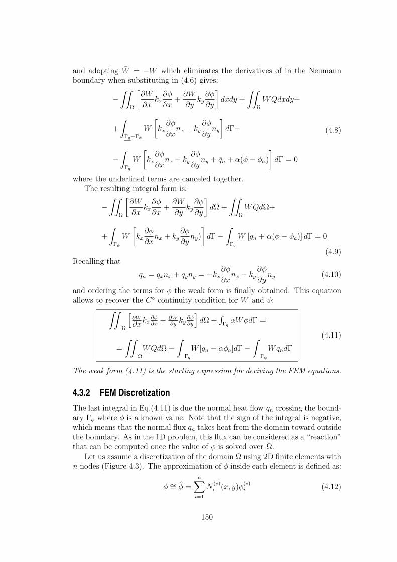
and adopting W = −W which eliminates the derivatives of in the Neumannboundary when substituting in (4.6) gives:

−∫∫

Ω

[∂W

∂xkx

∂φ

∂x+

∂W

∂yky

∂φ

∂y

]dxdy +

∫∫

Ω

WQdxdy+

+

∫

Γq+Γφ

W

[kx

∂φ

∂xnx + ky

∂φ

∂yny

]dΓ−

−∫

Γq

W

[kx

∂φ

∂xnx + ky

∂φ

∂yny + qn + α(φ− φa)

]dΓ = 0

(4.8)

where the underlined terms are canceled together.The resulting integral form is:

−∫∫

Ω

[∂W

∂xkx

∂φ

∂x+

∂W

∂yky

∂φ

∂y

]dΩ +

∫∫

Ω

WQdΩ+

+

∫

Γφ

W

[kx

∂φ

∂xnx + ky

∂φ

∂yny)

]dΓ−

∫

Γq

W [qn + α(φ− φa)] dΓ = 0

(4.9)Recalling that

qn = qxnx + qyny = −kx∂φ

∂xnx − ky

∂φ

∂yny (4.10)

and ordering the terms for φ the weak form is finally obtained. This equationallows to recover the C continuity condition for W and φ:

∫∫

Ω

[∂W

∂xkx

∂φ∂x

+ ∂W∂y

ky∂φ∂y

]dΩ +

∫Γq

αWφdΓ =

=

∫∫

Ω

WQdΩ−∫

Γq

W [qn − αφa]dΓ−∫

Γφ

WqndΓ

(4.11)

The weak form (4.11) is the starting expression for deriving the FEM equations.

4.3.2 FEM DiscretizationThe last integral in Eq.(4.11) is due the normal heat flow qn crossing the bound-ary Γφ where φ is a known value. Note that the sign of the integral is negative,which means that the normal flux qn takes heat from the domain toward outsidethe boundary. As in the 1D problem, this flux can be considered as a “reaction”that can be computed once the value of φ is solved over Ω.

Let us assume a discretization of the domain Ω using 2D finite elements withn nodes (Figure 4.3). The approximation of φ inside each element is defined as:

φ ∼= φ =n∑

i=1

N(e)i (x, y)φ

(e)i (4.12)

150

Figure 4.3: Discretization of a two-dimensional domain by tree-noded triangularelements.

where N(e)i (x, y) are the 2D shape functions function and φ(e) are the nodal

values of the approximated solution.The system of equations for the discretized domain is obtained substituting

the approximation (4.12) into the weak form (4.11) and choosing N weightingfunctions Wi, where N is the total number of nodes in the mesh

∫∫

Ω

[∂Wi

∂xkx

∂φ

∂x+

∂Wi

∂yky

∂φ

∂y

]dΩ +

∫

Γq

αWiφdΩ =

=

∫∫

Ω

WiQdΩ−∫

Γq

Wi[qn − αφa]dΓ−∫

Γφ

WiqndΓ i = 1, . . . , N

(4.13)The Galerkin form is obtained by making Wi = Ni. Assuming that all the

functions that appear in (4.13) are integrable and having in mind the additiveproperty of the integrals, the Galerkin form can be expressed as a function ofthe element contributions:

∑e

∫∫

Ω(e)

[∂N

(e)i

∂xkx

(n∑

j=1

∂N(e)j

∂xφ

(e)j

)+

∂N(e)i

∂yky

(n∑

j=1

∂N(e)j

∂yφ

(e)j

)]dΩ+

+∑

e

∫

Γ(e)q

αN(e)i

(n∑

j=1

N(e)j φ

(e)j

)dΓ =

=∑

e

∫∫

Ω(e)

N(e)i QdΩ−

∑e

∫

Γ(e)q

N(e)i [qn − αφa]dΓ−

∑e

∫

Γ(e)φ

N(e)i qndΓ

(4.14)where the sum applies are over all the elements discretizing the domain Ω.Expression (4.14) can be written in matrix form as

Ka = f (4.15)

151

The terms of K and f are obtained by assembling the elemental contributionsas usual. Because the shape function forms N

(e)i have a zero value outside the

element (e), we deduce that:

K(e)ij =

∫∫

Ω(e)

(∂N

(e)i

∂xkx

∂N(e)j

∂x+

∂N(e)i

∂yky

∂N(e)j

∂y

)dΩ+

+

∫

Γ(e)q

αN(e)i N

(e)j dΓ = K

(e)dij

+ K(e)cij

(4.16)

f(e)i =

∫ ∫

Ω(e)

N(e)i QdΩ−

∫

Γ(e)q

N(e)i [qn − αφa]dΓ−

∫

Γ(e)φ

N(e)i qndΓ (4.17)

The terms K(e)dij

and K(e)cij in (4.16) represent the elemental contributions due

to the conductivity and convection in the element stiffness matrix, respectively.These terms are obtained by:

K(e)dij

=

∫∫

Ω(e)

[∂N

(e)i

∂xkx

∂N(e)j

∂x+

∂N(e)i

∂yky

∂N(e)j

∂y

]dΩ (4.18)

K(e)cij

=

∫

Γ(e)q

αN(e)i N

(e)j dΓ (4.19)

The independent computation of K(e)dij

and K(e)cij simplifies the evaluation of

the element stiffness matrix coefficients.Similarly, the components of vector f

(e)i are:

f(e)i = f

(e)Qi

+ f (e)ci

+ qni(4.20)

where

f(e)Qi

=

∫∫

Ω(e)

N(e)i QdΩ (4.21)

is the contribution of the heat source over the domain

f(e)i = −

∫

Γ(e)q

N(e)i [qn − αφa]dΓ (4.22)

is the contribution of the heat flow trough the Neumann boundary where theflow is prescribed and

q(e)ni

= −∫

Γ(e)φ

N(e)i qndΓ (4.23)

is the “reaction” flow term over the boundary Γφ where the variable φ is pre-scribed. This flow is evaluated “a posteriori” once the nodal values of φ havebeen calculated.

Recall that the element boundary integral of (4.17) only contributes to thenodal force vector when the element has one or more sides over Γq or Γφ.

152

4.4 THREE-NODED TRIANGULAR ELEMENTLet us assume a three-noded triangular element discretization over the domain,as shown in Figure 4.3.

Each element node has one degree of freedom (d.o.f.) which correspondsto the nodal unknown value of φ. The unknown variation is expressed by thefollowing polynomial:

φ(x, y) = α0 + α1x + α2y (4.24)

To find the coefficients α0, α1 and α2 it is necessary to substitute the nodalcoordinates into Eq.(4.24) as follows

φ(e)1 = α0 + α1x

(e)1 + α2y

(e)1

φ(e)2 = α0 + α1x

(e)2 + α2y

(e)2

φ(e)3 = α0 + α1x

(e)3 + α3y

(e)3

(4.25)

Solving these equations and substituting the values of αi we obtain

φ(x, y) = 12A(e) [(a

(e)1 + b

(e)1 x + c

(e)1 y)φ

(e)1 + (a

(e)2 + b

(e)2 x + c

(e)2 y)φ

(e)2 +

+(a(e)3 + b

(e)3 x + c

(e)3 y)φ

(e)3 ]

(4.26)

wherea

(e)i = x

(e)j y

(e)k − x

(e)k y

(e)j

b(e)i = y

(e)j − y

(e)k

c(e)i = x

(e)k − x

(e)j

(4.27)

Indexes i, j, k go from 1 to 3 (Figure 4.3). Permuting the indexes allows tofind the expression for each parameter.

The element area A(e) is obtained by the determinant of the coefficients inEq.(4.25) as follows

2A(e) =

∣∣∣∣∣∣∣

1 x(e)i y

(e)i

1 x(e)j y

(e)j

1 x(e)k y

(e)k

∣∣∣∣∣∣∣(4.28)

Eq.(4.26) can be compacted as

φ =3∑

i=1

N(e)i φ

(e)i = N

(e)1 φ

(e)1 + N

(e)2 φ

(e)2 + N

(e)3 φ

(e)3 (4.29)

which allows identifying the element shape functions by:

N(e)i (x, y) =

1

2A(e)(a

(e)i + b

(e)i x + c

(e)i y); i = 1, 2, 3 (4.30)

153

Figure 4.4: Shape functions for the three-noded triangular element.

In the 3-noded triangular element these shape functions are expressed bylinear polynomials with coefficients depending on the nodal coordinates. Thenodal shape functions take a unit value at the node and zero at the other nodes,as usual (Figure 4.4).

As for the 1D case, the global shape functions of a node has a unit valueat the node and zero at any other node. Also, the influence domain for thisfunction corresponds to all the elements surrounding the node.

4.4.1 Elemental stiffness matrixFrom Eq.(4.30) we deduce

∂N(e)i

∂x=

bi

2A(e);

∂N(e)i

∂y=

ci

2A(e)(4.31)

Substituting Eqs.(4.30) and (4.31) into (4.18) and (4.19) gives

K(e)dij

=

∫∫

Ω(e)

1

4A(e)2[kxbibj + kycicj]dΩ =

1

4A(e)[kxbibj + kycicj] (4.32)

and the K(e)d matrix is obtained by

K(e)d =

1

4A(e)

kxb1b1 + kyc1c1 kxb1b2 + kyc1c2 kxb1b3 + kyc1c3

kxb2b1 + kyc2c1 kxb2b2 + kyc2c2 kxb2b3 + kyc2c3

kxb3b1 + kyc3c1 kxb3b2 + kyc3c2 kxb3b3 + kyc3c3

(e)

(4.33)

The evaluation of the integral defined in (4.19) yields the convection stiffnessmatrix as

K(e)c =

∫

Γ(e)q

α

N(e)1 N

(e)1 N

(e)1 N

(e)2 N

(e)1 N

(e)3

N(e)2 N

(e)1 N

(e)2 N

(e)2 N

(e)2 N

(e)3

N(e)3 N

(e)1 N

(e)3 N

(e)2 N

(e)3 N

(e)3

(e)

dΓ (4.34)

It is important to note that the above integral is computed over the length ofthe sides of the triangular element laying on the Neumann boundary. Thereforethe shape function for the third node which does not belong to a side takes azero value over that side. This allows us to simplify expression (4.34) dependingon the element’s side where the boundary integral is computed.

154

Hence, for side 1-2, N(e)3 = 0 and

K(e)c12

=

∫

l(e)12

α

N(e)1 N

(e)1 N

(e)1 N

(e)2 0

N(e)2 N

(e)1 N

(e)2 N

(e)2 0

0 0 0

dΓ (4.35)

For side 2-3, N(e)1 = 0 and

K(e)c23

=

∫

l(e)23

α

0 0 0

0 N(e)2 N

(e)2 N

(e)2 N

(e)3

0 N(e)3 N

(e)2 N

(e)3 N

(e)3

dΓ (4.36)

For side 1-3, N(e)2 = 0 and

K(e)c13

=

∫

l(e)13

α

N(e)1 N

(e)1 0 N

(e)1 N

(e)3

0 0 0

N(e)1 N

(e)3 0 N

(e)3 N

(e)3

dΓ (4.37)

Considering that α is constant over the element sides, the above expressionscan be integrated to obtain:

∫

l(e)ij

N(e)i N

(e)j dΓ =

l(e)ij /3; i = j

l(e)ij /6; i 6= j

(4.38)

where l(e)ij is the length of the (e) element’s side i− j; this gives:

K(e)c12

=αl

(e)12

6

2 1 01 2 00 0 0

; K(e)

c23=

αl(e)23

6

0 0 00 2 10 1 2

; K(e)

c13=

αl(e)13

6

2 0 10 0 01 0 2

(4.39)The total element stiffness matrix is obtained as:

K(e) = K(e)d + K(e)

c12+ K(e)

c23+ K(e)

c13(4.40)

We recall again that the contribution of matrices K(e)cij is only relevant if the

element side i − j belongs to the external Neumann boundary Γq. Also notethat we have obtained explicit expressions for the element stiffness matrix duethe linear form of the shape functions.

4.4.2 The equivalent nodal flux vectorThe generic expression of f (e) for the 3-noded triangular element is:

f (e) =

f(e)1

f(e)2

f(e)3

(4.41)

155

The heat source terms are deduced from Eq.(4.21)

f(e)Q =

f(e)Q1

f(e)Q2

f(e)Q3

=

∫∫

Ω(e)

N(e)1

N(e)2

N(e)3

QdΩ (4.42)

For a constant value of Q over the element, it is easy to obtain:

f(e)Q =

QA(e)

3

111

Hence, the total element flux is split in equal parts over the three nodes, asexpected.

From equation (4.22) the nodal flux contribution due convection is evaluatedas follows

f (e)c = −

∫

Γ(e)q

N(e)1

N(e)2

N(e)3

[qn − αφa]dΓ (4.43)

As for the convection stiffness matrix, the evaluation of the above integralrequires to consider the element’s side where the integral is computed. Thereforefor each side we have:

Side 1-2 (N(e)3 = 0)

f (e)c12

= −∫

l(e)12

N(e)1

N(e)2

0

[qn − αφa]dΓ (4.44)

Side 1-3 (N(e)2 = 0)

f (e)c13

= −∫

l(e)13

N(e)1

0

N(e)3

[qn − αφa]dΓ (4.45)

Side 2-3 (N(e)1 = 0)

f (e)c23

= −∫

l(e)23

0

N(e)2

N(e)3

[qn − αφa]dΓ (4.46)

Assuming that qn, α and φa are constant over the side gives

f (e)c12

= − l(e)12

2[qn − αφa]

110

(4.47)

156

with similar expressions for f(e)c13 and f

(e)c23 .

The last contributions to the nodal flux vector are the reactions at theboundary where φ is prescribed (Eq.4.23)). These fluxes are added directly tothe boundary nodes and are evaluated “a posteriori” once the nodal values ofφ have been computed.

Example 4.1 Heat conduction into a square domain

Solution

Consider the square domain shown in Figure 4.5. A known amount ofheat is generated internally due to a heat source and conduction effects.The goal is to compute the temperature distribution over the domain.

We assume that kx = ky = k = 2, 0 [cal/cm C] and Q =2,4 [cal/cm2s].Due to symmetry conditions only an eighth section of the domain is ana-lyzed. The boundary conditions are:

• Along the external boundary 4-6 α = 0, φ = 0

• Along the boundaries 1-6 and 1-4, the symmetry condition impliesthat

∂φ

∂n= 0

This means that the temperature gradient in the boundary’s normal di-rection is zero. The physical meaning of this condition corresponds to anisolated boundary. Because of the conditions applied, the heat flow onlygoes out the domain through the external side 1-4.

The analysis domain is discretized into a mesh of four 3-noded triangularelements as shown in Figure 4.5.

Because α = 0

K(e) = K(e)k =

k

4A(e)

b1b1 + c1c1, b1b2 + c1c2, b1b3 + c1c3

b2b1 + c2c1, b2b2 + c2c2, b2b3 + c2c3

b3b1 + c3c1, b3b2 + c3c2, b3b3 + c3c3

withbi = y

(e)j − y

(e)k

ci = x(e)k − x

(e)j

Following the element numbering shown in Figure 4.5b, for elements 1, 2and 4 we have:

K(1) = K(2) = K(4) =2, 0

42,52

2

6, 25 −6, 25 0−6, 25 6, 25 + 6, 25 −6, 25

0 −6, 25 6, 25

=

1 −1 0−1 2 −10 −1 1

157

Figure 4.5: a) Heat conduction in a square domain. b) Mesh of 3-noded trian-gular elements using the symmetry simplification.

For the element number 3:

K(3) =2, 0

46,252

6, 25 0 −6, 250 6, 25 −6, 25

−6, 25 −6, 25 12, 50

=

1 0 −10 1 −1−1 −1 2

158

bi ci

b1 = y(e)2 − y

(e)3 = −2, 5 c1 = x

(e)3 − x

(e)2 = 0

b2 = y(e)3 − y

(e)1 = 2, 5 c2 = x

(e)1 − x

(e)3 = −2, 5

b3 = y(e)1 − y

(e)2 = 0 c3 = x

(e)2 − x

(e)1 = 2, 5

Table 4.1: Coefficients bi and ci for elements 1, 2 and 4

bi ci

b1 = y(3)2 − y

(3)3 = 0 c1 = x

(3)3 − x

(3)2 = −2, 5

b2 = y(3)3 − y

(3)1 = 2, 5 c2 = x

(3)1 − x

(3)3 = 0

b3 = y(3)1 − y

(3)2 = −2, 5 c3 = x

(3)2 − x

(3)1 = 2, 5

Table 4.2: Coefficients bi and ci for element 3

The elemental nodal flux vectors are

f (e) = f(e)Q = QA(e)

3

111

f (e) = 2,4×2,52

3×2

111

= 2, 5

111

Assembly of the global stiffness matrix

The first steep is to identify the position of each coefficient of the elemen-tal stiffness matrix K through the correspondence between the local andglobal nodal numbers. From Figure 4.5 we deduce

K(1) =

1 2 3

1 K(1)11 K

(1)12 K

(1)13

2 K(1)21 K

(1)22 K

(1)23

3 K(1)31 K

(1)32 K

(1)33

K(2) =

2 4 5

2 K(2)11 K

(2)12 K

(2)13

4 K(2)21 K

(2)22 K

(2)23

5 K(2)31 K

(2)32 K

(2)33

159

K(3) =

2 5 3

2 K(3)11 K

(3)12 K

(3)13

5 K(3)21 K

(3)22 K

(3)23

3 K(3)31 K

(3)32 K

(3)33

K(4) =

3 5 6

3 K(4)11 K

(4)12 K

(4)13

5 K(4)21 K

(4)22 K

(4)23

6 K(4)31 K

(4)32 K

(4)33

The global stiffness matrix is:

K =

1 2 3 4 5 6

1 K(1)11 K

(1)12 K

(1)13 0 0 0

2 K(1)22 + K

(2)11 + K

(3)11 K

(1)23 + K

(3)13 K

(2)12 K

(2)13 + K

(3)12 0

3 K(1)33 + K

(3)33 + K

(4)11 0 K

(3)32 + K

(4)12 K

(4)13

4 K(2)22 K

(2)23 0

5 Symm. K(2)33 + K

(3)22 + K

(4)22 K

(4)23

6 K(4)33

Finally the elemental nodal flow are assembled into the vector f as follows

1 −1 0 0 0 0

−1 4 −2 −1 0 0

0 −2 4 0 −2 0

0 −1 0 2 −1 0

0 0 −2 −1 4 −1

0 0 0 0 −1 1

︸ ︷︷ ︸K

φ1

φ2

φ3

φ4

φ5

φ6

︸ ︷︷ ︸a

=

f(1)1 = 2, 5

f(1)2 + f

(2)1 + f

(3)1 = 7, 5

f(1)3 + f

(3)3 + f

(4)1 = 7, 5

f(2)2 = 2, 5 + R4

f(2)3 + f

(3)2 + f

(4)2 = 7, 5 + R5

f(4)3 = 2, 5 + R6

︸ ︷︷ ︸f

φ4 = 0

φ5 = 0

φ6 = 0

where R4, R5 y R6 are the unknown fluxes at the nodes 4, 5 and 6 respectively.Note that the value of φ is known at those nodes (φ4 = φ5 = φ6 = 0).

160

Solution of the system of equations gives

φ1 = 9, 3748 Cφ2 = 6, 8748 Cφ3 = 5, 3123 Cφ4 = 0 C; R4 = −9, 3748 cal/s/cm2

φ5 = 0 C; R5 = −18, 124 cal/s/cm2

φ6 = 0 C; R6 = −2, 5 cal/s/cm2

Let us compare the total flux generated in the domain (QA) with the flowthat goes out through the domain boundary

R4 + R5 + R6 = 29, 9988QA = 30

Hence, the total flux generated in the domain coincides with the total fluxthat goes out through the boundary. This proves the global equilibrium ofnodal fluxes which is a consequence of the flux balance (equilibrium) approachfollowed in the FEM.

161

Chapter 5

FEM ANALYSIS OF THE 3D POISSONEQUATION

5.1 INTRODUCTIONIn this chapter the formulation of the FEM applied to the 3D form of the Poissonequation is described. This chapter completes the study of problems with onevariable per node.

5.2 STEADY-STATE POISSON EQUATION IN 3DThe steady-state Poisson equation for a three-dimensional (3D) problem is

A(φ) : =∂

∂x

(kx

∂φ

∂x

)+

∂

∂y

(ky

∂φ

∂y

)+

∂

∂z

(kz

∂φ

∂z

)+ Q = 0 in Ω (5.1)

where φ(x, y, z) is the unknown function, kx, ky and kz are the conductivitiesin the x, y, z directions and Q is a heat source over the domain Ω.

As for the 1D and 2D cases this equation is obtained by considering thebalance of heat fluxes in a differential domain (Figure 5.1).

The boundary conditions are:

B(φ) :

Prescribed variable condition (Dirichlet condition):φ− φ = 0 on Γφ

Prescribed normal flux condition (Neumann condition):

kx∂φ

∂xnx + ky

∂φ

∂yny + kz

∂φ

∂znz + qn + α(φ− φa) = 0 on Γq

(5.2)

As for the 2D case, qn is the prescribed flux in the normal direction to theboundary Γq, φa is the external temperature, α is the convection coefficient andn = [nx, ny, nz]

T is the unit normal to Γq and Γ = Γφ ∪ Γq.

163

Figure 5.1: Three dimensional definition of the Poisson equation.

5.3 SOLUTION USING THE FINITE ELEMENT METHOD

5.3.1 Weak integral form

The equivalent integral form for the differential equations (5.1) and (5.2) areobtained applying the GWR method as

∫∫∫

Ω

W

[∂

∂x

(kx

∂φ

∂x

)+

∂

∂y

(ky

∂φ

∂y

)+

∂

∂z

(kz

∂φ

∂z

)+ Q

]dΩ+

+

∫∫

Γq

W

[kx

∂φ

∂xnx + ky

∂φ

∂yny + kz

∂φ

∂znz + qn + α(φ− φa)

]dΓ = 0

(5.3)where W and W are arbitrary weighting functions.

Integrating by parts the terms with second derivatives of φ in the first inte-gral and choosing W = −W gives:

−∫∫∫

Ω

(∂W

∂xkx

∂φ

∂x+

∂W

∂yky

∂φ

∂y+

∂W

∂zkz

∂φ

∂z

)dΩ+

+

∫∫∫

Ω

WQdΩ +

∫∫

Γq+Γφ

W

(kx

∂φ

∂xnx + ky

∂φ

∂yny + kz

∂φ

∂znz

)dΓ

−∫∫

Γq

W

[kx

∂φ

∂xnx + ky

∂φ

∂yny + kz

∂φ

∂znz + qn + α(φ− φa)

]dΓ = 0

(5.4)

where the underlined terms cancel together.

164

Figure 5.2: Solid domains discretized with finite elements.

Reordering the terms the weak form is finally expressed as

∫∫∫

Ω

[∂W∂x

kx∂φ∂x

+ ∂W∂y

ky∂φ∂y

+ ∂W∂z

kz∂φ∂z

]dΩ +

∫∫

Γq

WαφdΓ =

=

∫∫∫

Ω

WQdΩ−∫∫

Γq

W [qn − αφa]dΓ−∫∫

Γφ

WqndΓ

(5.5)

In the above equation the use of the normal flux definition has been consid-ered, i.e.

qn = qTn = qxnx + qyny + qznz = −kx∂φ

∂xnx − ky

∂φ

∂yny − kz

∂φ

∂znz (5.6)

The weak form (5.5) is the starting expression for deriving the FEM equa-tions.

5.3.2 FEM DiscretizationConsider the 3D domain discretizations shown in Figure 5.2 using finite elementswith n nodes. The approximation of the unknown φ within each element isexpressed as

φ ∼= φ =n∑

j=1

N(e)j (x, y, z)φ

(e)j (5.7)

where N(e)j are the shape functions of the 3D element and φ

(e)j are the nodal

values of the approximation function.

165

Substituting the above approximation into the weak form (5.5) and selectingthe same number of weighting functions as nodal unknowns, the approximateexpression of the weak form is obtained

∫∫∫

Ω

[∂Wi

∂xkx

∂φ

∂x+

∂Wi

∂yky

∂φ

∂y+

∂Wi

∂zkz

∂φ

∂z

]dΩ +

∫∫

Γq

WiαφdΓ =

=

∫∫∫

Ω

WiαφdΓ−∫∫

Γq

Wi[qn − αφa]dΓ−∫∫

Γφ

WiqndΓ

i = 1, 2, . . . , N

(5.8)

where N is total number of nodes in the mesh.The Galerkin symmetric form is obtained by choosing Wi = Ni. Assuming

that all the functions in the last expression can be integrated and using theadditive property of the integral, the weak form can be expressed as the sum ofthe element contributions as

∑e

∫∫∫

Ω(e)

[∂N

(e)i

∂xkx

(n∑

j=1

∂N(e)j

∂xφ

(e)j

)+

∂N(e)i

∂yky

(n∑

j=1

∂N(e)j

∂yφ

(e)j

)+

+∂N

(e)i

∂zkz

(n∑

j=1

∂N(e)j

∂zφ

(e)j

)]dΩ +

∫∫

Γ(e)q

N(e)i α

(n∑

j=1

N(e)j φ

(e)j

)dΓ

=

=∑e

∫∫∫

Ω(e)

N(e)i QdΩ−

∫∫

Γ(e)q

N(e)i (q − αφa)dΓ−

∫∫

Γ(e)φ

N(e)i qdΓ

i = 1, 2, . . . , N(5.9)

where the sum is performed over all the elements in the mesh.The above integral expression can be interpreted as the i -th row of the

algebraic equation system of the discretization, i.e.

Ki1φ1 + Ki2φ2 + · · ·+ KiNφN = fi, i = 1, 2, . . . , N (5.10)

The global equation system is therefore written as

Ka = f

or

1 2 N

i = 1 K11 K12 . . . K1N

i = 2 K21 K22 . . . K2N...

.... . .

......

.... . .

...i = N KN1 KN2 . . . KNN

︸ ︷︷ ︸K

φ1

φ2......

φN

︸ ︷︷ ︸a

=

f1

f2......

fN

︸ ︷︷ ︸f

(5.11)

166

As for the 1D and 2D cases, the K matrix and the f vector can be obtainedby assembling the stiffness matrices K(e) and the elemental nodal flux vectorsf (e) for each element given by:

K(e)

n× n=

K(e)11 . . . K

(e)1n

.... . .

...

K(e)n1 . . . K

(e)nn

(5.12)

f1(e)

n× 1=

f(e)1...

f(e)n

(5.13)

where n is the number of nodes in the element and

K(e)ij =

K(e)dij︷ ︸︸ ︷∫∫∫

Ω(e)

(∂N

(e)i

∂xkx

∂N(e)j

∂x+

∂N(e)i

∂yky

∂N(e)j

∂y+

∂N(e)i

∂zkz

∂N(e)j

∂z

)dΩ +

+

∫∫

Γ(e)q

αN(e)i N

(e)j dΓ

︸ ︷︷ ︸K

(e)cij

= K(e)kij

+ K(e)cij

(5.14)

K(e)dij

is the conduction stiffness term and K(e)cij is the convection stiffness term.

The second integral only appears in the Neumann boundary part where theconvection condition is prescribed.

For the flux vector

f(e)i =

∫∫∫

Ω(e)

N(e)i QdΩ

︸ ︷︷ ︸f(e)Qi

−∫∫

Γ(e)q

N(e)i (q − αφa)dΓ

︸ ︷︷ ︸f(e)ci

−q(e)ni

(5.15)

where f(e)Qi

is the nodal flux term related to the heat source Q, f(e)ci is the nodal

flux term related to the prescribed heat flux at the Neumann boundary and

q(e)ni =

∫∫

Γ(e)q

N(e)i qndΓ is the reaction flux in the node where the value of φ is

prescribed. Again, the term f(e)ci will be considered only in nodes that belong

to the Neumann boundary.In the next section the above expressions will be particularized the four-

noded tetrahedral element.

5.4 FOUR-NODED TETRAHEDRAL ELEMENTIn this section the four-noded tetrahedral element will be considered. Thiselement is also know as the linear tetrahedron (Figure 5.3).

167

Figure 5.3: Four-noded tetrahedral element.

The linear tetrahedron is the simplest 3D element, similarly as the three-noded triangular element is the simplest element for 2D problems. Both elementfamilies have similar properties.

The approximation of the unknown field inside each tetrahedron is expressedby the following linear polynomial interpolation

φ(e) = α0 + α1x + α2y + α3z (5.16)

From the above expression we can deduce

φ(e)1 = α0 + α1x

(e)2 + α2y

(e)1 + α3z

(e)1

φ(e)2 = α0 + α1x

(e)2 + α2y

(e)2 + α3z

(e)2

φ(e)3 = α0 + α1x

(e)3 + α2y

(e)3 + α3z

(e)3

φ(e)4 = α0 + α1x

(e)4 + α2y

(e)4 + α3z

(e)4

(5.17)

Solving this equation system and substituting the expression for αi intoEq.(5.16) and reordering terms yields:

φ =4∑

i=1

N(e)i (x, y, z)φ

(e)i = N

(e)1 (x, y, z)φ

(e)1 + · · ·+ N

(e)4 (x, y, z)φ

(e)4 (5.18)

where

N(e)i (x, y, z) =

1

6Ω(e)(a

(e)i + b

(e)i (x) + c

(e)i y + d

(e)i z) (5.19)

with

a(e)i =

∣∣∣∣∣∣∣

x(e)j y

(e)j z

(e)j

x(e)k y

(e)k z

(e)k

x(e)l y

(e)l z

(e)l

∣∣∣∣∣∣∣; b

(e)i = −

∣∣∣∣∣∣∣

1 y(e)j z

(e)j

1 y(e)k z

(e)k

1 y(e)l z

(e)l

∣∣∣∣∣∣∣

c(e)i =

∣∣∣∣∣∣∣

x(e)j 1 z

(e)j

x(e)k 1 z

(e)k

x(e)l 1 z

(e)l

∣∣∣∣∣∣∣; d

(e)i = −

∣∣∣∣∣∣∣

x(e)j y

(e)j 1

x(e)k y

(e)k 1

x(e)l y

(e)l 1

∣∣∣∣∣∣∣

(5.20)

168

The rest of the constants can be obtained by rotating the indexes (i, j, k, l)using the right-hand rule

The element volume Ω(e) can be found from the following determinant

6Ω(e) =

∣∣∣∣∣∣∣∣∣

1 x(e)i y

(e)i z

(e)i

1 x(e)j y

(e)j z

(e)j

1 x(e)k y

(e)k z

(e)k

1 x(e)l y

(e)l z

(e)l

∣∣∣∣∣∣∣∣∣(5.21)

The three dimensional shape functions forms are hyper-planes and N(e)i can

not be visualized as for the 2D problem. Note however that, as usual, the shapefunction N

(e)i take a unit value at the node and zero at the rest of the nodes.

Another difficulty related to 3D elements is the visualization of the results.There are some methodologies to help with this task, like the previous subdivi-sion in hexahedra followed by an automatic division in tetrahedra.

From the shape functions expression we deduce:

∂N(e)i

∂x=

bi

6Ω(e);

∂Ni

∂y=

ci

6Ω(e);

∂Ni

∂z=

di

6Ω(e)(5.22)

Substituting into K(e)ij gives

K(e)dij

=1

36Ω(e)(kxbibj + kycicj + kzdidj) (5.23)

and

K(e)d =

1

36Ω(e)

kxb1b1 + kyc1c1 + kzd1d1 . . . kxb1b4 + kyc1c4 + · · ·+ kzd1d4

kxb2b1 + kyc2c1 + kzd2d1 . . . kxb2b4 + kyc2c4 + · · ·+ kzd2d4

kxb3b1 + kyc3c1 + kzd3d1 . . . kxb3b4 + kyc3c4 + · · ·+ kzd3d4

kxb4b1 + kyc4c1 + kzd4d1 . . . kxb4b4 + kyc4c4 + · · ·+ kzd4d4

(5.24)is the conductivity stiffness matrix for the element.

The general expression for the element convection stiffness matrix is

K(e)c =

∫∫

Γ(e)q

N(e)1 N

(e)1 . . . N

(e)1 N

(e)4

.... . .

...

N(e)4 N

(e)1 . . . N

(e)4 N

(e)4

αdΓ (5.25)

The tetrahedron boundaries correspond to the element faces (Figure 5.3).

In that way the shape function N(e)i will have a null value if the i -th node does

not belong to the face where the integral is evaluated. From the shape functionexpression it is easy to obtain:

K(e)cij

=

∫∫

Γ(e)q

αN(e)i N

(e)j dΓ =

αA(e)

6; i = j

αA(e)

12; i 6= j

(5.26)

169

where A(e) is the tetrahedron’s face area where the convection boundary isprescribed.

As an example, for the face 1-2-4 of the tetrahedron shown in Figure 5.3,N

(e)3 = 0 and

K(e)c124

=

∫∫

Γ(e)q124

α

N(e)1 N

(e)1 N

(e)1 N

(e)2 0 N

(e)1 N

(e)4

N(e)2 N

(e)1 N

(e)2 N

(e)2 0 N

(e)2 N

(e)4

0 0 0 0

N(e)4 N

(e)1 N

(e)4 N

(e)2 0 N

(e)4 N

(e)4

dΓ (5.27)

If α is constant over the face 1-2-4

K(e)c124

=αA

(e)124

6

1 1/2 0 1/21/2 1 0 1/20 0 0 0

1/2 1/2 0 1

(5.28)

The same procedure is followed to evaluate K(e)c over the other faces of the

tetrahedron.As a conclusion, the element stiffness matrix can be written as:

K(e) = K(e)d + K(e)

c123+ K(e)

c124+ K(e)

c134+ K(e)

c234(5.29)

The equivalent nodal flux vector for a uniformly distributed heat source is

f(e)Q =

f(e)Q1

f(e)Q2

f(e)Q3

f(e)Q4

=

∫∫∫

Ω

N(e)1

N(e)2

N(e)3

N(e)4

QdΩ (5.30)

If Q is constant over the element

f(e)Q =

QΩ(e)

4

1111

(5.31)

Note that in this case the total flux over the element is uniformly distributedin all the element’s nodes, similarly as for the 3-noded triangle.

The vector associated to the ijl face where the normal flux is prescribed(Figure 5.3) is

f (e)cijl

= −∫∫

Γ(e)qijl

(qn−αφa)

N(e)i

N(e)j

N(e)k

N(e)l

dΓ = −∫∫

A(e)ijl

(qn−αφa)

N(e)i

N(e)j

0

N(e)l

dΓ (5.32)

170

where A(e)ijl is the ijl side area where N

(e)k = 0. If qn, α and φa are constant over

the face, then

f (e)cijl

= −A(e)ijl

3(qn − αφa)

1101

(5.33)

In a similar form, the expression for f(e)c can be obtained for the other faces

where the normal flux is prescribed.As a conclusion, the element equivalent flux vector can be written as:

f (e) = f(e)Q + f (e)

c123+ f (e)

c124+ f (e)

c134+ f (e)

c234(5.34)

where

f234 = −A(e)234

3(qn − αφa)

0111

, etc. (5.35)

171

Chapter 6

MATRIX FORMULATION FOR THE FEMSOLUTION OF THE POISSON EQUATION

6.1 INTRODUCTIONIn previous sections the Poisson equation has been analysed for 1D, 2D and 3Dproblems with the FEM. In this section, the FEM solution will be presented ina general form using a matrix formulation. This approach is useful to treat ina similar manner many other problems solved with the FEM.

6.2 MATRIX FORMULATION OF THE POISSON EQUATIONThe heat flow balance equation over an infinitesimal domain for 1D, 2D or 3Dproblems can be expressed in a matrix form as

∇Tq−Q = 0 (6.1)

where ∇ is the gradient vector operator and q is flux vector given by

1D: ∇ =[

∂∂x

], q = [q]

2D: ∇ =[

∂∂x

, ∂∂y

]T

, q = [qx, qy]T

3D: ∇ =[

∂∂x

, ∂∂y

, ∂∂z

]T

, q = [qx, qy, qz]T

(6.2)

The extended form of Eq.(6.1) corresponds to the heat flow balance equationobtained in previous chapters. For example, Eq.(6.1) has the following form for2D problems: [

∂

∂x,

∂

∂y

]qx

qy

−Q =

∂qx

∂x+

∂qy

∂y−Q = 0 (6.3)

The gradient vector is defined as

g = ∇φ (6.4)

173

where1D: g = [g] =

[∂φ∂x

]

2D: g = [gx, gy]T =

[∂φ∂x

, ∂φ∂y

]T

3D: g = [gx, gy, gz]T =

[∂φ∂x

, ∂φ∂y

, ∂φ∂z

]T

(6.5)

The relationship between the heat flow vector and the gradient vector isdefined by Fourier’s law

q = −Dg = −D∇φ (6.6)

where D is the conductivity matrix given by

1D: D = [k]

2D: D =

[kx 00 ky

]

3D: D =

kx 0 00 ky 00 0 kz

(6.7)

Substituting Eq.(6.6) into (6.1) the matrix form of the flux balance equationis obtained as

∇T (D∇φ) + Q = 0 en Ω (6.8)

Expanding this equation, the usual form of the Poisson equation is obtained.For 2D problems

[∂

∂x,

∂

∂y

] [kx 00 ky

]

∂φ∂x∂φ

∂y

+ Q =

∂

∂x

(kx

∂φ

∂x

)+

∂

∂y

(ky

∂φ

∂y

)+ Q = 0 (6.9)

The boundary conditions can be described in a general way as follows.

Prescribed variable condition

φ− φ = 0 on Γφ (6.10)

Prescribed flux condition

nTD∇φ + qn + α(φ− φq) = 0 on Γq (6.11)

where n is the external normal to the boundary Γq and the rest of the termshave the usual meaning.

174

6.3 WEAK INTEGRAL FORMThe equivalent weak integral form of the balance equation and the boundaryconditions can be obtained from the GWR method as

∫

Ω

W [∇TD∇φ + Q] +

∮

Γq

W [nTD∇φ + qn + α(φ− φa)]dΓ = 0 (6.12)

Integrating by parts the term with second derivates in the first integral andselecting W = −W , the weak form is obtained as

−∫

Ω

(∇T W )D∇φdΩ +

∫

Ω

WQdΩ−∫

Γq

W [qn − α(φ− φa)]dΩ +

∫

Γφ

WnTD∇φdΩ = 0 (6.13)

Having in mind the definition of the heat flow and selecting W = δφ as thevirtual variation of the unknown and ∇ = δg as the virtual gradient vector, theweak form can be rewritten as

∫

Ω

δgTqdΩ +

∫

Ω

δφQdΩ−∫

Γq

δφ[qn − α(φ− φa)]dΓ−∫

Γφ

δφqndΓ = 0 (6.14)

Eq.(6.14) can be named as the virtual variation principle and it is equivalentto the virtual work principle for solid mechanics. The virtual field δφ satisfiesthe boundary conditions at the Dirichlet boundary. Therefore if φ = 0 on Γφ

then also δφ = 0 on Γφ and the last integral in (6.14) can be omitted.The integral expression in (6.13) (or the equivalent one in (6.14)) is the

starting point for deriving the FEM discretized equations.

6.4 MATRIX FORM OF THE FEM EQUATIONSThe finite element approximation is expressed for a n-noded element in matrixform as

φ =n∑

i=1

N(e)i φ

(e)i = [N

(e)1 , N

(e)2 , . . . , N (e)

n ]

φ(e)1

φ(e)2

...

φ(e)n

= N(e)a(e) (6.15)

withN(e) = [N

(e)1 , N

(e)2 , . . . , N

(e)n ]

a(e) = [φ(e)1 , φ

(e)2 , . . . , φ

(e)n ]T

(6.16)

175

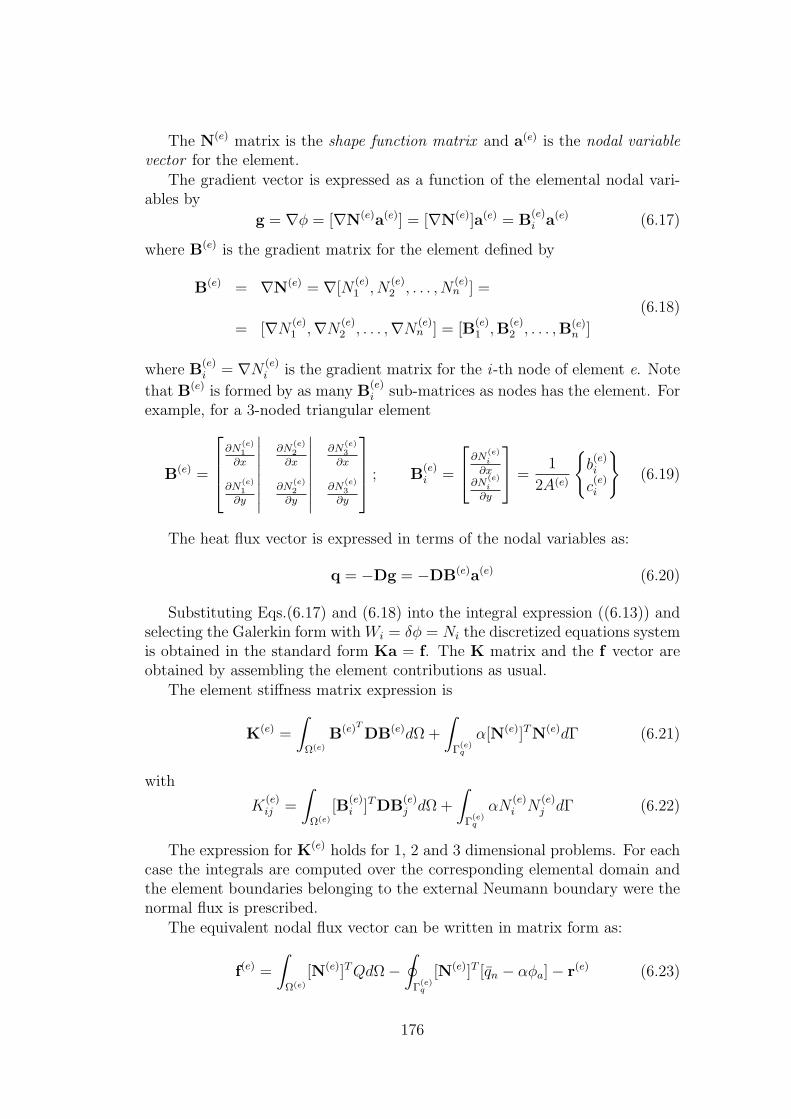
The N(e) matrix is the shape function matrix and a(e) is the nodal variablevector for the element.

The gradient vector is expressed as a function of the elemental nodal vari-ables by

g = ∇φ = [∇N(e)a(e)] = [∇N(e)]a(e) = B(e)i a(e) (6.17)

where B(e) is the gradient matrix for the element defined by

B(e) = ∇N(e) = ∇[N(e)1 , N

(e)2 , . . . , N

(e)n ] =

= [∇N(e)1 ,∇N

(e)2 , . . . ,∇N

(e)n ] = [B

(e)1 ,B

(e)2 , . . . ,B(e)

n ]

(6.18)

where B(e)i = ∇N

(e)i is the gradient matrix for the i -th node of element e. Note

that B(e) is formed by as many B(e)i sub-matrices as nodes has the element. For

example, for a 3-noded triangular element

B(e) =

∂N(e)1

∂x

∣∣∣∣∂N

(e)2

∂x

∣∣∣∣∂N

(e)3

∂x

∂N(e)1

∂y

∣∣∣∣∂N

(e)2

∂y

∣∣∣∣∂N

(e)3

∂y

; B

(e)i =

∂N(e)i

∂x∂N

(e)i

∂y

=

1

2A(e)

b(e)i

c(e)i

(6.19)

The heat flux vector is expressed in terms of the nodal variables as:

q = −Dg = −DB(e)a(e) (6.20)

Substituting Eqs.(6.17) and (6.18) into the integral expression ((6.13)) andselecting the Galerkin form with Wi = δφ = Ni the discretized equations systemis obtained in the standard form Ka = f. The K matrix and the f vector areobtained by assembling the element contributions as usual.

The element stiffness matrix expression is

K(e) =

∫

Ω(e)

B(e)T

DB(e)dΩ +

∫

Γ(e)q

α[N(e)]TN(e)dΓ (6.21)

with

K(e)ij =

∫

Ω(e)

[B(e)i ]TDB

(e)j dΩ +

∫

Γ(e)q

αN(e)i N

(e)j dΓ (6.22)

The expression for K(e) holds for 1, 2 and 3 dimensional problems. For eachcase the integrals are computed over the corresponding elemental domain andthe element boundaries belonging to the external Neumann boundary were thenormal flux is prescribed.

The equivalent nodal flux vector can be written in matrix form as:

f(e) =

∫

Ω(e)

[N(e)]T QdΩ−∮

Γ(e)q

[N(e)]T [qn − αφa]− r(e) (6.23)

176

with

f(e)i =

∫

Ω(e)

N(e)i QdΩ−

∮

Γ(e)q

N(e)i [qn − αφa]dΓ− q(e)

ni(6.24)

As usual, the integrals are evaluated over the corresponding elemental do-main.

The r(e) vector corresponds to the unknown “reaction” flux in the nodeswere the φ variable is prescribed. These fluxes are computed “a posteriori”once the solution for the nodal value of φ is found.

It is important to note that the matrix formulation provides a general frame-work for solving any Poisson problem in 1D, 2D and 3D. The matrix formulationpresented in this section is applied in similar way to solid mechanics and fluidmechanics problems solved using the FEM.

6.5 THE MATRIX EQUILIBRIUM EQUATIONS OBTAINEDFROM THE NODAL FLUXES

The usual procedure to obtain the global equations system is applying theconcept of nodal flux balance (equilibrium). The process is similar to usingKirchhoff’s law in electrical networks or in hydraulic networks. Expressingthe fluxes in the element “sides” as a function of the nodal variables and theexternal actions via the balance equilibrium equation for each element, andimposing flux balance at all nodes yields the global equilibrium equations asKa = f. The “flux addition” procedure allows to obtain K and f by assemblingthe expressions for K(e) and f(e) for each element.

The flux balance expression will be described for the 1D and 2D elementsshown in Figure 6.1.

6.5.1 One dimensional 2-noded element

We will start with the simplest 1D element under a uniform flux Q and twonodal fluxes q

(e)1 y q

(e)2 applied at nodes 1 and 2 respectively.

Let us consider the global flux balance expression over the element writtenin the weak integral form, or the equivalent expression derived from the virtualvariation principle

∫

l(e)δgT q dx +

∫

l(e)δφQ dx− δφ

(e)1 q

(e)1 − δφ

(e)2 q

(e)2 = 0 (6.25)

The negative signs in the above equation are due the flux definition for q(e)1

and q(e)2 which go out the element (the heat goes out the element).

Note that δφ are virtual variations of φ and δg is the virtual gradient field(δg = ∇δφ).

177

Figure 6.1: Flux balance in a 1D 2-noded element (a) and in a 2D 3-nodedtriangle (b)

Eq.(6.25) allows expressing the “virtual work” produced by the nodal fluxesin terms of the elemental variables as:

[δa(e)]Tq(e) =

∫

l(e)δgqdΩ +

∫

l(e)δφQdΩ (6.26)

with

δa(e) = [δφ(e)1 , δφ

(e)2 ]T , q(e) = [q

(e)1 , q

(e)2 ]T (6.27)

where q(e) is the so called vector of the interelemental balancing nodal fluxes.Let us substitute the FEM approximation into Eq.(6.26). The φ and δφ

fields can be expressed inside each element in a matrix form by

φ =2∑

i=1

N(e)i φ

(e)i = N(e)a(e) (6.28)

δφ =2∑

i=1

N(e)i δφ

(e)i = N(e)δa(e) (6.29)

with

N(e) = [N(e)1 , N

(e)2 ], a(e) = [φ

(e)1 , φ

(e)2 ]T (6.30)

178

andδa(e) = [δφ

(e)1 , δφ

(e)2 ]T (6.31)

The virtual gradient is expressed in terms of the nodal virtual variables by

δg = ∇δφ = [∇N(e)]δa(e) = B(e)δa(e) (6.32)

with

∇ =

[∂

∂x

], B(e) = [B

(e)1 , B

(e)2 ], B

(e)i =

[∂N

(e)i

∂x

](6.33)

Substituting the above expression into (6.26) and extracting δa(e) in thesecond term gives

[δa(e)]Tq(e) = [δa(e)]T−[

∫

l(e)[B(e)]TDB(e)dΩ]a(e) +

∫

l(e)[N(e)]T QdΩ]

(6.34)

Having in mind that the virtual variables δφ(e)i are arbitrary, the above

equation must be true for any value of δa(e); this gives

q(e) = −[∫

l(e)[B(e)]TDB(e)dx

]a(e) +

∫

l(e)[N(e)]T Qdx (6.35)

or

q(e) = −K(e)a(e) + f(e) (6.36)

where

K(e) =

∫

l(e)[B(e)]TDB(e)dx (6.37)

f(e) =

∫

l(e)[N(e)]T Qdx (6.38)

are the elemental stiffness matrix and the nodal flux vector due the uniformdistributed Q source.

Eq.(6.36) is the flux balance equation for the element and express the equi-librium (balance) between the interelemental balancing nodal fluxes, the nodalflux dues the Q source and the fluxes due the gradient of φ inside the element.

Note the analogy between Eq.(6.36) and the equation expression the equi-librium of nodal forces for a discrete system (Eq.(1.6)). This analogy also holdsfor the assembling process.

Eq.(6.36) is the key to obtain the global equilibrium equation in terms of thenodal variables. The process is similar to that explained for discrete systems.For each node the equilibrium of fluxes is considered taking into account thecontribution from all the elements sharing the node.

Therefore the expression for balance of nodal fluxes is written as

∑e

q(e)i = qext

j j = 1, 2, . . . N (6.39)

179

where the sum is over all the elements that share the node with global numberj, qext

j is the external flux that goes into the j node (in general qextj = 0) and N

is the total number of nodes in the mesh.Expressing the values of q

(e)i in terms of the nodal variables a(e) and the

external fluxes f(e) via Eq.(6.36), the global system of equations is obtained inthe usual form Ka = f. The stiffness matrix K and the nodal flux vector f areassembled from the element contributions following the same rules as for thediscrete systems.

It is important to understand that this assembling process coincides withthat explained in the previous chapter using the weak integral form and theadditive properties of the integrals defined over the analysis domain.

To clarify this concept the assembling process will be repeated for the three-noded triangular element.

6.5.2 2D three-noded triangular elementConsider the three-noded triangular element shown in Figure 6.1b. The elementis subjected to a uniform distributed source Q, to the normal fluxes throughthe boundaries sides Γq and to the interelemental fluxes. The flux balanceexpression for all the fluxes and the inner gradients can be expressed by thevirtual variation principle as:

∫∫

Ω(e)

[δg(e)]TqdΩ +

∫∫

Ω(e)

δφQdΩ−∫

Γ(e)q

δφqndΓ− [δa(e)]Tq(e) = 0 (6.40)

whereδg(e) = [δgx, δgy]

T = ∇(δφ) (6.41)

q = [qx, qy]T = −Dg = −D∇φ, ∇ =

∂∂x∂∂x

(6.42)

δa(e) = [δφ(e)1 , δφ

(e)2 , δφ

(e)3 ]T (6.43)

q(e) = [q(e)1 , q

(e)2 , q

(e)3 ]T (6.44)

In the above expressions q(e)i is the interelemental nodal flux that goes out

through the i -th node. This flux can be expressed as the sum of the fluxes inthe x and y directions.

It is important to note that the third integral in the expression (6.40) onlyshould be considered if the element has sides on the Neumann boundary werethe flux is prescribed to qn. For elements laying in the interior domain, thefluxes along the sides cancel out in the assembly process, as these fluxes areidentical but with opposite sign for the two elements sharing a side. Also, ifany convection with the external environment exist it is necessary to add theterm α(φ− φa) to qn. For simplicity reasons we do not consider this term here.

180

The FEM discretization is written in matrix form as

φ =3∑

i=1

N(e)i φ

(e)i = N(e)a(e) (6.45)

g = B(e)a(e), δg = B(e)δa(e) (6.46)

q = −Dg = −DB(e)a(e) (6.47)

withN(e) = [N

(e)1 , N

(e)2 , N

(e)3 ] (6.48)

B(e) = [B(e)1 ,B

(e)2 ,B

(e)3 ], B

(e)i = ∇N

(e)i =

∂N(e)i

∂x∂N

(e)i

∂y

(6.49)

D =

[kx 00 ky

](6.50)

Substituting these expressions into the integral form and extracting δa(e) weobtain

[δa(e)]Tq(e) = [δa(e)]T[−

∫∫

Ω(e)

[B(e)]TDB(e)dΩ]a(e)+

+

∫∫

Ω(e)

[N(e)]T QdΩ−∮

Γ(e)q

[N(e)]T qndΓ

] (6.51)

This givesq(e) = −K(e)a(e) + f (e) (6.52)

with

K(e)ij =

∫∫

Ω(e)

[B(e)i ]TDB

(e)j dΩ

f(e)i =

∫∫

Ω(e)

N(e)i QdΩ−

∮

Γ(e)q

N(e)i qndΓ

(6.53)

The assembling process follows the usual steps of imposing the equilibriumof nodal fluxes as ∑

e

q(e)i = qext

j j = 1, 2, . . . N (6.54)

Substituting in (6.54) the expressions for q(e)i from Eq.(6.53) we obtain the

global equation systems of equations in matrix form Ka = f were matrix Kand vector f are formed by assembling the contributions if K(e) and f (e) foreach element in the standard way.

181

Chapter 7

SHAPE FUNCTIONS FOR 2D AND 3DELEMENTS WITH C CONTINUITY

7.1 INTRODUCTIONThis chapter extends the concepts previously studied for the analysis of 2Dproblems with the FEM using triangular and quadrilateral elements. The useof higher order elements with arbitrary geometry including curved sides isnow considered. The isoparametric formulation and numerical integration ismandatory in these cases. These topics are explained in Chapter 8.

The chapter is organized as follows. In the first sections we detail thesystematic derivation of the shape functions for rectangular and triangular el-ements of different order of approximation. Next, some rules for the analyticalcomputation of the element integrals over rectangles and straight side trianglesare given. The same topics are then explained for 3D elements of tetrahedraland prismatic shape.

7.2 DERIVATION OF THE SHAPE FUNCTIONS FOR Co TWODIMENSIONAL ELEMENTS

Next, we will derive nex the shape functions for different triangular and rect-angular elements with Co continuity. The possibilities of distorting these ele-ments into arbitrary shapes including curved sides will be treated in Chapter8 using the concept of isoparametric interpolation.

7.2.1 Complete polynomials in two dimensions. Pascal’s triangleWe recall that the chosen displacement field can only reproduce exactly apolynomial solution of an order equal to or less than that of the completepolynomial contained in the shape functions. Consequently, the finite elementsolution will improve as the degree of such a complete polynomial increases.

183

Fig. 7.1: Pascal’s triangle in two dimensions

A 2D complete polynomial of nth degree can be written as

f(x, y) =

p∑i=1

αixjyk ; j + k ≤ n (7.1)

where the number of terms is

p = (n + 1)(n + 2)/2 (7.2)

For a linear polynomial (p = 3)

f(x, y) = α1 + α2x + α3y (7.3a)

and for a quadratic polynomial (p = 6)

f(x, y) = α1 + α2x + α3y + α4xy + α5x2 + α6y

2 (7.3b)

The terms of a 2D complete polynomial can be readily identified by meansof the Pascal’s triangle (Figure 7.1).

The shape functions of many elements contain incomplete polynomial terms.For instance, the 4-noded rectangle includes the term α4xy from the quadraticpolynomial (Section 7.3.1). These terms involve nodal variables which in gen-eral do not contribute to increasing the order of the approximation. Thisshould be taken into account when designing a new element.

7.2.2 Shape functions of Co rectangular elements. Natural coordi-nates in two dimensions

A local coordinate system ξ, η is defined for each element in order to facilitatethe derivation of the shape functions. Such a natural or intrinsic coordinatesystem is normalized so that the element sides are located at ξ = ±1 andη = ±1 as shown in Figure 7.2. The natural coordinate ξ was introduced for1D rod elements in Chapter 2. It is easy to deduce from Figure 7.2 that

ξ =x− xc

a; η =

y − yc

b(7.4)

184

Fig. 7.2: Geometry of a generic rectangular element. Cartesian and natural coor-dinates

where xc and yc are the coordinates of the element centroid. Thus

dξ

dx=

1

a;

dη

dy=

1

b(7.5)

The differential of area in both systems is related by

dx dy = ab dξ dη (7.6)

The integration of a function f(x, y) over a rectangular element can beexpressed in the natural coordinate system by

∫∫

A(e)

f(x, y) dx dy =

∫ +1

−1

∫ +1

−1

g(ξ, η)ab dξ dη (7.7)

The shape functions when expressed in the natural coordinates must sat-isfy the same requirements as in cartesian coordinates. Therefore, the shapefunctions of Co continuous elements must satisfy:

a) Condition of nodal compatibilitya) Condition of nodal compatibility

Ni(ξj, ηj) =1 i = j0 i 6= j

(7.8)

b) Rigid body conditionb) Rigid body condition

n∑i=1

Ni(ξ, η) = 1 (7.9)

Two element families can be clearly identified within the Co continuousrectangular elements, i.e. the Lagrange family and the Serendipity family.The derivation of the shape functions for each of these two element families ispresented next.

185

7.3 LAGRANGE RECTANGULAR ELEMENTSThe shape functions of Lagrange elements can be obtained by the simple prod-uct of the two one dimensional (1D) Lagrange polynomials corresponding tothe natural coordinates ξ and η of the node. Thus, if liI(ξ) is the Lagrangepolynomial of order I in the ξ direction for node i and liJ(η) is the Lagrangepolynomial of order J in the η direction for node i, the shape function of nodei is

Ni(ξ, η) = liI(ξ) liJ(η) (7.10)

The 1D Lagrange polynomials for each node can be obtained by Eq.(3.9)which can be indistinctly used for the coordinates ξ or η. Figure 7.3 shows someof the more popular Lagrange rectangular elements. Note that the number ofnodes in each of the two directions ξ and η are the same along any nodal line.This is a particular feature of Lagrange elements.

The polynomial terms contained in the shape functions can be directlyobtained from the Pascal’s triangle as shown in Figure 7.3. Note that theshape functions are not complete polynomials and all contain some incompletepolynomial terms.

The derivation of the shape functions for the more popular Lagrange rect-angular elements is presented next.

7.3.1 Four-noded Lagrange rectangleThis is the simplest element of the Lagrange family. We will derive its shapefunctions again using natural coordinates (Figure 7.4).

Let us consider a generic node i. The 1D shape functions corresponding tothe local directions ξ and η coincide with the shape functions of the 2-nodedbar element. Thus, it is easy to find

li1(ξ) =1

2(1 + ξξi) ; li1(η) =

1

2(1 + ηηi) (7.11)

where ξi and ηi take the values given in the table of Figure 7.4. The shapefunction of any node can be written in compact form as

Ni(ξ, η) = li1(ξ)li1(η) =

1

4(1 + ξξi)(1 + ηηi) (7.12)

Figure 4.16 shows in graphic form the shape function of node 1. It is easyto verify that the shape functions (7.12) satisfy the conditions (7.8) and (7.9).

7.3.2 Nine-noded quadratic Lagrange rectangleThe shape functions of the 9-noded Lagrange rectangle (Figure 7.5) are ob-tained by the product of two 1D quadratic polynomials in ξ and η. These

186

Fig. 7.3: Some Lagrange rectangular elements. Polynomial terms contained in theshape functions

polynomials are obtained from the shape functions of the quadratic rod ele-ment (Eq.(3.11)). Thus, for node 1

l12(ξ) =1

2(ξ − 1)ξ ; l12(η) =

1

2(η − 1)η (7.13)

187

Fig. 7.4: Four-noded Lagrange rectangular element

and the shape function is

N2(ξ, η) = l12(ξ)l12(η) =

1

4(ξ − 1)(η − 1)ξ η (7.14)

Following a similar procedure for the rest of the nodes, the shape functionscan be written in compact form as

a) Corner nodesa) Corner nodes

Ni =1

4(ξ2 + ξξi)(η

2 + ηηi) ; i = 1, 3, 5, 7 (7.15)

b) Mid-side nodesb) Mid-side nodes

Ni =1

2η2

i (η2 − ηηi)(1− ξ2) +

1

2ξ2i (ξ

2 − ξξi)(1− η2) ; i = 2, 4, 6, 8 (7.16)

c) Central nodec) Central node

N9(ξ, η) = (1− ξ2)(1− η2) (7.17)

188

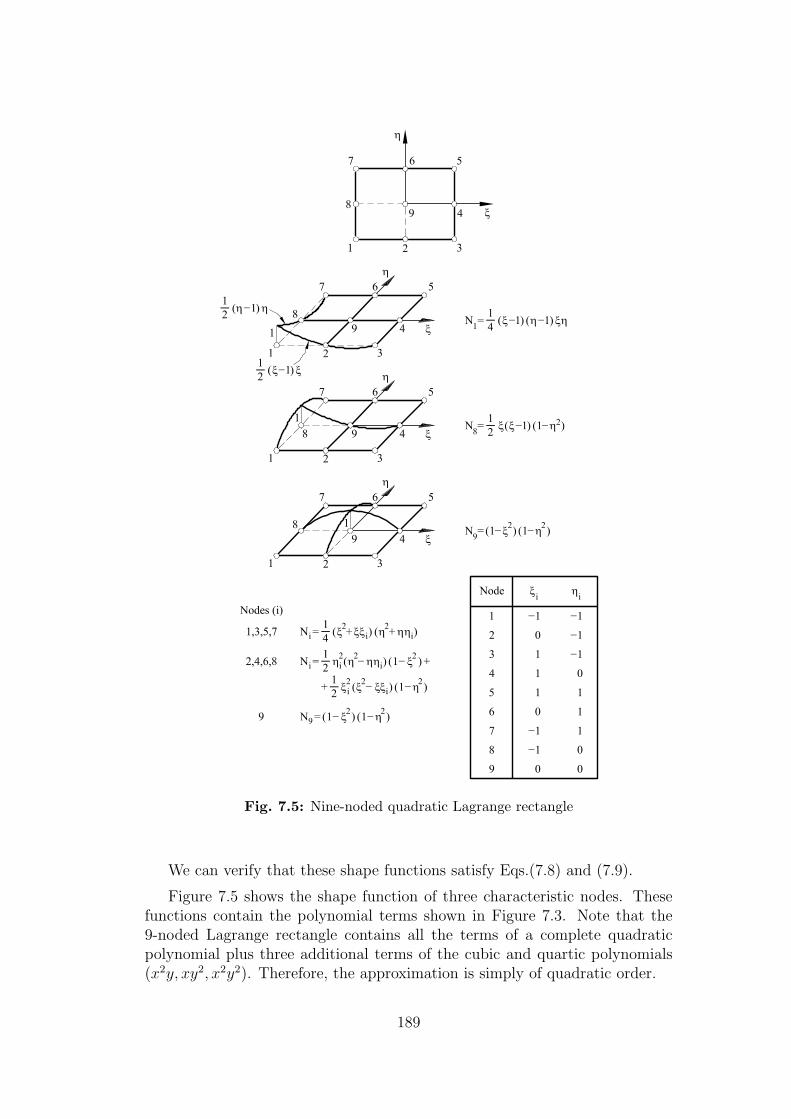
Fig. 7.5: Nine-noded quadratic Lagrange rectangle

We can verify that these shape functions satisfy Eqs.(7.8) and (7.9).

Figure 7.5 shows the shape function of three characteristic nodes. Thesefunctions contain the polynomial terms shown in Figure 7.3. Note that the9-noded Lagrange rectangle contains all the terms of a complete quadraticpolynomial plus three additional terms of the cubic and quartic polynomials(x2y, xy2, x2y2). Therefore, the approximation is simply of quadratic order.

189

Fig. 7.6: Sixteen-noded cubic Lagrange rectangular element. Shape functions innatural coordinates

7.3.3 Sixteen-noded cubic Lagrange rectangle

This element has four nodes in each of the two directions ξ and η. The shapefunctions are obtained by the product of two cubic 1D Lagrange polynomials inthe ξ and η directions deduced from Eq.(3.12). Figure 7.6 shows the resultingexpressions of the shape functions. Figure 7.3 shows that the shape functionare complete cubic polynomials and contain the following additional terms:x3y, x2y2, xy3, x3y2, x2y3 and x3y3 from the quartic, quintic and sexticpolynomials. The shape functions satisfy Eqs.(7.8) and (7.9).

7.3.4 Other Lagrange rectangular elements

The shape functions of higher order Lagrange rectangular elements with 5, 6,7, etc. nodes in each of the ξ and η directions are obtained by the product of

190

Fig. 7.7: Lagrange rectangular elements with different number of nodes along eachlocal direction

fourth, fifth, sixth, etc. degree 1D Lagrange polynomials in ξ and η, similarto the linear, quadratic and cubic elements previously studied. It is easy toverify that the shape functions of a Lagrange element with n nodes in each ofthe two local directions ξ and η contain a complete nth degree polynomial andn(n + 1)/2 terms of incomplete polynomials of a higher degree which can bededuced from the Pascal’s triangle.

Lagrange elements can have different number of nodes in each local direc-tion ξ or η (Figure 7.7). The shape functions in this case are obtained bythe product of the adequate 1D polynomials in ξ and η corresponding to thenumber of nodes in each direction. The shape functions now contain a com-plete 2D polynomial of a degree equal to the smallest degree of the two 1Dpolynomials in each local direction. Therefore, the degree of approximation ofthe element does not change by simply increasing the number of nodes in oneof the two local directions only. This explains why these elements are not verypopular and they are only occasionaly used as a transition between elementsof two different orders.

7.4 SERENDIPITY RECTANGULAR ELEMENTSSerendipity elements are obtained as follows. First the number of nodes defin-ing a 1D polynomial of a given degree along each side is chosen. Then, theminimum number of nodes within the element is added so that a completeand symmetrical 2D polynomial of the same degree as the 1D polynomial cho-sen along the sides is obtained. Figure 7.8 shows some of the more popularSerendipity elements and the polynomial terms contained in the shape func-tions. Note that the simplest element of the Serendipity family, i.e. the 4-nodedrectangle, coincides with the same element of the Lagrange family. Also notethat the quadratic and cubic elements of 8 and 12 nodes, respectively, do nothave interior nodes, whereas the 17 node element requires a central node toguarantee the complete quartic approximation, as is explained next.

The derivation of the shape functions of Serendipity elements are not asstraightforwad as those of Lagrange elements. In fact, some ingenuity is neededand this explains the name Serendipity, after the ingenuous discoveries of thePrince of Serendip quoted in the romances of Horacio Walpole in the eighteenthcentury.

191

Fig. 7.8: Some Serendipity elements and terms contained in their shape functions

7.4.1 Eigth-noded quadratic Serendipity rectangle

The shape functions of the side nodes are readily obtained as the product ofa second degree polynomial in ξ (or η) and another one in η (or ξ). It canbe checked that this product contains the required complete quadratic terms

192

(Figure 7.9). For these nodes we obtain

Ni(ξ, η) =1

2(1 + ξξi)(1− η2) ; i = 4, 8

Ni(ξ, η) =1

2(1 + ηηi)(1− ξ2) ; i = 2, 6

(7.18)

Unfortunately this strategy can not be applied for the corner nodes, sincein this case the product of two quadratic polynomials will yield a zero value atthe center and thus the criterion of Eq.(7.9) would be violated. Consequently,a different procedure is followed as detailed below.

Step 1 . The shape function of the corner node is initially assumed to bebi-linear, i.e. for node 1 (Figure 7.9) we have

NL1 =

1

4(1− ξ)(1− η) (7.19)

This shape function is equal to one at the corner node and takes the valuezero at all the other nodes, except for the two nodes 2 and 8 adjacent to node1 where it takes the value 1/2.

Step 2 . The shape function is made zero at node 2 by subtracting from thebi-linear function one half of the quadratic shape function (7.19) of node 2:

N1(ξ, η) = NL1 −

1

2N2 (7.20)

Step 3 . Function N1 still takes the value 1/2 at node 8. Hence, the final stepis to substract from N1 one half of the quadratic shape function of node 8(Eq.(7.18)), i.e.

N1(ξ, η) = NL1 −

1

2N2 − 1

2N8 (7.21)

It can be verified that the resulting function N1 satisfies the conditions (7.8)and (7.9) and contains the desired (quadratic) polynomial terms. Therefore,it is the shape function of node 1 we are looking for.

Following the same procedure for the rest of the corner nodes yields thefollowing general expression

Ni(ξ, η) =1

4(1 + ξξi)(1 + ηηi)(ξξi + ηηi − 1) ; i = 1, 3, 5, 7 (7.22)

Figure 7.9 shows that the shape functions of the 8-noded Serendipity ele-ment contain a complete quadratic polynomial and two terms x2y and xy2 ofthe cubic polynomial. Therefore, this element has the same approximation asthe 9-noded Lagrange element and it has a node less. This makes the 8-nodedquadrilateral in principle more competitive for practical purposes (see Section8.1.2 for further details).

193

Fig. 7.9: 8-noded quadratic Serendipity rectangle. Derivation of the shape functionsfor a mid-side node and a corner node

7.4.2 Twelve-noded cubic Serendipity rectangle

This element has four nodes along each side and a total of twelve side nodeswhich define the twelve term polynomial approximation shown in Figure 7.8.The shape functions are derived following the same procedure explained forthe 8-noded element. Thus, the shape functions for the side nodes are obtainedby the simple product of two Lagrange cubic and linear polynomials. For thecorner nodes the starting point is again the bilinear approximation. This initialshape function is forced to take a zero value at the two side nodes adjacent tothe corner node by subtracting the shape functions of those nodes weightedby the factors 2/3 and 1/3. Figure 7.10 shows the expression of the shapefunctions which can be derived by the reader as an exercise.

It is simple to check that the element satisfies conditions (7.8) and (7.9).

194

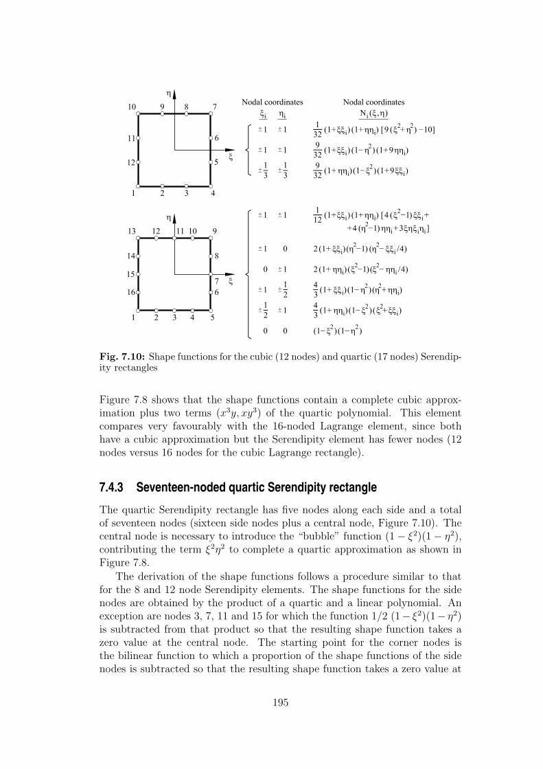
Fig. 7.10: Shape functions for the cubic (12 nodes) and quartic (17 nodes) Serendip-ity rectangles

Figure 7.8 shows that the shape functions contain a complete cubic approx-imation plus two terms (x3y, xy3) of the quartic polynomial. This elementcompares very favourably with the 16-noded Lagrange element, since bothhave a cubic approximation but the Serendipity element has fewer nodes (12nodes versus 16 nodes for the cubic Lagrange rectangle).

7.4.3 Seventeen-noded quartic Serendipity rectangle

The quartic Serendipity rectangle has five nodes along each side and a totalof seventeen nodes (sixteen side nodes plus a central node, Figure 7.10). Thecentral node is necessary to introduce the “bubble” function (1− ξ2)(1− η2),contributing the term ξ2η2 to complete a quartic approximation as shown inFigure 7.8.

The derivation of the shape functions follows a procedure similar to thatfor the 8 and 12 node Serendipity elements. The shape functions for the sidenodes are obtained by the product of a quartic and a linear polynomial. Anexception are nodes 3, 7, 11 and 15 for which the function 1/2 (1− ξ2)(1− η2)is subtracted from that product so that the resulting shape function takes azero value at the central node. The starting point for the corner nodes isthe bilinear function to which a proportion of the shape functions of the sidenodes is subtracted so that the resulting shape function takes a zero value at

195

these nodes. Finally, the shape function for the central node coincides withthe bubble function. Figure 7.10 shows the shape functions for this element.

Figure 7.8 shows that the shape functions contain a complete quartic ap-proximation plus two additional terms (x4y and yx4) from the quintic polyno-mial. The corresponding quartic Lagrange element has 25 nodes (Figure 7.2)and hence the 17-noded Serendipity rectangle is in principle more competitivefor practical purposes.

7.5 SHAPE FUNCTIONS FOR Co CONTINUOUS TRIANGU-LAR ELEMENTS

The shape functions for the more popular Co continuous triangular elementsare complete polynomials whose terms can be readily identified by the Pas-cal’s triangle. This also defines the position of the nodes within the element.We recall, for instance, that the shape function of the 3-noded triangle is lin-ear. Similarly, the six and ten-noded triangles define the following completequadratic and cubic approximations

6-noded triangle

φ = αo + α1x + α2y + α3xy + α4x2 + α5y

2 (7.23)

10-noded triangle

φ = αo + α1x + α2y + α3xy + α4x2 + α5y

2 + α6x3 + α7x

2y + α8xy2 + α9y3

(7.24)The αi parameters are obtained by the same procedure as described for

the 3-noded triangle in Chapter 4. This method has obvious difficulties forhigh order elements and it is simpler to apply the technique based on areacoordinates that is explained below.

7.5.1 Area coordinatesLet us join a point P within a triangle of area A with the three vertices 1, 2,3 (Figure 7.11). This defines three sub-areas A1, A2 and A3 corresponding tothe triangles P13, P12 and P23, respectively (note that A1 + A2 + A3 = A).The area coordinates are defined as

L1 =A1

A; L2 =

A2

A; L3 =

A3

A(7.25)

Obviously

L1 + L2 + L3 =A1 + A2 + A3

A=

A

A= 1 (7.26)

196

Fig. 7.11: Area coordinates for a triangle

The position of point P can be defined by any two of these three coordi-nates. The area coordinates of a node can be interpreted as the ratio betweenthe distance from point P to the opposite side divided by the distance fromthe node to that side (Figure 7.11). Thus, area coordinates of the centroidare L1 = L2 = L3 = 1/3. Area coordinates are also known as barycentric,triangular, and trilinear coordinates and they are typical of geometry treatises[F3]. In the FEM context area coordinates have proved to be very useful forderiving the shape functions of triangular finite elements.

Area coordinates are also of interest to define a parametric interpolationof the element geometry. For a straight side triangle the following relationshipbetween the area and cartesian coordinates can be written

x = L1x1 + L2x2 + L3x3

y = L1y1 + L2y2 + L3y3

(7.27)

This equation system is completed with Eq.(7.26) so that L1, L2 and L3

can be obtained in terms of the cartesian coordinates by

Li =1

2A(e)(ai + bix + ciy) (7.28)

where A(e) is the area of the triangle and ai, bi, ci coincide with the values givenin Eq.(4.27) for the 3-noded triangle. It is concluded that the area coordinatescoincide precisely with the shape functions of the 3-noded triangular element.

197

7.5.2 Derivation of the shape functions for Co continuous triangles

The shape functions for triangles containing complete Mth degree polynomialscan be obtained in terms of the area coordinates as follows. Let us consider anode i characterized by the position (I, J,K) where I, J and K are the powersof the area coordinates L1, L2 and L3, respectively in the expression of theshape function of the node. Thus, I + J + K = M and the shape function ofnode i is given by

Ni = liI(L1) liJ(L2) liK(L3) (7.29)

where liI(L1) is the 1D Lagrange Ith degree polynomial in L1 which takes thevalue one at node i (Eq.(3.6a)), i.e.

liI(L1) =∏j=1,Ij 6=i

(L1 − Lj

1

)(Li

1 − Lj1

) (7.30)

with identical expressions for liJ(L2) and liK(L3). In Eq.(7.30) Li1 is the value

of L1 at node i.

The main difficulty in applying Eq.(7.29) is to deduce the values of I, J,Kfor each node. This can be done simply by noting that: a) the shape functionof a corner node depends on a single area coordinate only and thus the corre-sponding I, J or K power for that node is equal to M ; b) all nodes located onthe lines L1 = constant have the same value for I and the same occurs with L2

and J and L3 and K; and c) the values of I, J and K associated with L1, L2

and L3, respectively, decrease progressively from the maximum value for thelines Li = 1 at the corner nodes, to a value equal to zero at the lines Li = 0which coincide with the opposite side to each corner node i (Figure 7.12).

This procedure will be clarified next with some examples of its application.

7.5.3 Shape functions for the 3-noded linear triangle

The shape functions of the 3-noded triangle are linear polynomials (M = 1).The area coordinates and the values of I, J,K for each node can be seen inFigure 7.12.

Node 1

Position (I, J,K) : (1, 0, 0)

Area coordinates: (1, 0, 0)

N1 = l11(L1) = L1 (7.31)

It is straight-forward find N2 = L2 and N1 = L3 as expected.

198

Fig. 7.12: Linear, quadratic and cubic triangular elements. Area coordinates andvalues of (I, J,K) for each node

7.5.4 Shape functions for the six-noded quadratic triangleThe shape functions for this element are complete quadratic polynomials (M =2). The area coordinates and the values of I, J and K at each node are shownin Figure 7.12.

Node 1

Position (I, J,K) : (2, 0, 0)Area coordinates: (1, 0, 0)

N1 = l12(L1) =(L1 − 1/2)L1

(1− 1/2) 1= (2L1 − 1)L1 (7.32)

Node 4

Position (I, J,K) : (1, 1, 0)Area coordinates: (1/2, 1/2, 0)

N4 = l21(L1) l21(L2) =L1

1/2

L2

1/2= 4L1L2 (7.33)

199

Fig. 7.13: Shape functions of a corner node and a side node for a quadratic triangle

Following the same procedure for the rest of nodes we find (that)

N1 = (2L1 − 1)L1 ; N2 = (2 L2 − 1)L2 ; N3 = (2L3 − 1)L3

N4 = 4L1L2 ; N5 = 4 L2L3 ; N6 = 4L1L3

(7.34)

Figure 7.13 shows two characteristic shape functions for this element.

7.5.5 Shape functions for the ten-noded cubic triangleThe shape functions for this element are complete cubic polynomials (M = 3).Figure 7.12 shows the area coordinates and the values of I, J and K at eachnode:

Node 1

Position (I, J,K) : (3, 0, 0)Area coordinates: (1, 0, 0)

N1 = l13(L1) =(L1 − 2/3) (L1 − 1/3) L1

(1− 2/3) (1− 1/3) 1=

1

2L1 (3L1 − 1) (3L1 − 2) (7.35)

Node 4

Position (I, J,K): (2, 1, 0)Area coordinates: (2/3, 1/3, 0)

N4 = l22(L1) l21(L2) =(L1 − 1/3) L1

(2/3− 1/3) 2/3· L2

1/3=

9

2(3L1 − 1) L1L2 (7.36)

The same procedure applied to the rest of the nodes gives

N1 =1

2L1(3L1 − 1)(3L1 − 2) ; N2 =

1

2L2(3L2 − 1)(3L2 − 2)

N3 =1

2L3(3L3 − 1)(3L3 − 2) ; N4 =

9

2(3L1 − 1)L1L2)

N5 =9

2(3L2 − 1)L1 L2 ; N6 =

9

2(3L2 − 1)L2 L3

N7 =9

2(3L3 − 1) L2L3 ; N8 = 9

2(3L3 − 1)L3L1

N9 =9

2(3L2 − 1)L3 L1 ; N10 = 27L1L2L3

(7.37)

200

Fig. 7.14: Natural coordinates for a triangular element

A similar technique can be employed to derive the shape functions of higherorder triangular elements.

7.5.6 Natural coordinates for trianglesIt is very convenient to define a normalized coordinate system α, β (also callednatural coordinate system), such that the element has the sides over the linesα = 0, β = 0 and 1− α− β = 0 as shown in Figure 7.14. The shape functionsfor the 3-noded triangle can then be written as

N1 = 1− α− β ; N2 = α , N3 = β (7.38)

It is deduced that the area coordinates L2 and L3 coincide with the naturalcoordinates α and β, respectively and L1 = 1− α− β.

These coincidences allow us to express the shape functions of triangularelements in terms of the natural coordinates. This is particularly useful forderiving isoparametric triangular elements.

7.6 ANALYTIC COMPUTATION OF INTEGRALS OVERRECTANGLES AND STRAIGHT SIDE TRIANGLES

The integration of polynomials over 2D elements can be difficult and, in gen-eral, numerical integration is used. However, some interesting analytical ex-pressions in terms of the local cartesian coordinates x, y shown in Figure 7.15exist for rectangles and straight side triangles. A typical integral term such as

Cij = D

∫∫

A(e)

xmyn dA (7.39)

can be directly integrated by the following expressions:

201

Fig. 7.15: Local coordinate system x, y for the analytical computation of integralsover triangular and rectangular elements

Straight side triangular element

Cij = D cn+1[am+1 − (−b)m+1

] m!n!

(m + n + 2)!(7.40)

Rectangular element

C ij = D(2a)m+1 (2b)n+1

(m + 1) (n + 1)(7.41)

In the above m and n are integers and a, b and c are typical element di-mensions (Figure 7.15). Once K and f have been found in the local coordinatesystem x, y using the above expressions, they can be transformed into theglobal axes using the standard relationship (see Chapter 1)

Kij = TT Kij T , fi = TT f i (7.42)

where T is the 2× 2 coordinate transformation matrix

T =

[cos (xx) cos (xy)cos (yx) cos (yy)

](7.43)

with (xx) being the angle between the local x axis and the global x axis, etc.Other simple analytical forms in terms of area coordinates can be found

for area integrals over straight side triangles. A typical stiffness matrix terminvolves the cartesian derivatives of the shape functions. This is expressed interms of area coordinates by the standard chain rule

∂N1(L1, L2, L3)

∂x=

∂N1

∂L1

∂L1

∂x+

∂N1

∂L2

∂L2

∂x+

∂N1

∂L3

∂L3

∂x(7.44)

As the element sides are assumed to be straight, Eq.(7.28) leads to

∂Li

∂x=

bi

2A(e)and

∂Li

∂y=

ci

2A(e)(7.45)

202

where bi and ci are given by Eq.(4.27). Combining Eqs.(7.44) and (7.45) gives

∂Ni

∂x=

1

2A(e)

3∑i=1

bi∂Ni

∂Li

;∂Ni

∂y=

1

2A(e)

3∑i=1

ci∂Ni

∂Li

(7.46)

Thus, the element integrals can be easily expressed in terms of area coor-dinates and they can be directly computed by the following expressions

∫∫

A(e)

Lk1 Ll

2 Lm3 dA = 2A(e) k! l! m!

(2 + k + l + m)!(7.47a)

∮

l(e)Lk

i Llj ds = l(e)

k! l!

(1 + k + l)!(7.47b)

If one of the area coordinates is missing in the integrand, the correspondingpower is omitted in the denominator of Eqs.(7.47) and it is made equal to aunit value in the numerator.

The use of the natural coordinates α and β does not introduce any addi-tional difficulty. Exact expressions for the integrals over straight side trianglescan be found as

I =

∫∫

A(e)

αmβn dA =2A(e) Γ(m + 1) Γ(n + 1)

Γ (3 + m + n)(7.48)

where Γ is the Gamma function [R2]. When m and n are possitive integers

I = 2A(e) m! n!

(2 + m + n)!(7.49)

Note that this is just a particular case of Eq.(7.47a) when one of the areacoordinates is missing. Similarly, it is deduced from (7.47b) that

∮

l(e)αmds = l(e)

m!

(2 + m)!(7.50)

For curved side elements the computation of the cartesian derivatives of theshape functions requires a parametric formulation. This generally introducesrational terms in the integrals and makes the use of numerical integrationunavoidable.

Example: 7.1 Compute the stiffness matrix K(e)11 for an ortrothopic quadratic triangle with

straight sides and unit thickness.

-- Solution-- Solution

The first step is to obtain the cartesian derivatives of the shape function N1 expressedin terms of the area coordinates as

203

∂N1

∂x=

∂N1

∂L1

∂L1

∂x+

∂N1

∂L2

∂L2

∂x+

∂N1

∂L3

∂L3

∂x

∂N1

∂y=

∂N1

∂L1

∂L1

∂y+

∂N1

∂L2

∂L2

∂y+

∂N1

∂L3

∂L3

∂y

From Eq.(7.32) we deduce

∂N1

∂L1= 4L1 − 1 ;

∂N1

∂L2=

∂N1

∂L3= 0

and from Eq.(7.45)∂Li

∂x=

bi

2A(e);

∂Li

∂y=

ci

2A(e)

Therefore∂N1

∂x=

b1

2A(e)(4L1 − 1) ;

∂N1

∂y=

c1

2A(e)(4L1 − 1)

and

B1 =(4L1 − 1)

2A(e)

b1 00 c1

c1 b1

Matrix K(e)11 is thus obtained by

K(e)11 =

∫∫

A(e)BT

1 D B tdA =t

(2A(e))2

[b1 0 b1

0 c1 c1

]

d11 d12 0d12 d22 00 0 d33

×

×

b1 00 c1

c1 b1

∫∫

A(e)(4L1 − 1)2 dA

We deduce from Eq.(7.47a)

∫∫

A(e)(4L1 − 1)2 dA = 2A(e)

[16 · 2!

4!− 8 · 1!

3!+

12

]= A(e)

which leads to

K(e)11 =

14A(e)

[b21 d11 + c2

1 d33 b1c1 (d33 + d12)b1c1(d33 + d12) b2

1 d33 + c21d22

]

The rest of the K(e)ij matrices are obtained following an identical procedure. The

complete expression of the stiffness matrix for the quadratic triangle can be found in[C15] and [W2].

204

Fig. 7.16: Natural coordinate system for a right prism

7.7 SHAPE FUNCTIONS FOR 3D ELEMENTSWe will study next the derivation of two families of 3D solid elements: hexa-hedra and tetrahedra of different orders. In common with 2D solid elements,3D hexahedra can be of Lagrange or Serendipity types. The shape functionsof hexahedra elements are obtained for a right prismatic geometry in terms ofthe three natural coordinates following similar rules as for 2D rectangles. Theextension of hexahedra elements to model arbitrary 3D geometries of irregularshapes, including curved surfaces, is straightforward using an isoparametricformulation (Chapter 8).

The shape functions for Lagrange right prisms are simply obtained by theproduct of three Lagrange polynomials in 1D. The derivation of 3D Serendipityprismatic elements is more cumbersome, although again the same rules givenfor the 2D case apply (Chapter 8).

Like triangles, the shape functions for tetrahedra are complete polynomialsand they are more easily expressed in terms of volume and natural coordinates.

7.8 RIGHT PRISMSLet us consider a right prism with the natural coordinates ξ, η, ζ defined asshown in Figure 7.16. For an element with edges 2a× 2b× 2c we have

ξ =(x− xc)

a; η =

(y − yc)

b; ζ =

(z − zc)

c(7.51)

where (xc, yc, zc) are the coordinates of the element centroid. From Eq.(7.51)it is deduced that

dξ

dx=

1

a;

dη

dy=

1

b;

dζ

dz=

1

c(7.52)

205

and a differential of volume is expressed by

dx dy dz = abc dξ dη dζ (7.53)

The integration of a function f(x, y, z) over the element is expressed in thenatural coordinate system as

∫∫∫

V (e)

f(x, y, z) dV =

∫ +1

−1

∫ +1

−1

∫ +1

−1

f(ξ, η, ζ)abc dξ dη dζ (7.54)

Since the element is a right prism, the cartesian derivatives of the shapefunctions are directly obtained by

∂Ni

∂x=

1

a

∂Ni

∂ξ;

∂Ni

∂y=

1

b

∂Ni

∂η;

∂Ni

∂z=

1

c

∂Ni

∂ζ(7.55)

The shape functions must satisfy the standard conditions

Ni(ξj, ηj, ζj) =

1 if i = j

0 if i 6= j(7.56a)

andn∑

i=1

Ni (ξ, η, ζ) = 1 (7.56b)

7.8.1 Right prisms of the Lagrange familyThe shape functions of Lagrange right prisms are obtained by multilying three1D polynomial Lagrange polynomials as

Ni(ξ, η, ζ) = liI(ξ) liI(η) liI(ζ) (7.57)

where liI(ξ) is the Lagrange polynomial of Ith degree passing by node i, etc.For the same reasons mentioned in Section 7.3.4 it is usual, to choose the samepolynomial approximation in each of the three directions ξ, η and ζ.

The terms contained in the shape functions of prismatic elements arededuced from the Pascal’s tetrahedron. Figure 7.17 shows the linear andquadratic elements of this family whose shape functions are derived next.

Linear right prism of the Lagrange family

The simplest Lagrange prismatic element is the 8-noded linear prism shown inFigure 7.17.

The shape function of a node is obtained by multilying the three linearpolynomials in ξ, η and ζ, corresponding to the node. In general form

Ni(ξ, η, ζ) =1

8(1 + ξiξ) (1 + ηiη) (1 + ζiζ) (7.58)

206

Fig. 7.17: Linear and quadratic right prisms of the Lagrange family. Polynomialterms contained in the shape functions deduced from the Pascal’s tetrahedron

Note that:

1. The shape functions contain a complete linear polynomial in ξ, η, ζ andthe incomplete quadratic and cubic terms ξη, ξζ, ηξ and ξηζ, ξηζ (seeFigure 7.18).

2. The shape functions satisfy the conditions (7.56).

The linear hexahedron is a popular element due to the small number ofnodal variables, which is attractive for practical 3D analysis.

The linear hexahedron performs very well for problems with uniform gradi-ents, whereas its accuracy is poor for problems where strains gradient changesoccur.

207

Fig. 7.18: Shape functions for the linear right prism

Fig. 7.19: Quadratic right prism of the Lagrange family. Shape functions for acorner node and a mid-side node

208

Quadratic right prism of the Lagrange family

The quadratic Lagrange prism has 27 nodes (see Figure 7.19). The shapefunctions are obtained by the product of three 1D quadratic Lagrange poly-nomials. Figure 7.19 shows the derivation of the shape functions for a cornernode and a mid-side node. It is simple to extrapolate this procedure to obtainthe following general expressions

Corner nodes

Ni =1

8(ξ2 + ξξi)(η

2 + ηηi)(ζ2 + ζζi) ; i = 1, 3, 5, 7

19, 21, 23, 25 (7.59)

Mid-side nodes

Ni =1

4η2

i (η2 − ηηi)ζ

2(ζ2 − ζζi)(1− ξ2) +1

4ζ2i (ζ2 − ζζi)+

+ξ2i (ξ

2 − ξξi)(1− η2) +1

4ξ2i (ξ

2 − ξξi)η2i (η

2 − ηηi)(1− ζ2); i =

2, 4, 6, 810, 12, 14, 1620, 22, 24, 26

(7.60)Face nodes

Ni =1

2(1− ξ2)(1− η2)(ζ + ζiζ

2) +1

2(1− η2)(1− ζ2)(ξ + ξiξ

2)+

+1

2(1− ξ2)(1− ζ2)(η + ηiη

2); i = 9, 11, 13

15, 17, 27

(7.61)

Central internal node

N18 = (1− ξ2)(1− η2)(1− ζ2) (7.62)

Other hexahedral elements of the Lagrange family

The next members of the Lagrange family are the 64-noded cubic prism (4nodes along each edge) and the 125-noded quartic prism. Their shape func-tions are obtained by the product of three 1D cubic and quartic polynomialsrespectively. These elements in their right form are in general not competitiveversus the analogous Serendipity element which involve lewer nodal variables.

7.8.2 Serendipity prisms

Serendipity prisms are obtained by extension from the corresponding 2D rect-angular Serendipity elements. Figure 7.20 shows the first two elements in thefamily, i.e. the 8- and 20-noded right prisms. Note that the 8-noded prism iscommon to the Lagrange and Serendipity families and hence its shape func-tions coincide with those given in (7.58).

209

Fig. 7.20: 8-noded and 20-noded Serendipity prisms. Polynomial terms containedin the shape functions deduced from the Pascal’s tetrahedron

20-noded quadratic Serendipity prism

The shape functions are obtained using similar criteria as for the 8-noded rect-angle (Section 7.4.1). The shape functions for the side nodes are obtained bymultilying a 1D quadratic Lagrange polynomial and two 1D linear polynomialsexpressed in the natural coordinates. For the corner nodes, a two step proce-dure is followed. The first step involves the derivation of the trilinear functioncorresponding to the node. This function is subsequently modified so that ittakes a zero value at the side nodes, by subtracting one half of the values of theshape function of the side nodes adjacent to the relevant corner node underconsideration. See Section 7.4.1 for details.

Figure 7.21 shows the derivation of the shape function for a side node (20)and a corner node (13). The element shape functions are written in compactform as

Corner nodes

Ni =1

8(1+ ξiξ)(1+ ηiη)(1+ ζiζ)(ξiξ + ηiη + ζiζ− 2) ; i = 1, 3, 5, 7

13, 15, 17, 19 (7.63)

210

Fig. 7.21: 20-noded quadratic Serendipity prism. Shape functions for a side nodeand a corner node

Side nodes

Ni =1

4(1− ξ2)(1 + ηiη)(1 + ζiζ) ; i = 2, 6, 14, 18

=1

4(1− η2)(1 + ζiζ)(1 + ξiξ) ; i = 4, 8, 16, 20

=1

4(1− ζ2)(1 + ηiη)(1 + ξiξ) ; i = 9, 10, 11, 12

(7.64)

Note that:

1. The shape functions contain a complete quadratic polynomial plus theterms ξη2, ξ2η, ξ2ζ, ξ.ζ2, ζ2η, η2ζ, ξηζ, ξ2ηζ, ξη2ζ and ξηζ2. The shapefunctions satisfy the conditions in (7.56).

2. The 20-noded Serendipity prism has the same quadratic approximationas the 27-noded Lagrange prism. This means savings of 21 nodal vari-

211

Fig. 7.22: Shape functions for the 32-noded cubic Serendipity prism

ables per element, which explains the popularity of the 20-noded rightprism for practical applications.

32-noded cubic Serendipity prism

This element has 8 corner nodes and 24 nodes along the edges as shown in Fig-ure 7.22. The 12 face nodes define a cubic polynomial over each face as for thecorresponding quadrilateral element (see Section 7.4.2). The shape functionsfor the side nodes are obtained by multilying a 1D cubic Lagrange polynomialand two 1D linear polynomials expressed in the natural coordinates. For thecorner nodes the starting point is the trilinear shape function, from which aproportion of the shape functions of the side nodes are subtracted so that thefinal shape function takes a zero value at these nodes. The reader is invited toderive the expressions of the shape functions for this element shown in Figure7.22.

The shape functions contain a complete cubic polynomial (20 terms) plusthe following twelve terms: ξ3η, ξη3, η3ζ, ηζ3, ξζ3, ζ3ξ, ξ2ηζ, ξη2ζ, ξηζ2, ξ3ηζ,ξη3ζ, ξηζ3. Therefore, the cubic Serendipity prism has the same approximationas the analogous 64-noded Lagrangian prism, but with a substantial reduction

212

in the number of nodal variables. This element is less popular however thanthe 20-noded prism.

Example: 7.2 Compute the matrix K(e)11 for the 8-noded right prism of Figure 7.8 for a

homogeneous isotropic material.

-- Solution-- Solution

The cartesian derivatives of the shape function N1 are obtained using Eqs.(7.58) as(note that the element sides are straight)

∂N1

∂x=

∂N1

∂ξ

∂ξ

∂x=

1a

∂

∂ξ

[18(1− ξ)(1− η)(1− ξ)

]= − 1

8a(1− η)(1− ζ)

and

∂N1

∂y=

∂Ni

∂y

∂y

∂η= − 1

8b(1− ξ)(1− ζ)

∂N1

∂z=

∂Ni

∂z

∂z

∂ζ= − 1

8c(1− ξ)(1− η)

The strain matrix B1 is

B1 =18

−1a(1− η)(1− ζ) 0 0

0 −1b(1− ξ)(1− ζ) 0

0 0 −1c(1− ξ)(1− η)

−1b(1− ξ)(1− ζ) −1

a(1− η)(1− ζ) 0

−1c(1− ξ)(1− η) 0 −1

a(1− η)(1− ζ)

0 −1c(1− ζ)(1− η) −1

b(1− ξ)(1− ζ)

Matrix K(e)11 is obtained by

K(e)11 =

∫∫∫

V (e)BT

1 DB1dV =∫ +1

−1

∫ +1

−1

∫ +1

−1

BT1 DB1abc dξ dη dζ

213

Denoting ξ = 1− ξ, η = 1− η and ζ = 1− ζ we can write

D B1 =18

d11 d12 d13

d12 d22 d23 0

d13 d23 d33

d44

0 d55

d66

−1aηξ 0 0

0 −1bξζ 0

0 0 −1cξη

−1bξζ −1

aηζ 0

−1cξη 0 −1

aηζ

0 −1cξη −1

bξζ

=

=18

−d11

aηζ −d12

b ξζ −d13

cξη

−d12

aηζ −d22

bξζ −d23

cξη

−d13

aηζ −d23

bξζ −d33

cξη

−d44

bξζ −d44

aηζ 0

−d55

cξη 0 −d55

aηζ

0 −d66

cζη −d66

bξζ

Multiplying the previous equation by BT1 gives

BT1 DB1 =

=164

(d11a2 η1 + d44

b2 ξ2 + d55c2 ξ1)

(d12 + d44

)ξ3ab

(d13 + d55

)ξ4ac(

d22b2 ξ2 + d44

a2 η1 + d66c2 ξ1

) (d23 + d66

)ξ5bc

Symmetrical(

d33c2 ξ1 + d55

a2 η1 + d66b2 ξ2

)

with ξ1 = ξη, ξ2 = ξ2ζ2, ξ3 = ξηζ2, ξ4 = ξη2ζ, ξ5 = ξ2ηζ, η1 = η2ζ2.

Taking into account that

∫ +1

−1

ξ2dξ =

∫ +1

−1

η2dη =∫ +1

−1

ζ2

=83

∫ +1

−1

ξ dξ =∫ +1

−1

η dη =∫ +1

−1

ζ dζ = 2

214

we finally obtain

K(e)11 =

V (e)

8

19

(d11a2 + d44

b2 + d55c2

)1

6ab (d12 + d44) 16ac (d13 + d55)

19

(d22b2 + d44

a2 + d66c2

)1

6bc (d23 + d66)

Symmetrical 19

(d33c2 + d55

a2 + d66b2

)

The rest of the K(e)ij matrices are obtained following a similar procedure.

7.9 STRAIGHT EDGED TETRAHEDRAStraight edged tetrahedral elements are a direct 3D extension of straight sidedtriangles. Their shape functions are also complete polynomials whose termscan easily be deduced from the Pascal’s tetrahedron as shown in Figure 7.23.

The shape functions of tetrahedral elements can be written in terms ofvolume coordinates and/or natural coordinates. The volume coordinates areidentified by L1, L2, L3 and L4 and have a similar meaning to the area coor-dinates in triangles. Each coordinate Li is now defined as the ratio betweenthe volume of the tetrahedron formed by a point inside the element P and theface opposite node i, and the total volume (see Figure 7.24). Thus

Li =Volume Pjkl

V (e); i = 1, 2, 3, 4 (7.65)

Obviously, the following expression holds

L1 + L2 + L3 + L4 = 1 (7.66)

Volume coordinates can be used to define a linear interpolation of theelement geometry as

x =4∑

i=1

Li xi, y =4∑

i=1

Li yi, z =4∑

i=1

Li zi (7.67)

Eqs. (7.65) and (7.66) allow us to eliminate Li in terms of the cartesiancoordinates as

Li =l

6V (e)(ai + bix + ciy + diz) = Ni (7.68)

where ai, bi, ci, di coincide with the values given in Eq.(5.20) for the shapefunctions of the linear tetrahedron.

Eq.(7.68) allows us to obtain the cartesian derivatives of the volume coor-dinates as

∂Li

∂x=

l

6V (e)bi ;

∂Li

∂y=

l

6V (e)ci ;

∂Li

∂z=

l

6V (e)di (7.69)

215

Fig. 7.23: Straight edged tetrahedral elements: linear (4 nodes), quadratic (10nodes), cubic (20 nodes). Polynomial terms contained in the shape functions

The natural coordinates α, β, γ define a normalized straight tetrahedronwith faces for α = 0, β = 0, γ = 0 and 1− α− β − γ = 0 (Figure 7.25). For atetrahedron with edges a, b, c we have

α =x− xi

a; β =

y − yi

b; γ =

z − zi

c(7.70)

where i is the node taken as origin of the natural coordinate system. It isdeduced from Eq.(7.70)

dα

dx=

1

a;

dβ

dy=

1

b;

dγ

dz=

1

c(7.71)

216

Fig. 7.24: Volume coordinates in a tetrahedron

Fig. 7.25: Natural coordinate system α, β, γ in a tetrahedron

A differential of volume can be expressed as

dx dy dz = abc dα dβ dγ (7.72)

The integral of a function f(x, y, z) over the element can be written in thenatural coordinate system as

∫∫∫

V (e)

f(x, y, z) dx dy dz =

∫ 1

0

∫ 1−α

0

∫ 1−β−γ

0

f(α, β, γ)abc dα dβ dγ (7.73)

The shape functions of the linear tetrahedron can be expressed simply interms of the natural coordinates α, β, γ as

N1 = 1− α− β − γ ; N2 = α; N3 = β; N4 = γ (7.74)

Note that the shape functions in the natural coordinate system satisfyEqs.(7.56). Also from Eqs.(7.74) and (7.71) we obtain

∂Ni

∂x=

1

a

∂Ni

∂α;

∂Ni

∂y=

1

b

∂Ni

∂β;

∂Ni

∂z=

1

c

∂Ni

∂γ(7.75)

217

Fig. 7.26: 10-noded quadratic tetrahedron. Generalized coordinates I, J,K, L andnatural coordinates α, β, γ for each node

The relationship between the volume and natural coordinates is readilydeduced from Eqs.(7.68) and (7.74) as

L1 = 1− α− β − γ; L2 = α; L3 = β L4 = γ (7.76)

Volume coordinates allow us to express the element shape functions oftetrahedral elements by the product of four 1D Lagrange polynomials, in asimilar way as explained for triangular elements. Thus the shape function ofa node i with generalized coordinates (I, J,K, L) is given by

Ni = liI(L1) liI(L2) liK(L3) liL(L4) (7.77)

where the value of the generalized coordinates I, J,K, and L coincides with thepower of each volume coordinate in the expression of Ni. There I+J+K+L =M where M is the degree of the complete polynomial contained in Ni. Also,liI(Lj) is the Lagrange polynomial of Ith degree in Lj passing by node i (seeEq.(3.5)). Figures 7.26 and 7.27 show the values of the generalized coordinatesI, J,K, L for two typical tetrahedral elements.

The expression of the shape functions in terms of natural coordinates α, β, γis straightforward by making use of the transformations (7.76).

218

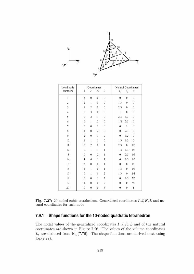
Fig. 7.27: 20-noded cubic tetrahedron. Generalized coordinates I, J,K, L and na-tural coordinates for each node

7.9.1 Shape functions for the 10-noded quadratic tetrahedron

The nodal values of the generalized coordinates I, J,K, L and of the naturalcoordinates are shown in Figure 7.26. The values of the volume coordinatesLi are deduced from Eq.(7.76). The shape functions are derived next usingEq.(7.77).

219

Node 1Position (I, J,K, L) : (2, 0, 0, 0). Volume coordinates : (1, 0, 0, 0)

N1 = l12(L1) =

(L1 − 1

2

)L1

1− 12

= (2L1 − 1)L1 (7.78)

Node 2

Position (I, J,K, L) : (1, 1, 0, 0). Volume coordinates : (12, 1

2, 0, 0)

N2 = l21(L1) l21(L2) =L1

12

L2

12

= 4L1 L2 (7.79)

The same procedure gives

N3 = (2L2 − 1) ; N7 = 4 L2 L4

N4 = 4L2 L3 ; N8 = 4 L3 L4

N5 = (2 L3 − 1)L− 3 ; N9 = 4 L1 L4

N6 = 4 L1 L3 ; N10 = (2 L4 − 1) L4

(7.80)

The expression of Ni in terms of the natural coordinates is obtained usingEq.(7.76). The cartesian form of Ni for a straight edged tetrahedron is directlyobtained from Eq.(7.68).

The shape functions of this element contain all the terms of a quadraticpolynomial (Figure (7.23)) and they satisfy Eqs.(7.56).

7.9.2 Shape functions for the 20-noded quadratic tetrahedronThe nodal values of the generalized coordinates I, J,K, L and α, β, γ are shownin Figure 7.27. From Eqs.(7.77) we obtain:

Node 1

Position (I, J,K, L) : (3, 0, 0, 0). Volume coordinates : (3, 0, 0, 0)

N1 = l13 (L1) =

(L1 − 2

3

) (L1 − 1

3

)L1

(1− 2

3

) (1− 1

3

)1

=1

2L1(3L1 − 1) (3L1 − 2) (7.81)

Node 2

Position (I, J,K, L) : (2, 1, 0, 0). Volume coordinates : (23, 1

3, 0, 0)

N2 = l22(L1) L21(L2) =

(L1 − 1

3

)L− 1

(23− 1

3

)23

L2

13

=9

2(3L1 − 1) L1 L2 (7.82)

220

Fig. 7.28: Local coordinate system xyz for the analytical computation of volumeintegrals over right prisms

Following a similar procedure gives

N3 =9

2(3L2 − 1)L1L2 ; N9 =

9

2(3L1 − 1)L1L3 ; N15 =

9

2(3L1 − 1)L1L4

N4 =1

2L2(3L2 − 1)(3L2 − 2) ; N10 = 27 L1 L2L3 ; N16 = 27L1L2L4

N5 =9

2(3L2 − 1)L2 3 ; N11 =

9

2(3L2 − 1)L2 L4 ; N17 =

9

2(3L4 − 1)L4 L2

N6 =9

2(3 L3 − 1)L3 L2 ; N12 = 27 L2 L3 L4 ; N18 =

9

2(3L4 − 1)L4 L3

N7 =1

2L3(3L3 − 1)(3L3 − 2) ; N13 =

9

2(3L3 − 1)L3 L4 ; N19 =

9

2(3L4 − 1)L4 L1

N8 =9

2(3L3 − 1)L3L1 ; N14 = 27L1L3L4 ; N20 =

1

2L4(3L4 − 1)(3L4 − 2)

(7.83)Eqs.(7.76) allows us to express Ni in terms of the natural coordinates. The

cartesian form of Ni for a straight edged tetrahedron is obtained substitutingEq.(7.68) into above expressions. Note that the shape functions are completecubic polynomials and they satisfy Eq.(7.56).

7.10 COMPUTATION OF THE ELEMENT INTEGRALS

7.10.1 Analytical computation of element integrals

In general, the computation of the element integrals is carried out via numericalintegration. Useful analytical rules can, however, be derived for straight edgedtetrahedra or right prisms as shown below.

Volume integrals over right prisms can be computed exactly using the localcoordinate system xyz shown in Figure 7.28. For instance, the integral over aface with x = constant, is first obtained by Eq.(7.41) and then a simple line

221

integral in the z direction is performed. The resulting local stiffness matrixK is next transformed to the global axes xyz by a transformation similar toEq.(7.42) taking into account the third cartesian axis. This procedure is notapplicable to non-regular or hexahedra curved sides for which the use of anisoparametric formulation and numericaly integration is essential.

The integrals over straight-sided tetrahedra have simpler expressions. Thus,the volume integral of a polynomial term expressed in volume coordinates isgiven by

∫∫∫

V (e)

Lk1L

l2L

m3 Ln

4 dV = 6V (e) k! l! m! n!

(k + l + m + n + 3)!(7.84)

Similarly, the surface integrals over the element faces can be obtained byEqs.(7.40) or (7.38).

The use of natural coordinates does not introduce any additional difficulty.The volume integrals are computed by

∫∫∫

V (e)

αkβlγm dV = 6V (e) k! l! m!

(k + l + m + 3)!(7.85)

and the surface integrals can be obtained by Eq.(7.48). Recall that if any ofthe coordinates is missing in the integrals of Eqs.(7.84) and (7.85) then thecorresponding power is made equal to one in the numerator and to zero in thedenominator of the corresponding right-hand side.

Curved-side tetrahedra require an isoparametric formulation and numericalintegration (Chapter 8).

Example: 7.3 Compute the submatrix K(e)11 of a 20-noded quadratic tetrahedron with

straight sides.

-- Solution-- Solution

We compute first the cartesian derivatives of the shape function N1 expressed in termsof volume coordinates. For instance,

∂N1

∂x=

∂N1

∂L1

∂L1

∂x+

∂N1

∂L2

∂L2

∂x+

∂N1

∂L3

∂L3

∂x+

∂N1

∂L4

∂L4

∂x

Since N1 = L1(2L1 − 1) we have from Eq.(7.68)

∂N1

∂x= (4L1 − 1)

bi

6V (e)

Following a similar procedure gives

∂N1

∂y= (4L1 − 1)

ci

6V (e)and

∂N1

∂z= (4L1 − 1)

di

6V (e)

222

The strain matrix B1 is written as

B1 =(4L1 − 1)

6V (e)

bi 0 00 ci 00 0 di

ci bi 0di 0 bi

0 di ci

=(4L1 − 1)

6V (e)B1

and matrix K(e)11 is given by

K(e)11 =

∫∫∫

V (e)BT

1 DB1dV =1

36(V (e))2B

T

1 DBT

1

∫∫∫

V (e)(4L1 − 1)2 dV

Making use of Eq.(7.84) gives finally

K(e)11 =

160V (e)

(d11b21 + d44c21 + d55d21) b1c1(d12 + d44) (d13b1d1 + d55d1c1)

(d22c21 + d44b21 + d66d21) c1d1(d23 + d66)

Symmetrical (d33d21 + d55b21 + d66c21)

The rest of the K(e)ij matrices are obtained in a similar manner.

223

Chapter 8

2D AND 3D ISOPARAMETRIC ELEMENTS

8.1 ISOPARAMETRIC QUADRILATERAL ELEMENTSWe recall that the term “isoparametric” means that the standard shape func-tions are used to interpolate the element geometry in terms of the nodal coor-dinates. Thus, the geometry of a 2D isoparametric quadrilateral with n nodesis expressed as

x =n∑

i=1

Ni(ξ, η) xi ; y =n∑

i=1

Ni(ξ, η) yi (8.1)

where Ni(ξ, η) are the standard displacement shape functions. Eqs.(8.1) relatethe cartesian and the natural coordinates at each point. Such a relationshipmust be unique and this is satisfied if the Jacobian matrix of the coordinatetransformation x, y → ξ, η has a constant sign over the element [S14].

It can be shown that this condition is satisfied for linear quadrilateral el-ements if all internal angles between two element sides are greater than 180

[S14]. For quadratic elements it is additionally required that the side nodesare located within the “middle third” of the distance between adjacent corners[J5]. There are no practical rules for higher order quadrilateral elements andthe constant sign of the Jacobian is the only possible verification in this case.Figure 8.1 shows some examples of 2D isoparametric elements.

Most of the ideas of the isoparametric formulation originated from the workof Taig [T1, T2], who derived 4-noded isoparametric quadrilaterals. Theseconcepts were generalized to more complex 2D and 3D elements by Irons [I2,7].

Eq.(8.1) allows us to obtain a relationship between the derivatives of theshape functions with respect to the cartesian and the natural coordinates. Ingeneral, Ni is expressed in terms of the natural coordinates ξ and η and thechain rule of derivation yields

∂Ni

∂ξ=

∂Ni

∂x

∂x

∂ξ+

∂Ni

∂y

∂y

∂ξ

∂Ni

∂η=

∂Ni

∂x

∂x

∂η+

∂Ni

∂y

∂y

∂η

(8.2)

225

Fig. 8.1: Some two-dimensional isoparametric elements

In matrix form

∂Ni∂ξ∂Ni∂η

=

∂x∂ξ

∂y∂ξ

∂x∂η

∂y∂η

︸ ︷︷ ︸J(e)

∂Ni∂x∂Ni∂y

= J(e)

∂Ni∂x∂Ni∂y

(8.3)

where J(e) is the Jacobian matrix of the transformation between the cartesianand natural coordinates. The superindex e in J denotes that this matrix isalways computed at element level. We deduce from Eq.(8.3)

∂Ni∂x∂Ni∂y

=

[J(e)

]−1

∂Ni∂ξ∂Ni∂η

=

1∣∣∣J(e)

∣∣∣

∂y∂η

− ∂y∂ξ

−∂x∂η

∂x∂ξ

∂Ni∂ξ∂Ni∂η

(8.4)

where∣∣∣J(e)

∣∣∣ is the determinant of the Jacobian matrix. This determinant also

relates the differential of area in the two coordinate systems, i.e.

dx dy =∣∣∣J(e)

∣∣∣ dξ dη (8.5)

226

The terms of the Jacobian matrix are computed using the isoparametricapproximation (8.1), i.e.

∂x

∂ξ=

n∑i=1

∂Ni

∂ξxi ;

∂x

∂η=

n∑1=1

∂Ni

∂ηxi; etc. (8.6)

and

J(e) =n∑

i=1

∂Ni∂ξ

xi∂Ni∂ξ

yi

∂Ni∂η

xi∂Ni∂η

yi

(8.7)

For a rectangular element

J(e) =

[a 00 b

]and |J(e)| = ab (8.8)

8.1.1 Stiffness matrix and load vector of isoparametric quadrilateralSubstituting the cartesian derivatives of the shape functions from Eq.(8.4)into (6.19) yields the general form of the gradient matrix for an isoparametricquadrilateral element in terms of the natural coordinates by

Bi(ξ, η) =

∂Ni∂x

∂Ni∂y

=1∣∣∣J(e)

∣∣∣

bi

ci

(8.9)

where

bi =∂y

∂η

∂Ni

∂ξ− ∂y

∂ξ

∂Ni

∂η; ci =

∂x

∂ξ

∂Ni

∂η− ∂x

∂η

∂Ni

∂ξ(8.10)

The element stiffness matrix for a 2D Poisson element can be written inthe normalized natural coordinate space as

K(e)ij =

∫ ∫

A(e)

BTi D Bj dxdy =

+1∫

−1

+1∫

−1

BTi (ξ, η) D Bj(ξ, η)

∣∣∣J(e)∣∣∣ dξ dη =

=

+1∫

−1

+1∫

−1

(kxbibj + kycicj)1∣∣∣J(e)

∣∣∣dξdη =

=

+1∫

−1

+1∫

−1

Gij dξdη (8.11a)

with

Gij = (kxbibj + kycicj)1∣∣∣J(e)

∣∣∣(8.11b)

227

Eq.(8.11a) shows that the integrand of K(e)ij contains rational functions in

ξ and η. An exception to this rule is when the determinant of the Jacobianmatrix is constant. This only occurs for rectangular elements (and for straightside triangles). In these cases the element integrals contain simple polynomialsand the analytical expressions of Section 7.6 can be applied. However, forgeneral quadrilateral shapes the analytical integration of K

(e)ij is difficult (and

in most cases impossible!) and the only option is to use numerical integration.

A similar procedure will be followed to compute the equivalent nodal forcevectors for isoparametric elements. For example, for the case of a heat source

f(e)i =

∫∫

A(e)

NiQdx dy =

∫ +1

−1

∫ +1

−1

NiQ∣∣∣J(e)

∣∣∣t dξ dη (8.12)

Numerical integration is also typically used to compute integrals such asthat of Eq.(8.12).

Example: 8.1 Formulate an isoparametric quadrilateral of 4 nodes.

Solution

The actual and normalized geometries of the element are shown in the Figure 8.2below.

The isoparametric description of the geometry is written as

x =

xy

=

4∑i=1

Ni(ξ, η)

xi

yi

(8.13)

where Ni(ξ, η) = 14 (1 + ξξi)(1 + ηiη).

Fig. 8.2: Four-noded isoparametric quadrilateral. Actual and normalized geometry

228

The above expression maps the natural coordinates of each element point on to thecartesian space. For instance, the cartesian position of the central point O withnatural coordinates (0,0) is

xO =4∑

i=1

Ni(0, 0)

xi

yi

=

1

4

x1 + x2 + x3 + x4

y1 + y2 + y3 + y4

(8.14a)

Point A at the center of side 1–2 with natural coordinates (0,-1) is locatedin the cartesian space at

xA =4∑

i=1

Ni(0,−1)

xi

yi

=

1

2

x1 + x2

y1 + y2

(8.14b)

We can observe that the isoparametric description is useful to express all the elementexpressions in the natural coordinate system.

The Jacobian matrix of Eq.(8.7) is given by

J(e) =4∑

i=1

ξi

4(1 + ηηi)xi

ξi

4(1 + ηηi)yi

ηi

4(1 + ξξi)xi

ηi

4(1 + ξξi)yi

(8.15)

The cartesian derivatives of the shape functions are obtained from Eq.(8.4) as

∂Ni

∂x∂Ni

∂y

=1

|J(e)|4∑

j=1

ηj

4(1 + ξξj)yj −ξj

4(1 + ηηj)yj

−ηj

4(1 + ξξj)xj

ξj

4(1 + ηηj)xj

ξi

4(1 + ηηi)

ηi

4(1 + ξξi)

(8.16)

From above equations we deduce

∂Ni

∂x∂Ni

∂y

=

bi

ci

(8.17a)

with

bi =αi

1 + αi2ξ + αi

3η + αi4ξη

βi1 + βi

2ξ + βi3η + βi

4ξη, ci =

αi5 + αi

6ξ + αi7η + αi

8ξη

βi5 + βi

6ξ + βi7η + βi

8ξη(8.17b)

where αi1 · · ·αi

8, βi1 · · ·βi

8 are nodal parameters depending on the nodal coordinates.

Clearly, the element strain matrix and the stiffness matrix now contains rational poly-nomials making exact integration over an arbitrary quadrilateral domain is extremelydifficult. This problem can be overcome by using numerical integration (Section 8.3).

The above equations simplify considerably for rectangular shapes. For a rectangle ofsize 2a× 2b we have

J(e) =

[a 00 b

], |J(e)| = ab and dx dy = ab dξ dη (8.18)

229

The cartesian derivatives of the shape functions are now simply given by

∂Ni

∂x∂Ni

∂y

=

ξi

4b(1 + ηηi)

ηi

4a(1 + ξξi)

(8.19)

The element stiffness matrix is expressed in the natural system by

K(e)ij =

∫ +1

−1

∫ +1

−1

BTi DBi ab dξ dη (8.20)

The integral expression of K(e)ij now contains polynomial expressions in ξ, η, ξ2, η2 and

ξη which can be directly computed noting that∫ +1

−1

∫ +1

−1

C[1, ξ, η, ξ2, η2, ξη] dξ dη = C

[4, 0, 0,

4

3,4

3, 0

](8.21)

where C is a constant parameter.

8.1.2 A comparison between the 8- and 9-noded isoparametric quadri-laterals

It is interesting to assess the circumstances under which the linearly distorted8 and 9-noded quadrilaterals can fully represent any quadratic cartesian ex-pansion. The straight-sided element geometry is exactly approximated by thebilinear (subparametric) interpolation

x =4∑

i=1

Nixi (8.22)

where Ni = 14(1+ξξi)(1+ηηi) are the shape functions of the 4-noded rectangle.

We wish to be able to reproduce

u = α1 + α2x + α3y + α4x2 + α5xy + α6y

2 (8.23)

Noting that the bilinear form contains terms such as 1, ξ, η and ξη and bysubstituting Eq.(8.22) into (8.23) the above can be written as

u = β1 + β2ξ + β3η + β4ξ2 + β5ξη + β6η

2 + β7η2 + β8ξ

2 + β9ξ2η2 (8.24)

where β1 to β9 depend on the values of α1 to α6.We shall now try to match the terms arising from the quadratic expansion

of the 8-noded Serendipity shown in Figure 7.8. Noting the terms occuring inthe Pascal’s triangle of Figure 7.8, the interpolation can be written as

u = b1 + b2ξ + b3η + b4ξ2 + b5ξη + b6η

2 + b7ξη2 + b8ξ

2η (8.25)

230

It is evident that for arbitrary values of η1 to η9 it is impossible to matchthe coefficients b1 to b8 due to the absence of the term ξ2η2 in Eq.(8.25).

For the 9-noded Lagrange element (Figure 7.5) the expansion similar toEq.(8.24) gives

u = b1 + b2ξ + b3η + b4ξ2 + b5ξη + b6η

2 + b7ξη2 + b8ξ

2η + b9ξ2η2 (8.26)

and the matching of the coefficients in Eqs.(8.24) and (8.26) can be madedirectly.

We conclude that the 9-noded elements can better represent quadraticcartesian polynomials on linearly distorted shapes and therefore are gener-ally preferable in modelling smooth solutions. Figure 8.3 shows an exampleof this for the analysis, with 8- and 9-node elements, respectively of a simplebeam solution where exact answers are quadratic. With no distorsion both el-ements with a full (3×3) integration rule give exact results but when distortedonly the 9-node element does so, the 8-noded element giving a significant stressfluctuation.

A similar argument leads to the conclusion that in 3D, again only 27-nodedLagrangian elements are capable of reproducing fully a quadratic function incartesian coordinates when trilinearity distorted.

8.2 ISOPARAMETRIC TRIANGULAR ELEMENTSThe isoparametric interpolation for triangular elements is written as

x =n∑

i=1

Ni(L1, L2, L3) xi ; y =n∑

i=1

Ni(L1, L2, L3) yi (8.27)

The computation of the cartesian derivatives of Ni and the Jacobian matrixis inmediate for straight side triangles (see Example 8.2) giving

J(e) =

[x2 − x1 y2 − y1

x3 − x1 y3 − y1

](e)

and |J(e)| = 2A(e) (8.28)

The computation of the element integrals in this case is simple via theanalytic expressions of Section 7.6.

For curved side triangles it is convenient to use the natural coordinates αand β defined in Figure 7.14. This implies that L2 and L3 will be replaced byα and β, respectively, and L1 by 1 − α − β in all expressions. The compu-tation of the cartesian derivatives of Ni follows precisely the steps describedin the previous section, simply changing the coordinates ξ and η for α and β,respectively. For instance

∂Ni

∂x∂Ni

∂y

=1

|J(e)|

∂y

∂β− ∂y

∂α

−∂x

∂β−∂x

∂α

∂Ni

∂α∂Ni

∂β

(8.29)

231

Fig. 8.3: Quadratic Serendipity and Lagrangian 8- and 9-noded elements in regularand distorted form. Elastic deflection of a beam under constant moment. Note poorresults of 8-noded element

J(e) =n∑

i=1

∂Ni

∂αxi

∂Ni

∂αyi

∂Ni

∂βxi

∂Ni

∂βyi

(8.30)

∂x

∂α=

n∑i=1

∂Ni(α, β)

∂αxi ;

∂x

∂β=

n∑i=1

∂Ni(α, β)

∂βxi ; etc. (8.31)

The element stiffness matrix is obtained by an expression analogous toEq.(8.11a) by

K(e)ij =

∫ 1

0

∫ 1−β

0

BTi D Bj

∣∣∣J(e)∣∣∣dαdβ =

∫ 1

0

∫ 1−β

0

Gij (α, β) dαdβ (8.32)

232

where all the terms in Bi and Gij are deduced from Eqs. (8.11) simply sub-stituting ξ and η for α and β, respectively.

For curved side triangles the integrand of Eq.(8.32) is a rational polynomialand numerical integration is needed.

Example: 8.2 Derive the expression of the Jacobian matrix for an isoparametric trianglewith straight sides.

Solution

As the element sides are straight, a linear interpolation for the geometry will suffice,i.e.

x = L1x1 + L2x2 + L3x3

y = L1y1 + L2y2 + L3y3

(8.33)

where xi, yi i = 1, 2, 3 are the coordinates of the three vertex nodes.

Recall that L1 = 1− L2 − L3. Substituting this into the above gives

x = x1 + (x2 − x1)L2 + (x3 − x1)L3

y = y1 + (y2 − y1)L2 + (y3 − y1)L3

(8.34)

The Jacobian matrix is obtained from

∂Ni∂L2

∂Ni∂L3

=

∂x∂L2

∂y∂L2

∂x∂L3

∂y∂L3

∂Ni∂x∂Ni∂y

= J(e)

∂Ni∂x∂Ni∂y

(8.35)

The Jacobian matrix is deduced from the above two equations as

J(e) =

∂x∂L2

∂y∂L2

∂x∂L3

∂y∂L3

=

[x2 − x1 y2 − y1

x3 − x1 y3 − y1

](8.36)

The cartesian derivatives are obtained by (noting that∣∣∣∣J(e)

∣∣∣∣ = 2A(e))

∂Ni∂x∂Ni∂y

=

1

2A(e)

[y3 − y1 y1 − y2

x1 − x3 x2 − x1

]

∂Ni∂L2

∂Ni∂L3

(8.37)

Let us verify the above expression for the simple 3-noded triangle. For instance, for

i = 1,∂N1

∂L2=

∂N1

∂L3= −1 (as N1 = L1 = 1− L2 − L3) and

∂N1∂x∂N1∂y

=

1

2A(e)

y2 − y3

x3 − x2

(8.38)

Note the coincidence with the expression obtained using Eqs.(4.30) directly.

The expression for the cartesian derivatives obtained is completely general for straightside triangles of any approximation order (i.e. quadratic, cubic, etc.).

233

Fig. 8.4: Gauss quadratures over quadrilateral elements, a) 1×1, b) 2×2, c) 3×3,d) 4× 4 integration points

8.3 NUMERICAL INTEGRATION IN TWO DIMENSIONS

It has been shown in the previous section that all element integrals can bewritten in the natural coordinate space making use of the isoparametric for-mulation. The numerical integration by a Gauss quadrature will be considerednext.

8.3.1 Numerical integration in quadrilateral domains

The integral of a term g(ξ, η) over the normalized isoparametric quadrilateraldomain can be evaluated using a 2D Gauss quadrature by

∫ +1

−1

∫ +1

−1

g(ξ, η) dξ dη =

∫ +1

−1

dξ

[nq∑

q=1

g(ξ, ηq)Wq

]=

np∑p=1

nq∑q=1

g(ξp, ηq)WpWq

(8.39)

where np and nq are the number of integration points along each natural co-ordinate ξ and η respectively; ξp and ηq are the natural coordinates of the pthintegration point and Wp,Wq are the corresponding weights.

The coordinates and weights for each natural direction are directly deducedfrom those given in Table 3.3 for the 1D case. Recall that a 1D quadratureof qth order integrates exactly a polynomial of degree q ≤ 2n − 1. Figure 8.4shows the more usual quadratures for quadrilateral elements.

Example: 8.3 Integrate numerically the function f(ξ, η) = ξ2η2 over a rectangular elementwith dimensions 2a× 2b.

Solution

Since the element is rectangular |J(e)| = ab (see Eq.(8.18)).

The integrand is a quadratic function in ξ and η and hence a 2 × 2 quadrature is

234

needed (Figure 8.4b). Thus

I =∫∫

A

ξ2η2dA = ab

∫ +1

−1

∫ +1

−1

ξ2η2 = ab

2∑p=1

2∑q=1

(ξ2η2)p,qWpWq =

= ab

[(−√

33

)2(−√

33

)2 + (−√

33

)2(√

33

)2 + (√

33

)2(−√

33

)2 + (√

33

)2(√

33

)2]

=49ab

which is the exact solution.

8.3.2 Numerical integration over triangles

The Gauss quadrature for triangles is written as

∫ 1

0

∫ 1−L3

0

f(L1, L2, L3) dL2 dL3 =

np∑p=1

f(L1p , L2p , L3p) Wp (8.40)

where np is the number of integration points: L1p , L2p , L3p and Wp are the areacoordinates and the corresponding weight for the pth integration point.

Figure 8.5 shows the more usual coordinates and weights; the term “ac-curacy” in the figure refers to the highest degree polynomial which is exactlyintegrated by each quadrature. Figure 8.5 is also of direct application forcomputing the integrals defined in terms of the natural coordinates α and β,simply recalling that L2 = α, L3 = β and L1 = 1− α− β.

It is important to note that the weights in Figure 8.5 are normalized so thattheir sum is 1/2. In many references this value is changed to the unity andthis requires the sum of Eq.(5.91) to be multiplied by 1/2 so that the elementarea is correctly computed in those cases.

Example: 8.4 Compute the area of a triangular element with straight sides by numericalintegration.

Solution

A(e) =

∫∫

A(e)

dx dy =

∫ 1

0

∫ 1−β

0

|J (e)| dα dβ = |J (e)|∑

p

Wp =|J (e)|

2(8.41)

which corresponds with the value obtained in Eq.(8.28).

For further information on numerical integration over triangular domainssee refs. [C15], [C19], [D10], [H20] y [Z6].

235

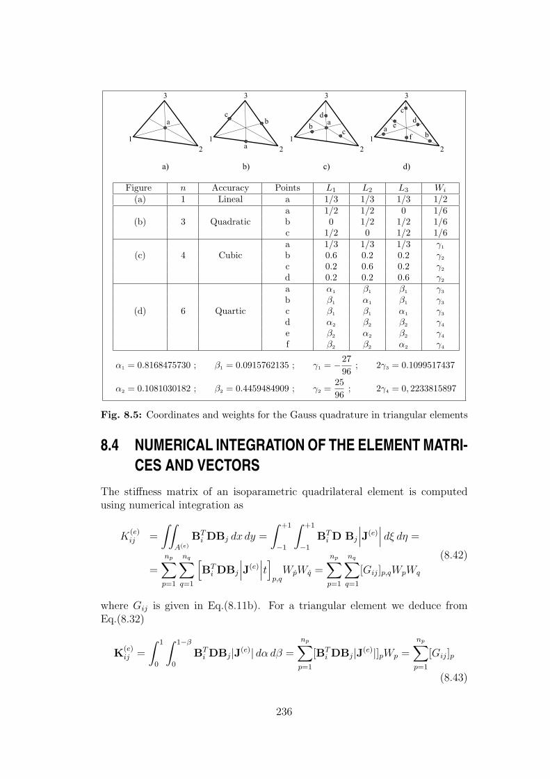
Figure n Accuracy Points L1 L2 L3 Wi

(a) 1 Lineal a 1/3 1/3 1/3 1/2a 1/2 1/2 0 1/6

(b) 3 Quadratic b 0 1/2 1/2 1/6c 1/2 0 1/2 1/6a 1/3 1/3 1/3 γ1

(c) 4 Cubic b 0.6 0.2 0.2 γ2

c 0.2 0.6 0.2 γ2

d 0.2 0.2 0.6 γ2

a α1 β1 β1 γ3

b β1 α1 β1 γ3

(d) 6 Quartic c β1 β1 α1 γ3

d α2 β2 β2 γ4

e β2 α2 β2 γ4

f β2 β2 α2 γ4

α1 = 0.8168475730 ; β1 = 0.0915762135 ; γ1 = −2796

; 2γ3 = 0.1099517437

α2 = 0.1081030182 ; β2 = 0.4459484909 ; γ2 =2596

; 2γ4 = 0, 2233815897

Fig. 8.5: Coordinates and weights for the Gauss quadrature in triangular elements

8.4 NUMERICAL INTEGRATION OF THE ELEMENT MATRI-CES AND VECTORS

The stiffness matrix of an isoparametric quadrilateral element is computedusing numerical integration as

K(e)ij =

∫∫

A(e)

BTi DBj dx dy =

∫ +1

−1

∫ +1

−1

BTi D Bj

∣∣∣J(e)∣∣∣ dξ dη =

=

np∑p=1

nq∑q=1

[BT

i DBj

∣∣∣J(e)∣∣∣t

]p,q

WpWq =

np∑p=1

nq∑q=1

[Gij]p,qWpWq

(8.42)

where Gij is given in Eq.(8.11b). For a triangular element we deduce fromEq.(8.32)

K(e)ij =

∫ 1

0

∫ 1−β

0

BTi DBj|J(e)| dα dβ =

np∑p=1

[BTi DBj|J(e)|]pWp =

np∑p=1

[Gij]p

(8.43)

236

where the position of the integration points and the corresponding weights isobtained from Figure 8.5.

The numerical integration of the stiffness matrix requires the evaluation ofthe Jacobian J(e) and its determinant, the strain matrix Bi and the constitutivematrix D at each integration point. Similarly, the numerical integration of theequivalent nodal flux vector due to a heat source for isoparametric quadrilateralelements gives

f(e)bi

=

∫ +1

−1

∫ +1

−1

NiQ∣∣∣J(e)

∣∣∣dξdη =

np∑p=1

nq∑q=1

(NiQ

∣∣∣J(e)∣∣∣)

p,qWp Wq (8.44)

For triangular elements the double sum is replaced by the single sum ofEq.(8.43).

The computation of the equivalent nodal flux vector due to surface fluxesdeserves a special comment. Let us recall that this vector has the followingexpression (see Eq.(4.57))

f(e)i =

∮

l(e)Ni(αφa − qn)dS (8.45)

where l(e) is the loaded element boundary. In general this boundary representsa line ξ = constant or η = constant in the natural coordinate space (seeFigure 8.6). Therefore, the differential of length over the side η = 1 for anisoparametric quadrilateral element is computed by

(ds)η=1 = (dx2 + dy2)η=1 =

[√(dxdξ

)2

η=1+

(dydξ

)2

η=1

]dξ =

=

[√√√√(

∑ni=1

dNi

dξxi

)2

η=1

+

(∑n

i=1dNi

dξyi

) 2

η=1

]dξ = c(ξ) dξ

(8.46)

Substituting Eq.(8.46) into (8.45) yields a line integral which is a functionof the natural coordinate ξ only. This is computed using a 1D quadrature by

f(e)i =

∮

l(e)Ni(αφa − qn)c(ξ)dξ =

∫ +1

−1

g(ξ)dξ =

np∑p=1

g(ξp)Wp (8.47)

For three-noded triangles and four-noded quadrilaterals, f(e)i has the fol-

lowing expression for a uniform boundary flux

f(e)i =

l(e)

2(αφa − qn) (8.48)

237

Fig. 8.6: Normal flux across a boundary of a 2D element

8.5 COMPUTER PROGRAMMING OF K(e) AND f (e)

Previous sections provided all the necessary expressions for programming thecomputation of the stiffness matrix and the equivalent nodal force vector foreach element. The basic steps involved in programming the computation ofK(e) and f (e) for quadrilateral elements are given next.

Figure 8.7 shows the flow diagram for computing of K(e) as deduced fromEq. (8.42).

The evaluation of the constitutive matrix D can be taken out of the nu-merical integration loop if the material properties are homogeneous over theelement. The case of D variable is treated simply by using a standard inter-polation within the element in terms of the nodal values as

D =n∑

i=1

NiDi (8.49)

Eq.(8.49) is used to obtain the values of D at the Gauss points within thenumerical integration loop.

Figure 8.8 shows the flow chart for computing the flux vector f (e) for thecase of a heat source Q as deduced from Eq.(8.44).

The computation of the heat source Q can be taken out from the numericalintegration loop if it is constant over the element. A variable heat source canbe accounted for by interpolating the known nodal values, in the same way aswas done for matrix D in Eq. (8.49).

The flow charts in Figures 8.7 and 8.8 are completely general and applicableto most problems solved with the FEM.

238

Fig. 8.7: Flow chart for the computation of K(e)

8.6 OPTIMAL POINTS FOR COMPUTING GRADIENT FLUXES

The gradient (and the fluxes) are obtained from the derivatives of the unknownfunction φ. Therefore, their approximation is always of a lower order than thatfor φ. In general, if the shape functions are complete polynomials of pth degreethe approximation for the fluxes will be a polynomial of degree p− 1 or p− 2,depending if they are obtained as first or second derivatives of the φ field,respectively.

It can be proved that the fluxes from the finite element solution can beconsidered a least square interpolation of the exact flux field [Z6]. Naturally,the exact flux field is unknown. However, an enhanced stress distribution canbe found by the following property of the Gauss quadrature: A nth degree

239

Fig. 8.8: Flow diagram for computing f (e) for the case of body forces

polynomial and a n− 1th degree polynomial, obtained by least square fittingof the first one, take the same values at the points of the Gauss quadrature oforder nth. Hence, we can obtain an approximation of the fluxes and the gra-dients that is one order higher higher by computing these at the Gauss points.This important property will be clarified with the following two examples.

Example: 8.5 Verify that a second degree polynomial, and a first degree polynomial ob-tained by least square smoothing of the another, take the same values at the pointsof the Gauss quadrature of order 2.

Solution

Let us consider the second degree polynomial (n = 2)

f(x) = 1 + x + x2

We will now obtain a first degree polynomial (n = 1) which approximates f(x) in theleast square sense; i.e. find a polynomial

g(x) = a + bx

240

Fig. 8.9: Least square approximation of a quadratic polynomial by a linear one.Intersection of both polynomials at the points of the Gauss quadrature of order 2

such that it minimizes the functional

M =∫ +1

−1

[f(x)− g(x)

]2

dx =∫ +1

−1

[(1− a) + (1− b)x + x2

]2

dx

be a minimum.

The parameters a and b are obtained by making

∂M

∂a= 0 =⇒

∫ +1

−1

−2[(1− a) + (1− b)x + x2

]dx = 0

∂M

∂b= 0 =⇒

∫ +1

−1

−2x[(1− a) + (1− b)x + x2

]dx = 0

which gives a = 43 y b = 1.

Figure 8.9 shows the two polynomials f(x) and g(x). Note that both polynomialstake the same values at the points of the Gauss quadrature of order 2.

Example: 8.6 Verify that a cubic polynomial and a quadratic one obtained by least squaresmoothing of the former, take same values at the points of the 3rd order Gaussquadrature.

Solution

Let us consider the third degree polynomial (n = 3)

f(x) = 1 + x + x2 + x3

We will obtain the second degree polynomial g(x) = a + bx + cx2, such that

M =∫ +1

−1

[f(x)− g(x)

]2

dx =∫ +1

−1

[(1− a) + (1− b)x + (1− c)x2 + x3

]2

dx

241

Fig. 8.10: Least square interpolation of a cubic polynomial by a quadratic one.Intersection of both polynomials at the points of the Gauss quadrature of order 3

is a minimum.

The three constants a, b, and c are obtained by solving the following system

∂M

∂a= 0 =⇒ 1− a +

1− c

3= 0

∂M

∂b= 0 =⇒ 1− b

3+

15

= 0

∂M

∂c= 0 =⇒ 1− a

3+

1− c

5= 0

which gives

a = 1 ; b =85

y c = 1

Figure 8.10 shows that the exact and interpolating polynomials take the same valuesat the three points of the 3rd order Gauss quadrature (i,e. ξ = 0 and ξ = ±

√3/3).

The following conclusions can be drawn from what is explained:

1. If the exact distribution of the gradient g (and the flux q) field is apolynomial of nth degree and the approximate finite element solution isa polynomial of n−1th degree, the computation of q (or g) at the pointsof the Gauss quadrature of nth order gives the exact values.

2. The evaluation of q or g at the Gauss quadrature points chosen for theintegration of K(e) yields a solution of one approximation order higherthan at any other point within the element.

242

Fig. 8.11: Optimal points for computation of the gradients and the fluxes in some1D and 2D elements

The evaluation of gradients and fluxes at the so called “optimal” quadra-ture points is therefore of higher accuracy than at any other element point.The nodal stress values can subsequently be obtained from a local or globalsmoothing of the Gauss point values.

The above concepts are rigorously true for 1D elements. For 2D and 3Delements the sampling of the gradients and the fluxes at the “optimal” Gaussquadrature points leads also to a substantial improvement in the results. Fi-gure 8.11 shows the optimal points for computation of gradients and fluxes forsome 1D and 2D elements. Extrapolation to the 3D case is simple.

These concepts extend naturally for elasticity problems (Chapter 9) wherethe Gauss point and optimal for the sampling of the strains εεε and the stressesσσσ. Figure 8.12 shows an example of the analysis of a cantilever beam analyzedwith 8-noded Serendipity rectangles. The accuracy of the shear stress sampledat the 2× 2 Gauss points is noticeable.

8.7 SELECTION OF THE QUADRATURE ORDERThe number of integration points is selected according to the degree of thepolynomials appearing in the element integrals. Isoparametric elements con-tain rational terms within the integrals and exact integration is not longerpossible. The alternative is to choose a quadrature order which integrates ex-actly the same expression for a rectangular or straight side triangular element.This quadrature is termed in practice full integration or standard integration.Remember that in these cases the Jacobian matrix is constant and the elementintegrals have a simple analytical form.

243

Fig. 8.12: Exact and minimum quadrature rules for some rectangular and straightside triangular elements

The minimum quadrature order for the stiffness matrix should preserve theconvergence rate of the element. This is achieved by choosing a quadraturewhich integrates exactly all the complete polynomial terms contained in theshape functions. For rectangular elements this quadrature is of lower orderthan that required for the exact integration of the element stiffness matrix and,thus, some economy is obtained. Figure 8.12 shows the exact and minimumquadratures for some popular rectangular and triangular elements. Note thatboth quadratures coincide for triangles.

Some authors associate the name “minimum quadrature” to that whichguarantees that the element can reproduce in the limit a constant gradient(or strain) field [Z6,15]. This implies that the quadrature chosen should eval-uate exactly the element area (or volume), which simply requires the exactcomputation of the following integral

A(e) =

∫∫

A(e)

dA =

∫∫

A(e)

∣∣∣J (e)∣∣∣ dξ dη

In rectangles and straight side triangles this condition is too weak as itrequires a single point quadrature which generally violates the minimum re-quirement for preserving the element convergence as described above (with theexception of 3-noded triangles).

244

Fig. 8.13: a) Propagable mechanisms in the 4-noded rectangle with a single inte-gration point, b) Mechanisms in the 8-noded and 9-noded quadrilaterals induced byreduced 2×2 quadrature. The mechanism in the 8-noded element are not propagablein a mesh

Extreme care must also be taken so that a lower order quadrature doesnot introduce internal mechanisms in the element. These mechanisms appearwhen the interpolation field for the main variables field generates a gradient(or strain) field which vanishes at the integration points, thus yielding a sin-gular stiffness matrix. Sometimes these mechanisms are compatible betweenadjacent elements and lead to the singularity of the global stiffness matrix and,consequently, to an incorrent solution. A typical example of this situation isthe two mechanisms induced by the reduced one point quadrature in the four-noded rectangle for 2D elasticity problems as shown in Figure 8.13a. Thismechanism invalidates this reduced quadrature for practical purposes unlesssome stabilization techniques are used.

In some cases, the mechanisms induced by the reduced integration of thestiffness matrix can not propagate in the mesh, and this preserves the cor-rectness of the solution. This happens for the single mechanism originated bythe 2 × 2 reduced quadrature in the eight-noded rectangle for 2D elasticityproblems, as shown in Figure 8.13b. Unfortunately this is not the case for the9-noded Lagrangian as the reduced integration introduces three mechanisms(Figure 8.13) Two of which are propagable and can polute the solution andhence it is not recommended practice.

Note that the minimum quadrature points coincide in most cases with theoptimum points for the computation of fluxes (or stresses). This can be easilyverified by comparing the minimum and optimum quadratures shown in Fig-

245

ures 8.9 and 8.10, respectively. This important coincidence is shown clearly inthe analysis of a cantilever beam using 8-noded Serendipity rectangles. Figure8.14 shows that the shear force distribution within each element is parabolicand, therefore, far from the correct linear solution. However, the tangentialstresses at the 2× 2 Gauss quadrature coincide with the exact values and thesimple linear interpolation of the stresses gives the exact shear force distribu-tion.

Fig. 8.14: Cantilever beam analyzed with four 8-noded Serendipity rectangles. Lin-ear extrapolation of the shear force values from the transverse sections correspondingto the 2× 2 Gauss quadrature

246

8.8 THE PATCH TEST FOR 2D ELEMENTSApplication of the patch test to triangular and quadrilateral elements followsthe general lines described in Section 3.9 for 1D elements. Here once again thetest is a necessary and sufficient condition for the convergence of the element.

The application of the patch test to a 2D element can take the followingthree different modalities.

Patch test A. A known linear field up is prescribed at all nodes of a patchof 2D elements, where Qp are prescribed temperatures in a heat conductionproblem, or prescribed displacements in an elasticity problems, etc. For eachinternal node j in the patch we verify that (Figure 8.13)

Kijapj − fp

j = 0 (8.50)

where apj is the nodal unknown vector corresponding to the known field and

fpj is a vector resulting from any external flux (or force) required to satisfy the

governing differential equations for the known solution. Generally, in problemsexpressed in cartesian coordinates fp

j = 0.

Patch test B. Only the values of up corresponding to the boundaries of thepatch are inserted only and ai is found as (Figure 8.13)

ai = K−1ii (fp

i −Kijuj) i 6= j (8.51)

and compared against the exact value.Patch tests A and B also involve the computation of the fluxes (stresses)

within the elements and the comparison with the expected “exact” values(Figure 8.15).

Satisfaction of patch tests A and B is a necessary condition for convergenceof the element.

Patch test C. The assembled matrix system of the whole patch is written as

Ka = fp (8.52)

where the bar denotes the patch values and fp represents prescribed bound-ary forces corresponding to the known solution. The solution for a is soughtafter fixing the minimum number of degrees of freedom necessary to eliminatethe singularity of the stiffness equation (i.e. one temperature for the heatconduction problem or the displacements for 2D elasticity problems) and it iscompared with the known solution.

Patch test C allows us to detect any singularity in the stiffness matrix. Thistest is therefore an assessment of the stability of the finite element solution andhence provides not only a necessary but a sufficient condition for convergence.

247

i i

Test A Test B

a prescribed on all nodes

Kij aj = fi verified at node i

a prescribed at edges of patch

ai = Kii–1 (fi – Kij aj) (j = i) solved

y

x

Natural boundary

conditions specified

Minimum esential

boundary conditions

(a) (b)

Fig. 8.15: Patch tests of form A, B and C

When the patch is reduced to just one element the C test is termed thesingle-element test. This test is one requirement of a good finite element formu-lation as, on occasion, a larger patch may not reveal the intrinsic instabilitiesof a single element. A typical example is the 8-noded isoparametric elementfor elasticity problems with reduced 2×2 Gauss quadrature. Here the singulardeformation mode of a single element dissappears when several elements areassembled. The satisfaction of the single-element test is not a sufficient con-dition for convergence and the test of at least one internal element boundaryneeds to be tested to assess sufficiency.

8.9 3D ISOPARAMETRIC ELEMENTS

3D elements with arbitrary geometry, as those shown in Figure 8.16, can beeasily derived using an isoparametric formulation. The element geometry isdefined in terms of the nodal coordinates, whereas the element integrals areperformed over normalized cubes or tetrahedra using simple transformations.

Let us consider first the case of hexahedral elements. The coordinates of a

248

Fig. 8.16: 3D isoparametric elements. Actual and normalized geometries

point within a n-noded element are expressed in isoparametric form as

x =

xyz

=

n∑i=1

Ni

xi

yi

zi

= N x(e) (8.53)

249

with

N = [N1,N2, . . . ,Nn] ; Ni =

Ni

Ni

Ni

; Ni = f(ξ, η, ζ) (8.54)

where Ni are the shape functions used for the displacement field.

Eq.(8.53) relates the cartesian and the natural coordinates. This relation-ship is uniquely defined if the sign of the determinant of the Jacobian trans-formation x, y, z → ξ, η, ζ is positive over the element. This is usually fulfilledexcept for very distorted element shapes.

The cartesian derivatives of the shape functions are computed followingthe same procedure as explained for 2D elements. The chain rule of derivationgives

∂Ni

∂ξ

∂Ni

∂η

∂Ni

∂ζ

=

∂x

∂ξ

∂y

∂ξ

∂z

∂ξ

∂x

∂η

∂y

∂η

∂z

∂η

∂x

∂ζ

∂y

∂ζ

∂z

∂ζ

∂Ni

∂x

∂Ni

∂y

∂Ni

∂z

= J(e) ∂Ni

∂x(8.55)

where J(e) is the Jacobian matrix. Using Eq.(8.53) gives

J(e) =n∑

i=1

∂Ni

∂ξxi

∂Ni

∂ξyi

∂Ni

∂ξzi

∂Ni

∂ηxi

∂Ni

∂ηyi

∂Ni

∂ηzi

∂Ni

∂ζxi

∂Ni

∂ζyi

∂Ni

∂ζzi

(8.56)

The cartesian derivatives of Ni are computed as

∇∇∇Ni =

∂Ni

∂x∂Ni

∂y∂Ni

∂z

=

[J(e)

]−1

∂Ni

∂ξ∂Ni

∂η∂Ni

∂ζ

(8.57)

The volume differential is expressed as

dx dy dz =

∣∣∣∣J(e)

∣∣∣∣ dξ dη dζ (8.58)

250

The strain matrix of an isoparametric prismatic element can be expressedin terms of natural coordinates using Eq.(8.57) as

Bi(ξ, η, ζ) =∇∇∇Ni =

bi

ci

di

(8.59)

with

bi

ci

di

=

3∑

k=1

J(e)

1k

J(e)

2k

J(e)

3k

∂Ni

∂ξk

(8.60)

where J(e)

ij is the term ij of the inverse Jacobian matrix [J(e)]−1, ξ1 = ξ, ξ2 = ηand ξ3 = ζ.

The general form of the stiffness matrix of a 3D isoparametric hexahedralelement is therefore

K(e)ij =

∫∫∫

V (e)

BTi D Bj dV =

=

∫ +1

−1

∫ +1

−1

∫ +1

−1

BTi (ξ, η, ζ)D Bj(ξ, η, ζ)

∣∣∣J(e)∣∣∣ dξ dη dζ =

=

∫ +1

−1

∫ +1

−1

∫ +1

−1

Gij(ξ, η, ζ) dξ dη dζ (8.61a)

withGij = BT

i D Bj

∣∣∣J(e)∣∣∣ (8.61b)

where bij = bibj, cij = cicj and dij = didj, with bi, ci, di as given in Eq.(7.84)and dij are the terms of the constitutive matrix D of Eq.(6.7). Matrix Gwill typically contain rational polynomials arising from the Jacobian inversecontributions. Numerical integration is therefore the recommended option inthese cases.

Isoparametric tetrahedral elements follow a similar procedure. The geome-try interpolation is once again defined by Eq.(8.53) with Ni expressed in termsof volume or natural coordinates. The computation of the cartesian derivativesof Ni for straight side tetrahedra is immediate from Eqs.(8.57). The elementintegrals are directly expressed in terms of volume or natural coordinates. Nat-ural coordinates are more convenient for curved tetrahedra. The derivation ofthe stiffness matrix follows the same steps explained for hexahedral elementssimply substituting the coordinates ξ, η, ζ for α, β, γ, respectively. The result-ing stiffness matrix has the form

K(e)ij =

∫ 1

0

∫ 1−α

0

∫ 1−α−β

0

Gij(α, β, γ) dα dβ dγ (8.62)

where G(α, β, γ) is deduced from Eq.(7.61b).

251

Fig. 8.17: Gauss quadratures of 1×1×1 and 2×2×2 points in hexahedral elements

8.10 NUMERICAL INTEGRATION IN THREE DIMENSIONS

8.10.1 Hexahedral elements

Let us consider the integration of a function f(x, y, z) over a hexahedralisoparametric element. The following transformations are required

∫∫∫

V (e)

f(x, y, z) dx dy dz =

∫ 1

−1

∫ 1

−1

∫ 1

−1

f(ξ, η, ζ)∣∣∣J(e)

∣∣∣ dξ dη dζ =

=

∫ +1

−1

∫ +1

−1

∫ +1

−1

g(ξ, η, ζ) dξ dη dζ (8.63)

The use of a Gauss quadrature leads to

∫ +1

−1

∫ +1

−1

∫ +1

−1

g(ξ, η, ζ) dξ dη dζ =

∫ +1

−1

∫ +1

−1

np∑p=1

Wp g(ξp, η, ζ) dη dζ =

=

∫ +1

−1

nq∑q=1

np∑p=1

WpWqg(ξp, ηq, ζ) dζ =

=nr∑

r=1

nq∑q=1

np∑p=1

WpWqWrg(ξp, ηq, ζr) (8.64)

where np, nq and nr are the integration points via the ξ, η, ζ directions, re-spectively, ξp, ηq, ζr are the coordinates of the integration point (p, q, r) andWp,Wq,Wr are the weights for each natural direction.

The local coordinates and weights for each quadrature are deduced fromTable 3.3 for the 1D case. We recall that a qth order quadrature integratesexactly a 1D polynomial of degree 2q − 1. This rule helps us to identify thenumber of integration point in each natural directions. Figure 8.17 shows thesampling points for the 1× 1× 1 and 2× 2× 2 quadratures.

252

8.10.2 Tetrahedral elementsA Gauss quadrature for tetrahedral elements formulated in terms of volumecoordinates is written as∫ 1

0

∫ 1−L1

0

∫ 1−L1−L2

0

f(L1, L2, L3, L4)dL1dL2dL3 =

np∑i=1

f(L1i, L2i

, L3i, L4i

)Wi

(8.65)Figure 8.18 shows the position of the integration points and the correspond-

ing weights for the linear, quadratic and cubic quadratures.Note that the weights in Figure 8.18 have been normalized so that their

sum is 1/6. In this manner, the element volume is computed exactly. Thus

V (e) =

∫ ∫ ∫

V (e)

dV =

∫ +1

−1

∫ +1

−1

∫ +1

−1

|J(e)|dξdηdζ =

= |J(e)|∫ +1

−1

∫ +1

−1

∫ +1

−1

dξdηdζ =

= |J(e)|np∑i=1

Wi = 6V (e)

np∑i=1

Wi = V(e) (8.66)

8.11 NUMERICAL INTEGRATION OF THE ELEMENTMATRICES

8.11.1 Isoparametric hexahedral elementsCombining Eqs.(8.61) and (8.64) yields the stiffness matrix of an isoparametrichexahedral element as

K(e)ij =

∫∫∫

V (e)

BTi DBj dx dy dz =

∫ +1

−1

∫ +1

−1

∫ +1

−1

BTi DBj

∣∣∣J(e)∣∣∣ dξ dη dζ =

=

np∑p=1

nq∑q=1

nr∑r=1

[BT

i D Bj

∣∣∣J(e)∣∣∣]

p,q,r

WpWqWr =

=

np∑p=1

nq∑q=1

nr∑r=1

[Gij]p,q,rWpWqWr (8.67)

where Gij was given in Eq.(8.61b).The computation of the equivalent nodal force vectors involving volume

integrals follows an identical procedure. For the nodal flux vector

f(e)i =

∫ ∫ ∫

V (e)

Ni Q dxdydz =

∫ +1

−1

∫ +1

−1

∫ +1

−1

Ni Q∣∣∣J(e)

∣∣∣dξ dη dζ =

=

np∑p=1

nq∑q=1

nr∑r=1

[Ni Q

∣∣∣J(e)∣∣∣]

p,q,r

WpWqWr (8.68)

253

Figure np Precision Points L1 L2 L3 L4 wi

(a) 1 Linear a 1/4 1/4 1/4 1/4 1/6a α β β β 1/24b β α β β 1/24

(b) 4 Quadratic c β β α β 1/24d β β β α 1/24a 1/4 1/4 1/4 1/4 γb 1/3 1/6 1/6 1/6 δ

(c) 5 Cubic c 1/6 1/3 1/6 1/6 δd 1/6 1/6 1/3 1/6 δe 1/3 1/6 1/6 1/3 δ

α = 0.58541020 ; β = 0.13819660 ; γ = − 2

15; δ =

3

40

Fig. 8.18: Coordinates and weights for the Gauss quadrature in tetrahedra

The case of surface fluxes is somewhat more complicated. To explain theprocess let us asssume that a distributed flux tn acts orthogonally to the ele-ment face corresponding to ζ = +1 defined by nodes 5 to 8 (Figure 8.19). Thecomputation of the equivalent nodal vector for this case requires evaluating theterm t dA where t contains the global components of the surface flux acting onthe element face and dA is the area differential. Thus, if n is the unit normalto the face we have

t = tnn with n = [nx, ny, nz]T (8.69)

Vector n is obtained by the cross product of vectors ~V1 and ~V2 tangent tothe lines η = constant and ξ = constant over the face, respectively. Thus

~V1 =(∂x

∂ξ~i +

∂y

∂ξ~j +

∂z

∂ξ~k)

ζ=+1dξ

~V2 =(∂x

∂η~i +

∂y

∂η~j +

∂z

∂η~k)

ζ=+1dη

(8.70)

Eq.(8.70) shows that the components of ~V1 and ~V2 coincide with the termsin the first and second row of the Jacobian matrix of Eq.(8.56).

254

Fig. 8.19: Normal flux acting on a face of a hexahedral element

The unit normal vector is

n =~V1 × ~V2

|~V1 × ~V2|(8.71)

Noting that dA = |~V1 × ~V2| gives

n =1

dA

J12J23 − J22J13

J21J13 − J11J23

J11J32 − J21J12

(e)

ζ=+1

dξ dη =1

dAj(e)dξ dη (8.72)

where the J(e)ij terms are deduced from Eq.(8.56).

The final expression of the equivalent nodal force vector is

f(e)ti =

∫∫

A(e)

Ni tn dA =

∫ +1

−1

∫ +1

−1

Ni tn j(e) dξ dη =

=

np∑p=1

nq∑q=1

[Ni j(e) tn]p,qWpWq (8.73)

where j(e) is deduced from Eq.(8.72). Also note that in Eq.(8.73) Ni =Ni(ξ, η, ζ = +1).

8.11.2 Isoparametric tetrahedral elementsThe element stiffness matrix and the equivalent nodal force vector for isopara-metric tetrahedra are computed by

K(e)ij =

np∑p=1

[Gij(α, β, γ)

]pWp (8.74a)

255

f(e)i =

np∑p=1

[NiQ|J(e)|

]pWp (8.74b)

whereGij = BT

i (α, β, γ)DBj(α, β, γ)|J(e)|For the case of surface fluxes we have

f(e)ti =

np∑p=1

[Nij

(e)tn

]pWp (8.75)

where the different terms have the same meaning as for hexahedra.

8.11.3 Selection of the quadrature orderThe selection of the quadrature order for hexahedral and tetrahedral elementsfollows the same rules given for 2D solid elements. The full (exact) quadraturefor linear and quadratic prisms is 2× 2× 2 and 3× 3× 3, respectively. Thesequadratures are also recommended for distorted shapes.

The reduced 1 × 1 × 1 and 2 × 2 × 2 quadratures induce spurious modesin the 8-noded and 27-noded elements, respectively. The performance of the20-noded Serendipity elements generally improves with the 2× 2× 2 reducedquadrature. However, this quadrature must be used with extreme care as itcan lead to spurious mechanisms in certain problems, in a similar way as for2D quadrilaterals.

For linear and quadratic tetrahedra the 1 and 4 points quadratures yieldexact integration. Cubic tetrahedra require a quadrature of quartic precissionfor the exact integration of all the stiffness matrix terms.

The subroutines for computing K(e) and f (e) follow precisely the same stepsas for 2D elements.

8.12 PERFORMANCE OF 3D SOLID ELEMENTS3D solid elements behave in general terms very similarly to their analogous 2Delements. Hexahedral elements are more accurate than tetrahedra of the sameorder. Low order elements like the 8-noded hexahedron or 4-noded tetrahedronrequire fine meshes for problems with high gradients and higher order elementsgive more satisfactory results in these cases.

The 27-noded Lagrange element performs better than the 20-noded Serendip-ity one for representing a quadratic function on trilinearly distorted shapes.The reasons are similar to those given to explain the better performance of the9-noded element when linearly distorted. The performance of the 20-nodedSerendipity element in those cases can be improved by using 2 × 2 × 2 re-duced integration. However, great care should be taken when using a reducedquadrature for the quadratic Serendipity element.

256

Despite its highest cost the 27-noded Lagrange element is therefore gener-ally preferable for modelling smooth solutions on distorted geometries.

We emphasize that mesh generation is one of the crucial problems for prac-tical 3D analysis. Here, tetrahedral elements are by far the more versatileoption for the discretization of complex 3D geometries. Much research onthe development of efficient mesh generators for tetrahedral and hexahedralelements has been carried out in recent years. This issue is of even greaterimportance if adaptive refinement strategies are used.

257

Chapter 9

2D SOLIDS. LINEAR TRIANGULAR ANDRECTANGULAR ELEMENTS

9.1 INTRODUCTIONThis chapter initiates the application of the FEM to structures which satisfythe assumptions of two-dimensional (2D) elasticity (i.e. plane stress or planestrain). Many of the concepts in this chapter will be useful when dealing withother structural problems in subsequent chapters. Therefore, this chapter isintroductory to the application of the FEM to continuous 2D and 3D struc-tures.

There are a wide number of structures of practical interest which can beanalyzed following the assumptions of 2D elasticity. All these structures havea sort of prismatic geometry. Depending on the relative dimensions of theprism and the loading type, the following two categories can be distinguished:

Plane stress problems. A prismatic structure is under plane stress if one ofits dimensions (thickness) is much smaller than the other two and all the loadsare contained in the middle plane of the structure (Figure 9.1). Amongst thestructural problems that can be included in the plane stress category we findthe analysis of deep beams, plates and walls under in-plane loading, buttressdams, etc.

Plane strain problems. A prismatic structure is under plane strain if oneof its dimensions (length) is larger than the other two and all the loads areuniformly distributed along its length and they act orthogonally to the longi-tudinal axis (Figure 9.2). Amongst the structures which follow the plane strainassumption we can list containing walls, gravity dams, pressurised pipes, andalso many problems of geotechnical engineering (tunnels, foundations, etc.).

One of the main advantages of 2D elasticity theory is that it allows thestudy of plane stress and plane strain problems in a unified manner. Weshould recall however that each problem conceptually represents a class ofvery different structural types.

2D elasticity theory provides a mathematical model by which the behaviour

259

Fig. 9.1: Examples of plane stress problems

of a real 3D structure is represented by that of a 2D solid. The finite elementmethod allows us to obtain an approximation to the “exact” solution of the2D elasticity equations using 2D solid elements. The accuracy of the finiteelement solution will depend on the element type and the quality of the meshchosen.

The chapter starts with a brief description of the basic concepts of 2D elas-ticity theory. Then the finite element solution using simple 3-noded trianglesand 4-noded quadrilaterals is presented. Most of the finite element expressionsare completely general and applicable to any other 2D solid element types. Thegeneral derivation of the element shape functions and the formulation of higherorder triangular and quadrilateral elements and of isoparametric elements arestudied in the next chapter.

9.2 TWO DIMENSIONAL ELASTICITY THEORYNext, we present the concepts of 2D elasticity theory needed for the applicationof the FEM.

9.2.1 Displacement fieldBoth the plane stress and plane strain assumptions imply that the transversesections to the longitudinal axis z deform in the same manner and also that thelongitudinal displacement is negligible. Therefore, only a generic 2D transverse

260

Fig. 9.2: Examples of plane strain problems

section defined in the plane x− y needs to considered for the analysis (Figures9.1 and 9.2). The displacement field of the generic section is defined by thedisplacements in the x and y direction of all its points. The displacementvector is defined as

u(x, y) =

u(x, y)v(x, y)

(9.1)

where u(x, y) and v(x, y) are the displacements of the point in directions x andy, respectively.

9.2.2 Strain fieldThe displacement field (9.1) allows the corresponding strains to be derivedfrom standard elasticity theory [T6]. This gives

εx =∂u

∂x

εy =∂v

∂y

γxy =∂u

∂y+

∂v

∂xγxz = γyz = 0

(9.2)

The longitudinal strain εz is assumed to be zero in the plane strain case.Conversely, εz is not zero in plane stress situations, although the conjugatestress σz is assumed to be zero. Therefore, εz need not be considered for either

261

Fig. 9.3: Deformation of an infinitesimal 2D domain and definition of strains

plane stress or plane strain problems as the work performed by the longitudinalstrains (i.e. σzεz) is always zero. Consequently, the strain vector is defined incases simply as

ε = [εx, εy, γxy]T (9.3)

The graphical meaning of the strains for 2D problems is shown in Figure9.3.

9.2.3 Stress field

It is deduced from Eq.(9.2) that the shear stresses τxz and τyz are zero. Also,for the same reasons as explained above, the longitudinal stress σz does notcontribute to the internal work and the stress vector is defined for both planestress and plane strain cases as (Figure 9.3)

σ = [σx, σy, τxy]T (9.4)

9.2.4 Stress-strain relationship

The relationship between stresses and strains is derived from 3D elasticitytheory [T6] using the assumptions stated above (i.e. σz = 0 for plane stress,εz = 0 for plane strain, and γxz = γyz = 0 in both cases). After same simplealgebra (see Example 4.1) the following matrix relationship can be obtained

σ = D ε (9.5)

262

where D is the elastic material matrix (or constitutive matrix)

D =

d11 d12 0d21 d22 00 0 d33

(9.6)

It can be proved from the Maxwell-Betti theorem that D is always sym-metrical [T6] and d12 = d21. For isotropic elasticity we have

Plane stress Plane strain

d11 = d22 =E

1− ν2d11 = d22 =

E(1− ν)

(1 + ν)(1− 2ν)

d12 = d21 = νd11 d12 = d21 = d11ν

1− ν

d33 =E

2(1 + ν)= G d33 =

E

2(1 + ν)= G

(9.7)

where E is the Young modulus and ν the Poisson’s ratio.For an orthotropic material with principal orthotropy directions along the

1, 2, 3 axes, matrix D has the following expression [T6]:

Plane-stress

D =1

1− νxyνyx

E1 ν21E1 0ν12E2 E2 0

0 0 (1− ν12ν21)G12

(9.8a)

Plane strain

D =1

ad− bc

aE1 bE1 0cE2 dE2 00 0 (ad− bc)G12

(9.8b)

where1

G12

' 1 + ν21

E1

+1 + ν12

E2

(9.9a)

anda = 1− ν23ν32 ; b = ν12 + ν32ν13

c = ν21 + νyzν31 ; d = 1− ν13ν31

(9.9b)

The symmetry of D requires

E2

E1

=ν12

ν21

(plane stress) andE2

E1

=b

c(plane strain) (9.10)

If the orthotropy directions 1, 2 are inclined at an angle φ with respect tothe global axes of the structure 1, 2 (Figure 9.4) the constitutive relationshipis derived as follows. First, the strains in local axes 1, 2 are expressed in termsof the global strains by

ε′ = Tε (9.11)

263

Fig. 9.4: Orthotropic material with principal orthotropy directions 1, 2

with [C15]

T =

cos2φ sen2φ sen φ cos φsen2φ cos2φ −sen φ cos φ

−2senφ cos φ 2sen φ cos φ cos2φ− sen2φ

(9.12)

The global stresses are related to those in the local axes by [T6]

σ = TT σ′ (9.13)

The stress-strain relationship in the local axes is written as

σ′ = D′ε′ (9.14)

where D′ is given by Eq.(9.8).Finally, from Eqs.(9.1), (9.13) and (9.14) we obtain

σ = TTD′Tε = D ε (9.15)

with

D = TTD′T (9.16)

It is easy to check that matrix D is also symmetrical.The dij coefficients for anisotropic elasticity can be found in references [H2]

and [L1].If the solid is subjected to initial strains such as thermal strains, the con-

stitutive relationship (9.5) must be modified. The total strain ε is now equalto the sum of the elastic (εe) and the initial (ε0) strains, whereas in Eq.(9.5)all the strains were considered to be elastic. Since the stresses are proportionalto the elastic strains, the constitutive equation is now written as

σ = D εe = D(ε− ε0) (9.17)

For the case of initial strains due to thermal effects and isotropic material,vector ε0 has the following expressions

264

Plane stress Plane strain

ε0 =

α∆Tα∆T

0

ε0 = (1 + ν)

α∆Tα∆T

0

(9.18)

where α is the thermal expansion coefficient and ∆T is the temperature incre-ment at each point.

The difference between the values of ε0 for plane stress and plane strain isdue to the different assumptions for σz and εz in each case (see Examples 4.2and 4.3).

For anisotropic materials, the initial strains due to thermal effects are con-sidered first in the principal directions of the material and then are transformedto global axes to find the global components of ε. In these cases the tangentialstrain τ xy is not longer zero [H2], [Z6].

The solid can also be initially subjected to stresses defined by a vectorσ0. These initial stresses can have different sources. For instance, if a part ofthe material is removed from a deformed structure under a set of loads, thenautomatically a new deformation is originated due to the existance of initialstresses. The total stresses in the new equilibrium configuration are obtainedby the sum of the initial ones and those originated in the deformation process.For the more general case

σ = D(ε− ε0) + σ0 (9.19)

whereσ0 = [σ0

x, σ0

y, τ0

xy]T (9.20)

is the initial stress vector. A practical example of initial stresses is the analysisof a tunnel in geotechnical engineering, where the equilibrium of the excavatedzone depends on the initial stresses in the zone before the excavation. Initialstresses are also very common in welded mechanical parts and here they areusually termed “residual” stresses.

Example: 9.1 Find the constitutive equation for an isotropic elastic material under planestress and plane strain conditions.

-- Solution-- Solution

The starting point is the constitutive equation for 3D isotropic elasticity [T6]

εx =(σx − νσy − νσz)

E; εy =

(σy − νσx − νσz)E

; εz =(σz − νσx − νσy)

E

γxy =2(1 + ν)

Eτxy ; γxz =

2(1 + ν)E

τxz ; γyz =2(1 + ν)

Eτyz

These equations will be now simplified using the plane stress and plane strain as-sumptions.

265

Plane stress: σz = 0; γxz = γyz = 0

Substituting the plane stress conditions into the above equations we have

εx =1E

(σx − νσy), εy =1E

(σy − νσx), γxy =2(1 + ν)

Eτxy

εz = − ν

E(σx + σy) ; τxz = τyz = 0

These equations yield the relationship between σx, σy, τxy and the correspondingstrains as

σx =E

1− ν2(εx + νεy); σy =

E

1− ν2(εy + νεx); τxy =

E

(1 + ν)γxy

from which the coefficients of D in Eq.(9.6) can be deduced.

Substituting the expressions of σx and σy for εz we find that

εz = −ν(εx + εy)

Therefore, the longitudinal strain εz can be obtained “a posteriori” in terms of εx

and εy.

Plane strain: εz = 0; γxz = γyz = 0

From the general equations relating strains and stresses we have

εx =1E

(σx − νσy − νσz); εy =1E

(σy − νσx − νσz) = 0

εz = 0 =1E

(σz − νσx − νσy) ; γxy =2(1 + ν)

Eτxy ; τxz = τyz = 0

From the condition εz = 0 we find σz = ν(σx + σy). Substituting this value into theother equations we find

σx =E(1− ν)

(1 + ν)(1− 2ν)

(εx +

ν

1− νεy

)

σy =E(1− ν)

(1 + ν)(1− 2ν)

(εy +

ν

1− νεx

)

τxy =E

2(1 + ν)γxy

from which the expression (9.6) for D can be obtained.

The same procedure can be used for orthotropic or anisotropic materials taking as astarting point the corresponding expressions of 3D elasticity [T6].

266

Example: 9.2 Find the initial strain vectors due to thermal effects for 2D isotropic elas-ticity.

-- Solution-- Solution

The main assumption is that the total strains are the sum of the elastic and thethermal ones. Also, it is assumed that a thermal expansion (or contraction) originatesaxial strains of value α∆T , where α is the thermal expansion coefficient and ∆T thetemperature increment. With these assumptions the total strains for 3D isotropicelasticity can be written as (see first equation of Example 4.1).

εx = εex + ε0

x =1E

(σx − νσy − νσz) + α∆T

εy = εey + ε0

y =1E

(σy − νσz − νσx) + α∆T

εz = εez + ε0

z =1E

(σz − νσx − νσy) + α∆T

γxy =2(1 + ν)

Eτxy ; γxz =

2(1 + ν)E

τxz ; γyz =2(1 + ν)

Eτyz

Plane stress σz = γxz = γyz = 0

Substituting these conditions into above equations we have

εx =1E

(σx − νσy) + α∆T ; εy =1E

(σy − νσx) + α∆T

εz = − ν

E(σx + σy) + α∆T ; γxy =

2(1 + ν)E

τxy ; τxz = τyz = 0

Solving for σx, σy and τxy gives

σx =E

1− ν2

[(εx − ε0

x) + ν(εy − ε0y)

]

σy =E

1− ν2

[(εy − ε0

y) + ν(εx − ε0x)

]

τxy =E

2(1 + ν)γxy

which can be written in the form σ = D (ε− ε0), with ε0 = α∆T [1, 1, 0]T being theinitial strain vector and D the matrix given in (9.6) and (9.7).

Plane strain εz = γxz = γyz = 0

From the general expressions we find

εx =1E

(σx − νσy − νσz) + α∆T

εy =1E

(σy − νσx − νσz) + α∆T

0 = 1E (σz − νσx − νσy) + α∆T

γxy =2(1 + ν)

Eτxy ; τxz = τyz = 0

267

From the third equation we find that

σz = ν(σx + σy)− E α ∆T

Substituting this value into the first two equations yields

εx =1E

[(1− ν2)σx − ν(1 + ν)σy

]+ (1 + ν)α∆T

εy =1E

[(1− ν2)σy − ν(1 + ν)σx

]+ (1 + ν)α∆T

γxy =2(1 + ν)

Eτxy

Solving for σx, σy and τxy gives

σx =E(1− ν)

(1 + ν)(1− 2ν)

[(εx − (1 + ν)α∆T ) +

ν

1− ν(εy − (1 + ν)α∆T )

]

σy =E(1− ν)

(1 + ν)(1− 1ν)

[(εy − (1 + ν)α∆T ) +

ν

1− ν(εx − (1 + ν)α∆T )

]

τxy =E

2(1 + ν)γxy

which can be written in matrix form as σ = D(ε− ε0), where

ε0 = (1 + ν)α∆T [1, 1, 0]T

is the initial strain vector and D the matrix given in Eqs.(9.6) and (9.7).

Example: 9.3 Explain the meaning of the initial strains for the bar in Figure 9.5 subjectedto a uniform temperature increase.

-- Solution-- Solution

Let us assume first that the bar is clamped at one end and free at the other end(Figure 9.5a). Under a uniform temperature increment the bar will increase in lengthby the amount

∆l = α ∆T l

and the corresponding “initial” strain is

ε0x =

∆l

l= α ∆T

Since the bar is free to move horizontally, the total elongation is equal to that pro-duced by the thermal increment and, therefore, the elastic strain is equal to zero,i.e.

εex = εx − ε0

x = α ∆T − α ∆T = 0

Thus, from Eq.(9.17) it is deduced that the stresses in the deformed bar are zero.

268

Fig. 9.5: Interpretation of initial thermal strains, a) Clamped/free bar, b) Fullyclamped bar, c) 2D solid

Let us consider now the fully clamped bar of Figure 9.5b. To compute the ini-tial strains let us assume that the bar points are free to move horizontally. Underthese conditions the “initial” elongation of the bar will coincide with that of theclamped/free bar of Figure 9.5a, i.e. ε0

x = α∆T . However, since the bar points havethe horizontal displacement restrained (due to the two clamped ends), the “elasticstrain”is now

εex = εx − ε0

x = 0− α∆T = −α∆T

and by using Eq.(9.17) it is deduced that the bar is subjected to a uniform axial forceof value N = −αEA∆T .

Therefore, the initial thermal strains can be interpreted as the strains induced inthe constraint-free body by a temperature increment occuring in some points (Figure9.5c). Satisfaction of the kinematic (displacement) boundary conditions provides thevalues of the actual (total) strains. The difference between total and initial strainsyields the “elastic” strains responsible for the stresses in the body.

It is also deduced from this example that a thermal increment produces no stressesin a body which can move freely in space.

269

9.2.5 Virtual work expressionPVW is written for 2D elasticity problems as

∫ ∫

A(δεxσx + δεyσy + δγxyτxy)t dA =

∫ ∫

A(δubx + δvby)t dA +

+∮

l(δutx + δvty)t ds +

∑

i

(δui Ui + δvi Vi) (9.21)

The second term in Eq.(9.21) represents the virtual work of the forcesper unit area bx, by; the surface tractions tx, ty; and the point loads Ui, Vi,respectively. The first term represents the work performed by the stressesσx, σy, τxy over the virtual strains δεx, δεy y δγxy. A and l denote respectivelythe area and the boundary of the transverse section of the solid and t itsthickness. For plane stress problems t is the actual thickness of the solid. Forplane strain situations the analysis domain is a unit slice and it is usual totake t equal to one.

Eq.(9.21) can be written in matrix form as∫ ∫

AδεT σt dA =

∫ ∫

AδuTbt dA +

∮

lδuT tt ds +

∑

i

δuTi qi (9.22)

where

δε =[δεx, δεy, δγxy

]T; δu =

[δu, δv

]T; b =

[bx, by

]T

t =[tx, ty

]T; δui =

[δui, δvi

]T; qi =

[Ui, Vi

]T

(9.23)

The above equations show that the PVW integrals involve up to first deriva-tives of the displacements only. Hence, Co continuous elements can be used.This requirement holds for all elasticity elements (i.e. 2D/3D solids and ax-isymmetric solids).

Eq.(9.22) is the starting point to derive the discretized finite element equa-tions as described in the next section.

9.3 FINITE ELEMENT FORMULATION. THREE-NODEDSOLID TRIANGULAR ELEMENT

We will study first the simple 3-noded solid triangular element. This is con-sidered to be the first element used for the analysis of structural problems.Prior to the finite element era, Courant successfully used linear polynomicalapproximations over triangular regions to solve differential equations in 2Ddomains [C6]. Some years later Turner et al. [T12] in their classic paper pro-posed the discretization of 2D solid domains into simple triangles as a way to

270

analyze solids using matrix structural techniques. This explains why the 3-noded triangle is sometimes known as the Turner element. This element soonbecame very popular among engineers and it was widely used in the analysisof many structures in aeronautical and civil engineering [A10,11], [C18]. Wenote the impact of this element in the study of gravity dams and tunnels forpractical civil engineering applications [Z12]. The key to the success of the3-noded triangle is its simplicity which allows the assimilation of the FEMand the standard matrix method for bar structures known to most structuralengineers. Conversely, it has limited accuracy due to the linear displacementapproximation yielding constant strain and stress fields. Hence, fine meshesare required to capture accurate solutions in zones of high displacement gra-dients. This is however not a serious problem due to its versatile geometry,which is also very adequate for adaptive mesh refinement, as shown in Chap-ter 15. In summary, the 3-noded triangular element has the ideal features tointroduce the application of the FEM to the analysis of 2D solids.

9.3.1 Discretization of the displacement field

Figure 9.6 shows the transverse section of a solid analized under the assump-tions of plane elasticity. As usual the first step is the discretization of theanalysis domain as a mesh of finite elements. Figure 9.6 shows the mesh of3-noded triangles chosen. The accuracy of the finite element solution can ob-viously be improved by using a finer mesh.

A typical 3-noded solid triangular element is characterized by the num-bering of its nodes and their coordinates x, y. The three nodes have a globalnumbering i, j, k which corresponds to the local numbers 1, 2, 3 respectively.It is convenient to use the local numbering to compute the element matricesand vectors and to use the correspondance between local and global number-ing (Figure 9.5) for the assembly process, as in the matrix analysis of barstructures [L3].

Let us consider an individual triangle like that shown in Figure 9.6. Thetwo cartesian displacements of an arbitrary point within the element can beexpressed in terms of the nodal displacements as

u = N1u1 + N2u2 + N3u3

v = N1v1 + N2v2 + N3v3

(9.24)

where (ui, vi) and Ni are the horizontal and vertical displacements and theshape function of node i, respectively. There is not a fundamental reason tochoose the same approximation for the vertical and horizontal displacements.However, the same interpolation for both displacements is typically used inpractice.

271

Fig. 9.6: Discretization of a structure in 3-noded solid triangular elements

Eq.(9.24) is written in matrix form as

u =

uv

=

[N1 0 N2 0 N3 00 N1 0 N2 0 N3

]

u1

v1

u2

v2

u3

v3

(9.25)

oru = N a(e) (9.26)

where

u =

uv

(9.27)

is the displacement vector of a point,

N = [N1,N2,N3] ; Ni =[Ni 00 Ni

](9.28)

are the shape function matrices of the element and the ith node, respectively,and

a(e) =

a(e)1

a(e)2

a(e)3

with a(e)i =

ui

vi

(9.29)

272

are the nodal displacement vectors of the element and of ith node, respectively.Note that N and a(e) contain as many matrices Ni and vectors a

(e)i as

element nodes. This is a general rule which applies in all cases, as will be seenthroughout this book.

The shape functions for the 3-noded triangular element can be found asfollows.

The three nodes define a linear displacement field which can be written as

u = α1 + α2x + α3y

v = α4 + α5x + α6y(9.30)

Since we have assumed the same interpolation for u and v, it is sufficient toderive the shape function for one of the two displacements. Thus, for instance,the nodal horizontal displacement values are deduced from Eq.(9.30) as

u1 = α1 + α2x1 + α3y1

u2 = α1 + α2x2 + α3y2

u3 = α1 + α2x3 + α3y3

(9.31)

Solving for α1, α2 and α3 and substituting into Eq.(9.30) yields

u =1

2A(e)

[(a1 + b1x + c1y)u1 + (a2 + b2x + c2y)u2 + (a3 + b3x + c3y)u3

]

(9.32a)

where A(e) is the element area and

ai = xjyk−xkyj , bi = yj−yk , ci = xk−xj ; i, j, k = 1, 2, 3 (9.32b)

Comparing Eqs.(9.32) and (9.24) the expression for the shape functions isfound to be as

Ni =1

2A(e)(ai + bix + ciy) , i = 1, 2, 3 (9.33)

The form of the linear shape functions is shown in Figure 9.7. It can bechecked that the shape function Ni takes the value one at node i and zero atthe other two nodes.

9.3.2 Discretization of the strain fieldSubstituting Eq.(9.24) into (9.2) gives the three characteristic strains as

εx =∂u

∂x=

∂N1

∂xu1 +

∂N2

∂xu2 +

∂N3

∂xu3

εy =∂v

∂y=

∂N1

∂yv1 +

∂N2

∂yv2 +

∂N3

∂yv3 (9.34)

γxy =∂u

∂y+

∂v

∂x=

∂N1

∂yu1 +

∂N1

∂xv1 +

∂N2

∂yu2 +

∂N2

∂xv2 +

∂N3

∂yu3 +

∂N3

∂xv3

273

Fig. 9.7: Shape functions for the 3-noded solid triangular element

In matrix form

ε =

∂u∂x∂v∂y

∂u∂y + ∂v

∂x

=

∂N1∂x 0

... ∂N2∂x 0

... ∂N3∂x 0

0 ∂N1∂y

... 0 ∂N2∂y

... 0 ∂N3∂y

∂N1∂y

∂N1∂x

... ∂N2∂y

∂N2∂x

... ∂N3∂y

∂N3∂x

u1

v1

u2

v2

u3

v3

(9.35)

or

ε = Ba(e) (9.36)

where

B = [B1,B2,B3] (9.37)

is the element strain matrix, and

Bi =

∂Ni∂x 0

0 ∂Ni∂y

∂Ni∂y

∂Ni∂x

(9.38)

is the strain matrix of node i.

274

Note that B contains as many Bi matrices as element nodes. This is also ageneral property. Particularizing Eqs.(9.37) and (9.38) for the 3-noded trianglewe obtain (using Eq.(9.33))

B =1

2A(e)

b1 0... b2 0

... b3 0

0 c1... 0 c2

... 0 c3

c1 b1... c2 b2

... c3 b3

(9.39)

and, therefore

Bi =1

2A(e)

bi 00 ci

ci bi

(9.40)

We note that the expression of Bi in Eq.(9.38) is completely general andapplicable to any 2D solid element.

9.3.3 Discretization of the stress fieldThe discretized expression of the stress field within the element is obtained bysubstituting Eq.(9.36) into (9.5) as

σ = Dε = DBa(e) (9.41)

If initial strains and stresses are considered we deduce from Eq.(9.17)

σ = D(ε− ε0) + σ0 = DB a(e) −Dε0 + σ0 (9.42)

Note that the strain matrix for the 3-noded triangle is constant (Eq.(9.40)).This implies that both the strain and stress fields are constant within the ele-ment. This is a consequence of the linear displacement interpolation chosenwhich, naturally, has constant first derivatives. Therefore, a finer mesh willbe needed in zones where stress gradients are higher, so that the stress field isaccurately approximated.

9.3.4 Discretized equilibrium equationsThe discretized equilibrium equations for the 3-noded triangle will be derivedby applying the PVW to an individual element. We note that the expressionsderived hereafter are completly general and aplicable to any 2D solid element.

Let us assume that the following external forces act on the element (Figure9.8): a) distributed forces b acting per unit area (body forces), and b) dis-tributed forces t acting along the element sides belonging to a boundary line(surface tractions).

Note that the surface tractions due to the interaction of adjacent elementsare excluded “a priori” they cancel themselves out during the assembly process.

275

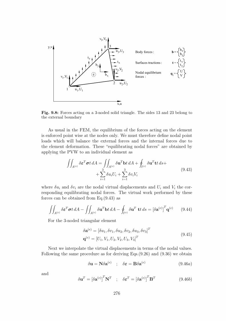
Fig. 9.8: Forces acting on a 3-noded solid triangle. The sides 13 and 23 belong tothe external boundary

As usual in the FEM, the equilibrium of the forces acting on the elementis enforced point wise at the nodes only. We must therefore define nodal pointloads which will balance the external forces and the internal forces due tothe element deformation. These “equilibrating nodal forces” are obtained byapplying the PVW to an individual element as

∫ ∫

A(e)δεT σt dA =

∫ ∫

A(e)δuTbt dA +

∮

l(e)δuT tt ds+

+3∑

i=1

δuiUi +3∑

i=1

δviVi

(9.43)

where δui and δvi are the nodal virtual displacements and Ui and Vi the cor-responding equilibrating nodal forces. The virtual work performed by theseforces can be obtained from Eq.(9.43) as

∫ ∫

A(e)δεT σt dA−

∫ ∫

A(e)δuTbt dA−

∮

l(e)δuT tt ds = [δa(e)]

Tq(e) (9.44)

For the 3-noded triangular element

δa(e) = [δu1, δv1, δu2, δv2, δu3, δv3]T

q(e) = [U1, V1, U2, V2, U3, V3]T

(9.45)

Next we interpolate the virtual displacements in terms of the nodal values.Following the same procedure as for deriving Eqs.(9.26) and (9.36) we obtain

δu = Nδa(e) ; δε = Bδa(e) (9.46a)

andδuT = [δa(e)]

TNT ; δεT = [δa(e)]

TBT (9.46b)

276

Substituting the last equations into Eq.(9.44) gives

[δa(e)]T [∫ ∫

A(e)BT σt dA−

∫ ∫

A(e)NTbt dA−

∮

l(e)NT tt dS

]= [δa(e)]

Tq(e)

(9.47)Since the virtual displacements are arbitrary it is finally deduced that

∫ ∫

A(e)BT σt dA−

∫ ∫

A(e)NTbt dA−

∮

l(e)NT tt ds = q(e) (9.48)

Eq.(9.48) yields the equilibrating nodal forces q(e) in terms of the nodalforces due to the element deformation (first integral), the body forces (secondintegral) and the surface tractions (third integral). Substituting the stressesin terms of the nodal displacements from Eq.(9.42) gives

∫ ∫

A(e)BT (DBa(e) −Dε0 + σ0)t dA−

∫ ∫

A(e)NTbt dA−

∮

l(e)NT tt ds = q(e)

(9.49)and

[∫ ∫

A(e)BTDBt dA

]a(e) −

∫ ∫

A(e)BTDε0t dA +

+∫ ∫

A(e)BT σ0t dA−

∫ ∫

A(e)NTbt dA−

∮

l(e)NT tt dS = q(e)

(9.50)

orK(e)a(e) − f (e) = q(e) (9.51)

where

K(e) =∫ ∫

A(e)BTD Bt dA (9.52)

is the element stiffness matrix, and

f (e) = f (e)ε + f (e)

σ + f(e)b + f

(e)t (9.53)

is the equivalent nodal force vector for the element where

f (e)ε =

∫ ∫

A(e)BT Dε0t dA (9.54)

f (e)σ = −

∫ ∫

A(e)BT σ0t dA (9.55)

f(e)b =

∫ ∫

A(e)NTbt dA (9.56)

f(e)t =

∮

l(e)NT tt ds (9.57)

are the equivalent nodal force vectors due to initial strains, initial stresses,body forces and surface tractions, respectively.

The expressions for the element stiffness matrix and the equivalent nodalforce vectors given by Eqs.(9.52) - (9.57) are completely general and, therefore,

277

they are applicable to any 2D solid element. The particularization of theseexpressions for the 3-noded triangular element is given in the next section.

The global equilibrium equations for the whole mesh are obtained by es-tablishing that the nodes are in equilibrium, similarly as for 1D problems; i.e.the sum of all the equilibrating nodal forces at a node balance the externalpoint loads and ∑

e

q(e)i = pj (9.58)

where pj represents the vector of external point loads acting at node j andthe sum refers to all elements sharing the node. Eq.(9.58) is identical to thatstudied in Chapter 1 for bar structures. The equilibrium equations for thewhole mesh can thus be obtained following identical procedures as explainedfor bar structures. The global equilibrium equation is written in matrix formas

Ka = f (9.59)

where K and f are the global stiffness matrix and the equivalent nodal forcevector for the whole mesh. Both K and f are assembled from the elementcontributions in the standard manner.

We note once more that the equilibrating nodal forces due to the surfacetraction along the element interface cancel themselves out during the assemblyprocess. Therefore, only the surface tractions acting on the external boundariesof the structure must be considered in the analysis.

9.3.5 Stiffness matrix and equivalent nodal force vectors for the 3-noded solid triangular element

Stiffness matrixStiffness matrix

Eq.(9.52) can be written for the 3-noded triangle using (9.37) as

K(e) =∫ ∫

A(e)

BT1

BT2

BT3

D [B1,B2,B3]t dA =

=∫ ∫

A(e)

BT1 DB1 BT

1 DB2 BT1 DB3

. . . BT2 DB2 BT

2 DB3

Sym.. . . BT

3 DB3

t dA (9.60)

A typical element stiffness submatrix, K(e)ij , linking nodes i and j of the

element can be obtained as

K(e)ij =

∫ ∫

A(e)BT

i DBjt dA (9.61)

278

Substituting Eqs.(9.6) and (9.40) into Eq.(9.61) gives

K(e)ij =

∫ ∫

A(e)

1

2A(e)

[bj 0 cj

0 cj bj

]

d11 d12 0d21 d22 00 0 d33

1

2A(e)

bj 00 cj

cj bj

t dA (9.62)

Since the integrand of Eq.(9.62) is constant we can easily obtain

K(e)ij =

( t

4A

)(e) [bibjd11 + cicjd33 bicjd12 + bjcid33

cibjd21 + bicjd33 bibjd33 + cicjd22

](9.63)

The form of K(e)ij for plane stress and plane strain situations is simply ob-

tained by introducing the adequate values of the coefficients dij from Eq.(9.7).

Note that K(e)ij is always symmetrical as d12 = d21.

Equivalent nodal force vectorsEquivalent nodal force vectors

a) Body forces

f(e)b =

∫ ∫

A(e)NTbt dA =

∫ ∫

A(e)

NT1 b

NT2 b

NT3 b

t dA (9.64)

The nodal contribution of vector f(e)b is

f(e)bi

=∫ ∫

A(e)NT

i b t dA (9.65)

If the body forces b are uniformly distributed over the element we obtainusing Eq.(9.33)

fbi=

(At)(e)

3

bxby

(9.66)

i.e. the total force acting over the element is split into equal parts between thethree nodes of the triangle, as expected.

A particular case of body force is self weight with gravity acting in thedirection of the y-axis. In this case bx = 0 and by = −ρg where ρ and g arethe material density and the value of the gravity constant, respectively.

b) Surface loads

f(e)t =

∮

l(e)NT tt ds (9.67)

For a node i belonging to a loaded external boundary we have

f(e)ti =

∮

l(e)NT

i tt ds =∮

l(e)

Ni txNi ty

t ds (9.68)

279

We note that the shape function of a node not belonging to the loadedboundary takes a zero value. Thus, if the element side 1-2 is loaded withuniformly distributed tractions tx and ty, vector f

(e)t is simply

f(e)t =

(l12 t)(e)

2

txtytxty00

(9.69)

where l(e)12 is the side lentgth. Eq.(9.69) shows that the traction force acting

along the element side is distributed into equal parts between the two sidenodes. The expressions of f

(e)t for loaded sides 1-3 and 2-3 are

f(e)t =

(l13t)(e)

2

txty00txty

; f(e)t =

(l23t)(e)

2

00txtytxty

(9.70)

c) Forces due to initial strains

Substituting Eq.(9.37) into (9.54) gives

f (e)ε =

∫ ∫

A(e)BTDε0t dA =

∫ ∫

A(e)

BT1 Dε0

BT2 Dε0

BT3 Dε0

t dA (9.71)

and the equivalent nodal force of node i due to the initial strains is

f (e)εi

=∫ ∫

A(e)BT

i D ε0 t dA (9.72)

If ε0 is constant over the element we obtain using Eqs.(9.6) and (9.40)

f (e)εi

=∫ ∫

A(e)

1

2A(e)

[bi 0 ci

0 ci bi

]

d11 d12 0d21 d22 00 0 d33

ε0x

ε0y

γ0xy

t dA =

=t(e)

2

bi(d11ε

0x + d12ε

0y) + cid33γ

0xy

ci(d21ε0x + d22ε

0y) + bid33γ

0xy

(9.73)

For initial thermal strains, the expressions (9.18) for ε0 should be used.

280

d) Forces due to initial stresses

Substituting Eq.(9.37) into (9.55) gives

f (e)σ = −

∫ ∫

A(e)BT σ0t dA = −

∫ ∫

A(e)

BT1 σ0

BT2 σ0

BT3 σ0

t dA (9.74)

and the equivalent nodal force of node i due to the initial stresses is

f (e)σi

= −∫ ∫

A(e)BT

i σ0t dA (9.75)

For σ0 being constant over the element, we obtain using Eqs.(9.20) and(9.40)

f (e)σi

= −∫ ∫

A(e)

1

2A(e)

[bi 0 ci

0 ci bi

]

σ0x

σ0y

τ 0xy

t dA = −t(e)

2

biσ

0x + ciτ

0xy

ciσ0y + biτ

0xy

(9.76)

The above expressions allow us to compute the matrices and vectors forthe simple 3-noded triangle for 2D elasticity applications. Some comments andexamples showing the behaviour of this element are given in Sections 9.5 and9.6.

An example that illustrates the assembly and solution process is presentedbelow.

Example: 9.4 Analyze the plane structure of the figure below under self weight.

-- Solution-- Solution

Mesh topology

Element Nodal connections

1234

1 4 51 5 22 6 32 6 3

Plane strain situationu1 = u4 = 0

281

The assembly process is similar to that for matrix analysis of bar structures. Theglobal system of equations has the following form

1 2 3 4 5 6

1

2

3

4

5

6

(K(1)11 + K

(2)11 ) K

(2)13 0 K

(1)12 (K

(1)13 + K

(2)12 ) 0

(K(2)33 + K

(3)11 + K

(4)13 0 (K

(2)32 + K

(3)12 ) (K

(3)13 + K

(4)12 )

+K(4)11 )

K(4)33 0 0 K

(4)32

K(1)22 K

(1)23 0

Symm.

(K(1)33 + K

(2)22 + K

(3)23

+K(3)22 )

(K(4)22 + K

(3)33 )

a1

a2

a3

a4

a5

a6

=

r1 + f(1)1 +

f(2)1

(f(2)3 + f

(3)1 +

+f(4)1 )

f(4)3

r4 + f(1)2

(f(1)3 + f

(2)2 +

+f(3)2 )

f(3)3 + f

(4)2

where K(e)ij is obtained from Eq.(9.63) and f (e)

i from Eq.(9.64) with bx = 0 andby = −ρg. In both cases t = 1 should be taken.

The above system can be solved in the usual way by elliminating the rows and columnscorresponding to the prescribed displacements a1 and a4. Once the nodal displace-ments have been obtained the corresponding reactions r1 and r4 can be computed.

Finally, the constant strains and stresses within each element can be found “a poste-riori” from the known nodal displacements by Eqs.(9.36) and (9.41), respectively.

The reader is encouraged to repeat this exercise by him/herself.

9.4 THE FOUR NODED SOLID RECTANGULAR ELEMENT

9.4.1 Basic formulation

The 4-noded solid rectangle is the simplest of the quadrilateral solid elementfamily. This element was developed soon after the 3-noded solid triangle ofthe previous section. However, its irregular behaviour has motivated muchresearch which we will summarize here.

Figure 9.9 shows a deep beam discretized in a mesh of 4-noded rectan-gles. Let us consider an isolated element with the local coordinate system rand s shown in Figure 9.9. The four nodal displacements define a four-termpolynomial interpolation for the displacement field. The simplest interpolationsatisfying the condition of interelement compatibility and geometric invarianceis

u(x, y) = α1 + α2 r + α3 s + α4rs

v(x, y) = α5 + α6r + α7s + α8rs(9.77)

282

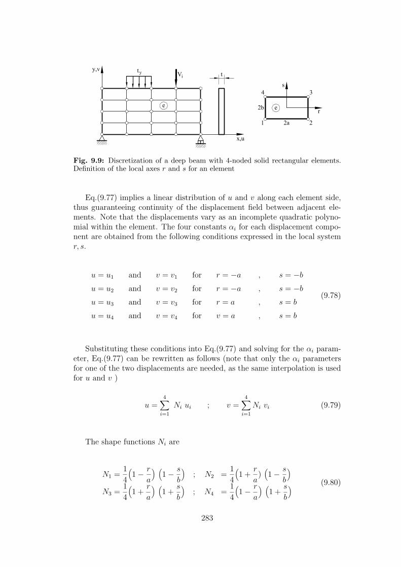
Fig. 9.9: Discretization of a deep beam with 4-noded solid rectangular elements.Definition of the local axes r and s for an element

Eq.(9.77) implies a linear distribution of u and v along each element side,thus guaranteeing continuity of the displacement field between adjacent ele-ments. Note that the displacements vary as an incomplete quadratic polyno-mial within the element. The four constants αi for each displacement compo-nent are obtained from the following conditions expressed in the local systemr, s.

u = u1 and v = v1 for r = −a , s = −b

u = u2 and v = v2 for r = −a , s = −b

u = u3 and v = v3 for r = a , s = b

u = u4 and v = v4 for v = a , s = b

(9.78)

Substituting these conditions into Eq.(9.77) and solving for the αi param-eter, Eq.(9.77) can be rewritten as follows (note that only the αi parametersfor one of the two displacements are needed, as the same interpolation is usedfor u and v )

u =4∑

i=1

Ni ui ; v =4∑

i=1

Ni vi (9.79)

The shape functions Ni are

N1 =1

4

(1− r

a

) (1− s

b

); N2 =

1

4

(1 +

r

a)

(1− s

b

)

N3 =1

4

(1 +

r

a

) (1 +

s

b

); N4 =

1

4

(1− r

a

) (1 +

s

b

) (9.80)

283

Eqs.(9.79) can be rewritten in matrix form as

u =

uv

=

N1 0

... N2 0... N3 0

... N4 0

0 N1... 0 N2

... 0 N3... 0 N4

u1

v1

u2

v2

u3

v3

u4

v4

= N a(e)

(9.81)where

N = [N1,N2,N3,N4] ; Ni =[Ni 00 Ni

]

a(e) =

a(e)1

a(e)2

a(e)3

a(e)4

; a(e)i =

ui

vi

(9.82)

are the shape function matrix and the displacement vector for the element andthe node i, respectively.

The element strain matrix is obtained from Eqs.(9.2) and (9.79) as

ε =4∑

i=1

Bia(e)i = [B1,B2,B3,B4]

a(e)1

a(e)2

a(e)3

a(e)4

= Ba(e) (9.83)

where Bi is given by precisely the same expression (9.40) derived for the 3-noded triangle. For the computation of Bi note that

∂Ni

∂x=

∂Ni

∂rand

∂Ni

∂y=

∂Ni

∂s(9.84)

The expression of the B matrix is shown in Box 4.1.The stiffness matrix and the equivalent nodal force vectors for the element

are obtained via the PVW as previously explained for the linear triangle. Theelement stiffness matrix is

K(e) =∫ ∫

A(e)BT D Bt dr ds =

=∫ ∫

A(e)

BT1 DB1 BT

1 DB2 BT1 DB3 BT

1 DB4

. . . BT2 DB2 BT

2 DB3 BT2 DB4

. . . BT3 DB3 BT

3 DB4

Sym. BT4 DB4

t. dr ds (9.85)

Box 4.1 shows that the strain matrix contains linear terms in r and s.Therefore, the integrand of Eq.(9.85) contains quadratic terms. However, the

284

B =

−b2 0 | b2 0 | b1 0 | −b1 00 −a2 | 0 −a1 | 0 a1 | 0 a2

−a2 b2 | −a1 b2 | a1 b1 | a2 b1

a1 =1

4b(1 +

r

a) , a2 =

1

4b(1− r

a)

b1 =1

4a(1 +

1

b) , b2 =

1

4a(1− 1

b)

K(e) =

2a11 a36 c41 b36 −a14 −a36 c14 b63

2a35 b63 c25 −a36 −a25 b36 c52

2a14 −a36 c14 b36 −a14 a63

2a25 b63 c52 a36 −a52

2a14 a36 c41 b63

Symmetric 2a25 b63 c25

2a11 −b36

2a25

aij = ai + aj , bij = ai − aj , cij = ai − 2aj

a1 =tbd11

6a, a2 =

tad22

6b, a3 =

td12

4, a4 =

tad33

6b, a5 =

tbd33

6a, a6 =

td33

4

Box 9.1 Strain and stiffness matrices for a 4-noded solid rectangular elementof dimensions 2a× 2b

simplicity of the element geometry allows an explicit integration of all terms.The resulting expression for K(e) is also shown in Figure 9.9.

In the same way, the equivalent nodal force vectors for the element areobtained by Eqs.(9.54)-(9.57) using the new expressions for Ni and Bi. It isinteresting that the nodal contributions of a uniformly distributed load overthe element (see Eq.(9.65)) are

f(e)bi

=(tA)(e)

4

bx

by

(9.86)

i.e. the total force is distributed in equal parts between the four nodes, likefor the 3-noded triangle.

Similarly, a uniformly distributed traction acting over a side is distributedin equal parts between the two side nodes.

285

Fig. 9.10: 4-noded solid rectangle subjected to pure bending, a) Initial geometry,b) Element distorsion, c) Correct deformation of a beam segment in pure bending

9.4.2 Some remarks on the behaviour of the 4-noded solid rectangleBoth the 3-noded solid triangle and the 4-noded solid rectangle perform excel-lently in problems where traction (or compression) is important. Conversely,the accuracy of both elements strongly deteriorates in situations where bendingmovements are involved, and very fine meshes are needed to obtain accuratesolutions in these cases (see Section 4.7).

The fact that the 4-noded solid rectangle cannot be used to model bendingdominated fields has a very instructive explanation. Let us consider the be-haviour of an isolated element subjected to pure bending (Figure 9.10). Theexact solution from beam theory is [T6]

u(r, s) =M

EIrs

v(r, s) =Ma2

2EI

(1− r2

a2

)+

Mb2

2EI

(1− s2

b2

) (9.87)

Since the element sides are straight, the 4-noded rectangle can only repre-sent the following bending mode (Figure 9.10)

u = urs ; v = 0 (9.88)

It is obvious from the above that the element cannot correctly reproducethe quadratic distribution of vertical displacements for the pure bending case.This leads to excessive stiffness, which is a natural consequence of the inabilityof the element sides to be curved.

Additionaly it is deduced from Eq.(9.87) that

γxy =∂u

∂y+

∂v

∂x= 0

i.e. the “exact” shear strain vanishes and only normal strains (and stresses)exist.

The shear strain field for the element is obtained from Eq.(9.88) as

γxy = ur (9.89)

286

i.e. the element has an “excess”of shear strain. This introduces an undesirableadditional stiffness which contributes to the poor ability of the element toreproduce bending modes. Similar results are obtained for bending momentsacting on the horizontal sides simply by changing the coordinate r for s inEq.(9.89).

The deficiencies of the 4-noded solid rectangle also show for more irregularquadrilateral shapes. These drawbacks are usually overcome in practice byusing very fine meshes. Other alternatives are possible, however, and some arepresented in the following sections.

Reduced integration of the shear stiffness terms

Eq.(9.89) clearly shows that the shear strain is zero at the element center only.Therefore, the excess of shear strain can be eliminated by sampling the shearstrain at the element center (r = s = 0). This is simply achieved by using areduced one point Gauss quadrature for the shear terms in the stiffness matrix.For this purpose the element stiffness matrix is split into two parts as

K(e) = K(e)a + K(e)

s (9.90)

where K(e)a and K(e)

s include the “axial” and “shear” contributions, respectivelygiven by

K(e)aij

=∫ ∫

A(e)BT

aiDaBaj

t dA ; K(e)sij

=∫ ∫

A(e)BT

siDtBsj

t dA (9.91)

with

Bai=

∂Ni

∂x0

0 ∂Ni

∂y

; Bsi

=[

∂Ni

∂y,

∂Ni

∂x

]

Da =[d11 d12

d12 d22

]; Ds = [ d33 ]

(9.92)

Matrix K(e)a is integrated exactly, either analytically or via a 2×2 Gauss

quadrature, whereas a single integration point is used for K(e)s . This “selected

integration” technique also improves the behaviour of 4-noded quadrilateralsof arbitrary shape.

The reduced integration of K(e)s can also be interpreted as a simple pro-

cedure to mitigate the excessive influence of the shear terms in the elementstiffness matrix. A disadvantage of reduced integration is that it produces aquadrilateral element that is not geometric-invariant (Section 3.10.4), althoughit passes the patch test and, therefore, it converges to the exact solution [3.3,Cook]. In Chapter 7 we will study the application of reduced integration toalleviate the influence of the transverse shear stiffness in Timoshenko beamelements. However, reduced integration of the stiffness matrix terms shouldalways be looked upon with extreme caution, as they can lead to internal

287

Fig. 9.11: Four node rectangle, a) Addition of a central node, b) Shape functionsfor the incompatible modes

mechanisms and to the violation of the patch test in some cases. Reduced in-tegration procedures will be further considered in Chapters 9-12 when dealingwith plates and shells.

Addition of internal modesAddition of internal modes

A method to enhance the flexibility of the 4-noded rectangle is to add to theoriginal interpolation internal displacement modes which vanish at the elementboundaries. The simplest mode is a “bubble”function associated with an extracentral node (Figure 9.11a). The displacement field is expressed as

u =5∑

i=1

Niui ; v =5∑

i=1

N5vi (9.93)

where N1, N2, N3, N4 are the linear functions of (9.80) and

N5 =[1−

(r

a

)2][1−

(s

b

)2](9.94)

The internal d.o.f u5 and v5 (also called hierarchical d.o.f [C23]) can beeliminated after the element stiffness matrix is obtained. Note that u5 and v5

are not absolute displacements and they represent the difference between thetotal displacements of the central node and the bilinear field defined by thefour corner displacements. For instance, the horizontal displacement of thecentral node is given by

u5 = u(0, 0) =

(4∑

i=1

Niui

)

0,0

+ u5 (9.95)

The behaviour of the modified 4-noded solid element can be improved byusing a reduced single point quadrature for the shear terms as described in theprevious section.

Addition of incompatible modesAddition of incompatible modes

The 4-noded rectangle can also be improved by adding to the original displace-

ment field the displacement modes 1 −(

ra

)2and 1 −

(sb

)2which are needed

288

to reproduce the exact solution (9.87) (Figure 9.11b). The new displacementfield is

u =4∑

i=1

Niui +[1−

(r

a

)2]u5 +

[1−

(s

b

)2]u6

v =4∑

i=1

Nivi +[1−

(r

a

)2]v5 +

[1−

(s

b

)2]v6

(9.96)

The additional generalized d.o.f. u5, v5, u6, v6 (also called “nodells” d.o.f.)are internal to each element and can be eliminated by static condensation.However, the displacements along the interelemental boundaries are discon-tinuous and the element is incompatible. Incompatible 4-noded quadrilateralsformulated in this way fail to pass the patch test under constant stress (orconstant strain) states unless they are rectangular.

Fortunately, the element satisfies the patch test for arbitrary quadrilateralshapes if the shear stiffness terms are evaluated using a reduced single pointGauss quadrature, whereas the rest of the stiffness terms can be exactly inte-grated [C15,T3]. The resulting element is geometrically invariant and does nothave spurious mechanisms. Box 9.2 shows the stiffness matrix for an homo-geneous and isotropic element with reduced integration after eliminating theinternal incompatible d.o.f. by static condensation [C15], [F11].

The incompatible modes technique can also be successfully applied to 4-noded quadrilaterals of arbitrary shape. More information can be found in[C15] and [Z6].

Use of an assumed strain fieldUse of an assumed strain field

Another procedure to enhance the performance of the 4-noded quadrilateralis to impose over the element an assumed strain field compatible with thecondition γxy = 0 for the pure bending case.

Dvorkin and Vassolo [D13] have proposed the following assumed strain field

εx = α1 + α2x + α3y ; εy = α4 + α5x + α6y ; γxy = α7 (9.97)

The αi parameters are expressed in terms of the nodal displacements bysampling the assumed strains at a number of element points and equaling theirvalues with those given by the strains deduced from the original displacementfield. This leads to a substitute strain matrix from which the element stiffnessmatrix can be directly obtained. More information on this element can befound in [D13].

9.5 PERFORMANCE OF THE 3-NODED SOLID TRIANGLEAND THE 4-NODED SOLID RECTANGLE

The 3-noded triangle and the 4-noded rectangle perform reasonably well underpure tension or compression dominated situations. In general the 4-noded

289

uv

=

4∑

i=1

Ni

ui

vi

+

[1−

( r

a

)2]

u5

v5

+

[1−

(s

a

)2]

u6

v6

K(e) =D t

12(1− α2)

C1 C5 C2 −C6 C4 −C5 C3 C6

C7 C6 C9 −C5 C10 −C6 C8

C1 −C5 C3 −C6 C4 C5

C7 C6 C8 C5 C10

C1 C5 C2 −C6

Symmetric C7 C6 C9

C1 −C5

C7

Plane stress : D = E ; α = ν

Plane strain : D =E

1− ν2; α =

ν

1− ν

C1 =a

b(−m2 − 1.5m + 5.5) , C4 =

a

b(−m2 + 1.5m− 3.5)

C2 =a

b(m2 − 1.5m− 2.5) , C5 = 1.5 (1 + m)

C3 =a

b(m2 + 1.5m− 0.5m) , C6 = 1.5 (1 + 3m)

C7 − C10 are obtained from C1 − C4 interchanging a by b

Box 9.2 Stiffness matrix for an homogeneous and isotropic four node rectan-gular element of dimensions 2a×2b with incompatible modes

element is more accurate than the 3-noded triangle for the same number ofd.o.f. in these cases (Section 9.6 and Figures 9.12 and 9.13). However, thebehaviour of both elements deteriorates in bending situations. Still, the 4-noded element has a superior performance for such problems. Indeed theaccuracy of the 4-noded rectangle increases substantially by adding the twoincompatible modes as described in Section 9.4.2. Good results for bendingdominated problems can be obtained by using higher order triangular andrectangular elements. A comparison of different triangular and rectangularelement in a bending problem is presented in Section 9.6.

The poorer performance of the 3-noded triangle is compensated by its ver-satility to discretize complex geometries using automatic mesh generators, andso it remains very popular.

The accuracy of both elements increases by using a higher order approxi-

290

Fig. 9.12: Square plate under parabolic traction. Analysis with 3- and 6-nodedtriangles and 4 and 9-noded rectangles

mation for the displacement field. This also allows curved sided elements to bederived using an isoparametric formulation as described in the next chapter.

9.6 GENERAL PERFORMANCE OF TRIANGULAR ANDRECTANGULAR ELEMENTS

Figures 9.12 and 9.13 show two examples which lead us to draw some inter-esting conclusions on the behaviour of rectangular and triangular elements.The first example is the analysis of a square plate under a parabolic tractionacting symmetricaly on two opposite sides. Different meshes of 3 and 6-nodedtriangles and 4 and 9-noded rectangles are used for the analysis. The numer-ical results for the horizontal displacement of the central point on the loadedside show that the 3-noded triangle is the less accurate of all elements stud-ied. Nevertheless 1% error with respect to the “exact” analytical solution isobtained using a fine mesh (Figure 9.12).

The accuracy increases notably for the same number of d.o.f. when 6-noded triangles are used and, even more, when either the 4- or the 8-noded

291

Fig. 9.13: Cantilever deep beam under parabolic edge load (ν = 0.2). Analysiswith 3- and 6-noded triangles, 4- and 9-noded rectangles and the 4-noded rectanglewith two incompatible modes

rectangles are used, as shown in Figure 9.12 [G3], [Y1]. Similarly good resultsare obtained with the 8-noded rectangle.

The second example is a cantilever deep beam under a parabolic edge load(Figure 9.13). The analysis is performed using the same elements as in theprevious example and, in addition, the 4-noded rectangle is enhanced with twoincompatible modes studied in Section 9.4.2. Results plotted in Figure 9.13show clearly the poor accuracy of the 3-noded triangle for bending dominatedproblems. The solution improves slightly for the quadratic triangular element.The 4-noded rectangle has an overstiff behaviour, as expected from its inabilityto reproduce pure bending situations. The solution improves however whenfiner meshes are used. Note the excellent performance of the incompatible4-noded rectangle and also of the 9-noded Lagrange rectangle. Similar goodresults are obtained using the 8-noded quadratic Serendipity rectangle.

These results can be generalized to other situations. Typically, rectanglesare more accurate than triangles for the same number of degrees of freedom.However, triangular elements are more versatile due to their better ability to

292

model complex geometries with unstructured meshes using automatic meshgenerators.

As a rule, low order elements are simpler to use, although finer meshes areneeded in zones where high stress gradients exist. Higher order elements aremore competitive in these regions.

9.7 CONCLUDING REMARKSThis chapter has presented the basic concepts for the analysis of 2D solids withthe FEM. The steps followed in the formulation of the kinematic variables,the strain and stress fields, the equilibrium expression via the PVW and thediscretization process are completely general and will repeatedly appear whenconsidering the finite element analysis of any other structure. The study ofthis chapter is therefore essential as a general introduction to the analysis ofcontinuous structures with the FEM.

The procedure for deriving the element stiffness matrix and the equivalentnodal force vector from the PVW has been detailed. The expressions of thedifferent matrices and vectors have general applicability to any element type.The particular form of these matrices for the 3-noded linear triangle and the4-noded rectangle has been given. The linear triangle has limited accuracy forcoarse meshes although its simplicity and versality make it probably the mostpopular element for practical analysis of 2D solids with arbitrary geometry.The basic 4-noded rectangle has some limitations when it comes to capturingpure bending modes. These defficiencies can be overcome by “ad hoc” proce-dures such as reduced integration, the addition of internal nodes and the useof an assumed strain field.

The derivation of higher order triangular and quadrilateral elements of ar-bitrary shape follows the concept studied in previous chapters for the Poissonequation. The basic ingredients are: a systematic procedure to obtain the shapefunctions, the use of an isoparametric formulation and numerical integration.These topics will be studied in the course on computational structural mecha-nics.

293

294

REFERENCIAS

A1 ABAQUS, Version 4.8, Users Manual, Hibbit, Karlsson and Sorensen Inc., 1989.

A2 Abel, J.F. y Desai, C.S., “Comparison of finite elements for plate bending”,Journal of Structural Divison , ASCE, Vol. 98, ST9, pp. 2143–48, 1972.

A3 ADINA version 5.0 Users Manual. Adina R & D, Massachusetts, USA,Noviembre 1989.

A4 Adini, A. y Clough, R.W., “Analysis of plate bending by the finite elementmethod”, Nat. Sci. Found, G7337, 1961,

A5 Ahmad, S., Irons, B.M. y Zienkiewicz, O.C., “Curved thick shell and membraneelements with particular reference to axisymmetric problems”, Proc. 2nd Conf.Matrix Methods in structural Mech, Air Force Inst. of Technol., Wright–Patterson A.F. Base, Ohio, 1968.

A6 Ahmad, S., “Curved finite elements in the analysis of solid shell and platestructures”, Ph.D. Thesis, Univ. of Wales, Swansea, 1969,

A7 Allman, D.L., “A compatible triangular element including vertex rotations forplane elasticity analysis”, RAE Rep. TR820826 , Farnborough, Hants., 1982.

A8 Alwar, R.S. y Ramachandran, K.N., “Theorical and photoelastic analysis ofthick slabs subjected to highly localised loads”, Building Science, Vol. 7, pp.159–66, 1972.

A9 ANSYS, Users Manual Revision 4.4, Swanson Analysis Systems Inc. 1989.

A10 Argyris, J.H. y Kelsey, S. Energy theorems and structural analysis, Butterworth,1960.

A11 Argyris, J.H., “Matrix dispacement analysis of anisotropic shells by triangularelements”, J. Roy. Aero. Soc., Vol. 69, pp. 801–5, 1965.

A12 Argyris, J.H., Fried, I. y Scharpf, D.W., “The TUBA family of plate elementsfor the matrix displacement method”, Aeronautical Journal of the Royal Aeron.Society, Vol. 72, pp. 701–9, 1968.

A13 Arnold, D.N. y Falk, S.N., “An uniformly accurate finite element method for theMindlin-Reissner plate”, Preprint 307, Inst. for Mathematics and its Applicat.,Univ. of Minnesota, Abril, 1987.

A14 Arnold, D.N. y Falk, R.S., “Edge effects in the Reissner-Mindlin plate theory”,Proc. Symposium an Analytical and Computational Models for Shells, ASME,Winter Annual Meeting, San Francisco, California, Diciembre, 1990.

A15 Arnold, D.N. y Falk, R.S., “The boundary layer for the Reissner-Mindlin plate”

245

a publicarse en SIAM, J. Math., 1991.

A16 Ashwell, D.G., Sabir, A.B. y Roberts, T.M., “Further studies in the applicationof curved finite elements to circular arches”, Int. Journ. Mech. Science, Vol.13, 6, pp. 507–17, 1971.

A17 Ashwell, D.G., “Strain elements with applications to arches, rings and cylindricalshells”, en Finite elements for thin shells and curved members, Eds. D.G.Ashwell y R.H. Gallagher, John Wiley, pp. 91–111, 1976.

A18 Ashwell, D.G. y Gallagher, R.H., (eds.), Finite element method for thin shellsand curved members, J. Wiley, 1976.

A19 Atamaz-Sibai, W. y Hinton, E., “Adaptive mesh refinement with the Morleyplate element”, Proc. of NUMETA 90 Conference, Swansea, Enero 1990, Vol.2, pp. 1049–57, Elsevier Appl. Science, London, 1990.

A20 Atamaz-Sibai, W., Hinton, E. y Selman, A., “Adaptive mesh refinement withthe Mindlin-Reissner elements”, Proc. of 2nd Int. Conf. an Computer AidedAnalysis and Design of Concrete Structures., Zell-an-see, Austria, Abril 1990,Pineridge Press, 1990.

A21 Ayad, R., Batoz, J.L., Dhatt, G. y Katili, I., “A study of recent triangularelements for thin and thick plates”. en European Conf. on New Advances inComputational Structural Mechanics, . P Lavedeze and O.C. Zienkiewicz (Eds.),pp. 471–9, Giens, Abril, 1991.

B1 Baldwin, J.T., Razzaque, A. y Irons, B.M., “Shape functions subroutine for anisoparametric thin plate element”, Int. J. Num. Meth. Engng., Vol. 7, pp. 431,1973.

B2 Bares, R., Tablas para el caculo de placas y vigas pared , Ed. Gustavo Gili,Barcelona, 1964.

B3 Bathe, K.J., “ADINA - A finite element program for automatic dynamicincremental non linear analysis”, Rep. 82448-1, Dept. Mech Engng., MIT,1978.

B4 Bathe, K.J., Finite element procedures in engineering analysis, Prentice Hall,Inc., 1982.

B5 Bathe, K.J. y Dvorkin,E.N., “ A four node plate bending element based onMindlin/Reissner plate theory and mixed interpolation”, Int. J. Numer. Meth.Eng., Vol. 21, pp. 367–383, 1985.

B6 Bathe, K.J. y Dvorkin, E.N., “A formulation of general shell elements. The useof mixed interpolation of tensorial components, Int. J. Meth. Engng. Vol. 22,pp. 697–722, 1986.

B7 Bathe, K.J., Bucalem, M.L. and Brezzi, F., “Displacement and stressconvergence of our MITC plate bending elements”, Eng. Comput., Vol. 7,

246

4, pp. 291–303, 1990.

B8 Batoz, J.L., Bathe, K.J. y Ho, L.W., “A study of three node triangular platebending elements”, Int. J. Num. Meth. Eng., Vol. 15, pp. 1771–812, 1980.

B9 Batoz, J.L., “An explicit formulation for an efficent triangular plate bendingelement”, Int. J. Num. Meth. Engng., Vol. 18, pp. 1077–89, 1982.

B10 Batoz, J.L. y Ben Tahor, M., “Evaluation of a new quadrilateral thin platebending element”, Int. J. Num. Meth. Engng., Vol. 18, pp. 1655–77. 1982.

B11 Batoz, J.L., Lardeur, P.A. “A discrete shear triangular nine dof element for theanalysis of thick to very thin plates”, Int. J. Num. Meth. Engng., Vol. 28, pp.5, 1989.

B12 Batoz, J.L. y Dhatt, G., “ A state of the art on the discrete Kirchhoff platebending elements”, en Calcul des Structures et Intelligence Artificielle, J.M.Fonet, P. Ladeveze y R. Ohayon (Eds.), Ed. Pluralis, 1988.

B13 Batoz, J.L. y Dhatt, G., Modelisation des structures par elements finis, Vol. 1:Solides elastiques, Vol. 2: Poutres et plaques, Hermes, Paris, 1990.

B14 Batoz, J.L. y Katili, I., “A new reliable and efficient discrete shear triangularplate bending element with incompatible modes”, Public. Interna, Univ. deTecnologıa de Compiegne, 1991

B15 Bazeley, G.P., Cheung, Y.K., Irons, B.M. y Zienkiewicz, O.C., “Triangularelements bending-conforming and non conforming solution”, Proc. Conf.Matrix Meth in Struct. Mech., Air Force Inst. of Tech., Wright PattersonA.F. Base, Ohio, 1965.

B16 Bell, K., “ A refined triangular plate bending finite element”, Int. J. Num.Meth. Engng., Vol. 1, pp. 101-22. 1969.

B17 Belytschko T., Tsay C.S. y Liu W.K., “A stabilization matrix for the bi-linearMindlin plate element”, Comp. Methods Appl. Mech. Eng., Vol. 29, pp. 313-327, 1981.

B18 Belytschko, T. y Tsay, C.S., “A stabilization procedure for the quadrilateralplate element with one point quadrature”, Int. J. Num. Meth. Engng., Vol.19, pp. 405–19, 1983.

B19 Belytschko, T., Stolarski, H. y Carpenter, N., “A C0 Triangular plate elementwith one point quadrature”, Int. J. Num. Meth, Engng., Vol. 20, pp. 787–802,1984.

B20 Belytschko, T., Liu, W.H., Shou-Jen Ong, J. y Lam, D., “Implementation andapplication of a 9–node Lagrange shell element with spurious mode control”,Comp. and Struct., Vol. 20, pp. 1–3, 121–8, 1985

B21 Bergan, P.G. y Felippa, C.A., “A triangular membrane element with rotationaldegrees of freedom”, Comp. Meth. Appl. Mech. Engng..

247

B22 Blanco, E., Estudio numerico y experimental de la influencia de distintosparametros en la respuesta de tableros oblıcuos de puentes de seccion transversallosa, Tesis Doctoral, E.T.S. de Ingenieros de Caminos, Univ. Politecnica deCatalunya, 1988.

B23 Bogner, F.K., Fox, R.L. y Schmit, L.A., “The generation of interelementcompatible stiffness and mass matrices by the use of interpolation formulae”,Proc. Conf. Matrix Methods in Struct. Mech., Air Force Inst. of Tech., WrightPatterson A. F. Base, Ohio, 1965.

B24 Bogner, F.K., Fox, R.L. y Schmit, L.A., “ A cylindrical shell discrete element”,AIAA Journal , Vol. 5, 4, pp. 745–50, 1967.

B25 Bonet, J. y Peraire, J., “An alternate digital tree algorithm for geometricsearching and intersection problems”, Int. J. Num. Meth, Engng., Vol. 31,pp. 1–17, 1991.

B26 Brezzi, F., Fortin, M. y Stenberg, R., “Error analysis of mixed interpolatedelements for Reissner-Mindlin plates”, Mathematical Models and Methods inAppl. Sciences, Vol. 1, 2 pp. 125–51, 1991.

B27 Budiansky, B. y Sanders, J.L. Jr., “On the best first order linear shell theory”,Progress in Applied Mech., MacMillan, New York, 1963.

B28 Bugeda, G. Utilizacion de tecnicas de estimacion de error y generacionautomatica de mallas en procesos de optimizacion estructural , Tesis Doctoral,E.T.S. de Ingenieros de Caminos Canales y Puertos de Barcelona, UniversidadPolitecnica de Cataluna, 1990.

B29 Bugeda, G., Oliver, J. y Onate, E., “Utilizacion de tecnicas de control de erroresy generacion automatica de mallas en la optimizacion estructural”, I Congresode Metodos Numericos en Ingenierıa, Las Palmas de Gran Canaria, Junio, 1990,G. Winter y M. Galante, (Eds.), SEMNI, Barcelona, 1990.

B30 Bugeda, G., Oliver, J., “Automatic adaptive remeshing for structural shapeoptimization”, en European Conf. on New Advances in ComputationalStructural Mechanics, P. Ladeveze y O.C. Zienkiewicz (Eds.) pp. 25–33, Giens,Abril, 1991.

B31 Bugeda, G., ‘FLAVIA. Programa para visualizacion grafica en 2 y 3dimensiones”, Publicacion Centro Internacional de Metodos Numericos enIngenierıa, Barcelona, 1992.

C1 Cantin, G. y Clough, R.W., “A curved cylindrical shell finite element”, AIAAJournal , Vol. 6, pp. 1057–62, 1968.

C2 Cantin, G., Loubignac, G. y Touzot, G., “An iterative algorithm to buildcontinous stress and displacement solutions”, Int. J. Num. Meth. Eng., Vol.12, pp. 1493–1506, 1978.

C3 Carpenter, N., Belytschko, T. y Stolarski, H., “Locking and shear scaling factors

248

in C0 bending elements”, Comput. and Struct., Vol. 22, pp. 39–52, 1986.

C4 Carpenter, N., Stolarski, H. y Belytschsko, T., “Improvements in 3 nodetriangular shell elements”, Int. J. Num. Meth. Engng., Vol. 23, pp. 1643–67, 1986.

C5 Casteleiro, M., Onate, E., Huerta, A., Roig, J. y Alonso, E., “Three dimensionalanalysis of no tension materials”, 4th. Int. Conf. on Rock Mech, Melbourne,Australia, 1983.

C6 Cervera, M., Oliver, Herrero, E. y Onate E., “A computational model forprogressive cracking in large dams due to swelling of concrete”, Int. Journalof Fracture, Vol. 35, n1,2,3, pp 573–85, 1990.

C7 Cervera, M., Oliver, J. y Galindo, M., “Simulacion numerica de patologıas enpresas de hormigon”, Monografıa N 4 , Centro Internacional de MetodosNumericos en Ingenierıa, Barcelona, 1991.

C8 Clough, R.W., “The finite element method in plane stress analysis”, Proc. 2ndA.S.C.E. Conf. in Electronic Computation , Pittsburgh, Pa., Sept. 1960.

C9 Clough, R.W. y Tocher, J.L., “Finite element stiffness matrices for analysis ofplates in bending”, Proc. Conf. Matrix Meth. in Struct. Mech, AFIT, Wright-Patterson, Air Force Base, Ohio, pp. 515-45. 1965.

C10 Clough, R.W. y Rashid, Y., “Finite element analysis of axisymmetric solids”,Journal of Engng. Mechanics Division, ASCE, Vol. 91, EMI, pp. 71–85, 1965.

C11 Clough, R.W. y Felippa, C.A., “A refined quadrilateral element for analysis ofplate bending”, Proc. 2d Conf. Mat. Meth. Struct. Mech., AFIT, Wright-Patterson, Air Force Base, Ohio, pp. 399–440, 1968.

C12 Clough, R.W., “Comparison of three dimensional finite elements”, ProceedingsSimposium on Applications of Finite Element Methods in Civil Engineering,Vanderbilt Univ., Nashville, Tenn., (publicado por ASCE), pp. 1–26, 1969.

C13 Clough, R.W. y Wilson, E.L., “Dynamic finite element analysis of arbitrary thinshells”, Comp. and Struct., Vol. 1, pp. 35, 1971.

C14 Connor, J. y Brebbia, C., “A stiffness matrix for a shallow rectangular shellelement”, Journal of Engng. Mech. Div., ASCE, Vol. 93, pp. 43–65, 1967.

C15 Cook, R.D., Malkus, D.S. y Plesha, M.E., , Concepts and application of finiteelement analysis, 4 ed., John Wiley and Sons, 1989.

C16 Courant, R., “Variational methods for the solution of problems of equilibriumand vibration”, Bull. Am. Math. Soc., Vol. 49, pp. 1–23, 1943.

C17 Cowper, G.R., Kosko, E., Lindberg, G.M. y Olson, D.M., “A high precisiontriangular plate bending element”, Report LR–514, National AeronauticalEstablishment , National Research Council of Canada, Ottawa, 1968.

249

C18 Cowper, G.R., Lindberg, G.M. y Olsen, M.D., “ A shallow finite element oftriangular shape”, Int. J. Solids and Struct., Vol. 6, 8, pp. 1133–56, 1970.

C19 Cowper, G.R., “Gaussian quadrature formulae for triangles”, Int. J. Num.Meth. Engng., Vol. 7, pp. 405–8, 1973.

C20 Crisfield, M.A., y Puthli, R.S., “Approximations in the non linear analysis ofthin plate structures”, en Finite elements in non linear mechanics, (Ed. P.Bergan et al.), Vol. 1, Tapir, Trondheim, Noruega, pp. 373–92, 1978.

C21 Crisfield, M.A., “A four-noded thin-plate bending element using shearconstrains. A modified version of Lyon’s element”,Comp. Meth. Appl. Mech.Eng., Vol. 38, pp. 93–120, 1983

C22 Crisfield, M.A., “A quadratic Mindlin element using shear constraints”, Computand Struct., Vol. 18, pp. 833–52, 1984.

C23 Crisfield, M.A., Finite element and solution procedures for structural analysis,Vol. I: Linear analysis, Pineridge Press, 1986.

CH1 Chan, A.S.L. y Firmin, A., “The analysis of cooling towers by the matrix finiteelement method”, Aeronaut. J., Vol. 74, pp. 826–35, 1970.

CH2 Cheung, Y.K., King. I.P. y Zienkiewicz, O.C., “Slab bridges with arbitraryshape and support condition - A general method of analysis based or finiteelements”, Proc. Inst. Civil Engng., Vol. 40, pp. 9–36, 1968.

CH3 Cheung, Y.K., “Finite strip analysis of elastic slabs”, Proc. Am. Soc. CivilEng., Vol. 94, pp. 1365–78, 1968.

CH4 Cheung, Y.K., “The finite strip method in the analysis of elastic plates with twoopposite simple supported ends”, Proc. Inst. Civil Engng, Vol. 40, pp. 1–7,1968

CH5 Cheung, Y.K., “Analysis of box girder bridges by the finite strip method”, Am.Conc. Inst. Public., SP 26, pp. 357–78, 1969.

CH6 Cheung, Y.K., “Folded plate structures by the finite strip method”, Am. Soc.Civil Eng., Vol. 96, pp. 2963–79, 1969.

CH7 Cheung, Y.K., “The analysis of cylindrical orthotropic curved bridge decks”,Pub. Int. Ass. Struct. Engng., Vol. 29, pp. 41–52, 1969.

CH8 Cheung, Y.K., The finite strip method in structural analysis, Pergamon Press,1976.

D1 Dawe, D.J., “Shell analysis using a simple facet element”, J. Strain Analysis,Vol. 7, pp. 266–70, 1972.

D2 Dawe, D.J., “Some higher order elements for arches and shells”, en Finiteelements for thin shells and curved members, (Ed.) D.G. Ashwell y R.H.

250

Gallagher, J. Wiley, pp. 131–53, 1976.

D3 Dawe, D.J., “Curved finite elements for the analysis of shallow and deep arches”,Comput. and Struct., Vol. 4, pp. 559–82, 1979.

D4 Delpak, R., Role of the curved parametric element in linear analysis of thinrotational shells, Ph.D Thesis, Dept. Civil Engineering and Building, ThePolytechnic of Wales, 1975.

D5 Dhatt, G., “Numerical analysis of thin shells by curved triangular elementsbased an discrete Kirchhoff hypothesis”, Proc. ASCE Symp. on Applications ofFEM in Civil Engng., Vanderbilt Univ., Nashville, Tenn., pp. 13–14, 1969.

D6 Dhatt, G., “An efficient triangular shell element”, AIAA J., Vol. 8, pp. 2100-2,1970.

D7 Dhatt, G. y Venkatasubby, S., “Finite element analysis of containment vessels”,Proc. First Conf. an Struct. Mech. in Reactor Tech., Vol. 5, Paper J3/6,Berlin, 1971.

D8 Dill, E.H., “A triangular finite element for thick plates”, ComputationalMechanics Vol. III , S.N. Atluri et al . (eds.), Springer Verlag, 1988.

D9 Donea J. y Lamain, L.G., “A modified representation of transverse shear in C0

quadrilateral plate elements”, Comp. Meth. Appl. Mech. Engng., Vol. 63, pp.183–207, 1987.

D10 Dumavanet, D.A., “High degree efficient symmetrical Gaussian quadrature rulesfor the triangle”, Int. J. Num. Meth. Engng., Vol. 21, Vol. 7, 1985.

D11 Dupuis, G. y Goel, J.J., “A curved finite element for thin elastic shells,”, Int.J. Solids and Struct., Vol. 6, 11, pp. 1413–28, 1970.

D12 Dvorkin, E.N. y Bathe, K.J., “A continuum mechanics based four node shellelement for general non-linear analysis”, Eng. Comp., Vol. 1, pp. 77–88, 1984.

D13 Dvorkin, E.N. y Vassolo, S.I. “A quadrilateral 2D finite element based on mixedinterpolation of tensorial components”, Eng. Comput., Vol. 6, pp. 217–24,1989.

F1 Felippa, C.A. y Bergan, P.G., “A triangular plate bending element based onenergy orthogonal free formulation”, Comp. Meth. Appl. Mech. Engng., Vol.61, pp. 129–60, 1981

F2 FEMGEM/FEMVIEW, The Finite Element Pre and Post–processor, UserManual, Femview Limited, Leicester, U.K., 1991.

F3 Ferrers, N.M., An elementary treatise on trilinear coordinates, the method ofreciprocal polars and the theory of projections, MacMillan , London, 1961.

F4 Flugge, N., Stresses in shells, Springer-Verlag, 1962.

251

F5 Fong, H.M., “Interactive graphics and commercial finite element codes”,Mechanical Engng., 106(6), pp. 18–27, 1989.

F6 Fraeijs de Veubeke, B., “Bending and stretching of plates”, Proc. Conf. MatrixMeth. in Structural Mech., Air Force Inst. of Tech., Wright Patterson, Air ForceBase, Ohio, 1965.

F7 Fraeijs de Veubeke, B., “A conforming finite element for plate bending”, Int. J.Solids and Struct., Vol. 4, pp. 95–108, 1968.

F8 Fried, I. y Yang, S.K., “Triangular nine degrees of freedom C0 plate bendingelement of quadratic accuracy”, Quart. Appl. Math., Vol. 31, pp. 303–312,1973.

F9 Fried, I., “Residual balancing technique in the generation of plate bending finiteelement”, Comput. and Struct., Vol. 4, pp. 771–78, 1974.

F10 Fried, I., “Shear in C0 and C1 plate bending elements”, Int. J. Solids andStruct., Vol. 9, pp. 449–60, 1973.

F11 Froier, M., Nilsson, L. y Samuelsson, A., “The rectangular plane stress elementby Turner, Pian y Wilson”, Int. J. Num. Meth. Engng., Vol. 8, 2, pp. 433–7,1974.

G1 Gallagher, R.H., “The development and evaluation of matrix methods for thinshell structural analysis”, Ph, D. Thesis, State Univ. New York, Buffalo, 1966.

G2 Gallagher, R.H., “Shell elements”, World Conf. on Finite Element Methods inStructural Mech., E1–E35, Bournemouth, Dorset, Inglaterra, Oct., 1975.

G3 Gallagher, R.H., Finite Element Analysis Fundamentals, Prentice–Hall,Englewood Cliffs, N.J., 1975.

G4 Giannini, M. y Miles, G.A., “A curved element approximation in the analysis ofaxisymmetric thin shells”, Int. J. Num. Meth. Eng., Vol. 2, pp. 459–70, 1970.

G5 Gould, P.L., Finite Element Analysis of shells of Revolutions, Pittman Pub.Co., Marsfield, MA, 1985.

G6 Grafton, P.E. y Strome, D.R., “Analysis of axi-symmetric shells by the directstiffness method”, A.I.A.A.J. , Vol. 1, pp. 2342–7, 1963.

H1 Harvey, J.W. y Kelsey, S., “Triangular plate elements with enforced continuity”,A.I.A.A.J., Vol. 9, pp. 1026–6, 1971.

H2 Hearmon, R.F.S., An introduction to applied anisotropic elasticity , Oxford Univ.Press, 1961.

H3 Hinton, E. y Cambell, J.S., “Local and global smoothing of discontinous elementfunctions using a least square method”, Int. J. Num. Meth. Eng., Vol. 8, pp.

252

461–80, 1979.

H4 Hinton, E. y Owen, D.R.J., Finite element programming, Academic Press, 1979.

H5 Hinton, E. y Owen, D.R.J., Introduction to finite element computations,Pineridge Press, 1980.

H6 Hinton, E. y Huang, H.C., “A family of quadrilateral Mindlin plate elementwith substitute shear strain fiels”, Comp. and Struct., Vol. 23, pp. 409–431,1986.

H7 Hinton, E. y Owen, D.R.J., Finite element software for plates and shells,Pineridge Press, 1988.

H8 Hinton, E., Ozakca, M. y Rao, N.V.R., “Adaptive analysis of thin shells usingfacet elements”, Internal Report Civil Engng Dpt., Univ. College of Swansea,CR/950/90, Abril, 1990.

H9 Hooley, R.F y Hibbert, P.D., “Bounding plane stress solutions by finiteelements”, Journal Struct. Division , ASCE, Vol. 92, ST1, pp. 39–48, 1966.

H10 Horrigmoe, G. y Bergan, P.G., “Non linear analysis of free form shells by flatfinite elements”, Comp. Meth. Appl. Mech. Engng., Vol. 16, pp. 11-35, 1979.

H11 Hrenikoff, A., “Solution of problems in elasticity by the framework method”, J.Appl. Mech., Vol. 18, pp. 169–75, 1991.

H12 Huang, H.C. y Hinton, E., “A nine node Lagrangian Mindlin plate element withenhanced shear interpolation”, Engng. Comput.. Vol. 1. pp. 369–79, 1984.

H13 Huang, H.C. y Hinton, E., “Lagrangean and Serendipity plate and shell elementsthrough thick and thin”, in Finite element methods for plate and shell structures,T.J.R. Hughes y E. Hinton (Eds.) Pineridge Press, 1986.

H14 Huang, H.C. y Hinton, E., “A new nine node degenerated shell element withenhanced membrane and shear interpolation”, Int. J. Num. Meth. Eng., Vol.22, pp. 73–92, 1986.

H15 Huang, H.C., Static and dynamic of plates and shells, Springer–Verlag, 1989.

H16 Huerta, A., Casteleiro, M. y Alonso, E., “Non linear numerical analysis of earthdam constructions”, in Numerical Methods for non Linear Problems, C. Taylor,E. Hinton, R. Owen y E. Onate (Eds.), Pineridge Press, 1984.

H17 Hughes, T.J.R., Taylor, R.L. y Kanoknukulchai W. , “A simple and efficientelement for plate bending”, Int. J. Num. Meth. Eng., Vol. 11, pp. 1529–43,1977.

H18 Hughes, T.J.R. y Cohen, M., “The Heterosis finite element for plate bending”,Comput. and Struct., Vol. 9, pp. 445–50, 1978.

253

H19 Hughes, T.J.R., Taylor, R.L., y Tezduyar, T.E., “Finite elements basedupon Mindlin plate theory with particular reference to the four node bilinearisoparametric element”, J. Appl. Mech., Vol. 46, pp. 587–596, 1981.

H20 Hughes, T.J.R. y Taylor, R.L., “The linear triangular plate bending element”,Proc. of 4th MAFELAP Conf., Brunel Univ.,Uxbridge, 1981, (Edited by J.R.Whiteman), pp. 127–42, Academic Press, 1982.

H21 Hughes, T.R.J., “The finite element method. Linear Static and Dynamicanalysis, Prentice Hall, 1987.

I1 I-DEAS, General capabilities, P-0100, Structural Dynamics ResearchCorporation, Milford, Ohio, USA, 1991.

I2 Irons, B.M., “Numerical integration applied to finite element method”, Conf.Use of Digital Computer in Struct. Eng., Univ. Newcastle, 1966.

I3 Irons, B.M., “ Engineering application of numerical integration in stiffnessmethod”, A.I.A.A.J., Vol. 14, pp. 2035–7, 1966.

I4 Irons, B.M., “A conforming quartic triangular element for plate bending”, Int.J. Num. Meth. Engng., Vol. 1, pp. 29–46, 1969.

I5 Irons, B.M. y Razzaque, A., “Experience with the patch test for convergenceof finite element method”, Mathematical Foundations of the Finite ElementMethod , pp. 557–87, (Ed. A.R. Aziz), Academic Press, 1972.

I6 Irons, B.M., “The semiloof shell element”, Finite elements for thin shells andcurved members, Cap. 11, pp. 197–222 (Eds.) D.G. Ashwell y R.H. Gallagher,J. Wiley, 1976.

I7 Irons, B.M. y Ahmad, S., Techniques of finite elements, Ellis Harwood,Chichester, 1980.

J1 Jirousek, J., “A family of variable section curved beam and thick shell ormembrane-stiffening isoparametric elements”, Int. J. Num. Meth. Eng., Vol.17, pp. 171–86, 1981.

J2 Jones, R.E. y Strome, D.R., “Direct stiffness method of analysis of shells ofrevolution using curved elements”, A.I.A.A.J., Vol. 4, pp. 1519–25, 1965.

J3 Jones, R.E. y Strome, D.R., “A survey of analysis of shells by the displacementmethod”, Proc. Conf on Matrix Methods in Struct. Mech., Air Force Inst. ofTech., Wright-Patterson, Air Force Base, Ohio, 1965.

J4 Jordan, F.F., “Stresses and deformations of the thin-walled pressurized torus”,J. Aerospace Science, Vol. 29, pp. 213–25, 1962

J5 Jordan, W.B., “The plane isoparametric structural element, General Electric Co,Report KAPL–M–7112 , Schenectadly, New York, 1970.

K1 Kabir, A.F. y Scordelis, A.C., “CURDI–Computer program for curved bridges

254

and flexible bents”, Internal Report, Dept. Civil Enginering, Univ. ofCalifornia, Berkeley, Septiembre, 1979.

K2 Kantorovitch, L.V. y Krylov, V.I., Approximate methods of higher analysis, J.Wiley, 1958.

K3 Klein, S., A study of the matrix displacement method as applied to shells ofrevolution, Proc. Conf. on Matrix Methods in Struct. Mech., Air Force Inst. ofTech., Wright Patterson Air Force Base, Ohio, Oct. 1965.

K4 Koiter, W.T., “A consistent first approximation in the general theory of thinelastic shells”, First IUTAM Sympos., (Ed. W.T. Koiter), North Holland, Vol.2, 1960.

K5 Kraus, H., Thin elastic shells, J. Wiley, 1967.

L1 Lekhnitskii, S.G., Theory of elasticity of an anisotropic elastic body , HoldenDay, San Francisco, 1963.

L2 Lim, P.T.K., Kilford, J.T. y Moffatt, K.R., “Finite element analysis of curvedbox girder bridges”, en Developments in Bridge Design and Constructions, (Ed.K.C. Rockey et al.), Crosby Lockwood, London, pp. 264–86, 1971.

L3 Livesley, R.K., “Matrix methods in structural analysis”, 2nd ed., PergamonPress, 1975.

L4 Loo, Y.C. y Cusens, Y.A.R., The finite strip method in bridge engineering,Viewpoint, 1978.

L5 Loubignac, B., Cantin, G. and Touzot, G., “Continuous stresses formulation infinite element analysis”, A.I.A.A. J., Vol. 15, pp. 1645–49, 1977.

L6 Lyons, L.P.R., “A general finite element system with special reference to theanalysis of cellular structures”, Ph D. Thesis, Imp. College of Sciene andTechnol., Londres, 1977.

M1 Mackerle, J. y Fredriksson B., Handbook of Finite Element Software, Chartwell-Bratt Ltd., Bromley, U.K., 1990.

M2 MacNeal, R.H., “A simple quadrilateral shell element”, Comp. and Struct., Vol.8, pp. 175–83, 1978.

M3 MacNeal, R.H., y Harder, R.L., “A proposed standard set of problems to testfinite element accuracy”, Finite Elements in Analysis and Design , Vol. 1, pp.3–20, 1985.

M4 Malkus, D.S. y Hughes, T.J.R., “Mixed finite element methods-reduced andselective integration techniques: A unification of concepts”, Comp. Meth. Appl.Mech. Eng., , Vol. 15, pp. 63–81, 1978.

M5 Marguerre, K., “Zur thorie der Gekrummten platte grosser formanderung”,Proc. 5th. Int. Congress Appl. Mech., J. Wiley, Londres, pp. 98–101, 1938.

255

M6 Mc. Henry, D., “A lattice analogy for the solution of plane stress problems”, J.Inst. Civ. Engng., Vol. 21, pp. 59–82, 1943.

M7 Melosh R.J., “A stiffness matrix for the analysis of thin plates in bending”,Journal of Aerosapce Science, Vol. 28, 1, pp. 34–42, 1961.

M8 Melosh, R.J., “ Basis of derivation of matrices for the direct stiffness method”,A.I.A.A.J., Vol. 1, 7, pp. 1631–37, 1963.

M9 Miquel, J., Botello, S., Buil, J. y Onate, E., “La presa boveda de Talvachia.Analisis estatico y dinamico”, Monografıa n 6, Centro Internacional de MetodosNumericos en Ingenierıa, Barcelona, 1991.

M10 Mindlin, R.D., “Influence of rotatory inertia and shear in flexural motions ofisotropic elastic plates”, J. Appl. Mech., Vol. 18, pp. 31–38, 1951.

M11 Moan, T. y Soreide, T., “The analysis of stiffened plates considering non linearmaterial and geometrical behaviour”, World Congress on Finite Elements inStructural Mechanics, (Ed. J. Robinson), Robinson & Assoc., Verwood, pp.14.1–14.28, 1975.

M12 Morley, L.S.D., “The triangular equilibrium element in the solution of platebending problems”, Aero Quart., Vol. 19, pp. 149–69, 1968.

M13 Morley, L.S.D., “On the constant moment plate bending element”, J, StrainAnalysis, Vol. 6, pp. 10–4, 1971.

M14 Morley, L.S.D., “Finite element criteria for some shells”, Int. J. Num. Meth.Engng., Vol. 20, pp. 587–92, 1984.

M15 Morris, A.J., “A deficiency in current finite elements for thin shell aplications”,Int. J. Solids Struct., Vol. 9, pp. 331–45, 1973.

M16 MSC/DYNA, Users Manual Demostration Manual and Theoretical Manual.The McNeal–Schwendler Corporation, Los Angeles, 1989.

N1 Narayanaswani, R. “Dependence of plate bending finite element deflections andeigenvalues on Poisson’s ratio”, A.I.A.A.J., Vol. 12. pp. 1420–21, 1974.

N2 NASTRAN, “Theoretical Manual”, MacNeal, R.H. (Ed.), McNeal–SchwendlerCorp., Los Angeles, 1972.

N3 Nguyen, V.P., “Automatic mesh generation with tetraedon elements”, Int. J.Num. Meth. Engng., Vol. 18, pp. 273–89, 1982.

N4 Noor, A., “Bibliography of books and monographs on finite element technology”,Appl. Mech. Rev., Vol. 44, 6, pp. 307–17, June, 1991.

N5 Novozhilov, V.V., Theory of thin shells., P. Noordhoff, 1959.

N6 Nygard,M.K., The free formulation for non linear finite elements withapplications to shells, Ph. D. Thesis, Univ. Trondheim, Norway, 1986.

256

O1 Oliver, J., “Un sencillo procedimiento para evitar la singularidad de elementosde lamina plana coplanares”, Comunicacion Privada, E.T.S Ing.de Caminos,Barcelona, 1982.

O2 Oliver, J., Cervera, M., Onate, E. y Herrero, E., “A case study of gravity damsubjected to severe internal actions: Description and numerical simulations”,Publicado en Sixth Congress on Large Dams, Commission Internationale desGrands Barrages, San Francisco, C.29, pp. 1387–409, 1988.

O3 Oliver, J., “Modelado de la fisuracion en estructuras de hormigon”, Publicacionde Investigacion PI-3 , Centro Internacional de Metodos Numericos deIngenierıa, Barcelona, 1990.

O4 Onate, E., “Comparisons of finite strip methods for the analysis of box girderbridges”, M. Sc. Thesis, Civil, Eng. Dpt., Univ. College of Swansea, 1976.

O5 Onate, E., Hinton, E. y Glover, N., “Techniques for improving the perfomanceof isoporametric shell elements”, Applied Numerical Modelling, C. Brebbia y E.Alarcon (eds.), Pentech Press, 1979.

O6 Onate, E. y Suarez, B., “The finite strip for the analysis of plate, bridge andaxisymmetric shell problems”, in Finite element software for plate and shellanalysis, E. Hinton y D.R.J. Owen (Eds.), Pineridge Press, Swansea, 1984.

O7 Onate, E. y Suarez, B., “A comparison of the linear, quadratic and cubic Mindlinstrip element for the analysis of thick and thin plates”, Computers and Struct.,Vol. 17, pp. 427–39, 1983.

O8 Onate, E. y Suarez, B., “An unified approach for the analysis of bridges, platesand axisymmeric shells using the linear Mindlin strip element”, Computer andStruct., Vol. 17, 3, pp. 407–26, 1986.

O9 Onate, E., Oliver, J. y Bugeda, G., “Finite element analysis of the nonlinear response of concrete dams subjected to internal loading”, Finite ElementMethods for Non Linear Problems, Europe–US Symposium, Trodheim, Norway,1985, P. Bergan et al. (Eds.), Springer–Verlag, 1985.

O10 Onate, E., Suarez, B. y Zienkiewicz, O.C., “Una metodologıa para obtenerelementos de placa de Reissner-Mindlin basados en campo de deformacionesde cortante impuestas”, Actas del I Congreso sobre Metodos Numericos enIngenierıa, Las Palmas de Gran Canaria, Junio 1990, (Eds.) G. Winter y M.Galante, SEMNI, Barcelona, 1990.

O11 Onate, E., Zienkiewicz, O.C., Suarez, B. y Taylor, R.L., “A methodologyfor deriving shear constrained Reissner-Mindlin plate elements”, Int. JournalNumerical Methods Eng., 1992.

O12 Onate, E. y Castro, J., “Derivation of plate elements based on assumed shearstrain fields” en Recent advances on Computational Structural mechanics”, P.Ladeveze and O.C. Zienkiewicz (Eds.), Elsevier Pub, 1991.

O13 Onate, E., Castro, J. y Kreiner, R., “Error estimation and mesh adaptivity

257

techniques for plate and shell problems”, en The 3rd. International Conferenceon Quality Assurance and Standars in Finite Element Methods, Stratford-upon-Avon, England, 10–12 September, 1991.

O14 Onate, E., y Castro, J., “Adaptive mesh refinement techniques for structuralproblems”, en The Finite Element Method in the 1990’s, A book dedicated toO.C. Zienkiewicz , E. Onate, J. Periaux and A. Samuelsson (Eds.) Springer–Verlag/CIMNE, Barcelona, 1991.

O15 Onate, E. y Castro, J., “Elementos de placa y laminas basados en camposde deformaciones impuestas”, Publicacion del centro Internacional de MetodosNumericos en Ingenierıa, 1991.

O16 Onate, E. “Error estimation and mesh adaptivity techniques for structuraland fluid flow problems”, Publicado en Mecanica Computacional , Vol. XII,S. Idelshon (Ed.), MECOM, Santa Fe, Argentina, 1991.

O17 Onate, E., Castro, J. y Bugeda, G., “Adaptive remeshing strategies forstructural analysis”, A publicarse en Int. J. Num Meth. Engng., 1992.

P1 Palaninathan, R. y Chadrasekharan, P.S., “Curved beam element stiffnessmatrix formulation”, Comp. Struct., Vol. 21, pp. 663–9, 1983.

P2 Pammaer, Z. y Szabo, L., “Stereo decomposition subroutines for threedimensional plotter programs”, Int. J. Num. Meth. Engng., Vol. 17, pp.1571–75, 1981.

P3 Papadopoulus, P. y Taylor, R.L., “A triangular element based on Reissner-Mindlin plate theory”, Int. J. Num. Meth, Engng., Vol. 5, pp. 1029–51, 1990.

P4 Parisch, H., “A critical survey of the 9 noded degenerate shell element withspecial emphasis on thin shell application and reduced integration”, Comp.Meth. Appl. Mech. Engng., Vol. 20, pp. 323–50, 1979.

P5 PATRAN Plus Users Manual, PDA Engineering, PATRAN Division, CostaMesa, California, USA, 1991.

P6 Pawsey, S.E., y Clough, R.W., “Improved numerical integration of thick shellelements”, Int. J. Num. Meth. Engng., Vol. 3, pp. 545–86, 1971.

P7 Peiro, J. A finite element procedure for the solution of the Euler equations onunstructured meshes, Ph.D. Thesis, Civil Eng. Dpt., Univ. College of Swansea,U.K., 1989.

P8 Peraire, J., Vahdati, M., Morgan, K. y Zienkiewicz, O.C., “Adaptive remeshingfor compressible flow computation”, J. Comp. Phys., Vol. 72, pp 449–66, 1987.

P9 Percy, J.H., Pian, T.M.H., Klein, S., y Navaratna, D.R., “Application ofmatrix displacement method to linear elastic analysis of shells of revolution”,A.I.A.A.J., Vol. 3, pp. 2138–45, 1965.

258

P10 Pissanetzky, S., “Kubik: An automatic three dimensional mesh generator”, Int.J. Num. Meth. Engng., Vol. 17, pp. 255–69, 1987.

P11 Popov, E.R., Penzien, J. y Liu, Z.A., “Finite element solution for axisymmetricshells”, Proc. Am. Soc. Civil Eng., EM, pp. 119–45, 1964.

P12 Perruchoud, M. y Frey, F., “How to modelize beams of slab–beam structures ina simple way”, Dpt. Genie Civil, Ecole Polytechnique Federale de Laussanne,Rapport Interne IREM90/3, Abril, 1990.

P13 Pres, W.H., Flannery, B.P., Teukolsky, S.A., Vetterling, W.T., NumericalRecipes. The art of Scientific Computing, Cambridge Univ. Press, 1986.

P14 Przemienieck, J.S., Theory of matrix structural analysis, Mc Graw Hill, NewYork, 1968.

P15 Pugh, E.D.L., Hinton, E. y Zienkiewicz,O.C., “A study of quadrilateral platebending elements with reduced integration”, J. Appl. Mech., Vol. 12, pp. 1059-1079, 1978.

R1 Radau, Journal of Math., Vol. 3, p. 283, 1880.

R2 Ralston, A., Introduccion al analisis numerico, Limusa–Wiley, 1970.

R3 Razzaque, A., Finite Element analysis of plates and shells, Ph.D. Thesis, CivilEng. Dpt, Univ. of Wales, Swansea, 1972.

R4 Reissner,E., “The effect of transverse shear deformation on the bending of elasticplates”, J. Appl. Mech., Vol. 12 pp. 69–76, 1945.

R5 Rosanoff, R.A. y Ginisburg, T.A., “Matrix error analysis for engineers”, Proc.First Conf. on Matrix Meth in Struct. Mech., Wright-Patterson, Air Force B.,Ohio, 1965.

R6 Rosanoff, R.A., Gloudemann, J.F. y Levy, S., “ Numerical conditioning ofstiffness matrix formulations for frame structures”, Proc. Second Conf. onMatrix Meth. in Struct. Mech., Wright–Pattersson, AFB, Ohio, 1968 (AFFDL-TR-68-150. Dec, 1969: AD-703-685 N.T.T.S) pp. 1029–60.

R7 Rossow, M.P. y Chen, K.C., “Computational efficiency of plate elements”,ASCE, 103, St2, pp. 447–51, 1977.

S1 SAMCEF, “User’s manual”, Samtech Ltd., Lieja, Belgica, 1991.

S2 Samuelsson, A., “The global constant strain condition and the patch test”, Ch.3, 46–68, Energy Methods in Finite Element Analysis, (EdS.) R. Glowinski,E.Y. Rodin y O.C. Zienkiewicz, J. Wiley, 1979.

S3 Sanders Jr., J.L. y Liepins, A., “Toroidal membrane under internal pressure”,A.I.A.A.J., Vol. 1, pp. 2105–10, 1963.

S4 Sander, G., “Bornes superieurs et infereures dans l’analyse matricielle desplaques en flexion-torsion”, Bull Soc. Royale des Sc. de Liege, Vol. 33, pp.

259

456–94, 1964.

S5 Selman, A., Hinton, E. y Atamaz–Sibai, W., “Edge effects in Mindlin–Reissnerplates using adaptive mesh refinement”, Internal Report, Civil Engng. Dpt.,Univ. College of Swansea, CR/1948/90, Abril 1990.

S6 Simo, J.C. y Fox, D.D., “On a stress resultant geometrically exact shell model.Part I: Formulations and optimal parametrizations”, Computer Methods inApplied Mech and Engng., Vol. 72, pp. 267–304, 1989.

S7 Simo, J.C., Fox, D.D. y Rifai, M.S., “On a stress resultant geometrically exactshell model. Part II. The linear theory: Computational aspects”, ComputerMethods in Applied Mech and Engng., Vol. 73, pp. 53–92, 1989.

S8 Simo , J.C. y Hughes, T.J.R., “On the variational formulations of assumed strainmethods”, J. Appl. Mech., Vol. 53, 1, pp.51–4, 1986.

S9 Specht, B., “Modified shape function for three noded plate bending elementpassing the patch test”, Int. J. Num. Meth. Engng., Vol. 26, pp. 705–15,1988.

S10 Stanley, G.M., Continuum based shell elements, Ph. D. Thesis, Dpt. Appl.Mechanics, Stanford Univ., 1985.

S11 Stenberg, R. y Vihinen, T, “Calculations with some linear elements for ReissnerMindlin plates”,European Conf. on New advances in Computational StructuralMechanics, . P Lavedeze and O.C. Zienkiewicz (Eds.), pp. 505–11, Giens, Abril,1991

S12 Stolarski, H. y Belytschko, T. “Membrane locking and reduced integration forcurved elements”, J. Appl. Mech., Vol. 49, pp. 172–6. 1982.

S13 Stolarski, H., Belytschko, T., Carpenter, N. y Kennedy, J.M., “A simpletriangular curved shell element”, Eng. Comput., Vol. 1, 3, pp. 210–8, 1984.

S14 Strang, S. y Fix, G.J., An analysis of the finite element method , Prentice Hall,1973.

S15 Stricklin, J.A., Navaratna, D.R. y Pian, T.H.H., “Improvements in the analysisof shells of revolution by matrix displacement method: Curved elements”,A.I.A.A.J., Vol. 4, pp. 2069–72, 1966.

S16 Stricklin, J.A., Haisler, W., Tisdale, P. y Gunderson, R., “A rapidely convergingtriangular plate element”, A.I.A.A.J., Vol. 7, pp. 180-1, 1969.

S17 Suarez, B., La formulacion de bandas finitas de Reissner-Mindlin para analisisde placas, puentes y laminas de revolucion , Tesis Doctoral, E.T.S. de Ingenierosde Caminos, Univ. Politecnica de Catalunya, 1982.

S18 Suarez, B.y Onate, E., “Aplicacion del metodo de la banda finita a estructuraslaminares prismaticos de espesor variable”, Publicacion interna, Centro. Int. deMet. Num. en Ingenierıa, Barcelona, 1992.

260

S19 Suarez, B. y Martel, E., “Analisis de la presa de Santa Coloma por el metodode elementos finitos”, Pub. IT-26, Cent. Int. de Met. Num. en Ing.,Barcelona,1991.

S20 Suarez, B., y Martel, E., “Analisis del edificio de turbinas de una centralhidroelectrica”, Pub. Cent. Int. de Met. Num. en Ing., Barcelona, 1991.

T1 Taig, I.C. y Kerr, R.I., “Some problems in the discrete element representationof aircraft structures”, en Matrix Methods of Structural Analysis, (Ed. B.M.Fraeijs de Veubeke), Pergamon Press, 1964.

T2 Taig, O.C., Structural analysis by the matrix displacement method , ElectricAviation report, No. 5017, 1961.

T3 Taylor, R.L., Beresford, P.J. y Wilson, E.L., “A non conforming element forstress analysis”, Int. J. Num. Meth. Engng., Vol. 10, pp. 1211-20, 1976.

T4 Taylor,R.L., Zienkiewcz,O.C., Simo,J.C. y Chan,A.H.C., “The patch test - Acondition for assesing FEM convergence”, Int. J. Numer. Meth. Eng., Vol. 22,pp. 32–62, 1986.

T5 Tessler, A. y Hughes, T.J.R., “An improved treatement of transverse shear inthe Mindlin type four quadrilateral element”, Comp. Meth. in Appl. Mech.and Engng., Vol. 39, pp. 311–35, 1983.

T6 Timoshenko, S.P. y Goodier, J.N., Teorıa de la elasticidad , Edic. Urmo, 1968.

T7 Timoshenko, S.P., Resistencia de Materiales, Partes I y II , Espasa-Calpe, 1970.

T8 Timoshenko S.P. y Woinowsky-Krieger S., Teorıa de Placas y Laminas,Ediciones Urmo, Bilbao, 1970.

T9 Timoshenko, S.P., y Young, D.M., Theory of Structures, 2d Edition. McGrawHill, 1965.

T10 Timoshenko, S.P. y Gere, J.H., Mecanica de Materiales, Union TipograficaEditorial Hispano–Americana, 1974.

T11 Tocher, J.L., Analysis of plates using triangular elements, Ph. D. Thesis, Dept.of Civil Engineering, University of California at Berkeley, 1962.

T12 Turner, M.J., Clough, R.W., Martin, H. y Topp, L.J., “Stiffness and deflectionanalysis of complex structures”, J. Aeron. Sci., Vol. 23, pp. 805–23, 1956.

T13 Tocher, J.L., y Kapur. K.K., “Comment on basis for derivation of matrices forthe direct stiffness method”, A.I.A.A.J., Vol. 6, pp. 1215–16, 1965.

V1 Vlasov, V.Z., General theory of shells and its application to engineering, NASATTF-99 , 1964.

W1 Washizu, K., Variational methods in elasticity and plasticity , Pergamon Press,1975.

261

W2 Weaver, W. (Jr.) y Johnston, P.R., Finite elements for structural analysis,Prentice Hall, 1984.

W3 Wempner, G.A., “Finite elements, finite rotations and small strains of finiteshells”, Int. J. Solids Struct., Vol. 5, pp. 117–53, 1964.

W4 Wempner, G.A., Oden, J.T. y Kross, D.A., “Finite elements analysis of thinshells”, Eng. Mech. Div. Proc. ASCE , Vol. 94, (EMS), pp. 1273–94, 1968.

W5 Wilson, E.L., “Structural analysis of axisymmetric solids”, A.I.A.A.J., Vol. 3,pp. 2269–74, 1965.

W6 Wilson, E.L., Taylor, R.L., Doherty, W.P. y Ghabussi, T., “Incompatibledisplacement models” en Numerical and Computer Methods in StructuralMechanics, (Eds.) S.T, Fenves, et al., Academic Press, 1973.

W7 Wilson, E.L., “Finite elements for foundations, joints and fluids”, Proc. Conf.on Numerical Methods in Soil and Rock Mechanics, Univ. of Kalsruhe, J. Wiley,1977.

W8 Willam, K.J. y Scordelis, A.C., “Cellular structures of arbitrary plan geometry”,J. Struct. Div., ASCE, pp. 1377-442, 1972.

W9 Wood, R.D., The application of finite element methods to geometrically nonlinear analysis, Ph. D. Thesis, Univ. of Wales, Swansea, 1973.

W10 Wood, R.D. y Zienkiewicz, O.C., “Geometrically non linear finite elementanalysis of beams, frames, arches and axisymmetric shells”, Comp. Struct.,Vol. 7, pp. 725–35, 1977.

W11 Wong, C.C.K. y Vardy, A.E., “Finite prism analysis of plates and shells”, Int.Journ. Num. Meth. Engng., Vol. 21, pp. 529–41, 1985.

Y1 Yang, T.Y., Finite Element Structural Analysis, Prentice Hall, 1986.

Z1 Zienkiewicz, O.C. y Cheung, Y.K., “The finite element method for analysis ofelastic isotropic and isotropic slabs”, Proc. Inst. Civ. Engng., Vol. 28, pp.471–88. 1964.

Z2 Zienkiewicz, O.C., Kalliappan, S, y King, I.P., “Stress analysis of rock as a notension material”, Geotechnique, Vol. 18, PP. 56, 1968.

Z3 Zienkiewicz, O.C., Too, J. y Taylor,R.L., “Reduced integration techniques ingeneral analysis of plates and shells”, Int. J. Num. Meth. Eng., Vol. 3, pp.275–90, 1971.

Z4 Zienkiewicz, O.C. y Too, J. “The finite element prism in analysis of thick simplysupported bridges”, Proc. Inst. Civ. Eng., Vol. 53, pp. 147–72, 1972.

Z5 Zienkiewicz, O.C., Bauer, J., Morgan, K. y Onate, E., “A simple and efficientshell element for axisymmetric shells”, Int. J. Num. Meth. Engng., Vol. 11,

262

pp. 1545–1559, 1977.

Z6 Zienkiewicz, O.C., El Metodo de los Elementos Finitos, 3era Edicion, Ed.Reverte, Barcelona, 1979.

Z7 Zienkiewicz, O.C. y Morgan, K., Finite Elements and Approximations, Ed. J.Wiley, 1980.

Z8 Zienkiewcz, O.C., Qu, S., Taylor, R.L. y Nakazawa,S., “The Patch test for mixedformulations”, Int. J. Num. Meth. Eng., Vol. 23, pp. 1873–1883, 1986.

Z9 Zienkiewicz, O.C. y Lefebvre, D., “Three field mixed approximation and theplate bending problem”, Comm. Appl. Numer. Meth., Vol. 3, pp. 301–9, 1987.

Z10 Zienkiewicz, O.C. y Zhu, J.Z., “A simple error estimator an adaptive procedurefor practical engineering analysis”, Int. J. Num. Meth. Engng., Vol. 24, pp.337–57, 1987.

Z11 Zienkiewicz, O.C. y Lefebvre, D., “ A robust triangular plate bending elementof the Reissner-Mindlin type”, Int. J. Num. Meth. Eng., Vol. 26, pp. 1169-84,1988.

Z12 Zienkiewicz, O.C. and Zhu, J.Z. “Error estimates and adaptive refinement forplate bending problems”, Int. J. Num. Meth. Engng,, Vol. 28, pp. 2839–543,1989.

Z13 Zienkiewicz, O.C. y Zhu, J.Z., “The three R′s of engineering analysis and errorestimation and adaptivity”, Comp. Meth. in Appl. Mech and Enegng.,Vol. 82,pp. 95–113, 1990.

Z14 Zienkiewicz, O.C., Taylor, R.L., Papadopoulus P. y Onate, E., “Plate bendingelements with discrete constraints: New Triangular Elements”, Computer andStruct., Vol. 35, pp, 4, 505–2, 1990.

Z15 Zienkiewicz, O.C. y Taylor, R.L. The Finite Element Method , 4a. Ed., Mc GrawHill, Vol. I, 1989, Vol. II, 1991.

Z16 Zienkiewicz, O.C. y Zhu, J.Z. “Superconvergent derivative recovery techniquesand a posteriori error estimations in the finite element method. Part I: A Generalsuperconvergent recovery technique”, Internal report CR/671/91, Univ. Collegeof Swansea, U.K., 1991, A publicarse en Int. J. Num. Meth. Engng.

Z17 Zienkiewicz, O.C. y Zhu, J.Z., “Superconvergent derivative recovery techniquesand a posteriori error estimations in the finite element method. Part II: TheZienkiewicz-Zhu a posteriori error estimator”, Internal report CR/672/91, Univ.College of Swansea, U.K., 1991. A publicarse en Int. J. Meth. Engng..

263