ht. 1. Engns Sci. Vol. 30, No. 5, pp. 611429, 1992 0020-7225192 $5.00 + O.iwf Printed in Great Britain. All rights reserved Copyright @ 1992 Pergamon Press plc

SIMILARITY SOLUTIONS OF BOUNDARY LAYER EQUATIONS FOR SECOND ORDER FLUIDS

M. PAKDEMIRLI Bogazid University, Faculty of Science, Department of Mathematics, PK2 Bebek, Istanbul, Turkey

E. S. SUHUBi Istanbul Technical University, Faculty of Science, Maslak 80626, Istanbul, Turkey

Abstract-In a previous paper [Znr. J. Engng Sci. 30, 523 (1!492)] boundary layer equations for second order fluids are derived. The general isovector fields for these equations are found by using exterior calculus. From the four independent isovectors only one provides useful solutions which is a scaling transformation. Using this isovector, the ordinary differential equations leading to the similarity solutions are found. The numerical solution of the equations are presented and the profile corresponding to the solution is discussed. The shear stress of the similarity solution is also calculated.

1. INTRODUCTION

The derivation of symmetry groups of partial differential equations employing exterior calculus are first discussed in a seminal paper by Harrison and Estabrook [2]. This study is based on Cartan’s geometric fo~ulation of partial differential equations in terms of exterior differential forms [3]. The analysis has been further exploited by Edelen [4,5] where a systematic approach for finding isovector fields of second order balance equations are also presented. The work has been generalised to balance equations of arbitrary order with arbitrary number of dependent and independent variables by @hubi 161. The formalism given in [6] is borrowed here to find the general isovector fields of the boundary layer equation which is essentially a third order balance equation. The advantage in using directly the results of [6] is that it makes great simplification in the calculations and the isovector fields are obtained by just manipulating the indicial equations without even considering the relevant forms. It is seen that only one isovector field leads to a nontrivial symmetry group of transformation which is none other than the scaling transformation. The simila~ty solution corresponding to this group may then be obtained as a group invariant solution and the ordinary differential equations in similarity variable leading to the similarity solution is found by using the particular isovector field generating that group. An analytical solution in power series valid at the near neighbourhood of zero is developed. However this series solution does not solve the actual problem, since it is not possible to satisfy the boundary conditions at infinity. But it provides valuable information about admissible initial conditions for smooth solutions. With the aid of this information the problem is expressed as an initial value problem and shooting method is used. For our problem initial value methods fail to produce results converging to the solutions and finite difference method is then used to numerically integrate the equations. The profiles as well as the shear stress corresponding to the solution are also discussed.

2. EQUATIONS DETERMINING ISOVECTOR FIELDS

To employ the formalism given in [6] we have to write the boundary layer equations (i.e. equation (4.22) and (4.23) in [l]) in the form of a balance equation. The balance equations of the third order can be written as follows

alP -+zz”=o axi (2.1)

611

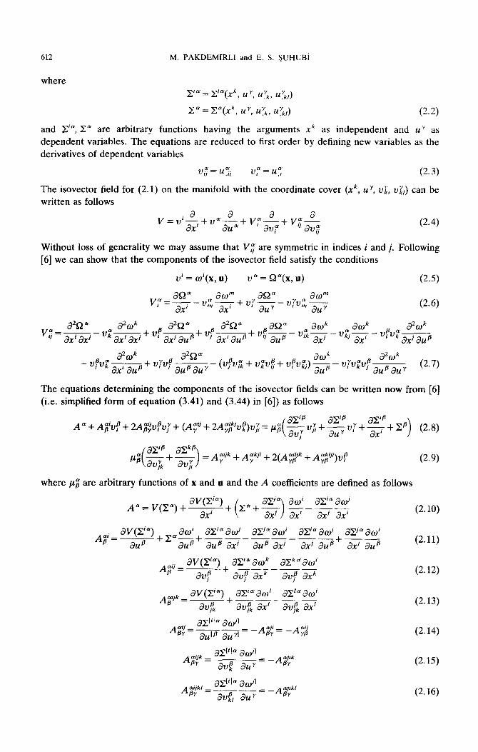
612 M. PAKDEMIRLI and E. S. SUHUBi

where

Y”= P(Xk, uy, UYk, uI;i,)

Z” = Y(Xk, uy, uy/,, UL,) (2.2)

and Zig Z” are arbitrary functions having the arguments xk as independent and uy as dependent variables. The equations are reduced to first order by defining new variables as the derivatives of dependent variables

v,? = uzi up = uf: (2.3)

The isovector field for (2.1) on the manifold with the coordinate cover (xk, u y, vi, vkyJ can be written as follows

(2.4)

Without loss of generality we may assume that VF are symmetric in indices i and j. Following [6] we can show that the components of the isovector field satisfy the conditions

vi = w’(x, II) vo= sP(X, u) (2.5)

vp=dn”_vq~+v~E$_vjv~!g ax’ Y (2.6)

a2wk a2&D 7+ v,s- axi ax? ax’ au B

a2Wk y @ d2s2” - v$J;~au+ V4J~

dWk d2Wk ~- ’ ’ aupauy (viva + v;v$ + viva) - -

dUfi vy?J~v~ ___ (2.7)

duo dUY

The equations determining the components of the isovector fields can be written now from (61 (i.e. simplified form of equation (3.41) and (3.44) in [6]) as follows

(2.9)

where @ are arbitrary functions of x and u and the A coefficients are defined as follows

A”= V(F) + av(P)

axi (2.10)

Ati = av(F) + z” ad I aPad acia awi a9 awi aP ad B

---- ---- -_ ad ad ad ad ad axi ad ad

+ ad ad (2.11)

(2.12)

(2.13)

(2.14)

(2.15)

aP ad ---

a$ axk

aP ad -- av$ ai

a-$il~ awjl A;;=--=

adfi ad -A;$ = -A;$

(2.16)

Similarity solutions of boundary layer equations for second order fluids 613

where for a scalar function f(x’, u *, vi”, Vi3

(2.17)

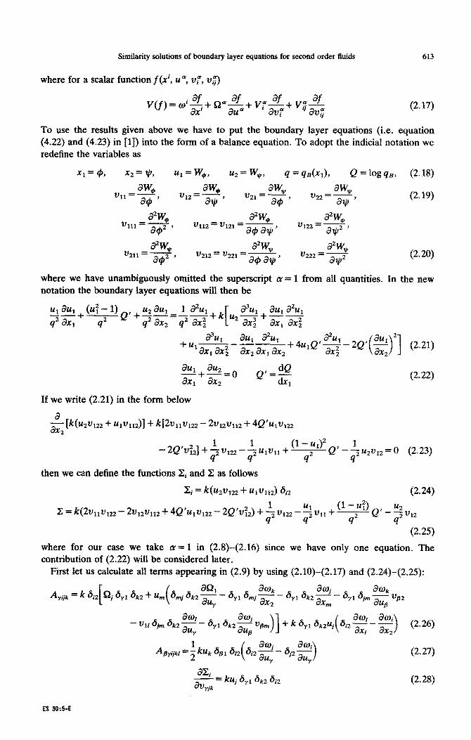
To use the results given above we have to put the boundary layer equations (i.e. equation (4.22) and (4.23) in [l]) into the form of a balance equation. To adopt the indicial notation we redefine the variables as

x1 = 4, x2= 3, 4 = JQ, u2 = w,, 4 = 4L4-4, Q = log qe, (2.18)

V aw, ll=atg’

3% aw, -3 viz=~* v21=atp’ %2- allr ,

a”% v11’=dQ12’

a’h vu2 = VI21 = -

i3'W@ --

ww v122 - w2 ’

$5 -- 21211 - a#2 ’

a”\ v212= w221=-

EJ'W, --

alar' v222- a+Q2

(2.19)

(2.20)

where we have unambiguously omitted the superscript cx = 1 from all quantities. In the new notation the boundary layer equations will then be

$4 au, a%, +u,----

ax1 ax; ax2 ax1 ax2 2Q’(zr2] (2.21)

(2.22)

If we write (2.21) in the form below

g Mu2v122 + UIVII~)]+ kPvl~v122- 2v12v112+ 4Q’ulv122

1 -2e’utl+~v,,-~~~v,,+

4 (’ - u1)2 Q’ - + ~~21,~ = 0

q2 9 (2.23)

then we can define the functions Xi and Z as follows

& = k(“2v122 + u1v112) 6i2 (2.24)

X = k(2v,,vm - 2V,,vit2 + 4Q?i1vIn - ~Q?.J:~) + 4 v,~ - 2v11 + 4 4

where for our case we take CY = 1 in (2.8)-(2.16) since we have only one equation. The contribution of (2.22) will be considered later.

First let us calculate all terms appearing in (2.9) by using (2.10)-(2.17) and (2.24)-(2.25):

(2.27)

(2.28)

ES SCM-E

614 M. PAKDEMIRLI and E. S. ?$JHUBi

Inserting (2.26)-(2.28) into (2.9) we finally obtain

(2.29) involves 16 equations some being identities and some come out to be exactly the same equations. The linearly independent equations are the following four equations

~+53v12+322=o 2 au, 2

as21 am, am, --v --v au2 ‘1 au,

-0 12z-

aa, am, amI - UlVll K - u2v12 du, - u2v22 z

(2.30)

(2.31)

(2.32)

~~~~~~~~~~~~~~~~~~~~~~~~~~~ 1 2 1 1

- 2u, 2 2122 - UlV11 do, aa2 amI am, --u,-v,,+u2-v2~+u2- au, au2 au2 ax,

(2.33) 2

Equation (2.30) is a polynomial in terms of v12 and v22 hence the coefficients should vanish

leading to the result

01 = %(X1) (2.34)

Similarly, equation (2.31) is a polynomial in terms of v ii and v12 and using the same argument

we conclude that

02 = ~2h x29 4 (2.35)

Q1 = Q,(x,, x2, Ul) (2.36)

Using (2.34)-(2.36) in (2.32) and (2.33) the equations simplify leading to

02 = ~2h x2) (2.37)

The above results are summarized as follows

ml= @lh) (2.38)

02 = %(X1, x2) (2.39)

0, = Q,(-% x2, 4 (2.40)

Similarity solutions of boundary layer equations for second order fluids

It can be easily shown that equation (2.22) puts a restriction

v,, f V**=O

on the isovector components leading to the equation

and this equation further separates into three equations

3Q,+3Q2_0

dxt -ig-

aw,+aQ2=Q -- -

ax, alcz

awl + asEll ai102 aa2 -- au’=---=0

ah 1 2 au2

Let us now cakulate a11 terms appearing in (2.8)

615

(2.41)

(2.42)

(2.43)

(2.441

(2.45)

(2.45)

(2.47)

(2.48)

(2.49)

616 M. PAKDEMIRLI and E. S. $UHUBi

X ( -2k~12 6i, + ( 2kv,, + 4kQ’ul f $) ai,) +k[zvlg2

a%, +u, --

(

a302 + v a%, a3sz, ~

‘12 ax, a_& ~

ax, ax: Irn au, a$ +fz112

au, ax, ax2

+ Vlm2

a2Ql a2W2 a2W2 -- hn2ax:-”

aQ

au, ax2 lz2 ax, ax2 + VlmVl2

au: ax2 )I + 2 Wvttcz - 2vtzw2 + 4Q’utvtzz - 2Q’(vtJ2)

I

+ -$ (~122 - uivll+ (I- u:>Q’ - ~2~12) I

(2.55)

Note that in obtaining (2.51)-(2.55) we have used (2.38)-(2.41). Inserting now (2.49)-(2.55) into (2.8) and making some rearrangements we obtain the equation

s+z-$ k v,~v~~~- v12v112 + ~Q’UIVIZZ - ~Q’(JJIz)’ Ul 1 2 I ( >

1 + -_t

4 ( ~122 - ul~ll+ (I- d>Q - 4~12 >I 4Q”Ulvlzz -~Q”(v~~)‘) - 2f (v,, - ulvll + (1 - u;‘)Q’

- uzv12 + (1 - u:> f$ 1 ( + Q, 4kQ’vnz

- P,y+ 2kvlz2 ax 3-2kv v %+2kv v afa

1 lz2 l1 ax, l1 lZ2dU1

4 aa1 __- +ql d”‘+ aW aSt t5V12-LuIV11~ 42 ax, 42 ax, q axI 42 au,

-2kv,,2~+kv,,2v,2~-4kQ’v,2~ 2 2 2

+4kQ’(v12)2~-4kQf(vl~)2~-~3+~vl~~ 2 1 4 ax2 4 2

u2 --V

$81 $02

4 2 12~-2kv~~--

1 axI ax2 + khzJ2~

1 2

Similarity solutions of boundary layer equations for second order fluids 617

ulvll + (1 - c&j’ - ~2~12) + k z ~112 + $+ 21122 2 2

+u a3Q1 a302 a3q

--

* ax1 ax; u1v12 ax1 a~; + k?Jll -++u1vp_ PQ*

au, a~$ au1 ax1 ax2

+ UlVl12 a-1 a202

--UlVll2 ax", $02

+ UlVll~lZ a3SZl

--

au, ax2 u*v*22 ax, ax2 au: ax2

a3q +u2--

a2m2

ax; W2’12 ax; --+~U~~I~~+U~V,,~ 12 12

- 2u2%2 d2W2 -Tg- f u2(%2)2 g$ + (v**v*a

2 12 ( 2+$ 1 2 >

- ~12~112 + Wulv122- 2Q’(G2) + VU? ~122 + ~223~122~ 1 2

a2Q1 2 8% + VI2 ax1 3x2 3- pf22v12 -$-!&+ 12 eJ12,'&- 11

am2 %2Vl22ax,

+u1v12v11 2% x+

12

ul(v12)25-pTg+ a-1 11

wl2vll2~ -1 1

d3Ql 3

+ wJll(~12)2~+2~2(V12)2~ #Ql

+ u22f12u122- 1 12 &A:

$Q, + u2(v12)3Yj--p-

do2 a2QJ2 + UlVl12

@Ql

1 v22v122ax,- w122axl ax2

du, ax2

+ Ul~l22 a28, 62%

au, ax, + vwm~ + U1~112fl22 aQ1 a2m2 --

au: u2vm ax”,

$Q* +2u2v122-----

#Ql au1 ax2

+2u2v*2v122--- au: I

(2.56)

Equation (2.56) can be considered a polynomial equation in terms of the variables vsi and 2/sij. In order to satisfy it identically the following relations should hold

((v12)3): gJ=o

a381 + dz~, ~~~~~ (q2v*1): 2ul------ ---

3~; ax2 au, ax2 3~;

(2.57)

(2.58)

618 M. PAKDEMIRLI and E. S. SUHUBi

(2.600)

(2.61)

(2.62)

(2.63)

(2.65)

(2.67)

-k~-2kQ’~+k~-2kQ’~-2kQ”m,+2kQt~=0 (2.68)

3. SOLUTION OF ISOVECTQR FIELD EQUATIONS

Equations (2.38)-(2.43), (2.46)-(2.48), (2.57)-(2.68) are bear partial ~ffer~~tia~ equations

of order three having four unknowns ml, wz, S& and SJ2 which are certain components of iscmector fields and aIs0 an arbitrary function q = &x1). Therefore the equations will determine the four unknowns and the structure of the arbitrary function.

Similarity solutions of boundary layer equations for second order fluids 619

Keeping in mind the restrictions (2.38)-(2.41) we begin solving Differentiating (2.47) with respect to u1 and u2 we obtain

the equations.

33-h =o

au, au, -_.

au:

Equations (2.46) and (2.48) are differentiated with respect to u2 yielding

a2Q2 -=

o a2Q2 o

ax2 au, -= au:

Equations (3.1) and (3.2) then yield the result

512 = Wl)UZ + Wl, x2)4 + F(x,, x2)

If (2.48) is differentiated with respect to u1

$81 o q=

or

Ql= G(x,, x2)4 + H(xl, x2)

(3.1)

(3.2)

(3.3)

(3.4)

(3.5)

If we now substitute (3.3) and (3.5) into (2.42) and (2.43) and eliminate p between them we obtain a polynomial in terms of ul, u2 and requiring that the coefficients should vanish we see that F and H vanishes and E and G can be written as follows

E(x,, x2) = $ WI, x2) = WI) - (3.6) 1

do2+$ ax

2 1

Ql= G(xl, x2)4 (3.7)

Q2 = Wl)u, + &I, x2)4 (3.8)

Equation (2.57) is then satisfied identically and substituting the results so found into (2.58) we find

G(x,, x2) =%+Z(x1) (3.9) 2

Inserting (3.9) into (3.6)2 and differentiating with respect to x2 we see that second derivative of o2 with respect to x2 vanishes or

02 = Cl(Xl)X2 f C2(Xl) (3.10)

If (3.10) is inserted into (3.9) we see that G depends on only x1 hence

Q, = G(x& (3.11)

Equations (2.60) and (2.61) are then satisfied identically. From equation (2.62) the following equation is derived

G(x,) - D(xl) + cl(xl) = $ (3.12) 1

Equation (2.63) supplies no new information whereas from (2.64) we obtain

ck) 01=- Q’

From (2.65) the following results are found

(3.13)

G(x,) = 9 I

c;=2& 4

(3.14)

620 M. PAKDEMIRLI and E. S. !$JHUBi

Inserting the results obtained into the equation (2.68) we obtain (3.14)? again. From (2.66) we obtain

I c; = 3c, 4

4‘ (3.15)

Comparing (3.14)2 and (3.15) we conclude that either q ’ = 0 or c3 = 0. The two cases will be considered separately.

(i) q =const.

The results up to this point are summarized as follows

01 = WI(XJ (3.16)

w2 = Ci(XI)% + c&1) (3.17)

Qi = Gui (3.18)

Q* = W&Z + E(x,, @I (3.19)

E(x, > x2) = 4 (3.20)

G - D(xl) + q(x,) = 2 1

G=cj q2

(3.21)

(3.22)

Using these results, it follows from (2.64) that ci(x,) = 0 and (2.65) is satisfied identically. Finally (2.66) leads to

o,=Gxl+H (3.23)

and from (3.21) D(x,) = 0. The remaining equations are satisfied identically and the final results for the case q = const. are as follows

o,=Gxi+H (3.24)

02 = c2(4 (3.25)

8, = Gul (3.26)

Q2 = 4(-m* (3.27)

(ii) c3 = 0

For this case c1 is const. from (3.15) and summarizing the results so far obtained we have

Cl 0, =-y

Q (3.28)

w2 = ClX2 + c2h) (3.29)

S&=0 (3.30)

Q2 = we2 + c;(~lb* (3.31)

From (2.66) we obtain for this case

q”q +q’2=0 (3.32)

Integrating (3.32) we find that

q = a(& + by (3.33)

where b can be taken as zero without loss of generality. From (2.67) we obtain the relation

D = -cl (3.34)

Similarity solutions of boundary layer equations for second order fluids 621

Therefore the final results for this case turns out to be with b = 0

4 = &)‘” (3.35)

w1= 2ciXl (3.36)

w2 = cix.2 (3.37)

s&=0 (3.38)

522 = -ciu2 (3.39)

The linearly independent isovectors will then be

(Vi) oi= 1. 02=0, s&=0, !&=o, q = const. (3.40)

(v,) 01 = Xl, o*=o, s-4=4, Q2=0, q = const. (3.41)

V-3) l&=0, 02 = G(Xl)> c&=0, Q* = c;wu1, q = const. (3.42)

(W al= 2% 02=x2, s&=0, Q2 = u21 q = a(Xp (3.43)

Let us now examine the isovectors. First isovector is a coordinate transformation in $ direction for q = const. or parallel flat plate case. Therefore supplies no new information. Second isovector makes a scaling on o1 and S& which provides no useful solutions. The arbitrary function c2(x1) in the third isovector also supplies no useful solutions. Only the fourth isovector which is a scaling transformation supplies useful informations leading to the similarity solutions. Note that q is not constant but a parabolic function for this case.

4. SIMILARITY SOLUTION

Let us now use the previous notation in which V, can be written as

v4=zCp$++V&+... *

(4. I)

From [6] we know that the similarity transformation equations corresponding to the isovector is [equation (5.6) in [6]]

w’~-62”=o

which for our isovector V, reduces to the equations

aw, aw, 2@-

a$ +waw= 0

24$$+waw,+w,=o allr

whose characteristic equations are

Hence the similarity variable is defined as

c = (q$2

(4.2)

(4.3)

(4.4)

(4.5)

(4.6)

and the unknown velocity components can then be defined as arbitrary functions of the similarity variable as follows

w, =f(lj) w, =g$g (4.7)

622 M. PAKDEMIRLI and E. S. SUHUBi

Substituting (4.6), (4.7) and their derivatives into the boundary layer equations ((4.22) and (4.23) of (11) we finally obtain

f* - 1 + 2gf’ - H’ = 2f” + K[2gf”’ - W” + 2ff” - (f ‘)*I (4.8)

@f’-2g’=O

and the boundary conditions ((4.24), (4.30) and (4.33) of [l]) take the form

where

f(O)=0

g(0) = 0

f(m) = 1

f’(m)=0

K = ka2

Hence (4.8) and (4.9) constitute a two-point boundary velocities in the boundary layer.

(4.9)

(4.10)

value problem to determine the

5. SERIES SOLUTIONS

By using Frobenius method we searched series solutions of (4.8) around 6 = 0. The form of the series will be

f =$oakEk+fi m g = 2 bkEk+p (5.1) k=O

substituting (5.1) into (4.8), and equating the powers

2f3boEBv1 + 2 [2(k + @bk - (k + j3 - l)ak_l]ijk+B-’ = 0 k=l

(5.2)

Since the equation has a singularity, then /3 #O so b. = 0 and for the other coefficients we write a recursive rehtiOn between the CO&i&INS ak and bk

b Jk+P-1) k

2(k + /3) ak-l k = 1, 2, 3, . . . (5.3)

Now inserting (5.1) into (4.8), and making the multiplications between the series we obtain

= 2 2 a,(k + /?)(k + B - l)Ek+B-2 + K [ 2 5 i: a,(n + /t?)(n + fi - l)(n + j3 - 2)bk_nEk+2B-3 k=O k=O n=O

- z. i. an(n + @@ + p - l)(n + p - 2)ak_,~k+2B-2

+ 2 5 2 a,(n + /3)(n + j3 - l)ak_n~k+2B-2 - kzon$o a,(n + /?)ak&k - n + p)p+2q k=O n=O

(5.4)

The first term at the right hand side of the equality has gkeB but all other terms have ck+2@. To equate the powers by shifting k, /3 should be an integer since k is an integer. With this

Similarity solutions of boundary layer equations for second order #kids 623

assumption we can arrange all terms as follows m k-2 CG k-l 00 k-2

c 2 a&k-Z-n fk+2B-2 - 1 + x c 2u,,(n f j3)bk_l_n~k+2B-2 - x z a,(n + ~)ak_2_,,~k+2B-2 k=2 n=O k-l n-0

= 2 ,z, ak+@(k -I- 2/3)(k + Z/3 - 1)Ek+2B--2

k=2 n=O

+ K 2 i ‘5* a,,(n + fi)(n + @ - l)(n + p - 2)bk+l_,ijk+2B-2 km-1 n=O

- i 5 a&l + fi)(n + @ - i)(n + fr - 2)iz&?+2@--2 k=O n==O

+ 2 $ i ff,,(n + fi)(n -h fi - l)@k-n‘$k+2B-2 k==O n=O

- 5 5 &,(ft “i- &&,(k -n + @]Ek+25-2] k-0 n=lJ

Taking the first term as k = -B we obtain

from where we conclude that @ = 1. Equation (5.5) then takes the form

Ka+%a~=l (k - 0)

2aobo = 12az + ~(12u~b,) (k = 1) k-2 k-l

c &@k_2_n -+ 2 &,(a f l)bk-l-n - y a& + l)ak_2-n

?I==0 n=O Pl=O

kfl

k

+ 2 z a& + l)nak_, - 5 ~,(?a + l)(k - n f l)&_, I

(k-2,3,4,,..) (5.91 fl=O n=O

Solving (5.7)-(5.9) SimuItan~us~y and using (5.3) the coefficients are obtained as follows

(5.10)

a2 =O (5.11)

1 a4=-gjdi

1 --a 240 o

(5.12)

(5.13) . . . . . ..f............

1 b 4

1=-aO (5.14)

fcaf- 1 b2=-

12 (5.15)

i-+=0 (5.16)

b ‘a; 4=iz (5.17)

b -1~a3-- 1 ‘-1152 ’ 576”

(5.18) . ..a........*.....*.

624 M. PAKDEMIRLI and E. S. SUHUBi

Inserting the coefficients into (5.1) we write the series solution as

f(5) = a”5 + q~2+fagC4+ (&jKlz;-&~ > p+. * *

z g(E) =+z&2+~ p+&)aop+ (ij&Ku++-p)56+. . .

(5.1s

(5.2C

Note that the first two boundary conditions in (4.9) are already satisfied by the solutions (5.15 and (5.20). Of course, we cannot apply boundary conditions at infinity because the solution I

only valid close to zero. But we note that the series solution (5.19) imposes a restriction on th admissible initial conditions for the function f(E). Indeed if we eliminate the arbitrary constar a0 between f’(0) and f”(0) we obtain the relation

K(f’(W2 - 1 f”(O) = 2 (5.21

Therefore if we want to solve the problem by using shooting methods we have to determin only one condition and using (5.21) the other condition can be calculated easily.

6. NUMERICAL SOLUTIONS

To find the numerical solutions of (4.8) let us reduce the equations into first order equatior by defining the functions

fi(5) =f(E)

HE) = g(5)

ME) =f’(5)

ME) =f”(E) (6. I

Rearranging the resulting terms we finally obtain the following systems of ordinary differenti; equations

fi=h

f;= &i/2 fi=_ti

f4’= ((f T - 1 - &if3 + %f3 - 2h)lK - vx +f :Yc% - u;) (6.;

and the corresponding boundary conditions

MO) = 0

MO) = 0

fl(a) = 1

Mm) = 0 (6.:

Initially at f = 0 the denominator of fi is zero so to eliminate the singularity we impose th condition that initially the numerator is also zero which yields exactly the same relation ;

given in (5.21) Taking the problem as in initial value problem we tried to find the arbitrary initial conditio

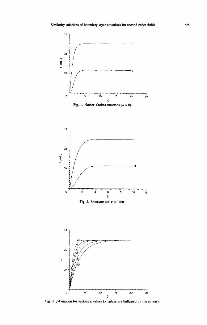
h(O) by the shooting method. The adaptive step size Runge-Kutta program failed to supply th solutions whereas for Navier-Stokes equations (i.e. K = 0 in (4.Q) we immediately obtain th solutions shown in Fig. 1. Realizing the stiffness in the equations we use Gear algorithm [7] an manage to find solutions for K s 0.001. For K = 0.001 the solutions are presented in Fig. 2. I

Si~~a~~ solutions of boundary layer quatious for second order fluids 62.5

0 5 10 15 20 25

E

Fig. 1. Navier-Stokes solutions (K = 0).

FI,

2 0

04

0 2 4 6 6 10 n

r

Fig. 2. Solutions for K = 0.001.

L~J~~~~~~~I(“~~~~~rI~)‘~/‘~~‘/‘:(~(~~~~/

0 5 10 15 20 25

c

Fig. 3. f-Function for various Y values (z values are indicated an the curves~.

626 M. PAKDEMIRLI and E. S. !jUHUBi

j

15 -

II_______- lo

0 5 10 15 20 25

E

Fig. 4. g-Function for various K values (K values are indicated on the curves).

0.6

0.4

f’

0.2

0 5 10 15 20 25

t

Fig. 5. First derivative off for various K values (K values are indicated on the curves).

-0.6 ~~--,---~, , , , , , / , , , ,

0 5 10 15 20 25

t

Fig. 6. Second derivative off for various K values (K values are indicated on the curves),

Similarity solutions of boundary layer equations for second order fluids 627

[8] it is mentioned that relaxation methods are to be preferred when the equations have extraneous solutions which, while not appearing in the final solution satisfying all boundary conditions, may wreak havoc on the initial value integrations required by shooting. It is also mentioned that the typical case is that of trying to maintain a dying exponential in the presence of growing exponentials. We therefore used DVCPR subroutine from IMSL library which is a finite difference algorithm and obtain the solutions for various K values. The initial estimated values of the function are provided from K = 0.001 solutions which are obtained by the Gear algorithm. In Fig. 3 the functionf, in Fig. 4 the function g, in Fig. 5 the functionf’, and in Fig. 6 the function f” are plotted for various values of K. Note that the curves corresponding to the value K = 0.001 in Fig. 2 and K = 0.1 in Figs 3 and 4 are very similar to each other.

In Fig. 3 for a fixed 5 value the @ component of velocity is lower for higher K values. But from Fig. 4 we cannot draw the same conclusion for v component of velocity where we have a complex relation changing for various locations of boundary layer. From Fig. 3 we can also conclude that for higher values of K the thickness of the boundary layer increases. Figure 5 is, as we will mention later, important in the sense that we can calculate shear stress by using it.

7. PROFILE OF THE SIMILARITY SOLUTION

Here our aim is to discuss the profile corresponding to the inviscid surface velocity distribution

qe = .(P (7.1)

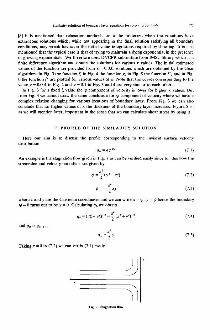
An example is the stagnation flow given in Fig. 7 as can be verified easily since for this flow the streamline and velocity potentials are given by

$+y24) (7.2)

(7.3)

where x and y are the Cartesian coordinates and we can write x = $J, y = # hence the boundary I/J = 0 turns out to be x = 0. Calculating q. we obtain

qo = (UX + I$)‘” = ; (x2 + y2y

and qB is qo Ix=0

qB=$

Taking x = 0 in (7.2) we can verify (7.1) easily.

(7.4)

(7.5)

Fig. 7. Stagnation flow.

628 M. PAKDEMIRLI and E. S. SUHUBi

1’1”1”“111”1”1’1”“““‘1”“““‘1”“1””1”1”’~~ 0 0.2 0.4 0.6 0.6 10 1.2

9

Fig. 8. Shear stress for various K values (K values are indicated on the curves).

The solutions can also be considered as the local solutions near the nose of blunt symmetric profiles.

The general algorithm for finding the profiles corresponding to (7.1) can be summarized as follows

f(z) = # + ill, (7.6)

is the complex potential function. At the boundary t+!~ = 0 so that we can write f(z)lB = @. The coordinates of the boundary will then be found by the following equation

= =f-‘(@Me = h(G) (7.7)

the magnitude of the velocity can be written as follows

4e = If’(z)1 (7.8)

Therefore the functional equation determining the profile is

If’(P(44l = qB(@) = @1’2 (7.9)

We do not have an analytical method to solve this equation and we have not taken up the approach of devising a numerical scheme, if it ever exists, to attack this problem.

8. SHEAR STRESS

We have derived the relation for shear stress in the previous paper [l]. Inserting the similarity solutions into equations (5.3) of [l] we finally arrive at the result

t GW = &1’2a2r#P2f’(0) (8-l) where f’(0) can be determined from Fig. 5 for the calculations. The shear stress is proportional to 1/Rein. In Fig. 8 the shear stress versus 9 coordinate is shown for various values of K.

REFERENCES

[l] M. PAKDEMIRLI and E. S. SUHUBi, Int. J. Engng Sci. 30, 523 (1992). [2] B. K. HARRISON and F. B. ESTABROOK, J. Math. Phys. l2,653 (1971). [3] E. CARTAN, Les Systkmes DiffPrentieLr Exthieurs et Leurs Applications Geometriques. Herrmann, Paris (1945).

Similarity solutions of boundary layer equations for second order fluids 629

[4] D. G. B. EDELEN, Isovector Methook for Equations of Balance. Sijthoff Noordhoff, Alphen aan den Rijn, The Netherlands (1980).

[5] D. G. B. EDELEN, Applied Exterior Calculus. Wiley, New York (1985). [6] E. S. SUHUBI, Int. I. Engng Sci. 29, 133 (1991). [7] C. W. GEAR, Commun. ACM M(3) (1971). [8] W. H. PRESS, B. P. FLANNERY, S. A. TEUKOLSKY and W. T. VETTERLING, Numerical Recipes.

Cambridge University Press (1989).

(Received 13 August 1991; accepted 11 September 1991)

ES 30:5-F