Parameter Estimation and Control of Nonlinearly ... - CiteSeerX

Parameter Estimation and Control of Nonlinearly

Parameterized Systems

by

Chengyu Cao

Submitted to the Department of Mechanical Engineering

in partial fulfillment of the requirements for the degree of

Doctor of Philosophy in Mechanical Engineering

at the

MASSACHUSETTS INSTITUTE OF TECHNOLOGY

September 2004

@ Massachusetts Institute of Technology 2004. All rights reserved.

Author ................... . ......... ........................Department of Mechanical Engineering

June 23, 2004

Certified by......... ........... .. .~. ...............

A.M. AnnaswamySenior Research Scientist

Thesis Supervisor

Accepted by ..................... ................................A.A. Sonin

Chairman, Department Committee on Graduate Students

ARCHIVES

MASSACHUSE'1S ISlTrUTE.OF TECHNOLOGY

MAY 0 5 2005

LIBRARIES

Parameter Estimation and Control of Nonlinearly Parameterized

Systems

by

Chengyu Cao

Submitted to the Department of Mechanical Engineeringon June 23, 2004, in partial fulfillment of the

requirements for the degree ofDoctor of Philosophy in Mechanical Engineering

Abstract

Parameter estimation in nonlinear systems is an important issue in measurement, diagnosisand modeling. The goal is to find a differentiator free on-line adaptive estimation algo-rithm which can estimate the internal unknown parameters of dynamic systems using itsinputs and outputs. This thesis provides new algorithms for adaptive estimation and controlof nonlinearly parameterized (NLP) systems. First, a Hierarchical Min-max algorithm isinvented to estimate unknown parameters in NLP systems. To relax the strong conditionneeded for the convergence in Hierarchical Min-max algorithm, a new Polynomial Adap-tive Estimator (PAE) is invented and the Nonlinearly Persistent Excitation Condition forNLP systems, which is no more restrictive than LPE for linear systems, is established forthe first time. To reduce computation complexity of PAE, a Hierarchical PAE is proposed.Its performance in the presence of noise is evaluated and is shown to lead to bounded er-rors. A dead-zone based adaptive filter is also proposed and is shown to accurately estimatethe unknown parameters under some conditions.

Based on the adaptive estimation algorithms above, a Continuous Polynomial AdaptiveController (CPAC) is developed and is shown to control systems with nonlinearities thathave piece-wise linear parameterizations. Since large classes of nonlinear systems can beapproximated by piece-wise linear functions through local linearization, it opens the doorfor adaptive control of general NLP systems. The robustness of CPAC under boundedoutput noise and disturbances is also established.

Thesis Supervisor: A.M. AnnaswamyTitle: Senior Research Scientist

2

Acknowledgments

First, I would like to thank my advisor, Dr. A.M.Annaswamy for her guidance, support and

help through my Ph.D. program. Her academic philosophy and research orientation have

influenced me a great deal. I also wish to thank the other members of my committee, Prof.

Kamal Youcef-Toumi, Prof. Alexandre Megretski and Prof. George Barbastathis for their

constructive suggestions and their time. I would also like to thank Dr. M. Srinivasan for

his guidance and help in the tissue modeling project. Finally, I would like to acknowledge

NSF under contract number ECS-0070039 with program monitor Dr. Paul Werbos.

3

Contents

1 Introduction 12

1.1 Current Research . . . . . . . . . . . . . . . . . . . . . . . . . . . . . . . 13

1.2 Thesis Contributions . . . . . . . . . . . . . . . . . . . . . . . . . . . . . 14

2 Conditions for Existence of Global and Local Minima in Neural Networks 19

2.1 Introduction . . . . . . . . . . . . . . . . . . . . . . . . . . . . . . . . . . 19

2.2 Global Convergence in Neural Networks . . . . . . . . . . . . . . . . . . . 21

2.2.1 Statement of the Problem . . . . . . . . . . . . . . . . . . . . . . . 21

2.2.2 A Collective Gradient Algorithm . . . . . . . . . . . . . . . . . . . 25

2.3 Conditions of Global Convergence . . . . . . . . . . . . . . . . . . . . . . 28

2.3.1 Example 1: Exponential Functions . . . . . . . . . . . . . . . . . . 29

2.3.2 Example 2: Sigmoidal Neural Network with 2 unknown parameters 33

2.3.3 Counter Example 1: Function with sin Component . . . . . . . . . 37

2.3.4 Counter Example 2: Sigmoidal Neural Network with 4 parameters . 40

2.3.5 Simulation Results . . . . . . . . . . . . . . . . . . . . . . . . . . 43

2.4 Implications on the Control of Nonlinear Dynamic Systems Using Neural

Networks . . . . . . . . . . . . . . . . . . . . . . . . . . . . . . . . . . . 44

2.5 Summary . . . . . . . . . . . . . . . . . . . . . . . . . . . . . . . . . . . 46

3 Hierarchical Min-max Algorithm 49

3.1 Introduction . . . . . . . . . . . . . . . . . . . . . . . . . . . . . . . . . . 49

3.2 Statement of the Problem . . . . . . . . . . . . . . . . . . . . . . . . . . . 50

3.2.1 The Min-max Parameter Estimation Algorithm . . . . . . . . . . . 52

4

3.2.2 Solutions of a* and #* . . . . . . . . . . . . . . . . . . . . . . . .

3.2.3 Properties of the Min-max Estimator . . . . . . . . . . . . . . . . .

3.3 Parameter Convergence in Systems with Convex/Concave Parameterization

3.3.1 Proof of Convergence . . . . . . . . . . . . . . . . . . . . . . . .

3.3.2 Sufficient Condition for Parameter Convergence . . . . . . . . . .

3.4 Parameter Convergence in Systems with a General Parameterization . . . .

3.4.1 Lower-level Algorithm . . . . . . . . . . . . . . . . . . . . . . . .

3.4.2 Higher-Level Algorithm . . . . . . . . . . . . . . . . . . . . . . .

3.4.3 The Hierarchical Algorithm . . . . . . . . . . . . . . . . . . . . .

3.4.4 Parameter Convergence with the Hierarchical Algorithm . . . . . .

3.4.5 Parameter Convergence when 0 E 1R2: An Example . . . . . . . .

3.4.6 Relation between NLPE and CPE . . . . . . . . . . . . . . . . . .

3.5 Simulation Results . . . . . . . . . . . . . . . . . . . . . . . . . . . . . .

3.6 Summary . . . . . . . . . . . . . . . . . . . . . . . . . . . . . . . . . . .

3.7 Appendix . . . . . . . . . . . . . . . . . . . . . . . . . . . . . . . . . . .

4 A Nonlinear Force-Displacement Model of Intra-abdominal Tissues

4.1 Introduction . . . . . . . . . . . . . . . . . . . . . . . . . . . . .

4.2 The Experiment . . . . . . . . . . . . . . . . . . . . . . . . . . .

4.3 The Model . . . . . . . . . . . . . . . . . . . . . . . . . . . . . .

4.4 Model Prediction . . . . . . . . . . . . . . . . . . . . . . . . . .

4.5 A Nonlinear Parameter Estimation Algorithm . . . . . . . . . . .

4.5.1 NLPE simulation results . . . . . . . . . . . . . . . . . .

5 Polynomial Adaptive Estimator

5.1 Introduction . . . . . . . . . . . . . . . . . . . . . . . .

5.2 The Structure of PAE . . . . . . . . . . . . . . . . . . .

5.2.1 Statement of the Problem . . . . . . . . . . . . .

5.2.2 Structure of Polynomial Adaptive Estimator . . .

5.2.3 Construction of A Polynomial Lyapunov function

5.2.4 Implementation of PAE . . . . . . . . . . . . . .

97

.. . . . 97

.. . . . 98

.. . . . 100

.. . . . 107

.. . . . 110

.. . . . 115

120

.. . . . . . . . . 120

.. . . . . . . . . 122

.. . . . . . . . . 122

.. . . . . . . . . 123

.. . . . . . . . . 126

.. . . . . . . . . 127

5

53

56

58

59

60

64

64

67

67

67

71

72

73

74

80

5.3 Polynomial Adaptive Estimator . . . . . . . . . . . . . . .

5.3.1 Properties of the PAE . . . . . . . . . . . . . . . .

5.4 Discretized-parameter Polynomial Adaptive Estimator . .

5.4.1 DPAE Algorithm . . . . . . . . . . . . . . . . . .

5.4.2 Extension to Higher Dimension . . . . . . . . . .

5.5 Nonlinear Persistent Excitation Condition . . . . . . . . .

5.5.1 Nonlinear Persistent Excitation Condition . . . . .

5.5.2 Comparison to LPE . . . . . . . . . . . . . . . . .

5.6 Simulation Results . . . . . . . . . . . . . . . . . . . . .

5.7 Summary . . . .. . . . . . . . . . . . . . . . . . . . . . .

5.8 Appendix . . . . . . . . . . . . . . . . . . . . . . . . . .

6 Hierarchical Polynomial Adaptive Estimator

6.1 Introduction . . . . . . . . . . . . . . . . . . . . . . . . .

6.2 Problem Formulation . . . . . . . . . . . . . . . . . . . .

6.3 Hierarchical Discretized-parameter Polynomial Adaptive I

PAE)..................................

6.3.1 Discretized-parameter Representation . . . . . . .

6.3.2 DPAE . . . . . . . . . . . . . . . . . . . . . . . .

6.3.3 Properties of PAE . . . . . . . . . . . . . . . . . .

6.3.4 Complete HDPAE . . . . . . . . . . . . . . . . .

6.4 Nonlinear Persistent Excitation Condition . . . . . . . . .

6.4.1 Nonlinear Persistent Excitation Condition . . . . .

6.5 Simulation Results of HDPAE . . . . . . . . . . . . . . .

6.6 Parameter Estimation in Static Systems . . . . . . . . . .

6.6.1 Parameter Estimation Algorithms for Static System

6.6.2 Global Convergence Result . . . . . . . . . . . . .

6.6.3 Dealing with Noise . . . . . . . . . . . . . . . . .

6.6.4 Simulation Results . . . . . . . . . . . . . . . . .

6.7 Comparison of different approaches . . . . . . . . . . . .

. . . . . . . . . 129

. . . . . . . . . 131

. . . . . . . . . 134

. . . . . 134

. . . . . . . . . 138

. . . . . . . . . 140

. . . . . . . . . 140

. . . . . . . . . 141

. . . . . . . . . 142

. . . . . . . . . 143

. . . . . . . . . 146

151

151

153

stimator (HD-

......... 155

.155

. . . . . . . . . 158

. . . . . . . . . 162

. . . . . . . . . 166

. . . . . . . . . 169

. . . . . . . . . 169

. . . . . . . . . 170

. . . . . . . . . 171

. . . . . . . . . 171

. . . . . . . . . 173

. . . . . . . . . 174

. . . . . . . . . 175

. . . . . . . . . 176

6

6.8 Sum m ary ................................ ..

7 Dead-zone Based Adaptive Filter 185

7.1 Introduction . . . . . . . . . . . . . . . . . . . . . . . . . . . . . . . . . . 185

7.2 Problem Formulation . . . . . . . . . . . . . . . . . . . . . . . . . . . . . 186

7.2.1 Polynomial Adaptive Estimator (PAE) . . . . . . . . . . . . . . . . 186

7.3 Filtered Deadzone Estimator . . . . . . . . . . . . . . . . . . . . . . . . . 188

7.3.1 Parameter Convergence of FDE . . . . . . . . . . . . . . . . . . . 193

7.3.2 Output Noise Filter . . . . . . . . . . . . . . . . . . . . . . . . . . 195

7.4 Model Disturbance . . . . . . . . . . . . . . . . . . . . . . . . . . . . . . 196

7.5 Simulation Results . . . . . . . . . . . . . . . . . . . . . . . . . . . . . . 198

8 Continuous Polynomial Adaptive Controller 201

8.1 Introduction . . . . . . . . . . . . . . . . . . . . . . . . . . . . . . . . . . 201

8.2 Problem Formulation . . . . . . . . . . . . . . . . . . . . . . . . . . . . . 202

8.3 The Companion Adaptive System . . . . . . . . . . . . . . . . . . . . . . 206

8.3.1 Properties of the Companion Adaptive System . . . . . . . . . . . 207

8.3.2 Stability Analysis . . . . . . . . . . . . . . . . . . . . . . . . . . . 209

8.3.3 Stability with disturbance . . . . . . . . . . . . . . . . . . . . . . 213

8.3.4 Stability under Bounded Output Noise . . . . . . . . . . . . . . . . 215

8.3.5 Extension to Higher Dimension . . . . . . . . . . . . . . . . . . . 218

8.4 Control Law . . . . . . . . . . . . . . . . . . . . . . . . . . . . . . . . . . 219

8.4.1 Class 1: . . . . . . . . . . . . . . . . . . . . . . . . . . . . . . . . 221

8.4.2 Class 2 . . . . . . . . . . . . . . . . . . . . . . . . . . . . . . . . 222

8.4.3 Class 3 . . . . . . . . . . . . . . . . . . . . . . . . . . . . . . . . 224

8.5 Simulation Results . . . . . . . . . . . . . . . . . . . . . . . . . . . . . . 227

8.6 Conclusion . . . . . . . . . . . . . . . . . . . . . . . . . . . . . . . . . . 230

7

. 178

List of Figures

2-1

2-2

2-3

2-4

Lyapunov function V(t) over 9 with 9* = 1 . . . . . . . . . . . . . . . . .

Lyapunov function V along [01 02] around 0 = [1 2 1 1]. . . . . . . . . . .

Lyapunov function V along [# 1 02] around 90 = [1 2 1 1]. . . . . . . . . . .

Trajectory of Lyapunov function V(t) with 0(0) = [1.02 2.02 1.0068 1.00951

3-1 A non-concave (and non-convex) function f(0, u) vs. 9, for u = 1, 0, -1.

f (0, 1):-, f (0, --1):- - -, f(0, 0):..... . . . . . . . . . . . . . . . . . . . .

3-2 The output error &E(t) with t using the hierarchical algorithm. f = 0.001

and J = 0.02. ......................................

3-3 The parameter estimate 0(t) with t using the hierarchical algorithm. True

parameter value 00 = 2. . . . . . . . . . . . . . . . . . . . . . . . . . . .

3-4 The evolution of the parameter region fk with t, using the hierarchical

algorithm. Note that Qk is updated at instants t* such that Ig(t) 6 for

k k] [t ~ ~ . . . . . . . . . . . . . . . . . . . . . . . . . . . . . . . . .

3-5 The upper-bounds fl and lower-bounds fkof f(0, ui) with t using the hi-

erarchical algorithm, for ui = 1, -1, 0. fi, f_:--, f2,f2:- - 3-, f,3:.....

4-1

4-2

4-3

4-4

4-5

4-6

4-7

Experimental and Filtered Signals of Input and Output . . . . . . .

Output Force F: Average of each group of filtered signals . . . . . .

Output Force F: Average of each group of filtered signals . . . . . .

Different Model Structures . . . . . . . . . . . . . . . . . . . . . .

Output Force Prediction of Various Models . . . . . . . . . . . . .

Output Force F: Model Prediction with the Parameter Identified .

Output Force F: Model Prediction with the Parameter Identified .

* . . . 99

. . . . 100

. . . . 102

. . . . 104

* . . . 106

* . . . 109

. . . . 110

8

41

45

46

47

74

75

76

77

78

4-8 Output Force F: Model Prediction of Sinusoidal Input with the Parameter

Identified . . . . . . . . . . . . . . . . . . . . . . . . . . . . . . . . . . . 1 13

4-9 Output Force F: Model Prediction of Sinusoidal Input Signal with the Pa-

rameter Identified . . . . . . . . . . . . . . . . . . . . . . . . . . . . . . . 114

4-10 Output Force F: Model Prediction of Parameters before NLPE and after

NLPE . . . . . . . . . . . . . . . . . . . . . . . . . . . . . . . . . . . . . 117

4-11 Trajectory of Parameter Estimate k12 in NLPE Algorithm . . . . . . . . . . 118

5-1 Output error . . . . . . . . . . . . . . . . . . . . . . . . . . . . . . . .. 143

5-2 Trajectory of auxiliary estimates 01 and,02 . . . .. . .. . . . . . . . . . . 144

5-3 Trajectory of Lyapunov function V(t) . . . . . . . . . . . . . . . . . . . . 144

6-1 Comparison of Different Algorithms . . . . . . . . . . . . . . . . . . . . . 176

6-2 Comparison of Different Algorithms . . . . . . . . . . . . . . . . . . . . . 177

7-1 Comparison of PAE and FDE in Case 1: - Unbiased Noise. Figures (a)-(c)

show the trajectories of estimates W' and '2, Noise filter error as of h - n,

and Lyapunov function V in PAE. Figures (d)-(f) show the trajectories of

estimates W1 and w2 , Noise filter error as of ft - n, and Lyapunov function

V in FDE . . . . . . . . . . . . . . . . . . . . . . . . . . . . . . . . . . . 198

7-2 Comparison of PAE and FDE in Case 2: - Biased Noise. Figures (a)-(c)

show the trajectories of estimates W-1 and '2, Noise filter error as of i! - n,

and Lyapunov function V in PAE. Figures (d)-(f) show the trajectories of

estimates W-1 and w2 , Noise filter error as of h - n, and Lyapunov function

VinFDE ...... ................................... 199

8-1 Structure of CPAC . . . . . . . . . . . . . . . . . . . . . . . . . . . . . . 205

8-2 CPAC - (Case 1): Trajectory of y, and reference signal r . . . . . . . . . 230

8-3 CPAC - (Case 2): Trajectory of y, and reference signal r . . . . . . . . . 230

8-4 Nominal Controller - ( Case 2, W- = w ): Trajectory of y, and reference

signal r . . . . . . . . . . . . . . . . . . . . . . . . . . . . . . . . . . . . 231

9

8-5 Nominal Controller - ( Case 2, - = w(1 + 2.2%) ): Trajectory of y, and

reference signal r . . . . . . . . . . . . . . . . . . . . . . . . . . . . . . . 231

8-6 Nominal Controller - (Case 2, w = w(1 - 2.2%) ): Trajectory of y, and

reference signal r . . . . . . . . . . . . . . . . . . . . . . . . . . . . . . . 232

10

List of Tables

3.1 Hierarchical Minmax Algorithm ....................... 68

4.1 Variance for Different Experimental Conditions . . . . . . . . . . . . . . . 101

4.2 Comparision of Prediction Errors for Various Models . . . . . . . . . . . . 107

4.3 Parameters Identified of Various Experiments . . . . . . . . . . . . . . . . 111

4.4 Model Prediction Error for Different Conditions . . . . . . . . . . . . . . . 112

6.1 HDPAE Simulation results . . . . . . . . . . . . . . . . . . . . . . . . . . 170

6.2 Comparison of different approaches . . . . . . . . . . . . . . . . . . . . . 176

11

Chapter 1

Introduction

The importance of mathematical models in every aspect of the physical, biological, and

social sciences is well known. Starting with a phenomenological model structure that

characterizes the cause and effect links of the observed phenomenon in these areas, the

parameters of the model are tuned so that the behavior of the model approximates the ob-

served behavior. Alternately, a general mathematical model such as a differential equation

or a difference equation can be used to represent the input-output behavior of the given

process and model outputs in some sense. In the model identification problem, parameter

estimation using observed input output signals in a given model structure is inevitable.

Besides the modeling problem, on-line estimation and diagnoses is another impor-

tant application area of adaptive estimators. Many systems contains uncertain information

which are always represented by unknown parameters especially for some systems which

work in changing outer-environments like aircraft or robots. In many cases, there is no way

or it is very difficult to measure these unknown or time changing parameters directly, like

the shifting of internal parameters or changing outer environments. In some situations the

unknown parameter can even be a virtual one if the mathematical model is not a physi-

cal one and just predicts the input output relationship well. In those situations, for either

estimation, diagnosis or control purposes, it is important to have some knowledge of the

unknown or changing internal parameters from measurable input output signals. Adaptive

estimators serve as a perfect tool in these applications since they are fast on-line recursive

algorithms and the estimation is updated adaptively with the changing parameters.

12

In addition to the pure estimation applications, adaptive estimators are always related

with adaptive control of partial known plants. Many adaptive controllers use adaptive es-

timators to construct the control law. This thesis concerns the parameter estimation and

adaptive control in a special class of dynamic systems where parameters occur nonlinearly.

1.1 Current Research

Adaptive control has emerged as a tool for controlling partial known plant for several

decades. The previous work is mainly about linearly parameterized systems, which is a

quite mature area and the results summarized in books such as [1]. However, linearly pa-

rameterized systems are just a special class and in most cases ideal situation of practical

systems. How to extend the adaptive estimator and controller into general nonlinearly pa-

rameterized (NLP) systems is an active research area which draws a lot of interests and

efforts.

Recently, a stability framework has been established for studying estimation and con-

trol of NLP systems in [1]-[8]. In [1 ]-[8], various NLP systems were considered and the

conditions for global stability, regulation and tracking were derived using a min-max algo-

rithm, while in [8], stability and parameter convergence in a class of discrete-time systems

was considered.

In the parameter estimation and control of dynamic systems, one commonly raised

question is that if you can differentiate the output signals to obtain the information about

system parameters. Measurement of output signal y does not mean y is also available from

output noise and measurement error. In a digital sampling system, measurement on y just

requires y to be measured in a desired precision. However, if you want to obtain i, high

precision time recording is also required and small error in y could be amplified. In contin-

uous system, differentiator is not a feasible implementation since its gain reaches infinity as

frequency increases. For a feasible physical implementation, we usually require the system

to be stable and proper. Adaptive estimator is an differentiator free feasible implementa-

tion and it uses only the input output signals. Bounded output noise or measurement error

results in bounded estimation error. In this thesis, differentiator free parameter estimators

13

are developed for NLP systems in the presence of noise. In some special cases, such as

Chapter 8 in this thesis, some stochastic properties of the noise can be exploited and the

parameter can be estimated exactly.

1.2 Thesis Contributions

The thesis contributions are mainly in two areas. One is the development of a series of new

adaptive estimation algorithms. Another is the adaptive control of NLP systems based on

these estimation algorithms. In the first case, adaptive estimation algorithms for general

NLP systems are developed and the Nonlinear Persistent Excitation (NLPE) condition for

parameter convergence is established. In the second case, a polynomial adaptive controller

(CPAC) is developed for a partial known plant with unknown parameters. Since there is no

general control law for nonlinear systems, we develop stable controllers for special classes

of NLP systems. In both estimation and control, the robustness of adaptive estimator and

controller is established in the presence of output noise. A brief description of the various

chapters in this thesis is given below.

In Chapter 2, we consider parameter estimation in static nonlinearly parameterized sys-

tems. The training of a neural network is basically a parameter estimation process which

finds the unknown parameters from the desired input output relationship. We consider the

problem of global convergence in a neural network whose parameters are unknown and are

to be identified. In particular, we examine conditions under which global and local minima

can occur. Two different training algorithms are considered for estimating the parameters,

which include the standard gradient algorithm, and a collective gradient algorithm. In the

former case, we provide some sufficient conditions under which global convergence can

occur, while in the latter case, we present necessary and sufficient conditions. We con-

clude with several examples of neural networks with a small number of neurons, and show

that these conditions are not satisfied, even in some simple examples, which leads to local

minima and therefore non-global convergence.

In the past few years, a stability framework for estimation and control of NLP systems

has been established. We address the issue of parameter convergence in such systems in

14

Chapter 3. Systems with both convex/concave and general parameterizations are consid-

ered. In the former case, sufficient conditions are derived under which parameter estimates

converge to their true values using a min-max algorithm. In the latter case, to achieve pa-

rameter convergence a hierarchical min-max algorithm is proposed where the lower-level

consists of a min-max algorithm and the higher-level component updates the bounds on

the parameter region within which the unknown parameter is known to lie. Using this

hierarchical algorithm, a necessary and sufficient condition is established for global pa-

rameter convergence in systems with a general nonlinear parameterization. In both cases,

the conditions needed are shown to be stronger than linear persistent excitation conditions

that guarantee parameter convergence in linearly parameterized systems. Explanations and

examples of these conditions and simulation results are included to illustrate the nature of

these conditions. A general definition of Nonlinear Persistent Excitation (NLPE) that leads

to parameter convergence of Hierarchical min-max algorithm is proposed at the end of the

paper.

Chapter 4 gives an application of Hierarchical min-max algorithm in dynamic system

modeling. The goal is to establish the parameterized model of force-displacement dynam-

ics of tissue in liver and esophagus of live animals. The raw data comes from the surgical

experiments performed in Harvard Medical school between 2001-2002. The input is the

displacement of a robotic end-effector to the tissue surface and the output is the force

response. The first step is to establish the parameterized model structure from physical

insights and simulations. The hierarchical min-max algorithm is then used for the purpose

of parameter estimation. After we have a model with a set of parameters which produces

the similar output as experimental data for same input signals, we can use this model to

simulate and generate the virtual force response when touching tissues/skins by the robotic

end-effector in virtual reality and it can be used to train new doctors for operations. It is

observed from the data that the differentiator methods cannot be applied in the practical dy-

namic system modeling. The optimization objective here is to minimize the error between

model output and experimental output for same input signals.

In Chapter 5, we propose a new Polynomial Adaptive Estimator(PAE) to estimate pa-

rameters that occur nonlinearly. The estimator is based on a polynomial nonlinearity in the

15

Lyapunov function which is chosen so that the nonlinearity in the unknown parameter is ac-

commodated as accurately as possible while maintain stability and parameter convergence.

We further extend the PAE algorithm to Discretized-parameter Polynomial Adaptive Esti-

mator(DPAE) and establish the Nonlinear Persistent Excitation Condition, which is similar

to linear persistent excitation condition and serve as a sufficient condition for parameters

to be identified in nonlinearly parameterized system. We show in this Chapter that the

DPAE algorithm has the ability to estimate parameters in any Lipschitz continuous nonlin-

ear function if the input and system variables satisfies the NLPE condition. The advantage

of DPAE over Hierarchical min-max is that it relaxes the parameter convergence condi-

tions. The NLPE condition for DPAE is much less restrictive than that associated with

Hierarchical min-max algorithm.

In Chapter 6, we propose a Hierarchical Discretized-parameter Polynomial Adaptive

Estimator (HDPAE) to estimate unknown parameters in Lipschitz continuous systems. It is

shown that under the same NLPE Condition, HDPAE has the ability to estimate unknown

parameters globally same as DPAE in Chapter 5, and is able to greatly reduce the compu-

tation complexity. Different parameter estimation algorithms for both static and dynamic

systems are given and comparison among them is discussed. It is shown that Hierarchical

Search algorithm for static systems and HDPAE for dynamic systems have the ability to

guarantee a globally convergent estimation however the gradient algorithms do not.

In Chapter 7, we focus on parameter estimation in systems with output noise. By adding

a dead-zone to the Polynomial Adaptive Estimator, it is shown that statistically the bounded

output noise can be filtered out and that the true unknown parameters are estimated exactly

under some conditions. This time-domain noise filter which applies to systems with un-

known parameters is denoted as filtered dead-zone estimator and it is later extended to

situation where the output noise is white noise. The difference between model disturbance

and output noise is discussed and the extension to situation where both of them exist is

proposed. It is noted that the same dead-zone technique to deal with output noise can be

applied to linear adaptive estimator, DPAE and HDPAE as well.

In Chapter 8, an adaptive controller for NLP systems is proposed. We propose a con-

tinuous polynomial adaptive controller (CPAC) which deals with piece-wise linearly pa-

16

rameterized functions as the same as traditional adaptive controller for linear ones. Since

most of the commonly encountered NLP systems can be piece-wise linearly approximated

through local linearization, the CPAC serves as a general tool for them. Stability of CPAC

with bounded output noise, disturbance and approximation error is also established. Con-

trol laws for several typical classes of NLP systems are provided to demonstrate the appli-

cations of the CPAC. The CPAC extends the traditional linear adaptive control theory to

general nonlinearly parameterized (NLP) systems and much more subsequent progress is

expected.

17

Bibliography

[1] K.S. Narendra and A.M. Annaswamy. Stable Adaptive Systems. Prentice-Hall, Inc.,

1989.

[2] A.M. Annaswamy, A.P. Loh, and F.P. Skantze. Adaptive control of continuous time

systems with convex/concave parametrization. Automatica, 34:33-49, January 1998.

[3] R. Ortega. Some remarks on adaptive neuro-fuzzy systems. International Journal of

Adaptive Control and Signal Processing, 10:79-83, 1996.

[4] A. M. Annaswamy, C. Thanomsat, N. Mehta, and A.P. Loh. Applications of adaptive

controllers based on nonlinear parametrization. ASME Journal of Dynamic Systems,

Measurement, and Control, 120:477-487, December 1998.

[5] J.D. Boskovi6. Adaptive control of a class of nonlinearly parametrized plants. IEEE

Transactions on Automatic Control, 43:930-934, July 1998.

[6] A. Kojid, A.M. Annaswamy, A.-P. Loh, and R. Lozano. Adaptive control of a class of

nonlinear systems with convex/concave parameterization. Systems & Control Letters,

37:267-274, 1999.

[7] A. P. Loh, A.M. Annaswamy, and F.P. Skantze. Adaptation in the presence of a

general nonlinear parametrization: An error model approach. IEEE Transactions on

Automatic Control, AC-44:1634-1652, September 1999.

[8] M.S. Netto, A.M. Annaswamy, R. Ortega, and P. Moya. Adaptive control of a class

of nonlinearly parametrized systems using convexification. International Journal of

Control, 73:1312-1321, 2000.

18

Chapter 2

Conditions for Existence of Global and

Local Minima in Neural Networks

2.1 Introduction

A neural network is a parameterized function which has been used for many years as a

universal approximation method to model an unknown static function. Assuming that the

underlying unknown static function is a mapping represented by

y = f(x) (2.1)

where x, y are inputs and outputs, the neural network is basically a parametric function

y = h(x, 0)

which can approximate the function in (2.1) by choosing appropriate parameters 0. The

training of a neural network is the process by which we find parameters that makes it

approximate the function in (2.1) as closely as possible. It is well known that several

networks such as multilayered neural networks [1, 2], and radial basis functions [3, 4] exist

that have such a universal approximation ability.

In this chapter, we address a simpler question than the above, which is the following.

19

Suppose that the underlying unknown static function has the same structure as that of a

neural network, where the unknown components are simply restricted to the parameter 9,

but otherwise h is known. Hence, the modeling of the unknown function in this context

reduces to estimation of the unknown parameter 9*. That is, we start with a system of the

form

y = h(x, 0*) (2.2)

where 9* is an unknown parameter in RN. The goal is to estimate 9* using an estimator of

the form

y = h(x, 0(t))

starting from arbitrary initial conditions $(to), and determine the conditions under which

global convergence is possible.

A necessary condition in any parameter convergence problem is identifiability. We

assume that h is identifiable throughout this chapter. To define this precisely, we denote the

input-output training data of the neural network as

(i, y0),= 1.. M. (2.3)

where M is the sample size. We now state the identifiability assumption.

Assumption 1 For the training data as in (2.3), if

h(xi, 0) = h(xi, 0*). i = 1..., M,

then

0 = 0*.

Assuming that the underlying neural network satisfies assumption 1, we consider the

standard gradient algorithm and a collective gradient algorithm where the training errors

from multiple inputs are collectively used to determine the gradient. These algorithms are

used to generate a recursive estimate 9 of 9. We then examine conditions under which 9

converges to 9* starting from arbitrary initial conditions, using both of these algorithms.

20

This chapter is organized as follows. In Section 2, we introduce the gradient algorithm

which is used to find unknown parameters 0* and the global convergence condition asso-

ciated with it is also proposed. In section 3, we present both cases where the collective

gradient algorithm leads to global convergence and case with no guarantee of the global

convergence. Section 4 summarizes the results and concludes the chapter.

2.2 Global Convergence in Neural Networks

2.2.1 Statement of the Problem

The system under consideration is assumed to be of the form

y(x, 9*) = h(x, 0*) (2.4)

where x, y : R -+ JR, x and y denote the input and output of the neural network, respec-

tively, 7 c IR, and 9* G IRN is the unknown parameter to be identified. For example,

9* represents the weights and biases in a single-layered neural network. We propose to

identify 0* using an estimator of the form

, )= =h(X, 0) (2.5)

and a recursive algorithm that generates an estimate 9(t) of 0* at each instant of time. The

goal of this chapter is to determine conditions under which O(t) converges asymptotically

to 9* starting from arbitrary values in IRN.

Generally, gradient algorithms are employed to find the weights of the neural network

[5].Typically, in these algorithms, the training error

M iV = -(yj - h (xi, 5)=

is used to determine the gradient, where xi and y are the training data defined in (2.3).

Below, we first present an instantaneous gradient algorithm and the related convergence re-

21

suits in [6]. We then present a collective gradient algorithm whose convergence conditions

are less restrictive.

Instantaneous Gradient Algorithm

In [6], a standard gradient algorithm (such as the back-propagation) was proposed, and is

of the form

0 = -(Q(x, ) y(x, 0*)) Vdh(x, 9). (2.6)

The following assumptions are made regarding h:

Assumption 2 We assume that the function h(x, 0) is differentiable and the magnitudes of

the first derivatives Veh(x, 9) are bounded.

We also assume that h is monotonic with respect to 9. That is, if A(x, 9) denotes the gradient

of h with respect to 9, i.e.

A(x, 0) = Veh(x, 9),

we assume that the following holds:

Assumption 3 A(x 1 , 0)A(x 2 , 9) ; Ofor any x 1 ,x 2 and 9.

The following definitions are useful for stating the convergence result:

Definition 1 Let q(a) = I(a) ® { q1 (a), y2 (a), .. . , 7n(a)} denote the orthogonal projection

of a vector 1 at a point a onto the surface whose tangent plane at a is defined by normals

{iy1 (a),.. . , i(a) }. The orthogonal projection is defined as

q(a) = (a) - E ' where

vy yy(a)- 2 2Vk, C {1 ,1n.., 1

k=1 1k 112

22

Definition 2 Let

H(9) = { u e(u,)=0}

HA(0) = {A(u,0) 1 u E H()}

1(9) = dim{L{HA(0)}} (2.7)

Ki = { 1 I() > i}

and

M(Im) = { 1 e(u(t), 9) = 0, t C m} (2.8)

The set A('M, 0) is the set of all normals to the manifold M at a point 9. Let

mu(Oa) = A(u,9a)®&A(IM, ma)

m (00) = A(u(ti),9a)A A('m,9a), (2.9)

we define a vector field q(9) such that

q(9) = m, (0) 0 E Ki

q (0) = mu (0) 0 E Kj+1. (2.10)

Definition 3 Let T, > 0, and let A(x, 0) = Veh(x, 0), with h(x, ) : JR x RN -+ R. Let

Qt = [to, to + TxI, T, > 0

= {ti E iQ, i= 1,...,Mjt+--tI>o},

Me, > 0

A(T, 0) = {A(x(tk), 0) 1 tk E I}

A function x(t) : JR -+ R is said to belong to the class UPNE on the interval t G [to, to + TxI

if it satisfies the three properties stated below:

23

(P1) linear independence is invariant: If the set A(Ia, 0a) is linearly independent for

some set *,, E Qt and 0a E Qo, then A(a, 0) is linearly independent for all 0 C Q0.

(P2) sufficient degree of excitation exists: There exists a set Jb C Qt consisting of N

elements such that A(4Ib, 0a) is linearly independent.

(P3) potential field exists: For the vector field q(0) constructed in (2.10), there exists a

potential field s(0) such that Vs = q.

The main convergence result in [6] is summarized in the following Theorem.

Theorem 1 Let Assumptions 1, 2 and 3 hold. For the system in (2.4)-(2.5), if for every

t > 0 there exist a t1 > t and T > 0 such that u(t) c UYE over the interval [t 1, t1 + T],

then lim 0(t) = 0t-+oo

The reader is referred to [6],[7] for the proof of Theorem 1.

As stated in the above theorem, global convergence in single-layered neural networks

can be guaranteed provided the properties (P1), (P2), and (P3) are satisfied by the input x.

Of the three, (P1) and (P2) are relatively easy to be guaranteed since they concern excitation

properties of the input, and are qualitatively related to linear independence. However, (P3)

concerns a topological property of the nonlinear system defined in (2.4), (2.5) and (2.6).

This property is central to the global convergence of the neural network and is needed in

order to guarantee the existence of a converging metric and therefore an associated Lya-

punov function. Only when q(0) is an irrotational field, i.e. V x q = 0, is it possible that

a potential field s can be found to make assumption (P3) satisfied. In general, there is no

guarantee that q(9) is irrotational and it is extremely difficult if not impossible to determine

what classes of x will satisfy these properties. It is therefore useful to examine if other

algorithms that do not require such restrictive assumptions can be determined that can still

guarantee global convergence. As shown in the next section, such an algorithm can indeed

be found.

24

2.2.2 A Collective Gradient Algorithm

Instead of determining the gradient by using a single input and output, we take an alterna-

tive approach in this section by collecting multiple input-output pairs (xi, yi), i = 1..., M,,

where yj = h(xi, 9*) and M is the number of input-output pairs. If we use the same esti-

mator structure as in (2.5), we can define the corresponding output error as

M IV (yi - h(i, 0))(2.11)

i= 2

We now determine the gradient algorithm using V, which can be viewed as a collective

output error for a range of inputs xi, i = 1, . .. , M. In this collective gradient algorithm we

update 9 using the negative gradient of V with respect to . That is,

O= -V V. (2.12)

The question that arises is if the estimator in (2.5) together with the gradient algorithm in

(2.12) can guarantee global convergence of 9 to 0*.

We assume N to be even for ease of exposition. Then the structure of the nonlinearity

h in a neural network is of the form

N/2

h(x, 0) = O9$g(ojx) (2.13)j=1

where 9 = { f1...., 9 N, ... , /,:, i..: -- , ON/2} are the parameters, and the input x and

output y belong to R. Combining (2.11) and (2.13), (2.12) can be rewritten as

M

9= E(yj - h(xj, $))vj (2.14)j=1

where

Vi = [g(ekIy)...., g(kix),..., g(4N/2x)- (2.15)

89(1X~)-J Og ij) -N/2 ag (NI2 T

25

From the neural network structure in (2.13), it is easy to see that Q defined below is an

invariant set

Q = {I90 = 0,, Oi = j, Vi # j}. (2.16)

For any O(to) E Q, we could see from (2.14) that O(t) E Q, t > to as well. Therefore we

focus on only those initial conditions that do not lie in Q from here onwards.

Define E = 1RN\ and 9 = 0 - *. We now state the convergence result in Theorem

2.

Theorem 2 Under assumption 1, if

V() -+ oc as 111-+ oo. (2.17)

for the system in (2.4) and estimator in (2.5), for any 0(to ) E E, the gradient algorithm in

(2.12) leads to 9(t) -+ 0* as t -+ oc if

VV = 0 4=> 0 = 0* 0 E E (2.18)

where V is defined as in (2.11).

Proof of Theorem 2: From (2.4), (2.5), (2.11), and (2.12), it follows that V is an au-

tonomous system of 9 with

Z (9) = -_IVdVI 2 < 0. (2.19)

Assumption I states V(6) is a positive definite function of 9, and Assumption 2.17 implies

that V(9) is a decrescent function of 9. From (2.19), it therefore follows that O(t) E L*.

Equation (2.19) and condition (2.18) implies that V (9) is a negative definite function of

9. Therefore, it follows that $(t) -- 0 as t -+ oc. Necessity of (2.18) can be proved in a

similar manner. 0

When condition (2.17) and (2.18) are satisfied, global convergence follows and a simple

example is

h(x, 9*) = xO*

where x, 9* E R. In general, however, condition (2.17) is not satisfied or difficult to check.

26

Hence, we have the following corollary which yields a convergence condition in a given

set under less restrictive conditions.

Assume the minimum limit value of V(9) as 9 -+ oc is C and we define a region

Q, = {0 1 V(9 - 0*) < C,0clRN}. (2.20)

and E1 = Q1\Q. The corollary below discusses convergence in the set E1 .

Corollary 1 Under assumption 1, for the system in (2.4) and estimator in (2.5), for any

O(to) E E1 , the gradient algorithm in (2.12) leads to 9(t) - 9* as t -+ oc iff

VOV =0<==*=0* EE 1 (2.21)

where V is defined as in (2.11).

Proof of Corollary 1: It follows from (2.19) that once 9(to) E E1, i.e.

V(to) < C, (2.22)

we have

$(t) E El, t > to. (2.23)

Because the minimum limit of V as o -+ cc is C, it follows that 0(t) will not converge to

oc and is bounded. Therefore, similar to the proof in Theorem 2, it is easy to show that

(2.21) is a sufficient and necessary condition for 0(t) -+ 0* as t -+ oc.

From Theorem 2 and Corollary 1, it is shown that the global convergence in region E

or at least in region E1 is equivalent to establishing condition (2.18). Since VOV = 0 holds

for any 9 that satisfiesM

E(yj - h(xj, 9))vj = 0, (2.24)j=1

it is of interest to examine conditions under which 9 is an extremum of V. More precisely,

we have the following property.

27

Property 1 If exists such that (2.24) is satisfied, then one of the following holds:

(i) 9 is a saddle point of V;

(ii) 9 is a local minimum of V;

(iii) 0 is a local maximum of V.

Remark 1: Theorem 2 implies that the collective gradient algorithm guarantees global

convergence if (2.18) is satisfied. It is worth noting that this condition is considerably less

restrictive than those needed by the instantaneous gradient algorithm which required [P1],

[P2] and [P3] to hold. In fact, we note that (2.18) is almost identical to [P1].

Remark 2: Suppose that a 9 that satisfies Property 1-(iii) exists, and V has no other

local extrema other than 9 and 0*. It follows that except for one initial condition where

9(to) = 0, all other initial conditions will converge to 0*. Therefore, to guarantee global

convergence, we need to address only O's that satisfy Property I -(i) and 1 -(ii).

The central question that remains to be pursued is if at a given point 9 in IRN, the

gradients vj defined as in (2.15) are linearly independent. Since the answer to this question

for a general function h(x, 9) depends on h, the derivation of constructive conditions for

checking linear independence at all 9 is extremely difficult if not impossible. In what

follows, we address specific examples of h and discuss the existence of local extremes.

In particular, we provide some counterexamples of h which indeed do have local saddle

points, and their implications.

2.3 Conditions of Global Convergence

Four different neural networks with very few parameters are considered in this section to

further evaluate if 9 that satisfies Property I -(i) and Property I -(ii) exists. In sections 3.1

and 3.2, we consider exponential and sigmoidal nonlinearities, respectively, with no output

weights. In section 3.3 and 3.4, we consider counter examples which are a function with

sin component and a sigmoidal nonlinearity with output weights, respectively.

28

2.3.1 Example 1: Exponential Functions

We consider a 3-node network of the form

3

h(x, 0*) = Zeo*xi=1

(2.25)

in this section. It follows that the collective gradient algorithm is given by

3 3

Oi= E(yj - E eixi)xjeixij=1 i=1

i = 1, 2,3. (2.26)

Here the invariant set is given by

Q = {010 = 9j, Vi # j and i, j = 1, 2 or 3}.

Before establishing the convergence, a lemma which shows the full rank of a matrix is

needed and stated below.

Lemma 1

eoii e01X2 e 1X3

e0 2xi eO2X2 e02x3

e03X1 e03X2 e03X3

(2.27)

is full rank where

Oi : 0j, xi # xj., Vi # j.

Proof of lemma 1: Without loss of generality, we assume

03 > 92 > 01

x 3 > X2 > X1.

Scale ith row by e-OixI and subtract the first row from the second and third rows, matrix

29

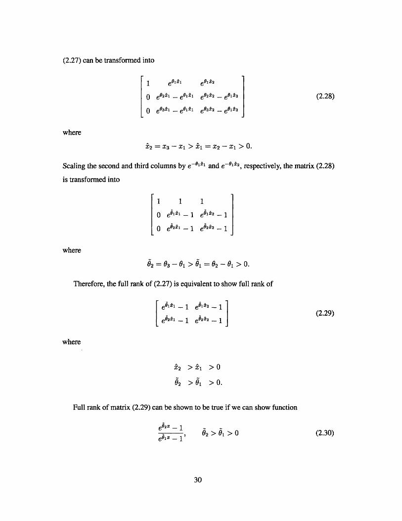
(2.27) can be transformed into

1

0

0

e9 12

e 02l - e*l:l e0 212 - e8 12

e 03&1 - eOi -" e'93&2 - e0

l12

where

2= X- x 1 > I = X2- X1 >0.

Scaling the second and third columns by e- 0 11 and e--1 12, respectively, the matrix (2.28)

is transformed into

1

0

0

1 1

e"11 - 1 eO1x2 _ 1

e21- 1 e02'2 1

where

02=03-01>01 =2-01>0.

Therefore, the full rank of (2.27) is equivalent to show full rank of

eo1X1 - 1 eC1X2 - 1

e21 - 1 ie0212 - 1

where

X2 > 1̂ > 0

02 > 01 > 0.

Full rank of matrix (2.29) can be shown to be true if we can show function

02 > 01 > 0

(2.28)

(2.29)

e0 2x _ 1

ebix - 1(2.30)

30

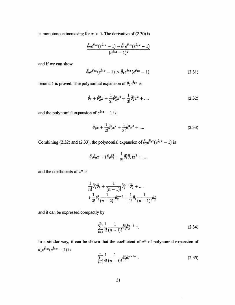
is monotonous increasing for x > 0. The derivative of (2.30) is

02e62X(elx - 1) - x 1)

(eOix - 1)2

and if we can show

62e02X (eolx 1) >ie"12 - 1).

lemma I is proved. The polynomial expansion of 62ex2x is

j2 + 2 X +13 2

(2.31)

(2.32)1 ' x3++ 23!+12X

and the polynomial expansion of ejlX - 1 is

1 d2

d +2! I1

+ - x 3 +3!

(2.33)

Combining (2.32) and (2.33), the polynomial expansion of 02 ei2X(eO1z - 1) is

5152 + 512 + -62 2)X2 + ..6102X +(0A 2! 1 2

and the coefficients of x" is

102+ 1 ~1§2n. n - 1)!

2 ( ) 1- 1)njI'(n 1)! 6

and it can be expressed compactly by

S 1 1 ~(- . - i) 2n-! +

=1 --i) 1"~z(2.34)

In a similar way, it can be shown that the coefficient of Xn of polynomial expansion of

01eG1x(ei2x - 1) isnl1 1 ~. ~ .

i-1 .(10" -- +1 (2.35)

31

Subtract (2.35) from (2.34), we get the coefficients of x' in polynomial expansion of

0 2e 02X(e6l _ 1) - 9iejx(e02x 1)

as

where m = (n - mod(n, 2))/2. Because 92 > 61, it follows that

i = 1, .., m. (2.36)For _ 2ann- +1 > 0,

For any i = 1..., m, because i <; 1, it follows

i!(n - i)!

(2.37)

From (2.37), we have

1 1i! (n -i)!

1 1> 0.

(i-1!(n +1- )(2.38)

Combining (2.36) and (2.38), we notice that all the coefficients of polynomial expansion of

b 2 e 02eX - 1) - Oiehl(e 6 2x 0 1)

are positive and it shows (2.31) is true. Therefore, the matrix in (2.27) is full rank. 0

We now show that using lemma 1, we can establish global convergence.

Theorem 3 For the function in (2.25), the collective gradient algorithm in (2.26) is glob-

ally convergent.

32

= i(i - 1)!(n - i)!

< (n+ 1 -i)(i -1)!(n -i)!

= (i - 1)!(n + 1 - i)!.

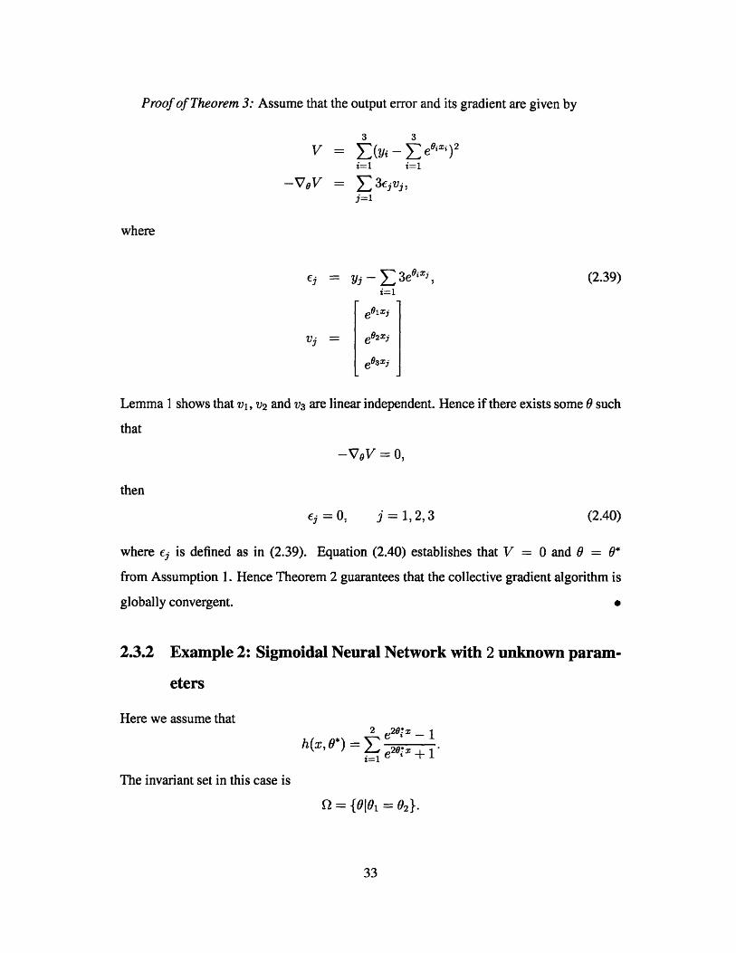
Proof of Theorem 3: Assume that the output error and its gradient are given by

3 3

V = (yi - eoixi )2i=1 i=1

-VoV =E 3cj v,j=1

Ej = yj -3eOix,

vi =

(2.39)

eolij

eO2xie 02Xj

Lemma I shows that v1, V and v3 are linear independent. Hence if there exists some 0 such

that

-VOV = 0,

then

Ej = 0, j = 1,2,3 (2.40)

where ej is defined as in (2.39). Equation (2.40) establishes that V = 0 and 9 = 0*

from Assumption 1. Hence Theorem 2 guarantees that the collective gradient algorithm is

globally convergent. 0

2.3.2 Example 2: Sigmoidal Neural Network with 2 unknown param-

eters

Here we assume that2

h(x, 0*) =

The invariant set in this case is

Q = {111 = 02}-

33

where

20; _e + 1e20x +1

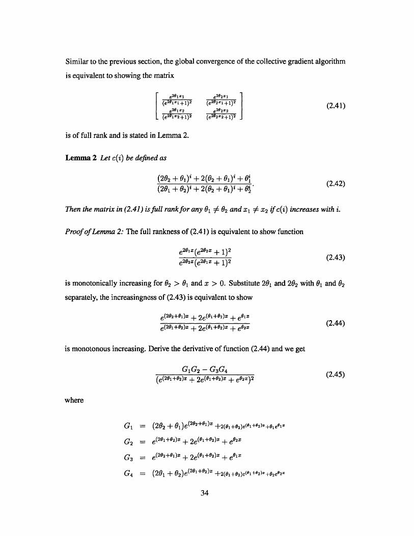
Similar to the previous section, the global convergence of the collective gradient algorithm

is equivalent to showing the matrix

e211 e2 0 2X1(e20 21+1) 2 ( 2M21+1) 2 (2.41)

e201X2 e282z2

(e291z2+1) 2 (e29 2x2+1) 2 j

is of full rank and is stated in Lemma 2.

Lemma 2 Let c(i) be defined as

(202 + 92)i + 2(02 + 0 1)' + O (2.42)( 201 +02 )i + 2(02 + 01 ) + O2

Then the matrix in (2.41) is full rank for any 01 7 02and x1 0 x 2 if c(i) increases with i.

Proof of Lemma 2: The full rankness of (2.41) is equivalent to show function

e201x(e292x + 1)2e kLI -(2.43)e202x(e 201x + 1)2 -

is monotonically increasing for 02 > 01 and x > 0. Substitute 20, and 202 with 01 and 02

separately, the increasingness of (2.43) is equivalent to show

e(202+01)X + 2e(0I+02)x + elx(e(201+02)X + 2e(01+02)x + e6

2x (2.44)

is monotonous increasing. Derive the derivative of function (2.44) and we get

G1 G2 - G3 G4

(e(2 01+ 02)x + 2e(01+02)x + e0 2x)2 (2.45)

where

G, = (202+ 01)e(202+O1)x +2(i1+0 2 )e(81+92)X+Oiee1z

G2 = e(201+02)X + 2e(O1+02)x + e0 2x

G 3 = e(202+01)X + 2e(O1+02)x + e"lx

G4 = (201+ 02 )e(201+02)X +2(O+O 2 )e(1+±4+2)0 2 eO2

34

Now let us express these using the polynomial expansion. The coefficient of x" in

polynomial expansion of G1 is

1 ((202 + 01)n+l + 2(01 + 02)n+1 + 0n+1). (2.46)n!

The coefficient of x" in polynomial expansion of G 2 is

1- ((201 + 02)n +2(01 + 02)n + 02). (2.47)n!

Combining (2.46) and (2.47), the coefficient of X" in polynomial expansion of G1G2 is

A (292 + 01)n+ + 2(0 + 02)"*' + on+1) +

1 i+

(n - i)! ((202 + 01)i+1 + 2(01 + 92)i+1 + 1

((201 + 02)"i + 2(01 + 92)"-i + on-i) . (2.48)

In a similar way, substituting j = n - 1 - i, the coefficient of G3G4 can be written as

4(21 + 2)n+1 +2(02 + 1)n+ + 2+1) +Ej=0

1 .((201 +0 2)"~j +2(02 + 01)7'-j(j + 1)!(n - 1 - j)!+02 ((202 + 91)j+1 + 2(02 + 6P)+1 + +1)

(2.49)

Subtract (2.49) from (2.48), we get the coefficient of Xn in polynomial expansion of G1G2 -

G3G4, which is

A ((202 + 01)n+1 + On+1 - (201 + )n+1 _ 0) +1+n!1 1 21

(j )! (n - ) i+ 1)! (n -1 - )

((201 + 02)"~ + 2(02 + 2)i + on-i)

((202 + 01)i+1 + 2(02 + 01)i+1 + 0(+1). (2.50)

35

In what follows, we will show coefficient in (2.50) is positive.

Coefficient in (2.50) can be rewritten as

((202 + 01)n+1 + 0+1 - (20, + 02)n+l

1 )1 1

i+1 i! (n -1- i)!

((2o1 + 2)" + 01)"-i + On-i)

((202 + 01)i+1+ 2(02 + 9)i+ 1+ 0(+1).

Let M = ['n-2i , (2.51) can be transformed as

4 ((202 + 01)n+1 + 0n+1 - (201 + 02)n+_n!1

i+1 i!(n- 1-i)!{((201 +02)"~i + 2(02 + 0 1)"-i + On-)

((202 + 1)i+1 + 2(02 + 91)i+1 + Oi+') _

((202 + 01)"- + 2(02 +)-~i + O;~.)

((202 + 02)+1 + 2(02 + 01)+1 + )}.

1 1< 0

n -t +

and

n-i > i +1, V1 < i < M 2 ~ 1

Coefficient (2.52) is positive is equivalent to

(202 + 01)n+1 + on+1 - (20, + 02)n+' - o7+1 > 0

and

((201 +02)j + 2(02 + 01)3 + 02)

36

(2.51)

Because

(2.52)

(2.53)

(2.54)

(2.55)

- n+1)

n-11

+ E i

20 +1 )

M

+{ En -i

((202 + 91)i + 2(02 + 01)i + Oi) >

((201 + 02)' + 2(02 + 01)' + 0)

((202 + 01)j + 2(02 + 01)j + oj) (2.56)

for any 02 > 01 and i > j. It follows easily that

(202+01) +2(02+01)+01 = (201+ 02) +2(02+01) +02

(292 + 01) > (201+02). (2.57)

Now that (2.42) increases with i, we know that inequality (2.56) holds. Another fact comes

from the increasness of (2.42) is

(202 + 01)' + 2(02 + 01)' + 0'.).O> )vi > 1. (2.58)( 201+02 )i + 2(02 + O1)i + 02-~ ~

Inequality (2.58) proves (2.55) and it is established that coefficient in (2.50) is positive.

Positive coefficient in (2.50) implies that G1G2 - G3G4 is always positive. It follows

that the derivative in equation (2.45) is positive and the full rank of (2.44) follows. This

proves Lemma 2.

About the condition that (2.42) increases with i, one observed fact is that for one num-

ber, if we participate them more evenly, the separated polynomial will increase slower and

this can be verified to hold numerically.

2.3.3 Counter Example 1: Function with sin Component

We now consider a counter-example of system where Assumption I and condition (2.17)

are satisfied, but condition (2.18) is not. This system is a network which contains sinusoidal

function as2 2

h(x, 0*) = -rx* + x2 sin(0*) + Visin(0*)

where 0*, x C R and x > 0.

When we increase sample size M, we could always find a training data as in (2.3) which

37

makes the function identifiable. Therefore, the following Lyapunov function follows as

V = 2 -x,> + x2 sin(O) + V\Ii sin(2) xO*-- r 71

--X sin (O*) + V§x-jsin (0*)) 2 (2.59)

In what follows, we will show that for this special case condition (2.17) in Theorem 2 is

satisfied, but condition (2.18) is not for any training data set

(xi, yi)

where xi > 0.

Equation (2.59) can be rewritten as

V = + x, sin(^) + Jzi sin(O)

-X2 sin(O*) + Voi sin(*)) 2

and it follows from the fact Isin(0) | < 1 that

(2.60)

(2.61)

M '2V > ( xi| - 2(x? +

i=1

_> M (-2 )2) fi2 -

7= ri

2

+ /)2). (2.62)

As jil -+ oo, the 92 term in (2.62) dominates and V -+ oc which proves condition (2.17).

For any xi in (2.60), now that xi > 0 and

yj -- h(xi, ) ; xi (* -7r

38

(2.63)

M- ((o?

(i=1 t

+ \/-i)) |A

we can always find some 0- such that

yi - h(xi, 0) > 0 vd < 0- (2.64)

For any trainset defined as in (2.60), we can find some 0- such that (2.64) holds for any

i = 1,.., M. Choosing some j such that

-2j7r C (-oo, 0-]. (2.65)

it follows that

h(xi, -2j7r)

h(xi, -2j - 7r)

= -4jxi

= (-4j - 2)x,

h(xi, -2jir - 7r/2) = (-4j - 1)xi + (xi + vG7).

Because

Xi < X2 + . V xj > 0.,

it follows from (2.65), (2.66) and (2.67) that

0 < y - h(xi, -2jr - 7r/2) < yj - h(xi, -2j7r) <

yj - h(xi, -2j7r - 7r) Vi = 1,.., M.

Therefore V(9) has the property of

V(-2jr - ir/2)

V(-2j7r - 7r/2)

< V(-2j7r)

< V(-2jir - 7r)

39

and

(2.66)

(2.67)

(2.68)

(2.69)

(2.70)

for j chosen as in (2.65) and there must exists some 9 E [-2j7r - 7r, -2j7r] and

ViV(9) I _O = 0. (2.71)

Equation (2.71) means that there is some 9 # 0* and

VOV(9) li= = 0

which implies that condition (2.18) is not satisfied. Hence, there exist many local minima

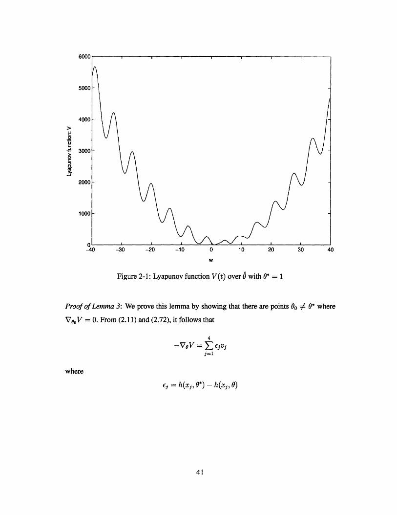
and prevent the global convergence of the collective gradient algorithms. In Figure 2-1, we

plot the Lyapunov function V w.r.t. 9. The choice of training set x = 1, 2 or 3 makes h

identifiable because the only global minimum happens at true unknown parameter 0* = 1

and it can be seen clearly when we zoom in the Figure. It is shown that there exist many

Icoal minimums which will prevent the global convergence.

2.3.4 Counter Example 2: Sigmoidal Neural Network with 4 parame-

ters

We now consider another system where assumption I is satisfied, but conditions (2.17) and

(2.18) are not. Here, the system is a sigmoidal neural network with 2 nodes and output

weights given by

h(x, 0*) = e (2.72)ex + e-P02

where the unknown parameters 9* = [9*, 92, 0*, 0*1T, the invariant set is

Q = {0 = [01 02 i 021|01 = 02, 01 = 02}-

In this case, we show that the global convergence is not guranteed in Lemma 3 by a counter

example.

Lemma 3 For the function in (2.72), the collective gradient algorithm is not globally con-

vergent.

40

6000

5000 F

4000 F

3000 -

2000 -

1000 -

U-40 -30 -20 -10 0 10 20 30 40

w

Figure 2-1: Lyapunov function V(t) over 0 with 0* = 1

Proof of Lemma 3: We prove this lemma by showing that there are points 00 $ 0* where

Va.V = 0. From (2.11) and (2.72), it follows that

4

-VOV = ZeVij=1

where

c = h(xj, 0*) - h(xj, 0)

41

.2

0

CL

I I

and [viv 2 v3v 4 ] forms the matrix A given by

e241m_1 -Ie241 -1+1

e2

2I_1 -1e202-1+1

O1Ize2 1x I

(e 201X1 +1) 2

O2gxe2O2zI

(e202xl+l)2

e201 2-1 e201X3-1 e201x4_1e201X2+1 e 2

+1M3+1 e201x4+1

e202x2-1 e 202-3-1 e

202W4 -1

e202X2+1 e

2'2-3+1 e

24 2X4+1

O~2e2O1X2 Oixae

2#1"3 01 4 e

2#1x4(e2 4

122+1)2 (e 201x3+1)

2 (e201 X4+1)

2

02Xe2t 22z 2 02X3e

242X3 02X4e

2O2x4

(e222+1)2 (e202x.3+1)2 (e2 42x4+1) 2

Denote the ith row of matrix A as ri. It follows that A is not full rank for 0 E 6 1, 0 2 or

6 3, where

8 1 = {11 # 02. (2.73)

82 = {0101 = 0}.

83 = {0102 = 0}.

This is because when 0 E 32, or 8 3 , the row r3 or r4 becomes zero, respectively and hence

A loses rank. Also, it follows from the definition of 8 1 such that

ri = r2 r3 = r4. (2.74)

We now examine if it is possible for

VV00 = 0 (2.75)

for 90 E 8 1 with 00 # 0*. To do this, we start with a Oo that satisfies Eqs.(2.73), (2.74) and

(2.75), and determine if a 0* exists under the same conditions.

Since Eq. (2.75) holds if

riE=0 for i=1,...,4

for 00 E 6 1, from Eq. ((2.74)), we have that (2.75) is equivalent to

C(OO, *)r1(60)

42

= 0

c(90, 0*)r3(0) = 0

where c(O0 , 0*) = [Ei E2 c3 E4 ]. Eq. 2.76) implies that there are 2 equations while 9* has

4 elements, and hence it implies that there exists some 0* $ 90 which satisfies (2.76). A

similar procedure can be used to find a 9* that exists for any 00 in 6 2 and e3 as well. That

is, we have established the existence of 00 : 0* for which Vo6 V = 0. Therefore from

theorem 2, it follows that no global convergence can be guaranteed.

Remark 3: It follows from (2.19) and Barbalatt's lemma that

lim VdV = 0.t-+00

If we define the set B as

B = {9 | 9 E, VOV = 0}.

it follows that 0(t) -+ B as t -+ oo. Lemma 3 shows that B can include at least one more

point other than 0* and hence that 9 converges to some Oo where 00 E B and 00 : 0*.

Remark 4: It should be noted that we can not avoid convergence to a local minimum

by increasing M. This is because in this case c, r1 and r3 will have M elements instead of

four in (2.76), but we still will have only two equations for four unknowns and the same

conclusions follow.

2.3.5 Simulation Results

In this section, we will give numerical results of the counter-example constructed in section

2.3.4. We will consider a sigmoidal neural networks with 4 parameters as defined in (2.72)

with input U = [1 2 3 4]. Choosing

00 = [12 11] E 4Di. (2.77)

using the procedure as discussed in section 2.3.4, we found

0* = [6.4855 - 3.4886 1.1 1.2] (2.78)

43

(2.76)

which satsfies

VV00 = 0. (2.79)

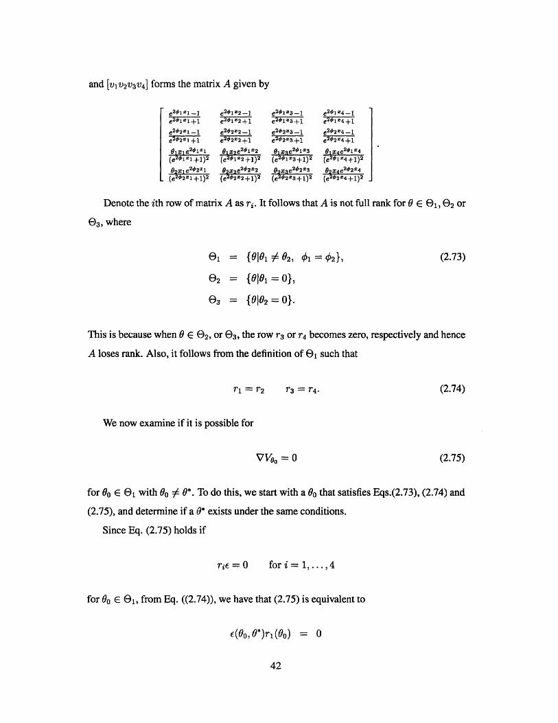
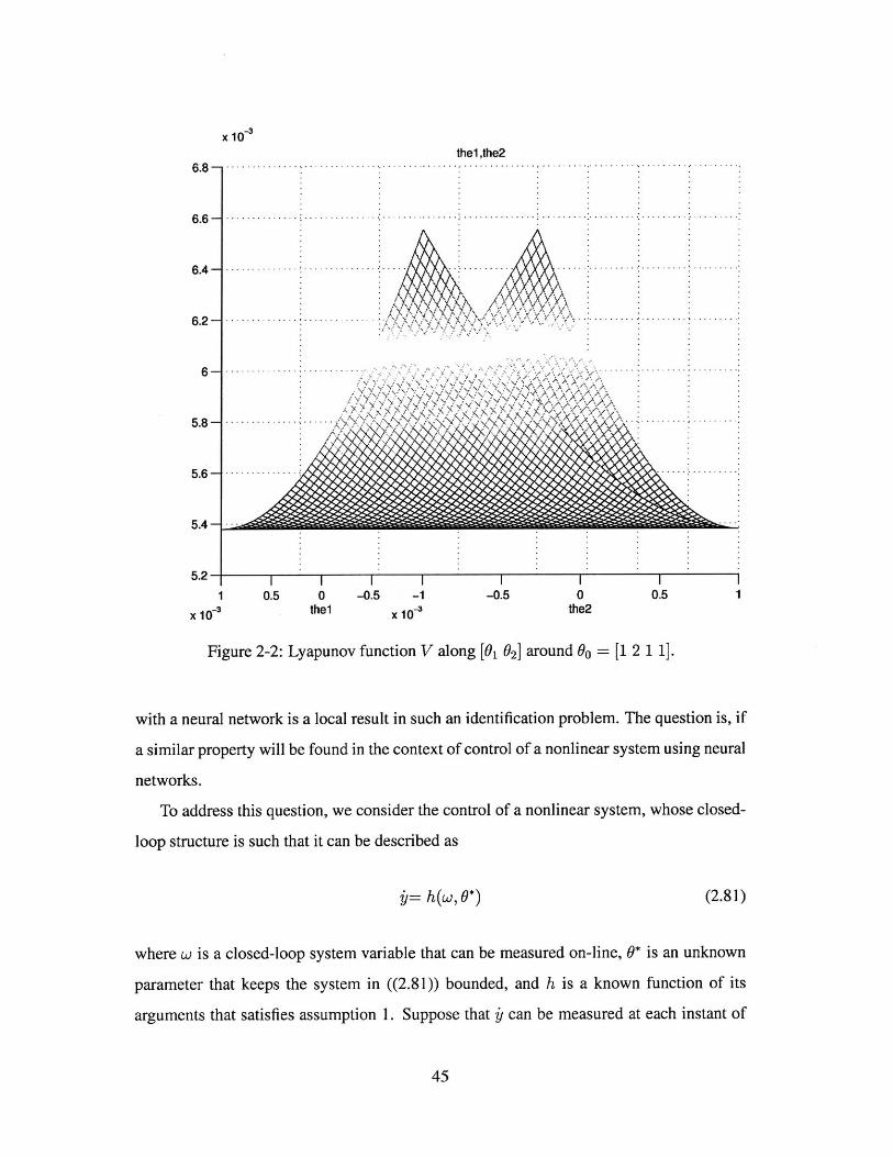
We plot the Lyapunov function V around equillibrium Oo in [01 02] and [# 1 0 2] space

respectively in Figures 2-2 and 2-3. It is shown clearly that 90 is not a local maximum.

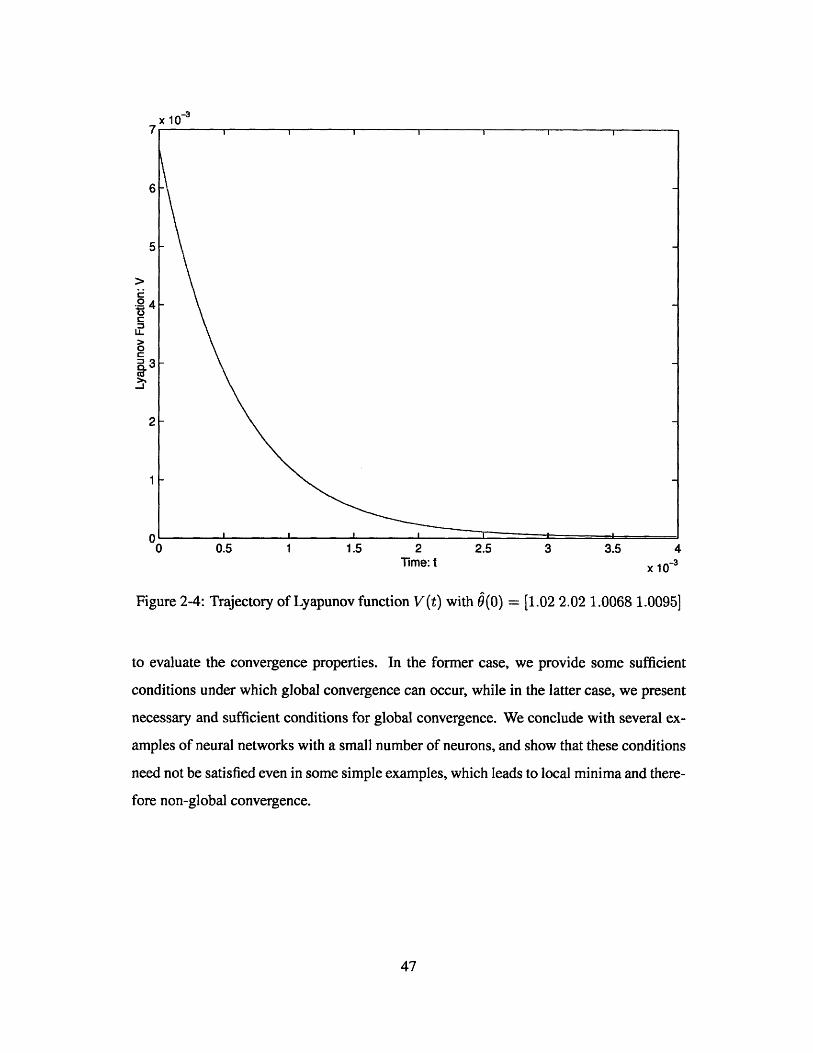
Simulation results shows that there are infinite points in E which can lead $(t) -+ 00 and

one example is 0(0) = [1.02 2.02 1.0068 1.0095] with V(t) plotted in Figure 2-4.

Increasing size of training data can not solve this singular problem. For example, when

we increase the training data set to

U = [0.5 12 3 4], (2.80)

using similar procedure, we found that for

0* = [6.2717 - 3.2760 1.1 1.2].,

VVoo = 0

where Oo = [12 11].

2.4 Implications on the Control of Nonlinear Dynamic Sys-

tems Using Neural Networks

The discussions above clearly indicate the following: Suppose that an unknown system is

in the form of a single-layer neural network whose number of nodes n is known, but its

weights are unknown and are to be estimated. If an identical neural network is constructed

whose nodes are equal to n in number, and whose weights are started from arbitrary loca-

tions and adjusted using the collective gradient algorithm so as to estimate the weights of

the first neural network, it is quite likely that the weight-estimates will not converge to their

true values, but to those where the tracking error reaches a local minimum which is larger

than zero. This establishes conclusively that it is quite likely that the best result achievable

44

.. .........

x 10'

6.8 - .- -. -

6.6 - .........

6.4- - -

6.2 --A -... - - -

6-

5.8-

thel,the2

& I--

-....... ..

5.6 -1.

5.4 -

5.2-

1x1e

I 10.5 0 -0.5

thel-1

x 10-3

Figure 2-2: Lyapunov function V along [01 92] around 0 = [1 2 1 1].

with a neural network is a local result in such an identification problem. The question is, if

a similar property will be found in the context of control of a nonlinear system using neural

networks.

To address this question, we consider the control of a nonlinear system, whose closed-

loop structure is such that it can be described as

y= h(w, 0*) (2.81)

where w is a closed-loop system variable that can be measured on-line, 0* is an unknown

parameter that keeps the system in ((2.81)) bounded, and h is a known function of its

arguments that satisfies assumption 1. Suppose that , can be measured at each instant of

45

-0.5 0the2

0.5 1

Pmr- t-t ] _ 7 ,

... . . . . . . . .

-.. ...

-

-3 phil,phi2

~.....................5.54 - -

5.52 -... ...

5.5. .. . . . . .. . . .

5.48

5 .4 . ..... ....

5.44

5.4

5.48

5.36

0.5-

-0.5--

phil -1 -0.8 -0.6 -0.4 -0.2 0 02 04 06 08 1x 10~

phi2

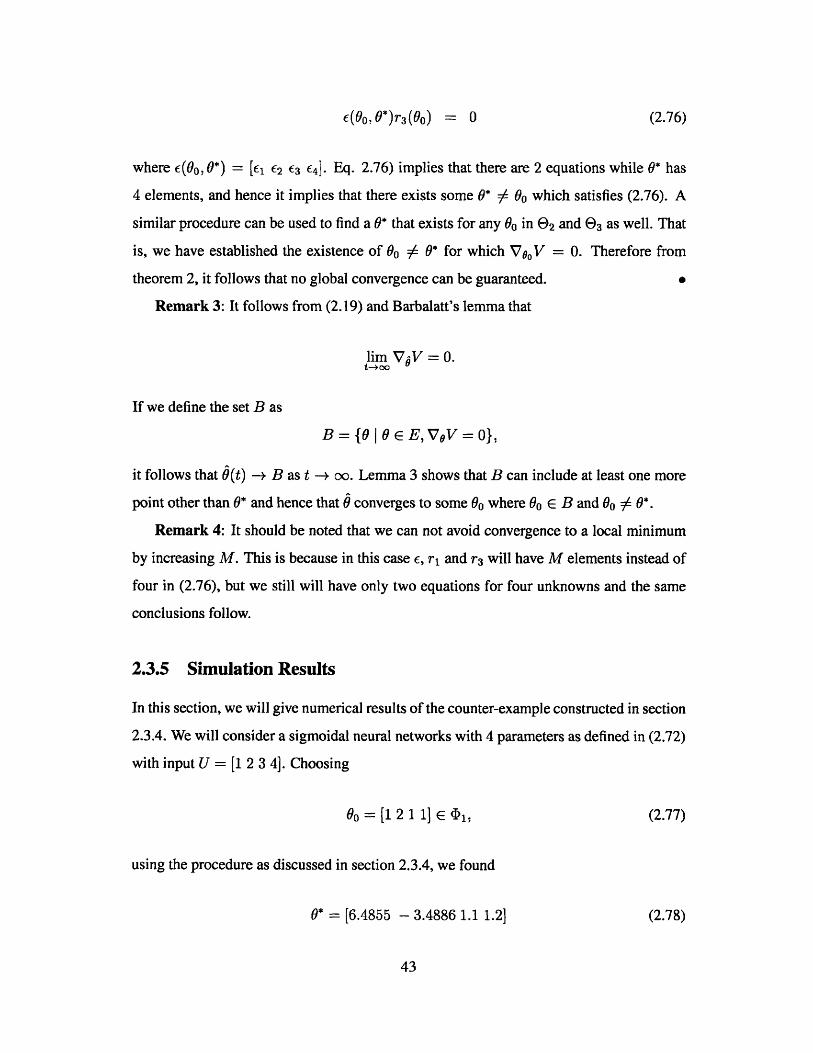
Figure 2-3: Lyapunov function V along [# q12] around 00 = [1 2 1 1].

time. This implies that the control of the system in (2.81) is equivalent to the identification

problem considered in section 2.1. It is therefore clear that in such cases, the statements

regarding the local behavior of neural networks are applicable to such a control problem

as well. Therefore control of general nonlinear systems using neural networks needs to be

approached with caution with care exercised to make sure that the local minima problems

are avoided.

2.5 Summary

In this chapter, we examine conditions under which the weights of a neural network can

converge starting from arbitrary values to those of another neural network with the same

structure. Both a standard gradient algorithm and a collective gradient algorithm are used

46

x 10-3

6-

5-

14--

LL

0C

Ca

-J

2-

0'0 0.5 1 1.5 2 2.5 3 3.5 4

Time: X 10~3

Figure 2-4: Trajectory of Lyapunov function V(t) with $(0) = [1.02 2.02 1.0068 1.0095]

to evaluate the convergence properties. In the former case, we provide some sufficient

conditions under which global convergence can occur, while in the latter case, we present

necessary and sufficient conditions for global convergence. We conclude with several ex-

amples of neural networks with a small number of neurons, and show that these conditions

need not be satisfied even in some simple examples, which leads to local minima and there-

fore non-global convergence.

47

Bibliography

[1] K. Hornik, M. Stinchcombe, and H. White. Multilayer feedforward networks are uni-

versal approximators. Neural Networks, 2:359-366, 1989.

[2] K. S. Narendra and K. Parthasarathy. Identification and control of dynamical systems

using neural networks. IEEE Transactions on Neural Networks, 1(1):4-26, March

1990.

[3] J. Park and I. W. Sandberg. Universal approximation using radial-basis function net-

works. Neural Computation, 3:246-257, 1991.

[4] R. M. Sanner and J. E. Slotine. Gaussian networks for direct adaptive control. IEEE

Transactions on Neural Networks, 3(6):837-863, November 1992.

[5] P. Werbos. The roots of backpropagation: From ordered derivative to neural networks

and political forecasting. Wiley, 1994.

[6] A. Kojic and A. M. Annaswamy. Global parameter convergence in systems with mono-

tonic parameterization. In Proceedings of the 2002 American Control Conference, An-

chorage, AL, 2002.

[7] A. Koji6. Global parameter identification in systems with a sigmoidal activationfunc-

tion. PhD thesis, MIT, Cambridge, MA, 2001.

[8] C. Cao and A. M. Annaswamy. Convergence properties of neural networks. Technical

Report 0301, Active-adaptive Control Laboratory, MIT, Cambridge, MA, 2003.

48

Chapter 3

Hierarchical Min-max Algorithm

3.1 Introduction

In this chapter, we consider parameter convergence in a class of continuous-time dynamic

systems. We begin with systems that have convex/concave parameterization and derive

sufficient conditions under which parameter convergence can occur in such systems. These

conditions are related to linear persistent excitation (LPE) conditions relevant for conver-

gence in linearly parameterized systems [1], and are shown to be stronger, with the addi-

tional complexity being a function of the underlying nonlinearity.

We also propose a new hierarchical min-max algorithm in this chapter in order to relax

the sufficient conditions for parameter convergence. The lower-level of this algorithm con-

sists of the same min-max algorithm as in [1, 5]. An additional higher-level component is

included in the hierarchical algorithm that consists of updating the bounds on the param-

eter region that the unknown parameter is assumed to belong to. We then show, using the

hierarchical algorithm, that parameter convergence can be accomplished globally under a

necessary and sufficient condition on the system variables and the underlying nonlinearity

f. Examples of functions that satisfy such a condition, which we denote as a condition

of Nonlinear Persistent Excitation (NLPE), and relations to LPE are also presented in this

chapter.

The chapter is organized as follows. Section 2 gives the statement of the problem,

the estimator based on the min-max algorithm and the properties. In section 3, parameter

49

estimation in functions that are concave/convex is considered, and a sufficient condition

for parameter convergence is derived. In section 4, a hierarchical min-max algorithm is

proposed and necessary and sufficient conditions for parameter convergence are proposed.

Examples and relation to LPE are also presented in this section. Simulation results are

included in Section 5. Summary and concluding remarks are stated in section 6. Proofs of

all properties, lemmas, and theorems can be found in Appendix A.

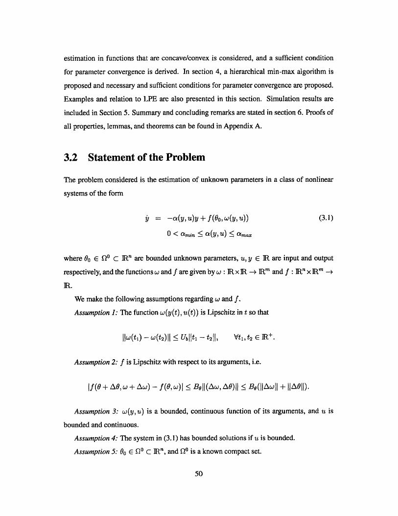
3.2 Statement of the Problem

The problem considered is the estimation of unknown parameters in a class of nonlinear

systems of the form

i = -a(y, u)y + f(00, w(y, U)) (3.1)

0 < amin a(y, u) amax

where 0 E fO C R are bounded unknown parameters, u, y e IR are input and output

respectively, and the functions w and f are given by w :R x R -+ FR" and f :R" x R'" -

IR.

We make the following assumptions regarding w and f.Assumption 1: The function w(y(t), u(t)) is Lipschitz in t so that

IIw(ti) - W(t2)II Ubl|t- -t 2 |-, Vtit 2 E IR+

Assumption 2: f is Lipschitz with respect to its arguments, i.e.

|f(0 +A01, w+Aw) - f(0, w)1 5 Be||l(Aw,A9)I 5 Be(I|AwI + IIAOII).

Assumption 3: w(y, u) is a bounded, continuous function of its arguments, and u is

bounded and continuous.

Assumption 4: The system in (3.1) has bounded solutions if u is bounded.

Assumption 5: Oo C O C CR, and QO is a known compact set.

50

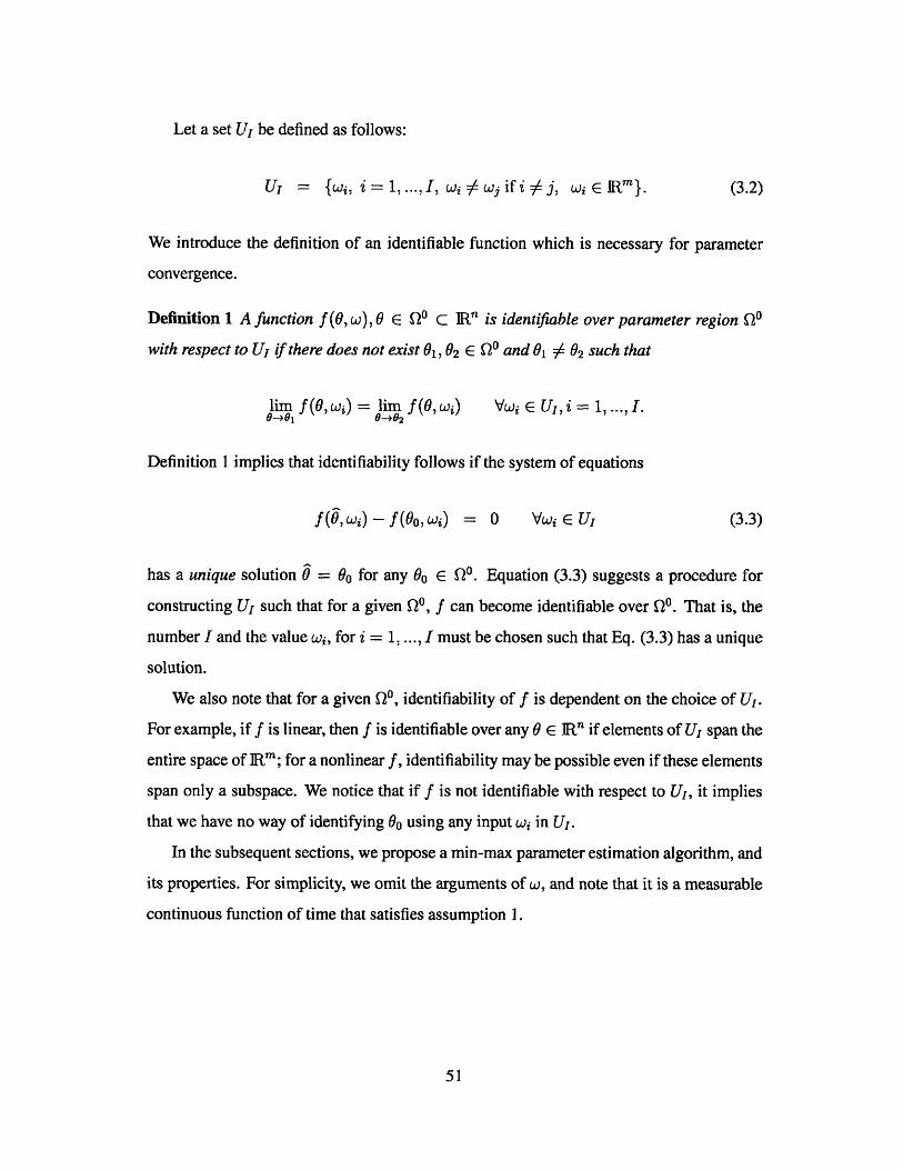
Let a set UT be defined as follows:

Ur = {wi, i = 1, ...,I, Wi = Wj if i #j, Wi ER"}. (3.2)

We introduce the definition of an identifiable function which is necessary for parameter

convergence.

Definition 1 A function f (0, w), 0 E QO c R is identifable over parameter region Q0

with respect to U1 if there does not exist 01,02 Q 0 and 01 = 02 such that

lim f(0, wi) = lim f(0, wi) VWj G U, i = 1, ..., I.0-401 0-+02

Definition I implies that identifiability follows if the system of equations

f(, w) - f (o, w) = 0 VWi E UI (3.3)

has a unique solution 9 = 00 for any 00 E QO. Equation (3.3) suggests a procedure for

constructing U, such that for a given QO, f can become identifiable over QO. That is, the

number I and the value wi, for i = 1, ..., I must be chosen such that Eq. (3.3) has a unique

solution.

We also note that for a given Q1, identifiability of f is dependent on the choice of U.

For example, if f is linear, then f is identifiable over any 9 E R' if elements of U span the

entire space of R'; for a nonlinear f, identifiability may be possible even if these elements

span only a subspace. We notice that if f is not identifiable with respect to U, it implies

that we have no way of identifying 0 using any input wi in U1.

In the subsequent sections, we propose a min-max parameter estimation algorithm, and

its properties. For simplicity, we omit the arguments of w, and note that it is a measurable

continuous function of time that satisfies assumption 1.

51

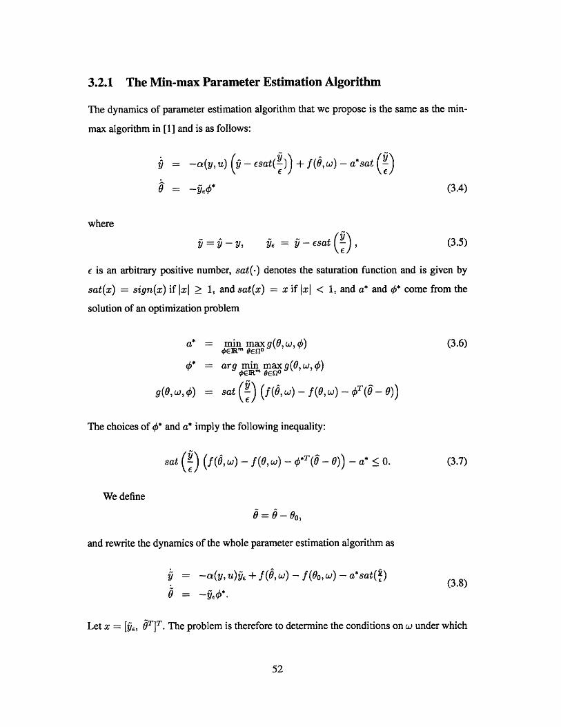
3.2.1 The Mmn-max Parameter Estimation Algorithm

The dynamics of parameter estimation algorithm that we propose is the same as the min-

max algorithm in [1] and is as follows:

y= -c(y, u) - Esat()) + f(9, w) - a*sat

0# (3.4)

where

Y , Ye = Y- esat( . (3.5)

c is an arbitrary positive number, sat(.) denotes the saturation function and is given by

sat(x) = sign(x) if JxJ _> 1, and sat(x) = x if IxI < 1, and a* and 0* come from the

solution of an optimization problem

a* = mi maxg(O,w,5) (3.6)

= arg min mag(OwO)

g(0, w, b) = sat (f ($, w) - f(0, w) - O( -_))

The choices of 0* and a* imply the following inequality:

sat ( (f(, W) - f (O, w) _ O*T(j _ 0)) - a* < 0. (3.7)

We define

9= -0,

and rewrite the dynamics of the whole parameter estimation algorithm as

y = -a(y, u)& + f(9, w) - f(Oo, w) - a*sat({)(3.8)

L = -Tsd*.

Let x = [Qe, ST]T. The problem is therefore to determine the conditions on w under which

52

the system (3.8) has uniform asymptotic stability in the large (u.a.s.l.) at x = 0.

3.2.2 Solutions of a* and 0*

In [1] and [5], closed form solutions to (3.6) when f is a concave/convex function of 00

and when f is a general function of 0o were derived, respectively. In both [1], [5], these

solutions were derived under the assumption that 9 E QO. In this chapter, results are

extended to the case when this assumption is omitted. For ease of exposition, we present

the results for the cases when (a) 9 is a scalar, and f is a general function of 9 and (b) 9

is a vector, and f is a convex/concave function of 9. We define a convex set C(2o) which

is constructed as follows: If Hf(O) is the convex hull, which is the smallest convex set

in M!n+ that contains {(., f(0, w)) 10 E QO}, then C(Qo) is the projection of Hf(Qo) on

1R" which contains Qo. Such a convex set is needed since (i) the hierarchical algorithm

discussed in section 3.4.3 can allow the parameter estimate to wander outside Qo, and (ii)

the solutions to the min-max algorithm differ depending whether 9 lies within this convex

set C(QO) or outside.

(a) 9 E QO C IR, and f is a general function of 9: In this case C() = [9min- Omax]-

Same as in [5], the following two definitions are useful.

Definition 2 A point 90 E 0, if 0* E C(Q0O) and

VfOo(9 - 00) 5 f(0,w) - f( 0 ,w). V9 E C() (3.9)

where VfOo = .

Definition 3 9c = #, n C(v0 ), where Oc denotes the complement of Oc.

We now state the solutions to (3.6) in case (a), when y > 0. The solutions when < 0

can be derived in a similar manner using the concave cover.

53

Denoting 0c = {=, .. . , 9m"}, 9i = [0i, 93] as in [5], we obtain that

= Vfb

= 0 if 'c= cij

= f(, w) - f(0i, w) - 0*( -')

if 9 E O'j

and if 9> Gma,

a* =f0

and if 0 < Omin,

a* =0

#*(Omax)

if f (max, W) + 0*(Omax)(0 - Omax) > f (, w)

/(Om.:,W)-f(,w) otherwise,Oma-

*(Omin)

if f (Gmin, w) + 0*(Omin)(0 - 9min) f(0, w)

A(Omin,w)- otherwise.

(3.12)

(b) 0 E 00 C R, f is a concave function of 9: The solutions to (3.6) are easier to find

when QO is a simplex, and are presented first:

Case (i): QO is a simplex: Very similar to [1], we have the following solutions:

54

0*

a*

0*a*

if C(QO), (3.10)

(3.11)

a*=0 1 7<OOEC()0 )

*= Vfj

a*=0 9<OO(C(Q0 )

*= Vfj

a*=Ai 9>0,OEC(Q0 )

4*A2

a*=0 jj>0,O0 C( 0 )

S* = A2

where [A 1 , A 2 ]T G-1b, A1 E JR, A2 E W,

-1 ~-(O-Osi)T

-1 -(- Os 2)T

-1 (-s4i)T

-(f(, w) - fsi)

b -(f(Ow) - fs2)

-(f(0,w) - fsn+l) .

9si, i = 1, ... , n + 1 are the vertices of Q1, and fsi = f(si, w).

Case (ii) QO is a compact set in Rn: We define a polygon P(P0 ) which contains QO,

Kwhose vertices are given by P1, P2 .... , PK. Denoting L = , we note that L

n + 1)hyperplanes can be constructing using a combination of n + 1 points from the K vertices

of the polygon. Denoting the vertices of the ith hyperplane as P, .., Pi 1 , and qi as the

slope of this hyperplane, we choose J as a set of the L hyperplanes such that

J = {ill <i<L, f(,w)-f(Pjiw)-#T( -Pi1 )

> 0. V 6 C P(00 )}.

We can derive the solutions to (3.6) as

55

where

A 2 = k

A1 = f(9,w)-f(P, w) - 3(-Py1 )

j = argmaxf(Pi,w)+q5(9-P,)iEJ

The solutions for the case when f is a convex function of 9 can be derived in a similar

manner.

(c) 9 C o C lnR, f is a general function of 0: Using the above two cases, and in partic-

ular, a combination of concave and convex covers, convex hull, and polygons, the solutions

to (3.6) can be found.

3.2.3 Properties of the Mn-max Estimator

In [1], the min-max estimator and therefore the resulting error model in (3.8) was shown

to be stable. The stability properties of this error model are summarized in Property I and

Property 2 below. In what follows, the quadratic function V is useful:

11 2V = (9,2 + T) = IIx(t)12.2 E+ T)=2

(3.13)

Property 1 summarizes the stability properties of (3.8).

56

a* = 0 j < 0, 0 E C(P(Q0 ))

S* = Vf

a* = 0 < 0,9 C(( 0 ))

#* = Vf_

a* = A, i > 0, E C(P(Q0 ))

a* = A2

a* = 0 > 0,1 C(P(QO))

$0* = A2II

Property 1

. _; - . (3.14)

Property I implies that the min-max estimator is stable. However whether the parameter

estimates will converge to their true values, that is, whether x will converge to the origin

is yet to be established. To facilitate parameter convergence discussions, an additional

property of the min-max estimator is stated in Property 2.

Property 2 If in Eq. (3.8),

JYE(tl)I _> 7, (3.15)

then

V(ti + T') < V(t1) - Cemin7 ̂f3.16)3(M + amax7)

where T' = , 0 < 0min < a(y, u) < amax, and

M = max{Jm(t)1},

m(t) = f(6,w) - f(Oo,w) - a*sat ( ). (3.17)

Property 2 implies that for parameter convergence to occur, & must become peri-

odically large. For this in turn to occur, examining the dynamics in (3.8) and defining

f(,10,w) = f(0,w) - f(O0,w), (i) f(0,0,w) must be large when |10|| is large and (ii)

a* must be small compared to f(0, 0, w). The condition (i) is related to persistent excita-

tion, and is similar to parameter convergence conditions in linearly parameterized systems.

Condition (ii) is specific to the min-max algorithm. In order to facilitate the latter, a few

properties of a* are worth deriving, and are enumerated below in Properties 3 and 4.

Noting that a* is defined as in (3.6), we denote

a* (0, w) = a* if < 0,

a*(0,w) = a* if S > 0.

57

It follows that a* and a*+ are well defined functions of 0 and w. We establish the following

properties about a*, a* (9, w) and a* (0, w)-

Property 3

Suppose for a given w, f(0, w) retains its curvature as 0 varies. We define

if f (0, w) is convex;

if f(0, w) is concave.(3.18)

Property 4 For a* and # defined as in (3.6) and (3.18), respectively, the following holds:

(i) a* = 0 if # = -1; (ii) a* = 0 if = 1;

(ii) #a* ! 0, for anyf#. (3.19)

Both Properties 3 and 4 are used in the next section for the proof of Theorem 1.

3.3 Parameter Convergence in Systems with Convex/Concave

Parameterization

We first focus on parameter convergence of the system (3.8) when f is convex/concave for

any 9 E Q1. For the sake of completeness, we include the definition of a concave/convex

function:

Definition 4 A function f (0) is said to be (i) convex on e if it satisfies the inequality

f(A01 + (1 - A)02) 5 Af(01) + (1 - A)f(0 2 ) V01 7 2 E (

and (ii) concave if it satisfies the inequality

f (A9 1 + (1 - A)02) > Af(0 1) + (1 - A)f(0 2) V9 1, 02 E 0

where 0 < A < 1.

58

-a* ( , w) < a* satj a* 0*( w)

O(P)=

We make a few qualitative comments regarding the solutions of (3.8) and their conver-

gence properties before establishing the main result. The main difficulty in establishing

parameter convergence is due to the presence of the time-varying function a* in (3.8). As

shown in properties 3-4 in Section 3.2.3, the magnitude of a* changes with the curvature of

f. As mentioned in Section 3.2.3, in order to establish parameter convergence, in addition

to f(0, 0, w) being large when 0 is large a* has to remain small. Property 3 shows that for

any nonzero value of g, a* can periodically take the value zero if f switches periodically

between concavity and convexity. This in turn implies that a* can periodically become

small if f continues to change its curvature, that is, ,3 changes from +1 to -1. As will be

shown in Section 3.3.1, the conditions for parameter convergence not only require that fbecome large for a large 9 but also require f to switch between convexity and concavity

over any given interval.

Yet another feature of the min-max algorithm is the use of the error 5, for adjusting

the parameter 0 instead of the traditional estimation error #. This was introduced in the

estimation algorithm to ensure a continuous estimator in the presence of a discontinuous

solution that can be obtained from the min-max optimization problem. The introduction of

a nonzero c can cause the parameter estimation to stop if Ig| becomes smaller than C. As a

result, the trajectories are shown to converge to a neighborhood D, of the origin rather the

origin itself.

In Section 3.3.1, we state and prove the convergence result. In Section 3.3.2, we dis-

cuss the sufficient condition that results in parameter convergence, specific examples of

f and counterexamples, and the relation to persistent excitation conditions that guarantee

parameter convergence in the case of linear parameterization.

3.3.1 Proof of Convergence

The first convergence result in this chapter is stated in Theorem 1.

Theorem 1 If (i) f(0, w(t)) is convex (or concave) on 0 for any w(t) E 1R', and (ii) for

every t1 > to, there exist positive constants To, c, and a time instant t2 G [ti., t1 + To] such

59

that for any 9

#(w(t 2)) (f (0,w(t2)) - f(o, w(t 2))) 'Ec -I o - (3.20)

where 6(w (t 2 )) is defined as in (3.18), then all trajectories of (3.8) will converge uniformly

to

DE= {x I V(x) 5 Y1}. (3.21)

where

x = [6B ,T]T, 1 = + 8BB 4, + 4B,), (3.22)

E is defined as in (3.8), c. is given by (3.20), Ub and B0 are defined as in Assumptions 1 and

2, and B, is the bound on $* in (3.4) so that

1k*(t)ll 5 B, V t > to. (3.23)

The proof of Theorem 1 follows by showing that if w and f are such that condition

(3.20) is satisfied, then &(t) becomes large at some time t over the interval [t 1 , t, + TO].

Once & (t) becomes large, it follows from Property 2 that V(t) decreases over the interval

[ti, ti + TO] by a finite amount.

Remark 1: If f is concave (or convex) and if f satisfies the inequality in Eq. (3.20), we

shall define that f satisfies the Convex Persistent Excitation (CPE) condition with respect to

w. Theorem I implies that if f satisfies the CPE condition with respect to w, then parameter

convergence to a desired precision follows.

Remark 2: From the definition of D6, it automatically follows that as e -+ 0, all trajectories

converge to the region x =: 0 and hence u.a.s.l. follows.

3.3.2 Sufficient Condition for Parameter Convergence

The CPE condition specifies certain requirements on f in order to achieve parameter con-

vergence. For a given f, theorem I does not state how w should behave over time in order

to satisfy (3.20). In this section, we state some observations and examples of w that satisfies

60

(3.20) for a general f.Equation (3.20) consists of two separate requirements. Denoting f = f(0, w)-f(0, w).

the first requirement is that the magnitude of f must be large. The second requirement is

that f must have the same sign as 3. The first component states that for a large parameter

error, there must be a large error in f. It is straightforward to demonstrate that this condi-

tion is equivalent to linear persistent excitation condition in [10], and is shown in section

3.3.2. The second requirement states what the sign of f should be in relation to the con-

vexity/concavity of f. If f is convex, f should be positive, and conversely, if f is concave,

f should be negative.

The coupling of convexity/concavity and the sign of the integral of f has the following

practical implications. To ensure parameter convergence, w must be such that one of the

following occurs: At least at one instant t2 C [t 1, ti + T],

(a) For the given W, w must change in such a way that the sign of f is reversed, while

keeping the convexity/concavity of f the same, or

(b) For the given 9, w must reverse the convexity/concavity of f, while preserving the

sign of f

Examples

We illustrate the above comments using specific examples of f. Suppose

f = e- T (3.24)

where w(t) : IR -+ 1R', 9 E C R'. It can be checked that f given in (3.24) is always

convex with respect to 9 for all w. Therefore, option (b) is not possible. Hence, W must be

such that f can switch sign for any 9 as required by option (a). One example of such an W

is if for any ti, there exists t2 E [ti. ti + T] such that

wT(t 2 ) V ;> eu (3.25)

61

where v is any unit vector in R. Another example which satisfies condition (3.20) is given

by

f =O'. w E R.

It is easy to show that for such an f, condition (b) is satisfied if W switches between w, and

w2 where 0 < wi < 1 and w2 > 1-

The above examples show that the condition on w that satisfies Eq. (3.20) varies with

f.

Relation to Conditions of Linear Persistent Excitation

The relation between CPE and LPE is worth exploring. For this purpose, we consider a

linearly parameterized system, which is given by Eq. (3.1) with

f(00, w) = 9O'q(w)

where O(w) E R. In this case, it is well known that the corresponding estimator is given

by equation (3.4) with a* = 0 and 0* = q [1]. The resulting error equations are summarized

by

y = -a(y, u)e + dT5(w)1 (3.26)

9 = -yb(w).

In [10], it is shown that u.a.s.l. of (3.26) follows under an LPE condition. For the sake of

completeness, we state this condition below.

Definition (LPE): # is said to be linearly persistently exciting (l.p.e.) if for every ti > to,

there exists positive constants To, 6o, eo and a subinterval [t2 , t 2 + 6o] E [tj. ti + To] such

that

f Th(w(T))drJ ;> coII1II. (3.27)

We now show the relation between the LPE condition and the CPE condition in (3.20).

When f(0, w) = 9TO(w), if Assumption I holds, it can be shown that the LPE condition

is equivalent to the following inequality: For every t1 > to and 9, there exists positive

62

constants To, co and a time instant t2 C [ti. ti + T] such that

If(Ow(t2)) - f(0, w(t 2)) > cu I1 - 0011. (3.28)

Since a linear function can be considered to be either convex or concave, the inequality in

(3.28) is equivalent to the CPE condition in (3.20). This equivalence is summarized in the

following lemma:

Lemma 1 When f (0, w) = OTcb(w), ifAssumption 1 holds, the CPE condition in Eq. (3.20)

is equivalent to the LPE condition in Eq. (3.27).

It should be noted that for a general nonlinear f, the CPE condition becomes more restric-

tive than the LPE condition. For example, for f as in (3.24), the CPE condition implies

that w must satisfy (3.25). On the other hand, if f = wTO, even if w is such that IwT(t 2 )vI

is periodically large, the LPE condition is satisfied.

A counter-example

For a general function f, it may not be possible to find a w that satisfies either condition (a)

or (b) mentioned above. A simple example is

f = cos(Ow)

where Iw I Wmaz and 0 E [0, 7r/(2wmax)]. We note that f is concave and monotonically

decreasing for any w with |w 1 <Wmax. Hence neither (a) nor (b) is satisfied. That is, it is

possible for the parameter estimate 0 of the min-max algorithm to get "stalled" in a region

in 00. This motivates the need for an improved min-max algorithm, and is outlined in

section 3.4.

63

3.4 Parameter Convergence in Systems with a General Pa-

rameterization

In the previous section, we showed that if a function f is convex (or concave), and if f

and w satisfy the CPE condition, then parameter convergence follows. However, as we

saw in section 3.3.2, not all convex/concave functions can satisfy the CPE condition. In

this section, we present a new algorithm which not only allows the persistent excitation

condition to be relaxed but also enables parameter convergence for non-convex and non-

concave functions.

The algorithm we present in this section is hierarchical in nature, and consists of a

lower-level and a higher-level. In the lower-level, for a given unknown parameter region QO,

the parameter estimate 0 is updated using the min-max algorithm as in (3.4). In the higher-

level, using information regarding the parameter estimate 9 obtained from the lower-level,

the unknown parameter region is updated as Q1. Iterating between the lower and higher

levels, the overall hierarchical algorithm guarantees a sequence of parameter region k.

The properties of these two levels are discussed in Sections 3.4.1 and 3.4.2, respectively. In

Section 3.4.4, we discuss conditions under which 0 converges to 00. Using these conditions,

the definition of persistent excitation for nonlinearly parameterized systems is introduced.

In Section 3.4.5, we present examples of such a Nonlinear Persistent Excitation (NLPE).

The relation between NLPE and CPE is discussed in Section 3.4.6.

3.4.1 Lower-level Algorithm

The lower-level algorithm consists of the min-max parameter estimation as in (3.4) with

the unknown parameter 00 E Qk. We show in this section that when this algorithm is used,

& (t) becomes small in a finite time, which is denoted as lower-level convergence. Once this

occurs, the parameter estimate 9, derived from the lower-level convergence, remains nearly

steady. This estimate, in turn, is used in the higher-level part of hierarchical algorithm to

update the unknown parameter region from Qk to Qk+1. The convergence of & is stated in

Lemma 2, and the characterization of the unknown parameter is stated in Lemma 3.

64

Lemma 2 For the system in (3.1) and the estimator in (3.4), given any positive T and 6,

there exists a finite time t1 such that

I &(t) _ I 6 for ti t < t + T. (3.29)

We note that for every specific w, a time t1 that satisfies (3.29) exists. However the

value of tj will depend on the choice of w. Since our goal is parameter convergence, we

require w to assume distinct values, i.e. persistently span a set of interest. This is stated in

the definition below.

Let U1 be defined as in Eq. (3.2).

Definition 5 w is said to persistently span U1 iffor any wi E U1 and any t1 , there exist a

finite T and ri such that

w(ri) = wi Tj E [ti. -,1 + Tj] i = 1,...,) L. (3.30)

Definition 5 implies that w periodically visits all points in U1.

Let

Bt = 2BO(bBo + 2Ub) + JBO, (3.31)

where Ub, BO and BO are defined in Assumption 1, Assumption 2 and (3.23) and 6 is any

positive number. If we choose T as

2 Bt(3 + )T = max T +

1<i< Bt

where T is given by (3.30), then Lemma 2 implies that there exists a finite time ti such that

|C(t)| :5 j ti :5 t < ti + T. (3.32)

When & satisfies (3.32), we refer to it as lower-level convergence. If w persistently spans

U, then Definition 5 and the choice of ri implies that atTj c- Et 1, tj + T, w(ri) = wi,

65

i=1..., I. The parameter estimate O(rj) at time instances are defined as

0C = r) i = 1, ..., I,

and are denoted as low-level convergent estimates. We characterize the region where the

unknown parameters lie in lemma 3 using these lower-level convergent estimates.

Lemma 3 For the system in (3.1) and estimator in (3.4), let £ be the unknown parameter

region and O$c, i = 1...., I, be the lower-level convergent estimates. If the input w persis-

tently spans U1, then

9o E f4)E (, WiI 6, , ).i=1

where

(, Wi,, 6, )= {O E QJf. i f (0, w) h} (3.33)

f. = f(Of, w) - a*(Of, w) - amaz - 2 Bt(6 + c)

f= f(7, wi) + a*(0 , w)+ amaz6 +2 Bt(65+E)}

and Bt as in (3.31).

Lemma 3 implies that the unknown parameter 0 lies in D, for a given wi. It should be

noted that in general, 4, need not be smaller than 0. However other properties of (D are

useful for characterizing the convergence behavior of the min-max algorithm. These are

enumerated below.

(P1): For J = c = 0, if a* = a*- = 0, then D, reduces to the manifold

f (A, w) = f (k, w).

(P2): Property (P3) implies that if (i) w is p.e. in U1 , (ii) f is identifable w.r.t. U1 , (iii)

6 = c = 0 and (iv) a* = a*- = 0, then

SE(Q ,wi, c, 6, ,) = {o}.

66

These properties are made judicious use of in designing the higher-level algorithm in

the section 4.2.

3.4.2 Higher-Level Algorithm

We now present the higher-level component of the hierarchical algorithm. Here, our goal is

to start from a known parameter region Qk that the unknown parameter 0 lies in, and update

it as Qk+1 using all available information from the lower-level component. In particular,

we use <), defined in Eq. (3.33) to update Qk. In order to reduce the parameter uncertainty,

different <Ds are computed by varying wi, i = 1, ... , I. The resulting QA+1 is therefore

chosen as

Qk+1 (bel 4 (Qk, 5W, IEl J,1~) (3.34)

3.4.3 The Hierarchical Algorithm

The complete hierarchical algorithm is stated in Table 3.1.

It should be noted that Steps 2 and 3 correspond to the lower-level and the higher-level

parts of the hierarchical algorithm, respectively. Also, we note that Step 2 requires the

closed-form solutions of a* and 0* which can be found as outlined in Section 2.1.

In order to obtain parameter convergence using the hierarchical algorithm, what remains

to be shown is whether Qk+1 is a strict subset of Qk.

3.4.4 Parameter Convergence with the Hierarchical Algorithm

We now address the parameter convergence of the hierarchical algorithm. We introduce a

definition for a "stalled" parameter region Ai:

For any QcQO, define f* and f* as

= Min f(0, wi). f* = max f(0, w;). (3.35)

67

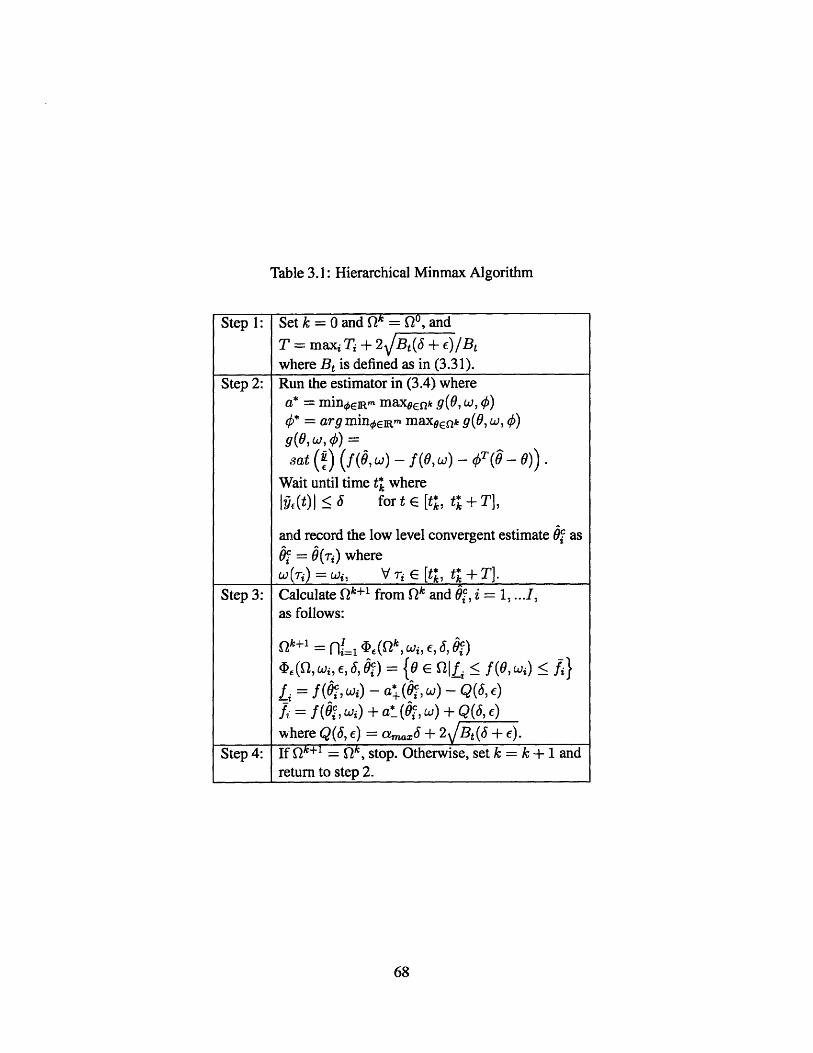
Table 3.1: Hierarchical Minmax Algorithm

68

Step 1: Set k = 0 and Q1 = QO, and

T = max, T +2 Bt( + c)/Btwhere Bt is defined as in (3.31).

Step 2: Run the estimator in (3.4) wherea* = min0E1Rm maxqEnk g(9, w, )0* = arg minoEim maxeEnk g(0, w,g(9, w, 0) =

sat (j) (f($,w) - f(0,W) - #T(- 6)).Wait until time t* where

IJ(t)I j for t E [t* , t* + T].

and record the low level convergent estimate Of as

9f = 0(rj) where

wr)=wi, V -ri E [t* , t* + T].Step 3: Calculate Qk+1 from Qk and Oi, i = 1, ...1,

as follows:

Qk+l ('(Q, , ,$)

(Q, wi, E, 6, 9[) = {OE Qfi < f (0,wi) Ai

f. = f($f,wos) - a*4(Of,w) - Q(5, c)= f(Oi, wi) + a* (6f, w) + Q(6, e)

where Q(6, e) = amax6 + 2 Bt(6 + c).

Step 4: If k+1 = k, stop. Otherwise, set k = k + 1 andreturn to step 2.

Then we define Aj(Q) to be a "stalled" estimate-region of Q as

Ai()= {( f (0, wL) - a*(0, wi) - D(E, 6) _

and f(0, wi) + a* (, wi) + D(E, 6) > f*}.

D(E, 6) = amax6 +2 Bt(6 +)

where

(3.36)

(3.37)

We prove a property of Li(Q) which explains why it corresponds to a "stalled" region

in Q.

Lemma 4 For some k, if c Ai(2I), V i = 1, .., I, then

Qk+1 .- Qk

In order to establish parameter convergence, we first characterize the region L that

the parameter estimate converges to in Lemma 5, and then establish the conditions under

which L simply coincides with the true parameter 00 in Theorem 2. The set L is defined as

follows:

(3.38)w e ), c n a n s e n B ( A i (

where B(X) is a box that contains any set X and is defined as

B(X) = {0 1110 - 611 5 TBO. V # E X}. (3.39)

Lemma 5 For the system in (3.1) and estimator in (3.4), under assumptions 1-4, the hier-

archical algorithm outlined in Table 3.1 guarantees that

lim (t) E L(Q0, c, 6).t-+oo (3.40)

Since e and 6 are arbitrary positive numbers, they can be chosen to be as small as

69

1))) ,

possible. When F -+ 0, 6 -+ 0, it follows directly from (3.36), (3.39) and (3.38) that

fim L(Q 0 , C, 6)= U n Li(o) (3.41)f-+OJ-O V nEno, with ooEn i=-1,--,I

where

AL(Q) = { f f(0, w) - a* (0, wi) < f*

and f(0, wi) + a* (0, wi) > f*}. (3.42)

with f* and f;* defined as in (3.35). From (3.41), we have the following theorem:

Theorem 2 For the system in (3.1) and estimator in (3.4), under assumptions 1-4,

lim =0 (3.43)t-+00,f-+-0,6-*0

if and only iffor any SCfo where o E Q2,

r Lj(9) =or f Li(r)= {0 0}. (3.44)

where 0 denotes the null set and L is defined as in (3.42).

Theorem 2 gives us a method to check if the hierarchical algorithm can estimate the

true parameters to any desired precision when we set c and 6 small enough for a specific

problem. We note that L(90, e, 6) is a continuous function of c and 6, and that as c and J

becomes small, L becomes arbitrarily close to the set {0o}. Hence the parameter estimate

converges to the true value with a desired precision.

Remark 3: If f(0, w) is identifiable over Q with respect to U1 , w persistently spans U1 ,

and f satisfies the inequality (3.44), we shall define that f satisfies the Nonlinear Persistent

Excitation (NLPE) condition with respect to w. Theorem 2 implies that NLPE of f with

respect to w is necessary and sufficient for parameter convergence to take place.

Remark 4: The requirement on w for f to satisfy the NLPE can sometimes be less stringent

than that on w for LPE. An example of this fact is for the parameter 0 = [01, 02 ]T, and the

70

cases (i) 1(0) = OTw, and (ii) f () = 01w1 cos(0 2w2 ) where w, and w2 are the elements of

w. Clearly, for a w such that w, = kw 2, where k is a constant, W does not satisfy LPE, but

f does satsify NLPE with respect to w. As shown in Section 3.3.2, NLPE can impose more

stringent conditions on w as well.

Remark 5: It should be noted that the NLPE condition guarantees parameter convergence

for any general nonlinear function f that is identifiable. This implies that the min-max

algorithm outlined in [5], which is applicable for even a non-convex (or a non-concave)

function, can be used to establish parameter convergence. We include simulation results of

such an example in Section 3.5.

Remark 6: It should be noted that a fairly extensive treatment of conditions of persistent

excitation has been carried out in [11, 12] for a class of nonlinear systems. The systems

under consideration in this chapter do not belong to this class. The most distinct features of

the system (3.1) is the presence of the quantity a* and the quantity f (0, w) -f (0o, w), where

the former can introduce equilibrium points other than zero and the latter is not Lipschitz

with respect to C - 9. As a result, an entirely different set of conditions and properties have

had to be derived to establish parameter convergence.

Remark 7: The closed-form solutions of a* and <0* can be calculated as shown in Section

2.1. It should be noted that these solutions have been derived without requiring that 9 E Q1,

thereby expanding the results of [1]. Since 9 can lie anywhere, subsequent iterations of the

hierarchical algorithm can be carried out during which time the corresponding min-max

solutions can be derived.

As is evident from (3.44), (3.35) and (3.42), to check if indeed the NLPE condition is

satisfied for every QCQO for a given f and w is a difficult task. In the following section,

we show that when 9 E JR2, if f is monotonic function of 9, identifiable with respect to U1,

and f is convex/concave, then the NLPE condition is satisfied.

3.4.5 Parameter Convergence when 9 E ]R2: An Example

When 9 = [01, 02] E JR 2 , the following lemma provides sufficient conditions for Eq. (3.44)

to hold and hence for the hierarchical algorithm to guarantee convergence.

71

Lemma 6 For system in (3.1), estimator in (3.4) where 9 E R 2, let 00 E QO and f be

identifiable over Q1 with respect to U2. If

(i) f (0, w) is convex (or concave) over all 9 in 0

W, W2E U1 (3.45)

(ii) f (9, wi) is monotonic with respect to 9 in Q"

WW2E U (3.46)

then equation (3.44) holds for any QO where 00 C Q.

The reader is refered to [13] for the proof.

3.4.6 Relation between NLPE and CPE

In what follows we compare the NLPE and the CPE conditions. In order to facilitate this

comparison, we restate the CPE condition in a simpler form:

Definition 6 f is said to satisfy the CPE' condition with respect to w if (i) f (, w(t)) is

convex (or concave) for any w (t) E I', and (ii) w is persistently spanning with respect to

U1, and (iii)for any 9, there exists wi E U such that

#8(wJ) (f(0, W) - f(0o, W)) ;> C. I1 - 0o1. (3.47)

We note that the only distinction between the inequalities in (3.20) and (3.47) is in the

value taken by w(t 2 ) for some t2 in the interval [t, t + T]. In (3.47) it implies that w(t 2 )

assumes one of the finite values wi in U, while in (3.20), the corresponding U can consist

of infinite values. If w is "ergodic" in nature so that it visits all typical values that it will

assume for all t over one interval, then it implies that the two conditions (3.20) and (3.47)

are equivalent. We shall assume in the following that the input is "ergodic."

Lemma 7 Let f (, wi) be convex (or concave) for all 9 E 0 , then the CPE' condition

implies the NLPE condition.

72

Remark 8: Lemma 7 shows that the CPE' condition is sufficient for the NLPE to hold

if f is convex (or concave). Clearly, the CPE' condition is not necessary, as shown by

the counterexample in Section 3.3.2. The NLPE condition therefore represents the most

general definition of persistent excitation in nonlinearly parameterized systems.

3.5 Simulation Results

We consider the system in (3.1) and the estimator in (3.4) to evaluate the performance of

the hierarchical algorithm. The system parameters are chosen as follows:

f = (0- 8 + 12exp f-5 ( - 2 +

where 0 is an unknown parameter that belongs to a known interval QO = [0, 5]. System

variable w is chosen as a sinusoidal function w = 1.1 sin(2t) and the true unknown parame-

ter 90 equals 2. We note that the function f is non-convex (and non-concave), whose values

are shown in Figure 1 for w = 1, -1, 0. It can be shown that f is identifiable with respect

to 0 and that w is persistently spanning with respect to U = {1, -1, 0}. The hierarchical

algorithm in Table 3.1 was implemented to estimate 00. The parameters c = 0.001 and

J = 0.02. Since w is a sinusoid, the parameter T was set to the corresponding period ir.

The resulting output error &, parameter estimate 0, and the update of the parameter regionQk are shown in Figures 2-4, respectively. The evolutions of the lower and upper bounds

fk and ji, i = 1, 2, 3 with respect to t are also shown in Figure 5. A similar convergence

was observed to occur for any 00 in Q1. These figures show that the update of Qk is not

necessarily periodic. Once & becomes smaller than J over an interval T, the corresponding

parameter estimates and the upper and lower bounds on fi and therefore the unknown pa-

rameter region are computed. It was also observed that just the min-max algorithm without

the higher level component did not result in parameter convergence.

73

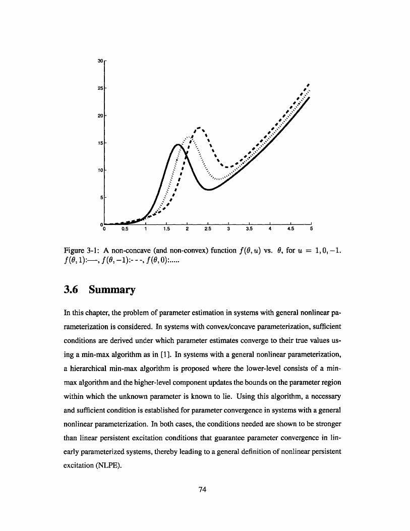
30

25-

20

15p

10-

5-

0 0.5 1 1.5 2 2.5 3 3.5 4 4.5 5

Figure 3-1: A non-concave (and non-convex) function f(0, u) vs. 0, for u = 1, 0., -1.f(9. 1):-, f(9. -1):---, f(0, 0).

3.6 Summary

In this chapter, the problem of parameter estimation in systems with general nonlinear pa-

rameterization is considered. In systems with convex/concave parameterization, sufficient

conditions are derived under which parameter estimates converge to their true values us-

ing a min-max algorithm as in [I]. In systems with a general nonlinear parameterization,

a hierarchical min-max algorithm is proposed where the lower-level consists of a min-

max algorithm and the higher-level component updates the bounds on the parameter region

within which the unknown parameter is known to lie. Using this algorithm, a necessary

and sufficient condition is established for parameter convergence in systems with a general

nonlinear parameterization. In both cases, the conditions needed are shown to be stronger

than linear persistent excitation conditions that guarantee parameter convergence in lin-

early parameterized systems, thereby leading to a general definition of nonlinear persistent

excitation (NLPE).

74

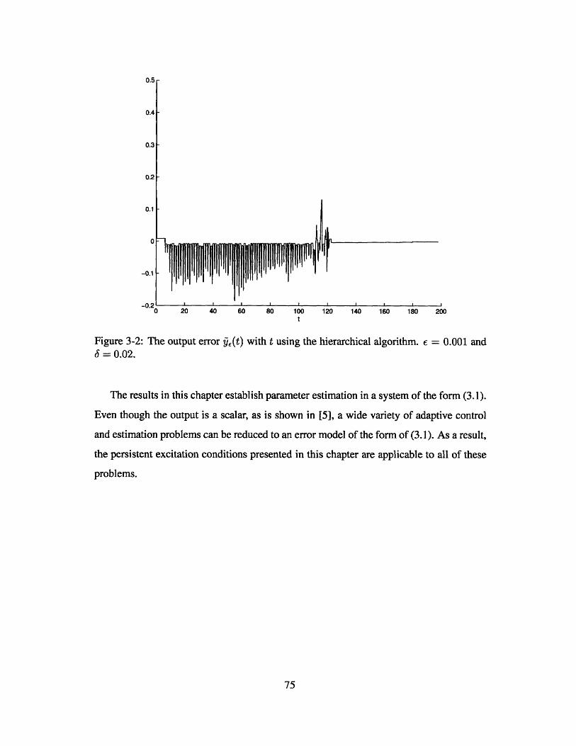
0.4-

0.3-

0.2-

0.1 -

0

-0.1

0 20 40 60 80 100 120 140 160 180 200t

Figure 3-2: The output error Q,(t) with t using the hierarchical algorithm. c = 0.001 andS = 0.02.

The results in this chapter establish parameter estimation in a system of the form (3.1).

Even though the output is a scalar, as is shown in [5], a wide variety of adaptive control

and estimation problems can be reduced to an error model of the form of (3.1). As a result,

the persistent excitation conditions presented in this chapter are applicable to all of these

problems.

75

0.5 r

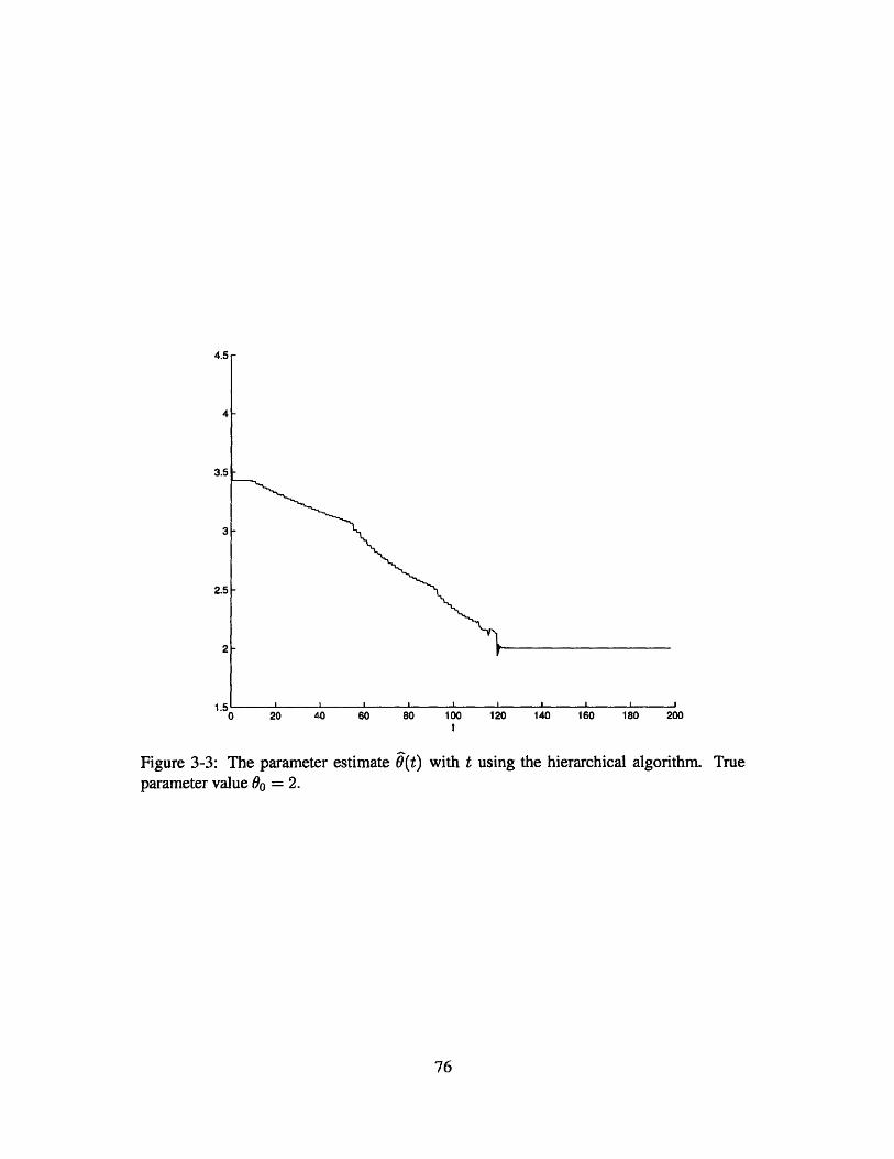
20 40 60 80 100 120 140 160 180 200-I- - L -

Figure 3-3: The parameterparameter value 0 = 2.

estimate O(t) with t using the hierarchical algorithm. True

76

4

3.5

3

2.5

2

1.5L0

4.5 r

4.5-

4-

3.5-

3-

2.5-

2-

1.5-

0.5-

010 20 40 60 80 100 120 140 160 180 200

t

Figure 3-4: The evolution of the parameter region pk with t, using the hierarchical algo-rithm. Note that Qk is updated at instants t* such that |Q(t) _< 6 for t E [t* - T, t*].

77

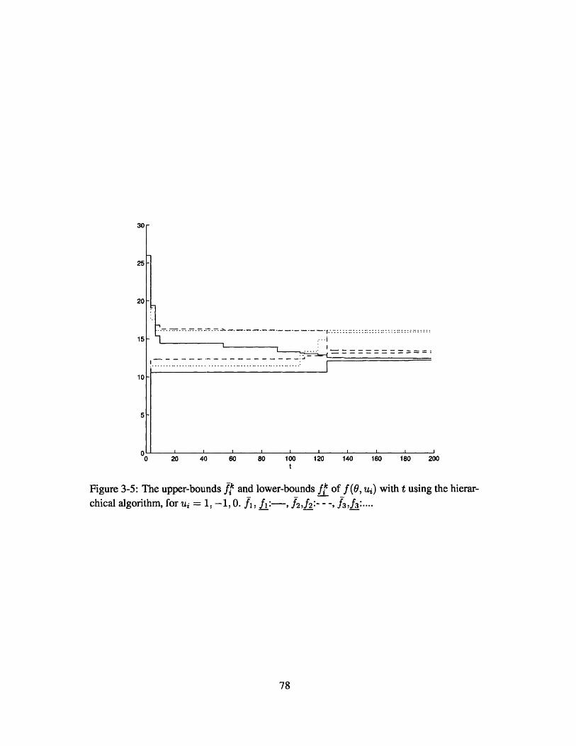
30 r

25-

20

15

10-

5-

0-0 20 40 60 80 100 120 140 160 180 200

t

Figure 3-5: The upper-bounds fi and lower-bounds f, of f(0, uj) with t using the hierar-chical algorithm, for ni = 1, -- 1, 0. fi, f:-, f2,f2:- -- , ff3:...

78

Bibliography

[1] A.M. Annaswamy, A.P. Loh, and F.P. Skantze. Adaptive control of continuous time

systems with convex/concave parametrization. Automatica, 34:33-49, January 1998.

[2] R. Ortega. Some remarks on adaptive neuro-fuzzy systems. International Journal of

Adaptive Control and Signal Processing, 10:79-83, 1996.

[3] A. M. Annaswamy, C. Thanomsat, N. Mehta, and A.P. Loh. Applications of adaptive

controllers based on nonlinear parametrization. ASME Journal of Dynamic Systems,

Measurement, and Control, 120:477-487, December 1998.

[4] J.D. Boskovi6. Adaptive control of a class of nonlinearly parametrized plants. IEEE

Transactions on Automatic Control, 43:930-934, July 1998.

[5] A. Kojid, A.M. Annaswamy, A.-P. Loh, and R. Lozano. Adaptive control of a class of

nonlinear systems with convex/concave parameterization. Systems & Control Letters,

37:267-274, 1999.

[6] A. P. Loh, A.M. Annaswamy, and F.P. Skantze. Adaptation in the presence of a

general nonlinear parametrization: An error model approach. IEEE Transactions on

Automatic Control, AC-44:1634-1652, September 1999.

[7] M.S. Netto, A.M. Annaswamy, R. Ortega, and P. Moya. Adaptive control of a class

of nonlinearly parametrized systems using convexification. International Journal of

Control, 73:1312-1321, 2000.

79

[8] F.P. Skantze, A. Kojic, A.P. Loh, and A.M. Annaswamy. Adaptive estimation of

discrete-time systems with nonlinear parametrization. Automatica, 36:1879-1887,

2000.

[9] K. S. Narendra and A. M. Annaswamy. Stable Adaptive Systems. Prentice-Hall, Inc.,

Englewood Cliffs, N.J., 1989.

[10] A.P. Morgan and K.S. Narendra. "On the stability of nonautonomous differential

equations .i= [A + B(t)}x with skew-symmetric matrix B(t)". SIAM Journal of

Control and Optimization, vol. 15:163-176, January 1977.

[11] E. Panteley, A. Loria, and A. Teel. Relaxed persistency of excitation for uniform

asymptotic stability. IEEE Transactions on Automatic Control, (to appear), 2001.

[12] Y. Zhang, P. Ioannou, and C. Chien. Parameter convergence of a new class of adaptive

controllers. IEEE Transactions on Automatic Control, 41:1489-1493, 1996.

[13] C.Cao, A.M. Annaswamy and A.Kojic. Technical Report, Active and Adaptive Con-

trol Lab, M.Il.T, 2002.

3.7 Appendix

Proof of Property 1: From (3.8) and (3.13), it follows that

V = y, + (3.48)

(f($,w) - f(O, w) - *T (0- 9o) - a*sat( ).

When | c| < E, it follows that g = 0 and hence, V= 0. When |Q| > c, it follows that

sat(v) = sign(Q). Then (3.48) is transformed into

V= -a(y, u)f + ,jsat( ) sat( )

+ (f(, W) - f (00, w) - #*T(O - 0)) - a*) . (3.49)

80

Combining (3.7) and (3.49), Property I is established.

Proof of Property 2: To prove Property 2, the following sublemma is needed.

Sublemma 2.1: For given systems

. = -k(t)x +z(t)

im = -kmXm+Zm

0

where k(t) > 0, km > 0 and

Iz(t) 15 zM V ;> to.

if x(to) 5 xm(to) < 0. k(t) < km,

then x(t) 5 xm(t), V t > to where xm(t) 0.

The proof of the sublemma is straight forward and is omitted. Now let us prove Property

2.

Without loss of generality, we assume that

ME(ti) --y. (3.50)

From (3.8), it follows that

& = -f(y, u)&- + m(t) (3.51)

where m(t) is defined as in (3.17). From Assumption 2, because Q2 is bounded, Idf(u, (D) -

f (u, w) , a* and therefore rn(t) are also bounded, with Im(t) bounded by M. Let ym(t) be

specified as the solution of the following differential equation for t > ti:

Ym= - 0 maxYm + M. ym(ti) = -7.

81

(3.52)

From (3.50), (3.51) and (3.52), Sublemma 2.1 implies that

YE(t1 + r) < yM(ti + T), V r > 0 and y(t, + ) 0.


Mym (t+) +

Cemax-y e~ " + M

Cymax

We note that ym (t, + T) is a concave function of r for T >0. From properties of concave

functions, it can be shown that ym(ti + -r) satisfies the inequality

ym(ti + -r) 5 ym(ti) + Vrym(ti + r) |L,. - (3.54)

From (3.53) and (3.54), we obtain that

g6(t, + r) -7+ (M + amax7y)r. for r > 0. (3.55)

For T' = we can verify easily from (3.55) that

Q(t) ! 0 V t E [tji. ti + T'].

From (3.55), we have that

I ti +T'tl

731& 6(r) dr > 7- 3(M+amax7)

Integrating (3.14) over [ti, t1 + T'], we have that

V(ti + T') : V(tl) -- amin 733(M + amax7)

For

we can obtain a similar result. This proves Property 2.

82

0

(3.53)

Proof of Property 3: Let us first prove that

(3.56)- a* (#, w) <; a* sat().

Since g(o, W, #) = 0, it follows that for at least one value of 0 in QO, g(G, w, #) = 0. This

proves

a* > 0. (3.57)

If Q > 0, from (3.57), (3.56) holds. If Q < 0, it follows that

a*sat(y) = a* (O, w)sat(-) ;> -a* (O,w).

Similarly, we can prove a* < a* (0, w) and Property 3 is established. 0

Proof of Property 4: Since P = -1, f(0, w) is concave. It follows from the solutions

of the min-max algorithm in section 2.1 that

a* = 0, if Q <0. (3.58)

which proves Property 4-(i). When Q > 0, it follows from the solutions of the min-max

algorithm that a* is nonnegative, hence

Oa*Q _< 0, if Q > 0.

When # = 1, proceeding in the same manner as above, it follows that

a* = 0.

fla*Q < 0.,

(3.59)

(3.60)if 0 = 1, and > 0,

if # = 1, and < 0. (3.61)

Equations (3.58)-(3.61) prove Property 4-(ii) and 4-(iii).

Proof of Theorem 1:

0

For any t1 and O(tj), it follows from (3.20) that there exists

83

and

t 2 < t + To such that

#(w(t 2)) (f (6(ti),w(t 2)) f (0, W(t 2))) C> E11(ti) - 0011 (3.62)

Without loss of generality, we assume that (w(t 2 )) = 1 which means that f(0, w(t 2 )) is

convex (or linear) over 0. The proof can be given in a similar manner if f(t 2 ) = -1. When

,#(t2) = 1, (3.62) can be rewritten as

f ((ti), w(t2)) - f (0, w(t2)) > (3.63)

E = CU||$(ti) - 0o|. (3.64)

If x(tj) E DE, we note that x(t) E DE for all t > ti, since V is a Lyapunov function.

Hence we assume that x(ti) D. It follows from the definition of V in (3.13) that either

(3.65)

If (3.65)-(ii) holds, it is easy to show that V decreases. If (3.65)-(i) holds, we show below

that Q,(t) will become large for some t > t1. Using the definitions of y1 in (3.22), it follows

from (3.64) and (3.65)-(i) that

E2> 2c(16BoU + 8BoB4 + 4BO). (3.66)

We shall show that if (3.66) holds, there exists t 3 C [t 2, t2 + T1] such that

(3.67)

where

mi2(Bo BTo + amax)'(3.68)

84

where

or (ii)|QI)| > Vr. 1

|J(N)| >! Min{1, S}

(0)||0(ti)|| > VF -

T 1 =

2- e(16BoU + 8B 9 BO + 4B )

2BBTo + 2earmax + 16BOUb + 8BOBO + 4BOf

c - (BoBjTo + amax)S

4BoU + 2BoBO + B2(3.69)

From (3.66), we can verify easily that both S and Ti are positive numbers. We prove (3.67)

by contradiction.

Suppose (3.66) holds and (3.67) is not true. Then it follows that

(a) IQ(t2 + T)I < 1 and (b) IY (t2 + T)I (3.70)

for any T c [0. T1I. From (3.8) and (3.70)(b), it follows that

(3.71)

We prove that &,(t) must become large over [t2 , t 2 + T,] by establishing lower bounds on

the bracketed term and the last term on the right hand side of Eq. (3.71).

It follows from equations (3.4), (3.70)(b), Assumption 2, and the fact that t 2 - t1 To

that

If (O(t2), W(t 2)) - f(O(ti),w (t 2))I < BoBOT6. (3.72)

Combining (3.63) and (3.72), we have that

(3.73)

From Assumption 1, it follows that

IIw(t 2 + T) - w(t 2)f1 < UbT. (3.74)

For r c [0, T], since Iy(t 2 + T) I 1 from (3.70(a)), by integrating (3.4) over [t 2 - t 2 + T],

we obtain that

0IO(t2 + r) - 0(t 2)|i BT. (3.75)

85

Y> -Orax6 + [f (, w) - f (0, w)] - a*sat( )C

f (O(t 2), w(t 2)) - f (o, w(t 2)) 2 - BOBOTo.

By combining (3.74), (3.75) and Assumption 2, it follows that

f2, - f2 - (f(0, w(t 2 + r)) f(0, w(t 2 )))|

Bo(2Ub + B4 )T (3.76)

which can be rewritten as

f2, - f(00, w(t2 + T)) >

f2 - f(0, w(t 2 )) - Bo(2U6 + BO)r (3.77)

where

f2r = f(9(t2 +r),w(t 2 + r))

f2 = f($(t2),w(t 2)). (3.78)

Combining (3.73) and (3.77), it follows that for any T E [0, Til,

2, - f(0,w(t2 + r)) >

- BeBOToS - Be(2Ub + BO)r (3.79)

which establishes a lower bound for the bracketed term in (3.71).

We now derive a lower bound for the third term in (3.71). For any 0, using the same

procedure as for equation (3.76), it can be shown that

IA, - - (f(0, W(t 2 + r)) - f(0,w(t 2)))|

Be(2Ub + BO)r (3.80)

where f2,, f2 are defined in (3.78). It follows from (3.75) that

0* (Ti) (0(t2 + r) -9(t 2 ))| Br. (3.81)

86

We know that at t2, because /(t 2 )= 1, it follows from Property 4-(ii) that

a*(9(t 2),w(t 2)) = 0. (3.82)

From the definition of a*, and the optimization problem in (3.6), we obtain that

a* (0(t 2), w(t2))

= max(2 - f (0, w(t 2)) - #*(t2)((t2) - 0))

a* (0(t 2 + T), W(t 2 + T)) = max (Lr

-f (0, C(t 2 + )) t +*(2 + )(6(t2 + 7) - )) (3.83)

where f2 T , /2 are defined as in (3.78). Because 0* (Tj + t) is the value that result in the

minimum value of a* (Q( + t), w(7i + t)), it follows that

a* (6(t 2 + r), W(t 2 + 7)) ax(h2

-f (0, W(t 2 + T)) - #*(t 2 )(6(t 2 + T) - 0)) . (3.84)

Combining (3.83) and (3.84), it follows that

a* (O(t2 + 7), w(t 2 + r)) a*((t 2), w(t 2))

+ max(j2r - f (0, w(t 2 + )) (3.85)

- (12 - f (0, W(t 2))) - 0*(Ti)(O(t2 + T) - 0(t 2 )))

where f2,, /2 are defined in (3.78). From Eqs. (3.81), (3.85), and (3.80) it follows that

a* (0(t 2 + T), W(t 2 + 7)) < (3.86)

a*((t 2 ), W(t 2 )) + Bo(2U + BO)T + B 2.


-*(6(t 2 + -r), (t 2 + ))sat( ) > -Bo(2U- + Bo)T - B2r. (3.87)

87

It follows from (3.87) and Property 3 that for all T E [0, T11,

(3.88)-a* ( (t2 + T), W (t2 + r))sat( ) >--Bo(2U + BO)r- B,2-r

which establishes a lower bound on the last term on the right hand side of Eq. (3.71).

Using (3.79) and (3.88), Eq. (3.71) leads to the inequality

y (t 2 +r) - (BBTo + amax)S

-(4BoU,+ 2BeBo +B )r

(3.89)

V r e [0,T 1].

Integrating both sides of (3.89) over [t 2, t2 + T1 ] where T1 is defined in (3.69), we have

(t2 + T1)- )> : ( - (BoBoTo + amax)-

(4BoUb + 2BB + Bo)r)dr

which can be simplified as

(> - (BoBoTo + amax)S)2

2(4BoUb + 2BoBo+B2)

Since (3.70) holds for all T- E [0, T1], we have that

0~2) > -E - .k

It follows from the definition of 6 in equation (3.68) that

- E(16BoUb + 8BoBo + 4B2)

Equation (3.92) c,

- 2EBoBoTo + 2Mamax + 16BoUb + 8BeBo + 4BO

an be rewritten as

F2 - 2i(BoBoTo + amax)> +

2(4BoUb+ 2BOBk + B2) - 2c + 26.

88

(t2 -I-T 1) - (3.90)

(3.91)

(3.92)

(3.93)

I

It follows from (3.90) and (3.91) that

(t2 + T1) > 2 - 2(B9B4,To + Omax)-~- 2(4BoUb+2BeB4 ,+B0) (3.94)

From (3.93), equation (3.94) can be simplified as

(t2 +T 1) > E + S. (3.95)

Equation (3.95) implies &,(t2 + T) > 6 which contradicts (3.70). Thus we have shown

that (3.67) must hold.

In summary, we have shown that if V(ti) > -y1, then either

t3 E [ti, t1 + To + T1], or

(3.96)

where t3 = t 2 + T1. From Property 2, it follows that if (3.96)-(i) holds, then there exists

T1= M+a such that

V(t 3 +Tj) _<V(t 3 ) - amin .3(M + amaxJ)

(3.97)

Similarly, if (3.96)-(ii) holds, then

V(ti + T) V(ti) - min 71j)-- 3(M + amax V7i)

(3.98)

where T' = Because V(t) is non-increasing, it follows from (3.97) and (3.98)2 Mama71,

that for any V(tj) > -yi,

(3.99)

where

T3= max{To + Ti + T(, T2 }

89

(i) j&,(t3)| ; min{1, S}1

(ii) |Wc(ti)| > vy.

V(tl + T31) <5 V(ti) - AV

AV = min{ amin amindi3(M + OimaxS) 3(M + amax'Yi)

This implies that V(t) decreases by a finite amount over erery interval T3 until trajectories

reach DE. This proves Theorem 1.

Proof of Lemma 2 For any m, if

I &(t)| 6 Vt E [to + mT, to + (m + 1)T], (3.100)

we are done. Otherwise, it means there exists t1 e [to + mT, to + (m + 1)T] such that

yE(ti)I > 6.

It follows from Property 2 that there exists T' = MJa such that

V(t 1 +T') V(t 1 )-

This implies that every time when |q,(t)I ;> 6,

amount. Now that V(to) is finite, these kind of

means that we can find a finite m* such that

CminJ

3(M + amax6)

Lyapunov function will decrease a small

situation can only happen finite times. It

|qe(t)| < 6 Vt E [to + m*T, to + (m* + 1)T ].

This establishes Lemma 2.

Proof of Lemma 3: We shall prove by contradiction that Lemma 3 holds. Assume that

00 V 4%(A wi, C 6, 0f) for some 1 < i < I. That is

or (ii)f(0 , wi) > fi,

for some 1 < i < I. Suppose (i) is true. Since 9f = 0(ri), case (i) implies that

f((Ti), w) - f(O0, w) - a*((T), w) - Qmax6 > 2 B,(6 + c). (3.101)

90

(i f(0, 1 i) < _L ,

From (3.8), Property 3 and the fact |,|I< 6, it follows that

Y y11

where

Y1 = -amax6 + f (9, w) - f(90 , w) - a*(9, w)

represents the lower bound of Q. Combining (3.101) and (3.103), it follows that

Y1 (Ti) > 2 VBt (6 + e.

From the definition of a*, and the optimization problem in (3.6), we obtain that

a+ (0 (ri), co ri))=

max (, - f (0, w(Ti)) - 0*(Ti)(6(Ti) - 0)

a*(0(Ti + t),w(ri + t)) = mac (fj t

-f (0, (ri + t)) - 0*(ri + t)((i + t) - 9))

(3.102)

(3.103)

(3.104)

(3.105)

where

iTt = f ((i + ), W(ri + )) (3.106)

Because * (7-i + t) is the value that result in the minimum value of a*(O(ri + t), w(ri + t)),

it follows that

a*(6(T±i + t),w (Ti + <m ax r - f (0,w (Ti + t)

(TO)(( t) - 9)).


a*, ((Ti +t),w(Ti + t) a* (0(Ti),w(Ti))

91

(3.107)

+max (ft - f(0, W(i + t)

- (fY,.- f(0, w( ))) - 0*(Ti)((T + t) - O(T)))

where fj and frt are defined as in (3.106). From Assumption 1, it follows that

Iw(7i + t) - w(ri)II < Ubt.

(3.108)

(3.109)

Since Ip&(ri + t) I 6, by integrating (3.4) over [i, 'rj + t], we obtain that

110(r + t) - O(Ti)| 5 6Bt. (3.110)

By combining (3.109), (3.110) and Assumption 2, it follows that

lJht - fr - (f(0, w( + t)) - f(0, w(T)))

<Bo(2Ub +6B 4 )t (3.111)

where f, and frt are defined as in (3.106). From (3.110), (3.111) and (3.108), we get

a* ( (r + t), w(ri + t)) a* (0(r), w(Ti)) +

Bq(2Ub + SB 4,+ SB2)t. (3.112)

Incorporating (3.111) and (3.112) into (3.103), we have that

y1 (-ri +t) - y(Ti) > -(4BeUb + 2JBeB4 + 6B)t.

which can be simplified using (3.31) and (3.104) as

(3.113)


(3.1 14)

92

y I( r + t) > 2 VB, (J+ c) - B, t.

S(Ti + t) > 2VBt(6 + c) - Btt.

Integrating both sides of (3.114) over [ri, r + rB] where TB = 2ViB (3 + c)/Bt,

(T2 +TB) - (ri) = 2 B,(6 + c) - Bet. (3.115)

Since 9(,ri) > -(j + c), we can rewrite (3.115) as

(3.116)

Equation (3.116) implies

& (Tj + TB) >8

and this contradicts the fact that J& (t) I K 6 over [ti, t1 + T]. Thus we conclude that the

assumption (i) that f < f. for some 1 < i < I is not true and hence

f(O0,w) > L = f (, w) - a* (j, w) - ama - 2 Bt( + e)

(3.117)

In the same manner, we can prove that

f(0, w) f = a*(9, w) + f(9f, w) + amaxJ + 2 Bt(6 + c)

Vi = 1,.., I. (3.118)

(3.117) and (3.118) concludes the proof of Lemma 3.

Proof of Lemma 4: This proof follows directly from the definition of Ai in (3.36) and

the construction of Qk+1 in (3.34).

Proof of Lemma 5: We start with the hierarchical algorithm shown in Table 3.1. Be-

cause Qk+1Cgk, there exists Q1 such that

Q1 = liM Ok.k-+oo

(3.119)

Corresponding to Q1, if the lower-level convergent estimate of 0 is given by 91, it follows

93

&(i + rB) > (6 + C) -

Vi = 1, .., I.

lim O(t)=O'.t-+oo

(3.120)

Suppose (3.40) does not hold, it implies that

(3.121)i~1

Then there exists an i. 1 < i < I such that

g V Ai(Q1) (3.122)

where 9j = 9(T) with w(r) = wi. We can prove (3.122) by contradiction. We assume that

oi E Ai(Ql) Vi = 1.., I.

Because

combining the definition of L(Q 0, E, 6) in (3.38), it follows that

0' E L(007 E)

which is a contradiction to (3.121). Thus (3.122) must be true if (3.40) does not hold.

Let f. and fj be lower and upper bounds in Q1 specified as

. = min f (0, wi).-1 oFnff =max f(0, wi).

OEnl

If we define

.= f(A1,wi) - a+(91, wi) - D(E,6)

f f (d, wi) +a* (,wi) + D(E, J)

where D(c, 6) is defined as in (3.37), equation (3.122) together with the definition of Aj

94

that

I|10' - Oi1||:5 JTBO,

imply that

> or f < f. (3.123)

Equation (3.123) implies that tighter bounds!. or fi can be found for f(0, wi) for c EQ1

which implies that a smaller set Q+1 can be found using L or fj. This contradicts the

assumption in (3.119) and Lemma 5 is proved.

Proof of Theorem 2: Sufficiency follows directly from Lemma 5 and equation (3.41).

To prove necessity, we assume that (3.44) does not hold. That is, there exists QcCO

where 0 E E such that

(i) fl i(Q) 4. and

i=1..,I(ii) On A(m) o {oo}. (3.124)

It implies that there exists some 6 E f 1,..., Ai(Q) and 0 $ 90. Assume that at iteration k,

the unknown parameter region Qk = = and the lower-level convergent parameter estimate

at this iteration is given by 6ck = 9. Then condition (ii) in (3.124) implies that

i=1,..,

since fi,,..., Ai(Q) is not empty. From Lemma 4, it follows that

Qi j= k = Q j = k+ 1, k + 2,.....

and b will remains at 9 ck always. Since 6ck # 0, the parameter estimate will not converge

to 0 even c and 6 approaches 0. This implies that (3.44) is a necessary condition for (3.43).

0

Proof of Lemma 7: For any QcQO where Oo Q, if (3.44) does not hold, it follows that

I I

nlA())o o and A() { o}. (3.125)i=1 i=1

95

From (3.125), it follows that there exists 9 0 0o such that

I

nc fAim~.

For this choice of 0, from (3.47) we have that there exists a w(9) such that

0(f(0, wt) - f(00,ioi)) > 0.

Without loss of generality, we assume that # = -1. It follows from Property 4-(i) that

a* (0, wi) = 0.

It follows from (3.128) and the definition of Ai(2) in (3.42) that

f(0, W) f*.-I

V 0c fAi(Q).

From the definition of j* in (3.35) and the fact that 0 E 0, it follows that

* f(0,wi).


f(0, wi) > f(90, wi)

which is a contradiction to (3.127) since 0 = -1. This proves Lemma 7.

96

(3.126)

(3.127)

(3.128)

(3.129)

(3.130)

(3.131)

0

Chapter 4

A Nonlinear Force-Displacement Model

of Intra-abdominal Tissues

4.1 Introduction

Advances in medical technology have necessitated the need for accurate medical simulation

techniques in general and virtual-reality based medical trainers in particular. The latter al-

lows physicians to be suitably trained via virtual patients before the actual clinical practice.

Towards this end, the creation of datasets that corresponds to a "Palpable Human" similar

to the Visible Human project initiated by the National Library Medicine, is extremely use-

ful. For example, force feedback from various parts of the anatomy in response to different

types of deformation will enable the characterization of Intra-abdominal tissues. An ad-

ditional advantage that can stem from this dataset is the classification of these soft tissues

according to their state of normalcy or malignancy.

With the above goals in mind, in this chapter, we embark on the characterization of

force-displacement relations of various intra-abdominal tissues. In [ ], an extensive charac-

terization of intra-abdominal tissues via experimental investigations was reported, thereby

enabling an overall framework for obtaining in vivo mechanical properties of these tissues.

In particular, force response for various displacement stimuli such as ramp-and-hold were

obtained. This data shed light on the isotropic properties of the organs, stiffness properties

before and after the death of the animal, the impedance properties of the organs, and their

97

power dissipation properties. A closer examination of this data reveals that the relationship

between the input stimulus and the output response is in fact nonlinear. In this chapter, we

derive a nonlinear model that quantifies this relationship.

The field of systems theory deals with the temporal response of relevant variables to

input stimulus. Depending upon the nature of the output response to inputs, the underlying

system is typically characterized as linear or nonlinear. If the property of superposition

is satisfied, then the system is referred to as linear and nonlinear, otherwise. Depending

upon whether the output responds to the input stimulus with a time-lag or not, the system

is characterized as dynamic or static. Finally, if the system parameters appear linearly or

nonlinearly, the underlying system is denoted as linearly parameterized or nonlinearly pa-

rameterized. As is shown in the subsequent sections, we demonstrate that the most accurate

model of intra-abdominal tissues is a dynamic, nonlinearly parameterized system.

This chapter is organized as follows. In section 2, the experimental details and the data

collected are briefly discussed. In section 3, the underlying model is presented. Various

features of the model and the reason for their inclusion are detailed. In section 4, the ability

of the model to predict the experimental data is demonstrated. In section 5, an algorithm for

automatic determination of the system parameters is derived and studied via simulations.

Summary and concluding remarks are included in section 6.

4.2 The Experiment

The experimental data for liver under in-vivo condition is shown in Figure 4-1 which shows

the ramp-and-hold displacement-input, the corresponding force-output, and both of their

filtered values. The filtering was carried out using a low-pass filter with a corner frequency

of 2 Hz. It is clear from Figure 4-1 that the heart-beat is present in the force-output, which

can be filtered out for the purposes of tissue-modeling. In what follows, we restrict our

attention only to the filtered output signals. As mentioned earlier, for any experiment i, the

ramp-hold tests were performed using five different input signals. For the same value of

the input, it was observed that different runs yielded different outputs. In figure 4-2, we

98

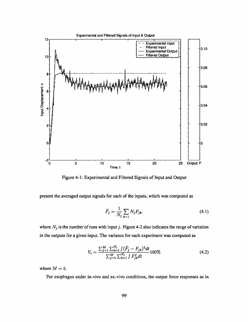
Experimental and Filtered Signals of Input & Output12

- - Experimental InputFiltered Input -0.10

- Experimental Output10 - Filtered Output

- - 0.08

8-r

X- -0.066-

E

CL0.04

a -- 4 -CL

2 -0.02

0 0

-210 5 10 15 20 25 Output: F

Time: t

Figure 4-1: Experimental and Filtered Signals of Input and Output

present the averaged output signals for each of the inputs, which was computed as

F= (Z NjFk . (4.1).7 k=1

where Nj is the number of runs with input j. Figure 4-2 also indicates the range of variation

in the outputs for a given input. The variance for each experiment was computed as

E=1 Ek1 f(Fj - Fik)2 dtVi =N-F dt_100% (4.2)

where M = 5.

For esophagus under in-vivo and ex-vivo conditions, the output force responses as in

99

Output Force: Filtered and Average of each group0.12

0.1

0.08 -

0.04 - ~ - --- -

LL; 0.06-N

0oe

-0.02-

0 5 10 15 20 25Time: t

Figure 4-2: Output Force F: Average of each group of filtered signals

Figure 4-3 for ramp-hold input signals has two overshoot peaks and are quite different from

above situations.

In Table 4.1, we list 17 for twenty-five experimental conditions. It should be noted

that the experiments were conducted using three different animals, where experiments 1-9,

10-19, and 20-25 corresponds to the first, second, and third animal, respectively.

4.3 The Model

In this section we derive a dynamic model that predicts the tissue behavior shown in figures

4-1 and 4-2. Figure 4-2 illustrates many interesting tissue properties. First, we see that

corresponding to ramp-hold inputs, the outputs have overshoot which decays and finally

100

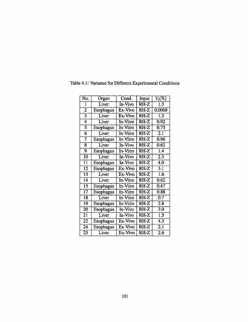
Table 4.1: Variance for Different Experimental Conditions

No. Organ Cond. Input V(%)I Liver In-Vivo RH-Z 1.32 Esophagus Ex-Vivo RH-Z 0.00683 Liver Ex-Vivo RH-Z 1.34 Liver In-Vitro RH-Z 0.925 Esophagus In-Vitro RH-Z 0.756 Liver In-Vitro RH-Z 2.17 Esophagus In-Vitro RH-Z 0.968 Liver In-Vivo RH-Z 0.629 Esophagus In-Vitro RH-Z 1.410 Liver In-Vivo RH-Z 2.311 Esophagus In-Vivo RH-Z 4.012 Esophagus Ex-Vivo RH-Z 3.113 Liver Ex-Vivo RH-Z 1.614 Liver In-Vitro RH-Z 0.6215 Esophagus In-Vitro RH-Z 0.4717 Esophagus In-Vitro RH-Z 0.8818 Liver In-Vitro RH-Z 0.719 Esophagus In-Vitro RH-Z 2.820 Esophagus In-Vivo RH-Z 3.021 Liver In-Vivo RH-Z 1.522 Esophagus Ex-Vivo RH-Z 4.324 Esophagus Ex-Vivo RH-Z 2.125 Liver Ex-Vivo RH-Z 2.6

101

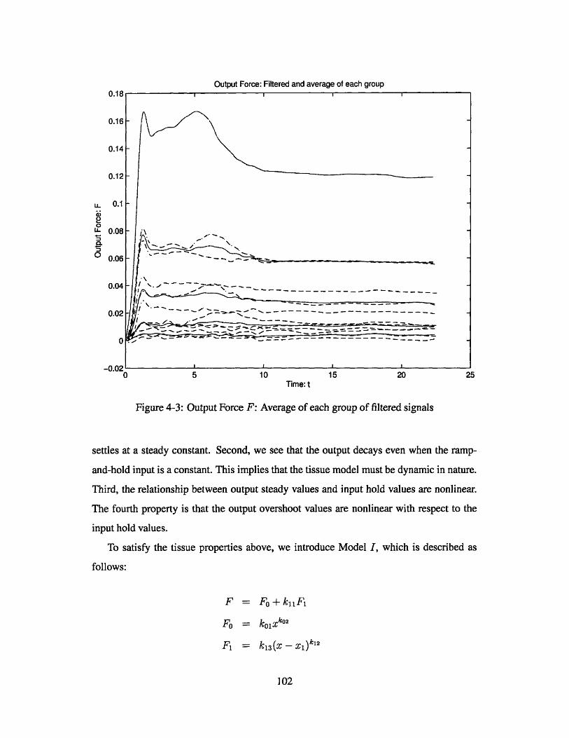
Output Force: Filtered and average of each group0.18 I I

0.16

0.14-

0.12-

u_ 0.1 -

0U.- 0.08

0 0.06

- -- ~ ~~ ~~ -- -~~~~~~~ -~-~'~~ ~~~ ~ - - -

0.02

0 5 10 15 20 25Time: t

Figure 4-3: Output Force F: Average of each group of filtered signals

settles at a steady constant. Second, we see that the output decays even when the ramp-

and-hold input is a constant. This implies that the tissue model must be dynamic in nature.

Third, the relationship between output steady values and input hold values are nonlinear.

The fourth property is that the output overshoot values are nonlinear with respect to the

input hold values.

To satisfy the tissue properties above, we introduce Model I, which is described as

follows:

F = Fo+ kn1 F1

F0 = k01 xk02

F1 = k13(x - X)k12

102

i1: = X

i2 = k13(X - X 1 )12 - X2. (4.3)

In (4.3), x is the displacement input to the tissue, and F is the measured force. The objective

here is to predict the input-output tissue behavior exhibited in Figure 4-1. The structure of

Model I is shown in Figure 4-4, where it can be seen that the output force F is a linear com-

bination of two components FO, which is from a nonlinear spring, and F1, which is from

a nonlinear spring-friction system. For a ramp-hold input signal, spring-friction system

output F will experience a pulse response which increases quickly during the input-ramp

period because the spring is compressed and decays gradually to zero in the input-hold

period because the compressed spring gradually come back to its natural length and the

energy is compensated in friction. Therefore, the steady output force is completely deter-

mined by static spring FO because the steady state of F will approaches zero for ramp-hold

inputs. The nonlinear spring contribution to FO characterizes the nonlinear steady input out-

put relationship in tissue dynamics while nonlinear spring in spring-friction component F

yields several of the nonlinear overshoot characteristics. Thus, it can be seen that Model I

captures the tissue properties. It will be shown later that using the above combination of

nonlinear springs where the nonlinearities are polynomial Model I is capable of predicting

the output accurately.

To show that Model I is the simplest spring-friction model which accurately character-

izes the tissue properties, we compare Model I with four other models denoted as Model 1

through Model 4 whose structures are shown in Figure 4-4. These models can be described

as follows. The output prediction of different models for same input signal are plotted in

Figure 4-5.

F = F

FO = kxko2. (4.4)

103

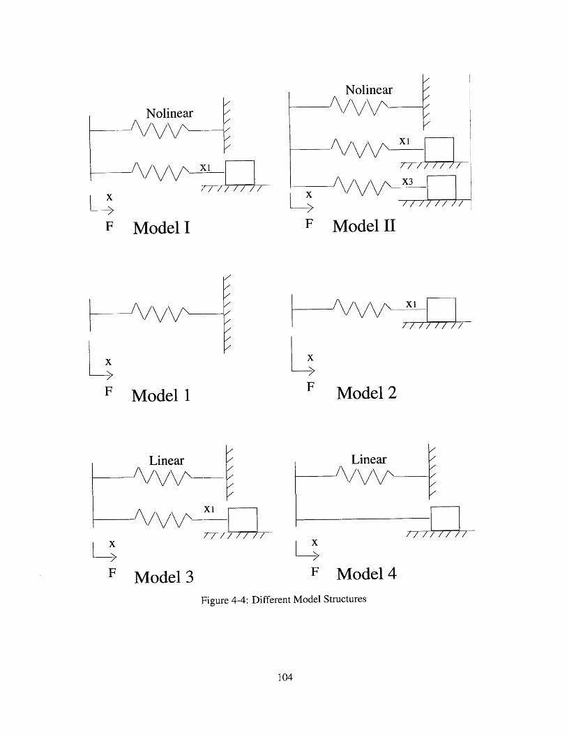
Nolinear

/7 7

Model I

Nolinear

/\/

x/ ///

F Model 11

/ xl 777

x

FModel 1

Linear

/ / ///7

Model 3

Model 2

Linear

xF Model 4

Figure 4-4: Different Model Structures

104

x

F

x

F

x

F

zzz\/Vv\-

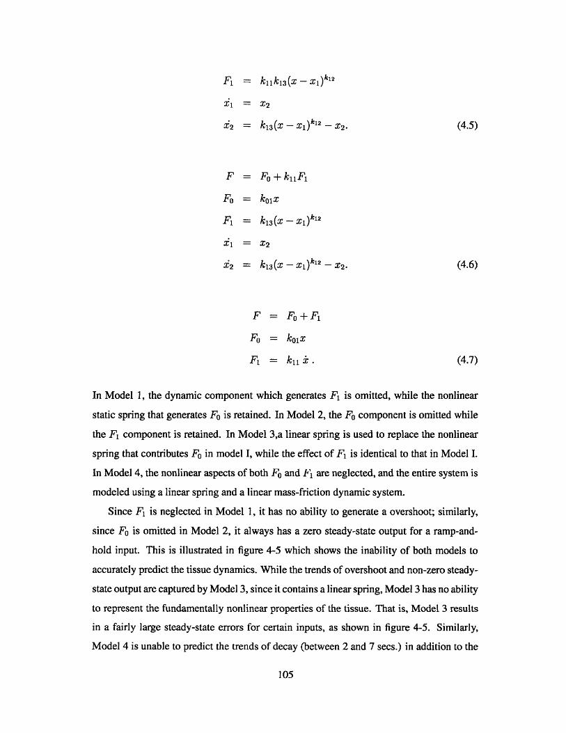
F1 = knjk 13 (X --x 1)k12

Y 1 = X2

i2 = kis(X- X)k12 - X2 . (4.5)

F = Fo+knF1

Fo = ko1x

F1 = k1 -- (X )k12

Y1 =X2

i2 = k13(X- X1)k12 - X2. (4.6)

F = Fo+ F1

Fo = ko1x

F, = k1ji. (4.7)

In Model 1, the dynamic component which generates F is omitted, while the nonlinear

static spring that generates FO is retained. In Model 2, the FO component is omitted while

the F1 component is retained. In Model 3,a linear spring is used to replace the nonlinear

spring that contributes FO in model I, while the effect of F is identical to that in Model I.

In Model 4, the nonlinear aspects of both FO and F are neglected, and the entire system is

modeled using a linear spring and a linear mass-friction dynamic system.

Since F is neglected in Model 1, it has no ability to generate a overshoot; similarly,

since FO is omitted in Model 2, it always has a zero steady-state output for a ramp-and-

hold input. This is illustrated in figure 4-5 which shows the inability of both models to

accurately predict the tissue dynamics. While the trends of overshoot and non-zero steady-

state output are captured by Model 3, since it contains a linear spring, Model 3 has no ability

to represent the fundamentally nonlinear properties of the tissue. That is, Model 3 results

in a fairly large steady-state errors for certain inputs, as shown in figure 4-5. Similarly,

Model 4 is unable to predict the trends of decay (between 2 and 7 secs.) in addition to the

105

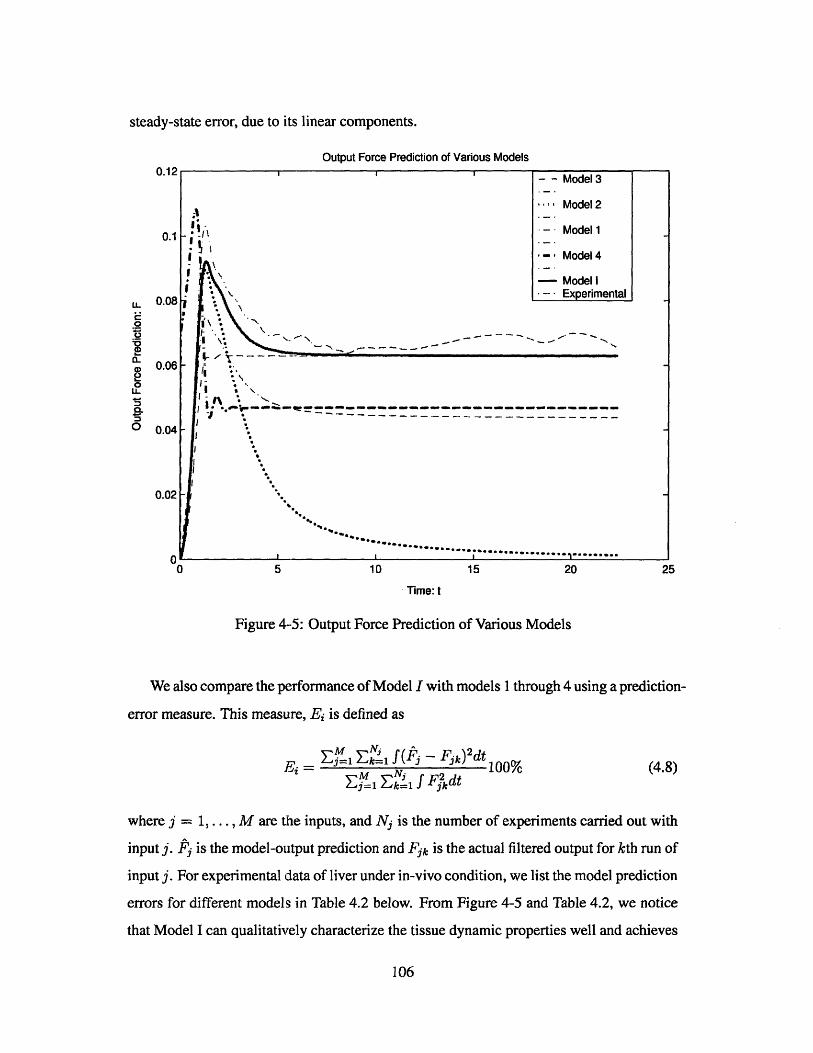
steady-state error, due to its linear components.

Output Force Prediction of Various Models0.12

- Model 3

Model 2

0.1 - Model 1

- Model 4

-~ -- Model I. - -Experimental

u_ 0.08E

.2

4) 0.06

LL

0.02-

I0 0

0 5 10 15 20 25

Time: t

Figure 4-5: Output Force Prediction of Various Models

We also compare the performance of Model I with models 1 through 4 using a prediction-

error measure. This measure, E is defined as

Mgi EN, f(F. - Fk) 2dtEi = 100% (4.8)

N- r2 fFdtj=1 E k=1 f F-'dt

where j =1. . . . , M are the inputs, and Nj is the number of experiments carried out with

input j. Fj is the model-output prediction and Fjk is the actual filtered output for kth run of

input j. For experimental data of liver under in-vivo condition, we list the model prediction

errors for different models in Table 4.2 below. From Figure 4-5 and Table 4.2, we notice

that Model I can qualitatively characterize the tissue dynamic properties well and achieves

106

Table 4.2: Comparision of Prediction Errors for Various Models

Model I (%) Model I (%) Model 2 (%) Model 3 (%) Model 4 (%)E 1.75 2.66 62.57 6.04 13.78

the minimum model prediction error. Any further simplication of the model as in model

1-4 will make the performance deteriorate or lose some key features of the tissue dynamics.

While Model I was found to be adequate for the experiment discussed above, in a few

cases, it was found that an additional component needed to be added to Model I, which

corresponded to the esophagus-tissue under in-vivo and ex-vivo conditions shown in Fig-

ure 4-3. It can be observed that the output force response corresponding to ramp-hold

input signals has two overshoots. The augmented model, denoted as Model II consists of

the components FO and F present in Model I, and has an additional mass-spring-friction

system whose input is delayed by a few seconds. This model is described below:

F(t) = Fo(t)+k 1 1F 1(t)+k 21F2 (t- T)

F0 = ko1xk02

F1 = ki 3(x - x 1 )k12

i2 = k13(X - X 1 )k12 - X1

F2 = k23 (x - x 3 )k22

i3 X4

Y4 = k23(X - X3)k22 - X4 . (4.9)

4.4 Model Prediction

In the previous section, we developed two models, Model I and Model II to predict the

tissue properties, with Model I representing the liver tissue at all conditions and the esoph-

agus tissue only under in-vitro conditions, and Model II representing the esophagus tissue

107

under in-vivo and ex-vivo conditions. We validate this model in this section by comparing

its predicted output values with actual outputs under various conditions.

Determining any dynamic model includes two steps, where the first step is the selection

of a suitable model structure, and the second step is the selection of the parameters of that

model. As mentioned above, we carried out the first step in the previous section, while we

proceed to the second step in this section.

As mentioned in the previous section, Model I includes five parameters koi, k02 , kjj, k12

and k13. Of these, the steady-state value of the output is a function of F whereas the tran-

sient properties of the output, such as overshoot and decay, are functions of F. It therefore

follows that kol and k0 2 can be determined by studying the steady-state component, while

the last three parameters can be found by monitoring the transient characteristics. Using

the functional form of F shown in Eq. (4.3), koi and k0 2 were calculated. To determine the

remaining three parameters, we first note that x, is nearly zero during the "ramp" portion

of the input, and hence, F1 = kuk1 3Xk12, which corresponds to the overshoot magnitude.

Therefore, using the overshoot values at different inputs, k12 and the product kjjk 13 can

be determined. We also note that only the parameter k13 controls the decay of the output

exhibited over the period [2sec., 9 sec.], and is a parameter of the linear first-order equation

i2 = k 13 (x - x 1 )k12 - X 2 (4.10)

Since the remaining parameters are known, using the input x and the measured output F,

x, and x2 can be calculated as functions of time. Using these values in turn, the parameter

kI13 can be determined using an adaptive estimation algorithm as in [ ]

2= -2 + k 13 (x - x 1 )k12

Ic13 = -(2 - x 2 )(x-)12 ( 411

It is also possible to identify all the five parameters simultaneously using a nonlinear per-

sistent excitation algorithm as in [2]. The same procedure can be used for determining the

parameters of Model II, where T is determined empirically by observing the lag between

108

the two times where the overshoots occur. The parameters thus obtained are shown in Table

4.3.

Once the parameters are determined using the above method, we obtain a complete

model of the tissue properties. In Figure 4-6, the predicted output of this model is plotted

and compared with the corresponding experimental output for various inputs. The specific

case of the liver tissue under in-vivo condition is shown in Figure 4-6.

E

CL

0.

0.12

0.1

0.08

0.06

0.04

0.02

0

-0.02'0

Output Force: Filtered and Model precidtion

- -

IN

_- -_- -

5 10 15 20 25

Time t

Figure 4-6: Output Force F: Model Prediction with the Parameter Identified

The figure shows that the model prediction is quite accurate for all inputs. Similarly,

the predictive ability of Model II is shown in Figure 4-7. The model prediction error E,

defined in Eq. (4.8), is calculated for all cases of liver-tissue and esophagus-tissue and

shown in Table 4.4.

We carried out another set of experiments to further test Models I and Ii. We varied the

109

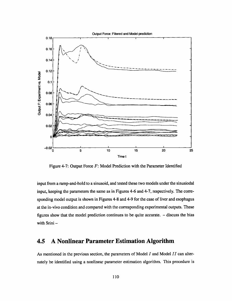
0.18

0.16

0.14

0.12

0.1

0.08

0.06

0.04

0.02

0

--0.020

Output Force: Filtered and Model prediction

- -- --

- - - -

-- M

5 10 15 20 25

Time t

Figure 4-7: Output Force F: Model Prediction with the Parameter Identified

input from a ramp-and-hold to a sinusoid, and tested these two models under the sinusiodal

input, keeping the parameters the same as in Figures 4-6 and 4-7, respectively. The corre-

sponding model output is shown in Figures 4-8 and 4-9 for the case of liver and esophagus

at the in-vivo condition and compared with the corresponding experimental outputs. These

figures show that the model prediction continues to be quite accurate. - discuss the bias

with Srini -

4.5 A Nonlinear Parameter Estimation Algorithm

As mentioned in the previous section, the parameters of Model I and Model II can alter-

nately be identified using a nonlinear parameter estimation algorithm. This procedure is

110

0

0

CL

0

Table 4.3: Parameters Identified of Various Experiments

No. i Model koi k02 k1 2 ki, k13 k2l k22 k2 3 TI I 0.00175 1.69 1.82 0.000765 0.12 II 0.00154 2.09 2.21 0.000481 0.03 2.39 0.000306 0.015 43 I 0.00666 1.48 1.86 0.00362 0.034 I 0.00157 2.31 2.48 0.000701 0.0075 I 0.00103 2.24 2.19 0.00113 0.0256 1 0.00124 2.73 2.62 0.000671 0.0077 I 0.000902 2.46 2.68 0.000464 0.0078 I 0.00095 2.68 2.91 0.000375 0.0049 1 0.00111 2.61 2.64 0.000602 0.00710 1 0.00279 1.54 1.91 0.00103 0.0311 II 0.00319 1.49 1.13 0.00436 0.04 2.37 0.000304 0.015 212 II 0.00367 1.52 0.934 0.0109 0.15 2.04 0.00053 0.015 213 I 0.00870 1.29 1.28 0.0102 0.1514 1 0.00187 1.96 2.34 0.000605 0.00715 1 0.000563 2.58 2.47 0.000777 0.00717 1 0.00177 2.20 2.28 0.000873 0.00518 1 0.000992 2.53 2.60 0.00062 0.00519 1 0.00219 2.34 2.30 0.00140 0.00520 II 0.00482 1.45 1.58 0.00178 0.009 2.04 0.000534 0.015 221 I 0.00200 1.70 2.14 0.000779 0.01522 1 0.000883 2.52 2.58 0.000726 0.00724 I 0.00627 1.45 1.79 0.00321 0.0625 I 0.000946 2.39 2.70 0.000325 0.006

111

Table 4.4: Model Prediction Error for Different Conditions

No. i Organ Condition Input V (%) E (%)I Liver In-Vivo RH-Z 1.9 1.32 Esophagus Ex-Vivo RH-Z 2.5 0.683 Liver Ex-Vivo RH-Z 1.9 1.34 Liver In-Vitro RH-Z 1.3 0.925 Esophagus In-Vitro RH-Z 1.9 0.756 Liver In-Vitro RH-Z 2.8 2.17 Esophagus In-Vitro RH-Z 1.6 0.968 Liver In-Vitro RH-Z 1.4 0.629 Esophagus In-Vitro RH-Z 1.8 1.410 Liver In-Vivo RH-Z 4.2 2.311 Esophagus In-Vivo RH-Z 8.1 4.012 Esophagus Ex-Vivo RH-Z 6.6 3.113 Liver Ex-Vivo RH-Z 2.6 1.614 Liver In-Vitro RH-Z 0.87 0.6215 Esophagus In-Vitro RH-Z 3.1 0.4717 Esophagus In-Vitro RH-Z 1.3 0.8818 Liver In-Vitro RH-Z 1.5 0.719 Esophagus In-Vitro RH-Z 3.1 2.820 Esophagus In-Vivo RH-Z 7.3 3.021 Liver In-Vivo RH-Z 2.3 1.522 Esophagus Ex-Vivo RH-Z 6.1 4.324 Esophagus Ex-Vivo RH-Z 2.8 2.125 Liver Ex-Vivo RH-Z 3.0 2.6

112

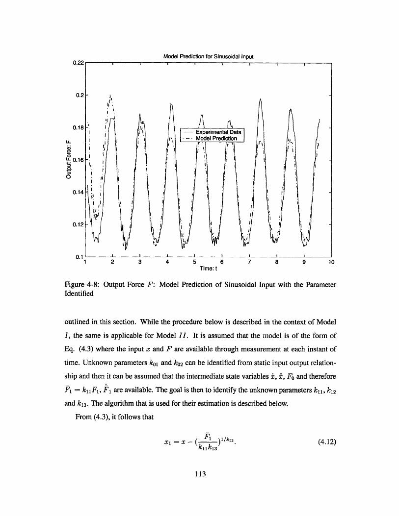
Model Prediction for Sinusoidal Input0.22

0.2 -

0.18 -- t -tExperimental Data- Model Prediction

LL0.16 -

CI-

0.14

0.12 -

0.1-1 2 3 4 5 6 7 8 9 10

Time: t

Figure 4-8: Output Force F: Model Prediction of Sinusoidal Input with the ParameterIdentified

outlined in this section. While the procedure below is described in the context of Model

I, the same is applicable for Model II. It is assumed that the model is of the form of

Eq. (4.3) where the input x and F are available through measurement at each instant of

time. Unknown parameters ko, and k02 can be identified from static input output relation-

ship and then it can be assumed that the intermediate state variables i, ,, F and therefore

P = kj 1F1 , F' are available. The goal is then to identify the unknown parameters k1j, k12

and k13 . The algorithm that is used for their estimation is described below.


X1 = x - ( )1/k 1 2 . (4.12)kujki3

113

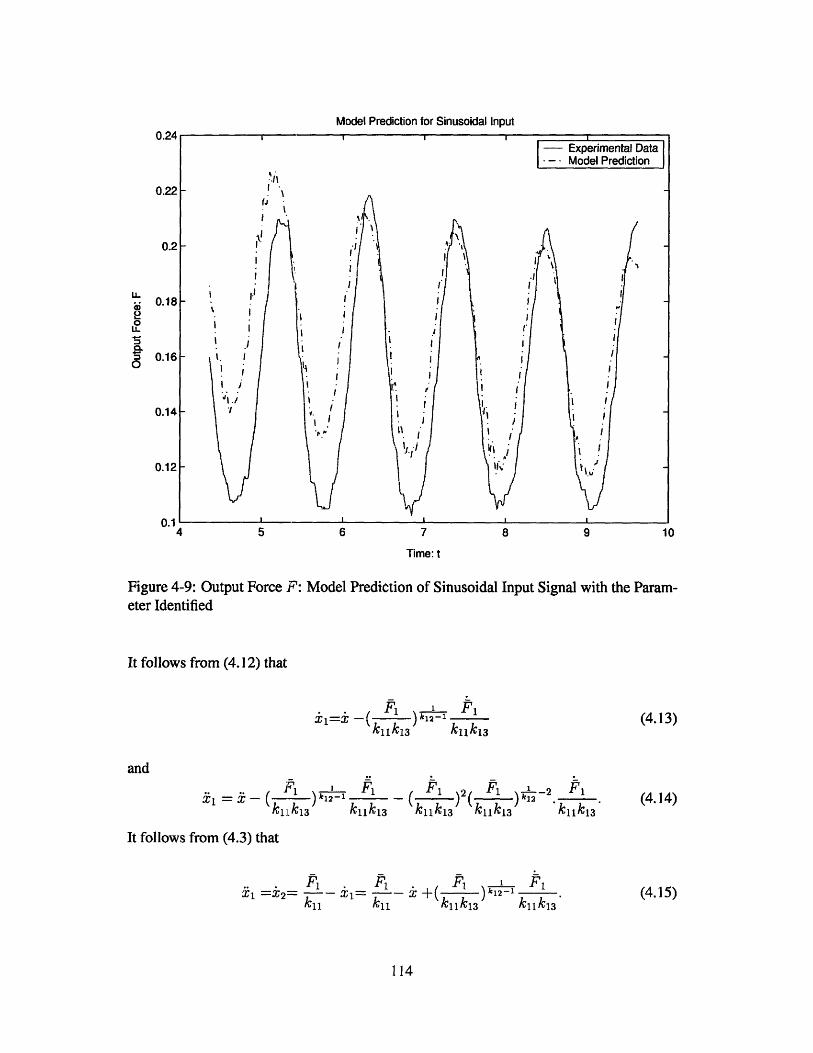
Model Prediction for Sinusoidal Input0.24

- Experimental Data-- Model Prediction

0.22-

0.2 - -

0.18 -0

LI

M 0.16 - I I -

0.14 ---

0.12 - - -

0.1 14 5 6 7 8 9 10

Time: t

Figure 4-9: Output Force F: Model Prediction of Sinusoidal Input Signal with the Param-eter Identified

It follows from (4.12) that

kjjk13 )k121 jk13 (.3

and

21 2- ) F1 F F1 -2 F,k- ki13)k121 kk 1kjjk k k13 kF 1 (4.14)


* F F1 . + F1 F1

=&2 - (k 31= X +( k1 1 k1 (4.15)ku ki kuk13 kk13

114

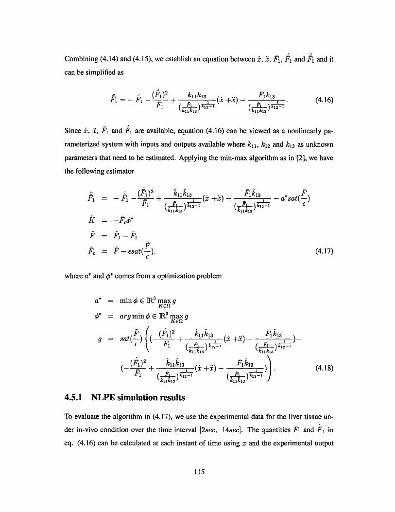
Combining (4.14) and (4.15), we establish an equation between i, 1, P1, F1 and F1 and it

can be simplified as

- (P)2 kjjk13 Pk13F+ ( F x +(i-)- 1 . (4.16)k jj k1 1 ki 3 2 -

Since i, &, F1 and F1 are available, equation (4.16) can be viewed as a nonlinearly pa-

rameterized system with inputs and outputs available where kil, k12 and k13 as unknown

parameters that need to be estimated. Applying the min-max algorithm as in [2], we have

the following estimator

F1 - (F 2 k 13 F, kl3_ 1 13 (F

FF,- + - ~a*sat(~

\ki Iki3 kiik1a'

F{ = -D*

FE = -Esat(). (4.17)

where a* and * comes from a optimization problem

a*= minqSE R3 maxgKEn

= argminqOcER 3maxgKEQ

g sat() - +( +)--\kjjk13 ki k11k3

(-)+ (_+_)_- )k13 (4.18)1 &. Fl k12-1 {.F k2-1

\ki Ik13 ) kjjkij /

4.5.1 NLPE simulation results

To evaluate the algorithm in (4.17), we use the experimental data for the liver tissue un-

der in-vivo condition over the time interval [2sec, 14sec]. The quantities P1 and F1 in

eq. (4.16) can be calculated at each instant of time using x and the experimental output

115

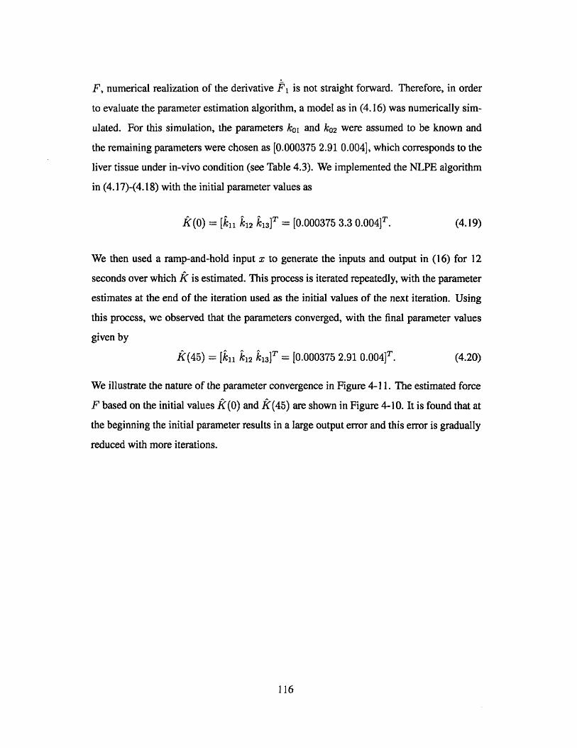
F, numerical realization of the derivative F1 is not straight forward. Therefore, in order

to evaluate the parameter estimation algorithm, a model as in (4.16) was numerically sim-

ulated. For this simulation, the parameters koi and k02 were assumed to be known and

the remaining parameters were chosen as [0.000375 2.91 0.004], which corresponds to the

liver tissue under in-vivo condition (see Table 4.3). We implemented the NLPE algorithm

in (4.17)-(4.18) with the initial parameter values as

k(0) = [kjj k1 2 k13]T = [0.000375 3.3 0 .0 0 4 ]T. (4.19)

We then used a ramp-and-hold input x to generate the inputs and output in (16) for 12

seconds over which k is estimated. This process is iterated repeatedly, with the parameter

estimates at the end of the iteration used as the initial values of the next iteration. Using

this process, we observed that the parameters converged, with the final parameter values

given by

K(45) = [k 11 k 12 k13]T = [0.000375 2.91 0 .0 04 ]T. (4.20)

We illustrate the nature of the parameter convergence in Figure 4-11. The estimated force

F based on the initial values k(0) and K(45) are shown in Figure 4-10. It is found that at

the beginning the initial parameter results in a large output error and this error is gradually

reduced with more iterations.

116

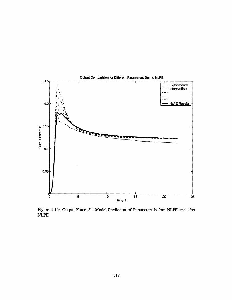
Output Comparision for Different Parameters During NLPE0.25

- Experimental-- Intermediate

- \ -- NLPE

... \--~ K

0

Figure 4-10:NLPE

5 10Time: t

15 20

Results

25

Output Force F: Model Prediction of Parameters before NLPE and after

117

AI.

0.2

0.15

0.1

L

0

0.05

0

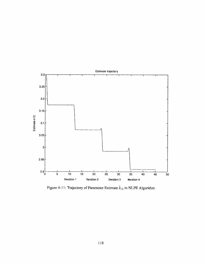
Estimate trajectory

0 5 10 15 20 25 30 35 40 45 50

Iteration 1 Iteration 2 Iteration 3 Iteration 4

Figure 4-11: Trajectory of Parameter Estimate k12 in NLPE Algorithm

118

3.3

3.25

3.2

3. 15

C'.J

(I)

w

3.1

I I I I - F

I I ILiL~_li

3.051

3

2.95

2.9

Bibliography

[I] K. S. Narendra and A. M. Annaswamy. Stable Adaptive Systems. Prentice-Hall, Inc.,

Englewood Cliffs, N.J., 1989.

[2] C.Cao, A.M.Annaswamy and A.Kojic. "Parameter Convergence in Nonlinearly Pa-

rameterized Systems". IEEE Transactions on Automatic Control, vol.48:163-176,

March 2003.

119

Chapter 5

Polynomial Adaptive Estimator

5.1 Introduction

The problem of parameter estimation in a nonlinearly parameterized system can be stated

as follows:

y= f(y, u,0) (5.1)

where f is nonlinear in the unknown parameter 0. The goal is to develop an estimator

Y= f (9, u, ) (5.2)

with 0 adjusted so that 9 -+ Oo.

A stability framework has been established for studying estimation and control of non-

linearly parameterized systems in [1]-[9]. In [1, 2], for example, stability and parameter

convergence with suitable NLPE conditions have been established. The problem however

is that the NLPE condition is quite restrictive, and requires a certain property to be satisfied

by all possible subsets in the parameter space and is rather difficult to check. One of the

reasons for this is that the unknown parameter is estimated using a quadratic nonlinearity

in the Lyapunov function which essentially generates a linear function in the parameter er-

ror. For example, for the system in (5.1), and the estimator in (5.2), suppose the parameter

120

estimation is chosen as

O= -9,#*

a Lyapunov function of the form

V = #2 /2 + 2/2

leads to a time-derivative

= (f(y, U, 0) - 0* - f(y, U, 00))

The term f(y, u, 0) - O*d is clearly linear in 0 and therefore in 0. Since f is not linear

in 0, it is clear that there are not enough degrees of freedom in the estimator. This is the

motivation for choosing a polynomial Lyapunov function

N

V = /2 + Zp 2 (i)i=1

where

Oi= -9#. i = 1,-.. N.

By choosing a p(-) in V and multiple parameter estimates 9i, we will generate a Lyapunov

derivative which gives us more degrees of freedom.

The chapter is organized as follows. Section 2 includes the statement of the problem

and description of the PAE algorithm. In Section 3, the PAE and its stability properties are

discussed in the simple case when the parametric nonlinearity is polynomial in nature. In

section 4, a DPAE algorithm is introduced to address general nonlinearities and the expan-

sion to higher dimension is explained. In Section 5, the NLPE condition and parameter

convergence are presented. It is shown that the NLPE condition is identical to the linear

persistent excitation condition. In section 6, simulation results are provided. Summary and

conclusions are stated in section 7.

121

5.2 The Structure of PAE

5.2.1 Statement of the Problem

We start with the simplest problem of a first order plant with a scalar unknown parameter

while the extension to unknown parameters and systems in higher dimension is discussed

later in this chapter. This plant can be described as

y= -ay + f (y U, 0) (5.3)

where 00 E E C IR is unknown parameter, E is the known compact set where the unknown

parameter 0 belongs to, y E IR is state variable, u E R" includes inputs, measurable

system variables and even system time t. We note that problem formulation in (5.3) also

include plants of the form

f= f(y, u,0)

since they can be transformed into (5.3) with f(y, u, 0) = ay + f(y, u, 0). Secondly, we

note that there exist multiple unknown parameters for nonlinear dynamic systems for the

same input-output relationship, which is different from linear systems. One simple example

of multiple true parameters is a periodic function which has f(y, u, 0) = f(y, U, 0 + A).

In this situation, we have no way to distinguish 00 from 90 + A. In nonlinear parameter

estimation, we denote E as the set of the unknown parameters where

E = {0 1 f(y,u,O) = f(y,u,G0),Vy,u,0 E 0}.

Remark 1: We note that for any parameter estimation algorithm, it has no ability to

distinguish the points in E just by using input and output information because their per-

formance are identical. Therefore, for a general nonlinear parameter estimation algorithm,

unlike the Linear Adaptive Estimation algorithm, it must have the ability to identify all the

points in E if it is globally convergent.

In this chapter, for all the situations where just the value of f(y, u, 0) matters, we use 0

to represent any point in (-) and we note that any result achieved for 0 holds for any point

122

in . We make the following assumptions regarding function f.Assumption 1: The function f(y, u, 0) is Lipschitz with its arguments x = [y, u, OJT,

i.e. there exists positive constant B such that

if (x + Ax) - f (x)I 5 BIIAxII. (5.4)

Assumption 2: Input signal u(t) is Lipschitz with respect to t, i.e. there exists constant

U such that

u(ti) - U(t 2)I 5 Ulti - t2 .

Assumption 3: Function f is bounded, i.e.

If (y, u, Oo)t I F,

Assumption 4: y is bounded by F2 .

Assumption 3 and 4 mean that Q, the derivative of state variable, is also bounded by

F = F1 + aF2. (5.5)

and therefore y will not jump and the maximum change rate of y is bounded by F. We

define the Lipschitz continuity of dynamic system as follows.

Definition 1 System in (5.3) is a Lipschitz continuous system if it satisfies Assumptions 1-4.

It is noted that nearly all the systems we encounter in practice are Lipschitz continuous. It

just requires the signal change rate in a nonlinear dynamic system to be bounded. Through

this chapter, we will restrict our attention to Lipschitz continuous systems.

5.2.2 Structure of Polynomial Adaptive Estimator

The Polynomial Adaptive Estimator(PAE) that we propose include several new features.

PAE expands the commonly used quadratic form Lyapunov functions and adopts a new

approach of auxiliary estimates, which uses 91, .., 8 N for one unknown parameter 90. The

123

PAE is of the form

=Y= -a( - esat( )) + #* a sat(,)

-Oii =1 ..., N (5.6)

where

c is an arbitrary positive number, sat(.) denote the saturation function and is given by

sat(x) = sign(x) if IxJ ;;> 1 and sat(x) = x if lxi < 1, and the calculation of a* and q*

will be discussed later.

Combining (5.3) and (5.6), we rewrite the dynamics of the entire system as

- YE i = 1.., N.

where

6i = ki - 0.

To consider stability, we introduce a Lyapunov function V as

N

V = g2 + Pi A() (5.7)

where pi(.) is a polynomial function. Therefore, the derivative of pi(.) is also a polynomial

function and denoted as gi where

dpi(x)dx Vi= 1...., N.

For V to become a Lyapunov function, the choices of pi needs to satisfies the following

124

= +Y = Cf~e OO*-~y~u00)-~sat f

S=Y - y 9,=9-Esat

conditions

(1) gi(d1 ) < 0 if di < 0

(2) gi(di) > 0 if 6i > 0

(3) pi(0) = 0

(4) gi(0) = 0 (5.8)

for any i = 1..., N and all possible values of 6i. If pi(6t ) satisfies (5.8), it can be shown

easily that pi(6i) is nonnegative with pi(9i) = 0 iff 6i = 0 and p2(d2) increases as |0i|

increases.

To make V a Lyapunov function, we need to make sure that V is nonpositive. Because

#= ag + e * -f(y, U, 0) -Egi(6i)#O -a*sat( ) .(5.9)-2 -

if we choose ,i= 1, ..., N and a* to make

Q#* - f(y, u, 0) - Eg(Ou)# - a*sat(A)) <0. (5.10)i=1

it follows that

V=-ap < 0 (5.11)

and V serve as a Lyapunov function.

We note that if Q = 0, inequality (5.10) holds always. If 9 # 0, it implies that | > f

and hence

sat(-) = sign().f

Inequality (5.10) can be transformed into

&esign(&e) sign(E)(#* - f(y, u, 0) - Egi(i)07) - a* < 0.i=1

Because &~sign(&E) ! 0, to achieve (5.11), we just need to choose 0b* and a* to make the

125

following inequality holds

sign(&,)(e(y, u, *) - f (y, u, 0)) - a* 0 (5.12)

where

N

e(y, u,O0,#*) = 0*-Egi(di)<*i=1

Because #* can be chosen arbitrarily, once they are determined, e becomes a function of

y,u and unknown parameters 00.

Now we establish the definition of a Polynomial Adaptive Estimator. Firstly, we need

to determine the order N of PAE and choose appropriate Lyapunov function components

pi. Secondly, in the running of the algorithm, design a methodology to find * and a* which

satisfies (5.12). The definition of a PAE is as follows.

Definition 2 The Polynomial Adaptive Estimator(PAE) is an adaptive estimation algo-

rithm in (5.6) which satisfies conditions (5.8) and (5.12).

This definition leaves a lot of room for constructing different PAE algorithms with two

fixed properties. One is the construction of a Lyapunov function which satisfies (5.8) and

another is the calculation of 0* and a* that satisfy (5.12). In section 5.2.3, we will propose

a method to construct such a Lyapunov function which is used through this chapter. In

section 5.2.4, we will discuss the calculation of 0* and a*.

5.2.3 Construction of A Polynomial Lyapunov function

We choose p(.) in the Lyapunov function in (5.7) as

) =+1 if i is odd;

pi(Oi) =7 i + . 1 if iis even (5.13)% i + 1

126

for i = 1. .., N, where ki is to be chosen appropriately. The corresponding gi is therefore

given by

gi(6i) = 6i if i is odd;

gi (i) = 9i-- + kie9 if i is even. (5.14)

In what follows we will show that (5.8) is satisfied with these choice of pi. Conditions 3

and 4 follow immediately. Conditions 1 and 2 in (5.8) follow as well when i is odd, as does

condition 2 in (5.8) when i is even. Hence, what remains to be shown is condition 1 when

i is even, which is not true for any 9i. However, the feature we can exploit is that the range

of 6i is constrained by Lyapunov function V defined as in (5.7) and we just need to choose

ki which makes condition 1 in (5.8) holds for any possible 9i. For any choice of initial 9i

and 9 at t = 0, the Lyapunov function is V(O). From (5.11), it follows that

V(t) < V(0) (5.15)

for any t > 0. Equation (5.15) implies that 9i is bounded and the bounds can be calculated

easily. Assume the lower bound of 9i is 9i, to make condition 1 in (5.8) satisfied, we just

need to choose ki which satisfies1

ki < - (5.16)

Choosing Lyapunov function V as in (5.13) and an appropriate ki that satisfies (5.16),

we establish stability of the PAE algorithm if (5.12) can be satisfied. Throughout the rest

of the chapter, we will choose Lyapunov function as in (5.13).

5.2.4 Implementation of PAE

One choice of #* and a* that satisfy (5.12) so that V is nonincreasing is as follows:

= arg min max h(y, 0, u)4EIRN 96no

a*= min max h(y, 0, u)4EN OE2o

127

N

h(y,9, u) = sign( ,)(*- f(y,u,90 ) - Igi(i)47) (5.17)

When conditions (5.17) and (5.8) are satisfied, it follows that the PAE is stable. However,

similar to the min-max algorithm in [1], this implies that a nonlinear optimization problem

has to be solved to obtain 0* at every time step. Given that the optimal 0* can lie anywhere

in an unconstrained region IRN, this is an extremely difficult task if not impossible. In the

next section, we will consider two examples where the solution to the above problem can

be obtained in a straightforward manner.

The motivation for the structure of the PAE in (5.6) and (5.17) and the polynomial Lya-

punov function in (5.13) is as follows: The nonlinear function f of the unknown parameter

90 is estimated using 0, and a*, which is added so as to guarantee stability, needs to be

made to approach zero. If a quadratic Lyapunov function and a single parameter estimation

for 0 is used, the Lyapunov derivative is of the form

#= -agy + y+ [f(yu,&) - f(y,u,Oo)] a*sat(). (5.18)

The term f(y, u, 0) - 0*§ is clearly linear in 9 and therefore in 0. Since f is not linear in

0, it is clear that there are not enough degrees of freedom in the estimator. In the PAE, by

choosing a p(.) in V and multiple parameter estimates 9j, instead of Eq. (5.18), we obtain

a Lyapunov derivative as in (5.9) which gives us more degrees of freedom. In particular,

the termN

0* - g;(A)#ii=1

provides us with a Polynomial approximation of f.It should be noted that even with these additional degrees of freedom, two problems

remain. The first is the requirement that a* has to approach zero. The second is the con-

struction of 0* such that Eq. (5.12) is satisfied. The introduction of p(.) and the additional

degrees of freedom makes the latter somewhat more complex. However, as shown in sec-

tion 5.5, the condition on persistent excitation leading to parameter convergence is much

simpler.

128

5.3 Polynomial Adaptive Estimator

We will consider two cases in this section where we will show how to choose 0* and a*

to form an Nth order polynomial expansion for the function f in (5.3) so that (5.12) is

satisfied. In case i, f is exactly an Nth order polynomial function over 0, and in case ii, f

can be approximated by a Nth order polynomials.

Case i: When f is exactly a Nth order polynomial, it implies that

N

f(y, u, 00) = ci~i (5.19)i=O

where ci is a known of y and u, while 90 is unknown. For the choice of V as in (5.13),

e(y, u, 9,) is written asN

e(y, u, 9*) = *- Z 9i()i=1

where gi is defined as in (5.14). We will choose q* in a way that

N N

0* - gi 49(0i) = i 0 ci6 (5.20)i=1 i=O

and

a* = 0. (5.21)

Because e(y, u, 09) can perfectly match f, there is no need to introduce a* or E. It can be

checked easily that choice of 0* and a* as in (5.20) and (5.21) satisfies (5.12).

We notice that Oi = i - 90 and gi is a ith order polynomial function of 90 and it can be

expressed as

gi= di(O-)Ooi. (5.22)j=0

With known 9i and ki, the calculation of coefficients of dij follows easily, with especially

doo = 1

dii = -1 if i is odd

dii = ki if i is even. (5.23)

129

It follows from (5.22) that equation (5.20) is equivalent to

wheredoo * * *

0 di * *

A= 0 0 d2 2 .. * (5.24)

0 0 0 .. dNN

and

C = [co c1 ... CN]T. (5.25)

The element of ith row and jth column of matrix A in (5.24) is

Aij = 0 i> j;

{dji < j

where dj, is defined as in (5.22) and (5.23). We notice that A is a upper-triangular matrix

and it must be full rank. It means that e(y, u, Oo) has the ability to match any Nth order

polynomial functions. Calculation of 0* follows easily as

#* = A~1C.

In fact, for a upper-triangular matrix, we even do not need to perform the matrix inversion

and we can get 0* through 0* one by one by simple manipulation.

Case ii: When function f is not exactly a Nth order polynomial however can be ap-

proximated by a Nth order polynomial, it follows that

N

f (y, u, Oo) = c00' + r(y, u, 0o) (5.26)i=O

where r(y, u, 0) is the residual error between objective function f and the Nth order poly-

130

nomial approximation and

Jr(y, u, Oo)| a*. (5.27)

Using the same method as in case i to calculate 0* as

N N

#* - #!gi(A) 1= Z cis9i=1 i=

a*= a*a

and it can be checked easily that such choice of a* and 0* satisfies (5.12). The PAE algo-

rithm is stated as

= a(y - esat(-))+#* - a*sat( )

9,=-g,~ i =1, ... , NOi = .7-y

9E = ii-CEsat

a = a*ax

= A~ 1C (5.28)

where

sat(.) denote the saturation function, A, C and a*a are defined in (5.24), (5.25) and (5.27)

respectively.

5.3.1 Properties of the PAE

In this section, we will establish some properties of the PAE algorithm in (5.28). For

the PAE in Case i of section 5.3, same properties and lemmas follow if we assume that

a*a, = 0. All the proofs of the properties and lemmas can be found in the Appendix.

First, we will establish some properties of 0*. We will show that 0* is bounded and

Lipschitz w.r.t. time t.

131

Property 1

* is bounded.

Property 2

|#* (t2) - 0* (t1)| I Q1|It2 - ti I.

In PAE, 0* is a known variable in the algorithm and the maximum change rate Qi can

be measured and kept on line. Unlike 0* which is calculated by solve a group of linear

equations, a* in PAE will be at a constant nonnegative value a*.. About a* ax, we have

the following property.

Property 3

-amax a*sat(y) ax-

The proof of this property is obvious now that Isat(j) 1. If we define

m(t) = #3 - f(y, u, 9o) - a*sat( ), (5.29)E

Property 4 shows that m(t) is bounded.

Property 4 There exists a finite positive M such that

Im(t)| < M (5.30)

where m(t) is defined as in (5.29).

Define

n(t) = 0* - f(y, u, Oo). (5.31)

we conclude that n(t) is Lipschitz w.r.t. t in the Property 5.

Property 5

In(t + T) - n(t)j 5 Qjr (5.32)

where

Q = B(U + F) + Qj, (5.33)

132

with B, U, F, Q, defined as in Assumptions 1, 2, Eq. (5.5) and Property 2 respectively.

Remark 2: In fact, the estimator variables <0*, a* and 0 are associated by a non-singular

matrix. From Assumptions 1-3, all the system variables u, y are Lipschitz w.r.t. time t,

therefore, all the variables in the algorithm are Lipschitz w.r.t. time t, i.e. change rate

bounded.

Next, we will show several lemmas related with the PAE. In the following lemma, it is

shown that when the output error is large, the Lyapunov function will decrease by a finite

amount.

Lemma 1 For the system in (5.3) and PAE as in (5.28), if

WQ,(*i) > 7,

then

V(ti + T') < V(ti) - ( y)-- 3(M + )

where T' = -y/(M + cry) and M is defined as in (5.30).

The proof of lemma I is shown in [2]. In the following Lemma, we show the relationship

between n (t) in (5.31) and output error Q9.


n(ti) > a-y+2 Q('Y+c)+2a*axor

n(ti) < -c-y - 2 Q(7 + ) - 2a*

for any positive constant -y at some time instant t1, then there exists some t2 E [t 1 . t1 + T]

and

11 (t2)I > I,

where

T, = 2 (y + C)/Q. (5.34)

and Q is defined as in (5.33).

133

The following lemma shows that for any time interval T and output error criteria -y, the

output convergence over interval T will happen.

Lemma 3 For any T, there exists positive integer s such that

I I-y (5.35)

for any t E [sT, (s + 1)T]..

5.4 Discretized-parameter Polynomial Adaptive Estima-

tor

In PAE discussed in section 5.3, the function f is approximated by a polynomial function

and we assume the coefficients in (5.26) which includes ci, i = 1, .., N and a,,, axare known.

To extend the PAE to arbitrary f, and when 0 is a vector, we will introduce a Discretized-

parameter Polynomial Adaptive Estimator(DPAE) in this section.

5.4.1 DPAE Algorithm

For a compact unknown parameter region Q = [0mi, 0max], we discretize the unknown

parameter region and represent them as a discrete set D of evenly distributed N points as

D = [X1, .. , i,.., XNI

± 9n max - min + Omax mn()j = min + "2N N

The minimum distance I of point 9 E Q towards the set D follows

1(0)

d(9)

2 = 1, .. , N. (5.36)

= min|110 - xxED

= argmin|i\o-x|XED

134

where d(9) is the projection of 0 on D and

1 max - min(1(0) - 2N (5.37)

From the Lipschitz property of function f and therefore f(y, u, 0o), it follows from (5.4)

and (5.37) that

If (yU,6) - f (yu, d(O)) IB(Omax - Omin) (5.38)

Choosing Lyapunov function same as discussed in section 2, we replace the unknown pa-

rameter region Q with discrete set D and it follows from (5.38) that the new system is

= -ay + f(y, u, #o) +,r

r < a*a

* B(Omax - Omin)ama = 2N

1 E c D (5.39)

where D is defined as in (5.36), B is defined as in Assumption 1, and e is the new unknown

parameter set where new defined unknown parameter o belongs to, and is defined as

E = {1 If (y, u, 0) - f(y, u, 0)I 1 a*ax, V y, u, 0 E D} (5.40)

Our goal is to construct an estimation set E which can estimate C D. Combining (5.38)

and (5.40), it follows that

d(O) c . V 00 cE

even e may also include other points.

For this new system in (5.39), we choose a N - 1 order PAE which satisfies

N-1

* -- *gi(Oi - 0) = f(y, u, 0) VO E D (5.41)i=1

a = a*ax

and construct the DPAE algorithm exactly same with PAE as in section 5.3 except the

135

determination of *, which needs to satisfy (5.41). To satisfy (5.41), we choose

$* = A'C

where A is an N by N matrix given by

1 .. .

A=w he . ais

with the ith row and jth column element aij as

ai = 1 1 < i < N

aij = -gy_1(0j_1 - Xi) 1 < i < N,2 < j N

where gi is defined as in (5.14) and C is an N by 1 vector given by

C = [f(y, u,Xi) .. f(y,u, Xi) ..f(y, u, XN)T. (5.43)

with the ith element b2 as

bi = f(y, u, xi).

It is straightforward to show that such choice of A and B satisfies equation (5.41). We

could check easily that the calculation of 0* and a* in DPAE algorithm satisfies (5.12) from

(5.41). To guarantee that the above DPAE has the same properties and lemmas as PAE in

section 5.3, one requirement is that A is full rank, which is stated in the following lemma.

Lemma 4 The matrix A as defined in (5.42) is full rank with D chosen as in (5.36) and gi

as defined in (5.14).

The proof of Lemma 4 can be found in the Appendix.

Because A is full rank, all the conditions in DPAE is the same as those with PAE as in

section 5.3 and therefore all the properties and lemmas in section 5.3.1 can be proved in a

136

(5.42)

similar manner with 9O E G instead of O( C . Therefore, bounds in DPAE like Q in (5.33)

and T, in (5.34) follow in a similar way as in PAE. We state the complete DPAE algorithm

below:

For any positive number -y, c and T,

9=-ae(q - csat( )) + #*-a*sat( )= 0

ge#*, = , .. ,N - 1Y^ Y= 9-y

e = eiisat

a = amax

= A'C

E = {01 E D, *(r1)- f(y(r1),u(ri-),9) #*(r1) +l,Vr 1 E [t1,ti +T],

1 & (T2)1 5 -y, V -r2 E [titi + T+ Ti]} (5.44)

where

= a'y+2 Q(Y+0)+2a*,

= N-

sat(.) denote the saturation function, A, C and a* are defined in (5.42), (5.43), and (5.39)

respectively.

Assume that 0 G E, first we need to find a time interval ti., ti + T + Ti] where the

output error convergence happens, i.e.

It/Cl 7(5.45)

over this interval. Then, E includes the set of all points in Q which satisfies

0*('r1) - 1 f(y(ri),U (ri), 0) 0*(t) + 1, V 1 E [t1, ti + T].

137

Lemma 3 implies that the output convergence will always happen, which means there will

always exist time interval [ti, t, + T + T] where (5.45) holds. From Lemma 2, it follows

that

*(r1) - f(y(ri), u(r1), Oo) *(t) + , V 71 E [ti, ti + T. (5.46)

Combining (5.46) and the definition of & in (5.44), we have that

0 e)

and hence

5.4.2 Extension to Higher Dimension

One important feature in the DPAE algorithm is that when the unknown parameter set is

a discretized set X E R, what really matter are the values of f(y, u, x) where x E X

but not the locations of x in the R axis. It means that even in section 5.4.1 we choose

x as its original value, we also can adjust the distance between different x or even adjust

the sequence of x just if we keep a mapping between points x with its original points in

Q space. The auxiliary estimates will run in the new X space and finally E will give

some x where f (y, u, x) matches f(y, u, 0). When we map x back to its original value

in Q, we still have an estimation of 0. What is affected here is the Lipschitz bounds of

the underlying function in X. If we put two points with different f (y, u, x) close to each

other, it implies that we have a very large B. From the discussion above, we notice that if

we apply DPAE, now that we use a discretized set D to represent the compact unknown

parameter set Q, it does not matter whether Q belongs to R or R" and we can extend the

DPAE into higher dimension of unknown parameters easily.

For an unknown parameter set Q E R and any given precision a*a, we can construct

a discrete set D E Q with N points and for any 9 E Q, there exists Di E D such that

If(y, u, 0) - f(y, u, Di)| I a *

138

The new unknown parameter set e is defined as in (5.40). The most common choice of D

is the grid points in Q. From Assumption 1, for any a*ax, we can find such a discrete set D

while N increases as a*a decreases. After that, we map the discrete set D into a discrete

set X c R with the same data points and establish a one to one mapping between these

two sets and we assume that

f(y, U, Xi) = f (y, u, Di) (5.47)

where xi are the mapping of Di on X. We perform the same DPAE as in section 5.4.1 with

X as the unknown parameter set instead of D. In DPAE algorithm we note that we just

need the value of f (y, u, xi) which can be achieved from (5.47) and there is no need for

f (y, u, x) where x V X. That is also the reason why we can choose X freely.

When we get an estimation E in X, performing simple mapping, it is equivalent to an

estimation in D where

e = {6O ED,#*(ri) - : ! f(y(ri), u(Tr), 6) *(71) + , V 7 c [ti, t1 + T.

|Q&(r2)l :5 7, V r2 E [ti, ti + T + T1]}.

Therefore, DPAE can be applied if unknown parameters in higher dimension nearly the

same way as for one-dimension.

When system variables is higher dimension, i.e.

= F(Y, u, 00)

where Y c JRL are measurable, we can treat them as L one-dimension system variable

systems and apply the DPAE algorithm above to perform the parameter estimation. By this

way, we can extend the DPAE algorithm to a more general Lipschitz nonlinear dynamic

system.

139

5.5 Nonlinear Persistent Excitation Condition

In previous sections, we introduced PAE and DPAE algorithms which generate E which

estimate the set of unknown parameters E, and showed that 0 ( E. In this section, we will

establish the Nonlinear Persistent Excitation condition which guarantee the convergence of

E to E in PAE and DPAE. The relationship between LPE and NLPE is also discussed in

section 5.5.2.

5.5.1 Nonlinear Persistent Excitation Condition

First, we will define the distance between two sets. For two sets E and E, we define the

distance II.I id between these two sets as below.

Definition 3

|I0 - |lid = maxmin l9- Oil.CE Oce

It can be checked easily that

118 - jlld = 110 - EOI|.

II - Old = co has two meanings. One is that for every point 0 E E, there is a point 0 E 0

such that

110 - Oil ;Eo

and another is that there is no point 0 G E such that

110 - Oil > co V 0 E E.

Global convergence of PAE and DPAE is said to follow if

11e - Olid - 0.

Now we introduce the NLPE condition which can guarantee the convergence of PAE

and DPAE.

140

Definition 4 NLPE: For problem formulation as in (5.3) under assumptions 1-4, y, u is

said to have nonlinearly persistent excitation iffor any t, there exists time constant T, co

and a time instant t1 C [t. t + T] such that

(f (y(ti), u(ti), 9) - f(y(ti), u(ti), Oo)) c o min|0 - 0o1 | V90 E e.OoE2

In the following, we will prove that under NLPE, DPAE can lead to global conver-

gence. For PAE, just the choice of polynomial estimator and #* has the ability to make a*

approaches 0, the global convergence can be proved easily using a similar way. We use

DPAE as the example just because DPAE involves set e and it is more difficult than PAE

to prove the convergence.

Theorem 1 For problemformulation as in (5.3) under assumptions 1-4, under NLPE con-

dition as in definition 4, for any f1, there exists a DPAE as in (5.44) which leads to

11e - 6l1d 5 1f. (5.48)

The proof of Theorem I can be found in Appendix.

5.5.2 Comparison to LPE

For linear systems, when the system variables u is Lipschitz w.r.t. time t, u(t) will change

gradually and any error introduced by 10'u - OTul will not disappear soon and it will cause

perturbation in the integral of the error. Thus the Linear Persistent Excitation is transformed

into the following one as in [2].

Definition 5 LPE: Assume u is Lipschitz w.r.t. time t, u is said to be linearly persistent

excitation if for any t, there exists time constant T, co and a time instant t, E [t. t + T]

such that

IOTU - p| coio - 001.

Remark 6: We notice here that when objective function is linear, the NLPE is just

transformed into LPE. The difference in right part is just because for linear function, there

141

is only one true unknown parameter. In fact, Linear Persistent Estimator can also be treated

as a first order PAE.


We consider a simple example with nonlinearly-parameterized parameter such as

p= -4y + U20 0 + u3o2

with the true unknown parameter 90 = 1. The known parameter region Q = [0, 2] where

Oo e Q. The input signal u is

u(t) = sin(2t + ir/2).

We choose Lyapunov function as

1 1 1 1V 2= 2 + 22+ 3k.

To design the Polynomial Adaptive Estimator, we first will determine the value of k ac-

cording to the discussion as in previous section. Choose k = 0.2 and it is shown that it

satisfies the requirement as in (5.8). The PAE estimator algorithm is stated below:

Q = -4Q + 00

01 = -0#92

0* = -02*k

q* = u 2 _ 0 _ 2k 2S

#* = #*01 +#*02+k 2#*

k = 0.2.

The simulation results are shown in Figures 5-1-5-3. Figure 5-1 shows the output error Qand Figure 5-2 shows the trajectories of estimates 01 and 92. Because it can be checked

142

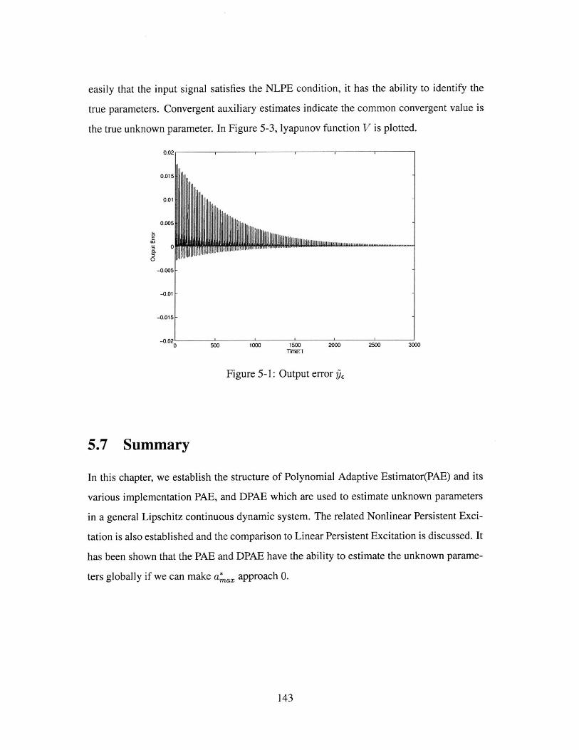
easily that the input signal satisfies the NLPE condition, it has the ability to identify the

true parameters. Convergent auxiliary estimates indicate the common convergent value is

the true unknown parameter. In Figure 5-3, lyapunov function V is plotted.

500 1000 15000 500 1000 1500 2000 2500 3000

Figure 5-1: Output error gE

5.7 Summary

In this chapter, we establish the structure of Polynomial Adaptive Estimator(PAE) and its

various implementation PAE, and DPAE which are used to estimate unknown parameters

in a general Lipschitz continuous dynamic system. The related Nonlinear Persistent Exci-

tation is also established and the comparison to Linear Persistent Excitation is discussed. It

has been shown that the PAE and DPAE have the ability to estimate the unknown parame-

ters globally if we can make a*. approach 0.

143

0.01!

0.01

-0.01

-0.015

W5 0

0 -0.0051

191IM01111m umn ..........

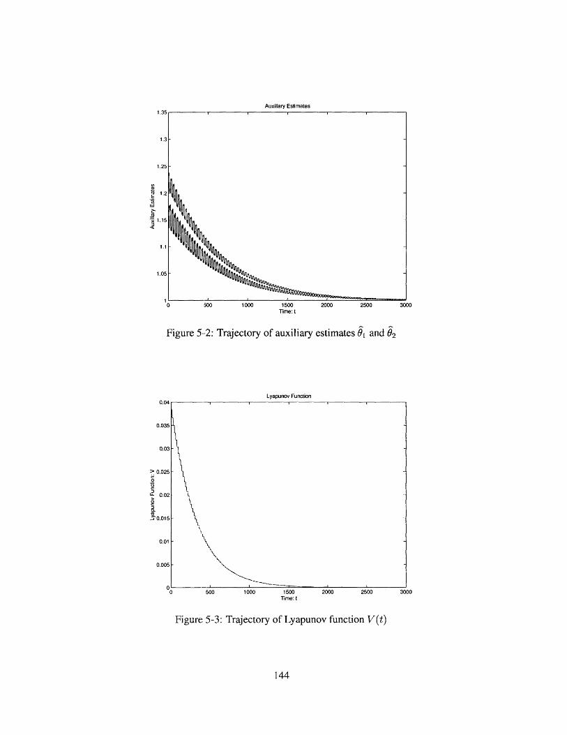
Auxillary Estimates1.35,

1.3

1.25F

12

E

'it

-~1.15

1.11

1.05

0 500 1000 1500 2000 2500 30lime: t

Figure 5--2: Trajectory of auxiliary estimates 01 and 02

Lyapunov Function0.04r

0.035

0.03

0.025i.LD

U-

0

CL(a

-J

0.02

0.015

0.01

0.005

0 500 1000 1500Time: t

2000 2500 3000

Figure 5-3: Trajectory of Lyapunov function V(t)

144

0

Bibliography

[I] A.M. Annaswamy, A.P. Loh, and F.P. Skantze. Adaptive control of continuous time systems

with convex/concave parametrization. Automatica, January 1998.

[2] C. Cao, A.M. Annaswamy, and A. Kojic. Parameter convergence in nonlinearly parameterized

systems. IEEE Antomatic Control, 48:397-412, March 2003.

[3] A. P. Loh, A.M. Annaswamy, and F.P. Skantze. Adaptation in the presence of a general non-

linear parametrization: An error model approach. IEEE Transactions on Automatic Control,

AC-44:1634-1652, September 1999.

[4] J.D. Boskovid. Adaptive control of a class of nonlinearly parametrized plants. IEEE Transac-

tions on Automatic Control, 43:930-934, July 1998.

[5] A. Kojid, A.M. Annaswamy, A.-P. Loh, and R. Lozano. Adaptive control of a class of nonlinear

systems with convex/concave parameterization. Systems & Contml Letters, 37:267-274, 1999.

[6] M.S. Netto, A.M. Annaswamy, R. Ortega, and P. Moya. Adaptive control of a class of nonlin-

early parametrized systems using convexification. International Journal of Control, 73:1312-

1321, 2000.

[7] A. Koji6 and A.M. Annaswamy. "Adaptive control of nonlinearly parametrized systems with a

triangular structure". Automatica, January 2002

[8] C. Cao and A.M. Annaswamy. "Active and Adaptive Control Lab Report 04-1, Mass. Inst. of

Tech.". February 2004

[9] K.S. Narendra and A.M. Annaswamy. Stable Adaptive Systems. Prentice-Hall, Inc., 1989.

145

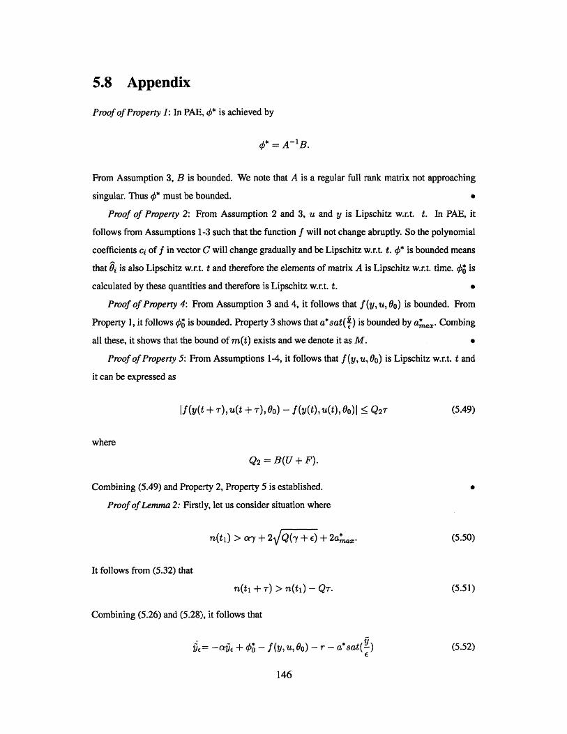
5.8 Appendix

Proof of Property 1: In PAE, (b* is achieved by

#* = A- 1 B.

From Assumption 3, B is bounded. We note that A is a regular full rank matrix not approaching

singular. Thus 0* must be bounded.

Proof of Property 2: From Assumption 2 and 3, u and y is Lipschitz w.r.t. t. In PAE, it

follows from Assumptions 1-3 such that the function f will not change abruptly. So the polynomial

coefficients ci of f in vector C will change gradually and be Lipschitz w.r.t. t. 0* is bounded means

that Oi is also Lipschitz w.r.t. t and therefore the elements of matrix A is Lipschitz w.r.t. time. #3 is

calculated by these quantities and therefore is Lipschitz w.r.t. t.

Proof of Property 4: From Assumption 3 and 4, it follows that f (y, u, 0) is bounded. From

Property 1, it follows #3 is bounded. Property 3 shows that a*sat(Y-) is bounded by a*a. Combing

all these, it shows that the bound of m(t) exists and we denote it as M.

Proof of Property 5: From Assumptions 1-4, it follows that f (y, u, 0) is Lipschitz w.r.t. t and

it can be expressed as

If(y(t + T), u(t + T),0) - f(y(t), u(t), 0) Q2r (5.49)

where

Q2 = B(U + F).

Combining (5.49) and Property 2, Property 5 is established.

Proof of Lemma 2: Firstly, let us consider situation where

n(ti) > ay + 2 Q -( + E) + 2a*M- (5.50)


n(ti + T) > n(ti) - Qr. (5.51)


YE= -aE + 0* - f (y, u, Oo) - r - a*sat( ) (5.52)

146

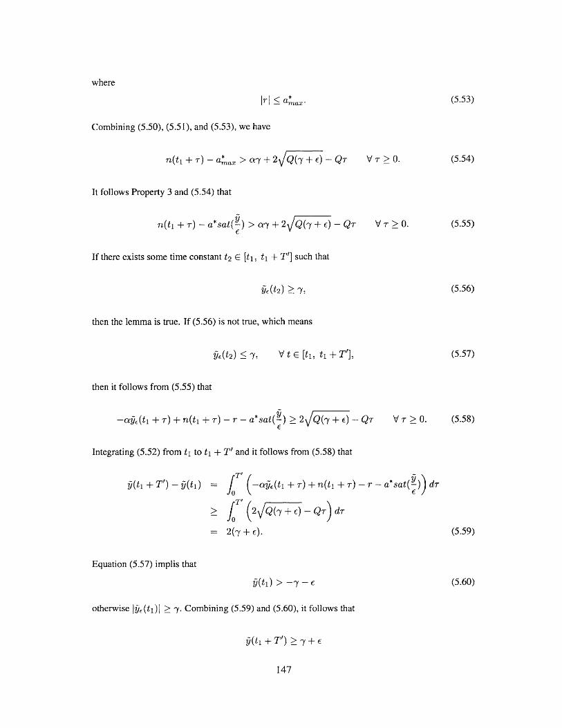
where

Irl <; a*a."

Combining (5.50), (5.51), and (5.53), we have

n(tj + T) - a*ax > a-(+2 Q(7 +e) - QT

It follows Property 3 and (5.54) that

n(ti + T) - a*sat( ) > ay +2 Q(y + e) - QT

If there exists some time constant t 2 E [ti, ti + T] such that

MO(t2 ) > -7.

then the lemma is true. If (5.56) is not true, which means

&(t2) :< Y. V t E [ti. ti + T'].

then it follows from (5.55) that

-Ce(ti + T) + n(ti + T)- r - a*sat()>2 Q(y+ C) - QT

Integrating (5.52) from t1 to t1 + T' and it follows from (5.58) that

p(ti + T') - Q(ti) - --a (ti + -r) + n(ti

- 2VQ(y + c) - QT) d

=2(-y + c).

Equation (5.57) implis that

(t1 ) > -y -

otherwise -y(ti)| ; y. Combining (5.59) and (5.60), it follows that

p(t + T') > 7 + e

147

(5.53)

V T > 0.

V r > 0.

(5.54)

(5.55)

(5.56)

(5.57)

V T > 0. (5.58)

+ T)- r - a*sat( ) dr

(5.59)

(5.60)

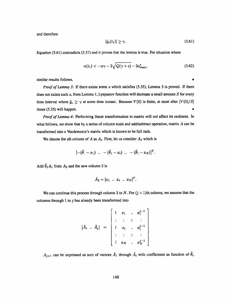
and therefore

|We(ti)| ! 7. (5.61)

Equation (5.61) contradicts (5.57) and it proves that the lemma is true. For situation where

n(ti) < -ay - 2 Q(y + E) - 2a*ma (5.62)

similar results follows. 0

Proof of Lemma 3: If there exists some s which satisfies (5.35), Lemma 3 is proved. If there

does not exists such s, from Lemma 1, Lyapunov function will decrease a small amount S for every

time interval where & -y at some time instant. Because V(O) is finite, at most after [V(O)/S

times (5.35) will happen. 0

Proof of Lemma 4: Performing linear transformation to matrix will not affect its rankness. In

what follows, we show that by a series of column scale and add/subtract operation, matrix A can be

transformed into a Vendemonts's matrix which is known to be full rank.

We denote the ith column of A as A2 . First, let us consider A 2 which is

[ -- : X i) - (01 - Xi) - (01 - ZN)].

Add 91A1 from A 2 and the new column 2 is

A2 = [X1 -- Xi -- N XT.

We can continue this process through column 3 to N. F

columns through 1 to j has already been transformed into

[Al .. Aj]=

1 X1

Xi

XN

'or (j + 1)th column, we assume that the

-i

J- 12N

Aj+l can be expressed as sum of vectors A, through Ai with coefficients as function of 9i.

148

Therefore, by subtract weighted A, through Ai from Ai+1, the new i + 1th column is

dj+ I= [zJ, .. Xq .. zyT

Repeat this process until the last column, and by simple matrix operation, the new matrix be-

comes

[Ali .. AN

X1 .. X1 -

N-1XN - N

Since (5.63) is Vandemeonts' matrix and is full rank, A if of full rank as well. 0

Proof of Theorem 1: We choose parameter T in DPAE same as the T in the NLPE condition

which is defined in definition 4. For problem formulation in (5.39) and DPAE as in (5.44), it follows

from Lemma 3 that the output error &e will converge for some interval [t., t + T + T1 ] for any -Y

where

When e pe e c tr2 E [t, t + T + TI]

When output convergence happens we construct the E) by

e = {OjO E D, 0(71) -/ f(y(-r), u('r),) 43(r1) +/3,Vr 1 E [t,t +T]} (5.64)

where

/3cY + 2 Q'+ 2a*az

It follows from Lemma 2 that

If (y ri), u(ri), 6) - #*0 /3 V r i c [t, t + T]

for any 0 E e. From NLPE condition, for any 0 E 0 there exists ti E [t., t + T] such that

If (y(ti),u(ti), 0) - f (y(ti), u(ti), Oo)I > Eo min 110 - OolIOoErIO

V0 0 c e.

149

(5.63)

(5.65)

(5.66)

1

I

1

It follows from (5.64) and (5.65), respectively, that

(5.67)

If (y01), 0(1), 0) - 0*0(ti) I #, VO E E)

If (y(t1), U(ti), 6) -O#(ti)| VO E 0.


If (y(ti), u(ti), 0) - f(y(ti), u(ti), 0)j 1 2/3

for any 9 E 6 and 9 E 0. It follows from equation (5.40) that

If (y(t1), u(ti), Oo) - f (y(ti), u(ti), 6)1 _< a* a

for any 0- E) and 0 E 8. Combining (5.68) and (5.69), it follows that

If(y(ti), u(ti),9o) - f(y(ti), u(ti), ) 1 2,8 + a*ax,

for any 0 E E and 9 E . Combining (5.66) and (5.70), it follows that for any 9 E E

min 1102P + a*mn| - 0||1 < max,

OoEno 60

which implies

|1 -) _ ell 2/3+ a*mnax

(5.68)

(5.69)

(5.70)

(5.71)

Now that we can choose y, e and N to make a* . and / arbitrary small, when we choose 2/3 +

aax = EOEi, (5.48) is satisfied and this proves Theorem 1.

150

Chapter 6

Hierarchical Polynomial Adaptive

Estimator

6.1 Introduction

Although Linear Adaptive Estimator and its related Linear Persistent Excitation(LPE) Condition

have been established for many years, the corresponding algorithm for general nonlinearly parame-

terized dynamic system is still out of reach. Even a lot of efforts have been made, such as min-max

algorithm and hierarchical min-max algorithm, there still exist some restrictions which prevent them

to be general approaches for nonlinearly parameterized systems. A stability framework has been es-

tablished for studying estimation and control of nonlinearly parameterized systems in [1]. In [2],

the min-max algorithm in [1] is further extended into a hierarchical one and its associated Non-

linear Persistent Excitation Condition associated is established. No matter in min-max algorithm

or its hierarchical one, it involves a nonlinear optimization problem at every time step. However,

the computation complexity is still not the main disadvantage which prevent these algorithms to

becomes a general solution for nonlinear parameterized system if we notice that they can not guar-

antee parameter convergence. The Nonlinear Persistent Excitation (NLPE) condition established

in [2] describes the condition under which the hierarchical min-max algorithm achieves parameter

convergence and it turns out this condition consists of too rigorous requirements. First, they require

the input u to be "ergodic", which means that u must keep revisiting some interesting points. This

condition is not required in LPE and it will be hard to be satisfied in practical problems. If u belongs

to higher dimension, it is possible that u will never come back to same values even it is bounded. It

151

makes situation worse if the nonlinear part contains both u and y now that there is no guarantee that

(u, y) can be "ergodic" even u is "ergodic". Secondly, unlike the LPE condition, the NLPE condi-

tion in [2] has an additional requirement which is a property needed to be satisfied by any subset of

the compact set that the unknown parameters belong to. This condition is extremely difficult to be

verified for a general nonlinear function and it is not true for all nonlinear functions even they are

Lipschitz and continuous.

In [1], a new algorithm named Polynomial Adaptive Estimator(PAE) is proposed. In that chap-

ter, it uses the technique of auxiliary estimates to form a polynomial approximation of nonlinear

function instead of linear approximation as in Linear Adaptive Estimator and min-max algorithms.

To make PAE a general approach for nonlinear Lipschitz continuous systems and not just poly-

nomial functions, Discretized-parameter Polynomial Adaptive Estimator(DPAE) is proposed as a

further development in [1]. The disadvantage of DPAE is the low computation efficiency. In this

chapter, we will propose a Hierarchical Discretized-parameter Polynomial Adaptive Estimator (HD-

PAE) which has the same convergence property as DPAE however greatly reduce the computation

complexity through the introduction of a hierarchical structure. Same as DPAE in [1], Nonlinear

Persistent Excitation(NLPE) condition which is no more restrictive than LPE for linearly parameter-

ized systems is established for HDPAE. In this chapter, we will show that under the NLPE condition

the HDPAE can lead to global parameter convergence for any nonlinear dynamic system that is Lip-

schitz continuous over a compact unknown parameter region, which covers most of the practical

systems that we encountered. With the introduction of HDPAE in this chapter, a computation effi-

cient parameter estimation algorithm for general nonlinear parameterized system is established for

the first time.

With a long history, all kinds of gradient algorithms are widely applied to estimate parameters

in nonlinear systems just because there is no other choice. With the introduction of HDPAE, we

will give a generalization of parameter estimation in both static and dynamic systems. Hierarchical

Search method, the counterpart of HDPAE in the static domain, is proposed to estimate unknown

parameter in Lipschitz continuous static systems. In the comparison among different algorithms, we

clearly show that the gradient algorithms which just exploit the local information have no guarantee

for global convergence for nonlinearly parameterized systems.

This chapter consists of two parts. Part I, which covers section 6.2 to 6.5, introduce the HDPAE

algorithm for Lipschitz continuous dynamic systems. Section 6.2 gives the problem formulation.

In section 6.3, HDPAE is given and the properties and lemmas of HDPAE are also proposed. Non-

152

linear Persistent Excitation(NLPE) condition under which HDPAE leads to global convergence is

proposed in section 6.4. In section 6.5, simulation results of HDPAE is given. Part II consists of

two sections. In section 6.6, different methods to estimate unknown parameters in static systems are

given. They consist of gradient algorithm, brute search and Hierarchical Search algorithm. In sec-

tion 6.7, generalization and comparison of different parameter estimation algorithms for both static

and dynamic systems are given and it is shown that gradient algorithms do not apply to general

nonlinearly parameterized systems.

6.2 Problem Formulation

We consider a problem formulation with one dimension state variable and the extension to higher

dimension can be easily derived as in [1].

The problem considered is the estimation of unknown parameters in nonlinear systems of the

form

S-ay + f(y, u, w*) (6.1)

where w* E QO C 1W are unknown parameters, y E JR is measurable state variable, u e R'

includes inputs, measurable system variables and even system time t, f0 is the known compact set

where the unknown parameters belongs to. Without loss of generality, we assume QO is a cubic

region, i.e.

oI = {01 E R"wmin <Gi <5 Wmax. i = 1, ... , n}. (6.2)

First, we note that problem formulation in (6.1) is a general problem formulation now that

y= f(y,u, w*)

can be transformed into (6.1) with

f (y, u, w*) = ay + f(y, u, w*).

Secondly, we note that there exist multiple unknown parameters for nonlinear systems, which is dif-

ferent from linear ones. One simple example is to consider a periodic function where f (y, u, w*) =

f(y, u, w* + A). In this situation, there is no way to distinguish w* with w* + A. Therefore, we

153

denote Q* as the set of the unknown parameters where

Q* = {w I f (y, u, w) = f (y, u, w*), V y, u, W E Q0}. (6.3)

Remark 1: We note that there is no way to distinguish the points in a* just by input and out-

put information because their performance are identical. Therefore, a general nonlinear parameter

estimation algorithm, unlike the Linear Adaptive Estimator, must have the ability to identify all the

points in Q*.

In the situations where just the value of f (y, u, w) matters, we use w* to represent any point in

* and we note that any result achieved for w* holds for any w E Q*.

About function f, we make the following assumptions.

Assumption 1: The function f (y, u, w) is Lipschitz with its arguments x = [y, u, w]T, i.e. there

exists positive constant B such that

if (x + Ax) - f (x)I BIIAx j. (6.4)

Assumption 2: Input signal u(t) is Lipschitz with respect to time t, i.e. there exists constant U

such that

|IU(ti) - U(t2)11 < U14i - t21-

Assumption 3: Function f is bounded, i.e.

If (y, u,w)l I F1, V w E 0.

Assumption 4: y is bounded by F2 .

Assumption 3 and 4 imply that y, the derivative of state variable, is also bounded by

F = F1 + aF2 (6.5)

and therefore y is Lipschitz with respect to time and the maximum change rate of y is bounded by

F. We define a Lipschitz continuous dynamic system as follows.

Definition 1 System in (6.1) is a Lipschitz continuous system if it satisfies Assumptions 1-4.

It is noted that nearly all the systems we encounter in practice are Lipschitz continuous. It just

154

requires the signal change rate in a nonlinear dynamic system to be bounded. Throughout this

chapter, we will restrict our attention to Lipschitz continuous systems.

6.3 Hierarchical Discretized-parameter Polynomial Adap-

tive Estimator (HDPAE)

In this section, the HDPAE is proposed. In section 6.3.1, we will introduce the method to dis-

cretize the unknown parameter region. In section 6.3.2, Discretized-parameter Polynomial Adap-

tive Estimator(DPAE), which is the element of HDPAE, is proposed. The properties of DPAE are

summarized in section 6.3.3. The complete HDPAE is proposed in section 6.3.4.

6.3.1 Discretized-parameter Representation

One important property of Lipschitz continuous funtion is that discrete points can represent its

adjacent region with finite precision. In section 6.3.1, we will give a systematic method of using

discrete set to represent continuous parameter region.

Let us introduce several useful definitions. First, we define the distance of one point to a discrete

set as follows.

Definition 2 For any point x, G IR" and a discrete set X 2 C W, the distance of x1 to X 2 is

defined as

l|x1, X2l1d = min lixi - x211. (6.6)X2EX2

Then, we define the distance between two discrete sets as follows.

Definition 3 For any sets X 1 , X 2 C R, the distance between them is defined as

IIX1, X 2 1d = Max llxi, X2||d = max min |ixi - x211. (6.7)X1E Xi X1 EXJ X2E X2

We could check easily that the norm definition is communicative, i.e.

IIX1, X 2 ld = |X2, X|ld. (6.8)

Finally, for any discrete set Z and distance eo, we define its eo-net E as follows.

155

Definition 4 The co-net of a discrete set Z E R' is defined as

E(Z, O) = {Xx E R, |X - Zld EO}. (6.9)

For compact region Q0 and any distance do, we can find a discrete set Zo which satisfies

n0 CE(Z 0 , do) (6.10)

where the dO-net of set Z 0 is defined as in (6.9). In what follows, we will show how to choose ZO

which satisfies (6.10). In every dimension of R, assume ith dimension, we choose a set Z E R

which consists of J uniformly distributed points

(6.11)

where

xi(j+1) - xij = do/

Wminj <

Wrnaxi - do/Vd <

Xil < Wminj + do/V

XiJ < Wmax,.

(6.12)

(6.13)

(6.14)

We could check easily that in R space

[Wmini, Wmaxj]E(Zi, d/v/i).

In order to achieve an organized discrete set Z 0, we choose ZO as a grid in R as follows:

ZO {(xi, .., z,.., ,X)|zi E ZiC }

where Z is defined as in (6.11). About ZO we have the following two properties.

Property 1

0 cE(Z, do).

6.15)

6.16)

6.17)

Proof of Property 1: For any x = [xi, .., xi, .., Xn] E R", it follows from (6.15) and (6.16) that

156

Zi = {xii, ... xii, ... xig}

there exists point Z. e D such that

|Zxj - xilI do /\hi. Vi = 1, .., n. (6.18)

Therefore, we have

||x - ZxI| < do (6.19)

and property I is proved.

Combining Property I and Assumption 1, the following property follows directly.

Property 2 For any x1 c 00, there exists X2 c ZO such that

If(y, u, Xi) - f(y, u, x2)1 Bd' (6.20)

for any y, u.

From Property 2, we note that for any true unknown parameter w* E Q* C no, there must exist

some z E ZO such that

If(y, u, z) - f (y, u, w*)I Bdo Vy.u. (6.21)

We denote the set of such zO as Zg which is stated as

Z$ = {z E Zol If (y, u, z) - f (y, u, w*) < Bdo Vy,u Vw* E *}. (6.22)

Now we can transform problem formulation in (6.1) into a problem formulation with true unknown

parameters Zg as in (6.22) and unknown parameter region as a discrete set Z0.It follows that

y = -ay + f (y, u, z*) + r(y, u, z*)

ZO E ZOCZ 0 (6.23)

r(y, u, z*) a*a.= Bdo (6.24)

where Z and Z 0 are defined as in (6.22) and (6.16).

We assume the discrete set Z 0 contains No points. For unknown parameter region which be-

longs to a discrete set, what really matters are the value of f (y, u, z) and it does not matter which

157

space it belongs to originally. we map ZO E R' into a discrete set E IR and establish a

one-to-one mapping H between them, i.e.

ZO = H(O&)

e0 = H-1(Z0 ). (6.25)

We note that both ZO and 0 0 contains NO discrete points and the commonly choice of G0 is to

distribute NO points uniformly between an interval [60 --Eax], for example [0. 1]. Define

E* = H-1(Zo) (6.26)

and the system in (6.24) is equivalent to the following system:

yi = -ay+f(y,u,6*)+r

0c E) OCE 0 = [01, ... , ONO]

Sa*ax = Bdo

f(y,u,Oi) = f(y,u,H(1 )) i = 1,..,N - 1.

In section 6.3.2, we will give the DPAE algorithm corresponding to the system in (6.27).

6.3.2 DPAE

To estimate unknown parameter in

the DPAE is stated below.

(6.27), we need a DPAE with order NO - 1 and the dynamics of

S=-a( - csat( )) + 0k - a*sat( )

=- No - 1 (6.28)

where

Q=9-y 9e= 9 -esat) (6.29)

E is an arbitrary positive number, sat(.) denote the saturation function and is given by sat(x) =

sign(x) if |xI _> 1 and sat(x) = x if jxj < 1, and the calculation of a* and #* will be discussed

later.

158

(6.27)

Combining (6.27) and (6.28), we rewrite the dynamics of the entire system as

=i &~4 i17..)No -1.

(6.30)

(6.31)

where

k = k - 0.

Same as the DPAE proposed in [1], we will first construct a polynomial Lyapunov function

which is stated in section 6.3.2

Polynomial Lyapunov Function

For system in (6.27) and the DPAE algorithm in (6.28), we introduce a polynomial Lyapunov func-

tion V as

(6.32)V = 2 + , 19i()

where pi (.) is a polynomial function. Therefore, the derivative of pi(.) is also a polynomial function

and denoted as gi where

gjx) W =dpi(x)dx

Vi = 1, ..., NO - 1. (6.33)

For V to become a Lyapunov function, pi needs to satisfy the following conditions

(1) g2(Oi)

(2) gi(6i)

(3) pi(0)

(4) gi(0)

<O if i <0

> 0 if di > 0

= 0

= 0 (6.34)

for any i = 1, .., NO - 1 and all possible values of i. If pi(9 z) satisfies (6.34), it can be shown

easily that pi (ji) is nonnegative with pi (§j) = 0 iff 6i = 0 and pi(9i) increases as Ii increases.

159

To make V a Lyapunov function, we need to make sure that V is nonpositive, i.e.

V= -a 2 + &N

- f(y, u,90) - [ i(6i)0! - r - a*sat() < 0.i=1 E

We note that if Q = 0, inequality (6.35) holds always. If Pe 7 0, it implies that |PI > e and hence

sat(-) = sign(Q,).

Inequality (6.35) is equivalent to

&sign(&) sign(P)(# - f(y,u,63) -

NO-1

Z gi(0i)40)i=1

- rsign(WE) - a* 5 0.

Because y 6sign(gy) ;. 0, to achieve (6.36), we need to choose 0* and a* as follows

= f(y, u, 0) VO E 60 (6.37)

a = a~am- (6

The choice of a* is straightforward. If the choice of 0* satisfies equation (6.38), it follows that

V< -ag 2 <0 (6

and V serves as a Lyapunov function.

Let us firstly find Lyapunov function which satisfies (6.34). We choose

1 +dpi (60 0!+1 if iis odd;

i+ 1 2

pi(i)1-= + . +

0! + 2 if i is even

.38)

.39)

(6.40)

for i = 1, .., NO - 1, where k is to be chosen appropriately. The corresponding gi follows

gi( A)

g1 (Oi)

= 61 if i is odd;

if i is even. (6.41)

In what follows we will show that (6.34) is satisfied with these choice of pi. Conditions 3 and 4

160

(6.35)

(6.36)

ro -1

#0* - ol#gi(oi - 0)

= 6i 1 + kii#

follow immediately. Conditions 1 and 2 in (6.34) follow as well when i is odd, as does condition

2 in (6.34) when i is even. Hence, what remains to be shown is condition 1 when i is even, which

is not true for any i, however the feature we can exploit is that the range of 02 is constrained by

Lyapunov function V defined as in (6.32) and we just need to choose ki which makes condition 1 in

(6.34) holds for any possible 0i. For any choice of initial 0i and y at t = 0, the Lyapunov function

is V(0). From (6.39), it follows that

V(t) < V(0) (6.42)

for any t > 0. Equation (6.42) implies that 6i is bounded and the bounds can be calculated easily.

Assume the lower bound of di is 6i, to make condition 1 in (6.34) satisfied, we just need to choose

ki which satisfies1

ki < - .1 (6.43)

Choosing Lyapunov function V as in (6.40) and an appropriate k as in (6.43), (6.34) is satisfied

and we establish a stability framework of the DPAE algorithm if (6.37) can be satisfied.

Implementation of DPAE

In DPAE, what remains is how to choose #* to make (6.37) satisfied, which is stated as follows:

(6.44)

where A is an NO by NO matrix given by

1

1


ai = 1 1 < i < No

aij = -g 3 -_(0i- - Oi) 1 < i < N0 2 < j < No

161

(6.45)

0 * = A-IC

A =

where gi is defined as in (6.41), 92 is defined as in (6.27), and C is an NO by 1 vector given by

C = [f (y, u,i1) .. f(y, u,O) .. f (y, u,NO )]T (6.46)

with the ith element ci as

ci= f (y, u, 2 ).

It is straightforward that such choices of A and B satisfy equation (6.37). In the lemma follows,

we will show A is full rank and therefore we will not encounter singular problem in (6.44).

Lemma 1 Matrix A as defined in (6.45) is fli rank.

Proof of Lemma I is in the Appendix.

6.3.3 Properties of PAE

In this section, we will establish some properties and lemmas related to DPAE proposed in section

6.3.2. All the proofs of the properties and lemmas are in the Appendix.

First we will establish some properties about g*. We will show that c* is bounded and Lipschitz

w.r.t. time t.

Property 3

#* is bounded. (6.47)

Property 4

I#0(t 2) - 00(tl)I Qit 2 - tiI. (6.48)

In DPAE, #* is a known variable in the algorithm and the maximum change rate Qi can be

measured and kept on line. #* is calculated by solving a group of linear equations and a* will keep

constant value a*ax. About a* we have the following property.

Property 5

-a* < a*sat(M) < a:max. (6.49)

The proof of this property is obvious now that Isat() < < 1.

Define

m(t) = 0* - f (y, u, 0*) - a*sat( ). (6.50)

the following Property 6 shows that m(t) is bounded.

162

Property 6 There exists finite positive M such that

Im(t)I M

where m(t) is defined as in (6.50).

Define

n(t) = #* - f (y, u, 60).

we conclude that n(t) is Lipschitz w.r.t. t in the Property 7.

Property 7

In(t + r) - n(t) 5 Q Ir

Q = B(U + F) + Qi,

with B, U, F, Qi defined as in Assumptions 1, 2, Eq. (6.5) and Property 4 respectively.

Remark 3: In fact, the estimator variables *, a* and 0 are related through a non-singular

matrix. Assumptions 1-3 state that signals u, y are Lipschitz w.r.t. t, which implies that all variables

in the algorithm are Lipschitz w.r.t. time.

Next, we will show several lemmas related with the DPAE. In the following lemma, it is shown

that when output error happens, the Lyapunov function will decrease.

Lemma 2 For the system in (6.27) and DPAE in (6.28), if

(6.55)

thena3

V(ti + T') < V(ti) - a7(-- 3 (M + a-y)

(6.56)

where T' = y/(M + a-y) and M is defined as in (6.51).

The proof of lemma 2 is shown in [2]. In the following Lemma, we show the relationship between

n(t) in (6.52) and the output error Pe.

163

(6.51)

(6.52)

where

(6.53)

(6.54)

Wce(t1)l ;> ^/.


n(ti) > ay + 2 Q(-y + e) + 2a*,, or

n(ti) < -a-y -2 Q(y+ E) -2a*

for any positive constant -y at some time instant t1, then there exists some t2 G [t 1 , t1 + T1] such

that

Jc(W2)| l> '-

where

Ti = 2 (7 + E)/Q. (6.57)

and Q is defined in (6.54).

The following lemma shows that for any time interval T and output error criteria -y, the output

convergence over interval T will happen.

Lemma 4 For any constant T, y, there exists a finite positive integer s such that

IYEI 7 (6.58)

for any t E [sT., (s + 1)T].

In what follows, we will state the complete DPAE for problem formulation as in (6.27).

For any positive number y, E and T,

= -( - esat(m)) + -a*sat()

Y Y02 = -p4[ i =1, ..., N - 1

= Q - esat

a = amax

4 = A-1C

0= {10 E 00, b(- r) - f (y(- 1), u(ri), 0) 4(t) +,V 1 E [t 1, t1 + T].,

I9(T2) 5 y,VT2 E [ti, ti + T + T1 ]} (6.59)

164

where

3 = a'y+ 2 Q(y+E)+ 2a*,

#*~~~ = [#) m*,..x*,-,

(6.60)

(6.61)

sat(.) denote the saturation function, A, C, Q, T and a*ax are defined in (6.45), (6.46), (6.54),

(6.57) and (6.24) respectively. Here 60 is the estimation of the true unknown parameter set E).When we are interested in R space, we need to map it back to obtain

Z0 = H-1(60). (6.62)

which is an estimation of Zg. About the relationship between Q* and Z0 , we have the following

lemma which serves as the basis for a hierarchical iteration.

Theorem 1 For any w* E Q*,

(i) w* - E(ZC , do);

(ii) 0* E(ZO/Z0, do).

(6.63)

(6.64)

Proqf of Lemma 1: Lemma 4 implies that the output convergence will always happen, which means

there exists time interval [ti. t1 + T + T] where

(6.65)I pEI 7.

During this convergence interval, it follows from lemma 3 that for any 0* E 0*,

f371 - Y # (ri), U ('T), 00) :! #0( ) + 0, V ri E [t I, ti + T]. (6.66)

From the construction of 60 as in (6.59), it follows that

00 E 60

0* 05.

Because there exists one to one mapping between E0 and Z 0 , it follows from (6.26), (6.62) and

165

(6.67)

(6.67) that

z$ E Z(&0)

zo* Z0/Z(E 0 ) (6.68)

for any zo E Z$. Combing Property I and (6.68), it follows that

w* E E(Z 07do)

* E(Z 0/Z0 , do) (6.69)

for any w* E W*. This proves the Theorem.

6.3.4 Complete HDPAE

From Theorem 1, we can establish a systematic method to reduce the unknown parameter region

and therefore establish the HDPAE. From Z0, a region 91 is constructed as follows:

01 = {z E R Izi - 29i : do/vdi for all i = 1, .., n, V o0 E Z0 }. (6.70)

We define the near complementaty set of Q1 in 0 as

n2 = {z E R| zi - i2| < do/sri for all i = 1,.., n. V .o C Z01Z 0 } (6.71)

and we can easily verify that

00 C Q1 Un'. (6.72)

We note that 01 is not exactly the complementary of 91 because they share some of the common

borders. For every single point z E R,

I zi - ijo I ! do / Vr. Vi = 1, ..,n

means a cubic centered at z and

Izi - < < do

166

means a ball centered at z and contains the cubic exactly. Thus, the following property can be shown

to be true straightforward.

Property 8

071 C

C

E(Z0, do)

E(Z0/Z0 , d0).

(6.73)

(6.74)

(6.75)

One corollary from Theorem I is as follows

Corollary 1

W * EG .1 V W* E Q*

where 61 is defined as in (6.70).

Proof of Corollary 1: It follows from (6.74) and (ii) of Theorem 1 that

(6.76)


(6.77)

Combining (6.76) and (6.77), it follows

w* E Q1. V W* E= * (6.78)

which proves the corollary.

Corollary I establishes that we can reduce the unknown parameter region from 00 to Q1, which

leads to a hierarchical algorithm. For new unknown parameter region Q1, we reduce dD half to

d' = do/2 (6.79)

and construct a new discrete set ZI as follows:

Z' = z - z= +d/(2*vi). orzj = zi-d./(2*v.) Vz= . . Z0}

(6.80)

167

&J* 01. V W* E Q*.

We note that for every point in Z0 , we construct 2' points. It can be verified easily that

Q' C.E (Z'I, d'). (6.81)

Now we have exactly the same DPAE problem formulation as before except using 01, d' and Z1 to

replace Q0, dO and ZO. Repeating this iteration and we establish the HDPAE.

In what follows, we state the complete HDPAE algorithm for problem formulation as in (6.1).

Step 1: Choose positive constant dO arbitrarily, construct ZO as in (6.16). Set j = 0.

Step 2: Establish a one-to-one mapping as in (6.25) to map Z' to 6'.

Step 3: Perform DPAE algorithm as in (6.59) with ZO and d0 replaced by Z' and di, which is

stated as follows.

For any positive number -y, E and T,

= -a( - esat(y)) + 4S - a*sat( )

0i = Q4. i:= 1, .. ,N - 1

9 = # - esat

a = amax

= A 1 C

G' = {010 E 6', 04 (1) - i3 f (y(T1 ),'u(T1), 0) f4 (t) +,6, V 71 [t1, t1 + T,

Ipd(T2)1 -y,Vr2 e [ti, ti + T + Ti]} (6.82)

where

= a +2 Q(7 + ) + a,*.x (6.83)

= [ * (6.84)

sat(.) denote the saturation function, A, C and a*ax are defined in (6.45), (6.46), and (6.24) re-

spectively.

Step 3: Let dj+1 = d3/2 and construct new discrete set Zj+1 from Zi as in (6.80) when j = 0.

Setj = j + 1.

Step 4: If achieve desired precision, stop. Otherwise, go back to step 2.

168

6.4 Nonlinear Persistent Excitation Condition

In previous sections, we introduce the HDPAE algorithm which generate Zi as an estimation of

the unknown parameters w*, however whether i can converges to w* remains unknown. In this

section, we will establish the Nonlinear Persistent Excitation condition which guarantee the global

convergence in the HDPAE. The relationship between LPE and NLPE is also discussed.

6.4.1 Nonlinear Persistent Excitation Condition

For the HDPAE algorithm in section 6.3.4, Zi serve as an estimation of the unknown parameter set

* and we record the final Zi when HDPAE stops as Z which serves as the estimation of *. Now

that both of Z and Q* can be a discrete set, a rigous definition of global convergence of the HDPAE

is that

||Z - f*||d -+ 0 (6.85)

as j -+ oo.

First, we state the NLPE condition as what follows.

Definition 5 NLPE: For problem formulation as in (6.1) under assumptions 1-4, y, u is said to

be nonlinearly persistent excitation iffor any t, there exist constant T, eo and a time instant ti G

[t. t + T] such that

I (f(y(ti), u(tj), w) - f (y(ti), u(ti), w*)) I co min 11w - w*I1 Vw E Q0

In the following, we will prove that under NLPE, the HDPAE can lead to globally convergent

estimation.

Theorem 2 Under NLPE condition as in (5), for any 'E, there exists a j in the HDPAE such that

Z=Z and

l1Z - * Il : . (6.86)

The proof of Theorem 2 can be found in the Appendix.

169

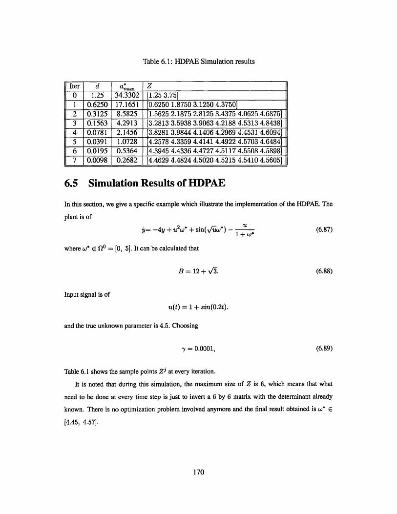
Table 6.1: HDPAE Simulation results

Iter d a*ax Z

0 1.25 34.3302 [1.25 3.75]1 0.6250 17.1651 [0.6250 1.8750 3.1250 4.3750]2 0.3125 8.5825 [1.5625 2.1875 2.8125 3.4375 4.0625 4.6875]3 0.1563 4.2913 [3.2813 3.5938 3.9063 4.2188 4.5313 4.8438]4 0.0781 2.1456 [3.8281 3.9844 4.1406 4.2969 4.4531 4.6094]5 0.0391 1.0728 [4.2578 4.3359 4.4141 4.4922 4.5703 4.6484]6 0.0195 0.5364 [4.3945 4.4336 4.4727 4.5117 4.5508 4.5898]7 0.0098 0.2682 [4.4629 4.4824 4.5020 4.5215 4.5410 4.5605]

6.5 Simulation Results of HDPAE

In this section, we give a specific example which illustrate the implementation of the HDPAE. The

plant is of

y= -4y + u2 * + sin(VTW*) -1 +w

(6.87)

where w* E DO = [0., 5]. It can be calculated that

B = 12 + vf/3. (6.88)

Input signal is of

u(t) = 1 + sin(0.2t).

and the true unknown parameter is 4.5. Choosing

-Y = 0.0001, (6.89)

Table 6.1 shows the sample points Zi at every iteration.

It is noted that during this simulation, the maximum size of Z is 6, which means that what

need to be done at every time step is just to invert a 6 by 6 matrix with the determinant already

known. There is no optimization problem involved anymore and the final result obtained is w* E

[4.45, 4.57].

170

6.6 Parameter Estimation in Static Systems

6.6.1 Parameter Estimation Algorithms for Static System

Parameter Estimation in static systems is an easier problem comparing to dynamic ones. We propose

the problem formulation as of

y = f (uw*) (6.90)

where w* E 0O C Wn is the unknown parameter, y E IR is output, and u E R"' is input. For a

nonlinear function, there may exist multiple w* and we record the set of all such w* as Q*, i.e.

Q* = {w | f(uw) = f(u,w*),V u,w o}. (6.91)

The extension to higher dimension of y can be easily made.

For system as in (6.90), we make the following assumption.

Assumption 5: Function f (x, w*) is Lipschitz with its arguments x = [u, w], i.e. there exists

constant B such that

If (x + Ax) - f (x)I < BIIAxII. (6.92)

Definition 6 System in (6.90) is a Lipschitz static system if it satisfies assumption 5.

In system (6.90), signals u(t) and y(t) can be obtained online and we can sample the signals at

any time instant. For a series of input-output pairs

[u(i), y(i)] for i = 1, 2,3....

where

f (u(i),w*) = y(i) V i. and V w* E Q*.

unknown parameter w* is identifiable if it satisfies the following condition.

Definition 7 For a set U1 of input output pairs

(U(i), y(0) i = 1,f... I

y(i) = f (0~), W), i=,.,I=>W E0.

(6.93)

(6.94)

(6.95)

171

Ur makes Q* identifiable.

We note that U1 defined as in (6.94) gives us enough information to identify X*. The existence

of such input-output set U1 is the sufficient condition to estimate the unknown parameters, which is

similar to the role of NLPE for nonlinear dynamic systems.

For U, defined as in (6.94), problem in (6.90) is equivalent to estimate all w E QO such that

f (u(i), w) = y(i), V (u(i), y(i)) E U1. (6.96)

and such w is exactly w*. To estimate w* in system (6.96), we will introduce several methods which

are listed below.

Hierarchical Search Algorithm

Using the same iteration technique as in the HDPAE, we propose a Hierarchical Search algorithm

below.

Step 1: Choose arbitrary do, construct discrete set ZO as in (6.16), set j = 0.

Step 2: Construct ZO = ZO. For any (u(i), y(i)) E U1 , if it satisfies

If(u(i), zo) - y(i)I > do. (6.97)

for some z 0 E Z0, remove zo from 20.

Step 3: When the size of Z0 can not be reduced anymore, set di+1 = di/2 and construct new

discrete set Zj+1 from Zi same as in the HDPAE.

Step 4: If di achieve desired precision, stop and Z = ZJ is the estimation of unknown parameter

Q*. Otherwise, set j = j + 1 and go back to step 2.

Brute Force Method

This method just search all the points in the unknown parameter region QO and check if there is

some points which can match all the input-output pairs [u(i), y(i)]. The rigorous description is just

the first step in hierarchical search when j = 0 and we set the desired precision to be do. Hence, do

means the final precision that Brute Search Mehtod can obtain. If we want to achieve fine precision,

we need to set do small and the points needed to be searched is huge.

172

Gradient Algorithm

We construct a Lyapunov function as of

V = E(y(i) - f(u(i), w)) 2 /2 (6.98)i=1.

where (u(i), y(i)) belongs to U defined as in (6.94). The process to find the optimum w* is the

routine descent gradient algorithm as follows:

I

w= -VV = - (y(i) - f(u(i), w))Vf(u(i), w). (6.99)i=1

Stochastic Gradient Algorithm

This algorithm is similar to gradient algorithm however it just apply one component of the gradient

at every time instant, i.e.

C= -VV = -(y(j(t)) - f(u(j(t)), w))Vwf(u(j(t)), w)., j(t) E U1 (6.100)

and the choice of j(t) is randomly w.r.t. time t. If we just choose U, be u[0, co) and choose j

serially, it becomes

6= -VV = -(y(t) - f (u(t), w))Vf (u(t), w). (6.101)

6.6.2 Global Convergence Result

About the global convergence of the Hierarchical Search algorithm, we note that it is exactly the

counterpart of the HDPAE in static systems. Using the same derivation as in Theorem I and Property

1, we can establish easily that at iteration j, Q* always belong to a cubic centered at Zi at step 3

with half of the edge as d'/y . Because dj keep reducing, we can achieve any desired precision

and therefore the Hierarchical Search algorithm is globally convergent. Same result holds for the

Brute Search algorithm if we discretize the unknown parameter using desired precision.

About gradient algorithm, it can stop prematurely at any point where

VV=O (6.102)

and a more detailed discussion about the convergence of gradient algorithm is proposed in [4].

173

About stochastic gradient algorithm, there even do not exist a Lyapunov function and you just go

around to try your luck. Even for some situations where the gradient algorithm works, there exists

some specific designed input u which can lead stochastic gradient algorithm into oo. Hence, for

general Lipschitz continuous nonlinear function, there is no guarantee of convergence for gradient

and stochastic gradient algorithms.

6.6.3 Dealing with Noise

In realistic situations where the given model f can not exactly describe the input output mapping

or there exist measurement errors in y and u, problem formulation in (6.96) is transformed into the

following one

y = f (u, w*) + 0(t) (6.103)

Io(t) < 0 (6.104)

where y, u, w* are same as described in problem formulation (6.90) and o(t) is the uncertainty or

noise added. For the problem formulation as in (6.103), the hierarchical search algorithm can be

modified as follows.

Step 1: Choose arbitrary do, construct ZO as in (6.16), set j = 0.

Step 2: Construct Z0 = ZO. For any series (u(i), y(i)), i = 1, 2..., if

If(u(i), zo) - V(i)I > do + 0 (6.105)

for some z E ^0, remove zo from 20.

Step 3: When the size of Z0 can not be reduced anymore, set di+1 = di/2 and construct new

discrete set Zj+ 1 from 2i same as in HDPAE. Set j = j + 1.

Step 4: If achieved desired precision, stop. Otherwise, go back to step 2.

Because of the existence of uncertainty, the final precision is not di which can approach zero

but di + 0 which is lower-bounded by 0.

The effects of noise and uncertainty are unpredictable in gradient algorithm because they just

exploit the local information. Even in cases where the gradient algorithm works, it is possible that

the algorithm divergence if noise and uncertainty perturb the dynamics at some critical point.

174

6.6.4 Simulation Results

For function2uw*

y = + (U2 + V ) sin(w*) (6.106)7r

where y, u, w* E JR, true unknown parameter w* = 1 and unknown parameter region QO

[-40. 40]. We choose U, = [1. 2. 3] which will make w* identifiable. Considering gradient

algorithm firstly, the Lyapunov function

3 2uwV = (Yi - + (2 + Vu) sin(w + 2u) /2

i=1

over w is plotted in Figure 6-1 and it is shown that there exists only one global minimum at w*

which verifies that U, makes w* idnetifiable. From Figure 6-1, we note that there exist many local

minima which prevent the gradient algorithm to converge. For stochastic gradient algorithm, we

even can easily choose a sequence of u which leads estimate to 00.

Now we apply the Hierarchical search algorithm. For this example, it can be easily derived that

B = 6/7r + 9 + - .

Choosing d0 = 20 and ZO = [-20, 20], the hierarchical algorithm gives the result of

Z = [0.9999943. 1.000013]

with di = 1.9073 x 10-5 after j = 21 iterations. Combining Z and di, the true unknown parameter

should satisfy

w* E [0.999975, 1.000032].

The totally searched points are 84. If we want to use brute search algorithm to achieve same preci-

sion, the points visited will be

80/di = 4.2 x 106.

This simulation illustrated that the Hierarchical Search algorithm is globally convergent and more

efficient than Brute Search algorithm.

175

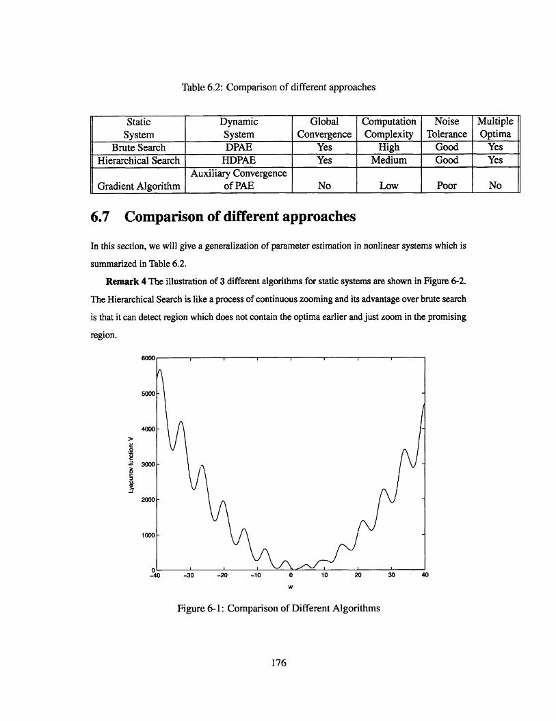
Table 6.2: Comparison of different approaches

Static Dynamic Global Computation Noise MultipleSystem System Convergence Complexity Tolerance Optima

Brute Search DPAE Yes High Good YesHierarchical Search HDPAE Yes Medium Good Yes

Auxiliary ConvergenceGradient Algorithm of PAE No Low Poor No

6.7 Comparison of different approaches

In this section, we will give a generalization of parameter estimation in nonlinear systems which is

summarized in Table 6.2.

Remark 4 The illustration of 3 different algorithms for static systems are shown in Figure 6-2.

The Hierarchical Search is like a process of continuous zooming and its advantage over brute search

is that it can detect region which does not contain the optima earlier and just zoom in the promising

region.

5000

4000

3000

2000

1000

-40 -30 -20 -10 0

W

Figure 6-1: Comparison of Different Algorithms

176

ts

0

CL

0c

10 20 30 40

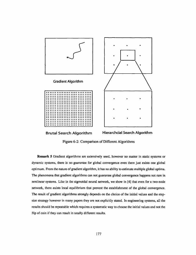
Gradient Algorithm

Brutal Search Algorithm Hierarchcial Search Algorithm

Figure 6-2: Comparison of Different Algorithms

Remark 5 Gradient algorithms are extensively used, however no matter in static systems or

dynamic systems, there is no guarantee for global convergence even there just exists one global

optimum. From the nature of gradient algorithm, it has no ability to estimate multiple global optima.

The phenomena that gradient algorithms can not guarantee global convergence happens not rare in

nonlinear systems. Like in the sigmoidal neural network, we show in [4] that even for a two-node

network, there exists local equilibrium that prevent the establishment of the global convergence.

The result of gradient algorithms strongly depends on the choice of the initial values and the step-

size strategy however in many papers they are not explicitly stated. In engineering systems, all the

results should be repeatable which requires a systematic way to choose the initial values and not the

flip of coin if they can result in totally different results.

177

Remark 6: Here we put the computation complexity of gradient algorithm low just because at

every time step the calculation of gradient increases linearly with dimension. It is quite doubtable

for the whole algorithm because we do not know if it can arrive the goal and how long it will

take. Even the Hierarchical search essentially still face the problem of dimension explosion as

Brute Search algorithm, it is highly parallel unlike the gradient algorithm which is serial and each

step must wait after its previous step finished. Our belief is that for general parameter estimation

in nonlinear Lipschitz continuous systems, there is no shortcut. When applying the Hierarchical

Search algorithm it is just a matter of computation ability which is increasing fast with new parallel

computers.

Remark 7 One question raised here for dynamic system is that if we can measure and calculate

i directly, then we can transform parameter identification in dynamic system into a static problem.

The advantage of PAE, which includes PAE, DPAE and HDPAE, over the direct derivative method

is that they do not need j and are not sensitive to the observation error or noise in y. The amplitude

of noise in y will cause error in the evaluation of j. However, for HDPAE, just the integral of noise

will perturb the estimator and the estimator can correct this perturbation. In [], it is clearly shown

that the correct way is to apply Adaptive Estimator to estimate the unknown parameters first and

then obtain j from estimated parameters while it is wrong to calculate j and then using y to estimate

the unknown parameters.

6.8 Summary

In this chapter, we propose a general and efficient parameter estimation algorithm for nonlinear

Lipschitz continuous system for the first time. Generalization of parameter estimation in both static

systems and dynamic systems are given and it is shown that gradient algorithms do not apply to

general nonlinear systems.

178

Bibliography

I] C. Cao and A.M. Annaswamy. A polynomial adaptive estimator for nonlinearly parameterized

systems. submitted to, August 2003.

[2] A.M. Annaswamy, A.P. Loh, and F.P. Skantze. Adaptive control of continuous time systems

with convex/concave parametrization. Automatica, 34:33-49, January 1998.


systems. IEEE Transactions on Antomatic Control, 48:397-412, March 2003.

[4] C. Cao and A.M. Annaswamy. Conditions for existence of global and local minima in neural

networks. 12th Yale Workshop, 33:33-49, July 2003.

Appendix

Proof of Lemma 1: Performing linear transformation to matrix will not affect its rankness and

determinant. In what follows, we show that by a series of column scale and add/subtract operation,

matrix A can be transformed into a Vendemonts's matrix which is known to be full rank.

We denote the ith column of A as A2 . Firslty, let us consider A 2 which is

S- 1) .. - - ) .. -(1 - ONO)]T. (6.107)

Add 91A1 from A2 and the new column 2 is

A2 = [O .. - O (6.108)

We can continue this process through column 3 to N. For j + 1th column, we assume that the

179

1, .., j column has already been transformed into

[Ai .. Aj] = 9.-1

ONO

(6.109)

Ajg1 can be expressed as sum of vectors A1 through Ai with coefficients as function of i.

Therefore, by subtract weighted A 1 through Ai from Ai+1, the new i + 1th column is

Ai+1 = [1 -- .-- NO]T. (6.110)

Repeat this process until the last column, and

comes

[Al .. AN]

1

by simple matrix oprtation, the new matrix be-

01

Oi

ONO

This matrix is Vandemeonts' matrix and it is full rank.

Proof of Property 3: In DPAE, 0* is achieved by

9 N0 -1

1

ON0-1

(6.111)

Therefore, A must be full rank too. e

#* = A- 1 B. (6.112)

From Assumption 3, B is bounded. We note that A is a regular full rank matrix not approaching

singular from Lemma 1. Thus 0* must be bounded. 0

Proof of Property 4: From Assumption 2 and 3, u and y is Lipschitz w.r.t. t. Property 3 implis

that 0* is bounded and hence ki is also Lipschitz w.r.t. t. Therefore the elements of matrix A and B

are Lipschitz w.r.t. time. #* is calculated by these quantities and therefore is Lipschitz w.r.t. t. .

Proof of Property 6: From Assumption 3 and 4, it follows that f (y, u, 0*) is bounded. From

Property 3, it follows #$3 is bounded. Property 5 shows that a*satUj) is bounded by aax,. Combing

180

all these, it shows that the bound of m(t) exists and we denote it as M.

Proof of Property 7: From Assumptions 1-4, it follows that f (y, u, 0*) is Lipschitz w.r.t. t and

it can be expressed as

|f (Y (t + T), U (t + T), 00*) - f (Y(t), U (t), 00*)| <; Q2 T

where

Q2 = B(U + F).

Combining (6.113) and Property 2, Property 7 is established.

Proof of Lemma 3: Firstly, let us consider situation where

(6.113)

0

(6.114)n(ti) > a-y + 2 Q(y + 6) + 2amax.


n(ti + r) > n(ti) - QT.


Y,= -a& + #* - f(y, u, 93) - r - a*sat( )

where

Irl < a*ax.

Combining (6.114), (6.115), and (6.117), we have

n(t + r) - az*ax > ay + 2 Q(y + e) - QT

It follows Property 5 and (6.118) that

n(t+ T)- a*sat( ) > ay + 2 Q(7 + E) - QT

If there exists some time constant t 2 E [ti, ti + T'] such that

p (t2 ) > 7-.

(6.115)

(6.116)

(6.117)

(6.118)V r > 0.

V r > 0. (6.119)

(6.120)

181

then the lemma is true. If (6.120) is not true, which means

&#(2) < . V t E [ti, ti + T'].

then it follows from (6.119) that

-a&e(ti + r) + n(tj + r) - r - a*sat(y) ! 2VQ(7 + e) - Qr

Integrating (6.116) from tj to ti + T' and it follows from (6.122) that

(6.121)

V r > 0. (6.122)

= 7T (-a,(ti + r) + n(ti + T) - r - a*sat( )) dr

> f"( Q(y + ) - Qr) dr

= 2(y + E).

Equation (6.121) implis that

(t1) > -r - e

otherwise -f(ti)I y. Combining (6.123) and (6.124), it follows that

(ti + T') > -y+ e

and therefore

IpE(tl)I > -Y.

Equation (6.125) contradicts (6.121) and it proves that the lemma is true. For situation where

n(ti) < -ay - 2 Q(y + ) - 2a*ax, (6.126)

similar results follows. 0

Proof of Lemma 4: If there exists some s which satisfies (6.58), Lemma 4 is proved. If there

does not exists such s, from Lemma 2, Lyapunov function will decrease a small amount S for every

time interval where & -y at some time instant. Because V(0) is finite, at most after [V(0)/S]

times (6.58) will happen. 0

Proof of Theorem 2: We choose parameter T in the HDPAE same as the T in the NLPE con-

182

(6.123)

(6.124)

(6.125)

P(ti + T') - 9(ti)

dition defined in Definition 5. For problem formulation in (6.1) and jth iteration of the HDPAE

as in (6.59), it follows from Lemma 4 that the output error g, will converge for some interval

[t. t + T + Ti] for any - where

W t(c2) e5 n, V we2 c [tr t + T + T

When output convergence happens we construct the Z by

(6.127)

where

6 = ay + 2 Q( Y+E) + 2a*ax-

It follows from Lemma 3 that

If (y r), u(T), 2) - *0 15 /3 V ri E [t, t + T]

for any 2 E Zj. From NLPE condition, for any z E Z there exists tj c [t. t + T] such that

If(y(ti), u(ti), z) - f(y(ti), u(ti), w*)| ;;> co mi |z - w*l l

It follows from (6.127) and (6.128), respectively, that

|f(y(ti), u(ti), z) - #*(ti)

lf(y(ti), u(ti), ) - #*(ti)

</3</3.

Vz C ±

V2 E Z .


If (y(ti), u(ti), z) - f(y(ti), u(ti), i) I 2/6

for any z E Z and Z E Zj. It follows from the definition of Zj as in (6.22) that

If (y(ti), u(ti), w*) - f (y(ti), u(ti), 2)1 < a*ax

183

(6.128)

VW* E Q*. (6.129)

(6.130)

(6.131)

(6.132)

Z zjz E Zj,00*(-ri) -P# 5 f (y(rl),I u(ri),I z) ! #*(-rl) +#, V-ri E [t, t+ T]

for any w* G Q* and 2 E Z. Combining (6.13 1) and (6.132), it follows that

If (y(ti), u(ti), w*) - f (y(ti), u(ti), z) 5 2/0 + a*ax (6.133)

for any w* E Q* and z E Z. Combining (6.129) and (6.133), it follows that for any z C Z

min 11Z2P + a*min z-w*1< 2/ + aa (6.134)

which implies2P3+ a*a

IVZ - Q*Ild < #+ *a

As j increases and we can choose y, e arbitrarily, a* a. and / can become arbitrarily small. If there

is some j such that 2P + a* < eoei, (6.86) is satisfied and this proves Theorem 2.

184

Chapter 7

Dead-zone Based Adaptive Filter

7.1 Introduction

Adaptive estimation algorithms have been developed for dynamic systems where the unknown pa-

rameters occur both linearly and nonlinearly over the past several errors. While stability properties

of these estimators have been studied in [10]-[5], parameter convergence properties have been stud-

ied in [10]-[8]. In the presence of external disturbances and noise, it is well known that for linearly

parameterized systems, either modifications in the adaptive law or persistently exciting reference

inputs have to be introduced to establish robustness. The same however has not been established

for nonlinearly parameterized systems thus far, and is addressed in this chapter. In particular, we

establish that when output noise is present, a modified algorithm that include a deadzone, similar

to that in [10], can be used to establish boundedness. We also show that the deadzone algorithm

filters the output noise statistically and guarantees the asymptotic convergence of the estimates to

true unknown parameters, and is denoted as the filtered deadzone estimator (FDE). The chapter

is organized as follows. In section 7.2, problem formulation is proposed and the inability of the

adaptive estimator to deal with output noise, without any modifications, is discussed. In section 7.3,

the FDE is proposed. Proof of asymptotic convergence is also given. In section 7.4, comparison

between output noise and model disturbance is discussed and the extension to situation where both

of them exist is made. Section 7.5 shows simulation results.

185


We consider a nonlinearly parameterized dynamic system with bounded output noise such as

N

S =-ay + E Ci(W*)ii=O

yn= y + n(t) (7.1)

where ci are measurable signals, w* E JR is unknown parameter, y E R is inaccessible state

variable, output noise n(t) is a stationary stochastic process and yn is measured output signal.

We make the following assumptions regarding the stationary stochastic process n(t).

Assumption 1: n(t)I 5 n.,,,, V t > 0 where nma is a known positive constant.

It can be shown that a typical measurement noise due to effects of quantization satisfies as-

sumptions 1. About the statistical properties of n(t), we will introduce later in the discrete-time

approximation.

7.2.1 Polynomial Adaptive Estimator (PAE)

In this section, we examine the properties of a Nth order PAE with N auxiliary estimates Wi, .. , WN

that was proposed in [8] for (7.1) in the absence of noise.

Suppose the Lyapunov function candidate is chosen as

N

V~ = yn2/2 + Pi p(Ci). C'i = Wi - w (7.2)i=1

where

_ 1p() = - if i is odd;

P (00 = . k + if i is even (7.3)

for i = 1, .., N, and ki is to be chosen appropriately as in [8]. The corresponding gi is the derivative

of pi w.r.t. Coi as of

gi(0i) = V if i is odd;

186

if i is even.

We note that Oi = - w* and gi is a ith order polynomial function of w* and it can be expressed as

gi= Edij(i)(w*)i. (7.5)j=0

The PAE is of the form

1? = + 0*

Oi i = 1, ... , N

= y- yn

#~* = A-1C (7.6)

where 0* = [$. , ... , 0* ]T_

(N + 1) matrix as of

sat(.) denote the saturation function, A is a non-singular (N + 1) x

doo

0

0

0

*

0

0

*

*

d22

0

.. *

.. *

-- *

.dNN

(7.7)

and

C = [co C1 ... cN]T. (7.8)

The element of ith row and jth column of matrix A in (7.7) is

I d(j-1)(j-1) i j

where d3i is defined as in (7.5).

We assume n is differential. Combining (7.1), (7.6) and (7.2), using the same derivation as in

[8], the derivative of V follows as

#r= p(a-

187

gi(00) = ici-1 + kiiii (7.4)

= -Q,#i,

and hence

V= -a99, - Q, n .

Since V cannot be guaranteed to be nonpositive in a compact set, it follows that V need not be

bounded. Therefore modifications in the adaptive law are needed.

7.3 Filtered Deadzone Estimator

The result of no convergence of PAE with output noise in section 7.2.1 raises a problem for its

application. To overcome this difficulty, we introduce a filtered deadzone estimator (FDE) as

0i = -17<A, i=1,..., N

n= y-yn

= yn - nmaxsat ( )= A- 1C

n = yn-y (7.9)

where h is the filted out output noise, 0* = [0*. * *T, A and C are defined as in (7.7) and

(7.8), and sat(.) denotes the saturation function and is given by sat(x) = sign(x) if Ixi ;> 1 and

sat(x) = x if Ix| < 1. In fact, the relationship between Qn, and gn is of

n - nmax if

S= 0 if

n + nmax if

9 n > nmax;

-nmax 5 1n nmax;

9 n < -nmax

and we use the Lyapunov function candidate

N

V = QL/2 + Zpi(s).i=1

where pi() are the same as in (7.3).

The following properties can be derived for the FDE:

fi = W2 - W*

188

(7.10)

(7.11)

ync

S*

Property 1

(i) 9ne > 0 => Q > Qe

(ii) Qne < 0 => Q< Qne

Proof of Property 1: First, let us consider case (i) in Property 1. Qn, > 0 implies from (7.10) that

gn > nmax and QnE = 9n - nmax. (7.12)

Because Qn = g + n and Inj 5 nmax, it follows from (7.12) that

9 > Qne

which proves Case (i). Case (ii) of Property 1 can be proved in a similar manner.

Assumption 1 just requires the output noise is bounded. The ouput noise only arises when you

measure the output y and it is in fact a discrete event process no matter in the algorithm simulation

in computer or realistic AD sampling process. The discrete time approximation of plant in (7.1) and

dead-zone filter in (7.9) are of

y((r + 1)A) - y(rA) -ay(rA) + N

A E ci(w*)ii=0

yn(rA) = y(rA) +n(rA) (7.13)

and

((r+ 1)A) - 9(rA)

AOi(( + 1)A) - 1(TA)A ~ = -yle(TA)5i. i=1,...,N (7.14)

where the algebraic relationships of #*(TrA), M(rA) and fi(rA) on state variables y(TrA), Q(rA)

9i(irA) are the same as in section 7.3.

Throughout this chapter, we assume the sampling time-interval A is very small and the discrete-

time approximation matches the continuous system well such that we can omit the effects of discrete

time approximation.

About output noise n(rA), we have the following assumption.

Assumption 2: n(i-A), T = 0,1,2, ... are i.i.d.

189

About 9, we have the following theorem.

Theorem 1 For problem formulation in (7.13) and FDE as in (7.14) under assumptions 1 and 2,

omitting the effects of discrete time approximation, it follows that

Prob[ lim . = 0] = 1.t-+00

(7.15)

Proof of Theorem 1: Lyapunov function candidate V in (7.11) is expressed as

NV(TrA) = ji&(rA) 2/2 + I pi(Co). ti = -i(-rA) - w* (7.16)

in discrete time approximation. Since we assume A is small enough and the discrete time approx-

imation matches the continuous system, we just keep the zero and first order of A and omit the

higher order terms in the expression of V((-r + 1)A) - V(-rA). We know yf,(rA) can always be

decomposed into intervals where in each interval yn(rA) is a series with the same sign. Without

loss of generally, we consider an interval [r 1 , T2] where r2 can be finite or infinite such that

- E [Ti, 72].

It follows from (7.16), (7.13) and (7.14) that

V((T+1)A)-V(TA) = Yne((r + 1)A) + ne(rA)) (-aA(9(TA) - y(rA)) + n(rA) - n((r + 1)A))2

(7.17)

and therefore

E (V((r + 1)A) - V(rA)) ='T=T

-aAndrA)Y(rA) + ((r - 1)A)1~T~2 +

T2 e( + 1)A) + gne(TA)) (n (-TA) n n((-r + 1) A)).

Omitting the higher order item of A,

V(rA) + ((r - 1)A) (rA)2

190

(7.18)

yne(TA) > 0,

and (7.18) can be written as

E (V((T + 1)A) - V(r A))1T-1Tj

T2

S: -aAnc(TA)y(TA) +T =71

(7.19)

z' PnE((T + 1)A) ± yflE(TA)) (n(TA) - n((TF + 1)A)).2

Since

yfEc(TA) = j(TrA) - n(TA) - nmax, (7.20)

it follows from (7.19) that

T2

(V((T + I)A) -T=T 1

T2

V(TA)) = 5 -aAnPc(TA) (TA) +T=Ti

y((r + 1)A) + (TA)) - 2nmax (n(-A) - n((T + 1)A))T= TI

T2-ET=TI

7t-rA) 2 - n((r + 1)A) 2

2

Now let us look at the propagation of n(rTA) in the entire system. n(TrA) will affect Oi((-r+1)A)

and this will further affect y((T + 2)A). The values of Q((T + 2)A) and Qns((T + 2)A) depends on

9((T + 2)A) and therefore depends on n(TA). Since

n(TA) isindependentof Q((T + i)A), i < 1. (7.21)

it follows that

Q((r + 1)A) + Q(TrA)) - 2nmax is independent of n(TrA) - n((r + 1)A) (7.22)

and therefore

E[ T ((T + 1)A) + (-TA)) - 2nmax

T=T1 2(n(TA) - n((T + 1)A))] =

S((T + 1)A) + 9(TA)) - 2 nmaxE[(A) - n((T +

If wr 2

It follows from Assumption 2 that

E[n(TA) - n((T + 1)A)] =

E[n(TA) 2 - n((T + 1)A) 2 ]

0

= 0

191

(7.23)

(7.24)

and therefore

E j((T + 1)A) + (rA)) - 2nmax ((A)((+1)A (,)2 - n(( + 1)A)22r

(7.25)

For intervals where Qan < 0, the only difference is (7.20) becomes

7.(rA) = Q(rA) - n(rA) + nmax (7.26)

and same results as in (7.25) follows. It can be checked easily from (7.25) that

E[t E ((T + 1)A) + ne(A)) (n(rA) - n((r + 1)A))] = 0T0 2

and therefore

Prob[ gn((- + 1)A) + ne(r))(n(rA) - n((r + 1)A)) = co] = 0r=O2

since its elements are continuous distributed p.d.f. and achieves maximum at zero. Because

00

Z(V((r + 1)A) - V(rA)) = V(oo) - V(O)

and the fact V(0) < oc and V(oo) > 0, it follows that

00

Z(V((,r + 1)A) - V(rA)) < oo.r=O


00

Prob[Z aA~n,(,rA) (-rA) < ool = 1.T0=

(7.27)

(7.28)

(7.29)

(7.30)

It follows from Property I that

yfe(TA)(TA) > Yfe (TA)2

Prob[E a9A.n(-rA) 2 <c] = 1.-r=O

and therefore

(7.31)

(7.32)

192

Equation (7.32) implies that

Prob[ lim Q.E(TA) = 0] = 1 (7.33)

which proves the Theorem.

We note here that probability 1 implies that it is always true of

lim D =0.t+oo

7.3.1 Parameter Convergence of FDE

Theorem I established that output error P, will converge to zero and parameter estimate is steady.

What remains is whether W will converge asymptotically to w*. First, we note that once Lyapunov

function V, which is defined as in (7.11), reaches zero, it will rest there and never left. This is

different from PAE where the noise will drive V away from zero. In this section, we will discuss if

(7.15) implies V = 0 and under what conditions.

In the system in (7.1), we have no assumption about the statistical properties of the output noise

n(t). Now we assume n(t) is of

n(t) = U[nL, nH] V t (7.34)

where U[nL, nH] is the uniform distribution in region [n. n H]. Of course it will satisfy

|nL| I ! nmax | nj HI n..z nH > nL. (7.35)

We define a signal x which is a function of Q = - y when

r - nmax + nH if > nmax - nH;

= 0 if -nmax - nL 5 nmax - nH; (7.36)

- nmax -nL if < -nmax -n.

About x, we have the following lemma.

Lemma 1 For problem formulation in (7.1), FDE in (7.9) and output noise as in (7.34), it follows

that

Prob[ lim x = 0] = 1. (7.37)t--+00

193

Proof of Lemma 1: If (7.37) does not hold, it implis that

Prob[x(t) # 0] > 0 (7.38)

as t -+ 00. x(t) 0 0 implies that

Y > nmax - nH or j < -nmax - nL- (7.39)

Combining (7.34), (7.38) and (7.39), it follows that

Prob[ph, 3 0] > 0 (7.40)

as t -+ oo which contradicts Theorem 1. Therefore, lemma 1 must hold.

Lemma I implies that

-nmax - nL Y nmax - nH (7.41)

if (7.34) and (7.35) hold.

In what follows, we will discuss the convergence of estimates for several cases.

Case 1: nL = -nmax, nH = nmax

It follows from (7.36) that x = Q and Lemma I states that

lim Q = 0.t-+oo

Thus, just the input signals satisfy the Nonlinear Persistent Condition established in [8], &, which

is derived from 0 cji~ = 0*, will converge to w* asymptotically. In case 1 of the simulation

results in section 7.5, the asymptotic convergence is illustrated.

Case 2: fL > - 1 max- nH = nmax

It follows from Theorem I that Qe will converge to zero as t -+oc and hence W come to some

steady value W-1. It follows from Lemma I that when t -+ oo, Q will always be nonpositive. Instead

of the NLPE condition, if for any t, there exists time constant T, co such that

ft+T (N

/ (Eci(Wi - (w*)i) dir > Eo11w-w*1I, (7.42)=at i=o oT nryi

it will guarantee the asymptotic convergence of W- to w*. The reason is that for any W" :A w*, if the

194

input satisfies (7.42), 9 will always become significantly positive. Hence, W must convege to w*. In

case 2 of the simulation results in section 7.5, the asymptotic convergence with biased output noise

is illustrated.

Case 3: White Noise

When n is white noise which is not bounded, for a given n.max we can decompose n into 2

components

n = ni + n2

where

ni = n n2 = 0 Inl <s nmax

ni=nmax n2=n-ni n > nmax

ni = -nmax n2 = n - ni n < -nmax.

For white noise, n can be very large howeverjust at very small measure in time. Choosing approprite

threshold value nmax to make

lim - n2|dtT-+oo TJ1=0

small, we can treat the effects of additional n2 as a disturbance which will perturb the convergence

of W-. We note that FDE does not depend on the initial value of W- and will correct the disturbance.

Thus, Z is not steady but perturbed at some amplitude. Choosing nma. which makes W perturbed

in the desired precision and we are done. The tradeoff here is just if we want higher precision of W-,

we need to set the value of nmax bigger and therefore the time needed for convergence is longer.

7.3.2 Output Noise Filter

After w- converges to w*, converges to zero as well and the output noise can be evaluated exactly.

We introduce the concept of the Filtered Deadzone Estimator as what follows.

Definition 1 In dynamic system with unknown parameters, the Filterd Deadzone Estimator (FDE)

is the method which applies the deadzone adaptive estimator to estimate the unknown parameters

and then filter out the output noise at the same time when parameter estimation converges.

195

In FDE, the estimation of output noise n is simply

= yn -

and it follows that

n -n=y -

which means that the errors of and ft to y and n are of the same amplitude and different sign.

The convergence of them happens at the same time. Now that both y and n are not accessible, the

indication of the convergence of 9 and ft is that 9,< converges to 0 and W keeps steady.

Another information which can be derived from the FDE is the derivative of y. Now that W -

w* and y -+ y, it follows naturally that the estimation of y is of

S=-a9 + 00*.

It is noted that this estimation will converge to the true derivative j and it is stable and free of noise.

If we want to calculate the derivative directly from measured yn, the uncertainty always exists and

the derivative could be very noisy.

7.4 Model Disturbance

In [10], same structure of FDE is used to deal with model disturbance, which is

N

y= -ay + E ci(w*) + 0 (7.43)i=O

where 1ol < 0.

For systems where both output noise and model disturbance exist, i.e.

N

y =cj(W*)i+Oi=O

yn = y+n

0 < 0

n < nmax- (7.44)

196

the modified FDE is of

= -(4 + # -a axsat0 -ma \nmaz /

= -Ynli/ i =1,.., N

ynf = yn - nmaxsatnmax

9n = y

* = A 1 C

amax = 0., (7.45)

where 4* = [4*. #* .,*}T A and C are defined as in (7.7) and (7.8), and sat(.) denotes the

saturation function and is given by sat(x) = sign(x) if lxi > 1 and sat(x) x if lxi < 1.

Choosing Lyapunov candidate V as

N

V = + Epi(k) (7.46)i=1

where pi() is defined as in (7.3), it follows that

V= -a~ne# - gnE i + nc -o - a*axsat ( n )). (7.47)

It can be checked easily that

nc (-o - amaxsat (m ))<o (7.48)

since lol 5 a*ax. It follows from (7.47) and (7.48) that

V< -a9j,9 - ne i. (7.49)

Using the same derivation as in Theorem 1, we have

Prob[ lim n = 0] = 1. (7.50)t-+cc

Therefore,

lim n, = 0t-+oo

197

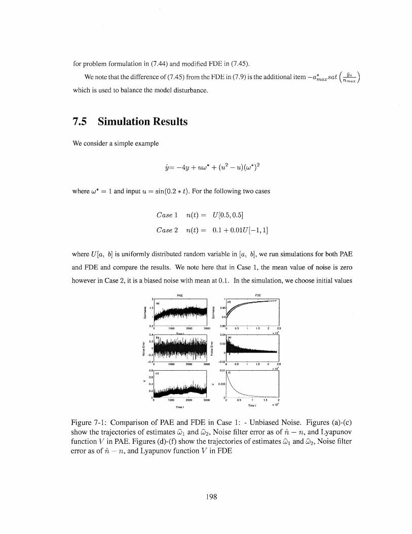
for problem formulation in (7.44) and modified FDE in (7.45).

We note that the difference of (7.45) from the FDE in (7.9) is the additional item -a*asat (max

which is used to balance the model disturbance.


We consider a simple example

i= - 4 y + uw* + (u2 _ )( *)2

where w* = 1 and input u = sin(0.2 * t). For the following two cases

Case 1 n(t) = U[0.5, 0.5]

Case 2 n(t) = 0.1 + 0.01U[-1, 1]

where U[a. b] is uniformly distributed random variable in [a. b], we run simulations for both PAE

and FDE and compare the results. We note here that in Case 1, the mean value of noise is zero

however in Case 2, it is a biased noise with mean at 0.1. In the simulation, we choose initial values

PAE

(a)

0.52

0 00

0 1000 2000 3000

0U 0-0.2

0 1000D 2000 3000

Tine

FDE

(d)

0.95

0.0

0 0.5 1 1.5 2 2.5

002

0 2.11-0.00

0 0.5 1 1.5 2 2.5

0.01 X10,

> 0.000

0 -- _______________

0 0.5 1 1.0 2

Time I x104

Figure 7-1: Comparison of PAE and FDE in Case 1: - Unbiased Noise. Figures (a)-(c)show the trajectories of estimates 01 and D2, Noise filter error as of h - 71, and Lyapunovfunction V in PAE. Figures (d)-(f) show the trajectories of estimates QD and 02, Noise filtererror as of h, - n, and Lyapunov function V in FDE

198

FDE

05

0 400 00 00 1000 000 10000 100.85

0.0s 0.02

0

2 0.01

z 00.005

00 200 400 600 a00 1000 0 5000 10000 15000

Figure 7-2: Comparison of PAE and FDE in Case 2: - Biased Noise. Figures (a)-(c) show

the trajectories of estimates L1 and 02, Noise filter error as of ii - n, and Lyapunov function

V in PAE. Figures (d)-(f) show the trajectories of estimates Li and w2, Noise filter error as

of n -- n, and Lyapunov function V in FDE

of [Qi, w2] as [L1. W2] = [0.9. 0.9]. Figures 7-1 and 7-2 show simulation results for case 1 and

2 respectively. In each figure, for both PAE in (7.6) and FDE in (7.9), it plots the trajectories of

parameter estimates Di and 02, noise error which is defined as

-Q = y - Q = - U,

and Lyapunov function V which is defined as in (7.2) for PAE and (7.11) for FDE. The simulation

results show clearly that for both cases, the FDE leads to asymptotic convergence of Q, Q, V and

Qpe. For PAE, none of these variables converges.

The ability that FDE can filter out biased measurement or noise is extremely useful in practical

applications. In the on-line measurement of dynamic systems, unlike the unbiased measurement

uncertainty which is always unavoidable and restricted by measurement precision, measurement

offset often means a quality problem and it is important that it can be detected on-line without

perturbing the normal process of the plant.

199

Bibliography


[2] A.M. Annaswamy, A.P. Loh, and F.P. Skantze. Adaptive control of continuous time systems






AC-44:1634-1652, September 1999.

[5] J.D. Boskovid. Adaptive control of a class of nonlinearly parametrized plants. IEEE Transac-




1321, 2000.

[7] A. Kojid and A.M. Annaswamy. "Adaptive control of nonlinearly parametrized systems with a


[8] C. Cao, and A.M. Annaswamy. A Polynomial Adaptive Estimator for nonlinearly parameterized

systems. Proceedings of American Control Conference 2004, Boston, MA.

[9] C. Cao, and A.M. Annaswamy. "A Dead-zone Based Filter for Systems with Unknown Param-

eters" Active and Adaptive Control Lab Report 04-2, Mass. Inst. of Tech., February 2004

200

Chapter 8

Continuous Polynomial Adaptive

Controller

8.1 Introduction

Adaptive control is an important area in the control theory which deals with the partial known plant.

The structured unknown information is usually expressed by unknown or time-changing parameters.

So far, the traditional adaptive controller can only deal with linearly parameterized systems. A lot

of efforts [1]-[10] have been made to extend the adaptive control to NLP systems, however they

are still restricted to some special situations and can not serve as the same tool as linear adaptive

controller for linearly parameterized systems.

The linear adaptive controller establishes a Lyapunov function as the quadratic form of out-

put error and parameter error, and the associated adaptive law guarantees the derivative of this

Lyapunov function is non positive. In [3], a polynomial adaptive estimator is proposed which mod-

ifies the Lyapunov function candidate and associated adaptive laws for polynomially parameterized

functions. In [4], a dead-zone based filter is proposed which provides a tool for adaptive estima-

tors to deal with output noise in some plants. As a further development of the polynomial adaptive

estimator, a Continuous Polynomial Adaptive Controller (CPAC) is proposed in this chapter. Us-

ing a new choice of polynomial Lyapunov function and adaptive law, we can deal with piece-wise

linearly parameterized systems as the traditional adaptive controller for the linearly parameterized

ones. Since most of the commonly encountered NLP systems can be approximated by piece-wise

linear functions, it provide a general tool to deal with them. Since disturbance always exists, the

201

approximation error between piece-wise linear function and original nonlinear function can also be

treated as disturbance. In this chapter, we also established the stability of CPAC under bounded

disturbance.

The CPAC consists of two parts. A companion adaptive system and a control law. The compan-

ion adaptive systems can be applied to any NLP systems which can be approximated by piece-wise

linear functions. It consists of two parts, a companion model and an adaptive law. For a piece-wise

linearly parameterized systems with all states measured, the asymptotic convergence of outputs of

the plant and the companion model is established for the first time as the same as the linear adaptive

theory for linearly parameterized ones. Unlike the plant which involved the unknown parameters,

the companion model is deterministic without any unknown information. Therefore, what required

for the control law is to find a controller for the companion model. Same control signal is applied to

the plant and results in the same stability and tracking properties as the companion model. Unlike

the companion adaptive system which is a general tool for NLP systems, the design of control law

is case by case since there does not exist a general control law for a nonlinear system even it is

deterministic. In this chapter, for several commonly encountered NLP systems, the control laws are

given as the examples of how to construct a complete CPAC, including some cases with unmeasured

states which requires an adaptive observer.

This chapter is organized as follows. Section 8.2 gives a general problem formulation which

states the approximation of a nonlinear function using piece-wise linear functions. Section 8.3

states the companion adaptive system corresponding to the plant in section 8.2. Extension to higher

dimension is also made. The stability and convergence properties for the error model and adaptive

law are established, and bounded disturbance is also considered. In section 8.4, control laws for

several classes of NLP systems are proposed and they demonstrate how to construct the complete

CPAC. Section 8.5 provides simulation results of CPAC for a specific NLP system and section 8.6

concludes the chapter.


In this chapter, we consider the adaptive control of nonlinearly parameterized systems. For sim-

plicity, we will consider the scalar case first and the extension to higher dimension is introduced

later.

202

The problem formulation is of

y= -ay + f (y, u, w) (8.1)

where a > 0 is a known constant, y E IR is state variable, u E- R' is control signal to be deter-

mined, w is unknown parameter which belongs to a continuous compact set Q = [Wmin- 1max] C

IR.

About f, we have the following assumption.

Assumption 1: Vy(t), u(t), f can be approximated by a piece-wise linear function over 11, i.e.

there exists a constant dmax > 0, N regions

[RI7 ni], i = 1,..,N (8.2)

and mi(y, u), ri(y, u) such that

N

QC Uni (8.3)i=1

|d(t)| = Imi(y,u)+ri(y,u)(w- Q)-f(y,u,w)| <dmax, wcij,Vi= 1,.., N(8.4)

2 =(8.5)

First, we note that a piece-wise linear function is a typical nonlinear function which implies

the extension of adaptive control theory from linearly parameterized systems to nonlinear ones.

Secondly, a large class of commonly encountered functions can be piece-wise linearly approximated

since any smooth function can be linearized locally. For example, if f is differentiable and its second

order derivative w.r.t. w is bounded, i.e.

a2f (y, U, W)f( 2 |5 q. (8.6)

we divide Q uniformly into N regions and we have

Imi(y, u) + ri(y, u)(W - (D) - f (y, u, w)I q maX min )2 V = 1,.., N (8.7)8N 2 i1., 87

203

where

mi(y,u) = f (y, u, C) (8.8)

ri(y,u) = af(yuW) (8.9)aw ~

= 2 .(8.10)

We now map the unknown parameter w E Q into a new pair of unknown parameters [9. (. as of

9= 0, if WE Q2

= if W E Qj (8.11)2

c E [-(max,(max]

6 E f= {61, .. , i, .. ON

i -=(N - 1)8max

(max = maxj=1,..,N 2 (8.12)

and Omax is an arbitrary positive constant.

With the unknown parameter transformation, the problem formulation in (8.1) under Assump-

tion I is equivalent to the following one:

b = -ay + m(y, u, 0) + r(y, u, 0)( + d(t)

d(t) _ dmax (8.13)

where unknown parameter [9, () is defined as in (8.12) and

m(y, u, 0) = mi(y, u), i = (N - 1)maxo + 1

r(y, u, 0) = ri(y, u). i = (N - 1)Emax, + 1

Id(t)I = f(y,u,w) -m(y,u,9) - r(y,u,9)(. (8.14)

We note here that even we do not know m(y, u, 0) and r(y, u, 0) since 9 is unknown, m(y, u, Oi)

and r(y, u, Oi) are available for specific Oi.

The structure of the CPAC for plant in (8.13) is illustrated in Figure 8-1. We note that the CPAC

204

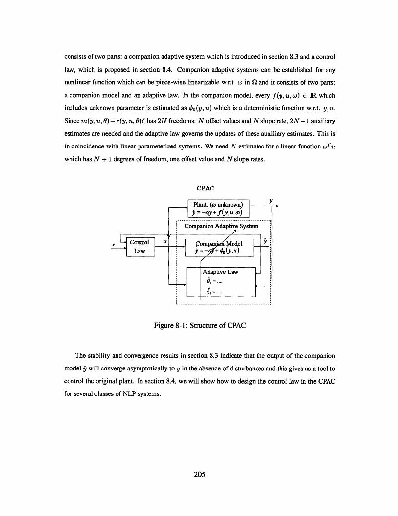
consists of two parts: a companion adaptive system which is introduced in section 8.3 and a control

law, which is proposed in section 8.4. Companion adaptive systems can be established for any

nonlinear function which can be piece-wise linearizable w.r.t. w in n and it consists of two parts:

a companion model and an adaptive law. In the companion model, every f(y, u, w) E R which

includes unknown parameter is estimated as 0(y, u) which is a deterministic function w.r.t. y, u.

Since m(y, u, 0) + r(y, u, 0)( has 2N freedoms: N offset values and N slope rate, 2N -1 auxiliary

estimates are needed and the adaptive law governs the updates of these auxiliary estimates. This is

in coincidence with linear parameterized systems. We need N estimates for a linear function wTu

which has N + 1 degrees of freedom, one offset value and N slope rates.

CPAC

r ControlLaw

,Plant: (iv unknown)jp= -ay + f(yu,)

Companion Adaptive System

Comp 'Model.Y= +0 (y' U)

Adaptive Law -

Figure 8-1: Structure of CPAC

The stability and convergence results in section 8.3 indicate that the output of the companion

model y will converge asymptotically to y in the absence of disturbances and this gives us a tool to

control the original plant. In section 8.4, we will show how to design the control law in the CPAC

for several classes of NLP systems.

205

8.3 The Companion Adaptive System

In what follows, we will introduce the companion adaptive system for (8.13). The companion

adaptive systems consists of two parts: the companion model as of

Y= -aQ + 0 (8.15)

and the adaptive law as of

0 if 945 > 0 and Gi Emax

Oi = 0 if Qo < 0 and i 0

M otherwise.

Vi = 1,.., N - 1

0 if P71i > 0 and di2(Max

di= 0 if rj < 0 and (i -(max

Q7gi otherwise.

Vi = 0,..,N - 1

C, = [r(y, u, 01),.., r(y, u,6),.., r(y, u,ON)]

Cm = [ ,u6).,my , 4,.,my ,N)

C, = [noro,1.., = , .., N--1r-1Y

(= [0o, ... , ON-1] Am (Cm - AG-q)

= -y (8.16)

where Ar is an N by N matrix given by

1 .. .. :

A,. (8.17)S..ai


i (8.18)

206

and A., is an N by N matrix with the ith row and jth column element aij as

ai = 1 1 < i < N

aij = -gj_.(Oj_ - 02) 1 <i<N, 2<j N

Xi- 1 if i is evengi() = kxi-1 +.Ti- 2 if i is even

k=N - 1

NEmax'

(8.20)

(8.21)

8.3.1 Properties of the Companion Adaptive System

The following property is useful since the non-singularity of A,. and Am is needed.

Property 1

det(A,.)

det(Am)

0

0 (8.22)

Proof of Property 1: It can be verified directly that A,. is a Vandemeonts' matrix and it is full rank.

In what follows, we show that by a series of column scale and add/subtract operation, matrix

Am can be transformed into a Vendemonts's matrix which is full rank.

We denote the ith column of Am as Ami. First, let us consider Am2 which is

[-(1 - 1)

Add 01 Am1 from Am2 and the new column 2 is

Am2 = [1 .. 0, .. ON]T-

207

with

and

(8.19)

- (OA - N)T.

We can continue this process through column 3 to N. For (j + 1)th column, we assume that the

columns through 1 to j have already been transformed into

[AM1 .Amji

7-1*

Oi 0.1-

ON -- N

Amj+i can be expressed as sum of vectors Am, through Am with coefficients as function of 0^.

Therefore, by subtract weighted Am, through Amj from Ami+i, the new i + 1th column is

Amji~ = [01 -- Nh -NIT.

Repeat this process until the last column, and

comes

[AM I. AmN]

by simple matrix operation, the new matrix be-

01

Oi

ON - N-1

(8.23)

Since (8.23) is the Vandemeonts' matrix and is full rank, Am is of full rank as well. a

In fact, det(A,) and det(Am) are fixed constants once (max and E) are determined. Even Am

is a function of 92, det(Am') does not depend on them. The following Property establishes the

boundness of auxiliary estimates 0i and (i.

Property 2

0 < IMI Emax

-(max Idit)I (max

i=1,.., N - 1

i =0,.--, N -i.

208

(8.24)

(8.25)

OIN-1

Proof of Property 2: For any i = 1,.., N - 1, it follows from (8.16) that

Oi

O

0 if Oj !9max

0 if Oi < 0 (8.26)

and (8.24) is established. Using a similar method, (8.25) can be established.

8.3.2 Stability Analysis

We first consider the ideal case where dmax = 0, which means that we have a function with piece-

wise linear parameterization. The extension to nonzero disturbance d(t) is discussed in section

8.3.3.

The adaptive laws in (8.16) can be rewritten as

Oi = # + Vi

S= 77i + Wi, i = 0, .., N - 1

Oi (0, (max),

Oi emax,

ej <0.

S(-(max, (max):

> (max,

< -(max.

i = 1,..,N - 1

i = 0,..,N - 1.

and the other algebraic relationships in the adaptive law are the same as in (8.16).

Define

6i = j - 8, i = 1, .., N - 1

= d- c, i = 0, .., N -- 1

209

where

(8.27)

0

0

0

if

if

if

vi

vi

vi

wi =

wi 5

Wi{ 0

0

0

if

if

if

(8.28)

(8.29)

we introduce a polynomial Lyapunov function as of

N-1 N-1

V = #2/2+ j P(t) + Z 6)(C)2/2i=1 i=O

p i(x) = {kxza/i + x -/(i - 1)

if i is even;

if i is odd.(8.31)

Combining (8.20) and (8.31), the derivative of pi (0) w.r.t. Oi is of

dpi (0j)d6i g(i k 1 +i-2

if i is even;

if i is odd.(8.32)

Property 2 implies that Oi(t) E [-Emax- Emax] for any t > 0. It can be checked that pi(x) is a

well-posed Lyapunov function candidate over [-omax, Emax] since

pi(O)

gi(x)

gi(x)

=0

dp2 (x)S (x < 0,x E [-max 0)

dx (8.33)

from the definition of k as in (8.21).

Lemma 1 For plant in (8.13) and the companion adaptive systems in (8.15) and (8.16), if dmax

0, then

-ag2. (8.34)

Proof of Lemma 1: It follows from (8.13), (8.16) and dmax = 0 that the error model of the plant and

the companion model can be written as

= a + o - (m(y, u,0) + r(y, u, )().

Combining (8.35), (8.27) and (8.32), we have

N-1 N-1

Y = -a2 + E gi()vi + E O(li - )wii=1 i=O

210

where

(8.30)

(8.35)

N

+ (o - (m(y, u, 0) + r(y, u, 0)() + E gi(0)ii=2

For a well-posed Lyapunov function, it follows from (8.33) that

gi (A) > 0

when

i = Omax.


gi(A)vi < 0

Using the same methodology, it can be shown that

gi(0i)vi 0

It can be verified easily that

i(ki)vi = 0 Oi E (0, emax)

since vi = 0 when 0 < Oi < Emax. It follows from Property 2 that

02(t) E [0. Emax], Vi = 0,.., N - 1. and t > 0.

Combining (8.39), (8.40), (8.41) and (8.42), we have

gi(A)vi 0

N-1

Vi = 1,.., N - 1

gi (6 )Vi 0.

Using the same method, it can be verified easily that

N-1

E i(i - ()Wi < 0.i=O

211

N-1

+ E (ii=0

- Oli ). (8.36)

(8.37)

(8.38)

i = emax. (8.39)

(8.40)

(8.41)

(8.42)

and hence

(8.43)

(8.44)

(8.45)

Combining (8.36), (8.44) and (8.45), we have

N

- (m(y, U, 0) + r(y, u, O)) + E gi()i=2

The equation

in (8.16) implies that

r(y,

for any Oj, j = 1,.., N - 1 and therefore

N-1

r(y, u, 0)( = - ig7(i=O

-A,9 = Cr

N-I

u, 0j) = - 0nii=O

Similarly, it can be verified that equation

Am 4 = Cm - A,C,

in (8.16) and the definition of Am in (8.19) implies that

N-+

M(y, U, 0j) + Ei=0

N-19 7li4 + Z gj(Oj - 0j)#i - #0 = 0

i=1Vj = 1,.., N - 1.

and thus

m(y, u, 0) +N-i N-1

E oi74(+ E gi(6)#i - 00 = 0i=O


N

Oo - (m(y, u, 0) + r(y, u, 0)() + Z gi(b)#ii=2

Combining (8.46) and (8.53), we have

N-1

+ E 01(iOi=O

-) = O, vE E, ( E [-(max, (m ax]

(8.53)

which proves Lemma 1.

The following lemma shows that will track y with the L 2 error bounded.

212

N-1

+ E 0!( i - 7)i=O

(8.46)

(8.47)

(8.48)

VO E 0, ( E [-(max, (maz] (8.49)

(8.50)

(8.51)

i=1VOc E). (8.52)

(8.54)

0

#<; -a92

Lemma 2 For plant in (8.13) and the companion adaptive systems in (8.15) and (8.16), if dmax =

0, then

0 2dt < 5 O (8.55)

Proof of Lemma 2: It follows from Lemma I that

f V dt < f -ap2 dt (8.56)

and therefore

V(oo) - V(0) j -aC2dt. (8.57)

Equation (8.57) implies that

f 0a 2dt < V(O) - V(oo). (8.58)

Since

V(t) > 0. Vt > 0. (8.59)

it follows from (8.58) that (8.55) holds which proves the Lemma.

8.3.3 Stability with disturbance

When dmax # 0, lemma I is replaced by the following lemma.

Lemma 3 For plant in (8.13) and the companion adaptive systems in (8.15) and (8.16), we have

V< -a2 + Pd(t). (8.60)

Proof of Lemma 3: It follows from (8.13) and (8.16) that the error model of the plant and companion

model can be written as

y= ay + qo - (m(y, u, 0) + r(y, u, 0)() + d(t) (8.61)

instead of (8.35). Using the same deviation as in the proof of lemma 1, (8.60) can be proved. .

With disturbance, Property 2 still holds which means that all auxiliary estimates are bounded

and they are stable in nature. In the following lemma, we will show that j is also bounded.

213

Lemma 4 For the plant in (8.13) and the companion adaptive systems in (8.15) and (8.16), we have

V < 0 if V > Vmaz

dm N-1

S( )2/2+ E p(Omax)+i=1

N-1

1 E9ax(2(max) 2/2i=O

Proof of Lemma 3: It follows from Property 2 that

19i(t) - 01 E [-(max, Emax] Vt > O, i = 1,..,N - 1

Vt > 0, i = 0,.., N - 1.T (i (t) - (I ) 2(max

The definition of p() in (8.3 1) implies that

p(0max) = max pi).xE[-emaz, emax]

i = 1,..,N - 1.

Combining (8.63) and (8.64), we have

N-i

Z 9)(c(t) - () 2 /2 <i=O

N-1

pi(rmax) +i=1i

N-1

E E)ax(2(max) 2 /2.i=O

V(t) Vmazx-

it follows from (8.30) and (8.65) that

(t)2 /2 > dmax /2.a

It follows from (8.67) and the fact d(t) dmax in (8.13) that

-a92 + d(t) < 0

which implies that

V (t) 0. if V(t) > Vmax.

214

Vmax (8.62)

(8.63)

N-1

pi(( - 0) +

(8.64)

If

(8.65)

(8.66)

(8.67)

(8.68)

(8.69)


2f ' Vmax (8.70)

if V(t) <_ Vmax and g is bounded.

With the disturbance, we can not talk about asymptotic convergence of to zero anymore.

However we still want to have some criteria about Q and some average quantity of Q could serve this

purpose, which is stated in the following lemma.

Lemma 5f[ {iz(t)2dt d2

li Lrnma (8.71)T-+oc T 4a2

where

d(t)Z2 t) (8.72)

2a

Proof of Lemma 3: It follows from Lemma 3 that

d(t) dt2-(v/ )2 + .() (8.73)2 ,/a 4a

Since |d(t) I dmax, we have

T T 2() maVd < -4 (a - )dt + max (8.74)

t= 0 t=0 2a 4a

and thusV(T)-V(0) T d(t) d(.5.<- ( - )dt + 2z (8.75)

aT - 1=0 2a 42

It follows from (8.30) and lemma 4 that both V(0) and V(T) are finite and

lim fo( dt < max (8.76)T-+oc T 4a2

which proves lemma 5.

8.3.4 Stability under Bounded Output Noise

In practical systems, output noise which prevents the using of the differentiator always exists. In

this section, we will establish the stability of the companion adaptive system under output noise.

215

With bounded output noise, plant (8.13) is transformed into

y = --ay+m(y,u,9)+r(y,u, )(+d(t)

d(t) dmaz

yn = y+n

In 1 nmax (8.77)

where unknown parameter [0, (] is defined as in (8.12), dmaz and nmax are the upperbounds of

absolute values of the disturbance and output noise. About plant in (8.77), we make the following

assumptions.

Assumption 2: V y(t), u(t), m(y(t), u(t), 9) and r(y(t), u(t), 9) are Lipschitz continuous w.r.t.

It follows from Assumption 2 and (8.77) that there eixsts N such that

in.(t)I N In(t)I Nbnmax. (8.78)

where

nx(t) = m(yn, u, O) + r(yn, u, 0)( - (m(y, u, 0) + r(y, u, 0)() (8.79)

The companion model is the same as in (8.15) and the adaptive law is of

0 if gnoi > 0 and j > Emz

Oi = 0 if n4i < 0 and i 0

1n,4 otherwise.

Vi = 1, .. ,N- 1

0 if nj > 0 and i > Cmax

(i 0 if j < 0 and i 5 -Cmez

90is otherwise.

Vi =0,..,N - 1

Cr [r(y, u,01),.., r(y, u,92 ),.., r(y, u,ON)]T

7 = [, ---, 77N-11 -A'Cr

Cm [m(y, u,01), .. , m(y, u, Oi), .. , m(y, u,N T

C77 == [ 70),.., fir77,.. , N- I7N - I

216

=[O,..., ONl]IA- 1 (Cm, -ACj)

= 9-y (8.80)

where the other definitions are the same as in (8.16). It is noted that all y are replace by yn in the

adaptive law since y is not measurable.

Lemma 6 For plant in (8.77) and the companion adaptive systems in (8.15) and (8.80) under As-

sumption 2, we have

V< -a0j2 + i(d(t) + nx(t)) (8.81)

where V is defined in (8.30) and nx(t) is defined in (8.79).

Proof ofLemma 6: It follows from (8.77) and (8.80) that the error model of the plant and companion

model can be written as

y= aQ + #O - (m(y, u, 0) + r(y, u, 0)() + d(t) (8.82)

instead of (8.35). Combining (8.82) and (8.78), it follows that

Y= ai + 0 - (m(yn, u, 0) + r(yn, u, 0)() + d(t) + n,(t)

where nz(t) is defined in (8.79). Using the same deviation as in the proof of lemma 1, we have

NV -aj 2 +P(d(t)+nx(t))+qn (o - (m(yn, U, 0) + r(yn, U, 0)() + E

i=2

Using the same method as in Lemma 3, it follows from (8.80) that

/ N#o - (m(yn, u, 0) + r(yn, u, 0)() + 1 gi (6)qi

i=2

Combining (8.83) and (8.84), we I

and Lemma 6 is proved.

N-1

+ E ij(O -i=O

N -1

gi(6)ki + E 01(Oi - ()ri=O

(8.83)

0)ri) = 0.

V< -ag2 + (d(t) + n,(t))

(8.84)

(8.85)

217

About the plant with bounded disturbance and output noise, we have the following lemmas

which can be derived from lemma 6 using the same methods as in section 8.3.3.

Lemma 7 For plant in (8.77) and the companion adaptive systems in (8.15) and (8.80) under as-

sumption 2, we have

1(t)I 2VmZ0a:

Vmax

Lemma 8

= (dmax + Nbnmax)+2 N-/2+ p (Ema,) +

i=1

0- z(t)2 dt (dmax + NbnmT--+oC T 4c 2

N-1

E EOMax(2(max) 2 /2i=O

(8.86)

where

~ d(t)+nx(t)2a

(8.87)

8.3.5 Extension to Higher Dimension

When w belongs to R instead of IR, if the plant is N piece-wise linear over w, it can be written as

n

y= -ay + m(y, u, 0) + 1 rj(y, U, 0)(ij=1

(8.88)

where

0 E O=f{1,.., i,..ON

(jE [-jax 5 jaz]

i -= (N - 1)emax

The companion model is the same as in (8.15) and the adaptive law is of

0

O5# 0

if qS > 0 and Oi ;> Omax

if 9#i < 0 and i 0

otherwise.

Vi = 1,..,N - 1

218

ax )2

0 if #7.j > 0 and ( (j

(j = 0 if 979j < 0 and (9, -maz

Ir jj otherwise.

Vi = 0,.., N - 1,j = 1, .. , n

Cr, = [rj(y,u,o1),..,r3 (yu,Fh), ..,r(y, u,ON) T

77i = [jo .., jN-1 = ]A Crj j= , .. ,n

Cm = [M(Y, U,01), . M(y, U, 00, .. , M(Y, U, N)]T

C77 = [ j ,,b .-1 N -1 hW -- 13T ,='',

n= [0,...,N-11 A'(Cm ArCi,)

j=1

= y

(8.89)

where the other definitions are the same as in the scalar case. Modify the Lyapunov function in

(8.30) intoN-1 n N-1

V = p2/2 + + z Z ( - (j)2/2. (8.90)i=1 j=1 i=0

using the similar methodology as in the proof of Lemma 1, it can be shown that

#V< -a7 2. (8.91)

The effects of nonzero disturbance is the same as in scalar case.

The extension of state variables and nonlinear functions to higher dimension, i.e.

X= AX + I[f1 (X, u, w1 ) ..f2 (X, u, w2), -, u2(X, U, w2) (8.92)

is straightforward since we can deal with every nonlinear function with unknown parameters sepa-

rately.

8.4 Control Law

In section 8.3, we introduced the companion adaptive system and showed that the adaptive law

and the error model between plat and companion model are globally stable under Assumption 1.

219

However how to choose control signal u is still an open problem. We note that comparing to the

plant in (8.13) which is partial known and contains unknown information, the companion model

Y= -_a + #o(y,u) (8.93)

involves no uncertain information. Therefore, the control law of the CPAC is simply to find a

controller for companion model (8.93). If the problem formulation is of

y= -ay + f(y) + u. (8.94)

equation (8.93) becomes

y= -ay + 00(y) + u (8.95)

and we simplly choose control law to be

U = -#o(y) + aQ -,8(p - r). # > 0. (8.96)

Combining (8.95) and (8.96), the closed-loop system is

= - -(8.97)

Theorem 1 For plant in (8.94), the companion adaptive systems in (8.95) (8.16), and control law

in (8.96), if dma = 0 and r is bounded, then

lim (t) = 0 (8.98)

Proof of Lemma 1: Bounded r implies bounded P from (8.97). It follows from Lemma 4 that , is

bounded and therefore y is bounded. It is noted that all variables in the adaptive law and the error

model between the plant and the companion model are related through non-singular relationships

and therefore Y is bounded for bounded y. Since Q E L 2 from Lemma 2, it follows from Barbalat's

lemma that (8.98) holds, which is the same as the proof for the linear parameterized systems. .

If we find the control law which stabilizes the companion model, same control signal stabilizes

the plant too. The reason we use plant (8.13) is to demonstrate that the companion adaptive system

in section 8.3 is universal for any nonlinear systems under Assumption 1. The design of control law

220

for nonlinear companion model is case by case even it is deterministic. In what follows, we will

introduce several more classes of nonlinearly parameterized systems where the control law is given

and we will keep in mind that the CPAC will not be restricted to these classes.

8.4.1 Class 1:

The plant is of

i= Ax + Blu + B2f (x, w) (8.99)

where x E R, u E Ru, f = [fi(X, w),.., fn,(X, w)JT and A, B 1 and B2 are matrices with

appropriate dimensions.

In addition to Assumption I for f, we make the following assumptions regarding the plant in

(8.99):

Assumption 3: (A, B 1 ) is controllable.

Assumption 4: B 2 C span(Bi).

It follows from Assumption 3 that there exists K E Wu x R' such that Ac = A + B 1K is

stable. Let

U = U1+U 2

ul = Kx, (8.100)

the system is transformed into

i= Acx + B1 u2 + B2f (x, w) (8.101)

and the companion model is of

.= Ac:z + BI 2 + B 24P (8.102)

where Pi = [00,.., #OnIT and the adaptive law for specific nonlinear function fi is the same as in

(8.16). It follows from assumption 4 that there exist B 3 E Wu7 x R"f such that

B 2 = BIB 3. (8.103)

221

Choosing

U2 = -B 3<( (8.104)

and the dynamics of the companion model under this control law is of

X= AcXk (8.105)

which is stable and the effects of unknown parameter is totally eliminated.

The entire CPAC is summarized as the companion model in (8.102), the adaptive law as in

(8.16), and the control law as in (8.100) and (8.104).

8.4.2 Class 2

The plant is of

y= -ay + uf (y,w) (8.106)

where a > 0 is known. a can also be unknown and the traditional linear adaptive control methods

can be applied for unknown a.

The stabilization of this system is easy and you just need to set u = 0. However if the purpose

is tracking a bounded reference signal r, you have to have the knowledge of f (y, w) whose sign and

value are unknown. This makes the problem difficult and is possible to be unstable in the control

process.

In addition to Assumption 1, we assume dma = 0 in this case for simplicity and we make the

following assumption about plant in (8.106).

Assumption 5:

f(0,w) # 0., (8.107)

f (r, w) : 0. (8.108)

The necessity of Assumption 5 is straightforward. If (8.107) is not satisfied, y = 0 is an

equilibrium point for the system and the controller loose control of the plant when y = 0 since

uf (0, w) = 0 always. If (8.108) is not satisfied, there is no u can make y = r.

The companion model is of

Y= -ai + <0o(y,u). (8.109)

222

Since u is linear and its linearity is kept in calculation of #o (y, u), it follows that

0o(y,u) = u5(y).

If we choose the control law as of

the closed loop companion model will be

UrU= -

O(y)

(8.110)

(8.111)

y= -a9 + ar (8.112)

and y will converge asymptotically to r.

However we note that since 0(y) could be zero and there is a problem in choosing the control

law as in (8.110). When (y) approaches zero, we just choose u as an arbitrary nonzero constant

and u approaches zero too, which implies that y will approaches zero. However we note that when

approaches zero, V will keep decreasing and can not stay in zero for a long time. The reason is

that for a finite u, it follows from Assumption 5 that y will not approaches zero and the output error

in Q will reduce V and drive q away from zero. When V is reduced to zero, 0- will approach f (y, w)

and we do not need to worry about the singular problem anymore.

For a more rigorous statement, we assume f is continuous and (8.107) implies that there exist

positive constants 6 and y6 such that

If (y, W) ;> 9, Vy E [-ye. Y].

Assume r < rmax, since u can not be infinite and we set some bounded value for u as

Umax - .maS/2

6= min{J,y}.

The control law is ofSor

U = Umax,

-Urnax,

if

if

if

IP)I < Umax

a > Umax

__ <-Umax,

223

(8.113)

where

(8.114)

(8.115)

(8.116)

If I I Um,, the control law in (8.116) is equivalent to (8.111). Otherwise, it follows from

(8.116) and (8.114) that

|(y)| . (8.117)2

If ly(t)I > y6, it follows from (8.115) and (8.116) that

Iy(t) - yV)OI (8.118)2

and output error exists. If Iy(t)I y6, it follows from (8.113) that

If (y, w)I 6 (8.119)

and

If (y,w) - k - (8.120)2

which will also result in output error. Therefore, the control law in (8.116) keeps reducing Lyapunov

function if

| I Um'=. (8.121)

Since V(0) is finite, control law in (8.116) is stable and will guarantee the asymptotic convergence

of y to any constant r.

8.4.3 Class 3

Now we consider a case where not all states measured. The plant is of

z = Ax+bu+bf(y,w)

y = cTX (8.122)

where x E R' are state variables, y E JR is measured output signal, u E IR is control signal to be

determined and A, b, c are in appropriate dimensions. In addition to Assumption 1 about f(y, W),

we make the following assumptions about (8.122).

Assumption 6: (A, b) is controllable.

Assumption 7: 3k, such that the A, = A + kocT is stable and cT(sI - A0 )b is strictly positive

real.

224

It follows from Assumption 6-7 that there exist k, and k, such that A, and A, are stable matrices

where

AC = A - bke

AO = A - kocT.

It follows from Assumption 7 and K-Y-P lemma that there exists P > 0 such that

Q = PA,+ AOP0

Pb = c.

We construct the companion model as of

(8.123)

(8.124)

i = Ai -kj+bu+boo

Y = cTi (8.125)

and the adaptive law is exactly the same one as in (8.16) using in the adaptation of auxiliary

estimates.

The error model between (8.122) and (8.125) now becomes

X= Aoi + bu + bbo

and we construct the Lyapunov function as of

N-1

V = iTPi/2 + Pi(Z ii=1

N-1

-) + E 01( ii=O


and therefore (8.127) implies that

iTPb = iTC =

r= iTQ + id(t) + (0 - (m(y, u, 9) + r(y, u, O))N

+ gi (6) oii=2

225

(8.126)

(8.127)

(8.128)

N-1

+ F 0 (i i -i=O

(8.12 .

(8.129)

Using the similar method as in Lemma 2, it can be shown that

V V'Q. < 0 (8.130)

if da, = 0 and

Es< iTQ1 + d(t) (8.131)

with disturbance. The discussion of the stability and output error is exactly the same as in section

8.3.2.

Since we establish the companion adaptive system, what left is to find the control law to control

companion model in (8.125), which is of

u T=ke -,Oo + kgr (8.132)

and the closed loop of the companion model is of

X= A,! + bkgr (8.133)

where A, is stable from (8.123) and kg is the gain which satisfies

-cTAC-'bkg = 1 (8.134)

and makes y = r in steady state. Thus, under assumptions 1,6,7, the complete CPAC includes the

companion model in (8.125), the adaptive law in (8.16) and the control law in (8.132).

Remark 4: We assume in Assumption I that a nonlinearly parameterized system can be approx-

imated by a piece-wise linear function for any y(t), this condition can be relaxed a little bit since

y(t) is bounded from stability. For a bounded reference signal r(t), P(t) is also bounded from the

control law and the companion model. It follows from Lemma 4 that for any given dmoc, the bounds

of y can be determined such that

y(t) E Yb(dmax) (8.135)

where Yb is some bounded region. Therefore, we just choose N big enough such that the distur-

bance due to approximation error is smaller than dmax for any y E yb and do not need to consider

unrestrained y which is sometimes difficult to establish for some functions like f = |y|W. We see

226

here the CPAC serve as a robust stable controller which is in contrast to the unconditional applica-

tion of traditional adaptive controller for NLP systems. Since linear adaptive controller uses a linear

function to approximate a global nonlinear function in the unknown parameter region, we have no

control of the amplitude of the approximation error or disturbance at given y. Therefore, big ap-

proximation error results in big y, which in turn results in bigger approximation error and this could

drive the whole system unstable. Under the CPAC structure, robustness of adaptive controller for

nonlinearly parameterized systems can be established under desired margin. In fact we can set de-

sired approximation error under the guaranteed stability and the trade-off is just between precision

and complexity.


We will use a plant in case 3 of section 8.4 as our simulation example. The plant is of

i = Ax+bu+bf(y,w)

y = cTX (8.136)

where

A=3 -2

b = [2 1]T

C = [1 0 ]T. (8.137)

From the results in case 3 of section 8.4, the companion model is of

X = A-kJ +bu+bpo

= ci.

the adaptive law is the same as in (8.16) and the control law is of

u = -kc - 0 + kr (8.138)

227

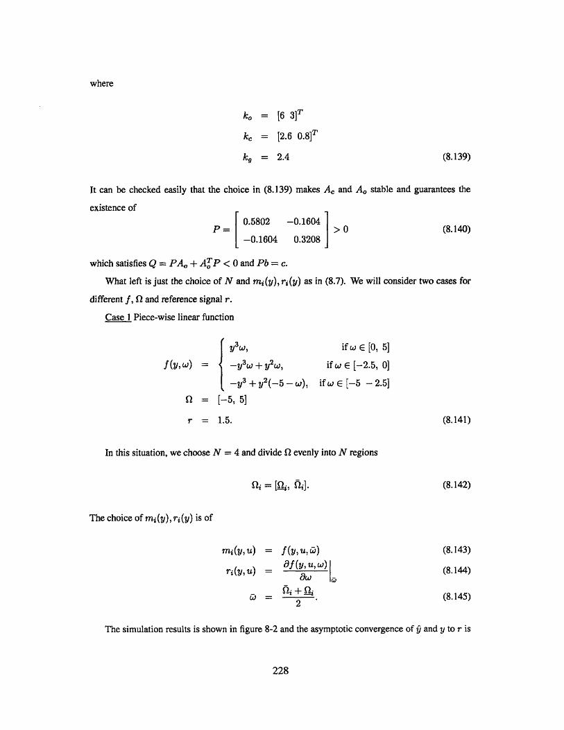
where

ko = [6 3 ]T

k, = [2.6 0 .8 ]T

kg = 2.4 (8.139)

It can be checked easily that the choice in (8.139) makes A, and AO stable and guarantees the

existence of

0.5802 -0.1604P = > 0 (8.140)

-0.1604 0.3208

which satisfies Q = PA0 + A'P < 0 and Pb = c.

What left is just the choice of N and mi(y), ri(y) as in (8.7). We will consider two cases for

different f, 1 and reference signal r.

Case I Piece-wise linear function

y3 w, if w E [0, 5]

f (y,w) = -yw + y 2w, if w E [-2.5, 0]

-y3 + y2 (-5 - w), if w E [-5 - 2.5]

Q = [-5. 5]

r 1.5. (8.141)

In this situation, we choose N = 4 and divide Q evenly into N regions

ni = [i. f2i]. (8.142)

The choice of mi(y), ri(y) is of

mi(y, u) = f (y, u, C) (8.143)

ri(y,u) = af(YW) (8.144)

W = + . (8.145)2

The simulation results is shown in figure 8-2 and the asymptotic convergence of i and y to r is

228

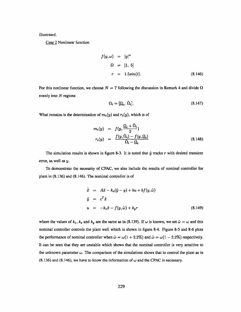
illustrated.

Case 2 Nonlinear function

f(y,w) = y]"'

92 = [1, 5]

r = 1.5sin(t). (8.146)

For this nonlinear function, we choose N = 7 following the discussion in Remark 4 and divide 0

evenly into N regions

Qi= [fi . (8.147)

What remains is the determination of mi (y) and ri (y), which is of

mi(y) = f(y'ii )fi y,) f - 2 y 4

ri(y) = - f (8.148)

The simulation results is shown in figure 8-3. It is noted that y tracks r with desired transient

error, as well as y.

To demonstrate the necessity of CPAC, we also include the results of nominal controller for

plant in (8.136) and (8.146). The nominal controller is of

. = AB-k o(q-y)+bu+bf(y,7W)

= CTx

U = -kcl - f (y, 6) + kgr (8.149)

where the values of kc, ko and kg are the same as in (8.139). If w is known, we set Ca' = w and this

nominal controller controls the plant well which is shown in figure 8-4. Figure 8-5 and 8-6 plots

the performance of nominal controller when c, = w(1 + 2.2%) and Co = w(1 - 2.2%) respectively.

It can be seen that they are unstable which shows that the nominal controller is very sensitive to

the unknown parameter w. The comparison of the simulations shows that to control the plant as in

(8.136) and (8.146), we have to know the information of w and the CPAC is necessary.

229

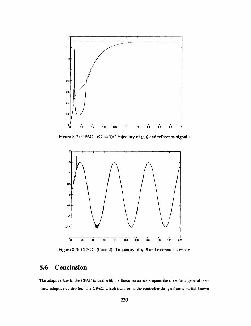
1.

1.4

1.2

0.8

0.6

0.4

0.2

0-0 0.2 0.4 0.6 0.8 1 1.2 1.4 1.6 1.8 A

Figure 8-2: CPAC - (Case 1): Trajectory of y, 9 and reference signal r

1.5

1

0.5

0

-1

-1.5 -

0 20 40 60 80 100 120 140 160 180 200

Figure 8-3: CPAC - (Case 2): Trajectory of y, ^ and reference signal r

8.6 Conclusion

The adaptive law in the CPAC to deal with nonlinear parameters opens the door for a general non-

linear adaptive controller. The CPAC, which transforms the controller design from a partial known

230

I II

- ... . . .... . . ... .. . . ...... . ..... ........ .. .... . .. . .....

-0.5

0.8

0.6

0.4

0.2

0

-0.2

-0.4

-0.6

-0.8

120 40 60 80 100 120 140 160 180 200

Figure 8-4: Nominal Controller - ( Case 2, W- = w ): Trajectory of y, and reference signal r

x 1080.

-0.5 F

-1

-1.51-

-2

-2.5 F

-3

20 40 60 80 100 120 140 160 180 200

Figure 8-5: Nominal Controllerreference signal r

- ( Case 2, W = w(1 + 2.2%) ): Trajectory of y, and

plant into a deterministic one, serves as a general tool to deal with nonlinearly parameterized sys-

tems. Stability of the CPAC with bounded disturbance is also established. For several classes of

231

5. 1

1

x 10"

2.5-

2-

1.5-

0.5-

0

0 20 40 60 80 100 120 140 16 180 200

Figure 8-6: Nominal Controller - (Case 2, W = w(1-2.2%)): Trajectory of y, and referencesignal r

NLP systems, the control laws are given and the complete CPACs are constructed. We note that the

CPAC is not restricted to these classes and more applications are worthy to be explored.

232

Bibliography

[I ] A.M. Annaswamy, A.P. Loh, and .P. Skantze. Adaptive control of continuous time systems




[3] C. Cao, and A.M. Annaswamy. A polynomial Adaptive Estimator for Nonlinearly Parameter-

ized Systems. Proceedings of American Control Conference 2004

[4] C. Cao, and A.M. Annaswamy. A Dead-zone Based Filter for Systems with Unknown Param-

eters. Proceedings of American Control Conference 2004.



AC-44:1634-1652, September 1999.

[6] J.D. Boskovi6. Adaptive control of a class of nonlinearly parametrized plants. IEEE Transac-


[7] A. Koji6, A.M. Annaswamy, A.-P. Loh, and R. Lozano. Adaptive control of a class of nonlinear

systems with convex/concave parameterization. Systems & Control Letters, 37:267-274, 1999.



1321, 2000.

[9] A. Kojid and A.M. Annaswamy. "Adaptive control of nonlinearly parametrized systems with a



233

Parameter Estimation and Control of Nonlinearly ... - CiteSeerX

Documents

Transcript of Parameter Estimation and Control of Nonlinearly ... - CiteSeerX