University of New Orleans University of New Orleans

ScholarWorks@UNO ScholarWorks@UNO

University of New Orleans Theses and Dissertations Dissertations and Theses

Fall 12-20-2017

Parameter Estimation Technique for Models in PSS/E using Real-Parameter Estimation Technique for Models in PSS/E using Real-

Time Data and Automation Time Data and Automation

Malavika Vasudevan Menon University of New Orleans, New Orleans, mvasudev@uno.edu

Follow this and additional works at: https://scholarworks.uno.edu/td

Part of the Electrical and Electronics Commons, and the Power and Energy Commons

Recommended Citation Recommended Citation Menon, Malavika Vasudevan, "Parameter Estimation Technique for Models in PSS/E using Real-Time Data and Automation" (2017). University of New Orleans Theses and Dissertations. 2436. https://scholarworks.uno.edu/td/2436

This Thesis is protected by copyright and/or related rights. It has been brought to you by ScholarWorks@UNO with permission from the rights-holder(s). You are free to use this Thesis in any way that is permitted by the copyright and related rights legislation that applies to your use. For other uses you need to obtain permission from the rights-holder(s) directly, unless additional rights are indicated by a Creative Commons license in the record and/or on the work itself. This Thesis has been accepted for inclusion in University of New Orleans Theses and Dissertations by an authorized administrator of ScholarWorks@UNO. For more information, please contact scholarworks@uno.edu.

University of New OrleansScholarWorks@UNO

University of New Orleans Theses and Dissertations Dissertations and Theses

Fall 12-20-2017

Parameter Estimation Technique for Models inPSS/E using Real-Time Data and AutomationMalavika Vasudevan Menon

Follow this and additional works at: http://scholarworks.uno.edu/td

Part of the Electrical and Electronics Commons, and the Power and Energy Commons

This Thesis is brought to you for free and open access by the Dissertations and Theses at ScholarWorks@UNO. It has been accepted for inclusion inUniversity of New Orleans Theses and Dissertations by an authorized administrator of ScholarWorks@UNO. The author is solely responsible forensuring compliance with copyright. For more information, please contact scholarworks@uno.edu.

Parameter Estimation Technique for Models in PSS/E usingReal-Time Data and Automation

A Thesis

Submitted to the Graduate Faculty of theUniversity of New Orleansin partial fulfillment of the

requirements of the degree of

Master of Sciencein

EngineeringElectrical Engineering

By

Malavika Vasudevan Menon

B-Tech. Mahatma Gandhi University, 2014

December, 2017

To my parents, and sister.

ii

iii  

Acknowledgement First and foremost, I offer my sincerest gratitude to my supervisor, Dr. Parviz Rastgoufard, who has supported me throughout my thesis with his patience and knowledge. His encouragement and support have been a major contribution to the completion of my thesis. I am grateful to the UNO - Power and energy Research Laboratory for all the opportunities and experiences. I sincerely thank Rastin Rastgoufard for his constant motivation by assigning different Python projects and guiding me to learn everything I know about Python. His expertise and knowledge have been crucial throughout my thesis and research work. I would like to express my sincere gratitude to Dr. Ittiphong Leevongwat for his technical support and valuable suggestions throughout my thesis and my time at school. His patience and way of teaching along with his cheerful attitude made research work and learning enjoyable. I further heartfully thank Dr. Ebrahim Amiri for his constant motivation and moral support. I also thank all the faculty and staff of the University of New Orleans for their support and providing me with quality education. Finally, I would like to thank my parents, Ajitha Menon and M.V. Menon, and sister, Mrinalini Menon for their constant support and unconditional love throughout my life. None of this would have been possible without them. I also would like to thank my friends for being there for me always and lifting my spirits when I needed it the most.

Contents

List of Figures vi

List of Tables ix

Abstract x

1 Problem Statement and Historical Review 11.1 Introduction . . . . . . . . . . . . . . . . . . . . . . . . . . . . . . . . . . . . 1

1.1.1 Challenges in Power System Planning . . . . . . . . . . . . . . . . . . 41.1.2 Time Frames in Reactive Power Analysis . . . . . . . . . . . . . . . . 5

1.2 Historical Background . . . . . . . . . . . . . . . . . . . . . . . . . . . . . . 61.3 Scope of Work . . . . . . . . . . . . . . . . . . . . . . . . . . . . . . . . . . . 11

2 Mathematical Background 132.1 Introduction . . . . . . . . . . . . . . . . . . . . . . . . . . . . . . . . . . . . 132.2 Static Var Compensator Modelling . . . . . . . . . . . . . . . . . . . . . . . 13

2.2.1 Thyristor Switched Capacitor . . . . . . . . . . . . . . . . . . . . . . 152.3 Generator Modeling . . . . . . . . . . . . . . . . . . . . . . . . . . . . . . . . 172.4 Exciter Modeling . . . . . . . . . . . . . . . . . . . . . . . . . . . . . . . . . 202.5 Transmission Line Modeling . . . . . . . . . . . . . . . . . . . . . . . . . . . 222.6 Transformer Modeling . . . . . . . . . . . . . . . . . . . . . . . . . . . . . . 232.7 Load Modeling . . . . . . . . . . . . . . . . . . . . . . . . . . . . . . . . . . 26

3 Main Focus and Contribution 293.1 Introduction . . . . . . . . . . . . . . . . . . . . . . . . . . . . . . . . . . . . 29

3.1.1 Hypersim . . . . . . . . . . . . . . . . . . . . . . . . . . . . . . . . . 293.1.2 SVC Physical Controller . . . . . . . . . . . . . . . . . . . . . . . . . 303.1.3 PSS/E . . . . . . . . . . . . . . . . . . . . . . . . . . . . . . . . . . . 30

3.2 Methodology . . . . . . . . . . . . . . . . . . . . . . . . . . . . . . . . . . . 313.2.1 Before addition of SVC . . . . . . . . . . . . . . . . . . . . . . . . . . 32

3.2.1.1 Steady State Analysis . . . . . . . . . . . . . . . . . . . . . 323.2.1.2 Dynamic Analysis . . . . . . . . . . . . . . . . . . . . . . . 33

3.2.2 After addition of SVC . . . . . . . . . . . . . . . . . . . . . . . . . . 363.3 Automation Process . . . . . . . . . . . . . . . . . . . . . . . . . . . . . . . 38

4 Test System 454.1 Introduction . . . . . . . . . . . . . . . . . . . . . . . . . . . . . . . . . . . . 454.2 Bus Data . . . . . . . . . . . . . . . . . . . . . . . . . . . . . . . . . . . . . 464.3 Transmission lines . . . . . . . . . . . . . . . . . . . . . . . . . . . . . . . . . 474.4 Transformer data . . . . . . . . . . . . . . . . . . . . . . . . . . . . . . . . . 484.5 Load data . . . . . . . . . . . . . . . . . . . . . . . . . . . . . . . . . . . . . 49

iv

4.6 Generator / Voltage Source . . . . . . . . . . . . . . . . . . . . . . . . . . . 494.7 Synchronous Condensers and Shunt Elements . . . . . . . . . . . . . . . . . 504.8 Static Var Compensators . . . . . . . . . . . . . . . . . . . . . . . . . . . . . 51

5 Analysis of Results 535.1 Introduction . . . . . . . . . . . . . . . . . . . . . . . . . . . . . . . . . . . . 535.2 Test Case Model . . . . . . . . . . . . . . . . . . . . . . . . . . . . . . . . . 535.3 Before addition of SVC . . . . . . . . . . . . . . . . . . . . . . . . . . . . . . 55

5.3.1 Steady State Analysis . . . . . . . . . . . . . . . . . . . . . . . . . . 555.3.2 Dynamic Analysis . . . . . . . . . . . . . . . . . . . . . . . . . . . . . 56

5.4 Finding the parameters of SVC model . . . . . . . . . . . . . . . . . . . . . 67

6 Concluding Remarks and Future Work 776.1 Conclusion . . . . . . . . . . . . . . . . . . . . . . . . . . . . . . . . . . . . . 776.2 Future Work . . . . . . . . . . . . . . . . . . . . . . . . . . . . . . . . . . . . 78

Bibliography 80

Appendix 83

Vita 109

v

List of Figures

2.1 SVC one-line diagram . . . . . . . . . . . . . . . . . . . . . . . . . . . . . . 142.2 Simplified block diagram of SVC unit . . . . . . . . . . . . . . . . . . . . . . 162.3 Simplified block diagram of SVC unit . . . . . . . . . . . . . . . . . . . . . . 172.4 Simple Excitation System in PSS/E [27] . . . . . . . . . . . . . . . . . . . . 212.5 Transmission line circuit diagram . . . . . . . . . . . . . . . . . . . . . . . . 222.6 Diagram of 2-winding transformer . . . . . . . . . . . . . . . . . . . . . . . . 242.7 Circuit Diagram of Induction motor load model . . . . . . . . . . . . . . . . 28

3.1 3-Bus Test System . . . . . . . . . . . . . . . . . . . . . . . . . . . . . . . . 343.2 3-Bus Test System Voltages with Fault at Bus-2 . . . . . . . . . . . . . . . 353.3 General form of reactor models [28] . . . . . . . . . . . . . . . . . . . . . . . 373.4 CSVGN3 model [27] . . . . . . . . . . . . . . . . . . . . . . . . . . . . . . . 383.5 Flow chart of PSS/E automation . . . . . . . . . . . . . . . . . . . . . . . . 393.6 Flow chart of complete automation process . . . . . . . . . . . . . . . . . . . 433.7 Variation of K ; Mvar output of SVC Model with respect to time . . . . . . 433.8 Variation of T1 ; Mvar output of SVC Model . . . . . . . . . . . . . . . . . . 433.9 Variation of T2 ; Mvar output of SVC Model with respect to time . . . . . . 443.10 Variation of T3 ; Mvar output of SVC Model . . . . . . . . . . . . . . . . . . 443.11 Variation of T4 ; Mvar output of SVC Model with respect to time . . . . . . 443.12 Variation of T5 ; Mvar output of SVC Model . . . . . . . . . . . . . . . . . . 44

4.1 IEEE 14 Bus Test System [2] . . . . . . . . . . . . . . . . . . . . . . . . . . 46

5.1 14-bus Test System in PSS/E . . . . . . . . . . . . . . . . . . . . . . . . . . 545.2 14-bus Test System in Hypersim . . . . . . . . . . . . . . . . . . . . . . . . . 555.3 Comparison between PSS/E and Hypersim test case with Bus-5 fault . . . . 585.4 Voltage waveforms of the base case and capacitor added at Bus-4 . . . . . . 595.5 Bus 4 fault with capacitor at Bus 3 . . . . . . . . . . . . . . . . . . . . . . . 605.6 Bus 4 fault with capacitor at Bus 5 . . . . . . . . . . . . . . . . . . . . . . . 615.7 Bus 4 fault with capacitor at Bus 6 . . . . . . . . . . . . . . . . . . . . . . . 615.8 Bus 4 fault with capacitor at Bus 7 . . . . . . . . . . . . . . . . . . . . . . . 625.9 Bus 4 fault with capacitor at Bus 8 . . . . . . . . . . . . . . . . . . . . . . . 625.10 Bus 4 fault with capacitor at Bus 9 . . . . . . . . . . . . . . . . . . . . . . . 635.11 Bus 4 fault with capacitor at Bus 10 . . . . . . . . . . . . . . . . . . . . . . 635.12 Bus 4 fault with capacitor at Bus 11 . . . . . . . . . . . . . . . . . . . . . . 645.13 Bus 4 fault with capacitor at Bus 12 . . . . . . . . . . . . . . . . . . . . . . 645.14 Bus 4 fault with capacitor at Bus 13 . . . . . . . . . . . . . . . . . . . . . . 655.15 Bus 4 fault with capacitor at Bus 14 . . . . . . . . . . . . . . . . . . . . . . 655.16 Test Matrix . . . . . . . . . . . . . . . . . . . . . . . . . . . . . . . . . . . . 665.17 Error function table for variation of K . . . . . . . . . . . . . . . . . . . . . 685.18 Case 1:Error function table for variation of T1 . . . . . . . . . . . . . . . . . 68

vi

5.19 Case 1:Error function table for variation of T2 . . . . . . . . . . . . . . . . . 695.20 Case 1:Error function table for variation of T3 . . . . . . . . . . . . . . . . . 695.21 Case 1: Error function table for variation of T4 . . . . . . . . . . . . . . . . . 695.22 Case 1:Error function table for variation of T5 . . . . . . . . . . . . . . . . . 705.23 Case 2: Error function table for variation of K . . . . . . . . . . . . . . . . . 705.24 Case 2: Error function table for variation of T2 . . . . . . . . . . . . . . . . . 705.25 Case 2: Error function table for variation of T1 . . . . . . . . . . . . . . . . . 705.26 Case 2: Error function table for variation of T3 . . . . . . . . . . . . . . . . . 705.27 Case 2: Error function table for variation of T4 . . . . . . . . . . . . . . . . . 705.28 Case 2: Error function table for variation of T5 . . . . . . . . . . . . . . . . . 705.29 Comparison of response with best value of K . . . . . . . . . . . . . . . . . 715.30 Comparison of response with best value of T1 . . . . . . . . . . . . . . . . . 715.31 Comparison of response with best value of T2 . . . . . . . . . . . . . . . . . 715.32 Comparison of response with best value of T3 . . . . . . . . . . . . . . . . . 715.33 Comparison of response with best value of T4 . . . . . . . . . . . . . . . . . 725.34 Comparison of response with best value of T5 . . . . . . . . . . . . . . . . . 725.35 Error function table for variation of all parameters simultaneously . . . . . . 725.36 Response of the test system in PSS/E with new parameters for SVC and

Hypersim HIL SVC at Bus-4 and a fault applied on Bus-5 . . . . . . . . . . 745.37 Response of the test system in PSS/E with original SVC and Hypersim HIL

SVC at Bus-4 and a fault applied on Bus-5 . . . . . . . . . . . . . . . . . . . 75

1 Case A:Error Function Table of K varied . . . . . . . . . . . . . . . . . . . . 842 Case A:Error Function Table of T1 varied . . . . . . . . . . . . . . . . . . . . 843 Case A:Error Function Table of T2 varied . . . . . . . . . . . . . . . . . . . . 854 Case A:Error Function Table of T3 varied . . . . . . . . . . . . . . . . . . . . 855 Case A:Error Function Table of T4 varied . . . . . . . . . . . . . . . . . . . . 856 Case A:Error Function Table of T5 varied . . . . . . . . . . . . . . . . . . . . 867 Case B:Error Function Table of K varied . . . . . . . . . . . . . . . . . . . . 868 Case B:Error Function Table of T1 varied . . . . . . . . . . . . . . . . . . . . 869 Case B:Error Function Table of T2 varied . . . . . . . . . . . . . . . . . . . . 8710 Case B:Error Function Table of T3 varied . . . . . . . . . . . . . . . . . . . . 8711 Case B:Error Function Table of T4 varied . . . . . . . . . . . . . . . . . . . . 8712 Case B:Error Function Table of T5 varied . . . . . . . . . . . . . . . . . . . . 8813 Error Function Table with SVC at Bus-3 with Bus-6 fault . . . . . . . . . . 8814 Error Function Table with SVC at Bus-3 with Bus-14 fault . . . . . . . . . . 8915 Error Function Table with SVC at Bus-4 with Bus-3 fault . . . . . . . . . . 8916 Error Function Table with SVC at Bus-4 with Bus-12 fault . . . . . . . . . . 9017 Bus 6 fault with SVC at Bus 3 . . . . . . . . . . . . . . . . . . . . . . . . . . 9118 Bus 7 fault with SVC at Bus 3 . . . . . . . . . . . . . . . . . . . . . . . . . . 9219 Bus 10 fault with SVC at Bus 3 . . . . . . . . . . . . . . . . . . . . . . . . . 9320 Bus 14 fault with SVC at Bus 3 . . . . . . . . . . . . . . . . . . . . . . . . . 9421 Bus 6 fault with SVC at Bus 3 . . . . . . . . . . . . . . . . . . . . . . . . . . 9522 Bus 6 fault with SVC at Bus 4 . . . . . . . . . . . . . . . . . . . . . . . . . . 9623 Bus 7 fault with SVC at Bus 4 . . . . . . . . . . . . . . . . . . . . . . . . . . 97

vii

24 Bus 9 fault with SVC at Bus 4 . . . . . . . . . . . . . . . . . . . . . . . . . . 9825 Bus 10 fault with SVC at Bus 4 . . . . . . . . . . . . . . . . . . . . . . . . . 9926 Bus 11 fault with SVC at Bus 4 . . . . . . . . . . . . . . . . . . . . . . . . . 10027 Bus 12 fault with SVC at Bus 4 . . . . . . . . . . . . . . . . . . . . . . . . . 10128 Bus 13 fault with SVC at Bus 4 . . . . . . . . . . . . . . . . . . . . . . . . . 10229 Bus 14 fault with SVC at Bus 4 . . . . . . . . . . . . . . . . . . . . . . . . . 10330 Bus 3 fault with SVC at Bus 5 . . . . . . . . . . . . . . . . . . . . . . . . . . 10431 Bus 6 fault with SVC at Bus 5 . . . . . . . . . . . . . . . . . . . . . . . . . . 10532 Bus 7 fault with SVC at Bus 5 . . . . . . . . . . . . . . . . . . . . . . . . . . 10633 Bus 10 fault with SVC at Bus 5 . . . . . . . . . . . . . . . . . . . . . . . . . 10734 Bus 11 fault with SVC at Bus 5 . . . . . . . . . . . . . . . . . . . . . . . . . 10835 Bus 14 fault with SVC at Bus 5 . . . . . . . . . . . . . . . . . . . . . . . . . 109

viii

List of Tables

4.1 Bus Data . . . . . . . . . . . . . . . . . . . . . . . . . . . . . . . . . . . . . 474.2 Transmission Line Parameters . . . . . . . . . . . . . . . . . . . . . . . . . . 484.3 Transformer Parameters . . . . . . . . . . . . . . . . . . . . . . . . . . . . . 484.4 Load Parameters . . . . . . . . . . . . . . . . . . . . . . . . . . . . . . . . . 494.5 Generator Parameters . . . . . . . . . . . . . . . . . . . . . . . . . . . . . . 504.6 Generator (GENCLS) Dynamic Parameters . . . . . . . . . . . . . . . . . . 504.7 Exciter (SEXS) Parameters . . . . . . . . . . . . . . . . . . . . . . . . . . . 504.8 Synchronous Condensers . . . . . . . . . . . . . . . . . . . . . . . . . . . . . 514.9 SVC Parameters . . . . . . . . . . . . . . . . . . . . . . . . . . . . . . . . . 514.10 SVC (CSVGN3) dynamic Parameters . . . . . . . . . . . . . . . . . . . . . . 52

5.1 Voltages (kV RMS) compared between PSSE and Hypersim . . . . . . . . . 565.2 Currents (A RMS) compared between PSSE and Hypersim . . . . . . . . . . 575.3 New SVC (CSVGN3) Parameters . . . . . . . . . . . . . . . . . . . . . . . . 76

ix

x  

Abstract The purpose of this thesis is to use automation to create appropriate models in PSS/E with the data from Hardware-in-Loop real-time simulations. With the increase in technology of power electronics, the use of High Voltage Direct Current Technology and Flexible Alternating Current Transmission System devices in the electrical power system have increased tremendously. Static Var Compensators are widely used and it is important to have accurate and reliable models for studies relating to power systems planning and interaction. An automation method is proposed to find the parameters of an SVC model in PSS/E with the data from the Hardware-in- loop real-time simulation of the SVC physical controller using Hypersim. The effect of the SVC on the system under steady state and fault conditions are analyzed with HIL simulation of an SVC physical controller in Hypersim and its corresponding model in PSS/E in the IEEE 14 bus system. The parameters of the SVC model in PSS/E can be effectively varied to bring its response closer to that of the response from HIL simulations in Hypersim. An error function is used as a measure to understand the extent of difference between the model and the physical controller. Keywords: Electrical, Power and Energy

Chapter 1Problem Statement and Historical

Review

1.1 Introduction

Todays power systems network is an enormous and complex network of interconnections

which includes buses, generators, transmission lines etc. This network is expanding and

increasing with growing load demands and requires the installation of new generators or lines

or extension of existing infrastructure. This increase in demand also leads to the unstable

operation of the power system and causes the system to be less reliable. Electric utilities

have the responsibility of maintaining the safety of their systems and planning for the future

power needs of their customers [2].

Flexible AC Transmission Systems (FACTS) controllers enable the efficient utilization

of the existing transmission and generator facilities instead of adding new facilities to the

infrastructure [17]. It requires lower investment and does not lead to any environmental

constraints. Devices such as Static VAR Compensators (SVC), Static Synchronous Compen-

sator (STATCOM), Thyristor Controlled Series Compensator (TCSC), Static Synchronous

Series Compensator (SSSC) and Unified Power Flow Controller (UPFC) are popular FACTS

controllers. Other than improving the voltage profile and reactive power FACTS devices

offer a wide range of benefits. FACTS technologies helps in the increase of power transfer

capabilities by 20-30% by the increase of the system flexibility [17]. They also improve the

1

loading ability of the system. The increase in the inclusion of renewables in the system such as

wind turbines leads to the absorption of large amounts of VARs (Volt-Amperes Reactive) due

to it being induction generators. Facts devices offer faster and smooth switching capacitor

operations along with voltage regulations and power factor corrections compared to the

traditional switched capacitors which causes stress due to frequent switching that leads to

transients to the grid and reduction of the life cycle of the capacitors [24].

SVC is one of the earliest and most commonly used FACTS devices due to its reasonable

cost and numerous advantages. It is found to be one of the mostly widely used FACTS

devices in China [3]. Analysis of the power system network is required to study and improve

it during different network events and addition of different units to meet demands. This

has been done by modeling the system and simulating the network events in power system

software. Simulation based analysis of the planning and design of power systems have been

done extensively for decades [3]. This type of analysis can be of many uses such as in the

planning and design of power systems which helps to decide future system requirements and

parameter selection for control systems, in the operation of the power system to determine

limits for operation and requirement for specific protection schemes, and in the fault analysis

to understand weak regions and analyze events that lead to major disturbances. Simulations

can help analyze the network and device surrounding the area of the fault in the pre-fault,

fault and post-fault durations.

Power system engineers use different software such as PSS/E, PSLF, EMTP, TSAT,

Hypersim, and RTDS and so on. Each software is different and has its own advantages and

limitations. PSS/E and PSLF have the capacity to model very large systems and are mainly

used to run load flow analysis in different contingencies. EMTP and MATLAB have the

2

ability to simulate and study transients and involve in circuit element based modeling. The

past few decades has the seen the evolution of simulation tools which were driven by the rapid

evolution of computing technologies. The capacity of simulation based tools to solve complex

problems in less time was enabled due the decrease in cost and the increase in performance

of computer technologies [31]. This led to the origin of digital real time simulators which

exploit advanced digital hardware and advanced computing methods to solve differential

equations which represents the power system in the speed of real world time. Hypersim

and RTDS are examples of real time simulators which can be used to study electromagnetic

transients in micro seconds. They also enable the analysis of physical hardware devices

with Hardware-in-loop (HIL) simulations which can connect the physical controller to the

simulator through input/output (I/O) channels.

With the growth of computing technologies and increase in the simulation and problem

solving capabilities, it is important to model devices and the system as accurate as possible

for us to understand and analyze the effects of these devices on the system as well as other

devices in the system and vice versa. At this time, it cannot be acceptable to question the

accuracy of the model used for analysis. After the commissioning of HVDC and FACTS

devices, the customers are usually provided with a black box model of their device. The

maintenance of the model is hard during the lifetime of the equipment. This can be due to

the fact that these models are based on a particular version of the simulation tool as the

models require certain static libraries that might be linked to the version and thus disabling

the model from following the actual control changes. Long term expertise is not necessarily

provided by the manufactures for model maintenance [31]. The manufacturer also supplies

physical replicas of the control system. The replica is a precise copy of the actual control

3

units installed on site.

This thesis aims in creating appropriate models in PSS/E for stability analysis studies

with the data from the field. A method of automation is proposed to find the parameters of

an SVC in PSS/E with the data from the Hardware-in-loop real-time simulation of the SVC

physical controller using Hypersim. It analyzes the dynamic and transient response of the

system with the SVC connected to it while subjecting it to different network events such as

three phase bus faults. The system dynamics are kept to a minimum to reduce the difference

between the software platforms and to focus on the dynamics of the SVC. The responses are

compared and an error function is used to measure the amount of difference between the

model and the replica. Selection of the parameters of the SVC model in PSS/E is based on

how close the response of the SVC is in PSS/E to that of the response in Hypersim with the

SVC physical controller. The comparison process is automated and the parameter set with

the least error function value is chosen.

1.1.1 Challenges in Power System Planning

Power system planning is one of the most important parts of maintaining a reliable and

secure power system network. Guidelines and standards are issues to enable a smooth process

even with which it would face numerous challenges which can be seen below [4] :

• Collection of wide variety of data from multiple sources

• Cooperative approach to developing, validating, specifying and using new planning

methods, tools and models

• Effective sharing and access to data

4

• Uncertainty in future demand including active and reactive power profiles under network

events

• Need for an array of models, standards and processes to address distribution networks

1.1.2 Time Frames in Reactive Power Analysis

NERC has issued a time frame for the reactive power planning and voltage control to clearly

understand the systems reactive capability requirements in [22] which can be seen below:

• Steady State / Pre-Contingency: Individual elements such as generators and dynamic

reactive resources are maintained at a desired voltage set point value to ensure other

voltages are maintained in the desired voltage range. Manual adjustments are required

to maintain this schedule. In this state, the grid is said to be operating in a secure state

which means no violations can be seen and thus no outage conditions are to happen.

• Transient: After a major network event or disturbance, the transient voltage stability is

analyzed with different transient stability tools. There are two main transient voltage

responses that can be seen in this period

– Transient voltage dip: dips or sags which are caused by oscillations which change

the active and reactive power flow and thus the voltage.

– Delayed voltage recovery: Delayed recovery in voltage due to fault as well as

stalling and restarting of induction motor which results in reactive power demand.

• Mid-term Dynamics : After the first swing during transients, if the system is stable, the

oscillations begin to dampen and return to a new steady state condition this period

5

during transition is called mid-term dynamics. The analysis during this period includes

the results of the automatic control devices and is within 3 minutes following an event

• Long term dynamics / Post-contingency: Once the system attains equilibrium, pose

contingency analysis is performed to ensure the system is stable and secure. The system

has to attain acceptable operating limits within 30 minutes following an event

This thesis deals with the accuracy of models and the selection of parameters for the simulation

models which falls under the category of power system planning and design.

1.2 Historical Background

Power electronics controllers will have greater significance over the reliability of the grid

and its performances over the next couple of years. The use of real time simulators and

hardware in the loop analysis are growing as can be seen in [31] which involves performing

simulations with different SVC replicas connected to the same simulator to study the levels

of interaction between the replicas and to improve the model of SVC in off-line simulations.

A Hardware-in the-loop test facility called SMARTE was set up which uses Hypersim

simulator to verify various modeling techniques and to test interoperability with the absence

of adverse interactions. This paper uses 3 study replicas of SVC controllers from 2 different

manufacturers which are connected to the 225kV substations situated in the West of France,

which is considered as the weak zone of the French grid. A large number of capacitors and 5

SVCs were installed in this zone to control voltage during events. The required part of the

network involving substations, lines, autotransformers, generation units and the SVC were

modeled in the Hypersim software. The replicas were connected to the simulator via input

6

and output signals (IO). Different types of network events such as transformer fault, line

fault or bus faults were simulated to examine the SVCs reaction by observing the positive

sequence voltage, reactive power and TCR firing angle.

The compatibility of generator models in different Power system simulation software such

as PSS/E, EMTP and Hypersim is shown in [20]. PSS/E is used to study electro-mechanical

dynamics whereas Hypersim and EMTP are used for electromagnetic dynamics and thus

the dynamic results between PSS/E and Hypersim are different. This paper is required to

achieve identical system results in order to compare the results of an SVC model in PSS/E to

that of the HIL simulation with the SVC replica in Hypersim. The IEEE 14 bus system along

with the models of the generator and excitation system were modeled in all three software.

To study the transients, a same network event such as bus faults were applied in different

location and the voltage profiles were plotted against each other. Sensitivity analysis of the

excitation system is carried out and the parameters with the most sensitivity are varied

within a specific range in one software to match the other software.

For over two decades, real-time simulators have been used by utilities, independent system

operators (ISO), manufacturers, research institutes and universities to test a range of controls

like HVDC, FACTS, generator controls, distributed generation, and smart grid [6]. The HIL

test which is an advanced test method allows the prototype (replica) of a unique device to be

analyzed under a range of realistic situations safely, frequently and efficiently. This paper

deals with the testing of a digital controller for a DC-DC buck converter and DC-AC converter.

These converters consist of basic elements such as switches, diodes and inverters that are used

in other devices such as FACTS, HVDC which predominant in power systems network. It was

found that HIL testing is useful to analyze the effectiveness of power electronic controllers by

7

being an intermediate step during the progress of an end product, reducing the development

cost and risks that are encountered during testing.

The complexity and size of power system network has led to the extensive use of FACTS

devices where they are not only able to improve the voltage and angle stability but also add

flexible operation capabilities. FACTS devices such as SVC, STATCOM, TCSC and SSSC

have their own characteristic and constraints and are represented by different models and

mathematical equations which depend on time frame and issue under analysis. For RCP and

HIL testing to be purposeful and relevant, it is important that the real-time simulations be

accurate portrayal of the real-world response. The accuracy and credibility of HIL testing is

shown in [25] by running a real-time simulation of an induction motor drive and comparing

it against a physical implementation of the same. Modeling was done of both the motor and

inverter in the Opal- RT platform to compare it to the actual motor drive. Motor control

was enabled with the implementation of Field Oriented Control (FOC) and tests were run to

examine both the steady state and dynamic response of the motor. While current outputs

for different frequencies were used to compare results in the case of steady state, the motor

start up stage was used to analyze the dynamic response. The results were highly close and

the waveforms overlapped with disregard able errors which validated the credibility of the

real-time HIL simulations.

The power system network of the present day is an intricate interconnected network

which is increasing every day to meet the increase in demands. Addition of new lines and

generators creates many environmental and economical restraints. Reactive power generation

i.e., FACTS devices is the one way to counteract this problem. The applications of the four

main FACTS devices which are STATCOM, SVC, TCSC and SSSC can be seen in [21]. Every

8

FACTS device has their own unique characteristics and limitations. The weakest bus is

chosen from the standard IEEE 14 bus system with the use of continuation power flow (CPF)

and then to determine the best location. The maximum loading factor (lambda) was taken

as the metric to analyze the different devices. When placed on bus 14, lambda increased

by 0.0808 for STATCOM, 0.0504 for SVC, 0.0348 for SSSC and 0.0332 for TCSC. When

comparing average costs, STATCOM was found to be the most expensive followed by SVC

and TCSC. It was found that advantages or savings by installing FACTS devices would

outweigh the additional costs in acceptable time [21].

Functional applications of real-time simulations for power and energy systems include

design and modeling, prototyping or rapid prototyping, testing, and teaching and training.

Developing a new model and designing a new device can be easily done with real-time

simulations as it produces results faster with higher accuracy [10]. It helps in creating

prototypes which are approximates of the real system that can be used in testing and

modification of the devices when and as required [3]. The most common application is

testing as it allows the modeling of the surrounding area which represents real physical field

environments [10]. It is a valuable tool in teaching and training as live feedback allows

understanding the response of the systems when changes and disturbances are brought

into the system [3]. The extensive and growing use of real-time simulations can be seen

in [10] which mentions examples in super large EMT real-time simulation, protection, device

interoperability, and PMU, Hybrid phasors/ EMT applications, HVDC testing, FACTS and D-

FACTS testing, Smart grid/ Distribution system applications and Multi-physics applications.

It is evident that real-time simulations in power systems valuable and predominant.

The steady state effect of an SVC on the IEEE 14 bus system can be seen in [23]. The

9

SVC was modeled as a fixed shunt capacitor in MATLAB/Simulink and connected to the

weakest buses of the system. The load is then increased by 10% and 20%. The voltage

profiles and reactive power profiles were analyzed of the base case against the profiles for

when the SVC is connected to the system. It was clear from the profiles that the SVC plays

a great importance in the voltage profile as well as the reactive power profile during load

variations in the system.

A study on the transient stability improvement of a system with the use of FACTS devices

is seen in [30]. MATLAB is used as the platform for modeling and analyzing the dynamic

system. The sim Power block set enables the modeling of power system network and element.

This paper analyzed the effect of FACTS controllers like SVC, STATCOM and SSSC on the

IEEE 5 machine 14 bus system. A 3-phase fault was applied on different buses with the SVC

connected to the system at different buses. The fault is applied at 0.5 secs and cleared after

0.1 secs. The results were analyzed and it was found that the time taken to attain system

stability decreased with the use of FACTS devices and the best case was found when the SVC

was connected at Bus 4. It was also found that the maximum overshoot values for relative

rotor angle positions decreased with the use of the FACTS controller and the best case was

found when the SVC was connected at Bus 3. This shows that transients are stabilized faster

with the use of FACTS devices.

The comparison of transient stability analysis and real time digital simulation can be

seen in [8]. Traditionally, real time simulators did not have the ability to simulate large-scale

power systems. The KEPS real Time Digital Simulator is the largest RTDS produced with

the ability to simulate large scale systems, the results of which are compared to that of

transient stability analysis software, PSS/E. It was found that most of the results were very

10

similar but had cases which exhibited differences. The main differences were found to be the

method in which the programs solved the differential equations which corresponds to the

system. Three disturbances were applied to the systems and the differences were analyzed in

detail.

According to the review of the above papers, it can be seen that creating accurate and

precise models in transient stability analysis platform is necessary and important. Also, a

methodical and efficient process of finding the parameters for the model has never been

performed with python automation. The focus of this thesis is to increase the accuracy of

the model of the SVC in PSS/E by finding the best set of parameters that would bring it

closer to that of the SVC physical controller with the least error function.

1.3 Scope of Work

The aim of this thesis is to create appropriate models in PSS/E for stability analysis studies

with the data from the field. An automation method is proposed to find the parameters of an

SVC model in PSS/E with the results from the HIL simulation of the SVC physical controller.

Different sets of parameters are assigned to the SVC model and the system voltages along

with the MVAR output of the SVC are compared when a three phase bus fault is applied and

cleared after a certain time along with the loss of a line. Chapter 2 describes the mathematical

background of the components used in the test system. This chapter is important as it is

necessary to know the underlying mathematics to understand and analyze the behavior of

each component. Chapter 3 provides an insight on what the focus of this thesis is and an

overall description of the methodology used in this research. Chapter 4 lists all the models

11

and components used in the test system. The process to find the best locations for the SVC

is also elaborated in this chapter. It allows us to see and analyze the dynamic responses of

the SVCs incorporating the differences in different platforms. Chapter 5 shows the results

of the analysis with error function table along with the voltage responses of the parameters

with the least error function. This is followed by the conclusion in Chapter 6 which analyzes

the results along with the future work.

12

Chapter 2

Mathematical Background

2.1 Introduction

Representation of the power system components mathematically is the first and most

important step in analyzing power systems and its stability. Power system planning and

operations depend extensively on tools which use models to ensure reliable and efficient

operation. There are different types of modeling depending on the type and requirement of

the equipments.

The mathematical modeling of all the electrical components used in the test system for

this thesis is dealt with in this chapter.

2.2 Static Var Compensator Modelling

Static Var Compensator is a type of FACTS device that is a shunt compensator which has

been in use since the 1970s [11]. It is used to influence the natural electrical characteristics of

the transmission line to increase the power for transmission and to control the voltage profile.

It consists of a set of power electronic devices for providing fast-acting reactive power. The

output of the SVC can be adjusted to produce either capacitive or inductive currents which

13

control the bus voltage of the electrical power system [1]. Thyristors play a significant part

in control of the reactive power flow which is done by controlling the firing angle [18]. The

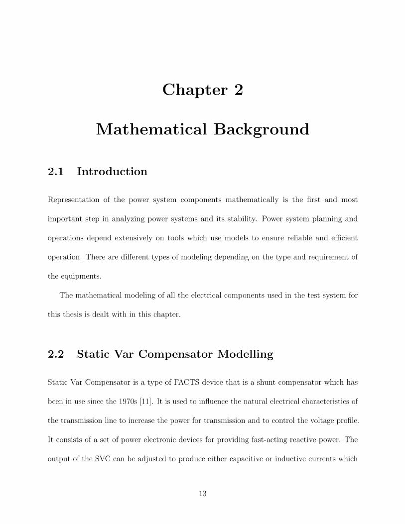
one-line diagram of an SVC is shown in Figure 2.1.

Figure 2.1: SVC one-line diagram

The SVC constitutes one or more banks of fixed or switched capacitors or reactors.

Components which can be used to design an SVC are:

• Thyristor Switched Capacitor

• Thyristor Controlled/Switched Reactor

• Harmonic Filters

• Mechanically Switched Capacitor/ Mechanically Switched Reactor

14

2.2.1 Thyristor Switched Capacitor

The thyristor Switched Capacitor consists of a capacitor connected in series with a bidirectional

valve and, mostly, a current limiting reactor. The current limiting reactor is used to limit the

effects of the capacitor switching [12]. The SVC in the study involves 3 TSC units which

results in a 0/+300 Mvar SVC.

The current through the TSC branch at any given time is given by [12,18],

i(t) =

(I cos(ω0t+α)

)−(I cos(α) cos(ωrt) +nBc

(VCo−

n2

n2 − 1V sin(α)

)sin(ωrt)

)(2.1)

In the equation above, the first part represents the steady state equation and the second part

represents the equation for the oscillatory transients. We assume that the TSC comprises of

capacitance, C and inductance, L with a sinusoidal input voltage. ω0 is the nominal angular

frequency, α is the current firing angle , ωr is the resonant frequency, n is the per unit natural

frequency and VCo is the voltage across the capacitor.

The current amplitude and n is given by,

I = VBCBL

BC +BL

(2.2)

n =1√

ω02LC

=

√XC

XL

(2.3)

BC and BL is the capacitor and reactor susceptance and XC and XL are the capacitor and

15

reactor reactance respectively. The TSC resonant frequency ωr is given by,

ωr = nω0 =1√LC

(2.4)

Thus, the magnitude of the TSC current can be given as,

I = VBCBL

BC +BL

= V BCn2

n2 − 1(2.5)

The SVC is represented as a one line diagram with a simplified block diagram of the

control units in Figure 2.2. It consists of a measuring system which measures the voltage

to be controlled. The voltage regulator determines the SVC susceptance needed to keep

the voltage at a desired value. This is done with the use of the voltage error which is the

difference between the measured voltage Vm and the reference voltage Vref . The distribution

unit determines which TSCs and TSRs needs to be switched in and out and finds the firing

angle of TCR. The synchronizing unit uses a Phase locked loop pulse generator to send the

required

Figure 2.2: Simplified block diagram of SVC unit

16

2.3 Generator Modeling

There are different types of models for the synchronous generator depending on type of

analysis and requirement. The classical generator model is used in this study. One of the

simplest yet useful representation of the synchronous generator is the classical model [16].

There are a few assumptions taken into consideration while representing the synchronous

generator by a classical model [16]. They are:

• The field current is assumed constant and exciter dynamics are not of concern

• The effect of damper windings is ignored

• The mechanical power input is assumed to be constant during the study period

• The saliency of the generator is neglected

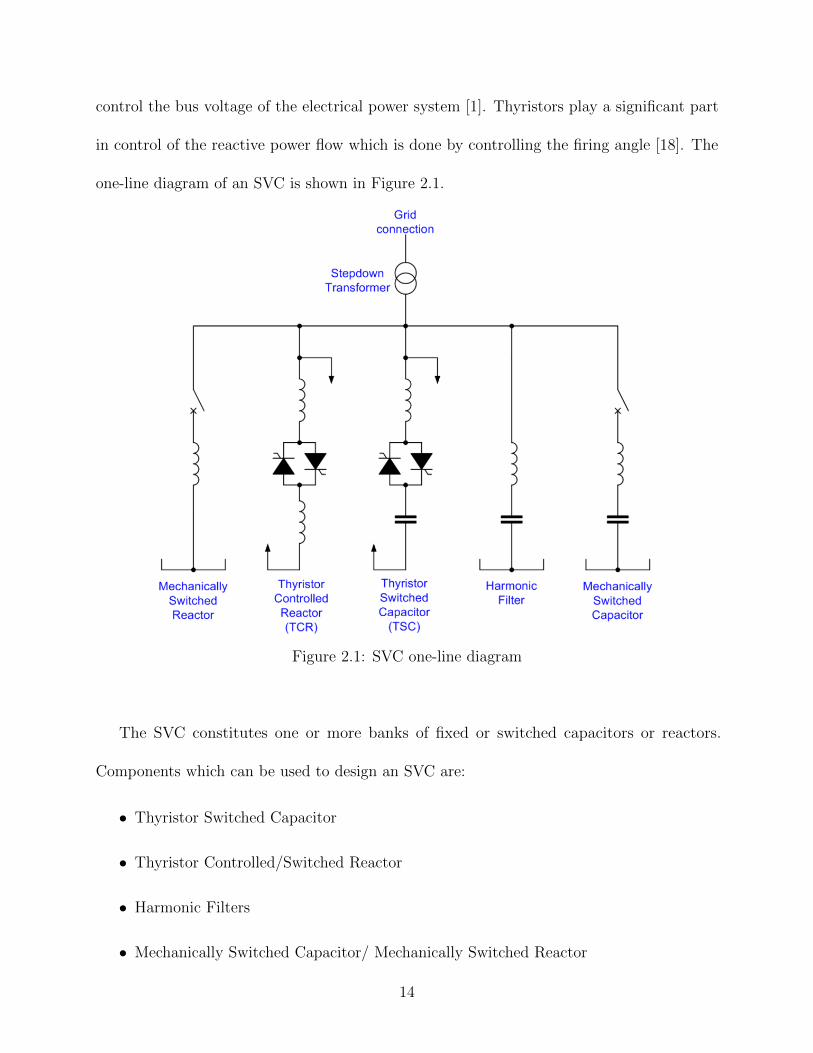
Figure 2.3: Simplified block diagram of SVC unit

17

The classical model representation can be seen in Figure 2.3. E 6 δ represents the complex

internal voltage of the generator and X represents the reactance. The generator is assumed

to be connected to an infinite bus is through a transformer and line and the bus voltage is

represented as V . The generator internal voltage angle delta is defined with respect to bus

voltage. The input mechanical power is Pi and output electrical power is Po

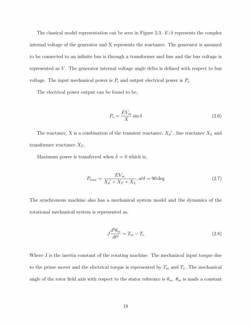
The electrical power output can be found to be,

Po =EV∞X

sin δ (2.6)

The reactance, X is a combination of the transient reactance, Xd′ , line reactance XL and

transformer reactance XT .

Maximum power is transferred when δ = 0 which is,

Pmax =EV∞

Xd′ +XT +XL

, atδ = 90 deg (2.7)

The synchronous machine also has a mechanical system model and the dynamics of the

rotational mechanical system is represented as,

Jd2θmdt2

= Tm − Te (2.8)

Where J is the inertia constant of the rotating machine. The mechanical input torque due

to the prime mover and the electrical torque is represented by Tm and Te. The mechanical

angle of the rotor field axis with respect to the stator reference is θm. θm is made a constant

18

in steady state by measuring it with respect to a synchronously rotating reference and hence,

θm = δm + ωmst (2.9)

The manipulation of the above equations leads to the equation given below,

d2δ

dt2=πfsH

(2.10)

This is called the swing equation of the synchronous generator which helps to analyze the

response of the generator. H is the machine inertia constant. If Pm = Pmax sin δ , then

there will be no speed change and no angle change. But if they are not equal due to some

disturbance in the system, then either the speed will increase or decrease with respect to

time.

In synchronous generators, the rotor has damper windings which causes it to act as

an induction motor during transients. This effect needs to be considered which evaluating

stability and leads to the equation,

H

πfs

d2∆δ

dt+D

d∆δ

dt+ Ps∆δ = 0 (2.11)

Where D is the damping coefficient and Ps is the synchronizing torque or power. Similarly,

the generator reactive power output is given by,

Qo =V∞(E cos(δ)− V∞)

Xd′ +XL +XT

(2.12)

19

Classic model has two main advantages beside its simplicity. First, all the voltages and

currents are phasors in the network reference frame, whereas in higher order models d q

representation is needed. The second important advantage is that the generator reactance

can be treated in similar way as transmission line reactances and can be combined with

network elements to form reduced admittance matrix.

2.4 Exciter Modeling

The basic function of an excitation system is to supply the required direct current to the field

winding of the synchronous generator. It automatically adjusts the field current to retain the

required terminal voltage.

Re and Le represent the resistance and inductance of the exciter field, then the voltage is

given by,

VR = Reie + Led

dtie (2.13)

and hence,

∆VR = Re∆ie + Led

dt(∆ie) (2.14)

The exciter field ie produces the rectified armature voltage Vf of the exciter which is given by,

∆Vf = K1∆ie (2.15)

20

Here, K1 is the rectified armature volts per ampere of exciter field current. This yields,

∆Vf (s)Ke

1 + sTe∆VR(s) (2.16)

where,

Ke =K1

Re

Te =LeRe

(2.17)

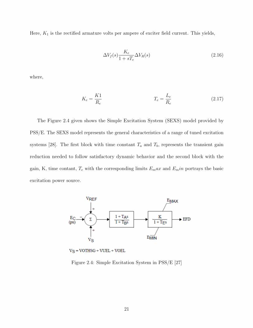
The Figure 2.4 given shows the Simple Excitation System (SEXS) model provided by

PSS/E. The SEXS model represents the general characteristics of a range of tuned excitation

systems [28]. The first block with time constant Ta and Tb, represents the transient gain

reduction needed to follow satisfactory dynamic behavior and the second block with the

gain, K, time contant, Te with the corresponding limits Emax and Emin portrays the basic

excitation power source.

Figure 2.4: Simple Excitation System in PSS/E [27]

21

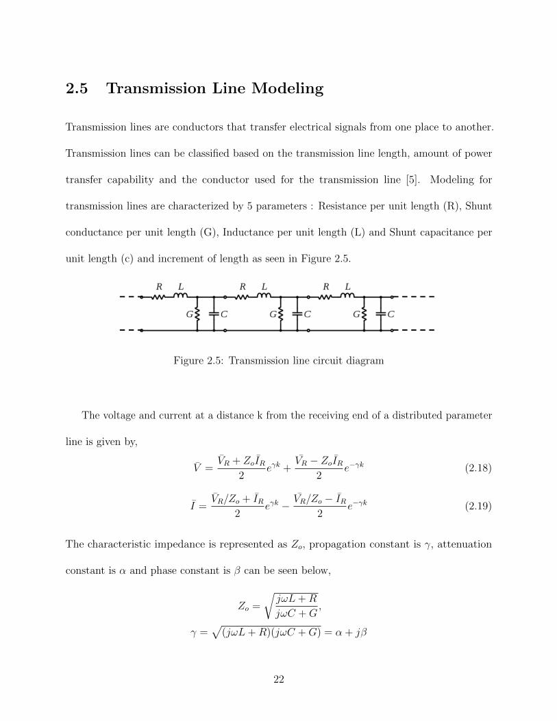
2.5 Transmission Line Modeling

Transmission lines are conductors that transfer electrical signals from one place to another.

Transmission lines can be classified based on the transmission line length, amount of power

transfer capability and the conductor used for the transmission line [5]. Modeling for

transmission lines are characterized by 5 parameters : Resistance per unit length (R), Shunt

conductance per unit length (G), Inductance per unit length (L) and Shunt capacitance per

unit length (c) and increment of length as seen in Figure 2.5.

Figure 2.5: Transmission line circuit diagram

The voltage and current at a distance k from the receiving end of a distributed parameter

line is given by,

V =VR + ZoIR

2eγk +

VR − ZoIR2

e−γk (2.18)

I =VR/Zo + IR

2eγk − VR/Zo − IR

2e−γk (2.19)

The characteristic impedance is represented as Zo, propagation constant is γ, attenuation

constant is α and phase constant is β can be seen below,

Zo =

√jωL+R

jωC +G,

γ =√

(jωL+R)(jωC +G) = α + jβ

22

This study includes π lines in the test system and the voltage and current equations for π

lines are represented as given below, where, S and R represent sending and receiving end of

the transmission line.

VS = VR cosh(γl) + ZcIR sinh(γl) (2.20)

IS = IR cosh(γl) +VRZc

sinh(γl) (2.21)

The characteristic impedance is given by,

Ze = Zo sinh(γl) (2.22)

When γl � 1, then, the transmission line is considered negligble, which gives,

Ze = Zc sinh(γl) ≈ Zcγl ≈ zl = Z (2.23)

and,

Ye2

=1

Zctanh(

γl

2) ≈ 1

Zc

γl

2≈ γl

2=Y

2(2.24)

2.6 Transformer Modeling

A transformer is an electrical device that takes electricity of one voltage and changes it

into another voltage [14]. They are used to change voltage levels as well as to control to

the voltage and reactive power flow. It works on the principle of electromagnetic induction

typically where, the primary is connected to a voltage supply and converts it into a magnetic

field and the secondary then converts the alternating magnetic field into electric power with

23

the required voltage level based on the number of windings in the coils. The equivalent circuit

diagram of a two-winding transformer is shown below in Figure 2.6

Figure 2.6: Diagram of 2-winding transformer

R1 and R2 represent the primary and secondary winding resistance and X1 and X2

represent the primary and secondary winding leakage reactance respectively. Number of turns

in the primary and secondary are n1 and n2.

The voltage at the primary and secondary side is represented as given below,

v1 = Z1i1 +n1

n2

v2 −n1

n2

Z2i2 (2.25)

v2 =n2

n1

v1 −n2

n1

Z1i1 + Z2i2 (2.26)

If we consider the nominal values, the above equation is represented as given below,

v1 = (n1

n1o

)2Z1oi1 +n1

n2

v2 −n1

n2

(n2

n2o

)2Z2oi2 (2.27)

24

v2 =n2

n1

v1 −n2

n1

(n1

n1o

)2Z1oi1 + (n2

n2o

)2Z2oi2 (2.28)

Z1o and Z2o represent the primary and secondary tap position whereas n1o and n2o

represent the primary and secondary number of turns.

The per unit representation of the voltage equations are as seen below,

v1 = n21Z1oi1 +

n1

n2

v2 − n22

n1

n2

Z2oi2 (2.29)

v2 =n2

n1

v1 − n21

n2

n1

Z1oi1 + n22Z2oi2 (2.30)

where,

n1 =n1

n1o

(2.31)

n2 =n2

n2o

(2.32)

Transformer Losses:

The transformer losses mainly comprise of winding and core losses. As the transformer

capacity increases, the transformer efficiency tend to increase. Transformers consists of only

electrical losses.

Core Losses : Core losses or iron losses depend on the magnetic properties of the material

used for the core. Core loss comprises of Hysteresis loss and Eddy current loss. Hysteresis

loss is due to the reversal of magnetization in the core and is given by,

Wh = ηBmax1.6fV (2.33)

25

It can be seen the loss depends on the flux density, Bmax, Volume, V, frequency of magnetic

reversals, f. η is Steinmetz hysteresis constant.

The eddy currents formed due to the induced emf in the core or iron body of the transformer

causes the eddy current loss. The eddy currents dissipate energy in the form of heat.

Copper Loss : Copper loss is caused because of the resistance of the transformer windings.

Copper loss in transformer varies with the load. Copper loss due to the primary is I12R1 and

secondary winding is I22R2. Where, I is the current and R is the resistance and 1 and 2

represent the primary and secondary respectively.

2.7 Load Modeling

A load is a device that is connected to a power system network that consumes power. Load

models represents the mathematical relationship between voltage and power. The voltage is

the input and the power, which can be either active or reactive is the output of the model.

Load models are used to analyze the stability of power systems such as steady state stability,

transient stability, long-term and voltage control. There are different types of load models

that depend on usage such Residential, commercial and industrial. Loads are very difficult to

model as there will be a variation in the load depending on time and practically, there is

no constant load. Loads can be motors, furnaces, appliances, lamps etc. There are different

types of load modeling - static, dynamic or a combination of both [15].

Static Load Models :

Static load models are models that represent the active and reactive powers as a function of the

magnitude and/or frequency of voltage. There are different types of static load models. The

26

most common types are constant power, constant current, constant impedance, polynomial,

exponential, slope values, frequency dependent.

Traditionally, the type of static load model used in the exponential load model which is

shown in Equation 2.34. It is a non-linear model in which the active and reactive power are

related to voltage as an exponential equation. Here, np and nq are parameters of the load

model.

P = PO

(V

VO

)np

(2.34)

Q = QO

(V

VO

)nq

(2.35)

Constant power, constant current and constant impendance models are special cases of the

exponential model.

Constant power load models are models in which the active and reactive powers are a

constant and are independent of the change in voltage. The models can be represented as

given below,

P = PO

(V

VO

)0

= PO (2.36)

Q = QO

(V

VO

)0

= QO (2.37)

Here, np = nq = 0. Similarly, np = nq = 1 for constant current models and np = nq =2 for

constant impedance models.

Dynamic Load Models :

The importance of load models has increased during the last decade. It represents the time

27

and voltage dependence of load. The modeling of dynamic load models is required to study

internal oscillations, stability of voltage and long-term stability analysis. The most commonly

used load models are Induction motor model, state space model and the transfer function

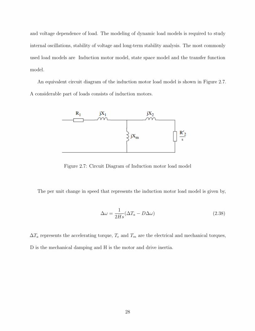
model.

An equivalent circuit diagram of the induction motor load model is shown in Figure 2.7.

A considerable part of loads consists of induction motors.

Figure 2.7: Circuit Diagram of Induction motor load model

The per unit change in speed that represents the induction motor load model is given by,

∆ω =1

2Hs(∆Ta −D∆ω) (2.38)

∆Ta represents the accelerating torque, Te and Tm are the electrical and mechanical torques,

D is the mechanical damping and H is the motor and drive inertia.

28

Chapter 3

Main Focus and Contribution

3.1 Introduction

The focus of this thesis is to use automation to create appropriate models in PSS/E with the

data from the field. This technique is used to find the parameters of an SVC in PSS/E with

the data from the Hardware-in-loop real-time simulation of the SVC physical controller using

Hypersim.

Power system planning is an important aspect in transmission for every utility and

transient stability analysis tools such as PSS/E are most commonly used. It is necessary

to make the models in use as accurate as possible and update them regularly. Python

programming language is used to find the parameters of the SVC model in PSS/E in a fast

and efficient manner. This process ensures that the SVC model in PSS/E behaves similar to

the actual SVC which is represented by the SVC physical controller.

3.1.1 Hypersim

Hypersim is the most advanced system which can simulate over 1000 3-phase buses in real-time

with high precision to study 3-phase electro-magnetic and electro-mechanical transients and

complex events which involves interaction between several controls, protection, HVDC and

29

FACTS System. It is known as the power system simulator of tomorrow with a proven track

record and constant updating to increase its performance, reliability and ease of use. Real-time

simulation enables execution at the same pace as real-world clock. This property allows the

availability of Rapid Control Prototyping (RCP) and Hardware-in-the-loop simulation [31].

3.1.2 SVC Physical Controller

The SVC physical controller or replica is an exact copy of the actual control cubicles installed

on the site. The SVC physical controller in the study is a 0/+300 Mvar SVC with 3 TSC

units. 2 TSCs are three-phase Y configuration and provides 75 Mvar whereas the third TSC

is delta configuration and provides 150 Mvar.

3.1.3 PSS/E

Power System Simulation for Engineering (PSS/E) is a transient stability analysis tool which

is widely used for planning of and analysis of power system networks. PSS/E is composed

of a comprehensive set of programs for studies of power system transmission network and

generation performance in both steady-state and dynamic conditions. PSS/E offers the

ability to drive itself from batch scripts using IPLAN, IDEV, and Python where IPLAN and

IDEV are PSS/E specific batch scripts. From its introduction in 1976, PSS/E has offered

comprehensive modeling capabilities.

30

3.2 Methodology

The methodology of this thesis is to find the parameters of the SVC model in PSS/E to

achieve results similar to that of the results with the SVC physical controller HIL simulation

in Hypersim. There are parameters that are unique to the SVC such as active range of

voltage control loop, size of reactor etc and depends on the design of the SVC needed to be

modeled. The methodology followed in this thesis can be divided into two parts analysis

before the addition of the SVC and analysis after the addition of the SVC model and

parameter manipulation. Analysis of the system before the addition of the SVC is important

as this step is required to reduce the difference between the two software platforms in-order

to clearly analyze the response of the SVC. It includes the steady state analysis and the

dynamics analysis. This forms the base for the rest of the analysis conducted in the thesis.

The generation of the test matrix can be seen in the test system chapter and explains the

selection of test cases. The system is subject to different network disturbances with the

addition of different network elements. This helps us select locations for the SVC that show

the least difference between the two software platforms. Analysis after the addition of SVC

involves applying different three phase bus faults and analyzing the dynamic response of

the SVC model in PSS/E against the SVC physical controller. The parameter manipulation

automation technique is then used to find the right set of parameters for the SVC model in

PSS/E and make its response similar to that of the SVC physical controller. The methodology

followed can be seen in the following sections with their flow charts.

31

3.2.1 Before addition of SVC

3.2.1.1 Steady State Analysis

Steady state studies are restrained to small and gradual changes in the system operating

conditions. It concentrates on restricting the bus voltages to their nominal values and to

make sure that the difference between the bus phase angles between are not too large and

analyzes the overloading power of equipment and transmission lines. This analysis is done

with the use of power flow calculations. The power flow analysis applies to the balanced,

steady-state operation of the power system and deals with positive-sequence models of all

system components.

The basic data required for power flow calculations such as line impedances and charging

admittances, transformer impedances and tap ratios, admittances of shunt connected devices

such as capacitors and reactors, load consumption at each bus, power output and voltage

magnitude of each generator along with its maximum and minimum reactive power outputs

are entered into the system models in Hypersim with modeling of single line diagram of the

test system and/or as raw data in the case of PSS/E. The load flow is calculated and the

results are analyzed. If the results match, we move on to the next phase or we are required

to make changes to the parameters of the network elements such that the power flow results

are similar. This forms the basis of our study as the dynamic analysis is dependent on this.

The IEEE 14 bus system is considered as the test system with the test data shown in

Chapter 4. The data is assigned to the models in PSS/E and Hypersim and the Newton

Raphson load flow analysis is performed. The results such as voltages, line and transformer

32

currents are compared. In our study, the comparison yielded matching results and did not

need any modifications to the parameters - they are shown in chapter 5.

3.2.1.2 Dynamic Analysis

The power flow model is taken as the base case for the dynamic analysis studies. Hypersim

has the ability to run dynamics and generate results with static voltage sources whereas

PSS/E cannot do so without a dynamic element. Therefore, a dynamic element needs to

be added in PSS/E with its appropriate parameters. The dynamic model of a generator is

considered here in this thesis.

The generator dynamic model includes the rotor model, excitation system model, governor

model and stabilizer model. The response of the governor and stabilizer models to electromag-

netic transients are slow and hence only the rotor model and exciter models are included. For

this study, it is necessary to reduce the system dynamics to reduce the differences between

the two software packages.

A near-ideal voltage source is modeled in PSS/E using GENCLS generator and SEXS

exciter models whereas an ideal voltage source is used in Hypersim. The GENCLS generator

model is a constant internal voltage and the SEXS excitation system model is a simplified

excitation systems offered by PSS/E. Parameters are assigned to the models and dynamic

analysis is performed on both the elements.

The generator and exciter models are first tried and analyzed on a three-bus system by

assigning parameters to the models. A three-phase bus fault is applied at Bus-2 and the

results are analyzed. The windowed rms values of the bus voltages are plotted for the analysis.

The 3-bus system modeled is shown in Figure 3.1 and the results can be seen in Figure 3.2.

33

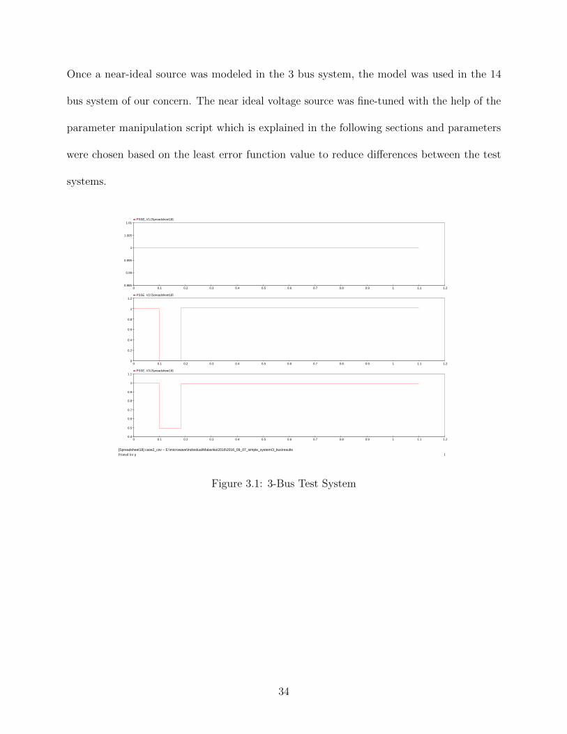
Once a near-ideal source was modeled in the 3 bus system, the model was used in the 14

bus system of our concern. The near ideal voltage source was fine-tuned with the help of the

parameter manipulation script which is explained in the following sections and parameters

were chosen based on the least error function value to reduce differences between the test

systems.

PSSE_V1 [Spreadsheet18]

0 0.1 0.2 0.3 0.4 0.5 0.6 0.7 0.8 0.9 1 1.1 1.20.985

0.99

0.995

1

1.005

1.01

PSSE_V2 [Spreadsheet18]

0 0.1 0.2 0.3 0.4 0.5 0.6 0.7 0.8 0.9 1 1.1 1.20

0.2

0.4

0.6

0.8

1

1.2

PSSE_V3 [Spreadsheet18]

0 0.1 0.2 0.3 0.4 0.5 0.6 0.7 0.8 0.9 1 1.1 1.20.4

0.5

0.6

0.7

0.8

0.9

1

1.1

[Spreadsheet18] case2_csv − E:\microwave\Individual\Malavika\2016\2016_09_07_simple_system\3_bus\resultsPrinted for p 1

Figure 3.1: 3-Bus Test System

34

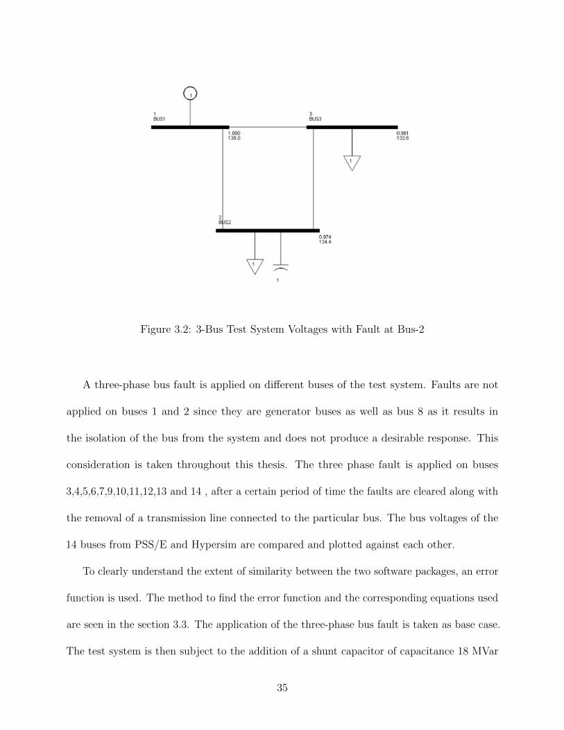
Figure 3.2: 3-Bus Test System Voltages with Fault at Bus-2

A three-phase bus fault is applied on different buses of the test system. Faults are not

applied on buses 1 and 2 since they are generator buses as well as bus 8 as it results in

the isolation of the bus from the system and does not produce a desirable response. This

consideration is taken throughout this thesis. The three phase fault is applied on buses

3,4,5,6,7,9,10,11,12,13 and 14 , after a certain period of time the faults are cleared along with

the removal of a transmission line connected to the particular bus. The bus voltages of the

14 buses from PSS/E and Hypersim are compared and plotted against each other.

To clearly understand the extent of similarity between the two software packages, an error

function is used. The method to find the error function and the corresponding equations used

are seen in the section 3.3. The application of the three-phase bus fault is taken as base case.

The test system is then subject to the addition of a shunt capacitor of capacitance 18 MVar

35

and 45MVar along with the application of bus fault in both software platforms. The addition

of a circuit element forms case 1 and case 2 respectively. Capacitors were chosen as the extra

circuit element as it injects MVar similar to TSC units in the SVC. All the 14 bus voltages

in all three cases were compared against each other. The capacitors are placed on all buses

except the generator buses. This led to 132 cases with 14 bus voltages for each case. The

error function was used to calculate the extent of difference between the 3 cases in PSS/E

and Hypersim. For a bus voltage for a particular fault scenario, if the error of bus voltage

was found to be less than 0.05 pu% in all three cases, then the bus was a viable location

for the SVC. This process was followed in all 132 cases and a test matrix was created with

the optimal location for SVC with the appropriate fault scenario. This method allows us to

find locations which show least variation in both software platforms when the test system is

subject to different network disturbances and changes. When the SVC model or Physical

controller are placed in these locations, their responses can be analyzed easily.

3.2.2 After addition of SVC

Once the optimal placement of the SVC is determined and a test matrix is created, the

simulations are run to find the right parameters and analyze the response of the SVC model

in PSS/E against the HIL simulation of the SVC physical controller in Hypersim. A range of

values are assigned to each parameter from which a parameter set is created for each iteration

and assigned to the SVC.The SVC is then placed at different locations and three phase bus

faults are applied to analyze the dynamic response in both software packages. The 14 bus

voltages were compared against each-other by plotting their responses for a visual analysis as

36

well as the use of the error function for a measurable analysis. The parameters which result

in least error is chosen as the desired set.

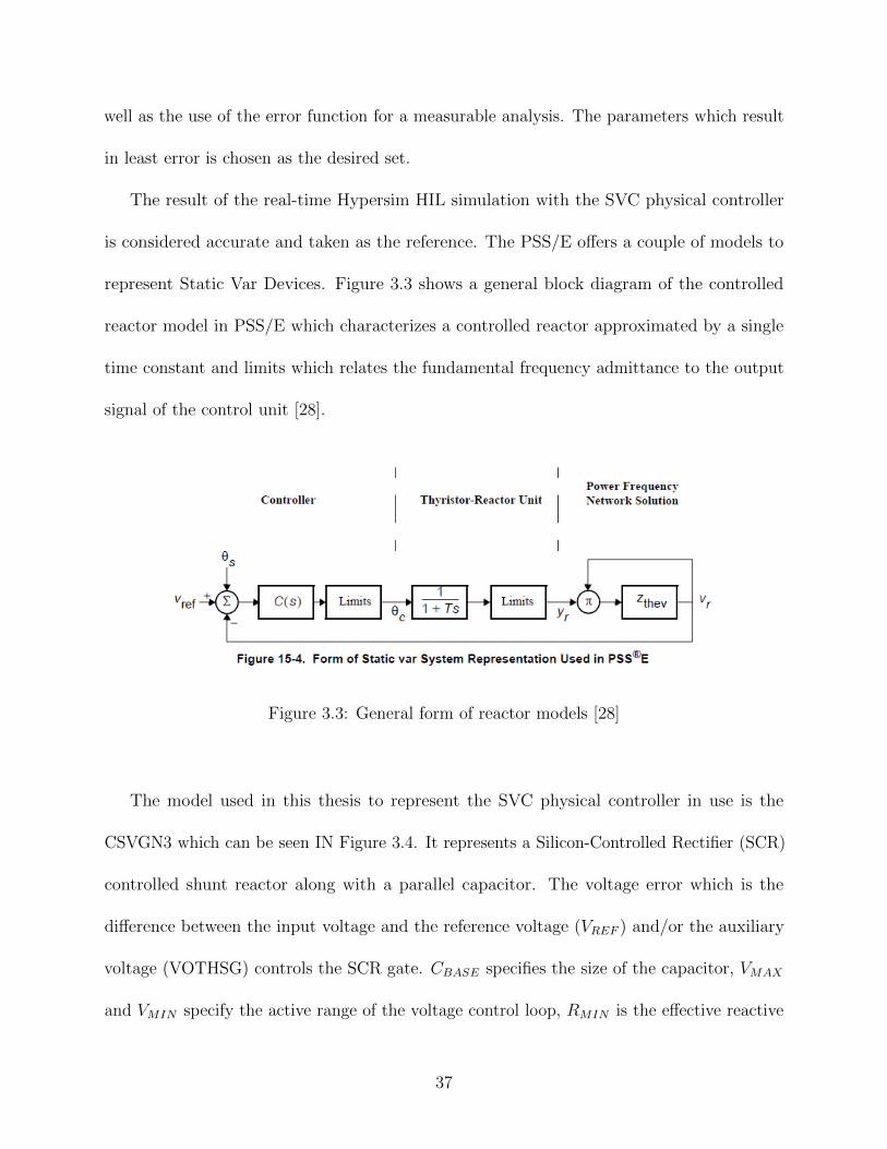
The result of the real-time Hypersim HIL simulation with the SVC physical controller

is considered accurate and taken as the reference. The PSS/E offers a couple of models to

represent Static Var Devices. Figure 3.3 shows a general block diagram of the controlled

reactor model in PSS/E which characterizes a controlled reactor approximated by a single

time constant and limits which relates the fundamental frequency admittance to the output

signal of the control unit [28].

Figure 3.3: General form of reactor models [28]

The model used in this thesis to represent the SVC physical controller in use is the

CSVGN3 which can be seen IN Figure 3.4. It represents a Silicon-Controlled Rectifier (SCR)

controlled shunt reactor along with a parallel capacitor. The voltage error which is the

difference between the input voltage and the reference voltage (VREF ) and/or the auxiliary

voltage (VOTHSG) controls the SCR gate. CBASE specifies the size of the capacitor, VMAX

and VMIN specify the active range of the voltage control loop, RMIN is the effective reactive

37

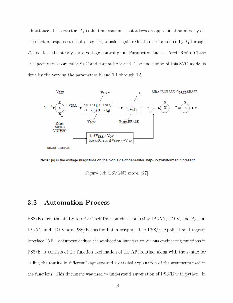
admittance of the reactor. T5 is the time constant that allows an approximation of delays in

the reactors response to control signals, transient gain reduction is represented by T1 through

T4 and K is the steady state voltage control gain. Parameters such as Vref, Rmin, Cbase

are specific to a particular SVC and cannot be varied. The fine-tuning of this SVC model is

done by the varying the parameters K and T1 through T5.

Figure 3.4: CSVGN3 model [27]

3.3 Automation Process

PSS/E offers the ability to drive itself from batch scripts using IPLAN, IDEV, and Python.

IPLAN and IDEV are PSS/E specific batch scripts. The PSS/E Application Program

Interface (API) document defines the application interface to various engineering functions in

PSS/E. It consists of the function explanation of the API routine, along with the syntax for

calling the routine in different languages and a detailed explanation of the arguments used in

the functions. This document was used to understand automation of PSS/E with python. In

38

this thesis, Python is used to automate the dynamics process in PSS/E and then take the

data and results to find the error and plot the voltage waveforms. Python has the ability to

run hundreds of different PSS/E simulations for a given network which is much faster than

executing PSS/E itself [29]. Figure 3.5 shows the flow chart for the automation process of

running dynamics in PSS/E.

Figure 3.5: Flow chart of PSS/E automation

The master code specifies all the buses at which faults need to be applied and the

corresponding lines that need to be disconnected after the removal of the fault. This enables

us to run all the necessary bus faults for a particular scenario or choose the faults that the

study requires. The master code is also used to call the rest of the python files needed to

perform the operations for the three phase faults as well as extract and use the results for

the error function.

39

Once the master code chooses the first fault scenario, the fault application code is called

which takes the *.sav file (saved case file) and the *.dyr file (dynamics data file) along with

the bus fault location and line to be removed. The loadflow function performs the Full

Newton-Raphson method (FNSL) to solve the load flow of the case. The convertlf function

performs the fixed slope decoupled Newton-Raphson power flow calculation (FDNS), converts

generators from power flow representation to prepare for dynamic studies (CONG), calculates

sparsity preserving ordering of buses for processing of network matrices (ORDR),factorizes

the network admittance matrix (FACT), and runs the switching study network solutions

(TYSL).The crtsnap function performs the operations which modifies the network solution

parameters, performs CONG, ORDR, FACT, TYSL and generates the conec, conet and

compile file. The tstep function performs the operations which again performs the CONG,

ORDR, FACT & TYSL and starts the process for fault application with a specified time

step. It specifies the time at which the bus fault is applied and its duration. It runs the

case (steady-state) for a specified amount of time (psspy.run()) and then applies a very large

negative shunt impedance on a given bus (psspy.shunt data) for another specified duration.

A transmission line is then disconnected (psspy.branch data()) and the bus fault is removed.

The shunt impedance (if present in the bus) is re-attached to the bus (psspy.shunt data()).

The duration of the entire simulation is also specified. A case.out file is generated at the

end of the simulation.The assign channels function assigns all the channels that is included

in the case.out file. It includes the Mvar output of the SVC (psspy.machine array channel)

and all the voltages of the 14 buses (psspy.voltage channel). Save txt function then converts

the case.out file into a text file. All the functions are called in the order of the function

explanations.

40

The trim code helps modify the data in to a usable format for plotting and data

manipulation. The data contains the voltage and Mvar values and the corresponding

time throughout simulation run. This is the process used to run the dynamic simulation in

PSS/E with Python.

The results obtained from PSS/E then need to be compared against the already available

Hypersim results. Since there are no changes made to the parameters in Hypersim, the results

always remain the same and are accessed when needed. The comparison process starts with

finding the error function value. The Mvar and voltage data from both software platforms

are linearly interpolated into a common time frame. For each bus fault, the absolute values

of the difference between the interpolated values of Hypersim and PSS/E are added together

and averaged by the total number of values taken during the difference calculation. The

error function which is the error in terms of parameters, the total error by bus faults are

taken and averaged by the number of bus faults. These errors have a unit of per unit percent.

Equation 3.1 represents the error difference for each bus fault and Equation 3.2 represents

the error difference for a set of parameters.

(Error by bus fault)B =

∑N1 |VPSS/E(t)− VHypersim(t)|

N× 100 (3.1)

(Error by parameters) =

∑B1 (Error by bus fault)

B(3.2)

In Equation 3.1 and Equation 3.2 B represents the number of bus faults and N represents

the number of voltage points taken for the difference calculation. These errors are then

tabulated in ascending order along with the corresponding parameters for easy analysis of

the results. The error function is expressed in percent per unit or pcu.

41

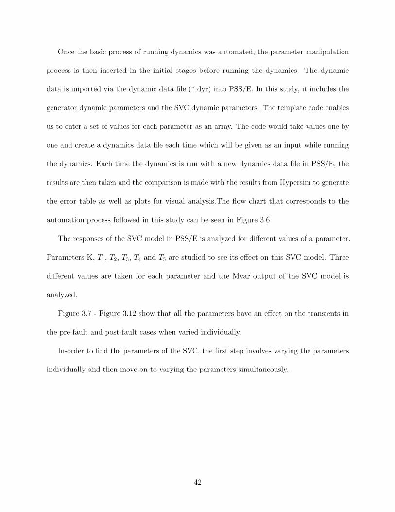
Once the basic process of running dynamics was automated, the parameter manipulation

process is then inserted in the initial stages before running the dynamics. The dynamic

data is imported via the dynamic data file (*.dyr) into PSS/E. In this study, it includes the

generator dynamic parameters and the SVC dynamic parameters. The template code enables

us to enter a set of values for each parameter as an array. The code would take values one by

one and create a dynamics data file each time which will be given as an input while running

the dynamics. Each time the dynamics is run with a new dynamics data file in PSS/E, the

results are then taken and the comparison is made with the results from Hypersim to generate

the error table as well as plots for visual analysis.The flow chart that corresponds to the

automation process followed in this study can be seen in Figure 3.6

The responses of the SVC model in PSS/E is analyzed for different values of a parameter.

Parameters K, T1, T2, T3, T4 and T5 are studied to see its effect on this SVC model. Three

different values are taken for each parameter and the Mvar output of the SVC model is

analyzed.

Figure 3.7 - Figure 3.12 show that all the parameters have an effect on the transients in

the pre-fault and post-fault cases when varied individually.

In-order to find the parameters of the SVC, the first step involves varying the parameters

individually and then move on to varying the parameters simultaneously.

42

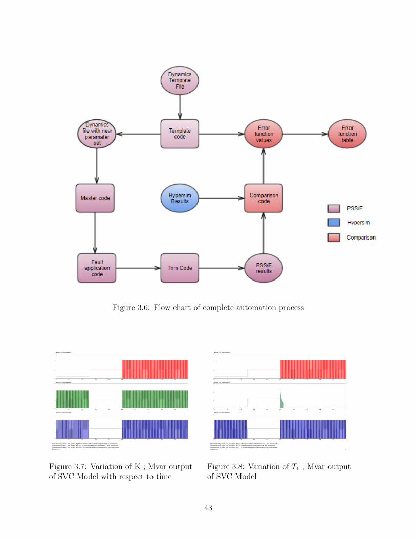
Figure 3.6: Flow chart of complete automation process

Mvar_Ka [Spreadsheet1]

0 0.1 0.2 0.3 0.4 0.5 0.6 0.7 0.8 0.9 10

2

4

6

Mvar_Kb [Spreadsheet2]

0 0.1 0.2 0.3 0.4 0.5 0.6 0.7 0.8 0.9 10

2

4

6

Mvar_Kc [Spreadsheet3]

0 0.1 0.2 0.3 0.4 0.5 0.6 0.7 0.8 0.9 10

2

4

6

[Spreadsheet1] case11_csv_svc@4_k@50 − E:\Individual\Malavika\Thesis\psse\14_bus_tests\results[Spreadsheet2] case11_csv_svc@4_k@100 − E:\Individual\Malavika\Thesis\psse\14_bus_tests\results[Spreadsheet3] case11_csv_svc@4_k@1000 − E:\Individual\Malavika\Thesis\psse\14_bus_tests\results

Printed for p 1

Figure 3.7: Variation of K ; Mvar outputof SVC Model with respect to time

Mvar_T1a [Spreadsheet5]

0 0.1 0.2 0.3 0.4 0.5 0.6 0.7 0.8 0.9 10

2

4

6

Mvar_T1b [Spreadsheet6]

0 0.1 0.2 0.3 0.4 0.5 0.6 0.7 0.8 0.9 10

2

4

6

Mvar_T1c [Spreadsheet7]

0 0.1 0.2 0.3 0.4 0.5 0.6 0.7 0.8 0.9 10

2

4

6

[Spreadsheet5] case11_csv_svc@4_t1@0_01 − E:\Individual\Malavika\Thesis\psse\14_bus_tests\results[Spreadsheet6] case11_csv_svc@4_t1@0 − E:\Individual\Malavika\Thesis\psse\14_bus_tests\results[Spreadsheet7] case11_csv_svc@4_t1@0_3 − E:\Individual\Malavika\Thesis\psse\14_bus_tests\results

Printed for p 1

Figure 3.8: Variation of T1 ; Mvar outputof SVC Model

43

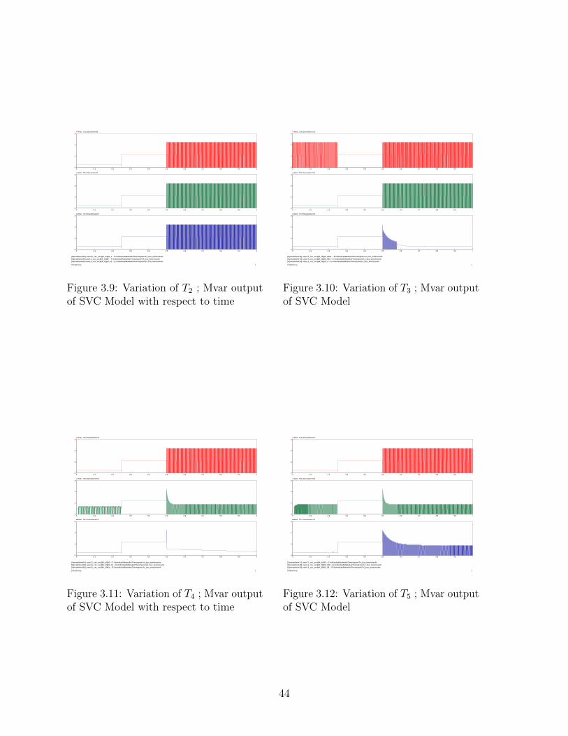
Mvar_T2a [Spreadsheet8]

0 0.1 0.2 0.3 0.4 0.5 0.6 0.7 0.8 0.9 10

2

4

6

Mvar_T2b [Spreadsheet9]

0 0.1 0.2 0.3 0.4 0.5 0.6 0.7 0.8 0.9 10

2

4

6

Mvar_T2c [Spreadsheet10]

0 0.1 0.2 0.3 0.4 0.5 0.6 0.7 0.8 0.9 10

2

4

6

[Spreadsheet10] case11_csv_svc@4_t2@0_1 − E:\Individual\Malavika\Thesis\psse\14_bus_tests\results[Spreadsheet8] case11_csv_svc@4_t2@0 − E:\Individual\Malavika\Thesis\psse\14_bus_tests\results[Spreadsheet9] case11_csv_svc@4_t2@0_01 − E:\Individual\Malavika\Thesis\psse\14_bus_tests\results

Printed for p 1

Figure 3.9: Variation of T2 ; Mvar outputof SVC Model with respect to time

Mvar_T3a [Spreadsheet11]

0 0.1 0.2 0.3 0.4 0.5 0.6 0.7 0.8 0.9 10

2

4

6

Mvar_T3b [Spreadsheet12]

0 0.1 0.2 0.3 0.4 0.5 0.6 0.7 0.8 0.9 10

2

4

6

Mvar_T3c [Spreadsheet13]

0 0.1 0.2 0.3 0.4 0.5 0.6 0.7 0.8 0.9 10

2

4

6

[Spreadsheet11] case11_csv_svc@4_t3@0_0001 − E:\Individual\Malavika\Thesis\psse\14_bus_tests\results[Spreadsheet12] case11_csv_svc@4_t3@0_093 − E:\Individual\Malavika\Thesis\psse\14_bus_tests\results[Spreadsheet13] case11_csv_svc@4_t3@0_3 − E:\Individual\Malavika\Thesis\psse\14_bus_tests\results

Printed for p 1

Figure 3.10: Variation of T3 ; Mvar outputof SVC Model

Mvar_T4a [Spreadsheet14]

0 0.1 0.2 0.3 0.4 0.5 0.6 0.7 0.8 0.9 10

2

4

6

Mvar_T4b [Spreadsheet15]

0 0.1 0.2 0.3 0.4 0.5 0.6 0.7 0.8 0.9 10

2

4

6

Mvar_T4c [Spreadsheet16]

0 0.1 0.2 0.3 0.4 0.5 0.6 0.7 0.8 0.9 10

2

4

6

[Spreadsheet14] case11_csv_svc@4_t4@0 − E:\Individual\Malavika\Thesis\psse\14_bus_tests\results[Spreadsheet15] case11_csv_svc@4_t4@0_01 − E:\Individual\Malavika\Thesis\psse\14_bus_tests\results[Spreadsheet16] case11_csv_svc@4_t4@1 − E:\Individual\Malavika\Thesis\psse\14_bus_tests\results

Printed for p 1

Figure 3.11: Variation of T4 ; Mvar outputof SVC Model with respect to time

Mvar_T5a [Spreadsheet17]

0 0.1 0.2 0.3 0.4 0.5 0.6 0.7 0.8 0.9 10

2

4

6

Mvar_T5b [Spreadsheet18]

0 0.1 0.2 0.3 0.4 0.5 0.6 0.7 0.8 0.9 10

2

4

6

Mvar_T5c [Spreadsheet19]

0 0.1 0.2 0.3 0.4 0.5 0.6 0.7 0.8 0.9 10

2

4

6

[Spreadsheet17] case11_csv_svc@4_t5@0 − E:\Individual\Malavika\Thesis\psse\14_bus_tests\results[Spreadsheet18] case11_csv_svc@4_t5@0_009 − E:\Individual\Malavika\Thesis\psse\14_bus_tests\results[Spreadsheet19] case11_csv_svc@4_t5@0_05 − E:\Individual\Malavika\Thesis\psse\14_bus_tests\results

Printed for p 1

Figure 3.12: Variation of T5 ; Mvar outputof SVC Model

44

Chapter 4

Test System

4.1 Introduction

This thesis uses the IEEE 14 bus system as the test system. The standard IEEE 14 bus

test case represents a portion of the American Electric Power System (in the Midwestern

US) as of February, 1962. The system consists of 14 buses, 5 synchronous machines, 3 of

which are synchronous compensators and 11 loads. It has a shunt capacitor and a total of 3

transformers of which, 2 are two-winding transformers and 1 is a three-winding transformer.

For simplicity, we consider a two-winding equivalent of the three-winding transformer which

leads to a total of 18 transmission lines. The total load of the system is 254 MW and 73.5

Mvar and has a base voltage of 138 kV with a 100 MVA base power. The basis of this

thesis involves the comparison of the transient stability software, PSS/E against the real-time

software, Hypersim. Th difference are reduced by reducing the system dynamics and hence

the synchronous generators are replaced by near-ideal generators or ideal voltage sources.

The voltage sources are placed on Bus 1 and Bus 2 with Bus 1 considered as the slack bus.

The test system can be seen in Figure 4.1.

45

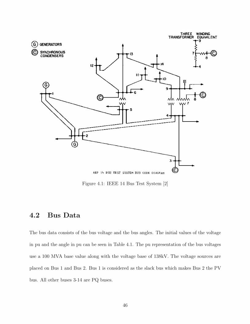
Figure 4.1: IEEE 14 Bus Test System [2]

4.2 Bus Data

The bus data consists of the bus voltage and the bus angles. The initial values of the voltage

in pu and the angle in pu can be seen in Table 4.1. The pu representation of the bus voltages

use a 100 MVA base value along with the voltage base of 138kV. The voltage sources are

placed on Bus 1 and Bus 2. Bus 1 is considered as the slack bus which makes Bus 2 the PV

bus. All other buses 3-14 are PQ buses.

46

Table 4.1: Bus Data

Bus Base Voltage (kV) Voltage (pu) Angle (Deg)

1 138 1.06000 0.0000

2 138 1.04500 -4.9826

3 138 1.01000 -12.7250

4 138 1.01767 -10.3128

5 138 1.01951 -8.7738

6 138 1.07000 -14.2209

7 138 1.06152 -13.3596

8 138 1.09000 -13.3596

9 138 1.05593 -14.9385

10 138 1.05099 -15.0972

11 138 1.05691 -14.7906

12 138 1.05591 -15.0755

13 138 1.05038 -15.1562

14 138 1.03553 -16.0336

4.3 Transmission lines

Parameters such as resistance, inductance, capacitance and conductance helps in the modelling

of transmission lines. These parameters form the line impedance and the line admittance

(susceptance) and are dependent on the type of conductor used and the length of the

transmission line. Table 4.2 shows the transmission line parameters for the 17 lines in the

14-bus system. In this study, all transmission lines are considered as π lines and the double

line between Bus 1 and Bus 2 is replaced by a single transmission line.

47

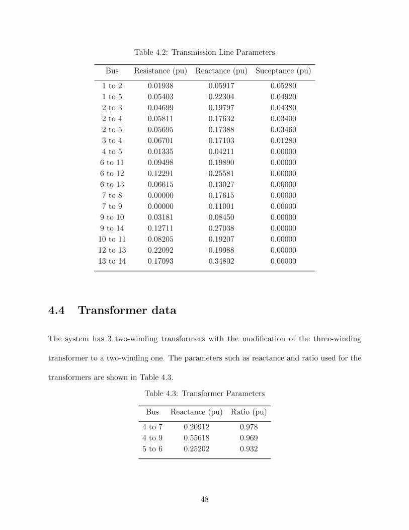
Table 4.2: Transmission Line Parameters

Bus Resistance (pu) Reactance (pu) Suceptance (pu)

1 to 2 0.01938 0.05917 0.05280

1 to 5 0.05403 0.22304 0.04920

2 to 3 0.04699 0.19797 0.04380

2 to 4 0.05811 0.17632 0.03400

2 to 5 0.05695 0.17388 0.03460

3 to 4 0.06701 0.17103 0.01280

4 to 5 0.01335 0.04211 0.00000

6 to 11 0.09498 0.19890 0.00000

6 to 12 0.12291 0.25581 0.00000

6 to 13 0.06615 0.13027 0.00000

7 to 8 0.00000 0.17615 0.00000

7 to 9 0.00000 0.11001 0.00000

9 to 10 0.03181 0.08450 0.00000

9 to 14 0.12711 0.27038 0.00000

10 to 11 0.08205 0.19207 0.00000

12 to 13 0.22092 0.19988 0.00000

13 to 14 0.17093 0.34802 0.00000

4.4 Transformer data

The system has 3 two-winding transformers with the modification of the three-winding

transformer to a two-winding one. The parameters such as reactance and ratio used for the

transformers are shown in Table 4.3.

Table 4.3: Transformer Parameters

Bus Reactance (pu) Ratio (pu)

4 to 7 0.20912 0.978

4 to 9 0.55618 0.969

5 to 6 0.25202 0.932

48

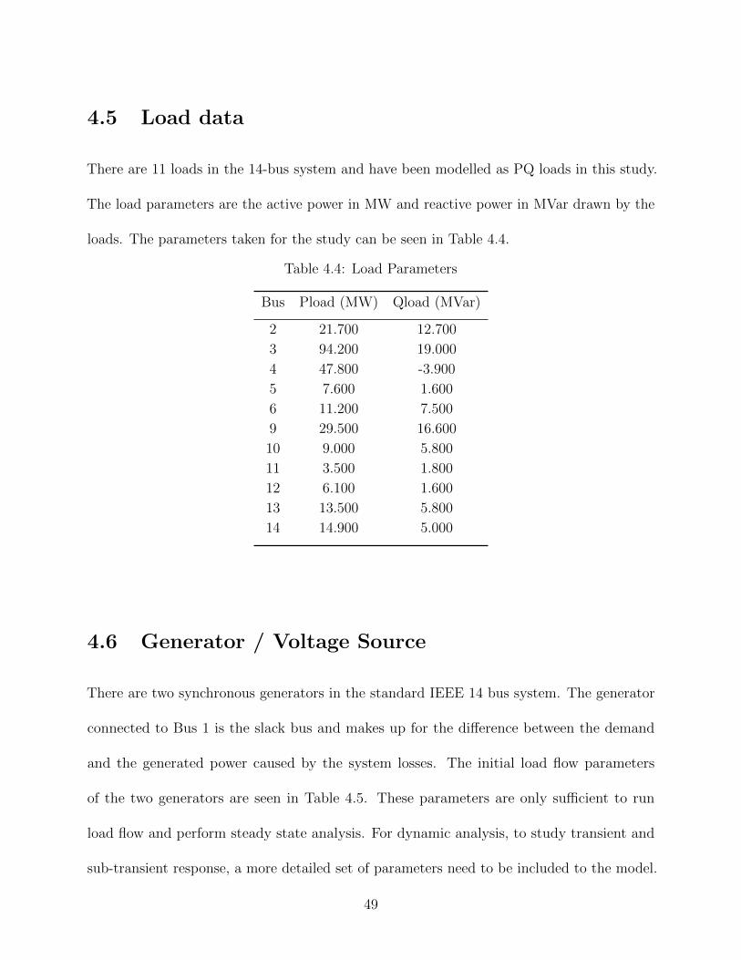
4.5 Load data

There are 11 loads in the 14-bus system and have been modelled as PQ loads in this study.

The load parameters are the active power in MW and reactive power in MVar drawn by the

loads. The parameters taken for the study can be seen in Table 4.4.

Table 4.4: Load Parameters

Bus Pload (MW) Qload (MVar)

2 21.700 12.700

3 94.200 19.000

4 47.800 -3.900

5 7.600 1.600

6 11.200 7.500

9 29.500 16.600

10 9.000 5.800

11 3.500 1.800

12 6.100 1.600

13 13.500 5.800

14 14.900 5.000

4.6 Generator / Voltage Source

There are two synchronous generators in the standard IEEE 14 bus system. The generator

connected to Bus 1 is the slack bus and makes up for the difference between the demand

and the generated power caused by the system losses. The initial load flow parameters

of the two generators are seen in Table 4.5. These parameters are only sufficient to run

load flow and perform steady state analysis. For dynamic analysis, to study transient and

sub-transient response, a more detailed set of parameters need to be included to the model.

49

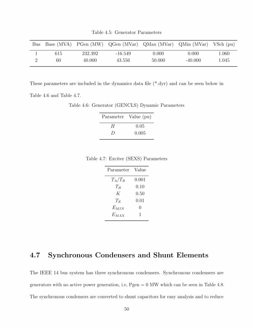
Table 4.5: Generator Parameters

Bus Base (MVA) PGen (MW) QGen (MVar) QMax (MVar) QMin (MVar) VSch (pu)

1 615 232.392 -16.549 0.000 0.000 1.060

2 60 40.000 43.556 50.000 -40.000 1.045

These parameters are included in the dynamics data file (*.dyr) and can be seen below in

Table 4.6 and Table 4.7.

Table 4.6: Generator (GENCLS) Dynamic Parameters

Parameter Value (pu)

H 0.05

D 0.005

Table 4.7: Exciter (SEXS) Parameters

Parameter Value

TA/TB 0.001

TB 0.10

K 0.50

TE 0.01

EMIN 0

EMAX 1

4.7 Synchronous Condensers and Shunt Elements

The IEEE 14 bus system has three synchronous condensers. Synchronous condensers are

generators with no active power generation, i.e, Pgen = 0 MW which can be seen in Table 4.8.

The synchronous condensers are converted to shunt capacitors for easy analysis and to reduce

50

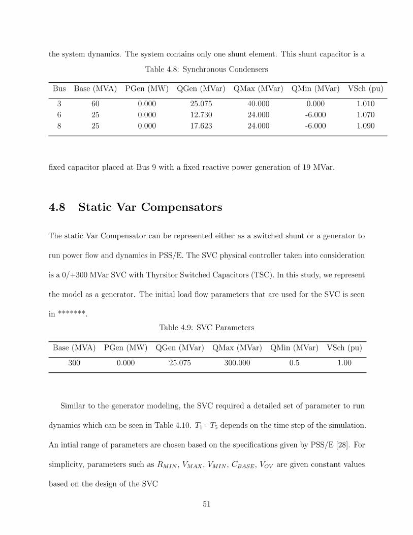
the system dynamics. The system contains only one shunt element. This shunt capacitor is a

Table 4.8: Synchronous Condensers

Bus Base (MVA) PGen (MW) QGen (MVar) QMax (MVar) QMin (MVar) VSch (pu)

3 60 0.000 25.075 40.000 0.000 1.010

6 25 0.000 12.730 24.000 -6.000 1.070

8 25 0.000 17.623 24.000 -6.000 1.090

fixed capacitor placed at Bus 9 with a fixed reactive power generation of 19 MVar.

4.8 Static Var Compensators

The static Var Compensator can be represented either as a switched shunt or a generator to

run power flow and dynamics in PSS/E. The SVC physical controller taken into consideration

is a 0/+300 MVar SVC with Thyrsitor Switched Capacitors (TSC). In this study, we represent

the model as a generator. The initial load flow parameters that are used for the SVC is seen

in *******.

Table 4.9: SVC Parameters

Base (MVA) PGen (MW) QGen (MVar) QMax (MVar) QMin (MVar) VSch (pu)

300 0.000 25.075 300.000 0.5 1.00

Similar to the generator modeling, the SVC required a detailed set of parameter to run

dynamics which can be seen in Table 4.10. T1 - T5 depends on the time step of the simulation.

An intial range of parameters are chosen based on the specifications given by PSS/E [28]. For

simplicity, parameters such as RMIN , VMAX , VMIN , CBASE, VOV are given constant values

based on the design of the SVC

51

Table 4.10: SVC (CSVGN3) dynamic Parameters

Parameter Value Range

K > 50 and < 1000

T1 <0.5

T2 <0.5

T3 <1=0.5

T4 <0.5

T5 < 0.05

RMIN Admittance of reactor

VMAX Maximum value of Voltage control loop

VMIN Minimum value of Voltage control loop

CBASE Size of capacitor < 500

VOV Over ride Voltage ≤ 0.5

52

Chapter 5

Analysis of Results

5.1 Introduction

For the analyzing the system in PSS/E against the HIL simulation of the system in Hypersim,

the 14 bus voltages, Mvar output of the SVC and the transmission line currents were taken

as the data for comparison. The fault is applied at 0.25 secs and cleared at 0.5 secs with a

total run time of 1 sec.

5.2 Test Case Model

The modified IEEE 14 bus system modeled in PSS/E and Hypersim can be seen in Figure 5.1

and Figure 5.2. The test system in Hypersim displays the fault breakers for all scenarios of

bus faults analyzed in this study. with the near-ideal voltage source and ideal voltage source.

The test case was modeled with the control blocks present in the software with Graphical

User Interface to enter the parameters in the case of Hypersim and as raw data in PSS/E

which can later be used to generate the one-line diagram in PSS/E. For the dynamic analysis,

built-in block for GENCLS and SEXS were present in PSS/E.

53

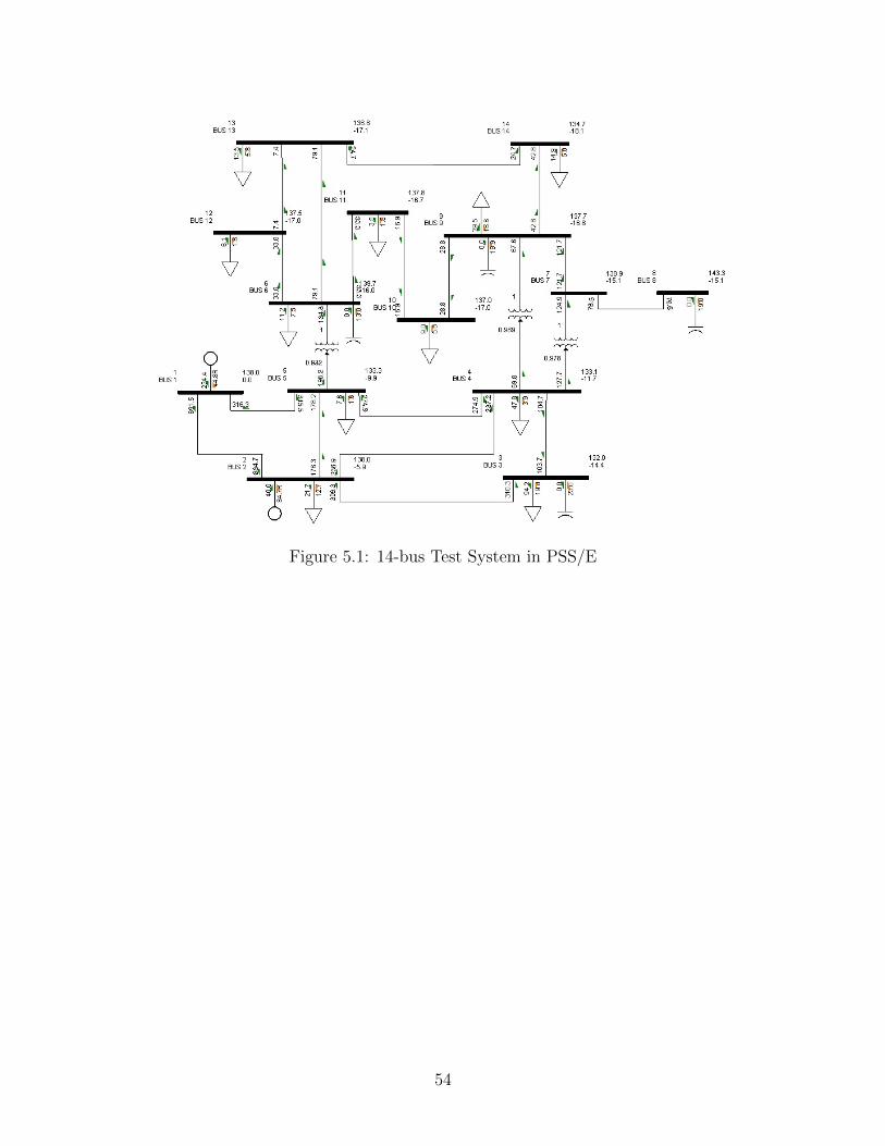
Figure 5.1: 14-bus Test System in PSS/E

54

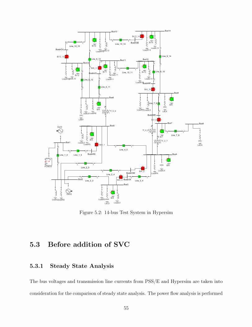
Bus2

Bus1

Bus3

Π

2 1

Line_2_3

Bus4

Π

2 1

Line_3_4

Π

2 1

Line_2_4Π

2 1

Line_1_5

Π

2 1

Line_2_5

Bus5

Π

2 1

Line_4_5

LoadR4

LoadC4

LoadR5LoadL5

LoadR2LoadL2 LoadR3

LoadL3

Π

2

1

Line_1_2

Bus6

Bus7 Bus8

Π

2 1

Line_7_8

LoadR6LoadL6

Bus9

Bus10

Π

2

1

Line_9_10

Π

2 1

Line_10_11

Bus11

Π

2

1

Line_6_11

Bus12

Bus13 Bus14

Π

2

1

Line_6_12

Π

2 1

Line_12_13

Π

2 1

Line_13_14

Π

2

1

Line_9_14

LoadR13LoadL13

LoadR12LoadL12

LoadR9LoadL9

LoadR10

LoadL10LoadR11

LoadL11

LoadR14LoadL14

Π

2

1

Line_7_9

Π

2

1

Line_6_13

A

PD

POWUV

1

2

Tf_4_7

1

2

Tf_4_9

1

2

Tf_5_6

P

Br3

P

Br3_4

LdLD

LdLN

LdLX

LdM7

Busbr34

P

Br5

P

Br6

P

Br7

P

Br9

P

Br10

P

Br11

P

Br12

P

Br14

P

Br13

P

Br4_2BusbrOW

PBr5_1

BusbrK9

PBr6_11

BusbrLS

PBr7_9

BusbrMK

PBr9_10

BusbrNP

PBr12_13

BusbrOU

PBr13_14

BusbrQE

P

Br4

Ge03

Ge0G

Figure 5.2: 14-bus Test System in Hypersim

5.3 Before addition of SVC

5.3.1 Steady State Analysis

The bus voltages and transmission line currents from PSS/E and Hypersim are taken into

consideration for the comparison of steady state analysis. The power flow analysis is performed

55

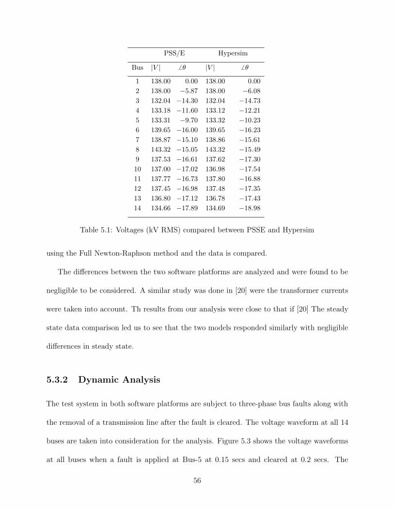
PSS/E Hypersim

Bus |V | 6 θ |V | 6 θ

1 138.00 0.00 138.00 0.00

2 138.00 −5.87 138.00 −6.083 132.04 −14.30 132.04 −14.734 133.18 −11.60 133.12 −12.215 133.31 −9.70 133.32 −10.236 139.65 −16.00 139.65 −16.237 138.87 −15.10 138.86 −15.618 143.32 −15.05 143.32 −15.499 137.53 −16.61 137.62 −17.3010 137.00 −17.02 136.98 −17.5411 137.77 −16.73 137.80 −16.8812 137.45 −16.98 137.48 −17.3513 136.80 −17.12 136.78 −17.4314 134.66 −17.89 134.69 −18.98

Table 5.1: Voltages (kV RMS) compared between PSSE and Hypersim

using the Full Newton-Raphson method and the data is compared.

The differences between the two software platforms are analyzed and were found to be

negligible to be considered. A similar study was done in [20] were the transformer currents

were taken into account. Th results from our analysis were close to that if [20] The steady

state data comparison led us to see that the two models responded similarly with negligible

differences in steady state.

5.3.2 Dynamic Analysis

The test system in both software platforms are subject to three-phase bus faults along with

the removal of a transmission line after the fault is cleared. The voltage waveform at all 14

buses are taken into consideration for the analysis. Figure 5.3 shows the voltage waveforms

at all buses when a fault is applied at Bus-5 at 0.15 secs and cleared at 0.2 secs. The

56

Line PSS/E Hypersim

1 to 2 691.2 691.99

1 to 5 316.1 315.49

2 to 3 308.3 309.58

2 to 4 236.7 236.99

2 to 5 176.3 177.60

3 to 4 102.2 104.76

4 to 5 273.8 274.33

6 to 11 33.3 33.27

6 to 12 33.6 33.80

6 to 13 78.9 79.13

7 to 8 76.6 76.68

7 to 9 121.2 121.99

9 to 10 28.7 28.91

9 to 14 42.6 42.83

10 to 11 16.9 16.61

12 to 13 7.4 7.43

13 to 14 24.7 24.66

Table 5.2: Currents (A RMS) compared between PSSE and Hypersim

voltage waveforms from PSS/E and Hypersim are overlapped against eachother for a clear

understanding.

The bus fault scenario can be split into three cases : Pre-fault, fault and Post-fault. The

source voltage used in both the software are ideal or near-ideal source and hence there are

no transients in either of the response during the pre-fault case. PSS/E always starts from

steady state conditions irrespective of the source modeled. During fault, the response in

both platforms are almost the same. The voltage dip has some differences in certain bus

voltages and can be neglected. The voltage drop in the case of Hypersim in ramped due to

the resistance in the breaker in the Hypersim software. Once the fault is cleared, both the

softwares retain the same steady state condition. The ramped increase again can be seen in

Hypersim during fault clearing.

57

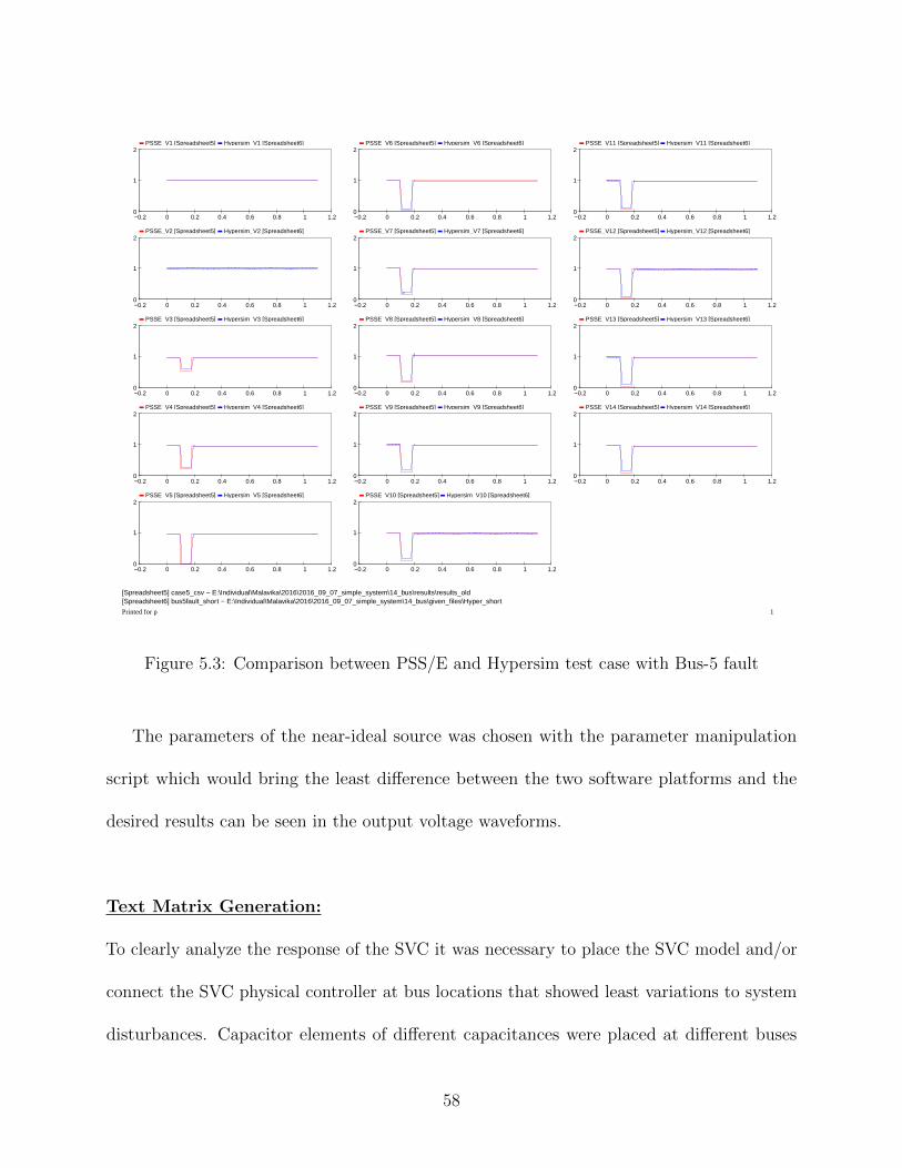
PSSE_V1 [Spreadsheet5] Hypersim_V1 [Spreadsheet6]

−0.2 0 0.2 0.4 0.6 0.8 1 1.20

1

2

PSSE_V2 [Spreadsheet5] Hypersim_V2 [Spreadsheet6]

−0.2 0 0.2 0.4 0.6 0.8 1 1.20

1

2

PSSE_V3 [Spreadsheet5] Hypersim_V3 [Spreadsheet6]

−0.2 0 0.2 0.4 0.6 0.8 1 1.20

1

2

PSSE_V4 [Spreadsheet5] Hypersim_V4 [Spreadsheet6]

−0.2 0 0.2 0.4 0.6 0.8 1 1.20

1

2

PSSE_V5 [Spreadsheet5] Hypersim_V5 [Spreadsheet6]

−0.2 0 0.2 0.4 0.6 0.8 1 1.20

1

2

PSSE_V6 [Spreadsheet5] Hypersim_V6 [Spreadsheet6]

−0.2 0 0.2 0.4 0.6 0.8 1 1.20

1

2

PSSE_V7 [Spreadsheet5] Hypersim_V7 [Spreadsheet6]

−0.2 0 0.2 0.4 0.6 0.8 1 1.20

1

2

PSSE_V8 [Spreadsheet5] Hypersim_V8 [Spreadsheet6]

−0.2 0 0.2 0.4 0.6 0.8 1 1.20

1

2

PSSE_V9 [Spreadsheet5] Hypersim_V9 [Spreadsheet6]

−0.2 0 0.2 0.4 0.6 0.8 1 1.20

1

2

PSSE_V10 [Spreadsheet5] Hypersim_V10 [Spreadsheet6]

−0.2 0 0.2 0.4 0.6 0.8 1 1.20

1

2

PSSE_V11 [Spreadsheet5] Hypersim_V11 [Spreadsheet6]

−0.2 0 0.2 0.4 0.6 0.8 1 1.20

1

2

PSSE_V12 [Spreadsheet5] Hypersim_V12 [Spreadsheet6]

−0.2 0 0.2 0.4 0.6 0.8 1 1.20

1

2

PSSE_V13 [Spreadsheet5] Hypersim_V13 [Spreadsheet6]

−0.2 0 0.2 0.4 0.6 0.8 1 1.20

1

2

PSSE_V14 [Spreadsheet5] Hypersim_V14 [Spreadsheet6]

−0.2 0 0.2 0.4 0.6 0.8 1 1.20

1

2

[Spreadsheet5] case5_csv − E:\Individual\Malavika\2016\2016_09_07_simple_system\14_bus\results\results_old[Spreadsheet6] bus5fault_short − E:\Individual\Malavika\2016\2016_09_07_simple_system\14_bus\given_files\Hyper_short

Printed for p 1

Figure 5.3: Comparison between PSS/E and Hypersim test case with Bus-5 fault

The parameters of the near-ideal source was chosen with the parameter manipulation

script which would bring the least difference between the two software platforms and the

desired results can be seen in the output voltage waveforms.

Text Matrix Generation:

To clearly analyze the response of the SVC it was necessary to place the SVC model and/or

connect the SVC physical controller at bus locations that showed least variations to system

disturbances. Capacitor elements of different capacitances were placed at different buses

58

along with the fault scenarios. The voltage waveform of the base case along with the 2 other

cases with the addition of capacitor elements can be seen in Figure 5.4. In Figure 5.4 three

cases have been overlapped against each other - The first one is the base case i.e., the test

system, the second one is the test system along with a 18Mvar capacitor at Bus-4 and the

third with a 45 Mvar capacitor at Bus-4. A fault is applied on Bus-5 on the test cases in

PSS/E and Hypersim.

0.0 0.2 0.4 0.6 0.8 1.0 1.2

0.0005,0.0005,0.0005

0.0

0.5

1.0

1.5

2.0Bus 1 Voltages

0.0 0.2 0.4 0.6 0.8 1.0 1.2

0.0006,0.0006,0.0006

0.0

0.5

1.0

1.5

2.0Bus 2 Voltages

0.0 0.2 0.4 0.6 0.8 1.0 1.2

0.0728,0.0729,0.073

0.0

0.5

1.0

1.5

2.0Bus 3 Voltages

0.0 0.2 0.4 0.6 0.8 1.0 1.2

0.026,0.0263,0.0267

0.0

0.5

1.0

1.5

2.0Bus 4 Voltages

0.0 0.2 0.4 0.6 0.8 1.0 1.2

0.0001,0.0001,0.0001

0.0

0.5

1.0

1.5

2.0Bus 5 Voltages

0.0 0.2 0.4 0.6 0.8 1.0 1.2

0.0443,0.0445,0.0448

0.0

0.5

1.0

1.5

2.0Bus 6 Voltages

0.0 0.2 0.4 0.6 0.8 1.0 1.2

0.0604,0.0607,0.0611

0.0

0.5

1.0

1.5

2.0Bus 7 Voltages

0.0 0.2 0.4 0.6 0.8 1.0 1.2

0.0631,0.0634,0.0638

0.0

0.5

1.0

1.5

2.0Bus 8 Voltages

0.0 0.2 0.4 0.6 0.8 1.0 1.2

0.0694,0.0697,0.0701

0.0

0.5

1.0

1.5

2.0Bus 9 Voltages

0.0 0.2 0.4 0.6 0.8 1.0 1.2

0.0692,0.0695,0.0699

0.0

0.5

1.0

1.5

2.0Bus 10 Voltages

0.0 0.2 0.4 0.6 0.8 1.0 1.2

0.0579,0.0581,0.0585

0.0

0.5

1.0

1.5

2.0Bus 11 Voltages

0.0 0.2 0.4 0.6 0.8 1.0 1.2

0.0508,0.051,0.0513

0.0

0.5

1.0

1.5

2.0Bus 12 Voltages

0.0 0.2 0.4 0.6 0.8 1.0 1.2

0.0535,0.0537,0.0541

0.0

0.5

1.0

1.5

2.0Bus 13 Voltages

0.0 0.2 0.4 0.6 0.8 1.0 1.2

0.0719,0.0722,0.0727

0.0

0.5

1.0

1.5

2.0Bus 14 Voltages

RMS vs. Time (s), Bus 5 fault with Capacitor Placed at Bus 4E=1.419, PSS/E BaseE=1.580, PSS/E 18MVARE=2.003, PSS/E 45MVAR

Hypersim BaseHypersim 18MVARHypersim 45MVAR

Figure 5.4: Voltage waveforms of the base case and capacitor added at Bus-4

This process is done such that capacitors are placed on all buses from 3-14 and bus faults

are applied on all buses from 3-7 and 9-14. This leads to 132 scenarios. The waveforms

like Figure 5.4 are studied ad their differences are analyzed. If the steady state waveforms

match, then the difference in the two platforms are biggest at the dip (during the fault).

The difference between the voltages (in pu) are calculated for each waveform at the dip and

those values with <0.03 pu. The error values shown in the legend is the total error between

59

Hypersim and PSS/E for the three scenarios whereas the values shown under each plot is the

error difference at the dip for each scenario. A table is also created which shows the error

differences at a time during the fault. The Figure 5.5 - Figure 5.15 show the error values

when a Bus-4 fault is applied with capacitors placed from Bus-3 to Bus-14.

Figure 5.5: Bus 4 fault with capacitor at Bus 3

60

Figure 5.6: Bus 4 fault with capacitor at Bus 5

Figure 5.7: Bus 4 fault with capacitor at Bus 6

61

Figure 5.8: Bus 4 fault with capacitor at Bus 7

Figure 5.9: Bus 4 fault with capacitor at Bus 8

62

Figure 5.10: Bus 4 fault with capacitor at Bus 9

Figure 5.11: Bus 4 fault with capacitor at Bus 10

63

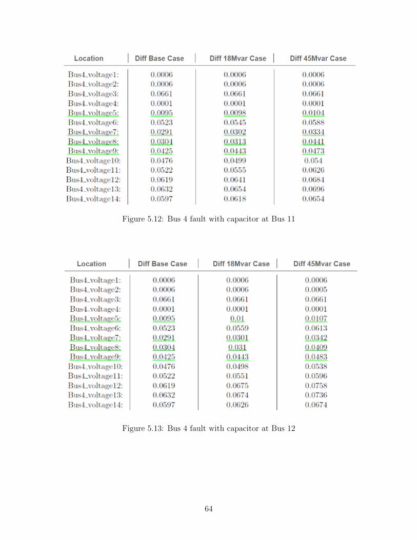
Figure 5.12: Bus 4 fault with capacitor at Bus 11

Figure 5.13: Bus 4 fault with capacitor at Bus 12

64

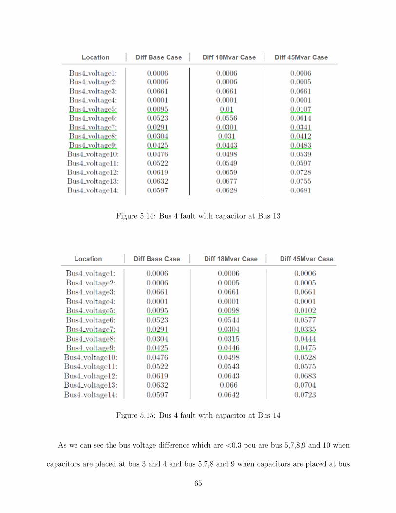
Figure 5.14: Bus 4 fault with capacitor at Bus 13

Figure 5.15: Bus 4 fault with capacitor at Bus 14

As we can see the bus voltage difference which are <0.3 pcu are bus 5,7,8,9 and 10 when

capacitors are placed at bus 3 and 4 and bus 5,7,8 and 9 when capacitors are placed at bus

65

5,6,7,8,9,10,11,12,13 and 14 and bus 5 when capacitor is placed at bus 8. Since the voltage at

bus 5 does not vary for bus 4 fault with various location of capacitor, this position is chosen

as one of the test cases.

Similar tables which show the error function value for all bus fault scenarios are created

and the cases with the least error (0.03 pu%) is marked. These cases form the test matrix

which includes the bus fault location as well as the location for the placement of the SVC. In

Figure 5.16 below, the locations and fault scenarios for testing the SVC model.

Figure 5.16: Test Matrix

66

5.4 Finding the parameters of SVC model

A range of values were given to each parameter - K, T1, T2, T3, T4 and T5. K ranged from

various values from 50-1000 initially. After every iteration, the range was reduced according

to the error function and to get more accurate results. The ranges for T1 - T4 always remained

< 0.5 and T5 < 0.05. The parameters were varied based on the error function.

The comparison of the plots of the voltage waveforms with SVC placed at different

locations with bus faults can been seen below. The MVar output of the SVC model in PSS/E

and the Mvar output of the SVC physical controller along with the 14 bus voltages are

overlapped against each other.

The first step involves varying the parameters individually. Error function tables are

created in-order to analyze which parameter has least difference. A range of values are given

to each parameter of the SVC model in PSS/E one at a time and the error function values

are tabulated in ascending order of error between the response of PSS/E and Hypersim. This

table helps us in creating a range for the variation of parameters are done simultaneously.

Figure 5.17 shows the error function table with varying values for parameter K when the

SVC is placed at Bus-5 and a fault is applied on Bus-3.

67

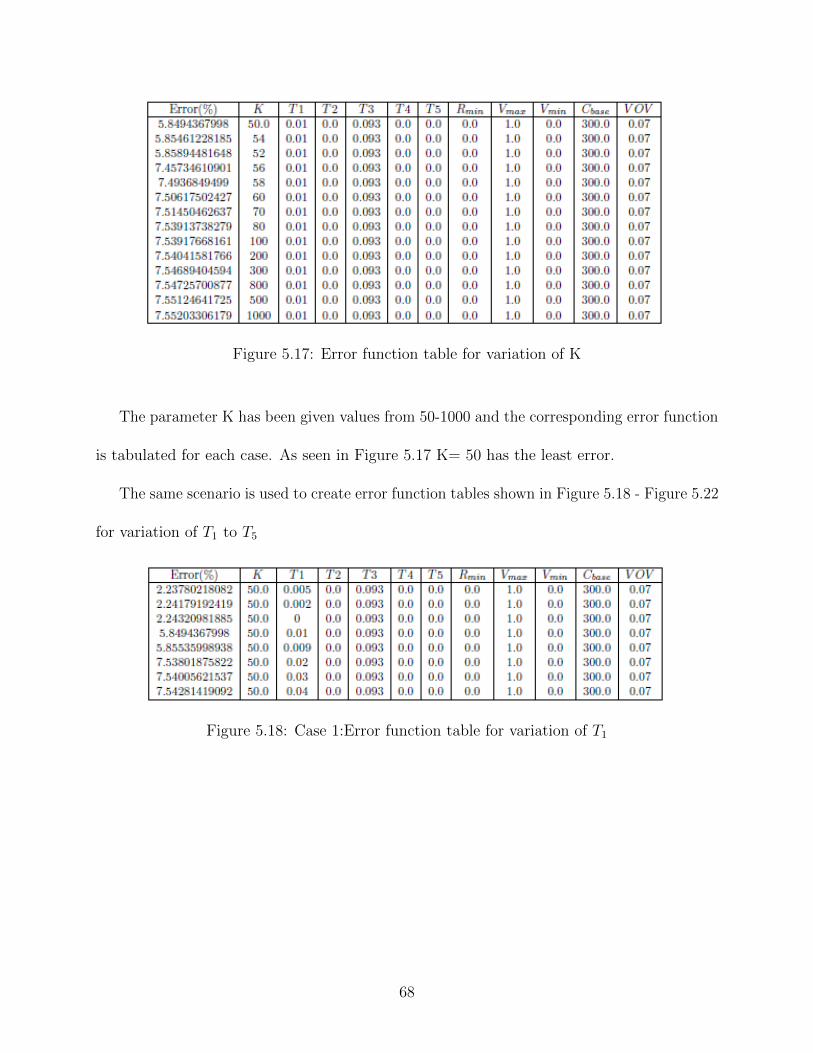
Figure 5.17: Error function table for variation of K

The parameter K has been given values from 50-1000 and the corresponding error function

is tabulated for each case. As seen in Figure 5.17 K= 50 has the least error.

The same scenario is used to create error function tables shown in Figure 5.18 - Figure 5.22

for variation of T1 to T5

Figure 5.18: Case 1:Error function table for variation of T1

68

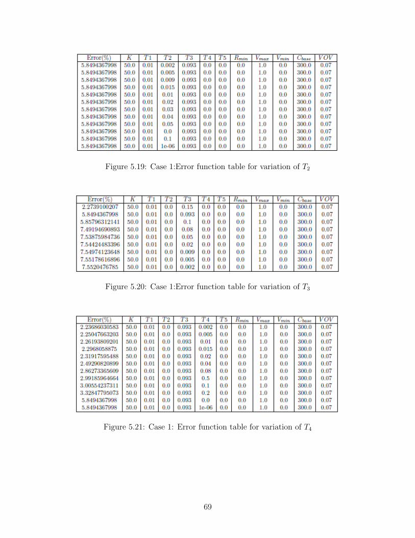
Figure 5.19: Case 1:Error function table for variation of T2

Figure 5.20: Case 1:Error function table for variation of T3

Figure 5.21: Case 1: Error function table for variation of T4

69

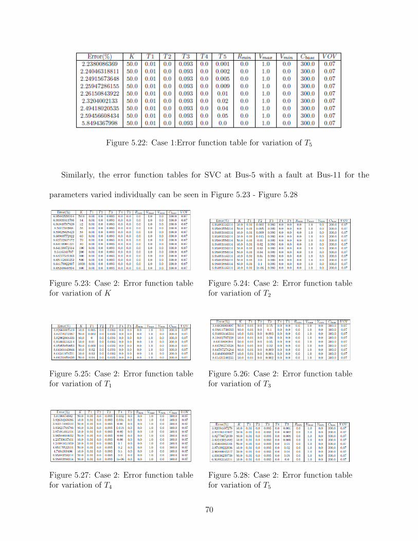
Figure 5.22: Case 1:Error function table for variation of T5

Similarly, the error function tables for SVC at Bus-5 with a fault at Bus-11 for the

parameters varied individually can be seen in Figure 5.23 - Figure 5.28

Figure 5.23: Case 2: Error function tablefor variation of K

Figure 5.24: Case 2: Error function tablefor variation of T2

Figure 5.25: Case 2: Error function tablefor variation of T1

Figure 5.26: Case 2: Error function tablefor variation of T3

Figure 5.27: Case 2: Error function tablefor variation of T4

Figure 5.28: Case 2: Error function tablefor variation of T5

70

The error tables tell us the value for each parameter which gives least error. Error tables

were also created with SVC placed at Bus-3 and Bus-4 with faults applied on different

locations. These tables can be seen in 6.2.

These best value of each parameter from the error function tables where taken and the

response of the SVC model against the SVC physical controller is analyzed individually. The

SVC is placed at Bus-4 and the fault is applied on Bus-5.

PSSE_Mvar [Spreadsheet2] Hypersim_Mvar [Spreadsheet1]

0 0.2 0.4 0.6 0.8 1−2

0

2

4

6

PSSE_V1 [Spreadsheet2] Hypersim_V1a [Spreadsheet1]

0 0.2 0.4 0.6 0.8 10.98

0.99

1

1.01

1.02

PSSE_V2 [Spreadsheet2] Hypersim_V2a [Spreadsheet1]

0 0.2 0.4 0.6 0.8 10.98

0.99

1

1.01

1.02

PSSE_V3 [Spreadsheet2] Hypersim_V3a [Spreadsheet1]

0 0.2 0.4 0.6 0.8 10.4

0.8

1.2

PSSE_V4 [Spreadsheet2] Hypersim_V4a [Spreadsheet1]

0 0.2 0.4 0.6 0.8 10

0.5

1

1.5

PSSE_V5 [Spreadsheet2] Hypersim_V5a [Spreadsheet1]

0 0.2 0.4 0.6 0.8 10

0.5

1

1.5

PSSE_V6 [Spreadsheet2] Hypersim_V6a [Spreadsheet1]

0 0.2 0.4 0.6 0.8 10

0.5

1

1.5

PSSE_V7 [Spreadsheet2] Hypersim_V7a [Spreadsheet1]

0 0.2 0.4 0.6 0.8 10

0.5

1

1.5

PSSE_V8 [Spreadsheet2] Hypersim_V8a [Spreadsheet1]

0 0.2 0.4 0.6 0.8 10

0.5

1

1.5

PSSE_V9 [Spreadsheet2] Hypersim_V9a [Spreadsheet1]

0 0.2 0.4 0.6 0.8 10

0.5

1

PSSE_V10 [Spreadsheet2] Hypersim_V10a [Spreadsheet1]

0 0.2 0.4 0.6 0.8 10

0.5

1

1.5

PSSE_V11 [Spreadsheet2] Hypersim_V11a [Spreadsheet1]

0 0.2 0.4 0.6 0.8 10

0.5

1

1.5

PSSE_V12 [Spreadsheet2] Hypersim_V12a [Spreadsheet1]

0 0.2 0.4 0.6 0.8 10

0.5

1

1.5

PSSE_V13 [Spreadsheet2] Hypersim_V13a [Spreadsheet1]

0 0.2 0.4 0.6 0.8 10

0.5

1

1.5

PSSE_V14 [Spreadsheet2] Hypersim_V14a [Spreadsheet1]

0 0.2 0.4 0.6 0.8 10

0.5

1

1.5

[Spreadsheet1] bus5fault_svcbus4 − E:\Individual\Malavika\2017\14bus_with_SVC\hyper_test_cases_3_30_2017\svc@4[Spreadsheet2] case5_csv_svc@4_kbest − E:\Individual\Malavika\Thesis\psse\14_bus_tests\results

Printed for p 1

Figure 5.29: Comparison of response withbest value of K

PSSE_Mvar [Spreadsheet2] Hypersim_Mvar [Spreadsheet1]

0 0.2 0.4 0.6 0.8 1−2

0

2

4

6

PSSE_V1 [Spreadsheet2] Hypersim_V1a [Spreadsheet1]

0 0.2 0.4 0.6 0.8 10.98

0.99

1

1.01

1.02

PSSE_V2 [Spreadsheet2] Hypersim_V2a [Spreadsheet1]

0 0.2 0.4 0.6 0.8 10.98

0.99

1

1.01

1.02

PSSE_V3 [Spreadsheet2] Hypersim_V3a [Spreadsheet1]

0 0.2 0.4 0.6 0.8 10.4

0.8

1.2

PSSE_V4 [Spreadsheet2] Hypersim_V4a [Spreadsheet1]

0 0.2 0.4 0.6 0.8 10

0.5

1

1.5

PSSE_V5 [Spreadsheet2] Hypersim_V5a [Spreadsheet1]

0 0.2 0.4 0.6 0.8 10

0.5

1

1.5

PSSE_V6 [Spreadsheet2] Hypersim_V6a [Spreadsheet1]

0 0.2 0.4 0.6 0.8 10

0.5

1

1.5

PSSE_V7 [Spreadsheet2] Hypersim_V7a [Spreadsheet1]

0 0.2 0.4 0.6 0.8 10

0.5

1

1.5

PSSE_V8 [Spreadsheet2] Hypersim_V8a [Spreadsheet1]

0 0.2 0.4 0.6 0.8 10

0.5

1

1.5

PSSE_V9 [Spreadsheet2] Hypersim_V9a [Spreadsheet1]

0 0.2 0.4 0.6 0.8 10

0.5

1

PSSE_V10 [Spreadsheet2] Hypersim_V10a [Spreadsheet1]

0 0.2 0.4 0.6 0.8 10

0.5

1

1.5

PSSE_V11 [Spreadsheet2] Hypersim_V11a [Spreadsheet1]

0 0.2 0.4 0.6 0.8 10

0.5

1

1.5

PSSE_V12 [Spreadsheet2] Hypersim_V12a [Spreadsheet1]

0 0.2 0.4 0.6 0.8 10

0.5

1

1.5

PSSE_V13 [Spreadsheet2] Hypersim_V13a [Spreadsheet1]

0 0.2 0.4 0.6 0.8 10

0.5

1

1.5

PSSE_V14 [Spreadsheet2] Hypersim_V14a [Spreadsheet1]

0 0.2 0.4 0.6 0.8 10

0.5

1

1.5

[Spreadsheet1] bus5fault_svcbus4 − E:\Individual\Malavika\2017\14bus_with_SVC\hyper_test_cases_3_30_2017\svc@4[Spreadsheet2] case5_csv_svc@4_t1best − E:\Individual\Malavika\Thesis\psse\14_bus_tests\results

Printed for p 1

Figure 5.30: Comparison of response withbest value of T1

PSSE_Mvar [Spreadsheet2] Hypersim_Mvar [Spreadsheet1]

0 0.2 0.4 0.6 0.8 1−2

0

2

4

6

PSSE_V1 [Spreadsheet2] Hypersim_V1a [Spreadsheet1]

0 0.2 0.4 0.6 0.8 10.98

0.99

1

1.01

1.02

PSSE_V2 [Spreadsheet2] Hypersim_V2a [Spreadsheet1]

0 0.2 0.4 0.6 0.8 10.98

0.99

1

1.01

1.02

PSSE_V3 [Spreadsheet2] Hypersim_V3a [Spreadsheet1]

0 0.2 0.4 0.6 0.8 10.4

0.8

1.2

PSSE_V4 [Spreadsheet2] Hypersim_V4a [Spreadsheet1]

0 0.2 0.4 0.6 0.8 10

0.5

1

1.5

PSSE_V5 [Spreadsheet2] Hypersim_V5a [Spreadsheet1]

0 0.2 0.4 0.6 0.8 10

0.5

1

1.5

PSSE_V6 [Spreadsheet2] Hypersim_V6a [Spreadsheet1]

0 0.2 0.4 0.6 0.8 10

0.5

1

1.5

PSSE_V7 [Spreadsheet2] Hypersim_V7a [Spreadsheet1]

0 0.2 0.4 0.6 0.8 10

0.5

1

1.5

PSSE_V8 [Spreadsheet2] Hypersim_V8a [Spreadsheet1]

0 0.2 0.4 0.6 0.8 10

0.5

1

1.5

PSSE_V9 [Spreadsheet2] Hypersim_V9a [Spreadsheet1]

0 0.2 0.4 0.6 0.8 10

0.5

1

PSSE_V10 [Spreadsheet2] Hypersim_V10a [Spreadsheet1]

0 0.2 0.4 0.6 0.8 10

0.5

1

1.5

PSSE_V11 [Spreadsheet2] Hypersim_V11a [Spreadsheet1]

0 0.2 0.4 0.6 0.8 10

0.5

1

1.5

PSSE_V12 [Spreadsheet2] Hypersim_V12a [Spreadsheet1]

0 0.2 0.4 0.6 0.8 10

0.5

1

1.5

PSSE_V13 [Spreadsheet2] Hypersim_V13a [Spreadsheet1]

0 0.2 0.4 0.6 0.8 10

0.5

1

1.5

PSSE_V14 [Spreadsheet2] Hypersim_V14a [Spreadsheet1]

0 0.2 0.4 0.6 0.8 10

0.5

1

1.5

[Spreadsheet1] bus5fault_svcbus4 − E:\Individual\Malavika\2017\14bus_with_SVC\hyper_test_cases_3_30_2017\svc@4[Spreadsheet2] case5_csv_svc@4_t2best − E:\Individual\Malavika\Thesis\psse\14_bus_tests\results

Printed for p 1

Figure 5.31: Comparison of response withbest value of T2

PSSE_Mvar [Spreadsheet2] Hypersim_Mvar [Spreadsheet1]

0 0.2 0.4 0.6 0.8 1−2

0

2

4

6

PSSE_V1 [Spreadsheet2] Hypersim_V1a [Spreadsheet1]

0 0.2 0.4 0.6 0.8 10.98

0.99

1

1.01

1.02

PSSE_V2 [Spreadsheet2] Hypersim_V2a [Spreadsheet1]

0 0.2 0.4 0.6 0.8 10.98

0.99

1

1.01

1.02

PSSE_V3 [Spreadsheet2] Hypersim_V3a [Spreadsheet1]

0 0.2 0.4 0.6 0.8 10.4

0.8

1.2

PSSE_V4 [Spreadsheet2] Hypersim_V4a [Spreadsheet1]

0 0.2 0.4 0.6 0.8 10

0.5

1

1.5

PSSE_V5 [Spreadsheet2] Hypersim_V5a [Spreadsheet1]

0 0.2 0.4 0.6 0.8 10

0.5

1

1.5

PSSE_V6 [Spreadsheet2] Hypersim_V6a [Spreadsheet1]

0 0.2 0.4 0.6 0.8 10

0.5

1

1.5

PSSE_V7 [Spreadsheet2] Hypersim_V7a [Spreadsheet1]

0 0.2 0.4 0.6 0.8 10

0.5

1

1.5

PSSE_V8 [Spreadsheet2] Hypersim_V8a [Spreadsheet1]

0 0.2 0.4 0.6 0.8 10

0.5

1

1.5

PSSE_V9 [Spreadsheet2] Hypersim_V9a [Spreadsheet1]

0 0.2 0.4 0.6 0.8 10

0.5

1

PSSE_V10 [Spreadsheet2] Hypersim_V10a [Spreadsheet1]

0 0.2 0.4 0.6 0.8 10

0.5

1

1.5

PSSE_V11 [Spreadsheet2] Hypersim_V11a [Spreadsheet1]

0 0.2 0.4 0.6 0.8 10

0.5

1

1.5

PSSE_V12 [Spreadsheet2] Hypersim_V12a [Spreadsheet1]

0 0.2 0.4 0.6 0.8 10

0.5

1

1.5

PSSE_V13 [Spreadsheet2] Hypersim_V13a [Spreadsheet1]

0 0.2 0.4 0.6 0.8 10

0.5

1

1.5

PSSE_V14 [Spreadsheet2] Hypersim_V14a [Spreadsheet1]

0 0.2 0.4 0.6 0.8 10

0.5

1

1.5

[Spreadsheet1] bus5fault_svcbus4 − E:\Individual\Malavika\2017\14bus_with_SVC\hyper_test_cases_3_30_2017\svc@4[Spreadsheet2] case5_csv_svc@4_t3best − E:\Individual\Malavika\Thesis\psse\14_bus_tests\results

Printed for p 1

Figure 5.32: Comparison of response withbest value of T3

From the above graphs, it is seen that parameters T1, T4 and T5 reduces the transients

71

PSSE_Mvar [Spreadsheet2] Hypersim_Mvar [Spreadsheet1]

0 0.2 0.4 0.6 0.8 1−2

0

2

4

6

PSSE_V1 [Spreadsheet2] Hypersim_V1a [Spreadsheet1]

0 0.2 0.4 0.6 0.8 10.98

0.99

1

1.01

1.02

PSSE_V2 [Spreadsheet2] Hypersim_V2a [Spreadsheet1]

0 0.2 0.4 0.6 0.8 10.98

0.99

1

1.01

1.02

PSSE_V3 [Spreadsheet2] Hypersim_V3a [Spreadsheet1]

0 0.2 0.4 0.6 0.8 10.4

0.8

1.2

PSSE_V4 [Spreadsheet2] Hypersim_V4a [Spreadsheet1]

0 0.2 0.4 0.6 0.8 10

0.5

1

1.5

PSSE_V5 [Spreadsheet2] Hypersim_V5a [Spreadsheet1]

0 0.2 0.4 0.6 0.8 10

0.5

1

1.5

PSSE_V6 [Spreadsheet2] Hypersim_V6a [Spreadsheet1]

0 0.2 0.4 0.6 0.8 10

0.5

1

1.5

PSSE_V7 [Spreadsheet2] Hypersim_V7a [Spreadsheet1]

0 0.2 0.4 0.6 0.8 10

0.5

1

1.5

PSSE_V8 [Spreadsheet2] Hypersim_V8a [Spreadsheet1]

0 0.2 0.4 0.6 0.8 10

0.5

1

1.5

PSSE_V9 [Spreadsheet2] Hypersim_V9a [Spreadsheet1]

0 0.2 0.4 0.6 0.8 10

0.5

1

PSSE_V10 [Spreadsheet2] Hypersim_V10a [Spreadsheet1]

0 0.2 0.4 0.6 0.8 10

0.5

1

1.5

PSSE_V11 [Spreadsheet2] Hypersim_V11a [Spreadsheet1]

0 0.2 0.4 0.6 0.8 10

0.5

1

1.5

PSSE_V12 [Spreadsheet2] Hypersim_V12a [Spreadsheet1]

0 0.2 0.4 0.6 0.8 10

0.5

1

1.5

PSSE_V13 [Spreadsheet2] Hypersim_V13a [Spreadsheet1]

0 0.2 0.4 0.6 0.8 10

0.5

1

1.5

PSSE_V14 [Spreadsheet2] Hypersim_V14a [Spreadsheet1]

0 0.2 0.4 0.6 0.8 10

0.5

1

1.5

[Spreadsheet1] bus5fault_svcbus4 − E:\Individual\Malavika\2017\14bus_with_SVC\hyper_test_cases_3_30_2017\svc@4[Spreadsheet2] case5_csv_svc@4_t4best − E:\Individual\Malavika\Thesis\psse\14_bus_tests\results

Printed for p 1

Figure 5.33: Comparison of response withbest value of T4

PSSE_Mvar [Spreadsheet2] Hypersim_Mvar [Spreadsheet1]

0 0.2 0.4 0.6 0.8 1−2

0

2

4

6

PSSE_V1 [Spreadsheet2] Hypersim_V1a [Spreadsheet1]

0 0.2 0.4 0.6 0.8 10.98

0.99

1

1.01

1.02

PSSE_V2 [Spreadsheet2] Hypersim_V2a [Spreadsheet1]

0 0.2 0.4 0.6 0.8 10.98

0.99

1

1.01

1.02

PSSE_V3 [Spreadsheet2] Hypersim_V3a [Spreadsheet1]

0 0.2 0.4 0.6 0.8 10.4

0.8

1.2

PSSE_V4 [Spreadsheet2] Hypersim_V4a [Spreadsheet1]

0 0.2 0.4 0.6 0.8 10

0.5

1

1.5

PSSE_V5 [Spreadsheet2] Hypersim_V5a [Spreadsheet1]

0 0.2 0.4 0.6 0.8 10

0.5

1

1.5

PSSE_V6 [Spreadsheet2] Hypersim_V6a [Spreadsheet1]

0 0.2 0.4 0.6 0.8 10

0.5

1

1.5

PSSE_V7 [Spreadsheet2] Hypersim_V7a [Spreadsheet1]

0 0.2 0.4 0.6 0.8 10

0.5

1

1.5

PSSE_V8 [Spreadsheet2] Hypersim_V8a [Spreadsheet1]

0 0.2 0.4 0.6 0.8 10

0.5

1

1.5

PSSE_V9 [Spreadsheet2] Hypersim_V9a [Spreadsheet1]

0 0.2 0.4 0.6 0.8 10

0.5

1

1.5

PSSE_V10 [Spreadsheet2] Hypersim_V10a [Spreadsheet1]

0 0.2 0.4 0.6 0.8 10

0.5

1

1.5

PSSE_V11 [Spreadsheet2] Hypersim_V11a [Spreadsheet1]

0 0.2 0.4 0.6 0.8 10

0.5

1

1.5

PSSE_V12 [Spreadsheet2] Hypersim_V12a [Spreadsheet1]

0 0.2 0.4 0.6 0.8 10

0.5

1

1.5

PSSE_V13 [Spreadsheet2] Hypersim_V13a [Spreadsheet1]

0 0.2 0.4 0.6 0.8 10

0.5

1

1.5

PSSE_V14 [Spreadsheet2] Hypersim_V14a [Spreadsheet1]

0 0.2 0.4 0.6 0.8 10

0.5

1

1.5

[Spreadsheet1] bus5fault_svcbus4 − E:\Individual\Malavika\2017\14bus_with_SVC\hyper_test_cases_3_30_2017\svc@4[Spreadsheet2] case5_csv_svc@4_t5best − E:\Individual\Malavika\Thesis\psse\14_bus_tests\results

Printed for p 1

Figure 5.34: Comparison of response withbest value of T5

and shows a big effect on the response.

The parameters which had the least error was taken as the basis for selecting the range for

variation simultaneously. This reduced the simulation time and also restricted the parameter

range for an accurate results. Figure 5.35 shows the error function table when the SVC is

placed at Bus-5 and a fault is applied on Bus-5 when all parameters are varied.

Figure 5.35: Error function table for variation of all parameters simultaneously

Similar simulations have been run for SVC at Bus-5 with fault at Bus-11, SVC at Bus-3

72

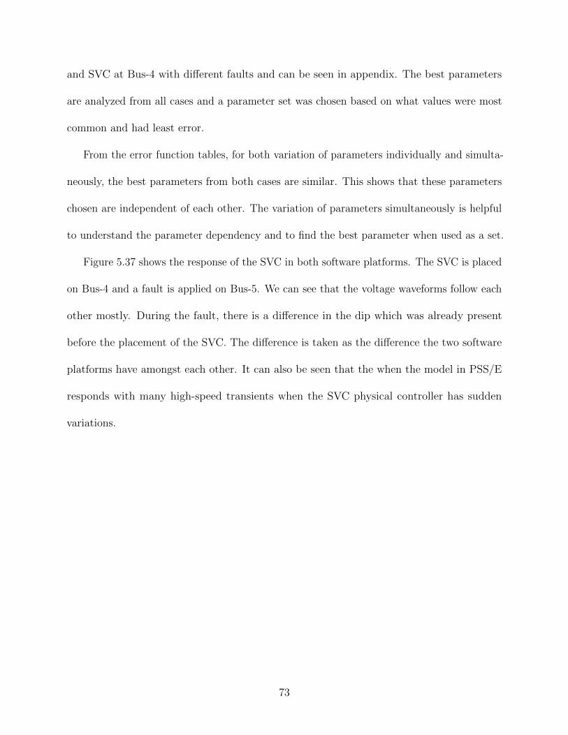
and SVC at Bus-4 with different faults and can be seen in appendix. The best parameters

are analyzed from all cases and a parameter set was chosen based on what values were most

common and had least error.

From the error function tables, for both variation of parameters individually and simulta-

neously, the best parameters from both cases are similar. This shows that these parameters

chosen are independent of each other. The variation of parameters simultaneously is helpful

to understand the parameter dependency and to find the best parameter when used as a set.

Figure 5.37 shows the response of the SVC in both software platforms. The SVC is placed

on Bus-4 and a fault is applied on Bus-5. We can see that the voltage waveforms follow each

other mostly. During the fault, there is a difference in the dip which was already present

before the placement of the SVC. The difference is taken as the difference the two software

platforms have amongst each other. It can also be seen that the when the model in PSS/E

responds with many high-speed transients when the SVC physical controller has sudden

variations.

73

PSSE_Mvar [Spreadsheet21] Hypersim_Mvar [Spreadsheet22]

0 0.2 0.4 0.6 0.8 1−2

0

2

4

6

PSSE_V1 [Spreadsheet21] Hypersim_V1a [Spreadsheet22]

0 0.2 0.4 0.6 0.8 10.98

0.99

1

1.01

1.02

PSSE_V2 [Spreadsheet21] Hypersim_V2a [Spreadsheet22]

0 0.2 0.4 0.6 0.8 10.98

0.99

1

1.01

1.02

PSSE_V3 [Spreadsheet21] Hypersim_V3a [Spreadsheet22]

0 0.2 0.4 0.6 0.8 10.4

0.8

1.2

PSSE_V4 [Spreadsheet21] Hypersim_V4a [Spreadsheet22]

0 0.2 0.4 0.6 0.8 10

0.5

1

1.5

PSSE_V5 [Spreadsheet21] Hypersim_V5a [Spreadsheet22]

0 0.2 0.4 0.6 0.8 10

0.5

1

1.5

PSSE_V6 [Spreadsheet21] Hypersim_V6a [Spreadsheet22]

0 0.2 0.4 0.6 0.8 10

0.5

1

1.5

PSSE_V7 [Spreadsheet21] Hypersim_V7a [Spreadsheet22]

0 0.2 0.4 0.6 0.8 10

0.5

1

1.5

PSSE_V8 [Spreadsheet21] Hypersim_V8a [Spreadsheet22]

0 0.2 0.4 0.6 0.8 10

0.5

1

1.5

PSSE_V9 [Spreadsheet21] Hypersim_V9a [Spreadsheet22]

0 0.2 0.4 0.6 0.8 10

0.5

1

1.5

PSSE_V10 [Spreadsheet21] Hypersim_V10a [Spreadsheet22]

0 0.2 0.4 0.6 0.8 10

0.5

1

1.5

PSSE_V11 [Spreadsheet21] Hypersim_V11a [Spreadsheet22]

0 0.2 0.4 0.6 0.8 10

0.5

1

1.5

PSSE_V12 [Spreadsheet21] Hypersim_V12a [Spreadsheet22]

0 0.2 0.4 0.6 0.8 10

0.5

1

1.5

PSSE_V13 [Spreadsheet21] Hypersim_V13a [Spreadsheet22]

0 0.2 0.4 0.6 0.8 10

0.5

1

1.5

PSSE_V14 [Spreadsheet21] Hypersim_V14a [Spreadsheet22]

0 0.2 0.4 0.6 0.8 10

0.5

1

1.5

[Spreadsheet21] case5_csv_svc@4 − E:\Individual\Malavika\2017\14bus_with_SVC\Psse_thesis_results\svc@4[Spreadsheet22] bus5fault_svcbus4 − E:\Individual\Malavika\2017\14bus_with_SVC\hyper_test_cases_3_30_2017\svc@4

Printed for p 1

Figure 5.36: Response of the test system in PSS/E with new parameters for SVC andHypersim HIL SVC at Bus-4 and a fault applied on Bus-5

With Figure 5.37, it is clear that the parameter finding methodology used has found the

parameters for the SVC model that responds similar to the response of the SVC physical

controller

For the purpose of validation and verification, the SVC model that was chosen to find the

parameters for was already modeled when the physical controller / actual SVC installed. The

response of the SVC model with the original parameters against the response of the SVC

physical controller can be seen in Figure 5.37

74

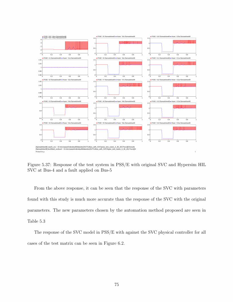
PSSE_SVC_Mvar [Spreadsheet8]Hyper_SVC_Mvar [Spreadsheet9]

0 0.2 0.4 0.6 0.8 1−2

0

2

4

6

PSSE_V1 [Spreadsheet8] Hyper_V1a [Spreadsheet9]

0 0.2 0.4 0.6 0.8 10.98

0.99

1

1.01

1.02

PSSE_V2 [Spreadsheet8] Hyper_V2a [Spreadsheet9]

0 0.2 0.4 0.6 0.8 10.98

0.99

1

1.01

1.02

PSSE_V3 [Spreadsheet8] Hyper_V3a [Spreadsheet9]

0 0.2 0.4 0.6 0.8 10.4

0.8

1.2

PSSE_V4 [Spreadsheet8] Hyper_V4a [Spreadsheet9]

0 0.2 0.4 0.6 0.8 10

0.5

1

1.5

PSSE_V5 [Spreadsheet8] Hyper_V5a [Spreadsheet9]

0 0.2 0.4 0.6 0.8 10

0.5

1

1.5

PSSE_V6 [Spreadsheet8] Hyper_V6a [Spreadsheet9]

0 0.2 0.4 0.6 0.8 10

0.5

1

1.5

PSSE_V7 [Spreadsheet8] Hyper_V7a [Spreadsheet9]

0 0.2 0.4 0.6 0.8 10

0.5

1

1.5

PSSE_V8 [Spreadsheet8] Hyper_V8a [Spreadsheet9]

0 0.2 0.4 0.6 0.8 10

0.5

1

1.5

PSSE_V9 [Spreadsheet8] Hyper_V9a [Spreadsheet9]

0 0.2 0.4 0.6 0.8 10

0.5

1

1.5

PSSE_V10 [Spreadsheet8] Hyper_V10a [Spreadsheet9]

0 0.2 0.4 0.6 0.8 10

0.5

1

1.5

PSSE_V11 [Spreadsheet8] Hyper_V11a [Spreadsheet9]

0 0.2 0.4 0.6 0.8 10

0.5

1

1.5

PSSE_V12 [Spreadsheet8] Hyper_V12a [Spreadsheet9]

0 0.2 0.4 0.6 0.8 10

0.5

1

1.5

PSSE_V13 [Spreadsheet8] Hyper_V13a [Spreadsheet9]

0 0.2 0.4 0.6 0.8 10

0.5

1

1.5

PSSE_V14 [Spreadsheet8] Hyper_V14a [Spreadsheet9]

0 0.2 0.4 0.6 0.8 10

0.5

1

1.5

[Spreadsheet8] case5_csv − E:\microwave\Individual\Malavika\2017\14bus_with_SVC\psse_test_cases_3_30_2017\svc@4\results[Spreadsheet9] bus5fault_svcbus4 − E:\microwave\Individual\Malavika\2017\14bus_with_SVC\hyper_test_cases_3_30_2017\svc@4

Printed for p 1

Figure 5.37: Response of the test system in PSS/E with original SVC and Hypersim HILSVC at Bus-4 and a fault applied on Bus-5

From the above response, it can be seen that the response of the SVC with parameters

found with this study is much more accurate than the response of the SVC with the original

parameters. The new parameters chosen by the automation method proposed are seen in

Table 5.3

The response of the SVC model in PSS/E with against the SVC physical controller for all

cases of the test matrix can be seen in Figure 6.2.

75

Table 5.3: New SVC (CSVGN3) Parameters

Parameter Value Range

K 50

T1 0.0

T2 0.002

T3 0.15

T4 0.002

T5 0.001

RMIN 0.0

VMAX 1.0

VMIN 0.0

CBASE 300.0

VOV 0.07

76

Chapter 6

Concluding Remarks and Future

Work

6.1 Conclusion

This thesis focuses on the method of automation to create appropriate models in PSS/E with

the data from the field.In this study, this methodology is used to find the appropriate model

of an SVC in PSS/E with the data from the HIL real-time simulation of an SVC physical

controller. Power system planning is an important aspect for the maintenance and reliability

of the power system network. As the network increases in size and complexity the requirement

of having more accurate and up-to-date models are necessary. The stability of the modified

IEEE 14-Bus system is analyzed when subject to severe network disturbances in both PSS/E

and Hypersim. Appropriate parameters were chosen for the SVC model in PSS/E with the

SVC physical controller HIL simulation as reference. Automation played a key role in the

process and highlighted its importance in terms of time and efficiency. The dynamic behavior

of the SVC model was analyzed in PSS/E as well as the SVC physical control with HIL

simulation in Hypersim. The main achievements of this research is summarized as given

below,

77

• The modified IEEE 14-Bus test system is modeled successfully in PSS/E and Hypersim

• The steady state analysis is performed and the results were similar in both software

platforms

• Near-ideal voltage source is modeled successfully. Dynamic analysis of the test system

is performed in both the platforms.

• The process of running dynamics in PSS/E is successfully automated along with the

automation of comparing the two platforms and finding the appropriate parameters

based on the error function stated in chapter 3.

• The automation method is implemented successfully to modify parameters in PSS/E

for the near-ideal voltage source based on the error function to reduce the difference

between the two platforms

• The optimal location for the SVC is found to clearly analyze the response of the SVC

when subject to network disturbances by reducing the difference of the two software.

• The parameters of the SVC is found with the methodology in chapter 3 to bring its

response closer to the response of the SVC physical controller. Dynamic response of

the SVCs are analyzed in PSS/E and Hypersim

6.2 Future Work

This study enables the use of automation techniques for modeling power system devices. The

methodology proposed can be used in the modeling other components such as generators,

78

loads etc.

When the simulation software being used is updated, this methodology can also be used

to update models of different components that are already in use with previous response of

the model or response from the field. This helps in retaining the accuracy of the models and

making the power system studies more reliable and effective.

This methodology can be used in any simulation software that enables its usage through

scripting methods.

The models that are previously in use can be verified against the physical controller or

the response of the devices from the field to ensure that the models in use are correct and

reliable. This methodology can also be used to bring the responses of the models already in

use closer to the required response and modify the models accordingly.

This study can also help in realizing that automation of various processes in power

system studies are fast-approaching and inevitable. It enables reliable operation of analysis

methodologies by reducing human error. It is also much faster and efficient when compared

to manual testing and analysis. The data results can be modified and portrayed in various

formats according to what is necessary and needed.

79

Bibliography

[1] IEEE Guide for the Functional Specification of Transmission Static Var Compensators.

Technical report, IEEE Std. 1031, 2011.

[2] U.S. Energy Information Administration. How Electricity is Delivered to Consumers.

https://www.eia.gov/Energyexplained/index.cfm?page=electricity delivery, 2016.

[3] J Belanger, P Venne, and JN Paquin. The What, Where and Why of Real-Time

Simulation. Planet RT, 1(0):1, 2010.

[4] Keith Bell. Methods and Tools for Planning the Future Power System: Issues and

Priorities. 2015.

[5] Arthur R. Bergen and Vijay Vittal. Power Systems Analysis. 2000.

[6] Seung Tae Cha, Qiuwei Wu, Arne Hejde Nielsen, Jacob Østergaard, and In Kwon Park.

Real-Time Hardware-in-the-Loop (HIL) Testing for Power Electronics Controllers. In

Power and Energy Engineering Conference (APPEEC), 2012 Asia-Pacific, pages 1–6.

IEEE, 2012.

[7] Illinois Center for a Smarter Electric Grid (ICSEG). IEEE 14-Bus System. http:

//publish.illinois.edu/smartergrid/case-2-ieee-14-bus-systems, 2014.

[8] Paul Forsyth, Rick Kuffel, Rudi Wierckx, Jin-Boo Choo, Yong-Beum Yoon, and Tae-

Kyun Kim. Comparison of Transient Stability Analysis and Large-Scale Real Time

80

Digital Simulation. In Power Tech Proceedings, 2001 IEEE Porto, volume 4, pages 7–pp.

IEEE, 2001.

[9] Charles A. Gross. Power System Analysis. 1979.

[10] Xavier Guillaud, M Omar Faruque, Alexandre Teninge, Ali Hasan Hariri, Luigi Vanfretti,

Mario Paolone, Venkata Dinavahi, Pinaki Mitra, Georg Lauss, Christian Dufour, et al.

Applications of Real-Time Simulation Technologies in Power and Energy Systems. IEEE

Power and Energy Technology Systems Journal, 2(3):103–115, 2015.

[11] Laszlo Gyugyi. Reactive Power Generation and Control by Thyristor Circuits. IEEE

Transactions on Industry applications, (5):521–532, 1979.

[12] Narain G Hingorani, Laszlo Gyugyi, and Mohamed El-Hawary. Understanding FACTS:

Concepts and Technology of Flexible AC Transmission Systems, volume 2. Wiley Online

Library, 2000.

[13] P. K. Iyambo and R. Tzoneva. Transient Stability Analysis of the IEEE 14-Bus Electric

Power System. In AFRICON 2007, pages 1–9, Sept 2007.

[14] Prabha Kundur, Neal J Balu, and Mark G Lauby. Power System Stability and Control,

volume 7. McGraw-hill New York, 1994.

[15] Kerstin Linden and Inger Segerqvist. Modelling of Load Devices and Studying Load

or System Characteristics. Master’s thesis, Chalmers University of Technology, August

1992.

81

[16] Jan Machowski, Janusz Bialek, and James Richard Bumby. Power System Dynamics

and Stability. John Wiley & Sons, 1997.

[17] Surekha Manoj and PS Puttaswamy. Importance of FACTS Controllers in Power Systems.

International Journal of Advanced Engineering Technology, 2(3):207–212, 2011.

[18] R Mohan Mathur and Rajiv K Varma. Thyristor-based FACTS Controllers for Electrical

Transmission Systems. John Wiley & Sons, 2002.

[19] PM Menghal and A Jaya Laxmi. Real Time Simulation: Recent Progress & Challenges. In

Power, Signals, Controls and Computation (EPSCICON), 2012 International Conference

on, pages 1–6. IEEE, 2012.

[20] Sowmya Munukuntla, Rastin Rastgoufard, and Parviz Rastgoufard. Sensitivity Analysis

of Synchronous Generators for Real-Time Simulations. In Green Energy and Systems

Conference (IGSEC), 2016 IEEE, pages 1–6. IEEE, 2016.

[21] Shravana Musunuri and Gholamreza Dehnavi. Comparison of STATCOM, SVC, TCSC,

and SSSC Performance in Steady State Voltage Stability Improvement. In North

American Power Symposium (NAPS), 2010, pages 1–7. IEEE, 2010.

[22] North American Electric Reliability Council (NERC). Reliability Guideline - Reactive

Power Planning. Technical report, 2016.

[23] Arun Pachori, Hemant Amhia, and Vikendra Moranya. Static VAR Compensation

Technique for IEEE 14-Bus System. International Journal of Emerging Technology and

Advanced Engineering, 3, 2013.

82

[24] Sidhartha Panda and NP Padhy. Power Electronics Based FACTS Controller for Stability

Improvement of a Wind Energy Embedded Distribution System. International Journal

of Electronics, Circuits and Systems, 1(1):30–37, 2007.

[25] Donghan Shi, Kun Han, Qi Chen, Peng Wang, Michael A Zagrodnik, and Gupta Amit.

Credibility Analysis for Real-Time Hardware-in-the-Loop Simulation Compared Against

Actual Plant. In Power Electronics and Motion Control Conference (IPEMC-ECCE

Asia), 2016 IEEE 8th International, pages 2775–2778. IEEE, 2016.

[26] PTI Siemens. Application Program Interface PSS/E-32. Technical report, Schenectady,

NY, USA, 2009.

[27] PTI Siemens. Model Library PSS/E-32. Technical report, Schenectady, NY, USA, 2009.

[28] PTI Siemens. Volume 2: Program Application Guide of PSS/E-32. Technical report,

Schenectady, NY, USA, 2009.

[29] Don Somatilake. Execution of Python Program Scripts to Automate PSS/E Simulations.

2016.

[30] Rajeev Kumar Verma and Sangeeta Mishra. A Study on Transient Stability Improvement

of 5-Machine 14-Bus System Using SVC. International Journal on Recent and Innovation

Trends in Computing and Communication, 2, 2014.

[31] D. Petesch S. Dennetier Y. Vernay, C. Martin. Hardware in the Loop Simulations to Test

SVC Performances on the French Grid. International Conference on Power Systems

Transients, 1, 2015.

83

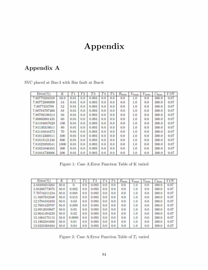
Appendix

Appendix A

SVC placed at Bus-3 with Bus fault at Bus-6

Figure 1: Case A:Error Function Table of K varied

Figure 2: Case A:Error Function Table of T1 varied

84

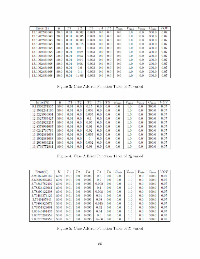
Figure 3: Case A:Error Function Table of T2 varied

Figure 4: Case A:Error Function Table of T3 varied

Figure 5: Case A:Error Function Table of T4 varied

85

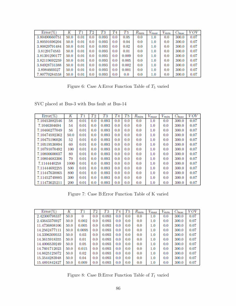
Figure 6: Case A:Error Function Table of T5 varied

SVC placed at Bus-3 with Bus fault at Bus-14

Figure 7: Case B:Error Function Table of K varied

Figure 8: Case B:Error Function Table of T1 varied

86

Figure 9: Case B:Error Function Table of T2 varied

Figure 10: Case B:Error Function Table of T3 varied

Figure 11: Case B:Error Function Table of T4 varied

87

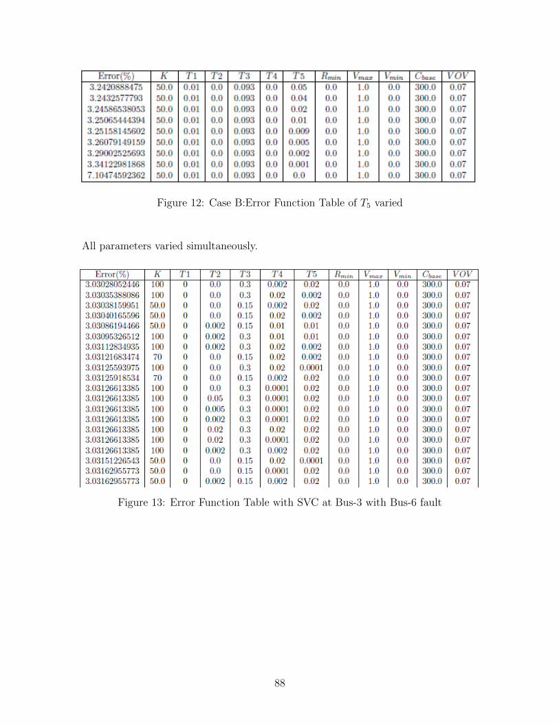
Figure 12: Case B:Error Function Table of T5 varied

All parameters varied simultaneously.

Figure 13: Error Function Table with SVC at Bus-3 with Bus-6 fault

88

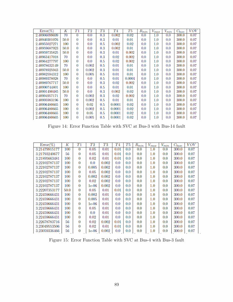
Figure 14: Error Function Table with SVC at Bus-3 with Bus-14 fault

Figure 15: Error Function Table with SVC at Bus-4 with Bus-3 fault

89

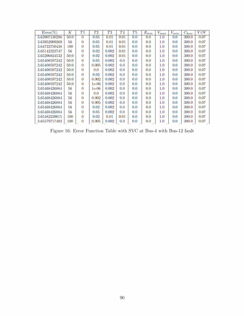
Figure 16: Error Function Table with SVC at Bus-4 with Bus-12 fault

90

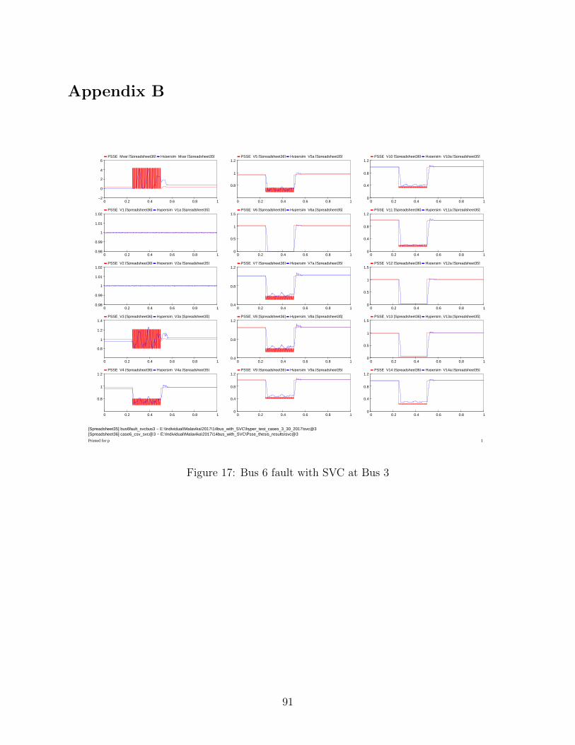
Appendix B

PSSE_Mvar [Spreadsheet36] Hypersim_Mvar [Spreadsheet35]

0 0.2 0.4 0.6 0.8 1−2

0

2

4

6

PSSE_V1 [Spreadsheet36] Hypersim_V1a [Spreadsheet35]

0 0.2 0.4 0.6 0.8 10.98

0.99

1

1.01

1.02

PSSE_V2 [Spreadsheet36] Hypersim_V2a [Spreadsheet35]

0 0.2 0.4 0.6 0.8 10.98

0.99

1

1.01

1.02

PSSE_V3 [Spreadsheet36] Hypersim_V3a [Spreadsheet35]

0 0.2 0.4 0.6 0.8 1

0.8

1

1.2

1.4

PSSE_V4 [Spreadsheet36] Hypersim_V4a [Spreadsheet35]

0 0.2 0.4 0.6 0.8 1

0.8

1

1.2

PSSE_V5 [Spreadsheet36] Hypersim_V5a [Spreadsheet35]

0 0.2 0.4 0.6 0.8 1

0.8

1

1.2

PSSE_V6 [Spreadsheet36] Hypersim_V6a [Spreadsheet35]

0 0.2 0.4 0.6 0.8 10

0.5

1

1.5

PSSE_V7 [Spreadsheet36] Hypersim_V7a [Spreadsheet35]

0 0.2 0.4 0.6 0.8 10.4

0.8

1.2

PSSE_V8 [Spreadsheet36] Hypersim_V8a [Spreadsheet35]

0 0.2 0.4 0.6 0.8 10.4

0.8

1.2

PSSE_V9 [Spreadsheet36] Hypersim_V9a [Spreadsheet35]

0 0.2 0.4 0.6 0.8 10

0.4

0.8

1.2

PSSE_V10 [Spreadsheet36] Hypersim_V10a [Spreadsheet35]

0 0.2 0.4 0.6 0.8 10

0.4

0.8

1.2

PSSE_V11 [Spreadsheet36] Hypersim_V11a [Spreadsheet35]

0 0.2 0.4 0.6 0.8 10

0.4

0.8

1.2

PSSE_V12 [Spreadsheet36] Hypersim_V12a [Spreadsheet35]

0 0.2 0.4 0.6 0.8 10

0.5

1

1.5

PSSE_V13 [Spreadsheet36] Hypersim_V13a [Spreadsheet35]

0 0.2 0.4 0.6 0.8 10

0.5

1

1.5

PSSE_V14 [Spreadsheet36] Hypersim_V14a [Spreadsheet35]

0 0.2 0.4 0.6 0.8 10

0.4

0.8

1.2

[Spreadsheet35] bus6fault_svcbus3 − E:\Individual\Malavika\2017\14bus_with_SVC\hyper_test_cases_3_30_2017\svc@3[Spreadsheet36] case6_csv_svc@3 − E:\Individual\Malavika\2017\14bus_with_SVC\Psse_thesis_results\svc@3

Printed for p 1

Figure 17: Bus 6 fault with SVC at Bus 3

91

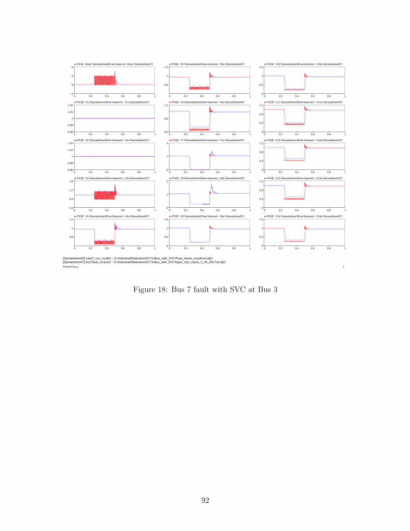
PSSE_Mvar [Spreadsheet36] Hypersim_Mvar [Spreadsheet37]

0 0.2 0.4 0.6 0.8 1−4

0

4

8

PSSE_V1 [Spreadsheet36] Hypersim_V1a [Spreadsheet37]

0 0.2 0.4 0.6 0.8 10.98

0.99

1

1.01

1.02

PSSE_V2 [Spreadsheet36] Hypersim_V2a [Spreadsheet37]

0 0.2 0.4 0.6 0.8 10.98

0.99

1

1.01

1.02

PSSE_V3 [Spreadsheet36] Hypersim_V3a [Spreadsheet37]

0 0.2 0.4 0.6 0.8 10.4

0.8

1.2

1.6

PSSE_V4 [Spreadsheet36] Hypersim_V4a [Spreadsheet37]

0 0.2 0.4 0.6 0.8 1

0.8

1

1.2

PSSE_V5 [Spreadsheet36] Hypersim_V5a [Spreadsheet37]

0 0.2 0.4 0.6 0.8 1

0.8

1

1.2

PSSE_V6 [Spreadsheet36] Hypersim_V6a [Spreadsheet37]

0 0.2 0.4 0.6 0.8 10.4

0.8

1.2

PSSE_V7 [Spreadsheet36] Hypersim_V7a [Spreadsheet37]

0 0.2 0.4 0.6 0.8 10

1

2

PSSE_V8 [Spreadsheet36] Hypersim_V8a [Spreadsheet37]

0 0.2 0.4 0.6 0.8 10

1

2

PSSE_V9 [Spreadsheet36] Hypersim_V9a [Spreadsheet37]

0 0.2 0.4 0.6 0.8 10

0.5

1

1.5

PSSE_V10 [Spreadsheet36] Hypersim_V10a [Spreadsheet37]

0 0.2 0.4 0.6 0.8 10

0.5

1

1.5

PSSE_V11 [Spreadsheet36] Hypersim_V11a [Spreadsheet37]

0 0.2 0.4 0.6 0.8 10

0.4

0.8

1.2

PSSE_V12 [Spreadsheet36] Hypersim_V12a [Spreadsheet37]

0 0.2 0.4 0.6 0.8 10

0.4

0.8

1.2

PSSE_V13 [Spreadsheet36] Hypersim_V13a [Spreadsheet37]

0 0.2 0.4 0.6 0.8 10

0.4

0.8

1.2

PSSE_V14 [Spreadsheet36] Hypersim_V14a [Spreadsheet37]

0 0.2 0.4 0.6 0.8 10

0.5

1

1.5

[Spreadsheet36] case7_csv_svc@3 − E:\Individual\Malavika\2017\14bus_with_SVC\Psse_thesis_results\svc@3[Spreadsheet37] bus7fault_svcbus3 − E:\Individual\Malavika\2017\14bus_with_SVC\hyper_test_cases_3_30_2017\svc@3

Printed for p 1

Figure 18: Bus 7 fault with SVC at Bus 3

92

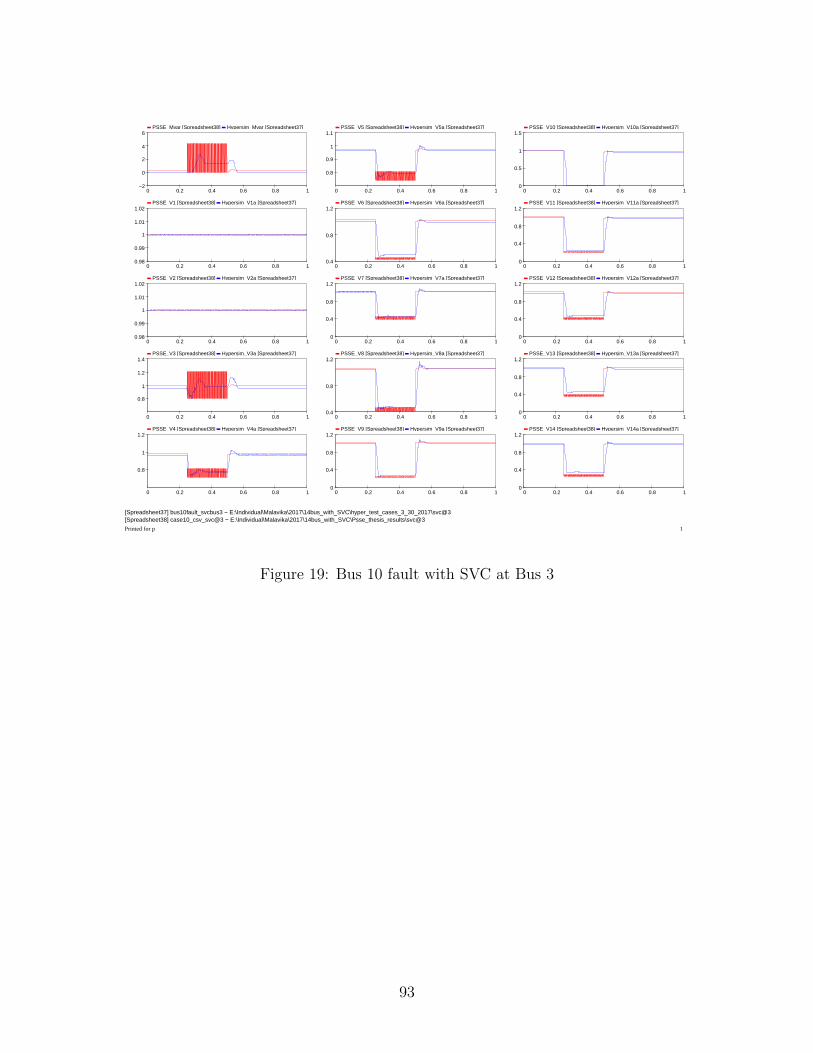
PSSE_Mvar [Spreadsheet38] Hypersim_Mvar [Spreadsheet37]

0 0.2 0.4 0.6 0.8 1−2

0

2

4

6

PSSE_V1 [Spreadsheet38] Hypersim_V1a [Spreadsheet37]

0 0.2 0.4 0.6 0.8 10.98

0.99

1

1.01

1.02

PSSE_V2 [Spreadsheet38] Hypersim_V2a [Spreadsheet37]

0 0.2 0.4 0.6 0.8 10.98

0.99

1

1.01

1.02

PSSE_V3 [Spreadsheet38] Hypersim_V3a [Spreadsheet37]

0 0.2 0.4 0.6 0.8 1

0.8

1

1.2

1.4

PSSE_V4 [Spreadsheet38] Hypersim_V4a [Spreadsheet37]

0 0.2 0.4 0.6 0.8 1

0.8

1

1.2

PSSE_V5 [Spreadsheet38] Hypersim_V5a [Spreadsheet37]

0 0.2 0.4 0.6 0.8 1

0.8

0.9

1

1.1

PSSE_V6 [Spreadsheet38] Hypersim_V6a [Spreadsheet37]

0 0.2 0.4 0.6 0.8 10.4

0.8

1.2

PSSE_V7 [Spreadsheet38] Hypersim_V7a [Spreadsheet37]

0 0.2 0.4 0.6 0.8 10

0.4

0.8

1.2

PSSE_V8 [Spreadsheet38] Hypersim_V8a [Spreadsheet37]

0 0.2 0.4 0.6 0.8 10.4

0.8

1.2

PSSE_V9 [Spreadsheet38] Hypersim_V9a [Spreadsheet37]

0 0.2 0.4 0.6 0.8 10

0.4

0.8

1.2

PSSE_V10 [Spreadsheet38] Hypersim_V10a [Spreadsheet37]

0 0.2 0.4 0.6 0.8 10

0.5

1

1.5

PSSE_V11 [Spreadsheet38] Hypersim_V11a [Spreadsheet37]

0 0.2 0.4 0.6 0.8 10

0.4

0.8

1.2

PSSE_V12 [Spreadsheet38] Hypersim_V12a [Spreadsheet37]

0 0.2 0.4 0.6 0.8 10

0.4

0.8

1.2

PSSE_V13 [Spreadsheet38] Hypersim_V13a [Spreadsheet37]

0 0.2 0.4 0.6 0.8 10

0.4

0.8

1.2

PSSE_V14 [Spreadsheet38] Hypersim_V14a [Spreadsheet37]

0 0.2 0.4 0.6 0.8 10

0.4

0.8

1.2

[Spreadsheet37] bus10fault_svcbus3 − E:\Individual\Malavika\2017\14bus_with_SVC\hyper_test_cases_3_30_2017\svc@3[Spreadsheet38] case10_csv_svc@3 − E:\Individual\Malavika\2017\14bus_with_SVC\Psse_thesis_results\svc@3

Printed for p 1

Figure 19: Bus 10 fault with SVC at Bus 3

93

PSSE_Mvar [Spreadsheet39] Hypersim_Mvar [Spreadsheet37]

0 0.2 0.4 0.6 0.8 1−2

0

2

4

6

PSSE_V1 [Spreadsheet39] Hypersim_V1a [Spreadsheet37]

0 0.2 0.4 0.6 0.8 10.98

0.99

1

1.01

1.02

PSSE_V2 [Spreadsheet39] Hypersim_V2a [Spreadsheet37]

0 0.2 0.4 0.6 0.8 10.98

0.99

1

1.01

1.02

PSSE_V3 [Spreadsheet39] Hypersim_V3a [Spreadsheet37]

0 0.2 0.4 0.6 0.8 10.8

1

1.2

1.4

PSSE_V4 [Spreadsheet39] Hypersim_V4a [Spreadsheet37]

0 0.2 0.4 0.6 0.8 1

0.8

0.9

1

PSSE_V5 [Spreadsheet39] Hypersim_V5a [Spreadsheet37]

0 0.2 0.4 0.6 0.8 1

0.8

0.9

1

PSSE_V6 [Spreadsheet39] Hypersim_V6a [Spreadsheet37]

0 0.2 0.4 0.6 0.8 10

0.4

0.8

1.2

PSSE_V7 [Spreadsheet39] Hypersim_V7a [Spreadsheet37]

0 0.2 0.4 0.6 0.8 10.4

0.6

0.8

1

1.2

PSSE_V8 [Spreadsheet39] Hypersim_V8a [Spreadsheet37]

0 0.2 0.4 0.6 0.8 10.4

0.6

0.8

1

1.2

PSSE_V9 [Spreadsheet39] Hypersim_V9a [Spreadsheet37]

0 0.2 0.4 0.6 0.8 10.4

0.6

0.8

1

1.2

PSSE_V10 [Spreadsheet39] Hypersim_V10a [Spreadsheet37]

0 0.2 0.4 0.6 0.8 10.4

0.8

1.2

PSSE_V11 [Spreadsheet39] Hypersim_V11a [Spreadsheet37]

0 0.2 0.4 0.6 0.8 10

0.4

0.8

1.2

PSSE_V12 [Spreadsheet39] Hypersim_V12a [Spreadsheet37]

0 0.2 0.4 0.6 0.8 10

0.4

0.8

1.2

PSSE_V13 [Spreadsheet39] Hypersim_V13a [Spreadsheet37]

0 0.2 0.4 0.6 0.8 10

0.5

1

1.5

PSSE_V14 [Spreadsheet39] Hypersim_V14a [Spreadsheet37]

0 0.2 0.4 0.6 0.8 10

0.4

0.8

1.2

[Spreadsheet37] bus13fault_svcbus3 − E:\Individual\Malavika\2017\14bus_with_SVC\hyper_test_cases_3_30_2017\svc@3[Spreadsheet39] case13_csv_svc@3 − E:\Individual\Malavika\2017\14bus_with_SVC\Psse_thesis_results\svc@3

Printed for p 1

Figure 20: Bus 14 fault with SVC at Bus 3

94

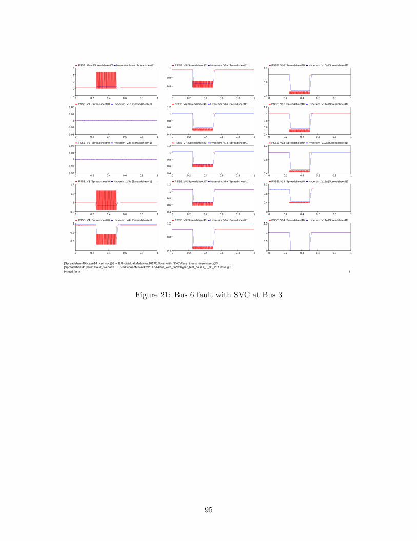
PSSE_Mvar [Spreadsheet40] Hypersim_Mvar [Spreadsheet41]

0 0.2 0.4 0.6 0.8 1−2

0

2

4

6

PSSE_V1 [Spreadsheet40] Hypersim_V1a [Spreadsheet41]

0 0.2 0.4 0.6 0.8 10.98

0.99

1

1.01

1.02

PSSE_V2 [Spreadsheet40] Hypersim_V2a [Spreadsheet41]

0 0.2 0.4 0.6 0.8 10.98

0.99

1

1.01

1.02

PSSE_V3 [Spreadsheet40] Hypersim_V3a [Spreadsheet41]

0 0.2 0.4 0.6 0.8 10.8

1

1.2

1.4

PSSE_V4 [Spreadsheet40] Hypersim_V4a [Spreadsheet41]

0 0.2 0.4 0.6 0.8 1

0.8

0.9

1

PSSE_V5 [Spreadsheet40] Hypersim_V5a [Spreadsheet41]

0 0.2 0.4 0.6 0.8 1

0.8

0.9

1

PSSE_V6 [Spreadsheet40] Hypersim_V6a [Spreadsheet41]

0 0.2 0.4 0.6 0.8 10.4

0.6

0.8

1

1.2

PSSE_V7 [Spreadsheet40] Hypersim_V7a [Spreadsheet41]

0 0.2 0.4 0.6 0.8 10.4

0.6

0.8

1

1.2

PSSE_V8 [Spreadsheet40] Hypersim_V8a [Spreadsheet41]

0 0.2 0.4 0.6 0.8 10.4

0.6

0.8

1

1.2

PSSE_V9 [Spreadsheet40] Hypersim_V9a [Spreadsheet41]

0 0.2 0.4 0.6 0.8 10.4

0.8

1.2

PSSE_V10 [Spreadsheet40] Hypersim_V10a [Spreadsheet41]

0 0.2 0.4 0.6 0.8 10.4

0.8

1.2

PSSE_V11 [Spreadsheet40] Hypersim_V11a [Spreadsheet41]

0 0.2 0.4 0.6 0.8 10.4

0.6

0.8

1

1.2

PSSE_V12 [Spreadsheet40] Hypersim_V12a [Spreadsheet41]

0 0.2 0.4 0.6 0.8 10.4

0.8

1.2

PSSE_V13 [Spreadsheet40] Hypersim_V13a [Spreadsheet41]

0 0.2 0.4 0.6 0.8 10

0.4

0.8

1.2

PSSE_V14 [Spreadsheet40] Hypersim_V14a [Spreadsheet41]

0 0.2 0.4 0.6 0.8 10

0.5

1

1.5

[Spreadsheet40] case14_csv_svc@3 − E:\Individual\Malavika\2017\14bus_with_SVC\Psse_thesis_results\svc@3[Spreadsheet41] bus14fault_svcbus3 − E:\Individual\Malavika\2017\14bus_with_SVC\hyper_test_cases_3_30_2017\svc@3

Printed for p 1

Figure 21: Bus 6 fault with SVC at Bus 3

95

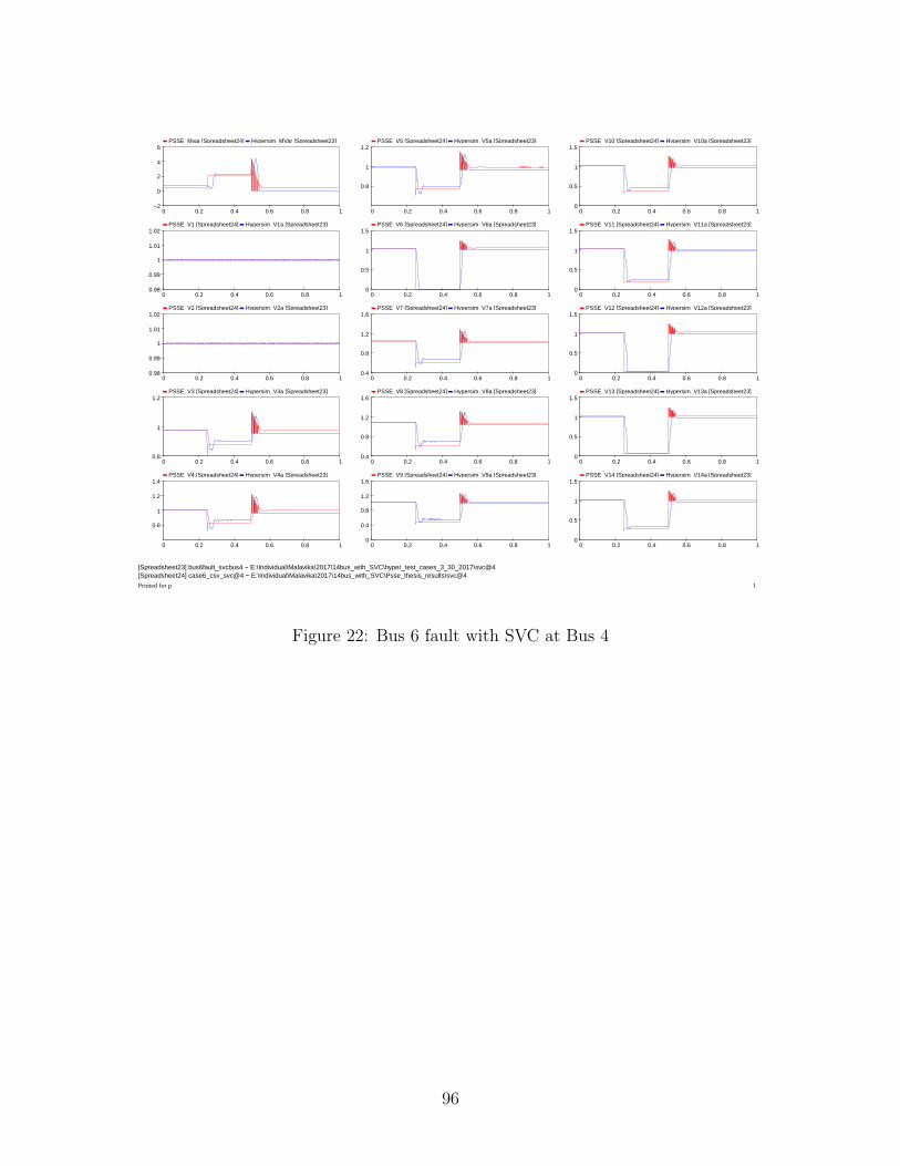
PSSE_Mvar [Spreadsheet24] Hypersim_MVar [Spreadsheet23]

0 0.2 0.4 0.6 0.8 1−2

0

2

4

6

PSSE_V1 [Spreadsheet24] Hypersim_V1a [Spreadsheet23]

0 0.2 0.4 0.6 0.8 10.98

0.99

1

1.01

1.02

PSSE_V2 [Spreadsheet24] Hypersim_V2a [Spreadsheet23]

0 0.2 0.4 0.6 0.8 10.98

0.99

1

1.01

1.02

PSSE_V3 [Spreadsheet24] Hypersim_V3a [Spreadsheet23]

0 0.2 0.4 0.6 0.8 10.8

1

1.2

PSSE_V4 [Spreadsheet24] Hypersim_V4a [Spreadsheet23]

0 0.2 0.4 0.6 0.8 1

0.8

1

1.2

1.4

PSSE_V5 [Spreadsheet24] Hypersim_V5a [Spreadsheet23]

0 0.2 0.4 0.6 0.8 1

0.8

1

1.2

PSSE_V6 [Spreadsheet24] Hypersim_V6a [Spreadsheet23]

0 0.2 0.4 0.6 0.8 10

0.5

1

1.5

PSSE_V7 [Spreadsheet24] Hypersim_V7a [Spreadsheet23]

0 0.2 0.4 0.6 0.8 10.4

0.8

1.2

1.6

PSSE_V8 [Spreadsheet24] Hypersim_V8a [Spreadsheet23]

0 0.2 0.4 0.6 0.8 10.4

0.8

1.2

1.6

PSSE_V9 [Spreadsheet24] Hypersim_V9a [Spreadsheet23]

0 0.2 0.4 0.6 0.8 10

0.4

0.8

1.2

1.6

PSSE_V10 [Spreadsheet24] Hypersim_V10a [Spreadsheet23]

0 0.2 0.4 0.6 0.8 10

0.5

1

1.5

PSSE_V11 [Spreadsheet24] Hypersim_V11a [Spreadsheet23]

0 0.2 0.4 0.6 0.8 10

0.5

1

1.5

PSSE_V12 [Spreadsheet24] Hypersim_V12a [Spreadsheet23]

0 0.2 0.4 0.6 0.8 10

0.5

1

1.5

PSSE_V13 [Spreadsheet24] Hypersim_V13a [Spreadsheet23]

0 0.2 0.4 0.6 0.8 10

0.5

1

1.5

PSSE_V14 [Spreadsheet24] Hypersim_V14a [Spreadsheet23]

0 0.2 0.4 0.6 0.8 10

0.5

1

1.5

[Spreadsheet23] bus6fault_svcbus4 − E:\Individual\Malavika\2017\14bus_with_SVC\hyper_test_cases_3_30_2017\svc@4[Spreadsheet24] case6_csv_svc@4 − E:\Individual\Malavika\2017\14bus_with_SVC\Psse_thesis_results\svc@4

Printed for p 1

Figure 22: Bus 6 fault with SVC at Bus 4

96

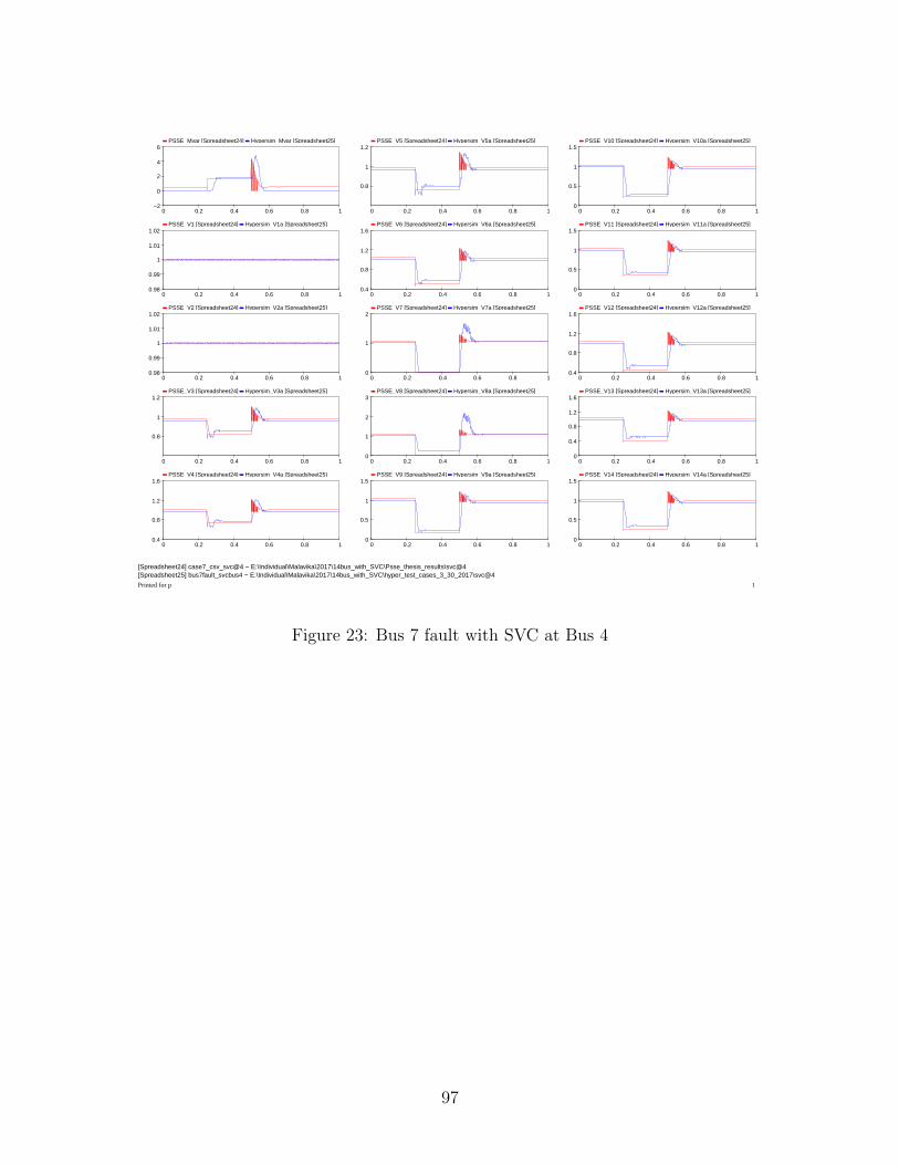
PSSE_Mvar [Spreadsheet24] Hypersim_Mvar [Spreadsheet25]

0 0.2 0.4 0.6 0.8 1−2

0

2

4

6

PSSE_V1 [Spreadsheet24] Hypersim_V1a [Spreadsheet25]

0 0.2 0.4 0.6 0.8 10.98

0.99

1

1.01

1.02

PSSE_V2 [Spreadsheet24] Hypersim_V2a [Spreadsheet25]

0 0.2 0.4 0.6 0.8 10.98

0.99

1

1.01

1.02

PSSE_V3 [Spreadsheet24] Hypersim_V3a [Spreadsheet25]

0 0.2 0.4 0.6 0.8 1

0.8

1

1.2

PSSE_V4 [Spreadsheet24] Hypersim_V4a [Spreadsheet25]

0 0.2 0.4 0.6 0.8 10.4

0.8

1.2

1.6

PSSE_V5 [Spreadsheet24] Hypersim_V5a [Spreadsheet25]

0 0.2 0.4 0.6 0.8 1

0.8

1

1.2

PSSE_V6 [Spreadsheet24] Hypersim_V6a [Spreadsheet25]

0 0.2 0.4 0.6 0.8 10.4

0.8

1.2

1.6

PSSE_V7 [Spreadsheet24] Hypersim_V7a [Spreadsheet25]

0 0.2 0.4 0.6 0.8 10

1

2

PSSE_V8 [Spreadsheet24] Hypersim_V8a [Spreadsheet25]

0 0.2 0.4 0.6 0.8 10

1

2

3

PSSE_V9 [Spreadsheet24] Hypersim_V9a [Spreadsheet25]

0 0.2 0.4 0.6 0.8 10

0.5

1

1.5

PSSE_V10 [Spreadsheet24] Hypersim_V10a [Spreadsheet25]

0 0.2 0.4 0.6 0.8 10

0.5

1

1.5

PSSE_V11 [Spreadsheet24] Hypersim_V11a [Spreadsheet25]

0 0.2 0.4 0.6 0.8 10

0.5

1

1.5

PSSE_V12 [Spreadsheet24] Hypersim_V12a [Spreadsheet25]

0 0.2 0.4 0.6 0.8 10.4

0.8

1.2

1.6

PSSE_V13 [Spreadsheet24] Hypersim_V13a [Spreadsheet25]

0 0.2 0.4 0.6 0.8 10

0.4

0.8

1.2

1.6

PSSE_V14 [Spreadsheet24] Hypersim_V14a [Spreadsheet25]

0 0.2 0.4 0.6 0.8 10

0.5

1

1.5

[Spreadsheet24] case7_csv_svc@4 − E:\Individual\Malavika\2017\14bus_with_SVC\Psse_thesis_results\svc@4[Spreadsheet25] bus7fault_svcbus4 − E:\Individual\Malavika\2017\14bus_with_SVC\hyper_test_cases_3_30_2017\svc@4

Printed for p 1

Figure 23: Bus 7 fault with SVC at Bus 4

97

PSSE_Mvar [Spreadsheet31] Hypersim_Mvar [Spreadsheet25]

0 0.2 0.4 0.6 0.8 1−2

0

2

4

6

PSSE_V1 [Spreadsheet31] Hypersim_V1a [Spreadsheet25]

0 0.2 0.4 0.6 0.8 10.98

0.99

1

1.01

1.02

PSSE_V2 [Spreadsheet31] Hypersim_V2a [Spreadsheet25]

0 0.2 0.4 0.6 0.8 10.98

0.99

1

1.01

1.02

PSSE_V3 [Spreadsheet31] Hypersim_V3a [Spreadsheet25]

0 0.2 0.4 0.6 0.8 1

0.8

1

1.2

PSSE_V4 [Spreadsheet31] Hypersim_V4a [Spreadsheet25]

0 0.2 0.4 0.6 0.8 10.4

0.8

1.2

1.6

PSSE_V5 [Spreadsheet31] Hypersim_V5a [Spreadsheet25]

0 0.2 0.4 0.6 0.8 1

0.8

1

1.2

PSSE_V6 [Spreadsheet31] Hypersim_V6a [Spreadsheet25]

0 0.2 0.4 0.6 0.8 10

0.4

0.8

1.2

1.6

PSSE_V7 [Spreadsheet31] Hypersim_V7a [Spreadsheet25]

0 0.2 0.4 0.6 0.8 10

0.5

1

1.5

2

PSSE_V8 [Spreadsheet31] Hypersim_V8a [Spreadsheet25]

0 0.2 0.4 0.6 0.8 10

1

2

PSSE_V9 [Spreadsheet31] Hypersim_V9a [Spreadsheet25]

0 0.2 0.4 0.6 0.8 10

0.5

1

1.5

PSSE_V10 [Spreadsheet31] Hypersim_V10a [Spreadsheet25]

0 0.2 0.4 0.6 0.8 10

0.5

1

1.5

PSSE_V11 [Spreadsheet31] Hypersim_V11a [Spreadsheet25]

0 0.2 0.4 0.6 0.8 10

0.5

1

1.5

PSSE_V12 [Spreadsheet31] Hypersim_V12a [Spreadsheet25]

0 0.2 0.4 0.6 0.8 10

0.5

1

1.5

PSSE_V13 [Spreadsheet31] Hypersim_V13a [Spreadsheet25]

0 0.2 0.4 0.6 0.8 10

0.5

1

1.5

PSSE_V14 [Spreadsheet31] Hypersim_V14a [Spreadsheet25]

0 0.2 0.4 0.6 0.8 10

0.5

1

1.5

[Spreadsheet25] bus9fault_svcbus4 − E:\Individual\Malavika\2017\14bus_with_SVC\hyper_test_cases_3_30_2017\svc@4[Spreadsheet31] case9_csv_svc@4 − E:\Individual\Malavika\2017\14bus_with_SVC\Psse_thesis_results\svc@4

Printed for p 1

Figure 24: Bus 9 fault with SVC at Bus 4

98

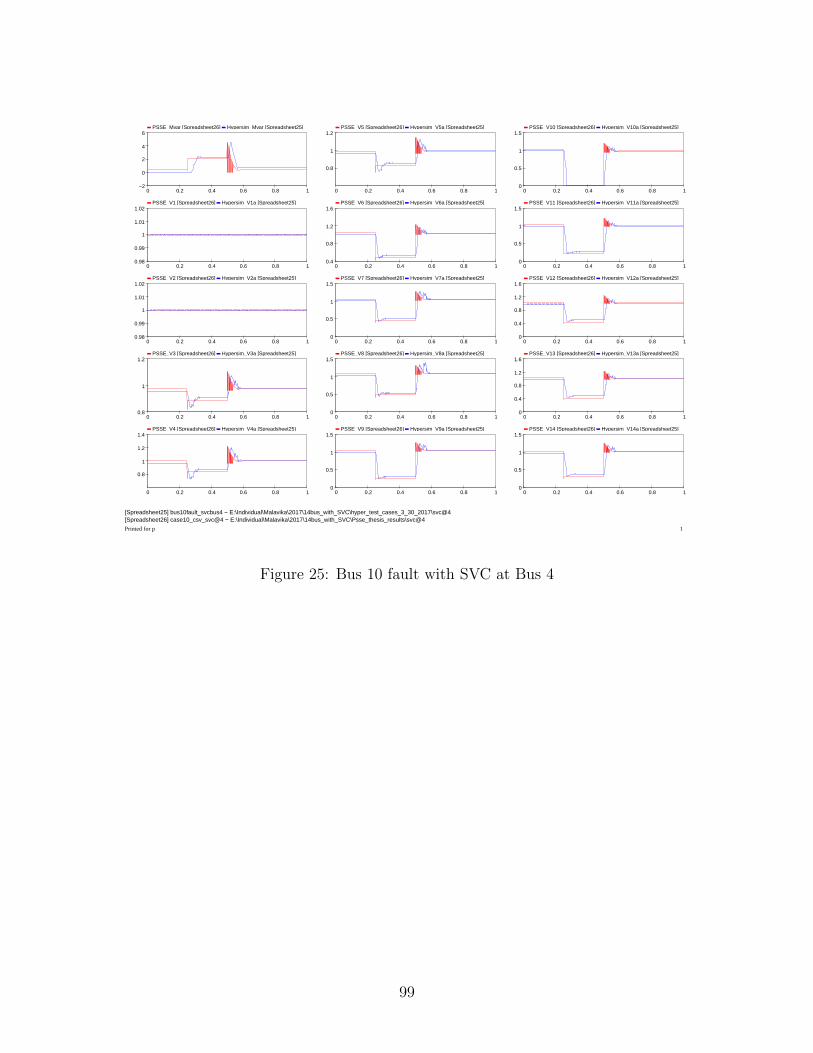
PSSE_Mvar [Spreadsheet26] Hypersim_Mvar [Spreadsheet25]

0 0.2 0.4 0.6 0.8 1−2

0

2

4

6

PSSE_V1 [Spreadsheet26] Hypersim_V1a [Spreadsheet25]

0 0.2 0.4 0.6 0.8 10.98

0.99

1

1.01

1.02

PSSE_V2 [Spreadsheet26] Hypersim_V2a [Spreadsheet25]

0 0.2 0.4 0.6 0.8 10.98

0.99

1

1.01

1.02

PSSE_V3 [Spreadsheet26] Hypersim_V3a [Spreadsheet25]

0 0.2 0.4 0.6 0.8 10.8

1

1.2

PSSE_V4 [Spreadsheet26] Hypersim_V4a [Spreadsheet25]

0 0.2 0.4 0.6 0.8 1

0.8

1

1.2

1.4

PSSE_V5 [Spreadsheet26] Hypersim_V5a [Spreadsheet25]

0 0.2 0.4 0.6 0.8 1

0.8

1

1.2

PSSE_V6 [Spreadsheet26] Hypersim_V6a [Spreadsheet25]

0 0.2 0.4 0.6 0.8 10.4

0.8

1.2

1.6

PSSE_V7 [Spreadsheet26] Hypersim_V7a [Spreadsheet25]

0 0.2 0.4 0.6 0.8 10

0.5

1

1.5

PSSE_V8 [Spreadsheet26] Hypersim_V8a [Spreadsheet25]

0 0.2 0.4 0.6 0.8 10

0.5

1

1.5

PSSE_V9 [Spreadsheet26] Hypersim_V9a [Spreadsheet25]

0 0.2 0.4 0.6 0.8 10

0.5

1

1.5

PSSE_V10 [Spreadsheet26] Hypersim_V10a [Spreadsheet25]

0 0.2 0.4 0.6 0.8 10

0.5

1

1.5

PSSE_V11 [Spreadsheet26] Hypersim_V11a [Spreadsheet25]

0 0.2 0.4 0.6 0.8 10

0.5

1

1.5

PSSE_V12 [Spreadsheet26] Hypersim_V12a [Spreadsheet25]

0 0.2 0.4 0.6 0.8 10

0.4

0.8

1.2

1.6

PSSE_V13 [Spreadsheet26] Hypersim_V13a [Spreadsheet25]

0 0.2 0.4 0.6 0.8 10

0.4

0.8

1.2

1.6

PSSE_V14 [Spreadsheet26] Hypersim_V14a [Spreadsheet25]

0 0.2 0.4 0.6 0.8 10

0.5

1

1.5

[Spreadsheet25] bus10fault_svcbus4 − E:\Individual\Malavika\2017\14bus_with_SVC\hyper_test_cases_3_30_2017\svc@4[Spreadsheet26] case10_csv_svc@4 − E:\Individual\Malavika\2017\14bus_with_SVC\Psse_thesis_results\svc@4

Printed for p 1

Figure 25: Bus 10 fault with SVC at Bus 4

99

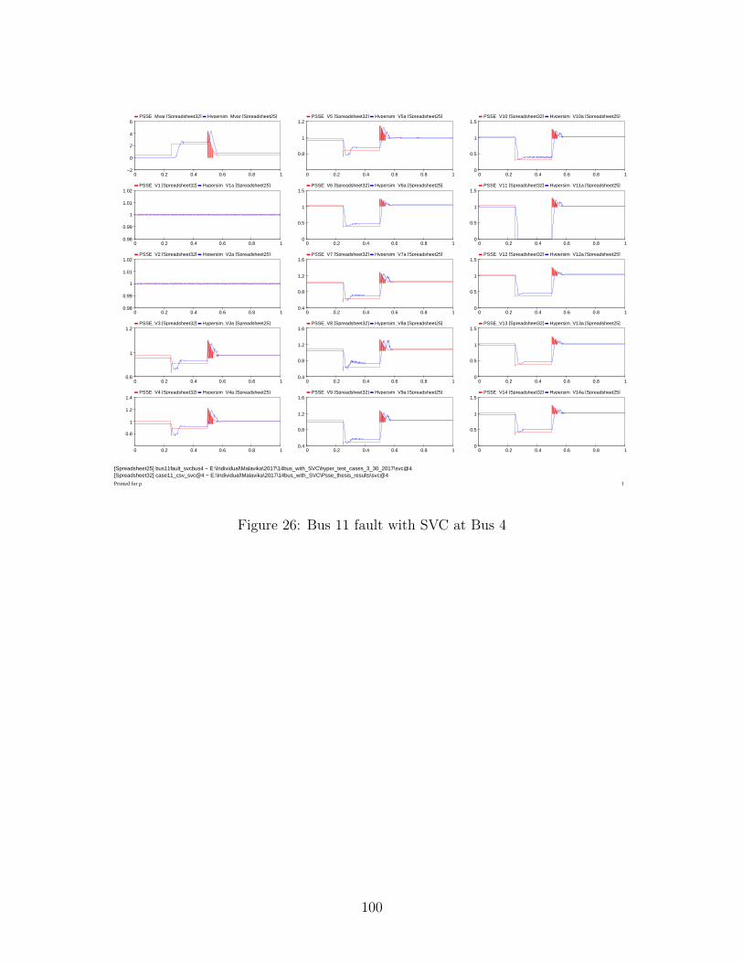
PSSE_Mvar [Spreadsheet32] Hypersim_Mvar [Spreadsheet25]

0 0.2 0.4 0.6 0.8 1−2

0

2

4

6

PSSE_V1 [Spreadsheet32] Hypersim_V1a [Spreadsheet25]

0 0.2 0.4 0.6 0.8 10.98

0.99

1

1.01

1.02

PSSE_V2 [Spreadsheet32] Hypersim_V2a [Spreadsheet25]

0 0.2 0.4 0.6 0.8 10.98

0.99

1

1.01

1.02

PSSE_V3 [Spreadsheet32] Hypersim_V3a [Spreadsheet25]

0 0.2 0.4 0.6 0.8 10.8

1

1.2

PSSE_V4 [Spreadsheet32] Hypersim_V4a [Spreadsheet25]

0 0.2 0.4 0.6 0.8 1

0.8

1

1.2

1.4

PSSE_V5 [Spreadsheet32] Hypersim_V5a [Spreadsheet25]

0 0.2 0.4 0.6 0.8 1

0.8

1

1.2

PSSE_V6 [Spreadsheet32] Hypersim_V6a [Spreadsheet25]

0 0.2 0.4 0.6 0.8 10

0.5

1

1.5

PSSE_V7 [Spreadsheet32] Hypersim_V7a [Spreadsheet25]

0 0.2 0.4 0.6 0.8 10.4

0.8

1.2

1.6

PSSE_V8 [Spreadsheet32] Hypersim_V8a [Spreadsheet25]

0 0.2 0.4 0.6 0.8 10.4

0.8

1.2

1.6

PSSE_V9 [Spreadsheet32] Hypersim_V9a [Spreadsheet25]

0 0.2 0.4 0.6 0.8 10.4

0.8

1.2

1.6

PSSE_V10 [Spreadsheet32] Hypersim_V10a [Spreadsheet25]

0 0.2 0.4 0.6 0.8 10

0.5

1

1.5

PSSE_V11 [Spreadsheet32] Hypersim_V11a [Spreadsheet25]

0 0.2 0.4 0.6 0.8 10

0.5

1

1.5

PSSE_V12 [Spreadsheet32] Hypersim_V12a [Spreadsheet25]

0 0.2 0.4 0.6 0.8 10

0.5

1

1.5

PSSE_V13 [Spreadsheet32] Hypersim_V13a [Spreadsheet25]

0 0.2 0.4 0.6 0.8 10

0.5

1

1.5

PSSE_V14 [Spreadsheet32] Hypersim_V14a [Spreadsheet25]

0 0.2 0.4 0.6 0.8 10

0.5

1

1.5

[Spreadsheet25] bus11fault_svcbus4 − E:\Individual\Malavika\2017\14bus_with_SVC\hyper_test_cases_3_30_2017\svc@4[Spreadsheet32] case11_csv_svc@4 − E:\Individual\Malavika\2017\14bus_with_SVC\Psse_thesis_results\svc@4

Printed for p 1

Figure 26: Bus 11 fault with SVC at Bus 4

100

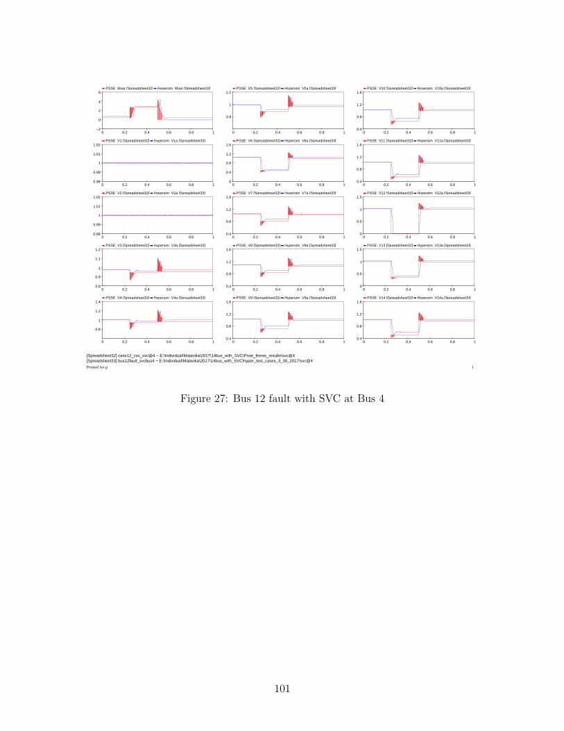
PSSE_Mvar [Spreadsheet32] Hypersim_Mvar [Spreadsheet33]

0 0.2 0.4 0.6 0.8 1−2

0

2

4

6

PSSE_V1 [Spreadsheet32] Hypersim_V1a [Spreadsheet33]

0 0.2 0.4 0.6 0.8 10.98

0.99

1

1.01

1.02

PSSE_V2 [Spreadsheet32] Hypersim_V2a [Spreadsheet33]

0 0.2 0.4 0.6 0.8 10.98

0.99

1

1.01

1.02

PSSE_V3 [Spreadsheet32] Hypersim_V3a [Spreadsheet33]

0 0.2 0.4 0.6 0.8 10.8

0.9

1

1.1

1.2

PSSE_V4 [Spreadsheet32] Hypersim_V4a [Spreadsheet33]

0 0.2 0.4 0.6 0.8 1

0.8

1

1.2

1.4

PSSE_V5 [Spreadsheet32] Hypersim_V5a [Spreadsheet33]

0 0.2 0.4 0.6 0.8 1

0.8

1

1.2

PSSE_V6 [Spreadsheet32] Hypersim_V6a [Spreadsheet33]

0 0.2 0.4 0.6 0.8 10

0.4

0.8

1.2

1.6

PSSE_V7 [Spreadsheet32] Hypersim_V7a [Spreadsheet33]

0 0.2 0.4 0.6 0.8 10.4

0.8

1.2

1.6

PSSE_V8 [Spreadsheet32] Hypersim_V8a [Spreadsheet33]

0 0.2 0.4 0.6 0.8 10.4

0.8

1.2

1.6

PSSE_V9 [Spreadsheet32] Hypersim_V9a [Spreadsheet33]

0 0.2 0.4 0.6 0.8 10.4

0.8

1.2

1.6

PSSE_V10 [Spreadsheet32] Hypersim_V10a [Spreadsheet33]

0 0.2 0.4 0.6 0.8 10.4

0.8

1.2

1.6

PSSE_V11 [Spreadsheet32] Hypersim_V11a [Spreadsheet33]

0 0.2 0.4 0.6 0.8 10.4

0.8

1.2

1.6

PSSE_V12 [Spreadsheet32] Hypersim_V12a [Spreadsheet33]

0 0.2 0.4 0.6 0.8 10

0.5

1

1.5

PSSE_V13 [Spreadsheet32] Hypersim_V13a [Spreadsheet33]

0 0.2 0.4 0.6 0.8 10

0.5

1

1.5

PSSE_V14 [Spreadsheet32] Hypersim_V14a [Spreadsheet33]

0 0.2 0.4 0.6 0.8 10.4

0.8

1.2

1.6

[Spreadsheet32] case12_csv_svc@4 − E:\Individual\Malavika\2017\14bus_with_SVC\Psse_thesis_results\svc@4[Spreadsheet33] bus12fault_svcbus4 − E:\Individual\Malavika\2017\14bus_with_SVC\hyper_test_cases_3_30_2017\svc@4

Printed for p 1

Figure 27: Bus 12 fault with SVC at Bus 4

101

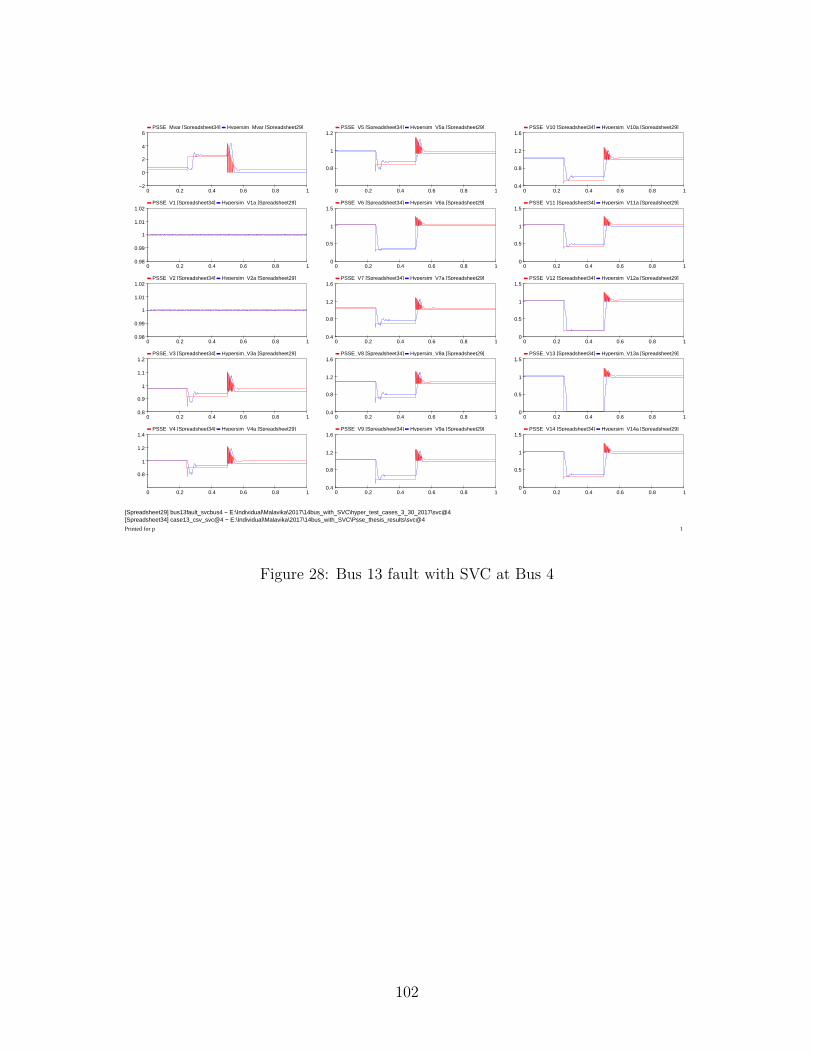
PSSE_Mvar [Spreadsheet34] Hypersim_Mvar [Spreadsheet29]

0 0.2 0.4 0.6 0.8 1−2

0

2

4

6

PSSE_V1 [Spreadsheet34] Hypersim_V1a [Spreadsheet29]

0 0.2 0.4 0.6 0.8 10.98

0.99

1

1.01

1.02

PSSE_V2 [Spreadsheet34] Hypersim_V2a [Spreadsheet29]

0 0.2 0.4 0.6 0.8 10.98

0.99

1

1.01

1.02

PSSE_V3 [Spreadsheet34] Hypersim_V3a [Spreadsheet29]

0 0.2 0.4 0.6 0.8 10.8

0.9

1

1.1

1.2

PSSE_V4 [Spreadsheet34] Hypersim_V4a [Spreadsheet29]

0 0.2 0.4 0.6 0.8 1

0.8

1

1.2

1.4

PSSE_V5 [Spreadsheet34] Hypersim_V5a [Spreadsheet29]

0 0.2 0.4 0.6 0.8 1

0.8

1

1.2

PSSE_V6 [Spreadsheet34] Hypersim_V6a [Spreadsheet29]

0 0.2 0.4 0.6 0.8 10

0.5

1

1.5

PSSE_V7 [Spreadsheet34] Hypersim_V7a [Spreadsheet29]

0 0.2 0.4 0.6 0.8 10.4

0.8

1.2

1.6

PSSE_V8 [Spreadsheet34] Hypersim_V8a [Spreadsheet29]

0 0.2 0.4 0.6 0.8 10.4

0.8

1.2

1.6

PSSE_V9 [Spreadsheet34] Hypersim_V9a [Spreadsheet29]

0 0.2 0.4 0.6 0.8 10.4

0.8

1.2

1.6

PSSE_V10 [Spreadsheet34] Hypersim_V10a [Spreadsheet29]

0 0.2 0.4 0.6 0.8 10.4

0.8

1.2

1.6

PSSE_V11 [Spreadsheet34] Hypersim_V11a [Spreadsheet29]

0 0.2 0.4 0.6 0.8 10

0.5

1

1.5

PSSE_V12 [Spreadsheet34] Hypersim_V12a [Spreadsheet29]

0 0.2 0.4 0.6 0.8 10

0.5

1

1.5

PSSE_V13 [Spreadsheet34] Hypersim_V13a [Spreadsheet29]

0 0.2 0.4 0.6 0.8 10

0.5

1

1.5

PSSE_V14 [Spreadsheet34] Hypersim_V14a [Spreadsheet29]

0 0.2 0.4 0.6 0.8 10

0.5

1

1.5

[Spreadsheet29] bus13fault_svcbus4 − E:\Individual\Malavika\2017\14bus_with_SVC\hyper_test_cases_3_30_2017\svc@4[Spreadsheet34] case13_csv_svc@4 − E:\Individual\Malavika\2017\14bus_with_SVC\Psse_thesis_results\svc@4

Printed for p 1

Figure 28: Bus 13 fault with SVC at Bus 4

102

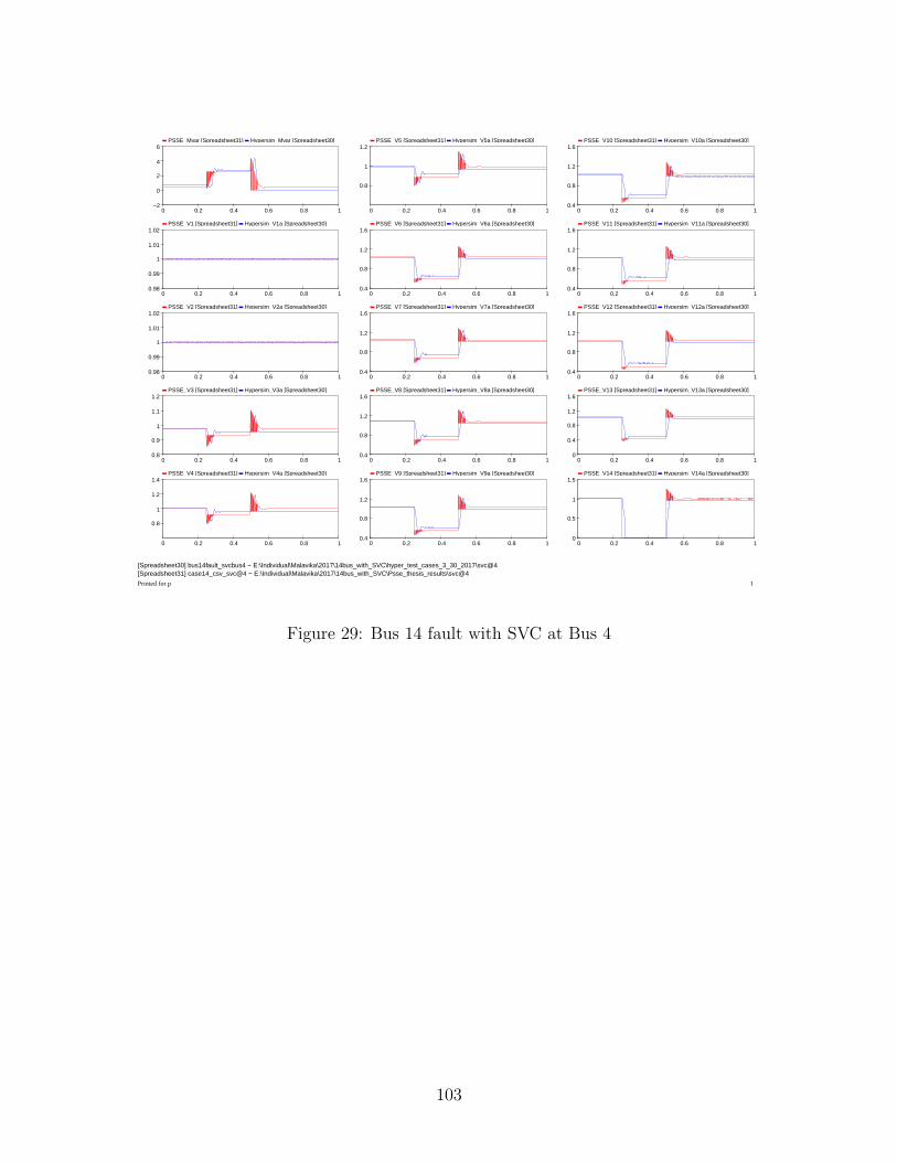
PSSE_Mvar [Spreadsheet31] Hypersim_Mvar [Spreadsheet30]

0 0.2 0.4 0.6 0.8 1−2

0

2

4

6

PSSE_V1 [Spreadsheet31] Hypersim_V1a [Spreadsheet30]

0 0.2 0.4 0.6 0.8 10.98

0.99

1

1.01

1.02

PSSE_V2 [Spreadsheet31] Hypersim_V2a [Spreadsheet30]

0 0.2 0.4 0.6 0.8 10.98

0.99

1

1.01

1.02

PSSE_V3 [Spreadsheet31] Hypersim_V3a [Spreadsheet30]

0 0.2 0.4 0.6 0.8 10.8

0.9

1

1.1

1.2

PSSE_V4 [Spreadsheet31] Hypersim_V4a [Spreadsheet30]

0 0.2 0.4 0.6 0.8 1

0.8

1

1.2

1.4

PSSE_V5 [Spreadsheet31] Hypersim_V5a [Spreadsheet30]

0 0.2 0.4 0.6 0.8 1

0.8

1

1.2

PSSE_V6 [Spreadsheet31] Hypersim_V6a [Spreadsheet30]

0 0.2 0.4 0.6 0.8 10.4

0.8

1.2

1.6

PSSE_V7 [Spreadsheet31] Hypersim_V7a [Spreadsheet30]

0 0.2 0.4 0.6 0.8 10.4

0.8

1.2

1.6

PSSE_V8 [Spreadsheet31] Hypersim_V8a [Spreadsheet30]

0 0.2 0.4 0.6 0.8 10.4

0.8

1.2

1.6

PSSE_V9 [Spreadsheet31] Hypersim_V9a [Spreadsheet30]

0 0.2 0.4 0.6 0.8 10.4

0.8

1.2

1.6

PSSE_V10 [Spreadsheet31] Hypersim_V10a [Spreadsheet30]

0 0.2 0.4 0.6 0.8 10.4

0.8

1.2

1.6

PSSE_V11 [Spreadsheet31] Hypersim_V11a [Spreadsheet30]

0 0.2 0.4 0.6 0.8 10.4

0.8

1.2

1.6

PSSE_V12 [Spreadsheet31] Hypersim_V12a [Spreadsheet30]

0 0.2 0.4 0.6 0.8 10.4

0.8

1.2

1.6

PSSE_V13 [Spreadsheet31] Hypersim_V13a [Spreadsheet30]

0 0.2 0.4 0.6 0.8 10

0.4

0.8

1.2

1.6

PSSE_V14 [Spreadsheet31] Hypersim_V14a [Spreadsheet30]

0 0.2 0.4 0.6 0.8 10

0.5

1

1.5

[Spreadsheet30] bus14fault_svcbus4 − E:\Individual\Malavika\2017\14bus_with_SVC\hyper_test_cases_3_30_2017\svc@4[Spreadsheet31] case14_csv_svc@4 − E:\Individual\Malavika\2017\14bus_with_SVC\Psse_thesis_results\svc@4

Printed for p 1

Figure 29: Bus 14 fault with SVC at Bus 4

103

PSSE_Mvar [Spreadsheet42] Hypersim_Mvar [Spreadsheet41]

0 0.2 0.4 0.6 0.8 1−2

0

2

4

6

PSSE_V1 [Spreadsheet42] Hypersim_V1a [Spreadsheet41]

0 0.2 0.4 0.6 0.8 10.98

0.99

1

1.01

1.02

PSSE_V2 [Spreadsheet42] Hypersim_V2a [Spreadsheet41]

0 0.2 0.4 0.6 0.8 10.98

0.99

1

1.01

1.02

PSSE_V3 [Spreadsheet42] Hypersim_V3a [Spreadsheet41]

0 0.2 0.4 0.6 0.8 10

0.5

1

1.5

PSSE_V4 [Spreadsheet42] Hypersim_V4a [Spreadsheet41]

0 0.2 0.4 0.6 0.8 10.4

0.8

1.2

1.6

PSSE_V5 [Spreadsheet42] Hypersim_V5a [Spreadsheet41]

0 0.2 0.4 0.6 0.8 1

0.8

1

1.2

1.4

PSSE_V6 [Spreadsheet42] Hypersim_V6a [Spreadsheet41]

0 0.2 0.4 0.6 0.8 10.4

0.8

1.2

1.6

PSSE_V7 [Spreadsheet42] Hypersim_V7a [Spreadsheet41]

0 0.2 0.4 0.6 0.8 10.4

0.8

1.2

1.6

PSSE_V8 [Spreadsheet42] Hypersim_V8a [Spreadsheet41]

0 0.2 0.4 0.6 0.8 10.4

0.8

1.2

1.6

PSSE_V9 [Spreadsheet42] Hypersim_V9a [Spreadsheet41]

0 0.2 0.4 0.6 0.8 10.4

0.8

1.2

1.6

PSSE_V10 [Spreadsheet42] Hypersim_V10a [Spreadsheet41]

0 0.2 0.4 0.6 0.8 10.4

0.8

1.2

1.6

PSSE_V11 [Spreadsheet42] Hypersim_V11a [Spreadsheet41]

0 0.2 0.4 0.6 0.8 10.4

0.8

1.2

1.6

PSSE_V12 [Spreadsheet42] Hypersim_V12a [Spreadsheet41]

0 0.2 0.4 0.6 0.8 10.4

0.8

1.2

1.6

PSSE_V13 [Spreadsheet42] Hypersim_V13a [Spreadsheet41]

0 0.2 0.4 0.6 0.8 10.4

0.8

1.2

1.6

PSSE_V14 [Spreadsheet42] Hypersim_V14a [Spreadsheet41]

0 0.2 0.4 0.6 0.8 10.4

0.8

1.2

1.6

[Spreadsheet41] bus3fault_svcbus5 − E:\Individual\Malavika\2017\14bus_with_SVC\hyper_test_cases_3_30_2017\svc@5[Spreadsheet42] case3_csv_svc@5 − E:\Individual\Malavika\2017\14bus_with_SVC\Psse_thesis_results\svc@5

Printed for p 1

Figure 30: Bus 3 fault with SVC at Bus 5

104

PSSE_Mvar [Spreadsheet48] Hypersim_Mvar [Spreadsheet46]

0 0.2 0.4 0.6 0.8 1−2

0

2

4

6

PSSE_V1 [Spreadsheet48] Hypersim_V1a [Spreadsheet46]

0 0.2 0.4 0.6 0.8 10.98

0.99

1

1.01

1.02

PSSE_V2 [Spreadsheet48] Hypersim_V2a [Spreadsheet46]

0 0.2 0.4 0.6 0.8 10.98

0.99

1

1.01

1.02

PSSE_V3 [Spreadsheet48] Hypersim_V3a [Spreadsheet46]

0 0.2 0.4 0.6 0.8 10.8

0.9

1

1.1

PSSE_V4 [Spreadsheet48] Hypersim_V4a [Spreadsheet46]

0 0.2 0.4 0.6 0.8 1

0.8

1

1.2

PSSE_V5 [Spreadsheet48] Hypersim_V5a [Spreadsheet46]

0 0.2 0.4 0.6 0.8 1

0.8

1

1.2

1.4

PSSE_V6 [Spreadsheet48] Hypersim_V6a [Spreadsheet46]

0 0.2 0.4 0.6 0.8 10

0.5

1

1.5

PSSE_V7 [Spreadsheet48] Hypersim_V7a [Spreadsheet46]

0 0.2 0.4 0.6 0.8 10.4

0.8

1.2

1.6

PSSE_V8 [Spreadsheet48] Hypersim_V8a [Spreadsheet46]

0 0.2 0.4 0.6 0.8 10.4

0.8

1.2

1.6

PSSE_V9 [Spreadsheet48] Hypersim_V9a [Spreadsheet46]

0 0.2 0.4 0.6 0.8 10

0.4

0.8

1.2

1.6

PSSE_V10 [Spreadsheet48] Hypersim_V10a [Spreadsheet46]

0 0.2 0.4 0.6 0.8 10

0.5

1

1.5

PSSE_V11 [Spreadsheet48] Hypersim_V11a [Spreadsheet46]

0 0.2 0.4 0.6 0.8 10

0.5

1

1.5

PSSE_V12 [Spreadsheet48] Hypersim_V12a [Spreadsheet46]

0 0.2 0.4 0.6 0.8 10

0.5

1

1.5

PSSE_V13 [Spreadsheet48] Hypersim_V13a [Spreadsheet46]

0 0.2 0.4 0.6 0.8 10

0.5

1

1.5

PSSE_V14 [Spreadsheet48] Hypersim_V14a [Spreadsheet46]

0 0.2 0.4 0.6 0.8 10

0.5

1

1.5

[Spreadsheet46] bus6fault_svcbus5 − E:\Individual\Malavika\2017\14bus_with_SVC\hyper_test_cases_3_30_2017\svc@5[Spreadsheet48] case6_csv_svc@5 − E:\Individual\Malavika\2017\14bus_with_SVC\Psse_thesis_results\svc@5

Printed for p 1

Figure 31: Bus 6 fault with SVC at Bus 5

105

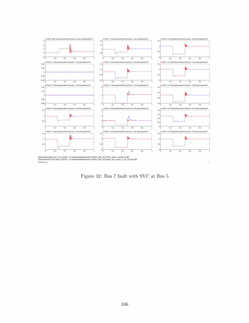
PSSE_Mvar [Spreadsheet46] Hypersim_Mvar [Spreadsheet47]

0 0.2 0.4 0.6 0.8 1−2

0

2

4

6

PSSE_V1 [Spreadsheet46] Hypersim_V1a [Spreadsheet47]

0 0.2 0.4 0.6 0.8 10.98

0.99

1

1.01

1.02

PSSE_V2 [Spreadsheet46] Hypersim_V2a [Spreadsheet47]

0 0.2 0.4 0.6 0.8 10.98

0.99

1

1.01

1.02

PSSE_V3 [Spreadsheet46] Hypersim_V3a [Spreadsheet47]

0 0.2 0.4 0.6 0.8 1

0.8

1

1.2

PSSE_V4 [Spreadsheet46] Hypersim_V4a [Spreadsheet47]

0 0.2 0.4 0.6 0.8 1

0.8

1

1.2

PSSE_V5 [Spreadsheet46] Hypersim_V5a [Spreadsheet47]

0 0.2 0.4 0.6 0.8 1

0.8

1

1.2

1.4

PSSE_V6 [Spreadsheet46] Hypersim_V6a [Spreadsheet47]

0 0.2 0.4 0.6 0.8 10.4

0.8

1.2

1.6

PSSE_V7 [Spreadsheet46] Hypersim_V7a [Spreadsheet47]

0 0.2 0.4 0.6 0.8 10

1

2

PSSE_V8 [Spreadsheet46] Hypersim_V8a [Spreadsheet47]

0 0.2 0.4 0.6 0.8 10

1

2

3

PSSE_V9 [Spreadsheet46] Hypersim_V9a [Spreadsheet47]

0 0.2 0.4 0.6 0.8 10

0.5

1

1.5

PSSE_V10 [Spreadsheet46] Hypersim_V10a [Spreadsheet47]

0 0.2 0.4 0.6 0.8 10

0.5

1

1.5

PSSE_V11 [Spreadsheet46] Hypersim_V11a [Spreadsheet47]

0 0.2 0.4 0.6 0.8 10

0.5

1

1.5

PSSE_V12 [Spreadsheet46] Hypersim_V12a [Spreadsheet47]

0 0.2 0.4 0.6 0.8 10.4

0.8

1.2

1.6

PSSE_V13 [Spreadsheet46] Hypersim_V13a [Spreadsheet47]

0 0.2 0.4 0.6 0.8 10

0.4

0.8

1.2

1.6

PSSE_V14 [Spreadsheet46] Hypersim_V14a [Spreadsheet47]

0 0.2 0.4 0.6 0.8 10

0.5

1

1.5

[Spreadsheet46] case7_csv_svc@5 − E:\Individual\Malavika\2017\14bus_with_SVC\Psse_thesis_results\svc@5[Spreadsheet47] bus7fault_svcbus5 − E:\Individual\Malavika\2017\14bus_with_SVC\hyper_test_cases_3_30_2017\svc@5

Printed for p 1

Figure 32: Bus 7 fault with SVC at Bus 5

106

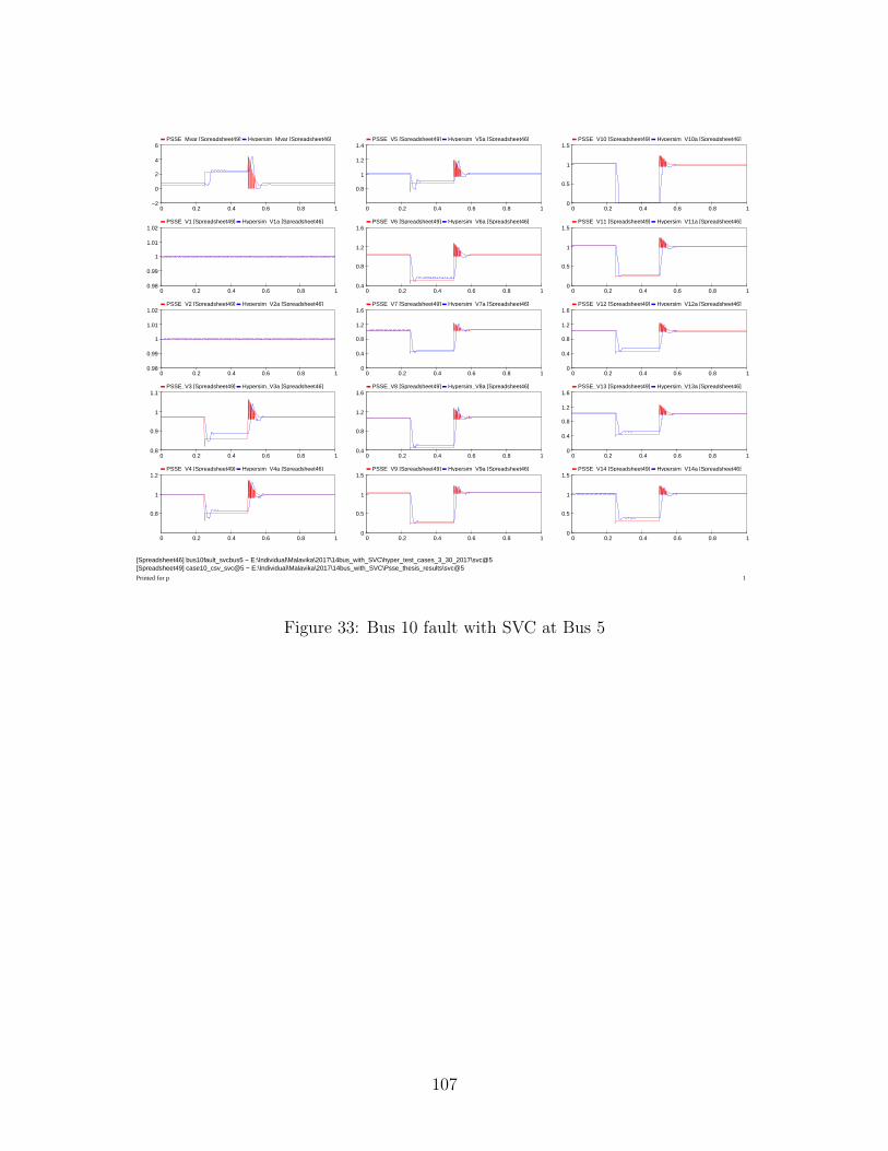
PSSE_Mvar [Spreadsheet49] Hypersim_Mvar [Spreadsheet46]

0 0.2 0.4 0.6 0.8 1−2

0

2

4

6

PSSE_V1 [Spreadsheet49] Hypersim_V1a [Spreadsheet46]

0 0.2 0.4 0.6 0.8 10.98

0.99

1

1.01

1.02

PSSE_V2 [Spreadsheet49] Hypersim_V2a [Spreadsheet46]

0 0.2 0.4 0.6 0.8 10.98

0.99

1

1.01

1.02

PSSE_V3 [Spreadsheet49] Hypersim_V3a [Spreadsheet46]

0 0.2 0.4 0.6 0.8 10.8

0.9

1

1.1

PSSE_V4 [Spreadsheet49] Hypersim_V4a [Spreadsheet46]

0 0.2 0.4 0.6 0.8 1

0.8

1

1.2

PSSE_V5 [Spreadsheet49] Hypersim_V5a [Spreadsheet46]

0 0.2 0.4 0.6 0.8 1

0.8

1

1.2

1.4

PSSE_V6 [Spreadsheet49] Hypersim_V6a [Spreadsheet46]

0 0.2 0.4 0.6 0.8 10.4

0.8

1.2

1.6

PSSE_V7 [Spreadsheet49] Hypersim_V7a [Spreadsheet46]

0 0.2 0.4 0.6 0.8 10

0.4

0.8

1.2

1.6

PSSE_V8 [Spreadsheet49] Hypersim_V8a [Spreadsheet46]

0 0.2 0.4 0.6 0.8 10.4

0.8

1.2

1.6

PSSE_V9 [Spreadsheet49] Hypersim_V9a [Spreadsheet46]

0 0.2 0.4 0.6 0.8 10

0.5

1

1.5

PSSE_V10 [Spreadsheet49] Hypersim_V10a [Spreadsheet46]

0 0.2 0.4 0.6 0.8 10

0.5

1

1.5

PSSE_V11 [Spreadsheet49] Hypersim_V11a [Spreadsheet46]

0 0.2 0.4 0.6 0.8 10

0.5

1

1.5

PSSE_V12 [Spreadsheet49] Hypersim_V12a [Spreadsheet46]

0 0.2 0.4 0.6 0.8 10

0.4

0.8

1.2

1.6

PSSE_V13 [Spreadsheet49] Hypersim_V13a [Spreadsheet46]

0 0.2 0.4 0.6 0.8 10

0.4

0.8

1.2

1.6

PSSE_V14 [Spreadsheet49] Hypersim_V14a [Spreadsheet46]

0 0.2 0.4 0.6 0.8 10

0.5

1

1.5

[Spreadsheet46] bus10fault_svcbus5 − E:\Individual\Malavika\2017\14bus_with_SVC\hyper_test_cases_3_30_2017\svc@5[Spreadsheet49] case10_csv_svc@5 − E:\Individual\Malavika\2017\14bus_with_SVC\Psse_thesis_results\svc@5

Printed for p 1

Figure 33: Bus 10 fault with SVC at Bus 5

107

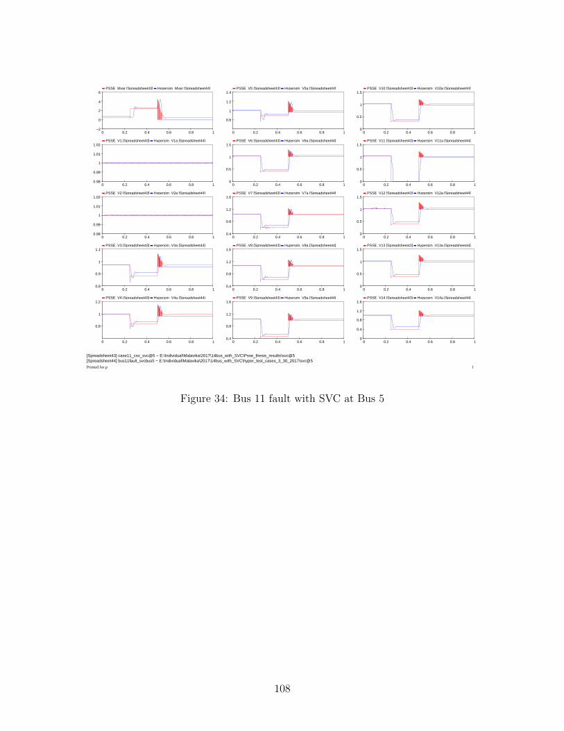
PSSE_Mvar [Spreadsheet43] Hypersim_Mvar [Spreadsheet44]

0 0.2 0.4 0.6 0.8 1−2

0

2

4

6

PSSE_V1 [Spreadsheet43] Hypersim_V1a [Spreadsheet44]

0 0.2 0.4 0.6 0.8 10.98

0.99

1

1.01

1.02

PSSE_V2 [Spreadsheet43] Hypersim_V2a [Spreadsheet44]

0 0.2 0.4 0.6 0.8 10.98

0.99

1

1.01

1.02

PSSE_V3 [Spreadsheet43] Hypersim_V3a [Spreadsheet44]

0 0.2 0.4 0.6 0.8 10.8

0.9

1

1.1

PSSE_V4 [Spreadsheet43] Hypersim_V4a [Spreadsheet44]

0 0.2 0.4 0.6 0.8 1

0.8

1

1.2

PSSE_V5 [Spreadsheet43] Hypersim_V5a [Spreadsheet44]

0 0.2 0.4 0.6 0.8 1

0.8

1

1.2

1.4

PSSE_V6 [Spreadsheet43] Hypersim_V6a [Spreadsheet44]

0 0.2 0.4 0.6 0.8 10

0.5

1

1.5

PSSE_V7 [Spreadsheet43] Hypersim_V7a [Spreadsheet44]

0 0.2 0.4 0.6 0.8 10.4

0.8

1.2

1.6

PSSE_V8 [Spreadsheet43] Hypersim_V8a [Spreadsheet44]

0 0.2 0.4 0.6 0.8 10.4

0.8

1.2

1.6

PSSE_V9 [Spreadsheet43] Hypersim_V9a [Spreadsheet44]

0 0.2 0.4 0.6 0.8 10.4

0.8

1.2

1.6

PSSE_V10 [Spreadsheet43] Hypersim_V10a [Spreadsheet44]

0 0.2 0.4 0.6 0.8 10

0.5

1

1.5

PSSE_V11 [Spreadsheet43] Hypersim_V11a [Spreadsheet44]

0 0.2 0.4 0.6 0.8 10

0.5

1

1.5

PSSE_V12 [Spreadsheet43] Hypersim_V12a [Spreadsheet44]

0 0.2 0.4 0.6 0.8 10

0.5

1

1.5

PSSE_V13 [Spreadsheet43] Hypersim_V13a [Spreadsheet44]

0 0.2 0.4 0.6 0.8 10

0.5

1

1.5

PSSE_V14 [Spreadsheet43] Hypersim_V14a [Spreadsheet44]

0 0.2 0.4 0.6 0.8 10

0.4

0.8

1.2

1.6

[Spreadsheet43] case11_csv_svc@5 − E:\Individual\Malavika\2017\14bus_with_SVC\Psse_thesis_results\svc@5[Spreadsheet44] bus11fault_svcbus5 − E:\Individual\Malavika\2017\14bus_with_SVC\hyper_test_cases_3_30_2017\svc@5

Printed for p 1

Figure 34: Bus 11 fault with SVC at Bus 5

108

PSSE_Mvar [Spreadsheet45] Hypersim_Mvar [Spreadsheet44]

0 0.2 0.4 0.6 0.8 1−2

0

2

4

6

PSSE_V1 [Spreadsheet45] Hypersim_V1a [Spreadsheet44]

0 0.2 0.4 0.6 0.8 10.98

0.99

1

1.01

1.02

PSSE_V2 [Spreadsheet45] Hypersim_V2a [Spreadsheet44]

0 0.2 0.4 0.6 0.8 10.98

0.99

1

1.01

1.02

PSSE_V3 [Spreadsheet45] Hypersim_V3a [Spreadsheet44]

0 0.2 0.4 0.6 0.8 10.8

0.9

1

1.1

PSSE_V4 [Spreadsheet45] Hypersim_V4a [Spreadsheet44]

0 0.2 0.4 0.6 0.8 1

0.8

1

1.2

PSSE_V5 [Spreadsheet45] Hypersim_V5a [Spreadsheet44]

0 0.2 0.4 0.6 0.8 1

0.8

1

1.2

1.4

PSSE_V6 [Spreadsheet45] Hypersim_V6a [Spreadsheet44]

0 0.2 0.4 0.6 0.8 10.4

0.8

1.2

1.6

PSSE_V7 [Spreadsheet45] Hypersim_V7a [Spreadsheet44]

0 0.2 0.4 0.6 0.8 10.4

0.8

1.2

1.6

PSSE_V8 [Spreadsheet45] Hypersim_V8a [Spreadsheet44]

0 0.2 0.4 0.6 0.8 10.4

0.8

1.2

1.6

PSSE_V9 [Spreadsheet45] Hypersim_V9a [Spreadsheet44]

0 0.2 0.4 0.6 0.8 10.4

0.8

1.2

1.6

PSSE_V10 [Spreadsheet45] Hypersim_V10a [Spreadsheet44]

0 0.2 0.4 0.6 0.8 10.4

0.8

1.2

1.6

PSSE_V11 [Spreadsheet45] Hypersim_V11a [Spreadsheet44]

0 0.2 0.4 0.6 0.8 10.4

0.8

1.2

1.6

PSSE_V12 [Spreadsheet45] Hypersim_V12a [Spreadsheet44]

0 0.2 0.4 0.6 0.8 10.4

0.8

1.2

1.6

PSSE_V13 [Spreadsheet45] Hypersim_V13a [Spreadsheet44]

0 0.2 0.4 0.6 0.8 10

0.4

0.8

1.2

1.6

PSSE_V14 [Spreadsheet45] Hypersim_V14a [Spreadsheet44]

0 0.2 0.4 0.6 0.8 10

0.5

1

1.5

[Spreadsheet44] bus14fault_svcbus5 − E:\Individual\Malavika\2017\14bus_with_SVC\hyper_test_cases_3_30_2017\svc@5[Spreadsheet45] case14_csv_svc@5 − E:\Individual\Malavika\2017\14bus_with_SVC\Psse_thesis_results\svc@5

Printed for p 1

Figure 35: Bus 14 fault with SVC at Bus 5

109

Vita

Malavika Vasudevan Menon was born in India, in 1992. She received her Bachelor of

Technology degree in Electronics and Communication Engineering from Mahatma Gandhi

University, Kerala, India, in 2014. She joined the University of New Orleans in Spring, 2015

to pursue a Master’s degree in Electrical Engineering.

She joined the Power and Energy Research Laboratory under Dr. Parviz Rastgoufard in

2015 and worked on projects in the area of Power systems transmission modeling, simulation,

and design and gained knowledge in using the software platforms such as PSS/E, EMTP,

Hypersim for steady state, dynamic, and hardware-in-the-loop modeling and simulation of

power systems.

110