Estimation of a trip table and the Θ parameter in a stochastic network

Transpn. Rex-A., Vol. 30, No. 4, pp. 287-305, 1996 Copyright G 1996 Elsevier Science Ltd

Pergamon Printed~in Great Britain. All rights reserved 0965-8564/96 $15.00 + 0.00

ESTIMATION OF A TRIP TABLE AND THE 0 PARAMETER IN A STOCHASTIC NETWORK

SHIHSIEN LIU Department of Transportation Management, Tamkang University, Taipei, Taiwan, R.O.C.

and

JON D. FRICKER School of Civil Engineering, Purdue University, West Lafayette, IN 47907-1284, U.S.A

(Received I3 March 1995)

Abstract-An origin-destination (O-D) table that accurately portrays a study area’s travel patterns is a valuable element in the modeling and analysis used to support public transportation investment decisions. The probabilistic approach to O-D table estimation involves a heuristic enumeration of link choice probabilities. The parameter 8, which reflects the variation in path choices among tripmakers, has not been discussed in the context of O-D table estimation, nor has an efficient way been demonstrated to determine the associated link use probabilities. This paper presents a method for O-D table estimation in a stochastic network. The “OD,Theta” method can not only estimate the O-D table, it also estimates the 8 parameter in the same process. The proposed method is illustrated using a sample test network. Finally, the method is applied to a real network, with the results compared to those from some well-known O-D estimation software. Copyright 0 1996 Elsevier Science Ltd

INTRODUCTION

The accuracy of an origin-destination (O-D) table estimated from link counts is affected by many factors, including the accuracy of the link counts and the assumed route choice behavior of the tripmakers. There are three main ways to approach this problem, all of which are based on explicit trip-making behavior.

The Gravity Model assumes that each trip interchange value is based on the level of productions and attractions at the trip origin and destination, and on a function that represents the spatial separation of each origin-destination pair. Because trip impedance between each O-D pair affects the level of the trip production and attraction, the main drawback of the gravity model is that it cannot handle with accuracy external-external (or ‘through’) trips (Willumsen, 1981).

A second approach uses mathematical programming techniques associated with equilibrium traffic assignment methods to estimate a trip matrix in a congested network. Based on the user equilibrium condition, Nguyen (1977) developed a bi-level programming structure to derive O-D tables from traffic counts via two models. By ‘bi-level programming problem’, we mean using two separate but interdependent optimization models to solve the problem iteratively. The major disadvantage of this approach is that a bi-level programming structure would pose computational difficulties for a large network.

The third approach, entropy maximization (EM) and information minimization (IM), can make full use of the information contained in the observed flows. Actually, EM and IM are two similar but distinct model types. EM assumes that observed link counts follow the multinomial distribution. This assumption provides the basis for modeling O-D trip patterns if no more information is known about the network flows. The IM model, however, adjusts the EM’s distribution assumption if given information about the degree to which O-D trips use each of the links in the network. Unfortunately, the link use information is usually derived from an outdated or artificially fabricated trip table.

287

288 Shihsien Liu and Jon D. Fricker

Models following the EM and IM philosophies are developed and analyzed in Van Zuylen and Willumsen (1980) and Beagan (1986) applied these methods on a small network. However, the input information is tedious and hard to generate in practice. A more recent version of The Highway Emulator (THE) (Bromage, 1988) has eased the input effort, but the underlying assumptions and the need to internally fabricate a ‘target’ trip table remain.

Probabilistic O-D estimation approaches such as EM and IM involve a heuristic enumeration of link choice probabilities. Most previous optimization approaches have neglected: (a) the fact that not all drivers will have perfect information on path travel costs; and (b) how sensitive drivers’ choices of paths are among reasonable candidate paths. By incorporating the assumption that the logit model describes driver route choice, the underspecified nature of this problem is resolved. This paper addresses networks that have stochastic characteristics (i.e. travelers’ perceptions of link costs vary) and extends the O-D estimation model to include the 0 route choice parameter at the same time.

NOTATION

A : set of links K : set of possible paths N : set of nodes 0 : stochastic assignment dispersion parameter

{(r&I : set of O-D pairs V r,s E N

6” = 1 if link a is on path k between r and s ak 1 0 otherwise

c, : observed travel cost on link a

cp = C(ca4s) : kth path travel cost from r to s

Pr : parobability of selecting path k from r to s P rsa : probability of choosing link a on all possible paths from r to s

T, : target trip interchange value from r to s, if available

4 rs : O-D flow from r to s pbs .

,&t . observed link volume on link a

a : estimated link volume on link a from the model

METHODOLOGY

The formulation

Given a set of link flows and link travel costs, estimating the best O-D table and 8 parameter can be interpreted as reversing the stochastic logit network loading process (Sheffi, 1985) so that the assigned link flows from the estimated O-D table and 0 parameter are close to the observed flows. Consequently, we can formulate the O-D table and 0 parameter estimation as minimizing the difference between modeled and observed flows, and solve the problem by using a stochastic logit assignment approach and nonlinear programming techniques. The formulation is as follows.

L(qr’, 0) =Min c [ c q” . (c Pr . 6:) - _x,0bs12

a F-s k

St.

qrs 2 0.

(1)

Because all variables must be non-negative, the optimal solution will be located either at the boundary point or in the interior of the feasible region, as shown in Fig. 1.

Estimation of a trip table 289

(a) (b)

Fig. I. Optimality in constrained cases.

The mathematical forms of Fig. l(a) and (b) are:

V(x) = () x’X- (2)

The above formulation can be interpreted as Primal and Dual problems in Linear Programming and converted to a Linear Complementarity Problem (LCP) (Bazaraa & Shetty, 1979). To make this conversion, eqn (1) is modified as follows.

L = Min c [ c q” . (c Fl .6z) - xzbs]* - c c wrs . qrs II ,s k I s

(3)

where qrs and 8 are decision variables and

Also, w” is the dual variable of O-D flow, 4”. From the optimality conditions in eqns (2), we get the following problem:

e = 0 + 2 c [ c(Pp5;) . (C qrs. ~(p;sb$) - Xp)] - wrs = 0 V(r,s) (4) 0 k IS k

dL .- wrs dw’S = 0 -_) W’S . qrs = 0.

wrs >_ 0

qrs 2 0

Using linear algebra, this formulation can be restated as:

W-M.q=b

w*q=o

WLO

q10

where W: M:

vector of dual variable of q” positive definite Hessian matrix of the objective function

(5)


vector of O-D flow to be estimated vector of right hand side

b = c P,,, . (-xibS). a

The formulation above is actually a LCP that is guaranteed to terminate in a finite number of steps with either an optimal or unbounded solution (Bazaraa & Shetty, 1979; Evans, 1971). In 1968, Lemke introduced a revised simplex method to solve this problem, but restricted both entering and leaving variables to be complementary to each other.

Solving the problem by using the derivative of the objective function with respect to 0 can accelerate convergence, but carries with it greater computational effort in path searching. To avoid path enumeration and to estimate both 0 and an O-D table, we separate the search procedures for the optimal solution into two stages. The first stage applies a logit-based assignment model combined with Lemke’s LCP algorithm to estimate the O-D table. Solutions from the first stage then act as an input to the second stage -the maximum likelihood method-to get the parameter 0. Iterations are repeated until the the first derivative of the maximum likelihood value approaches zero.

In 1974, Robillard showed how maximum likelihood could be used to estimate the parameters in the multipath assignment method introduced by Dial in 1971 (Dial, 197 1; Sheffi, 1985). Robillard used a link-based approach in applying the maximum likelihood method, but the search method he applied was deficient. Because a maximum likelihood formulation is an unconstrained problem, to calibrate a 0 parameter is to find the convergent point when the value of the first derivative of the objective function vanishes. However, Robillard estimated these first derivative function values by introducing two initial 0 parameters. If the signs of the two initial first derivative function values are the same, then the estimated interval of OS will be expanded by 10%. Otherwise, a binary search is used to locate the points for the next iteration.

Because the local optimal point is located where the first derivative vanishes, if the signs of the first derivatives of the objective function associated with two points, 0, and Q2, are opposite, then the optimal solution Q* exists between Qi and OZ. Fisk (1977) suggested a path-based approach to formulate the 0 calibration problem using the maximum likelihood method, in which the optimal solution can be searched more efficiently. Her search effort used the Hessian matrix-the second derivative of the objective function. However, the preliminary task of calculating each path probability can be costly, so Fisk’s approach becomes impractical when the network is large and has multiple paths.

Two-stage calibration for 0 Let x, : flow on link a

and

wheref;: flow on path k from r to s, and other notation is as before. The maximum likelihood method then can be formulated as:

where

Estimation of a trip table

Let

L(0) = lnX(~~}, 0) = CCC In(T).

rs k

Because

E(c;;‘) = c cr P; k

and

291

(7)

(8)

(9)

this is an unconstrained optimization problem. The stationary point can be obtained when the first derivative is zero:

From (8)

(10)

From (9)

aw a. = -y{C[cy . P,,, . qrsl - [I c:” .x:1)

i-s u ‘i

In eqn (lo), the first derivative of the maximum likelihood function contains only link variables. However, estimating the second derivative of the objective function, $& requires path enumeration, which makes this approach ineffective. To avoid directly computing the second derivative of the objective function, the secant method (Haggerty, 1972, pp. 53-54) approximates the second derivative value by using the slope of two first derivatives of the objective function. Starting at two initial values, the next point then can be obtained as shown in Fig. 2.

Based on this two-stage line search strategy, a convergent solution will be obtained by iterative applications of the LCP algorithm and the maximum likelihood method. There- fore, the optimal solution of an O-D table, as well as the 0 parameter, can be found. For this reason, we shall refer to the proposed method as the ‘OD.Theta’ approach.


aL(o) ao

Fig. 2. Line search by the Secant Method.

SOLUTION ALGORITHM

To estimate an O-D table and to calibrate a 0 parameter in a stochastic network, the steps in the proposed ODeTheta approach are as follows.

1.

2.

3. 4.

5.

6. 7.

8. 9.

Let RUN = 0, where RUN is the number of iterations so far. Start with two initial 0 values, say, 01 and 02. Let 0 = 01. If tripmakers will not accept distinctly inferior

paths, the possible range of 0 values will be between zero and some positive number. Determine all-to-all shortest paths (Minieka, 1978). A flow pattern in a real transportation network involves multiple O-D pairs. In an uncongested stochastic network, the all-to-all shortest path information is especially useful for the logit assignment model. This is because the defined route choice set involves a comparison at each intermediate node to determine whether the next sequential node is closer to the destination and farther away from the origin node. Such a sequence of nodes comprises a ‘reasonable’ route. (Sheffi, 1985, p. 288) RUN = RUN + 1 Traffic assignment by the logit model. To formulate the objective function using least squared error requires the link use probabilities from each O-D pair. The logit model as implemented by Dial’s algorithm (Dial, 1971; Sheffi, 1985) establishes the framework for estimating these P,,, values, which appear in eqns (5) and eqns (10). Least squared error formulation. Develop the least squared error objective function as in eqn (1) and convert the least squared form into a LCP standard form. In the converted formulation, only the O-D variables q’” are decision variables. Use the LCP algorithm to solve for the O-D table. Calculate Root Mean Square

RMSE= \j”l%;““‘;

where N is the number of links with observed link counts and a E set of links with counts. Check the first derivative of the likelihood function and calculate RMSE. If the values are within acceptable error or RUN reaches the maximum allowed number of iterations, STOP; otherwise, go to next step. If RUN = 1, then let 0 = O2 and go to Step 3; otherwise, go to next step. Find a new 01 by the Secant Method. Of the two old OS, keep the one with the lower absolute first derivative value as Q2, and go to Step 3.

The only input data are the observed link counts and link costs; the decision variables are the O-D table entries and the 0 parameter.

SAMPLE TESTS

In this section, a network used by Robillard (1974) and Fisk (1977) (see Fig. 3) is employed to demonstrate the estimation of both 0 and an O-D table. If the first two


link travel cost (observed flow)

Fig. 3. Robillard Network

iterations are not counted, the convergent solutions using bi-level programming are as shown in Fig. 4.

The final results are 0 = 1.35 (which matches the value found by both Robillard and Fisk) and the O-D matrix shown in Table 1.

The results not only verify that an O-D table and a 0 parameter can be estimated at the same time, but they also demonstrate that the OD.Theta algorithm matches the observed link volumes closely.

The next example will show that errors in an O-D table and in a 0 estimation can be caused by adopting a poor tripmaker path choice rule. The “hypothetical observed link counts” in Fig. 3 were obtained from a logit assignment using the input data-an O-D table and, a 8 parameter-and the assumption that tripmakers only choose ‘reasonable’ routes. By employing the same path choice rules, reversing the network loading procedures to estimate both an O-D table and a 8 parameter should duplicate the original conditions. However, in a real network, drivers may not always restrict their choices to ‘reasonable’ paths. If this ‘reasonable path’ rule is followed, the possible paths from ori- gins 1 and 2 to destination 9 in Fig. 3 will never include link (2,3). This is because, from node 2, the shortest path travel cost to the destination is 3 units. If drivers choose node 3 from node 2 as their next node, the shortest path travel cost to the destination from node 3 is still 3 units, which is not closer to the destination. Therefore, the ‘reasonable path’

( l&l : Maximum Likelihood Method) ae

0.060 , I

0.042 -

0.036 -

0.030 -

0.024 -

0.018 -

0.012 -

0.006 -

0 I I ; 2 3 4 S

Number of Iterations

Fig. 4. Convergent OD,Theta solutions for Robillard Network

12

8

6


Table I Multiple estimation result (0 = I .35)

Origin Destination

8 9

I 500 199 2 0 300

Flow

Link .Ps .P’

(12) 230 230.42

(134) 239 238.69

(l,5) 230 230.42

(2,3) 0 0

(2,5) 530 530.39

(376) 0 0

(4.5) 60 59.55

(437) 179 179.13

(56) 158 157.91

(538) 505 504.56

(539) I58 157.91

(639) I58 157.91

(738) 179 179.13

(g>9) I84 183.55

rule excludes paths l-2-3-6-9 and 2-3-6-9 from consideration, even though their total path costs are only one unit greater than some of the ‘reasonable’ paths. This is likely to make the logit assignment flow pattern less dispersed than the actual pattern.

If we redefine ‘reasonable’ paths as those whose sequence of nodes merely take tripmakers further away from their origin nodes, then the estimation results for Fig. 3 get worse. (See Fig. 5 and Table 2.) 0 = 1.926, which produces a flow pattern with an aver- age RMSE x 13 trips per link (vs nearly zero in Table 1). After changing the ‘reasonable path’ rule, some travelers now use link (2,3) to reach destination 9 from origin 1 or 2. In

0.160

0.096

0.080

0.064

0.048

0.032

0.016

0

Solutions of Algorithm (Modified Choice Set)

. . *.*

!..._ . ’ RMSE i

I : I I I I I I I I ; 2 j 4 ; 6 7 8

24

20

16

8

4

0

Number of Iterations

Fig. 5. Convergent solutions by changed choice set.


Table 2. Multiple estimation result after changed choice set (0 = 1.926)

Origin Destination

8 9

I 512 I85 2 0 312

Link Xobs

Flow

pt

(172) 230 239.27

(134) 239 221.39

(l>5) 230 235.73

(2,3) 0 17.98

(2,5) 530 532.8

(336) 0 17.98

(475) 60 34.35

(427) 179 187.04

(5,6) 158 151.26

(5>8) 505 500.36

(5>9) 158 151.26

(6>9) 158 169.24

(7,8) 179 187.04

(899) I84 175.6

both Figs 4 and 5, the compatible convergence behavior of the RMSE and first partial derivative values can be observed, although the RMSE plot levels out more quickly. In addition, some tests indicated that the derivative values are not as stable as the RMSE values, as the iterations continue toward the stopping criteria.

If we relax the ‘reasonable path’ definition as described above, more alternatives that are intuitively ‘reasonable’ can be considered and chosen. Link (2,3), although having no ‘observed’ link counts, is also modeled as being chosen by some travelers. Because the objective function is to minimize the least squared error, the model will decrease the path flow passing through link (2,3) to as close to zero as possible. This has the impact of increasing the flow on the other possible paths and increasing the value of the 8 parameter. When compared with the results in Table 1, the final solution in Table 2 underestimates the O-D flow from node 1 to node 9 and overestimates other O-D trips.

There is no general criterion by which to determine which path choice rule is better. However, if some links with observed link counts have not been selected by a model, then analysts need to revise the route choice rules.

Another small network, called Oct8X (see Fig. 6), was used for tests of the ‘OD.Theta’ approach and The Highway Emulator (THE). THE is a well-known software package that estimates O-D tables from link counts using the Maximum Entropy approach (Van Zuylen & Willumsen, 1980). THE’s O-D estimation algorithm makes the smallest possible adjustments to an initial trip table in order to match the observed link volumes (Bromage, 1988). Results from THE on ‘Oct8X’ are listed in Table 3.

For ‘Oct8X’, the OD.Theta approach finds the minimum RMSE when 8 = 0.413. (See Fig. 7.) The corresponding O-D table and link flows are summarized in Table 4.

If we check the estimated and observed trip ends of each origin and destination, we find that THE underestimates trips from zone 1 by 46.5% and trips to zone 2 by 51.4%. The difference in these two cases is less than 8% when the OD.Theta approach is used. The total number of observed trip ends is 16,225. However, THE underestimates this total by about 20%, while the OD.Theta total is within 1%. On a network designed for completely different purposes, the proposed OD.Theta approach meets important performance criteria very well.


In the next section, a real data set for a network near the Purdue University campus will be tested and the results will be compared with those from THE.

Fig. 6. Test network ‘OctSX’.

Table 3. O-D table for 0&8X by THE

0 1

D

2 3 4 Total

1 0 142 2068 1482 3692 2 888 0 908 363 2159 3 1293 1605 0 5 2903 4 2147 1775 227 0 4149

Total 4328 3522 3203 1850 12903

400

300-

RMSE I

200-

100 I I I I 0 0.4 0.8 1.2 1.6

Fig. 7. RMSE fit of Oct8X by OD.Theta.

Estimation of a trip table

Table 4. O-D table for Oct8X Fit by OD,Theta (0 - 0.413)

297

0 I

D

2 3 4 Total

I 0 4051 2206 638 6895 2 934 0 990 429 2353 3 537 1285 0 642 2464 4 2494 1907 I 0 4402

Total 3965 7243 3197 1709 I6114

Link

Flow

,@s P

(l,5) 6900 6894.57 (236) 2340 2358.07 (3,7) 2435 2446.74 (4>8) 4550 4390.34 (591) 3960 3965.42 (5,6) 3374 3325.53 (5.7) 2509 2504.16 (5>8) 1571 1730.12 (6>2) 7250 7252.76 (6.5) 880 858.59 (6.7) II00 1071.68 (639) 360 427.79 (7,3) 3170 3180.25 (775) 1285 1267.84 (7>6) 1589 1574.49 (834) 1845 1691.30 (835) 2350 2504.23 (836) 1898 2120.65 (839) 388 232.08 (936) 388 232.08 (9>8) 360 427.79

TESTS ON A REAL NETWORK

The Village Network

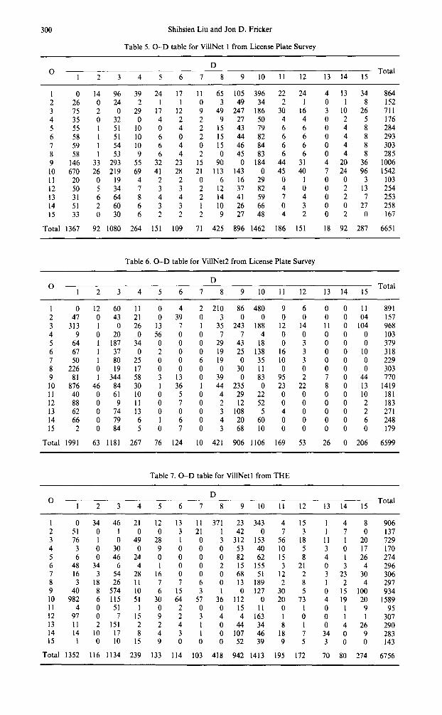
The street system adjacent to Purdue University’s campus is highly congested during the AM and PM peak hours. There is heavy pedestrian traffic crossing the streets near campus, including a state highway. In an effort to improve traffic flow and increase pedestrian safety, this street network (in what is known as ‘The Village’) underwent significant changes on 13 May 1991. The principal change was the conversion of four major arterial streets from 2- way to l-way operation. Figures 8 and 9 show the changes in detail. Data on link counts and turning movements were collected before and after the street network changes. In Septem- ber 1990 and September 1991, license plate surveys were conducted to estimate flow patterns within and through The Village. The Village network before 13 May 1991 (Fig. 8) is referred to as ‘VillNetl’; after that date (Fig. 9). it is called ‘VillNet2’. The O-D tables derived from the two license plate surveys are shown in Tables 5 and 6.

VillNet 1, a network representation developed to test traffic assignment models, contains links that portray turning movements at each major intersection in some detail. Con- servation of flow at each node was achieved by using a maximum entropy method contained in THE. The O-D table subsequently estimated by THE is listed in Table 7. The total O-D flows are 6756, which is close to the total of 6651 that was estimated by the first license plate survey.

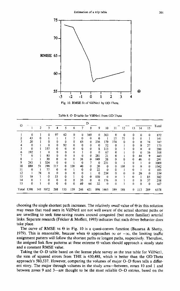
Using the same data, a best fit O-D estimate for VillNetl was found by searching for the minimum RMSE while assigning O-D traffic flow by OD.Theta. The results are shown in Fig. 10 and in Table 8.

The OD.Theta results show a 0 value of 0.255 for VillNet 1. A positive 0 value means that users are trying to choose their shortest paths; as 0 increases, the probability of


~~________---------.__ , 4 ------____________::------_._

: ‘, -I ----__ I ,’ ! ---33

#’ ! I I ,.d


Table 5. O-D table for VillNet 1 from License Plate Survey

D 0 Total

1 2 3 4 5 6 7 8 9 10 11 12 13 14 15

I 0 14 96 2 26 0 24 3 75 2 0 4 35 0 32 5 55 I 51 6 58 I 51 7 59 I 54 8 58 1 53 9 146 33 293 IO 670 26 219 I1 20 0 19 12 50 5 34 13 31 6 64 14 51 2 60 15 33 0 30

Total 1367 92 1080

39 24 17 11 65 105 396 22 24 4 13 34 2 1 1 0 3 49 34 2 1 0 I 8

29 17 12 9 49 247 186 30 16 3 10 26 0 4 2 2 9 27 50 4 4 0 2 5

10 0 4 2 15 43 79 6 6 0 4 8 10 6 0 2 15 44 82 6 6 0 4 8 10 6 4 0 IS 46 84 6 6 0 4 8 9 6 4 2 0 45 83 6 6 0 4 8

55 32 23 15 90 0 184 44 31 4 20 36 69 41 28 21 113 143 0 45 40 7 24 96

4 2 2 0 6 16 29 0 1 0 0 3 7 3 3 2 12 37 82 4 0 0 2 13 8 4 4 2 14 41 59 7 4 0 2 7 6 3 3 I 10 26 66 0 3 0 0 27 6 2 2 2 9 27 48 4 2 0 2 0

864 152 711 176 284 293 303 285

1006 1542

103 254 253 258 167

264 151 109 71 425 896 1462 186 151 18 92 287 6651

Table 6. O-D table for VillNet2 from License Plate Survey

0 D

Total 1 2 3 4 5 6 7 8 9 10 11 12 13 14 15

1 0 2 41 3 313 4 9 5 64 6 67 7 50 8 226 9 81 10 876 II 40 12 88 13 62 14 66 15 2

Total 1991

12 60 11 0 4 2 210 86 480 9 6 0 0 11 0 43 21 0 39 0 3 0 0 0 0 0 0 04 I 0 26 13 7 I 35 243 188 12 14 11 0 104 0 20 0 56 0 0 7 7 4 0 0 0 0 0 1 187 34 0 0 0 29 43 18 0 3 0 0 0 1 37 0 2 0 0 19 25 138 16 3 0 0 10 1 80 25 0 0 6 19 0 35 IO 3 0 0 0 0 19 17 0 0 0 0 30 11 0 0 0 0 0 1 344 58 3 13 0 39 0 83 95 2 7 0 44

46 84 30 I 36 1 44 235 0 23 22 8 0 13 0 61 10 0 5 0 4 29 22 0 0 0 0 10 0 9 11 0 7 0 2 12 52 0 0 0 0 2 0 74 13 0 0 0 3 108 5 4 0 0 0 2 0 79 6 1 6 0 4 20 60 0 0 0 0 6 0 84 5 0 7 0 3 68 10 0 0 0 0 0

63 1181 267 76 124 10 421 906 1106 169 53 26 0 206

891 157 968 103 379 318 229 303 770

1419 181 183 271 248 179

6599

Table 7. O-D table for VillNetl from THE

0 D

I 2 3 4 5 6 7 8 9 IO 11 12 13 14 15 Total

1 0 2 51 3 76 4 3 5 6 6 48 7 16 8 3 9 40 IO 982 11 4 12 97 13 11 14 14 15 1

Total 1352

34 46 0 1 I 0 0 30 0 46

34 6 3 54

18 26 8 514 6 115 0 51 0 7 2 151

10 17 0 10

116 1134

21 12 13 I1 371 23 343 4 15 1 4 8 0 0 3 21 1 42 0 7 3 1 7 0

49 28 1 0 3 312 153 56 18 11 1 20 0 9 0 0 0 53 40 10 5 3 0 17

24 0 0 0 0 82 62 15 8 4 I 26 4 1 0 0 2 15 155 3 21 0 3 4

28 16 0 0 0 68 51 12 2 3 23 30 11 7 7 6 0 13 189 2 8 1 2 4 10 6 15 3 1 0 127 30 5 0 15 100 51 30 64 57 36 112 0 20 73 4 19 20

1 0 2 0 0 15 11 0 I 0 1 9 15 9 2 3 4 4163 10 0 : I 2 2 4 I 0 44 34 8 I 0 26 8 4 3 1 0 107 46 18 7 34 0 9

15 9 0 0 0 52 39 9 5 3 0 0

239 133 114 103 418 942 1413 195 172 70 80 274

906 137 729 170 274 296 306 297 934

1589 95

307 290 283 143

6756

301 Estimation of a trip table

Fig. 10. RMSE fit of VillNetl by OD.Theta.

Table 8. O-D table for VillNetl from OD,Theta

0 D

1 2 3 4 5 6 7 8 9 10 11 12 13 14 I5 Total

1 0 1 0 97 62 0 0 349 0 363 0 0 0 0 0 872

2 43 0 I 1 I 7 0 0 0 I 1.5 71 0 0 1 141

3 20 1 0 0 0 0 63 0 236 179 174 0 0 0 74 747

4 0 1 0 0 92 0 0 0 0 52 0 1 0 0 27 173

5 0 I 157 0 0 0 0 0 8 113 0 1 0 0 0 280

6 192 1 0 0 0 0 1 0 28: 67 0 1 0 0 56 318

7 0 1 85 0 0 I 0 0 21 0 0 44 9 443

8 1 1 30 0 0 0 38 0 149 26 0 :, 0 46 0 291

9 243 I 524 0 0 1 0 7 0231 0 1 0 I 0 1009

10 888 51 I98 117 0 120 40 0 20 0 0 108 0 0 0 1542

I1 0 1 77 0 0 1 0 0 22 0 0 1 0 1 0 103

12 1 78 0 0 0 0 0 1 0 234 0 0 0 20 334

13 10 1 0 53 0 I 0 0 I50 0 0 1 0 1 8: 302 14 0 1 0 0 0 8 35 0 0 176 0 1 0 0 37 258

I5 0 I 0 0 0 0 69 64 32 0 0 I 0 0 0 167

Total 1398 141 1072 268 155 139 246 421 898 1463 189 188 0 113 289 6378

choosing the single shortest path increases. The relatively small value of 8 in this solution may mean that road users in VillNetl are not well aware of the actual shortest paths or are unwilling to seek time-saving routes around congested (but more familiar) arterial links. Separate research (Fricker & Moffett, 1993) indicates that such driver behavior does take place.

The curve of RMSE vs 8 in Fig. 10 is a quasi-convex function (Bazaraa & Shetty, 1979). This is reasonable, because when 8 approaches 00 or -00, the limiting traffic assignment pattern will follow the shortest paths or longest paths, respectively. Therefore, the assigned link flow patterns at these extreme 8 values should approach a steady state and a constant RMSE value.

Taking the O-D table based on the license plate survey as the true table for VillNetl, the sum of squared errors from THE is 430,488, which is better than the OD.Theta approach’s 580,537. However, comparing the volumes of major O-D flows tells a different story. The major through volumes in the study area-between, zones 10 and 1 and between zones 9 and 3-are thought to be the most reliable O-D entries, based on the


Table 9. Comparison of VillNet 1 through trip O-D entries

O-D entries

Method

License Plate OD.Theta THB43

U,lO) (10,1) (3,9) (933)

396 670 247 293 363 888 236 524 982 312 574

matching of vehicle license plate numbers. Assuming the O-D entries from the license plate approach are correct, THE gives a poorer estimate of these major through trips than does ODsTheta (see Table 9).

The reason why THE estimates these major through trips poorly might be EM’s underlying multinomial distribution, which assumes random variates with equal probability for each possible outcome. This assumption is derived from the physical law of molecular behavior, but this assumption may not be true when applied to driver route choice. One consequence would be a tendency to underestimate through trips. In contrast, the ODeTheta approach has the added flexibility of adjusting 8 in seeking the O-D table estimate whose traffic assignment pattern minimizes RMSE. In addition, EM cannot produce an accurate estimate for an O-D pair if the final solution must be zero (Bromage, 1988) and it provides an O-D table with systematic errors when the total O-D flow is not equal to the total number of trips in the ‘observed’ trip table (Gur, 1983; Willumsen, 1981).

The same network after changes The VillNet2 link counts used by THE lead to Table 10. The VillNet2 results from

OD.Theta are shown in Fig. 11 and Table 11. Comparing O-D estimates for VillNetl and VillNet2, the total PM peak hour O-D

volume estimated by THE increases by 500 trips. The total O-D volume estimated by OD.Theta is about 650 trips more for VillNet2 than for VillNetl, but closer to the license- plate-based Table 6 total than is THE.

The 8 parameter in The Village after the street system changes dropped from 0.255 to 0.118. This is ‘evidence’ of somewhat greater route choice dispersion than in VillNetl. Because many obvious direct routes between two points have been eliminated by the new one-way street pattern, motorists have been forced to try a variety of more circuitous routes to reach their destinations. As a member of the Mayor’s task force set up to study

Table IO. O-D table for VillNet2 from THE

0 D

Total I 2 3 4 5 6 7 8 9 IO 11 I2 I3 I4 I5

I 0 I4 0 5 I 9 12 I78 39 442 2 II9 0 0 2 I 4 6 I4 I8 163 3 I83 58 0 43 I4 73 106 21 338 43 4 5 I 55 0 3 4 5 I 17 3 5 I8 4 I89 33 0 I3 I9 2 60 8 6 40 1 18 4 I 0 15 4 48 159 7 IO 1 78 I4 4 I 0 I 99 39 8 36 3 0 2 0 3 3 0 II II9 9 46 8 368 65 20 3 0 5 0 I83 IO 1477 I3 2 I6 5 28 40 I71 129 0 11 10 1 81 14 5 0 I I I4 40 I2 5 6 I 9 3 I4 21 0 67 20 I3 8 2 69 12 4 0 0 I I10 34 I4 22 2 78 I4 5 0 8 3 26 87 15 9 2 97 4 1 7 IO I 30 4

Total 1988 II6 1036 237 67 159 246 403 1006 1344

7 2 0 0 174 883 4 I 0 0 66 398

60 I5 4 0 5 963 31004 102

IO 3 I 0 I5 375 9 9 0 0 2 310

17 2 18 0 7 291 2 0 I 0 47 227

I2 10 0 I 29 750 23 5 2 0 8 1919 0 2 0 1 6 176

I2 0 I 0 4 163 20 2 0 0 5 287 45 006 260 6 I I 0 0 173

I89 58 28 2 378 7257


RMSE

69-

68-

67 -

-1 -0.6 -0.2 0.2 0.6

Fig. 11. RMSE fit of VillNet2 by OD.Theta.

Table 11. O-D Table for VillNet2 from OD.Theta

0 D

1 2 3 4 5 6 7 8 Total

9 10 11 12 13 14 15

1 0 5 0 0 0 0 0 193 0 562 0 0 0 0 132 892 2 89 0 0 0 0 0 0 0 30 20 0 0 0 0 28 167 3 0 30 0 0 0 0 0 225 502 57 192 0 0 0 1 1007 4 34 1 0 0 73 0 0 0 0 0 0 0 0 0 0 108 5 89 1 38 256 0 0 0 0 0 0 0 0 0 0 0 384 6 284 I 49 0 0 0 0 0 0 0 0 0 0 0 0 334 7 0 1 36 0 0 1 0 0 86 104 0 0 19 0 0 247 8 161 0 112 0 0 0 0 0 19 0 0 0 0 0 13 305 9 0 1 502 0 0 I 0 0 0 231 I 76 0 0 0 812 10 1254 46 0 0 0 196 0 0 71 0 0 61 0 0 0 1628 11 0 1213 9 0 10 0 10 0 0 0 0 0 225 2 47 0 0 0 0 0 0 0 54 36 0 0 0 0 0 137 13 32 I 174 0 0 I 0 0138 0 0 0 0 0 0 346 14 0 1 16 0 0 1 0 0 27 109 0 0 0 0 94 248 15 0 1 29 0 0 0 0 3 0156 0 0 0 0 0 189

Total 1990 90 1169 265 73 201 0 421 928 1275 193 137 19 0 268 7029

the impacts of the new street pattern, the second author received numerous comments from local citizens about how they traveled between points in the Village network. The comments indicated a surprising lack of consensus on which new path between many given O-D pairs in VillNet2 is the ‘best’. Although VillNetl had more path alternatives than VillNet2 now does, VillNetl usually had one or two ‘obvious’ (commonly used) choices. While VillNet2 has fewer alternatives, often there is no clearly superior path choice, leading to greater dispersion in traffic flow, which is reflected in a lower 0 value.

For the VillNet2 network, the sum of squared errors with respect to the license plate O- D table is 668,806 from THE, and 851,698 from ODaTheta. Much of this error is associated with the major east-west through trips shown in Table 12. Both THE and OD.- Theta indicate a shift of through trips from the (9, 3) O-D pair to the parallel (10,l) O-D pair to the north that is not reflected in the license plate survey. Because VillNet2’s one- way pattern restricts the number of route choices previously available in VillNetl, the VillNet2 results may be an indication that OD.Theta performs better where a wider range of route alternatives exist.


Table 12. Sensitivity to network changes

Method Data Set (l,lO)

O-D Entries

(10,1) (339) (973)

VillNet I 396 670 241 293 License Plate VillNet2 480 876 243 344

VillNet I 343 982 312 574 THE VillNet2 442 1477 338 368

VillNet I 363 888 236 524 OD.Theta VillNet2 562 1254 502 502

CONCLUSIONS

Based on the tests of the OD.Theta method and comparisons with THE, several conclusions can be drawn.

1. Estimation of an O-D table and the 0 parameter for stochastic assignment can be accomplished at the same time. This improves the consistency of the estimation, because the O-D estimation occurs in conjunction with the value of the 0 parameter that best fits the observed link flows.

2. The input requirements are simplified. Only link volume counts and link travel costs are needed; no target trip table is required. If a target trip table can be partially or fully specified, terms can be added to the objective function that incorporate this additional information without affecting the problem structure.

3. O-D table estimation and 0 parameter calibration have been demonstrated on a real network that offered:

flow and link cost data of reasonable accuracy; a separately-estimated O-D table; a size and complexity greater than the test networks commonly seen in the literature; a change in network conditions (introduction of one-way arterials) that per- mitted some evaluation of model sensitivity.

The network dispersion parameter 0 was 0.255 in the original VillNet study area and decreased to 0.118 after the one-way street changes. This decreased 0 value can be interpreted in terms of decreased driver certainty in selecting shortest paths after many obvious direct paths have been made unusable.

Acknowledgments-This paper is based on research conducted with the support of the Purdue Research Foun- dation (PRF). A large part of the paper’s preparation took place while the second author was on sabbatical leave at the Department of Transportation Planning and Highway Engineering, Delft University of Technology, The Netherlands. The authors thank PRF, the faculty and research staff at Delft, and the anonymous reviewers for their assistance and helpful comments.

REFERENCES

Bazaraa M. S. and Shetty C. M. (1979) Nonlinear Programming: Theory and Algorithms. Wiley, New York. Beagan D. F. (1986) Estiminating a trip table from counts. McTrans 1, 8-9. Transportation Research Center,

University of Florida, Gainesville, FL. Bromage E. J. (1988) The Highway Emulator. Release 3.0, user’s manual, Central Transportation Planning Staff,

Boston. Dial R. B. (1971) A probabilistic multipath assignment model which obviates path enumeration. Tramp Rex 5,

83-111. Eaves B. C. (1971) The linear complementarity problem. Mgmt Sci. 17, 612-634. Fisk C. S. (1977) Note on the maximum likelihood calibration on Dial’s assignment method. Transpn Res. II,

67-68. Fricker J. D. and Moffett D. P. (1993) Traffic assignment model calibration when precision is essential. Proc.

43rd Annual Meeting, Institute of Transportation Engineers, The Hague, The Netherlands, pp. 258-26 I. Gur Y. J. (1983) Estimating trip tables from traffic counts: comparative evaluation of available techniques.

Transpn Res. Rec. 944, 113-l 17.


Haggerty G. B. (1972) Elementary Numerical Analysis with Programming. McGraw-Hill, New York. Lemke C. E. (1968) On complementary pivot theory. Mathematics of the Decision Sciences, Part I, pp. 95-114.

American Mathematical Society. Minieka E. (1978) Optimization Algorithmsfor Networks and Graphs, Marcel Dekker, New York. Nguyen S. (1977) Estimating an OD Matrix from Network Data: A Network Equilibrium Approach. Publication

No. 87, Centre de Recherche sur les Transports. Universite de Montreal. Robillard P. (1974) Calibration of Dial’s Assignment Method. Transpn Sci. 8, 117-125. Sheffi Y. (1985). Urban Transportation Networks: Equilibrium Analysis with Mathematical Programming Methods.

Prentice-Hall, Englewood Cliffs, N. J. Van Zuylen H. and Willumsen L. G. (1980) The most likely trip matrix estimated from traffic counts. Transpn

Res. 14B 281-293. Willumsen L. G. (1981) Simplified transport models based on traffic counts. Transportation 10, 257-278.

Estimation of a trip table and the Θ parameter in a stochastic network

Documents

Transcript of Estimation of a trip table and the Θ parameter in a stochastic network