www.elsevier.com/locate/cma

Comput. Methods Appl. Mech. Engrg. 196 (2007) 4577–4596

The representer method for state and parameter estimationin single-phase Darcy flow

Marco A. Iglesias, Clint Dawson *

Center for Subsurface Modeling – C0200, Institute for Computational Engineering and Sciences (ICES),

The University of Texas at Austin, Austin, TX 78712, United States

Received 23 January 2007; received in revised form 25 May 2007; accepted 29 May 2007Available online 16 June 2007

Abstract

The objective of this paper is to study the representer method for the inverse problem of combined parameter and state estimation insingle-phase Darcy flow in porous media. A variational formulation is posed for the generalized inverse problem in the sense of weightedleast-squares. An iterative representer-based algorithm is derived to approximate the Euler–Lagrange equations. It is proved that thelinearized problem can be solved exactly by an extension of the representer method which inherits the same well-known properties ofthis technique. Implementation of the numerical algorithm for synthetic numerical experiments shows improved estimates of the poorlyknown prior guess.� 2007 Elsevier B.V. All rights reserved.

Keywords: Parameter estimation; State estimation; Euler–Lagrange equations; Representer method; Inverse problem

1. Introduction

The representer method is a data assimilation techniquethat solves the generalized inverse problem of minimizing aweighted least-squares functional that penalizes the errormisfit in measurements and model dynamics. For someapplications, it has been proved [4] that the search spacefor the minimum of the cost functional is generated by afinite number of ‘‘representer’’ functions that depend onthe model dynamics and the corresponding measurementfunctional. The minimum of the least-squares problem isreduced to the solution of a linear system that allows oneto define the solution as a linear combination of the‘‘representers’’.

The representer method has been successfully imple-mented in oceanography and meteorology [4,5] where sev-eral validations have already been performed. For reservoirapplications, new technologies for data collection are

0045-7825/$ - see front matter � 2007 Elsevier B.V. All rights reserved.

doi:10.1016/j.cma.2007.05.024

* Corresponding author.E-mail address: clint@ices.utexas.edu (C. Dawson).

becoming available and it is of interest to apply data assim-ilation methods to this field. Baird and Dawson [2,3] haverecently introduced and studied the representer method forsingle-phase Darcy flow in porous media assuming perfectknowledge of the permeability field. However, it is also ofparticular importance to include the parameter estimationof reservoir properties into the data assimilation problem.In this case, even if the dynamics of the problem are linear,the parameter estimation becomes strongly nonlinear.

Several publications [1,12] have studied the implementa-tion of the Ensemble Kalman Filter for continuouslyupdating reservoir model properties by assimilating mea-sured data. This technique is easy to implement althoughits accuracy depends on the size of the ensemble under con-sideration. Computational cost for the simulation mayincrease with the size of the ensemble. Variational tech-niques have been proposed for the parameter estimationproblem, and a few recent papers describe the representermethod for the approximation of the inverse solution.For example, Eknes and Evensen [6] studied parameterestimation in an Ekman model with an iterative algorithmthat computes at each iteration the state and adjoint

4578 M.A. Iglesias, C. Dawson / Comput. Methods Appl. Mech. Engrg. 196 (2007) 4577–4596

variable with the representer method, while the parametersare computed with a gradient descent method. For inversegroundwater modeling, Valstar [10,11] derived a repre-senter-based algorithm which introduces an extra repre-senter for the parameter update.

In this paper, we study data assimilation in single-phaseDarcy flow in porous media. In Section 2, we define thegeneral inverse problem in the case of poorly known per-meability. We assume the measurements are formulatedas linear functionals. The model dynamics are a weak con-straint for the inverse problem of state and parameter esti-mation. The adopted variational approach is a weightedleast-squares where the weights are defined as the inverseof the prior covariances. In [7] we showed that these covari-ances play an important role in the inverse problembecause they determine the smoothness of the solution tothe Euler–Lagrange (EL) equations (the generalizedinverse). In fact, based on the regularity of the prior errorstatistics, model dynamics and measurement functionals,we have shown [7] the local existence of the solution tothe EL equations. This system of equations is nonlinearand an iterative scheme is proposed to approximate a solu-tion. In Section 3, we linearize the model equations with afirst order approximation around a forward model definedfor each level of the iteration in terms of previous esti-mates. The linearized inverse problem is solved with therepresenter method including an extra representer set offunctions for the parameter estimate as defined in [10]. InSection 4, we discuss the geometrical formulation of therepresenter method for the linearized parameter estimationproblem. We also formally provide some results to justifythat for the single-phase flow model, the representermethod is a solution to the linearized problem. It is alsoshown that the same structure is inherited for the classicalrepresenter method and a discussion about posterior errorestimates is provided. Finally, in Section 5 we present twosynthetic examples where the numerical algorithm wastested. We study the case of a two-dimensional data assim-ilation where both the model and the parameter areinverted. Numerical experiments show that this algorithmgenerates an inverse solution and a parameter estimate thatconsiderably improves the solution.

2. Generalized inverse formulation

The dynamical problem we consider is single-phasecompressible flow through porous media in a domainX � Rn, n P 2, having a boundary consisting of two dis-joint parts CN and CD. The system is governed by

c@p@t�r � ðKrpÞ ¼ F in X� ð0; T �; ð2:1Þ

p ¼ I in X� f0g; ð2:2ÞKrp � n ¼ BN on CN � ð0; T �; ð2:3Þp ¼ BD on CD � ð0; T �; ð2:4Þ

where p(x, t) is the pressure, c the constant compressibilityfactor, F the forcing function, I the initial pressure, and BN

and BD are the Neumann and Dirichlet boundary condi-tions, respectively. K is a symmetric positive definite matrixthat describes the permeability of the medium. In practice,functions F, I, BN, BD and K may not be known accuratelyor they may not even be available pointwise in the domain.With only poorly known available data, system (2.1)–(2.4)is called the ‘‘forward model’’ and its solution is a pressurefield denoted by pF. In general, pF is different from the‘‘true’’ pressure field pT obtained from (2.1)–(2.4) if themodel (i.e. functions F, I, BN, BD and K) were perfectlyknown.

For any pressure field p(x, t), the measurement (observa-tion) process is defined mathematically by

LmðpÞ ¼Z T

0

ZX

H mðx; tÞpðx; tÞdXdt; for m ¼ 1 . . . M ;

ð2:5Þ

for prescribed functions {H1, . . . ,Hm}.Assume there is a vector of M measurements

d = (d1, . . . ,dM)T taken from pT. These measurements areallowed to contain errors due to an imperfect measuringdevice, for example. In other words,

d ¼LðpTÞ þ �; ð2:6Þ

where � is a vector of measurement errors and LðpTÞ ¼ðL1ðpTÞ; . . . ; LMðpTÞÞ.

In order to characterize the true model let us assumethat there exist functions f, i, bN, bD and k such that thetrue pressure field is given by the solution to the followingsystem

c@p@t�r � ðKrpÞ ¼ F þ f in X� ð0; T �; ð2:7Þ

p ¼ I þ i in X� f0g; ð2:8ÞKrp � n ¼ BN þ bN on CN � ð0; T �; ð2:9Þp ¼ BD þ bD on CD � ð0; T �; ð2:10ÞK ¼ Kþ k on X: ð2:11Þ

For example, f is the error of the forcing term between thetrue and the forward model. In general, the error functionsadded to the prior data are the evidence of inherent uncer-tainty in the problem under consideration. They could bedefined as random fields with a specified covariance andmean. For this analysis, the error functions involved inthe previous system are viewed as deterministic controlvariables. Nevertheless, in the formulation we assume thatthere are previously defined error covariance functions(symmetric and positive definite) CF, CI, CN, CD and CK

related to the error functions f, i, bN, bD and k, respectively.Finally, the true solution is completely characterized if weconsider Eq. (2.6) where the measurement error is assumedto have a covariance matrix denoted by W�1.

Suppose now we are given prior functions (the bestavailable to us) F, I, BN, BD and K that uniquely define

M.A. Iglesias, C. Dawson / Comput. Methods Appl. Mech. Engrg. 196 (2007) 4577–4596 4579

the solution to the forward model. It is clear that pF in gen-eral will not agree with prescribed data. On the other hand,finding the true solution is not possible since the error func-tions are unknown. Then, the problem is to find a general-ized inverse as a pressure field providing the best fit to themodel and data. The strategy is based on the minimizationof a weighed least-squares functional. We expect the mini-mum to be a set of error functions f , i, bN, bD and k suchthat the generalized inverse solution p of (2.7)–(2.11) will bethe best fit to the measurements.

For clarity in the notation, given two arbitrary functionsf and g, we define the following operations:

f � g ¼Z T

0

dtZ

Xdx�

f ðx; tÞgðx; tÞ�;

f � g ¼Z

Xdx�

f ðxÞgðxÞ�;

f Hg ¼Z T

0

dtZ

CN

ds�

f ðs; tÞgðs; tÞ�;

f g ¼Z T

0

dtZ

CD

ds�

f ðs; tÞgðs; tÞ�:

It is assumed that in each case the domain of f and g is de-fined according to the domain of integration.

We denote by W the inverse of the measurement errorcovariance matrix. Furthermore, let WF be the formalinverse of CF [9, Chapter 7] which is also a symmetric posi-tive function such that

W Fðx; t; x00; t00Þ � CFðx00; t00; x0; t0Þ ¼ dðx� x0Þdðt � t0Þ: ð2:12Þ

With similar definitions for WI, WN, WD and WK, wedefine now a weighted least-squares cost functional

J½f ; i; bN; bD; k� ¼ ðd�LðpÞÞTWðd�LðpÞÞþ f � W F � f þ i � W I � i

þ bNHW NHbN þ bD W D bD

þ k � W K � k; ð2:13Þ

that penalizes the misfit between observations and model er-ror functions. The inverse problem is to find a minimum of(2.13) such that p satisfies (2.7)–(2.11). With a stochastic ap-proach, when the dynamics are linear and the prior errorsare assumed Gaussian, the least-squares functional is equiv-alent to the Bayesian maximum likelihood estimator [9].For nonlinear problems the least-squares functional canbe related to a best linear unbiased estimator. Therefore,the definition of the penalty functional is established in con-nection with other mathematical techniques to study inverseproblems. For practical applications the weights may be dif-ficult to find although they are not essential for the imple-mentation as will be shown in the following sections.

It is important to mention that for the correct physicalinterpretation as well as for existence and uniqueness ofthe model solution, the permeability tensor K has to bepositive definite. Eq. (2.11) has to be provided with anhypothesis on both K and k so that this requirement is ful-

filled. In the rest of this document we will consider the casewhere k is an isotropic field that can be written as kI, whereI is the identity matrix. For this case, the aforementionedrequirement implies that k has to be positive. In numericalapplications, pseudo-random fields are usually needed totest the capability of the inverse technique for estimatingpermeability. The corresponding covariance function hasto be adequately selected to prevent the generated fieldfrom having nonpositive values. However, if a permeabilityfield is not positive at some point of its domain, the entirefield must be totally discarded from the experiment.

3. The Euler–Lagrange equations

We point out that the penalty functional was defined interms of weight functions. However, in practice we mightbe given information only in term of prior error covari-ances (formal inverses of weights). Expressions and regu-larity for the weights may not be available and thennothing can be said a priori about the existence of a globalminimizer. Moreover, even if a global minimizer exits, itmay not be unique since the functional J is not in generalconvex. Having expressions for the prior error covariances,we can attempt to find a minimizer by solving the EL equa-tions that in general ensure the existence of an extremum.In [7] we showed that the necessary condition for an extre-mum of J gives rise to the following system of nonlinear ELequations:

Adjoint:

� c@k@t�r � ðKrkÞ ¼ ðd�LðpÞÞWH in X� ð0; T �;

ð3:1Þck ¼ 0 in X� fTg; ð3:2ÞKrk � n ¼ 0 on CN � ð0; T �; ð3:3Þk ¼ 0 on CD � ð0; T �: ð3:4Þ

State:

c@p@t�r � ðKrpÞ ¼ F þ CF � k in X� ð0; T �; ð3:5Þ

p ¼ I þ CI � ck in X� f0g; ð3:6ÞKrp � n ¼ BN þ CNHk on CN � ð0; T �; ð3:7Þp ¼ BD � CD ðKrk � nÞ on CD � ð0; T �: ð3:8Þ

Parameter:

K ¼ K � CK �Z T

0

rk � rp dt: ð3:9Þ

In Eq. (3.1) we have defined the vector H = (H1(x, t), Æ ,HM(x, t)). We remark that Eqs. (3.1)–(3.8) are the sameEL equations that were derived in [3] for Dirac deltaweights and for fixed permeability K. Here we have anadditional equation corresponding to the parameter thatmakes the problem nonlinear. In [7] we proved that undersome regularity conditions for the prior error covariances,

4580 M.A. Iglesias, C. Dawson / Comput. Methods Appl. Mech. Engrg. 196 (2007) 4577–4596

the forward model and the measurement functionals, theEL equations have a local solution (the generalizedinverse).

3.1. Linearization

The coupled set of nonlinear EL equations derived in theprevious section is going to be approximated by an iterativenumerical algorithm. An initial guess is used to initializedthe algorithm and updates are computed by solving a line-arized version of the EL equations. There are several possi-ble linearizations of the EL equations that may be found inthe literature [5, Section 3.3.3]. In this document we take afirst order approximation to problem (2.7)–(2.11) aroundan updated forward model determined by previous esti-mates. The linearized forward model is used to define thegeneralized inverse problem at each iteration step. The ELequations are derived for this linear problem and solvedexactly by the representer method. Consider the operator

Gðp;KÞ ¼

c @p@t �r � ðKrpÞ

pjt¼0

Krp � njCN

pjCD

K

26666664

37777775: ð3:10Þ

Note that a solution of the forward model (2.1)–(2.4) canbe read as

GðpF;KÞ ¼ ½F ; I ;BN;BD;K�T: ð3:11Þ

For n = 1 we define the initial guess of the algorithm asK0 K, F0 F, I0 I, B0

D BD and B0N ¼ BN. At the nth

step the nth forward model is defined by the solution to

c@pn

F

@t�r � ðKn�1rpn

FÞ ¼ F n�1 in X� ð0; T �; ð3:12Þ

pnF ¼ In�1 in X� f0g; ð3:13Þ

Kn�1rpnF � n ¼ Bn�1

N on CN � ð0; T �; ð3:14Þpn

F ¼ Bn�1D on Cn

D � ð0; T �: ð3:15Þ

Assuming that pn � pnF and Kn � Kn�1 are sufficiently small,

the first order approximation of G around the nth forwardmodel is computed

Gðpn;KnÞ � GðpnF;K

n�1Þ þ DGðpnF;K

n�1Þpn � pn

F

Kn � Kn�1

� �;

ð3:16Þ

where DG(p,K) is the Frechet derivative of G:

DGðp;KÞp

K

� �¼

c @p@t �r � ðKrpÞ � r � ðKrpÞ

pjt¼0

ðKrp � nþ Krp � nÞjCN

pjCD

K

26666664

37777775:

ð3:17Þ

From the definition of pnF (3.12)–(3.15) it follows that

Gðp;KÞ �

c @p@t �r � ðK

n�1rpÞ � r � ðK � Kn�1ÞrpnF

pjt¼0

ðKn�1rp � nþ ðK � Kn�1ÞrpnF � nÞjCN

pjCD

K

26666664

37777775;

ð3:18Þand obviously

GðpnF;K

n�1Þ � ½F n�1; In�1;Bn�1N ;Bn�1

D ;Kn�1�T: ð3:19ÞIt is notable that for each iteration the computation of theforward model is based on previous estimates. From (3.18)we note that linear model dynamics are governing theproblem and since the actual data d is also available at eachiteration step, we may apply the argument in Section 2 todefine a generalize inverse problem at this level. For thispurpose consider functions fn, in, bn

N, bnD and kn to account

for uncertainty and suppose the true solution (from whichdata is available) can be written as the solution of

Gðp;KÞ � ½F n�1 þ f n; In�1 þ in;Bn�1N þ bn

N;

Bn�1D þ bn

D;Kn�1 þ kn�T: ð3:20Þ

This inverse problem is solved by defining the nth penaltyfunctional Jn

Jn½p;K� ¼ ðd�LðpÞÞTWðd�LðpÞÞ þ f n � W F � f n

þ in � W I � in þ bnNHW NHbn

N

þ bnD W D bn

D þ kn � W K � kn: ð3:21Þ

The EL equations for this linear inverse problem are thefollowing:

State:

c@pn

@t�r � ðKn�1rpnÞ � r � ðKn � Kn�1Þrpn

F

¼ F n�1 þ CF � kn on X� ð0; T �; ð3:22Þpn ¼ In�1 þ CI � ckn in X� f0g; ð3:23ÞKn�1rpn � nþ ðKn � Kn�1Þrpn

F � n¼ Bn�1

N þ CNHkn on CN � ð0; T �; ð3:24Þpn ¼ Bn�1

D � CD Kn�1rkn � n on CD � ð0; T �: ð3:25Þ

Adjoint:

� c@kn

@t�r � ðKn�1rknÞ ¼ ðd�LðpnÞÞWH

in X� ð0; T �; ð3:26Þckn ¼ 0 in X� fT g; ð3:27ÞKn�1rkn � n ¼ 0 on CN � ð0; T �; ð3:28Þkn ¼ 0 on CD � ð0; T �: ð3:29Þ

Parameter:

Kn ¼ Kn�1 � CK �Z T

0

rkn � rpnF: ð3:30Þ

M.A. Iglesias, C. Dawson / Comput. Methods Appl. Mech. Engrg. 196 (2007) 4577–4596 4581

From the EL equations we consider the following updatesfor the forcing, initial and boundary conditions

F n F n�1 þ CF � kn; ð3:31ÞIn In�1 þ CI � ckn; ð3:32ÞBn

N Bn�1N þ CNHkn; ð3:33Þ

BnD Bn�1

D � CD Kn�1rkn: ð3:34Þ

In the following section we discuss the representer methodfor the solution to the linearized problem (3.22)–(3.30).

4. The representer method

4.1. Motivation

We proceed formally to show the idea behind the repre-senter method for solving the linearized inverse problemarising at each step of the iteration. For simplicity, onlyNeumann boundary conditions are considered (C = CN

and CD = ;). After the (n � 1)st step of the algorithm, anupdate ðKn�1; F n�1; In�1;Bn�1

N Þ is generated and an nth for-ward model can be computed by (3.12)–(3.14). We nowrecall that the prior error covariances are assumed to bepositive definite. Then, it is possible to find the square rootin the sense of [9, Chapter 7], that is

C12Fðx; t; x0; t0Þ � C

12Fðx00; t00; x0; t0Þ ¼ CFðx; t; x00; t00Þ: ð4:1Þ

For a better description of the spaces and the regularityconditions for the prior error covariances we refer thereader to [7]. For this analysis it is enough to define thefollowing spaces

K fK 2 C1;1ðXÞ : a 6 KðxÞ for all x 2 Xg ð4:2Þ

where a is a positive constant and

Pn fp 2 H 2;1ðXTÞ j p is solution of ð4:4Þ–ð4:7Þfor some ðf ; i; bN; kÞg; ð4:3Þ

where

c@p@t�r � ðKn�1rpÞ � r � ðKrpn

FÞ ¼ C12F � f

in X� ð0; T �; ð4:4Þ

p ¼ C12I � i in X� f0g; ð4:5Þ

Kn�1rp � nþ KrpnF � n ¼ C

12N bN on C� ð0; T �; ð4:6Þ

K ¼ C12K � k in X� f0g: ð4:7Þ

It is not difficult to see [7, Lemma 1] that those terms in theright hand side of (4.4)–(4.7) are as smooth as the squareroot of the covariances. Therefore, we may assume for-mally that the square root covariances are smooth enoughsuch that for any combination of

ðf ; i; bN; kÞ 2 L2ð0; T ; L2ðXÞÞ � L2ðXÞ� L2ð0; T ; L2ðCÞÞ � L2ðXÞ; ð4:8Þ

problem (4.4)–(4.7) admits a unique solution in Pn �K.We now formally define the following operator onPn �K:

Anðp;KÞ ¼

AnFðp;KÞ

AnI ðp;KÞ

AnNðp;KÞ

AnKðp;KÞ

26664

37775

¼

c @p@t �r � ðK

n�1rpÞ � r � ðKrpnFÞ

pjt¼0

ðKn�1rp � nþ KrpnF � nÞjCN

K

26664

37775 ð4:9Þ

and a bilinear form is defined on ½Pn �K�2 as

Bn½ðp1;K1Þ; ðp2;K2Þ� ¼ AnFðp1;K1Þ � W F � An

f ðp2;K2Þþ An

I ðp1;K1Þ � W I � AnI ðp2;K2Þ

þ AnNðp1;K1ÞHW NHAn

Nðp2;K2Þþ An

Kðp1;K1Þ � W K � AnKðp2;K2Þ:

ð4:10Þ

With this definition, the nth penalty functional (3.21) iswritten in the following way

Jn½p;K� ¼ Bn½ðp � pnF;K � Kn�1Þ; ðp � pn

F;K � Kn�1Þ�þ ðd�LðpÞÞWðd�LðpÞÞ: ð4:11Þ

Recalling that WF, WI, WN and WK are assumed symmet-ric positive definite, we have the following:

Lemma 4.1. Bn is an inner product on Pn �K.

Proof. Since Bn is symmetric and the weights are positivedefinite, Bn is positive semidefinite. We need to show onlythat Bn[(p,K), (p,K)] = 0 implies (p,K) = (0, 0). AssumeBn[(p,K), (p,K)] = 0 for some ðp;KÞ 2 Pn �K. This meansthat there exists functions f, i, bB, k such that p, K solves:

c@p@t�r � ðKn�1rpÞ � r � ðKrpn

FÞ ¼ C12F � f

in X� ð0; T �; ð4:12Þ

p ¼ C12I � i in X� f0g; ð4:13Þ

Kn�1rp � nþ KrpnF � n ¼ C

12N bN on C� ð0; T �; ð4:14Þ

K ¼ C12K � k in X� f0g: ð4:15Þ

On the other hand, Bn[(p,K), (p,K)] = 0 yields

AnFðp;KÞ � W F � An

Fðp;KÞ þ AnI ðp;KÞ � W I � An

I ðp;KÞþ An

Nðp;KÞHW NHAnNðp;KÞ þ An

Kðp;KÞ � W K � AnKðp;KÞ

¼ 0: ð4:16Þ

From the definition of An (4.9) and using the fact that (p,K)solves (4.12)–(4.15), the previous expression implies

kf k2L2ð0;T ;L2ðXÞÞ þ kik

2L2ðXÞ þ kbNk2

L2ðCÞ þ kkk2L2ðXÞ ¼ 0: ð4:17Þ

4582 M.A. Iglesias, C. Dawson / Comput. Methods Appl. Mech. Engrg. 196 (2007) 4577–4596

Then f = 0, i = 0, bN = 0 and k = 0 (in the sense of (4.8)).Directly from (4.15) it follows K = 0 and from (4.12)–(4.14) we see that p is the weak solution of a parabolicequation with zero forcing, zero initial condition and zeroboundary data. It follows from standard techniques [8,Chapter 4] that kpkH2;1ðXTÞ 6 0 which in turn implies p = 0in Pn. Therefore, Bn defines an inner product onPn �K. h

Theorem 1. Pn �K is a Hilbert-Space with the inner prod-

uct given by

Bn½ðp1;K1Þ; ðp2;K2Þ� ¼ hðp1;K1Þ; ðp2;K2Þi: ð4:18Þ

Proof. We take a Cauchy sequence in Pn �K with respectto h,i defined above. By definition of Pn there are sequencesfm, im, bm

N and km such that, for all m,

c@pm

@t�r � ðKn�1rpmÞ � r � ðKmrpn

FÞ ¼ C12F � fm

in X� ð0; T �; ð4:19Þ

pm ¼ C12I � im in X� f0g; ð4:20Þ

Kn�1rpm � nþ KmrpnF � n ¼ C

12N bm

N on C� ð0; T �;

ð4:21Þ

Km ¼ C12K � km in X� f0g: ð4:22Þ

Note that for all m and j

kðpm � pj;Km � KjÞknP �K

¼ hðpm � pj;Km � KjÞ; ðpm � pj;Km � KjÞi¼ kfm � fjk2

L2ð0;T ;L2ðXÞÞ þ kim � ijk2L2ðXÞ

þ kbmN � bj

Nk2L2ð0;T ;L2ðCÞÞ þ kkj � kmk2

L2ðXÞ: ð4:23Þ

Since (pm,Km) is Cauchy with respect to h,i, as m,j!1, thelast expression goes to zero which means that each term ofthe right hand side goes to zero. Then fm, im, bm

N and km areCauchy sequences in L2(0,T; L2(X)), L2(X), L2(0,T; L2(C))and L2(X), respectively. By completeness we choose f*, i*,bN and k* which are limits of those sequences in the corre-sponding spaces. From the assumption of smooth squareroot covariances, as we already remarked [7, Lemma 1]the right hand side of (4.4)–(4.7), for f*, i*, bN and k* issmooth enough to generate an admissible solutionðp;KÞ 2 Pn �K. Moreover,

kðp � pm;K � KmÞkn

P �K

¼ kf � fmkL2ð0;T ;L2ðXÞÞ þ ki � imkL2ðXÞ

þ kbN � bmNk

2L2ð0;T ;L2ðCÞÞ þ kk � kmk2

L2ðXÞ ð4:24Þand therefore as m!1, (pm,Km)! (p*,K*) with the norminduced by h,i and we have proved the result. h

Corollary 1. If the measurement functional L defined in

(2.5) is continuous in H2,1(XT), then it is continuous with

respect to h,i.

Proof. We prove it is continuous at 0. Take any sequence(pm,Km)! (0,0) in Pn �K. By the same argument of theprevious proof we take functions fm, im, bm

N and km such that(pm,Km) satisfies

c@pm

@t�r � ðKn�1rpmÞ � r � ðKmrpn

FÞ ¼ C12F � fm

in X� ð0; T �; ð4:25Þ

pm ¼ C12I � im in X� f0g; ð4:26Þ

Kn�1rpm � þKmrpnF � n ¼ C

12N bm

N

on C� ð0; T �; ð4:27Þ

Km ¼ C12K � km in X� f0g ð4:28Þ

and since

kðpm;KmÞknP �K ¼ kfmk2

L2ð0;T ;L2ðXÞÞ þ kimk2L2ðXÞ

þ kbmNk

2L2ð0;T ;L2ðCÞÞ þ kkmk2

L2ðXÞ; ð4:29Þ

then fm, im, bmN and km go to zero in the appropriate spaces.

From (4.28) it is clear that Km! 0 in C1;1ðXÞ. From stan-dard energy inequalities [8, Chapter 4] we may concludethat pm satisfies,

kpmkH2;1ðXTÞ 6 Cðkr � KmrpnFkjL2ð0;T ;L2ðXÞÞ

þ kC1=2F � fmkL2ð0;T ;L2ðXÞÞ þ kC

1=2I � imkL2ðXÞ

þ kC1:2N bm

NkH1=2;1=4ðCTÞ

þ kKmrpnF � nkH1=2;1=4ðCTÞÞ; ð4:30Þ

where C is a constant that depends on X and the C1,1 �norm of Kn�1 which at this step is given. From expression(4.30) we observe that as m!1, pm! 0 in H2,1(XT).Therefore, since by hypothesis L is continuous inH2,1(XT), it follows that LðpmÞ !Lð0Þ ¼ 0. h

Remark 1. From this corollary and the Riez representationtheorem we have that for each m = 1, . . . ,M there exists(qm,lm) such that for all ðp;KÞ 2 Pn �K

hðp;KÞ; ðqm; lmÞi ¼LmðpÞ: ð4:31Þ

It is now clear that we may write any arbitrary ðp;KÞ 2Pn �K by

ðp;KÞ ¼ ðpnF;K

n�1Þ þXM

m¼1

bmðqm; lmÞ þ ðp;KÞ ð4:32Þ

for some {bm}, where, for all m,

hðp;KÞ; ðqm; lmÞi ¼ 0: ð4:33Þ

Therefore, from (4.11) and Lemma 4.1

Jn½p;K� ¼XM

m;j¼1

bmbjhðqm; lmÞ; ðqj; ljÞi þ hðp;KÞ; ðp;KÞi

þ ðd�LðpÞÞTWðd�LðpÞÞ ð4:34Þ

M.A. Iglesias, C. Dawson / Comput. Methods Appl. Mech. Engrg. 196 (2007) 4577–4596 4583

and from (4.31)

Jn½p;K� ¼XM

m;j¼1

bmbjLjðqmÞ þ hðp;KÞ; ðp;KÞi

þ ðd�LðpÞÞTWðd�LðpÞÞ: ð4:35Þ

Also from (4.31) we may obtain

LmðpÞ ¼ hðp;KÞ; ðqm; lmÞi

¼ hðpnF;K

n�1Þ; ðqm; lmÞi þXM

j¼1

bjhðqj; ljÞ; ðqm; lmÞi

þ hðp;KÞ; ðqm; lmÞi¼Lmðpn

FÞ þ bjLmðqjÞ: ð4:36Þ

Defining the matrix R so that Rm;j ¼LmðqjÞ, we concludethat

LðpÞ ¼LðpnFÞ þ Rb: ð4:37Þ

Then,

Jn½p;K� ¼ bTRbþ hðp;KÞ; ðp;KÞi ð4:38Þþ ðd�Lðpn

FÞ � RbÞTWðd�LðpnFÞ � RbÞ:

ð4:39Þ

If (p,K) minimizes Jn, then

hðp;KÞ; ðp;KÞi ¼ 0: ð4:40Þ

From the definition of Pn and h,i we have that p* = 0 andK* = 0. Therefore, the minimization of Jn is reduced to theminimization of

Jn ¼ bTRbþ ðd�LðpnFÞ � RbÞTWðd�Lðpn

FÞ � RbÞ:ð4:41Þ

This is exactly the same expression in [4, Chapter 5, (5.5.13)].There, it is shown that the optimum for b is given by

ðRþW�1Þb ¼ d�LðpnFÞ: ð4:42Þ

We have shown that the solution to the linearized minimi-zation problem can be expressed in terms of a finite linearcombination of functions where the coefficients are thesolution to the finite-dimensional system (4.42). Finally,the same argument used in [4, Chapter 5, (5.5.13)] showsthat for the optimum,

Jn ¼ ðd�LðpnFÞÞðRþW�1Þ�1ðd�Lðpn

FÞÞ: ð4:43Þ

5. Implementation

In this section, we derive an algorithm that computes anupdate (pn,kn,Kn) which we expect to be a good approxi-mation of the original EL equations. At the nth iterationwe are given Kn�1; F n�1; In�1;Bn�1

N ;Bn�1D . After computing

the nth forward model solution pnF, the linearized problem

(3.22)–(3.30) is solved by the representer method. If there isevidence that the forward model itself is close enough tothe true model, we conclude that convergence is achieved

since there is not enough information (except noise) to con-tinue the inversion. The problem is now to solve the linear-ized EL equations. From the previous section we mayassume that the solution can be written as a linear combi-nation of M ‘‘representer’’ functions to be determined.Assume that

kn ¼XM

m¼1

bnman

m; ð5:1Þ

pn ¼ pnF þ

XM

m¼1

bnmrn

m; ð5:2Þ

Kn ¼ Kn�1 þXM

m¼1

bnmcn

m; ð5:3Þ

where anm, rn

m, cnm are the adjoint, state and parameter repre-

senters, respectively, and bnm are the representers coeffi-

cients. In (5.3) we note the extra representer for theparameter unknown as also used in [10]. If we substitutethe expression (5.1) into (3.26)–(3.29) we obtain that eachadjoint representer an

m satisfies

� c@an

m

@t�r � ðKn�1ran

mÞ ¼ H m in X� ð0; T �; ð5:4Þ

canm ¼ 0 in X� fTg; ð5:5Þ

Kn�1ranm � n ¼ 0 on CN � ð0; T �; ð5:6Þ

anm ¼ 0 on CD � ð0; T �; ð5:7Þ

where the representers coefficients are given by

bnm ¼

Xmj

ðdi �LiðpnÞÞW im; ð5:8Þ

or

bn ¼Wðd�LðpnÞÞ: ð5:9Þ

Next we substitute the expressions (5.1) and (5.3) into(3.22)–(3.25) to find that each parameter representer cn

m

satisfies

cnm ¼ �CK �

Z T

0

ranm � rpn

F: ð5:10Þ

Substituting (5.2) and (5.3) into expression (3.30) and using(3.12)–(3.15) we directly find that the state representer rn

m isthe solution to the problem

c@rn

m

@t�r � ðKn�1rrn

mÞ � r � ðcnmrpn

FÞ ¼ CF � anm

in X� ð0; T �; ð5:11Þrn

m ¼ CI � canm in X� f0g; ð5:12Þ

Kn�1rrnm � n ¼ �cn

mrpnF � nþ CNHan

m on CN � ð0; T �;ð5:13Þ

rnm ¼ �CD ðKn�1ran � nÞ on CD � ð0; T �: ð5:14Þ

In order to compute the updated estimates (5.1)–(5.3) weneed to find the actual representer coefficients. Therefore,

4584 M.A. Iglesias, C. Dawson / Comput. Methods Appl. Mech. Engrg. 196 (2007) 4577–4596

consider again Eq. (5.8) and note that bn is given by theactual pressure which is still unknown (and in fact alsodepends on bn

m). However, if we substitute the expression(5.2) in (5.9) we find that

bn ¼W d�L pnF þ

XM

k¼1

bnkrn

k

! !ð5:15Þ

and since Lm is linear, the last expression reduces to

W�1bn ¼ d�LðpnFÞ �

XM

k¼1

bnkLðrn

kÞ !

; ð5:16Þ

which can be written as

ðRn þW�1Þbn ¼ d�LðpnFÞ; ð5:17Þ

where the matrix Rn is given by Rnij ¼Liðrn

j Þ. Note that, inorder to update the algorithm we do not need to compute(5.1) and (5.2) and therefore, storage of the representers isnot required. In fact, we may substitute expression (5.8)

Table 1Initial exact forward model solution, initial permeability, and errorthresholds for each experiment

Experiment peF(x,y, t) K h1 hL2

1 cos(2pt)cos(p/2x)cos(p/2y) 4.0 5.577e�3 1.6e�32 cos(pt)cos(p/2x)cos(p/2y) 3.0 1.700e�3 6.44e�43 cos(pt)cos(p/2x)cos(p/2y) 3.0 1.700e�3 6.44e�44 cos(2pt)cos(p/2x)cos(p/2y) 3.0 6.9e�3 1.9e�3

Table 2Parameters for the prior covariances

Experiment r2F r2

K r2N r2

I rF

1 – 3.0 – 0.06 –2 0.2 1.5 0.01 – 1.03 – 1.5 – – –4 – 3.0 – – –

Fig. 1. Experiment 1. Left: true permeabi

into the adjoint problem (3.26)–(3.29) to solve for k. Wecompute pn and Kn directly from (3.22)–(3.25) and (3.30),respectively.

Remark 2. It is a simple exercise to show that, for allm 2 {1, . . . ,M}, ðqm; lmÞ ¼ ðrn

m; cnmÞ where rn

m and cnm are the

solutions of (5.10) and (5.11)–(5.14), respectively, and(qm,lm) were derived in (4.31). Then we have found aformula to compute the representers that were obtainedwith an abstract formulation presented in Section 4.Further, problem (4.42) is the same as (5.17) and byuniqueness of the linear finite-dimensional problem bn ¼ b.Then, a unique expression for the solution to the linear nthinverse problem is now available in terms of the represent-ers that in turn can be calculated with the expressionspresented in this section.

Remark 3. In the Appendix (Eq. (A.9)) it is shown that thematrix Rn þW�1 equals the cross-covariance of the linear-ized model measurement misfit.

We summarized the results of this and the previous sec-tion in the following algorithm. Starting withðp0

F;K0; F 0; I0;B0

N;B0DÞ ¼ ðpF;K; F ; I ;BN;BDÞ, some thresh-

old h, prior error covariances and data observations, then,

Outer Loop: (over n)Input: Kn�1; F n�1; In�1;Bn�1

N ;Bn�1D

1. Compute the nth forward model (pnF) by solving

(3.12)–(3.15). If kd�LðpnFÞk 6 h. Stop

rK rI w�1 M kK � KkL2

0.75 1.5 5.0e�5 14 3.9040.9 – 5.0e�5 14 2.5020.9 – 5.0e�5 14 2.5020.75 – 9.0e�4 16 1.983

lity field. Right: inverse permeability.

M.A. Iglesias, C. Dawson / Comput. Methods Appl. Mech. Engrg. 196 (2007) 4577–4596 4585

2. Inner Loop (for m = 1, . . . ,M)

Fig.

–

Pre

ssur

e

–

–

Pre

ssur

e

(2.1) Compute anm by solving (5.4)–(5.7).

2. Experiment 1. Parameter posterior variance for n = 4.

0 0.1 0.2 0.3 0.4 0.5–1

0.5

0

0.5

1

1.5

2

Time

Truen=1n=2n=3n=4Obs

0–1

–0.5

0

0.5

1

1.5

Pre

ssur

e

0 0.1 0.2 0.3 0.4 0.50.2

0.1

0

0.1

0.2

0.3

0.4

0.5

Time

Truen=1n=2n=3n=4Obs

0–0.2

–0.1

0

0.1

0.2

0.3

0.4

0.5

Pre

ssur

e

Fig. 3. Experiment 1. Time series of pressure at four d

(2.2) Compute cnm from (5.10).

(2.3) Solve (5.11)–(5.14) to obtain rnm.

3. Find bn with (5.17).4. Solve (3.26)–(3.29) to find kn.5. Compute Kn from (3.30).6. Solve (3.22)–(3.25) for pn.7. Update F n�1; In�1;Bn�1

N and Bn�1D (3.31)–(3.34).

Output: (pn,kn,Kn).

A stopping criteria is selected for the nth forward modelwhen the misfit between data and measurements is smallerthan some threshold h determined for example, by thenumerical error of the method applied to compute the for-ward model. Therefore, we are assuming that below thisthreshold the nth forward model is close enough to the dataand there is no need to continue the inversion. If this crite-ria is satisfied at level n, the output is given with the stateand parameter of the previous step. Another criteria fordetermine convergence of this scheme can be defined interms of the difference between pn

F and pn in some norm.We should expect that as the forward model is closer tothe observational data, the inverse and the forward model

0.1 0.2 0.3 0.4 0.5Time

Truen=1n=2n=3n=4Obs

0.1 0.2 0.3 0.4 0.5Time

Truen=1n=2n=3n=4Obs

ifferent measurement locations.

4586 M.A. Iglesias, C. Dawson / Comput. Methods Appl. Mech. Engrg. 196 (2007) 4577–4596

should be closer too. A discussion about the cost of thisalgorithm may be found in [3], which for this case shouldbe considered at each iteration.

Finally, it is important to mention that the representermethod allows one to define expressions for the posteriorcovariance of measurements and model errors. For the lin-earized problem, the same formulas for the posterior errorcovariance of forcing, initial and boundary conditions canbe derived in the same way as in [4, Chapter 3]. With thesame arguments, in the Appendix A, we show that, forthe inverse permeability Kn, the posterior error covariance is

E KnTðxÞ � KnðxÞ;Kn

Tðx0Þ � Knðx0Þ� �¼ Cn

Kðx; x0Þ � cnðxÞðRn þW�1Þ�1cnðx0Þ; ð5:18Þ

where cnðxÞ ¼ ðcn1ðxÞ; . . . ; cn

MðxÞÞ, KnT is the true permeability

of the linearized problem and CnK is the prior error covari-

ance for the nth problem. For this analysis we assume thatCn

K is the same for each iteration step and equal to the ori-ginal prior error covariance CK defined in Section 2. A sim-ilar formula to (5.18) in a discrete formulation was

Fig. 4. Experiment 1. Pressure profile at the observation time t = T/4. Top lefinverse (n = 4) solution. Asterisk: measurement location.

obtained in [10] for the parameter estimation in groundwa-ter modeling.

6. Numerical experiments

In this section, we present four synthetic numerical exper-iments where the iterative scheme derived in the last sectionis implemented. For these experiments the domain X is asquare with length of each side equal to two, and only Neu-mann boundary conditions are considered. The final time isT = 0.5 and the compressibility factor is constant c = 1 foreach experiment. The sampling functional for these experi-ments is the evaluation at some space–time coordinates.

A continuous Galerkin approximation is used for the spa-tial discretization of the variational formulation. For com-putational purposes we used bi-quadratic shape functionson 9-node elements with an 8 · 8 grid. Time discretizationwas implemented with a Backward–Euler scheme with 40time steps. For each experiment, the initial forward model(initial guess) is obtained by choosing functions F, I andBN such that the exact solution (peF) to Eqs. (2.1)–(2.4) is

t: initial forward solution (initial guess). Top right: true solution. Bottom:

M.A. Iglesias, C. Dawson / Comput. Methods Appl. Mech. Engrg. 196 (2007) 4577–4596 4587

the function given in Table 1, with constant prior permeabil-ity K, also given in the table. Convergence of the algorithm isdetermined using the criteria described in the previous sec-tion. More precisely we define the following thresholds,

h1 ¼1

2kpF � peFk1; hL2 ¼ 1

2kpF � peFkL2ðL2Þ; ð6:1Þ

where pF is the forward model computed numerically. Thefactor 1/2 was taken arbitrarily. In a more realistic settingwhere the exact forward model solution is not known, thesethresholds could be determined, for example, by computingforward solutions using coarse and fine meshes to approx-imate the discretization error. Recall that at each outerloop of the algorithm above, we compute the nth forwardmodel solution pn

F. If at the nth iteration kd�LðpnFÞk1 >

h1, then we compute the inverse solution pn at step n.If kpn � pn

FkL2ðL2Þ 6 hL2 , we determine that convergence isachieved. In Table 1, we also show the convergence thresh-olds for each experiment.

The algorithm of the previous section was presentedunder the general consideration that the observational data,permeability, forcing, initial and boundary conditions are

Fig. 5. Experiment 1. Pressure profile at the initial time t = 0. Top left: initial f

subject to errors. However, in the experiments we considersome of these cases independently. We must point out thatthe main goal of this paper is the analysis of the model whenthe permeability is poorly known. Therefore, all the experi-ments assume that the true permeability field is differentfrom the prior guess. For example, in the first experimentwe study a model that is subject to error in the initial condi-tion while the rest (forcing and boundary conditions) areassumed correct. By this we mean that the true solution fromwhich synthetic data is obtained, has the same forcing andboundary conditions as the forward model. It is worth not-ing that the formulation for this case is the same as before,except that in the corresponding cost functional we mustomit the corresponding error functions f and bN (See(3.21)). This new formulation is equivalent to (but not thesame as) considering the equations in the algorithm withthe posterior error covariances (CF and CN) equal to zero.The same idea is applied for experiment 2 where we assumeerror in the forcing and boundary conditions, and in exper-iments 3 and 4 where only the permeability is estimated.

We generated pseudo-random errors for the ini-tial (experiment 1), forcing and boundary conditions

orward solution. Top right: true solution. Bottom: inverse (n = 4) solution.

4588 M.A. Iglesias, C. Dawson / Comput. Methods Appl. Mech. Engrg. 196 (2007) 4577–4596

(experiment 2) and the permeability (experiments 1–3)according to the following covariances:

CFðx; x0; t; t0Þ ¼ r2F exp

jx� x0j2

r2F

!dðt � t0Þ;

CIðx; x0Þ ¼ r2I exp

jx� x0j2

r2I

!; ð6:2Þ

CKðx; x0Þ ¼ r2K exp

jx� x0j2

r2K

!;

CNðx; x0; t; t0Þ ¼ r2Ndðx� x0Þdðt � t0Þ;

W�1 ¼ w�1I: ð6:3Þ

The generated pseudo-random errors were added to theprior fields F, I, BN, K and the simulation produced a solu-tion which was taken to be the ‘‘true solution’’ for eachexperiment. Finally, this solution was sampled at M/2

Fig. 6. Experiment 1. Pressure profile at time t = T/2. Top left: initial forw

measurement locations at two different times (t = T/4 andt = 3T/4). Gaussian noise with mean zero and variancew�1 was added to these measurements. Pertinent informa-tion is presented in Table 2, where in the last column weshow the L2-error of the true permeability function withrespect to the prior guess.

From expressions (6.2) it is clear that the integralsweighted with CK, CF and CI in problems (5.10)–(5.12),(3.22), (3.23) and (3.30)–(3.32) become convolutionsover the domain. Although these experiments are per-formed with a small number of degrees of freedom, theseconvolutions are extremely expensive. For an efficient com-putation of those terms, the Fast Fourier Transform wasimplemented.

It is important to note that the true solution from whichthe measurements were taken was generated according tothe covariances previously defined. They are also the samecovariances used in the algorithm except for experiment 4where the true permeability was explicitly prescribed. Inother words, for experiments 1–3 the parameter deviations

ard solution. Top right: true solution. Bottom: inverse (n = 4) solution.

M.A. Iglesias, C. Dawson / Comput. Methods Appl. Mech. Engrg. 196 (2007) 4577–4596 4589

have the distributions given by (6.2) with the correspondingparameters from Table 2. For experiment 4, the permeabil-ity deviation is defined as a step function. Although it is notassumed to have any given distribution, a prior errorcovariance is defined for the purpose of computing the con-volution in expressions (5.10) and (3.30) of the algorithm.

The values of the variances presented in Table 2 are per-haps not realistic in the sense that they do not represent apercentage of the actual quantity for which they account.Since we are most interested in the response of this methodto estimation of the parameter K, we choose a largercovariance for the permeability to show the power of thetechnique. Note for example that the variance for the per-meability is large compared with the nominal value of K.

We apply the representer method at each iteration, usingthe same algorithm, grid and time step as those used tocompute the initial guess. This give us a numerical approx-imation to the minimizer of the cost functional associatedwith the linearized inverse problem. For each experimentwe analyze the behavior of the prior nth penalty functionthat is defined by

JnF ¼ ðd�Lðpn

FÞÞW�1ðd�LðpnFÞÞ; ð6:4Þ

which is the penalty functional (3.21) evaluated at the nthforward model. After the inversion at level n, we computethe posterior penalty functional with expression (4.43).

Table 3Numerical results

n kKn � Kn�1kL2ðXÞ JnF Jn

1 2.9052 4.665e+4 1.907e+12 1.0863 1.851e+3 1.8523 2.289e�1 3.768 1.828e�14 3.8e�2 5.786e�2 2.901e�2

Experiment 1.

Fig. 7. Experiment 2. Left: true permeabi

6.1. Experiment 1

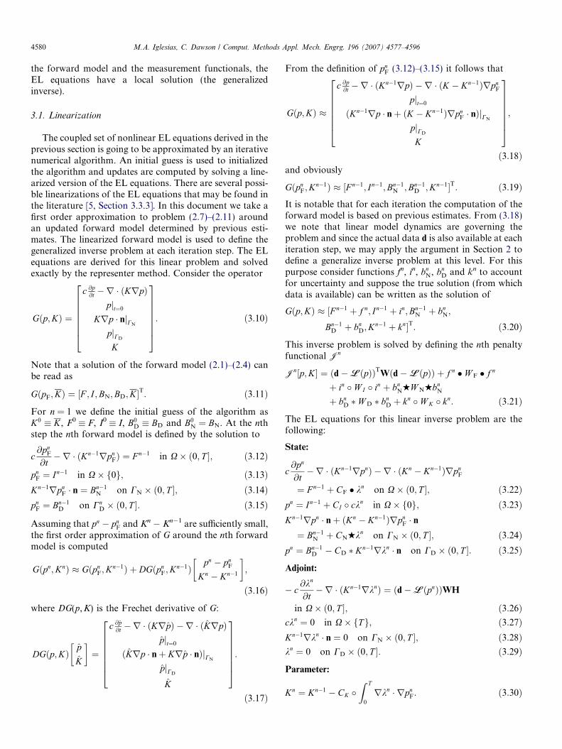
In Fig. 1 we present the ‘‘true permeability’’ used tocompute the measurements, and the inverse permeabilityfield computed using the representer method. It is clear thatfrom an initial guess K ¼ 4:0, the inverse permeabilityshows vast improvement over the domain. Fig. 2 showsthe posterior variance for the parameter estimate computedfrom the expression (5.18) (with x = x 0) at the final itera-tion. We observe a considerable reduction of the constantprior error variance r2

K ¼ 3:0. The improvement for boththe parameter and the solution is quite good for the inverseestimate obtained from the algorithm, which for this exper-iment converged after four iterations. The time series forthe nth inverse solution vs. the true solution at four ofthe measurement locations is presented in Fig. 3. Similarresults are seen at the other measurement locations. Aswe expected, the inverse solution is the best fit to the modeldynamics and the measurements. Fig. 4 compares the pres-sure profiles at the measurement time t = T/4. Improve-ment of the state is excellent not only at the measurementlocations (asterisks) but also in the entire domain. In thisexperiment, the initial condition was assumed incorrectand the inverse solution at time t = 0 shows substantialimprovement, as can be observed from Fig. 5. Finally, wepresent in Fig. 6 a comparison of the true and inverse pres-sure fields at time T/2, a time at which no measurements

kd�LðpnFÞk1 kpn � pn

FkL2ðL2Þ kKn � KkL2

1.001 4.003e�1 1.6837.499e�2 2.280e�2 1.0751.158e�2 4.299e�3 1.0339.990e�4 9.260e�4 1.025

lity field. Right: inverse permeability.

4590 M.A. Iglesias, C. Dawson / Comput. Methods Appl. Mech. Engrg. 196 (2007) 4577–4596

were taken. It is notable that the inverse solution showsglobal improvement.

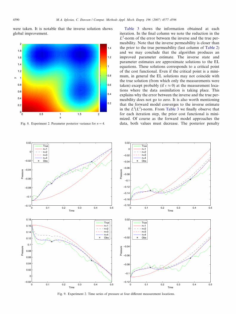
Fig. 8. Experiment 2. Parameter posterior variance for n = 4.

0 0.1 0.2 0.3 0.4 0.5–0.12

–0.1

–0.08

–0.06

–0.04

–0.02

0

0.02

Time

Pre

ssur

e

Truen=1n=2n=3n=4Obs

0 0.1 0.2 0.3 0.4 0.5–0.02

0

0.02

0.04

0.06

0.08

0.1

0.12

0.14

0.16

0.18

Time

Pre

ssur

e

Truen=1n=2n=3n=4Obs

Fig. 9. Experiment 2. Time series of pressure

Table 3 shows the information obtained at eachiteration. In the final column we note the reduction in theL2-norm of the error between the inverse and the true per-meability. Note that the inverse permeability is closer thanthe prior to the true permeability (last column of Table 2)and we may conclude that the algorithm produces animproved parameter estimate. The inverse state andparameter estimates are approximate solutions to the ELequations. These solutions corresponds to a critical pointof the cost functional. Even if the critical point is a mini-mum, in general the EL solutions may not coincide withthe true solution (from which only the measurements weretaken) except probably (if � � 0) at the measurement loca-tions where the data assimilation is taking place. Thisexplains why the error between the inverse and the true per-meability does not go to zero. It is also worth mentioningthat the forward model converges to the inverse estimatein the L2(L2)-norm. From Table 3 we finally observe thatfor each iteration step, the prior cost functional is mini-mized. Of course as the forward model approaches thedata, both values must decrease. The posterior penalty

0 0.1 0.2 0.3 0.4 0.5–0.18

–0.16

–0.14

–0.12

–0.1

–0.08

–0.06

–0.04

–0.02

0

0.02

Time

Pre

ssur

e

Truen=1n=2n=3n=4Obs

0 0.1 0.2 0.3 0.4 0.5–0.12

–0.1

–0.08

–0.06

–0.04

–0.02

0

0.02

Time

Pre

ssur

e

Truen=1n=2n=3n=4Obs

at four different measurement locations.

M.A. Iglesias, C. Dawson / Comput. Methods Appl. Mech. Engrg. 196 (2007) 4577–4596 4591

functional has a statistical interpretation that we do notattempt to study in the present case. At this point we notethere is a decrease from the prior to the posterior penalty ateach iteration. In fact, we must emphasize that as the dataerror misfit decreases, both the prior and posterior costfunctional reduce to zero. Then, from expression (6.4) wenote that when convergence is achieved, the nth forwardmodel fits the data d. Thus, we may expect the the nthinverse solution to be a good approximation to the nonlin-ear EL equations while it provides an improved estimate ofthe measurement vector.

6.2. Experiment 2

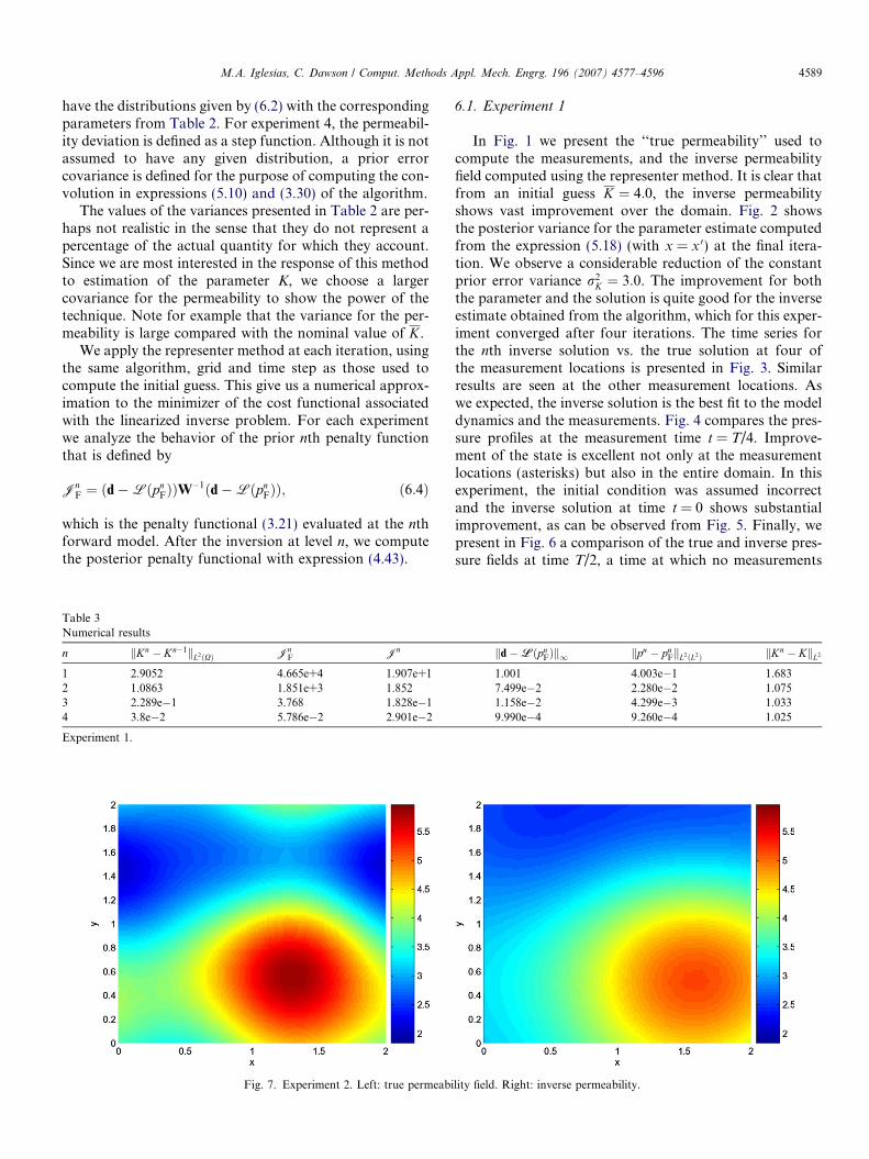
In the second experiment, we assume errors in the forc-ing and the boundary conditions. In Fig. 7, we present thetrue and the inverse permeability fields for this case. Theinverse permeability shows improvement in some parts ofthe domain. Fig. 8 shows the posterior variance for theparameter estimate computed from the expression (5.18)

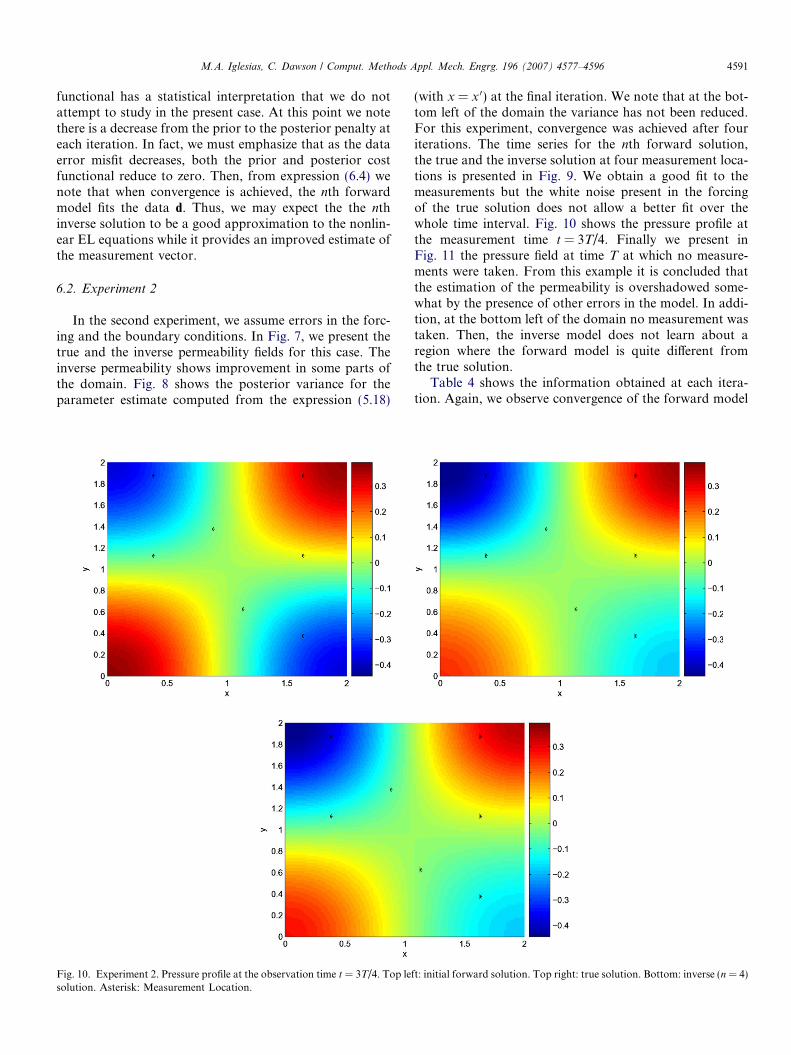
Fig. 10. Experiment 2. Pressure profile at the observation time t = 3T/4. Top lesolution. Asterisk: Measurement Location.

(with x = x 0) at the final iteration. We note that at the bot-tom left of the domain the variance has not been reduced.For this experiment, convergence was achieved after fouriterations. The time series for the nth forward solution,the true and the inverse solution at four measurement loca-tions is presented in Fig. 9. We obtain a good fit to themeasurements but the white noise present in the forcingof the true solution does not allow a better fit over thewhole time interval. Fig. 10 shows the pressure profile atthe measurement time t = 3T/4. Finally we present inFig. 11 the pressure field at time T at which no measure-ments were taken. From this example it is concluded thatthe estimation of the permeability is overshadowed some-what by the presence of other errors in the model. In addi-tion, at the bottom left of the domain no measurement wastaken. Then, the inverse model does not learn about aregion where the forward model is quite different fromthe true solution.

Table 4 shows the information obtained at each itera-tion. Again, we observe convergence of the forward model

ft: initial forward solution. Top right: true solution. Bottom: inverse (n = 4)

Fig. 11. Experiment 2. Pressure profile at time t = T. Top left: initial forward model. Top right: true Solution. Bottom: inverse (n = 4) solution.

Table 4Numerical results

n kKn � Kn�1kL2ðXÞ JnF Jn kd�Lðpn

FÞk1 kpn � pnFkL2ðL2Þ kKn � KkL2

1 1.401 1.716e+3 2.043 3.083e�1 6.748e�2 1.3692 6.213e�1 9.763e+1 4.354e�1 5.681e�2 1.953e�2 1.0393 8.180e�2 1.147 9.991e�3 6.776e�3 2.262e�3 1.0154 2.584e�3 8.030e�4 3.800e�4 1.980e�3 8.800e�5 1.0145 – – – 1.000e�4 – –

Experiment 2.

4592 M.A. Iglesias, C. Dawson / Comput. Methods Appl. Mech. Engrg. 196 (2007) 4577–4596

to the inverse estimate. While the inverse permeability doesnot appear to give as good a fit to the true permeability asin experiment 1, the L2 error between the inverse and truepermeabilities are almost identical to that obtained inexperiment 1 (see Table 3).

6.3. Experiments 3 and 4

Suppose now that the only uncertainty in the model isthe permeability. In experiment 3 the true solution is

obtained as in experiment 2 but without errors in the forc-ing and the boundary conditions. It can be seen from Figs.12 and 13 that the inverse permeability shows betterimprovement than experiment 2, where additional modelerrors were present. It is also shown that the posteriorerror covariance for the inverse has reduced compared tothat in Fig. 8. Note that to obtain convergence requiresmore iterations than in experiment 2, but there is a greaterreduction of the error in the permeability (final column ofTable 5).

Fig. 13. Parameter posterior variance for n = 4 for experiment 3.

Fig. 12. Experiment 3. Left: true permeability field. Right: inverse permeability.

M.A. Iglesias, C. Dawson / Comput. Methods Appl. Mech. Engrg. 196 (2007) 4577–4596 4593

This example shows that even if no measurements areassimilated in a certain region of the domain, it is still pos-sible to obtain good estimates as long as the forward modeldoes not contains source of errors that influences theestimation.

Table 5Numerical results

n kKn � Kn�1kL2ðXÞ JnF Jn

1 1.656 1.729e+3 1.548e+12 6.935e�1 1.143e+1 1.1163 1.645e�1 2.161 4.681e�14 1.042e�1 3.508e�1 2.685e�15 7.871e�2 2.092e�1 1.641e�16 6.044e�2 1.303e�1 1.044e�17 4.703e�2 8.487e�2 6.978e�28 3.706e�2 5.826e�2 4.493e�2

Experiment 3.

In the previous experiments we assumed that the truesolution was obtained by adding pseudo-random errorsto permeability, boundary conditions, forcing terms, etc.However, in experiment 4 we suppose that the true perme-ability is given by

Kðx; yÞ ¼4 if x 2 ½0; 1�2 if x 2 ð1; 2�:

�ð6:5Þ

Fig. 14 shows the inverse permeability which improves sig-nificantly from the prior K ¼ 3:0. With this experiment weobserve that even if we do not have knowledge of the priorerror statistics, it is still possible to obtain a reasonableparameter estimate.

From Table 6 we note again a reduction in the errorbetween the inverse and the true permeability. However,at the final iteration (n = 4) we observe a slight increasein that error. We remark once more that this informationwas presented as a way to understand the improvementof the inverse permeability over the prior. It should notbe interpreted as a lack of convergence. What we have issimply that the inverse permeability that generates theinverse solution (at n = 4) has slightly larger L2 error thanthe previous inverse permeability (n = 3). Nevertheless, theinverse solution (at n = 4) is considerably better than theprior guess.

kd�LðpnFÞk1 kpn � pn

FkL2ðL2Þ kKn � KkL2

3.093e�1 7.187e�2 1.1077.772e�2 1.942e�2 6.838e�18.833e�3 2.627e�3 5.891e�12.495e�3 1.373e�3 5.257e�12.024e�3 1.069e�3 4.810e�11.679e�3 8.320e�4 4.494e�11.394e�3 6.540e�4 4.266e�11.157e�3 5.190e�4 4.097e�1

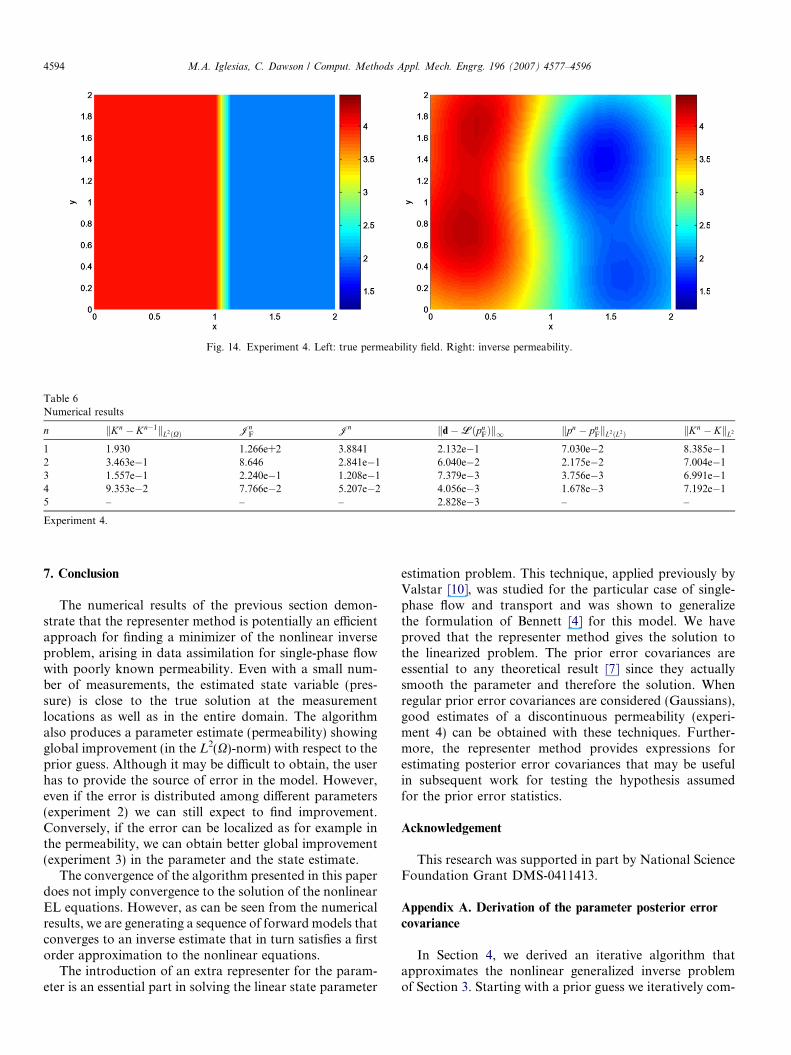
Fig. 14. Experiment 4. Left: true permeability field. Right: inverse permeability.

Table 6Numerical results

n kKn � Kn�1kL2ðXÞ JnF Jn kd�Lðpn

FÞk1 kpn � pnFkL2ðL2Þ kKn � KkL2

1 1.930 1.266e+2 3.8841 2.132e�1 7.030e�2 8.385e�12 3.463e�1 8.646 2.841e�1 6.040e�2 2.175e�2 7.004e�13 1.557e�1 2.240e�1 1.208e�1 7.379e�3 3.756e�3 6.991e�14 9.353e�2 7.766e�2 5.207e�2 4.056e�3 1.678e�3 7.192e�15 – – – 2.828e�3 – –

Experiment 4.

4594 M.A. Iglesias, C. Dawson / Comput. Methods Appl. Mech. Engrg. 196 (2007) 4577–4596

7. Conclusion

The numerical results of the previous section demon-strate that the representer method is potentially an efficientapproach for finding a minimizer of the nonlinear inverseproblem, arising in data assimilation for single-phase flowwith poorly known permeability. Even with a small num-ber of measurements, the estimated state variable (pres-sure) is close to the true solution at the measurementlocations as well as in the entire domain. The algorithmalso produces a parameter estimate (permeability) showingglobal improvement (in the L2(X)-norm) with respect to theprior guess. Although it may be difficult to obtain, the userhas to provide the source of error in the model. However,even if the error is distributed among different parameters(experiment 2) we can still expect to find improvement.Conversely, if the error can be localized as for example inthe permeability, we can obtain better global improvement(experiment 3) in the parameter and the state estimate.

The convergence of the algorithm presented in this paperdoes not imply convergence to the solution of the nonlinearEL equations. However, as can be seen from the numericalresults, we are generating a sequence of forward models thatconverges to an inverse estimate that in turn satisfies a firstorder approximation to the nonlinear equations.

The introduction of an extra representer for the param-eter is an essential part in solving the linear state parameter

estimation problem. This technique, applied previously byValstar [10], was studied for the particular case of single-phase flow and transport and was shown to generalizethe formulation of Bennett [4] for this model. We haveproved that the representer method gives the solution tothe linearized problem. The prior error covariances areessential to any theoretical result [7] since they actuallysmooth the parameter and therefore the solution. Whenregular prior error covariances are considered (Gaussians),good estimates of a discontinuous permeability (experi-ment 4) can be obtained with these techniques. Further-more, the representer method provides expressions forestimating posterior error covariances that may be usefulin subsequent work for testing the hypothesis assumedfor the prior error statistics.

Acknowledgement

This research was supported in part by National ScienceFoundation Grant DMS-0411413.

Appendix A. Derivation of the parameter posterior error

covariance

In Section 4, we derived an iterative algorithm thatapproximates the nonlinear generalized inverse problemof Section 3. Starting with a prior guess we iteratively com-

M.A. Iglesias, C. Dawson / Comput. Methods Appl. Mech. Engrg. 196 (2007) 4577–4596 4595

pute an estimate (pn,kn,Kn) that solves a linear inverseproblem at the nth step for the penalty functional givenby (3.21). This problem was stated as to find fn, in, bn

N, bnD

and kn in (3.20) such that pn is a best fist in the least-squaressense given by Jn. On the other hand, in Section 2 the errorfunctions fn, in, bn

N, bnD and kn were introduced in order to

account for the uncertainty of the problem. Therefore,those errors functions can be viewed as random fields withsome properties. Assuming as before that the error covari-ances are given

Eðf nðx; tÞ; f nðx0; t0ÞÞ ¼ CFðx; t; x0; t0Þ;EðinðxÞ; inðx0ÞÞ ¼ CIðx; x0Þ;Eðbn

Nðx; tÞ; bnNðx0; t0ÞÞ ¼ CNðx; t; x0; t0Þ;

EðbnDðx; tÞ; bn

Dðx0; t0ÞÞ ¼ CDðx; t; x0; t0Þ;EðknðxÞ; knðx0ÞÞ ¼ CKðx; x0Þ;

Eð�j; �mÞ ¼W�1jm

ðA:1Þ

and uncorrelated ([4, Chapter 5])

Eðf n; inÞ ¼ 0; Eðf n; bnNÞ ¼ 0; Eðf n; bn

DÞ ¼ 0; Eðf n; knÞ ¼ 0;

Eðf n; �mÞ ¼ 0; Eðin; bnNÞ ¼ 0; Eðin; bn

DÞ ¼ 0; Eðin; knÞ ¼ 0;

Eðin; �mÞ ¼ 0; EðbnD; b

nNÞ ¼ 0; Eðbn

D; knÞ ¼ 0; Eðbn

D; �mÞ ¼ 0;

EðbnN; k

nÞ ¼ 0; EðbnN; �mÞ ¼ 0; Eðkn; �mÞ ¼ 0:

ðA:2Þ

Note that during the iterative algorithm we assume theprior error covariances remain the same. In this section,we want to obtain a formula for the posterior error covari-ance for the parameter. In other words, we find the covari-ance for the error between the true and the inverse estimateof the parameter. Let ðpn

T;KnTÞ be the true solution of the

nth problem which we assume is the solution of (3.20) fora set of error functions fn, in, bn

N, bnD and kn. Then, by

(2.6) note that for each m = 1, . . . ,M

Eðdm �LmðpnFÞ; dj �Ljðpn

FÞÞ¼ EðLmðpn

T � pnFÞ þ �m;Ljðpn

T � pnFÞ þ �jÞ

¼ EðLmðpnT � pn

FÞ;LjðpnT � pn

FÞÞ þ EðLmðpnT � pn

FÞ; �jÞþ Eð�m;Ljðpn

T � pnFÞÞ þ Eð�m; �jÞ: ðA:3Þ

From the definition of the inner product in terms of thebilinear form (4.10), the operator defined in (4.9) and thedefinition of formal inverse (2.12), we compute

LmðpnT � pn

FÞ ¼ hðpnT � pn

F;KnT � Kn�1Þ; ðrn

m; cnmÞi

¼ Bn½ðpnT � pn

F;KnT � Kn�1Þ; ðrn

m; cnm�

¼ f n � anm þ in � can

m þ bnNHan

m

þ bnD ð�Kn�1ran � nÞ þ kn � W K � cn

m:

ðA:4Þ

Note that we are including Dirichlet boundary conditionsfor which the operator An (4.9) has an extra componentAn

Dðp;KÞ ¼ pjCD. From (A.1) and (A.2),

EðLjðpnT � pn

FÞ;LmðpnT � pn

FÞÞ¼ an

j � CF � anm þ can

j � CI � canm þ an

j HCNHanm

þ ð�Kn�1ranj � nÞ CD ð�Kn�1ran

m � nÞþ cn

j � W K � cnm; ðA:5Þ

while

EðLmðpnT � pn

FÞ; �jÞ ¼ Eð�m;LjðpnT � pn

FÞÞ ¼ 0: ðA:6ÞAgain, from (4.9), (4.10) and (2.12) we obtain

hðrnj ; c

nj Þ; ðrn

m; cnmÞi ¼ Bn ðrn

j ; cnj Þ; ðrn

m; cnmÞ

h i¼ an

j � CF � anm þ can

j �CI � canm

þ anj HCNHan

m

þ ð�Kn�1ranj � nÞ CD ð�Kn�1ran

m � nÞþ cn

j �W K � cnm: ðA:7Þ

Comparing (A.5) and (A.7) we realize

EðLjðpnT � pn

FÞ;LmðpnT � pn

FÞÞ ¼ hðrnj ; c

nj Þ; ðrn

m; cnmÞi ¼ Rn

jm;

ðA:8Þ

where the last equality comes from Remarks 1 and 2 as wellas the definition of the representer matrix Rn which isclearly symmetric. Combining (A.3), (A.6), (A.7) and(A.1) we have

Eðdm �LmðpnFÞ; dj �Ljðpn

FÞÞ ¼ Rnmj þ W �1

mj : ðA:9Þ

Observation 1. Eq. (A.9) implies that Rn + W�1 equals thecross-covariance of the linearized model measurementmisfit.

Observation 2. For each m = 1, . . . ,M, the representers(rm,cm) are the cross-covariance between the error parame-ter and the mth measurement error.

Proof. From (2.6) and (A.2)

Eðkn; dm �LmðpnFÞ

TÞ ¼ Eðkn;LmðpnT � pn

FÞ þ �mÞ¼ Eðkn;Lmðpn

T � pnFÞÞ þ Eðkn; �mÞ

¼ Eðkn;LmðpnT � pn

FÞÞ: ðA:10Þ

Eq. (A.4) and the covariances relations (A.1) and (A.2) giveus

Eðkn;Lmðp � pnFÞÞ ¼ Eðkn; f nÞ � an

m þ Eðkn; inÞ � canm

þ Eðkn; bnNÞHan

m

þ Eðkn; bnDÞ ð�Kn�1ran � nÞ

þ Eðkn; knÞ � W K � cnm

¼ Eðkn; knÞ � W K � cnm

¼ CK � W K � cnm ¼ cn

m: ðA:11Þ

Therefore,

EðknðxÞ; ðdm �LmðpnFÞ

TÞ ¼ cnmðxÞ: � ðA:12Þ

4596 M.A. Iglesias, C. Dawson / Comput. Methods Appl. Mech. Engrg. 196 (2007) 4577–4596

Now we derive the formula for the posterior error covari-ance for the parameter. Observe that

EðKnT � Kn;Kn

T � KnÞ

¼ E KnT � Kn�1 �

Xm

i¼1

bnmcn

m;KnT � Kn�1 �

Xm

i¼1

bnmcn

m

!

¼ Eðkn; knÞ � 2E kn;Xm

i¼1

bnmcn

m

!þ E

Xm

i¼1

bnmcn

m;Xm

i¼1

bnmcn

m

!;

ðA:13Þ

where we have used the fact that KnT ¼ Kn�1 þ kn. We now

define cn ¼ ðcn1; . . . ; cn

MÞ. From (5.17), (A.11) and the factthat Rn and W are symmetric,

EðknðxÞ; ðbnÞTcnðx0ÞÞ¼ EðknðxÞ; ðd�Lðpn

FÞÞTðRn þW�1Þ�T

cnðx0Þ¼ EðknðxÞ; ðd�Lðpn

FÞÞTÞðRn þW�1Þ�1

cnðx0Þ¼ cnðxÞðRn þW�1Þ�1

cnðx0Þ: ðA:14Þ

From (A.9)

EððbnÞT; ðbnÞTÞ¼ ðRn þW�1Þ�1E ðd�Lðpn

F� �T

; ðd�LðpnFÞÞ

TÞðRn þW�1Þ�1

¼ ðRn þW�1Þ�1ðRn þW�1ÞðRn þW�1Þ�1

¼ ðRn þW�1Þ�1: ðA:15Þ

Thus,

EððbnÞTcnðxÞ; ðbnÞTcnðx0ÞÞ ¼ cnðxÞEðbn; ðbnÞTÞcnðx0Þ¼ cnðxÞðRn þW�1Þ�1

cnðx0Þ:ðA:16Þ

From (A.13), (A.14), (A.1) and (A.16) we finally obtain

EðKnTðxÞ � KnðxÞ;Kn

Tðx0Þ � Knðx0ÞÞ

¼ CKðx; x0Þ � cnðxÞðRn þW�1Þ�1cnðx0Þ: ðA:17Þ

References

[1] S.I. Aanonsen, G. Naevdal, L.M. Johnsen, E. Vefring, Reservoirmonitoring and continuous model updating using the ensembleKalman filter, in: SPE Annual Technical Conference and Exhibition,(SPE 84372), 2003.

[2] J. Baird, C. Dawson, A Posteriori Error Estimation of the Repre-senter Method for in Single-Phase Darcy Flow in Porous Media,Comp. Meth. Appl. Mech. Eng. 196 (2007) 1623–1632.

[3] J. Baird, C. Dawson, The representer method for data assimilation insingle-phase Darcy flow in porous media, Comput. Geosci. (2006) 1–25, doi:10.1007/s10596-005-9006-2.

[4] A.F. Bennett, Inverse Methods in Physical Oceanography, Cam-bridge University Press, New York, 1992.

[5] A.F. Bennett, Inverse Methods of the Ocean Atmosphere, CambridgeUniversity Press, New York, 2002.

[6] M. Eknes, G. Evensen, Parameter estimation solving a weakconstraint variational formulation for an Ekman model, J. Geophys.Res. 102 (1997) 479-12, 491.

[7] M. Iglesias, C. Dawson, Local existence of the generalized inverse forpermeability and state estimation in single-phase Darcy flow, ICESReport 07-03, Institute for Computational Engineering and Science(ICES), The University of Texas at Austin, 2007. http://www.ices.utexas.edu/research/reports/2007/0703.pdf.

[8] J.L. Lions, E. Magenes, Non-Homogeneous Boundary Value Prob-lems and Applications, vol. II, Springer-Verlag, Berlin, 1972.

[9] A. Tarantola, Inverse Problems Theory: Methods for Data Fittingand Model Parameter Estimation, Elsevier, New York, 1987.

[10] J.R. Valstar, Inverse modeling of groundwater flow and transport,Ph.D. Thesis, Delf University of Technology, Delf, Netherlands,2001.

[11] J.R. Valstar, D.B. McLaughlin, C.B.M. te Stroet, F.C. van Geer, Arepresenter-based inverse method for groundwater flow and transportapplications, Water Resources Research, 40, W05116, doi:10.1029/2003WR002922.

[12] E.H. Vefring, G. Naevdal, T. Mannseth, Near-well reservoir moni-toring through the ensemble Kalman filter, in: Proceeding of SEP/DOE Improved Oil Recovery Symposium (SPE 75235), 2002.