Application of matched ®ltering and parameter estimationtechnique to low latitude whistlers

R.P. Singha, D.K. Singha, Ashok K. Singha, D. Hamarb, J. Lichtenbergerb,*aAtmospheric Research Laboratory, Physics Department, Banaras Hindu University, Varanasi, 221 005, India

bGeophysical Department, EoÈtvoÈs University, Budapest, Pf. 32, H-1532, Hungary

Received 11 December 1998; received in revised form 25 May 1999; accepted 9 June 1999

Abstract

The Matched Filtering and Parameter Estimation (MFPE) technique developed for the analysis of mid/high

latitude whistlers has been extended to analyze whistlers recorded at low latitude ground station Varanasi, India(geomagnetic latitude 148 55 ' N, longitude 1538 59 ' E, L = 1.07). Some of the whistlers recorded at Varanasi arefound to have propagated along higher L-values (L > 2). It has been argued that these whistlers after exiting theionosphere have propagated towards the equator in the Earth-ionosphere waveguide. Trace splitting is observed

below the nose frequency and above 2.0 kHz, a result in agreement with mid/high latitude whistlers. The tracesplitting structure revealed by MFPE demonstrates the complexities of whistler wave propagation and is quitehelpful in deriving information about high resolution features of the duct structure. The banded features observed in

the dynamic spectrum are clearly seen in the output of the matched ®lter. The observed banded features may arisedue to interference between the wavelets propagating in the duct/waveguide. # 1999 Elsevier Science Ltd. All rightsreserved.

1. Introduction

The analogue methods (Sonograph or Rayspan

type) of spectrum analysis are not suitable for the high

accuracy analysis of whistlers. To overcome this di�-

culty and also to increase the speed of data processing,

di�erent digital methods have been developed

(Coroniti et al., 1971; Coster, 1974; Kodera et al.,

1976). Mikhajlova and Kapustina (1978), using a digi-

tal Gaussian ®lter, analyzed electron and proton whis-

tlers and achieved a much higher accuracy in

determining the frequency±time and amplitude±time

laws obtained by using the classical methods of

dynamic spectrum analysis. The matched ®ltering tech-

nique has been developed for the analysis of whistlers

recorded at mid and high latitudes (Hamar and

Tarcsai, 1982; Hamar et al., 1990, 1992; Lichtenberger

et al., 1991). In this technique, dispersive digital ®lters

are used whose frequency±time response are matched

with the frequency±time response of the signal to be

analyzed. For a whistler trace, matched ®ltering yields

the arrival time and approximate amplitude for a given

frequency. The technique strongly discriminates any

signals or noises which do not approximately obey the

model dispersion relation and yields a higher resol-

ution in frequency and time than is possible using the

conventional technique. It has been observed that

whistlers which appear as a single trace on a conven-

tional spectrograms usually contain many ®ne struc-

ture components with amplitudes di�ering in time and

frequency (Hamar et al., 1992). Individual components

Journal of Atmospheric and Solar-Terrestrial Physics 61 (1999) 1081±1092

1364-6826/99/$ - see front matter # 1999 Elsevier Science Ltd. All rights reserved.

PII: S1364-6826(99 )00033-4

* Corresponding author. Tel.: +36-1-372-2906; fax: +36-1-

372-2927.

E-mail address: spacerg@sas.elte.hu (J. Lichtenberger).

Fig. 1. Dynamic spectra of whistlers recorded at Varanasi on (a) 8 March 1991, at 01:24 IST (the sampling frequency was 16 kHz);

(b) 18 March 1991 at 00:56 IST (the sampling frequency was 12 kHz); and (c) 19 February 1997 at 00:11 IST (the sampling fre-

quency was 12 kHz). The amplitude scale is linear in arbitrary units.

R.P. Singh et al. / Journal of Atmospheric and Solar-Terrestrial Physics 61 (1999) 1081±10921082

of ®ne structure are easily analyzed to determine accu-rately the L-value of propagation, travel time residualsand electron density. The ®ne structure can give insight

into the whistler duct structure and hence the ductingmechanism.In this paper, we have tested the reliability of the

matched ®ltering and parameter estimation technique

in analysing whistlers recorded at the low latitudeground station Varanasi. High resolution dynamicspectra revealing the ®ne structure of whistlers were

obtained. High resolution travel time residual curveswere also obtained. The results presented in this paperclearly support the applicability of the MFPE tech-

nique with suitable modi®cations to the initial par-ameters and steps used in the technique.

2. Experimental data and method of analysis

Whistlers recorded at Varanasi formed part of thepresent study. The vertical component of the electric®eld of a whistler wave is recorded by using a T type

antenna, a pre/main ampli®er and cassette tape recor-der. The data are stored in analogue form on magnetictapes. We have analyzed whistlers recorded during

1991, 1993 and 1997. The whistlers were digitized

using a 12 or 16 kHz sampling frequency depending

on the whistler trace. A typical example of convention-

al (FFT) spectral analysis is shown in Fig. 1. The spec-

trogram shows a good quality whistler with strong

background noise at the lower frequencies. The whis-

tler spectrogram was scaled visually and frequency±

time ( f±t ) pairs thus obtained were processed with the

FIT method (Tarcsai, 1975) to obtain the parameters

of the whistlers and the dispersing medium.

The matched ®lter (MF) can be constructed by using

the whistler parameters: source time T0, zero frequency

dispersion D0, nose frequency fn and equatorial elec-

tron gyrofrequency fHeq. These parameters for the cho-

sen whistlers are given in Table 1. At the beginning of

the computation less accurate values of these par-

ameters were used and, after each computation, the

values were approaching closer to those reported in

Table 1. The dynamic spectra were scaled and matched

®ltering was carried out. A typical example of dynamic

spectra after MF analysis is shown in Fig. 2; it is

clearly seen that the atmospherics and other noises

have been suppressed. Using f±t parameters of the

matched ®lter output, a second ®ltering was carried

out for the better estimation of the parameters; a ®lter

Fig. 1 (continued)

R.P. Singh et al. / Journal of Atmospheric and Solar-Terrestrial Physics 61 (1999) 1081±1092 1083

bandwidth of 200 Hz was used. The digitized wave-

form, matched ®lter output, output envelope andsmoothed output envelope are given in Fig. 3. In fact,the ®lter output, output envelope and smoothed output

envelope represent the main stages of the procedure.The above procedure facilitates determination of theinitial time and the magnitude of all local maxima of

the smoothed envelope. Thus, for a given frequency aset of arrival times are obtained. This procedure isrepeated for every 10 Hz frequency step across therange of whistler frequency. In some cases, the above

procedure was repeated for 2 and 5 Hz frequencysteps. However, the results obtained did not change.

3. Results and discussions

The whistlers recorded at Varanasi during 1990±1997 usually show sharp dynamic spectra which

implies that the ducts through which the whistlers havepropagated are narrow in width and well de®ned. Theamplitude of the whistler wave is a function of fre-

quency. Some of the traces clearly show a bandednature of the dynamic spectrum. A proper explanationof the banded nature of the whistler wave should besearched for either in the source or in the propagation

mechanism of the wave from the source to the obser-vation points. There is no report of banded structurein the emitted radiation from the lightning discharge

which is the natural source of whistler waves analysedin this paper. Two discharges separated by a veryshort time may cause a similar banded structure.

Therefore, the banded structure could probably beattributed to propagation. The detailed analysis of thedynamic spectrum shows that some of these whistlershave propagated a path for which L > 2. The obser-

vation of such whistlers clearly supports the idea thatthese whistlers have propagated along higher L-valuesand, after they exit the duct, they penetrate the iono-

sphere, and are trapped in the Earth-ionosphere wave-guide. The wave-normal angle at the entrance into theduct waveguide is such that they propagate towards

the equator and are received at the low latitude stationVaranasi. Shimakura et al. (1987, 1991) presentedwhistler traces which support the hypothesis that whis-

tlers propagated in the Earth-ionosphere waveguide

mode before being received, on the ground. Such a

propagation mechanism have been discussed by Singh

et al. (1992). Hayakawa et al. (1990), based on spaced

direction-®nding measurements at three stations in

southern China, suggested that the propagation of

whistlers in the Earth-ionosphere waveguide after iono-

spheric transmission is more likely towards higher lati-

tudes than towards the equator. But, at Varanasi, we

have recorded a large number of whistlers which show

equatorward propagation in the Earth-ionosphere

waveguide (Singh, 1995). These whistlers have been

analyzed to yield information about the equatorial

electron density, large scale electric ®eld, duct width

and duct lifetime (Singh, 1993, 1995; Singh et al.,

1998).

The accuracy and e�ectiveness of the technique has

been discussed at length by comparing the convention-

al dynamic spectra and high resolution dynamic spec-

tra (Hamar et al., 1990, 1992; Lichtenberger et al.,

1991). The high resolution dynamic spectra contain

trace splitting over a given frequency range either

quasi-symmetrically or asymmetrically with respect to

a vertical theoretical trace (Hamar et al., 1992). We

have shown, in Fig. 4, an example of an idealized loca-

lized trace splitting event for the whistlers recorded at

Varanasi. In Fig. 4, the f±t pairs and amplitudes

obtained from the peaks (only peaks with an ampli-

tude above a certain limit are considered) of the

smoothed envelopes of the MF output are plotted. In

this plot the relative time (obtained by subtracting the

theoretical (®tted) travel time from the measured t( f )

data) is used. These are transformed plots where whis-

tler traces appear straightened. On such plots a model

whistler will appear as a straight line, while sferics

would appear as hyperbola, like the isochrones shown

in Fig. 4. The traces in Fig. 4 clearly di�er from verti-

cal lines. The deviation from the ideal (vertical) line

which corresponds to the theoretical longitudinal

propagation is between 25 ms. In Fig. 4a two splitting

events can be observed with 8±10 ms width at 3 and

4.6 kHz. The bandwidths of these events are less than

200 Hz. In Fig. 4b the deviation of the trace from the

vertical line is smaller (23 ms), and a discontinuity can

be seen around 3000 Hz, corresponding to the dynamic

Table 1

Charactersitic parameters of the whistlers and plasma medium

Date of whistler recording 8 March 1991 18 March 1991 19 February 1997

Equatorial gyrofrequency fHeq (kHz) 160248 1852101 4929

Nose frequency fn (kHz) 55216 63234 1823

Dispersion D0 (s1/2) 33.320.2 29.220.3 9.520.2

L-value 1.7620.18 1.6820.31 2.6120.16

Equatorial electron density neq (cmÿ3) (4.722.3) � 103 (5.024.4) � 103 40210

R.P. Singh et al. / Journal of Atmospheric and Solar-Terrestrial Physics 61 (1999) 1081±10921084

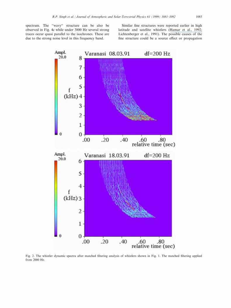
spectrum. The ``wavy`` structure can be also beobserved in Fig. 4c while under 3800 Hz several strong

traces occur quasi parallel to the isochrones. These aredue to the strong noise level in this frequency band.

Similar ®ne structures were reported earlier in highlatitude and satellite whistlers (Hamar et al., 1992;

Lichtenberger et al., 1991). The possible causes of the®ne structure could be a source e�ect or propagation

Fig. 2. The whistler dynamic spectra after matched ®ltering analysis of whistlers shown in Fig. 1. The matched ®ltering applied

from 2000 Hz.

R.P. Singh et al. / Journal of Atmospheric and Solar-Terrestrial Physics 61 (1999) 1081±1092 1085

e�ects from the source to the receiver; the latter are

more likely. Usually the Earth-ionosphere waveguide

path is small (propagation time <<Dt010 ms) and

propagation through the waveguide is similar topropagation in free space. Hence the ®ne structure can-

not be caused by the Earth-ionosphere waveguide

mode of propagation. The ®ne structure may be due to

variations in the refractive index of the ionospheric

and magnetospheric plasma. The ionospheric pathbeing much shorter than the magnetospheric path, it

would require much larger gradients in the ionospheric

refractive index than in the magnetospheric refractive

index, and can be achieved only when there are large

gradients in the electron density of the ionosphere.

Since no mechanism can sustain a large gradient in theionospheric electron density, it is likely that the ®ne

structure occurs as the wave propagates through the

magnetosphere. Whistlers propagate through the mag-

netosphere in ducts; ®ne structures of the duct (due to

®ne variations in electron density) may cause changes

in arrival time. Model calculations show that, if thewhistler consists of two closely spaced traces, the sep-

aration of the traces by matched ®ltering is limited to

Dt= 1.6/Df, that is Dt = 8 ms, in our case, when

Df= 200 Hz. To increase the resolution by increasing

the ®lter bandwidth does not lead better results due tothe increasing discrepancy between the natural whistler

signal and the matched ®lter. If the trace splitting is

attributed to the ®ne structure in magnetospheric ducts

then, assuming longitudinal propagation, one can esti-

mate the order of magnitude of density ¯uctuations

and scale sizes involved. Hamar et al. (1992) have dis-cussed possible signatures of the ®ne structure within

ducts and have suggested that a proper explanation of

the splitting should be searched for in the theory of

the ducted propagation of whistlers. It may be noted

that the fractional di�erence between the group vel-

ocities of di�erent modes propagating through a bell-shaped duct is of the same order as the fractional split-

ting time (Scarabucci and Smith, 1971). The splitting

reported by Scarabucci and Smith (1971) using homo-

geneous ducts appears at high frequencies, mainly

above the nose frequency, whereas in the present casesplitting has appeared at frequencies well below the

nose frequency. Hence, before making detailed com-

parisons, the mode theory should be extended to

include the e�ect of inhomogeneities in the medium's

parameters.

The travel time residuals as a function of frequency

are shown in Fig. 5. This curve is typical of observed

whistlers and may have resulted from the usual ap-proximations made in whistler analysis (omission of

a + 1 term and ionic term in the refractive index,

strictly ®eld-aligned propagation instead of the actual

snake-like ray path). It is worth noting that the re-

siduals lie within 22 ms. The small values of traveltime residuals clearly support the idea of whistler wave

propagation through narrow ducts which is inferred

Fig. 2 (continued)

R.P. Singh et al. / Journal of Atmospheric and Solar-Terrestrial Physics 61 (1999) 1081±10921086

Fig. 3. Digitized waveform, matched ®lter output, output envelope and smoothed output envelope corresponding to the dynamic

spectra of whistlers shown in Fig. 1.

Fig. 4. Isochrones of whistlers shown in Fig. 1.

R.P. Singh et al. / Journal of Atmospheric and Solar-Terrestrial Physics 61 (1999) 1081±10921088

from the sharpness of the dynamic spectrum usually

observed at low latitude stations.

The amplitude variation with frequency is shown in

Fig. 6. The amplitude of the di�erent whistler com-

ponents at a given frequency was obtained by normaliz-

ing the matched ®lter output maxima with the sum of

the squared ®lter coe�cients. The value thus obtained is

only an average of the amplitude over the ®lter length.

Repeating this procedure for di�erent frequencies, the

amplitude variation with frequency along the whistler

trace was obtained. The amplitude maxima at di�erent

frequencies clearly correlate with the amplitudes rep-

resented by the colours in the dynamic spectra.

Contrary to the assumption that the energy per unit

bandwidth should be constant, the amplitude variation

is complex. This may be due to frequency dependent

absorption, ampli®cation due to wave-particle inter-

actions, focussing/ducting along the path of propa-

gation, etc. The variation of amplitude with frequency

may also be explained by considering the interference

between two components of the re¯ected wave from the

trough and crest portions of the electron density distri-

bution forming the duct, while propagating through the

duct. The constructive interference gives amplitude

maxima and destructive interference produces ampli-

tude minima. The condition for interference depends

upon the phase di�erence of the two waves, and hence

on the frequency of wave, and the structure and widthof the duct. A detailed study of this mechanism will becommunicated in a separate paper.

4. Conclusions

Whistler waves recorded at the low latitude station

Varanasi (L = 1.07), India, have been analyzed usingthe high resolution digital Matched Filtering andParameter Estimation technique. The following points

emerge from the present study:

. the Matched Filtering and Parameter Estimationtechnique developed for the analysis of mid/high

latitude whistlers is, after suitable modi®cations,capable of analyzing whistlers recorded at low lati-tude stations;

. accurate analysis shows that whistlers have propa-

gated in the Earth-ionosphere waveguide towardsthe equator after emerging from the ionosphere;

. the trace splitting observed below the nose frequency

may yield information about ®ne structures presentin the duct;

. the sharp dynamic spectrum and small travel time

residuals indicate that the duct supporting the whis-tler waves at low latitudes must be narrow andsharp;

Fig. 4 (continued)

R.P. Singh et al. / Journal of Atmospheric and Solar-Terrestrial Physics 61 (1999) 1081±1092 1089

Fig. 5. Travel time residuals for whistlers shown in Fig. 1.

R.P. Singh et al. / Journal of Atmospheric and Solar-Terrestrial Physics 61 (1999) 1081±10921090

Fig. 6. Amplitude variations with frequency for the whistlers shown in Fig. 1.

R.P. Singh et al. / Journal of Atmospheric and Solar-Terrestrial Physics 61 (1999) 1081±1092 1091

. the variation of amplitude with frequency showingbanded structures in the dynamic spectrum may

arise due to interference between the wavelets propa-gating through the duct/waveguide.

Acknowledgements

The work is supported by the Department ofScience and Technology (International Division)Government of India and OMFB, Government of

Hungary through a joint collaborative project.

References

Coroniti, F.V., Fredricks, R.W., Kennel, C.F., Scarf, F.L.,

1971. Fast time resolved spectral analyses of VLF banded

emission. Journal of Geophysical Research 76, 2366.

Coster, C., 1974. Calibration of a VLF goniometers receiver

and development of a method for coumpter processing of

whistlers. ESA-ESTEC, Nordwijk, Holland.

Hamar, D., Tarcsai, G., 1982. High resolution frequency time

analysis of whistlers using digital matched ®ltering Ð part

1: theory and simulation studies. Annales Geophysicae 38,

119±128.

Hamar, D., Tarcsai, G., Lichtenberger, J., Smith, A.J.,

Yearby, K.H., 1990. Fine structures of whistlers recorded

digitally at Halley, Antarctica. Journal of Atmospheric

and Terrestrial Physics 52, 801±810.

Hamar, D., Ferencz, C., Lichtenberger, J., Tarcsai, G., Smith,

A.J., Yearby, K.H., 1992. Trace splitting of whistler: a sig-

nature of ®ne structure or mode ®tting in magnetospheric

ducts. Radio Science 27, 341.

Hayakawa, M., Ohta, K., Shimakura, S., 1990. Spaced direc-

tion ®nding of night time whistlers at low and equatorial

latitudes and their propagation mechanism. Journal of

Geophysical Research 95, 15,091±15,102.

Kodera, K., de Villedary, C., Gendrin, R., 1976. A new

method for the numerical analysis of non-stationary sig-

nals. Physics of Earth and Planetary Interior 12, 142±150.

Lichtenberger, J., Tarcsai, G., Pa sztor, S., Ferencz, C.,

Hamar, D., Molchanov, O.A., Golyavin, A.M., 1991.

Whistler doublets and hyper®ne structure recorded digi-

tally by the signal analyser and sampler on the Active sat-

ellite. Journal of Geophysical Research 96, 21,149.

Mikhajlova, G.A., Kapustina, O.V., 1978. Spectrum-time

analysis of whistlers by numerical methods. Geomagnetica

I Aeronomia 18, 473 [Russian].

Scarabucci, R.R., Smith, R.L., 1971. A study of magneto-

spheric ®eld oriented irregularities Ð the mode theory of

bell-shaped ducts. Radio Science 6, 65±87.

Shimakura, S., Tsubaki, A., Hayakawa, M., 1987. Very unu-

sual low latitude whistlers with additional traces of earth-

ionosphere waveguide propagation e�ect. Journal of

Atmospheric and Terrestrial Physics 49, 1081±1091.

Shimakura, 2., Moriizumi, M., Hayakawa, M., 1991.

Propagation mechanism of very unusual low latitude whis-

tlers with additional traces of earth-ionosphere waveguide

propagation e�ect. Planetary and Space Science 39, 611±

616.

Singh, U.P., Singh, A.K., Lalmani, Singh R.P., Singh, R.N.,

1992. Hybrid-mode propagation of whistlers at low

latitudes. Indian Journal of Radio Space Physics 21, 246±

249.

Singh, A.K., 1995. Study of inner magnetosphere by VLF

waves, Ph.D. thesis, Banaras Hindu University, India.

Singh, R.P., 1993. Whistler studies at low latitudes: a review.

Indian Journal of Radio Space Physics 22, 139±155.

Singh, R.P., Singh, A.K., Singh, D.K., 1998. Plasmaspheric

parameters as determined from whistler spectrograms: a

review. Journal of Atmospheric and Terrestrial Physics 60,

495±508.

Tarcsai, G., 1975. Routine whistler analysis by mean of accu-

rate curve ®tting. Journal of Atmospheric and Terrestrial

Physics 37, 1447±1457.

R.P. Singh et al. / Journal of Atmospheric and Solar-Terrestrial Physics 61 (1999) 1081±10921092