Aalborg Universitet

Parameter Estimation and Model Selection for Mixtures of Truncated Exponentials

Langseth, Helge; Nielsen, Thomas Dyhre; Rumí, Rafael; Salmerón, Antonio

Published in:International Journal of Approximate Reasoning

DOI (link to publication from Publisher):10.1016/j.ijar.2010.01.008

Publication date:2010

Document VersionPreprint (usually an early version)

Link to publication from Aalborg University

Citation for published version (APA):Langseth, H., Nielsen, T. D., Rumí, R., & Salmerón, A. (2010). Parameter Estimation and Model Selection forMixtures of Truncated Exponentials. International Journal of Approximate Reasoning, 51(5), 485-498.10.1016/j.ijar.2010.01.008

General rightsCopyright and moral rights for the publications made accessible in the public portal are retained by the authors and/or other copyright ownersand it is a condition of accessing publications that users recognise and abide by the legal requirements associated with these rights.

? Users may download and print one copy of any publication from the public portal for the purpose of private study or research. ? You may not further distribute the material or use it for any profit-making activity or commercial gain ? You may freely distribute the URL identifying the publication in the public portal ?

Take down policyIf you believe that this document breaches copyright please contact us at vbn@aub.aau.dk providing details, and we will remove access tothe work immediately and investigate your claim.

Downloaded from vbn.aau.dk on: August 06, 2015

Parameter Estimation and Model Selection for

Mixtures of Truncated Exponentials

Helge Langsetha, Thomas D. Nielsenb, Rafael Rumıc, Antonio Salmeronc

aDepartment of Computer and Information Science, The Norwegian University of Scienceand Technology, Trondheim (Norway)

bDepartment of Computer Science, Aalborg University, Aalborg (Denmark)cDepartment of Statistics and Applied Mathematics, University of Almerıa, Almerıa (Spain)

Abstract

Bayesian networks with mixtures of truncated exponentials (MTEs) supportefficient inference algorithms and provide a flexible way of modeling hybrid do-mains (domains containing both discrete and continuous variables). On theother hand, estimating an MTE from data has turned out to be a difficult task,and most prevalent learning methods treat parameter estimation as a regressionproblem. The drawback of this approach is that by not directly attempting tofind the parameter estimates that maximize the likelihood, there is no principledway of performing subsequent model selection using those parameter estimates.In this paper we describe an estimation method that directly aims at learningthe parameters of an MTE potential following a maximum likelihood approach.Empirical results demonstrate that the proposed method yields significantly bet-ter likelihood results than existing regression-based methods. We also show howmodel selection, which in the case of univariate MTEs amounts to partitioningthe domain and selecting the number of exponential terms, can be performedusing the BIC-score.

1. Introduction

Domains involving both discrete and continuous variables represent a chal-lenge to Bayesian networks. The main difficulty is to find a representation of thejoint distribution of the continuous and discrete variables that supports an effi-cient implementation of the usual inference operations over Bayesian networks(like those found in junction tree-based algorithms for exact inference). Compu-tationally, exact inference algorithms require that the joint distribution over thevariables of the domain is from a distribution-class that is closed under addi-tion and multiplication. The simplest way of obtaining such a distribution is toperform a discretization of the continuous variables (Friedman and Goldszmidt,1996; Kozlov and Koller, 1997). Mathematically, this amounts to approximatingthe density function of every continuous variable by a step-function. However,discretization of variables can lead to a dramatic loss in precision, which is oneof the reasons why other approaches have received much attention recently. The

Preprint submitted to Elsevier May 28, 2009

mixtures of truncated exponentials (MTE) framework (Moral et al., 2001) hasalso received increasing interest over the last few years. One of the advantagesof this representation is that MTE distributions allow discrete and continuousvariables to be treated in a uniform fashion, and since the family of MTEs isclosed under addition and multiplication, inference in an MTE network can beperformed efficiently using the Shafer-Shenoy architecture (Shafer and Shenoy,1990).

Cobb et al. (2006) empirically showed that many distributions can be ap-proximated accurately by means of an MTE distribution, and they argue thatthis makes the MTE framework very attractive for Bayesian network models.Nevertheless, data-driven learning methods for MTE networks have receivedonly little attention. In this context, focus has mainly been directed towardsparameter estimation, where the most prevalent methods look for the MTE pa-rameters minimizing the mean squared error w.r.t. a kernel density estimate ofthe data (Romero et al., 2006).

Although the least squares estimation procedure can yield a good MTEmodel in terms of generalization properties, there is no guarantee that the esti-mated parameter values will be close to the maximum likelihood (ML) parame-ters. This has a significant impact when considering more general problems suchas model selection and structural learning, as many standard score functions formodel selection, including the Bayesian information criterion (BIC) (Schwarz,1978), assume ML parameter estimates to be available.

In this paper we propose a new parameter estimation procedure for uni-variate MTE potentials. The procedure directly aims at estimating the MLparameters for an MTE density, and we show how to utilize the learned ML es-timates for model selection using the BIC score. The proposed learning methodis empirically compared to the least squares estimation method described byRomero et al. (2006), and it is shown that it offers a significant improvement interms of likelihood as well as in generalization ability.

The method described in this paper is a first step towards a general maxi-mum likelihood-based approach for learning Bayesian networks with MTE po-tentials. Thus, our objective is solely to demonstrate that maximum likelihoodestimators for MTE distributions can be found, and show how these estimatorscan be utilised for model selection. We will therefore prefer simple and robustmethods over state-of-the-art optimisation techniques that can be harder to un-derstand, implement, and examine. Furthermore, we shall only hint at some ofthe complexity problems that are involved in learning general MTE potentials.Learning MTE potentials using more efficient techniques is left as a topic forfuture research.

2. Preliminaries

Throughout this paper, random variables will be denoted by capital letters,and their values by lowercase letters. In the multi-dimensional case, boldfacedcharacters will be used. The domain of the variables X is denoted by ΩX. The

2

MTE model is defined by its corresponding potential and density as follows(Moral et al., 2001):

Definition 1. (MTE potential) Let X be a mixed n-dimensional random vector.Let W = (W1, . . . , Wd)

T and Z = (Z1, . . . , Zc)T be the discrete and continuous

parts of X, respectively, with c + d = n. We say that a function f : ΩX 7→ R+0

is a Mixture of Truncated Exponentials (MTE) potential if for each fixed valuew ∈ ΩW of the discrete variables W, the potential over the continuous variablesZ is defined as:

f(z) = a0 +

m∑

i=1

ai exp bT

i z , (1)

for all z ∈ ΩZ, where ai ∈ R and bi ∈ Rc, i = 1, . . . , m. We also say that f

is an MTE potential if there is a partition D1, . . . , Dk of ΩZ into hypercubesand in each Dℓ, f is defined as in Equation (1). An MTE potential is an MTEdensity if it integrates to 1.

In the remainder of this paper we shall focus on estimating the parametersfor a univariate MTE density. Not surprisingly, the proposed methods alsoimmediately generalize to the special case of conditional MTEs having onlydiscrete conditioning variables.

3. Expressiveness of the MTE models

In this section we will explore the expressiveness of the MTE framework,with the aim of showing that any univariate distribution function can be ap-proximated arbitrarily well by an MTE potential. We will tie our argument tothe example in Figure 1, but the results obtained are general in nature.

Consider first the left panel of Figure 1, where the target distribution of ourexample is given by the solid line. The target distribution, f(x), is a mixtureof two Gaussian distributions, one centred at − 1

2 and the other at 12 . Both

Gaussian distributions have standard deviation 1, and the mixture weights are.25 and .75, respectively. The left panel of Figure 1 also shows how a standarddiscretization scheme can be utilised to approximate f(x). Let fD(x | k) be theapproximation of f(x) obtained by dividing the range of X into k equally sized

intervals. Note that fD(x | k) requires k − 1 parameters to be fully specified,namely the amount of mass allocated to each interval except the last one. It is

obvious that if we measure the error of fD(x | k) as∫ b

x=a

(

fD(x | k)− f(x))2

dx,

then this error can be made arbitrarily small by increasing k. Since the class ofMTE distributions contains all distributions obtainable by discretization, we canalso approximate any f(x) arbitrarily well using MTEs. This representation maynot be optimal, though. In the left panel of Figure 1, 15 parameters were usedto obtain the approximation, but it is still rather crude and the representationalpower of MTEs are not fully utilised.

3

The right panel of Figure 1 explore a different strategy for approximatingf(x), as we here define an approximation by increasing the number of expo-nential terms, without dividing the support of the distribution into intervals.We will denote approximations generated in this way by fe(x |m), and for a

given set of parameters α we define fe(x |m, α) =∑m

s=−m αs exp(s x). In the

reminder of this section we investigate approximations of the type fe(x |m, α)and we will show that this strategy for approximating f(x) can also be madearbitrarily accurate (wrt. our error measure) simply by increasing m. The rightpanel of Figure 1 shows this visually: We are again using 15 parameters, but thequality of the approximation is now so good that it is not possible to visuallydistinguish the true distribution from the approximation.

−1 −0.8 −0.6 −0.4 −0.2 0 0.2 0.4 0.6 0.8 10

0.2

0.4

0.6

0.8

1

1.2

1.4

−1 −0.8 −0.6 −0.4 −0.2 0 0.2 0.4 0.6 0.8 10

0.2

0.4

0.6

0.8

1

1.2

1.4

(a) Approximation improved by (b) Approximation improved byincreasing no. intervals increasing no. exponential terms

Figure 1: Two different strategies for approximating a distribution function. The gold stan-dard model is in this case a mixture of two Gaussians, one centred at − 1

2, the other at 1

2.

We will make this argument by first restating a basic result from linearalgebra, and then show how this generalises to our setting. Let us start byconsidering an n-dimensional real vector z ∈ R

n. Let e1, . . . , ek be a set oforthogonal basis vectors in R

n (k < n), and consider the task of approximating z

by a vector in the span of the basis vectors. Let 〈x,y〉 denote the inner productbetween two vectors x and y; when both x and y are in R

n we use 〈x,y〉 = xTy.It is well-known that the least-squares solution to this approximation problemis to find the projection of z onto the space spanned by the basis vectors, i.e.,to choose

z←

k∑

j=1

〈ej , z〉√

〈ej , ej〉· ej. (2)

Next, we generalize this result from approximations in Rn to approximations

in a space containing functions, with the idea that we can approximate a functionf as a linear combination of basis functions. In particular, we will consider thespace of all functions that are squared integrable on an interval [a, b]. This space

4

is often denoted L2[a, b], so for a real function f we have that f ∈ L2[a, b] if

and only if∫ b

x=af(x) · f(x) dx <∞. To find an analogue to the projections in

Equation (2) we must define the inner product between two functions f and g,

and in L2[a, b] this is done as 〈f, g〉 =∫ b

af(x) · g(x) dx. Furthermore, we say

that two functions f an g are orthogonal if and only if 〈f, g〉 = 0.Focus on L2[0, 2π] and consider the task of finding the Fourier series ap-

proximation of a function f . This amounts to approximating f by a sum oftrigonometric functions, i.e., it is a solution to our original approximation prob-lem, where the functions 1, sin(x), cos(x), sin(2x), cos(2x), sin(3x), . . . take therole of the orthogonal1 basis-vectors e1 . . .ek used when making approxima-tions in R

n. Recall that the Fourier series approximation of f can be writtenas

f(x)←

k∑

j=1

〈ej , f〉√

〈ej , ej〉· ej(x). (3)

This gives an operational description of how to approximate any f ∈ L2[0, 2π]by a sum of trigonometric functions.

The last step in our argument is to recall that the approach of Equation (3)is valid also when the trigonometric functions are replaced by other orthogo-nal basis functions; in this case Equation (3) is called a Generalized Fourierseries. Since we look for MTE approximations, we are interested in the spanof the exponential functions 1, exp(x), exp(−x), exp(2x), exp(−2x), . . .. Theexponential functions are dense in L2[a, b], loosely meaning that any functionf can be approximated arbitrarily well by a linear combination of exponentialfunctions. Unfortunately, the specified exponential functions are not orthogo-nal, so an orthogonalisation process (also known as a Gram-Schmidt process)must be conducted before the generalised Fourier coefficients can be found. Theapproximation of Figure 1 is made in this way, starting from the 15 functionsexp(−7x), . . . , exp(7x).

When we in the following look at ways to learn MTEs, we are trying to finda balance between the number of split points and the number of exponentialterms: we aim for an approximation, where the support of the density maybe divided into “a few” intervals, each interval containing “a few” exponentialterms. Our goal is therefore to find a parameterization that is close to minimal,and that at the same time offers robust techniques for learning the parametersfrom data. This will be the topic of the remainder of the paper.

4. Maximum Likelihood Parameter Estimation for Univariate MTEs

The problem of estimating a univariate MTE density from data can be di-vided into three tasks: i) Partition the domain of the variable into disjoint

1Recall that we haveR

2π

x=0sin(nx) cos(mx) dx ≡ 0 for integer n,m, and that if we also

assume that n 6= m we getR

2π

x=0sin(nx) sin(mx) dx =

R

2π

x=0cos(nx) cos(mx) dx ≡ 0.

5

intervals, ii) determine the number of exponential terms for each interval, andiii) estimate the parameters for a given interval and a fixed number of exponen-tial terms. At this point we will concentrate on the estimation of the parameters,assuming that the split points are known, and that the number of exponentialterms is fixed. We will return to the two remaining tasks in Section 5.

We start this section by introducing some notation. Consider a randomvariable X with density function f(x) and assume that the support of f(x) isdivided into M intervals Ωi

Mi=1. Focus on one particular interval Ωm. As a

target density for x ∈ Ωm we will consider an MTE with 2 exponential terms:

f(x|θm) = km + amebmx + cmedmx, x ∈ Ωm. (4)

This function has 5 parameters, namely θm = (km, am, bm, cm, dm)T. For no-tational convenience we may sometimes drop the subscript m when clear fromthe context.

4.1. The Likelihood Landscape

For an MTE of the form given in Equation (4), the shape of the likelihoodlandscape is not well-known. To investigate this, we sampled two datasets of 50and 1000 samples from the distribution

f(x) =

52(exp(5)−1) exp(5x)− 5

2(exp(−5)−1) exp(−5x) if x ∈ [−1, 1],

0 otherwise.

The profile likelihood of the two datasets are shown in Figure 2, where the valueat the point (b0, d0) is given as maxk,a,c

∏

i k + a exp(b0 · xi) + c exp(d0 · xi)and the product is over all samples in the data set.

From the figure we see that the profile likelihood is symmetric around theline b = d, i.e. that the profile likelihood of a sample at point (b0, d0) is identicalto the one at (d0, b0). The consequence is that the parameters of an MTE arenot identifiable in a strict sense. This is not surprising, as MTE models are gen-eralized mixture models (“generalized” because we do not demand the weightsto be positive and sum to one). Furthermore, we see that for the relatively smalldataset of 50 samples, the profile likelihood is fairly flat, so finding a local max-ima using a standard hill-climbing approach may be very slow. Furthermore,the profile likelihood is multi-modal. On the other hand, the profile likelihoodis peaked for the large sample. To be successful in learning MTEs, an algorithmmust therefore be able to handle “flat” multi-modal likelihood landscapes aswell as very peaked likelihood landscapes.

4.2. Parameter Estimation by Maximum Likelihood

Assume that we have a sample x = (x1, . . . , xn)T and that nm of the nobservations are in Ωm. To ensure that the overall parameter-set is a maximumlikelihood estimate for Θ = ∪mθm, it is required that

∫

x∈Ωm

f(x|θm) dx = nm/n. (5)

6

−6 −4 −2 0 2 4 6−6

−4

−2

0

2

4

6

b

d

−6 −4 −2 0 2 4 6−6

−4

−2

0

2

4

6

b

d

Figure 2: Profile likelihood of example data sampled from a known distribution. The leftpanel shows the results using 50 samples, the right plot gives the result for 1000 samples.

Given this normalization, we can fit the parameters for each interval Ωm sepa-rately, i.e., the parameters in θm are optimized independently of those in θm′ .Based on this observation, we shall only describe the learning procedure fora fixed interval Ωm, since the generalization to the whole support of f(x) isimmediate.

Assume now that the target density is as given in Equation (4), in whichcase the likelihood function for a sample x is

L(θm|x) =∏

i:xi∈Ωm

km + amebmxi + cmedmxi

. (6)

To find a closed-form solution for the maximum likelihood estimators, we needto differentiate Equation (6) wrt. the different parameters and set the resultsequal to zero. To exemplify, we perform this exercise for bm, and obtain

∂L(θm|x)

∂bm

=∑

i:xi∈Ωm

∂L(θm|xi)

∂bm

∏

j:xj∈Ωm,j 6=i

L(θm|xj)

= amxi

∑

i:xi∈Ωm

ebmxi

∏

j:xj∈Ωm,j 6=i

(

km + amebmxj + cm edm xj)

. (7)

Unfortunately, Equation (7) is non-linear in the unknown parameters θm. Fur-thermore, both the number of terms in the sum as well as the number of termsinside the product operator grows as O(nm); thus, the maximization of thelikelihood becomes increasingly difficult as the number of observations rise.

Alternatively, one might consider maximizing the logarithm of the likelihood,or more specifically a lower bound for the likelihood using Jensen’s inequality.By assuming that km > 0, am > 0 and cm > 0 we have

7

log (L(θm|x)) =∑

i:xi∈Ωm

log (km + am exp(bm xj) + cm exp(dm xj))

≥∑

i:xi∈Ωm

log (km) +∑

i:xi∈Ωm

log (am exp(bm xj)) +∑

i:xi∈Ωm

log (cm exp(dm xj))

= nm [log(km) + log(am) + log(cm)] + (bm + dm)∑

i:xi∈Ωm

xi,

(8)

and the idea would then be to maximize the lowerbound of Equation (8) topush the likelihood upwards (following the same reasoning underlying the EMalgorithm (Dempster et al., 1977) and variational methods (Jordan et al., 1999)).Unfortunately, though, restricting km, am and cm to be positive enforces toostrict a limitation on the expressiveness of the distributions we learn.

Another possibility would be to use a modified version of the EM algorithmable to handle negative components. For example, Farag et al. (2004) considerthe estimation of linear combinations of Gaussians. However, in each iterationof their procedure, the parameters are optimized by Lagrange maximization,which in the case of our likelihood function (Equation (6)) does not provide anysimplification.

The main problem when trying to apply the EM algorithm to MTE densitiesis to find a formulation of the problem, where the inclusion of latent variablessimplifies the estimation when the values of the latent variables are fixed. How-ever, if this conditional density is also of MTE shape, the maximisation of theconditional expectation with respect to the parameters in each iteration wouldagain be as difficult as the original problem. In this case, even the use of a flexi-ble implementation like Monte Carlo EM (see, for instance Tanner (1996)) doesnot provide any simplification, as approximating the integral associated withthe conditional expectation by simulation produces a sum of MTE functions,which again is as difficult to optimize as the original likelihood.

Instead, we opt for an approximate solution obtained by solving the likeli-hood equations by numerical means. The proposed method for maximizing thelikelihood is based on the observation that maximum likelihood estimation forMTEs can be seen as a constrained optimization problem, where constraintsare introduced to ensure that both f(x|θm) ≥ 0, for all x ∈ Ωm, and thatEquation (5) is fulfilled. A natural framework for solving this is the Lagrangemultipliers, but since solving the Lagrange equations are inevitably at leastas difficult as solving the unconstrained problem, this cannot be done analyt-ically. In our implementation we have settled for a numerical solution basedon Newton’s method; this is described in detail in Section 4.2.2. However, it iswell-known that Newton’s method is quite sensitive to the initialization-values,meaning that if we initialize a search for a solution to the Lagrange equationsfrom a parameter-set far from the optimal values, it will not necessarily con-verge to a useful solution. Thus, we need a simple and robust procedure forinitializing Newton’s method, and this is described next.

8

4.2.1. Naıve Maximum Likelihood for MTE Distributions

The general idea of the naıve approach is to iteratively update the parameterestimates until convergence. More precisely, this is done by iteratively tuningpairs of parameters, while the other parameters are kept fixed. We do this ina round-robin manner, making sure that all parameters are eventually tuned.

Denote by θt

= (kt, at, bt, ct, dt)T

the parameter values after iteration t of thisiterative scheme. Algorithm 4.1 is a top-level description of this procedure,where steps 4 and 5 correspond to the optimization of the shape-parametersand steps 6 and 7 distribute the mass between the terms in the MTE potential(the different steps are explained below).

Algorithm 4.1 The algorithm learns a “rough” estimate of the parameters ofan MTE with two exponential terms.

1: function Naıve MTE(x)

2: Initialize θ0; t← 0.

3: repeat

4: (a′, b′)← argmaxa,b L(kt, a, b, ct, dt |x)5: (c′, d′)← arg maxc,d L(kt, a′, b′, c, d |x)6: (k′, a′)← argmaxk,a L(k, a, b′, c′, d′ |x)7: (k′, c′)← argmaxk,c L(k, a′, b′, c, d′ |x)8: θ

t+1 ← (k′, a′, b′, c′, d′)T

9: t← t + 110: until convergence

11: return θt

For notational convenience we shall define the auxiliary function p(s, t) =∫

x∈Ωms exp(tx) dx; p(s, t) is the integral of the exponential function over the

interval Ωm. Note, in particular, that p(s, t) = s · p(1, t), and that p(1, 0) =∫

x∈Ωmdx is the length of the interval Ωm. The first step above is initialization.

In our experiments we have chosen b0 and d0 as +1 and −1, respectively. Theparameters k0, a0, and c0 are set to ensure that each of the three terms in theintegral of Equation (5) contribute with equal probability mass, i.e.,

k0 ←nm

3n · p(1, 0),

a0 ←nm

3n · p(1, b0),

c0 ←nm

3n · p(1, d0).

Iteratively improving the likelihood under the constraints is actually quitesimple as long as the parameters are considered in pairs. Consider Step 4 above,where we optimize a and b under the constraint of Equation (5) while keepingthe other parameters (kt, ct, and dt) fixed. Observe that if Equation (5) isto be satisfied after this step we need to make sure that p(a′, b′) = p(at, bt).

9

Equivalently, there is a functional constraint between the parameters that weenforce by setting a′ ← p(at, bt)/p(1, b′). Optimizing the value for the pair (a, b)is now simply done by line-search, where only the value for b is considered:

b′ = argmaxb

L

(

k,p(at, bt)

p(1, b), b, ct, dt

∣

∣

∣

∣

x

)

.

Note that at the same time we choose a′ ← p(at, bt)/p(1, b′). A similar procedureis used in Step 5 to find c′ and d′.

Steps 6 and 7 utilize the same idea, but with a different normalization equa-tion. We only consider Step 6 here, since the generalization is immediate. Forthis step we need to make sure that

∫

x∈Ωmk + a exp(b′ x) dx =

∫

x∈Ωmkt +

at exp(b′ x) dx, for any pair of parameter candidates (k, a). By rephrasing, wefind that this is obtained if we insist that k′ ← kt− p(a′− at, b′)/p(1, 0). Again,the constrained optimization of the pair of parameters can be performed usingline-search in one dimension (and let the other parameter be adjusted to keepthe total probability mass constant).

Note that Steps 4 and 5 do not move “probability mass” between the threeterms in Equation (4), these two steps only fit the shape of the two exponentialfunctions. On the other hand, Steps 6 and 7 assume the shape of the exponen-tials fixed, and proceed by moving “probability mass” between the three termsin the sum of Equation (4).

4.2.2. Refining the Initial Estimate

The parameter estimates returned by the line-search method can be furtherrefined by using these estimates to initialize a nonlinear programming prob-lem formulation of the original optimization problem. In this formulation, thefunction to be maximized is again the log-likelihood of the data, subject to theconstraints that the MTE potential should be nonnegative, and that

g0(x, θ) ≡

∫

x∈Ωm

f(x |θ) dx−nm

n= 0.

Ideally the nonnegative constraints should be specified for all x ∈ Ωm, but sincethis is not feasible we only encode that the function should be nonnegative inthe endpoints ωs and ωe of the interval (we shall return to this issue later).Thus, we arrive at the following formulation:

Maximize log L(θ |x) =∑

i:xi∈Ωm

log L(θ |xi)

Subject to g0(x, θ) = 0,

f(ωs |θ) ≥ 0,

f(ωe |θ) ≥ 0,

To convert the two inequalities into equalities we introduce slack variables:

f(x |θ) ≥ 0⇔ f(x |θ)− s2 = 0, for some s ∈ R;

10

we shall refer to these new equalities using g1(e1, θ, s1) and g2(e2, θ, s2), respec-tively. We now have the following equality constrained optimization problem:

Maximize log L(θ |x) =∑

i:xi∈Ωm

log L(θ |xi)

Subject to g(x, θ) =

g0(x, θ)g1(ωs, θ, s1)g2(ωe, θ, s2)

= 0.

This optimization problem can be solved using the method of Lagrangemultipliers. That is, with the Lagrangian function l(x, θ, λ, s) = log L(θ |x) +λ0g0(x, θ) + λ1g1(ωs, θ, s1) + λ2g2(ωe, θ, s2) we look for a solution to the equal-ities defined by

A(x, θ, λ, s) = ∇l(x, θ, λ, s) = 0.

Such a solution can be found numerically by applying Newton’s method. Specif-ically, by letting θ

′ = (θT, s1, s2)T, the Newton updating step is given by

[

θ′t+1

λt+1

]

=

[

θ′t

λt

]

−∇A(x, θ′t, λt)

−1A(x, θ′t, λt),

where θ′t and λt are the current estimates and

A(x, θ′t, λt) =

[

∇θ

′ l(x, θ′, λ)g(x, θ′)

]

;

∇A(x, θ′t, λt) =

[

∇2

θ′

θ′ l(x, θ′, λ) ∇g(x, θ′)

∇g(x, θ′)T 0

]

.

As initialization values, θ0, we use the maximum likelihood estimates re-turned by the line-search method described in Section 4.2, and in order to con-trol the step size during updating, we employ the Armijo rule (Bertsekas, 1996).For the test results reported in Section 7, the Lagrange multipliers were initial-ized (somewhat arbitrarily) to 1 and the slack variables were set to

√

f(ωs |θ0)

and√

f(ωe |θ0), respectively.Finally, it should be emphasized that the above search procedure may lead

to f(x |θ) being negative for some x. In the current implementation we haveaddressed this problem rather crudely: simply terminate the search when nega-tive values are encountered. Moreover, due to numerical instability, the searchis also terminated if the determinant for the system is close to zero (< 10−9) orif the condition number is large (> 109). Note that by terminating the searchbefore convergence, we have no guarantees about the solution. In particular,the solution may be worse than the initial estimate. In order to overcome thisproblem, we always store the best parameter estimates found so far (includingthose found by line search) and return these estimates upon termination.

11

5. Model Selection for Univariate MTE

So far we have mainly considered MTEs with two exponential terms andwith pre-specified spilt points. However, when learning an MTE potential thesemodel parameters (i.e., the model structure) should ideally also be deduced fromdata.

In this section we pose MTE structure learning as a model selection prob-lem. For the score function specification, one might take a Bayesian approachand define a candidate score function based on a conjugate prior for the MTEdistribution. As a possible prior distribution, we could again look towards theMTE distribution; recall that the class of MTE distributions is closed underaddition and multiplication. Unfortunately, the parameters defining an MTEdistribution are not independent (as we shall see below), and it is not apparenthow to specify a joint prior MTE distribution so that only admissible parameterconfigurations (i.e., those specifying an MTE density) contribute with non-zeroprobability mass. As an alternative, we resort to penalized log-likelihood whenscoring the model structures. Specifically, we use the Bayesian information cri-terion (BIC) (Schwarz, 1978):

BIC (f) =

n∑

i=1

log f(xi | θ)−dim(f)

2log(n),

where dim(f) is the number of free parameters in the model. To determinedim(f), consider an MTE potential f(x |θ) defined by the functions

fj(x|θj) = a(j)0 +

mj∑

i=1

a(j)i exp

(

b(j)i · x

)

, 1 ≤ j ≤M,

for all x ∈ Ωj = [ω(j)s ; ω

(j)e ]. In order for f(x) to be a density, each sub-function

fj(x |θj) should be both non-negative and account for some probability mass cj

(i.e.,∫

x∈Ωjfj(x |θj)dx = cj) s.t.

∑M

j=1 cj = 1. First, we ensure that fj(x |θj)

is non-negative by adding a positive value a′0, thus tying the parameter a0 in

θj . Next, to ensure that∫

x∈Ωjfj(x |θj)dx = cj we note that

∫

x∈Ωj

f(x |θj)dx = a0

(

ω(j)e − ω(j)

s

)

+

mj∑

i=1

a(j)i

b(j)i

(

exp(

b(j)i ω(j)

e )− exp(b(j)i ω(j)

s

))

,

and by tying, say a(j)1 , such that

a(j)1 = b

(j)1

cj −∑mj

i=2a(j)i

b(j)i

(

exp(

b(j)i ω

(j)e

)

− exp(

b(j)i ω

(j)s

))

− a0

(

ω(j)e − ω

(j)s

)

exp(b(j)1 ω

(j)e )− exp(b

(j)1 ω

(j)s )

we have that∫

x∈Ωjf(x)dx = cj . For the function fj(x |θj), the number of free

parameters is therefore 2 ·mj − 1, and hence the number of free parameters in

12

f(x |θ) is given by dim(f) =∑M

j=1(2 ·mj − 1) + (M − 1) =∑M

j=1 2 ·mj − 1,where the last M − 1 parameters encode the probability masses assigned to theM intervals or, equivalently, the choice of split points.

Based on the score function above, we can now define a search method forlearning the structure of an MTE. The method is recursive and relies on twoother methods for learning the number of exponential terms and the location ofthe split points, respectively.

When learning the number of exponential terms, for a fixed interval Ωj, wefollow a greedy approach and iteratively add exponential terms (starting withthe MTE potential having only a constant term) as long as the BIC score im-proves or until some other termination criterion is met. The method is summa-rized by the pseudo-code in Algorithm 5.1, where the functionEstimate MTE Parameters(x, ωs, ωe, i) implements the parameter estima-tion procedure described in Section 4.2 for an MTE density defined over theinterval [ωs, ωe] and with i exponential terms. It should be emphasized that themain aim of Algorithm 5.1 (as well as Algorithms 5.2 and 5.3 below) is only toconvey the general structure of a possible learning algorithm. Time complexityis therefore given less attention at this point, but will be further addressed atthe end of the section.

Algorithm 5.1 The algorithms learns an MTE density (including the numberof exponential terms) for the interval [ωs, ωe].

1: function Candidate MTE(x, ωs, ωe)2: i← 0 ⊲ i specifies the number of exponential terms3: (tmpθ, tmpBIC )← Estimate MTE Parameters(x, ωs, ωe, i)4: repeat

5: i← i + 16: (bestθ, bestBIC )← (tmpθ, tmpBIC )7: (tmpθ, tmpBIC )← Estimate MTE Parameters(x, ωs, ωe, i)8: until termination ⊲ E.g. tmpBIC ≤ bestBIC or max-iter. reached9: return (bestθ, bestBIC )

For a given interval Ωj there is in principle an uncountable number of possiblesplit points; however, the BIC function will assign the same score to any twosplit points that define the same partitioning of the training data. We thereforedefine the candidate split points based on the number of ways in which we cansplit the training data. Given these candidate split points we take a myopicapproach and select the split point with the highest BIC score, assuming thatthe score cannot be improved by further refinement of the two sub-intervalsdefined by the chosen split point (see Algorithm 5.2).

Based on the two methods above, we can now outline a simple procedurefor learning the structure (and the parameters) for an MTE density: recursivelyselect the best split point (if any) for the current (sub)-interval. The overallalgorithm is summarized in Algorithm 5.3, which takes as input an MTE modelcurrentθ defined over the interval [ωs, ωe], i.e., the algorithm should be invoked

13

Algorithm 5.2 The algorithm finds a candidate split point for the interval[ωs, ωe]. We use the notation x(x > xi) to denote the data points x in x forwhich x > xi; analogously for x(x ≤ xi).

1: function Candidate Split MTE(x, ωs, ωe)2: bestBIC ← −∞3: for i← 1 : n− 1 do ⊲ n is the number of data points4: θ1 ← Candidate MTE(x(x ≤ xi), ωs, xi)5: θ2 ← Candidate MTE(x(x > xi), xi, ωe)6: if BIC(θ1, θ2,x) > bestBIC then

7: bestBIC ← BIC(θ1, θ2,x)8: bestSplit ← (xi+1 − xi)/29: θ

∗1 ← θ1

10: θ∗2 ← θ2

11: return (θ∗1, θ

∗2, bestBIC , bestSplit)

with x, ωs, ωe, and Candidate MTE(x, ωs, ωe).

Algorithm 5.3 The algorithm learns the parameters and the structure of anMTE potential for the interval [ωs, ωe]. The algorithm is invoked with currentθ,which is an MTE for [ωs, ωe] without split points (found using Algorithm 4.1).Note that x(x ≤ candSplit) denotes the data points x in x for which x ≤candSplit ; analogously for x(x > candSplit)

1: function Learn MTE(x, ωs, ωe, currentθ)2: currentBIC ← BIC(x, ωs, ωe, currentθ)3: [θ1, θ2, candSplit , candBIC ]← Candidate Split MTE(x, ωs, ωe)4: if candBIC > currentBIC then

5: (splitsl, θl)← Learn MTE(x(x ≤ candSplit), ωs, candSplit , θ1)6: (splitsr, θr)← Learn MTE(x(x > candSplit), candSplit , ωe, θ2)7: splits← [splitsl, candSplit , splitsr]8: Θ← (θl; θr)9: else

10: splits = []11: Θ = []

12: return (splits, θ)

The worst case computational complexity of the algorithm above is O(n3),where n is the number of data points (we assume that the number of exponentialterms is significantly smaller than n). This is clearly prohibitive for all but thesmallest data sets. In order to overcome this problem, we can instead pre-specify a collection of candidate split points found by making an equal-widthor equal frequency partitioning of the data. If there are r such split points,then the worst case time complexity becomes O(n · r2). The results presentedin Section 7 are based on r = 5 candidate split points found by equal frequencypartitioning of the data.

14

6. Parameter Estimation by Least Squares

We have now presented a maximum likelihood framework for learning uni-variate MTE potentials from data. In order to compare the merits of this newlearning algorithm with a baseline method, we will proceed by describing thehitherto most used method for learning MTEs from data (Rumı et al., 2006;Romero et al., 2006). This technique is commonly denoted least squares (LS) es-timation because it looks for parameter values that minimize the mean squarederror between the fitted model and the empirical density of the sample. In earlywork on MTE parameter estimation (Rumı et al., 2006), the empirical densitywas estimated using a histogram. In order to avoid the lack of smoothness,especially when data is scarce, Romero et al. (2006) proposed to use kernels toapproximate the empirical density instead of histograms, and this is also theapproach we will follow here.

As the LS method does not directly seek to maximize the likelihood of themodel, the resulting LS parameters are not guaranteed to be close to the MLparameters. This difference was confirmed by our preliminary experiments, andhas resulted in a few modifications to the LS method presented by Romero et al.(2006): i) Instead of using Gaussian kernels, we used Epanechnikov kernels,which tended to provide better ML estimates in our preliminary experiments.ii) Since the smooth kernel density estimate assigns positive probability mass,p∗, outside the truncated region (called the boundary bias by Simonoff (1996)),we truncate and reweight the kernel density with 1/(1 − p∗). iii) In order toreduce the effect of low probability areas during the least squares calculations,the summands in the mean squared error are weighted according to the empiricaldensity at the corresponding points.

Assume that there are nm points in the original sample, x, that fall insideΩm. Without loss of generality, in order to simplify the notation, we will assumewithin this section that all the elements of sample x belong to Ωm. In whatfollows we denote by y = (y1, . . . , ynm

)T the values of the empirical kernelfor sample x = (x1, . . . , xnm

)T, and with reference to the target density inEquation (4), we assume initial estimates for a0, b0 and k0 (we will later discusshow to get these initial estimates). With this outset, c and d can be estimatedby minimizing the weighted mean squared error between the function c exp dxand the points (x,w), where w = y− a0 exp b0x − k0. Specifically, by takinglogarithms, the problem reduces to linear regression:

ln w = ln c exp dx = ln c+ dx,

which can be written as w∗ = c∗ + dx; here c∗ = ln c and w∗ = ln w.Note that we here assume that c > 0. In fact the data (x,w) is transformed, ifnecessary, to fit this constraint, i.e., to be convex and positive. This is achievedby changing the sign of the values w and then adding a constant to make thempositive. We then fit the parameters taking into account that afterwards thesign of c should be changed and the constant used to make the values positiveshould be subtracted.

15

A solution to the regression problem is then defined by

(c∗, d) = arg minc∗,d

(w∗ − c∗ − dx)Tdiag (y) (w∗ − c∗ − dx),

where diag(·) takes a vector as input and returns a diagonal matrix with thatvector on its diagonal.

The solution can be described analytically:

c∗ =wTdiag (y)x− d ·

(

xTy)2

xTy

d =(wTy)(xTy) − (

∑

i yi) (wTdiag (y)x)

(xTy)2− (

∑

i yi) · xTdiag (y)x.

Once a, b, c and d are known, we can estimate k in f∗(x) = k + aebx + cedx.If we let s = y − aebx − cedx − k, we have that k ∈ R should be the valueminimizing the error

Error(k) =1

nm

sTdiag (y) s.

This is achieved for

k =(y − aebx − cedx)Ty

∑

i yi

.

Here we are assuming a fixed number of exponential terms. However, as theparameters are not optimized globally, there is no guarantee that the fittedmodel minimizes the weighted mean squared error. This fact can be somewhatcorrected by determining the contribution of each term to the reduction of theerror as described by Rumı et al. (2006).

The initial values a0, b0 and k0 can be arbitrary, but “good” values canspeed up convergence. We consider two alternatives: i) Initialize the valuesby fitting a curve aebx to the modified sample by exponential regression, andcompute k as before. ii) Force the empiric density and the initial model to havethe same derivative. In the current implementation, we try both initializationsand choose the one that minimizes the squared error.

7. Experimental Comparison

In order to evaluate the proposed learning algorithm we have sampled datasetsfrom six distributions: An MTE density defined by two regions, a beta distri-bution Beta(0.5, 0.5), a standard normal distribution, a χ2 distribution witheight degrees of freedom, and a log-normal distribution LN (0, 1). From eachdistribution we sampled two different training sets having sizes 1000 and 50,respectively. This last dataset is devoted to show the performance of the differ-ent methods when data is scarce. In order to check the predictive ability of theestimated models, a test set of size 1000 was also sampled.

16

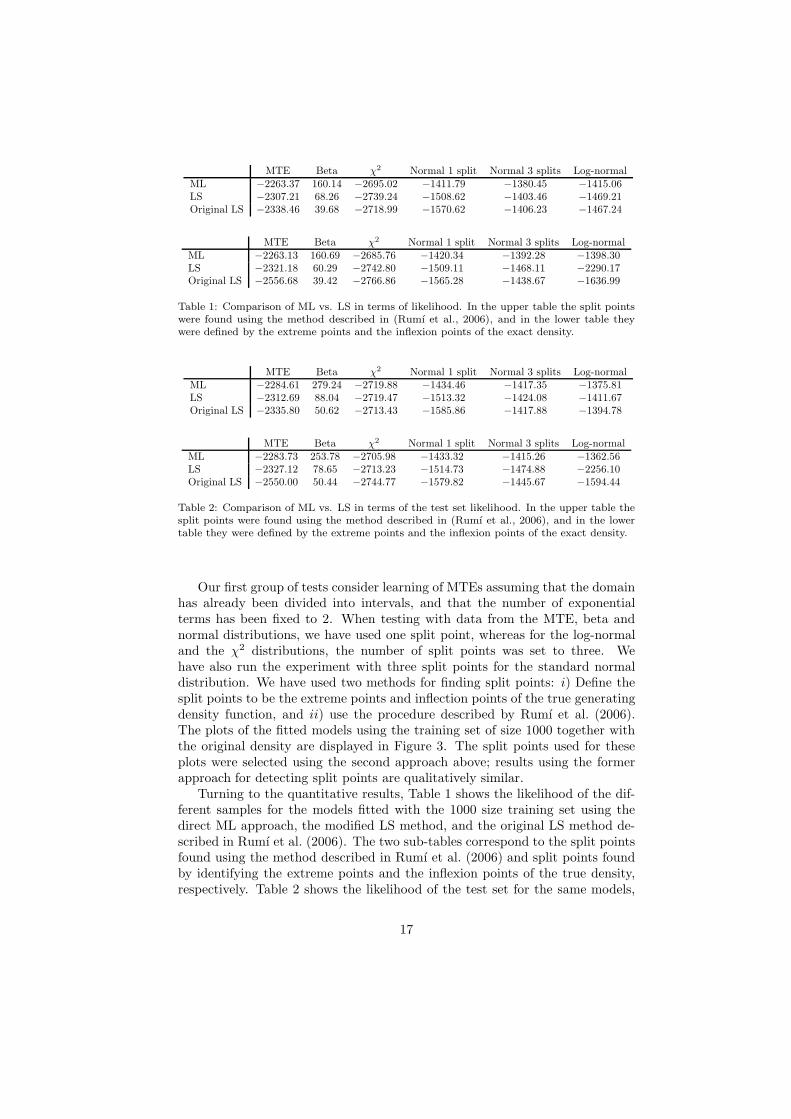
MTE Beta χ2 Normal 1 split Normal 3 splits Log-normalML −2263.37 160.14 −2695.02 −1411.79 −1380.45 −1415.06LS −2307.21 68.26 −2739.24 −1508.62 −1403.46 −1469.21Original LS −2338.46 39.68 −2718.99 −1570.62 −1406.23 −1467.24

MTE Beta χ2 Normal 1 split Normal 3 splits Log-normalML −2263.13 160.69 −2685.76 −1420.34 −1392.28 −1398.30LS −2321.18 60.29 −2742.80 −1509.11 −1468.11 −2290.17Original LS −2556.68 39.42 −2766.86 −1565.28 −1438.67 −1636.99

Table 1: Comparison of ML vs. LS in terms of likelihood. In the upper table the split pointswere found using the method described in (Rumı et al., 2006), and in the lower table theywere defined by the extreme points and the inflexion points of the exact density.

MTE Beta χ2 Normal 1 split Normal 3 splits Log-normalML −2284.61 279.24 −2719.88 −1434.46 −1417.35 −1375.81LS −2312.69 88.04 −2719.47 −1513.32 −1424.08 −1411.67Original LS −2335.80 50.62 −2713.43 −1585.86 −1417.88 −1394.78

MTE Beta χ2 Normal 1 split Normal 3 splits Log-normalML −2283.73 253.78 −2705.98 −1433.32 −1415.26 −1362.56LS −2327.12 78.65 −2713.23 −1514.73 −1474.88 −2256.10Original LS −2550.00 50.44 −2744.77 −1579.82 −1445.67 −1594.44

Table 2: Comparison of ML vs. LS in terms of the test set likelihood. In the upper table thesplit points were found using the method described in (Rumı et al., 2006), and in the lowertable they were defined by the extreme points and the inflexion points of the exact density.

Our first group of tests consider learning of MTEs assuming that the domainhas already been divided into intervals, and that the number of exponentialterms has been fixed to 2. When testing with data from the MTE, beta andnormal distributions, we have used one split point, whereas for the log-normaland the χ2 distributions, the number of split points was set to three. Wehave also run the experiment with three split points for the standard normaldistribution. We have used two methods for finding split points: i) Define thesplit points to be the extreme points and inflection points of the true generatingdensity function, and ii) use the procedure described by Rumı et al. (2006).The plots of the fitted models using the training set of size 1000 together withthe original density are displayed in Figure 3. The split points used for theseplots were selected using the second approach above; results using the formerapproach for detecting split points are qualitatively similar.

Turning to the quantitative results, Table 1 shows the likelihood of the dif-ferent samples for the models fitted with the 1000 size training set using thedirect ML approach, the modified LS method, and the original LS method de-scribed in Rumı et al. (2006). The two sub-tables correspond to the split pointsfound using the method described in Rumı et al. (2006) and split points foundby identifying the extreme points and the inflexion points of the true density,respectively. Table 2 shows the likelihood of the test set for the same models,

17

0 5 10 15 20

0.00

0.05

0.10

0.15

0.20

0.25

Den

sity

0.0 0.2 0.4 0.6 0.8 1.0

0.0

0.5

1.0

1.5

2.0

2.5

3.0

3.5

Den

sity

(a) MTE (b) Beta

0 5 10 15 20 25

0.00

0.02

0.04

0.06

0.08

0.10

0.12

Den

sity

−3 −2 −1 0 1 2 3

0.0

0.2

0.4

0.6

Den

sity

(c) χ2 (d) Gaussian, 1 split

−3 −2 −1 0 1 2 3

0.0

0.1

0.2

0.3

0.4

0.5

Den

sity

0 5 10 15 20

0.0

0.1

0.2

0.3

0.4

0.5

0.6

0.7

Den

sity

(e) Gaussian, 3 splits (f) Log-Normal

Figure 3: The plots show the results of samples from different distributions. The gold-standarddistribution is drawn with a thick line, the MTE with Lagrange-parameters are given withthe dashed line, and the results of the LS approach are given with the thin, solid line.

18

MTE Beta χ2 Normal 1 split Normal 3 splits Log-normalML −2319.24 256.27 −2265.76 −1486.58 −1530.58 −1605.60LS −2612.27 48.82 −2858.66 −1506.39 −1491.58 −1652.98Original LS −2337.54 −9.57 −2823.48 −1505.06 −1455.52 −1462.99

MTE Beta χ2 Normal 1 split Normal 3 splits Log-normalML −2318.29 228.45 −2588.22 −1470.2 −1501.53 −1491.56LS −2649.21 68.37 −2885.46 −1585.78 −1513.75 −2277.66Original LS −2529.87 −28.05 −2837.81 −1527.32 −1484.77 −2165.59

Table 3: Comparison of ML vs. LS estimated with a sample of size 50 in terms of the testset likelihood. In the upper table the split points were found using the method described in(Rumı et al., 2006), and in the lower table they were defined by the extreme points and theinflexion points of the exact density.

and Table 3 shows the likelihood of the test set for the models fitted with the50 size training set. From the results we clearly see that the ML-based methodoutperforms the LS method in terms of likelihood. This is hardly a surprise, asthe ML method is actively using likelihood maximization as its target, whereasthe LS methods do not. On the other hand, the LS and Original LS seem tobe working at comparable levels. Most commonly (in 15 out of 24 runs), LSis an improvement over its original version with large training sets, but withsmall training sets it behaves much worse. The explanation is that the weightsused in the new version of LS are not so accurate, and so the estimations areunstable. We can also see from Table 3 that the ML approach appears to overfitthe data, and therefore achieves a lower testset likelihood than the original LSfor the “Normal 3 splits” and “Log-normal” datasets. This is not surprising, asthe number of parameters used by the ML approach to fit the distributions arefar above what turns out to be “BIC-optimal” (see below).

Our last set of tests focused on the BIC-based model selection algorithmfor finding split points and determining the number of parameters inside eachinterval; for these tests we allowed at most two exponential terms and fivecandidate split points (found using equal-frequency binning). The results, givenin Table 4, clearly show the desired effect: The BIC-based method is less proneto overfitting the data, and although a smaller likelihood is obtained on thetraining data, the predictive ability of the data is better than when learningwith fixed split points. Plots of the learned MTEs are shown in Figure 4,where it is interesting to note how the BIC-based learning algorithm choosesdifferent model structures for the different data-sizes. Look, for instance, atthe Beta distribution in Part (b) of Figure 4. When only 50 training examplesare used, we fit a function with two exponential terms to the whole supportof the density (no split points are selected); when 1000 cases are available, thelearning prefers to use two intervals. Furthermore, for the first interval of theMTE distribution (Part (a)), the learning based on 1000 cases finds support forusing one exponential term to approximate the density. When learning from50 cases, the algorithm did not get the same support, and therefore opted for

19

MTE Beta χ2 Normal Log-normalTraining-set Log likelihood −94.90 14.80 −122.30 −62.84 −65.18Test-set Log likelihood −2052.00 130.60 −2500.93 −1210.18 −1225.36

MTE Beta χ2 Normal Log-normalTraining-set Log likelihood −2270.76 161.21 −2727.76 −1422.58 −1432.83Test-set Log likelihood −2285.25 249.45 −2702.67 −1430.88 −1358.38

Table 4: The results of the BIC-based learning approach. In the upper table the resultsare based on learning from 50 data-points, the lower table reports the results based on 1000training examples.

a constant in that part of the domain. Finally, it is interesting to see thatthe log-normal (Part (e)) is approximated using 0 split points (when learningfrom 50 cases) or 1 split point (when learning from 1000 cases). This should becompared to the 3 split points used to generate the results in Figure 3 (f).

8. Conclusions and Future Work

In this paper we have introduced maximum likelihood learning of MTEs.Finding maximum likelihood parameter estimates is interesting not only in itsown right, but also as a tool for doing more advanced learning, like modelselection. We have proposed algorithms that use the BIC criteria (Schwarz,1978) to choose the number of exponential terms required to approximate thedensity function properly, as well as for determining the location of the split-points for partitioning the domain of the variables. The experiments carried outshow that the estimations obtained by ML improve the ones provided by theleast squares method both in terms of likelihood of the training data and of thepredictive ability (measured by likelihood of a separate test-set).

We are currently working on ML-based learning of conditional distributions,starting from the ideas published in (Moral et al., 2003). However, accuratelylocating the split-points for a conditional MTE is even more difficult than whenlearning marginal distributions; locating the split-points for a variable will notonly influence the approximation of its distribution, but also the distributionsfor all its children.

Acknowledgments

This work has been partly supported by the Spanish Ministry of Scienceand Innovation through project TIN2007-67418-C03-02 and by EFRD (FEDER)funds.

References

Bertsekas, D., 1996. Constrained optimization and Lagrange multiplier methods.Academic Press Inc.

20

0 5 10 15

0.00

0.05

0.10

0.15

0.20

0.25

0.30

Den

sity

0.0 0.2 0.4 0.6 0.8 1.0

01

23

4

Den

sity

(a) MTE (b) Beta

0 5 10 15 20 25

0.00

0.05

0.10

0.15

0.20

Den

sity

−3 −2 −1 0 1 2 3

0.0

0.1

0.2

0.3

0.4

0.5

0.6

Den

sity

(c) χ2 (d) Gaussian

0 5 10 15 20

0.0

0.1

0.2

0.3

0.4

0.5

0.6

0.7

Den

sity

(e) Log-Normal

Figure 4: The plots show the results of the BIC-based learning. The gold-standard distributionis drawn with a thick line, the MTE with BIC-based learning from 50 examples are are givenwith the dashed line, and the results of the BIC-based learning from 1000 cases are given withthe thin, solid line.

21

Cobb, B., Shenoy, P., Rumı, R., 2006. Approximating probability density func-tions with mixtures of truncated exponentials. Statistics and Computing 16,293–308.

Dempster, A., Laird, N., Rubin, D., 1977. Maximun likelihood from incompletedata via the EM algorithm. Journal of the Royal Statistical Society B 39, 1– 38.

Farag, A., El-Baz, A., Gimel’farb, G., 2004. Density estimation using modifiedexpectation-maximization algorithm for a linear combination of Gaussians.In: Proceedings of the International Conference on Image Processing (ICIP).pp. 1871–1874.

Friedman, N., Goldszmidt, M., 1996. Discretizing continuous attributes whilelearning Bayesian networks. In: Proceedings of the Thirteenth InternationalConference on Machine Learning. pp. 157–165.

Jordan, M. I., Ghahramani, Z., Jaakkola, T. S., Saul, L. K., 1999. An intro-duction to variational methods for graphical models. Machine Learning 37,183–233.

Kozlov, D., Koller, D., 1997. Nonuniform dynamic discretization in hybrid net-works. In: Geiger, D., Shenoy, P. (Eds.), Proceedings of the 13th Conferenceon Uncertainty in Artificial Intelligence. Morgan & Kaufmann, pp. 302–313.

Moral, S., Rumı, R., Salmeron, A., 2001. Mixtures of truncated exponentialsin hybrid Bayesian networks. In: ECSQARU’01. Lecture Notes in ArtificialIntelligence. Vol. 2143. pp. 135–143.

Moral, S., Rumı, R., Salmeron, A., 2003. Approximating conditional MTE dis-tributions by means of mixed trees. In: ECSQARU’03. Lecture Notes in Ar-tificial Intelligence. Vol. 2711. pp. 173–183.

Romero, V., Rumı, R., Salmeron, A., 2006. Learning hybrid Bayesian networksusing mixtures of truncated exponentials. International Journal of Approxi-mate Reasoning 42, 54–68.

Rumı, R., Salmeron, A., Moral, S., 2006. Estimating mixtures of truncatedexponentials in hybrid Bayesian network. Test 15, 397–421.

Schwarz, G., 1978. Estimating the dimension of a model. Annals of Statistics 6,461–464.

Shafer, G. R., Shenoy, P. P., 1990. Probability Propagation. Annals of Mathe-matics and Artificial Intelligence 2, 327–352.

Simonoff, J., 1996. Smoothing methods in Statistics. Springer.

Tanner, M., 1996. Tools for statistical inference. Springer.

22