The `window problem' for series ofcomplex exponentialsT.I. Seidman,1 S.A. Avdonin,2 and S.A. Ivanov3AbstractUnder a suitable sparsity condition on the exponents � = f�k = �k+ i�kg, itis shown that the individual terms cT = fck ei�kTg can be obtained from ob-servation of the L2 function f(t) = P ck ei�kt through the `window' t 2 [0; �]| with an `2 estimate (uniform for such �) asymptotically as T; � ! 0. Someapplications are given to control theory for partial di�erential equations.KeyWords: exponential series, uniform estimate, window problem, asymp-totic, distributed parameter control.AMS Subject Classification: 42C15, 47A57, 93B28, 42A55

1Department of Mathematics and Statistics, University of Maryland Baltimore County,Baltimore, MD 21250, USA; e-mail: seidman@math.umbc.edu2Department of Applied Mathematics and Control, St. Petersburg State University,Bibliotechnaya sq. 2, 198904 St. Petersburg, Russia, and Department of Mathematics andStatistics, The Flinders University of South Australia, GPO Box 2100, Adelaide SA 5001,Australia; email: avdonin@ist. inders.edu.au3Russian Center of Laser Physics, St.Petersburg State University, Ul'yanovskaya 1,198904 St.Petersburg, Russia; e-mail: sergei.ivanov@pobox.spbu.ru1

1. IntroductionFor any �xed exponent sequence � = f�k = �k + i�kg in C+ (i.e., with4�k � 0), consider the set M =M(�) of all complex functions f expressibleas �nite sums of the form f(t) =Xk ckei�kt(1.1)for t 2 IR. The `window problem' of the title refers to the extraction of thesequence of individual terms cT = �ckei�kT�(for some speci�ed T � 0) from observation of f `through a window': re-stricting t to a small interval (0; �). Under appropriate hypotheses on �, i.e.,assuming a `separation condition' which we here express in the form:# f� 2 � : 0 < j�� ��j � rg � �(r) for each �� 2 �;(1.2)for a suitable function � : IR+ ! IR+, the operatorC = CT� : f 7! cT :M� ! `2(1.3)will be continuous from M� :=[closure of M in L2(0; �)] for any � > 0 andany T > 0.For real f�kg we would be considering `nonharmonic Fourier series' in(1.1) while for purely imaginary f�kgwe would have Dirichlet seriesPk cke��kt(cf. [13]) and consideration of the M�untz-Sz�asz Theorem for polynomialsP ckx�k (cf., e.g., [2]) on setting x = e�t.Our object is to verify continuity and to estimate the norm kCT� k| withespecial concern for the asymptotics �; T ! 0, noting that kCT� k must blowup as � ! 0 and, since we are considering classes of sequences admittingunbounded f�kg, must also blow up as T ! 0.4It is obviously su�cient to ask that �k be bounded below, since an invertible multipli-cation of f in (1.1) by e��t has the e�ect of shifting � by i�. The choice of lower bound 0for �k is purely for expository convenience, but note also (5:1.1).2

THEOREM 1: Given � : IR+ ! IR+ nondecreasing with �(s)=s2integrable, let � be any sequence in C+ satisfying the condition (1.2). Then,for any � > 0 and any T > 0 the map CT� de�ned by (1.3) is continuous:M� ! `2 and we have an estimatelog kCT� k � Q := Q1(�) +Q2(T ) +Q�(1.4)uniformly for such f�g, with Q1(�); Q2(�), and the constant Q� de�ned interms of �(�) and a suitably chosen auxiliary function (�).The paper by W.A.J. Luxemburg and J. Korevaar [10], considered similarquestions for � `close to imaginary' and with T = �, showing the (uniform)continuity of C although with no concern for the asymptotics. The papers[17] and [18] adapted the methods of [10], with a somewhat di�erently ex-pressed separation condition for the sequence �, to consider real �k andestimate kC0�k as � ! 0. [For real �k the norm is independent of T . Wenote from those papers that the computation gives Q1(�) = O(1=�) for aquadratically growing sequence (�k � �ck2) and an example by Korevaarincluded in [17] indicates that this is sharp; more generally, it was shown in[18] that this becomes O(��1=[p�1]) when �k � �ckp with 1 < p < 1.] Theobject of this paper is to extend that analysis to the consideration of complexexponent sequences �k = �k + i�k with �k � 0, for which the normalizationimplied here with T > 0 will be particularly appropriate.We may note that much of our personal motivation for this investiga-tion comes from the relation between exponential series such as (1.1) andconsiderations of control theory for distributed parameter systems; see [1]for a treatment of the theory and application of exponential families in thiscontext. The context suggests an interpretation of CT� as related to an ob-servation problem: observing some functional on the solution of a partialdi�erential equation over a time interval (0; �) in order to predict the solu-tion state at a time T ; see Section 6.Nonharmonic Fourier series (of the form (1.1) with real �k) su�ce for con-sideration of controllability/observability issues for the wave equation andfor undamped rod [6] or plate [14], [7] equations. However, we note thattreatment of the heat equation [11] involves such expansions with pure imag-inary �k, i.e., Dirichlet series. Because of the smoothing associated with theheat equation, so the solution semigroup is compact, it is then important that3

one is `predicting' the solution state at a time T > 0: typically one takes Tto be �, the end of the observation interval | as in [10], which was motivatedby this problem through [11]. For the one-dimensional heat equation withT = � (where we have �k � ik2 for k = 1; 2; : : :), we will obtain as in [15]an estimate O(1=�) for log kC��k: an example by G�uichal [4] shows that thisis sharp. More general complex exponent sequences arise for considerationof damping for a plate model and we will also show how a control-theoreticresult (cf., Hansen [5]) can be easily obtained for such problems (with anasymptotic estimate) by using the Theorem above.2. PreliminariesFor the next sections we �rst �x � : IR+ ! IR+ as in Theorem 1, i.e., suchthat (i) � : IR+ ! IR+ is nondecreasing with � � 0 on some [0; r0],(ii) Z 10 [�(s)=s2] ds <1:(2.1)This is equivalent to the hypotheses on �(�) we already imposed in Theorem 1since the requirement in (i) that � vanish on some [0; r0) is actually redun-dant: in any case, by (ii) there must be r0 > 0 with �(r0) < 1 so j����j � r0for all pairs �; �� 2 �, i.e., the sequence must be uniformly separated and wecan take � vanishing on [0; r0] for this r0. The integrability condition (ii) isalso closely related to the standard condition that Pk 1=j�kj be convergent| indeed, writing �(r) for the left hand side of (1.2), one hasX( 1j�� ��j : �� 6= � 2 �) = Z 1r0 d�(r)jrj = Z 1r0 �(r)r2 drby an integration by parts, noting that �(r)=r � �(r)=r ! 0 at 1 as inLemma 1-(iv) below. In this section we introduce the class of functions !(�)satisfying(i) ! : IR+ ! IR+ is continuous, increasing, and unbounded,(ii) !(s)=s2 is decreasing, with Z 10 [!(s)=s2] ds =: B! <1(2.2)and provide some technical lemmas which we will need later. The last ofthese, designated a `Theorem' (and almost the same as the construction4

which forms the heart of [10], [17], [18]), provides the construction of a `mol-li�er function' P (�) with relevant properties.LEMMA 1:(i) If ! 2 , then !(s)=s! 0 as s! 0;1, but is not integrable at 1.(ii) If ! 2 , then sups>0f!(s)=sg � B! <1 and 0 � !0(s) � 2B!.(iii) If 2 also increases rapidly enough thatA1 := Z 10 se� (s) ds <1;(2.3)then we have, for any � > 0,Z 10 e� (�s) d~�(s) � 2B~�B A1�(2.4)for any nondecreasing ~� with ~�(r)=r � B~� <1,(iv) For �(�) satisfying (2.1), we have supf�(s)=sg � B� with �(s)=s! 0as s!1. Further, setting#(s) := 2 Z 1r0 �(r)r s2s2 + r2 dr = � Z 10 �(r) d "log 1 + s2r2!# :(2.5)we have # 2 and #(s) � 2�Rr0�2 Z 1R �(r)r s2s2 + r2 dr(2.6)for any R > r0.Proof: For ! 2 , we have !(s)=s � !(a)=s on [a;1) so !(s)=s cannotbe integrable at1. Since ! is increasing, we have !(s)=s = R1s !(s)=r2 dr <R1s !(r)=r2 dr so !(s)=s ! 0 as s ! 1. Similarly, we have !(s)=s =2 R 2ss !(s)=r2 dr � 2 R 2ss !(r)=r2 dr � 2 R 2s0 !(r)=r2 dr ! 0 as s ! 0. Fromthe above, we have !(s)=s � B! := R10 !(r)=r2 dr. [We remark that thisargument also applies to � as in Theorem 1: even if � is not in we do have�(s)=s ! 0 and �(s)=s � B� < 1.] Since !(s)=s2 is decreasing, we have0 � [!(s)=s2]0 = [!0 � 2!(s)=s]=s2 so !0 � 2!(s)=s � 2B!. This completesthe proof of (i), (ii) as well as part of (iv).5

For (iii), an integration by parts shows thatZ R0 e� (�s) d~�(s) = ~�(s)s se� (�s)!�����R0 + Z R0 ~�(s)s [� 0(�s)]se� (�s) ds� B~�Re� (�R) + Z R0 B~� [�2B ] se� (�s) dssince the boundary term at 0 vanishes and 0 � 2B . Now (2.4) follows bygoing to the limit as R ! 1 through a sequence such that Re� (�R) ! 0,possible by (2.3). In particular, setting � = 1 and ~�(s) � s in (2.4) givesA0 := Z 10 e� (s) ds <1:(2.7)For (iv), note that continuity and unboundedness of # follow, e.g., fromthe Monotone Convergence Theorem, while the correct monotonicity in s of#(s) and of #(s)=s2 follow immediately from the form of (2.5). The integra-bility follows on interchange of integration to getZ 10 #(s)s2 ds = � Z 10 �(r)r2 dr:(2.8)Finally, (2.6) follows from comparison of the integrals over [r0; R] and [R;1)after replacing �(r) by �(R) and noting that t log(1+ 1=t) is increasing, say,from t = r20=s2 to t = R2=s2.Given any ! 2 , we introduce functions �; q : IR+ ! IR+ de�ned by�(s) := 1s + 2 "!(s)s + Z 1s !(r)r2 dr# ;q(s) := 8>>>><>>>>: 0 for 0 � s � 1,� Z s1 r2 d!(r)r2 for s � 1,= 2 Z s1 !(r)r dr � !(s) + !(1)(2.9)using integration by parts to obtain the second expression for q when s � 1.LEMMA 2: For ! 2 the functions �; q of (2.9) are continuous and6

(i) � : (0;1)! (0;1) is decreasing with �(s)!1; 0 as s! 0;1; hencethere is a continuous decreasing inverse function �(�1) : (0;1)! (0;1),(ii) q : [1;1) ! IR+ is increasing with q(s) ! 1 as s ! 1; hence thereis a continuous increasing inverse q(�1) : IR+ ! [1;1); further, q(s)=s ! 0as s!1 and, �nally, Z 1s dq(r)r2 = !(s)s2 for s � 1:(2.10)Proof: The continuity of � is clear and we need only note Lemma 1-(i) to see that �(s) ! 0 as s ! 1. Since !(s)=s2 is decreasing, the �rstexpression for q in (2.9) shows that q(�) is increasing from q(1) = 0 and,indeed, that q(s) � q(~s)� h!(r)=r2is~s � !(~s)� ~s2[!(s)=s2]for s > ~s, whence q(s) !1 as s !1 (as we may �rst choose ~s so !(~s) isarbitrarily large and then the last term goes to 0). The second expressiongives q(s)s � 2s Z s1 !(r)r drso, as the integrand goes to 0, we have q(s)=s ! 0 as s ! 1. An integra-tion by parts, using the information that �(1) = 0, then gives for � thealternative formula: �(s) = 1=s+ 2 Z 1s (1=r) dq(r)with dq > 0 so �(�) is decreasing and, since the second term here is positive,we must have �(s) ! 1 as s ! 0. The integrability at 1 of dq(r)=r cer-tainly implies integrability of dq(r)=r2 = �d[!(r)=r2], giving (2.10).At this point we can de�ne the functions appearing in (1.4) in Theorem 1:given choices of !; as above, we setQ1(�) := maxf12 ; !(�(�1)(�=2))gQ2(T ) := min� n (T � 2B �)� 12 log� : 0 < 2� � minf1; T=B go(2.11) 7

where (T ) := sup�>0fh(�)� T �g withh(�) := #(�) + (2 log 2) q(�) + (c=x) ��(�) usingx = 12(1� e�2); c := j log(1� x)j = � log 12(1 + e�2):(2.12)Note that Lemma 2-(i) ensures that Q1(�) is de�ned. The behavior of Q1 forsmall � > 0 depends only on the tail of ! (large s) with Q1 !1 as � ! 0.As # 2 we have #(�)=� ! 0 and Lemma 2 then ensures that h(�)=� ! 0so h(�) < T� for T > 0 and large � > 0, whence is �nite. [One mightfurther remark on the relation of (2.12) to the Legendre-Fenchel dual.] ThusQ2 is well-de�ned. Since h(�)!1 as � !1 so (T )!1 as T ! 0, wehave Q2(T )!1 as T ! 0; compare Remark 2, below.THEOREM 2: For any ! 2 and any � > 0 (for simplicity we onlyconsider � � 2) there exists an entire function P = P�(�;!) such that(i) P (0) = 1 and e�i(�=2)zP (z) is of exponential type �=2 with jP (z)j � 1on the upper half-plane C+ (in particular, for real z),(ii) P (is) is real and positive for real s � 0 withP (is) � e�[(2 log 2) q+(s)+(c=x) s�(s)](2.13)where q+ := maxfq; 0g with q; � as in (2.9) and c; x as in (2.12),(iii) jP (s)j � eQ1(�) e�!(jsj) for real s with Q1 as in (2.11).As already noted, a version of this theorem was proved by W.A.J. Luxemburgand J. Korevaar [10] for the case of � in a complex sector and this was latermodi�ed by T.I. Seidman [17] and by T.I. Seidman and M.S. Gowda [18] toobtain more explicit estimates in the case of real �, giving the asymptoticsas � ! 0. Here we follow the scheme of the proof in [18], making suchmodi�cations as are necessary for the present more general setting.Proof: For any � � 1 (to be chosen for (2.17) later; we will also assumethat q(�) � 1=2), we setzj := q(�) + j=2; aj := 1=q(�1)(zj)(2.14)so j = 2[q(1=aj)�q(�)]; this index j = 0; 1; : : : is unrelated to the index of �.Each aj is a continuous decreasing function of the choice of �. For s � 0 we8

then de�ne n = n(s) := � 0 if 0 � s � �minfj : aj � 1=sg for s � �.(2.15)Note that aj � 1=s just when zj = q(1=aj) � q(s), i.e., just when j=2 �q(s) � q(�). Thus, (2.15) gives n(s) = d2[q(s) � q(�)]e for s � � whichensures, with q(�) � 1=2, that n(s) � 2q+(s) for all s � 0. With n = n(s),noting that 1=q(�1)(z) is decreasing, we have the integral comparison1Xn aj = an + 1Xn+1 2[zj+1 � zj]q(�1)(zj) < an + Z 1zn 2 dzq(�1)(z)< 1s + Z 1q(s) 2 dzq(�1)(z) = 1s + 2 Z 1s dq(r)r =: �(s):(2.16)Note that (2.16) is independent of the choices of s � � > 1 and, in particular,for s = � (so n(s) = 0) we consider �(�) := 2P10 aj < 2�(�). This can bemade arbitrarily small by taking � large while, on the other hand, � > 2a0 =2=� so �(1) > 2 � �. By the continuity of � 7! � (which follows, e.g., fromthe Dominated Convergence Theorem), we can thus choose � = ��(�) to getexactly �(�) = �, i.e.,1X0 aj = �=2 for � = ��(�) < �(�1)(�=2):(2.17)We now de�ne P (�) in terms of the sequence (aj) by an in�nite product:P (z) := ei(�=2)z 1Yj=0 cos(ajz) = 1Yj=0 12 �1 + e2iajz� :(2.18)Since convergence of P aj as in (2.16), (2.17) implies that of P j cos(ajz)�1juniformly on bounded sets in C, this in�nite product converges to an entirefunction. Clearly P (0) = 1 and for z 2 C+ one has je2iajzj � 1 so jP (z)j � 1.Since j cos(az)j � eajzj for a > 0 and all z 2 C, the product e�i(�=2)zP (z) isthen of exponential type P aj = �=2, as desired, completing the proof of (i).For pure imaginary z = is, it is clear from (2.18) that P (is) is real andpositive. For s � 0 we take n = n(s) and split the product into those factors9

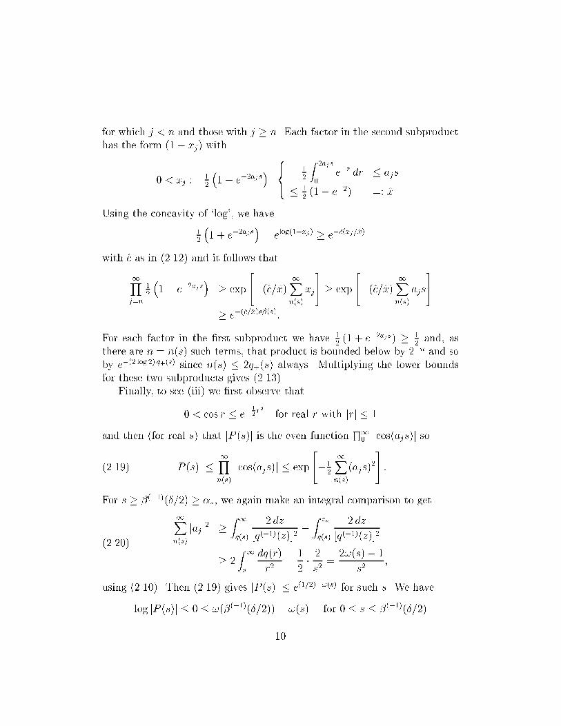
for which j < n and those with j � n. Each factor in the second subproducthas the form (1� xj) with0 < xj := 12 �1� e�2ajs� 8><>: = 12 Z 2ajs0 e�r dr � ajs� 12 (1� e�2) =: xUsing the concavity of `log', we have12 �1 + e�2ajs� = elog(1�xj) � e�c(xj=x)with c as in (2.12) and it follows that1Yj=n 12 �1 + e�2ajs� � exp 24�(c=x) 1Xn(s) xj35 � exp 24�(c=x) 1Xn(s) ajs35� e�(c=x)s�(s):For each factor in the �rst subproduct we have 12 (1 + e�2ajs) � 12 and, asthere are n = n(s) such terms, that product is bounded below by 2�n and soby e�(2 log 2) q+(s) since n(s) � 2q+(s) always. Multiplying the lower boundsfor these two subproducts gives (2.13).Finally, to see (iii) we �rst observe that0 < cos r � e� 12 r2 for real r with jrj � 1and then (for real s) that jP (s)j is the even function Q10 j cos(ajs)j sojP (s)j � 1Yn(s) j cos(ajs)j � exp 24�12 1Xn(s)(ajs)235 :(2.19)For s � �(�1)(�=2) � ��, we again make an integral comparison to get1Xn(s) jajj2 � Z 1q(s) 2 dz[q(�1)(z)]2 � Z znq(s) 2 dz[q(�1)(z)]2� 2 Z 1s dq(r)r2 � 12 � 2s2 = 2!(s)� 1s2 ;(2.20)using (2.10). Then (2.19) gives jP (s)j � e(1=2)�!(s) for such s. We havelog jP (s)j � 0 � !(�(�1)(�=2))� !(s) for 0 � s � �(�1)(�=2)10

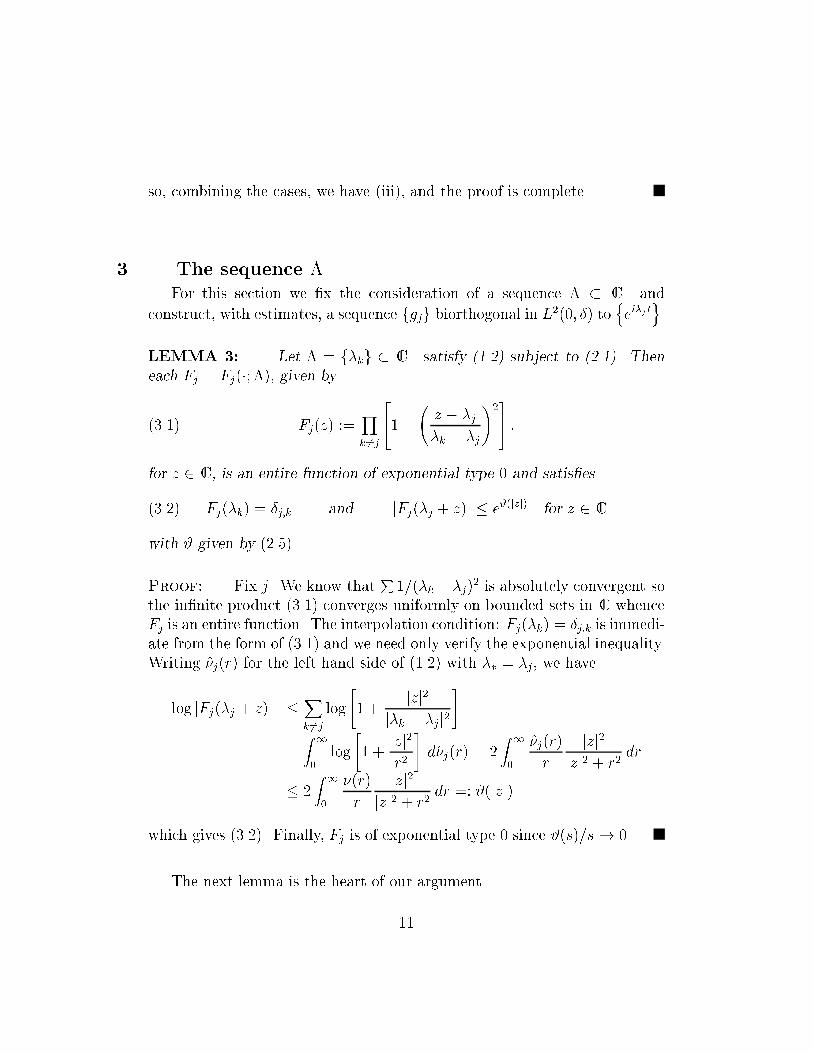
so, combining the cases, we have (iii), and the proof is complete.3. The sequence �For this section we �x the consideration of a sequence � � C+ andconstruct, with estimates, a sequence fgjg biorthogonal in L2(0; �) to nei�j to.LEMMA 3: Let � = f�kg � C+ satisfy (1.2) subject to (2.1). Theneach Fj = Fj(�; �), given byFj(z) := Yk 6=j 241� z � �j�k � �j!235 :(3.1)for z 2 C, is an entire function of exponential type 0 and satis�esFj(�k) = �j;k and jFj(�j + z)j � e#(jzj) for z 2 C(3.2)with # given by (2.5).Proof: Fix j. We know that P 1=(�k� �j)2 is absolutely convergent sothe in�nite product (3.1) converges uniformly on bounded sets in C whenceFj is an entire function. The interpolation condition: Fj(�k) = �j;k is immedi-ate from the form of (3.1) and we need only verify the exponential inequality.Writing �j(r) for the left hand side of (1.2) with �� = �j, we havelog jFj(�j + z)j �Xk 6=j log "1 + jzj2j�k � �jj2#= Z 10 log "1 + jzj2r2 # d�j(r) = 2 Z 10 �j(r)r jzj2jzj2 + r2 dr� 2 Z 10 �(r)r jzj2jzj2 + r2 dr =: #(jzj)which gives (3.2). Finally, Fj is of exponential type 0 since #(s)=s! 0.The next lemma is the heart of our argument.11

LEMMA 4: Let 2 with A0 := R10 e� < 1. For � > 0 considerthe molli�er P (�) constructed in Theorem 2 in terms of ! := # + using(2.5). Now, with (3.1), de�ne functions Gj on C byGj(z) := Fj(z)P (z � �j)P (i�j)(3.3)and then functions gj on IR bygj(t) = 12� Z 1�1Gj(s) eist ds:(3.4)We will then have:(i) for real s, each Gj satis�es the estimate:jGj(s+ �j)j � heQ1(�)eh(�j )i e� (jsj)(3.5)with Q1 as in (2.11) and h as in (2.12),(ii) for each j; k we set � = �jk := j�k � �jj=2 and havejhGj; Gkij � 4A0 e2Q1(�)eh(�j)eh(�k)e� (�)(3.6)so, in particular, each Gj is in L2(IR) and, as a function on C,(iii) each Gj is entire with e�i(�=2)zGj(z) of exponential type �=2,(iv) each gj is an L2 function with support in [0; �] and the sequence fgjgis biorthogonal to the exponentials:hgj; ei�kti = �j;k:(3.7)Proof: From (3.3) we have Gj(s+ �j) = Fj(�j + [s� i�j])P (s)=P (i�j).From Theorem 2-(ii,iii) and the de�nition of h(�) in (2.11) we have����� P (s)P (i�j) ����� � eQ1(�)e�!(jsj)e#(�j)�h(�j ) :12

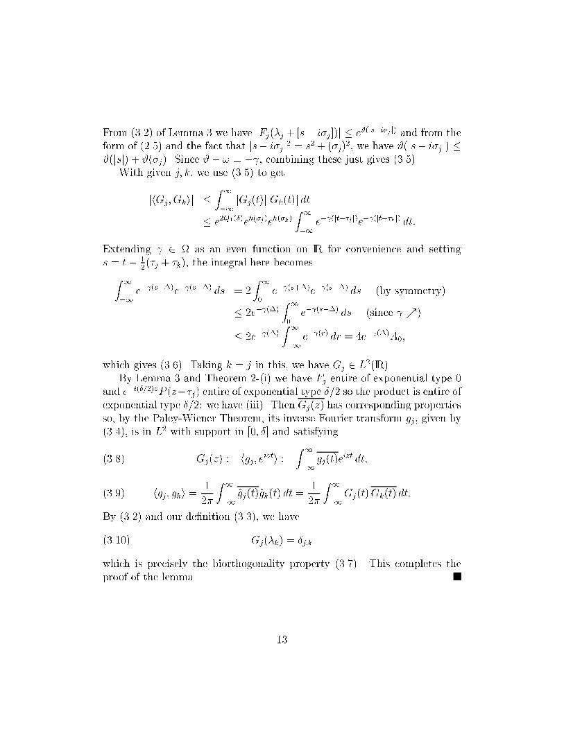
From (3.2) of Lemma 3 we have jFj(�j + [s� i�j])j � e#(js�i�j j) and from theform of (2.5) and the fact that js� i�jj2 = s2 + (�j)2, we have #(js� i�jj) �#(jsj) + #(�j). Since #� ! = � , combining these just gives (3.5).With given j; k, we use (3.5) to getjhGj; Gkij � Z 1�1 jGj(t)jjGk(t)j dt� e2Q1(�)eh(�j)eh(�k) Z 1�1 e� (jt��j j)e� (jt��k j) dt:Extending 2 as an even function on IR for convenience and settings = t� 12(�j + �k), the integral here becomesZ 1�1 e� (s+�)e� (s��) ds = 2 Z 10 e� (s+�)e� (s��) ds (by symmetry)� 2e� (�) Z 10 e� (s��) ds (since %)� 2e� (�) Z 1�1 e� (r) dr = 4e� (�)A0;which gives (3.6). Taking k = j in this, we have Gj 2 L2(IR).By Lemma 3 and Theorem 2-(i) we have Fj entire of exponential type 0and e�i(�=2)zP (z��j) entire of exponential type �=2 so the product is entire ofexponential type �=2: we have (iii). Then Gj(�z) has corresponding propertiesso, by the Paley-Wiener Theorem, its inverse Fourier transform gj, given by(3.4), is in L2 with support in [0; �] and satisfyingGj(z) := hgj; eizti := Z 1�1 gj(t)eizt dt;(3.8) hgj; gki = 12� Z 1�1 gj(t)gk(t) dt = 12� Z 1�1Gj(t)Gk(t) dt:(3.9)By (3.2) and our de�nition (3.3), we haveGj(�k) = �j;k(3.10)which is precisely the biorthogonality property (3.7). This completes theproof of the lemma.13

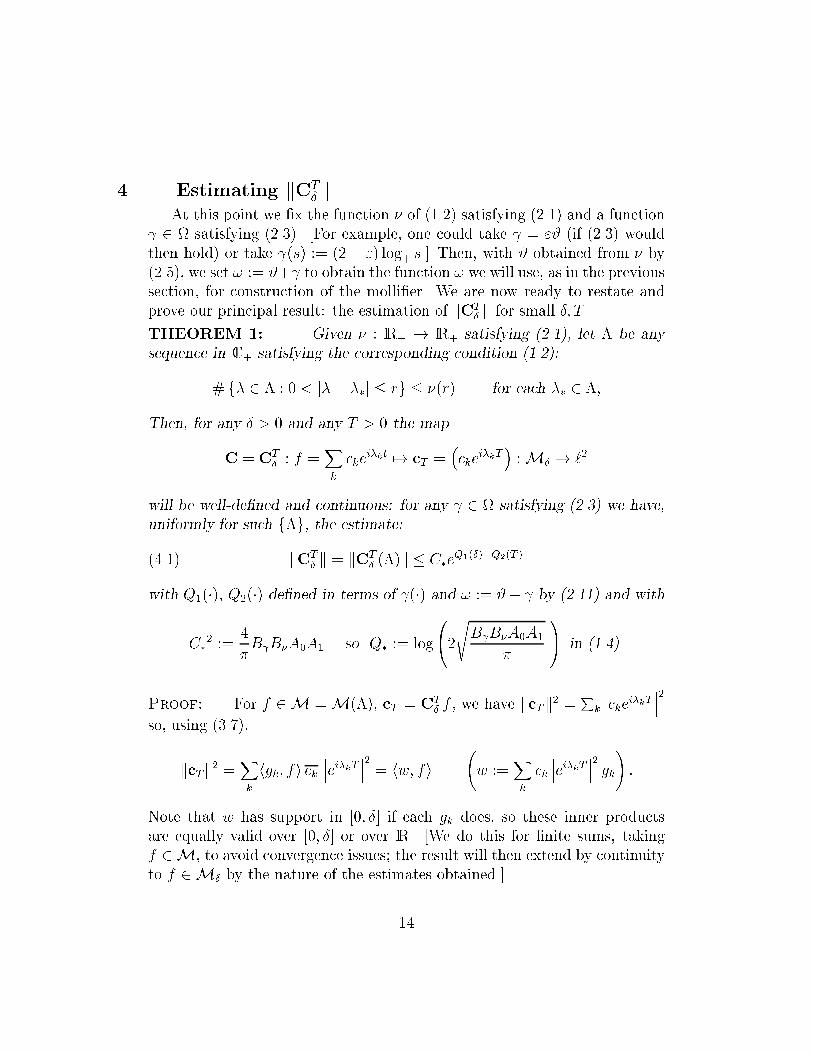
4. Estimating kCT� kAt this point we �x the function � of (1.2) satisfying (2.1) and a function 2 satisfying (2.3). [For example, one could take = "# (if (2.3) wouldthen hold) or take (s) := (2 + ") log+ s.] Then, with # obtained from � by(2.5), we set ! := #+ to obtain the function ! we will use, as in the previoussection, for construction of the molli�er. We are now ready to restate andprove our principal result: the estimation of kCT� k for small �; T .THEOREM 1: Given � : IR+ ! IR+ satisfying (2.1), let � be anysequence in C+ satisfying the corresponding condition (1.2):# f� 2 � : 0 < j�� ��j � rg � �(r) for each �� 2 �;Then, for any � > 0 and any T > 0 the mapC = CT� : f =Xk ckei�kt 7! cT = �ckei�kT� :M� ! `2will be well-de�ned and continuous: for any 2 satisfying (2.3) we have,uniformly for such f�g, the estimate:kCT� k = kCT� (�)k � C�eQ1(�)+Q2(T )(4.1)with Q1(�); Q2(�) de�ned in terms of (�) and ! := #+ by (2.11) and withC�2 := 4�B B�A0A1 so Q� := log0@2sB B�A0A1� 1A in (1.4).Proof: For f 2 M =M(�), cT = CT� f , we have kcTk2 = Pk ���ckei�kT ���2so, using (3.7),kcTk2 =Xk hgk; fi ck ���ei�kT ���2 = hw; fi w :=Xk ck ���ei�kT ���2 gk! :Note that w has support in [0; �] if each gk does, so these inner productsare equally valid over [0; �] or over IR. [We do this for �nite sums, takingf 2 M, to avoid convergence issues; the result will then extend by continuityto f 2 M� by the nature of the estimates obtained.]14

We now consider the operator ��� acting on `2 by the in�nite matrix (�j;k)given by �j;k = �Tj;k := ei�jT ei�kT hgj; gki(4.2)(which reduces to (3.9) when T = 0). With a bit of manipulation we obtainkwk2 =Xj "Xk �j;k �ckei�kT�# (cjei�jT ) = h���cT ; cT iso kwk2 � k���k kcTk2. We then havekcTk2 = hw; fi � kwkkfk � k���k1=2kcTkkfkwhich shows that kCT� k � k���k1=2.The Hermitian symmetry of (�j;k) means that ��� is self-adjoint on `2,whence the norm k���k is just the spectral radius. By the Gershgorin Theorem(or, equivalently, observing that (�j;k) also acts as an operator on `1) thespectrum is bounded by supj fPk j�j;kjg whence, as ���ei�jT ��� = e��jT , etc.,kCT� k2 � supj (e��jT Xk e��kT jhgj; gkij) ;(4.3)which we will estimate using (3.9) and (3.6). For 0 � � � 1=2 we have (�j�k � �jj) � (�j�k � �jj+ �j�k � �jj)� (�) + 2B �j�k � �jjwhence � (�) � 2B �(�j + �k)� (�j�k � �jj) in (3.6), (3.9) soe��jT e��kT jhgj; gkij � 42�A0 e2Q1(�)e2 (T�2B �)e� (�j�k��j j):(4.4)Summing over k, we getXk e� (�j�k��j j) = Z 10 e� (�r) d�j(r)= Z 10 [�j(r) 0(�r)�] e� (�r) dr� Z 10 "�(r)r 2B �# re� (�r) dr� 2B B� Z 10 (�r)e� (�r) dr = 2B B�A1/�(4.5)15

and, as this last is independent of j, (4.3) and (4.4) then givekCT� k � 2p� qB B�A0A1 eQ1(�) e (T�2B �)p�(4.6)which we may optimize over � to get (4.1), as desired. [It would, of course,be possible to further optimize (4.6) over the choice of (for given �(�); �),but we do not pursue this.]5. Remarks and examples5:1. Comparison with [18]The results of [18] apply to classes of sequences f�g which do not involvecomplex exponents and a fortiori do not permit, as in Theorem 1 here, thepossibility of unbounded f�kg | while, on the other hand, those resultsprovide an estimate which does not blow up as T ! 0. For comparison, weconsider � = f�k = �k + i�kg with bounded imaginary part:0 � �k � �� (all k);(5:1.1)obviously generalizing the restriction �k � 0 in [18]; compare footnote4. In[18] the separation condition was given in the form:j�k � �jj � m for jk � jj � m;(5:1.2)which there presumed a lineal ordering of � along IR. Geometrically, thecondition (5:1.2) just means that no interval of length m can contain morethan m of the exponents �k, which now implies (1.2) if we would take�(r) := 2m for m � r < m+1 (m = 0; 1; : : :):(5:1.3)The determining sequence f mg11 of (5:1.2) was required in [18] to satisfy 0 := 0 < 1 � 2 � � � � with 1Xm=1 1 m <1(5:1.4) 16

and the choice (5:1.3) of � then givesZ 10 �(s)s2 ds = 1Xm=1 Z m+1 m 2ms2 ds = 2 1Xm=1 1 mso (5:1.4) just provides the hypotheses on � for Theorem 1. What we observeat this point is that the `sup' in (2.12) was taken over all � > 0 because itwas needed for � = �j in getting (3.5) and �j was otherwise unrestricted. Ifwe are now imposing (5:1.1), then (�) can be rede�ned in (2.12) by takingthe `sup' only over the compact interval [0; ��] | which gives (T ) boundeduniformly in T � 0 and so Q2(T ) bounded uniformly in T � 0. Finally, weobserve that Q(�) was de�ned in [18] in relation to(s) := 2 1Xm=1 log "1 + s2 2m #exactly (to within an additive constant, independent of �) as we have herede�ned Q1(�) in relation to #(s), given by (2.5), and an elementary computa-tion shows that #(s) � (s) if we are using (5:1.3) in (2.5). Thus, our presentresult is truly a generalization of that of [18] for this situation on making thisrede�nition in (2.12) to take advantage of the imposition of (5:1.1).REMARK 1: Quite generally, we note a partial converse for our re-sults: when f�kg is unbounded, the norm must blow up as T ! 0.One way to see this is to note that kCT� k � supkf���e��kT ��� =kei�ktkg andthen that sup�>0fp2�e��T g � 1=pT !1. Alternatively, if � is unboundedit contains an unbounded subsequence �0 with P�k�1 <1 and we can thenshow that kCT� (�0)k ! 1 which implies the same for CT� (�). De�neF : c0 7! f =Xk ckei�kt :M0� =M�(�0) � L2(0; �)for any sequence c0 = (c1; : : :) 2 `2. Then, as kei�ktk2 = h1� e�2�k�i =(2�k) inL2(0; �), we see thatP kei�ktk2 <1 so F is continuous and, indeed, compact.On the other hand, a bound on kCT� (�0)k as T ! 0 would imply a bound oncT ! c0 and so invertibility of F, which is impossible for compact F.17

5:2. Some examplesWe may consider as examples exponent sequences distributed along a rayin C+ like powers: �k = a+ ckp (k = 0; 1; : : :)(5:2.1)for some constants a; c 2 C+ with c 6= 0 and some p > 1. Obviously, theexponents are densest near �0 = a so the left hand side �(r) in (1.2) will belargest when �� � (�k + �0)=2 with �k � �0 � 2r so k � [2r=jcj]1=p, whichgives �(r) � [2r=jcj]1=p; similarly, the minimal separation r0 is between �0and �1, giving r0 = jcj. Thus we may take�(r) = � 0 for 0 � r < r0 := jcjC�r1=p for r � r0, with C� := (2=jcj)1=p(5:2.2)which gives (1.2) for this � and satis�es (2.1). Using this in (2.5) gives#(s) � C#s1=p as s!1 withC# := 2C� Z 10 r1=p drr(1 + r2) = C� � csc �2p(5:2.3)(and # � C 0#s2 with C 0# := 21+1=p=jcj2(2 � 1=p) giving the behavior forsmall s). [We may note that essentially the same behavior occurs whenone has only asymptotic equivalence of �k to (5:2.1).] If � were the unionofm such sequences, then the determination of r0 must be veri�ed separately,but we could certainly use the bound �(r) = m(2r=minfjcjg)1=p in (1.2).For expository simplicity we just take = "# here (as at the beginningof Section 4) which gives !(s) � C!s1=p for large s. Using this in (2.9), weget q(s) � Cqs1=p and �(s) � C�s1=p�1 as s!1 so �(�1)(�) � (C�=�)p=(p�1)as � ! 0 whence (2.11) gives Q1(�) = !(�(�1)(�=2)) � C1=�1=(p�1), as in[18]. Since the terms comprising h in (2.12) are of the same order, we haveh(s) � Chs1=p as s!1 and this gives (T ) � C =T 1=(p�1) as T ! 0. Sincethis dominates log�, we take � ! 0 as T ! 0 in the optimization de�ningQ2 and get Q2(T ) � C2=T 1=(p�1) as T ! 0. In this case, at least, the twoterms in the exponent in (4.1) are of the same order with respect to theirarguments. For the setting T = � of [10] this giveslog kCTTk � CT�1=(p�1)(5:2.4) 18

for the problem of [11], in which � is the spectrum of a Sturm{Liouvilleoperator so we have this distribution with c = i�=` and p = 2; this islog kCTTk � C=T as in [15] and [4]. [Note that it would also have beenpossible, much as was done for (5:2.3), to obtain the various coe�cientsC�; : : : recursively as we proceeded above, had we wished to obtain not onlythe order but some explicit estimate of the constant C in (5:2.4) as well.]If one speci�cally considers Dirichlet series, i.e., taking �k = i�k with0 � �1 < �2 < : : :, then (1.1) becomesf(t) = 1Xk=1 cke��kt (0 < t � �)(5:2.5)(or, equivalently, setting e�� � x := e�t < 1 one has f(x) = Pk ckx�k).Results on the determinability of coe�cients are available (cf., e.g., [13] and[2]) when Pk 1=�k < 1 | i.e., under weaker conditions than we have beenimposing through (1.2) or (5:1.2) so the force of Theorem 1 is in the unifor-mity with respect to these classes of sequences and in the estimate (4.1) wehave obtained:1Xk=1 e�2�kT jckj2 � C2�e2[Q1(�)+Q2(T )] Z �0 ����� 1Xk=1 cke��kt�����2 dt;(5:2.6)bounding the asymptotics as � ! 0 and/or T ! 0.REMARK 2: We conclude this subsection with the comment that itis precisely the asymptotic behavior of �(�) at in�nity which determines theasymptotics of our estimate (4.1) as � ! 0 or T ! 0.Suppose we were to have � and ~�, each satisfying (2.1), with � = O(~�) asr!1. Tracking through the de�nitions (2.5), (2.9), (2.11), (2.12) | muchas was done to get (5:2.4) above from (5:2.2) | we see that (for a suitablechoice of in taking ! = #+ and ~! = ~# + ) one has:at 1 : # = O(~#); ! = O(~!); � = O( ~�); q = O(~q); h = O(~h);near 0 : �(�1)(�) � K ~�(�1)(�=K); (T ) � K ~ (T =K) for some K:It then follows from (2.11) that, for some K,Q1(�) � K ~Q1(�=K); Q2(T ) � K ~Q2(T=K)(5:2.7) 19

as �; T ! 0 in Theorem 1; of course, if ~� corresponds to a kp distribution as in(5:2.1) above, then this becomes the more usual Q1 = O( ~Q1); Q2 = O( ~Q2).Indeed, looking more closely shows that if � � � at 1 we may take K ! 1near 0 here which con�rms our assertion that the asymptotics of (1.4) arejust determined by the asymptotic behavior of �(s) for large s | althoughone also needs some r0 > 0 as in (2.1-i), i.e.,j�� �0j > r0 for �; �0 2 � with � 6= �0:(5:2.8)5:3. A related estimationSuppose, rather in contrast to (5:1.2) which is uniform over C+, thatone were to have available an asymptotic lower bound �M (�) for possible`M -clustering' of the sequence �:# h�\fz 2 C+ : jz � ~zj < �M(R)gi �M if j~zj � R;(5:3.1)for some nondecreasing function �M with �M(0) > 0, i.e., one cannot havemore than M elements of � in any disk ~D(~z) of radius �M(j~zj), dependingon its location,~D(~z) := fz 2 C : jz � ~zj < �M(j~zj)g (~z 2 C+):From this information | (5:3.1), for some �xed M , together with (5:2.8) |we can obtain the uniform estimate (1.2). [The case of interest is �M (r) =o(r) as r!1 and we assume this.]LEMMA 5: Suppose the set � satis�es (5:3.1) for large R and some�xed M ; suppose also that there is some uniform lower bound r0 for theseparation of elements of �. Then � satis�es (1.2) with�(r) = O Z 2r0 s ds[�M (s)]2! as r !1:(5:3.2)Further, this gives uniformity of (1.2) for a family f�g of sequences if thesparsity condition (5:3.1) is uniform over the family.Proof: For given r > 0, we can always �nd (depending on r) a set of20

centers f�j : j = 1; : : : ; N(r)g such that the set of disks f ~D(�j)g covers the`2r'-semidisk: S(r) := fz 2 C+ : jzj � 2rg � N(r)[j=1 ~D(�j):One way to do this covering is to proceed incrementally: assuming S(r) hasbeen covered by N(r) suitable disks, cover an additional semi-annulus byevenly spacing disks of radius �M(r) about p2�M(r) apart (taking about2�r=p2�M(r) disks) so the incremental semi-annulus has width p2�M(r).Roughly, this would give dN=dr � �r=�2, although one may not expectattainability of precisely this constant.We then claim that, for any disk of radius r (i.e., D := fz 2 C+ : jz� zj �rg), one has a covering D � Sj ~D(zj) using N(r) disks ~D(zj). To see this,note �rst that [�T D] � S(r) if jzj � r so we may then take zj := �j. Whenjzj > r, we set u := z=jzj, � := (jzj � r)u 2 C+ and then take zj := � � iu�j(j = 1; : : : ; N(r)). It is not hard to see that this choice gives D � [��iuS(r)]and also jzjj > j�jj so �M(jzjj) � �M(j�jj) whence this is again a suitablecovering. Noting that each of the disks ~D(zj) contains at most M elementsof �, we may take �(r) :=MN(r)(5:3.3)and have (1.2). [As (5:3.1) is only known to be valid for R > R0, we modifythis by adding a bound N� � #f� 2 � : j�j � R0g (which can be obtainedfrom r0, assumed known) to the right hand side of (5:3.3) and then proceedas before without changing the asymptotics.] We may then integrate theearlier estimate for dN=dr and combine this with (5:3.3) to get (5:3.2) asdesired.If we have no information about � beyond (5:3.1), then we are consideringa set of exponents distributed over C+ with a density roughly likeM=�[�M ]2.If we are to use such a � in (1.1), then we must verify (2.1-ii) from (5:3.2):one easily sees that this is equivalent to integrability on IR+ of [�M ]�2 so,for example, our theory applies if (5:3.1) holds with �M(R) � R� (or with�M(R) � pR[logR]�) for some � > 1=2.If, on the other hand, we were to know that � lies on a ray: s 7! [a+ cs]as in (5:2.1) (or on/near some curve with an asymptotic direction given21

by c 2 C+), then this information could be combined with (5:3.1) by amodi�cation of the argument for Lemma 5: we observe that, as there and alsoin the treatment of (5:2.1), it is su�cient to bound the number of exponentsin an initial segment of length 2r (i.e., for 0 � s � 2r=jcj) which we can doby covering that segment with disks of radius �M(R). Since `covering' nowmeans covering segment length (rather than area of S), the bound (5:3.2)now becomes, by a similar analysis,�(r) �M Z 2r0 dR�M (R)(5:3.4)for large r. [This, of course, appears independent of a; c (provided one boundsa), since length along the ray or curve will always be asymptotically equiva-lent to distance R from the origin.]As an example, for the situation of (5:2.1) we get � � j�k � �k�1j �jcjpkp�1 and R � jcjkp so �1(R) � jcj1=ppR1�1=p from which (5:3.4) gives,asymptotically, the same result as (5:2.2). More generally, consider �k � '(k)for a suitable function ' : IR+ ! C+ so �1 � inffj'0(s) : j'(s)j � rg. If (s) := j'(s)j is increasing with 0 � aj'0j for large s and some a > 0,then the increase in j�kj is comparable to the separation and, if j'0j wouldbe increasing, we would have �1(r) � j'0(s)j with j'(s)j � r, whence �1 �j'0 � j'j(�1)j asymptotically. Using this in (5:3.4), one gets simply�(r) � (const )j'j(�1)(2r);(5:3.5)which, of course, coincides with (5:2.2) for the case (5:2.1).6. Applications to system theory6:1. An abstract systemWe now consider an abstract (autonomous, linear) `observation system'z := b � y on (0; �) with _y +Ay = 0;(6:1.1)in which we observe an output z and seek an operator giving the state atsome time T for the ODE, i.e.,OOO : z(�) 7! y(T ):(6:1.2) 22

Note that (6:1.1) is essentially `formal': y(0) is unknown and, indeed, we arenot even requiring that y have a well-de�ned value at t = 0 while b need notactually be in the dual of the state space Y but need only act continuouslyon solutions of _y +Ay = 0, i.e., on the range of the semigroup generated by�A. It is not di�cult to verify that U = OOO� then provides a nullcontrol forthe adjoint system:� _x +A�x = �u(t)b; x(T ) = �gives x(0) = 0 by taking u(�) = U� on (0; �):(6:1.3)We refer to (existence and) boundedness of OOO as continuous observabilityfor the system (6:1.1) | obviously dependent on T; �;b;A | and to theexistence of a bounded U giving (6:1.3) as exact nullcontrollability for theadjoint system; these properties are equivalent `by duality' in that one cantake U = OOO�. For T = � it is equivalent to replace (6:1.3) by_x+A�x = �u(t)b; x(0) = �gives x(T ) = 0 for u(t) = [U�](T � t) on (0; T ):(6:1.4)IfA has a basis of eigenvectors f�kg with corresponding eigenvalues f�kg,then one has formal expansionsy(t) =Xk cke��kt�k; z(t) =Xk cke��kt(6:1.5)with ck = �kck where �k := b � �k. We then have, formally,OOOz := y(T ) =Xk �cke��kT 0� "e��k(T�T 0)�k �k#(6:1.6)for any 0 < T 0 � T , provided no �k = 0. We recognize the sequence ofcoe�cients (cke��kT 0) as CT 0� z for � = f�kg with �k := i�k and then notethat (6:1.6) gives boundedness of OOO if fi�kg satis�es (1.2), subject to (2.1),and providedeither �e��k(T�T 0)k�kk=�k� 2 `2or �e��k(T�T 0)=�k� 2 `1 and f�kg is a Riesz basis for Y(6:1.7) 23

for some choice of T 0 2 (0; T ].Given a family of operators fAg for (6:1.1), we say that they are uniformlyobservable (for given T; �;b) if fOOO = OOO(A; � � �)g is uniformly bounded. Thiswill clearly be the case if (6:1.7) holds uniformly and � = �(A) satis�es (1.2)for each A of the family, with the same �(�) satisfying (2.1). Equivalently, wesay that (6:1.3) is uniformly nullcontrollable if the family of correspondingnullcontrol operators fU = U(A; � � �)g is uniformly bounded.6:2. Boundary control of the heat equationConsider a system governed by the homogeneous heat equation�ut = (pux)x � qu (0 < x < `)ux���x=0 � 0; u���x=` � 0(6:2.1)with initial conditions: u���t=0 = u0(�). Here, �; p; q are bounded functions with�; p > 0 bounded away from 0: physically, � is heat capacity, p is a di�usioncoe�cient and q gives the rate of heat transfer to the environment alongthe rod. If the initial state u0(�) is unknown, we may wish to determinethe internal state | say, at some later time T | by observation of thetemperature u���x=0 at, e.g., the insulated end.5 This amounts to seeking anoperator OOO : u(�; 0) 7! u(T; �) : L2(0; �)! L2(0; `);(6:2.2)much as in (6:1.2). The relevant eigenpairs f�k; �kg are here given by theSturm-Liouville problem�(p�0)0 + q� = ��� on (0; `)�0(0) = 0 = �(`)(6:2.3)for which it is standard that the eigenvalues f�kg are real and distinct andthat the eigenfunctions f�kg are real and are orthogonal (with respect to the�-weighted inner product for L2(0; `)) and so may be taken as orthonormal.5Comparing with (6:1.1), we note that this boundary observation b : u 7! u���x=0 willnot act continuously on the nominal state space Y = L2(0; `), but does act on D(A).24

It is also standard that �k = �k(0) � m > 0 for use in (6:1.5) and (6:1.7) andthat f�kg is quadratically distributed:0 < �k � c(k + 12)2(6:2.4)with c easily computed from �; p by integration over (0; `). It follows that� := fi�kg satis�es (1.2) with �(r) � pr, as in (5:2.2) for p = 2. As inthe previous subsection, it then follows that OOO is a well-de�ned boundedoperator with log kOOOk = O(1=T ) as in [15], [4]. This means that the heatequation (6:2.1) is continuously observable (with an asymptotic estimate as� = T ! 0) and that the adjoint problem (controlling the input ux at x = 0as a nonhomogeneous boundary condition) is exactly nullcontrollable, usingcontrols in L2(0; �) for arbitrarily small � > 0. Such observability has, ofcourse, long been known (e.g., since [11]) and, as in [11], this 1-dimensionalargument gives corresponding results by separation of variables when, e.g., qhas the form q1(x)+q2(y) in the 2-d heat equation on a rectangle (or similarlyfor 3-d): ut = �u� qu(6:2.5)with separable boundary conditions and observation along one of the sides;compare (6:1.4).REMARK 3: Taking � � 1 � p for expository simplicity, we show,subject to a uniform bound jqj �M , that the family of observation problemsut = uxx � qu (0 < x < `)ux���x=0 � 0; u���x=` � 0 u���t=0 = ??OOO = OOOq : u(�; 0) =: z 7! u(T; �)(6:2.6)is uniformly observable (whence, also, we have uniform nullcontrollability forthe corresponding family of adjoint boundary control problems).From our theory above, it is su�cient for this to show that (5:2.8) and(asymptotically, say, for r; j�j � R� > 0)) (1.2) hold, uniformly for suchq(�). We note that � = �q is obtained with � = i� where � = �(Aq) is aneigenvalue for the Sturm-Liouville operator Aq : y 7! �y00+qy (with the BC:y0(0) = 0 = y(`) specifying the domain). By the Courant Minmax Theorem,these eigenvalues depend monotonically on the corresponding quadratic form25

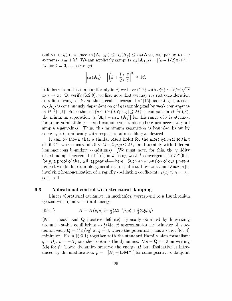
and so on q(�), whence �k(A(�M)) � �k(Aq) � �k(AM), comparing to theextremes q � �M . We can explicitly compute �k(A�M) = [(k+1=2)�=`]2�M for k = 0; : : : so we get������k(Aq)� ��k + 12� � �2����� �M:It follows from this that (uniformly in q) we have (1.2) with �(r) � (`=�)p2ras r!1. To verify (5:2.8), we �rst note that we may restrict considerationto a �nite range of k and then recall Theorem 1 of [16], asserting that each�k(Aq) is continuously dependent on q if q is topologized by weak convergencein H�1(0; `). Since the set fq 2 L1(0; `) : jqj �Mg is compact in H�1(0; `),the minimum separation j�k(Aq)� �k�1(Aq)j for this range of k is attainedfor some admissible q | and cannot vanish, since these are necessarily allsimple eigenvalues. Thus, this minimum separation is bounded below bysome r0 > 0, uniformly with respect to admissible q as desired.It can be shown that a similar result holds for the more general settingof (6:2.1) with constraints 0 < M� � �; p �M+ (and possibly with di�erenthomogeneous boundary conditions). [We must note, for this, the validityof extending Theorem 1 of [16], now using weak-* convergence in L1(0; `)for p; a proof of that will appear elsewhere.] Such an extension of our presentremark would, for example, generalize a recent result by Lopez and Zuazua [9]involving homogenization of a rapidly oscillating coe�cient: �(x=")ut = uxxas "! 0.6:3. Vibrational control with structural dampingLinear vibrational dynamics, in mechanics, correspond to a Hamiltoniansystem with quadratic total energyH = H(p; q) := 12hM�1p; pi+ 12hQq; qi(6:3.1)(M =\mass" and Q positive de�nite), typically obtained by linearizingaround a stable equilibrium so 12hQq; qi approximates the behavior of a po-tential well: Q = �2 =�q2 at q = 0, where the potential has a strict (local)minimum. From (6:3.1) together with the standard Hamiltonian formalism:_q = Hp, _p = �Hq one then obtains the dynamics: M�q +Qq = 0 on writingM�q for _p. These dynamics preserve the energy H but dissipation is intro-duced by the modi�cation: _p = �[Hq +DM�1] for some positive selfadjoint26

operator D (noting that that gives _H = �hHp;DM�1pi = �h _q;D _qi � 0)which leads to: M�q+D _q+Qq = 0. This can be put in the form: _y+Ay = 0of (6:1.1) on taking, e.g.,y = 0@ M�1=2pQ1=2q 1A ;A = 0@ D E�E� 000 1A ; with E := Q1=2M�1=2D :=M�1=2DM�1=2(6:3.2)The operator A0 (corresponding to the undamped setting with D = 0) isskew adjoint, which would then make � real in (6:1.5); more generally, sinceD is again positive the eigenvalues of A for the damped setting have positivereal parts so one still has � � C+, as is appropriate for our analysis.For continuum mechanics we will haveq = u(�) = [pointwise deviation from the equilibrium con�guration on ]and Q a di�erential operator for functions on . For simplicity, assumeuniform density � � 1 so M is the identity: p = ut and E = Q1=2, D = Din (6:3.2). The damped dynamics (without forcing) are then given by thepartial di�erential equationutt +Dut +Qu = 0 on (6:3.3)with suitable homogeneous boundary conditions at � := @, correspondingto the domain of Q so Q is selfadjoint (and positive de�nite) with respect topivoting on the inner product of L2(). We will also be taking observationand control as acting at (part of) the boundary of .The operator Q is given by the stress-strain response of the material and,following Euler, we take the stress (material distortion) to be proportionalto the linearized curvature �u so12hQu; ui = 12 Z a (�u)2 dapproximating the potential . Thus, taking a � 1 for simplicity, we haveQ = �2 | although this will give Q1=2 = �� only for special choices ofboundary conditions as in (6:3.8) below. [This choice of Q implicitly assumesthe stress is dominated by exion { neglecting material distortions associatedwith tension, shear, or torsion which might otherwise be included.]In general the dissipation operator need not be closely related to the op-eratorQ, but for our example we consider a form of structural damping. This27

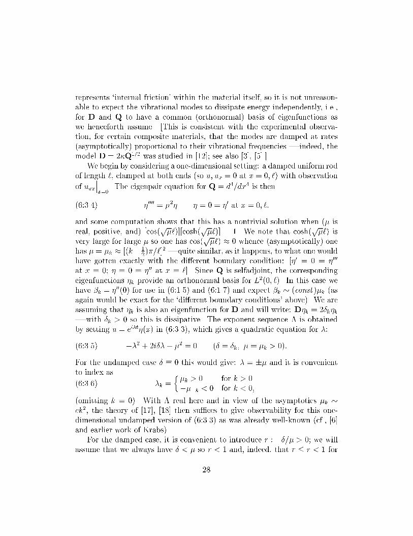
represents `internal friction' within the material itself, so it is not unreason-able to expect the vibrational modes to dissipate energy independently, i.e.,for D and Q to have a common (orthonormal) basis of eigenfunctions aswe henceforth assume. [This is consistent with the experimental observa-tion, for certain composite materials, that the modes are damped at rates(asymptotically) proportional to their vibrational frequencies | indeed, themodel D = 2�Q1=2 was studied in [12]; see also [3], [5].]We begin by considering a one-dimensional setting: a damped uniform rodof length `, clamped at both ends (so u; ux = 0 at x = 0; `) with observationof uxx���x=0. The eigenpair equation for Q = d4=dx4 is then�0000 = �2� � = 0 = �0 at x = 0; `:(6:3.4)and some computation shows that this has a nontrivial solution when (� isreal, positive, and) [cos(p�`)][cosh(p�`)] = 1. We note that cosh(p�`) isvery large for large � so one has cos(p�`) � 0 whence (asymptotically) onehas � = �k � [(k� 12)�=`]2 | quite similar, as it happens, to what one wouldhave gotten exactly with the di�erent boundary condition: [�0 = 0 = �000at x = 0; � = 0 = �00 at x = `]. Since Q is selfadjoint, the correspondingeigenfunctions �k provide an orthonormal basis for L2(0; `). In this case wehave �k = �00(0) for use in (6:1.5) and (6:1.7) and expect �k � (const )�k (asagain would be exact for the `di�erent boundary conditions' above). We areassuming that �k is also an eigenfunction for D and will write: D�k = 2�k�k| with �k > 0 so this is dissipative. The exponent sequence � is obtainedby setting u = ei�t�(x) in (6:3.3), which gives a quadratic equation for �:��2 + 2i��+ �2 = 0 (� = �k; � = �k > 0):(6:3.5)For the undamped case � � 0 this would give: � = �� and it is convenientto index as �k = ��k > 0 for k > 0���k < 0 for k < 0,(6:3.6)(omitting k = 0). With � real here and in view of the asymptotics �k �ck2, the theory of [17], [18] then su�ces to give observability for this one-dimensional undamped version of (6:3.3) as was already well-known (cf., [6]and earlier work of Krabs).For the damped case, it is convenient to introduce r := �=� > 0; we willassume that we always have � < � so r < 1 and, indeed, that r � �r < 1 for28

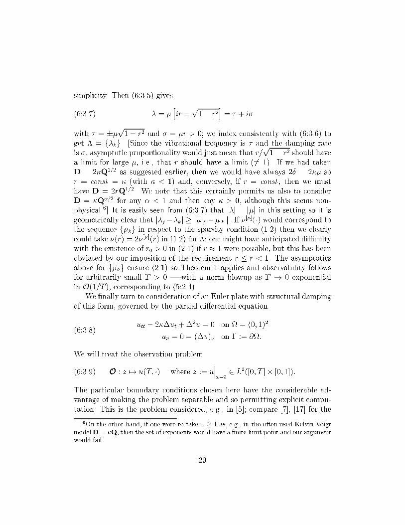
simplicity. Then (6:3.5) gives� = � hir �p1� r2i = � + i�(6:3.7)with � = ��p1� r2 and � = �r > 0; we index consistently with (6:3.6) toget � = f�kg. [Since the vibrational frequency is � and the damping rateis �, asymptotic proportionality would just mean that r=p1� r2 should havea limit for large �, i.e., that r should have a limit (6= 1). If we had takenD = 2�Q1=2 as suggested earlier, then we would have always 2� = 2�� sor = const = � (with � < 1) and, conversely, if r = const , then we musthave D = 2rQ1=2. We note that this certainly permits us also to considerD = �Q�=2 for any � < 1 and then any � > 0, although this seems non-physical.6] It is easily seen from (6:3.7) that j�j = j�j in this setting so it isgeometrically clear that j�j��kj � j�jjj��jkjj. If � [�](�) would correspond tothe sequence f�kg in respect to the sparsity condition (1.2) then we clearlycould take �(r) = 2� [�](r) in (1.2) for �; one might have anticipated di�cultywith the existence of r0 > 0 in (2.1) if r � 1 were possible, but this has beenobviated by our imposition of the requirement r � �r < 1. The asymptoticsabove for f�kg ensure (2.1) so Theorem 1 applies and observability followsfor arbitrarily small T > 0 | with a norm blowup as T ! 0 exponentialin O(1=T ), corresponding to (5:2.4).We �nally turn to consideration of an Euler plate with structural dampingof this form, governed by the partial di�erential equationutt � 2��ut +�2u = 0 on = (0; 1)2u� = 0 = (�u)� on � := @:(6:3.8)We will treat the observation problemOOO : z 7! u(T; �) where z := u���x=0 2 L2([0; T ]� [0; 1]):(6:3.9)The particular boundary conditions chosen here have the considerable ad-vantage of making the problem separable and so permitting explicit compu-tation. This is the problem considered, e.g., in [5]; compare [7], [17] for the6On the other hand, if one were to take � � 1 as, e.g., in the often-used Kelvin-VoigtmodelD = �Q, then the set of exponents would have a �nite limit point and our argumentwould fail. 29

undamped version of this. To avoid some expositional complications, we willassume it given that u has mean 0 in (6:3.8), i.e., that this is true for theinitial data u; ut���t=0.The eigenvalues for the Laplace operator (��) on = (0; 1)2 with Neu-man boundary conditions are �jk := (j2 + k2)�2 for j; k = 0; 1; : : : (omitting�00 = 0 by our simplifying assumption, so we always have � > 0). Withthe damping operator D = �2�� we have � = �� and, as for the one-dimensional case above, (6:3.7) applies with r = �. It will be necessary forus to partition the eigenvalues to get a family of scalar problems involvingexponent sequences �j := f�[j]k g where�k = �[j]k := ( a+j + c+k2 for k = 0; 1; : : :a�j + c�k2 for k = �0;�1; : : :with c� := h��p1� �2i �2; a�j := c�j2:(6:3.10)[This requires us to distinguish, as indices, between k = +0 and k = �0,which would be potentially awkward for j = 0 where a+0 = 0 = a�0 ouromission of the `00' terms eliminates that.] We have the orthonormal basisfor L2(0; 1) �k(x) = (1 if k = 0; cos(k�x)p2 if k = 1; 2; : : :)and separation of variables in (6:3.8) gives the expansionu(t; x; y) = 1Xj=0 �1Xk=�0 cjk ei�[j]k t �jkj(x)�j(y):(6:3.11)The key to our treatment of (6:3.8) is reduction of the problem to asequence of independent simpler problems, involving one �j at a time, byintroducing zj(t) := hz(t; �); �ji = �1Xk=�0 cjk ei�[j]k t(6:3.12)for j = 0; 1; : : :With j �xed, (6:3.12) is of the form (1.1) for the exponents �j.Since each �j consists of the union of two copies of (5:2.1), we may (as notedfollowing (5:2.2)) take �(r) = 4r in (1.2) for r > r0 and note that (since we30

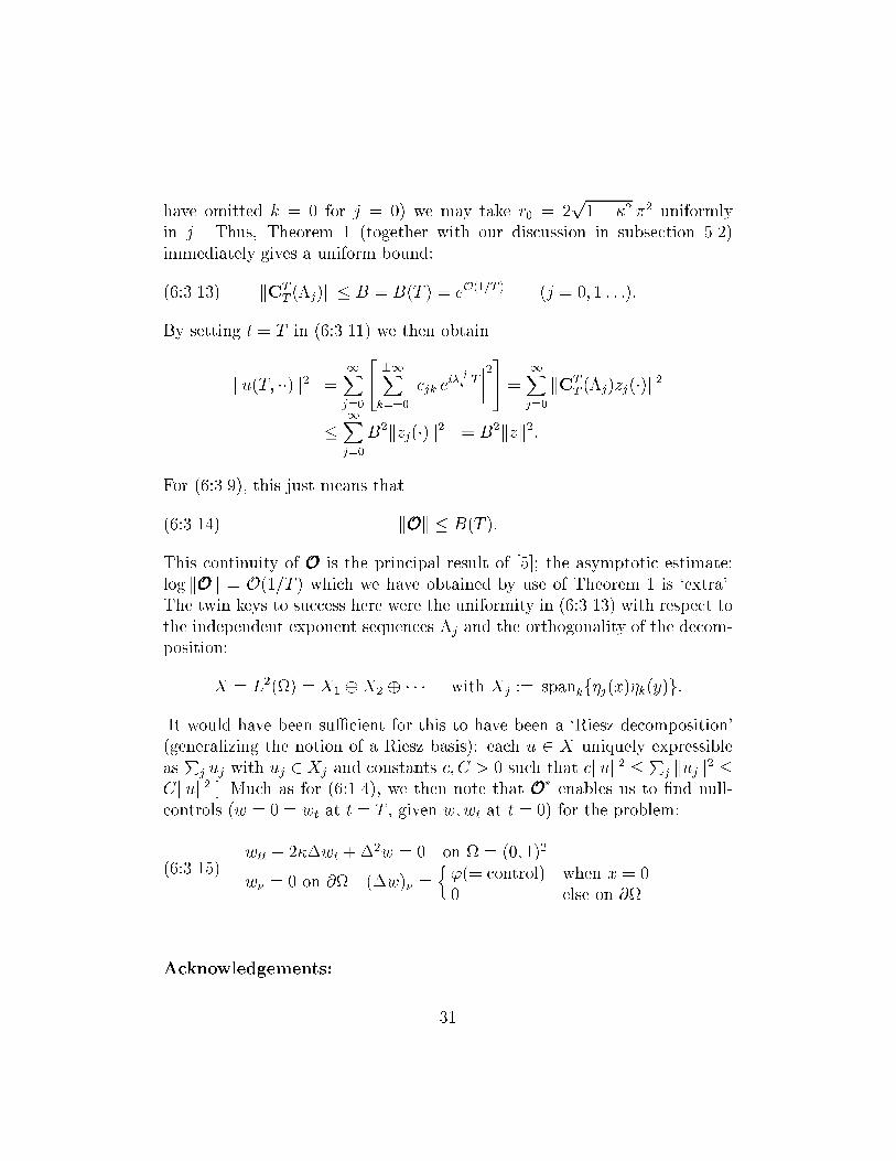
have omitted k = 0 for j = 0) we may take r0 = 2p1� �2 �2 uniformlyin j. Thus, Theorem 1 (together with our discussion in subsection 5.2)immediately gives a uniform bound:kCTT (�j)k � B = B(T ) = eO(1=T ) (j = 0; 1 : : :):(6:3.13)By setting t = T in (6:3.11) we then obtainku(T; ��)k2 = 1Xj=0 24 �1Xk=�0 ����cjk ei�[j]k T ����235 = 1Xj=0 kCTT (�j)zj(�)k2� 1Xj=0B2kzj(�)k2 = B2kzk2:For (6:3.9), this just means thatkOOOk � B(T ):(6:3.14)This continuity of OOO is the principal result of [5]; the asymptotic estimate:log kOOOk = O(1=T ) which we have obtained by use of Theorem 1 is `extra'.The twin keys to success here were the uniformity in (6:3.13) with respect tothe independent exponent sequences �j and the orthogonality of the decom-position:X = L2() = X1 �X2 � � � � with Xj := spankf�j(x)�k(y)g:[It would have been su�cient for this to have been a `Riesz decomposition'(generalizing the notion of a Riesz basis): each u 2 X uniquely expressibleas Pj uj with uj 2 Xj and constants c; C > 0 such that ckuk2 � Pj kujk2 �Ckuk2.] Much as for (6:1.4), we then note that OOO� enables us to �nd null-controls (w = 0 = wt at t = T , given w;wt at t = 0) for the problem:wtt � 2��wt +�2w = 0 on = (0; 1)2w� = 0 on @ (�w)� = �'(= control) when x = 00 else on @.(6:3.15)Acknowledgements: 31

This work was partially supported by the US National Science Foundation(grant #DMS-95-01036). The work of S. Avdonin and of S. Ivanov was alsosupported in part by the Russian Fundamental Research Foundation (grants# 97-01-01115, # 99-01-00744) and by the Australian Research Council. Weare grateful to R. Triggiani and to S. Antman for fruitful discussions con-cerning systems with structural damping and corresponding controllabilityproblems. We are also grateful to the (anonymous) referee for his detailedand useful suggestions.References[1] S.A. Avdonin and S.A. Ivanov, Families of Exponentials. The Methodof Moments in Controllability Problems for Distributed Parameter Sys-tems, Cambridge Univ. Press, New York, 1995.[2] P.Borwein and T. Erdelyi, Polynomials and Polynomial Inequalities,Springer-Verlag, New York, 1995.[3] S. Chen and R. Triggiani, Proof of extensions of two conjectures onstructural damping for elastic systems, Paci�c Journal of Mathematics,136, pp. 299{331 (1989).[4] E. G�uichal, A lower bound of the norm of the control operator for theheat equation , J. Math. Anal. Appl. 110, no.2, pp. 519{527 (1985).[5] S.W. Hansen, Bounds on functions biorthogonal to sets of complex ex-ponentials; control of damped elastic systems , J. Math. Anal. and Appl.158, pp. 487{508 (1991).[6] W. Krabs, On Moment Theory and Controllability of One-DimensionalVibrating Systems and Heating Processes (Lecture Notes in Control andInf. Sci. #173), Springer-Verlag, New York, 1992.[7] W. Krabs, G. Leugering, and T.I. Seidman, On boundary controllabilityof a vibrating plate, Appl. Math. Opt. 13, pp. 205{229 (1985).[8] G. Leugering and E.J.P. Georg Schmidt, Boundary control of a vibratingplate with internal damping,Math. Methods in the Appl. Sciences, v.11.pp. 573{586 (1989) 32

[9] A. Lopez and E. Zuazua, Some new results related to the nullcontrolla-bility of the 1� d heat equation, preprint, �Ecole Polytechnique (1997).[10] W.A.J. Luxemburg and J. Korevaar, Entire functions and M�untz{Sz�asztype approximation, Trans. Amer. Math. Soc. 157, pp. 23{37 (1971).[11] V.J. Mizel and T.I. Seidman, Observation and prediction for the heatequation, I, J. Math. Anal. Appl. 28, pp. 303{312 (1969).[12] D.L. Russell, Mathematical models for the elastic beam and the control{theoretic implications, in H. Brezis, M.G. Crandall, and F. Kappel (eds.),Semigroup Theory and Applications, Longman, New York, 1985.[13] L. Schwartz, �Etude des sommes d'exponentielles (2me ed.), Hermann,Paris, 1959.[14] T.I. Seidman, Boundary observation and control of a vibrating plate, inF. Kappel, K. Kunisch, W. Schappacher (eds.), Control Theory for Dis-tributed Parameter Systems and Applications (LNCIS #54) Springer-Verlag, Berlin, 1983.[15] T.I. Seidman, Two results on exact boundary controllability of parabolicequations, Appl. Math. Optim. 11, no.2, pp. 145{152 (1984).[16] T.I. Seidman, A convergent approximation scheme for the inverseSturm{Liouville problem, Inverse Problems 1, pp. 251{262 (1985).[17] T.I. Seidman, The coe�cient map for certain exponential sums, Nederl.Akad. Wetensch. Proc. Ser. A, 89 (= Indag. Math. 48), pp. 463{478(1986).[18] T.I. Seidman and M.S. Gowda, Norm dependence of the coe�cient mapon the window size, Math. Scand. 73, pp. 177{189 (1994).33