The fast multipole boundary element method for potential ...

The fast multipole boundary element method for

potential problems: A tutorial

Y.J. Liu a,*, N. Nishimura b,1

a Department of Mechanical, Industrial and Nuclear Engineering, University of Cincinnati, P.O. Box 210072, Cincinnati, OH 45221-0072, USAb Academic Center for Computing and Media Studies, Kyoto University, Kyoto 606-8501, Japan

Received 6 May 2005; accepted 23 November 2005

Available online 15 March 2006

Abstract

The fast multipole method (FMM) has been regarded as one of the top 10 algorithms in scientific computing that were developed in the 20th

century. Combined with the FMM, the boundary element method (BEM) can now solve large-scale problems with several million degrees of

freedom on a desktop computer within hours. This opened up a wide range of applications for the BEM that has been hindered for many years by

the lack of efficiencies in the solution process, although it has been regarded as superb in the modeling stage. However, understanding the fast

multipole BEM is even more difficult as compared with the conventional BEM, because of the added complexities and different approaches in

both FMM formulations and implementations. This paper is an introduction to the fast multipole BEM for potential problems, which is aimed to

overcome this hurdle for people who are familiar with the conventional BEM and want to learn and adopt the fast multipole approach. The basic

concept and main procedures in the FMM for solving boundary integral equations are described in detail using the 2D potential problem as an

example. The structure of a fast multipole BEM program is presented and the source code is also made available that can help the development of

fast multipole BEM codes for solving other problems. Numerical examples are presented to further demonstrate the efficiency, accuracy and

potentials of the fast multipole BEM for solving large-scale problems.

q 2006 Elsevier Ltd. All rights reserved.

Keywords: Fast multipole method; Boundary element method; 2D potential problems

1. Introduction

The boundary integral equation (BIE) formulations and

their numerical solutions using boundary element method

(BEM) for mechanics problems originated about 40 years ago.

The 2D potential problem was first formulated in terms of a

direct BIE and solved by Jaswon [1]. This work was later

extended by Rizzo to the vector case—2D elastostatic problem

[2]. Following these early works, extensive research efforts

have been made for the development of the BIE/BEM. Some of

the important textbooks and research volumes in English can

be found in Refs. [3–9].

Although the BEM has enjoyed the reputation of easy

meshing in modeling for many problems, its efficiency in

solutions has been a serious problem for analyzing large-scale

0955-7997/$ - see front matter q 2006 Elsevier Ltd. All rights reserved.

doi:10.1016/j.enganabound.2005.11.006

* Corresponding author. Tel.: C1 513 556 4607; fax: C1 513 556 3390.

E-mail addresses: [email protected] (Y.J. Liu), [email protected].

jp (N. Nishimura).1 Tel.: C81 (75) 753 7457; fax: C81 (75) 753 7450.

models that have emerged in applications with the availability

of more powerful computers. For example, while the finite

element method (FEM) has been used routinely to solve models

with several millions of degrees of freedom (DOF’s), the BEM

has been limited to solving problems with a few thousands

DOF’s for many years. This is because the conventional BEM in

general produces dense and non-symmetric matrices that,

although smaller in sizes, requiresO(N2) operations to compute

the coefficients and another O(N3) operations to solve the

system using direct solvers (where N is the number of equations

of the linear system).

In the mid of 1980s, Rokhlin and Greengard [10–12]

pioneered the innovative fast multipole method (FMM) that

can be used to accelerate the solutions of boundary integral

equations by several folds, promising to reduce the CPU time

in FMM accelerated BEM to O(N). However, it took almost a

decade for the mechanics community to realize the potential of

the FMM for the BEM. Some of the early research on FMM–

BEM in applied mechanics can be found in Refs. [13–17],

which show great promises of the FMM–BEM for solving

large-scale engineering problems. Most recently, composite

material models containing tens of thousands of fibers [18,19]

and models of electromagnetic wave scatterings from a full

Engineering Analysis with Boundary Elements 30 (2006) 371–381

www.elsevier.com/locate/enganabound

http://www.elsevier.com/locate/enganabound

mailto:[email protected]



Y.J. Liu, N. Nishimura / Engineering Analysis with Boundary Elements 30 (2006) 371–381372

aircraft at giga hertz frequencies [20] all have been solved

successfully by using the FMM–BEM within hours and with

moderate computing resources. A comprehensive review of the

FMM BIE/BEM can be found in Ref. [21].

However, the use of the fast multipole method has increased

the complexity in implementations of the BIE/BEM. Although

there are many research papers dealing with the various

subjects of the FMM–BEM, very few can be used as

introductory materials to learn the new approach for

researchers who are familiar with the conventional BEM or

for new comers who are often frustrated with even the

conventional BIE/BEM formulations and implementations.

The research papers are often concise, without detailed

information, which made the understanding of the FMM–

BEM difficult. To fill the gap and hence promote the FMM–

BEM in the BIE/BEM research community, we will provide in

this paper an introduction to the FMM–BEM with complete

information on formulations, discretizations and implemen-

tations using the 2D potential problem as an example.

This paper is organized as follows: in Section 2, we review

the BIE formulation for potential problems and the conven-

tional BEM in discretization of the BIE. In Section 3, we

present the complete formulations and algorithms used in the

FMM–BEM for 2D potential problem. In Section 4, we discuss

the programming issues in FMM–BEM using a Fortran code

that is available from the authors with this paper. In Section 5,

we show some example problems solved by using the provided

code to demonstrate the efficiencies of the FMM–BEM for

large-scale problems. We conclude the article with some

discussions in Section 6.

2. BIE formulation and the conventional BEM approach

The boundary integral equation formulation and its

discretization using the conventional BEM for potential

problems is summarized in this section. Consider the following

Laplace equation governing potential problems (for example, a

steady-state heat conduction problem) in a 2D domainV (Fig. 1)

V2fðxÞZ 0; cx2V ; (1)

1

2

r

S(=S1 S2)

x

y

n

V

Fig. 1. Domain V and its boundary S.

under the boundary conditions

fðxÞZ �fðxÞ; cx2S1; (2)

qðxÞhvf

vnðxÞZ �qðxÞ; cx2S2; (3)

where f is the potential field in domain V, SZS1gS2 the

boundary of V, n the outward normal, and the barred quantities

indicate given values on the boundary.

The solution to the boundary value problem described by

Eqs. (1)–(3) can be written as the following representation

integral (see, e.g. Refs. [7–9])

fðxÞZ

ðS

½Gðx; yÞqðyÞKFðx; yÞfðyÞ�dSðyÞ; cx2V; (4)

where G(x,y) is the Green’s function given by

Gðx; yÞZ1

2pln

1

r

� �; (5)

for 2D problems, and

Fðx; yÞZvGðx; yÞ

vnðyÞZ

1

2pr

vr

vn(6)

with r being the distance between the collocation point x and

field point y (Fig. 1).

Letting x/S (Fig. 1), we obtain the following boundary

integral equation [7–9]

CðxÞfðxÞZ

ðS

½Gðx; yÞqðyÞKFðx; yÞfðyÞ�dSðyÞ; cx2S; (7)

in which the second-term on the right-hand side is a singular

integral of the Cauchy-principal value (CPV) type, and the

coefficient

CðxÞZK

ðS

Fðx; yÞdSðyÞ; (8)

which is also a CPV integral. If the boundary S is smooth at the

collocation point x, we simply have C(x)Z1/2. Note that by

substituting (8) into (7), we can obtain the following weakly-

singular form of the BIE (see, e.g. Refs. [22,23]) for potential

problemsðS

Fðx; yÞ½fðyÞKfðxÞ�dSðyÞZ

ðS

Gðx; yÞqðyÞdSðyÞ; cx2S; (9)

in which no singular integrals exist. One can choose either BIE

(7) or (9) in the discretization using the BEM, depending on

which form is more convenient.

As an example of discretization schemes, we use constant

boundary elements, that is, dividing the boundary S into N line

segments (elements) and placing one node on each element

(Fig. 2). We obtain the following discretized equation of BIE

(7) for node i [7–9]

1

2fi Z

XNjZ1

½gijqjKfijfj�; for iZ 1; 2;.;N (10)

1

2

r

i (x )

yn

V

S

∆Sj

Fig. 2. Discretization of the boundary S using constant elements.

1

2

r

S0

z0

z

n

zLzL'

zc'

zc

Fig. 3. Complex notation and the related points for fast multipole expansions.

Y.J. Liu, N. Nishimura / Engineering Analysis with Boundary Elements 30 (2006) 371–381 373

where fj and qj (jZ1,2,.,N) are the nodal values off and q on

element DSj (Fig. 2), respectively, and the coefficients are

given by

gij Z

ðDSj

Gðx; yÞdSðyÞ; fij Z

ðDSj

Fðx; yÞdSðyÞ;

for i; jZ 1; 2;.;N

(11)

with the collocation point x being placed at node i. In matrix

form, Eq. (10) is written as

1

2

f1

f2

«

fN

8>>>><>>>>:

9>>>>=>>>>;

C

f11 f12 / f1N

f21 f22 / f2N

« « 1 «

fN1 fN2 / fNN

266664

377775

f1

f2

«

fN

8>>>><>>>>:

9>>>>=>>>>;

Z

g11 g12 / g1N

g21 g22 / g2N

« « 1 «

gN1 gN2 / gNN

26664

37775

q1

q2

«

qN

8>>><>>>:

9>>>=>>>;: (12)

In the conventional BEM approach, a standard linear system

of equations is formed as follows by applying the boundary

condition (either Eq. (2) or (3)) at each node and switching the

columns in the two matrices in Eq. (12)

a11 a12 / a1N

a21 a22 / a2N

« « 1 «

aN1 aN2 / aNN

26664

37775

l1

l2

«

lN

8>>>><>>>>:

9>>>>=>>>>;

Z

b1

b2

«

bN

8>>>><>>>>:

9>>>>=>>>>;; or

AlZ b;

(13)

where A is the coefficient matrix, l the unknown vector and b

the known right-hand side vector. Obviously, the construction

of matrix A requires O(N2) operations using the two

expressions in Eq. (11) and the size of the required memory

for storing A is also O(N2) since A is in general a non-

symmetric and dense matrix. The solution of system in Eq. (13)

using direct solvers such as Gauss elimination is even worse,

requiring O(N3) operations because of this general matrix. That

is why the conventional BEM approach for solving the BIE’s is

in general slow and inefficient for large-scale problems, despite

its robustness in the meshing stage as compared with other

domain based methods.

3. The fast multipole method—formulation

The fast multipole method can be employed to accelerate

the BEM for solving Eq. (7) or (9). The main idea of the FMM

is to translate the node-to-node (or element-to-element)

interactions to cell-to-cell interactions, where cells can have

a hierarchical (tree) structure with the smallest cells (leaves)

containing a specified number of elements. Iterative equation

solvers (such as GMRES) are used in the FMM, where matrix–

vector multiplications (as for the left-hand side of Eq. (13)) are

calculated using fast multipole expansions. Using the FMM for

the BEM, the solution time of a problem can be reduced to

order O(N). The memory requirement can also be reduced to

O(N) since iterative solvers do not need to store the entire

matrix in the memory.

In this section, we first discuss the expansions that are used

in the fast multipole method for 2D potential problems. The

results of these expansions are scattered in the literature (see,

e.g. Ref. [12]) and are summarized herein for completeness.

Then, we describe the main procedures and algorithms in the

fast multipole BEM.

Consider first the following integral with the G kernel in

BIE (7) or (9)ðS0

Gðx; yÞqðyÞdSðyÞ; (14)

in which S0 is a subset of S and away from the collocation point

x (Fig. 3). For convenience, we introduce the complex notation,

that is, replace the collocation point x and field point y by z0Zx1Cix2 and zZy1Ciy2 (with iZ

ffiffiffiffiffiffiK1

phere), respectively

(Fig. 3). We write


Gðx; yÞZRefGðz0; zÞg; (15)

where

Gðz0; zÞZK1

2plnðz0KzÞ: (16)

Thus, the integral in (14) is equivalent to the real part of the

following integralðS0

Gðz0; zÞqðzÞdSðzÞ: (17)

We now introduce several important concepts in the fast

multipole method that are the building blocks for the FMM–

BEM.

3.1. Multipole expansion (moments)

Assuming zc is a point close to the field point z (Fig. 3), that

is, jzKzcj/jz0Kzcj, we write

Gðz0; zÞZK1

2plnðz0KzÞ

ZK1

2plnðz0KzcÞC ln 1K

zKzcz0Kzc

� �� :

Applying the following Taylor series expansion

lnð1KxÞZKXNkZ1

xk

k; for jxj!1;

we obtain

Gðz0; zÞZ1

2p

XNkZ0

Okðz0KzcÞIkðzKzcÞ; (18)

where, for convenience, we have introduced

IkðzÞZzk

k!; for kR0; OkðzÞZ

ðkK1Þ!

zk; for kR1;

and O0ðzÞZKlnðzÞ:

The derivatives of functions Ik(z) and Ok(z) satisfy:

I 0kðzÞZ IkK1ðzÞ; for kR1; and O0kðzÞZKOkC1ðzÞ;

for kR0:

Note that in the G kernel given in Eq. (18), z0 and z are

separated now due to the introduction of the ‘mid point’ zc,

which is a key in the FMM. The integral in (17) is now

evaluated as followsðS0

Gðz0; zÞqðzÞdSðzÞ

Z1

2p

ðS0

XNkZ0

Okðz0KzcÞIkðzKzcÞ

" #qðzÞdSðzÞ

that is, the multipole expansion

ðS0

Gðz0; zÞqðzÞdSðzÞZ1

2p

XNkZ0

Okðz0KzcÞMkðzcÞ; (19)

where

MkðzcÞZ

ðS0

IkðzKzcÞqðzÞdSðzÞ; (20)

are called moments about zc, which are independent of the

collocation point z0 and only need to be computed once. After

these moments are obtained, the integral can be evaluated

readily using Eq. (19) for any collocation point z0 away from S0(which will be within a cell centered at zc).

Detailed analysis of the errors in these multipole expansions

and the subsequent translations can be found in Ref. [12].

3.2. Moment-to-moment translation (M2M)

If the point zc is moved to a new location zc 0 (Fig. 3), the

following translation holds for the moments

Mkðzc0 ÞZ

ðS0

IkðzKzc0 ÞqðzÞdSðzÞ

Z

ðS0

IkððzKzcÞC ðzcKzc0 ÞÞqðzÞdSðzÞ:

Applying the binomial formula

ðaCbÞn ZXnmK0

n

m

� �ambnKm;

wheren

m

� �Z

n!

ðnKmÞ!m!Z

n

nKm

� �;

we obtain

Mkðzc0 ÞZXklZ0

IkKlðzcKzc0 ÞMlðzcÞ: (21)

This is the M2M translation for the moments when zc is

moved to zc 0. Note that there are only a finite number of terms

in this translation.

3.3. Local expansion and moment-to-local translation (M2L)

Suppose zL is a point close to the collocation point z0(Fig. 3), that is, jz0KzLj/jzcKzLj. From the multipole

expansion (Eq. (19)), we have:

f ðz0Þh

ðS0

Gðz0; zÞqðzÞdSðzÞZ1

2p

XNkZ0

Okðz0KzcÞMkðzcÞ: (22)

We now expand f(z0) about point zL, using the Taylor series

expansion, that is


f ðz0ÞZXNlZ0

f ðlÞðzLÞIlðz0KzLÞ: (23)

We evaluate

f ðlÞðzLÞZðK1Þl

2p

XNkZ0

OlCkðzLKzcÞMkðzcÞ:

Substituting this result into (23), we obtain the following

local expansionðS0

Gðz0; zÞqðzÞdSðzÞZXNlZ0

LlðzLÞIlðz0KzLÞ; (24)

where the coefficients are given by the following M2L

translation

LlðzLÞZðK1Þl

2p

XNkZ0

OlCkðzLKzcÞMkðzcÞ: (25)

3.4. Local-to-local translation (L2L)

If the point for local expansion is moved from zL to zL 0

(Fig. 3), we have the following expression using a local

expansion from Eq. (24)ðS0

Gðz0;zÞqðzÞdSðzÞZXNlZ0

LlðzLÞIlðz0KzLÞ

ZXNlZ0

LlðzLÞIlððz0KzL0 ÞC ðzL0KzLÞÞ:

Applying the formula ðaCbÞlZPl

mZ0

l

m

� �amblKm, and

the relationPN

lZ0

PlmZ0Z

PNmZ0

PNlZm, we obtainð

S0

Gðz0;zÞqðzÞdSðzÞZXNlZ0

LlðzL0 ÞIlðz0KzL0 Þ; (26)

where the new coefficients are given by the following L2L

translation

LlðzL0 ÞZXNmZl

ImKlðzL0KzLÞLmðzLÞ: (27)

ReplacingmKl by k, we can also write (27) in an alternative

form

LlðzL0 ÞZXNkZ0

IkðzL0KzLÞLlCkðzLÞ: (28)

3.5. Expansions for integrals with the F kernel

We now consider the integral with the F kernel in BIE (7) or

(9) in the complex notationðS0

Fðz0; zÞfðzÞdSðzÞ; (29)

where

Fðz0; zÞZvG

vnZ ðn1 C in2ÞG

0 Z nðzÞG0;

with G0 hvG

vz:

(30)

Thus,

Fðx; yÞZRefFðz0; zÞgZ n1 Re G0Kn2 Im G0 (31)

We have (Eq. (18))

Gðz0; zÞZ1

2p

XNkZ0

Okðz0KzcÞIkðzKzcÞ:

Therefore

G0 Z1

2p

XNkZ1

Okðz0KzcÞIkK1ðzKzcÞ; (32)

and the integral in (29) becomesðS0

Fðz0; zÞfðzÞdSðzÞZ1

2p

XNkZ1

Okðz0KzcÞNkðzcÞ;

where

NkðzcÞZ

ðS0

nðzÞIkK1ðzKzcÞfðzÞdSðzÞ: (33)

These are the moments for the F kernel integral, which are

similar to those in Eq. (20) for the G kernel integral. It can

also be shown that the M2M, M2L and L2L translations

remain the same for the F kernel integral, except for the fact

that N0Z0. That is, the translations used for Mk can be applied

directly for Nk.

3.6. FMM algorithms and procedures

The algorithms and main procedures in the FMM–BEM are

as follows:

Step 1. Discretization. For a given problem, discretize the

boundary S as usual as in the conventional BEM (e.g. using

constant elements as shown in Fig. 2).

Step 2. Determine the tree structure of the mesh. For a 2D

problem, for example, consider a square that covers the entire

boundary S and call this square the cell of level 0 (Fig. 4).

Then, start dividing this parent cell into four equal child cells

of level 1. Continue dividing in this way, that is, take a

parent cell of level l and divide it into four child cells of

level lC1. Stop dividing a cell if the number of elements in

that cell is less than a specified number (this number is 1 in

the example shown in Fig. 4). A cell having no child cells is

called a leaf (e.g. the shaded cells in Fig. 4). Note that the

edge length of a child cell is one-half of that of its parent

cell. An element is considered within a cell if the center of

the element is inside that cell. A quad-tree structure of the

cells covering all the elements is thus formed using this

procedure (Fig. 5).

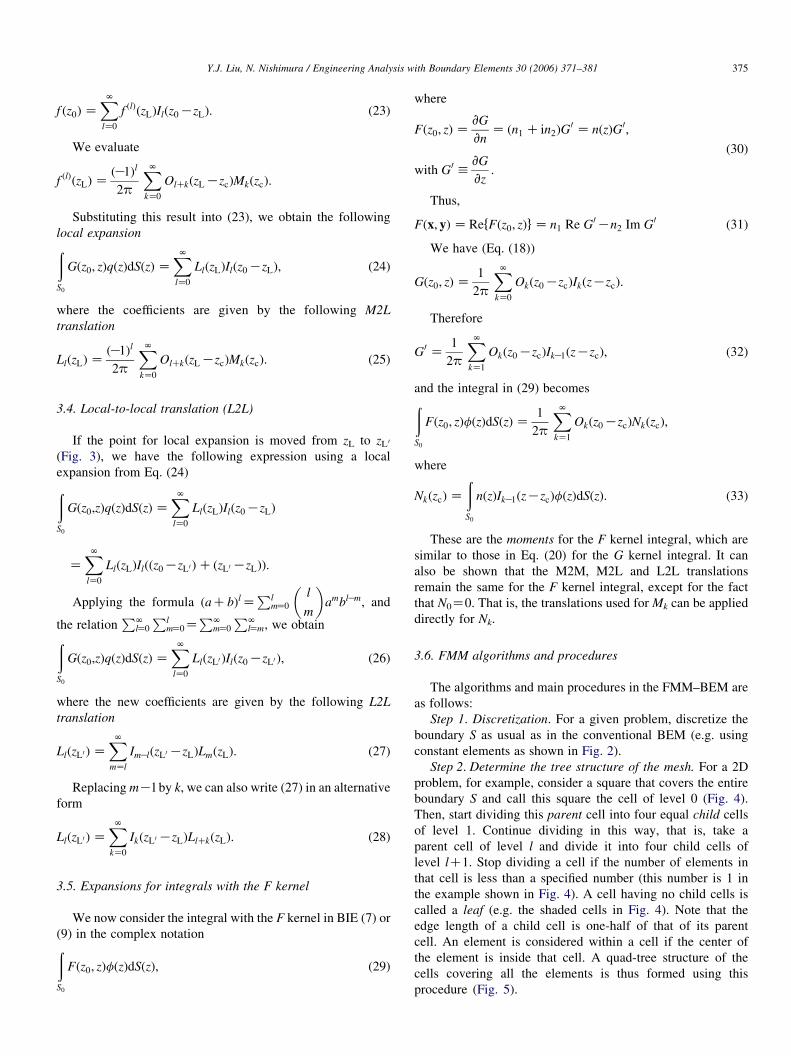
0

32

1

12

3 4 5 6 78

9

10

11

12

13

14

1516

17181920

21

22

23

24

25

26

27

28

29

30

Fig. 4. A hierarchical cell structure covering all the boundary elements (the

small square on the side shows the numbering scheme for the child cells of any

given parent cell).


Step 3. Upward pass. Compute the moments on all cells, at

all levels with 1R2, and for up to p terms, tracing the tree

structure upward. For a leaf, Eq. (20) is applied directly (with

S0 being the elements contained in the leaf and zc the centroid

of the leaf). For a parent cell, the moment is calculated by

summing the moments on its four child cells using the M2M

translation, that is, Eq. (21), in which zc 0 is the centroid of the

parent cell and zc the centroid of a child cell (Fig. 6).

Step 4. Downward pass. To describe the downward pass, we

first define a few terms. Two cells are said to be adjacent cells

at level l if they have at least one common vertex. Two cells are

said to be well separated at level l if they are not adjacent at

level l but their parent cells are adjacent at level lK1. The list

of all the well-separated cells from a level l cell C is called the

interaction list of C. Cells are called to be far cells of C if their

parent cells are not adjacent to the parent cell of C (Fig. 7). We

now compute the local expansion (coefficients) on all cells

starting from level 2 and tracing the tree structure downward to

all the leaves. The local expansion associated with a cell C is

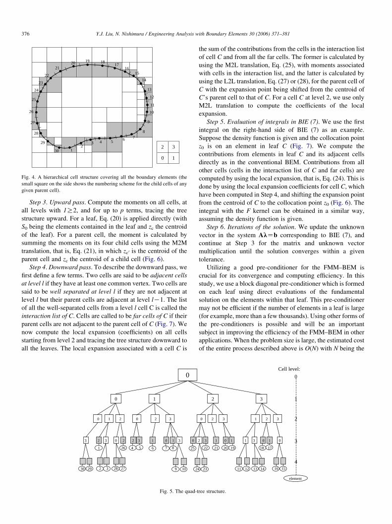
0

0 1

0 1 2 0 2 3

2930 109

1

3

32

874 5 6

2

2526

2728

2 0 23 2 3 1 0 1 3 0

Fig. 5. The quad-t

the sum of the contributions from the cells in the interaction list

of cell C and from all the far cells. The former is calculated by

using the M2L translation, Eq. (25), with moments associated

with cells in the interaction list, and the latter is calculated by

using the L2L translation, Eq. (27) or (28), for the parent cell of

C with the expansion point being shifted from the centroid of

C’s parent cell to that of C. For a cell C at level 2, we use only

M2L translation to compute the coefficients of the local

expansion.

Step 5. Evaluation of integrals in BIE (7). We use the first

integral on the right-hand side of BIE (7) as an example.

Suppose the density function is given and the collocation point

z0 is on an element in leaf C (Fig. 7). We compute the

contributions from elements in leaf C and its adjacent cells

directly as in the conventional BEM. Contributions from all

other cells (cells in the interaction list of C and far cells) are

computed by using the local expansion, that is, Eq. (24). This is

done by using the local expansion coefficients for cell C, which

have been computed in Step 4, and shifting the expansion point

from the centroid of C to the collocation point z0 (Fig. 6). The

integral with the F kernel can be obtained in a similar way,

assuming the density function is given.

Step 6. Iterations of the solution. We update the unknown

vector in the system AlZb corresponding to BIE (7), and

continue at Step 3 for the matrix and unknown vector

multiplication until the solution converges within a given

tolerance.

Utilizing a good pre-conditioner for the FMM–BEM is

crucial for its convergence and computing efficiency. In this

study, we use a block diagonal pre-conditioner which is formed

on each leaf using direct evaluations of the fundamental

solution on the elements within that leaf. This pre-conditioner

may not be efficient if the number of elements in a leaf is large

(for example, more than a few thousands). Using other forms of

the pre-conditioners is possible and will be an important

subject in improving the efficiency of the FMM–BEM in other

applications. When the problem size is large, the estimated cost

of the entire process described above is O(N) with N being the

2 3

0 2 3 1 2 3

Cell level:

1

0

2

3

4

1920

1211234

22 21

1413

18 17

1516

element

2 3 1 1 1 3 0 010

ree structure.

Fig. 6. Upward and downward passes using expansions and translations in the FMM.


number of elements or nodes, if the number of terms p in the

multipole expansions and the number of elements in a leaf are

kept constant (see Ref. [21]).

Cell C

Adjacent cells(direct)

Cells in interactionlist (M2L)

Far cells(L2L)

Fig. 7. Grouping of the cells for cell C (black one) at level l.

4. The fast multipole method—programming

We now discuss the main structure of an FMM–BEM code

for solving general 2D potential problems. This Fortran code is

based on an earlier code that was used for 2D crack and rigid-

line inclusion problems governed by Laplace equation and

formulated using a hypersingular BIE [18]. This general 2D

FMM–BEM code for potential problems can be expanded to

solve 3D potential problems, 2D and 3D elasticity problems,

using constant or higher-order elements.

The flowchart of the 2D FMM–BEM code is given in Fig. 8.

The chart shows the main tasks for the program and the related

subroutines. The source code for the iterative solver GMRES

can be downloaded from the website netlib (http://www.netlib.

org/). The program starts with reading in the data for the

boundary nodes and elements, and the parameters used in the

fast multipole expansions and solver GMRES. Then, the quad-

tree structure is created and the right-hand side vector is

computed using the FMM algorithms (this need to be done only

once). The main part of the program is in two subroutines

prepared for GMRES, msolve which prepares a pre-condition-

ing matrix for the iterative solver, and matvec which provides

the algorithm for the matrix-vector multiplication (Al in Eq.

(13)) using the fast multipole algorithms (by calling the upward

and dwnwrd subroutines).

The source code, input files (one for element data and one

for parameters) and an output file are available from the authors

[24]. The main variables in the subroutines are explained in the

source code, and the format of the input and output files are

self-explaining in these files.

http://www.netlib.org/

http://www.netlib.org/

Start the ProgramInitiate parameters and

call FMM BEM (fmmmain.f)

Read in the BEM model (prep_model.f)

Construct the tree structure(tree.f)

Compute the right-hand side vector(fmmbvector.f)

Call GMRES solver (dgmres.f)

msolve.f

matvec.f

Output the results

Stop

upward.f

dwnwrd.f

upward.f

dwnwrd.f

moment.f

direct.f

moment.f

direct.f

Fig. 8. Flow chart for the FMM–BEM code.


5. Numerical examples

We present two numerical examples to demonstrate the

accuracy and efficiency of the FMM–BEM for 2D potential

problems. All the computations were done on a Pentium IV

laptop PC with a 2.4 GHz CPU, 1 GB RAM and 40 GB hard

drive. The largest model with 1.4 million equations run for less

than 11,000 CPU seconds on this laptop.

5.1. An annular region

We first consider a simple potential (e.g. heat conduction)

problem in an annular region as shown in Fig. 9, for which the

available analytical solution can be used to check the BEM

a b

O

V

Sb

Sa

Fig. 9. A simple potential problem in an annular region V.

results. The field f is given on the inner boundary Sa, while the

normal derivative is given on the outer boundary Sb. The

analytical solution for this (axisymmetric) problem is given by

fðrÞZfa Cqbb lnr

a

� �;

where fa and qb are the given values off and q on the boundary

Sa and Sb, respectively, and r is the radial coordinate in a polar-

coordinate system centered at O. This gives

fb ZfðbÞZfa Cqbb lnb

a

� �; qa Z

vf

vnðaÞZKqb

b

a:

For the test problem, we choose aZ1, bZ2, faZ100, and

qbZ200. This gives

fb Z 377:258872; qa ZK400:0:

We discretize the inner and outer boundaries with the same

number of elements and run both the FMM–BEM code and a

conventional BEM code using also constant elements. The

conventional BEMcode uses a direct solver (Gauss elimination)

for solving the linear system. For the FMM–BEM, the numbers

of terms for both moments and local expansions were set to 15,

the maximum number of elements in a leaf to 20, and the

tolerance for convergence of the solution to 10K8. The FMM–

BEM results converged in 11 iterations for the smallest model

(with 36 elements) and in 43 iterations for the largest model

(with 9600 elements). These numbers can be reduced to 9 and 28

iterations, respectively, if the tolerance is reduced to 10K6.

Table 1 shows the results offb and qa for this problem using

both the FMM–BEM and the conventional BEM as the total

number of elements increase from 36 to 9600. As we can see,

the results for both FMM–BEM and conventional BEM

converge quickly to the exact solution for the mesh with only

72 constant elements with a relative error of 0.1%. The results

continue to improve until the mesh with 4800 elements. For the

two larger meshes (with 7200 and 9600 elements), the results

for qb deviate slightly from the exact solution for both FMM–

BEM and conventional BEM, which may be caused by

truncation errors. In general, the FMM–BEM is found to be

Table 1

Results of the potential and normal derivative for the annular region

N qa fb

FMM–BEM Conventional

BEM

FMM–BEM Conventional

BEM

36 K401.771619 K401.771546 376.723694 376.723612

72 K400.400634 K400.400662 377.140967 377.140972

360 K400.014881 K400.014803 377.254774 377.254783

720 K400.003468 K400.003629 377.257857 377.257873

1440 K400.000695 K400.000533 377.258607 377.258622

2400 K400.001929 K400.000612 377.258795 377.258783

4800 K400.001557 K400.000561 377.258852 377.258856

7200 K399.997329 K399.998183 377.258848 377.258857

9600 K399.997657 K399.996874 377.258859 377.258871

Analytical

solution

K400.0 377.258872

0

200

400

600

800

1,000

1,200

1,400

0 1,000 2,000 3,000 4,000 5,000 6,000 7,000 8,000 9,000 10,000

DOF's

Tot

al C

PU

tim

e (s

ec.)

Conventional BEM

FMM BEM

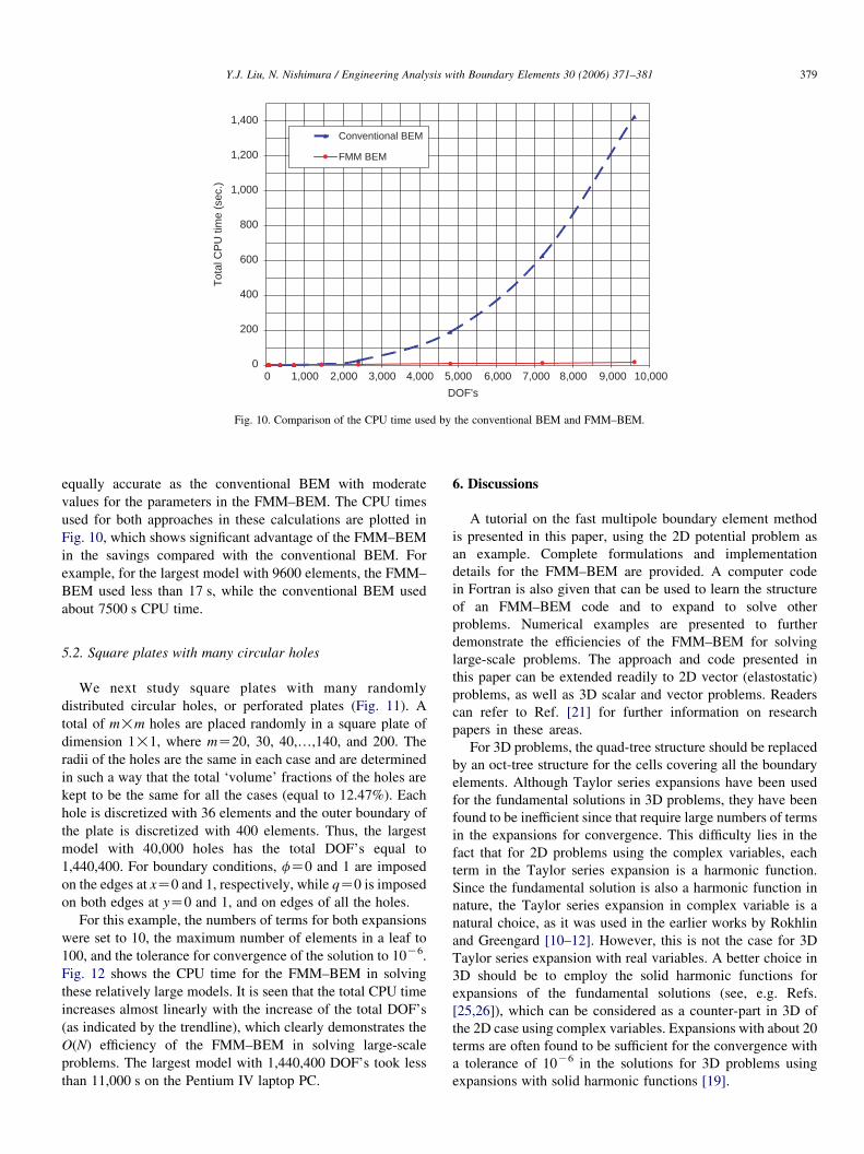
Fig. 10. Comparison of the CPU time used by the conventional BEM and FMM–BEM.


equally accurate as the conventional BEM with moderate

values for the parameters in the FMM–BEM. The CPU times

used for both approaches in these calculations are plotted in

Fig. 10, which shows significant advantage of the FMM–BEM

in the savings compared with the conventional BEM. For

example, for the largest model with 9600 elements, the FMM–

BEM used less than 17 s, while the conventional BEM used

about 7500 s CPU time.

5.2. Square plates with many circular holes

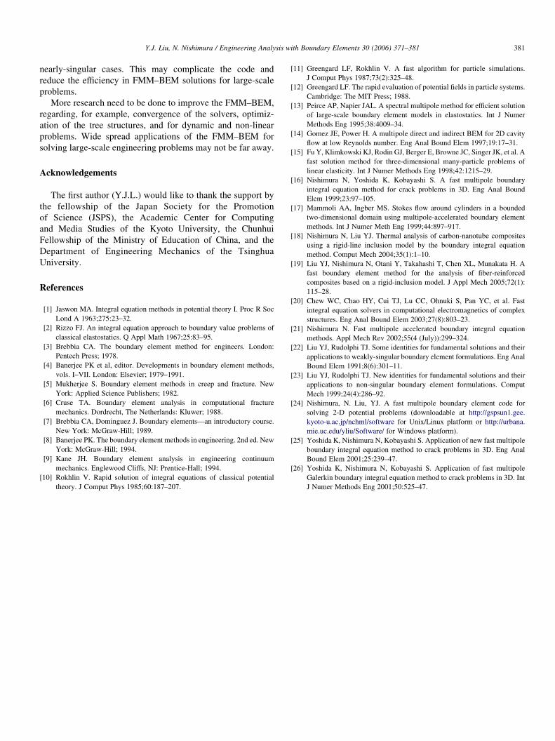
We next study square plates with many randomly

distributed circular holes, or perforated plates (Fig. 11). A

total of m!m holes are placed randomly in a square plate of

dimension 1!1, where mZ20, 30, 40,.,140, and 200. The

radii of the holes are the same in each case and are determined

in such a way that the total ‘volume’ fractions of the holes are

kept to be the same for all the cases (equal to 12.47%). Each

hole is discretized with 36 elements and the outer boundary of

the plate is discretized with 400 elements. Thus, the largest

model with 40,000 holes has the total DOF’s equal to

1,440,400. For boundary conditions, fZ0 and 1 are imposed

on the edges at xZ0 and 1, respectively, while qZ0 is imposed

on both edges at yZ0 and 1, and on edges of all the holes.

For this example, the numbers of terms for both expansions

were set to 10, the maximum number of elements in a leaf to

100, and the tolerance for convergence of the solution to 10K6.

Fig. 12 shows the CPU time for the FMM–BEM in solving

these relatively large models. It is seen that the total CPU time

increases almost linearly with the increase of the total DOF’s

(as indicated by the trendline), which clearly demonstrates the

O(N) efficiency of the FMM–BEM in solving large-scale

problems. The largest model with 1,440,400 DOF’s took less

than 11,000 s on the Pentium IV laptop PC.

6. Discussions

A tutorial on the fast multipole boundary element method

is presented in this paper, using the 2D potential problem as

an example. Complete formulations and implementation

details for the FMM–BEM are provided. A computer code

in Fortran is also given that can be used to learn the structure

of an FMM–BEM code and to expand to solve other

problems. Numerical examples are presented to further

demonstrate the efficiencies of the FMM–BEM for solving

large-scale problems. The approach and code presented in

this paper can be extended readily to 2D vector (elastostatic)

problems, as well as 3D scalar and vector problems. Readers

can refer to Ref. [21] for further information on research

papers in these areas.

For 3D problems, the quad-tree structure should be replaced

by an oct-tree structure for the cells covering all the boundary

elements. Although Taylor series expansions have been used

for the fundamental solutions in 3D problems, they have been

found to be inefficient since that require large numbers of terms

in the expansions for convergence. This difficulty lies in the

fact that for 2D problems using the complex variables, each

term in the Taylor series expansion is a harmonic function.

Since the fundamental solution is also a harmonic function in

nature, the Taylor series expansion in complex variable is a

natural choice, as it was used in the earlier works by Rokhlin

and Greengard [10–12]. However, this is not the case for 3D

Taylor series expansion with real variables. A better choice in

3D should be to employ the solid harmonic functions for

expansions of the fundamental solutions (see, e.g. Refs.

[25,26]), which can be considered as a counter-part in 3D of

the 2D case using complex variables. Expansions with about 20

terms are often found to be sufficient for the convergence with

a tolerance of 10K6 in the solutions for 3D problems using

expansions with solid harmonic functions [19].

Fig. 11. Square plates with large numbers of randomly distributed circular holes.


Constant elements can certainly be replaced by higher-order

elements to improve the accuracy of an FMM–BEM code.

However, this may not be advantageous considering the

efficiency of the code for large-scale problems. For constant

elements, all the integrals are evaluated analytically, for all

10

100

1,000

10,000

100,000

1.0E+04 1.0E+05

D

Tot

al C

PU

tim

e (s

ec.)

CPU time

Trendline

Fig. 12. Total CPU time used by the FMM–BEM for

non-singular, nearly-singular and singular cases. There are no

numerical integrations at all in the code. For higher-order

elements, however, this may no longer be the case and one will

have to introduce numerical integrations for the direct

evaluations of the integrals that can involve singular and

y = 0.0018x1.0913

1.0E+06 1.0E+07

OF's

solving the plate-hole problems (log–log scale).


nearly-singular cases. This may complicate the code and

reduce the efficiency in FMM–BEM solutions for large-scale

problems.

More research need to be done to improve the FMM–BEM,

regarding, for example, convergence of the solvers, optimiz-

ation of the tree structures, and for dynamic and non-linear

problems. Wide spread applications of the FMM–BEM for

solving large-scale engineering problems may not be far away.

Acknowledgements

The first author (Y.J.L.) would like to thank the support by

the fellowship of the Japan Society for the Promotion

of Science (JSPS), the Academic Center for Computing

and Media Studies of the Kyoto University, the Chunhui

Fellowship of the Ministry of Education of China, and the

Department of Engineering Mechanics of the Tsinghua

University.

References

[1] Jaswon MA. Integral equation methods in potential theory I. Proc R Soc

Lond A 1963;275:23–32.

[2] Rizzo FJ. An integral equation approach to boundary value problems of

classical elastostatics. Q Appl Math 1967;25:83–95.

[3] Brebbia CA. The boundary element method for engineers. London:

Pentech Press; 1978.

[4] Banerjee PK et al, editor. Developments in boundary element methods,

vols. I–VII. London: Elsevier; 1979–1991.

[5] Mukherjee S. Boundary element methods in creep and fracture. New

York: Applied Science Publishers; 1982.

[6] Cruse TA. Boundary element analysis in computational fracture

mechanics. Dordrecht, The Netherlands: Kluwer; 1988.

[7] Brebbia CA, Dominguez J. Boundary elements—an introductory course.

New York: McGraw-Hill; 1989.

[8] Banerjee PK. The boundary element methods in engineering. 2nd ed. New

York: McGraw-Hill; 1994.

[9] Kane JH. Boundary element analysis in engineering continuum

mechanics. Englewood Cliffs, NJ: Prentice-Hall; 1994.

[10] Rokhlin V. Rapid solution of integral equations of classical potential

theory. J Comput Phys 1985;60:187–207.

[11] Greengard LF, Rokhlin V. A fast algorithm for particle simulations.

J Comput Phys 1987;73(2):325–48.

[12] Greengard LF. The rapid evaluation of potential fields in particle systems.

Cambridge: The MIT Press; 1988.

[13] Peirce AP, Napier JAL. A spectral multipole method for efficient solution

of large-scale boundary element models in elastostatics. Int J Numer

Methods Eng 1995;38:4009–34.

[14] Gomez JE, Power H. A multipole direct and indirect BEM for 2D cavity

flow at low Reynolds number. Eng Anal Bound Elem 1997;19:17–31.

[15] Fu Y, Klimkowski KJ, Rodin GJ, Berger E, Browne JC, Singer JK, et al. A

fast solution method for three-dimensional many-particle problems of

linear elasticity. Int J Numer Methods Eng 1998;42:1215–29.

[16] Nishimura N, Yoshida K, Kobayashi S. A fast multipole boundary

integral equation method for crack problems in 3D. Eng Anal Bound

Elem 1999;23:97–105.

[17] Mammoli AA, Ingber MS. Stokes flow around cylinders in a bounded

two-dimensional domain using multipole-accelerated boundary element

methods. Int J Numer Meth Eng 1999;44:897–917.

[18] Nishimura N, Liu YJ. Thermal analysis of carbon-nanotube composites

using a rigid-line inclusion model by the boundary integral equation

method. Comput Mech 2004;35(1):1–10.

[19] Liu YJ, Nishimura N, Otani Y, Takahashi T, Chen XL, Munakata H. A

fast boundary element method for the analysis of fiber-reinforced

composites based on a rigid-inclusion model. J Appl Mech 2005;72(1):

115–28.

[20] Chew WC, Chao HY, Cui TJ, Lu CC, Ohnuki S, Pan YC, et al. Fast

integral equation solvers in computational electromagnetics of complex

structures. Eng Anal Bound Elem 2003;27(8):803–23.

[21] Nishimura N. Fast multipole accelerated boundary integral equation

methods. Appl Mech Rev 2002;55(4 (July)):299–324.

[22] Liu YJ, Rudolphi TJ. Some identities for fundamental solutions and their

applications to weakly-singular boundary element formulations. Eng Anal

Bound Elem 1991;8(6):301–11.

[23] Liu YJ, Rudolphi TJ. New identities for fundamental solutions and their

applications to non-singular boundary element formulations. Comput

Mech 1999;24(4):286–92.

[24] Nishimura, N. Liu, YJ. A fast multipole boundary element code for

solving 2-D potential problems (downloadable at http://gspsun1.gee.

kyoto-u.ac.jp/nchml/software for Unix/Linux platform or http://urbana.

mie.uc.edu/yliu/Software/ for Windows platform).

[25] Yoshida K, Nishimura N, Kobayashi S. Application of new fast multipole

boundary integral equation method to crack problems in 3D. Eng Anal

Bound Elem 2001;25:239–47.

[26] Yoshida K, Nishimura N, Kobayashi S. Application of fast multipole

Galerkin boundary integral equation method to crack problems in 3D. Int

J Numer Methods Eng 2001;50:525–47.

http://http://gspsun1.gee.kyoto-u.ac.jp/nchml/software

http://http://gspsun1.gee.kyoto-u.ac.jp/nchml/software

http://http://urbana.mie.uc.edu/yliu/Software/

http://http://urbana.mie.uc.edu/yliu/Software/

The fast multipole boundary element method for potential ...

Documents

Transcript of The fast multipole boundary element method for potential ...