INTERNATIONAL JOURNAL FOR NUMERICAL AND ANALYTICAL METHODS IN GEOMECHANICS, VOL. 12, 401-417 (1988)

DYNAMIC STRESS ANALYSIS OF A CLASS OF GEOMECHANICS PROBLEMS BY THE BOUNDARY

ELEMENT METHOD

SHAHID AHMAD'

Department of Civil Engineering, State University of New York at Buffalo, U.S.A.

SUMMARY

This paper presents the application of an advanced BEM for periodic and transient dynamic stress analyses of a class of geomechanics problems. For transient dynamic analysis, the problem is first solved in the Laplace transform space, which happens to be similar to the periodic dynamic analysis, and then the time domain solution is obtained by numerical inversion of transform domain solutions. The numerical implementation of the BEM used to present the results in this paper is complete and most general available to date. It is capable of treating very large, multi-layered problems by substructuring and satisfying the equilibrium and compatibilities at the interfaces. With the help of this substructuring, capability problems related to layered media and soil-structure interaction have been analysed. A number of examples are presented and through comparisons with available analytical and numerical results, the applicability and usefulness of the present analysis to real geomechanical problems are established.

INTRODUCTION

In recent years, the usefulness of numerical techniques in solving dynamic stress analysis problems in geomechanics has been fully recognized by geotechnical engineers. In a broad sense, the available numerical techniques can be divided into four main categories: namely (1) the finite element method (FEM), (2) the finite difference method (FDM), (3) lumped parameter models, and (4) the boundary element method (BEM). Of these, the most versatile and widely used method is the FEM. It is capable of handling complex structure geometry, medium inhomogenei- ties and complicated material behaviour. However, in dynamic stress analysis problems of geomechanics, the FEM cannot properly model the geometry of the problem which has boundaries extending to infinity (such as a layered soil medium). Similarly, the FDM has not been used frequently, primarily because of difficulties associated with handling semi-infinite medium geometries and complicated boundary conditions. The use of lumped parameter model is also rather restricted to some machine foundation problems, because exact expressions for impedance functions, which are the basis of this approach, can be obtained only for a few very simple cases.

Although the boundary integral formulation for elasto-dynamics have existed in the classical literature, their applications to the solutions of boundary-value problems only started with the advent of computers in the early sixties with Banaugh and Goldsmith' solving an elastic wave scattering problem. Since then a number of applications primarily involving half-space have been presented by many authors, demonstrating that the boundary element formulations can be used for dynamic stress analysis of geomechanics problems. For example, Cruse and Rizzo2 presented

Assistant Professor.

0363-906 1/88/04040 1-1 7$08.50 0 1988 by John Wiley & Sons, Ltd.

Received 27 July 1987 Revised 10 November 1987

402 SHAHID AHMAD

numerical results for the two-dimensional problem of the elastic half-space under transient load; Niwa et ~ l . , ~ . ~ Kobayashi et ~ l . , ~ . ~ and Manolis and Beskos’ solved the problem of transient wave scattering by cavities of arbitrary shape due to the passage of travelling waves; Dominguez and Alarcona applied the BEM to determine the dynamic stiffness of rigid strip footings; Kobayashi and Nishimura’ used the BEM to obtain periodic dynamic responses of a tunnel and a column in a half-space subjected to plane waves of oblique incidence: and Abascal and Dominguez’O, l1 studied the influence of a non-rigid soil base on the compliances of a rigid surface footing and response of the rigid surface strip footing to incident waves.

However, most of the above-mentioned work suffers from one or more of the following: lack of generality, simplified assumption of constant variation of the field variables, modelling of boundary geometry by using straight-line segments, inadequate treatment of singular integrals, and unacceptable level of accuracy. The approach of modelling the boundary geometry by straight-line segments and assuming the field variables to be constant within a segment may be used for a very simple problem, but for relatively complex problems and higher frequencies the results are unacceptable and easily leads to ill-conditioning of the system matrix. For example, Spyrakox31 finds hi5 flexible strip footing results to be affected due to the absence of corner and edges in his modelling (this is a consequence which arises due to the use of constant elements). Rice and Sadd32 found that dominant errors in their method arise from integrating the Green’s function over the singularity (this actually is a result of inadequate treatment of singular integral^'^). As pointed out by Kobayashi and Nishimura’ and Niwa et it is crucial to use higher order boundary elements for boundary modelling of a steady-state dynamic problem so that it is fine enough to be compatible with the wavy nature of the solution. In addition, it should be noted that none of the above-mentioned algorithms is capable of solving general two- dimensional elastodynamic or visco-elastodynamic problems because they cannot take care of edges and corners which are always present in a real problem.

The numerical implementation of the BEM used to present the results in this paper is an advanced algorithm for accurate elastodynamic analyses of any general two-dimensional pro- blem involving complicated geometry and boundary conditions. In this implementation, families of isoparametric curvilinear boundary elements are used, and the normal and singular integrals have been evaluated in an accurate and elegant manner by using superior and sophisticated integration techniques.

Since the BEM for a Laplace domain transient dynamic problem (for a single Laplace transform parameter) is identical to that for a steady-state dynamic problem, the solution for a transient dynamic problem has been obtained by first solving the problem in the Laplace transform domain for a number of Laplace transform parameters, and then performing the numerical inversion of the Laplace domain solutions.

In this paper, a number of examples are presented to show the utility of the present analysis in the context of geomechanical applications. Complete details of the numerical algorithm are available e1~ewhere.l~. l 5

BOUNDARY ELEMENT FORMULATION

The boundary integral equation in the Laplace transformed domain can be derived by combining the fundamental point-force solution of the governing differential equation of motion with the Graffis dynamic reciprocal theorem,’ as

[Gij(x, 5, s)<(x, s)-Fij(X, 5, s)Ci(x, s)] dS(x) (1)

DYNAMIC ANALYSIS BY BEM 403

The steady-state elastodynamic problems can be solved by using the above equation, if the complex Laplace transform parameter s is replaced by iw, o being the circular frequency of the forced vibration. In equation (1): Ui and are the displacement and traction vectors, respectively; 6 and x are the field points and source points, respectively; and the body force and initial conditions are assumed to be zero. The fundamental solution G, and Fij (see Reference 2) are the displacements and tractions at x, resulting from a unit harmonic force of the form e-iwT (or e-sT) at 6 and are listed in Appendix I. It can be seen that these fundamental solutions have modified Bessel functions embedded in them. The asymptotic series expansions of these functions for small and large values of argument (i.e. frequencies) can be found in Reference 13.

The tensor cij of equation (1) can be expressed as

c i j - -s..-p. f j z j (2) where pij is the discontinuity (or jump) term which has the following characteristics: (i) for a point 6 inside the body pij = 0, (ii) for a point 6 exterior to the body p = a,, and (iii) for a point 6 on the surface it is a real function of the geometry of the surface in the vicinity of 6. For Liapunov smooth surfaces, pij = 0.5 dij.

Once the boundary solution is obtained, equation (1) can also be used to find the interior displacements, and the interior stresses can be obtained from

ajk(67 S)= Ccjk(X, 6 7 s)K(X, S ) - F y j k ( X , 6, S)Gi(X, s)IdS(x) (3) I The above equation is obtained by differentiating equation (1) w.r.t. 5 and using the constitutive equation for the homogeneous isotropic, linear elastic material^.'^ The functions cGk and F y j k of the above equation are listed in Appendix 11.

The stresses at the surface can be calculated by using the constitutive equations, the directional derivatives of the displacement vector and the values of field variables.16

The boundary integral formulation can also take account of internal viscous dissipation of energy (damping); this can be accomplished by replacing the elastic parameters 1 and p (Lam6 constants) by their complex counterparts A* and p*:

1* = A( 1 + 2ip) p * = p ( 1 + 2 @ ) (4)

leaving Poisson's ratio unaltered. By analogy with single degree-of-freedom systems, the damping ratio /3 is equal to 0 ~ / 2 p , where v is the coefficient of viscosity of a Kelvin-Voigt model.

NUMERICAL IMPLEMENTATION

The boundary element formulation described above has been implemented in a large general- purpose boundary element system. Details of this implementation can be found in References 14 and 15. In this paper, only the summary of important features of the implementation is presented, as follows:

1. The geometry and the boundary values of displacements and tractions are represented by isoparametric quadratic shape functions.

2. The numerical integration is carried out to a preselected three to five digit precision uniformly for all integrals (both singular and non-singular integrals). This requires extensive self-adaptive subdivision of elements to reflect the behaviour of the kernel-shape-function-Jacobian pro- ducts. These are discussed extensively in the boundary element l i t e r a t ~ r e . ' ~ - ' ~ ' ~ ~

404 SHAHID A H M A D

3. Substructuring facilities have been provided, since in geomechanics it allows the modelling of layering of soils and soil--structure interaction problems. Essentially substructuring technique allows a problem geometry to be modelled as an assembly of several generic modelling regions (GMR). The GMRs are assembled together by enforcing the continuity of displacements and equilibrium of tractions across common boundary elements.

4. After the system equations are obtained in the form

CAI (4 = CBI { Y } ( 5 )

An out-of-core complex solver developed using softwares from LINPAC (Reference 30) is used to obtain the unknown boundary values. In this solver in order to minimize the time requirements, the solution process is carried out using block form of matrix. In equation (5 ) , { y } and {x} are the vectors of known and unknown field quantities, respectively; and [ B ] and [ A ] are the coefficient matrices related to them.

5. The numerical solution of the transient dynamic problem in Laplace transformed domain essentially consists of a series of solutions to a steady-state dynamic problem for a number of discrete values of the transformed parameter s. The final solution is then obtained by a numerical inversion of the transformed domain solutions to the time domain. Thus, the steady-state dynamic boundary element formulation and its numerical implementation pre- sented in previous sections are also valid for Laplace transformed transient dynamic analysis. In this work, D ~ r b i n ’ s ~ ~ method for inverse Laplace transformation is used because of its high accuracy. l 4 A detailed description of the numerical procedure for the direct Laplace transform of the boundary conditions and inversion of the transform domain solutions can be found in References 14, 20, 22 and 23.

EXAMPLES O F APPLICATIONS

In order to demonstrate usefulness, accuracy and applicability of the present methodology in geotechnical engineering problems, a series of examples of application are presented. The accuracy of the developed technique is evaluated by comparing the results obtained by the present analysis with the available analytical and numerical results. In all cases, SI (international system) units are used with metre (m) for length, Newton (N) for force, the seconds (s) for time, except otherwise specified.

Dynamic response of rigid strip footings on non-homogeneous viscoelastic soils

In this example, the vertical and rocking oscillations of a massless rigid strip footing on non- homogeneous viscoelastic soils are analysed. The compliances obtained by the present analysis are compared with those obtained by Gazetas and R o e s ~ e t . ~ ~ , 2 5 These researchers used a semi- analytical approach to obtain the compliances. They replaced the actual integral for the response function by a discrete Fast Fourier Transform.

The soil profile for the present example consists of a viscoelastic stratum (with shear modulus pl) overlaying a viscoelastic half-space (having a shear modulus pz). The Poisson’s ratio and the viscous damping ratio are assumed to be the same for both the stratum and the underlaying half- space, i.e. v = 0-4 and p = 0.05. The depth of the stratum is taken as H = 2 8 , where 2 8 is the width of the rigid strip footing on the surface of the stratum. In the present example, the stratum is assumed to be a horizontal boundless layer. This assumption has been made only for the purpose of comparison of results with those of Gazetas and Roe~set,’~ since their method is limited to rigid surface foundation on horizontally layered soils. Otherwise, the present methodology is

DYNAMIC ANALYSIS BY BEM 405

capable of modelling any realistic soil profile and it can analyse dynamic response of a rigid or flexible surface foundation as well as that of a rigid or flexible embedded foundation. This is possible because the flexibility of the foundation can be taken into account by modeling the actual foundation along with the underlaying soil.

For the purpose of comparison, the rigid strip footing is assumed to be completely bonded to the surface of the top stratum layer for vertical oscillations, and under relaxed boundary conditions for rocking oscillations.

The geometry of the problem was modelled by discretizing the top soil surface into 20 isoparametric quadratic elements, six of which were at the soil-foundation interface, and the interface between the top stratum and the underlaying half-space, is represented by 15 quadratic elements. Based on the results of a convergence study, the discretization of the free surface and the layer interface were only extended up to a distance 15B from the centreline of the foundation. In this modelling the geometrical symmetry of the problem was taken into account which reduced the amount of computation by half.

The values of compliance coefficients were obtained for dimensionless frequencies a, = wB/C,, ranging from zero to 2.5 ( B = half-width of the foundation, w = angular excitation frequency and C,, =shear wave velocity in the top layer). The vertical and rocking compliance coefficients are defined as follows:

Fl wo P

F,, + iF,, = __

P1 B240 Frl + iFr2 = ~

M (7)

where P and M are the amplitudes of vertical force and moment, respectively; wo and b0 are the amplitudes of vertical displacement and rotation, respectively; F,,, and F,., are the real parts of the compliances; and F,,, and Fr2 are the imaginary parts of the compliances.

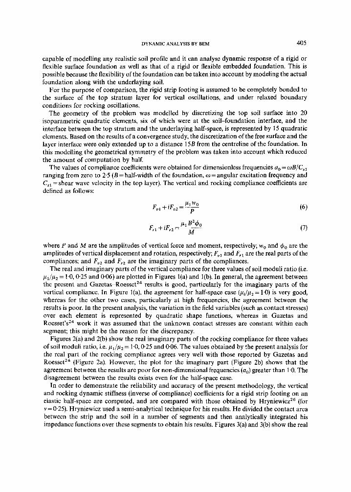
The real and imaginary parts of the vertical compliance for three values of soil moduli ratio (i.e. pl/p2 = 1.0,0.25 and 0.06) are plotted in Figures l(a) and l(b). In general, the agreement between the present and Gazetas -R~esse t~~ results is good, particularly for the imaginary parts of the vertical compliance. In Figure l(a), the agreement for half-space case ( p i / p 2 = 1.0) is very good, whereas for the other two cases, particularly at high frequencies, the agreement between the results is poor. In the present analysis, the variation in the field variables (such as contact stresses) over each element is represented by quadratic shape functions, whereas in Gazetas and Roe~set’s,~ work it was assumed that the unknown contact stresses are constant within each segment; this might be the reason for the discrepancy.

Figures 2(a) and 2(b) show the real imaginary parts of the rocking compliance for three values of soil moduli ratio, i.e. p1/p2 = 1.0,0.25 and 0.06. The values obtained by the present analysis for the real part of the rocking compliance agrees very well with those reported by Gazetas and RoessetZ4 (Figure 2a). However, the plot for the imaginary part (Figure 2b) shows that the agreement between the results are poor for non-dimensional frequencies (ao) greater than 1.0. The disagreement between the results exists even for the half-space case.

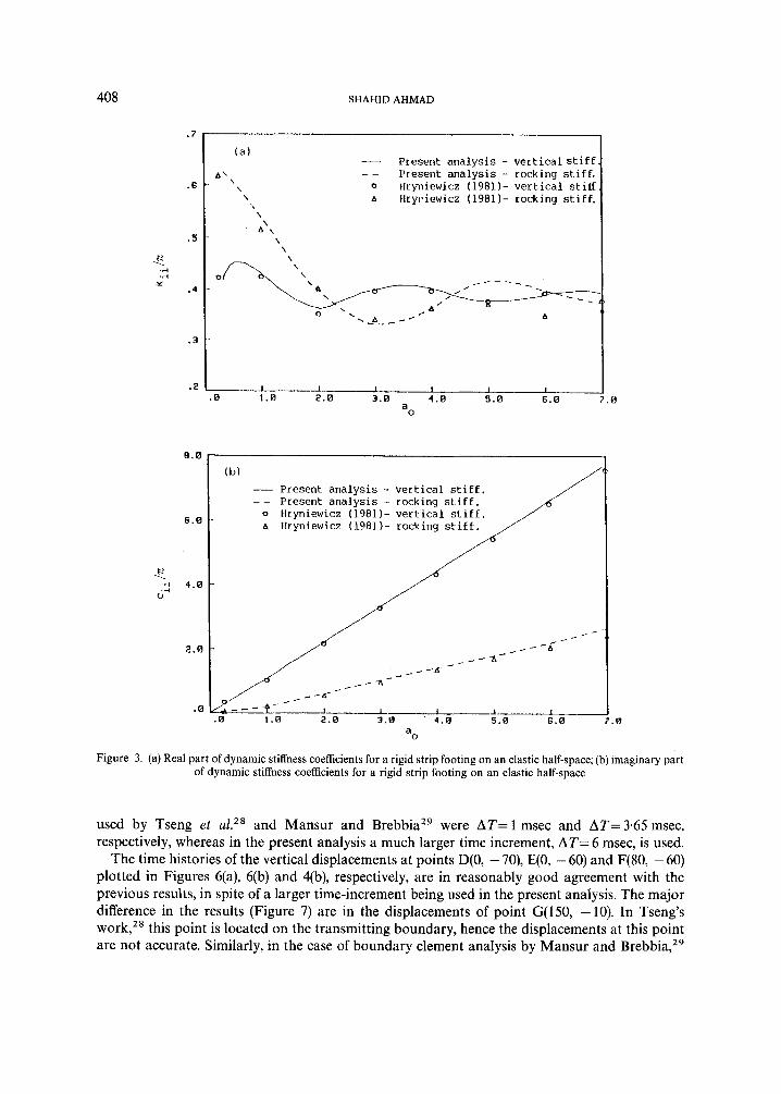
In order to demonstrate the reliability and accuracy of the present methodology, the vertical and rocking dynamic stiffness (inverse of compliance) coefficients for a rigid strip footing on an elastic half-space are computed, and are compared with those obtained by Hryniewicz26 (for v = 0.25). Hryniewicz used a semi-analytical technique for his results. He divided the contact area between the strip and the soil in a number of segments and then analytically integrated his impedance functions over these segments to obtain his results. Figures 3(a) and 3(b) show the real

406 SHAHID AHMAD

. 4

2 .2 ftr

.0

0

A 0

b

(a)

0

-.2 .00 .50 1 . 0 0 1.50 2 .00

aO

. 4

2

( b ) - Present analysis (ul/v2 = 1.0 i - - Present analysis (11 /II = 0.25) . . . . . , . . Present analysis (v : /v i = 0.06)

0 Gazetas-Roesset (p1/p2 = 0.06)

0 Gazetas-Roesset ( p ,/v = 1 . 0 ) A Gazetas-Roesset (vl/v2 = 0.25)

(. o.., . . .. .

.0 I I I I I .OO . 5 0 I .E0 1.50 2.00

a

5 0

I

5 0

Figure 1. (a) Vertical compliances (real part); (b) vertical compliances (imaginary part)

and imaginary parts of the stiffness coefficients. From these figures, it can be seen that the agreement between the two results is very good for low to high frequencies (up to a, = 4.0). For very high frequencies, Hryniewicz’sZ6 assumption that the contact stresses are constant within each segment of the contact area leads to small errors in his results.

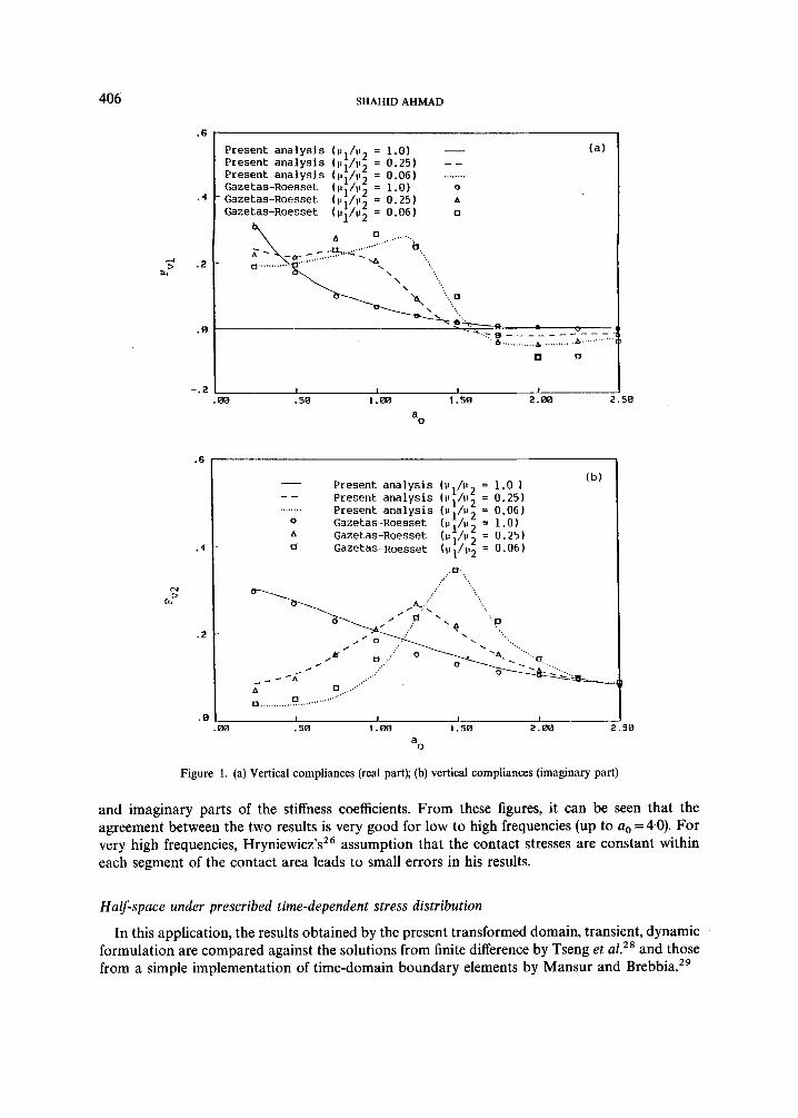
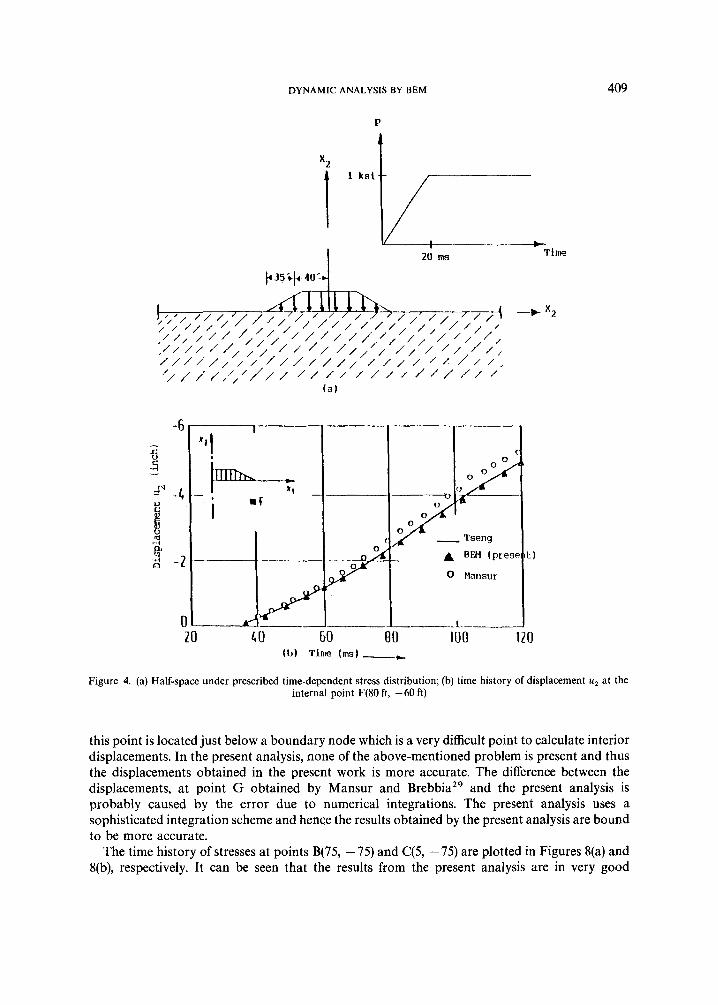
Half-space under prescribed time-dependent stress distribution

In this application, the results obtained by the present transformed domain, transient, dynamic formulation are compared against the solutions from finite difference by Tseng et aLZ8 and those from a simple implementation of time-domain boundary elements by Mansur and Brebbia.”

DYNAMIC ANALYSIS BY BEM 407

.6

-4 h> . 4

.2

- -- .... ....

Present analysis (pl/p2 = 1.0) Present analysis ( ~ I ~ / \ I ~ =_ 0 . 2 5 ) Present analysis ( ~ ~ , / t i ~ - 0 . 0 6 ) Gazetas-Roesset ( I I ~ / I I ~ = 1.0)

A Gazetas-Roesset (p1/p2 = 0 . 2 5 ) 0 Gazetas-Roesset . .. ...'..

- ---* _....... - n .......... ..

(a)

.0 1 I I I I .00 .50 1 .BB 1.50 2 .00

0

. e

.6

N > ru

. 4

. 2

.t

- Present analysis (11 /P 1.0) <- - Present analysis ( p 1 / p 2 0 . 2 5 ) ........ Present analysis (v1/p2 = 0.06)

Gazetas-Roesset (iI:/p: = 1.0) A Gazetas-Roesset ( l l l / v 2 1 0 . 2 5 ) 0 Gazetas-Roesset (v1/p2 - 0.06)

(b)

50

50

Figure 2. (a) Rocking compliances (real part); (b) rocking compliances (imaginary part)

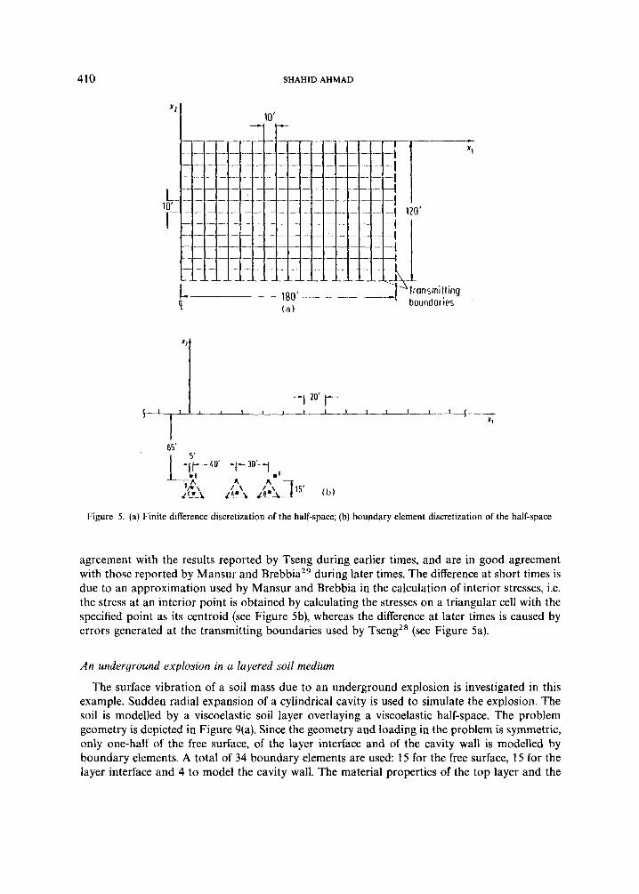
The problem to be analysed is depicted in Figure 4(a). The half-space was initially at rest and then a part of its surface is disturbed by a vertical pressure which is continuous in both time and space. Tseng used a transmitting boundary along with a generalized lumped parameter model to analyse this problem. Figure 5(a) shows the finite difference model used by Tseng and Figure 5(b) shows the BEM model used by Mansur. The BEM model for the present analysis is similar to that used by Mansur.

The material properties of the half-space are: modulus of elasticity E = 200 ksi, Poisson's ratio v=O.15 , and mass density p = 1.9534 x 10-41b-sec2/in4. For this problem, the time increments

408

.7

.6

.5

K \

.r( .r(

Y . 4

.3

. 2

SHAHID AHMAD

(a) Present analysis - vertical stiff Present analysis - rocking stiff.

\ 0 Hryniewicz (1981)- vertical stiff \ A Hryi.iewicz (1981)- rocking stiff.

- - -

A'\ -

\ \

A \ - \

\

- - - - - - 0 0 % -- - - -

A' 0 '\

\ -A- - - A

-

I I I 1 I I

I

1.a

8 .0

6 . 0

e \

.rl 4 . 0 6''

2 . 0

.0

( b ) - Present analysis - vertical stiff. _ _ Present analysis - rocking stiff. o llryniewicz (1981)- vertical stiff. A Hryniewicz (1981)- rocking stiff.

a

Figure 3. (a) Real part of dynamic stiffness coefficients for a rigid strip footing on an elastic half-space; (b) imaginary part of dynamic stiffness coefficients for a rigid strip footing on an elastic half-space

used by Tseng et a1.28 and Mansur and Brebbia29 were AT= 1 msec and AT= 3.65 msec, respectively, whereas in the present analysis a much larger time increment, AT= 6 msec, is used.

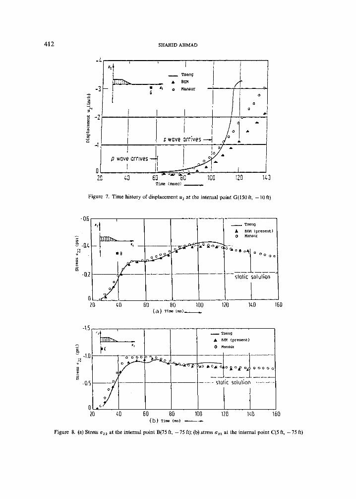
The time histories of the vertical displacements at points D(0, - 70), E(0, - 60) and F(80, - 60) plotted in Figures 6(a), 6(b) and 4(b), respectively, are in reasonably good agreement with the previous results, in spite of a larger time-increment being used in the present analysis. The major difference in the results (Figure 7) are in the displacements of point G(150, -10). In Tseng's work,28 this point is located on the transmitting boundary, hence the displacements at this point are not accurate. Similarly, in the case of boundary element analysis by Mansur and Brebbia,29

DYNAMIC ANALYSIS BY BEM

A x2

1

409

c 1 r

ksi-/,

Figure 4. (a) Half-space under prescribed time-dependent stress distribution; (b) time history of displacement ti2 at the internal point F(80 ft, -60 ft)

this point is located just below a boundary node which is a very difficult point to calculate interior displacements. In the present analysis, none of the above-mentioned problem is present and thus the displacements obtained in the present work is more accurate. The difference between the displacements, at point G obtained by Mansur and Brebbia29 and the present analysis is probably caused by the error due to numerical integrations. The present analysis uses a sophisticated integration scheme and hence the results obtained by the present analysis are bound to be more accurate.

The time history of stresses at points B(75, - 75) and C(5, - 75) are plotted in Figures 8(a) and 8(b), respectively. It can be seen that the results from the present analysis are in very good

410 SHAHID A H M A D

10' -1 I-

Figure 5. (a) Finite difference discretization of the half-space; ) boundary element discretization of the ..ilf-space

agreement with the results reported by Tseng during earlier times, and are in good agreement with those reported by Mansur and Brebbia29 during later times. The difference at short times is due to an approximation used by Mansur and Brebbia in the calculation of interior stresses, i.e. the stress at an interior point is obtained by calculating the stresses on a triangular cell with the specified point as its centroid (see Figure 5b), whereas the difference at later times is caused by errors generated at the transmitting boundaries used by Tseng2* (see Figure 5a).

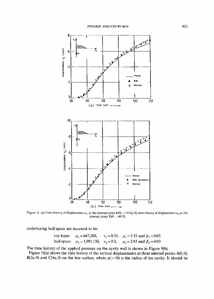
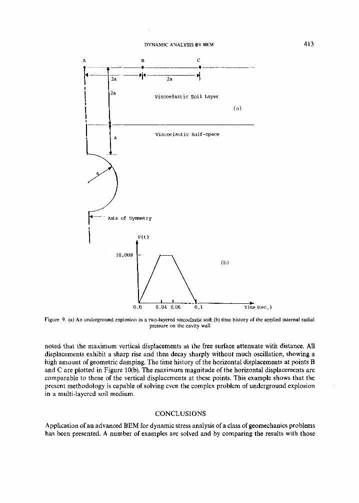
An underground explosion in a layered soil medium

The surface vibration of a soil mass due to an underground explosion is investigated in this example. Sudden radial expansion of a cylindrical cavity is used to simulate the explosion. The soil is modelled by a viscoelastic soil layer overlaying a viscoelastic half-space. The problem geometry is depicted in Figure 9(a). Since the geometry and loading in the problem is symmetric, only one-half of the free surface, of the layer interface and of the cavity wall is modelled by boundary elements. A total of 34 boundary elements are used: 15 for the free surface, 15 for the layer interface and 4 to model the cavity wall. The material properties of the top layer and the

DYNAMIC ANALYSIS BY BEM 41 1

20 40 60 80 I00 120 ( a ) Time (rns) -

( b ) Time (m)-

Figure 6. (a) Time history of displacement u2 at the internal point D(0, -70 ft); (b) time history of displacement tit at the internal point E(0, -60 ft)

underlaying half-space are assumed to be:

top layer: pl =647,200, v1 =0.35, p1 = 3.25 and B1 =0.05 half-space: p 2 = 1,991,150, V2=0.3 , p2=2.85 and B2=0*03

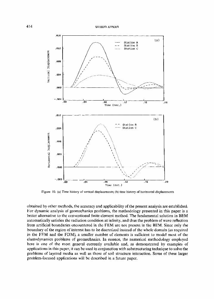
The time history of the applied pressure on the cavity wall is shown in Figure 9(b). Figure 10(a) shows the time history of the vertical displacements at three selected points A(O,O),

B(2a, 0) and C(4a, 0) on the free surface, where a( = 10) is the radius of the cavity. It should be

412 SHAHlD AHMAD

b I I - 4 -

- Tseng & BM 0 m s u r

t /- -3 - I

n .,

0

c i g -2

1

i: - - 0

0 A I I I aN

01

m - s wave ar r i ves 4 P - la

I -1

p wave arrives

100 120 1co 0 * I 20 LO

Figure 7. Time history of displacement u2 at the internal point G(150 ft, - 10 ft)

20 60 eo 100 120 110 160 ( a ) Time (ins)-

- Tseng A BEN (present)

XI 0 Mansur - .r( a - -1.0

e 0

In 0

N N

v) 0 -0.5 slotic solution -

0 -' 20 LO 60 80 100 120 140 160

(b) Tine (ms) - Figure 8. (a) Stress (rZ2 at the internal point B(75 ft, -75 ft); (b) stress (rz2 at the internal point C(5 ft, -75 ft)

DYNAMIC ANALYSIS BY BEM 413

Figure 9. (a) An underground explosion in a two-layered viscoelastic soil; (b) time history of the applied internal radial pressure on the cavity wall

noted that the maximum vertical displacements at the free surface attenuate with distance. All displacements exhibit a sharp rise and then decay sharply without much oscillation, showing a high amount of geometric damping. The time history of the horizontal displacements at points B and C are plotted in Figure 10(b). The maximum magnitude of the horizontal displacements are comparable to those of the vertical displacements at these points. This example shows that the present methodology is capable of solving even the complex problem of underground explosion in a multi-layered soil medium.

CONCLUSIONS

Application of an advanced BEM for dynamic stress analysis of a class of geomechanics problems has been presented. A number of examples are solved and by comparing the results with those

414

I I t I

.OO . 0 4 .09 .I2 . 16 .20 Time (sec.)

.012

.m9

.006

. BE13

. 0 0 E

-.m3

( b )

Station B Station C

,...... - - . '.. . . , . . . . . . . . .

Figure 10. (a) Time history of vertical displacements; (b) time history of horizontal displacements

obtained by other methods, the accuracy and applicability of the present analysis are established. For dynamic analysis of geomechanics problems, the methodology presented in this paper is a better alternative to the conventional finite element method. The fundamental solution in BEM automatically satisfies the radiation condition at infinity, and thus the problem of wave reflection from artificial boundaries encountered in the FEM are not present in the BEM. Since only the boundary of the region of interest has to be discretized instead of the whole domain (as required in the FEM and the FDM), a smaller number of elements is sufficient to model most of the elastodynamics problems of geomechanics. In essence, the numerical methodology employed here is one of the most general currently available and, as demonstrated by examples of applications in this paper, it can be used in conjunction with substructuring technique to solve the problems of layered media as well as those of soil-structure interaction. Some of these larger problem-focused applications will be described in a future paper.

DYNAMIC ANALYSIS BY BEM 41 5

ACKNOWLEDGEMENTS

The author wishes to record his gratitude to Professor P. K. Banerjee of SUNYAB and Dr. R. B. Wilson of Pratt and Whitney for several useful discussions during the course of this work.

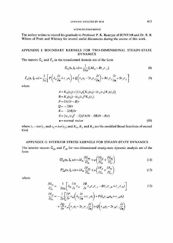
APPENDIX I: BOUNDARY KERNELS FOR TWO-DIMENSIONAL STEADY-STATE DYNAMICS

The tensors cij and Fij in the transformed domain are of the form

1 Cij(x, 5, w) = ~ [Ad,, - Br,ir, , ] 2XP

1 +Rr,ir,ji'n+Sr,ir,j ar

where

where z1 = iwr/c, and z2 = iwr/c,; and K O , K , and K , are the modified Bessel functions of second kind.

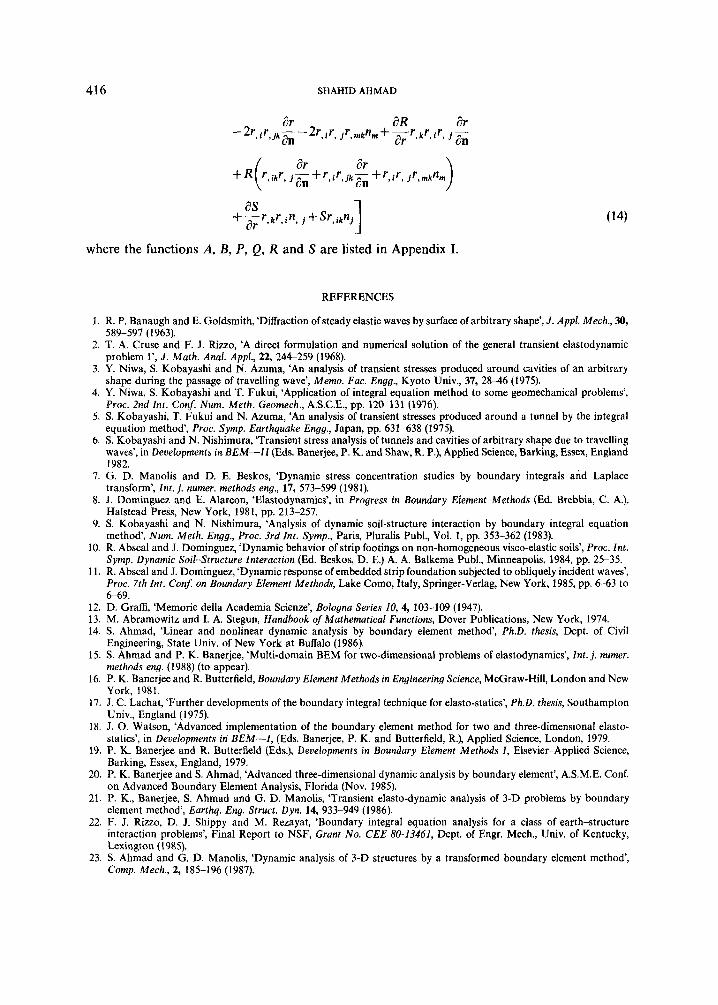
APPENDIX 11: INTERIOR STRESS KERNELS FOR STEADY-STATE DYNAMIC§

The interior tensors Gijk and Fijk for two-dimensional steady-state dynamic analysis are of the form

where

1 a A aB j-B(r,,r, jk+r, jr,ik)

t aP - aFij ~ - - - 2n [- dr rik ( d i j g + r, + P(dijr,mknm + r, jkni) a c k

an

416 SHAHID AHMAD

Br aR ar -2r , i r . - -2r , i r9 j r ,mknm+-r ,kr , i r , j -

9 Jk an ar an

where the functions A, B, P, Q, R and S are listed in Appendix I.

REFERENCES

1. R. P. Banaugh and E. Goldsmith, ‘Diffraction of steady elastic waves by surface of arbitrary shape’, J . Appl. Mech., 30,

2. T. A. Cruse and F. J. Rizzo, ‘A direct formulation and numerical solution of the general transient elastodynamic problem 1’, J. Math. Anal. Appl., 22, 244-259 (1968).

3. Y. Niwa, S. Kobayashi and N. Azuma, ‘An analysis of transient stresses produced around cavities of an arbitrary shape during the passage of travelling wave’, Memo. Fac. Engg., Kyoto Univ., 37, 28-46 (1975).

4. Y. Niwa, S. Kobayashi and T. Fukui, ‘Application of integral equation method to some geomechanical problems’, Proc. 2nd Inf. Con$ Num. Me&. Geomech., A.S.C.E., pp. 12&131 (1976).

5. S. Kobayashi, T. Fukui and N. Azuma, ‘An analysis of transient stresses produced around a tunnel by the integral equation method‘, Proc. Symp. Earthquake Engg., Japan, pp. 631438 (1975).

6. S. Kobayashi and N. Nishimura, ‘Transient stress analysis of tunnels and cavities of arbitrary shape due to travelling waves’, in Developments in BEM-I2 (Eds. Banerjee, P. K. and Shaw, R. P.), Applied Science, Barking, Essex, England 1982.

7. G. D. Manolis and D. E. Beskos, ‘Dynamic stress concentration studies by boundary integrals and Laplace transform’, Int. j . numer. methods eng., 17, 573-599 (1981).

8. J. Dominguez and E. Alarcon, ‘Elastodynamics’, in Progress in Boundary Element Methods (Ed. Brebbia, C. A,), Halstead Press, New York, 1981, pp. 213-257.

9. S. Kobayashi and N. Nishimura, ‘Analysis of dynamic soil-structure interaction by boundary integral equation method’, Num. Meth. Engg., Proc. 3rd Int. Symp., Paris, Pluralis Publ., Vol. 1, pp. 353-362 (1983).

10. R. Abscal and J. Dominguez, ‘Dynamic behavior of strip footings on non-homogeneous visco-elastic soils’, Proc. Int. Symp. Dynamic Soil-Structure Interaction (Ed. Beskos, D. E.) A. A. Balkema Publ., Minneapolis, 1984, pp. 25-35.

11. R. Abscal and J. Dominguez, ‘Dynamic response of embedded strip foundation subjected to obliquely incident waves’, Proc. 7th Int. Con$ on Boundary Element Methods, Lake Como, Italy, Springer-Verlag, New York, 1985, pp. 6-63 to 6 6 9 .

589-597 (1963).

12. D. Graffi, ‘Memorie della Academia Scienze’, Bologna Series 10, 4, 103-109 (1947). 13. M. Abramowitz and I. A. Stegun, Handbook of Mathematical Functions, Dover Publications, New York, 1974. 14. S. Ahmad, ‘Linear and nonlinear dynamic analysis by boundary element method’, Ph.D. thesis, Dept. of Civil

Engineering, State Univ. of New York at Buffalo (1986). 15. S. Ahmad and P. K. Banerjee, ‘Multi-domain BEM for two-dimensional problems of elastodynamics’, Int. j . numer.

methods eng. (1988) (to appear). 16. P. K. Banerjee and R. Butterfield, Boundary Element Methods in Engineering Science, McGraw-Hill, London and New

York, 1981. 17. J . C. Lachat, ‘Further developments of the boundary integral technique for elasto-statics’, Ph.D. thesis, Southampton

Univ., England (1975). 18. J. 0. Watson, ‘Advanced implementation of the boundary element method for two and three-dimensional elasto-

statics’, in Developments in BEM-I, (Eds. Banerjee, P. K. and Butterfield, R.), Applied Science, London, 1979. 19. P. K. Banerjee and R. Butterfield (Eds.), Developments in Boundary Element Methods I , Elsevier-Applied Science,

Barking, Essex, England, 1979. 20. P. K. Banerjee and S. Ahmad, ‘Advanced three-dimensional dynamic analysis by boundary element’, A.S.M.E. Conf.

on Advanced Boundary Element Analysis, Florida (Nov. 1985). 21. P. K., Banerjee, S. Ahmad and G. D. Manolis, ‘Transient elasto-dynamic analysis of 3-D problems by boundary

element method‘, Earthq. Eng. Struct. Dyn. 14, 933-949 (1986). 22. F. J. Rizzo, D. J. Shippy and M. Rezayat, ‘Boundary integral equation analysis for a class of earth-structure

interaction problems’, Final Report to NSF, Grant No. CEE 80-13461, Dept. of Engr. Mech., Univ. of Kentucky, Lexington (1985).

23. S. Ahmad and G. D. Manolis, ‘Dynamic analysis of 3-D structures by a transformed boundary element method‘, Camp. Mech., 2, 185-196 (1987).

DYNAMIC ANALYSIS BY BEM 41 7

24. G. Gazetas and J. M. Roesset, ‘Forced vibrations of strip footings on layered soils’, Meth. Struct. Anal., A.S.C.E., 1,

25. G. Gazetas and J. M. Roesset, ‘Vertical vibrations of machine foundation’, J . Geotech. Eng. Dio., lOS(GT12),

26. Z. Hryniewicz, ‘Dynamic response of a rigid strip on an elastic half-space’, Comp. Meth. in Appl. Mech. Engr., 25,

27. S . Mukherjee, Boundary Elements in Creep and Fracture, Applied Science, London, 1982. 28. M. N. Tseng and A. R. Robinson, ‘A transmitting boundary for finite difference analysis of wave propagation in

29. W. J. Mansur and C. A. Brebbia, ‘Transient elastodynamics’, in Topics in Boundary Element Research, Vol. 2,

30. J. J. Dongarra, U N P A C K User’s Guide, SIAM, Philadelphia, PA, 1979. 31. C. C. Spyrakos, ‘Dynamic response of strip-foundation by the time domain BEM-FEM method‘, Ph.D. thesis, Univ. of

32. J. M. Rice and M. H. Sadd, ‘Propagation and scattering of SH waves in semi-infinite domains using a time-dependent

33. Y. Niwa, S. Kobayashi and T. Fukui, ‘Application of integral equation method to some geomechanical problems’,

34. F. Durbin, ‘Numerical inversion of Laplace transforms: an efficient improvement to Dubner and Abates method’,

115-131 (1976).

1435-1454 (1979).

355-364 (1981).

solids’, Project No. N R 064-183, Univ. of Illinois, Urbana (1975).

Springer-Verlag, New York, 1985.

Minnesota, Minneapolis (1984).

boundary element method’, J. Appl. Mech., 51, 641-645 (1984).

Proc. 2nd Int. Con$ Num. Meth. in Geomech., A.S.C.E., 1976, pp. 12G131.

Comput. J., 17, 371-376 (1974).