Journal of Computational Physics 192 (2003) 105–123

www.elsevier.com/locate/jcp

A fictitious domain/finite element method for particulate flows

C. Diaz-Goano a,*, P.D. Minev b, K. Nandakumar a

a Department of Chemical and Materials Engineering, 536 Chemical and Materials Engineering Building,

University of Alberta, Edmonton, Alb., Canada T6G 2G6b Department of Mathematical and Statistical Sciences, University of Alberta, Edmonton, Alb., Canada T6G 2G1

Received 25 November 2002; received in revised form 5 May 2003; accepted 24 June 2003

Abstract

The paper presents a finite element method for the direct numerical simulation of 3D incompressible fluid flows with

suspended rigid particles. It uses the fictitious domain approach extending the fluid domain into the domain occupied

by the particles. Although the idea for the present formulation came from the fictitious domain formulation of Glo-

winski et al. [J. Comput. Phys. 169 (2001) 363] it finally yielded a new scheme which allows for a more efficient inte-

gration of the system of equations and which is easier to implement algorithmically. It also avoids the need to grid the

rigid particles and solves the entire problem on a single Eulerian grid. The spatial discretization is performed with

P2 � P1 finite elements but any other stable pair of approximations can be used. The present scheme is compared to a

second order scheme based on the approach in Glowinski et al. [loc. cit.] using the test case of a single sphere in a

viscous liquid. Its accuracy/costs performance is excellent.

� 2003 Elsevier B.V. All rights reserved.

AMS: 65N35; 65N22; 65F05; 35J05

Keywords: Finite element method; Fictitious domain method; Particulate flow

1. Introduction

The mathematical description of multiphase flows, similarly to the mathematical description of turbu-

lence, is still a significant challenge for the mathematicians and engineers working in this area. The models

based on the interpenetrating continua hypothesis suffer of similar closure problems as the Reynolds-

averaged turbulence models. Therefore, in the recent years some efforts were concentrated on the direct

simulation of multiphase flows which would allow, again similarly to the turbulence case, for a more ac-

curate solution of the closure problems. This is a very demanding computational task which requires the

development of new discretization techniques and computer implementations.

*Corresponding author. Tel.: +780-987-8745; fax: +780-987-5349.

E-mail addresses: carolina@ualberta.ca (C. Diaz-Goano), minev@ualberta.ca (P.D. Minev), kumar.nandakumar@ualberta.ca

(K. Nandakumar).

0021-9991/$ - see front matter � 2003 Elsevier B.V. All rights reserved.

doi:10.1016/S0021-9991(03)00349-8

106 C. Diaz-Goano et al. / Journal of Computational Physics 192 (2003) 105–123

Generally speaking, there are two main classes of methods for direct simulations of multiphase flows.

The first type are methods which discretize the Navier–Stokes equations on a fixed, Eulerian grid and move

the particles in this grid. Probably the most prominent work in this direction (in the case of flows with

distributed rigid particles) was done by a group of researchers from the Universities of Houston and

Minnesota (see [1,2] and the references therein). In the case of distributed fluid particles, a similar approach

was introduced by Tryggvason and collaborators (see [3]). The second type of methods uses moving grids

and usually requires remeshing and re-interpolation. Examples of such techniques are the one developed by

Hu [4] and Johnson and Tezduyar [5]. It is hard to judge and compare the merits of these two approaches.In our view, the first approach is more attractive because it allows for the use of structured grids which are

much more preferable in view of the parallelization of the algorithm. Moreover, it completely avoids the

need of a mesh generation in very complex domains which is also a challenging algorithmic problem.

Therefore, in a preliminary study we used the fictitious domain approach of [2] to develop a formally

second order (in space and time) finite element scheme (see [6]). Then we modified it, in an attempt to make

it more efficient and as a result we devised a new scheme, still based on the fictitious domains idea. The

numerical experiments showed a very satisfactory performance of this scheme. Its key novelty is that it

approximates both, the fluid velocity field and the Lagrange multiplier for imposition of the rigid bodymotion on the same fixed Eulerian grid. This allowed us to avoid the gridding of the rigid particles.

Moreover, using a properly weighted H1 norm for the imposition of the rigid body motion, we were able to

reduce the work for computing the fluid/rigid particles velocities and enhance the stability of the algorithm

(this was verified only experimentally). The derivation of this scheme and its assessment is a subject of the

rest of this paper.

In Section 2, we discuss the fictitious domain approach and the Distributed Lagrange Multipliers (DLM)

method of Glowinski et al. [2], and derive the starting formulation for the present scheme. There we also

describe the splitting algorithm and the finite element discretization with P2 � P1 elements. In Section 3, wecompare the results of the simulation of a rigid sphere falling in a viscous liquid with available experimental

data and results obtained with the scheme described in [6]. In addition, two other simulations are presented

there: a spherical particle in a rotating cylinder and two spherical particles settling under gravity and in-

teracting with each other (drafting, kissing and tumbling). Finally, the conclusions are summarized in

Section 4.

2. A fictitious domains formulation using a global Lagrange multiplier

2.1. Governing equations

We consider a bounded domain X1 with an external boundary C filled with a Newtonian liquid of density

q1 and viscosity l1. Within this liquid we consider n rigid particles occupying a domain X2 ¼Sn

i¼1 X2;i and

having densities q2;i; i ¼ 1; . . . ; n. Let us also denote the interface between X1 and X2 by R and the entire

domain filled with the fluid and the particles by X ¼ X1 [ X2. The equations of motion of the fluid in X1 are

the Navier–Stokes equations (presented here in a dimensionless, stress-divergence form)

q1

Duu1

Dt¼ r � rr1; r � uu1 ¼ 0 in X1; ð1Þ

where uu1 is the velocity, D=Dt denotes the full derivative in time (including the advection terms), rr1 is the

stress tensor and q1 is the fluid density. rr1 is defined as usual as rr1 ¼ pp1dþ 2l1D½uu1� with pp1 being

the pressure in the liquid phase, D½uu1� ¼ 0:5½ruu1 þ ðruu1ÞT� being the rate-of-strain tensor and d being the

Kronecker tensor. The boundary conditions on C are not of a concern for the present method and therefore

we assume the simplest case of homogeneous Dirichlet conditions. On the internal boundary of X1, R, we

C. Diaz-Goano et al. / Journal of Computational Physics 192 (2003) 105–123 107

presume a no-slip condition for the velocity. The problem requires an initial condition for the velocity

which we presume to be in the form uu1ðx; 0Þ ¼ u0, r � u0 ¼ 0. The equations of motion of a rigid particle

are usually written in terms of the velocity of its centroid Ui and its angular velocity xi, i ¼ 1; . . . ; n. Theyread

MidUi

dt¼ Migþ Fi; ð2Þ

Iidxi

dtþ xi � Iixi ¼ Ti; ð3Þ

where Mi is the particle mass, g is the gravity acceleration, Fi is the total hydrodynamic force acting on it, Iiis its tensor of inertia, and Ti is the hydrodynamic torque about its center of mass.

2.2. Fictitious domain approach and the DLM method

Before the presentation of the new technique, we would like to briefly review the fictitious domain

approach and its implementation in the DLM method of Glowinski et al. [2]. The fictitious domain ap-proach extends the fluid equations of motion into the domain occupied by the particles, X2, and imposes the

rigid body motion described by Eqs. (2) and (3) onto the restriction of the so extended velocity field. The

DLM method enforces this constraint by introducing localized (distributed within each particle) Lagrange

multipliers fi, and relaxing the constraint by means of a weak formulation. After an extensive manipulation

of the governing equations of both, the liquid and the particle phases, the following combined variational

principle is derived in [2]: 1 Find u 2 H10ðXÞ; p 2 L2

0ðXÞ ¼ fq 2 L2ðXÞ jRX qdx ¼ 0g; f 2 H1ðX2Þ;U 2 R3, and

x 2 R3 that satisfy:ZXq1

Du

Dt

�� g

�� vdxþ ð1� q1=q2Þ M

dU

dt

��� g

�� Vþ I

dx

dt� n�þZXr : D½v�dx

¼ hf; v� ðVþ n� rÞiX28v 2 H1

0ðXÞ; V 2 R3; n 2 R3; ð4Þ

ZXqr � udx ¼ 0 8q 2 L2ðXÞ; ð5Þ

hg; u� ðUþ x� rÞiX2¼ 0 8g 2 H1ðX2Þ; ð6Þ

u jt¼0¼ u0; U jt¼0¼ U0; x jt¼0¼ x0: ð7Þ

Here v, V and n are properly chosen test functions for the fluid velocity, particle velocity and the

particle angular velocity equations, r ¼ x� X with X being the coordinate vector of the centroid of the

particle, and r is a properly extended to X2 stress tensor. The fluid velocity is discretized on a fixed

(Eulerian) grid that covers the entire domain X and the Lagrange multiplier f is discretized on a

separate grid that covers the particle. The combined equations (4)–(7) are discretized in time and split

into the following substeps:

1 In [2], the combined equation is derived for the case of one particle only (Mi ¼ M , q2;i ¼ q2, Ui ¼ U, x ¼ xi, f ¼ fi), but its

generalization for the multiparticle case is straightforward.

108 C. Diaz-Goano et al. / Journal of Computational Physics 192 (2003) 105–123

2.2.1. Incompressibility constraint

At this substep, a fluid velocity field and pressure, based on the Eulerian grid, are computed so that the

velocity is divergence free (see [2, Eqs. (45) and (46)]). This is in fact a Darcy problem which is resolved in

[2] by means of an Uzawa/conjugate-gradient preconditioned iteration.

2.2.2. Advection–diffusion

At this substep, the incompressible fluid velocity is further advected and diffused (see [2, Eq. (47)]).

Further, the particle velocity and the position of its centroid are predicted [2, Eqs. (48) and (49)].

The first two substeps constitute a splitting algorithm for the Navier–Stokes equations which is very

similar to the so-called velocity-correction projection. The only difference is that in this algorithm, the

incompressibility constraint is strictly enforced via Uzawa iteration while the velocity-correction projection

method does only one step of this iteration using the same preconditioner (a homogeneous Neumannboundary value problem for the pressure Poisson equation). Since it has been proved that the velocity-

correction method achieves optimal error in time for the velocity (see [7]) there is no need for additional

iterations in the first substep since in the second substep the incompressibility of the fluid velocity is de-

stroyed anyway. It is further influenced in the next substep which enforces the rigid body motion.

Therefore, in [6], in the first two substeps we used a second order pressure-correction projection method

combined with the method of characteristics.

2.2.3. Rigid body constraint

This is the substep that enforces the side constraint, Eq. (6). It is done in a typical for such constraints

inner/outer iteration loop. The correction to the fluid velocity u is computed in the outer loop and then used

to compute the correction to the Lagrange multipliers f in the inner loop (see [2, Eqs. (62)–(74)]). The DLMmethod uses a conjugate gradient iteration for both, the inner and the outer loop. Note that in this inner/

outer loop, one needs to solve one linear system for the fluid velocity and one linear system for the re-

striction of f over each of the particle domains X2;i at each iteration step. It is precisely at this step where the

present technique differs most significantly from the DLM method. By using a globally rather than a locally

defined Lagrange multiplier and enforcing the constraint given by Eq. (6) with a properly weighted inner

product, it avoids the need to solve the linear systems over each of the particles. Instead, it solves just one

linear system for the globally defined Lagrange multiplier, whose size is equal to the size of the fluid velocity

system solved in the outer iteration of DLM. The savings in CPU time of the present procedure clearlygrow linearly with the number of particles. The memory for the storage of one extra global vector is usually

less than the memory for the storage of the additional connectivity tables and matrices for the Lagrange

multipliers of the DLM method (even for the case of one particle). Note that the matrices of the problem

for the global Lagrange multiplier in the present procedure are the same as the matrices of the problem that

defines the fluid velocity.

The new fictitious domain formulation and its numerical discretization are presented in the next two

subsections.

2.3. A new fictitious domain formulation

For the derivation of the new formulation, it is more convenient first to define a velocity field u2ðx; tÞwhich is continuous within the region occupied by any given particle, and zero in X1. Clearly, u2 2 L2ðXÞ,and u2ðx; tÞjXi

¼ UiðtÞ þ xiðtÞ � ðx� XiðtÞÞ. The momentum equation for the restriction of u2 on X2;i, u2;i,

can be written in the following integral form:

d

dt

ZX

q2;iu2 dX ¼ZX

ðq2;i � q1ÞgdXþZoX

rr1ni ds ð8Þ

2;i 2;i 2;i

C. Diaz-Goano et al. / Journal of Computational Physics 192 (2003) 105–123 109

with ni being the outward normal to the surface of the ith particle. The last term in this equation represents

the total hydrodynamic force acting on the surface of the ith particle. Let us denote by r1 the continuous

extension of the stress rr1 over the entire domain X. Such an extension can always be constructed and this is

the basis for the different fictitious domain methods that are proposed in the literature. Then using the

divergence theorem we can rewrite Eq. (8) in the following form:

ZX2;i

D

Dtðq2;iu2ÞdX ¼

ZX2;i

ðq2;i � q1ÞgdXþZX2;i

r � r1 dX: ð9Þ

A natural way to extend the stress tensor in X2;i is to assume that it is Newtonian and extend the velocity

field uu1 to u1 such that u1jX1¼ uu1, the pressure to some p1 such that p1jX1

¼ pp1, and write r � r1 ¼ �rp1 þl1r2u1. Then, Eq. (9) can be rewritten as

ZX2;i

D

Dtðq2;iu2;iÞdX ¼

ZX2;i

ðq2;i � q1ÞgdXþZX2;i

��rp1 þ l1r2u1

�dX: ð10Þ

Now if we adopt the notation

F ¼ �q1Du1Dt þ l1r2u1 �rp1 in X2;i; i ¼ 1; . . . ; n;

0 in X1

�ð11Þ

the equation for the ith particle momentum becomes

ZX2;i

D

Dtðq2;iu2 � q1u1ÞdX ¼

ZX2;i

½ðq2;i � q1Þgþ F�dX: ð12Þ

Because of Eq. (11), we can now extend the momentum equation (1) to the entire X as

q1

Du1Dt

¼ �rp1 þ l1r2u1 � F; r � u1 ¼ 0 in X: ð13Þ

The additional force per unit volume F in this equation can be interpreted as the interaction force between

the two phases. As discussed by Glowinski et al. [2] it enforces the rigid body motion onto the fluid velocity

field within each of the particles. If we impose this additional constraint onto u1, i.e.,

u1 ¼ u2 in X2;i ð14Þ

then momentum equation for the ith particle, Eq. (12), can be written asZX2;i

D

Dt½ðq2;i � q1Þu2�dX ¼

ZX2;i

½ðq2;i � q1Þgþ F�dX: ð15Þ

Now we recall that u2 is a rigid body velocity field, i.e., u2ðx; tÞjXi¼ UiðtÞ þ xiðtÞ � ðx� XiðtÞÞ. Then Eq.

(15) implies the following equation for Ui

DMidUi

dt¼ DMigþ

ZX2;i

FdX; ð16Þ

where DMi ¼RX2;i

ðq2;i � q1ÞdX. The angular velocity xi can be recovered from the no-slip boundary con-

dition on the surface of the ith particle. It reads

UiðtÞ þ xiðtÞ � ðx� XiðtÞÞ ¼ u1 on oX2;i:

110 C. Diaz-Goano et al. / Journal of Computational Physics 192 (2003) 105–123

Then clearlyZoX2;i

ðxiðtÞ � ðx� XiðtÞÞ � nds ¼ZoX2;i

ðu1 �UiðtÞÞ � nds

which yields, using the Stokes theorem, that

xiðtÞVXi ¼ 0:5

ZX2;i

r� ðu1 �UiðtÞÞdX;

where VXi is the volume of the ith particle. Finally, the strong formulation of the present version of the

fictitious domain method is given by

q1

Du1Dt

¼ �rp1 þ l1r2u1 � F; r � u1 ¼ 0 in X; ð17Þ

DMidUi

dt¼ DMigþ

ZX2;i

FdX; i ¼ 1; . . . ; n; ð18Þ

xiðtÞVXi ¼ 0:5

ZX2;i

r� ðu1 �UiðtÞÞdX; i ¼ 1; . . . ; n; ð19Þ

UiðtÞ þ xiðtÞ � ðx� XiðtÞÞ ¼ u1 in X2;i; i ¼ 1; . . . ; n: ð20Þ

From this set of equations, it is clear that F is a term that enforces the constraint given by Eq. (20) onto u1and u2. It is non-zero only within the domain occupied by the particles and therefore it is closely related to

the distributed Lagrange multiplier of Glowinski et al. [2]. However, its impact on the fluid velocity field is

global, over the entire domain, due to Eq. (17). This led us to the idea to define another, global Lagrange

multiplier, k, which is related to F through the following boundary value problem

� akþ l1r2k ¼ F in X;

k ¼ 0 on C;ð21Þ

where a > 0 is a constant to be defined later. This is a well-posed problem for F 2 L2, and it is more con-

venient to use its unique solution to impose the constraint of Eq. (20). The benefit of using it, is that it has the

same regularity as u1 and therefore they can be discretized on the same grid (i.e., discretization space). With

this definition of k and a proper choice for a, as it will become clear in the following section, we can sig-

nificantly decrease the computational expenses for the iterative solution of the system of equations (17)–(20).

Substituting F from Eq. (21) into Eqs. (17)–(20) we obtain the following system which will be used

further to compute u1, Ui and xi

q1

Du1 ¼ �rp1 þ l1r2u1 þ ak� l1r2k; r � u1 ¼ 0 in X; ð22Þ

Dt

DMidUi

dt¼ DMig�

ZX2;i

akdX� l1

ZoX2;i

ok

onds; i ¼ 1; . . . ; n; ð23Þ

VXixi ¼ 0:5

ZX2;i

r� ðu1 �UiÞdX; i ¼ 1; . . . ; n; ð24Þ

C. Diaz-Goano et al. / Journal of Computational Physics 192 (2003) 105–123 111

UiðtÞ þ xiðtÞ � ðx� XiðtÞÞ ¼ u1 in X2;i; i ¼ 1; . . . ; n: ð25Þ

Note that in the second equation we have integrated r2k by parts. Note also that this choice for k is similar

to the choice of Lagrange multiplier in [2] if the inner product for imposition of the rigid body constraint is

chosen to be the H1 inner product. In the present case, however, k is defined over the entire computational

domain while in [2] it is defined only locally, within the areas occupied by the particles. The global Lagrange

multiplier will allow for a change in the fictitious domain method as proposed in [1,2], which generally

increases the efficiency of the method and simplifies it (see the following section).

In addition to the system of equations (22)–(25) we also need to solve an equation for the position of the

center of mass of each particle which reads

oXi

ot¼ Ui; i ¼ 1; . . . ; n:

Remark 1. An idea for using the fluid velocity grid points inside the particles together with surface control

points for imposition of the rigid body motion is given in [1, Remark 6.4]. The suggestion there is to use

Dirac d-functions to span the Lagrange multipliers inside the particles.

Remark 2. Remark 7.3 of [1] suggests to compute the particles centroidal and angular velocities in a way

similar to the one suggested above.

2.4. Discretization procedure

We discretize the system of equations (22)–(25) using a finite element procedure although finite difference

or finite volume based procedures can also be used. Note that only Eqs. (22) and (25) require weak for-

mulations. Eqs. (23) and (24) are an ordinary differential and an algebraic equation. The overall problem is

in fact a Navier–Stokes problem with an additional constraint given by Eq. (25), and therefore we chose todiscretize it with a projection scheme (for u1 and p1) combined with an additional iteration for the impo-

sition of the rigid body constraint. The scheme is derived from the (formally) second order in time char-

acteristic/projection scheme described in [8]. In space we used P2 � P1 finite elements which resulted in a

formally second order spatial discretization for the velocity. The algorithm can be summarized in the

following four steps.

2.4.1. Substep 1 (advection)

The advective part of the system is integrated with the method of characteristics [8]. If x is an ap-

proximation of the foot of the characteristic originating at x then the advected velocity is given by~uun1ðxÞ ¼ un1ðxÞ; ~uun�1

1 ðxÞ ¼ un�11 ðxÞ. x is usually approximated with an Euler explicit scheme [8].

The center of mass of the ith particle is predicted explicitly as

Xp;nþ1i ¼ Xn�1

i þ 2dtUni ; ð26Þ

where dt is the time step.

2.4.2. Substep 2 (diffusion)

If we set s0 ¼ 3=ð2dtÞ, s1 ¼ �2=dt, s2 ¼ 1=ð2dtÞ, then this substep can be written as

q1s0u�1 � l1r2u�1 ¼ �q1ðs1~uun1 � s2~uu

n�11 Þ � rpn in X;

u� ¼ 0 on C:ð27Þ

1

112 C. Diaz-Goano et al. / Journal of Computational Physics 192 (2003) 105–123

2.4.3. Substep 3 (incompressibility)

s0 u��1�

� u�1�¼ �r pnþ1

1

�� pn1

�in X;

r � u��1 ¼ 0 in X;

u��1 � n ¼ 0 on C;

ð28Þ

where n being the outward normal to C.

2.4.4. Substep 4 (rigid body constraint)

The rigid body motion is imposed iteratively using the following iteration. Let us first set the 0th ap-proximation for knþ1, unþ1

1 , Unþ1i , xnþ1

i and unþ12 as

k0;nþ1 ¼ 0;

u0;nþ11 ¼ u��1 ;

s0U0;nþ1i ¼ �s1U

ni � s2U

n�1i þ g;

VXix0;nþ1i ¼ 0:5

ZXi

r� u0;nþ11 dX;

u0;nþ12 ¼ U0;nþ1

i þ x0;nþ1 � x�

� Xp;nþ1i

�:

We also need to set k1;nþ1 ¼ kn. If we denote the difference between two subsequent iterations for a quantity

Q by dQ, i.e., dQkþ1 ¼ Qkþ1 � Qk then the subsequent iterates are computed for kP 0 by

ðq1s0I � l1r2Þdukþ1;nþ11 ¼ aI � l1r2ð Þdkkþ1;nþ1 in X;

dukþ1;nþ11 ¼ 0 on C;

�ð29Þ

DMis0dUkþ1;nþ1i ¼ �

RX2;i

adkkþ1;nþ1 dXþ l1

RoX2;i

odkkþ1;nþ1

onds; i ¼ 1; . . . ; n;

VXixkþ1;nþ1i ¼ 0:5

RXir� ukþ1;nþ1

1 dX; i ¼ 1; . . . ; n;

ukþ1;nþ12 ¼ Ukþ1;nþ1

i þ xkþ1;nþ1i � x� Xp;nþ1

i

� �in X2;i; i ¼ 1; . . . ; n;

ukþ1;nþ12 ¼ 0 in X1

8>>>>><>>>>>:

ð30Þ

1þ q1q2;i�q1

� �aI � l1r2ð Þdkkþ2;nþ1 ¼ � q1s0I � l1r2ð Þ ukþ1;nþ1

1 � ukþ1;nþ12

� �in X2;i; i ¼ 1; . . . ; n;

1þ q1q2;i�q1

� �aI � l1r2ð Þdkkþ2;nþ1 ¼ 0 in X1;

dkkþ2;nþ1 ¼ 0 on C;

8>>><>>>:

ð31Þ

where I is the identity operator. Note that in the last set of equations which determines the incrementof k, we used the fact that u2 is a rigid body velocity field inside each particle and therefore r2u2 ¼ 0 in

X2;i.

Upon convergence for some k ¼ N we set unþ11 ¼ uNþ1;nþ1

1 , Unþ1i ¼ UNþ1;nþ1

i , xnþ1 ¼ xNþ1;nþ1, knþ1 ¼kNþ1;nþ1. The equation of the center of mass of the particles is solved with a second order predictor–cor-

rector procedure, the predictor being given by Eq. (26), and the corrector being given by

Xnþ1 ¼ Xn þ 0:5dt Unþ1�

þUn�: ð32Þ

i i i

C. Diaz-Goano et al. / Journal of Computational Physics 192 (2003) 105–123 113

Similarly to the iteration in [2], instead of the present (Richardson) iteration we can also adopt a conjugate

gradient type of iterative algorithm for imposition of the rigid body constraint. The numerical tests show

that only few iterations per time step of the present procedure are necessary to obtain very reasonable

results.

Note that in the above splitting algorithm only Eqs. (27)–(29) and (31) constitute boundary value

problems for PDEs and in order to discretize them with finite elements we need to derive proper weak

formulations. As it is usual for finite element projection schemes (see [9]) we choose u�1 to be inH10ðXÞ and p1

to be in H1ðXÞ. The final velocity of Substep 3, u��1 , is also projected onto H10ðXÞ as discussed in [9]. Since the

Lagrange multiplier k is a solution to a boundary value problem similar to the problem for u1, it is naturally

chosen to be in H10ðXÞ. Actually it plays the role of a correction to both, the fluid and particle velocities. Of

course, this correction will increase the divergence of the fluid field and in order to control better the di-

vergence of this correction one may decompose the interaction force F into a divergence free part, k, and a

curl free part, rp2, and define both to be a solution of a Stokes-like problem. This would require to do one

projection step for the additional pressure p2 at each iteration for imposition of the rigid body motion. The

present algorithm seems to be reasonably stable as it is, and therefore we did not try this more expensive

alternative. Note that the DLM method has the same problem with the enforcement of the incompress-ibility constraint since the incompressible velocity field produced at its first substep (unþ1=3 in the notations

of [2]) loses its incompressibility in the subsequent substeps of the spitting. The final field of this method

(unþ1 in the notations of [2]) is not incompressible but the incompressibility can also be enforced in the way

suggested above. In fact, the linear system for the fluid velocity that arises from the fictitious domain

approach can be written in the form

A LT KT

L 0 0

K 0 0

24

35 unþ1

pnþ1

knþ1

24

35 ¼

f0

0

24

35;

where A is the total velocity matrix (a linear combination of the mass and stiffness matrices), L is the di-vergence matrix and K is the coupling matrix between the fluid velocity and the Lagrange multiplier k (in

the present method it reduces to the velocity mass matrix). This problem can be considered as an extended

Stokes problem, and it can be resolved with a preconditioned inner/outer iteration similar to the one used to

solve the Stokes problem alone (Uzawa iteration). The preconditioner for the pressure equations can be

chosen to be a Laplace operator with homogeneous Neumann boundary conditions. The preconditioner for

the equations for knþ1 is given by Eq. (31). As a result of such an iteration both, the incompressibility and

the rigid body constraints will be imposed very strictly but it will require the solution of one pressure

Poisson problem and one problem of type of Eq. (31) in the inner step, and one problem involving the totalmatrix A in the outer step. This is an expensive procedure and the numerical results indicated that the

present splitting/iterative procedure produces very accurate results and it is reasonably stable. If the sta-

bility becomes a problem, it is recommendable that the pressure pnþ1 is corrected once more after Substep 4,

repeating Substep 3.

The weak formulations of Eqs. (27) and (28) are given by

Find u�1 2 H10ðXÞ such thatZ

Xq1s0u

�1v

�þ l1ru�1rv

�dX ¼ �

ZXq1ðs1~uun1:þ s2~uu

n�11 ÞvdXþ

ZXpn1r � vdX 8v 2 H1

0ðXÞ: ð33Þ

Find pnþ11 2 H1ðXÞ such that

ZXr pnþ1

1

�� pn1

�rqdX ¼ s0

ZXq1u

�1rqdX 8q 2 H1ðXÞ: ð34Þ

114 C. Diaz-Goano et al. / Journal of Computational Physics 192 (2003) 105–123

Find u��1 2 H10ðXÞ such that

ZXq1s0 u��1

�� u�1

�vdX ¼

ZXpnþ11 r � vdX 8v 2 H1

0ðXÞ: ð35Þ

As discussed in [9] the last step can be eliminated but it usually reduces the divergence of the so com-

puted velocity field. In the present context, since we do not control the divergence of the iterative correction

k, it is advisable to solve Eq. (35). Before we give the weak formulation of Eq. (31) we note that if we choose

a ¼ q1s0 the problem described by Eq. (29) can easily be resolved and the solution is

ukþ1;nþ11 ¼ uk;nþ1

1 þ ðkkþ1;nþ1 � kk;nþ1Þ:

Thus, this choice for a is very natural. Moreover, this choice yields an inner product for imposition of therigid body motion which is a compromise between the H1 and the L2 inner products, and given by

q1s0ð�; �Þ0 þ l1ðr�;r�Þ0 where ð�; �Þ0 denotes the usual L2 inner product. It recovers the L2 inner product in

the limit dt ! 0. It is precisely this trick, that makes the present algorithm more efficient compared to the

DLM method (including the stress formulation of the DLM method presented in [10]). Instead of solving

one global problem for the extended velocity u1 [2, Eq. (62)] and one local problem per particle [2, Eq. (65)],

in the present case it is necessary to solve only one global problem for k (Eq. (36) below) at each iteration

step for imposition of the rigid body constraint. The numerical results with the DLM version presented in

[6] and the present method seem to indicate that this choice for a also accelerates the convergence of thisiteration.

Finally, the weak formulation of Eq. (31) is given by

Find kkþ2;nþ1 2 H10ðXÞ such that

ZX

1

�þ q1

q2;i � q1

�q1s0dk

kþ2;nþ1v�

þ l1rdkkþ2;nþ1rv�dX

¼ �Xn

i¼1

ZX2;i

q1s0 ukþ1;nþ11

�� ukþ1;nþ1

2

�v�

Xn

i¼1

ZX2;i

l1r ukþ1;nþ11

�� ukþ1;nþ1

2

�rvdX

þ l1

Xn

i¼1

ZoX2;i

nr ukþ1;nþ11

�� ukþ1;nþ1

2

�vds 8v 2 H1

0ðXÞ: ð36Þ

The surface integral in the right-hand side is a result of the integration by parts of the Laplacian over eachof the particles. The numerical experience shows that this integral as well as the surface integral in the first

equation of (30) are usually very small and do not seem to alter significantly the results in case of spherical

particles. Therefore, they are not taken into account in the results of Section 3.

The formulation given by Eqs. (33)–(36) are discretized by means of P2 � P1 finite elements using P2

interpolation for the velocity and k and P1 interpolation for the pressure. The grid is a fixed tetrahedral

Eulerian grid that discretizes X. The resulting linear systems are solved by means of a parallel version of the

conjugate gradients method. To complete the discussion on the numerical algorithm, we need to specify the

quadrature rule that is used to compute the integrals in these formulations. These are of course a Gausstype quadratures that insure the exactness of the integration. Only the integrals in the right hand side of Eq.

(36) can cause some troubles since the domain of integration is not (in general) exactly covered with finite

elements. In case that the surface of the particle intersects the interior of a given element we adjusted the

Gaussian integration weights of the Gauss points inside the particle so that their sum is equal to one. This is

a simple procedure that is not exact anymore but makes the corresponding quadrature consistent. More

sophisticated solutions like adaptive integration procedures [11] can also be used but this simple fix seems to

C. Diaz-Goano et al. / Journal of Computational Physics 192 (2003) 105–123 115

work well on reasonably fine grids (see the next section). The ultimate solution of this problem is to

subdivide the elements intersected by the boundaries of the particles into tetrahedra, so that the particle

boundary is covered entirely with faces of these tetrahedra, and then integrate over this locally refined grid.

This subdivision problem is relatively easy to perform algorithmically since the particle shape is known.

Moreover, it does not require a lot of computational resources. We are presently working on the imple-

mentation of this approach.

2.5. Collision strategy

For handling more than one particle a collision treatment mechanism has to be added to prevent par-

ticles from interpenetrating each other. To avoid this overlapping a repulsive force was added to Eq. (16).

Two different repulsive forces were tried. The first one was of the form suggested by Glowinski et al. [1],where a short-range repulsion force between particles that are near contact is introduced. For two given

particles i and j the force is calculated as:

FR ¼ ci;j�

ðdi;j � Ri � Rj � qÞq

GiGj

di;j; ð37Þ

where ci;j is a scaling factor, � is a small positive number, di;j is the distance between the center of the two

particles, Ri;Rj are the radius of the the particles, q is the range of the repulsion force and Gi, Gj are the

center of mass of both particles. In this approach, the choice of the scaling and stiffness parameters (ci;j and�) is very important, and in general, the ideal values of these parameters may vary. Therefore, we considered

the following, nonparametric approach. We first check if the separation distance between the particles is

larger than a given threshold value calculated as a function of the particles radius and the mesh resolution.

If the distance is less than this value then the repulsive force is calculated iteratively so that both particlesmove along the line that passes through the center of mass of both particles and that the minimum distance

is still maintained.

The algorithm can be summarized as follows (see also Fig. 1):

1. Estimate the particle�s position Xi with the velocity calculated from Eq. (32).

2. Calculate the separation distance between particles and detect possible collisions:

si;j ¼ jXi � Xjj � ðRi þ RjÞ; ð38Þ

where si;j is the separation distance between two spherical particles i, j, Xi and Xj are the centroidal

coordinates of the ith and jth particles and Ri and Rj are their radii.

3. Update the particles positions. If si;j is less than a minimum separation distance (the maximum allowedthickness of the film between any two particles) � then the ith (respectively, jth) particle is moved away

at a distance Dri ¼ ðMjð�� si;jÞÞ=ðMi þMjÞ (respectively Drj ¼ ðMið�� si;jÞÞ=ðMi þMjÞ), alongside the lineconnecting the centroids.

4. Step 3 is equivalent to a correction of the velocity of the ith particle given by

DUi ¼Dridt

: ð39Þ

This correction is added to the particle�s velocity. On the other hand, this correction is equivalent to

adding of an additional force to the particle momentum equation.

In order to impose that the fluid velocity in the region occupied by the particles is equal to the new

particle velocity we need to perform again Substep 4 of the splitting algorithm above and continue itera-

tively until both, the rigid body constraint and the minimum separation distance criteria are met. However,

if we choose � to be small, one iteration of this algorithm is enough to impose them with a reasonable

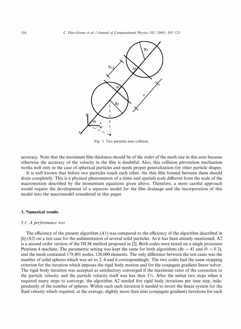
Fig. 1. Two particles near collision.

116 C. Diaz-Goano et al. / Journal of Computational Physics 192 (2003) 105–123

accuracy. Note that the maximum film thickness should be of the order of the mesh size in this area becauseotherwise the accuracy of the velocity in the film is doubtful. Also, this collision prevention mechanism

works well only in the case of spherical particles and needs proper generalization for other particle shapes.

It is well known that before two particles touch each other, the thin film formed between them should

drain completely. This is a physical phenomenon of a (time and spatial) scale different from the scale of the

macromotion described by the momentum equations given above. Therefore, a more careful approach

would require the development of a separate model for the film drainage and the incorporation of this

model into the macromodel considered in this paper.

3. Numerical results

3.1. A performance test

The efficiency of the present algorithm (A1) was compared to the efficiency of the algorithm described in

[6] (A2) on a test case for the sedimentation of several solid particles. As it has been already mentioned, A2

is a second order version of the DLM method proposed in [2]. Both codes were tested on a single processorPentium 4 machine. The parametric setting was kept the same for both algorithms (Re ¼ 41 and Fr ¼ 0:3),and the mesh contained 179,401 nodes, 120,000 elements. The only difference between the test cases was the

number of solid spheres which was set to 2, 4 and 6 correspondingly. The two codes had the same stopping

criterion for the iteration which imposes the rigid body motion and for the conjugate gradient linear solver.

The rigid body iteration was accepted as satisfactory converged if the maximum ratio of the correction to

the particle velocity and the particle velocity itself was less then 1%. After the initial two steps when it

required many steps to converge, the algorithm A2 needed five rigid body iterations per time step, inde-

pendently of the number of spheres. Within each such iteration it needed to invert the linear system for thefluid velocity which required, at the average, slightly more than nine (conjugate gradient) iterations for each

C. Diaz-Goano et al. / Journal of Computational Physics 192 (2003) 105–123 117

component of the velocity. For the same problem, the present algorithm (A1) converged within one rigid

body iteration per time step. The number of (conjugate gradient) iterations for each component of the

velocity was between seven and eight (with the same stopping criterion). Taking into account that the

algorithm A2 requires, in addition to the solution of the system for the fluid velocity (which is also solved

by A1), to solve also one (relatively) small linear system for the Lagrange multiplier in each particle, it is

clear that the present algorithm is faster. Moreover, the saving in CPU time increases with the number of

spheres involved. The decrease in the number of rigid body iterations should be attributed to the inner

product used to impose the rigid body constraint in the present case.Since it is natural to think that the decrease in the number of iterations would lead to loss of accuracy,

the accuracy of the method was further tested on three problems for which either experimental data is

available or which have a well-known solution.

3.2. Case 1: single particle sedimentation

The first benchmark problem was the sedimentation of a single particle in a Newtonian liquid. Mordant

et al. [12] provide extensive experimental data for this flow at a variety of Reynolds numbers and density

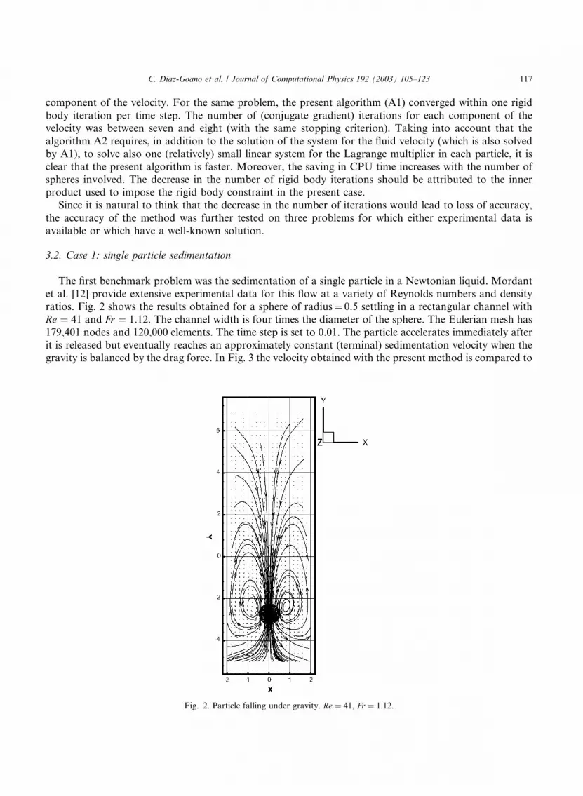
ratios. Fig. 2 shows the results obtained for a sphere of radius¼ 0.5 settling in a rectangular channel with

Re ¼ 41 and Fr ¼ 1:12. The channel width is four times the diameter of the sphere. The Eulerian mesh has

179,401 nodes and 120,000 elements. The time step is set to 0.01. The particle accelerates immediately after

it is released but eventually reaches an approximately constant (terminal) sedimentation velocity when thegravity is balanced by the drag force. In Fig. 3 the velocity obtained with the present method is compared to

Fig. 2. Particle falling under gravity. Re ¼ 41, Fr ¼ 1:12.

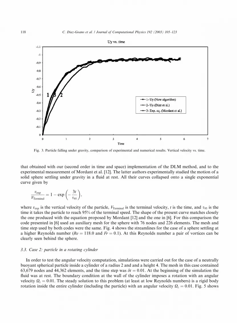
Fig. 3. Particle falling under gravity, comparison of experimental and numerical results. Vertical velocity vs. time.

118 C. Diaz-Goano et al. / Journal of Computational Physics 192 (2003) 105–123

that obtained with our (second order in time and space) implementation of the DLM method, and to the

experimental measurement of Mordant et al. [12]. The latter authors experimentally studied the motion of a

solid sphere settling under gravity in a fluid at rest. All their curves collapsed onto a single exponential

curve given by

vexpVTerminal

¼ 1� exp � 3ts95

� �;

where vexp is the vertical velocity of the particle, VTerminal is the terminal velocity, t is the time, and s95 is thetime it takes the particle to reach 95% of the terminal speed. The shape of the present curve matches closely

the one produced with the equation proposed by Mordant [12] and the one in [6]. For this comparison the

code presented in [6] used an auxiliary mesh for the sphere with 76 nodes and 226 elements. The mesh andtime step used by both codes were the same. Fig. 4 shows the streamlines for the case of a sphere settling at

a higher Reynolds number (Re ¼ 118:0 and Fr ¼ 0:1). At this Reynolds number a pair of vortices can be

clearly seen behind the sphere.

3.3. Case 2: particle in a rotating cylinder

In order to test the angular velocity computation, simulations were carried out for the case of a neutrally

buoyant spherical particle inside a cylinder of a radius 2 and and a height 4. The mesh in this case contained

63,679 nodes and 44,362 elements, and the time step was dt ¼ 0:01. At the beginning of the simulation the

fluid was at rest. The boundary condition at the wall of the cylinder imposes a rotation with an angular

velocity Xz ¼ 0:01. The steady solution to this problem (at least at low Reynolds numbers) is a rigid body

rotation inside the entire cylinder (including the particle) with an angular velocity Xz ¼ 0:01. Fig. 5 shows

Fig. 4. Particle falling under gravity. Re ¼ 118, Fr ¼ 0:10.

C. Diaz-Goano et al. / Journal of Computational Physics 192 (2003) 105–123 119

the rotating cylinder and the evolution of the sphere�s angular velocity with time. The angular velocity

increases until it almost matches that of the wall. The difference between the angular velocities (of the

sphere and the wall) can be attributed to the mesh resolution.

Fig. 5. (a) Sphere in a rotating cylinder. (b) Angular velocity vs. time (dimensionless).

120 C. Diaz-Goano et al. / Journal of Computational Physics 192 (2003) 105–123

3.4. Case 3: particle–particle interactions

To test the collision prevention mechanism, simulations were conducted using a mesh of 306,231 nodes

and 205,800 elements and two spherical particles of an equal size. The Reynolds number was set to 67. Thedensity ratio was q2;i=q1 ¼ 9:44. Initially both, the liquid and the particles were at rest. No-slip conditions

were prescribed on all the walls. Both spheres had a radius of 0.4. Their initial positions were ð0:0; 6:0; 0:0Þand ð0:0; 5:0; 0:0Þ, respectively.

Fig. 6 shows different frames captured with a high speed camera in our laboratory, the conditions of the

experiment being similar to the conditions of the numerical simulation. Fig. 7 shows the results of our

numerical simulations as described before. In both cases, the upper sphere initially settles slower than the

bottom sphere. After a while, the velocity of this upper sphere increases and it starts catching the leading

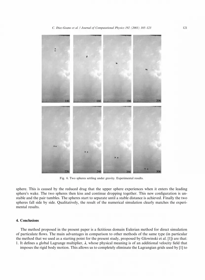
Fig. 6. Two spheres settling under gravity. Experimental results.

C. Diaz-Goano et al. / Journal of Computational Physics 192 (2003) 105–123 121

sphere. This is caused by the reduced drag that the upper sphere experiences when it enters the leadingsphere�s wake. The two spheres then kiss and continue dropping together. This new configuration is un-

stable and the pair tumbles. The spheres start to separate until a stable distance is achieved. Finally the two

spheres fall side by side. Qualitatively, the result of the numerical simulation clearly matches the experi-

mental results.

4. Conclusions

The method proposed in the present paper is a fictitious domain Eulerian method for direct simulation

of particulate flows. The main advantages in comparison to other methods of the same type (in particular

the method that we used as a starting point for the present study, proposed by Glowinski et al. [1]) are that:

1. It defines a global Lagrange multiplier, k, whose physical meaning is of an additional velocity field that

imposes the rigid body motion. This allows us to completely eliminate the Lagrangian grids used by [1] to

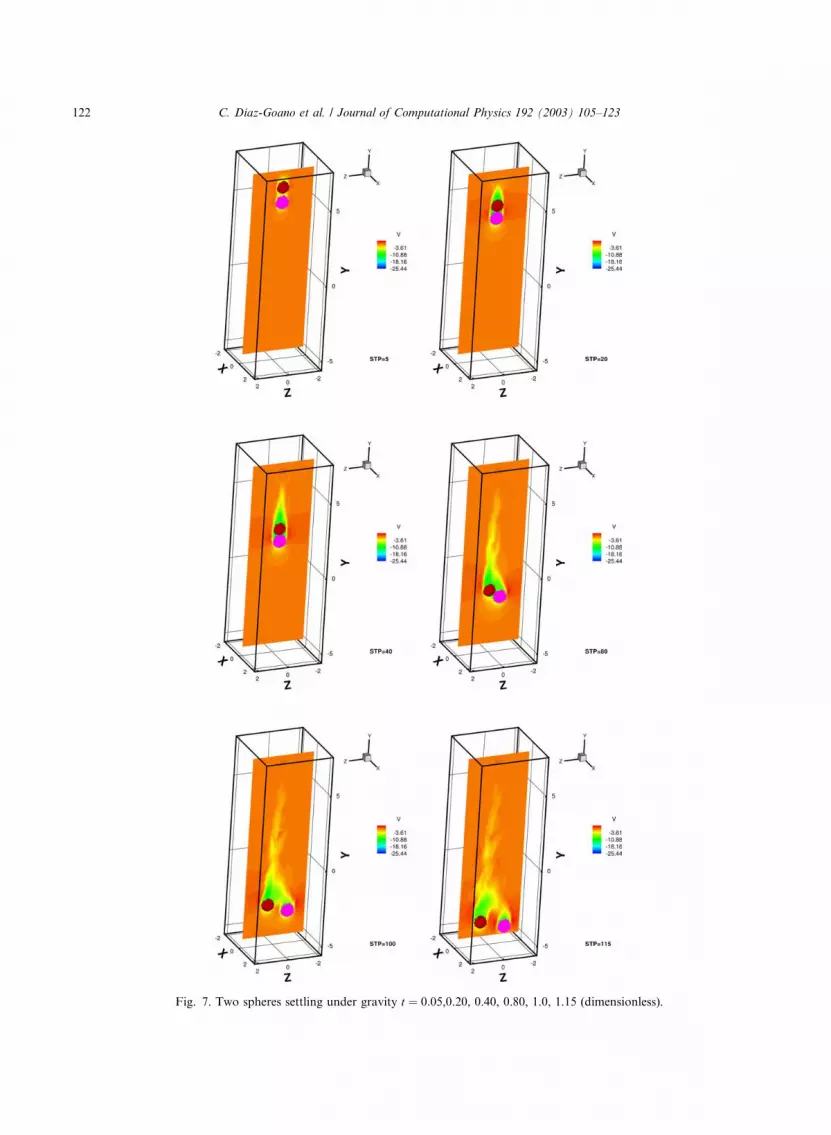
Fig. 7. Two spheres settling under gravity t ¼ 0:05,0.20, 0.40, 0.80, 1.0, 1.15 (dimensionless).

122 C. Diaz-Goano et al. / Journal of Computational Physics 192 (2003) 105–123

C. Diaz-Goano et al. / Journal of Computational Physics 192 (2003) 105–123 123

discretize the distributed Lagrange multipliers in their case. This allows for the use of basically only one

solver on relatively regular grids which facilitates the parallel implementation of the method.

2. The global Lagrange multiplier, together with a proper choice for the inner product that is used to im-

pose the rigid body constraint allows to avoid the need to solve the linear system for computing the dis-tributed Lagrange multipliers in each particle. Although this system is not large, it eventually is to be

solved on each iteration of step of Substep 4 of the algorithm above. If the flow contains many particles,

the savings can be significant.

3. The present algorithm employs a second order in time, incremental projection scheme for the resolution

of the generalized Stokes problem which, as our numerical experience shows, performs significantly bet-

ter than a first order scheme for almost the same expenses. The spatial discretization is also second order

accurate for the velocity and the Lagrange multiplier and first order accurate for the pressure.

In addition to these advantages, this method retains all the advantages of the DLM method proposed byGlowinski et al. [1] (see the conclusions of this paper).

Acknowledgements

The authors would like to thank Ahmed Sameh from Purdue University for the very fruitful discussions

about the fictitious domain method. This work was partially supported by the Natural Sciences and En-

gineering Research Council of Canada (NSERC) and by Alberta Informatics Circle of Research Excellence(iCORE).

References

[1] R. Glowinski, T. Pan, T. Hesla, D. Joseph, J. Periaux, A fictitious domain approach to the direct numerical simulation of

incompressible viscous flow past moving rigid bodies: Application to particulate flow, J. Comput. Phys. 169 (2001) 363.

[2] R. Glowinski, T. Pan, T. Hesla, D. Joseph, A distributed Lagrange multiplier/fictitious domain method for particulate flows, Int.

J. Multiphase Flow 25 (1999) 755.

[3] G. Tryggvason, B. Bunner, A. Esmaeeli, D. Juric, N. Al-Rawahi, W. Tauber, J. Han, S. Nas, Y.-J. Jan, A front-tracking method

for viscous incompressible multi-fluid flows, J. Comp. Physics 169 (2001) 708.

[4] H.H. Hu, Direct simulation of flows of solid–liquid mixtures, Int. J. Multiphase Flow 22 (1996) 335.

[5] A. Johnson, T. Tezduyar, 3D simulation of fluid–particle interactions with the number of particles reaching 100, Comp. Meth.

Appl. Mech. Engng. 145 (1997) 301.

[6] C. Diaz-Goano, P. Minev, K. Nandakumar, A Lagrange multipliers/fictitious domain approach to particulate flows, in: W.

Margenov, Yalamov (Eds.), Lecture Notes in Computer Science, vol. 2179, Springer, Sozopol, Bulgaria, 2001, p. 409.

[7] J. Guermond, J. Shen, Velocity-correction projection methods for incompressible flows, SIAM J. Num. Anal. 41 (2003) 112.

[8] P. Minev, C. Ethier, A semi-implicit projection algorithm for the Navier–Stokes equations with application to flows in complex

geometries., in: M.G. et al. (Ed.), Notes on Numerical Fluid Mechanics, Vieweg, Braunschweig/Wiesbaden, 1999, p. 223, 73.

[9] J. Guermond, P. Minev, Analysis of a projection/characteristic scheme for incompressible flow, Comm. Numer. Meth. Engng. 19

(2003) 535.

[10] N. Patankar, P. Singh, D. Joseph, R. Glowinski, T. Pan, A new formulation of the distributed Lagrange multiplier/fictitious

domain method for particulate flows, Int. J. Multiphase Flow 26 (2000) 1509.

[11] T. Chen, P. Minev, K. Nandakumar, A finite element technique for multifluid incompressible flow using Eulerian grids, J. Comp.

Phys. 187 (2003) 255.

[12] N. Mordant, J. Pinton, Velocity measurement of a settling sphere, Eur. Phys. J. B 18 (2000) 343.