A Finite Difference Fictitious Domain Wavelet Method for ...

EUROPEAN JOURNAL OF PURE AND APPLIED MATHEMATICSVol. 14, No. 3, 2021, 706-722ISSN 1307-5543 – ejpam.comPublished by New York Business Global

A Finite Difference Fictitious Domain Wavelet Methodfor Solving Dirichlet Boundary Value Problem

Francis Ohene Boateng1,∗, Joseph Ackora-Prah2, Benedict Barnes2,John Amoah-Mensah3

1 Department of Mathematics Education, Faculty of Applied Sciences and MathematicsEducation, Akenten Appiah-Menka University of Skills Training and EntrepreneurialDevelopment, Kumasi, Ghana2 Department of Mathematics, Faculty of Physical and Computational Sciences, KwameNkrumah University of Science and Technology, Kumasi, Ghana3 Department of Computer Science, Faculty of Physical Sciences, Sunyani TechnicalUniversity, Sunyani, Ghana

Abstract. In this paper, we introduce a Finite Difference Fictitious Domain Wavelet Method(FDFDWM) for solving two dimensional (2D) linear elliptic partial differential equations (PDEs)with Dirichlet boundary conditions on regular geometric domain. The method reduces the 2D PDEinto a 1D system of ordinary differential equations and applies a compactly supported wavelet toapproximate the solution. The problem is embedded in a fictitious domain to aid the enforcementof the Dirichlet boundary conditions. We present numerical analysis and show that our methodyields better approximation to the solution of the Dirichlet problem than traditional methods likethe finite element and finite difference methods.

2020 Mathematics Subject Classifications: 65N06, 65N30, 65N85

Key Words and Phrases: fictitious domain, Dirichlet problem, wavelet, finite difference, finiteelement

1. Introduction

The Dirichlet Problem (DP) for linear elliptic PDE in 2D is found in many physicalproblems that are governed by partial differential equations. These physical problemsinclude vibration of solids, flow of fluids, diffusion of chemicals, spread of heat, structureof molecules, propagation of waves, laser beam models, financial models, etc [14]. Due tothe significance of the DP in the field of engineering and the sciences, researchers havedone a lot of work into improving the solution methods, both analytically and numerically

∗Corresponding author.DOI: https://doi.org/10.29020/nybg.ejpam.v14i3.3893

Email addresses: [email protected], [email protected] (F. O. Boateng),[email protected] (J. Ackora-Prah), [email protected] (B.Barnes),[email protected] (J. Amoah-Mensah)

http://www.ejpam.com 706 © 2021 EJPAM All rights reserved.

F. O. Boateng et al. / Eur. J. Pure Appl. Math, 14 (3) (2021), 706-722 707

[1, 7, 13]. However, challenges including difficulty in evaluating integrals analytically,approximation based on truncation of infinite series required, inappropriate solution spaceand many more, militate against analytical approaches. In particular, DP for linear ellipticPDE in 2D, in functional space may not have analytic solution and so the solution needsto be approximated numerically [15].

With the availability of powerful computers, the emphasis on solving Dirichlet Prob-lem in 2D is gradually shifting away from the analytical method of solutions towardsnumerical computations and analysis [14]. Numerical methods do not involve the searchfor an explicit or implicit function that describes the Dirichlet Problem. They largelyutilize discretization techniques to reduce the continuous linear elliptic PDE and Dirichletboundary conditions to discrete system that are suitable for high speed computer solu-tion. These methods are known to generate approximate solutions. The Finite DifferenceMethod (FDM) and Finite Element Method (FEM) are some of the traditional methodsused to solve this problem. Numerical methods that will produce high accurate, fast con-vergent and stable solution to the Dirichlet Problem in 2D than the traditional methods isparamount. Besides, the method must also reduce the complexity in obtaining the solutionto this problem. In recent times, wavelet methods are known to be effective and efficientmethods for solving Dirichlet Problem for linear elliptic PDEs in 2D [10, 12]. In waveletmethods, we are able to obtain information in both frequency and time domains, includingboundary information of the PDE equation. Undoubtedly, the vanishing moment prop-erty of wavelet enables the wavelet series solution to converge rapidly to a point in thedomain as compared to the afore mentioned traditional numerical methods for solving theDirichlet Problem for linear elliptic PDE in 2D.

2. The FDFDWM

In this paper, we introduce the FDFDWM as a numerical approach to solving theDirichlet Problem for linear elliptic PDE in 2D on a regular geometric domain. Thismethod aims at providing approximate solution to the DP, that is better in terms ofaccuracy and rate of convergence than that of the traditional methods mentioned. It em-ploys Daubechies scaling functions with a fictitious domain approach. Daubechies waveletfunction of order N has the largest number of vanishing moments which are compactlysupported on [0, 2N − 1]. Moreover, the high number of vanishing moments lead to highcompressibility of orthonormal solution in Ω ⊂ H. The use of the Daubechies scalingfunction offers the FDFDWM the flexibility to obtain a more accurate and stable solutionto the problem at hand in a functional space [2]. The fictitious domain approach of theFDFDWM also makes it easier to deal with the Dirichlet boundary condition. Notably, theFDFDWM reduces the linear elliptic PDE in two dimensional coordinates into a system ofone dimensional ordinary differential equations. This approach reduces considerably thecomplexities involved in the solution process, hence reduces the computational cost.

Now, we give the outline of the FDFDWM for solving the Dirichlet problem on regulardomains. We consider the case of a rectangular domain. Thus;

• The Dirichlet Problem is defined on an open domain with a rectangular boundary.


• The two dimensional problem is reduced to a one dimensional problem by discretizingalong one of the variables (y−coordinate or x−coordinate) using difference quotientand leaving the other variable undiscretized.

• The original domain of the problem is embedded in a slightly larger but simpledomain, in this case a rectangular domain. This extended domain is termed as afictitious domain.

• The One dimensional problem is formulated as a variational problem in the fictitiousdomain.

• A compactly supported wavelet, in this case Daubechies wavelet is used for thenumerical approximation in the larger domain.

• The resultant linear system in the large domain is then solved.

We consider a general linear second order elliptic equation of the form

−n∑

i,j=1

∂

∂xj

(aij(x)

∂φ

∂xi

)+

n∑i=1

bi(x)∂φ

∂xi+ c(x)φ = f(x), x ∈ Ω (1)

where the coefficient aij , bi, c and f satisfy the following conditions:

aij ∈ C1(Ω), i, j = 1, . . . , n;

bi ∈ C(Ω), i = 1, . . . , n;

c ∈ C(Ω), f(x) ∈ C(Ω),

and

n∑i,j=1

aij(x)ηiηj ≥ τn∑

i=1

η2i , ∀η = (η1, . . . , ηn) ∈ Rn, x ∈ Ω; (2)

with τ being a positive constant independent of x and η. The fourth condition (2) isreferred to as uniform ellipticity. In this paper, we restrict ourselves to the case where thecoefficient aij(x) in equation (1) reduces to a scalar multiple, aI of unit matrix, were a isa smooth function.

We consider, the Dirichlet Problem in a regular (i.e. rectangular) domain, Ω = [p, q]×[r, s] ∈ R2 with boundary ∂Ω, given as

−∇ · (a∇φ) + b∇φ+ cφ = f in Ωφ(x, y) = g on ∂Ω

(3)

where the coefficients a = a(x, y), b = b(x, y) and c = (x, y) are smooth in ∂Ω whichsatisfy

a(x, y) ≥ a0 > 0, c(x, y)− 1

2∇ · b(x, y) ≥ 0, for all x, y ∈ Ω (4)


and where f is a given function and g is the boundary data.The first stage of the FDFDWM is to reduce the two dimensional DP in equation (3)

to a system of ordinary differential equations. To achieve this, equation (3) is discretizedalong one of the spatial variables (say y), with equally spaced sample, yi = i∆y. Thus

p = y0 < y1 < · · · < yNy = q

and

∆y =q − pNy

=q − p2m

where Ny = 2m and m is the resolution.

We use central difference approximation:

d2φ

dy2≈ φ(x, y + ∆y)− 2φ(x, y) + φ(x, y −∆y)

∆y2(5)

anddφ

dy≈ φ(x, y + ∆y)− φ(x, y −∆y)

2∆y(6)

with an error term O(y2) for each approximation.

Substituting equations (5) and (6) into (3), we have

−a[d2φ

dx2+φi+1(x)− 2φi(x) + φi−1(x)

∆y2

]+ b

[dφ

dx+φi+1(x)− φi−1(x)

2∆y

]+ cφi(x) = f(x, y)

(7)Expanding and simplifying (7), we obtain

−β1d2φi

dx2+ β2

dφi

dx+ β3φ

i+1 + β4φi + β5φ

i−1 = β6fi (8)

where

β1 = a∆y2, β2 = b∆y2, β3 = b∆y

2− a, β4 = 2a+ c∆y2,

β5 = −(a+ b∆y

2) and β6 = ∆y2

Now, we letφiΣ(x) = β3φ

i+1 + β4φi + β5φ

i−1. (9)

Then equation (8) is

−β1d2φi

dx2+ β2

dφi

dx+ φiΣ(x) = β6f

i, (10)

which is represented in a vector form as

−∇ · (β1∇φi) + β2∇φi + φiΣ = β6fi for i = 1, 2, 3, . . . . (11)

Equation (11) is a one dimensional system of ordinary differential equations obtainedas a result of the reduction of (1).


2.1. Variational Formulation of the DP

The next stage of the FDFWDM is to write equation (11) in a weak form and seek asolution in a Sobolev space H1. We achieve this by multiplying (11) by a test function,v ∈ H1

0 and integrating over the domain Ω, that is∫Ω

(−∇ · (β1∇φi) + β2∇φi + φiΣ

)vdx =

∫Ωβ6f

iv dx (12)

Using the first Green’s identity and noting that v = 0 on the ∂Ω, we arrive at the followingweak form,

find φi ∈ H1(ΩF ) such that∫Ω

(β1∇φi∇v + β2∇φiv + φiΣv

)dx =

∫Ω β6f

iv dx ∀v ∈ H10 .

(13)

We define α : V × V → R and a linear functional L : V → R, where α(·, ·) over spaceV is continuous. Then we express equation (13) in a bilinear form as

α(v, η) =

∫Ω

(β1∇v∇η + β2∇vη + vη) dx ∀v, η ∈ V (14)

and

L(v) = β6

∫Ωfvdx (15)

We note from (1) that when b = 0, the bilinear becomes symmetrical, that is α(v, η) =α(η, v).

2.2. Fictitious Domain Formulation of the DP

The FDFDWM uses the fictitious domain approach to handle the boundary conditions.The idea behind the fictitious domain approach is to embed the original domain, Ω of theDP (1) in a slightly larger but simple (rectangular) domain, ΩF . This is done in order tohandle the difficulties usually associated with taking care of boundary conditions.

Now, we let V be a closed subspace H1p (ΩF ) given as

v : v = v|Ω, v ∈ V = H1p (ΩF )

The choice for V , considering the Dirichlet boundary condition is H10 (Ω). We also define

Vp (ΩF ) byVp (ΩF ) = v ∈ H1

0 (ΩF ) : v on ∂Ω is periodic on. (16)

Given some s > 0, suppose that ΩF = (0, s)2 then the periodicity property in (16) impliesthat v (0, y) = v (s, y) and v (x, 0) = v (x, s). Following from equations (14) and (15), theDP (3) can be formulated as a variational problem. That is,

find φi ∈ H1(ΩF ), ∀v ∈ H10 so that

α(φi, v) = L(v).(17)


2.3. Wavelet Approximation of the DP

One cardinal aspect of the FDFDWM is the approximation of the DP using waveletseries solution. Generally, wavelet approximations give a more stable and accurate solu-tions and also provide information on the boundary data. We use the Daubechies waveletfor approximating the solution of the DP due to the fact that it has the highest numberof vanishing moments among the compactly supported wavelets [4, 5]. This makes thewavelet series approximation converges rapidly to the desired solution.

We begin formulating the FDFDWM solution by letting, Vj be a finite dimensionalsubspace of V . The problem now becomes;

find φij in Vj such that

α(φij , vj) = L(vj) ∀vj ∈ Vj .(18)

We express equation (18) in an expanded form as

β1

∫ΩF

∇φij∇vjdx+ β2

∫ΩF

∇φijvjdx+

∫ΩF

φiΣ,jvjdx = β6

∫ΩF

f ivjdx (19)

Substituting equation (9) into (19), we obtain

β1

∫ΩF

∇φij∇vjdx+β2

∫ΩF

∇φijvjdx+

∫ΩF

(β3φ

i+1j + β4φ

ij + β5φ

i−1j

)vjdx = β6

∫ΩF

f ivjdx

(20)where f i ∈ L2 is an extension of f(x, yi) in the fictitious domain, ΩF .

To obtain approximate solution of the DP in equation (18), we employ Daubechies scalingfunction. We seek a solution that is written as a linear combination of scaling functionand coefficient. Thus, we define the FDFDWM solution for resolution m with a scalingparameter k at a fixed y−coordinate, yi, as

φw(x, yi) = 2m2

∑k

ξik,mϕ(2mx− k) (21)

where φw is the FDFDWM solution and ξik,m are the scaling coefficient values to bedetermined.

Now, we set up a linear system for equation (20) to solve for ξik,m. Substituting equa-tion (21) into (20) and simpling gives,

2m2 β1

∑k

ξik,m

∫ϕ′(2mx− k)ϕ′(2mx− j)dx

+2m2 β2

∑k

ξik,m

∫ϕ′(2mx− k)ϕ(2mx− j)dx

+2m2 β3

∑k

ξi+1k,m

∫ϕ(2mx− k)ϕ(2mx− j)dx


+2m2 β4

∑k

ξik,m


+2m2 β5

∑k

ξi−1k,m


= 2m2 β6f

i

∫ϕ(2mx− k)ϕ(2mx− j)dx (22)

We set up a linear system from equation (22) by introducing connection coefficients.

That is,

Ω2k−j =

∫ ∞−∞

ϕ′(X − k)ϕ′(X − j)dx, for derivative d = 2,

Ωk−j =

∫ ∞−∞

ϕ′(X − k)ϕ(X − j)dx, for derivative d = 1

and the Kronecker-delta function,

δk,j =

∫ ∞−∞

ϕ(X − k)ϕ(X − j)dx

where we set X = 2mx

We handle the exterior nodes of ξi+1k,m and ξi−1

k,m by applying a shift to the scaling func-tions in the following manner:

ξi+1k,mϕ(2mx− k)ϕ(2mx− j) = ξik,mϕ(2mx− k + 1)ϕ(2mx− j) (23)

andξi−1k,mϕ(2mx− k)ϕ(2mx− j) = ξik,mϕ(2mx− k − 1)ϕ(2mx− j) (24)

Substituting equations (23) and (24) into (22), we obtain∑k

[ξik,mΩ2

k−j + β2ξik,mΩk−j + β3ξ

ik,mδk+1,j + β4ξ

ik,mδk,j + β5ξ

ik,mδk−1,j

]= β6f

iδk,j (25)

We write equation (25) as a linear system in a vector form, given by

A1~ξ +A2

~ξ +A3~ξ +A4

~ξ +A5~ξ = F (26)

whereA1 = β1

∑k

Ω2k−j , A2 = β2

∑k

Ωk−j , A3 = β3

∑k

δk+1,j ,

A4 = β4

∑k

δk,j , A5 = β5

∑k

δk−1,j and F = β6fiδk,j

The indexes k and j are delimited to the whole domain. We recall that, the originaldomain is discretized with Nx functions. The fictitious domain approach requires that


N − 1 scaling functions be added to each end of the domain, then the new domain,spanned by the fictitious domain will expand from −(N−1) to Nx−1+(N−1). This willresult in a linear system with size, Nx +2(N −1). Thus, −(N −1) ≤ k ≤ Nx − 1+(N −1)and −(N − 1) ≤ j ≤ Nx − 1 + (N − 1), and so equation (26) will be an (Nx + 2(N − 1))×(Nx + 2(N − 1)) linear system.

We use Daubechies scaling functions of order six (i.e DN6) to construct matrices forthe linear system. The matrices A1 and A2 are (2N −3)-diagonal (Nx +2(N −1))× (Nx +2(N − 1)) matrices. We reserve the first and last rows for the enforcement of the Dirichletboundary condition. We treat thoroughly the implementation of the boundary conditionsin section 2.4

We present matrices, A1 and A2 as follows:

A1 = β1

0 0 0 0 0 0 0 · · ·Ω2−1 Ω2

0 Ω21 Ω2

2 Ω23 Ω2

4 0 · · ·Ω2−2 Ω2

−1 Ω20 Ω2

1 Ω22 Ω2

3 Ω24 0 · · ·

Ω2−3 Ω2

−2 Ω2−1 Ω2

0 Ω21 Ω2

2 Ω23 Ω2

4 0 · · ·Ω2−4 Ω2

−3 Ω2−2 Ω2

−1 Ω20 Ω2

1 Ω22 Ω2

3 Ω24 0

0 Ω2−4 Ω2

−3 Ω2−2 Ω2

−1 Ω20 Ω2

1 Ω22 Ω2

3 Ω24

......

......

......

......

. . .

(27)

A2 = β2

0 0 0 0 0 0 0 · · ·Ω−1 Ω0 Ω1 Ω2 Ω3 Ω4 0 · · ·Ω−2 Ω−1 Ω0 Ω1 Ω2 Ω3 Ω4 0 · · ·Ω−3 Ω−2 Ω−1 Ω0 Ω1 Ω2 Ω3 Ω4 0 · · ·Ω−4 Ω−3 Ω−2 Ω−1 Ω0 Ω1 Ω2 Ω3 Ω4 0

0 Ω−4 Ω−3 Ω−2 Ω−1 Ω0 Ω1 Ω2 Ω3 Ω4...

......

......

......

.... . .

(28)

It is important to note that the values of the connection coefficient are precomputed. Inthis case a parallelization may be applied in the implementation.

The rest of the matrices, A3, A4 and A5 are obtained from the Kronecker-delta functionas super-diagonal, diagonal and subdiagonal matrices respectively. That is,

A3 =

0 β3 0 0 0 0 0 0 0 · · ·0 0 β3 0 0 0 0 0 0 · · ·0 0 0 β3 0 0 0 0 0 · · ·0 0 0 0 β3 0 0 0 0 · · ·0 0 0 0 0 β3 0 0 0 · · ·0 0 0 0 0 0 β3 0 0 · · ·...

......

......

......

......

. . .

(29)


A4 =

β4 0 0 0 0 0 0 0 0 · · ·0 β4 0 0 0 0 0 0 0 · · ·0 0 β4 0 0 0 0 0 0 · · ·0 0 0 β4 0 0 0 0 0 · · ·0 0 0 0 β4 0 0 0 0 · · ·0 0 0 0 0 β4 0 0 0 · · ·...

......

......

......

......

. . .

(30)

and

A5 =

0 0 0 0 0 0 0 0 0 · · ·β5 0 0 0 0 0 0 0 0 · · ·0 β5 0 0 0 0 0 0 0 · · ·0 0 β5 0 0 0 0 0 0 · · ·0 0 0 β5 0 0 0 0 0 · · ·0 0 0 0 β5 0 0 0 0 · · ·...

......

......

......

......

. . .

(31)

Combining equation (27), (28), (29), (30), and (31), we obtain a linear system

A~ξ = F (32)

where A =∑5

i=1Ai

In order to construct the weak formulation for the function f(x, yi) on the right handside of equation (32), we give the definitions and state the theorems relevant for the weakformulation.

Definition 1. The orthogonal projection of the function f(x, y) at a fixed y− coordinate,yi onto a subspace Vm is defined by

Pmf(x, yi)

=∑k

(∫f(x, yi)ϕm,k(x)dx

)ϕm,k(x) (33)

Definition 2. The function f(x, y) sampled at a fixed y− coordinate, yi is also defined by

Smf(x, yi)

=∑k

2−m2 f(k/2m)ϕm,k(x) (34)

Now, state two theorems relevant to the approximation of the function on the righthand side.

Theorem 1. If m1(τ) = 0 for τ = 0, 1, . . . ,M, then L2 error is:

ε1 = ‖Pmf(x, yi)

− f(x, yi)‖2 ≤ λ12−m(M+1)

where λ1 is a constant dependent on f(x, yi) and the scaling functions but independent ofm and M .


The proofs of theorems 1 and 2 can be found in [3]. From theorem 1, we observethat for a given Daubechies scaling function, M + 1 represents the number of vanishingmoments (i.e. N = M + 1). Following from definition 2, we obtain theorem 2.

Theorem 2. If m2(τ) = 0 for τ = 0, 1, . . . ,M, then L2 error is:

ε2 = ‖Pmf(x, yi)

− Sm

f(x, yi)

‖2 ≤ λ22−m(M+1)

where λ2 is a constant independent of m and M but dependent on f(x, yi) and the waveletsystem.

We note that the L2 errors, ε1 and ε2 in theorems 1 and 2 respectively are bothbounded above by 2−m(M+1). This means nodal values of the original function at fixedy− coordinate, f(x, yi) can be used rather than the sampling values from Sm

f(x, yi)

which are yet to be determined. Therefore the f(x, yi) nodal values can be utilized at theright hand side of equation (32).

2.4. Incorporating Dirichlet Boundary Conditions

One of the main challenges with Wavelet - Galerkin is the treatment of boundaryconditions. In this paper, we use the fictitious boundary condition approach to enforcethe Dirichlet boundary condition [11]. We handle the left boundary by replacing the firstequation of (32) by the following equation.

φ(x, yi) =∑k

ξik,mϕ(−k) = g(yi)

We take inner product of the RHS with ϕ(−j) to obtain,∑k

ξik,m

∫ ∞−∞

ϕ(−k)ϕ(−j)dx = g(yi)

This results in a Kronecker-delta function on the left,∑k

ξik,mδk,j = g(yi) (35)

Evaluating the Dirichlet boundary expressed in equation (35), we obtain an identitywhose Nth column has the value 1, and g(yi) representing the first element of the righthand side. In similar vein the right boundary of the system is handled.

3. Numerical Results

In this section we present the results obtained from numerical experiments carried outusing the FDFDWM on some linear elliptic PDEs with Dirichlet boundary conditions. Theresults from the FDFDWM are compared with the results from two traditional methods;FDM and FEM, to determine the level of accuracy of our method. The outcome of theexperiments are presented in a form of two dimensional graphs and tables. All numericalexperiments are performed using MATLAB.


3.1. The FDFDWM Test Cases

Now, we consider numerical experiments performed using FDFDWM approach onPDEs with Dirichlet boundary conditions on rectangular domains. In each of the twocases presented here, the domain of the boundary value problem is placed in a slightlylarger rectangular domain referred to as the fictitious domain. The Daubechies scalingfunctions of orders D6, D8, D10, D12, D14, D16, D18 and D20 with varying levels ofresolution (i.e. m = 0,m = 1,m = 2 and m = 3) are used and analyzed in the experiments.

Test Case 1A Dirichlet problem defined on a rectangular domain, Ω = [−5, 5]× [−5, 5] embedded in afictitious domain ΩF = [−8, 8]× [−8, 8] with a Dirichlet boundary condition g = sin(x+y)is considered for the first numerical test. The problem is given as

−∆φ+ φ = 3 sin(x+ y) in Ωφ(x, y) = g on ∂Ω

(36)

The Dirichlet problem (36) is first solved using FDFDWM with D6 at varying levels ofresolution, starting from m = 0 to m = 3 , corresponding to a basis of 8, 16, 32 and 64translated scaling functions with support intersecting with [−5, 5] on both the horizontaland vertical axes. The values of the approximate solutions are used to generate two dimen-sional coordinates surface graphs shown in figures 1. This is first to illustrate the abilityof the FDFDWM to approximate the solution to the Dirichlet boundary value problem(36). We demonstrate further the level of accuracy of the FDFDWM by comparing the ap-proximate solutions of FDM, FEM and FDFDWM with the exact solution of problem (36).

Test Case 2In the second test, we consider another Dirichlet problem defined on a rectangular do-main, Ω = [−3, 3]× [−3, 3] embedded in a fictitious domain ΩF = [−5, 5]× [−5, 5] with aDirichlet boundary condition g = x2 + y2. We write the problem as

−∆φ+ φ = x2 + y2 − 4 in Ωφ(x, y) = g on ∂Ω

(37)

Similar procedure as used for equation (36) is also applied to equation (37) to generatetwo dimensional coordinates surface graphs shown in figures 3.

Test Case 3A Poisson equation is considered for the third numerical test. It is defined on a rectangulardomain, Ω = [0, 1] × [0, 1] embedded in a fictitious domain ΩF = [−0.5, 1.5] × [−0.5, 1.5]with a Dirichlet boundary condition g = sinπx+ sinπy. The problem is given as

−∆φ = sinπx+ sinπy in Ωφ(x, y) = 0 on ∂Ω

(38)

The FDFDWM is used to compute the approximate solution for problem (38) in similarmanner, using wavelet order D6 and resolution at levels, m = 1,m = 2,m = 3 and


m = 4 respectively. The resulting approximate solution is presented in two dimensionalco-ordinates surface graph shown in figure 5.

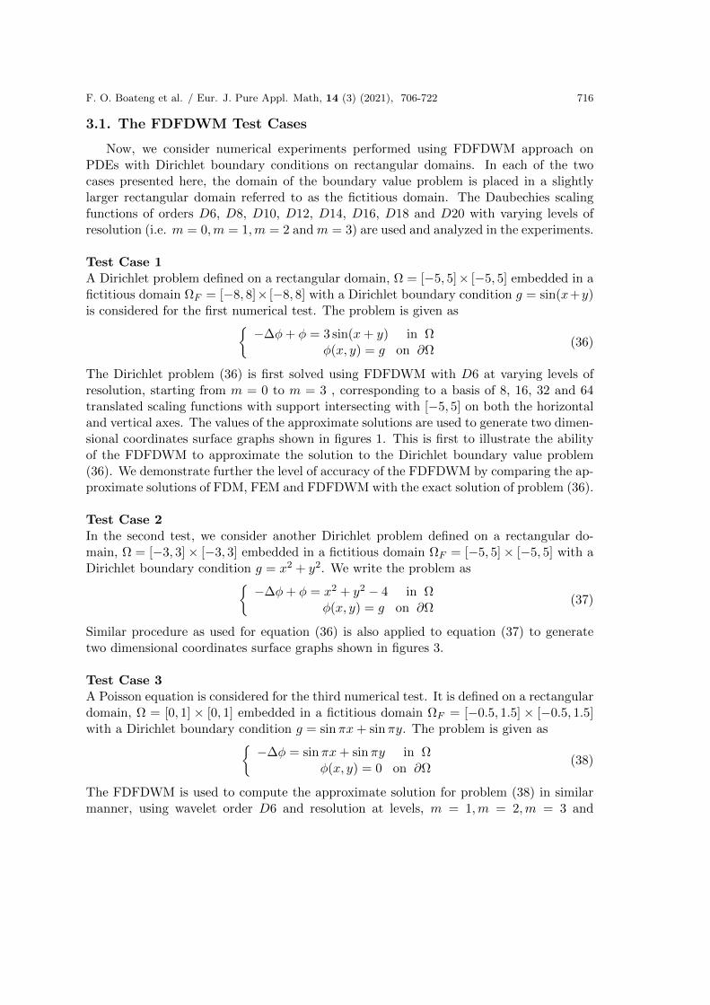
Figure 1: The FWDFDM approximation on a rectangular domain for D6 and m = 0, 1, 2 and 3

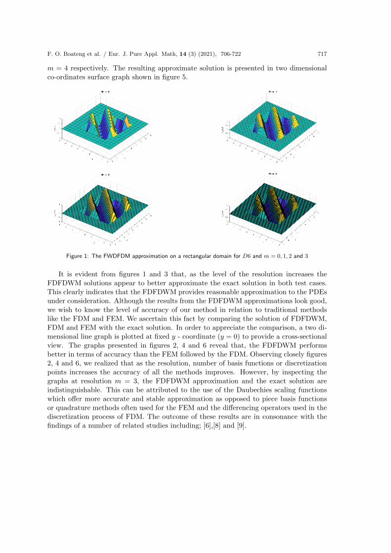
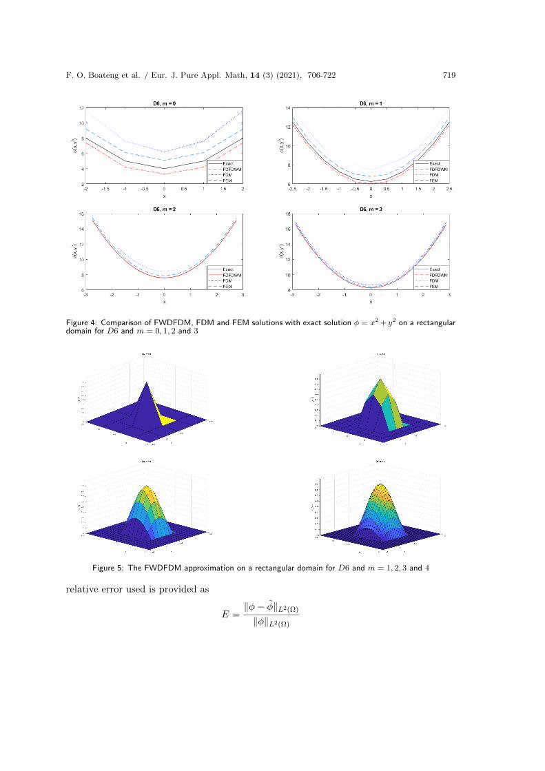
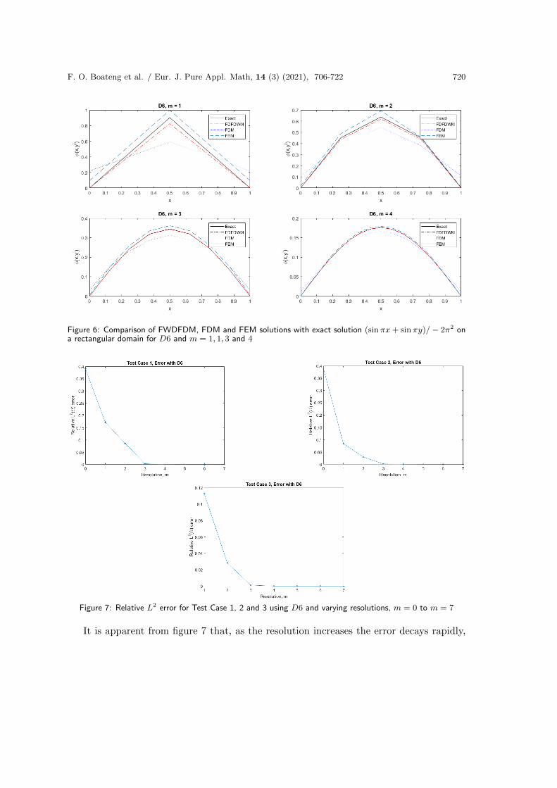
It is evident from figures 1 and 3 that, as the level of the resolution increases theFDFDWM solutions appear to better approximate the exact solution in both test cases.This clearly indicates that the FDFDWM provides reasonable approximation to the PDEsunder consideration. Although the results from the FDFDWM approximations look good,we wish to know the level of accuracy of our method in relation to traditional methodslike the FDM and FEM. We ascertain this fact by comparing the solution of FDFDWM,FDM and FEM with the exact solution. In order to appreciate the comparison, a two di-mensional line graph is plotted at fixed y - coordinate (y = 0) to provide a cross-sectionalview. The graphs presented in figures 2, 4 and 6 reveal that, the FDFDWM performsbetter in terms of accuracy than the FEM followed by the FDM. Observing closely figures2, 4 and 6, we realized that as the resolution, number of basis functions or discretizationpoints increases the accuracy of all the methods improves. However, by inspecting thegraphs at resolution m = 3, the FDFDWM approximation and the exact solution areindistinguishable. This can be attributed to the use of the Daubechies scaling functionswhich offer more accurate and stable approximation as opposed to piece basis functionsor quadrature methods often used for the FEM and the differencing operators used in thediscretization process of FDM. The outcome of these results are in consonance with thefindings of a number of related studies including; [6],[8] and [9].


Figure 2: Comparison of FWDFDM, FDM and FEM solutions with exact solution φ = sin(x+y) on a rectangulardomain for D6 and m = 1, 2 and 3


3.2. Error Analysis for FDFDWM

Here, the relative error using L2 vector norm is computed for each of the test caseswith varying resolutions (i.e m = 0, 1, 2, 3, 4, 5, 6, 7) and scaling function order D6. The


Figure 4: Comparison of FWDFDM, FDM and FEM solutions with exact solution φ = x2 + y2 on a rectangulardomain for D6 and m = 0, 1, 2 and 3


relative error used is provided as

E =‖φ− φ‖L2(Ω)

‖φ‖L2(Ω)


Figure 6: Comparison of FWDFDM, FDM and FEM solutions with exact solution (sinπx+ sinπy)/− 2π2 ona rectangular domain for D6 and m = 1, 1, 3 and 4

Figure 7: Relative L2 error for Test Case 1, 2 and 3 using D6 and varying resolutions, m = 0 to m = 7

It is apparent from figure 7 that, as the resolution increases the error decays rapidly,

REFERENCES 721

indicating good convergence of the approximate solution to the exact solution. Althoughusing Daubechies scaling functions with genus D6 at varying resolutions appears to gen-erate reasonable approximation to the PDEs under consideration using the FDFDWM, itis essential to examine instances where the genus of the scaling functions increases.

Table 1: Relative L2 error for φ = (sinπx+sinπy)/−2π2 approximation and condition number of FDFDWM’ssystem matrix

m = 1 m = 2

DN Error (L2) Cond. Num Error (L2) Cond. Num.

6 1.72273872e-01 266545.642 8.59266326e-02 1216547.557

8 1.34574728e-01 299652.198 5.82274887e-02 2549819.826

10 1.00084497e-01 313878.814 2.37372575e-02 4877499.258

12 9.03869299e-02 452164.135 1.00522059e-02 6225570.392

14 8.17337237e-02 724845.847 6.08648401e-03 9913426.592

16 7.99390005e-02 1095616.081 4.19176077e-03 12874663.138

18 7.62888260e-02 1479906.308 1.24158634e-03 19988975.378

20 7.39675096e-02 2129604.614 1.02026987e-04 31017665.097

In table 1, we display the condition number of the coefficient matrix of FDFDWMprovided in equation (32) together with the relative L2 norm error at m = 1 and m = 2,and varying scaling function genus from D6 to D20 for test case 1. The table revealsthat the approximation of the FDFDWM gets better as the genus of the scaling functionsincreases from D6 to D20. However, we realized that for D12 and above, the effect of theincrement in the genus on the accuracy of the approximation diminishes. We noticed thatthe condition number grows as the resolution increases and same when the genus of thescaling function increases. Observably, we believe that the condition number is one of thecontributing sources of error in the FDFDWM.

4. Conclusion

We have demonstrated in this paper that the FDFDWM is comparable to the tra-ditional FEM and FDM approaches, and has inherently better accuracy to the approx-imation of the Dirichlet problem for linear elliptic partial differential equation in twodimension. It is much easier increasing the Daubechies scaling function order and resolu-tion to obtain more accurate solutions. Also the reduction of the problem from 2D to 1Dminimizes the complexities associated with solving PDEs in higher order.

References

[1] J D Anderson. Fundamentals of Aerodynamics, 4th Ed. McGraw–Hill, 2007.

[2] B Barnes, E Osei-Frimpong, F O Boateng, and J Ackora-Prah. A two-dimensionalchebyshev wavelet method for solving partial differential equations. Journal of Math-ematical Theory and Modeling, 6(8):124–138, 2016.

REFERENCES 722

[3] C S Burrus, R A Gophinath, and H Guo. Wavelets and Wavelet Transforms. CreativeCommons Attribution License, OpenStax-CNX, 2015.

[4] I Daubechies. Ten lectures on wavelets, volume 61. In NSF-CBMS Regional Con-ference Series in Applied Mathematics, Philadelphia, 1992. Society for Industrial andApplied Mathematics.

[5] L Debnath and F A Shah. Wavelet Transforms and Their Application. SpringerScience+Business Media New York, 2nd edition, 2015.

[6] R K Deka and A H Choudhury. Solution of two point boundary value problems usingwavelet integrals. Int. J. Contemp. Math. Sciences, 4(15):695–717, 2009.

[7] M Eckert. The Dawn of Fluid Dynamics: A Discipline Between Science and Tech-nology. Wiley, 2006.

[8] R Glowinski, T W Pan, R O Wells, and X Zhou. Wavelet and finite element solutionsfor the neumann problem using fictitious domains. Journal of Computational Physics,(126):40–51, 1996.

[9] R O Wells Jr and X Zhou. Wavelet solutions for the dirichlet problem. NumericalMathematics, 70:379–396, 1995.

[10] A Katunin. Solution of plane dirichlet problem using compactly supported 2d waveletscaling functions. Scientific Research of the Institute of Mathematics and ComputerScience, 1(11):31–40, 2012.

[11] D Lu, T Ohyoshi, and L Zhu. Treatment of boundary conditions in the application ofwavelet-galerkin method to an sh wave problem. International Journal of the Societyof Materials Engineering for Resources, 5(1):15–25, 1997.

[12] V Mishra and Sabina. Wavelet-galerkin finite difference solutions of odes. AMO-Advanced Modeling and Optimization, 13(3):539–549, 2011.

[13] S Nazarenko. Fluid Dynamics via Examples and Solutions. CRC Press (Taylor andFrancis group), 2014.

[14] W A Strauss. Partial Differential Equations an Introduction. Wiley, New Jesse, 2008.

[15] E Suli. Finite Element Methods for Partial Differential Equations. Lecture Notes.Lecture Notes. Mathematical Institute University of Oxford, 2012.

A Finite Difference Fictitious Domain Wavelet Method for ...

Documents

Transcript of A Finite Difference Fictitious Domain Wavelet Method for ...