1

A Pacific interdecadal climate oscillation withimpacts on salmon production

by Nathan J. Mantua, Steven R. Hare, Yuan Zhang,

John M.Wallace, and Robert C. Francis

Submitted to theBulletin of the American Meteorological SocietyAugust 29th, 1996

Revised January 3rd, 1997

Accepted January 8th, 1997

corresponding author: Nathan Mantua, Joint Institute for the Study of the Atmosphere

and Oceans (JISAO*), University of Washington, Box 354235, Seattle, WA 98195-4235.

e-mail: mantua@atmos.washington.edu

*JISAO contribution #379

2

Abstract

Evidence gleaned from the instrumental record of climate data identifies a robust, recur-

ring pattern of ocean-atmosphere climate variability centered over the mid-latitude North

Pacific basin. Over the past century, the amplitude of this climate pattern has varied irreg-

ularly at interannual-to-interdecadal time scales. There is evidence of reversals in the pre-

vailing polarity of the oscillation occurring around 1925, 1947, and 1977; the last two

reversals correspond with dramatic shifts in salmon production regimes in the North

Pacific Ocean. This climate pattern also affects coastal sea and continental surface air

temperatures, as well as streamflow in major west coast river systems, from Alaska to Cal-

ifornia.

3

September 1915(Pacific Fisherman 1915)

”Never before have the Bristol Bay [Alaska] salmon packers returned to port

after the season’s operations so early.”

“The spring [chinook salmon] fishing season on the Columbia River [Washing-

ton and Oregon] closed at noon on August 25, and proved to be one of the best

for some years.”

1939 Yearbook(Pacific Fisherman 1939)

“The Bristol Bay [Alaska] Red [sockeye salmon] run was regarded as the great-

est in history.”

“The [May, June and July chinook] catch this year is one of the lowest in the his-

tory of the Columbia [Washington and Oregon].”

August/September 1972(Pacific Fisherman 1972)

“Bristol Bay [Alaska] salmon run a disaster.”

“Gillnetters in the Lower Columbia [Washington and Oregon] received an unex-

pected bonus when the largest run of spring chinook since counting began in

1938 entered the river.”

1995 Yearbook(Pacific Fishing 1995)

“Alaska set a new record for its salmon harvest in 1994, breaking the record set

the year before.”

“Columbia [Washington and Oregon] spring chinook fishery shut down; west

coast troll coho fishing banned.”

4

1. Introduction

Pacific salmon production has a rich history of confounding expectations. For much

of the past two decades salmon fishers in Alaska have prospered while those in the Pacific

Northwest have suffered. Yet, in the 1960s and early 1970s, their fortunes were essen-

tially reversed. Could this pattern of alternating fishery production extremes be connected

to climate changes in the Pacific basin?

In this article we present a synthesis of results derived from the analyses of climate

records and data describing biological aspects of variability in the large marine ecosys-

tems of the northeast Pacific Ocean. Our goal is to highlight the widespread connections

between interdecadal climate fluctuations and ecological variability in and around the

North Pacific basin.

A considerable body of literature has been devoted to the discussion of persistent

widespread changes in Pacific basin climate that took place in the late 1970’s (Namias

1978, Trenberth 1990, Ebbesmeyeret al. 1991, Graham 1994, Trenberth and Hurrell

1994). Several studies have also documented interdecadal climate fluctuations in the

Pacific basin, of which the changes that took place in the late 1970’s are but a single real-

ization (Ebbesmeyeret al. 1989, Francis and Hare 1994-Hare and Francis 1995, hereafter

FH-HF, Latif and Barnett 1994, 1996, Ware 1995, Hare 1996, Zhang 1996, and Zhanget

al. 1997, hereafter ZWB).

Widespread ecological changes related to interdecadal climate variations in the

Pacific have also been noted. Dramatic shifts in an array of marine and terrestrial ecologi-

cal variables in western North America coincided with the changes in the state of the

5

physical environment in the late 1970’s (Venricket al. 1987, Ebbesmeyeret al. 1991, Bro-

deur and Ware 1992, Roemmich and McGowan 1995, Franciset al. 1997). Rapid changes

in the production levels of major Alaskan commercial fish stocks have been connected to

interdecadal climate variability in the northeast Pacific (Beamish and Boullion 1993, Hol-

lowed and Wooster 1994, FH-HF), and similar climate-salmon production relationships

have been observed for some salmon populations in Washington, Oregon, and California

(Francis and Sibley 1991, Anderson 1996).

Our results add support to those of previous studies suggesting that the climatic

regime shift of the late 1970’s is not unique in the century-long instrumental climate

record, nor in the record of North Pacific salmon production. In fact, we find that signa-

tures of a recurring pattern of interdecadal climate variability are widespread and detect-

able in a variety of Pacific basin climate and ecological systems. This climate pattern--

hereafter referred to as thePacific (inter)Decadal Oscillation, or PDO (following co-

author S.R.H.’s suggestion)--is a pan-Pacific phenomenon that also includes interdecadal

climate variability in the tropical Pacific.

2. Data and Methodology

We analyze a wide collection of historical records of Pacific basin climate and

selected commercial salmon landings. Specifically, this study examines records of: (i)

tropical and Northern Hemisphere extratropical sea surface temperature (SST) and sea

level pressure (SLP); (ii) wintertime North American land surface air temperatures and

precipitation; (iii) wintertime northern hemisphere 500-mb height fields; (iv) SST along

6

the west coast of North America; (v) selected streamflow records from western North

America; and (vi) salmon landings from Alaska, Washington, Oregon and California.

Monthly mean SST data for the period of record 1900-1993 were obtained from an

updated version of the quality controlled U.K. Meteorological Office Historical SST

Dataset (HSSTD) provided by the Climatic Research Unit, University of East Anglia

(Folland and Parker 1990, 1995). These data are on a 5o latitude by 5o longitude grid. The

monthly mean, 1o latitude by 1o longitude gridded data of the Optimally Interpolated SST

(OISST, Reynolds and Smith 1994) are averaged into 5o boxes and used to extend the

HSSTD through the 1994-May 1996 period of record. We also use 2o latitude by 2o longi-

tude Comprehensive Ocean-Atmosphere Data Set (COADS, Fletcheret al. 1983) SST for

the period of record 1900-1992 in the construction of Fig. 2.

Monthly mean SLP data were obtained from two sources: first, 5o latitude by 5o lon-

gitude gridded fields from the Data Support Section/Computing Facility at the National

Center for Atmospheric Research (NCAR) for the period of record 1900-May 1996 (Tren-

berth and Paolino 1980); and second, 2o latitude by 2o longitude gridded surface marine

observations from COADS for the period of record 1900-1992, which are used to con-

struct the SLP map in Fig. 2 and the station-based Southern Oscillation Index (SOI) shown

in Fig. 1.

For the period of record 1900-1992, the COADS-based SOI used here was con-

structed following ZWB. The Tahiti pole is defined as the average SLP anomaly from 20o

N to 20o S latitude from the International Dateline to the coast of the South and Central

7

America, while the Darwin pole is defined as the average SLP anomaly over the remainder

of the global tropical oceans within the same range of latitudes. Missing SOI values for

the period of record 1913-1920, and 1993-May 1996, were estimated from a linear regres-

sion with the traditional Tahiti-Darwin SOI based on the common period of record 1933-

1990, obtained from the NOAA/NCEP Climate Prediction Center. For an early descrip-

tion of the Southern Oscillation the reader is referred to Walker and Bliss (1932).

Gridded, global, land surface air temperature and precipitation anomalies for the

period of record 1900-1992, based on station data, were obtained from the Carbon Diox-

ide Information Analysis Center in Oak Ridge, TN. The air temperature data are provided

as monthly anomalies on a 5o latitude by 10o longitude grid, over land only (Joneset al.

1985). We used “cold-season” means (November through March) for Fig. 3a. The precip-

itation anomalies are provided as (3-month) seasonal mean anomalies on a 4o latitude by

5o longitude grid, over land only (Eischeidet al. 1991). We used the December-January-

February seasonal mean anomalies in constructing Fig. 3b.

Gridded, Northern Hemisphere 500-mb height fields were obtained from NMC oper-

ational analysis fields, as described by Kushnir and Wallace (1989). November through

March mean anomalies were used in constructing Fig. 4.

Monthly mean streamflow records for the Kenai River at Cooper’s Landing, Alaska,

the Skeena River at UKC, British Columbia, Canada, the Fraser River at Hope, British

Columbia, Canada, and the Columbia River at The Dalles, Oregon, were obtained from

the National Water Data Exchange, which is part of the USGS. The monthly records were

used to generate annual water year (October-September) flow indices for each stream.

8

The time series labelled BC/Columbia Streamflow in Fig. 5 is a composite of the normal-

ized Skeena, Fraser, and Columbia river water year streamflow anomalies.

Coastal SST time series for British Columbia stations were obtained from the Insti-

tute of Ocean Sciences in Sidney, British Columbia, Canada. The time series for coastal

BC SST shown in Fig. 5 is a composite of eight individual time series from the following

coastal observing stations: Amphitrite Point, Departure Bay, Race Rocks, Langara Island,

Kains Island, Mc Innes Island, Entrance Island, and Pine Island. We use a composite

index in an attempt to emphasize regional-scale nearshore SST variability over the fines-

cale variability that exists in that topographically diverse region.

Monthly mean values for Scripps Pier SST were obtained from the Scripps Institu-

tion of Oceanography in La Jolla, California. Scripps Pier SST variability is well corre-

lated with that along the Alta and Baja California coastline (J.A. Mc Gowan 1996,

personal communication).

Coastal Gulf of Alaska cold season air temperatures were obtained from the National

Climate Data Center. The November-March mean Gulf of Alaska air temperatures shown

in Fig. 5 are a composite of Kodiak, King Salmon, and Cold Bay, Alaska, station records.

Prior to compositing, each individual SST, streamflow and air temperature time

series was normalized with respect to the 1947-1995 period of record, a period for which

data are available for all the time series used in the construction of Fig 5. The mean for the

available period of record was then removed from the composite time series before plot-

ting in Fig. 5.

9

Alaska salmon landings for the period of record 1925-1991 were provided by the

Alaska Department of Fish and Game (1991). Catch data for 1992 through 1995 were

obtained from Pacific Fishing magazine (1994, 1995). We focus on the catch records of

sockeye salmon in western and central Alaska, and that of pink salmon in central and

southeast Alaska (shown in Fig. 6). These four regional stocks account for about 75% of

Alaska’s annual salmon catch. The period of record from 1920 through the 1930’s repre-

sents a “fishing-up” period while the industry was experiencing rapid growth. Subsequent

to the late 1930’s fisheries for these stocks have been fully developed, and the catch

records are good indicators of stock abundance (Beamish and Bouillon 1993, FH-HF).

Additionally, the record of chinook salmon catch from the Columbia River for the

period of record 1938-1993 and coho landings from Washington-Oregon-California

(WOC) for the period of record 1925-1993 are also shown. These records were obtained

from the Washington Department of Fisheries (WDF), the Oregon Department of Fish and

Wildlife (ODFW), and the California Department of Fish and Game (WDF and ODFW

1992).

Parallel EOF/PC analyses of the monthly SST and SLP anomaly fields, carried out

independently by two of the co-authors, were based on the temporal covariance matrix

from the 1900-1993 period of record. For SST, we used the covariance matrix created

from monthly HSSTD anomalies poleward of 20oN in the Pacific basin (Zhang 1996). For

SLP, we used the covariance matrix created from monthly NCAR SLP anomalies pole-

ward of 20oN and between 110oE and 110oW (Hare 1996). The resulting November-

10

March mean PC’s were normalized prior to plotting in Fig. 1. The leading PC for SLP in

the North Pacific sector is labelled NPPI, while that for SST is labelled PDO.

3. Characteristics of the PDO

Of particular interest to this study is the fact that, since at least the 1920’s, interdec-

adal fluctuations in the dominant pattern of North Pacific SLP (NPPI) have closely paral-

leled those in the leading North Pacific SST pattern (PDO) (Fig. 1, Zhang 1996, ZWB,

Latif and Barnett 1996). It is this coherent, interdecadal time scale ocean-atmosphere co-

variability that we see as the essence of the PDO climate signature. For convenience,

throughout the remainder of this report we refer to the time history of the leading eigen-

vector of North Pacific SST as an index for the state of the PDO.

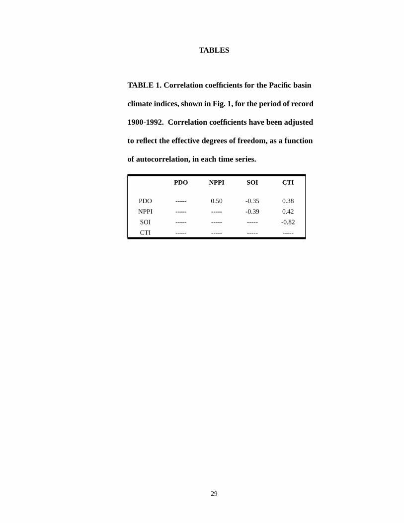
Also shown in Fig 1 are the SOI and the Cold Tongue Index (CTI, which is the aver-

age SST anomaly from 6oN-6oS, 180o-90oW), indices commonly used to monitor the

atmospheric and oceanic aspects of ENSO, respectively. The SOI and CTI are correlated

with the PDO (see Table 1) such that warm- (cold-) phase ENSO-like conditions tend to

coincide with the years of positive (negative) polarity in the PDO. Interestingly, fluctua-

tions in the CTI are mostly interannual, while those in the PDO are predominantly inter-

decadal (ZWB).

Interdecadal and interannual time scales are both apparent in the indices of atmo-

spheric variability at low- and high-northern latitudes over the Pacific. The NPPI and SOI

are correlated such that the mean wintertime Aleutian Low tends to be more (less) intense

during winters with weakened (intensified) easterly winds near the equator in the Pacific.

11

Correlations between the atmospheric and oceanic climate indices shown in Fig. 1

within respective high- and low-latitude ranges are relatively strong. The NPPI is moder-

ately well-correlated with that of the extratropical SST, while at tropical latitudes the SOI

and CTI are very well-correlated (see Table 1).

By regressing the records of wintertime SST and SLP upon the PDO index, the spa-

tial patterns typically associated with a positive unit standard deviation of the PDO are

generated (Fig. 2a). The largest PDO-related SST anomalies are found in the central

North Pacific Ocean, where a large pool of cooler than average surface water has been

centered for much of the past 20 years. The peak amplitude of the SST regression coeffi-

cients in the cold pool are on the order of -0.5oC. The narrow belt of warmer than average

SST that, in the past two decades, has prevailed in the nearshore waters along the west

coast of the Americas is also a distinctive feature of this pattern. Note also that the South-

ern Hemisphere midlatitude SST signature is very similar to that in the northern extratrop-

ics. The SLP anomalies that are typical of the positive PDO are characterized by basin-

scale negative anomalies between 20oN and 60oN. The peak amplitude of the mid-latitude

wintertime SLP signature is about 4mb, which represents an intensification of the clima-

tological mean Aleutian Low. This SLP pattern is very similar to the dominant pattern of

wintertime North Pacific SLP variability. It is noteworthy that there are no strong PDO

signatures in the Atlantic or Indian Ocean SST and SLP fields.

Shown in Fig. 2b are the SST and SLP fields regressed upon the CTI, thus this map

shows anomalies typically associated with a unit standard deviation ENSO index. Com-

paring Fig. 2a with Fig. 2b, it is evident that the tropical PDO-spatial signatures are in

12

many ways reminiscent of canonical warm-phase ENSO SST and SLP anomalies (Ras-

mussen and Carpenter 1982). However, the PDO-amplitudes in the tropical fields are

weaker than those obtained by regressing the surface fields upon the CTI. Likewise, the

PDO-regression amplitudes in the Northern Hemisphere extratropics are stronger than

those obtained from regressions upon the CTI (ZWB).

To establish the significance and consistency of polarity reversals in time--referred to

by some authors asregime shifts--FH-HF and Hare (1996) utilized a technique known as

intervention analysis (Box and Tiao 1975), which is an extension of AutoRegressive Inte-

grated Moving Average (ARIMA) modeling (Box and Jenkins 1976). We applied this

analysis to each of the time series shown in Fig. 1. Intervention analysis is essentially a

two sample t-test that can be applied to autocorrelated data, which is a common feature of

environmental time series. While interventions can take many forms, we tested only step

interventions. The implicit model, therefore, for each variable is a sequence of abruptly

shifting levels, accounting for a significant portion of the total variance, around which

occurs residual variability, either random or autocorrelated1.

The statistical significance of the intervention model parameters are shown in Table

2. Excluding the CTI, polarity reversals in 1977 are supported in each of the time series

1. We followed the standard three step process in fitting the intervention models. First we identify a model.For all time series, the initial model consisted of five parameters: Three interventions, a lag-1 autoregres-sive term and a constant. The three interventions (phase reversals) we used were 1925, 1947 and 1977.The timing of the interventions was derived independently in earlier studies by several of the authors inthis study (FH-HF, ZWB). In the second step, parameters are estimated for significance. If any parame-ters are statistically insignificant, the least significant is dropped and the remaining parameters re-esti-mated. This sequence is repeated as necessary. The model is then accepted if the final step, a white noisetest for model residuals, is passed.

13

shown in Fig. 1. Additional sign reversals in 1925 and 1947 are supported by the PDO

and NPPI time series, but not for the SOI or CTI.

The implications of this statistical exercise are as follows. We have identified an

interdecadal climate signal that is evident in the oceanic and atmospheric climate record.

We attribute these signatures to the PDO. During this century, using the North Pacific SST

pattern time series as the indicator of polarity, the PDO waspredominantly positive

between 1925 and 1946, negative between 1947 and 1976, and positive since 1977. Note

that these multi-decade epochs contain intervals of up to a few years in length in which the

polarity of the PDO is reversed (e.g. the positive PDO values in 1958-61, and the strongly

negative PDO values in 1989-91).

4. Coastal and continental signatures of the PDO

The signature of the PDO is clearly evident in the wintertime surface climate record

for much of North America, but not for that of the other continents. The strongest coeffi-

cients of wintertime air temperature regressed upon the PDO index are located in north-

western North America (Fig. 3a,cf. Latif and Barnett 1994 Fig. 5b), with local maxima of

opposing centers over south central Alaska/western Canada and the southeastern United

States. The PDO is positively correlated2 with wintertime precipitation along the coast of

the central Gulf of Alaska and over northern Mexico and south Florida, and negatively

2. To highlight the regional patterns of the PDO Dec-Feb precipitation signal over the North American con-tinent, the correlation map is shown instead of the regression map. The regression coefficients areskewed towards extreme values in the Pacific Northwest and central Gulf of Alaska. Typical precipitationanomalies for a unit standard deviation positive PDO are about +20 to +30 mm for the central Gulf ofAlaska, -20 to -30 mm for western Washington state, -40 mm for the Hawaiian Islands, +5mm over north-ern Mexico, and -10 mm over the Great Lakes.

14

correlated with that over much of the interior of North America and over the Hawaiian

Islands.

The continental PDO surface climate signatures are consistent with PDO-related cir-

culation anomalies on the hemispheric scale. The Pacific/North America (PNA) (Wallace

and Gutzler 1981) pattern emerges when the cold season (November-March) 500-mb

height fields are regressed upon the PDO index for the period of record 1951-1990 (Fig.

4). This relationship suggests that during epochs in which the PDO is in its positive polar-

ity, coastal central Alaska tends to experience an enhanced cyclonic (counterclockwise)

flow of warm, moist air, which is consistent with heavier than normal precipitation. Wash-

ington state and British Columbia also tend to be subject to an increased flow of relatively

warm humid air, but in their case it is within an area of enhanced anticyclonic circulation

that is dynamically unfavorable for heavier than normal precipitation.

In an analysis of springtime (April 1st) snowcourse data for the western U.S., Cayan

(1996) finds that the leading eigenvector of snowpack variability, what he calls theIdaho

pattern, is centered in the Pacific Northwest. Cayan’s time series for the Idaho pattern has

tracked our PDO index since at least 1935 (when his data begins). This pattern of snow-

pack variability is consistent with the PDO-related wintertime air temperature and precip-

ition patterns shown in Fig. 3: relatively warm (cool) winter air temperatures and

anomalously low (high) precipitation during positive (negative) PDO years contribute to

reduced (enhanced) snowpack in the Pacific Northwest. Furthermore, Cayan’s composite

wintertime 700-mb height fields for the extreme years reveal that variability in the Idaho

snowpack pattern is largely controlled by PNA circulation anomalies (compare Cayan’s

Figs. 3 and 6 with our Figs. 3b and 4).

15

We used the PDO correlation and regression maps (Figs. 2 and 3) as guides to search

for the local and regional instrumental records of PDO-driven climate variability shown in

Fig. 5. Wintertime surface air temperature along the Gulf of Alaska, and SST near the

coast from Alaska to southern California, varies in phase with the PDO. During positive

PDO years the annual water year discharge in the Skeena, Fraser, and Columbia Rivers is

on average 8%, 8%, and 14% lower, respectively, than that during negative PDO years. In

contrast, positive-PDO-year discharge from the Kenai River in the central Gulf of Alaska

region is on average about 18% higher than that during the negative polarity PDO years.

Cayan and Peterson (1989) also noted that this dipole pattern in west coast streamflow

fluctuations is related to the favored pattern of SLP variability in the North Pacific.

5. The PDO and salmon production in the northeast Pacific

Commercial fisheries for Alaskan pink and sockeye salmon are among the most

lucrative in the U. S. (U.S. Dept. of Commerce 1994, 1995). The unique life history of

salmon, which begins and ends in freshwater streams and involves an extensive period of

feeding in the ocean pasture, makes them vulnerable to a variety of environmental

changes. A growing body of evidence suggests that many populations of Pacific salmon

are strongly influenced by marine climate variability (Pearcy 1992, Beamish and Bouillon

1993, FH-HF, Beamishet al. 1995, Franciset al. 1997).

A remarkable characteristic of Alaskan salmon abundance over the past half-cen-

tury has been the large fluctuations at interdecadal time scales which resemble those of the

PDO (Fig. 6, see also Table 3) (FH-HF, Hare 1996). Time series for Washington-Oregon-

California (WOC) coho and Columbia River spring chinook landings tend to be out of

16

phase with the PDO index (Fig. 6), though the correspondence is less compelling than that

with Alaskan salmon. The weaker connections between the WOC and Columbia River

salmon populations and the PDO may be a result of differing environmental/biological

interactions. On the other hand, climatic influences on salmon in their southern ranges

may also be masked or overwhelmed by anthropogenic impacts: Alaskan stocks are pre-

dominantly wild spawners in pristine watersheds, while the WOC coho and Columbia

River spring chinook are mostly of hatchery origin and originate in watersheds that have

been significantly altered by human activities.

The best-fit interventions for the Alaskan sockeye stocks occur two and three years

after those identified in the PDO history, while the best-fit interventions for the Alaskan

pink salmon stocks occur one year following the climate shifts (FH-HF). It is believed

that sockeye and pink salmon abundances are most significantly impacted by marine cli-

mate variability early in the ocean phases of their life cycles (Hare 1996). If this is true,

the key biophysical interactions are likely taking place in the nearshore marine and estua-

rine environments where juvenile salmon are generally found.

Recent work suggests that the marine ecological response to the PDO-related envi-

ronmental changes starts with phytoplankton and zooplankton at the base of the food

chain and works its way up to top level predators like salmon (Venricket al. 1992, FH-HF,

Roemmich and McGowan 1995, Hare 1996, Brodeuret al. 1996, Franciset al. 1997).

This “bottom-up” enhancement of overall productivity appears to be closely related to

upper ocean changes that are characteristic of the positive polarity of the PDO. For exam-

ple, some phytoplankton/zooplankton population dynamics models are sensitive to speci-

fied upper ocean mixed-layer depths and temperatures. For the decade following the

17

1960-76 period of record, such models have successfully simulated aspects of the

observed increases in Gulf of Alaska productivity as a response to an observed 20 to 30%

shoaling and 0.5 to 1o C warming of the mixed-layer (Polovinaet al. 1995).

To the extent that high streamflows favor high survival of juvenile salmon, PDO-

related streamflow variations are likely working in concert with the changes to the near-

shore marine environment in regard to impacts on salmon production. For Alaskan

salmon, the typical positive PDO year brings enhanced streamflows and nearshore ocean

mixed layer conditions favorable to high biological productivity. Generally speaking, the

converse appears to be true for Pacific Northwest salmon.

6. Discussion

Our synthesis of climate and fishery data from the North Pacific sector highlights the

existence of a very large scale, interdecadal, coherent pattern of environmental and biotic

changes. It has recently come to our attention that Minobe (1997) has compiled a comple-

mentary study of North Pacific climate variability that includes SST indices from the

coastal Japan and Indian Ocean-maritime continent regions. Especially relevant to our

work is the fact that Minobe used instrumental records to independently identify the same

dates we promote for climatic regime shifts (1925, 1947, and 1977). Also intriguing is

Minobe’s analysis of (tree-ring) reconstructed continental surface temperatures that sug-

gest PDO-like climate variability has a characteristic recurrance interval of 50 to 70 years,

and that these fluctuations are evident throughout the past three centuries.

It is clear from a visual inspection of the time series shown in Figs. 1, 5, and 6 that

not all changes in our PDO index are indicative of interdecadal regime shifts that are

18

equally apparent in the other indices. The difficulties inherent in real-time assessment of

the state of the PDO are illustrated by the recent period of record: Alaskan salmon catches

and coastal SSTs have remained above average since the late 1970s, while, in contrast, the

PDO index dipped well below average from 1989-1991, and has hovered around normal

since this time. Without the benefit of hindsight it is virtually impossible to characterize

such periods and to recognize long-lived regime shifts at the time they occur.

The ENSO and PDO climate patterns are clearly related, both spatially and tempo-

rally, to the extent that the PDO may be viewed as ENSO-like interdecadal climate vari-

ability (Tanimoto et al. 1993; ZWB). While it may be tempting to interpret interdecadal

climatic shifts as responses to individual (tropical) ENSO events, it seems equally con-

ceivable that the state of the interdecadal PDO constrains the envelope of interannual

ENSO variability.

To our knowledge, there are no documented robust relationships between Pacific

salmon abundance and indices of ENSO. The slowly varying time series of salmon

catches examined in this study are much more coherent with the interdecadal aspects of

the PDO than the higher frequency fluctuations in tropical ENSO indices. In the future it

seems very likely that the PDO will continue to change polarity every few decades as it

has over the past century, and with it the abundance of Alaskan salmon and other species

sensitive to environmental conditions in the North Pacific and adjacent coastal waters.

This climatic-regime driven model of salmon production has broad implications for

fishery management (Hare 1996, Adkisonet al. 1996). The most critical implication con-

cerns periods of low productivity, such as currently experienced by WOC salmon. Man-

19

agement goals, such as the current legislative mandate to double Washington State salmon

production3 (Salmon 2000 Technical Report 1992), may simply not be attainable when

environmental conditions are unfavorable. Conversely, in a period of climatically-favored

high productivity, managers might be well-advised to exercise caution in claiming credit

for a situation that may be beyond their control.

Acknowledgments: We thank Ileana Bladé and Nick Bond for carefully reading an

early draft of this article and offering constructive critiques. This study was prompted by

the University of Washington’s interdisciplinary project forAn Integrated Assessment of

the Dynamics of Climate Variability, Impacts, and Policy Response Strategies for the

Pacific Northwest, and was funded by NOAA’s cooperative agreement #NA67RJ0155,

Washington Sea Grant, andThe Hayes Center. This is JISAO contribution #379.

3. “The [Washington State] legislature hereby establishes a production goal to double the state-wide salmoncatch by the year 2000 . . . ”(Salmon 2000, Technical Report1992).

20

References

Adkison, M.D., R.M. Peterman, M.F. Lapointe, D.M. Gillis, and J. Korman, 1996: Alter-

native models of climatic effects on sockeye salmon (Oncorhynchus nerka) pro-

ductivity in Bristol Bay, Alaska and Fraser River, British Columbia.Fish.

Oceanogr., 5, (In Press).

Alaska Department of Fish and Game (ADFG), 1991: Alaska commercial salmon

catches, 1878-1991. Reg. Info. Rep. 5J91-16. Division of Commercial Fish,

Juneau, AK. 88p.

Anderson, J.J. 1996: Decadal climate cycles and declining Columbia River salmon.Jour-

nal of North American Fisheries Management, in review.

Beamish, R. J. and D.R. Bouillon, 1993: Pacific salmon production trends in relation to

climate. Can. J. Fish. Aquat. Sci., 50, 1002-1016.

________, G.E. Riddell, C.-E. M. Neville, B.L. Thomson, and Z. Zhang, 1995: Declines

in chinook salmon catches in the Strait of Georgia in relation to shifts in the marine

environment.Fish. Oceanog., 4, 243-256.

Box, G.E.P., and G.M. Jenkins, 1976: Time series analysis: forecasting and control.

Revised edition Holden-Day, San Francisco, CA. 575p.

________, and G.C. Tiao, 1975: Intervention analysis with applications to economic and

environmental problems.J. Am. Stat. Assoc., 70: 70-79.

21

Brodeur, R.D., and D. M. Ware, 1992: Interannual and interdecadal changes in zooplank-

ton biomass in the subarctic Pacific Ocean. Fish. Oceanogr.1, 32-38.

________, B.W. Frost, S.R. Hare, R.C. Francis, and W.J. Ingraham, Jr. 1996: Interannual

variations in zooplankton biomass in the Gulf of Alaska and covariation with Cali-

fornia Current zooplankton.Calif. Coop. Oceanic Fish. Invest. Rep.37, In Press.

Cayan, D. R., and D.H. Peterson, 1989: The influence of the North Pacific atmospheric

circulation and streamflow in the west. InAspects of Climate Variability in the

Western Americas, D.H. Peterson ed., Geophys. Monogr.55, Amer. Geophys.

Union, Washington, DC, 375-397.

________, 1996: Interannual climate variability and snowpack in the western United

States.J. Clim., 9, 928-948.

Ebbesmeyer, C.C., C. A. Coomes, G. A. Cannon, and D. E. Bretschneider, 1989: Linkage

of ocean and fjord dynamics at decadal period. In: D.H. Peterson [ed.] Climate

Variability on the eastern Pacific and western North America, Geophys. Monogr.

55, Am. Geophys. Union, 399-417.

________, D. R. Cayan, D. R. McLain, F. H. Nichols, D. H. Peterson, K. T. Redmond,

1991: 1976 step in the Pacific climate: forty environmental changes between

1968-1975 and 1977-1985. In J. L. Betancourt and V. L. Tharp, [ed.],Proc. Sev-

enth Annual Pacific Climate Workshop, April 1990, Asilomar, CA. Calif. Dept. of

Water Res., Interagency Ecological Studies Program Tech. Rep.26.

22

Eischeid, J.K., H.F. Diaz, R.S, Bradley, and P.D. Jones. 1991: A comprehensive precipita-

tion data set for global land areas. DOE/ER-69017T-H1,TR051, U.S. Dept. of

Energy, Carbon Dioxide Res. Program, Washington, D.C.

Fletcher, J.O., R.J. Slutz and S.D. Woodruff, 1983: Towards a comprehensive ocean-

atmosphere dataset.Trop. Ocean-Atmos. Newslett., 20, 13-14.

Folland, C.K., and D.E. Parker, 1990: Observed variations of sea surface temperature. In

Climate-Ocean Interaction, M.E. Schlesinger [ed.], Kluwer, Dordrecht, 21-52.

________, and ________, 1995: Correction of instrumental biases in historical sea sur-

face temperature data.Quart. J. Roy. Meteorol. Soc., 121, 319-367.

Francis, R.C., and T.H. Sibley, 1991: Climate change and fisheries: what are the real

issues?NW Env. Journ., 7, 295-307.

________, and S. R. Hare, 1994: Decadal-scale regime shifts in the large marine ecosys-

tems of the North-east Pacific: a case for historical science.Fish. Oceanogr.3,

279-291.

________, ________, A. B. Hollowed, and W. S. Wooster, 1997: Effects of interdecadal

climate variability on the oceanic ecosystems of the northeast Pacific. To appear

in J. Clim.

Graham, N.E., 1994: Decadal-scale climate variability in the 1970s and 1980s: observa-

tions and model results.Clim. Dyn.10, 135-159.

23

Hollowed, A.B., and W.S. Wooster, 1992: Variability of winter ocean conditions and

strong year classes of Northeast Pacific groundfish.ICES mar. Sci. Symp.,195,

433-444.

Hare, S.R. and R. C. Francis, 1995: Climate change and salmon production in the North-

east Pacific Ocean.Can. Spec. Publ. Fish. Aquat. Sci.121, 357-372.

________, 1996: Low-frequency climate variability and salmon production. Ph. D. thesis,

University of Washington, Seattle, 306p.

Jones, P.D., S.C.B. Raper, B.D. Santer, B.S.G. Cherry, C.M. Goodes, P.M. Kelly, T.M.L.

Wigley, R.S. Bradley and H.F. Diaz, 1985: A Grid Point Temperature Data Set for

the Northern Hemisphere. U.S. Dept. of Energy, Carbon Dioxide Res. Div., Tech.

Rep.TR022, 251p.

Kushnir, Y., and J.M. Wallace 1989: Low frequency variability in the Northern Hemi-

sphere winter: Geographical distribution structure and time-scale.J. Atmos.Sci.,

46, 3122-3142.

Latif, M. and T.P. Barnett, 1994: Causes of decadal climate variability over the north

Pacific and North America.Science266, 634-637.

________ and ________, 1996: Decadal climate variability over the North Pacific and

North America: dynamics and predictability. To appear inJ. Clim.

Minobe, S., 1997: A 50-70 year climatic oscillation over the North Pacific and North

America. Submitted toGeophys. Res. Lett., October 1996. In review.

24

Namias, J. 1978: Multiple causes of the North American abnormal winter of 1976-77.

Mon. Wea. Rev.106, 279-295.

Pacific Fisherman, 1915: September 1915. M. Freeman Publications, Portland, OR.

________, 1939: 1939 Yearbook. M. Freeman Publications, Portland, OR.

________, 1972: August/September 1972. M. Freeman Publications, Portland, OR.

Pacific Fishing, 1994: 1994 Yearbook. Pacific Fishing Partnership, Seattle, WA, VolXV.

________, 1995: 1995 Yearbook. Pacific Fishing Partnership, Seattle, WA, Vol.XVI .

Pearcy, W.G., 1992: Ocean ecology of north Pacific salmonids. University of Washington

Press, Seattle, WA. 179p.

Polovina, J.J., G.T. Mitchum and G.T. Evans, 1995: Decadal and basin-scale variation in

mixed layer depth and the impact on biological production in the Central and

North Pacific, 1960-88.Deep Sea Res.42, 1701-1716.

Rasmussen, E. M. and T.H. Carpenter 1982: Variations in tropical sea surface temperature

and surface wind fields associated with the Southern Oscillation/El Niño.Mon.

Wea. Rev., 110, 354-384.

Reynolds, R. W. and T. M. Smith, 1995: A high resolution global sea surface temperature

climatology.J. Clim., 8, 1571-1583.

Roemmich, D. and J. McGowan, 1995: Climatic warming and the decline of zooplankton

in the California Current.Science267, 1324-1326.

25

Salmon 2000 Legislation, 1988: Washington State Senate Bill 6647, Olympia, Washing-

ton.

Tanimoto, Y., N. Iwasaka, K. Hanawa, and Y. Toba, 1993: Characteristic variations of sea

surface temperature with multiple time scales in the North Pacific.J. Clim., 6,

1153-1160.

Trenberth, K.E. and D.A. Paolino, Jr. 1980: The northern hemisphere sea-level pressure

data set: trends, errors and discontinuities.Mon. Wea. Rev.108, 855-872.

________, 1990: Recent observed interdecadal climate changes in the northern hemi-

sphere.Bull. Am. Met. Soc.71, 988-993.

________ and J.W. Hurrell, 1994: Decadal atmosphere-ocean variations in the Pacific.

Clim. Dyn.9, 303.

United States Department of Commerce 1994:Fisheries of the United States.Silver

Springs, MD.

________ 1995: Current Fishery Statistics No. 9400, Silver Springs, MD.

Venrick, E.L., and J.A. McGowan, D.R. Cayan, and T.L. Hayward, 1987: Climate and

chlorophyll a: long-term trends in the central north Pacific Ocean.Science238,

70-72.

WDF and ODFW, 1992: Status Report: Columbia River Fish Runs & Fisheries, 1938 -

91. Washington Dept. of Fisheries and Oregon Dept. of Fish and Wildlife, Port-

land, Oregon.

26

Walker, G.T. and E.W. Bliss 1932: World Weather V, Mem.R. Meteorol. Soc., 4, 53-84.

Wallace, J.M., and D.S. Gutzler 1981: Teleconnections in the geopotential height field

during the Northern Hemisphere winter.Mon. Wea. Rev., 109, 784-812.

Ware, D.M., 1995: A century and a half of change in the climate of the NE Pacific.Fish.

Oceanogr.4, 267-277.

Zhang, Y., 1996: An observational study of atmosphere-ocean interactions in the northern

oceans on interannual and interdecadal time-scales. Ph. D. thesis, University of

Washington, Seattle.

________, J.M. Wallace, D.S. Battisti, 1997: ENSO-like interdecadal variability: 1900-

93. To appear inJ. Clim.

27

List of Figures

Figure 1: Normalized winter mean (November-to-March) time histories of Pacific cli-

mate indices. Dotted vertical lines are drawn to mark the PDO polarity rever-

sal times in 1925, 1947, and 1977. Positive (negative) values of the NPPI

correspond to years with an deepened (weakened) Aleutian Low. The negative

SOI is plotted so that it is in phase with the tropical SST variability captured by

the CTI. Positive value bars are black, negative are grey.

Figure 2: COADS SST (color shaded) and SLP (contoured) regressed upon (a) the PDO

index and (b) the CTI for the period of record 1900-1992. Contour interval is

1 mb, with additional contours drawn for +/- 0.25 and 0.50 mb. Positve (nega-

tive) contours are dashed (solid).

Figure 3: Maps of PDO-regression and correlation coefficients: (a) November-March sur-

face air temperature regressed upon the PDO index shown in Fig. 1; contour

interval is 0.2oC. (b) Correlation coefficients (x100) between December-Feb-

ruary precipitation and the PDO index shown in Fig. 1; contour interval is 10.

Positive (negative) contours are solid (dashed).

Figure 4: Wintertime Northern Hemisphere 500-mb heights regressed upon the PDO

index for the period of record 1951-1990. Contour interval is 5m, positive

(negative) contours are solid (dashed).

Figure 5: Selected regional climate time series with PDO signatures. Dotted vertical lines

are drawn to mark the PDO polarity reversal times in 1925, 1947, and 1977.

28

Bars are shaded as in Figure 1, with the shading convention reversed for the

BC/Washington Streamflow index.

Figure 6: Selected Pacific salmon catch records with PDO signatures. For Alaska catch,

black (grey) bars denote values that are greater (less) than the long-term

median. The shading convention is reversed for WOC coho and Columbia

River spring chinook catch. Dotted vertical lines are drawn in each panel to

mark the PDO polarity reversal times in 1925, 1947, and 1977. At the top, the

PDO index is repeated from Figure 1.

29

TABLES

TABLE 1. Correlation coefficients for the Pacific basin

climate indices, shown in Fig. 1, for the period of record

1900-1992. Correlation coefficients have been adjusted

to reflect the effective degrees of freedom, as a function

of autocorrelation, in each time series.

PDO NPPI SOI CTI

PDO ----- 0.50 -0.35 0.38

NPPI ----- ----- -0.39 0.42

SOI ----- ----- ----- -0.82

CTI ----- ----- ----- -----

30

TABLE 2. P-values for tests of step-changes in the mean level of

the Pacific basin climate indices shown in Fig. 1. The four time

periods tested for changes in the mean level were 1900-1924, 1925-

1946, 1947-1976, 1977-1996. P-values greater than 0.05 are

labeled “n.s.” (not significant).

Climate Index Intercept 1925 step 1947 step 1977 step

PDO n. s. .001 .000 .000

NPPI .005 .001 .000 .000

SOI n. s. n. s. n. s. .001

CTI n. s. n. s. n. s. n. s.

31

TABLE 3. Percent change in mean catches of four

Alaskan salmon stocks following major PDO

polarity changes in 1947 and 1977. Mean catch

levels were estimated from intervention models

fitted to the data and incorporating a 1-year lag for

both pink salmon stocks, a 2-year lag for western

sockeye and a 3-year lag for central sockeye.

salmon stock 1947 step 1977 step

western AK sockeye -37.2% +242.2%

central AK sockeye -33.3% +220.4%

central AK pink -38.3% +251.9%

southeast AK pink -64.4% +208.7%

32

Normalized winter mean (November-to-March) time histories of Pacific climate indices.

Dotted vertical lines are drawn to mark the PDO polarity reversal times in 1925, 1947, and

1977. Positive values of the NPPI correspond to years with a deepened Aleutian Low.

The negative SOI is plotted so that it is in phase with the equatorial SST anomalies cap-

tured by the CTI. Positive value bars are filled with black, negative with grey shading.

1900 1920 1940 1960 1980 2000

Figure 1

PDO

NPPI

-SOI

CTI

Pacific Basin Climate Indicesno

rmal

ized

am

plitu

des

1900 1920 1940 1960 1980 2000

33

COADS SST (color shaded) and SLP (contoured) regressed upon (a) the PDO index and

(b) the CTI for the period of record 1900-1992. Contour interval is 1 mb, with additional

contours drawn for +/- 0.25 and 0.50 mb. Positive (negative) contours are broken (solid).

-3

-2

-2

-1-1

-1

0

0

00

0

0

0

0

-0.6

-0.4

-0.2

0.0

0.2

0.4

0.8

-2

-1-1

0

0

0

0

0

(a) SST and SLP regressed on the PDO index

(b) SST and SLP regressed on the CTI

Figure 2

oC

34

Maps of PDO-regression and correlation coefficients for the period of record 1900-1992:

(a) November-March surface air temperature regressed upon the PDO index shown in Fig.

1; contour interval is 0.2oC. (b) Correlation coefficients (x100) between December-Feb-

ruary precipitation and the PDO index shown in Fig. 1; contour interval is 10. Positive

(negative) contours are solid (dashed).

160W 120W 80W 40W

20N

40N

60N

160W 120W 80W 40W

20N

40N

60N

11

1.6

0 -0.4

-38

2719

-27

26 36

Dec-Feb precipitation correlations

Nov-Mar surface air temperature

regressed on the PDO index ( oC): 1900-1992

with the PDO index (x100): 1900-1992

(a)

(b)

Figure 3

-46

35

Wintertime Northern Hemisphere 500-mb heights regressed upon the PDO index for the

period of record 1951-1990. Contour interval is 5m, positive (negative) contours are solid

(dashed).

0

30E

60E

90E

120E

150E

180

150W

120W

90W

60W

30W

0

Nov-Mar 500-mb heights regressed on the PDO index

Figure 4

- 4520

0

10

0 - 5

36

Selected regional climate time series with PDO signatures. Dotted vertical lines are drawn

to mark the PDO polarity reversal times in 1925, 1947, and 1977. Bars are shaded as in

Figure 1, with the shading convention reversed for the BC/Washington Streamflow index.

1900 1920 1940 1960 1980 2000

Gulf of Alaska Air Temperature

British Columbia Coastal SST

Scripps Pier SST

Gulf of Alaska Streamflow

BC/Washington Streamflow

Regional Climate Indices with PDO variability

Figure 5

1900 1920 1940 1960 1980 2000

norm

aliz

ed a

mpl

itude

s

selected Pacific salmon catch records

annu

al c

atch

in m

illio

ns

37

Figure 6: Selected Pacific salmon catch records with PDO signatures. For Alaska

catches, black (grey) bars denote values that are greater thant the long-term median. The

shading convention is reversed for WOC coho and Columbia River spring chinook. Light,

dotted vertical lines are drawn to mark the PDO reversal times at 1925, 1947, and 1977.

The PDO index from Figure 1 is repeated in the top panel.

0

50

0

20

40

0

50

100

0

50

100

0

0.5

0

5

1900 1920 1940 1960 1980 2000

western Alaska sockeye

central Alaska sockeye

central Alaska pink

southeast Alaska pink

Columbia River spring chinook

Washington-Oregon-California coho

PDO

0

2

-2