Energy Vol. ?. No. 7. ~0. 613-625. 1982 036bW2/82/07Ml!-13f03 0010

Prmted m Great Britain Q 1982 Pergamon Press I td

A MARKET PENETRATION MODEL FOR RESIDENTIAL PHOTOVOLTAIC DEPLOYMENT AND ITS APPLICATION IN WASHINGTON STATE?

GENE M. MESHER,~ BARRY HYMAN,$ CHARLES KIPPENHAN,§ and RICHARD ZERBE,~

University of Washington, Seattle, WA 98195, U.S.A.

(Received 3 December 1981)

Abstract-A model is developed for examining the adoption of photovoltaic systems in single family residences. The model treats photovoltaic devices as consumer durables with a potential for providing a return on investment. In a series of scenarios, we examine a range of estimated market penetrations in Washington State by the year 2000 under a variety of economic and policy conditions.

INTRODUCTION

Studies of the potential of photovoltaics indicate that it may one day be possible to produce small-scale photovoltaic systems at prices affordable to the genera1 public. If this occurs, power planners will need to modify existing planning techniques to include estimates of the future generation capacity to be brought on-line through decisions made by consumers. Market penetration models may be a useful tool to aid power planners in estimating the future role these personal energy devices will play.

Government policy makers have a problem similar to that of energy planners with regard to personal electric power energy systems. Almost every energy technology used in this country today has been developed with strong government support.’ Energy policy makers have the problem of identifying which policy strategies will most effectively help new technologies to develop to the point where they can compete with the historically subsidized technologies that now provide virtually all electric power in this country. Thus, a second use of market penetration models is to provide a means by which policy planners can examine the effect which various policy options may have on consumer acceptance of technologies like photovol- taics.

The goal of this analysis is to examine the potential contribution of small photovoltaic systems sold to individual consumers.l( We present a model (PVMPS) to estimate the market potential of personally owned photovoltaic power systems and apply this mode1 to the specific case of Washington State. The model assumes that differences in income levels imply differences, on average, in demand for electricity, as well as differences in the desire to purchase a new product. Individual purchase decisions (assumed to be based on the economic desirability of owning a photovoltaic power system at a given point in time) are integrated over the entire population to produce a market penetration value for that year. PVMPS also simulates the effect of weather conditions and electricity demand patterns on the economic attractiveness of photovoltaics. Scenarios are presented to depict a probable range of future events including an examination of the effect strong government support would have on the deployment of photovoltaics in Washington.

There are, of course, limitations to the model described here. The model itself was developed specifically from the standpoint of owners of single-family homes making the purchasing decisions. Thus, only a portion of the total potential market is considered. The multi-family residential, utility, industrial and commercial sectors are not examined. Neither is the energy storage issue considered in detail in this study. However, since the existing large hydroelectric system in the Pacific Northwest could conceivably be used as a regional energy storage system long before other forms of cheap energy storage are available, the implications

tBased on a thesis submitted by the senior author in partial fulfillment of the requirements for an M.S.E. degree, The research was conducted as part of a project on decentralized electricity generation sponsored by the Ford Foundation.

SProgram in Social Management of Technology. PDepartment of Mechanical Engineering. IIA discussion of other approaches to examining market potential is contained in Ref. 2.

613

614 GENE M. MESHER et al.

of this idea are discussed as a special case of significance to the development of solar energy in Washington.3.

MARKET PENETRATION CONCEPTS AND MODELS

The economics of photovoltaic devices will continue to improve in the foreseeable future, due to the following reasonably predictable trends: (1) As real income rises, the demand for electricity will increase, since electricity is a normal good. Thus, economic growth will increase the demand for total electricity production including cost-competitive alternatives to con- ventional power generation: (2) The prices of fossil and nuclear power generation will continue to increase while the price of photovoltaic devices will be constantly declining.

Of course, if the price of substitutes for power generation, e.g. conservation, falls sufficiently, this could offset the effect of higher incomes on the demand for electricity. The promise of photovoltaic systems may also be thwarted by a breakthrough of an even cheaper form of power generation (e.g., fuel cells or fusion). In this paper, however, we treat conventional power generation as the only competition to photovoltaics.

Market penetration models of consumer durables Recently, Mahajan and Muller have reviewed the subject of the market penetration of

consumer durables.4 Most of the early models have been developed to “deal only with social and behavioral influences on the timing of adoption. Economic forces, such as price, are ignored”.5 For this reason, we could not pursue most models of this type since the data on social and behavioral influences on the market for photovoltaics is nonexistent. One model was found, however, which did provide a useful approach to photovoltaic market modelling. This was the study by Bonus in which the market penetratration of consumer durables was developed as a function of consumer income.6

Solar market models In a recent review of solar energy market penetration models, four of the most prominent

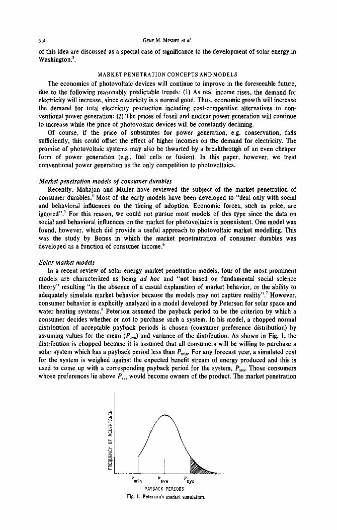
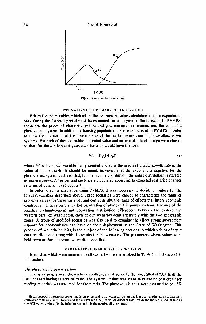
models are characterized as being ad hoc and “not based on fundamental social science theory” resulting “in the absence of a casual explanation of market behavior, or the ability to adequately simulate market behavior because the models may not capture reality”.’ However, consumer behavior is explicitly analyzed in a model developed by Peterson for solar space and water heating systems.’ Peterson assumed the payback period to be the criterion by which a consumer decides whether or not to purchase such a system. In his model, a chopped normal distribution of acceptable payback periods is chosen (consumer preference distribution) by assuming values for the mean (Pay,) and variance of the distribution. As shown in Fig. 1, the distribution is chopped because it is assumed that all consumers will be willing to purchase a solar system which has a payback period less than Pmi,. For any forecast year, a simulated cost for the system is weighed against the expected benefit stream of energy produced and this is used to come up with a corresponding payback period for the system, Psys. Those consumers whose preferences lie above Psys would become owners of the product. The market penetration

P min

P ave P

SYS

PAYBACK PERIODS

Fig. 1. Peterson’s market simulation.

A market penetration model for residential photovoltaic deployment 615

for that year is then the cross-hatched area shown in Fig. 1. A market penetration forecast is created by repeating this process for each year during the forecasting period.

Peterson’s simulation model has two significant drawbacks. First, the payback period is a crude and often quite inadequate measure of the profitability of purchasing a product. If we assume that consumers respond to profitability, other indicies such as the net present value, the benefit-cost ratio and the internal rate of return better characterize the desirability of an investment than the payback period.t

The second problem with Peterson’s model is the assumption that consumer preferences are normally distributed with regard to the average acceptable payback period. As product related information diffuses, consumer preferences could be expected to change to accept longer payback periods. This will provide logistic growth typical of market penetration phenomena since the cumulative normal distribution is equal to a logistic function. This approach, however, requires assuming the shape of the consumer preference distribution as well as the payback period (P,,,) at which the average consumer decides to purchase the system. For this reason, a different simulation approach, using the net present value, was taken in this paper.

A PHOTOVOLTAIC MARKET PENETRATION SIMULATION

In our new model, PVMPS, consumer behavior is assumed to be a function of income. This assumption serves the same role in the analysis as Peterson’s conjecture of a normal variation to consumer preference, except that the income distribution is a logarithmic rather than a normal distribution function. An advantage of using the income distribution is that it is readily obtainable, while the consumer preference distribution which Peterson hypothesizes would require a survey to measure. Another advantage of using income as the independent variable is that income is also a critical parameter in predicting demand for electricity.‘”

In PVMPS, the probability of ownership of a solar power system is derived from the Quasi-Engel function (defined as the probability of ownership of a good within a given income class as a function of income), a concept which Bonus applied to analyze consumer preferences for durable goods (televisions, refrigerators, etc.).

Another feature of PVMPS is that it involves comparison of solar-generated power with electricity consumed on an hourly basis. Most simulations use only annual energy output to analyze system utility and are thus insensitive to the effect of diurnal or seasonal variations on the output characteristics and the demand for the power generated. Since surplus power could be sold by the consumer to the utility at a price which is different from the price at which the consumer purchases power from the utility, these generation and demand variations need to be accounted for.

PVMPS is composed of three main parts: the solar energy calculations, the life-cycle cost-benefit evaluation, and the market simulation. Each of these will now be described.

Solar energy calculation The power output for a specified system location and orientation is computed on an hourly

basis with given weather conditions as input values. Hourly data for one day during each month of the year were taken from data recorded at

weather stations in the study area.” Information from the weather data file is used in the calculation of the hourly values of solar energy collected on a surface having the orientation specified for the photovoltaic panels. This involved summing the components of the direct beam radiation, diffuse radiation and ground reflections appropriate to the solar position and the position of the panels.

Life-cycle-cost-benefit analysis Once the output of the photovoltaic device has been determined, hourly use profiles of the

user are compared with the output of the system to determine how much power can be utilized on-site and how much will be surplus. The amount of electricity used during hour j of the day

fZerbe has shown how net present value, benefit-cost ratio, and the internal rate of return can be normalized to give consistent and correct ranking of alternative investments in terms of their profitability.’

EGY Vol. 7. No. 7-D

616 GENE M. ME~HER et al.

during a typical day of month i, is written as

X, = (X/8760) MUFJ: HU& (1)

where X is the annual usage. The monthly usage factor MUFi is the daily residential electrical usage for a typical day during the ith month divided by the average daily residential usage during the year. The hourly usage factor HUF is defined as the ratio of usage during hour j to the average hourly usage and is assumed to be composed of a base load factor (night and early morning electrical demand), an intermediate load factor (daytime demand), and a peak load factor (during the early evening).‘*

Factors affecting the annual demand for electricity, X, in the residential sector have been studied by Halvorsen.13 In Halvorsen’s analysis, the annual demand for electricity is related log-linearly to several factors, the most important being the positive correlation of demand for electricity with income (Y) and the negative correlation of demand to the unit price of electricity (U). Halvorsen also correlated electrical demand with the price of natural gas (G), annual heating degree days (D), percent of population living in rural areas (R), and average size of households (H). Demand for a household is then

X=b,U+b,Y+b,G+b,D+b,R+b,H, (2)

where bi is the elasticity of demand with respect to the ith factor and all variables are in logarithmic form.

Since the unit price (d/kWh) at which power can be sold by the owner of the photovoltaic system to the utility will most likely be different from the residential rate for electricity, the value of a given amount of electricity generated is equal to the cost of purchasing that amount of power from the utility, or the amount for which that power could be sold to the utility, whichever is greater. In PVMPS, the amount of electricity generated by the on-site system and the amount of electricity consumed on-site is calculated on an hourly basis for a typical day during each month. It is assumed all electricity generated during a given hour in excess of the on-site demand during that hour is sold to the local utility.

The total value of the electricity generated in any year i by the photovoltaic power system is the sum over that year of the values of the power consumed on-site and the power which is sold to the utility, viz.

or

&=(Qc+QsSi)& ifSis

Vi=Q,SiU, if $21,

(3)

where

Q, = Qc + Qs.

Here, Vi is the annual value of electricity generated in the ith year; Qp QC, and Qs are the annual quantities of power generated, consumed on-site, and sold, Si is the sales multiplier defined as the ratio of the price at which electricity is sold to the utility to the residential retail-price of electricity, and Ui is the unit retail price of electricity for residential customers. For simplicity, we have assumed that both Si and Vi are constant during a given year. However, since both Si and Ui are allowed to vary from year to year, the calculation for Vi is repeated for each year of the system lifetime.

The investment required to purchase the photovoltaic power system is treated as a loan, with a chosen loan rate and period. The principal of the loan is equal to the system capital cost. The loan payments are then treated as annuities paid out by the buyer. Using the formula for an

A market penetration model for residential photovoltaic deployment 617

annuity, the cost of a photovoltaic system in the ith year of operation is

Ci = Csys rl[ 1 - (1+ r)-N]*

Here, r equals the loan rate when i is less than the loan period and zero otherwise, and CSyF is the total system cost.

The net present value can then be calculated by taking the difference between V and Ci for each year of the operational lifetime of the system, discounted back to the year for which the market penetration is being estimated. In addition, the possibility of a tax credit is included and the amount of the credit is added as a benefit in the first year of operation, viz.

(5)

where T is the fractional tax credit and d is the discount rate. The net present value then serves as a parameter of the Quasi-Engel function of the market simulation discussed below.

Market simulation model The market simulation model developed here is similar to that used by Bonus in his

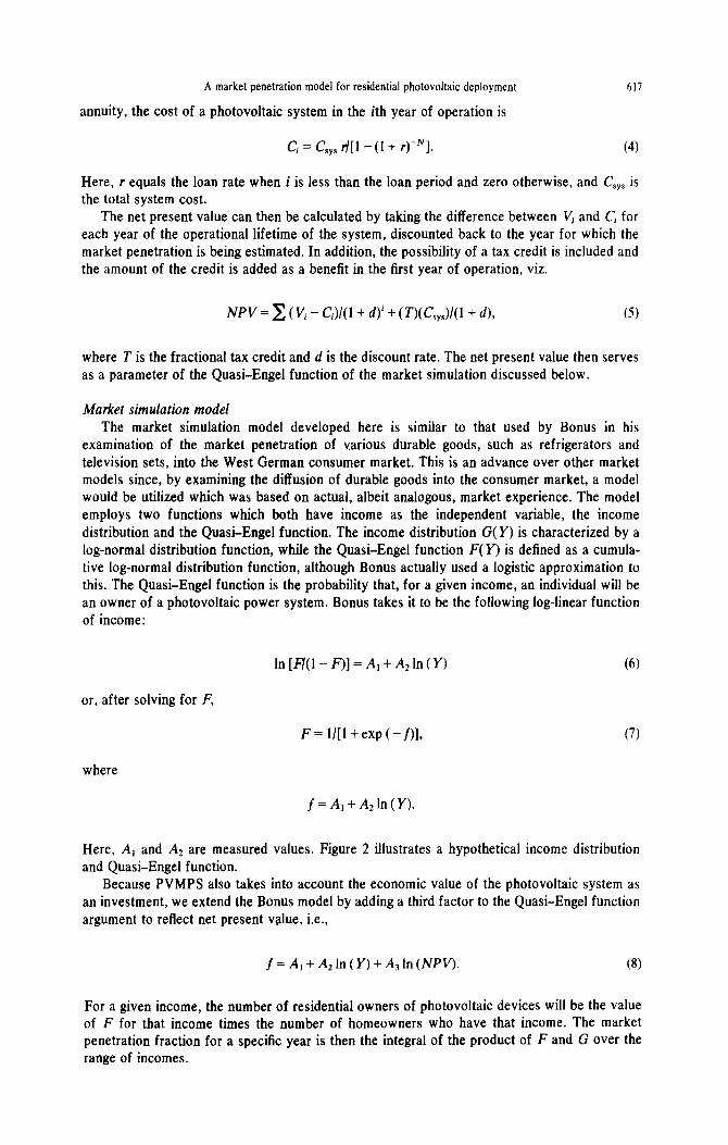
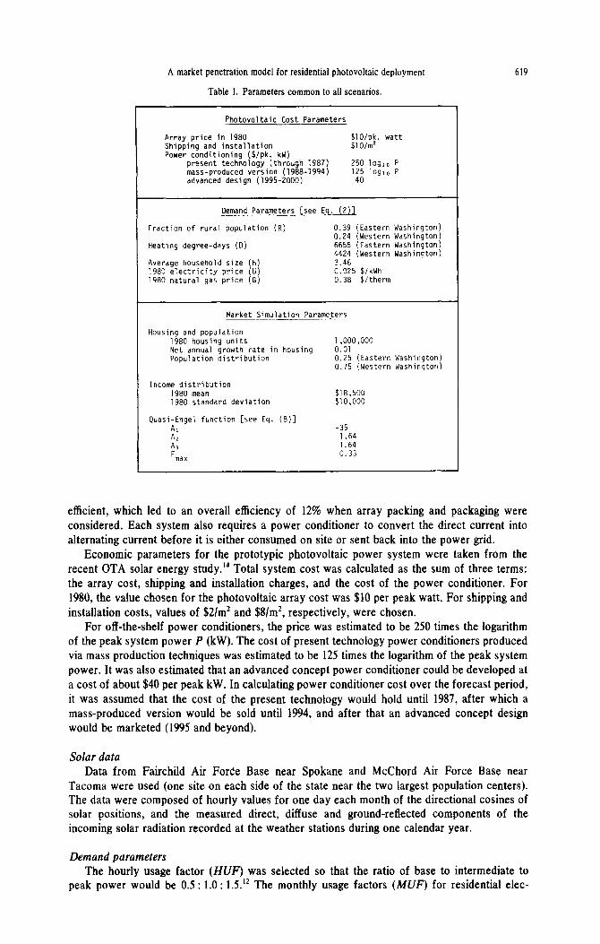
examination of the market penetration of various durable goods, such as refrigerators and television sets, into the West German consumer market. This is an advance over other market models since, by examining the diffusion of durable goods into the consumer market, a model would be utilized which was based on actual, albeit analogous, market experience. The model employs two functions which both have income as the independent variable, the income distribution and the Quasi-Engel function. The income distribution G(Y) is characterized by a log-normal distribution function, while the Quasi-Engel function F(Y) is defined as a cumula- tive log-normal distribution function, although Bonus actually used a logistic approximation to this. The Quasi-Engel function is the probability that, for a given income, an individual will be an owner of a photovoltaic power system. Bonus takes it to be the following log-linear function of income:

ln[fl(l-F)]=Al+Azln(Y) (6)

or, after solving for F,

F = l/[l + exp ( - f)], (7)

where

f=A,+A21n(Y).

Here, A, and A2 are measured values. Figure 2 illustrates a hypothetical income distribution and Quasi-Engel function.

Because PVMPS also takes into account the economic value of the photovoltaic system as an investment, we extend the Bonus model by adding a third factor to the Quasi-Engel function argument to reflect net present value, i.e.,

f=A,+A21n(Y)+A,ln(NPV). (8)

For a given income, the number of residential owners of photovoltaic devices will be the value of F for that income times the number of homeowners who have that income. The market penetration fraction for a specific year is then the integral of the product of F and G over the range of incomes.

618 GENE M. MESHER ef al.

Y min

INCOME

Fig. 2. Bonus’ market simulation.

ESTIMATING FUTURE MARKET PENETRATION

Values for the variables which affect the net present value calculation and are expected to vary during the forecast period must be estimated for each year of the forecast. In PVMPS, these are the prices of electricity and natural gas, increases in income, and the cost of a photovoltaic system. In addition, a housing population model was included in PVMPS in order to allow the calculation of the absolute size of the market penetration of photovoltaic power systems. For each of these variables, an initial value and an annual rate of change were chosen so that, for the kth forecast year, each function would have the form

w, = W&l + &Jt, (9)

where W is the model variable being iterated and r, is the assumed annual growth rate in the value of that variable. It should be noted, however, that the exponent is negative for the photovoltaic system cost and that, for the income distribution, the entire distribution is iterated as income grows. All prices and costs were calculated according to expected real price changes in terms of constant 1980 dol1ars.t

In order to run a simulation using PVMPS, it was necessary to decide on values for the forecast variables described above. Three scenarios were chosen to characterize the range of probable values for these variables and consequently, the range of effects that future ecomonic conditions will have on the market penetration of photovoltaic power systems. Because of the significant climatological and population distribution differences between the eastern and western parts of Washington, each of our scenarios dealt separately with the two geographic zones. A group of modified scenarios was also used to examine the effect strong government support for photovoltaics can have on their deployment in the State of Washington. This process of scenario building is the subject of the following sections in which values of input data are discussed along with the results for the scenarios. The parameters whose values were held constant for all scenarios are discussed first.

PARAMETERS COMMON TO ALL SCENARIOS

Input data which were common to all scenarios are summarized in Table 1 and discussed in this section.

The photovoltaic power system The array panels were chosen to be south facing, attached to the roof, tilted at 23.8” (half the

latitude) and having an area of 59 m*. The system lifetime was set at 30 yr and no cost credit for roofing materials was assumed for the panels. The photovoltaic cells were assumed to be 15%

tit can be readily shown that converting future prices and costs to constant dollars and then applying the real discount rate is equivalent to using current dollars and the market (nominal) value for discount rate. We define the real discount rate as (I+ j)/(l + i) - I, where j is the inflation rate and i is the nominal discount rate.

A market penetration model for residential photovoltaic deployment 619

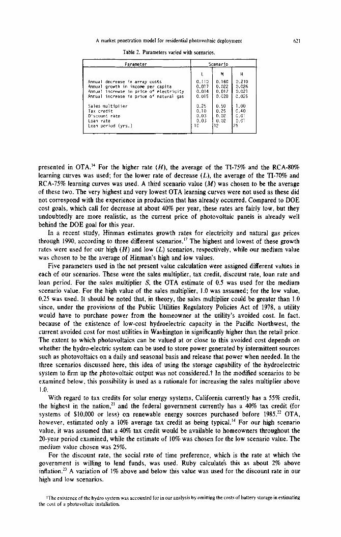
Table 1. Parameters common to all scenarios.

Photovoltaic Cost Parameters

Array price in 1980 Shipping and installation

:;KJ$;$. watt

Power conditioning ($/pk. kW) present technology (through 1987) 250 log,, P mass-produced version (1988-1994) 125 log,, P advanced design (1995-2000) 40

Demand Parameters [see Eq. (2)1

Fraction of rural population (R)

Heating degree-days (D)

Average household size (H) 1980 electricity price (U) 1980 natural gas price (G)

0.39 (Eastern Washington) 0.24 (Western Washington) 6655 (Eastern Washington) 4424 (Western Washington) 3.46 0.025 $/kWh 0.38 $/therm

Market Simulation Parameters

Housing and population 1980 housing units 1,000,000 Net annual growth rate in housing 0.01 Population distribution 0.25 (Eastern Washington)

0.75 (Western Washington)

Income distribution 1980 mean 1980 standard deviation fl::%

Quasi-Engel function [see Eq. (a)]

Al -35

AZ 1.64

A3 1.64 F 0.33 max

efficient, which led to an overall efficiency of 12% when array packing and packaging were considered. Each system also requires a power conditioner to convert the direct current into alternating current before it is either consumed on site or sent back into the power grid.

Economic parameters for the prototypic photovoltaic power system were taken from the recent OTA solar energy study.14 Total system cost was calculated as the sum of three terms: the array cost, shipping and installation charges, and the cost of the power conditioner. For 1980, the value chosen for the photovoltaic array cost was $10 per peak watt. For shipping and installation costs, values of $2/m* and $8/m*, respectively, were chosen.

For off-the-shelf power conditioners, the price was estimated to be 250 times the logarithm of the peak system power P (kW). The cost of present technology power conditioners produced via mass production techniques was estimated to be 125 times the logarithm of the peak system power. It was also estimated that an advanced concept power conditioner could be developed at a cost of about $40 per peak kW. In calculating power conditioner cost over the forecast period, it was assumed that the cost of the present technology would hold until 1987, after which a mass-produced version would be sold until 1994, and after that an advanced concept design would be marketed (1995 and beyond).

Solar data Data from Fairchild Air Force Base near Spokane and McChord Air Force Base near

Tacoma were used (one site on each side of the state near the two largest population centers). The data were composed of hourly values for one day each month of the directional cosines of solar positions, and the measured direct, diffuse and ground-reflected components of the incoming solar radiation recorded at the weather stations during one calendar year.

Demand parameters The hourly usage factor (HUF) was selected so that the ratio of base to intermediate to

peak power would be 0.5 : 1.0 : 1.5.‘* The monthly usage factors (MUF) for residential elec-

620 GENE M. MESHER ef al.

tricity were developed from utility data on total power consumption for the residential sector for each month during a specific year.?

A number of input values was required to estimate the annual demand for electricity (X) for residential customers from Eq. (2). The demand equation coefficients (b,, . . . , bs) were taken from Halvorsen.‘3 The percentage of population living in rural areas (R) was based on values for counties in western and eastern Washington; both R and H, the average household size, were taken from 1970 census data. I5 The annual heating degree-days (D) for eastern and western Washington were taken from a standard handbookI while unit prices of electricity (U) and natural gas (G) in 1980 were taken from a recent study on the state’s energy future.”

Market simulation parameters Also shown in Table 1 are the parameters used to construct the income distribution function

G(Y) and the argument of the Quasi-Engel function in Eq. (8). Data on the housing stock and its projected growth rate were obtained from a study on solar energy for the Pacific North- west.” Census data were then used to estimate how much of the state’s population was located in the eastern and western regions of the state.15

The income distribution for the homeowning population was approximated by using data from 1977 joint tax returns for all taxpayers in Washington.” A log-normal distribution was then fitted to these data and this function was then converted to 1980 dollars, the base year used in this study.

The parameter A, was chosen such that the minimum value of the Quasi-Engel function would be just to the right of the maximum annual income within the state during the year in which the net present value of photovoltaics devices first becomes positive. In this way, the market penetration curve over time is assured to be continuous since the fraction captured cannot suddenly jump once economic turnover occurs.

For the income coefficient AZ, we sought the most appropriate value from among Bonus’ empirical results for cameras, projectors, typewriters, vacuum cleaners, cars, and refrigerators.6 We concluded that among that group the A2 value for refrigerators would most closely be applicable to photovoltaics, since both products are relatively expensive, strictly utilitarian, non-portable consumer durables for home use.

Both Al and A2 were held constant in our analysis. As described by Bonus, this assumes that no market diffusion is occurring and that photovoltaics will penetrate the market solely as the result of cost effectiveness. This assumption should yield quite conservative projections for the market penetration values.

The net present value coefficient, A3, is also assumed to be fixed and equal to the income coefficient, AZ. Thus, a change in the profitability of the investment is treated as if it would have the same effect on ownership as a change in income, and any changes in the Quasi-Engel function will be due to changes in the economic climate for the photovoltaics market, as system prices fall and per capita income grows.

For our estimate of the upper limit of photovoltaic penetration in the single family housing population, we found that 87% of all single family housing in the state was owner occupied.*’ If houses have random roof orientations, 50% will be aligned within 45 degress of south and thus have a favorable roof orientation, Assuming that 75% of all homes are not seriously obstructed by large trees, hills, etc., then the product of these three factors yields a market upper limit (F,,,) of 33% of all single family housing.

SCENARIO VARIABLES

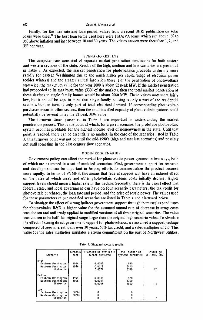
Model parameters which we allowed to vary between scenarios were of two types; rates of real changes in prices and estimates of the economic parameters affecting the net present value calculation. These values are listed in Table 2 and discussed below.

Rates at which photovoltaic array costs are assumed to decrease were selected for each of three scenarios. These annual rates of real decrease in price were based on the learning curves

tFor western Washington, the monthly demand was based on 1980 data obtained from C. O’Paterny, Power Management Division, Seattle City Light. For eastern Washington, 1980 data were obtained from D. Deniston, Consumer Services Department, Washington Water Power.

A market penetration model for residential photovoltaic deployment

Table 2. Parameters varied with scenarios.

621

Parameter

Annual decrease in array costs Annual growth in income per capita Annual increase in price of electricity Annual increase in price of natural gas

Sales multiplier Tax credit Discount rate Loan rate Loan period (yrs.)

L

0.110 0.017 0.014 0.015

0.25 0.10 0.03 0.03

10

znario

M

0.160 0.022 0.017 0.020

0.50 0.25 0.02 0.02 12

1 H

0.210 0.026 0.021 0.025

1.00 0.40 0.01 0.01

25

presented in 0TA.14 For the higher rate (H), the average of the TI-75% and the RCA-SO% learning curves was used; for the lower rate of decrease (L), the average of the TI-70% and RCA-75% learning curves was used. A third scenario value (M) was chosen to be the average of these two. The very highest and very lowest OTA learning curves were not used as these did not correspond with the experience in production that has already occurred. Compared to DOE cost goals, which call for decrease at about 40% per year, these rates are fairly low, but they undoubtedly are more realistic, as the current price of photovoltaic panels is already well behind the DOE goal for this year.

In a recent study, Hinman estimates growth rates for electricity and natural gas prices through 1990, according to three different scenarios.” The highest and lowest of these growth rates were used for our high (H) and low (L) scenarios, respectively, while our medium value was chosen to be the average of Hinman’s high and low values.

Five parameters used in the net present value calculation were assigned different values in each of our scenarios. These were the sales multiplier, tax credit, discount rate, loan rate and loan period. For the sales multiplier S, the OTA estimate of 0.5 was used for the medium scenario value. For the high value of the sales multiplier, 1.0 was assumed; for the low value, 0.25 was used. It should be noted that, in theory, the sales multiplier could be greater than 1.0 since, under the provisions of the Public Utilities Regulatory Policies Act of 1978, a utility would have to purchase power from the homeowner at the utility’s avoided cost. In fact, because of the existence of low-cost hydroelectric capacity in the Pacific Northwest, the current avoided cost for most utilities in Washington in significantly higher than the retail price. The extent to which photovoltaics can be valued at or close to this avoided cost depends on whether the hydro-electric system can be used to store power generated by intermittent sources such as photovoltaics on a daily and seasonal basis and release that power when needed. In the three scenarios discussed here, this idea of using the storage capability of the hydroelectric system to firm up the photovoltaic output was not considered.? In the modified scenarios to be examined below, this possibility is used as a rationale for increasing the sales multiplier above 1 .o.

With regard to tax credits for solar energy systems, California currently has a 55% credit, the highest in the nation?’ and the federal government currently has a 40% tax credit (for systems of $10,000 or less) on renewable energy sources purchased before 1985.” OTA, however, estimated only a 10% average tax credit as being typicaLi For our high scenario value, it was assumed that a 40% tax credit would be available to homeowners throughout the 20-year period examined, while the estimate of 10% was chosen for the low scenario value. The medium value chosen was 25%.

For the discount rate, the social rate of time preference, which is the rate at which the government is willing to lend funds, was used. Ruby calculates this as about 2% above inflation.23 A variation of 1% above and below this value was used for the discount rate in our high and low scenarios.

+The existence of the hydro system was accounted for in our analysis by omitting the costs of battery storage in estimating the cost of a photovoltaic installation.

622 GENE M. MESHER et al.

Finally, for the loan rate and loan period, values from a recent SERI publication on solar loans were used.” The best loan terms used here were FHA/VA loans which run about 1% to 3% above inflation and last between 10 and 30 years. The values chosen were therefore 1,2, and 3% per year.

SCENARIO RESULTS The computer runs consisted of separate market penetration simulations for both eastern

and western sections of the state. Results of the high, medium and low scenarios are presented in Table 3. As expected, the market penetration for photovoltaics proceeds uniformly more rapidly for eastern Washington due to the much higher per capita usage of electrical power (colder winters) and the greater annual insolation there. For the penetration of photovoltaics statewide, the maximum value for the year 2000 is about 22 peak MW. If the market penetration had proceeded to its maximum value (33% of the market), then the total market penetration of these devices in single family homes would be about 2000 MW. These values may seem fairly low, but it should be kept in mind that single family housing is only a part of the residential sector which, in turn, is only part of total electrical demand. If corresponding photovoltaic purchases occur in other sectors, then the total installed capacity of photovoltaic systems could potentially be several times the 22 peak MW value.

The turnover times presented in Table 3 are important in understanding the market penetration process. This is the point at which, for a given scenario, the prototype photovoltaic system becomes profitable for the highest income level of homeowners in the state. Until that point is reached, there can be essentially no market. In the case of the scenarios listed in Table 3, this turnover point will not be until the mid-1990’s (high and medium scenarios) and possibly not until sometime in the 21st century (low scenario).

MODIFIED SCENARIOS

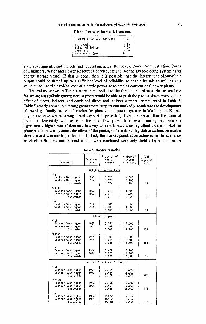
Government policy can affect the market for photovoltaic power systems in two ways, both of which are examined in a set of modified scenarios. First, government support for research and development can be important in helping efforts to commercialize the product succeed more rapidly. In terms of PVMPS, this means that federal support will have an indirect effect on the rates at which array and other photovoltaic systems costs initially decline. Higher support levels should mean a higher rate in this decline. Secondly, there is the direct effect that federal, state, and local government can have on four scenario parameters; the tax credit for photovoltaic purchases, the loan rate and period, and the price of resale power. The values used for these parameters in our modified scenarios are listed in Table 4 and discussed below.

To simulate the effect of strong indirect government support through increased expenditures for photovoltaics R&D, a higher value for the assumed annual rate of decrease in array costs was chosen and uniformly applied to modified versions of all three original scenarios. The value was chosen to be half the original range larger than the original high scenario value. To simulate the effect of strong direct government support for photovoltaics, we assumed a support package composed of zero interest loans over 30 years, 50% tax credit, and a sales multiplier of 2.0. This value for the sales multiplier simulates a strong commitment on the part of Northwest utilities,

Table 3. Standard scenario results.

Turnover Fraction of available Total number of Installed Scenario date market captured systems purchased pk. cap. (MW)

High Eastern Washington 1994 0.0082 840 Western Washington 1996 0.0078 2470

Statewide 0.0079 3310 22

Medium Eastern Washington 1994 0.0044 470 Western Washington 1996 0.0044 1'390

Statewide 0.0044 1860 12

I nw __.. Eastern Washington 2000+ Western Washington

I I 2000+

Statewide

A market penetration model for residential photovoltaic deployment

Table 4. Parameters for modified scenarios.

623

state governments, and the relevant federal agencies (Bonneville Power Administration, Corps of Engineers, Water and Power Resources Service, etc.) to use the hydro-electric system as an energy storage vessel. If that is done, then it is possible that the intermittent photovoltaic output could be firmed up to a sufficient level of reliability to enable its sale to utilities at a value more like the avoided cost of electric power generated at conventional power plants.

The values shown in Table 4 were then applied to the three standard scenarios to see how far strong but realistic government support would be able to push the photovoltaics market. The effect of direct, indirect, and combined direct and indirect support are presented in Table 5. Table 5 clearly shows that strong government support can markedly accelerate the development of the single-family residential market for photovoltaic power systems in Washington. Especi- ally in the case where strong direct support is provided, the model shows that the point of economic feasibility will occur in the next few years. It is worth noting that, while a significantly higher rate of decrease in array costs will have a strong effect on the market for photovoltaic power systems, the effect of the package of the direct legislative actions on market development was much greater still. In fact, the market penetration achieved in the scenarios in which both direct and indirect actions were combined were only slightly higher than in the

Table 5. Modified scenarios.

Scenario

Fraction of Number of Peak Turnover Market Systems Capacity

Date Captured Purchased (W)

indirect (R&D) Support

High Eastern Washington 1990 0.025 2,500 Western Washington 1992 0.020 6,400

Statewide 0.022 8.900 59

Medium

Eastern Washington 1992 0.012 1,200 Western Washington 1992 0.011 3,300

Statewide 0.011 4,500 30

LOW Eastern Washington 1992 0.006 600 Western Washington 1994 0.005 1,500

Statewide 0.005 2,100 14

High Eastern Washington Western Washington

Statewide

Medium Eastern Washington Western Washington

Statewide

Low Eastern Washington Western Washington

Statewide

Direct Support

1982 1984

1984 1984

1984 1984

0.163 17,000 0.082 25.200 0.102 42,200 278

0.102 10,600 0.048 24,600 0.088 25,200 166

0.062 6,400 0.027 8.400 0.036 14,800 97

Combined Direct and Indirect.

1982 1982

1982 1984

High Eastern Washington Western Washington

Statewide

Medium Eastern Washington Western Washington

Statewide

Low Eastern Washington

0.166 17,300 0.084 25,700 0.105 43.000

0.108 11,300 0.051 15,500 0.065 26,800

283

176

114 -I

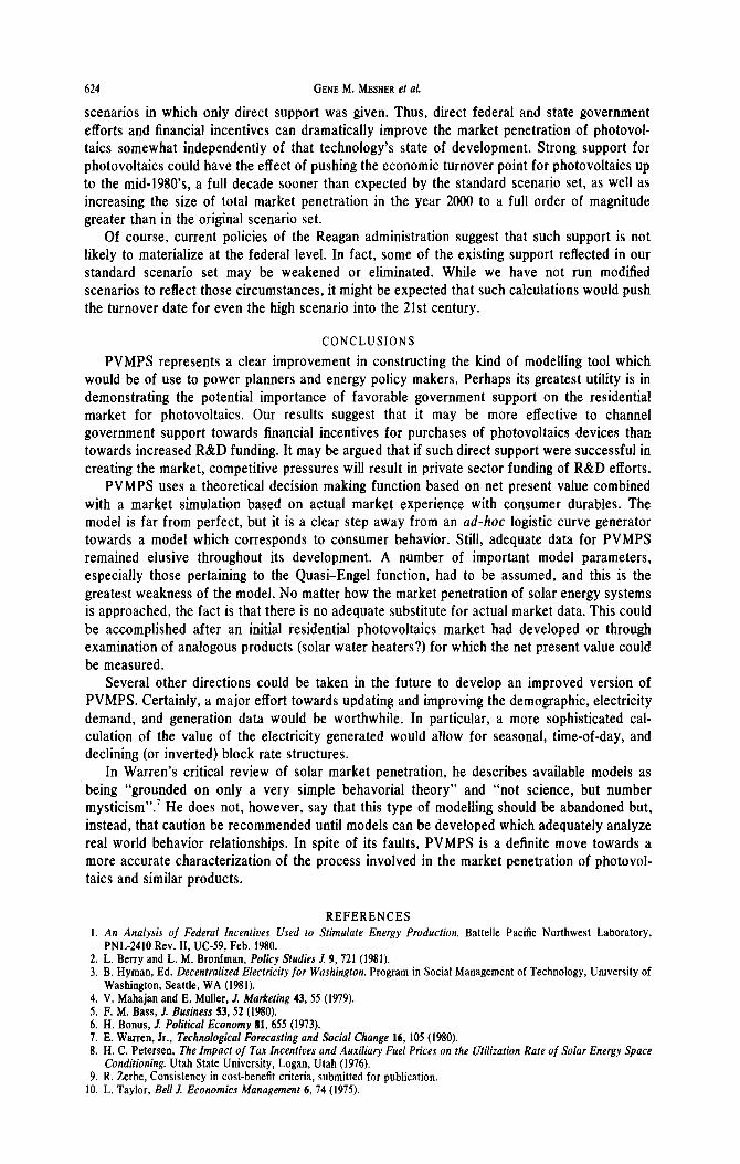
624 GENE M. MESHER et al.

scenarios in which only direct support was given. Thus, direct federal and state government efforts and financial incentives can dramatically improve the market penetration of photovol- taics somewhat independently of that technology’s state of development. Strong support for photovoltaics could have the effect of pushing the economic turnover point for photovoltaics up to the mid-1980’s, a full decade sooner than expected by the standard scenario set, as well as increasing the size of total market penetration in the year 2000 to a full order of magnitude greater than in the original scenario set.

Of course, current policies of the Reagan administration suggest that such support is not likely to materialize at the federal level. In fact, some of the existing support reflected in our standard scenario set may be weakened or eliminated. While we have not run modified scenarios to reflect those circumstances, it might be expected that such calculations would push the turnover date for even the high scenario into the 21st century.

CONCLUSIONS

PVMPS represents a clear improvement in constructing the kind of modelling tool which would be of use to power planners and energy policy makers. Perhaps its greatest utility is in demonstrating the potential importance of favorable government support on the residential market for photovoltaics. Our results suggest that it may be more effective to channel government support towards financial incentives for purchases of photovoltaics devices than towards increased R&D funding. It may be argued that if such direct support were successful in creating the market, competitive pressures will result in private sector funding of R&D efforts.

PVMPS uses a theoretical decision making function based on net present value combined with a market simulation based on actual market experience with consumer durables. The model is far from perfect, but it is a clear step away from an ad-hoc logistic curve generator towards a model which corresponds to consumer behavior. Still, adequate data for PVMPS remained elusive throughout its development. A number of important model parameters, especially those pertaining to the Quasi-Engel function, had to be assumed, and this is the greatest weakness of the model. No matter how the market penetration of solar energy systems is approached, the fact is that there is no adequate substitute for actual market data. This could be accomplished after an initial residential photovoltaics market had developed or through examination of analogous products (solar water heaters?) for which the net present value could be measured.

Several other directions could be taken in the future to develop an improved version of PVMPS. Certainly, a major effort towards updating and improving the demographic, electricity demand, and generation data would be worthwhile. In particular, a more sophisticated cal- culation of the value of the electricity generated would allow for seasonal, time-of-day, and declining (or inverted) block rate structures.

In Warren’s critical review of solar market penetration, he describes available models as being “grounded on only a very simple behavorial theory” and “not science, but number mysticism”.’ He does not, however, say that this type of modelling should be abandoned but, instead, that caution be recommended until models can be developed which adequately analyze real world behavior relationships. In spite of its faults, PVMPS is a definite move towards a more accurate characterization of the process involved in the market penetration of photovol- taics and similar products.

REFERENCES 1. An Analysis of Federal Incentives Used to Stimulafe Energy Production. Battelle Pacific Northwest Laboratory,

PNL-2410 Rev. II, UC-59, Feb. 1980. 2. L. Berry and L. M. Bronfman, Policy Studies J. 9,721 (1981). 3. B. Hyman, Ed. Decentralized Electricity for Washington. Program in Social Management of Technology, Umversity of

Washinglon, Seattle, WA (1981). 4. V. Mahajan and E. Muller, J. Marketing 43, 55 (1979). 5. F. M. Bass, /. Business 53, 52 (1980). 6. H. Bonus, J. Polifical Economy 81,655 (1973). 7. E. Warren, Jr., Technological Forecasting and Social Change 16, 105 (1980). 8. H. C. Petersen, The Imvact of Tax Incentives and Auxiliarv Fuel Prices on fhe Utilization Rate of Solar EnerPv Soace

Conditioning. Utah State University, Logan, Utah (1976). . 9. R. Zerbe, Consistency in cost-benefit criteria, submitted for publication.

10. L. Taylor, Bell I. Economics Management 6, 74 (1975).

-. .

A market penetration model for residential photovoltaic deployment 625

II. Weather Tapes for UWENSOL Computer Program, Professor C. Kippenhan, Mechanical Engineering Dept., Uni- versity of Washington, Seattle, WA.

12. L. Goldstein and G. Case, “PVSS: A Photovoltaic System Simulation Program User’s Manual” SAND-77-0814, Sandia Labs., Albuquerque, NM (1977).

13. R. Halvorsen, The Review of Economics and Statistics 57, I2 (1975). 14. Application of Solar Technology to Today’s Energy Needs. Vols. I and II, U.S. Congress, Office of Technology

Assessment, Washington, DC (1978). 15. “1970 Census of Population”, Vol. 1, Part 49, Bureau of the Census, Washington, DC (1973). 16. C. Strock and R. Koral [Eds]. Handbook of Air Conditioning, Heating and Ventilation. Industrial Press, New York

(1%5). 17. G. Hinman, “A Review of Current Energy Forecasts for the State of Washington”, Washington State Energy Office,

Olympia, WA (1979). 18. T. Dolan, Definition of Housing Stock, Department of Energy, Region X, Seattle, WA (1977). 19. 1977 Individual Income Tax Returns: Statistics of Income, Internal Revenue Service, Washington, DC (1979). 20. J. Hubert, Federal Home Loan Bank, Seattle, personal communication. 21. Making the Solar Loan, Solar Energy Research Institute, Golden, CO (1980). 22. Sec. 202 of P.L. %-223. The Crude Oil Windfall Profits Tax of 1980. 23. M. Ruby, Economic analysis of air pollution cont;ols: A case study. Master’s Thesis, University of Washington.

Seattle, WA (1978).