A First-Generation Metric Linkage Disequilibrium Map of Bovine Chromosome 6
Upload
ua-birminghamCategory
view
0download
0
A General Statistical Framework for Unifying Intervaland Linkage Disequilibrium Mapping Toward
High-Resolution Mapping of Quantitative TraitsXiang-Yang LOU George CASELLA Rory J TODHUNTER Mark C K YANG and Rongling WU
The nonrandom association between different genes termed linkage disequilibrium (LD) provides a powerful tool for high-resolutionmapping of quantitative trait loci (QTL) underlying complex traits This LD-based mapping approach can be made more efficient when itis coupled with interval mapping characterizing the genetic distance between markers and QTL This article describes a general statisticalframework for simultaneously estimating the linkage and LD that are related in a two-stage hierarchical sampling scheme This frameworkis constructed within a maximum likelihood context and can be expanded to fine-scale mapping of complex traits for different populationstructures and reproductive behaviors We provide a closed-form solution for joint estimation of quantitative genetic parameters describingQTL effects QTL position and residual variances and population genetic parameters describing allele frequencies and QTL-marker LDWe perform simulation studies to investigate the statistical properties of our joint analysis model for interval and LD mapping An exampleusing body weights of dogs from a multifamily outcrossed pedigree illustrates the use of the model
KEY WORDS EM algorithm Interval mapping Linkage disequilibrium Maximum liklihood estimate Quantitative trait loci
1 INTRODUCTION
The motivation of this article arises from problems in thehigh-resolution genetic mapping of quantitative traits withDNA-based polymorphic markers The polygenic inheritanceand environmental sensitivity of quantitative traits complicatethe analysis and modeling of their genetic architecture as spec-ified by the number distribution actions and interactions of theunderlying genes that is quantitative trait loci (QTL) (Mackay2001) Molecular genetic markers derived from polymorphicsites in the genome have proven to be powerful tools for char-acterizing and mapping individual QTL for a quantitative traitThe basic principle of such QTL mapping proceeds by count-ing the expected recombination events occurring between themarkers and putative QTL during meiosis One of the geneticstrategies for QTL mapping is to make use of the markerndashQTLrecombinants created in marker-genotyped generations throughcontrolled crosses This strategy is called linkage analysis In-terval mapping of QTL based on the multilocus linkage analysisof two flanking markers and a QTL bracketed by the markers al-lows for a systematic scan for the genome-wide distribution ofQTL (Lander and Botstein 1989) Substantial extensions of in-terval mapping into more general situations have been reported(reviewed in Jansen 2000)
Interval mapping utilizes the information about gene segre-gation and transmission in a well-constructed pedigree and is
Xiang-Yang Lou is Postdoctoral Research Associate under the guidanceof Dr Rongling Wu and George Casella is Distinguished Professor andChair Department of Statistics University of Florida Gainesville FL 32611Rory J Todhunter is Associate Professor The James A Baker Institute forAnimal Health College of Veterinary Medicine Cornell University IthacaNY 14853 Mark Yang is Professor Department of Statistics University ofFlorida Gainesville FL 32611 Rongling Wu is Associate Professor De-partment of Statistics University of Florida Gainesville FL 32611 (E-mailrwustatufledu) and Adjunct Distinguished Professor Zhejiang Forestry Uni-versity LinrsquoAn Zhejiang 311300 China Rongling Wu conceived the ideaof this study wrote this manuscript and was responsible for directing theresearch The authors thank the associate editor and an anonymous refereefor their constructive comments on this manuscript This work is supportedin part by a National Science Foundation grant (9971586) to G Casella anOutstanding Young Investigators Award of the National Science Foundationof China (30128017) a University of Florida Research Opportunity Fund(02050259) and a University of South Florida Biodefense grant (7222061-12)to R Wu and the Morris Animal Foundation contract grant (722206212) toR J Todhunter The publication of this manuscript is approved as journal seriesNo R-09584 by the Florida Agricultural Experiment Station
limited for the fine-scale mapping of QTL unless the size ofthe pedigree is large An alternative strategy of QTL mappingis based on linkage disequilibrium (LD) analysis which usesrecombinant events in a population generated at a historicaltime before genotyping starts Because the extent of disequi-librium between two genes decays exponentially toward at arate depending on the recombination fraction (Lynch and Walsh1998) the detection of significant LD after a number of gener-ations may imply a tight linkage between the marker and QTLFor this reason LD-based mapping provides a powerful way offine-scale mapping of QTL Although the use of LD mappinghas led to successful high-resolution mapping of several humandiseases (eg Haumlstbacka et al 1992 1994) the prerequisite ofthis strategy that LD is due to tight linkage between the QTLand marker may not hold In populations where evolutionaryforces such as selection drift population structure and pop-ulation admixture act the disequilibrium can also be detected(Lynch and Walsh 1998) Such an LD is regarded as spuriousbecause it provides no information about the markerndashQTL link-age
Many strategies have been developed to combine the advan-tages of linkage and LD analysis traditionally considered sepa-rate strategies For example in human genetics a family-basedLD strategy called transmissiondisequilibrium testing (TDT)was devised to simultaneously determine the linkage and LDbetween a marker and a disease gene (Allison 1997) Severalstudies have considered the joint modeling of linkage and LDmapping for quantitative traits as well as its advantages com-pared with pure linkage mapping or pure LD mapping (Wu andZeng 2001 Wu Ma and Casella 2002 Fan and Xiong 2002Farnir et al 2002 Meuwissen Karlsen Lien Olsaker andGoddard 2002 Lund Sorensen Guldbrandtsen and Sorensen2003 Perez-Enciso 2003) However these studies provided asolution only for some very specific problems because theywere not formulated under a general statistical framework bywhich analysis and modeling of QTL mapping can be read-ily extended to different populations reproductive behaviorsmarker systems and pedigree structures Moreover in many of
copy 2005 American Statistical AssociationJournal of the American Statistical Association
March 2005 Vol 100 No 469 Theory and MethodsDOI 101198016214504000001295
158
Lou et al Unifying Interval and Linkage Disequilibrium Mapping 159
the cited studies the statistical properties of the joint linkage-LD analysis have not been investigated through either analyticalor numerical approaches
In this article we develop a general framework for integratinginterval and LD mapping to enforce the efficiency and effective-ness of high-resolution mapping of quantitative traits Our inte-grative model makes use of genetic information from the familypedigree and population data by adopting a two-stage hierarchi-cal sampling scheme as reported by Wu and Zeng (2001) andWu et al (2002) The upper hierarchy of this scheme describesthe gene distribution in a natural population from which a sam-ple is randomly drawn (LD analysis) and the lower hierarchydescribes gene segregation in the progeny population derivedfrom matings (linkage analysis) These two hierarchies are con-nected through population and Mendelian genetic theories In arecent study Lou et al (2003a) derived a closed-form solutionfor estimating population genetic parameters such as allele fre-quencies and LD within the maximum likelihood frameworkHere we extend the idea of two-stage hierarchical samplingscheme to jointly model interval and LD mapping by imple-menting the closed-form EM algorithm of Lou et al (2003a)Compared with the earlier work by Wu and Zeng (2001) andWu et al (2002) this extended model displays increased com-putational efficiency and provides more precise estimates of theQTL genomic location and genetic effects because a pair offlanking markers that bracket the QTL are used simultaneously
2 TERMINOLOGY AND NOTATION
21 Haplotype Diplotype and Zygote Genotype
Suppose that there are L loci A1 AL on a chromo-some which are segregating in a random mating natural pop-ulation At locus l (l = 1 L) there are kl alleles denotedby Al
1 Alkl
The haplotype that is a linear arrangement ofalleles from the L loci on one member of a pair of homolo-gous chromosomes (Cepellini et al 1967) can be described bya vector of L dimensions containing one allele from each ofthe L loci The alleles from all of the L loci form nh =prodL
l=1 kl
haplotypes During the process of pollination paternally- andmaternally-derived haplotypes will randomly unite to form n2
hcombinations among which there are a total of nh(nh + 1)2different zygotic configurations or diplotypes (Morton 1983)Because different diplotypes may have the same genotype thenumber of multilocus genotypes nz =prodL
l=1 (kl + 1)kl2 willbe less than the number of diplotypes Let Hξ Dξξ prime or HξHξ prime and Zυ be the haplotype ξ (ξ = 1 nh) diplotype ξξ prime (ξ leξ prime = 1 nh) and zygote genotype υ (υ = 1 nz) To dis-tinguish between polymorphic markers and quantitative traitloci composing L-locus haplotypes we let G(Dξξ prime) Gm(Dξξ prime)and Gq(Dξξ prime) denote the many-to-one mapping operators tak-ing the genotypes at all loci marker loci and QTL of diplo-type Dξξ prime
We use an example to demonstrate the concepts of haplo-type diplotype and zygote genotype Consider two biallelicloci A and B on the same chromosome having alleles A aand B b The haplotypes of these two loci are the combinationsof alleles AB Ab aB and ab These haplotypes (or gametes)are randomly paired to generate 10 diplotypes ABAB ABAbABaB ABab AbAb AbaB Abab aBaB aBab and abab
where ldquo rdquo denotes the separation of the maternally and pater-nally derived gametes Of the foregoing diplotypes the fourthand sixth cannot be genotypically distinguished from each an-other Thus we actually have only nine distinguishable geno-types expressed as AABB AABb AAbb AaBB AaBb AabbaaBB aaBb and aabb
22 Recombination and Reduced Recombination
During the meiotic stage of life the diplotype (zygotic con-figuration) arising from the unification of maternal and paternalhaplotypes will generate new haplotypes for the next genera-tion Some of these new haplotypes will be different from thematernal and paternal haplotypes that form the diplotype be-cause of the occurrence of recombination events between a pairof contiguous loci For example diplotype ABab will generatefour haplotypes AB ab Ab and aB with the first two identi-cal to the haplotypes composing the parental diplotype and thesecond two due to the recombination or crossover between thetwo loci The frequency at which the recombinant types occuramong the total number of haplotypes termed the recombina-tion fraction depends on the genetic distance between the twoloci Thus the recombination fraction (and therefore the geneticdistance) can be estimated by counting the relative numbersof recombinant and nonrecombinant haplotypes that the zy-gote produces But whether recombinant and nonrecombinanttypes can be genotypically distinguished from each other in agenotyped family depends on the heterozygosity of a diplotypeFor those completely homozygous diplotypes (eg ABAB) thegenotypic distinction between recombinant and nonrecombi-nant haplotypes is not possible despite the fact that these twotypes occur at the same time
In this study we construct a general framework for integrat-ing the advantages of interval and LD mapping of complextraits Traditional interval mapping is based on a known link-age group throughout which every two flanking markers arescanned to test whether a putative QTL is located between thetwo markers Unlike such a traditional treatment however ourintegrative model assumes that the recombination fraction be-tween the two markers is unknown a priori to better specifythe relationships among the markers and QTL Let r1 r2 andr be the recombination fractions between the left marker (ofalleles A and a) and QTL (of alleles Q and q) between theQTL and the right marker (of alleles B and b) and betweenthe two markers Thus if r1 and r2 are estimated then thelocation of the QTL within the marker interval can be deter-mined The estimation of r1 or r2 is based on the observationsof the recombinant and nonrecombinant types For a completelyheterozygotic diplotype AQBaqb the eight haplotypes that itproduces are distinguishable based on their formation mecha-nisms resulting from the recombination or nonrecombinationFor those partially heterozygotic diplotypes however differentformation mechanisms may lead to the same haplotype For ex-ample diplotype AQBAQb produces two distinguishable hap-lotypes AQB and AQb each of which may result from eitherrecombination (R) or nonrecombination (N) between each oftwo pairs of adjacent loci (ie A and Q Q and B) describedby NN NR RN or RR Assuming that there is no interferencethe frequencies of these four genotypically indistinguishableformation mechanisms for each haplotype can be expressed in
160 Journal of the American Statistical Association March 2005
Table 1 Examples of Reducible Recombination
Parental Formation Formation Frequency of Statediplotype Haplotype mechanism frequency reduced recombination vector
AQBAQb AQB NN (1 minus r1)(1 minus r2)2 5 (0 0)NR (1 minus r1)r22RN r1(1 minus r2)2RR r1r22
AQb NN (1 minus r1)(1 minus r2)2 5 (0 0)NR (1 minus r1)r22RN r1(1 minus r2)2RR r1r22
AQBAqb AQB NN (1 minus r1)(1 minus r2)2 (1 minus r2)2 (0 minus1)RN r1(1 minus r2)2
AQb NR (1 minus r1)r22 r22 (0 1)RR r1r22
AqB NR (1 minus r1)r22 r22 (0 1)RR r1r22
Aqb NN (1 minus r1)(1 minus r2)2 (1 minus r2)2 (0 minus1)RN r1(1 minus r2)2
AQBaQb AQB NN (1 minus r1)(1 minus r2)2 (1 minus r1)(1 minus r2)2 (minus1 minus1)RR r1r22 r1r22 (1 1)
AQb NR (1 minus r1)r22 (1 minus r1)r22 (minus1 1)RN r1(1 minus r2)2 r1(1 minus r2)2 (1 minus1)
aQB NR (1 minus r1)r22 (1 minus r1)r22 (minus1 1)RN r1(1 minus r2)2 r1(1 minus r2)2 (1 minus1)
aQb NN (1 minus r1)(1 minus r2)2 (1 minus r1)(1 minus r2)2 (minus1 minus1)RR r1r22 r1r22 (1 1)
NOTE The state of recombination is expressed as 1 for recombined (R) minus1 for nonrecombined (N) and 0 for reducible
terms of r1 and r2 with the form given in Table 1 which sumto 5 independent of the values of r1 and r2 Thus these fourmechanisms together (or the corresponding haplotype) are suf-ficient for the characterization of the recombination and can beregarded as reduced recombination
Diplotype AQBAqb produces four different haplotypes AQBand Aqb due to either NN or RN and AQb and AqB due to ei-ther NR or RR (see Table 1) The sum of the frequencies ofthe two corresponding formation mechanisms for each haplo-type is dependent on only one term determined by r1 Thus thetwo different mechanisms together form the reduced recombi-nation Similarly diplotype AQBaQb also forms four differenthaplotypes Yet two formation mechanisms for each haplotypeshould each be viewed as the reduced recombination becausethe sum of the frequencies of the two mechanisms includes twononreducible terms (see Table 1) In general the reduced re-combination for a haplotype can be characterized by three dif-ferent states for any two adjacent loci recombined nonrecom-bined and reducible (ie the haplotype can be reduced to arecombinant or nonrecombinant) coded by 1 minus1 and 0 (seeTable 1) As shown later the reducible state is trivially suffi-cient for the formation of a closed form for estimating r1 or r2We use γς (ς = 1 3Lminus1) to denote a reduced recombina-tion vector for a L-locus haplotype (There are a total of 3Lminus1
such vectors because we have three states between two adjacentgenes) The reduced recombination vector for a diplotype de-noted by R is the combination of γς for the maternal parentand γς prime for the paternal parent
23 Population Genetic and GeneTransmission Parameters
We let pξ and Pξξ prime denote the frequencies of haplotype Hξ
and diplotype Dξξ prime in the study population If the population is
at HardyndashWeinberg equilibrium then we have
Pξξ prime =
p2ξ when ξ = ξ prime
2pξpξ prime otherwise
The haplotype frequency pξ contains different components de-termined by allele frequencies at each loci and coefficientsof linkage disequilibrium of different orders among these loci(Lynch and Walsh 1998) Lou et al (2003a) provided a gen-eral model for describing pξ in terms of allele frequencies andlinkage disequilibria
For pure LD mapping (Lou et al 2003a) we draw samplesin the same generation from a natural population By testingfor the statistical significance of LD we can make an inferenceabout a possible tight linkage between markers and QTL How-ever in a joint analysis of interval mapping and LD mappingour samples are derived from both the natural (parental) pop-ulation and its offspring population which thus forms a two-stage hierarchical sampling scheme When the samples fromthe older (generation t) parental population contain informationabout allele frequencies and LD the samples from the younger(generation t + 1) offspring population contain gene segrega-tion and transmission determined by the Mendelian laws andrecombination fractions The estimation of the recombinationfractions is based on gene transmission from the parental to off-spring generation We let rl denote the recombination fractionbetween loci Al and Al+1
24 Penetrance Function
For a quantitative trait there is no one-to-one correspon-dence between the genotype and phenotype (y) The conditionalprobability of observing the corresponding phenotype given a
Lou et al Unifying Interval and Linkage Disequilibrium Mapping 161
specified genotype termed the penetrance function is thus for-mulated to describe the expression of the genotype Becausethe phenotype of a trait is genetically determined only by thegenotypes at the putative QTL the penetrance function given adiplotype Dξξ prime can be expressed as
f ( y|Dξξ prime) =sum
s
I(gs|Dξξ prime)1radic
2πσexp
[
minus ( y minus micros)2
2σ 2
]
(1)
where micros is the genotypic mean of QTL genotype gs σ 2 is theresidual variance and I(gs|Dξξ prime) is the indicator variable
I(gs|Dξξ prime) =
1 if gs = Gq(Dξξ prime) that is QTL genotype gs
is compatible with diplotype Dξξ prime0 otherwise
We designate f ( ym|Dmξξ prime) f ( y p|D p
ξξ prime) and f ( yo|Doξξ prime) as the
penetrance functions of phenotype given diplotype Dξξ prime for thematernal parent (m) paternal parent (p) and offspring (o)There is the same penetrance function between the maternaland paternal parent if there is no sex effect In many studiesthe same penetrance may be assumed for the parental and off-spring generations
Table 2 lists the genetic terminology used in our genetic map-ping It also gives the corresponding definitions and symbols
3 THE MODEL
31 The Complete-Data Likelihood
For our mapping study aimed at estimating haplotype fre-quencies QTL effects and positions (measured by the recom-bination fractions) marker data (M) zygote genotype (Z)
diplotypes (D) haplotype (H) reduced recombination (R)and phenotype data (y) are viewed as the complete data Themarker and phenotypic data denoted in boldface are observeddata whereas zygote genotypes and diplotypes (containing pu-tative QTL) of the parents and offspring and reduced recombi-nation configurations of the offspring denoted in mathematicalface are unobserved (or missing) data Suppose that there are Nunrelated families drawn from a randomly mating populationIf there are no phenotypic covariances between parents and off-spring then the likelihood function of the complete data can beexpressed as
L(|ymypyoMmMpMoDmDpDoR)
prop Pr[DmDp|Pξξ prime]
timesNprod
i=1
f ( ymi |Dm
i )f ( y pi |D p
i )
timesNiprod
j=1
[Pr(DoijRij|Dm
i D pi )f ( yo
ij|Doij)]
(2)
where yrsquos are the phenotypic vectors Drsquos are the diplotype vec-tors R is the reduced recombination matrix for the offspring is the unknown vector containing population genetic para-meters (haplotype frequencies P) quantitative genetic pa-rameters (QTL genotypic values and residual variance Q)and QTL positions (measured by recombination fractions R)i denotes the ith family derived from the ith maternal and ith pa-ternal parent j denotes the jth offspring within the ith familyand Ni is the number of offspring within family i
Table 2 Definitions and Symbols Used to Describe Genetic Terminology in QTL Mapping
Terminology Symbol Definition
Allele Al1 Al
klDifferent copies of a gene at the same locus
Allele frequency pl1 pl
klRelative proportion of an allele in a population
Diplotype Dξξ prime A set of haplotype pairs (one from the maternal parent and the other from the paternal parent) withthe same genotype
Maternal diplotype Dmξξ prime
Paternal diplotype Dpξξ prime
Offspring diplotype Doξξ prime
Diplotype frequency Pξξ prime Relative proportion of a diplotype in a populationHaplotype Hξ A linear arrangement of alleles on the same chromosomeHaplotype frequency pξ Relative proportion of a haplotype in a populationHardyndashWeinberg equilibrium HWE A population state in which genotype frequency is the product of the corresponding allele frequen-
ciesGenotype Zv The particular alleles at specified loci present in an organismGenotype frequency Pv Relative frequency of a genotype in a populationLinkage Co-segregation between alleles at different loci in a progeny populationLinkage disequilibrium D Nonrandom association between alleles at different loci in a populationLocus l The chromosomal position at which a gene residesMolecular marker M A particular DNA sequence that displays polymorphisms among individualsNonallele Alleles from different lociPenetrance f (y |Dξξ prime ) Percentage frequency with which a gene exhibits its effectPhenotype y or y Physical visible characteristics of a genotypeQTL Quantitative trait locus a hypothesized region with alleles triggering an effect on a quantitative traitRecombinant R The exchange of DNA segments between the maternal and paternal chromosomes
Nonrecombinant N DNA sequence with no exchange between the homologous chromosomesReduced recombination R The recombination that occurs between a pair of loci but cannot be observed
Recombination fraction r Relative proportion of recombinant gametes that is gametes that contain alleles from different pa-ternal chromosomes
Zygote Zv The combination of two allele or haplotypes each from a different parentHeterozygote The combination of different alleles at a locusHomozygote The combination of the same allele at a locus
162 Journal of the American Statistical Association March 2005
The probability Pr[DmDp|Pξξ prime] is the joint probability ofmaternal and paternal parental diplotypes which depends ona specific sampling scheme for example stratified groupedcensored or truncated Specially there is a multinomial distri-bution for simple random samples
Pr[DmDp|Pξξ prime ] propnhprod
ξleξ prime(Pξξ prime)
Nmξξ prime +Np
ξξ prime
where Nmξξ prime and Np
ξξ prime are the numbers of maternal and paternalparents with diplotype Dξξ prime The probability Pr(Do
ijRij|Dmi
D pi ) is the conditional probability of offspring j of family i hav-
ing diplotype Doij and reduced recombination Rij given parental
diplotypes Dmi and D p
i Of the three subsets of unknown para-meters P is contained within Pr[DmDp|Pξξ prime ] Q is con-tained within the penetration functions and R is containedwithin Pr(Do
ijRij|Dmi D p
i )The maximum likelihood estimators (MLEs) of the unknown
parameters under the complete-data likelihood function (2) aregiven in Appendix A
32 The Incomplete-Data Likelihood
In the genetic mapping of complex traits only marker andphenotype data are observed whereas the data on diplotypesrecombination events and QTL genotypes are missing The ob-served data alone are viewed as incomplete data of the previ-ously specified complete-data model
The likelihood of the incomplete data including the pheno-type (y) and marker information (M) can be formulated as
L(|ymypyoMmMpMo)
prop Pr[MmMp|Pξξ prime ]
timesNprod
i=1
nhsum
ξleξ prime
nhsum
ζleζ prime
Pr(Dmξξ prime |Mm
i )Pr(D pζζ prime |Mp
i )
times f ( ymi |Dm
ξξ prime)f ( y pi |D p
ζζ prime)
timesNiprod
j=1
nhsum
τleτ prime
3Lminus1sum
ςς prime
[Pr(MijDo
ττ prime Rςς prime |Dmξξ primeD p
ζζ prime)
times f ( yij|Dττ prime)]
(3)
where Pr(Dmξξ prime |Mm
i ) and Pr(D pζζ prime |Mp
i ) are the conditional prob-
abilities of the maternal (Dmξξ prime) and paternal diplotypes (D p
ζζ prime )
given maternal (Mmi ) and paternal marker genotypes (Mp
i ) forthe ith family and Pr(MijDo
ττ primeRςς prime |Dmξξ primeD p
ζζ prime) is the con-ditional probability of offspring having marker genotype Mijdiplotype Do
ττ prime and reduced recombination Rςς prime given maternaldiplotype Dm
ξξ prime and paternal diplotype D pζζ prime
It can be seen from (4) that the observed data constitute anormal mixture model that is difficult to solve for the MLEsHowever maximizing the expected complexdata likelihood anddetecting the corresponding MLEs is simple Thus to obtain theMLEs of the incomplete-data likelihood we attempt to maxi-mize the completedata likelihood by replacing it by its condi-tional expectation given the incomplete data This expectation
is computed with respect to the conditional distribution of thecomplete data given the incomplete data and the current es-timate of the unknown vector Appendix B describes thederivation procedures and the implementation of the EM algo-rithm to obtain the estimates
33 Asymptotic VariancendashCovariance Matrix
After the point estimates of parameters are obtained by theEM algorithm it is necessary to derive the variancendashcovariancematrix and evaluate the standard errors of the estimates Be-cause the EM algorithm does not automatically provide theestimates of the asymptotic variancendashcovariance matrix forparameters an additional procedure has been developed to es-timate this matrix (and thereby standard errors) when the EMalgorithm is used (Louis 1982 Meng and Rubin 1991) Thesetechniques involve calculation of the incomplete-data informa-tion matrix which is the negative second-order derivative ofthe incomplete-data log-likelihood Louis (1982) established animportant relationship among the information for the complete(Icom) incomplete (Iincom) and missing data (Imiss) expressedas Iincom = Icom minus Imiss Because it is difficult to evaluateIincom directly Louisrsquo relationship allows for an indirect eval-uation based on Icom and Imiss The derivation procedures ofIcom and Imiss are given in Appendix C Meng and Rubin(1991) proposed a so-called ldquosupplementedrdquo EM algorithm orSEM algorithm to estimate the asymptotic variancendashcovariancematrices which can also be used for calculating the standarderrors for the MLEs of our QTL parameters
4 A CASE STUDY FROM A CANINE HIPDYSPLASIA PROJECT
A canine pedigree was developed to map QTL responsiblefor canine hip dysplasia (CHD) using molecular markers Sevenfounding greyhounds and six founding Labrador retrievers wereintercrossed followed by backcrossing F1rsquos to the greyhoundsand Labrador retrievers and intercrossing the F1rsquos A series ofsubsequent intercrosses among the progeny at different genera-tion levels led to a complex network pedigree structure (Fig 1)which maximized phenotypic ranges in CHD-related quantita-tive traits and the chance to detect substantial LD (Todhunteret al 2003 Bliss et al 2002) A total of 148 dogs from this out-bred population were genotyped for 240 microsatellite markerslocated on 38 pairs of autosomes and 1 pair of sex chromosome(Mellersh et al 2000 Breen et al 2001) A number of CHD-associated morphological traits that display remarkable dis-crepancies between greyhounds and Labrador retrievers weremeasured to examine the genetic and developmental basis ofCHD In this study body weight at age 8 months is used as anexample to illustrate our approach
The 148 dogs selected from this canine pedigree (see Fig 1)include 2ndash18 offspring and their parents for each of 22 fami-lies Because most of the selected families were derived fromcrosses between the unrelated founders the families selectedfor a joint linkage and LD analysis can be roughly assumed tobe random samples However a more precise analysis shouldimplement the network structure of the pedigree All of the38 autosomes carrying different numbers of markers werescanned for the existence of QTL affecting body weights us-ing our joint analytical model The critical value for claim-ing the chromosome-wide existence of QTL was determined
Lou et al Unifying Interval and Linkage Disequilibrium Mapping 163
Figure 1 Diagram of an Outbred Pedigree in Canine Squares and circles represent males and females Filled and open portions of each symbolrepresent the proportion of greyhound and Labrador retriever alleles possessed by that dog
through permutation tests (Churchill and Doerge 1994) Thelog-likelihood ratios calculated from 1000 permutation testswere approximately chi-squared-distributed whose 1 per-centile was used as the critical threshold (significance levelα = 001)
By comparing the α = 001 threshold (3229) determinedfrom permutation tests with the log-likelihood values calcu-lated at every 2 cM on each marker interval composed of twoadjacent markers we detected four QTL for body weights lo-cated on different chromosomes As an example Figure 2 illus-trates a profile of the log-likelihood ratios across chromosome35 of length 3994 cM carrying four markers REN172L08REN94K23 REN214H22 and REN01G01 The profile has apeak of value 35 at 89 cM from marker REN172L08 suggest-ing the existence of a significant body weight QTL around thatposition
As with traditional interval mapping (Lander and Botstein1989) our joint model can estimate the positions of the QTLand the effects due to their gene actions and interactions Likeusual LD mapping our joint model provides the MLEs for theallele frequencies of QTL and QTL marker and QTLndashQTL link-age disequilibria (Lou et al 2003a) Table 3 gives the MLEsof haplotype frequencies genotypic means of the QTL andthe residual variance along with their respective standard er-rors From the haplotype frequencies we estimate the allele fre-quencies and linkage disequilibria (Lou et al 2003a) whereas
from the genotypic means we estimate the additive and domi-nant genetic effects (Lynch and Walsh 1998) The MLE of thefrequency of the favorable allele that increase body weight forthe QTL detected on chromosome 35 was pQ = 505 with areasonably small standard error 0725 (see Table 3) This QTLdisplaying a high heterozygosity was found to have strong link-age disequilibria with the two markers flanking it whose esti-mates are reasonably precise
As expected the estimate of the additive genetic effect (a =478 kg) exhibits much greater precision than that of the dom-inant effect (d = minus132 kg) (see Table 3) This QTL triggersan effect body weight in an additive manner The estimated ad-ditive and dominant genetic effects along the estimated QTLallele frequencies allow for the estimation of average effectα = a + d(pq minus pQ) that quantifies the value of the QTL car-ried by a parent and transmitted to its offspring (Lynch andWalsh 1998) The average effect of this QTL was estimated as480 or 117 times the phenotypic standard deviation for bodyweight The additive and dominant genetic variances of thisQTL estimated from σ 2
a = 2pQpqα2 and σ 2
d = 4p2Qp2
qd2 were829 and 44 accounting for 49 (narrow-sense heritability) and03 of the total phenotypic variance
It should be pointed out that the profile of the log-likelihoodratios is quite flat at the left of the peak in the case of chro-
164 Journal of the American Statistical Association March 2005
Figure 2 The Profile of the Log-Likelihood Ratios for Testing a QTL Affecting Body Weights on Chromosome 35 of Canine The horizontal linedenotes the critical threshold for claiming the existence of a QTL at α = 001
mosome 35 (see Fig 2) This may result from the left markerREN172L08 being associated through LD with a second body
weight QTL on a different chromosome In other words thepossible existence of LD between this marker and any QTL lo-
Table 3 MLEs and Their Standard Errors (SEs) of Population and Quantitative GeneticParameters for the Body Weight QTL Bracketed by a Pair of Markers on Canine
Chromosome 35 in a Multifounder and Multigeneration Dog Pedigree
Parameters MLE SE
Population genetic parametersHaplotype frequencies pAQB 3731 0719
pAQb 808eminus31 0pAqB 2359 0688pAqb 0422 0232paQB 0367 0300paQb 0953 0365paqB 2168 0525paqb 127eminus07 898eminus05
Allele frequencies and LD pA 6512 0521pQ 5051 0725pB 8626 0414
DAB 0473 0237DAQ 0442 0379DQB minus0258 0232
DAQB 0442 0480
Quantitative genetic parametersGenotypic means (kg) microo
QQ 3306 61microo
Qq 2350 60microo
qq 2696 43
Genetic effects (kg) micro 2828 41a 305 34d minus651 70
Average effect (kg) α 312Additive genetic variance σ 2
a 486Dominance genetic variance σ 2
d 1059
Residual variance σ 2 802 83Phenotypic variance σ 2
P = σ 2a + σ 2
d + σ 2 2347Narrow-sense heritability h2 21Dominance ratio da 213
Lou et al Unifying Interval and Linkage Disequilibrium Mapping 165
cated outside chromosome 35 affects the precision of the es-timate of the QTL position A similar problem occurs in purelinkage analysis which led Zeng (1994) to propose using mul-tiple regression analysis to remove the influence of all QTLsoutside the marker interval considered
5 MONTE CARLO SIMULATION
To demonstrate the statistical properties of our approach weperformed a simulation study that includes two different steps(1) map construction assuming that marker order is unknownand (2) QTL mapping based on a known linkage map In thesecond step the estimates of QTL effect QTL position allelefrequency and QTL-marker linkage disequilibrium can be usedto assess the estimation precision of these parameters in the realexample of canine mapping described earlier
We mimic the dog pedigree structure described earlier to ran-domly sample 20 independent families and 9 offspring fromeach family We also consider a linkage group whose mark-ers are not evenly distributed This type of linkage group com-prises five markers with the recombination fractions 200 020150 and 015 between a pair of two adjacent markers fromthe left to right (Table 4) Except for a triallelic third marker allother markers are biallelic The hypothesized values for the al-lele frequencies of different markers and their pairwise linkagedisequilibria are given in Table 2 assuming that no high-orderlinkage disequilibria exist These five markers segregating in anatural population are transmitted from parents to offspring
By assuming that the gene order of these simulated mark-ers is unknown we calculate the log-likelihood ratios for allpossible markers and choose one having the largest ratio as amost likely order In our example the joint model correctly de-
termines the gene order in 60 of 200 simulation replicatesTable 4 lists the MLEs of the population genetic parametersand recombination fractions between different marker pairs av-eraged over all of the 200 replicates As seen from the squareroots of mean squared errors the joint model proposed can wellestimate these parameters However the estimation precisionof the recombination fractions will be reduced when there is aweak linkage (see Table 2) or when linkage disequilibria do notexist between different markers (results not shown)
In the second step we simulated a QTL in the middle oftwo sparse markers 1 and 2 and of two tightly linked markers4 and 5 on a known marker order given in Table 4 This QTLis segregating in a simulated population with allele frequencies6 versus 4 has the additive effect of 122 and dominant effectof 61 and contributes 40 to the total phenotypic variance(equivalent to the residual variance of 10) As illustrated by theprofiles of the log-likelihood ratios this QTL can be identifiedbut with better mapping precision when two flanking markersare tightly (Fig 3) than loosely linked (Fig 4) Also the map-ping precision of QTL depends on the magnitude of LD TheQTL can be better detected when the markers and QTL displayLD in contrast to when there is no LD between these loci Thisadvantage is more pronounced for two loosely linked markers(see Fig 4) than for tightly linked markers (see Fig 3) Similartrends were detected for the precision of the MLEs of the addi-tive and dominant effects of the QTL and the residual variance(results not shown) These results suggests that a high-densitymap is necessary for the precise mapping of QTL when LD islow whereas a moderate-density map is adequate when a highdegree of LD exists
Table 4 MLEs of Population Genetic Parameters and the Linkage Between Five Simulated Markers Segregating Among20 Full-Sib Families Each of 9 Individuals
Markers onlinkage group
Allelefrequencies
Linkage disequilibrium
rl( l+1) Dl( l+1) Dl(l+2) Dl(l+3) Dl(l+4)
Given values|
M1 6| 200 04
M2 6 04| 020 04 [02 02]
M3 [3 3] [02 02] 04| 150 [02 02] 04
M4 6 04| 015 [02 02]
M5 6|
Estimated values|
M1 5996(0573)| 2012(0615) 0388(0280)
M2 5969(0549) 0396(0286)| 0196(0179) 0382(0272) [0209(0264) 0166(0255)]
M3 [3028(0469) 2975(0053)] [0182(0222) 0181(0238)] 0383(0299)| 1530(0281) [0196(0237) 0189(0219)] 0377(0261)
M4 [6079(0542)] 0373(0289)| 0149(0136) [0194(0227) 0202(0225)]
M5 6008(0526)|
NOTE The numbers in the round parentheses are the square roots of the MSEs of the MLEs r l (l +1) is the recombination fraction between two adjacent markers whereas D l (l +1) D l (l +2) D l (l +3) and D l (l +4) are the linkage disequilibria between two adjacent markers and two markers separated by one two and three markers
166 Journal of the American Statistical Association March 2005
Figure 3 The Profiles of the Log-Likelihood Ratios for a QTL Located Between Two Tightly Linked Markers (M4 and M5) A peak of the profileis detected although it is higher in the case where there are LD (mdash) than in the case where there is no LD between the markers and QTL (- - -)Note that there is the same critical threshold between the two cases because they share identical simulation conditions
6 DISCUSSION
We have developed a general statistical framework for inte-grating different mapping strategies interval mapping and LDmapping for the molecular dissection of complex traits By tak-ing advantage of each strategy our integrative approach makesit possible to perform high-resolution mapping of complextraits based on the principle of LD The prerequisite of apply-ing LD to QTL mapping is that its occurrence is due to a tightlinkage rather than to other evolutionary factors (Lynch andWalsh 1998) A pure LD analysis would result in false positivesas documented in Alzheimerrsquos disease mapping (Emahazionet al 2001) when evolutionary factors (eg selection muta-tion population structure population admixture) are involvedin the generation of disequilibrium In addition our mapping
approach which jointly models the linkage and LD betweenmarkers and QTL can handle the information from multiplesegregating families It will be reduced to the traditional intervalmapping approach (Lander and Botstein 1989) when no infor-mation is included about the genetic structure of the populationfrom which the families are randomly sampled
There are four significant contributions to current QTL map-ping studies made by the approach proposed in this articleFirst although joint linkage and LD analysis has received muchattention in fine-scale mapping of QTL (Wu and Zeng 2001 Wuet al 2002 Fan and Xiong 2002 Farnir et al 2002 Meuwissenet al 2002 Lund et al 2003 Perez-Enciso 2003) none of thosestudies presented genetic models and statistical methodologiesthat can accommodate different mapping populations geneticdesigns pedigree structures and marker systems Here we have
Figure 4 The Profiles of the Log-Likelihood Ratios for a QTL Located Between Two Sparsely Linked Markers (M1 and M2) When there areLD between the markers and QTL the profile has a flat peak on the interval of markers flanking the QTL (mdash) When no LD exists between differentloci such a peak is not obvious (- - -)
Lou et al Unifying Interval and Linkage Disequilibrium Mapping 167
generalized all of these approaches within a statistical frame-work into which QTL mappers can easily incorporate variablesof interest to fit their problems This generalized frameworkcan be reduced to various special cases For example by set-ting the maternal diplotype (Dm
ξξ prime ) equal to the paternal diplo-type (D p
ζζ prime ) the model is reduced to autogamous plant systemssuch as Arabidopsis and rice
Second similar to our recent model of pure LD (Lou et al2003a) the joint model is sophisticated and robust to an arbi-trary number of markers and alleles at each locus and linkagedisequilibria of different orders and epistatic interactions be-tween different QTL Clearly this will make our joint modelbroadly useful in different situations and for different purposesThird with simulated data we have demonstrated the powerof high-resolution mapping for complex traits using LD Theuse of LD in QTL mapping can increase the high-resolutionmapping power of QTL especially when marker density is nothigh (see Figs 3 and 4) as compared with pure linkage map-ping using recombination events in genotyped generations Thisresult will have immediate implications for the determinationof QTL mapping strategies in those organisms in which thereare substantial linkage disequilibria throughout the genomesFor example according to our previous observations (Lou et al2003b) linkage disequilibria frequently occur within a regionof 20ndash30 cM in canines Thus a moderately dense linkagemap for canine may be adequate for high-resolution mappingof QTL Finally our QTL model proposed here does not relyon a linkage map of known marker order We have also imple-mented the algorithm for map construction and thus can makeuse of markers whose map orders are not known for QTL map-ping
We performed different simulation schemes by changing thevalues of model parameters in their space to study the statis-tical properties of our model on one hand and to pinpoint theoptimal genetic experimental design for the most efficient uti-lization of the model on the other hand The results from thesesimulations suggest that our model displays adequate power todetect QTL if it exists and provides reasonable estimates of ge-netic parameters for the detected QTL The simulation resultsguide us in developing a high-density map for the precise map-ping of QTL when LD is low and a moderate-density map whena high degree of LD exists Such a preference between high-and moderate-density maps is consistent with empirical resultsfrom LD analysis of molecular markers (Rafalski 2002)
Our approach is unique in that it embeds LD analysis in atraditional interval mapping process It relies on a two-stage hi-erarchical sampling strategy at the population level and at theoffspring-within-family level Theoretically information aboutthe parents can enhance our analytical power and precision butmay be missing in practice The model requires further inves-tigation about the effects of missing data at the parental levelon the parameter estimation The likelihood functions for twomissing-data situations are given in Appendix D Also in thecurrent model we used two flanking markers at a time to lo-cate a QTL bracketed by the markers based on the markerndashQTLlinkage and disequilibrium This strategy does not consider theimpact on the estimate of the log-likelihood ratio test statisticsof other possible QTL located on the same chromosome Thisquestion may have contributed to an overestimation of genetic
effects of the detected QTL in the dog example although otherfactors such as a small size of dog samples and multiple linkedQTL would also cause this overestimation A hypothesizedQTL in a tested marker interval can be separated from thoseoutside the interval for a pure interval mapping by includingthe rest of the markers (except for the flanking markers underconsideration) as cofactors (Zeng 1994) For our joint intervaland LD mapping analysis QTL on different chromosomes hav-ing an association with one or two of the flanking markers mayalso affect the calculations of log-likelihood ratios (see Fig 2)Similarly by combining our joint mapping analysis and mul-tiple regression analysis the influence of the QTL outside theinterval considered can be removed An extensive investigationof this combination analysis is needed
APPENDIX A ESTIMATES FOR THECOMPLETEndashDATA LIKELIHOOD FUNCTION
This appendix gives the MLEs of the unknown parameters underthe complete-data likelihood function (2) We define the indicators
ziξξ primeζζ prime =
1 if the maternal and paternal parents of family i havediplotypes Dξξ prime and Dζζ prime
0 otherwise
and
zij(ξξ primeζζ prime)(ττ primeςς prime) =
1 if offspring j of family i derived fromparental diplotypes Dξξ prime and Dζζ prime pro-duces diplotype Dττ prime and reduced recombi-nation Rςς prime
0 otherwise
Then we rewrite the likelihood function (2) as
L(ymypyoDmDpDoR|)
propNprod
i=1
nhsum
ξleξ prime
nhsum
ζleζ prime
ziξξ primeζζ prime Pξξ primePζζ prime f ( ym
i |Dmξξ prime )f ( y p
i |D pζζ prime )
timesNiprod
j=1
nhsum
τleτ prime
3Lminus1sum
ςς prime
[zij(ξξ primeζζ prime)(ττ primeςς prime)
times Pr(Doττ prime Rςς prime |Dm
ξξ prime D pζζ prime )f ( yo
ij|Doττ prime )
]
The natural logarithm of the likelihood function can be expressedas
ln L(ymypyoDmDpDoR|)
= constant +Nsum
i=1
nhsum
ξleξ prime
[
ln Pξξ prime
( nhsum
ζleζ primeziξξ primeζζ prime +
nhsum
ζleζ primeziζζ primeξξ prime
)]
+Nsum
i=1
nhsum
ξleξ prime
[
ln f ( ymi |Dm
ξξ prime )nhsum
ζleζ primeziξξ primeζζ prime
+ ln f ( y pi |D p
ξξ prime )nhsum
ζleζ primeziζζ primeξξ prime
]
+Nsum
i=1
Nisum
j=1
nhsum
ξleξ prime
nhsum
ζleζ prime
nhsum
τleτ prime
3Lminus1sum
ςς primezij(ξξ primeζζ prime)(ττ primeςς prime)
times [ln Pr(Doττ prime Rςς prime |Dm
ξξ prime D pζζ prime ) + ln f ( yo
ij|Doττ prime )
]
168 Journal of the American Statistical Association March 2005
= constant +nhsum
ξ=1
nξ ln pξ
+ nr1 ln r1 + nr1 ln(1 minus r1)
+ nr2 ln r2 + nr2 ln(1 minus r2) + middot middot middot+ nrLminus1 ln rLminus1 + nrLminus1 ln(1 minus rLminus1)
+Nsum
i=1
nhsum
ξleξ prime
[
ln f ( ymi |Dm
ξξ prime )nhsum
ζleζ primeziξξ primeζζ prime
+ ln f ( y pi |D p
ξξ prime )nhsum
ζleζ primeziζζ primeξξ prime
]
+Nsum
i=1
Nisum
j=1
nhsum
ξleξ prime
nhsum
ζleζ prime
nhsum
τleτ prime
[
ln f ( yoij|Do
ττ prime )3Lminus1sum
ςς primezij(ξξ primeζζ prime)(ττ primeςς prime)
]
where
nξ =Nsum
i=1
nhsum
ζleζ prime
[ ξsum
ξ prime=1
(ziξ primeξζζ prime + zi
ζζ primeξ primeξ ) +nhsum
ξ prime=ξ
(ziξξ primeζζ prime + zi
ζζ primeξξ prime )
]
nrl =Nsum
i=1
Nisum
j=1
nhsum
ξleξ prime
nhsum
ζleζ prime
nhsum
τleτ prime
3Lminus1sum
ςς prime
zij(ξξ primeζζ prime)(ττ primeςς prime)
times[γ 2
ς l(1 + γς l) + γ 2ς primel(1 + γς primel)]
2
nrl =Nsum
i=1
Nisum
j=1
nhsum
ξleξ prime
nhsum
ζleζ prime
nhsum
τleτ prime
3Lminus1sum
ςς prime
zij(ξξ primeζζ prime)(ττ primeςς prime)
times[γ 2
ς l(1 minus γς l) + γ 2ς primel(1 minus γς primel)]
2
and γς l (l = 1 Lminus1) is element l of γς The MLEs can be derivedby differentiating the log-likelihood with respect to then settingeach derivative equal to 0 and solving the set of simultaneous equa-tions The MLEs are
pξ = nξsumnh
ζ=1 nζ
ξ = 12 nh
rl = nrl
nrl + nrl
l = 12 L minus 1
microms =
sumNi=1sumnh
ξleξ prime [I(gs|Dξξ prime )ymisumnh
ζleζ prime ziξξ primeζζ prime ]
sumNi=1sumnh
ξleξ prime [I(gs|Dξξ prime )sumnh
ζleζ prime ziξξ primeζζ prime ]
microps =
sumNi=1sumnh
ζleζ prime [I(gs|Dζζ prime )y pisumnh
ξleξ prime ziξξ primeζζ prime ]
sumNi=1sumnh
ζleζ prime [I(gs|Dζζ prime )sumnh
ξleξ prime ziξξ primeζζ prime ]
microos =
Nsum
i=1
Nisum
i=1
nhsum
ξleξ prime
nhsum
ζleζ prime
nhsum
τleτ prime
3Lminus1sum
ςς prime
[zij(ξξ primeζζ prime)(ττ primeςς prime)I(gs|Do
ττ prime )yoij]
times( Nsum
i=1
Nisum
i=1
nhsum
ξleξ prime
nhsum
ζleζ prime
nhsum
τleτ prime
3Lminus1sum
ςς prime
[zij(ξξ primeζζ prime)(ττ primeςς prime)
times I(gs|Doττ prime )
])minus1
σm2 =sumN
i=1sumnh
ξleξ prime sumnhζleζ prime zi
ξξ primeζζ primesum
s[I(gs|Dmξξ prime )( ym
i minus microms )2]
N
σ p2 =sumN
i=1sumnh
ζleζ prime sumnhξleξ prime zi
ξξ primeζζ primesum
s[I(gs|D pζζ prime )( y p
i minus microps )2]
N
and
σ o2 =Nsum
i=1
Nisum
j=1
nhsum
ξleξ prime
nhsum
ζleζ prime
nhsum
τleτ prime
3Lminus1sum
ςς prime
zijξξ primeζζ primeττ primeςς prime
timessum
s[I(gs|Do
ττ prime )( yoij minus microo
s )2]( Nsum
i=1
Ni
)minus1
APPENDIX B ESTIMATES FOR THEINCOMPLETEndashDATA LIKELIHOOD FUNCTION
In this Appendix we describe derivation of the MLEs of the un-known parameter vector for the incomplete data followed by theimplementation of the EM algorithm to estimate the MLEs We rewritethe likelihood of the incomplete data (y and M) described in (4) as
L(|ymypyoMmMpMo)
propNprod
i=1
nhsum
ξleξ prime
nhsum
ζleζ prime
wiξξ primeζζ primePξξ primePζζ prime f ( ym
i |Dmξξ prime )f ( y p
i |Dζζ prime )
timesNiprod
j=1
nhsum
τleτ prime
3Lminus1sum
ςς prime
[wij
(ξξ primeζζ prime)(ττ primeςς prime) Pr(Doττ prime Rςς prime |Dm
ξξ prime D pζζ prime )
times f ( yij|Doττ prime )
]
(B1)
where
wiξξ primeζζ prime =
1 if diplotypes Dmξξ prime and Dp
ζζ prime are compatible withthe marker genotypes of the maternal and paternalparent-forming family i
0 otherwise
=
1 if Gm(Dξξ prime) = Mmi and Gm(Dζζ ) = Mp
i0 otherwise
and
wij(ξξ primeζζ prime)(ττ primeςς prime) =
1 if diplotype Doττ prime and reduced recombi-
nation Rςς prime produced by maternal and
paternal diplotypes Dmξξ prime and D p
ζζ prime are com-patible with the marker genotype of off-spring j from family i
0 otherwise
where the remaining notation is as described in Section 32As mentioned earlier the missing data in our model are zygote
genotypes and diplotypes (containing putative QTL) of the parentsand offspring and reduced recombination configurations of the off-spring The observed data are the marker genotypes and phenotypes ofthe parents and offspring The conditional distribution of the missingdata given the observed data connects the complete-data likelihoodLc(|ymypyoMmMpMoDmD pDoR) and the observeddata likelihood L(|ymypyoMmMpMo) The conditional dis-tribution of parental diplotypes given the observed data is expressedas
k1(DmD p|ymypyoMmMpMo)
= wiξξ primeζζ primePξξ primePζζ prime f ( ym
i |Dmξξ prime )f ( y p
i |D pζζ prime )
Lou et al Unifying Interval and Linkage Disequilibrium Mapping 169
timesNiprod
j=1
nhsum
τleτ prime
3Lminus1sum
ςς prime
[wij
(ξξ primeζζ prime)(ττ primeςς prime)
times Pr(Doττ prime Rςς prime |Dm
ξξ prime D pζζ prime )f ( yo
ij|Doττ prime )
]
times( nhsum
ξleξ prime
nhsum
ζleζ prime
wiξξ primeζζ primePξξ primePζζ prime f ( ym
i |Dmξξ prime )f ( y p
i |D pζζ prime )
timesNiprod
j=1
nhsum
τleτ prime
3Lminus1sum
ςς prime
[wij
(ξξ primeζζ prime)(ττ primeςς prime)
times Pr(Doττ prime Rςς prime |Dm
ξξ prime D pζζ prime )f ( yo
ij|Doττ prime )
])minus1
(B2)
and the conditional distribution of the diplotype and reduced recombi-nation of the offspring given the observed data and parental diplotypesis expressed as
k2(DoR|ymypyoMmMpMoDmD pDo)
= wij(ξξ primeζζ prime)(ττ primeςς prime) Pr(Do
ττ prime Rςς prime |Dmξξ prime D p
ζζ prime )f ( yoij|Do
ττ prime )
times( nhsum
τleτ prime
3Lminus1sum
ςς prime
[wij
(ξξ primeζζ prime)(ττ primeςς prime) Pr(Doττ prime Rςς prime |Dm
ξξ prime D pζζ prime )
times f ( yoij|Do
ττ prime )])minus1
(B3)
Denote the conditional distributions of the missing data at different
hierarchies [(B2) and (B3)] by π iξξ primeζζ prime and π
ij(ξξ primeζζ )(ττ primeςς prime) Maxi-
mization of the observed data likelihood is achieved by differentiatingthe log-likelihood of (B1) which leads to
part
partln L(|ymypyoMmMpMo)
=Msum
i=1
nhsum
ξleξ prime
part ln Pξξ primepartP
( nhsum
ζleζ primeπ i
ξξ primeζζ prime +nhsum
ζleζ primeπ i
ζζ primeξξ prime
)
+Msum
i=1
nhsum
ξleξ prime
(part ln f ( ym
i |Dmξξ prime )
partQ
nhsum
ζleζ primeπ i
ξξ primeζζ prime
+part ln f ( y p
i |D pξξ prime )
partQ
nhsum
ζleζ primeπ i
ζζ primeξξ prime
)
+Msum
i=1
Nisum
j=1
nhsum
ξleξ prime
nhsum
ζleζ prime
nhsum
τleτ prime
3Lminus1sum
ςς primeπ
ij(ξξ primeζζ prime)(ττ primeςς prime)
times( part ln Pr(Do
ττ prime Rςς prime |Dmξξ prime D
pζζ prime )
partR+
part ln f ( yoij|Do
ττ prime )
partQ
)
(B4)
and solving the corresponding log-likelihood equationsWe implement the EM algorithm to estimate population genetic
parameters P (including markerndashQTL haplotype frequencies allelefrequencies and linkage disequilibria) quantitative genetic parame-ters Q (including QTL effects and residual variance) and QTL posi-tions R In the E step using (B2) and (B3) calculate the conditional
probability πi(t)ξξ primeζζ prime of the diplotypes of the maternal (Dm
ξξ prime ) and pater-
nal parents (D pζζ prime ) generating family i and the conditional probability
πij(t)(ξξ primeζζ prime)(ττ primeςς prime) of offspring j with diplotype Do
ττ prime and reduced re-
combination Rςς prime from family i derived from maternal parental diplo-
type Dmξξ prime and paternal parental diplotype D p
ζζ prime In the M step us-ing (B4) obtain the MLEs of the unknown parameters by substituting
ziξξ primeζζ prime and zij
(ξξ primeζζ prime)(ττ primeςς prime) with πi(t)ξξ primeζζ prime and π
ij(t)(ξξ primeζζ prime)(ττ primeςς prime) These
two steps are repeated until convergence
APPENDIX C DERIVATIONS OF THE ASYMPTOTICVARIANCEndashCOVARIANCE MATRIX
As shown by Louis (1982) the observed information (Iincom) canbe obtained by subtracting the missing information (Imiss) from thecomplete information (Icom) Using Louisrsquo notation we denote thecomplete data by x = (x1 x2 xn)T the observed data by y =( y1 y2 yn)T and the parameter vector by θ The likelihood ofthe incomplete data is expressed as
fY (y|θ) =int
RfX(x|θ)dmicro(x) (C1)
where R = x y(x) = y and micro(x) is a dominating measure For (C1)we have the score
part ln fY (y|θ)
partθ=int
R
fX(x|θ)int
R fX(x|θ)dmicro(x)
part ln fX(x|θ)
partθdmicro(x) (C2)
and the Hessian matrix
part2 ln fY (y|θ)
partθ partθT
=int
R
fX(x|θ)int
R fX(x|θ)dmicro(x)
part2 ln fX(x|θ)
partθ partθT dmicro(x)
+int
R
fX(x|θ)int
R fX(x|θ)
part ln fX(x|θ)
partθdmicro(x)
part ln fX(x|θ)
partθT dmicro(x)
minusint
R
fX(x|θ)int
R fX(x|θ)dmicro(x)
part ln fX(x|θ)
partθdmicro(x)
timesint
R
fX(x|θ)int
R fX(x|θ)dmicro(x)
part ln fX(x|θ)
partθT dmicro(x) (C3)
When x1 x2 xn are independent but not necessarily identicallydistributed and yi(x) = yi(xi) we have R = R1 times R2 times middot middot middot times Rn Tomake the score (C2) and the Hessian matrix (C3) more tractable weneed to use Fubinirsquos theorem By incorporating Fubinirsquos theorem thescore and the Hessian matrix can now be expressed as
part ln fY(y|θ)
partθ=
nsum
i=1
int
Ri
fX(xi|θ)int
RifX(xi|θ)dmicro(xi)
part ln fX(xi|θ)
partθdmicro(xi)
(C4)
and
part2 ln fY (y|θ)
partθ partθT
=nsum
i=1
int
Ri
fX(xi|θ)int
RifX(xi|θ)dmicro(xi)
part2 ln fX(xi|θ)
partθ partθT dmicro(xi)
+nsum
i=1
int
Ri
fX(xi|θ)int
RifX(xi|θ)dmicro(xi)
part ln fX(xi|θ)
partθ
part ln fX(xi|θ)
partθT dmicro(xi)
minusnsum
i=1
[int
Ri
fX(xi|θ)int
RifX(xi|θ)dmicro(xi)
part ln fX(xi|θ)
partθdmicro(xi)
timesint
Ri
fX(xi|θ)int
RifX(xi|θ)dmicro(xi)
part ln fX(xi|θ)
partθT dmicro(xi)
]
(C5)
170 Journal of the American Statistical Association March 2005
Based on (C4) and (C5) the complete Icom and missing informa-tion Imiss can be calculated using Louisrsquo formulas from which theobserved information Iincom is estimated
In our situation the observed information matrix can be readily es-timated for haplotype frequencies genotypic means the residual vari-ance and the QTL position (measured by the recombination fractionsbetween the QTL and flanking markers) A further step is needed to de-rive the variancendashcovariance matrices for allele frequencies and link-age disequilibria from the haplotype frequencies (see Lou et al 2003a)and for the additive and dominant genetic effects from the genotypicmeans It is not difficult to obtain the variancendashcovariance matrices forallele frequencies and genetic effects because they are linear functionsof haplotype frequencies and genotypic means
Because the analytical expression for estimating the variances andcovariances of linkage disequilibria does not exist we derive an ap-proximate expression for these variances and covariances using thedelta method derived from a Taylorrsquo series expansion If a parametervector φ is a function of the characteristic parameter θ [ie φ = f (θ)]then the approximate variancendashcovariance of φ = f (θ) is
var(φ) = partf (θ)
partθvar(θ)
partf (θ)
partθT (C6)
In our situation we have
var
DABDAQDBQ
DAQB
=
1 minus pA minus pB 1 minus pA minus pQ 1 minus pB minus pQminuspB 1 minus pA minus pQ minuspB
1 minus pA minus pB minuspQ minuspQminuspB minuspQ 0minuspA minuspA 1 minus pB minus pQ
0 minuspA minuspBminuspA 0 minuspQ
1 minus DAB minus DAQ minus DBQ minus pA minus pB minus pQ + 2pApB + 2pApQ + 2pBpQ2pA pB + 2pBpQ minus DAB minus DBQ minus pB2pApQ + 2pBpQ minus DAQ minus DBQ minus pQ
2pBpQ minus DBQ2pApB + 2pA pQ minus DAB minus DAQ minus pA
2pApB minus DAB2pApQ minus DAQ
T
times ˆvar
pAQBpAQbpAqBpAqbpaQBpaQbpaqB
times
1 minus pA minus pB 1 minus pA minus pQ 1 minus pB minus pQminuspB 1 minus pA minus pQ minuspB
1 minus pA minus pB minuspQ minuspQminuspB minuspQ 0minuspA minuspA 1 minus pB minus pQ
0 minuspA minuspBminuspA 0 minuspQ
1 minus DAB minus DAQ minus DBQ minus pA minus pB minus pQ + 2pApB + 2pApQ + 2pBpQ2pApB + 2pBpQ minus DAB minus DBQ minus pB2pApQ + 2pBpQ minus DAQ minus DBQ minus pQ
2pBpQ minus DBQ2pApB + 2pApQ minus DAB minus DAQ minus pA
2pApB minus DAB2pApQ minus DAQ
APPENDIX D LIKELIHOOD FUNCTIONS FORSOME SPECIAL CASES
We have derived a general likelihood function for joint interval andLD mapping However in practice there are many special cases If
parent phenotypes are not available then the likelihood can be reducedto a marginal form
L(|yoMoDmDpDoR)
prop Pr[DmDp|Pξξ prime ]Nprod
i=1
Niprod
j=1
p(DoijRij|Dm
i D pi )f ( yo
ij|Doij)
The marginal likelihoods for two other special cases can also be for-mulated as
L(|ymypyoDoR)
propsum
Pr[DmDp|Pξξ prime ]
timesNprod
i=1
f ( ymi |Dm
i )f ( y pi |D p
i )
timesNiprod
j=1
[Pr(DoijRij|Dm
i D pi )f ( yo
ij|Doij)]
(D1)
when parental diplotypes are not available and as
L(|yoDoR) propsum
Pr[DmDp|Pξξ prime ]
timesNprod
i=1
Niprod
j=1
[Pr(DoijRij|Dm
i Dpi )f ( yo
ij|Doij)] (D2)
when both diplotypes and phenotypes of the parents are not availableIn both (D1) and (D2)
sumdenotes the summation over [DmDp] isin
[DD] compatible with Do[Received June 2003 Revised June 2004]
REFERENCES
Allison D B (1997) ldquoTransmission-Disequilibrium Tests for QuantitativeTraitsrdquo American Journal of Human Genetics 60 676ndash690
Bliss S Todhunter R J Quaas R Casella G Wu R L Lust GWilliams A J Hamilton S Dykes N L Yeager A Gilbert R OBurton-Wurster N I and Acland G M (2002) ldquoQuantitative Genetics ofTraits Associated With Hip Dysplasia in a Canine Pedigree Constructed byMating Dysplastic Labrador Retrievers With Unaffected Greyhoundsrdquo Amer-ican Journal of Veterinary Research 63 1029ndash1035
Breen M Jouquand S Renier C Mellersh C S et al (2001)ldquoChromosome-Specific Single-Locus FISH Probes Allow Anchorage of an1800-Marker Integrated Radiation-HybridLinkage Map of the Domestic DogGenome to All Chromosomesrdquo Genome Research 11 1784ndash1795
Cepellini R Curtoni E S Mattiuz P L Miggiano V Scudeller G andSerra A (1967) Histocompatibility Testing Copenhagen Munksgaard
Churchhill G A and Doerge R W (1994) ldquoEmpirical Threshold Values forQuantitative Trait Mappingrdquo Genetics 138 963ndash971
Emahazion T Feuk L Jobs M Sawyer S L Fredman D et al (2001)ldquoSNP Associations Studies in Alzheimerrsquos Disease Highlight Problems forComplex Disease Analysisrdquo Trends in Genetics 17 407ndash413
Fan R Z and Xiong M M (2002) ldquoCombined High-Resolution Linkageand Association Mapping of Quantitative Trait Locirdquo European Journal ofHuman Genetics 11 125ndash137
Farnir F Grisart B Coppieters W Riquet J Berzi P Cambisano NKarim L Mni M Moisio S Simon P Wagenaar D Vilkki J andGeorges M S (2002) ldquoSimultaneous Mining of Linkage and Linkage Dis-equilibrium to Fine Map Quantitative Trait Loci in Outbred Half-Sib Pedi-grees Revisiting the Location of a Quantitative Trait Locus With Major Effecton Milk Production on Bovine Chromosome 14rdquo Genetics 161 275ndash287
Haumlstbacka J de la Chapelle A Kaitila I Sistonen P Weaver A andLander E (1992) ldquoLinkage Disequilibrium Mapping in Isolated FounderPopulations Diastropic Dysplasia in Finlandrdquo Nature Genetics 2 204ndash221
Haumlstbacka J de la Chapelle A Mahtani M Clines G Reeve-Daly M PDaly M et al (1994) ldquoThe Diastropic Dysplasia Gene Encodes a Novel Sul-fate Transporter Positional Cloning by Fine-Structure Linkage Disequilib-rium Mappingrdquo Cell 78 1073ndash1087
Jansen R C (2000) ldquoQuantitative Trait Loci in Inbred Linesrdquo in Handbookof Statistical Genetics eds D J Balding M Bishop and C Cannings NewYork Wiley pp 567ndash597
Lou et al Unifying Interval and Linkage Disequilibrium Mapping 171
Lander E S and Botstein D (1989) ldquoMapping Mendelian Factors Underly-ing Quantitative Traits Using RFLP Linkage Mapsrdquo Genetics 121 185ndash199
Lou X-Y Casella G Littell R C Yang M C K Johnson J A andWu R L (2003a) ldquoA Haplotype-Based Algorithm for Multilocus LinkageDisequilibrium Mapping of Quantitative Trait Loci With Epistasisrdquo Genet-ics 163 1533ndash1548
Lou X-Y Todhunter R J Lin M Lu Q Liu T Wang Z H Bliss SCasella G Acland A C Lust G and Wu R L (2003b) ldquoThe Extent andDistribution of Linkage Disequilibrium in Caninerdquo Mammalian Genome 14555ndash564
Louis T A (1982) ldquoFinding the Observed Information Matrix When Using theEM Algorithmrdquo Journal of the Royal Statistical Society Ser B 44 226ndash233
Lund M S Sorensen P Guldbrandtsen B and Sorensen D A (2003)ldquoMultitrait Fine Mapping of Quantitative Trait Loci Using Combined LinkageDisequilibria and Linkage Analysisrdquo Genetics 163 405ndash410
Lynch M and Walsh B (1998) Genetics and Analysis of Quantitative TraitsSunderland MA Sinauer
Mackay T F C (2001) ldquoThe Genetic Architecture of Quantitative TraitsrdquoAnnual Reviews of Genetics 35 303ndash339
Mellersh C S Hitte C Richman M Vignaux F Priat C Jouquand SWerner P Andre C DeRose S Patterson D F Ostrander E A andGalibert F (2000) ldquoAn Integrated Linkage-Radiation Hybrid Map of the Ca-nine Genomerdquo Mammalian Genome 11 120ndash130
Meng X-L and Rubin D B (1991) ldquoUsing EM to Obtain AsymptoticVariancendashCovariance Matrices The SEM Algorithmrdquo Journal of the Ameri-can Statistical Association 86 899ndash909
Meuwissen T H E Karlsen A Lien S Olsaker I and Goddard M E(2002) ldquoFine Mapping of a Quantitative Trait Locus for Twinning Rate UsingCombined Linkage and Linkage Disequilibrium Mappingrdquo Genetics 161373ndash379
Morton N E (1983) Methods in Genetic Epidemiology Basel KargerPeacuterez-Enciso M (2003) ldquoFine Mapping of Complex Trait Genes Combin-
ing Pedigree and Linkage Disequilibrium Information A Bayesian UnifiedFrameworkrdquo Genetics 163 1497ndash1510
Rafaski A (2002) ldquoApplications of Single Nucleotide Polymorphisms in CropGeneticsrdquo Current Opinions in Plant Biology 5 94ndash100
Todhunter R J Bliss S P Casella G Wu R Lust G Burton-Wurster N I Williams A J Gilbert R O and Acland G M (2003) ldquoGe-netic Structure of Susceptibility Traits for Hip Dysplasia and MicrosatelliteInformativeness of an Outcrossed Canine Pedigreerdquo Journal of Heredity 9439ndash48
Wu R L and Zeng Z-B (2001) ldquoJoint Linkage and Linkage DisequilibriumMapping in Natural Populationsrdquo Genetics 157 899ndash909
Wu R L Ma C-X and Casella G (2002) ldquoJoint Linkage and Linkage Dis-equilibrium Mapping of Quantitative Trait Loci in Natural Populationsrdquo Ge-netics 160 779ndash792
Zeng Z-B (1994) ldquoPrecision Mapping of Quantitative Trait Locirdquo Genetics136 1457ndash1468
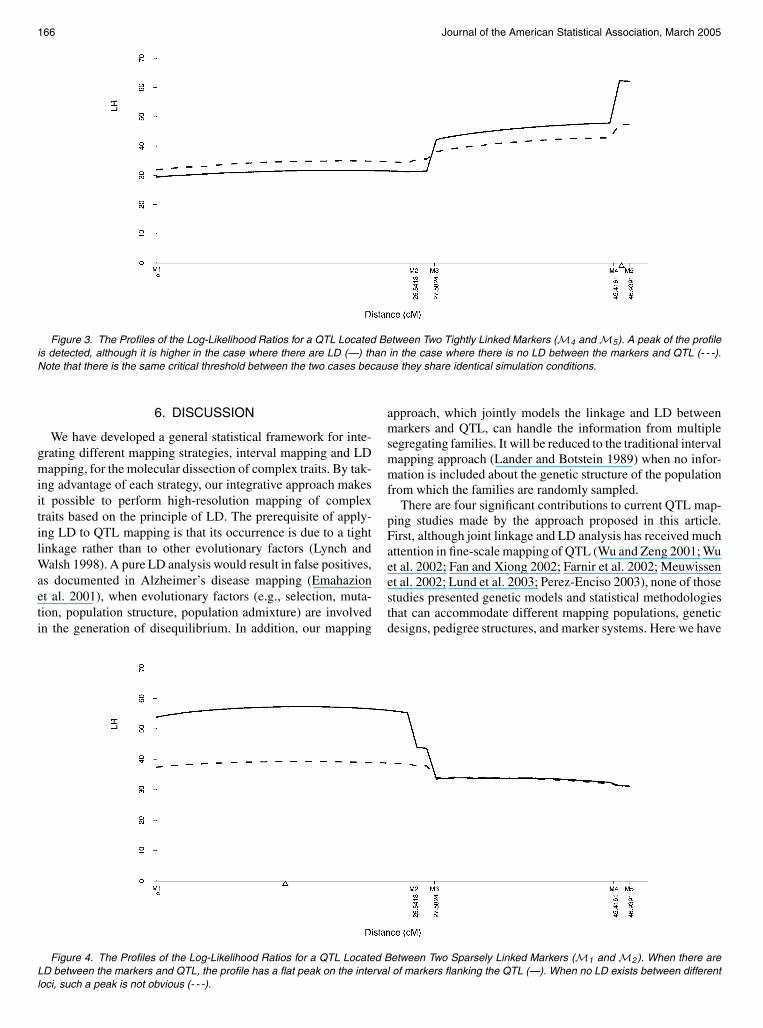
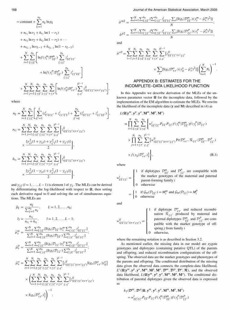
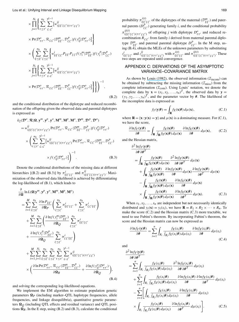
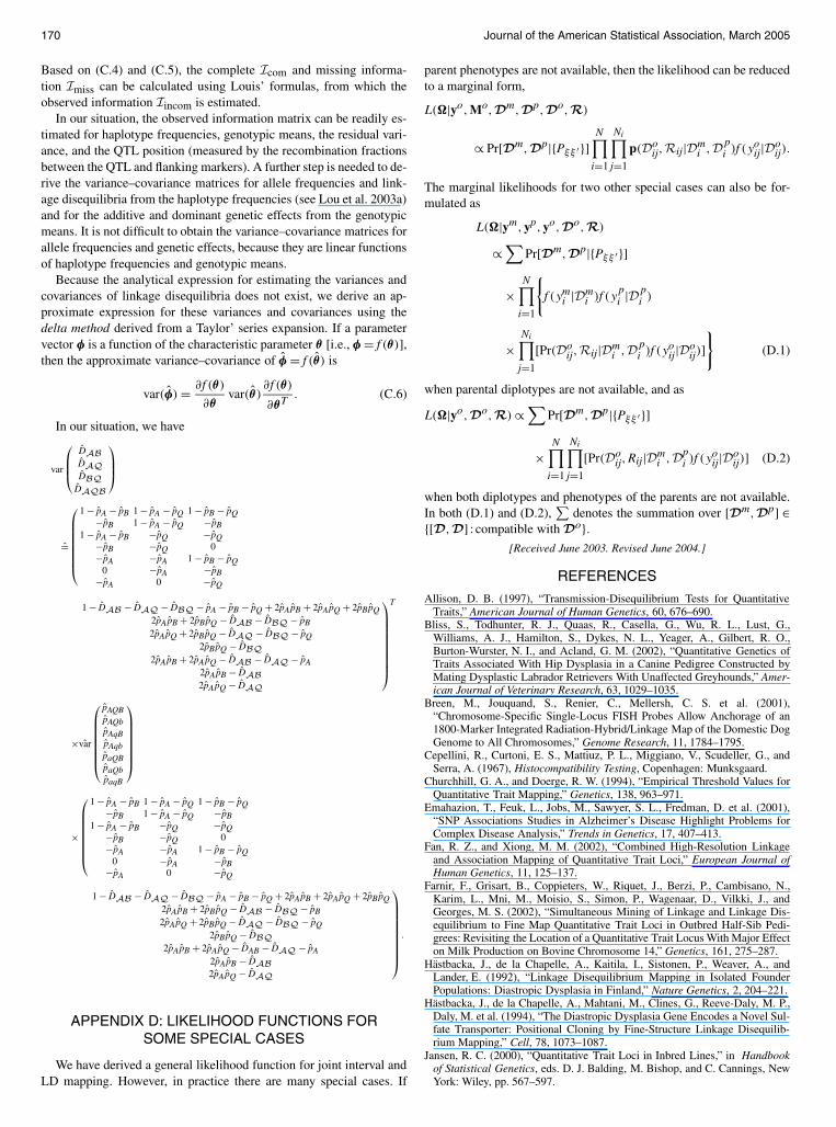
Copyright © 2022 FDOKUMEN