Aggregating Distributional Treatment Effects: ABayesian Hierarchical Analysis of the Microcredit

Literature

Rachael Meager∗†

November 27, 2018

Abstract

Studies of microcredit show positive and negative treatment effects at cer-tain quantiles of household outcome distributions. I develop new Bayesianhierarchical models to aggregate the evidence on these effects and assess theirgeneralizability. I provide a broadly-applicable limited-information model en-forcing quantile monotonicity via variable transformation. Partially discreteoutcomes such as profit are aggregated using full-data mixture models. Acrossall outcomes I find a precise, generalizable zero effect from the 5th to 75thquantiles, and large yet heterogeneous and uncertain effects on the right tails.Households who had previously operated businesses account for the majorityof the impact and the uncertainty.

∗The London School of Economics. Contact: rmeager@lse.ac.uk†Funding for this research was generously provided by the Berkeley Initiative for Transparency in the Social

Sciences (BITSS), a program of the Center for Effective Global Action (CEGA), with support from the Laura andJohn Arnold Foundation. I am immensely grateful to Ted Miguel and the team at BITSS. I also thank Esther Duflo,Abhijit Banerjee, Anna Mikusheva, Rob Townsend, Victor Chernozhukov, Isaiah Andrews, Tamara Broderick, RyanGiordano, Jonathan Huggins, Jim Savage, Andrew Gelman, Tetsuya Kaji, Michael Betancourt, Bob Carpenter, BenGoodrich, Whitney Newey, Jerry Hausman, John Firth, Cory Smith, Arianna Ornaghi, Greg Howard, Nick Hagerty,Jack Liebersohn, Peter Hull, Ernest Liu, Donghee Jo, Matt Lowe, Yaroslav Mukhin, Ben Marx, Reshma Hussam, YuShi, Frank Schilbach, David Atkin, Gharad Bryan, Oriana Bandiera, Dean Karlan, Greg Fischer, and the audiencesof many seminars for their feedback and advice. I thank the authors of the 7 microcredit studies, and the journalsin which they published, for making their data and code public. All my code and data is accessible online athttps://bitbucket.org/rmeager/aggregating-distributional-treatment-effects. I welcome feedback via email.

1

1 Introduction

Financial market expansions in the developing world have the potential to createwinners and losers. Increasing access to credit in particular may have heteroge-neous effects both because borrowers differ in their investment opportunities andbecause of general equilibrium dynamics (Banerjee 2013, Kaboski and Townsend2011). Proponents of financial interventions such as microcredit claim that the pos-itive impact on high-productivity borrowers justifies continued market expansion;detractors claim that the resulting "saturation" of credit markets leads to exploitativelending practices which systematically harm the most vulnerable borrowers (Ahmad2003, Roodman 2012). The debate continues despite decades of research becausethe microcredit literature has focused on estimating average treatment effects whichcannot evince this heterogeneity. Although recent studies have estimated sets ofquantile treatment effects to address this concern, the findings differ across contexts,impeding the formulation of any general consensus and leaving open the possibilityof cherrypicking results (Banerjee et al 2015a, Crepon et al 2015, Angelucci et al2015). Existing meta-studies of microcredit ignored these sets of quantile effects dueto a lack of methodology to aggregate them (Meager 2018, Vivalt 2017, Banerjee etal 2015b). In this paper I develop such methodology and aggregate the evidence onthe distributional treatment effects of microcredit.

Microcredit institutions reached 132 million low-income clients with a global loanportfolio worth 102 billion dollars in 2016, and the figure is growing yearly (Micro-finance Barometer, 2017). At this scale, even small negative impacts for a subset ofborrowers would be a concern, and several governments have curtailed microfinanceoperations ostensibly for this reason (Microfinance Focus 2011, Banerjee 2013, Brezaand Kinnan 2018). Yet even in cases where microcredit benefits all households, anunequal distribution of benefits has the potential to affect social and political insti-tutions (Acemoglu and Robinson 2008, Acemoglu et al 2015). Several randomizedtrials find evidence of negative effects at lower quantiles of household business prof-its, but others find zero impact on most of the distribution; some found positiveeffects at the upper quantiles but these were typically imprecise (Augsburg et al2015, Attanasio et al 2015, Banerjee et al 2015a, Crepon et al 2015, Angelucci et al2015, Tarozzi et al 2015, Karlan and Zinman 2011). The lack of a general consensusis due to both a lack of power to estimate distributional effects relative to averageeffects (Leon and Heo 2009) and the possibility of genuine differences in the impactof microcredit across settings.

Aggregating the evidence on these distributional effects across contexts permits

2

estimation of the typical impact that microcredit is likely to have in future policycontexts. Combining information from multiple studies improves power and preventscherrypicking, that is, undue focus on the most extreme effects in the literature,which may be the least likely to replicate (Rubin 1981). However, contextual het-erogeneity across sites makes it difficult to combine the microcredit studies: poolingthe data and performing one analysis is likely to underestimate the true uncertainty(Gelman et al 2004). Here, as in most of social science, the extent of true hetero-geneity in the impact of microcredit across settings is unknown. Aggregation raisesthe question of external validity: the extent to which the recorded impact of a policyin one setting predicts its impact in another, and the extent to which the average ofall effects predicts the next effect (Allcott 2015, Bisbee et al 2016). If microcredithas different distributional impacts in different contexts, it may be imprudent to useresults from one context to guide policy another context (Pritchett and Sandefur2015). It is therefore important to use an aggregation method that incorporatesuncertainty about the heterogeneity in effects across studies.

Bayesian hierarchical models provide one such framework for evidence aggrega-tion. These models estimate the heterogeneity across studies and use this informa-tion to adjust the uncertainty about the typical impact and likely future impact innew settings. By assessing both within-study and across-study variation within asingle model, the hierarchical approach is able to separate genuine heterogeneity ineffects from the influence of sampling variation (Wald 1947, Rubin 1950, Efron andMorris 1975, Rubin 1981, Gelman et al 2004). This structure nests both the full-pooling case in which the treatment effects are homogeneous, and the no-poolingcase in which the effects are so heterogenous as to contain no information abouteach other. Hierarchical models can also implement a range of intermediate "partialpooling" solutions, borrowing some power across studies to improve inference on allunknown parameters only to the extent suggested to be appropriate by the data(Gelman et al, 2004).1

The hierarchical approach is well established in statistics and is increasingly usedfor evidence aggregation in economics (Chib and Greenberg 1995, Dehejia 2003,Hsiang, Burke & Miguel 2013, Vivalt 2016, Bandiera et al 2017, Meager 2018). Theimplementation is typically Bayesian due to the potential for improved performancein practice, especially when there are few studies (Rubin 1981, Chung et al 2013).Partial pooling models have also been used to borrow power across regions or sub-

1Classical meta-analysis methods typically select the full-pooling solution ex-ante, and modernapplied analysis of multiple experiments in economics has tended to compute both full poolingand no pooling models without attempting to access the range of potential solutions in between(Banerjee et al 2015c).

3

units when studying large geographic areas, or to combine multiple estimates withina study (Hull 2018, Chetty and Hendren 2018, Chetty, Friedman and Rockoff 2014).Yet within the hierarchical framework there are no tools to aggregate distributionaleffects such as sets of quantile treatment effects. Even outside of the hierarchicalframework, the economics literature on external validity and generalizability hasfocused on different kinds of average effects (Heckman, Tobias, & Vytlacil 2001,Angrist 2004, Angrist & Fernandez-Val 2010, Bertanha & Imbens 2014, Allcott2015, Dehejia, Pop-Eleches and Samii 2015, Gechter 2015, Athey & Imbens 2016,Andrews and Oster 2018). This necessitates the development of new methods foraggregating evidence on distributional treatment effects in the presence of treatmenteffect heterogeneity.

Estimating sets of quantile treatment effects provides a general approach to theanalysis of treatment effect heterogeneity. With a binary treatment, the quantiletreatment effects measure the difference between the unconditional quantiles of thetreatment and control groups: this captures any difference in the two cumulativedistribution functions. Although the set of quantile treatment effects does not esti-mate the quantiles of the distribution of individual treatment effects, heterogeneityin the effects on different quantiles is evidence of heterogeneity in these individual ef-fects. Other methods such as interacting treatment with covariates in a linear meanor median regression constrains the differences to operate through specific channels.If the researcher does not have access to the right covariates, or does not enter themin the correct way - perhaps themselves transformed or interacted with each other -the heterogeneity will not be detected.2 If an intervention generally alters householdrisk exposure then there are no covariates which can predict the resulting hetero-geneity in outcomes; sets of quantiles can detect the resulting change in dispersionof outcomes. Sample quantiles also have desirable robustness properties relative tosample means, particularly in the presence of heavy-tailed underlying data (Koenkerand Basset 1978).

Aggregating sets of quantiles presents new challenges relative to average effects.Existing Bayesian hierarchical models for average effects such as Rubin (1981) usethe knowledge that the within-study sampling variation of both means and quan-tiles is often asymptotically Gaussian (Mosteller 1946). However, an aggregation

2In most cases it is not possible to avoid this problem because the total number of potentialcombinations of interacted covariates tends to be larger than the data set, necessitating machinelearning methods which do not readily provide information on which covariates or which combi-nation best predict the heterogeneity. One way this has been avoided in practice is by researchersselecting the few variables they believe are important ex-ante, but this opens up the possibility ofspecification searching and cherrypicking results.

4

model for sets of quantiles must also pass information across the quantiles, becausequantiles must be monotonically increasing; failure to incorporate this structuremay result in the quantile crossing problem (Koenker 2005).3 To solve this problemI exploit the fact that Bayesian inference treats unknown objects as random vari-ables: the quantile treatment effects can be constrained to imply monotonic outcomequantiles by transforming the implied unconditional quantiles using functions thatonly have support on monotonic vectors. In contrast to ex-post rearrangements orsmoothing strategies which impose one particular monotonizing procedure (He 1997,Chernozhukov et al 2010), my strategy selects the monotonic vector most likely tobe the true parameter from a range of possible solutions. I provide monte carlo sim-ulations showing that the model performs well for inference on the quantile effectsin general, as well as showing certain cases where the inference breaks down on thecovariation parameters.

A second problem arises in aggregating quantile effects on the microcredit databecause business outcomes contain point masses at zero. These are due to house-holds who either do not operate a business or only operate seasonally, and thisinformation must remain in the sample to capture any business creation effects ofmicrocredit. The discrete spikes mean that the asymptotic sampling distributionof the quantiles is no longer Gaussian (Mosteller 1946). To aggregate evidence onquantile effects in this setting, I build richly-parameterised mixture models thatcapture the economic structure of the variables. The model allows microcredit toaffect all aspects of the distribution, and I aggregate by placing a hierarchy on theseeffects which permits partial pooling across sites. The implied quantile effects canbe recovered using the method of Castellaci (2012). This approach automaticallysatisfies the monotonicity constraints and passes information across quantiles via thefunctional form assumptions. Model fit assessment and model selection will be nec-essary to ensure reliable inference; I fit models using both Pareto distributions andLognormal distributions based on the existing literature on the tail shape of profitsand earnings (Piketty 2015, Gabaix 2008, Roy 1950) and find that the Lognormalfits the data better.

Applying these models to seven randomized trials of expanding access to mi-crocredit, I find a precise zero effect on household outcomes from the 5th to 75thpercentiles. Above the 75th percentile, there is substantial probability of a large pos-itive impact on most outcomes, but there is greater uncertainty around this effectdue to greater heterogeneity within and across studies. Thus, I find some evidence

3This problem can occur in the aggregation process even if it is not present in the originalstudies because weighted averages of monotonic objects need not be monotonic.

5

of the potential for positive effects and no evidence of systematic harm to any groupof borrowers, as there are no generalizable negative quantile effects at any part ofthe distribution. Part of the greater uncertainty in the tails is due to the tail shapeof the business variables, which are so heavy that average treatment effect analysisand Gaussian asymptotics are likely to be unreliable on this data (Koenker and Bas-set 1978, Mosteller 1946). The likelihood of large, economically important increasein household profits and consumption is far greater than the chance of a zero ornegative impact, but there is substantial uncertainty about the specific effect size inany context. By contrast, classical full pooling methods applied to the same datadeclare "statistically significant" effects in the right tail of business variables as aresult of ignoring the heterogeneity across sites.

Further analysis reveals that both the majority of the right tail impact of micro-credit and the heterogeneity across studies occurs within the group of householdswho had previous business experience. This group of households sees increases inconsumption above the 75th percentile, although there is still a precise zero effectbelow that. To better understand the overall pattern of results, in an appendix Ipursue a bounding exercise to show that the precise and generalizable impact at zerois unlikely to be due to low take-up of loans. This implies an increase in economicinequality even within the group of households who previously operated businesses,such that the social welfare effects of microcredit are likely to be complex. 4

2 Data and Context

Microcredit has the potential for heterogeneous effects both because households dif-ferentially select into take-up, and because those who do take up have differentoutcomes depending on how they use the loan or whether they experience shocks(Banerjee 2013). Even certain households who do take up may experience no ben-efit, perhaps because the terms of the loan may be restrictive and undesirable forinvestment purposes, or the term to maturity may be too short (Banerjee 2013).But even when borrowers do benefit on average, those who don’t take up may end

4While the set of studies here may not be a representative sample of all possible microcreditinterventions, there is little reason to suspect publication bias in this literature. The papers herepublished a variety of results most of which were null results in the framework of null-hypothesissignificance testing. This leads to less risk of classical publication bias in which only "significant"results appear in the literature. However, it is still possible that these studies are not representativeof the world. To address this issue requires substantially more structure and has thus far beenignored in the meta-analysis literature. This may be because such an exercise requires the develop-ment of aggregation techniques that can account for differential types of studies in a more complexway than a simple meta-regression, which fails to share information across the study types.

6

up worse off: there is the potential for winners and losers in general equilibriumdue to effects on wages or displacement of informal lending (Kaboski and Townsend2011, Morduch 1999). Another concern is that multiple microlenders into a commu-nity can lead to predatory lending practices and "overlending" to households whocannot feasibly repay the loan (Shicks 2013, Ahmad 2003). This motivated the "NoPago" movement against microcredit in Nicaragua and was ostensibly part of whythe government of Andhra Pradesh shut microcredit down during the crisis of 2010(Microfinance Focus 2011, Banerjee 2013). Even if the groups of households who ex-perience such effects are small, the social welfare consequences could be substantial,particularly if economic inequality across households is affected. Average treatmenteffects will not reveal these consequences: microcredit access could have zero im-pact on average, yet large positive or large negative impacts for different types ofhouseholds.

Motivated by these concerns, several studies of microcredit reported sets of quan-tile treatment effects for the main outcomes. Some studies did find evidence thatmicrocredit interventions help some households and harm others: many studiesfound large, positive yet imprecisely estimated impacts on the upper tail, and a fewalso recorded imprecise negative effects at the lower tail (Angelucci et al. 2015,Augsburg et al. 2015, Banerjee et al. 2015b, Crepon et al. 2015). Yet certain stud-ies recorded noisy positive effects at the lower tail of some outcomes (such as profitin Banerjee et al 2015b) or negative effects at the upper tails (household businessincome in Angelucci et al 2015). In many of these same cases the quantile treatmenteffects recorded exact zeroes, estimated with relatively high precision, for the centralquantiles. While certain studies, such as Crepon et al 2015, recorded "statisticallysignificant" tail effects on both ends, almost all studies recorded imprecise estimatesat the upper tails. In this setting, the gains from aggregating evidence across thesestudies may be considerable in both precision and an improved understanding of thegeneral pattern of quantile treatment effects.

Estimating sets of quantile treatment effects has many advantages over other ap-proaches to heterogeneous effects in this setting (Banerjee et al 2015b). Microcreditplausibly impacts households’ risk exposure - both because they could use credit asconsumption insurance, and because they could change their business strategy as aresult of the loan - so researchers need to be able to detect changes in the spread ofthe distribution which by definition won’t be predicted by observables. Even whenchanges in the distribution result from heterogeneous effects rather than changes torisk exposure, microcredit is an intervention for which even households with similarcovariates could have considerably different treatment effects due to unobserved het-

7

erogeneity in ability and access to productive opportunities (Kaboski and Townsend,2011). The possibility of general equilibrium effects within the villages themselvesmake it important to assess the impact of treatment on the overall shape of thedistribution at the village level, and to characterise heterogeneity based on relativeposition (ranks or quantiles) rather than absolute values of covariates. In any case,baseline covariates are not available for many of the microcredit studies. Finally, assome of the outcome variables of interest have heavy tails, the robustness propertiesof quantiles are beneficial in the microcredit setting.

To aggregate the evidence on the quantile treatment effects of microcredit, Iuse data from seven studies which meet the following inclusion criteria: the mainintervention must be an expansion of access to microcredit either at the communityor individual level, the assignment of access must be randomized, and the study mustbe published before February 2015 (the period of my literature search). The selectedstudies are: Angelucci et al. 2015, Attanasio et al. 2015, Augsburg et al. 2015,Banerjee et al. 2015b, Crepon et al. 2015, Karlan and Zinman 2011, and Tarozzi etal. 2015, six of which were published in a special issue of the American EconomicsJournal: Applied Economics.5 6 I restrict the sample to randomized controlledtrials (RCTs) because they typically have high internal validity for estimating causaleffects, and because as yet there is no established methodology designed to aggregateboth RCTs and observational evidence in a single framework.7

I analyse six outcomes linked to the claim that offering households more crediton more favourable terms should stimulate entrepreneurship (Morduch 1999, Yunus2006, Roodman 2012). These include: household business expenditures, businessrevenues, and business profits, household consumption, consumer durables spend-ing and temptation goods spending. Because microfinance insitutions (MFIs) offerlower interest rates relative to informal moneylenders, poor entrepreneurs may beable to start new businesses or grow their existing businesses, increasing their busi-ness expenditures, revenues and ultimately profits (Yunus 2006). Greater economic

5Other RCTs of microfinance tend to randomly vary certain characteristics of the loans them-selves, which allows researchers to understand the impact of these features of the loans but com-plicates the inference on the general impact of the standard microcredit model (Field et al 2013).Karlan and Zinman 2009 expands access to consumer credit, but microcredit is often consideredcategorically different to consumer credit; see Banerjee 2013 for a deeper discussion of this.

6I focus on expanding access to microcredit because this is the intervention closest to thepolicy of subsidizing microfinance institutions (MFIs) or promoting interventions under the generalumbrella of "microcredit".

7Existing meta-analyses and other evidence aggregation exercises have either cherrypicked cer-tain observational studies deemed "good enough", or thrown all types of studies into a singleanalysis, a strategy which is likely to violate exchangeability assumptions on the treatment effectsdiscussed in section 3.

8

prosperity should enable households to increase their consumption in the mediumand long run. Yet even households without business investment opportunities mayuse microloans to shift spending away from "temptation goods" (pleasurable butnonproductive or even harmful expenditures) and towards durable goods (Roodman2012, Banerjee 2013). This situation might arise if access to microcredit increases ahousehold’s expectation of escaping poverty in the future, or if microcredit solves aself-control problem (Banerjee and Mullainathan 2010, Banerjee 2013). In general,I analyse the effect of expanding access itself, often called the Intention to TreatEffect in the original studies (Banerjee et al 2015b). The network links betweenhouseholds, the potential for general equilibrium effects, and the impact of the mereexpectation of taking up credit in the future even if one does not take it up todaymeans that the Stable Unit Treatment Value Assumption (SUTVA) is likely to beviolated within a community that experiences any increase in access (Banerjee 2013,Kinnan and Townsend 2012, Breza 2012).8

Despite the restrictive inclusion criteria, the selected studies still differ substan-tially in their implementations and local contexts (see table 7 in Appendix E). Theycover seven different countries, they have different partner NGOs, offering similarbut not identical loan contract structures with different interest rates and loan sizes,and they differ in terms of their randomization units - five randomized at the commu-nity level and two at the individual level - with various encouragement and samplingdesigns. Given this heterogeneity across studies, it seems likely that there might beimportant heterogeneity in the resulting effects. However, the 95% confidence in-tervals of the quantile effects do overlap across most of the studies, suggesting theremay be meaningful similarities across settings.9 In this context, where the general-izability of the evidence across settings is unclear ex-ante, the Bayesian hierarchicalframework is an appropriately cautious way to proceed with evidence aggregation.

The open data policies of the American Economics Journal: Applied Economicsand Science allow me access to the microdata from all of these experiments, suchthat I can standardize which quantiles I compute across studies and can constructeach underlying variable in a uniform manner across studies. The variables weremeasured in different currencies, in different years, and over different time periods(this matters because these are all flow variables). I standardize all measurements

8To investigate the role of take-up in this context, I pursue a bounds analysis explained furtherin Appendix D.

9This pattern was also observed in the average treatment effects in these studies, which turnedout to have only moderate underlying heterogeneity despite these contextual differences (Meager2018). However, similarities in the average treatment effects may be uninformative about thetrue generalizability of the effects if indeed these averages are composed of heterogeneous quantileeffects.

9

to be USD PPP in 2009 dollars over a two-week period. Business variables requirefurther standardization: to capture the potential for microcredit to allow individualsto open new businesses or to switch to operating any existing seasonal businessesthroughout the year, households with no business or missing business data haveprofits imputed as zero. This was the decision made by the original authors ofmany of the seven studies, although not all of them. Because the business creationchannel is closely tied to the central claims of Yunus (2006), I employ this strategythroughout to business expenditures and revenues as well.10 Other than standard-izing the definition and construction of variables as much as possible, in most otherrespects I have attempted to conform to the decisions made by the original authorsthemselves. 1112

Household and study-level covariates may play some role in determining hetero-geneity in the quantile treatment effects, but there are limitations to pursuing acovariates analysis in this literature. Only three of the microcredit RCTs collectedcomprehensive individual-level baseline surveys. One pre-treatment variable wasrecorded at endline in all studies due to its theoretical importance: a binary in-dicator that a household had previous experience operating a business (Banerjeeet al 2015b). Although covariates at the study level may also predict variation ineffects across context, there at least seven such covariates and only seven studies, soconventional regression analysis will be overfitted and misleading. It is still usefulto aggregate the evidence without conditioning on covariates, as this permits anunderstanding how much unconditional heterogeneity there is; if there is little or novariation across settings, further analysis is a less pressing concern for future work.

10While it would be ideal to examine effects on other variables such as income and assets, themeasurement and definition of those variables differed across the studies to such an extent that it isunclear how to aggregate them. This issue was noted in Meager (2018) and in my pre-registration:https://osf.io/tdvc8/ .

11Certain potential issues such as attrition or sample selection were left as they were in thestudies themselves and in most cases I have used the entire sample available in the online datasets. Ethiopia is the only exception: this study contained a cross-randomized family planningtreatment. I use only the pure control and the pure microcredit samples, which is the conservativechoice given that we do not know how microcredit interacts with family planning (the studyestimates a very imprecise interaction).

12I do not winsorize any of the variables because most of the studies did not do so, and Augsburget al (2015) found that winsorizing outliers sometimes made results statistically significant whenthey were not significant in the full sample. If the extreme values do not change the point estimatebut increase the uncertainty, winsorising them may underestimate the true uncertainty. As myanalysis shows, the behaviour of the upper tails turn out to play an important role in determiningthe impact of microcredit.

10

3 Methodology

3.1 Bayesian Hierarchical Models

3.1.1 Hierarchical Models

Consider a body of evidence consisting of K studies indexed by k, each of whichprovides some k-specific data Yk about a given policy intervention. The K data setstaken together form one large data set, denoted Y = YkKk=1. Each study has a site-specific parameter of interest θk ∈ Θk, which could be the average treatment effectof microloan access on household business expenditures, or the entire set of quantiletreatment effects. The full data in each site k consists of Nk households, summingto N households in the total combined sample of all studies. In some cases, analystswill not have access to the full underlying data, only to the estimated effects andtheir standard errors from each of the K papers, denoted θk, sekKk=1. The generalstructure and intuition in the aggregation problem is the same in both cases and Iconsider models applicable to both situations.

Suppose that the analyst wishes to learn about the expected value of these θkKk=1

parameters, incorporating uncertainty due to unobserved differences across studysites or settings. This is often of interest because such an object corresponds tosome population average value of this parameter, say θ = E[θk] with the expecta-tion taken across the sites rather than across households. Incorporating site-leveluncertainty permits inference not just to unobserved households in the existing sitesbut to unobserved sites themselves, and thus, such a procedure may permit extrap-olation beyond the current set of studies.13 One can learn about this θ using theevidence on θkKk=1, but the optimal learning procedure depends on the heterogene-ity or dispersion of θkKk=1 around θ, denoted Σθ (Rubin 1981, Gelman et al 2004).This Σθ describes the signal strength of any θk for inference about the general effectθ, and thus the signal strength of θ as a predictor of θK+1 if the sites are sufficientlycomparable.14 Here Σθ parameterizes a notion of generalizability of the evidencecontained in Y to external settings, which captures the definition of external va-lidity in Allcott (2015) and Dehejia et al. (2015). If Σθ = 0, then θ is a perfectpredictor of θK+1; if not, there will be some extrapolation error which grows large asthe parameter Σθ grows large. Hence, this Σθ determines the optimal aggregationmethod and the relevance of θ for policy purposes.

13If this population parameter effectively does not exist, and it is impossible to update beliefsabout economic mechanisms across settings, then much of economics is called into question.

14Technically the sites must be "exchangeable", this condition is discussed later in this section.

11

Joint estimation of θ and Σθ is the core challenge of aggregation across studies.Before aggregation occurs, the data has been analyzed separately in each study:this constitutes a "no pooling" model, where each effect θk is estimated using onlythe data from its own site, Yk. The resulting estimates, denoted θkKk=1, are onlyoptimal for the set θkKk=1 if K < 3 and if indeed no general common parameterθ exists.15 The heterogeneity of θkKk=1 is generally biased upwards for Σθ becauseit includes the sampling variation of each θk around its θk (Stein 1951, James andStein 1961). These estimates or the underling data must be combined in some wayto estimate θ, Σθ and θK+1. A "full pooling" aggregation method is an estimationprocedure for θ which uses all the data Y and assumes that θk = θk′ ∀ k, k′. This as-sumption may be made explicitly or implicitly: any estimator that does not leveragethe K-site structure nor estimate Σθ is a full pooling estimator. A "partial pooling"estimator uses the full data Y to estimate θ but does not assume θk = θk′ ∀ k, k′. Apartial pooling aggregation procedure provides estimates of θ, Σθ as well as new es-timates of θkKk=1 produced by transferring some information across sites, denoted(θ, Σθ, θkKk=1).

Hierarchical modeling is a general framework for implementing partial poolingto aggregate evidence across studies which jointly estimates θ and Σθ. The defin-ing characteristic of these models is a multi-level structure, which defines a set ofparameters at the site level, θkKk=1, a set of parameters at the population level,θ, and a relationship between them. One way to realize this structure is to use amulti-level likelihood which expresses the dependence of the data on the entire setof parameters (Efron & Morris 1975, Rubin 1981, Gelman et al. 2004). The "lowerlevel" of the model describes the dependence between the data and local parametersin site k:

Yk ∼ f(·|θk) ∀ k. (3.1)

The "upper level" of the model describes the potential for statistical dependencebetween local parameters and general parameters via some likelihood function ψ(·),which contains the parameter Σθ either implicitly or explicitly depending on thespecific model. Hence, while in general ψ(·|θ,Σθ), this second argument is oftenimplicit and thus, for simplicity, notationally suppressed. This upper level "general"or "parent" distribution is then denoted:

θk ∼ ψ(·|θ) ∀ k. (3.2)

15If K ≥ 3 all no-pooling estimators are risk-dominated in terms of MSE by partial poolingestimators. The formal proof of this statement is in Stein 1956, and further discussion is in Efron& Morris 1975.

12

A hierarchical likelihood contains both levels:

L(Y|θ) =K∏k=1

f(Yk|θk)ψ(θk|θ). (3.3)

This likelihood structure nests common approaches to understanding the evidencefrom multiple studies, including both the no-pooling and full-pooling models. Themodel can detect these cases because the parameters that govern the ψ(·) function,including its implicit structure on Σθ, are estimated rather than imposed ex-ante.For example, the model may estimate that θk ≈ θk′ ∀ k, k′, and hence that Σθ = 0,if that is supported by the data. This result would recover the full-pooling model’ssolution, up to a degrees of freedom correction. Alternatively, the model can estimatevery large dispersion in θkKk=1 such that in fact θkKk=1 = θkKk=1, and as suchrecover the no-pooling model’s solution. For applications in economics, where itis reasonable to think that neither extreme is likely to describe the data well, themodel’s main advantage is that it can recover a solution anywhere on the spectrumbetween these two extremes if that intermediate solution is most supported by thedata. The model’s estimation of θ and Σθ are appropriately influenced by the extentof this "partial pooling" (also called "shrinkage", because the estimates are pulledcloser together, so the variance is "shrunk"). Hence, although some efficiency is lostif in reality Σθ ∈ 0,∞, the hierarchical approach is more robust than the fullpooling or no pooling approaches.

While in principle the hierarchical model could be specified with a nonparametriclikelihood, a parametric structure is often preferable in low-data environments, suchas evidence aggregation with a small or moderate number of studies.16 Any partialpooling model must impose some structure to determine the extent of the poolingand how the pooling will be informed by the data. If the analyst faces a low-dataenvironment at the cross-study level, this structure must not be too flexible or themodel risks overfitting the scarce data that is available. Nonparametric methodsoften lack the power to deliver reliable inference at the general level, because theylack the structure of parametric models. As a result, hierarchical models used forevidence aggregation of scalar parameters often specify ψ = N(θ,Σ2

θ) due to thedesirable frequentist properties of the resulting model (Efron and Morris 1975).This functional form appears more restrictive than the no-pooling or full-poolingmodels implemented using ordinary least squares regression, but in fact the Normalmodel still nests both of these cases since it can estimate Σθ → ∞ or Σθ = 0

16A similar point and a proof of the nonparametric identification is provided in Andrews andKasy 2017.

13

respectively. The no-pooling and full-pooling models do not specify parametricupper-level structure only because they impose such strong assumptions about Σθ.Parametric hierarchical likelihoods relax the assumptions on Σθ without providingtoo many degrees of freedom relative to the number of studies being aggregated.

When parametric structure is needed, the key insight of Rubin (1981) is that onecan use knowledge of the sampling behaviour of certain statistics, in his case samplemeans and differences in sample means, to inform this choice. Even with limitedinformation about the θk parameters, usually in the form of reported estimates andstandard errors θk, sekk=1

K , one often knows their approximate sampling behaviourunder assumptions that seem reasonably mild. For example, sample means and byextension parameter estimates from linear regressions estimated by ordinary leastsquares often satisfy the Law of Large Numbers and the Central Limit Theorem,such that asymptotically

θk ∼ N(θk, se2k). (3.4)

In the full data case, one can analogously specify the within-sample variation usingthe structure imposed by the original studies. For example, if each study of a binarytreatment indicator ran linear regressions of the form ynk = µk+τkTnk for householdn in site k, then the point estimates can be analytically replicated by the model

ynk ∼ N(µk + τkTnk, σ2k). (3.5)

Since these functional forms reflect underlying knowledge of the data or statisticsbeing studied, hierarchical models based on these structures can more effectivelyseparate the sampling variation from the between-study variation in effects (Rubin1981). With the local variation specified in a particular way, the choice of the parentdistribution that governs the between-study heterogeneity in effects can now be madein view of tractability and performance properties measured by the Mean SquaredError. These considerations typically motivate the use of Gaussian structure atthe upper level of the model because they implement beneficial forms of shrinkageacross the studies and have been shown to perform well for a variety of problems(McCullough and Neuhaus 2011, Efron and Morris 1975, Gelman et al 2004). Inparticular, if one is concerned with inference on only location and scale parameters,McCullough and Neuhaus (2011) shows that the Gaussian performs well even if thetrue underlying distribution is not Gaussian.17

17There are still important limitations to this approach, such as the restriction to single-peakeddistributions which prevents for example detection of subclusters in the data, but with only sevenstudies the microcredit literature is unlikely to provide a fruitful setting for reliable cluster detec-tion.

14

Hierarchical models do require that θkKk=1 be “exchangeable”, such that theirjoint distribution is invariant to permutation of the indices (Diaconis, 1977). Thismeans the analyst must have no knowledge of the ordering or any sub-clustering ofthe treatment effects a priori that is not specified in the model (Rubin 1981). If eco-nomic theory demands that a particular covariate should be correlated in a certainway with the treatment effects, that can be translated into conditional exchangeabil-ity by introducing this covariate into the model. Yet theory and prior knowledgerarely provide certainty about these relationships, and building sufficiently weakstructure that still permits inference on the role of covariates is typically challeng-ing in a low-data environment. In the absence of strong prior knowledge about thetreatment effects, exchangeability is a reasonable structure to impose (Gelman etal 2004).18 Any future site for which θK+1 is used to predict the effect must beexchangeable with the sites in the sample for this prediction to be valid, which isgenerally a requirement for predicting out-of-sample effects (see for example Allcott2015).

3.1.2 Bayesian Implementation

While hierarchical models can be estimated using frequentist methods, in practiceBayesian inference offers several advantages. The first is accurate characterizationof the uncertainty on all parameters produced by jointly estimating all unknowns.Commonly used maximum likelihood techniques estimate the upper level first andthen condition on the point estimates using the "empirical Bayesian" approach fromEfron & Morris (1975). This ignores the uncertainty about the upper level parame-ters, θ and Σθ, when computing uncertainty intervals on the lower level parameters,and thereby systematically underestimates the uncertainty at the lower level (Rubin1981). This conditioning is required for tractability in the maximum likelihood esti-mation (MLE) framework as it is commonly implemented, because of the nonlinearinterdependencies between θkKk=1, θ, and Σθ.19 By contrast, Bayesian inferencejointly and simultaneously estimates all unknowns, accurately characterizing theuncertainty at every level of the model and producing coherent inference acrosslevels.

Bayesian inference proceeds by specifying a prior on all unknowns, P(θ), andcombining it with the likelihood via Bayes’ rule to generate the the joint posterior

18It is possible to build a more complex structure that allows "partial exchangeability" if this isdesired. See Albert and Chib 1997.

19While MLE methods that do not inappropriately condition on unknowns are theoreticallyavailable, they seem to be largely unused in practice.

15

distribution f(θ|Y). The specification of a proper prior distribution ensures thatf(θ|Y) is a proper probability distribution with desirable decision-theoretic proper-ties such as admissibility (Efron 1982, Berger 2013). All proper Bayesian posteriorsare consistent in the frequentist sense under similar conditions that make MLE con-sistent, as long as the prior has support over the true parameters, so aggregationperformed in this framework will asymptotically deliver the correct answer as morestudies are done (for the details see Van der Vaart 1998).

In a low-data environment, specifying informative priors can substantially im-prove the performance of the hierarchical model. If the analyst only has vagueknowledge of the location of this likely region, then the priors can be made quitediffuse or “weakly informative” (Gelman et al 2008). If there is substantial expertknowledge of the likely values before seeing the data, perhaps from economic theoryor previous studies, this can be incorporated using stronger priors. Even if the priordistributions introduce some bias due to incorrect centering, they may still improvethe mean squared error of the estimation by reducing the variance (Chung et al.2013, 2015). In low-data environments such as the cross-study level of the hierar-chical model, overfitting and high variance can be the major obstacle to makingreasonable inferences or predictions. Thus, the priors perform regularization in theclassical sense: they introduce new information that constrains the fit of the modelin ways beneficial to inference (Hastie, Tibshirani and Friedman 2009, section 10.2).Priors also increase the tractability and speed of the estimation by targeting regionsof the parameter space that are more likely to contain relevant values.

Bayesian inference also provides a framework for thinking about the distributionof the treatment effect in a hypothetical future site θK+1. This is often the object ofmost interest for policymakers, but the distribution of this object must be computedaccounting for the full joint posterior uncertainty rather than conditioning on aparticular point estimate.20The Bayesian approach delivers the correct uncertaintyinterval in the form of posterior predictive inference (Gelman et al., 2004), whichaverages over the posterior uncertainty on the unknowns (θ,Σθ). Formally, the

20The full joint posterior uncertainty accounts perfectly for the uncertainty about how well thenew location matches the old location, if the new site is exchangeable with the old sites, and themodel structures are correct. If these conditions do not hold, we have modelling uncertainty, whichis not accounted for in any meta-analytic methods at present (nor in any of the popular analyticmethods used in empirical economics). However, attempts to account for this uncertainty withinthe status quo have all been informal, subjective and opaque; for example, experts picking andchoosing which existing sites they think are most relevant for some particular new setting is not atransparent or reproducible aggregation method.

16

posterior predictive distribution is:

f(θK+1|Y) =∫ψ(θK+1|θ)f(θ|Y)dθ (3.6)

Specifically for aggregating distributional effects, the Bayesian approach has an-other advantage in incorporating knowledge about the properties of θ, because itoffers a natural mechanism for implementing constraints on parameters. If the pa-rameter θ can only belong to some subset of the parameter space, AΘ ⊂ Θ, thisproduces the following restricted likelihood:

LAΘ(Y|θ) = L(Y|θ) · 1θ ∈ AΘ. (3.7)

While this is conceptually simple, implementing the restriction is not straightfor-ward in some cases, such as the one considered here. However, because Bayesianinference treats unknown parameters as random variables, a statistical transforma-tion of variables can impose constraints throughout the entire estimation withoutany distortion of the probability space. If θ is a multivariate random variable withPDF pθ(θ) then a new random variable θ∗ = f(θ) for a differentiable one-to-oneinvertible function f(·) with domain Aθ has density

p(θ∗) = pθ(f−1(θ))|det(Jf−1(θ))|. (3.8)

Therefore to implement inference using LAΘ(Y|θ), leading to the correctly con-strained posterior fAΘ(θ|Y), we specify the model as usual and then implement atransformation of variables from θ to θ∗. We then perform Bayesian inference usingL(Y|θ∗) and P(θ∗), derive f(θ∗|Y), and then reverse the transformation of variablesto deliver f(θ|Y) · 1θ ∈ AΘ. Frequentist implementation of constraints typicallymust reckon with the constraints twice, first in point estimation and second in in-terval estimation, and it can be costly to ensure coherence between the two or toextent the consequences to other parameters; the Bayesian implementation ensurescoherence because the constraint is imposed on the parameter itself and is thus ac-counted for in both estimation and inference using the resulting joint posterior ofall unknowns.

Tractability issues can arise in Bayesian inference on hierarchical models due tothe same issues that lead frequentists to adopt Empirical Bayes, these can often besurmounted by the use of Markov Chain Monte Carlo (MCMC) methods. Thesemethods construct a Markov chain which has the posterior distribution as its invari-ant distribution, so that in the limit, the draws from the chain are ergodic draws

17

from the posterior. This chain is constructed by drawing from known distributionsat each “step” and using a probabilistic accept/reject rule for the draw based onthe posterior distribution’s value at the draw. While these chains always convergeto the correct distribution in the limit, popular algorithms such as the Metropolis-Hastings or Gibbs samplers can be prone to inefficient random walk behavior whenthe unknowns are correlated, as with hierarchical models. Instead, I use Hamilto-nian Monte Carlo (HMC) methods, which can better estimate hierarchical models(Betancourt and Girolami, 2013).21

3.2 Limited Information Asymptotic Quantile Models

Consider the task of aggregating sets of quantile treatment effects and assessingtheir generalizability. First recall that the uth quantile of some outcome is the valueof the inverse CDF at u:

QY (u) = F−1Y (u). (3.9)

Performing quantile regression for some quantile u in site k when the only regressoris the binary treatment indicator Tnk requires estimating:

Qynk|T (u) = β0k(u) + β1k(u)Tnk (3.10)

For a single quantile u, the treatment effect is the univariate parameter β1k(u).If there is only one quantile of interest, a univariate Bayesian hierarchical modelcan be applied, as in Reich et al (2011). But in the microcredit data, researchersestimated a set of 10 quantiles U = 0.05, 0.15, ..., 0.95 and interpolated the resultsto form a "quantile difference curve". This curve is constructed by computing thequantile regression at all points of interest:

Qyik|T = Qyik|T (u) = β0k(u) + β1k(u)Tik ∀ u ∈ U (3.11)

The results of this estimation are two |U|-dimensional vectors containing interceptand slope parameters. For the microcredit data, I work with the following vector of

21HMC uses discretized Hamiltonian dynamics to sample from the posterior, which can be com-bined with the No-U-Turn sampling method (NUTS) to auto-tune the step sizes in the chain(Hoffman and Gelman, 2011). This algorithm is automated in the software package Stan, a freestatistical library which calls C++ to fit Bayesian models from R or Python (Stan DevelopmentTeam, 2017).

18

10 quantile effects:

β0k = (β0k(0.05), β0k(0.15), ...β0k(0.95))

β1k = (β1k(0.05), β1k(0.15), ...β1k(0.95))(3.12)

The quantile difference curve is the vector β1k, often linearly interpolated. Witha binary treatment variable, the parameters in a quantile regression are simple func-tions of unconditional outcome quantiles. Let Q0k(u) be the value of the controlgroup’s quantile u in site k, and let Q1k(u) be the value of the treatment group’squantile u in site k. Then:

Q0k = Q0k(u) ∀ u ∈ U

Q1k = Q1k(u) ∀ u ∈ U.(3.13)

Then the vectors of intercepts and slopes for the quantile regression curves canbe reformulated as

β0k = Q0k

β1k = Q1k −Q0k.(3.14)

Hence, while the quantile difference curve β1k need not be monotonic, it must im-ply a monotonic Q1k when combined with a monotonic β0k. The fact that any infer-ence done quantile-by-quantile may violate monotonicity of (Q1, Q0, Q1k, Q0kKk=1)is a well-understood problem (Chernozhukov et al. 2010). Partial pooling for aggre-gation can exacerbate this problem because even if every lower level Q1k and Q0k

satisfies monotonicity, their "average" or general Q1 and Q0 may not do so. Thus,unlike quantile crossing within a sample, the crossing in this setting is not necessarilythe result of an incorrect asymptotic assumption or an extrapolation to a poorly-covered region of the covariate space. Indeed, for binary treatment variables, thewithin-sample estimators always satisfy monotonicity, but the averaging and poolingof these estimators may introduce crossing where none existed.22 Ideally, therefore,an aggregation model should fit all quantiles simultaneously, imposing the mono-tonicity constraint. Aggregating the quantile difference curves, β1kKk=1, requiresmore structure than aggregating quantile-by-quantile, but permits the transmissionof information across quantiles.

I propose a general methodology to aggregate reported information on quantile22Yet even if quantile crossing does not arise, neighboring quantiles contain information about

each other not just because of monotonicity but because smooth distributions have quantiles thattend to lie close to each other; using that information can improve the estimation and reduceposterior uncertainty.

19

difference functions building on the approach of Rubin (1981) and a classical resultfrom Mosteller (1946) about the joint distribution of sets of empirical quantiles.Mosteller shows that if the underlying random variable is continuously distributed,then the asymptotic sampling distribution of a vector of its empirical quantiles isa multivariate Normal centered at the true quantiles and with a known variance-covariance structure. This implies that the difference of the empirical quantile vec-tors from two independent samples, β1k = (Q1k − Q0k), is also asymptotically amultivariate Gaussian. The theorem offers a foundation for a hierarchical quantiletreatment effect aggregation model using the knowledge that the sampling variationis approximately a multivariate Gaussian, and that as a result modelling the par-ent distribution as Gaussian will be both tractable and have attractive performance(Rubin 1981, Efron and Morris 1975). The resulting analysis requires only the lim-ited information reported by each study (although it can be fit to the full data) andis applicable to any continuous distribution as long as there is sufficient data in eachof the studies to make the asymptotic approximation reasonable.

For this model, the data are the vectors of sample quantile differences β1kKk=1

and their sampling variance-covariance matrices Ξβ1kKk=1. Thus, the lower levelf(Yk|θk) = f(β1k|β1k) is given by the expression:

β1k ∼ N(β1k, Ξβ1k) ∀ k (3.15)

The upper level of the model ψ(θk|θ) is therefore:

β1k ∼ N(β1,Σ1) ∀ k. (3.16)

However, the estimated (β1, β1kKk=1) from this likelihood may not respect theimplied quantile ordering restriction when combined with the estimated controlquantiles, even if β1ks do. We need to add the relevant constraints to this model,but these difference functions are not the primary objects on which the constraintsoperate. While (β1, β1kKk=1) need not be monotonic, they must imply monotonic(Q1, Q1kKk=1) when combined with (Q0, Q0kKk=1). Since the objects (Q1, Q0, Q1k, Q0kKk=1)define the constraints, they must appear in the model.

Once the quantiles (Q1, Q0, Q1k, Q0kKk=1) appear in the model, transformingthem into monotonic vectors will fully impose the relevant constraint on (β1, β1kKk=1).This strategy exploits the fact that Bayesian inference treats unknown parametersas random variables, so applying the transformation of variables formula and thenreversing the transform at the end of the procedure completely preserves the pos-

20

terior probability mass, and hence correctly translates the uncertainty intervals. Iproceed with a transform proposed for use in Stan (2016), but in theory any validmonotonizing transform will do, since it is always perfectly reversed.23 Considermonotonizing the |U|-dimensional vector β0, with uth entry denoted β0[u]. One canmap β0 to a new vector β∗0 as follows:

β∗0 [u] =

β0[u], if u = 1

log(β0[u]− β0[u− 1]) if 1 < u < |U|(3.17)

Any vector β0 to which this transform is applied and for which inference is performedin the transformed space will always be monotonically increasing. For the rest of thepaper, I denote parameters for which monotonicity has been enforced by performinginference on the transformed object as in equation 3.17 with a superscript m. Thus,by applying the transform, I work with βm0 rather than an unconstrained β0.

Employing a monotonizing transform is an appealing alternative to other methodsused in the econometrics literature to ensure monotonicity during quantile regres-sion. Restricting the Bayesian posterior to have support only on parameters whichimply monotonic quantiles means that, for example, the posterior means are thosevalues which are most supported by the data and prior information from the setwhich satisfy the constraint. Frequentist solutions such as rearrangement, smooth-ing or projection each prevent the violation of the constraint in one specific waychosen a priori according to the analyst’s own preferences (He 1997, Chernozhukovet al. 2010). While each strategy performs well in terms of bringing the estimatescloser to the estimand (as shown in Chernozhukov et al. 2010) the Bayesian trans-formation strategy can flexibly borrow from each of the strategies as and when thedata supports their use. Imposing the constraint throughout the inference avoidsthe additional complications of choosing when during aggregation one should im-plement the ex-post fixes proposed in the frequentist literature; for example, in thecase of rearrangement, it would be hard to interpret the result of partially poolinginformation on the 25th quantile only to have some other quantile substituted in forcertain studies ex-post.

Equipped with this monotonizing transform, it is now possible to build modelswith restricted multivariate Normal distributions which only produces monotoni-cally increasing vectors. I propose the following model to perform aggregation in ahierarchical framework, taking in the sets of empirical quantiles Q1k, Q0kKk=1 and

23While some transforms may perform better than others in certain cases, to my knowledge thereis little research on this issue that presently permits us to choose between transforms.

21

their sampling variance-covariance matrices Ξ1k, Ξ0kKk=1 as data. For this hierar-chical quantile set model, the lower level f(Yk|θk) is:

Q0k ∼ N(βm0k, Ξ0k) ∀ k

Q1k ∼ N(Qm1k, Ξ1k) ∀ k

where Q1k ≡ βm0k + β1k

(3.18)

The upper level ψ(θk|θ) is:

βm0k ∼ N(βm0 ,Σ0) ∀ k

β1k ∼ N(β1,Σ1) ∀ k

where β1 ≡ Qm1 − βm0

(3.19)

The priors P(θ) are:

βm0 ∼ N(0, 1000 ∗ I10)

β1 ∼ N(0, 1000 ∗ I10)

Σ0 ≡ diag(ν0)Ω0diag(ν0)′

Σ1 ≡ diag(ν1)Ω1diag(ν1)′

where ν0, ν1 ∼ halfCauchy(0, 20) and Ω0,Ω1 ∼ LKJCorr(1).

(3.20)

This formulation is convenient as the form of Ξ1k is exactly derived in theMosteller (1946) theorem, though the individual entries need to be estimated. Thestructure could be modified to take in the empirical quantile treatment effectsβ1kKk=1 and their standard errors instead of Q1k if needed. The model imposes nostructure on (Σ,Σ0), other than the logical requirement of positive semi-definiteness.This complete flexibility is made possible by the discretization of the quantile func-tions; these matrices could not take unconstrained form if the quantile functionshad been modelled as draws from Gaussian Processes.24 Overall, this structurepasses information across the quantiles in two ways: first, by imposing the order-ing constraint, and second, via the functional form of Σk from the Mosteller (1946)theorem.

The above model implements partial pooling not only on the β1kKk=1 parameters24Gaussian Processes in general are too flexible to fit at the upper level of these models for

this application, and popular covariance kernels tend to have identification issues that limit theirusefulness in the current setting. In particular, most tractable and popular kernels do not permitthe separation of dispersion of points within the functional draws from dispersion of points acrossthe functional draws.

22

but also on the β0kKk=1 parameters, that is, the control group quantiles. Thetechnical reason for this is that one needs to define a notion of a general β0 in orderto define the constraint on the general β1 and the predicted β1,K+1. However, thisstructure also provides us with useful insight that allows us to better interpret theresults of the partial pooling on β1kKk=1. Suppose for example that we observesubstantial pooling on β1kKk=1, but we also observe this on β0kKk=1; in that case,we observe similarities in the treatment effects perhaps only because we have studiedplaces with similar control groups. In that case it will be hard to justify extrapolationto another setting with a substantially different value of β0k. On the other hand,suppose that we observe substantial pooling on β1kKk=1 but no pooling at all onβ0kKk=1. Then we have learned much more generalisable information, because wenow know that the treatment effects can be similar even when the underlying controldistributions are different.

3.2.1 Model Performance

To assess the performance of the model, I provide Monte Carlo simulations under avariety of data scenarios and report the coverage of the posterior intervals. Ideally,the 50% posterior interval should contain the true parameter 50% of the time, andthe analogous property should hold for the 95% posterior interval. When the datais simulated from the model itself this property is guaranteed in Bayesian inference,however, in practice one typically does not have the luxury of fitting data that oneknows originates from a particular model. Therefore, all the monte carlo simulationsI provide here fit the model above to data generated from a somewhat differentmodel. In particular, I always simulate data for which my priors are incorrect; asthe priors are reasonably diffuse they should not compromise the inference, and nordo they.

The results in table 1 show that the model typically provides approximately nom-inal coverage on β1, and often provides greater than nominal coverage, regardless ofthe generating process. However, inference on the β0 and the covariation parametersΣ0,Σ1 is more sensitive to underlying conditions. When there is large variation inthe data within sites, the model can have difficulty with achieving nominal coverageon the 50% interval for these parameters, although the 95% interval usually retainsits coverage properties. The fact that the model has trouble when the data ex-hibits large variation reflects one of the conditions of the Mosteller (1946) theorem,namely that the underlying density that generates the data is not vanishing in theneighbourhood of the quantile. While this condition is formally satisfied in the sim-

23

ulations, the model seems to be affected regardless: the poor average performancein these cases is generated by difficulty characterising the extremal quantiles wherethe density is thinnest.

Encouragingly, when the data variation is moderate or small, the model doesreasonably well on most parameters even when the full pooling or no pooling casesapproximately hold. The no pooling case provides some trouble for inference onΣ0,Σ1 due to the extreme cross-site variation. Large within-site data variationseems to cause difficulties for the 50% intervals in the full pooling inference, butthe 95% intervals retain their coverage properties even in this case. There are someresults in the table that do not fit the broad patterns laid out here, but this maybe due to the relatively small number of MC runs (due to the relatively long timeit takes to run the model). The results point to overall good performance, althoughsuggesting that caution should be applied when approaching data sets that havehigh variance or heavy tails even when the theoretical conditions for asymptoticnormality are formally satisfied.

3.2.2 Interpretation

The goal of the hierarchical model is to estimate the central location and the dis-persion in the distributions from which each of the observed β0k, β1k are drawn.This permits analysts and policymakers to formulate expectations about what maybe likely in future settings. The expectations are taken over the distribution ofthe vectors β0k, β1k, not over households; this point is crucial to avoid confusionabout how to interpret quantiles in a hierarchical setting. The estimate of β0 is anestimate of the expected marginal distributions of the control groups’ outcomes inthe set of sites exchangeable with the K sites at hand, subject to the constraint thatthese objects all be monotonic. The estimate of β1 is an estimate of the expecteddifferences between the marginal outcomes of the treatment and control groups inthe set of exchangeable sites, subject to the known properties of each of the groupsdistributions. While the monotonicity constraint complicates the interpretation rel-ative to unconstrained Gaussian models, the broad intuition is that the parametersβ0, β1 provide an estimate of the centrality of the individual distributions over thevector spaces in which β0k, β1k live.

Quantile effects are often subject to misinterpretation. Quantiles do not satisfylaws of iterated expectations, so the treatment effects at the quantiles of the outcomedistribution (which is what is delivered here) are not the quantiles of the distribu-

24

tion of treatment effects.25 Another source of confusion is that while unconditionalquantiles of a distribution correspond to specific data points in the sample, thesedata points (and the individuals who produce them) are not meaningful in them-selves. It does not make sense to think of quantile estimation as applying to specifichouseholds nor "tracking" them across time or place. As stressed in Koenker 2005,the fact that one can locate the specific data point that sits at a particular samplequantile does not mean that this datum is deeply related to the population quantilein some way: it happens to be the best estimate of that population quantile, nothingmore. The population quantile is a parameter, not an "uber household"; the samplehousehold whose outcome value is "selected" as a quantile estimate is not playingthe role of an individual in the world but rather the role of a sample order statisticof similar general stature to a sample mean. If the sample had realised differently,a different household would have been selected as the estimate, but the populationquantile remains the same.26

Koenker’s point extends fully to the case of aggregation of quantiles. The hi-erarchical nature of the model does not imply that the information or outcome ofany specific individual household is being passed (or not passed) up to the "general"level of the model. Rather, the model posits the potential existence of a general ormeta-distribution which governs the K observed distributions and observed differ-ences between the treatment and control distributions in each site. We then studythe means and covariance matrices of these parent distributions in an attempt tounderstand how useful that structure is for prediction. In this context, the relativepositions of e.g. the 25th quantile in site 1 and the 25th quantile in site 2, and howsimilar they are to the expected value of the 25th quantile taken across all the sites,is simply a question: how similar are the value of the 25th quantiles are in all thesites we have studied? If the answer is "not very similar" this is not a problem forinterpretation of the quantiles, but simply a possible state of reality we have fullyanticipated in the model and which will be expressed by a very large covariancematrix (or at least a large entry on the diagonal for that quantile).

In fact, the expected value of the quantile treatment effect in the hierarchicalcontext does not find solutions corresponding to single households, but rather, takesweighted averages of the K solutions. Suppose for example that all consumption

25While it would be nice to know the latter object, this is not estimable without considerableadditional structure

26Another common misunderstanding is that "only" the "chosen" household contributes to theinference at any given quantile. In fact, in quantile estimation, as in mean estimation, all the house-hold data points together determine the best estimate of a point (or set of points) correspondingto a population object of interest.

25

values in one site lie below all those in another site. This does not mean that thelower quantiles of the general distribution are all taken from the first site, nor thatthe upper quantiles of the general distribution are all taken from the second site.Instead, the procedure examines each site’s data set quantile by quantile and asks"What is the average estimate of this quantile, and how similar are these quantilesacross sites?". The expected value of a given quantile taken over all sites for examplemay not correspond to any household’s value or any specific quantile effect in anysite, any more than the expectation of a set of values would correspond to anyone of the values: it wouldn’t, except by chance. The expected median is notnecessarily the median of the K medians and nor does it need to be such in order tobe interpreted: the expectation is formulated over a posited distribution of medians,which corresponds to the question: "What should I expect the median to be in thesekinds of places?"

Hence, β0 and β1 should not be interpreted as the quantiles or differences ofsome aggregated data set; rather, they are the expected quantiles and differences inany given site with this expectation taken across sites, subject to the monotonicityconstraint in this case. The hierarchical model does not attempt to arrange all theindividual data points or quantile difference estimates in some kind of grand order(nor would it be clear how to interpret such an exercise). Quantile regression permitsone to infer the shapes of distributions, not to track individuals specifically over timeor over ranks of relative groups one could decide to place them in. The goal of thehierarchical quantile model is to infer a set of true differences that correspond to apopulation distribution’s response to a treatment, and to understand how differentthese responses are across settings.

3.3 Full Information Parametric Quantile Models

The strength of the model based on the Mosteller (1946) theorem is that it works forany continuous outcome variable; its weakness is that it only works for continuousvariables. In the microcredit data, this approach will work for household consump-tion, consumer durables spending and temptation goods spending. But householdbusiness profit, revenues and expenditures are not continuous because many house-holds either did not own or did not operate their businesses in the month prior tobeing surveyed and therefore recorded zero for these outcomes. This creates large"spikes" at zero in the distributions, as shown in the histograms of the profit datafor the sites (Appendix A, figure 7). This spike undermines the performance of theMosteller theorem and of the nonparametric bootstrap for standard error calcula-

26

tion. The Mexico data provides the cleanest example of this, shown in AppendixA figure 8: the first panel is the result of using the Mosteller asymptotic approxi-mation, and the second panel is the result of the nonparametric bootstrap appliedto the standard errors on the same data. The former produces the dubious resultthat the uncertainty on the quantiles in the discrete spike is the same as the uncer-tainty in the tail; the latter produces the dubious result that the standard errors areexactly zero at most quantiles.

The potential for quantile regression techniques to fail when the underlying datais not continuous is a well-understood problem (Koenker and Hallock 2001; Koenker2011). In some cases, "dithering" or "jittering" the data by adding a small amount ofrandom noise is sufficient to prevent this failure and reliably recover the underlyingparameters (Machado and Santos Silva, 2005). As shown in Appendix A this doesnot work for microcredit data. An alternative method to aggregate the quantiletreatment effects must be developed for these three outcomes, and for any outcomeof interest which is not continuously distributed.

However, when the Mosteller (1946) approximation cannot be applied due to thepresence of discrete probability masses in the distribution of the outcome variable,the researcher typically has some contextual or prior economic knowledge of whythese masses arise. It may be possible to explicitly model the processes that generatethe probability density functions (PDFs) of household outcomes. I pursue a flexibleand richly-parametised approach at the data level using mixtures of distributions inwhich treatment can affect all aspects of the shapes of the component distributionsas well as the weights on each of the components themselves.27 While this requiressubstantial input from the researcher and the aggregation model must be tailored toeach specific case, this method will automatically solve the two problems discussedwith quantile aggregation. Directly modelling the PDFs as proper densities, whichtherefore integrate to proper and thus weakly monotonic Cumulative Density Func-tions, will automatically deliver monotonically increasing vectors of quantiles. Themodel transfers information across neighbouring quantiles because they are directlylinked by the functional form assumptions.

For the household business variables in the microcredit data, there is sufficient27I do not use the popular Bayesian nonparametric technique of using mixtures of Gaussians

governed by a Dirichlet Process because applying a hierarchical model to these infinite-dimensionalPDFs does not provide the information we want in this application. For example, the DirichletProcess is governed by a base distribution and a parameter α, but placing a hierarchy on either ofthese does not readily admit a useful interpretation: we actually do not care how many componentsare used to model the distributions (governed by α) nor how similar are the component distributionsto one another (governed by the parameters on the components), we care about how similar is theultimate change in the overall distributional shape resulting from treatment.

27

contextual economic information to build a parametric model. In this setting, eco-nomic theory predicts that these variables should be mixtures of spikes at zero andcontinuous tails because they are the output of a partially discrete decision process.First, a household has an extensive margin decision to make about whether to op-erate a business this season or not. This decision may be different at different timesof the year depending on the outside options, as many households in these contextsengage in seasonal agricultural labour or intermittent construction labour for partof the year, only operating their businesses during the "lean season". Only thosehouseholds who decide to open and operate their businesses go on to make an inten-sive margin decision, the result of which manifests some continuous expenditures,revenues and profit. This explains the spike at zero observed in all three businessvariables, which is a real feature of the generating process and not an artefact of thedata collection.

Economic theory and prior research suggest that the continuous portions of busi-ness variables such as revenues and profit tend to follow power laws or other fat-tailedlaws (Stiglitz 1969, Gabaix 2008, Allen 2014, Bazzi 2016). Hence, the outcome PDFcan be modeled as a mixture of three distributions: a lower tail, a spike at zero, andan upper tail. As Tnk may affect the mass in the components and the shape of thetail components, I specify treatment effects on all aspects of this mixture PDF. Themodel can then aggregate the effect of the treatment on each of the parameters thatgovern the distribution, as well as the implied quantile treatment effects.

The risk in specifying any parametric structure based on contextual and priorinformation is that our knowledge may be insufficient or incorrect, leading to poorinference. It is advisable therefore to assess the sensitivity to the choice of functionalform, as well as to assess model fit and avoid reliance on models that fail to approx-imate the data well. In the case of household business variables the distribution ofthe tails could reasonably be modelled by a Pareto distribution, as in Piketty 2015or Bazzi 2016. However, a Log-Normal distribution would allow for more mass nearthe lower bound of the distribution per Roy 1950 and is analogous to log transform-ing the positive values in the sample, a common practice in applied microeconomics(see for example Banerjee et al 2015b). I fit both models to the microcredit dataand examine the posterior fit of each model in order to select between them, and Idetermine what if any inferences are robust to the choice of tail distribution.

Consider the following tailored hierarchical PDF model to aggregate the quantileeffects on household business profit. Denote the probability mass in the jth mixturecomponent for a household n with treatment status Tnk to be Λj(Tnk) for j = 1, 2, 3.This dependence can be modeled using a multinomial logit specification, denoting

28

the intercept in site k for mixture component j as αjk and the treatment effect asπjk. For the spike at zero, the Dirac delta function can be used as a distribution,denoted δ(x) for a point mass at x. If using the LogNormal distribution for thetails, then each are governed by a location parameter and a scale parameter. Thelatter can only be positive valued so I employ the exponential transform to ensurethe support constraint is satisfied. I model the location parameter using a linearregression format in which the value for the control group in site k is µk and the valuefor the treatment group is µk +τk. The scale parameter is modelled with the controlgroup’s value being exp(σck) and the treatment group’s value being exp(σck + σtk).

The lower level of the likelihood f(Yk|θk) is specified according to this mixturedistribution. Let j = 1 denote the negative tail of the household profit distribution,let j = 2 denote the spike at zero, and let j = 3 denote the positive tail. Then thehousehold’s business profit is distributed as follows:

ynk|Tnk ∼ Λ1k(Tnk)LogNormal(−ynk|µ1k + τ1kTnk, exp(σc1k + σt1kTnk))

+Λ2k(Tn)δ(0)

+Λ3k(Tn)LogNormal(ynk|µ3k + τ3kTnk, exp(σc3k + σt3kTnk) ∀ k

where Λjk(Tnk) = exp(αjk + πjkTnk)∑j=1,2,3 exp(αjk + πjkTnk))

(3.21)

The upper level ψ(θk|θ) is:

(α1k, α2k, α3k, π1k, ...)′ ≡ ζk ∼ N(ζ,Υ) ∀ k (3.22)

For tractability and simplicity I enforce diagonal Υ for the microcredit analysis.This prevents the model from using correlations in the distribution of say α1kKk=1

and α2kKk=1, a restriction enforced only because the correlations are hard to esti-mate with seven sites and this can introduce substantial additional variance into theestimation procedure. The restriction also means that the model needs only weakpriors P(θ) as follows:

ζ ∼ N(0, 10)

Υ ≡ diag(νΥ)ΩΥdiag(νΥ)′

νΥ ∼ halfCauchy(0, 5)

ΩΥ = I|ζ|

αmk ∼ N(0, 5).

(3.23)

The Pareto model is defined analogously in the Online Appendix.

29

3.3.1 Recovering quantile effects from this model

Quantile recovery is nontrivial in this setting because mixture distributions in gen-eral do not have analytical quantile functions. However, because the mixture dis-tribution in this particular model has components with disjoint supports, one canapply the method of Castellacci (2012) to compute the quantiles analytically. Giventhe profit model above I derive the quantile function using this method for eachmodel. The result for the LogNormal model is:

Q(u) = −LogNormal−1(

1− u

Λ1(Tn) | µ1k + τ1kTnk, exp(σc1k + σt1kTnk))∗ 1u < Λ1(Tn)

+ 0 ∗ 1Λ1(Tn) < u < (Λ1(Tn) + Λ2(Tn))

+LogNormal−1(u− (1− Λ3(Tn))

Λ3(Tn) | µ3k + τ3kTnk, exp(σc3k + σt3kTnk))∗ 1u > (1− Λ3(Tn))

(3.24)

The Pareto model is defined analogously. The full posterior distribution of the en-tire set of quantiles and thus the implied quantile treatment effects is easily computedfrom the posterior distribution of the unknown parameters within the Bayesianframework, by applying the computation to every MCMC draw from the joint pos-terior distribution. This method ensures that the uncertainty on the quantiles im-plied by the uncertainty on the parameters that govern the tailored hierarchicalPDF model is translated exactly.

To analyse household business expenditures, revenues and profits, I fit both thePareto and LogNormal models and use posterior predictive checking to select thestructure that fits the data best (Gelman et al 2004). This requires simulating datafrom the posterior distribution of each model, and then comparing the quantilesof the simulated data to the quantiles of the real data. As the Online Appendixshows, the LogNormal model outperforms the Pareto in terms of predicting theactual observed control group quantiles, particularly in the right tail. The Paretoshape has too little mass near zero and too much mass in the tail relative to theLogNormal. However, the broad patterns observed in the results of the LogNormalmodel are also observed in the Pareto model, and are thus robust to choice of taildistribution (see Online Appendix). In particular, both models show a precise zeroimpact at most quantiles, and then the potential for large increases in the right tails.

30

4 Results

4.1 Main Results

4.1.1 Consumption Variables

The limited information hierarchical quantile aggregation model based on the Mosteller(1946) theorem is used to estimate the general quantile treatment effects for house-hold consumption, consumer durables spending and temptation goods. Figure 1shows the posterior distribution of the generalized quantile treatment effects β1 foreach of the consumption outcomes, with the full-pooling aggregation results shownfor comparison. Each graph has a line depicting the posterior mean of the quantiles,a shaded area showing the central 50% posterior interval for the quantiles, and alighter shaded area showing the central 95% posterior interval. The results showsthat microcredit has a precise, generalizable zero effect below the 75th percentile.Beyond this point there is an imprecise positive effect that exhibits high varianceacross sites. A comparison of the no pooling model (the estimates from the papers),the partial pooling model and the full pooling model, is in table 2. The resultsshow that the full pooling model and the BHM typically produce similar output forthe 5th to 75th quantile of household outcomes, but diverge in the upper tail. Thisdifference itself may be a signal the presence of heterogeneous effects across settings,although when the difference is small it is challenging to know whether this is simplya degrees of freedom issue.

A clearer signal of the detected heterogeneity in the tail is that the inference onthe predicted effect in the next site is substantially more uncertain in the hierarchicalcontext. Posterior predictive distributions of these consumption variables are shownin figure 2 with the full-pooling model for comparison. The results show considerablymore uncertainty about the outcomes, particularly at the right tail, than would besuggested by taking either the full-pooling model or the posterior distribution of β1

from the partial pooling model (figure 1). Particularly for household consumption,the model declines to make any strong prediction at the tail, with a positive effectbeing only moderately more likely than a negative effect at the 90th percentile andabove. Formal pooling metrics from previous literature computed for the threeconsumption variables are shown in Appendix B, table 4. The level of pooling onthe quantile difference curves is intermediate, but typically much more than the levelof pooling on the quantiles themselves.28 In any case, the full-pooling model seems

28This should be interpreted with caution, and I have not emphasized these results because

31

to underestimate the uncertainty on effect on the upper quantiles that one mightexpect to see in the next site, and thus delivers inference with higher precision thanis warranted by the evidence.

The site-specific results from the Bayesian hierarchical model illuminate howthese general results arise at the upper level of the model. Table 2 and figures inAppendix C display these results for each site, with the no-pooling results shownfor comparison. There is moderate, although not extensive, pooling of the functionstogether for these outcomes. However, the curves are typically quite similar to eachother even in the no-pooling model, with most of their posterior mass located nearzero for the majority of the quantiles. This supports the notion of a generalizableand replicable zero effect on the shape of the distribution, except at the upper tailwhere there is both more uncertainty within each site and less apparent similarityacross sites.

4.1.2 Business Variables

The quantile treatment effect results from the the Lognormal hierarchical PDF mod-els for all business outcomes are shown in figure 3 with the full pooling results shownfor comparison. A comparison of the no pooling model (the estimates from the pa-pers), the partial pooling model and the full pooling model, is in table 3. The modelsfind a precise and generalizable zero effect below the 75th percentile, although thelower tail of profit is an imprecise zero. Above the 75th percentile there is a largepositive point estimate, but much less precision and more uncertainty, due to het-erogeneity both within and across sites. By contrast, the full pooling models findmuch larger and more precise "statistically significant" effects in the tails.29 In afrequentist sense, the apparently "statistically significant" results in the upper tails"detected" in the full pooling model are eliminated by the application of a hierar-chical model. In a Bayesian sense, the full pooling model is misleadingly precise inthe upper tail, and the posterior uncertainty we should have about these tail effects

in this case the different pooling metrics often return substantially different results for the samevariables. This suggests that perhaps there is more work to be done on pooling metrics in practice.But overall, there is almost zero pooling of the control group quantiles according to two of the threemetrics, and intermediate pooling according to the third metric. All the metrics show much morepooling on β1 than on β0: this indicates that the control groups are substantially different in acrossstudies, and suggests that the zero impact along most of the distribution is indeed generalizableacross heterogeneous contexts.

29The difference is dramatic because when the tails are sparse, a little more pooling goes a longway; yet as with consumption, the presence of different point estimates in the tails is itself a signalof heterogeneity across settings, such that the full pooling assumption is unwarranted in this settingand unlikely to produce reliable inference.

32

is much larger. However, there is more than a 90% probability of a positive effecton the 85th and 95th quantiles of all the distributions, suggesting that microcreditmay indeed be affecting these tails in some positive way.

The posterior predicted quantile results for future effects, again computed usingthe Castellacci (2012) formula, are shown in figure 4 with the full pooling resultsfor comparison. Any detected heterogeneity in the quantile treatment effects onhousehold business outcomes is typically localized above the 85th percentile. Belowthis point, the effect is zero and reasonably generalizable, but above this point thehigh variation and sparsity in the tails means that there is great uncertainty aboutthe exact impact microcredit will have on the right tail of the next distribution towhich it is applied. Using pooling metrics to assess the heterogeneity in the effectsspecified within the tailored hierarchical PDF models across sites shows reasonablegeneralizability, with approximately 60% pooling on average across all metrics (seeAppendix B).30 Yet as before, the full pooling model displays unwarranted precisionand magnitude of impact relative to the more moderate and uncertain predictionmade by the hierarchical model.

An important reason for the uncertainty in the right tail of business outcomes isthat they exhibit extreme kurtosis, that is, the tails of these variables are very heavy.The positive tail of profit, which is less heavy than that of revenues and expenditures,has an excess kurtosis of 811 in the Lognormal Model (see calculations in AppendixE). For reference, the standard Laplace distribution has an excess kurtosis of 3, yeteven in that case the sample median is 2-3 times more efficient than the sample meanas an estimator of the location parameter (Koenker and Bassett 1978). The Paretomodels fit to the business data find scale parameters close to zero, indicating thatthe tails are heavy enough to impede the functioning of the central limit theorem andeven the law of large numbers (see Online Appendix). This suggests that the averagetreatment effects estimated via OLS regression in the original studies and thus theanalysis in Meager (2018) may be unreliable for these variables, both because theyinvoke Gaussian asymptotics which do not hold, and because in this case the meanitself is not reliable as a summary statistic of the underlying distribution.

30There is again noticeable dispersion in the pooling metrics results, which suggests that thesemetrics should be interpreted with caution. Nevertheless there is a reasonable amount of common-ality across sites, and again there is much more pooling of information on treatment effects thanon control group quantile values, suggesting that these results are somewhat generalizable to othersites with different control group distributions. These results are computed separately for the twosets of treatment effects that parameterize these tailored hierarchical PDF models: the categoricallogit switching effects, are shown in table 5 and the tail shape effects are shown in table 6. In eachtable, the same pooling metrics for the control group values of the relevant parameters are shownfor comparison. For both sets of effects, there is moderate or substantial pooling on the treatmenteffects, but only mild to moderate pooling on the control group means.

33

4.2 The role of business experience

While the results of the hierarchical aggregation display less heterogeneity across theexperiments than the disaggregated results suggested, understanding the remainingheterogeneity is important. There are a number of covariates both within andacross sites which could predict these differences in the distributional effects ofmicrocredit in theory. At the household level, the most relevant pre-treatmentcovariate is the previous business experience of the households in the sample, asmeasured by their operation of a business prior to the microcredit intervention.As different study populations had differing prevalence of households with theseprior businesses, conditioning the analysis on this variable could help to explain theremaining heterogeneity in the causal impact of microcredit.

To assess the importance of previous business experience in modulating the causalimpact of microcredit, I split the entire sample by a binary indicator of prior busi-ness ownership and separately analyze the two subsamples. Fitting the Bayesianhierarchical quantile aggregation models to each group shows that the impact of mi-crocredit differs across the two types of households. Figures 5 and 6 show the generaldistributional impact of microcredit on the six household outcomes of interest foreach of the household types. For most outcomes, households with no prior businessownership see negligible impact of microcredit across the entire distribution, lead-ing to a generalizable and precise impact of zero across all quantiles, with only asmall increase in the variance in the right tail. Households with prior businesses areresponsible for the positive and large point estimates in the right tails, but also forthe noise in that tail, suggesting that they are also the source of the heterogeneouseffects. This confirms the results of Banerjee et. al. (2015b) and Meager (2018),which performed similar analyses within a single site and for the average effectsrespectively, and found differences in the way households with business experiencerespond to microcredit relative to those without such experience.

A closer examination of the results yields indirect evidence about the differentways in which these two types of households respond to increased access to microcre-dit. For households with business experience, there is strong evidence of a positiveeffect on total consumption at the 95th percentile, whereas households without ex-perience see little impact on total consumption at any quantile (figure 5). Theseexperienced households are largely responsible for the large point estimates and themassive uncertainty in the tails of the profit, revenues and expenditures distributionsat the general level. However, examining the point estimates here with caution giventhe great uncertainty surrounding them, it does seem that inexperienced households

34

are responsible for the imprecise yet positive point estimate at the 95th percentileof consumer durables spending, while the experienced households generally do notalter their durables consumption at all (figure 5). Taken together, this suggests thatsome households who don’t have prior businesses may generally use microcredit tochange the composition of their consumption bundles; but even this smaller effectoccurs only in the tail and is imprecisely estimated (figure 5).

5 Discussion

The aggregated distributional effects show no evidence that access to microcreditcauses any negative shifts in the distribution of household outcomes. While mod-erately negative impacts are within the 95% posterior interval of the effects on theupper tails of most of the distributions, the point estimate and vast majority of theposterior mass is positive in those cases. The only variable with larger uncertainty atthe lower tail is profit, but the point estimate is zero and the uncertainty is symmet-ric around that point. This provides reasonably strong evidence against the notionthat microcredit causes substantially worse outcomes for some group of householdsthan they would have experienced in its absence. While a lack of negative quantileeffects does not imply that no household experiences any harm from microcredit,it does imply that any households who does experience harm is approximately can-celed out by others who experience benefits, such that these groups are swappingranks in the outcome distribution rather than contributing to any change in theshape of that distribution. The community as a whole however does not experienceany systematic worsening of its economic outcomes.

The precise zero effect from the 5th to 75th percentile of most of the householdoutcomes is a true zero and not a mechanical artefact of the spike at zero nor aneconomic consequence of the low takeup. Consumption, consumer durables andtemptation goods do not exhibit a spike of households who record an outcome equalto zero (this is almost true by definition, since it is hard to survive on nothing), yetmicrocredit still has a precisely estimated zero effect for most of the distribution.Even for profit, revenues and consumption the spike only accounts for at most 50%of the outcome distribution, yet the zero effect applies to 75% of the distribution.Similarly, Bosnia and the Philippines had over 90% takeup and yet still exhibitedzero effects from the 5th to 75th percentile (see Appendix C). The bounding exercisein Appendix D aggregates all the data on the question of takeup and shows thateven the effects on the outcome distribution for those who take up microloans arelikely to be zero along most of the distribution.

35

I do find evidence of large positive effects of microcredit on the right tail of alloutcome distributions, although these effects are imprecisely estimated and het-erogeneous across contexts. Thus, the quantile analysis effectively decomposes thesmall and moderately noisy average treatment effect estimates from all the papers,aggregated in Meager (2018), into an imprecise yet large effect on the tail, and aprecise zero everywhere else. These tail effects are large enough to be economicallyimportant and are typically concentrated among those households who have pre-vious experience operating businesses, for whom we can rule out a zero effect onconsumption at the 95th percentile, though the estimate is still quite imprecise, asshown in figure 5. Thus overall the aggregated distributional analysis provides evi-dence that microcredit is likely to do some good and no systemic harm. While themodels are unable to precisely predict the effect on the right tail, and thus cannotconfidently predict the impact in the next location into which microcredit expands,it is more likely to be positive than negative. Of course, for most of the community,it appears that no systematic change is occurring and the majority of the outcomedistribution looks the same in both treatment and control.

What are the economic consequences of potentially increasing the right tail ofconsumption and business outcomes while leaving the rest of the distribution un-changed? This pattern means that expanding access to microcredit is likely tocause an ex-post increase in economic inequality across households, which may beimportant if inequality leads to capture of local political institutions or other ad-verse social consequences (Acemoglu and Robinson 2008). However, that increaseis entirely generated by the right tail expanding rightwards: a probable improve-ment of economic circumstance for some, with no corresponding systematic loss forany group of households. A rightward expansion of the upper tail does not meansthat the richer households are getting richer, because quantile effects cannot be lo-calised to any particular households without invoking a rank invariance assumptionor some comparable structure (which is unrealistic for credit market interventions).The interpretation of the quantile effect results presented here must remain at thegroup level, and thus, we cannot infer which households specifically benefit from thelikely expansion of the right tail. More detailed baseline data may have permittedan exploration of this question, although such households may well look identicalto others along all the covariates we can measure (as suggested in Kaboski andTownsend 2011).

This pattern of probable yet variable expansion in the right tail, combined withthe inability to localise the effects to particular households in these data sets, high-lights the value of locating and studying these highly productive individuals. Studies

36

such as Hussam, Rigol and Roth 2017, which leverages local knowledge to lend toborrowers with high marginal returns to capital, are valuable both because theseindividuals seem to be the only households positively benefiting and because thebenefits are large. My aggregated analyses largely confirms those results, yet addsthe nuance that we cannot expect the results observed in such papers to replicateelsewhere, and there may well be contexts in which these positive tail effects willnot materialise. However, my analysis also demonstrates the challenges of inferenceon these highly productive households because, almost by definition, their returnsfollow heavy-tailed distributions. Under such circumstances, studies that appear tobe well-powered may be underpowered to detect these effects, which suggests thatthere are likely benefits to either powering studies to detect effects on heavy-taileddistributions or emphasising aggregated results rather than individual studies.

The heavy tails (extreme kurtosis) in the household business outcomes has bothmethodological and economic implications. Ordinary least squares regressions suchas those performed in the original randomized controlled trials are likely to performpoorly compared to quantile regression techniques or parametric modelling of thetail (Koenker and Basset 1978, Koenker and Hallock 2011). More substantively,heavy tails suggest that in these populations, certain individual households accountfor large percentages of the total business activity. It may be challenging to un-derstand the economies of developing countries if we trim or winsorize the mostproductive households who make up a large percentage of total economic activity.It might be more useful to study mechanisms that can produce fat-tailed outcomes,such as multiplicative production functions, experimentation or investments with arelatively high risk exposure and long maturation horizons. The fact that house-holds with prior businesses increase their consumption (figure 5) may suggest theyhave some expectation of future increases in profits or earnings. This highlights thepotential benefits of studying these households over longer time horizons, or perhapstaking multiple observations of the same households as in the Townsend Thai Data(2018) and as suggested in McKenzie (2012).

My analysis is not exhaustive, and the conclusions I can draw are limited by theconstraints of my framework and of the original studies. It may be that if micro-credit interventions were studied over a 10 or 20 year horizon, the imprecise taileffects we observe after two years could either become precise or could lead to ben-efits across the entire distribution. If the studies had a richer set of baseline data,a deeper understanding of the household-level distributional impacts of expandingaccess to microcredit could be generated by including baseline covariates and per-haps leveraging more economics knowledge of the contextual microstructure to the

37

analysis. It would be informative to apply an individual-level structural model tothis data, such that one could infer the distribution of individual-level treatmenteffects, but there is currently no established methodology for aggregating structuralparameters. Finally, by restricting the selected set of studies to be RCTs, there is apossibility of a sample selection bias due to the conditions required to perform fieldexperiments; as yet, there is no established method for combining experimental andobservational studies in a single aggregation framework. Despite these cautions, theconclusion of the current analysis remains salient. In general there is likely to beno difference between the treatment and control groups below the 75th quantile infuture sites that receive more access to microcredit, and while we cannot reliablypredict the effect above the 75th percentile, the aggregated evidence suggests it islikely to be positive.

6 Conclusion

The microcredit results demonstrate the value of analysing and aggregating evidenceusing appropriate methodology rather than a "default" approach restricting oneselfto conditional means. The models developed in this paper could be used to study thedistributional effects of other financial interventions, trade and innovation policies,educational subsidies, and local migration incentives, all of which have social welfareimplications (Borusyak and Jaravel 2018, Duflo, Dupas and Kremer 2017, Chetty,Hendren, and Katz 2016, Bryan, Chowdhury and Mobarak 2014). There are manysettings in which quantiles are implicated in policy directly, often because taxationand welfare policies are explicitly made with reference to quantiles of the incomedistribution; in such settings, the conditional mean often contains little informationabout the policy’s impacts (Bitler, Gelbach and Hoynes 2006, Ramnath and Tong2017). Quantile regression also allows detection of changes in total inequality inthe distribution of outcomes even when this is not predicted by any of the covari-ates we can collect, which is increasingly important given the potentially harmfulconsequences of social and economic inequality in modern economies. In addition,the approaches I provide here can accommodate the heavy tails found in many eco-nomic data sets (Bazzi 2016, Pancost 2016, Gabaix 2008, Fama 1965). Multi-studyaggregation of quantile effects within the Bayesian hierarchical framework can thusdeliver inference that is both more informative and more reliable than analyses ofaverage treatment effects alone.

38

Table 1: Simulation Results: Coverage of Limited-Information Quantile Model Pos-terior Inference under Cross-Site Variation (CSV) and Data Variation (DV)

Features β1: 50% 95% β0: 50% 95%

Little CSV, Little DV 0.524 0.976 0.560 0.952Little CSV, Moderate DV 0.644 0.980 0.480 0.936Large CSV, Moderate DV 0.532 0.956 0.448 0.928Large CSV, Large DV 0.568 0.992 0.512 0.944

Moderate CSV, Large DV 0.632 0.988 0.480 0.940Little CSV, Large DV 0.596 0.996 0.548 0.984

Moderate CSV, Little DV 0.512 0.952 0.488 0.912Very Large CSV, Large DV 0.476 0.928 0.266 0.688

Approx No Pooling, Moderate DV 0.480 0.944 0.434 0.870Approx Full Pooling, Moderate DV 0.668 0.988 0.668 0.996Approx Full Pooling, Very Large DV 0.758 0.998 0.576 0.972

Σ1 (off diag): 50% 95% Σ1 (diag) :50% 95% (diag)

Little CSV, Little DV 0.903 1 0.880 0.996Little CSV, Moderate DV 0.932 1 0.884 0.996Large CSV, Moderate DV 0.845 1 0.616 0.996Large CSV, Large DV 0.933 1 0.868 1

Moderate CSV, Large DV 0.887 1 0.810 1Little CSV, Large DV 0.927 1 0.820 1

Moderate CSV, Little DV 0.807 1 0.520 0.992Very Large CSV, Large DV 0.336 1 0.850 0.998

Approx No Pooling, Moderate DV 0.593 0.998 0.454 0.926Approx Full Pooling, Moderate DV 1 1 0.420 0.996Approx Full Pooling, Very Large DV 1 1 0.026 0.998

Σ0 (off diag): 50% 95% Σ0 (diag): 50% 95%

Little CSV, Little DV 0.857 1 0.476 0.996Little CSV, Moderate DV 0.878 1 0.444 1Large CSV, Moderate DV 0.255 1 0.304 0.984Large CSV, Large DV 0.083 0.999 0.196 0.992

Moderate CSV, Large DV 0.101 1 0.198 0.994Little CSV, Large DV 0.675 1 0.228 1

Moderate CSV, Little DV 0.800 1 0.420 0.980Very Large CSV, Large DV 0.497 0.994 0.426 0.944

Approx No Pooling, Moderate DV 0.560 0.995 0.362 0.866Approx Full Pooling, Moderate DV 1 1 0.684 0.996Approx Full Pooling, Very Large DV 1 1 0.052 1

Notes: CSV is Cross-Site Variation, DV is Data Variation. Simulation runs kept smalldue to relatively long runtime for model fit, but results are relatively stable within runsets. For this exercise, the CSV in β0k space is typically larger than that in β1k space, toreflect the likely reality of comparing quite different places with plausibly similar effects.[Back to main]

39

Table2:

Con

sumption:

Com

paris

onOfN

oPo

oling,

PartialP

oolin

gan

dFu

llPo

olingResults

Qua

ntile

:5th

15th

25th

35th

45th

55th

65th

75th

85th

95th

NoPo

oling

Bosnia

-211

5.1

-2.5

-4.7

-34.4

-2.3

4.6

4.1

0.4

(-6,2.1)

(3.2,18.7)

(-10.5,20.7)

(-41.6,36.6)

(-17.1,7.6)

(-76.4,7.6)

(-7.8,3.2)

(-6.5,15.8)

(-2.2,10.4)

(-12.7,13.6)

India

-213.2

8-12.8

-7.7

-64.5

-1.2

8.2

-1.1

-6.4

(-7,3)

(2.1,24.4)

(-12.1,28.1)

(-69.3,43.7)

(-22.3,6.8)

(-135.5,6.5)

(-7.3,4.8)

(-8.2,24.7)

(-7,4.7)

(-23.5,10.7)

Mexico

-9.3

4.1

12.3

0.8

-5.2

0.9

0.2

-2.6

1.6

3.6

(-13.9,-4

.8)

(-1.3,9.5)

(-7.6,32.1)

(-18.6,20.2)

(-9.8,-0.5)

(-22.5,24.2)

(-6.3,6.7)

(-9.6,4.3)

(-5.4,8.5)

(-5.3,12.5)

Mon

golia

-1.5

5.5

6.5

-0.9

-7.1

-16.3

-12.2

5.3

3.7

(-5.8,2.7)

(-0.8,11.7)

(-9.4,22.4)

(-30.8,29.1)

(-17.3,3.1)

(-46.1,13.5)

(-5.9,3.9)

(-6,10.4)

(-0.5,11.2)

(-6.7,14)

Morocco

-0.5

16.6

-8.2

87.4

4.1

104

-1.4

40.1

-2.6

-54

(-6.1,5.1)

(-5.4,38.7)

(-35.6,19.1)

(-27.2,202)

(-11.6,19.9)

(-30.2,238.3)

(-8,5.3)

(-6.7,86.9)

(-9.8,4.6)

(-96.3,-1

1.8)

PartialP

oolin

gBosnia

-17.7

-0.3

5.7

-0.3

5.3

-16.2

0.7

5.2

(-4,2)

(1.7,13.9)

(-5.8,5.9)

(-6,15.5)

(-5.6,5.1)

(-8.8,15.8)

(-4.7,2.5)

(-0.9,13.1)

(-3.2,5.9)

(-3.2,12.4)

India

-1.5

8.3

1.6

3-3

-1.3

-0.3

7.4

-2.2

3.1

(-5.1,2.3)

(-0.7,17.9)

(-4.6,11.4)

(-22.9,22.1)

(-10.4,2.6)

(-37.8,17.7)

(-4.2,3.8)

(-3.4,18.8)

(-6.5,1.9)

(-10.9,14.8)

Mexico

-7.3

3.2

2.4

3-3.5

4.4

-0.3

0.2

-1.1

3.4

(-12,-2

.5)

(-0.9,7.3)

(-7.4,15.9)

(-4,10.5)

(-9,0.8)

(-2.8,14.4)

(-5.5,5.6)

(-5.2,5.1)

(-6.6,5)

(-1.7,9)

Mon

golia

-0.3

3.9

-0.1

4.2

-1.5

3.6

-0.3

4.2

1.7

4.6

(-3.5,2.9)

(-0.7,8.7)

(-7,6.6)

(-3.9,12.2)

(-7.8,3.2)

(-5.6,11.1)

(-3.7,3.2)

(-0.8,9.4)

(-2.2,6.6)

(-0.8,10.4)

Morocco

-0.7

11.4

-576.6

4.7

89.9

0.2

36.7

-2.8

-31.9

(-4.8,3.5)

(-10.2,33.3)

(-18.9,4.5)

(7.7,152.6)

(-2.8,13.8)

(-6.3,215.9)

(-4.6,4.9)

(-1.4,76.9)

(-7.9,1.9)

(-70.9,7.3)

Ave

rage

-20

-0.4

-1.1

-0.8

2.8

4.1

64.1

19.4

(-9.7,7.2)

(-4.6,4.5)

(-4.4,4.1)

(-6.6,4.8)

(-9.1,6.8)

(-3,9.1)

(-1.8,9.9)

(-2.3,13.5)

(-14.2,16.8)

(-26.1,62.4)

FullPo

oling

Ave

rage

-3.9

0.2

-0.9

-1.8

-1.3

2.5

3.6

6.1

6.4

13.9

(-7.6,-0.1)

(-2.6,3.1)

(-3.7,1.9)

(-4.8,1.2)

(-5,2.4)

(-1.4,6.3)

(-0.8,7.9)

(0.1,12.1)

(-2,14.7)

(-4.8,32.6)

Notes:Allun

itsareUSD

PPP

pertw

oweeks.Es

timates

areshow

nwith

their95

%un

certaintyintervalsbe

low

them

inbrackets.In

this

case

thefullpo

olingan

dno

poolingmod

elsarefreque

ntist

.[Backto

main]

40

Table3:

Profi

t:Com

paris

onOfN

oPo

oling,

PartialP

oolin

gan

dFu

llPo

olingResults

Qua

ntile:

5th

15th

25th

35th

45th

55th

65th

75th

85th

95th

NoPoo

ling

Bosnia

00

00

00

0122.7

117.1

148.9

(0,0)

(0,0)

(0,0)

(0,0)

(0,0)

(0,0)

(0,0)

(57.5,164.1)

(30.1,189.1)

(-53.7,322.2)

Ethiopia

-5.8

-1.8

-0.5

00.2

0.5

0.9

1.7

3.4

10.1

(-11.7,0.7)

(-3.2,-0.4)

(-1.1,0.1)

(-0.7,0.7)

(-0.5,1)

(-0.4,1.5)

(-0.3,2.4)

(-0.3,3.9)

(-0.5,7.4)

(-2.6,21.5)

India

00

00

00

00

-6.7

7.9

(-5.2,1.7)

(0,0)

(0,0)

(0,0)

(0,0)

(0,0)

(0,0)

(0,0)

(-17.6,6.1)

(-36.5,59.3)

Mexico

00

00

00

00

010.2

(0,0)

(0,0)

(0,0)

(0,0)

(0,0)

(0,0)

(0,0)

(0,0)

(0,0)

(-4.3,26.3)

Mon

golia

-1.8

-0.8

00

00

00

0-0.2

(-5.1,2)

(-2.2,0.6)

(0,0)

(0,0)

(0,0)

(0,0)

(0,0)

(0,0)

(0,0)

(-1.3,0.6)

Morocco

-30.3

1.5

2.2

00

3.8

7.8

14.5

28.6

78.5

(-70.4,12.2)

(-6.4,8.7)

(-1,4.5)

(0,0)

(0,2.7)

(0.2,8.1)

(1.9,14.7)

(4,26.7)

(4.7,54.8)

(-20,183.5)

Philip

pines

0-27.8

-13.6

-10.3

-6.3

0.2

10.8

30.6

72.8

222

(0,0)

(-49.7,6.2)

(-39.5,6.5)

(-42.1,13.8)

(-46.1,24.3)

(-51.1,40.3)

(-58.8,66.5)

(-72.7,113.3)

(-99.2,216.7)

(-206.1,614.1)

Partial

Poo

ling

Bosnia

00

00

00

089.5

79.5

129.2

(0,0)

(0,0)

(0,0)

(0,0)

(0,0)

(0,0)

(0,0)

(15.3,144.7)

(22.7,146.3)

(15.3,249.8)

Ethiopia

-3.7

-1.2

-0.4

00.2

0.4

0.8

1.5

2.9

8.4

(-9.3,1.5)

(-2.6,0)

(-0.9,0.1)

(-0.7,0.7)

(-0.5,0.9)

(-0.4,1.3)

(-0.3,2)

(-0.2,3.3)

(-0.2,6.3)

(-1.5,18.6)

India

00

00

00

00

-0.1

25.3

(-3.9,1.3)

(0,0)

(0,0)

(0,0)

(0,0)

(0,0)

(0,0)

(0,0)

(-11.4,10.4)

(-19,64.5)

Mexico

00

00

00

00

012.2

(0,0)

(0,0)

(0,0)

(0,0)

(0,0)

(0,0)

(0,0)

(0,0)

(0,0)

(-1.8,25.7)

Mon

golia

-1-0.6

00

00

00

00

(-3.6,1.7)

(-1.8,0.6)

(0,0)

(0,0)

(0,0)

(0,0)

(0,0)

(0,0)

(0,0)

(-0.7,0.6)

Morocco

-35.8

-0.6

1.2

00

35.9

11.3

23.6

74.6

(-69.4,-3

.2)

(-7,6.1)

(-1.6,4.1)

(0,0)

(-0.3,2.6)

(-0.7,6.9)

(0.2,12.2)

(1.7,22.6)

(2.5,48)

(-17.5,168.4)

Philip

pines

0-4.9

-0.7

2.6

7.1

13.7

24.1

41.5

77201

(0,0)

(-33.6,18.7)

(-19.1,14.6)

(-18.2,20.1)

(-17.8,28.4)

(-18.1,40.9)

(-18.5,61.5)

(-20.9,98.1)

(-31.4,180.5)

(-80.2,491.6)

Ave

rage

00

00

00

02.8

6.9

20.8

(-49.6,4.4)

(-9.2,0.2)

(-2.9,0.5)

(-1.2,3.1)

(-1.1,7)

(-2,12.5)

(-3,20)

(-4.5,31.5)

(-4.6,57.2)

(-5.5,165.1)

FullPoo

ling

Ave

rage

2.4

00

00

00

5.6

21106

(-2.6,7.4)

(0,0)

(0,0)

(0,0)

(0,0)

(0,0)

(0,0)

(3.5,7.7)

(15.8,26.3)

(80.1,132.6)

Notes:Allun

itsareUSD

PPP

pertw

oweeks.Estim

ates

areshow

nwiththeir95%

uncertaintyintervalsbe

low

them

inbrackets.In

this

case

allintervals

areBayesianbu

ttheNo

Poo

lingan

dFu

llPoo

lingmod

elsreplicatein

afrequentistfram

ework.

Becau

sethesepo

steriors

arefattailed,

theestimateprov

ided

isthepo

steriormedianvalue.

[Backto

main]

41

−100

0

100

0.25 0.50 0.75Quantiles

Qua

ntile

trea

tmen

t effe

ct (

US

D P

PP

per

fort

nigh

t)

Posterior quantile effects on consumption

−100

0

100

0.25 0.50 0.75Quantiles

Qua

ntile

trea

tmen

t effe

ct (

US

D P

PP

per

fort

nigh

t)

Full Pooling quantile effects on consumption

−30

0

30

60

0.25 0.50 0.75Quantiles

Qua

ntile

trea

tmen

t effe

ct (

US

D P

PP

per

fort

nigh

t)

Posterior quantile effects on consumer durables

−30

0

30

60

0.25 0.50 0.75Quantiles

Qua

ntile

trea

tmen

t effe

ct (

US

D P

PP

per

fort

nigh

t)

Full Pooling quantile effects on consumer durables

−20

−10

0

10

20

0.25 0.50 0.75Quantiles

Qua

ntile

trea

tmen

t effe

ct (

US

D P

PP

per

fort

nigh

t)

Posterior quantile effects on temptation goods

−20

−10

0

10

20

0.25 0.50 0.75Quantiles

Qua

ntile

trea

tmen

t effe

ct (

US

D P

PP

per

fort

nigh

t)

Full Pooling quantile effects on temptation goods

Figure 1: General Quantile Treatment Effect Curves (β1) for consumption-typevariables. The dark line is the posterior mean, the opaque color bands are the central50% posterior uncertainty interval, the translucent color bands are the central 95%posterior uncertainty interval. [Back to main]

42

−100

0

100

0.25 0.50 0.75Quantiles

Qua

ntile

trea

tmen

t effe

ct (

US

D P

PP

per

fort

nigh

t)Posterior Predictive quantile effects on consumption

−100

0

100

0.25 0.50 0.75Quantiles

Qua

ntile

trea

tmen

t effe

ct (

US

D P

PP

per

fort

nigh

t)

Full Pooling quantile effects on consumption

−30

0

30

60

0.25 0.50 0.75Quantiles

Qua

ntile

trea

tmen

t effe

ct (

US

D P

PP

per

fort

nigh

t)

Posterior Predictive quantile effects on consumer durables

−30

0

30

60

0.25 0.50 0.75Quantiles

Qua

ntile

trea

tmen

t effe

ct (

US

D P

PP

per

fort

nigh

t)Full Pooling quantile effects on consumer durables

−20

−10

0

10

20

0.25 0.50 0.75Quantiles

Qua

ntile

trea

tmen

t effe

ct (

US

D P

PP

per

fort

nigh

t)

Posterior Predictive quantile effects on temptation goods

−20

−10

0

10

20

0.25 0.50 0.75Quantiles

Qua

ntile

trea

tmen

t effe

ct (

US

D P

PP

per

fort

nigh

t)

Full Pooling quantile effects on temptation goods

Figure 2: Posterior Predictive Quantile Effect Curves (β1,K+1) for consumption-type variables.The dark line is the posterior mean, the opaque color bands are thecentral 50% posterior predictive uncertainty interval, the translucent color bandsare the central 95% posterior predictive uncertainty interval. [Back to main]

43

−200

−100

0

100

200

0.25 0.50 0.75Quantiles

Qua

ntile

trea

tmen

t effe

ctPosterior quantile effects on profit

−200

−100

0

100

200

0.25 0.50 0.75Quantiles

Qua

ntile

trea

tmen

t effe

ct

Full Pooling posterior quantile effects on profit

−100

0

100

200

300

400

0.25 0.50 0.75Quantiles

Qua

ntile

trea

tmen

t effe

ct

Posterior quantile effects on revenues

−100

0

100

200

300

400

0.25 0.50 0.75Quantiles

Qua

ntile

trea

tmen

t effe

ct

Full Pooling posterior quantile effects on revenues

0

200

400

0.25 0.50 0.75Quantiles

Qua

ntile

trea

tmen

t effe

ct (

US

D P

PP

)

Posterior quantile effects on expenditures

0

200

400

0.25 0.50 0.75Quantiles

Qua

ntile

trea

tmen

t effe

ct

Full Pooling posterior quantile effects on expenditures

Figure 3: General Quantile Treatment Effect Curves (β1) for business variablesfrom the LogNormal model. The dark line is the median posterior draw, the opaquebars are the central 50% interval, the translucent bands are the central 95% interval.[Back to main]

44

−2000

0

2000

0.25 0.50 0.75Quantiles

Qua

ntile

trea

tmen

t effe

ct

Posterior predicted quantile effects on profit

−2000

0

2000

0.25 0.50 0.75Quantiles

Qua

ntile

trea

tmen

t effe

ct

Full Pooling Model posterior quantile effects on profit

−2500

0

2500

5000

7500

10000

0.25 0.50 0.75Quantiles

Qua

ntile

trea

tmen

t effe

ct (

US

D P

PP

)

Posterior predicted quantile effects on revenues

−2500

0

2500

5000

7500

10000

0.25 0.50 0.75Quantiles

Qua

ntile

trea

tmen

t effe

ct

Full Pooling posterior quantile effects on revenues

0

2500

5000

7500

10000

0.25 0.50 0.75Quantiles

Qua

ntile

trea

tmen

t effe

ct

Posterior predicted quantile effects on expenditures

0

2500

5000

7500

10000

0.25 0.50 0.75Quantiles

Qua

ntile

trea

tmen

t effe

ct

Full Pooling posterior quantile effects on expenditures

Figure 4: Posterior predicted quantile treatment effect curves for Business Variablesfrom the LogNormal model. The dark line is the median, the opaque bars are thecentral 50% interval, the translucent bands are the central 95% interval. [Back tomain]

45

−50

0

50

100

0.25 0.50 0.75Quantiles

Qua

ntile

trea

tmen

t effe

ct (

US

D P

PP

per

fort

nigh

t)Posterior quantile effects on consumption, PB=0

−50

0

50

100

0.25 0.50 0.75Quantiles

Qua

ntile

trea

tmen

t effe

ct (

US

D P

PP

per

fort

nigh

t)

Posterior quantile effects on consumption, PB=1

−25

0

25

50

0.25 0.50 0.75Quantiles

Qua

ntile

trea

tmen

t effe

ct (

US

D P

PP

per

fort

nigh

t)

Posterior quantile effects on consumerdurables, PB=0

−25

0

25

50

0.25 0.50 0.75Quantiles

Qua

ntile

trea

tmen

t effe

ct (

US

D P

PP

per

fort

nigh

t)Posterior quantile effects on consumerdurables, PB=1

−20

−10

0

10

20

0.25 0.50 0.75Quantiles

Qua

ntile

trea

tmen

t effe

ct (

US

D P

PP

per

fort

nigh

t)

Posterior quantile effects on temptation, PB=0

−20

−10

0

10

20

0.25 0.50 0.75Quantiles

Qua

ntile

trea

tmen

t effe

ct (

US

D P

PP

per

fort

nigh

t)

Posterior quantile effects on temptation, PB=1

Figure 5: General Quantile Treatment Effect Curves split by prior business owner-ship (β1) for consumption-type variables. The dark line is the posterior mean, theopaque color bands are the central 50% posterior uncertainty interval, the translu-cent color bands are the central 95% posterior uncertainty interval. [Back to main]

46

−200

0

200

0.25 0.50 0.75Quantiles

Qua

ntile

trea

tmen

t effe

ct

Posterior quantile effects on profit PB=0 (cubed root)

−200

0

200

0.25 0.50 0.75Quantiles

Qua

ntile

trea

tmen

t effe

ct

Posterior quantile effects on profit PB=1

−200

0

200

400

600

0.25 0.50 0.75Quantiles

Qua

ntile

trea

tmen

t effe

ct

Posterior quantile effects on revenues PB=0

−200

0

200

400

600

0.25 0.50 0.75Quantiles

Qua

ntile

trea

tmen

t effe

ct

Posterior quantile effects on revenues PB=1

0

200

400

0.25 0.50 0.75Quantiles

Qua

ntile

trea

tmen

t effe

ct

Posterior quantile effects on expenditures PB=0

0

200

400

0.25 0.50 0.75Quantiles

Qua

ntile

trea

tmen

t effe

ct

Posterior quantile effects on expenditures PB=1

Figure 6: General Quantile Treatment Effect Curves (β1) for business variablessplit by prior business ownership. The dark line is the median, the opaque bars arethe central 50% interval, the translucent bands are the central 95% interval. Displayis in cubed root of USD PPP due to the scale differences in the uncertainty at theright tail versus the rest of the distribution. [Back to main]

47

Appendix A Data and Dithering

0

50

100

150

200

250

−15000 −10000 −5000 0 5000

coun

t

Mexico raw profit (Green = Treatment, Red = Control)

0

10

20

30

40

50

−20 −10 0 10 20

coun

t

Mongolia raw profit (Green = Treatment, Red = Control)

0

250

500

750

0 1000 2000 3000 4000

coun

t

Bosnia raw profit (Green = Treatment, Red = Control)

0

100

200

300

−1000 −500 0 500 1000

coun

t

India raw profit (Green = Treatment, Red = Control)

0

25

50

75

100

−1000 −500 0 500 1000

coun

t

Morocco raw profit (Green = Treatment, Red = Control)

0

50

100

150

200

−10000 −5000 0 5000 10000

coun

t

Philippines raw profit (Green = Treatment, Red = Control)

0

100

200

300

400

−200 0 200 400 600

coun

t

Ethiopia raw profit (Green = Treatment, Red = Control)

Figure 7: Histograms of the profit data in each site, in USD PPP per 2 weeks.Display truncated both vertically and horizontally in most cases. [Back to main]

48

−20

0

20

40

60

0.25 0.50 0.75Quantiles

Qua

ntile

trea

tmen

t effe

ct (

US

D P

PP

per

fort

nigh

t)

Naive application of asymptotic theorem to quantile effects on Mexico profit data

0

10

20

30

40

0.25 0.50 0.75Quantiles

Qua

ntile

trea

tmen

t effe

ct (

US

D P

PP

per

fort

nigh

t)

Nonparametric bootstrapped quantile effects on Mexico profit data

Figure 8: Quantile TEs for the Mexico profit data, Mosteller theorem approxima-tion standard errors (above) and nonparametrically bootstrapped standard errors(below). The green line is the estimated effect, the opaque bands are the central50% interval, the translucent bands are the central 95% interval. The output ofthese estimators should be similar if the Mosteller (1946) theorem holds, but it isnot similar because profit is not in fact continuously distributed. This is due to adiscrete probability mass at zero, reflecting numerous households who do not operatebusinesses. [Back to main]

49

Dithering is often an effective strategy for partially discrete data: In fact, a smallamount of dithering is necessary for the microcredit data on consumer durablesspending and temptation goods spending to conform to the Mosteller approximation,as this data is actually somewhat discrete. However, in the microcredit businessdata, the complications caused by these spikes at zero are not effectively addressedby dithering. The results in figure 9 show that applying the Mosteller theorem tothe dithered profit data leads to inference that is too precise in the tail relative tothe results of the bootstrap on the same data.

0

10

20

30

40

0.25 0.50 0.75Quantiles

Qua

ntile

trea

tmen

t effe

ct (

US

D P

PP

per

fort

nigh

t)

Naive application of asymptotic theorem to quantile effects on Mexico profit data (dithered)

0

10

20

30

40

0.25 0.50 0.75Quantiles

Qua

ntile

trea

tmen

t effe

ct (

US

D P

PP

per

fort

nigh

t)

Nonparametric bootstrapped quantile effects on Mexico profit data (dithered)

Figure 9: Quantile TEs for the dithered Mexico profit data, Mosteller theorem ap-proximation standard errors (above) and nonparametrically bootstrapped standarderrors (below). The green line is the estimated effect, the opaque bands are thecentral 50% interval, the translucent bands are the central 95% interval. Ditheringis a simple strategy which can overcome problems associated with quantile regres-sion on discrete distributions, recommended in Machado & Santos Silva (2005) andKoenker (2011). It has failed in this case. [Back to main]

50

Appendix B Pooling Metrics

B.1 Pooling Metrics for Hierarchical Models

The hierarchical framework also provides several natural metrics to assess the ex-tent of pooling across sites shown in the posterior distribution (Gelman et al. 2004,Gelman and Pardoe 2006). In the context of multi-study aggregation under theassumption of exchangeability, the extent of pooling across study sites has a nat-ural interpretation as a measure of generalizability. The magnitude of Σθ and themagnitude of the uncertainty interval on the predicted effect in the next site θK+1is of utmost interest. Yet the drawback of using |Σθ| as a pooling metric is that itmay be unclear what constitutes a large or small magnitude in any given context.Thus, other pooling metrics have been developed for the univariate case, where θ isa scalar and thus Σθ is a scalar, denoted σ2

θ . As I extend these metrics to apply tothe multivariate distributional effects typically computed by economists, a generaloverview of their scalar counterparts is given here.

The most prevalent metric in the literature is the conventional “pooling factor”metric, defined as follows (Gelman and Hill 2007):

ω(θk) ≡se2k

σ2θ + se2

k

. (B.1)

This metric has support on [0,1] because it decomposes the potential variation inthe estimate in site k into genuine underlying heterogeneity and sampling error. Itcompares the magnitude of σ2

θ to the magnitude of se2k, the sampling variation in

the no-pooling estimate of the treatment effect from site k. Here, ω(θk) close to1 indicates that σ2

θ is smaller than the sampling variation, indicating substantialpooling of information and a “small” σ2

θ (and the reverse if the metric is close to0). If the average of these K pooling metrics across sites is above 0.5, the genuineunderlying heterogeneity is smaller than the average sampling variance.

The fact that the ω(θk) uses sampling variation as a comparison is inherentlyBayesian, and makes a statement about information in the data rather than a state-ment about the world. Thus it may be beneficial to use an alternative poolingmetric. Meager (2018) proposed the use of the following metric based on relativegeometric proximity, defined as follows:

ω(θk) ≡ ω : θk = ωθ + (1− ω)θk. (B.2)

This metric scores how closely aligned the posterior mean of the treatment effectin site k, denoted θk, is to the posterior mean of the general effect θ versus theseparated no-pooling estimate θk. Here, ω(θk) > 0.5 indicates that the generalizedtreatment effect is actually more informative about the effect in site k than theseparated estimate from site k is for site k (since θk is our best estimate of θk). Thisω(θk) is the "brute force" version of the conventional pooling metric because it isidentical in models which partially pool on only one parameter, but may differ inmodels that pool across multiple parameters. I truncate this metric to lie on [0, 1] to

51

preserve comparable scales across metrics, as the occasions on which it falls outsidethis range are due to shrinkage on other parameters.

Another pooling metric that can be computed for these models is the “general-ized pooling factor” defined in Gelman and Pardoe (2006), which takes a differentapproach using posterior variation in the deviations of each θk from θ. Let Epost[.]denote the expectation taken with respect to the full posterior distribution, anddefine εk = θk − θ. Then the generalized pooling factor for θ is defined:

λθ ≡ 1−1

K−1∑Kk=1(Epost[εk]− Epost[εk])2

Epost[ 1K−1

∑Kk=1(εk − εk)2]

. (B.3)

The denominator is the posterior average variance of the errors, and the numeratoris the variance of the posterior average error across sites. If the numerator is rela-tively large then there is very little pooling, as the variance in the errors is largelydetermined by variance across the blocks of site-specific errors. If the numeratoris relatively small then there is substantial pooling. Gelman and Pardoe (2006)interpret λθ > 0.5 as indicating a higher degree of general or “population-level”information relative to the degree of site-specific information.

[Back to main]

B.1.1 Pooling Metrics for Nonparametric Quantile Treatment Effects

Conventional pooling metrics for hierarchical models are designed to be applied tounivariate treatment effects. For the multivariate Normal quantile curve aggrega-tion models, the object that governs the dispersion of β1k around β1 is the parentvariance-covariance matrix Σ1. The raw size of this matrix is the purest metric ofthat dispersion, but this can only be measured in terms of a certain matrix norm,and different norms will give different answers. I proceed using a statistical argu-ment to determine the appropriate norm.31 Consider the idiosyncratic k-specificcomponents ξk = β1k − β1, so that ξk ∼ N (0,Σ1). The question of how much het-erogeneity there is in the set β1kKk=1 is isomorphic to the question of how far awayfrom 0 is the typical draw of ξk. The answer turns out to be defined by the trace ofΣ1, or the Frobenius norm of Σ1/2

1 .To see why the trace of Σ1 is a sensible metric for the average magnitude of ξk,

consider the transformed variable zk ≡ Σ−1/21 ξk ∼ N (0, I). Then, considering the

variance of ξk, we have ‖ξk‖2 =∥∥∥Σ−1/2

1 zk∥∥∥2

= z′kΣ1zk. Thus, we can get the expectedsquared distance of ξk from 0 by computing E[z′kΣ1zk]. Since zk follows a standardmultivariate Normal, this expectation is simply the trace of Σ1. To see this anotherway, recall that in a finite dimensional Euclidean space, taking any orthonormalbasis e, we have tr(A) = ∑n

i=1〈Aei, ei〉. Thus, the trace of Σ1 determines how faraway we push any orthonormal basis vector away from itself by premultiplying byΣ1, and this defines a notion of dispersion in the space spanned by e. In addition,

31I thank Tetsuya Kaji for his conceptualization of this approach and his major contribution tothis argument.

52

because tr(Σ1) is equivalent to the Frobenius norm of Σ1/21 , it is submultiplicative

and unitarily invariant.Defining tr(Σ1) as the preferred metric allows the natural extension of the uni-

variate pooling metrics to the multivariate Normal objects in the hierarchical like-lihood. Recalling that the model implies β1k ∼ N (β1, Ξβ1k + Σ1), we can computethe percentage of total variation of the no-pooling quantile treatment effect curveestimates around their true mean β that is due to sampling variation from Ξβ1k.Hence, I construct a matrix-valued version of the conventional pooling metric asfollows:

ω(β) = 1K

K∑k=1

tr(Ξβ1k)tr(Ξβ1k + Σ)

= 1K

K∑k=1

tr(Ξβ1k)tr(Ξβ1k) + tr(Σ)

(B.4)

The suitability of the trace operator here suggests a general method for con-structing pooling factors on multivariate treatment effects. Consider the Gelmanand Pardoe (2006) pooling metric which, for univariate treatment effects, compareswithin-variation in the posterior draws of each β1k to the between variation in theposterior draws of β1kKk=1. One can take the sum of this metric evaluated at eachquantile treatment effect as the trace did for the conventional pooling metric. Herethe sum must be normalized to ensure the result lies on the interval [0,1]. Defining|U| = U and using β[u] to refer to the uth entry in the vector of effects, I define themultivariate analogue of the Gelman & Pardoe (2006) metric for a U -dimensionaltreatment effect as follows:

λβ1 = 1K

K∑k=1

(1− 1

U

U∑u=1

var(E[β1k[u]− β1[u]])E[(var(β1k[u]− β1[u])]

). (B.5)

I define the multivariate analogue of the "brute force" pooling metric defined inMeager (2015) for a U-dimensional treatment effect as follows, using β[u] to refer tothe uth entry in the vector of effects:

ω(β1) = 1K

K∑k=1

1U

U∑u=1

β[u]1k − β1k[u]β1[u]− β1k[u]

. (B.6)

[Back to main]

B.1.2 Pooling Metrics for Parametric Quantile Treatment Effects

In tailored hierarchical PDF models, the upper level variance-covariance matrixV is the object that governs the dispersion of the treatment effects and thus theheterogeneity. The raw size of this matrix is one metric of that dispersion, and asdiscussed above, the trace of the matrix captures a notion of dispersion on the setof θkKk=1. However, it is unclear in this setting what we should compare against‖V ‖ because modelling the outcomes explicitly means we do not have recourse to a

53

sampling variance-covariance matrix within the model itself. In order to constructa sampling variance-covariance matrix, I fit a no-pooling version of the tailoredPDF model, omitting the upper level of the hierarchy. I use the set of no poolingmodel parameters ζkKk=1 and their accompanying posterior variance-covariancematrix Σζ to construct the pooling metrics of interest. Hence, the translation of theconventional pooling metric in this case is

ωV (β) = 1K

K∑k=1

tr(Σζk)tr(Σζk + V )

= 1K

K∑k=1

tr(Σζk)tr(Σζk) + tr(V )

.

(B.7)

In this paper, the matrix V has been constrained to be diagonal for tractabilitypurposes, so I construct a comparably diagonal Σζk from each site using the marginalposteriors for each component. The Gelman and Pardoe pooling metric and thebrute force pooling metric are extended to the tailored hierarchical PDF as in themultivariate Normal model case.

B.2 Results

Table 4: Pooling Factors for Nonparametric Quantile Models on Consumption

Outcome Treatment Effects Control Group Meansω(β1) ω(β1) λ(β1) ω(β0) ω(β0) λ(β0)

Consumption 0.252 0.730 0.703 0.004 0.298 0.049Consumer Durables 0.276 0.658 0.930 0.053 0.532 0.013Temptation Goods 0.284 0.552 0.589 0.017 0.495 0.004

Notes: All pooling factors have support on [0,1], with 0 indicating no pooling and 1 indicatingfull pooling. The ω(·) refers to the conventional pooling metric that scores signal strength at thegeneral level against average signal strength at the local level. The ω(·) refers to theproximity-based "brute force" pooling metric that measures the geometric proximity of the partialpooling estimate to the no-pooling and full-pooling estimates. The λ(·) refers to the Gelman andPardoe (2006) pooling metric that scores the posterior variation at the general level against theaverage posterior variation at the local level. [Back to main]

54

Table 5: Pooling Factors for Categorical Logit Effects (Reference Category: Positive)

Outcome Treatment Effects Control Group Meansω(κj) ω(κj) λ(κj) ω(ρj) ω(ρj) λ(ρj)

Profit (Negative vs Positive) 0.378 0.712 0.913 0.146 0.424 0.248Profit (Zero vs Positive) 0.133 0.496 0.690 0.012 0.381 0.495Expenditures (Zero vs Positive) 0.085 0.625 0.788 0.010 0.489 0.561Revenues (Zero vs Positive) 0.137 0.695 0.881 0.010 0.503 0.566

Notes: All pooling factors have support on [0,1], with 0 indicating no pooling and 1indicating full pooling. The ω(·) refers to the conventional pooling metric that scoressignal strength at the general level against average signal strength at the local level. Theω(·) refers to the proximity-based "brute force" pooling metric that measures thegeometric proximity of the partial pooling estimate to the no-pooling and full-poolingestimates. The λ(·) refers to the Gelman and Pardoe (2006) pooling metric that scoresthe posterior variation at the general level against the average posterior variation at thelocal level. [Back to main]

Table 6: Pooling Factors for Lognormal Parameters

Location Parameters

Outcome Treatment Effects Control Group Meansω(τj) ω(τj) λ(τj) ω(µj) ω(µj) λ(µj)

Profit (Negative Tail) 0.422 0.786 0.938 0.294 0.252 0.274Profit (Positive Tail) 0.185 0.711 0.870 0.009 0.019 0.002Expenditures 0.100 0.592 0.712 0.003 0.017 0.001Revenues 0.048 0.293 0.393 0.002 0.007 0.001

Scale Parameters

Profit (Negative Tail) 0.307 0.424 0.681 0.290 0.366 0.465Profit (Positive Tail) 0.118 0.529 0.739 0.026 0.035 0.064Expenditures 0.036 0.302 0.392 0.006 0.169 0.017Revenues 0.051 0.457 0.540 0.007 0.047 0.020

Notes: All pooling factors have support on [0,1], with 0 indicating no pooling and 1indicating full pooling. The ω(·) refers to the conventional pooling metric that scoressignal strength at the general level against average signal strength at the local level. Theω(·) refers to the proximity-based "brute force" pooling metric that measures thegeometric proximity of the partial pooling estimate to the no-pooling and full-poolingestimates. The λ(·) refers to the Gelman and Pardoe (2006) pooling metric that scoresthe posterior variation at the general level against the average posterior variation at thelocal level. [Back to main]

55

Appendix C Site-Specific Shrinkage Results fromAll Models

This section provides the results of the site-specific shrinkage from all the modelsfit in the main body of the paper, in order of appearance in the text.

No Pooling Partial Pooling

Mexico

Mongolia

Bosnia

IndiaM

orocco

0.25 0.50 0.75 0.25 0.50 0.75

0

20

40

0

100

200

−100

0

100

200

0

25

50

75

−100

−75

−50

−25

0

Quantiles

Qua

ntile

trea

tmen

t effe

ct (

US

D P

PP

per

fort

nigh

t)

Posterior quantile effects on consumption for each country

Figure 10: Site by site results for the consumption outcomes. [Back to main]

56

No Pooling Partial Pooling

Mexico

Mongolia

Bosnia

India

0.25 0.50 0.75 0.25 0.50 0.75

0

10

20

30

−8

−4

0

0.0

2.5

5.0

7.5

10.0

−2000

−1000

0

1000

2000

Quantiles

Qua

ntile

trea

tmen

t effe

ct (

US

D P

PP

per

fort

nigh

t)

Posterior quantile effects on consumer durables for each country

Figure 11: Site by site results for the consumer durables outcomes.[Back to main]

57

No Pooling Partial Pooling

Mexico

Mongolia

Bosnia

IndiaM

orocco

0.25 0.50 0.75 0.25 0.50 0.75

−1

0

1

−20

−10

0

10

20

−40

−20

0

−12

−8

−4

0

−5

0

5

Quantiles

Qua

ntile

trea

tmen

t effe

ct (

US

D P

PP

per

fort

nigh

t)

Posterior quantile effects on temptation for each country

Figure 12: Site by site results for the temptation outcomes. [Back to main]

58

No Pooling Partial Pooling

Mexico

Mongolia

Bosnia

IndiaM

oroccoP

hilippinesE

thiopia

0.25 0.50 0.75 0.25 0.50 0.75

−20−10

0102030

−2.5

0.0

2.5

5.0

0

100

200

−100

0

100

200

050

100150200

−3000

−2000

−1000

0

−10

0

10

Quantiles

Qua

ntile

trea

tmen

t effe

ct (

US

D P

PP

per

fort

nigh

t)

Posterior quantile effects on Expenditures for each country

Figure 13: Site by site results for the expenditures outcomes. [Back to main]

59

No Pooling Partial Pooling

Mexico

Mongolia

Bosnia

IndiaM

oroccoP

hilippinesE

thiopia

0.25 0.50 0.75 0.25 0.50 0.75

0

20

40

60

−3

−2

−1

0

1

0

200

400

600

−100

0

100

200

−100

0

100

200

300

−2000

−1000

0

1000

0

10

20

Quantiles

Qua

ntile

trea

tmen

t effe

ct (

US

D P

PP

per

fort

nigh

t)

Posterior quantile effects on revenues for each country

Figure 14: Site by site results for the revenues outcomes. [Back to main]

60

No Pooling Partial Pooling

Mexico

Mongolia

Bosnia

IndiaM

oroccoP

hilippinesE

thiopia

0.25 0.50 0.75 0.25 0.50 0.75

0

10

20

−4

−2

0

2

0

100

200

300

−25

0

25

50

0

100

−200

0

200

400

600

−10

0

10

20

Quantiles

Qua

ntile

trea

tmen

t effe

ct (

US

D P

PP

per

fort

nigh

t)

Posterior quantile effects on profit for each country

Figure 15: Site by site results for the profit outcomes. [Back to main]

61

Appendix D The role of take-up

One concern about the models presented in the main analysis is that they ignore therole of differential take-up in explaining the impact of microcredit. While the resultsof the analysis stand for themselves as group-level causal impacts, the economicinterpretation of the results might differ if we knew, for example, that the zeroimpact along most of the outcome quantiles was entirely due to lack of take-up bymost of the households in the sample. The main results contain suggestive evidencethat the lack of impact at most quantiles is not solely due to lack of take-up: the2 sites that randomized loan access rather than branch access and therefore hadalmost full take-up (Bosnia and the Philippines) displayed the same trend as all theother sites (Appendix C). Yet the observed pattern of zeroes could still be due tolow differential in take-up between treatment and control group, which was recordedin most sites. It would be ideal to understand the effect of microcredit on those whoare induced to take up loans by this random expansion of access.

There is no satisfactory way to identify the distributional treatment effect onlyon those households who were randomly induced to take up a loan (the "compliers"in the Neyman-Rubin causal framework), because it is unlikely that the Stable UnitTreatment Value Assumption (SUTVA) holds for individual households within avillage.32

I pursue a bounding exercise that provides suggestive evidence that take-up pat-terns are unlikely to be responsible for the precise zero results along most of thedistribution. Ideally, the right comparison to make is between the group of house-holds who took up microcredit only due to the random expansion of access, andthe same group of households in the control group. This comparison estimates thedistributional effect on the compliers. But we cannot identify those households inthe control group, because they are indistinguishable from the "never taker" house-holds.33 Nor can we separate the compliers from the "always takers" in the treatmentgroup. However, under a set of broadly reasonable assumptions for the microcreditsetting - i.e. excluding SUTVA - it is possible to develop bounds on the changes inthe compliers’ distribution.

Consider the conventional Neyman-Rubin causal model with no defiers, and as-sume that selection into treatment is monotonically increasing in the treatmenteffect, so that the always-takers have the largest effects, the compliers have mod-erate effects and the never-takers have the smallest effects. This is reasonable formicrocredit because it costs something to access microloans, but that something isusually time and energy rather than physical assets; so poor households with big

32If SUTVA did hold, using ITT as an instrument for takeup would identify the average effect oncompliers (aka the Local Average Treatment Effect) which in this literature is exactly the objectof interest. However, to my knowledge an analogous result is not available for quantiles of thedistribution of outcomes for the complier population, and SUTVA most likely does not hold herein any case. Without SUTVA it may still be possible to infer certain average characteristics ofthe compliers as in Finkelstein and Notowidigdo (2018), but this exercise does not easily extendto quantiles and relies on zero effects for never takers.

33The households in the control group who do manage to access microcredit are the always takersand not the compliers against which the appropriate comparison can be made.

62

effects are more likely to be "always takers" than rich households with small effects.Then, even under moderate violations of SUTVA and moderate rank re-ordering ofhouseholds (even such that they can cross ranks with households from other groups),it is the case that the following bounds hold.

Denote the three groups of households: always takers, compliers and never tak-ers, G ∈ AT,C,NT. Suppose that the three groups have ordered distributionaltreatment effects despite the SUTVA violations, in order to make the notion of se-lection on treatment effects coherent without SUTVA. Denote the quantiles of agroup’s outcome distribution QG(TU, T ) where TU is a binary indicator of takingup the loans, and T is any vector of assigned treatment status for the householdsin the given village or local area. A sufficient, though strong, condition for ordereddistributional effects is that pointwise for any u:QAT (1, T )(u)−QAT (0, T ′)(u) ≥ QC(1, T )(u)−QC(0, T ′)(u) ≥ QNT (1, T )(u)−QNT (0, T ′)(u) ∀ T, T ′.

(D.1)

Thus, regardless of the particular treatment regime, these types are ordered bytheir quantile treatment effects. This ordering would be implied by a similar order-ing on the individual treatment effects, but as this ordering does not imply a fullordering on the individual effects, it is more general. Armed with this condition I canderive bounds without assuming that there is no effect on the never-takers (in con-trast to Imbens and Rubin 1997, Abadie Angrist and Imbens 2002, and Finkelsteinand Notowidigdo 2018) which is fortunate because this is unlikely when SUTVAis violated in general, and particularly when other households in one’s village aretaking up new sources of credit.

First, consider comparing the outcome of the households who take up in treatmentversus those households who do not take up in control, as a potential upper bound onthe distributional effects on compliers. These groups are composed of combinationsof the three groups denoted above, so denote the quantiles of a combination oftwo groups by Q(QG, QG′) such that Q(QAT (1, T ), QC(1, T )) applies to householdswho take up in the treatment group, and Q(QNT (0, T ′), QC(0, T ′)) applies to thosewho do not in control. The quantiles of the combined group do not have simplerelationships to the quantiles of each underlying group in general, particularly whenthe groups may be of differing size in the sample (and population). Regardless,there are partial orders on the distributions represented by these quantile functionsthat allow the derivation of sufficient conditions for the following upper boundarycondition to hold pointwise for any quantile u:Q(QAT (1, T )(u), QC(1, T )(u))−Q(QNT (0, T ′)(u), QC(0, T ′)(u)) ≥ QC(1, T )(u)−QC(0, T ′)(u) ∀ T.

(D.2)In this case, first order stochastic dominance of certain pairs of group outcomespermits the following sufficient conditions for this bound to hold. First notice thatby definition if FG FOSD FG′ , then QG(u) ≥ QG′(u) for all u. If these two groupsare combined by simple pooling, as in the above exercise, then the quantiles ofthe pooled data will lie weakly below the more favourable distribution and weaklyabove the less favourable distribution, such that QG(u) ≥ Q(QG, QG′)(u) ≥ QG′(u). This is true no matter the relative size of the two groups being pooled. Thus asufficient condition for the bound to hold is that QAT (1, T ) FOSD QC(1, T ) and

63

QC(0, T ′) FOSD QNT (0, T ′). That is, always takers have better outcomes fromtaking up loans than compliers do, and compliers have better outcomes withouttaking up loans than never-takers do. The dominance does not have to hold acrossT allocations in this case, as long as it holds within them. While the sufficientcondition is much stronger than the necessary condition, which is simply the bounditself, this exercise provides some understanding of the kinds of situations in whichthe bound may be reasonable.

Now consider comparing the outcome of the households who take up in treatmentversus those households who take up loans in control. For this comparison to forma lower bound on the distributional effects for compliers, it must be that

Q(QAT (1, T )(u), QC(1, T )(u))−QAT (1, T ′)(u) ≤ QC(1, T )(u)−QC(0, T ′)(u) ∀ T, T ′ : T ′ < T.(D.3)

This is the place where SUTVA violations make the comparison challenging andrequire us to compare distributions across values of T. In this case, we are comparingacross a case of some T to a case where fewer people are actually taking up the loanbecause fewer people are treated, hence, the considered alternative T ′ has fewer non-zero entries, and is thus smaller in magnitude. If SUTVA holds, then the T argumentis irrelevant, and the sufficiency condition for D.2 is sufficient for this bound as well.If SUTVA does not hold, then there are two cases to consider. Either the violationpushes up the value of QAT (1, ·), in which case the earlier sufficiency condition stillholds. If the violation pushes down the value of the quantiles, however, there is anadditional requirement that it must do so in a moderate way: sufficient, but againnot necessary for this, would be that the SUTVA violation adjustment not be bothnegative and larger in magnitude than the treatment effect on compliers at thatquantile.

These bounds will make sense when selection probability is monotonically in-creasing as the treatment effect grows larger, and when the levels of the outcomesare somewhat positively correlated with this treatment effect. They will be unlikelyto hold if either of these two patterns does not hold in the data. Thus while thesebounds may not be applicable to every situation, they do seem applicable to themicrocredit data. As discussed above, since it generally takes a lot of time and effortto access microcredit, households are more likely to do so if their own treatment ef-fects are larger. Further, while we cannot be sure this reflects a full ordering withinsites, the cross-site correlation between the average treatment effects and the controlgroups’ levels of consumption, profit, etc is generally positive (Meager, 2018). Thisat least provides suggestive evidence that a positive correlation between levels andeffects may be present within sites as well, and that as a result, these bounds arereasonable.

I compute these bounds and I find that the posited lower bound does lie weaklybelow the posited upper bound in all cases (and strictly below in the case of con-sumption). However, the bounds are very close together and overall similar to themain distributional effect estimated by comparing treatment status itself (the "ITT"comparison, or the "access as treatment" comparison). Comparing the householdswho took up the loans in the treatment group to households in the control groupwho did not take up loans produces largely similar results - although they are weakly

64

more positive - as comparing all treated and control households, as shown in figure16. Consumption is an exception to this trend, and the positive non-zero results forthis comparison are interesting, but as an upper bound this does not overshadow thenull results on the rest of the variables. The results of comparing the households whotook up the loans in the treatment group to households who took up in the controlgroup for all outcomes is shown in figure 17. These effects tend to be broadly similarto the impact of mere access, in that they are zero almost everywhere, although onaverage the effects are estimated to lie weakly below the ITT effect. While thisanalysis provides suggestive evidence that microcredit’s lack of impact below the75th quantile is not solely due to lack of take-up, it is not conclusive. A structuralanalysis of this data or an additional experiment would be required to obtain a moredefinitive answer to this question.

65

−250

0

250

500

0.25 0.50 0.75Quantiles

Qua

ntile

effe

ct (

US

D P

PP

per

fort

nigh

t)

Posterior quantile effects on profit: Takeup vs Compliant Control

0

500

1000

0.25 0.50 0.75Quantiles

Qua

ntile

effe

ct (

US

D P

PP

per

fort

nigh

t)

Posterior quantile effect on revenues: Takeup vs Compliant Control

0

300

600

900

0.25 0.50 0.75Quantiles

Qua

ntile

effe

ct (

US

D P

PP

per

fort

nigh

t)

Posterior quantile effects expenditures: Takeup vs Compliant Control

−30

0

30

60

90

0.25 0.50 0.75Quantiles

Qua

ntile

effe

ct (

US

D P

PP

)

Posterior quantile effects on consumption: Takeup vs Compliant Control

−30

0

30

60

90

0.25 0.50 0.75Quantiles

Qua

ntile

effe

ct (

US

D P

PP

)

Posterior quantile effects on consumer durables: Takeup vs Compliant Control

−30

0

30

60

90

0.25 0.50 0.75Quantiles

Qua

ntile

effe

ct (

US

D P

PP

)

Posterior quantile effects on temptation goods: Takeup vs Compliant Control

Figure 16: General Quantile Treatment Effect Curves for Business Outcomes:Treated households who took up vs Compliant control households who did not takeup. This effect should overestimate the true impact of microcredit on those whotake it up in a simple selection framework. Consumption variables are in USD PPPper two weeks, business variables are in cubed root of USD PPP per two weeks dueto the scale differences in their uncertainty intervals. The dark line is the median,the opaque bars are the central 50% interval, the translucent bands are the central95% interval. [Back to main]

66

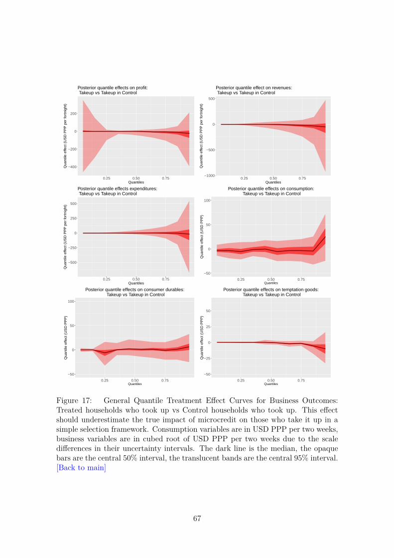
−400

−200

0

200

0.25 0.50 0.75Quantiles

Qua

ntile

effe

ct (

US

D P

PP

per

fort

nigh

t)

Posterior quantile effects on profit: Takeup vs Takeup in Control

−1000

−500

0

500

0.25 0.50 0.75Quantiles

Qua

ntile

effe

ct (

US

D P

PP

per

fort

nigh

t)

Posterior quantile effect on revenues: Takeup vs Takeup in Control

−500

−250

0

250

500

0.25 0.50 0.75Quantiles

Qua

ntile

effe

ct (

US

D P

PP

per

fort

nigh

t)

Posterior quantile effects expenditures: Takeup vs Takeup in Control

−50

0

50

100

0.25 0.50 0.75Quantiles

Qua

ntile

effe

ct (

US

D P

PP

)

Posterior quantile effects on consumption: Takeup vs Takeup in Control

−50

0

50

100

0.25 0.50 0.75Quantiles

Qua

ntile

effe

ct (

US

D P

PP

)

Posterior quantile effects on consumer durables: Takeup vs Takeup in Control

−50

−25

0

25

50

0.25 0.50 0.75Quantiles

Qua

ntile

effe

ct (

US

D P

PP

)

Posterior quantile effects on temptation goods: Takeup vs Takeup in Control

Figure 17: General Quantile Treatment Effect Curves for Business Outcomes:Treated households who took up vs Control households who took up. This effectshould underestimate the true impact of microcredit on those who take it up in asimple selection framework. Consumption variables are in USD PPP per two weeks,business variables are in cubed root of USD PPP per two weeks due to the scaledifferences in their uncertainty intervals. The dark line is the median, the opaquebars are the central 50% interval, the translucent bands are the central 95% interval.[Back to main]

67

Appendix E Tabular results

Table 7: Lender and Study Attributes by Country

Country Bosnia &Herzegovina Ethiopia India Mexico Mongolia Morocco The Philippines

StudyCitation

Augsburget al (2015)

Tarozziet al (2015)

Banerjeeet al (2015b)

Angelucciet al (2015)

Attanasioet al (2015)

Creponet al (2015)

Karlan andZinman (2011)

Treatment

Lend tomarginallyrejectedborrowers

Openbranches

Openbranches

Openbranches,promoteloans

Open branches,target likelyborrowers

Openbranches

Lend tomarginalapplicants

RandomizationLevel Individual Community Community Community Community Community Individual

Urban orRural? Both Rural Urban Both Rural Rural Urban

TargetWomen? No No Yes Yes Yes No No

MFI alreadyoperateslocally?

Yes No No No No No Yes

MicroloanLiabilityType

Individual Group Group Group Both Group Individual

Collateralized? Yes Yes No No Yes No No

Any otherMFIs

competing?Yes No Yes Yes Yes No Yes

HouseholdPanel? Yes No No Partial Yes Yes No

Interest Rate(Intendedon Average)

22% APR 12% APR 24% APR 100% APR 24% APR 13.5% APR 63% APR

SamplingFrame

MarginalApplicants

RandomSample

Householdswith at least1 womanage 18-55of stableresidence

Womenages 18-60who ownbusinessesor wish tostart them

Women whoregisteredinterestin loansand meteligibilitycriteria

RandomSampleplusLikely

Borrowers

MarginalApplicants

StudyDuration 14 months 36 months 40 months 16 months 19 months 24 months 36 months

Note: The construction of the interest rates here is different to the construction of Banerjee et al (2015a); they have taken themaximal interest rate, whereas I have taken the average of the intended range specified by the MFI. In practice the differences inthese constructions are numerically small. This table was also printed in Meager (2018) which used the same studies.[Back to main]

68

Excess Kurtosis in LogNormal distributions is the extent to which tail indicesare greater, and thus the extent to which the tails are heavier, than those of theGaussian. For a LogNormal parameterised as

LogNormal(y|µ, σ) = 1√2πσy

exp(−(log(y)− µ)2

2σ2

)

the excess kurtosis is

exp(4σ2) + 2 exp(3σ2) + 3 exp(2σ2)− 6.

I compute the kurtosis for the general control group based on the posterior meanvalues of µ and σ for this group in the tables below. The example in the text isobtained using µ2 and σc2.

Table 8: All General-Level Posterior Marginals for the LogNormal Profit Modelmean MCMC error sd 2.5% 25% 50% 75% 97.5% # effective draws R

µ1 3.200 0.008 0.732 1.722 2.784 3.200 3.615 4.698 9, 099 1.000µ2 3.843 0.007 0.818 2.225 3.356 3.845 4.324 5.496 15, 000 1.000τ1 0.094 0.001 0.094 -0.099 0.045 0.095 0.143 0.273 6, 719.600 1.001τ2 0.077 0.0005 0.042 -0.007 0.054 0.078 0.102 0.157 7, 566.232 1.000σµ1 1.659 0.008 0.654 0.867 1.227 1.514 1.923 3.302 7, 284.792 1.000σµ2 2.033 0.006 0.677 1.153 1.574 1.889 2.332 3.711 15, 000 1.000στ1 0.117 0.004 0.128 0.005 0.035 0.079 0.154 0.459 1, 090.338 1.003στ2 0.055 0.001 0.052 0.002 0.020 0.043 0.075 0.183 1, 323.050 1.004σc1 0.452 0.002 0.145 0.180 0.374 0.447 0.525 0.761 7, 205.404 1.000σc2 0.225 0.001 0.101 0.022 0.167 0.225 0.284 0.428 10, 278.910 1.000σt1 0.022 0.001 0.094 -0.162 -0.024 0.022 0.067 0.206 6, 128.028 1.001σt2 0.017 0.0003 0.029 -0.043 0.001 0.017 0.032 0.072 9, 321.264 1.000σσc

10.302 0.002 0.164 0.122 0.196 0.262 0.357 0.724 5, 126.273 1.001

σσc2

0.242 0.001 0.100 0.125 0.176 0.220 0.280 0.499 9, 328.806 1.000σσt

10.163 0.002 0.116 0.034 0.089 0.134 0.201 0.467 2, 860.338 1.001

σσt2

0.046 0.001 0.037 0.002 0.020 0.038 0.062 0.140 2, 034.778 1.002β11 -1.965 0.016 1.273 -4.525 -2.715 -1.958 -1.193 0.527 6, 334.358 1.000β12 0.025 0.001 0.114 -0.187 -0.035 0.019 0.080 0.265 6, 957.068 1.001β21 0.390 0.010 0.906 -1.379 -0.168 0.367 0.918 2.255 7, 964.995 1.000β22 -0.067 0.001 0.104 -0.279 -0.124 -0.066 -0.012 0.143 8, 309.348 1.001σβ11 2.767 0.017 1.277 0.770 1.959 2.560 3.346 5.904 5, 636.316 1.000σβ12 0.128 0.002 0.125 0.005 0.047 0.096 0.168 0.446 5, 901.720 1.001σβ21 1.603 0.014 0.902 0.130 0.990 1.532 2.093 3.672 3, 987.814 1.002σβ22 0.146 0.002 0.114 0.007 0.065 0.124 0.197 0.432 5, 234.755 1.001σβ31 1.450 0.014 0.889 0.091 0.815 1.381 1.942 3.493 3, 896.658 1.001σβ32 0.117 0.002 0.109 0.004 0.041 0.089 0.161 0.390 5, 085.964 1.002

Note: The β3 parameters are normalized to be zero at the general level as required formultinomial logit models. The site-specific effects still have variation around this zeroanchor as reported.

69

Table 9: All General-Level Posterior Marginals for the LogNormal Revenues Modelmean MCMC error sd 2.5% 25% 50% 75% 97.5% # effective draws R

µ1 4.472 0.007 0.873 2.733 3.959 4.479 4.992 6.193 15, 000 1.000τ1 0.083 0.001 0.068 -0.058 0.045 0.086 0.123 0.211 10, 482.840 1.000σµ1 2.181 0.007 0.718 1.258 1.693 2.030 2.496 3.982 10, 285.460 1.000στ1 ] 0.140 0.001 0.080 0.039 0.089 0.124 0.171 0.329 5, 189.630 1.001σc1 0.213 0.001 0.136 -0.063 0.134 0.214 0.292 0.485 11, 190.950 1.000σt1 -0.010 0.0003 0.031 -0.071 -0.028 -0.011 0.008 0.052 9, 554.774 1.000σσc

10.331 0.001 0.135 0.171 0.241 0.301 0.383 0.668 8, 452.406 1.001

σσt1

0.062 0.0004 0.033 0.020 0.040 0.055 0.075 0.146 6, 447.524 1.000β11 0.011 0.008 0.734 -1.464 -0.424 -0.004 0.443 1.521 8, 107.184 1.001β12 -0.063 0.001 0.081 -0.235 -0.101 -0.058 -0.020 0.091 6, 772.048 1.001σβ11 1.209 0.010 0.760 0.064 0.637 1.164 1.645 2.912 5, 305.339 1.001σβ12 0.095 0.001 0.091 0.003 0.032 0.071 0.129 0.327 5, 418.020 1.001σβ21 1.192 0.010 0.762 0.062 0.615 1.147 1.631 2.894 5, 341.343 1.001σβ22 0.095 0.001 0.091 0.003 0.033 0.071 0.130 0.328 5, 944.329 1.000

Note: The β3 parameters are normalized to be zero at the general level as required formultinomial logit models. The site-specific effects still have variation around this zeroanchor as reported. Note also that σt1 can be negative as this is the effect specified onthe exponential level.

Table 10: All General-Level Posterior Marginals for the LogNormal ExpendituresModel

mean MCMC error sd 2.5% 25% 50% 75% 97.5% # effective draws R

µ1 4.042 0.006 0.733 2.563 3.593 4.047 4.483 5.528 15, 000 1.000τ1 0.103 0.001 0.048 0.005 0.076 0.104 0.132 0.198 8, 840.624 1.000σµ1 1.867 0.005 0.624 1.061 1.449 1.735 2.135 3.449 15, 000 1.001στ1 0.078 0.001 0.060 0.004 0.035 0.067 0.106 0.226 1, 919.668 1.002σc1 0.303 0.002 0.171 -0.037 0.204 0.304 0.401 0.649 8, 974.738 1.001σt1 -0.008 0.001 0.045 -0.092 -0.033 -0.009 0.016 0.082 5, 069.866 1.000σσc

10.421 0.002 0.171 0.218 0.309 0.382 0.489 0.845 8, 374.404 1.001

σσt1

0.094 0.001 0.051 0.035 0.062 0.082 0.111 0.217 3, 164.881 1.001β11 0.234 0.009 0.694 -1.177 -0.180 0.233 0.653 1.645 6, 027.909 1.000β12 -0.116 0.001 0.117 -0.349 -0.177 -0.114 -0.053 0.112 7, 262.210 1.000σβ11 1.148 0.011 0.712 0.062 0.613 1.102 1.565 2.729 4, 414.652 1.001σβ12 0.157 0.002 0.125 0.007 0.071 0.132 0.209 0.465 5, 601.528 1.000σβ21 1.119 0.011 0.707 0.056 0.580 1.075 1.535 2.714 4, 076.193 1.001σβ22 0.159 0.002 0.124 0.007 0.074 0.136 0.212 0.463 5, 427.373 1.001

Note: The β3 parameters are normalized to be zero at the general level as required formultinomial logit models. The site-specific effects still have variation around this zeroanchor as reported.Note also that σt1 can be negative as this is the effect specified on theexponential level.

70

For visual ease, the figures below graph the treatment effects and posterior predicted effects for each of thedimensions of change permitted in the model.

Expenditure (Spike vs Positive)

Profit (Negative vs Positive)

Profit (Spike vs Positive)

Revenue (Spike vs Positive)

−0.50 −0.25 0.00 0.25 0.50Posterior mean, 50% interval (box), and 95% interval (line)

for each exponentiated multiplicative Treatment Effect

BHM Posterior Full Pooling Model

Category Allocation Effects (Reference category: positive tail) Posterior distribution of treatment effects on Logit Scale

Figure 18: Posterior distributions for the logit treatment effects (πj) on categoryassignment. These treatment effects are specified as an exponentiated multiplicativefactor on the control group proportion of households in the category: if πj = 0 theeffect is zero, if πj < 0 the treatment increases the proportion of households in thepositive tail relative to other categories. [Back to main]

71

Expenditure

Profit (Negative)

Profit (Positive)

Revenue

−0.50 −0.25 0.00 0.25 0.50Posterior mean, 50% interval (box), and 95% interval (line)

for each exponentiated multiplicative Treatment Effect

BHM Posterior Full Pooling Model

Logmean Parameter Effects (exponentiated multiplicative) Posterior distribution of treatment effects

Expenditure

Profit (Negative)

Profit (Positive)

Revenue

−0.50 −0.25 0.00 0.25 0.50Posterior mean, 50% interval (box), and 95% interval (line)

for each exponentiated multiplicative Treatment Effect

BHM Posterior Full Pooling Model

Logvariance Parameter Effects (exponentiated multiplicative) Posterior distribution of treatment effects

Figure 19: Posterior distributions for the location treatment effects (τj) and thescale treatment effects (σtj). [Back to main]

72

Expenditure (Spike vs Positive)

Profit (Negative vs Positive)

Profit (Spike vs Positive)

Revenue (Spike vs Positive)

−0.8 −0.4 0.0 0.4 0.8Posterior mean, 50% interval (box), and 95% interval (line)

for each logit scale treatment effect

BHM Posterior Full Pooling Model

Category Allocation Effects on Logit Scale Posterior Predicted treatment effect

Expenditure

Profit (Negative)

Profit (Positive)

Revenue

−0.8 −0.4 0.0 0.4 0.8Posterior mean, 50% interval (box), and 95% interval (line)

for each exponentiated multiplicative Treatment Effect

BHM Posterior Full Pooling Model

Logmean Tail Effects (exponentiated multiplicative) Posterior predicted treatment effect

Expenditure

Profit (Negative)

Profit (Positive)

Revenue

−0.8 −0.4 0.0 0.4 0.8Posterior mean, 50% interval (box), and 95% interval (line)

for each exponentiated multiplicative Treatment Effect

BHM Posterior Full Pooling Model

Logvariance Effects (exponentiated multiplicative) Posterior predicted treatment effect

Figure 20: Posterior predicted distributions for the logit treatment effects on cate-gory assignment and tail shape effects. [Back to main]

73

References

[1] Abadie, A., Angrist, J. and Imbens, G. (2002) "Instrumental Variables estimatesof the effect of subsidised training on quantiles of trainee earnings." Economet-rica, 70(1) 91-117.

[2] Acemoglu, D., and Robinson, J. A. (2008). "Persistence of power, elites, andinstitutions." American Economic Review, 98(1), 267-93.

[3] Acemoglu, D. Suresh Naidu, Pascual Restrepo, James A. Robinson, (2015)"Chapter 21 - Democracy, Redistribution, and Inequality", The Handbook ofIncome Distribution, Editor(s): Anthony B. Atkinson, François Bourguignon,Elsevier, Volume 2, 2015, Pages 1885-1966.

[4] Acharya, A., Blackwell, M., & Sen, M. (2016). "Explaining causal findings with-out bias: Detecting and assessing direct effects." American Political ScienceReview, 110(3), 512-529.

[5] Ahmad, M. M. (2003). "Distant voices: the views of the field workers of NGOsin Bangladesh on microcredit." The Geographical Journal, 169(1), 65-74.

[6] Albert, J and Siddhartha Chib (1997) "Conditionally Independent HierarchicalModels", Journal of the American Statistical Association, September 1997, Vol.92, No. 439

[7] Allcott, H. (2015). "Site Selection Bias in Program Evaluation." The QuarterlyJournal of Economics, 130(3), 1117-1165.

[8] Allen, T. (2014). "Information frictions in trade". Econometrica, 82(6), 2041-2083.

[9] Andrews, I., and Maximilian Kasy (2017) "Identification of and Correctionfor Publication Bias", NBER Working Paper No. 23298, March 2017, RevisedNovember 2017

[10] Andrews, I., and Oster, E. (2017). "Weighting for External Validity" (No.w23826). National Bureau of Economic Research.

[11] Angelucci, M., Dean Karlan, and Jonathan Zinman. 2015. "Microcredit Im-pacts: Evidence from a Randomized Microcredit Program Placement Exper-iment by Compartamos Banco." American Economic Journal: Applied Eco-nomics, 7(1): 151-82.

[12] Angrist, J. D. (2004). "Treatment effect heterogeneity in theory and practice".The Economic Journal, 114(494), C52-C83.

[13] Angrist, J., and Ivan Fernandez-Val . (2010). "Extrapolate-ing: External valid-ity and overidentification in the late framework" (No. w16566). National Bureauof Economic Research.

74

[14] Athey, S., and Guido Imbens. "Recursive partitioning for heterogeneous causaleffects." Proceedings of the National Academy of Sciences 113, no. 27 (2016):7353-7360.

[15] Attanasio, O., Britta Augsburg, Ralph De Haas, Emla Fitzsimons, and HeikeHarmgart. (2015). "The Impacts of Microfinance: Evidence from Joint-LiabilityLending in Mongolia." American Economic Journal: Applied Economics, 7(1):90-122.

[16] Augsburg, B., Ralph De Haas, Heike Harmgart, and Costas Meghir. 2015. "TheImpacts of Microcredit: Evidence from Bosnia and Herzegovina." AmericanEconomic Journal: Applied Economics, 7(1): 183-203.

[17] Autor, D. H., Katz, L. F., and Krueger, A. B. (1998). "Computing inequal-ity: have computers changed the labor market?". The Quarterly Journal ofEconomics, 113(4), 1169-1213.

[18] Autor, D. H., Dorn, D., Hanson, G. H., and Song, J. (2014). "Trade adjustment:Worker-level evidence". The Quarterly Journal of Economics, 129(4), 1799-1860.

[19] Bandiera, O, G. Fischer, A. Prat and E.Ytsma (2017) "DoWomen Respond Lessto Performance Pay? Building Evidence from Multiple Experiments" WorkingPaper Version October 2017

[20] Banerjee, A. (2013). "Microcredit under the microscope: what have we learnedin the past two decades, and what do we need to know?". Annu. Rev. Econ.,5(1), 487-519.

[21] Banerjee, A., Dean Karlan, and Jonathan Zinman. (2015a). "Six RandomizedEvaluations of Microcredit: Introduction and Further Steps." American Eco-nomic Journal: Applied Economics, 7(1): 1-21.

[22] Banerjee, A., Esther Duflo, Rachel Glennerster, and Cynthia Kinnan. (2015b)."The Miracle of Microfinance? Evidence from a Randomized Evaluation."American Economic Journal: Applied Economics, 7(1): 22-53.

[23] Banerjee, Abhijit, Esther Duflo, Nathanael Goldberg, Dean Karlan, RobertOsei, William Pariente, Jeremy Shapiro, Bram Thuysbaert, and ChristopherUdry. (2015c) "A multifaceted program causes lasting progress for the verypoor: Evidence from six countries." Science 348, no. 6236 (2015): 1260799.

[24] Banerjee, A., & Mullainathan, S. (2010). The shape of temptation: Implicationsfor the economic lives of the poor (No. w15973). National Bureau of EconomicResearch. NBER Working Paper No. 15973, Issued in May 2010

[25] Bazzi, S. (2016) "Wealth Heterogeneity and the Income Elasticity of Migration"American Economic Journal: Applied, 9(2), 219-55.

[26] Bell, A., Raj Chetty, Xavier Jaravel, Neviana Petkova, and John Van Reenen(2017) "Who Becomes an Inventor in America? The Importance of Exposureto Innovation" NBER Working Paper No. 24062, December 2017

75

[27] Bertanha, M., and Guido Imbens (2014). "External validity in fuzzy regressiondiscontinuity designs" (No. w20773). National Bureau of Economic Research.

[28] Betancourt, M. J., and Mark Girolami. (2013). "Hamiltonian Monte Carlo forhierarchical models." arXiv preprint arXiv:1312.0906

[29] Bisbee, J., Rajeev Dehejia, Cristian Pop-Eleches, Cyrus Samii. "Local Instru-ments, Global Extrapolation: External Validity of the Labor Supply". Journalof Labor Economics, Volume 35, Number S1, pp. S99-S147.

[30] Borusyak, K., & Jaravel, X. (2018). "The Distributional Effects of Trade: The-ory and Evidence from the United States." Working Paper Version.

[31] Breza, E., & Kinnan, C. (2018). "Measuring the equilibrium impacts of credit:Evidence from the Indian microfinance crisis" (No. w24329). National Bureauof Economic Research

[32] Breza, E. (2012). "Peer effects and loan repayment: Evidence from the krishnadefault crisis." Working paper.

[33] Bryan, G., Chowdhury, S., & Mobarak, A. M. (2014). "Underinvestment in aprofitable technology: The case of seasonal migration in Bangladesh." Econo-metrica, 82(5), 1671-1748.

[34] Castellacci, Giuseppe, (2012) "A Formula for the Quantiles of Mix-tures of Distributions with Disjoint Supports". Available at SSRN:http://ssrn.com/abstract=2055022 or http://dx.doi.org/10.2139/ssrn.2055022

[35] Chernozhukov, V., Ivan Fernandez-Val, and Alfred Galichon.(2010) "Quantileand probability curves without crossing." Econometrica 78.3 1093-1125.

[36] Chetty, R., Hendren, N., and Katz, L. F. (2016). "The effects of exposure to bet-ter neighborhoods on children: New evidence from the Moving to Opportunityexperiment." American Economic Review, 106(4), 855-902.

[37] Chetty, R., and Hendren, N. (2018). The impacts of neighborhoods on inter-generational mobility I: Childhood exposure effects. The Quarterly Journal ofEconomics, 133(3), 1107-1162.

[38] Chetty, R., Friedman, J. N., & Rockoff, J. E. (2014). Measuring the impactsof teachers I: Evaluating bias in teacher value-added estimates. American Eco-nomic Review, 104(9), 2593-2632

[39] Chib, S., & Greenberg, E. (1995). Hierarchical analysis of SUR models with ex-tensions to correlated serial errors and time-varying parameter models. Journalof Econometrics, 68(2), 339-360.

[40] Chung, Y., Gelman, A., Rabe-Hesketh, S., Liu, J., & Dorie, V. (2015). Weaklyinformative prior for point estimation of covariance matrices in hierarchicalmodels. Journal of Educational and Behavioral Statistics, 40(2), 136-157.

76

[41] Chung, Y., Rabe-Hesketh, S., Dorie, V., Gelman, A., & Liu, J. (2013). A non-degenerate penalized likelihood estimator for variance parameters in multilevelmodels. Psychometrika, 78(4), 685-709.

[42] Crepon, Bruno, Florencia Devoto, Esther Duflo, and William Pariente. 2015."Estimating the Impact of Microcredit on Those Who Take It Up: Evidencefrom a Randomized Experiment in Morocco." American Economic Journal: Ap-plied Economics, 7(1): 123-50.

[43] Dehejia, R., Pop-Eleches, C., and Samii, C. (2015). "From Local to Global:External Validity in a Fertility Natural Experiment" (No. w21459). NationalBureau of Economic Research.

[44] Dehejia, R. H. (2003). "Was there a Riverside miracle? A hierarchical frameworkfor evaluating programs with grouped data." Journal of Business & EconomicStatistics, 21(1), 1-11.

[45] Diaconis, Persi (1977) "Finite Forms of De Finetti’s Theorem on Exchangeabil-ity" Synthese, 36, 1977, 271-281

[46] Duflo, E., Pascaline Dupas and Michael Kremer, (2017) "The Impact of FreeSecondary Education: Experimental Evidence from Ghana" Working Paper,2017

[47] Duvendack, M., Richard Palmer-Jones & Jos Vaessen (2014) "Meta-analysis ofthe impact of microcredit on women’s control over household decisions: method-ological issues and substantive findings", Journal of Development Effectiveness,6:2, 73-96

[48] Efron, B., and Morris, C. (1975). "Data analysis using Stein’s estimator andits generalizations". Journal of the American Statistical Association, 70(350),311-319.

[49] Fama, Eugene F., (1963), "Mandelbrot and the Sta-ble Paretian Hypothesis", The Journal of Business, 36,http://EconPapers.repec.org/RePEc:ucp:jnlbus:v:36:y:1963:p:420.

[50] Fama, Eugene F. (1965) "Portfolio Analysis In A Stable Paretian Market."Management Science 11.3 : 404-419. Business Source Complete. Web. 10 Aug.2016.

[51] Fogli, A and Guerrieri, V. (2017). "The End of the American Dream? Inequalityand Segregation in US cities." In 2017 Meeting Papers (No. 1309). Society forEconomic Dynamics.

[52] Gabaix, X. (2008) "Power Laws in Economics and Finance" NBERWorking Paper No. 14299, accessed online August 12th 2016,http://www.nber.org/papers/w14299

77

[53] Gechter, M. (2015). "Generalizing the Results from Social Experiments: Theoryand Evidence from Mexico and India". manuscript, Pennsylvania State Univer-sity.

[54] Gelman, A., and Carlin, J. (2014). "Beyond power calculations: Assessing typeS (sign) and type M (magnitude) errors." Perspectives on Psychological Science,9(6), 641-651.

[55] Gelman, A., John B. Carlin, Hal S. Stern and Donald B. Rubin (2004) "BayesianData Analysis: Second Edition", Taylor & Francis

[56] Gelman, A., Jakulin, A., Pittau, M. G., & Su, Y. S. (2008). "A weakly infor-mative default prior distribution for logistic and other regression models". TheAnnals of Applied Statistics, 2(4), 1360-1383.

[57] Gelman, A.,& Jennifer Hill (2007) "Data anlysis using regression and multilevelheirarchical models” Cambridge Academic Press.

[58] Gelman, A., and Pardoe, I. (2006). "Bayesian measures of explained varianceand pooling in multilevel (hierarchical) models". Technometrics, 48(2), 241-251.

[59] Gelman, A., and Rubin, D. B. (1992)." Inference from iterative simulation usingmultiple sequences". Statistical science, 457-472.

[60] Giordano, R., Tamara Broderick, Rachael Meager, Jonathan Huggins, MichaelJordan (2016) "Fast robustness quantification with variational Bayes" ICMLWorkshop on Data4Good: Machine Learning in Social Good Applications, NewYork, NY, arXiv:1606.07153

[61] Hartley, H. O., and Rao, J. N. (1967). "Maximum-likelihood estimation for themixed analysis of variance model". Biometrika, 54(1-2), 93-108.

[62] Hussam, R., Rigol, N., and Roth, B. (2017). "Targeting high ability en-trepreneurs using community information: Mechanism design in the field."Working Paper, Nov 2017

[63] Hastie, T., Tibshirani, R., and Friedman, J. (2009). "The elements of statisticallearning". Second Edition. Springer Series in Statistics.

[64] He, X. (1997). "Quantile Curves without Crossing". The American Statistician,51(2), 186-192. doi:10.2307/2685417

[65] Heckman, J., Tobias, J. L., and Vytlacil, E. (2001). "Four parameters of interestin the evaluation of social programs". Southern Economic Journal, 211-223.

[66] Higgins, J. P. and Sally Green (Eds) (2011) "Cochrane handbook for systematicreviews of interventions" (Version 5.1.0). Chichester: Wiley-Blackwell.

[67] Hlavac, Marek (2014). "stargazer: LaTeX/HTML code and ASCII text for well-formatted regression and summary statistics tables". R package version 5.1.http://CRAN.R-project.org/package=stargazer

78

[68] Hoffman, M. D.,& Gelman, A. (2014)."The no-U-turn sampler: Adaptivelysetting path lengths in Hamiltonian Monte Carlo". The Journal of MachineLearning Research, 15(1), 1593-1623.

[69] Hsiang, S. M., Burke, M., and Miguel, E. (2013). "Quantifying the influence ofclimate on human conflict." Science, 341(6151), 1235367.

[70] Hull, P. (2018). Estimating hospital quality with quasi-experimental data.Chicago Working Paper.

[71] Imbens, G. W., & Rubin, D. B. (2015). "Causal inference in statistics, social,and biomedical sciences." Cambridge University Press.

[72] Imbens, G.W and Rubin D.B (1997) "Estimating outcome distributions forcompliers in instrumental variables models" The Review of Economic Studies,64(4), 555-574

[73] James, William, and Charles Stein. (1961) "Estimation with Quadratic Loss."In Proceedings of the Fourth Berkeley Symposium on Mathematical Statisticsand Probability, 1:361?379, 1961.

[74] Jones, C. I. (2015). "Pareto and Piketty: The macroeconomics of top incomeand wealth inequality." The Journal of Economic Perspectives, 29(1), 29-46.

[75] Kaboski, J. P., and Townsend, R. M. (2011). "A structural evaluation of alarge?scale quasi?experimental microfinance initiative". Econometrica, 79(5),1357-1406.

[76] Karlan, D., and Zinman, J. (2009). "Observing unobservables: Identifying infor-mation asymmetries with a consumer credit field experiment." Econometrica,77(6), 1993-2008.

[77] Karlan, Dean and Jonathan Zinman (2011) "Microcredit in Theory and Prac-tice: Using Randomized Credit Scoring for Impact Evaluation", Science 10 June2011: 1278-1284

[78] Katz, L. F., Kling, J. R., & Liebman, J. B. (2001). "Moving to opportunityin Boston: Early results of a randomized mobility experiment." The QuarterlyJournal of Economics, 116(2), 607-654.

[79] Kinnan, C., & Townsend, R. (2012). Kinship and financial networks, formalfinancial access, and risk reduction. American Economic Review, 102(3), 289-93.

[80] Koenker R and Gilbert Bassett, Jr. (1978) "Regression Quantiles" Economet-rica, Vol. 46, No. 1. (Jan., 1978), pp. 33-50.

[81] Koenker, R, and Kevin F. Hallock. (2001). "Quantile Regression." Journal ofEconomic Perspectives, 15(4): 143-156

79

[82] Koenker, R (2005) "Quantile Regression", Econometric Society Monographs No.38, Cambridge University Press 2005

[83] Koenker, R, (2011) "Additive models for quantile regression: Model selectionand confidence bandaids" Brazilian Journal of Probability and Statistics, 2011,Vol. 25, No. 3, 239-262

[84] Leon, A. C., and Heo, M. (2009). "Sample Sizes Required to Detect Interactionsbetween Two Binary Fixed-Effects in a Mixed-Effects Linear Regression Model."Computational Statistics & Data Analysis, 53(3), 603?608.

[85] Machado, J.A.F, and J. M. C. Santos Silva (2005) "Quantiles for Counts" Jour-nal Of The American Statistical Association Vol. 100 , Iss. 472

[86] McCulloch, Charles and Neuhaus, John M. "Misspecifying the Shape of a Ran-dom Effects Distribution: Why Getting It Wrong May Not Matter". Statist.Sci. 26 (2011), no. 3, 388–402.

[87] McKenzie, D. (2012). "Beyond baseline and follow-up: The case for more T inexperiments." Journal of development Economics, 99(2), 210-221.

[88] Meager, R. (2018). "Understanding the Impact of Microcredit Expansions: ABayesian Hierarchical Analysis of 7 Randomised Experiments." Accepted in theAmerican Economics Journal: Applied, January 2018

[89] Microfinance Barometer (2017) "Microfinance Barometer 8th Edition: Is Mi-crofinance Still Working?", Convergences, France, www.convergences.org, 2017

[90] Microfinance Focus (2011) "Six Microfinance Crises the sector does notwant to remember." http://www.microfinancefocus.com/6-microfinance-crises-sector-does-not-want-remember

[91] Morduch, J. (1999). "The microfinance promise." Journal of economic literature,37(4), 1569-1614.

[92] Mosteller (1946) "On Some Useful "Inefficient" Statistics" The Annals of Math-ematical Statistics, Vol. 17, No. 4. (Dec., 1946), pp. 377-408

[93] Pancost, A. (2016) "Do Financial Factors Drive Aggregate Productivity? Ev-idence from Indian Manufacturing Establishments" Working Paper, accessedonline August 2016

[94] Piketty, T. (2015). About capital in the twenty-first century. American Eco-nomic Review, 105(5), 48-53.

[95] Pritchett, Lant & J. Sandefur (2015) "Learning from Experiments when ContextMatters" American Economic Association 2015 Preview Papers, accessed onlineFebruary 2015

[96] Reich, B. J., Fuentes, M., & Dunson, D. B. (2011). Bayesian spatial quantileregression. Journal of the American Statistical Association, 106(493), 6-20.

80

[97] Roodman, D. (2012). "Due diligence: An impertinent inquiry into microfi-nance". CGD Books.

[98] Roy, A. D. (1950). "The distribution of earnings and of individual output." TheEconomic Journal, 60(239), 489-505.

[99] Rubin, D. B. (1981). "Estimation in parallel randomized experiments. Journalof Educational and Behavioral Statistics", 6(4), 377-401.

[100] Rubin, H. (1950). "Note on random coefficients". Statistical inference in dy-namic economic models, 419-421.

[101] Schicks, J. (2013). "From a supply gap to a demand gap? The risk and con-sequences of over-indebting the underbanked." In Microfinance in DevelopingCountries (pp. 152-177). Palgrave Macmillan, London.

[102] Stan Development Team (2017) "Stan Modeling Language: User’s Guide andReference Manual." Version 2.17.0.

[103] Stiglitz, J. E., and Weiss, A. (1981). "Credit rationing in markets with imper-fect information". The American economic review, 71(3), 393-410.

[104] Stein, C. (1956) "Inadmissibility of the usual estimator for the mean of a multi-variate normal distribution," Proceedings of the Third Berkeley Symposium onMathematical Statistics and Probability, Berkeley and Los Angeles, Universityof California Press, 1956, Vol. 1, pp. 197-206.

[105] Tarozzi, Alessandro, Jaikishan Desai, and Kristin Johnson. (2015). "The Im-pacts of Microcredit: Evidence from Ethiopia." American Economic Journal:Applied Economics, 7(1): 54-89.

[106] Townsend,R.M. (2018) "Townsend Thai Project Household Annual Resurvey,2017 (Rural)", https://doi.org/10.7910/DVN/UW4VKE, Harvard Dataverse,V1

[107] Vivalt, E. (2016) "How much can we generalise from impact evaluations?"Working Paper, NYU

[108] Van der Vaart, A.W. (1998) "Asymptotic Statistics", Cambridge Series in Sta-tistical and Probabilistic Mathematics, Cambridge University Press

[109] Wald, A. (1947). "Foundations of a general theory of sequential decision func-tions". Econometrica, Journal of the Econometric Society, 279-313.

[110] Wickham, H. (2009) “ggplot2: elegant graphics for data analysis”. SpringerNew York, 2009.

[111] Yunus, M, (2006) "Nobel Lecture", Oslo, December 10, 2006.

81