Detecting ecological responses to flow variation usingBayesian hierarchical models

J . ANGUS WEBB*, MICHAEL J. STEWARDSON† AND WAYNE M. KOSTER ‡

*Department of Resource Management and Geography, and the eWater CRC, University of Melbourne, Carlton, Vic., Australia†Department of Civil and Environmental Engineering, and the eWater CRC, University of Melbourne, Parkville, Vic., Australia‡Department of Sustainability and Environment, Arthur Rylah Institute for Environmental Research, Heidelberg, Vic., Australia

SUMMARY

1. Inferring effects of environmental flows is difficult with standard statistical approaches

because flow-delivery programs are characterised by weak experimental design, and

monitoring programs often have insufficient replication to detect ecologically significant

effects. Bayesian hierarchical approaches may be more suited to the task, as they are more

flexible and allow data from multiple non-replicate sampling units (e.g. rivers) to be

combined, increasing inferential strength.

2. We assessed the utility of Bayesian hierarchical models for detecting ecological effects of

flow variation by conducting both hierarchical and non-hierarchical analyses on two

environmental endpoints. We analysed effects of discharge on salinity in the Wimmera

and Glenelg rivers (Victoria, Australia) using a linear regression with autocorrelation

terms, and on Australian smelt in the Thomson River (Victoria, Australia) using a multi-

level covariate model. These analyses test some of the hypotheses upon which

environmental flow recommendations have been made for these rivers.

3. Discharge was correlated with reduced salinity at six of 10 sites, but with increased

salinity at two others. The results were very similar for hierarchical and non-hierarchical

models. For Australian smelt, the hierarchical model found some evidence that excess

summer discharge reduces abundance in all river reaches, but the non-hierarchical model

was able to detect this response in only one reach.

4. The results highlight the power and flexibility of Bayesian analysis. Neither of the

models fitted would have been amenable to more widely used statistical approaches, and

it is unlikely that we would have detected responses to flow variation in these data had we

been using such techniques. Hierarchical models can greatly improve inferential strength

in the data-poor situations that are common in ecological monitoring, and will be able to be

used to assess the effectiveness of environmental flow programs and maximise the benefits

of large-scale environmental flow monitoring programs.

Keywords: assessment, Bayesian hierarchical modelling, borrowing strength, environmental flows,monitoring

Introduction

The provision of environmental flows is a critical part

of maintaining ecological integrity in regulated river

systems (Poff et al., 1997; Tharme, 2003; Arthington

et al., 2006). However, providing flows to the envi-

ronment may be economically costly due to foregone

consumptive benefits (e.g. agriculture; Qureshi et al.,

Correspondence: J. Angus Webb, Department of Resource Management and Geography, University of Melbourne, 221 Bouverie St,

Carlton, 3010 Vic., Australia. E-mail: angus.webb@unimelb.edu.au

Freshwater Biology (2010) 55, 108–126 doi:10.1111/j.1365-2427.2009.02205.x

108 � 2009 Blackwell Publishing Ltd

2007), and also socially divisive due to the inevitable

self-interest of consumptive and environmental water

users (Schofield & Burt, 2003). Given these tensions, it

is important to demonstrate the ecological benefits of

environmental flows, particularly in regions with

fully- or over-allocated water resources such as

south-east Australia. To date, relatively few published

examples demonstrate the environmental effects of

flow enhancement (Siebentritt, Ganf & Walker, 2004;

Hancock & Boulton, 2005; Chester & Norris, 2006;

Hou et al., 2007; Lind, Robson & Mitchell, 2007), and

all of these studies have been performed opportunis-

tically around individual flow events and ⁄or rela-

tively small areas. There is a lack of wide-scale and ⁄or

generalised findings concerning the effects of envi-

ronmental flows. Why might this be the case?

Most environmental flow-delivery programs are

characterised by weak experimental design in terms

of replication, spatial and temporal confounding and

nature of the treatment (i.e. flow). These issues make it

difficult to use common statistical methods to infer the

effects of changes in flow. The provision of environ-

mental flows is usually a patchy phenomenon, both in

space and time. Putting aside the scenario of single

specific flow events delivered to defined geographic

areas referred to above, it is often difficult or impos-

sible to identify the point in time separating ‘before’

from ‘after’, or to positively identify sites as ‘impact’

or ‘control’. Moreover, the level of flow enhancement

is likely to be continuous, rather than categorical.

Thus, while a BACI (before-after control-impact;

Underwood, 1997) or related design is generally seen

as the best way of detecting impacts (including

beneficial impacts) in river systems (Downes et al.,

2002), such analyses are rarely possible for assessing

the effects of environmental flows.

Establishing monitoring programs with sufficient

replication to give a high level of statistical power is

another issue. Limited monitoring budgets may make

it impossible to design programs with sufficient

replication and may mean that monitoring is ‘piggy-

backed’ upon existing programs, potentially exacer-

bating the experimental design problems outlined

above. Furthermore, the heterogeneous and intercon-

nected nature of river systems make it difficult to

assign sufficient replicates that meet the assumptions

of standard statistical models (i.e. independent,

differing minimally apart from the treatment; Downes

et al., 2002).

The problems outlined with factorial designs

imply that a gradient-based approach to assessing

the effects of environmental flows might be more

appropriate. Such a framework is more flexible and

can better cope with the variable nature of flow

delivery by describing continuous relationships

between flow and environmental response. This

approach capitalises on the fact that the magnitude

of environmental flows delivered is likely to be

continuous rather than categorical. Moreover, the

relationships developed may find use in predictive

models that can be used to refine flow allocations

(e.g. Arthington et al., 2006). However, the replication

problem described for factorial designs still applies

to gradient-based approaches. It may be impossible,

either financially or physically, to sample with

sufficient replication of directly comparable sites to

detect statistically significant relationships between

flow and response.

Bayesian statistical approaches may be able to

mitigate some of these difficulties. Bayesian modelling

is inherently flexible (Clark, 2005). This flexibility

means that models are formulated to conform to the

requirements of the data, whereas standard statistical

approaches must force the data to comply with the

requirements of a relatively small number of model

types (McCarthy, 2007). Employing a hierarchical

model within a Bayesian framework may also miti-

gate the replication problems outlined above. Bayes-

ian hierarchical models are finding increasing use in

ecology (e.g. Ver Hoef & Frost, 2003; Wikle, 2003;

Martin et al., 2005; Webb & King, 2009). They allow the

construction of far more complex models than is

possible with traditional statistical approaches, and

are particularly suited to dealing with the complex-

ities of spatiotemporal aspects in ecology (Clark,

2005). To explain why a Bayesian hierarchical

approach may reduce the problems associated with

insufficient replication requires a brief explanation of

Bayesian theory.

Bayesian modelling revolves around Bayes’ Theo-

rem (Bayes, 1763; reprinted in Barnard, 1958). In

simple terms, the theorem provides a mathematical

expression for updating our estimate of some statis-

tical parameter, say h, given a set of observations,

y. The theorem states that

PðhjyÞ / PðyjhÞ � PðhÞ ð1Þ

Bayesian modelling for detecting effects of flow 109

� 2009 Blackwell Publishing Ltd, Freshwater Biology, 55, 108–126

In words, the ‘posterior’ probability distribution (left-

hand term) of a parameter (h) given (signified by ‘|’)

the data at hand (y) is proportional to the product of

the ‘likelihood function’ (the probability of y given h),

and the prior probability distribution for h (our

estimate of likely values of h before collecting any

data) (Gelman et al., 2004). The presence of the prior

distribution is the source of much controversy

concerning Bayesian modelling, as it can be seen as

making the analyses overly subjective (McCarthy,

2007). However, when little information exists con-

cerning a parameter, one is able to assign a so-called

minimally informative or ‘vague’ prior distribution.

Such a prior has only slight effects on the posterior

distribution, and indeed a familiar analysis (e.g.

ANOVAANOVA or regression) carried out using Bayesian

methods and vague priors for the parameters (e.g.

regression slope) will usually come up with a similar

distribution for that parameter as the almost univer-

sally used ‘frequentist’ (see McCarthy, 2007 for an

explanation of frequentism) model.

Hierarchical modelling can be done within a

frequentist framework (Lele, Dennis & Lutscher,

2007), but in this paper we concentrate on the

Bayesian version. A Bayesian hierarchical model

treats multiple sampling units (e.g. sites or groups

of sites) as ‘exchangeable’. This means that the

parameter values (e.g. mean abundance) that

describe each unit are expected to be similar (but

not necessarily the same). An identical assumption is

made in every analysis (frequentist or Bayesian), as

replicates within sampling units are assumed to be

independent and identically distributed. Exchange-

ability of parameter values is achieved by assigning a

prior distribution in which the prior parameter

values (e.g. site mean) for all sampling units are

viewed as a sample from a common distribution. The

parameters (e.g. mean across all sites) of this distri-

bution are known as ‘hyperparameters’. Mathemat-

ically, a simple hierarchical relationship might be

expressed as,

yijjhj � Normalðhj; r2Þ

hjjl � Normalðl; g2Þð2Þ

where data (y) are collected within sampling units and

h is the mean of the distribution of data within each

sampling unit. The values for h are themselves drawn

from a larger scale distribution characterised by the

hyperparameters l and g2.

This approach contrasts with a non-hierarchical

version, where we would separately assign a vague

prior distribution to h for each unit. In the hierarchical

model, the entire set of observed data can be used to

estimate the values of the hyperparameters, even

though those values are not observed (Gelman et al.,

2004). For both model types, the data within each

sampling unit are then used to update the prior for

that unit. Thus, the only difference between the two

model types is the presence of the common distribu-

tion for prior parameter values in the hierarchical

model. Because the hyperparameters are unknown,

they also require prior distributions. If there is little

prior information on the relationship amongst sam-

pling units, one should use minimally informative

priors.

There are two practical effects of the Bayesian

hierarchical approach to analysis (Gelman et al., 2004),

both of which improve our capacity to detect impor-

tant associations in the data. These are ‘borrowing

strength’, where the uncertainty of parameter values

(e.g. site-level mean) at the sampling unit level is

reduced; and ‘shrinkage’, where mean parameter

values are drawn towards an overall mean of all the

sampling units. Thus, inferential power at the level of

the sampling unit is improved and unexplained

variability among the sampling units is reduced, both

of which mitigate the issues of insufficient replication

outlined above.

A criticism we have encountered of the Bayesian

hierarchical approach, and its assumption of

exchangeability, is the occurrence of known or sus-

pected systematic differences among the sampling

units. However, such differences can be explicitly

accounted for by extending the concept of exchange-

ability to ‘conditional exchangeability’ whereby we

specify that prior values for parameters are drawn

from the same distribution conditional upon other

information (Gelman et al., 2004). If we believe that

parameter values at different sites should vary with

some other parameter that characterises those sites

(e.g. increase with distance downstream), this can be

built into a covariate model for the hyperparameters.

The covariate model represents a working hypothesis

about why sampling units might differ, and the

results of the analysis tell us what support exists for

this. Once again, conditional exchangeability is an

110 J. A. Webb et al.

� 2009 Blackwell Publishing Ltd, Freshwater Biology, 55, 108–126

implicit concept in many well-known analyses. For

example, in a linear regression, we model the data as

having a common variance around a mean that is

conditional upon the estimated regression slope and

intercept, and the value of the independent variable.

Gelman et al. (2004) observe that conditional

exchangeability means that exchangeable models

become almost universally applicable, because differ-

ences among the sampling units can be accommo-

dated. For a conditional model, shrinkage and

borrowing strength will increase the inferential

strength of the analysis, with the difference that

posterior parameter estimates will be drawn towards

an overall mean that is conditional upon the covariate

data. Moreover, the ability to employ conditional

exchangeability means that even data from a set of

relatively different sampling units can be analysed

together, further reducing the replication problem.

This study assessed the utility of Bayesian hierar-

chical modelling for assessing the environmental

effects of flow. We conducted analyses on two very

different endpoints (detailed below), and also pro-

duced both hierarchical and non-hierarchical versions

of each model to assess whether taking a hierarchical

approach affects the results of the analysis. The work

was undertaken as part of the development work for

an integrated statewide program for the assessment of

effects of environmental flows in Victoria, Australia

(VEFMAP; Cottingham, Stewardson & Webb, 2005).

We assessed effects of flow on (i) salinity in the

Glenelg and Wimmera rivers and (ii) abundance of

fish – Australian smelt, Retropinna semoni (Weber,

1895) in the Thomson River (Fig. 1). Whilst all of these

rivers have environmental flow recommendations

that are to be met by releases from upstream

impoundments, there have only been occasional

releases. Thus, for the reasons outlined above we

could not test the effect of implementation of an

environmental flows program. Flows – whether due

to runoff or to intentional release from storages – vary,

and both deliberate releases and unregulated tribu-

tary input can contribute to achieving a target envi-

ronmental flow regime. The analyses seek to identify a

link between variation in flow and ecosystem

response. In so doing, we test hypotheses underlying

environmental flow recommendations (see Methods

for details). Such validation is a critical part of any

robust assessment method (Arthington et al., 2006).

The data were taken from existing monitoring pro-

grams funded by the local catchment management

authorities. The salinity analysis has a rich data set, a

simple model and an expectation that salinity will

respond to discharge on a daily (or near daily) time

scale. Conversely, the Australian smelt analysis is

relatively data poor, the model is more complex and

must take sampling artefacts into account and fish are

expected to respond to discharge on a yearly time

scale. These disparate examples should provide a

Fig. 1 Sites map. The large map shows the

locations of the Glenelg, Wimmera and

Thomson rivers within the state of

Victoria, Australia. Maps show the site

locations and numbers for the two

analyses, and the reach numbers for the

Thomson River.

Bayesian modelling for detecting effects of flow 111

� 2009 Blackwell Publishing Ltd, Freshwater Biology, 55, 108–126

good test of the generality of Bayesian hierarchical

modelling for detecting ecological effects of flow

variation and hence whether this approach can be

used to assess the effectiveness of environmental flow

programs.

Methods

Study areas

The Glenelg River is situated in the south-west of

Victoria (Fig. 1). The river’s headwaters lie in the

Grampians National Park, and the river discharges to

the ocean at the township of Nelson. Approximately

two-thirds of the catchment has been cleared for

agriculture. The river is regulated by the presence of

Rocklands Reservoir, a 348 GL storage built in 1954.

Mean annual flow downstream of the dam has been

reduced from 113 to 42.7 GL. Elevated salinity levels

are a major issue for the Glenelg River (SKM, 2007).

The Wimmera River lies in western Victoria (Fig. 1),

and is the largest endoreic (not flowing to the ocean)

river in the state. The headwaters lie in the Mt

Buangor State Park and the river discharges into Lake

Hindmarsh to the northwest. Approximately 85% of

the catchment has been cleared for agriculture. The

river has been regulated since the 1840s. This has led

to the reduction of small to medium-sized flow

events, and an increase in the frequency and duration

of cease-to-flow events. Water from Rocklands Reser-

voir is piped to the Wimmera River for agricultural

and consumptive purposes. Elevated salinity has been

identified as the primary water quality issue for the

Wimmera River (SKM, 2002).

The Thomson River is situated in the east of Victoria

(Fig. 1). Its headwaters lie on the Baw Baw Plateau

and it runs to the south-east before joining with the

Latrobe River. There is considerable agricultural

development on the alluvial plains in the southern

section of the river. The major regulating structure on

the river is Thomson Dam, an 1123 GL storage that

diverts water from the catchment into the water

supply of the city of Melbourne and also regulates

flow for irrigation purposes downstream. From an

average annual yield for the river of 410 GL, Thomson

Dam diverts up to 265 GL into Melbourne’s water

supply. Maintaining or enhancing native fish com-

munities was identified as one of the objectives of the

Thomson River environmental flows study, with

availability of suitable inundated habitat being one

mechanism through which this objective might be met

(EarthTech, 2003). More detailed information on the

Thomson River and its catchment is available in

Gippel & Stewardson (1995).

Salinity model

Data, data treatment and rationale for model. Daily

salinity and discharge data were available for six sites

on the Glenelg River and four sites on the Wimmera

River (Fig. 1). Although longer data series are publicly

available (see http://www.vicwaterdata.net), we re-

stricted the analyses to the period 1 January 2000 to

the latest data available at the time of analysis (16

April 2007).

Environmental flow recommendations have been

made for all sites (SKM, 2002, 2003) using a standard

method for Victorian rivers (DNRE, 2002). In the

environmental flow reports, it is hypothesised that

recommended summer low-flow rates should main-

tain water quality. However, discharges over the

defined ‘summer’ period (1 December–31 May) have

often fallen well short of the recommended rates

(Figs 2 & 3), with the recommended levels

almost never being met during some summers

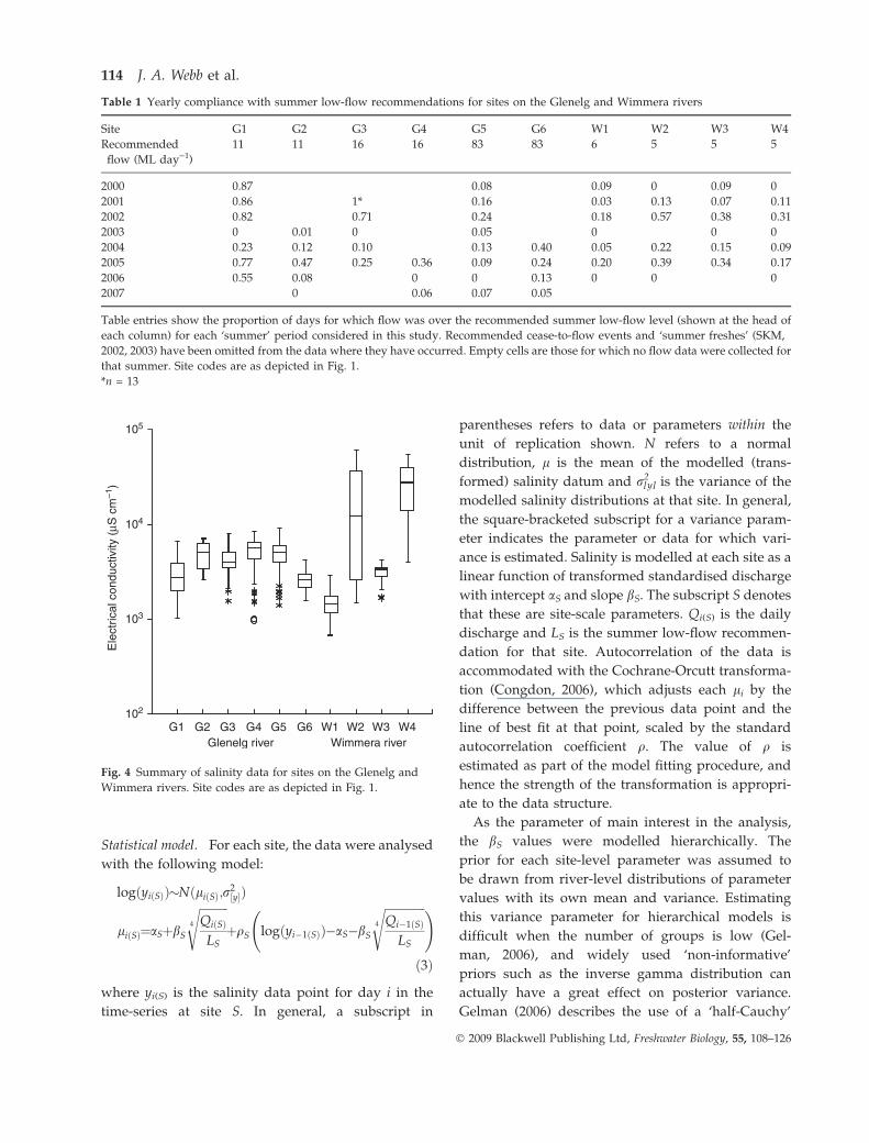
(Table 1). Salinities in the two rivers generally lie in

the range 1000–10 000 lS cm)1, but higher salinities

(>50 000 lS cm)1) are found occasionally at two of the

sites on the Wimmera River (Fig. 4).

An initial examination revealed what appeared to

be roughly linear negative relationships between

salinity and flow, but also that the data series were

characterised by very high temporal autocorrelation.

Accordingly, we analysed the data as a linear regres-

sion of salinity against flow with extra terms to

account for temporal autocorrelation.

Because it is hypothesised that recommended min-

imum flow rates will maintain water quality, we used

the summer low-flow recommendations to scale the

discharge data from each site. This produces a flow

metric related directly to the environmental flow

recommendations, and is also comparable among

sites – a characteristic that will facilitate a hierarchical

treatment of the data.

We extracted sequences of daily flow and salinity

data for the ‘summer’ period from the complete

records for each site. We removed any sequences

of data where the discharges qualified as a

112 J. A. Webb et al.

� 2009 Blackwell Publishing Ltd, Freshwater Biology, 55, 108–126

recommended ‘summer fresh’ – (a short period of

elevated discharge as defined in the Victorian FLOWS

method; DNRE, 2002), reasoning that these relatively

infrequent events would have a large influence on

salinity, and would confound the detection of any

influence of the summer low flows. We also removed

days with zero flow, of which there were some long

sequences in the record. Finally, both discharges and

salinity values are positively skewed, and were

transformed in the analysis. Salinity data were log10-

transformed and discharge data (scaled by recom-

mended summer low-flow volumes) were 4th root-

transformed (eqn 3). This transform provided a more

even spread of the explanatory variable than other

potential transformations we examined.

100

300

400

200

100

300

400

200

50

100

150

50

100

150

100

200

300

100

200

300

10410310210110–110–20

G3

G1(a)

(b)

(c)

(d)

(e)

(f)

G4

G5

G6

G2

Num

ber

of d

ays

Discharge (ML d–1)

Fig. 2 Summer discharge data for the Glenelg River sites.

The vertical dotted line is the recommended summer

low-flow discharge. Data are presented on a log10(Q + 0.001)

scale to allow the plotting of Q = 0 ML day)1 data

(0.001 ML day)1 was the minimum non-zero flow). Data

treatment is as described for Table 1. Site codes are as

depicted in Fig. 1.

50

100

150

(a)

(b)

(c)

(d)

200

400

600

200

400

600

100

200

300

10410310210110–110–20

W3

W1

W4

W2

Num

ber

of d

ays

Discharge (ML d–1)

Fig. 3 Summer discharge data for the Wimmera River sites.

Plotting options are as described for Fig. 2. Data treatment is as

described for Table 1. Site codes are as depicted in Fig. 1.

Bayesian modelling for detecting effects of flow 113

� 2009 Blackwell Publishing Ltd, Freshwater Biology, 55, 108–126

Statistical model. For each site, the data were analysed

with the following model:

logðyiðSÞÞ�NðliðSÞ;r2½y�Þ

liðSÞ¼aSþbS

ffiffiffiffiffiffiffiffiffiffiQiðSÞLS

4

sþqS logðyi�1ðSÞÞ�aS�bS

ffiffiffiffiffiffiffiffiffiffiffiffiffiffiQi�1ðSÞ

LS

4

s !

ð3Þ

where yi(S) is the salinity data point for day i in the

time-series at site S. In general, a subscript in

parentheses refers to data or parameters within the

unit of replication shown. N refers to a normal

distribution, l is the mean of the modelled (trans-

formed) salinity datum and r2[y] is the variance of the

modelled salinity distributions at that site. In general,

the square-bracketed subscript for a variance param-

eter indicates the parameter or data for which vari-

ance is estimated. Salinity is modelled at each site as a

linear function of transformed standardised discharge

with intercept aS and slope bS. The subscript S denotes

that these are site-scale parameters. Qi(S) is the daily

discharge and LS is the summer low-flow recommen-

dation for that site. Autocorrelation of the data is

accommodated with the Cochrane-Orcutt transforma-

tion (Congdon, 2006), which adjusts each li by the

difference between the previous data point and the

line of best fit at that point, scaled by the standard

autocorrelation coefficient q. The value of q is

estimated as part of the model fitting procedure, and

hence the strength of the transformation is appropri-

ate to the data structure.

As the parameter of main interest in the analysis,

the bS values were modelled hierarchically. The

prior for each site-level parameter was assumed to

be drawn from river-level distributions of parameter

values with its own mean and variance. Estimating

this variance parameter for hierarchical models is

difficult when the number of groups is low (Gel-

man, 2006), and widely used ‘non-informative’

priors such as the inverse gamma distribution can

actually have a great effect on posterior variance.

Gelman (2006) describes the use of a ‘half-Cauchy’

Table 1 Yearly compliance with summer low-flow recommendations for sites on the Glenelg and Wimmera rivers

Site G1 G2 G3 G4 G5 G6 W1 W2 W3 W4

Recommended

flow (ML day)1)

11 11 16 16 83 83 6 5 5 5

2000 0.87 0.08 0.09 0 0.09 0

2001 0.86 1* 0.16 0.03 0.13 0.07 0.11

2002 0.82 0.71 0.24 0.18 0.57 0.38 0.31

2003 0 0.01 0 0.05 0 0 0

2004 0.23 0.12 0.10 0.13 0.40 0.05 0.22 0.15 0.09

2005 0.77 0.47 0.25 0.36 0.09 0.24 0.20 0.39 0.34 0.17

2006 0.55 0.08 0 0 0.13 0 0 0

2007 0 0.06 0.07 0.05

Table entries show the proportion of days for which flow was over the recommended summer low-flow level (shown at the head of

each column) for each ‘summer’ period considered in this study. Recommended cease-to-flow events and ‘summer freshes’ (SKM,

2002, 2003) have been omitted from the data where they have occurred. Empty cells are those for which no flow data were collected for

that summer. Site codes are as depicted in Fig. 1.

*n = 13

102

103

104

105

G1 G2 G3 G4 G5 G6 W1 W2 W3 W4Wimmera riverGlenelg river

Ele

ctric

al c

ondu

ctiv

ity (

μS c

m–1

)

Fig. 4 Summary of salinity data for sites on the Glenelg and

Wimmera rivers. Site codes are as depicted in Fig. 1.

114 J. A. Webb et al.

� 2009 Blackwell Publishing Ltd, Freshwater Biology, 55, 108–126

distribution as a minimally informative prior for

such parameters. The construction of such a prior

requires some extra parameters in the model,

namely:

bS ¼ /þ f � gS

f � Nð0;A2ÞgS � Nð0; r2

½g�Þr½b� ¼ fj j � r½g�

ð4Þ

where / is the overall mean of the distribution of bS

values, and f and gS dictate the deviation of

individual bS values from /. Parameters that are

not subscripted are calculated at the highest level of

the hierarchy – the river. A is the ‘scale’ parameter

for the half-Cauchy distribution, and corresponds to

the median of the prior standard deviation. The

posterior standard deviation, r[b], of the distribution

of bS values is then calculated as shown. The

hierarchical structure of the model is illustrated in

Fig. 5.

Smelt model

Data, data treatment and rationale for model. Fish

abundance data were available for 18 sites spread

across six reaches (R1–R6) of the Thomson River

(Fig. 1). There were three years worth of data (2005,

2006, 2007), with one bank-mounted or boat electro-

fishing sample being taken per site in autumn each

year (late March–early April), with the exception of

site T9, where no sample was taken in 2007. Twenty-

four fish species were found in total, but samples were

numerically dominated (58% of total abundance) by

Australian smelt – hereafter referred to as smelt.

Because of its abundance, we chose to concentrate on

smelt for this analysis, acknowledging that it is only

one species of the native fish community that the

environmental flow program was designed to protect.

Very few smelt were caught in Reach 6 where the

river is wider and deeper than preferred by this

species (see Pusey, Kennard & Arthington, 2004), and

so we restricted the analysis to reaches 2–5. Figure 6

shows the numbers of smelt sampled at each site

(standardised to 30 min of electrofishing time), and

μi(S)

σ2[y ]

σ2[η]

αSρS

φ ζ

σ[β]

River

Site

Data

Parameter Level

βS

ηS

yi(S)

Fig. 5 Hierarchical structure for the salinity model. Refer to

Methods section for definitions of the parameters.

R2 R3 R4a R4b R5

Reach #

# S

mel

t sam

pled

(30

min

–1)

10

40

100

400

2007

2006

2005

Fig. 6 Smelt data for the Thomson River. Figure shows

standardised (per 30 min of electrofishing time) numbers of

smelt sampled at each site during each year. Reach codes are as

depicted in Fig. 1. Symbols denote sampling year as per the inset

key. Vertical lines illustrate the range of numbers sampled

within each reach for any 1 year.

Bayesian modelling for detecting effects of flow 115

� 2009 Blackwell Publishing Ltd, Freshwater Biology, 55, 108–126

shows that large variations occur between individual

sites and among years.

Adult smelt are not considered to be particularly

flow sensitive. However, the eggs and larvae are often

found in low-flow environments (King, 2004), and

Milton & Arthington (1985) hypothesised that low-

flow conditions would favour larval smelt both in

terms of prey abundance and reduced physical

disturbance. Conversely, aseasonal flow releases dur-

ing periods of spawning and larval development may

damage eggs attached to submerged vegetation, and

flush eggs and larvae downstream (Pusey et al., 2004).

Spawning commences when temperatures exceed

15 �C (Milton & Arthington, 1985), meaning that

spawning in the Thomson River should commence

in late spring and extend into summer.

With the above in mind, we can formulate a simple

conceptual model for the expected response of smelt

to discharge. We hypothesise that the number of fish

recruiting to the adult population will be a function of

the amount of slow-flow habitat in the river over the

summer period, and that the amount of habitat is a

function of the provision of discharges that are

sufficient to provide habitat, but not so great that

the habitat becomes too disturbed. In such analysis,

we would prefer to use either a direct or modelled

quantification of slow-flow habitat. Such data will be

available as part of the wider environmental flows

monitoring programs being developed as part of

VEFMAP (Chee et al., 2006) but are not yet available.

Summer (1 December–30 April) low-flow recommen-

dations for the Thomson River (EarthTech, 2003) were

specified at least partly with the provision of slow-

flow habitat in mind. As such, using average summer

discharge data, scaled by the low-flow recommenda-

tions (as was previously done for the salinity model)

should provide a rough surrogate of available habitat

across the season. However, in the Thomson River,

summer low-flow recommendations are exceeded

almost all the time because the river is used to deliver

irrigation water downstream (Table 2, Fig. 7). Thus

our a priori expectation is that these higher than

recommended flows may lead to a reduction in

available habitat, and therefore in smelt abundance.

There were several factors arguing against the use of

the site-level smelt abundance data to assess the effects

of discharge. First, as noted above fish abundances

often show great site-to-site variability because of fish

mobility and schooling behaviour, and responses may

be more likely to be detected at the reach (i.e. 10 s of

km) scale (e.g. Pyron, Lauer & Gammon, 2006). Data

must be combined at the reach scale for such an

analysis, and this was done within the model. Second,

the efficiency of fish collection appeared to be affected

by discharge and turbidity on the day of sampling

(W. M. Koster, pers. obs.), with lower efficiency

associated with high turbidity and discharge. We

tested and allowed for these effects within the struc-

ture of the model (see detail below). Prior to the

analysis, we standardised the data to account for

different electrofishing efforts among samples. The

abundances were also log10-transformed during the

analysis, as the data were positively skewed.

Statistical model. The model is conceived as a multi-

layer model, with the data effectively being adjusted

for day-of-sampling discharge and turbidity effects

before being aggregated at the reach-level and passed

to the main analysis. The transformed site-level

abundance data were modelled as

logðyiðSTÞÞ � NðliðSTÞ; r2½y�Þ

liðSTÞ ¼ hiðSTÞ þ d logðTuiðSTÞ Þ þ c logðQiðTÞÞ

ð5Þ

where yi(ST) is the abundance data i = 1…3 within

each site (S) within each reach (T), li(ST) is the mean of

the modelled (transformed) abundance for sample i,

r2[y] is the variance of this distribution and h i(ST) is the

mean of the modelled abundance once the effects of

turbidity and discharge have been taken into account.

Tui(ST) and Qi(T) are turbidity and discharge on the day

of sampling, respectively (discharge is only measured

at the reach scale). These data were log-transformed to

maximise the spread of the explanatory variables in

the analysis. The parameters d and c are coefficients

for turbidity and flow covariates. As with the salinity

analysis, the absence of a subscript indicates a

Table 2 Yearly compliance with summer low-flow recommen-

dations for reaches on the Thomson River

Reach R2 R3 R4a R4b R5

Recommended

flow (ML day)1)

125 125 20 50 70

2005 0.733 1 1 0.285 0.997

2006 0.979 1 1 0.301 0.999

2007 1 1 0.976 0.279 0.918

Table interpretation is as described for Table 1, except that flow

recommendations are taken from EarthTech (2003). Reach codes

are as depicted in Fig. 1.

116 J. A. Webb et al.

� 2009 Blackwell Publishing Ltd, Freshwater Biology, 55, 108–126

river-level parameter. The adjusted site-level data

were aggregated at the reach scale such that

hiðSTÞ � NðuiðTÞ; r2½h�Þ ð6Þ

where ui(T) is the mean of the distribution of site-

level observations for the reach during year i, and

other subscripts and parameters follow the naming

conventions above. Within each reach, the reach-level

mean abundances for each year were regressed

against the average discharge for that summer period

scaled against the low-flow recommendation (eqn 7).

As with the salinity analysis, scaling of the flow data

in this way serves to maximise similarity of the

regression coefficients among reaches, and log-trans-

formation of the flows maximised the spread of the

predictor variable.

uiðTÞ ¼ kT þ pT

logðQÞiðTÞlogðLTÞ

ð7Þ

For this model, kT and pT are regression intercept and

slope parameters, respectively, logðQÞiðTÞ is the aver-

age log-transformed summer discharge over the

12 months preceding sampling and LT is the summer

low-flow recommendation for that reach. Finally, the

regression slope pT was modelled hierarchically

among the reaches, using the same half-Cauchy prior

structure as was employed for the salinity model

above:

pT ¼ wþ f � gT

f � Nð0;A2ÞgT � Nð0; r2

½g�Þr½p� ¼ fj j � r½g�

ð8Þ

where, w is the overall mean of pT values, r[p] is the

standard deviation of this distribution and f, g and A

have the same meanings as for the salinity model. The

hierarchical structure of the model is illustrated in

Fig. 8.

Implementation

We used minimally informative prior distributions for

all parameters that required them. These distributions

were N (0, 10002) for unbounded means (salinity: bS,

aS, /; smelt: kT, w, d, c); ‘half-normal’ (i.e. reflected

around zero) |N (0, 1002)| for non-hierarchical

standard deviations (salinity: r[y]; smelt: r[y], r[h])

and U[)1,1] for the autocorrelation parameter qS in

the salinity analysis, where U denotes the uniform

distribution. Following Gelman (2006), the prior dis-

tributions for r2[g] were set as C(0.5,0.5), where C

refers to the gamma distribution, and which is also

equivalent to a chi-square distribution with 1 d.f.

(Gelman et al., 2004). The scale parameter A, was set to

0.05 for the salinity analysis and 5 for the smelt

104103102101Discharge (ML d–1)

200

100

50

100

150

50

100

50

100

150

50

100

150

Num

ber

of d

ays R4a

R2

(b)

(e)

(c)

(d)

(a)

R4b

R5

R3

Fig. 7 Summer discharge data for the Thomson River. Data are

presented on a log10 scale. Other plotting options are as

described for Fig. 2. Data treatment is as described for Table 1.

Reach codes are as depicted in Fig. 1.

Bayesian modelling for detecting effects of flow 117

� 2009 Blackwell Publishing Ltd, Freshwater Biology, 55, 108–126

analyses. An appropriate value for A should be a little

higher than the expected standard deviation of the

between-groups distribution (Gelman, 2006). In this

case, we determined the values by looking at the level

of variation amongst groups in non-hierarchical ver-

sions of the analyses (see below).

The models were written and implemented in the

Markov chain Monte-Carlo-based Bayesian analysis

software WINBUGSWINBUGS 1.4.2 (http://www.mrc-bsu.ca-

m.ac.uk/bugs; Lunn et al., 2000). The ‘step’ function

was used to calculate probabilities on selected param-

eters of the form Pr (X > 0). For interpretation,

probabilities near 1.0 imply strong support for the

hypothesis that X > 0, probabilities near 0 imply

strong support for the opposite (i.e. that X < 0), and

probabilities near 0.5 support the ‘null hypothesis’ of

no effect. We also used the models to produce ‘fake

data’ to conduct posterior predictive checks of model

performance (Gelman & Hill, 2007), and to make

specific predictions about expectations for salinity and

smelt under different conditions. For salinity, the

posterior predictive check was done by assessing the

correlation between the simulated data and the

recorded transformed salinity values. The model

was also used to predict the absolute effect on salinity

of changes in low flows. The scenario chosen was an

increase in discharge from half the recommended

summer low flow to double the threshold (i.e. a

fourfold increase in flow). For smelt, we used prob-

ability values for each simulated data point – Pr (‘fake

data’ > data) to assess model fit by looking at the

distribution of probabilities for the entire data set.

Probabilities near 0.5 indicate a good fit of the model

to that data point, while probabilities near 0 or 1

indicate a poor fit (W.A. Link, USGS, pers. comm.).

We also predicted the average number of smelt

expected to be sampled (under average turbidity

and day of sampling flow) in each reach if summer

low-flow recommendations were being met in full.

In WINBUGSWINBUGS, three independent Markov chains

were run simultaneously. Convergence of the inde-

pendent chains was checked using the modified

Gelman-Rubin diagnostic (Brooks & Gelman, 1998).

We observed severe autocorrelation within the Mar-

kov chains for the smelt model, and applied ‘thin-

ning’, where only a certain proportion of the Markov

chain values are retained for parameter estimation.

Thinning allows a robust estimate of the parameter

distribution with fewer Markov chain values when

autocorrelation is present. Details of this and other

implementation statistics are presented in Table 3.

The WINBUGSWINBUGS code for all models is available in

Supporting Information.

To test the effect of using a hierarchical approach,

we also ran non-hierarchical versions of the models.

This was done by removing the higher-level hyper-

parameters from the model, and instead assigning

minimally informative prior distributions to the

parameters at the lower level (site for the salinity

model, reach for the smelt model). For the salinity

model, the hierarchical version still treated rivers

separately. It would have been possible to run a

Parameter Levelyi(ST)

μi(ST)

θi(ST)

σ2[θ] γ σ2[y ]δ

ϕi(T)

λT πT

ηT

σ[π]

σ2[η]ψ ζ

River

Reach

Data

Fig. 8 Hierarchical structure for the smelt model. Refer to

Methods section for definitions of the parameters.

118 J. A. Webb et al.

� 2009 Blackwell Publishing Ltd, Freshwater Biology, 55, 108–126

version of the model where rivers were treated as a

third level in the hierarchy, but there is little point in

conducting hierarchical analyses when the number of

groups (in this case rivers) is less than three as there is

very little information to assess between-group vari-

ance, and so no basis for shrinkage of group-level

estimates (Gelman, 2006). For the smelt model, the

‘non-hierarchical’ version still handled data adjust-

ment for discharge and turbidity identically to the

first model, but the reaches were treated indepen-

dently when assessing the effects of average summer

discharge on fish abundance.

Results

Salinity model

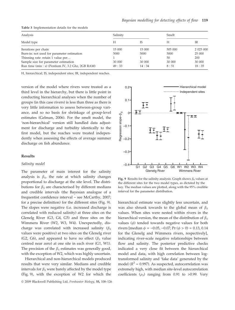
The parameter of main interest for the salinity

analysis is bS, the rate at which salinity changes

proportional to discharge at the site level. The distri-

butions for bS are characterised by different medians

and credible intervals (the Bayesian analogue of a

frequentist confidence interval – see McCarthy, 2007;

for a precise definition) for the different sites (Fig. 9).

The slopes were negative (i.e. increased discharge is

correlated with reduced salinity) at three sites on the

Glenelg River (G3, G4, G5) and three sites on the

Wimmera River (W2, W3, W4). Unexpectedly, dis-

charge was correlated with increased salinity (bS

values were positive) at two sites on the Glenelg river

(G2, G6), and appeared to have no effect (bS value

centred near zero) at one site in each river (G1, W1).

The precision of the bS estimates was generally good,

with the exception of W2, which was highly uncertain.

Hierarchical and non-hierarchical models produced

results that were very similar. Medians and credible

intervals for bS were barely affected by the model type

(Fig. 9), with the exception of W2 for which the

hierarchical estimate was slightly less uncertain, and

was also shrunk towards to the global mean of bS

values. When sites were nested within rivers in the

hierarchical version, the mean of the distribution of bS

values (/) tended towards negative values for both

rivers [median / = )0.05, )0.07; Pr (/ > 0) = 0.13, 0.14

for the Glenelg and Wimmera rivers, respectively],

indicating river-scale negative relationships between

flow and salinity. The posterior predictive checks

indicated a very close fit between the hierarchical

model and data, with high correlation between log-

transformed salinity and ‘fake data’ generated by the

model (R2 = 0.997). As suspected, autocorrelation was

extremely high, with median site-level autocorrelation

coefficients (qS) ranging from 0.91 to >0.99. Very

Table 3 Implementation details for the models

Analysis Salinity Smelt

Model type H IS H IR

Iterations per chain 15 000 15 000 505 000 2 025 000

Burn-in: not used for parameter estimation 5000 5000 5000 25 000

Thinning rate: retain 1 value per… 1 1 50 200

Sample size for parameter estimation 30 000 30 000 30 000 30 000

Run time (min : s) (Pentium IV, 3.2 Ghz, 2GB RAM) 49 : 33 14 : 34 8 : 51 18 : 35

H, hierarchical; IS, independent sites; IR, independent reaches.

–0.4

–0.2

0

0.1

Wimmera RiverGlenelg River

Reg

ress

ion

slop

e–β S

–0.1

–0.3

0.2Independent sites

Hierarchical model

G1 G2 G3 G4 G5 G6 W1 W2 W3 W4

Fig. 9 Results for the salinity analysis. Graph shows bS values at

the different sites for the two model types, as dictated by the

key. The median values are plotted, along with the 95% credible

interval for the parameter distribution.

Bayesian modelling for detecting effects of flow 119

� 2009 Blackwell Publishing Ltd, Freshwater Biology, 55, 108–126

similar results were seen for the non-hierarchical

model.

For the prediction of effects of changes in flow,

there was a wide range of absolute expected effects

(Table 4), with the value for W2 clearly being beyond

the realm of possibility. The percentage changes show

a far narrower range of values.

Smelt model

The parameter of main interest for the smelt analysis

is pT, the slope of the relation between reach-level

smelt abundance and proportional achievement of the

summer low-flow recommendation. For the hierarchi-

cal model, all reaches had probabilities that pT was >0

of between 0.1 and 0.3, suggesting that increasing

discharge was associated with a reduced number of

smelt at the reach scale (Table 5). This was also

reflected in the distribution of w – the mean of pT

slopes [median w = )1.32, Pr (w > 0) = 0.21]. When

the reaches were treated independently, there was a

far larger range of probabilities (Table 5). Median pT

values for each reach generally differed between the

hierarchical and independent reaches analyses, with

the medians being more consistent across reaches for

the hierarchical model. Credible intervals for pT were

wider for all reaches in the independent reaches

model, particularly so for reaches 3 and 4b (Fig. 10).

The covariates d and c also had substantial probabil-

ities of the parameter being less than zero for both the

hierarchical and independent reaches models (Ta-

ble 5). Thus, both higher turbidity and discharge on

the day of sampling appear to reduce the number of

fish being caught.

The distribution of probability values for the sim-

ulated data showed a reasonable fit of the hierarchical

model to the data. The model fit to the data was poor

[arbitrarily defined as Pr (‘fake data’ >data) <0.2 or

Table 4 Predicted effects of flow increases on salinity

G1 G2 G3 G4 G5 G6 W1 W2 W3 W4

Change (salinity) 1.1 · 10)4 240 )450 )640 )510 51 0 )4.0 · 1010 )5.2 )3000

% change 0 5 )10 )13 )10 5 0 )9 )2 )12

Table shows the median predicted effect on salinity of increasing flow from half the recommended summer low-flow threshold to

double the threshold, expressed as absolute (precise to two significant figures) and percentage changes. [Correction added after online

publication 31 March 2009: Value for G6, Change (salinity) should be ‘51’ instead of ‘)51’].

Table 5 Results for the smelt model

Pr (parameter value >0)

Hierarchical

model

Independent

reaches model

pT

R2 0.11 0.05

R3 0.30 0.86

R4a 0.25 0.42

R4b 0.26 0.30

R5 0.21 0.28

Covariates

d 0.01 0.02

c 0.11 0.11

Table shows the probabilities that parameter values are >0 for

the reach-scale regression slopes and for the covariate effects of

turbidity and flow.

Independent reaches

Reach

Hierarchical model

–49.3–20

–10

10

20

Reg

ress

ion

slop

e –π

T

0

30

R2 R3 R4a R4b R5

Fig. 10 Results for the smelt analysis. Graph shows pT

values for the different reaches for the two model types as

dictated by the key. Plotting options are as for Fig. 9. For

the error bar that extends beyond the range of the y-axis,

the 2.5th percentile is given by the number adjacent to the

error bar.

120 J. A. Webb et al.

� 2009 Blackwell Publishing Ltd, Freshwater Biology, 55, 108–126

>0.8] for 10 of the 44 data points, although only one

fake data point had a probability of <0.1, >0.9 of being

greater than the data point. Fit of the non-hierarchical

model to the data was slightly better, with the model

being a poor fit (as defined above) to nine of the data

points, with none of the fake data points exceeding the

Pr <0.1, >0.9 threshold.

The median predicted number of smelt under

compliant low-flow conditions was higher for all

reaches than the average number of fish captured

(Fig. 11). However, uncertainty in the predicted

numbers means that the credible intervals overlap

with the sampled data. The greatest predicted

improvement occurred for reach 4a and the smallest

for 4b.

Discussion

Bayesian hierarchical models for detecting ecosystem

responses to changes in flow

The analyses show that Bayesian hierarchical methods

can be used to detect environmental responses to flow

variation using standard monitoring data. This is

important because monitoring data sets – commis-

sioned and funded by the management agencies –

generally have greater spatial and temporal coverage

than can be funded in a research project, and thus will

usually be the only data available to assess whether

environmental flow programs have been successful.

Analysis of such data sets should allow us to detect

effects at large spatial and temporal scales, increasing

the generality of the findings concerning smaller-scale

interventions, and providing support for a large-scale

approach to monitoring the effects of environmental

flows. Analyses such as these also test the predictions

made in environmental flow assessments, potentially

supporting the robustness of an assessment method

(Arthington et al., 2006). More generally, because we

have focussed on detecting general flow-ecology

responses, rather than responses to specific environ-

mental flow events, the conclusions have more

general implications for predicting effects of changes

in flow regimes, not just changes due to environmen-

tal flow releases. Such findings can also potentially

be used to refine environmental flow assessment

methods leading to improved future flow assess-

ments.

Interpreting the results from this study

Salinity model. The initial examination of discharge

versus salinity revealed generally negative relation-

ships between the two variables, leading to the

reasonable conceptual model that increased flow

serves to dilute saline waters, leading to a decrease

in salinity. However, the presence of high temporal

autocorrelation in the data meant that some of these

apparent relationships were not detected once auto-

correlation had been accounted for. Our initial

hypothesis was confirmed for six of the 10 sites only.

There were two sites where the results were

opposite to our expectation. At these sites, flow events

were correlated with an increase in salinity. Such a

situation could occur when discharges disrupt strat-

ified hypersaline pools and move salts downstream.

This potential negative effect of increasing low flows

is seen as an issue of concern in the Wimmera River

(H. Christie, WCMA, pers. comm.), and specific

monitoring and modelling is being undertaken to

determine what magnitude of discharge could cause

such a mobilization of salt. Similar situations have

been observed in some rivers in south-west Western

Australia (R. Donohue, W.A. Department of Water,

Reach

1

102

103

104

10

Pre

dict

ed #

sm

elt s

ampl

ed (

30 m

in–1

)

R2 R3 R4a R4b R5

Fig. 11 Predicted numbers of smelt that would be sampled

under compliant low-flow conditions. Filled circles are the

average number of fish sampled for each reach over

the course of the study. Other plotting options are as for

Fig. 9.

Bayesian modelling for detecting effects of flow 121

� 2009 Blackwell Publishing Ltd, Freshwater Biology, 55, 108–126

pers. comm.), and so the results are not without

precedent.

There were also two sites (G1, W1) where there was

no apparent effect of increased discharge on salinity.

These are the most upstream sites for each river

(Fig. 1), and also generally have low salinities com-

pared to other sites (Fig. 4). Even under low-flow

conditions high salinities are not expected at these

upstream sites and thus salinity fluctuations are not

expected with changing flows.

These results argue against the ubiquitous hypoth-

esis that summer low flows should help to maintain

water quality at all sites and instead compel us to

consider mechanisms that may differ among sites.

The estimates of effects of increased flow on salinity

levels translate the model, with its transformations and

standardizations of data, back to expectations of real-

world effects. However, the absolute changes in salinity

predicted for site W2 is clearly not a realistic estimate. It

is probably not advisable to consider absolute effects

for a model where autocorrelation of data is so

important, as it is very difficult to predict an absolute

salinity without knowing what the salinity was the

previous day. Analyses conducted at a larger temporal

scale (e.g. seasonal or yearly) are more likely to be able

to tie flow regimes to average salinities. The percentage

changes take more uniformly realistic values. Larger

percentage reductions are expected in reaches with

generally higher salinities, with smaller or zero reduc-

tions predicted for reaches with lower salinities. These

predictions could be used in a predictive sense to

inform either case-specific or general decisions about

flow releases targeting salinity.

Smelt model. The hierarchical model provides some

support for the hypothesis that higher than recom-

mended summer discharges in the Thomson river

lead to a reduction in the abundance of smelt. That the

Bayesian hierarchical approach could provide such an

indication is encouraging given that (i) smelt are not

considered to be an overtly flow-sensitive species and

(ii) we had only a very small data set (effectively 15

reach-scale data points analysed in five different

three-point regressions). Collection of data over a

larger number of years will improve the power of the

statistical analyses, but the results show that the

hierarchical approach to the analysis, and the result-

ing borrowing of strength, reduces the impact of the

short time-series of data.

The findings support the hypotheses of Milton &

Arthington (1985) and Pusey et al. (2004) that higher

flows over the larval and juvenile period could be

expected to reduce smelt abundance in streams.

Elevated summer discharges in the Thomson River

occur principally to deliver irrigation water down-

stream. As such, there will always be tension between

consumptive water requirements and environmental

requirements. A reduction in the numbers of smelt – a

species that is common and widespread in southern

and eastern Australia (Pusey et al., 2004) – is unlikely

to be seen as a sufficient ecological impact for flow-

delivery rules to be reassessed. However, it is likely

that any effects on smelt populations also occur for

less common species, especially those that have

greater adult sensitivity to flow. For these species,

aseasonal flow regimes may lead to serious impacts,

possibly even local-scale extirpation. Future work will

attempt to extend the analyses to rarer taxa.

The analysis also found strong evidence that the

efficiency of sampling is affected by turbidity and

discharge on the day of sampling. This effect is probably

a result of stunned fish going un-noticed in turbid water

or being washed away from the sampling point. In the

present analysis, there was some correlation of both day

of sampling discharge and day of sampling turbidity to

summer discharge. The model quantified these effects

and adjusted the data accordingly prior to the assess-

ment of average summer flow on reach-scale abun-

dance. A failure to account for these effects in the model

would have led to a bias in the results, overstating the

effect of summer flows on smelt abundance.

The prediction of increased smelt abundance under

fully compliant low-flow conditions follows logically

from the findings of the analysis. Whilst these

predictions are associated with high uncertainty, they

provide an indication of the potential benefits of

improved compliance with summer low flows. It is

also worth noting that the greatest and smallest

improvements in predicted fish abundances (reaches

4a, 4b, respectively) occur for the reaches with the

greatest and least oversupply of water during the

summer months (Fig. 7). Thus, although we would

expect other factors not included in the statistical

model (e.g. availability of food and preferred physical

habitat) to affect the reach-scale regression estimates,

and hence the predictions of abundance, it appears

that flow does have an important influence on

Australian smelt.

122 J. A. Webb et al.

� 2009 Blackwell Publishing Ltd, Freshwater Biology, 55, 108–126

The benefits of Bayesian hierarchical models

We hypothesised that a Bayesian hierarchical

approach to data analysis could serve to reduce the

effects of low numbers of sampling units. Our results

show that the hierarchical approach will be of benefit

in this regard when data are sparse at the sampling

unit level (e.g. site, reach), but will otherwise have

minor effects. There was virtually no effect of taking a

hierarchical approach to the salinity analysis, as the

large number of data points at each site overwhelmed

the hierarchical prior distribution. Conversely, in the

hierarchical version of the smelt model, where there

were few data per reach, consistency among reaches

was increased (shrinkage) and uncertainty within

reaches decreased (borrowing strength). Indeed, only

by taking a hierarchical approach to the analysis, were

we able to detect a potential relationship between

summer flows and smelt abundance. It is likely that

a non-hierarchical analysis of the smelt data would

have concluded that the result in R2 (Table 5) was a

type 1 error (false positive) given the inconsistent or

inconclusive responses noted in other reaches. As

noted above, hierarchical models can be fitted in a

non-Bayesian framework (Lele et al., 2007). However,

the flexibility of the Bayesian approach makes the

formulation and fitting of such models relatively

straightforward in comparison to other methods.

We also argued for a gradient-based approach to

detecting effects of differences in flow, and that the

flexibility of Bayesian analyses means that they are

suited to detecting responses across complex ecolog-

ical gradients. This flexibility has been highlighted in

this study, where we fitted two very different

models. The ability to readily incorporate temporal

autocorrelation terms into the salinity analysis meant

that we were able to take advantage of the high

resolution, regular time-series of data available at

each site and the multi-level smelt model was able to

account for the confounding influences of turbidity

and discharge on the day of sampling when assess-

ing effects of flow on fish abundances. It would be

far more difficult, and with regard to some aspects

impossible, to conduct these using more familiar

statistical techniques.

It would be possible to perform the salinity analysis

using standard regressions at each site. However, one

would then have to adjust for temporal autocorrela-

tion of the data using a post hoc adjustment (Legendre

& Legendre, 1998), rather than being able to estimate

and account for autocorrelation whilst simultaneously

estimating parameters of interest as we did here. Such

an analysis would be confined to site-scale models,

although our findings suggest this is of little impor-

tance in this data-rich case. Similarly, the smelt

analysis would be possible by undertaking a multiple

regression to assess the effects of turbidity and

discharge on sample numbers, adjusting the data

manually using the output from this analysis, taking

the reach-level averages of the adjusted data, and then

performing separate reach-level regressions against

summer discharge. However, such an analysis would

utilise point estimates for the adjusted site-level data

and reach-level averages, and would therefore ignore

the uncertainty of these variables. Also, similar to the

salinity model, there would be no ability for a

hierarchical treatment of the reach-scale regressions.

Arguably, such a program of analysis is cumbersome

and incomplete in comparison with the hierarchical

approach, which provides a coherent and integrated

model and accounts for uncertainty at each spatial

scale of interest.

The models presented in this study should be

viewed as ‘first versions’ to be updated as part of an

iterative adaptive framework. It is not difficult to see

where the models may be improved. The occasional

unexpected results produced by the salinity model

imply that the conceptual model is lacking structural

elements to explain some aspects of salinity dynamics

(e.g. disruption of saline pools). For the smelt model,

by using summer discharge as a surrogate for slow-

flow habitat, we are implicitly assuming a loose linear

relationship between these variables. Such an assump-

tion will break down beyond a relatively narrow

range of flows, and we require direct quantification of

slow-flow habitat to provide a stronger conceptual

linkage between flow and response. As mentioned

above, such information will be provided by VEF-

MAP and will provide a better structural basis for

future models. As data from the monitoring program

begin to inform our knowledge of ecosystem response

to flow, we predict that the models will evolve in

other ways, although it is difficult to predict what

changes will occur. It would also have been possible

to assess the fit of different model structures to the

existing data. Such models may consider different sets

of covariates; or may employ non-normal distribu-

tions and nonlinear relationships rather than

Bayesian modelling for detecting effects of flow 123

� 2009 Blackwell Publishing Ltd, Freshwater Biology, 55, 108–126

transforming the data. Such ‘multi-model’ analyses

(sensu Burnham & Anderson, 2002) will be under-

taken when the monitoring data for the Victorian

environmental flows program are analysed, but are

beyond the scope of the current study. Importantly,

we should never imagine that any model is final, and

view Bayesian hierarchical modelling as providing a

coherent and flexible framework for iteratively build-

ing a rigorously tested knowledge base for environ-

mental flow management.

However, when using hierarchical modelling, it is

important to check whether sampling units really are

exchangeable. If responses really do differ among

individual rivers, and we fail to account for these in a

covariate model for the hyperparameters, then it is

possible that the shrinkage caused by a hierarchical

model will distort the results. Distortion of this kind

can only happen when the hierarchical approach has a

large effect on results (i.e. a data-poor analysis), and it

is possible to test for such an effect. Post hoc tests of

model fit to data, including those conducted for this

study and also other methods (Gelman & Hill, 2007),

ask whether the statistical model could have gener-

ated the data set to which it is being fitted, and would

demonstrate if the model was distorting the results for

one or more rivers.

Despite this cautionary note, we believe that the

hierarchical model should be the starting point for

any analyses of the types presented here. Assuming

that sampling units (e.g. rivers) behave similarly is a

reasonable preliminary hypothesis, and is consistent

with the principle of Occam’s Razor. Through tests

such as those outlined above, we can determine

whether the sampling units are exchangeable,

whether some sort of covariate model can be used to

make them conditionally exchangeable, or whether

sub-sets of samplings units should be analysed

separately because of differences we do not under-

stand. However, we believe that the opposite stand-

point is implicit in many analyses (i.e. an assumption

that all sampling units are different). Such an

assumption leaves little opportunity to generalise

beyond the sampling unit scale, other than through

observing that similar patterns are seen for different

sampling units (e.g. two rivers in Kennard et al., 2007).

The Bayesian hierarchical approach provides a rigor-

ous statistical framework for assessing the level of

similarity across sampling units and allows us to

generalise to wider scales where justified.

Conclusions

In the introduction to this paper we argued that it is

important to be able to detect the effects of environ-

mental flows, and that thus far successful determina-

tion of flow–ecology responses has usually been

restricted to smaller-scale interventions for which

individual effects have been detected. This study has

demonstrated that Bayesian hierarchical modelling

can be used to detect the effects of flow on environ-

mental variables, and hence this approach should be

useful for inferring the effects of large-scale environ-

mental flow programs. Unique to the hierarchical

approach, the properties of borrowing strength and

shrinkage mean that conclusions will be greatly

strengthened in data-poor situations, but will be

almost unaffected when data are plentiful. The flex-

ibility of Bayesian modelling allows us to formulate

more physically realistic models of response to flow,

and these models can be updated as new knowledge

and data become available via an iterative cycle of

model development. Moreover, the Bayesian ap-

proach makes fitting hierarchical models relatively

straightforward. The Bayesian hierarchical framework

allows us to test the generality of responses across

larger scales, using standard monitoring data to test

hypotheses of interest. Environmental flow monitor-

ing programs such as VEFMAP require a large

investment of public money, and we believe that

Bayesian hierarchical modelling of results will max-

imise the benefits of such programs.

Acknowledgments

This research was supported by the Victorian Depart-

ment of Sustainability and Environment, as part of

VEFMAP. We acknowledge the support of VEFMAP

team members Yung En Chee, Peter Cottingham,

Sabine Schreiber, Michael Jensz and Andrew Sharpe

as well as the scientific steering committee (Gerry

Quinn, Angela Arthington, Mark Kennard, Barbara

Downes, Alison King, Wayne Tennant), and the CMA

Environmental Water Requirement officers in this

larger project. Several of the above named provided

useful comments on an earlier version of this manu-

script. We also thank Michael McClain and Ken

Newman for their reviews of the submitted manu-

script. We thank Simon Bonner and other members of

the BUGS community for their assistance with model

124 J. A. Webb et al.

� 2009 Blackwell Publishing Ltd, Freshwater Biology, 55, 108–126

formulation. The map in this paper was produced by

Chandra Jayasuriya of the Department of Resource

Management and Geography. Data for the analyses in

this paper were commissioned and provided by the

Glenelg, Wimmera and West Gippsland catchment

management authorities. We would particularly like

to thank Matt O’Brien, Hugh Christie and Jodie

Halliwell for their assistance with data.

References

Arthington A.H., Bunn S.E., Poff N.L. & Naiman R.J.

(2006) The challenge of providing environmental flow

rules to sustain river ecosystems. Ecological Applica-

tions, 16, 1311–1318.

Barnard G.A. (1958) Studies in the history of probability

and statistics. IX. Thomas Bayes’ essay towards solving

a problem in the doctrine of chances. Biometrika, 45,

293–295.

Brooks S.P. & Gelman A. (1998) General methods for

monitoring convergence of iterative solutions. Journal

of Computational and Graphical Statistics, 7, 434–455.

Burnham K.P. & Anderson D.R. (2002) Model Selection

and Multimodel Inference. Springer, New York.

Chee Y., Webb A., Stewardson M. & Cottingham P.

(2006) Victorian Environmental Flows Monitoring and

Assessment Program: Monitoring and Assessing Environ-

mental Flow Releases in the Thompson River. eWater

Cooperative Research Centre, Melbourne, Vic.

Chester H. & Norris R. (2006) Dams and flow in the Cotter

River, Australia: effects on instream trophic structure

and benthic metabolism. Hydrobiologia, 572, 275–286.

Clark J.S. (2005) Why environmental scientists are

becoming Bayesians. Ecology Letters, 8, 2–14.

Congdon P. (2006) Bayesian Statistical Modelling. John

Wiley & Sons, Guildford.

Cottingham P., Stewardson M. & Webb A. (2005) Victorian

Environmental Flows Monitoring and Assessment Program.

Stage 1: Statewide Framework. CRC for Freshwater Ecol-

ogy and CRC for Catchment Hydrology, Melbourne,

Vic. Available at: http://tinyurl.com/2feys3 (last acc-

essed on 6 March 2009).

DNRE (2002) The FLOWS Method: A Method for Determin-

ing Environmental Water Requirements in Victoria. Vic-

torian Department of Natural Resources and

Environment, Melbourne, Vic. Available at: http://

tinyurl.com/yws84m (last accessed on 6 March 2009).

Downes B.J., Barmuta L.A., Fairweather P.G., Faith D.P.,

Keough M.J., Lake P.S., Mapstone B.D. & Quinn G.P.

(2002) Monitoring Ecological Impacts: Concepts and

Practice in Flowing Waters. Cambridge University Press,

Cambridge.

EarthTech (2003) Thomson River Environmental Flow

Requirements & Options to Manage Flow Stress. Earth

Tech Engineering Pty Ltd, Melbourne, Vic.

Gelman A. (2006) Prior distributions for variance param-

eters in hierarchical models (comment on article by

Browne and Draper). Bayesian Analysis, 1, 515–534.

Gelman A. & Hill J. (2007) Data Analysis Using Regression

and Multilevel ⁄Hierarchical Models. Cambridge Uni-

versity Press, Cambridge, New York.

Gelman A., Rubin J.B., Stern H.S. & Rubin D.B. (2004)

Bayesian Data Analysis. Chapman & Hall ⁄ CRC, Boca

Raton, FL.

Gippel C.J. & Stewardson M.J. (1995) Development of an

environmental flow management strategy for the

Thomson River, Victoria, Australia. Regulated Rivers –

Research and Management, 10, 121–135.

Hancock P.J. & Boulton A.J. (2005) The effects of an

environmental flow release on water quality in the

hyporheic zone of the Hunter River, Australia. Hydro-

biologia, 552, 75–85.

Hou P., Beeton R.J.S., Carter R.W., Dong X.G. & Li X.

(2007) Response to environmental flows in the lower

Tarim River, Xinjiang, China: ground water. Journal of

Environmental Management, 83, 371–382.

Kennard M.J., Olden J.D., Arthington A.H., Pusey B.J. &

Poff N.L. (2007) Multiscale effects of flow regime and

habitat and their interaction on fish assemblage struc-

ture in eastern Australia. Canadian Journal of Fisheries

and Aquatic Sciences, 64, 1346–1359.

King A.J. (2004) Ontogenetic patterns of habitat use by

fishes within the main channel of an Australian

floodplain river. Journal of Fish Biology, 65, 1582–1603.

Legendre P. & Legendre L. (1998) Numerical Ecology, 2nd

English edn. Elsevier, Amsterdam.

Lele S.R., Dennis B. & Lutscher F. (2007) Data cloning:

easy maximum likelihood estimation for complex

ecological models using Bayesian Markov chain Monte

Carlo methods. Ecology Letters, 10, 551–563.

Lind P.R., Robson B.J. & Mitchell B.D. (2007) Multiple

lines of evidence for the beneficial effects of

environmental flows in two lowland rivers in Victo-

ria, Australia. River Research and Applications, 23, 933–

946.

Lunn D.J., Thomas A., Best N. & Spiegelhalter D. (2000)

WinBUGS – a Bayesian modelling framework: con-

cepts, structure, and extensibility. Statistics and Com-

puting, 10, 325–337.

Martin T.G., Kuhnert P.M., Mengersen K. & Possingham

H.P. (2005) The power of expert opinion in ecological

models using Bayesian methods: impact of grazing on

birds. Ecological Applications, 15, 266–280.

McCarthy M.A. (2007) Bayesian Methods for Ecology.

Cambridge University Press, Cambridge, New York.

Bayesian modelling for detecting effects of flow 125

� 2009 Blackwell Publishing Ltd, Freshwater Biology, 55, 108–126

Milton D.A. & Arthington A.H. (1985) Reproductive

strategy and growth of the Australian Smelt, Retropin-

na semoni (Weber) (Pisces, Retropinnidae), and the

Olive Perchlet, Ambassis nigripinnis (De-Vis) (Pisces,

Ambassidae), in Brisbane, Southeastern Queensland.

Australian Journal of Marine and Freshwater Research, 36,

329–341.

Poff N.L., Allan J.D., Bain M.B., Karr J.R., Prestegaard

K.L., Richter B.D., Sparks R.E. & Stromberg J.C. (1997)

The natural flow regime. BioScience, 47, 769–784.

Pusey B.J., Kennard M.J. & Arthington A.H. (2004)

Freshwater Fishes of North-Eastern Australia. CSIRO

Publishing, Collingwood, Vic.

Pyron M., Lauer T.E. & Gammon J.R. (2006) Stability of

the River Wabash fish assemblages from 1974 to 1998.

Freshwater Biology, 51, 1789–1797.

Qureshi M.E., Connor J., Kirby M. & Mainuddin M. (2007)

Economic assessment of acquiring water for environ-

mental flows in the Murray Basin. Australian Journal of

Agricultural and Resource Economics, 51, 283–303.

Schofield N. & Burt A. (2003) Issues in environmental

water allocation – an Australian perspective. Water

Science and Technology, 48, 83–88.

Siebentritt M.A., Ganf G.G. & Walker K.F. (2004) Effects

of an enhanced flood on riparian plants of the River

Murray, South Australia. River Research and Applica-

tions, 20, 765–774.

SKM (2002) Stressed Rivers Project – Environmental Flow

Study: Wimmera River System. Sinclair Knight Merz,

Melbourne, Vic.

SKM (2003) Stressed Rivers Project – Environmental Flow

Study: Glenelg River System. Sinclair Knight Merz,

Melbourne, Vic.

SKM (2007) Development of a Program to Monitor Environ-

mental Flows in the Glenelg River: Issues Paper. Sinclair

Knight Merz, Melbourne, Vic.

Tharme R.E. (2003) A global perspective on environmen-

tal flow assessment: emerging trends in the develop-

ment and application of environmental flow

methodologies for rivers. River Research and Applica-

tions, 19, 397–441.

Underwood A.J. (1997) Experiments in Ecology: Their

Logical Design and Interpretation Using Analysis of

Variance. Cambridge University Press, New York.

Ver Hoef J.M. & Frost K.J. (2003) A Bayesian hierarchical

model for monitoring harbor seal changes in Prince

William Sound, Alaska. Environmental and Ecological

Statistics, 10, 201–219.

Webb J.A. & King E.L. (2009) A Bayesian hierarchical

trend analysis finds strong evidence for large-scale

temporal declines in stream ecological condition

around Melbourne, Australia. Ecography, 32, 215–225.

Wikle C.K. (2003) Bayesian hierarchical models for

predicting the spread of ecological processes. Ecology,

84, 1382–1394.

Supporting Information

Additional Supporting Information may be found in

the online version of this article:

Appendix S1. WINBUGSWINBUGS code and for the hierar-

chical and independent sites salinity models. The

models were created in WINBUGSWINBUGS 1.4.2. The file

contains extensive explanatory notes on the data

structures and code. The complete data set has not

been included

Appendix S2. WINBUGSWINBUGS code and for the hierar-

chical and independent reaches smelt models. The

models were created in WINBUGSWINBUGS 1.4.2. The file

contains extensive explanatory notes on the data

structures and code. The complete data set has not

been included

Please note: Wiley-Blackwell are not responsible for

the content or functionality of any supporting

materials supplied by the authors. Any queries (other

than missing material) should be directed to the

corresponding author for the article.

(Manuscript accepted 11 February 2009)

126 J. A. Webb et al.

� 2009 Blackwell Publishing Ltd, Freshwater Biology, 55, 108–126