1

The Role of Integrated Pest Management Practices in the U.S. Nursery

Industry: A Bayesian Hierarchical Poisson Approach

Wan Xu

PhD Student

Food and Resource Economics Department

University of Florida

Gainesville, FL 32611

Email: wanxu@ufl.edu

Hayk Khachatryan

Assistant Professor

Food and Resource Economics Department

Mid-Florida Research & Education Center

University of Florida

2725 Binion Road, Apopka, FL 32703

Email: hayk@ufl.edu

Selected Paper prepared for presentation at the Southern Agricultural Economics

Association’s 2015 Annual Meeting, Atlanta, Georgia, January 31-February 3, 2015

Copyright 2015 by Wan Xu and Hayk Khachatryan. All rights reserved. Readers may make

verbatim copies of this document for non-commercial purposes by any means, provided that this

copyright notice appears on all such copies.

2

1. Introduction

The U.S. nursery industry has experienced unprecedented growth and innovations, which

was reflected by substantial increases in sales revenues in the last two decades (Hall, Hodges,

and Palma, 2011). Pest management has then become an important part of the nursery production

systems in the U.S. in terms of cost and time savings (Pandit, Paudel, and Hinson, 2012).

Recently, due to the increasing chemical costs, pest chemical resistance issues, and

environmental impacts in the production of nursery plants, Integrated Pest Management (IPM),

which include a combination of mechanical & physical control, biological control, chemical

control, and cultural control, have played an essential role in solving pest problems effectively

and managing ecosystem sustainably (Sellmer et al. 2004). According to the Environmental

Protection Agency (EPA, 2011), IPM is defined as a sustainable approach to control and treat

pests by combining different management tools while minimizing its economic, health, and

environmental risks. Since the inception of IPM practices in 1972, results from empirical

literatures have demonstrated that a systematic use of IPM practices can benefit greenhouse and

nursery growers by producing healthy nursery plants while reducing environmental risks and

associated pesticide costs (Fulcher and White 2012, Fernandez-Cornejo and Ferraioli 1999,

Raupp and Cornell 1988). A lot of evidence is showed that IPM practices can increase

production efficiency and improve nursery firm’s profitability (Burkness and Hutchison, 2008;

Fernandez-Cornejo, 1996). Recently, Alston (2011) also found that the health conditions for both

workers and consumers can be greatly improved through adopting more efficient and

environmental friendly IPM practices.

3

Although a lot of studies have been focused on IPM technology adoptions in agriculture,

most of them are dealt with food crops and few has been analyzed the relationship between

firm’s characteristics and the IPM practice adoptions in the U.S. nursery industry. Recently, Li et

al. (2013) examined how grower’s characteristics influenced the adoption of IPM in greenhouse

and nursery production, but their research was limited only in three northeast states in the U.S. In

addition, many studies on IPM technology adoptions in agriculture were analyzed by count data

models using maximum likelihood estimations (Mishra and Park 2005, Paxton et al. 2011,

Pandit, Paudel, and Hinson 2012). Count data are usually modeled with Poisson regression.

However, it is well-known that count data are often over-dispersed (i.e. there are extra-variability

than the expected counts), which makes Poisson model inadequately fit the data (King, 1989).

Although negative binomial regression is a good way in dealing with over-dispersion by the

frequentist method, the dispersion parameter estimated by maximum likelihood is usually not

robust, which can cause bias and result in incorrect statistical inferences (Lloyd-Smith, 2007).

Compared with frequentist methods which rely on asymptotic approximation and assume

unknown parameters are fixed, Bayesian methods, which provide another way to treat

parameters as random variables and make probability statements about parameters based on

Bayes’ theorem, are gaining more popularities in the applied agricultural researches (Du,Yu, and

Hayes, 2011). Kuhner (2006) argued that Bayesian approach is more accurate by combining

appropriate prior information in the data within a solid theoretical framework. Bornn and Zidek

(2012) pointed out it can estimate any parameter of the functions directly and provide

interpretable results in terms of probabilities. Furthermore, with a concern on missing values in

the survey such as national nursery survey, Bayesian approach can reduce estimation bias and

risk to some degree through parameter simulations. There are many examples of utilizing

4

Bayesian methods in applied studies (e,g. Sparks and Campbell, 2014; Du,Yu, and Hayes, 2011;

Chib, Nardari and Shephard, 2002; Ouedraogo and Brorsen, 2014).

Understanding nursery firm’s IPM adoption behavior is important and useful in terms of

expanding sustainability, and gaining more government/agency supports and investments on the

effective and environmental friendly IPM practices. Therefore, in order to account for nursery

firm’s heterogeneity, incorporate prior information, and capture parameter uncertainty, this paper

applies a Hierarchical Poisson model from a Bayesian perspective to analyze the relationship

between nursery firm’s characteristics and the adoption of sustainable IPM practices in nursery

production. Different Bayesian specifications are compared and tested, where the selection is

based on deviance information criterion (DIC). Hence, the rest of the paper is organized as

follows. The data source and its structure is described in section 2. In section 3, the detailed

Bayesian Hierarchical Poisson regression method is reviewed and discussed. In section 4,

discussion focuses on the posterior inferences and policy implications. Lastly, section 5 provides

a summary and conclusion.

2. Data Source

Data for this research was obtained from the 2009 U.S. National Nursery Survey, which

was conducted by the Green Industry Research Consortium, consisting of a group of agricultural

economists and horticulturalists. Since its inception in 1989, the 2009 survey is the fifth effort to

collect comprehensive data about greenhouse and nursery product types, production and

management practices, marketing practices, and regional trades in nursery products. In 2009, a

total of 3,044 firms responded from a randomly selected sample of 17,019 firms in all 50 states,

with an 18% response rate (Hall, Hodges, and Palma 2011).

5

Twenty-two different Integrated Pest Management (IPM) practices were listed in Table 1.

More than 50% of the respondents used IPM practices of removing infested plants, using

cultivation & hand weeding, spot treatment with pesticides, and alternating pesticides to avoid

chemical resistance. Figure 1 summarized the number of IPM practices used by nursery firms.

We can see that the majority of nursery firms adopted from 4 to 10 IPM practices and more than

150 firms used 8 IPM practices. Firms with gross sales revenues less than $10,000 were

excluded from the data analysis in order to match with the industry reporting procedure of

USDA. The firm size (large or small) was determined based on the gross sales revenue with the

threshold of $500,000 (Hinson et al., 2012). Indicator variables including multiple forward

contracts (forward) and computer technology usage (comscore) were created if there was more

than one type of buyer for forward contracting, and more than 3 computerized functions used

respectively (Hinson et al., 2012). Other dummy variables affecting management and planning

such as product uniqueness (product) and ability to hire competent management (ability) were

also created based on the rating scales in the survey. After cleaning up the incorrect entries and

missing values, a total of 1672 firms will be used in this analysis.

In the study, I will investigate the primary factors that influence the number of IPM

practice adoptions by nursery firms. The outcome variable is the number of IPM practices (ipm).

Explanatory variables hypothesized to influence the number of IPM practices consist of firm size

(𝑓𝑖𝑟𝑚_𝑠𝑖𝑧𝑒), number of years in operation (age), numbers of trade show attended (tradeshow),

computer technology usage (comscore), brokering plants form other growers (broker), product

uniqueness (product), multiple forward contracts (forward), ability to hire competent

management (ability), and regions which include Northeast (region_northeast), South

(region_south), West (region_west), and Midwest (region_midwest). Variable names and

6

descriptive statistics are provided in Table 2. The baseline Poisson model can be presented by the

following equation:

log(𝐸(𝑖𝑝𝑚|𝑋)) = 𝛽0 + 𝛽1𝑠𝑖𝑧𝑒 + 𝛽2𝑎𝑔𝑒 + 𝛽3𝑐𝑜𝑚𝑠𝑐𝑜𝑟𝑒 + 𝛽4𝑡𝑟𝑎𝑑𝑒𝑠ℎ𝑜𝑤 + 𝛽5𝑏𝑟𝑜𝑘𝑒𝑟 +

𝛽6 𝑝𝑟𝑜𝑑𝑢𝑐𝑡 + 𝛽7 𝑓𝑜𝑟𝑤𝑎𝑟𝑑 + 𝛽8𝑎𝑏𝑖𝑙𝑖𝑡𝑦 + 𝛽9𝑟𝑒𝑔𝑖𝑜𝑛𝑛𝑜𝑟𝑡ℎ𝑒𝑎𝑠𝑡 + 𝛽10𝑟𝑒𝑔𝑖𝑜𝑛𝑠𝑜𝑢𝑡ℎ +

𝛽11𝑟𝑒𝑔𝑖𝑜𝑛𝑤𝑒𝑠𝑡 (1)

3. Method

The Poisson distribution is often used to model the number of events occurring randomly

through a fixed time or space interval (Cameron and Trivedi, 2005; Frank, 1967). It is the basic

regression model for count data, and it is usually expressed as: 𝑦𝑖~𝑃𝑜𝑖𝑠𝑠𝑜𝑛 (𝜆𝑖), where 𝜆𝑖 =

exp(𝑥𝑖𝑇𝛽), 𝑥𝑖=[1, 𝑥𝑖1, … 𝑥𝑖𝑘] is the predictor vector, and 𝑦𝑖 is a non-negative integer. The unique

feature of Poisson model is the equal-dispersion assumption, i.e. 𝑉𝑎𝑟(𝑦𝑖) = 𝐸(𝑦𝑖) =

𝜆𝑖. However, due to individual level heterogeneity, correlation among observations, incorrect

model specifications or variance functions, count data are often over-dispersed which causes the

variance greater than the mean (King, 1989; Winkelmann, 2008). Ignoring over-dispersion in the

Poisson model will eventually result in underestimated standard errors and incorrect statistical

inferences. There are several ways to handle this extra variability in Poisson model by frequentist

methods such as quasi-likelihood Poisson regression which scales the covariance within the

Poisson regression, negative binomial regression which mixes a random gamma variable with

the same mean as Poisson, and Hierarchical Poisson regression which includes random effects

etc. (McCullagh and Nelder, 1989; Breslow, 1984).

Hierarchical Poisson regression has the same log link function as Poisson’s, but

incorporates a random effect in the mean structure which is often demonstrated to be more

effective and efficient in dealing with over-dispersion (Breslow, 1984). In this research, we

7

analyze nursery firm’s IPM adoption behaviors by utilizing a Bayesian method to the

Hierarchical Poisson model. We assume the number of IPM practices adopted by each nursery

firm (𝑖𝑝𝑚𝑖) follows Poisson random variable with unknown parameter 𝜆𝑖 (i.e. intensity or

adoption rate per year):

𝑖𝑝𝑚𝑖|𝜆𝑖~𝑃𝑜𝑖𝑠𝑠𝑜𝑛 (𝜆𝑖) (2)

A log link function is then used to form the linear predictors:

log(𝜆𝑖) = 𝑥𝑖𝑇𝛽 + 𝜃𝑖 , 𝜃𝑖~𝑁 (0, 𝜎2) , (3)

where 𝜃𝑖 is the random effect that captures firm-level heterogeneity and accounts for over-

dispersion (Breslow, 1984). The likelihood for the data given covariate matrix X and parameter

vector 𝛽 is the product of each Poisson PDF reflecting the additional random effect added in the

model:

𝐿(𝒊𝒑𝒎|𝑿, 𝛽) = ∏ 𝑃(𝑖𝑝𝑚𝑖|𝜆𝑖) =𝑛𝑖=1 ∏

𝜆𝑖𝑖𝑝𝑚𝑖𝑒−𝜆𝑖

𝑖𝑝𝑚𝑖!

𝑛𝑖=1 , where 𝜆𝑖 = exp(𝑥𝑖

𝑇𝛽 + 𝜃𝑖) (4)

In this Bayesian analysis, a non-informative normal prior is placed on each 𝛽𝑗 since it is

relatively flat to the likelihood function and has least influence on the posterior distributions (Lee

2004), and an inverse gamma prior with fixed shape and scale parameter is placed on the

variance of the random effect 𝜃𝑖 (Draper, 1996):

𝛽𝑗~𝑁(0, 100) (5)

𝜎2~𝑖𝑔𝑎𝑚𝑚𝑎(0.01, 0.01) (6)

According to Bayes rule (Carlin and Louris 2000), the posterior distribution of 𝛽 given {X,

𝒊𝒑𝒎} is: 𝑝(𝛽|𝑿, 𝒊𝒑𝒎) =𝑝(𝒊𝒑𝒎|𝐗, 𝛽)𝑝(𝛽)

∫ 𝑝(𝒊𝒑𝒎|𝐗, 𝛽)𝑝(𝛽)d𝛽∞

0

(i.e. posterior ∝ prior × likelihood).

In order to check for over-dispersion and assess goodness of fit, a Pearson’s chi-square

statistic 𝜒P2 = ∑

(𝑖𝑝𝑚𝑖−𝐸(𝑖𝑝𝑚𝑖))2

𝑉𝑎𝑟(𝑖𝑝𝑚𝑖)

𝑛𝑖=1 is calculated, and a rule of thrum for equal-dispersion is that

8

the Pearson’s chi-square statistic/d.f. approximately equals to one (McCullagh and Nelder,

1989). If over-dispersion is present and significant in the data, a Bayesian framework of negative

binomial regression is also estimated and compared with Bayesian Hierarchical Poisson regression

in terms of deviance information criteria (DIC), which is a Bayesian alternative to Akaike

Information Criterion (AIC) and Bayesian Information Criterion (BIC) assessment tools, and a

smaller DIC usually indicates a better fit for the data (Spiegelhalter et al. 2002). For Bayesian

negative binomial model, we assume 𝑖𝑝𝑚𝑖|𝜇, 𝑘~𝑁𝐵 (𝜇, 𝑘). It naturally accounts for over-

dispersion since the variance estimate (i.e. 𝑉𝑎𝑟(𝑖𝑝𝑚𝑖) = 𝜇 + 𝑘𝜇2) is always greater than for

Poisson distribution with same mean (i.e. E(𝑖𝑝𝑚𝑖) = 𝜇 = exp(𝑥𝑖𝑇𝛽)) (Faraway,2006). Non-

informative normal priors are placed on 𝛽 with 𝛽𝑗~𝑁(0, 100), and a gamma prior with fixed shape

and scale parameter is placed on the dispersion parameter k: k~𝑔𝑎𝑚𝑚𝑎(0.001, 0.001).

Since the exact inference may not always be guaranteed (i.e. posterior distribution does

not have a closed form), in this application, a stochastic simulation method-Markov Chain Monte

Carlo (MCMC) is used to sample posterior distributions and make posterior statistical inferences

(Robert and Casella 2004). In this research, we first generate 200,000 Gibbs samplers with a

burn-in of 10,000 iterations. Due to high autocorrelation introduced via the Gibbs sampling, we

then control the thinning rate of the simulation by keeping every 5th of the iterations for

calculating all the posterior estimates including posterior means, posterior standard deviations,

and 95% highest posterior density (HPD) etc. Finally we check the Markov Chain convergences

such as trace plots, autocorrelation plots, and kernel density plots etc.

9

4. Results

All inferences about coefficients 𝛽 were based on posteriors 𝑝(𝛽|𝑿, 𝒊𝒑𝒎). Table 3

provided the result of Poisson regression from the Bayesian perspective. The p-value (i.e. less

than .001) of the Pearson chi-square statistic indicated that there was a greater variability among

the IPM practice counts than would be expected for Poisson distribution (i.e. over-dispersion), so

the Poisson model didn’t fit the data well. The Bayesian Hierarchical Poisson regression was

then estimated and summarized in Table 4. Compared with Bayesian Poisson regression in Table

3, the parameter estimates were similar, but an inflated covariance matrix affected standard

errors, and hence p-values in a conservative way. From the goodness of fit measures in Table 4,

we can see that the Pearson chi-square statistic significantly decreased with a large p-value of

0.922, and the value of DIC was much smaller than that of Bayesian Poisson model in Table 3,

which suggested that the Bayesian Hierarchical Poisson model fitted the data adequately. In

addition, in comparison with negative binomial regression from Bayesian standpoint in Table 5,

the value of DIC in Table 4 was still lower, which again confirmed that Bayesian Hierarchical

Poisson model was superior in capturing over-dispersion and accounting for unobserved

heterogeneity in this study. The diagnostic plots including trace, autocorrelation, and kernel

density plot for each covariate were provided in Figure 2, which demonstrated all excellent

convergence and good mixing of the MCMC samplers by Bayesian Hierarchical Poisson model.

The regression results of negative binomial and hierarchical Poisson using maximum likelihood

estimations were also provided in Table 7 for references.

The posterior summary which included mean, standard deviation, percentiles, and 95%

highest posterior density (HPD) for Bayesian Hierarchical Poisson model was presented in Table

4. We found that except for age and region_west, all the other covariates were positive and

10

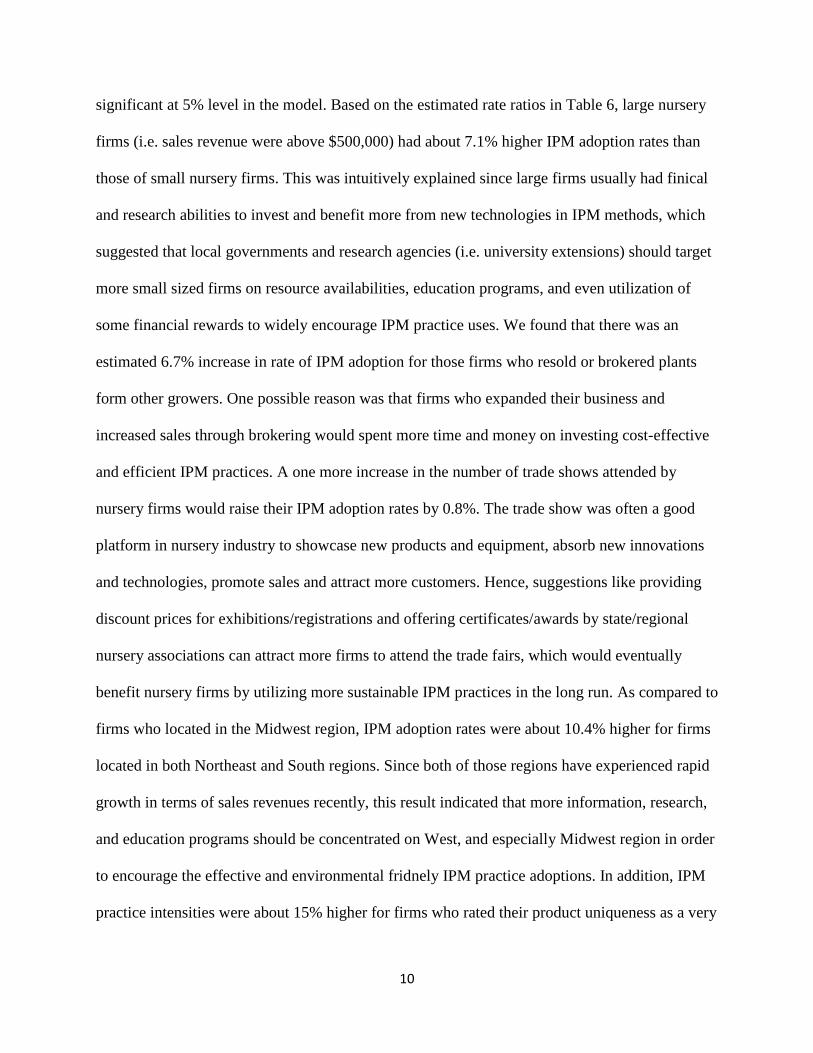
significant at 5% level in the model. Based on the estimated rate ratios in Table 6, large nursery

firms (i.e. sales revenue were above $500,000) had about 7.1% higher IPM adoption rates than

those of small nursery firms. This was intuitively explained since large firms usually had finical

and research abilities to invest and benefit more from new technologies in IPM methods, which

suggested that local governments and research agencies (i.e. university extensions) should target

more small sized firms on resource availabilities, education programs, and even utilization of

some financial rewards to widely encourage IPM practice uses. We found that there was an

estimated 6.7% increase in rate of IPM adoption for those firms who resold or brokered plants

form other growers. One possible reason was that firms who expanded their business and

increased sales through brokering would spent more time and money on investing cost-effective

and efficient IPM practices. A one more increase in the number of trade shows attended by

nursery firms would raise their IPM adoption rates by 0.8%. The trade show was often a good

platform in nursery industry to showcase new products and equipment, absorb new innovations

and technologies, promote sales and attract more customers. Hence, suggestions like providing

discount prices for exhibitions/registrations and offering certificates/awards by state/regional

nursery associations can attract more firms to attend the trade fairs, which would eventually

benefit nursery firms by utilizing more sustainable IPM practices in the long run. As compared to

firms who located in the Midwest region, IPM adoption rates were about 10.4% higher for firms

located in both Northeast and South regions. Since both of those regions have experienced rapid

growth in terms of sales revenues recently, this result indicated that more information, research,

and education programs should be concentrated on West, and especially Midwest region in order

to encourage the effective and environmental fridnely IPM practice adoptions. In addition, IPM

practice intensities were about 15% higher for firms who rated their product uniqueness as a very

11

important factor affecting their management and planning. Similarly, IPM intensities were 7.3%

higher for firms who indicated a higher importance rating on their ability to hire competent

management as a factor in impacting their business. As expected, firms who focused more on

product uniqueness would make great efforts on improving their plant’s health and nutrition, and

hence investing and adopting more economical and effective IPM practices. Similarly, if firms

were able to hire competent management, they would utilize more cost-effective and efficient

IPM practices to treat their pest problems. Furthermore, firms who used multiple forward

contracts (forward) and more computerized functions in assisting with their production

(comscore) can greatly increase their IPM adoption rates. For instance, there were around 31.7%

and 28.5% increase in rate of IPM adoption for nursery firms who intensively used computer

technologies, and who had multiple type of forward contracts respectively. Forwarding contracts

can be very useful in expanding firm’s markets, increasing their sales and growth while

minimizing firm’s risks by specifying a guaranteed price, quantity, and quality. Therefore, this

indicated that having multiple forward contracts with different buyers would motivate firms to

invest and apply more economical and effective IPM practices for quality assurances. The

findings also suggested that local nursery associations and research centers could provide more

computer technology trainings or workshops to promote more sustainable IPM practices utilized

by nursery firms.

12

5. Conclusion

Given the increasing concerns on sustainability, and potential advantages of the effective,

economical, and environmentally sustainable IPM practices, this research explored the

relationship between nursery firms’ characteristics and adoptions of IPM practices by utilizing a

recent national nursery survey. In order to account for firm’s heterogeneity, incorporate prior

information in the estimation, capture parameter uncertainties and reduce biases due to large

amount of missing information in the data, we applied a Bayesian Hierarchical Poisson

regression with MCMC Gibbs sampling algorithms. In this study, we demonstrated that Bayesian

Hierarchical Poisson model was robust and superior in capturing over-dispersion as compared to

Poisson and negative binomial models from Bayesian frameworks.

We identified several positive and significant factors affecting the rate of IPM adoption,

and our results suggested that considerable marketing effects should be made on educating and

encouraging small firms (i.e. sales revenue were below $500,000) to adopt more efficient and

sustainable IPM practices in the West and Midwest regions. In addition, we found that the IPM

adoption rates were higher for firms who had higher importance ratings on their product

uniqueness and ability to hire competent management. Moreover, nursery firms who brokered

plants from other growers or had multiple forward contracts with buyers often applied more IPM

practices than those firms who didn’t. Furthermore, we also observed that the more computerized

functions used by firms, the greater impacts on IPM practice adoptions would be. Therefore,

local governments and research agencies could target on offering some training

courses/workshops of computer technology applications so as to motivate more adoptions of

IPM practices by nursery firms. However, this research also had a limitation since it was based

13

on a single cross-sectional data. Future research could focus on modeling how the rate of IPM

adoption is changed over time if a rich longitudinal data is available.

14

References

Alston, D.G. “The Integrated Pest Management Concept.” Utah Pests Fact Sheet, Utah

State University Cooperative Extension, Logan, UT, 2011. Available at

http://extension.usu.edu/htm/publications/file=6182 (accessed May 2014).

Bornn, L., and J. V. Zidek. “Efficient Stabilization of Crop Yield Prediction in the Canadian

Prairies.” Agricultural and Forest Meteorology 152 (2012):223-232.

Breslow, N. E. “Extra-Poisson Variation in Log-Linear Models.” Applied Statistics 33 (1984):

38-44.

Burkness, E. C., and W. D. Hutchison. “Implementing Reduced-Risk Integrated Pest

Management in Fresh-Market Cabbage: Improved Net Returns via Scouting and Timing

of Effective Control.” Journal of Economic Entomology 101 (2008): 461-471.

Cameron, A.C., and P. K. Trivedi. Microeconometrics: Methods and Applications.

Cambridge University Press, 2005.

Carlin, B. and T. A. Louris. Bayes and Empirical Bayes Methods for Data Analysis, 2nd ed.

London: Chapman & Hall, 2000.

Chib, S, F. Nardari, F, and N. Shephard. “Markov chain Monte Carlo methods for stochastic

volatility models.” Journal of Econometrics 116 (2002): 225-257.

Draper, D. “Discussion of the Paper by Lee and Nelder,” Journal of the Royal Statistical Society

B (1996): 662–663.

Du, X., C. L. Yu, and D. J. Hayes. “Speculation and Volatility Spillover in the Crude Oil and

Agricultural Commodity Markets: A Bayesian Analysis.” Energy Economics 33 (2011):

497-503.

Faraway, J. J. Linear Models with R. Boca Raton, Florida: Chapman and Hall/CR, 2006.

Fernandez-Cornejo, J., and J. Ferraioli. “The Environmental Effects of Adopting IPM

Techniques: The Case of Peach Producers.” Journal of Agricultural and Applied

Economics 31 (1999): 551-564.

Frank, A. H. Handbook of the Poisson Distribution. New York: John Wiley & Sons, 1967.

Fulcher, A. F., and S. A. White. IPM for Select Deciduous Trees in Southeastern US Nursery

Production. Knoxville: Southern Nursery IPM Working group in cooperation with the

Southern Region IPM Center, 2012.

Hall, C. R., A.W. Hodges, and M. A. Palma. “Sales, Trade Flows and Marketing Practices within

the U.S. Nursery Industry.” Journal of Environmental Horticulture 29 (2011): 14-24.

Hinson, R. A., K. P. Paudel, and M. Vela stegui. “Understanding Ornamental Plant Market

Shares to Rewholesaler, Retailer, and Landscaper Channels.” Journal of Agricultural

and Applied Economics 44 (2012): 173–189.

King, G. “Variance Specification in Event Count Models: From Restrictive Assumptions

to a Generalized Estimator.” American Journal of Political Science 33 (1989): 762-784.

Kuhner, K. M. “LAMARC 2.0: Maximum Likelihood and Bayesian Estimation of

Population Parameters.” Bioinformatics Applications Note 22 (2006): 768-770.

Lee, P. M. Bayesian Statistics: An Introduction, 3rd ed. London: Arnold, 2004.

Li, J., M. I. Gómez, B. J. Rickard, and M. Skinner. “Factors Influencing Adoption of Integrated

Pest Management in Northeast Greenhouse and Nursery Production.” Agricultural and

Resource Economics Review 42 (2013): 310-324.

15

Lloyd-Smith, J. O. “Maximum likelihood estimation of the negative binomial dispersion

parameter for highly overdispersed data, with applications to infectious diseases.” PLoS

ONE, 2007.

McCullagh, P., and J. A. Nelder. Generalized Linear Models. Second Edition, London: Chapman

& Hall, 1989.

Mishra, A. K., and T. A. Park. “An Empirical Analysis of Internet Use by U.S. Farmers.”

Agricultural and Resource Economics Review 34 (2005): 253-264.

Ouedraogo, F. B., and B.W. Brorsen. “Bayesian Estimation of Optimal Nitrogen Rates with a

Non-Normally Distributed Stochastic Plateau Function.” Conference Proceedings of

SAEA Annual Meeting, Dallas, Texas, 2014.

Pandit, M., K. P. Paudel, and R. Hinson. “Intensity of Integrated Pest Management (IPM)

Practices Adoption by U.S. Nursery Crop Producers.” Conference Proceedings of AAEA

Annual Meeting, Seattle, Washington, 2012.

Paxton, K.W., A.K. Mishra, S. Chintawar, J.A. Larson, R.K. Roberts, B.C. English, D.M.

Lambert, M.C. Marra, S.L. Larkin, J.M. Reeves, and S.W. Martin. “Intensity of Precision

Agriculture Technology Adoption by Cotton Producers.” Agricultural and Resource

Economics Review 40 (2011): 133-144.

Raupp, M.J., and C.F. Cornell. “Pest Prevention: Treating Pests to the IPM Treatment.”

American Nurseryman 167 (1988): 59-62, 65-67.

Robert, C. P. and G. Casella. Monte Carlo Statistical Methods, 2nd ed. New York: Springer-

Verlag, 2004.

Sellmer, J.C., N. Ostiguy, K. Hoover, and K.M. Kelley. “Assessing the Integrated Pest

Management Practices of Pennsylvania Nursery Operations.” HortScience 39 (2004):

297-302.

Sparks, C., and J. Campbell. “An Application of Bayesian Methods to Small Area Poverty Rate

Estimates.” Population Research and Policy Review 33 (2014): 455-477.

Spiegelhalter, D. J., N. G. Best, B.P. Carlin, and A. van der Linde. “Bayesian Measures of Model

Complexity and Fit.” Journal of Royal Statistical Society 64 (2002): 583–639.

U.S. Environmental Protection Agency. “Health and Safety Fact Sheets: Integrated Pest

Management Principles.” Washington, D.C., 2011. Available online at

http://www.epa.gov/pesticides/factsheets/ipm.htm (accessed March 8, 2013).

Winkelmann, R. Econometric Analysis of Count Data. 5th edition, Berlin: Springer, 2008.

16

Table 1: List of IPM Practices

IMP Practice Used Percent of

Respondents

A. Remove infested plants 74.1%

D. Use cultivation, hand weeding 66.0%

N. Spot treatment with pesticides 62.3%

B. Alternate pesticides to avoid chemical resistance 51.5%

L. Inspect incoming stock 49.5%

C. Elevate or space plants for air circulation 48.2%

O. Ventilate greenhouses 34.4%

J. Use mulches to suppress weeds 33.4%

M. Manage irrigation to reduce pests 31.5%

R. Adjust fertilization rates 31.0%

I. Adjust pesticide applic. to protect beneficial insects 30.7%

V. Use pest resistant varieties 29.9%

E. Disinfect benches/ground cover 28.9%

K. Beneficial insect identification 24.1%

H. Monitor pest population with tarp/sticky boards 20.8%

Q. Keep pest activity records 17.7%

T. Use bio pesticides / lower toxicity 15.5%

P. Use of beneficial insects 14.7%

G. Soil solarization/sterilization 8.7%

S. Use screening/barriers to exclude pests 8.3%

U. Treat retention pond water 3.8%

F. Use sanitized water foot baths 2.2%

17

Table 2: Variable Description and Summary Statistics

Variable Description Mean Std. Dev. Min Max

ipm Number of IPM practices adopted (0-22) 8.405 4.395 0.000 22.000

firm_size Firm size (1 if large, 0 otherwise) 0.410 0.492 0.000 1.000

age Firm age in terms of 2009 27.511 21.588 0.000 177.000

tradeshow Number of trade shows attended 1.621 3.634 0.000 98.000

comscore Computer technology usage (1 if more than 3 functions used, 0

otherwise)

0.545 0.498 0.000 1.000

broker Resell or broker plants form other growers (1 if Yes, 0 otherwise) 0.418 0.493 0.000 1.000

product Product uniqueness (1 if rated greater than 3, 0 otherwise) 0.647 0.478 0.000 1.000

forward Forward contract types (1 if more than 1, 0 otherwise) 0.061 0.240 0.000 1.000

ability Ability to hire competent management (1 if rated more than 3, 0

otherwise)

0.162 0.369 0.000 1.000

region Northeast, South, West, Midwest 2.376 0.939 1.000 4.000

18

Table 3: Posterior Summary Result for Bayesian Poisson Regression

Parameter Mean Std. Dev. Percentiles 95% HPD Interval

25% 50% 75% Lower Upper

Intercept 1.685 0.030 1.665 1.685 1.705 1.624 1.740

firm_size 0.068 0.020 0.055 0.068 0.081 0.030 0.107

age 0.001 0.000 0.001 0.001 0.001 -0.000 0.002

comscore 0.265 0.019 0.253 0.265 0.278 0.227 0.302

tradeshow 0.007 0.002 0.005 0.007 0.008 0.003 0.010

broker 0.057 0.017 0.045 0.056 0.069 0.023 0.090

product 0.131 0.019 0.119 0.131 0.144 0.096 0.168

forward 0.239 0.030 0.217 0.239 0.259 0.179 0.297

ability 0.068 0.022 0.054 0.068 0.083 0.023 0.111

region_ northeast 0.092 0.029 0.071 0.092 0.111 0.038 0.150

region_south 0.095 0.025 0.078 0.095 0.112 0.048 0.146

region_west 0.069 0.029 0.050 0.069 0.088 0.012 0.124

𝜒P 2 1 3315.800 30.519 3293.800 3314.500 3335.200 3256.400 3374.000

DIC2 9987.670

Note: 1: Pearson Chi-Square Statistic with a p-value less than .001

2: Deviance Information Criterion (DIC)

19

Table 4: Posterior Summary Result for Bayesian Hierarchical Poisson Regression

Parameter Mean Std. Dev. Percentiles 95% HPD Interval

25% 50% 75% Lower Upper

Intercept 1.602 0.044 1.571 1.601 1.631 1.518 1.688

firm_size 0.069 0.028 0.050 0.069 0.087 0.014 0.122

age 0.001 0.001 0.001 0.001 0.001 -0.000 0.002

comscore 0.275 0.028 0.256 0.275 0.294 0.221 0.329

tradeshow 0.008 0.003 0.006 0.008 0.010 0.002 0.015

broker 0.065 0.025 0.048 0.065 0.082 0.016 0.114

product 0.140 0.026 0.122 0.140 0.157 0.090 0.192

forward 0.251 0.048 0.219 0.251 0.283 0.155 0.341

ability 0.071 0.034 0.048 0.070 0.093 0.005 0.138

region_ northeast 0.099 0.045 0.069 0.099 0.130 0.007 0.183

region_south 0.099 0.038 0.073 0.099 0.124 0.028 0.174

region_west 0.064 0.042 0.036 0.064 0.092 -0.016 0.149

𝜎2 0.130 0.010 0.123 0.130 0.136 0.112 0.150

𝜒P21 1579.900 74.731 1528.800 1579.000 1629.700 1428.100 1723.300

DIC2 9137.019

Note: 1: Pearson Chi-Square Statistic with a p-value of 0.922

2: Deviance Information Criterion (DIC):

20

Table 5: Posterior Summary Result for Bayesian Negative Binomial Regression

Parameter Mean Std. Dev. Percentiles 95% HPD Interval

25% 50% 75% Lower Upper

Intercept 1.680 0.045 1.649 1.679 1.709 1.591 1.767

firm_size 0.065 0.029 0.045 0.065 0.084 0.004 0.118

age 0.001 0.001 0.001 0.001 0.001 -0.000 0.002

comscore 0.263 0.028 0.245 0.263 0.282 0.210 0.318

tradeshow 0.008 0.004 0.006 0.008 0.011 0.001 0.016

broker 0.060 0.025 0.043 0.059 0.077 0.011 0.112

product 0.136 0.027 0.119 0.136 0.154 0.080 0.186

forward 0.247 0.050 0.214 0.247 0.281 0.150 0.342

ability 0.072 0.034 0.050 0.072 0.095 0.007 0.141

region_ northeast 0.096 0.045 0.066 0.096 0.126 0.005 0.180

region_south 0.095 0.038 0.070 0.096 0.121 0.020 0.167

region_west 0.070 0.043 0.042 0.070 0.100 -0.013 0.154

k1 0.138 0.004 0.135 0.138 0.141 0.131 0.144

DIC2 9470.988

Note: 1: Dispersion parameter

2: Deviance Information Criterion (DIC)

21

Table 6: Rate Ratio Estimates and 95% HPD Intervals from Bayesian Hierarchical Poisson

Regression

Covariate Estimate 95% HPD Interval

Lower Upper

firm_size 1.071 1.014 1.129

age 1.001 0.999 1.002

comscore 1.317 1.247 1.390

tradeshow 1.008 1.002 1.015

broker 1.067 1.016 1.121

product 1.150 1.090 1.207

forward 1.285 1.168 1.406

ability 1.073 1.005 1.148

region_northeast 1.104 1.008 1.201

region_south 1.104 1.026 1.187

region_west 1.066 0.979 1.156

22

Table 7: Results of Maximum Likelihood Estimates for Negative Binomial and Hierarchical

Poisson Regressions

Negative Binomial Hierarchical Poisson

Parameter Estimate Std Err P-Value Estimate Std Err P-Value

Intercept 1.682 0.044 <.0001 1.683 0.042 <.0001

firm_size 0.065 0.029 0.025 0.065 0.027 0.018

age 0.001 0.001 0.087 0.001 0.001 0.074

comscore 0.263 0.028 <.0001 0.263 0.027 <.0001

tradeshow 0.008 0.004 0.020 0.008 0.003 0.006

broker 0.059 0.025 0.020 0.059 0.024 0.016

product 0.135 0.027 <.0001 0.134 0.026 <.0001

forward 0.246 0.049 <.0001 0.245 0.047 <.0001

ability 0.072 0.033 0.030 0.072 0.032 0.025

region_ northeast 0.095 0.044 0.032 0.094 0.043 0.027

region_south 0.094 0.036 0.010 0.094 0.035 0.007

region_west 0.069 0.042 0.100 0.069 0.040 0.088

k1 0.137 0.010

𝜎2 0.118 0.008

Note: 1: Dispersion parameter

23

Figure 1: Number of IPM Practices Used by Nursery Firms

24

Figure 2: Convergence Diagnostic Plots for Each Covariate Based on Bayesian Hierarchical

Poisson Regression

25

Figure 2: Convergence Diagnostic Plots for Each Covariate Based on Bayesian Hierarchical

Poisson Regression (Continued)