Gannini foundation - AgEcon Search

378.794G43455S-80-1

Ganninifoundation

of A ricultural Economics

DEMAND

RELATIONSHIPS

FOR VEGETABLES:

wile Memorial Book Collectioi:

Division of Agricultural Economics

A Review of

Past Studies

California Agricultural Experiment Station

Giannini Foundation Special Report 80-1

Division of Agricultural Sciences

UNIVERSITY OF CALIFORNIA

3-77f.-194-1.4.1 3 LI 5 S

- - 1

University of California, DavisDepartment of Agricultural Economics

DEMAND RELATIONSHIPS FOR VEGETABLES: A REVIEW OFPAST STUDIES

by

Carole Frank Nuckton

PREFACE

This report is a sequel to Demand Relationships for California Tree

Fruits, Grapes, and Nuts: A Review of Past Studies.-11 Like the former

report, this one brings together in summary form much of what is known

empirically about the demand for agricultural commodities of major im-

portance in California. In a survey of this nature, no attempt has been

made to evaluate or criticize the studies.

The report on tree fruits, grapes, and nuts has proved valuable to

researchers in determining what has been done in a particular commodity

area, what methodologies have been used, and in what areas original or

updated research is most needed. Neither that report nor this one is

intended as a substitute for turning to the original studies themselves.

On the contrary, through this medium the researcher is able to turn more

quickly to the studies of particular relevance to his/her interest.

1/ By Carole Frank Nuckton. Giannini Foundation of AgriculturalEconomics Special Report, University of California, Division of AgriculturalSciences Special Publication No. 3247, August 1978.

TABLE OF CONTENTS

Page

INTRODUCTION 1

DEMAND STUDIES FOR VEGETABLES, AGGREGATED

Abstract 12

Related Studies . • • • • ......... ▪ 15

DEMAND STUDIES FOR SEVERAL TYPES OF VEGETABLES

Abstracts . . . • • • • 17

Related Studies 27

DEMAND STUDIES FOR INDIVIDUAL VEGETABLE TYPES

Asparagus . . • • • • • 32

Beans . . • • • 33

•Brussels Sprouts. . . . 51

Cabbage . . . • • • . - . . _ . 56

Carrots . . • • • • . 60

Celery 68

Corn, Sweet . . • • • • • 73

Cucumbers . . ........... • • 77

Lettuce . . • • • • • 84

Melons. . . • • • • • • • • • • • • • • • • • • 92

Onions. • • . . . . . . 102

Peas. • • 114• • •

Peppers . ......... . . . . 117

Potatoes. . . , . (-1721---7)

Strawberries and Other Berries. 138• • • • • • • .

Tomatoes. • • • • • • • • • • • • • • • 143 .

Author Index 165

LIST OF TABLES

Page

1 California Vegetables: Share of U.S. Production and Gross 4Sales Value, 1977.

Selected Econometric Analyses with Flexibility or ElasthityEstimates for:

2 Beans. . . . ; • • • • • • • • 49

3 Cabbage. • • • • 58

4 Carrots. . .. 66

5 Corn, Sweet .. • • . 75

6 Cucumbers 82

7 Lettuce . . . . . . . . . . . . 90

8 Melons . . . . . . . . . . 99

9 Onions . . ? • • • • • 111

10 Peas . . . . • . . . • 116

11 Peppers. . • • • • • • • 119

12 Potatoes . • • • • • • • 135

13 Tomatoes . . . . . . . . . . . . • . • • 161

11

DEMAND RELATIONSHIPS FOR VEGETABLES: A REVIEW OFPAST STUDIES

by

Carole Frank Nuckton*

INTRODUCTION

Estimates of relationships between prices and quantities sold, and

other factors affecting levels of demand are essential ingredients of

economic analyses pertaining to agricultural commodities. Information

about such estimates is scattered through a wide range of articles and

research studies. This report compiles and summarizes the current state

of knowledge concerning demand relationships for vegetables. It is

similar to a 1978 report: Demand! Relationships for California Tree

11Fruits, Grapes, and Nuts: A Review of Past Studies.--

Selection of the studies to be included in this report involved

first a searching and then a sorting process. From all studies gathered

in a particular commodity area, those of special methodological interest

or particular empirical interest were abstracted. All other studies in

the group were referenced with a short descriptive paragraph in a

lated studies" section for each vegetable or vegetable group. Summary

*Research Associate, Department of Agricultural Economics, Universityof California, Davis.

1/ By Carole Frank Nuckton. Giannini Foundation of AgriculturalEconomics, University of California, Division of Agricultural SciencesSpecial Publication No. 3247, August 1978.

tables present flexibility or elasticity estimates from the studies as

well as other information, concisely reported. Due to the fact that

quite a few of the studies included more than one vegetable or even many

types of vegetables, the report is divided into three sections:

1. A short section in which studies of demand for vegetables in

aggregate was estimated.

2. A section in which many vegetables were included in one study.

3. A third and major section presenting demand studies for a single

vegetable. Various groupings were considered--e.g., leafy green, root

and tuberous--but it was thought simpler to present the vegetables in

alphabetic order. Some of the studies in this section also include more

than one vegetable so that overlapping categorization prohibited any but

the alphabetic arrangement. For those studies including more than one

vegetable, abstracts will appear under the vegetable section coming first

alphabetically, and then they are cross-referenced under the other vege-

tables covered. If elasticity or flexibility estimates were made, they

will appear in each of the respective vegetable summary tables.

In some of the commodity areas, a great deal of research has been

done. For several of the vegetables, however, there were no published

studies to be found. Notice in the alphabetic listing several vegetables,

important to California agriculture, are missing: artichokes, broccoli,

cauliflower, garlic, and spinach. It is equally as important for the

user of this report to notice the need for updating or even for an ini-

tial study in one commodity area as it is for him/her to review what has

been done in another. A few studies of historical interest have been

included in this report, even though the estimates themselves would

probably not be applicable today.

3

It is important to keep in mind while studying the summaries, the

proportion of the particular crop that is produced in California. As a

general rule, if California produces only a small proportion of the

nation's crop, then demand for the California product will be more elas-

tic than for the total product. Table 1 presents California production

of each vegetable as a percentage of total U.S. production of that vege-

table. The information in Table I can be referred to and used in con-

junction with the demand estimates for each of the vegetables as they

appear throughout the report.

While the emphasis is on California vegetables, the report includes

studies done in many other states, even demand studies for the product

of another state (Hawaiian vine vegetables, Michigan celery, New Mexico's

lettuce). An initial requirement for inclusion in the report is that

the commodity be of importance in California as well. Table I also in-

cludes farm-level sales value for each vegetable in 1977.

The Abstracts

Included in each of the abstracts are:

1. The full reference.

2. The scope of the demand analysis. The study may analyze,

for example, the national demand for a California product, the demand

in a specific consumer market for a product grown elsewhere in the na-

tion, the demand for a commodity to the processing market, etc.

3. The purpose of the study as stated by the author. The

studies were undertaken for a variety of reasons, among them: aiding

4

TABLE 1: California Vegetables: Share of U.S.Production and Gross Sales Value, 1977

California Share Valueof U.S. Production

-percent- -million dollars-

Asparagus 50.9 42.8

BeansDryGreen LimaSnap

Brussels Sprouts

Cabbage /

Carrots /7

Celery //

Corn, Sweet

Cucumbers /

Lettuce

Melons

Onions

Peas

Peppers, Bell

Potatoes

Strawberries

18.0 81.658.2 16.63.9 9.6

74.3 12.8

7.9 16.1

46.9 77.4

70.7 96.4

1.8 9.9

10.4 15.2

74.1 305.0

58.0 62.4

29.4 46.7

2.4 2.1

28.1 19.0

6.2 124.9

80.2 168.4

TomatoesFresh 35.5 154.0Processing 85.8 426.2

Source: California Statistical Abstract, 1978, Table G-21, pp. 93-94.

5

in establishing the orderly marketing of a commodity, evaluating the

Impact of various public policies, forecasting future prices, estimating

margins, examining interregional competition, understanding intraseasonal,

demand, etc.

4. The observational interval (weekly, monthly, annual, etc.)

and the period of analysis for time series studies. For cross-sectional

analyses, the year or year's in which the observations were made are indi-

cated.

5. Specification and estimation procedure. The report includes

a spectrum of models from the simplest of price forecasting equations to

complex simultaneous systems including retail demand, derived demands,

supply response and market allocation equations to fresh, processed, or

frozen markets.

In some of the more complete studies, the theoretical underpinnings

are examined thoroughly, preliminary to the empirical derivations. Also,

in some studies the results of the demand analysis are used in a further

application such as in a quadratic programming model or in forecasting

future prices. Neither the theoretical analyses preliminary to the de-

mand estimation nor the applications succeeding it are included in this'

report. Also, information given about the product other than demand,

such as production, yield, costs, or supply is not reviewed here. It is

possible that abstracting one aspect of a work, removing this aspect

from its context, may misrepresent some of the studies. The reader,

therefore, must keep in mind that the empirical demand estimates pre-

sented in this report may not have been the main thrust of the study

6

being reviewed. This report is not intended as a substitute for detailed

analysis of the original research report.

6. Estimation results. Whenever possible, the equations or

a representative equation of the study are presented. A danger in Ab-

stracting some of the more complex econometric models is that the reviewer

is open to misinterpreting the analysis or to reporting results that the

author may not consider the most consequential. An attempt has been made

to present the equation or equations that the author indicated as the

best result--if it was so indicated. Exhibited in conjunction with the

-2equation, if these were given in the study, are the R2

or R value, the

t-statistics or the standard errors of the coefficients, and the Durbin-

Watson statistic. For estimation procedures other than the ordinary

least squares, however, the meaning of the Above statistics is somewhat

distorted. The author may, therefore, have chosen not to report them.

The Summary Tables

Following the abstracts of selected studies in each commodity group

are found tables that summarize empirical results in a concise way. It

will be useful at this point for the reader to refer to one of the summary

tables (Beans, page 49) as the columns are explained, one by one. The

first column gives the last name of the author or authors and the date of

the study. The second column indicates the geographical area covered by

the dependent variable. Thus a price forecasting equation for a Califor-

nia vegetable would have "California" in the second column even though it

is U.S. demand for the California product that is being estimated.

The next two columns are the time period covered by the study and

the observational interval used. Frequently, when monthly observational

intervals have been used, intraseasonal estimates are obtained. If the

study uses cross-sectional analysis, instead of time series, this will

be noted in the "observational interval" column. The year or years in

which the observations were made will be indicated in the "time period"

column.

Columns indicating the form of the equation and the method of esti-

mation appear next on the tables. Among the studies reported in the

summary tables, five forms for estimation were used: linear, double log,

semilog, first differences of the variables, and the first differences

of the logs. Any equation of the form: Y = a 4. b1X1 4....4.bnXn, where

neither Y nor any of the X's are in logarithms of the natural units, is

denoted "linear." This does not mean that some of the variables them-

selves may not be ratios, proportions, or in per capita terms, or that

the equation may not be a polynomial of some degree other than one. One

study is linear, but in the first differences of the variables. By

"double log" is meant that the dependent variable and all the explanatory

variables are in logarithmic form, usually, but not necessarily, to the

base e. "Semilog" is used to denote an equation in which at least one

variable on the right hand side is in logarithmic form, whereas the de-

pendent variable is in natural units. First differences of the logarithms

are used in a few of the models.

In some cases the studies contain other models besides the ones re-

ported in the tables. One cannot tell from the table alone, for example,

8

whether the author had also used two stage least squares or a double log

form if ordinary least squares in linear form is reported. As in the

abstracts, we have endeavored to present the results that the author in-

dicated as best. If both linear and double log forms were estimated,

but there was no clear choice between them statistically or theoretically,

and if the elasticities or flexibilities based on the linear form were

not calculated in the study, then for convenience, the double log re-

sults were Chosen for the summary table. The "market level" column is

important to keep in mind while studying the estimates. The farm level

demand is generally more inelastic than the processor, wholesale, or re-

tail levels. The product column is included to distinguish between esti-

mates for the total crop and those for a specific market--fresh, canned,

frozen, etc.

The remaining columns present the demand estimates in the form of

either flexibilities or elasticities-1"_-price, income, and the cross

effect. The latter will be footnoted in the tables in order to indicate

1/ The price flexibility is defined as the percentage change inprice withrespect to a one percent change in quantity. Similarly, theincome flexibility is the percentage Change in price for a one percentchange in income. The cross flexibility is the percentage change in price

for a one percent change in the quantity of some other product--usuallyconsidered a substitute. In some studies, however, a cross-price effect

rather than a flexibility is estimated. The column will be labeled there-

fore "cross effect" rather than "cross flexibility." The three elasti-

cities are the percentage change in quantity with respect to a one per-

cent change in own price, in income, and in the price of another good or

goods, respectively.

9

the specific cross relationship that has been measured.rMany studies

of agricultural commodities assume that quantity is determined by factors

outside the model. Price, therefore, is taken as the dependent variable

and a price flexibility rather than an elasticity is estimated.j It is

not, however, correct to invert the flexibility in order to get an elas-

ticity estimate; this is sometimes done, but can only be taken as a rough

approximation of the elasticity.

Whenever flexibilities are presented in the tables, the reader may

assume, in general, that price was the dependent variable in the equation;

whereas, the elasticities were usually based on son e measure of quantity.

It was not felt necessary, therefore, to add an additional column to the

table indicating whether it was quantity or price that was being explained

by the regression.

When an equation referred to in the table is linear, then the cor-

responding elasticities or flexibilities are computed at the means of the

variables unless otherwise indicated in a footnote to the table.

Related Studies

Immediately following the summary tables for each commodity or comr

modity group is a section entitled "Related Studies." Full references

are given and a one- or two-sentence comment About each study. These

additional references should prove useful to those who wish to go more

deeply into the background of a commodity.

10

The Author Index

At the conclusion of the report is found a complete index by first

author's and other authors' last names. The page numbers refer to each

place in the report where a study by the author is mentioned--either an

abstract, in a summary table, or in the related studies section.

A Word of Caution

One rust remember that the elasticities and flexibilities exhibited

in the tables represent various attempts to estimate the actual value.

The estimates will change considerably for differing time spans, for al—

ternative choices of variables, for various functional forms and methods

of estimation. It is not legitimate, therefore, to appropriate one of

these numbers as the flexibility or the elasticity. Rather, the numbers

can be taken as general indicators. If several different studies find

the nationwide elasticity for a commodity less than one (in absolute

value), one can say with some confidence that demand for that product

is inelastic.

Abbreviations

Several abbreviations have been used throughout the report and will

be introduced here:

OLS = ordinary least squares;

TSLS = two state least squares;

3SLS = three stage least squares;

USDA = United States Department of Agriculture;

11

ERS = Economic Research Service;

ESCS = Economics, Statistics, and Cooperatives Service;

-2R2 or R = the coefficient of determination, unadjusted and adjusted,

respectively;

DW = the Durbin-Watson statistic;

wrt = with respect to.

12

DEMAND STUDIES FOR VEGETABLES, AGGREGATED

Abstract

BEN C. FRENCH. Some Characteristics of Demand for Frozen Vegetables.

California Agricultural Experiment Station, Giannini Foundation of

Agricultural Economics, Research Report No. 266, September 1963.

Scope: U.S. frozen vegetables including asparagus, Brussels sprouts,

snap beans, lima beans, broccoli, cauliflower, cut corn, peas, and

spinach.

Purpose: To develop quantitative estimates of demand relationships that

may be used "as guides to processors and others in formulating marketing

policies and programs" and also used "in models of interregional compe-

tition and economic projections of importance to the industry." p. 1.

Observational Interval: Annual.

Period of Analysis: 1947 through 1962.

Specification and Estimation Procedure: Because of multicollinearity among

prices of frozen vegetables (trending downward during the period of anal-

ysis) and per capita consumption and income (both upward), it was impossible

to separate the effects on consumption of price changes from those of

income changes. Accordingly, cross-section estimates of the income-

consumption relationship for families in different income classes were

used as a parameter in the time series analysis. Three sources of cross-

section data were used: a 1950-51 Bureau of Labor Statistics study, a

1955 USDA household food consumption study, and regional sales surveys

appearing in the trade magazine, Quick Frozen Foods, in 1958, 1959 and

13

1960. Income elasticities from all three sources were derived and compared.

The estimates based on the 1955 USDA study were considered best for use in

the time series analysis.

Six alternative empirical specifications were made of the general

model:

PF = bo + biQF + b2QR + bpc + b4logI + b5T + u

where: F, R, and C refer to frozen, fresh, and canned, respectively;

price (P), quantity (Q), and income (I) are in per capita terms; and

T is a trend variable. The version reported below assumes that the

b2'

b3,

and b5 coefficients

are zero and incorporates the income elas-

ticity just discussed, into the estimation.

In addition, some analysis was done on individual vegetable prices:

1. The ratios of the annual prices of individual vegetables to the

arithmetic means of all vegetable prices.

2. The differences between annual prices of individual vegetables

and the arithmetic means of all vegetable prices.

3. The annual relative share of total vegetable expenditures held

by each type of vegetable.

Estimation Results:

P = 39.93 - 3.106 (QF

9.62log I) + U(.331)

.87 DW = 1.51

where:

PF = FOB price, deflated by the Consumer Price Index, cents per pound;

F = per capita annual consumption, pounds;

I = index of per capita income (1959 = 100).

(The standard error is in the parenthesis).

14

"A final estimate of the demand relationships suggests that at recent

levels of consumption the price flexibility for frozen vegetables is in

the neighborhood of -2.0." p. 56.

15

Related Studies; Vegetables, Auregated

Brandow, G. E. Interrelations Among Demand for Farm Products andImplications for Control of Market Supply. Pennsylvania AgriculturalExperiment Station, Bulletin No. 680, August 1961. The complete demandmodel had several parts: retail-level demand, farm-level demand fordomestic food use ci -,rived from retail demand, industrial and exportdemand, total demanc for food and cotton, and finally the demand for feedgrains and oilseeds. Vegetables were considered as a group. The retail-level elasticity estimate was -.30; farm level, -.10.

Cromarty, William A. "An Econometric Moael for United States Agriculture."Journal of the American Statistical Association, Vol. 54, No. 287,September 1959, pp. 556-577. Agriculture as an economic sector was dis-aggregated into 12 commodity groups in order to examine major supply, de-mand, and price relationships within agriculture and between agriculture andthe nonfarm sector. Two linear demand equations were estimated by OLS forthe vegetable group for the period 1929 through 1953, and from these equa-tions the following price elasticities were derived as the reciprocal ofthe flexibilities: fresh, -1.706; processed, -5.714.

Fox, Karl A. The Analysis of Demand for Farm Products. USDA, TechnicalBulletin No. 1081, 1953. "The study presented, in terms of simplediagrams, demand-supply structures for a number of farm products . . ."including livestock and crops. The diagrams were of help in determiningwhether a single-equation or simultaneous-equation method is required tomeasure U.S. consumer demand for the product. Many statistical demandequations for 1922 through 1941 were presented and discussed. Priceflexibilities based on the vegetable equations are presented here.

Commodity Effect on Price of a One Percent Change in:

Production Disposable Income

Potatoes -3.51 1.20Onions -2.27 1.00Truck crops for

the fresh market -1.03 .81

yONerlove, Marc. "Distributional Lags and Estimation of Long-Run SupplyL-/and Demand Elasticities: Theoretical Considerations." Journal of Farm

Economics, Vol. XL, No. 2, May 1958, pp. 301-311; and Marc Nerlove andWilliam Addison. "Statistical Estimation ofiLong-Run Elasticities ofSupply and demand." journal of Farm Economics, Vol. XL, No. 4,November 1958, pp. 861-880. Although the coefficient of price (short-runelasticity) for vegetables in U.K., 1921-1938, was not significantly

16

different from zero and the long-run elasticity of demand could thereforenot be calculated, the study is nevertheless of considerable methodologicalinterest. The first paper advances the hypothesis that the long-runelasticity of demand cannot be estimated directly. The function that isusually estimated is merely a line through a series of different short-rundemand curves. It is neither the short- nor the long-run demand. Usinga distributed lag model, however, the recovery of long-run elasticitiesfrom the estimated equation becomes feasible. Statistical supply analysiswas also performed for 20 fresh market vegetables in the U.S.

17

DEMAND STUDIES FOR SEVERAL TYPES OF VEGETABLES

Abstracts

RICHARD M. ADAMS, WARREN E. JOHNSTON, and GORDON A. KING. Some Effects

of Alternative Energy Policies on California Annual Crop Production.

California Agricultural Experiment Station, Giannini Foundation of

Agricultural Economics, Research Report No. 326, September 1978.

Scope: Cropping patterns under alternative assumptions for ten California

vegetable crops (broccoli, cantaloupes, carrots, cauliflower, celery,

lettuce, onions, potatoes, fresh tomatoes, and processing tomatoes) and

nine field crops.

Purpose: It. . . to evaluate the price, quantity, acreage, and 'welfare'

effects of changes in statewide and subregional energy restraints, in

increased energy costs, and in product demand levels." p. 7.



Specification and Estimation Procedure: For use in the quadratic pro-

gramming model, slope coefficients and flexibility estimates from 27

linear, OLS price forecasting equations from Adam's Ph.D. dissertation

were used.

Estimation Results:

18 •

Summary of Vegetable Price-Forecasting LquationiA/

Vegetable

Adjustedb/

intercept-

Slops coefficientwith respect to

c/California productiom-

Price flexibility withrespect to California

production. 1967-72, ,

Broccoli

Early spring 15.30 -1.520 -0.21Fall 12.47 -3.280 -0.29

_cARIALLIELE

Spring 9.54 -1.038 -0.19Summer , 8.23 -0.281 -0.36

Carrots

Winter 9.19 -1.107 -0.41Early summer 6.30 -0.901 -0.43Late fall 6.00 -0.649 -0.11

Cauliflower

Early spring 16.00 -5.670 -0.50

Fall 15.00 d/-4.030-, if

Celery

Winter 10.06 -1.660 -0.81Spring 9.59 -1.795 -0.69Early summer 7.14 -1.099 -0.32Late fall 7.08 -0.419 -0.63

Lettuce

Winter 9.08 -0.314 -0.22Early spring 12.23 -1.226 -0.33Summer 7.09 -0.202 -0.10Fall 10.31 -0.518 -0.41

Onions

Late spring 5.36 d/-0.408- f/

Late summer 3.02 -0.072 :0.14

Potatoes

Winter 4.53 -0.695 -0.65Late spring 5.50 -0.148 -1.21Early summer 5.38 -1.260 -1.22Late summer 5.45 -1.227 -1.24

Fall 5.40 d/-0.442- f/

Tomatoes

68.00 -2.4801! -0.27Processing

Tomatoes - fresh .

Early spring 15.88 -3.170 f/Early summer 15.79 -0.575 =0.14Early fall 16.63 -0.468 -0.18

, -

a/ Summarized from Richard M. Adams. A Quadratic Programming Approach to the Production of California Field and Vegetable Crops Emphasizing Land, Water, and Energy Use. Unpublished Ph.D. dissertation, University of California,Davis, Sept. 1975.

b/ Independent variables, other than "California production" were evaluated atmean levels and added to the intercept term, resulting in a general price-forecasting equation of the form: Pci ai + diQci. Units of the interceptterms are in dollars per cwt. for all vegetables, excluding processing toma-toes, which is in dollars per ton. The intercept was then "adjusted" toensure consistency of 1972 prices and quantities; i.e., to ensure that 1972quantity levels resulted in approximate 1972 prices when used in the price-forecasting equation framework.

c/ Units of the slope coefficients are million cwt. for all vegetables, exceptprocessing tomatoes, which is expressed in million tons.

d/ Due to statistical insignificance of the estimated slope coefficient, theincorporated slope coefficient is derived from other season price-flexibilitiesfor the same crop, at relevant price and quantity levels.

e/ Slope coefficiept derived from King, Jesse, and French--reviewed in thisreport. -

f/ Price-flexibility not calculated due to use of other season slope coefficients.

19

O. P. BLAICH. Strength-of-Demand for 120 Market Categories of Food; 1957-

1961. University of California Agricultural Extension Service, April 1963.

Scope: Estimates of the "strength-of-demand" for all foods: vegetables,

fruit, nuts, assorted animal products, and starches and sugars for the

United States were made.

Purpose: . . . to satisfy a wide variety of needs for information relating

to the medium long-run demand for food and its many component items. The

material should be adaptable to the needs of farmers, marketers of farm

products, suppliers of farm inputs, and consumers."



p• i.

Specification and Estimation Procedure: Strength-of-demand attempts to

measure shifts of the demand curve due to changes in consumer income,

tastes, and prices of substitutes or complements, as opposed to movements

along the curve due to changes in the quantity of the product available.

If the exact relationship between price and quantity were known, then a

price-quantity observation to the right of the curve would represent a

strong demand shift; to the left, a weak one.

Estimates of the elasticities of demand for each of the vegetables

were taken from other sources. Since statistical estimates of demand

relationships are never exact, a range was constructed for use in the

strength-of-demand formula resulting thereby in a range for the strength

also (S/ . . S").

20

S expressed as a proportion and in per capita terms was calculated

using:

s -2A2.q p

where:

S represents the measure of strength-of-demand;

Aq measures the observed change in quantity during an interval oftime;

Ap represents the observed change in price during the same intervalof time; and

e is the elasticity of demand.

For convenience, the S range was given a letter rating where:

A = strong demand S' > 0, S" > S';

B = indeterminate S' < 0, S" > 0;

C = weak demand S' < S" S" < 0.

Since S was calculated in per capita terms, S = 0 could still reflect a

strong demand for the product in view of the expected population growth

of the United States during the 19601s.

Estimation Results:

21

Estimation results:

Fresh Vegetables: Strength-of-Demand at the Farm Level, Trend ofPrices, Trend of Per Capita Consumption, United States, 1957-1961

: 1957-61 Average :Suggested Range of : Strength-of-Lemand :Per Cent Chance in,- 1/ :Price Elasticity : Range :

Item : :Per Capita: :: Price : Con- : From : To : From : To :Rating: : sumption : : : :

Asparagus + 3.8 - 14.0 -0.1 -2.0* - 3.6 + 3.6 BArtichokes - 2.3 +10.1 -0.1 -2.0* + 9.9 + 5.5 ALima Beans - 1.0 4. 3.3 -0.8 -2.2 + 2.5 + 1.1 ASnap Beans - 0.8 - 3.0 -0.8 -2.2* - 3.6 - 4.8 CBeets - 5.1 -10.0 -0.1 -2.0* -10.5 -20.2 C-

Broccoli + 0.0 - 5.0 -0.1 -2.0* - 4.4 + 7.0 BBrusselsSprouts - 3.5 0.0 -0.1 -2.0* - 0.h - 7.0 C

Cabbage - 2.4 - 1.8 -0.3 -0.7 - 2.5 - 3.5 CCantaloupe + 0.2 - 1.8 -0.4 -1.2 - 1.7 - 1.6 CCarrots - 0.1 - 2.5 -0.1 -2.0* - 2.5 - 2.7 C

Cauliflower + 5.5 - 5.5 -0.2 -1.0* - 4.4 ox CCelery - 7.4 - 2.0 -0.3 -0.9 - 4.2 - 8.7 CSweet Corn - 0.4 + 0.4 -0.2 -0.8 - 0.3 - 0.1 CCucumber + 1.0 - 0.3 -0.7 -2.1 + 0.4 + 1.8 AEggplant - 0.8 0.0 -0.1 -2.0* - 0.1 - 1.6 C

Garlic -10.1 + 7.1 -0.1 -1.0* + 6.1 - 3.0 BKale + 5.6 0.0 -0.1 -2.0* + 0.6 +11.2 ALettuce - 2.4 + 0.5 -0.2 -3.0 0.0 - 6.7 cOnions - 1.3 0.0 -,0.2 -0.6 - 0.3 - 0.8 CGreen Peas + 1.8 -12.5 -0.2 -0.8 -12.1 -11.1 c-

Green Peppers - 3.9 + 3.0 -0.7 -2.0 + 0.3 - 14.8 B-Spinach + 2.4 - 5.0 -0.1 -2.0* - /4.8 - 0.2 CTomatoes + 1.4 + 0.7 -2.3 -6.5 + 3.9 + 9.8 A

* The estimates of elasticity marked with an asterisk are based largely onjudgment.

1/ The least squares trend calculated as a percent of the five-year mean.

22

Item

.Frozen Vegetables: Strength-of-Demand at the Farm Level, Trend ofPrices, Trend of Per Capita Consumption, United States, 1957-1961

: 1957-61 Average ,:Suggested Range of : Stren7th-of-Demandn:Per Cent Change in:Price Elasticity_ : hange

: :Per Capita:: Price : Con- : From : ' To ' : From: : sumption :

Asparagus +6.5Beans, .Snap -0.8Beans, .Lina +1.2Carrots.Peas

BroccoliSpinachCauliflowerCorn (Sweet)Potatoes

+2.8-2.7+5.50.0-3.7

+ 7.7- 1.7-.1.3+ 7.7+ 1.5

+ 4.4+ 1.4+ 6.6+ 2.4.+22.8

•

: To :Rating,

-0.2 -2.5* + 9.0 +24.0 A+-0.8 -2.5* - 2.3 - 3.7 C-0.8 -2.5* - 0.3 - 1.7 C-0.2 -2.5* + 7.0 - 1.5 e-0.8 -4.0 + 0.4 - 4.1 ,Er-

-2.5* + 5.0 +11.4 . A.-0.2 -2.5* + 0.9 - 5.4 B--0.2 -1.5* + 7.7 +14.8 A-0.2 -1.0* + 2.4 + 2.4 A-0.2 -2.0* +22.1 +15.4 A+

* These elasticities were based on fresh estimates, making a moderate upwardallowance.

.Canned Vegetables: Strength-of-Demand at the Farm Level, Trend ofPrices, Trend of Per Capita Consumption, United States, 1957-1960

: 1957-61 Average ,:Suggested Range of : Strenzth-of-Eemand:Per Cent Chance jai/:Price Elasticity : • Range

Re:7i : :Per Capita: . :: Price : Con- : From : To : From : To

: sumption ::Rating

AsparagusBeans, LimaBeans, SnapBeetsCarrots

+6.5-1.2-2.9+0.3-3.7

Cabbage(Sauerkraut) -0.5

Corn -o.6Peas (Green) -1.0Potatoes -2.2Spinach. -2.7

Tomatoes (Whole) +3.7Tomato Products +3:7Sweet Potatoes +2.3

- 1.3- 4.8+ 1.9- 2.1+ 6.0

+ 0.6- 1.7- 1.9+22.9- 3.3+ 0.9+ 4.2+ 2.0

-0.2-0.8-0.8-0.2-0.2

-0.2-0.2-0.8

-0.2

-1.1-1.1-0.2

-2.5*-2.5*-2.5*-2.5*-2.5*

-1.o*-1.0*-4.0-2.5*-2.5*

-3.3-3.3-2.5*

0.0- 5.8- 0.4- 2.0+ 5.3

+ 0.5- 1.8- 2.7+22.5- 3.8

+ 5.0+ 8.3+ 2.5

+15.0- 7.8- 5.4- 1.3- 3.2

A

+0.1- 2.3- 5.9+17.4 .A+-10.0

+13.1+16.4 A*+7.8•

* The estimates of elasticity marked-with an asterisk are based largelyon judgment.

1/ The least squares trend calculated as a percent of the five-year mean.

23

GENE A. MATHIA and RONALD A. SCHRIMPER. Analysis of Shifts in Demand and

Supply Affecting U.S. and P.C. Vegetable Production and Price Patterns.

North Carolina State University, Economics Information Report No. 35,

January 1974.

Scope: U.S. demand for cabbage, cucumbers, peppers, potatoes, snap beans,

sweet corn, sweet potatoes, and tomatoes.

Purpose: . . . to examine some of the important changes in national

production and prices of fresh and processed forms of selected vegetables

and to identify relative demand and supply inducements that have been

operating." p. 8.



Specification and Estimation Procedure: Linear OLS regressions were fitted

for each of the eight vegetables in which the grower price was a function

of quantity, income, U.S. population, time, and the price of a substitute.

For most vegetables the substitute was the price of the processed product.

The coefficient of the population variable was restricted in the estimation

process to guarantee that the elasticity of demand with respect to popula-

tion changes was unity.

Estimation Results:

24

a/Demand Relationships for Selected Fresh Vegetables-

Product Constantb/

Quantity/ - Population-.

c/ Income' - Time-

ePrice of

/fSubstitute- R

2Mean Values

Price Quantity

Cabbage 1.67 -.00016* .0174 .0028 -.094 .0691* .64 2.84 19,945

Cucumbers 6.50 -.00081* .0192 -.0083 .139 .0271* .39 6.27 4,295

Peppers 5.55 -.00140* .0272 .0171* -.220 .35 10.14 3,500

Potatoes - .34 -.00002* .0222 .0047 -.068 .3146* .62 2.33 232,062

Snapbeans - .51 -.00111* .0269 .0285** -.461** .0409* .79 70.89 4,368

Sweet corn 5.18 -.00043** .0290 -.0057 .078 .0375 .55 4.61 12,285

Sweet potatoes 4.64 -.00051** .0311 .0042 -.204 .3674** .90 4.79 11,065

Tomatoes (domestic) .90 .00008 -.0079 .0333** -.411** -.0212 .73 9.35 19,412

(total)111 1.47 .00003 1/ .0307** -.384* -.0151 .72 9.35 21,527

Elasticities'Price Income

- .89 .38

-1.80 -1.15

-2.07 1.50

- .50 .43

-2.25 2.52

- .87 - .46

- .85 .33

jI i/

j/

a/ Price is the dependent variable and is expressed in dollars per cwt. deflated by Consumer Price Index (1967 = 100). Thepopulation coefficient was constrained at a level which yielded a population elasticity equal to one.

b/ Quantity is expressed in 1,000 cwt. and represents total domestic production for all products except sweet potatoes andwhite potatoes. Total quantity sold off farms was used for these two products.

Cl Population is coded in million people and the coefficients were not tested statistically.

d/ Income is expressed in billion dollars deflated by the Consumer Price Index (1967 = 100). Average real income was 429.2million dollars.

e/ Time begins with 1949 = 1, 1950 = 2, etc.

f/ The price substitute variable is the deflated price of the processed form in dollars per ton for cabbage, cucumbers, snap-beans, sweet corn and tomatoes. A substitute product was not included for peppers. The deflated price of white potatoesin dollars per cwt. was used as the sweet potato substitute and deflated price of sweet potatoes in dollars per cwt. wasused as the white potato substitute. The Consumer Price Index (1967 = 100) was used as the deflater in all cases.

I/ Computed at mean price and quantity levels.

h/ Includes domestic production and net imports.

i/ Absolute value was less than -.00005.

jj Elasticity was not calculated because of the insignificant positive sign for quantity coefficient.Significant at the .10 level.

** Significant at the .01 level.

25

RONALD CARL MITTELHAMMER. The Estimation of Domestic Demand for Salad

Vegetables Using A Priori Information. Unpublished Ph.D. dissertation,

Washington State University, 1978.

Scope: U.S. demand for cabbage, carrots, celery, cucumbers, green peppers,

lettuce, and tomatoes.

Purpose: It . . the econometric estimation of annual aggregate domestic

demand schedules for fresh vegetables both at the retail level and at the

derived farm level. A secondary objective was to examine the empirical

behavior and assess the usefulness of the technique of mixed statistical

estimation which allows the incorporation of linear probabilistic constraints

on the parameters . 4 • p. V.



Specification and Estimation Procedure: A simultaneous system of seven

retail-level demand equations for the seven vegetables, using linear pro-

babilistic constraints- and including all cross-price effects, was estimated

by 3SLS, mixed estimation technique. A reasonable range was established for

the direct and cross elasticities using previous studies, introspection, and

subjective beliefs; and the estimates were constrained by the model to fall

within these limits. The own-price elasticity for carrots, for example, was

constrained to -.5 ± .3. The direct elasticities and cross elasticities

calculated at the mean from the structural equations are presented below.

1/ The constraints included 21 inexact symmetry constraints, sevenmean-level direct price elasticity constraints, seven mean-level incomeelasticity constraints and six mean-level cross elasticity constraints.

26

In addition, seven margin equations were estimated by the TSLS nixed

estimation technique. Elasticities were constrained to fall within a

probable range. Margin estimation results are published in: Ron C.

Mittelhammer and David W. Price, "Estimating the Effects of Volume, Prices,

and Costs on Marketing Margins of Selected Fresh Vegetables through Mixed

Estimation," Agricultural Economics Research, Vol. 30, No. 4, October 1978.

In the dissertation, the retail equations and the margin relationships

were used to estimate demand at the farm level.

Estimation Results:

Retail price and income elasticities at the mean level of the data,1954-1975

With respect to:Elasticityof: p p

CAB CAR PCEL PCUC PGP PLET PTOM Y TIT CPI CPI• CPI -C-FT-..M- CPI

QCAB

QCAR

QCEL

QCUC

QGP

QLET

QTOM

-.286 -.136 .162 -.034 .011 .018 .131

-.118 -.448 .181 -.027 -.074 -.029 .032 .231

.138 .176 -.254 -.124 .080 -.149 .128 .442

-.050 -.045 -.215 -.501 .037 -.015 .237 .215

.012 -.096 .107 .029 -.228 -.144 -.187 .506

.006 -.012 -.064 -.004 -.046 -.106 .038 .629

.236 .010 .040 .043 -.044 .028 -.515 .201

where and Q are price deflated by the consumers' price index and quantity,CPI

respectively, for each vegetable; and CAB, CAR, CEL, CUC, GP, LET, TOM stand

for: cabbage, carrots, celery, cucumbers, green peppers, lettuce, and tomatoes.

27

Related Studies for Several Types of VeFetablesAnalyzed in One Study

Bohall, Robert W. Pricing Performance of the Marketing System for SelectedFresh Pinter Vegetables. Unpublished Ph.D. dissertation, Department ofEconomics, North Carolina State University, 1971. A model evaluatingpricing performance for carrots, lettuce, and tomatoes was developed.Three publications--one for each vegetable--based on the dissertation arereviewed in this report.

Foytik, Jerry. Monthly Variations in Demand for Hawaii Vegetables. Paperpresented at the Western Agricultural Economics Association, Corvallis,Oregon, July 1969. Monthly data for 1961 through 1967 were used to deriveboth farm and wholesale level demand functions for nine vegetables inHawaii: cucumbers, snap beans, head cabbage, Chinese cabbage, peppers,celery, daikon, lettuce, tomatoes, and green onions. Deflated price wasfitted by OLS as a linear function of quantity and income. Dummy variableswere used to allow variation in both the intercept and quantity-slope on abimonthly basis.

Foytik, Jerry, Cesar Velasco, and Lya Valenzuela. An Examination of VegetablePrice Relationships in Chile. A study conducted in cooperation with theChile-California program, October 1967. Differences in various retailvegetable prices among cities were estimated as a function of distance froma base city. Monthly variations in the price-quantity relationship forcauliflower, squash, onions, carrots, and green peas were determined by thegraphic method--that is: P = f(Q) + g(M) where price is a function ofquantity and also of month; f(Q) was plotted first, then the predicted pricefor a particular month was read by adding or subtracting the deviation, g(M),above or below the demand function, f(Q).

Garoyan, Leon and A. N. Halter. Termination of the Bracero Program: AnAnalysis of Economic Impact on Major Labor Intensive Horticultural Crops.Prepared for the National Commission on Food Marketing, December 1965. Thestudy of impact of the termination of the bracero program included priceand production forecasting equations for asparagus, cantaloupes, lemons,oranges, lettuce, strawberries, and tomatoes grown in California.

George, P. S. and G. A. King. Consumer Demand for Food Commodities inthe United States with Projections for 1980. California AgriculturalExperiment Station, Giannini Foundation of Agricultural Economics,Monograph No. 26, March 1971. A matrix of retail demand interrelationshipsfor 49 major food commodities (or commodity groups) in the U.S. was estimated.The 49 commodities were categorized into 15 groups and demand for eachcommodity was estimated as a function of own-price, prices within the group,price indexes of other groups and income. In most cases more than oneequation was fitted so one coefficient based on statistical properties, hadto be chosen for use in the matrix. A second matrix giving farm-level

28

elasticities was derived from the retail-level elasticities and the elas-ticities of price transmission. Results of own-price elasticities forvarious vegetables were:

Retail Level Farm Level

Lettuce -- -0.1414 -0.0956Tomatoes -0.3846 -0.3551Beans -0.2550 -0.2343Onions - -0.2500 -0.1152Carrots -0.4971 -0.34384

Other fresh vegetables -0.3200 a/

WM 111.111....

Canned peas -0.1850 -0.1812Canned corn -0.2550 ...-

Canned tomatoes -0.1760 -0.1760Dry vegetables -0.4800 -0.4532Frozen vegetables -1.0344 --

Potatoes -0.3086 -0.1496

a/ Not computed•

Hammig, Michael Dean. Supply Response and Simulation of Supply and Demandfor the U.S. Fresh Vegetable Industry. Unpublished Ph.D. dissertation,Department of Agricultural Economics, Washington State University, 1978.Using demand and margin relationships estimated by Mittelhammer (reviewedin this report), the relevant supply response relations and necessarylinkages between supply and demand were estimated, completing the freshsalad vegetable model. The vegetables included in the complete subsectormodel were cabbage, carrots, celery, cucumbers, green peppers, lettuce, andtomatoes.

Fassano Zuhair A. "Urban Food Consumption Patterns in Canada". AgricultureCanada, Publication No. 77/1, January 1977. Demand parameters for 122 fooditems were estimated from data from the 1974 Urban Family Food ExpenditureSurvey conducted in 14 Canadian cities with 5,952 families and unattachedindividuals. Expenditures and quantity elasticities with respect to incomeand to family size were computed from singe equations in semi-log formfor each commodity. Price elasticities for each commodity were derivedfrom equations in which the quantity of the commodity purchased was fittedas a function of its price in the week the purchase was made, the purchasingfamily's income and family size. During the survey period there was enoughvariation in prices to obtain statistically significant results for mostcommodities. Direct price elasticities for various fresh, canned, andfrozen vegetables were:

29

Potatoes -0.8448Tomatoes -1.5190Lettuce -0.3731Carrots 70.5207Celery -0.2940Onions -0.9264Cabbage -0.5834Cauliflower -0.4834Turnips -0.6374Beans, green & yellow -0.8389Corn -1.0179Cucumbers -0.7820Mushrooms -1.0083Canned peas -0.8070Canned corn -0.7603Canned baked beans -0.8810Frozen peas -0.6392Frozen green beans -0.7296Frozen potatoes -0.3711Frozen corn -0.4256

Meissner, Frank. Regional Supply-Demand Balances for Selected Fruits andVegetables. Stanford Research Institute, prepared for the Western PacificRailroad Company, December 1959. Supply-demand--i.e. production-consumptionrelationships--for tomatoes, peaches, pears, grapes, asparagus, lettuce,dry onions, cantaloupes, and other melons were studied for each of thefollowing geographical areas: Southern California, Northern California,the Northwest, the Mountain States, and the East. Forecasts of supply,demand, and supply-demand balances were prepared for 1965, 1970, and 1975.

Parker, Arthur F. and W. W. McPherson. Changes in Seasonal FOB PricePatterns in Florida: Celery, Sweet Corn, Green Peppers, Irish Potatoes,and Tomatoes, 1950-51 through 1965-66. Florida Agricultural ExperimentStation, Economics Mimeo Report EC69-13, June 1969. Monthly indexes foreach vegetable were constructed: each monthly price was divided by theyearly average price; a three year moving average of this ratio was thenexpressed as a percent which was regressed on time and tested forstatistically significant changes in seasonal effects over time.

Pamareda, Carlos and Richard L. Simmons. "A Programming Model with Riskto Evaluate Mexican Rural Wage Policy." Operational Research Quarterly,Vol. 28, No. 4, ii, pp. 997-1011. For use in a linear programming model,linear demand functions for tomatoes, peppers, cucumbers, cantaloupes, andhoneydews were estimated by OLS using dummy variables for monthly shifts.An earlier version--abstracted in this report on page 80--computed U.S.import demand from Mexico for tomatoes, peppers, and cucumbers, by subtract-ing estimated fixed U.S. supplies from the total demand functions. In this1977 model, monthly stepwise linear supply functions were used instead ofthe estimated fixed supply to determine the net demand. Thus, the slopesare identical to the model reported on page 80, but the intercepts differ.

30

Price, David W., Dorothy Z. Price, and Donald A. West. The Effects ofSocio-Economic and Psychological Variables on TW9es of Fruits and VegetablesConsuwed. Paper presented at the American Association of AgriculturalEconomics, Blacksburg, Virginia, August 1978. From a sample of 497Washington state households with an 8-12 year old child, factor analysiswas performed, relating fruit and vegetables preferences to certain psy-chological variables such as need level and family management style.Liquid assets had a significant effect on consumption of certain fruitsand vegetables.

Purcell, J. C. and K. E. Ford. "Consumption Requirements and ProspectiveDemand for Fruits and Vegetables in the South." In The Fruit and VegetableIndustry of the South, Adjusting for the Future. North Carolina State,Agricultural Policy Institute, in cooperation with the University ofFlorida, February 1965. No statistical analysis of demand was performed,but factors affecting demand for various fruits and vegetables were dis-cussed. Elasticities from the Brandow study (see page 15) were presented,as well as quantity and expenditure income elasticities from an Atlantaconsumer-household survey.

Raunikar, Robert, J. C. Purcell, and J. C. Elrod. Consumption and Expendi-ture Analysis for Fruits and Vegetables in Atlanta, Georgia. GeorgiaAgricultural Experiment Station, Technical Bulletin No. 53, June 1966.Data from a consumer panel in Atlanta, Georgia, in which households keptdiaries of food quantities and expenditures for a period of six years(1957 through 1962), were used in the analyses. Four statistical models--linear, modified hyperbolic, semi-exponential, and logarithmic--wereestimated by OLS, relating both quantities purchased of the variousfruits and vegetables and expenditures to socio-economic variables.

Raunikar, Robert, J. C. Purcell, and J. C. Elrod. Spatial and TemporalAspects of the Demand for Food in the United States, X11". Potatoes,

Sweet Potatoes, and XV. Dry Beans. Georgia Agricultural ExperimentStation, Research Bulletins 134, 138, and 139, respectively, June 1973. Inaddition to the three vegetable reports, similar bulletins were alsopublished for beef, pork, poultry, fish and shellfish, eggs, table fats,frozen desserts, cheese, canned milk, citrus, apples, peanut butter, andsalted peanuts. In each of the bulletins, demand for the commodity--meaning the quantity taken, assuming sufficient supply and 1965 prices--wasestimated for 14 regional markets and 79 primary markets both an a percapita and aggregate basis. Socio-economic factors affecting consumptionwere analyzed using data from a panel of consumers in Atlanta. The relation-ships included the influence of household income, age composition, and race.An adjustment factor to account for regional differences was developed fromthe USDA national household survey for 1965-1966. Characteristics of themarkets were compiled from 1950 and 1960 census data. Estimates were madefor 1965; projections for 1985.

31

Rockwell, George R., Jr. Income and Household Sige: Their Effects onFood Consumption. USDA, Agricultural Marketing Service, Marketing ResearchReport No. 340, June 1959. Using a 1955 food consumption survey of 6,060U.S. households, the relationship between consumption (in terms of quantityand in terms of value), family income, and family size was analyzed. The

sample was divided into farm and nonfarm and then each group was divided

into high, medium, and low income groups--the income ranges being set to

equalize the number in each group for each of the two sectors. Vegetableswere grouped into: pocatoes and sweet potatoes, dark green and deep yellow,

other green, tomatoes, and other; and income elasticity estimates for fresh,

frozen, canned, dried, strined or chopped, and juice were made.

32

DEMAND STUDIES FOR INDIVIDUAL VEGETABLE TYPES

Asparagus

Related Studies

French, Ben C. and Jim L. Matthews. "A Supply Response Model for PerennialCrops." American journal of Agricultural Economics, Vol. 53, No. 3,August 1971, pp. 478-490. To test the general, theoretical supply responsemodel for perennial crops, a supply equation for asparagus was estimated foreach of three regions: California, Midwest-East, and Northwest.

Hoos, Sidney. Statistical Analysis of the Annual Average FOB Prices ofCalifornia Canned! Asparagus, 1925-26 to 1950-51. California AgriculturalExperiment Station, Giannini Foundation of Agricultural Economics, Mimeo-graphed Report No. 112, 1951. The report is one of an annual series issuedby the Giannini Foundation of Agricultural Economics for use by the Californiacanned asparagus industry. Other reports in the series include: G. M.Kuznets and H. R. Wellman, Report No. 80, 1942; Hoos, Report No. 95, 1949,Hoos, Report No. 106, 1950. Price forecasting equations were fitted by OLSunder alternative specifications. Each report updates the previous one byadding more time series data.

Stover, H. J. An Analysis of the Prices Received for Canned Asparagusby Canners in California—Seasons 1925-26 through 1934-35. CaliforniaAgricultural Experiment Station, Giannini Foundation of AgriculturalEconomics, Mimeographed Report No. 40, 1935. In the graphic analysis:(1) FOB prices were plotted against California shipments of canned asparagus1925 through 1934, (2) the price deviations from the average relation in(1) were plotted against consumer income, and (3) deviations from (2) wereplotted against time.

33

Beans

Abstracts

J. H. DROGE and P. H. REED. Prediction Analysis of United States and

Wisconsin Wholesale Prices of Canned Cut Green Beans, Sbeet Corn, and

Sweet Peas, 1948-1968. College of Agricultural Life Sciences, University

of Wisconsin, Agricultural Economics Project Report, January 1973.

Scope: National canner brand and Wisconsin private label f.o.b. price

relationships for canned cut green beans, sweet corn, and peas.

Purpose: . . . to formulate an appropriate set of six f.o.b. price

prediction equations . . . to test the forecasting accuracy . . . and to

update each equation to reflect the additional 1967-68 market year,"



p.

Specification and Estimation Procedure: Since there was low correlation

2.

between national canners brand and Wisconsin private label prices (r =

.22 for beans), separate price forecasting equations were estimated for

each set of prices for each of the three vegetables. A step-wise re-

gression procedure by OLS was used to determine which variables other

than the a priori essential ones should be included in each equation.

Each of the resulting six statistically best equations was validated by

comparing the 1967-68 predicted price with the actual price. In each case

the actual price was within the 95 percent confidence interval for forecast

error. The equations were then rerun using the 1967-68 data. The updated

equations appear below.

34

Estimation Results:

Canned Vegetable F.O.B. Price Prediction Equations-

Cut Green Beans:

National Canner Brands

Yt w +80.7562 + 0.3014Z2t + 0.3168Z7t - 0.1078Z9t.

(0.0721) (0.1618) (0.0307)R2 = .757 n 4.6870, D-W statistic = 2.4500 (inconclusive).

Wisconsin Private Label Brands

Yi = +235.4027 - 12.5680Zit + 0.3729Z t - 10.5065Zgt 1.0668Z6t,

(3.7031) (0.0956) (3.2354) (0.4939)

R2 = .877 D-W statistic = 2.1445 (negative).

Sweet Corn:


Yk = +256.6703 - 17.7851Z1k + 11.6396Z - 2.9418Z6k + 0.4823Z7k

(1.9249) (2.0768) (0.5161) (0.0965)

+ 0.5619Z8k'

(0.1607)

R2 = .970


D-W statistic = 2.0659 (negative).

17( = +459.3961 - 23.1948Z1k + 17.1013Z k - 13.4599Z5k - 2.9188Z6k

(2.0179) (2.0319) (2.7212) (0.9579)

- 16.6752Z9k'

(4.7277)

R2 = .967 D-W statistic = 2.4767 (inconclusive).

Sweet Peas:


Yj = +1.2062 - 4.1395Zij - 6.1997Z9 + 0.7851Z11i + 0.1799Z13j,

(1.0978) (1.0382) (0.0493) (0.0611)

R2 is .983 D-W statistic • 1.9203 (negative).


Yi = +93.2543 + 0.7189Z8k - 1.1278Z6 + 0.5966Z7i - 3.3912Z14j

(0.1941) (0.4170) (0.1277) (1.9346)

-0. 061

(0.0234)

R2 = .843 ,D-W statistic = 1.9300 (negative).

35

where:

Description of Variables:

Yt

= Canned cut green beans; fancy grade market year FOB price per dozenNo. 303 cans of U.S. national canner brands expressed in cents;

Y/ = Canned cut green beans; market year fancy grade FOB price per dozenNo. 303 cans of Wisconsin private label brands expressed in cents;

Yk

= Canned golden cream style sweet corn; fancy grade market year FOBprice per dozen No. 303 cans of U.S. national canner brands expressedin cents;

Y1 = Canned golden whole kernel sweet corn; fancy grade market year FOBprice per dozen No. 303 cans of Wisconsin private label brands expressedin cents;

Yj = Canned sweet peas; fancy grade market year FOB price per dozen No.303 cans of U.S. national canner brands expressed in cents;

Y/ = Canned sweet peas; fancy grade market year FOB price per dozen No.303 cans of Wisconsin private label brands expressed in cents;

Z/ = U.S. per capita supply of shelf-size canned snap beans plus total perltcapita frozen supply of snap beans;

Zlk

= U.S. per capita total supply of shelf-size canned sweet corn in poundsnet weight;

Z1l

= U.S. per capita supply of canned plus frozen green peas in pounds;j

Z2t

= Price variable for substitute canned vegetables in shelf-size cans;U.S. per capita supply weighted national canner brands f.o.b. price incents per dozen No. 303 cans (included canned vegetables are sweetcorn and green peas, and computations are based on price series included.in this study);

Z/ = Same as variable Z2t except based on Wisconsin private label f.o.b.2t

prices;

Z/ = U.S. per capita personal disposable income expressed in thousand3dollars squared $1,000

2;

Z1 = U.S. per capita market year carry-in stocks of canned snap beans5tplus canned green peas in pounds net weight;

36

Z5k

= U.S. per capita market year carry-in stocks (August 1st) of shelf-sizecanned sweet corn in pounds net weight;

Z6t

= Z6k

= Z6j

= The time trend variable, market year 1948-49 = 48;

Z = •7t Yt -1'

Z7k

= y •

Z = •7j Yj-1'

Z8k

= BLS index of wholesale frozen pea prices (1957-59=100);

Z9t

= U.S. per capita market year carry-in stocks (July 1st) of shelf-sizecanned snap beans in pounds net weight multiplied by Z7t

(or Y );t-1

Z9k

= U.S. per capita supply of frozen snap beans and green peas in pounds;

= U.S. per capita market year carry-in stocks of shelf-size canned snapbeans, sweet corn and green peas in pounds net weight;

= BLS reported retail price of national canner brands canned sweet peasZllj

expressed in cents per dozen No. 303 cans;

= BLS wholesale price index for fresh and dried vegetables (1957-59=100);713j

Z14j

= U.S. per capita supply of shelf-size canned snap beans, sweet corn andgreen peas in pounds net weight;

Z15j

= U.S. per capita market year carry-in stocks (June 1st) of shelf-sizecanned green peas in pounds net weight multiplied by Y1 .

j-1

(Standard errors are in parentheses.)

37

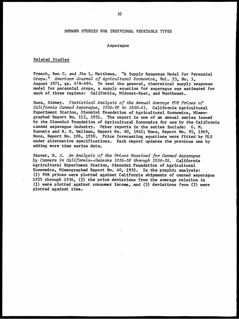
JERRY FOYTTK. Demand Characteristics for Vine Vegetables in Honolulu,

Hawaii, 1947-1961. Hawaii Agricultural Experiment Station, Bulletin No.

23, July 1964.

Scope: Snap beans, cucumbers, and tomatoes at the Honolulu wholesale

market.

Purpose: To analyze empirically how monthly price and quantity data

indicate that changes in market supply are responsible for much of the

variation in prices of vine vegetables.

Observational Interval: Monthly.


Specification and Estimation Procedure: For each vegetable, a price

dependent equation was fitted as function, parabolic in both quantity

and time. Then, monthly shift effects were determined graphically.

Estimation Results:

Snap beans

P = 37.00 - 17.50 + 1.402 + 0.555T + 0.542T

2 + f(M)

Cucumbers

P = 26.57 - 7.90Q + 0.80,2 + 0.162T + 0.0448T2 + f(M)

Tomatoes

P = 29.82 - 4.40Q + 0.30,2 + 0.153T + 0.0969T

2 + f(M)

where:

P = monthly wholesale price, cents per pound;

= monthly wholesale market supply in 100,000 pounds;

T = time measured from 1954;

f(M) = the monthly effect determined graphically.

38

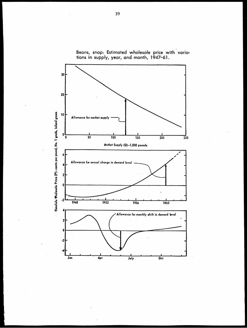
The top panels of the following three figures show the parabolic

price-quantity relationships when the trend and seasonal effects are set

at their means (zeroes) for the period of study. The annual shifts in

demand are shown in the middle panels, holding quantities constant at their

means. Finally, the residuals from the equations were plotted (12 obser-

vations each year, each equation) and the monthly effects were graphed

(bottom panels). The curves in the bottom panels show the shifts in the

price-quantity relationships from month to month as the year progresses.

FlwAPD Y. KREBS, MAPVIN L. PAYENGA, and JOHN N. LEHKFR. Various Price and

Supply Contro7 Programs for Navy Beans: A Simulation Analysis. Michigan

State University, Department of Agricultural Economics, Report No. 212,

January 1972.

Scope: U.S. demand for navy beans (99 percent Michigan produced).

Purpose: "To explore the effects of variations in these (government commodity)

programs, a computer simulation model of the navy bean's supply and demand

behavior was developed and employed," p. 3.



Specification and Estimation Procedure: For use in the simulation model a

three equation demand model was estimated by 3SLS in which the four endogenous

variables were: domestic use of navy beans, exports, price, and small white

bean price. A fourth equation established an identity.

39

Hono

lulu

Wholesale Pri

ce (P)--

cents pe

r pound, No. 1 gra

de, Island grown

30

20

10

Beans, snap: Estimated wholesale price with varia-tions in supply, year, and month, 1947-61.

Allowance for market supply

50 100 150 200 250

Market Supply (2)-1,000 pounds

Allowance for annual change in demand level

1948 1952 1956 1960

-4

(Allowance for monthly shift in demand level

Jan Apr July Oct

40

Honolulu Wholesak Price (P) --

cents per pound, No. 1 grade, Island grown

Cucumbers: Estimated wholesale price with variationsin supply, year, and month, 1947-61.

20

154-

10

f0


100 200

Market Supply (Q)--1,000 pounds

300 400

Allowance for annual change in demand level

. I . I I 1948 1952 1956 1960

Allowance for monthly shift in demand level

elm

JanI

Apr July Oct

41

20

15

Tomatoes: Estimated wholesale price with variationsin supply, year, and month, 1947-61.


300 400 500

Market Supply (3)-1,000 pounds

600 700

Allowance for annual change in demand level.

aI a a a I a a a I a a a I a

-2

1948 1952 1956 1960

Allowance for monthly shift in demand level

-4 4—I--Jan

• a I I

Apr July Oct

42

Estimation Results:

pomp* - -548.0 - 80.2 PNB* + 13.6 PSW* + .024 USPOP + 696.3 D1(.097) (.026) (.877) (.513)

R2 = .75

EXQ* = -15,332.2 - 63.8 PNB* + .324 UKPOP(.401) (4.186)

R2

.55

PSW* = -2.3 + .736 PNB* - .0034 PRODSW + .0005 USPOP(3.359) (3.090) (2.582)

R2 = .88

PRODNB-CCCQt = Ding, + EXQt CANEXt

where: * = endogenous variable;

DOMQt • = total U.S. commercial consumption of Michigan navy beans in

year t (1,000 cwt.);

EXQt • = total U.S. and Canadian export shipments of navy beans in year

t (1,000 cwt.);

PNBt • = average quoted grower price for CHP navy beans--September

through April in year t ($/cwt.);

PSW • = average quoted grower price for small white beans--Septemberthrough April in year t ($/cwt.);

USPOPt

= U.S. population in year t (1,000 people);

D1

= dummy variable (1 if 1958 or after, 0 if not) to account for an

otherwise unexplained demand shift apparently occurring in 1958;

UKPOPt

= United Kingdom population in year t (1,000 people);

CANEXt

= total Canadian exports of navy beans in year t (1,000 cwt.);

PRODSWt

= total small white bean production in year t (1,000 cwt.);

PRODNBt

= Michigan annual production of navy beans in year t (1,000 cwt.);

CCCQt = Commodity Credit Corporation acquisitions of navy beans in

year t (1,000 cwt.).

(t-statistics are in parentheses.)

43

R. J. VANDENBORRE. An Econometric Investigation of the Impact of Governmental

Support Programs on the Production and Disappearance of Important Varieties

of Dry Edible Beans. California Agricultural Experiment Station, Giannini

Foundation of Agricultural Economics, Research Report,No. 294, December 1967.

Scope: White beans (navy, small white, and great northerns), blackeyes, and

large and small limas in the U.S.

Purpose: It. . . to evaluate the impact of governmental support programs on

the production and disappearance of some varieties of dry edible beans . . .

Primarily, the study attempts to answer this question: What would have been

the situation with respect to production and disappearance of these com-

modities had there been no price-support program for them?" p. 1.


Period of Analysis: 1948/49 through 1963/64.

Specification and Estimation Procedure: Both a supply-response model and a

price-demand model were estimated. Since government takeover of a commodity

is a function of the difference between the free-market price and the support

price, and since the free-market price cannot be observed in years when

takeover actually occurs, in the demand model, government acquisitions were

estimated by: (1) the support price and (2) factors thought to determine

the free-market price. A six-equation model was estimated for white beans

by TSLS: disappearance and government acquisitions of navy beans, dis-

appearance and acquisitions of small whites, ending stocks of small whites,

and price of great northern beans. Since there was no government program

for blackeyes, a two-equation model--supply and price--sufficed. For large

and small limas, again a six-equation model was estimated by TSLS. The

estimations were then used to simulate the behavior of the dry bean market

under various assumptions about government interference.

44

Price-demand structure for white classes of dry edible beans

• %.1/v = 3.62477 - .28322 y,,. + .08269 (v-7t +(.09190) (.05373)-10t Yl2e

- .90644x + .78091 x7t +u

7tit •(.41081) (.12587)

2R2 = .92 d = 2.81 (0.-

/

714t -;-1.58754 - .01929

(YlOt Yl2t) + .01105 v(.18235)

-26t(.05564)

+ .55279 x + .69240 it x2t + .03092 x

5t - .81436 x + u

(.46998) (.18010) (.15200) (.18236) it 8t

R2 = .92 d- 3.02 (i)

v 8t

= .32261 + .08889 Yllt

.08568- (.01677)

Y12t '30965 xlt u9t(.01876) (.09968)

R2 = .74 d = 2.02 (n)

v = -.62231 - .05285 y + .03245 y27t - .11106 xit-13t (.01818) llt

(.01909) (.06045)

+ .55341 x4t + .11209 x

6t + u

10t- (.18029) (.02629)

R2 = .86 d = 2.27 (i)

y9t = .008$0 - .02011 yin + .00892 v :g 9) (22594 Y13t +:02:2) x4t ullt(.00834) (.00979)

- (12t

R = .71 d = 2.59 (i)

YlOt 3.09932 + .48622

Yllt .07555 x3t + 1.73402 xit + 1112

(.22027) (.58355) (2.0561)

R2 = .39 • . d = 2.48 (i)

1/ Coefficients on y10t

and y12t

were nearly identical; to save on

on degrees of freedom'

v 10t

and ynt were added together and the equation- run again.

2/ Where the symbol (i) follows the statistic d, the Durbin-Watsontest for serial correlation of the error term was inconclusive; (n) indicatesthat the test showed no serial correlation.

45

where:

Y7t

8t

379t

= commercial wholesale disappearance of navy beans in pounds percapita in t (production + beginning stocks + government domesticsales - government takeover - direct purchases by the government);

= commercial wholesale disappearance of small whites in pounds percapita in t (production + beginning stocks - government takeoverending stocks);

= commercial ending stocks of small whites in pounds per capita in ;

10t = average wholesale price of great northerns in cents per pound;

= average wholesale price of navy beans in cents per pound;llt

y12t

= average wholesale price of small whites in cents per pound;

13t = government takeover of small whites in pounds per capita in t;

Yl4t = government takeover of navy beans in pound's per capita in t;

26t = difference between actual market price of navy beans per poundand the support price in t

Y27t = difference between actual market price of small whites per pound and the support price in t;

xlt

= log of disposable income per capita (original series--thousanddollars per capita);

x2t

= production + beginning stocks + government domestic sales ofnavy beans - direct government purchases in pounds per capitain t;

x3t

= production + beginning stocks of great northerns in poundsper capita in t;

x4t

= production + beginning stocks of small whites in pounds percapita in t;

xSt

= support price of navy beans in cents per pound in t;

x6t

= support price of small whites in cents per pound in t;

46

and

x7t m dummy variable in the navy bean model (x7t E= 1 for 1958/59

through 1963/64, 1.2 0 for all other years).


Price-demand structure for blackeyes

Yl5t61857 + .01659

i;11t 021843 y

16t15951 xit +u nt

"(.01169) (.00497) (.07372)

R2 = .74 d = 2.32 (n)

'17t -.04649 - .00224

-00743 yi6t + .36962 x9t +

11t ul4t

-(.00481) (.00734) (.11436)

where:

R2 = .76 d = 2.12 (n)

15t = production t + beginning stocks t - ending stocks t in pounds

per capita;

16t average price of blackeyes in cents per pound in t;

= 17t

ending stocks of blackeyes in pounds per capita in t;

= average price of navy beans in cents per pound in t (computed);9Ilt

x9t production t blackeyes + beginning stocks t blackeyes in poundsper capita.


Price-demand structure for limas:

y18t

= 1.23907 - .03277 N 4- .02424 y23t - .77652 x.(.00659)

22t(.01686) (.06442)

It u: 15t

R2 = .96 d = 1.51 (i)

y19t = .12194 + .00789 y - .02607 y23t .73945 y24t + .08727 )(lot + 1116t

(.00456) 22t

(.01586) (.32217) (.06190)

R2 = .48 d = 2.81 (i)

1/v = 34.82951 + .82261 y23t

+ 14.46928 v 23.69600- x'28t it(.74234) (13.37828)-24t

- 26.87131 x10t

- .79155 x12t

+ u17t(3.34720) (.76117)

R2 = .96 d = 1.67 (i)

47

Y21t 16107 - .01309 y23t - .09927 v'18t

.09627 y25t + .08251 xlit + unt

(.00627) (.07994) (.25715) (.12663)

R2 = .37 2.12 (n)

y 1

- .13745 y22t + .10670 y29t - 2.90368 xlt.-/= 469705 - 4.20760Y25t 18t

(.16208) (.09549) (.01908)

+ .97589 xllt

+ .09871 x13t + u20t

(.11857) (.03583)

R2 = .98 d = 2.50 (i)

Y20t= -4.85796 + .14110 y

22t - .09951 Y23t 4'35855 Y18t

(.01181) (.01210) (.34519)

+ 2.90368 xlt

+ u1St(.27002)

R2 = .98 d 2.40 (i)

where:

Y18t = production t + beginning stocks t - ending stocks t - government

takeover t of large limas in pounds per capita;

= ending stocks of large limas in pounds per capita in t;Yl9t

= 20t

production t + beginning stocks t - ending stocks t -government takeover t of small limas in pounds per capita;

= 321t

ending stocks of small limas in pounds per capita in t; 7

22t = wholesale price of large limas in cents per pound in t;

23t = wholesale price of small limas in cents per pound in t;

Y24tgovernment takeover of large limas in pounds per capita in t;

=

525tgovernment takeover of small limas in pounds per capita in t;

7=

28t difference between actual market price of large limas in tand support price in t;

329t = difference between actual market price of small limas in t 7

and support price in t;

48

and

x10t

= production t + beginning stocks t of large limas in poundsper capita;

xllt

= production t + beginning stocks t of small limas in poundsper capita;

x12t

= support price of large limas in cents per pount in t;

x13t

= support price of small limas in cents per pound in t.


TABLE 2: Selected Econometric Analyses With Flexibility or Elasticity Estimate!:; for Beans

Author andDate

Geograph-ical Area

TimePeriod

Observa-tionalInterval

Form ofEquation

Method ofEstimation

MarketLevel Product

PriceFlexibility

PriceElasticity

IncomeElasticity

CrossElasticity

Droge andReed, 1973

U.S. andWisconsin

1948-1968 Annual linear OLS FOB National

cannerbrand

Wisconsinprivatelabel

-.1506

-.4096

Foytik Hawaii 1957-1961 Monthly linear OLS Wholesale fresh

snapbeans

a/1.-0.625-11.-1.062111.-0.696IV.-0.621

Krebs,Hayenga,and Lehker,1972

U.S. 1951-1967 Annual linear 3SLS farm navy

beans -0.14

Vandenboore,1967 U.S. 1948/49-

1963/64 Annual linear TSLS farm navy

smallwhitesblackeyessmalllimaslargelimas

-0.81

-2.01-0.44

-2.50

-0.68

-1.62

+0.55-0.35

+5.19

-1.38

1.73.S./

0.28$-"

d/5.78-

e/0.31-

a/ Four quarters of the year

b/ wrt. small whites

c/ wrt. navy

d/ wrt. large limas

e/ wrt. small limas

50

Related Studies, Beans

Allen, M. B. and A. D. Seale, Jr. An Evaluation of the Competitiv Position

of the Snap Bean Industry in Mississippi and Competing Areas. MississippiAgricultural Experiment Station, Agricultural Economics Technical PublicationNo. 3, December 1960. This report was not available, but it is presumed thatthe treatment was similar to the report on the green pepper industry--reviewed here on page 117 and the one on the cabbage industry—reviewed onpage 56.

Cain, Jarvis L. and Ulrich C. Toensmeyer. Interregional Competition inMaryland Produced Fresh Market Green Beans. Maryland Agricultural ExperimentStation, MP 731, October 1969. The transportation model was utilized toevaluate the least cost distribution pattern for fresh green beans grown inMaryland and in competing states. The optimum distribution pattern from 31shipping points to 15 major cities was compared to the actual pattern andon the basis of discrepancies, possible alternatives were suggested toMaryland growers.

Hathaway, Dale E. The Effects of the Price Support Pro grain on the Dry BeanIndustry in Michigan. Michigan Agricultural Experiment Station, TechnicalBulletin No. 250, April 1955. Three statistical models were developed fordry beans: acreage planted, yield, and price. In the two structuralequations, (1) Michigan farm price was seen as a linear function of theamount delivered to the government under the price support program (endogenous),supply of U.S. pea and medium white beans, consumer income, and supply ofgreat northern beans; (2) the amount delivered to the government, as a functionof supply minus the right hand side of equation (1)--i.e., price. The reducedform was estimated by OLS, and the structural coefficients were recovered.

Nichols, T. Everett. Interregional Competition in Marketing Snap Beans. NorthCarolina State University, Agricultural Economics Information Series No.113, April 1964. The transportation model was used to determine the optimumshipping pattern of snap beans to 22 major markets from 25 to 30 states forselected weeks of 1956.

51

Brussels Sprouts

Abstract

BFN C. FRENCH and MASAO MATSUMOTO. An Analysis of Price and Supply Rela-

tionships in the U.S. Brussels Sprouts Industry, California Agricultural

Experiment Station, Giannini Foundation of Agricultural Economics, Research

Report No. 308, March 1970.

Scope: U.S. demand for California-grown frozen and fresh Brussels sprouts.

Purpose: "to develop economic information which may aid the thinking of

leaders in the Brussels sprouts marketing program and also be of value

to individual firms, growers, and public agencies concerned with the

industry," pp. 1-2.



Specification and Estimation Procedure: Brussels sprouts demand estimates

were made at several levels as part of a complete system describing the total

economic environment in which Brussels sprouts are produced and marketed.

The report explains the theoretical relationships believed to hold, derives

the equations to be estimated empirically, and then uses the results to

generate expected values of the endogenous variables under alternative

conditions that may hold in the future.

Farm-level demand involved four equations in this one component of the

model. The first three--(1) freezer demand for the raw product, (2) frozen

allocation, and (3) fresh allocation were estimated as a simultaneous system

by TSLS. The fourth--fresh market demand--was estimated by OLS. Because of

52

multicollinearity between per capita food expenditures and per capita

disappearance of frozen Brussels sprouts, the equation was constrained

by the assumption that the coefficient of the former was equal to one

(for a one percent increase in expenditures on food, a one percent increase

In the price of fresh Brussels sprouts was assumed).

Another component of the model involved estimating the U.S. demand

facing freezers. This relationship was estimated both by OLS, and by

TSLS with a sales allocation equation.

Estimation Results:

Farm-Level Equations

Freezer Raw Product Demand

Qpct - 172 P )Dpct-1

= 1.5352 + 0.0576 (Ppct-1 - c

pct-1 1.

gpct(0.0178)

SUBt - 1.8455 0.0350 L

t.

(0.4169) Dpu8t-1 (0.0903)

,Frozen Allocation

Qpct = 0.2853 + 0.2551

Pgpct - 0.0754 F

gfct-1Dpct-1 (0.0484) (0.0473)

- 0.0787 Cct - 0.4687 Lg .

(0.0696) (0.1540)

where

1=Pgfct 2 gfct-1

+ Pgfct-2).

53

Fresh Allocation

.Qfct

= Bct

Act - 1.172 Q

pct

Fresh Market Demand

log Pgfct

where:

= 5.6766 - 0.5830 log Xbpt

- 0.6887 log Xbft(0.1317) (0.1954)

- 3.5835 log Xvt + 1.0000 log Ft

(1.8737)

R2 = .56 DW = 1.62

0 = quantity of Brussels sprouts frozen in California, millionPc

pounds;

D = quantity of California frozen Brussels sprouts sold (disappear-pc

ance), August 1 - July 31, million pounds;

P c = average f.o.b. California freezer price for Brussels sprouts,p

grade A, 10-ounce packages, cents-per pound;

C = cost of freezing Brussels sprouts in California excluding rawpc

product cost, 10-ounce packages, cents per pound;

= average price received by California growers for Brusselsgpc

sprouts for freezing, cents per pound;

S = United States cold storage holding of Brussels sprouts onAugust 31, million pounds;

US

= United States quantity of frozen Brussels sprouts sold (dis-pus

appearance), August 1 - July 31, million pounds;

L = A dummy shift variable to allow for possible changes in levelof supply response or allocation with the establishment of theBrussels Sprouts Marketing Program. L = 0 prior to 1958; L = 1from 1958;

54

= average price received by California growers for fresh marketgfcBrussels sprouts, cents per pound;

C = representative cost of growing Brussels sprouts in California,gccents per pound;

0fc = quantity of fresh market Brussels sprouts produced in California,

million pounds;

Pc = yield per acre of Brussels sprouts in California, cents per acre;

Ac = acres of Brussels sprouts planted in California;

'bp = D N = United States per capita disappearance of frozen

pusBrussels sprouts, pounds;

Xbf = 0fus 4- N = United States per capita disappearance of fresh

Brussels sprouts, pounds;

Xv = United States per capita total vegetable consumption, pounds

retail weight, calendar year;

F = United states per capita total food expenditures expressed asan index, 1957-1959 = 100.

(ctandard errors are in parentheses.)

Ordinary least squares

log P =pct

Demand Facing Freezers

5.8161 - 0.6322 log Xbpt

- 0.1528 log Xbft(0.0780) (0.1157)

- 3.2167 log X + 1.0000 log Yt

(1.1095) vt

P2 = .88

Two-stage least squares

DW = 1.70.

log. PPct

= 5.8975 - 0.6747 log X, - 0.2020 logDpt Xbft

(0.0775) (0.1130)

- 3.2898 log Xvt + 1.0000 log Y.

(1.0508)

55

where:

Variables are as defined previously and

Y = R • F

R = proportion of United States homes with refrigerators.

\

56

Cabbage

Abstracts

Y. P. ALLEN and A. D. SEALE, JR. An rvaluation of the Competitive Position

of the Cabbage Industry in Mississippi and Competing Areas. Mississippi

Agricultural Experiment Station, Agricultural Economics Technical Publication

No. 2, September 1960.

Scope: Cabbage unloads from Mississippi and competing early spring pro-

duction areas (including California) at 35 consuming centers.

Purpose: To describe production trends, estimate demand in specified con-

suming centers, estimate transportation charges, and determine prices and

revenues which would be associated with different situations.

Observational Interval: Weekly.

Period of Analysis: April 25 through July 19, 1959.

Specification and Estimation Procedure: Because of the incompleteness of

the data in some of the consuming centers, an analysis of the price-quantity

relationships was made for each center for the eight marketing weeks, but

only those giving an inverse relationship were used in the price equation.

Eight centers and data for eight weeks made a total of 64 observations for

use in estimating the overall price equation by OLS in double log form.

Statistical tests revealed significant differences in intercepts among the

eight weeks; the adjustments were reported. Besides the quantity variable,

the population variable had a statistically significant coefficient which

was used to adjust the intercept according to the population of each of the

35 consuming centers.

57

Based on the estimated demand functions, the optimum distribution

pattern- -maximizing net revenues to producing areas --was computed.

Estimation Results:

For all eight periods:

ln P = 4.40548 - .43138 lnX1 + .37923 InX

2(.07722) (.08667)

R2 = .319

where:

P = average weekly wholesale price in dollars;

= quantity in carlot unloads;

X2 = population in thousands.


D. MILTON SHUFFETT. The Detrand and Price Structure for Selected Vege-

tables. Abstracted under tomatoes on page 158.

TABLE 3: Selected Econometric Analyses With Flexibility or Elasticity Estimates for Cabbage

Observa-Author and Geograph- Time tional Form of Method of Market Price Price .

Date ical Area Period Interval Equation Estimation Level Flexibility Elasticity

Allen andSeale 1960 U.S. April Weekly double

25- logJuly19,1959

OLS Wholesale -.431

Shuffett,1954 U.S. 1921- Annual first

1941 differ-ences ofthe logar-ithms

OLS farm -2.398

OD

59

Related Study, Cabbage

Mathia, Gene A. and Richard A. King. An Analysis of Locatione Advantagein the National Cabbage Market. North Carolina University, EconomicsResearch Report No, 8, January 1969. Using the transportation model, theactual and the optimum shipping patterns for spring and for fall cabbagefrom shipping points in four regions of the country to 22 receiving marketswere compared.

60

Carrots

Abstracts

ROBERT W. BOHALL. Pricing Performance in Marketing Fresh Winter Carrots.

USDA, ERS, Marketing Research Report No. 963, 1972.

Scope: Vinter carrots marketed in 10 major consuming centers geographi-

cally dispersed across the United States.

Purpose: "To evaluate whether short-run changes in carrot prices were

consistent with a competitive marketing system. . ." p. 2.


Period of Analysis: First week of January through the last week in March

for three years--1966, 1967, and 1968.

Specification and Estimation Procedure: As part of the analysis the re-

lationship between FOB prices of Lower Rio Grande Valley carrots and the

quantity of carrots available--both from Texas and from Southern California-

Arizona--was estimated by OLS. Also included were rainfall and temperature

variables to capture the effect of the weather on quality.

In addition, the difference between shipping-point and consuming-

center prices was explored and found to be directly related to the costs

of transporting, handling, and storing the carrots.

Estimation Results:

Y = 12.76 - 0.0063 XCTJ

= 0.0107 XCCAj

= 0.172 Rj - 0.047 T

j-1Cj(0.0027) (0.0021) (0.018) (0.016)

- 0.039 Tj-2

(0.015)

where:

DW = 0.95 R2 = 0.88

YCj

= the FOB price of Lower Rio Grande Valley carrots,48-1's mesh, in week j;

61

XCTj

= total carlots of carrots shipped from Texas in week j;

XCCAj

= total carlots of carrots shipped from California andArizona in week j;

R = deviation from normal Lower Rio Grande Valley rainfallfor Division 10 the previous September = -0.34 inchesin September 1965 for winter 1966; -3.18 inches In Sep-tember 1966 for winter 1967; and 14.07 inches in Septem-ber 1967 for winter 1968;

TJ1 2

= average high temperature at Weslaco, Tex., weather sta-tion 2E, j-1 = previous week, j-2 = week 2 weeks previous:and

j = weeks 1-39 with 1-13 = winter 1966; 14-26 = winter 1967;and 27-39 = winter 1968.


CARL E. SHAFER. A Statistical Analysis of Season's Average Prices for

Texas Winter Carrots and Early Spring Onions, 1954-64. Texas A & M Uni-

versity, Department of Agricultural Economics and Sociology, Technical

Research Report No. 66-2, 1966.

Scope: Texas grower-level and FOB, and California FOB carrot prices;

Texas grower-level onion prices.

Purpose: "(1) to develop price equations which would he useful in both

explaining past price behavior and in forecasting the forthcoming season's

average price and (2) to provide some evaluation regarding volume restric-

tion policies for carrots and onions." p. 1.



Specification and Estimation Procedure: Alternative specifications for

the grower-level carrot equations included: data on a per capita and on a

total basis, in linear and double log form, in first differences and in

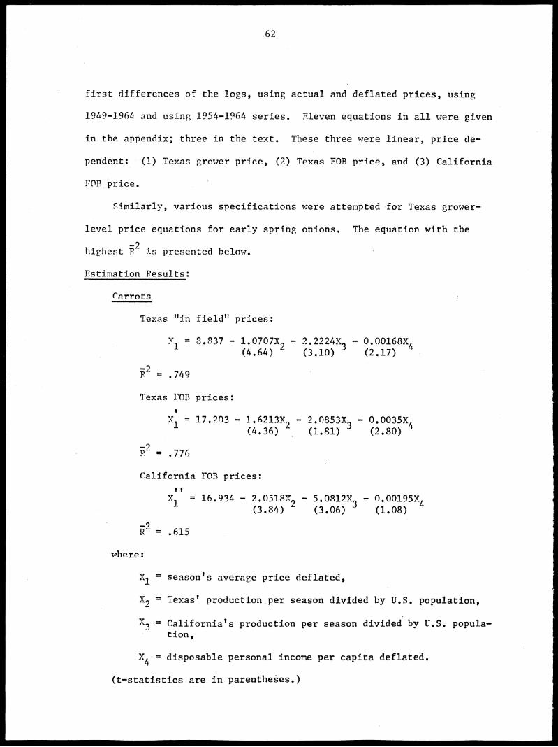
62

first differences of the logs, using actual and deflated prices, using

1949-1964 and using 1954-1964 series. Eleven equations in all were given

in the appendix; three in the text. These three were linear, price de-

pendent: (1) Texas grower price, (2) Texas FOB price, and (3) California

FOB price.

Similarly, various specifications were attempted for Texas grower-

level price equations for early spring onions. The equation with the

-highest P

2 is presented below.

Estimation Results:

Carrots

Texas "in field" prices:

= 1

8.837 - 1.0707X2 - 2.2224X - 0.00168X

4 (4.64) (3.10) (2.17)

-9R- = .749

Texas FOB prices:

X1 = 17.203 - 1.6213X

2 - 2.0853X

3 - 0.0035X

4(4.36) (1.81) (2.80)

-1P- = .776

California FOB prices:

it

X1

= 16.934 - 2.0518X2 - 5.0812X

3 - 0.00195X

4(3.84) (3.06) (1.08)

_2R - = .615

where:

X1 = season's average price deflated,

X2 = Texas' production per season divided by U.S. population,

X1 = California's production per season divided by U.S. popula-tion,

X4 = disposable personal income per capita deflated.


63

Onions

X1 = 12.2705 -

0.001118X2 " - 0 001105X

3(4.22) (4.47)

-2R = 0.72

where:

X1 = deflated season's average price received by Texas growers

in dollars per hundredweight,

X2 = season's early spring onion production in Texas in 1,000

hundredweight units,

X3 = stocks of onions on hand January 1 in 1,000 hundredweight

units.


- CARL E. SHAFER and CHRISS H. CARLSON. Intraseasonal Price Analysis for

Texas and California Carrots. Texas A & M University, Department of

Agricultural Economics and Rural Sociology, Technical Report No. 71-5, 1975.

Scope: Texas carrots, December through May; California carrots, May

through November.

Purpose: tt. . .to examine weekly price and supply variables so that an

optimum within season or intraseasonal rate of movement-to-market patterns

may be developed.

Observational Interval: Annual, monthly, and weekly.

Period of Analysis: Annual, various time periods; monthly, 1966 through

1969; weekly, 1956 through 1968 and 1966 through 1969.

Specification and Estimation Procedure: First, several season average price

(annual data) equations were fitted by nu for various time periods. Texas

FOB prices, Texas grower-level prices, and California prices were seen as

64

functions of Texas production, California production, income, and a dummy

variable for the 1961-1966 marketing order. FlexThilities for the Texas

FOB level, 1954-1969 equation appear in Table 4.

Next a monthly analysis was performed using Texas FOB prices for

December-nay and California FOB prices for June-November. Price, lagged

one month, was an important variable in four of the equations.

Using weekly data--Texas FOB prices for the first 20 odd weeks and

California (Salinas) prices for the remainder of the year--several equa-

tions were fitted: one for each year, 1956-1968; one pooling all the

data; and one using dummy variables to allow yearly intercept shifts.

The latter equation is presented below.

Finally, several alternative specifications were run using weekly

data for 1966-1968. Fifty-two week series used both Texas and California

prices, and separate estimations used Texas prices only and California

prices only. In some of the equations, price, lagged one week, was a sta-

tistically significant variable. In one Texas-California price equation,

,a dummy variable was used to separate the two price series and it re-

vealed that Texas FOE prices were on the average about 21 cents per bag

greater than California prices.

Estimation Results:

P'= -0.03200 TXSH -0.00612 CFRR -0.05601 CFTR(6.89) (0.40) (2.05)

-0.01988 OTKH -0.73339 INPC + 18.392 (1956)(6.43) (2.86) 18.299 (1957)

19.085 (1958)19.015 (1959)18.575 (1960)

R2 = 0.67

where:

65

19.881 (1961)

20.430 (1962)

20.238 (1963)

21.059 (1964)

21.777 (1965)

23.675 (1966)

23.583 (1967)

27.369 (1968)

P = FOB weekly shipping point price; Texas prices for first 20odd weeks and California prices (Salinas) for the remainderof the year.

TXSH = Texas shipments, carlot equivalents/10;

CFRR = California rail shipments, carlot equivalents/10;

CFTR = California truck shipments, carlot equivalents/10;

OTRH = on-track holdings of carrots at 16 terminal markets,carlot equivalents/10;

INPC = quarterly per capita income.


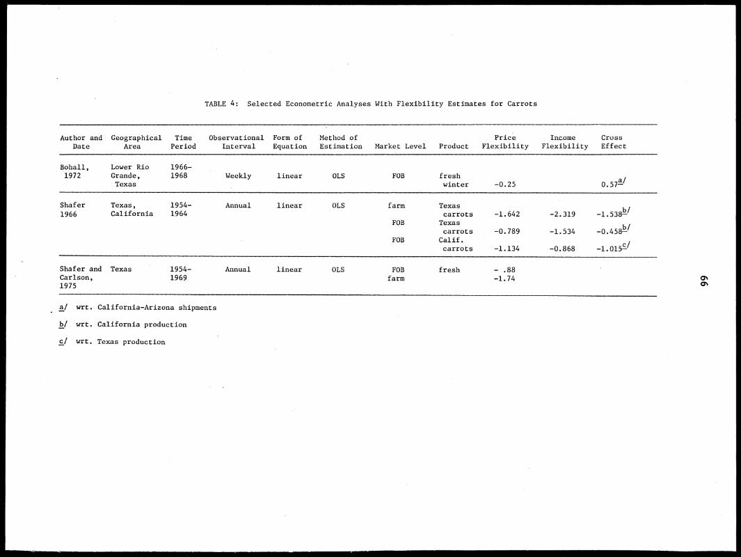
TABLE 4: Selected Econometric Analyses With Flexibility Estimates for Carrots

Author andDate

GeographicalArea

TimePeriod

ObservationalInterval

Form ofEquation

Method ofEstimation Market Level Product

PriceFlexibility

IncomeFlexibility

CrossEffect

Bohall,1972

Lower RioGrande,Texas

1966-1968 Weekly linear OLS FOB fresh

winter -0.25a /

0.5T-

Shafer

1966

Texas,California

1954-1964

Annual linear OLS farm

FOB

FOB

TexascarrotsTexascarrotsCalif.carrots

-1.642

-0.789

-1.134

-2.319

-1.534

-0.868

-1.53811/

b/-0.458--

c/-1.015-

Shafer andCarlson,

Texas 1954-1969

Annual linear OLS FOBfarm

fresh - .88-1.74

1975

a/ wrt. California-Arizona shipments

b/ wrt. California production

C! wrt. Texas production

67

Related Studies, Carrots

Shafer, Carl F., A Preliminary Analysis of Price and Demand Relationshipsfor South Texas Pinter Carrots. Texas A & M University, Department ofAgricultural Economics and Sociology, Department Information Report 65-1,1965. Price-quantity relationships for South Texas winter carrots at theretail, FOB, wholesale, and grower levels were discussed and graphed.

Shafer, Carl E., "The Effect of a Marketing Order on Winter Carrot Prices."American journal of Agricultural Economics, Vol. 50, No. 4, November 1968,pp. 879-887. In order to test the hypothesis that during the marketingorder period (1961-1966), the demand curve for Texas carrots shifted out-ward, three linear regressions were run including a dummy variable forthe marketing order years. The variable was statistically significant inthe Texas grower-level price equation but not in the FOB-level nor in theCalifornia FOB price equation. The conclusion was that demand relationsfor carrots in Texas and in California did not appear to shift signifi-cantly during the marketing order period but that the in-field--FOB mar-gin was narrowed.

68

Celery

Abstracts

THOMAS S. CLEVENGER. Price Prediction Equations for Michigan Cooperative

CeZery. Michigan State University, Agricultural Economics Report No. 122,

April 1969.

scope: Michigan Celery Promotion Cooperative prices.

Purpose: To develop equations computationally usable to the Cooperative

Price Committee.


Period of Analysis: 1963 through 1966 (also updated through 1967).

Specification and Estimation Procedure: The 15 week marketing season was

divided into two periods of seven and eight weeks, respectively, because

a better fit was obtained for the two equations than for a single one.

Also the source of competing celery switched--Santa Maria, California, in

the first period, Salinas, California, in the second. The linear equations

were estimated by OLS. At the end of the report they were reestimated,

including 1967 data.

Estimation Results:

First period (seven weeks)

lm, t += 62.7915 - 0.00190 + 0.9680P

1P -1m(30.4854) (0.0010) (0.0551)Th

f'

t

9R- = .95

where:

+ I = Michigan Celery Promotion Cooperative unweighted averagePlm, t

FOB shipping point price in cents per crate of 2-1/2size celery for any week t + 1 during the first sevenweeks of the Cooperative's marketing season.

69

0 = Sun of (1) number of MIct,ipan Celery Promotion Coopera-tive 2-1/2 dozen crates on inventory Saturday eveningfor any week t, and (2) number of richlgan Celery Pro-motion Cooperative 2-1/2 dozen crates harvested for anyweek t + 1, both prior to the eighth week of the Coop-erative's marketing season.

f = Midpoint of santa Maria, California, FOB shippingn, t

point price range in cents per crate of 2-1/2 sizecelery on Friday of week t prior to the eighth week ofthe Cooperative's marketing season.


Second period (eight weeks)

= 97.1591 - 0.00280, + 0.2351P + 0.5216Psf, r2m, t +(33.5785) (0.0009)

LA11 (0.0734)

7717 (n.1385)

P2 = .7R

where:

t + 1

+ 0.1234Pof t

(0.0597) '

= michigan Celery Promotion Cooperative unweighted averageFOB shipping point price in Cents per crate of 2-1/2size celery for any week t + 1 during the last eightweeks of the Cooperative's marketing season.

= Sum of (1) number of Michigan Celery Promotion Coopera-tive 2-1/2 dozen crates on inventory Saturday eveningfor any week t from the seventh week on, and (2) numberof Michigan Celery Promotion Cooperative 2-1/2 dozencrates harvested for any week t + 1 from the eighth tothe season's completion.

Pm7

= Michigan Celery Promotion Cooperative unweighted averageFOB shipping point price in cents per crate of 2-1/2size celery during the seventh week of the Cooperative'smarketing season.

Psf, t

= Midpoint of Salinas, California, FOB shipping pointprice range in cents per crate of 2-1/2 size celery onFriday of week t from the seventh week to the week priorto the season's completion.

Pof, t

= Midpoint of Orange County, New York, FOP, shipping pointprice range In cents per crate of 2-1/2 size celery onFriday of week t from the seventh week to the week priorto the season's completion.


70

7kTARSITALL P. COWIN and BILLIE q. LLOYD. Competition Between Florida and

California Celery 1711 the Chicago PParket. Florida Agricultural Experiment

Station, Bulletin No. 636, vovember 1961.

Scope: Florida and California celery in nine large supermarkets in the

Chicago metropolitan area.

Purpose: To determine the nature of the competitive relationship between

California and Florida celery.

Observational Interval: Daily.

Period of Analysis: Nay and June 1958.

Specification and Estimation Procedure: Displays of Florida Pascal type

celery were placed adjacent or near to the Utah type, California-grown

celery in nine Chicago supermarkets. The stores were carefully selected

so that three drew from high income clientele; three, from medium; and

three, from lower Income groups. An attempt was made to hold all factors

other than price (e.g. size, grade, quality of the display) constant. On

the assumption that the competitive advantage lay with California celery,

in all test combinations, the Florida product was sold at prices lower

than the price of the California product. Price differences ranged be-

tween two and 18 cents. From the data, double-log quantity-price relation-

ships were estimated by nLS and cross elasticities examined. The effects

on Florida price of various supply changes from either Florida or Cali-

fornia celery were discussed and shown in several three dimensional graphs.

Estimation Results:

in 01 = 1.14475 - 1.015691nP

1 + 0.587091nP

2'

ln 07 = 3.20911 + 0.659471nP1 - 2.553011nP

2

71

where:

= quantity Florida celery purchased,'1

0 = quantity California celery purchased,'2

P1 = price of Florida celery,

P9 = price of California celery.

72

Related Studies, Celery

Godwin, Marshall R., Competitors in the Celery Market. Florida Agricul-tural Experiment Station, Agricultural Economics Report No. 59-6, February1959. A report based on the same study as the one reviewed here on page70. The Agricultural Economics report was written in less technicallanguage than WAS the Bulletin.

Godwin, Marshall R. and William T. Manley, Customer Preference Aspects ofCompetition Between Florida and California Celery. Florida Agricul-tural Experiment Station, Bulletin No. 648, June 1962. Consumer testswere done in four large retail stores in Dayton, Ohio. Comparisons weremade between Florida Summer Pascal and the Utah type grown in Californiaand between the Utah type grown in Florida and the same type grown inCalifornia. Results indicated that the Utah type from either state N.Tspreferred to the Pascal type and that there wasn't much difference be-tween the two Utah types--unless the place of origin was identified. Inthis latter case, celery from California was clearly preferred. In allcombinations, prices were the same for both.

73

Corn, Sweet

Abstracts

D. L. BROOKE and J. B. BELL. Market Structure and the Economic Analysis

of the Florida Sweet Corn Industry. Florida Agricultural Experiment

Station, Bulletin No. 696, October 1965.

. Scope: Florida sweet corn FOB prices.

Purpose: "to develop basic economic information necessary to an under-

standing of the market structure of the Florida sweet corn industry."

p. 6.

Observational Interval: TJeekly--the winter season from the second week

in February through the third week in February; the spring season from

the last week in February through the last week in May.


Specification and Estimation Procedure: Ten independent variables were

considered in the explanation of the variation in the weekly FOB price.

Using a stepwise regression procedure, these were narrowed to three:

Florida carlot shipments, the terminal market price of the previous week,

and the market tone on Monday. The resulting equations--one for fall and

winter, one for spring--were satisfactory for price prediction purposes

(R2 = .86; .92, respectively), but multicollinearity prevented the deri-

vation of significant price elasticities. Consequently, a regression for

each season was fitted in which the FOB price was a simple linear function

of weekly carlot shipments. Prices were predicted at (1) the mean of the

shipment variable, (2) at the mean plus one standard deviation, (3) at the

74

mean minus one standard deviation, and (4) at the point of unitary elas-

ticity. Elasticities were calculated for (1), (2), and (3) and are pre-

sented in Table 5.

Estimation Results:

Winter

Y = 4.24 - .0174X

R = .72 F = 114.9 (significant at the 99% confidence level)

Spring

Y = 3.68 - .00219X

R2 = .84 F = 206.3 (significant at the 99% confidence level)

where:

Y = FOB price for week wr,

X = carlot shipments for week w.

J. H. DROGE and R. H. REED. Prediction Analysis of United States and

Wisconsin Wholesale Prices of Canned Cut Green Beans, Sweet Corn, and

Sweet Peas. Abstracted under beans on page 33.

TABLE 5: Selected Econometric Analyses With Flexibility or Elasticity Estimates for Sweet Corn

Author Observa-and Geograph- Time tional Form of Method of Price PriceDate ical Area Period Interval Equation Estimation Market Level Product Flexibility Elasticity

Brooke Florida 1960/61 Weekly linear OLS FOB winter -1.37 (R + (Y)--1and 1962/63 -2.72 (50Bell, -7.83 (X - a)1965 spring -1.34 (TC +a)

-3.04 (R)-13.15 (5-C - a)

Droge U.S. and 1948- Annual linear OLS FOB cannedand Wisconsin 1968 sweetReed, corn:

1973 Nationalcannerbrand -.7353

Wisconsinprivatelabel -.9358

a/ Price elasticities were computed at the mean of the shipment variable and at the mean plus and the mean minus

one standard deviation.

76

Related Study, Sweet Corn

Cain, Jarvis L. and Ulrich C. Toensmeyer. interregional Competition inMaryland Produced, Fresh Market Sweet Corn. Maryland Agricultural Fx-periment Station, rr 735, October 1969. Transportation rates from 23shipping points for sweet corn to 13 major cities were estimated by re-gression analysis for use in the transportation model in order to testthe hypothesis that "the present distribution pattern causes Marylandproduced sweet corn to be allocated to major markets at least transpor-tation cost to the fresh vegetable industry in Maryland and competingstates." D. 3.

77

Cucumbers

Abstracts

RCBFRT CASTRO and PICHATT L. L'ir”olls. The Demand for Green Pcprers, Cucum-

hers, and Cantaloupes in the Pinter reaon. North Carolina State Univer-

sity, Economics Pesearch Report No. 27, April 1974.

Scope: U.S. demand relationships for green peppers, cucumbers, and can-

taloupes at the wholesale level.

Purpose: . . .to estimate demand functions for each of the five months

of the winter season and to test statistically t-hether the slope and/or

Intercept of the demand functions differ among months." D. 5.

Observational Interval: Monthly for peppers and cucumbers; weekly for

. cantaloupes.

Period of Analysis: 1959/60 through 1970/71 for peppers and cucumbers;

1971 through 1972 for cantaloupes.

Specification and Estimation Procedure: An analysis of covariance model

was used to test for seasonal differences using dummy variables to allow

for possible month to month changes in intercepts and slopes. The hypoth-

esis testing was done on a deflated (by the CPI), linear version of the

model, but an undeflated, a double log, and a separate-monthly-equations

version were also fitted by OLS.

Estimation Results:

In the green peppers model there seemed to be some difference among

the months but it was not possible to determine whether the difference was

to changes in intercepts or in slopes. In the cucumbers model the difference

78

seemed to be due to changes in slopes; in the cantaloupe model, to Changes

in intercepts. Elasticity estimates appear in the respective tables in

this report.

ROBERT S. FIRCH and ROBERT A. YOUNG. An Economic Study of the Winter

Vegetable Export Industry of Northwest Mexico. Abstracted under tomatoes

on page 148.

JERRY FOYTIK. Demand Characteristics for Vine Vegetables in Honolulu,

Hawaii, 1947-1961. Abstracted under beans on page 37.

I. A. LINDSTROM and R. A. KING. The Demand for North Carolina Slicing

Cucumbers and Green Peppers. North Carolina State College, Agricultural

Economics Information Series No. 49, March 1956.

Scope: North Carolina grower-level prices for cucumbers and green peppers.

Purpose: To improve the decisions of vegetable producers regarding crop

acreages based on expected prices and expected costs of production.

Observational Interval: Annual (also daily).

Period of Analysis: Cucumbers—l925 through 1941; post-war equations were

also fitted. Green peppers—l925 through 1954, excluding 1942 through 1945.

fpecification and Estimation Procedure: Several alternative specifications

were fitted by OLS in which North Carolina grower-level cucumber prices

were seen as a function of N.C. production and U.S. disposable income:

linear with and without a trend variable, first differences of the logs,

and logarithims of actual values. The equation in first differences of

the logs was determined statistically best. An equation including the

post-war years (1946-1954) was also fitted; the coefficient estimates ob-

tained differed from those in the pre-war equation by less than four percent.

79

Daily cucumber prices from June 8 through July 3, 1953, on the Clinton,

North Carolina, market were fitted by OLS as a function of New York whole-

sale market prices earlier the same morning and the supply that day on the

Clinton market. Both linear and double log forms were used. Also, the

daily price of cucumbers on the New York wholesale market was estimated in

a linear equation as a function of the available supply that day, the avail-

able supply the preceding day, and the highest price paid the preceding day.

Similarly, for green peppers, equations using annual data were fitted,

and daily Clinton prices and New York wholesale market prices were analyzed.

Graphic analysis of the annual data revealed that a logarithmic specifica-

tion would fit better than a linear one. Two double log equations were

fitted by OLS--one for 1925 through 1941 and a second including also the

post-war years through 1954.

Estimation Results:

Cucumbers (1925/26-1940/41):

A in XI = -0.0369 - 0.7135 A in X

2 + 1.7013 A in X

3(.2287) (.9725)

R2 = .5027

where:

X1 = the annual average price received by North Carolina farmers,

dollars per bushel;

X2 = the production of cucumbers in North Carolina, thousand

bushels;

X3 = U.S. disposable income, billions of dollars.


Green Peppers (1925-1954, excluding the war years):

in X1 = 0.3784 - 0.5975 in X

2 + 1.466 in X

3(.1582) (.1926)

R2 = .7593

where the variables are defined as above.

80

RICFATT L. SIrriOvS and CAPLOS POMAREDA. "Fauilibrium Quantity and Timing

of Mexican Vegetable Exports." American Journal of Agricultural Economics,

Vol. 57, No. 3, August 1975, pp. A72-479.

scope: Vegetables produced in two regions of the Mexican state of Sinaloa.

Purpose: t I. . .to evaluate the impact of changes in economic factors on

equilibrium timing and quantity of tomato, pepper, and cucumber exports."

P. A72.

Observational Tnterval: Monthly.

Period of Analysis: December through May (tomato exports) and December

through April (peppers and cucumbers), 1960 through 1972.

Specification and Estimation Procedure: For use in a linear programming

model, T. and Canadian fresh market demand for Yexican-grown tomatoes,

green peppers, and cucumbers was estimated. A single equation OLS linear

model, for each vegetable was used with dummy variables to allow monthly

changes in both the intercepts and slopes. Florida shipping-point prices

were used for peppers and cucumbers; Nogales prices, for tomatoes. Fixed

supplies from Florida and other U.S. produCtion areas were subtracted

from the estimated demand functions to obtain import demand functions;

marketing charges (sales commissions, U.S. tariff, and transportation

charges) were substracted from the import demand functions to obtain

Culiacan at-plant demand functions. The equations were converted to terms

of pesos per kilogram and are presented below.

81

Mexican demand equations for eleven Mexican-produced crops were taken

/from Duloy and Norton,2 for use in the L.P. model. The L.P. results in-

dicated that the expected increases in the minimum farm wage rates would

reduce exports of the three vegetables substantially.

Fstimation Results:

Estimated Demand Functions forExport Vegetables FOB Culiacan, Mexico

Product Month Demand Equation'

Tomatoes Dec. P 3.351 — 0.000043755 Q(U.S. and Canada) Jan. P 3.184 — 0.000036722 Q

Feb. P 2.856 — 0.000020254 QMar. P 4.309 — 0.000044305 QApr. P a 3.229 - 0.000019006 QMay P = 3.533 - 0.000039815 Q

Peppers Dec. P 1.905 — 0.00046591 QJan. P = 4.270 — 0.00040690 QFeb. P = 5.092 — 0.00026592 QMar. P = 5.90, — 0.00035203 QApr. P 3.896 — 0.00042629 Q

Cucumbers Dec. P a 1.752 — 0.00016589 QJan. P it 2.419 — 0.00011539 QFeb. P a 2.636 — 0.00009907 QMar. P a 3.121 — 0.00015937 QApr. P a 1.591 — 0.00008637 Q

Price is measured in pesos per kilo and g in metric tons.

1/ John Duloy and Roger D. Norton, "CHAC, A Programming Model ofMexican Agriculture", Multi-Level Planning: Case Studies in Mexico, eds.Louis M. Goreux and Alan S. Marine, Amsterdam: North-Holland PublishingCo., 1973, pp. 291-337.

TABLE 6: Selected Econometric Analyses With Flexibility or Elasticity Estimates for Cucumbers

Author Observa-and Geograph- Time tional Form of Method of Price Income Price

Date ical Area Period Interval Equation Estimation Market Level Flexibility Flexibility Elasticity

Castro U.S. 1959/60- Monthly linear OLS Wholesale Dec. -.57and 1970/71 Jan. -.83Simmons, Feb. -.94

1974 Mar. -.86Apr. -.83

Firch U.S. 1961- Weekly linear OLS shipping from Mexico -.306

and 1966 point from else- coI.)

Young, prices-- where -.380

1968 Nogales, total quan-Arizona tity -.685

aFoytik, Hawaii 1957- Monthly linear OLS Wholesale I.-0.479.

/—

1964 1961 11.-0.905111.-0.731IV.-0.607

Lindstrom North 1925- Annual first OLS farm -0.71 1.70

and King, Carolina 1941 differ-

1956 encesof thelogs

a/ For the four quarters of the year

83

Related Studies, Cucumbers .

Farris, Dennis E. and R. A. King. Interregional Competition in MarketingSlicing Cucumbers. North Carolina State College, Agricultural EconomicsInformation Series No. 78, September 1960. In order to measure the loca-tional advantage of producers of cucumbers in North Carolina relative toproducers in other states, the transportation model WAS used. Distribu-tian patterns from 28 shipping points (North Carolina, 9 other southernstates, 7 northeastern states, 6 midwestern states, and 5 western states)to 32 major markets for the weeks between June 12 and July 20, 1956, wereanalyzed. Observed shipping point price differences were compared withexpected price differences predicted by the model.

Hartman, Peter. The Effects of Mexican Imports on Florida Cucumber Prices.University of Florida, Food and Resource Economics Department. Paper pre-sented in the student section of the American Agricultural Economics Asso-ciation Annual Meeting, August 1978. In order to determine the effectfrom Mexican imports on prices received by Florida cucumber growers, aprice forecasting equation was fitted by OLS. Price was predicted as alinear function of the quantity from Mexico, the quantity from Florida, thequantity from the rest of the U.S., last year's price, and U.S. personalincome. The overall price flexibility with respect to the sum of threequantities was -.33.

Seale, Arthur D. Jr., Richard A. King, and Loyd C. Martin. VegetablePrices and Market Structure. North Carolina Agricultural Experiment Sta-tion, Technical Bulletin No. 134, August 1958. Using annual data, for1925/26 through 1940/41, two price forecasting equations were fitted--onefor cucumbers, one for green peppers. The cucumber equation, in firstdifferences of the is the same as the one reported on page 79.The green pepper equation was in double-log form; the price flexibilityestimate was -.604.

84

Lettuce

Abstracts

O. P. PLAICH. Supply and Demand Relations for California Summer Head

Lettuce. Statement at a hearing to consider some of the economic effects

of the California Yarketing Order for summer head lettuce, Oct. 16, 1962.

Scope: New York wholesale prices.

Purpose: To address "a number of questions that might arise in regulating

the shipments of summer head lettuce as is authorized under the marketing

order which is now in effect in California." p. 1.

Observational Interval: veekly.

Period of Analysis: May 1 through October 1, 1961.

epecification and Estimation Procedure: meekly New York wholesale prices

were fitted by OLS as a linear function of the quantity received in New

York, the rail shipments from California in the previous week, and the

weekly average temperature in New York.

Long-run U.S. consumption, long-run supply response, and short-run

California harvest response to weekly price changes were also a part of

the report.

Estiration Results:

Pny

= 492.5-1/ - 2.61Q + .13C + 2.30T(4.23) (2.21) (1.02)

P. = .55

1/ The constant was adjusted for the influence of the prices ofsubstitutes computed at average levels.

85

where:

Pny

= the weekly average wholesale price of California lettuce in,the New York market in cents per carton of 24,

= the weekly truck and rail receipts in the New York area incarlot equivalents,

C = rail shipments leaving California the previous week in carlotequivalents,

T = the weekly average 8 a.m. temperature in New York.


PORERT V. POPALL. Pricing Performance in Marketing Fresh T?inter Lettuce.

USDA, FRS, Marketing Research Report No. 956, 1972.

Scope: Minter lettuce produced in Yuma County, Arizona and Imperial and

Riverside Counties, California.

Purrose: ft. . .to determine if the behavior of weekly lettuce prices at

shipping points and wholesale terminal markets is generally consistent

with a competitive marketing system." p.

Observational Interval: T.Teekly.

Period of Analysis: The first week in January through the last week in

arch, 1966 through 1968.

Specification and rstimation Procedures: As Part of the study an CLF1

multiple regression was used to estimate how FOB shipping point prices

varied with changes in the quantity of lettuce available. Included were

temperature and rainfall variables to capture effects of the weather on

lettuce quality--and on its price.

In addition, other analyses included: the relationship between

Arizona and California shipping-point prices (no statistically significant

difference), the gross margin between shipping-point prices and wholesale

86

terminal narl,et prices at 12 consuming centers, the breakdown of the gross

margin Into transportation costs, precooling costs, and the residual, and

tests of the correlation between shipping point prices and wholesale prices

at the 12 centers.

rstimation 'results:

Y = 14.61 - 0.00392 + 0.414 P.. - 0.040 - 3.35 P.,rAi 3(0.00055) - (0.086) 0.018)Ti-1 (0.76)

;here:

P.

= 0.50

= the blend FOE price of California-Arizona lettuce, cartonsof 24's in week j;

= total standardized carlot equivalents of 1,030 cartons shippedfrom California and Arizona in hundreds, rail and trucks, inweek j;

= total previous 7ovember-December rainfall at the Yuma, Ariz.,International Airport = 2.25 inches in 1965 for winter season1966; 0.02 inches in 1966 for winter 1967; and 2.10 inches in1967 for winter 1968;

previous week's average high temperature at Yuma, Ariz., In-ternational Airport;

P. = ratio of average total standardized carlot equivalents of 1,030cartons of 24's shipped from California and Arizona the pre-vlous 2 weeks to the current week's shipments; and

j = weeks with 1-13 = winter 1966, 14-26 = winter 1967, and27-39 = winter 1968.


THOMAS F. CLEvEYGFR and T-T. VERNON SI-WILEY. "Intraseasonal Demand-Supply

Pelationships for Lettuce." Proceedings, Western Economics Association,

47th Annual Meeting, Moscow, Idaho, July 1974, pp. 18-21.

Scope: U.S. farm-level demand and supply for lettuce.

87

Purpose: . .to report the results of empirically estimating intra-

seasonal farm level demand and supply parameters for United States lettuce

using simultaneous equations. . "p. 18.

Observational Interval: Annual


!znecification and Estimation Procedure: Four seasonal demand and four

supply equations (winter, spring, summer, and fall) were estimated by

TSLS, where the quantity supplied each season and the farm-level price re-

ceived were considered endogenous to the system. OLS estimates were pre-

sented for comparison. The structural demand equations for both estima-

tion techniques are presented below. The quantity supplied for each of

the four seasons was seen to be a linear function of the farm-level price,

acres planted to lettuce in the current year, and the yield for the same

season the previous year.

Estimation Results:

TSLS and OLS Demand Equations for the United StatesSeasonal Lettuce Ybdels, 1949-1970

Regression Coefficients' --

Season Model Constant Qt DI4

mt-1 R2

Winter TSLS

OLS

Spring TSLS

OLS

Summer TSLS

OLS

Fall TSLS

OLS

7.9283

3.0520

26.3827

6.0988

-0.0023( 2.68)*

+0.0062(0.06)

-0.0055(3.44)*

-0.0004

+0.0057(2.62)*+0.0004(0.28)

+0.0045(3.81)*

+0.0021

+0.6165(2.15)*+0.0253(0.11)

+0.7797(2.19)*

-0.2242

.36

.11

.48

.17

(. 0.75) (1.80)* ( 0.95).

4.0157 -0.0003 +0.0024 -0.1260 .33.

( 1.03) (2.33)* (0.18)3.3612 -0.00002 +0.0017 -0.1830 .29

(0.09) (1.88)* ( 1.20)

11.6995 -0.0016 +0.0039 -0.887 .43( 2.27)* (2.94)* ( 0.49)

7.2436 -0.0006 +0.0025 -0.1541 .35( 1.50) (2.29)* ( 0.82)

* Indicates significance at 0.10 level.

1/ Farm level price for lettuce (pft) is the dependent variable.

88

0 = quantity of U.S. lettuce supplied, 100,000 pounds;-t

PI = U.S. per capita disposable personal income in the previoust-1/4three-month period (dollars seasonally adjusted to annualrates);

= average retail marketing margin for the same season the pre-vious year, cents per head.


P. F. rcGLOTFLTr. PricePeZations7iipsin the Western Lettuce Industry.

Arizona Agricultural Fxperiment Station, Pulletin No. 287, June 1957.

Scope: '!ew York Ilholesale Prices.

Purpose: To explain as much of the wide fluctuations in lettuce prices as

possible "In terms of volume of shipments, income, and other factors, in

order that producers and others connected with the industry may gain some

understanding of the factors behind changes in lettuce prices."

01-servational interval: Annual.

p• 3.

Period of Analysis: 1930 through 1955, excluding 1942 through 1946.

Specification and rstination Procedure: Four price forecasting equations--

nne for each season--were estimated by OLS.

rstiration Pesults:

'Inter: P = 842.85 - .3738)(1

(2.6099)

pring: P = 510.73 -

+ .7206X2 - 29.0472X3

(4.2849) (2.3429)

.1007Y + .2295X2 +

17.0538X

3(1.9476) (4.0516) (1.4532)

rnrmer: P = 428.01 - .0832X1 + .5233X9 -

(1.5351) (3.7794)

Fall: P = 720.41 - .3243X1 + .6050X2

20.7382X3

(1.6444)

- 11.7262X3

R2

(2.6025) (5.7762) (1.7214)

P2 = .82

P2 = .93

.78

= .92

89

where:

P = New York wholesale price, dollars per crate;

Xi = total carlot unloads of lettuce in New York during a particularseason;

X2

per capita disposable income;

X3 = time, 1930 = 1, 1931 = 2, . . 1955 = 20 (excluding the war

years).


D. MILTON SHUFFETT. The Demand and Price Structure for Selected Vegetables.

Abstracted under tomatoes on page 158.

TABLE 7: Selected Econometric Analyses With Flexibility or Elasticity Estimates for Lettuce

'Observa-

Author and Geograph- Time tional Form of Method of Market Price Price

Date ical Area Period Interval Equation Estimation Level Flexibility Elasticity

Blaich, 1962 New York May to Weekly linear OLS Wholesale -0.544

Market October1961

Bohall, 1972 Calif.- Jan.- Weekly linear OLS FOB -1.81Arizona March,

1966-1968

q.)

Clevenger and U.S. 1949-Shelley, 1974 1970 Annual linear TSLS farm -0.18 winter

-0.10 spring-1.43 summer-0.33 fall

McGlothlin, New York 1930-1957 Market 1955,

exclu-ding1942-1946

Annual linear OLS Wholesale -1.0162 winter-1.9942 spring-2.1455 summer-0.9532 fall

91

Related Studies, Lettuce

Firch, Robert S. and Daniel P. Mathews. The Arizona Lettuce Industry.Arizona Agricultural Experiment Station, Technical Bulletin No. 188,January 1971. The bulletin was based on a master's thesis entitledIntraseasona1 Demand for Arizona Lettuce. The effects of changes inquantity and income on Arizona lettuce prices, for two periods 1948through 1958 and 1959 through 1967, were summarized in a table. Nostatistical tests were reported.

Foos, Sidney. Statistical Analysis of the Annual Farm Prices for SeasonalTypes of Commercial Head Lettuce, 1918-1947. California AgriculturalExperiment Station, Giannini Foundation of Agricultural Economics, Mimeo-graphed Report No. 92, May 1948. Both price dependent and quantity de-pendent multiple regressions were fitted using annual observations foryearly averages and for each of four seasons; 1918 through 1947. Anotherset of equations was fitted in which the war years were excluded. Theelasticities were not computed in the study, but using the data provided,Jerry Foytik calculated them at about -0.5 for all lettuce and about -0.3for the seasonal types considered separately (Competition in the LettuceIndustry unpublished paper, Department of Agricultural Economics, Uni-versity of California, Davis, October 1972).

Miklius, W. "Short-run Effects of the California Summer Head LettuceMarketing Order." Proceedings of the Western Farm Economics Association,Los Angeles, 1966, pp. 179-185. Several statistical analyses were per-formed to test the effectiveness of the short-lived 1959-1960 marketingorder for California summer head lettuce. The indications were that themarketing order had no significant effect on increasing lettuce prices, inreducing lettuce-price variances, or in reducing the frequency of lowlettuce prices. Furthermore, apparently the marketing order contributedlittle to grower revenues. An attempt was also made to estimate what theprice would have been during the 1959-1960 period without the marketingorder.

92

Melons

Abstracts

ROBERT CASTRO and RICHARD L. SIMMONS. The Demand for Green Peppers, Cucum-

bers, and Cantaloupes in the Winter Season. Abstracted under cucum-

bers on page 77.

ADRIAN FAJARDO-CHRISTEN. Demand for Honey Dew Melons in the New York City

Wholesale Market, With Special Reference to the Potential Market for

Supplies from Peru. Florida Agricultural Experiment Station, Agricultural

Economics Report No. 14, November 1970.

,Scope: New York wholesale prices for honeydew melons.

Purpose: ". . .to estimate the wholesale demand, an a seasonal basis, for

honeydew melons in the New York City wholesale market. There WAS a par-

ticular interest in estimating prices that might be expected for potential

supplies from Peru during the winter months.

Observational Interval: Monthly.


Specification and Estimation Procedure: The year WAS divided into three

marketing periods based on the geographical source of supply: (1) NoveMber

through January, (2) February through April, and (3) May through October.

Two approaches were used. First, in an analysis of covariance model four

equations were fitted by OLS: (1) intercepts allowed to vary by using

monthly dummy variables and slopes of the honeydew quantity variable al-

lowed to vary using a dummy variable for each marketing period; (2) inter-

cepts varied, but not slopes; (3) slopes varied, but not intercepts; and

93

(4) all dummy variables removed. Pecause it was decided that there was

probably also significant variation in the other two coefficient estimates

(quantity of Spanish melons and income) among periods, in the second ap-

proach separate equations for each of the three rarketinr periods were

run. It was believed that the second approach produced more accurate es-

timates. monthly dummy variables were used in each equation to allot' in-

tercept shifts.

FstinotIon Results:

Intercepts of honeydew price-quantity relationship

Nov.-Jan. Feb.-tor. ray-Oct.

rase, last month ofperiod 11.16 6.94 9.71

1st month!' .23 .23 1.15(.73) (.14) (.62)

2nd month!' - .69 - .33 1.41(.75) (.17) (.57)

3rd month—a! _ _ 1.21(.55)

a/4th month— _ _ 1.71

(.61)

5th month!.- _ 1.50(.61)

Coefficients of independent variables

fluantity honeydewmelons

Ouantity Spanishmelons

Income

-.000130 -.000019 -.000015(.000079) (.000007) (.00000P)

-.0n0062 -.000031 -.000007(.000019) (.000060) (.000028)

.010276 .008594 .n05458(.002736) (.002898) (.001408)

r2 .552 .105 .539

a/ Differences from base month.


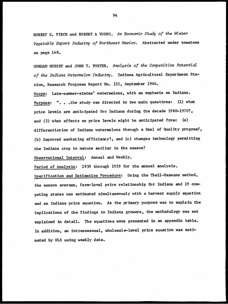
94

ROBERT S. FIRCH and ROBERT A YOUNG. An Economic Study of the Winter

vegetable Export Industry of Northwest Mexico. Abstracted under tomatoes

on page 148.

GORHAM HUSSEY and JOHN T. PORTER. Analysis of the Competitive Potential

of the Indiana Watermelon Industry. Indiana Agricultural Experiment Sta-

tion, Research Progress Report No. 152, September 1964.

Scope,: Late-summer-states' watermelons, with an emphasis on Indiana.

Purpose: . . .the study was directed to two main questions: (1) what

price levels are anticipated for Indiana during the decade 1960-1970?,

and (2) what effects on price levels might be anticipated from: (a)

differentiation of Indiana watermelons through a Seal of Quality program?,

(b) improved marketing efficiency?, and (c) changes technology permitting

the Indiana crop to mature earlier in the season?

Observational Interval: Annual and Weekly.

Period of Analysis: 1939 through 1959 for the annual analysis.

Specification and Estimation Procedure: Using the Theil-Basmann method,

the season average, farm-level price relationship for Indiana and 19 com-

peting states was estimated simultaneously with a harvest supply equation

and an Indiana price equation. As the primary purpose was to explain the

implications of the findings to Indiana growers, the methodology was not

explained in detail. The equations were presented in an appendix table.

In addition, an intraseasonal, wholesale-level price equation was esti-

mated by OLS using weekly data.

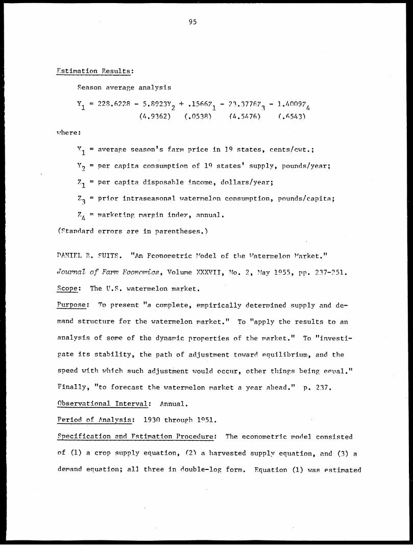
95

Tstimation Results:

Season average analysis

Y1 = 228.6228 - 5.892

3Y2 + .15667

1 - 21.17767

3 - 1.40097

4- - (4.9162) (.0518) (4.5476) (.6543)

where:

V = average season's farm price in 19 states, cents/cwt.;1

Y, = per capita consumption of 19 states' supply, pounds/year;

71 = per capita disposable income, dollars/year;

3 = prior intraseasonal watermelon consumption, pounds/capita;

4 = marketing margin indey, annual.


DANIEL E. SUITS. "An Econometric 14odel of the vaterrelon I4arket."

Journal of Farm Economics, Volume )(XXVII, No. 2, May 1955, pp. 237-251.

Scope: The U.S. watermelon market.

Purpose: To present "a complete, empirically determined supply and de-

mand structure for the watermelon market." To "apply the results to an

analysis of some of the dynamic properties of the market." To "investi-

gate its stability, the path of adjustment toward equilibrium, and the

speed with which such adjustment would occur, other things being eoval."

Finally, "to forecast the watermelon market a year ahead." p. 237.



Specification and Estimation Procedure: The econometric model consisted

of (1) a crop supply equation, (2) a harvested supply equation, and (3) a

demand equation; all three in double-log form. Equation (1) was estimated

96

by OLS; (2) and (3) as a simultaneous system using maximum likelihood,

limited information. In an ingenious adaption of the cobweb model, equa-

tions (2) and (3) determine the equilibrium price if less than the entire

crop is harvested; (1) and (3) if the entire crop is harvested. The model

was then used to describe the dynamics of the watermelon market and to

forecast production and price.

Estimation Results:

Crop Supply (1919-1951):

(1) Q = .587P 1 - .320C

1 + 34.41J - .141T

1 - 155.97K + 768.735

- - -.(.156) (.095) (27.40) (.238) (45.17)

Parvested Supply:

(2a) X = .237 + 1.205Q - 118.041 or,

(.110) (.114)

(2b) X = Q whichever is smaller

Demand:

(3) P = 1.530 - 1.110 -ffx - .682F - 140.163(.088) (.246) (.183)

XDividing (3) by the coefficient of IT yields the more familiar form:

X(3*) TT= 1.378 - .901P - .614F - 126.273

where:

= the commercial crop of watermelons available for har-vest, millions;

P-1'

C-1'

T-1

= prices of watermelons, cotton, and commercial truck,lagged one year, dollars per thousand;

J, K = dummy variables representing the government cottonpolicy and the war respectively;

W = index of southern farm wage rates;

X = the number of watermelons harvested, in millions;

N = population;

Y = disposable income;

F = freight cost.

97

H. 0. A. WOLD. "A Case Study of Interdependent Versus Causal Chain Systems.

Review of the International Statistical Institute, Vol. 26, No. 1/3, 1958,

pp. 5-25.

Scope: The U.S. watermelon market.

Purpose: To compare the interdependent versus the causal chain systems,

the Suits' econometric (model for watermelons (interdependent). was reviewed

and then respecified.



Epecification and Estimation Procedure: Wold specified a "causal chain"

model consisting of three independent equations in double-log form: (1)

the supply relation (regulated by producers), (2) the demand equation

(regulated by consumers), and (3) price mechanism (regulated by merchants).

Equation (3) replaced Suits' harvested supply equation. (The Suits' paper

is reviewed on page 95.) The three equations were assumed autonomously

determined, so they could be estimated by OLS. The OLS elasticity esti-

mates were substantially lower than the Suits' limited information esti-

mates, leading to the conclusion that the latter were probably subject to

"hybrid bias"--"a consequence of interdependent systems being constructed

as a hybrid between static and dynamic approaches." p. 15.

Estimation Results:

Supply Relation (1919-1951):

(6) Q 0.587P-1 - 0.320C_

1 - 0.141T 4. 0.0343 - 0.156K + 0.769

Demand Relation (1931-1951):

X*(7) 0.206 + 0.430 cm- - 1.088

98

Price Mechanism (1931-1951):

(8)

where:

= 0.261 [-0) + 1.215 - 1.280NL

Q = the number, in millions, of watermelons available for harvest;

P,C,T = average annual farm prices of watermelons (dollars per thou-sand), cotton (dollars per pound) and commercial truck (priceindex for vegetables);

J,K = dummy variables representing government cotton policy and thewar, respectively. J is 1 for 1934-1951, K is 1 for 1943-1946; otherwise J and K are 0;

X = the number of watermelons harvested, in millions;

N = Unites States population, July 1st;

Y = disposable income of the United States;

X* = consumer demand, estimated as watermelon harvest X in theyears when only part of the crop is harvested:

X* = X in years when X F Q,

X* is unknown in other years, that is, in 1941-45 and 1948.

L = a U.S. cost of living index. Thus P/L and Y/NL are (thelogarithms of) real price and real per capita income.

Subscripts indicate lags so that P_1 means that P is lagged one year rel-

ative to Q.

TABLE 8: Selected Econometric Analyses With Flexibility or Elasticity Estimates for Melons

Observa-Author and Geograph- Time tional Form of Method of Market Price Income Cross Price Income

Date ical Area Period Interval Equation Estimation Level Product Flexibility Flexibility Effect Elasticity Elasticity

Castro and U.S. 1959/60 Weekly linear OLS wholesale canta- -0.041 Feb.Simmons,1974

1970/71 loupes -0.146 Mar.-0.094 Apr.

Fajardo- New York 1951- Monthly linear OLS wholesale honeyChristen,1970

1967 dewmelonsNov.-Jan. -.148Feb.-Apr. -.094May -Oct. -.198

.302

.340

.180

a/-.072-

a--.007/a—-.002/

Firch and U.S. 1961- Weekly linear OLS shipping- canta-Young, 1968 1966 point loupes:

prices,Nogales,Arizona

from Mex. -0.087totalquantity -0.098 1/40

Watermelons:from Mex. -0.113totalquantity -0.080

1/40

Suits, 1955 U.S. 1930- Annual double limited farm water-1951 log informa-

tion,maximumlikeli-hood

melons -0.901 1.378

Wold, 1958 U.S. 1930- Annual double OLS farm water-1951 log melons -0.206 0.430

PL' wrt. Spanish melons

100

Related Studies, Melons

Farrell, Kenneth R. Sales of Cantaloupes in Selected! Retail Stores inMinneapolis, Minnesota. A report to the California Cantaloupe AdvisoryBoard, 1961. Twelve retail stores in Minneapolis-St. Paul, of the samechain, were selected as test stores for promotion of California canta-loupes. Four display techniques were rotated among the stores every twoweeks. Results were tested by discriminant analysis and by analysis ofvariance and covariance. In addition, a multiple regression was fittedin which the average weekly sales volume was seen as a function of canta-loupe prices, prices of substitutes, and temperature.

Fowler, Mark L. and George L. Klein. Some Economic Factors Affecting theOklahoma Watermelon Industry. Oklahoma State University, Department ofAgricultural Economics, Processed series P-312, March 1959. Two OLS price-dependent equations were estimated using annual data, 1921 through 1955,omitting 1942-1945. The first, in first differences of the logs, fittedU.S. farm price as a function of production, income, and temperature.The second attempted to capture a seasonal effect. With the data in actualvalues, early summer prices were fitted to late spring production and toearly summer production, income, and a trend.

L'Esperance, Wilford L. "A Case Study in Prediction: The Market forWatermelons." Econometrica, Vol. 32, No. 1-2, January-April, 1964, pp.163-173. Forecasts using the reduced form of an interdependent simulta-neous equation system, limited information (Suits' model, see page 95),were compared with those of a single equation OLS model. The predict-ability of Suits' interdependent model was also compared with the causalchain system (Wold's model, see page 97). In both comparisons, theinterdependent system gave generally better forecasts than the alternativemodels.

Rauchenstein, E. Economic Aspects of the Cantaloupe Industry. CaliforniaAgricultural Experiment Station, Bulletin No. 419, February 1927. Fivescatter diagrams (1922-1926) were made plotting daily shipments from Im-perial Valley, California, against the FOB daily prices. The relationshipwas fitted mathematically in double log form; other factors affecting pricewere discussed_ but not fitted. A. multiple regression in semi-log form wasalso estimated in which the logs of New York prices were predicted byquantity and a temperature variable.

Rauchenstein, Emil. Factors Affecting the Price of Watermelons at LosAngeles. California Agricultural Experiment Station, Hilgardia Vol. 3,No. 12, June 1928. Watermelon prices at Los Angeles were estimated indouble-log form with a multiple regression using five factors: carlotarrivals, carlots an track, temperature, a seasonal index, and carlotarrivals of cantaloupes. This study is of historical interest in that thesolution, steps from the five normal equations were spelled out.

101

Seale A. D. Jr. and M. B. Allen. Reactive Programming of Supply andDemand for Watermelons Produced in Mississippi and Competing Areas.Mississippi Agricultural Experiment Station, Agricultural Economics Tech-nical Publication No. 1, June 1959. For use in a reactive programmingmodel, demand functions for 20 consuming centers for 13 marketing weeksin 1956 were estimated (in Price = a + b In quantity + c In population).To determine whether or not the 260 observations could be pooled; statis-tical (F) tests were performed, with the result that the coefficient es-timates could remain the same but the intercepts should be allowed tovary (by using dummy variables) over the 13 marketing weeks. The samemodel was used in a Journal of Farm Economics article (Vol. XLI, No. 5,December 1959, pp. 1012-1022) to illustrate the reactive programmingtechnique.

Thompson, Stanley R. A Simultaneous and Recursive Econometric Model ofthe U.S. Watermelon Market: A Comparison and Evaluation, 1974. An un-published student paper in which two watermelon models were updated to1971 and compared: Suits' 1955 simultaneous, interdependent model andWold's causal chain, recursive model. Both Suits' and Wold's papers arereviewed in this report on pages 95 and 97, respectively. On agoodness of fit basis, the explanatory power of the recursive model equa-tions was somewhat superior to the simultaneous formulation. The simulta-neous model emerged as a superior formulation when the evaluation criterionwas derived from an analysis of turning point errors.

102

nnions

Abstracts

TFOYAF, F. CLFVErGFP and FREDEPICK F. GFITHMAN. Market Prospects for Nev

ifexicoir Lettuce, Onions, Potatoes, and Sz.7eet Potatoes. New nexico Ag-

gricultural Experiment Station, Bulletin No. 649, February 1977.

Scope: U.F. demand for onions, potatoes, and sweet potatoes. (The lettuce

equations were not statistically satisfactory.)

Purpose: . . .to (1) determine the optimal distribution for selected New

Mexico fresh vegetables, and (2) establish whether production and marketing

of these vegetables could be profitably increased."

Observational Tnterval: Annual.

p. 6.

Period of Analysis: 1950 through 1972 for onions, 1957 through 1972 for

potatoes and sweet potatoes.

c7pec1fication and Estimation Procedure: Farm-level, linear, price fore-

casting equations were estimated by oLs for onions, potatoes, and sweet

potatoes, and elasticities were computed at the means of the variables.

The price flexibility for lettuce (-.93) ,;ras taken from another study.--1/

From these estimates, wholesale demand equations were calculated for 37

markets (onions), 17 markets (potatoes), 21 markets (sweet potatoes), and

21 markets (lettuce) for use in a reactive programming model.

1/ Tjjp V. Shelley, A Simultaneous-Fquation Analysis of the UnitedStates Lettuce Demand and SuppZy, 1949-1970, unpublished M.S. thesis, De-partment of AgrIcultural Economics and Agricultural Business, New MexicoState University, August 1971.

103

Fstination Results:

Onions

P = 31.03 - .00012 Q + .00649 DI + 33.97 DFI(5.98) (4.49) (3.79

.79 DW = 2.66

Potatoes

P = 2.91 - .0006 Q - .0604 CPFI + .0004 POP(2.09) (3.82) (2.11)

P2 = .56

sweet Potatoes

DV = 1.893 inconclusive

P = 13.46 - .00028 Q - .04802 CPFT(5.12) (4.69)

R2 = .68

where:

DV = 1.645 inconclusive

P = seasonal average price per hundredweight in dollars receivedby farmers for the commodity, deflated by the consumer priceindex with 1967 = 100,

= total quantity produced of a commodity during the season inthousands of hundredweight,

DI = annual total personal disposal-le income in the United statesin billions of dollars,

POP = annual total rnited Ftates population in thousands,

CPFT = consumer food price index as a measure of the aggregate pricelevel with 1967 = 100,

PFT = the deflated consumer food price index by the consumer priceindex with 1967 = 100.


104

CO7rOLLY, r7AN. Feas-7.7)77:ty ()fa CentraZ Union Sales Organization for

,(7out7' Texas. Texas Agricultural Trarket Research and Development Center,

Texas A&M University, Information Report YRC-71-1, August 1971.

Scone: 7outh Texas dry onions.

Purpose: In order to examine the expected performance of a proposed cen-

tral sales organizational structure, several aspects of the industry were

analyzed. The FOR price analysis is reviewed here.


Period of Analysis: 1960 through 1970. Price analysis was also done for

1055 through 1970, but the better fit obtained for the shorter period was

attributed in part to the initiation of a federal market order in 1961.

Specification and Ystimation Procedure: In a preliminary analysis using

linear OLS price-dependent equation, it was found that increases in U.S.

Income had no statistically significant effect on the FOR price of South

Texas onions. Two further specifications were run: in double-long form

and in first differences of the actual data. In both versions the FOB

price was fitted as a function of per capita supply of January 1 storage

stocks and the per capita supply of South Texas onions produced.

Fstimation Results:

log Y = 1.78 - 2.22 log X1 - 1.51 log X2(7.46) (10.24)

-1P- = .92

where:

Y = actual annual average FOB price per cwt,

X1 = per capita supply of January 1 storage stocks,

X2 = per capita supply of South Texas onions.


105

EDWARD V. JESSE. Structure of the Intraseasonal Pricing Mechanism for

Late Summer Onions, 1930-68. USDA, ERS, Marketing Research Report No.

1004, July 1973.

Scope: Michigan shipping point prices.

Purpose: To analyze how an initial price level is established at the

beginning of the storage season, to identify factors causing price vari-

ability during the storage season, and to determine whether the structure

of the pricing mechanism differed during the period of futures trading

from the period preceding and from the period following trading.

Observational Interval: Annual and weekly.


Specification and Estimation Procedure: First, a "tone price" equation

was estimated for the pre- and post-futures trading subperiods (1930/31-

1942/43 and 1959/60-1967/68), the trading subperiod (1944/45-1958/59), and

for the entire period (1930/31-1958/59). The tone price variable (the

simple average of western Michigan FOB shipping point prices in the weeks

preceding November 1st) was seen as a function of Michigan production, the

total U.S. late summer onion production, and a trend. Then, three storage

interval relations were estimated for the same subperiods and the total

period: (1) November-December, (2) January-February, and (3) March-April.

The dependent variable in each case was price in a particular week minus

the "tone price" for that year. The explanatory variables were a weekly

trend and the proportion of the total late crop shipped in the respective

week.

106

Each of the equations discussed above was fitted by OLS, with all

the variables, and a second time, using backwards stepwise regression re-

taining only those variables showing a statistically significant relation-

ship with the dependent variable.

Since statistical tests on the subperiods did not show consistent

differences, only the tone price equation using pooled data will be pre-

sented below.

Estimation Results:

0P = 1.783 - .396 Michprod - .048 Lateprod + .021 Year

(.058) (.016) (.004)

P.2 = .80

where:

0P = simple average of deflated western Michigan weekly prices

for weeks prior to November 1, dollars per 50-pound bag;

ifichprod = "ichigan late summer onion production in million hundred-weight;

Lateprod = total U.S. late summer onion production in million hun-dredweight;

Year = annual trend, 1930/31 season = 1, . . 1967/68 = 38.


EDWARD V. JESSE. Structure of Seasonal Supply and Demand in the Onion

Market. USDA, ERS, marketing Research Report No. 985, February 1973.

Scope: U.S. seasonal supply and demand for onions.

Purpose: To develop and estimate a statistical model incorporating factors

thought to influence seasonal average prices and production in order to

represent the structure of supply and demand and "to assess possible dif-

ferences in the basic structure of onion supply and demand between the

futures trading and post-trading periods." p. 1.

107



Specification and Estimation Procedure: First, the supply and demand

models for three seasons--late summer (August, September, and October),

early spring (March, April, and May), and intermediate (May, June, July,

August)--were estimated for two disjoint time periods: (1) the futures-

trading period, 1946/47 through 1958/59 and (2) the post-trading period,

1959/60 through 1969/70. Statistical tests were performed testing the

null hypothesis of no significant difference between the trading and post-

trading periods. Since the hypothesis was not rejected for any of the

three seasons, the data were pooled and the overall seasonal supply-demand

structure was explored by OLS. Using a backwards stepwise regression pro-

cedure, only variables contributing significantly to the explanation of

the variation in the dependent variable were retained.

Estimation Results:

Late Summer

Price = 10.54 - 0.77 Prod.(0.12)

Early Spring

R2 = .66 DW = 1.58

Price = 13.53 - 2.77 Prod. - 1.93 Lagprod. R = .59 DW = 2.41(0.59) (0.40)

Intermediate:

Price = 5.50 - 1.48 Prod. + 0.12 Trend(0.49) (0.03)

where:

R2 = .40 DW = 1.94

Price = season average grower price for onions in dollars per cwt.,deflated by index of prices received by farmers for allproducts, 1957-59 = 100,

108

Prod = seasonal onion production in pounds per capita;

Lagprod = per capita onion production in pounds for preceding season-al crop (storage stocks January 1st);

Trend = crop year, 1946/47 = 1, . . . 1969/70 = 24.


CAPL E. FRAFFR. IntraseasonaZ Price Analysis for South Texas Early Spring

Onionr. Texas AM University, Department of Agricultural Economics and

Pural Sociology, Technical Report No. 72-3, 1972.

Scope: South Texas FOB prices.

Purpose: 11. . .to determine those factors and variables which influence

South Texas FOB onion price per 50 pound bag (yellow granex medium) during

the weeks of the early spring onion marketing season." p. 1.

Observational Interval: Annual and weekly.

Period of Analysis: 1955 through 1970 for one equation using annual data;

1966 through 1971 for all other equations.

Specification and Estimation Procedure: In order to analyze the factors

affecting the price of Texas onions, several equations were fitted by OLS:

1. Season average price (annual data), deflated by the CPT, as a

function of per capita Texas production and stocks, in both linear and

double log forms.

2. Season average price as a function of total production and total

stocks.

1. Storage onion stocks as a function of late-summer production in

several functional forms (carry-over).

4. Simple linear regressions among planted acreage, harvested acreage,

yield, and production for Texas early spring and late summer onions.

109

5. Weekly data to estimate prices as related to Texas shipments,

other shipments, rain the previous week, and on-track holdings. The

weekly data equations were fitted for each season (year) separately, then

for all seasons (years), and finally using the pooled data, dummy variables

were used to allow intercept changes each year. It is the latter equation

that is reported below.

6. A buyer's expectations model into which the previous week's price-3

were incorporated, fitted both with and without seasonal dummies.

Estimation Results:

P = - 0.02088 OTSH - 0.01287 TXSH + 0.08631 RAIN-1(4.54) (5 . 03) (1.79)

R2 = 0.75

where:

- 0.02928 OTKH + 4.44123 (1966)(2.33) 3.92256 (1967)

5.56878 (1968)3.18687 (1969)4.73145 (1970)

P = South Texas FOB price per 50 lb. bag, yellow granex mediumanions;

OTSH = other than Texas shipments, carlots;

TXSH = Texas shipments, carlots;

RAIN-1 = rainfall in Lower Rio Grande Valley in previous week, inches;

OTKH = on-track holdings in 16 major terminal markets.


CARL E. SHAFER. A Statistical Analysis of Season Average Prices for

Texas Winter Carrots and Early Spring Onions. Abstracted under carrots

on page 61.

110

D. MILTON SHUFFETT. The Demand cold Price Structure for Selected Vegetables.


DANIEL B. SUITS and SUSUNU KOIZUMI. "The Dynamics of the Onion Market."

Journal of Farm Economics, Vol. XXXVIII, No. 2, May 1956, pp. 475-484.

Scope: The aggregated onion market for the U.S.

Purpose: The systematic oscillations of prices and outputs (almost a

textbook example of an agricultural cobweb system) were modeled in a three-

equation econometric system in order to analyze their dynamic properties.



Specification and Estimation Procedure: The three equations of the system

(supply, demand, and an unharvested crop forecasting equation) were esti-

mated independently by OLS. The demand equation was fitted in the first

differences of the logs of the annual mean values of the variables.

Estimation Results:

A Log Pf = - 2.27 A Log (D/N) + 1.31 A Log (Y/N) + .681

(.4) (.2)

-2R = .81

where:

P = farm price of onions,

D/N = crop-year demand per capita (crop less unharvested crop lessnet exports divided by U.S. population);

Y/N = U.S. per capita disposable income.


The coefficient estimates are very comparable to those obtained by

Shuffett reviewed on page 158.

TABLE 9: Selected Econometric Analyses With Flexibility or Elasticity Estimates for Onions

Observa-

Author and Geograph- Time tional

Date ical Area Period IntervalForm ofEquation

Method ofEstimation

MarketLevel Product

PriceFlexibility

CrossEffect

PriceElasticity

IncomeElasticity

Clevenger U.S. 1950- Annual

and 1972linear OLS farm fresh -.98

Geithman,1977

Connolly, U.S. 1960- Annual1971 1970

doublelog

OLS FOB South Texasdry onions -1.51 -2.22_4.1

Jesse, 1973 U.S. 1946/47 Annual linear OLS farm fresh -3.0 late

1969/70 summer-0.96 early '

spring

b/-0.71—

-1.0 May-Aug.

Shafer, 1966 Texas 1954- Annual1964

doublelog

OLS farm fresh -0.974

Shafer, 1972 Texas 1966- Annual19711966- Weekly1970

linear OLS farm

FOB

early springonionsyellow gran-ex mediumonions

-1.34

-0.32

c/-1.4a-

Shuffett, 1954 U.S. 1921- Annual1941

firstdiffer-ences ofthe logs

OLS farm late onions -2.855

Suits and U.S. 1929- AnnualKoizumi, 19591956

firstdiffer-ences ofthe logs

OLS farm fresh -.4 .6

a/ wrt. per capita January 1 storage stocks

b/ wrt. late summer production

c/ wrt. stocks, January 1

112

Related Studies, Onions

Branson, Robert E. A Summary Analysis of In-Store Onion Promotion Testsand Test Shipments of Pre-Packaged South Texas Onions. Texas A&M Univer-sity, Texas Agricultural Market Research and Development Center, Informa-tion Report rRc 69-2, September 1969. A promotion test was conducted in1963 in 40 retail food stores operated by two national chains in fourcities. Promotion bins were used in the stores in Denver and St. Louis;a special trading stamp promotion, in Cincinnati; and, as a control, nopromotion, in Omaha. The 1964 promotion tests were conducted at 56 storesin Oklahoma City, Kansas City, St. Louis, and Nashville, but this timeboth promotion and control stores were located in each city. For bothyears the tests indicated that promotion can effectively increase demandfor the mild flavored Texas onions.

Chen, Chao-chen. An Analysis of the Supply-Demand-Price Structure ofOnions in the United States. Unpublished Ph.D. dissertation, Departmentof Agricultural Economics, Cornell University, 1965. Although the dis-sertation was not available, seasonal elasticity estimates were reportedin the 7estern Extension Marketing Committee (A Handbook on Elasticity ofDemand for Agricultural Products in the United States, 17:MC PublicationYo. 4, July 1967). For the period 1947 through 1962, U.S. farm-levelprice elasticity estimates for onions were:

Early Spring -1.74Late Spring -1.02Early Summer -0.68Late Summer -0.18

At the retail level, the "all season" elasticity was reported: -0.59.

Johnson, Aaron C., Jr. Effects of Futures Trading on Price Performancein the Cash Onion Market, 1930-68. USDA, ERS, Technical Bulletin No. 1470,February 1973. "Farm, shipping point, and wholesale onion prices on botha weekly and a monthly basis were used to assess the impact of trading inonion futures contracts on the performance of cash onion prices." Theperiod 1930 through 1968 consists of three subperiods: no futures trading1930-1940; active futures trading 1946-1957; and no futures trading 1959-1968. "Price variations over time, including year-to-year, within-season,seasonal, and within-month price changes, and price variations over spacewere considered. Evaluation of the results from all the analyses. . .support the general conclusion that there was no significant change inprice performance over the entire period." From the abstract.

Lester, Bernard W. and Robert E. Branson. An Analysis of Prices Receivedfor Pre-Package(' and 50-Pound Sack South Texas Onions, 1965. Texas A&MUniversity, Progress Report No. 2384; December 1965. Correlation analysisbetween prices received for the 50-pound sack and for each of several

113

smaller pre-packaged test sizes was performed. Statistically significant(by the t-test) higher prices were received for two out of three smallersize packs when compared with the 50-pound sacks; lower prices, for themilitary 12-pound pack. Aggregating the smaller size packs for comparisonwith the 50-pound pack resulted in statistically significant results onlywhen the military 12-pound pack was excluded.

Stone, Kenneth, Dale Young, Eldon Dixon, and Daniel Padberg. ConsumerPreferences for Nev York Onions. Cornell University, Department of Ag-ricultural Economics, A.E. Ext. 75-19, June 1975. A questionnaire soli-citing responses about onion purchase and preferences was mailed to 7,395New York households. On the useable responses (31.56 percent), chisquare tests were used to evaluate comparisons. The sample had a high-income bias, but results indicated that consumers preferred smaller-than-25-pound packages, mesh bags (though acceptance of the plastic bag isgrowing), and a mild flavored onion.

Working, Folbrook. "Price Effects of Futures Trading." Stanford Univer-sity, Food Research Institute Studies, Vol. 1, No. 1, February 1960,pp. 3-31. Statistical evidence was presented on the impact of hedgingon onion cash prices. The evidence indicated that futures trading sub-stantially reduced the amount of variation in spot prices of onions.

114

Peas

Abstracts

J. H. DROGE and R. H. REED. Prediction Analysis of United States and

Wisconsin Wholesale Prices of Canned Cut Green Beans., Sweet Corn, and

Sweet Peas, 1948-1968. Abstracted under beans on page 33.

H. H. HUTCHINGS and G. B. DAVIS. An Economic Analysis of Interregional

Competition in the Frozen Pea Industry. Oregon Agricultural Experiment

Station, Technical Bulletin No. 72, November 1963.

Scope: A six production regions-ten consuming regions model of the U.S.

frozen pea industry.

Purpose: "To determine supply, demand, and price relationships for frozen

peas. . .To determine the competitive position of the major pea-freezing

areas of the United States. . .To project an efficient pattern of growth

for this industry." p. 6. There were, in addition, some methodological

objectives.



Specification and Estimation Procedure: In estimating the demand function

for frozen peas, several models were specified but only one of these was

presented in the bulletin. This OLS equation in linear form appears below.

Regional adjustments in per capita consumption and prices were made using

1955 information in order to adapt the model to regional demand functions

for use in the interregional competition model.

115

Estimation Results:

Q = .390610 - .079385 P + .002256 DI(.026883) (.000498)

R2 = .914

where:

Q = the estimated U.S. per capita disappearance of frozenpeas, pounds;

P = the average retail price, cents per 10-ounce package;

DI = the average U.S. per capita disposable income, 1947-49 dollars.




TABLE 10: Selected Econometric Analyses with Flexibility or Elasticity Estimates for Peas

Author Observa-Priceand Geograph- Time tional Form of Method of Price

Date ical Area Period Interval Equation Estimation Market Level Product Flexibility Elasticity

Droge U.S. and 1948- Annual linear OLS FOB canned:and Wisconsin 1968 NationalReed, canners1973 brand -.2076

Wisconsin1--,private cN

label -.2090

Hutch- U.S. 1950/51 Annual linear OLS retail frozen -.6760ings 1959/60andDavis,1961

Shuffett, U.S. 1921- Annual first OLS farm fresh -0.3531974 1941 differ-

ences of FOB canned -0.624the logs

117

Peppers

Abstracts

Y. B. ALLEN and A. D. SEALE, JR. An Evaluation of the Competitive Posi-

tion of the Green Pepper Industry in Prisoir;sippi an-7 Competing Areas.

Mississippi Agricultural Experiment Station, Agricultural Economics Tech-

nical Publication No. b., l'arch 1961.

Scope: rississippi and other early summer producing areas of green pep-

pers.

Purpose: To describe production trends, to estimate demand in specified

consuming centers, to estimate transportation charges from producing to

consuming areas, and to determine prices and revenues which would be

associated with alternative production and distribution patterns.



Specification and Estimation Procedure: Since several alternative analyses

of weekly price-quantity relationships for 23 consuming centers did not

yield logical demand functions, a demand function was developed usinF,, an-

nual data. First differences of the logs of the variables were specified

and fitted by OLS. Using the price flexibility from the resulting equation,

the average demand level (A) for each of seven weekly periods was computed

using the average weekly price, the average weekly carlot receipts, and

the average population for the 23 cities. There was a downward but not

consistent trend in the A values, so they were adjusted to an average trend.

Then, demand functions for each city for each period were developed by fur-

ther adjusting the intercept by the population of the city times the posi-

tive flexibility estimate from the original equation.

118

Based on the demand functions and transportation charge estimates,

alternative distribution patterns were evaluated.

Estimation Results:

The U.S. time series equation.

A In P = -.05126 - .78335 A in Q + .91320 A In I

R2 = .53

where:

= farm price per cwt.,

= quantity in thousand cwt.,

I = U.S. total disposable incone in billions of dollars.

(All coefficients were significant at the 99 percent confidence level.)

ROBERT CASTRO and RICHARD L. SIMMONS. The Demand for Green Peppers,

Cucumbers, and Cantaloupes in the Winter Season. Abstracted under cucum-

bers on page 77.

ROBERT S. FIRCH and ROBERT A. YOUNG. An Economic Study of the Winter

Vegetable Export Industry of Northwest Mexico. Abstracted under tomatoes

on page 148.

I. A. LINDSTROM and R. A. KING. The Demand for North Carolina Slicing

Cucumbers and Green Peppers. Abstracted under cucumbers on page 77.

RICHARD L. SIMMONS and CARLOS POMARIEDA. "Equilibrium Quantity and Timing

of Mexican Vegetable Exports." AJAE. Abstracted under cucumbers an

page 80.

TABLE 11: Selected Econometric Analyses With Flexibility or Elasticity Estimates for Peppers

Author and Geographical Time Observational Form of Method of Price Income Price

Date Area Period Interval Equation Estimation Market Level Product Flexibility Flexibility Elasticity

Allen and U.S. 1929- Annual first OLS farm fresh -.78335 .91320

Seale, 1961 1958 differ- green

ences of peppers

the logs

Castro and U.S. 1959/60- Monthly linear OLS wholesale fresh -.52 Dec.

Simmons, 1970/71 green -.50 Jan.

1974 peppers -.92 Feb.-.71 Mar.-.67 Apr.

Firch and U.S. 1961-

Young, 1966

1968

Weekly linear OLS shipping- quantitypoinE fromprices, other-Nogales, than-Arizona Mexican

sources -0.653

totalquantity -0.820

Lindstrom North 1925- Annual double OLS farm fresh -0.5975 1.4666

and King, Carolina 1954, log green

1956 exclu- peppers

ding1942-1945

120

Related Studies, Peppers

Castro S., Roberto and J. A. Seagraves. The Supply of Pinter Green Peppersin noric7a. North Carolina State University, Economics Research ReportNo. 31, December 1974. A supply response model was estimated. The analy-sis indicated that "the expected total revenue from green peppers, thetotal revenue from tomatoes lagged two periods, the cost of producing greenpeppers, and the lagged dependent variable were the most important vari-ables affecting the acreage used for winter green peppers in Florida."From the abstract.

Farris, Donald F. and Richard A. King. Interregional Competition ink'arketinc Green Peppe:s. North Carolina State College, Agricultural Eco-nomics Tnformation Series No. P7, December 1961. The weekly shipments ofgreen peppers during the 1956 season Nay 28th through July 27th) fromNorth Carolina and six other states to 21 shipping points were analyzedusing the transportation model.

121

Potatoes

Abstracts

y A. A. ARAJI and W. C. SPARKS. Economic Value of Agricultural Research,

A Case Study--Potato Storage Research. Idaho Agricultural Experiment

Station, Research Bulletin No. 101, March 1977.

Scope: U.S. potatoes.

Purpose: ft. . .to analyze the contribution of the new potato storage

technique developed at Aberdeen (Idaho) to various sectors of the economy

and to estimate the rate of return to investment in the project." p. 5.



Specification and Estimation Procedure: As part of the analysis a linear

price response equation was estimated by OLS.

Estimation Results:

P = -4.1756 + .04705U - .00001 Q+ .0078C(2.19)1? (2.52) P (1.95)

R2 = .501

where:

P = price per cwt. received by farmers for potatoes,

U = United States population,

Qp = quantity of potatoes produced in the United States,

C = per capita potato consumption in the United States.


THOMAS S. CLEVENGER and FREDERICK F. GEITHMAN. Market Prospects for New

Mexico's Lettuce, Onions, Potatoes, and &vet Potatoes. Abstracted under

onions on page 102.

122

ROGER W. GRAY, VERNON L. SORENSON, and WILLARD W. COCHRANE. An Economic

Analysis of the Impact of Government Programs on the Potato Industry of

the United States. Minnesota Agricultural Experiment Station, North Cen-

tral Regional Publication No, 42, June 1954.

Scope: The U.S. potato market.

Purpose: In order to assess the impact of government programs on the in-

dustry, a lengthy, thorough analysis was done.


Period of Analysis: 1870 through 1909 and 1910 through 1942.

Specification and Estimation Procedure: Estimation of demand functions

was only a part of the study but is of interest because of the change of

sign for the trend variable for the two time periods estimated. Demand

was rising during the earlier period (partly due to immigration from Euro-

pean potato-consuming countries) and falling over time after 1910. The

per capita equations were both linear and in logarithms of the variables;

the total market equations were linear. The time effect for the total

market demand was graphed along with price and production in a three di-

mensional figure presented below.

Estimation Results:

Market Demand for Potatoes

Period 1 (1870-1909):

Y* = 90.5625 - .3967 X + 2.6494 T P2 = .89

Period 2 (1910-1942):

Y = 250.7345 - .5108 X - .0788 T R2 = .84

where:

Y* = deflated farm price per bushel,

X = U.S. production in millions of bushels,

T = time in years.

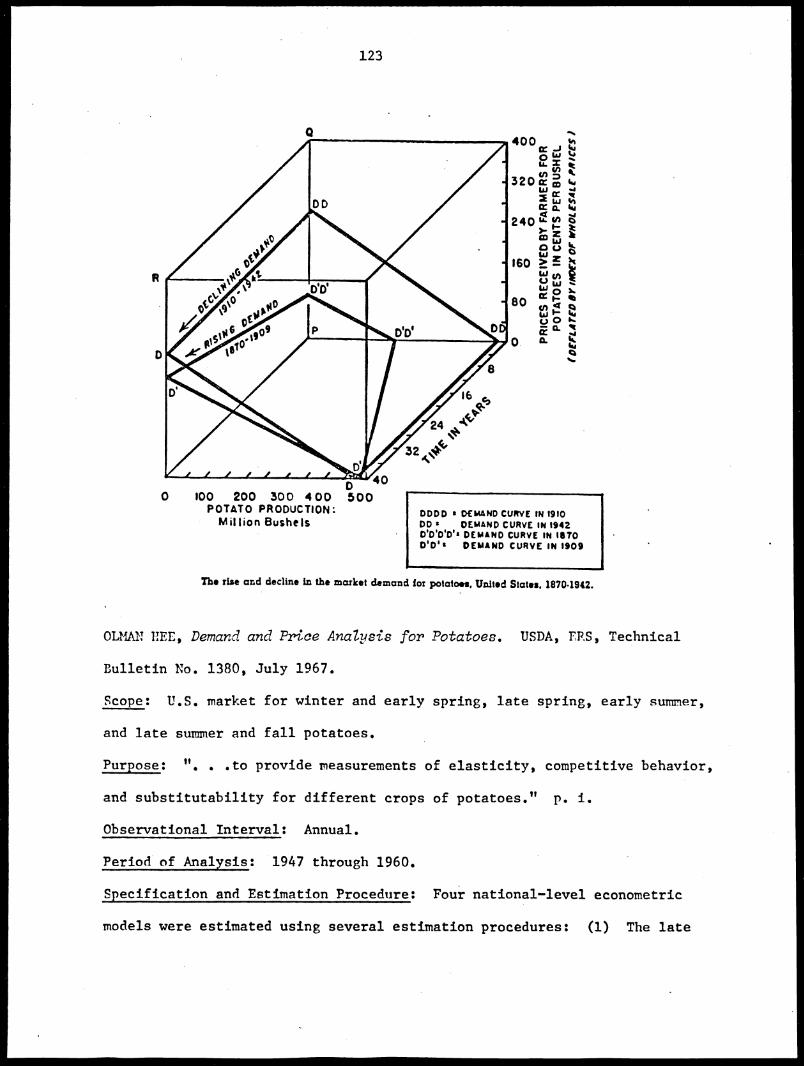
123

0 100 200 300 400 500POTATO PRODUCTION:

Million Bushels

400cro

320 coLI Dw2 wcr

240 IA' :2z160 w> z

w u,w

re g80 cf

ta U0

00.

(

DEPLArro sY IN

DEX OF WHOLESALE PRICES)

DODD I DEMAND CURVE IN 191000 DEMAND CURVE IN 1942D'O'D'O' DEMAND CURVE IN 11170WO' s DEMAND CURVE IN 1909

The rise and decline in the market demand for potatoes, United States, 1870-1942.

OLMAN NEE, Demand and Price Ancaysis for Potatoes. USDA, FRS, Technical

Bulletin No. 1380, July 1967.

Scope: U.S. market for winter and early spring, late spring, early summer,

and late summer and fall potatoes.

Purpose: ". . .to provide measurements of elasticity, competitive behavior,

and substitutability for different crops of potatoes." p. 1.



Specification and Estimation Procedure: Four national—level econometric

models were estimated using several estimation procedures: (1) The late

124

summer and fall crop model was primarily a utilization model, rather than

testIng for substitutability. The four equations--consumption for food

(retail-level prices), consumption for feed and for starch (farm-level

prices), and the farm-to-retail spread--were estimated by OLS, TSLS, and

limited information, maximum likelihood. (2) The winter and early spring

and (3) the late spring models

tatoes for food and demand for

demand for the seasonal crop.

included detnand equations for storage po-

potatoes to go to storage as well as the

Yodel (2) was estimated by the same three

techniques, hut model (3) had only one endogenous variable per equation, so

OLS was used. (4) The early summer model (July-August) tested for

substitutability between the early summer crop and late spring potatoes in

early summer and also late summer potatoes on the market in early summer.

OLS, TSLS, and limited information estimation techniques were used on (4).

Estimation Results: Rather than duplicating the many equations here, the

limited information, maximum likelihood elasticity estimates for (1), (2),

and (4) and the OLS elasticities for (3) are presented in Table 12.

RONALD A. SCFRIMPER and GENE A. MATHIAi "Reservation and Market Demands

for Sweet Potatoes at the Farm Level." American Journal of Agricultural

Economics, Vol. 57, No. 1, February 1975, pp. 119-121.

Scope: U.S. commercial demand for sweet potatoes and demand for on-farm

use in the 13 sweet potato producing states.

Purpose: To explain trends that had been observed in the sweet potato

industry: a stable quantity in commercial channels, declines in on-farm

use, in real farm price, and in acreage.

125



Specification and Estimation Procedure: The quantity of sweet potatoes

entering commercial channels, the quantity reserved for on-farm use, and

the farm price received were considered as simultaneously determined. A

3SLS procedure was used. Prices were deflated by the Consumer Price Index

(1967 = 100). The final structural equations appear below.

In addition, the reduced-form equations were used to predict the farm

price and the commercial quantity to 1980 under alternative assumptions

about total production and projected values for income, population, and

the price of white potatoes.

Estimation Results:

0 = 7,609 - 1,606P + 59r + 947Y + 479P - 271T.s(196) s (1326)

(23/)W- (78)

0 = 10,180 - 1,37IP + 829F + 1,076Z - 175P - 2,4011nT(205) s (331) (1023) (254)w (602)

where:

Qs= total sweet potato production sold off farms in 1000 cwt.,

Ps = real farm price ($/cwt.) received for sweet potatoes,

N = two year moving average of total U.S. population in millions asof July 1,

Y = real per capita personal disposable income in thousand dollars,

Pw = real farm price ($/cwt.) received for white potatoes,

T = time trend (1949 = 1, 1950 = 2, etc.),

Qr = total on-farm use of sweet potatoes in 1000 cwt.,

F = total farm population in 13 major sweet potato producing statesin millions as of April 1,

126

Z = real per capita net farm income in thousand dollars for the same13 states.




JEROME B. SIEBERT. An Analysis of the California Potato Industry's Market

Alternatives. California Agricultural Experiment Station, Giannini Foun-

dation of Agricultural Economics, Information Series No. 67-2, December 1967.

,Scope: California late spring potatoes.

Purpose: To provide some insight into the consequences of diverting pro-

duction into processing Channels in order to increase the price of potatoes

sold in fresh channels.



Specification and Estimation Procedure: Three price forecasting equations

in double-log form were estimated by OLS. The equation considered both

simplest and statistically best is presented below.

Estimation Results:

lnX = 10.5097 - .83531nX2 - 2.78971nX

31(-1.9644) (-7.3247)

R2 = .8776

where:

X1 = California late spring seasonal potato price adjusted by the

Consumer Price Index, dollars per cwt;

X2 = California late spring potato production, pounds per capita;

127

X3 = May 1 stocks of U.S. raw potatoes other than California late

spring production, pounds per capita.


WILL M. SIMMONS. An Economic Study of u.r. Potato Industry. USDA,

FRS, Agricultural Economic Report No. 6, March 1962.

Scope:

Purpose:

U.S. potatoes including seasonal and regional analysis.

"This potato study is part of a continuing program of economic

research designed to provide information on factors influencing supply,

demand, and price of important agricultural commodities. Such a study

has special interest at this time because of recurring overproduction and

consequent low prices to potato growers in recent years." From the Pre-

face.


Period of Analysis: 1951 through 1960 and one equation for the 1930

through 1941 period.

Specification and Estimation Procedure: Thirteen price-dependent, linear,

OLS equations were fitted: total U.S. production 1930-1941, total U.S.

production 1951-1960, winter and early spring production, late spring

production, early summer production, late summer and fall production, late

summer and fall in the eastern region, late summer and fall in the central

region, late summer and fall in the western region, late summer and fall

in Maine, late summer and fall in the Red River Valley of North Dakota and

Minnesota, late summer and fall in Idaho, and late summer and fall in

Maine. All variables were expressed in first differences. A representa-

tive equation appears below, and selected flexibilities computed at the

means of the variables appear in Table 12.

128

Estimation Results:

Late summer and fall production in the western region, 1951-1960:

P = -0.038 + 0.036 0 7 (LS+F) - 0.006 D - 0.142 G 7 + 0.386 0 7 (V+ES+LS)(.042) 1. (.004) (.044) (.062)

where:

- 0.161 Q (LS+F)-t7 P- = .94

P = season average price received by farmers, late summerand fall potatoes in the western region, deflated byindex of prices received by farmers for all farm pro-ducts;

0,(L5+F) = per capita production of late summer and fall potatoesin the western region;

D = per capita disposable income;

G = quantity of late summer and fall potatoes diverted underthe government programs in the western region;

0 (W+ES+LS) = per capita production of winter, early spring, and latespring potatoes in the western region;

n(Ls+F)-17 = per capita production of late summer and fall potatoesoutside of the western region.


FREDERICV V. VAUCE. Demand and Price Analysis: Some Examples from Agri-

culture. USDA, EPS, Technical Rulletin No 1316, November 1964.

Scope: A general work on the methodology of estimating demand curves.

Among the examples were three vegetable estimations: U.S. retail price for

potatoes, sweet potatoes, and tomatoes.

Purpose: To present a base book in the area of demand and price analysis.

"To make real progress, the statistician, the economic theorist, and the

mathematician must cooperate closely with one another. Pure economic

129

theory is merely idle amusement unless it is tested and applied. On the

other hand, the compilation of statistical data is of no value unless the

data are used to test and to quantify theory."


P• 9.

Period of Analysis: 1948 through 1962 for potatoes and sweet potatoes,

1950 through 1962 for tomatoes.

Specification and Estimation Procedure: Price forecasting equations for

each vegetable were fitted by OLS where the retail price was a linear

function of per capita consumption and per capita disposable income. The

farm-retail spread was also estimated as a function of the same two ex-

planatory variables, and then the farm-level equations were derived by sub-

tracting the spread from the retail equations. The equation sets for

potatoes and tomatoes are presented below.

Estimation Results:

Potatoes

R = 197.918 - 1.448 Q + .00751 Y(.469) (.00698)

A

S = 32.354 - .365 Q + .02065 Y(.132) (.00197)

F = 165.564 - 1.083 Q - .01854 Y

Tomatoes

R2 = .6424

R2 = .9654

R = 42.582 - 1.907 Q + .00595 Y R2 = .7291

(1.020) (.00197)AS = 21.574 - 1.070 Q + .00593 Y

(.734) (.00142)

F = 21.008 - .837 Q + .00002

R2 = .7901

130

where:

P = retail price per pound,

S = farm-retail spread per pound,

= per capita consumption, pounds,

Y = disposable income per capita.


HOLBROOK WORKING. Factors Affecting the Price of Minnesota Potatoes.

Minnesota Agricultural Experiment Station, Technical Bulletin No. 25,

October 1925 (of historical interest).

Scope: Price of Minnesota potatoes in St. Paul and Minneapolis.

Purpose: To bring together information which helps in answering ques-

tions such as: Why does the price of potatoes change so much from year to

year? Pow much are prices affected by a ten percent increase in production?



Specification and Estimation Procedure: Five factors were considered to

affect the variation in potato prices. These were discussed one by one and

then the effect of that factor was removed graphically leaving the residual

to be explained by the next factor. First, changes in the value of the

dollar were removed from the original potato price-against-time graph.

Second, the general increase in the value of potatoes (an upward trend)

was removed. Next, the fluctuation in potato production in percent above

or below "normal" was taken away. Fourth, an adjustment was made for the

price of potatoes in August. Finally, a proxy to measure the variation in

quality of Minnesota potatoes was created (the difference is price between

131

Minnesota potatoes and "Maine" and "State and Western" potatoes in New

York City), and its effect removed. The figures below show how close

this procedure came to explaining the variation in potato prices. One

final factor was considered, but the data were not available to use--the

loss in storage from rot which WAS expected to have an inverse effect on

price just as any other change in quantity would. The years in which field

blight (causing rot in storage) was heavy or light corresponded closely

with the remaining peaks and troughs, respectively.

Estimation Results:

scALtPEACECHANGES

orWADE

. + tO

+M0

. —W

..—t0

... —TO

.

.

UNCORRECTED

CORRECTED fORmug Or DOUAIAND TREND

. .

..

,

.

,

i ..I

CORRECTED ALSOfiDA WE OfLATE CROP

i, i 1

CDR RE CTED ALSOfOR PRICES is 'AUGUST

,

I ti

-

CORRECTED ALSO?oft QuAury

•

•

1 1

4

1

I

Met 140 MW MIS MIO IRIS

Changes Remaining To Be Explained at Successive Stages in the Study

132

DOLLARS

PER CWT.

3.7S

ISO

125

2.75

230

1.15'

L50

L25

1400 1

.75

.25

ACTUAL PRICE

ESTIMATED PRICE

•

.00 1 I 1 1 1 I 1 III I 1 I I 111 titOZ 190S nm 14115 192.0

Fig. II. Actual and Estimated Prices of Potatoes, 1902-23

The hollow circles connected by the dotted lines show what the price would have

been each year since 1902 if it had been affected by these five factors only. The

solid circles show what the price actually was. The five factors explain most of the

changes in the price of potatoes.

PINEAS ZUSMAN, "Econometric Analysis of the Market for California Early

Potatoes," FiZgardia, V. 33, No. 11, December 1962 pp. 539-668.

'cope: The California early potato market relative to the U.S. market.

Purpose: "To analyze quantitatively the static and dynamic properties of

the rarket for California early potatoes." p. 539.


Period of Analysis: 1930 through 1958. The 1942 through 1950 period was

excluded since the heavy support program during this period was expected

to alter the structure substantially.

133

Specification and Estimation Procedure: An econometric model of 14 linear

equations consisting of 14 endogenous, 15 exogenous, 8 lagged endogenous,

and several lagged exogenous variables was constructed. Six of the equa-

tions were treated as a simultaneous subsystem and estimated by TSLS:

(1) transfer farm-retail, late crop, (2) demand for late potatoes for food,

September-February, (3) demand for late potatoes for nonhuman use, (4)

supply of late potatoes in September-February, (5) late crop supply (iden-

tity I), and (6) late crop supply (identity II). The remaining eight ecia-

tions were estimated by OLS: (1) production--late crop, (2) demand for

potatoes in the spring, (3) California supply identity, (4) other spring

potatoes supply identity, (5) California production response, (6) other

spring production response, (7) transfer farm-retail, California, (8)

transfer farm-retail, other spring potatoes. The three demand relation-

ships are presented below.

Estimation Results: Demand for late potatoes for food, September-February

(TSLS)

Y6t

= - .951326 - .061216 Y3t (.000197)

Z6t + .003383 - .000137

(.0379) (.00420) -

- .004209 Z-

(.00411) 7t

Demand for late potatoes for nonhuman use (TSLS):

v = - .149629 + .136288 Ylt - .073369 Y

2t + .004926 Z

2,t-1(.0498) (.0432) (.00168)

Demand for potatoes in the spring (OLS):

Y8t

= - 8.552166 - 8.152740 Y7t - 19.568923 Y

(2.152) (8.497)

- 10.252981 Y10 * + 004885 Z

2 - .002842 Z

6t + 006765 Z

7tt(3.435) (.0641) •(.00136) (.0258)

= .6867

134

Y = quantity per capita of late potatoes consumed as food September-February, bushels per capita;

Y3 = real retail price of potatoes in September-February, dollars per

72

bushel;

= time (calendar year 1925 = 1);

= real United States per capita disposable income, dollars percapita;

77 = real index of retail prices of cereals and bakery products;

= quantity per capita of late potatoes fed to livestock, lost,etc., bushels per capita;

Y1 = per capita production of late potatoes, bushels per capita;

Y, = real average price received by growers of late crop in September-February, dollars per bushel;

Yo = real retail price of potatoes in the spring, dollars per bushel;

Y7 = quantity per capita of late potatoes carried over to the spring

bushels per capita;

= per capita consumption of California spring potatoes, bushelsper capita;

Y10

= per capita consumption of other states spring potatoes, bushelsper capita.


TABLE 12: Selected Econometric Analyses With Flexibility or Elasticity Estimates for Potatoes

Observa-

Author and Oeograph- Time tional Form of Method of Market

Date ical Area Period Interval Equation Estimation Level ProductPrice

Flexibility

ClevengerandGeithman.1977

U.S. 1957- Annual linear OLS tare potat0e.

1972 sweet

potatoes

Hee. 1967 U.S. 1947- Annual linear limited late summer

1960 informa- and fall

tion retail for food

farm fur feed

farm for starch

limited winter and

informa-Zrrkio:PdringLion

OLS

limitedinforma-tion

farm

farm

farm

fall (from

storage)

for foodfall (from

storage)early summer(Joky-August) early summerpotatoes

late springpotatoes

late summer

potatoes(early maturing)

Schrimper andMathis, 1975

U.S. 1949-1972

Annual

Shuffett, U.S. 1921- Annual-

1954 1941

Siebert, 1967 California 1956- Annual1966

Simmons. 1962 U.S. 1951- Annual1960

linear 3SLSfarm

suP,!C__2(2!..Descommercial use

on-tarm use

first OLSdiffer-enc. ofthe loge

farm early and inter-

mediate croplate croptotal crop

-2.114-4.028-3.517

double OLS farm late spring

log crop

first dif- OLSferences ofthe variables

farm U.S. winter andearly spring crop

U.S. late spring

U.S. late summerand fall

n.s.-4.00

-5.00

Income Cross Price

Flexibility Effect Elasticity

IncomeElasticity Cross Elasticity

-0.83

-1.05

0.07-0.21-0.51-1.01

0.32 n.s. 2.07-2.63

-0.34 n.s. 0.17-0.21

0.38 n.5. 0.38-0.59

0.48 n. s. 1.32-1.88

0.52 n.a. 0.44111 0.20-0.67

-0.18 0.8911-0.52

d/

-0.480.24 n.s. 0.29

0.21 0-0.65 0.21 s o!'-1.25

-1.20

-2.441/,-1.412'

Waugh. 1964 U.S. 1948- Annual linear OLS utatoes

1962 retailfaro

retailfarm

sweet potatoes

-2.567 .212-5.277 -1.439

- .764 - .627

-1.148 -1.6h2

Zusman. 1962 U.S. 1938- Annual linear ISIS1958.exclu-ding OLS1942-1950

farm

late potatocrop -7.225 .909 2.717h/

spring potatoes -3.39711/1 .989 -1.4151-1

-1.780-

a/ n.s. nut statistically significant by

- the [-tent, 90 percent, one-tailed con-fidence level.

6/ wrt. late spring potatoes

t/ wrt. late ,ummer potatoes

4/ wrt. early summer potatoes

el the positive coefficient inditates asubstitution effect with white potatoes

set. other U.S. raw potato supplies

gj wrt. stock, ot storage potatoes

h/ set. cereals and baker, products

i/ wrt. per cAptta consumption of Calitorald

spring potatoeN

pcsr ..apita quantity of t.trcv ovcr

potatoes

k/ . per cap :011:,1111,L IOU

ot r - han-Ca 1 itornia ttio rot

LA)

136

Related Studies Potatoes

Brandow, G. E. Causes of Changes in the Prices of Potatoes. PennsylvaniaAgricultural Experiment Station, Journal Series Paper No. 1331, June 1946.The variations in the U.S. farm, Pennsylvania farm, N. Y. wholesale, andU.S. retail prices for the 20 years between World Wars I and II were an-alyzed by graphics and by correlation with changes in U.S. production.

Foytik, Jerry and Ann Hertzendorf. Consumption Patterns for Potatoes,Rice, and Macaroni in Northern California, 1968. California AgriculturalExperiment Station, Bulletin No. 848, January 1971. The report describesthe findings about the prevailing purchase and use of patterns in NorthernCalifornia from interviews made at 1192 households.

Grieg, W. Smith, Forrest O. Strand, and Henry Larzelere. Relative RetailSales and Elasticity of Demand for Dehydrated Mashed Potato Products.Cooperative Extension, Michigan State University, Agricultural EconomicsReport No. 732, July 1958. Market tests at seven retail stores in theDetroit area were performed on a new potato flake product and sales werecompared with two other dehydrated products already on the market.

Grieg, W. Smith and Leroy Blakeslee. Potatoes: Optimum Use and Distri-bution with Comparative Costs by Major Regions of the U.S. College ofAgriculture Research Center, Washington State University, Bulletin No.865, August 1978. A linear programming model was used to minimize thetotal cost of production, processing, and distribution of major productforms (fresh, potatoes for chips, frozen french fries, and dehydration)from nine major U.S. potato producing areas.

Hee, Olman. A Seasonal Potato Market: Area of Competitive Behavior.USDA, ERS. Paper presented at the American Farm Economics AssociationAnnual Meeting, August 1964. From two reduced form, price dependent,linear equations estimated by OLS, direct price and cross elasticitieswere computed for late spring potatoes and for fall (storage) potatoes.A more complete analysis is found in the study by Hee, reviewed in thisreport on page 123.

Mathia, Gene A. and Richard A. King. Planning Data for the &met PotatoIndustry. North Carolina State College, Agricultural Economics InformationSeries No. 97, December 1962. A study of the optimum number, size, andlocation of sweet potato processing plants in Eastern North Carolinacounties. An economic-engineering approach was used to estimate assemblyand processing costs.

137

MtCorkle, Chester O. and Yair Mundlak. "Statistical Analysis of SupplyResponse in Late Spring Potatoes." California Agricultural ExperimentStation, Htilgardia, Vol. 24, No. 16, April 1956. An acreage responsefunction was specified for late spring potatoes in California. From al-ternative expressions of this function, estimated by OLS, it was deter-mined that a large part of the variation in acreage could be explainedby gross income from competing crops, potato prices from previous season(s),and acreage available to be planted in potatoes.

Meinken, Kenneth W. Factors That Affect Price and Distribution of NewJersey Potatoes. New Jersey Agricultural Experiment Station, BulletinNo. 786, June 1957. Several price forecasting equations were fitted indouble log form, by OLS: (1) New Jersey farm-level price as a functionof New Jersey production and Long Island production; (2) Maine farm-levelprice as a function of Maine production, production in eight eastern late-potato states, and production in nine central late-potato states; (3) LongIsland farm-level price as a function of Long Island production, New Jerseyproduction, and production in eight eastern late-potato states and westernNew York.

Mundlak, Yair and Chester O. MtCorkle, Jr. "Statistical Analysis of SupplyResponse in Late Spring Potatoes in California." Journal of Farr? Economics,Vol. XXXVIII, No. 2, May 1956, pp. 553-569. Several formulations of acreageresponse equations were estimated by OLS for the period 1929 through 1953.

Summers, Larry V. and Carole Drury. Marketing Northwest Potatoes. IdahoAgricultural Experiment Station, Bulletin No. 529, December 1971. A des-cription was given of the recent changes and the present importance ofpotato production and marketing in four regions of the Northwest: Washing-ton; ten southwest counties of Idaho and Malheur County, Oregon; other ,counties in Idaho; other counties in Oregon. Growth rates, marketing pat-terns, and price changes were compared among the regions and with the totalU.S. potato production.

Young, Ralph and William G. Tomek. A Comparison of Marketing Strategiesfor Potatoes in Upstate New York. Department of Agricultural Economics,Cornell University, Staff Paper No. 78-15, June 1978. A price forecastingequation was used in two of six marketing strategies evaluating the effectof hedging on a farmer's returns. From March 31, 1968 to March 31, 1977,the midpoint of the N. Y. price range for the last full week in March wasfitted by OLS as a linear function of price the last full week of the pre-vious October and total U.S. production of fall potatoes the previous year.

Zusman, P. "An Investigation of the Dynamic Stability and Stationary Statusof the United States Potato Market." Econometrica, Vol. 30, No. 3, July 1962.The paper is based on the same model as the larger work reviewed in this re-port on page 132.

138

Strawberries and Other Berries

Abstracts

T,47ILIAM F. COBLE. Tennessee's Competitive Position in Producing and !Ica,-

Ptr03,71%erries. Tennessee Agricultural Experiment Station, Bul-

letin No. 132, September 1961.

Scope: U.S. strawberry farm prices and acreage response.

Purpose: To present information of help in determining Tennessee's com-

petitive status in the strawberry industry.

Observationpl Tnterval: Annual.

Period of Analysis: 1929 through 1958, excluding 1942 through 1947.

Specification and Estimation Procedure: As part of the study a price fore-

casting equation was fitted by OLS in first differences of the logs.

Graphic analysis revealed a cobweb-like behavior in production and prices.

Accordingly, acreage response was seen as a function of deflated prices,

lagged two years, as well as per capita income and strawberry consumption.

Estimation Pesults:

in X = - 0.0170 - 0.0595 A in X,) + 0.8175 b. ln Xl - 0.6959 A in X41(0.1003) (0.2077) (0.3626)

n2 =

T.There:

X1 = average farm price of strawberries, cents per pound;

X2 = production of strawberries in pounds;

Y.3 = disposable personal income per capita;

Y4 = consumption of strawberries per capita.


139

G. L. MEHREN and H. E. ERDMAN. "An Approach to the Determination of Intra-

seasonal Shifting of Demand." Journal of Farm Economics, Vol. 27, No. 2,

May 1946, pp. 587-596.

Scope: Louisiana auction prices in response to total U.S. strawberry

shipments and in response to Louisiana and other-than-Louisiana shipments.

Purpose: To determine It . .whether changes in price of a perishable pro-

duct during its marketing season represent intraseasonal movements along a

single seasonal demand function or a systematic pattern of intraseasonal

shifts of the demand function itself." p. 587.

Observational Interval: Annual--using the weekly average of daily obser-

vations for the same week of each marketing season, not corresponding to

calendar classification.


Specification and Estimation Procedure: Separate linear multiple regres-

sions were fitted by OLS for each week of seven weeks of the Louisiana

marketing season. The equations were of the form:

P =a1 +b1QUS

+c1I + d

1T and

..

P = a2 + b

2QL + c2Q0 + d

2I + e

2T

where:

P = the weekly weighted average of daily auction prices of Loui-siana strawberries,

Qu.s. = U.S. shipments of strawberries in cars,

= shipments of Louisiana strawberries in cars,QL

Q0 = shipments of other-than-Louisiana strawberries in cars,

I = index of nonagricultural income for April of each year(1924-29 = 100),

T = time in years (origin = 1933).

140

Estimation Results: In the 14 equations, all coefficient estimates were

statistically significant (by the t-test) except for the one associated

with Louisiana shipments in week seven. The explanatory power of all

equations was good.

The net regressions of price on U.S. shipments (holding all other

variables constant at their mean values) revealed an interesting pattern:

Week of Season

1.

2.

3.

4.

5.

6.

7.

Constant Slope Coefficient, U.S. Quantity

4.1013 -0.0042

3.9692 -0.0029

4.1703 -0.0027

3.9147 -0.0018

3.8474 -0.0016

4.0330 -0.0016

2.6818 -0.0006

"The striking fact is the systematic decrease in slope from week to week

as the season progresses. The probability of the purely fortuitous oc-

currence of this stable pattern seems indeed small. It is evident. .

that either for constant shipments or for constant price, elasticity of

demand increases as the season advances." p. 594-5

141

Related Studies, Strawberries and Other Berries

Bain, Beatrice M. and Sidney Hoos. The California Strawberry Industry--Changing Economic and Marketing Relationships. California AgriculturalExperiment Station, Giannini Foundation of Agricultural Economics, ResearchReport No. 267, January 1963. The informational report was made in viewof two dramatic changes that took place in the strawberry industry afterWorld War II: "(1) the growth in importance of the Pacific Coast in theproduction of strawberries, with the greatest increase found in California,and (2) the shift in utilization of the strawberry crop--with a larger per-centage of the national production going into processing. . ." p. 1. Aspart of the report, several OLS grower-level price analyses were performedconsidering fresh and processing berries, both aggregated and disaggregateciAnnual data for the years 1947 through 1961 were used.

Cravens, M. E. and L. U. Cockroft. Trend's in the Ohio Strawberry Industry.Ohio Agricultural Experiment Station, Research Bulletin No. 787, January1957. As part of the report on the Ohio and U.S. strawberry industry, anOLS price forecasting equation. forOhio strawberries was fitted using an-nual data, 1919 through 1954.

Dennis, Carleton C. "Strawberry Prices and Marketing Margins." QuarterlyBulletin, Michigan Agricultural Experiment Station, Vol. 43, No. 3,February 1961, pp. 648-659. In investigating the marketing situation forMichigan strawberries, several simple, linear, price dependent regressionswere fitted by OLS: Michigan fresh, California fresh, U.S. fresh, and U.S.processing.

Dennis, C. C. and L. L. Sammet. "Interregioaal Competition in the FrozenStrawberry Industry." California Agricultural Experiment Station, Hilgardia,Vol. 31, No. 15, December 1961, pp. 499-611. Using an adaption of thelinear programming transportation problem, optimal locations of processingplants for frozen strawberries was determined under the assumptions ofseveral different models. Projections of frozen strawberry consumption byregion were made to 1970, for use in the models.

Dennis, C. C. and L. L. Sammet. Regional Location of Production and Dis-tribution of Frozen Strawberries. California Agricultural Experiment Sta-tion, Giannini Foundation of Agricultural Economics, Mimeographed ReportNo. 231, June 1960. A study was made of the comparative advantage of dif-ferent U.S. producing regions in supplying frozen strawberries to thenational market. The report is one of a series on the supply and distri-bution of frozen fruits and vegetables.

142

French, B. C. "Trends in Blueberry Consumption." Quarterly Bulletin ofthe Michigan Agricultural Experiment Station, Vol. 40, No. 1, August 1957,pp. 34-43. From food consumption records of the Michigan State UniversityConsumer Panel (about 250 urban families), trends in blueberry consumptionwere compared with some national-level statistics, 1929-1954.

Mathia, Gene A. and Ronald A. Schrimper. The Fresh Market Demand for Blue-berries. Department of Economics, North Carolina State University atRaleigh, Economics Research Report No. 22, July 1972. Wholesale marketdaily demand relationships (1965-1971) were estimated by OLS from threesupply areas--North Carolina, New Jersey, and Michigan--to ten major metro-politan areas. Demand for fresh blueberries was found to be highly elas-tic when elasticities were computed at the means of the variables forseveral of the equations.

143

Tomatoes

Abstracts

ROBERT W. ROHALL. Pricing Performance in Marketing Fresh Winter Tomatoes.

USDA, ERS, Marketing Research Report No. 977, 1972.

Scope: FOB prices of southern Florida large and extra-large vine-ripe

tomatoes, also Mexican winter tomatoes marketed from Arizona.

Purpose: . . .to determine if the behavior of weekly tomato prices at

shipping points and wholesale terminal markets is generally consistent

with a competitive marketing system." p.


Period of Analysis: First week of January through the last week in March

for three years--1966, 1967, and 1968.

Specification and Estimation Procedure: As part of the analysis, a price

forecasting equation for Florida large and extra-large vine-ripe tomatoes

was estimated by OLS. Two weather variables--the previous week's average

low temperature at Pompano Beach and the total previous October rainfall--

were included as proxies for quality differences. To allow for a build-

up of supplies in marketing channels, the ratio of average Florida ship-

ments over the previous two weeks to the current week's shipment was added

as a variable.

Another equation was fitted which estimated the relationship between

weekly, Nogales, Arizona, shipping-point prices of Mexican tomatoes and

the quantity of tomatoes available. The Arizona equation included two

dummy variables to separate the three years so that the discontinuity in

the data series was accounted for.

144

Estimation Results:

The Florida Equation:

YTFj

= 15.62 - 0.00n4 X . - 0.0012 - 0.0466 Tj-1

- 0.0191 R.- TF3(0.0014) (0.0007) • (0.0167) (0.0096) 3

- 2.9957 P.(n.648) 3

w7lere:

R2 = 0.73

v = the 'tor, price of southern Florida large and extra-largeTFjvine-ripe tomatoes in 20-pound cartons, week j;

Fj = total carlots of tomatoes shipped from Florida in week j;I

U = total carlots of tomatoes shipped from Mexico, week j;1T

Tj..1 = previous week's average low temperature at Pompano Beach, Fla.;

P = total previous October rainfall at Pompano Beach, Fla., =34.40 inches in 1965 for winter of 1966; 12.72 inches in 1966for winter of 1967; and 13.77 inches in 1967 for winter of196P;

P. = ratio of average shipments from Florida the previous 2 weeksto the current week's shipments; and

j = weeks 1-39 with 1-13 = winter 1966, 14-26 = winter 1967, and27-39 = winter 1968.


The Arizona Equation:

Y . = 1.79 - 0.0017 + 0.0495 T . 0.7729 P. - 1.55 D,cTMJ -(0.0008) 4-"J (0.0281)

C32 (0.4342) 3 (0.25) uu

where:

- 1.79 D67

(0.26)R2 = 0.68

Y = the Nogales, Ariz., FOE price of Mexican 6 x 6 tomatoes inTHj3-layer lugs, week j;

X . = total carlots of tomatoes shipped from Mexico, week j;TUJ

145

TCj-2

= average high temperature, Culiacan, Mexico,

P4 ratio of average shipments from Florida theto the current week's Florida shipments;

D66 = dummy or indicator variable for 1966 winter1966 and 0 for 1967 and 1968;

D67

= indicator variable for 1967 winter season =0 for 1966 and 1968; and

2 weeks previous;

previous 2 weeks

season = 1.0 for

1.0 for 1967 and

j = weeks 1-39 with 1-13 = winter 1966, 14-26 = winter 1967, and27-39 = winter 1968.


WEN S. CHERN and RICHARD E. JUST. Econometric Analysis of Supply Response

and Demand for Processing Tomatoes in California. California Agricultural

Experiment Station, Giannini Foundation of Agricultural Economics, Mono-

graph No. 37, September 1978.

Scope: Processing tomatoes in ten major producing counties in California.

Purpose: . .to assess the effect of contracting on acreage and price

determination in the raw tomato market and to estimate the impact of the

tomato harvester on structural parameters of acreage response and demand

for processing tomatoes in California." From the Abstract.



Specification and Estimation Procedure: First, using ten-county aggregate

1/data, an earlier model— was updated by adding three more years of data

(1973 through 1975). The model included: (1) an acreage response equation;

1/ Wen S. Chern, Supply Response and Price-Demand Relationship forCalifornia Processing Tomatoes, Unpublished Ph.D. dissertation, Departmentof Agricultural Economics, University of California, Berkeley, 1975.

146

(2) the demand for processing tomatoes as a function of grower price, in-

ventory of tomato products, weighted FOB price of tomato products, and

disposable income; and (3) acreage related to quantity demanded and yield.

The estimates of the updated (2) and (3) were quite similar to the earlier

version, but notable changes occurred in the acreage response equation (1).

The 3SLS estimate of the price elasticity of acreage response, for example,

increased to 2.70 for 1951-1975, up from 1.66 for 1951-1972. It was noted

that the previous model included only six years of the post-harvester

period and so actually reflected mainly the pre-harvester situation.

In order to increase the sample size so that pre- and post-harvester

time periods could be investigated, pooled time series and cross-section

(nine county/) analysis was performed. When the number of time series

observations is small compared with the number of cross-section units,

however, the 3SLS estimator does not exist. Three different techniques

were therefore used at the second of the three stages resulting in models:

III. Covariances between counties constrained to be zero, IV. Covariances

between equations constrained to be zero, and V. Ridge regression (a scalar

times an Identity matrix). It was thought that all three versions improved

upon the efficiency of TSLS estimates (II). The system was also estimated

by OLS

Since Fresno County was an important tomato producer only after the

adoption of the harvester, pre-harvester estimates (1951-1963) exclude

Fresno. Two sets of post-harvester estimates were done--with and without

Fresno County.

2/ Merced County was excluded since noncontract acreage predominatedthere.

147

Estimation Results:

Aggregate ten county demand results by three estimation methods, 1951-1975:

Normalized Estimationvariable method Constant in P ln R in I R

2

3SLS 4.28 -.703 1.247 .629 .82(.81) (.45) (.42) (.10)

in Qc 2SLS 4.19 -.659 1.195 .633 .91(.81) (.45) (.42) (.10)

OLS 3.61 -.284 .875 .608 .92(.52) (.23) (.25) (.09)

where:

Qc am purchased quantity (production), thousand tons;

P a grower price, dollars per ton;

R a January-March, weighted average of product prices, dollars;

I a U.S. disposable personal incomes, billion dollars.


Pooled time series and cross-section demand results by five estimation

methods, 1951-1963 and 1967-1975:i F ,-

Postharvester ,

(1967-1975)

ElasticityEstimation

methodPreharvester(1951-1963)

WithoutFresno County 4

IncludingFresno County.i .

/ (OLS)

.

-.82 -.37

II (2SLS) -1.91 - .61 ' - .73

Growerprice III (351.5) -1.65 - .19 - .16

IT (3ILS) -.73 -.18 a

V (3SL5) -1.60 -5.53 - .39

I (OLS) -.14 -.13 -.10

11 (251.5) -.19 -.15 -.13

Inventory III (3SLS) - .16 - .24 - .27

.IV (3SLS) - .16 - .01

9(351.5) -.07 .39.

I (OLS) 1.64 .29

_.

.40

II (231.5) 1.86 .23 .33

Consumerincome III (131.5) 1.64 .76 .97

rir (31) 1.67 .27

V (111.3) 1.57 .85 1.15

•I (OLS) 1.80 .77 .94

II (211S) 2.65 1.03 1.27

Produceprice III (151.1) 2.10 . .2630

IV (131.1) 1.49 .67

' V (351.1) ' 2.49 .44 .64_ 1

148

Note that, except for V (3SLS), demand for processing tomatoes at

the grower-level became more inelastic after the adoption of the harvester,

as did the income elasticity. The aggregate estimates in the previous

table appear in most cases to fall in between the pooled pre-and post-

harvester elasticities. Also, note that in all cases the elasticity with

respect to the price of tomato products is greater in absolute value than

that with respect to the grower price.

ROBERT S. FIRCH and ROBERT A. YOUNG. An Economic Study of the Pinter Vege-

table Export Industry of Northwest Mexico. Arizona Agricultural Experiment

Station, Technical Bulletin No. 179, October 1968.

Scope: U.S. demand for Mexican-grown tomatoes, cantaloupes, peppers,

watermelons, cucumbers, eggplant, summer squash, and green beans.

Purpose: ” . .to present information which will assist. . .individuals

and organizations in both nations to understand the effects" of important

economic relationships in the production, packing, exportation, and dis-

tribution of fresh winter vegetables from the Northwest Coast of Mexico.

p. 9.



Specification and Estimation Procedure: By far the most important exported

vegetable is fresh tomatoes, so a more complete specification of the demand

for tomatoes was done. First, six separate equations for each year were

fitted by OLS with the weekly price in Nogales, Arizona, as a linear func-

tion of the U.S. per capita shipments from West Mexico and shipments from

149

all other sources. Only the 1963 equation, however, produced significant

statistical results. The six-year average of the residuals (R) from the

equations was then added as a variable to capture any systematic seasonal

variation. The six years of data were combined and another equation was

fitted including R and also U.S. per capita disposable income. In another

version, five 0-1 dummies for five of the six years replaced the income

variable. Finally, to get a measure of the total elasticity of demand,

the quantities from Mexico and from all other sources were summed and the

equation was rerun with R and the five dummies.

Demand for the other six vegetables was estimated in two ways: (1)

price as a function of the quantity from West Mexico and from all other

sources and (2) price as a function of the total supply.

Estimation Results:

Tomatoes

(1) P = 5.2547 - 0.2818 QI - 0.1438 p2 + 1.1126 R - 1.3259 T1(0.1028) (0.0503) (0.2124) (0.2482)

- 0.4428 T2 - 02908 T - 0.0836 T - 0.4168 T35(0.2371) (0.2366) (0.2333) (0.2330)

R- = .31

where:

P = price in Nogales, Arizona;

0 = shipments per capita (U.S.) of tomatoes from Vest Mexico;

0 = shipments per capita (U.S.) of tomatoes from all other'2sources;

R = the average of the residuals from the six yearly equations;

T1,...,T5 = 0-1 dummy variables for five of the six years.


150

(2) P 5.0394 - 0.1606 Q3 + 1.0439 R 1.2655 T, - 0.4716 T2(0.0499) (0.2043) (0.2444) (0.2365)

- 0.2958 T3 - 0.0987 T

4 - 0'4733 T

5(0.2369) (0.2336) (0.2335)

-2R .30

where:

Q3 ... total shipments of tomatoes to United States markets.

Other variables are as defined above.

Regression Estimates from Single Equation Model

Vegetable b,1

b,I

b, I AdjustedIV

Cantaloups

Peppers

Watermelons

Cucumbers

Eggplant

Squash

16.5806

37.6223

145.3294

30.8032

6.2107

13.4445

- 0.9082f(0.3446)- 0.4907

(0.4742)-10.57401:

(2.9204)- 2.3464$

(0.3302)- 0.36201.

(0.1406)- 0.9605f

(0.3610)

-0.2170(0.2563)

-5.2202$(1.5063)

-0.7223(1.8015)

-2.9089$(0.6255)

-0.8025$(0.2639)-1.5400(0.9574)

0.2960

0.1671

0.4553

0.6382

0.1805

0.1512

*P = b„ + b. log Q, + b: log Q: + ewhere P =--- Price in Nogales, Arizona

Q = Shipments of vegetables from West MexicoQ: =-- Shipments of vegetables from all other sources.tT test significant at 5 percent levelIT test significant at 1 percent level

Demand in the Total Market

Vegetable I b.I

b. 11, i

Cantaloups

Peppers

Watermelons

Cucumbers

Eggplant

Squash

16.7430

4,4.2183

140.2008

35.2157

6.8600

12.9151

-1.0187$(0.3382)

-6.5533t(1.7009)-7.0590$(1.8369)-5.2546$(1.0344)

-1.1238-f(0.3221)-1.8200

- (1.1325)

0.2777

0.2325

0.3309

0.3888

0.1615

0.0445

*p b. + b.Q3 ewhere P Price in Nogales, Arizona

Q3 Shipments of vegetables from all sources.tT test significant at 5 percent levelT test significant at 1 percent level

151

JERRY FOYTIK. Demand Characteristics for Vine Vegetables in Honolulu,

Hawaii, 1947-1961. Abstracted under beans on page 37.

MARSHALL R. GODWIN and WILLIAM T. MANLEY. Demand and Competitive Relation-

ships for Florida and Greenhouse-Grown Tomatoes. Florida Agricultural

Experiment Station and the Institute of Food and Agricultural Sciences in

Cooperation with the USDA, Bulletin No. 703, December 1965.

Scope: Florida vine-ripened and mature green tomatoes and greenhouse-

grown tomatoes from the Great Lakes region.

Purpose: To examine the characteristics of demand for the three types of

tomatoes - -the relationship between the price of each of these products and

the quantities that consumers will purchase and the economic interrelation-

ships among the three kinds of tomatoes.

Observational Interval: Daily.

Period of Analysis: April 22 through June 1, 1963.

Specification and Estimation Procedure: Market experiments were conducted

at six retail food centers in northwestern Ohio. The stores selected were

representative of population variation with respect to race, income, and

ethnic background. All three types of tomatoes were of U.S. No. 1 quality.

Prices were varied in four cent intervals above and below a base price for

each type. Thirty-one different price combinations generated the test data.

Price elasticities and substitution relationships are summarized below.

152

Estimation Results:

Effect of Price on Purchase of Tomatoes

Product Type:

Greenhouse-grown

Vine-ripened

Repacked (mature green)

Sales Response to a 1Percent Price Change:

-1.8

-1.8

-1.7

Substitution relationships between greenhouse-grown, vine-ripe:sad,and mature green tomatoes.

A One Percent PriceChange for:

Percentage Effect on Sales of:

Greenhouse-Grown Vine-Ripened Mature GreenTomatoes Tomatoes Tomatoes

Greenhouse-growntomatoes .31 None

Vine-ripenedtomatoes Al .25

Mature greentomatoes .39 1.01

E. V. JESSE and M. J. MACHADO. Trende in Production and Marketing of

California Fresh Market Tomatoes. University of California Agricultural

Extension Service, Division of Agricultural Sciences, 75-BL/1871, April

1974.

Scope: In a technical appendix to the general report, an econometric

model of the pricing system for California fresh tomatoes, including

seasonal variations, was estimated.

Purpose: Information from interrelationships analyzed in the model may be

helpful in understanding "how prices evolve" and can be used "to protect

production and price levels under alternative market conditions." pp. 16-

17.

153

Observational Interval: Annual. The three seasons--spring, summer, and

fall--were treated separately.


Specification and Estimation Procedure: A three equation, econometric

model was estimated. First, three acreage response equations for the three

seasonal crops were fitted by OLS since the independent variables were con-

sidered predetermined. Planted acreage was expressed as a function of a

declining weighted average price for the preceding three years, the wage

rate for farm labor, the standard deviation of grower returns over the

past five years (a measure of risk), a trend variable, and the California

average contract price for cannery tomatoes (a competing crop).

The two linear equations for harvest tonnage supply and demand for

each of the three seasons were over-identified and were estimated by TSLS.

The endogenous variables were price and production; the exogenous, an

other-states competing production variable, the date of first reported

seasonal shipment, a trend variable, the California average contract price

for cannery tomatoes, and acreage planted.

Estimation Results:

1.. SpringA

Demand: PF = 14.685 + 3.002 QF - 2.470 C + .066 F + .243 T(2.883) 1.140) (.043) (.054)

R2 = .70

ASupply: QF u -.104 + .011 PF + .153 A

(.014) (.029)

R2

us .63

154

2. Summer

Demand: PF = 10.72 - 4.513 QF - .591 C - .043 F + .668 T(1.490) (1.289) (.037) (.137)

R2 = .77

Supply: QF = -.948 + .119 PF + .181.A - .007 Pc(.032) (.026) (.014)

R2 = .85'

3. Fall

^Demand: P = 13.666 - 2.620 Ov - .301 C - .035 F + .335 TF

(1.306) L. (1.052) (.017) (.117)

R2 = .83

Supply: QF = -1.605 + .177 PF + .175 A(.032) (.033)

R2

)= .61

where:

PF = California season-average grower returns for fresh tomatoes,, dollars per cwt.;

PF

QFAQF

= returns as estimated from the reduced form equation;

= California seasonal production, million cwt.;

= production as estimated from the reduced form equation;

C = competitive production--seasonal production in states other thanCalifornia, million cwt.;

F = date of first reported seasonal shipments, expressed as thedeviation in number of days from the mean first-shipment-date,1948-1972;

T = time, 1948 = 1, 1949 = 1972 = 25;

A = planted acreage, 1000 acres;

P = California average contract price for cannery tomatoes, dollarsper ton.


155

GORDON A. KING, EDWARD V. JESSE, and BEN C. FRENCH. Economic Trends in

the Processing Tomato Industry. California Agricultural Experiment Sta-

tion, Giannini Foundation of Agricultural Economics, Information Series

No. 73-4, November 1973.

Scope: In the appendix of the report on the U.S. tomato processing in-

dustry, estimates of U.S. demand for canned tomatoes, tomato juice, catsup

and chili sauce, puree, and paste at the FOB price level were presented.

Purpose: The demand analysis provided statistical background for the over-

all, general report which included structural characteristics of the pro-

cessed tomato industry (at the grower and processor levels), trends in per

capita consumption, trends in the supply and disposition of tomato pro-

ducts, factors influencing the utilization of tomatoes by region, trends

in production and cost, and a verbal description of demand for processed

tomato products.


Period of Analysis: 1948 through 1971 for canned tomatoes and juice; 1948

through 1967 for catsup and chili sauce; 1953 through 1971 for paste.

Specification and Estimation Procedure:

1. Canned whole tomatoes. Two equations of a theoretical five-

equation system were estimated by TSLS: domestic consumption and change

in canners' stocks. Export and import equations were not estimated due to

difficulty in obtaining data. It was noted that exports amounted to only

one percent of the total U.S. supply of canned tomatoes. The quantity im-

ported, which amounted to approximately ten percent of U.S. supply, was

treated as a predetermined variable in the system. The fifth equation es-

tablished the identity: the total quantity equals the quantity packed plus

imports (minus exports) minus the change in stocks.

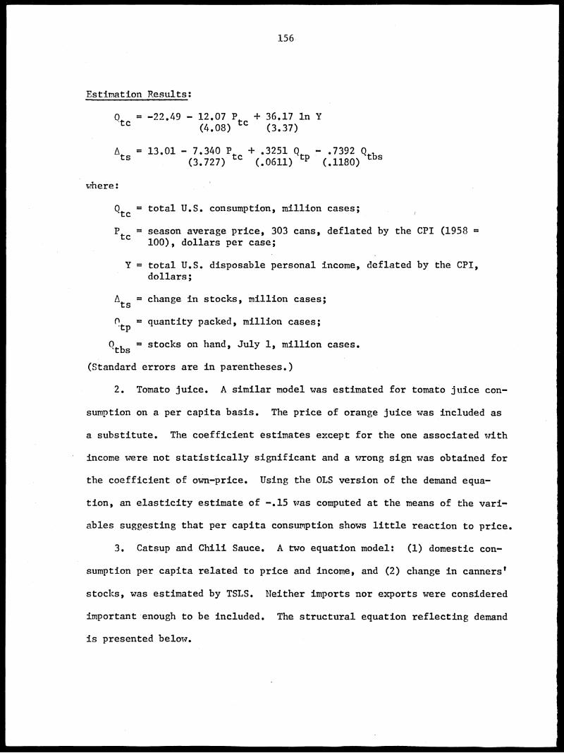
156

Estimation Results:

= -22.49 - 12.07 Ptc + 36.17 in Y

-tc (4.08) (3.37)

Ats

= 13.01 - 7.340 Ptc + .3251 Q

tp .7392 0:413

(3.727) (.0611) (.1180) s

where:

Qtc

= total U.S. consumption, million cases;

Ptc

= season average price, 303 cans, deflated by the CPI (1958 =100), dollars per case;

Y = total U.S. disposable personal income, deflated by the CPI,dollars;

Ats

= change in stocks, million cases;

tp = quantity packed, million cases;

0 tbs

= stocks on hand, July 1, million cases..


2. Tomato juice. A similar model was estimated for tomato juice con-

sumption on a per capita basis. The price of orange juice was included as

a substitute. The coefficient estimates except for the one associated with

income were not statistically significant and a wrong sign was obtained for

the coefficient of own-price. Using the OLS version of the demand equa-

tion, an elasticity estimate of -.15 was computed at the means of the vari-

ables suggesting that per capita consumption shows little reaction to price.

3. Catsup and Chili Sauce. A two equation model: (1) domestic con-

sumption per capita related to price and income, and (2) change in canners'

stocks, was estimated by TSLS. Neither imports nor exports were considered

important enough to be included. The structural equation reflecting demand

is presented below.

157

Estimation Results:

5275 - .0260 P + .2318 In Y/cQcc/c =

(.0079) c (.0260)

where:

Qcc/c= per capita consumption of catsup and chili sauce, cases;

Pc = season average price, 14 oz. fancy, deflated by the CPI,

dollars per case;

Y/c = per capita disposable personal income, deflated by the CPI,dollars.


4. Puree. A similar model WAS estimated, but the incomplete data

series produced statistically unsatsifactory results.

5. Paste. The severe deficiency of tomato paste data on pack and

stock, meant that only a "particularly naive" model could be fitted, de-

fining supply as the sum of California institutional pack, California

beginning stocks, and U.S. imports. The need for a separate import de-

mand equation WAS emphasized, due to the importance of imparts to U.S.

total supply. The reduced farm equation (1st stage, OLS) was considered

satisfactory in that the coefficients associated with pack, stock, and

income were of expected sign and statistically significant. A positive

(incorrect) sign, however, WAS obtained for the coefficient associated

with imports; but as is suggested above, import demand should not have

been considered a predetermined variable in the system. The second stage,

structural demand equation was not estimated due to data-insufficiency.

Estimation Results:

Ps = -7.497 - .2015 Qs - .7864 Qsb + .2371 Qsin + 6.320 In Y(.0918) P (.1807) s (.1764) (4.582)

R2 = .69 DW 1.25, inconclusive at the 5% level

158

where:

Ps = season average price, 10 oz. can, deflated by the CPI, dollars

per case;

Qsp = California institutional pack, million cases;

= California beginning stocks, million cases;Qsbs

Qsm = quantity imported, million cases;

Y = total U.S. personal disposable income, deflated by the CPI,dollars.



USDA, Agricultural Marketing Service, Technical Bulletin No. 1105, December

!1.954.

Scope: Demand for lettuce, onions, potatoes, cabbage, peas, and tomatoes.

Purpose: To discuss the principal economic forces that influence the price

and consumption of six important vegetable crops.

Observational Interval: Annual. (Seasonal analysis was also done for

lettuce cabbage, peas, and tomatoes.)

Period of Analysis: 1921 through 1941, then computed values of the de-

pendent variables were reported through 1952.

Specification and Estimation Procedure: One question that was considered

for each vegetable was whether the traditional single-equation analysis

could be used to measure the elasticity of demand with respect to price.

Single equations in first differences of the logarithms of the variables

estimated by OLS gave satisfactory results for late onions, potatoes, sum-

mer and fall cabbage, fresh and canned peas. Simultaneous equation esti-

mation methods were apparently needed for "lettuce and for the winter and

159

spring seasons for certain other crops because of the importance of non-

harvesting for economic reasons and for tomatoes because of dual outlets

for the crop." p. 2. The simultaneous system estimated for tomatoes will

be reviewed here, but the single equations for lettuce (not statistically

significant), onions, potatoes, cabbage, peas, and tomatoes (not statis-

tically significant) were reported in Buchholz, Judge, and West-1/ and will

not be repeated here. Elasticity estimates will appear in the relevant

summary tables of this report.

For tomatoes: the original structural relationship of (1) retail

price as a function of domestic (Qd) plus imported quantity (Qi), and in-

come (Y); and (2) imported quantity as a function of retail price minus

duty (T), and income was converted to a just-identified system and farm

price (Pf) was substituted for retail price:

Pf = al + biQd + clQi + d

lY

= a2 + b2-Pf

+ c2 T + d

2Y

i

Domestic quantity was considered predetermined; the reduced form, therefore,

fitted Pf and Qi as functions of Qd, T, and Y. The data were expressed in

first differences of the logarithms. The recovered structural equations

are presented below.

Estimation Results:

Pf = -0.007 - 0.45Qd -(.15)

Qi 0.043 + 0.27Pf -(.35)

0.18Q + 0.11Y(.76) (.90)

0.22T + 0.69Y(.26) (.79)

2R = .35

R2 21. .05

1/ H.E. Buchholz, G.G. Judge, and V.I. West. A Summary of SelectedEstimated Behavior Relationships for Agricultural Products. Illinois Ag-ricultural Experiment Station, Research Report AERR-57, October 1962, pp.104-108. Short summaries of the empirical findings from many sources ofboth demand and supply relationships for food, meat, livestock, products,feed grains, fruits and vegetables, cotton, tobacco, and coffee were givenin the Buchholtz, et al. report.

160

where:

P = price of tomatoes received by farmers,

Qd = per capita domestic production,

Qi per capita imports,

Y = per capita disposable income,

T = duty on imports.


RICHARD L. SIMMONS and CARLOS POMAREDA. "Equilibrium Quantity and Timing

of Mexican Vegetable Exports." Abstracted under cucumbers on page 80.

FREDERICK V. WAUGH. Demand and Price Analysis: Some Excinples from

Agriculture. Abstracted under potatoes on page 128.

V

TABLE 13: Selected Econometric Analyses With Flexibility or Elasticity Estimates for Tomatoes

Author andDate

Ceograph-ical Area

TimePeriod

Ohserva-vationalInterval

Form ofEquation

Method ofEstimation

Market PriceLevel Product Flexibility

IncomeFlexibility

CrossEffect

PriceElasticity

IncomeElasticity

Bohall,1972

Florida 1966-1968

Weekly linear OLS FOB large and -1.19extra-large vineripe

a /-0.15-

Chern and

7'Listt/,1978

California 1951-c

1963/-

1967,111975-

Annual

doublelog

3SLS;pooledcross See-tion, timeseries; co-variancesbetweencountiesconstrainedto be zero

grower processingtomatoes

-1.65

- .16

1.64

.97

Firch andYoung, 1968

U.S. 1961-1966

Weekly linear OLS shipping fresh:point from W.prices-- Mexico -0.181Nogales, from else-Arizona where -0.157

total ship-ments -0.278

Foytik, 1964 Hawaii 1947-1961

Monthly linear OLS l.-0.343-/wholesale fresh e

11.-0.399111.-0.414IV.-0.399

Jesse andMachado,1974

California 1948-1972

Annual linear TSLS farm freshsummer -1.0fall -1.0

King, Jesse,and French,1973

U.S. 1948-1971

1948-19711948-19671953-1971

Annual semilog

TSLS

OLS

TSLS

OLS

cannedwholetomatoes

FOR, tomato juiceprocessors

catsup & chilisauce

f/paste - .28-

- .87

- .15

- .65

Waugh, 1964 U.S. 1950-1962

Annual linear OLS retail - .853fresh

iarm -1.010

.360

.003

a/ wrt.11exican shipments

b/ for other elasticity estAmates byvarious methods see the review in

c/ pre-harvester I/ wrt. California institutionald/ post-harvester

162

Related Studies, Tomatoes

Brandt, Jon A., Ben C. French, and Edward V. Jesse. Economic Performanceof the Processing Tomato Industry. California Agricultural ExperimentStation, Giannini Foundation Information Series No. 78-1, Division ofAgricultural Sciences Bulletin No. 1888, Davis, April 1978. ". . .thefirst of two reports dealing with the economics of the U.S. processingtomato industry." (p. ii). This report is primarily descriptive in na-ture and discusses: (1) structural characteristics and adjustments ofthe industry at both the grower and processor levels, (2) measurement ofeconomic performance including technological progress, employment and pro-ductivity, tomato plant capacity utilization, product quality, price per-formance and variability, profits, ang processor-grower price spreads.

Brown, J. D. and M. E. Cravens. Retail Margins on Tomatoes. Ohio Agri-cultural Research and Development Center, Wooster, Ohio, Research Bulletin984, February 1966. Wholesale-retail margins for three types of freshtomatoes—tube, vine-ripe, and greenhouse—were calculated from wholesaleand retail prices measured weekly at 214 Ohio retail food stores fromMarch 27 through June 17, 1961.

Brooker, John R. and James L. Peterson. The Winter Fresh Tomato Industry,A Systems Analysis. USDA, ERS in cooperation with the University ofFlorida's Agricultural Experiment Station and Food and Resource EconomicsDepartment, Agricultural Economics Report No. 330, April 1976. A computermodel was constructed with an interseasonal and an intraseasonal phase tosimulate the long-run effects of alternative supply controls and marketingpolicies on handlers of fresh winter tomatoes at the U.S.-Mexican border,on Florida producers and handlers, and an U.S. consumers.

Cain, Jarvis L. and Ulrich C. Toensmeyer. Interregional Competition inMaryland Produced Fresh Market Tomatoes. Maryland Agricultural ExperimentStation, Bulletin No. 741, October 1969. A linear programming transporta-tion model was used to evaluate the competitive position of Maryland freshtomatoes in 13 major eastern and midwestern markets. The solution pro-vided the minimum cost distribution pattern from major producing areas tothe 13 markets. The optimum WAS then compared with actual weekly shipmentdata.

Chern, Wen S. "Acreage Response and Demand for Processing Tomatoes inCalifornia." American Journal of Agricultural Economics, Vol. 58, No. 2,May 1976, pp. 209-216. Demand for processing tomatoes produced in tenCalifornia counties was estimated for 1951 through 1972 by OLS and by 3SLSas a part of a three equation system. This model WAS updated in 1978 andthe later version is reviewed in this report on page 145.

163

Dillman, Buddy L. and Donald E. Farris. Arkansas' Competitive Positionin Marketing Fresh Tomatoes. University of Arkansas, Agricultural Experi-ment Station, Bulletin 663, February 1963. The possibility of expandingproduction of Arkansas fresh tomatoes was investigated by exploring loca-tional advantages using an interregional competitive model.

Feick, Lawrence F. and Ulrich C. Toensmeyer. Delaware Household Consump-tion of Fresh Tomatoes. Delaware Agricultural Experiment Station, Bul-letin No. 424, February 1978. In a mail survey of 500 Delaware consumers--response rate 23.6 percent--it was found that taste was a more importantdeterminant of purchase than was price or other considerations. This is ofinterest in that taste is of lower priority to growers than are otherfeatures such as: suitability for mechanical harvesting, high yield,disease resistance, and capability of ripening at the same time.

Goble, W. E. and Erven J. Long. Marketing Tennessee Tomatoes. Universityof Tennessee Agricultural Experiment Station, Bulletin No. 226, June 1953.The report gives the findings from a four-year, three-phase project:phase 1, a study of production and marketing practices in West Tennessee;phase 2, interviews to determine consumers preferences regarding qualityand characteristics of tomatoes; phase 3, controlled market experimentsin Knoxville retail grocery stores.

Lee, Woo Bong. "The Competitive Nonlinear Spatial Equilibrium Analysis--An Empirical Study." The Southern Economic Journal, Vol. 41, No. 1, July1974. For use in a nonlinear (quadratic) spatial equilibrium model, re-duced form demand and supply functions for fresh and processing tomatoeswere estimated for nine regions of the U.S.

Hoos, Sidney. Tomatoes and Tomato Products--Economic Trend's and F.O.B.Price Relationships. California Agricultural Experiment Station, GianniniFoundation of Agricultural Economics, Mimeographed Report No. 185, March1956. The report summarized economic trends in the tomato industry inCalifornia: production, acreage, yield, farm prices, the various processedproducts, canners' pack and shipments, and consumption. In addition, FOBcanners' price relationships for canned tomatoes were estimated. In theequation selected as best for statistical and economic reasons, the averageannual FOB price of California canned tomatoes was expressed as a linearfunction of California canners' pack and movement, the log of the index ofU.S. disposable personal income, and an adjusted index of competing cannedvegetable prices.

Roos, Sidney and R. D. Aplin. California Canned Tomatoes: Analysis ofF.O.B. Price Relationships. California Agricultural Experiment Station,Giannini Foundation of Agricultural Economics, Mimeographed Report No. 156,June 1953. As part of the report, price forecasting equations for FOBprices of California canned tomatoes were fitted by OLS with alternativecombinations of independent variables. In the equation selected as statis-tically best, the FOB price was expressed in log-linear form as a functionof California canners' pack, an index of U.S. disposable personal income,an index of prices for competing canned vegetables, and a trend variable.

164

Jesse, Edward V. "Marketing California Fresh Market Tomatoes: Trends andOutlook." The Vegetable Situation, No. 193, USDA-ERS, August 1974. Ab-stract, p. 31: "California provides about a third of the fresh tomatoesmarketed commercially in the United States, and is the only domestic sourceof supplies during the late fall marketing season. This report tracestrends in production and marketing of the state's crop in 1948-72."

Mathia, Gene A. and John R. Brooker. Vine-Ripe Tomato Production andMarketing in North Carolina and Tennessee. Southern Cooperative SeriesBulletin No. 230, June 1978. In order to investigate the economic poten-tial for expansion of vine-ripe tomato production in North Carolina andTennessee, a linear programming model was used. Demand elasticities forthe model were obtained from secondary sources.

Sullivan, G. H., A. J. Minden, and L. F. Schrader. "Interregional Competi-tion in Processed Tomato Products." Florida State Horticultural SocietyProceedings, Vol. 86, November 1973. "A quantitative evaluation of inter-regional competition and projected advantage was completed for the proces-sed tomato industry using linear programming techniques. Results of thisanalysis indicated that under current regional cost structures, the WesternRegion will likely continue to expand tomato production at the expense ofproduction areas in the Midwestern and Eastern Regions. However, it wasfound that the interregional dominance of the Western Region was tenuouslyheld for the production of selected tomato products and subject to substan-tive dilution if lower production cost structures, attainable through theimplementation of available cost reducing technologies, were realized incompeting supply regions." p. 289.

Uhl, Joseph N. The Demand and Price Structure for Processed Tomato Products:Preliminary Findings and Implications for Interregional Research. Depart-ment of Agricultural Economics, Purdue University, paper presented at theNCM-44 meeting, Chicago, September 1969. Three separate wholesale-leveldemand equations--fall, winter, and spring--were fitted by OLS for each ofthree tomato products--whole pack, catsup, and juice.

165

AUTHOR INDEX

Page Page

Adams, R. M. 17 Elrod, J. C. 30Allen, M. B. 50, 56, 58, Erdman, H. E. 139

101, 117.Aplin, R. D. 163 Fajardo-Christen, A. 92, 99Araji, A. A. 121 Farrell, K. 100

Farris, D. E. 83, 120, 163Bain, B. M. 141 Feick, L. F. 163Bell, J. B. 73, 75 Firch, R. S. 78, 82, 91, 94,Blaich, O. P. 19, 84, 90 99, 118, 119,Blakeslee, L. 136 148, 161Bohall, R. W. 27, 60, 66, 85, Ford, K. E. 30

90, 143, 161 Fowler, M. L. 100Brandow, G. E. 15, 136 Fox, Karl A. 15Brandt, J. A. 162 Foytik, J. 27, 37, 49, 78,Branson, R. E. 112 82, 136, 151,Brooke, D. L. 73, 75 161Brooker, J. R. 162, 164 French, B. C. 12, 32, 51, 142,Brown, J. D. 162 155, 161, 162

Cain, J. L. 50, 76, 162 Garoyan, L. 27Carlson, C. H. 63, 66 Geithman, F. F. 102, 111, 121,Castro, R. 77, 82, 92, 99, 135

118, 119 George, P. S. 27Goble, W. E. 138, 163

Chen, C. 112 Godwin, M. R. 70, 72, 151Chern, W. S. 145, 161, 162 Gray, R. W. 122Clevenger, T. S. 68, 86, 90, Grieg, W. S. 136

102, 111, 121, Halter, A. N. 27135 Hammig, M. D. 28

Cochrane, W. W. 122 Hartman, P. 75Cockroft, L. U. 141 Hassan, Z. A. 28Connolly, C. 104, 111 Hathaway, D. E. .50Cravens, M. E. 141, 162 Hayenga, M. L. 38, 49Cromarty, W. A. 15 Hee, O. 123, 135, 136

Hertzendorf, Ann 136Davis, G. B. 114, 116 Hoos, S. 32, 91, 141,Dennis, C. C. 141 163Dillman, B. 163 Hussey, G. 94Dixon, E. 113 Hutchings, H. M. 114, 116Droge, J. H. 33, 49, 74, 75,

114, 116 Jesse, E. V. 105, 106, 111,Drury, C. 137 152, 155, 161,

162, 164

166

Johnson, A. C.Johnston, W. E.Just, R. E.

Klein, G. L.King, G. A.King, R. A.

Koizumi, S.Krebs, E. H.

Larzelere, H.Lee, W. B.Lehker, J. N.L'Esperance, W. L.Lester, B. W.Lindstrom, I. A.

Lloyd, Billie S.Long, E. J.

Machado, M. J.Manley, W. T.Mathia, G. A.

Mathews, D. W.Matsumoto, M.Matthews, J. L.McCorkle, C. 0.McGlothlin, R. S.McPherson, W. W.Mehren, G. L.Meinken, K. W.Meissner, F.Miklius, W.Minden, A. J.Mittelhammer, R. C.Mundlak, Y.

Nerlove, M.Nichols, T. E.

Padberg, D.Parker, A. F.Peterson, J. L.Pomareda, C.

Page

11217145, 161

10017,27,155,16159, 78, 82, 83,118, 120, 136

110, 11138, 49

13616338,499211278, 82, 118,11970163

152, 16172, 15123, 59, 124,135, 136, 142,9143, 513213788, 9029139137299116425137

1550

1132916229, 80, 118160

Porter, J. T.Price, D. W.Price, D. Z.Purcell, J. C.Rauchenstein, E.Raunikar, R.Reed, R. H.

Rockwell, G. R., Jr.

Sammet, L. L.Schrader, L. F.Schrimper, R. A.

Seagraves, J. A.Seale, A. D., Jr.

Shafer, C. E.

Shelley, W. V.Shuffett, D. M.

Siebert, J. B.Simmons, R. L.164

Simmons, W. M.Smith, G. W.Sorenson, V. L.Sparks, W. C.Stone, K.Stover, H. J.Strand, F. 0.Suits, D. B.Sullivan, G. H.Summers, L.

Thompson, S. R.Toensmeyer, U. C.Tomek, W. G.Uhl, J. N.

Valenzuela, LyaVandenborre, R. J.Velasco, C.

Page

943030301003033, 49, 74, 75114, 11631

14116423, 124, 135,14212050, 56, 58, 83,101, 11761, 63, 66, 67,108, 109, 11186, 9057, 58, 59, 110,111, 115, 116,135, 158126, 13529, 77, 80, 82,92, 99, 118,119, 160127, 1351281221211133213695, 99, 110,1111164137

10150, 76, 162, 163137164

97

43, 4927

Waugh, F. V. 128, 135, 160,161

167

Page

West, D. A. 30

Wold, H. 0. A. 97, 99Working, H. 113, 130

Young, D. 113

Young, R. 137

Young, R. A. 78, 82, 94, 99,118, 119, 148, 161

Zusman, P. 132, 135, 137

Waite Memorial Book Col!Kilo.,

Wigan of Agricultural Economics

Gannini foundation - AgEcon Search

Documents

Transcript of Gannini foundation - AgEcon Search