Historic, archived document

Do not assume content reflects current

scientific knowledge, policies, or practices.

/

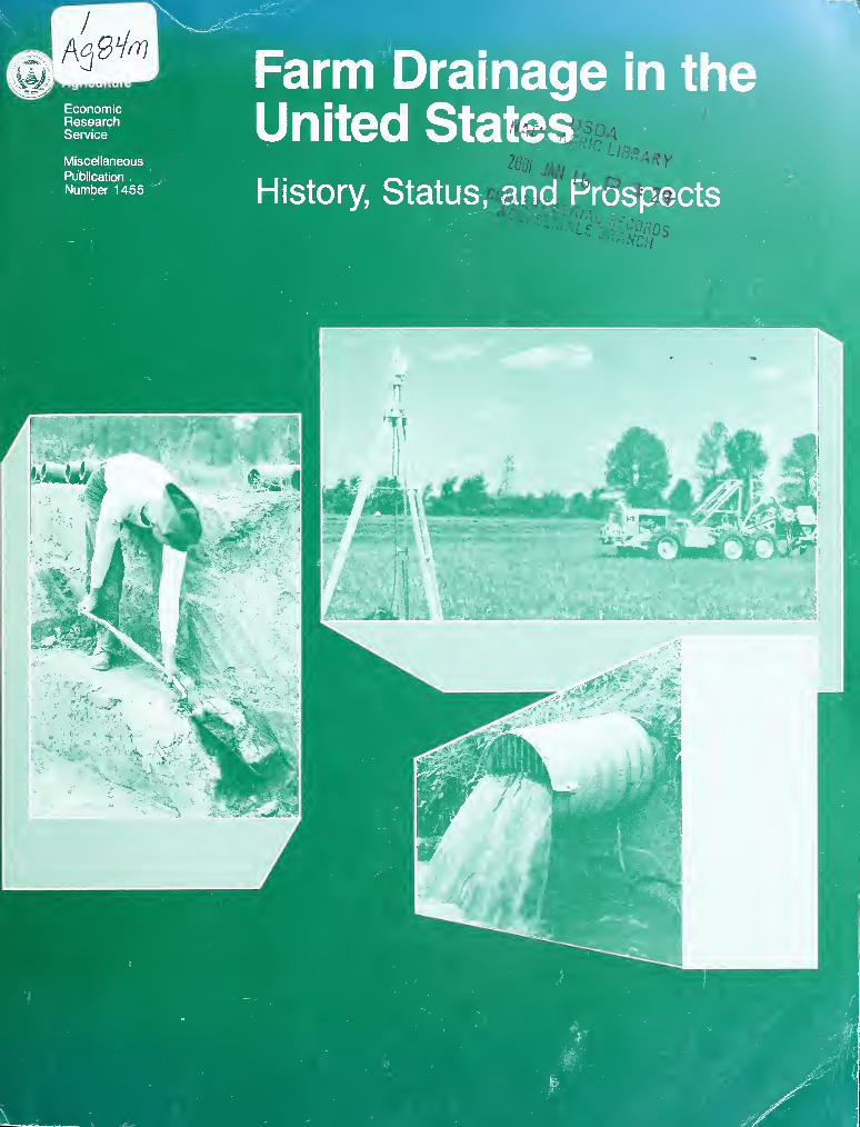
EconomicResearchService

Miscellaneous

Publication

Number 1455

Farm Drainage in theUnited State

History, Status, a10$

Sales Information

Additional copies of this publication can be purchased from the Superinten-

dent of Documents, U.S. Government Printing Office, Washington. DC 20402.

Ask for the publication by name, and write to the above address for price

information, or call the GPO order desk at (202) 783-3238. You can also

charge your purchase to your VISA, MasterCard, Choice, or GPO deposit

account. Bulk discounts available. Foreign address customers, please add 25

percent extra for postage.

Microfiche copies ($6.50 each) can be purchased from the National

Technical Information Service, 5285 Port Royal Road, Springfield, VA 22161.

Ask for the publication by name. Enclose check or money order, payable to

NTIS; add $3 handling charge for each order. Call NTIS at (703) 487-4650

and charge your purchase to your VISA, MasterCard, American Express, or

NTIS deposit account. NTIS will RUSH your order within 24 hours for an

extra $10; call (800) 336-4700.

The Department of Agriculture has no copies for free mailing.

Farm Drainage in the United States: History, Status, and Prospects.

Edited by George A. Pavelis. Economic Research Service, U.S. Depart-

ment of Agriculture. Miscellaneous Publication No. 1455.

Document Delivery Services BranchUSDA, National Agricultural LibraryNal Bldg.

y

10301 Baltimore Blvd.Beltsville, MD 20705-2351

Abstract

This publication covers the historical, technological, economic, and environ-

mental aspects of agricultural drainage. It draws from the combined

knowledge of academic and U.S. Department of Agriculture professionals in

public policy, drainage theory, planning, engineering, environmental science,

and economics. The main purpose is to review the evolution of modern farm

drainage and to identify farm drainage objectives for agricultural extension

specialists and agents, environmental specialists, drainage consultants, in-

stallation contractors, and educators. Farm production, water management,

and other benefits and costs associated with the drainage of wet soils on

farms are described within the context of existing USDA programs and

other Federal policies for protecting wetlands.

Keywords: Soil and water management, irrigation, drainage development,

drainage benefits, environmental improvement, drainage

districts, drainage models, drainage planning.

Cooperators

Agricultural Research Service

Cooperative State Research Service

Economic Research Service

Extension Service

Soil Conservation Service

Cornell University

North Carolina State University

Ohio State University

Utah State University

University of Wisconsin-Madison

This bulletin was processed in the Information Division, Economics ManagementStaff, USDA, by Jim Carlin, editorial assistance, and Susan Yanero, graphics.

Washington, DC 20005-4788 December 1987

Foreword

The U.S. Department of Agriculture (USDA) is pleased to release this

cooperative publication on farm drainage, primarily as a general information

document. Several factors prompted its preparation: (1) wide recognition of

the public policy connections between the economic and environmental

aspects of drainage, accentuated most recently by stringent wetland protec-

tion provisions in the Food Security Act of 1985; (2) a drainage technology

still undergoing important changes; and (3) the uncertain status of informa-

tion collection activities on drainage, particularly at the Federal level.

The most recent rapid developmental era for drainage reclamation drew to

a close about 1965. Drainage is the most extensive soil and water manage-ment activity in agriculture. Approximately 110 million acres of the land

within farms are artificially drained in the United States. About 9 million

acres, or 25 percent, of the irrigated cropland in the Western States are

artificially drained.

Drainage can also have adverse effects in some situations by reducing or

degrading wetlands vital to wildlife and serving hydrologic functions such as

flood flow regulation. Drainage activities can also affect the quality of water

bodies receiving drainage water.

Drainage investigations in USDA began with the Reclamation Act of 1902.

This act is best known as creating the Bureau of Reclamation in the Depart-

ment of the Interior. A drainage unit to service irrigation project planning

was simultaneously authorized for USDA. In 1962. Public Law 87-732, the

Drainage Referral Act, was enacted which prohibited USDA from assisting

landowners in draining potholes and marshes in Minnesota and the Dakotas

if wildlife would be materially harmed.

Currently, USDA technical and financial assistance is no longer provided as

a matter of policy except in unique circumstances as part of a conservation

system related to irrigation water control, or as an essential element of an

environmental system of practices. Thus, for USDA, this publication

represents an end to the era of strong USDA support and assistance for

drainage development activities.

Under USDA's Water Bank Program, begun in 1970 under the authority of

Public Law 91-559, wetlands along major migratory waterfowl flyways can

be protected from agricultural use or drainage development by 10-year

rental agreements with eligible owners or operators. As of 1987, about

8,000 agreements covering 870,000 acres of wetlands or adjacent land had

been negotiated with farmers. Two-thirds of these agreements are still in

force. In USDA's Agricultural Conservation Program (ACP), financial

assistance for farm drainage is prohibited by appropriation language unless

it is an essential element of an erosion control, water quality, or environ-

mental system of practices. By the late 1970's, less than 4 percent of all

costs of installing or maintaining farm drainage systems came from ACPcost sharing or Farmers Home Administration loans. Cost sharing for limited

drainage assistance as described above is now less than l/20th of 1 percent

of all ACP cost shares.

Since 1973. USDA's Soil Conservation Service has not provided technical

assistance for the drainage of specified wetlands, as defined by the Fish and

Wildlife Service of the Department of the Interior. Since 1975, the policy has

been broadened to include nearly all freshwater and saline-water areas.

Drainage activities of USDA are subject also to the provisions of Executive

Order 11990, issued in May 1977. Executive Order 11990 is intended to

"avoid to the extent possible the long and short term adverse impacts

associated with the destruction or modification of wetlands and to avoid

direct or indirect support of new construction in wetlands whenever there is

a practicable alternative." The Food Security Act. signed by President

Reagan in December 1985, denies farm program benefits to producers whogrow annual crops on wetlands drained after December 1985.

It is within such laws and policies that USDA will assist in improving

drainage on existing cropland through better design, construction, andmaintenance. For example, adequate drainage is sometimes necessary for

successful no-till conservation farming. Also, intensive irrigation, as practiced

on a large scale in the Western States, requires continued attention to

drainage to prevent rising water tables and damaging accumulations of

soluble salts in soils, and in controlling chemicals or other harmful agents

in drainage waters.

This publication is the product of efforts by several USDA agencies and

cooperating universities to consolidate up-to-date knowledge on farmdrainage. It draws from the combined knowledge of specialists in public

policy, drainage science, planning, engineering, and economics (see appendix

C). It is not highly technical or policy oriented, but reviews the history, pur-

poses, social and economic implications, and modern methods of farm

drainage.

USDA greatly appreciates the assistance of the following academic

cooperators:

• Cornell University, College of Agriculture and Life Sciences, Depart-

ment of Agricultural Economics.

• North Carolina State University, College of Agriculture, Department of

Agricultural and Biological Engineering.

• Ohio State University, Department of Agricultural Engineering.

• Utah State University, College of Agriculture and Agricultural Experi-

ment Station, Department of Agricultural and Irrigation Engineering.

• University of Wisconsin-Madison, College of Agricultural and Life

Sciences, School of Natural Resources.

Orville G. Bentley George S. Dunlop Ewen M. Wilson

Assistant Secretary Assistant Secretary Assistant Secretary

Science and Education Natural Resources for Economics

and Environment

hi

Summary

Drainage, the practice of removing excess water from agricultural land, has

its origin at least 2,500 years ago when Herodotus wrote about drainage

works near the city of Memphis in Egypt. Today, drainage is practiced widely,

being criticized severely by some and praised by others.

Without drainage, it is hard to imagine the U.S. Midwest as we know it in

the 20th century, the epitome of agricultural production. Much of Ohio,

Indiana, Illinois, and Iowa originally was swamp, or at least too wet to farm.

Aquatic plants, swarms of mosquitoes, and outbreaks of malaria and other

diseases were common. Without drainage, irrigation development in the

Western United States would have failed through waterlogging and salina-

tion, as is happening in some areas. Drainage was part of the "developmen-

tal ethos," the drive to develop the land and make it productive.

Because of drainage, better than half the original wetlands in this country

are no more. In addition to impairing various hydrologic functions of

wetlands, drainage has drastically reduced the habitat for water-based

wildlife, and flyways for migrating birds have been severely affected. In

some States, as much as 95 percent of the wetlands have been converted.

These conversions have affected the opportunities for hunters and recrea-

tionists to enjoy their sport. Possibly more important, they have affected the

natural balance of nature and may well have endangered, or at least severely

restricted, a number of species of birds and other wildlife.

Recently, evidence shows that not only the loss of wetland habitat is involved,

but that drainage effluent can have severe adverse effects on water and

land quality. High concentrations of toxic elements in California's Kesterson

Reservoir have been attributed to agricultural drainage upslope. Thus the

"environmental ethic" is at odds with the "developmental ethic." While the

benefits of drainage can be counted in terms of enhanced development and

increased economic activity, the cost to the environment may also be high.

This bulletin provides an overview of agricultural drainage. Included are a

historical perspective of drainage, a review of its practical purposes, an

assessment of technological progress, some economic evaluations, a discus-

sion of institutional mechanisms, and a consideration of environmental

values. Finally, an attempt is made to place these various components into a

challenging perspective in relation to present and future needs.

Highlights

Controversy has frequently been associated with drainage. In the Middle

Ages, the fens in England were drained to stabilize and increase

agricultural production. These actions were not appreciated by the

fishermen and fowlers who saw their livelihood threatened. Interest in

drainage ebbed from the early years until the 19th century, when there wasrenewed activity in Europe and the United States. Early interest in the

United States was not confined to development and enhanced agricultural

production, but also stressed human health aspects, as illustrated by the

draining of Central Park in New York City in 1858. In recent years, these

health benefits were taken for granted, or overlooked, in part because wenow operate at the margin: the great swamps and extensive breeding

grounds for mosquitoes have been eliminated.

IV

An important initial Federal milestone was the passage of the SwamplandActs of 1849 and 1850. These acts transferred federally held swamplands to

the States on condition that proceeds from their sale be invested in works

needed to reclaim them. The Reclamation Act of 1902 illustrates another

milestone in Government policy in that it signaled the intention of the

Federal Government to become directly involved in land reclamation andassociated drainage enterprises.

The Flood Control Act of 1944 and the Federal Watershed Protection andFlood Prevention Act of 1954 broadened Government involvement in

drainage activities. They were preceded by the work of the Civilian

Conservation Corps during the Depression and the technical or financial

assistance programs of USDA's Soil Conservation Service (SCS) andAgricultural Stabilization and Conservation Service (ASCS). While ASCSfinancial assistance is no longer provided and technical assistance from SCSis restricted, these programs have played an important role in improved soil

and water management on farms.

The pendulum has swung away from development in the last 20 years as a

balance was sought between development, reclamation, and drainage on the

one hand, and preservation of environmental values on the other. This

balance is illustrated by the National Environmental Policy Act of 1969, the

Clean Water Act as amended in 1977, and Executive Order 11990 issued by

President Carter in 1977. The order instructs Federal agencies to avoid

where possible the long- and short-term adverse effects of destroying or

modifying wetlands.

Further, new farm legislation, the Food Security Act of 1985 signed by Presi-

dent Reagan in December 1985, denies price support and other farm pro-

gram benefits to producers who grow crops on converted wetlands. Also,

the elimination of investment tax credits and restrictions on expending farm

conservation investments under the Tax Reform Act of 1986 are further

disincentives to bringing new lands into production through drainage.

Thus, current USDA programs are intended, within the limitations noted

above, to help landowners improve drainage on existing agricultural fields

where excessive wetness, waterlogging, or salinity hamper efficient produc-

tion. It is USDA policy to preserve remaining wetlands and protect wildlife

values wherever possible. Corrective measures are also required whereagricultural practices, including drainage, threaten offsite environmental

values.

Technology has evolved along with drainage policy. After centuries of hand-

installed drainage systems, the introduction of the trenching machine and

the steam engine revolutionized the practice in the late 19th century.

Another leap forward occurred in the 1960's with the introduction of cor-

rugated plastic tubing installed with laser-beam controlled high-speed

trenchers or drain plows. In the late 1970's, there came into practice the

application of drainage theory in the form of computerized design methods

and models. Thus, we have witnessed in the past 20 years a dramatic

modernization of drainage practices, with the potential for cost reduction,

better design, and advanced installation practices. The most recent

technological change is the application of water management systems that

incorporate drainage, drainage restrictions, and subirrigation in one

sophisticated operation to optimize soil water conditions for crop growth. At

the same time, sufficient experimental data are available to make at least

approximate assessments of the effect of drainage on crop yield, so that

economic optimization procedures can be applied to develop "best"

drainage system designs.

In making the decision whether and how to drain land, one must be awareof the benefits and drawbacks associated with the practice. The purpose of

drainage varies with the climate and the type of farming. In humid areas, its

dominant purpose is to remove excess soil water. This allows equipment

movement into fields for timely farm operations, warms soils early in the

season, provides adequate aeration for root activity and crop growth,

reduces diseases in livestock and crops, and reduces surface runoff. These

benefits in turn reduce erosion and surface waste pollution, especially by

phosphates. The benefits include reduced risk in farming and higher yields

of better quality crops, thus tending to increase income as well as reduce its

variability.

In arid regions where land is irrigated, the dominant purpose of drainage is

to remove salts from the root zone. Salts always accumulate in irrigated

fields unless drainage is present, ultimately causing severe salination andenvironmental degradation. "Ultimately" may be in a matter of a few years,

or many decades.

Juxtaposed to the benefits are potential disbenefits. Nitrogen, from fertilizer

or natural sources, may be leached out of the soil and contribute to

eutrophication (a reduction in oxygen) in downstream water bodies. Somemobile pesticides may also be leached out. The leaching of salts from

irrigated lands to keep the lands productive may cause increased salt loads

downstream. Primarily, the removal of wetlands by drainage changes the

landscape, alters hydrologic processes, and reduces habitat for waterfowl

and other wildlife.

Not recognized as a significant potential problem until recently was the

leaching by drainage waters of trace elements in toxic concentrations from

natural geologic formations. Unexpected high levels of selenium (and

possibly other elements, such as boron and molybdenum) were found in the

early 1980's in soils, waters, plants, and wildlife in the Kesterson Reservoir,

an area used for disposal of agricultural drainage water. Similar natural

resource problems related to irrigation drainage may be occurring

elsewhere. The Department of the Interior is currently investigating 19 such

situations in the Western States.

The planning and design of drainage systems require a thorough under-

standing of the various components of such systems and their interaction.

The primary components are the outlet, the collection system (including both

surface and subsurface drains), and certain land treatment systems such as

bedding or smoothing. The planning may involve one landowner or many and

often concerns agricultural interests as well as environmental groups. Good

planning takes into account various environmental values as well as those of

agriculture, provides for flood protection if large projects are involved, and

considers the economic impacts as well as the financial and political

realities of implementing the plan.

Because of the need for cooperation among landowners to provide

appropriate outlets to dispose of drainage waters, a variety of drainage

organizations has been created under State laws. The most common of these

is the corporate drainage district. This is an organization with taxing

powers that constructs and maintains drainage outlets for the area it

serves. In recent years, a number of States have enacted legislation permit-

ting multiple-purpose districts, often called conservancy districts. Their

objectives may include drainage but can go well beyond that to consider

numerous other water and resource management objectives. Whereas in the

past, the activity of drainage districts often has been dominant in the

drainage field, of late more drainage is completed privately than through

district organizations.

At what rate have drainage organizations and individual farmers improvedland by drainage and invested in drainage improvement? How does this

investment compare to the total capital investment in agriculture and whathave been the returns? Reliable information on these questions is hard to

obtain. Combining whatever data could be gleaned from the Census of

Drainage and the Census of Agriculture from 1920 forward, with statistics

from USDA and other specialists, reveals the following picture.

As of 1985, an estimated 110 million acres of agricultural land in the United

States benefited from artificial drainage. At least 70 percent of the drained

land is in crops, 12 percent in pasture, 16 percent in woodland, and 2 per-

cent in miscellaneous uses. Although recent trends have been toward morefarm drainage systems, 60 percent of the area drained still depends on

public outlets installed by counties or drainage and conservancy districts.

The average U.S. real cost of providing group drainage outlets was $225/acre

in 1985. and has been essentially constant since 1915. The cost of providing

surface drainage has risen since 1965 (to $140/acre), while the cost of subsur-

face drainage has dropped substantially (to $415/acre). These trends reflect

the impact of the new plastic materials for subsurface drains and more effi-

cient trenching methods.

The capital value of all U.S. farm drainage work now in place is estimated

to be over $40 billion, based on replacement costs as of 1985. This includes

$15 billion (36 percent) for public drains and $25 billion (64 percent) for

onfarm systems. Allowing for depreciation, the net capital value of all U.S.

farm drainage work as of 1985 was estimated to be near $25 billion—$15

billion (60 percent) for public drains and $10 billion (40 percent) for onfarm

systems.

Compared with the market value of all farm real estate in the United States

($690 billion in 1985), drainage improvements represent between 4 and 6

percent of the total (up to 7 percent if buildings are excluded). Percentages

for highly drained States range considerably more—up to 30 percent in

Michigan; 25 percent in Indiana and Ohio; 20 percent in Louisiana; 15 per-

cent in Arkansas, Delaware, and Mississippi; and 10 percent in Florida,

Iowa. Minnesota, and the two Carolinas. Details are in table 11-7.

The aggregate nature of available data makes it impossible to estimate the

actual increase in value for all land that has been drained. However, by

separating economic statistics for counties with a relatively high incidence

from those with a low incidence of drainage, one can show a substantial dif-

ference in value of crops and livestock sold, and of land values, in favor of a

high incidence of drainage. An analysis of 1982 Census of Agriculture data

indicates that real estate values per acre for 256 predominantly agricultural

counties throughout the Eastern States with a high incidence of drainage

averaged 27 percent more than values in 1,422 other agricultural counties.

This translates to an expected average capital benefit of about $270 per

drained acre in 1982. By 1985 the average benefit was down to $200 per

acre, the result of generally declining agricultural land values. In 1986, the

average expected benefit figure fell further, to about $175 per acre.

vn

It would be useful to have continuing overall estimates of the increased

value of production associated with drainage, or of the returns on the

investment, because the feasibility of drainage changes with costs, commodity

prices, and other factors. While a general farm-level benefit/cost (B/C) ratio

for drainage in the East fell from 1.30 to 0.75 between 1982-86, the B/C

ratios appeared to still exceed 1.0 in seven Eastern States: Arkansas,

Missouri, Kentucky, Virginia, Missisippi, South Carolina, and Florida.

The technologies exist to make fairly precise B/C evaluations for specific

field situations, as illustrated in figure 6-10. Such "anecdotal" calculations

verify that the return on investment can be very high. It also is clear that

the response is highly site specific. For example, the irrigated Imperial

Valley in California would be out of production for all practical purposes

were it not for intensive drainage. In other irrigated areas, natural drainage

rates are high enough to require no artificial drainage at all.

To the extent statistics are available, it is clear that investment in drainage

has been substantial. It is equally clear that investment will continue. First

of all, there will be an increasing need for repair, maintenance, and

replacement of existing systems. Second, there will be pressures for addi-

tional drainage, either to control salinity in irrigated soils or to enhance pro-

duction on presently cultivated land.

Perceptions about the status and trends of agricultural drainage are a func-

tion of the extent and quality of available data. Existing information tends to

give an incomplete picture. It is based on "unstable" data in the sense that

the data collected at different times are based on different definitions and

techniques and thus tend to be unreliable, especially for comparisons over

time. Interest in drainage as such may be decreasing, but interest in

wetlands, or their remnants, is increasing. A good data base is crucial to in-

formed decisionmaking or policy development.

Future Trends and Prospects

What of the future? USDA's National Resources Inventory (NRI) of 1982 in-

dicates that nearly 28 million acres of existing nonirrigated crops andpastures have drainage problems, of which 15-20 percent are also con-

sidered wetlands. An added 12 million acres of rural land have at least a

medium potential for drainage and conversion to crop production. Nearly 30

percent of the potentially drained and converted acres are now wetlands.

About 25 percent of the wetlands vulnerable to conversion are prime water-

fowl habitat. Thus, the pressure for drainage to expand agriculture tends to

be for lands generally not considered of prime value to waterfowl, although

other environmental benefits may also be sacrificed. There are definite

restrictions, and no national need to expand the cultivated land base

through drainage.

Unless economic conditions change drastically, it is expected that drainage

activity will be concentrated at the "intensive margin" rather than the "ex-

tensive margin." Landowners will strive to improve production efficiency by

raising production per acre and product quality. This will place greater

demands on intensive drainage on currently cultivated lands. In the samevein, there is likely to be more emphasis on repair and maintenance of

existing systems, and on replacement of deteriorating systems, activities not

usually in conflict with the environment, wildlife, or other interests.

There is a growing realization that drainage is simply a component of a total

water management system. Total water management may be seen as a com-

bination drainage and subirrigation system with semiautomatic feedback

controls. On a broader scale, it may be seen as also including managementof ground-water quality and offsite effects. One may expect technological

advances to make far more effective control of soil water status possible

and profitable. One also may anticipate greater conceptual recognition in in-

tegrating various interests in the development and execution of water

management plans.

A specific example of the need for a total water management approach is

provided by the drainage of irrigated land. The 1982 NRI indicated that

improved drainage or other water conservation and management measures

would benefit at least a third of our irrigated cropland. More and more, it

will be imperative to integrate the planning and operation of irrigation anddrainage systems so as to provide maximum benefit to the land and

minimum disbenefit downstream. To achieve this, the salt load in the

drainage water must be managed explicitly. The occurrence of toxic

substances other than the traditionally recognized salts may introduce

important new management challenges.

Drainage technology plays an important role in these situations, but it does

not operate in isolation. Returning to the Kesterson Reservoir case, a solu-

tion to the kinds of complex environmental issues encountered there mayinvolve, besides drainage, irrigation technology, desalting, waterfowl, and

other wildlife toxicology investigations, wildlife management, institutional

changes, and legal or contractual arrangements.

On a broader base, the need is clear for better and more explicit standards

for decisionmaking. Using an assumed value of waterfowl hunting, an

economic comparison can be made of the relative value of wetlands for

agricultural production or for recreation. In the abstract, the same can be

done for other, intrinsic or explicit, values of wetlands. In practice, neither

the methodology nor the data base exist for such an analysis. Whether a

totally rational economic analysis ever can or should be the basis for

deciding the advisability of further drainage may be debated. However,

there can be no argument that better decisions can be expected if the infor-

mation base is improved.

The improved data base requires information on the value of drainage for

agricultural production; the value of wildlife habitat for recreation and

other ecologic purposes; the value of wetlands for hydrologic management of

ground and surface water; and the value of wetlands for maintaining

flyways. Specific decisions on individual parcels of land require specific in-

formation. Assessing the effectiveness of existing policies and institutions, or

determining the need for changes in them, one needs aggregate data.

Historic data bases have suffered from lack of continuity, from changes in

definitions over time, and from inconsistencies of data from different

sources.

Better information is needed. The decennial census of drainage was elim-

inated by Congress late in 1986. This will require new approaches and coor-

dinated data collection programs. The slack may be taken up by periodic

inventories conducted in USDA. The importance of drainage in terms of

capital investment as well as its effect on production warrant good data,

especially because interactions with wildlife and environmental interests

are becoming more important with time. There is more interest in environ-

i\

mental issues than in past decades. Moreover, the stress on the environment

from expanding development and growing populations makes the interaction

more acute technically.

Drainage will continue to play an important part in water and land manage-

ment. Drainage technology will continue to change as it has in the last 30

years. Emphasis will shift to management of total systems, with increasing

importance of offsite effects and of interaction between agricultural produc-

tion interests and nonagricultural concerns. The need for national assess-

ment of alternative strategies, using sound economic methodology, will

become greater as the pressure on natural resources continues to increase.

Drainage in the past could be characterized as driven by the developmental

ethos. It then encountered, and clashed with, the environmental ethic. In the

future, one can expect a coming to terms of the two viewpoints. Solutions

will be sought that enhance both agricultural production and a variety of

environmental values, including wildlife protection.

Jan van Schilfgaarde

Director, Mountain States AreaAgricultural Research Service, USDA

Contents

Page

Chapter 1. A Framework for Future Farm Drainage Policy: TheEnvironmental and Economic Setting

by Stephen C. Smith and Dean T. Massey 1

The Policy Context for Future Drainage 2

The Extensive Margin 5

The Intensive Margin 8

References 11

Chapter 2. A History of Drainage and Drainage Methodsby Keith H. Beauchamp 13

The Early Background 13

Drainage in the United States 15

Materials and Methods forSubsurface Drainage 19

Surface Drainage Measures and Techniques 24

Excavating Ditches and Channels 25

Pumping for Drainage 27

References 28

Chapter 3. Advances in Drainage Technology: 1955-85

by James L. Fouss and Ronald C. Reeve 30

Technological Challenges 30

Advances in Materials and Materials Handling 31

Corrugated Plastic Tubing 33

Synthetic Drain Envelope Materials 36

Drainage Equipment 38

Laser Automatic Grade Control 43

Drainage and Water Management Systems 45

References 45

Chapter 4. Purposes and Benefits of Drainage

by N. R. Fausey, E. J. Doering, and M. L. Palmer 48

Purposes of Drainage 48

Primary Benefits of Drainage 49

Associated Benefits of Drainage 51

Chapter 5. Preserving Environmental Values

by Carl H. Thomas 52

Identification and Measurement 52

Ecological Concerns 59

Comprehensive Evaluations 61

References 61

Chapter 6. Principles of Drainage

by R. Wayne Skaggs 62

Drainage Requirements 63

Drainage Theory and Practice 65

Surface Drainage 70

XI

Contents

Page

Simulation of Drainage Systems 71

Subirrigation 72

Offsite Effects 74

References 76

Chapter 7. Drainage System Elements

by Walter J. Ochs, Richard D. Wenberg, andGordon W. Stroup 79

Outlets 79

Collection Systems 80

Land Treatment Practices 83

Land Protection Practices 89

Drainage System Combinations 89

References 90

Chapter 8. Planning Farm and Project Drainage

by Thomas C. G. Hodges and Douglas A. Christensen .... 91

General Design and Economic Considerations 91

Planning Farm Drainage 92

Planning Project Drainage 93

Drainage in Irrigation Project Planning 95

References 95

Chapter 9. Drainage for Irrigation: Managing Soil Salinity

and Drain-Water Quality

by Glenn J. Hoffman and Jan van Schilfgaarde 96

Elements in Salinity Control 96

Leaching 96

Additional Drainage 97

Drain Depth 98

Drain-Water Disposal 98

Minimizing Adverse Effects 99

References 100

Chapter 10. Drainage Institutions

by Carmen Sandretto 101

Elements of Drainage Law 101

Public Drainage Organizations 103

Multipurpose Districts 107

References 108

Chapter 11. Economic Survey of Farm Drainage

by George A. Pavelis 110

Areas and Uses of Drained Land 110

Investment and Drainage Cost 117

Growth of Drainage Capital 119

Status of Drainage in 1985 120

Drainage in the Humid East 126

\n

Contents

Page

Drainage and Irrigation 131

References 135

Chapter 12. Drainage Potential and Information Needsby Arthur B. Daugherty and Douglas G. Lewis 137

Remaining Drainage Potential 137

Drainage Information 139

References 142

Chapter 13. Drainage Challenges and Opportunities

by Fred Swader and George A. Pavelis 144

Preservation of Wetlands 144

The Function of Wetlands 146

Rates of Wetland Conversion 146

Supply of Wetland Products 147

Do Wetlands Need More Protection? 147

National and Regional Wetland Conversions 148

Balancing Competing Natural Resource Values 152

Improving Drainage Information 154

Maintenance and RepairChallenges 155

Salinity and Water Quality Control 156

Drainage is Water Management 156

Challenges for Research and Education 157

References 158

Appendix A: Executive Order No. 11990:

Protection of Wetlands 160

Appendix B: Selected State Drainage Authorities 162

Appendix C: Acknowledgments and Contributors 167

Appendix D: English and Metric Conversion Equivalents 170

Xlll

Chapter 1

A Framework for Future FarmDrainage Policy:

The Environmental andEconomic Setting

Stephen C. SmithSchool of Natural ResourcesCollege of Agriculture and Life SciencesUniversity of Wisconsin-Madison

Dean T. MasseyEconomic Research Service, USDAUniversity of Wisconsin-Madison

1

Farm drainage had been a part of U.S. land policy

debates since colonial times and will remain an ac-

tive policy issue into the foreseeable future. Thesocioeconomic context for making these policy deci-

sions has not been static over the centuries, despite

a similarity in the issues underlying arguments over

major land use changes. Conflicts have arisen over

a broad array of policy questions, such as clearing

and draining the Mississippi Delta, draining prairie

potholes, managing return flows irrigated land, con-

trolling water levels on coastal lands, and draining

wet soils.

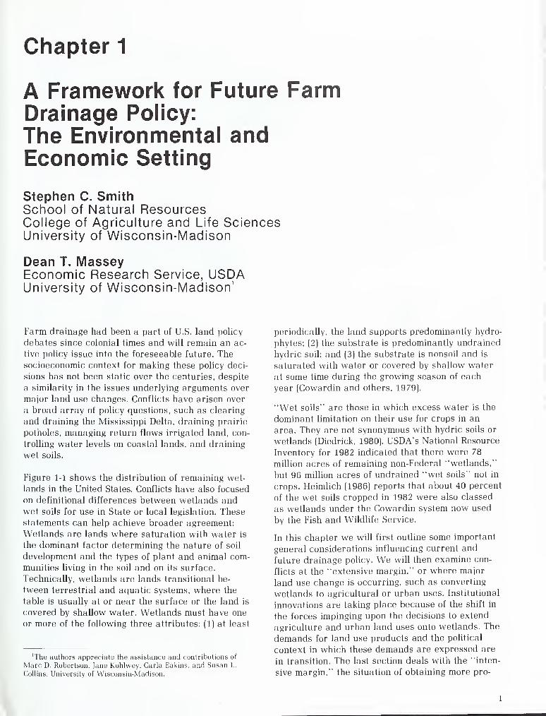
Figure 1-1 shows the distribution of remaining wet-

lands in the United States. Conflicts have also focused

on definitional differences between wetlands andwet soils for use in State or local legislation. Thesestatements can help achieve broader agreement:

Wetlands are lands where saturation with water is

the dominant factor determining the nature of soil

development and the types of plant and animal com-

munities living in the soil and on its surface.

Technically, wetlands are lands transitional be-

tween terrestrial and aquatic systems, where the

table is usually at or near the surface or the land is

covered by shallow water. Wetlands must have one

or more of the following three attributes: (1) at least

'The authors appreciate the assistance and contributions of

Marc D. Robertson, fane Kohlwey. Carta Eakins, and Susan L.

Collins. University of Wisconsin-Madison.

periodically, the land supports predominantly hydro-

phytes; (2) the substrate is predominantly undrained

hydric soil; and (3) the substrate is nonsoil and is

saturated with water or covered by shallow water

at some time during the growing season of each

year (Cowardin and others, 1979).

"Wet soils" are those in which excess water is the

dominant limitation on their use for crops in an

area. They are not synonymous with hydric soils or

wetlands (Diedrick, 1980). USDA's National Resource

Inventory for 1982 indicated that there were 78

million acres of remaining non-Federal "wetlands,"

but 96 million acres of undrained "wet soils" not in

crops. Heimlich (1986) reports that about 40 percent

of the wet soils cropped in 1982 were also classed

as wetlands under the Cowardin system now used

by the Fish and Wildlife Service.

In this chapter we will first outline some important

general considerations influencing current and

future drainage policy. We will then examine con-

flicts at the "extensive margin," or where major

land use change is occurring, such as converting

wetlands to agricultural or urban uses. Institutional

innovations are taking place because of the shift in

the forces impinging upon the decisions to extend

agriculture and urban land uses onto wetlands. The

demands for land use products and the political

context in which these demands are expressed are

in transition. The last section deals with the "inten-

sive margin," the situation of obtaining more pro-

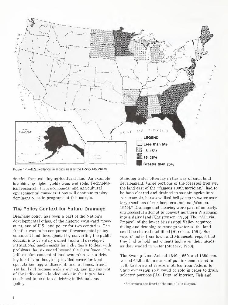
Figure 1-1 —U.S. wetlands lie mostly east of the Rocky Mountains.

duction from existing agricultural land. An example

is achieving higher yields from wet soils. Technolog-

ical research, farm economics, and agricultural

environmental considerations will continue to play

dominant roles in programs at this margin.

The Policy Context for Future Drainage

Drainage policy has been a part of the Nation's

developmental ethos, of the historic westward move-

ment, and of U.S. land policy for two centuries. Thefrontier was to be conquered. Governmental policy

enhanced land development by converting the public

domain into privately owned land and developed

institutional mechanisms for individuals to deal with

problems that extended beyond the farm fence. The

Jeffersonian concept of landownership was a driv-

ing ideal even though it provided cover for land

speculation, aggrandizement, and, at times, fraud.

Yet land did become widely owned, and the concept

of the individual's landed stake in the future has

continued to be a force driving individuals andpolicy.

115-25%

Greater than 25%

Standing water often lay in the way of such land

development. Large portions of the forested frontier,

the land east of the "famous 100th meridian," had to

be both cleared and drained to sustain agriculture.

For example, horses walked belly-deep in water over

large sections of northeastern Indiana (Wooten,

1955).* Drainage and clearing were part of an early,

unsuccessful attempt to convert northern Wisconsin

into a dairy land (Christensen, 1958). The "Alluvial

Empire" of the lower Mississippi Valley required

diking and draining to manage water so the land

could be cleared and tilled (Harrison, 1961). Sur-

veyors' notes from Iowa and Minnesota report that

they had to hold instruments high over their heads

as they waded in water (Murray, 1953).

The Swamp Land Acts of 1849, 1850. and 1860 con-

verted 64.9 million acres of public domain land in

both Eastern and Western States from Federal to

State ownership so it could be sold in order to drain

selected portions (U.S. Dept. of Interior, Fish and

''References are listed at the end of this chapter.

Wildlife Service, 1972). In the arid West, drainage

presented different problems because of the variable

character of the soil, and irrigation. Yet drainage

was often still necessary for a sustained agriculture.

Drainage continues to inspire public debate almost

100 years after Frederick Jackson Turner, the Uni-

versity of Wisconsin historian, observed that the

Census of 1890 no longer marked a line distinguish-

ing a frontier (Turner, 1938). Turner outlined the

ways in which the frontier shaped the character of

its inhabitants and their culture. These traits of in-

dependence and the value of land can still be seen

in the drive to drain and "conquer" the swamp. Of

course, the underlying potential for substantial

capital gains and a better life for the developer

should not be neglected. The strength of this drive

can be seen today in the continued loss of wetlands.

Yet, "... thoughtful students will remember that

across the Delta lie the skeletons of many abandoned

attempts toward its reclamation" (Harrison, 1961).

The same is true of all regions of the Nation.

The push to drain is very old. Early settlers brought

with them experience in drainage and an awareness

of the differing and conflicting values involved. The

draining of England's fens is an example. In the

Middle Ages, fishers and fowlers did not appreciate

the reduction of the natural channels and habitat,

although farmers were pleased that the productivity

of marketable crops increased per acre (Summers,

1976). Drained land produced different products.

People valued these products and activities dif-

ferently, resulting in conflicts. Such conflicts over

wetland use persist in England today and are the

subject of intense political struggles and headlines

in the daily press (Observer, June 24; July 1;

October 5, 1984).

Many of these same values are at stake today, but

with a difference. The developmental ethos today

faces a strong challenge from proponents of the

"environmental ethic" (Leopold, 1949). This counter-

balancing is the essence of the current public policy

debate over draining wetlands. The 1960's and

1970's were decades of expanded and deepened

environmental understanding. The issues raised by

the environmentalists were not new, because people

had been expressing concerns about draining

wetlands for decades.

The 1960's and 1970's were, nevertheless, threshold

years of change. For the first time, a broad base of

public support was mobilized for significant polit-

ical, legislative, and judicial action favoring an

environmental perspective. Federal and State laws

were enacted, new administrative rules were pro-

mulgated, and court decisions were rendered deal-

ing with vanishing wetlands.

The environmental ethic encompassed more than

the older conservation ethic by considering whole

ecological systems. 2 Greater attention will be given

to the ecological-environmental effects of draining

both wetlands and wet soils. The steps in deciding

to drain will need clear delineation, and the market

and nonmarket effects from draining or not draining

will have to be analyzed. At times these considera-

tions may limit drainage; at other times, drainage

may be essential for achieving the desired public

and private products.

The 1960's and 1970's were also years of expanding

world agricultural markets and of production

adjustments to meet market demands of timeliness.

Agriculture's response to these market developments

put pressure on both the extensive and intensive

margins. The extensive margin was changed by

draining wetlands and converting them to agricul-

tural uses, as in the Mississippi Delta. Intensive

margins were likewise pushed by tiling wet soils,

which increased production per acre. The area of

intensive land use increased while the area of

extensive land use decreased. The boundary of

transference between these margins is at the heart

of the debate between using land for food and fiber

or for "environmental" products and services.

Market forces will continue to affect the demand for

agricultural products and, consequently, the demandfor optimally drained land. The dynamics of these

markets put a premium on avoiding risks from

excessive moisture and thus tend to encourage

drainage.

Technological change in agriculture will be another

strong force affecting drainage. The history of

technical change is well known, and the productivity

of U.S. agriculture is a wonder in today's world.

American consumers have benefited by resultant

low-cost food and fiber. Farm numbers, especially

midsized farms, and farm production have declined.

The number of smaller and larger farms continues

to increase. These changes have produced greater

income equity between commercial farm and non-

farm employment.

All of the ramifications of past technological triumphs

in agriculture are not the primary concern here, but

the forces that shaped these trends must be con-

sidered because they bear on drainage policy. The

future will be shaped by a blend of these shifting

forces and will include new technologies. Within

2The conservation ethic received broad-based support at the

turn of the century with the establishment of the Forest Service

and the National Park Service. Notable conservation leaders of

the time were Theodore Roosevelt. John Muir, and Gifford

Pinchot.

this context, there lies a potential for revolutionary

change in agricultural production.

Estimating future production, however, is increas-

ingly difficult because of the changing structure of

agriculture and its supporting industries. Not only

will new production techniques have to be mas-

tered, but their articulation into the system will

follow new and significantly different institutional

and organizational channels (Ruttan and others,

1979). In fact, agriculture could avoid the problems

that have plagued sectors of U.S. manufacturing,

like the automobile and steel industries, if the issues

of articulation are appropriately addressed.

Why will the future be different? Smaller and

decreasing numbers of farms and farmers will have

had and continue to have important political impli-

cations in terms of legislative representation at all

levels of government. Coalitions between agricul-

tural interests and other groups will be increasingly

important in accomplishing related legislative objec-

tives. Marshalling legislative support for consider-

ing agricultural as well as other views of wetland

laws will require skilled political talent to attract

urban votes and to gain the understanding of those

who promote environmental interests. These

changes become significant since the demands for

the environmental products of wetlands are largely

expressed through governmental organizations.

The market for technical innovations will change,

altering the path of technology adoption. The num-

ber of buying firms will continue to decline but they

will be bimodally distributed in size, lumped at the

lower and higher ends of the scale. The characteris-

tics of the remaining firms will determine whether

this distribution and organization will affect the use

of pesticides, seed corn, semen, and induced animal

"twinning." Projections for increased productivity

have been based on the traditionally correct assump-

tion of a large number of competitive farms. That

market is changing, and this may affect both the

production and application of new technology. Will

the same forces for rapid adoption work with a

smaller number of highly commercial farms as in

the past? Will the incentive structure for innovation

remain the same? How will contract sales as a form

of production and marketing affect innovation andper-unit production?

The structure of the everchanging farm supply

industry will significantly determine when and

under what conditions new technology is released.

The "biotech" industry has gone through the first

flutter of adjustment. As maturity comes, as foreign

competition becomes more intense, and as large cor-

porate structures and their decision processes exert

influence, estimating future onfarm productivity

becomes very difficult because of the multiple

forces affecting new technology.

The thrust for future productivity increases will

come from research (English and others, 1984).

There is a ferment and excitement in laboratories

across the Nation about potentials for major tech-

nical change. In some areas, commercialization is

moving rapidly and broadly covering sectors of food

and fiber production. The technical capability of in-

creasing food and fiber productivity appears to be

at the threshold of a dramatic upward surge.

Observers suggest that photosynthesis enhance-

ment, crop bioregulators, and twinning techniques

are ready for early adoption by farm operators (Lu

and others, 1979). A survey of plant scientists by

Merz and Neumeyer indicates that new technologies

can increase the yield of corn up to 40 percent

(Rosenblum, 1983).

Gains in livestock production can come from such

innovations as shortening the time between genera-

tions, determining sex, increasing efficiency in the

use of feed, improving health, and transplanting

embryos. For example, "Milk production may be

increased by between 10 to 33 percent without pro-

portionately increasing feed intake" (Rosenblum,

1983).

The Economic Research Service (ERS) labels the

future as fueled by "science power" in contrast to

the mechanical power, horse power, or hand powerof past decades (Lu and Quance, 1979). Conferences

and studies during the past few years point in this

direction. ERS economists have recently summarized

productivity growth estimates for purposes of mak-

ing long-range projections to the year 2000 and

beyond (Maetzold and others, 1983). These authors

suggest using an annual growth rate of 1.5 to 2 per-

cent for estimating future agricultural productivity.

Rates of productivity increase have not tapered off

or flattened, as was projected in the late 1970's.

Productivity increases are highly correlated with

public and private investment in research (Johnson

and Wittner, 1984). By continuing to invest in pro-

ductivity increases, the Nation will be offered a

broader array of policy options for resource man-

agement, including drainage, than would happenwithout a priority on research to increase produc-

tivity. Thus, the argument for both private and

public investment in research is justified by more

than greater farm income and low-cost food and

fiber. The ability to consider alternative resource

management options is generated by the ability to

supply food and fiber from a smaller land base.

Thus, innovative policy options are increasingly

viable. Within the intensive margin, policy options

preserve prime agricultural land and, at the exten-

sive margin, they restrict using land for agriculture

with severe limitations, such as wetlands, highly

erosive land, and land with a depleted ground-water

supply.

If the increased per-unit productivity potential is

realized, the Nation may be able to produce enough

food and fiber to satisfy the U.S. market and help

supply the world on a smaller land base. Pressure

on the extensive margin, such as draining wetlands,

could be reduced. Drainage policymakers would

have to consider this change in pressure and

develop program options which encourage agricul-

tural production only on areas of highest productiv-

ity. In such a situation, wetlands most valuable as

wetlands would not have to be drained. Production

increases would come at the intensive margin by

improving the use of the existing land base, includ-

ing the use of drainage. In the competition for land

for agricultural use, a policy premium assisted by

legislation might be placed on prime agricultural

land.

The Extensive Margin

Nationally, the extensive margin of agricultural

land use is dynamic, with land continuously going

into and out of agricultural uses. If the total agri-

cultural land base is conceptualized, the extensive

margin is at the edge of transference between farm-

ing and extensive land uses such as forest land,

rangeland, and wetlands. As a part of the process

of change, wetlands continue to be converted to

agricultural and other uses. "New" land also con-

tinues to be brought into cultivation by irrigation,

with drainage often being an integral component.

Because drainage has been an essential part of the

Nation's agricultural development for the past twocenturies, the area of wetlands has continued to

diminish. Clear quantitative estimates of the loss of

"original" wetlands are not available due to "lack

of sound baseline data. ..." (Weller, 1981). How-ever, estimates by the U.S. Congress' Office of

Technology Assessment (OTA) indicate that "... as

much as 50 percent of the original wetlands mayhave been converted" (OTA, 1984). In some regions,

only "remnant" wetlands remain with between 90and 95 percent of the original area lost in Illinois.

Iowa, and lowland forests in Missouri (Weller,

1981).

In other regions, according to the OTA, the percent-age of remaining wetlands is substantial, still with anational estimate of "... 50 percent of the original

wetland . . . being . . . converted." This percentageis based on an original area of 185 million acres.

Between the mid-1950's and 1970's, the "actual loss

of freshwater vegetated wetlands totaled 14.6

million acres. Agricultural land use was responsible

for 80 percent of these losses" (OTA, 1984). Esti-

mates from the National Wetlands Inventory are

similar. They indicate that 54 percent of the original

wetlands have been drained, of which 87 percenthave been converted to agriculture (Tiner, 1984).

The extensive agricultural margin has continued to

expand into wetlands in all regions of the Nation.

Estimates from a National Research Council (NRC)

report on "Impacts of Emerging Agricultural Trendson Fish and Wildlife Habitat" indicate that "86 per-

cent of the original Mississippi bottom land will be

destroyed by 1995 . . . and ... all of the remaining

(prairie potholes) area will be lost by 2055 ..."

(NRC, 1982). Weller contends "... most wetlands

would disappear between 2000 and 2200 if the pres-

ent rate of drainage continues" (Weller, 1981). Suchdeclines are sufficient to render the small size of re-

maining wetlands increasingly visible. A broadly

based public with a heightened environmental ethic

is capable of focusing attention on the environmen-

tal and ecological consequences of these losses.

Such a concentrated focus plays a significant role

in the process of social and public valuation as well

as in benefit-cost calculation of whether or not to

drain. Many of the contending interests and values

are not new and were evidenced 500 years ago in

the British fens. The fowlers of that day valued the

water fowl breeding grounds, much as the duck

hunters of today value the prairie potholes and the

backwaters of the Mississippi Delta.

Agriculture's expansion across the Nation with the

assistance of drainage was accomplished through

the use of a set of institutions built both upon con-

cepts of private property and the valuation of these

rights through markets for land, corn, wheat, soy-

beans, cotton, timber, and the like. Governmental

agricultural policy generally supported these

markets and the resulting distribution of income.

Land and water policies (even levee construction)

were used to subsidize this system of property

rights and markets.

The products of wetlands, such as water fowl,

water quality, water flow regulation, or fisheries

are not owned as private property. Evaluating themin their natural state involves a nonmarket decision

made without market criteria. During periods of

"abundance" in the 1880's, wildlife products were

sold after capture on local markets, but extinction

and dramatic population reductions raised issues of

public concern. Federal and State governments have

maintained their proprietary interests and devel-

oped systems of regulations for managing these

resources, but they have not generally relied upon

the market as a mechanism for evaluating or dis-

tributing rights.

The public policy actions supporting drainage have

been numerous at all levels of government, with

Federal policy dating back to the Swamp Land Acts

of 1849. 1850, and 1860. The Agricultural Conserva-

tion Program (ACP), the Soil Conservation Service

(SCS), and federally supported educational andresearch programs also furthered the extension of

drainage. In addition, general agricultural price

support programs and other policies have encour-

aged the expansion of agriculture onto newly

drained land (Goldstein, 1971).

State laws enabled drainage districts at the local

level to deal with legal and financial problems of

drainage extending beyond the farm fence. Federal

and local efforts in levee construction, dating backto the early 1700's, contributed to both urban andagricultural development, including irrigation andrelated drainage. Governmental structures havebeen used by local interests to support the historic

development policy which included drainage andthe loss of wetlands. For the most part, these

policies have been fashioned around and supportive

of private property and markets.

Products from drained land are largely valued

through markets while products from undrained

land are valued outside of the market. They are

"nonmarket" goods and services. Nonmarket valua-

tions depend on other institutional forms, such as

referenda, legislative bodies, and governmental

administrative agencies. For these institutions to be

effective, a base of public consensus must be

created and reflected through the organizational

processes.

The environmental movement of the 1960's and1970's spawned increasing interest in the impor-

tance of wetlands and support for restricting

drainage. Environmental and supply-management

considerations prompted the elimination of ACPcost-share payments to farmers who drained land to

bring new farmland into production. SCS Regulation

108 recognized the value of wetlands and elim-

inated technical assistance for bringing newwetlands into production. Environmentalists also

used the National Environmental Policy Act (NEPA)

to oppose drainage projects, and they supported the

Federal Water Bank Program in 1970. which pro-

vided Federal funds to rent wetlands from land-

owners for a 10-year period to prevent their

drainage. 34*

The lack of clear, understandable, and additive

national wetland data was recognized with the

establishment of a national inventory and with in-

ventories in many States. Such inventories grewfrom an understanding that wetlands were dis-

appearing increment by increment without a clear

appreciation of the effect of losing one more incre-

ment. It was not possible to focus public decision-

making without knowing the size and importance of

the remaining aggregate of all wetlands and how an

incremental loss would affect that whole. Public

decisions at the local. State, and national levels

needed to be based upon a definition of the

resource and upon reasonably accurate estimates of

its quality and quantity. Such a perspective is no

different than that of the agricultural or urban land

developers. They also look at the resources under

their control, and generally evaluate their actions

on the basis of a market outcome for the proposed

product. Because markets do not exist for the public

goods and services of wetlands, a public interest

over private property had to be established. This

processs is going on in the courts. Congress. State

legislatures, and administrative agencies. Michigan,

Minnesota, and Wisconsin have adopted legislation

requiring statewide programs for mapping and in-

ventorying wetland resources. 5 - 6 - 7

Much of the political argument over these programs

focused upon disagreements over the definition of

wetlands. Circular 39 (U.S. Dept. Interior. 1972)

and other Fish and Wildlife Service classification

schemes (Cowardin. 1979) have significantly amelio-

rated many disputes. State legislators and political

interests, however, have had their own economic

concerns to protect, thus necessitating negotiation

as well as self-education. Farm drainage interests

have often questioned and, at times, on principle,

opposed inventories as well as wetland managementlegislation. The redefinition of property rights has

been at issue.

The States have related their mapping programs to

State decisionmaking. For example, Minnesota has a

provision for its own water bank and wetland tax

credits. 8 9 Michigan has a program giving the State

an option to purchase wetlands. 10 Wisconsin estab-

lishes links with shoreland protection legislation. 11

*These and subsequent footnotes refer to legal citations listed

after the chapter's text.

Wetland inventories are increasingly viewed as

essential for proper wetland management and for

making decisions on whether to allow the drainage

of additional wetlands.

State laws relating to wetlands have increased

dramatically in the past 50 years. States adopted 79

laws relating to wetlands from 1795 to 1934. In the

20 years from 1935 to 1954 the number was 110.

Then 70 were adopted during 1955-64. But during

the 14-year period from 1965 to 1978, State legisla-

tures adopted 355 wetland-related laws (USDA.

RCA, 1980).

Navigable waterways have historically been a

Federal responsibility. This was recognized further

in the Rivers and Harbors Act of 1899, which gave

the Army Corps of Engineers authority over the dis-

charge of refuse, dredge, and fill material. 12 The

authority evolved in part into section 404 of the

Clean Water Act of 1977, which extends the

authority beyond navigation to one of preventing

pollutant discharges and of promoting the purposes

of the Act. 13 Environmental groups have used this

section to restrict drainage and to insure clean

water. Permits issued under section 404 are for in-

dividual actions, and backlogs can exist if a high

percentage of permits are contested. The Corps

wanted to speed up decisionmaking by changing the

permit procedure. Interim rules were issued in

1982, and the procedure became part of the

reauthorization debate for the Clean Water Act.

Environmental groups feared that wetlands would

be more rapidly depleted under the interim rules

and that a basis for litigation would be denied. 14 Anagreement was reached February 10, 1984, andapproved by the U.S. District Court for the District

of Columbia, on an order that overturned some of

the interim rules. The court's order gives protection

to wetlands, such as an estimated 700,000 acres of

prairie potholes, and directs the Corps to apply,

nationwide, the decision in Avoyelles SportsmenLeague v. Alexander. It held that discharges caused

by land clearing are subject to section 404 permits. 15

Before then, the Corps had applied the Alexander

decision only within Louisiana.

The coastal zone also has received national andState attention because of the effect of drainage.

Recognizing the National Marine Fisheries Service

as a consultant for section 404 determinations as

well as other Federal and State interests, highlights

the importance of fishery interests in the wetlands

of the thin perimeter around the contiguous 48

States.

Wildlife and other supporting groups see section

404 authority as important legislation and wouldlike to have it continue to be a part of the wetland

decision process. In essence, a complex of legisla-

tive authorities come into play with the control of

navigable waters, such as the authority in the Clean

Water Act to prevent pollutant discharges, the

authority of the Fish and Wildlife Service over

migratory waterfowl, the authority of USDA to pro-

vide cost-sharing and technical assistance for con-

servation practices, and USDA's general farm sup-

port programs with incentives for moving onto less

productive agricultural land (Goldstein. 1971).

The above complex is pluralistic, and built uponolder authorities. But the pieces are beginning to

take shape for a reformulation of propertied rela-

tionships. New public interests are emerging.

Perhaps it is time to stand back from the fray of

economic and jurisdictional controversy and begin

to evaluate the adequacy of Federal, State, andlocal wetland policies.

Several areas of concern related to drainage might

be noted, such as fishery values or flood water

retention, but migratory waterfowl and its habitat

illustrate the need for policy re-evaluation and a

reformulation of propertied relationships. Habitat

for migratory waterfowl, of course, is international

in character, but we shall only note the prairie

pothole situation, the river backwaters and flood-

plains, and bayous and waterways along the Missis-

sippi and the coast. Farm drainage has interacted

with the ecology of these flyways for many years.

The potholes are often grouped within the intensive

margin in our terminology. Draining potholes,

however, means changing land use and pushing

cultivated agriculture onto noncultivated land, even

though the geographic area is within the farm firm.

We have had a Federal policy (and many States

have had their own policies) of purchasing selected

wetlands to preserve migratory waterfowl habitat,

but can enough land be purchased in the right

places to do an adequate job? To make these deci-

sions, not only are wetland inventories needed, but

also better ecological information on the various

species to be protected. The direction of muchpublic action is to attach clear public value to the

ecological system and to consider this whole as the

economic product. Migratory birds are covered by

Federal legislation: can the value attached to these

birds be extended to their habitat? The full defini-

tion of this product needs exploration in economic,

legal, scientific, and aesthetic terms (Stone, 1976).

An array of public processes such as purchase, tax-

ation, cost-sharing, and police power could be

brought to a focus, including attaching public prop-

erty rights to the ecological system. (Note the

Wyoming Federal Court ruling to eliminate fencing

on private land to protect antelope habitat under

the Unlawful Enclosures of Public Lands Act. U.S.A.

vs. Wyoming Wildlife Federation. Case No. C84-013

6-B, U.S. Dist. Court, Wyoming.)

The movement for wetland protection at the State

level has gone beyond the inventory, taxation, and

public purchase stages to the use of police power.

As of 1986, 13 States had adopted comprehensive

legislation addressing the issue of freshwater and

coastal wetland preservation. For example, see 16 17

is. i9. 20 These statutes depend on good wetland map-

ping programs and other information, and establish

police power authority by findings that describe

wetland values and consequences of unregulated

development. These findings provide the policy

underlying the statute, alert property owners and

the general public to the need for regulation, and

aid the appropriate agency in interpreting the act

and administering permits. At least five other States

are at various stages of discussing and passing com-

prehensive legislation: California, Idaho, Illinois,

Indiana, and Nebraska.

Regulated activities vary from State to State andare the subject of heated debate. They include

specific conduct, such as drainage and filling, as

well as any activity that impairs the natural value

of wetlands. Exemptions to drainage are bargained,

as in Massachusetts, where the statute specifies

that the regulation shall not apply to any mosquito

control work, to maintenance of drainage and flood-

ing systems of cranberry bogs, or to work performed

for normal maintenance or improvement of land in

agricultural use. 21 Some issues under this statute

have been litigated, with its constitutionality sup-

ported. For our purposes, it is enough to note the

movement toward comprehensive wetland legislation

to deal with the specific land at the extensive

margin through the use of policing.

The developmental ethos with its strong private prop-

erty value is still an active national force. It hasfueled the drainage movement and given it a base of

legitimacy. The economic gain from converting vast

areas of wetlands was reflected in increased in-

come, capital gains, and settlement of the continent.

But the markets that produce such benefits do not

reflect all the societal values in drainage or wet-

lands. The environmental movement gave new policy

weight to the conservation and the environmentalethic as largely nonmarket values. The synthesis of

this confrontation, arising from a maturing Nation,

is really just beginning.

The earlier expansion of the extensive margin wasseldom easy or cost-free, but there was a supporting

consensus that it was right. That consensus no

longer exists, and future drainage will have to be

justified in an increasingly detailed fashion. Im-

agination and innovation will be needed in policy,

and new legal doctrines will be developed. Thejustification will assume an added dimension as newtechnology contributes to per-unit production in-

creases. Are the acres drained to extend the margin

for agricultural production necessary to meet

agricultural production goals, and are they in the

public interest?

The pushing back of the extensive margin by

drainage is only partly market-driven. The market

for farm and forest products and the market for

land remain major forces, but nonmarket valuation

will be increasingly important. The valuations will

be made by Federal, State, and local agencies, and

also by courts, legislatures, and a variety of other

means. The pluralistic character of this process is

frequently of great value since incremental ad-

justments at times forestall all-out commitments

with possible major pitfalls. Pluralism also requires

insight and imagination to insure the decisions will

not be choked by the burden of "too many wheels to

turn." The challenge is to define more clearly the

product to be created with this interaction between

drainage and wetlands.

The Intensive Margin

The intensive margin refers to additional drainage

on existing farms. Generally, the issue is not the

conversion of nonagricultural land to agriculture

but increasing the intensity of agriculture through

drainage and achieving greater production and net

return.

Increasing the intensity of use is not a new objec-

tive of drainage. The tile drain introduced in NewYork State in 1835 by John Johnston was an effort

in this direction. Johnston claimed that "he never

made any money farming until he drained his land"

(USDA, Yearbook of Agriculture, 1938). Land grant

college experiment stations and USDA have for

many years directed research toward a better

understanding of soil-plant-moisture relationships.

The science of dealing with wet soils and drainage

has moved forward on a worldwide basis, supported

by a long history of work in the Netherlands and in

less developed countries. With an excellent network

of scientific communication, these efforts are part

and parcel of current and future high-technology

agriculture. Hanson and Larson observed that

through drainage, irrigation, and improved tillage,

significant physical improvements in soil have been

made. "But relative to the changes that will be

made, we have literally scratched the surface.

Substantial acres. . .produce low yields because of

too much or too little water" (Hanson and Larson,

1983). Drainage research and practice will be a

major issue in an age of "high-tech." An increasingly

important element of crop production will be provid-

ing the plant with optimum water for an economic

return as well as a high-quality environment.

The intensive margin has been and continues to be

influenced by the major forces noted in the policy

introduction to our discussion. The developmental

ethos contained a drive for expansion onto newland. But increased productivity per unit was also

an ingrained social value of master workmanship

(Brewster, 1953). These values were expressed in

such common phrases as "making two blades of

grass grow where only one did before," and "mak-

ing the desert bloom through irrigation rather than

dryland farming."

Accepted modes of behavior are beginning to shift

with the environmental movement playing no small

part. Some new programs are in place, so whenfarmers calculate a net return from an investment

in drainage, they must relate to the water bank,

property tax credits, income tax considerations, and

interest rates, besides yield changes on various soils

under alternative conditions of wetness and dryness.

The work habits of yesterday are quite different

than those of today. The "rubble" of conservation

tillage is beginning to "look good," and wetlands for

habitat have a broader base of acceptance amongagricultural landowners.

Drainage has an environmental effect that is only

now being recognized in some regions of the Nation,

though not new to the irrigated West. This is nolonger just a Western issue. In fact, the AmericanSociety of Civil Engineers held a 1982 Conference

on "Environmentally Sound Water and Soil Manage-ment" in Florida (Kruse, 1982). Soil salinity control,

flows, ground-water protection from contamination,

managed recharge percolation, and reduced flood

flows are environmental benefits of drainage. Thus,

drainage at the intensive margin also has values not

clearly reflected in the market.

Drainage is an important water management tool

for achieving acceptable levels of quality as well as

quantity in both the East and West. The quality of

the return flow, with or without irrigation, will beincreasingly important and will become a part of

environmental chemical management. Questions will

be asked about the chemical composition of the

water that comes out of farm drains and flows into

district systems. For example, water purity prob-

lems plagued the Kesterson Wildlife Refuge, Calif.,

when excess selenium appeared in return flows.

The necessity of an environmentally sound manage-

ment of agricultural chemicals is clear: some aspects

are understood, but the research agenda is long and

difficult. Drainage in water-quality management will

be a significant issue for the next two decades.

Today's science will be pushing tomorrow's technol-

ogy. Commercial plant breeders are moving with the

market and developing varieties designed for con-

servation tillage and greater salinity tolerance as

well as higher yields on prime land. Many questions,

however, await better answers. To what extent can

plants be adapted to conditions which will reduce

the need for drainage? And, can pest resistance be

integrated to reduce the need for chemicals and

thus the need to drain for improved water quality?

Managing water will be an important component of

more intensive plant management, and in manysituations drainage will help achieve technical

precision. Because of the variability of conditions

throughout the Nation, the role of drainage will dif-

fer by locality, necessitating area-by-area evalua-

tions. Questions concerning both new investment

and reinvestment will be raised. Millions of acres

are already drained, and many farm operations will

have to evaluate their existing drainage systems.

They must determine if the existing system performs

optimally, or if reinvestment would yield a suffi-

ciently high economic return to warrant change and

redesign.

These determinations can be complex. Current

technologies of drainage must be assessed as well

as those of related disciplines associated with in-

tegrated crop management. Also, new materials, ad-

vanced equipment, and computer assistance have

added a precision unknown in earlier days. These

advances, coupled with progress in soil science and

in determining soil-water-plant relationships, as

well as improved operating techniques, result in a

decision process that is a process of sophisticated

integration.

The decisionmaking sciences have continued to

advance along with the biological and physical

sciences. Studies have revealed the diversity of

needs on a State-by-State basis. These studies inte-

grate the appropriate information into an economic

frame of reference with indicators of profitability,

or lack of it, under specified conditions. Such

research is useful for local situations, but because

of limited assumptions and purposes, it does not

provide details for making broader generalizations.

For example, interest rates, discount rates, rental

alternatives, tax assumptions, and the effects of

excess moisture on crops are dealt with in a variety

of ways. An outline of the decision path and an

explanation of alternatives would be useful for indi-

vidual farmers and public entities. Such an outline

would not only aid farm operators and public of-

ficials, but also soil scientists, drainage engineers,

and plant specialists as they approach their respec-

tive tasks.

Computer software is beginning to address this

problem through programs which relate drainage

system design, crop yield, water management, and

economic return. The number of economic and

engineering modeling packages such as DRAINMODwill increase. As these programs are improved, ac-

cepted, and used, the ability to compare analyses

from various regions will increase. Thus, the areas

where drainage at the intensive margin is profitable

can be more clearly defined. A review of selected

research suggests that drainage can be a profitable

investment at the district and individual farm level

on some of the most poorly drained land. In other

situations, the net benefit is zero or a loss. At some

locations, drainage is going forward with the objec-

tive of achieving a break-even level of intensifica-

tion, with the long-term goal being a capital gain

associated with a change in land use. (The studies

examined included Barrows and others, 1982:

Dudek and Horner. 1981; Fritz and others. 1980:

Horner and Dudek, 1980; Horner and others, 1983;

Kanwar and others. 1983; Leitch and Scott, 1977;

Leitch and Keresters, 1981; Nolte and Dudek, 1984;

Schwab and others, 1975; Schwab and others, 1981;

and Skaggs and Nassehzadeh-Tabrizi, 1983.)

The focus on the intensive margin, however, does

not mean that individual farm operators can always

accomplish successful water management by them-

selves. Collective action for water management has

a long history and will remain important for carry-

ing water management beyond the farm. For example,

drainage districts were organized to convey

drainage water from many farms to a "natural"

waterway. Some form of collective action wasnecessary to finance projects, to deal with questions

of trespass, and {%) overcome blocking action by un-

cooperative individuals. For example, in 1839, the

Michigan legislature provided that, upon petition,

the lands of persons "who would not voluntarily

permit the construction of a ditch" could be opened

to drain swamps, bogs, meadows, or other lowlands

(Lauer, 1959). Many States developed comparable

legislation for formalizing collective action into

district-enabling acts. History and the associated

law cannot be delineated in detail here other than

to note a complex legal and political backgound.

Districts represent local economic interests attempt-

ing to extend and enhance individual property

values. Today the role of the older, single-purpose

drainage district is often incorporated into county

governments or commissions.

If exploiting the intensive margin continues to be

economical, the increased sophistication and size of

farm businesses may require a rethinking of manyfarm drainage systems because of the increased

load such systems will have to handle and the needto control soil moisture and chemicals more precisely.

Old small districts may have to reorganize to deal

with today's larger problems. Such reorganizations

tend to create organizations capable of providing

more comprehensive water management. This trend

will be important for providing adequate service to

the farmer as well as for meeting an increasingly

broad spectrum of Federal and State water re-

quirements. Farm drainage at the intensive marginwill be included within the web of comprehensive

water planning and management, requiring the in-

tegration of water quality, quantity, and rights.

The full potential of drainage at the intensive

margin has not been realized. Productivity gains

from better water control and longer term resource

enhancement are often possible. Also, environmen-

tal enhancement at the intensive margin through

water quality control will be significant. Achieve-

ment of these values will depend upon scientific

advances and market value of agricultural products.

Footnotes

342 U.S. Code, Sec. 4321 et seq. (1982).416 U.S. Code, Sees. 1301 to 1311 (1982).5Michigan Compiled Laws Annotated, Sees. 321.10(1)0), (g)

(Supp. 1983-1984).

^Minnesota Statutes Annotated, Sec. 105.391 (Subd. 1) (West

Cum. Supp. 1984).

'Wisconsin Statutes, Sec. 23.32(2)(a) (1981-1982).8Minnesota Statutes Annotated, Sec. 105.392 (West 1977 &

Cum. Supp. 1984).

Minnesota Statues Annotated, Sees. 272.02 (Subd. 1) (15),

273.115 (West Cum. Supp. 1984).10Michigan Compiled Laws Annotated, Sec. 321.206(2) (Cum.

Supp. 1983-1984).

"Wisconsin Statutes. Sec. 59.971 (1981-82).1233 U.S. Code. Sec. 401-412 (1982).1333 U.S. Code, Sec. 1344 (1982).14 Nebraska v. Rural Electrification Admin., 12 Environmental

Reporter-Cases 1156 (D. Neb. 1978).15511 Fed. Supp. 278 (Western District Louisiana 1981).

16Connecticut General Statutes. Sec. 22a-36 to 45 (1983).

"Massachusetts Annotated Law, Chap. 131, Sees. 40. 40A

(Michie/Lawyers Co-op, 1981).18New Hampshire Revised Statutes Annotated, Sees. 483-A:l

to :6 (1983 and Cum. Supp. 1983).19New York Environmental Conservation Law, Sec. 24-0101 to

15-0601 (McKinney Cum. Supp. 1983-1984).20Rhode Island General Laws, Sec. 2.1-18 to -25 (1976 & Cum.

Supp. 1983).

^Massachusetts Annotated Laws, Chap. 131, Sec. 40

(Michie/Lawyers Co-op, 1981).

10

References

Barrows, R., David Henneberry, and Sarah

Schwartz. 1982. "Individual Economic Incentives,

The Tax System and Wetland Protection Policy: AStudy of Returns to Wetland Drainage in

Southeastern Wisconsin." ASAE Paper No. 82-2034.

Am. Soc. Agr. Engr., St. Joseph, Mich.

Bishop, R. A. 1981. Iowa's Wetlands. Proceedings,

Iowa Academy of Science, Vol. 88, pp. 11-16.

Brewster, John M. 1958. "Technological Advance

and the Future of the Family Farm," Journal of

Farm Economics, Vol. 40, pp. 1,596-1,612.

Carstensen, Vernon. 1958. Farms or Forests. College

of Agriculture, Univ. of Wisconsin, Madison, July,

p. 6.

Cowardin, Lewis M., Virginia Carter, Francis Golet,

and Edward LaRoe. 1979. Classification of Wetlands

and Deepwater Habitats of the United States. U.S.

Dept. Int., Fish and Wildlife Serv., p. 103.

Diedrick, R. T. 1980. The Agriculture Value of WetSoils in the Upper Midwest. Staff paper, U.S. Dept.

Agr., Soil Cons. Serv., St. Paul, Minn.

Dudek, Daniel, and Gerald L. Horner. 1981. "Return

Flow Control Policy and Income Distribution AmongIrrigators," American Journal of Agricultural

Economics, Vol. 63, No. 3, pp. 438-446.

English. Burton C, James A. Maetzold, Brian R.

Holding, and Earl O. Heady. 1984. Future Agricul-

tural Technology and Resource Conservation. Pro-

ceedings of the RCA Symposium: Future Agricul-

tural Technology and Resource Conservation. Ames,

Iowa: Iowa State Univ. Press.

Frayer, W. E., T. J. Monahan, D. C. Bowden, and F.

A. Gaybill. 1983. Status and Trends of Wetlands

and Deepwater Habitats in the Conterminous United

States, 1950's to 1970's. U.S. Dept. Int., Fish and

Wildlife Serv., p. 32.

Fredrickson, L. H. 1981. Paper prepared for the

House Subcommittee on Fisheries and Wildlife.

Fritz, J. C. Gerald Horner, and J. H. Snyder. 1980.

The Economic Feasibility of Installing Subsurface

Tile Drainage in the Panoche Water District, San

Joaquin Valley, California. Information Series 80-3,

Giannini Foundation of Agricultural Economics,

Univ. of California.

Goldstein, Jon. 1971. Competition for Wetland in the

Midwest: An Economic Analysis. Resources for the

Future, Inc. Baltimore: The Johns Hopkins Press.

Hanson, L., and W. E. Larson. 1983. "Frontiers in

Soil Science: The Next Twenty Years," MinnesotaScience, Vol. 38, No. 3. pp. 2, 3. 14.

Harrison, Robert W. 1981. Alluvial Empire: A Study

of State and Local Efforts Toward Land Develop-

ment in the Alluvial Valley of the Lower Mississippi

River. Little Rock, Arkansas: Pioneer Press.

Heathcote, J. M. 1876. Reminiscences of Fen andMere. London: Longmans, Green & Co.

Heimlich, Ralph E. 1986. Personal compilation of

land use capability subclass "w" land by types of

wetland; data from the 1982 National Resources

Inventory.

Horner, G., and D. J. Dudek. 1980. "An Analytical

System for the Evaluation of Land Use and WaterQuality Policy Impacts upon Irrigated Agriculture,"

Operations Research in Agriculture and WaterResources. Amsterdam: North Holland Publishing

Co., pp. 537-568.

Horner, G. L., C. V. Moore, and R. E. Howitt. 1983.

"Increasing Farm Water Supply by Conservation,"

California Agriculture. Vol. 37, Nos. 11 and 12, pp.

6-7.

Johnson, G. L., and S. H. Wittner. 1984. Agricultural

Technology Until 2030. Special Report No. 12, Mich.

Agr. Expt. Sta., East Lansing.

Kanwar. R. S., H. P. Johnson, D. Schult, T. E. Fenton,

and R. D. Hickman. 1983. "Drainage Needs and

Returns in North Central Iowa," Transactions of the

ASAE, Vol. 26, No. 2, pp. 457-464.

Korte, P., and L. H. Fredrickson. 1977. "Loss of

Missouri's Lowland Hardwood Ecosystem," Trans-

actions of North American Wildlife and Natural

Resources Conference, Vol. 42, pp. 31-41.

Kruse, E. Gordon, Chuck R. Burdick, and Yousef A.

Yousel (co-editors). 1982. Environmentally SoundWater and Soil Management. New York: Am. Soc.

Civ. Engr.

Lauer, T. E. 1959. "District Control of WaterResources," University of Detroit Law Journal, Vol.

37, No. 1. pp. 28-35.

Leitch. Jay A., and Daniel Kerestes. 1981.

Agricultural Land Drainage: Costs and Returns in

Minnesota. Staff Paper P 81-15, Dept. Agr. and

Appl. Econ., Univ. of Minnesota, St. Paul.

11

Leitch, Jay A., and D. P. Scott. 1977. "Economic

Impact of Flooding on Agricultural Production in

Northeast Central North Dakota." Agr. Econ. Rpt.

No. 120, Dept. Agr. Econ., No. Dak. Agr. Exp. Sta.,

Fargo.

Leopold, Aldo. 1949. A Sand County AJmanac.

Oxford Univ. Press.

Lu, Yeo-Chi, and Leroy Quance. 1979. Agricultural

Productivity: Expanding the Limits. AIB-431. U.S.

Dept. Agr., Econ. Res. Serv.

Lu, Yeo-Chi, Philip Cline. and Leroy Quance. 1979.

Prospects for Productivity Growth in U.S. Agricul-

ture. AER-435. U.S. Dept. Agr., Econ. Res. Serv.

Maetzold, Jim, Thyrele Robertson, Klaus Alt, Neill

Schaller, and Tom Dempster. 1983. "Issue Paper for

Basic Assumptions Work Group: Agricultural Pro-

duction Technology Estimates for the RCA and RPAProcess." U.S. Dept. Agr., Econ. Res. Serv.

McLean, J. J. P.. and G. O. Schwab. 1983. "Flood

Peak Flows and Subsurface Drainage." ASAE PaperNo. 82-2053, Am. Soc. Agr. Engr., St. Joseph, Mich.

Murray, William G. 1953. Appraisal of Potawatomi

Tracts in Iowa and Kansas, 1846. Prepared for the

U.S. Dept. Justice. Ames, Iowa.

National Research Council. 1982. Impacts of Emerg-

ing Agricultural Trends on Fish and Wildlife

Habitat. Wash., DC: National Academy Press.

Nolte, B. H., and R. D. Devick. 1984. "Economic Fac-

tors of Drainage Related to Corn Production," Na-

tional Corn Handbook. Coop. Ext. Serv., Ohio State

Univ., Columbus.

Pavelis, George A. 1978. Natural Resource Capital

Stocks: Measurement and Significance for U.S. Agri-

culture Since 1900. Abstract No. 199, Proceedings of

the American Association for the Advancement of

Science. AAAS Pub. 78-2.

Redelfs, Ann Ellen. 1983. "Wetland Values andLosses in the United States." M.S. thesis, OklahomaState Univ.. Stillwater.

Rosenblum, John W. (editor). 1983. Agriculture in

the Twenty-first Century. New York: John Wiley andSons.

Ruttan, Vernon W.. Robert E. Evenson, and Paul E.

Waggoner. 1979. "Economic Benefits from

Research: An Example from Agriculture," Science,

Vol. 205. pp. 1,101-1,107.

Schrader, T. A. 1955. "Waterfowl and the Potholes

of the North Central States," Water: Yearbook of

Agriculture, 1955. U.S. Dept. Agr., pp. 596-604.

Schwab, G. O., N. R. Fausey, and C. R.Weaver.1975. Tile and Surface Drainage of Clay Soils. Ohio

Agr. Res. and Dev. Ctr., Wooster.

Schwab, G. O., B. H. Nolte, and M. L. Palmer. 1981

and 1982. Drainage

—

What is it Worth on Corn

Land, and Drainage

—

What is it Worth for Soybeans

Land? Soil and Water Series Nos. 23 and 24, Agr.

Engr., Ohio State Univ., Columbus.

Skaggs, R. W., and A. Nassehzadeh-Tabrizi. 1983.

Optimum Drainage for Corn Production. Tech. Bui.

No. 273, North Carolina Agr. Res. Serv., State Univ.,

Raleigh.

Stone, Christopher. 1976. Toward Legal Rights for

Natural Systems. Proceedings from the 41st North

American Wildlife Conference, Wash., DC, pp. 31-38.

Summers, Dorothy. 1976. The Great Level, A History

of Drainage and Land Reclamation in the Fens.

North Pomfret, Vermont: David and Charles.

Tiner, Ralph W. 1938. Wetlands of the United States:

Current Status and Recent Trends. U.S. Dept. Int..

Fish and Wildlife Serv.

Turner, Henry Jackson. 1938. "The Significance of

the Frontier in American History." Presented at

Am. Hist. Assoc, July 12, 1938. In The Early

Writings of Frederick Jackson Turner. Freeport,

N.Y.: Books for Libraries Press.

U.S. Congress, Office of Technology Assessment.

1984. Wetlands: Their Use and Regulation.

U.S. Congress, U.S. Department of Agriculture.

1980. "Soil, Water and Related Resources of the

United States: Analysis of Resource Trends." Part

II, 1980 RCA Appraisal.

U.S. Department of Agriculture. 1938. Soils and

Men: Yearbook of Agriculture, 1938.

U.S. Department of the Interior, Fish and Wildlife

Service. 1972. Wetlands of the United States. Circ.

No. 39.

van Schilfgaarde, Jan. (editor). 1974. Drainage for

Agriculture. Monograph No. 17, Am. Soc. Agronomy,

Madison, Wise.

Weller, Milton W. 1981. "Estimating Wildlife and

Wetland Losses Due to Drainage and Other Pertur-

bations," Jour. Paper No. 1794. Minn. Agr. Exp.

Sta.. St. Paul.

Wooten, Hugh H., and Lewis A. Jones. 1955. "The

History of Our Drainage Enterprises," Water: Year-

book of Agriculture, 1955. U.S. Dept. Agr.. pp.

478-491.

12

Chapter 2

A History of

Drainage andDrainage Methods

Keith H. BeauchampConsulting Drainage EngineerSoil Conservation Service Engineer (ret.)

Jacksonville, Illinois

From earliest days, mankind has devised ways of

managing water by various means involving its sup-

ply, removal, or regulation. Archeological studies in-

dicate that land drainage began thousands of years

before the Christian era. In one account van

Schilfgaarde (1971) reported that water manage-

ment for agricultural purposes could be traced to

Mesopotamia some 9,000 years ago. Herodotus, a

Greek historian of the fifth century B.C., wrote that

on a voyage to Egypt, the priests there told him of

drainage work around the ancient city of Memphis,

accomplished by Min, the first king of Egypt.

This chapter documents how farm drainage has

evolved from the contributions of various civiliza-

tions and individuals, first in the Old World andthen in the United States. These original develop-

ments are the context of the subsequent discussion

of present-day technologies by Fouss and Reeve.

The Early Background

About 400 B.C., the Egyptians and Greeks drained

land using a system of surface ditches to drain in-

dividual areas. The oldest known engineering draw-ing, illustrated on Egyptian papyrus around 250B.C., is a Greek plan of a rectangular ditching

system. It is preserved at the University of Lille in

France (Sutton, 1958).

Historic evidence indicates that serious drainage

problems developed in irrigated areas. A major

reason for the decline and disappearance of someancient civilizations based on irrigation was their

failure to heed the drainage hazard (Donnan, 1976).

Marcus Porcius Cato, 234 to 149 B.C., apparently

wrote the first specific directions for draining land.

A Roman statesman and orator and also the first

important Latin prose writer, Cato, late in life

turned to agriculture and farmed on a large scale.

His only complete surviving work is a treatise on

agriculture written about 160 B.C. Manley Miles

(1892) quotes Cato:

In the winter it is necessary that the water be

led off from the fields. On a declivity it is

necessary to have many drains. When the first

of the autumn is rainy there is a great danger

from water; when it begins to rain the whole of

the servants ought to go out with sarcles, and

other iron tools, open the drains, turn the

water into its channels, and take care of the

corn fields, that flow from them. Wherever the

water stands amongst the growing corn, or in

other parts of the corn fields, or in the ditches

or where there is anything that obstructs its

passage, that should be removed, the ditches

opened, and the water let away ... If the

place is wet, it is necessary that the drains be

made shelving, three feet broad at the top, four

feet deep, and one foot and a quarter wide at

the bottom. Lay them in the bottom with stones.

If there are no stones to be got, lay them with

green willow rods, placed contraryways; if

rods cannot be got, tie twigs together.

The Romans first used open drains to remove ponded

surface water; closed drains soon followed for

removing surplus water from the soil itself. Placing

a layer of gutter or house tile face up in the bottom

of the drain to prevent washing was recommendedfor covered drains. The trenches were then half filled

13

with stones or gravel or bundles of brush fitted

together. The rest of the trench was filled in with

the excavated material. These Romans were appar-

ently the sole authorities on land drainage, and

their methods were used with little improvement for

more than 1,000 years. Donnan (1976) reported that

the Roman Empire's easternmost province of

Panonia had drainage ditches constructed in the

third century A.D. which are still functional. The

Romans drained the Po, Arno, and Tiber Valleys

and exported their knowledge of drainage to col-

onies in North Africa and Asia Minor. Later writers

generally followed Cato's recommendation with

some improvements and variations (Weaver, 1964).

The European Heritage

Weaver (1964) reported on a 1770 discovery in

England of an underground drain in Sussex County

filled with alder branches, probably built about

1400 A.D. The reclamation of the English fens is dis-

cussed by Pickels (1925), Donnan (1976), and in an

unpublished paper by Elmer Gain, a former drain-

age engineer in SCS. Gain lists Wheeler (1868) and

Darby (1940) in his references. The English fens

cover an area of about 680,000 acres on the east

coast of England. This area originally consisted of

fresh and tidewater peat marshes, frequently

flooded by storm tides from the North Sea and the

overflow from several converging rivers. The land is

now protected from the sea by dikes and levees. In-

terior drainage is through numerous ditches leading

to the dikes, where water is raised and discharged by

pumps.

The Romans were the first to install drainage in

Britain with considerable success. However, their

works generally deteriorated after their occupation

ended.

About 1250 A.D., work began in England to prevent

flooding. About 1500, the first large design for

drainage was started. An Act of Parliament in 1600

provided for the reclamation of hundreds of thou-

sands of acres of marshes. However, the drained

peat land subsided over time and natural flow wasno longer possible by 1700.

Windmills were used to pump the water from small

dikes to a main drain and from the drain to the

rivers, probably starting about 1640. Eventually

flows from the rivers were pumped against the tide

into the sea. About 1820, the steam engine beganreplacing the windmill. Drainage improvements con-

tinued during the 19th and 20th centuries. The fens

are now a prosperous agricultural region.

The practice of building dikes to protect and reclaim

lands along the lower reaches of the rivers and sea

coasts abounds in most of northern Europe. Prob-

ably the most important and successful drainageworks of this nature are in The Netherlands

(Donnan, 1976).

Approximately two-fifths of The Netherlands lies

below sea level. Without protection by dikes anddunes, these areas would be inundated by tides

twice daily. In the first century A.D., the inhabi-

tants of these marsh areas built extensive moundsto live on. Attempts to secure greater protection bybuilding dikes were made in the eighth and ninth

centuries. By 1300, various regions of the nation's

coastal belt were enclosed by dikes as protection

against either the sea or rivers. Up until 1450,

bursting dikes devastated many villages or causedwhole areas to disappear. Better dike placement

and construction have since provided more suc-

cessful reclamation projects.

A problem from protective embankments that arose

almost immediately in Holland was the need for also

removing excess precipitation. Since the 13th cen-

tury, a complicated organization of landholders

gradually developed to deal with this problem.

Small tracts of land reclaimed by dikes, known as

polders, were directly or indirectly used as storage

basins for collecting this water, which was then

pumped to the sea or rivers by windmill power.

In 1839, the Government of Holland began draining

Haarlem Lake (Pickels, 1925). The original plans for

this project, calling for windmills, had been devel-

oped by Leeghwater some 200 years before. Thelake was about 15 miles long, 8 miles wide, 13 feet

deep, and covered about 44,000 acres, with the lake

bottom below sea level. It was emptied by large

pumps after being enclosed by a dike. The workwas completed in 1848. The bottom of the former

lake is now cultivated and provides homes for

several thousand people. Large pumps are used to

remove the interior drainage water from openditches.

Pickels also notes that several similar large projects

were carried out in France, including the La Gironde

project, with about 1.5 million acres, and the Forez

project, with about 140,000 acres.

Early Methods and Materials

Subsurface drainage conduits made of sticks, brush,

and stones were generally used in Europe until at

least the 17th century. However, Weaver (1964) sug-

14

gested that clay tiles similar to those used today

may have been used at the time of Christ. French

farmers are generally credited with being the first

to use clay tile for farm drainage purposes. Theyused a modified form of medieval clay roofing tile.

This type of tile drainage was used at least into the

14th or 15th centuries.

Weaver indicated that in the garden of the Monastery

of Maubeuge, in France, a system of pipe drains

was discovered laid at a depth of 4 feet throughout

the whole garden. This work had probably been

completed before 1620. About 10 inches long and 4

inches in diameter, these pipes are the first knowncylindrical tile drains. These types of early clay

drain tile became forgotten for generations.

In Britain, the use of tile drainage has been traced

at least to the 15th century, but it seems that in-

terest in drainage waned after the decline of the

Romans; its potential was "rediscovered" in the

18th century (van Schilfgaarde, 1971).

A horseshoe-shaped tile was the first form of clay

tile drainage used in England. The tiles formed a

simple arch or tunnel when placed open side down,

end to end, along the bottom of a trench andcovered with soil. Later, these horseshoe tiles wereplaced on a flat piece of burned clay or pallet the

length and width of the tile. The pallet protected the

bottom of the trench and made a closed conduit for

the water to flow through. These tiles were hand-

made and consequently very costly. Weaver (1964)

reported on the use of horseshoe tile laid in 1760 on

the Grandbury estate in Suffolk, England.

Cylindrical drainage pipes were first manufacturedin England in 1810 by John Reade, a gardener at

Horsemenden. His handmade tiles were a great

improvement over the old brush and stone drains

and proved more popular than horseshoe drains. Amachine for making clay tile was invented in 1840:

it became the forerunner of a clay pipe extruder

patented in 1843. This new machine greatly reduced

the cost of drain tile and led to its increased use.

Portland cement was first used to make drain tile in

1830 (Donnan, 1976).

Mole drainage was also used centuries ago in

Europe. This was accomplished by a machine knownas a mole ditcher. It consisted of a bullet-nosed

steel cylinder attached to some type of wheel frame

or plow. The ditcher was pulled by oxen through

the soil to form a tunnel to carry away drainage

water (King and Lynes, 1946).

Drainage in the United States

American farmers have drained their lands since

the early days of settlement. Land drainage hasbeen an important factor in developing our Nationand increasing farm wealth. Even urban develop-

ment has depended upon drainage. In New York City,

for example, Central Park was drained in 1858,

primarily for public health purposes.

Colonial Period

Events and developments in Europe from the close

of the 15th through the 17th centuries set the

groundwork for American drainage practices. Early

settlers in America brought European drainage

methods with them, such as small open ditches to

drain wet spots in fields and cleaning out small

streams. At first only small, scattered areas weredrained by the individual owners. Extensive drain-

age outlets beyond individual property boundaries

were at first seldom necessary along the eastern

seaboard. There was one notable exception: in

1754, the Colony of South Carolina passed an act

for draining the Cacaw Swamp.

In 1763, the Dismal Swamp area of Virginia andNorth Carolina was surveyed by George Washington

and others with a view to land reclamation and in-

land water transportation. In 1778, while

Washington was President, the Dismal Swamp Canal

Company was chartered by Virginia and North

Carolina.

The first known colonywide drainage law wasenacted in New Jersey on September 26, 1772, and

re-enacted in the new State constitution on July 2,

1776. A drainage outlet for the City of New Orleans

was constructed around 1794 (Gain and Patronsky,

1973). Early drainage works also were constructed

in Delaware, Maryland, New Jersey, Massachusetts,

South Carolina, and Georgia, under the authority of

colonial and State laws.

American farmers increasingly found that large

outlets beyond individual farm boundaries werenecessary to provide proper farm drainage. Theconstruction of such outlets has been facilitated

greatly by the establishment of drainage districts,

county drains, or other drainage enterprises

organized under State laws. These outlets have

been effective in draining large areas in the coastal

plains, the upland prairies of the midwestern farm

States, lake plains, and along many streams andriver bottoms.

15

The first onfarm drainage involved only small open

ditches. However, although ditches might make it

possible to cultivate the land, they did not lower

ground-water tables fast enough after rains to per-

mit the land to produce a maximum yield of crops.

The shallow ditches were seldom deep enough to

intercept hillside seepage. But if more ditches were

used they occupied too much land. The solution wasto have small covered drains emptying into open

ditches, thus permitting the land over the drains to

be cultivated.

Early settlers in New York and New England used

subsurface drainage in addition to open ditches.

Material used for buried drains prior to the use of

tile included poles, logs, brush, lumber of all sorts

including sawmill slabs, stones laid in various pat-

terns, bricks, and straws. The latter was sometimes

twisted into rope by a special machine. Logs wereeither bored or split with the inside scraped out.

Concrete made of hydraulic cement, lime (which

hardens under water), and coarse sand was also

used to shape a conduit. The only limit to the type

of material or method of use was the imagination of

the user. Weaver's book (1964) has many sketches

on how these drains were constructed.

immense swarms of mosquitos and horse flies.

From Chicago to the place where we forded the

Des Plaines, the country presents a low. flat

and swampy prairie, very thickly covered with

high grass, aquatic plants, and among others

the wild rice.

Pickels (1925) noted that Government Land Office

records show that one-fourth of Illinois and still

larger portions of other States were swampland.

Twenty-one counties in northwestern Ohio andnortheastern Indiana included much low land

originally too wet to cultivate. At the time of settle-

ment, much of the land in north-central Iowa was in

shallow sloughs too wet for normal cultivation.

Large areas in western Minnesota, northeastern

Arkansas, the gulf plains of Texas, and the delta

areas of Mississippi and Louisiana were originally

swamp and overflow areas. Drainage permitted cul-

tivation of these areas (Wooten and Jones, 1955).

Hay and Stall (1976) reported on the development of

surface drainage in east-central Illinois covering a

basin of 1,250 square miles in parts of Ford, Cham-paign, and Vermilion Counties. To quote from their

report on early conditions of areas in the north-

central States:

Drainage Moves West

By the 1850's, population pressure and a need for

more and better farmland than was available on the

eastern seaboard precipitated full-scale settlement

of the Ohio and Mississipppi River Valleys. In its

natural state, much of the fertile land in north-

western Ohio, northern Indiana, north-central

Illinois, north-central Iowa, and southeastern

Missouri was either swamp or frequently too wet

to farm.

What these tracts were once like is described in the

report on Long's expedition to the source of the St.

Peter's River in 1823. Sutton (1957) quoted from a

part of this report as follows:

Near to this house we passed the state line

which divides Ohio from Indiana . . . Thedistance from this to Fort Wayne is 24 miles,

without a settlement; the country is so wet that

we scarcely saw an acre of land upon which a

settlement could be made. We traveled for a

couple of miles with our horses wading through

water, sometimes to the girth. Having found a

small patch of esculent-grass (which from its

color is known here by the name of bluegrass),

we attempted to stop and pasture our horses,

but this we found impossible on account of the

"In its natural state, east-central Illinois was a

wide flat of gently rolling swampy expanse

covered with tall bluestem and cord grass.

Forested areas of various sizes were found

along the three river channels. North Fork,

Middle Fork, and Salt Fork in the Vermilion

watershed. Some trees also grew along the

tributary creeks. All early settlements werelocated in these wooded areas along the

streams. The prairies were of little interest to

early settlers, but presented formidable bar-

riers to be crossed. A Vermilion County history

. . . describes the 'raw prairies with miles and

miles of swamps with a heavy wild grass, and

there was no drainage at all. Streams hadworn no channels for the water courses." The

swampy land was considered worthless for

farming, but was grazed by cattle in dry

seasons. It was only after outlet channels were

opened that the swampy areas could be tiled

and cultivated.

"Life in the early settlements of this region

was hard, especially near the swamps. Prob-

lems of human health were frequently reported

in the records. There were epidemics of

malaria with 'severe sickness and fatalities

without exception." One senior citizen in Cham-

16

paign County told of illness due to malaria in

her family every summer and fall as late as

1900. Accounts also tell of cholera, milk

sickness, ague, and fever. Plagues of mos-

quitoes and flies were also reported. It is easy

to understand the account of the young manwho refused to trade his horse and saddle for

a full section of swampy land in that period. At

1976 prices a 640-acre tract would sell for

more than a million dollars.

"Transportation at the time of the early set-

tlements was extremely difficult. The early

trails followed the glacial moraine ridges

whenever possible. The lowlands were im-

passable in wet seasons, and bridges across

the streams were few and far between. Reports

tell of travel by boat across lower areas andskating for miles in winter. An 1867 map of

Vermilion County, which was well settled at

that time, shows no 'through roads.' Theygenerally extended a few miles from a town

past several farmsteads, only to come to a

dead end at some farm. . .

"Thus problems of health and transportation

as well as agriculture crippled by poorly drained

fields existed in this region through the early

years of settlement. Satisfactory solutions werenot achieved until 'hundreds of miles of ditches

and thousands of miles of tile drains' were in-

stalled on the land. This area now ranks as the

most productive land in Illinois and in the en-

tire Cornbelt."

The Swamp Land Act

Beginning about 1830, increased public pressure

was brought on Congress to release for private

development large areas of swamp and wetlands

still owned by the Government. After 20 years of

deliberation, Congress passed the Swamp Land Acts

of 1849 and 1850. These were the first important

pieces of Federal legislation relating to land drain-

age. The Acts granted nearly 64 million acres to

Louisiana in 1849, and to 14 other States in 1850

and 1860. These vast areas of swampy and overflow

lands went to the States on condition that funds

from their sale be used to build the drains andlevees necessary to reclaim them. No important

reservations were attached to this transfer, and the

States were free to dispose of the land as they sawfit (Wooten and Jones, 1955; Harrison, 1961).

The States did not immediately develop the lands as

anticipated. State legislatures, facing the same

Figure 2-1 —The Little River Drainage District's flooding ditches

seen north from the Cotton Plant Road, Dunklin County. Missouri.

dilemma as Congress, passed the holdings on to the

counties for sale to private owners and corpora-

tions. After 20 years of experimenting, landownerslearned of the great costs in reclamation work. Lit-

tle or no progress occurred in land sales until State

laws permitted organization of drainage and levee

districts, or allowed county governments to

establish projects with the consent of the majority

of beneficiaries.

An early example of such a project was the Little

River Drainage District in southeastern Missouri.

This district, 90 miles long and from 4 to 30 miles

wide, contained about 500,000 acres of rich alluvial

land. The district provided outlets into the Missis-

sippi River for an additional 614,000 acres and a

diversion system for discharging runoff from

another 750,000 acres of Ozark highlands.

First petitioned in 1905, the Little River District wasincorporated in 1907 after lengthy court litigation.

Construction lasted from 1914 to 1929. A headwater

diversion system with 50 miles of channel and 40

miles of levees was built by dragline. The interior

drainage outlet channels, 887 miles in length, were

originally built with floating dredges and were later

maintained by draglines. Almost 88 million cubic

yards of earth were moved in constructing the chan-

nels and levees. The required $ll-million construc-

tion cost was raised by the sale of bonds, which

were redeemed by taxes assessed on 436.000 acres.

The Corps of Engineers provided protection from the

Mississippi River floods with levees and floodways

along the river (fig. 2-1) through which district

drainage was discharged (Gain and Patronsky,

1973).

17

In the lower Mississippi Valley States, administering

swampland funds was a major political, economic,

and social issue for more than 30 years. State and

Federal legislators alike underrated the complexity

and cost of flood control and drainage in the area.

Receipts from the sale of swamplands were a pit-

tance compared with the cost of flood control and

drainage. The experience in flood control and

drainage engineering gained in trying to meet the

provisions of the grants formed the basis for large

drainage projects subsequently undertaken by local

districts, the States, and the Federal Government.

Many of the legal and administrative concepts and

procedures developed under the Swamp Land Acts

became imbedded in later flood control and

drainage projects (Wooten and Jones, 1955).

Reclamation and Other Federal Programs

With the Reclamation Act of 1902 began the

gradual reversal of the Swamp Land Act precedent

of only State and local involvement in land reclama-

tion. The Reclamation Act, in setting up the Bureau

of Reclamation, resulted in the establishment of a

drainage specialist position and staff in USDA. This

specialist's first duty was to investigate drainage

methods to correct alkali damage caused by irriga-

tion water seepage. Within 2 years, these duties

were enlarged to include other drainage problems.

Thus, what was USDA's Bureau of Agricultural

Engineering (BAE) became involved in agricultural

drainage.

During the 1920's and 1930's, the Depression and

unforeseen difficulties in developing lands forced

many drainage enterprises to default on their debts

and generally neglect maintenance work. The

capacity of many systems was insufficient to pro-

vide good drainage. Many farms within project

areas were sold for taxes or mortgage foreclosure.

In 1935, Congress authorized the Reconstruction

Finance Corporation to refinance drainage and

irrigation districts in distress. This assistance

enabled districts in 26 States to continue operations

during the Depression. Drainage enterprises also

received assistance through Civilian Conservation

Corps (CCC) camps and other Federal relief

agencies.

In 1935, the BAE became responsible for 46 CCCcamps involved in the rehabilitation and recon-

struction of drainage improvements organized under

State drainage laws. In December 1938, respon-

sibility for the CCC camps as well as other drainage

activities in USDA was then assigned to the SCS.

Figure 2-2— Drainage rehabilitation work occurred during the De-pression thanks in part to the Civilian Conservation Corps.

Drainage work carried on by the CCC (fig. 2-2) andother public works programs played an important

part in conditioning drained land for the neededgreat expansion in agricultural production during

and following World War II (Sutton. 1957). In 1941,

drainage and irrigation work had been approved by

USDA as conservation practices to be included in

farm conservation plans.

The Flood Control Act of 1944 authorized the Corps

of Engineers to construct major drainage outlets

and flood control channels. This work encouraged

the organization or reactivation of many drainage

districts, particularly in the Mississippi River

Valley, in order to improve local drainage ditches

and reap the benefits of better outlet drainage. In

1954, the Federal Watershed Protection and Flood

Prevention Act (P.L. 83-566) authorized USDA to

plan and construct various watershed works of im-

provement, including drainage outlet channels, in

cooperation with State and local governments.

Working through local soil conservation districts,

SCS provided technical assistance on farm drainage

measures and practices in farm conservation plans.

These measures have included field ditches, sub-

surface drains, structures to admit water into

18

ditches to prevent erosion, protection of tile outlets,

and development of surface field drainage.

Drainage of Western Irrigated Lands

In personal communication (1984), William W.Donnan, consulting drainage engineer, Pasadena,

California, offered this account of some of the

history of drainage in the arid West:

"Drainage problems were an almost inevitable

consequence of irrigation development in the

arid west. One can trace the ancient irrigation

canals out of the Salt River in Arizona, near

present day Phoenix. These canals were built

by the Hohokam Indians in about 900 A.D.

Their lands eventually became waterlogged

and the only vestige of their occupation in the

area is the Casa Grande Monument. It is inter-

esting to note that by 1911, with the completion

of Roosevelt Dam, the Salt River Valley wasagain developed for irrigation. Drainage soon

became a problem once more! In 1918, a study

by James Marr showed that pumping would

lower the water table. By 1922 over 100,000

acre feet of ground water was being pumpedand the drainage problem was eliminated.

"Other western irrigation projects quickly

evidenced a need for drainage remedial

measures. The Newlands Project in Nevada,

the first project ever developed by the Bureauof Reclamation, became so waterlogged that

much of the land was unfit for cropping. M.R.

Lewis and Sidney Harding made an investiga-

tion which prescribed open drains to combatthe problem. Samuel Fortier and V.C. Conemade investigations of the drainage problems

in the San Joaquin Valley of California in 1905

and 1906. As a result, from 1907 to 1922, the

Modesto Irrigation District spent $356,000 to

construct an open, gravity system for 45,000

acres. Later they resorted to pumping for

drainage, installing 77 wells. The pumpedwater was used to irrigate additional acres of

land. W. L. Powers made investigations of

methods for draining the marsh lands of

Western Oregon in 1916-18. At the same time

Dean Bloodgood demonstrated that pumping for

drainage in the Mesilla Valley of New Mexicowas successful.

"Perhaps the grand-daddy of all drainage prob-

lems in the early days of the irrigated west

was the Imperial Valley of California. Irriga-

tion was first brought into the valley in 1901

from the Colorado River. A U.S. Department of

Agriculture Soil Survey of 1902 called attention

to the potential drainage hazard. In 1908 C.E.

Tait recommended the need for drainage reme-dial measures on some of the waterloggedareas. By 1919 some 200,000 acres were in

some degree affected by high water tables andsalt accumulation. In 1921, the Imperial Irriga-

tion District started construction on an opendrain system costing $2,500,000. This systemwas only partially successful but it did provide

an excellent outlet system for the subsequenttile drainage systems on the individual farms.

In 1929 the District purchased a tile laying

machine and installed the first 5 miles of tile

drains. Subsequently drainage contractors

came into the Valley to perform this service.

For many years over 200 miles of drains wereinstalled each season. Today over 80 percent of

the cropland is tile or tube drained.

"Almost all of the Bureau of Reclamation

Irrigation Projects have had to provide for

drainage remedial measures. Projects such as

the Columbia Basin in Washington, the GrandValley (Nebraska), Big Horn Basin (Montanaand Wyoming), Oahe (South Dakota), WeberBasin (Utah), Garrison (North Dakota), Big

Thompson (Colorado), have all had drainage

problems as a consequence of irrigation

enterprise."

Materials and Methods for

Subsurface Drainage

The first use of clay tile for underground farm

drainage in the United States is attributed to John

Johnston, a native of Scotland who lived in the

Finger Lakes region of New York State, near

Geneva. Weaver (1964) records that Johnston im-

ported patterns for horseshoe-type drain tile from

Scotland in December 1835. Tiles were made from

these patterns at the B.F. Whartenby pottery at

Waterloo, New York, in 1835. The first tiles were

made entirely by hand out of plastic clay rolled into

sheets about a half-inch thick. These sheets werecut into rectangles of the desired size and bent over

a pole in the shape of a horseshoe; they were allowed

to air-dry and then baked in a kiln.

Clay Tile Fabrication

A crude molding machine installed in the Whartenby

factory in 1838 made the process of making tile

much cheaper and faster. Then, sometime after 1851,

19

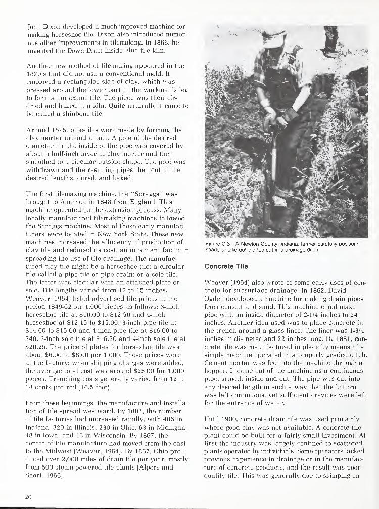
John Dixon developed a much-improved machine for

making horseshoe tile. Dixon also introduced numer-

ous other improvements in tilemaking. In 1866, he

invented the Down Draft Inside Flue tile kiln.

Another new method of tilemaking appeared in the

1870's that did not use a conventional mold. It

employed a rectangular slab of clay, which waspressed around the lower part of the workman's leg

to form a horseshoe tile. The piece was then air-

dried and baked in a kiln. Quite naturally it came to

be called a shinbone tile.

Around 1875, pipe-tiles were made by forming the

clay mortar around a pole. A pole of the desired

diameter for the inside of the pipe was covered by

about a half-inch layer of clay mortar and then

smoothed to a circular outside shape. The pole waswithdrawn and the resulting pipes then cut to the

desired lengths, cured, and baked.

The first tilemaking machine, the "Scraggs" wasbrought to America in 1848 from England. This

machine operated on the extrusion process. Manylocally manufactured tilemaking machines followed

the Scraggs machine. Most of these early manufac-

turers were located in New York State. These newmachines increased the efficiency of production of

clay tile and reduced its cost, an important factor in

spreading the use of tile drainage. The manufac-

tured clay tile might be a horseshoe tile; a circular

tile called a pipe tile or pipe drain; or a sole tile.

The latter was circular with an attached plate or

sole. Tile lengths varied from 12 to 15 inches.

Weaver (1964) listed advertised tile prices in the

period 1849-62 for 1,000 pieces as follows: 3-inch

horesehoe tile at $10.00 to $12.50 and 4-inch

horseshoe at $12.15 to $15.00; 3-inch pipe tile at

$14.00 to $15.00 and 4-inch pipe tile at $16.00 to

$40; 3-inch sole tile at $16.20 and 4-inch sole tile at

$20.25. The price of plates for horseshoe tile wasabout $6.00 to $8.00 per 1,000. These prices wereat the factory; when shipping charges were added,

the average total cost was around $25.00 for 1,000

pieces. Trenching costs generally varied from 12 to

14 cents per rod (16.5 feet).

From these beginnings, the manufacture and installa-

tion of tile spread westward. By 1882, the numberof tile factories had increased rapidly, with 486 in

Indiana. 320 in Illinois, 230 in Ohio, 63 in Michigan,

18 in Iowa, and 13 in Wisconsin. By 1867, the

center of tile manufacture had moved from the east

to the Midwest (Weaver, 1964). By 1867, Ohio pro-

duced over 2,000 miles of drain tile per year, mostly

from 500 steam-powered tile plants (Alpers andShort, 1966).

Figure 2-3—A Newton County, Indiana, farmer carefully positions

spade to take out the top cut in a drainage ditch.

Concrete Tile

Weaver (1964) also wrote of some early uses of con-

crete for subsurface drainage. In 1862, David

Ogden developed a machine for making drain pipes

from cement and sand. This machine could makepipe with an inside diameter of 2-1/4 inches to 24

inches. Another idea used was to place concrete in

the trench around a glass liner. The liner was 1-3/4

inches in diameter and 22 inches long. By 1881, con-

crete tile was maunfactured in place by means of a

simple machine operated in a properly graded ditch.

Cement mortar was fed into the machine through a

hopper. It came out of the machine as a continuous

pipe, smooth inside and out. The pipe was cut into

any desired length in such a way that the bottom

was left continuous, yet sufficient crevices were left

for the entrance of water.

Until 1900, concrete drain tile was used primarily

where good clay was not available. A concrete tile

plant could be built for a fairly small investment. At

first the industry was largely confined to scattered

plants operated by individuals. Some operators lacked

previous experience in drainage or in the manufac-

ture of concrete products, and the result was poor

quality tile. This was generally due to skimping on

;.'u

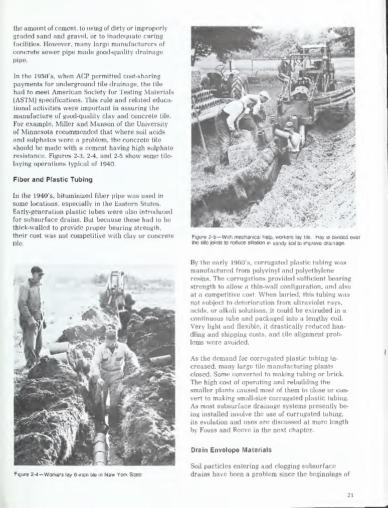
the amount of cement, to using of dirty or improperly

graded sand and gravel, or to inadequate curing

facilities. However, many large manufacturers of

concrete sewer pipe made good-quality drainage

pipe.

In the 1950's, when ACP permitted cost-sharing

payments for underground tile drainage, the tile

had to meet American Society for Testing Materials

(ASTM) specifications. This rule and related educa-

tional activities were important in assuring the

manufacture of good-quality clay and concrete tile.

For example, Miller and Manson of the University

of Minnesota recommended that where soil acids

and sulphates were a problem, the concrete tile

should be made with a cement having high sulphate

resistance. Figures 2-3, 2-4, and 2-5 show some tile-

laying operations typical of 1940.

Fiber and Plastic Tubing

In the 1940's, bituminized fiber pipe was used in

some locations, especially in the Eastern States.

Early-generation plastic tubes were also introduced

for subsurface drains. But because these had to be

thick-walled to provide proper bearing strength,

their cost was not competitive with clay or concrete

tile.

Figure 2-5— With mechanical help, workers lay tile. Hay is blinded overthe title joints to reduce siltation in sandy soil to improve drainage.

Figure 2-4—Workers lay 6-inch tile in New York State

By the early 1960's, corrugated plastic tubing wasmanufactured from polyvinyl and polyethylene

resins. The corrugations provided sufficient bearing

strength to allow a thin-wall configuration, and also

at a competitive cost. When buried, this tubing wasnot subject to deterioration from ultraviolet rays,

acids, or alkali solutions. It could be extruded in a

continuous tube and packaged into a lengthy coil.

Very light and flexible, it drastically reduced han-

dling and shipping costs, and tile alignment prob-

lems were avoided.

As the demand for corrugated plastic tubing in-

creased, many large tile manufacturing plants

closed. Some converted to making tubing or brick.

The high cost of operating and rebuilding the

smaller plants caused most of them to close or con-

vert to making small-size corrugated plastic tubing.

As most subsurface drainage systems presently be-

ing installed involve the use of corrugated tubing,

its evolution and uses are discussed at more length

by Fouss and Reeve in the next chapter.

Drain Envelope Materials

Soil particles entering and clogging subsurface

drains have been a problem since the beginnings of

21

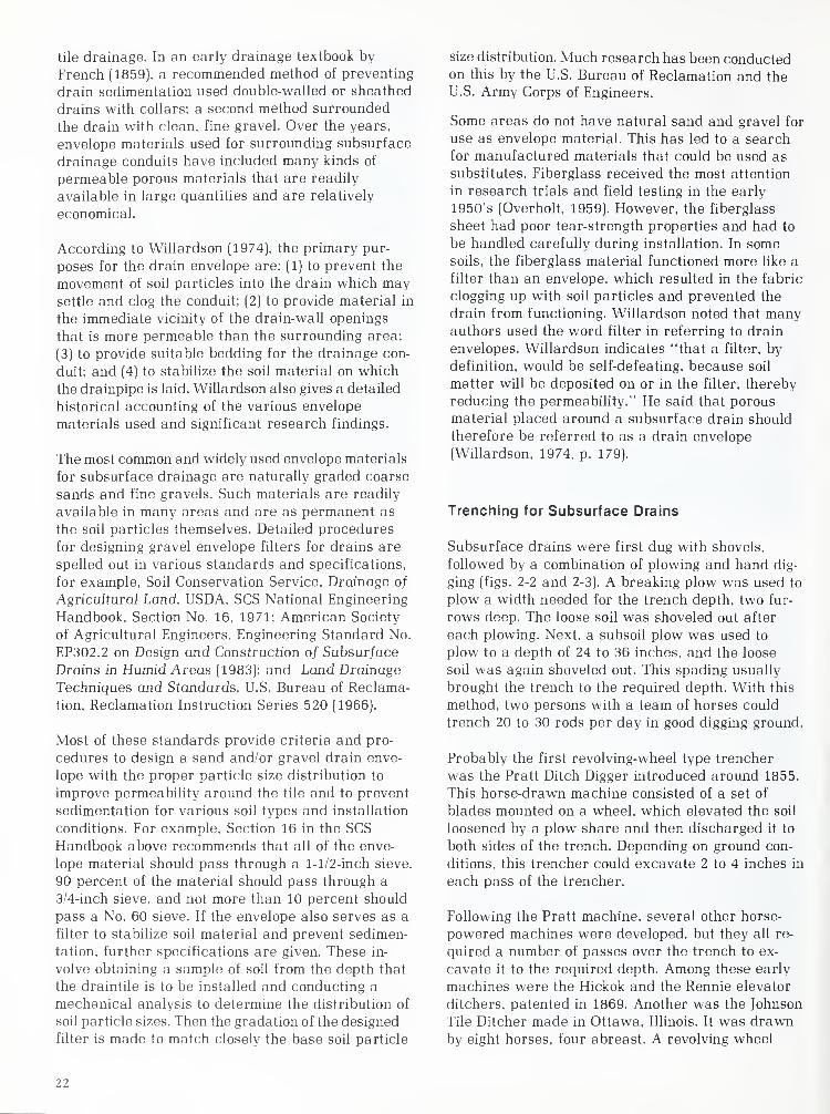
tile drainage. In an early drainage textbook by

French [1859], a recommended method of preventing

drain sedimentation used double-walled or sheathed

drains with collars; a second method surrounded

the drain with clean, fine gravel. Over the years,

envelope materials used for surrounding subsurface

drainage conduits have included many kinds of

permeable porous materials that are readily

available in large quantities and are relatively

economical.

According to Willardson (1974), the primary pur-

poses for the drain envelope are: (1) to prevent the

movement of soil particles into the drain which maysettle and clog the conduit; (2) to provide material in

the immediate vicinity of the drain-wall openings

that is more permeable than the surrounding area;

(3) to provide suitable bedding for the drainage con-

duit: and (4) to stabilize the soil material on which

the drainpipe is laid. Willardson also gives a detailed

historical accounting of the various envelope

materials used and significant research findings.

The most common and widely used envelope materials

for subsurface drainage are naturally graded coarse

sands and fine gravels. Such materials are readily

available in many areas and are as permanent as

the soil particles themselves. Detailed procedures

for designing gravel envelope filters for drains are

spelled out in various standards and specifications,

for example. Soil Conservation Service, Drainage of

Agricultural Land, USDA, SCS National Engineering

Handbook. Section No. 16, 1971; American Society

of Agricultural Engineers, Engineering Standard No.

EP302.2 on Design and Construction of Subsurface

Drains in Humid Areas (1983); and Land Drainage

Techniques and Standards, U.S. Bureau of Reclama-

tion, Reclamation Instruction Series 520 (1966).

Most of these standards provide criteria and pro-

cedures to design a sand and/or gravel drain enve-

lope with the proper particle size distribution to

improve permeability around the tile and to prevent

sedimentation for various soil types and installation

conditions. For example. Section 16 in the SCSHandbook above recommends that all of the enve-

lope material should pass through a 1-1/2-inch sieve,

90 percent of the material should pass through a

3/4-inch sieve, and not more than 10 percent should

pass a No. 60 sieve. If the envelope also serves as a

filter to stabilize soil material and prevent sedimen-

tation, further specifications are given. These in-

volve obtaining a sample of soil from the depth that

the draintile is to be installed and conducting a

mechanical analysis to determine the distribution of

soil particle sizes. Then the gradation of the designed

filter is made to match closely the base soil particle

size distribution. Much research has been conductedon this by the U.S. Bureau of Reclamation and the

U.S. Army Corps of Engineers.

Some areas do not have natural sand and gravel for

use as envelope material. This has led to a search

for manufactured materials that could be used as

substitutes. Fiberglass received the most attention

in research trials and field testing in the early

1950's (Overholt, 1959). However, the fiberglass

sheet had poor tear-strength properties and had to

be handled carefully during installation. In somesoils, the fiberglass material functioned more like a

filter than an envelope, which resulted in the fabric

clogging up with soil particles and prevented the

drain from functioning. Willardson noted that manyauthors used the word filter in referring to drain

envelopes. Willardson indicates "that a filter, by

definition, would be self-defeating, because soil

matter will be deposited on or in the filter, thereby

reducing the permeability." He said that porous

material placed around a subsurface drain should

therefore be referred to as a drain envelope

(Willardson. 1974, p. 179).

Trenching for Subsurface Drains

Subsurface drains were first dug with shovels,

followed by a combination of plowing and hand dig-

ging (figs. 2-2 and 2-3). A breaking plow was used to

plow a width needed for the trench depth, two fur-

rows deep. The loose soil was shoveled out after

each plowing. Next, a subsoil plow was used to

plow to a depth of 24 to 36 inches, and the loose

soil was again shoveled out. This spading usually

brought the trench to the required depth. With this

method, two persons with a team of horses could

trench 20 to 30 rods per day in good digging ground.

Probably the first revolving-wheel type trencher

was the Pratt Ditch Digger introduced around 1855.

This horse-drawn machine consisted of a set of

blades mounted on a wheel, which elevated the soil

loosened by a plow share and then discharged it to

both sides of the trench. Depending on ground con-

ditions, this trencher could excavate 2 to 4 inches in

each pass of the trencher.

Following the Pratt machine, several other horse-

powered machines were developed, but they all re-

quired a number of passes over the trench to ex-

cavate it to the required depth. Among these early

machines were the Hickok and the Rennie elevator

ditchers, patented in 1869. Another was the Johnson

Tile Ditcher made in Ottawa, Illinois. It was drawnby eight horses, four abreast. A revolving wheel

2J

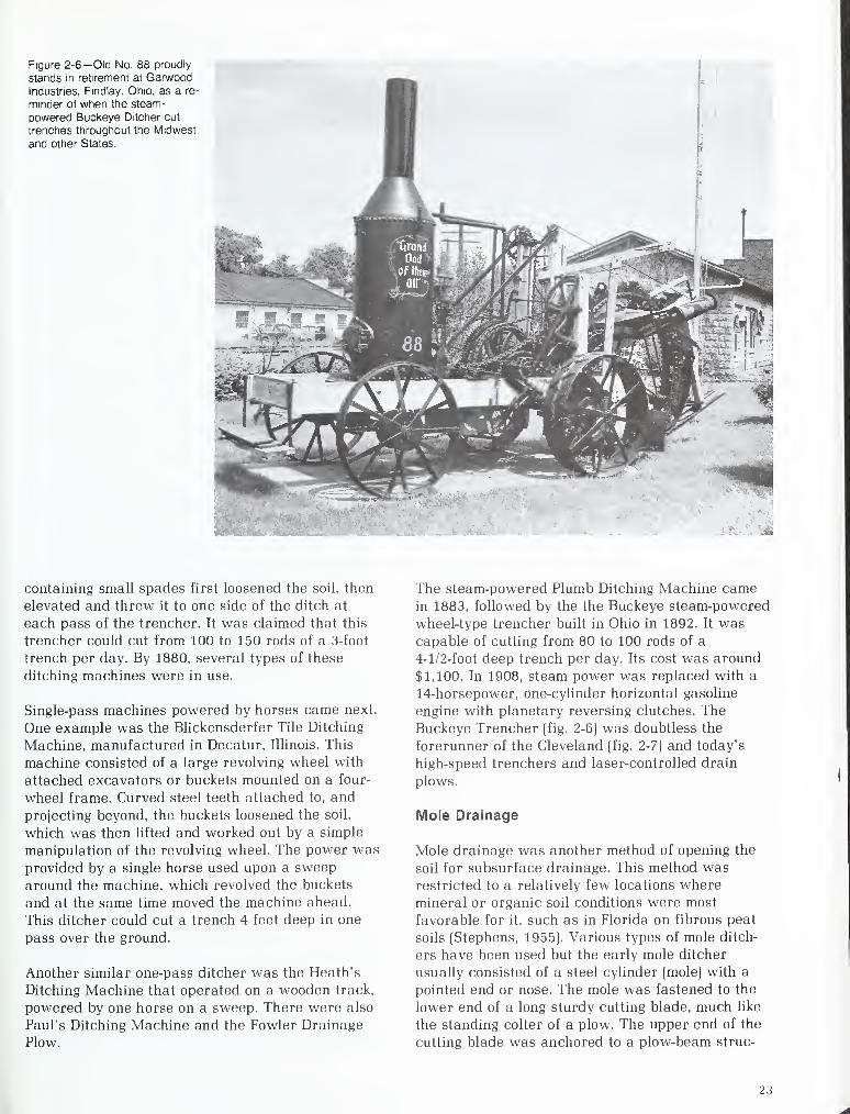
Figure 2-6— Old No. 88 proudly

stands in retirement at GarwoodIndustries, Fmdlay, Ohio, as a re-

minder of when the steam-

powered Buckeye Ditcher cut

trenches throughout the Midwest

and other States.

containing small spades first loosened the soil, then

elevated and threw it to one side of the ditch at

each pass of the trencher. It was claimed that this

trencher could cut from 100 to 150 rods of a 3-foot

trench per day. By 1880, several types of these

ditching machines were in use.

Single-pass machines powered by horses came next.

One example was the Blickensderfer Tile Ditching

Machine, manufactured in Decatur, Illinois. This

machine consisted of a large revolving wheel with

attached excavators or buckets mounted on a four-

wheel frame. Curved steel teeth attached to, and

projecting beyond, the buckets loosened the soil,

which was then lifted and worked out by a simple

manipulation of the revolving wheel. The power wasprovided by a single horse used upon a sweep

around the machine, which revolved the buckets

and at the same time moved the machine ahead.

This ditcher could cut a trench 4 feet deep in one

pass over the ground.

Another similar one-pass ditcher was the Heath's

Ditching Machine that operated on a wooden track,

powered by one horse on a sweep. There were also

Paul's Ditching Machine and the Fowler Drainage

Plow.

The steam-powered Plumb Ditching Machine camein 1883, followed by the the Buckeye steam-powered

wheel-type trencher built in Ohio in 1892. It wascapable of cutting from 80 to 100 rods of a

4-1/2-foot deep trench per day. Its cost was around

$1,100. In 1908, steam power was replaced with a

14-horsepower, one-cylinder horizontal gasoline

engine with planetary reversing clutches. The

Buckeye Trencher (fig. 2-6) was doubtless the

forerunner of the Cleveland (fig. 2-7) and today's

high-speed trenchers and laser-controlled drain

plows.

Mole Drainage

Mole drainage was another method of opening the

soil for subsurface drainage. This method wasrestricted to a relatively few locations where

mineral or organic soil conditions were most

favorable for it, such as in Florida on fibrous peat

soils (Stephens, 1955). Various types of mole ditch-

ers have been used but the early mole ditcher

usually consisted of a steel cylinder (mole) with a

pointed end or nose. The mole was fastened to the

lower end of a long sturdy cutting blade, much like

the standing colter of a plow. The upper end of the

cutting blade was anchored to a plow-beam struc-

23

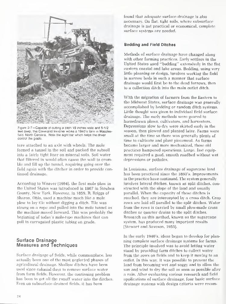
Figure 2-7— Capable of cutting a ditch 19 inches wide and 5-1/2

feet deep, this Cleveland trencher works a 1940's farm in Maccles-

field, North Carolina. Note the sight bar which helps the driver

control the grade.

ture attached to an axle with wheels. The mole

formed a tunnel in the soil and packed the subsoil

into a fairly tight liner on mineral soils. Soil water

that filtered in would often cause the wall to crum-

ble and fill up the tunnel, requiring going over the

field again with the ditcher in order to provide con-

tinued drainage.

According to Weaver (1964), the first mole plow in

the United States was introduced in 1867 in Steuben

County, New York. However, in 1859, B. Briggs of

Sharon. Ohio, used a machine much like a mole

plow to lay tile without digging a ditch. Tile wasstrung on a rope and pulled into the mole tunnel as

the machine moved forward. This was probably the

beginning of today's mole-type machines that canpull in corrugated plastic tubing on grade.

Surface DrainageMeasures and Techniques

Surface drainage of fields, while commonplace, has

actually been one of the most neglected phases of

agricultural drainage. Shallow ditches have beenused since colonial days to remove surface waterfrom farm fields. However, the continuing problemhas been to get all the runoff water into the ditches.

Even on subsurface drained fields, it has been

found that adequate surface drainage is also

necessary. On flat, tight soils, where subsurface

drainage is not practical or economical, complete

surface systems are needed.

Bedding and Field Ditches

Methods of surface drainage have changed along

with other farming practices. Early settlers in the

United States used "bedding" extensively in the flat

eastern coastal and lake areas. Bedding, using very

little planning or design, involves working the field

in narrow beds in such a manner that surface

drainage would first be to the dead furrows, then

to a collection ditch into the main outlet ditch.

With the migration of farmers from the Eastern to

the Midwest States, surface drainage was generally

accomplished by bedding or random ditch systems.

Little thought was given to individual field surface

drainage. The early methods were geared to

horsedrawn plows, cultivators, and harvesters.

Depressions slow to dry were skirted early in the

season, then plowed and planted later. Farms weresmall at the time so there was generally plenty of

time to cultivate and plant piecemeal. As farms

became larger and more mechanized, these old

practices hampered operations. Large, fast equip-

ment required a good, smooth roadbed without wetdepressions or potholes.

In Louisiana, surface drainage of sugarcane land

has been practiced since the 1860's. Improvements

in the practice have continued. The system generally

involves lateral ditches, known as split ditches, con-

structed with the slope of the land and usually

parallel. When the capacity of these ditches is

reached, they are intercepted by a cross ditch. Crop

rows are laid off parallel to the split ditches. Waterfrom the rows is carried by small plow-made cross

ditches or quarter drains to the split ditches.

Research on this method, known as the sugarcane

system, has produced many important results

(Stewart and Saveson, 1955).

In the early 1940's, ideas began to develop for plan-

ning complete surface drainage systems for farms.

The principle involved was to avoid letting water

stand by providing farm ditches to collect water

from the rows on fields and to keep it moving to an

outlet. In this way, it was possible to prevent the

land from becoming wet and soggy and to allow the

sun and wind to dry the soil as soon as possible after

a rain. After evaluating various research and field

applications of surface drainage, four basic surface

drainage systems with design criteria were recom-

J4

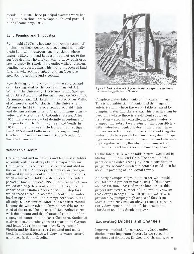
mended in 1950. These principal systems were bed-

ding, random ditch, cross-slope ditch, and parallel

ditch (Beauchamp. 1952).

Land Forming and Smoothing

By the mid-1940's, it became apparent a system of

ditches like those described above could not easily

drain land with numerous small pockets, wherewater is likely to pond because it cannot get to the

surface drains. The answer was to allow each crop

row to carry its runoff to its outlet without erosion,

ponding, or overtopping. This led to the idea of land

forming, whereby the entire land surfaces are

modified by grading and smoothing.

Row drainage and land forming were studied andcriteria suggested by the research work of A.J.

Wojta of the University of Wisconsin; L.L. Saveson

of USDA's Agricultural Research Service (ARS); L.F.

Hermsmeier and C.L. Larson in the Red River Valley

of Minnesota; and W. Harris of the University of

Arkansas. In 1947, the SCS conducted field trials

and demonstrations of land forming in many conser-

vation districts of the North-Central States. After

1950, there was a slow but definite acceptance of

this practice in the Midwest, East, and South. In

1952, the practice was included for the first time in

the ACP National Bulletin as "Shaping or LandGrading to Provide Permanent Slopes Needed for

Surface Drainage."

Water Table Control

Draining peat and muck soils and high water tables

on sandy soils has always been a major problem.

Drainage studies on organic soils were initiated in

the early 1900's. Another problem was overdrainage,

followed by subsequent settling of the organic soils

when a low water table existed over an extended

period of time (Stephens, 1955). The practice of con-

trolled drainage began about 1930. This generally

consisted of installing check dams with stop logs

which were raised or lowered to control the waterlevel in open ditches. The attempt here was to take

off only that amount of water that was detrimental,

keeping the water table as high as possible for the

good of the crop. The success of this method varied

with the amount and distribution of rainfall and the

seepage of water into the controlled area. Studies of

early controlled drainage were reported by Clayton

and Jones (1941) in the northern Everglades of

Florida and by Harker (1941) on sand and mucklands in Indiana. Figure 2-8 shows a water control

gate used in South Carolina.

Figure 2-8—A water-control gate operates at capacity after heavyrams near Neggetts, North Carolina.

Complete water table control then came into use.

This is a combination of controlled drainage andsub-irrigation, where the water table is raised by

pumping water into the system. This practice can be

used only where there is a sufficient supply of

irrigation water. In controlled drainage, water is

pumped into subsurface drains or into open ditches

with water-level control gates in the drain. These

ditches serve both as drainage outlets and irrigation

water inlets to a parallel subsurface system. Pump-

ing can remove excess drainage water and also sup-

ply irrigation water, thereby maintaining water

tables at correct levels for optimum crop growth.

By the late 1940's, water table control was used in

Michigan, Indiana, and Ohio. The spread of this

practice was aided greatly by farm electrification

programs, because automatic controls could then be

used for pumping on individual farms.

An early example of group action for water table

control was a project in north-central Ohio known

as "Marsh Run." Started in the late 1950's, this

project involved a number of landowners growing

truck crops in organic soil. Irrigation water was

provided by pumping high stages of flow from

Marsh Run Creek into an above-ground reservoir.

Early development and use of this practice in

Florida is noted by Stephens (1955).

Excavating Ditches and Channels

Improved methods for constructing large outlet

ditches were important factors in the spread and

efficiency of drainage. Ditches and channels, even

25

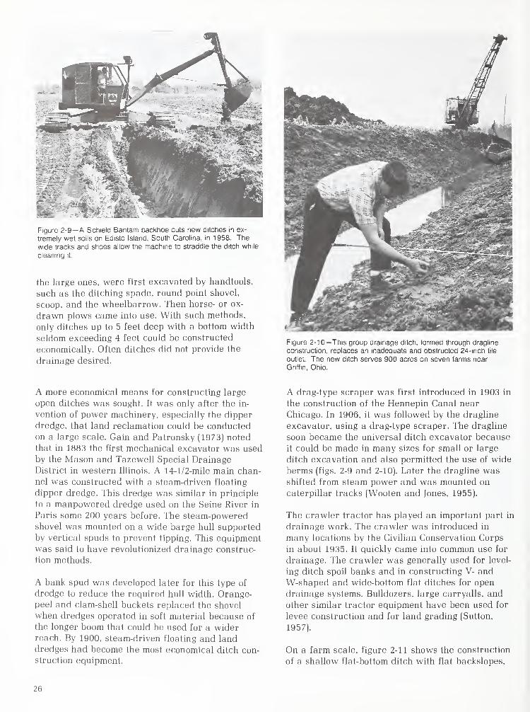
Figure 2-9— A Schield Bantam backhoe cuts new ditches in ex-

tremely wet soils on Edisto Island, South Carolina, in 1958. Thewide tracks and shoes allow the machine to straddle the ditch while

cleaning it.

the large ones, were first excavated by handtools,

such as the ditching spade, round point shovel,

scoop, and the wheelbarrow. Then horse- or ox-

drawn plows came into use. With such methods,

only ditches up to 5 feet deep with a bottom width

seldom exceeding 4 feet could be constructed

economically. Often ditches did not provide the

drainage desired.

Figure 2-10—This group drainage ditch, formed through dragline

construction, replaces an inadequate and obstructed 24-inch tile

outlet. The new ditch serves 900 acres on seven farms near

Griffin, Ohio.

A more economical means for constructing large

open ditches was sought. It was only after the in-

vention of power machinery, especially the dipper

dredge, that land reclamation could be conducted

on a large scale. Gain and Patronsky (1973) noted

that in 1883 the first mechanical excavator was used

by the Mason and Tazewell Special Drainage

District in western Illinois. A 14-1/2-mile main chan-

nel was constructed with a steam-driven floating

dipper dredge. This dredge was similar in principle

to a manpowered dredge used on the Seine River in

Paris some 200 years before. The steam-poweredshovel was mounted on a wide barge hull supported

by vertical spuds to prevent tipping. This equipmentwas said to have revolutionized drainage construc-

tion methods.

A bank spud was developed later for this type of

dredge to reduce the required hull width. Orange-peel and clam-shell buckets replaced the shovel

when dredges operated in soft material because of

the longer boom that could be used for a widerreach. By 1900, steam-driven floating and land

dredges had become the most economical ditch con-

struction equipment.

A drag-type scraper was first introduced in 1903 in

the construction of the Hennepin Canal near

Chicago. In 1906, it was followed by the dragline

excavator, using a drag-type scraper. The dragline

soon became the universal ditch excavator because

it could be made in many sizes for small or large

ditch excavation and also permitted the use of wide

berms (figs. 2-9 and 2-10). Later the dragline wasshifted from steam power and was mounted on

caterpillar tracks (Wooten and Jones, 1955).

The crawler tractor has played an important part in

drainage work. The crawler was introduced in

many locations by the Civilian Conservation Corps

in about 1935. It quickly came into common use for

drainage. The crawler was generally used for level-

ing ditch spoil banks and in constructing V- and

W-shaped and wide-bottom flat ditches for open

drainage systems. Bulldozers, large carryalls, and

other similar tractor equipment have been used for

levee construction and for land grading (Sutton,

1957).

On a farm scale, figure 2-11 shows the construction

of a shallow flat-bottom ditch with flat backslopes,

L'f,

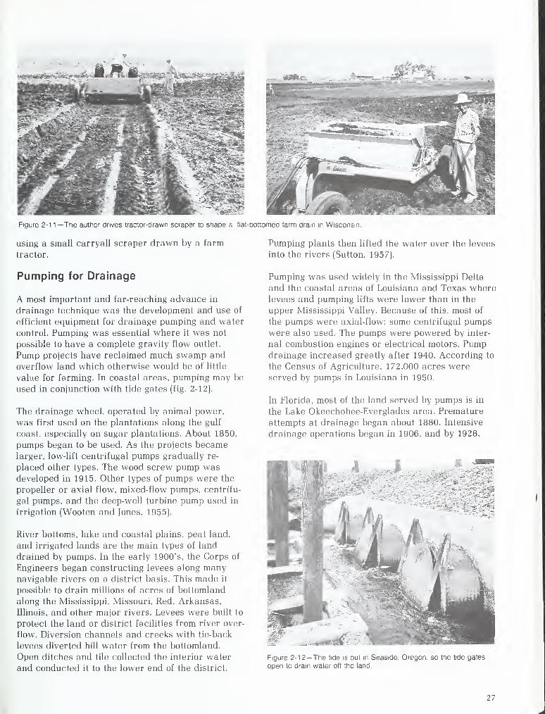
Figure 2-1 1 —The author drives tractor-drawn scraper to shape a flat-bottomed farm dram in Wisconsin

using a small carryall scraper drawn by a farm

tractor.

Pumping for Drainage

A most important and far-reaching advance in

drainage technique was the development and use of

efficient equipment for drainage pumping and water

control. Pumping was essential where it was not

possible to have a complete gravity flow outlet.

Pump projects have reclaimed much swamp and

overflow land which otherwise would be of little

value for farming. In coastal areas, pumping may be

used in conjunction with tide gates (fig. 2-12).

The drainage wheel, operated by animal power,

was first used on the plantations along the gulf

coast, especially on sugar plantations. About 1850,

pumps began to be used. As the projects becamelarger, low-lift centrifugal pumps gradually re-

placed other types. The wood screw pump wasdeveloped in 1915. Other types of pumps were the

propeller or axial flow, mixed-flow pumps, centrifu-

gal pumps, and the deep-well turbine pump used in

irrigation (Wooten and Jones, 1955).

River bottoms, lake and coastal plains, peat land,

and irrigated lands are the main types of land

drained by pumps. In the early 1900's, the Corps of

Engineers began constructing levees along manynavigable rivers on a district basis. This made it

possible to drain millions of acres of bottomland

along the Mississippi, Missouri, Red, Arkansas,

Illinois, and other major rivers. Levees were built to

protect the land or district facilities from river over-

flow. Diversion channels and creeks with tie-back

levees diverted hill water from the bottomland.

Open ditches and tile collected the interior water

and conducted it to the lower end of the district.

Pumping plants then lifted the water over the levees

into the rivers (Sutton, 1957).

Pumping was used widely in the Mississippi Delta

and the coastal areas of Louisiana and Texas wherelevees and pumping lifts were lower than in the

upper Mississippi Valley. Because of this, most of

the pumps were axial-flow; some centrifugal pumpswere also used. The pumps were powered by inter-

nal combustion engines or electrical motors. Pumpdrainage increased greatly after 1940. According to

the Census of Agriculture, 172,000 acres wereserved by pumps in Louisiana in 1950.

In Florida, most of the land served by pumps is in

the Lake Okeechobee-Everglades area. Premature

attempts at drainage began about 1880. Intensive

drainage operations began in 1906, and by 1928,

--^:

Figure 2-12—The tide is out in Seaside, Oregon, so the tide gates

open to drain water off the land.

27

reversible pumps were necessary to pump water

from the fields in wet seasons and then from the

canals into the fields during dry seasons. Most of

the pumps were of the axial flow or propeller type.

In 1950, pumps served 293.000 acres in Florida

(Stephens, 1955).

Most of the river drainage and levee districts in the

upper Mississippi Valley also operated pumping

plants and found them to be essential to drainage

work. Most of the pumping districts, particularly

along the Illinois River, were established after 1905.

The pumps of the early districts were generally too

small and were supplemented or entirely replaced

by new ones. By 1950, the area served by pumps in

Illinois was 315,000 acres, in Missouri 67,000 acres,

and in Iowa 82,000 acres (Sutton, 1955).

Before 1914. all pumping districts in the upper

Mississippi Valley used steam engines as a source

of power. Between 1914 and 1918, all new pumping

plants were equipped with electric motors, and

some of the old steam plants changed to electric

power. The first diesel engine was installed in 1928.

Diesel power was then used in most new installa-

tions and in many old plants (Pickels, 1929).

Interest in small, individually owned pumping plants

increased after the early 1940's. They were used

primarily where there was no gravity outlet for sub-

surface drains within the farm boundary. The outlet

ditches in many locations were not deep enough to

provide adequate drainage. This type of pumpingcould often replace long tile mains or long deepoutlet ditches. In many cases, pumping allowed

landowners to proceed on their own without waiting

for district or group action. Individual farm pump-ing was also used in a water table control system.

An example is the low land near the Great Lakes.

High lake levels often kept outlets from functioning

and caused crop losses. Because pumping lifts wereusually low, propeller-type pumps were generally

adequate. Progress in the development of onfarmpumping was due mostly to the wide availability of

electricity on farms by the mid-1950's, along with

improved efficiency of tractors and internal com-

bustion engines for power.

References

Alpers, R. }., and T. N. Short. 1966. CJay DraintiJe

and Its Use. Proceedings of the ASAE National

Drainage Symposium. Am. Soc. Agr. Engr., St.

Joseph, Mich.

Beauchamp, Keith H. 1952. "Systems of Surface

Drainage of Tight Soils," Agricultural Engineering.

Vol. 33. No. 4 (April).

Clayton, B. C, and L. A. Jones. 1941. "Controlled

Drainage in the Northern Everglades of Florida,"

Agricultural Engineering. Vol. 22 (August).

Darby, H. C. 1940. The Draining of the Fens. Cam-bridge, England: Cambridge University Press.

Donnan, William W. 1976. An Overview of DrainageWorldwide. Proceedings of the Third National ASAEDrainage Symposium. Am. Soc. Agr. Engr., St.

Joseph, Mich.

Gain, Elmer W., and Richard J. Patronsky. 1973.

Historical Sketches on Channel Modification. ASAEPaper No. 73-2537. Am. Soc. Agr. Engr., St. Joseph.

Mich.

Harker, David H. 1941. "Controlled Drainage," Agri-

cultural Engineering. Vol. 22, No. 4 (April).

Harrison, Robert W. 1961. AJJuvial Empire: A Study

of State and Local Efforts Toward Land Develop-

ment in the Alluvial Valley of the Lower Mississippi

River. Little Rock, Ark.: Pioneer Press.

Hay. Ralph C, and John B. Stall. 1976. History of

Channel Improvements in an Illinois Watershed.

ASAE Paper No. 76-2506. Am. Soc. Agr. Engr., St.

Joseph, Mich.

King, James A., and W. S. Lynes. 1946. Tile

Drainage. (4th edition). Mason City, Iowa: MasonCity Brick and Tile Company.

Miles, Manley. 1892. Land Drainage. New York:

Orange Judd Company.

Overholt, Virgil. 1959. "Fiberglass Filter for Tile

Drains," Agricultural Engineering. Vol. 40. pp.

604-607.

Pickels, George W. 1925. Drainage and Flood-

Control Engineering. New York: McGraw-Hill BookCompany.

Pickels, G. W., and F. B. Leonard. 1929. Engineering

and Legal Aspects of Land Drainage in Illinois.

Bulletin No. 12. Illinois Geological Survey.

Soil Conservation Society of America. 1956. OurWater Resource. Des Moines, Iowa.

28

Stephens, John C. 1955. "Drainage of Peat and

Muck Lands," Yearbook of Agriculture, 1955. U.S.

Dept. Agr., pp. 539-557.

Stewart, K. V., Jr., and L. L. Saveson. 1955.

"Systems for Draining the Surface," Yearbook of

Agriculture, 1955. U.S. Dept. Agr., pp. 499-507.

Sutton, John G. 1955. "The Use of Pumps for

Drainage," Yearbook of Agriculture, 1955. U.S.

Dept. Agr., pp. 528-538.

Sutton, John G. 1957. "Drainage Developments Dur-

ing the Past 50 Years," Agricultural Engineering.

Vol. 8, No. 6 (JuneJ.

van Schilfgaarde, Jan. 1971. Drainage Yesterday,

Today, and Tomorrow. Proceedings of the ASAENational Drainage Symposium. Am. Soc. Agr. Engr.,

St. Joseph, Mich.

van Veen, J. 1948. Dredge Drain Reciamation: TheArt of a Nation. The Hague: Mortmas Nishoft.

Weaver, Marion M. 1964. History of Tile Drainage.

Waterloo, New York: M. M. Weaver.

Wheeler, W. H. 1868. A History of the Fens of South

Lincolnshire. (Publisher unknown).

Willardson, Lyman S. 1974. "Envelope Materials,"

Drainage for Agriculture (ed. J. van Schilfgaarde).

Monograph No. 17. Am. Soc. Agronomy, Madison,

Wise.

Sutton, John G. 1958. "Appraising Our Drainage

Job," Land Improvement. Vol. 5, No. 4 (April).

Wooten, Hugh H., and Lewis A. Jones. 1955. "TheHistory of Our Drainage Enterprises," Yearbook of

Agriculture, 1955. U.S. Dept. Agr., pp. 478-491.

29

Chapter 3

Advances in DrainageTechnology: 1955-85

James L. FoussAgricultural Research Service, USDABaton Rouge, Louisiana

Ronald C. ReeveDrainage ConsultantColumbus, Ohio

Advances in agricultural drainage technology within

the past 30 years are described in terms of changes

and improvements in drainage conduit materials

and/or installation methods. Drainage technology

changed and modernized more during 1965-75 than

in the previous 100 years. Slow, inefficient installa-

tion of heavy rigid conduit materials (clay and con-

crete) gave way to light-weight flexible corrugated

plastic drain tubing installed with laser-beam-

controlled high-speed trenchers and plow-type

equipment (Fouss. 1974: Reeve. 1978: Teach. 1972).

We accordingly review major technological develop-

ments in materials and equipment, plus other tech-

nology developed to design drainage and water

management systems through computerized simula-

tion and design procedures (Skaggs, 1980).

Technological Challenges

The development of a rapid and low-cost technique

for subsurface drainage has challenged engineers

and inventors for centuries. Many ideas have

emerged, but very few have found widespread use

or application. With the advent of the power trench-

ing machine in about 1875, the goal of mechanizeddrain installation seemed to have been reached—and

it lasted about 100 years. However, the extremely

large amount of drainage work that was needed

around the world required even less labor, morespeed, and lower costs. Efforts to modify the mole

drainage concept and installation methods wereparticularly important. The goal was to use the in-

herent high speed of installation of mole drainage

and its elimination of relatively slow ditching and

backfilling operations associated with conventional

drainage methods. Because the mole drain collapsed

after a short time in many soils, much of the

research concerned stabilizing the mole channel

with structural support, using a tube or liner.

A second technological challenge involved develop-

ing a means to design optimal agricultural drainage

systems on a probability basis that would properly

account for the spatial variations in the drained soil

and the time variations in weather, as described

and recommended by van Schilfgaarde (1965). Opti-

mized drainage system design had long evaded

drainage engineers. With high-speed computers,

substantial progress has been made in meeting this

challenge, thus providing another significant ad-

vance in drainage technology.

Progress was also made possible in the drainage

industry because of technological developments in

other industries and areas, such as plastic mate-

rials, synthetic fabrics, construction equipment,

electronic (laser) equipment, and computer indus-

tries. A number of the advances in these other

fields seemingly came along just in time to meet the

needs of a developing new thrust in the drainage

field. Some of the innovations came about directly

in the drainage industry, but many were adopted

and/or adapted from developments originally in-

tended for other purposes. Examples are heavy

earth-moving machinery developed for construction,

lasers developed for alignment tasks in civil

construction, and synthetic fabrics developed by

30

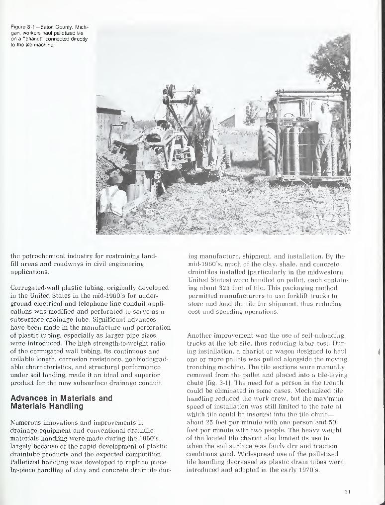
Figure 3-1— Eaton County, Michi-

gan, workers haul palletized tile

on a "chariot" connected directly

to the tile machine.

^-*>J^^^ Z?": :" ^V

the petrochemical industry for restraining land-

fill areas and roadways in civil engineering

applications.

Corrugated-wall plastic tubing, originally developed

in the United States in the mid-1960's for under-

ground electrical and telephone line conduit appli-

cations was modified and perforated to serve as a

subsurface drainage tube. Significant advances

have been made in the manufacture and perforation

of plastic tubing, especially as larger pipe sizes

were introduced. The high strength-to-weight ratio

of the corrugated wall tubing, its continuous andcoilable length, corrosion resistance, nonbiodegrad-

able characteristics, and structural performance

under soil loading, made it an ideal and superior

product for the new subsurface drainage conduit.

Advances in Materials andMaterials Handling

Numerous innovations and improvements in

drainage equipment and conventional draintile

materials handling were made during the 1960's.

largely because of the rapid development of plastic

draintube products and the expected competition.

Palletized handling was developed to replace piece-

by-piece handling of clay and concrete draintile dur-

ing manufacture, shipment, and installation. By the

mid-1960"s, much of the clay, shale, and concrete

draintiles installed (particularly in the midwestern

United States) were handled on pallet, each contain-

ing about 325 feet of tile. This packaging methodpermitted manufacturers to use forklift trucks to

store and load the tile for shipment, thus reducing

cost and speeding operations.

Another improvement was the use of self-unloading

trucks at the job site, thus reducing labor cost. Dur-

ing installation, a chariot or wagon designed to haul

one or more pallets was pulled alongside the moving

trenching machine. The tile sections were manually

removed from the pallet and placed into a tile-laying

chute (fig. 3-1). The need for a person in the trench

could be eliminated in some cases. Mechanized tile

handling reduced the work crew, but the maximumspeed of installation was still limited to the rate at

which tile could be inserted into the tile chute

—

about 25 feet per minute with one person and 50

feet per minute with two people. The heavy weight

of the loaded tile chariot also limited its use to

when the soil surface was fairly dry and traction

conditions good. Widespread use of the palletized

tile handling decreased as plastic drain tubes were

introduced and adopted in the early 1970"s.

M

Smooth-Wall Plastic Tubing Plastic-Lined Mole Drains

Polyethylene plastic tubing, a British development,

was first manufactured in the United States in

about 1941. According to Schwab (1955), the Corps

of Engineers investigated the use of "perforated

plastic tubing" installed with cable-laying machines

for airport drainage as early as 1946. Schwab's

research from 1947 to 1954 is the earliest known

use of plastic draintubes for agriculture in the

United States. 1 He conducted field experiments in

Iowa where smooth-wall polyethylene plastic tubes

of various diameters and wall thicknesses were

pulled into a mole-drain channel in clay soil with a

mole plow. Schwab indicated that it was necessary

to handle the smooth-wall plastic drain in 20-foot

straight lengths because the tubing would kink

when coiled.

From these early studies, Schwab developed

guidelines on minimum tube-wall thickness for

various drain diameters to insure drain conduit

deflection of less than 20 percent of the original

diameter. When inspected in 1966, 17 years after

installation, these drains remained in good condition

(Fouss, 1968). The results from these pioneering

experiments provided many of the technical back-

ground data for the initial ASTM minimum re-

quirements for plastic drain strength-deflection

standards.

In the United States, smooth-wall plastic tubing wasnot used widely for agricultural subsurface

drainage, primarily because of its higher unit cost

and the greater material weight per unit length re-

quirement as compared with other materials andconfigurations. In the mid-1960's, limited use wasmade of 4-inch diameter, smooth-wall, polyethylene

plastic drain tubing in the Lower Rio Grande Valley

of Texas. The tubing was installed as deep as 6 feet

with a special narrow-wheel trencher (Myers andothers, 1967; Rektorik and Myers, 1967).

In The Netherlands, De Jager (1960) conducted ex-

periments with polyethylene tubes pulled into mole

drains, but finally selected a narrow trenching

machine to install 6-meter (19.7 feet) lengths of rigid

vinyl plastic drain pipe. According to van Someren

(1964), by the late 1960's, trenched-in polyvinylchlo-

ride (PVC) plastic drain pipes were used on up to 80

percent of the installations in The Netherlands.

'The authors acknowledge this pioneering research of ProfessorSchwab and his generous help in reviewing this chapter.

Considerable international research was conducted

from the late 1940's to the mid-1960's on the use of

plastic liner as a structural reinforcement for the

mole-drain channel. The results of this research

were important in providing the foundation for sub-

sequent investigative and developmental workleading to significant input to current drainage

technology (Edminster, 1965). Janert (1952)

developed a machine that formed and installed a

semirigid vinyl plastic drain from rolls of sheet film.

The plastic strip was heated to provide sufficient

flexibility for forming it into a tubular drain. The

plow-type, drain-laying machine was constructed

with an inclined planelike digging blade which

opened a trench about twice the diameter of the

drain. Production models of this machine were sold

in East Germany in the late 1950's. but its use wasnot widespread.

In the United States, Busch (1958) modified a mole

plow for feeding a PVC plastic strip into a mole-

drain channel and forming it into an arch-shaped

mole liner. This research precipitated a series of

refinements, modifications, and new developments

by both American and British investigators. Atubular mole liner, formed from a PVC sheet, wasdeveloped in 1960 by a team at the Caterpillar

Tractor Company. Further studies led to the devel-

opment and testing of the stronger zippered-type

tubular PVC plastic mole liner (Fouss and Donnan

(1962) in the United States and Ede (1963) and Boa

(1963) in the United Kingdom).

Most of these early experimental plastic drains

were 2-1/2 to 3 inches in diameter. Materials han-

dling for the plastic mole liner was exceptionally ef-

ficient. For example, a 60-pound roll of 0.015-inch

thick PVC sheet, 10 inches wide by 10 inches in

diameter would form 600 feet of installed 3-inch

diameter drain (lined mole channel). This was a

truly remarkable materials handling advantage over

conventional practice. Ede (1965) and Fouss (1965)

reported that thin-walled plastic liners, although of-

fering significant materials handling advantages,

were not strong enough to withstand deformation

under long-term soil loading. Thus, the plastic-lined

mole drain concept was not pursued further,

primarily because of the appearance of the superior

corrugated-wall plastic tubing which could be easily

placed in a trench or a subsurface channel formed

with plow-type equipment.

This early research on plastic-lined mole drains

demonstrated the need for a systems approach in

V2

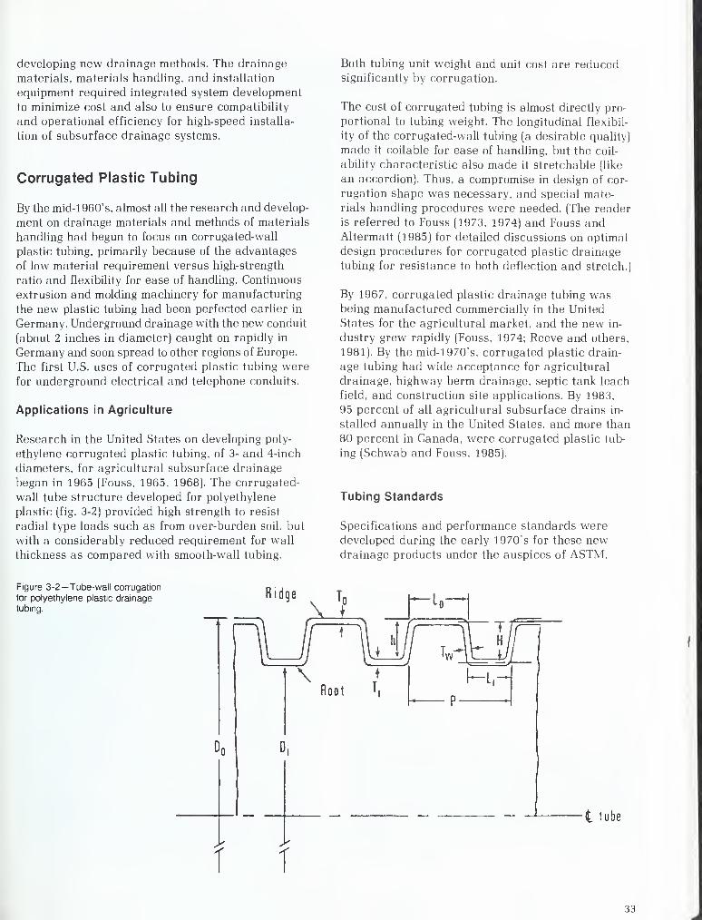
developing new drainage methods. The drainage

materials, materials handling, and installation

equipment required integrated system development

to minimize cost and also to ensure compatibility

and operational efficiency for high-speed installa-

tion of subsurface drainage systems.

Corrugated Plastic Tubing

By the mid-1 960's, almost all the research and develop-

ment on drainage materials and methods of materials

handling had begun to focus on corrugated-wall

plastic tubing, primarily because of the advantages

of low material requirement versus high-strength

ratio and flexibility for ease of handling. Continuous

extrusion and molding machinery for manufacturing

the new plastic tubing had been perfected earlier in

Germany. Underground drainage with the new conduit

(about 2 inches in diameter) caught on rapidly in

Germany and soon spread to other regions of Europe.

The first U.S. uses of corrugated plastic tubing were

for underground electrical and telephone conduits.

Applications in Agriculture

Research in the United States on developing poly-

ethylene corrugated plastic tubing, of 3- and 4-inch

diameters, for agricultural subsurface drainage

began in 1965 (Fouss, 1965, 1968). The corrugated-

wall tube structure developed for polyethylene

plastic (fig. 3-2) provided high strength to resist

radial type loads such as from over-burden soil, but

with a considerably reduced requirement for wall

thickness as compared with smooth-wall tubing.

Both tubing unit weight and unit cost are reducedsignificantly by corrugation.

The cost of corrugated tubing is almost directly pro-

portional to tubing weight. The longitudinal flexibil-

ity of the corrugated-wall tubing (a desirable quality)

made it coilable for ease of handling, but the coil-

ability characteristic also made it stretchable (like

an accordion). Thus, a compromise in design of cor-

rugation shape was necessary, and special mate-

rials handling procedures were needed. (The reader

is referred to Fouss (1973, 1974) and Fouss andAltermatt (1985) for detailed discussions on optimal

design procedures for corrugated plastic drainage

tubing for resistance to both deflection and stretch.)

By 1967, corrugated plastic drainage tubing wasbeing manufactured commercially in the United

States for the agricultural market, and the new in-

dustry grew rapidly (Fouss. 1974; Reeve and others,

1981). By the mid-1970's, corrugated plastic drain-

age tubing had wide acceptance for agricultural

drainage, highway berm drainage, septic tank leach

field, and construction site applications. By 1983.

95 percent of all agricultural subsurface drains in-

stalled annually in the United States, and more than

80 percent in Canada, were corrugated plastic tub-

ing (Schwab and Fouss, 1985).

Tubing Standards

Specifications and performance standards weredeveloped during the early 1970's for these newdrainage products under the auspices of ASTM,

Figure 3-2—Tube-wall corrugation

for polyethylene plastic drainage

tubing.

t tube

33

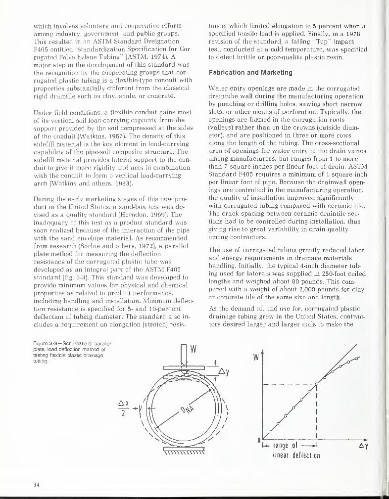
which involves voluntary and cooperative efforts

among industry, government, and public groups.

This resulted in an ASTM Standard Designation

F405 entitled 'Standardization Specification for Cor-

rugated Polyethylene Tubing" (ASTM, 1974). Amajor step in the development of this standard was

the recognition by the cooperating groups that cor-

rugated plastic tubing is a flexible-type conduit with

properties substantially different from the classical

rigid draintile such as clay, shale, or concrete.

Under field conditions, a flexible conduit gains most

of its vertical soil load-carrying capacity from the

support provided by the soil compressed at the sides

of the conduit (Watkins, 1967). The density of this

sidefill material is the key element in load-carrying

capability of the pipe-soil composite structure. The

sidefill material provides lateral support to the con-

duit to give it more rigidity and acts in combination

with the conduit to form a vertical load-carrying

arch (Watkins and others. 1983).

During the early marketing stages of this new pro-

duct in the United States, a sand-box test was de-

vised as a quality standard (Herndon, 1969). The

inadequacy of this test as a product standard wassoon realized because of the interaction of the pipe

with the sand envelope material. As recommendedfrom research (Sorbie and others, 1972), a parallel

plate method for measuring the deflection

resistance of the corrugated plastic tube wasdeveloped as an integral part of the ASTM F405

standard (fig. 3-3). This standard was developed to

provide minimum values for physical and chemical

properties as related to product performance,

including handling and installation. Minimum deflec-

tion resistance is specified for 5- and 10-percent

deflection of tubing diameter. The standard also in-

cludes a requirement on elongation (stretch) resis-

tance, which limited elongation to 5 percent when a

specified tensile load is applied. Finally, in a 1978

revision of the standard, a falling "Tup" impact

test, conducted at a cold temperature, was specified

to detect brittle or poor-quality plastic resin.

Fabrication and Marketing

Water entry openings are made in the corrugated

draintube wall during the manufacturing operation

by punching or drilling holes, sawing short narrowslots, or other means of perforation. Typically, the

openings are formed in the corrugation roots

(valleys) rather than on the crowns (outside diam-

eter), and are positioned in three or more rows

along the length of the tubing. The cross-sectional

area of openings for water entry to the drain varies

among manufacturers, but ranges from 1 to morethan 7 square inches per linear foot of drain. ASTMStandard F405 requires a minimum of 1 square inch

per linear foot of pipe. Because the drainwall open-

ings are controlled in the manufacturing operation,

the quality of installation improved significantly

with corrugated tubing compared with ceramic tile.

The crack spacing between ceramic draintile sec-

tions had to be controlled during installation, thus

giving rise to great variability in drain quality

among contractors.

The use of corrugated tubing greatly reduced labor

and energy requirements in drainage materials

handling. Initially, the typical 4-inch diameter tub-

ing used for laterals was supplied in 250-foot coiled

lengths and weighed about 80 pounds. This com-

pared with a weight of about 2,000 pounds for clay

or concrete tile of the same size and length.

As the demand of, and use for, corrugated plastic

drainage tubing grew in the United States, contrac-

tors desired larger and larger coils to make the

Figure 3-3— Schematic of parallel-

plate, load deflection method of

testing flexible plastic drainage

tubing.

\\\\\\\\\\\\\linear deflection

u

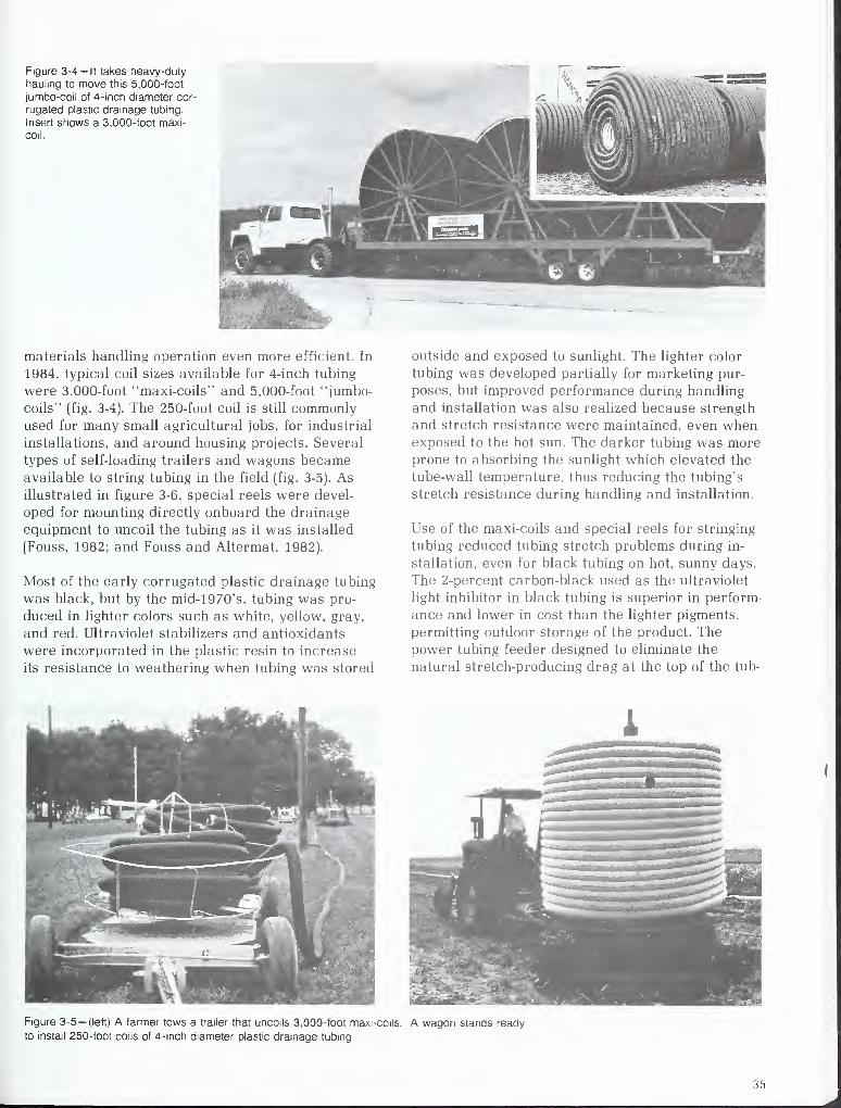
Figure 3-4 — It takes heavy-duty

hauling to move this 5,000-foot

jumbo-coll of 4-inch diameter cor-

rugated plastic drainage tubing.

Insert shows a 3,000-foot maxi-

coll.

materials handling operation even more efficient. In

1984, typical coil sizes available for 4-inch tubing

were 3,000-foot "maxi-coils" and 5,000-foot "jumbo-

coils" (fig. 3-4). The 250-foot coil is still commonlyused for many small agricultural jobs, for industrial

installations, and around housing projects. Several

types of self-loading trailers and wagons becameavailable to string tubing in the field (fig. 3-5). Asillustrated in figure 3-6, special reels were devel-

oped for mounting directly onboard the drainage

equipment to uncoil the tubing as it was installed

(Fouss, 1982; and Fouss and Altermat, 1982).

Most of the early corrugated plastic drainage tubing

was black, but by the mid-1970's, tubing was pro-

duced in lighter colors such as white, yellow, gray,

and red. Ultraviolet stabilizers and antioxidants

were incorporated in the plastic resin to increase

its resistance to weathering when tubing was stored

outside and exposed to sunlight. The lighter color

tubing was developed partially for marketing pur-

poses, but improved performance during handling

and installation was also realized because strength

and stretch resistance were maintained, even whenexposed to the hot sun. The darker tubing was moreprone to absorbing the sunlight which elevated the

tube-wall temperature, thus reducing the tubing's

stretch resistance during handling and installation.

Use of the maxi-coils and special reels for stringing

tubing reduced tubing stretch problems during in-

stallation, even for black tubing on hot, sunny days.

The 2-percent carbon-black used as the ultraviolet

light inhibitor in black tubing is superior in perform-

ance and lower in cost than the lighter pigments,

permitting outdoor storage of the product. The

power tubing feeder designed to eliminate the

natural stretch-producing drag at the top of the tub-

Figure 3-5— (left) A farmer tows a trailer that uncoils 3,000-foot maxi-coils.

to install 250-foot coils of 4-inch diameter plastic drainage tubing.

A wagon stands ready

35

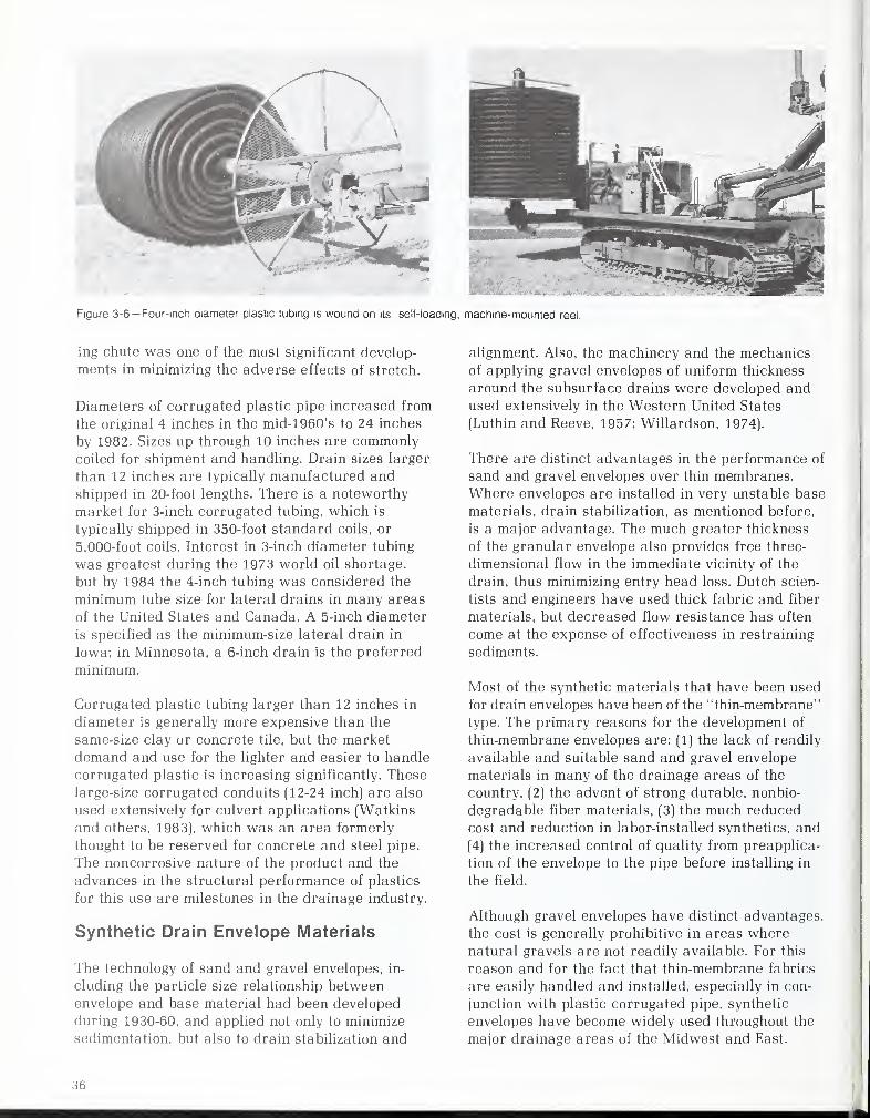
Figure 3-6— Four-inch diameter plastic tubing is wound on its self-loading, machine-mounted reel.

ing chute was one of the most significant develop-

ments in minimizing the adverse effects of stretch.

Diameters of corrugated plastic pipe increased from

the original 4 inches in the mid-1960's to 24 inches

by 1982. Sizes up through 10 inches are commonly

coiled for shipment and handling. Drain sizes larger

than 12 inches are typically manufactured and

shipped in 20-foot lengths. There is a noteworthy

market for 3-inch corrugated tubing, which is

typically shipped in 350-foot standard coils, or

5,000-foot coils. Interest in 3-inch diameter tubing

was greatest during the 1973 world oil shortage,

but by 1984 the 4-inch tubing was considered the

minimum tube size for lateral drains in many areas

of the United States and Canada. A 5-inch diameter

is specified as the minimum-size lateral drain in

Iowa; in Minnesota, a 6-inch drain is the preferred

minimum.

Corrugated plastic tubing larger than 12 inches in

diameter is generally more expensive than the

same-size clay or concrete tile, but the market

demand and use for the lighter and easier to handle

corrugated plastic is increasing significantly. These

large-size corrugated conduits (12-24 inch) are also

used extensively for culvert applications (Watkins

and others, 1983), which was an area formerly

thought to be reserved for concrete and steel pipe.

The noncorrosive nature of the product and the

advances in the structural performance of plastics

for this use are milestones in the drainage industry.

Synthetic Drain Envelope Materials

The technology of sand and gravel envelopes, in-

cluding the particle size relationship betweenenvelope and base material had been developed

during 1930-60, and applied not only to minimize

sedimentation, but also to drain stabilization and

alignment. Also, the machinery and the mechanics

of applying gravel envelopes of uniform thickness

around the subsurface drains were developed andused extensively in the Western United States

(Luthin and Reeve, 1957; Willardson. 1974).

There are distinct advantages in the performance of

sand and gravel envelopes over thin membranes.

Where envelopes are installed in very unstable base

materials, drain stabilization, as mentioned before,

is a major advantage. The much greater thickness

of the granular envelope also provides free three-

dimensional flow in the immediate vicinity of the

drain, thus minimizing entry head loss. Dutch scien-

tists and engineers have used thick fabric and fiber

materials, but decreased flow resistance has often

come at the expense of effectiveness in restraining

sediments.

Most of the synthetic materials that have been used

for drain envelopes have been of the "thin-membrane"

type. The primary reasons for the development of

thin-membrane envelopes are: (1) the lack of readily

available and suitable sand and gravel envelope

materials in many of the drainage areas of the

country, (2) the advent of strong durable, nonbio-

degradable fiber materials, (3) the much reduced

cost and reduction in labor-installed synthetics, and

(4) the increased control of quality from preapplica-

tion of the envelope to the pipe before installing in

the field.

Although gravel envelopes have distinct advantages,

the cost is generally prohibitive in areas wherenatural gravels are not readily available. For this

reason and for the fact that thin-membrane fabrics

are easily handled and installed, especially in con-

junction with plastic corrugated pipe, synthetic

envelopes have become widely used throughout the

major drainage areas of the Midwest and East.

i6

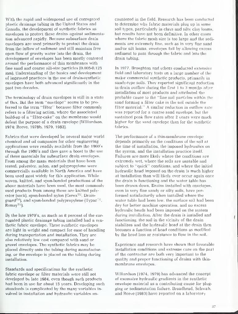
With the rapid and widespread use of corrugated

plastic drainage tubing in the United States and

Canada, the development of synthetic fabrics as

envelopes to protect these drains against sedimenta-

tion advanced rapidly. Because subsurface drain

envelopes are used primarily to protect the drain

from the inflow of sediment and still maintain free

open flow of gravity water into the drain, the

development of envelopes has been mostly centered

around the performance of thin membranes with

fine sand and coarse silt-size particles (0.005-0.125

mm). Understanding of the basics and development

of improved practices in the use of drain-synthetic

envelopes have both advanced significantly in the

past two decades.

The terminology of drain envelopes is still in a state

of flux. But the term "envelope" seems to be pre-

ferred to the term "filter" because filter commonly

refers to a filtering action, where the associated

build-up of a "filter-cake" on the membrane would

defeat the purpose of a drain envelope (Willardson,

1974; Reeve, 1978b. 1979, 1982).

Fabrics that were developed by several major world

chemical and oil companies for other engineering

applications were readily available from the 1960's

through the 1980's and thus gave a boost to the use

of these materials for subsurface drain envelopes.

From among the many materials that have been

tested, polyester, nylon, and polypropylene were

commercially available in North America and have

been used most widely for this application. While

woven, knitted, and spun-bonded productions of the

above materials have been used, the most commonly

used products from among these are knitted poly-

ester (sock), spun-bonded nylon (Cerex™, Drain-

guard™), and spun-bonded polypropylene (Typar™,

Remay™).

By the late 1970's, as much as 8 percent of the cor-

rugated plastic drainage tubing installed had a syn-

thetic fabric envelope. These synthetic envelopes

are light in weight and compact for ease of handling

during transportation and installation. They are

also relatively low cost compared with sand or

gravel envelopes. The synthetic fabrics may be

placed directly onto the tubing during manufactur-

ing, or the envelope is placed on the tubing during

installation.

Standards and specifications for the synthetic

fabric envelope or filter materials were still not

developed by late 1984, even though such products

had been in use for about 15 years. Developing such

standards is complicated by the many variables in-

volved in installation and hydraulic variables en-

countered in the field. Research has been conducted

to determine why fabric materials plug up in somesoil types, particularly in clays and silty clay loams,

but results have not been definitive. In other cases

where the fabric mesh size is too large and the sedi-

ments are extremely fine, such as in very fine sand

and/or silt loams, envelopes fail by allowing excess

sediment to pass through the fabric and into the

drain tubing.

In 1977, Broughton and others conducted extensive

field and laboratory tests on a large number of the

major commercial synthetic products, primarily in

sandy-type soils. They reported significant reduction

in drain outflow during the first 1 to 3 months after

installation of most products and attributed the

probable cause to the "fine soil particles within the

sand forming a filter cake in the soil outside the

filter material." A similar reduction in outflow rate

was reported for a coarse sand envelope, but the

sustained peak flow rates after 2 years were muchhigher for the sand envelope than for the synthetic

fabrics.

The performance of a thin-membrane envelope

depends primarily on the conditions of the soil at

the time of installation, the imposed hydraulics on

the system, and the installation practice itself,

Failures are more likely where the conditions are

extremely wet, where the soils are unstable andsubject to "quick" conditions, and where the initial

hydraulic head imposed on the drain is much higher

at installation than will likely ever occur again once

the drain is functioning and the water table has

been drawn down. Drains installed with envelopes,

even in very fine sandy or silty soils, have per-

formed satisfactorily when installed where the

water table had been low, the surface soil had been

dry for better machine operation, and no excess

hydraulic heads had been imposed on the system

during installation. After the drain is installed and

functioning, the soil in the vicinity of the drain

stabilizes and the hydraulic head at the drain then

becomes a function of head conditions as modified

by the head loss or resistance to flow in the soil.

Experience and research have shown that favorable

installation conditions and extreme care on the part

of the contractor are both very important to the

quality and proper functioning of drains with thin-

membrane envelopes.

Willardson (1974, 1979) has advanced the concept

of excessive hydraulic gradients in the synthetic

envelope material as a contributing cause for plug-

ging or sedimentation failure. Broadhead, Schwab,

and Reeve (1983) have reported on a laboratory

37

evaluation procedure that tested the soil particle-

size distribution to determine the suitable opening

sizes for the synthetic drain envelope. They also

tested noncohesive sandy soils and showed that

drain sedimentation can be prevented by selecting

an envelope material with an effective opening or

mesh size that is less than about 2.4 times the

diameter of the 60-percent (D-60) size of the sand

particles.

An ASTM Task Force Committee used a laboratory

testing program with problem soils to evaluate the

suitability of various synthetic envelope materials

for the purpose of developing a workable specifica-

tion and standard. The Committee's work on com-

mercial synthetic envelope materials in the late

1970's did not lead to conclusive results or a ten-

tative standard, and thus the Committee wasdisbanded.

Drainage Equipment

Along with the rapid adoption of corrugated plastic

drainage tubing worldwide, many significant im-

provements and innovations were made in drainage

equipment and materials handling methods. Of par-

ticular significance was the development of newand improved methods for automatically controlling

depth and grade on modern high-speed installation

machines. By the mid-1970's, a totally new outlook

was given to installation and its cost, and many in-

novative revisions were made in field operational

procedures.

Trenching Machines

There are two basic types of trenching machines

used to install subsurface drainage: the wheel-type

and the ladder- or chain-type. The wheel-type

machine remained essentially unchanged in basic

design for almost a full century (1850 to 1950) ex-

cept for improvements in engines, power train,

steering, and quality and hardness of steel used in

the parts subject to wear. Drainage contractors

made many of the design improvements to the dig-

ging wheel mechanism, power plant, and traction

systems. From about 1945 to 1960, almost all

trenching machines sold were first modified by

contractor-owners before they were put in service.

Whereas track-type trenching machines were the

standard for many decades, rubber-tired, wheel-

type trenchers were introduced in the early 1950's

and became popular among contractors. The

rubber-tired machine could often travel over public

roadways to the next job site, something not possi-

ble with the earlier track-laying machines.

By the late 1960's, higher speed trenching machines

were in demand because of the greater ease of

handling the corrugated plastic drainage tubing.

The development of high-speed trenchers (those ca-

pable of installing at least 50 feet of drain per

minute) became practical with the concurrent devel-

opment of laser-beam automatic grade control.

The new generation of trenchers utilized super-

charged engines and hydrostatic transmission

drives. A modern high-speed wheel-type trencher

and a high-speed ladder-chain-type machine are

shown in figures 3-7 and 3-8. Figure 3-9 is a

backfilling machine. There are several manufac-

turers of these types of trenching machines (figs. 3-7

to 3-12). Modern trenchers include five typical

features: machine-mounted reels for coils of tubing,

tube feeding and guiding devices, grooving devices

for trench bottoms, blinding and backfilling attach-

Figure 3-7—A high-speed trench-

er on low-pressure rubber tires

lays tubing.

38

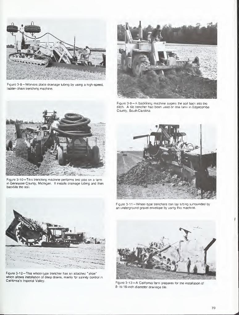
Figure 3-8— Workers place drainage tubing by using a high-speed,

ladder-chain trenching machine.

Figure 3-10—This trenching machine performs two jobs on a farm

in Genessee County, Michigan. It installs drainage tubing and then

backfills the soil.

Figure 3-12—This wheel-type trencher has an attached "shoe"which allows installation of deep drains, mainly for salinity control in

California's Imperial Valley.

Figure 3-9— A backfilling machine augers the soil back into the

ditch. A tile trencher had been used on this farm in EdgecombeCounty, South Carolina.

IfW^ife

Figure 3-1 1 —Wheel-type trenchers can lay tubing surrounded by

an underground gravel envelope by using this machine.

Figure 3-13—A California farm prepares for the installation of

8- to 16-inch diameter drainage tile.

19

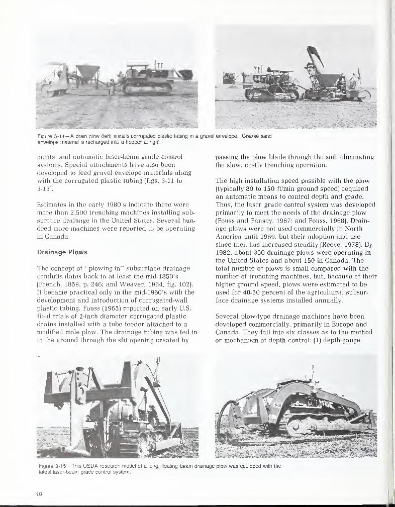
Figure 3-14— A dram plow (left) installs corrugated plastic tubing in a gravel envelope. Coarse sand

envelope material is recharged into a hopper at right.

ments, and automatic laser-beam grade control

systems. Special attachments have also been

developed to feed gravel envelope materials along

with the corrugated plastic tubing (figs. 3-11 to

3-13).

Estimates in the early 1980's indicate there were

more than 2,500 trenching machines installing sub-

surface drainage in the United States. Several hun-

dred more machines were reported to be operating

in Canada.

Drainage Plows

The concept of "plowing-in" subsurface drainage

conduits dates back to at least the mid-1850's

(French, 1859, p. 246; and Weaver, 1964. fig. 102).

It became practical only in the mid-1960's with the

development and introduction of corrugated-wall

plastic tubing. Fouss (1965) reported on early U.S.

field trials of 2-inch diameter corrugated plastic

drains installed with a tube feeder attached to a

modified mole plow. The drainage tubing was fed in-

to the ground through the slit opening created by

passing the plow blade through the soil, eliminating

the slow, costly trenching operation.

The high installation speed possible with the plow

(typically 80 to 150 ft/min ground speed) required

an automatic means to control depth and grade.

Thus, the laser grade control system was developed

primarily to meet the needs of the drainage plow

(Fouss and Fausey. 1967; and Fouss, 1968). Drain-

age plows were not used commercially in North

America until 1969, but their adoption and use

since then has increased steadily (Reeve, 1978). By

1982. about 350 drainage plows were operating in

the United States and about 150 in Canada. The

total number of plows is small compared with the

number of trenching machines, but, because of their

higher ground speed, plows were estimated to be

used for 40-50 percent of the agricultural subsur-

face drainage systems installed annually.

Several plow-type drainage machines have been

developed commercially, primarily in Europe and

Canada. They fall into six classes as to the method

or mechanism of depth control: (1) depth-gauge

>^i*£k

Figure 3-15—This USDA research model of a long, floating-beam drainage plow was equipped with the

latest laser-beam grade control system.

40

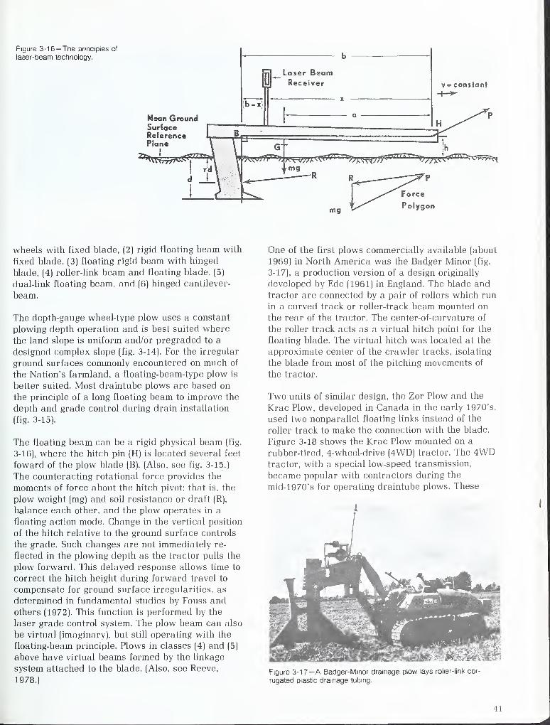
Figure 3-16—The principles of

laser-beam technology.

Mean GroundSurfaceReferencePlane

y = constant

^777T>-C55yP^

mg Polygon

wheels with fixed blade, (2) rigid floating beam with

fixed blade, (3) floating rigid beam with hinged

blade, (4) roller-link beam and floating blade, (5)

dual-link floating beam, and (6) hinged cantilever-

beam.

The depth-gauge wheel-type plow uses a constant

plowing depth operation and is best suited where

the land slope is uniform and/or pregraded to a

designed complex slope (fig. 3-14). For the irregular

ground surfaces commonly encountered on much of

the Nation's farmland, a floating-beam-type plow is

better suited. Most draintube plows are based on

the principle of a long floating beam to improve the

depth and grade control during drain installation

(fig- 3-15).

The floating beam can be a rigid physical beam (fig.

3-16), where the hitch pin (H) is located several feet

foward of the plow blade (B). (Also, see fig. 3-15.)

The counteracting rotational force provides the

moments of force about the hitch pivot; that is, the

plow weight (mg) and soil resistance or draft (R),

balance each other, and the plow operates in a

floating action mode. Change in the vertical position

of the hitch relative to the ground surface controls

the grade. Such changes are not immediately re-

flected in the plowing depth as the tractor pulls the

plow forward. This delayed response allows time to

correct the hitch height during forward travel to

compensate for ground surface irregularities, as

determined in fundamental studies by Fouss and

others (1972). This function is performed by the

laser grade control system. The plow beam can also

be virtual (imaginary), but still operating with the

floating-beam principle. Plows in classes (4) and (5)

above have virtual beams formed by the linkage

system attached to the blade. (Also, see Reeve,

1978.1

One of the first plows commercially available (about

1969) in North America was the Badger Minor (fig.

3-17), a production version of a design originally

developed by Ede (1961) in England. The blade and

tractor are connected by a pair of rollers which run

in a curved track or roller-track beam mounted on

the rear of the tractor. The center-of-curvature of

the roller track acts as a virtual hitch point for the

floating blade. The virtual hitch was located at the

approximate center of the crawler tracks, isolating

the blade from most of the pitching movements of

the tractor.

Two units of similar design, the Zor Plow and the

Krac Plow, developed in Canada in the early 1970's,

used two nonparallel floating links instead of the

roller track to make the connection with the blade.

Figure 3-18 shows the Krac Plow mounted on a

rubber-tired, 4-wheel-drive (4WD) tractor. The 4WDtractor, with a special low-speed transmission,

became popular with contractors during the

mid-1970's for operating draintube plows. These

Figure 3-17—A Badger-Minor drainage plow lays rolier-link cor-

rugated plastic drainage tubing.

4 1

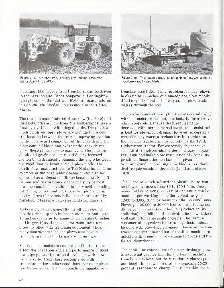
Figure 3-18—A rubber-tired, 4-wheel-drive tractor is mountedwith a dual-link Krac-Piow.

Figure 3-19—This tractor carries, at left, a Hoes Plow with a floating

rigid-beam and hinged blade.

machines, like rubber-tired trenchers, can be driven

to the next job site. Other nonparallel floating-link-

type plows like the Link and RWF are manufactured

in Canada. The Wedge Plow is made in the United

States.

The German-manufactured Hoes Plow (fig. 3-19) andthe Hollanddrain Plow from The Netherlands have a

floating rigid beam with hinged blade. The physical

hitch points on these plows are mounted in a cen-

tral location between the tracks, improving traction

by the downward component of the plow draft. Theclose-coupled blade and hydrostatic track drives

make these plows easy to maneuver. The plowing

depth and grade are controlled during forward

motion by hydraulically changing the angle betweenthe rigid floating beam and the plow blade. TheBarth Plow, manufactured in The Netherlands, is an

example of the parallel-link beam: it can also be

operated as a hinged cantilever-beam plow. Specifi-

cations and performance characteristics of most

drainage machines available in the world, including

trenchers, plows, and backhoes, are published in

the Drainage Contractor's Blackbook, prepared by

Agri-Book Magazine of Exeter, Ontario, Canada.

Today's plows can generally install corrugated

plastic drains up to 6 inches in diameter and up to

10 inches diameter for some plows. Drains 8 inches

and larger, if used for collector main lines, are

often installed with trenching equipment. Thus,

many contractors who use plows also have a

trencher to install the larger size main lines.

Soil type, soil moisture content, and buried rocks

affect the operation and field performance of most

drainage plows. Operational problems with plows

usually differ from those encountered with

trenchers under similar conditions. For example, a

few buried rocks that can completely immobilize a

trencher pose little, if any, problem for most plows.

Rocks up to 12 inches in diameter are often merely

lifted or pushed out of the way as the plow blade

passes through the soil.

The performance of most plows varies considerably

with soil moisture content, particularly for cohesive

(clay type) soils. Because draft requirements

decrease with increasing soil moisture, a moist soil

is best for plowing-in drains. However, excessively

wet soils may cause a serious loss in traction for

the crawler tractor, and especially for the 4WD,rubber-tired tractor. For extremely dry cohesive

soils, draft requirements for the plow may becomevery high and make plow installation of drains im-

practical. Some attention has been given to

oscillating and/or vibrating plow blades to reduce

draft requirements in dry soils (Child and others,

1979).

The speed at which subsurface plastic drains can

be plowed-in ranges from 80 to 150 ft/min. Under

many field conditions, 2,000 ft of draintube can be

installed per working hour; the typical range is

1,500 to 3,000 ft/hr for many installation conditions.

Plowing-in 20,000 to 30,000 feet of drain tubing per

day is common practice. The high production (in-

stallation) capabilities of the draintube plow make it

well-suited for large-scale projects. The farmer-

customer often prefers that drainage installations

be done with plow-type equipment, because the con-

tractor can get into and out of the field much more

quickly with a minimum of damage to crops and lit-

tle soil disturbance.

The capital investment cost for most drainage plows

is somewhat greater than for the typical modern

trenching machine, but the installation charge per

unit length for plowed-in drains is typically 15-25

percent less than the charge for trenched-in drains.

\i

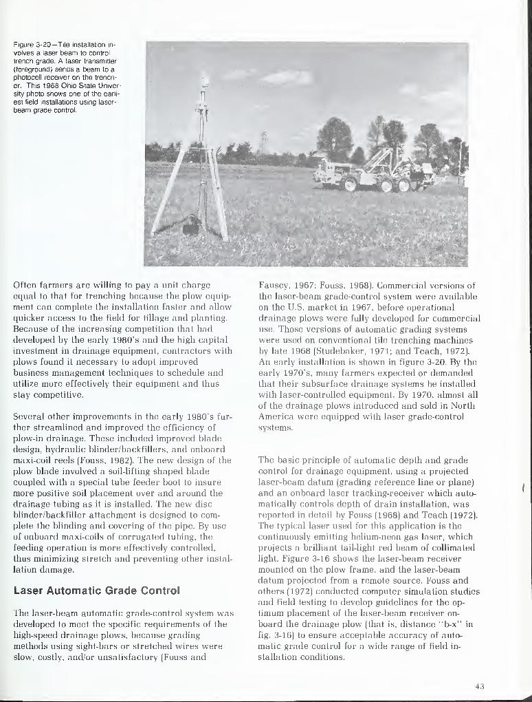
Figure 3-20— Tile installation in-

volves a laser beam to control

trench grade. A laser transmitter

(foreground) sends a beam to aphotocell receiver on the trench-

er. This 1968 Ohio State Univer-

sity photo shows one of the earli-

est field installations using laser-

beam grade control.

&&&

Often farmers are willing to pay a unit charge

equal to that for trenching because the plow equip-

ment can complete the installation faster and allow

quicker access to the field for tillage and planting.

Because of the increasing competition that haddeveloped by the early 1980's and the high capital

investment in drainage equipment, contractors with

plows found it necessary to adopt improved

business management techniques to schedule andutilize more effectively their equipment and thus

stay competitive.

Several other improvements in the early 1980's fur-

ther streamlined and improved the efficiency of

plow-in drainage. These included improved blade

design, hydraulic blinder/backfillers, and onboard

maxi-coil reels (Fouss, 1982). The new design of the

plow blade involved a soil-lifting shaped blade

coupled with a special tube feeder boot to insure

more positive soil placement over and around the

drainage tubing as it is installed. The new disc

blinder/backfiller attachment is designed to com-

plete the blinding and covering of the pipe. By use

of onboard maxi-coils of corrugated tubing, the

feeding operation is more effectively controlled,

thus minimizing stretch and preventing other instal-

lation damage.

Laser Automatic Grade Control

The laser-beam automatic grade-control system wasdeveloped to meet the specific requirements of the

high-speed drainage plows, because grading

methods using sight-bars or stretched wires wereslow, costly, and/or unsatisfactory (Fouss and

Fausey, 1967; Fouss, 1968). Commercial versions of

the laser-beam grade-control system were available

on the U.S. market in 1967, before operational

drainage plows were fully developed for commercial

use. Those versions of automatic grading systems

were used on conventional tile trenching machines

by late 1968 (Studebaker, 1971; and Teach, 1972).

An early installation is shown in figure 3-20. By the

early 1970's, many farmers expected or demandedthat their subsurface drainage systems be installed

with laser-controlled equipment. By 1970, almost all

of the drainage plows introduced and sold in North

America were equipped with laser grade-control

systems.

The basic principle of automatic depth and grade

control for drainage equipment, using a projected

laser-beam datum (grading reference line or plane)

and an onboard laser tracking-receiver which auto-

matically controls depth of drain installation, wasreported in detail by Fouss (1968) and Teach (1972).

The typical laser used for this application is the

continuously emitting helium-neon gas laser, which

projects a brilliant tail-light red beam of collimated

light. Figure 3-16 shows the laser-beam receiver

mounted on the plow frame, and the laser-beam

datum projected from a remote source. Fouss and

others (1972) conducted computer simulation studies

and field testing to develop guidelines for the op-

timum placement of the laser-beam receiver on-

board the drainage plow (that is, distance "b-x" in

fig. 3-16) to ensure acceptable accuracy of auto-

matic grade control for a wide range of field in-

stallation conditions.

43

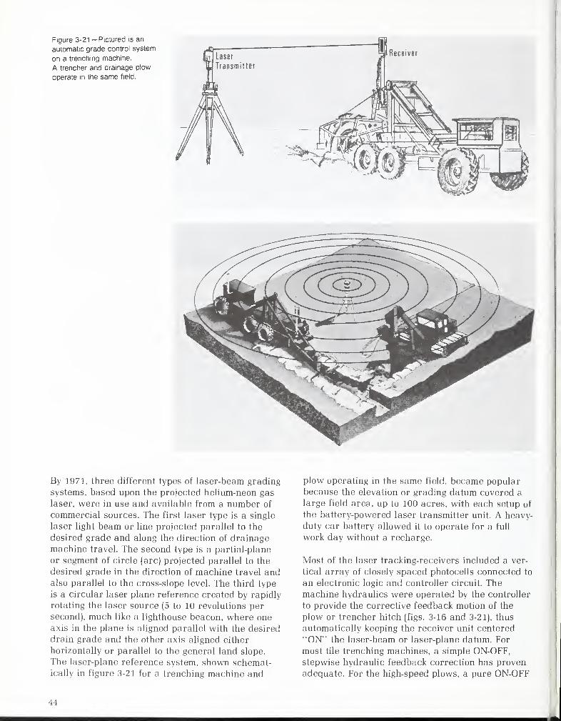
Figure 3-21 —Pictured is an

automatic grade control system

on a trenching machine.

A trencher and drainage plow

operate in the same field.

By 1971, three different types of laser-beam grading

systems, based upon the projected helium-neon gas

laser, were in use and available from a number of

commercial sources. The first laser type is a single

laser light beam or line projected parallel to the

desired grade and along the direction of drainage

machine travel. The second type is a partial-plane

or segment of circle (arc) projected parallel to the

desired grade in the direction of machine travel andalso parallel to the cross-slope level. The third type

is a circular laser plane reference created by rapidly

rotating the laser source (5 to 10 revolutions per

second), much like a lighthouse beacon, where one

axis in the plane is aligned parallel with the desired

drain grade and the other axis aligned either

horizontally or parallel to the general land slope.

The laser-plane reference system, shown schemat-ically in figure 3-21 for a trenching machine and

plow operating in the same field, became popularbecause the elevation or grading datum covered a

large field area, up to 100 acres, with each setup of

the battery-powered laser transmitter unit. A heavy-

duty car battery allowed it to operate for a full

work day without a recharge.

Most of the laser tracking-receivers included a ver-

tical array of closely spaced photocells connected to

an electronic logic and controller circuit. Themachine hydraulics were operated by the controller

to provide the corrective feedback motion of the

plow or trencher hitch (figs. 3-16 and 3-21J,thus

automatically keeping the receiver unit centered

"ON" the laser-beam or laser-plane datum. For

most tile trenching machines, a simple ON-OFF,stepwise hydraulic feedback correction has proven

adequate. For the high-speed plows, a pure ON-OFF

4-1

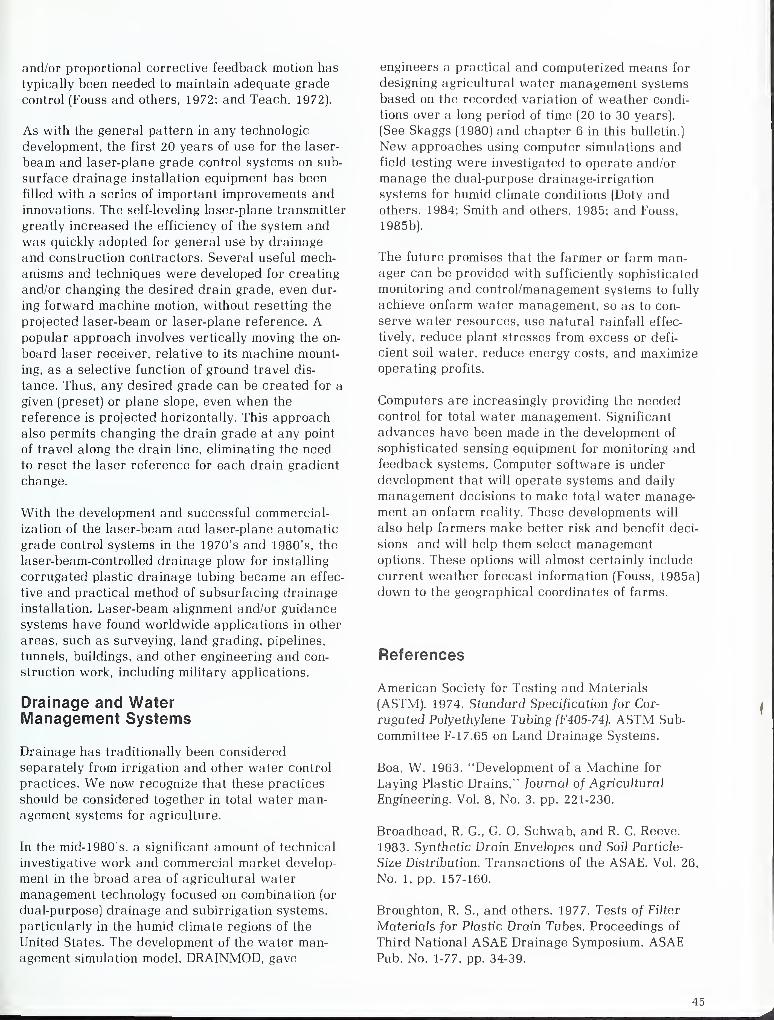
and/or proportional corrective feedback motion has

typically been needed to maintain adequate grade

control (Fouss and others, 1972; and Teach, 1972).

As with the general pattern in any technologic

development, the first 20 years of use for the laser-

beam and laser-plane grade control systems on sub-

surface drainage installation equipment has been

filled with a series of important improvements and

innovations. The self-leveling laser-plane transmitter

greatly increased the efficiency of the system and

was quickly adopted for general use by drainage

and construction contractors. Several useful mech-

anisms and techniques were developed for creating

and/or changing the desired drain grade, even dur-

ing forward machine motion, without resetting the

projected laser-beam or laser-plane reference. Apopular approach involves vertically moving the on-

board laser receiver, relative to its machine mount-

ing, as a selective function of ground travel dis-

tance. Thus, any desired grade can be created for a

given (preset) or plane slope, even when the

reference is projected horizontally. This approach

also permits changing the drain grade at any point

of travel along the drain line, eliminating the need

to reset the laser reference for each drain gradient

change.

With the development and successful commercial-

ization of the laser-beam and laser-plane automatic

grade control systems in the 1970's and 1980's, the

laser-beam-controlled drainage plow for installing

corrugated plastic drainage tubing became an effec-

tive and practical method of subsurfacing drainage

installation. Laser-beam alignment and/or guidance

systems have found worldwide applications in other

areas, such as surveying, land grading, pipelines,

tunnels, buildings, and other engineering and con-

struction work, including military applications.

Drainage and WaterManagement Systems

Drainage has traditionally been considered

separately from irrigation and other water control

practices. We now recognize that these practices

should be considered together in total water man-agement systems for agriculture.

In the mid-1980's, a significant amount of technical

investigative work and commercial market develop-

ment in the broad area of agricultural water

management technology focused on combination (or

dual-purpose) drainage and subirrigation systems,

particularly in the humid climate regions of the

United States. The development of the water man-

agement simulation model, DRAINMOD, gave

engineers a practical and computerized means for

designing agricultural water management systems

based on the recorded variation of weather condi-

tions over a long period of time (20 to 30 years).

(See Skaggs (1980) and chapter 6 in this bulletin.)

New approaches using computer simulations andfield testing were investigated to operate and/or

manage the dual-purpose drainage-irrigation

systems for humid climate conditions (Doty andothers, 1984; Smith and others, 1985; and Fouss,

1985b).

The future promises that the farmer or farm man-ager can be provided with sufficiently sophisticated

monitoring and control/management systems to fully

achieve onfarm water management, so as to con-

serve water resources, use natural rainfall effec-

tively, reduce plant stresses from excess or defi-

cient soil water, reduce energy costs, and maximizeoperating profits.

Computers are increasingly providing the neededcontrol for total water management. Significant

advances have been made in the development of

sophisticated sensing equipment for monitoring andfeedback systems. Computer software is under

development that will operate systems and daily

management decisions to make total water manage-ment an onfarm reality. These developments will

also help farmers make better risk and benefit deci-

sions and will help them select managementoptions. These options will almost certainly include

current weather forecast information (Fouss, 1985a)

down to the geographical coordinates of farms.

References

American Society for Testing and Materials

(ASTM). 1974. Standard Specification for Cor-

rugated Polyethylene Tubing (F405-74). ASTM Sub-

committee F-17.65 on Land Drainage Systems.

Boa, W. 1963. "Development of a Machine for

Laying Plastic Drains," Journai of Agricultural

Engineering. Vol. 8, No. 3, pp. 221-230.

Broadhead, R. C, G. O. Schwab, and R. C. Reeve.

1983. Synthetic Drain Envelopes and Soil Particle-

Size Distribution. Transactions of the ASAE. Vol. 26,

No. 1, pp. 157-160.

Broughton, R. S., and others. 1977. Tests of Filter

Materials for Plastic Drain Tubes. Proceedings of

Third National ASAE Drainage Symposium. ASAEPub. No. 1-77, pp. 34-39.

45

Busch, C. D. 1958. "Low Cost Subsurface

Drainage," Agricultural Engineering. Vol. 39, No. 2,

pp. 92-93, ff.

Child, Jr.. J.L., J. L. Fouss. and E. K. Nowicki. 1979.

Dynamic Plow Assembly and Methods of Operating

Same. U.S. Pat. No. 4,179,227 (12/18/79). Appl.

825,192 (8/17/77). Assignee: Hancor, Inc., Findlay,

Ohio. (18 pages, 14 figures, 42 claims.)

De Jager, A. W. 1960. "Review of Plastic Drainage

in The Netherlands," Netherlands Journal of Agri-

cultural Science. Vol. 8, No. 4, pp. 261-270.

Doty, C. W., J. E. Parsons, A. N. Tabrizi, and R. W.Skaggs. 1984. Stream Water Levels Affect Field

Water Tables and Corn Yields. Transactions of the

ASAE. Vol. 27, No. 5, pp. 1300-1306.

Ede, A. N. 1961. "Floating-Beam Mole Plough

Trials," Farm Mechanics. Vol. 13, No. 144, pp.

274-275.

Ede, A. N. 1963. "New Methods of Field Drainage,"

Agriculture. Vol. 70, No. 2, pp. 82-86.

Ede, A. N. 1965. New Materials and Machines for

Drainage. Proceedings of ASAE Conference on

Drainage for Efficient Crop Production. December,

Chicago, pp. 58-61.

Edminster, T. W. 1965. The Challenge of NewTechnology in Drainage. Proceedings of ASAE Con-

ference on Drainage for Efficient Crop Production.

December, Chicago, pp. 43-45.

Fouss, J. L., and W. W. Donnan. 1962. "Plastic-lined

Mole Drains," Agricultural Engineering. Vol. 43, No.

9, pp. 512-515.

Fouss. J. L. 1965. Plastic Drains and Their Installa-

tion. Proceedings of ASAE Conference on Drainage

for Efficient Crop Production. December, Chicago,

pp. 55-57.

Fouss, J. L., and N. R. Fausey. 1967. "Laser BeamDepth Control for Drainage Machine," Ohio Report.

Vol. 52, No. 4, pp. 51-53.

Fouss, }. L. 1968. Corrugated Plastic Drains Plowed-

in Automatically. Transactions of the ASAE. Vol. 11,

pp. 804-808.

Fouss, J. L., N. R. Fausey, and R. C. Reeve. 1972.

Draintube Plows: Their Operation and Laser GradeControl. Proceedings of Second National ASAEDrainage Symposium. St. Joseph, Mich., pp. 39-42.

Fouss, J. L. 1973. Structural Design Procedure for

Corrugated Plastic Drainage Tubing. TB-1466. U.S.

Dept. of Agr., Agr. Res. Serv.

Fouss, J. L. 1974. "Drain Tube Materials and In-

stallation," Drainage for Agriculture, (ed. Jan van

Schilfgaarde). Monograph No. 17, Am. Soc. Agron.

Madison, Wise, pp. 147-177, 197-200.

Fouss, J. L. 1982. Modernized Materials Handling

and Installation Implements for Plow-type Drainage

Equipment. Proceedings, Second International

Drainage Workshop, Washington, DC. December,

pp. 41-51.

Fouss, J. L., and W. E. Altermatt. 1982. Drainage-

plow 'Boot' Design to Improve Installation of Cor-

rugated Plastic Tubing. Proceedings of Fourth Na-tional ASAE Drainage Symposium. ASAE Pub. No.

12-82, pp. 102-104.

Fouss, J. L. 1985a. Daily Weather Forecast Rainfall

Probability as an Input to a Water ManagementSimulation Model. ARS-30. U.S. Dept of Agr., Agr.

Res. Serv. Proceedings of the USDA ARS/SCSNatural Resources Modeling Workshop, October

17-21, 1983. Pingree Park, Col.

Fouss, J. L. 1985b. Simulated Feedback-Operation of

Controlled-Drainage/Suhirrigation Systems." Tran-

sactions of the ASAE. Vol. 28, No. 3, pp. 839-847.

Fouss, J. L., and W. E. Altermatt. 1985. Strength vs.

Stretch of Corrugated Plastic Drainage Tubing.

Tech. Bull. 1H, Hancor, Inc., Findlay, Ohio.

French, H. F. 1859. Farm Drainage. New York: A. O.

Moore and Co.

Janert, H. 1952. "Die Mechanisierung der

Drainarbeiten." Wasserwirtchaft Wassertechnik,

2, pp. 392-397.

Luthin, J. N., and R. C. Reeve. 1957. "The Design of

a Gravel Envelope for Tile Drains." In Drainage of

Agricultural Lands (ed. James N. Luthin).

Monograph No. 7, Am. Soc. Agron. Madison, Wise,

pp. 339-344.

Myers, V. I., R. J. Rektorik, and C. A. Wolfe, Jr.

1967. Deflection Tests and Trench Conditions for

Plastic Drain Pipe." Transactions of the ASAE. Vol.

10, pp. 454-547.

Reeve, R. C. 1978a. Trenchless Drainage. Pro-

ceedings of the International Drainage Workshop,

(ed. Jans Wesseling). May 16-20, 1978, Wageningen,

The Netherlands. Paper 3.09, pp. 571-589.

46

1978b. "Synthetics at Work,'

Drainage Contractor Magazine. Vol. 5, No. 1, p. 80.

Hensall, Ontario, Canada.

. 1979, Synthetic Drain EnveJope

Materiais - Technical Information. Columbus, Ohio:

Advanced Drainage Systems, Inc.

. 1981. Filter and Envelope Materials.

Presented at Subsurface Drainage Workshop. ADSReprint, Univ. of 111., February.

. 1982. Synthetic Envelope Materials

for Subsurface Drainage. Proceedings, 2nd Interna-

tional Drainage Workshop, Washington, DC.

December 5-11.

Reeve, R. C, R. E. Slicker, and T. J. Lang. 1981. Cor-

rugated Plastic Tubing. Proceedings, Am. Soc. Civ.

Engr. International Conference on Underground

Plastic Pipe. pp. 277-242.

Rektorik, R. }., and V. I. Myers. 1967. Polyethylene

Drainage Pipe Installation Techniques and FieJd Per-

formance. Transactions of the ASAE. Vol. 10, pp.

458-459, 461.

Schwab, G. O. 1955. "Plastic Tubing for Subsurface

Drainage." AgricuJturaJ Engineering, Vol. 36, No. 2,

pp. 86-89, 92.

Schwab, G. O., and J. L. Fouss. 1985. "Plastic Drain

Tubing: Successor to Shale Tile," AgricuJturaJ

Engineering. Vol. 66, No. 7, pp. 23-26.

Skaggs, R. W. 1978. A Water Management ModeJ

for Shallow Water TabJe Soils. Technical Report No.

134, Water Resources Institute of the University of

North Carolina. N.C. State Univ., Raleigh.

Skaggs, R. W. 1980. A Water Management ModeJ

for Artificially Drained Soils. Technical Bulletin No.

267, N.C. Agr. Serv., N.C. State Univ., Raleigh.

Smith, M. C, R. W. Skaggs, and J. E. Parsons. 1985.

"Subirrigation System Control for Water Use Effi-

ciency." Transactions of the ASAE. Vol. 28, No. 2,

pp. 489-496.

Sorbie, F. I., J. L. Fouss, and G. O. Schwab. 1972.

Comparison of Strength Test Methods for Cor-

rugated Plastic Drainage Tubing. Transactions of

the ASAE. Vol., 15, pp. 445-447.

Studebaker, D. C. 1971. "The Laser-plane System,"

AgricuJturaJ Engineering. Vol. 53, No, 8, pp. 418-419.

Teach, T. L. 1972. Automatic Laser Grade Controls.

Society of Automotive Engineers, Earthmoving In-

dustry Conference, Central Illinois Section, Peoria,

April 10-12. Paper No. 720386.

van Schilfgaarde, J. 1965. "Transient Design of

Drainage Systems," JournaJ of the Irrigation andDrainage Division. ASCE. Vol. 91 (IR3), pp. 9-22.

Van Someren, C. L. 1964. "The Use of Plastic

Drainage Pipes in The Netherlands." (Translations

from Coltuurtechnik 1,2,3). Government Service for

Land and Water Use, Maleibaan 21, Utrecht, TheNetherlands.

Watkins, R. K. 1967. The Development of Structural

Concepts for Buried Pipes Externally Loaded.

Bulletin No. 7, Engineering Experiment Station, UtahState Univ., Logan.

Watkins, R. K., R. C. Reeve, and J. B. Goddard. 1983.

"Effect of Heavy Loads on Buried Corrugated

Polyethylene Pipe." Transportation Research Board,

National Academy of Sciences, Washington, DC,

pp. 99-108.

Weaver, M. M. 1964. History of Tile Drainage.

Waterloo, N.Y. Private Publication, (ref. fig. 102).

Willardson, L. S. 1974. "Envelope Materials,"

Drainage for Agriculture. Chap. 9. (ed. Jan van

Schilfgaarde). Monograph No. 17, Am. Soc. Agron.

Madison, Wise, pp. 178-200.

Willardson, L. S. 1979. "Hydraulic Gradients in

Envelope Materials," ARR-W-8/June. Utah State

Univ., Logan.

47

Chapter 4

Purposes and Benefits of

Drainage

N.R. FauseyAgricultural Research Service, USDAOhio State University

E.J. DoeringAgricultural Research Service, USDAMandan, North Dakota

M.L. PalmerDepartment of Agricultural EngineeringOhio State University

The importance of drainage to public health and the

economic well-being of the Nation is generally not

understood, we believe, because of a public percep-

tion of drainage as only the process of converting

valuable wetlands to other uses. We accordingly

review the several purposes and benefits of drain-

ing wet soils now in use for cropland, pasture,

rangeland, and forestland. However, we do not con-

sider the benefits of, or issues involved in, draining

wetlands for conversion to new cropland, develop-

ment sites, and other uses. According to an Office

of Technology Assessment report cited earlier by

Smith and Massey (OTA, 1984), agricultural

drainage and land clearing have been responsible

for most wetland conversions since the mid-1950's,

and there is still significant pressure to convert

wetlands to other uses.

Although drainage is a mechanism by which this

conversion takes place, pressures for and against

conversion are exerted by competing economic and

other public values. Competition issues are reviewed

by Swader. But, our discussion focuses on the moreimmediate practical purposes and benefits of drain-

ing wet soils now in agricultural or forest uses on

farms.

Purposes of Drainage

The underlying objectives in draining wet soils on

farms are to minimize risk, improve efficiency, and

increase net income. Drainage is best viewed as a

water management practice, whose practical pur-

poses are different for different climatic regions

and land uses. A farmer may drain land for several

reasons: to reduce diseases of crops and livestock;

to leach salt from irrigated land; or to removeexcess soil water, improving trafficability for

machinery and the crop rooting environment.

Figures 4-1 and 4-2 illustrate the effects of poor

drainage on cotton and corn crops.

Another important purpose is to protect the soil

from uncontrolled runoff and erosion. Closely

related farm or nonfarm purposes of drainage are

to stabilize roadways and building foundations, to

improve the usefulness of recreation areas, to

reduce flooding, and to facilitate land disposal of

waste water.

How wet soils are drained depends on soil type,

climate, topography, and intended land use.

Grading, field ditches, swales, and other im-

provements may be adequate for managing surface

water (fig. 4-3). Subsurface drains must be used to

manage excess soil water and to remove excess

soluble salts from the soil (fig. 4-3). Both surface

and subsurface drainage improvements are often

needed to properly manage the excess water. Whenproperly done, drainage has various primary and

associated benefits.

48

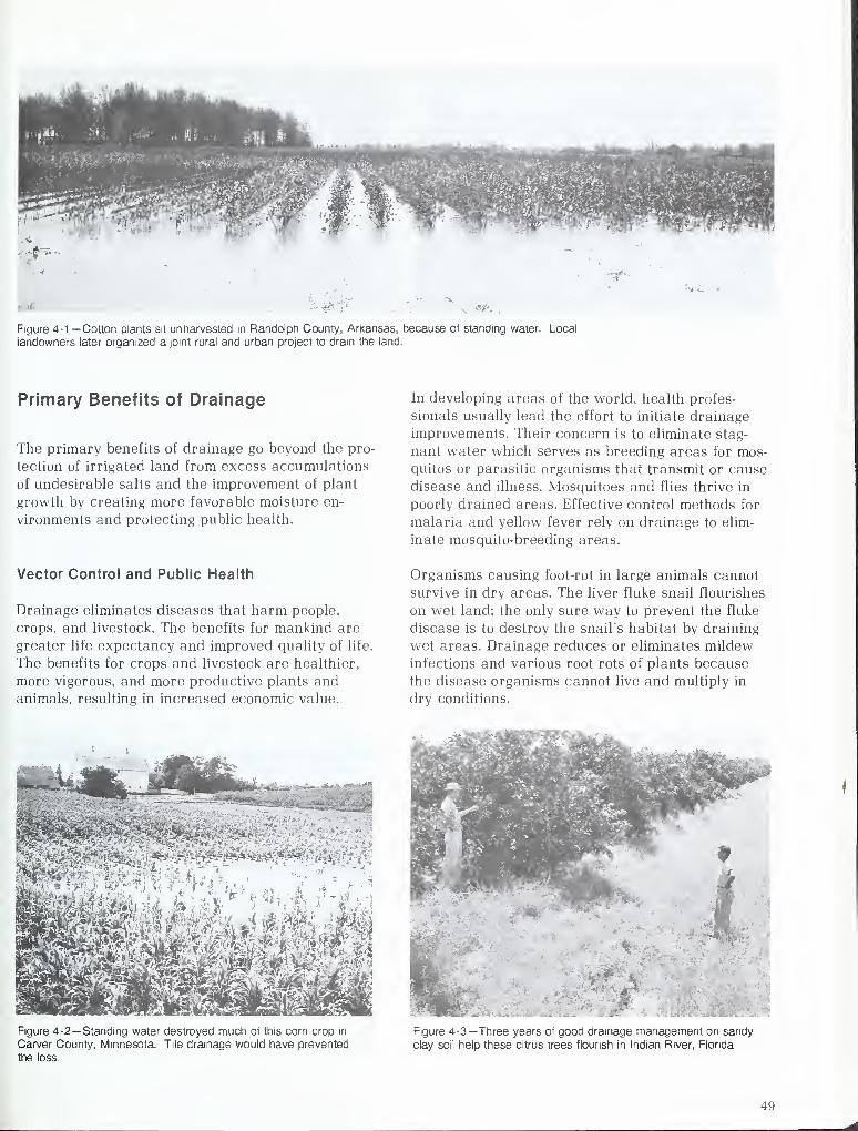
Figure 4-1 —Cotton plants sit unharvested in Randolph County, Arkansas, because of standing water. Local

landowners later organized a joint rural and urban project to drain the land.

Primary Benefits of Drainage

The primary benefits of drainage go beyond the pro-

tection of irrigated land from excess accumulations

of undesirable salts and the improvement of plant

growth by creating more favorable moisture en-

vironments and protecting public health.

In developing areas of the world, health profes-

sionals usually lead the effort to initiate drainage

improvements. Their concern is to eliminate stag-

nant water which serves as breeding areas for mos-

quitos or parasitic organisms that transmit or cause

disease and illness. Mosquitoes and flies thrive in

poorly drained areas. Effective control methods for

malaria and yellow fever rely on drainage to elim-

inate mosquito-breeding areas.

Vector Control and Public Health

Drainage eliminates diseases that harm people,

crops, and livestock. The benefits for mankind are

greater life expectancy and improved quality of life.

The benefits for crops and livestock are healthier,

more vigorous, and more productive plants andanimals, resulting in increased economic value.

Organisms causing foot-rot in large animals cannot

survive in dry areas. The liver fluke snail flourishes

on wet land; the only sure way to prevent the fluke

disease is to destroy the snail's habitat by draining

wet areas. Drainage reduces or eliminates mildew

infections and various root rots of plants because

the disease organisms cannot live and multiply in

dry conditions.

Figure 4-2— Standing water destroyed much of this corn crop in

Carver County, Minnesota. Tile drainage would have prevented

the loss.

Figure 4-3—Three years of good drainage management on sandy

clay soil help these citrus trees flourish in Indian River, Florida.

49

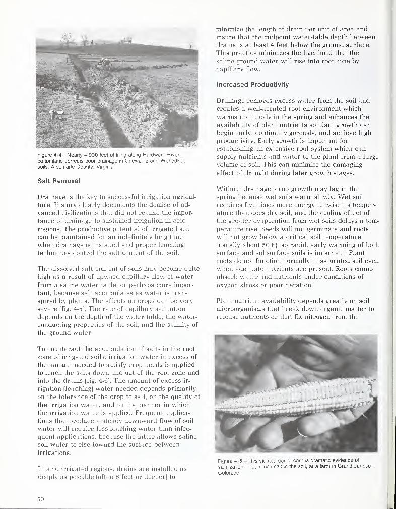
Figure 4-4— Nearly 4.000 feet of tiling along Hardware River

bottomland corrects poor drainage in Chewacla and Wehadkeesoils. Albemarle County, Virginia.

Salt Removal

Drainage is the key to successful irrigation agricul-

ture. History clearly documents the demise of ad-

vanced civilizations that did not realize the impor-

tance of drainage to sustained irrigation in arid

regions. The productive potential of irrigated soil

can be maintained for an indefinitely long time

when drainage is installed and proper leaching

techniques control the salt content of the soil.

The dissolved salt content of soils may become quite

high as a result of upward capillary flow of water

from a saline water table, or perhaps more impor-

tant, because salt accumulates as water is tran-

spired by plants. The effects on crops can be very

severe (fig. 4-5). The rate of capillary salination

depends on the depth of the water table, the water-

conducting properties of the soil, and the salinity of

the ground water.

To counteract the accumulation of salts in the root

zone of irrigated soils, irrigation water in excess of

the amount needed to satisfy crop needs is applied

to leach the salts down and out of the root zone and

into the drains (fig. 4-6). The amount of excess ir-

rigation (leaching) water needed depends primarily

on the tolerance of the crop to salt, on the quality of

the irrigation water, and on the manner in which

the irrigation water is applied. Frequent applica-

tions that produce a steady downward flow of soil

water will require less leaching water than infre-

quent applications, because the latter allows saline

soil water to rise toward the surface between

irrigations.

In arid irrigated regions, drains are installed as

deeply as possible (often 8 feet or deeper) to

minimize the length of drain per unit of area and

insure that the midpoint water-table depth between

drains is at least 4 feet below the ground surface.

This practice minimizes the likelihood that the

saline ground water will rise into root zone by

capillary flow.

Increased Productivity

Drainage removes excess water from the soil and

creates a well-aerated root environment which

warms up quickly in the spring and enhances the

availability of plant nutrients so plant growth can

begin early, continue vigorously, and achieve high

productivity. Early growth is important for

establishing an extensive root system which can

supply nutrients and water to the plant from a large

volume of soil. This can minimize the damaging

effect of drought during later growth stages.

Without drainage, crop growth may lag in the

spring because wet soils warm slowly. Wet soil

requires five times more energy to raise its temper-

ature than does dry soil, and the cooling effect of

the greater evaporation from wet soils delays a tem-

perature rise. Seeds will not germinate and roots

will not grow below a critical soil temperature

(usually about 50°F), so rapid, early warming of both

surface and subsurface soils is important. Plant

roots do not function normally in saturated soil even

when adequate nutrients are present. Roots cannot

absorb water and nutrients under conditions of

oxygen stress or poor aeration.

Plant nutrient availability depends greatly on soil

microorganisms that break down organic matter to

release nutrients or that fix nitrogen from the

Figure 4-5—This stunted ear of corn is dramatic evidence of

salinization— too much salt in the soil, at a farm in Grand Junction,

Colorado.

nil

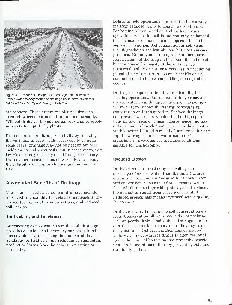
Figure 4-6— Bare soils bespeak the damages of soil salinity.

Proper water management and drainage could have saved this

cotton crop in the Imperial Valley, California.

atmosphere. These organisms also require a well-

aerated, warm environment to function normally.

Without drainage, the microorganisms cannot supply

nutrients for uptake by plants.

Drainage also stabilizes productivity by reducing

the variation in crop yields from year to year. In

some years, drainage may not be needed for good

yields on normally wet soils, but in other years, very

low yields or no yields may result from poor drainage.

Drainage can prevent these low yields, increasing

the reliability of crop production and minimizing

risk.

Associated Benefits of Drainage

The main associated benefits of drainage include

improved trafficability for vehicles, implements, im-

proved timeliness of farm operations, and reduced

soil erosion.

Trafficability and Timeliness

By removing excess water from the soil, drainage

provides a surface soil layer dry enough to handle

farm machinery, increasing the number of days

available for fieldwork and reducing or eliminating

production losses from the delays in planting or

harvesting.

Delays in field operations can result in losses rang-

ing from reduced yields to complete crop failure.

Performing tillage, weed control, or harvesting

operations when the soil is too wet may be impossi-

ble because the equipment cannot operate for lack of

support or traction. Soil compaction or soil struc-

ture degradation are less obvious but more serious

problems. Not only must the agronomic timeliness

requirements of the crop and soil conditions be met,

but the physical integrity of the soil must be

preserved. Otherwise, a long-term loss in production

potential may result from too much traffic or soil

manipulation at a time when puddling or compaction

occurs.

Drainage is important in all of trafficability for

farming operations. Subsurface drainage removes

excess water from the upper layers of the soil pro-

file more rapidly than the natural processes of

evaporation and transpiration. Surface drainage

can prevent wet spots which often hold up opera-

tions on low areas or cause inconvenience and loss

of both time and productive area when they must be

worked around. Rapid removal of surface water and

rapid lowering of the soil-water content aid

materially in providing soil moisture conditions

suitable for trafficability.

Reduced Erosion

Drainage reduces erosion by controlling the

discharge of excess water from the land. Surface

drains and terraces are designed to remove water

without erosion. Subsurface drains remove water

from within the soil, providing storage that reduces

the amount of runoff from subsequent rainfall.

Reduced erosion also means improved water quality

for streams.

Drainage is very important to soil conservation ef-

forts. Conservation tillage systems do not perform

well on poorly drained soils; thus, drainage can be

a critical element for conservation tillage systems

designed to control erosion. Drainage of grassed

waterways by subsurface drains is often essential

to dry the channel bottom so that protective vegeta-

tion can be maintained, thereby preventing rills and

eventually gullies.

51

Chapter 5

Preserving Environmental Values

Carl H. ThomasSoil Conservation Service, USDAWashington, DC

Assessments of drainage needs are incomplete

without considering environmental ramifications.

Farmland drainage may have both beneficial andadverse effects on the environment. These must be

recognized along with any farm production benefits

and costs. Environmental components include such

items as natural beauty; archeological, historical,

biological, and geological resources; ecological

systems; and air and water quality. Although manyeffects of farmland drainage on the environment are

not economic in nature, they may provide important

evidence for judging the value of proposed plans.

Farm drainage programs can benefit the environment

or have a neutral effect if multiobjective or

multipurpose projects include the management,

preservation, or restoration of one or moreenvironmental components.

Identification and Measurement

Modern agriculture has grown more intensive anddependent upon an industrialized technology to

meet demands for food, fiber, and forest products.

Water management through drainage is an impor-

tant aspect of this technology. Conflicts often arise

between drainage interests and ecological or en-

vironmental interests.

The technical responsibility in this situation re-

quires that ecological knowledge be blended with

hydrologic knowledge and that both be responsive to

the objectives of private landowners and national

taxpayers, who subsidize drainage on privately

owned lands to the extent that there is Federal par-

ticipation or assistance. Realistic options can be

developed for the conservation, use, and manage-

ment of all natural resources, including wetlands.

The key to decisionmaking on wetlands use is to

maximize the well-being of people. In most in-

stances, this happens by explicitly recognizing the

functions that wetlands perform and counting the

loss as these functions are sacrificed or impaired.

Functional Values of Wetlands

Wetlands are lands transitional between terrestrial

and aquatic systems. The water table is usually at

or near the surface, or the land is covered by

shallow water. Wetlands must periodically support

hydrophytes, and the substrate must be predom-

inantly undrained hydric soils. Examples of

estuarine as well as forested and emergent

freshwater wetlands are in figures 5-1 to 5-4.

Ten specific functional values of wetlands are gen-

erally acknowledged: habitat for fisheries, habitat

for wildlife, water recharge and discharge, flood

storage and desynchronization, shoreline anchoring

and dissipation of erosive forces, sediment and con-

taminant trapping, nutrient retention and removal,

food chain support, active recreation, passive

recreation, and heritage value. More complete

definitions of these functions follow, along with

their economic and other values. The descriptions

are largely adapted from Adamus and Stockwell

(1983).

Habitat for Fisheries. Fisheries are the fin fish and

shellfish resources within the interior or coastal

areas of the United States. The habitat includes

biological, physical, and chemical factors that affect

the food, cover, metabolism, attachment, predator

avoidance, and other life requirements of the adult

or larval forms. The direct economic significance of

providing habitat for fisheries is that fisheries are

clearly vital to regional and national economies as

well as to the social well-being of people in pro-

viding environmental amenities.

Habitat for Wildlife. Habitat pertains to those

features which affect the food, water, cover, and

reproductive needs for birds, mammals, reptiles,

and amphibians in the place where they live. Thedirect economic significance of wetland habitat for

wildlife includes consumptive and nonconsumptive

r,j

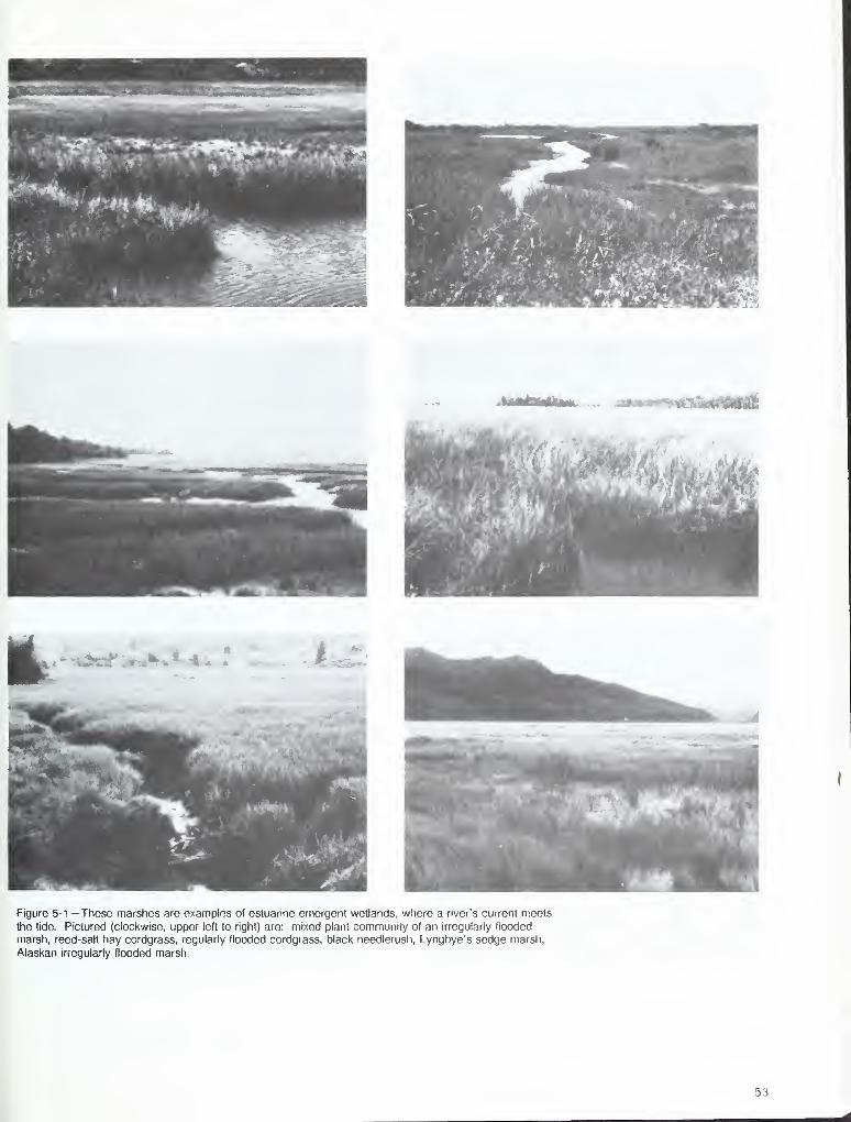
'mm

Figure 5-1 —These marshes are examples of estuarine emergent wetlands, where a river's current meets

the tide. Pictured (clockwise, upper left to right) are: mixed plant community of an irregularly flooded

marsh, reed-salt hay cordgrass, regularly flooded cordgrass, black needlerush, Lyngbye's sedge marsh,

Alaskan irregularly flooded marsh.

53

^pw^*?

1*5»

r

!

Figure 5-2 -Example of forested wetlands (clockwise, upper left to right): red maple swamp, Atlantic white

cedar swamp, bald cypress swamp, bottomland hardwood swamp, riparian forested wetlands (those located

on the banks of a natural water body), Alaskan forested wetlands mixed with scrub-shrub wetlands.

ri4

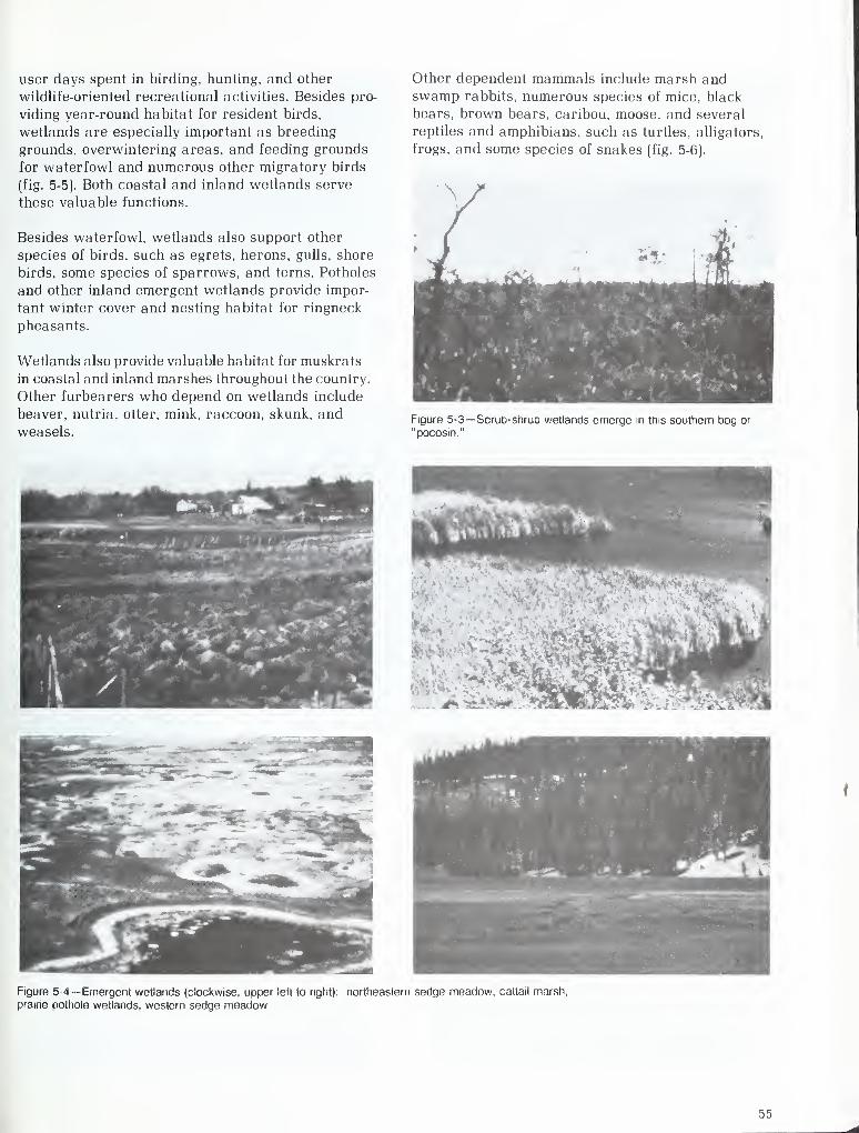
user days spent in hireling, hunting, and other

wildlife-oriented recreational activities. Besides pro-

viding year-round habitat for resident birds,

wetlands are especially important as breeding

grounds, overwintering areas, and feeding grounds

for waterfowl and numerous other migratory birds

(fig. 5-5). Both coastal and inland wetlands serve

these valuable functions.

Besides waterfowl, wetlands also support other

species of birds, such as egrets, herons, gulls, shore

birds, some species of sparrows, and terns. Potholes

and other inland emergent wetlands provide impor-

tant winter cover and nesting habitat for ringneck

pheasants.

Wetlands also provide valuable habitat for muskrats

in coastal and inland marshes throughout the country.

Other furbearers who depend on wetlands include

beaver, nutria, otter, mink, raccoon, skunk, andweasels.

Other dependent mammals include marsh andswamp rabbits, numerous species of mice, black

bears, brown bears, caribou, moose, and several

reptiles and amphibians, such as turtles, alligators,

frogs, and some species of snakes (fig. 5-6).

Figure 5-3— Scrub-shrub wetlands emerge in this southern bog or

"pocosin."

Figure 5-4— Emergent wetlands (clockwise, upper lefl to right): northeastern sedge meadow, cattail marsh,

prairie pothole wetlands, western sedge meadow.

v,

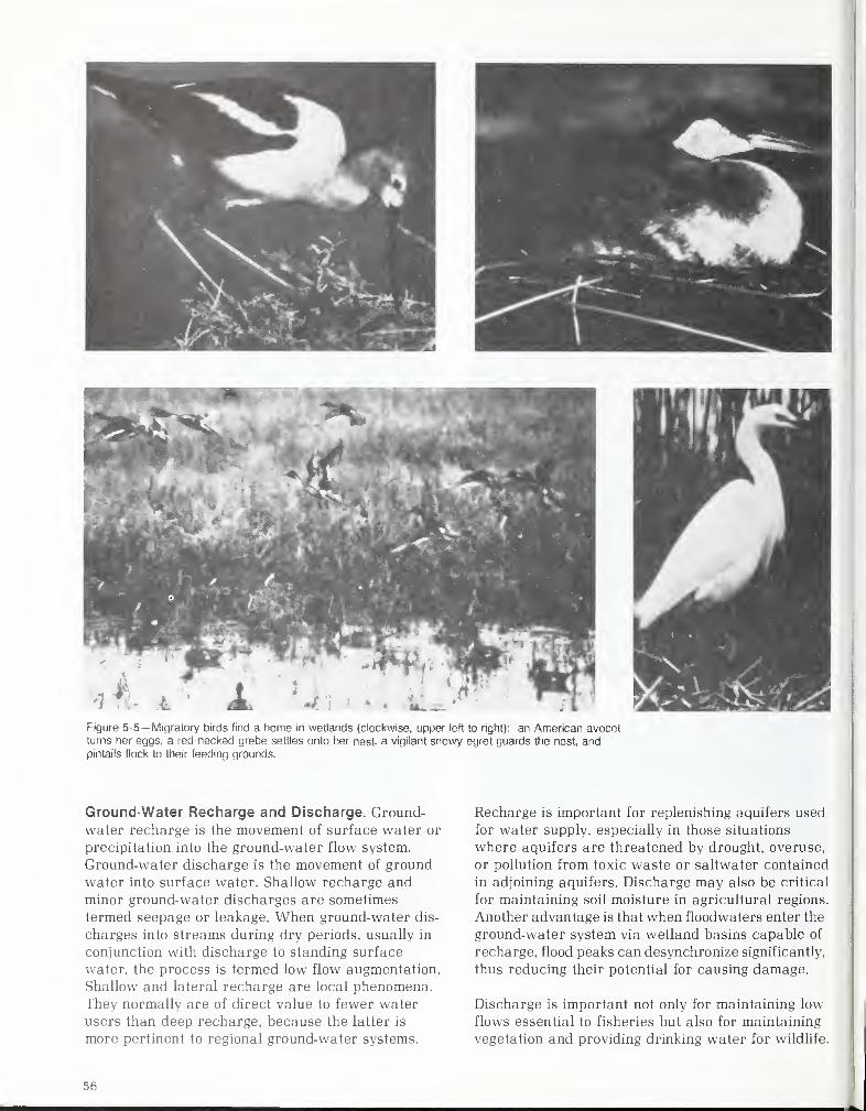
Figure 5-5— Migratory birds find a home in wetlands (clockwise, upper left to right): an American avocetturns her eggs, a red-necked grebe settles onto tier nest, a vigilant snowy egret guards the nest, andpintails flock to their feeding grounds.

Ground-Water Recharge and Discharge. Ground-

water recharge is the movement of surface water or

precipitation into the ground-water flow system.

Ground-water discharge is the movement of ground

water into surface water. Shallow recharge and

minor ground-water discharges are sometimes

termed seepage or leakage. When ground-water dis-

charges into streams during dry periods, usually in

conjunction with discharge to standing surface

water, the process is termed low flow augmentation.

Shallow and lateral recharge are local phenomena.

They normally are of direct value to fewer water

users than deep recharge, because the latter is

more pertinent to regional ground-water systems.

Recharge is important for replenishing aquifers used

for water supply, especially in those situations

where aquifers are threatened by drought, overuse,

or pollution from toxic waste or saltwater contained

in adjoining aquifers. Discharge may also be critical

for maintaining soil moisture in agricultural regions.

Another advantage is that when floodwaters enter the

ground-water system via wetland basins capable of

recharge, flood peaks can desynchronize significantly,

thus reducing their potential for causing damage.

Discharge is important not only for maintaining low

flows essential to fisheries but also for maintaining

vegetation and providing drinking water for wildlife.

56

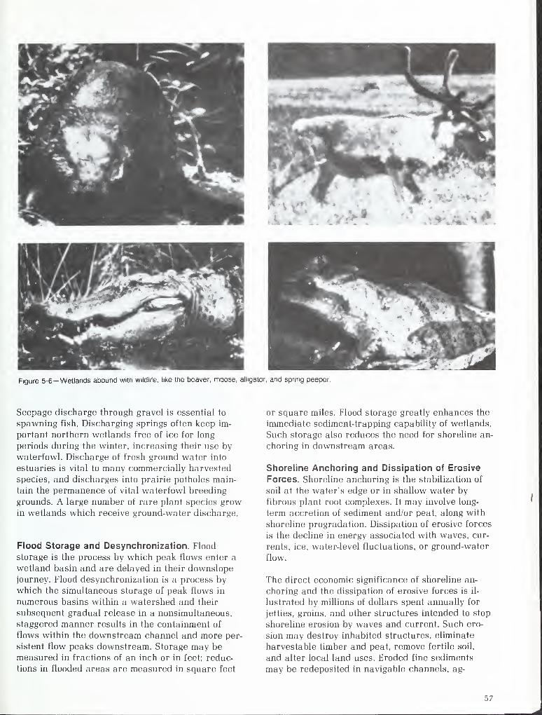
ft *<•*. *

INL ^*fe/^HpB

fe. t* * T^"••

' s£l^J^^^H^T^^*

I^Hl ' .JwaHlf|fft», «

^di^kwk.^~^» fif

r.T5

Figure 5-6— Wetlands abound with wildlife, like the beaver, moose, alligator, and spring peeper

Seepage discharge through gravel is essential to

spawning fish. Discharging springs often keep im-

portant northern wetlands free of ice for long

periods during the winter, increasing their use by

waterfowl. Discharge of fresh ground water into

estuaries is vital to many commercially harvested

species, and discharges into prairie potholes main-

tain the permanence of vital waterfowl breeding

grounds. A large number of rare plant species growin wetlands which receive ground-water discharge.

Flood Storage and Oesynchronization. Flood

storage is the process by which peak flows enter a

wetland basin and are delayed in their downslope

journey. Flood desynchronization is a process by

which the simultaneous storage of peak flows in

numerous basins within a watershed and their

subsequent gradual release in a nonsimultaneous,

staggered manner results in the containment of

flows within the downstream channel and more per-

sistent flow peaks downstream. Storage may be

measured in fractions of an inch or in feet; reduc-

tions in flooded areas are measured in square feet

or square miles. Flood storage greatly enhances the

immediate sediment-trapping capability of wetlands.

Such storage also reduces the need for shoreline an-

choring in downstream areas.

Shoreline Anchoring and Dissipation of Erosive

Forces. Shoreline anchoring is the stabilization of

soil at the water's edge or in shallow water by

fibrous plant root complexes. It may involve long-

term accretion of sediment and/or peat, along with

shoreline progradation. Dissipation of erosive forces

is the decline in energy associated with waves, cur-

rents, ice, water-level fluctuations, or ground-water

flow.

The direct economic significance of shoreline an-

choring and the dissipation of erosive forces is il-

lustrated by millions of dollars spent annually for

jetties, groins, and other structures intended to stop

shoreline erosion by waves and current. Such ero-

sion may destroy inhabited structures, eliminate

harvestable timber and peat, remove fertile soil,

and alter local land uses. Eroded fine sediments

may be redeposited in navigable channels, ag-

5 7

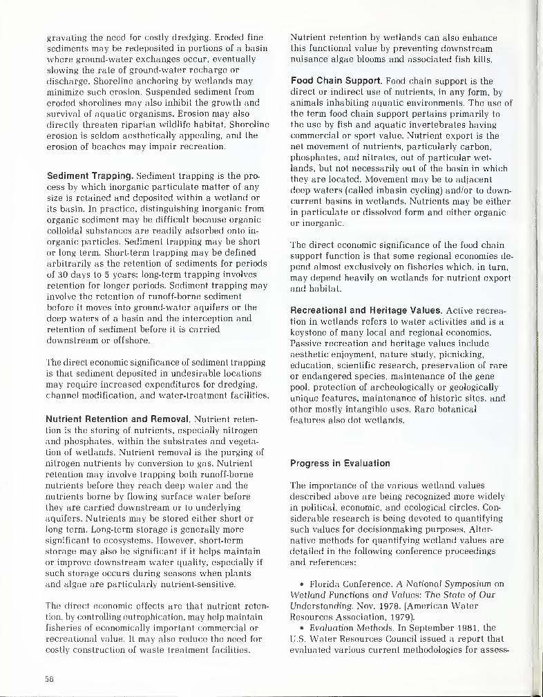
gravating the need for costly dredging. Eroded fine

sediments may be redeposited in portions of a basin

where ground-water exchanges occur, eventually

slowing the rate of ground-water recharge or

discharge. Shoreline anchoring by wetlands mayminimize such erosion. Suspended sediment from

eroded shorelines may also inhibit the growth and

survival of aquatic organisms. Erosion may also

directly threaten riparian wildlife habitat. Shoreline

erosion is seldom aesthetically appealing, and the

erosion of beaches may impair recreation.

Sediment Trapping. Sediment trapping is the pro-

cess by which inorganic particulate matter of any

size is retained and deposited within a wetland or

its basin. In practice, distinguishing inorganic from

organic sediment may be difficult because organic

colloidal substances are readily adsorbed onto in-

organic particles. Sediment trapping may be short

or long term. Short-term trapping may be defined

arbitrarily as the retention of sediments for periods

of 30 days to 5 years; long-term trapping involves

retention for longer periods. Sediment trapping mayinvolve the retention of runoff-borne sediment

before it moves into ground-water aquifers or the

deep waters of a basin and the interception and

retention of sediment before it is carried

downstream or offshore.

The direct economic significance of sediment trapping

is that sediment deposited in undesirable locations

may require increased expenditures for dredging,

channel modification, and water-treatment facilities.

Nutrient Retention and Removal. Nutrient reten-

tion is the storing of nutrients, especially nitrogen

and phosphates, within the substrates and vegeta-

tion of wetlands. Nutrient removal is the purging of

nitrogen nutrients by conversion to gas. Nutrient

retention may involve trapping both runoff-borne

nutrients before they reach deep water and the

nutrients borne by flowing surface water before

they are carried downstream or to underlying

aquifers. Nutrients may be stored either short or

long term. Long-term storage is generally moresignificant to ecosystems. However, short-term

storage may also be significant if it helps maintain

or improve downstream water quality, especially if

such storage occurs during seasons when plants

and algae are particularly nutrient-sensitive.

The direct economic effects are that nutrient reten-

tion, by controlling eutrophication, may help maintain

fisheries of economically important commercial or

recreational value. It may also reduce the need for

costly construction of waste treatment facilities.

Nutrient retention by wetlands can also enhancethis functional value by preventing downstreamnuisance algae blooms and associated fish kills.

Food Chain Support. Food chain support is the

direct or indirect use of nutrients, in any form, by

animals inhabiting aquatic environments. The use of

the term food chain support pertains primarily to

the use by fish and aquatic invertebrates having

commercial or sport value. Nutrient export is the

net movement of nutrients, particularly carbon,

phosphates, and nitrates, out of particular wet-

lands, but not necessarily out of the basin in whichthey are located. Movement may be to adjacent

deep waters (called inbasin cycling) and/or to down-current basins in wetlands. Nutrients may be either

in particulate or dissolved form and either organic

or inorganic.

The direct economic significance of the food chain

support function is that some regional economies de-

pend almost exclusively on fisheries which, in turn,

may depend heavily on wetlands for nutrient export

and habitat.

Recreational and Heritage Values. Active recrea-

tion in wetlands refers to water activities and is a

keystone of many local and regional economies.

Passive recreation and heritage values include

aesthetic enjoyment, nature study, picnicking,

education, scientific research, preservation of rare

or endangered species, maintenance of the gene

pool, protection of archeologically or geologically

unique features, maintenance of historic sites, and

other mostly intangible uses. Rare botanical

features also dot wetlands.

Progress in Evaluation

The importance of the various wetland values

described above are being recognized more widely

in political, economic, and ecological circles. Con-

siderable research is being devoted to quantifying

such values for decisionmaking purposes. Alter-

native methods for quantifying wetland values are

detailed in the following conference proceedings

and references:

• Florida Conference. A National Symposium on

Wetland Functions and Values: The State of OurUnderstanding. Nov. 1978. (American WaterResources Association, 1979).

• Evaluation Methods. In September 1981, the

U.S. Water Resources Council issued a report that

evaluated various current methodologies for assess-

58

ing wetland values. (U.S. Water Resources Council,

1981).

• National WetJand Inventory. U.S. Fish and

Wildlife Service. (Frayer and others, 1983).

• NationaJ WetJands Workshop. A National

Wetlands Values Assessment Workshop was held in

May 1983. (U.S. Dept. Interior, 1984).

• A Method for Wetland Functional Assessment.

March 1983. Federal Highway Administration.

(Adamus and Stockwell, 1983).

Many other technical publications on wetlands have

resulted from other symposia, seminars, and

workshops. However, generally acceptable methods

for quantifying wetland values as marketable goods

and services have not yet been developed for manyof the wetland functions.

about 93.7 million acres of palustrine wetlands

existed, with over half the area forested wetlands

and a third emergent wetlands. By contrast, only

5.2 million acres of estuarine wetlands then existed.

This amounts to an area approximately the size of

Massachusetts, or 0.3 percent of the land surface of

the conterminous 48 States (Tiner, 1984).

Small net gains in deepwater habitats— artificial

lakes, reservoirs, and coastal waters—occurred be-

tween about 1955 and 1975 (Frayer and others,

1983). Total lake area increased by 1.4 million

acres; about 94 percent of this gain was in the

eastern part of the country. These lakes and reser-

voirs were mostly created from uplands, although

some vegetated wetlands were destroyed in the

process.

Ecological Concerns

Jahn (1978) wrote that a watershed can be subdivid-

ed into three habitat units: freshwater, saltwater,

and terrestrial. The interrelationships among these

varied aquatic and terrestrial habitats provide

stability to ecological systems and processes.

Cairns (1978) noted that any modification of inland

water displacing or impairing ecosystem structure

or function is a degradation of ecological integrity.

Degradation occurs because plant and animal

organisms depend on a given set of environmental

conditions. When these conditions are disrupted or

changed, the dependent species must adjust, move,

or die.

Wetland Resources and Losses

Wetlands exist in every State. Their abundance

varies with climate, soils, geology, land use, and

other regional differences. Estimates of the area of

wetlands at the time of original settlement range

around 215 million acres for the conterminous 48

United States (Roe and Ayres, 1954). In 1955. an

estimated 108 million acres of wetlands existed

(Frayer and others, 1983). Today's wetland

resources in the conterminous 48 States cover about

99 million areas, or 46 percent of our original

wetlands (Tiner, 1984). Tiner estimates Alaska's

wetland resources at approximately 200 million

acres.

Palustrine wetlands (generally inland), including

freshwater marshes and swamps, constituted 94

percent of the wetlands in the 48 States. In 1975,

Some additional wetlands have also formed along

the edges of new water bodies. During 1955-75,

coastal open waters increased by 200,000 acres.

Much of this gain was in Louisiana at the expense

of coastal wetlands, which were rapidly being flooded

permanently. During the same period, 200,000 newacres of unvegetated wetland flats and 2.1 million

acres of ponds were created.

Pond area nearly doubled between 1955-75, increas-

ing from 2.3 million acres to 4.4 million acres,

primarily because of farm pond construction in the

adjacent Central and Mississippi waterflow flyways.

Most of the pond acreage was on uplands, although

145,000 acres of forested wetlands and 385,000

acres of emergent wetlands were changed to open

water (Tiner, 1984). According to the most recent

(1982) National Resources Inventory (NRI) completed

by USDA, there were about 78.2 million acres of

nonfederally owned wetlands in the United States.

Of this total, 65.3 million acres (83 percent) were

privately owned while 12.9 million acres (17 per-

cent) were owned by State and local governments.

Tiner (1984) considers agricultural development to

be responsible for 87 percent of the recent wetland

losses in the United States, while urban and other

developments caused 8 percent and 5 percent of the

losses, respectively.

Monetary net worth does not describe the total

value of wetland protection, maintenance, and/or

enhancement. The inability to quantify the full

monetary value of wetlands, coupled with the

overestimate of monetary benefits, can often result

in decisions to drain wetlands at the expense of

numerous wetland values.

5')

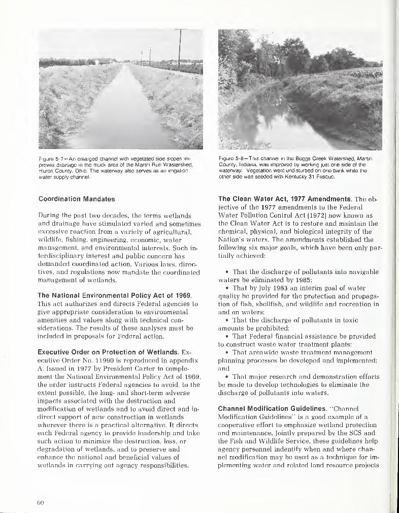
BB !

Figure 5-7— An enlarged channel with vegetated side slopes im-

proves drainage in the muck area of the Marsh Run Wastershed,

Huron County, Ohio. The waterway also serves as an irrigation

water supply channel.

Figure 5-8— This channel in the Boggs Creek Watershed, Martin

County, Indiana, was improved by working just one side of the

waterway. Vegetation went undisturbed on one bank while the

other side was seeded with Kentucky 31 Fescue.

Coordination Mandates

During the past two decades, the terms wetlandsand drainage have stimulated varied and sometimesexcessive reaction from a variety of agricultural,

wildlife, fishing, engineering, economic, watermanagement, and environmental interests. Such in-

terdisciplinary interest and public concern hasdemanded coordinated action. Various laws, direc-

tives, and regulations now mandate the coordinated

management of wetlands.

The National Environmental Policy Act of 1969.

This act authorizes and directs Federal agencies to

give appropriate consideration to environmental

amenities and values along with technical con-

siderations. The results of these analyses must be

included in proposals for Federal action.

Executive Order on Protection of Wetlands. Ex-

ecutive Order No. 11990 is reproduced in appendix

A. Issued in 1977 by President Carter to comple-

ment the National Environmental Policy Act of 1969,

the order instructs Federal agencies to avoid, to the

extent possible, the long- and short-term adverse

impacts associated with the destruction andmodification of wetlands and to avoid direct and in-

direct support of new construction in wetlands

wherever there is a practical alternative. It directs

each Federal agency to provide leadership and take

such action to minimize the destruction, loss, or

degradation of wetlands, and to preserve andenhance the national and beneficial values of

wetlands in carrying out agency responsibilities.

The Clean Water Act, 1977 Amendments. The ob-

jective of the 1977 amendments to the Federal

Water Pollution Control Act (1972) now known as

the Clean Water Act is to restore and maintain the

chemical, physical, and biological integrity of the

Nation's waters. The amendments established the

following six major goals, which have been only par-

tially achieved:

• That the discharge of pollutants into navigable

waters be eliminated by 1985;

• That by July 1983 an interim goal of water

quality be provided for the protection and propaga-

tion of fish, shellfish, and wildlife and recreation in

and on waters;

• That the discharge of pollutants in toxic

amounts be prohibited;

• That Federal financial assistance be provided

to construct waste water treatment plants;

• That areawide waste treatment managementplanning processes be developed and implemented;

and• That major research and demonstration efforts

be made to develop technologies to eliminate the

discharge of pollutants into waters.

Channel Modification Guidelines. "Channel

Modification Guidelines" is a good example of a

cooperative effort to emphasize wetland protection

and maintenance. Jointly prepared by the SCS and

the Fish and Wildlife Service, these guidelines help

agency personnel indentify when and where chan-

nel modification may be used as a technique for im-

plementing water and related land resource projects

60

under the authorities of the SCS for planning small

watershed and resources conservation and develop-

ment projects (figs. 5-7 and 5-8). The guidelines

stipulate that efforts will be made to maintain andrestore streams upon which fish and wildlife

resources depend (U.S. Depts. Interior andAgriculture, 1979).

Comprehensive Evaluations

Despite current oversupply problems confronting

U.S. agriculture, it is unrealistic to assume that on a

permanent basis significantly less land will be

devoted to agricultural production in the

foreseeable future. However, food and fiber produc-

tion should be balanced with the other products of

land, including those produced by wetlands. All

possible measures should be incorporated in

specific drainage plans and designs to minimize

degradation of wetland values. Such evaluations

should serve as a positive catalyst to pull together

all interests and responsibilities. Mutual coopera-

tion and understanding can lead to the planning and

completion of only such added drainage as may be

needed in the public interest and within constraints

that maintain the important values associated with

the remaining wetlands.

This action supports USDA's policy which is to

assure that the values of fish and wildlife are

recognized and that their habitats, both terrestrial

and aquatic (including wetlands), are considered

when the Department carries out its missions. USDAsupports research and management programs that

respond to the economic, ecological, educational,

recreational, scientific, and aesthetic values of fish

and wildlife. Its goals are to improve, where needed,

fish and wildlife habitats, and to ensure the

presence of diverse native and other populations of

wildlife, fish, and plant species (USDA, 1983).

References

Adamus, Paul R., and C. T. Stockwell. 1983. AMethod for WetJand Functional Assessment. U.S.

Dept. Trans., Fed. Hwy. Adm. Rpt. Nos. FHWA-IP-82-23 and FHWA-IP-83-24.

American Water Resources Association. 1979.

Wetland Functions and VaJues: The State of OurUnderstanding. Proceedings of the National Sym-posium on Wetlands. Tech. Pub. No. TPS 79-2.

Minneapolis.

Cairns, John, Jr. 1978. Wildlife and America. Council

on Environmental Quality. Govt. Print. Off.

Cowardin, Lewis M., Virginia Carter, Francis C.

Golet, and Edward T. LaRoe. 1979. Classification of

WetJands and Deepwater Habitats of the United

States. U.S. Dept. Interior, Fish and Wildlife Serv.

Rpt. No. FWS/OBS-79/31.

Frayer, W. E., T. J. Monahan, D. C. Bowden, and F.

A. Graybill. 1983. Status and Trends of Wetlands

and Deepwater Habitats in the Conterminous United

States: 1950's to 1970's. Fort Collins, Colo.: Depart-

ment of Forests and Wood Sciences, Colorado State

Univ.

Jahn, Lawrence R. 1978. "Values of Riparian

Habitat to Natural Ecosystems," Protection andManagement of Floodplain WetJands and Riparian

Ecosystems. Gen. Tech. Rpt. WO-12. U.S. Dept. Agr„Forest Service.

Lonard, Robert L., and others. 1981. Analysis of

Methodologies Used for the Assessment of WetlandVaiues. U.S. Water Resources Council, Washington,

DC.

Roe, H. B., and Q. C. Ayres. 1954. Engineering for

Agricultural Drainage. New York: McGraw-Hill Book

Company.

Tiner, Ralph W., Jr. 1984. Wetlands of the United

States: Current States and Recent Trends. U.S. Dept.

Interior, Fish and Wildlife Serv.

U.S. Congress, Office of Technology Assessment.

1984. Wetlands, Their Use and Regulation. Rpt. No.

OTA-O-207. Govt. Print. Off.

U.S. Department of Agriculture. 1983. U.S. Fish and

Wildlife Policy. Dept. Reg. 9500-4.

U.S. Department of the Interior and U.S. Department

of Agriculture. 1979. Channel Modification

Guidelines (amended).

ui

Chapter 6

Principles of Drainage

R. Wayne SkaggsDepartment of Biological and Agricultural

EngineeringNorth Carolina State University, Raleigh

A review of drainage principles appropriately begins

with the hydrologic cycle, the main components of

which are illustrated in figure 6-1. Precipitation fall-

ing to the earth's surface either infiltrates into the

soil profile or moves from the area by overland flow

which may eventually enter a stream or other surface-

water outlet. The infiltrated water may be stored in

the unsaturated zone or percolate downward to a

saturated zone. Water may be removed from the

profile by evapotranspiration (ET) and by natural

drainage processes. These processes may include

ground-water flow to streams or other surface

outlets, vertical seepage to underlying aquifers, or

lateral flow (interflow) which may reappear at the

surface at some other point in the landscape. In

many soils, the natural drainage processes are suf-

ficient for the growth and production of agricultural

crops. In other soils, artificial drainage is needed

for efficient agricultural production.

Soils may have poor natural drainage for a numberof reasons. Lands with surface elevations close to

that of the drainage outlet (section D, in fig. 6-1)

may have permanently high water tables. Land that

is far removed from the drainage outlet, such as

sections B and C may have high water during

critical periods of the growing season. Other lands

may be poorly drained because of seepage from

upslope areas (section B) or because they are in

depressional areas with no surface water outlet.

Water drains slowly from soils with tight subsur-

face layers, regardless of where these layers are in

the landscape; so soils may have poor natural

drainage because of restricted permeability or

hydraulic conductivity of the profile.

Climate is another important factor affecting the

need for artificial drainage. Natural drainage at a

rate that may be sufficient for agriculture in a sec-

tion of Nebraska where annual rainfall is 20 inches

per year, for example, may be inadequate in Loui-

siana where the annual rainfall is 55 inches.

Nowhere is this factor more evident than in

irrigated semiarid areas. Lands that have been

farmed for centuries under dryland cultures often

develop high water tables and become water-logged

after irrigation is established. By contrast, natural

drainage may be adequate in other soils and the

several-fold increase in the amount of water applied

to the surface because of irrigation will not result

in poorly drained conditions. Seepage from unlined

irrigation canals or from reservoirs may also result

in poorly drained soils in areas where they did not

previously exist.

All soils require satisfactory drainage for efficient

agricultural production; many need improved or ar-

tificial drainage. Soils may be poorly drained because

of climate and irrigation practices, position in the

landscape in relation to drainage outlets or irriga-

tion canals, or low permeability and/or restricting

layers in the soil profile.

In most cases, improved drainage practices can be

used to satisfy agricultural requirements. These will

be discussed first, followed by the factors control-

ling the movement and storage of water in the soil

profile and methods that can be used to satisfy

drainage requirements. Examples are given to

describe the design and operation of a drainage

system and the concepts of controlled drainage andsubirrigation. The concluding section discusses

some principles that can be used to consider offsite

impacts of drainage and related water managementpractices.

62

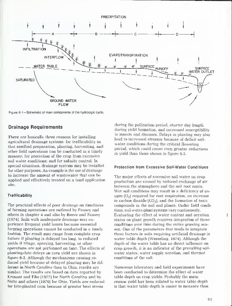
PRECIPITATION

SATURATED

GROUND WATERFLOW

Figure 6-1 —Schematic of main components of the hydrologic cycle.

Drainage Requirements

There are basically three reasons for installing

agricultural drainage systems: for trafficability so

that seedbed preparation, planting, harvesting, and

other field operations can be conducted in a timely

manner; for protection of the crop from excessive

soil water conditions; and for salinity control. In

special situations, drainage systems may be installed

for other purposes. An example is the use of drainage

to increase the amount of wastewater that can be

applied and effectively treated on a land application

site.

Trafficability

The practical effects of poor drainage on timeliness

of farming operations are outlined by Fausey andothers in chapter 4 and also by Reeve and Fausey

(1974). Soils with inadequate drainage may ex-

perience frequent yield losses because essential

farming operations cannot be conducted in a timely

fashion. The result may range from complete crop

failure if planting is delayed too long, to reduced

yields if tillage, spraying, harvesting, or other

operations are not performed on time. The effects of

planting-date delays on corn yield are shown in

figure 6-2. Although the mechanisms causing re-

duced yield because of delayed planting may be dif-

ferent in North Carolina than in Ohio, results are

similar. The results are based on data reported by

Krenzer and Fike (1977) for North Carolina and by

Nolte and others (1976) for Ohio. Yields are reducedfor late-planted corn because of greater heat stress

during the pollination period, shorter day length

during yield formation, and increased susceptibility

to insects and diseases. Delays in planting may also

lead to increased stresses because of deficit soil-

water conditions during the critical flowering

period, which could cause even greater reductions

in yield than those shown in figure 6-2.

Protection from Excessive Soil-Water Conditions

The major effects of excessive soil water on crop

production are caused by reduced exchange of air

between the atmosphere and the soil root zones.

Wet soil conditions may result in a deficiency of ox-

ygen (0 2 ) required for root respiration, an increase

in carbon dioxide (C0 2 ), and the formation of toxic

compounds in the soil and plants. Under field condi-

tions, soil-water-plant systems vary continuously.

Evaluating the effect of water content and aeration

status on plant growth requires integration of these

conditions over time during the entire growing sea-

son. One of the parameters that tends to integrate

these factors in soils requiring artificial drainage is

water table depth (Wesseling, 1974). Although the

depth of the water table has no direct influence on

crop growth, it is an indicator of the prevailing soil-

water status, water supply aeration, and thermal

conditions of the soil.

Numerous laboratory and field experiments have

been conducted to determine the effect of water

table depth on crop yields. Probably the main

reason yield has been related to water table depth

is that water table depth is easier to measure than

63

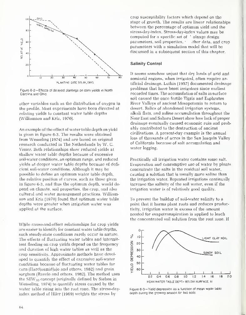
100

-

__0HI0

\

\8

q \_i \LiJ 60 \ N.>-

UJ \ \> \ \l~

\ \< 4C \ N.-J \ »vUJ \ \a:

20

n |I

1

\ \\ \

\ \\ \

10 20 JO 40 50 60 70 80

PLANTING DATE DELAY, DAYS

Figure 6-2— Effects of delayed plantings on corn yields in North

Carolina and Ohio.

other variables such as the distribution of oxygen in

the profile. Most experiments have been directed at

relating yields to constant water table depths

(Williamson and Kriz, 1970).

An example of the effect of water table depth on yield

is given in figure 6-3. The results were obtained

from Wesseling (1974) and are based on original

research conducted in The Netherlands by W. C.

Visser. Both relationships show reduced yields at

shallow water table depths because of excessive

soil-water conditions, an optimum range, and reduced

yields at deeper water table depths because of defi-

cient soil-water conditions. Although it may be

possible to define an optimum water table depth,

the relative position of curves, such as those given

in figure 6-3, and thus the optimum depth, would de-

pend on climate, soil properties, the crop, and also

cultural and water management practices. William-

son and Kriz (1970) found that optimum water table

depths were greater when irrigation water wasapplied at the surface.

While cause-and-effect relationships for crop yields

are easier to identify for constant water table depths,

such steady-state conditions rarely occur in nature.

The effects of fluctuating water tables and intermit-

tent flooding on crop yields depend on the frequency

and duration of high water tables as well as the

crop sensitivity. Approximate methods have devel-

oped to quantify the effect of excessive soil-water

conditions because of fluctuating water tables for

corn (Hardjoamidjojo and others, 1982) and grain

sorghum (Ravelo and others, 1982). The method uses

the SEW30 concept (originally defined by Sieben in

Wesseling, 1974) to quantify stress caused by the

water table rising into the root zone. The stress-day-

index method of Hiler (1969) weights the stress by

crop susceptibility factors which depend on the

stage of growth. The results are linear relationships

between the percentage of optimum yield and the

stress-day-index. Stress-day-index values may be

computed for a specific set of ' ainage design

parameters, soil properties, ' .ther data, and crop

parameters with a simulation model that will be

discussed in a subsequent section of this chapter.

Salinity Control

It seems somehow unjust that dry lands of arid andsemiarid regions, when irrigated, often require ar-

tificial drainage. Luthin (1957) documented drainage

problems that have beset irrigators since earliest

recorded times. The accumulation of salts in surface

soil caused the once fertile Tigris and Euphrates

River Valleys of ancient Mesopotamia to return to

desert. Relics of abandoned irrigation systems,

alkali flats, and saline accumulation throughout the

Near East and Sahara Desert show how lack of proper

drainage eventually caused economic ruin and prob-

ably contributed to the destruction of ancient

civilizations. A present-day example is the annual

loss of thousands of acres in the San Joaquin Valley

of California because of salt accumulation and

water logging.

Practically all irrigation water contains some salt.

Evaporation and consumptive use of water by plants

concentrate the salts in the residual soil water,

causing a solution that is usually more saline than

the irrigation water. Repeated irrigations continually

increase the salinity of the soil water, even if the

irrigation water is of relatively good quality.

To prevent the buildup of soil-water salinity to a

point that it harms plant roots and reduces produc-

tivity, irrigation water in excess of the amount

needed for evapotranspiration is applied to leach

the concentrated soil solution from the root zone. If

u~>

UJ<ra.UJQo_l

10 / /\w ^^\LIGHT CLAY SOIL

20 1 /30 1

SANDY SOIL

40 -

50

601 1 1 1

0.2 0.4 0.6 0.8 1.0 1.2 14 1.6

MEAN WATER TABLE DEPTH BELOW SURFACE, M

1.8 2.0

Figure 6-3— Yield depression as a function of mean water table

depth during the growing season for two soils.

64

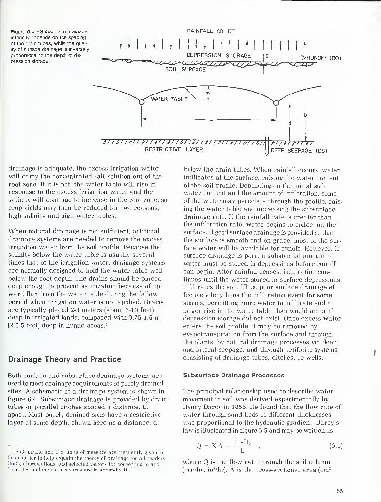
Figure 6-4— Subsurface drainage

intensity depends on the spacing

of the dram tubes, while the qual-

ity of surface drainage is inversely

proportional to the depth of de-

pression storage.

RAINFALL OR ET

I I I I I I I I I I I f f I ft t t I f t f |

_i_S zz> RUNoFF (RO)

T777777777777777T777T777T7T77717T777177RESTRICTIVE LAYER

TT7TTT7TtT.DEEP SEEPAGE (DS)

drainage is adequate, the excess irrigation water

will carry the concentrated salt solution out of the

root zone. If it is not, the water table will rise in

response to the excess irrigation water and the

salinity will continue to increase in the root zone, so

crop yields may then be reduced for two reasons,

high salinity and high water tables.

When natural drainage is not sufficient, artificial

drainage systems are needed to remove the excess

irrigation water from the soil profile. Because the

salinity below the water table is usually several

times that of the irrigation water, drainage systems

are normally designed to hold the water table well

below the root depth. The drains should be placed

deep enough to prevent salinization because of up-

ward flux from the water table during the fallow

period when irrigation water is not applied. Drains

are typically placed 2-3 meters (about 7-10 feet)

deep in irrigated lands, compared with 0.75-1.5 m(2.5-5 feet) deep in humid areas. 1

Drainage Theory and Practice

Both surface and subsurface drainage systems are

used to meet drainage requirements of poorly drained

sites. A schematic of a drainage system is shown in

figure 6-4. Subsurface drainage is provided by drain

tubes or parallel ditches spaced a distance, L,

apart. Most poorly drained soils have a restrictive

layer at some depth, shown here as a distance, d,

'Both metric and U.S. units of measure are frequently given in

this chapter to help explain the theory of drainage for all readers.Units, abbreviations, and selected factors for converting to andfrom U.S. and metric measures are in appendix D.

below the drain tubes. When rainfall occurs, waterinfiltrates at the surface, raising the water content

of the soil profile. Depending on the initial soil-

water content and the amount of infiltration, someof the water may percolate through the profile, rais-

ing the water table and increasing the subsurface

drainage rate. If the rainfall rate is greater than

the infiltration rate, water begins to collect on the

surface. If good surface drainage is provided so that

the surface is smooth and on grade, most of the sur-

face water will be available for runoff. However, if

surface drainage is poor, a substantial amount of

water must be stored in depressions before runoff

can begin. After rainfall ceases, infiltration con-

tinues until the water stored in surface depressions

infiltrates the soil. Thus, poor surface drainage ef-

fectively lengthens the infiltration event for somestorms, permitting more water to infiltrate and a

larger rise in the water table than would occur if

depression storage did not exist. Once excess water

enters the soil profile, it may be removed by

evapotranspiration from the surface and through

the plants, by natural drainage processes via deep

and lateral seepage, and through artificial systems

consisting of drainage tubes, ditches, or wells.

Subsurface Drainage Processes

The principal relationship used to describe water

movement in soil was derived experimentally by

Henry Darcy in 1856. He found that the flow rate of

water through sand beds of different thicknesses

was proportional to the hydraulic gradient. Darcy's

law is illustrated in figure 6-5 and may be written as:

KA H r H 2(6.1]

where Q is the flow rate through the soil column

(cm 3/hr, in3

/hr), A is the cross-sectional area (cm 2.

65

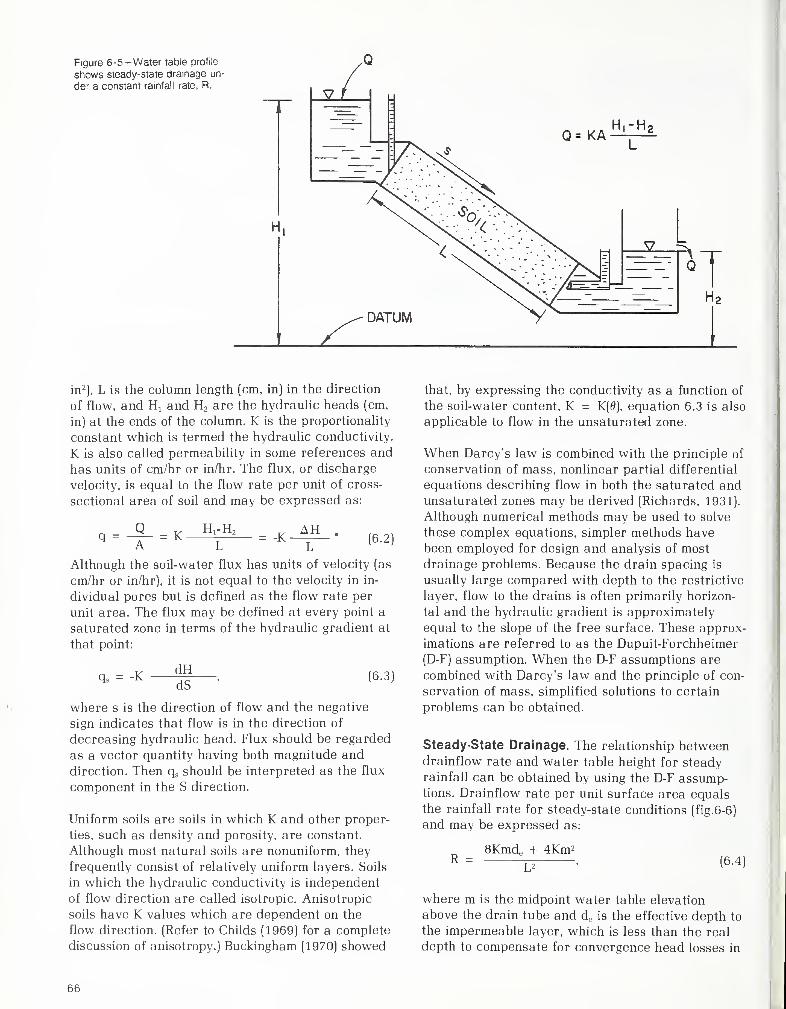
Figure 6-5-Water table profile

shows steady-state drainage un-

der a constant rainfall rate, R.

H,

DATUM

in 2), L is the column length (cm, in) in the direction

of flow, and Hj and H2 are the hydraulic heads (cm,

in) at the ends of the column. K is the proportionality

constant which is termed the hydraulic conductivity.

K is also called permeability in some references and

has units of cm/hr or in/hr. The flux, or discharge

velocity, is equal to the flow rate per unit of cross-

sectional area of soil and may be expressed as:

Q = Q = KHrH 2 = -K

AH(6.2)A L L

Although the soil-water flux has units of velocity (as

cm/hr or in/hr), it is not equal to the velocity in in-

dividual pores but is defined as the flow rate per

unit area. The flux may be defined at every point a

saturated zone in terms of the hydraulic gradient at

that point:

q s = -KdHdS

(6.3)

where s is the direction of flow and the negative

sign indicates that flow is in the direction of

decreasing hydraulic head. Flux should be regarded

as a vector quantity having both magnitude and

direction. Then qs should be interpreted as the flux

component in the S direction.

Uniform soils are soils in which K and other proper-

ties, such as density and porosity, are constant.

Although most natural soils are nonuniform, they

frequently consist of relatively uniform layers. Soils

in which the hydraulic conductivity is independent

of flow direction are called isotropic. Anisotropic

soils have K values which are dependent on the

flow direction. (Refer to Childs (1969) for a complete

discussion of anisotropy.) Buckingham (1970) showed

that, by expressing the conductivity as a function of

the soil-water content, K = K(0), equation 6.3 is also

applicable to flow in the unsaturated zone.

When Darcy's law is combined with the principle of

conservation of mass, nonlinear partial differential

equations describing flow in both the saturated andunsaturated zones may be derived (Richards, 1931).

Although numerical methods may be used to solve

these complex equations, simpler methods have

been employed for design and analysis of most

drainage problems. Because the drain spacing is

usually large compared with depth to the restrictive

layer, flow to the drains is often primarily horizon-

tal and the hydraulic gradient is approximately

equal to the slope of the free surface. These approx-

imations are referred to as the Dupuit-Forchheimer

(D-F) assumption. When the D-F assumptions are

combined with Darcy's law and the principle of con-

servation of mass, simplified solutions to certain

problems can be obtained.

Steady-State Drainage. The relationship betweendrainflow rate and water table height for steady

rainfall can be obtained by using the D-F assump-tions. Drainflow rate per unit surface area equals

the rainfall rate for steady-state conditions (fig.6-6)

and may be expressed as:

R =8Kmde + 4Km2

(6.4)

where m is the midpoint water table elevation

above the drain tube and d e is the effective depth to

the impermeable layer, which is less than the real

depth to compensate for convergence head losses in

6 b

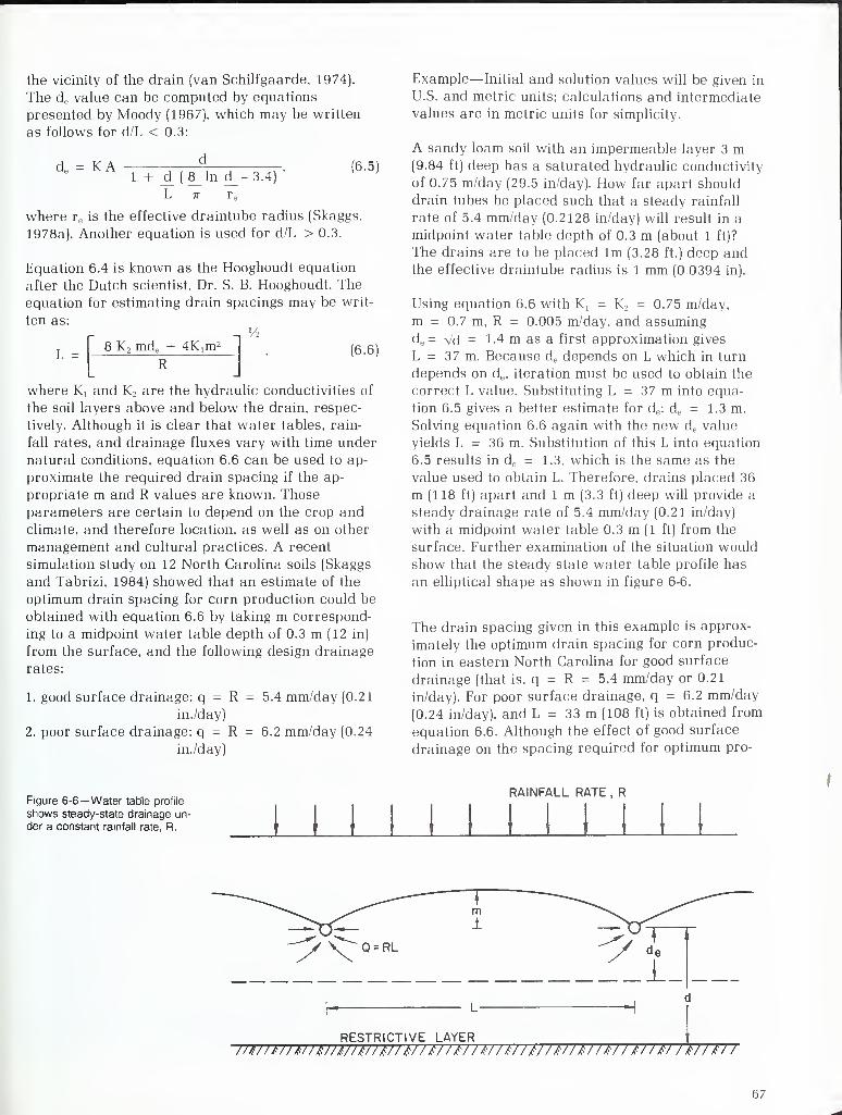
the vicinity of the drain (van Schilfgaarde, 1974).

The d e value can be computed by equations

presented by Moody (1967), which may be written

as follows for d/L < 0.3:

KA1 +

(6.5)_d (8_In d_- 3.4)

'

L 7r r e

where re is the effective draintube radius (Skaggs,

1978a). Another equation is used for d/L > 0.3.

Equation 6.4 is known as the Hooghoudt equation

after the Dutch scientist. Dr. S. B. Hooghoudt. The

equation for estimating drain spacings may be writ-

ten as:

8 K 2 mde + 4K xm2

H(6.6)

where Kj and K 2 are the hydraulic conductivities of

the soil layers above and below the drain, respec-

tively. Although it is clear that water tables, rain-

fall rates, and drainage fluxes vary with time under

natural conditions, equation 6.6 can be used to ap-

proximate the required drain spacing if the ap-

propriate m and R values are known. Those

parameters are certain to depend on the crop and

climate, and therefore location, as well as on other

management and cultural practices. A recent

simulation study on 12 North Carolina soils (Skaggs

and Tabrizi, 1984) showed that an estimate of the

optimum drain spacing for corn production could be

obtained with equation 6.6 by taking m correspond-

ing to a midpoint water table depth of 0.3 m (12 in)

from the surface, and the following design drainage

rates:

1. good surface drainage: q = R = 5.4 mm/day (0.21

in./day)

2. poor surface drainage: q = R = 6.2 mm/day (0.24

in./day)

Example— Initial and solution values will be given in

U.S. and metric units; calculations and intermediate

values are in metric units for simplicity.

A sandy loam soil with an impermeable layer 3 m(9.84 ft) deep has a saturated hydraulic conductivity

of 0.75 m/day (29.5 in/day). How far apart should

drain tubes be placed such that a steady rainfall

rate of 5.4 mm/day (0.2128 in/day) will result in a

midpoint water table depth of 0.3 m (about 1 ft)?

The drains are to be placed lm (3.28 ft.) deep andthe effective draintube radius is 1 mm (0.0394 in).

Using equation 6.6 with K1= K 2

= 0.75 m/day,

m = 0.7 m, R = 0.005 m/day, and assuming

d e = Vd = 1.4 m as a first approximation gives

L = 37 m. Because de depends on L which in turn

depends on d e , iteration must be used to obtain the

correct L value. Substituting L = 37 m into equa-

tion 6.5 gives a better estimate for de : de = 1.3 m.

Solving equation 6.6 again with the new de value

yields L = 36 m. Substitution of this L into equation

6.5 results in de = 1.3, which is the same as the

value used to obtain L. Therefore, drains placed 36

m (118 ft) apart and 1 m (3.3 ft) deep will provide a

steady drainage rate of 5.4 mm/day (0.21 in/day)

with a midpoint water table 0.3 m (1 ft) from the

surface. Further examination of the situation would

show that the steady state water table profile has

an elliptical shape as shown in figure 6-6.

The drain spacing given in this example is approx-

imately the optimum drain spacing for corn produc-

tion in eastern North Carolina for good surface

drainage (that is, q = R = 5.4 mm/day or 0.21

in/day). For poor surface drainage, q = 6.2 mm/day

(0.24 in/day), and L = 33 m (108 ft) is obtained from

equation 6.6. Although the effect of good surface

drainage on the spacing required for optimum pro-

Figure 6-6—Water table profile

shows steady-state drainage un-

der a constant rainfall rate, R.

RAINFALL RATE , R

1 1 I M 11 1 11

RESTRICTIVE LAYER77777777777777777777777777777777777777777777777777777777777777

67

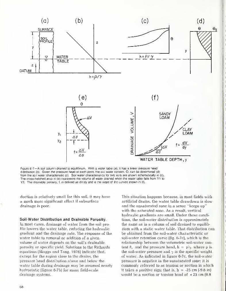
(a)

SURFACE

DATUM

h=/D/7

y 2

(f)

> SANDY /

UJ LOAM /5 / /r> / /_lo / /clay> / / LOAMLU //O<7^ S f=

dv

<CCQ

^—

'

WATER TABLE DEPTH, y

Figure 6-7—A soil column drained to equilibrium. With a water table (a), it has a linear pressure head

distribution (b). Given the pressure head at each point, the soil water content, O, can be determined (d)

from the soil water characteristic (c). Soil water characteristics for two soils are shown schematically in (c).

The cross-hatched area in (e) represents the volume of water drained when the water table fails from Y1 to

Y2. The dramable porosity, f, is defined as dV/dy and is the slope of the curves shown in (f).

duction is relatively small for this soil, it may have

a much more significant effect if subsurface

drainage is poor.

Soil-Water Distribution and Drainable Porosity.

In most cases, drainage of water from the soil pro-

file lowers the water table, reducing the hydraulic

gradient and the drainage rate. The response of the

water table to removal or addition of a given

volume of water depends on the soil's drainable

porosity or specific yield. Solutions to the Richards

equations (Skaggs and Tang, 1976) indicate that,

except for the region close to the drains, the

pressure head distribution above and below the

water table during drainage may be assumed nearly

hydrostatic (figure 6-7b) for many field-scale

drainage systems.

This situation happens because, in most fields with

artificial drains, the water table drawdown is slow

and the unsaturated zone in a sense "keeps up"with the saturated zone. As a result, vertical

hydraulic gradients are small. Under these condi-

tions, the soil-water distribution is approximately

the same as in a column of soil drained to equilib-

rium with a static water table. That distribution can

be obtained from the soil-water characteristic or

soil-water retention curve (fig. 6-7c), which is the

relationship between the volumetric soil-water con-

tent 6, and the pressure head, h = pAy, where p is

the soil-water pressure and 7 is the specific weight

of water. As indicated in figure 6-7c, the soil-water

pressure is negative in the unsaturated zone; it is

commonly referred to as tension or suction in which

it takes a positive sign: that is. h = -25 cm (-9.8 in)

would be a suction or tension head of + 25 cm (9.8

68

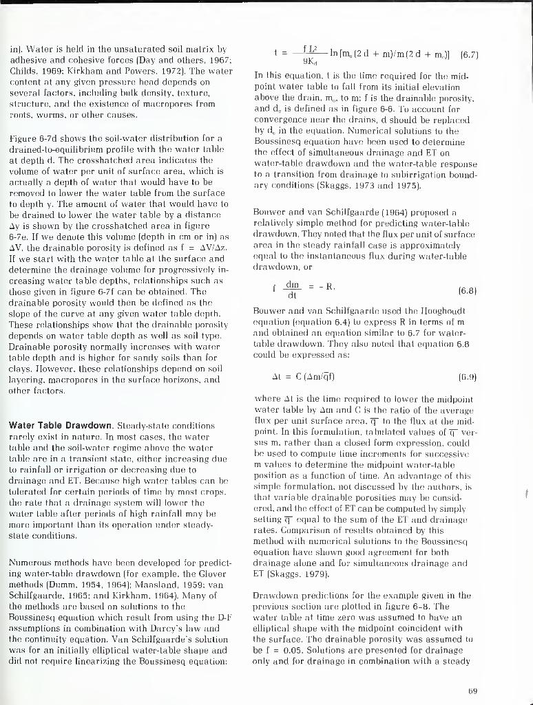
in). Water is held in the unsaturated soil matrix by

adhesive and cohesive forces (Day and others, 1967;

Childs, 1969; Kirkham and Powers, 1972). The water

content at any given pressure head depends on

several factors, including bulk density, texture,

structure, and the existence of macropores from

roots, worms, or other causes.

Figure 6-7d shows the soil-water distribution for a

drained-to-equilibrium profile with the water table

at depth d. The crosshatched area indicates the

volume of water per unit of surface area, which is

actually a depth of water that would have to be

removed to lower the water table from the surface

to depth y. The amount of water that would have to

be drained to lower the water table by a distance

Ay is shown by the crosshatched area in figure

6-7e. If we denote this volume (depth in cm or in) as

AV, the drainable porosity is defined as f = AV/Az.

If we start with the water table at the surface and

determine the drainage volume for progressively in-

creasing water table depths, relationships such as

those given in figure 6-7f can be obtained. Thedrainable porosity would then be defined as the

slope of the curve at any given water table depth.

These relationships show that the drainable porosity

depends on water table depth as well as soil type.

Drainable porosity normally increases with water

table depth and is higher for sandy soils than for

clays. However, these relationships depend on soil

layering, macropores in the surface horizons, and

other factors.

Water Table Drawdown. Steady-state conditions

rarely exist in nature. In most cases, the water

table and the soil-water regime above the water

table are in a transient state, either increasing due

to rainfall or irrigation or decreasing due to

drainage and ET. Because high water tables can be

tolerated for certain periods of time by most crops,

the rate that a drainage system will lower the

water table after periods of high rainfall may be

more important than its operation under steady-

state conditions.

Numerous methods have been developed for predict-

ing water-table drawdown (for example, the Glover

methods (Dumm, 1954. 1964); Maasland, 1959; van

Schilfgaarde, 1965; and Kirkham, 1964). Many of

the methods are based on solutions to the

Boussinesq equation which result from using the D-F

assumptions in combination with Darcy's law andthe continuity equation. Van Schilfgaarde's solution

was for an initially elliptical water-table shape anddid not require linearizing the Boussinesq equation:

iU9KH

ln[m (2d + m)/m(2d + m,,)] (6.7)

In this equation, t is the time required for the mid-

point water table to fall from its initial elevation

above the drain, mo, to m; f is the drainable porosity,

and de is defined as in figure 6-6. To account for

convergence near the drains, d should be replaced

by d e in the equation. Numerical solutions to the

Boussinesq equation have been used to determine

the effect of simultaneous drainage and ET onwater-table drawdown and the water-table response

to a transition from drainage to subirrigation bound-

ary conditions (Skaggs, 1973 and 1975).

Bouwer and van Schilfgaarde (1964) proposed a

relatively simple method for predicting water-table

drawdown. They noted that the flux per unit of surface

area in the steady rainfall case is approximately

equal to the instantaneous flux during water-table

drawdown, or

fdmdt

= -R.(6.8)

Bouwer and van Schilfgaarde used the Hooghoudt

equation (equation 6.4) to express R in terms of mand obtained an equation similar to 6.7 for water-

table drawdown. They also noted that equation 6.8

could be expressed as:

At = C(Am/qf) (6.9)

where At is the time required to lower the midpoint

water table by Am and C is the ratio of the averageflux per unit surface area, q~ to the flux at the mid-

point. In this formulation, tabulated values of q-ver-

sus m, rather than a closed form expression, could

be used to compute time increments for successive

m values to determine the midpoint water-table

position as a function of time. An advantage of this

simple formulation, not discussed by the authors, is

that variable drainable porosities may be consid-

ered, and the effect of ET can be computed by simply

setting q~ equal to the sum of the ET and drainage

rates. Comparison of results obtained by this

method with numerical solutions to the Boussinesq

equation have shown good agreement for both

drainage alone and for simultaneous drainage andET (Skaggs. 1979).

Drawdown predictions for the example given in the

previous section are plotted in figure 6-8. Thewater table at time zero was assumed to have an

elliptical shape with the midpoint coincident with

the surface. The drainable porosity was assumed to

be f = 0.05. Solutions are presented for drainage

only and for drainage in combination with a steady

h<i

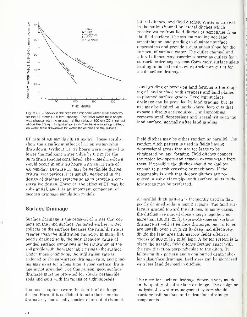
o 100

L = 36mde = 13mK = 0.75 m/df = 005ET= 4.Smm/d

100 150

TIME, HOURS

200

Figure 6-8— Shown is the predicted midpoint water table elevation

tor the 36-meter (118 teet) spacing. The initial water table shapewas elliptical with the midpoint at the surface, 100 cm (25.4 inches)

above the drains. Evapotranspiration may have a significant effect

on water table drawdown for water tables close to the surface.

lateral ditches, and field ditches. Water is carried

to the outlet channel by lateral ditches whichreceive water from field ditches or sometimes fromthe field surface. The system may include land

smoothing or land grading to eliminate surface

depressions and provide a continuous slope for the

removal of surface water. The outlet channel andlateral ditches may sometimes serve as outlets for a

subsurface drainage system. Conversely, surface inlets

leading to buried mains may provide an outlet for

local surface drainage.

Land grading or precision land forming is the shap-

ing of land surface with scrapers and land planes

to planned surface grades. Excellent surface

drainage can be provided by land grading, but its

use may be limited on lands where deep cuts that

expose subsoils are required. Land smoothing

removes small depressions and irregularities in the

land surface, normally after land grading.

ET rate of 4.8 mm/day (0.19 in/day). These results

show the significant effect of ET on water-table

drawdown. Without ET, 32 hours were required to

lower the midpoint water table by 0.2 m for the

36 m drain spacing considered. The same drawdownwould occur in only 20 hours with an ET rate of

4.8 mm/day. Because ET may be negligible during

critical wet periods, it is usually neglected in the

design of drainage systems so as to provide a con-

servative design. However, the effect of ET may be

substantial, and it is an important component of

modern drainage simulation models.

Surface Drainage

Surface drainage is the removal of water that col-

lects on the land surface. As noted earlier, water

collects on the surface because the rainfall rate is

greater than the infiltration capacity. In many flat,

poorly drained soils, the most frequent cause of

ponded surface conditions is the saturation of the

soil profile with the water table rising to the surface.

Under these conditions, the infiltration rate is

reduced to the subsurface drainage rate, and pond-

ing may exist for a long time if good surface drain-

age is not provided. For this reason, good surface

drainage must be provided for slowly permeable

soils and soils with fragipans or tight subsoils.

The next chapter covers the details of drainage

design. Here, it is sufficient to note that a surface

drainage system usually consists of an outlet channel,

Field ditches may be either random or parallel. Therandom ditch pattern is used in fields having

depressional areas that are too large to be

eliminated by land forming. Field ditches connect

the major low spots and remove excess water from

them. If possible, the ditches should be shallow

enough to permit crossing by machinery. If the

topography is such that deeper ditches are re-

quired, a subsurface pipe with surface inlets in the

low areas may be preferred.

A parallel ditch pattern is frequently used in flat,

poorly drained soils in humid regions. The land sur-

face is graded toward the ditches. In many cases,

the ditches are placed close enough together, no

more than 100 m (325 ft), to provide some subsurface

drainage as well as surface drainage. Such ditches

are usually over 1 m (3.28 ft) deep and effectively

divide the land area into narrow fields often in

excess of 800 m (1/2 mile) long. A better system is to

place the parallel field ditches further apart with

the row direction perpendicular to the ditch. Byfollowing this pattern and using buried drain tubes

for subsurface drainage, field sizes can be increased

with less land devoted to ditches.

The need for surface drainage depends very muchon the quality of subsurface drainage. The design or

analysis of a water management system should

consider both surface and subsurface drainage

components.

7(1

Simulation of Drainage Systems

The design and operation of each component of a

water management system should consider the

climate, soil properties, site conditions, and crop

requirements. Further, the design of one component

should depend on the other components. For example,

a field with good surface drainage will require less

intensive subsurface drainage than if surface

drainage were poor. This requirement has been

clearly demonstrated in both field studies of crop

response (Schwab and others, 1974) and by theoret-

ical methods. The relative importance of water-

management components varies with the weather.

In humid regions, a well-designed drainage system

may be critical in some years yet provide essentially

no benefits in others. Thus, methods for designing

and evaluating multicomponent drainage and irriga-

tion systems should provide a capability of identify-

ing sequences of weather conditions that are

critical to crop production and of describing the

performance of the system during those periods.

An effective method of analyzing multicomponentdrainage and irrigation systems is the use of

computer-based models to simulate their perform-ance over several years of climatological record.

Several models have been developed (Lagace, 1973;

Belmans and others, 1983). DRAINMOD, a water-

management simulation model developed at NorthCarolina State University (Skaggs, 1978b, 1980), will

be used to demonstrate this approach and to further

examine the interactions and effectiveness of sur-

face and subsurface drainage.

Inputs to the model include soil properties, crop

parameters, drainage system parameters, andclimatological data. The model is based on a water

balance in the soil profile which is computed on anhourly basis by using approximate methods to

calculate infiltration, drainage, subirrigation, andET (as limited by both atmospheric and soil-water

conditions). The quality of surface drainage depends

on the depth of depressional storage, which mayvary from about 1 mm (0.0394 in) for land-formed

fields that have been smoothed, to greater than 30

mm (1.18 in) for fields with numerous potholes anddepressions or that do not have adequate surface

outlets (Gayle and Skaggs, 1978). Thus, the effect of

improving surface drainage can be simulated by

varying the average depth of depressional storage.

The intensity of subsurface drainage depends on the

drain depth and spacing as well as the hydraulic

conductivity of the soil layers and depth to the

restricting layer.

Approximate methods based on the stress-day index

concept (Hiler, 1969) were incorporated in the

model (Skaggs and Tabrizi, 1983) to predict the

effect of excessive and deficient soil-water condi-

tions on corn yields. The effect of trafficability andplanting date delay are also evaluated by using

relationships such as those given in figure 6-2.

The simulation output includes daily infiltration,

water-table depth, depth of surface, dry zone, sub-

surface drainage, runoff, and ET. Monthly and yearly

summaries of these values, as well as the number of

days suitable for fieldwork are also in the output.

The corn yield response as a percentage of the

potential yield, which is defined as the average

yield that would be obtained if all soil-water

stresses were eliminated, is predicted for each year

of the simulation.

As an example of the use of simulation models for

the analysis of drainage systems, results for aneastern North Carolina soil. Rains sandy loam, will

be presented. This soil has a nearly level surface

with a hydraulic conductivity of about 1 m/day

(39.37 in/day) and a profile depth of 1.4 m (55.12 in).

It requires artificial drainage for trafficability and

protection from excessive soil water during wet

periods. Details of the soil properties and other

input data are given elsewhere (Skaggs and Tabrizi,

1983). Simulations were conducted for several drain

spacings with both good and poor drainage using

weather data from Wilson, North Carolina.

Average predicted relative yields for the 26-year

simulation period are plotted as a function of drain

spacing in figure 6-9. Relationships for both good

(depressional storage, s = 2.5 mm, 0.0985 in) and

poor (s = 25 mm, 0.9850 in) surface drainage are

presented. A maximum average relative yield (YR of

0.78) was predicted for a spacing of L = 20 m (66

ft) for good surface drainage and for L = 17 m (56

ft) for poor surface drainage. Higher average yields

were not obtained because of deficit soil-water con-

ditions which caused drought stresses during

several years. Yields increased with better drainage

(closer drain spacing) until the maximum was ob-

tained. Further decreases in drain spacing caused

the average YR values to drop slightly, showing a

tendency for overdrainage if the drains were spaced

too closely together.

These results showed clearly that the drain spacing

required for a given level of production is depend-

ent on the quality of surface drainage. The bene-

ficial effect of surface drainage increases with

drain spacing and is particularly important for poor

subsurface drainage. For example, the predicted

71

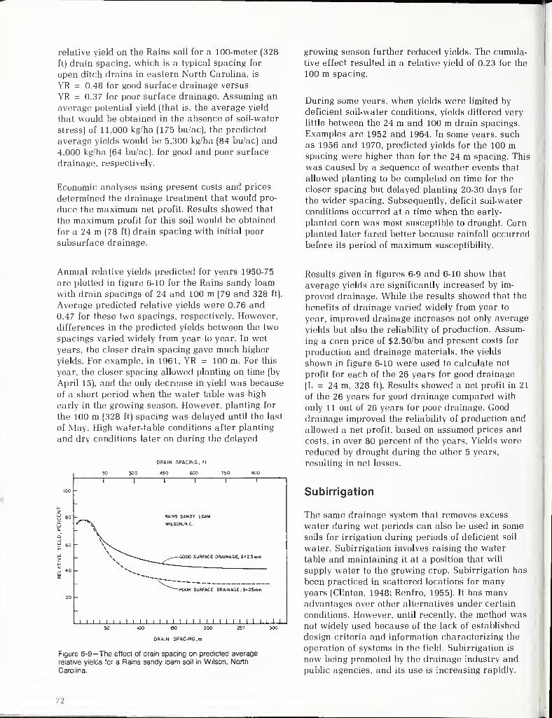
relative yield on the Rains soil for a 100-meter (328

ft) drain spacing, which is a typical spacing for

open ditch drains in eastern North Carolina, is

YR = 0.48 for good surface drainage versus

YR = 0.37 for poor surface drainage. Assuming an

average potential yield (that is, the average yield

that would be obtained in the absence of soil-water

stress) of 11,000 kg/ha (175 bu/ac), the predicted

average yields would be 5,300 kg/ha (84 bu/ac) and

4,000 kg/ha (64 bu/ac), for good and poor surface

drainage, respectively.

Economic analyses using present costs and prices

determined the drainage treatment that would pro-

duce the maximum net profit. Results showed that

the maximum profit for this soil would be obtained

for a 24 m (78 ft) drain spacing with initial poor

subsurface drainage.

growing season further reduced yields. The cumula-

tive effect resulted in a relative yield of 0.23 for the

100 m spacing.

During some years, when yields were limited by

deficient soil-water conditions, yields differed very

little between the 24 m and 100 m drain spacings.

Examples are 1952 and 1964. In some years, such

as 1956 and 1970, predicted yields for the 100 mspacing were higher than for the 24 m spacing. This

was caused by a sequence of weather events that

allowed planting to be completed on time for the

closer spacing but delayed planting 20-30 days for

the wider spacing. Subsequently, deficit soil-water

conditions occurred at a time when the early-

planted corn was most susceptible to drought. Corn

planted later fared better because rainfall occurred

before its period of maximum susceptibility.

Annual relative yields predicted for years 1950-75

are plotted in figure 6-10 for the Rains sandy loam

with drain spacings of 24 and 100 m (79 and 328 ft).

Average predicted relative yields were 0.76 and

0.47 for these two spacings, respectively. However,

differences in the predicted yields between the two

spacings varied widely from year to year. In wet

years, the closer drain spacing gave much higher

yields. For example, in 1961, YR = 100 m. For this

year, the closer spacing allowed planting on time (by

April 15), and the only decrease in yield was because

of a short period when the water table was high

early in the growing season. However, planting for

the 100 m (328 ft) spacing was delayed until the last

of May. High water-table conditions after planting

and dry conditions later on during the delayed

DRAIN SPACING, ft.

150 300 450 600 750 900

100

1 1 1 1 1 1

80 RAINS SANDY LOAM

\ WILSON, NX.

feO ~ vv

\_.— GOOD SURFACE DRAINAGE, S-2 Smm

10

~POOH SURFACE DRAINAGE . S- 25mm

20

1 1 11 1 1 1 1 1 1 1 1 1 1 1 1 1 1 1 1 1 1 1 1 1 1 1 1 1 1 1

150 200

DRAIN SPACING,

m

Figure 6-9—The effect of drain spacing on predicted average

relative yields fcr a Rams sandy loam soil in Wilson, North

Carolina.

Results given in figures 6-9 and 6-10 show that

average yields are significantly increased by im-

proved drainage. While the results showed that the

benefits of drainage varied widely from year to

year, improved drainage increases not only average

yields but also the reliability of production. Assum-

ing a corn price of $2.50/bu and present costs for

production and drainage materials, the yields

shown in figure 6-10 were used to calculate net

profit for each of the 26 years for good drainage

(L = 24 m, 328 ft). Results showed a net profit in 21

of the 26 years for good drainage compared with

only 11 out of 26 years for poor drainage. Good

drainage improved the reliability of production and

allowed a net profit, based on assumed prices and

costs, in over 80 percent of the years. Yields were

reduced by drought during the other 5 years,

resulting in net losses.

Subirrigation

The same drainage system that removes excess

water during wet periods can also be used in some

soils for irrigation during periods of deficient soil

water. Subirrigation involves raising the water

table and maintaining it at a position that will

supply water to the growing crop. Subirrigation has

been practiced in scattered locations for manyyears (Clinton, 1948; Renfro, 1955). It has manyadvantages over other alternatives under certain

conditions. However, until recently, the method wasnot widely used because of the lack of established

design criteria and information characterizing the

operation of systems in the field. Subirrigation is

now being promoted by the drainage industry and

public agencies, and its use is increasing rapidly.

72

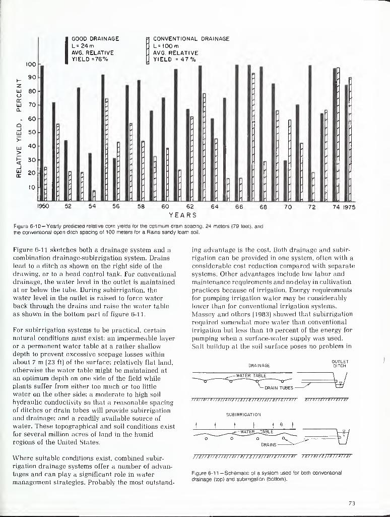
I-

100

90

LU 80OrrLU toa.

» 60Q_lLU 50>-

UJ 40>

< 30_lUJ 20

GOOD 1DRAINAGE * CONVENTIONAL (DRAINAGE

1 L = 24 m \ L =1 00 m

1 AVG. RELATIVE , AVG. RELATIVE

_] YIELD =76%

\ YIELD = 47%

pi•>

- * *

'

*

'*l

n ,p -

_ • p •* <

* .* <• '

<• ' -H .<

*

„*

*

*

3

*

*

**

* *

-

* p

-<

* '* *

*-

' *" *« *

*

*

p •>

** ' * _ * • *

'*

**

< >* '

' " • »

<-

,* n * ' * ' * * + .*

• > *>*

* • * *

1 * * » , -

R4

' *'

. pi c*

- - » * r

.f

*<

. * .*>

' * _ p- * ' «* - * ., '

.

'

I

'

.

'r-

t* *

* *• * '* ' - * - * - <

-

*-

*» <•

*

B :

10 -.

1950 52 54 56 58 60 62

YEARS64 66 68 70 72 74 1975

Figure 6-10— Yearly predicted relative corn yields for the optimum dram spacing, 24 meters (79 feet), and

the conventional open ditch spacing of 100 meters for a Rains sandy loam soil.

Figure 6-11 sketches both a drainage system and a

combination drainage-subirrigation system. Drains

lead to a ditch as shown on the right side of the

drawing, or to a head control tank. For conventional

drainage, the water level in the outlet is maintained

at or below the tube. During subirrigation, the

water level in the outlet is raised to force waterback through the drains and raise the water table

as shown in the bottom part of figure 6-11.

For subirrigation systems to be practical, certain

natural conditions must exist: an impermeable layer

or a permanent water table at a rather shallow

depth to prevent excessive seepage losses within

about 7 m (23 ft) of the surface; relatively flat land,

otherwise the water table might be maintained at

an optimum depth on one side of the field while

plants suffer from either too much or too little

water on the other side; a moderate to high soil

hydraulic conductivity so that a reasonable spacing

of ditches or drain tubes will provide subirrigation

and drainage; and a readily available source of

water. These topographical and soil conditions exist

for several million acres of land in the humidregions of the United States.

Where suitable conditions exist, combined subir-

rigation drainage systems offer a number of advan-

tages and can play a significant role in water

management strategies. Probably the most outstand-

ing advantage is the cost. Both drainage and subir-

rigation can be provided in one system, often with a

considerable cost reduction compared with separate

systems. Other advantages include low labor and

maintenance requirements and no delay in cultivation

practices because of irrigation. Energy requirements

for pumping irrigation water may be considerably

lower than for conventional irrigation systems.

Massey and others (1983) showed that subirrigation

required somewhat more water than conventional

irrigation but less than 10 percent of the energy for

pumping when a surface-water supply was used.

Salt buildup at the soil surface poses no problem in

DRAINAGEOUTLETDITCH

-WATER TABLE

DRAIN TUBES -

77777777777777777777777777777777777777777"

SUBIRRIGATION

I I

y77777777777777777

777777777777777777/77777777777^7777777" 7T77777T77T77777W

Figure 6-1 1 —Schematic of a system used for both conventional

drainage (top) and subirrigation (bottom).

73

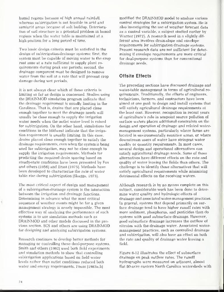
humid regions because of high annual rainfall,

whereas subirrigation is not feasible in arid and

semiarid areas because of salt buildup. Deteriora-

tion of soil structure is a potential problem in humidregions when the water table is maintained at a

high position for a long period of time.

Two basic design criteria must be satisfied in the

design of subirrigation-drainage systems: first, the

system must be capable of moving water to the crop

root zone at a rate sufficient to supply plant re-

quirements during peak use periods; second, the

drainage component must be designed to removewater from the soil at a rate that will prevent crop

damage during wet periods.

It is not always clear which of these criteria is

limiting so far as design is concerned. Studies using

the DRAINMOD simulation program indicate that

the drainage requirement is usually limiting in the

Carolinas. That is, drains that are placed close

enough together to meet the drainage needs will

usually be close enough to supply the irrigation

water needs when the outlet water level is raised

for subirrigation. On the other hand, simulations for

conditions in the Midwest indicate that the irriga-

tion requirement is usually limiting. In this case,

drains placed close enough together to satisfy the

drainage requirements, even when the system is being

used for subirrigation, may not be close enough to

supply the irrigation requirements. Methods for

predicting the required drain spacing based on

steady-state conditions have been presented by Foxand others (1956) and Ernst (1975). Methods havebeen developed to characterize the rate of watertable rise during subirrigation (Skaggs, 1973).

The most critical aspect of design and managementof a subirrigation-drainage system is the interaction

between the irrigation and drainage functions.

Determining in advance what the most critical

sequence of weather events might be for a given

management strategy is nearly impossible. The most

effective way of analyzing the performance of such

systems is to use simulation methods such as

DRAINMOD and other models discussed in the pre-

vious section. SCS and others are using DRAINMODfor designing and analyzing subirrigation systems.

Research continues to develop better methods for

managing or controlling these dual-purpose systems.

Smith and others (1982) used both field experiments

and simulation methods to show that controlling

subirrigation applications based on field waterlevels rather than outlet conditions reduced both

water and energy requirements. Fouss (1983a, b)

modified the DRAINMOD model to analyze various

control strategies for a subirrigation system. He is

also investigating the use of weather forecast data

as a control variable, a subject studied earlier by

Warner (1972). A research need in a slightly dif-

ferent area involves drain-slope and envelope

requirements for subirrigation drainage systems.

Present research data are not sufficient for deter-

mining if envelope requirements are more critical

for dual-purpose systems than for conventional

drainage needs.

Offsite Effects

The preceding sections have discussed drainage and

water-table management in terms of agricultural re-

quirements. Traditionally, the efforts of engineers,

technicians, farmers, and contractors have been

aimed at one goal: to design and install systems that

will satisfy agricultural drainage requirements at

the least cost. However, recognition in recent years

of agriculture's role in nonpoint source pollution of

surface waters places additional constraints on the

design and operation of drainage and related water-

management systems, particularly where farms are

located in environmentally sensitive areas, or where

downstream users of water have stringent water

quality or quantity requirements. In most cases,

several design and operational alternatives can

satisfy agricultural drainage needs. Some of those

alternatives have different effects on the rate and

quality of water leaving the fields than others. The

challenge is to identify those alternatives that will

satisfy agricultural requirements while minimizing

detrimental effects on the receiving waters.

Although research is by no means complete on this

subject, considerable work has been done to deter-

mine water quality and hydrologic effects of

drainage and associated water-management practices.

In general, systems that depend primarily on sur-

face drainage tend to have higher runoff rates with

more sediment, phosphorus, and pesticides than do

systems with good subsurface drainage. However,

good subsurface drainage increases the outflow of

nitrates with the drainage water. Associated water-

management practices, such as controlled drainage

and subirrigation, will also have an effect on both

the rate and quality of drainage water leaving a

field.

Figure 6-12 illustrates the effect of subsurface

drainage on peak outflow rates. The runoff

hydrographs were measured on adjacent, almost

flat 80-acre eastern North Carolina watersheds with

74

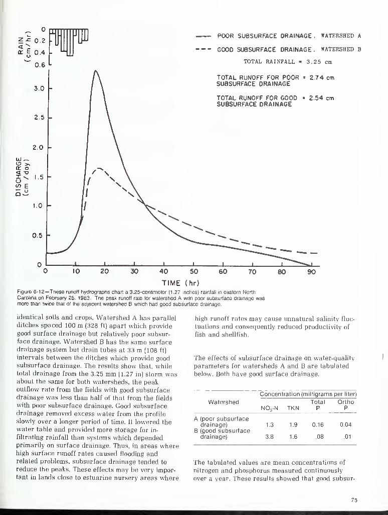
POOR SUBSURFACE DRAINAGE ,WATERSHED A

GOOD SUBSURFACE DRAINAGE, WATERSHED B

TOTAL RAINFALL = 3.25 cm

TOTAL RUNOFF FOR POOR * 2 74 cmSUBSURFACE DRAINAGE

TOTAL RUNOFF FOR GOOD • 2.54 cmSUBSURFACE DRAINAGE

TIME (hr)

Figure 6-12—These runoff hydrographs chart a 3.25-centimeter (1.27 inches) rainfall in eastern North

Carolina on February 28, 1983. The peak runoff rate for watershed A with poor subsurface drainage wasmore than twice that of the adjacent watershed B which had good subsurface drainage.

identical soils and crops. Watershed A has parallel

ditches spaced 100 m (328 ft) apart which provide

good surface drainage but relatively poor subsur-

face drainage. Watershed B has the same surfacedrainage system but drain tubes at 33 m (108 ft)

intervals between the ditches which provide goodsubsurface drainage. The results show that, whiletotal drainage from the 3.25 mm (1.27 in) storm wasabout the same for both watersheds, the peakoutflow rate from the fields with good subsurfacedrainage was less than half of that from the fields

with poor subsurface drainage. Good subsurfacedrainage removed excess water from the profile

slowly over a longer period of time. It lowered the

water table and provided more storage for in-

filtrating rainfall than systems which dependedprimarily on surface drainage. Thus, in areas wherehigh surface runoff rates caused flooding andrelated problems, subsurface drainage tended to

reduce the peaks. These effects may be very impor-tant in lands close to estuarine nursery areas where

high runoff rates may cause unnatural salinity fluc-

tuations and consequently reduced productivity of

fish and shellfish.

The effects of subsurface drainage on water-quality

parameters for watersheds A and B are tabulated

below. Both have good surface drainage.

Concentration (milligrams per liter)

WatershedN03-N TKN

TotalP

OrthoP

A (poor subsurfacedrainage) 1.3

B (good subsurfacedrainage) 3.8

1.9

1.6

0.16

.08

0.04

.01

The tabulated values are mean concentrations of

nitrogen and phosphorus measured continuously

over a year. These results showed that good subsur-

75

face drainage increased nitrate outflow but reduced

the loss of phosphorus (P) to drainage waters.

Improvement of surface drainage has the opposite

effect. Thus, if P concentrations in receiving waters

are critically high, better subsurface drainage

would improve the situation. Improved surface

drainage or the use of drainage outlet controls to

increase surface runoff would also reduce nitrate

outflow. Controlled drainage methods have been used

(Willardson and others, 1972: Gilliam and others,

1979) to promote denitrification and to reduce the

amount of nitrate entering ground and surface

waters. Skaggs and Gilliam (1981) used field results

and simulation modeling to show the effects of

drainage design and operation on nitrate losses

from a soil with poor natural drainage. The systems

considered satisfied agricultural drainage require-

ments for corn. Results showed an annual average

loss of 39 kg/ha (35 lbs/ac) for a conventional system

with poor surface drainage and good subsurface

drainage. By improving the surface drainage andcontrolling the subsurface outlet during the winter

months, the annual nitrate loss could be reduced to

14.5 kg/ha (12.9 lbs/ac).

Clinton, F. M. 1967. "'Invisible Irrigation on Egin

Bench," Reclamation Era. Vol. 34, pp. 182-184.

Day, P. R., G. H. Bolt, and D. M. Anderson. 1967.

"Nature of Soil Water." Irrigation of Agricultural

Lands (ed. R. M. Hagan and others). Monograph No.

11. Madison, Wise: Am. Soc. Agron., pp. 193-208.

Dumm, L. D. 1954. "New Formula for Determining

Depth and Spacing of Subsurface Drains in Ir-

rigated Lands," Agricultural Engineering. Vol. 35,

pp. 726-730.

Dumm, L. D. 1964. Transient Flow Concept in Sub-

surface Drainage: Its Validity and Use. Transactions

of the ASAE. Vol. 7, No. 2, pp. 142-146.

Ernst, L. F. 1975. Formulae for Groundwater Flow in

Areas With Subirrigation by Means of Open Con-

duits With a Raised Water Level. Misc. reprint 178.

Wageningen, The Netherlands: Institute for Landand Water Management Research.

These examples emphasize that various drainage

and associated water-management practices have

different effects on the rate and quality of runoff

water. By careful design and operation of water-

management systems, agricultural managementrequirements may be satisfied while minimizing

offsite detrimental effects. To achieve this goal, the

principles involved and the factors controlling off-

site conditions and requirements as well as farm

drainage needs must be understood and considered.

Fouss, J. L. 1983a. Simulated Controlled Operation

of Subsurface Drainage - Irrigation Systems. ASAEPaper No. 83-2567. St. Joseph, Mich.: Am. Soc. Agr.

Eng.

Fouss, J. L. 1983b. Daily Weather Forecast Rainfall

Probability as an Input to a Water ManagementSimulation Model. Proceedings of the Natural

Resources Modeling Symposium, U.S. Dept. Agr.,

Agr. Res. Serv.

References

Belmans, C, J. G. Wesseling, and R. A. Feddes.

1983. "Simulation Model of the Water Balance in a

Cropped Soil: SWATRE." Journal of Hydrology. Vol.

63, pp. 271-286.

Bouwer, FL, and J. van Schilfgaarde. 1963.

Simplified Method of Predicting the Fall of WaterTable in Drained Land. Transactions of the ASAE.Vol. 6, No. 4, pp. 288-291, 296.

Buckingham, E. 1907. Studies of the Movement of

Soil Moisture. Bull. No. 38, U.S. Dept. Agr., Bureauof Soils.

Childs, E. C. 1969. Introduction to the Physical Basis

of Soil Water Phenomena. London: Wiley-

Interscience, pp. 125-128.

Fox, R. L., J. T. Phelan, and W. D. Criddle. 1956.

"Design of Subirrigation Systems," Agricultural

Engineering. Vol. 37, No. 2, pp. 103-107.

Gayle, G. A., and R. W. Skaggs. 1978. Surface

Storage on Bedded Cultivated Lands. Transactions

of the ASAE. Vol. 21, No. 1, pp. 102-104, 109.

Gilliam, J. W., R. W. Skaggs, and S. B. Weed. 1979.

"Drainage Control to Diminish Nitrate Loss from

Agricultural Fields, "Journal of Environmental

Quality. Vol. 8, pp. 137-142.

Hardjoamidjojo, S., R. W. Skaggs, and G. O.

Schwab. 1982. Predicting Corn Yield Response to Ex-

cessive Soil Water Conditions. Transactions of the

ASAE. Vol. 25, No. 4, pp. 922-927, 934.

76

Hiler, E. A. 1969. Quantitative Evaluation of Crop-

Drainage Requirements. Transactions of the ASAE.

Vol. 12, No. 3. pp. 499-505.

Richards, L. A. 1965. "Physical Conditions of Waterin Soil," Methods of Soii Anaiysis. Monograph No. 9,

Madison, Wise: Am. Soc. Agron.

Kirkham, D. 1964. Physical Artifacts and Formulas

for Approximating Water Tabie FaJi in Tile-Drained

Land. Soil Sci. Soc. Amer. Proc, Vol. 28, pp.

585-590.

Kirkham, D., and W. L. Powers. 1972. Advanced Soil

Physics. New York: Wiley-Interscience.

Krenzer, E. G., Jr., and W. T. Fike. 1977. Corn Pro-

duction Guide—Planting and Plant Population. North

Carolina Agr. Ext. Serv., N.C. State Univ., Raleigh.

Lagace, R. 1973. "Modele de Comportenent des

Nappe en Sol Agricole," Genie Rural - Laval,

(Quebec, Canada), Vol. 5, No. 4, pp. 26-35.

Schwab, G. O., N. R. Fausey, and D. W. Michener.

1974. Comparison of Drainage Methods in a HeavyTextured Soil. Transactions of the ASAE. Vol. 17,

No. 3, pp. 424, 425, 428.

Skaggs, R. W. 1973. Water Table Movement During

Subirrigation. Transactions of the ASAE. Vol. 16,

No. 5, pp. 988-993.

Skaggs, R. W. 1975. "Drawdown Solutions for

Simultaneous Drainage and ET," Journal of the Ir-

rigation and Drainage Division. ASCE. Vol. 101(IR4),

pp. 279-291.

Luthin, J. N. 1957. "Drainage of Irrigated Lands,"

Drainage of Agricultural Lands (ed. J. N. Luthin).

Monograph No. 11. Madison, Wise: Am. Soc.

Agron., pp. 344-371.

Massey, F. C, R. W. Skaggs, and R. E. Sneed. 1983.

Energy and Water Requirements for Subirrigation

Versus Sprinkler Irrigation. Transactions of the

ASAE. Vol. 26, No. 1, pp. 126-133.

Moody, W. T. 1966. "Nonlinear Differential Equa-

tion of Drain Spacing," Journal of the Irrigation and

Drainage Division. ASCE. Vol. 92(IR2), pp. 1-9.

Nolte, B. H., D. M. Byg, and W. E. Gill. 1976. Timely

Field Operations for Corn and Soybeans in Ohio.

Bull. 605. Coop. Ext. Serv., Ohio State Univ., Columbus.

Ravelo, C. J., D. L. Reddell, E. A. Hiler, and R. W.Skaggs. 1982. Incorporating Crop Needs into

Drainage System Design. Transactions of the ASAE.Vol. 25, No. 3, pp. 623-629, 637.

Reeve, R. C, and N. Fausey. 1974. "Drainage andTimeliness of Farming Operations," Drainage for

Agriculture. Monograph No. 17 (ed. J. van

Schilfgaarde). Madison, Wise: Am. Soc. Agron., pp.

55-66.

Renfro, George, Jr. 1955. "Applying Water Underthe Surface of the Ground." Water: Yearbook of

Agriculture, 1955. U.S. Dept. Agr., pp. 173-178.

Skaggs, R. W. 1978b. A Water Management Model

for Shallow Water Table Soils. Technical Report No.

134. Water Resources Research Institute of the

Univ. of North Carolina. N.C. State Univ., Raleigh.

Skaggs, R. W. 1979. Factors Affecting Hydraulic

Conductivity Determinations from DrawdownMeasurements. ASAE Paper No. 79-2075, presented

at the summer meeting of the Am. Soc. Agr. Eng.,

Winnipeg, Manitoba.

Skaggs, R. W. 1980. A Water Management Model

for Artificially Drained Soils. Technical Bulletin No.

267. North Carolina Agri. Res. Serv., N.C. State

Univ., Raleigh.

Skaggs, R. W., and J. W. Gilliam. 1981. Effect of

Drainage System Design and Operation on Nitrate

Transport. Transactions of the ASAE. Vol. 24, No. 4,

pp. 929-934.

Skaggs, R. W., and A. Nassehzadeh-Tabrizi. 1983.

Optimum Drainage for Corn Production. Technical

Bulletin No. 274. North Carolina Agri. Res. Serv.,

N.C. State Univ., Raleigh.

Skaggs, R. W., and A. Nassehzadeh-Tabrizi. 1984.

Determining Design Drainage Rates for Optimum

Drainage. ASAE Paper No. 84-1055, St. Joseph,

Mich.: Am. Soc. Agr. Engr.

77

Skaggs, R. W., and Y. K. Tang. 1976. "Saturated

and Unsaturated Flow to Parallel Drains," Journal

of Irrigation and Drainage Division. ASCE. Vol.

102(IR2). pp. 221-238.

Smith, M. C., R. W. Skaggs, and J. E. Parsons. 1982.

Subirrigation System Control for Water Use Efficiency.

ASAE Paper No. 82-2520. St. Joseph, Mich.: Am.Soc. Agr. Engr.

van Schilfgaarde, J. 1965. "Transient Design of

Drainage Systems," Journal of the Irrigation and

Drainage Division. ASCE. Vol. 91(IR3), pp. 9-22.

van Schilfgaarde, J. 1974. "Nonsteady Flow to

Drains," Drainage for Agriculture. Monograph No.

17. (ed. J. van Schilfgaarde). Madison, Wise: Am.Soc. Agron., pp. 245-270.

Warner, R. C. 1972. A Management Model for a

Controlled Drainage and Subirrigation System. M.S.

thesis, Clemson Univ., Clemson, S.C.

Wesseling. J. 1974. "Crop Growth and Wet Soils."

Drainage for Agriculture. Monograph No. 17 (ed. J.

van Schilfgaarde). Madison. Wise: Am. Soc. Agron.

pp. 7-37.

Williamson, R. E., and G. J. Kriz. 1970. Response of

Agricultural Crops to Flooding, Depth of WaterTable and Soil Composition. Transactions of the

ASAE. Vol. 13, No. 1. pp. 216-220.

Willardson, L. S., and others. 1972. Nitrate Reduc-

tion with Submerged Drains. Transactions of the

ASAE. Vol. 15, No. 1, pp. 84-90.

78

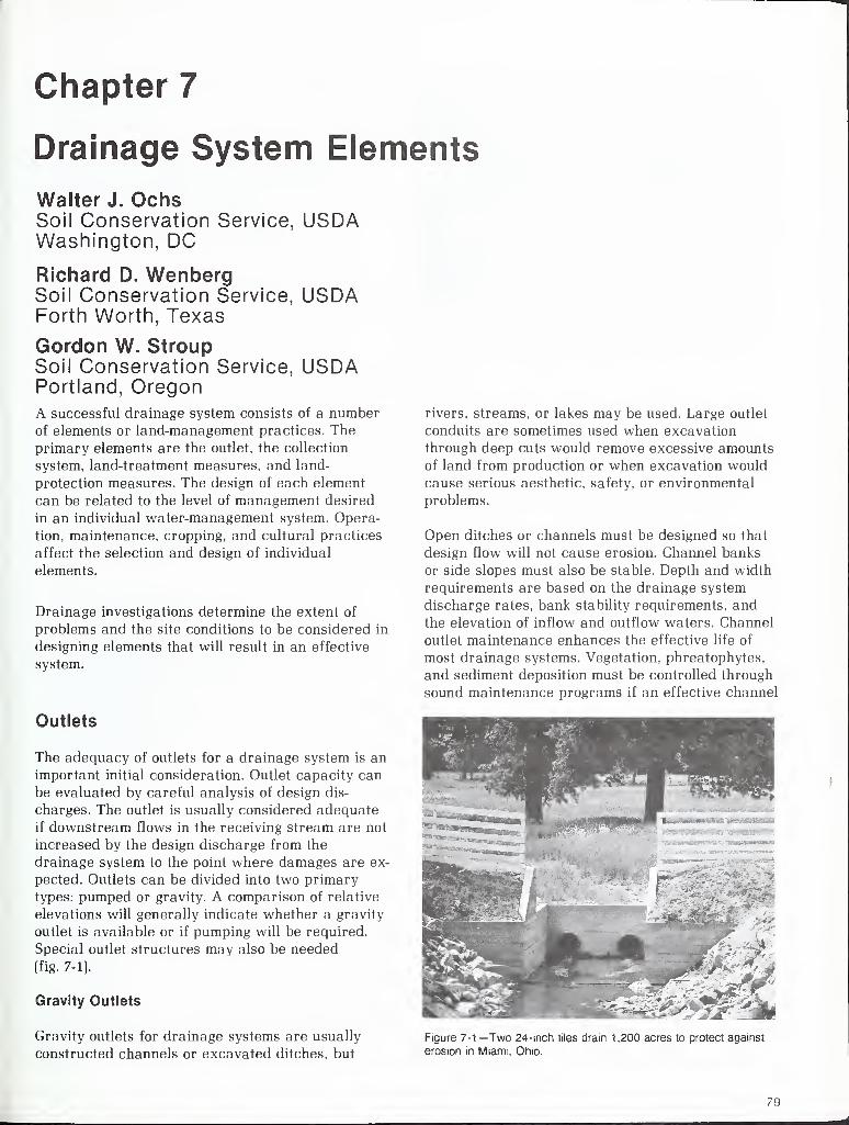
Chapter 7

Drainage System Elements

Walter J. OchsSoil Conservation Service, USDAWashington, DC

Richard D. WenbergSoil Conservation Service, USDAForth Worth, Texas

Gordon W. StroupSoil Conservation Service, USDAPortland, OregonA successful drainage system consists of a numberof elements or land-management practices. The

primary elements are the outlet, the collection

system, land-treatment measures, and land-

protection measures. The design of each element

can be related to the level of management desired

in an individual water-management system. Opera-

tion, maintenance, cropping, and cultural practices

affect the selection and design of individual

elements.

Drainage investigations determine the extent of

problems and the site conditions to be considered in

designing elements that will result in an effective

system.

Outlets

The adequacy of outlets for a drainage system is an

important initial consideration. Outlet capacity can

be evaluated by careful analysis of design dis-

charges. The outlet is usually considered adequate

if downstream flows in the receiving stream are not

increased by the design discharge from the

drainage system to the point where damages are ex-

pected. Outlets can be divided into two primary

types: pumped or gravity. A comparison of relative

elevations will generally indicate whether a gravity

outlet is available or if pumping will be required.

Special outlet structures may also be needed(fig. 7-1).

Gravity Outlets

Gravity outlets for drainage systems are usually

constructed channels or excavated ditches, but

rivers, streams, or lakes may be used. Large outlet

conduits are sometimes used when excavation

through deep cuts would remove excessive amounts

of land from production or when excavation would

cause serious aesthetic, safety, or environmental

problems.

Open ditches or channels must be designed so that

design flow will not cause erosion. Channel banks

or side slopes must also be stable. Depth and width

requirements are based on the drainage system

discharge rates, bank stability requirements, and

the elevation of inflow and outflow waters. Channel

outlet maintenance enhances the effective life of

most drainage systems. Vegetation, phreatophytes,

and sediment deposition must be controlled through

sound maintenance programs if an effective channel

Figure 7-1 —Two 24-inch tiles drain 1,200 acres to protect against

erosion in Miami, Ohio.

79

Air Relief Valve

Siphon Breaker

Trash Rack

Max, W. S—>J1

— —

I

? — —Min. W. S.-L I

' Pump

Forebay B Sumpsiii= in

=

hie in 5 in =iii=

Submerged Discharge'

SURFACE AND SUBSURFACE WATER

jrMotor

tH

PumpMax.

W.S.

111=111 =111 =111 sill=1=1

r- 111Drain^ -

> 3hi

in

iiTsin

Min.W.S.

Sump i

x±

Discharge Pipe

] Free Discharge

5 HIS |||= ||| = ||| = 111= 111 = 111= 111= 111= 1

SUBSURFACE WATER ONLY

Figure 7-2—A schematic of pumping plant layouts.

and drainage system is to continue to function

(USDA, SCS, 1971).

Pumped Outlets

Pumps can be used for the discharge of water from

drainage systems when a gravity flow outlet cannot

be obtained because of insufficient outlet depth, or

if outlet capacity is restricted because of backwaterfrom storm or tidal flooding. Pumped outlets are

normally more expensive than gravity outlets whenthe entire life of a drainage system is considered

because of the initial equipment cost as well as the

maintenance costs and energy requirements. Adetailed evaluation is often needed to detemine the

most effective and economical method of discharg-

ing the drainage water. Pumped outlets may be

preferred in some systems to protect wetland areas

which are valuable wildlife habitats.

Pumping plants can include one or more pumps,

power units, and appurtenances for lifting collected

drainage water to a shallower gravity outlet (fig.

7-2). Planning a pumped outlet requires considera-

tion of the entire drainage system so that diver-

sions, storage areas, channels, and gravity outlets

are used to the best advantage in determining

capacity, size, and operation of the pumps. Somepump outlets operate for relatively short periods

when high water levels in the receiving stream

would restrict flow capacity enough to cause ex-

cessive crop damage.

Collection Systems

A drainage system must include drains to collect

water from surface depressions, very flat surfaces,

and excessive soil water in the crop root zone. The

collection system contains elements such as drain-

age field ditches, subsurface drainage conduits,

pumped well drains, and/or combinations of the

three. Subsurface drains and surface drainage field

ditches are often constructed on the same land.

Both are often needed to provide the cropping

environment desired for effective production. Collec-

tion systems must be designed to remove excess

water from the surface of the soil and the crop root

Hi I

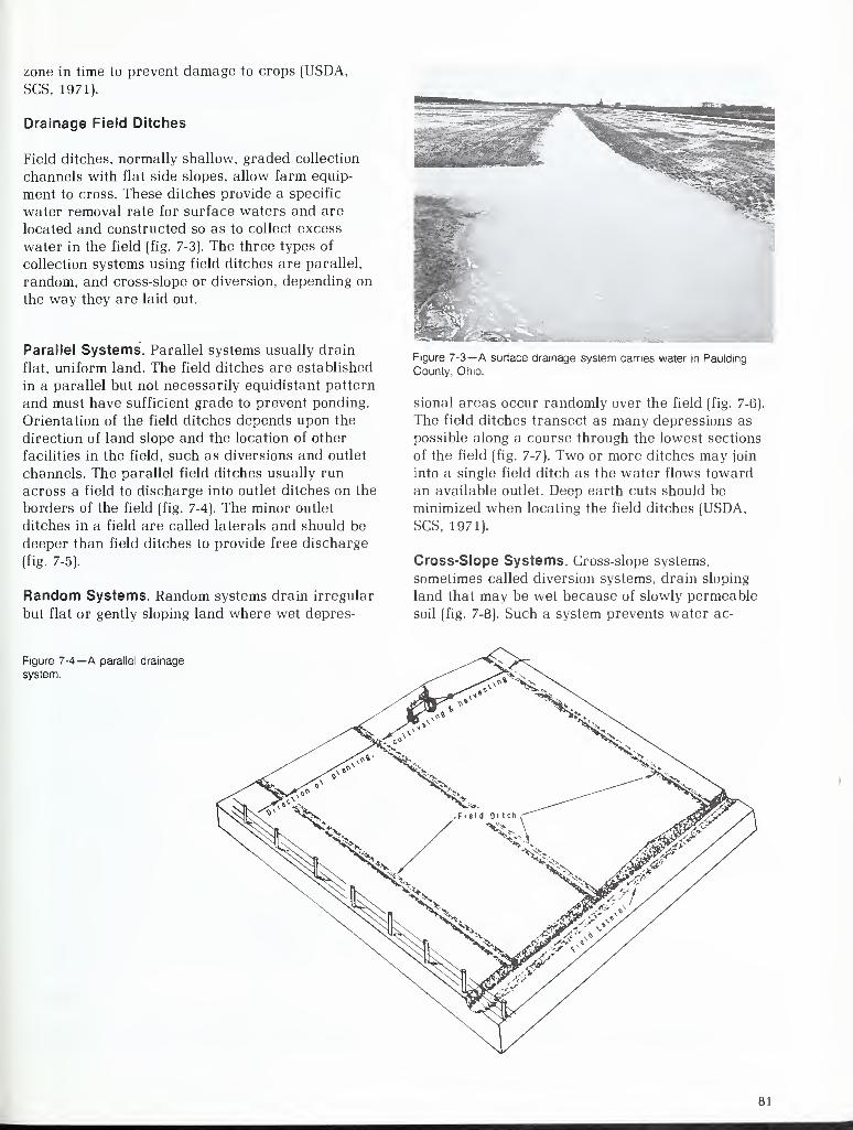
zone in time to prevent damage to crops (USDA,

SCS, 1971).

Drainage Field Ditches

Field ditches, normally shallow, graded collection

channels with flat side slopes, allow farm equip-

ment to cross. These ditches provide a specific

water removal rate for surface waters and are

located and constructed so as to collect excess

water in the field (fig. 7-3). The three types of

collection systems using field ditches are parallel,

random, and cross-slope or diversion, depending on

the way they are laid out.

Parallel Systems. Parallel systems usually drain

flat, uniform land. The field ditches are established

in a parallel but not necessarily equidistant pattern

and must have sufficient grade to prevent ponding.

Orientation of the field ditches depends upon the

direction of land slope and the location of other

facilities in the field, such as diversions and outlet

channels. The parallel field ditches usually run

across a field to discharge into outlet ditches on the

borders of the field (fig. 7-4). The minor outlet

ditches in a field are called laterals and should be

deeper than field ditches to provide free discharge

(fig. 7-5).

Random Systems. Random systems drain irregular

but flat or gently sloping land where wet depres-

Figure 7-3—A surface drainage system carries water in Paulding

County, Ohio.

sional areas occur randomly over the field (fig. 7-6).

The field ditches transect as many depressions as

possible along a course through the lowest sections

of the field (fig. 7-7). Two or more ditches may join

into a single field ditch as the water flows toward

an available outlet. Deep earth cuts should be

minimized when locating the field ditches (USDA,

SCS, 1971).

Cross-Slope Systems. Cross-slope systems,

sometimes called diversion systems, drain sloping

land that may be wet because of slowly permeable

soil (fig. 7-8). Such a system prevents water ac-

Figure 7-4—A parallel drainage

system.

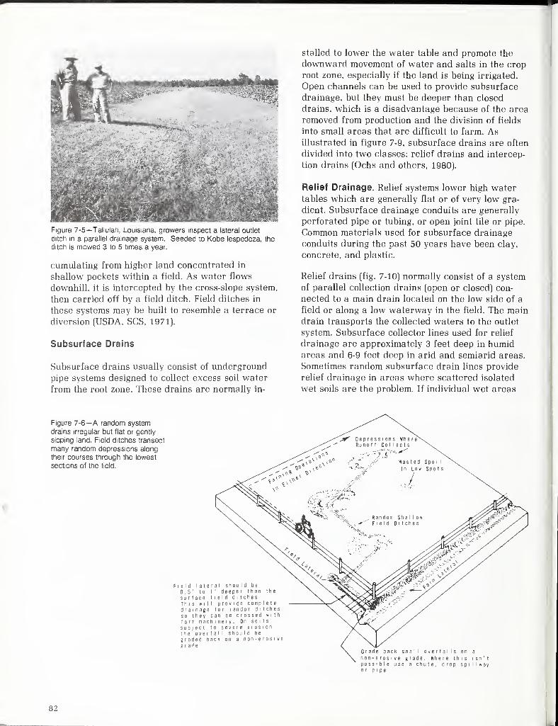
Figure 7-5— Tallulah, Louisiana, growers inspect a lateral outlet

ditch in a parallel drainage system. Seeded to Kobe lespedeza, the

ditch is mowed 3 to 5 times a year.

cumulating from higher land concentrated in

shallow pockets within a field. As water flows

downhill, it is intercepted by the cross-slope system,

then carried off by a field ditch. Field ditches in

these systems may be built to resemble a terrace or

diversion (USDA, SCS, 1971).

Subsurface Drains

Subsurface drains usually consist of underground

pipe systems designed to collect excess soil water

from the root zone. These drains are normally in-

stalled to lower the water table and promote the

downward movement of water and salts in the crop

root zone, especially if the land is being irrigated.

Open channels can be used to provide subsurface

drainage, but they must be deeper than closed

drains, which is a disadvantage because of the area

removed from production and the division of fields

into small areas that are difficult to farm. Asillustrated in figure 7-9, subsurface drains are often

divided into two classes: relief drains and intercep-

tion drains (Ochs and others, 1980).

Relief Drainage. Relief systems lower high watertables which are generally flat or of very low gra-

dient. Subsurface drainage conduits are generally

perforated pipe or tubing, or open joint tile or pipe.

Common materials used for subsurface drainage

conduits during the past 50 years have been clay,

concrete, and plastic.

Relief drains (fig. 7-10) normally consist of a system

of parallel collection drains (open or closed) con-

nected to a main drain located on the low side of a

field or along a low waterway in the field. The maindrain transports the collected waters to the outlet

system. Subsurface collector lines used for relief

drainage are approximately 3 feet deep in humidareas and 6-9 feet deep in arid and semiarid areas.

Sometimes random subsurface drain lines provide

relief drainage in areas where scattered isolated

wet soils are the problem. If individual wet areas

Figure 7-6—A random system

drains irregular but flat or gently

sloping land. Field ditches transect

many random depressions along

their courses through the lowest

sections of the field.

Field lateral shou I d be0.5' to 1

' deeper than the

surface field ditchesThis will provide comp I e t e

drainage for random ditchesso they can be crossed withfarm machinery. On soilssubject to severe erosionthe overfall should be

graded back on a non-erosg r a n e

Grade back small overfalls on a

non-erosive grade. Where this isn'tpossible use a chute, drop spillwayor pipe

82

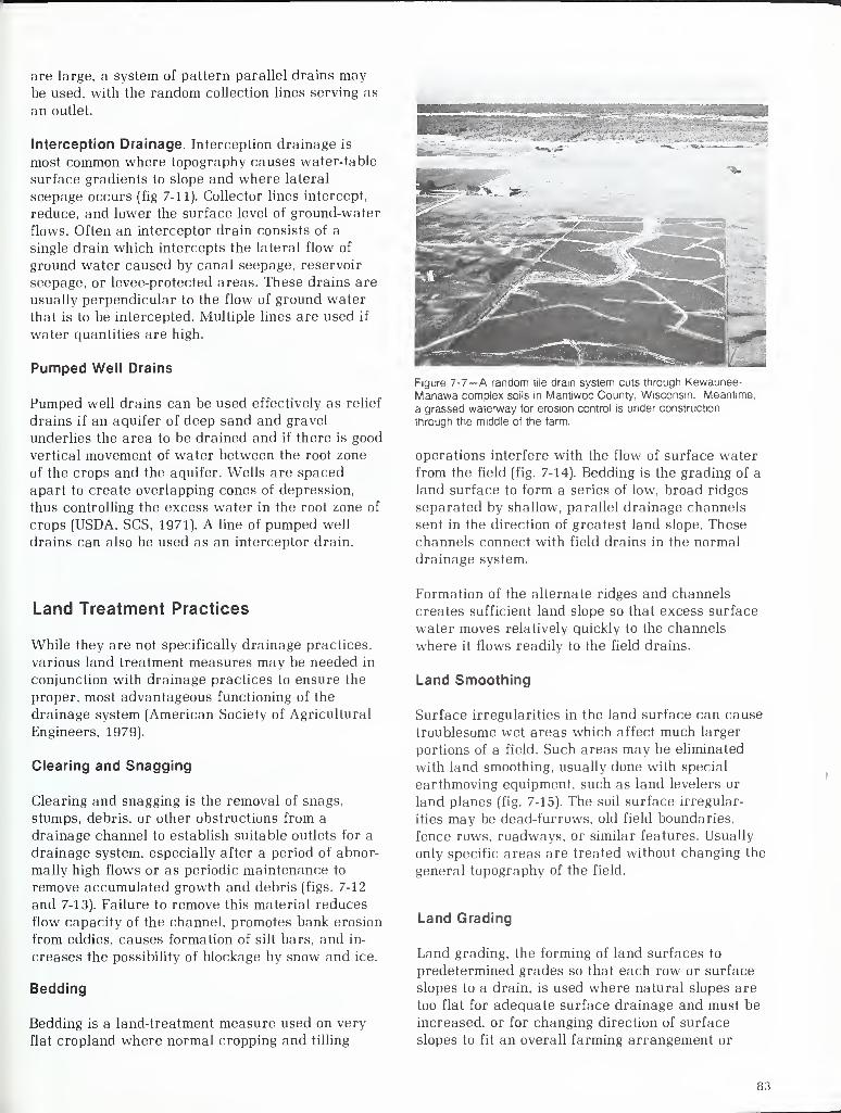
are large, a system of pattern parallel drains maybe used, with the random collection lines serving as

an outlet.

Interception Drainage. Interception drainage is

most common where topography causes water-table

surface gradients to slope and where lateral

seepage occurs (fig 7-11). Collector lines intercept,

reduce, and lower the surface level of ground-water

flows. Often an interceptor drain consists of a

single drain which intercepts the lateral flow of

ground water caused by canal seepage, reservoir

seepage, or levee-protected areas. These drains are

usually perpendicular to the flow of ground water

that is to be intercepted. Multiple lines are used if

water quantities are high.

Pumped Well Drains

Pumped well drains can be used effectively as relief

drains if an aquifer of deep sand and gravel

underlies the area to be drained and if there is good

vertical movement of water between the root zone

of the crops and the aquifer. Wells are spaced

apart to create overlapping cones of depression,

thus controlling the excess water in the root zone of

crops (USDA, SCS, 1971). A line of pumped well

drains can also be used as an interceptor drain.

Figure 7-7—A random tile dram system cuts through Kewaunee-

Manawa complex soils in Mantiwoc County, Wisconsin. Meantime,

a grassed waterway tor erosion control is under construction

through the middle of the farm.

operations interfere with the flow of surface water

from the field (fig. 7-14). Bedding is the grading of a

land surface to form a series of low, broad ridges

separated by shallow, parallel drainage channels

sent in the direction of greatest land slope. These

channels connect with field drains in the normal

drainage system.

Land Treatment Practices

While they are not specifically drainage practices,

various land treatment measures may be needed in

conjunction with drainage practices to ensure the

proper, most advantageous functioning of the

drainage system (American Society of Agricultural

Engineers, 1979).

Clearing and Snagging

Clearing and snagging is the removal of snags,

stumps, debris, or other obstructions from a

drainage channel to establish suitable outlets for a

drainage system, especially after a period of abnor-

mally high flows or as periodic maintenance to

remove accumulated growth and debris (figs. 7-12

and 7-13). Failure to remove this material reduces

flow capacity of the channel, promotes bank erosion

from eddies, causes formation of silt bars, and in-

creases the possibility of blockage by snow and ice.

Bedding

Bedding is a land-treatment measure used on very

flat cropland where normal cropping and tilling

Formation of the alternate ridges and channels

creates sufficient land slope so that excess surface

water moves relatively quickly to the channels

where it flows readily to the field drains.

Land Smoothing

Surface irregularities in the land surface can cause

troublesome wet areas which affect much larger

portions of a field. Such areas may be eliminated

with land smoothing, usually done with special

earthmoving equipment, such as land levelers or

land planes (fig. 7-15). The soil surface irregular-

ities may be dead-furrows, old field boundaries,

fence rows, roadways, or similar features. Usually

only specific areas are treated without changing the

general topography of the field.

Land Grading

Land grading, the forming of land surfaces to

predetermined grades so that each row or surface

slopes to a drain, is used where natural slopes are

too flat for adequate surface drainage and must be

increased, or for changing direction of surface

slopes to fit an overall farming arrangement or

83

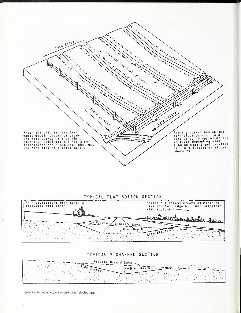
TYPICAL FLAT BOTTOM SECTION.Fill depressions with material Spread out excess excavated material

here so that ridge Hill not interferewith equipment- —

S&j&SL,

TYPICAL V-CHANNEL SECTION

-^_— _N aj uj_a_l_ Ground Level\- s/dT-^— '

: r™.— rr — -,°Pe.

j— M i n . Depth — —_^_

Figure 7-8— Cross-slope systems dram sloping land

84

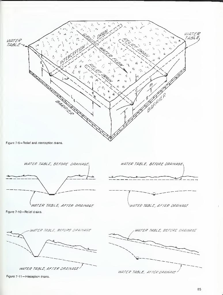
warts?

warts?

Figure 7-9— Relief and interception drains.

W/ir£/? r/?jffL£ 3EFOtf£ £>/Z4/A(4<S£ Hi4T£/? raSLt, £££#££ £>#4/M4G£

^WtfrfR T/)BL£ /Ifrf/? £>&4//MG£

Figure 7-10— Relief drains.

-«--

KyMT£P TABLf, /?£££/? 0/?/2/A//?&£

W4T£tf rdtfl £, SFFO/Ff Ptf/l/.V/IZf tV/lff/? r43L£ &£.F£/F<F £>M4/Atf£f

nur£/? r/i£L£t/t£r££ ££/?//)/JG£

Figure 7-1 1 — Inteception drams.

TNs

W4r££ 7%£L£ J/*T&?'£>/?/?/M4<?£

85

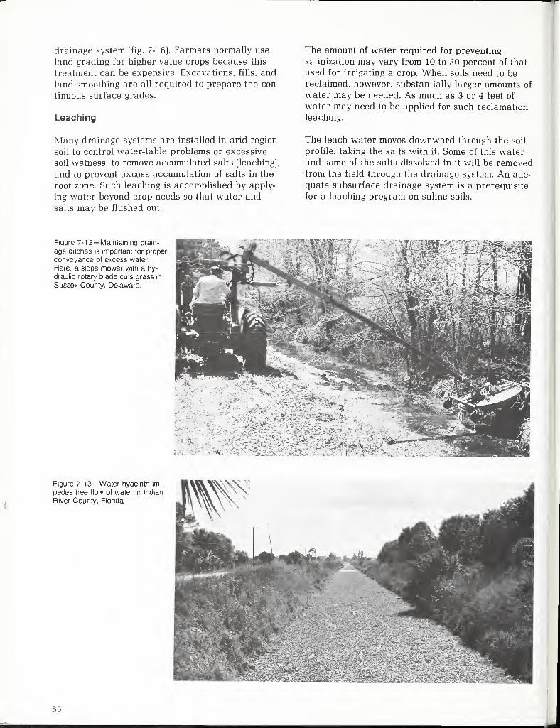
drainage system (fig. 7-16). Farmers normally use

land grading for higher value crops because this

treatment can be expensive. Excavations, fills, and

land smoothing are all required to prepare the con-

tinuous surface grades.

Leaching

The amount of water required for preventing

salinization may vary from 10 to 30 percent of that

used for irrigating a crop. When soils need to be

reclaimed, however, substantially larger amounts of

water may be needed. As much as 3 or 4 feet of

water may need to be applied for such reclamation

leaching.

Many drainage systems are installed in arid-region

soil to control water-table problems or excessive

soil wetness, to remove accumulated salts (leaching),

and to prevent excess accumulation of salts in the

root zone. Such leaching is accomplished by apply-

ing water beyond crop needs so that water and

salts may be flushed out.

The leach water moves downward through the soil

profile, taking the salts with it. Some of this waterand some of the salts dissolved in it will be removedfrom the field through the drainage system. An ade-

quate subsurface drainage system is a prerequisite

for a leaching program on saline soils.

Figure 7-12— Maintaining drain-

age ditches is important for proper

conveyance of excess water.

Here, a slope mower with a hy-

draulic rotary blade cuts grass in

Sussex County, Delaware.

'^H^f^'rX;:W,.

Figure 7-13—Water hyacinth im-

pedes free flow of water in Indian

River County, Florida.

86

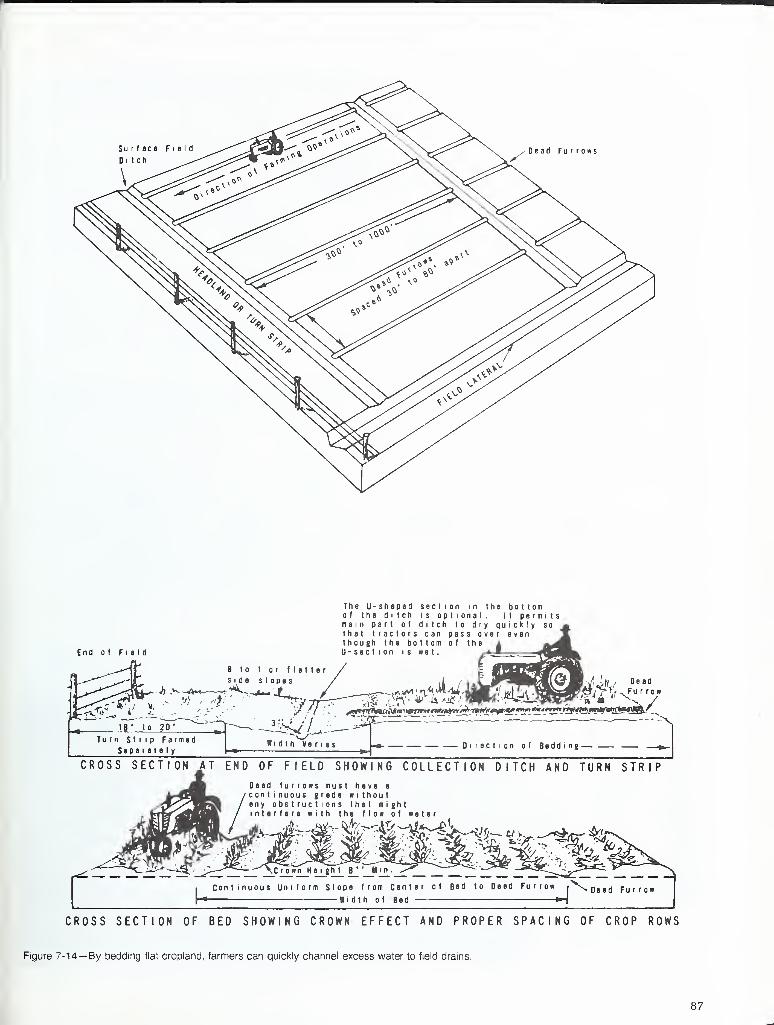
Surface Field

DitchDead Furrows

End of Field

The U-shaped section in the bottomof the ditch is optional. It permitsmain part of ditch to dry quickly sothat tractors can pass over eventhough the bottom of theU-section is net.

i < - V,J^^^By?ftw «W u^wff Dead

~^ iai ' i^M-iMMj 1

, J V^3fcs^P£*i , > , Fu r r o »

Direction of Bedding—CROSS SECTION,AT END OF FIELD SHOWING COLLECTION DITCH AND TURN STRIP

ad furrows must have a

ntinuout grade withouty obstructions that mightterfere with the flow of water

-#-.tri^MV%*****%own He i gh t

6 '

' Mi n

.

Continuous Uniform Slope from Center of Bed to Dead Furrow |^,[)ead FurrowWidth of Bed »-|

CROSS SECTION OF BED SHOWING CROWN EFFECT AND PROPER SPACING OF CROP ROWS

Figure 7-14— By bedding flat cropland, farmers can quickly channel excess water to field drains.

87

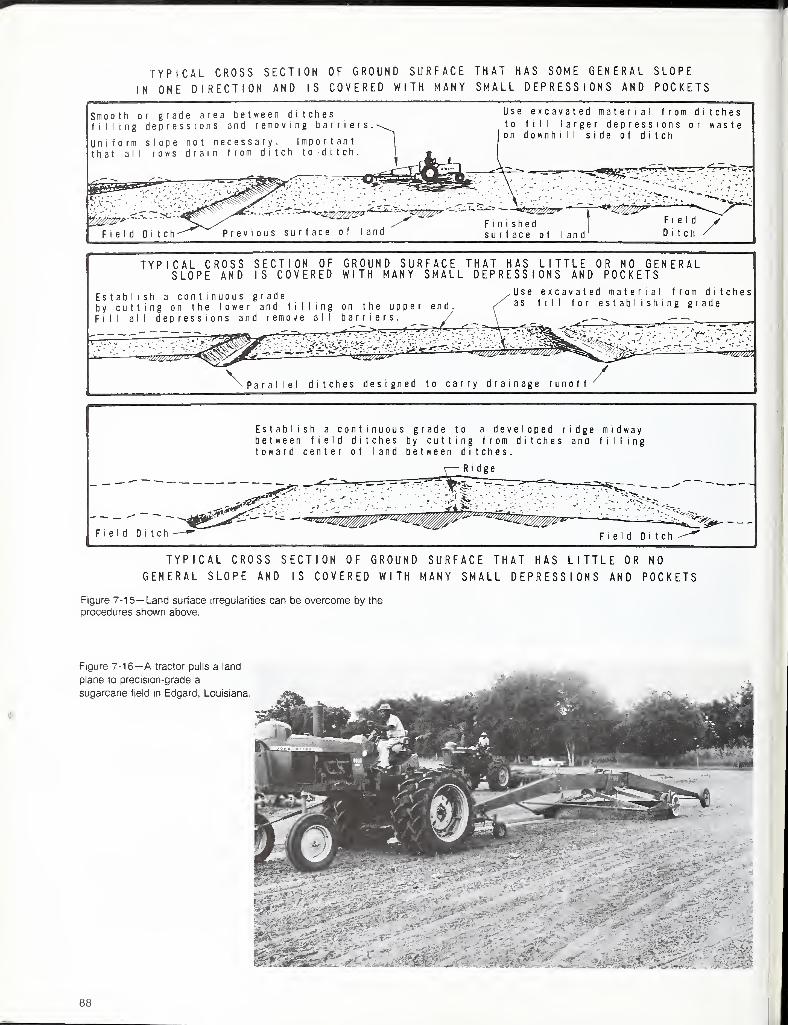
TYPICAL CROSS SECTION OF GROUND SURFACE THAT HAS SOME GENERAL SLOPE

IN ONE DIRECTION AND IS COVERED WITH MANY SMALL DEPRESSIONS AND POCKET!

Smooth or grade area between ditchesfilling depressions and removing barriers.

Uniform slope not necessary. Importantthat all rows drain from ditch to ditch.

Use excavated material from d

to fill larger depressions oron downhill side of ditch

^^3

i t cheswaste

Field Ditch Previous surface of landFinishedsurface of land

-*Bcrt^-Fi e I d

Ditch /TYPICAL CROSS SECTION OF GROUND SURFACE THAT HAS LITTLE OR NO GENERAL

SLOPE AND IS COVERED WITH MANY SMALL DEPRESSIONS AND POCKETS

Establish a continuous gradeby cutting on the lower and filling on the upper end.

Fill all depressions and remove all barriers. /

Use excavated material from ditchesas fill for establishing grade

,&* J

\ Par

/

asggjg;

allel ditches designed to carry drainage runof

Establish a continuous grade to a developed ridge midwaybetween field ditches by cutting from ditches ana fillingtoward center of land between ditches.

R i dge

Field Ditch§*- ---

Field Ditch

TYPICAL CROSS SECTION OF GROUND SURFACE THAT HAS LITTLE OR NO

GENERAL SLOPE AND IS COVERED WITH MANY SMALL DEPRESSIONS AND POCKETS

Figure 7-15— Land surface irregularities can be overcome by the

procedures shown above.

Figure 7-16—A tractor pulls a land

plane to precision-grade a

sugarcane field in Edgard, Louisiana.

&K

88

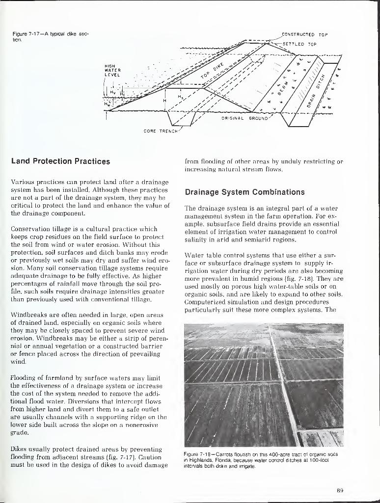
Figure 7-17—A typical dike sec-

tion.

CONSTRUCTED TOP

CORE TRENCH^

Land Protection Practices

Various practices can protect land after a drainage

system has been installed. Although these practices

are not a part of the drainage system, they may be

critical to protect the land and enhance the value of

the drainage component.

Conservation tillage is a cultural practice whichkeeps crop residues on the field surface to protect

the soil from wind or water erosion. Without this

protection, soil surfaces and ditch banks may erode

or previously wet soils may dry and suffer wind ero-

sion. Many soil conservation tillage systems require

adequate drainage to be fully effective. As higher

percentages of rainfall move through the soil pro-

file, such soils require drainage intensities greater

than previously used with conventional tillage.

Windbreaks are often needed in large, open areas

of drained land, especially on organic soils wherethey may be closely spaced to prevent severe winderosion. Windbreaks may be either a strip of peren-

nial or annual vegetation or a constructed barrier

or fence placed across the direction of prevailing

wind.

Flooding of farmland by surface waters may limit

the effectiveness of a drainage system or increase

the cost of the system needed to remove the addi-

tional flood water. Diversions that intercept flows

from higher land and divert them to a safe outlet

are usually channels with a supporting ridge on the

lower side built across the slope on a nonerosive

grade.

Dikes usually protect drained areas by preventing

flooding from adjacent streams (fig. 7-17). Caution

must be used in the design of dikes to avoid damage

from flooding of other areas by unduly restricting or

increasing natural stream flows.

Drainage System Combinations

The drainage system is an integral part of a water

management system in the farm operation. For ex-

ample, subsurface field drains provide an essential

element of irrigation water management to control

salinity in arid and semiarid regions.

Water table control systems that use either a sur-

face or subsurface drainage system to supply ir-

rigation water during dry periods are also becoming

more prevalent in humid regions (fig. 7-18). They are

used mostly on porous high water-table soils or on

organic soils, and are likely to expand to other soils.

Computerized simulation and design procedures

particularly suit these more complex systems. The

Figure 7-18— Carrots flourish on this 400-acre tract of organic soils

in Hightends, Florida, because water control ditches at 100-foot

intervals both dram and irrigate.

8 'J

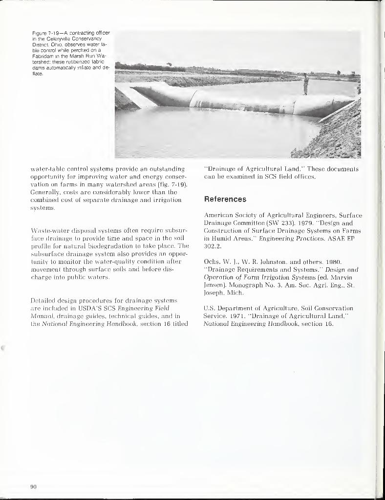
Figure 7-19—A contracting officer

in the Celeryville Conservancy

District. Ohio, observes water ta-

ble control while perched on a

Fabndam in the Marsh Run Wa-tershed; these rubberized fabric

dams automatically inflate and de-

flate.

water-table control systems provide an outstanding

opportunity for improving water and energy conser-

vation on farms in many watershed areas (fig. 7-19).

Generally, costs are considerably lower than the

combined cost of separate drainage and irrigation

systems.

Waste-water disposal systems often require subsur-

face drainage to provide time and space in the soil

profile for natural biodegradation to take place. The

subsurface drainage system also provides an oppor-

tunity to monitor the water-quality condition after

movement through surface soils and before dis-

charge into public waters.

Detailed design procedures for drainage systems

are included in USDA"S SCS Engineering Field

Manual, drainage guides, technical guides, and in

the National Engineering Handbook, section 16 titled

"'Drainage of Agricultural Land." These documentscan be examined in SCS field offices.

References

American Society of Agricultural Engineers, Surface

Drainage Committee (SW 233). 1979. "Design andConstruction of Surface Drainage Systems on Farmsin Humid Areas," Engineering Practices. ASAE EP302.2.

Ochs, W. J., W. R. Johnston, and others. 1980.

"Drainage Requirements and Systems," Design andOperation of Farm Irrigation Systems (ed. MarvinJensen). Monograph No. 3, Am. Soc. Agri. Eng., St.

Joseph, Mich.

U.S. Department of Agriculture, Soil Conservation

Service. 1971. "Drainage of Agricultural Land,"

National Engineering Handbook, section 16.

90

Chapter 8

Planning Farm and ProjectDrainage

Thomas C. G. Hodges and Douglas A. ChristensenSoil Conservation Service, USDAFort Worth, Texas

Because drainage usually involves substantial long-

term investments of capital and other costs, the

proper planning of farm and project drainage

systems is essential. Successful farm drainage

results in higher average and more stable farm in-

come since well-planned drainage systems ensure a

more efficient use of resources.

General Design and EconomicConsiderations

Soils needing improved drainage usually have the

greatest wetness problems during spring and fall,

which cause planting and harvesting delays that

reduce crop yields. Even when crops are planted on

time, a high water table restricts root development

and plant growth. As drier summer months approach,

the water table level drops quickly and plants

become susceptible to drought stress because the

root system cannot reach the water table level.

Plants tend to respond to improved drainage quickly,

so crop yields usually jump the first year after

drainage systems are installed. However, a numberof years of improved yields are necessary to

recover the initial investment. Farm drainage

systems sometimes cost as much as or more than

the land itself, especially when major outlet systems

are needed. Further, regular maintenance expend-itures are necessary to keep subsurface and sur-

face drainage systems functioning well.

Farm drainage systems cannot function properly

without adequate outlets or disposal works such as

streams, rivers, bays, or pumps. Drainage improve-

ment may be as minor as installing a short field

drain to improve a wet spot on a farm field, or as

complex as enlarging major channels and tributaries

with tile or open drainage ditches to remove excess

water from entire fields. The areas to be drained

may range from less than an acre to thousands of

acres.

Drainage improvements are technically complex andmust meet proper design standards to be effective.

In many cases, entire communities help plan anddevelop adequate drainage systems. Besides improv-

ing farm systems, existing farm drain outlet systems

may need to be enlarged and deepened. Majorsystems may require that highway and railroad

culverts and bridges be reorganized or modified.

Many States have passed laws that permit drainage

districts or similar organizations to develop, plan,

and install appropriate drainage works andsystems (see chapter 10).

Proper drainage systems can improve the local

economy and environment of entire communities,

with initial farm benefits spreading to agribusi-

nesses and financial institutions.

In planning farm and project drainage systems,

existing problems must be correctly identified

before appropriate solutions can be designed. Someproblems involve excessive water seepage from ad-

jacent hillsides. Other areas have pothole problems

where surface water is trapped in dish-shaped

depressions. Irrigation may aggravate drainage

problems when excess runoff and percolated water

must be carried away. In delta and coastal areas,

drainage is essential to carry floodwaters caused by

heavy rainfall from flatlands with fine textured

soils, or from areas with perched water tables

where water cannot move freely.

Ml

Various drainage problems and the damages they

cause are prime economic considerations in the

design of drainage systems. These damages on

cropland are reflected in increases in production

costs and reduced crop yields from excessive wet-

ness. The design of the system takes into account

cost efficiency as well as maintenance of crop pro-

ductivity and farm income. Important design factors

are proper ditch, tile, or channel depth and capacity,

road culvert and bridge openings, geologic condi-

tions, and downstream outlets which receive runoff

water while minimally affecting environmental and

economic resources.

In a sound drainage design, installation and mainte-

nance costs need to be balanced to ensure that the

system will function properly through its expected

lifespan. Careful operation and maintenance of the

system are necessary to attain the expected bene-

ficial effects that justify the investment.

Drainage engineers have worked to balance field

drain depth and capacity to fit the needs of crop

production. As farming practices change, design

criteria also change. For example, when farming

progressed from animal power to machine power,

better drainage became necessary to support heavy

equipment and provide proper traction. Tile or

other pipe drains were buried deeper to avoid being

damaged by heavy equipment, and surface drains

were designed to permit crossing by large

machinery.

Drainage systems must remove large volumes of

water quickly for plant survival and steady crop

growth. Plant requirements dictate the degree of

drainage that is justified. Field crops can usually

sustain wetter conditions than some specialty crops

such as vegetables. Removing runoff from moderate

rainfall episodes may suffice for field crops, but for

vegetable crops, quick removal may be necessary.

SCS has established design standards for various

resource areas and cropping systems within each State.

Total water management requires sophisticated

design and operation; this provides better use of

resources and higher crop yields. Subirrigation

helps moderate water-table fluctuations during low-

water periods from spring to fall. Engineers channel

and tile grades and install water control devices in

onfarm systems and outlet channels. Such intensive

water management requires more maintenance to

monitor soil moisture, rainfall, and runoff conditions

and to operate control devices. Water control struc-

tures are installed in the farm drainage systems to

reduce drainage when soils are dry. Sometimes

farmers pump water into the blocked off channels

to increase flow into the fields. Vegetation control is

easier because water in the ditches inhibits plant

growth.

Planning Farm Drainage

As a principle, the net economic benefit from

improved onfarm drainage is the amount by whichnet income with the drainage system exceeds net

income without the system. The net income changemay come from increased crop production, reducedproduction costs, or both. Net income is the com-

puted value of production less all associated costs

of production, including cost of the drainage system

itself. The latter also includes the value of any land

required by ditches or other improvements. Thegross value of crop production is the crop yield

times the price per unit of yield. Crop production

costs include the cost of seed, labor, power, water,

chemicals, and other materials plus prorated land,

machinery, or management charges. Crop produc-

tion costs with and without drainage systems maybe obtained from nearby farmers and local agri-

cultural leaders.

Feasibility Calculations

Benefit-cost ratios are a relative measure of annual

benefits of a proposed improvement compared with

its costs. Average annual installation cost is deter-

mined by amortizing the initial cost of a drainage

system at a current interest or other specified rate

over the life of the investment. In SCS, farm

drainage systems are usually amortized over an

expected life of 25 years and project systems for 50

years, assuming reasonable maintenance. The annual

cost of operation and maintenance, plus any other

recurring costs, are then added to amortized in-

stallation costs to get total annual costs. Theaverage benefit-cost ratio, total annual benefit

divided by total annual cost, shows the benefits

expected for each dollar of cost.

Many farmers encounter times when equipment gets

stuck in wet areas during farming operations,

resulting in lost time or the need to keep an extra

tractor nearby to pull the equipment out. Crops fre-

quently need to be replanted, requiring more pro-

duction inputs. Also, farmers may need to wait until

the ground freezes before they can harvest crops. If

the ground does not freeze, the crop may be lost if it

is wet at harvesttime. The extent to which these

MJ

drainage problems are reduced or eliminated is a

clear economic benefit of drainage systems.

Reliable information about changes in crop yield

with and without drainage is not as available as

that for production inputs. Farmers' experience is

one good source, although many do not keep in-

dividual field records, and yield differences are

more varied than production inputs. Information

from farmers, supplemented by data from research

and agricultural leaders, can be used to estimate

expected changes in yields and costs under various

conditions. Computer simulation models are also used

for estimating yield differentials.

Optimum Drainage Design

Drainage design decisions can be guided more effi-

ciently by referring to research than by makingfield-by-field calculations. Farm operators can makea partial comparison of open or surface versus sub-

surface drainage themselves when the soils andother conditions permit either method. The costs of

each method and effects of open drains or reducing

land in production can also be determined fairly

easily. However, data are not always available for

assessing the effect of alternative degrees of

drainage on crop yields.

Researchers have more access to data, methods,

and computer models to determine optimum drain

spacings and types of drainage. For example, USDAscientists have developed an "Erosion-Productivity

Impact Calculator" (EPIC), a comprehensive mathe-

matical model for determining the relationship be-

tween rates of water-induced soil erosion and soil

productivity in different U.S. regions (Williams andothers, 1983). Drainage conditions are one element

of the hydrology submodel of EPIC, along with rain-

fall, runoff, evapotranspiration, percolation, lateral

subsurface water flow, and irrigation. Other sub-

models consider weather, erosion, nutrients, soil

temperature, tillage practices, and economics. TheEPIC model thus permits a simultaneous analysis of

how crop yields, gross farm income, production

costs, and net income may be affected by numerousphysical and economic variables, including drainage.

A planning and optimizing model more specific to

questions of drainage system design is DRAINMOD,developed by agricultural engineers at North

Carolina State University. This model encompassesmulticomponent water management systems involving

surface drainage, subsurface drainage, subirriga-

tion, and sprinkler irrigation. It considers the

effects of alternative system designs involving dif-

ferent depths and spacing of subsurface drains oncrop yields, production and investment costs, andfarm profits. (See the Skaggs segment for a detailed

description and illustrated uses of DRAINMOD.)

A third model, combining a simulation model withan optimizing routine to minimize costs, has beendeveloped at Colorado State University (Durnford,

1982). Its object is to identify economically optimumdrainage systems using open and closed relief

drainage systems for arid irrigated areas. Thedrains facilitate proper leaching, thus limiting the

net buildup of the water table and reducing the

accumulation of salts in the root zone, especially if

the ground water is saline. Durnford's model is

adaptable to planning irrigation drainage in various

regions of the United States and other nations. Oneapplication has been to the Beni Magdoul area in

Middle Egypt.

Economic evaluations for project systems are

basically similar to those used for planning farmdrainage but naturally require a broader perspec-

tive. Yield and production input data need to be

representative, not site-specific. Alternative

drainage scenarios considering costs, production

inputs, and outputs are developed for each different

project area. Net returns with and without improveddrainage are compared to determine net benefits.

The costs of the project and associated improve-

ments are compared with all benefits in determining

net benefits and benefit-cost ratios.

A final point to mention for farm drainage planning

is that it often involves only one or a few decision-

makers—the owner, manager, or renter. They makecapital investments considering their individual in-

terests in the farm and its operations, accounting

for needs, costs, and effects. Detailed soil, cropping

system, and engineering data are used to determine

the type and extent of the problems and neededtreatment measures. All decisionmakers fit the cost

and expected benefits of drainage systems into their

overall financial or management plans.

Planning Project Drainage

The proper functioning of farm drainage systems

depends upon proper outlets. When several farms

have inadequate outlets, farmers need to plan a

satisfactory outlet system together. Project drainage

plans involve much the same basic information as farm

plans, but because many farmers and other interests

can be involved, quick agreements are frequently

difficult.

93

Information Needs

As the characteristics of decisionmakers in project

planning are diverse, inventory data can be moregeneral and less site-specific. Project planning must

also consider onfarm drainage needs. Reliable soils

and crop system data are necessary for both levels

of planning.

Engineering data ordinarily deal more with the

hydraulics of stream systems rather than with

single streams or specific farm situations. Engineers

estimate costs for the main and tributary channel-

work providing outlets for farm drainage. Theystudy alternate channel sizes to determine whichwill produce the most net benefits. Tributaries are

evaluated separately to determine if improvements

within them are justified in terms of producing net

benefits. Instream water control devices are ex-

amined for any possible complementary irrigation

benefits.

Environmental considerations also become morecritical in project planning because outlet im-

provements may disturb environmental resources,

especially if they impinge on fish and wildlife

habitat. SCS and the Fish and Wildlife Service

(FWS) have jointly developed and adopted uniform

Channel Modification Guidelines to assist their per-

sonnel in identifying when and where channel

modifications may be used as a technique for im-

plementing drainage and other land and waterresource projects. These standards require efforts

to maintain or restore streams, riparian vegetation,

and wetlands as viable ecosystems for fish andwildlife.

Moving water in main and tributary streams andchannels to areas where discharge water can movefreely without causing downstream damages can be

a different design problem. Proper planning of proj-

ect drainage must include the analyses of flood-

water from high direct precipitation which must be

carried by the project systems. This is one respect

in which project drainage is more complex than on-

farm drainage. Road and railroad bridges andculverts may be modified, and utilities may need to

be altered or moved. Drainage water from one farm

is channeled across another farm, sometimes from

one county to another county, and sometimes from

one State to another.

SCS provides technical assistance for farm and pro-

ject drainage planning, which must conform to State

and local laws and follow approval standards andspecifications. SCS project drainage assistance is

authorized under the Watershed Protection andFlood Prevention Act (P.L. 83-566), which calls for a

comprehensive approach toward solving flood

protection, water supply, drainage, and other

watershed problems. SCS investigates hydraulic

systems, hydrologic effects downstream, economicand social impacts, and project feasibility. Studies

are made to evaluate environmental resources andtheir protection. Similar studies are undertaken by

SCS in Resource Conservation and Development(RC&D) Projects involving drainage.

Cooperation in Drainage Planning

The Marshyhope Creek Watershed (100,600 acres)

spanning the Delaware-Maryland boundary is a

good example of how diverse environmental,

political, and economic interests can be brought

together to solve serious resource managementproblems. The project sponsors include the

Delaware State Soil Conservation Commission, the

Caroline County (Md.) Commissioners, the Caroline

Soil Conservation District, and the town of

Federalsburg, Md. The headwaters are in Kent

County, Del. The main channel flows southwest-

wardly into Sussex County, Del., then across the

State border into Caroline County, and outlets at

Federalsburg.

For more than 30 years, Kent County farmers hadtried to develop a drainage outlet system but hadfaced political and legal opposition by other

municipal, county, and State interests. Federalsburg,

subject to floodwater damage during large storms,

feared additional damages if major upstream chan-

nelworks were installed. Planning investigations

revealed that 25 subareas in the watershed needed

channelwork. Each had adequate drainage outlets

above Federalsburg. Hydrologic studies showed that

24 of the 25 subareas could be drained without

additional damage to Federalsburg. The largest

subarea that drained all of the Kent County portion

of the watershed would cause a slight increase in

flood stage at Federalsburg (in the event of a

1-percent chance flood event). Such an event has a

statistical probability of recurring once in 100

years. It may actually recur more or less frequently

than this.

Federalsburg rejected proposals for flood protection

other than channel enlargement to carry induced

flood flows caused by the upstream work. The final

watershed plan included channelwork in the 25

subareas and through Federalsburg. State and

Federal agencies also helped protect fish habitats in

Smithville Lake. Caroline County.

'14

After reviewing several alternative solutions to

flood problems, Federalsburg agreed to the enlarge-

ment of the channel through town to carry increased

flows (assuming a storm equal to the 1935 storm)

caused by channelwork upstream. The sponsors andfish and wildlife interests agreed to include a filter

strip and sediment trap above Smithville Lake. Thecost of the Federalsburg channel was included as

part of the cost of the work in the subarea, mostly

upstream, because hydrologic studies indicated that

this area was the primary source of the Smithville

subarea channel cost.

The general watershed plan was completed January

1964 and subsequently approved for construction by

Congress. It included 468 miles of channelwork in

25 subareas and 9,000 feet of channel enlargement

in Federalsburg. The sediment control devices wereincluded as part of the channelwork in the

Smithville subarea.

Drainage in Irrigation Project Planning

The protection of irrigated soils from excessive

accumulation of water (waterlogging) and salts is a

major initial consideration in planning irrigation

projects. Historic and probable declines in the pro-

ductivity of irrigated soils in arid regions can be

attributed to soil properties that inhibit downwarddrainage, high rates of evapotranspiration, and poor

water quality. Proper recognition of these problemsand alternatives for preventing them with artificial

drainage systems is indispensable to the project

planning process. Correcting them later can be ex-

pected to be much more costly than initial avoidance.

Moreover, the adverse effects of rising water tables

and soil salinity on irrigated land are not just long-

term problems; they can become serious after only a

few irrigation seasons. The project's economic justi-

fication weakens in two major respects: additional

capital is needed to solve the problem and/or losses

in productivity mean reduced benefits.

Strzepek, Wilson, and Marks (1982) indicate that

drainage planning for irrigated areas involves three

interacting planning levels: the overall feasibility

determination level (general economic justification

and essential irrigation and drainage facilities), the

infrastructural or collector drain level, and the field

drain level. The field drains (surface or buried) con-

trol soil water conditions, while the collectors

remove the drained water to the main drainagechannels. Strzepek and coworkers found, for example,that the location, size, and type of collectors areeconomically interrelated with the spacing, size,

and type of field drains. The design problem is to

determine the particular characteristics of collec-

tors and field drains that will minimize total cost of

providing required drainage, considering locational

variations in soil permeability, uncertain cropyields, cropping patterns, and other factors.

Drainage planning for irrigated areas will increas-

ingly require a fourth planning level and cost

element—one of designing project drainage systemsand arrangements that minimize or eliminate the

adverse effects of chemical-laden waters on crops,

wildlife, and human habitats, either within project

areas or on offsite areas. In this larger social con-

text, the total project cost would be the sum of

within-project investment and operating costs plus

offsite damages or disbenefits. Adverse effects andalternatives for minimizing them are considered at

more length in the next segment.

References

Durnford, D. 1982. Optimal Drain Design: An In-

cremental Net Benefit Approach. Ph.D. dissertation.

Colorado State Univ., Fort Collins.

Strzepek, Kenneth M., John L. Wilson, and David H.

Marks. 1982. Planning and Design of Agricultural

Drainage Under Uncertainty: A Dynamic Multi-Level

Approach. Rpt. No. 21, Dept of Civil Engineering,

Massachusetts Institute of Technology, Cambridge.

U.S. Department of Agriculture, Soil Conservation

Service and Forest Service. 1964. Watershed WorkPlan for the Marshyhope Creek Watershed. (Cooper-

ative report with the Delaware State Soil Conserva-

tion Commission and local sponsors in Caroline

County, Dorchester County, and the town of

Federalsburg, Maryland.)

Williams, J. R., K. G. Renard, and P. T. Dyke. 1983.

"EPIC: A New Method for Assessing Erosion's Effect

on Productivity," Journal of Soil and Water Conser-

vation. Vol. 38, No. 5, pp. 381-383.

95

Chapter 9

Drainage for Irrigation:

Managing Soil Salinity and DrainWater Quality

Glenn J. HoffmanAgricultural Research Service, USDAFresno, California

Jan van SchilfgaardeAgricultural Research ServiceFort Collins, Colorado

Salinity control and the removal of excess water

are the major objectives of drainage in irrigated

agriculture. These objectives are related. Excess

water may induce high water tables which, if saline,

contribute to the salination of soils. In humidregions, salinity control is of limited concern

because rainwater is almost free of dissolved salts;

thus, excess salinity occurs in rainfed areas wherethere is brine spillage, waste disposal, excess fer-

tilization, or seawater intrusion in coastal regions.

As supplemental irrigation increases in humid regions,

soil salinity and water-quality problems like those in

arid regions may become more prevalent.

Elements in Salinity Control

The key to salinity control is a net downward move-

ment of soil water through the root zone. All soils

and irrigation waters contain a mixture of soluble

salts, with the concentration of these salts in the

soil solution usually higher than that in the applied

water. This increase in salinity results from plant

transpiration and evaporation from the soil surface,

which selectively remove water, thus concentrating

the salts in the remaining soil solution. To prevent

soil salinity from reaching harmful levels, one must

drain (leach) a portion of this concentrated soil solu-

tion below the crop root zone. Salt will be leached

from the soil whenever water applications exceed

evapotranspiration, provided soil infiltration anddrainage rates are adequate. Even in well-managed,

high-yielding fields, however, the soil water may be

several times more saline than the irrigation water.

With insufficient leaching, this ratio can easily

increase at least 10 times and damage crops. The

amount of leaching required depends on the quality

of the irrigation water, the crop grown, and the

uniformity of irrigation. Subsurface drainage is

essential for sustained irrigated agriculture wheresalinity is a hazard.

In areas where the ground water is deep or nonexis-

tent, salts accumulated in the root zone can be forced

downward by irrigating if the substrata are perme-

able. Of course, this leaching process can continue

only until the level of the ground water extends upinto the crop root zone. In some irrigated areas,

rainfall is sufficient to leach the salts below the

root zone. In this case, extra irrigation water for

leaching is not required and in fact will cause the

water table to rise unnecessarily. Without proper

drainage, the water table may remain in the root

zone too long and reduce crop productivity.

Leaching

The amount of leaching required to maintain a

viable irrigated agriculture depends upon several

factors: the salt content of the irrigation water, soil,

and ground water; the salt tolerance of the crop;

climatic conditions; and soil and water management.

If leaching is inadequate, harmful salt accumula-

tions can develop within a few cropping seasons.

The fraction of the applied water that must pass

through the root zone to prevent harmful salt

accumulations in the soil is the leaching require-

ment. Once salts have accumulated to the maximumtolerable limit for the crop under a given set of con-

ditions, any added salt from subsequent irrigations

Mil

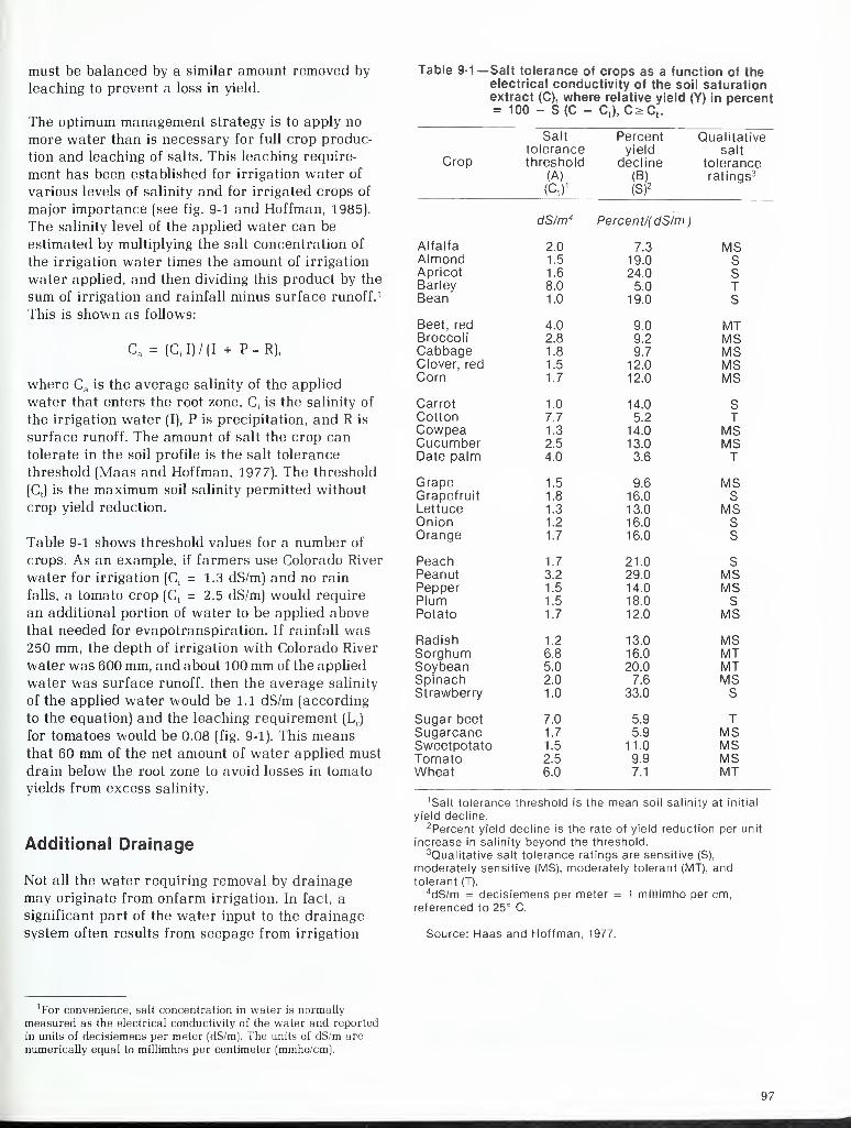
must be balanced by a similar amount removed by

leaching to prevent a loss in yield.

The optimum management strategy is to apply no

more water than is necessary for full crop produc-

tion and leaching of salts. This leaching require-

ment has been established for irrigation water of

various levels of salinity and for irrigated crops of

major importance (see fig. 9-1 and Hoffman, 1985).

The salinity level of the applied water can be

estimated by multiplying the salt concentration of

the irrigation water times the amount of irrigation

water applied, and then dividing this product by the

sum of irrigation and rainfall minus surface runoff. 1

This is shown as follows:

C a = (Q I) / (I + P - R),

where C a is the average salinity of the applied

water that enters the root zone, Ci

is the salinity of

the irrigation water (I), P is precipitation, and R is

surface runoff. The amount of salt the crop can

tolerate in the soil profile is the salt tolerance

threshold (Maas and Hoffman, 1977). The threshold

(C() is the maximum soil salinity permitted without

crop yield reduction.

Table 9-1 shows threshold values for a number of

crops. As an example, if farmers use Colorado River

water for irrigation (C, = 1.3 dS/m) and no rain

falls, a tomato crop (C, = 2.5 dS/m) would require

an additional portion of water to be applied above

that needed for evapotranspiration. If rainfall was250 mm, the depth of irrigation with Colorado River

water was 600 mm, and about 100 mm of the applied

water was surface runoff, then the average salinity

of the applied water would be 1.1 dS/m (according

to the equation) and the leaching requirement (Lr )

for tomatoes would be 0.08 (fig. 9-1). This meansthat 60 mm of the net amount of water applied must

drain below the root zone to avoid losses in tomato

yields from excess salinity.

Additional Drainage

Not all the water requiring removal by drainage

may originate from onfarm irrigation. In fact, a

significant part of the water input to the drainage

system often results from seepage from irrigation

Table 9-1— Salt tolerance of crops as a function of theelectrical conductivity of the soil saturationextract (C), where relative yield (Y) in percent= 100 - S(C - C

t ),C>C

t.

Salt Percent Qualitativetolerance yield salt

Crop threshold decline tolerance(A) (B) ratings3

(Ct )

1(S)

2

dS/m 4 Percent/(dS/m)

Alfalfa 2.0 7.3 MSAlmond 1.5 19.0 SApricot 1.6 24.0 sBarley 8.0 5.0 TBean 1.0 19.0 S

Beet, red 4.0 9.0 MTBroccoli 2.8 9.2 MSCabbage 1.8 9.7 MSClover, red 1.5 12.0 MSCorn 1.7 12.0 MS

Carrot 1.0 14.0 SCotton 7.7 5.2 TCowpea 1.3 14.0 MSCucumber 2.5 13.0 MSDate palm 4.0 3.6 T

Grape 1.5 9.6 MSGrapefruit 1.8 16.0 SLettuce 1.3 13.0 MSOnion 1.2 16.0 SOrange 1.7 16.0 S

Peach 1.7 21.0 SPeanut 3.2 29.0 MSPepper 1.5 14.0 MSPlum 1.5 18.0 SPotato 1.7 12.0 MS

Radish 1.2 13.0 MSSorghum 6.8 16.0 MTSoybean 5.0 20.0 MTSpinach 2.0 7.6 MSStrawberry 1.0 33.0 S

Sugar beet 7.0 5.9 TSugarcane 1.7 5.9 MSSweetpotato 1.5 11.0 MSTomato 2.5 9.9 MSWheat 6.0 7.1 MT

1 Salt tolerance threshold is the mean soil salinity at initial

yield decline.2 Percent yield decline is the rate of yield reduction per unit

increase in salinity beyond the threshold.

Qualitative salt tolerance ratings are sensitive (S),

moderately sensitive (MS), moderately tolerant (MT), andtolerant (T).

4dS/m = decisiemens per meter = 1 millimho per cm,

referenced to 25° C.

Source: Haas and Hoffman, 1977.

^or convenience, salt concentration in water is normally

measured as the electrical conductivity of the water and reported

in units of decisiemens per meter (dS/m). The units of dS/m are

numerically equal to millimhos per centimeter (mmho/cm).

97

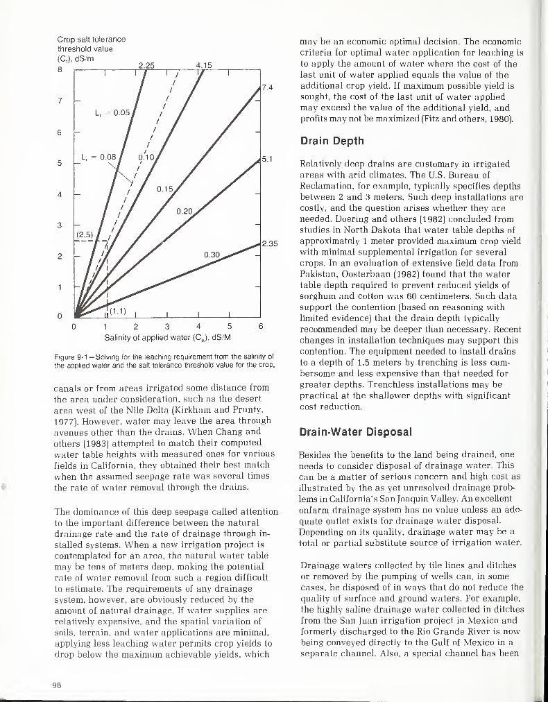
Crop salt tolerance

threshold value

(Ct ),dS/m

2.25 4.15

2.35

12 3 4

Salinity of applied water (C£

5

dS/M

Figure 9-1 —Solving for the leaching requirement from the salinity of

the applied water and the salt tolerance threshold value for the crop.

canals or from areas irrigated some distance from

the area under consideration, such as the desert

area west of the Nile Delta (Kirkham and Prunty,

1977). However, water may leave the area through

avenues other than the drains. When Chang and

others (1983) attempted to match their computed

water table heights with measured ones for various

fields in California, they obtained their best match

when the assumed seepage rate was several times

the rate of water removal through the drains.

The dominance of this deep seepage called attention

to the important difference between the natural

drainage rate and the rate of drainage through in-

stalled systems. When a new irrigation project is

contemplated for an area, the natural water table

may be tens of meters deep, making the potential

rate of water removal from such a region difficult

to estimate. The requirements of any drainage

system, however, are obviously reduced by the

amount of natural drainage. If water supplies are

relatively expensive, and the spatial variation of

soils, terrain, and water applications are minimal,

applying less leaching water permits crop yields to

drop below the maximum achievable yields, which

may be an economic optimal decision. The economic

criteria for optimal water application for leaching is

to apply the amount of water where the cost of the

last unit of water applied equals the value of the

additional crop yield. If maximum possible yield is

sought, the cost of the last unit of water applied

may exceed the value of the additional yield, andprofits may not be maximized (Fitz and others, 1980).

Drain Depth

Relatively deep drains are customary in irrigated

areas with arid climates. The U.S. Bureau of

Reclamation, for example, typically specifies depths

between 2 and 3 meters. Such deep installations are

costly, and the question arises whether they are

needed. Doering and others (1982) concluded from

studies in North Dakota that water table depths of

approximately 1 meter provided maximum crop yield

with minimal supplemental irrigation for several

crops. In an evaluation of extensive field data from

Pakistan, Oosterbaan (1982) found that the water

table depth required to prevent reduced yields of

sorghum and cotton was 60 centimeters. Such data

support the contention (based on reasoning with

limited evidence) that the drain depth typically

recommended may be deeper than necessary. Recent

changes in installation techniques may support this

contention. The equipment needed to install drains

to a depth of 1.5 meters by trenching is less cum-

bersome and less expensive than that needed for

greater depths. Trenchless installations may be

practical at the shallower depths with significant

cost reduction.

Drain-Water Disposal

Besides the benefits to the land being drained, one

needs to consider disposal of drainage water. This

can be a matter of serious concern and high cost as

illustrated by the as yet unresolved drainage prob-

lems in California's San Joaquin Valley. An excellent

onfarm drainage system has no value unless an ade-

quate outlet exists for drainage water disposal.

Depending on its quality, drainage water may be a

total or partial substitute source of irrigation water.

Drainage waters collected by tile lines and ditches

or removed by the pumping of wells can, in some

cases, be disposed of in ways that do not reduce the

quality of surface and ground waters. For example,

the highly saline drainage water collected in ditches

from the San Juan irrigation project in Mexico and

formerly discharged to the Rio Grande River is nowbeing conveyed directly to the Gulf of Mexico in a

separate channel. Also, a special channel has been

MB

constructed for conveying the highly saline, drain-

age water from the Wellton-Mohawk irrigation proj-

ect in southwestern Arizona to a point on the

Colorado River below the last place where water is

taken from the river for beneficial use. Conveyance

to sumps for evaporation or reclamation by desa-

lination are other possibilities for disposal. In manycases, however, the disposal of drainage water in a

way that does not harm stream and ground water is

not practical or possible. There may be several

reasons for this: the cost is prohibitive; the drainage

water is neither collected nor pumped but moves by

underground flow to streams and ground-water

basins; or the quality of the drainage water, though

somewhat diminished, is such that it still has value

for irrigation or other purposes.

Where the flow of agriculture drainage water to

bodies of surface and ground water cannot be

eliminated, quality degradation can be reduced by

minimizing the amount of salt leaving the root zone.

That amount can be reduced by decreasing evapo-

transpiration or by removing accumulated salts in

the smallest volume of water compatible with the

leaching requirement. Simultaneously reducing

evapotranspiration and the amount of water ap-

plied decreases the amount of salt that must be

removed from the drainage water. This can be

achieved in a variety of ways, such as using closed

water conveyance systems, eliminating nonbene-

ficial vegetation, and growing crops with lower

evapotranspiration requirements as a consequence

of the season or length of their growth period.

Removal of excess dissolved salts consistent with

the leaching requirement maximizes the salt concen-

tration of the soil solution and drainage waters, andhelps produce harmless, slightly soluble salts, such

as lime and gypsum, in the soil. It also minimizes the

solution of soil minerals and fossil salt deposits

which commonly occur in geologic materials below

the root zone.

Unusually high and nonuniform soil permeability,

and an excessive and nonuniform application of ir-

rigation water are the chief causes of excessive

leaching. Minimizing the amount of salt leaving the

root zone in drainage water is, therefore, strongly

influenced by irrigation efficiency. The leaching of

dissolved salts is more efficient and the problems of

excessively high and nonuniform soil permeability

are reduced when applied water moves through the

soil by unsaturated flow. Irrigation by sprinkler and

trickle systems permits uniform and controlled rates

of water application.

Agricultural drainage waters sometimes contain

nutrients and chemicals in sufficient concentrations

to help or harm users of the water or the aquatic

environment. Aside from the salts associated with

salinity, subsurface drainage may contain nitrates

and trace elements that harm the environment.

Nitrogen in drainage effluent is normally in the

form of nitrate because it is not adsorbed on soil

particles. After reaching surface waters, these

nitrates may contribute to eutrophication (a situa-

tion where minerals and certain nutrients rob water

of oxygen, and thus favor plants over animal life). In

high concentrations, nitrates may cause or at least

contribute to methemoglobinemia (a poisoning of the

blood) in infants and certain disorders in ruminant

animals. High nitrate concentrations in subsurface

drainage can originate from a number of sources:

excessive fertilizer, geologic deposits, natural

organic matter, decomposition of human or animal

wastes, or possibly by deep percolation of nitrates

because of a lack of complete efficiency of the root

system in absorption. The management goal in

drainage and fertilizer practice is to minimize the

nitrate concentration of drainage waters.

Minimizing Adverse Effects

In recent years, experts have become increasingly

concerned with the significance of the degradation

of irrigation return flows due to leaching of trace

elements. These elements have accumulated in the

soils, and the drainage waters have injured fish and

wildlife and could potentially affect human health.

As an example, the west side of the San Joaquin

Valley has serious drainage and salt managementproblems because the disposed drainage water is

damaging valley waterfowl, agricultural lands, and

the San Joaquin River. The original plan called for

the drainage water to be diverted from the valley

through the San Luis Drain to the Sacramento-San

Joaquin Delta, and then into the San Francisco Bay

and the Pacific Ocean. Construction of the drain

began but it was not completed because of environ-

mentally based objections and lack of construction

funds in the mid-1970's. As a result, no acceptable

receiving water was identified, and most drainage

was discharged through the incomplete drain to the

Kesterson National Wildlife Refuge, where it was

expected to evaporate. Deformities in waterfowl

observed at Kesterson have called attention to high

levels of selenium and other trace metals, such as

boron, in drainage water from the valley.

Although continued operation of the current system

appears unacceptable, shutting down the system

99

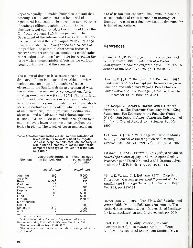
appears equally untenable. Estimates indicate that

possibly 500,000 acres (200,000 hectares) of

agicultural land could be lost over the next 30 years

if drainage effluent containing salt or trace

elements is not controlled, a loss that could cost the

California economy $1.5 billion per year. The

Department of the Interior and the State of Califor-

nia have initiated the San Joaquin Valley Drainage

Program to identify the magnitude and sources of

the problem; the potential alternative bodies of

receiving water; and options (including modification

of agricultural practices) available for resolving the

issue without unacceptable effects on the environ-

ment, agriculture, and the economy.

The potential damage from trace elements in

drainage effluent is illustrated in table 9-2, wheretypical concentrations of a number of trace

elements in the San Luis drain are compared with

the maximum recommended concentrations for ir-

rigating sensitive crops (Pratt, 1973). The criteria on

which these recommendations are based include:

toxicities in crops grown in nutrient solutions; short-

term soil culture experiments in which the amountof an element required to produce toxicities wasobserved; and soil-plant-animal relationships for

elements that are toxic to animals through the food

chain at levels lower than those that produce tox-

icities in plants. The levels of boron and selenium

are of paramount concern. This points up how the

concentrations of trace elements in drainage ef-

fluent is the most pressing new issue in drainage for

irrigated agriculture.

References

Chang, A. C, R. W. Skaggs, L. F. Hermsmeier, andW. R. Johnston. 1983. Evaluation of a WaterManagement Model for Irrigated Agriculture. Trans-

actions of the ASAE. Vol. 26, pp. 412-418, 422.

Doering, E. J., L. C. Benz, and G. I. Reichman. 1982.

Shallow-water-table Concept for Drainage Design in

Semi-arid and Sub-humid Regions. Proceedings of

Fourth National ASAE Drainage Symposium, Chicago,

111., December 13-14, 1982. pp. 34-41.

Fitz, Joseph C, Gerald L. Horner, and J. Herbert

Snyder. 1980. The Economic Feasibility of Installing

Subsurface Tile Drainage in the Panoche Water

District, San Joaquin Valley, California. University of

California, Div. of Agricultural Sciences Bui. No.

1897.

Table 9-2— Recommended maximum concentration of

trace elements in waters used to irrigate

sensitive crops on soils with low capacity to

retain these elements in unavailable formscompared with typical values from the SanLuis drain

Typica concentrations RecommendedElement in San Luis drain 1 concentration

of irrigation 2

mg/m3,(ppb) mg/m3

,(ppb)

Aluminum 100 5,000Arsenic 10 100Boron 14,000 750Cadmium 10 10Chromium 18 100Copper 10 200Iron 80 5,000Lead 10 5,000Lithium — 2,5003

Molybdenum — 10Nickel 10 200Selenium 310 20Zinc 10 2,000

— = not available.1 Values reported by California Department of Water

Resources during first half of 1984 near Mendota, Calif.

Recommendations from Pratt, 1973.3Recommended maximum concentration for irrigated citrus

in 75 mg/m 3.

Hoffman, G. J. 1985. "Drainage Required to ManageSalinity," Journal of the Irrigation and Drainage

Division. Am. Soc. Civ. Engr. Vol. Ill, pp. 199-206.

Kirkham, D., and L. Prunty. 1977. Upslope Recharge,

Downslope Waterlogging, and Interceptor Drains.

Proceedings of Third National ASAE Drainage Sym-

posium. ASAE Pub. No. 1-77, pp. 40-50, 54.

Maas, E. V.. and G. J. Hoffman. 1977. "Crop Salt

Tolerance—Current Assessment." Journal of The Ir-

rigation and Drainage Division, Am. Soc. Civ. Engr.

Vol. 103, pp. 115-134.

Oosterbaan, O. J. 1982. Crop Yield, Soil Salinity, and

Water Table Depth in Pakistan. Wageningen, The

Netherlands: Annual Report, International Institute

for Land Reclamation and Improvement, pp. 50-54.

Pratt, P. F. 1973. Quality Criteria for Trace

Elements in Irrigation Waters. Station Bulletin,

California Agricultural Experiment Station, Davis.

100

Chapter 10

Drainage Institutions

Carmen SandrettoEconomic Research Service, USDAEast Lansing, Michigan

Early in the development of American agriculture,

when good land was abundant and available for

cultivation, areas with wet soils and natural

wetlands were often bypassed. Many farms contained

tracts of land too wet for use even as pasture ex-

cept during dry seasons, and large areas were too

swampy or frequently flooded to make regular cul-

tivation practical. As tillable land became scarcer

and higher in price, farmers began to explore ways

of reclaiming lands with wetness problems through

improved drainage.

Drainage for agriculture has traditionally been

recognized as an endeavor beneficial to the public

because excess water can influence public health,

farm production, farm income, and real estate

values. A number of the States recognized early the

right of every landowner to a drainage outlet, per-

mitting an owner intending to drain to apply to a

designated official, pay any damages, and if the

necessity were proved, secure an easement to con-

struct and maintain a private outlet for the drain

across a neighbor's land.

Agricultural drainage often needs an artificial drain

constructed or a natural watercourse improved,

which in turn, may affect the land of other individ-

uals. Efforts to improve drainage outlets often

benefit more than one farm and the cost is greater

than any one individual wants to assume. These cir-

cumstances have encouraged legislation permitting

the organization of public corporations or local

improvement districts to facilitate artificial

drainage activities.

Elements of Drainage Law

Drainage law focused historically on promoting

drainage for two purposes: removing excess water

from the land so it could be cultivated or otherwise

developed, and enhancing public health because

swamps and low-lying areas were potential breeding

places for malaria-carrying mosquitoes. These con-

siderations were the basis for allowing private

individuals to drain their lands (Beck, 1972).

The issues associated with drainage law deal with

repelling water at the boundaries of one's land as

well as with disposing of excess water once it has

entered. Because remedial actions taken by individ-

ual landowners interfere with the natural processes

of water arriving on or leaving their land, what land-

owners do will likely affect someone else's land.

Over the years, the courts have molded a substan-

tial portion of the common law of drainage and havefrequently quoted three Latin maxims in their

deliberations (Beck, 1972). Translated, they are:

1. Water runs and ought to run, as it has used to

run.

2. Whose is the soil, his it is even to the skies andto the depths below.

3. Use your own property in such a manner as

not to injure that of another.

Basic Drainage Law Doctrines

Given the background provided by the common lawof drainage and the modifications resulting from

court action, three rules concerning drainage of dif-

fused surface waters have been identified. Follow-

ing is a brief summary of them as drawn from Beck

(1972).

The common enemy rule, or, as it is sometimes

mistakenly called, the common-law rule, recognizes

surface water as a common enemy which each land-

owner may try to control by retention, diversion,

repulsion, or altered transmission. The focus is on

two points: the necessity of improving lands,

recognizing that some injury results from even

minor improvements, and a philosophical preference

for the freedom of landowners to deal with their

own land essentially as they see fit.

101

The common enemy rule permits landowners to

drain or repel diffused surface water if they act

reasonably under the circumstances. Collecting and

discharging large or unusual quantities of diffused

surface water onto adjoining land where it maycause damage is considered unreasonable.

The natural flow rule, or, as it is sometimes called,

the civil law rule, places a natural easement upon

the lower land for the drainage of surface water in

its natural course. The natural flow of the water

cannot be obstructed by the owner of the lower land

to the detriment of the owner of the higher land.

Because there has to be some drainage rule, looking

to the law of nature for the rule is reasonable. The

Supreme Court of Illinois in 1869 stated:

The right of the owner of the higher land to

drainage is based simply on the principle that

nature has ordained such drainage. ... As water

must flow, and some rule in regard to it must be

established . . . there can clearly be no other rule

at once so equitable and so easy of application as

that which enforces natural laws. There is no sur-

prise or hardship in this, for each successive

owner takes whatever advantages or inconven-

iences nature has stamped upon his land.

The need to drain land in order to develop it cer-

tainly does not mean that a landowner should be

able to force a neighbor or the public to pay for it.

In the early development of this country, a presump-

tion in favor of drainage existed because it wasviewed as a public benefit, but today policy mayfavor the retention of natural areas and wetlands.

This policy consideration would reject the commonenemy rule and tend to support the natural flow rule.

The reasonable use modification in applying the

natural flow rule has been to promote drainage.

However, the basic principle generally applicable to

landownership should apply: landowners should be

able to use their property as they see fit as long as

they do not unreasonably injure someone else's

property. Certainly natural flow can be altered in

many instances without doing any injury or damageto another tract.

Under the reasonable use rule, landowners are

legally privileged to make reasonable use of their

land even though the flow of surface waters is

altered and causes some harm to others. Those land-

owners incur liability when harmful interference

with the flow of surface waters becomes unreason-

able. The underlying philosophy of this approach is

dissatisfaction with rules that either favor the

upper landowner, as does the natural flow rule, or

that envision conflict between adjoining land-

owners, as does the common enemy rule.

Beck (1972) has identified the following questions as

basic to an analysis of a situation under the

reasonable use rule:

(1) Was there a reasonable necessity for altering

the drainage pattern to make use of the land?

(2) Was the altering done in a reasonable man-ner? That is, was due care taken to prevent in-

jury to another's land? Was the natural drainage

pattern followed as much as possible? Is the

artificial system reasonably feasible?

(3) Does the benefit from the actor's conduct

reasonably outweigh the gravity of the harm to

others? This test is the traditional nuisance

balancing approach, which has the distinct ad-

vantage of keeping up to date.

All of the common-law rules concerning drainage of

diffused surface waters involve elements of uncer-

tainty. Under the natural flow rule, dominant

owners must show that they are dominant and that

the lower owner(s) obstructed the natural drainage

pattern. The common enemy rule is uncertain

because to permit one set of owners to get rid of dif-

fused surface water as best they can may not be an

overall benefit if their action brings them into con-

flict with neighbors who have the same rights. Thereasonable use test is uncertain because it depends

upon not only whether landowners make reasonable

use of their land but also whether it is reasonable

in the larger setting.

The modifications of the common enemy and natural

flow rules have done much to alleviate the early at-

tendant injustices. The reasonable use rule seems

the most just because it considers the individual cir-

cumstances of each case.

An inevitable consequence of a complex society is

the diminution in control that landowners have over

their land. The public interest concept appears to

be expanding. In attempting to resolve problems

among individuals, the reasonable use test seems

best because it analyzes the gravity of harm versus

the utility of the benefit. An element of public in-

terest is interjected in these cases in ascertaining

not just the utility to the individual but to the public

as well.

102

The question arises whether there is really any dif-

ference between the independent reasonable use

rule and the reasonable use modifications of the

common enemy and natural flow rules. In a growing

number of jurisdictions, all conduct of a landowner

with reference to diffused surface waters is subject

to the reasonable use rule, whether as a modifica-

tion of one of the other rules or as an independent

test (Beck, 1972).

The general rules formulated from a composite of

the basic rules and their modifications with respect

to the law of drainage of diffused surface waters

can be summarized as follows:

1. A landowner may not obstruct the natural

flow in a watercourse (liberally defined in

some jurisdictions) to the injury of another.

2. A landowner may not collect unusual amounts

of diffused surface waters and discharge

them onto adjoining land to its injury.

3. A landowner may not divert onto another's

land, to its injury, diffused surface waters

from an area that did not naturally drain that

way.

4. A landowner may drain diffused surface

water into a watercourse (liberally defined in

some jurisdictions) subject to the overtaxing

capacity, the anticollecting-and-discharging,

and the antidiversion rules.

5. In all other respects concerning their conduct

with diffused surface waters, landowners are

subject to a rule of reasonable use of their

land, whether it relates to acceleration or

repulsion of flow.

Drainage Rights

Easements for a landowner to drain excess water

across the land of another may be obtained the wayany other easement is, through grant, express or

implied, or through prescription. A number of States

provide for use of eminent domain power by private

individuals to drain land. This individual exercise of

eminent domain is distinct and separate from the

use of the power by entities such as drainage

districts. Eminent domain is limited to a public use

or public purpose, which may create some difficulties

in use of the power for draining private lands.

However, some State constitutions authorize use of

eminent domain for this purpose, and some courts

construe the benefit to the public health or economy

arising from drainage as a sufficient public pur-

pose. Also, it is possible to create a license for

drainage purposes (Beck, 1972).

Public Drainage Organizations

The expansion of agricultural development in manyparts of the Nation was accomplished through

cooperation among groups of landowners with com-

mon drainage interests engaging in communityundertakings to remove excess water from their

holdings. These efforts eventually resulted in the

creation of public organizations to improve off-farm

drainage facilities.

Early attempts at drainage improvement by individ-

ual landowners were often unsatisfactory because

outlets were inadequate to carry off the excess

water. Individual efforts to improve drainage werefollowed by cooperation between groups of adjacent

landowners to obtain effective drainage at lower

cost. However, these attempts at cooperation in the

construction of drains and the distribution of costs

often failed because of inherent weaknesses in such

voluntary associations. Also, cooperating groups did

not possess the power to compel all landowners whobenefited from the drainage works to pay their fair

share of the costs, nor did they have a mechanism

to permit construction of drains across the lands of

an owner who refused to consent when circumstances

made such construction necessary to secure adequate

outlets.

Types of Drainage Organizations

The failure of individual and voluntary cooperative

efforts to establish economic drainage improve-

ments led to legislation authorizing the formation of

public organizations with certain powers to allow

improved drainage of agricultural lands. Legislative

authority for the creation of drainage districts as it

exists today dates back to the 19th century.

The formation of public drainage organizations

usually involves a multistage process which varies

in detail from State to State, but which contains

elements common to all. Enabling legislation sets out

the procedure for the formation of a drainage

district, indicates the powers it has, and imposes a

duty on the district to keep drainage systems ade-

quately repaired. Appendix B is a synopsis of laws

and regulations pertaining to drainage in selected

States.

Drainage organizations have generally been referred

to as public corporations or as quasimunicipal cor-

103

porations. Drainage districts or close approxima-

tions of them are authorized in 45 States. In 39

States, entities actually denominated "drainage

districts" may be formed for various drainage pur-

poses (Beck, 1972). In some States, several types of

drainage districts may be created. Many States also

authorize multipurpose districts to engage in

drainage projects. One factor accounting for the

diversity in public organizations has been the

tendency to move from single-purpose to multipur-

pose districts without doing away with the old

districts.

The administrative structure established to provide

unified action for handling a drainage problem is

commonly referred to as its organization; all

drainage activities under the direct managementand supervision of one organization constitute one

project. Drainage projects are those activities

undertaken to provide new construction or replace-

ment construction or to provide maintenance and

operation of existing drainage works, and are usually

classified into three groups:

1. Drains owned by one landowner; the land-

owner may be an individual, a partnership, anestate, a private corporation, or an institution.

2. Cooperative or mutual drains that represent

undertakings by two or more landowners coop-

erating without special organization under

State drainage laws for the construction or

operation of drainage works benefiting their

lands. Many cooperative or group drainage

projects have received assistance andguidance from SCS.

3. Legally organized public drains that represent

community or public drainage undertakings

accomplished through some form of govern-

mental organization. These organizations can

be administered by public officials of a county,

a township, a State, an agency of the Federal

Government, or by specially elected or

appointed officials or boards. General or

special State laws provide for equitable

cooperation among landowners who will

benefit by a particular drainage undertaking.

A variety of drainage organizations have beenauthorized in nearly all States, with the corporate

district and the county drain constituting the twoprincipal types. A system of county drainage dis-

tricts has been created in some States, whereas in

others, special drainage districts have been formed.

Besides the two principal types of drainage organ-

izations, some minor types exist: (1) township drains,

which are generally similar in form to county drains

but are controlled by officers of the townships; (2)

State drainage projects controlled by State officials,

usually embracing some State land; (3) irrigation

districts, similar to drainage districts, that have

drained land within the irrigation districts; (4) com-

mercial companies reclaiming and improving poorly

drained land for future sale; (5) cooperative or

mutual undertakings without formal corporate

organization; and (6) individual landowners in-

cluding farm partnerships and farm corporations

(Bureau of the Census, 1961).

In several States, some difficulty exists in distin-

guishing between drainage districts and county

drains. Many of the organizations classified as

county drains were named "drainage districts" in

the law. District organizations, under the manage-

ment of their own officials, were generally con-

sidered better suited to larger and more costly

undertakings because they provided landowners

with a greater degree of local control. County

drains administered by county officials were

generally more economical for administering small

enterprises with relatively simple engineering and

financing problems and were most commonly

adopted in States where drainage improvements

were being provided to land already in farms.

Drainage districts were generally confined to areas

where reclamation and development of unimproved

lands for new farms had been an important con-

sideration in establishing drainage organizations.

The 1950 Census of Drainage treated the drained

lands of each county in States having predominantly

county drains as a single drainage organization. The

States were designated as "county-drain" States:

Delaware, Indiana, Iowa, Kentucky, Michigan, Min-

nesota. Ohio. Oklahoma, North Dakota, and South

Dakota. Delaware's predominant form of drainage

organization, however, is the drainage district. Thirty

other States were identified as "drainage-district"

States. The six New England States. Pennsylvania,

and West Virginia were determined, for the purpose

of the Census, not to have drainage organizations

(Bureau of the Census, 1952).

The geographic distribution of agricultural lands

served by organized drainage projects of 500 acres

or more is presented in figure 10-1. The greatest

concentration of agricultural land within drainage

project boundaries is found in the Great Lakes, Up-

per Midwest. Lower Mississippi Valley, Gulf, and

Delmarva regions. California's drainage enterprises

are typically associated with irrigation projects.

104

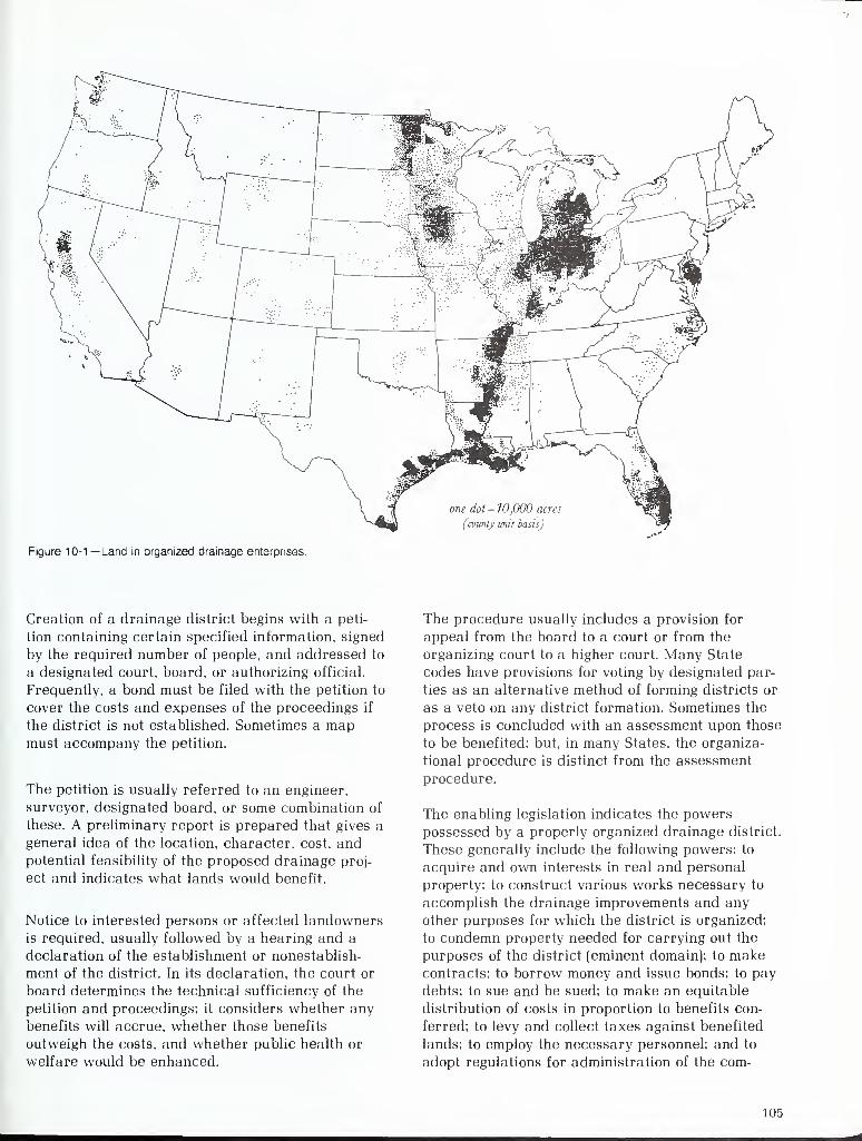
Figure 10-1— Land in organized drainage enterprises.

Creation of a drainage district begins with a peti-

tion containing certain specified information, signed

by the required number of people, and addressed to

a designated court, board, or authorizing official.

Frequently, a bond must be filed with the petition to

cover the costs and expenses of the proceedings if

the district is not established. Sometimes a mapmust accompany the petition.

The petition is usually referred to an engineer,

surveyor, designated board, or some combination of

these. A preliminary report is prepared that gives a

general idea of the location, character, cost, andpotential feasibility of the proposed drainage proj-

ect and indicates what lands would benefit.

Notice to interested persons or affected landowners

is required, usually followed by a hearing and a

declaration of the establishment or nonestablish-

ment of the district. In its declaration, the court or

board determines the technical sufficiency of the

petition and proceedings: it considers whether any

benefits will accrue, whether those benefits

outweigh the costs, and whether public health or

welfare would be enhanced.

The procedure usually includes a provision for

appeal from the board to a court or from the

organizing court to a higher court. Many State

codes have provisions for voting by designated par-

ties as an alternative method of forming districts or

as a veto on any district formation. Sometimes the

process is concluded with an assessment upon those

to be benefited; but, in many States, the organiza-

tional procedure is distinct from the assessment

procedure.

The enabling legislation indicates the powers

possessed by a properly organized drainage district.

These generally include the following powers: to

acquire and own interests in real and personal

property; to construct various works necessary to

accomplish the drainage improvements and any

other purposes for which the district is organized;

to condemn property needed for carrying out the

purposes of the district (eminent domain); to makecontracts; to borrow money and issue bonds; to pay

debts; to sue and be sued; to make an equitable

distribution of costs in proportion to benefits con-

ferred; to levy and collect taxes against benefited

lands; to employ the necessary personnel; and to

adopt regulations for administration of the com-

105

pleted project or projects (Beck. 1972; Yohe. 1927).

The codes usually impose on the district a duty to

keep the drainage and related works in repair.

What can be drained through the auspices of drain-

age districts varies from State to State. The focus is

usually on either the nature of the land, the purpose

to be accomplished, or the nature of the water. In

some States, combinations of the foregoing are

stated; a few States make no specific statements.

The area of a drainage project is usually defined as

the area benefited by the drainage works. The area

improved or benefited for agriculture as a result of

the drainage facilities is what is considered in proj-

ects undertaken by landowners, either individually

or cooperatively (Beck, 1972).

Drainage district statutes normally do not specify

any particular geographic area to be included, but

they do require the petition to contain some descrip-

tion of the proposed boundaries. Various govern-

mental bodies with final creative approval of

districts, or governmental officials such as State

engineers, have differing degrees of control over the

boundaries. In any case, the legal document estab-

lishing the district defines its boundaries. In most

States, if public drains are administered countywide

or on the basis of established political boundaries,

the boundaries are determined by the area directly

benefited. In special districts organized primarily

for purposes other than drainage, the entire area in

the district defines the boundaries, even though only

part may be benefited (Bureau of the Census, 1961).

Several States require the district land to be

contiguous, while others specifically allow noncon-

tiguous areas, and some States do not permit

districts to cross county lines. Several States have

language relating to natural drainage basins, and

many States provide for mergers of two or more

districts and for subdistricts or interstate districts

(Beck, 1972).

After a drainage district is formed and certain land

is included, the drainage activities of individual

landowners may be restricted. Essentially all

jurisdictions give drainage districts the power of

eminent domain to foster their purposes, but its ex-

ercise is usually limited in some way (Beck, 1972).

A project need not provide complete drainage for

the area served. Many projects, especially public

drains, provide only the principal channel or outlet

drain. The construction of laterals and field drains

required to provide optimum drainage may be left to

individual landowners. These drains and other water-

control works installed by farmowners on their ownfarms, either inside or outside the boundaries of anorganized drainage district, are probably either

supplemental to or entirely independent of the

drainage works installed by a district organized to

improve lands for agriculture.

Administration and Financing

Public drainage projects are administered by a

board of drainage commissioners who are either

elected by the residents or landowners of the

district (in some States, voting power is based on

acreage), or are appointed by the organization's

creative authority. In many States, board membersmust be real property owners in, and residents of,

the county or district involved. In a few States, ex-

isting local officials supervise drainage projects.

Courts generally hold that a majority of the board

can act to bind the district. Although commissioners

may usually exercise great discretion in carrying

out the governing function, they can be challenged

for such improper activity as misapplication of

funds (Beck, 1972).

Drainage improvements may be financed in several

ways. An assessment against benefited land is most

common, but much discretion is often given to the

assessing authorities in determining what consti-

tutes a benefit and the procedures involved in the

assessment process.

Many States have specific provisions dealing with

organizational costs, construction costs, and

maintenance costs. A uniform tax on all property

within the district is often used to cover organiza-

tional costs, but construction and maintenance costs

are generally recovered from tax levies based on

assessed benefits to the respective tracts of land.

Frequently, separate funds are maintained for each

cost category. Because expensive drainage projects

cannot be financed through a single year's levy,

provisions usually exist for a variety of borrowing

and repayment methods (Beck, 1972).

As custodians of the project, the drainage commis-

sioners are responsible for maintenance and repair

of the drainage system. Deterioration of facilities

and subsequent loss of efficiency in removing excess

water can occur rapidly if regular inspections andmaintenance are neglected. Proper maintenance can

yield substantial benefits through increased effi-

ciency and extended life of the project (Yohe. 1927).

Many public drainage organizations are established

for a specific purpose, such as to construct new

106

drainage facilities or to enlarge or renovate

facilities built by an earlier organization. After

accomplishing their immediate objectives, many of

these organizations become inactive or dissolve, so

when further work is needed, a new drainage organ-

ization must be formed. Over the years, drainage

organizations have overlapped, and only a small

number of organizations may be currently active.

Usually the functions of an inactive organization are

assumed by a new organization, although control

sometimes passes from one organization to another

through court action.

Many cases exist in which drainage districts have

failed, bonds have not been refunded, and owners

of assessed lands have not paid their assessments.

The drainage codes of most States provide steps for

dissolving defunct drainage districts which specify

who can initiate the procedure, where the dissolving

power lies, and what conditions must exist before it

can be exercised. Lack of dissolution, however, has

been more of a problem than dissolution. Districts

have simply withered away, the commissioners or

directors have disappeared, and projects have been

left uncompleted and/or unmaintained (Beck, 1972).

The substantial amount of litigation in the courts

over the years demonstrates that many of the

drainage districts established years ago were ill-

conceived; land was forfeited for failure to payassessments, and many bondholders could not

recover the full face value of their bonds. Recent

trends indicate a preference for multipurpose

districts (conservancy and water management, for

example). The result may be improved natural

resource management through emphasis on better

planning and coordinating than occurred histori-

cally with the single-purpose districts.

Multipurpose Districts 1

Several States have enacted legislation in recent

years authorizing the creation of general multipur-

pose districts which are permitted to perform manyfunctions, including draining wetlands. Most of

these have retained their statutes permitting the

creation and operation of separate drainage

districts. Multipurpose districts have no primary

purpose except the very general one of promoting

public welfare as it relates to the total water

resources. This differs from special-purpose

'This section on multipurpose districts was prepared by Dean T.

Massey.

districts with a primary purpose. For example, mostirrigation districts can engage in some drainage;

however, drainage is only incidental to the primarypurpose of irrigation.

Multipurpose districts that provide for wetlanddrainage as one function have different names in

different States. For example, they are known as

conservancy districts in Indiana, New Mexico,

Montana, Ohio, and Oklahoma; as water conservancy

districts in Nevada and Utah; as watershed conser-

vancy districts in Kentucky; and as river conservancy

districts in Illinois. Kansas and South Dakota havewatershed districts, Alabama has water manage-ment and drainage districts, North Dakota has

water resources districts, and Wyoming has water-

shed improvement districts. Nebraska's natural

resources districts probably have the broadest

powers of any multipurose districts. Minnesota has

both conservancy and watershed districts that mayperform drainage functions. The relevant State

codes are listed with other references to this

volume.

Multipurpose districts generally perform several

functions, which may include preventing and

controlling floods; constructing flood prevention

structures, including levees; improving stream chan-

nels; preventing and controlling erosion and

sedimentation; regulating stream flows and lake

levels and conserving water; improving drainage

and reclaiming or filling wet or overflowed lands;

diverting or changing water courses; promoting

recreation; providing, developing, and conserving

water supply for domestic, industrial, recreational,

and other public uses; providing for sanitation and

public health, and regulating the use of streams,

ditches, or water courses for the disposition of

waste; relocating, extending, replacing, modifying,

consolidating, or abandoning drainage systems

within a multipurpose district; and operating and

maintaining drainage systems.

Multipurpose districts are generally initiated with a

petition signed by a requisite number of landowners

which is submitted to the county board of super-

visors or county agency, officer, or court. After a

public hearing to determine the necessity of estab-

lishing a district, the governmental authority will

establish a district. Sometimes a referendum is held.

A board of directors, usually appointed by the sameauthority that established the district, governs the

district. Areas included in a district do not have to

coincide necessarily with county boundaries. Areas

can be smaller or larger than a county.

107

Multipurpose districts may purchase, lease, and

own land, and, if necessary, may acquire such

interests by eminent domain. They may enter into

contracts and construct and maintain structures

and facilities. Districts generally have power to levy

taxes, borrow money, issue bonds, and levy special

assessment of lands benefited.

. 1961. "Drainage of Agricultural

Lands," Census 0/ Agriculture, 1960, Vol. IV.

1981. "Drainage of Agricultural

Lands," Census 0/ Agriculture, 1978, Vol. 5, Special

Reports, Part 5.

References

Yohe, H. D. 1927. Organization, Financing and Ad-

ministration of Drainage Districts. Farmers' Bulletin

No. 815., U.S. Dept. Agr.

Beck, Robert E. 1972. "The Law of Drainage," In

Waters and Water Rights. Vol. 5. (ed. Robert EmmetClark). Indianapolis, Ind.: The Allen Smith Company.

Hannah, H. W., N. G. P. Krausz, and D. L. Uchtmann.

1979. Illinois Farm Drainage Law. Coop. Ext. Serv.

Circular 751, Univ. of Illinois, Urbana.

Indiana Farm Bureau, Inc. 1981. The County

Drainage Board, Recodified 1981. Indianapolis, Ind.

Michigan Department of Agriculture, Division of

Intercounty Drains. 1984. Personal communication.

Nolte, Byron H. 1981. The Ohio Drainage Laws Peti-

tion Procedure. Coop. Ext. Serv. Bulletin 482, Ohio

State Univ. and County Engineers Association of

Ohio, Columbus.

Nolte, Byron H.. and Eugene H. Derickson. 1976.

Conservation Improvement Projects Through Soil

and Water Conservation Districts. Coop. Ext. Serv.

Bulletin 606, Ohio State Univ., Columbus.

State statutory references:

California Water Code, Sees. 8502, 8550, 8551,

8750. 8751, 8758 (West 1971 and CumulativeSupplement 1984), Sees. 20700, 22095 (West 1984),

Sees. 50110, 50300. 50932, 56010 to -014, 56018to -020, 56030, 56041 to -042, 56050, 56055, 56070to -071, 56074 to -076, 56083 to -084, 56095, 56104,56110 to -117 (West 1966 and Cumulative Supple-

ment 1984), and Sees. 70150, 74522 to -525 (West1966).

Alabama Code, Sees. 9-9-1 to 9-9-80 (1980).

Illinois Annotated Statutes, Ch. 42, Sees. 383 to

410.1 (Smith-Hurd 1976 and Cumulative Supplement

1984-1985).

Indiana Code Annotated, Sees. 13-3-3-1 to 13-3-3-102

(Burns 1981 and Cumulative Supplement 1984).

Kansas Statutes Annotated, Sees. 24-1237 (1981 andCumulative Supplement 1983).

North Carolina Department of Natural Resources

and Community Development, Division of Soil and

Water Conservation. 1984. Personal communication.

Kentucky Revised Statutes, Sees. 262.700 to 262.990

(1981 and Cumulative Supplement 1984).

U.S. Congress, Office of Technology Assessment.

1984. Wetlands: Their Use and Regulation. Report

OTA-O-206, March.

Minnesota Statutes Annotated, Sees. 111.01 to

111.82 and 112.34 to 112.86 (West 1977 and

Cumulative Supplement 1984).

U.S. Department of Commerce, Bureau of the Cen-

sus. 1932. Drainage of Agricultural Lands. 1930.

Montana Code Annotated, Sees. 85-9-101 to 85-9-632

(1983).

1952. "Drainage of Agricultural

Lands," Census 0/ Agriculture, 1950, Vol. IV.

Nebraska Revised Statutes, Sees. 2-3201 to 2-3275

(1977 and Cumulative Supplement 1982).

108

Nevada Revised Statutes, Sees. 541.010 to 541.420

(1983).

New Mexico Statutes Annotated. Sees. 73-14-1 to

73-14-88 (1978 and Cumulative Supplement 1983).

North Dakota Century Code. Sec. 61-16.1-01 to

61-16.1-63 (Supplement 1983).

Ohio Revised Code Annotated, Sees. 1515.01 to

1515.30 (Page 1978 and Supplement 1983) and Chs.

6131, 6133. 6135, 6137 (Page 1977 and Supplement

1983).

Oklahoma Statutes Annotated, Title 82, Sees. 531 to

688.1 (West 1970 and Cumulative Supplement1983-1984).

South Dakota Codified Laws Annotated, Sees.

46A-2-1 to 46A-2-37 (1983).

Utah Code Annotated, Sees. 73-9-1 to 73-9-43 (1980and Supplement 1983).

Wyoming Statutes Annotated, Sees. 41-8-101 to

41-8-126 (1977 and Cumulative Supplement 1983).

109

Chapter 11

Economic Survey of Farm Drainage

George A. PavelisEconomic Research Service, USDAWashington, DC

This overview briefly addresses a series of drainage

development and economic questions: At what rate

have drainage organizations and individual farmers

in the United States improved land by drainage?

How has the cost of drainage changed over time?

How have past investments in drainage added to the

Nation's agricultural capital and wealth? How does

drainage capital relate to land and its value in dif-

ferent States and regions? How does drainage con-

tribute to farm production, and what is the sig-

nificance of maintaining a productive irrigated

agriculture through proper drainage and related

water management strategies?

The density map in figure 11-1 indicates the general

distribution of drained agricultural land in the

United States. The total area drained in 1985 wasaround 110 million acres, of which about 70 percent

was cropped and 12 percent grazed. Woodlands ac-

counted for 16 percent, with the balance (2 percent)

in farmsteads and other miscellaneous uses.

multiple functions. They may engage in drainage only

or in both irrigation and drainage. According to the

Bureau of the Census, 20 percent of the 840 or more

U.S. irrigation districts maintain about 14,000 miles

of drains. Most of the drains serve projects originally

constructed by the Bureau of Reclamation but paid

for and now operated by water users. Also, about

15,000 miles (13 percent) of the irrigation canals

and ditches in the United States are lined to

minimize conveyance losses and drainage problems

connected with seepage (U.S. Dept. Commerce, 1982).

The connection between organized drainage and the

difficulty of obtaining reliable current information is

that many organizations have kept few records on

project activity within their areas and these maypertain only to the construction period. Organiza-

tion officials may not have been replaced as they

retired or moved away, so it is difficult to locate

responsible individuals or otherwise gain access to

available records.

Areas and Uses of Drained Land

Although poor drainage and its effects are evident

even to the untrained eye, good natural drainage

and functioning drain systems often go unnoticed.

This unseen attribute of drainage is one reason whyreliable information on this important land improve-

ment is difficult to obtain from landowners or farm

operators.

Another reason is that in its primary developmental

period, 1870-1920, and again in a secondary period

during 1945-60, much new drainage occurred within

organized drainage districts, or county and town-

ship drains. These came to be called drainage

"enterprises" (U.S. Dept. Commerce, 1961). Theycan be organized in several ways and can have

The estimates on drainage compiled for this survey

are based on Bureau of the Census information, sup-

plemented with data available from USDA agencies

and drainage specialists. The Bureau of the Census

completed a Census of Drainage Organizations

about every 10 years between 1920 and 1978 (13

U.S. Code 142). It also collected some drainage

information from farmers in its regular Censuses of

Agriculture for 1920, 1930, 1969, and 1974. The

References section contains numerous Department

of Commerce publications on drainage and related

agricultural topics dating from 1930 to 1985.

In 1978, the Bureau of the Census did not request

information on land drained from either drainage

organizations or farmers but rather compiled county-

level estimates provided by local offices of SCS (U.S.

Dept. Commerce, 1981). Also, no specific questions

110

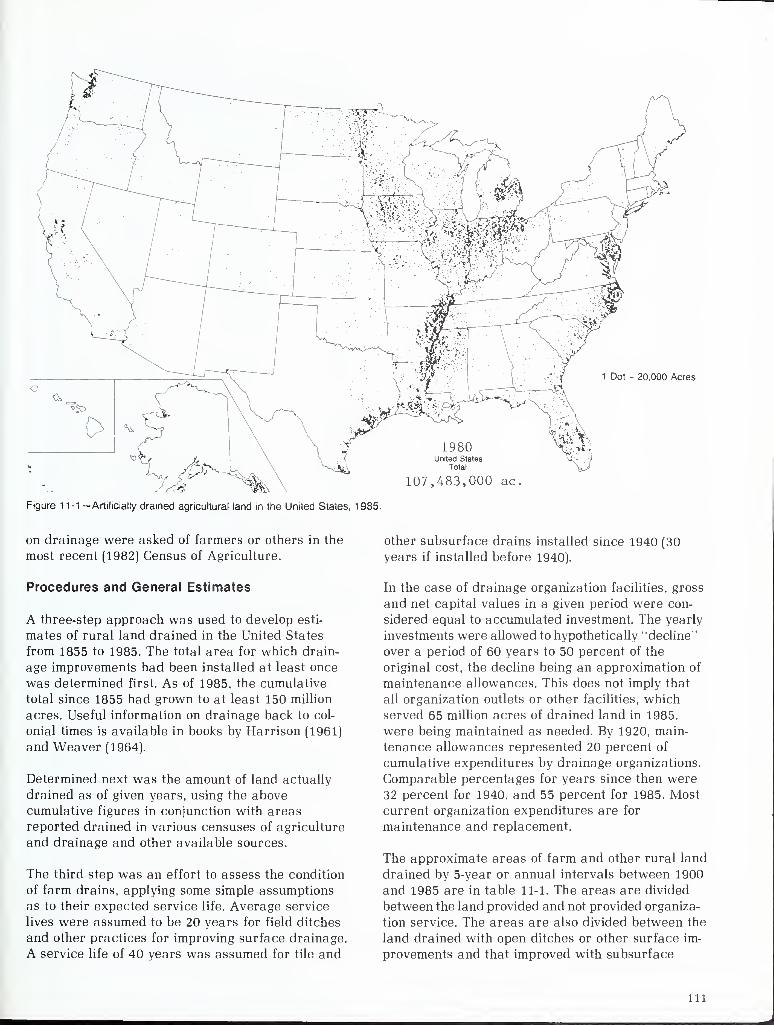
1 Dot - 20,000 Acres

107,483,000 ac.

Figure 11-1 —Artificially drained agricultural land in the United States, 1985.

on drainage were asked of farmers or others in the

most recent (1982) Census of Agriculture.

Procedures and General Estimates

A three-step approach was used to develop esti-

mates of rural land drained in the United States

from 1855 to 1985. The total area for which drain-

age improvements had been installed at least once

was determined first. As of 1985, the cumulative

total since 1855 had grown to at least 150 million

acres. Useful information on drainage back to col-

onial times is available in books by Harrison (1961)

and Weaver (1964).

Determined next was the amount of land actually

drained as of given years, using the above

cumulative figures in conjunction with areas

reported drained in various censuses of agriculture

and drainage and other available sources.

The third step was an effort to assess the condition

of farm drains, applying some simple assumptions

as to their expected service life. Average service

lives were assumed to be 20 years for field ditches

and other practices for improving surface drainage.

A service life of 40 years was assumed for tile and

other subsurface drains installed since 1940 (30

years if installed before 1940).

In the case of drainage organization facilities, gross

and net capital values in a given period were con-

sidered equal to accumulated investment. The yearly

investments were allowed to hypothetically "decline"

over a period of 60 years to 50 percent of the

original cost, the decline being an approximation of

maintenance allowances. This does not imply that

all organization outlets or other facilities, which

served 65 million acres of drained land in 1985,

were being maintained as needed. By 1920, main-

tenance allowances represented 20 percent of

cumulative expenditures by drainage organizations.

Comparable percentages for years since then were

32 percent for 1940, and 55 percent for 1985. Most

current organization expenditures are for

maintenance and replacement.

The approximate areas of farm and other rural land

drained by 5-year or annual intervals between 1900

and 1985 are in table 11-1. The areas are divided

between the land provided and not provided organiza-

tion service. The areas are also divided between the

land drained with open ditches or other surface im-

provements and that improved with subsurface

ill

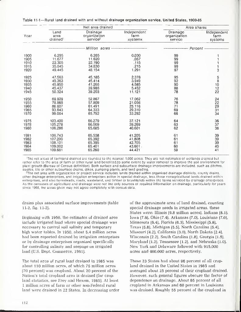
Table 11-1— Rural land drained with and without drainage organization service, United States, 1900-85

Net area drained Area shares

Land Drainage Independent Drainage ndependentYear area organization farm organization farm

drained 1 service2 systems service systems

Percent —

991900 6.295 6.265 0.030 1

1905 11.677 11.620 .057 99 1

1910 22.305 22.190 .115 99 1

1915 35.045 34.830 .215 99 1

1920 49.445 48.154 1.291 97 3

1925 47.563 45.185 2.378 95 51930 49.363 45.414 3.949 92 81935 45.850 41.265 4.585 90 101940 45.437 39.985 5.452 88 121945 50.324 39.203 11.121 78 22

1950 69.929 52.867 17.062 76 241955 78.865 57.809 21.056 78 221960 86.607 61.491 25.116 71 291965 93.643 64.333 29.310 69 31

1970 99.084 65.792 33.292 66 34

1975 103.400 66.279 37.121 64 361978 105.278 66.009 39.269 63 371980 106.286 65.685 40.601 62 38

1981 106.743 65.538 41.205 61 391982 107.200 65.392 41.808 61 391983 108.101 65.395 42.705 61 391984 109.002 65.401 43.601 . 60 401985 109.681 65.260 44.421 59 41

1The net areas of farmland drained are rounded to the nearest 1,000 acres. They are not estimates of wetlands drained but

rather refer to the area of farm or other rural land benefited. to some extent by water removal to improve the soil environment for

plant growth (Bureau of Census definition). Both surface and subsurface drainage improvements are included, such as ditches,

swales, tile or other subsurface drains, dikes, pumping plants, and land grading.2The net area with organization or project service includes lands drained within organized drainage districts, county drains,

other drainage enterprises, and irrigation enterprises active in special drainage, less those nonagricultural lands drained within

enterprises, and also farmsteads, roads, wasteland, and timber or brushlands within the farms serviced by drainage enterprises.

As the censuses of agriculture and drainage were not the only sources of required information on drainage, particularly for years

since 1959, the areas given may not agree completely with census data.

drains plus associated surface improvements (table

11-2, fig. 11-2).

Beginning with 1950, the estimates of drained area

include irrigated land where special drainage wasnecessary to control soil salinity and temporary

high water tables. In 1950, about 5.4 million acres

had been reported drained by irrigation enterprises

or by drainage enterprises organized specifically

for controlling salinity and seepage on irrigated

land (U.S. Dept. Commerce, 1961).

of the approximate area of land drained, counting

special drainage needs in irrigated areas, these

States were: Illinois (9.8 million acres), Indiana (8.1),

Iowa (7.8), Ohio (7.4), Arkansas (7.0), Louisiana (7.0),

Minnesota (6.4), Florida (6.3), Mississippi (5.8),

Texas (5.8). Michigan (5.5), North Carolina (5.4),

Missouri (4.2), California (3.0), North Dakota (2.4).

Wisconsin (2.2), South Carolina (1.8), Georgia (1.5),

Maryland (1.2), Tennessee (1.2), and Nebraska (1.0).

New York and Delaware followed with 915,000

acres and 460,000 acres, respectively.

The total area of rural land drained in 1985 wasabout 110 million acres, of which 75 million acres

(70 percent) was cropland. About 20 percent of the

Nation's total cropland area is drained (for crop-

land statistics, see Frey and Hexem, 1985). At least

1 million acres of farm or other non-Federal rural

land were drained in 22 States. In decreasing order

These 23 States had about 96 percent of all crop-

land drained in the United States in 1985 and

averaged about 25 percent of their cropland drained.

However, such general figures obscure the factor of

dependence on drainage. About 65 percent of all

cropland in Arkansas and 60 percent in Louisiana

was drained. Roughly 55 percent of the cropland in

112

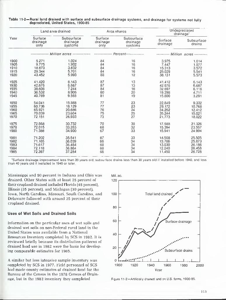
Table 11-2— Rural land drained with surface and subsurface drainage systems, and drainage for systems not fullydepreciated, United States, 1900-85

Land area drained Area shares Undepreciateddrainage 1

Year Surface Subsurface Surface SubsurfaceSurfacedrainage

Subsurfacedrainage drainage drainage drainageonly systems only systems drains

Million

3.9751900 5.271 1.024 84 16

dcres

1.0141905 9.775 1.902 84 16 7.447 1.8771910 18.673 3.632 84 16 15.313 3.5721915 29.344 5.701 84 16 25.029 5.5411920 43.452 5.993 88 12 38.131 5.573

1925 41.420 6.143 87 13 41.412 6.1431930 42.676 6.687 87 13 42.676 6.6871935 38.606 7.244 84 16 32.697 6.1181940 36.532 8.905 80 20 19.298 4.7111945 40.769 9.555 81 19 15.800 3.291

1950 54.041 15.888 77 23 22.849 9.3321955 60.736 18.129 77 23 29.172 10.7681960 65.921 20.686 76 24 34.252 12.4121965 70.039 23.604 75 25 35.244 15.0211970 72.151 26.933 73 27 21.773 18.022

1975 72.668 30.732 70 30 17.588 21.3261978 72.015 33.263 68 32 15.394 23.5571980 71.386 34.900 67 33 15.941 24.994

1981 71.202 35.541 67 33 14.508 25.5051982 71.165 36.039 66 34 13.786 25.8731983 71.617 36.484 66 34 13.030 26.1881984 72.118 36.884 66 34 12.240 26.4581985 72.397 37.284 66 34 11.450 26.728

1 Surface drainage improvement less than 20 years old; subsurface drains less than 30 years old if installed before 1940, and less

than 40 years old if installed in 1940 or later.

Mississippi and 50 percent in Indiana and Ohio wasdrained. Other States with at least 25 percent of

their cropland drained included Florida (45 percent),

Illinois (35 percent), and Michigan (30 percent).

Iowa, North Carolina, Missouri, South Carolina, andDelaware followed with around 25 percent of their

cropland drained.

Uses of Wet Soils and Drained Soils

Information on the particular uses of wet soils anddrained wet soils on non-Federal rural land in the

United States was available from a National

Resources Inventory completed by SCS in 1982. It is

reviewed briefly because its distribution patterns of

drained land use in 1982 were the basis for develop-

ing comparable estimates for 1985.

A similar but less intensive sample inventory wascompleted by SCS in 1977. Field personnel of SCShad made county estimates of drained land for the

Bureau of the Census in the 1978 Census of Drain-

age, but in the 1982 inventory they completed

Mil. ac.

1 iU

^~100 u Total land drained S _

//

/80 -

1 /

. ^surface drainage-60

40^^ •

1/ ..-•••

20.•* Subsurface drains

/y ....-"....J.-M*" 1 1 1 I I I I

1900 1920 1940 1960 1980 2000

Year

Figure 11-2— Artificially drained land on U.S. farms, 1900-85.

113

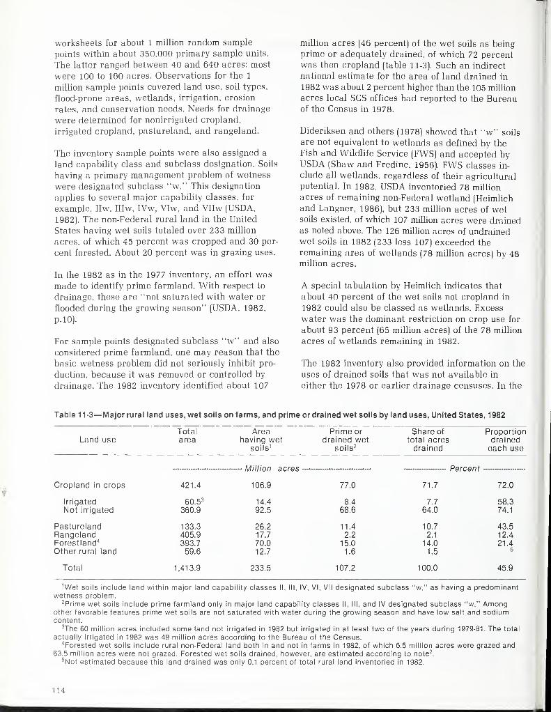
worksheets for about 1 million random sample

points within about 350,000 primary sample units.

The latter ranged between 40 and 640 acres; most

were 100 to 160 acres. Observations for the 1

million sample points covered land use, soil types,

flood-prone areas, wetlands, irrigation, erosion

rates, and conservation needs. Needs for drainage

were determined for nonirrigated cropland,

irrigated cropland, pastureland, and rangeland.

The inventory sample points were also assigned a

land capability class and subclass designation. Soils

having a primary management problem of wetness

were designated subclass "w." This designation

applies to several major capability classes, for

example, IIw, IIIw, IVw, VIw, and VIIw (USDA,

1982). The non-Federal rural land in the United

States having wet soils totaled over 233 million

acres, of which 45 percent was cropped and 30 per-

cent forested. About 20 percent was in grazing uses.

In the 1982 as in the 1977 inventory, an effort wasmade to identify prime farmland. With respect to

drainage, these are "not saturated with water or

flooded during the growing season" (USDA. 1982,

p.10).

For sample points designated subclass "w" and also

considered prime farmland, one may reason that the

basic wetness problem did not seriously inhibit pro-

duction, because it was removed or controlled by

drainage. The 1982 inventory identified about 107

million acres (46 percent) of the wet soils as being

prime or adequately drained, of which 72 percentwas then cropland (table 11-3). Such an indirect

national estimate for the area of land drained in

1982 was about 2 percent higher than the 105 million

acres local SCS offices had reported to the Bureauof the Census in 1978.

Dideriksen and others (1978) showed that "w" soils

are not equivalent to wetlands as defined by the

Fish and Wildlife Service (FWS) and accepted byUSDA (Shaw and Fredine, 1956). FWS classes in-

clude all wetlands, regardless of their agricultural

potential. In 1982. USDA inventoried 78 million

acres of remaining non-Federal wetland (Heimlichand Langner, 1986). but 233 million acres of wetsoils existed, of which 107 million acres were drainedas noted above. The 126 million acres of undrainedwet soils in 1982 (233 less 107) exceeded the

remaining area of wetlands (78 million acres) by 48million acres.

A special tabulation by Heimlich indicates that

about 40 percent of the wet soils not cropland in

1982 could also be classed as wetlands. Excess

water was the dominant restriction on crop use for

about 93 percent (65 million acres) of the 78 million

acres of wetlands remaining in 1982.

The 1982 inventory also provided information on the

uses of drained soils that was not available in

either the 1978 or earlier drainage censuses. In the

Table 11-3— Major rural land uses, wet soils on farms, and prime or drained wet soils by land uses, United States, 1982

Total Area Prime or Share of ProportionLand use area having wet drained wet total acres drained

soils 1 soils2 drained each use

Million

Cropland in crops 421.4 106.9 77.0 71.7 72.0

Irrigated 60.53 14.4 8.4 7.7 58.3Not irrigated 360.9 92.5 68.6 64.0 74.1

Pastureland 133.3 26.2 11.4 10.7 43.5Rangeland 405.9 17.7 2.2 2.1 12.4

Forestland 4 393.7 70.0 15.0 14.0 21.4Other rural land 59.6 12.7 1.6 1.5 5

Total 1,413.9 233.5 107.2 100.0 45.9

1Wet soils include land within major land capability classes II, III. IV, VI. VII designated subclass "w," as having a predominantwetness problem.

2Prime wet soils include prime farmland only in major land capability classes II, III, and IV designated subclass "w." Amongother favorable features prime wet soils are not saturated with water during the growing season and have low salt and sodiumcontent.

3The 60 million acres included some land not irrigated in 1982 but irrigated in at least two of the years during 1979-81. The total

actually irrigated in 1982 was 49 million acres according to the Bureau of the Census.4 Forested wet soils include rural non-Federal land both in and not in farms in 1982. of which 6.5 million acres were grazed and

63.5 million acres were not grazed. Forested wet soils drained, however, are estimated according to note2.

5Not estimated because this land drained was only 0.1 percent of total rural land inventoried in 1982.

114

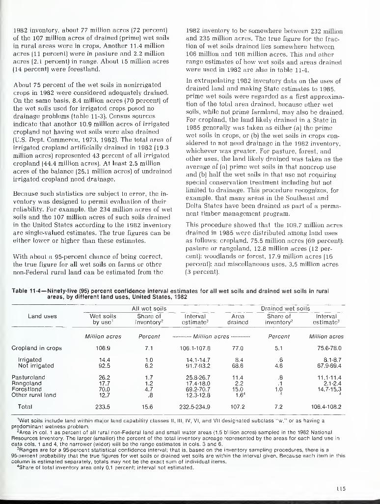
1982 inventory, about 77 million acres (72 percent)

of the 107 million acres of drained (prime) wet soils

in rural areas were in crops. Another 11.4 million

acres (11 percent) were in pasture and 2.2 million

acres (2.1 percent) in range. About 15 million acres

(14 percent) were forestland.

About 75 percent of the wet soils in nonirrigated

crops in 1982 were considered adequately drained.

On the same basis, 8.4 million acres (70 percent) of

the wet soils used for irrigated crops posed no

drainage problems (table 11-3). Census sources

indicate that another 10.9 million acres of irrigated

cropland not having wet soils were also drained

(U.S. Dept. Commerce, 1973, 1982). The total area of

irrigated cropland artificially drained in 1982 (19.3

million acres) represented 43 percent of all irrigated

cropland (44.4 million acres). At least 2.5 million

acres of the balance (25.1 million acres) of undrained

irrigated cropland need drainage.

Because such statistics are subject to error, the in-

ventory was designed to permit evaluation of their

reliability. For example, the 234 million acres of wetsoils and the 107 million acres of such soils drained

in the United States according to the 1982 inventory

are single-valued estimates. The true figures can be

either lower or higher than these estimates.

With about a 95-percent chance of being correct,

the true figure for all wet soils on farms or other

non-Federal rural land can be estimated from the

1982 inventory to be somewhere between 232 million

and 235 million acres. The true figure for the frac-

tion of wet soils drained lies somewhere between106 million and 108 million acres. This and other

range estimates of how wet soils and areas drainedwere used in 1982 are also in table 11-4.

In extrapolating 1982 inventory data on the uses of

drained land and making State estimates to 1985,

prime wet soils were regarded as a first approxima-tion of the total area drained, because other wetsoils, while not prime farmland, may also be drained.

For cropland, the land likely drained in a State in

1985 generally was taken as either (a) the prime

wet soils in crops, or (b) the wet soils in crops con-

sidered to not need drainage in the 1982 inventory,

whichever was greater. For pasture, forest, andother uses, the land likely drained was taken as the

average of (a) prime wet soils in that noncrop use

and (b) half the wet soils in that use not requiring

special conservation treatment including but not

limited to drainage. This procedure recognizes, for

example, that many areas in the Southeast andDelta States have been drained as part of a perma-

nent timber management program.

This procedure showed that the 109.7 million acres

drained in 1985 were distributed among land uses

as follows: cropland, 75.5 million acres (69 percent);

pasture or rangeland, 12.8 million acres (12 per-

cent); woodlands or forest, 17.9 million acres (16

percent); and miscellaneous uses, 3.5 million acres

(3 percent).

Table 11-4— Ninety-five (95) percent confidence interval estimates for all wet soils and drained wet soils in rural

areas, by different land uses, United States, 1982

Land uses

All wet soils Drained wet soils

Wet soils

by use 1

Share of

inventory2

Interval

estimate3

Areadrained

Share of

inventory2

Interval

estimate3

Cropland in crops

Irrigated

Not irrigated

PasturelandRangelandForestlandOther rural land

Total

Million acres

106.9

14.4

92.5

26.217.7

70.0

12.7

233.5

Percent

7.1

1.0

6.2

1.7

1.2

4.7

.8

15.6

Million acres

106.1-107.8

14.1-14.7

91.7-93.2

25.8-26.7

17.4-18.0

69.2-70.7

12.3-12.8

232.5-234.9

77.0

8.4

68.6

11.4

2.2

15.0

1.64

107.2

Percent Million acres

5.1 75.6-78.0

.6

4.6

8.1-8.7

67.9-69.4

.8

.1

1.04

11.1-11.4

2.1-2.4

14.7-15.34

7.2 106.4-108.2

1Wet soils include land within major land capability classes II, III, IV, VI, and VII designated subclass "w," or as having a

predominant wetness problem.2Area in col. 1 as percent of all rural non-Federal land and small water areas (1.5 billion acres) sampled in the 1982 National

Resources Inventory. The larger (smaller) the percent of the total inventory acreage represented by the areas for each land use in

data cols. 1 and 4, the narrower (wider) will be the range estimates in cols. 3 and 6.3Ranges are for a 95-percent statistical confidence interval; that is, based on the inventory sampling procedures, there is a

95-percent probability that the true figures for wet soils or drained wet soils are within the interval given. Because each item in this

column is estimated separately, totals may not be the exact sum of individual items.4Share of total inventory area only 0.1 percent; interval not estimated.

115

Organized and Independent Drainage

Since about 1960, two major shifts appear to have

occurred in drainage: one is a trend away from

organizing new projects toward farmers independ-

ently installing their own systems (Gain, 1967), and

the other is that the area with subsurface drains

has increased more rapidly than that improved

through open or surface drainage (table 11-1, table

11-2, fig. 11-2). The changing condition of drainage

systems on farms and possible needs for redrainage

were approximated by analyzing these changes.

A rapid developmental period for organized project

drainage began about 1870 and ended about 1920,

by which time 48 million acres had been drained

within organization service areas. This area wasover 97 percent of all land then drained in the

United States (table 11-1). The true organization

share was likely less than this, however, because

1920 was the first time farmers were asked to

report how much of their land was artificially

drained. Before 1920, the Bureau of the Census and

USDA had cooperated in collecting drainage

statistics but only from drainage districts and other

public organizations.

A new surge of organized project drainage followed

World War II and continued until the early 1960's.

By 1965, the area of drained land served by organi-

zations had grown to 64 million acres, but hadfallen to about 70 percent of all drained land. This

was because independent farm systems had expanded

even more rapidly during the same period. For ex-

ample, between 1945 and 1965, nearly 42 percent,

or 18 million acres of the 43 million acres of newly

drained land, did not rely on organization facilities.

Since 1965, new drainage has primarily involved in-

dependent farm installations. The area served by

drainage organizations within projects apparently

peaked in 1978 at about 66 million acres.

Despite these changes, about 60 percent of the

farmland drained in the United States in 1985 still

relied on arterial drains installed by townships,

counties, special drainage districts, and other

organizations. The proportion of drained land served

by drainage organizations is 80-85 percent in leading

drainage States like Indiana, Ohio, Minnesota,

Michigan, and California. Group or organized ef-

forts are required for successful drainage of large

areas, especially if irrigated.

Another factor to consider is that much of the newinvestment in farm drainage will replace existing

systems using organization facilities. Also, while

larger and fewer farms imply more freedom for

owners and operators to drain independently of

other farms, that implication can be misleading.

Enlarged farm units may encompass land already

drained and requiring group outlets. Also, what is

reported as a large farm operating unit for census

purposes may not be a single block of land but a

number of separated owned and/or rented tracts.

The need for cooperation in drainage tends to

increase with the intensity of drainage development

within an area. Its success is determined by

climate, soils, topography, and other field condi-

tions, as well as by economics. Any significant

future expansion of project drainage may occur in

connection with new conversions of wetland forests

and other low-lying areas to agricultural, urban, or

industrial uses (U.S. Dept. Commerce, 1981, p. vi).

But significant new organized activity may also be

stimulated by an increasing concern with salinity

and seepage in irrigated areas and the modernization

of existing drainage systems on farms, including

those not now using organization outlets.

Drainage Methods

Surface improvements are still the predominant

form of drainage on U.S. farms or other rural land.

In 1985, at least 72 million acres (66 percent) were

drained with bedding, open ditches, or other surface

improvements. Complete data are not available, but

up to 37 million acres (35 percent of the total) were

possibly drained with underground tile or the newer

types of plastic tube drains (table 11-2, fig. 11-2).

Gains in subsurface systems in relation to surface

drainage since 1960 can be attributed to muchimproved equipment and material, lower mainte-

nance costs, and minimal land loss for underground

drainage. Other technological advances, like laser-

beam grade-control devices, have made both

methods of drainage and other land-shaping activ-

ities more cost-efficient (van Schilfgaarde, 1971;

Donnan and Schwab, 1974).

Information was inadequate to permit a breakdown

of surface drainage improvements by whether they

are intended to simply dispose of excess precipita-

tion and runoff or, as subsurface systems are usually

designed, to regulate water tables as well as improve

surface drainage. Program data from USDA agencies

going back to 1940 combined with general trends

noted in historical census statistics were the main

basis for separating and analyzing surface and sub-

surface systems (USDA, 1981a, b,c). For this survey,

deep ditches used for water table control, as in the

Mississippi Delta and coastal areas where tiling is

not feasible, were regarded as surface drains.

116

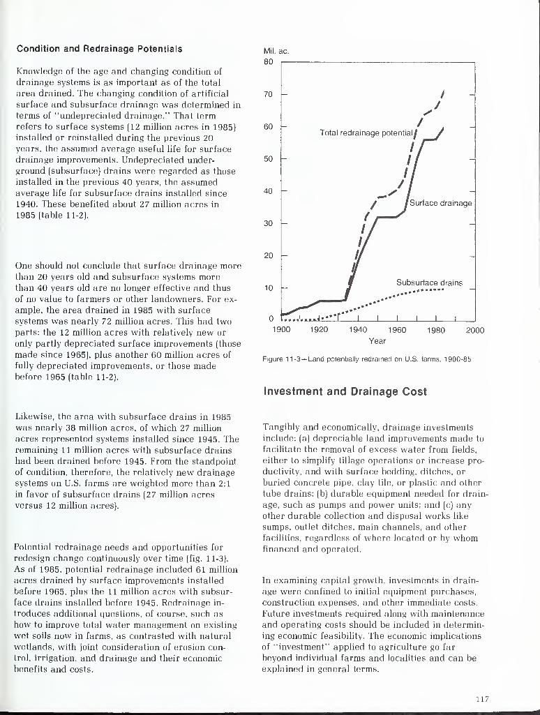
Condition and Redrainage Potentials

Knowledge of the age and changing condition of

drainage systems is as important as of the total

area drained. The changing condition of artificial

surface and subsurface drainage was determined in

terms of "undepreciated drainage." That term

refers to surface systems (12 million acres in 1985)

installed or reinstalled during the previous 20

years, the assumed average useful life for surface

drainage improvements. Undepreciated under-

ground (subsurface) drains were regarded as those

installed in the previous 40 years, the assumedaverage life for subsurface drains installed since

1940. These benefited about 27 million acres in

1985 (table 11-2).

One should not conclude that surface drainage morethan 20 years old and subsurface systems morethan 40 years old are no longer effective and thus

of no value to farmers or other landowners. For ex-

ample, the area drained in 1985 with surface

systems was nearly 72 million acres. This had two

parts: the 12 million acres with relatively new or

only partly depreciated surface improvements (those

made since 1965), plus another 60 million acres of

fully depreciated improvements, or those madebefore 1965 (table 11-2).

Mil. ac.

80

70

60

50

40

30

20 -

10

Total redrainage potential!

/ /Surface drainage

Subsurface drains

tTr...... 4-"T J L J L

1900 1920 1940 1960 1980 2000

Year

Figure 11-3— Land potentially redrained on U.S. farms, 1900-85

Investment and Drainage Cost

Likewise, the area with subsurface drains in 1985

was nearly 38 million acres, of which 27 million

acres represented systems installed since 1945. Theremaining 11 million acres with subsurface drains

had been drained before 1945. From the standpoint

of condition, therefore, the relatively new drainage

systems on U.S. farms are weighted more than 2:1

in favor of subsurface drains (27 million acres

versus 12 million acres).

Potential redrainage needs and opportunities for

redesign change continuously over time (fig. 11-3).

As of 1985, potential redrainage included 61 million

acres drained by surface improvements installed

before 1965, plus the 11 million acres with subsur-

face drains installed before 1945. Redrainage in-

troduces additional questions, of course, such as

how to improve total water management on existing

wet soils now in farms, as contrasted with natural

wetlands, with joint consideration of erosion con-

trol, irrigation, and drainage and their economic

benefits and costs.

Tangibly and economically, drainage investments

include: (a) depreciable land improvements made to

facilitate the removal of excess water from fields,

either to simplify tillage operations or increase pro-

ductivity, and with surface bedding, ditches, or

buried concrete pipe, clay tile, or plastic and other

tube drains; (b) durable equipment needed for drain-

age, such as pumps and power units; and (c) any

other durable collection and disposal works like

sumps, outlet ditches, main channels, and other

facilities, regardless of where located or by whomfinanced and operated.

In examining capital growth, investments in drain-

age were confined to initial equipment purchases,

construction expenses, and other immediate costs.

Future investments required along with maintenance

and operating costs should be included in determin-

ing economic feasibility. The economic implications

of "investment" applied to agriculture go far

beyond individual farms and localities and can be

explained in general terms.

117

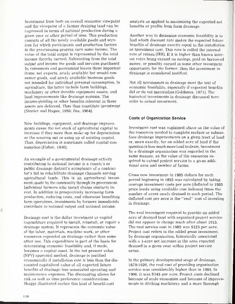
Investment from both an overall economic viewpoint

and the viewpoint of a farmer draining land can be

expressed in terms of national production during a

given year or other period of time. This production

consists of all the newly available goods and serv-

ices for which participants and production factors

in the provisioning process earn some income. The

value of the total output is represented by the total

income thereby earned. Subtracting from the total

output and income the goods and services purchased

by consumers and government leaves three important

items: net exports, newly available but unsold con-

sumer goods, and newly available business goods

not intended for individual personal consumption. In

agriculture, the latter include farm buildings,

machinery or other durable equipment assets, and

land improvements like drainage systems. The

income-yielding or other benefits inherent in these

assets are deferred. They thus constitute investment

(Stonier and Hague, 1956; Fox, 1964).

New buildings, equipment, and drainage improve-

ments cause the net stock of agricultural capital to

increase if they more than make up for depreciation

or the wearing out or using up of existing capital.

Thus, depreciation is sometimes called capital con-

sumption (Fisher, 1930).

An example of a governmental drainage activity

contributing to national income is a county's or

public drainage district's acceptance of a contrac-

tor's bid to rehabilitate drainage channels serving

agricultural lands. This is an agricultural invest-

ment, made by the community through its government.

Individual farmers who install drains similarly in-

vest. In addition to prospectively increasing farm

production, reducing costs, and otherwise benefiting

farm operations, investments by farmers immediately

contribute to national output and national income.

Drainage cost is the dollar investment or capital

expenditure required to install, reinstall, or repair a

drainage system. It represents the economic value

of the labor, materials, machine work, or other

resources expended on drainage rather than some

other use. This expenditure is part of the basis for

determining economic feasibility and, if made,

becomes a capital asset. In the net present value

(NPV) appraisal method, drainage is justified

economically if installation cost is less than the dis-

counted capitalized value of all expected future

benefits of drainage less associated operating andmaintenance expenses. The discounting allows for

risk as well as time preference considerations.

Skaggs illustrated earlier this kind of benefit-cost

analysis as applied to maximizing the expected net

benefits or profits from farm drainage.

Another way to determine economic feasibility is to

find which discount rate makes the expected future

benefits of drainage exactly equal to the installation

or investment cost. This rate is called the internal

rate of return (IRR). If it is higher than known inter-

est rates being earned on savings, paid on borrowedmoney, or possibly earned in some other investment

opportunity for the farmer, then the investment in

drainage is considered justified.

Not all investments in drainage meet the test of

economic feasibility, especially if expected benefits

did or do not materialize (Goldstein, 1971). Thehistorical investments in drainage discussed here

refer to actual investment.

Costs of Organization Service

Investment cost was explained above as the value of

the resources needed to complete surface or subsur-

face drainage improvements on a given tract of land

or, more exactly, for an added acre of land if the

question is how much more land to drain. Investment

by a drainage organization was regarded in the

same manner, as the value of the resources re-

quired to extend project service to a given addi-

tional area and number of farms.

Gross new investment in 1985 dollars for each

period beginning in 1855 was calculated by taking

average investment costs per acre (deflated to 1985

price levels using available cost indexes) times the

number of acres newly drained in each period. Thedeflated cost per acre is the "real" cost of investing

in drainage.

The real investment required to provide an addedacre of drained land with organized project service

did not appear to change much after about 1915.

The real service cost in 1985 was $225 per acre.

Project cost refers to the added gross investment,

by drainage organization, historically associated

with a 1-acre net increase in the area reported

drained in a given year within project service

areas.

In the primary developmental stage of drainage,

1870-1920, the real cost of providing organization

service was considerably higher than in 1985. In

1900, it was $345 per acre. Project costs declined

because of scale economies and because of improve-

ments in ditching machinery and a more thorough

118

understanding of the physics of drainage (van

Schilfgaarde, 1971).

Costs of Drainage on Farms

The average investment cost of open or other sur-

face drainage was about $140 per acre in 1985.

About 72.4 million acres were then improved for

surface drainage. The real cost of surface drainage

improvements appears to have fluctuated over time,

ranging from $225 per acre in 1900 to the low of

$125 per acre in 1950. It rose to $210 per acre by

1970 but by 1985 had again declined to $140 per

acre. These costs exclude timber clearing or other

land reclamation activities often associated with

drainage development.

The investment needed to install subsurface drains

on U.S. farms averaged about $415 per acre in

1985. About 37.3 million acres were then drained

this way. This cost was only about half the per-acre

real cost estimated for 1965. Notable declines in the

real cost of subsurface drains have resulted from

such technological advances as continuous cor-

rugated plastic tubing, improved manufacturing

methods and materials, improved distribution and

marketing, and advances in field installation tech-

niques and construction equipment. Laser-beam

grade-control devices on trenching and other

drainage equipment are notable examples (Donnan

and Schwab, 1974; van Schilfgaarde, 1971).

Investment Trends

For both organized and independent farm drainage

activity, long-term trends in investment parallel

expansions in the area drained, but only in a

general way, because of changes in prices anddrainage technology. Nearly 46 million acres of

newly drained land were added to organization

service areas during 1900-20 (table 11-1). In 1985

dollars, organization investment averaged $320million per year during this primary development

period.

The rate of new investment by drainage organiza-

tions peaked at $460 million per year during

1905-10. During 1910-30, it dropped back to around

$300 million per year. It was very low during the

Depression through World War II. During 1945-60,

investment by drainage organizations recovered to

about $75 million per year. It continued around this

level until 1980. It fell to about $50 million per year

during 1981-85.

Rather large areas were newly improved with sur-

face drainage up until 1920 and again between

1940 and 1970 (table 11-2, fig. 11-2). Investments in

actual as well as real dollars increased sharply

after World War II because of newly stimulated

project activity, better yet more costly drainagemethods, and higher costs for materials.

Excepting an apparent lull during 1915-25, farmersin the United States have installed new tile, plastic,

or other subsurface drains at a steady rate. Asharp increase in both surface and subsurfacedrainage followed World War II. The area improvedbecause surface drainage increased by 875,000acres per year during 1945-80, compared with

425,000 acres per year improved with subsurface

drains (table 11-2). However, investments in subsur-

face drains averaged $465 million per year during

1945-80, compared with $190 million per year for

surface drainage. This increase occurred despite

the much higher per acre cost of subsurface drains.

One factor was that subsurface drainage hadbecome more cost-effective, both absolutely andrelatively. Absolute gains in cost effectiveness for

subsurface drains occurred because their actual in-

stallation cost did not rise as rapidly as prices in

general. Relative gains for subsurface drains oc-

curred because their real cost per acre declined in

relation to the real cost of surface drainage.

Growth of Drainage Capital

The buildup of drainage investments over time

becomes a stock of drainage capital, much like an

irrigation reservoir creates a stock of water by im-

pounding runoff. Thus, any drainage improvement

can be regarded as involving prior investments and

sacrifices in consumption in exchange for future

production and other benefits.

The accumulated real investments in drainage for

the United States were measured as accumulated

annual investments indexed (deflated) year by year

to a particular base year, chosen here as the year

1985. The indexing was necessary to allow for

changes in investment rates due simply to changes

in the prices of materials, labor, and other input

factors. The indexed or constant-dollar investments

recognize that changes have occurred in materials

and methods as well as in the area drained.

Drainage works and improvements were also valued

terms of the hypothetical cost of replacing them at a

particular time, regardless of when they were built

or made. This concept of value is not as theoretical

as it may appear. It is a common basis for insurance

coverage and an important barrier to replacing ob-

solete or deteriorated improvements.

119

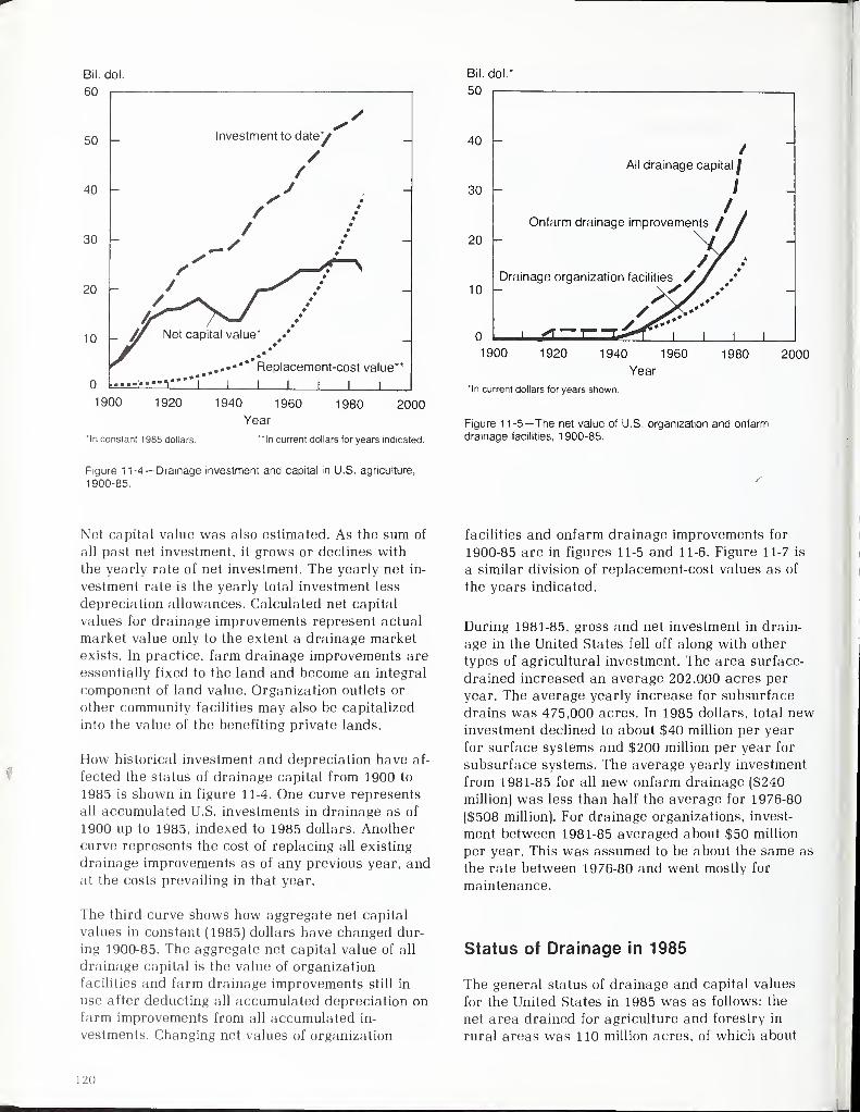
Bil. dol

60

50 -

40

30 -

20

10 -

1900

/SInvestment to dateV

//

S i

//

" —

- // Net capital value* * -

f .< *

1920 1980 20001940 1960

Year

'In constant 1985 dollars. "In current dollars for years indicated.

Bil. dol.*

50

40

30

20

10

All drainage capitalf

Onfarm drainage improvements

Drainage organization facilities // »

J L

Figure 11-4 — Drainage investment and capital in U.S. agriculture,

1900-85.

1900 1920 1940 1960 1980 2000

Year

*ln current dollars for years shown

Figure 11-5—The net value of U.S. organization and onfarm

drainage facilities. 1900-85.

S

Net capital value was also estimated. As the sum of

all past net investment, it grows or declines with

the yearly rate of net investment. The yearly net in-

vestment rate is the yearly total investment less

depreciation allowances. Calculated net capital

values for drainage improvements represent actual

market value only to the extent a drainage market

exists. In practice, farm drainage improvements are

essentially fixed to the land and become an integral

component of land value. Organization outlets or

other community facilities may also be capitalized

into the value of the benefiting private lands.

How historical investment and depreciation have af-

fected the status of drainage capital from 1900 to

1985 is shown in figure 11-4. One curve represents

all accumulated U.S. investments in drainage as of

1900 up to 1985. indexed to 1985 dollars. Another

curve represents the cost of replacing all existing

drainage improvements as of any previous year, andat the costs prevailing in that year.

The third curve shows how aggregate net capital

values in constant (1985) dollars have changed dur-

ing 1900-85. The aggregate net capital value of all

drainage capital is the value of organization

facilities and farm drainage improvements still in

use after deducting all accumulated depreciation on

farm improvements from all accumulated in-

vestments. Changing net values of organization

facilities and onfarm drainage improvements for

1900-85 are in figures 11-5 and 11-6. Figure 11-7 is

a similar division of replacement-cost values as of

the years indicated.

During 1981-85, gross and net investment in drain-

age in the United States fell off along with other

types of agricultural investment. The area surface-

drained increased an average 202,000 acres per

year. The average yearly increase for subsurface

drains was 475,000 acres. In 1985 dollars, total newinvestment declined to about $40 million per year

for surface systems and $200 million per year for

subsurface systems. The average yearly investment

from 1981-85 for all new onfarm drainage ($240

million) was less than half the average for 1976-80

($508 million). For drainage organizations, invest-

ment between 1981-85 averaged about $50 million

per year. This was assumed to be about the same as

the rate between 1976-80 and went mostly for

maintenance.

Status of Drainage in 1985

The general status of drainage and capital values

for the United States in 1985 was as follows: the

net area drained for agriculture and forestry in

rural areas was 110 million acres, of which about

120

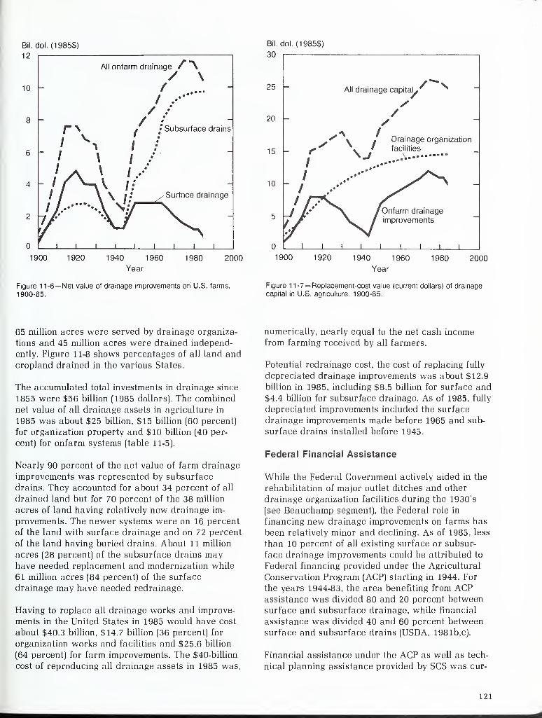
Bil.dol. (1985$)

12

10

All onfarm drainage f \

/ \

• Subsurface drains

Surface drainage

r i i

1900 1920 1940 1960 1980 2000

Year

Figure 1 1-6— Net value of drainage improvements on U.S. farms,

1900-85.

Bil.dol. (1985$)

30

25

20 -

15 -

10 -

All drainage capital/

/V

//

S . - Drainage organization

^^ \ ' facilities

Onfarm drainage

improvements

_L

1900 1920 1940 1960 1980 2000

Year

Figure 11-7— Replacement-cost value (current dollars) of drainage

capital in U.S. agriculture. 1900-85.

65 million acres were served by drainage organiza-

tions and 45 million acres were drained independ-

ently. Figure 11-8 shows percentages of all land and

cropland drained in the various States.

The accumulated total investments in drainage since

1855 were $56 billion (1985 dollars). The combined

net value of all drainage assets in agriculture in

1985 was about $25 billion, $15 billion (60 percent)

for organization property and $10 billion (40 per-

cent) for onfarm systems (table 11-5).

Nearly 90 percent of the net value of farm drainage

improvements was represented by subsurface

drains. They accounted for about 34 percent of all

drained land but for 70 percent of the 38 million

acres of land having relatively new drainage im-

provements. The newer systems were on 16 percent

of the land with surface drainage and on 72 percent

of the land having buried drains. About 11 million

acres (28 percent) of the subsurface drains mayhave needed replacement and modernization while

61 million acres (84 percent) of the surface

drainage may have needed redrainage.

Having to replace all drainage works and improve-

ments in the United States in 1985 would have cost

about $40.3 billion, $14.7 billion (36 percent) for

organization works and facilities and $25.6 billion

(64 percent) for farm improvements. The $40-billion

cost of reproducing all drainage assets in 1985 was,

numerically, nearly equal to the net cash income

from farming received by all farmers.

Potential redrainage cost, the cost of replacing fully

depreciated drainage improvements was about $12.9

billion in 1985, including $8.5 billion for surface and

$4.4 billion for subsurface drainage. As of 1985, fully

depreciated improvements included the surface

drainage improvements made before 1965 and sub-

surface drains installed before 1945.

Federal Financial Assistance

While the Federal Government actively aided in the

rehabilitation of major outlet ditches and other

drainage organization facilities during the 1930's

(see Beauchamp segment), the Federal role in

financing new drainage improvements on farms has

been relatively minor and declining. As of 1985, less

than 10 percent of all existing surface or subsur-

face drainage improvements could be attributed to

Federal financing provided under the Agricultural

Conservation Program (ACP) starting in 1944. For

the years 1944-83, the area benefiting from ACPassistance was divided 80 and 20 percent between

surface and subsurface drainage, while financial

assistance was divided 40 and 60 percent between

surface and subsurface drains (USDA, 1981b, c).

Financial assistance under the ACP as well as tech-

nical planning assistance provided by SCS was cur-

121

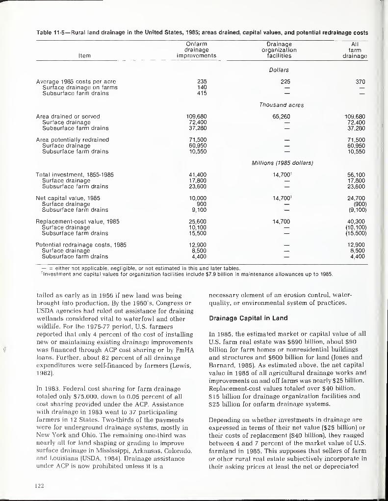
Table 11-5— Rural land drainage in the United States, 1985; areas drained, capital values, and potential redrainage costs

Item

Onfarmdrainage

improvements

Drainageorganization

facilities

All

farmdrainage

Average 1985 costs per acreSurface drainage on farmsSubsurface farm drains

Area drained or servedSurface drainageSubsurface farm drains

Area potentially redrainedSurface drainageSubsurface farm drains

Total investment, 1855-1985Surface drainageSubsurface farm drains

Net capital value, 1985Surface drainageSubsurface farm drains

Replacement-cost value, 1985Surface drainageSubsurface farm drains

Potential redrainage costs, 1985Surface drainageSubsurface farm drains

235140415

109,68072,40037,280

71,50060,95010,550

41,4001 7,80023,600

10,000900

9,100

25,60010,10015,500

12,9008,5004,400

Dollars

225 370

Thousand acres

65,260 109,68072,40037,280

— 71,50060,95010,550

Millions (1985 dollars)

14,700 1 56,10017,80023,600

14,700 1 24,700(900)

(9,100)

14,700 40,300(10,100)

(15,500)

— 12,9008,5004,400

— = either not applicable, negligible, or not estimated in this and later tables.

investment and capital values for organization facilities include $7.9 billion in maintenance allowances up to 1985.

tailed as early as in 1956 if new land was being

brought into production. By the 1960's, Congress or

USDA agencies had ruled out assistance for draining

wetlands considered vital to waterfowl and other

wildlife. For the 1975-77 period, U.S. farmers

reported that only 4 percent of the cost of installing

new or maintaining existing drainage improvementswas financed through ACP cost sharing or by FmHAloans. Further, about 82 percent of all drainage

expenditures were self-financed by farmers (Lewis,

1982).

In 1983, Federal cost sharing for farm drainage

totaled only $75,000, down to 0.05 percent of all

cost sharing provided under the ACP. Assistance

with drainage in 1983 went to 37 participating

farmers in 12 States. Two-thirds of the paymentswere for underground drainage systems, mostly in

New York and Ohio. The remaining one-third wasnearly all for land shaping or grading to improvesurface drainage in Mississippi, Arkansas, Colorado,

and Louisiana (USDA, 1984). Drainage assistance

under ACP is now prohibited unless it is a

122

necessary element of an erosion control, water-

quality, or environmental system of practices.

Drainage Capital in Land

In 1985, the estimated market or capital value of all

U.S. farm real estate was $690 billion, about $90

billion for farm homes or nonresidential buildings

and structures and $600 billion for land (Jones and

Barnard, 1985). As estimated above, the net capital

value in 1985 of all agricultural drainage works and

improvements on and off farms was nearly $25 billion.

Replacement-cost values totaled over $40 billion,

$15 billion for drainage organization facilities and

$25 billion for onfarm drainage systems.

Depending on whether investments in drainage are

expressed in terms of their net value ($25 billion) or

their costs of replacement ($40 billion), they ranged

between 4 and 7 percent of the market value of U.S.

farmland in 1985. This supposes that sellers of farm

or other rural real estate subjectively incorporate in

their asking prices at least the net or depreciated

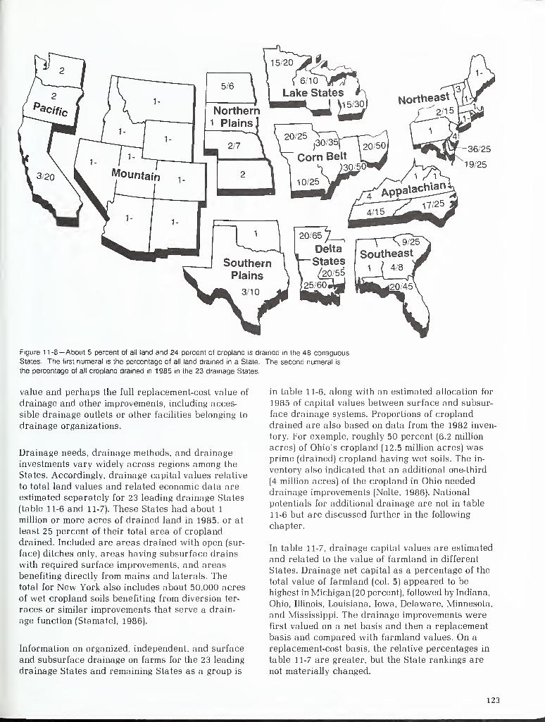
Figure 1 1-8— About 5 percent of all land and 24 percent of cropland is drained in the 48 contiguous

States. The first numeral is the percentage of all land drained in a State. The second numeral is

the percentage of all cropland drained in 1985 in the 23 drainage States.

value and perhaps the full replacement-cost value of

drainage and other improvements, including acces-

sible drainage outlets or other facilities belonging to

drainage organizations.

Drainage needs, drainage methods, and drainage

investments vary widely across regions among the

States. Accordingly, drainage capital values relative

to total land values and related economic data are

estimated separately for 23 leading drainage States

(table 11-6 and 11-7). These States had about 1

million or more acres of drained land in 1985, or at

least 25 percent of their total area of cropland

drained. Included are areas drained with open (sur-

face) ditches only, areas having subsurface drains

with required surface improvements, and areas

benefiting directly from mains and laterals. Thetotal for New York also includes about 50,000 acres

of wet cropland soils benefiting from diversion ter-

races or similar improvements that serve a drain-

age function (Stamatel, 1986).

Information on organized, independent, and surface

and subsurface drainage on farms for the 23 leading

drainage States and remaining States as a group is

in table 11-6, along with an estimated allocation for

1985 of capital values between surface and subsur-

face drainage systems. Proportions of cropland

drained are also based on data from the 1982 inven-

tory. For example, roughly 50 percent (6.2 million

acres) of Ohio's cropland (12.5 million acres) wasprime (drained) cropland having wet soils. The in-

ventory also indicated that an additional one-third

(4 million acres) of the cropland in Ohio needed

drainage improvements (Nolte, 1986). National

potentials for additional drainage are not in table

11-6 but are discussed further in the following

chapter.

In table 11-7, drainage capital values are estimated

and related to the value of farmland in different

States. Drainage net capital as a percentage of the

total value of farmland (col. 5) appeared to be

highest in Michigan (20 percent), followed by Indiana,

Ohio, Illinois, Louisiana, Iowa, Delaware, Minnesota,

and Mississippi. The drainage improvements werefirst valued on a net basis and then a replacement

basis and compared with farmland values. On a

replacement-cost basis, the relative percentages in

table 11-7 are greater, but the State rankings are

not materially changed.

123

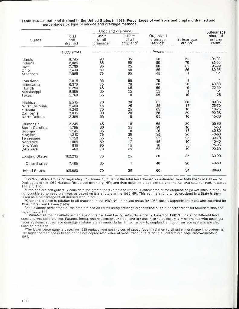
Table 11-6— Rural land drained in the United States in 1985: Percentages of wet soils and cropland drained andpercentages by type of service and drainage methods

Total

Cropland drainage

OrganizedSubsurfaceshare ofShare Share

States 1 land of all of all drainage Subsurface onfarmdrained drainage2 cropland 3 service4 drains5 value6

7,000 acres

Illinois 9,795 90 35 50 85 95-99

Indiana 8,085 85 50 80 70 85-95

Iowa 7.790 90 25 60 85 95-99

Ohio 7,400 80 50 85 65 80-95

Arkansas 7,085 75 65 45 1 MLouisiana 7,015 55 60 70 1 1

Minnesota 6,370 75 20 80 20 40-80

Florida 6,290 45 45 60 5 20-60

Mississippi 5,805 60 55 55 1 1-1

Texas 5,760 55 10 65 10 25

Michigan 5,515 70 30 85 60 80-95

North Carolina 5,400 45 25 25 15 35-75

Missouri 4,240 70 25 65 10 10-25

California 3,015 90 20 85 80 90-98

North Dakota 2,365 95 6 65 10 15-30

Wisconsin 2,245 45 10 65 30 55-90

South Carolina 1,755 60 25 20 10 15-50

Georgia 1,545 35 8 20 15 40-80

Maryland 1,210 75 30 35 20 40-80

Tennessee 1,150 55 15 25 25 30-70

Nebraska 1,005 80 7 45 10 10-40

New York 915 90 15 10 55 75-95

Delaware 460 70 25 55 10 20-60

Leading States 102,215 70 25 60 35 60-90

Other States 7,465 30 1 40 20 40-80

United States 109,680 70 20 60 34 60-90

1 Leading States are listed separately, in decreasing order of the total land drained as estimated from both the 1978 Census of

Drainage and the 1982 National Resources Inventory (NRI) and then adjusted proportionately to the national total for 1985 in tables

11-1 and 11-5.2Cropland drained generally considers the greater of (a) cropland wet soils considered prime cropland or (b) wet soils in crop use

not considered to need drainage, as based on State totals in the 1982 NRI. This estimate for drained cropland in a State is then

taken as a percentage of all drained land in col. 1.

3Cropland drained in relation to all cropland in the 1982 NRI; cropland areas for 1982 closely approximate those also reported for

1982 in Frey and Hexem (1985).

"Approximate percentage of the area drained on farms using drainage organization outlets or other disposal facilities; also seenote 2

, table 11-1.

Estimated as the maximum percentage of drained land having subsurface drains, based on 1982 NRI data for different land

uses and wet soils drained. Pasture, forest, and miscellaneous rural land are assumed to be essentially all drained with open (sur-

face) systems; subsurface drainage systems are assumed to be limited largely to cropland, although surface systems are also

used on cropland.6The lower percentage is based on 1985 replacement-cost values of subsurface in relation to all onfarm drainage improvements.

The higher percentage is based on the net depreciated value of subsurface in relation to all onfarm drainage improvements in

1985.

124

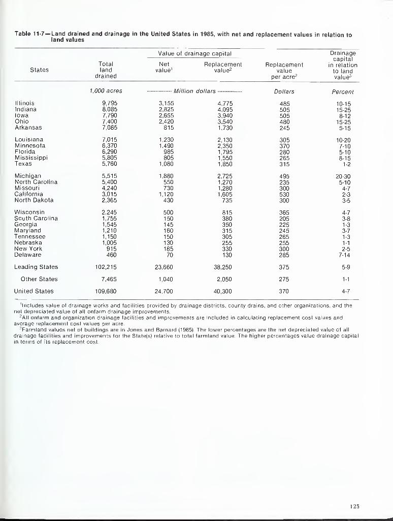
Table 11-7— Land drained and drainage in the United States in 1985, with net and replacement values in relation toland values

Value of drainage capital Drainagecapital

Total Net Replacement Replacement in relationStates land value 1 value2 value to land

drained per acre2 value3

7,000 acres

9,795

Dollars

485

Percent

10-15Illinois 3,155 4,775Indiana 8,085 2,825 4,095 505 15-25Iowa 7,790 2,655 3,940 505 8-12Ohio 7,400 2,420 3,540 480 15-25Arkansas 7,085 815 1,730 245 5-15

Louisiana 7,015 1,230 2,130 305 10-20Minnesota 6,370 1,490 2,350 370 7-10Florida 6,290 985 1,795 280 5-10Mississippi 5,805 805 1,550 265 8-15Texas 5,760 1,080 1,850 315 1-2

Michigan 5,515 1,880 2,725 495 20-30North Carolina 5,400 550 1,270 235 5-10Missouri 4,240 730 1,280 300 4-7

California 3,015 1,120 1,605 530 2-3

North Dakota 2,365 430 735 300 3-5

Wisconsin 2,245 500 815 365 4-7

South Carolina 1,755 150 380 205 3-8

Georgia 1,545 145 350 225 1-3

Maryland 1,210 160 315 245 3-7

Tennessee 1,150 150 305 265 1-3

Nebraska 1,005 130 255 255 1-1

New York 915 185 330 300 2-5

Delaware 460 70 130 285 7-14

Leading States 102,215 23,660 38,250 375 5-9

Other States 7,465 1,040 2,050 275 1-1

United States 109,680 24.700 40,300 370 4-7

includes value of drainage works and facilities provided by drainage districts, county drains, and other organizations, and the

net depreciated value of all onfarm drainage improvements.2AII onfarm and organization drainage facilities and improvements are included in calculating replacement cost values and

average replacement cost values per acre.3Farmland values net of buildings are in Jones and Barnard (1985). The lower percentages are the net depreciated value of all

drainage facilities and improvements for the State(s) relative to total farmland value. The higher percentages value drainage capital

in terms of its replacement cost.

125

These indicators of the importance in 1985 of drain-

age in the farm capital structure of individual

States are not claimed to be highly precise, nor

should they be taken as measures of drainage

benefits as such. They do tend to be higher in States

more dependent on public drains and where onfarm

subsurface drains predominate, especially if the

improvements are valued on a net or depreciated

basis.

The dependence on drainage organizations as well

as drainage methods used on farms differ by region,

and also by States within regions. In terms of area,

surface drainage was more common than subsurface

drainage in 1985 in all leading drainage States

other than Illinois, Indiana, Iowa, Ohio, and

Michigan (table 11-6). However, because of their

long life and greater installation cost, subsurface

drains accounted for most of the capital value of on-

farm drainage, nationally and for most States.

Notable exceptions are Arkansas. Louisiana, and

Mississippi. In these States, open and other forms of

surface drainage were still the norm in 1985, in

terms of net and replacement values as well as area

(table 11-6, col. 6).

Differences in Cost

Variations in capital values based on replacement

costs have some practical uses for anticipating the

probable cost (marginal cost) of additional drainage

in individual States. Costs can be expected to be

higher if subsurface drains are involved and/or

where organization outlets are necessary than

where surface drainage not using public outlets is

common (table 11-7, col. 4). The average costs per

acre given for various States would approach actual

field costs to the extent the probabilities of the addi-

tional drainage being surface or subsurface or

requiring group outlets correspond to existing pat-

terns of systems and drainage methods, such as

those indicated in table 11-6. But however figured,

State averages are not substitutes for carefully

determining marginal drainage costs in specific

cases.

Drainage in the Humid East

Research by Irwin (1979), Skaggs and Nassehzadeh-

Tabrizi (1983), van't Woudt and Hagan (1975),

Smedema and Rycroft (1984), and numerous other

investigators indicates that correcting poor

drainage condition improves the yield of nearly all

field and fruit crops. Broadly speaking, the ex-

pected longrun benefits vary with expected farm

prices, production costs, climate, soils, and

hydrology. Within a field to be drained, the benefits

or installation costs also depend on such design fac-

tors as the depth and spacing of the drains andactual rainfall conditions.

Dideriksen and others (1978) have reported that 25

percent of the value of all U.S. crops sold comesfrom artificially drained land. At a regional level,

some shares they gave for drained land were 75

percent for cotton and soybeans from the Delta

States, 40 percent for corn and soybeans from the

Corn Belt, and 40 percent for oats, barley, and hayproduced in the Lake States. As these shares are

equal to the shares of cropland drained, they

presume equal average productivity for drained andother cropland.

An important related question examined here waswhether localities in the generally humid Eastern

United States with fairly large fractions of their

cropland drained tend to be more productive and

exhibit higher real estate values than surrounding

areas with smaller proportions of their land drained.

Such economic differences cannot be credited en-

tirely to differences in drainage intensity. Thedifferences favoring drainage are believed to be on

the conservative side, however, because the com-

parisons are between different levels of drainage

intensity, not between drained land and undrained

land with drainage problems. Such ideal comparisons

on a broad scale were not feasible for this review.

To recognize various soil and climatic conditions

and numerous combinations of farming enterprises,

the analysis covered all 2,006 reporting counties in

the 31 Eastern States, for which necessary census

information was available on drained land, farm

production, and land values.

The Census of Drainage for 1978 was used first to

identify those counties in the humid East with high

concentrations (percentages) of drained land (U.S.

Dept. Commerce, 1981). The criterion for "high

drainage" varied rather arbitrarily from State to

State (fig. 11-9). It ranged from at least 5 percent of

a county's land area drained in New England and

upper Northeast States like New York and Penn-

sylvania to 40 percent of the land drained in heavily

drained States like Indiana, Ohio, Illinois, Louisiana,

and Florida. On this procedure, 307 eastern counties

were identified as being highly drained. (See figure

11-9.) A few counties were included where the

percentage of land drained was low but where the

land drained in a State was most concentrated.

For 1978, an average of 44 percent of the land wasdrained in the 307 counties highly drained. Some in

126

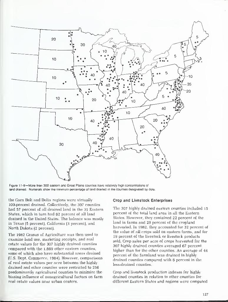
Figure 11-9— More than 300 eastern and Great Plains counties have relatively high concentrations of

land drained. Numerals show the minimum percentage of land drained in the counties designated by dots.

the Corn Belt and Delta regions were virtually

100-percent drained. Collectively, the 307 counties

had 57 percent of all drained land in the 31 Eastern

States, which in turn had 82 percent of all land

drained in the United States. The balance was mostly

in Texas (5 percent), California (3 percent), andNorth Dakota (2 percent).

The 1982 Census of Agriculture was then used to

examine land use, marketing receipts, and real

estate values for the 307 highly drained counties

compared with the 1,699 other eastern counties,

some of which also have substantial areas drained

(U.S. Dept. Commerce, 1984). However, comparisons

of real estate values per acre between the highly

drained and other counties were restricted to 256

predominantly agricultural counties to minimize the

biasing influence of nonagricultural factors on farm

real estate values near urban centers.

Crop and Livestock Enterprises

The 307 highly drained eastern counties included 15

percent of the total land area in all the Eastern

States. However, they contained 22 percent of the

land in farms and 29 percent of the cropland

harvested. In 1982, they accounted for 32 percent of

the value of all crops sold on eastern farms, and for

19 percent of the livestock or livestock products

sold. Crop sales per acre of crops harvested for the

307 highly drained counties averaged 67 percent

higher than for the other counties. An average of 44

percent of the farmland was drained in highly

drained counties compared with 6 percent in the

less-drained counties.

Crop and livestock production indexes for highly

drained counties in relation to other counties for

different Eastern States and regions were computed

127

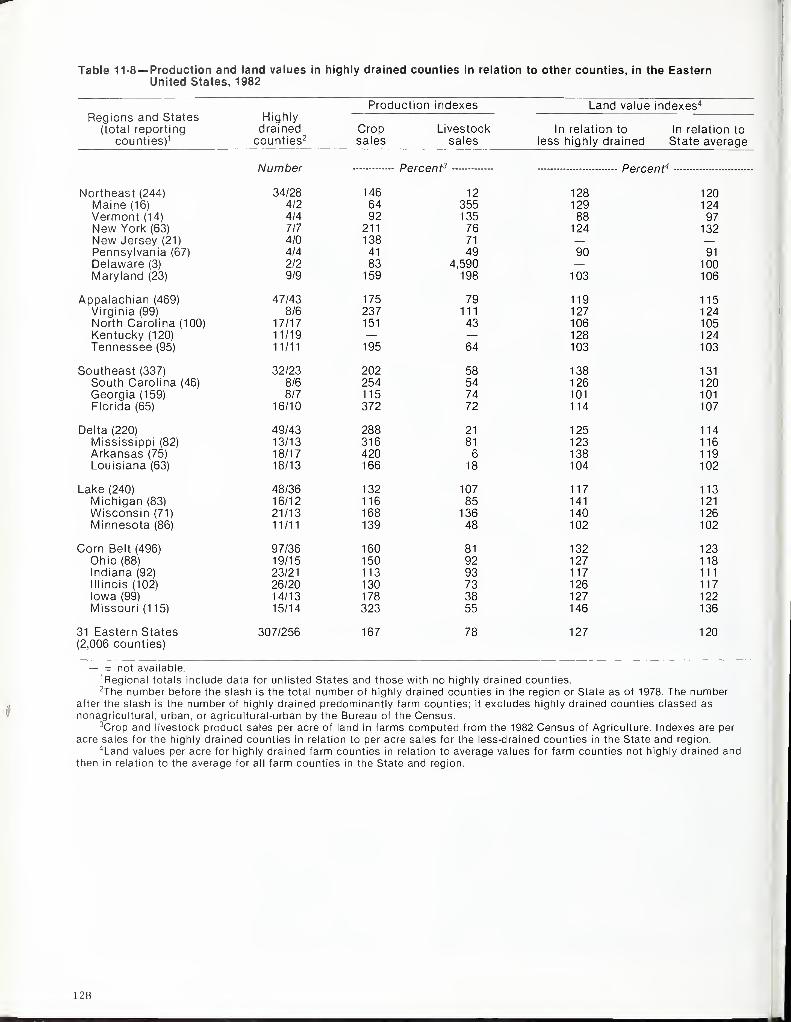
Table 11-8— Production and land values in highly drained counties in relation to other counties, in the EasternUnited States, 1982

Production indexes Land value indexes4

Regions and States Highly(total reporting drained Crop Livestock In relation to In relation to

counties) 1 counties2 sales sales less highly drained State average

Number Percent3 Percent4

Northeast (244) 34/28 146 12 128 120Maine (16) 4/2 64 355 129 124Vermont (14) 4/4 92 135 88 97New York (63) 7/7 211 76 124 132New Jersey (21) 4/0 138 71 — —Pennsylvania (67) 4/4 41 49 90 91

Delaware (3) 2/2 83 4,590 - 100Maryland (23) 9/9 159 198 103 106

Appalachian (469) 47/43 175 79 119 115Virginia (99) 8/6 237 111 127 124

106 105128 124

North Carolina (100) 17/17 151 43Kentucky (120) 11/19 — —Tennessee (95) 11/11 195 64 103 103

Southeast (337) 32/23 202 58 138 131

126 120South Carolina (46) 8/6 254 54Georgia (159) 8/7 115 74 101 101Florida (65) 16/10 372 72 114 107

125 114Delta (220) 49/43 288 21

Mississippi (82) 13/13 316 81 123 116Arkansas (75) 18/17 420 6 138 119Louisiana (63) 18/13 166 18 104 102

117 113Lake (240) 48/36 132 107Michigan (83) 16/12 116 85 141 121Wisconsin (71) 21/13 168 136 140 126Minnesota (86) 11/11 139 48 102 102

Corn Belt (496) 97/36 160 81 132 123Ohio (88) 19/15 150 92 127 118Indiana (92) 23/21 113 93 117 111Illinois (102) 26/20 130 73 126 117Iowa (99) 14/13 178 38 127 122Missouri (115) 15/14 323 55 146 136

31 Eastern States(2,006 counties)

307/256 167 78 127 120

— = not available.1 Regional totals include data for unlisted States and those with no highly drained counties.2The number before the slash is the total number of highly drained counties in the region or State as of 1978. The number

after the slash is the number of highly drained predominantly farm counties; it excludes highly drained counties classed as

nonagricultural, urban, or agricultural-urban by the Bureau of the Census.3Crop and livestock product sales per acre of land in farms computed from the 1982 Census of Agriculture. Indexes are per

acre sales for the highly drained counties in relation to per acre sales for the less-drained counties in the State and region.4Land values per acre for highly drained farm counties in relation to average values for farm counties not highly drained and

then in relation to the average for all farm counties in the State and region.

128

(table 11-8). The production indexes indicate the

extent to which gross farm income was derived

from crops and livestock products in the highly

drained counties compared with other counties.

Average crop and livestock product sales per acre

were weighted by total sales volume as well as total

areas in farms.

In Arkansas, for example, crop sales for 1982 in 18

highly drained counties averaged $168 per acre of

land in farms. The average for the 57 other counties

in Arkansas was $40 per acre, giving a ratio of 4.2

($168/$40) or a 420-percentage index favoring drain-

age. Sales of livestock and poultry products averaged

$10 per acre in the highly drained counties com-

pared with $162 per acre in the other counties, giv-

ing an index of 6 percent ($10/$162). Crop production

in Arkansas is clearly concentrated in the counties

most heavily drained, namely those toward the

Mississippi River. Other counties are geared more

to livestock and poultry production.

In 12 other Eastern States, crop sales per acre in

highly drained counties ranged from 105-370 per-

cent of crop sales for the less-drained counties.

These States were Florida, Missouri, Mississippi,

South Carolina, Virginia, New York, Tennessee,

Iowa, Wisconsin, Louisiana, Maryland, and Ohio

(table 11-8).

Crop production in 1982 appeared to be less impor-

tant in counties with more drained land than in

other areas of Maine, Vermont, Pennsylvania, and

Delaware. These States are important for dairy,

poultry, and other livestock as well as crop produc-

tion. The extreme livestock product index (4590) for

the two highly drained counties in Delaware (Kent

and Sussex) can be attributed to their concentrated

poultry industry, which depends in part on locally

grown feed crops produced on drained land.

States where both crop and livestock production

tended to be concentrated in counties that have ex-

tensive areas drained were Maryland, Virginia, and

Wisconsin. For these States, the crop sales and

livestock sales indexes in table 11-8 both exceeded

100 percent.

Total Farm Production

Combined crop and livestock product sales per farm

acre are a measure of average resource productivity

among different farms and producing areas. Compar-

isons between highly drained and other counties in

the Eastern States suggest that total sales per acre

were greater for counties with larger amounts of

drained land. Drainage appeared to be most cor-

related with total farm output in 12 States:

Delaware (index = 235), Maine (212), Mississippi

(189), Maryland (184), South Carolina (161), Virginia

(157), Missouri (146), Wisconsin (142), Vermont

(132), and Ohio, Iowa, and Tennessee (122). Theseindexes express average total farm product sales

per acre for the highly drained counties as a

percentage of the average for counties with less

land drained.

A precaution on these indexes is that they do not

fully allow for the fact that, in many localities,

agriculture would not be possible without drainage.

Wet soils are more productive when drained. Theymay be either more productive or less productive

than other soils with good natural drainage. This

factor partly explains the fairly low indexes for

leading drainage States like Louisiana, North

Carolina, Arkansas, Michigan, and Indiana. Theanalysis was conducted across regions and States

to compensate for limiting the comparisons to a

single crop year like 1982.

Land Value Influences

Real estate values are a measure of the capitalized

net economic returns expected from land as a factor

of production, along with related buildings or other

structures. Real estate values in 1982 for 256 highly

drained and predominantly agricultural counties in

the East averaged 27 percent more (index 127) than

values for the 1,422 other agricultural counties

(table 11-8).

Real estate values per acre in the 14 most intensively

drained farm counties in Missouri ran an average

of 46 percent higher than in Missouri's other 93

agricultural counties. Additional States with

relatively high land value indexes for the counties

most drained included Michigan (141), Wisconsin

(140), Arkansas (138), Maine (129), New York (124),

Kentucky (128), Virginia, Ohio, and Iowa (all 127),

and Illinois and South Carolina (126). These indexes

express average real estate values per farm acre

for the highly drained and predominantly agricul-

tural counties as a percentage of the average for

agricultural counties with less land drained. All

averages were weighted according to total areas in

farms and total farm real estate values for the two

groups of counties in each State.

Drainage appears to strongly influence farm real

estate values in the Southeast. Values per acre in

1982 in the 23 highly drained agricultural counties

129

in South Carolina, Georgia, and Florida ran 38 per-

cent more than in their 252 other farm counties, 53

of which are in Alabama. Alabama and some other

Eastern States are not listed in table 11-8 because

they have no counties with at least 5 percent of the

land area drained for agriculture.

Drainage appeared to positively influence land

values in all eastern regions and States listed in

table 11-8, except Vermont and Pennsylvania. Farmreal estate values between highly drained and other

counties were not compared in New Jersey, because

its four highly drained counties also happen to be

highly urbanized.

Average real estate values per farm acre for the

highly drained farm counties as a percentage of

averages for all farm counties in a State were also

computed (table 11-8). Because average land values

for States are published at fairly frequent intervals,

these indexes would be useful for estimating land

value differentials in dollars for highly drained

counties under market conditions where their land

values per acre tended to change proportionately

with those for other counties.

Separate values for land and buildings would im-

prove these comparisons but were not available for

counties. This was possible earlier in relating

drainage investment to farmland values for leading

drainage States (table 11-7). Irwin (1979) computed

net land values in determining whether Ontario

farmers wishing to increase production should

acquire additional land or should tile-drain existing

wet soils. While the net economic benefits of the

expansion or drainage alternatives were not

calculated, Irwin found that tile drainage was only

10-60 percent as costly as purchasing additional

land in Ontario in 1979. depending on the county.

Changing Feasibility of Drainage

Commodity prices, production costs, drainage costs,

and land values change both absolutely and in rela-

tion to each other from year to year. The same is

true of associated environmental benefits or

disbenefits. Thus, the economic feasibility of

drainage must be determined on a case-by-case

basis at a particular time by farmers and other

decisionmakers, with respect to the benefits anddisbenefits or other costs of concern to them.

Data on production and land value differences for

highly drained counties or other areas are useful

for explaining different rates of drainage develop-

ment among regions. Those data also help identify

areas where economic pressures for added drainage

may be the greatest. For example, the ratio in 1985of added onfarm benefits to drainage per dollar of

field installation cost (B/C ratio) averaged about

0.90 for the 307 highly drained counties studied in

25 Eastern States. In 1982 the average B/C ratio for

the East was near 1.30; in 1978 it was 1.40.

These ratios take as added costs per acre average

U.S. surface and subsurface drainage installation

costs in table 11-5 adjusted to the average State

replacement costs in table 11-7. Added benefits are

approximated as average land value differentials

from the 1982 census (table 11-8) adjusted accord-

ing to changes in yearly land values reported by

ERS (Jones and Barnard, 1985: USDA, 1986). Thedrop in the overall eastern B/C ratio from 1.30 in

1982 to 0.90 in 1985, and to 0.75 in 1986 was mainly

attributable to falling land values.

Drainage costs increased by 10 percent from

1982-86 while benefits fell by about 35 percent.

Farm real estate values in the East had risen from

an average of $935 per acre in 1978 to $1,360 per

acre in 1982. By 1985, they had fallen by 25 percent

and by 1986 by 35 percent (to $920 per acre) from

1982 levels.

In 1985, there were nine Eastern States where the

farm-level B/C ratio for added drainage was at least

1.0, including Arkansas (ratio = 1.90), Missouri

(1.75), Kentucky (1.65), Virginia (1.37), Mississippi

(1.32). South Carolina (1.30), Wisconsin (1.14),

Michigan (1.07), and Florida (1.05). Note the

predominance of the Mississippi Valley and Southern

States in this listing. In 1986 the B/C ratio was 1.0

or more in only seven of these States: Missouri

(1.60). Kentucky (1.60), Arkansas (1.55), Virginia

(1.45), South Carolina (1.25), Mississippi (1.20), and

Florida (1.0).

Between 1982 and 1986, the "average" B/C ratio for

drainage in Missouri fell from 2.85 to 1.60. It fell

from 1.36 to 0.78 in Ohio, from 1.35 to 0.57 in Iowa,

for 1.30 to 0.70 in Illinois, and from near 1.0 to 0.50

in Indiana. Between 1982-86, the average B/C ratio

for the Corn Belt region dropped from 1.35 to 0.70.

while in the Lake States it fell from 1.20 to 0.75.

Drainage and National Policy

Comparing production and land values for highly

drained and other counties in the Eastern States

was not an argument for converting remaining wet-

lands to agricultural uses through drainage and

associated clearing or other land reclamation ac-

130

tivities. If economically feasible, drainage is still a

recommended practice on wet soils, as contrasted

with wetlands. As already noted, the preservation

of wetlands with their wildlife and other environ-

mental values has been national policy in USDA andother Federal agencies since the 1950's.

The Food Security Act of 1985 denied price support

and other farm program benefits to producers whouse converted wetlands for producing annual crops.

The possible effects of such legislation on conver-

sion decisions by farmers and others were recently

examined by USDA in another report (Heimlich andLangner, 1986). An earlier study by Goldstein (1971)

dealt with similar questions.

Heimlich and Langner analyzed after-tax net income

in representative situations, considering conversion

costs, benefits with and without price supports,

capital gains, and tax liability. They found, for

example, that withholding price supports maydiscourage decisions of farmers to drain wetlands

in some situations, but not if capital gains and other

tax advantages are a primary motive for conversion

by farmers or other owners of wetlands.

The Food Security Act of 1985 also required USDAto develop plans and give technical assistance to

property owners, agencies of State and local

governments, and interstate river basin commissions

for the protection of both the quality and quantity of

subsurface waters and also for the control of salinity

in agriculture. The buildup of salts in poorly drained

irrigated soils, saline or contaminated drain waters

leaving irrigated areas but used again elsewhere

for irrigation or wildlife, and rising water tables

from irrigation demonstrate that irrigation anddrainage are interrelated aspects of water manage-ment in agriculture, especially in arid regions.

Drainage and Irrigation

Water management systems that can be used for

drainage as well as subirrigation as needed werestressed earlier as an important technological

development, especially for organic types of soils

common in the Southeast and Mississippi Delta

regions.

In addition to containing 57 percent of the drained

land in the East in 1982, the 307 highly drained

counties discussed above also contained more than

half (3.9 million acres, 52 percent) of the 7.6 million

acres irrigated in the East. Arkansas, Florida, Loui-

siana, Missouri, Mississippi, Georgia, and New

Jersey have large areas drained and large areasirrigated (compare figs. 11-1 and 11-10). In 1978, the

land reported drained plus that reported irrigated

easily exceeded all the reported land in farms in 37

of the 92 highly drained counties in these States.

Data from the 1982 inventory indicate that 85 percent

of the cropland irrigated in Louisiana appears to beland that is also drained (fig. 11-10). Mississippi,

Missouri, and Florida follow with 80 percent, 70

percent, and 60 percent, respectively.

The Great Plains States present a contrasting situa-

tion. Of the 649 counties in the six central Plains

States, 37 are highly drained and comparativelyhumid (fig. 11-9). Note that 14 are in the gulf coastarea in Texas, where average annual rainfall varies

between 25-50 inches. Average rainfall is at least

20 inches for all of the 28 other highly drainedcounties in the Great Plains.

In 1982, crop sales per acre in farms for the 37

highly drained counties in the Great Plains States

averaged 3.5 times the average for the 612 other

counties. Farm real estate values per acre tended to

be about 90 percent higher in Plains counties with

substantial areas of drained land compared with

other counties. Livestock product sales per acre for

the highly drained counties were only 55 percent as

much as in the other counties. However, these com-parisons involve humid versus semi-arid climates

more than different intensities of drainage underuniform climatic conditions.

Drainage and the Irrigated West

The Great Plains States are a transitional region in

other respects. In 1985, they had almost 12 million

acres of drained land. This was over 10 percent of

the national total of 110 million acres. California,

North Dakota, Nebraska, and Texas were among the

22 States leading in drainage (table 11-6, fig. 11-8).

Drainage is mostly on an organized basis in these

and other Western States, especially where it is

necessary to prevent or correct soil salinity andrising water tables in irrigated areas. Luthin andReeve (1957) indicate that the chief causes of salinity

and drainage problems in irrigated soils and for af-

fected local and other areas are unfavorable soil

conditions restricting percolation, excess water

application, and seepage from irrigation canals,

ditches, and rivers. They cite studies of the Bureauof Reclamation which indicated that 25 percent of

the water entering unlined canals was lost before

reaching farmers' fields.

131

In 1978, about 400 of the 7,360 irrigation organiza-

tions in the 17 Western States and Louisiana main-

tained 17,500 miles of irrigation drains. California

led with 4.400 miles, followed by Texas (2,500 mi.),

Washington (2,100 mi.), Idaho (1,400 mi.), Montana

(1,350 mi.), Wyoming (1,300 mi.), and Oregon (1,000

mi.) (U.S. Dept. Commerce, 1982). About 60 percent

of the drains benefited irrigated lands within pro-

jects originally constructed by the Bureau of

Reclamation but paid for and now operated by

water users organized as districts.

Lining irrigation supply canals and ditches can also

correct or prevent seepage-related drainage prob-

lems, in addition to conserving water and reducing

maintenance costs. Water savings result from

reductions in canal seepage and transpiration from

undesirable vegetation in or adjacent to ditches and

canals. In 1978, there were nearly 15,000 miles of

lined irrigation canals in the West. This was an in-

crease of nearly 25 percent since 1969 (U.S. Dept.

Commerce, 1973, 1982). While 75 percent of the

newly lined canals were in California, lining activity

increased sharply in Oregon, New Mexico, Nevada,

Nebraska, Idaho, and Colorado.

The drainage investment and capital estimates

given earlier (table 11-7) could be divided only

roughly between drainage associated or not

associated with irrigation, based primarily on

leading drainage States that also have large areas

irrigated. These include California, Nebraska,

Texas, Arkansas, Florida, and Louisiana. In 1985,

these six States accounted for about 22 percent of

all U.S. land drained, and for at least $5.4 billion

(22 percent) of the net national investment in

drainage (table 11-7). They accounted for 70 percent

of the cropland irrigated, and for nearly 85 percent

of the 19.3 million acres of irrigated cropland

drained (1982 data).

The estimated capital value in 1985 of drains on

irrigated farms and those drains managed by irriga-

tion organizations in these six States was at least

$2.5 billion; this was around 45 percent of their in-

vestment in drainage. The percentage for California

was over 90 percent. The U.S. investment in irriga-

tion drainage was at least $2.9 billion. This

represented an estimated 10 percent of all drainage

capital and an estimated 6 percent of all irrigation

capital. These tentative estimates consider the pro-

portion of drainage capital specific to irrigation in a

State to be at least equal to the proportion of all

drained land in irrigated crops in the 1982 inven-

tory. (Also see tables 11-6, 11-7, and U.S. Dept. Com-

merce, 1973.)

The percentages of irrigated cropland drained in

the leading irrigation and drainage States are in

figure 11-10. The average was nearly 25 percent for

the 17 Western States and Hawaii. Percentages for

the Eastern States refer only to the proportion of all

irrigated cropland having wet soils that have beendrained.

Drainage, water conservation, and related manage-ment needs on irrigated lands are not confined to

the States with established irrigation economies. In

the 1982 inventory, drainage treatment or other

strategies for better water management were con-

sidered primary treatment needs on 19.5 million

acres of irrigated land in the United States. This

was between 32-44 percent of all cropland irrigated

on U.S. farms in 1982 (table 11-9). About 16.3

million acres (84 percent) of the irrigated land

needing treatment were in the 21 principal irriga-

tion States.

The inventoried additional drainage and other

water management needs on irrigated cropland are

most reliable for three particular States: California

(4.3 million acres), Texas (2.5 million acres), and

Nebraska (1.8 million acres). Percentages of the ir-

rigated cropland involved were 55 percent for

California, 47 percent for Texas, and 30 percent for

Nebraska.

Estimates for the Great Plains, Mountain, and

Pacific regions each meet a similar reliability test;

that is, the irrigated land requiring better water

management, including drainage, equaled or ex-

ceeded 0.1 percent (1.5 million acres) of the nearly

1.5 billion acres of U.S. rural land covered by the

1982 inventory. Details for the U.S. production

regions are in table 11-9.

Irrigation in Farm Production

Maintaining the productivity advantages of irriga-

tion through proper soil drainage, minimizing the

needs for scarce and costly water supplies, and

controlling the off-site discharge of chemicals and

other harmful agents in drainage effluent from

irrigated lands are important economic and environ-

mental goals, within as well as outside of

agriculture.

Tradeoffs between these goals are inevitable

because in many areas of the West irrigation is

indispensable for sustained agricultural production.

It is also an important contributor to the overall

productivity of U.S. agriculture. To illustrate these

points, information on land use and the value of

132

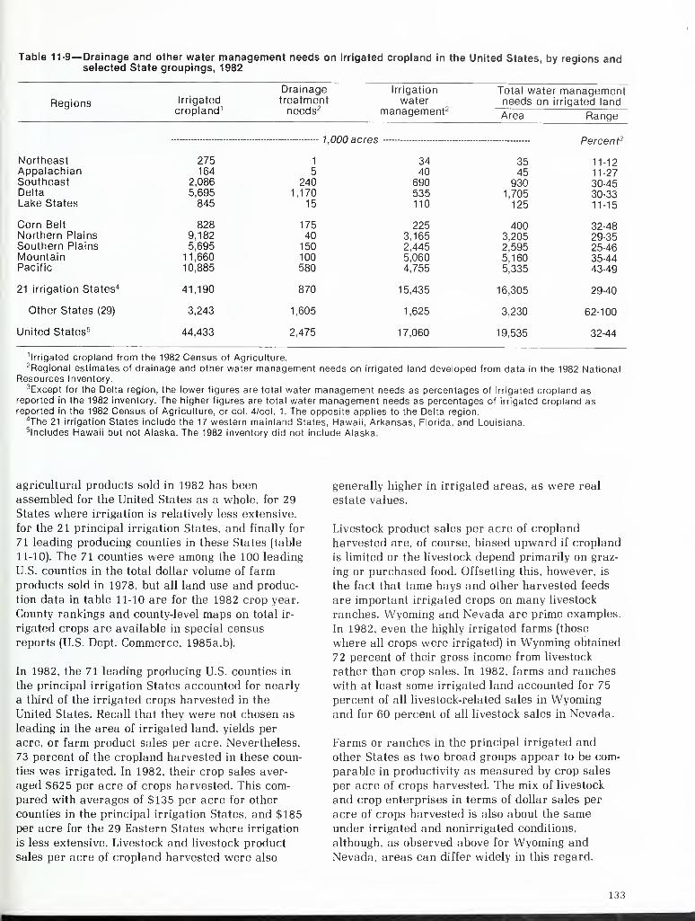
Table 11-9— Drainage and other water management needs on irrigated cropland in the United States, by regions andselected State groupings, 1982

Regions Irrigated

cropland 1

Drainagetreatmentneeds2

Irrigation

watermanagement2

Total water managementneeds on irrigated land

Area Range

NortheastAppalachianSoutheastDeltaLake States

275164

2,0865,695845

1,000 acres -

1

5240

1,17015

3440

690535110

3545

9301,705125

Percent3

11-1211-27

30-4530-3311-15

Corn Belt

Northern PlainsSouthern PlainsMountainPacific

8289,1825,695

11,66010,885

17540150100580

2253,1652,4455,0604,755

4003,2052,5955,1605,335

32-4829-3525-4635-4443-49

21 irrigation States4 41,190 870 15,435 16,305 29-40

Other States (29) 3,243 1,605 1,625 3,230 62-100

United States5 44,433 2,475 17,060 19,535 32-44

irrigated cropland from the 1982 Census of Agriculture.2 Regional estimates of drainage and other water management needs on irrigated land developed from data in the 1982 National

Resources Inventory.3Except for the Delta region, the lower figures are total water management needs as percentages of irrigated cropland as

reported in the 1982 inventory. The higher figures are total water management needs as percentages of irrigated cropland asreported in the 1982 Census of Agriculture, or col. 4/col. 1. The opposite applies to the Delta region.

4The 21 irrigation States include the 17 western mainland States, Hawaii, Arkansas, Florida, and Louisiana.includes Hawaii but not Alaska. The 1982 inventory did not include Alaska.

agricultural products sold in 1982 has beenassembled for the United States as a whole, for 29

States where irrigation is relatively less extensive,

for the 21 principal irrigation States, and finally for

71 leading producing counties in these States (table

11-10). The 71 counties were among the 100 leading

U.S. counties in the total dollar volume of farmproducts sold in 1978, but all land use and produc-

tion data in table 11-10 are for the 1982 crop year.

County rankings and county-level maps on total ir-

rigated crops are available in special census

reports (U.S. Dept. Commerce, 1985a, b).

In 1982, the 71 leading producing U.S. counties in

the principal irrigation States accounted for nearly

a third of the irrigated crops harvested in the

United States. Recall that they were not chosen as

leading in the area of irrigated land, yields per

acre, or farm product sales per acre. Nevertheless,

73 percent of the cropland harvested in these coun-

ties was irrigated. In 1982, their crop sales aver-

aged $625 per acre of crops harvested. This com-

pared with averages of $135 per acre for other

counties in the principal irrigation States, and $185per acre for the 29 Eastern States where irrigation

is less extensive. Livestock and livestock product

sales per acre of cropland harvested were also

generally higher in irrigated areas, as were real

estate values.

Livestock product sales per acre of cropland

harvested are, of course, biased upward if cropland

is limited or the livestock depend primarily on graz-

ing or purchased food. Offsetting this, however, is

the fact that tame hays and other harvested feeds

are important irrigated crops on many livestock

ranches. Wyoming and Nevada are prime examples.

In 1982, even the highly irrigated farms (those

where all crops were irrigated) in Wyoming obtained

72 percent of their gross income from livestock

rather than crop sales. In 1982, farms and ranches

with at least some irrigated land accounted for 75

percent of all livestock-related sales in Wyomingand for 60 percent of all livestock sales in Nevada.

Farms or ranches in the principal irrigated and

other States as two broad groups appear to be com-

parable in productivity as measured by crop sales

per acre of crops harvested. The mix of livestock

and crop enterprises in terms of dollar sales per

acre of crops harvested is also about the same

under irrigated and nonirrigated conditions,

although, as observed above for Wyoming and

Nevada, areas can differ widely in this regard.

133

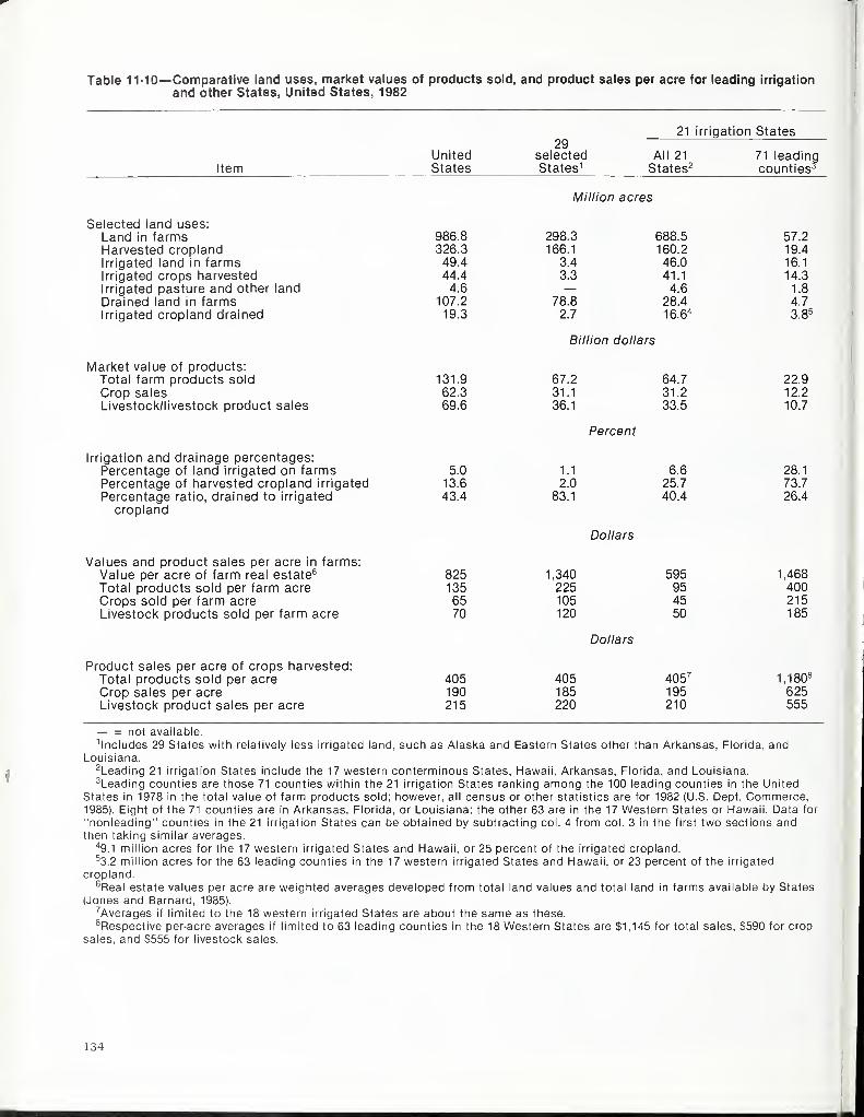
Table 11-10—Comparative land uses, market values of products sold, and product sales per acre for leading irrigation

and other States, United States, 1982

21 irrigation States

Item

29United selected All 21 71 leading

>untiesyStates States 1 States2 cc

Million acres

986.8 298.3 688.5 57.2326.3 166.1 160.2 19.449.4 3.4 46.0 16.1

44.4 3.3 41.1 14.34.6 — 4.6 1.8

107.2 78.8 28.4 4.7

19.3 2.7 16.64 3.85

Billion dollars

131.9 67.2 64.7 22.962.3 31.1 31.2 12.2

69.6 36.1 33.5 10.7

Selected land uses:Land in farmsHarvested croplandIrrigated land in farmsIrrigated crops harvestedIrrigated pasture and other land

Drained land in farmsIrrigated cropland drained

Market value of products:Total farm products soldCrop salesLivestock/livestock product sales

Irrigation and drainage percentages:Percentage of land irrigated on farmsPercentage of harvested cropland irrigated

Percentage ratio, drained to irrigated

cropland

Values and product sales per acre in farms:Value per acre of farm real estate6

Total products sold per farm acreCrops sold per farm acreLivestock products sold per farm acre

Product sales per acre of crops harvested:Total products sold per acreCrop sales per acreLivestock product sales per acre

Percent

5.0 1.1 6.6

13.6 2.0 25.7

43.4 83.1 40.4

Dollars

825 1,340135 22565 10570 120

595954550

Dollars

405 405190 185215 220

28.1

73.726.4

1,468400215185

405 7 1,180195 625210 555

— = not available.

includes 29 States with relatively less irrigated land, such as Alaska and Eastern States other than Arkansas, Florida, andLouisiana.

2Leading 21 irrigation States include the 17 western conterminous States, Hawaii, Arkansas, Florida, and Louisiana.3Leading counties are those 71 counties within the 21 irrigation States ranking among the 100 leading counties in the United

States in 1978 in the total value of farm products sold; however, all census or other statistics are for 1982 (U.S. Dept. Commerce,1985). Eight of the 71 counties are in Arkansas, Florida, or Louisiana; the other 63 are in the 17 Western States or Hawaii. Data for

"nonleading" counties in the 21 irrigation States can be obtained by subtracting col. 4 from col. 3 in the first two sections andthen taking similar averages.

49.1 million acres for the 17 western irrigated States and Hawaii, or 25 percent of the irrigated cropland.

53.2 million acres for the 63 leading counties in the 17 western irrigated States and Hawaii, or 23 percent of the irrigated

cropland.6Real estate values per acre are weighted averages developed from total land values and total land in farms available by States

(Jones and Barnard, 1985).7Averages if limited to the 18 western irrigated States are about the same as these.

Respective per-acre averages if limited to 63 leading counties in the 18 Western States are $1,145 for total sales, $590 for crop

sales, and $555 for livestock sales.

134

Concluding Note

This descriptive overview of drainage development,

capital growth, and related economic questions does

not assume that the factors historically or recently

affecting drainage activities will hold in the future.

However, the information is useful for several

purposes:

• Explaining major changes in technical

methods and relating these to the responses of

farmers and drainage organizations,

• Estimating the costs and investment

requirements associated with the redesign of

existing drain systems,

• Discussing the social costs and the role of

drainage in agricultural production, as animportant element of land water resource

management on farms as well as balancedenvironmental planning,

• Assessing remaining potentials for drainage

consistent with public policy, and

• Improving the quality of statistical information

about drainage, including the quality of ad-

ministrative arrangements for collecting it.

References

Donnan, W. W., and G. O. Schwab. 1974. "Current

Drainage Methods in the USA," Drainage for

Agriculture. Monograph No. 17 (ed., Jan vanSchilfgaarde). Am. Soc. Agron., Madison, Wise.

Dideriksen, Raymond I., A. R. Hidlebaugh, and Keith

O. Schmude. 1978. "Wet Soils for Crop Production

in the United States," Wetland Functions andValues: The State of Our Understanding. AmericanWater Resources Assoc.

Fisher, Irving. 1930. The Theory of Interest. NewYork: Kelly and Milliman.

Fox. Karl. 1965. Intermediate Economic Statistics.

New York: John Wiley and Sons.

Frey, H. Thomas, and Roger W. Hexem. 1985. Major

Uses of Land in the United States: 1982. AER-535,

U.S. Dept. Agr., Econ. Res. Serv.

Gain, Elmer W. 1967. Land Drainage for Production

of Food and Fiber Crops. Proceedings, International

Conference on Water for Peace, Wash., DC. Vol. 7,

pp. 451-461.

Goldstein, Jon H. 1971. Competition for Wetlands in

the Midwest: An Economic Analysis. Resources for

the Future, Inc. Baltimore: Johns Hopkins Press.

Harrison, Robert W. 1961. Alluvial Empire: A Study

of State and Local Efforts Toward Land Develop-

ment in the Alluvial Valley of the Lower Mississippi

River. Little Rock, Ark.: Pioneer Press.

Heimlich, Ralph E., and Linda L. Langner. 1986.

Swampbusting: Wetland Conversion and Farm Pro-

grams. AER-551. U.S. Dept. Agr., Econ. Res. Serv.

Irwin, Ross W. 1979. On-Farm Drainage Benefit.

Final Report, OMAF Research Programs 39, Project

A-39-742. Univ. of Guelph School of Engineering,

Guelph, Ontario.

Jones, John, and Charles H. Barnard. 1985. FarmReal Estate: Historical Series Data. 1950-85. SB-738.

U.S. Dept. Agr., Econ. Res. Serv.

Lewis, Douglas. 1982. Land Drainage Investment

Survey, 1975-77. ERS Staff Report No. AGES820525.U.S. Dept. Agr., Econ. Res. Serv.

Luthin, James N., and Ronald C. Reeve. 1957.

"Drainage of Irrigated lands," Drainage of

Agricultural Lands. Monograph No. 7 (ed. James H.

Luthin). Am. Soc. Agron.. Madison, Wise.

Nolte, Byron H. 1986. Cropland Erosion andDrainage Status in Eastern Ohio. Ohio State Univer-

sity, Columbus. Coop. Ext. Circular AGDEX 751/752.

March.

Shaw, Samuel P., and C. Gordon Fredine. 1956.

Wetlands of the United States. Circular 39, U.S.

Dept. Interior, Fish and Wildlife Serv.

Skaggs, R. W., and A. Nassehzadeh-Tabrizi. 1983.

Optimum Drainage for Corn Production. Technical

Bulletin 274. North Carolina Agri. Res. Serv. N.C.

State Univ., Raleigh.

Smedema, Lambert, and David W. Rycroft. 1984.

Land Drainage: Planning and Design of Agricultural

Drainage Systems. Ithaca, N.Y.: Cornell Univ. Press.

Stamatel, Henry. 1986. Assistant State Conserva-

tionist, SCS/USDA, Syracuse, N.Y. Personal

communication, May 7.

Stonier, Alfred W., and Douglas C. Hague. 1956. ATextbook of Economic Theory. London: Longmans,

Green and Co., Ltd.

135

U.S. Department of Agriculture. 1981a. Statistical

Reporting Service. Agricultural Statistics, annual.

. 1981b. Agricultural Stabilization and

1961. "Drainage of Agricultural

Conservation Service. Agricuitural Conservation

Program: 45-year Statistical Summary.

1981c. Agricultural Stabilization and

Conservation Service. Practice Cost-Shares by

States: 30-year Summary, 1944-74.

. 1982. Soil Conservation Service, and

Iowa State University Statistical Laboratory. Basic

Statistics. 1977 National Resources Inventory.

SB-686.

. 1984. Agricultural Stabilization and

Conservation Service. Agricultural Conservation

Program: Statistical Summary, 1983 Fiscal Year.

.1986. Outlook and Situation Summary:

Agricultural Resources. April 9.

U.S. Department of Commerce, Bureau of the Cen-

sus. 1932. Drainage of Agricultural Lands, 1930.

. 1942. Drainage of Agricultural Lands:

Land in Drainage Enterprises, Capital Invested, and

Drainage Works, 1940.

. 1943. Drainage of Alluvial Lands: AComparison of Agriculture Within and Outside of

Drainage Enterprises in the Alluvial Lands of the

Lower Mississippi Valley.

1952. "Drainage of Agricultural

Lands, I960," Census of Agriculture. 1959. Vol. IV.

1973. "Irrigation and Drainage on

Farms." Census of Agriculture, 1969. Vol. II.

1973. "Drainage of Agricultural

Lands," Census of Agriculture, 1969. Vol. II.

. 1981. "Drainage of Agricultural

Lands," Census of Agriculture, 1978. Vol. 5.

. 1982., "Irrigation." Census of

Agriculture. 1978. Vol. 4.

. 1984. "Geographic Area Series for

States and Outlying Areas," Census of Agriculture,

1982. Vol. I, parts 1-54.

. 1985a. "Ranking of States and Coun-

ties," Census of Agriculture, 1982. Vol. 2: Subject

Series, part 3.

. 1985b. "Graphic Summary," Census

Lands." Census of Agriculture. 1950. Vol. IV.

of Agriculture. 1982. Vol. 2: Subject Series, part 1.

van't Woudt, Bessel D., and Robert M. Hagan. 1957.

"Crop Responses at Excessively High Moisture

Levels," Drainage of Agricultural Lands (ed., JamesN. Luthin). Monograph No. 7. Am. Soc. Agron..

Madison, Wise.

van Schilfgaarde, Jan. 1971. Drainage Yesterday.

Today and Tomorrow. Paper presented at ASAENational Drainage Symposium, Chicago. Dec. 6-7.

Weaver, M. M. 1964. History of Tile Drainage in

America Prior to 1900. Waterloo, N.Y.: Private

publication.

136

Chapter 12

Drainage Potential andInformation Needs

Arthur B. DaughertyNatural Resource EconomicsDivisionEconomic Research ServiceUSDAUniversity Park, Pennsylvania

Douglas G. Lewis*North Carolina Department of

Natural Resources andCommunity DevelopmentRaleigh, North Carolina

Drainage is an important consideration whenexamining the quality of the land resource. Pros-

pects for drainage are based on the drainage poten-

tials or "needs" for various agricultural purposes

as identified by SCS in its periodic inventories of

the Nation's soil and water resources.

Remaining Drainage Potential

Major national data series do not contain a variable

representing the continuum of drainage opportu-

nities at a particular location. For the most part,

they must be evaluated on a field-by-field basis.

However, some information is assembled at the

national level which gives an indication of addi-

tional drainage potentials on existing and potential

cropland, but it is unclear at what points on the

water management continuum a drainage system is

called for and when agricultural use is considered

inappropriate because of the degree of wetness.

The principal sources of information on remaining

drainage potential have been SCS's periodic conser-

vation and resource inventories (USDA, 1962 and

*Formerly with the Economic Research Service, USDA, Raleigh,

North Carolina.

1971 and USDA, SCS, 1980). The most recent of

these surveys is the 1982 National Resources Inven-

tory (NRI).

Inventories Before 1982

The 1958 Conservation Needs Inventory (CNI) did

not report drainage potentials as such. Instead, the

area of cropland having excess water as either a

dominant or secondary problem was reported.

Excess water was defined as a high water table or

temporary flooding which prevented or limited the

use of conservation cropping systems or practices

(USDA, 1962, p. 139). About 15 percent (60 million

acres) of nonirrigated cropland had excess water as

a dominant problem (table 12-1). Excess water was

a secondary problem on an additional 12.5 million

acres.

In the 1967 CNI, 43 million acres of nonirrigated

cropland in tillage rotation were considered to have

drainage problems. This area constituted about 10

percent of all nonirrigated cropland in tillage rota-

tion in the 48 conterminous States and Hawaii.

The 1977 NRI reported 357.2 million acres of nonir-

rigated cropland in the same 49 States. Of this

nonirrigated cropland, 36.5 million acres or about

137

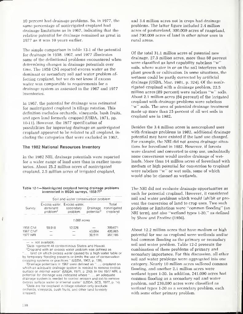
10 percent had drainage problems. So, in 1977, the

same percentage of nonirrigated cropland had

drainage limitations as in 1967, indicating that the

relative potential for drainage remained as great in

1977 as it was 10 years earlier.

and 3.4 million acres not in crops had drainage

problems. The latter figure included 2.4 million

acres of pastureland, 300,000 acres of rangeland,

and 700,000 acres of land in other minor uses in

rural areas.

The simple comparison in table 12-1 of the potential

for drainage in 1958, 1967, and 1977 illustrates

some of the definitional problems encountered whendetermining changes in drainage potentials over

time. The 1958 CNI reported excess water as the

dominant or secondary soil and water problem af-

fecting cropland, but we do not know if excess

water was comparable to requirements for a

drainage system as assessed in the 1967 and 1977

inventories.

In 1967, the potential for drainage was estimated

for nonirrigated cropland in tillage rotation. This

definition excludes orchards, vineyards, bush fruits,

and open land formerly cropped (USDA, 1971, pp.

10-11). However, the 1977 specification of

possibilities for improving drainage on nonirrigated

cropland appeared to be related to all cropland, in-

cluding the categories that were excluded in 1967.

The 1982 National Resources Inventory

In the 1982 NRI, drainage potentials were reported

for a wider range of land uses than in earlier inven-

tories. About 25.2 million acres of nonirrigated

cropland, 2.5 million acres of irrigated cropland,

Of the total 31.1 million acres of potential newdrainage, 27.5 million acres, more than 88 percent

were classified as land capability subclass "w"soils, where water in or on the soil interferes with

plant growth or cultivation. In some situations, the

wetness could be partly corrected by artificial

drainage (USDA, Mar. 1981, p. 324). Of the nonir-

rigated cropland with a drainage problem, 22.5

million acres (89 percent) were subclass "w" soils.

About 2.1 million acres (84 percent) of the irrigated

cropland with drainage problems were subclass

"w" soils. The area of potential drainage treatment

made up more than 25 percent of all wet soils in

cropland use in 1982.

Besides the 3.4 million acres in noncropland uses

with drainage problems in 1982, additional drainage

potential may have existed if the land use changed.

For example, the NRI did not assess drainage situa-

tions for forestland in 1982. However, if forests

were cleared and converted to crop use, undoubtedly

some conversions would involve drainage of wet-

lands. More than 14 million acres of forestland with

medium or high potential for conversion to cropland

were subclass "w" or wet soils, some of which

would also be classed as wetlands.

Table 12-1 — Nonirrigated cropland having drainage problemsinventoried in USDA surveys, 1958-77 1

Soil and water conservation problem

Excess water, Excess water, Total

Survey dominant secondary Drainage nonirrigated

problem2 problem potential 3 cropland

7,000 acres

1958 CNI1967 CNI"

1977 NRI

59,918 12,526

43,004

36,511

399,671

420,865

357,166

— = not available.

'Data represent 48 conterminous States and Hawaii.2Cropland with an excess water problem was defined as

"... land on which excess water caused by a high water table or

by temporary flooding prevents or limits the use of conservation

cropping systems or practices." (USDA, 1962, p. 139).3Drainage potentials in 1967 were defined as ".

. . cropland on

which an adequate drainage system is needed to remove excesssurface or internal water" (USDA, 1971, p. 210). In the 1977 NRI, a

potential for drainage was indicated where "... an adequatedrainage system is needed to control erosion and (or) to removeexcess surface water or internal water" (USDA, SCS, 1977. p. 14).

4 Data are for cropland in tillage rotation only (exclude

orchards, vineyards, bush fruits, and other land formerly

cropped).

The NRI did not evaluate drainage opportunities as

such for potential cropland. However, it considered

soil and water problems which would inhibit or pre-

vent the conversion of land to crop uses. Two such

problems or limitations were "common flooding" (an

NRI term), and also "wetland types 1-20," as defined

by Shaw and Fredine (1956).

About 12.2 million acres that have medium or high

potential for use as cropland were wetlands and/or

had common flooding as the primary or secondary

soil and water problem. Table 12-2 presents the

combination of these problems of primary and

secondary importance. For this discussion, all other

soil and water problems were aggregated into one

category. Nearly 10 million acres suffered commonflooding, and another 2.1 million acres werewetland types 1-20. In addition, 241,000 acres had

common flooding as a secondary soil and water

problem, and 239,000 acres were classified as

wetland types 1-20 as a secondary problem, each

with some other primary problem.

138

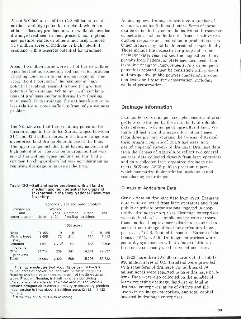
About 500,000 acres of the 12.2 million acres of

medium- and high-potential cropland, which had

either a flooding problem or were wetlands, needed

drainage treatment in their present, noncropland

use (pasture, range, or other minor use). This left

11.7 million acres of medium- or high-potential

cropland with a possible potential for drainage.

About 1.6 million acres were in 1 of the 20 wetland

types but had no secondary soil and water problem

affecting conversion to and use as cropland. This

area, about 1 percent of the medium- or high-

potential cropland, seemed to have the greatest

potential for drainage. While land with combina-

tions of problems and/or suffering from flooding

may benefit from drainage, the net benefits may be

less relative to areas suffering from only a wetness

problem.

The NRI showed that the remaining potential for

farm drainage in the United States ranged between

31.1 and 42.8 million acres. In the lower range wasinventoried land drainable in its use at the time.

The upper range included land having medium andhigh potential for conversion to cropland that wasone of the wetland types and/or land that had a

common flooding problem but was not identified as

requiring drainage in its use at the time.

Table 12-2— Soil and water problems with all land of

medium and high potential for croplandinventoried in the 1982 National ResourcesInventory

Secondary soil and water problem

Primary soil Wetlandand types Common Other Total

water problem None (1-20) flooding problems

7,000 acres

None 91,165 91,165

Wetland types 1,605 72 211 224 2,112

(1-20)

Common 7,571 1,1 12 1 57 868 9,608

flooding

Other 34,714 239 241 14,644 49,837

problemsTotal 2 135,056 1,422 509 15,736 152,722

1 This figure indicates that about 12 percent of the 9.6

million acres of convertible land with common (frequent)

flooding can also be considered to be 1 of the 20 wetland

types. Frequent flooding in itself is not an identifying

characteristic of wetlands. The total area of land where a

wetland designation is either a primary or secondary problemin conversion is thus about 3.5 million acres (2.112 + 1.422

mil. ac).2 ltems may not sum due to rounding.

Achieving new drainage depends on a number of

economic and institutional factors. Some of these

can be estimated by or for the individual farmowneror operator, such as the benefit from a positive pro-

duction response or a reduction in production costs.

Other factors may not be determined so specifically.

These include the necessity for group action for

drainage water removal and the acquisition of anypermits from Federal or State agencies needed for

installing drainage improvements. Any drainage of

potential cropland must be consistent with present

and prospective public policies concerning produc-

tion levels and resource conservation, including

wetland preservation.

Drainage Information

Examination of drainage accomplishments and pros-

pects is constrained by the availability of reliable

data relevant to drainage of agricultural land. Vir-

tually all historical drainage information comes

from three primary sources: the Census of Agricul-

ture; program reports of USDA agencies; and

periodic special surveys of drainage. Drainage data

from the Census of Agriculture reflect two general

sources: data collected directly from farm operators

and data collected from organized drainage dis-

tricts. SCS and ASCS publish program reports

which summarize their technical assistance and

cost-sharing on drainage.

Census of Agriculture Data

Census data on drainage date from 1920. Drainage

data were collected from farm operators and from

public or private organizations engaged in coop-

erative drainage enterprises. Drainage enterprises

were defined as ". . . public and private corpora-

tions and local improvement districts organized to

secure the drainage of land for agricultural pur-

poses. ..." (U.S. Dept. of Commerce, Bureau of the

Census, 1922, p. 348). Drainage enterprises weregenerally synonomous with drainage districts, a

term more commonly used in recent censuses.

In 1920 more than 53 million acres out of a total of

956 million acres of U.S. farmland were provided

with some form of drainage. An additional 39

million acres were reported to have drainage prob-

lems. Data were also collected on the number of

farms reporting drainage, land use on land in

drainage enterprises, miles of ditches and tile

drains in drainage enterprises, and total capital

invested in drainage enterprises.

139

Data collection in the 1930 Census of Agriculture

was comparable to the 1920's except for the change

in land use information on drained land. Farm

operators reported drainage on 44.5 million acres, a

decline from 1920's levels. However, over 66 million

acres within drainage enterprises were drained

sufficiently to produce a normal crop, more than

compensating for the decline reported by farm

operators.

The 1940 Census of Drainage was the first which

excluded individual farm operators and focused

data collection entirely on cooperative drainage

enterprises. The number of reported projects declined

from 1930 to 1940, but the area within their bound-

aries increased slightly to 87 million acres. Morethan 75 million acres received sufficient drainage

for a normal crop at a capital investment of $692

million. The slight increase in total investment and

the facilities of ditches and tile drains represented

by that investment was made despite the general

economic depression of the time.

Data on drainage enterprises are relatively consis-

tent regarding method of collection and content

from 1920 through 1940. However, several pro-

cedural changes began in 1950. The main changes

were: drainage enterprises under 500 acres wereexcluded, drainage enterprises absorbed by a later

project were not enumerated, and the data on enter-

prises under common management were consolidated

into one report. The geographic area considered

expanded with each Census.

Comparability of data was probably significantly

affected by the addition or deletion of States, whichcan be accounted for, and by excluding enterprises

of 500 acres or less, which can only be estimated.

About 5 percent of the land in drainage enterprises

would have been deleted from the 1940 total hadthis rule then applied. The number of separate

drainage enterprises would have decreased by 53

percent.

Almost 103 million acres were reported as net land

drained in 1950 within drainage enterprises. Whilepublished on the same line as land in drainage

enterprises from the previous three Censuses of

Drainage, the reports are not necessarily compar-able because not all land within the boundary of a

drainage enterprise was artificially drained. Thelands may have received some benefit, however,when artificial drainage on adjacent land enhancedthe natural drainage patterns.

The 1950 Census marked a change in the financial

data collected. In Censuses before 1950, all capital

investment accumulated prior to the census date

was requested. Investment data for the 1950 Census

referred only to investments made during the

preceding decade. Annual revenue data were also

collected and combined with beginning and ending

indebtedness and operation and maintenance costs

to construct an approximate equation of the finan-

cial status of drainage enterprises for the decade.

This was an effort to separate new capital invest-

ment from operation and maintenance costs and to

identify total tax revenue.

The 1960 Census of Drainage did not include data

from projects where land was drained solely

because of irrigation. The total area in drainage

projects serving agricultural lands was 101.9

million acres in 1960. This total excluded about 3

million acres of drained irrigated land and 6 million

acres of swamp and wasteland counted in 1950.

Thus, the remaining 92.3 million acres werepredominantly agricultural lands benefiting from

artificial drainage within drainage projects.

Drainage data collection in the 1970's marked a

partial return to earlier procedures. Data werecollected from farm operators in the 1969 Census of

Agriculture and from drainage projects via the 1972

Census of Governments. Data covered all 50 States

for both censuses and were reported as part of the

Census of Agriculture. Farm operators responding

to the 1969 Census reported draining nearly 60

million acres. Analysts agree that the 1969 and the

1974 estimate (42.8 million acres) greatly under-

stated the total drained. Considerable data

available from the Census of Governments detailed

the number of project employees, debt, expendi-

tures, and revenues.

The most recent published data on drainage comefrom the 1978 Census. Data on land drained werecollected in yet another manner because of the poor

quality of the 1974 Census reports. State and county

SCS officials estimated land benefiting from artifi-

cial drainage for individual counties which wascombined with financial and employment data from

drainage districts obtained in the 1977 Census of

Government. The 1978 estimates of land drained

within each county totaled about 105.3 million

acres. Financial data were shown for only one

fiscal year in both the 1972 and 1977 Census of

Governments.

Table 12-3 summarizes the geographic coverage anddata acquisition of the Census Bureau from 1920 to

140

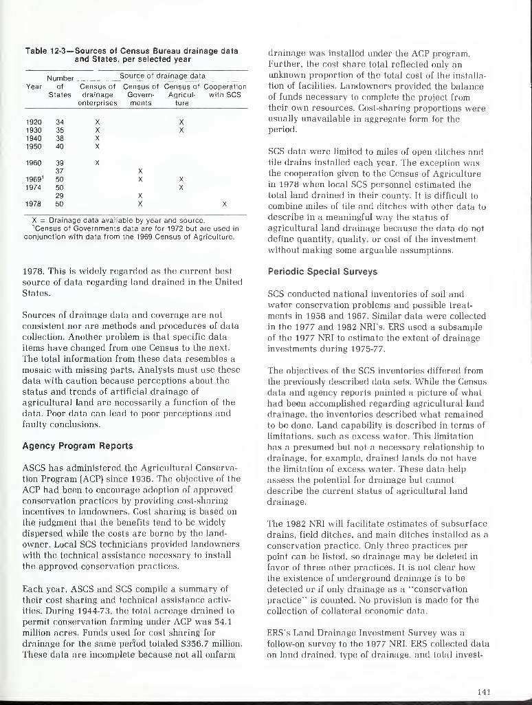
Table 12-3—Sources of Census Bureau drainage dataand States, per selected year

Year

Numberof

States

Source of drainage data

Census of Census of Census of Cooperationdrainage Govern- Agricul- with SCS

enterprises ments ture

1920 34

1930 35

1940 38

1950 40

1960 39

37

1969 1 501974 50

29

1978 50

X = Drainage data available by year and source.

Census of Governments data are for 1972 but are used in

conjunction with data from the 1969 Census of Agriculture.

1978. This is widely regarded as the current best

source of data regarding land drained in the United

States.

Sources of drainage data and coverage are not

consistent nor are methods and procedures of data

collection. Another problem is that specific data

items have changed from one Census to the next.

The total information from these data resembles a

mosaic with missing parts. Analysts must use these

data with caution because perceptions about the

status and trends of artificial drainage of

agricultural land are necessarily a function of the

data. Poor data can lead to poor perceptions and

faulty conclusions.

Agency Program Reports

ASCS has administered the Agricultural Conserva-

tion Program (ACP) since 1936. The objective of the

ACP had been to encourage adoption of approved

conservation practices by providing cost-sharing

incentives to landowners. Cost sharing is based on

the judgment that the benefits tend to be widely

dispersed while the costs are borne by the land-

owner. Local SCS technicians provided landowners

with the technical assistance necessary to install

the approved conservation practices.

Each year, ASCS and SCS compile a summary of

their cost sharing and technical assistance activ-

ities. During 1944-73, the total acreage drained to

permit conservation farming under ACP was 54.1

million acres. Funds used for cost sharing for

drainage for the same period totaled $356.7 million.

These data are incomplete because not all onfarm

drainage was installed under the ACP program.

Further, the cost share total reflected only anunknown proportion of the total cost of the installa-

tion of facilities. Landowners provided the balanceof funds necessary to complete the project fromtheir own resources. Cost-sharing proportions wereusually unavailable in aggregate form for the

period.

SCS data were limited to miles of open ditches andtile drains installed each year. The exception wasthe cooperation given to the Census of Agriculture

in 1978 when local SCS personnel estimated the

total land drained in their county. It is difficult to

combine miles of tile and ditches with other data to

describe in a meaningful way the status of

agricultural land drainage because the data do not

define quantity, quality, or cost of the investment

without making some arguable assumptions.

Periodic Special Surveys

SCS conducted national inventories of soil andwater conservation problems and possible treat-

ments in 1958 and 1967. Similar data were collected

in the 1977 and 1982 NRI's. ERS used a subsample

of the 1977 NRI to estimate the extent of drainage

investments during 1975-77.

The objectives of the SCS inventories differed from

the previously described data sets. While the Census

data and agency reports painted a picture of whathad been accomplished regarding agricultural land

drainage, the inventories described what remained

to be done. Land capability is described in terms of

limitations, such as excess water. This limitation

has a presumed but not a necessary relationship to

drainage, for example, drained lands do not have

the limitation of excess water. These data help

assess the potential for drainage but cannot

describe the current status of agricultural land

drainage.

The 1982 NRI will facilitate estimates of subsurface

drains, field ditches, and main ditches installed as a

conservation practice. Only three practices per

point can be listed, so drainage may be deleted in

favor of three other practices. It is not clear howthe existence of underground drainage is to be

detected or if only drainage as a "conservation

practice" is counted. No provision is made for the

collection of collateral economic data.

ERS's Land Drainage Investment Survey was a

follow-on survey to the 1977 NRI. ERS collected data

on land drained, type of drainage, and total invest-

141

ment for 1975-77. About 29 million acres were

affected by drainage investments in the United

States during the 3-year period. Almost 6.5 million

acres were drained by new systems and 22.5 million

acres were drained by additions to existing

drainage during the 3 years.

interests makes the information needed for decision-

making more complex. In short, increased efforts

and expenditures to improve data collection are

needed to ensure a more accurate "mosaic"describing agricultural land drainage, and thus

more rational private drainage investments andpublic policy decisions.

Conclusions on Drainage Information

Perceptions about the status and trends of artificial

drainage of agricultural land are a function of the

extent and quality of drainage data. Existing infor-

mation tends to give an incomplete picture of land

drainage. Although Census data are widely used as

the authoritative source of drainage information,

such information has been based at various times

on the Census of Agricuture, the Census of

Drainage, the Census of Governments, and SCSestimates. Not all farm operators know what part of

their land is drained, nor do drainage district or

SCS personnel. Published Census reports

acknowledge the double counting of some drainage

while some land is overlooked. Although the defini-

tion of drainage has changed little over time,

specific data items have changed as have defini-

tions of the relevant universe, such as what con-

stitutes a farm, whether to include drained irrigated

land, and public versus private drainage enter-

prises. It is not possible to assess the effectiveness

of existing systems so it is implicit in the data that

all systems remain equally effective in removing

excess water.

Another problem is that new drainage investments

cannot be separated from maintenance expenditures.

Some data, the number of drainage district employ-

ees, for example, are of questionable usefulness in

evaluating the status or trends of agricultural

drainage.

ASCS and SCS reports are limited to programparticipants and include only the cost-sharing por-

tion of total investment. Some data are reported in

units which cannot be meaningfully integrated with

other data sets. The periodic surveys tend to

address drainage remaining to be done rather than

drainage which has been done. The exceptions are

the 1982 NRI and the 1975-77 trend data from the

1978 Resource Economics Survey.

Given these limitations, use agricultural land

drainage data with caution. Changes in policies andinstitutions affecting drainage certainly change the

benefits and costs of draining, both to the individual

and to society at large. Greater attention to societal

References

Shaw, Samuel P., and G. Gordon Fredine. 1956.

Wetlands of the United States. Circular 39. U.S.

Dept. Interior, Fish and Wildlife Serv.

U.S. Department of Agriculture, Agricultural

Stabilization and Conservation Service. 1981.

Agricultural Conservation Program, 45-year

Statistical Summary, 1936-1980.

1975. Practice Cost-shares by States:

30-year Summary, 1944-1974.

Agricultural Conservation Program:

Statistical Summary, annual.

Economic Research Service. 1982.

Land Drainage Investment Survey, 1975-77: A Report

on Landownership Follow-on Survey. ERS Staff

Report AGES820525.

Soil Conservation Service. 1977. Ero-

sion Inventory. Instructions for the PSU and Point

Data Collection. June.

1980. Basic Statistics-1977 National

Resource Inventory.

1962. Basic Statistics—National Inven-

tory of Soil and Water Conservation Needs. SB-317.

August.

. 1971. Basic Statistics—National Inven-

tory of Soil and Water Conservation Needs, 1976.

SB-461. January.

. 1981. "Soil and Water Resources Con-

servation Act, 1980 Appraisal." Soil, Water and

Related Resources in the United States: Status, Con-

dition, and Trends. March.

U.S. Department of Commerce, Bureau of the Cen-

sus. 1922. "Irrigation and Drainage," U.S. Census,

1920, Vol. VII.

142

1930. "Drainage of Agricultural

Land," U.S. Census, 1930.

_. 1973. "Drainage of AgriculturalLands," U.S. Census of Agriculture, 1969, Vol. IV

1942. "Drainage of Agricultural

Lands," U.S. Census of Agriculture, 1940.

1952. "Drainage of Agricultural

Land," U.S. Census of Agriculture, 1950, Vol. IV.

1961. "Drainage of Agricultural

Land," U.S. Census of Agriculture, 1959, Vol. IV.

1977. "Irrigation and Drainage onFarms," U.S. Census of Agriculture, 1974, Vol. II,

part 9.

1981. "Drainage of AgriculturalLands," U.S. Census of Agriculture, 1978, Vol. 5,

special reports, part 5.

143

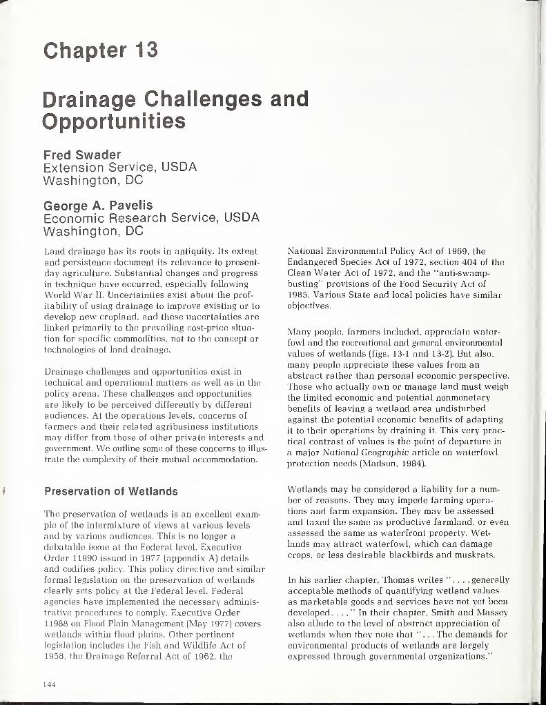
Chapter 13

Drainage Challenges andOpportunities

Fred SwaderExtension Service, USDAWashington, DC

George A. Pavelis

Economic Research Service, USDAWashington, DC

Land drainage has its roots in antiquity. Its extent

and persistence document its relevance to present-

day agriculture. Substantial changes and progress

in technique have occurred, especially following

World War II. Uncertainties exist about the prof-

itability of using drainage to improve existing or to

develop new cropland, and these uncertainties are

linked primarily to the prevailing cost-price situa-

tion for specific commodities, not to the concept or

technologies of land drainage.

Drainage challenges and opportunities exist in

technical and operational matters as well as in the

policy arena. These challenges and opportunities

are likely to be perceived differently by different

audiences. At the operations levels, concerns of

farmers and their related agribusiness institutions

may differ from those of other private interests andgovernment. We outline some of these concerns to illus-

trate the complexity of their mutual accommodation.

National Environmental Policy Act of 1969, the

Endangered Species Act of 1972, section 404 of the

Clean Water Act of 1972, and the "anti-swamp-

busting" provisions of the Food Security Act of

1985. Various State and local policies have similar

objectives.

Many people, farmers included, appreciate water-

fowl and the recreational and general environmental

values of wetlands (figs. 13-1 and 13-2). But also,

many people appreciate these values from an

abstract rather than personal economic perspective.

Those who actually own or manage land must weigh

the limited economic and potential nonmonetary

benefits of leaving a wetland area undisturbed

against the potential economic benefits of adapting

it to their operations by draining it. This very prac-

tical contrast of values is the point of departure in

a major National Geographic article on waterfowl

protection needs (Madson, 1984).

Preservation of Wetlands

The preservation of wetlands is an excellent exam-ple of the intermixture of views at various levels

and by various audiences. This is no longer a

debatable issue at the Federal level. Executive

Order 11990 issued in 1977 (appendix A) details

and codifies policy. This policy directive and similar

formal legislation on the preservation of wetlands

clearly sets policy at the Federal level. Federal

agencies have implemented the necessary adminis-

trative procedures to comply. Executive Order

11988 on Flood Plain Management (May 1977) covers

wetlands within flood plains. Other pertinent

legislation includes the Fish and Wildlife Act of

1958, the Drainage Referral Act of 1962, the

Wetlands may be considered a liability for a num-

ber of reasons. They may impede farming opera-

tions and farm expansion. They may be assessed

and taxed the same as productive farmland, or even

assessed the same as waterfront property. Wet-

lands may attract waterfowl, which can damagecrops, or less desirable blackbirds and muskrats.

In his earlier chapter, Thomas writes "... .generally

acceptable methods of quantifying wetland values

as marketable goods and services have not yet been

developed. ..." In their chapter, Smith and Masseyalso allude to the level of abstract appreciation of

wetlands when they note that ".. .The demands for

environmental products of wetlands are largely

expressed through governmental organizations."

144

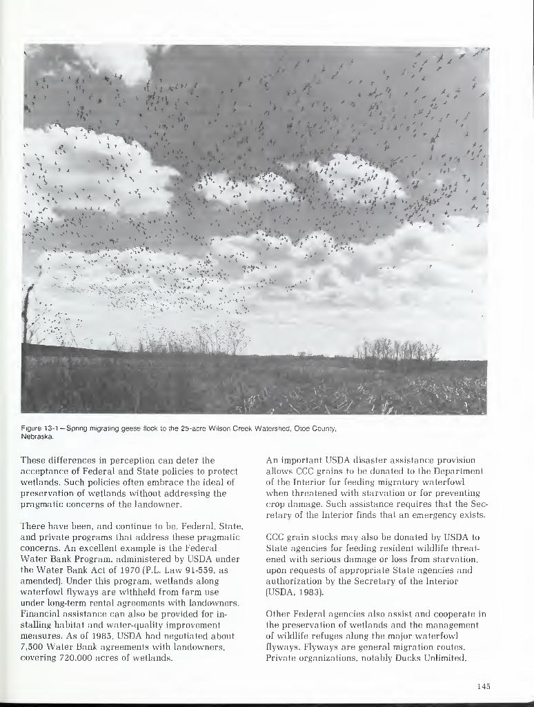
'X «*v i

Figure 13-1 —Spring migrating geese flock to the 25-acre Wilson Creek Watershed, Otoe County,

Nebraska.

These differences in perception can deter the

acceptance of Federal and State policies to protect

wetlands. Such policies often embrace the ideal of

preservation of wetlands without addressing the

pragmatic concerns of the landowner.

There have been, and continue to be, Federal, State,

and private programs that address these pragmatic

concerns. An excellent example is the Federal

Water Bank Program, administered by USDA under

the Water Bank Act of 1970 (P.L. Law 91-559, as

amended). Under this program, wetlands along

waterfowl flyways are withheld from farm use

under long-term rental agreements with landowners.

Financial assistance can also be provided for in-

stalling habitat and water-quality improvement

measures. As of 1985, USDA had negotiated about

7,500 Water Bank agreements with landowners,

covering 720,000 acres of wetlands.

An important USDA disaster assistance provision

allows CCC grains to be donated to the Department

of the Interior for feeding migratory waterfowl

when threatened with starvation or for preventing

crop damage. Such assistance requires that the Sec-

retary of the Interior finds that an emergency exists.

CCC grain stocks may also be donated by USDA to

State agencies for feeding resident wildlife threat-

ened with serious damage or loss from starvation,

upon requests of appropriate State agencies and

authorization by the Secretary of the Interior

(USDA, 1983).

Other Federal agencies also assist and cooperate in

the preservation of wetlands and the managementof wildlife refuges along the major waterfowl

flyways. Flyways are general migration routes.

Private organizations, notably Ducks Unlimited,

145

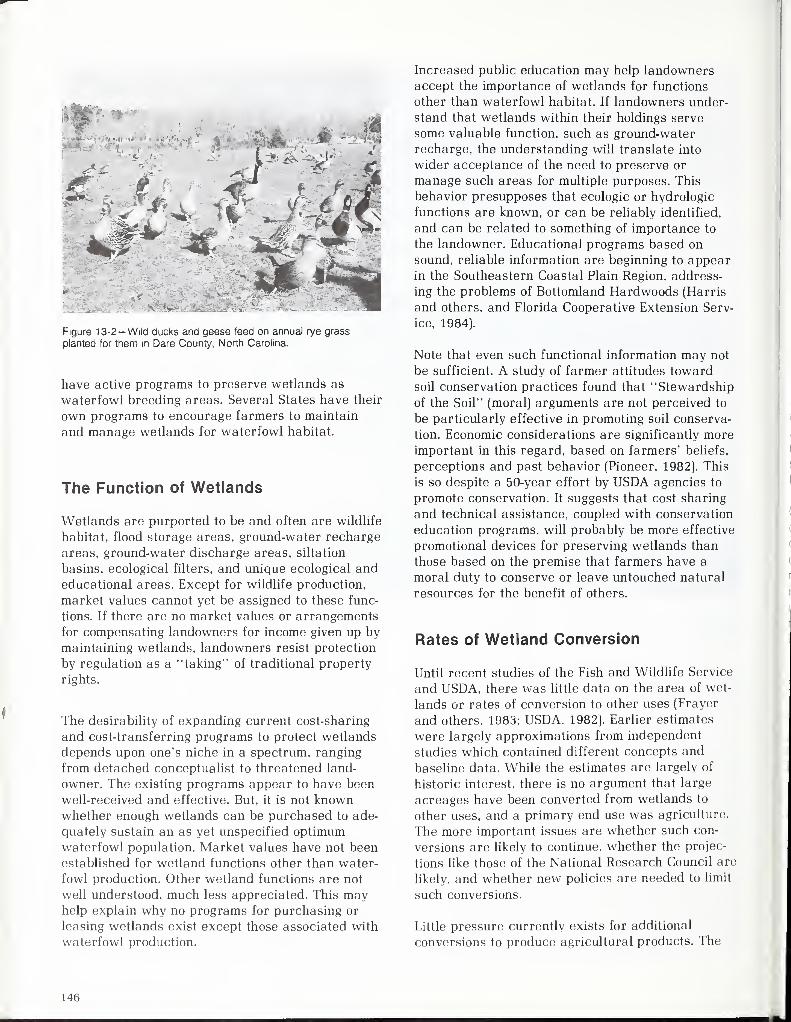
Figure 13-2— Wild ducks and geese feed on annual rye grass

planted for them in Dare County, North Carolina.

have active programs to preserve wetlands as

waterfowl breeding areas. Several States have their

own programs to encourage farmers to maintain

and manage wetlands for waterfowl habitat.

The Function of Wetlands

Wetlands are purported to be and often are wildlife

habitat, flood storage areas, ground-water recharge

areas, ground-water discharge areas, siltation

basins, ecological filters, and unique ecological and

educational areas. Except for wildlife production,

market values cannot yet be assigned to these func-

tions. If there are no market values or arrangements

for compensating landowners for income given up by

maintaining wetlands, landowners resist protection

by regulation as a "taking" of traditional property

rights.

The desirability of expanding current cost-sharing

and cost-transferring programs to protect wetlands

depends upon one's niche in a spectrum, ranging

from detached conceptualist to threatened land-

owner. The existing programs appear to have been

well-received and effective. But, it is not knownwhether enough wetlands can be purchased to ade-

quately sustain an as yet unspecified optimumwaterfowl population. Market values have not been

established for wetland functions other than water-

fowl production. Other wetland functions are not

well understood, much less appreciated. This mayhelp explain why no programs for purchasing or

leasing wetlands exist except those associated with

waterfowl production.

Increased public education may help landowners

accept the importance of wetlands for functions

other than waterfowl habitat. If landowners under-

stand that wetlands within their holdings serve

some valuable function, such as ground-water

recharge, the understanding will translate into

wider acceptance of the need to preserve or

manage such areas for multiple purposes. This

behavior presupposes that ecologic or hydrologic

functions are known, or can be reliably identified,

and can be related to something of importance to

the landowner. Educational programs based on

sound, reliable information are beginning to appearin the Southeastern Coastal Plain Region, address-

ing the problems of Bottomland Hardwoods (Harris

and others, and Florida Cooperative Extension Serv-

ice, 1984).

Note that even such functional information may not

be sufficient. A study of farmer attitudes toward

soil conservation practices found that "Stewardship

of the Soil" (moral) arguments are not perceived to

be particularly effective in promoting soil conserva-

tion. Economic considerations are significantly moreimportant in this regard, based on farmers' beliefs,

perceptions and past behavior (Pioneer, 1982). This

is so despite a 50-year effort by USDA agencies to

promote conservation. It suggests that cost sharing

and technical assistance, coupled with conservation

education programs, will probably be more effective

promotional devices for preserving wetlands than

those based on the premise that farmers have a

moral duty to conserve or leave untouched natural

resources for the benefit of others.

Rates of Wetland Conversion

Until recent studies of the Fish and Wildlife Service

and USDA, there was little data on the area of wet-

lands or rates of conversion to other uses (Frayer

and others, 1983; USDA, 1982). Earlier estimates

were largely approximations from independent

studies which contained different concepts and

baseline data. While the estimates are largely of

historic interest, there is no argument that large

acreages have been converted from wetlands to

other uses, and a primary end use was agriculture.

The more important issues are whether such con-

versions are likely to continue, whether the projec-

tions like those of the National Research Council are

likely, and whether new policies are needed to limit

such conversions.

Little pressure currently exists for additional

conversions to produce agricultural products. The

146

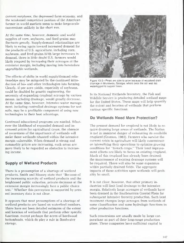
current surpluses, the depressed farm economy, and

the weakened competitive position of the American

farmer in world markets seem to make large-scale

conversions unlikely in the short run.

At the same time, however, domestic and world

supplies of corn, soybeans, and feed grains mayfluctuate greatly. Supply-demand relationships are

likely to swing again toward increased demand for

the products of U.S. agriculture, including corn,

soybeans, and feed grains.With large increases in

demand, there is little doubt U.S. farmers would

likely respond by increasing their acreages at the

extensive margin, including moving into heretofore

unprofitable wetlands.

The effects of shifts in world supply/demand rela-

tionships may be mitigated by the continued intro-

duction of bio- and other technologies into farming.

Clearly, if per acre yields, especially of soybeans,

could be doubled by genetic engineering, the

necessity of expanding cropland acreage by various

means, including drainage, would greatly decrease.

At the same time, however, intensive water manage-

ment, including controlled drainage systems for wet

soils, may be a profitable component of using newtechnologies to their best advantage.

Continued educational programs are needed. What-ever the likelihood of expanded demand and in-

creased prices for agricultural crops, the absence

of awareness of the importance of wetlands will

make those wetlands situated within the intensive

margin vulnerable. When demand is strong and

commodity prices are increasing, such areas are

more likely to be regarded as obstacles to increas-

ing income.

Supply of Wetland Products

There is a presumption of a shortage of wetland

products. Smith and Massey state that "Because of

the increasing scarcity of wetland products and the

heightened public valuation, private decisions at the

extensive margin increasingly face a public choice

test." Whether this perception is supported by pres-

ent inventory data is not clear.

It appears that most presumptions of a shortage of

wetland products are based on waterfowl numbers.

There have not been detailed estimates of the extent

and location of wetlands that perform other specific

functions, except perhaps the acres of hardwoodbottomlands, which do play a role in floodwater

storage.

Figure 13-3— Pines are able to grow because of woodland ditch

drainage in Brunswick, Georgia, where once the soil was too

waterlogged to support trees.

In its National Wetlands Inventory, the Fish and

Wildlife Service is producing detailed wetland maps

for the United States. These maps will help quantify

the extent and location of wetlands that perform

various specific functions.

Do Wetlands Need More Protection?

The present demand for cropland is not likely to re-

quire draining large areas of wetlands. The Nation

is not in imminent danger of exhausting its available

cropland (Crosson, 1982). Farmers who survive the

current crisis in agriculture will likely concentrate

on intensifying their operations to optimize growing

conditions for "hi-tech crops." Their land improve-

ment efforts are likely to focus on existing cropland.

Much of this cropland has already been drained;

the maintenance of existing drainage systems will

be required. There will also be some expansion

within partially drained fields. The aggregate

impacts of these activities upon wetlands will prob-

ably be small.

It is not clear, however, that other primary in-

dustries will limit land drainage to the intensive

margin. Relatively large acreages of wetlands have

been drained in the Southeastern Coastal Plain for

subsequent intensive forestry production. Such land

treatment changes large acreages from wetlands of

some classification and some hydrologic functions to

other productive functions.

Such conversions are usually made by large cor-

porations as part of their long-range production

plans. These companies have sufficient capital to

147

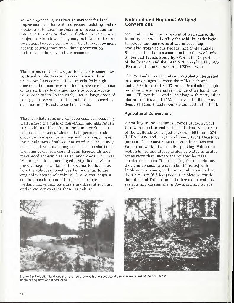
retain engineering services, to contract for land

improvement, to harvest and process existing timber

stocks, and to clear the remains in preparation for

intensive forestry production. Such conversions are

subject to State laws. They may be influenced moreby national export policies and by State employment

growth policies than by wetland preservation

policies at either level of governments.

The purpose of these corporate efforts is sometimes

confused by short-term intervening uses. If the

prices for farm commodities are relatively high

there will be incentives and local pressures to lease

or use such newly drained lands to produce high-

value cash crops. In the early 1970's, large areas of

young pines were cleared by bulldozers, converting

eventual pine forests to soybean fields.

The immediate returns from such cash cropping maywell recoup the costs of conversion and also return

some additional benefits to the land development

company. The use of chemicals to produce cash

crops discourages forest regrowth and suppresses

the populations of subsequent weed species. It maynot be good wetland management, but the short-term

cropping of cleared coastal plain forestlands maymake good economic sense to landowners (fig. 13-4).

While agriculture has played a significant role in

the drainage of wetlands, this scenario illustrates

how the role may sometimes be incidental to the

original purposes of drainage. It also challenges a

candid consideration of the possible scope of

wetland conversion potentials in different regions,

and in industries other than agriculture.

National and Regional WetlandConversions

More information on the extent of wetlands of dif-

ferent types and suitability for wildlife, hydrologic

functions, and agricultural use is becomingavailable from various Federal and State studies.

Recent national assessments include the WetlandsStatus and Trends Study by FWS in the Departmentof the Interior, and the 1982 NRI, completed by SCS(Frayer and others, 1983, and USDA, 1982).

The Wetlands Trends Study of FWS photo-interpreted

land use changes between the mid-1950's andmid-1970's for about 3,600 randomly selected sample

units (each 4 square miles). On the other hand, the

1982 NRI identified land uses along with many other

characteristics as of 1982 for about 1 million ran-

domly selected sample points examined in the field.

Agricultural Conversions

According to the Wetlands Trends Study, agricul-

ture was the observed end use of about 87 percent

of the wetlands developed between 1954 and 1974

(USDA, 1985, and Frayer and Tiner, 1984). Nearly 98percent of the conversions to agriculture involved

Palustrine wetlands. Broadly speaking, Palustrine

wetlands are inland freshwater or water-saturated

areas more than 30-percent covered by trees,

shrubs, or mosses. If not meeting these conditions,

they can be small areas (under 20 acres) with

freshwater regimes, with any standing water less

than 2 meters (6.6 feet) deep. Complete scientific

definitions of Palustrine and other major wetland

systems and classes are in Cowardin and others

(1979).

Figure 13-4— Bottomland wetlands are being converted to agricultural use in many areas of the Southeast:

channelizing (left) and clearcuttmg.

148

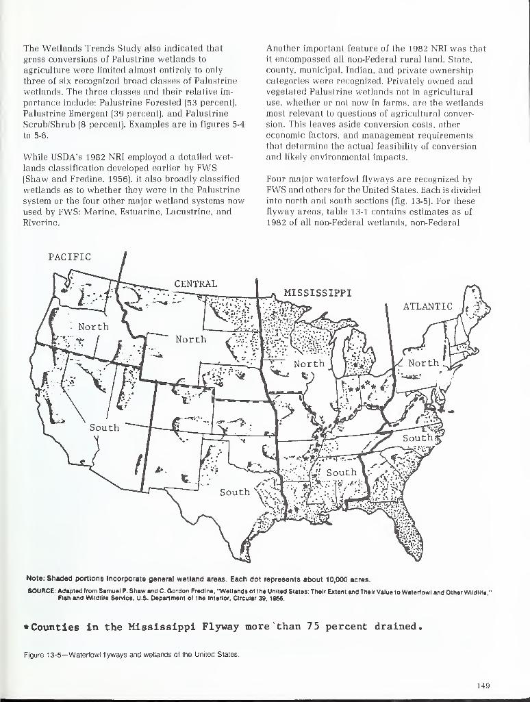
The Wetlands Trends Study also indicated that

gross conversions of Palustrine wetlands to

agriculture were limited almost entirely to only

three of six recognized broad classes of Palustrine

wetlands. The three classes and their relative im-

portance include: Palustrine Forested (53 percent).

Palustrine Emergent (39 percent), and Palustrine

Scrub/Shrub (8 percent). Examples are in figures 5-4

to 5-6.

While USDA's 1982 NRI employed a detailed wet-

lands classification developed earlier by FWS(Shaw and Fredine, 1956), it also broadly classified

wetlands as to whether they were in the Palustrine

system or the four other major wetland systems nowused by FWS: Marine, Estuarine, Lacustrine, and

Riverine.

Another important feature of the 1982 NRI was that

it encompassed all non-Federal rural land. State,

county, municipal, Indian, and private ownership

categories were recognized. Privately owned andvegetated Palustrine wetlands not in agricultural

use, whether or not now in farms, are the wetlands

most relevant to questions of agricultural conver-

sion. This leaves aside conversion costs, other

economic factors, and management requirements

that determine the actual feasibility of conversion

and likely environmental impacts.

Four major waterfowl flyways are recognized by

FWS and others for the United States. Each is divided

into north and south sections (fig. 13-5). For these

flyway areas, table 13-1 contains estimates as of

1982 of all non-Federal wetlands, non-Federal

PACIFIC

Note: Shaded portions incorporate general wetland areas. Each dot represents about 10,000 acres.

SOURCE. Adapted from Samuel P. Shaw and C. Gordon Fredine. "Wetlands of the United States: Their Extent and Their Value to Waterfowl and Other Wildlife'

Flan and Wildlife Service, U.S. Department of the Interior, Circular 39, 1956.

Counties in the Mississippi Flyway more than 75 percent drained.

Figure 13-5— Waterfowl flyways and wetlands of the United States.

149

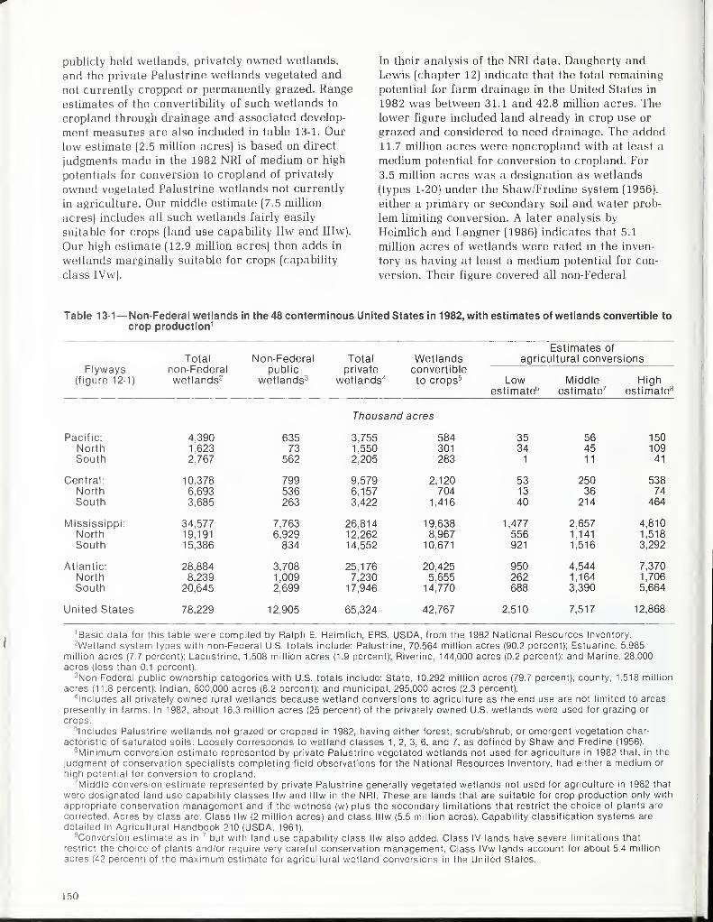
publicly held wetlands, privately owned wetlands,

and the private Palustrine wetlands vegetated and

not currently cropped or permanently grazed. Range

estimates of the convertibility of such wetlands to

cropland through drainage and associated develop-

ment measures are also included in table 13-1. Our

low estimate (2.5 million acres) is based on direct

judgments made in the 1982 NRI of medium or high

potentials for conversion to cropland of privately

owned vegetated Palustrine wetlands not currently

in agriculture. Our middle estimate (7.5 million

acres) includes all such wetlands fairly easily

suitable for crops (land use capability IIw and IIIw).

Our high estimate (12.9 million acres) then adds in

wetlands marginally suitable for crops (capability

class IVw).

In their analysis of the NRI data, Daugherty andLewis (chapter 12) indicate that the total remaining

potential for farm drainage in the United States in

1982 was between 31.1 and 42.8 million acres. The

lower figure included land already in crop use or

grazed and considered to need drainage. The added

11.7 million acres were noncropland with at least a

medium potential for conversion to cropland. For

3.5 million acres was a designation as wetlands

(types 1-20) under the Shaw/Fredine system (1956),

either a primary or secondary soil and water prob-

lem limiting conversion. A later analysis by

Heimlich and Langner (1986) indicates that 5.1

million acres of wetlands were rated in the inven-

tory as having at least a medium potential for con-

version. Their figure covered all non-Federal

Table 13-1— Non-Federal wetlands in the 48 conterminous United States in 1982, with estimates of wetlands convertible to

crop production 1

Totalnon-Federalwetlands 2

Non-Federalpublic

wetlands3

Totalprivate

wetlands 4

Wetlandsconvertibleto crops 5

Estimates of

agricultural conversionsFlyways

(figure 12-1) Lowestimate6

Middleestimate7

Highestimate8

Thousand acres

Pacific:

NorthSouth

4,3901,6232,767

63573

562

3,7551,5502,205

584301283

3534

1

564511

15010941

Central:

NorthSouth

10,3786,6933,685

799536263

9,5796,1573,422

2,120704

1,416

531340

25036

214

53874

464

Mississippi:NorthSouth

34,57719,191

15,386

7,7636,929834

26,81412,26214,552

19,6388,967

10,671

1,477556921

2,6571,141

1,516

4,8101,5183,292

Atlantic:

NorthSouth

28,8848,239

20,645

3,7081,0092,699

25,1767,230

17,946

20,4255,655

14,770

950262688

4,5441,1643,390

7,3701,7065,664

United States 78,229 12,905 65,324 42,767 2,510 7,517 12,868

1 Basic data for this table were compiled by Ralph E. Heimlich, ERS, USDA, from the 1982 National Resources Inventory.2Wetland system types with non-Federal U.S. totals include: Palustrine, 70.564 million acres (90.2 percent); Estuarine, 5.985

million acres (7.7 percent); Lacustrine, 1.508 million acres (1.9 percent); Riverine, 144,000 acres (0.2 percent); and Marine, 28,000

acres (less than 0.1 percent).3Non-Federal public ownership categories with U.S. totals include: State, 10.292 million acres (79.7 percent); county, 1.518 million

acres (11.8 percent); Indian, 800,000 acres (6.2 percent); and municipal, 295,000 acres (2.3 percent).

includes all privately owned rural wetlands because wetland conversions to agriculture as the end use are not limited to areas

presently in farms. In 1982, about 16.3 million acres (25 percent) of the privately owned U.S. wetlands were used for grazing or

crops.

includes Palustrine wetlands not grazed or cropped in 1982, having either forest, scrub/shrub, or emergent vegetation char-

acteristic of saturated soils. Loosely corresponds to wetland classes 1, 2, 3, 6, and 7, as defined by Shaw and Fredine (1956).6Minimum conversion estimate represented by private Palustrine vegetated wetlands not used for agriculture in 1982 that, in the

judgment of conservation specialists completing field observations for the National Resources Inventory, had either a medium or

high potential for conversion to cropland.7 Middle conversion estimate represented by private Palustrine generally vegetated wetlands not used for agriculture in 1982 that

were designated land use capability classes IIw and IIIw in the NRI. These are lands that are suitable for crop production only with

appropriate conservation management and if the wetness (w) plus the secondary limitations that restrict the choice of plants are

corrected. Acres by class are: Class IIw (2 million acres) and class IIIw (5.5 million acres). Capability classification systems are

detailed in Agricultural Handbook 210 (USDA, 1961).

Conversion estimate as in7 but with land use capability class IIw also added. Class IV lands have severe limitations that

restrict the choice of plants and/or require very careful conservation management. Class IVw lands account for about 5.4 million

acres (42 percent) of the maximum estimate for agricultural wetland conversions in the United States.

150

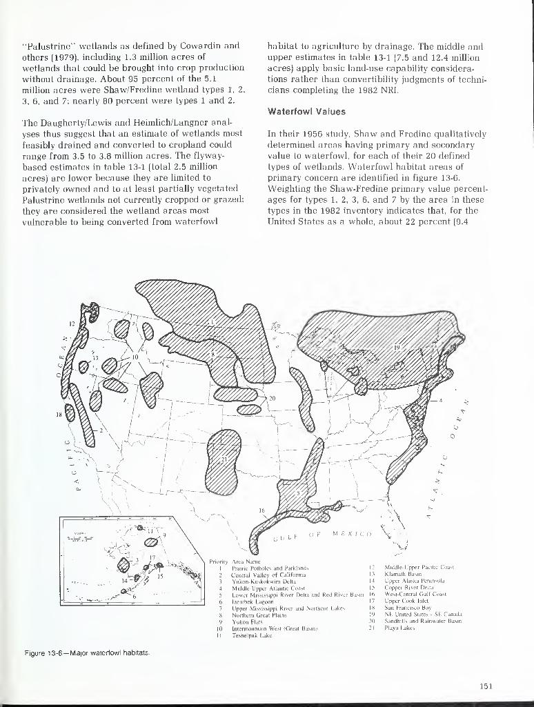
"Palustrine" wetlands as defined by Cowardin and

others (1979), including 1.3 million acres of

wetlands that could be brought into crop production

without drainage. About 95 percent of the 5.1

million acres were Shaw/Fredine wetland types 1', 2,

3. 6. and 7; nearly 80 percent were types 1 and 2.

The Daugherty/Lewis and Heimlich/Langner anal-

yses thus suggest that an estimate of wetlands most

feasibly drained and converted to cropland could

range from 3.5 to 3.8 million acres. The flyway-

based estimates in table 13-1 (total 2.5 million

acres) are lower because they are limited to

privately owned and to at least partially vegetated

Palustrine wetlands not currently cropped or grazed;

they are considered the wetland areas most

vulnerable to being converted from waterfowl

habitat to agriculture by drainage. The middle andupper estimates in table 13-1 (7.5 and 12.4 million

acres) apply basic land-use capability considera-

tions rather than convertibility judgments of techni-

cians completing the 1982 NRI.

Waterfowl Values

In their 1956 study, Shaw and Fredine qualitatively

determined areas having primary and secondary

value to waterfowl, for each of their 20 defined

types of wetlands. Waterfowl habitat areas of

primary concern are identified in figure 13-6.

Weighting the Shaw-Fredine primary value percent-

ages for types 1, 2, 3, 6, and 7 by the area in these

types in the 1982 inventory indicates that, for the

United States as a whole, about 22 percent (9.4

unt\ Area Name1 Prairie Potholes and Parklands 12 Middle- Upper Pacific Coast

2 Central Valley of California 13 Klamath Basin

3 Yukon-Kuskokwim Delta 14 Upper Alaska Peninsula

4 Middle-Upper Atlantic Coast 1? Copper River Delta

5 Lower Mississippi River Delta and Red River Basin 16 West-Central Gult Coast

6 Izembek Lagoon 17 Upper Cook Inlet

7 Upper Mississippi River and Northern Lakes 18 San Francisco Bav

g Northern Great Plains 19 NE United Slates - SE Canada

9 Yukon Flats 20 Sandhills and Rainwater Basin

10 Intermountain West (Great Basin) 21 Plava Lakes

11 Teshelpuk Lake

Figure 13-6— Major waterfowl habitats.

151

million acres) of the 42.7 million acres of remaining

private Palustrine vegetated wetlands theoretically

convertible to crop production are of primary value

to waterfowl, although Shaw and Fredine considered

all wetlands to have at least a "lesser" value for

waterfowl. Under the minimum conversion estimate

in table 13-1, between 550,000 acres and 700,000

acres (22-28 percent) of the wetlands drained and

converted to agriculture could be regarded as having

primary value to waterfowl. For the middle

estimate, the amount would be between 1.6 and 2.1

million of the 7.5 million acres converted. The max-

imum conversion would involve between 2.8 and 3.6

million acres of wetlands having a primary value to

waterfowl.

This brief examination of wetlands from the view-

point of wildfowl and conversion questions also

reveals that States within the Mississippi and Atlan-

tic Flyways contain 81 percent of all non-Federal

wetlands, 89 percent of State, county, and other

non-Federal publicly owned wetlands, and 80 per-

cent of all privately owned wetlands (table 13-1).

More important, these two humid-area flyways

apparently contain 92 percent of the vegetated

Palustrine wetlands not currently in agriculture.

Smith and Massey observed that pressures for com-

plete evaluation of all wetland benefits for wildlife,

hunters, farmers, and other interests will increase

with wider public recognition of their alternative

uses and their reduction to a remnant level. Someproducts of wetlands, such as waterfowl hunting,

are more readily evaluated than others. Pending the

completion of coordinated studies, opportunities for

combining information on the value of different uses

developed in separate studies and from independent

sources should not be overlooked. The next section

outlines some of these possibilities.

Balancing Competing NaturalResource Values

Miller and Hay (1981) have studied the relationship

between wetland habitat availability, hunter success,

and the level of duck hunting in the Mississippi

Flyway. This is a 14-State area extending through

Minnesota, Wisconsin, and Michigan, the entire

Corn Belt, and the Mississippi Delta, plus Kentucky,

Tennessee, and Alabama (fig. 13-1). Other approaches

to determining waterfowl habitat values in the

Upper Midwest were examined earlier by Goldstein

(1971). Miller and Hay estimated that in 1975

waterfowl habitat had a value (consumer surplus

value) to duck hunters of $29 per day of hunting per

year, based on cited earlier work of Hay with Char-

bonneau. Capitalized into the indefinite future at a

7-3/8-percent discount rate in 1984 prices, this

amounted to $160 per acre of lost wildlife habitat.

A similar study for the Pacific Flyway by Hammackand Brown (1971) was based not on days hunted,

but on the value hunters placed on a duck bagged,

estimated at $9.80 per duck at 1984 prices. This con-

verts to a capitalized value of about $220 per acre

of habitat, assuming an average of 1.6 birds per

year are bagged per acre of habitat and again capi-

talizing into the indefinite future at 7-3/8 percent.

These two research studies suggest that an acre of

wetlands available for duck hunting in 1984 had a

market value ranging from $160 to $220 per acre,

for an average of $190 per acre. It is not advisable

to relate precisely such wide-area values to the

marginal values of particular wetlands if converted

to agriculture, so only broad estimates can be made.

According to the 1978 Census of Drainage, there

were 20 predominantly agricultural counties within

the 14-State Mississippi Flyway with 75 percent or

more of their land area drained (U.S. Dept. of Com-merce, 1981). The 20 counties are listed in table

13-2. Figure 13-5 shows their general location. Five

of the 20 counties are more than 90-percent drained:

Mississippi County, Arkansas (99 percent);

Mississippi County, Missouri (98 percent); HancockCounty, Ohio (96 percent); Dunklin County, Missouri

(96 percent); and New Madrid County, Missouri (94

percent).

The rationale for looking at counties already inten-

sively drained is that, if not in agriculture, large

areas in these localities would have remained as or

would revert to wetlands and waterfowl habitat.

Their present market values in agricultural use are

guides to the market value of an additional acre of

wetlands converted to farming, though not neces-

sarily in the same county. This value, less the net

cost of conversion, can be related to waterfowl

hunting values as an opportunity cost—one of a

class of benefits given up when draining wetlands.

Net conversion costs are actual draining and/or

associated clearing costs less the value of wood or

other products removed in the process. For the nine

counties of table 13-2 located in the northern section

of the Mississippi Flyway (Michigan, Ohio, Indiana,

and Iowa), net conversion costs in 1984 averaged an

estimated $550 per acre. Conversion costs for the

11 counties located in the southern section averaged

$435 per acre (Herrington and Schulstad, 1978).

152

The next step is to subtract conversion costs from

market values of farmland. According to the most

recent Census of Agriculture and USDA sources, in

1984 the market value of farmland without

buildings for the 20 high-drainage counties within

the Mississippi Flyway averaged $1,105 per acre

(U.S. Dept. Commerce, 1983; Jones, 1985). This pro-

vides a rough measure of the market value in 1984

of an added acre of remnant wetlands within the

Mississippi Flyway converted to agriculture by

drainage and/or necessary clearing. Deducting a net

conversion cost of $477 per acre, the added net

agricultural market value would be $628 per acre.

This is a farm use value to compare with the above

values of $160 to $220 per acre associated with not

converting additional wetlands to agriculture.

For situations similar to those in the 20 Mississippi

Flyway counties more than 75-percent drained,

waterfowl hunting values in 1984 averaged 25 to 35

percent of net agricultural values, depending on

whether the above Miller-Hay waterfowl hunting

value of $160 per acre or the Hammack-Brownvalue of $220 per acre is compared with the net

agricultural value of $628 per acre. If the twowaterfowl habitat value estimates are given equal

weight (averaged to $190 per acre), the 1984 water-

fowl values of wetlands within the Mississippi

Flyway were about 30 percent of the corresponding

agricultural value of drained wetlands (table 13-2).

But, this percentage ranged from 63 percent for

conditions represented by Sharkey County,

Mississippi, to 21 percent for conditions

Table 13-2—Waterfowl hunting values compared with agricultural values for the 20 agricultural counties in theMississippi Flyway where at least 75 percent of the farmland area is drained

Counties (States) 1

Farmland value, 1984Farmland Relative

area Sale Net waterfowldrained value2 value3

1984values4

1986

Percent Dollars per acre - Percent

80 735 300 63 12485 760 325 58 14088 875 325 58 15486 890 340 56 141

99 960 525 36 67

96 965 530 36 79

75 990 555 34 5385 1,015 580 33 58

94 1,045 610 31 64

98 1,040 605 31 64

86 1,225 675 30 6283 1,250 700 27 58

96 1,305 755 25 52

49 1,190 755 25 42

86 1,345 795 24 49

79 1,230 795 24 39

75 1,385 835 23 5082 1,400 850 22 49

80 1,475 925 21 69

80 1,335 900 21 34

Sharkey (Mississippi)

St. Francis (Arkansas)Clinton (Michigan)Shiawassee (Michigan)Mississippi (Arkansas)

Dunklin (Missouri)Washington (Mississippi)

Crittenden (Arkansas)New Madrid (Missouri)Mississippi (Missouri)

Paulding (Ohio)

Crawford (Ohio)Hancock (Ohio)Jefferson Davis (Louisiana)Henry (Ohio)

East Carroll (Louisiana)Wells (Indiana)

Adams (Indiana)

Pocahontas (Iowa)

Acadia (Louisiana)

Average, 20 counties 5 86 1,105 628 30 58

1 Counties listed according to highest waterfowl hunting values relative to agricultural land values in 1984.2Land without buildings, based on Census of Agriculture for 1982 and Jones (1985).3Sale value less average net costs of draining or clearing and draining. Net drainage costs for listed counties in Mississippi,

Arkansas, Missouri, and Louisiana averaged $435 per acre. These costs exceed drainage costs in chapter 11, averaged for these

four States, by about 60 percent, indicating that substantial clearing and other preparation costs are likely in converting southern

wetlands to agriculture. Costs for the remaining listed counties in the Northern States within the Mississippi Flyway (Michigan,

Ohio, Indiana, Iowa) averaged $550 per acre. These costs exceed drainage costs in chapter 11, averaged for these four States, by

about 10 percent.4 Ratio of average waterfowl hunting value per acre ($190) to net farmland values for 1984 or 1986. The $190 per acre is the

average of $160 per acre and $220 per acre. See text.5Averages based on 5.7 million acres in farms and 4.9 million acres drained in the 20 counties. Drainage intensities are assumed

to be approximately the same in 1984 and 1986 as reported in the 1978 Census of Drainage (U.S. Dept. Commerce, 1981).

153

represented by Pocahontas County, Iowa, and

Acadia County, Louisiana. It is interesting to note

that nearly the same fraction (80 percent) of the

farmland in these three counties is drained, but

agricultural land values differ considerably.

Excluding buildings, in 1984 values were $735 per

acre in Sharkey County, $1,335 per acre in Acadia

County, and $1,475 per acre in Pocahontas County.

Waterfowl habitat values relative to the potential

agricultural values of remnant wetlands change as

the demands for and supplies of waterfowl habitat

and farmland change. Lacking actual data, assume

that between 1984-86 habitat values and drainage

conversion costs in the Mississippi Flyway were

stable. Between 1984 and 1986 average farmland

values did fall except in New Jersey, Virginia, and

New England (USDA, 1986). Percentage decreases in

average farm real estate values per acre for the

eight Mississippi Flyway States represented in table

13-2 were: Iowa (-44 percent), Indiana (-34 percent),

Ohio (-30 percent), Mississippi (-23 percent), and

Mississippi (-20 percent). The relative waterfowl

values in table 13-2 were approximated by applying

percentage statewide decreases in land values be-

tween 1982, 1984, and 1986 to county land values

reported in the 1982 Census.

The sensitivity of relative waterfowl values to

changing farmland values can be shown by compar-

ing waterfowl value indexes for 1984 and 1986.

Between 1984 and 1986, the waterfowl value index

rose from 63 to 124 percent for Sharkey County,

Mississippi. It rose from 58 to 154 percent for

Clinton County, Michigan. The relative value of

wetlands for waterfowl habitat increased more in

the northern than in the southern States of the

Mississippi Flyway because agricultural land values

fell more in the northern States. For example, be-

tween 1984 and 1986 the relative waterfowl value

percentage rose from 21 to 69 percent for Pocahontas

County, Iowa, but from 21 to only 34 percent for

Acadia County, Louisiana.

The average waterfowl value index for wetlands for

the 20 highly drained counties in table 13-2 as a

group rose from 30 to 58 percent between 1984 and

1986. For all counties in table 13-2, nonagricultural

benefits of wetlands other than waterfowl hunting

values would need to be less significant in 1986

than in 1984 to justify wetland preservation. Preser-

vation of waterfowl habitat alone would be justified

for the first four county situations in the table,

although the situations are not necessarily typical

for the entire county.

Under such conditions, the incentive to drain addi-

tional wetlands is reduced in two ways: (1) For

operators wishing to expand operations, the cost of

simply purchasing additonal cropland as against

draining wetlands for crop use would fall, and

(2) existing landowner options for marketing water-

fowl hunting values and/or other beneficial qualities

of wetlands to hunters or public agencies, by meansof purchase, lease, or easements, would be moreattractive. How well the agricultural, nonagri-

cultural. and environmental benefits of wetlands

are quantified or otherwise identified will determine

the ultimate success of such institutional arrange-

ments for optimum wetland use.

The research opportunity suggested by these possible

outcomes is to periodically update information like

that in tables 13-1 and 13-2 for all flyways as

farmland values and recreational demands change.

The fact that State Experiment Stations and USDAalready monitor land values on a regular basis for

many other purposes would facilitate this workconsiderably.

Such research would enable environmentalists andpublic officials to identify localities where lease andpurchase of remaining true wetlands to farming in-

terests would likely be the least costly. It would also

improve predictions on the future rate of wetland

conversions, based on anticipated waterfowl hunt-

ing demands as well as anticipated demands for the

products of competing industries. These include not

only agriculture, but also forestry, resort, and

residential community development, and other activ-

ities like airport construction. More specific

analyses of farm drainage adoption and optimum

design decisions have been completed by Goldstein

(1971), Irwin (1980), and Skaggs and Nassehzadeh-

Tabrizi (1983).

Improving Drainage Information

Perceptions on the status and trends of wetlands

depend on the amount and quality of data concern-

ing the current extent of drainage. Government

statistics have tended to give an incomplete picture

of land drainage. Census-type data have been widely

used as the most authoritative source of information.

However, they have been based at various times on

the Census of Agriculture, the Census of Drainage,

the Census of Governments, annual SCS planning

assistance progress reports, and ASCS cost-sharing

reports. Not all farm operators know what part of

their land is drained.

'Douglas Lewis contributed information for this section.

154

Although the definition of drainage has changed little

over time, specific data items have changed, as

have definitions of the relevant universe, such as

what constitutes a farm, how drained irrigated land

is considered, and what constitutes public versus

private drainage enterprises. Moreover, it has not

been possible to assess the effectiveness of different

drainage improvements in different regions. As a

result, in official reports, all systems appear to be

equally effective in removing excess water or soil

salts in the case of irrigation-associated drainage.

Another problem is that new drainage investments

have not been reported separately from expendi-

tures for maintenance. The 1983 Farm Expenditure

Survey, conducted by NASS, was a first effort to

pick up both kinds of financial information.

ASCS and SCS reports are also limited to programparticipants and typically give only the cost-sharing

portion of total investment. Some information is

given in units not easily integrated with other data

sources. Periodic agency surveys have tended to

address additional drainage needs rather than im-

provements already in place. The 1982 inventory

conducted by SCS and a 1978 Resource Economics

Survey conducted by ERS attempted to correct this

problem.

Given these limitations, caution is recommended in

using historical agricultural land drainage data.

Changes in policies and institutions affecting

drainage certainly change the benefits and costs of

draining, both to individual farmers and society at

large. Greater attention to societal interests meansthat the information needed for decisionmaking

becomes more complex. In short, increased efforts

and expenditures to improve data collection are

needed to ensure a more accurate mosaic of

agricultural land drainage, thus permitting morerational private drainage investments and public

policy decisions.

USDA's role in farmland development through

drainage has diminished considerably since its

agricultural conservation and resource improvement

started in the 1930's. In 1960, drainage accounted

for about 9 percent of all conservation cost-sharing

assistance to farmers: about 40 percent of this

assistance went for open drains compared with 60

percent for subsurface or pipe drains. By 1983,

drainage accounted for only $51,000, or 0.02 percent

of all ACP assistance. Also, in 1983, only 8 percent

of the ACP assistance was for surface or opendrainage systems.

The minor USDA role in current drainage activities

was also indicated in a 1978 Resource EconomicsSurvey (Lewis, 1982). During 1975-77, cost sharing

and loan programs of USDA represented only about4 percent of the capital funds spent for onfarmdrainage improvements. Nearly 82 percent camefrom farmers' own funds. The remaining 14 percent

was obtained from loans.

The basic drainage information challenge, however,comes from another quarter. Legislation has beenpassed to discontinue the Census of DrainageOrganizations taken every 10 years since 1920 bythe Department of Commerce. As already noted,

USDA has eliminated drainage as a practice

qualifying for cost-sharing assistance. USDA does

provide technical assistance for draining wet soils

but not for land classified as wetlands.

Governmental agencies unquestionably have beenone of the primary users of the information they

develop at public expense for public use. But, as anagency's own drainage program activities are scaled

back, its capacity to produce and even its interest

in statistical information tend to weaken. Thechallenge, therefore, is to develop plans to acquire

coordinated information on farm and other drainage

activities, including wetland conversions, without

relying on Census-type and other formal data-

gathering programs. This is an opportunity for

wildlife, agricultural, forestry, and other commer-cial interests to pool their knowledge and resources

for research, management, and policymaking. Suchefforts will require the participation of all

interested sectors of the economy, including Federal

agencies.

Maintenance and Repair Challenges

Open drains traditionally have not been maintained

in a timely manner which decreases their effective-

ness. This is especially true for open drains used as

outlets for numerous onfarm drainage systems.

Studies by Burris and others in Ohio (1985) showedthat the net benefit of an effective annual

maintenance program over periodic reconstruction

(15-year cycle) averaged $12.70 per acre.

A good maintenance program for any type of drain-

age system is just as necessary as proper design

and construction. Sound maintenance plans should

be developed that consider system effectiveness as

well as environmental concerns. When systems

involve more than one landowner, the assignment of

responsibility for maintenance should be outlined

155

and agreed upon by the concerned parties in the

original plans.

Salinity and Water Quality Control

Drainage systems can help maintain salinity levels

in crop root zones within safe limits for crop

production. Sound irrigation water management can

reduce and, in some cases, eliminate the need for

artificial drainage systems. Using drainage water as

a supplemental source of irrigation is now receiving

special attention. If successful, drainwater use for

irrigation will reduce drainwater flow and thus

ease discharge problems that now exist or could

develop in arid and semiarid climates. Drainwater

quality is a growing concern, particularly for trace

elements and the salt load. Efforts to handle these

problems must be considered in all system designs

and farming operations in these climates.

Drainage is Water Management

Agricultural drainage always has been viewed as a

process of land conversion, improvement of the soil

environment for plants either with or without irriga-

tion, and elimination of operational hazards and

nuisances. Drainage is now seen as a key aspect of

water management, not as a purpose or activity in

itself. Water is the resource basically involved,

whether the purpose is to remove or otherwise con-

trol it on cropland, to avoid offsite wildlife and

other environmental disbenefits from chemically

polluted drain waters, to control salinity on irri-

gated soils, or to limit the intrusion of agriculture

and other land uses into wetland areas. No one

denies that large areas of former wetlands are nowin urban and agricultural uses (Shaw and Fredine

(1956), Tiner, (1984), and U.S. Congress, (1984).) But.

it is also true that neither surface nor subsurface

drainage improvements, nor provisions for proper

drainage on irrigated lands, necessarily mean a loss

in wetlands as conventionally defined.

The concept of drainage as water management has

even stronger support in new drainage systems based

on rainfall probabilities and in water control

systems usable either for water removal or subirri-

gation, depending on growing-season variations in

soil moisture conditions. Such systems are already

viewed as the best context for anticipating the

future character of water management on farms

and for agriculture generally.

To consider drainage as water management is to

advocate a complete analysis of drainage benefits,

costs, and environmental impacts in particular

cases. Nonagricultural aspects are acknowledged to

be very significant and variously include hydrologic,

water quality, climatic, recreational, and educa-

tional values (Thomas, chap. 5, and Bardecki, 1984).

This does not mean such values have an importance

overwhelming all others, although they maysupersede all others for prescribed areas or

wetland types. It may be more meaningful as well

as less controversial to quantify these values from a

water-resource rather than from a wetland vantage

point.

As true wetlands are drained and converted to

agricultural or other uses, most of the values said to

be lost are associated with a changed or impaired

water and aquatic plant environment, not with

drained land as such. Similarly, benefits from im-

proved drainage in wet soils not considered

wetlands are associated with improved moisture

and other soil conditions for crops and more effi-

cient field operations. The result is essentially the

same when irrigated lands are adequately drained.

Within these newer concepts, several additional

challenges call for policy attention and study of the

future of farm drainage.

Agricultural drainage can have positive and

negative consequences, both on farms and offsite.

The problem is that the consequences are fre-

quently not associated with the original decision-

maker, beneficiary, or loser. Further, some drainage

activities on farms are clearly neutral in their

consequences. They may involve nonirrigated soils

or irrigated soils but not hurt wildlife and wetlands,

at least not as generally defined. Separating the

neutral from known or potentially controversial

situations is one way to simplify matters for policy-

makers as well as for other scientists.

Fausey and colleagues observed that by increasing

moisture storage capacity, good drainage can re-

duce runoff and erosion damage, thus improving the

effectiveness and durability of soil conservation

measures like minimum tillage and grassed water-

ways. Their observations illustrate how water

management strategies can have multiple onsite and

offsite benefits as well as costs and particular detri-

mental effects. While many of the various purposes

and effects of soil and water management as

described by agronomists, soil scientists, and

engineers seem readily usable for structuring com-

plete benefit/cost studies, not much economic

research of this kind has been done. It is important

because farm output-increasing or cost-decreasing

strategies like irrigation and drainage are some-

156

times questioned as perhaps benefiting agriculture

at society's expense, especially when water supplies

are being diminished and crops are in surplus.

Challenges for Research and Education

A first research and educational challenge is to in-

crease our understanding of how all drainage bene-

fits and costs, in both a direct and opportunity

sense, can be related to each other in the sameframework in analyzing alternative private deci-

sions and public policies. In effect, this will remove

potential market-failure situations as described by

Langner (1985). It will also improve predictions on

the scope and location of additional drainage and

thus on the likely nature of possible controversies,

providing a rational basis for actually resolving

disputes. It will require cooperation amongengineers, biologists, extension specialists, and

social scientists throughout the research process,

especially in the planning stage.

Surveys and inventories are an important statistical

resource in benefit/cost studies, but analysts need

to proceed from similar definitions. The economic

evaluation of the environmental costs of agricultural

activities requires survey data developed on an inter-

disciplinary basis (Miranowski, 1983). Just as it is

possible to define away problems, it is also possible

to provoke them by arbitrary definitions and classi-

fications tilting toward a particular but not agreed-

upon point of view. Agricultural and environmental

advocates can be expected to cooperate in examin-

ing drainage if they agree, at least in principle, on

the expected costs and benefits of drainage, on the

kinds of lands and soil conditions involved, and on

the environmental benefits or disutilities created

elsewhere.

Another research opportunity is implied in the

Smith and Massey observation that past agri-

cultural productivity projections were based on

assumptions of competition. This is a situation in

which there are many farms, with none individually

having an appreciable influence on product prices

and input costs. For the most part, this still

characterizes American agriculture. A research

challenge here is to study technological and

marketing activities in the drainage industry itself,

given the reduced number of farmers, overcapacity

problems in agriculture, and concern over losses of

wetlands. The size, location, form of business

organization, and probable public agricultural

policies for remaining farms, plus any remaining

natural limitations to production, will be the keys to

anticipating where additional drainage will likely

occur.

We close with a few recurring ideas. We do not

know enough about most of the real functions of

wetlands, especially noncoastal wetlands, to predict

the specific effects of either maintaining or draining

such wetlands for agriculture and other uses. Drain-

ing hardwood bottomlands is an exception, becauseflood storage capacities of such wetlands can be

calculated within reasonable limits of accuracy.

It follows that if the functions are not known andthe effects of wetland preservation or drainage are

not known, it is difficult to formulate new drainage

policies or develop programs to inform farmers,

landowners, or policymakers about the value of re-

taining wetlands. The same difficulties apply in in-

creasing public awareness of the contributions of

agricultural drainage to public health, land settle-

ment, and economic development.

Efforts should be made to identify and measure all

functional values of wetlands. Meanwhile, real oppor-

tunities exist for developing educational programs

of more immediate interest to, and effectiveness for,

farm operators and wildlife interests.

Many landowners attach no intrinsic value to

wetlands but view them as any other pieces of prop-

erty. If the property has no intrinsic value and no

apparent functional value, it must either be written

off as having no value or converted to something of

value. It follows that, in the absence of existing

functional values, or the opportunity to develop

such values, conversion to other uses becomes the

only rational option. This challenge to researchers

and educators can be expressed as a series of frank

questions.

Can programs be developed to manage wetlands to

provide some incentive for wetland retention and to

provide some tangible benefits to the farm oper-

ator? Are there things that farmers themselves

might do to increase the returns from retained wet-

lands? Can their wetlands and those of other pri-

vate landowners be managed to produce economic

returns in the form of trappable furbearers or leased

hunting rights? Can the waterfowl hunting values

like those in table 13-2 be converted to landowner

income to maintain wetlands? Such programs would

take the question of wetland retention, at least in

some cases, from the realm of abstract values to

tangible returns. The potential for such programs

has been acknowledged within various Federal

agencies (Tiner, 1984), but there is little identifiable

movement toward such programs.

Some recognition is beginning to emerge at the State

level (Harris and others, 1984; Malecki, 1985;

157

Davidson, 1984). But, much of the literature con-

tinues to deal with the generalities or potential for

drainage impacts on wetlands (Redelfs, 1983;

Sullivan, 1985). They do not address the highly

technical matters of actual impacts. Other studies

discuss the potential for legislative solutions rather

than opportunities for enlisting the assistance of

landowners in protecting wetlands for their func-

tional values (Kusler, 1983: Bell, 1981). Drainage

and wetlands preservation of natural resource man-

agement as a stable element of both depends on

public policies and private actions that accom-

modate both landowner and public interests.

References

Bardecki. Michael J. 1984. "What Value

Wetlands?," Journal of Soil and Water Conserva-

tion. Vol. 39, No. 3, May-June, pp. 166-169.

Bell, H. E., II. 1981. Illinois Wetlands: Their Value

and Management. Illinois Institute of Natural

Resources, Chicago.

Burris, Robert L.. Dana C. Chapman, and Gary L.

Overmein. 1985. Economics of Ditch Maintenance in

Northwestern Ohio. Presented at Am. Soc. of Civil

Engineers Irrigation and Drainage Specialty Confer-

ence, San Antonio, Tex., July 16-19.

Cowardin, Lewis F., Francis C. Golet, and Edward T.

LaRoe. 1979. Classi/ication of Wetlands and Deep-

water Habitats of the United States.

FWS/OBS-79/31. U.S. Dept. of the Interior, Fish and

Wildlife Serv.

Crosson, P. R. 1982. The Cropland Crisis — Myth or

Reality?. Resources for the Future, Inc., Wash., DC.

Davidson, B. 1984. "Texas Wetlands—A Valuable

Resource," Texas Water Resources. Vol. 20, No. 1.

Texas Water Resources Institute, College Station.

Frayer, W. E., T. J. Monahan, D. C. Bnwden, and F.

A. Graybill. 1983. Status and Trends of Wetlands

and Deepwater Habitats in the Conterminous United

States. 1950's to 1970' s. U.S. Dept. of the Interior,

Fish and Wildlife Serv., and Department of Forest

and Wood Sciences, Colorado State Univ., Ft.

Collins.

Hammack. Judd, and Gardner Mallard Brown, Jr.

1974. Waterfowl and Wetlands: Toward Bioeco-

nomic Analysis. Baltimore: Johns Hopkins Press for

Resources for the Future, Inc.

Harrington, Billy E., and Robert N. Schulstad. 1978.

Conversion of Delta Woodland and Pasture to Crop-

land: Economic Feasibility and Implications. Bulletin

858. Arkansas Agr. Expt. Sta., Fayetteville.

Harris, L. D., R. Sullivan, and L. Badger. 1984. Bot-

tomland Hardwoods: Valuable, Vanishing,

Vulnerable. Florida Coop. Ext. Serv. SP-28. Univ.

Florida, Gainesville.

Heimlich, Ralph E., and Linda L. Langner. 1986.

Swampbusting: Wetland Conversions and Farm Pro-

grams. AER-551. U.S. Dept. of Agr., Econ. Res. Serv.

Irwin, Ross W. 1980. On-Farm Drainage Benefit.

Final Report Project A-39-742. Univ. of Guelph,

School of Engineering, Guelph, Ontario.

Jones, John F. 1985. U.S. Dept. Agr., Econ., Res.

Serv. Special data developed for authors.

Kusler, J. A. 1983. Our National Wetland Heritage:

A Protection Guidebook. The Environmental Law In-

stitute, Wash.. DC.

Langner, Linda L. 1985. Economic Perspective on

the Effects of Federal Conservation Policy on Wild-

Life Habitat. Transactions, North American Wildlife

and Natural Resources Conferences, Wash., DC.

March 18-20.

Lewis. Douglas. 1982. Land Drainage Investment

Survey, 1975-77. ERS Staff Report No. AGES820505.U.S. Dept. Agr., Econ. Res. Serv.

Madson, John. 1984. "American Waterfowl:

Troubles and Triumphs," National Geographic. Vol.

166, No. 5, pp. 562-599.

Malecki, R. 1985. "Agriculture and Wetlands: ANew Perspective," New York Food and Life Science

Quarterly. Vol. 15, No. 3, pp. 11-13. New York State

Agri. Exp. Sta., Ithaca.

Goldstein, Jon H. 1971. Competition for Wetlands in

the Midwest: An Economic Analysis. Baltimore:

Johns Hopkins Press for Resources for the Future.

Inc.

Miller, Jon R., and Michael J. Hay. 1981. "Deter-

minants of Hunter Participation: Duck Hunting in

the Mississippi Flyway," American Journal of Agri-

cultural Economics. Vol. 63, No. 4, pp. 677-684.

158

Miranowski, John A. 1983. "Agricultural Impacts on

Environmental Quality," Water Resources Research:

Problems and Potentials for Agriculture and Aural

Communities. Ankeny, Iowa: Soil Conservation Society

of America.

Pioneer Hi-Bred International, Inc. 1982. Soil Con-

servation Attitudes and Practices: The Present and

the Future. Des Moines, Iowa.

Redelfs, A. E. 1983. Wetlands Values and Losses in

the United States. M.S. thesis, Oklahoma State

Univ., Stillwater.

Shaw, Samuel P.. and C. Gordon Fredine. 1956.

Wetlands of the United States. Circular 39. U.S.

Dept. Interior, Fish and Wildlife Serv.

Skaggs, R. W., and A. Nassehzadeh-Tabrizi. 1983.

Optimum Drainage for Corn Production. Technical

Bulletin No. 274. North Carolina Agri. Res. Serv.,

State Univ., Raleigh.

Sullivan, J. D. 1985. Stream Channelization in NewYork: Impacts on Agriculture and the Environment.

M.S. thesis. Cornell University, Ithaca, N.Y.

Tiner, R. J., Jr. 1984. Wetlands of the United States:

Current Status and Recent Trends. U.S. Dept. In-

terior, Fish and Wildlife Serv.

U.S. Congress, Office of Technology Assessment.

1984. Wetlands: Their Use and Regulation. March.

U.S. Department of Agriculture, Economic ResearchService. 1986. Outlook and Situation Summary;Agricultural Resources, April 9.

U.S. Department of Agriculture, Soil Conservation

Service. 1961. Land Capability Classification.

AH-210.

U.S. Department of Agriculture, Soil Conservation

Service and Iowa State University. 1982. Basic

Statistics, 1977 National Resources Inventory

SB-686. (Statistical Bulletin in process for 1986 In-

ventory; wetland data retrievable from computer

files).

U.S. Department of Commerce. 1981. "Drainage of

Agricultural Lands," Census of Agriculture, 1978.

Vol. 5: Special Reports, part 5.

159

Appendix A

Executive Order 11990:Protection of Wetlands

(Federal Register, Vol. 42, No. 101,Wednesday, May 25, 1977)

By virtue of the authority vested in me by the Con-

stitution and statutes of the United States of

America, and as President of the United States of

America, in furtherance of the National Environ-

mental Policy Act of 1969, as amended (42 U.S.C.

4321 et seq.), in order to avoid to the extent possible

the long and short term adverse impacts associated

with the destruction or modification of wetlands

and to avoid direct or indirect support of newconstruction in wetlands wherever there is a prac-

ticable alternative, it is hereby ordered as follows:

Section 1. (a) Each agency shall provide leadership

and shall take action to minimize the destruction,

loss or degradation of wetlands, and to preserve

and enhance the natural and beneficial values of

wetlands in carrying out the agency's responsibil-

ities for (1) acquiring, managing, and disposing of

Federal lands and facilities; and (2) providing

Federally undertaken, financed, or assisted con-

struction and improvements; and (3) conducting

Federal activities and programs affecting land use,

including but not limited to water and related land

resources planning, regulating, and licensing

activities.

(b) This Order does not apply to the issuance by

Federal agencies of permits, licenses, or allocations

to private parties for activities involving wetlands

on non-Federal property.

Sec. 2. (a) In furtherance of Section 101(b)(3) of the

National Environmental Policy Act of 1969 (42 U.S.C.

4331(b)(3) to improve and coordinate Federal plans,

functions, programs and resources to the end that

the Nation may attain the widest range of beneficial

uses of the environment without degradation andrisk to health or safety, each agency, to the extent

permitted by law, shall avoid undertaking or provid-

ing assistance for new construction located in wet-

lands unless the head of the agency finds (1) that

there is no practicable alternative to such construc-

tion, and (2) that the proposed action includes all

practicable measures to minimize harm to wetlands

which may result from such use. In making this find-

ing the head of the agency may take into account

economic, environmental and other pertinent

factors.

(b) Each agency shall also provide opportunity

for early public review of any plans or proposals

for new construction in wetlands, in accordance

with Section 2(b) of Executive Order No. 11514, as

amended, including the development of procedures

to accomplish this objective for Federal actions

whose impact is not significant enough to require

the preparation of an environmental impact state-

ment under Section 102(2)(C) of the National En-

vironmental Policy Act of 1969, as amended.

Sec. 3. Any requests for new authorizations or

appropriations transmitted to the Office of Manage-

ment and Budget shall indicate, if an action to be

proposed will be located in wetlands, whether the

proposed action is in accord with this Order.

Sec. 4. When Federally-owned wetlands or portions

of wetlands are proposed for lease, easement, right-

of-way of disposal to non-Federal public or private

parties, the Federal agency shall (a) reference in

the conveyance those uses that are restricted under

identified Federal, State or local wetlands regula-

tions; and (b) attach other appropriate restrictions

to the uses of properties by the grantee or pur-

chaser and any successor, except where prohibited

by law; or (c) withhold such properties from

disposal.

Sec. 5. In carrying out the activities described in

Section 1 of this Order, each agency shall consider

factors relevant to a proposal's effect on the sur-

vival and quality of the wetlands. Among these fac-

tors are:

160

(a) public health, safety, and welfare, including

water supply, quality, recharge and discharge; pol-

lution; flood and storm hazards; and sediment and

erosion;

(b) maintenance of natural systems, including

conservation and long term productivity of existing

flora and fauna, species and habitat diversity and

stability, hydrologic utility, fish, wildlife, timber,

and food and fiber resources; and

(c) other uses of wetlands in the public interest,

including recreational, scientific, and cultural uses.

Sec. 6. As allowed by law, agencies shall issue or

amend their existing procedures in order to comply

with this Order. To the extent possible, existing pro-

cesses, such as those of the Council on Environ-

mental Quality and the Water Resources Council,

shall be utilized to fulfill the requirements of this

Order.

Sec. 7. As used in this Order:

(a) The term "agency" shall have the samemeaning as the term "Executive agency" in Section

105 of Title 5 of the United States Code and shall in-

clude the military departments; the directives con-

tained in this Order, however, are meant to apply

only to those agencies which perform the activities

described in Section 1 which are located in or

affecting wetlands.

(b) The term "new construction" shall include

draining, dredging, channelizing, filling, diking, im-

pounding, and related activities and any structures

or facilities begun or authorized after the effective

date of this Order.

(c) The term "wetlands" means those areas

that are inundated by surface or ground water with

a frequency sufficient to support and under normal

circumstances does or would support a prevalence

of vegetative or aquatic life that requires saturated

or seasonally saturated soil conditions for growth

and reproduction. Wetlands generally include

swamps, marshes, bogs, and similar areas such as

sloughs, potholes, wet meadows, river overflows,

mud flats, and natural ponds.

Sec. 8. This Order does not apply to projects

presently under construction, or to projects for

which all of the funds have been appropriated

through Fiscal Year 1977, or to projects and pro-

grams for which a draft or final environmental

impact statement will be filed prior to October 1,

1977. The provisions of Section 2 of this Order shall

be implemented by each agency not later than

October 1, 1977.

Sec. 9. Nothing in this Order shall apply to

assistance provided for emergency work, essential

to save lives and protect property and public health

and safety, performed pursuant to Sections 305 and306 of the Disaster Relief Act of 1974 (88 Stat. 148,

42 U.S.C. 5145 and 5146).

Sec. 10. To the extent the provisions of Sections 2

and 5 of this Order are applicable to projects

covered by Section 104(h) of the Housing andCommunity Development Act of 1974, as amended(88 Stat. 640, 42 U.S.C. 5304(h)), the responsibilities

under those provisions may be assumed by the

appropriate applicant, if the applicant has also

assumed, with respect to such projects, all of the

responsibilities for environmental review, decision-

making, and action pursuant to the National

Environmental Policy Act of 1969, as amended.

The White House Jimmy Carter

May 24, 1977

Protection of Wetlands

(Statement by the President Accompanying Executive

Order 11990. May 24, 1977)

The Nation's coastal and inland wetlands are vital

natural resources of critical importance to the people

of this country. Wetlands are areas of great natural

productivity, hydrological utility, and environmental

diversity, providing natural flood control, improved

water quality, recharge of aquifers, flow stabilization

of streams and rivers, and habitat for fish and

wildlife resources. Wetlands contribute to the

production of agricultural products and timber, and

provide recreational, scientific, and aesthetic

resources of national interest.

The unwise use and development of wetlands will

destroy many of their special qualities and impor-

tant natural functions. Recent estimates indicate

that the United States has already lost over 40

percent of our 120 million acres of wetlands inven-

toried in the 1950's. This piecemeal alteration and

destruction of wetlands through draining, dredging,

filling, and other means has had an adverse

cumulative impact on our natural resource and on

the quality of human life.

161

The problem of loss of wetlands arises mainly from

unwise land use practices. The Federal Government

can be responsible for or can influence these

practices in the construction of projects, in the

management of its own properties, and in the provi-

sions of financial or technical assistance.

In order to avoid to the extent possible the long andshort term adverse impacts associated with the

destruction or modification of wetlands and to avoid

direct or indirect support of new construction in

wetlands wherever there is a practicable alternative,

I have issued an Executive Order on the protection

of wetlands.

Appendix B

Selected State DrainageAuthorities

Carmen Sandretto and Dean T. Massey

For all States with established public drainage

organizations, the basic enabling statutes determine

the types of organization permitted. In some States,

the authority to establish drainage districts is

conferred by the legislature on the governing body

of the county in which the largest portion of the

affected area is situated. In other States, the

authority is vested in counties, or in district or

circuit courts. The clerk of the superior court is

vested with this authority in some jurisdictions

(North Carolina is one example). Boards of drainage

commissioners have jurisdiction in others.

Drainage authorities for California, Illinois, Indiana,

Michigan, North Carolina, and Ohio are herein sum-

marized and provided as examples of different

systems. (References consulted appear at the end of

the basic text chapter on Drainage Institutions).

These six States account for about one-third of the

agricultural land drained in the United States

(Bureau of the Census, 1981). ' While the statutes

are somewhat similar for any public drainage orga-

nization, they reflect adaptation of general prin-

ciples to the particular needs of individual States.

Several uniform requirements are: (1) the drainage

activity must, in addition to improving or reclaiming

agricultural land, be beneficial to the public health,

utility, or welfare; (2) the cost of the drainage worksmust not exceed the estimated benefits to be derived

by the land affected; and (3) the indebtedness

incurred must not exceed the actual assessments

levied for the purpose of liquidating such debts.

In some States, a system of county drainage districts

has been created; in others, special drainage

districts have been formed (Illinois has the largest

number of these organizations). Of the six States

discussed here, California, Indiana, Michigan, and

Ohio have county drainage districts, and also have

provisions for intercounty or interstate drainage

districts if circumstances warrant such joint

ventures. California permits the formation of

districts with a primary purpose other than

drainage, such as irrigation, but the districts maycarry out drainage as a secondary purpose. Illinois,

Indiana, and Ohio authorize multipurpose districts

that include agricultural drainage as one of their

functions. In Indiana, separate funds are employed

to finance the various functions carried out by the

drainage organization. In Ohio, soil and water

conservation districts can also implement drainage

improvements. Several types of cost-sharing arrange-

ments are available in Ohio, including provisions for

State help in financing.

'References cited in appendix B are listed in the Referencessection of chapter 10.

California

California authorizes the creation and operation of

county drainage districts, of special districts with

drainage as a secondary purpose, and of the

Sacramento and San Joaquin Drainage District.

The creation of a county drainage district is initiated

by a petition signed by at least 100 owners or at

162

least 50 percent of the owners of real property

within the proposed district. This petition is submit-

ted to the county board of supervisors, which then

adopts and publishes a resolution stating its intention

to create a district and setting a date for a public

hearing on the petition.

After the public hearing, the board of supervisors

may issue an order forming a district. That order

names the district and describes its boundaries,

which may be set to include areas within a village

or city if the governing boards of those areas

approve. However, if 10 percent of the district's

registered voters so request, the county board of

supervisors must first submit the creation of a

district to a vote.

The governing body of a district is a board of direc-

tors consisting of at least five members. If the

district does not include any incorporated areas,

the county board of supervisors serves as the board

of directors. Boards of directors of districts con-

taining incorporated areas are comprised of the

presiding officer of each city or village within the

district, the chairperson of the county board of

supervisors, a member of the governing body of

each city or village within the district (other than

the presiding officer), and two members of the county

board of supervisors (other than the chairperson).

A county drainage district in California has the

authority to acquire, hold, and use real and personal

property within the district; to exercise powers of

eminent domain; to make and accept contracts; to

employ personnel; to acquire, construct, andoperate all types of land drainage systems; and to

sell property. District directors can also adopt

ordinances relating to the operation of a district in

the same manner as a county board of supervisors.

Before constructing a drainage system or holding a

vote on the issuing of bonds, a general survey mustbe prepared on any problems anticipated in protect-

ing the land within the district from storm, overflow,

or waste waters. Survey documents include a gen-

eral description of the work to be performed,

general plan and general specifications of the

proposed work, any property to be acquired, andestimated cost for the proposed work. If the general

survey is approved, precise plans and specifications

are prepared. Work may begin after the final plans

are adopted by a four-fifths majority of the board.

District boards are empowered to levy and collect

taxes, borrow money and incur indebtedness, and

direct payment of all lawful claims against the

district. Taxes may be levied on the equalized

assessed value of all taxable real property in the

district to assist in repaying bonds, as well as the

cost of maintaining, operating, extending, or repair-

ing any work or improvements.

Special assessments to cover the costs of drainage

construction may be levied against the property in

the district benefited if approved by four-fifths of

the district board of directors. County drainage

districts are also empowered to charge and collect

fees for providing and operating storm drainage

facilities.

Bonds may be issued after the district board has

approved the general survey and after the issuance

has been approved by two-thirds of the registered

voters in the district casting votes in a special

referendum. A district may not incur an indebted-

ness exceeding 15 percent of the assessed value of

all taxable real property in the district. Proceeds

from the sale of bonds can only be used for acquiring

property and performing construction work.

California also permits the formation of special

purpose districts that may have a primary purpose

other than drainage, but that can also carry out

drainage as a secondary purpose. Irrigation dis-

tricts, for example, are permitted to provide for

drainage made necessary by irrigation. Such

districts may be created upon petition by owners of

land irrigated from a common source and by the

same system of works.

Special purpose districts include reclamation

districts empowered to construct, maintain, and

operate drains, canals, sluices, water gates, levees,

pumping plants, dams, diversion works, or irrigation

works. The purpose of these districts is to reclaim

land subject to overflow or to incursion from tidal

or inland waters. These districts are created upon

petition of owners of one-half or more of any lands

subject to flood or overflow, susceptible to reclama-

tion and who desire to reclaim the land. Another

special purpose district, the levee district, operates

to protect land from overflow. Drainage is also one

of the several special purposes of water conserva-

tion districts.

The Sacramento and San Joaquin Drainage District,

located in the 5-million-acre San Joaquin Valley,

was formed under California statutes in 1913, and

is managed and controlled by a seven-member

reclamation board appointed by the governor. Thedistrict constructs, maintains, and operates ditches,

163

canals, pumping plants, and other drainage works.

The board adopts plans for a project, estimates

costs and expenses, and may then levy assessments

upon lands benefited within the district for workperformed.

Illinois

The civil-law principles of natural drainage apply to

all Illinois farmlands, regardless of whether they

are in drainage districts. However, natural drain-

age rules do not adequately meet the needs of land-

owners in many parts of the State. To cover the

inadequacies of natural drainage rules and to pro-

vide landowners with a means for securing proper

drainage, the legislature passed laws providing for

drainage districts based on a system of assessments

which permit districts to include only lands bene-

fited (Hannah, Krauz, and Uchtmann, 1979).

All drainage districts in Illinois are subject to the

following general principles:

1. Assessments can be levied only against land

which is benefited.

2. Assessments on land cannot exceed the

benefits which the land will receive.

3. Drainage districts are public corporations

charged with specific governmental functions.

If necessary, the districts may acquire rights

in land by instituting eminent domainproceedings and paying just compensation to

the owner.

4. Assessments are not limited to land alone

but may be levied against improvements,

provided that there are benefits to the

improvements.

In Illinois, landowners in the proposed drainagedistricts initiate organization by filing a petition in

the circuit court of the county in which most of the

proposed district lies. The petition must be signed

either by a majority of the landowners who ownone-third of the land, or by one-third of the land-

owners who own a majority of the land. A petition

signed by one-tenth of the landowners who own at

least one-fifth of the land is also valid, but then a

referendum is also required.

Any petition must include the name of the proposeddistrict, a statement showing its necessity, a

description of the proposed work, a description of

boundaries and approximate area of the lands that

would be affected, the names of landowners, and a

formal request for the organization of the district

and appointment of commissioners.

After the court finds for the petitioners, the county

board or chief executive officer appoints three com-

missioners. These commissioners must examine the

land and prepare a report showing the feasibility of

the proposed project, its probable annual cost, whatlands will be benefited and the aggregate benefits,

whether aggregate benefits equal or exceed costs,

and whether the proposed district includes all the

lands benefited. The commissioners may alter the

plan in the petition to secure maximum benefits andminimize damages.

The activities of Illinois drainage districts may be

financed through assessments, loans or grants,

notes, or bonds (with specific limitations on bonding

authority). The scope of activities for drainage

districts includes drainage planning as well as the

construction and maintenance of improvements for

flood control, conservation, regulation, utilization,

and disposal of water and water resources.

5. Benefits, or the estimated value of the

proposed drainage works to a particular

property, are not limited to agricultural or

sanitary benefits, but may include other

kinds, such as those for a railroad or

manufacturing concern. Therefore, assess-

ments may be levied against such property.

6. Landowners are entitled to a hearing on the

question of benefits before they can be com-

pelled to pay drainage assessments.

7. Drainage districts are dependent solely uponstatute, and these statutes must be fulfilled

to make their organization legal.

In carrying out their activities, drainage districts in

Illinois may cooperate and enter into agreements

with other kinds of districts, proper Federal or

State agencies, and municipal corporations. Provi-

sions exist for annexation or detachment of lands

and for the consolidation of drainage districts. Thedissolution of drainage districts may be initiated by

petition from at least three-fourths of the adult land-

owners who own not less than three-fourths of the

land or by a majority of the drainage commis-

sioners. The court may order dissolution after a

hearing, provided that the district is free of debt,

that no contracts will be impaired, and that the

costs of dissolving the district are advanced by the

petitioners.

164

Indiana Michigan

Indiana has a system of county drainage boards.

Each board consists of three appointees who must

be resident freeholders of the county and

knowledgeable in drainage matters. In addition, the

elected county surveyor serves on the board as anex officio, nonvoting member.

Each regulated drain in a county is under the

jurisdiction of the board, but private and mutual

drains are handled separately. However, land

drained by a private or mutual drain is subject to

assessment for construction, reconstruction, or

maintenance as a regulated drain if any part of the

land is drained by a regulated drain.

The county surveyor is the technical authority on

the construction, reconstruction, and maintenance

of all regulated drains or proposed regulated drains

in the county. The county surveyor classifies all

regulated drains in the county as drains in need of

reconstruction, maintenance, or abandonment, and

submits a written report setting forth the classifica-

tion of regulated drains in order of priority for

action by the board.

Michigan has a system of drainage organizations

based on individual counties plus a number of inter-

county drainage districts. Of the 83 counties in the

State, approximately 70 have an elected county

drain commissioner. In the remaining counties

(usually those with small populations, little

agriculture, and limited drainage problems), the

county road commission handles the drainage

matters within its jurisdiction.

Intercounty drainage districts exist in places wheredrains cross county boundaries. In these cases, a

drainage board is organized to administer the inter-

county drainage district. The board is composed of

a representative from the Michigan Department of

Agriculture and of drain commissioners from the

affected counties.

County drainage systems in Michigan are supported

through special taxes levied on properties that

benefit from the drainage facilities. The county

drain commissioners assess the tax on the basis of a

determination of the beneficial effects to individual

properties.

In determining the benefits of drainage, the

surveyor and board may consider a number of fac-

tors, including the characteristics of the watershed,

soil type, land use and number of acres in each

tract, and the increased value accruing to each

tract from the construction, reconstruction, or

maintenance of drains.

Each county has a general drain improvement fund

to pay the cost of constructing or reconstructing a

regulated drain. A maintenance fund for each

regulated drain is used for the necessary repair or

maintenance of that particular drain.

If the board determines that the cost of constructing

or reconstructing a particular drain is in excess of

the amount that assessed landowners may conven-

iently pay in installments over a 5-year period, it

may authorize the sale of bonds to finance the proj-

ect. A redemption fund is then established for each

project for which the board authorizes the sale of

bonds.

Indiana drainage codes also contain provisions for

handling situations involving more than one county,

municipalities, interstate drains, and cooperative

projects with State or Federal agencies.

North Carolina

In North Carolina, drainage districts are considered

political subdivisions of the State. They are

established by petitioning the clerk of court, with

the petition specifically identifying the lands involved

and the proposed drainage or reclamation activity.

All landowners in the district must be notified of

the proposal. The clerk, upon receipt of the petition,

appoints a disinterested board of viewers to examine

the land and project, and to report back to the

clerk. The feasibility, benefits, and necessity of the

project are all determined.

After the district is formally established, the board

of viewers classifies the lands therein according to

five types based upon the extent of benefits. After

notice and hearing, this report is also subject to

clerk of court approval. It may be further appealed

to superior court.

After the district is established, it is operated by an

elected board of drainage commissioners, with a

treasurer appointed by the clerk of court. Theboard is the central decisionmaking authority,

although some items are subject to approval by the

clerk of court.

165

The construction or improvement process is

controlled by an appointed superintendent of con-

struction or engineer. The contract-letting is subject

to public notice and sealed bidding, with the

contract based upon the board of viewers' final

report, which is fixed with the clerk. The drainage

commissioners have control of the maintenance and

repair of the project after completion.

Because the establishment of new districts has

decreased over time, organized drainage activities

in North Carolina are currently concerned mostly

with the improvement, renovation, enlargement, and

extension of canals and other existing works. The

procedure for improving and enlarging the original

project is again a step-by-step process involving the

commissioners, the clerk of court, a separate board

of viewers, notice of and hearing on any proposal,

and the opportunity for appeal to the superior

court. The feasibility, benefit, and necessity of the

improvement or enlargement is determined only

after notices and hearings.

The authority for the collection of costs is specified.

Initially, the cost of the projects plus 3 years'

maintenance is certified to the clerk, placed in a

drainage record, and collected on an annual basis.

An assessment roll is to be prepared by the board

of drainage commissioners, specifying the owners of

land and the amount of assessment.

The commissioners may levy annual maintenance

assessments based upon the previous classifications

of land. The amount of assessment is subject to

clerk of court approval, and collection is the respon-

sibility of the county tax collector.

Ohio

Drainage laws in Ohio are broad in scope and are

administered by the boards of county commissioners.

A wide variety of drainage-related improvements

may be planned, financed, and constructed, using

either the petition procedure or the mutual agree-

ment procedure. When drainage improvement af-

fects land in two or more counties, the proceedings

are conducted by a joint board of county commmis-

sioners. A representative of the director of the Ohio

Department of Natural Resources is an ex officio

member of the joint board but able to vote only in

the case of a tie.

The petitioning procedure may be initiated by any

benefiting owner(s) or public body and filed with the

board of county commissioners. The board of county

commissioners, the county engineer, and other

interested parties view the proposed drainage im-

provement. The first hearing is held after proper

notification of affected owners, and the county then

files a preliminary report, including an estimate of

cost, comments on feasibility of the project, and the

engineer's opinion as to whether benefits from the

project are likely to exceed the estimated cost.

If the board of county commissioners grants the

petition, the county engineer is responsible for mak-

ing surveys, developing plans, and estimating the

cost of construction. The plans must provide for ero-

sion and sediment control measures as part of the

permanent improvement. If the land required

exceeds specified amounts, the owner(s) shall be

compensated by removal of the extra land from the

taxable valuation of the property. A schedule of

assessments of benefits and damages may be pre-

pared, but as an alternative, the board of county

commissioners may pass a resolution to levy a tax

on all the property listed and assessed for taxation

in the county to cover the construction and main-

tenance costs of a drainage improvement (Nolte,

1981).

All landowners whose names appear in the county

engineer's schedule of assessments and damagesmust receive proper notice of the final hearing. Theboard determines when assessments are to be paid

and whether bonds are to be issued, and orders the

county engineer to let contracts for construction.

Upon completion of construction, the assessments

are adjusted pro rata from the estimated to the

final cost. This assessment plus maintenance costs

for 1 year are levied upon each parcel of land.

The board of county commissioners establishes and

maintains a fund for the repair, upkeep, and perma-

nent maintenance of each drainage improvement,

obtained through an annual assessment upon the

benefited owners. Any owner may apply for a

reduction in the maintenance assessment to allow

for work the owner proposes to do on any portion of

a public ditch, watercourse, or other improvement.

The county engineer recommends the reduction in

the maintenance assessment, and the board confirms

or rejects the allowances.

The board of county commissioners may grant any

owner a reduction of not more than 50 percent of

the annual maintenance assessment provided that

such owner has filed with the county engineer pro-

per certification from the board of the soil and

water conservation district of the county where the

land is located. Such an owner must follow certain

166

practices in the cultivation or management of

agricultural land, practices that are designed to

reduce surface water runoff and erosion of sediment

and silt into drainage channels. The county engineer

has the right to inspect the premises of any ownerclaiming assessment reduction and to ask the soil

and water conservation district to review any cer-

tificate on file. Such a certificate remains in effect

until canceled by the board of county commissioners

(Nolte, 1981).

The board of county commissioners, with the advice

of the county engineer, may also enter into agree-

ments with local soil and water conservation

districts for the purpose of planning, constructing,

or maintaining drainage improvements. Certain

types of drainage improvements are eligible for State

financial assistance (Nolte and Derickson, 1976).

The legislature has established a rotary fund to

help pay initial expenses, including the costs of

surveys, plans, and appraisals for soil and water

conservation. Applications for a repayable advance

from the rotary fund are submitted to the Ohio Soil

and Water Conservation Commission by the board

of county commissioners.

Applications for cost-share funds are submitted by

the board of county commissioners to the Ohio Soil

and Water Conservation Commission. Agreementsmay be authorized to provide up to 50 percent of

the non-Federal cost of construction of an approvedimprovement.

The mutual agreement procedure applies in Ohio

when one or more owners desire to join in the

construction of a drainage improvement and are

willing to pay the cost of construction. The mutual

agreement, with plans approved by a registered

professional engineer and with construction sched-

ules, is submitted to the clerk of the board of county

commissioners, and is reviewed by the county engi-

neer. The county engineer prepares benefit assess-

ment schedules for maintenance purposes, and the

board of county commissioners holds a hearing to

approve the schedules.

The landowners contract for and pay the cost of the

construction plus the estimated cost of maintenance

for 1 year. The construction must be acceptable to

the county engineer and certified to be in accord-

ance with the plans. The improvements and mainte-

nance are under the direction of the board of county

commissioners and are funded by an annual assess-

ment upon the benefited owners (Nolte, 1981).

Appendix C

Acknowledgments andContributors

This cooperative publication was planned by an ad

hoc committee including James L. Fouss, Agri-

cultural Research Service; Walter J. Ochs, Soil Con-

servaton Service; George A. Pavelis, Economic

Research Service; Paul E. Schleusener, Cooperative

State Research Service; Fred Swader, Extension

Service; and Jan van Schilfgaarde, Agricultural

Research Service. Raymond L. Bridge, Division of

Information, Economics Management Staff, assisted

with early editorial suggestions. James R. Carlin and

other staff of the Information Division assisted with

editing, design, art preparation, and publication.

The various chapters of this publication were exten-

sively reviewed and discussed by authors and

others at a Drainage Workshop in Denver, Colorado,

April 11-12, 1984. Workshop Advisors were

Professor David J. Allee, Department of Agricultural

Economics, Cornell University; Professor Glenn O.

Schwab, Department of Agricultural Engineering,

Ohio State University; Dr. Gerald B. Welsh,

SCS/ARS Research Coordinator, Soil Conservation

Service, USDA; and Professor Lyman S. Willardson,

Department of Agricultural and Irrigation Engineer-

ing, Utah State University.

167

Courtesy copies of most chapters in draft were

informally provided staff from the Fish and Wildlife

Service (FWS), U.S. Department of the Interior, whodiscussed their National Wetlands Inventory and

related activities at the workshop in Denver. Gary

L. Hickman provided helpful comments on the initial

manuscript in June 1984. This USDA project wasreviewed further with FWS personnel in Washing-

ton, DC, September 1984, and the completed

publication was reviewed by Dr. William O. Wilen

and other FWS staff. A number of photographs for

the work have been generously provided by FWSthrough Dr. Wilen, Coordinator of its National

Wetlands Inventory.

Others providing reviews, information, or editorial

support included Professors Robert E. Beck of

Southern Illinois University and Byron H. Nolte, Ex-

tension Agricultural Engineer, Ohio State University;

also Susan Collins, Carla Eakins, Jane Kohlwey, and

Marc Robertson of the University of Wisconsin-

Madison. Swayne F. Scott, National Irrigation

Engineer for the Soil Conservation Service, Henry

Stamatel, Assistant State Conservationist for NewYork (SCS), and Donald McCandless of the Northeast

Technical Center, SCS, provided reviews or special

information, as did Economic Research Service staff

Dwight M. Gadsby, Ralph E. Heimlich, Gerald L.

Horner, John E. Hostetler, and Gary C. Taylor.

The present affiliations of authors and others

directly involved in the publication follow:

David J. Allee

(Advisor)

Linda G. Allen

(Word-processing

assistance)

Glennis J. Beaird

(Word-processing

assistance)

Professor of Economics

Department of Agricultural

Economics

Cornell University

Ithaca, New York

Bureau of Census

U.S. Department of CommerceWashington, DC(Formerly with Economic

Research Service, USDA)

Resources and Technology

Division

Economic Research Service,

USDAWashington, DC

James R. Carlin

(Editorial Advisor)

Douglas A.

Christensen

Ann M. Crowell

(Word-processing

assistance)

Arthur B.

Daugherty

Eugene J. Doering

William E. Donnan

James L. Fouss

Thomas C. G.

Hodges

Division of Information

Economics Management Staff.

USDAWashington, DC

Economist

South National Technical

Center

Soil Conservation Service,

USDAFort Worth, Texas

Federal Aviation AgencyWashington, DC(Formerly with Economic

Research Service, USDA)

Agricultural Economist

Resources and Technology

Division

Economic Research Service,

USDAWashington, DC

Agricultural Engineer

Northern Great Plains

Research Center

Agricultural Research

Service, USDAMandan, North Dakota

Consulting Drainage Engineer

and former Agricultural

Research Service Engineer

Pasadena, California

Agricultural Engineer

Agricultural Research

Service, USDALouisiana State University

Baton Rouge, Louisiana

Head, Economics, Social

Sciences and Evaluation

Staff

South National Technical

Center

Soil Conservation Service,

USDAFort Worth, Texas

Keith H.

BeauchampSoil Conservation Service

Engineer (ret.) andConsulting

Drainage Engineer

605 Webster AvenueJacksonville, Illinois

Glen L. Hoffman Research Leader

Water Management Research

Laboratory

Agricultural Research

Service, USDAFresno, California

168

Douglas Lewis

Dean T. Massey

Division of Soil and WaterConservation

Department of Natural

Resources and CommunityDevelopment

State of North Carolina

Raleigh, North Carolina

Agricultural Economist andAttorney

Law School, University of

Wisconsin

Madison, Wisconsin

R. Wayne Skaggs

Stephen C. Smith

Professor of Soil and WaterEngineering

Department of Biological andAgricultural Engineering

North Carolina State

University

Raleigh, North Carolina

Associate DeanSchool of Natural Resources

College of Agricultural andLife Sciences

University of Wisconsin

Madison, Wisconsin

Walter J. Ochs

Melville L. Palmer

George A. Pavelis

Ronald C. Reeve

Carmen Sandretto

Paul E.

Schleusener

Glenn O. Schwab(Advisor)

Agricultural and Rural

Development Department

The World BankWashington, DC

Extension Agricultural

Engineer

Ohio State University

Columbus, Ohio

Resources and Technology

Division

Economic Research Service,

USDAWashington, DC

Drainage Consultant

Columbus, Ohio

Agricultural Economist

Resources and Technology

Division

Economic Research Service,

USDAWashington, DC

Agricultural Engineer (ret.)

Cooperative State Research

Service, USDAWashington, DC

Professor of Soil and WaterEngineering

Department of Agricultural

Engineering

Ohio State University

Columbus, Ohio

Gordon W. Stroup

Fred Swader

Jan van

Schilfgaarde

Carl H. Thomas

Gerald B. Welsh(Advisor)

Richard Wenberg

Lyman S.

Willardson

(Advisor)

Drainage Engineer

Western National Technical

Center

Soil Conservation Service,

USDAPortland, Oregon

National Program Leader for

Water Resources

Extension Service, USDAWashington, DC

Director, Mountain States

AreaAgricultural Research

Service, USDAFort Collins, Colorado

Chief Biologist (ret.)

Soil Conservation Service,

USDAWashington, DC

Research Coordinator,

SCS/ARSSoil Conservation Service,

USDAWashington, DC

National Drainage Engineer

Soil Conservation Service,

USDAWashington, DC

Professor of Irrigation

Department of Agricultural

and Irrigation Engineering

Utah State University

Logan, Utah

169

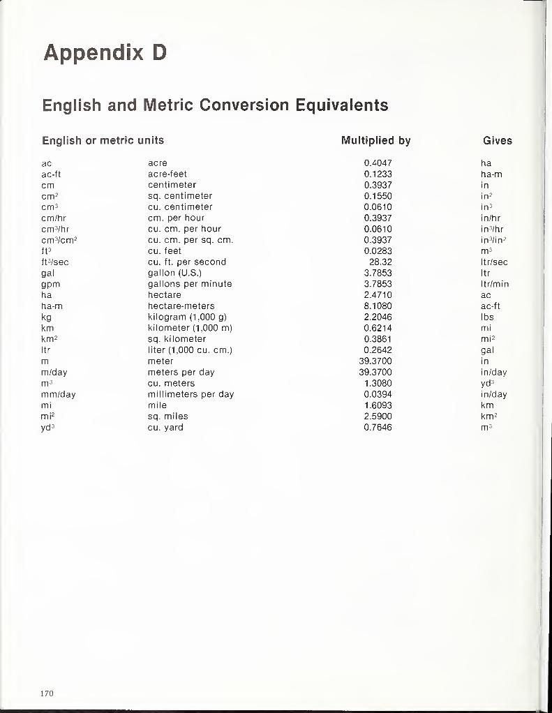
Appendix D

English and Metric Conversion Equivalents

English or metric units

ac acre

ac-ft acre-feet

cm centimeter

cm 2 sq. centimeter

cm 3 cu. centimeter

cm/hr cm. per hour

cm 3/hr cu. cm. per hour

cm 3/cm 2 cu. cm. per sq. cm.

ft 3 cu. feet

ft 3/sec cu. ft. per secondgal gallon (U.S.)

gpm gallons per minute

ha hectare

ha-m hectare-meters

kg kilogram (1,000 g)

km kilometer (1,000 m)

km 2 sq. kilometer

Itr liter (1,000 cu. cm.)

m meter

m/day meters per day

m 3 cu. meters

mm/day millimeters per daymi mile

mi 2 sq. miles

yd 3 cu. yard

Multiplied by Gives

0.4047 ha

0.1233 ha-m0.3937 in

0.1550 in 2

0.0610 in 3

0.3937 in/hr

0.0610 in 3/hr

0.3937 in 3/in 2

0.0283 m 3

28.32 Itr/sec

3.7853 Itr

3.7853 Itr/min

2.4710 ac

8.1080 ac-ft

2.2046 lbs

0.6214 mi

0.3861 mi 2

0.2642 gal

39.3700 in

39.3700 in/day

1.3080 yd 3

0.0394 in/day

1.6093 km2.5900 km 2

0.7646 m 3

170

NATIONAL AGRICULTURAL

1022573675

UNITED STATES DEPARTMENT OF AGRICULTUREECONOMIC RESEARCH SERVICE1301 NEW YORK AVENUE, NW.WASHINGTON, D. C. 20005-4788