Facing the Development Challenge in Mozambique - AgEcon ...

Facing the Development Challenge

in Mozambique

An Economywide Perspective

Finn TarpChanning ArndtHenning Tarp JensenSherman RobinsonRasmus Heltberg

RESEARCHREPORT 126INTERNATIONAL FOOD POLICY RESEARCH INSTITUTEWASHINGTON, D.C.

Copyright © 2002 International Food Policy Research Institute. All rights reserved.Sections of this report may be reproduced without the express permission of, but with acknowledgment to, the International Food Policy Research Institute.Printed in the United States of America

International Food Policy Research Institute2033 K Street, NWWashington, DC, 20006–1002 U.S.A.Telephone +1-202-862-5600www.ifpri.org

Library of Congress Cataloging-in-Publication Data

Facing the development challenge in Mozambique : an economywideperspective / Finn Tarp ... [et al.].

p. cm.—(Research report / International Food Policy Research Institute; 126)ISBN 0–89629–131–6 (alk. paper)

1. Structural adjustment (Economic policy)—Mozambique– 2. Mozambique—Economic conditions—1975– 3. Mozambique—Social conditions—1975– 4. Agriculture—Economic aspects—Mozambique. 5. Poverty—Mozambique. I. Tarp, Finn, 1951– II. Research report (International Food Policy Research Institute); 126

HC890.F3 2002338.9679—dc21

2002155321

Contents

Tables iv

Figures viii

Foreword ix

Acknowledgments xi

Summary xiii

1. Introduction 1

2. Economic and Social Structure in Perspective 3

3. The Path to Economic Collapse 19

4. Stabilization and Structural Adjustment 27

5. Linkage and Multiplier Analysis Based on the Social Accounting Matrix 45

6. A CGE Model for Mozambique 61

7. Aid Dependence 76

8. The Agricultural Bias Revisited 86

9. Marketing Margins and Agricultural Technology 102

10. Agricultural Technology, Risk, and Gender 109

11. Food Aid 119

12. Scenario Building: The Merged Model 126

13. A Standard World Bank–IMF Simulation Framework with CGE Features 148

14. Lessons Learned 164

Appendix A: The CGE-Model Specification 167

Appendix B: The Merged Model 177

Appendix C: Variable Definitions in Chapter 13 180

Acronyms and Abbreviations 181

Bibliography 183

iii

Tables

2.1 Comparative overview 4

2.2 Structure of production and employment, 1996 7

2.3 Chenery-Syrquin regression results 9

4.1 Real gross domestic product (GDP), 1991–96 32

4.2 Sectoral shares of real value-added, 1991–96 33

4.3 Sectoral shares of nominal value-added, 1991–96 33

4.4 Real GDP expenditures, 1991–96 34

4.5 Nominal GDP expenditures, 1991–96 34

4.6 Public financial expenditures, 1992–96 35

4.7 Money stock, Maputo CPI, and exchange rate, 1991–96 36

4.8 Current account balance, 1991–96 37

4.9 Capital account balance, 1991–96 37

4.10 Financing of the balance of payments, 1991–96 38

4.11 Social indicators, 1991–96 38

5.1 Comparison of 1994 data sources 40

5.2 Labels of the Macroeconomic social accounting matrix (MACSAM) 47

5.3 Balanced 1995 Macroeconomic social accounting matrix for Mozambique 49

5.4 Sectoral production costs 50

5.5 Sectoral domestic production 51

5.6 Composition of sectoral supplies 51

5.7 Composition of sectoral demand 52

5.8 Agricultural commodity multipliers 54

5.9 Sectoral commodity multipliers 56

5.10 Household multipliers 59

iv

6.1 Production structure of the economy 63

6.2 Support set end points on predicted values for imports 70

6.3 Trade parameter support sets and estimates 71

6.4 Correlations and pseudo R-squared for macroaggregates 73

6.5 Measures of fit for exports and imports 73

7.1 Experiment descriptions for aid dependence simulations 78

7.2 Macroeconomic indicators for aid dependence simulations 78

7.3 Real GDP components for aid dependence simulations 79

7.4 Price indices and agricultural terms of trade for aid dependence simulations 83

8.1 Experiment descriptions for agricultural bias simulations 87

8.2 Price indices and agricultural terms of trade for agricultural bias simulations 90

8.3 Macroeconomic indicators for agricultural bias simulations 91

8.4 Real GDP components for agricultural bias simulations 92

8.5 Macroeconomic indicators for agricultural bias simulations 97

8.6 Real GDP components for agricultural bias simulations 98

8.7 Price indices and agricultural terms of trade for agricultural bias simulations 99

9.1 Experiment descriptions for marketing margin and agricultural technology simulations 104

9.2 Macroeconomic indicators and prices for marketing margin and agricultural technology simulations 104

9.3 Equivalent variation on consumption for marketing margin and agricultural technology simulations 106

9.4 Components of real GDP for marketing margin and agricultural technology simulations 106

9.5 Factor price indices for marketing margin and agricultural technology simulations 107

10.1 Female labor share by agricultural activity for agricultural technology, risk, and gender simulations 110

10.2 Cassava production, price, and risk premium for agricultural technology, risk, and gender simulations 113

10.3 Macroeconomic indicators for agricultural technology, risk, and gender simulations 114

10.4 Agricultural terms of trade in value-added terms for agricultural technology, risk, and gender simulations 115

10.5 Equivalent variation on consumption for agricultural technology, risk, and gender simulations 115

TABLES v

10.6 Factor price indices for agricultural technology, risk, and gender simulations 116

11.1 Experiment descriptions for food aid simulations 121

11.2 Declines in technology used to simulate drought for food aid simulations 121

11.3 GDP and welfare for food aid simulations 122

11.4 Equivalent variation on consumption for food aid simulations 123

11.5 Grain and food aid imports for food aid simulations 123

11.6 Agricultural terms of trade for food aid simulations 123

11.7 Factor price indices for food aid simulations 125

12.1 Parameter values for the merged model, 1995–97 129

12.2 Parameter values for the optimistic scenario in the merged-model simulations, 1998–2002 130

12.3 Growth in the material balance for the merged-model simulations, 1995–2002 132

12.4 Growth in sectoral GDP for the merged-model simulations, 1995–2002 133

12.5 Growth in sectoral exports for the merged-model simulations, 1995–2002 133

12.6 Current account of the balance of payments for the merged-model simulations, 1995–2002 135

12.7 Price inflation for the merged-model simulations, 1995–2002 136

12.8 Capital account of the balance of payments for the merged-model simulations, 1995–2002 137

12.9 Government budget for the merged-model simulations, 1995–2002 138

12.10 Government finance for the merged-model simulations, 1995–2002 139

12.11 Money supply for the merged-model simulations, 1995–2002 139

12.12 Parameter values for the pessimistic scenario in the merged-model simulations, 1998–2002 140

12.13 Growth in material balance for the merged-model simulations, 1995–2002 142

12.14 Growth in sectoral GDP for the merged-model simulations, 1995–2002 143

12.15 Growth in sectoral exports for the merged-model simulations, 1995–2002 143

12.16 Price inflation for the merged-model simulations, 1995–2002 143

12.17 Current account of the balance of payments for the merged-model simulations, 1995–2002 144

12.18 Capital account of the balance of payments for the merged-model simulations, 1995–2002 145

12.19 Government budget for the merged-model simulations, 1995–2002 145

12.20 Government finance for the merged-model simulations, 1995–2002 145

vi TABLES

12.21 Money supply for the merged-model simulations, 1995–2002 146

13.1 Real side of the merged model 150

13.2 Financial side of the merged model 151

13.3 Real-side variables in the merged model 152

13.4 Financial-side variables in the merged model 153

13.5 CGE-model variables 155

13.6 Price inflation for the integrated-model simulations, 1998–2002 160

13.7 Inflation in domestic world market prices for the integrated-model simulations, 1998–2002 161

13.8 Growth in factor returns for the integrated-model simulations, 1998–2002 161

13.9 Equivalent variation for the integrated-model simulations, 1998–2002 162

TABLES vii

Figures

2.1 Southern Africa’s per capita gross national product, 1995 6

2.2 Investment and savings regression results 10

2.3 International trade regression results 11

2.4 Structure of production regression results 12

2.5 Allocation of income regression results 13

2.6 Education regression results 14

2.7 Labor by sector: Urbanization and share of labor in agriculture regression results 15

11.1 Maize production and imports for food aid simulations 120

viii

Foreword

S ince early 1996, IFPRI’s Trade and Macroeconomics Division has been working withcountry-based and international collaborators on a multiyear research project entitledMacroeconomic Reforms and Regional Integration in Southern Africa (MERRISA),

with funding from Danida and German Agency for Technical Cooperation. The project com-prised two interlinked components: a set of six in-depth country studies on Malawi, Mozam-bique, South Africa, Tanzania, Zambia, and Zimbabwe, and a study of regional integrationpossibilities and the impact of global trade reform on the study’s subject countries.

MERRISA’s central hypothesis was that agricultural growth and transformation are cru-cial in generating sustainable and equitable growth in southern African economies. But thekey question was why various reform programs had failed to generate stronger responses byAfrican agricultural sectors—especially smallholder sectors. MERRISA was specifically de-signed to examine a variety of macroeconomic and trade policy reform packages for theirability to enhance agricultural performance and contribute to economic growth and povertyreduction.

This volume comprehensively reports the results of the country study on Mozambique. Itrepresents ongoing collaboration between IFPRI’s Trade and Macroeconomics Division anda research group based at the Development Economics Research Group (DERG) within theUniversity of Copenhagen’s Institute of Economics. Close links were also established withMozambican researchers at the Research Office of the Ministry of Planning and Finance inMaputo, and, in the later stages of the project, with Purdue University.

In line with the methodology and organization of country studies under MERRISA, thisreport incorporates both historical analysis and formal modeling. Historical records provideinvaluable information on past policies and actual country performance. Historical analysiscannot, however, establish the strength of causal relationships between policy instruments andoutcomes. The modeling approaches used in this study, including computable general equi-librium (CGE) modeling, enable the specification of important multisectoral linkages that op-erate simultaneously and interactively within the national economy. The models also incor-porate special structural features that reflect southern African characteristics, such as homeconsumption and high transportation and transaction costs on staples like cassava and maize.

Underpinning the modeling is an economywide database, a social accounting matrix(SAM), that emphasizes the agricultural sector and different household groups. The SAM in-tegrates national income, input-output, flow-of-funds, and foreign trade statistics into a com-prehensive and consistent data set, thereby illustrating that, even in “data-poor” contexts,much can be done in terms of quantitative economic analysis. To facilitate the estimation ofa consistent SAM, IFPRI developed a new estimation approach during the 1990s that allowsthe incorporation of errors in variables, inequality constraints, and prior knowledge about any

ix

part of the SAM. This entropy methodology—further developed in this study—deserves at-tention because it provides an efficient approach of incorporating data from scattered sourcesinto a consistent framework.

The more wide-ranging benefit of MERRISA’s Mozambique country study is its broadperspective on the economywide effects of agricultural growth and its contribution to the un-derstanding of potential macroeconomic policies in achieving more rapid, equitable, and sus-tainable growth in Mozambique and the surrounding region. The report confirms the impor-tance of the agricultural sector in any satisfactory development process in Mozambique. Agri-cultural development is key to achieving the twin goals of growth and improved income dis-tribution. The report also demonstrates that the successful implementation of such a strategyrelies heavily on both appropriate government action and active donor support.

The authors outline what can be gained by making better use of available knowledge,tools, and data systems in one of the poorest countries in the world. Importantly, while theanalyses in this volume are specific to Mozambique, the analytical approach is applicable toa series of countries both within and outside Africa. As such, this report’s research results andpolicy conclusions should prove relevant and useful to the policymaking process in Mozam-bique and elsewhere.

Joachim von BraunDirector General

x FOREWORD

xi

Acknowledgments

T his report presents findings from the Mozambique country component of the projectMacroeconomic Reforms and Regional Integration in Southern Africa (MERRISA).The work is a joint output of a multiyear collaborative research effort involving re-

searchers in IFPRI’s Trade and Macroeconomics Division and research institutions in Den-mark, the United States, and Mozambique. We are deeply grateful to IFPRI’s former directorgeneral, Per Pinstrup-Andersen, who was not only instrumental in establishing the project butalso provided inspiration, foresight, and continued support during all stages of our work.

This study would not have been possible without the unfailing backing and collaborationof a large group of friends and colleagues. In Mozambique, we relied on support from Dr.Mario F. da Graça Machungo, who—as former Prime Minister of Mozambique and chairmanof a leading commercial bank—was an obvious choice as member of the MERRISA advisoryboard. We are honored he accepted our invitation to serve in this capacity; his presence didmuch to help achieve our overall aim of producing a policy-relevant study of the academicstandard necessary for an IFPRI research report.

Also in Mozambique, we collaborated closely with the Gabinete de Estudos (GE) of theMinistry of Planning and Finance, including in particular its director Pedro Couto and his as-sistant Antonio Sousa Cruz. Their effective advice, help, and friendship provided an indis-pensable foundation for our work. It is our hope that they have benefited in some measurefrom our joint efforts in their challenging duties in an important policy think tank of the Gov-ernment of Mozambique. At the end of the day this will be the ultimate test of whether wehave reached our overall goal and increased capacity building in one of the poorest countriesof the world. Among other staff with whom we have interacted we would like to mention TimBuehrer, Bruce Bolnick, Per-Åke Andersson, and Antonio Franco, who all formed part of theHarvard Institute of International Development support team within the GE.

Given our work depended greatly on national accounts data, we sincerely thank Mr. SaideDade, director of the National Institute of Statistics, as well as João Loureiro, Orlando Comé,Antonio Lazo, Walter Cavero, Argentina Macisse, and Magda Ascues, who did a magnificentjob helping us on many occasions by explaining the ins and outs of Mozambican data. Par-ticular thanks are also due to Dr. Admir Bay, then managing director of SEMOC; José CarlosTrinidade, director, AMODER; and Trine Næraa-Nicolajsen, who served as Mozambiquecountry consultants to the MERRISA project and provided welcome inputs and insights.

Among many others who have contributed in their capacity as Mozambican governmentstaff and advisers or as academic researchers, we would like to mention Adriano Maleiane,João Z. Carillho Louisa Diogo, Maria Eugenia Pires, Youlanda Fortes, José Sulemane, Vito-ria Ginja, Ken Simler, Gabriel Labão Dava, Ian McDonald, Margaret McCuen, Jan Low, Ed-uardo Oliveiras, Domingos F. Diogo, Rui Ribeiro, Fernando Songane, Fernanda Cabanas, Ar-

xii ACKNOWLEDGMENTS

lito Cuco, Eduardo João, Alejandro Antonio Olivares, David Tschirley, Ana Paula Santos,Selma L. Sawaya, Jørgen Strange Hansen, Antonio Olivares, Angelo E. Mondlane, JoséLoureiro, Artur Gobe, Alberto Bila, Rodrigues Pereira, Clara de Sousa, Carla Honwana, andBart Pijnenburg.

The international donor community in Mozambique is considerable. We benefited frommany interactions with, for example, World Bank staff including Peter Moll, Jehan Arulpra-gasam, Maria Nieta Dengo, Daniel de Sousa, and others. From the European Union, JohnRook was most helpful, and among USAID staff we would like to mention Richard Newberg,Julie Born, Luisa Capelao, Richard P. Harber, Tim Born, and Jim Jackson. Moreover, wewould like to express our special thanks to Danida, not only for generous financial supportbut also for the many productive meetings with the two Danish Ambassadors in Mozambiqueduring project implementation, Thomas Schjerbeck and Ole Blicher-Olsen. We are also grate-ful for help from their Danish staff, including Peter Juul Larsen, Preben Gondolf, and EstherLønstrup, and the Mozambican staff at the Danish Embassy in Maputo, who made our manyvisits so much easier.

Finally, no research project can meet with success without administrative and secretarialsupport. We are grateful to Maria Cohan and Vibeke Kovsted for all their efforts and patientsmiles during long working hours. The same goes for all the other staff in IFPRI’s Trade andMacroeconomics Division, who contributed so effectively to this project.

The authors accept sole responsibility for the ideas expressed in this work and for anyomissions or errors of fact or interpretation.

xiii

Summary

Following Mozambique’s economic collapse in 1986, the country began a wide-rang-ing process of reform, with the support of the international community. The diagnosiswas of an economy that failed to maintain monetary control, consumed beyond its

means, focused production excessively on nontraded goods, and relied on inefficient and in-flexible microeconomic structures. Nevertheless, Mozambique was also at war. The pace ofstabilization and structural adjustment quickened after 1992, when, concurrent with the de-mise of apartheid, civil strife finally came to an end. After more than 10 years of adjustment,the reform program has now been essentially implemented. Yet, this does not imply, as shownin this study, that sufficient conditions for sustained economic development are in place.Mozambique remains very poor, and even under highly optimistic assumptions about the fu-ture, the development process is set to last for decades.

This report attempts to respond to some of the basic development challenges facingMozambique and to provide both qualitative and quantitative insights for policymaking in theyears to come. Throughout, the issues addressed are approached from an economywide per-spective.

This study forms a part of the multicountry research initiative, Macroeconomic Reformsand Regional Integration in Southern Africa. This initiative covers six countries in the regionand pays particular attention to the evaluation of the merits of alternative development strate-gies. The choice and design of an appropriate development strategy is by no means immedi-ately evident for any developing country. However, for a country with abundant arable landand scarce human and physical capital, such as Mozambique, the role of agriculture in de-velopment is particularly interesting. In keeping with the focus on agriculture, a social ac-counting matrix (SAM) for 1995, with significant agricultural sector detail, was constructedas part of this study. The SAM contains 40 activities, including 13 agricultural and 2 food-processing activities, 3 factors of production, and 2 households (urban and rural). It capturestwo innovative but fundamental features of the Mozambican economy: high marketing costsfor domestic, imported, and exported goods; and the significant prevalence of home con-sumption, particularly for rural households.

The report begins by putting the economic and social characteristics of Mozambique inregional perspective, tracing the historical path to economic collapse and providing a detailedanalysis and assessment of the stabilization and structural adjustment program. The studyshows that the program successfully stabilized inflation and markedly augmented reliance onmarket forces. Relative macroeconomic stability combined with the high and stable (reported)investment level give rise to optimism for the future. Indeed, economic growth has been rel-atively rapid since 1992. Still, recovery from a low point resulting from the war, drought, andprior economic mismanagement has been a major aspect of the turnaround. Underlying real

xiv SUMMARY

development constraints remain much the same and the more difficult development chal-lenges lie ahead.

The 1995 SAM provides a picture of the structure of the economy. It is used to highlightthe importance of agricultural development through a series of traditional SAM-based multi-plier analyses. These analyses show that agriculture has large sectoral multiplier effects rela-tive to nonagriculture and that applying scarce capital to agriculture is generally more effec-tive than applying it to industry and services. The SAM also forms the basis for a static com-putable general-equilibrium (CGE) model with an unusually solid empirical foundation interms of its model parameter values and structure, including a maximum entropy approach toparameter estimation for CGE models. This approach applies information theory to estimat-ing parameters in a system of nonlinear simultaneous equations. The trade parameter esti-mates obtained point strongly to the need for development efforts to aid in the transformationof domestic output into export products. Moreover, the CGE model is capable of capturingmany key aspects of the performance of the Mozambican economy in the postwar period.

The CGE model is used in a series of concrete analyses in which attention focuses on theimpact and design of economic policy. The challenges addressed are: aid dependency, theprice incentives facing the agriculture sector, agricultural technology and marketing margins,risk-reducing behavior and gender roles in agricultural production, and food aid distribution.A variety of insights emerge, including, for example, that priority should be given to simulta-neous improvement in agricultural productivity, especially in small-scale farming, and in mar-keting infrastructure to reduce marketing costs. Another key example is that technologicalchange in cassava appears to be a particularly strong lever for increasing female and overallhousehold welfare. In general, the results in this report suggest a strong potential for agricultural-led development with attractive distributional implications, provided adequatepolicy measures are taken. The results also suggest that the negative effects of unavoidablenatural calamities can be minimized if appropriate schemes for distributing food aid are putin place.

While the static CGE model developed in this study is capable of providing many policy-relevant insights, it cannot be relied on as a guide in budgetary planning within a medium-term framework. This task is important in Mozambique, which is saddled with considerableinternational debt. For this reason, a set of coherent macroeconomic medium-term scenariosfor Mozambique was developed on the basis of standard World Bank and International Mon-etary Fund simulation tools. While widely used within these institutions, the projection mod-els are less well-known elsewhere, and in Mozambique there is an evident gap in applyingthem so that both sides of the policy negotiation table are equally in command of analyticalresults and insights. For this reason, a merged version of these tools is laid out in some detail,and three different scenarios are elaborated on. The importance of debt relief and access to in-ternational capital markets in underpinning economic development in Mozambique stand out.Nevertheless, the merged-model framework does not provide critically important informationon distributional issues and relative prices. For this reason, Chapter 13 presents a simple, butinnovative, SAM methodology for integrating macroeconomic and CGE models. This frame-work is subsequently applied to integrate the merged and the static CGE model into a dynamicCGE model with an aggregated financial sector. This model amounts to a modern simulationtool that accounts for relative prices and income distribution. Given the growing availabilityof SAMs for a wide range of developing countries, it is argued that data requirements can inmany cases be fulfilled in practice without major difficulty. Implementation of the proposedCGE model is therefore not only desirable but a feasible operational proposal for how to move

beyond the simple framework widely used by the World Bank and the International MonetaryFund.

Finally, this study aims to demonstrate that sophisticated analytical tools can be of signif-icant value, even in “data-poor” situations. The need for a clear perspective and in-depth un-derstanding of the socioeconomic complexities of the country in question stands out. How-ever, while the analyses in this report are Mozambique specific, the basic analytical approachis replicable and could be brought to bear on other countries both within and outside Africa.

SUMMARY xv

C H A P T E R 1

Introduction

F ew nations have endured the tumultuous changes that have characterized Mozambiquein the past three decades. The combined legacies of colonialism, idealism, socialism,war fuelled by racism, economic collapse, and structural adjustment (inspired by stout

liberalism) have made a lasting impact on the structure of the economy. In the early 1990s,Mozambique was frequently referred to as “the poorest country in the world.” Reasonableeconomic growth performance since 1992 combined with economic disasters elsewhere hasput an end to this unwanted distinction. Nevertheless, the country remains poor by almost anymeasure.

In economywide studies, such as this report, social accounting matrices (SAMs) and com-putable general-equilibrium (CGE) models have become important analytical workhorses.These basic frameworks have by now been applied fairly frequently in the African context.For example, Sahn, Dorosh, and Younger (1996) applied a SAM/CGE approach to investigatethe impact of structural adjustment on poverty in a number of African countries. They con-cluded that, in most countries, adjustment policies have not hurt and may have helped the poor.These conclusions are widely contested. De Maio, Stewart, and van der Hoeven (1999) arguethat the core result is a reflection of the assumptions made in developing the CGE modelsrather than of reality. Our study attempts to advance the state of the art in CGE modeling ofAfrican economies and, as such, implicitly addresses some (but certainly not all) of the criti-cisms advanced by de Maio, Stewart, and van der Hoeven.

The analyses conducted in this study run the gamut from the standard (such as descriptiveanalysis, SAM construction, and multiplier analysis); to the recent (such as estimation of SAMcoefficients based on information theory, merged real and financial sector simulation model-ing, and incorporation of risk in a CGE model; to the novel (such as explicit incorporation ofhome consumption in a SAM/CGE framework, examination of gender issues in a CGE model,development of a new method for estimation of critical model parameters, and the treatmentof macroeconomics in dynamic CGE models). The research aims to demonstrate that sophis-ticated tools can be of significant value, even in data-poor situations.

A further word on data and methodologies is merited. Economic collapse and war were notkind to data-gathering systems in Mozambique. One might construe that this study shouldhave been delayed until improved data systems had been established. We reject this conjec-ture. We do not believe that scattered and potentially inconsistent data sources necessarilyimply simplistic analysis. Often, fundamental decisions must be made fairly early in a newlyrelaunched development process, such as the one ongoing in Mozambique, and those

This chapter was written by Channing Arndt and Finn Tarp.

1

decisions should be made using the bestpossible analysis. Also, advanced tools nowexist to extract information from scatteredor inconsistent data sources, and these toolswere employed to develop a fairly detailedand consistent image of the economy. Asnew data emerge, they can be relatively eas-ily incorporated into the analytical frame-works put forward here for updated eco-nomic analyses.

We take as a point of departure the needfor moving on from stabilization and ad-justment to focusing on transformation anddevelopment. As such, we try to respond tothe signpost outlined in the work by Corniaand Helleiner (1994). They argue that it istime to call a formal end to the decade of“structural adjustment,” agree that there areno economic “quick fixes” for Africa, andreactivate the development debate. This de-bate is, in their view and ours, nowhere near“the end of its history.” Another signpost,the so-called Berg Report (World Bank1982), is widely regarded as the seminaldocument in launching the era of structuraladjustment. Despite its general focus, theBerg Report recognized up front that thepolicy changes recommended were basi-

cally short-run. Perhaps obscured by theconsiderable difficulties encountered in theimplementation of structural adjustmentprograms throughout Africa, the same re-port also highlighted the critical importanceof long-run investments and programs thatmust form part of a coherent developmentstrategy. The report placed particular em-phasis on agricultural research, infrastruc-ture, and human resources—a view echoedin this study.

After more than 10 years of structuraladjustment in Mozambique the programhas, essentially, been implemented. How-ever, more-or-less complete implementa-tion of the structural adjustment programdoes not imply that sufficient conditions forsustained economic development are inplace, and long-run strategy debate shouldnow take center stage. For a country withabundant arable land and scarce human andphysical capital such as Mozambique, therole of agriculture is of particular interest.This report pursues this approach with theworking hypothesis that the agriculturalsector is crucially important in any work-able development strategy.

2 CHAPTER 1

C H A P T E R 2

Economic and Social Structure in Perspective

This chapter argues that, although Mozambique is currently among the world’s least de-veloped countries as judged by most economic and social indicators, the country hasgood prospects for sustained and broad-based growth.

Mozambique’s excellent natural harbors along the Indian Ocean are among the best inAfrica, and they make the country an important provider of transport and services in southernAfrica. Moreover, population density (20 people per square kilometer) is quite low (Table2.1).1 The population census carried out in 1997 found a population of 15.3 million, comparedwith the 18.3 million projected from the previous census, which was taken in the 1970s. Se-vere food insecurity, disease, and migration caused by war and natural disasters (see Chapter3) account for the difference.

Mozambique’s role as a regional transport provider emerged during its colonial days (seeChapter 3 for more detail), and regional transport dominates physical infrastructure and themodern part of the economy. While Mozambique is relatively well connected to its neighbors,domestic transport of people and goods is costly and cumbersome. Road and rail networkshave expanded east to west, linking the harbors of Maputo, Beira, and Nacala with the min-ing and industrial centers of South Africa, Zimbabwe, and Malawi. However, infrastructurefor north–south domestic transport and trade is poor: rail links are completely lacking, and per-manent roads minimal.

Estimates vary as to how much land in Mozambique is cultivable. The World Bank (1996)records that 46 percent of Mozambique’s land area is cultivable, providing on average around12 to 13 hectares to the country’s 3 million farm families. Much of this land is not yet used.Mozambique has ample water resources from rainfall and river systems, especially in the cen-tral and northern areas of the country. Major river systems include the Zambezi, Save, andLimpopo rivers. These and other rivers hold the promise of developing intensive irrigated agri-culture sometime in the future.

The agricultural sector consists of a large number of dispersed smallholders cultivating 95percent of all farmland, with the remaining being cultivated by a limited number of large plan-tations. Food production is dominated by cassava, maize, groundnuts, cowpeas, sorghum, andmillet, which account for some 80 percent of food energy intake at the national level. The main

This chapter was written by Rasmus Heltberg.

1Southern Africa is defined in this report as including Angola, Botswana, Lesotho, Malawi, Mozambique,Namibia, South Africa, Swaziland, Zambia, and Zimbabwe.

3

export crops are cotton and cashews, grownby smallholders. In addition, seafood is amajor export product.

Soils in Mozambique are of mixed qual-ity. Prime agricultural land is in the northernand central parts as well as in river valleysthroughout the country, where soils are fer-tile and water-retentive. The principalsource of regional variation in croppingpractices is rainfall, which declines in quan-tity and predictability from north to south.The northern and central provinces haverelatively ample and reliable rainfall. Thesouthern provinces tend to have sandy, in-fertile soils, except for river valleys and cer-tain coastal plains; and rainfall is scarcerand more irregular. Much of the southernportion of Mozambique offers good pastureland free from tse-tse fly, but water scarcitycan be a problem. Therefore, regular rain-fall and fertile soils make for more intensiveagriculture in the central and northern por-tions of the country, while extensive agri-cultural practices prevail in most of the drysouth, which is subject to regular droughts

and floods. Variation in rainfall determinesthe probability of crop failure and is there-fore a major cause of food insecurity. In thenorth, households report one to two monthsof annual food insecurity whereas, in thesouth, five months of food insecurity everyyear is normal.

Mozambique has three main farmingsystems. The relatively extensive agro-pastoral practices in the southern areas resemble farming systems in Zimbabwe’sdry lands. They are a response to frequentdroughts. Cattle stocks were decimated bythe war. On the dry lands, farmers operate asubstantial number of different machambas(plots). In areas along rivers and close to thecoast, where soils are good and moisture isplentiful, land is scarce and fallow periodsshort. The more intensive and diversifiednorthern areas, where agroforestry is com-mon, resembles southern Tanzania. Here,farmers practice strategies of long-fallowshifting cultivation of maize, sorghum, mil-let, cassava, and other crops. Cashews andcotton are the major cash crops and have

4 CHAPTER 2

Table 2.1 Comparative overview

Sub- High Southern Saharan South Latin income

Socioeconomic indicator Mozambique Africa Africa Asia America countries Year

Population density (people per square kilometer) 20 33 24 256 23 29 1994Population in cities with more than 1 million

people (percentage of total population) 14 7 8 10 28 33 1995GNP per capita, atlas method (U.S. dollars) 80 1,293 490 350 3,320 24,930 1995Life expectancy at birth, total (years) 46.5 56.0 52.2 61.3 69.1 77.3 1995Mortality rate, infant (per 1,000 live births) 126 82 n.a. n.a. n.a. n.a. 1995Mortality rate, under five years

(per 1,000 live births) 190 126 n.a. n.a. n.a. n.a. 1995Safe water (percentage of population with access) 28 56 47 63 80 94 1995Sanitation (percentage of population with access) 23 46 n.a. 29 68 92 Latest

1990–95Population growth 2.37 2.41 2.81 1.97 1.77 0.69 meanHealth expenditure, public (percentage of GDP) 4.6 3.0 n.a. n.a. n.a. n.a. LatestSchool enrollment, primary (percentage of gross) 60 108 72 98 110 103 LatestIlliteracy rate, adult (percentage of people

over 15 years) 60 32 n.a. n.a. n.a. n.a. LatestFertilizer use (100 grams per hectare of arable land) 22 311 135 803 647 1,169 1994

Source: Fan, Zhang, and Robinson 2001. They constructed GDPs for the four economic sectors based on various China State Statistical Bu-reau (SSB) publications.

Note: N.a. means not available.

potential for expansion (World Bank 1996).The highlands in the center of the countryshare features with Malawi and Zimbabwe.Maize, beans, and cassava are the majorfood crops, and beans and potatoes the cashcrops. In the dry season, farmers cultivateplots in valleys; and, in the rainy season,rainfed plots in the uplands are cultivated.In addition, a majority of urban families op-erate machambas and many towns are sur-rounded by green belts (MPF/EMU/IFPRI1998).

The country has substantial potentialenergy, water, forest, mineral, and marineresources. Except for shrimp, all of these re-sources are either underexplored or entirelyundeveloped. The Tete highlands hold 6 bil-lion tons2 of known coal reserves. At Panda,large fields of natural gas are now being de-veloped. There might be oil as well. Foreignmining companies are prepared to invest inthese resources. In addition, the massivehydroelectricity potential of the Zambezi,which flows 819 kilometers through thecountry, could make Mozambique a majorsource of electric power for the region. It isas yet untapped, except for the CahoraBassa dam, built by the Portuguese andcompleted just before independence in1974.

Despite more-or-less uncontrolled col-lection of fuel wood, Mozambique still hasmany hardwood forest reserves. Around 25percent of Mozambique is thought to havecapacity for producing hardwood, eucalyp-tus, and pine timber, and private investorsare expressing interest in developing this re-source. Mozambique has important re-serves of high-quality iron ore and of therare mineral tantalite, which is used in theelectronics and steel industry. It also hassome gold. Mozambique’s pleasant climate,

long beautiful beaches, and Indian Oceanislands—including the United Nations Edu-cational, Scientific, and Cultural Organiza-tion (UNESCO) heritage site MozambiqueIsland—make it a potentially attractive hol-iday resort.

Economic and SocialOverview

Throughout the first half of the 1990s,Mozambique had a lower recorded averageincome than any other country for whichWorld Bank data is available.3 Accordingto the World Bank’s World DevelopmentIndicators, Mozambique even held therecord as the world’s poorest country with agross national product (GNP) per capita ofUS$80 in 1995 and 1996. According to thenational accounts from the National Insti-tute of Statistics (NIS), which are relied onin subsequent chapters, gross domesticproduct (GDP) per capita was US$121 andUS$146 in 1995 and 1996, respectively. Inthe WDI tables, Ethiopia, Tanzania, andZaire follow closely after Mozambique.The huge disparities in GNP per capita insouthern Africa are evident (Figure 2.1).The GNP per capita (unweighted means)for southern Africa and for all of Sub-Saharan Africa is much higher, at US$1,293and US$490, respectively. When incomestatistics are corrected for differences inpurchasing power—GDP adjusted for “pur-chasing power parity” or PPP, an index usedto reflect the purchasing power of curren-cies by comparing prices among a broaderrange of goods and services than conven-tional exchange rates—the differences innominal income shrink, but Mozambiquestill remains the poorest country in the region.

ECONOMIC AND SOCIAL STRUCTURE IN PERSPECTIVE 5

2Throughout this report, “ton” refers to the metric ton.

3The main data source for this section is the World Development Indicators in World Bank (1997b, 1998). Theadvantage of the WDI data set is that it is comparable across countries and continents. The drawback is that theWDI national accounts figures quoted in this chapter are inconsistent with figures in later chapters. For these rea-sons, comparisons are made whenever appropriate and feasible.

During the 1990s, the economy hasgone through a recovery process, analyzedin detail in Chapter 4. Despite a severedrought in 1991, real GDP growth over theperiod 1990–97 averaged 7 percent per yearaccording to the WDI, and 5.1 percent ac-cording to NIS figures. The Mozambicangrowth rate is high by regional and Sub-Saharan African standards. Growth hasbeen especially good in recent years—including 1997, where it reached 12.5 per-cent. Growth has been broad-based, withmanufacturing, transport, energy, and serv-ices showing high levels of change. Thishas been accompanied by a fall in inflation,which reached a record low of 5.8 percentin 1997, as reported by the InternationalMonetary Fund (IMF 1999).

Foreign aid is very important. Accord-ing to the WDI, over the period 1990–96Mozambique received, on average, foreignaid corresponding to 92 percent of GNP. Ifinstead the NIS national account estimatesare used, foreign aid was around 46.6 per-cent of GNP. In any case, Mozambique isone of the most aid-dependent countries inthe world. In September 2001, Mozam-

bique reached the completion point underthe Heavily Indebted Poor Countries(HIPC) initiative and had its external debtstock reduced by around 75 percent.

In comparing the structure of produc-tion in Mozambique to the Sub-Saharan av-erage (Table 2.2), the picture depends againon the data source. According to the WDI,agriculture contributes 32.8 percent of GDPand employs 83 percent of the population.According to NIS figures, agriculturalvalue-added was 25.3 percent of GDP in1996. As can be seen from Table 2.2, in theaverage Sub-Saharan African country only19 percent of GDP comes from agriculture,with 68 percent of the population employedthere. The share of industry value-added inGDP (for 1996) was 23.8 percent accordingto the WDI. According to NIS, it was 20.8percent. This is below the Sub-SaharanAfrica average of 27.2 percent. The servicesector produced 39.3 percent of GDP ac-cording to WDI, and 51.2 percent accordingto NIS. This paints the picture of an econ-omy where most of the population survivesin subsistence agriculture, where the indus-trial and manufacturing sectors are lagging

6 CHAPTER 2

0

500

1,000

1,500

2,000

2,500

3,000

3,500

U.S. dollars

Figure 2.1 Southern Africa’s per capita gross national product, 1995

Moz

ambi

que

Mal

awi

Zambi

a

Ang

loa

Zimba

bwe

Lesot

ho

Swaz

iland

Nam

ibia

Bot

swan

a

South

Afric

a

Source : World Bank 1997b and 1998.

behind, but still having important commer-cial activities relating to transport servicesboth internally and with neighboring coun-tries.

Social indicators give a gloomy imageof human development in Mozambique,even before accounting for the AcquiredImmune Deficiency Syndrome (AIDS)pandemic. Life expectancy at birth is low(46.5 years), even by African standards(Table 2.1). Infant and under-five mortalityrates are high when compared with neigh-boring countries. Out of 1,000 children, 126die before age one and 190 die before theyreach the age of five—50 percent more thanthe average for the region. The proportionof population with access to safe water andsanitation is low, at 28 and 23, respectively,a key reason for poor health. Population isestimated to be growing at a rate of 2.4 per-cent per year, which is normal in the regionbut high when compared with any othercontinent.4

Mozambique has made gains in humandevelopment. This reflects the prioritygiven by the Frente de Libertação deMoçambique (Frelimo) government to ex-pand public health and education services.Public expenditures on health constitute 4.6percent of GDP in Mozambique, a largershare than in any other southern African

country (Table 2.1). Yet, in this kind ofcomparison, Mozambique’s low level of in-come makes even modest health expendi-tures in absolute terms look large.

Statistics on education show that thegreat gains achieved in the immediate post-independence period from a massive educa-tion effort have been eroded because of thewar, with primary school enrolment stand-ing at 60 percent in 1995, down from 99percent in 1980. This 1995 level is lowcompared with neighboring countries,many of which have primary school enrol-ment rates close to 100 percent, reflectingalphabetization programs that span adultpopulations. Secondary and tertiary educa-tion have shown small improvements in en-rolment (up to 7 percent and 0.5 percent, re-spectively, from only 5 and 0.1 percent in1980), but remain at very low levels. Notsurprising, Mozambique achieves a verylow score on the Human DevelopmentIndex of the United Nations DevelopmentProgramme—ninth from the bottom.

Structural Transformation

Certain regularities or standard featuresstand out in development processes. Akey regularity is that, as countries grow,they experience sectoral shifts in the


Table 2.2 Structure of production and employment, 1996

Value-added (percentage of GDP) Agricultural

share of laborRegion/Country Agriculture Industry Services (percentage)

Sub-Saharan Africa (average) 19.0 27.2 46.6 68.0Mozambique

World Development Indicators (WDI) estimate 32.8 23.8 39.3 83.0National Institute of Statistics (NIS) estimate 25.3 20.8 51.2 n.a.

Source: Fan, Zhang, and Robinson 2001. They constructed GDPs for the four economic sectors based on var-ious China State Statistical Bureau (SSB) publications.

Note: N.a. means not available.

4However, with a prevalence of Human Immunodeficiency Virus (HIV) of about 12 percent of the adult popula-tion, all human development indicators are set to decline dramatically. For example, NIS projects life expectancyto decline to 35 years by 2010.

composition of output and employment. Intheir pioneering work, Chenery andSyrquin (1975) studied this transformationprocess on the basis of cross-sections ofcountries. They worked with three stages ofeconomic transformation: primary produc-tion, industrialization, and the developedeconomy. They described regularities ofeach stage—including shifts in the sectoralcomposition of income, employment, andtrade—and analyzed the sources of growth.Chenery, Syrquin, and Robinson (1986) ap-plied and expanded the framework to studya wide range of issues related to growth,structural change, trade patterns, and devel-opment strategy.

In this section, Chenery and Syrquin’sregression analysis is repeated on a paneldata set that is multicountry and up-to-date.The major difference from their work is theuse of a different and more recent data setand the use of a GDP measure corrected fordifferences in purchasing power acrosscountries. The results are used to illustratewhere Mozambique stands in the transfor-mation process by comparing the data forMozambique with an average or standardpattern of transformation derived from thecross-country estimation. Mozambique isalso compared with the nine other countriesin southern African. The average cross-country pattern estimated from the paneldata set is a useful benchmark for compari-son. It captures the historical and cross-sectional experience of a large number ofcountries at different levels of development.

Panel data are cross-country and time-series data that are pooled. The strategy is toinclude observations on all the countrieswith available data for the period 1980–96or a part of the period. The model to be es-timated—with a range of endogenous vari-ables describing the processes of resourceaccumulation, allocation, distribution, anddemographic change—is identical to Chen-ery and Syrquin’s model:

Zit = α + β1 1n(Yit) + β2(1n[Yit])2 + β3(1n[Nit])

+ β4(1n[Nit])2 + β5T1 + β6T2 + ui+εit

where the endogenous, Z, is expressed as ashare (for example, investment share ofGDP).

The explanatory variables are per capitaincome, Y, and population size, N. Sub-script i denotes countries, and t, years. Percapita income is a measure of the stage ofdevelopment of the country. Population sizeis a proxy for market size and scaleeconomies, taking account of the fact thatsmall and large countries develop differ-ently. The variables T1 and T2 are time dum-mies for the first and second half of the1980s, respectively. T1 is equal to 1 for1980–84 and to 0 in all other years, and T2

is equal to 1 in 1985–89 and to 0 in otheryears. The reference period (no dummy de-fined) is 1990–96. The variable ui is a country-specific error component estimatedwith random effects, and εit is a randomerror.

Analysis is carried out for the followingendogenous variables, chosen among thoseused by Chenery and Syrquin (1975) andfor which information is readily availablefor Mozambique: investment, saving, pri-vate consumption, government consump-tion, sector value-added (agriculture, indus-try and services), education expenditures,total imports, total exports, and service ex-ports—all expressed as shares of GDP. Inaddition, analysis is performed on enrol-ment in primary school as a portion of thetotal population in the relevant age group,on the share of labor in agriculture and onthe degree of urbanization.

The equation is estimated in quadraticlogarithmic form to provide maximum flex-ibility, as well as to avoid heteroscedastic-ity. Using ratios on the left-hand side alsohelps to mitigate problems of heteroscedas-ticity. Chenery and Syrquin (1975) and Ch-enery, Syrquin, and Robinson (1986) distin-guish among countries according to theirsize (large and small countries) and exportorientation (manufacturers and primary ex-porters). This is not done here. Instead,focus is limited to one overarching regres-sion (for each of the endogenous variables)

8 CHAPTER 2

for the entire sample of countries. This isjudged to be the best way to provide a sim-ple yet powerful cross-country comparativeoverview.

Data are taken from World Bank (1998),in which data for 229 countries and territo-ries are listed. After exclusion of missingdata, around 150 countries remain withvalid data. (The sample size and number ofcountries vary across equations.) The panelis unbalanced, since a number of countrieshave valid data for a subset of the sampleperiod only. For income, GDP per capita in

constant 1987 U.S. dollars corrected for dif-ferences in PPP is used. The advantage ofusing the PPP measure of national incomeis that it facilitates comparison across coun-tries, by showing the real purchasing powerof per capita GDP. In fact, Chenery andSyrquin had envisaged that use of PPP-adjusted GDP measures would be a meansof improving their estimates once such adata series became available.

Table 2.3 lists the results. Generally, the equations fit the data well, and the in-cluded explanatory variables explain in a


Table 2.3 Chenery–Syrquin regression results

Standard deviationSample

Dependent variable Ln Y (Ln Y)2 Ln N (Ln N)2 T1 T2 Constant size e u

Investment/GDP 39.62 -1.99 -4.6 0.20 1.45 -0.57 -147.78 2,194 5.08 8.45(10.0) (9.1) (3.6) (3.4) (4.8) (2.0) (3.1)

Saving/GDP 29.27 -0.92 -2.56 0.15 2.36 0.80 -154.21 2,250 6.54 12.23(4.7) (2.4) (0.6) (1.0) (6.6) (2.5) (3.5)

Imports/GDP 47.05 -2.97 -24.11 0.52 -3.02 -4.49 109.14 2,258 8.44 20.34(4.8) (4.9) (2.9) (1.9) (5.4) (8.9) (1.4)

Exports/GDP 10.11 -0.20 -14.71 0.32 -2.84 -3.29 121.01 2,257 7.24 19.94(1.3) (0.4) (1.9) (1.3) (6.4) (8.4) (1.7)

Agricultural value-added/GDP -47.29 2.34 -0.94 0.03 0.30 1.26 251.84 2,053 3.55 8.13(15.8) (12.6) (0.3) (0.3) (1.8) (8.7) (9.2)

Industry value-added/GDP 20.37 -0.65 12.11 -0.31 3.10 0.94 -201.48 1,992 4.28 9.77(4.9) (2.5) (3.1) (2.5) (13.3) (4.6) (5.7)

Service value-added/GDP 26.03 -1.61 -12.88 0.34 -3.34 -2.25 63.51 1,991 4.88 11.34(5.5) (5.5) (3.1) (2.5) (12.7) (9.7) (1.7)

Private consumption/GDP -39.24 1.45 6.59 -0.23 2.62 1.00 241.13 2,219 6.22 13.56(6.9) (4.1) (1.4) (1.5) (8.2) (3.5) (5.4)

Government consumption/GDP 9.09 -0.57 -4.12 0.08 0.03 0.13 25.64 2,280 3.44 5.48(2.9) (2.9) (1.7) (1.1) (0.2) (0.8) (1.1)

Education spending/GDP 6.83 -0.40 2.33 -0.08 -0.04 -0.09 -40.97 624 0.91 1.75(5.2) (4.9) (2.8) (3.0) (0.4) (1.1) (4.9)

Gross primary enrolment/Population in relevant age group 64.06 -3.47 -25.4 0.82 -3.08 0.46 2.31 755 7.45 15.91

(6.1) (5.4) (2.9) (3.0) (4.0) (0.62) (2.3)Birth rate -7.33 0.54 20 -0.72 3.73 2.14 -83.22 1,384 1.92 15.17

(3.7) (4.4) (7.6) (8.5) (30.7) (19.4) (3.8)Mortality rate -9.29 0.52 5.77 -0.22 0.80 0.28 14.34 1,383 0.93 4.48

(9.3) (8.6) (4.8) (5.7) (13.2) (4.9) (1.4)Agricultural labor share -6.15 0.17 14.70 -0.66 -2.7 1.07 9.98 1,452 1.57 28.21

(2.99) (1.3) (3.9) (5.4) (17.9) (8.7) (0.3)Urbanization 14.57 -0.72 18.4 -0.38 -3.77 -2.21 -212.86 2,441 2.32 25.68

(7.09) (5.68) (5.8) (3.6) (26.1) (19.6) (8.4)

Sources: Authors’ calculations based on the adjusted Chenery-Syrquin model and data from World Bank (1998).Notes: Data indicate random effects estimation of equation 1; t–statistics are shown in parenthesis. ε is a random error term; u is the

country-specific error component estimated with random effects.

statistically significant way a substantialpart of the observed process of structuralchange. The R-squared statistic is not agood measure of fit in the random effectsmodel. Instead, the estimated standard er-rors of ui and eit are reported.

The estimated functional relationships,normally referred to as Kuznets curves,were plotted (Figures 2.2 through 2.7). Thelines in the figures show the regressionfunctions from the random effect models.

The data points show the latest available(normally 1996) actual value for 10 south-ern Africa countries. Note that the markeddata points only represent a very small sub-set of the total data points used to generatethe regressions. According to the WDI,Mozambique’s PPP-adjusted GDP percapita for 1996 is US$414, the lowest in theregion and third lowest worldwide. For easeof exposition and comparability, only theWDI national accounts figures are plotted

10 CHAPTER 2

AGO

BWA

MOZ

MWI

NAMSWZ

ZAF

ZMB

ZWE

Predicted investment

AGO

BWA

LSO

MOZ

MWI NAMSWZ

ZAF

ZMB

ZWE

Predicted savings

0

5

10

15

20

25

30

35

40

45

50

100 1,000 10,000 100,000

Per capita gross domestic product (log axis)

Actual investment (1996) Actual savings (1996)

Per

cen

tag

eo

fG

DP

Figure 2.2 Investment and savings regression results

Sources: Authors’ calculations based on the adjusted Chenery-Syrquin model and data from World Bank(1998).

Notes: MOZ means Mozambique; AGO means Angola; BWA means Botswana; SWZ means Swaziland; NAMmeans Namibia; LSO means Lesotho; MWI means Malawi; ZAF means South Africa; and ZMB meansZambia. PPP means purchasing power parity—an index used to reflect the purchasing power ofcurrencies by comparing prices among a broader range of goods and services than conventionalexchange rates. Mozambique appears with a PPP-corrected GDP value of 370 1987 U.S. dollars becausefixed prices are used.

here (obviously the NIS national accountestimates would yield a somewhat differentpicture).

The Kuznets curves are drawn for acountry with a population of 15.3 million toprovide comparability with Mozambique.Hence, the vertical distance between thedata point for Mozambique and the regres-sion line indicates the extent to whichMozambique is different from the expected

or average, given its level of developmentand population size. Hence, the figures areuseful for providing a comparative illustra-tion of Mozambique’s current developmentposition both with respect to the “average”long-run transformation process and withrespect to its neighbors in the region. Forthe other countries, caution is necessarywhen making vertical comparisons betweenactual country data points and the


Actual imports (1996) Actual exports (1996)

�

�

0

10

20

30

40

50

60

70

80

90

100

110

120

100 1,000 10,000 100,000

Per capita gross domestic product in constant PPP dollars

�

Figure 2.3 International trade regression results

Per

cen

tag

eo

fg

ross

do

mes

tic

pro

du

ct

Sources: Authors’calculations based on the adjusted Chenery-Syrquin model and data from World Bank (1998).


�

�

�

�

�

�

�

�

ZWE

ZMB

ZAF

SWZ

SWZ

NAM

MWI

MOZ

LSO

BWA

AGO

Predicted exports

ZMB

ZAF Predicted imports

NAM

MWI

MOZ

LSO

BWA

AGO

regression lines, since the lines depend onpopulation size and shift up or down ac-cording to the population of each country.The shift is largest for countries that are ei-ther substantially larger (South Africa) orsmaller (Lesotho or Swaziland) thanMozambique. The effect of population sizeis most pronounced with respect to trade re-lationships, where the import and exportpropensities exhibit a strong tendency to

decline with size of the country. Most othervariables considered here are not very sen-sitive to population size.

In terms of accumulation of physicalcapital (Figure 2.2), the savings rate appearsto be increasing almost linearly with in-come, while investment increases in a con-cave functional form. Countries with lowand lower-middle incomes show a strongtendency to have a savings deficit, and

12 CHAPTER 2

Predicted agricultural

value-added

AGO

BWA

LSO

MOZ

MWI

NAM

Predicted service

value-added

ZAF

ZMB

ZWE

Predicted industry

value-added

AGO

BWA

LSO

MOZ

MWI

NAM

SWZ

ZAFZMB

ZWE

0

10

20

30

40

50

60

70

100 1,000 10,000 100,000


Industry value-added (1996) Agricultural value-added (1996)

Figure 2.4 Structure of production regression results

Per

cen

tag

eo

fG

DP


Notes: MOZ means Mozambique; AGO means Angola; BWA means Botswana; SWZ means Swaziland; NAMmeans Namibia; LSO means Lesotho; MWI means Malawi; ZAF means South Africa; and ZMB meansZambia. PPP means purchasing power parity—an index used to reflect the purchasing power ofcurrencies by comparing prices among a broader range of goods and services than conventionalexchange rates.

richer countries have a savings surplus. Theactual investment ratios for the southernAfrican countries for 1996 are plotted witha dot; and actual savings, with a cross. Itcan be seen that Mozambique, which in-vests 48 percent of its GDP according toWDI, has the largest investment ratio in theregion, substantially above the average atits income level. With savings running at

20 percent of GDP, it is clear that this ex-traordinarily high level of investment isonly possible because of aid inflows.Mozambique’s large investment rate may inpart be a result of aid donor reluctance to fi-nance recurrent government expenditures.

The development pattern of trade (Fig-ure 2.3) shows the import ratio to be first in-creasing in income and later decreasing,


AGO

BWA

LSOMOZ

MWI

NAM

SWZ

ZAF

ZMB

ZWE

Predicted private

consumption

AGO

BWA

LSO

MOZ

MWI

NAM

SWZ ZAFZMBZWE

Predicted government

consumption

0

10

20

30

40

50

60

70

80

90

100

100 1,000 10,000 100,000


Private consumption (1996) General government consumption (1996)

Figure 2.5 Allocation of income regression results



Per

centa

ge

of

GD

P

while the export ratio is increasing in in-come throughout the relevant range. The re-sult of subtracting the two lines is a patternof trade balance deficit at low levels of in-come and surplus at higher levels, which isconsistent with the patterns of savings andinvestment (Figure 2.2). Trade and savingsdeficits at low levels of income are financedby capital imports, which are, on average,

replaced by capital exports at higher levelsof per capita GDP. Chenery and Syrquin(1975) reported the same in their data for1950–70. Mozambique’s large aid volumemanifests itself as an export share that issomewhat higher than the average, coupledwith an import share that is much higherthan both its exports and the average importshare.

14 CHAPTER 2

ZWE

ZMB

ZAF

SWZ

NAMMWI

MOZ

LSO

BWA

AGO

Predicted primary

school enrolment

(left axis)

ZWE

ZMB

ZAFSWZ

NAM

MWI

MOZ

LSO

BWA

0

20

40

60

80

100

120

140

100 1,000 10,000 100,000


0

2

4

6

8

10

12

14

Predicted public

education spending

(right axis)



Figure 2.6 Education regression results

Primary school enrolment (1996) Public spending on education (1996)

Pri

mar

yen

rolm

ent

asa

per

cen

tag

eo

fp

op

ula

tio

nin

rele

van

tag

e

Sp

end

ing

asa

per

cen

tag

eo

fG

DP

Still, it is interesting that Mozambique’sexport performance appears relatively goodwhen evaluated in a framework like thisone. Mozambique exports a higher share ofits production than Malawi, Lesotho, andSouth Africa. The size of the country mat-

ters a great deal for trade orientation. Forexample, the international trade (exportsplus imports) of small Swaziland is veryhigh—around 90 percent of its GDP. As al-ready mentioned, for countries much largeror smaller than Mozambique the predicted


Predicted agricultural

labor share

AGO

BWA

LSO

MOZ

MWI

NAM

SWZ

ZAF

ZMB

ZWE

Predicted

urbanization

AGO

BWA

LSO

MOZ

MWI

NAM

SWZ

ZAF

ZMB

ZWE

0

10

20

30

40

50

60

70

80

90

100

100 1,000 10,000 100,000


Figure 2.7 Labor by sector: Urbanization and share of labor in agricultureregression results



Urban population share (1996) Labor force in agriculture (1996)

Per

centa

ge

of

popula

tion

relationship is not well represented by theplotted regression line. For South Africa,with a population of 37.6 million, the pre-dicted import share is 32 percent of GDP in-stead of the 37 percent implied by the plot-ted relationship based on Mozambique’spopulation size.

In the plotted production structure (Fig-ure 2.4), the Kuznets curves show a famil-iar pattern. The share of industry value-added strongly increases with income, theagriculture share of value-added decreasesequally strongly, while the service sectorshare of value-added increases at a slowerrate and tends to decline again at high lev-els of income. This pattern is remarkablysimilar to Chenery and Syrquin’s (1975)findings. It appears that, although other as-pects of economic structure and policy havechanged since their study, the factors driv-ing the sectoral structure of production re-main fundamentally the same.

The share of Mozambique’s value-added derived from agriculture is 37 per-cent (according to WDI). This is exceededonly by Malawi within the region, but stillis less than expected for a country at itslevel of development and population. Incontrast, and rather surprisingly, the shareof industry value-added is actually higherthan expected, at 24 percent, although thisis low by regional standards, where onlyMalawi has a lower share of industry value-added. Within the region, Mozambique andMalawi stand out as rather similar, mainlyagricultural, producers with relatively littleindustry. Mozambique’s share of servicevalue-added is 39 percent (not shown inFigure 2.4), slightly lower than predicted.This seems odd given the traditional role ofMozambique as a service provider. It mayreflect the degraded state of service andtourist infrastructure, which was not yetfully rehabilitated in 1996, the year towhich the data refer. However, the share ofagricultural value-added was on a down-ward trend during the economic recovery of

the 1990s. The service sector recoveredfaster than agriculture.

As to the allocation of income betweenprivate and government consumption (Fig-ure 2.5), the average panel data patternshows that government consumption tendsto lie within a rising but fairly flat band—roughly between 10 and 20 percent of GDP.This is not very different from the levelfound by Chenery and Syrquin (1975) for1950–70. Mozambique’s share of govern-ment consumption, at 12 percent, is thelowest in its region and close to the ex-pected. If in fact government recurrentspending is being financed by donors overthe investment budget, this figure may wellunderstate the actual rate of governmentconsumption. Private consumption is de-creasingly tied to income, which correlatesto the increasing savings rate (Figure 2.2).Mozambique’s rate of private consumptionis similar to that of other countries in the re-gion, although below the predicted value.

Another aspect of the accumulationprocess is education (Figure 2.6). Theanalysis of education is based on two dataseries: enrolment in primary school and ed-ucation spending as a share of GDP. Differ-ences in the quality of education unfortu-nately are not captured in this type of data.The average pattern is that countries spendan increasing share of their income on edu-cation up to a point, after which spendingdeclines somewhat. Mozambique is spend-ing considerably above the level predictedby its GDP, but the high levels of educationspending do not as yet show up in the sta-tistics on school enrolment for Mozam-bique. Not only is the proportion ofMozambican children attending schoolslightly lower than predicted based on in-come level (60 percent), it is also the lowestin the region. The poor state of rural infra-structure and the destruction of schools dur-ing the war may account for the apparentparadox of high education spending andfew children attending schools, although

16 CHAPTER 2

enrolment rates are on the rise. Predictedprimary gross enrolment increases from 66percent of children at Mozambique’s levelof income to slightly more than 100 percentat Botswana’s and South Africa’s levels ofincome.5

The strong education record of manysouthern African countries is apparent (Fig-ure 2.6). Zimbabwe, Swaziland, Namibia,Botswana, and South Africa all spend morethan predicted on education, around 6 to 8percent of GDP. Malawi and Zambia, incontrast, spend several times less on educa-tion and well below their predicted level.Furthermore, with the exception of Mozam-bique, all countries in the region are abovetheir predicted level for gross enrolment.

It is interesting to compare the predictedrelationships in Figure 2.6 with the resultsof Chenery and Syrquin (1975). On thebasis of data from 1950–70, they reportedmuch lower levels of enrolment at all in-come levels—around 20 to 30 percentagepoints below the enrolment curve in Figure2.6. This probably reflects the increasedawareness worldwide, during recentdecades, of the importance of basic educa-tion. Higher enrolment rates do not seem tohave translated into markedly higher educa-tion spending than what Chenery andSyrquin reported for 1950–70. If anything,education spending in the poorest countrieshas gone down since that period.

The last Kuznets curve is concernedwith demography and the distribution of thelabor force. The share of total labor forceemployed in the primary sector and the de-gree of urbanization (Figure 2.7) are closelyrelated, but not identical, measures. Thesedata further underscore the well-known fact

that the agricultural labor share (Figure 2.4)decreases as development proceeds, al-though at a decreasing rate. The decline inprimary sector employment is far less steepthan the decline in the sector’s share ofvalue-added. In Mozambique, the primarysector employs 83 percent or more of theworkforce (according to 1990 data). This isaround 41 percentage points above the pre-dicted share. This again demonstrates thecrucial importance of agriculture in em-ploying people in Mozambique. It is inter-esting to compare expected primary em-ployment with the actual values for thesouthern African region. With the exceptionof South Africa, all the countries of the re-gion have higher primary employmentshares than predicted by the random effectsmodel—many of them substantially.6 Thismay be related to the other finding that allof southern Africa (except Botswana) is lessurbanized than predicted and by implicationhas relatively low shares of employment inindustry and services.

The high degree of agricultural employ-ment in southern Africa is striking whencomparing labor by sector (Figure 2.7) withstructure of production (Figure 2.4), whichindicates that most of the countries in theregion derive a comparatively low share oftotal value-added (relative to the expectedat that income level) from the primary sec-tor. This finding means that productivity perworker in the primary sector is low in mostof the Southern African countries, not onlyrelative to other sectors, but also when com-pared with the average pattern at similarlevels of development. Low productivity in agriculture translates into poverty and chronic food insecurity. Increased


5Primary gross enrolment is the proportion of all primary students to all primary school aged childred in the pop-ulation. Percentages over 100 percent indicate that over-aged children are attending primary school.

6The flat line for agricultural employment (Figure 2.7) reflects the choice of estimator. Use of ordinary leastsquares (OLS) estimation results in a much steeper relationship, more in accordance with Chenery and Syrquin’sfindings (also based on OLS estimation). The random effects estimator is a weighted average using OLS and es-timates from fixed-effect parameters, where the weights applied depend on the number of countries and the vari-ances. In this particular regression, this procedure results in estimates very close to the fixed-effect estimates.

agricultural productivity is a key priorityand would help raise incomes, enhancefood security, raise foreign exchange earn-ings and provide momentum to the trans-formation of the country.

Looking Ahead

Given favorable external and climatic con-ditions and proper domestic policies, basedon the review in this chapter there wouldseem to be chances for sustained, poverty-alleviating growth—based on natural re-sources—that could bring Mozambique’seconomic, social, and poverty indicators onpar with or in excess of the average for Sub-Saharan Africa. Thus, a necessary, overallpolicy objective over the coming years willbe to sustainably develop the country’s nat-ural resource potential to provide exportearnings, employment, and governmentrevenue.

Production of food and cash crops canincrease either by expanding cultivated areaor by yield growth (production per hectare).In spite of the generally plentiful land re-sources, land constraints are emerging in

certain parts of the country (Tschirley andWeber 1994; Marrule 1998). This under-lines the importance of ensuring land tenurerights. Average crop yields in Mozambiqueare substantially lower than yields in otherAfrican countries. By transferring success-ful varieties and ensuring that fundamentalfarming practices are improved through ex-tension services it should be technicallypossible to achieve a substantial yieldgrowth within a short period of time inMozambique. In addition to better technol-ogy, agricultural development requires bet-ter marketing channels, as further discussedin Chapters 4, 9, and 10. Cost-effective andcompetitive means of moving agriculturalproducts from farms to consumers (eithernationally or internationally) are needed tointegrate subsistence farmers into the casheconomy.

If appropriate policy action is backed bysufficient investment from domestic andforeign sources, the future of Mozambiquemay indeed look bright, as explained inChapters 4 through 14. First, Chapter 3places Mozambique’s experience in histori-cal context.

18 CHAPTER 2

C H A P T E R 3

The Path to Economic Collapse

Mozambican people of Bantu origin were in contact with Indonesian and Arab tradersas early as 300 A.D., and from 700 A.D. Mozambique became fully integrated intothe Indian Ocean trade network. From approximately 1100 A.D., trade increased;

Mozambican culture still bears distinct evidence of the Arab influence in this activity. Tradein gold, particularly with the Shona kingdoms in present-day Zimbabwe—but also in ivory,other metals, and hides—attracted the Portuguese. From 1505 the Portuguese became established at Sofala and started over the next 125 years to expand inland, especially up theZambezi.

The early colonial economic system, aside from trade in gold, was based on a so-calledprazo system whereby Portuguese settlers were granted land and absolute power and author-ity over the local people. This system was abandoned before 1700, as indigenous resistancetoward the Portuguese pushed the colonialists out of rural areas. Yet, the rise in slave trade fol-lowed soon after, and a variety of policies to ensure an ample supply of cheap labor were putinto place once slavery was officially abolished, around 1850. Portuguese colonialism inten-sified at the end of the nineteenth century, but Portugal did not have sufficient capital andpower to enforce the occupation. This became possible instead through the investment of for-eign capital and a variety of British, Rhodesian, and South African companies. These compa-nies were given extensive concessions and administrative rights so that by 1917—when theoccupation was complete—Mozambique was to a large extent run by foreign capital.

Forced labor and taxes, which could only be settled in cash, were institutionalized by thePortuguese. This left the rural populations with little alternative but to try to increase their pro-duction of marketed crops, such as cashews and cotton, or work as wage labor on plantations,in major investment programs in Mozambique, or in the mines in South Africa. Regardingwork wage, the colonial power received payments in gold directly from South Africa, whereasthe migrant mine workers, who in some periods amounted to 25 percent of the total activemale labor force, were paid in escudos at a much lower rate. With Mozambique’s unique ge-ographical location, the Portuguese also managed to generate substantial amounts of foreigncurrency receipts through the provision of transit services.

Soon after the Salazar government came to power in Portugal in the mid-1920s, substan-tial numbers of Portuguese settlers were sent to Mozambique to work either as farmers or inpublic and private services, including the marketing system. The presence of the large num-ber of Portuguese settlers led to an increase in imports of consumer goods from Portugal. Inaddition, some manufacturing industries were established. Yet they were—with the exception

This chapter was written by Channing Arndt, Henning Tarp Jensen, and Finn Tarp.

19

of processing of agricultural export crops—typically based on the manufacture of im-ported raw materials, geared primarily to-ward the needs of the Portuguese. Thus, ad-jacent growth effects benefiting the localpopulation were relatively limited, althoughtheir purchasing power and the supply ofmanufactured goods did increase some-what. In parallel, a tightening of the laborlaw system meant that practically allMozambican men had to work at least sixmonths a year as unskilled wage labor untilthe abolition of forced labor laws in 1961.Finally, smallholder cash cropping(cashews and cotton in particular) in-creased, but this was because of pressure togenerate funds for tax payments.

Consequently, the traditional food-producing activities in the rural sector (suchas cassava and maize) were increasinglyleft in the hands of women and children.Support services for food crop productionwere absent, so the potential economic im-pact of this sector was not developed. Focusin agricultural research, extension, and mar-keting was instead on export crops (includ-ing, in addition to cashews and cotton,crops such as sugar, tea, coconuts, and cit-rus) and on food crop production under-taken by commercial settlers and in largeplantations. Similarly, little credit reachedsmallholders, who continued to be ex-tremely dispersed.

Even by the standards of colonial ad-ministration in Africa, little investment wasmade in social infrastructure in Mozam-bique, especially in the rural areas, and jobsrequiring even minimal skills were re-stricted to Europeans. In other words, theeconomy catered to the needs of the Por-tuguese, who assumed responsibility for abroad range of functions. Local people wereleft without access to education and train-ing, except for the teaching carried out bymissionaries. Thus, the accumulation ofhuman capital was extremely limited duringthe colonial period, and black Mozambicanliteracy remained at less than 10 percent(Green 1991). Secondary and technical ed-

ucation grew after 1960, and a newly estab-lished university enrolled up to 1,500 stu-dents. Yet, these institutions almost exclu-sively served the settler community, whichhad gradually grown to approximately200,000. As a result, at independence thenumber of Mozambicans with universitytraining amounted to only approximately 40according to the Food and Agriculture Or-ganization of the United Nations (FAO1982).

Regarding physical infrastructure, basiccommunications were, as discussed inChapter 2, either lacking or designed toconnect the hinterland with the ports on thecoast. The north–south links within thecountry were not developed, and neitherwere marketing networks to move grainfrom the surplus-producing areas in thenorth to traditional food-deficit areas in thesouth. Instead, the urban areas in the southwere in large part fed through imports ofwheat, which reached more than 100,000tons per year before independence. Thecountry was generally self-sufficient inmaize and rice, and it appears that the ruralpopulation practicing traditional agriculturemanaged to maintain its self-sufficiencyconditions, except in emergency situationsor as a consequence of forced cash crop-ping. Yet, calorie supplies were far belownutritional requirements (FAO 1982).

The last 15 years of colonial rule werecharacterized by the struggle for independ-ence, particularly in the north; the removalof much of the racially discriminating legis-lation, such as the labor laws; the continuedinflow of Portuguese settlers; and an in-crease in foreign investments. In addition,Portugal was for the first time transferringsubstantial financial resources to Mozam-bique. Consequently, industries oriented to-ward the internal market—such as foodprocessing, textiles, and machinery andequipment—increased much more than in-dustries geared toward exports. Moreover,the focus in the composition of importsshifted from consumption to capital goods.Hence, this period saw capital accumulation

20 CHAPTER 3

and growth until 1973, but the boom restedon relatively shaky political and economicfoundations. Accordingly, the basic con-tours of the colonial system outlined aboveremained unchanged. Thus, the economydepended heavily on imports and rested onagricultural exports, migrant worker remit-tances, and transit and tourist services.Added to this were widespread administra-tive controls (reviewed further below) and aphenomenal reliance on Portuguese humancapital.

The struggle for liberation from thecolonial power gained its modern expres-sion with the formation of the liberationmovement, Frelimo, in 1962. The initialoutlook was based on the general winds ofchange, which swept the African continent,and the movement was in essence constitu-tionalist and nonviolent. However, Frelimoopted for armed battle from 1964, under theleadership of its first president, EduardoMondlane, and with military and materialsupport from Eastern Europe and someAfrican countries. The Nordic countries andthe Netherlands gave humanitarian assis-tance, whereas many western countries sup-ported the Portuguese colonial power.

Mondlane was assassinated in 1969,shortly after the Second Congress of theFrelimo party in 1968, and was succeededby the charismatic Samora Moises Machel.Frelimo effectively controlled a third of thecountry, mainly in the north, and had pene-trated as far south as the Manica and Sofalaprovinces when the Portuguese ArmedForces overthrew the Portuguese govern-ment in April of 1974. An agreement wasreached shortly after in Lusaka thatMozambique would become independenton June 25, 1975, under the leadership ofFrelimo.

During the 1974–75 transition periodand the first year of independence, some 90percent of the settlers, or an estimated200,000 people, left Mozambique. This leftthe country with deserted and damaged cap-ital stock and seriously depleted numbers of

skilled and semiskilled workers as well asexperienced professionals and administra-tors. Moreover, external service and touristreceipts started dropping dramatically.South Africa took steps to cut back severelythe number of migrant laborers, abolish thegold payments of miners’ deferred wages,and divert transit cargo elsewhere. Mozam-bique also incurred heavy financial lossesbecause of the application of the United Na-tions Resolution on Sanctions againstSouthern Rhodesia and Support to the Pa-triotic Front.

The events described above clearlyhighlight the vulnerable situation of theMozambican economy after independence,including the dependence of the balance ofpayments on migrant labor and transportservices to neighbors, which viewed thechanges in Mozambique with hostility. In1975–77, the attention of key—but very in-experienced and, in some cases, rather dog-matic—policymakers focused on trying tocome to grips with the management of theeconomy, including specifically feeding thecities, particularly in the southern part of thecountry; dealing with the balance of pay-ments squeeze; arresting the economic de-cline of the years immediately proceedingindependence; and planning for the futureon the basis of socialist principles. The lastwas based on the assumption that industryshould be a leading sector, with agricultureplaying a more passive supporting role.

Thus, the early post-independence yearscan be described as a period of crisis man-agement. In spite of the enormous difficul-ties of the hectic transition, these years werealso full of idealistic optimism and a senseof national reconstruction and consolida-tion, fueled by the speed with which Fre-limo came to power. Added to this, eco-nomic decline immediately before and after1975 was actually halted (Green 1991), anda recovery started during 1977–81 helpedby foreign capital inflows (FAO 1982;World Bank 1996).

THE PATH TO ECONOMIC COLLAPSE 21

Economic Transformation,Socialism, and Central Planning

At independence, a new constitution wasintroduced with a 230-member People’sAssembly as supreme state authority. Yet,effective control of the highly centralizedpolitical and executive system of govern-ment was vested in the dominant organ ofthe ruling Frelimo party, the 10-memberStanding Political Committee. The drive to-ward centralized decisionmaking in theseyears appeared for many—at both nationaland international levels—to be the onlypractical way out. The departure of the Por-tuguese left an administrative vacuum inMozambique, which had also been tightlygoverned during colonial times.

Government intervention in agriculturalpricing and marketing, for example, waswell established in pre-independenceMozambique. The colonial Portuguese gov-ernment set producer and consumer pricesas well as marketing margins for an exhaus-tive list of products at the various stages ofthe production and marketing chain. Pro-ducer prices were differentiated accordingto origin (by region) and quality, and profitmargins varied by groups of products andmarketing agents. Finally, a state marketingboard for cereals, which acted as wholesalerand operated a network of warehouses, hadbeen created in the 1960s. The political pre-mium on keeping prices stable in post-independence Mozambique was no doubtconsiderable. Therefore, it is hardly surpris-ing that Frelimo initially chose to adopt thisprice-setting and marketing system—although in an expanded, yet simplifiedform, where panterritorial pricing was ap-plied.

The focus on centralized decision-making was also in line with the ideologicalpreferences of the members of the new gov-ernment. They were obviously influencedby their experiences during the liberationstruggle, where the only material supportcame from Eastern European countries, in

combination with a dedication to the pro-motion of national unity and the eliminationof colonial exploitation and domination.Accordingly, the rationale for governmentintervention started changing, and subse-quent policy actions were conceived withinthe framework of a centrally planned econ-omy. All land, banks, schools, and medicalservices were nationalized; and administra-tors were appointed by the state to run themore than 2,000 abandoned commercialfarms and industrial companies.

The desirability of these initial stepswas strongly reaffirmed by the Third Con-gress of Frelimo in 1977. On the same oc-casion, the establishment of a people’sdemocracy and the construction of the ma-terial and ideological basis for a socialistsociety became basic political aims. TheCongress also outlined the strategy andpolicies for a radical transformation of socioeconomic structures (Frelimo 1977).Focus was put squarely on the role of thestate in savings, investment, production andtrade, and the annual central state plan—theso-called Plano Estatal Central—whichcontained detailed investment and outputtargets that acquired the status of law. Meet-ing targets, set by the central planning au-thorities, became obligatory, with little ref-erence to costs and profits, and state controlstarted permeating almost all commercialactivities in the economy. Private compa-nies remained in existence, but as small-scale entities subject to strict regulation.

Four key programs, which were furtherdetailed in the 10-year Indicative Perspec-tive Plan, Plano Prospectivo Indicativo,launched in December of 1981 (Govern-ment of Mozambique 1981), made up thecore of the longer-term development strat-egy. This strategy comprised creation anddevelopment of heavy industry, develop-ment of a state agricultural sector, coopera-tive transformation of the countryside, andmassive human resource development. Theplan was meant to ensure that the 1980swould be the “decade for the victory overunderdevelopment.” Annual GDP growth

22 CHAPTER 3

rates of no less than 17 percent and a five-fold increase in agricultural production by1990 were hoped for. Accordingly, the in-vestment component of the plan was formi-dable, and a series of projects that werehighly capital-intensive were pursued, in-cluding plants to produce iron and steel,aluminum, chemicals, fertilizers, paper, andheavy engineering goods (Economist Intel-ligence Unit 1996).

In the rural sector, government startedto make tenuous efforts at transforming thecountryside. The provision of public serv-ices to the dispersed rural population wasexpanded in a remarkable manner in thelate 1970s to make a real breakthrough insmallholders’ livelihood (Tarp 1984). Nu-merous communal villages were estab-lished to help in this process. Nevertheless,focus in the allocation of investment re-sources in the agricultural sector remainedon the state farms. Safeguarding the infra-structure left behind by the Portuguese ap-peared a sensible goal to strive to achieve,and further consolidation and expansionwas enthusiastically planned with the assis-tance of large numbers of foreign advisersfrom Eastern European countries as well asa range of multilateral and bilateral donoragencies (FAO 1977).

The state farms were meant to serve ascenters of excellence for the promotion ofrural development in their respective areasof influence. They were also expected toprovide badly needed employment as wellas urban food supplies and export products,underpinning in this way the government’stransformation strategy. Yet, Mozambiquecompletely lacked the necessary human andcapital resources to achieve growth ratessuch as those foreseen in the Indicative Per-spective Plan. Investments did not yield ex-pected economic returns, and a critical for-eign debt burden started accumulating.Moreover, the inability of the governmentto provide adequate support on a continu-ous basis for smallholder developmentgradually started affecting confidence inFrelimo.

With the benefit of hindsight, the over-all economic development strategy decidedupon at the Third Congress can certainly beassessed as misguided. This was not, how-ever, quite as obvious at the time, given theoverall political Cold War climate and therelative macroeconomic stability, whichmeant that centrally planned, state-led de-velopment appeared as an option—which itdoes not today. Moreover, urban bias as tra-ditionally defined was not characteristic ofthis period. This is evidenced not only bythe investments made in rural developmentand state farm units already referred toabove, but also by the fact that real agricul-tural producer prices in Mozambique werein 1981 and 1982 significantly above the1976 level for all crops (Tarp 1990).

The Fourth Congress of Frelimo and the EconomicAction ProgramFrelimo had already started, during thepreparations of the Fourth Congress held inApril of 1983, to reassess previous eco-nomic policies and the general economic,social and geopolitical situation of thecountry. The government readily recog-nized that the course of events was mostdistressing, and that previous economic policy—which had generated an inefficientuse of resources, in particular in the infla-tionary environment that started to developafter 1981—had to be revised (Frelimo1982, 1983). Attention was drawn to theneglect of the smallholder farm subsector inthe allocation of basic inputs and invest-ment resources. The government identified“giantism” of state farms, excessive central-ization of decisionmaking, and the manage-ment system’s rigidity and inability to ad-just quickly to changing needs as the mainproblems to be resolved. It also recognizedthat planning as so far practiced, on thebasis of a set of material balances, had leftthe economic system inflexible and ex-tremely vulnerable to exogenous shocks in-volving sudden decreases in efficiency of


resource use and increases in costs of pro-duction. Attention was furthermore calledto the need for taking account of overallmacroeconomic resource constraints.

Consequently, Frelimo called for a re-ordering of priorities and the preparation ofan economic action program for the1984–86 period. Mozambique committeditself to initiating a set of reforms, includinggreater economic flexibility and decentral-ization as well as reliance on market forces.The country put renewed emphasis on theimportance of the smallholder sector. Pri-vate initiative was to be promoted in all sec-tors of the economy, and reforms were in-stituted in labor legislation and in the regu-lation of foreign investment. The govern-ment also took measures to strengthen pub-lic finances, including curtailing the mount-ing deficits of state farms. A new system formanagement of foreign currency was intro-duced that, among other things, made itlegal for companies to retain some foreigncurrency earnings. Moreover, export re-sponsibility was delegated from the centralstate export company, Empresa Nacional deComercialisação Moçambicana (ENA-COMO), to some of the factories or pro-cessing companies for crops such as cotton,cashews, and tea.

The government also promoted the roleof the private sector in marketing, stressingthat the state marketing company Agricom,which purchased around 40 percent of thetotal amount of crops marketed, should actas a buyer of last resort and not as a monop-sonist in the procurement of crops fromsmallholder farmers. Moreover, nominalconsumer and agricultural producer priceswere raised significantly; and prices ofsome crops, such as fruits and vegetables,were liberalized. Producer incentives alsocame more into focus as an issue and over-all objective—exemplified partly throughthe increasing use of the rural terms of tradeas a criterion in price setting, and partlythrough preoccupation with the availabilityof consumer items.

Nevertheless, the measures actuallytaken were not sufficient to reverse the neg-ative economic trend, and the centralizedcontrol and structure of the economy re-mained intact. Hostilities in rural areas es-calated, as further discussed below; and thegovernment was forced to rely on direct ad-ministrative allocation of resources, as isnormally the case in circumstances of war.Thus, despite the pragmatic guidelines em-anating from the Fourth Congress and sum-marized in an action plan, relatively littlecould in fact be done. In spite of a decisivepolitical move by Samora Machel to stopthe war by signing the “Nkomati Accordbetween the Governments of South Africaand Mozambique” in 1984, South Africanbacking of the rebel movement ResistenciaNacional de Moçambique (Renamo) con-tinued unabated.

Economic Collapse

Misguided economic policy was not theonly force undermining economic progressafter the Third Congress in 1977. Mozam-bique became a vocal member of the groupof frontline states in opposition to theRhodesian and South African governments,and by the early 1980s Renamo initiated se-rious efforts to topple the Frelimo govern-ment. Renamo had been created by thewhite regime in Rhodesia in the late 1970s,but was mainly financed and trained bySouth Africa after Zimbabwe gained inde-pendence in 1980. The South Africanapartheid regime’s backing of Renamoformed part of the overall regional strategyto destabilize neighboring countries; andthe social, human, and economic impact ofthe war can only be characterized as disas-trous. A 1988 U.S. State Department report(the so-called Gersony report) led U.S. offi-cials to conclude that what happened inMozambique was one of the most brutalholocausts against ordinary people since theWorld War II.

The United Nations Children’s Fund(UNICEF 1989) estimates were shocking.

24 CHAPTER 3

More than 1 million people died in Mozam-bique during the 1980s; close to 5 millionwere displaced from rural areas inside andoutside of Mozambique; and a large part ofthe country’s infrastructure was destroyed,including most of the social and economicinvestments Frelimo had initiated in thesecond half of the 1970s. Accordingly,some 1,000 clinics and health posts as wellas 3,000 schools were destroyed or closeddown, and no less than 400 teachers werekilled. Road communications were totallydisrupted throughout the country; and themarketing system, which had started to re-gain momentum during 1977–81, was againseriously affected. Hence, the number oftraders, estimated at about 6,000 at inde-pendence, continued to drop to fewer than2,000 in 1990. The traders were mostly con-centrated in provincial or district capitals,as their shops and transport means had beendestroyed.

Rural smallholder farmers were, inother words, practically cut off from mar-kets for their output, inputs, and essentialconsumer goods. Marketed production felldrastically, and subsistence agriculture wasseriously disrupted also, as most areas wereaffected by insecurity and killings. Esti-mates vary, but it is illustrative that directand indirect 1980–88 economic losses fromthe war were calculated in the late 1980s atUS$15 billion (Green 1991), three timesMozambique’s total foreign debt or 20times what Mozambique received in loansand grants from abroad in 1988. Moreover,defense expenditures by the governmentsurged, leaving little or no room to rehabil-itate depleted human and physical capitalresources.

As if war and destabilization were notenough, along with other southern Africancountries, Mozambique suffered from a se-ries of repeated droughts from the late1970s, and other natural disasters came inthe form of floods and typhoons. Thedroughts in 1982 and 1983 had, for exam-ple, a devastating additional negative effecton agricultural output.

By 1986, the events described abovecaused complete economic collapse. Theindustrial sector was unable to cope withthe large investment projects initiated. Cen-tralized control of prices and distribution,lack of foreign exchange, shortage of in-puts, the disruptive effects of war, irregularpower supplies, and the world recession inthe early 1980s made it impossible to main-tain production levels. Thus, industry oper-ated at 20–30 percent capacity only, and by1986 industrial output was less than half its1981 level. A similar downward trend oc-curred in the agricultural sector. The offi-cially marketed production of agriculturalproducts fell by more than 50 percent dur-ing the first half of the 1980s, and food aidgrew to some 500,000 tons on an annualbasis, or more than 85 percent of the totalofficial grain supply. In spite of the food aidinflows, which became an important sourceof government revenue, per capita foodconsumption fell by more than one-thirdfrom 1979 to 1986.

The government budget deterioratedfrom a small surplus in 1980 to a 48 percentdeficit in 1986, and defense gradually cameto account for no less than 30 percent oftotal outlays. On average, public deficitsamounted to 16.6 percent of GDP duringthis period, while the fiscal deficit—includ-ing grants from foreign donors—averaged11.1 percent of GDP. More than 40 percentof the public deficits, including grants, werefinanced by expanding the domestic moneysupply and the rest by foreign loans, as do-mestic bond financing could not be reliedon. Hence, domestic credits tripled from1981 to 1986.

Meanwhile, the official exchange rate ofthe metrical (Mt) was kept fixed in relationto the U.S. dollar, and exchange rate adjust-ments hardly ever occurred. Thus, parallelmarkets for goods and foreign exchangeemerged because of the combination offixed prices, loss of monetary control, andan increasing excess demand for consumergoods and marketed crops. Prices surged onthe parallel markets, and by 1986 the price


of foreign exchange on the black marketwas 50 times higher than the official rate.The recession and the grossly overvaluedexchange rate had, in combination with thewar and destabilization, disastrous effectson exports. South African traffic throughMaputo harbor had, for example, by 1986been reduced to only 10 percent of the 1973level, and by the middle of the 1980s totalexports of goods and services were lessthan 30 percent of the 1980 level.

Imports contracted as well, but the dropwas more limited than that of exports.Hence, while total exports covered 50 per-cent of imports in 1981, they covered lessthan 25 percent in 1986. Consequently, thecountry developed a heavy dependence onforeign grants and loans. At the end of1986, total outstanding international debtamounted to US$3.4 billion compared withUS$750 million in the early 1980s. Sched-uled debt service reached 275 percent of ex-ports in 1986. Moreover, aid flows ac-counted for more than half of GDP, andcapital expenditures—which remainedstagnant in nominal terms during1981–86—were almost completely donorfinanced by 1986, leaving little room for thegovernment to maneuver.

In sum, GDP fell at 6 percent per year inreal terms from 1981 to 1986, and the

accumulated per capita probably amountedto about 45 percent during the same period(Tarp 1990; World Bank 1996). Moreover,internal and external economic balanceshad by 1986 become close to impossible tomanage, while the majority of the small-holder sector was left in an extremely vul-nerable situation. The overwhelming shareof the population was poor in absoluteterms (Green 1991), and social indicatorswere among the worst in the world. Gener-alized shortages were endemic, parallelmarkets grew rapidly, the exchange ratewas grossly overvalued, and dependency ondonors for financial assistance and food aidexcessive.

Hence, by 1986 it was clear that thegovernment was losing effective control ofthe economy. The nation-building efforts ofFrelimo had not succeeded as originally de-signed, and popular support was dwindling.The social fabric of the country was threat-ened and crisis management had becomethe order of the day with little attention toneeds in the medium and long term. Eco-nomic reforms were clearly required, buteven more so was the need for peace. Thiswas repeatedly stressed by Samora Machel,who died in a plane crash in 1986 and wassucceeded as president by JoaquimChissano.

26 CHAPTER 3

C H A P T E R 4

Stabilization and Structural Adjustment

To counteract the widespread economic collapse discussed in Chapter 3, the Govern-ment of Mozambique introduced the comprehensive Economic Rehabilitation Programin 1987. Subsequently, the reform effort was renamed Economic and Social Rehabili-

tation Program (ESRP) in 1989 to put focus on the social dimension of the effort.7 The statedintention of the program was to lay the foundation for economic growth through a shift to amore market-based economy. ESRP, as originally conceived, was fairly standard in design. Itresponded to an economy that was failing to maintain monetary control, consuming beyondits means, focusing production excessively on nontraded goods, and relying on inefficient andinflexible microeconomic structures. Moreover, ESRP included a series of standard stabiliza-tion measures, such as fiscal adjustment, monetary restraint, and devaluation of the exchangerate. To enhance microeconomic efficiency and the capacity of the economy to withstand ex-ternal shocks, substantial price and trade liberalization was pursued. Similarly, institutional re-forms of the financial sector and a privatization program for state enterprises were included askey components of the program.

External agencies played a major role in the design of ESRP. The IMF and World Banktook the lead in program formulation and implementation. Conditionality was phrased in stan-dard terms, as suggested above, and the policy framework papers in which initiatives to be un-dertaken were outlined were mainly drafted in Washington, D.C. The ability of the Mozambi-can government to enter into effective dialogue was severely constrained, and issues of own-ership of the program were quickly glossed over. In sum, the IMF and the World Bank exertedmassive influence on the policymaking process. In the early years of program implementation,bilateral donors fully supported the line pursued by these agencies and remained largely pas-sive in the macroeconomic policy dialogue. Instead, bilateral donors continued to pursue theimplementation of their respective aid programs over which the government had some—butby no means exclusive—control. Gradually the position of the World Bank and IMF began tochange, and criticism of the orthodox approach surfaced. The introduction of a social dimen-sion of adjustment in the reform program is an early illustration of this, but during the 1990sthe restrictive nature of the fiscal tightness of ESRP also came under fire. Moreover, internaldisagreements between the IMF and the World Bank emerged in the second half of the 1990s,and little by little a more unorthodox—and much less monolithic—policy line gained influ-ence. In parallel with this process, the large number of mainly foreign nongovernmental


7For simplicity, adjustment programs ongoing since 1987 are collectively referred to in this report as ESRP.

27

organizations (NGOs)—in some yearsnumbering more than 70—remainedlargely without influence on macroeco-nomic policy. Instead, they continued im-plementing a wide variety of humanitarian,reconstruction, and development projects atfield level in a large number of localitiesthroughout Mozambique.

Policy Measures

As a result of the forces referred to above,considerable price liberalization occurred inthe three years following the initiation ofthe reforms. While products with fixedprices accounted for about 70 percent ofGDP in 1986, this proportion had fallen toabout 30 percent by 1989. Four years later,in July 1993, the government took the sub-stantial step of liberalizing prices for majorfood products, such as maize meal, cookingoil, and rice. Price liberalization continuedsuch that early in 1996 administered con-sumer prices were limited to wheat flour,bread, rents, fuels, utilities, and certaintransportation fares. By the end of 1996,these few remaining controls had eitherbeen removed or a regular update systemhad been put in place, usually referencingworld prices (World Bank/Republic ofMozambique 1996).

However, minimum producer prices fornine agricultural products—including whitemaize, beans, groundnuts, sunflower, rawcashews, cotton, mafurra, paddy, and to-bacco—persisted into 1996 (World Bank1996). Particular concern was attached tothe impacts of minimum prices on maizemarkets, even though the minimum priceswere not generally enforced. Thus, therewere reports of selective sanctions againsttraders purchasing at prices below mini-mum price levels (Moll 1996). Since risk ofsanction works against the development ofprivate trading activities, the World Bank

and other donors continued to push for abo-lition of de jure minimum prices. Conse-quently, the government transformed foodcrop minimum prices to so-called indicativeprices in 1997. In sum, domestic price lib-eralization was carried out closely meetingESRP intentions.

Evidence on how producer price liberal-ization affected consumer prices is scarceand mainly qualitative. Definitive conclu-sions, therefore, cannot be drawn. Lookingat how marketing margins for agriculturalgoods evolved from 1991, it would appear,however, that margins for traded agricul-tural products (including maize, rawcashews, and other export crops) have de-creased, while margins for several non-traded products (such as cassava and otherbasic food crops) have increased.8 Accord-ingly, for traded agriculture it would appearthat falling producer prices have led to evengreater decreases in consumer prices. Theevidence is less clear in nontraded sectors.

Trade liberalization, including a movefrom a system of managed trade toward aliberal trade regime with imports subject toad valorem tariffs, has been more gradual.Since 1987, quantitative restrictions on im-ports and exports have been scrapped, thenumber and average level of tariff rates sub-stantially reduced, and licensing proceduressimplified or rendered automatic. Accord-ingly, the import tariff structure imple-mented in November 1996 contained onlythree rates: 2.5, 7.5, and 35 percent (Min-istry of Planning and Finance 1996). De-spite the simplified tariff rate structure, itstill implies significant effective protectionfor some agricultural processing industries.For example, the rate applied to wheat is 2.5percent, while the rate applied to wheatflour is 35 percent. This implies that the ef-fective protection afforded to wheat millingactivities is quite high. Also an export tax of20 percent has been in place for raw

28 CHAPTER 4

8These margins have been calculated based on revised national accounts for 1991–96, discussed later in this chapter

cashews to protect the domestic cashewprocessing industry.

The area of trade policy that caused thegravest concerns was customs administra-tion. In 1995, the Maputo port authority re-ported that between 300 and 400 importcontainers had been sitting at the port formore than 180 days, and that the averagetime in port was 114 days (Castro 1995).Available evidence suggests, moreover, thattraders were able to use illicit means tospeed up the importing process, and evenavoid import duties. The unsustainable situ-ation in Maputo port gave momentum toongoing efforts to reform the customs ad-ministration.

A key component of ESRP was a com-prehensive privatization program initiatedin 1989. Progress was slow initially but ac-celerated in the mid-to-late 1990s, with 125public firms privatized in 1994 and 261 pri-vatized in 1995 (Sowa 1996). By mid-1999,more than 1,200 firms had been privatized,87 of these categorized as large enterprises.Relatively few large enterprises, such as thenational airline, remain in state hands. It isdifficult to assess the efficacy of the pro-gram by the usual means—dividing thescheduled number of enterprises to be soldby the specified date by the number actuallysold—because the number of firms slatedfor privatization rapidly grew over thelength of the privatization process.

An important nonprice objective in theprivatization process was the preference forMozambican buyers over foreign buyers.The most tangible indicator of this policywas the difference in financing require-ments. Typically, foreign investors were re-quired to pay cash, while Mozambican in-vestors were offered installment plans. Fig-ures from early 1996 indicate that Mozam-bicans played a significant role in purchas-ing state assets, with the overwhelming ma-jority of firms (many of them very small)purchased by Mozambicans and a slightmajority of the amounts agreed to be paidcoming from Mozambicans (Sowa 1996).

While these differential financing require-ments seem to have augmented the level ofparticipation of Mozambican business peo-ple, this result came at a considerable cost.Sowa (1996) found that approximately halfthe installment funds due were in default.

Despite these problems, the privatiza-tion program was successful based on howmany assets moved from the state into pri-vate hands. Even by mid-1996, the WorldBank referred to the program as “one of thelargest in Africa” (Sowa 1996, 1). Contin-ued rapid privatization since 1996 impliesthat the vast bulk of economic activity isnow in private hands. A joint study by theWorld Bank and the Government ofMozambique found that enterprises had in-creased output four times over in the three-year period following privatization (WorldBank and Republic of Mozambique 1997).Some cautionary words are in order how-ever. First, this figure refers to firms priva-tized very early in the process Most firms—particularly large firms—were privatizedlater, and their performance has yet to beformally assessed. Second, privatization oc-curred within a generally improving macro-economic environment, and it is difficult toassess the counterfactual: how well thefirms would have done had a credible com-mitment been made to keep them in statehands.

Another key component of ESRP wasthe privatization of the commercial finan-cial sector. In 1989, the banking system ef-fectively consisted of two state-ownedbanks, Banco de Moçambique (BM) andBanco Popular de Desenvolvimento (BPD).In efforts to gain control over money cre-ation, the commercial banking functions ofthe BM were extracted in 1992 through thecreation of Banco Commercial de Moçam-bique (BCM). Privatization of the BCMwas contemplated shortly after, but auditsof its accounts for 1992 revealed “substan-tial losses,” mainly because of soft loans toparastatals. Continued poor performance ofboth the BCM and BPD impaired the

STABILIZATION AND STRUCTURAL ADJUSTMENT 29

ability of the BM to maintain monetarycontrol; faced with the consequences ofslow and partial banking reform, in March1995 the government decided to proceed asquickly as possible with the privatization ofboth financial institutions (World Bank1995a). Subsequently, BCM was privatizedin the summer of 1996, while privatizationof BPD occurred in late 1997.

The agricultural marketing system isnow to a large extent in private hands, andmajor markets for agricultural output, par-ticularly in the central region, appear to beactive. Thus, circuits for treating marketedagricultural production have been develop-ing, while state involvement in purchase,storage, and transport of marketed surplushas been declining, particularly in thesouthern and central parts of the country. In1994, the state marketing enterprise, Agri-com—which was entrusted with a broadmandate for purchasing, storing, and trans-porting a wide array of agricultural prod-ucts—was restructured and renamed Insti-tuto de Cereais de Moçambique (ICM).

The reconstructed institution was subse-quently given a mandate to act as a buyer oflast resort, to manage strategic stocks to en-sure food security, and to contribute to thestabilization of producer and consumerprices. Despite the official status, ICM haseffectively operated like a private organiza-tion given no budgetary allocations, work-ing capital, or donor support have been re-ceived (Coulter 1996). Yet, it is still an im-portant player in the procurement of agri-cultural output, with a storage capacity ofapproximately 235,000 tons.

Since the cessation of hostilities in1992, the use of agricultural production in-puts has remained rudimentary. It is diffi-cult to determine whether the negligible useof purchased inputs is a result of lack of ef-fective demand or limited supply. An exam-ination of Sementes de Moçambique(Semoc), the major seed company ofMozambique, provides some insight intothe current state of input markets. As a for-mer state enterprise, Semoc was privatized

as part of the privatization program. Since1994, the company had made substantial ef-forts to develop a retail network, but re-tracting donor support for resettlement ofdisplaced people meant that weak salesfailed to cover costs. The company survivedby downsizing, generating revenue throughtrading activities, and converting land pre-viously allocated to seed production activi-ties to straight agricultural production. Asof the mid-1990s, Semoc estimated that themarket for seed would grow slowly and thatit would be forced to rely on other incomesources for several years before being ableto focus exclusively on its core, seed-producing business (Bay 1996).

While substantial infrastructure invest-ments have resulted in a distinctly im-proved primary and secondary road system,serious problems remain in transportingagricultural surplus from the farm gate tothe roads. This difficulty is compounded bya war-induced shortage of animal traction.The fertile northern parts of the country re-main poorly integrated with the rest of thecountry, while distinct improvements havebeen made in the southern regions. The ex-tent of the road network improvements inthe south can be measured in part by a de-tailed study of maize market integration be-tween Maputo and Chimoio (a major mar-ket on the Beira corridor). It suggests thatsignificant price linkages exist betweenthese two markets (Donovan 1996).

The marketing of raw cashews has beenthe focus of intense policy debate in recentyears. Having raised a ban on exports in1991, the government set and abided by aschedule for eliminating the export tax onraw cashews by 2000. Previous lack ofcompetition in export markets and extraor-dinary inefficiency in domestic cashew pro-cessing permitted the domestic price forraw cashews to fall to 16 percent of the ex-port price or about one-third the level re-ceived by farmers in neighboring Tanzania(Castro 1995). More recently, privatizedcashew processors have realized efficiencygains. Accordingly, increased competition

30 CHAPTER 4

between processors and exporters allowedproducer prices to increase to 40 percent ofthe export price in 1996.

Macroeconomic reform efforts inMozambique formed the core of ESRP pro-gram over the past decade. Nevertheless,despite stated intentions from the outset,fiscal adjustment on any significant scaleonly began more recently. Effects of ESRPare visible on the expenditure side. Initia-tives to raise government revenue collec-tion included the privatization of the cus-toms administration and the planned intro-duction of a value-added tax (VAT). Over-all, the key recommendation of the WorldBank’s first public expenditure review in1989, to increase government revenues, hasso far not been achieved. The persistent in-flows of substantial amounts of aid havetherefore been essential in financing publicexpenditure. Efforts toward retrenching thegovernment workforce have not been suc-cessful, but the so-called peace dividend didmaterialize. In combination with strict lim-its on wages and salaries of civil servants,spending on public administration and de-fense has been reduced significantly.

On the monetary side, ESRP was veryspecific in recommending monetary re-straint. However, the entanglement of thecentral and commercial banking functionsof the BM was a stumbling block. Thus,while the BM performed central bank func-tions, it also held more than two-thirds of allcommercial loans, with the majority of itsportfolio directed toward parastatals. Directsubsidies to these companies, amounting to12 percent of GDP in 1987, had been sub-stantially reduced by 1992, but indirect sub-sidies through soft loans from the BMproved difficult to control. A survey of in-dustrial companies in 1993 found that moststate-owned companies had nonperformingloans with the banking system (Castro1995). Privatization of the BCM coincidedwith the regaining of monetary control in1996. The annual inflation rate dropped tosingle-digits, having hovered around 50percent over most of the previous period.

Although adjustment to the new low-infla-tionary environment was slow, nominal in-terest rates started to provide market-oriented signals from the mid-1990s as evi-denced by real interest rates turning positiveafter 1995.

Overvaluation of the exchange rate in1987 was of major concern, and devalua-tion of the exchange rate was one of the es-sential building blocks in the structural ad-justment program. Between 1987 and 1995,the exchange rate continuously lost valuerelative to major currencies in nominalterms. Whether these devaluations werelarge enough to bring the real exchange rateto an equilibrium level is debatable. Parallelmarkets existed throughout this period;however, parallel and official rates haveconverged. In 1987, parallel markets tradedthe metical at 50 times the official rate. By1995, this differential had narrowed to ap-proximately 10 percent. With the establish-ment of monetary control in 1996, the ex-change rate came into line with the rate onparallel markets. Subsequently, these paral-lel markets have all but vanished.

Reform efforts have also been directedtoward the social sector, in particular thehealth and education networks. Educationalrehabilitation has focused on primary edu-cation, where nearly all the school networkhas been rebuilt after massive war-induceddestruction. Rehabilitation of health carehas also seen some progress, with the recentinitiation of a six-year health program. Inline with the general liberalization efforts,private education was reintroduced in 1990,while private health care has been allowedsince 1992. A variety of safety net initia-tives has also been pursued, but the need forconcerted attention to social issues iswidely recognized.

Economic Performance

Given the momentous economic and politi-cal changes over the past decade, the scopefor recuperation and improvement in eco-nomic performance has, particularly since


1992, been enormous. However, assessingsuch change critically depends on the avail-ability of reliable data. The National Insti-tute of Statistics has produced coherent setsof national accounts in accordance with theUnited Nations System of National Ac-counts (NIS 1997).9 The NIS figures differfrom the previous official national accountspublished by the National Directorate ofPlanning (NDP). These differences reflectthat the NDP data are based on problematicestimation and cross-checking procedures(Johnson 1995). More specifically, the NDPnational accounts rely heavily on data fromtechnical ministries and public enterprises,and they do not capture a variety of activi-ties in the services sector. In contrast, theNIS data are based on a variety of surveys,10

and adjustment is made for items that gounnoticed in the NDP approach, includingimputed values for a variety of informalsector activities. Accordingly, the more reli-able NIS data is the main data source usedin what follows. Yet, because data on bal-ance of payments are compiled in accor-dance with NDP national accounts only,both data sets are needed for a coherent as-sessment.

In terms of the evolution of real GDP(Table 4.1), it appears that overall growth ofreal GDP was respectable in the period

1991–96, according to NIS data. A dramaticdrought-induced fall in real GDP in 1992was reversed the following year, markingthe beginning of a period with continuousgrowth. NIS and NDP growth rate esti-mates, as expected, paint different picturesof the evolution of GDP. Thus, NIS dataimply a significant drop and consequent re-bound in 1992–93, and reasonably high andstable growth rates during 1994–96. The of-ficial NDP figures, on the other hand, implythat the drought did not affect real GDP sig-nificantly, while an unprecedented 19 per-cent growth rate followed in 1993. Afterthis jump, the NDP recorded more modestgrowth rates in 1994–95, while the 1996 es-timated performance matches that of NIS.In sum, the two sets of data share some sim-ilarities, including low growth in thedrought-stricken year of 1992, followed byhigh growth in 1993, a leveling off through1995, and a resumption of high growth in1996. Nevertheless, the NIS data tell a storyof an economy that has maintained stabilityand continuity in the adjustment process,while the NDP figures indicate more erraticmovements. The NIS data are judged to bea more adequate picture of the post-1992period.

Changes in the component shares of realvalue-added indicate that the agricultural

32 CHAPTER 4

Table 4.1 Real gross domestic product (GDP), 1991–96

GDP (100 billion metical in 1991 prices)

Indicator 1991 1992 1993 1994 1995 1996

Real gross domestic product (NIS) 29.0 26.6 28.9 31.1 32.5 34.8Growth rate (NIS) (percentage) … -8.1 8.4 7.8 4.3 7.1Growth rate (NDP) (percentage) … -0.8 19.3 4.4 1.4 6.4

Source: MPF (1997); Banco de Moçambique 1997; and NIS 1997.Notes: MPF means Ministry of Planning and Finance; NIS means National Institute of Statistics; NDP means

National Directorate of Planning; and ellipses (…) mean not applicable.

9Officially, the NIS was only established in 1998, superceding the National Directorate of Statistics; for sim-plicity, however, the acronym NIS is used here to reflect both institutions.

10These include demographic, expenditure, and production surveys.

sector share increased from 1994 to con-tribute almost one-third of total real GDP in1996 (Table 4.2). The investment-relatedconstruction sector and export-orientedtransport and communications sector alsoincreased during the period, whereas sharesfor the commerce, service, and manufactur-ing sectors (excluding food processing) de-clined.

The changing structure of nominalvalue-added (Table 4.3) sharply contraststhe structure of real value-added. By 1996,the nominal share of agricultural value-added declined to 25 percent, while thecommerce share increased to 25 percent.

Changes in real GDP shares show that therelative movements of value-added acrosssectors differ significantly. Accordingly, theprice of labor-intensive agricultural value-added has decreased relative to other sec-tors. This is most likely a result of down-ward pressures on agricultural producerprices given increased production. Thus, re-peated depreciation of the exchange rate inMozambique has been unable to counteractthe general downward pressures on agricul-tural prices. The decline in the price of rel-ative agricultural value-added appears espe-cially steep compared with the price in thecapital-intensive commerce sector.


Table 4.2 Sectoral shares of real value-added, 1991–96

Share of real value-added (percentage)

Sector 1991 1992 1993 1994 1995 1996

Agriculture 30.7 26.8 30.4 28.1 31.5 32.6Fisheries 3.5 3.3 3.3 2.9 2.8 2.8Agricultural processing 6.5 6.6 5.6 5.5 5.7 7.1Mining 0.4 0.3 0.3 0.3 0.4 0.3Manufacturing 2.8 2.7 2.5 1.6 1.7 0.8Construction 6.5 7.1 6.7 8.1 9.0 9.6Transport and communication 7.0 9.3 10.3 10.1 10.9 11.3Commerce 23.3 23.2 19.9 21.4 19.9 18.2Other services 19.3 20.8 21.1 21.9 18.1 17.3

Total 100.0 100.0 100.0 100.0 100.0 100.0

Source: NIS 1997.Note: The base year for real value-added is 1991.

Table 4.3 Sectoral shares of nominal value-added, 1991–96

Share of nominal value-added (percentage)

Sector 1991 1992 1993 1994 1995 1996

Agriculture 30.7 25.7 28.0 24.2 23.3 25.3Fisheries 3.5 4.0 3.5 3.0 3.9 3.1Agricultural processing 6.5 5.7 4.8 5.6 5.7 5.9Mining 0.4 0.3 0.4 0.4 0.5 0.4Manufacturing 2.8 2.7 2.1 1.1 1.3 1.3Construction 6.5 8.3 7.7 11.4 12.5 12.8Transport and communication 7.0 7.5 8.1 7.5 6.9 6.0Commerce 23.3 21.9 17.5 22.3 23.9 25.3Other services 19.3 23.9 27.9 24.4 22.0 19.9

Total 100.0 100.0 100.0 100.0 100.0 100.0

Source: NIS 1997.

In the evolution of the expenditure com-ponents of real GDP, the share of privatemarketed consumption declined signifi-cantly from almost 75 percent to less than60 percent of GDP in the period 1991–96(Table 4.4). Moreover, government con-sumption declined as a share of real GDP.These developments imply that the overallcontribution of consumption toward GDPhas decreased significantly.

The mirror image of the large drop inthe share of real consumption is a signifi-cantly reduced ratio of the negative tradebalance to GDP. Thus, the export share in-creased during 1995–96 to almost 20 per-cent, while the import share decreased to 34percent. This reflects a drop in imports ofconsumer goods, while the share of real in-vestment (which is import heavy) increasedin more recent years. It is uncertain whether

the increasing share of real investment canbe characterized as robust. Nevertheless,data indicate that the share remained at 25percent in 1997.

Nominal GDP shares (Table 4.5) areonly slightly different from real GDP shares(Table 4.4), reflecting that changes in rela-tive prices among the different expenditurecomponents of GDP were minor. Consis-tent with price movements in the agricul-ture and commerce sectors, the imputedprice of home-consumed production fellrelative to marketed consumption. From thereal GDP shares, it is clear that this shift inrelative prices was accompanied by a shiftin the consumption pattern away from mar-keted consumption toward home-consumedproduction. It is also clear that the relativeprice of investment goods rose signifi-cantly. This fits well with a similar increase

34 CHAPTER 4

Table 4.4 Real GDP expenditures, 1991–96

Real GDP expenditure (percentage)

GDP component 1991 1992 1993 1994 1995 1996

Home consumption 23 20 23 22 23 23Marketed consumption 73 70 64 61 62 59Government consumption 12 12 14 19 10 9Gross investment 23 23 22 25 28 25Exports 12 15 13 14 17 19Imports -42 -40 -36 -41 -40 -34

Total 100 100 100 100 100 100

Source: NIS 1997.

Table 4.5 Nominal GDP expenditures, 1991–96

Nominal GDP expenditure (percentage)

GDP component 1991 1992 1993 1994 1995 1996

Home consumption 23 19 22 19 19 19Marketed consumption 73 73 65 63 65 62Government consumption 12 14 16 21 10 9Gross investment 23 27 27 32 36 30Exports 12 15 13 13 19 19Imports -42 -49 -43 -48 -49 -39

Total 100 100 100 100 100 100

Source: NIS 1997.

in the relative price of imports. Nonethe-less, real investment expenditures increasedover time, indicating that the increased rel-ative prices on imports primarily had a neg-ative effect on imports of consumer goods.

The lack of a discernible trend in thetrade balance deficit until 1995 causedmuch concern. Nevertheless, a significantimprovement of the trade balance deficitwas recorded in 1996, mainly caused by im-port compression (Table 4.5), and data sug-gest that the trade balance as a share ofGDP fell to a new low in 1997. The maindriver behind the improvement in 1996 wasa significant decline in the imports of pri-mary agriculture and agricultural process-ing, while a smaller contribution came froma fall in imports, unrelated to agriculture.The significant decrease in imports of agri-culturally related goods is related in partic-ular to the bumper crop that resulted fromthe generous weather conditions in 1996.Thus, imports of maize as food aid, reducedsignificantly in 1995, all but vanished in1996. The decrease in nonagricultural im-ports can also be traced to decreases in im-ports of consumption-related items, whileimports of, for example, construction mate-rials and industrial machinery, increased.The increase in exports can be attributed inlarge measure to processed cashews.

A summary of developments in publicfinances indicates that the total deficit fellsignificantly in real terms in 1995 and 1996

(Table 4.6). Moreover, the emphasis on ex-penditure cutbacks over the adjustmentprocess shifted the recurrent fiscal deficit toa surplus from 1995. Given real govern-ment investment also fell, the deficit on thetotal balance decreased. Nevertheless,falling grants imply that the deficit aftergrants remained high.

Concerning recurrent expenditures, de-fense spending made up an overwhelming34 percent of the recurrent budget in 1992,increasing even further to a staggering 38percent in 1994. That year was character-ized by large, externally funded mine re-moval and disarmament programs, counter-acting the ongoing process of downsizingmilitary capacity. In contrast, defense ex-penditures were 23 to 24 percent of recur-rent expenditures in 1995–96. The cutbackin defense spending—that is, the peace div-idend—therefore proved to be a major pre-condition for the recurrent budget surplusand accompanying reduction in the overallbudget deficit.

A significant drop in the real value ofgrants caused 1996 real investment expen-diture to fall back to its 1992 level. It is im-portant to note, however, that the invest-ment budget likely contains recurrent ex-penditure items. For example, all aid-funded spending, including spending ontechnical assistance, is categorized as in-vestment. Hence, the 1994 investment fig-ure is very likely inflated, so the balance


Table 4.6 Public receipts and expenditures, 1992–96

Public receipts and expenditures (billion metical in 1992 prices)

Receipts and expenditures 1992 1993 1994 1995 1996

Tax receipts 661 768 660 675 669Current expenditures 765 820 855 612 592Current balance -104 -52 -196 62 77Investment expenditures 694 771 916 801 711Total balance -798 -823 -1,111 -738 -633Grants 690 655 803 584 441Balance after grants -108 -168 -309 -154 -193

Source: MPF (various years).

between recurrent spending and investmentexpenditures should be interpreted withcaution.

Turning to revenues, total tax receipts inreal terms essentially remained constantthroughout 1992–96, indicating a decline intax receipts by 1996 to a very low 12 per-cent of GDP. The poor revenue perform-ance is consistent with relatively stronggrowth in sectors of the economy that donot form part of the tax base. Thus, tax per-formance supports the observation that realgrowth was relatively strong in the informalagricultural sector in Mozambique and thatmajor tax reforms have yet to be imple-mented.

Inflation and money-stock growth ratesfor the period 1991–96 (Table 4.7) indicatethat greater monetary stability emerged in1996 after a period of being clearly out ofcontrol. Inflation surged at the onset of theadjustment period in 1987, resulting fromcurrency devaluation and deregulatedprices, which hit rates of around 200 per-cent per year. However, annual inflation,measured by the GDP deflator, had alreadybeen reduced to around 50 percent by theend of 1988, and inflation, measured by thecalendar-year change in the Maputo con-sumer price index (CPI), remained at ap-proximately this level until 1996, when in-flation dropped considerably. However, thenumbers for money stock, Maputo CPI, andexchange rate growth do not provide a clearpicture of the actual speed with which priceinflation was brought down. Thus, almostcomplete price stability was registered be-

tween April 1996 and April 1997, with aninflation rate of no more than 4.6 percent.

The monetary authorities did not man-age to control the money stock immediatelyafter the initiation of ESRP. Money stockand inflation rates soared until the bankingreform in 1995. The narrow money supply(M1) and CPI were closely correlated inthis period, becoming even closer during1996. Thus, the annual growth rates of M1and CPI were very similar for 1996, andboth were significantly down from the pre-vious year. The relationship between M1and CPI growth rates suggests that, in thisperiod, inflation was to a large extent amonetary problem, although this is a debat-able issue. In any case, neither general pres-sures on wages, expansion of private sectorcredit, nor growth in government expendi-ture appear to be plausible causes for theobserved inflation rates (Economist Intelli-gence Unit 1997).

The metical to U.S. dollar exchange ratewas devalued several times after the incep-tion of ESRP in 1987 and, following a verylarge initial jump, moved more or less inline with the domestic inflation rate. De-spite an initial depreciation of around 700percent, the overvaluation at that time islikely to have been much greater. This im-plies that the depreciation of the meticalcontinuously lagged behind the rate of do-mestic inflation and, consequently, thatMozambique experienced an overvaluedexchange rate during much of the structuraladjustment period. This may well have con-tributed to the impressive return to price

36 CHAPTER 4

Table 4.7 Money stock, Maputo CPI, and exchange rate, 1991–96

Growth (percentage)

Monetary and price indicator 1991 1992 1993 1994 1995 1996

M1 35.7 59.3 78.8 57.6 56.2 19.9CPI 35.2 54.5 43.6 70.1 55.0 16.2Exchange rate growth 54.4 69.6 53.1 58.9 50.2 25.3

Source: MPF (various years); Banco de Moçambique (various years).Note: The consumer price index is for Maputo city, and the exchange rate is for meticais to U.S. dollars. The

growth rates for M1 and CPI refer to calendar year changes measured in December.

stability in 1996 and 1997. Although it islikely that the metical was still overvaluedin 1996, it stabilized along with prices. Ac-cordingly, during a six-month stretch in1996, the metical was depreciated by only3.6 percent against the U.S. dollar, implyinga further real appreciation.11

The current account components indi-cate improved balance of trade, accordingto official figures12 (Table 4.8). Moreover,the service balance has improved in recentyears because interest payments have stabi-lized and service account income has in-creased. Despite these improvements, thecurrent account balance has remained es-sentially unchanged because of develop-ments of capital transfers. The dollar valueof foreign capital transfers decreased by 60

percent from its peak in 1994, and becausethe majority of these transfers were not re-turned, this drop represents a major de-crease in grant-aid allocations. However, alarge part of this decrease can also be re-lated to the completion of aid-financed spe-cial programs, as well as to the inflow offood aid related to the 1992 drought. Sincethese externally financed projects are likelyto have been very import-intensive, a largeshare of the concurrent decrease in importswas probably caused by the discontinuanceof these projects. Nevertheless, the pictureof a significant decrease in direct transfersof grant aid still remains.

The capital account balance improvedsignificantly in terms of U.S. dollars (Table4.9). Accordingly, the capital account


11It is likely that part of the currency overvaluation problem was related to “Dutch disease” effects stemmingfrom the substantial inflows of foreign aid, which increased the demand for local currency and therefore exertedupward pressure on the exchange rate.

12The trade balance data included in the balance of payments are the official data compiled by the NDP. Ac-cordingly, the current account closely resembles the NDP estimate of the trade balance deficit. Even though theofficial data are presented in U.S. dollars, they also represent the trends of real domestic currency. Furthermore,they are comparable with the general trends of the NIS national accounts data.

Table 4.8 Current account balance, 1991–96

Current account balance (millions of U.S. dollars)

Current account item 1991 1992 1993 1994 1995 1996

Exports 162 139 132 150 174 226Imports -899 -855 -955 -1,018 -727 -802Trade balance -736 -716 -823 -869 -553 -576Service balance -110 -133 -127 -160 -127 -89Capital transfers 609 609 628 702 339 283Current account balance -237 -239 -321 -327 -341 -382

Source: MPF (various years); Banco de Moçambique (various years).

Table 4.9 Capital account balance, 1991–96

Capital account balance (millions of U.S. dollars)

Capital account item 1991 1992 1993 1994 1995 1996

New external loans 144 170 186 260 282 347Amortization -354 -350 -324 -317 -270 -196Direct investment 22 25 32 35 45 72Capital account -188 -155 -107 -22 58 224


changed from a large deficit in 1993 to alarge surplus in 1996. Mozambique wasable to attract external loans on an increas-ing scale since 1993, reaching a level thatsurpassed capital transfers in 1996. Accord-ingly, this makes up the lion’s share of thebig improvement in the capital account bal-ance when combined with the 40 percentdecrease in amortization payments. Suchpayments have been decreasing, stemmingfrom a combination of debt reschedulingand reductions. The direct investment com-ponent showed significant progress, reach-ing a peak in 1996, when it climbed to morethan 20 percent of the value of new externalloans.

The financing requirement for the balance-of-payments deficit decreased dra-matically in 1996, while the current account

remained unchanged and the capital ac-count significantly improved (Table 4.10).Despite the fall in the financing require-ment, debt relief remained high, making itpossible to increase foreign exchange re-serves yearly from 1994 to 1996. Further-more, changes in arrears were an importantsource of finance in several years.

Social sector rehabilitation shows someprogress. From the observations regardingimmunization against diphtheria andmeasles, it is clear that extension of healthcare improved during 1991–96 (Table4.11). The infant mortality rate is anotherindicator of the revitalized health system,which declined after the 1992 ceasefire.Nevertheless, absolute 1996 levels werestill among the worst in the world. The re-construction of the educational system

38 CHAPTER 4

Table 4.10 Financing the balance of payments, 1991–96

Balance of payments (billion metical in 1992 prices)

Balance of payments item 1991 1992 1993 1994 1995 1996

Change in reserves -13 -40 46 -53 -60 -158Debt relief 385 669 212 232 125 310Change in arrears 86 -222 178 168 191 -61Financing 458 407 436 347 256 90


Table 4.11 Social indicators, 1991–96

Balance of payments item 1991 1992 1993 1994 1995 1996

Immunization, DPT(percentage of children under 12 months) 46 50 49 55 57 n.a.

Immunization, measles (percentage of children under 12 months) 55 56 62 65 71 n.a.

Mortality rate, infant (per 1,000 live births) n.a. 134 n.a. n.a. 126 123

School enrolment, primary (percentage gross) 67 n.a. n.a. 57 58 60

School enrolment, secondary (percentage gross) 8 n.a. n.a. 7 7 7

School enrolment, tertiary (percentage gross) n.a. n.a. n.a. 0.4 0.4 0.5

Primary education, teachers 22,236 22,474 22,396 n.a. 24,575 n.a.Pupil-teacher ratio, primary 54.7 53.4 54.8 n.a. 57.6 n.a.

Source: World Bank 1997b.Note: N.a. means not available.

made only slow progress over the period, aswitnessed by gross school enrolment. Thus,the enrolment rate of the priority sector ofprimary education only modestly increased,while enrolment rates in secondary and ter-tiary education remained essentially un-changed. The increasing number of primaryschool teachers and the concurrent increasein the pupil–teacher ratios show, however,that total enrolment in primary educationincreased significantly. Thus, the slowprogress in the gross enrolment rate can beattributed mainly to a significant increase inthe number of school age children.

Future Challenges

The IMF and World Bank singled out majormacroeconomic reform issues at the begin-ning of the adjustment process. Issues in-cluded consumption beyond Mozambique’smeans, production focused excessively onnontradable goods, and lack of monetaryand credit control. In addition, the economywas characterized as inefficient and inflexi-ble because of government failures in termsof interventionist measures and outdatedlegislation. It is clear that action was subse-quently taken to address each of these prob-lem areas. Hence, most of the available pol-icy measures that were perceived to be pre-conditions to achieving economic stabilityand growth were in fact deployed.

In terms of GDP performance, re-spectable rates of growth occurred inMozambique up until the mid-1990s. More-over, it is clear that established targets of4–5 percent growth on an annual basis werein general surpassed (Arneberg 1996;World Bank 1997a). Nevertheless, consid-ering the very low initial level of GDP fol-lowing the collapse in 1986, the virtualstandstill of the economy in 1987–91, andthe drought in 1992, the recorded growthactually appears less impressive.

Real investment expenditures, whichgrew quickly from 1992 to 1996, appearedto stabilize thereafter at a reasonable 25 per-cent of GDP. In the past, concern was ex-pressed over the effectiveness of invest-ment expenditures. One explanation for theapparently low impact of investment wasthat investment figures were too high be-cause of the common practice of includingforeign-funded items of a recurrent naturein the investment budget. This practice haspreviously given an upward bias to officialinvestment figures.13 Yet, NIS allocates ex-penditure between consumption and invest-ment on the basis of expenditure categories.As such, the NIS investment figures arerepresentative of actual investment levels.This implies that statistical considerationsare not likely to form part of the explanationas to why growth rates in real GDP percapita stayed low before 1996. Accordingly,it seems that the productivity of past invest-ment undertaken was lower than could rea-sonably be expected. Nevertheless, withreference to the apparently good 1997 GDPperformance, it may be that a turning pointhad been reached.

During the adjustment period, invest-ment expenditures relied heavily on aidgrants for financing, particularly because ofthe poor performance of government rev-enue. Advancements in attracting foreigndirect investment and foreign loans indicatethat Mozambique has taken tentative stepstoward lowering its dependence on foreignaid transfers. Moreover, some externally fi-nanced, so-called mega projects have beenidentified by potential investors, in particu-lar including the Caharro Bassa dam, analuminum smelter, and a reduced-ironplant. Nevertheless, in general, aid transferswill continue to play a big role as a sourceof investment finance in at least themedium-term. This is underpinned by the critical fact that relative prices of


13Official government investment figures amounted to about 45 percent of total investment in 1995, as estimatedby NIS.

investment goods rose during the adjust-ment period.

Regarding consumption, the overly high1991 private consumption share of GDP, at96 percent, had been reduced to slightlymore than 80 percent in 1996. Since thegovernment consumption share of GDPalso fell over this period, reasonableprogress was made in reducing the initialconsumption to GDP imbalance. This trendwas confirmed in preliminary data for 1997.One of the major features of the seeminglystable and continuous economic growth inthe mid-1990s was that growth in the infor-mal agricultural sector had been high.

A pertinent issue of macroeconomic sta-bilization yet to be addressed effectively isfiscal adjustment. Despite improvements inthe government budget balances to 1996,the development of the government revenueside remained unsatisfactory. Poor perform-ance in most of the government revenueitems meant that, overall, government rev-enue consistently failed to keep pace withGDP. Data has yet to confirm whether theprivatization of the much-criticized cus-toms administration has increased the effi-ciency and attractiveness of the Maputoport as a provider of transit services toSouth Africa, but import tariffs should haverisen with better custom declarations con-trol. Nevertheless, widespread tax exemp-tions that in the past detracted substantiallyfrom the revenue-generating capability ofthe important goods related taxes, is athorny issue. Furthermore, since it is diffi-cult to tax the growing informal sector ac-tivities, government clearly needs to pursuefurther fiscal reforms, including the designof more efficient mechanisms for generat-ing revenue in the growing market-orientedpart of the economy.

Given the poor performance of the gov-ernment revenue side, all of the budget ad-justments to 1996 took place on the expen-diture side of the budget. A large part of theadjustment was achieved through the so-called peace dividend. However, instead ofcutting back on the work force, the govern-

ment compressed wages and salaries ofcivil servants as part of the process of re-turning to a recurrent budget surplus. Thisled to the double-edged challenge of wagedecompression and the need to reduce em-ployee numbers. Furthermore, much atten-tion should be directed toward the modern-ization of budgetary and financial adminis-trative procedures. Corruption was on theincrease both as a consequence of inappro-priate legislation and the failure of the legalsystem to address this issue in the transitionfrom a command-type to a market econ-omy. In sum, while fiscal adjustment tookplace over the adjustment period, this re-mains a fragile area of the reform efforts.

Throughout the adjustment period, thebalance of payments was strongly affectedby developments in debt rescheduling, debtreductions, and aid grants. Foreign debtoriginally started accumulating in the late1970s and early 1980s, and the buildup in-tensified during the war. In the early 1990sall debt indicators reached massive andclearly unsustainable levels, and despitedebt relief, new loan financing of the con-tinuing current account deficits meant thatin 1995 the debt stock stood at US$5.78 bil-lion, or 16 times export earnings. The debtservice obligations related to this huge for-eign currency debt continuously strainedthe balance of payments.

The debt-reduction initiative was madeall the more important given decreases inforeign capital transfers in general and aidgrants in particular. The sharp negativetrend observed in the 1994–96 data canlargely be explained by the external fundingof special programs in 1994. Nonetheless,an additional downward movement is ap-parent in aid grants awarded to Mozam-bique. Increasing loan inflows and reduc-tions in amortization payments led to de-creasing grants and increasing investmentexpenditures. This situation should haveimproved in recent years; nevertheless, toavoid a recurrence, continued aid inflows ata high level and on grant and concessionary

40 CHAPTER 4

terms are indispensable in helping to closethe financing gap from the current account.

In the past, the large deficit on the for-eign trade account, with imports and ex-ports hovering around 50 and 15 percent,respectively, of GDP were a cause of con-cern to policymakers. More recently, ex-ports have been picking up, and since theimport-GDP ratio declined in 1996–97, theratio of trade balance deficit to GDP wasbrought down substantially. Encouragingly,import compression was achieved withoutimpairing GDP growth or investmentspending. Yet, while some transformationof production took place on the import side,possibilities for relatively easy import sub-stitution and recovery are limited to a fewsectors, including grain milling. Moreover,progress on the export side cannot be attrib-uted to a structural shift in the transforma-tion of production. Accordingly, majorbreakthroughs are needed on the export sideto continue the trend of reducing the dependency on net capital transfers—including aid from abroad.

Furthermore, the decreasing consump-tion share of GDP has not been associatedwith the necessary shift in consumption pat-terns toward a better balance between pri-vate and public consumption. For example,expenditures need to increase, particularlyin the educational sector, where pressurehas mounted from a quickly expandingpopulation.

The excessive monetary growth andhigh inflation rate were two of the problemareas identified by ESRP. Although lack ofmonetary control was identified as a prob-lem from the outset, progress toward stabi-lizing monetary growth was made only latein 1996–97, when reconstruction and priva-tization of the commercial parts of the for-merly state-owned financial institutionswere carried out. The fact that monetarygrowth essentially made up for nominalGDP growth means that the velocity ofmoney circulation of M1 remained fairlyconstant after 1992.

Very high monetary growth rates havegenerated substantial seigniorage revenueover the years. This income corresponds tothe amount of real resources appropriatedby the government by means of printingmoney, and it adds up to around 10 percentof GDP per year. This income has, however,been directed mainly to the state enterprisesector through the previously mentionedsoft loans. The new low-inflationary envi-ronment is likely to be associated with agradual lowering of inflationary expecta-tions. Accordingly, the velocity of circula-tion should have begun to fall since the late1990s, enabling the government to capturesome seigniorage revenue without risking arenewed spurt in inflation.

The developments of the sectoral in-come shares of GDP show that the relativeprice of value-added across sectors changedsignificantly during 1992–96. The relativeprice of value-added in capital-intensivesectors, such as commerce and construc-tion, rose, while prices in agriculture de-clined. This is a clear indication that capitalremained a scarce and constraining factorduring the period.

Following the drought of 1992, majoremergency packages of food aid flowedinto Mozambique from abroad. Goodweather conditions thereafter meant thatdomestic production was increasingly ableto substitute for this emergency assistance.Thus, the large decreases in food imports ofmaize were associated with concurrent in-creases in the real value of production of 30to 40 percent, in 1995 and 1996. Followinganother bumper crop in 1997, Mozambiqueachieved self-sufficiency in maize, andsome progress was even made toward ex-porting surplus production. However, thepotential for relatively easy import substitu-tion as part of the recovery process was ex-pended, requiring the exploration of morefundamental changes in the developmentconstraints faced by agricultural producers.

In this regard, significant efforts and resources were invested in improving primary and secondary roads as well as


rehabilitating the rail networks. These ef-forts were first steps to promoting Mozam-bique as an efficient provider of transportservices to neighboring countries, and assuch they provided Mozambique with pos-sibilities for generating additional foreignexchange earnings. Transit services after1991 were Mozambique’s major export ar-ticle, surpassing even the critically impor-tant fisheries sector.

Nevertheless, extension of infrastruc-ture to underdeveloped rural areas remainedinadequate as of 1996. While improve-ments in infrastructure are likely to boostthe livelihood of some smallholders, this isby itself insufficient to reduce poverty on amajor scale. The production technology,used in small-scale agricultural production,continues to be very rudimentary. Since lit-tle was achieved over the adjustment periodin this area, technological improvementsthereafter are critical for ongoing agricul-tural development. Nevertheless, the finan-cial needs associated with improved pro-duction methods mean that technologicalextension on any larger scale must go handin hand with an extension of the branchnetwork of the financial system to the ruralareas. However, this will be likely to mate-rialize only in the longer perspective, andthen only in connection with increased mar-keting opportunities and better enforcementof contract laws. Small-scale agriculturaldevelopment also depends on a proper solu-tion to the problem of land entitlements, asmentioned in Chapter 2.

Developments in the production ofprocessed food also bear evidence to thepoor state of the road network. Overall,grain-milling production remained atroughly the same level during 1993–96, andsince the real value of grain milling importsstill made up almost 75 percent of domesticproduction, this sector seems to have poten-tial for domestic expansion and import sub-

stitution. However, grain-milling importsconsisted mainly of processed rice andwheat flour, while domestic production wasmainly maize flour. Following the 1993price liberalization for maize flour, outputincreased in 1994 only, so domestic produc-tion still hovered around the 1991 level.Moreover, the large effective protection af-forded to domestic wheat-flour milling andthe 1996 domestic price liberalization hadnot, based on available data at the time ofthis study, resulted in any import substitu-tion. Accordingly, the potential for importsubstitution in processed food productionremained untapped.14

In summary, one of the primary aims ofthe reform measures introduced in the ad-justment process was to shift the composi-tion of domestic output toward tradablegoods. In fact, while the export share ofGDP has gone up by about 50 percent, thiswas in large measure because of one prod-uct—cashews. Imported food aid hadceased, so a major component of importsubstitution occurred as part of the return tomore normal conditions, following the se-vere drought and the cessation of hostilitiesin 1992. The majority of import substitutionpossibilities, associated with the recoveryof the agricultural sector, have been ex-ploited already, so ongoing developmentstrategies must increasingly focus on thetradability of Mozambican goods.

The microeconomic instruments used toenhance efficiency under ESRP include theprivatization of state enterprises and the lib-eralization of prices. During the period ofsocialist rule, all banks and the vast major-ity of companies had been nationalized, andthe efficiency of production declined. Thus,great potential existed for efficiency gainsat the outset of the privatization program.Coming from a slow start, privatization ofthe important larger state companies accel-erated in 1995 and essentially progressed to

42 CHAPTER 4

14In reaction to the improved incentives, a lot of investment in large-scale milling capacity was undertaken in themajor cities during 1997–99.

completion. While the goal of moving as-sets from state into private hands waslargely attained, an authoritative assessmentof the impacts of privatization remains to bedone. Nevertheless, it is fair to concludethat the privatization of the commercialparts of the formerly state-owned banks, to-gether with the entrance of new banks,helped to increase competition in the finan-cial sector. In addition, the stated goals re-garding domestic price liberalization wasessentially met, and domestic price liberal-ization is no longer a major policy issue.

By the end of the adjustment period, re-habilitation of the social sector still pre-sented major challenges for the govern-ment. Revitalization of the health care sys-tem was reflected in a decreasing childmortality rate, but a lot remained to bedone. Improvements to the devastated edu-cational system had also taken place.Hence, the school network, which wasclosed down because of the civil war, wasclose to fully reconstructed; and the numberof primary school teachers had increased.These improvements were not, however,able to meet the increasing requirements ofa country experiencing rapidly growingpopulation from significant numbers of re-turning refugees and other displaced peo-ple. Thus, significant budgetary realloca-tion toward social sectors was an essentialpriority.

Conclusions

More than a decade after the start of the sta-bilization and structural adjustment pro-gram, and after five years of peace, macro-economic stabilization was achieved inMozambique by 1997. Indicators for thattime show that monetary control was effec-tive and inflation was low. Furthermore,stable growth was reached in the secondhalf of the 1990s leaving few policy-induced distortions in its wake. As such,key recommendations of the liberal reformprogram were achieved. While some see theresults as wholly satisfactory, it is also clear

that much of the progress realized in themid-1990s can be attributed to economicrecovery from an extraordinarily suppres-sive environment. In any case, it is evidentthat the long climb toward greater prosper-ity has only just begun. Many basic require-ments for economic growth, such as physi-cal infrastructure, functioning governmentadministration, and human capital still suf-fered from prolonged neglect and underde-velopment by 1997. In addition, structuralimbalances, including severe aid depend-ency, continued to be endemic and the vul-nerability to exogenous shocks remained aslarge as ever. This was demonstratedvividly in early 2000 when massive flood-ing caused a catastrophe in southernMozambique.

Progress from 1992 to 1997 included re-ducing the excessive consumption share ofGDP and improving the foreign trade posi-tion. Yet, the composition of private con-sumption remained highly focused on homeconsumption of own production. Moreover,it was clear that fiscal and administrativechanges were critically needed. The turn-around in the trade balance in particular wasachieved through a decrease in the importsof consumer goods. The actual import sub-stitution that occurred over the period hadin large measure been related to the recov-ery of the agricultural sector, following the1992 drought and the cessation of hostili-ties. Some possibilities for import substitu-tion remain, for example, in grain-millingactivities. Nevertheless, the ongoing needfor imports of investment and essential con-sumer goods to underpin developmentstrictly limits the effectiveness of additionalimport compression. This highlights theneed to improve the tradability of Mozam-bican products and their competitiveness indomestic and international markets.

In sum, the successful stabilization ofinflation and monetary growth as well asthe high and stable investment level re-ported in this chapter are cause for opti-mism. Many distorting policy-induced in-terventions were also removed during the


adjustment phase. Nevertheless, natural re-covery from the damages of war and dislo-cation was a significant contributor to theturnaround. The underlying real develop-ment constraints remained much the sameby 1997, and while market forces had beenset free, the government was left with littlecapacity or ability to act. The alleviation of

widespread poverty remained an elusivegoal without institutional requirements—such as an effective regulatory frameworkand the promotion of agricultural produc-tion and food security beyond mere marketliberalization—being given top priority,and, hence, difficult development chal-lenges remain.

44 CHAPTER 4

C H A P T E R 5

Linkage and Multiplier Analysis Based onthe Social Accounting Matrix

The 1995 social accounting matrix for Mozambique—called MOZAM for short—wasdeveloped under the project Macroeconomic Reforms and Regional Integration inSouthern Africa.15 No up-to-date SAM for Mozambique was previously available. The

methodological approach used relies partly on a descriptive analysis grounded in MOZAMand its aggregate macroeconomic version, MACSAM (for Mozambique Macro-SAM). ThisSAM confirms the critical importance of high marketing costs, the sizeable share of agricul-tural production consumed on-farm, and the severe capital constraint, which inhibits marketedagricultural production particularly.

A series of multipliers is also derived from MOZAM, and a structural decomposition ofthese is undertaken following the structural path procedure introduced by Defourny and Thor-becke (1984). Finally, a novel interpretation of the multiplier for value-added by capital (re-ferred to as the “capital multiplier”) is developed as part of the analysis to reach conclusionsabout development strategy and the allocation of scarce capital.

SAM Construction

In 1991 the NIS started producing coherent sets of national accounts in accordance with theUnited Nations System of National Accounts. The NIS figures differ substantially from the of-ficial national accounts published by the National Directorate of Planning (Table 5.1). As al-ready pointed out in Chapter 4, these differences reflect that the NDP data have been based ondubious estimation procedures and poor cross-checking (Johnson 1995). More specifically,the NDP national accounts rely heavily on data from technical ministries and public enter-prises. They do not, for example, capture the importance of home consumption of own pro-duction in the subsistence sector and a variety of activities in the services sector. In addition,the NDP data are not representative of economic activity in the formal private sector follow-ing the economic reforms undertaken since 1987 in the context of the Economic Rehabilita-tion Program. In contrast, the NIS data are based on a variety of surveys,16 and they have been


15Comprehensive documentation of the construction of the new 1995 Mozambican SAM is available in Arndt etal. (1998), and can be accessed through IFPRI’s homepage, http://www.cgiar.org/ifpri/index1.htm.

16These include surveys of demographic features as well as expenditure and production patterns, which havebeen used to estimate the dimensions of consumption of own production. Moreover, the careful accounting ofmarketing margins, reflected in this chapter, was based on price differentials between producer and consumerprices.

45

adjusted for items unnoticed in the NDP ap-proach. Finally, the new NIS accounts pro-vide GDP from the expenditure as well asthe income side.

MOZAM incorporates a complete andcoherent data set, based on NIS informa-tion, which is amenable to in-depth eco-nomic analysis. Furthermore, MOZAMcontains a reasonable amount of detail onthe production side, covering 40 activities.With 13 agriculture and 2 agricultural pro-cessing activities, the agricultural sector isparticularly well represented.17 There arealso 40 commodities, 3 factors of produc-tion (agricultural and nonagricultural labor,and capital),18 and 2 household types (urbanand rural).19 In addition, government expen-diture is divided into 2 separate accounts:recurrent government and government in-vestment. The division of government ex-penditure highlights the role of aid inflowsfor the financing of investment for recon-struction purposes, and it also facilitates theexamination of recurrent expenditures rela-

tive to tax revenue. An NGO account cap-tures transactions related to NGOs, while acapital account reflects the private sectorsavings–investment balance.

MOZAM includes a number of innova-tive features, reflected in MACSAM labels(Table 5.2). In household demand, homeconsumption of own production is distin-guished from private consumption of mar-keted commodities. Home consumptionavoids trade and transport margins, whichcan represent 50 percent or more of themarketed price. Thus, MOZAM capturesprevailing incentives for households toavoid markets and function more as au-tonomous production and consumptionunits. Marketing margins are in focus in re-lation to decisions about production for ex-port and domestic consumption. However,transaction costs are also important for im-ported commodities. Domestic, export, andimport marketing margins are therefore ex-plicitly broken out for each activity inMOZAM.

46 CHAPTER 5

17Agricultural and agriculturally related activities include maize, rice, other grains, cassava, beans, other basiccrops, raw cashews, raw cotton, other export crops, other crops, livestock, forestry, and fisheries along with grainmilling and other food processing. These activities correspond one-to-one with the commodity specification inMOZAM. The only exception is that an additional commodity, wheat, has no domestic activity because it is onlyimported.

18Land is relatively abundant in Mozambique, and data on returns to land are nonexistent. Some work (Ministryof Agriculture 1992) does indicate that these returns are not zero, as often assumed but the cost share of land issurely small and is therefore lumped into the returns to capital in MOZAM.

19A large national household survey carried out in 1996–97 facilitates further disaggregation and allows more in-depth analyses of distributional issues.

Table 5.1 Comparison of 1994 data sources

Data source (100 billion metical)

Planning Statistics Percentage differenceMacroeconomic indicators (NDP) (NIS) (NIS as base)

GDP 86.5 108.4 -20.2Investment 60.1 33.0 128.6Exports 20.2 14.9 35.4Imports 68.4 55.7 22.6Trade balance -48.2 -40.9 -18.0

Source: Compiled by authors.Note: NIS means National Institute of Statistics; NDP means National Directorate of Planning.

LINKAGE AND MULTIPLIER ANALYSIS BASED ON THE SOCIAL ACCOUNTING MATRIX 47

Tabl

e 5.

2 L

abel

s of

the

mac

roec

onom

ic s

ocia

l acc

ount

ing

mat

rix (M

ACSA

M)

Rec

eipt

sE

xpen

ditu

res

1.2.

3.4.

5.6.

7.8.

9.10

.11

.12

Rec

urre

ntIn

dire

ctG

over

nmen

tR

est o

fA

ctiv

ities

Com

mod

ities

Fact

ors

Ent

erpr

ises

Hou

seho

lds

gove

rnm

ent

taxe

sin

vest

men

tN

GO

Cap

ital

the

wor

ldTo

tal

1.A

ctiv

ities

Mar

kete

d H

ome

Tota

l sal

espr

oduc

tion

cons

umpt

ion

2.C

omm

oditi

esIn

term

edia

te

Priv

ate

Gov

ernm

ent

Exp

ort

Gov

ernm

ent

NG

ON

on-

Exp

orts

To

tal

cons

umpt

ion

cons

umpt

ion

cons

umpt

ion

subs

idie

sin

vest

men

tco

nsum

ptio

ngo

vern

men

t (F

OB

)m

arke

ted

of m

arke

ted

inve

stm

ent

com

mod

ities

com

mod

ities

3.Fa

ctor

sV

alue

-add

ed

Val

ue-a

dded

at f

acto

r co

stat

fac

tor

cost

4.E

nter

pris

esG

ross

Su

bsid

ies

Ent

erpr

ise

prof

itsin

com

e

5.H

ouse

hold

sW

ages

D

istr

ibut

ed

Soci

al

Net

tran

sfer

sH

ouse

hold

in

clud

ing

prof

itsse

curi

tyby

wor

kers

inco

me

mix

ed in

com

e

6.R

ecur

rent

C

onsu

mpt

ion

Fact

or

Ent

erpr

ise

Inco

me

Indi

rect

tax

Gov

ernm

ent

gove

rnm

ent

taxe

sta

xes

taxe

sta

xes

reve

nue

to

recu

rren

t go

vern

men

tre

ceip

ts

7.In

dire

ctIm

port

Out

put

Tari

ffs

plus

ta

xes

tari

ffs

taxe

sou

tput

taxe

s

8.G

over

nmen

t A

id in

G

over

nmen

t in

vest

men

tgo

vern

men

t ai

d re

ceip

tsbu

dget

9.N

GO

Aid

in

NG

O a

id

NG

O b

udge

tre

ceip

ts

10.

Cap

ital

Ret

aine

d H

ouse

hold

Gov

ernm

ent

Gov

ernm

ent

Net

cap

ital

Tota

lea

rnin

gssa

ving

ssa

ving

s 1

savi

ngs

2in

flow

asa

ving

s

11.

Res

t of

Impo

rts

Impo

rts

the

wor

ld(C

IF)

12.

Tota

lTo

tal

Tota

l V

alue

-add

edE

nter

pris

e H

ouse

hold

Ta

x fi

nanc

ed

Indi

rect

tax

Gov

ernm

ent

NG

O

Non

- Fo

reig

n co

mm

odity

pa

ymen

tsat

fac

tor

cost

expe

nditu

rein

com

e go

vern

men

t re

ceip

tsin

vest

men

tco

nsum

ptio

ngo

vern

men

tex

chan

ge

supp

lyal

loca

ted

expe

nditu

rele

ss e

xpor

t in

vest

men

tav

aila

ble

subs

idie

s

Sour

ce:

Aut

hors

’199

5 m

acro

-SA

M f

or M

ozam

biqu

e (M

AC

SAM

).N

otes

:N

GO

mea

ns n

ongo

vern

men

tal o

rgan

izat

ion;

FO

B m

eans

fre

e on

boa

rd; C

IF m

eans

cos

t, in

sura

nce,

and

fre

ight

.a A

mou

ntin

g, in

pri

ncip

le, t

o th

e su

m o

f th

e ba

lanc

e of

pay

men

ts e

ntri

es n

ot a

ppea

ring

els

ewhe

re in

row

or

colu

mn

11.

Finally, to obtain the balanced MAC-SAM, as well as the disaggregatedMOZAM, the minimum cross-entropy esti-mation procedure proposed by Golan,Judge, and Miller (1996) was used (Table5.3). This method takes all the consistencyrequirements of the SAM into account, andthe aggregate macroeconomic totals ofMOZAM were in all cases within 1 percentof the previously balanced MACSAM.Since entries were disaggregated on thebasis of different, not fully compatible datasources, adjustments to individual cells ofMOZAM were necessary. Differences fromthe original data (the estimation “prior”)were generally small—that is, less than 1percent—and seldom more than 20 percent(in such cases from a small base).

Macroeconomic Characteristics and ConstraintsA coherent 1995 macroeconomic profile ofthe Mozambican economy can be derivedfrom MACSAM, which confirms thatMozambique is indeed a very poor country,even when exact GDP estimates differ.Using an exchange rate of 8,890 meticalsper U.S. dollar and an estimated populationof 16 million, per capita income amountedto only US$121 in 1995 market prices.MACSAM also documents that home con-sumption accounts for almost 19 percent oftotal GDP, and private consumption of mar-keted commodities makes up 62 percent.Since home consumption avoids marketingmargins, this item actually accounts for amuch higher proportion of “real” householddemand than is reflected in MACSAM, anissue that is further pursued in “SectoralCharacteristics and Economic Linkages,”later in this chapter.

Turning to the external balance, importsadd up to some 49 percent of GDP, whileexports are 19 percent. This sizeable for-eign trade deficit is financed by an inflow offoreign capital, mainly in the form of aid.External capital inflows to the government

and NGO budgets in MACSAM can be di-rectly attributed to foreign donors. More-over, a major share of net capital inflows tothe capital account, derived on a residualbasis, is in fact related to foreign aid, ascommercial borrowing from abroad is verylimited. Mozambique is therefore one of themost aid-dependent countries in the world,and the sustainability of these aid flows is amatter of serious concern.

Private and government investment ac-count for 19 percent and 17 percent of GDP,respectively. The productivity of invest-ment gives rise to concern, as growth of percapita GDP was around 4 to 6 percent peryear from 1992 to 1996. A balanced assess-ment must, nevertheless, take into accountthat some donor-funded investment may berecurrent in practice. In any case, given theneed to reconstruct Mozambique after along and vicious war, the country mustmaintain investment at a high level in theyears to come. When it comes to investmentfinancing, dependence on external sourcesis daunting. Total domestic enterprise,household, and recurrent government sav-ings account for 11 percent of GDP, equiv-alent to a mere 31 percent of total savings.Hence, more than two-thirds of total sav-ings come from external sources. Maintain-ing a high and efficient level of investmentand lowering aid dependency is a challeng-ing task, given the imperative of increasingthe absolute level of consumption of theMozambican population.

In relative terms, private consumption,including consumption of home-producedgoods and marketed goods, makes up some81 percent of GDP. Government and NGOconsumption amounts to almost 13 percentof GDP. While consumption should rise inabsolute terms because of widespreadpoverty, consumption in the longer termwill have to fall to a much lower relativelevel, unless donors are willing to maintainthe extraordinarily high level of aid.

Aid inflows registered in the govern-ment budget make up more than 40 percentof total revenue. Aid is therefore the largest

48 CHAPTER 5


Tabl

e 5.

3 B

alan

ced

1995

mac

roec

onom

ic s

ocia

l acc

ount

ing

mat

rix fo

r Moz

ambi

que

Rec

eipt

s E

xpen

ditu

res

(100

bill

ion

met

ical

)

1.2.

3.4.

5.6.

7.8.

9.10

.11

.12

Rec

urre

ntIn

dire

ctG

over

nmen

tR

est o

fA

ctiv

ities

Com

mod

ities

Fact

ors

Ent

erpr

ises

Hou

seho

lds

gove

rnm

ent

taxe

sin

vest

men

tN

GO

Cap

ital

the

wor

ldTo

tal

1.A

ctiv

ities

244.

332

.427

6.6

2.C

omm

oditi

es12

1.2

107.

016

.70.

028

.65.

533

.532

.434

4.9

3.Fa

ctor

s15

5.8

155.

8

4.E

nter

pris

es62

.962

.9

5.H

ouse

hold

s91

.759

.01.

33.

415

5.4

6.R

ecur

rent

go

vern

men

t10

.91.

32.

42.

55.

522

.5

7.In

dire

ct ta

xes

-0.3

5.9

5.5

8.G

over

nmen

t in

vest

men

t17

.617

.6

9.N

GO

5.5

5.5

10.

Cap

ital

1.5

13.6

4.5

-11.

025

.033

.5

11.

Res

t of

the

wor

ld83

.983

.9

12.

Tota

l27

6.6

344.

915

5.8

62.9

155.

422

.55.

517

.65.

533

.583

.9

Sour

ce:

Aut

hors

’cal

cula

tions

and

the

1995

mac

ro-S

AM

for

Moz

ambi

que

(MA

CSA

M).

Not

e:R

ows

and

colu

mns

do

not a

lway

s su

m to

tota

ls b

ecau

se o

f ro

undi

ng.

single revenue item. Other importantsources of revenue are consumption taxesand import tariffs, accounting for 27 per-cent and 15 percent of the total, respec-tively, while income taxes yield 6 percentonly. The composition of revenue clearlyreflects both the dramatic aid dependenceof the Mozambican government and thelow level of development. Trade taxes haveso far been one of the few administrativelyfeasible ways of mobilizing revenue fromdomestic sources. Since they have been de-creasing in line with the reform efforts,there is now a pressing need for reformingthe income tax system. Yet, it will take timebefore such changes can have any majorimpact.20

Government recurrent consumptionamounts to less than 10 percent of GDP.21

This is low given the critically importantrole of the state in further development inMozambique. Hence, in line with the im-plementation of public sector reforms toimprove government effectiveness andgood governance, this share should in-crease. Finally, total government revenueand expenditure (including investment)imply a financing requirement of 3 percentof GDP. This is not by itself a critical figure.It is, nevertheless, high in light of the lowdomestic household and enterprise savings,

amounting to less than 9 percent of GDP—putting the vulnerable, aid-dependent na-ture of the Mozambican government intoperspective.

Sectoral Characteristics andEconomic Linkages

The disaggregated nature of MOZAMmakes it possible to extend the brief macro-economic analysis based on MACSAM to asectoral level. More in-depth analytical in-sights regarding the agricultural sector arepursued in this section as SAM multipliersare derived and decomposed. A full versionof MOZAM is available, as already noted,in Arndt et al. (1998). Highlights only areprovided in the following discussion.

MOZAM

The activity columns of MOZAM indicatethat value-added at factor cost amounts to56 percent of total production costs inMozambique (Table 5.4). The share ofvalue-added is particularly high in agricul-ture, where intermediate inputs account forless than 16 percent of total sectoral costs.The limited intermediate input use in agri-culture reflects the rudimentary nature oftechnology used in this labor-intensive

50 CHAPTER 5

20Ongoing reforms include the introduction of value-added taxes and revisions of the income tax system.

21If the recurrent items in government investment expenditures were taken into account, this share would besomewhat higher.

Table 5.4 Sectoral production costs

Production costs (100 billion metical)

Cost item Agriculture Industry Services Commerce All sectors

Intermediate inputs 8.8 49.5 47.4 15.4 121.1Labor (wages) 41.9 13.4 25.7 10.9 92.0Capital (profits) 5.1 16.6 18.9 23.2 63.8Output taxes -0.2 -0.1 0.0 0.0 -0.3

Total sectoral costs 55.6 79.5 92.0 49.4 276.5Share in total costs (percentage) 20.1 28.7 33.3 17.9 100.0

Source: Authors’ disaggregated (micro-) SAM for Mozambique (MOZAM).

sector. In fact, almost 90 percent of value-added in agriculture represent labor wages.A more detailed analysis of agricultural sec-tor costs of production show that—exceptfor raw cotton, other export crops, and fish-eries—the low share of value-added by cap-ital is, indeed, a general sectoral character-istic.22 In contrast, the share of value-addedby labor is 45 percent in industry and 32percent in commerce. Hence, under the rateof return assumption already referred to, theintensity of capital is relatively high in theproduction of commerce activities.

In the activity rows of MOZAM, production is transformed into home-consumed and marketed production. Thesecond group corresponds to 88 percent ofthe value of total domestic production(Table 5.5). Yet, in agriculture, marketed

production accounts for only 45 percent ofdomestic production, valued at producerprices (that is, excluding marketing marginsand consumption taxes). This is a startlingfeature of the underdeveloped Mozambicaneconomy, since roughly 75 percent of theMozambican population depends on agri-culture for their livelihoods. It also followsfrom the sectoral domestic production datathat home consumption is mainly a ruralphenomenon (Table 5.5).

Total commodity supply in the columnsof MOZAM does not include the supply ofgoods for home consumption in the activityrows. Consequently, agriculture’s share oftotal marketed supply is very low (Table5.6). Industry plays a significant role in for-mal sector sales, and it is also the sector inwhich imports make up an overwhelming


Table 5.5 Sectoral domestic production

Domestic production (100 billion metical)

Production item Agriculture Industry Services Commerce All sectors

Urban home consumption 3.0 0.0 0.6 0 3.6Rural home consumption 27.4 0.2 1.3 0 29.0Marketed production 25.2 79.2 90.1 49.4 243.9

Total sectoral production 55.6 79.5 92.0 49.4 276.5Share in total production (percentage) 20.1 28.7 33.3 17.9 100.0


Table 5.6 Composition of sectoral supplies

Sectoral supplies (100 billion metical)

Supply item Agriculture Industry Services All sectors

Domestic production 25.1 79.2 90.1 194.4Marketing margins 12.5 37.0 0.0 49.4Consumption taxes 0.9 7.6 2.2 10.8Import tariffs 0.2 5.6 0.0 5.9Imports 5.0 64.7 14.2 83.9

Total sectoral supply 43.8 194.1 106.6 344.5Share of total supply (percentage) 12.7 56.3 30.9 100.0


22Assuming that the rate of return to capital is the same across all sectors of the economy, the implication is thatcapital stocks (and the implied capital intensities in production) are relatively small in the majority of the agri-cultural subsectors.

share of supply. Thus, industry is the sectorin which government has, at least in thetimeframe of this study, relatively easy ac-cess to revenue in the form of consumptiontaxes and import tariffs.

The data on composition of sectoralsupplies confirm that commercial marginsare particularly important in agriculture(Table 5.6). In fact, they account for 29 per-cent of the total value of the supply of mar-keted agricultural products. In industry, thecorresponding share is 19 percent, whereasthe service sector has, by definition, nomarketing costs. The high share of com-mercial margins in marketed agriculture ex-plains why home consumption of agricul-tural products is so widespread. Moreover,it illustrates that heavily home-consumedsubsectors, such as cassava and other basiccrops, are burdened with average domesticmarketing costs of 80 percent of the marketprices. In contrast, maize faces more mod-est margins of around 25 percent.

The demand side of the Mozambicaneconomy, in the commodity rows ofMOZAM, is dominated by private con-sumption, but the two investment accountsalso make up a considerable share of finaldemand (Table 5.7). Moreover, the exportshare of the industrial sector is small. Thissector therefore runs a large trade deficit. Incontrast, both the marketed agriculture andservice sectors run trade surpluses with ex-port shares of around 20 percent. Within

agriculture, more than two-thirds of exportscome from fisheries.

The disaggregation of factor and house-hold accounts in MOZAM indicates that 80percent of capital income is paid to urbanhouseholds, whereas 60 percent of wage in-come goes to rural households. Given thatthe large majority of Mozambicans arerural, this depicts an unequal distribution ofincome between rural and urban areas.Poverty, though certainly acute for someurban people, is mainly a rural phenome-non. While urban dwellers save 12.5 per-cent of their income, the equivalent savingsrate is only 3.8 percent in rural areas.

Finally, MOZAM implies that whileagriculture is crucial for the subsistence andemployment of the large majority of theMozambican population, agricultural GDPamounts to only 28 percent of total GDP, in-cluding marketed production at marketprices as well as home consumption at pro-ducer prices. On the other hand, services,industry, and commerce account for 27 per-cent, 25 percent, and 20 percent of GDP, respectively.

Multiplier and StructuralPath Analyses

SAM-based multiplier models belong to theclass of general-equilibrium models thatuse fixed prices in assessing the economiceffects of exogenous changes in income and

52 CHAPTER 5

Table 5.7 Composition of sectoral demand

Sectoral demand (100 billion metical)

Demand item Agriculture Industry Services All sectors

Intermediate consumption 15.0 57.7 48.4 121.1Private consumption 20.1 70.9 15.8 106.8Government consumption 0.0 0.0 16.8 16.8NGO consumption 0.0 0.0 5.5 5.5Private investment 0.1 30.8 2.3 33.1Government investment 0.0 27.6 0.8 28.4Exports 8.6 7.1 17.0 32.7

Total sectoral demand 43.8 194.1 106.6 344.5Share of total demand (percentage) 12.7 56.3 30.9 100.0


demand. The common distinguishing fea-tures of these models include three basicsets of assumptions. First, prices are fixed.Accordingly, conclusions about quantitiesare drawn on the basis of values. Second,functional relationships are taken as linearin the SAM columns. This implies, amongother things, that Leontief production func-tions are relied on in the activity columns,and there is no substitution between importsand domestic production in the commoditycolumns.23 Third, multiplier models are demand driven. Accordingly, there are nosupply-side constraints on economic activity.24

In the MOZAM-multiplier application,activities, commodities, factors, enterprises,and households are specified as endogenousaccounts, whereas government recurrent,indirect taxes, government investment,NGOs, capital, and the rest of the world arekept exogenous. Thus, only two kinds ofshocks are possible, working through thecommodity and the household accounts, re-spectively.25 In the analyses, reference ismade to individual as well as total and sec-toral multipliers. The total multiplier for do-mestic activity output following from ashock to a commodity is defined as the sum

of the multipliers (down the column of themultiplier matrix) for all of the affected ac-tivity accounts. For example, a one-unit in-crease in the demand for maize generates anincrease in total domestic production of2.10 units (Table 5.9). Other total multipli-ers can be defined with respect to total sup-ply, value-added, enterprise income, andhousehold income.26 Accordingly, the totalmultiplier for household income followingfrom a shock to the cassava commodity ac-count, for example, is defined as the sum ofthe individual household income multipli-ers with respect to cassava. The sectoralcommodity multiplier is, in turn, defined asthe weighted average of the total multipliersbelonging to a given set of commodity ac-counts where the weights reflect 1995shares in total sectoral supply.27

In the analysis, particular attention isalso paid to the capital multipliers.28 Capitalis—from an overall point of view—the crit-ically scarce factor of production inMozambique. Nevertheless, some limitedcapital is available for economic expansion.As such, capital should be considered, froman analytical point of view, as freely avail-able when marginal expansion in specificsectors of production is considered. This is


23Leontief production functions are characterized by constant returns to scale as well as no substitution in fac-tors or intermediate inputs. Moreover, consumption shares of the households in the relevant columns of the SAMare constant.

24SAM multiplier analysis is a static analysis that cannot capture the full dynamic returns to investments.

25A more traditional input–output multiplier analysis would have to be used if home consumption were to bemade an exogenous demand component. This is not pursued here.

26Linkages to enterprise income closely match linkages to capital. This is because the MOZAM framework al-locates all of the capital income to the enterprise account, which in turn distributes most of this income to thehousehold accounts. It is only because of small-enterprise taxes and retained earnings that the multipliers are notperfectly identical. Consequently, the interpretation of the linkages to the enterprise account is the same as theinterpretation of the linkages to capital. Hence reference is not made to enterprise income multipliers in what fol-lows.

27The total multipliers for agricultural commodities with respect to domestic production are, for example, aver-aged to arrive at what is termed the sectoral commodity multiplier for agriculture. In other words, this sectoralmultiplier reflects the increase in domestic production that would ensue with an increase in the demand for the“average” agricultural commodity.

28In what follows, “capital multiplier” is used as shorthand for “value-added by capital multiplier.” Note that,since the prices of capital (the rates of return) are assumed constant, the capital multipliers actually measure theadditional physical capital needed to sustain the multiplier process.

54 CHAPTER 5

Tabl

e 5.

8 A

gric

ultu

ral c

omm

odity

mul

tiplie

rs

Oth

erO

ther

Oth

erba

sic

Raw

Raw

expo

rtO

ther

Mea

sure

Mai

zeR

ice

Whe

atgr

ains

Cas

sava

Bea

nscr

ops

cash

ews

cott

oncr

ops

crop

sL

ives

tock

For

estr

yF

ishe

ries

Act

ivit

ies

and

com

mod

itie

sN

onco

mm

erce

act

iviti

es1.

542.

990.

002.

301.

921.

591.

992.

482.

472.

011.

092.

502.

712.

33D

omes

tic c

omm

erce

0.29

0.30

0.00

0.73

0.95

0.39

0.70

0.54

0.22

0.29

0.43

0.47

0.37

0.29

Exp

ort c

omm

erce

0.02

0.03

0.00

0.03

0.02

0.02

0.03

0.05

0.04

0.23

0.02

0.03

0.05

0.02

Impo

rt c

omm

erce

0.25

0.25

0.00

0.22

0.20

0.31

0.27

0.22

0.30

0.29

0.16

0.23

0.22

0.21

Tota

l act

iviti

es2.

103.

580.

003.

283.

092.

312.

993.

293.

032.

811.

703.

223.

352.

86To

tal c

omm

oditi

es2.

583.

621.

003.

493.

412.

773.

293.

483.

413.

222.

323.

453.

543.

35

Fac

tors

and

ent

erpr

ises

Agr

icul

tura

l lab

or0.

771.

690.

001.

060.

690.

700.

851.

200.

890.

720.

431.

191.

280.

58N

onag

ricu

ltura

l lab

or0.

250.

320.

000.

420.

470.

300.

410.

380.

300.

340.

250.

340.

350.

31C

apita

l0.

420.

500.

000.

700.

820.

510.

710.

640.

560.

640.

430.

570.

580.

61To

tal f

acto

rs1.

442.

510.

002.

181.

981.

521.

972.

221.

741.

711.

102.

112.

221.

50To

tal e

nter

pris

es0.

410.

490.

000.

690.

810.

510.

700.

630.

550.

630.

420.

560.

580.

60

Hou

seho

lds

Urb

an h

ouse

hold

s0.

580.

840.

000.

941.

000.

670.

910.

900.

740.

790.

530.

820.

850.

73R

ural

hou

seho

lds

0.82

1.62

0.00

1.18

0.92

0.80

1.01

1.27

0.96

0.86

0.54

1.24

1.31

0.73

Tota

l hou

seho

lds

1.41

2.47

0.00

2.12

1.91

1.48

1.91

2.17

1.70

1.66

1.07

2.06

2.17

1.45

Sour

ce:

Aut

hors

’cal

cula

tions

and

the

disa

ggre

gate

d (m

icro

-) S

AM

for

Moz

ambi

que

(MO

ZA

M).

exactly the assumption underlying standardSAM-multiplier analysis, in which capitalis treated as a fully unconstrained, endoge-nous factor. It is evident, however, that therelative scarcity of capital at the macro-economic level has a fundamental impacton how the multiplier results should be in-terpreted. Normally, large multipliers in tar-get sectors are welcome. They signal big ef-fects on the economy. However, capitalmultipliers also measure the additionalnumber of capital units needed to sustainthe multiplier process. Thus, under condi-tions of generalized capital scarcity, maxi-mizing the overall production and incomeeffects presumes that capital use is mini-mized. Assuming that the rates of return tocapital are the same across sectors, it fol-lows that it is the ratio between the multi-plier in focus in the target sector and thecapital multiplier, rather than the targetmultipliers per se, that is the proper meas-ure to focus on.29

This approach is adopted in the follow-ing discussion. While it is methodologicallydifferent, it is similar in spirit to the con-strained multiplier analysis proposed byParikh and Thorbecke (1996). Their startingpoint is that well-defined, but limited, ex-cess capacities exist in certain productionsectors. On this basis, in addition to the un-constrained multipliers, they derive so-called mixed multipliers, which come intoeffect as capacity constraints are reached.The final multipliers put forward by Parikhand Thorbecke (1996) are defined as the

sum of the unconstrained and mixed multi-pliers. However, this route is not appropri-ate here. First, detailed data are not avail-able on the amount of excess capital inMozambique. Second, a major objective ofthis report is to identify the sectors in whichexpansion should originate, with a view toallocating available capital most effectively.Hence, the multiplier methodology mustallow capital to adjust endogenously in themultiplier analysis.30

Finally, path-multiplier decompositions,as described in Defourny and Thorbecke(1984), are relied on to investigate the im-portance of capital-intensive marketingservices in the transformation of domesticproduction into home-consumed and mar-keted goods. Structural path analysis is de-signed to provide a more detailed picture ofthe effects of shocks to exogenous ac-counts. The SAM multipliers measure thecumulative effects from a shock, while thepath analysis decomposes the multiplierinto direct and indirect components. The ef-fect on domestic marketing margins follow-ing a shock to the demand for a given com-modity can therefore be divided into effectsrelated to the marketing of the final domes-tic product and the marketing of intermedi-ate inputs, respectively. Thus, the structuralpath decomposition is useful in this contextin understanding the nature and strength oflinkages that work through the commercesector, which is the focus of the discussionof incentives to consume on-farm ratherthan supplying to the market.31


29The implicit assumption of a uniform rate of return to capital across sectors is relied on in the sectoral rankingin this report. Ranking according to changes in the returns to capital (that is, the capital multiplier) as done inwhat follows is only consistent with the desired ranking according to changes in the stock of capital (that is, cap-ital used in the multiplier process) when the rate of return to capital is uniform.

30Subramanian and Sadoulet (1990) suggest the use of yet another analytical framework in which supply con-straints are binding right from the outset, with Lewis and Thorbecke (1992) being an illustrative application.Since the focus of the present report is on the magnitude of traditional multipliers and on the allocation of scarcecapital among the various production sectors, capital is not seen as binding for individual sectors. This is whythe constrained multiplier approach was not adopted here.

31A complete structural path analysis has been carried out as part of the research reported here. Tables with thefull set of total influences (in the notation of Defourny and Thorbecke) can be obtained from the authors. For rea-sons of space, only selected results are given here given the focus on decomposition related to marketing.

Concerning linkages from commoditydemand, it is clear that the agriculture andservices sectors have large linkages to do-mestic production, total supply, value-added, and household income. However, in-dustry has in general rather small linkages(Table 5.9). It also appears that the sectoralcommodity multiplier of services with re-spect to domestic production, amounting to2.56, is lower than that of agriculture (2.75).Since the linkage from services to the capital-intensive activity of domestic com-merce is relatively small (0.19), it mightseem that an increase in services could ex-pand production without significant strainon scarce capital. Yet, this is an incompleteassessment, as only capital used in market-ing services is considered. Account mustalso be taken of the capital used in actual“physical” service production, reflected in acapital multiplier of 0.60. On this basis, itcan be concluded that an increase in overalldomestic production is most effectively

arrived at in terms of capital used by ex-panding the agriculture sector. This is re-flected in the fact that the ratio between theoutput and capital multipliers (that is,2.75/0.59 = 4.66) is largest in domesticagricultural production.32

Agriculture has the largest sectoral mul-tipliers when it comes to factor and house-hold income. A one-unit expansion in thedemand for the “average” agricultural goodwill create additional factor returns of 1.72units. Furthermore, since the ratio betweenvalue-added and the individual capital mul-tiplier is largest for agriculture, this sectorstimulates valued-added through a more ef-fective use of capital than is the case for theother two sectors. Similarly, a unit expan-sion of agriculture will increase householdincome by 1.67 units. This is more (both ab-solutely and relative to the capital multi-plier) than what would result from stimulat-ing the services and industry sectors. Fi-nally, the increase in income following

56 CHAPTER 5

32Assuming a rate of return to capital of 10 percent, the additional domestic production per unit of capital usedin the multiplier process can be calculated as 2.75/(0.59/0.10) = 0.47. Assuming—as previously mentioned—auniform rate of return to capital across sectors, it follows that ranking based on the capital multiplier is the sameas ranking based on capital used in the multiplier process.

Table 5.9 Sectoral commodity multipliers

Measure Agriculture Industry Services

Activities and commoditiesNoncommerce 2.03 1.34 2.17Domestic commerce 0.45 0.21 0.19Export commerce 0.03 0.03 0.02Import commerce 0.23 0.24 0.18

Total activities 2.75 1.81 2.56Total commodities 3.14 2.47 3.08

Factors and enterprisesAgricultural labor 0.79 0.25 0.34Nonagricultural labor 0.33 0.29 0.51Capital 0.59 0.47 0.60

Total factors 1.72 1.01 1.44Total enterprises 0.58 0.46 0.59

HouseholdsUrban households 0.76 0.56 0.79Rural households 0.91 0.42 0.60

Total households 1.67 0.97 1.39

Source: Authors’ calculations and the disaggregated (micro-) SAM for Mozambique (MOZAM).

from a demand shock to the agriculture sec-tor are directed relatively more toward ruralareas.

Turning to the multipliers, followingshocks to the demand for specific agricul-tural commodities, they span a broad spec-trum of combinations of linkages (Table5.8).33 The commodities can be groupedinto categories with markedly differentcharacteristics as regards their potential forfurthering domestic production, value-added, and household income, including amore equal distribution of income. Thesecharacteristics are, in turn, largely deter-mined by the size of the total multipliers.The amount of capital necessary to fuel themultiplier process does, however, also playa role in ranking the commodities, espe-cially in the case of maize.

Rice is the crop with the highest link-ages. It faces reasonably low domestic mar-keting costs, reflected in a multiplier of0.30. In addition, capital costs for rice thatare associated with the multiplier processare relatively low.34 In addition, the totalvalue-added to the capital multiplier ratio(2.51/0.50 = 5.02) is very high, and thesame goes for the relative domestic activityand household multipliers. Thus, MOZAMimplies that expanding rice production ap-pears attractive. Yet, current rice productioncannot expand much in reality because ofexisting land and water constraints, whichwould eventually be felt.

Maize is the second-largest individualcrop in MOZAM when both marketed andhome-consumed production are taken into

account, and the production of marketedmaize has relatively small overall linkages(Table 5.8). Yet, the multiplier process fol-lowing an expansion of this crop also facesrelatively low domestic marketing and cap-ital constraints. The path multiplier analysisshows that 52 percent of the marketingcosts pertain to the marketing of the finaldomestic product, and that 48 percent canbe attributed to the multiplier process asso-ciated with the marketing of intermediateinputs. It follows that the total structuralpath influence associated with the market-ing of the final domestic product is 0.15(0.29 * 0.52). This is relatively low com-pared with other commodities, such as cas-sava and other basic food crops, where theshare of home-consumed production is alsohigh. Thus, the potential to transform home-consumed maize into marketed maize ap-pears promising relative to other agricul-tural products.

Maize is also characterized by high ra-tios between the different total multipliersand the capital multiplier (Table 5.8), im-plying that an expansion of this crop mightbe an attractive policy option in formulatingagricultural development strategies. This isparticularly so since maize has significantnatural potential for expansion. Further-more, the high linkage to agricultural laborincome, relative to nonagricultural labor(0.77/0.25 = 3.08) and capital (0.77/0.42 =1.83) means that it is the rural populationthat benefits most from expanding maizeproduction. Nevertheless, given the limita-tions of the multiplier analysis, it should be


33Official government investment figures amounted to about 45 percent of total investment in 1995, as estimatedby NIS. For reasons of space, comments are not included on other grains (mainly sorghum), beans, other exportcrops (citrus fruits, copra, and sugar crops), and other crops (various minor crops, sunflower, and mafurra). Thesecommodities represent crops that have either low multipliers (beans and other crops) or high capital multipliers(other grains and other export crops). Their importance is clear from the main text. The two agricultural pro-cessing commodities—flour milling and other food processing—have multipliers similar to those of industry.Textiles, often considered of interest because they use raw cotton as an input, do not perform better than the otherindustrial commodities in terms of multipliers.

34Terms such as “marketing costs” or “use of capital” include both the direct costs related to the expansion of aparticular commodity that is shocked and the derived use of marketing services and capital in the multiplierprocess.

noted that the possibility of relatively easyimport substitution has essentially been ex-hausted. Further growth in production willmost likely have to be accompanied by ex-pansion of investments in small- and large-scale milling, or expansion of exports,which would require developing export-oriented institutions. In Chapter 6, the ca-pacity of export institutions, measured byan elasticity of transformation between ex-ports and domestically marketed maize, isestimated to be quite low, implying that ex-ports must be accompanied by developmentof export institutions.

Livestock and forestry are characterizedby high linkages to noncommerce domesticproduction, while the domestic marketingand capital multipliers are of intermediatesize. The path multiplier analysis revealsthat the influence associated with the mar-keting of the final domestic products isaround 0.13, which is rather low. Increasingthe share of marketed production of thesegoods (including particularly activities suchas small ruminants and firewood collection)is therefore a promising option. Further-more, livestock and forestry have very highmultiplier ratios relative to the capital mul-tipliers, and high linkages to agriculturallabor mean that an expansion of these mar-keted commodities will benefit rural overurban households. Thus, livestock andforestry are sectors of considerable interestin future agricultural development inMozambique, particularly since they are as-sociated with considerable potential for ex-pansion. This last observation reflects boththe natural-resource endowment ofMozambique and the elimination of live-stock herds during the war period.

Raw cashews show high linkages tononcommerce domestic production, but thissector is also associated with relatively highdomestic marketing and capital multipliers.

The result is that value-added and house-hold-income multipliers relative to the cap-ital multiplier are lower than that of live-stock and forestry, but still relatively highand—in this respect—comparable withmaize. Yet, the path analysis shows that themarketing costs of the final domestic prod-uct are high (0.34). Thus, the potential forshifting the balance between home-consumed and marketed raw cashews is notvery promising in contrast to, for example,maize. Nevertheless, a caveat to the multi-plier analysis is that the cashew processingsector is relatively inefficient, as it stands inthe data set. Accordingly, a more efficientprocessing sector could possibly spur struc-tural changes and raise the creation ofvalue-added in the primary production sector.

Home consumption as a share of do-mestic production ranges between 38 and80 percent for the 5 agricultural productssingled out above.35 However, despite theseshares of home-consumed production, theassociated marketing constraints are notparticularly large, with the possible excep-tion of raw cashews. It follows that theshare of home, consumed production could,and should, decline. This is not true for cas-sava and other basic crops (largely vegeta-bles), which face very high domestic mar-keting constraints. Furthermore, the exces-sive marketing costs are the main reason forthe high capital multipliers since thesecrops are certainly among the least capital-intensive in production. The path analysisshows that the influences associated withthe marketing of final domestic productionof cassava and other basic crops are 0.89and 0.60, respectively. Consequently, thesecommodities have very limited potential formarket development. Low ratios of total-to-capital multipliers are also characteristic.Nevertheless, insurance, or safety-first,

58 CHAPTER 5

35The shares of home consumption in total production valued at producer prices are rice, 80 percent; maize, 63percent; livestock, 50 percent; forestry, 48 percent; and raw cashews, 38 percent. In comparison, home-consumedcassava and other basic crops make up 92 percent and 62 percent of total production, respectively.

considerations, which are not captured inthe SAM multiplier analysis, are particu-larly important for cassava production, asfurther discussed in Chapter 10.

The fisheries sector36 has high linkagesto noncommerce domestic production andis associated with a low domestic marketingmultiplier. However, both the dependenceon intermediate inputs and the high share ofcapital in total value-added imply that thecapital multiplier ends up quite high. Thislowers the ratio between the total multipli-ers and the capital multiplier considerably.Expansion of fisheries does therefore notappear particularly attractive in a situationwhere capital is scarce and natural re-sources are constrained. This result is fur-ther underlined by the fact that a low ratiobetween rural and urban household multi-pliers for fisheries implies that an overallexpansion of this sector does not seem to

carry attractive equity and poverty allevia-tion effects.

Finally, raw cotton has some attractivecharacteristics, such as a low capital multi-plier, because of its role as a direct inputinto the textile industry. As such, raw cottonhas relatively high total multipliers per unitof capital. Thus, it comes out as a borderlinecase between fisheries on the one hand andlivestock and forestry on the other. Yet, themultiplier process associated with an ex-pansion of the textile sector, which drivesthe demand for raw cotton, is not attractiveaccording to the 1995 MOZAM. Again, acaveat to the multiplier analysis is that amore efficient processing sector could pos-sibly raise the creation of value-added in theprimary production sector, or that the devel-opment of trade links could allow the rawcotton production sector to tap into exportmarkets.37


36The activity “fisheries” is treated here as an aggregate, and subsectors such as small-scale fisheries, which havesubstantially different characteristics in terms of imported intermediates, are not accounted for separately. Furthermore, if the generation of exports was the exclusive focus, it is relevant to recall that both raw cotton andfisheries are important. Yet expanding them will, in the Mozambican situation of scarce capital, take place at asubstantial cost to other sectors. Moreover, exports are exogenous in the SAM framework applied here. They aretherefore set at a level provided by the analyst rather than being an endogenous response, as in a fully specifiedCGE model.37While no raw cotton was exported in 1995, exports rose considerably in later years.

Table 5.10 Household multipliers

Measure Urban households Rural households

Activities and commoditiesNoncommerce activities 1.44 2.03Domestic commerce 0.26 0.32Export commerce 0.03 0.03Import commerce 0.21 0.25

Total activities 1.94 2.63Total commodities 2.36 2.55

Factors and enterprisesAgricultural labor 0.38 0.86Nonagricultural labor 0.30 0.33Capital 0.45 0.51

Total factors 1.13 1.70Total enterprises 0.44 0.50

HouseholdsUrban households 1.57 0.71Rural households 0.52 1.95

Total households 2.09 2.66

Source: Authors’ calculations and the disaggregated (micro-) SAM for Mozambique (MOZAM).

The second category of exogenousshocks that can initiate a MOZAM multi-plier process—that is, shocks to householdincome—can be implemented either by in-creasing social security transfers from gov-ernment or transfers from abroad (Table5.10). Such shocks have uniformly highermultipliers when they work through ruralrather than urban households. People inrural areas demand more agricultural prod-ucts, and the feedback mechanism for ex-penditures and income has fewer leakagesbecause of the lower rural savings rate. Inaddition, value-added and household-income multipliers are in all cases higherrelative to capital multipliers when ruralrather than urban income expands.

Conclusions

The macroeconomic situation of Mozam-bique leaves much to be desired, as dis-cussed above. Poverty is widespread, andthe room for income redistribution is non-existent. Thus, growth must form the coreof any future development strategy to in-crease consumption in absolute terms. Yet,investment is only being maintained at areasonable level because of the influx ofaid. It follows that mobilizing savings andchanging the consumption-investment bal-ance, as well as making the best of capitalinvestments actually undertaken, are criticalmacroeconomic challenges in promotinglonger-term growth in Mozambique. More-over, government revenue needs to in-crease. To overcome these problems, theeconomic reform program must shift itsfocus from the macroeconomic stabilizationachieved in the 1990s, to addressing thefundamental need for structural change anddevelopment.

The sectoral GDP figures, especially thelow share of agriculture, are unusual giventhe low level of development of theMozambican economy. They are, however,a reflection of geography, poor infrastruc-ture, and the role of Mozambique as aprovider of services to neighboring coun-

tries. In any case, agricultural developmentis currently the only way of providing alivelihood for the vast majority of the pop-ulation. It is also a particularly effectiveway of increasing the extremely low ruralsavings rate and might enable the govern-ment to diversify revenue sources awayfrom the present excessive dependence onimport related consumption taxes and im-port tariffs.

The critical importance of agriculturealso clearly emerges from the multiplier andstructural path analysis discussed above.Agriculture has much larger sectoral link-ages than industry, and agriculture is moreeffective than either industry or services ingenerating additional value-added under theconditions of scarce capital. In addition, thesectoral commodity multipliers confirm thatagricultural expansion is the most appropri-ate way of reducing the inequality in therural-urban income distribution. Growthstrategies for reducing poverty must focus onthe agricultural sector. This observation isfurther reinforced by the fact that exogenousincome transfers have, in the case ofMozambique, higher multiplier effects whenthey are channeled through rural people.

While agriculture has high average mul-tipliers, the specific agricultural commoditymultipliers and path analyses demonstratelarge intrasectoral differences. For example,agricultural development in Mozambiquecannot rely in any significant way—from astrictly economic perspective—on expand-ing or shifting the balance between home-consumed and marketed production of cas-sava and other basic crops. Similarly, theraw cotton and fisheries sectors do not ap-pear to be very promising, while livestockand forestry present reasonably well, partic-ularly in terms of smallholder production.In addition, as demonstrated here, maizeand to a lesser degree rice must form part ofthe very core of any short-to medium-termMozambican development strategy. Cas-sava is added to this list in Chapter 10 because of its particular insurance charac-teristics.

60 CHAPTER 5

C H A P T E R 6

A CGE Model for Mozambique

A s previously discussed, a computable general-equilibrium model was developed forMozambique. A complete list of the equations of the model are in Appendix A.38 Inmany ways, the Mozambican model employed for the simulations described in Chap-

ters 7–11 is standard; however, it also exhibits a number of important departures from stan-dard neoclassical CGE models. These departures include taking explicit account of the costsassociated with marketing goods.

The large costs associated with marketing agricultural production imply that much of therural population consumes a large part of their own produce. The explicit inclusion of homeconsumption of own production represents another departure from standard neoclassical mod-els. This feature is important because it enables poor rural households to avoid the marketingcosts associated with marketed agricultural products. The combined modeling of home con-sumption and marketing costs is important because it represents two sides of the same coin.Other nonstandard features of the Mozambican CGE model include imperfect mobility oflabor between agricultural and nonagricultural occupations and minimum production levelsfor certain agricultural crops given safety-first considerations. The discussion of the Mozam-bican CGE model in this chapter focuses on these special characteristics.

The empirical foundations for the departures from more standard models vary in strength.Those departures thought to have the strongest empirical basis are incorporated into a baseCGE model developed from the 1995 base-year SAM presented in Chapter 5. This model isthen subjected to a novel and rigorous empirical testing procedure (see “Validation and Esti-mation,” below; and also Arndt, Robinson, and Tarp 2002). The procedure essentially ad-dresses two questions. First, can the model reproduce recent historical economic performancein Mozambique? Second, for which values of behavioral parameters, chosen from an accept-able prior distribution, does the model best reproduce the historical record?

In sum, this chapter presents an empirical and theoretical hypothesis concerning the struc-ture of the Mozambican economy in the form of a CGE model, tests this hypothesis againstthe historical record, and estimates acceptable parameter values that best fit the historicalrecord. This exercise provides both a basis on which to judge the capacity of the model to trackeconomic events and an empirical foundation for behavioral relationships. The validation and


38The model presented here was developed under the project Macroeconomic Reforms and Regional Integrationin Southern Africa, and applied for the first time by Arndt et al. (2000) in the study underlying Chapter 9. Sub-sequently, many of the new features—including marketing margins and home consumption—were included inthe so-called standard IFPRI CGE model (Lofgren, Harris, and Robinson 2001).

61

estimation procedure used here for a macro-economic model is in the spirit of Hansenand Heckman (1996). They argue that thedistinction between calibration (estimation)and verification (validation) is often con-trived and that what is needed is a clearlystated criterion for picking the parametersof a model and assessing the quality of thatselection. The procedure presented belowprovides both.

It is asserted, on the basis of the resultsfrom the estimation and validation proce-dure, that the model adequately reproducesthe historical record. Consequently, the esti-mated vector of behavioral parameters isaccepted, and the implications of these parameter-value estimates are discussed.Finally, the basic model structure, parame-terized with the estimated vector, is deemedsuitable for policy analysis.

Model Characteristics

The standard neoclassical CGE model as-sumes (1) perfect competition, profit, andutility maximization by firms and con-sumers, respectively; (2) no transactionscosts; and (3) perfect mobility of factors ofproduction (land excepted). This model isused regularly as benchmark in economicmodeling. From this basic structure, a largenumber of models with differing character-istics can be developed (see Dervis, deMelo, and Robinson 1982).

In the Mozambican economy, cross-hauling involving two-way trade of thesame commodity can be found in many sec-tors, examples being food processing andother services. Cross-hauling is efficientlydealt with in the context of the 1-2-3 modelby Devarajan et al. (1997). This model is atthe core of the Mozambican CGE model.Imperfect substitution between domesticand foreign commodities are dealt withthrough an Armington constant elasticity ofsubstitution (CES) function on the import

side and a constant elasticity of transforma-tion (CET) function on the export side.

Furthermore, the core 1-2-3 model canbe extended easily to reflect conditions inthe economy that contradict the assump-tions underlying the standard neoclassicalmodel. For example, unemployment can bemodeled easily by assuming a fixed nomi-nal wage and a variable supply of labor, asopposed to the standard case of a variablewage and a fixed, fully employed supply oflabor. In addition, the model can be alteredrelatively easily to accommodate fixed fac-tors of production or factors of productionthat move sluggishly between being em-ployed in various activities.

The choice of macroclosure imposed onthe model often receives considerablescrutiny. Since the model is a closed sys-tem, it must satisfy Walras’ law. Walras’ lawstates that if all but one equation in a closedsystem are satisfied, the final equation mustbe satisfied as well. In addition, basicmacroeconomic balances imply that privatesavings + government savings + foreignsavings = aggregate investment. One ofthese elements must be allowed to adjust,unencumbered by any behavioral equation,if the model is to simultaneously satisfy thisidentity and Walras’ law.

Theoretical perspectives on the opera-tion of the macroeconomy also play a keyrole. The “neoclassical” closure views in-vestment as endogenous and determined byavailable savings. This is the most com-monly employed closure. Since aid flowsare such a dominant driver of investment inMozambique, this is the closure employedfor most of the simulations in this report aswell as for the estimation and validation ex-ercise. However, alternative choices ofmacroclosure exist. One alternative is a“Keynesian” closure, which views invest-ment as exogenous. In this specification,total savings must adjust to attain the spec-ified level of investment. An adapted

62 CHAPTER 6

A CGE MODEL FOR MOZAMBIQUE 63

version of this closure is used for parts ofthe trade policy analyses in Chapter 8.39

Here, the primary concern is with eluci-dating key elements in the structure of theMozambican economy and fashioning aCGE model that reflects these elements.Extensions to the core 1-2-3 model are pre-sented below. The departures from the stan-

dard neoclassical model are present in some(but not all) of the models employed foranalysis in Chapters 7–11. The importanceof these features follows directly from thestructure of the Mozambican economy(Table 6.1) and the discussion in Chapter 5.As mentioned, Appendix A contains the fullset of equations.

39Much literature exists on the implications of alternative macroeconomic closures. Refer to, for example, Tay-lor (1990) and Sen (1963). The choice of external closure is mainly driven by the policy environment. It dependsin particular on whether the country pursues a fixed or a flexible exchange rate regime. The choice of macro-economic closure affects model behavior and results.

Table 6.1 Production structure of the economy

Activity (percentage)

Export share Import share DomesticSector/Category Value-added Exports Imports of output of absorption margin

Grain 5.7 0.2 4.0 0.8 42.4 27.4Cassava 6.1 0.0 0.0 0.0 0.0 302.5Raw cashews 0.7 0.2 0.0 5.7 0.0 44.2Raw cotton 0.3 0.0 0.0 0.0 0.0 0.0Other export crops 0.6 2.4 0.1 54.8 8.2 52.3Basic food crops 6.8 0.3 1.6 0.9 10.9 111.2Livestock 2.4 0.1 0.2 0.4 7.4 13.6Forestry 3.3 1.7 0.0 9.3 0.2 14.9Fisheries 4.3 21.3 0.0 71.5 0.0 44.3Mining 0.5 2.6 0.3 77.6 41.1 8.9Food processing 2.8 8.6 18.8 13.7 26.9 58.7Textiles and leather 1.0 6.8 2.8 67.8 39.5 36.2Wood 0.5 1.2 0.6 21.7 19.9 26.0Paper and packaging 0.1 0.0 1.4 1.2 40.7 37.4Fuels and chemicals 0.5 1.1 18.5 15.4 54.2 46.7Nonmetals 0.3 0.0 3.1 0.7 39.9 31.6Metals 0.2 0.7 1.4 41.3 56.2 23.4Machinery and equipment 0.2 0.6 28.7 17.5 76.2 14.0Electricity and water 0.6 0.0 1.4 0.0 21.0 0.0Construction 12.6 0.0 0.0 0.0 0.0 0.0Transport and communication 6.8 23.9 4.8 21.7 12.3 0.0Banking and insurance 7.2 0.9 0.2 2.2 1.2 0.0Dwellings 1.1 0.0 0.0 0.0 0.0 0.0Public administration 3.7 0.0 0.0 0.0 0.0 0.0Education 1.7 0.0 0.0 0.0 0.0 0.0Health 0.6 0.0 0.0 0.0 0.0 0.0Other services 7.5 27.3 12.0 39.5 40.0 0.0Commerce 21.9 0.0 0.0 0.0 … …Total 100.0 100.0 100.0 … … …Average … … … 12.5 26.9 11.9

Source: Authors’ calculations and the disaggregated (micro-) SAM for Mozambique (MOZAM).Note: An ellipsis (…) means not applicable.

Four significant departures from thestandard neoclassical model stand out: mar-keting margins, home consumption, agri-cultural versus nonagricultural labor, andagricultural household behavior. These arediscussed below; their implications are pur-sued in subsequent chapters.

Marketing Margins

Marketing margins reflect storage andtransportation costs, as well as risk associ-ated with trading activities and limited op-portunities for diversification. Since theCGE model is created with a medium-termfocus, it is assumed that marketing tech-nologies remain fixed over the experimenthorizon. The marketing margins are intro-duced into the static CGE model by assum-ing that each unit of a given productiongood requires a fixed amount of marketingservices to reach the market. Since the cur-rent model framework treats imported andexported goods as inherently different fromdomestically consumed production, mar-keting margins related to exports, imports,and domestic goods were accounted forseparately. The commercial services neededfor marketing purposes are all produced do-mestically and considered to be similar innature, that is, the same trucks and storagefacilities were considered to be used formarketing each of the three different typesof goods. Accordingly, a single productionactivity provides the commercial servicesassociated with the marketing of commodi-ties. Transaction costs vary among sectors,as emphasized in Chapter 5. They are zeroin service sectors, by definition, while theyare nonzero and can become very large inother goods sectors. The data indicate thatthe cost of delivering certain agriculturalcrops to domestic consumers surpasses thecost of the product at the farm or factorygate (Table 6.1).

All versions of the model are extendedto include marketing margins. Marketingcosts vary depending on whether the prod-uct is imported, exported, or domestically

produced and marketed. Different marginrates are therefore specified for imports, ex-ports, and domestically marketed produc-tion. As shown in Appendix A, marketingmargins enter equations (A1) through (A3),which determine domestic market prices forimports, exports, and domestically mar-keted production. The parameters MRMim,MREie, and MRDi (where the last is tabu-lated in percentage terms in Table 6.1) de-note the quantity of commercial services re-quired to market one unit of imported, ex-ported, and domestically produced com-modities, respectively. These fixed quanti-ties of commercial services are multipliedby their price, PQAimr, to obtain nominalwedges between border and factory orfarm-gate prices, on the one hand; and toobtain domestic prices for imports, exportsand domestically marketed commodities,on the other. In relation to domesticallymarketed production, this implies that com-mercial services are treated as another inter-mediate input. Production of commercialservices is capital intensive. As a result, astrong relationship exists between returns tocapital and the commercial service price.

Home Consumption

Almost all Mozambican households havesome money income, either from goodssales or from factor remunerations. This in-come is used for purchases of essentialgoods that cannot be produced by thehouseholds themselves. Nevertheless, thepossibility of home consumption enableshouseholds to bypass the market in so far asthey can produce consumption goods them-selves. The presence of high marketingmargins implies the existence of significantwedges between farmgate sales prices andmarket prices. Rather than sell at a lowprice and purchase at a high price, house-holds—particularly rural agriculturalhouseholds—can opt to consume at leastsome of what they produce. In this way, ex-plicit modeling of the interaction betweenmarketing costs and home consumption

64 CHAPTER 6

becomes essential for assessing importantaspects of the economy, such as poverty al-leviation and welfare improvements for thepoorest households.

Home-consumed and marketed con-sumption of all commodities are captured ina linear expenditure system (LES) formula-tion. This is illustrated in equations (A42)through (A43) of Appendix A. The parame-ters gammahi,hh and gammami,hh indicateminimum consumption levels for home-consumed and marketed commodities, re-spectively. Supernumerary income—defined as household income less savings,taxes, and the cost of minimum consump-tion levels—is allocated across commodi-ties through the share parameters betahi,hh

and betami,hh, Elasticities of substitution be-tween home-consumed and marketed com-modities are determined by the minimumconsumption parameters gammahi,hh andgammami,hh, If these minimum consumptionparameters are set at zero, cross-price elas-ticities are of the Cobb-Douglas type andequal to one. The price equation (A3) indi-cates that the home-consumed price,PDCH, is not laden with marketing mar-gins. In contrast, the marketed consumptionprice, PC, is laden with both marketingmargins and consumption taxes. In thisway, the model fully captures the avoidanceof marketing-related costs through homeconsumption.

Finally, the estimated parameters of theutility function (the estimation procedure isoutlined in the next section) set the quantityof home consumption to be relatively in-sensitive to changes in price through rela-tively high values on gammahi,hh, especiallyfor rural households. This implies that mar-

keted production of agricultural commodi-ties would tend to be more variable thantotal production volume, as rural house-holds sell more in good years and retain agreater share of harvest to meet familyneeds in poor years.40

Agricultural Versus Non-agricultural Labor

Existing evidence suggests that gener-ally substitution between agricultural andnonagricultural labor is imperfect in devel-oping countries. This is even more the casein Mozambique, where agricultural laborconsists mainly of smallholder farmers liv-ing in rural areas (Naeraa-Nicolajsen 1998).Accordingly, the skill levels of these farm-ers are so different from what is required innonagricultural production that anychangeover to nonagricultural activities ishighly unlikely over the medium term.

In spite of the fact that the majority ofthe rural population has no means of work-ing in a nonagricultural production activity,it is clear that urban households are alsosupplying some agricultural labor to thefactor market. This labor supply is mainlyassociated with the maintenance of the so-called Machambas. Since agricultural pro-duction from these small plots is alreadymaintained as a side occupation in mostcases, this part of the supply of agriculturallabor is not likely to substitute for nonagri-cultural labor either, at least over themedium term. Changeover from the nona-gricultural to the agricultural labor categoryis not likely either, since the flow of peopleaway from refugee camps and urban zonesback to the countryside following the end of


40The presence of a significant share of home consumption potentially has profound implications for the responseof home-consuming households to exogenous shocks. If a household avoids markets for at least one commodity,household decisionmaking becomes nonseparable in the sense that production decisions are linked to the house-hold’s utility-maximization problem rather than being the solution to a pure profit-maximization problem. Pro-duction decisions for subsistence goods depend on shadow values rather than on market prices. As a result, shiftsin policy variables that affect market prices for subsistence goods, such as import tariffs, might have no effect onthe household’s optimal production levels (Sadoulet and de Janvry 1995). An attempt to model nonseparablehousehold behavior within the framework of a 1-2-3 model can be found in Lofgren and Robinson (1999).

the civil war has ended by now. Overall, themost representative specification of labormobility over the medium term is to set thesubstitution elasticity between agriculturaland nonagricultural labor to zero, therebyfixing labor supplies inside each of the twocategories. This implies, among otherthings, that wage rates are allowed to di-verge between agricultural and nonagricul-tural labor.

Nevertheless, the possibility for some(imperfect) labor mobility was introducedinto the model through a constant elasticityof transformation function between agricul-tural and nonagricultural labor. The CETfunction and its first-order condition for in-come maximization are illustrated in equa-tions (A15) through (A16). The CET speci-fication differs from migration models inthe Harris–Todaro tradition. In these mod-els, urban labor is often assumed to be sub-stantially more productive than rural labor.Urban migration can, as a consequence, in-crease average labor productivity and thuswelfare.

If imperfect substitution between agri-cultural and nonagricultural labor is permit-ted, a pertinent general-equilibrium ques-tion is to which households does the incomegenerated by those units of labor—whichhave moved category—accrue? Little em-pirical data exist on migration patterns andremittances, although remittances are re-garded as important in some regions(Naeraa-Nicolajsen 1998). In the SAM, in-come generated by agricultural labor ac-crues primarily, but not exclusively, to therural household, while income generated bynonagricultural labor accrues primarily, butnot exclusively, to the urban household. Forthe sake of simplicity, rural and urbanhouseholds can be assumed to receive con-stant shares (those shares implied by theSAM) of income generated by agriculturaland nonagricultural labor. This impliesequally proportioned shifts in labor be-tween categories across households. Thus,if the agricultural labor force declines by 1percent, causing a 2 percent rise in the

nonagricultural labor force, these same per-centage changes are assumed to apply to thelabor endowment of each type in eachhousehold.

It is a relatively simple matter to dropthe equations relating to the CET specifica-tion and fix labor supplies in agriculture andnonagriculture. As noted above, all modelversions used this factor market closure inthe end. In the validation and estimation ex-ercise, quantities of labor were fixed inagriculture and nonagriculture on the basisof rural and urban population data. As a re-sult, the substitution parameter, f, was notestimated either.

Agricultural Household Behavior

Two perceptions of agricultural householdbehavior merit investigation, and they bothappear to have strong potential general-equilibrium effects. First, there is evidencesuggesting differing sex roles in agriculturalproduction (NDR 1992; Ministry of Agri-culture and Fisheries/Michigan State Uni-versity 1997; Liberman 1989; Pehrsson1993; Pitcher 1996; Waterhouse 1997;ZADP 1997). While there are wide varia-tions across regions as well as some contra-dictory results from separate studies carriedout in the same regions, the general storyruns as follows: Men clear land and tendlivestock. In addition, they are more in-volved in production of cash crops thanfood crops. Women perform householdchores, tend the food crops, and are respon-sible for a substantial share of cash cropproduction. Second, safety-first considera-tions are likely to play an important role inrelation to agricultural production. Themodeling of safety-first considerations can,as further discussed in Chapter 10, be im-plemented through the parameter RISKj,which enters equations (A12) and (A25).

Ample evidence exists to support thefirst three departures from the standard neo-classical model. However, it should be em-phasized that the deviations from the

66 CHAPTER 6

standard neoclassical model listed under theagricultural household behavior rubric areof a more stylized nature. It should also beemphasized that all of these deviations fromthe standard neoclassical model, includingthe deviations listed under the agriculturalhousehold behavior rubric, are potentiallyapplicable to numerous regions across theAfrican continent.

Validation and Estimation

Despite their popularity, CGE models arefrequently criticized for resting on weakempirical foundations (McKitrick 1998; deMaio, Stewart, and van der Hoeven 1999).Criticism focuses, in particular, on weakempirical foundations for estimates for be-havioral parameters. The problem is notconfined to CGE models but has been rec-ognized for complex simulation models ingeneral (Schmalensee, Stoker, and Judson1998).

For developed countries, major micro-econometric exercises have been under-taken to estimate behavioral parameters,notably trade parameters. These include ef-forts by the IMPACT project, the U.S. In-ternational Trade Commission, and the U.S.Central Intelligence Agency (Alaouze1976, 1977; Alaouze, Marsden, and Zeitsch1977; Shiells, Stern, and Deardorff 1989;Shiells 1991; Shiells and Reinert 1991;Shiells, Roland-Holst, and Reinert 1993;and Goodman 1973). Despite these andother efforts, the microeconometrics litera-ture is widely viewed as providing onlyspotty coverage of the parameters of inter-est (Hansen and Heckman 1996; McKitrick1998). In addition, it is far from clear thatresults from microeconometric studies canbe applied appropriately to the more aggre-gate sectoral and household representationsusually present in CGE models. For devel-oping countries, the lack of an empiricalbasis for behavioral parameters is evenmore severe. As a result, debate over appro-priate values for behavioral parameters re-mains highly contentious. This is particu-

larly true for trade parameters in CGE mod-els employing Armington-type trade as-sumptions, such as the one employed in thisstudy.

The dearth of estimates of behavioralparameters has generally led analysts tospecify functional relationships that requirerelatively few behavioral parameters.Hence, the ubiquity of the CES functionalform in applied general-equilibrium analy-sis. This parsimony with respect to thenumber of behavioral parameters comes ata cost in terms of flexibility in representingtechnology or preferences (Jorgenson 1984;Uzawa 1962; McFadden 1963).

Direct econometric approaches to esti-mating CGE models have been used (Jor-genson 1984; Jorgenson and Slesnick 1997;McKitrick 1998). However, lack of data,computational and conceptual difficulties inestimation, and uncertainty concerning thevalidity of resulting estimates have beenformidable barriers to application of theeconometric approach. Existing applica-tions reflect these difficulties. First, econo-metric estimates are almost always obtainedusing annual data. The elasticities obtainedare thus short run. However, many CGEanalyses consider a significantly longer ad-justment timeframe, often three to fiveyears. Short-run elasticities are likely to un-derstate the response capacity of agentsover this longer time frame. Second, giventhe large number of parameters to be esti-mated, long-time series data for numerousvariables are required to provide sufficientdegrees of freedom for estimation. In manycases, the economy is likely to have under-gone structural changes over the period,which may or may not be reflected appro-priately in the estimation procedure.

Finally, even those econometric esti-mates designed specifically to feed parame-ter estimates to CGE models undertake es-timation without imposition of the full setof general-equilibrium constraints. Whilethe estimated parameters might provide ahighly plausible description of historicalproduction and consumption data sets, the


68 CHAPTER 6

estimated values will not be fully compati-ble with the general-equilibrium systemthey are designed to represent. For exam-ple, predicted values from separate econo-metric production and consumption sys-tems have the potential to grossly violateproduct balance conditions for some yearsof historical data.

As an alternative to the econometric ap-proach, some CGE researchers employ asimple “validation” procedure by whichthey run a model forward over a historicalperiod and compare results for some vari-ables. The results can provide a basis for re-vising estimates of some important parame-ters, recalibrating the model in a kind of in-formal Bayesian estimation procedure. Ex-amples of this approach include Gehlhar(1994); Kehoe, Polo, and Sancho (1995);and Dixon, Parmenter, and Rimmer (1997).Unlike econometric approaches, this ap-proach makes limited use of the historicalrecord and provides no statistical basis forjudging the robustness of estimated param-eters.

In this study, a maximum-entropy ap-proach was employed to estimation of be-havioral parameters for a CGE model. Thisapproach is similar to the econometric ap-proach of Jorgenson (1984) in that the fullhistorical record can be employed, and sta-tistical tests for estimated parameter valuesare available. It is similar to the multiperiodvalidation and calibration approach in thatthe full model tracks the historical record ofexogenous variables, and the maximum-entropy approach can be applied in the ab-sence of copious data. This approach en-ables researchers to use all available data,take into account all relevant constraints,employ prior information about parametervalues, and apply variable weights to alter-native historical targets. Available informa-tion does not need to be complete or eveninternally consistent. The philosophy of themaximum-entropy approach is to use allavailable information and to avoid assum-ing any information not available (such as

strong assumptions about the distribution oferror terms).

Maximum-Entropy Estimation for a CGE Model

The maximum-entropy approach is moti-vated by “information theory” and the workof Shannon (1948), who defined a functionto measure the uncertainty, or entropy, of acollection of events. The approach is nowwidely used to estimate and make infer-ences when information is incomplete,highly scattered, or inconsistent (Kapur andKesavan 1992). Golan, Judge, and Miller(1996) bring the general regression modelinto the entropy and information frameworkby specifying an error term for each equa-tion, without assuming any specific formfor the error distribution. In addition, theframework allows specification of a priordistribution for the parameters to be esti-mated. The result is a flexible estimationframework that supports the use of infor-mation in many forms and with varying de-grees of confidence. The power of theframework stems from its efficient use ofscarce information.

In the entropy estimation formulationapplied here, the static CGE model attemptsto track the historical record over a series oftime periods. Historical statistics are di-vided into three groups. The first groupcontains exogenous variables (variableswhose values are determined outside of themodel) observable from historical data.This group would typically contain histori-cal data on tax rates, employment, worldprices, and government spending. The sec-ond group contains exogenous variables notobservable from historical data. Rates oftechnical change by industry are prominentmembers of this group for most developingcountries, including Mozambique. Thethird group contains endogenous variables(variables whose values are determined bythe model) observable from the historicalrecord. This group would typically contain

information on items such as GDP, exports,imports, and household consumption.

If the known exogenous variables andarbitrary values for the unknown exogenousvariables and behavioral parameters (suchas Armington substitution elasticities) areimposed on a CGE model, the model gen-erates a “prediction” for a large number ofendogenous variables whose actual valuesare also available from the historical record.The values predicted by the model can thenbe compared with the historical record. Themaximum-entropy approach provides aframework for formally comparing a di-verse set of model-predicted values withtheir corresponding historical values for aseries of time periods. The entropy criterioncan then be used to choose parameter val-ues, such as Armington substitution param-eters and rates of technical change, that per-mit the model to best track the historicalrecord. In addition, economic theory, em-pirical experience with CGE models, andthe econometric literature provide someguidance on likely values and acceptableranges for parameter estimates. This infor-mation can be imposed in the form of priordistributions. When prior distributions areimposed, the maximum entropy approachstrikes a balance between tracking the his-torical record and respecting the prior dis-tributions.

An Application to Mozambique

Data and estimation. The primary datasource employed for estimation is the NISnational accounts data for the period1991–96. Product balance statements for184 commodities are available for the pe-riod and provide information on imports,exports, tariff revenue, total production,

marketing margins, intermediate consump-tion, and household consumption (split be-tween the rural and urban sectors as well ashome versus marketed consumption).Value-added and additional tax informationis also available for 26 sectors. These dataare supplemented by data from the Mozam-bique Anuário Estatístico (MPF variousyears). This source provides information onexchange rates, government expenditure(broken between recurrent and investment),government tax revenues, remittances, andaid in the government budget.

In the model to be estimated, the dataare aggregated to 6 commodities (food,cash crops, processed food, seafood, manu-factures, and services) and 7 activities,which correspond one-to-one to the com-modities plus the commerce activity. Thebase year for the model is 1995, which cor-responds to the base year for the SAM. In1991, war was ongoing and data quality isthought to be exceedingly poor. As a result,this year is excluded from the analysis. Thedata set thus comprises five years(1992–96), including the base year. Thepaucity of time-series data implies that an-nual observations must be employed in es-timation. The estimated elasticities apply tothis relatively short time frame.

The GDP deflator is used to convert alldata to real 1995 values. The following his-torical data series from the observed exoge-nous variables vector are imposed on themodel: the exchange rate (metical to U.S.dollars),41 total nongovernmental organiza-tion activity, total government expenditureand government investment, subsidies toenterprises, social security payments, net-remittances, tariff rates by commodity, andworld price changes for exports and importsby commodity. Indices of world prices forimports and exports are derived from


41Even though Mozambique conducts very little direct trade with the United States, the exchange rate of meticalto U.S. dollars was chosen. Three reasons underpin this choice. First, the value of aid flows, which are extremelyimportant, and remittances, which are somewhat important, are recorded in U.S. dollars. Second, many interna-tional transactions are denominated in dollars even if the United States plays no part in the transaction. Third, themetical-U.S. dollar exchange rate behaved similarly to a trade-weighted exchange-rate index over the estimationperiod.

national accounts data presented in Chapter4. The indices exhibit considerable pricevariation for most commodities, whichbodes well for identifying trade parameters.

Data are not available on the evolutionof the stock of labor and capital. Agricul-tural and nonagricultural labor stocks areassumed to vary proportionately with ruraland urban population respectively. Ruraland urban population estimates are derivedfrom Bardalez (1997). Estimates for thecapital stock were obtained using a variantof the perpetual inventory method of Nehruand Dhareshwar (1993). They describe theevolution of the capital stock as follows:

(1)

where K0 is the initial capital stock, It is in-vestment in period t, and φ is the rate ofgeometric decay.

Unfortunately, neither a long series ofinvestment data nor an estimate of an initialcapital stock is available. An estimate of thecapital stock in 1995, the base year, was ob-tained by dividing total payments to capital,derived from national accounts data, by anassumed rate of return to capital. An annualrate of return of 0.17 was assumed, whichaccords with the high rates of return to cap-ital experienced over the period and simplegrowth accounting equations. Remainingcapital stocks can then be determined byapplying the evolution equation for capitalstock under an assumed rate of decay.Nehru and Dhareshwar (1993) apply a rateof decay of 0.04 to all countries in theirsample. However, they admit that develop-

ing countries are likely to have higher ratesof decay. For Mozambique, rapid rates ofdecay can be expected for road investment,which claims a relatively high share of totalinvestment. A rate of decay of 0.075 wasapplied.

Finally, some exogenous parameters,derived from the 1995 SAM, are held con-stant throughout the estimation period.These include input-output coefficients; in-come, enterprise, factor, and consumptiontax rates; most output tax rates; householdand enterprise savings rates; commoditycost shares in government consumption andinvestment; and commodity cost shares inprivate investment. In these cases, eithertime-series data on these coefficients areunavailable or the coefficients are small andhave remained relatively constant through-out the period.

Eight sets of variables are targeted. Anerror term measures the difference betweenvalues predicted by the model and the valueof the historical targets. Historical targetvariables include GDP (a), total sales by ac-tivity (b), the value of imports by commod-ity (c), value of exports by commodity (d),consumption tax revenue (e), value of totalprivate investment (f), the value of homeconsumption by commodity and householdtype (g), and value of marketed consump-tion by commodity and household type (h).For example, the relationship between ac-tual and predicted GDP determines thevalue of the error term associated with GDPas follows:

(2)

70 CHAPTER 6

Table 6.2 Support set end points on predicted values for imports

Year Low (percentage of actual values) High (percentage of actual values)

1996 42 1581994 42 1581993 28 1721992 14 186

Sources: Authors’ calculations and the disaggregated (micro-) SAM for Mozambique (MOZAM).Note: Predicted values in 1995 always equal actual values because 1995 is the base year.

a p

t t tGDP GDP e t T= + ∀ ∈

1

0

0

(1 ) (1 )t

t i

t t i

i

K K Iϕ ϕ−

−=

= − + −∑

where GDPta is actual GDP in period t and

GDPtp is predicted GDP in period t.

In the entropy estimation formulation,support sets on error terms set the maxi-mum divergence of the predicted valuefrom the historical target. The upper andlower support points for predicted values ofimports are represented by commodity as apercentage of historical targets (Table 6.2).These support sets are typical of those em-ployed for almost all target variables ex-cepting GDP.42 Support sets are relativelywide. In addition, because data quality isbelieved to be poorer for 1992 and 1993than for subsequent periods, support setsare widened for these periods. The supportsets on the error for GDP are significantlytighter—the error in predicting GDP can beno larger than 15 percent of actual GDP forall periods. All support sets, on error terms,

are symmetric three-point (lower, upper,and zero) prior distributions.

Prior distributions for parameters wereset wide to contain all possible parametervalues. For trade parameters associatedwith the CES aggregator functions, three-point prior distributions (Table 6.3) were seton elasticities, with the lower point set at0.3, the central point set at 1.5, and theupper point set at 9.0. The central point,which corresponds to the prior, was given aweight of 0.5. Weights on the upper andlower points were set such that the expectedvalue of the prior distribution was 1.5.43 Thesupport set is the same for the CET except-ing the upper point, which is set at fiverather than nine to reflect the limited exportcapacity of the economy.

On the consumption side, estimation focused on minimum consumption levels in the linear expenditure system. Other


Table 6.3 Trade parameter support sets and estimates

Export elasticity Import elasticity

Activity Estimate Prior value High Low Estimate Prior value High Low

Food 0.72 1.50 5.00 0.30 5.54 1.50 9.00 0.30(0.500) (0.128) (0.372) (0.500) (0.069) (0.431)

Cash crops 2.20 1.50 5.00 0.30 0.69 1.50 9.00 0.30(0.500) (0.128) (0.372) (0.500) (0.069) (0.431)

Fish 0.74 1.50 5.00 0.30 n.a. n.a. n.a. n.a.(0.500) (0.128) (0.372)

Processed food 0.33 1.50 5.00 0.30 0.57 1.50 9.00 0.30(0.500) (0.128) (0.372) (0.500) (0.069) (0.431)

Manufacturing 0.56 1.50 5.00 0.30 0.87 1.50 9.00 0.30(0.500) (0.128) (0.372) (0.500) (0.069) (0.431)

Services 2.84 1.50 5.00 0.30 1.85 1.50 9.00 0.30(0.500) (0.128) (0.372) (0.500) (0.069) (0.431)

Sources: Authors’ calculations and the disaggregated (micro-) SAM for Mozambique (MOZAM).Notes: Prior weights for each point in the support sets are shown in parentheses below each point. N.a. means

not available.

42For some very small flows, support points are set very wide, such as with small but positive imports of cashcrops, which occur in each year.

43The CES import aggregator function is not defined numerically for an elasticity of one. To permit estimation,the import elasticities were bounded initially to be greater than one. If an elasticity estimate struck its bound, thebounds were shifted to the elasticity range less than one. This process continued until an interior solution (no im-port elasticities on bounds) was found. Prior distributions remained the same for all solutions.

parameters of the linear expenditure systemare implied by choice of minimum con-sumption levels and base-year data. Equallyweighted three-point prior distributions forminimum home and marketed consumptionlevels were centered on one-third and one-fifth of base-year consumption levels, re-spectively, for all households and com-modities. Lower and upper limits on theprior distributions were set at 50 percentand 150 percent of these central levels.

Equally weighted two-point supportsets for prior distributions were set on pa-rameters for technical change. Rates ofHick’s neutral technical change over the es-timation period were calculated for manu-factures and services–the two activitieswhere weather or other external factors donot play a major role in determining pro-ductivity levels. These support sets were setquite wide, with the lower point set at –20percent per year and the upper point set at24 percent per year, implying a prior meanvalue on technical progress of 2 percent peryear. For agricultural activities (food andcash crops) and for the fishing activity in1993, technology parameter support setswere specified for each year, reflecting sig-nificant variation in climatic conditionsover the estimation period.44 Lower andupper points on technology parameterswere set at 25 percent and 250 percent, re-spectively, of the level observed in 1995.Weights on support set points were chosenso that the prior value for the technologyparameter was exactly the 1995 level.

Finally, some elements of the unob-served exogenous variables vector were

estimated without any prior distributions. Inparticular, levels for output subsidies tofood processing and manufacturing activi-ties were set as free variables with no priorlevels for the years 1992–94. This choicereflects subsidies in the form of soft loansfrom state-run banks (or the central bank it-self) directed toward these activities overthis period.45 The soft loans permitted se-lected firms in manufacturing and food pro-cessing to pocket the inflation-induced in-crease in product price over the period (ifthey repaid the loan, which they often didnot). Since inflation rates hovered around50 percent over the period, easy access tolow-cost credit represented a large subsidyat that time. This subsidy appears to havemanifested itself in the national accounts inthe form of reduced input costs. Failure toaccount for implicit state subsidies to man-ufacturing and food-processing industriesimplies rapid technological regress over theestimation period—a highly implausible re-sult.

Allowing net capital inflows to adjustendogenously closes the model. The ex-change rate is fixed to the historical target.Thus, net capital inflows expand or contractdepending on the gap between domesticsavings and nongovernment investment.46

Measures of fit. This section examinessome measures of goodness of fit betweenactual and predicted values. This study fol-lows Kehoe, Polo, and Sancho (1995) inemploying simple correlations and pseudoR-squared measures to determine goodnessof fit.47 Movement of macroeconomic aggregates over the estimation period

72 CHAPTER 6

44Use of data on climatic conditions (for example, rainfall) as instrumental variables in estimation of agriculturaltechnology parameters would be an interesting extension.

45To the extent that subsidization of certain industries through the banking system continued into 1995, this sub-sidization is inadequately captured in the available social accounting matrix. However, by 1995, it had becomeclear that the banking system had been a conduit for subsidies to state enterprises, and steps had been taken tominimize the flow (Castro 1995).

46This is also the only feasible closure. Credible data on capital inflows is nonexistent. Official capital inflowdata correspond with a different (and lower-quality) set of national accounts, as discussed in Chapter 4. The twosets of national accounts differ substantially in levels for almost all aggregates of importance—such as GDP, ex-port, imports, and the trade balance—as well as trends in these aggregates.

correlates nicely with the historical data(Table 6.4). Values for the pseudo R-squared tend to be substantially lower thanthe correlations. Unlike linear regression,which forces the sum of the error terms toequal zero, predicted values in this maxi-mum entropy procedure can consistently di-verge from actual values by either a positiveor negative amount. All of the predictedvalues for the aggregates studied, exceptingtotal imports, exhibit a tendency toward ei-ther positive or negative consistent diver-gence from the actual value.

As to goodness of fit for exports and im-ports (Table 6.5), performance in terms ofcorrelation and R-squared varies substan-tially from more than 0.9 to negative values.For the major import commodity (manufac-tures with a 53 percent share) and exportcommodity (services with a 52 percentshare), predicted values track historical val-ues quite closely. Small flows, such as ex-ports of food and imports of cash crops,tend to be predicted with a lesser degree ofaccuracy. This result is intuitive. General-equilibrium models perform best in


Table 6.4 Correlations and pseudo R–squared for macroaggregates

Indicator Correlation R-squareda

GDP 0.99 0.81Private investment 0.92 0.83Value of intermediate consumption 0.97 0.84Total sales 0.97 0.55Total exports 0.80 0.62Total imports 0.62 0.65

Sources: Authors’ calculations and the disaggregated (micro-) SAM for Mozambique (MOZAM).aThe pseudo R-squared measure employed is simply ESS/TSS, where ESS is the error sum of squares and TSSis the total sum of squares.

Table 6.5 Measures of fit for exports and imports

Processed WeightedMeasure Food Cash crops Fish food Manufactures Services averagea

ExportsShare in 1995 0.01 0.04 0.21 0.17 0.05 0.52 n.a.Correlation 0.35 0.91 0.14 -0.48 0.60 0.91 0.50R-squaredb 0.10 0.96 -2.03 -0.66 0.39 0.76 0.46

ImportsShare in 1995 0.06 0.00 0.00 0.22 0.53 0.18 n.a.Correlation 0.87 -0.60 n.a. 0.51 0.90 0.89 0.81R-squaredb 0.79 -0.08 n.a. 0.43 0.92 0.63 0.75

Sources: Authors’ calculations and the disaggregated (micro-) SAM for Mozambique (MOZAM).aFor the cases of negative R-squared in the export row, these values were set to zero for the purposes of theweighted R-squared calculation, with the weights corresponding to 1995 export or import shares as appropriate.bThe pseudo R-squared measure employed is simply 1 – ESS/TSS, where ESS is the error sum of squares andTSS is the total sum of squares.

47The pseudo R-squared measure employed is simply 1 – ESS/TSS, where ESS is the error sum of squares, andTSS is the total sum of squares. The use of ordinary least squares imposes conditions on error term estimates thatimply various properties for R-squared. These properties are not present in the maximum-entropy estimator. Forexample, estimation by ordinary least squares implies that RSS/TSS = 1 – ESS/TSS, where RSS is regressionsum of squares. The maximum-entropy procedure employed does not impose this relationship.

analyzing issues where general-equilibriumfeedbacks matter. As a result, the modelshould be more adept at predicting largerflows.

Two prominent exceptions to this ruleof thumb are exports of seafood andprocessed food. Each commodity’s share oftotal exports is significant; nevertheless,correlations are small or negative and R-squared is negative for each commodity.These poor performances probably indicatethat exogenous factors, operating outside ofthe model, had a stronger impact on exportsof seafood and processed food than the fac-tors contained within the model. In the caseof seafood, exports are materially affectedby weather and ocean conditions, particu-larly for shrimp. Regarding processed food,exports of this commodity are composedprimarily of sugar, cashews, and cottonfiber. As discussed in Chapter 4, each ofthese constituent industries operated in acomplex and rapidly evolving regulatoryenvironment over the estimation period.These policy constraints and shifts are im-possible to incorporate into the model atthis level of aggregation, but they haveclearly affected export performance forcashews and sugar and quite likely have af-fected export behavior for cotton fiber.

Under this criterion, model predictionsof import behavior perform well with aweighted correlation of 0.81 and a weightedR-squared of 0.75 (Table 6.5). Model pre-dictions of export behavior are less favor-able, with a weighted correlation of 0.50and a weighted R-squared of 0.46 (with thetruncation of R-squared measures at zero).In sum, the model is capable of explainingmany salient aspects of the performance ofthe Mozambican economy in the period fol-lowing the civil war. This is remarkablegiven the tumultuous changes that charac-terized the period and the relative paucity of

good information on economic perform-ance. The fit of the model was deemed to beadequate enough to proceed to estimatingbehavioral parameters.

Trade parameter estimates. Estimatedexport elasticities for four commodities(food, seafood, processed food, and manu-factures) are low. For services and cashcrops, estimated export elasticities movesubstantially above the prior levels. Sinceservices made up more than half of exportsin value terms in 1995, the elastic transfor-mation estimate is interesting. A statisticaltest was conducted by the authors to deter-mine if the prior elasticity of 1.5 is consis-tent with the data.48 The χ2

1 statistic (notshown in Table 6.3) was 2.2 and fails to re-ject the null hypothesis.49 The basic storyemerging from the estimates is thatMozambique is an economy with little ca-pacity to shift production between domesticand export markets for many export com-modities. The loss of contact with exportmarkets that occurred during the civil warperiod appears to have restricted the capac-ity of firms to access export markets. In ad-dition, the structural changes brought aboutby the economic reform program haveharmed some traditional exporters, such ascashew processors, and opened export op-portunities in other sectors, such as food.For example, Mozambique has begun ex-porting small quantities of maize. However,a lack of well-established export institu-tions hinders export capacity in maize andother commodities (World Bank 1996). Theexport elasticity estimates indicate that, formost commodities, similar difficulties existin tapping export markets.

While economic collapse and war pro-foundly affected export volumes, importvolumes remained substantial thanks tolarge influxes of foreign aid. As a result, im-porting institutions functioned throughout

74 CHAPTER 6

48Full details are available from the authors.

49Imposing an export elasticity of 1 for services results in failure of the routine to find a feasible solution withthe optimal solution as starting values.

the estimation period. In the circumstancesof Mozambique, calamities strike regularly.This causes substitution of food aid importsfor domestic production, reflected in highsubstitution elasticities between domesticand imported food. Substitution elasticitiesbetween domestic and imported nonfooditems appear to be smaller.

Yellow maize contributed a substantialportion of food imports, particularly in theearly postwar period. For example, in 1993maize constituted approximately 60 percentof food imports, with the vast bulk of maizeimports coming in the form of yellow maizeas food aid (NIS 1997; Donovan 1996).Even though Mozambican consumers ex-press a clear preference for white maize,substitution possibilities (in times of crisis)appear to be strong. A test of the null hy-pothesis, of an import elasticity on food ofthree, was rejected by the data at the 95 per-cent confidence level (χ2

1 statistic of 5.9).This result agrees with available micro-

economic evidence. The Ministry of Agri-culture and Michigan State University(1994) conducted a study of white versusyellow maize consumption. They foundthat, with equal prices, consumers over-whelmingly favor white maize. However,when presented with a hypothetical game ofmaize purchasing, consumers indicated thatthey would switch rapidly to yellow maizeif its price fell relative to white maize. Low-income consumers, who make up the bulkof the population, indicated the greatest de-gree of price sensitivity.

Manufactures represent a second inter-esting case. (Note that, as previously men-tioned, this category does not include foodprocessing, which is a separate industry.)Manufactures claimed by far the largest im-port share in 1995 (Table 6.5). In addition,domestic manufactures production is small,accounting for less than 2 percent of value-added at factor cost in 1995. On the basis ofvolume alone, domestic manufactures can-not substitute substantially for importedmanufactures. However, this does not nec-essarily imply that the degree of substi-

tutability between existing domestic manu-factures and imported manufactures issmall. Estimation results indicate an elastic-ity that is slightly lower than one. This iswithin the range of values frequently em-ployed in the context of developing country.However, a statistical test fails to reject thenull hypothesis of an elasticity of 2. The χ2

1

statistic is only 0.1, indicating reasonableconsistency of the data with a wide range ofpossible values for the import elasticity formanufactures.

Conclusions

The Mozambican CGE model presentedhere accounts for imperfect substitution be-tween imports and domestically marketedproduction and imperfect transformation ofproduction into exports. The 1-2-3 coremodel is extended to take account of mar-keting margins and home consumption ofown production. These features are essentialto capture Mozambican characteristics,such as vast distances and an underdevel-oped economic infrastructure. Other exten-sions to the standard model include the pos-sibility of allowing for imperfect labor mo-bility between agriculture and nonagricul-ture and allowing for special householdcharacteristics, such as safety-first consider-ations and differing sex roles in agriculturalproduction.

The extended 1-2-3 model has also beensubjected to an estimation and validationprocedure. The reasonable fit between val-ues predicted by the CGE model and actualvalues strengthen confidence in the modelfor policy simulation purposes. The esti-mated trade parameters for Mozambiquepoint strongly to the need for developmentefforts to aid in the transformation of do-mestic products into export products. It alsoindicates that substitution elasticities be-tween imported and domestically producedgoods are relatively high. This is especiallyso for food crops after times of natural disasters.


C H A P T E R 7

Aid Dependence

M ozambique remains, as demonstrated in Chapter 5, dependent on the goodwill of bi-lateral and multilateral donor agencies to make aid transfers on a large scale; andthe analyses in this chapter further illustrate the critical support that foreign capital

inflows in general and aid transfers in particular provide to the Mozambican economy. Theanalyses are based on simulations using the CGE model in Chapter 6. Special characteristicsand specifications necessary for the analysis of aid dependence are discussed below. Althoughthis chapter includes a discussion of the overall importance of foreign capital inflows, thefocus is on the impact of reducing Mozambican aid dependence. The experiments are de-signed to reflect a gradual lowering of total net foreign capital inflows through a gradual uni-form lowering of the different items of foreign capital inflow. The decision to lower all capi-tal inflows simultaneously and uniformly was based on a desire to maintain comparabilityacross experiments. It is, however, not essential to the analysis that the items are lowered uniformly.

The fact that most aid inflows are channeled through government accounts is reflected inthe specification of the CGE model, where aid inflows are accounted for on the revenue sideof the government investment budget. In contrast, foreign savings inflows are accounted foron the revenue side of the capital account.50 Since government investment expenditures are de-termined from the macroclosure as discussed below, the government investment budget willnot balance in general. The deficit is financed by drawing on the capital account. It followsthat foreign savings inflows act as a source of financing for government investment, in thesame way as foreign aid inflows. This implies that foreign savings and aid inflows are indis-tinguishable in this model as far as the impact on the rest of the economy is concerned.

The fact that foreign savings and aid enter the model indistinguishably implies that the ini-tial decline in foreign capital inflows can be interpreted as reflecting the impact of a pure re-duction in foreign aid inflows. Such an interpretation is reasonable because foreign savingsand aid constitute the main components of foreign capital inflows. Yet, this point of departureimplies that the design of the experiments and the macroclosure must accord with this char-acteristic. A basic feature of any attempt at reducing aid dependence in Mozambique is that

This chapter was written by Henning Tarp Jensen, and Finn Tarp.

50The remaining foreign capital inflows in the form of remittances and aid funding of the NGO budgets are ofminor importance, since they account for less than 20 percent of total transfers in the 1995 base year. Aid inflowsinto the government investment budget account for more than a third, while foreign savings inflows into the cap-ital account amount to almost half of total transfers in 1995.

76

overall foreign capital inflows are going todecline. Although some small recentprogress has been made, Mozambique stillfaces large problems in tapping into inter-national capital markets. Access to foreignborrowing is far from being sufficient to fi-nance the imports of essential physical pro-ductive resources. It follows that increasingthe foreign savings inflow cannot be ex-pected to be automatically forthcoming inresponse to declining aid transfers. The aiddependence experiments are thereforebased on the presumption that reductions inaid inflows lead to significant reductions intotal net capital inflows.

The design of the macroclosure used inthe experiments here reflects the authors’assessment of the government’s reaction inrelation to the erosion of a significantsource of revenue. The macroclosure en-sures that private and government invest-ment expenditures vary in proportion toeach other. As such, the macroclosure re-flects the view that adjustment following adecline in foreign aid inflows will affectboth investment components. While gov-ernment investment expenditures are fi-nanced mainly by foreign aid inflows, pri-vate investment is financed by regular for-eign savings. Accordingly, the specificationof the macroclosure for the investmentitems is based on the presumption that“crowding-out” of private investment oc-curs when aid inflows are reduced.

The macroclosure also specifies recur-rent government expenditures as a fixedproportion of absorption. This reflects themaintained assumption that administrationexpenditures are more difficult to reducethan investment expenditures. Overall, themacroclosure is designed to support the in-terpretation of the initial decline in foreigncapital inflows as reflecting the impact ofreductions in foreign aid inflows.

The factor market closure is based on apresumption that current levels of factoremployment will be maintained after a re-duction in aid inflows. This implies that in-creased unemployment is not allowed to be

part of the adjustment to decreases in capi-tal inflows. One argument for choosing thisfactor market closure is that the alternativeclosure is hard to justify. Allowing for un-employment would require specifyingnominal wages exogenously. Such a fixed-wage specification would be ad hoc andwould contrast with the medium-term per-spective of the experiments. It was there-fore decided to retain the full-employmentfactor market closure. Another argument formaintaining full employment is that the em-ployees associated with aid-financed proj-ects are likely to be relatively well quali-fied. Decreasing aid-financed expenditureson domestic investment will mainly affectthe formal industry sector, where skills arerelatively high and employees are relativelywell equipped to find employment else-where. Decreasing aid inflows supposedlydo not have any major impact on the em-ployment status of the agricultural sector,where subsistence farming is widespread.The distinction between the agricultural andnonagricultural labor categories is thereforemaintained, and substitution between thetwo labor types is not provided for in thesimulations.

A set of experiments was conducted onthe basis of the model closure describedabove (Table 7.1). Given that total aid in-flows amounted to around 40 percent oftotal capital inflows in 1995, it follows thatthe first experiment can be given two dif-ferent interpretations: a full elimination ofaid inflows combined with a significant in-crease in net foreign borrowing, or a (large)partial elimination of aid inflows combinedwith some small increase in foreign bor-rowing. Given that Mozambique has lowaccess to overseas financial markets, thelatter interpretation is used here. Moreover,the second experiment, which includes a 40percent reduction in net foreign capital in-flows, is interpreted as the full eliminationof all aid inflows. The remaining experi-ments, 3 through 5, which are based on thesame model closure consideration dis-cussed above, are included to complete the

AID DEPENDENCE 77

general picture of the importance of capitalinflows.51

Reducing net foreign capital inflows hassignificant repercussions on key macroeco-nomic indicators (Table 7.2). Each consecu-tive 20 percent reduction in net foreign cap-ital inflows leads to an average decrease innominal absorption of approximately 5 per-cent. Nevertheless, the marginal welfarecost of reducing foreign capital inflows in-creases as the level of capital inflows de-creases. Accordingly, the first and last 20percent declines in foreign capital inflowsimply 4.8 and 5.8 percent drops, respec-tively, in nominal absorption. It follows thatchanging price incentives and reallocationof productive resources provide some insu-lation from the initial impact of reducingcapital inflows, but the effect graduallyweakens. Overall, it can be concluded that,while the structure of the economy does pro-vide for some insulation against the adverse

effects of declining aid inflows, the associ-ated loss of welfare remains substantial.

Eliminating all foreign capital inflowshas a large negative effect on real GDP. Ac-cordingly, the results of experiment 5 indi-cate that the full elimination of foreign cap-ital inflows leads to a 5.2 percent decreasein real GDP. The sequence of experimentsshows that gradually decreasing foreigncapital inflows has an increasingly negativeimpact on real value-added. This impliesthat changing relative prices and realloca-tion of productive resources are also impor-tant in ameliorating the negative impact onvalue-added. The results of experiment 1show that this effect is particularly strong inthe initial phase, indicating that a partialelimination of aid inflows will not have amajor impact on real GDP. Assuming thatthe net result of the full elimination of aidinflows is a 40 percent reduction in total netforeign capital inflows, experiment 2

78 CHAPTER 7

Table 7.1 Experiment descriptions for aid dependence simulations

Simulation Description

Base run Base runExperiment 1 20 percent reduction in foreign capital inflowsExperiment 2 40 percent reduction in foreign capital inflowsExperiment 3 60 percent reduction in foreign capital inflowsExperiment 4 80 percent reduction in foreign capital inflowsExperiment 5 100 percent reduction in foreign capital inflows

Source: Authors’ static CGE-model experiment design.

Table 7.2 Macroeconomic indicators for aid dependence simulatons

Base run Change from base run (percentage)(100 billion

Indicator metical) Experiment 1 Experiment 2 Experiment 3 Experiment 4 Experiment 5

Real GDP 172.1 -0.5 -1.3 -2.3 -3.6 -5.2Nominal GDP 172.1 -1.8 -3.1 -4.0 -4.6 -4.9Nominal absorption 223.3 -4.8 -9.9 -15.3 -20.9 -26.7

Source: Authors’ static CGE-model simulations.

51Given that the use and impact of net foreign borrowing and aid inflows differ, the macroclosure should in prin-ciple be reconsidered when analyzing reductions in net foreign borrowing. This is not done here.

indicates that the termination of aid receiptswill result in a mere 1.3 percent decline inreal GDP.52

Experiment 5 leads to a 4.9 percent de-crease in nominal GDP, implying that theGDP deflator is almost unaffected by a totalelimination of foreign capital inflows.However, while a gradual elimination ofcapital inflows has a decreasing negativemarginal effect on nominal value-added, ithas an increasing negative marginal impacton real value-added. It follows that the GDPdeflator suffers a strong initial decline thatis only gradually reversed. Comparingnominal GDP and absorption, it appearsthat import substitution and export transfor-mation combined with full employment offactors ensure that the impact on value-added is relatively modest.

Overall, it can be concluded that signif-icant welfare costs are associated with atotal elimination of foreign capital inflowsin Mozambique. These welfare costs comeabout through the forced reduction in thetrade balance deficit. The combination ofdecreasing imports and increasing transfor-

mation of domestic production into exportsreduces the quantity of goods available fordomestic absorption. Nevertheless, the in-creasing export transformation of produc-tion ensures that real GDP declines onlymodestly. A partial reduction in foreign aidinflows reduces real value-added onlyslightly. The effect on welfare in terms ofnominal absorption is also going to bedampened by significant changes in priceincentives, but the negative impact isnonetheless significant. Overall, the fullelimination of aid inflows is likely to yielda decrease in welfare of around 10 percent.

The real GDP components confirm thatsignificant reallocation among the final de-mand components would occur following acomplete elimination of foreign capital in-flows (Table 7.3). Since net foreign capitalinflows add up to the trade balance deficit,it follows that eliminating net foreign capi-tal inflows is tantamount to eliminating thetrade balance deficit. The sequence of ex-periments implies that exports and importscontribute equally to the elimination of thetrade balance deficit. Since services have a

AID DEPENDENCE 79

Table 7.3 Real GDP components for aid dependence simulations


GDP component metical) Experiment 1 Experiment 2 Experiment 3 Experiment 4 Experiment 5

Exports 32.7 14.9 31.0 48.0 65.9 84.4Imports 83.9 -6.4 -12.3 -17.9 -23.1 -28.1Home consumption 32.6 -1.5 -2.7 -3.7 -4.5 -5.3Marketed

consumption 106.8 -2.3 -4.0 -5.3 -6.2 -6.8Recurrent

government 16.8 -3.7 -8.1 -13.2 -18.7 -24.5Nongovernmental

organizations 5.5 -14.1 -31.0 -50.9 -73.8 -100.0Investment 61.5 -11.0 -23.5 -37.1 -51.9 -67.4Real GDP 172.1 -0.5 -1.3 -2.3 -3.6 -5.2


52Alternative experiments with unemployment indicate that the macroeconomic impact of a full elimination ofcapital inflows will only be moderately stronger. However, the alternative experiments also indicate that the ame-liorating impact of initial changes in capital inflows is significantly moderated. Reductions in aid inflows in par-ticular are likely to have a stronger real macroeconomic impact when unemployment appears.

80 CHAPTER 7

large export share and a relatively high elas-ticity of transformation, service exports ex-pand considerably. Accordingly, the servicesector accounts for the main part of the ex-pansion of exports. In contrast, the mainpart of the decrease in imports is directly re-lated to the demand effects of declining for-eign capital inflows. It follows that aroundtwo-thirds of the decline is accounted for bydeclining imports of investment-relatedtransport and machinery equipment.

The macroclosure has important impli-cations for the impact of changing capitalinflows on the composition of final de-mand. The choice of a savings-driven in-vestment closure in the current experimentsimplies that the total elimination of net for-eign capital inflows leads to a reduction inreal investment by more than two-thirds.Moreover, real recurrent government ex-penditure declines by 25 percent, in linewith the significant decline in absorptionexpenditure. Since economic activity ingeneral and imports in particular remain atreasonable nominal levels, it follows thatgovernment domestic revenue remains rea-sonably stable. Taken together, the develop-ment of government revenue and recurrentexpenditure implies that the governmentwill be able to increase its own financing ofinvestment expenditures. This is particu-larly important when foreign aid inflowsinto the government investment budget areeliminated. Nevertheless, the chosenmacroclosure implies that the governmentwill continue to run an overall budgetdeficit. This is consistent with the notionthat both government and private invest-ment are squeezed.

Since the significant expansion of ex-ports ensures that aggregate real value-added does not respond too strongly to de-clining capital inflows, aggregate house-

hold income and consumption decline onlymoderately. Moreover, import prices in-crease significantly because of the strongnominal exchange rate depreciation, imply-ing that market prices increase faster thanproducer prices. Combined with the fixedbudget shares of the household consump-tion patterns, this explains in part why realmarketed consumption declines slightlyfaster than real home-consumed produc-tion. Another part of the explanation is thatthe decline in rural household income (andhome consumption) is more moderate thanthe decline in urban household income.Overall, the experiments imply that the rel-ative share of informal sector production inhousehold consumption is going to increaseas a response to decreasing capital inflows.However, because of increased activity inthe tradable goods sectors, the informal sec-tor is going to remain constant as a share oftotal value-added. Finally, the externally fi-nanced NGO sector vanishes with the dis-appearance of capital inflows.53

Looking at the gradual elimination ofnet foreign capital inflows, several regular-ities in the impact on the composition offinal demand can be observed. All final de-mand components are declining continu-ously except exports, which increasesteadily. Among the domestic demand com-ponents some differences in the rates of de-cline can be observed. While the rate of de-cline for government consumption andoverall investment has a tendency to in-crease with the reductions in foreign capitalinflows, the rates of decline for the privateconsumption components are decreasing.The increasing rate of decline for overall in-vestment is related to the declining rate ofdepreciation of the exchange rate. The ex-change rate depreciation insulates the do-mestic currency revenues of foreign capital

53The 100 percent decline of real NGO demand in Experiment 5 is because all NGO revenues come from abroad.When all capital inflows are eliminated, the NGO sector, by definition, disappears. Accordingly, the 100 percentdecline reflects the elimination of the NGO sector from the model in Experiment 5, not that a lower bound hasbeen struck.

inflows somewhat, but the decreasing rateof depreciation implies that the domesticcurrency value of foreign currency inflowsis decreasing at an increasing rate. Sinceforeign capital inflows constitute a signifi-cant source of finance for investment ex-penditures, this explains the increasing rateof decline for real investment.

The falling rate of decline for realhousehold consumption reflects the de-crease in nominal GDP.54 While overallhousehold consumption decreases in linewith nominal GDP, the two individual com-ponents of household consumption declineat different rates. The marginal impact onmarketed consumption declines rapidlyfrom a high initial level, whereas the mar-ginal effect on home consumption declinesmore slowly from a smaller initial level.This implies that the informal sector shareof household consumption is increasing at adecreasing rate. In fact, the last 20 percentreduction of capital inflows in experiment 5has a stronger negative effect on home con-sumption than on marketed consumption,implying that the informal sector share ofhousehold consumption decreases slightly.The increasing rate of decline for govern-ment consumption follows the pattern ofnominal absorption.

The above observations on the gradualelimination of capital inflows have implica-tions for the impact of reductions in aid in-flows. A partial reduction in aid inflowsrepresented by experiment 1 leads to de-clining imports and increasing exports.While the absolute impact on real exportsof a full elimination of capital inflows islarger than on real imports, the opposite istrue for a partial elimination of aid in-flows—exports increase significantly in rel-ative terms, but changes to real imports aremore important in absolute terms. Accord-

ingly, experiment 1 indicates that importsubstitution and outright reductions in de-mand for imported goods are going to bemore important than increased export trans-formation in the adjustment to declining aidinflows. Reduction in the demand for in-vestment goods is going to be especiallyimportant, but also reductions in demandfor imported services are going to be large.Some small import substitution is going tooccur in agriculture and related sectors.

As indicated above, a reduction in capi-tal inflows will have a particularly strongeffect on investment. Accordingly, a partialreduction in aid inflows reduces real invest-ment expenditures by 11 percent. This sig-nificant reduction in investment affects notonly the level of imports but also the levelof domestic activity. Accordingly, the de-cline in expenditures on construction re-duces value-added in this sector by approx-imately 0.9 percent of total economywideGDP. The reduction in real value-added bythe construction sector is therefore largerthan the 0.5 percent overall decline in realGDP. It follows that the impact on the con-struction sector represents the main trans-mission mechanism between reductions inaid inflows and the domestic economy. Itcan also be noted that the marginal impacton real investment is increasing with thelevel of reduction in aid inflows, and thisspills over into the impact on real GDP.Hence, the full elimination of aid inflowsleads to a reduction in value-added by con-struction amounting to 2.0 percent of totalreal GDP, implying a 1.3 percent overall de-cline in real GDP. It follows that continuingreductions in aid dependence will entail increasingly negative repercussions on the domestic economy through the construction-investment channel.

54Changes in real household consumption reflect changes in nominal GDP, since the closure specifies the con-sumer price index as numeraire.

AID DEPENDENCE 81

82 CHAPTER 7

Reductions in aid inflows will also havenoticeable negative effects on rural andurban household consumption.55 The differ-ent impacts on the two consumption itemsare partly related to the different develop-ments of producer and consumer prices andpartly to the fact that home consumption ismainly associated with rural households.Farmers actually increase value-added byagricultural production marginally becauseof slightly increasing agricultural importsubstitution and export transformation.Consequently, rural household income doesnot decrease as much as urban householdincome. It follows that home consumptionis somewhat insulated from decreases inforeign aid inflows. In contrast, marketedconsumption by urban households is de-creasing markedly, particularly because ofthe loss of income from the constructionsector. This indicates that reductions in aidinflows will hurt the formal urban sectormore than it will hurt the informal rural sec-tor. A complete elimination of aid inflowswill, however, markedly reduce consump-tion in both rural and urban areas.

Declining real government consump-tion in relation to a partial reduction in aidinflows is dictated by the model closure.The 4.8 percent decline in nominal govern-ment consumption is consistent with themarked decline in nominal absorption.Nevertheless, real government consump-tion declines by only 3.7 percent, since thedeclining aid inflows lead to declining do-mestic prices in all service sectors. Whilereal imports decline by 6.4 percent, the par-tial reduction in aid inflows leads to a muchsmaller 0.7 percent reduction in nominalimport expenditures. This implies that themain loss of government revenue is relatedto other indirect taxes on goods, such as

consumption and circulation taxes. Impor-tant revenue losses also follow from small,direct tax components, including factor andenterprise taxes. They suffer from decliningcapital income. Overall, the 1.5 percent de-crease in government revenues implies anincrease in the recurrent budget surplus.However, the increasing recurrent budgetsurplus is not large enough to finance thesignificantly increasing deficit on the gov-ernment investment budget. This is consis-tent with the notion underlying the modelclosure—that reduction in aid inflows isgoing to result in “crowding-out” of privateinvestment.

The impact of the elimination of foreigncapital inflows on agricultural terms oftrade were evaluated at different points inthe price mechanism (Table 7.4). While rel-ative agricultural export, producer, andvalue-added prices increases, relative agri-cultural import and consumer prices de-crease. Overall, agricultural producers aregaining in relative terms because of higherrelative prices on agricultural goods, whilerural consumers of agricultural goods aregaining in relative terms from lower rela-tive market prices. The increases in relativeagricultural producer prices are a result ofthe markedly declining demand for con-struction, while the demand for primaryagricultural goods is maintained. Moreover,service sector producer and consumerprices are competitively lowered. The de-clining commercial-service price putsdownward pressure on agricultural and in-dustry sector market prices. Since servicesdo not face any marketing costs, by defini-tion, it follows that the downward pressureon service sector market prices is transmit-ted directly to service sector producerprices.

55The interpretation of experiments 1 and 2 as proper reflections of reductions in aid inflows has to be qualifiedsomewhat in relation to the two household consumption items. Since the reductions in capital inflows include re-ductions in remittances to households, this will overstate the negative impact as compared with pure reductionsin aid inflows. Nevertheless, the total effect of a full elimination of remittances amounts to less than 0.5 percentof household consumption. The results can therefore be taken to properly reflect reductions in aid inflows in aqualitative sense.

The drastic decline in demand for con-struction also lowers the demand for non-agricultural labor and capital in this sectormarkedly. This releases large productive re-sources that are subsequently reallocated toother productive sectors. Some of the re-leased resources flow into primary agricul-ture and agricultural processing. Demandfor primary agricultural goods is main-tained because of increasing intermediateinput demands from agricultural processingindustries and some limited scope for im-port substitution. The demand for agricul-tural processing is in turn supported by in-creasing incentives for export transforma-tion.56 Finally, it is important to note that de-mand for agricultural goods is supported byimportant feedback effects stemming from

the link between agricultural labor incomeand the high agricultural budget shares thatcharacterize rural households. It followsthat the overall impact of an elimination offoreign capital inflows on price incentivesis unequivocally positive for the rural agri-cultural sector.

From the sequence of experiments, itappears that the initial reductions in capitalinflows have strong effects on relative agri-cultural prices. This observation underpinsthe argument that changes in price incen-tives are more important than quantitativeadjustments in relation to initial reductionsin capital inflows. All agricultural terms oftrade related to the production side respondpositively to reductions in aid receipts. Theimpact on relative agricultural value-added

56 Export transformation provides little support to demand for primary agriculture because of low export shares.

AID DEPENDENCE 83

Table 7.4 Price indices and agricultural terms of trade for aid dependence simulations

Change from base run (percentage)

Prices Base run Experiment 1 Experiment 2 Experiment 3 Experiment 4 Experiment 5

ImportAgricultural terms of trade 100 -0.3 -0.6 -0.8 -1.0 -1.1Agricultural prices 100 3.9 7.5 10.6 13.3 15.6Nonagricultural prices 100 4.3 8.1 11.5 14.5 16.9

ExportAgricultural terms of trade 100 2.8 5.0 6.8 8.1 9.1Agricultural prices 100 9.8 18.5 26.1 32.6 37.9Nonagricultural prices 100 6.8 12.8 18.2 22.7 26.4

RetailAgricultural terms of trade 100 -0.4 -0.6 -0.7 -0.7 -0.4Agricultural prices 100 -0.1 -0.1 -0.1 0.0 0.3Nonagricultural prices 100 0.3 0.5 0.7 0.7 0.7

ProducerAgricultural terms of trade 100 1.1 2.2 3.2 4.2 5.2Agricultural prices 100 0.4 1.0 1.7 2.5 3.3Nonagricultural prices 100 -0.7 -1.2 -1.5 -1.7 -1.8

Value-addedAgricultural terms of trade 100 2.7 5.1 7.1 8.7 10.1Agricultural prices 100 0.4 0.9 1.6 2.5 3.4Nonagricultural prices 100 -2.3 -4.0 -5.1 -5.8 -6.1

Exchange rate 100 6.1 11.6 16.4 20.5 23.9Commercial service price 100 -2.9 -5.3 -7.3 -8.9 -10.1


prices is particularly strong in relation to apartial or total elimination of aid inflows.Accordingly, experiment 2 shows that rela-tive agricultural value-added prices in-crease by more than 5 percent when all aidinflows are eliminated. The increasing agri-cultural terms of trade follow from declin-ing nonagricultural, as well as increasingagricultural, value-added prices. The in-creasing agricultural value-added prices aredriven mainly by the strong increases in do-mestic agricultural export prices, whichagain follow from significant reductions inthe price of marketing services and astrongly depreciating exchange rate.57 Asfor agricultural terms of trade related to theconsumption side, it appears that all indicesdecline. Overall, the impact of reductions inaid inflows on price incentives appears un-equivocally positive for the rural agricul-tural sector.

Conclusions

The analyses of the experiments in thischapter clearly indicate that reductions inaid inflows have significant welfare impli-cations. A partial reduction or total elimina-tion of foreign aid inflows would representa substantial reduction in overall foreigncapital inflows. Mozambique is facing largeproblems in tapping into international capi-tal markets, and access to foreign borrow-ing is far from being sufficient to financethe imports of essential physical productiveresources.

Declining aid inflows lead to a declinein the trade balance deficit because of a lackof alternative financing. The adjustment in-cludes both reduced imports and increasedexports, underpinned by a significant depre-ciation in the real exchange rate. The tradebalance adjustment mirrors the characteris-

tics of the initial Mozambican trade pattern,as it includes a significant expansion ofservice sector exports and a strong contrac-tion of imports of investment-related trans-port and machinery equipment. In addition,some small import substitution is going tooccur in agriculture and related sectors.While the expansion of exports is supplydriven and underpinned by changing pro-ducer price incentives, the decrease in im-ports of investment goods is mainly relatedto the demand-side effects of declining aidinflows. Consequently, the termination ofall aid inflows leads to a reduction in realinvestment by almost 25 percent.

Crowding-out of private investment islikely to occur when aid financing of gov-ernment investment declines. Overall, theexpenditures on construction for investmentpurposes will be the main transmissionchannel between declining aid transfers andthe domestic economy. Continuing reduc-tions in aid dependence will entail increas-ingly negative repercussions on the domes-tic economy through the construction-investment channel. Moreover, the un-avoidably negative future impact on thecapital stock is likely to add significantly tothe decline in future domestic economic activity.

The composition of the governmentbudget will also have to change when aidinflows are reduced. While government re-current expenditures are likely to declinewith the general level of absorption, domes-tic revenues are likely to remain reasonablystable, since nominal imports decline onlyslightly. While the increasing surplus overthe recurrent budget leads to an importantincrease in the government’s own financingof investment expenditures, it is not largeenough to finance the significantly increas-ing deficit from the government investment

84 CHAPTER 7

57 The lower marketing costs and exchange rate depreciation also benefit nonagricultural value-added prices.However, the producer prices of the declining construction and service sector dominate the impact on nonagri-cultural producer prices. Moreover, relatively large intermediate input-cost shares imply that the decline in pro-ducer prices has a strong negative impact on value-added prices in the nonagricultural sector. Input price in-creases induced by exchange rates also add to the decline in the nonagricultural value-added prices.

budget. The government will continue torun overall budget deficits, and some pri-vate investment will be crowded out.

The composition of household con-sumption will change in favor of home-consumed production because of relativeprice changes and changes in the distribu-tion of household income. Accordingly, theoverall household budget share of informalsector production is going to increase, im-plying that home consumption is somewhatinsulated from decreases in foreign aid in-flows. In contrast, marketed consumptionby urban households is going to decreasemarkedly because of a loss of income fromthe construction sector. While the elimina-tion of aid inflows will reduce consumptionfor all households, it will hurt the formalurban sector more than it will affect the in-formal rural sector.

Reductions in aid inflows have strongeffects particularly on relative agricultural

producer prices. Changes in price incen-tives alter the allocation of productive re-sources and ensure that the macroeconomicimpact of reductions in aid inflows is some-what ameliorated. Demand for primaryagricultural goods is maintained in the faceof reduced aid inflows because of increas-ing intermediate input demands from agri-cultural processing industries and somelimited scope for import substitution. It fol-lows that relative agricultural export, pro-ducer, and value-added prices increase,while relative agricultural import and con-sumer prices decrease. Overall, agriculturalproducers are gaining in relative terms be-cause of higher relative prices on agricul-tural goods, while rural consumers of agri-cultural goods gain in relative terms fromlower relative consumer prices. The overallimpact of an elimination of foreign aid in-flows on price incentives is unequivocallypositive for the rural agricultural sector.

AID DEPENDENCE 85

C H A P T E R 8

The Agricultural Bias Revisited

T he World Bank carried out a large-scale inquiry into the actual level of agricultural biasassociated with import-substituting policies in the late 1980s (Krueger, Schiff, andValdes 1988). The study made a decisive effort to call attention to the sectoral impact

of macroeconomic policies, but it assumed with little hesitation that agricultural products aretradable and perfect substitutes in import and export. The core finding of Krueger, Schiff, andValdes, as well as others, was that trade and exchange rate policies supporting import substi-tution have a strongly negative impact on relative price incentives aimed at agricultural pro-ducers. The study also found that agricultural export taxes lower domestic export prices, whilenonagricultural import tariffs in import-competing sectors, such as fertilizer and pesticides, in-crease the cost of agricultural production inputs significantly. Finally, the study found over-valued exchange rates very damaging.

It is characteristic of the Krueger-inspired literature on agricultural bias that it focusesstrongly on distortions in the domestic-pricing mechanism. The trade policy interventions actto change domestic prices of exports and imports, while the ultimate measure of agriculturalbias is based on price terms of trade for agricultural producers. No account is taken of quan-tity adjustments in goods and factor markets or in the external account. This is critical. Quan-tity adjustments can potentially affect relative agricultural prices strongly. The choice of a partial-equilibrium approach becomes even more questionable with the knowledge that im-port-substituting trade policies may induce demand-side constraints on economic growth. Em-phasizing the role of the agricultural sector as the primary driving force in economic devel-opment is often justified by the potential for income feedback effects on the rest of the econ-omy. It follows that analyses of the relative price impact of macroeconomic policy measuresmust take these important mechanisms into account.

These points are pursued by Bautista et al. (2001), who compare the partial and general-equilibrium approaches and find severe deficiencies in the partial-equilibrium methodology.They analyze the impact of agricultural export taxes and nonagricultural import tariffs, rely-ing on a stylized Tanzanian CGE model. From this analysis it emerges that the level of agri-cultural bias is significantly moderated in the context of their stylized economy. The exchangerate effects, which were singled out as a very damaging source of agricultural bias in the partial-equilibrium literature, display a minor impact on relative agricultural prices.

This chapter reports a similar set of trade policy experiments for the case of Mozambique.While the Mozambican CGE model set out in Chapter 6 is similar in structure to the Tanzan-ian one, there are also important differences. The Mozambican model accounts for marketing


86

margin wedges between producer and retailprices and associated home consumption ofown production. Moreover, in the presentcontext, the implications of the closure ofthe CGE model are investigated in detail;and, in contrast to Bautista et al. (2001), astandard factor market closure is applied.Nevertheless, the two models are suffi-ciently similar in structure to make a com-parison based on country-specific charac-teristics.

Two kinds of trade policies were exper-imented with, including a uniform 25 per-cent tariff on nonagricultural imports and auniform 25 percent tax on agricultural ex-ports (Table 8.1). Moreover, separate exper-iments are implemented with fixed andflexible exchange-rate regimes. Altogether,the distinctions between nonagriculturalimport tariffs and agricultural export taxesversus fixed and flexible exchange-rateregimes give rise to four different types ofexperiments, which are analyzed under dif-ferent macroclosures below.

In the partial-equilibrium literature, sig-nificant attention was paid to the impor-tance of overvalued exchange rates, but thecause of the overvaluation was only identi-fied in qualitative terms, not as an integralelement of the measurement of agriculturalbias. This approach is not possible in thecontext of the CGE-model framework. Theexchange rate solution of a CGE model is

by definition an equilibrium solution, giventhe distortions imposed on the model. Ac-cordingly, the analysis of deviations of theexchange rate from the fundamental equi-librium exchange rate (FEER) level re-quires the specification of FEER, and theexplicit formulation of the distortions thatlead to deviations from FEER.

In the current study, FEER is defined asthe exchange rate solution to a base runwhere all indirect taxes directly enteringinto the price mechanism have been re-placed by nondistorting income taxes. Theagricultural export taxes and nonagricul-tural import tariffs represent the distortionsthat lead to deviations of the exchange ratefrom the base-run FEER level. In the baserun, foreign capital inflows, which havenonzero net values, are compensated for.This is based on pragmatic grounds. Severeaid-dependency is an important and stub-born feature for Mozambique. This charac-teristic should therefore be taken into ac-count in the derivation of FEER becausedonor support for Mozambique is likely tocontinue.

The distinction between external clo-sures for fixed and flexible exchange rates(Table 8.1) is used to decompose the totaleffect of price incentives from trade policyinterventions into direct price effects andindirect exchange rate effects.58 SinceFEER is defined as the exchange rate in the

THE AGRICULTURAL BIAS REVISITED 87

Table 8.1 Experiment descriptions for agricultural bias simulations


Base run Tax distortions eliminatedExperiment 1 25 percent import tariffs on nonagriculture, with flexible exchange rateExperiment 2 25 percent import tariffs on nonagriculture, with fixed exchange rateExperiment 3 25 percent export taxes on agriculture, with flexible exchange rateExperiment 4 25 percent export taxes on agriculture, with fixed exchange rate


58This decomposition has no relation to the original direct and indirect effects as defined in the partial-equilib-rium literature. In the current context, indirect effects reflect exchange-rate effects, while total effects reflect thefull impact of the policy intervention under study.

base-run, undistorted economy, experi-ments with a fixed exchange rate are goingto reflect FEER. In contrast, experimentswith a flexible exchange rate and exoge-nously imposed net inflows of foreign cap-ital are going to reflect the so-called officialexchange rate (OER). From the definitionsof FEER and OER, it follows that total ef-fects of price incentives can be measured bythe distance between the base run and theexperiments with flexible exchange rates(reflecting OER), while indirect effects ofexchange rates are measured by the dis-tance between the experiments with fixedand the flexible exchange rates (reflectingFEER and OER, respectively).59

The traditional partial-equilibrium liter-ature focused narrowly on the impact onagricultural price incentives through thepricing mechanism without regard to poten-tial feedback effects associated with quan-tity adjustments. This approach is likely tooverstate relative price effects becausequantity adjustments lower the need forprice adjustments. The CGE model usedhere explicitly allows for quantity adjust-ment, except for some restrictions impliedby the model closure. The choice of factormarket closure for the current experimentsimplies that agricultural and nonagriculturallabor supplies are fixed. Moreover, thescope for changes in the sectoral composi-tion of final demand is determined by thecombined choice of macroeconomic andexternal closures.

It follows that price and quantity adjust-ments in the experiments depend heavily onthe choice of macroclosure (Table 8.1).

Strong quantity adjustment in the foreigncapital account can occur under a fixed ex-change rate regime, but exchange rate ad-justment under a flexible exchange rateregime can also alter the domestic currencyvalue of capital inflows significantly. Theseadjustments can have considerable reper-cussions on the domestic economy, depend-ing on the macroclosure. The choice ofmacroclosure is important for the propermeasurement of total and indirect exchangerate effects. The approach in this chapter isto make use of different macroclosures tomeasure upper and lower bounds for thetotal and indirect exchange rate effects. Ac-cordingly, two kinds of macroclosure aredistinguished, one with savings-driven in-vestment and one that is balanced, whichmeans that private investment remainsfixed in proportion to nominal absorption,while a savings rate—in this case, the aver-age household savings rate—is allowed tovary to clear the domestic capital account.60

A macroclosure with savings-driven in-vestment implies that changes in foreigncapital inflows strongly affect investmentexpenditures. Since investment goods orig-inate almost exclusively in the nonagricul-tural sector, a savings-driven investmentclosure means that increasing or decreasingcapital inflows have maximum negative orpositive effect on relative agriculturalprices. In contrast, a balanced macroclosureimplies that changes in foreign capital in-flows affect the different components offinal demand in a balanced way. It followsthat the balanced macroclosure maintainsthe structure of nominal demand and

88 CHAPTER 8

59The flexible exchange rate experiments are essential for the measurement of both total and indirect exchangerate effects. It is therefore important to specify a proper exogenous level of foreign capital inflows. Trade policyinterventions are likely to affect both the exchange rate and the level of net capital inflows. Since reasonable es-timates of changes to net capital inflows are not available, the initial (base run) level of capital inflows is im-posed on all flexible exchange rate experiments.

60Household savings rates are allowed to vary proportionately. This implies that urban households take most ofthe adjustment, while the savings of poor rural households remain low.

minimizes the relative price effects ofchanging foreign capital inflows.61

Agricultural export taxes lead to ex-change rate depreciation in the experimentsusing a flexible exchange rate. This impliesan increase in the domestic currency valueof foreign capital inflows. Since investmentgoods originate in the nonagricultural sec-tor, the savings-driven investment closureleads to lower bounds for the total effectson agricultural terms of trade, while thebalanced macroclosure leads to upperbounds. In contrast, the stronger expansionof capital inflows in the experiments with afixed exchange rate implies that the ex-change rate effects reflect a relative de-crease in capital inflows. The savings-driven investment closure therefore leads toupper bounds for the indirect exchange rateeffects on agricultural terms of trade, whilethe balanced macroclosure leads to lowerbounds.

Nonagricultural import tariffs imply astrong exchange rate appreciation in the ex-periment with a flexible exchange rate. Asavings-driven investment closure thereforeleads to upper bounds for indirect exchangerate effects on agricultural terms of trade,while the balanced macroclosure leads tolower bounds. In contrast, the stronger con-traction of capital inflows in the experimentwith a fixed exchange rate means that a sav-ings-driven investment closure leads tolower bounds for indirect exchange rate ef-fects on agricultural terms of trade, whilethe balanced macroclosure leads to upperbounds.

The choice of model closure is also im-portant for the implied structure of the base-

run, undistorted economy. The base run isbased on an external closure with fixed for-eign capital inflows and a flexible exchangerate; and a macroclosure, with savings-driven investment. The motivation for theexternal closure is that capital inflows (in-cluding aid) are presumed to remain rea-sonably constant after the elimination of alltax distortions in the price mechanism. Thesavings-driven investment closure was cho-sen because the increase in the domesticcurrency value of foreign capital inflows isexpected to affect investment expendituresin particular.

The evaluation of the total and indirectexchange rate effects on relative price in-centives will be based on average agricul-tural terms of trade evaluated at differentpoints in the pricing mechanism. Value-added prices are the most appropriate meas-ures of relative price incentives for the allo-cation of productive resources. However,agricultural terms of trade evaluated atother points in the pricing mechanism makeit possible to trace out the causes of the im-pact on value-added prices and to evaluatethe effects on demand-side incentives af-fecting consumer prices.62

Simulations with a Savings-Driven InvestmentClosure

Quantity Adjustments in the Foreign Trade Account

When a savings-driven investment closureis applied, changes in foreign capital in-flows play a critical role in economic


61Both of the macroclosures maintain recurrent government expenditures as well as government investment asfixed proportions of nominal absorption. The two macroclosures arguably represent extreme cases when it comesto the impact of foreign-capital inflows on the domestic economy. Changes in investment expenditures are likelyto be politically more feasible than changes in recurrent expenditures, but recurrent expenditures will also haveto change in response to strong changes in net capital inflows. Macroeconomic adjustment would in reality liesomewhere between savings-driven investment and a balanced macroclosure.

62The original price incentive measures in the partial-equilibrium literature were also based on agricultural termsof trade measures.

90 CHAPTER 8

adjustments, and effects on nonagriculturalinvestment expenditures are, as pointed outabove, particularly strong. It is therefore in-structive to review in some detail the mech-anisms underlying the quantity adjustmentsin the foreign trade account before summa-rizing the results of the policy simulations.

A uniform nonagricultural import tariffof 25 percent leads, under a fixed exchangerate regime, to a 33 percent decline in totalcapital inflows. This effect is driven mainlyby tariff-induced increases in domestic im-port prices, which lower import demand.The decrease in capital inflows induces astrong negative demand-side effect on in-vestment. Investment is also hurt from thesupply side, since machinery and equip-ment are not produced domestically.

In addition, decreasing import demandlowers the commercial service price. Thismoderates the decreasing import demandbut also underpins increased exports ofgoods and services. Incentives for exports

of industry sector goods improve directlyfrom lower marketing costs. More impor-tantly, domestic producer and consumerprices for services are competitively low-ered because of declining producer pricesfor industry goods. The result is strongly in-creasing exports from the service sector.The channel for prices of commercial serv-ices has little effect on the level of foreigncapital inflows but is very important for therelative development of individual trade ag-gregates. Lower marketing costs lead to in-creased export earnings, which in turn fi-nance a more moderate decline in importsof essential intermediate inputs and invest-ment goods.

Under a flexible exchange rate regime,exchange rate appreciation acts to maintainthe foreign currency level of capital in-flows. The appreciation curtails importprice increases for essential intermediate in-puts and investment goods, limiting supply-side effects. The appreciation also lowers

Table 8.2 Price indices and agricultural terms of trade for agricultural bias simulations


Prices Base run Experiment 1 Experiment 2 Experiment 3 Experiment 4

ImportAgricultural terms of trade 100 -16.2 -17.0 -0.0 0.0Agricultural prices 100 -8.3 -2.9 0.2 0.0Nonagricultural prices 100 9.3 17.1 0.2 0.0

ExportAgricultural terms of trade 100 -0.8 4.1 -35.0 -35.2Agricultural prices 100 -10.0 5.0 -34.8 -35.2Nonagricultural prices 100 -9.2 0.9 0.4 -0.0

RetailAgricultural terms of trade 100 -6.6 -6.9 -0.0 -0.0Agricultural prices 100 -4.7 -4.8 0.0 0.0Nonagricultural prices 100 1.9 2.4 0.0 0.0

ProducerAgricultural terms of trade 100 1.4 4.3 -1.1 -1.2Agricultural prices 100 -2.1 -0.8 -1.1 -1.2Nonagricultural prices 100 -3.5 -4.9 0.0 0.0

Value-addedAgricultural terms of trade 100 8.1 14.6 -1.2 -1.4Agricultural prices 100 -2.5 -1.2 -1.3 -1.3Nonagricultural prices 100 -9.8 -13.8 -0.1 0.0

Exchange rate 100 -9.0 0.0 0.3 0.0Commercial service price 100 -5.9 -9.7 -0.2 0.0


the domestic currency value of foreign cap-ital inflows. This induces a demand-side ef-fect similar to the one in the experimentwith a fixed exchange rate. Since the ex-change rate appreciates by 9 percent, thedomestic currency value of foreign capitalinflows drops by 9 percent (Table 8.2). Thisstands in contrast to the 33 percent reduc-tion in the experiment with a fixed ex-change rate. It follows that the exchangerate effects in the import tariff experimentsreflect a relative 24 percent increase in for-eign capital inflows, while the total effectsreflect a 9 percent decrease.

While agricultural exports are small, therelative importance of capital inflows isalso borne out by the experiments on agri-cultural export taxes. The fixed exchangerate experiment implies a 1.1 percent in-crease in foreign capital inflows because ofdecreasing export earnings. Moreover, the0.3 percent exchange rate depreciation(Table 8.2) leads to a 0.3 percent increase incapital inflows in the experiment with aflexible exchange rate. It follows that theexchange rate effects in the export tax ex-periments reflect a decrease of 0.8 percentin foreign capital inflows, while the total ef-fects reflect a 0.3 percent increase.

Finally, in the case of Mozambique, in-vestment expenditures are allocated mainlybetween two sectors—construction, andmachinery and equipment. While construc-tion is only produced domestically, the ma-chinery and equipment sector has an importshare exceeding 75 percent. Decreasing for-eign financing of investment expenditures

on transport machinery and equipment isautomatically evened out by an almost sim-ilar decrease in imports. In contrast, a de-crease in foreign financing of constructionfor investment purposes falls squarely onthe domestic economy. It follows that theimpact of changing capital inflows on thedomestic economy is determined mainly bythe impact on the construction sectorthrough the investment channel.

Macroeconomic ImpactThe results of the four policy experimentswith savings-driven investment indicatethat nonagricultural import tariffs havesmall negative effects on real GDP (Table8.3). The negative impact is slightlystronger in the experiment with a fixed ex-change rate, where foreign capital inflowsdecrease the most. Nevertheless, total andindirect exchange rate effects on real GDPare marginal. The impact on nominal GDPis slightly negative under a fixed exchangerate, while it is visibly positive in the exper-iment with a flexible exchange rate. Over-all, the positive total effects on nominalGDP and the GDP deflator are dominatedby a positive, indirect exchange rate effect.

Since real and nominal GDP capture theimpact on domestic income generation,these measures are not affected directly bychanges in foreign capital inflows. In con-trast, nominal absorption, which is a meas-ure of welfare, is strongly affected bychanges in capital inflows. The welfare im-plications of nonagricultural import tariffsare therefore very different between the


Table 8.3 Macroeconomic indicators for agricultural bias simulations


Indicator metical Experiment 1 Experiment 2 Experiment 3 Experiment 4

Real GDP 172.1 -0.2 -0.5 -0.0 -0.0Nominal GDP 172.1 2.9 -0.2 -0.2 -0.1Nominal absorption 227.6 0.0 -8.1 -0.1 0.2


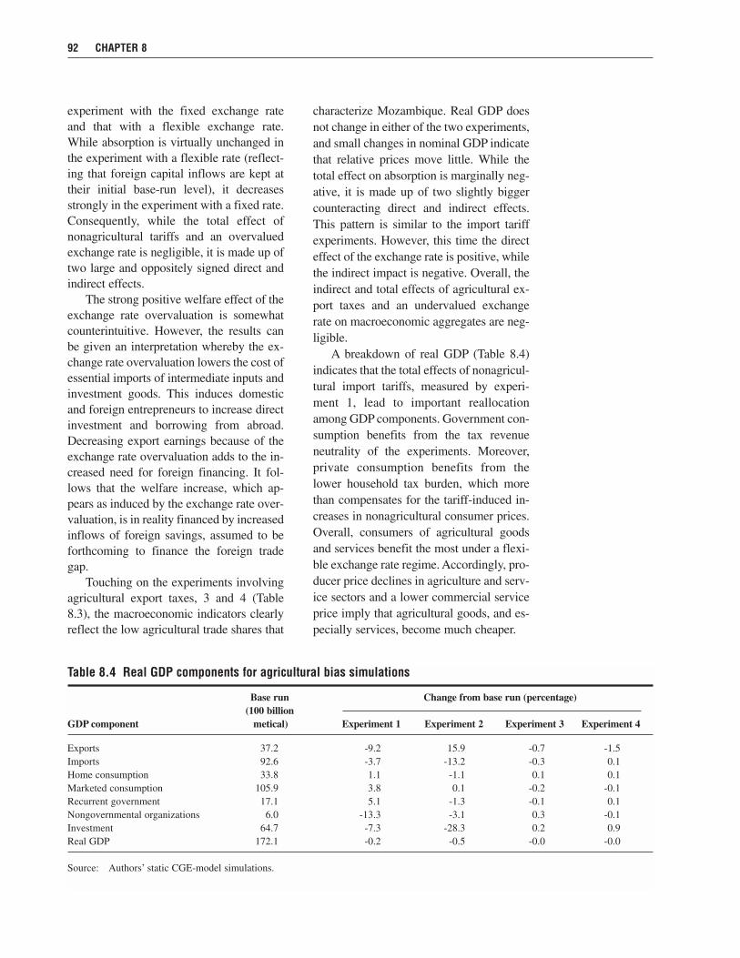
92 CHAPTER 8

experiment with the fixed exchange rateand that with a flexible exchange rate.While absorption is virtually unchanged inthe experiment with a flexible rate (reflect-ing that foreign capital inflows are kept attheir initial base-run level), it decreasesstrongly in the experiment with a fixed rate.Consequently, while the total effect ofnonagricultural tariffs and an overvaluedexchange rate is negligible, it is made up oftwo large and oppositely signed direct andindirect effects.

The strong positive welfare effect of theexchange rate overvaluation is somewhatcounterintuitive. However, the results canbe given an interpretation whereby the ex-change rate overvaluation lowers the cost ofessential imports of intermediate inputs andinvestment goods. This induces domesticand foreign entrepreneurs to increase directinvestment and borrowing from abroad.Decreasing export earnings because of theexchange rate overvaluation adds to the in-creased need for foreign financing. It fol-lows that the welfare increase, which ap-pears as induced by the exchange rate over-valuation, is in reality financed by increasedinflows of foreign savings, assumed to beforthcoming to finance the foreign tradegap.

Touching on the experiments involvingagricultural export taxes, 3 and 4 (Table8.3), the macroeconomic indicators clearlyreflect the low agricultural trade shares that

characterize Mozambique. Real GDP doesnot change in either of the two experiments,and small changes in nominal GDP indicatethat relative prices move little. While thetotal effect on absorption is marginally neg-ative, it is made up of two slightly biggercounteracting direct and indirect effects.This pattern is similar to the import tariffexperiments. However, this time the directeffect of the exchange rate is positive, whilethe indirect impact is negative. Overall, theindirect and total effects of agricultural ex-port taxes and an undervalued exchangerate on macroeconomic aggregates are neg-ligible.

A breakdown of real GDP (Table 8.4)indicates that the total effects of nonagricul-tural import tariffs, measured by experi-ment 1, lead to important reallocationamong GDP components. Government con-sumption benefits from the tax revenueneutrality of the experiments. Moreover,private consumption benefits from thelower household tax burden, which morethan compensates for the tariff-induced in-creases in nonagricultural consumer prices.Overall, consumers of agricultural goodsand services benefit the most under a flexi-ble exchange rate regime. Accordingly, pro-ducer price declines in agriculture and serv-ice sectors and a lower commercial serviceprice imply that agricultural goods, and es-pecially services, become much cheaper.

Table 8.4 Real GDP components for agricultural bias simulations


GDP component metical) Experiment 1 Experiment 2 Experiment 3 Experiment 4

Exports 37.2 -9.2 15.9 -0.7 -1.5Imports 92.6 -3.7 -13.2 -0.3 0.1Home consumption 33.8 1.1 -1.1 0.1 0.1Marketed consumption 105.9 3.8 0.1 -0.2 -0.1Recurrent government 17.1 5.1 -1.3 -0.1 0.1Nongovernmental organizations 6.0 -13.3 -3.1 0.3 -0.1Investment 64.7 -7.3 -28.3 0.2 0.9Real GDP 172.1 -0.2 -0.5 -0.0 -0.0


The total effects on GDP componentsclearly show that investment is affected theworst by nonagricultural import tariffs andthe associated overvalued exchange rate. Asnoted above, investment is squeezed bothfrom the supply and demand sides. Sincecapital transfers finance more than 70 per-cent of total investment expenditures, theeffect on demand-side revenue from over-valuation of the exchange rate completelydominates the total effect on investment.The strong negative total effect on exportsis also mainly due to the exchange rateovervaluation, which lowers domestic ex-port prices. Overall, total effects of nonagri-cultural import tariffs on imports, exports,and investment are strongly negative, whiletotal effects on private and government con-sumption are positive.

The indirect exchange rate effects ofimposing high nonagricultural import tar-iffs also imply strong changes among GDPcomponents. This is closely connected withthe fact that the indirect exchange rate ef-fects reflect a 9 percent exchange rate ap-preciation and a 24 percent increase in for-eign capital inflows. Overall, indirect ex-change rate effects on consumption, invest-ment, and imports are strongly positive. Therelative increase in foreign capital inflowsinduces an especially strong positive, indi-rect effect on investment. In contrast, the in-direct exchange rate effect on exports isstrongly negative because of the exchangerate appreciation and the increased domes-tic demand for production.

In the experiments involving agricul-tural export taxes, 3 and 4, the total effectson the composition of real GDP are againsmall because of very low agricultural ex-port shares. Exports drop because of de-clines in domestic agricultural export pricesinduced by export taxes, while imports dropbecause of the exchange rate depreciation,which increases domestic import prices.

Home consumption of own production in-creases because of downward pressures onagricultural producer prices. Finally, up-ward pressure on nonagricultural marketprices implies that private and governmentmarket-based consumption decline. Over-all, the (small) total effects of agriculturalexport taxes include lower consumptionand foreign trade, and increasing invest-ment.

Agricultural export taxes also havesome visible indirect exchange rate effectson the composition of GDP. These effectsreflect the 0.3 percent depreciation in ex-change rates and a relative 0.8 percent de-crease in foreign capital inflows. The de-crease in capital inflows, combined with in-creases in import prices of investmentgoods induced by exchange rates, implies arelatively strong negative, indirect ex-change rate effect on investment. Further-more, the exchange rate depreciation im-proves the trade balance through increasingexports and decreasing imports. In sum, theindirect exchange rate effects of agriculturalexport taxes are generally negative for con-sumption, investment, and imports, andpositive for exports.

Agricultural Terms of TradeThe agricultural terms of trade were evalu-ated at different points in the pricing chain(Table 8.2). The total effect of nonagricul-tural import tariffs is to lower the terms oftrade evaluated at domestic import pricesby 16.2 percent. The fall in the price ofcommercial services improves domesticprices for agricultural imports prices morethan for nonagricultural import. Accord-ingly, the price channel for commercialservices moderates the negative total effecton relative prices for agricultural import.63

The indirect exchange rate effect on relativeprices of agricultural imports is only mar-ginally positive because the exchange rate

63Agricultural import prices would have decreased by 20 percent by definition, had marketing margins not beenpresent in the model.


appreciation and the decline in commercialservice prices affects agricultural and non-agricultural import prices in a similar way.This is so because marketing margin ratesfor imported agricultural and nonagricul-tural goods are similar.

The total effect of nonagricultural im-port tariffs on relative agricultural exportprices is modest. The small total incentiveeffect is due to almost equivalent rates ofdecline in agricultural and nonagriculturalexport prices. The negative impact on do-mestic agricultural export prices is noted.The 6.3 percent decline in the commercialservice price should increase relative agri-cultural export prices. However, the largeshare of marketing costs in the value ofagricultural exports also implies that agri-cultural export prices are sensitive to ex-change rate changes. It follows that the 9percent exchange rate appreciation has aparticularly negative effect on agriculturalexport prices. Overall, the total effect ofnonagricultural import tariffs is to lowerrelative agricultural export prices by 0.8percent.64

While the indirect exchange rate effectsare negative for agricultural and nonagri-cultural export prices alike, agriculturalprices are affected the most because of themutually reinforcing effects of the ex-change rate appreciation and the relative 5.1percent increase in the commercial serviceprice. High agricultural margins for exportmarketing imply that increased commercialservice costs worsen the agricultural termsof trade. Moreover, the exchange rate ap-preciation worsens the agricultural terms oftrade even further because of the impliedexchange rate sensitivity. Overall, the indi-rect exchange rate effect on relative agricul-tural export prices is a drop of 4.9 percent.

The total effect on agricultural terms oftrade evaluated at the prices for compositegoods is strongly negative. This is a result

of declining agricultural and increasingnonagricultural price indices. The decline inagricultural market prices follows from de-clining producer prices and marketingcosts. Lower producer prices and marketingcosts also have a tendency to lower non-agricultural market prices. However, tariff-induced increases in nonagricultural importprices dominate. Overall, the total effect ofnonagricultural import tariffs is to decreaserelative agricultural market prices by 6.6percent.

The indirect exchange rate effect on rel-ative agricultural market prices is small.This effect reflects a 9 percent exchangerate appreciation and 24 percent increase inforeign capital inflows. On the one hand,the appreciation leads to lower nonagricul-tural market prices for imported goods be-cause of relatively high nonagricultural im-port shares. On the other hand, increasedforeign capital inflows lead to increased de-mand and prices for nonagricultural invest-ment goods (construction). Finally, the 5.1percent increase in the commercial serviceprice increases agricultural market pricesrelatively strongly. Overall, the indirect ex-change rate effect of nonagricultural importtariffs leads to a small 0.3 percent net in-crease in relative agricultural market prices.

The total incentive effects of nonagri-cultural import tariffs include increasingrelative agricultural producer prices. Therelative drop in nonagricultural producerprices may seem counterintuitive, sincenonagricultural import tariffs are supposedto protect nonagriculture. The reason forthis effect is partly to be found in the differ-ences in marketing margin rates betweensectors. Import tariffs induce a drop in im-port demand. This leads to a fall in the com-mercial service price, which imparts adownward pressure on agricultural and in-dustry sector market prices. Since no mar-keting margin is added to service sector

94 CHAPTER 8

64Notice, however, that the high negative total effects on domestic export prices has a larger impact on nonagri-cultural producer price incentives because of the larger nonagricultural export shares.

activities, this leads to a competitive lower-ing of service sector market and producerprices. The producer price in the construc-tion sector also declines because of declin-ing foreign financing for investment pur-poses. Overall, the nonagricultural importtariffs lead to a total 1.4 percent increase inrelative agricultural producer prices in spiteof the protection afforded by the import tar-iffs to the nonagricultural sector.

The indirect exchange rate effect ofnonagricultural import tariffs on relativeagricultural producer prices is moderatelynegative. As mentioned previously, the ex-change rate effect reflects an exchange rateappreciation and a relative increase in for-eign capital inflows. The exchange rate ap-preciation works to lower the producerprices on (nonagricultural) exports directly,while the increase in foreign capital inflowsleads to increasing demand and producerprices for construction. In addition, the rel-ative increase in the commercial serviceprice leads to competitive increases in serv-ice sector producer prices. The net result ofthese disparate effects is that the indirect ex-change rate effect of nonagricultural importtariffs amounts to a 2.9 percent decrease inrelative agricultural producer prices.

The total effect of nonagricultural im-port tariffs on relative agricultural value-added prices is strongly positive. The posi-tive total incentive effects for agriculturalproducers cannot be explained by relativechanges in producer prices. They onlychange slightly. Rudimentary productiontechnologies imply that agricultural value-added prices decrease by a mere 2.5 percentin accordance with producer prices. In con-trast, nonagricultural value-added prices de-crease by 9.8 percent in the more input-intensive nonagricultural sectors. This ismuch stronger than the 3.5 percent declinein nonagricultural producer prices. Conse-quently, nonagricultural value-added pricesparticularly are negatively affected bynonagricultural import tariffs through theinput cost channel.

The individual price indices indicatethat changes in producer prices and value-added prices are correlated for both agricul-ture and nonagriculture. However, interme-diate input costs are clearly important forthe nonagricultural sector. This can be seenfrom the fact that percentage changes differmarkedly between nonagricultural producerprices and value-added prices. The effect oflarge input costs has two dimensions. Thefirst is to introduce sensitivity to changes ininput prices. The second is to increase sen-sitivity to changes in producer prices. Sincethe average input cost share of nonagricul-tural production is 50 percent, both dimen-sions are important for nonagriculturalprices.

Overall, the total effect of nonagricul-tural import tariffs on relative agriculturalvalue-added prices is 8.1 percent. It followsthat this positive total effect mainly stemsfrom the high sensitivity of nonagriculturalvalue-added prices to changes in producerprices and from the tariff-induced increasesin consumer price, which increase nonagri-cultural input prices. Since the agriculturalterms of trade evaluated at value-addedprices is the most appropriate measure ofrelative incentives for agricultural produc-ers, nonagricultural import tariffs and theassociated overvalued exchange rate implya bias against nonagriculture rather than abias against agriculture.

The indirect exchange rate effect ofnonagricultural import tariffs on relativeagricultural value-added prices is stronglynegative. Accordingly, the positive total ef-fect follows from a strong positive effect ondirect prices, which reflects a 33 percent in-crease in capital inflows. In contrast, the in-direct exchange rate effect reflects a 9 per-cent exchange rate overvaluation and a 24percent increase in capital inflows. Overall,the indirect exchange rate effect of nonagri-cultural import tariffs works to lower rela-tive agricultural value-added prices by 6.5 percent. This cannot be explained aloneby the modest indirect exchange rate effecton relative agricultural producer prices,


implying that the input cost channel plays arole. Hence, the positive indirect exchangerate effect on relative agricultural value-added prices results from the combinationof increasing relative agricultural producerprices, a high sensitivity of nonagriculturalvalue-added prices to declining producerprices and tariff-induced increases in non-agricultural input prices.

The last two experiments, 3 and 4, areused to analyze the impact of a uniform 25percent agricultural export tax. The impacton relative prices is generally small, sinceagricultural export shares are low. The onlymajor impact of the 25 percent agriculturalexport tax is to decrease relative agricul-tural export prices by 35 percent. The rea-son for this seeming inconsistency is thatagricultural marketing margin rates are rel-atively high. High margins imply that do-mestic export prices are especially sensitiveto changes in the domestic currency valueof world market prices.65 Since agriculturalexport taxes subtract from the domestic cur-rency value of the world market prices forexports, domestic agricultural export pricesreact strongly to export taxes.

In general, agricultural export taxeshave only marginal effects on nonagricul-tural prices. The declining agriculturalterms of trade evaluated at producer andvalue-added prices reflect the strongly de-clining producer prices for exports. Themild impact is a result of the low agricul-tural export shares. In conclusion, the totalincentive effects of agricultural export taxesare moderately adverse toward agriculturalproduction in general but very adverse to-ward production of agricultural exportgoods in particular. The indirect exchangerate effects on agricultural terms of trade

following from the 0.3 percent undervalua-tion of the exchange rate are very small.Overall, the agricultural export taxes lead toa positive indirect incentive effect on rela-tive agricultural value-added prices in theorder of 0.2 percent.

Simulations with a BalancedMacroclosure

Quantity Adjustments in the Foreign Trade Account

This section presents trade policy analysesof export taxes and import tariffs in the con-text of a balanced macroclosure where theprivate investment share of absorption isfixed. Government consumption and in-vestment are also fixed in proportion tonominal absorption, so constant shares areclose to being maintained in absorption.66

Maintaining private investment as a con-stant share of absorption requires allowinga savings rate—in this case the averagehousehold savings rate—to vary and thusmaintain equilibrium between savings andinvestment.

In general, changes in the foreign capi-tal inflows do not depend much on thechoice of macroclosure. This is so becausethe changes in the commercial service priceand the exchange rate are similar irrespec-tive of the choice of macroclosure.

Under a fixed exchange rate regime,nonagricultural import tariffs lead to a 29percent drop in foreign capital inflows, ascompared with 33 percent under a savings-driven investment closure. The mechanismremains the same as before, namely tariff-induced increases in domestic import pricesdrive nonagricultural imports of investment

96 CHAPTER 8

65Marketing costs make up for the difference between domestic agricultural prices and the world market price indomestic currency. If marketing margins were not accounted for, a uniform 25 percent agricultural export taxwould lead to a 25 percent decrease in domestic agricultural export prices, by definition.

66Were it not for the revenue-driven NGO demand component, which is relatively small, fixed government con-sumption and total investment shares of absorption would imply a constant private consumption share of ab-sorption as well.

goods and services down. Moreover, thenon-agricultural import tariff experimentwith a flexible exchange leads to a 9 percentdecline in the domestic currency value ofcapital inflows regardless of the choice ofmacroclosure. In the following, total effectsaccordingly reflect a 9 percent decline incapital inflows, while the indirect effects re-flect a 20 percent increase.

The total effects of agricultural exporttaxes reflect a 0.3 percent increase in capi-tal inflows regardless of the choice ofmacroclosure. Moreover, the current indi-rect effects reflect a 0.9 percent decrease incapital inflows as compared with a 0.8 per-cent decrease with savings-driven invest-ment. In general, it can be concluded thatthe policy impacts on foreign capital in-flows do not depend on the choice ofmacroclosure. The experiments with a bal-anced macroclosure are therefore compara-ble to the experiments with a savings-driven investment closure in relation totheir impacts on capital inflows.

Macroeconomic ImpactBoth nonagricultural import tariffs and agri-cultural export taxes have effects on aggre-gate real GDP similar to the experimentswith a savings-driven investment closure(Table 8.5). While there are real small neg-ative real effects of imposing nonagricul-tural import tariffs, agricultural export taxesshow no visible effects on real GDP. Theimpact on nominal macroeconomic indica-tors is also very similar to the previous ex-periments with savings-driven investment.

Overall, the positive total effects of non-agricultural tariffs on nominal GDP and theGDP deflator are dominated by positive in-direct exchange rate effects.

The marginal total effect of nonagricul-tural import tariffs on nominal absorption isagain made up of strong direct and indirecteffects. Furthermore, the positive indirecteffect of exchange rates still follows fromthe 20 percent increase in capital inflows.The impact of agricultural export taxes re-mains small. Again, a 0.9 percent decreasein capital inflows leads to a negative indi-rect exchange rate effect on nominal ab-sorption. Overall, the effects of export taxesand import tariffs on macroeconomic indi-cators do not change much with the changeto a balanced macroclosure.

In line with the previous set of experi-ments, small changes in real GDP coversignificant changes in the composition offinal demand (Table 8.6). Total effects ofnonagricultural import tariffs do not changemuch with the change to a balanced macro-closure, except for a more moderate declinein real investment and a smaller expansionof private marketed consumption. Accord-ingly, the conclusion remains that privateand government consumption expands atthe expense of real investment.

The fact that the composition of realGDP still changes may seem like a paradoxgiven that the balanced macroclosure main-tains the structure of domestic nominal de-mand. However, changing relative pricesaffect the composition of real final demand.Tariff-induced increases in nonagricultural


Table 8.5 Macroeconomic indicators for agricultural bias simulations


Indicator metical) Experiment 1 Experiment 2 Experiment 3 Experiment 4

Real GDP 172.1 -0.2 -0.4 -0.0 -0.0Nominal GDP 172.1 2.7 -0.7 -0.2 -0.1Nominal absorption 227.6 -0.1 -7.6 -0.1 0.2


import prices lead to increasing prices fornonagricultural investment goods. In con-trast, service prices are competitively low-ered. Overall, the total effects of nonagri-cultural import tariffs still involve decreas-ing trade and investment, and increasingconsumption.

The indirect exchange rate effects ofnonagricultural import tariffs are also af-fected strongly by the change to a balancedmacroclosure. Since the indirect exchangerate effects reflect a 20 percent increase incapital inflows, the change to a balancedmacroclosure moderates the relative expan-sion of nonagricultural investment demandin favor of a stronger expansion of moreagriculturally oriented consumption de-mand.

The negative indirect exchange rate ef-fect on exports is also moderated with a bal-anced macroclosure. Accordingly, the moremoderate 3.8 percent increase in marketingcosts lowers competitive price increases inthe service sector. Nevertheless, exportsstill decline by around 20 percent becauseof declines in domestic export prices in-duced by changes in the exchange rate anda general increase in domestic absorptionresulting from increased capital inflows.

Overall, indirect exchange rate effectsof nonagricultural import tariffs continue toinvolve increasing real consumption, in-vestment, and imports; and decreasing ex-

ports. However, the choice of a balancedmacroclosure implies a stronger increase inconsumption, a more moderate increase ininvestment, and a more moderate decreasein exports. The contemporary expansion ofreal consumption and investment continueto reflect a relative 20 percent increase inforeign capital inflows for financing purposes.

The change to a balanced macroclosurealso affects the impact of agricultural exporttaxes on the composition of final demand.While total and indirect exchange rate ef-fects are small, the change in tradeoff be-tween private consumption and investmentdemand remains visible. The total effect oninvestment turns positive, while the impacton private consumption becomes negative.Overall, the total effect of agricultural ex-port taxes continues to include a reductionin trade, while total effects on investmentand consumption are marginal.

The most visible impact of the balancedmacroclosure in relation to the agriculturalexport tax experiments is on the indirect ex-change rate effects. Accordingly, the nega-tive indirect effect on investment is clearlymoderated at the expense of a negative in-direct effect on private consumption. Over-all, the indirect exchange rate effects ofagricultural export taxes include decreasingconsumption, investment and imports, andincreasing exports.

98 CHAPTER 8

Table 8.6 Real GDP components for agricultural bias simulations


GDP component metical) Experiment 1 Experiment 2 Experiment 3 Experiment 4

Exports 37.2 -9.9 11.1 -0.7 -1.4Imports 92.6 -4.0 -13.0 -0.2 0.1Home consumption 33.8 0.8 -1.8 0.1 0.2Marketed consumption 105.9 0.9 -8.1 0.0 0.3Recurrent government 17.1 4.8 -1.6 -0.1 0.1Nongovernmental organizations 6.0 -13.4 -4.2 0.3 -0.0Investment 64.7 -2.3 -11.1 -0.1 0.2Real GDP 172.1 -0.2 -0.4 -0.0 -0.0


Agricultural Terms of TradeThe impact of nonagricultural import tariffson relative agricultural import prices is notaffected in any important way by the choiceof macroclosure (Table 8.7). Average mar-keting margin rates are similar for agricul-tural and nonagricultural imports. It followsthat slightly varying changes in the com-mercial service price and the exchange rateleave the agricultural terms of trade virtu-ally unaffected by the choice of macroclo-sure (Tables 8.1 and 8.7). Overall, the non-agricultural import tariffs lead to a strongnegative total effect of –16.2 percent onrelative agricultural import prices, while theovervalued exchange rate leads to a smallpositive indirect exchange rate effect of 0.7percent.

Agricultural export prices are somewhatmore sensitive to the choice of macroclo-sure, since agricultural marketing marginrates are relatively high. The total effects of

nonagricultural import tariffs reflect a 6.3percent decline in the commercial serviceprice, compared with a 5.9 percent declinewith savings-driven investment. It followsthat the total effect of nonagricultural im-port tariffs on relative export prices remainsaround –1.0 percent, regardless of thechoice of macroclosure.

In contrast, indirect exchange rate ef-fects reflect an increase of 3.8 percent in thecommercial service price compared with a5.1 percent increase with savings-driven in-vestment. The more moderate increase inmarketing costs benefits relative agricul-tural export prices. It follows that thechange to a balanced macroclosure moder-ates the negative indirect effect on agricul-tural export prices. Nevertheless, the ex-change rate appreciation and the relative in-crease in the commercial service price stillimply that nonagricultural import tariffslead to a strong negative indirect exchange


Table 8.7 Price indices and agricultural terms of trade for agricultural bias simulations


Prices Base run Experiment 1 Experiment 2 Experiment 3 Experiment 4

ImportAgricultural terms of trade 100 -16.2 -16.9 0.0 0.0Agricultural prices 100 -8.1 -2.5 0.2 0.0Nonagricultural prices 100 9.6 17.4 0.2 0.0

ExportAgricultural terms of trade 100 -1.0 3.3 -35.0 -35.1Agricultural prices 100 -9.9 4.0 -34.8 -35.1Nonagricultural prices 100 -9.0 0.7 0.3 0.0

RetailAgricultural terms of trade 100 -7.5 -10.0 0.0 0.1Agricultural prices 100 -5.4 -7.1 0.1 0.1Nonagricultural prices 100 2.2 3.2 0.0 0.0

ProducerAgricultural terms of trade 100 -0.8 -3.2 -1.0 -0.9Agricultural prices 100 -4.0 -7.1 -1.0 -0.9Nonagricultural prices 100 -3.2 -4.0 0.0 0.0

Value-addedAgricultural terms of trade 100 5.3 4.8 -1.1 -1.0Agricultural prices 100 -4.7 -8.3 -1.2 -1.0Nonagricultural prices 100 -9.5 -12.5 -0.1 0.0

Exchange rate 100 -8.8 0.0 0.3 0.0Commercial service price 100 -6.3 -11.4 -0.1 0


rate effect of –4.3 percent on relative agri-cultural export prices.

Nonagricultural import tariffs decreaserelative prices for agricultural goods by 7.5and 10.0 percent, respectively, in the exper-iments with flexible and fixed exchangerates. Accordingly, a balanced macroclo-sure implies a stronger negative total effect,composed of a stronger negative direct ef-fect and a stronger positive indirect ex-change rate effect. The individual price in-dices indicate that the change to a balancedmacroclosure has a negative impact on agri-cultural prices (Tables 8.2 and 8.7). Theseagricultural price effects are the most im-portant effects of a change to a balancedmacroclosure.

Overall, the strong negative total effectof nonagricultural import tariffs on relativeagricultural composite prices still followsfrom the combination of increase in non-agricultural market prices and decreases inagricultural market prices. Consequently,the import tariffs increase domestic non-agricultural (import) prices, while decreasesin producer prices and marketing costs de-crease agricultural market prices.

Nonagricultural import tariffs decreaserelative agricultural producer prices by 0.8percent in the experiment with flexible ex-change rates and by 3.2 percent in the ex-periment with fixed exchange rates. As a re-sult, the change to a balanced macroclosureleads to a negative total effect and a positiveindirect exchange rate effect. The individ-ual price indices indicate that a balancedmacroclosure affects nonagricultural pro-ducer prices positively and agricultural pro-ducer prices negatively (Tables 8.2 and8.7). The reason is that adjustment to de-clining capital inflows are shifted fromnonagricultural investment goods to agri-cultural consumer goods.

Overall, the negative total effect ofnonagricultural import tariffs on relativeagricultural producer prices continues to bethe net outcome of simultaneous declines inagricultural and service sector producerprices. Producer prices in industry and man-

ufacturing sectors generally decline lessthan in other sectors because of tariff pro-tection and lower marketing costs. The pos-itive indirect exchange rate effect reflects astrong positive impact on agricultural pro-ducer prices. While the relative demand in-crease for agricultural consumption goodsdirectly affects the domestic economy, in-creasing demand for nonagricultural invest-ment goods leaks out partly through im-ports. Accordingly, the 20 percent increasein capital inflows increases agricultural pro-ducer prices more strongly than nonagricul-tural producer prices.

Nonagricultural import tariffs increaserelative agricultural value-added prices by5.3 percent and 4.8 percent, respectively, inthe experiments with flexible and fixed ex-change rates. The positive total effect ismoderated by the change to a balancedmacroclosure, while the indirect exchangerate effect has turned marginally positive.The balanced macroclosure affects agricul-tural value-added prices positively (themajor impact) and nonagricultural value-added prices negatively. This was also thecase for producer prices. This might suggestthat the change to a balanced macroclosureaffects relative agricultural value-addedprices through its impact on agriculturalproducer prices. However, the effect of thechange to a balanced macroclosure onnonagricultural producer prices is also im-portant, since the input cost channel magni-fies the effect of producer prices changes onvalue-added prices.

Overall, nonagricultural import tariffshave a total effect of 5.3 percent on relativeagricultural value-added prices. The totaleffect on relative producer prices is small. Itfollows that the positive total effect mainlystems from the input cost channel includingthe very sensitive nature of nonagriculturalvalue-added prices to changes in producerprices, and the tariff-induced price in-creases for nonagricultural inputs. Nonagri-cultural import tariffs also lead to a positiveindirect exchange rate effect of 0.5 percenton relative value-added prices. The small

100 CHAPTER 8

positive indirect effect results because agri-cultural and nonagricultural value-addedprices increase in parallel between the fixedand flexible exchange rate experiments.The reason is that the structure of domesticfinal demand is maintained almost constant.This minimizes the relative price impact ofthe relative 20 percent increase in capital in-flows.

The change to a balanced macroclosurehas very little importance for the results inthe experiments with agricultural exporttaxes. Total and indirect exchange rate ef-fects remain small because of the very lowagricultural export shares in the model.Consequently, the conclusion remains thatagricultural export taxes reduce agriculturalproducer incentives slightly, while price in-centives for production of agricultural ex-port crops are reduced strongly.

Conclusions

During the 1980s the benefits of free tradeand deregulated markets were increasinglyemphasized, and partial-equilibrium studiesin the late 1980s concluded that import-substituting trade and exchange rate poli-cies have strong negative effects on agricul-tural production incentives. The generalityof these conclusions are, however, seriouslyquestioned when the analysis is performedinside a general-equilibrium framework.Our experiments suggest that quantity ad-justment in the foreign trade account is im-portant to consider when analyzing the agri-cultural bias in a general-equilibriumframework. The specific characteristics ofthe model are important for the results ob-tained. High agricultural marketing margins

imply that agricultural price incentives im-prove when declining demand for market-ing services, driven by declining trade, low-ers the price of marketing services. More-over, increases in industry input costs, be-cause of import tariffs or exchange rate de-preciation, tend to benefit relative agricul-tural price incentives. Overall, the biasagainst agriculture following from agricul-tural export taxes is minor, while nonagri-cultural import tariffs actually increase agri-cultural production incentives strongly.

The impact of import-substituting poli-cies on relative agricultural value-addedprices suggests that historical policies maynot have imparted an agricultural bias inMozambique, as previously believed. Con-sequently, the increasing agricultural shareof value-added up through the early 1990s,identified in Chapter 4, appears to havecome about not so much because of struc-tural adjustment induced improvements toagricultural price incentives, but rather be-cause the sector was recovering from thewar in the 1980s and early 1990s, and thedrought in 1992. However, it is important tobe aware of the limitations of the resultspresented in this chapter. Accordingly, thefact that agricultural export taxes have little effect on relative agricultural price in-centives rests squarely on the fact that agri-cultural export shares are small in themodel. These results cannot be used toargue that export taxes on, for example, rawcashews can make up a vital source of gov-ernment revenue. This would require thatagricultural export shares, a key structuralcharacteristic of the model, increased substantially.


C H A P T E R 9

Marketing Margins and Agricultural Technology

F ollowing the peace agreement in 1992 and the first free general elections in 1994, dis-placed people returned to rural agricultural areas in massive numbers. This played animportant role in the recovery of aggregate agricultural production, as discussed in

Chapter 4. Nevertheless, production technologies employed by most farmers remain rudi-mentary and the quality of inputs is poor. Therefore significant possibilities exist for shiftingto better production technologies through using improved seed varieties and other improvedinputs, and through better farming practices (Bay 1998). Moreover, a key problem limiting theimpact of market reforms and the potential benefits of better agricultural technology is thatmany farmers do not have access to markets. The lack of markets is widespread, and transac-tions costs are very high. Some progress has been made regarding the extension of primaryand secondary road networks, and this has been accompanied by some integration of tradingactivities between different parts of the country. The overall goal of bringing the different re-gions into a single, integrated domestic economy that links rural production areas with urbanconsumption centers through the establishment of countrywide transport, storage, and com-munication facilities is, however, far from achieved.

Against this background, this chapter presents a quantitative assessment of the potentialbenefits from increases in the productivity of the agricultural sector and improvements to mar-keting networks. The analysis is based on the CGE model set out in Chapter 6. The 1995 SAMshows that marketing margins for some sectors were as high as three times the producer pricein 1995, and they are especially large for primary agricultural production. These marketingcosts represent wedges between producer and purchaser prices, and partly explain why morethan half of agricultural production remains unmarketed. Since the vast majority of the popu-lation relies on agricultural production for their livelihood, potential exists for very large in-come gains through improved market integration in rural areas. Synergy between a poverty-reducing strategy of increasing agricultural productivity and parallel improvements in themarketing infrastructure can be expected.

Simulations

Marketing margins in the model, discussed here, are based on the distinction between factoryand farmgate prices on the one hand and purchaser prices on the other, reflecting storage and

This chapter was written by Channing Arndt, Henning Tarp Jensen, Sherman Robinson, and Finn Tarp.

102

marketing costs.67 The marketing marginswere introduced into the CGE modelthrough commercial service coefficients.This treatment amounts to assuming thateach production good from a given produc-tion sector requires a fixed amount of mar-keting services to reach the market. Inessence, they are input-output coefficientsrelating the demand for commerce servicesrequired to move goods from producer tomarket. A single production activity pro-vides the marketing services associatedwith imported, exported, and domesticallymarketed commodities.

The model formulation incorporateshome consumption and marketed consump-tion through a linear expenditure system(LES). In this formulation, the marginalbudget shares of marketed and nonmar-keted goods are fixed and each commodityhas an associated minimum consumptionlevel below which physical consumptioncannot fall. Home-consumed goods are, asalready noted, valued at producer prices,while marketed goods are valued at pur-chaser prices, including consumption taxesand marketing margins. Labor supplies arefixed in the agricultural and nonagriculturalsectors.68 As a result, wage rates are al-lowed to diverge between agricultural andnon-agricultural labor.

In the model, implementation of agri-cultural technology improvements, throughHicks-neutral productivity increases, isstraightforward and in line with our focuson the productivity-enhancing importanceof introducing better-quality inputs, such as

improved seed, in combination with betterfarming practices. Reductions in marketingmargins are modeled through scaling downthe commercial service coefficients furtherdiscussed below.69 In the analysis, invest-ment expenditures associated with im-proved technology and marketing infra-structure are ignored. This treatmentamounts to assuming that these investmentsare undertaken before the current simula-tions, and the analysis makes no attempt toquantify the costs of realizing the policy ini-tiatives studied here. The focus is instead onbenefits.

The simulations include a uniform 30percent improvement in productivity acrossagricultural sectors and a 15 percent reduc-tion in the commercial service coefficientsfor imported, exported, and domesticallyproduced and marketed commodities(Table 9.1). Achieving agricultural produc-tivity growth on the order of 30 percent inMozambique is probably feasible over areasonably short time span because of therudimentary nature of current agriculturalproduction practices. Reductions in market-ing margins on the order of 15 percent arealso feasible, given the scope for improvingthe marketing system after the devastationcaused by the war. While a 15 percent gainmay come relatively cheaply, large invest-ments in marketing infrastructure willlikely be needed to achieve significant fur-ther declines in marketing costs. In short,the costs of achieving these gains are notexplicitly included in the model. However,the costs of attaining these gains are likely

MARKETING MARGINS AND AGRICULTURAL TECHNOLOGY 103

67The price gap may reflect some degree of imperfect competition. In the SAM and the model, they are assumedto reflect real costs.

68Simulations with a specification of constant elasticity of transformation between agricultural and nonagricul-tural labor supplies lead to the same conclusions.

69The current experiments analyze the effects of reductions in the demand for marketing services following frominvestment in marketing infrastructure. The experiments do not take account of potential efficiency gains in theproduction of commercial services associated with improvements to the marketing infrastructure. The demandeffect is assumed to dominate, at least initially, in the Mozambican context. Better infrastructure will make it pos-sible to transport, for example, 1 ton of maize faster and with less input of work-hours and fuel, but the truckscarrying the cargo remain the same. In any case, efficiency gains in the provision of marketing services wouldyield similar qualitative results, reinforcing the conclusions derived from the analysis in this chapter.

to be relatively low. For the attainment offurther gains, a more detailed considerationof cost would be desirable.

The productivity increase of 30 percentfor all agricultural products (experiment 1)yields an aggregate welfare improvement of6.8 percent (the change in absorption de-flated by the aggregate CPI (Table 9.2). Theproductivity increase raises output and low-ers relative prices significantly in the agri-cultural sector. The price decline moderatesthe increase in aggregate rural income and

transmits much of the gain to the urban sec-tor. Since agriculture has very high trademargins, the greater output generates a sig-nificant increase in demand for commerceservices, driving up their price. The result isthat the gap between supplier and marketprices for exports and imports rises. Exportsdecrease more than imports in real terms,and a mild depreciation of the real ex-change rate (3.3 percent) restores equilib-rium in the trade balance.70

104 CHAPTER 9

Table 9.1 Experiment descriptions for marketing margin and agricultural technologysimulations

Experiment Description

Base run Base social accounting matrix (SAM) data set for 1995Experiment 1 Increase in productivity by 30 percent for all agricultural productsExperiment 2 Reduction of marketing margins for all goods by 15 percentExperiment 3 Scenarios 1 and 2 combined

Source: Authors’ static CGE-model experiment design.

Table 9.2 Macroeconomic indicators and prices for marketing margin and agriculturaltechnology simulations


Indicator metical) Experiment 1 Experiment 2 Experiment 3

Real GDP 172.1 6.8 5.0 12.2Absorption 223.3 6.8 4.9 12.9Price indices

Value-added 100 1.4 5.3 7.3Export producer 100 4.8 5.3 10.3Import purchaser 100 6.2 0.2 6.4

Cost of living indicesRural 100 -5.9 2.8 -3.1Urban 100 3.7 -0.8 3.0

Real exchange rate index 100 3.3 -0.1 2.8Agricultural terms of trade

Producer 100 -24.9 7.4 -17.8Value-added 100 -29.4 7.1 -22.4Export 100 -1.8 6.7 5.1Import 100 0.2 -0.6 -0.5

Price of commerce 1 9.8 2.2 12.7


70The real exchange rate is defined as the ratio between an index composed of domestic exports and importsprices, and an index composed of prices of domestically marketed and nonmarketed goods.

The 15 percent reduction in marketingmargins (experiment 2) leads to a 4.9 per-cent increase in welfare. This is a large wel-fare gain.71 The decrease in marketing mar-gins narrows the spread between producerand purchaser prices, raising the former andlowering the latter. Both producers and con-sumers gain, and the gains are spreadevenly across the economy, as further dis-cussed below. The impact on trade is theconverse of experiment 1: exports gainslightly more than imports, and the real ex-change rate appreciates slightly (0.1 per-cent), to restore equilibrium.

Results from combining the first twoexperiments (experiment 3) support the hy-pothesis that prior improvements in market-ing infrastructure allow the economy toreap greater benefits from improvements inagricultural productivity. The increase inwelfare in experiment 3 is about 10 percentgreater than the sum of the effects of exper-iments 1 and 2 run separately. The reduc-tion in marketing margins diminishes thedecrease in agricultural producer prices thatwould otherwise follow from the significantexpansion of supply as agricultural produc-tivity rises. Improvements to the marketingnetwork ensure that increased productionfollowing agricultural productivity im-provements benefits both farmers and con-sumers more, as the gap between producerand purchaser prices is narrowed.

The relative changes in the cost-of-living indices for rural and urban house-holds differ across the simulation scenar-ios.72 Gains in agricultural productivity (ex-periment 1) lower agricultural prices signif-icantly, and since rural households allocatea larger share of their budget to agricultural

goods, their cost-of-living index falls rela-tive to that of urban households. In contrast,lower marketing margins (experiment 2) in-crease producer prices in agriculture and in-crease the relative cost of living for ruralhouseholds with significant home con-sumption. The effects on cost of living withthe combined scenario (experiment 3) arevery close to the sum of the two separateexperiments.

Increased agricultural productivity,which increases output, worsens the agri-cultural terms of trade (Table 9.2). De-creased marketing costs improve the agri-cultural terms of trade by increasing theproducer price of agriculture more than thatof nonagriculture. In the combined scenario(experiment 3), however, the agriculturalproductivity effect is stronger and the termsof trade move significantly against agricul-ture. From a policy perspective, the com-bined scenario is attractive because the ad-verse terms-of-trade effect of increasingagricultural productivity is significantlyameliorated.

The welfare impact of the experimentsin terms of changes in household consump-tion is measured by equivalent variationfrom the base (Table 9.3).73 Given that av-erage household savings rates are assumedfixed in the model, these measures providea good indicator of the distributional impactof the scenarios between rural and urbanhouseholds. Rural households are the maingainers from increased agricultural produc-tivity. The significant increases in agricul-tural production are accompanied by sub-stantial decreases in producer prices, sorural household income increases onlyslightly. Yet, rural households benefit


71Both static gains from trade liberalization, for example, rarely exceed 1 percent.

72The numeraire is the cost-of-living index, including urban and rural household consumption. Changes in theindividual rural and urban indices are therefore relative to an average. Thus, when the cost of living of urbanhouseholds drops rural people must experience an opposite effect.

73Equivalent variation measures the lump-sum transfer that would make the household indifferent between thescenario and the base case plus the transfer.

106 CHAPTER 9

significantly on the consumption side, sincethey allocate a relatively large share of theirbudgets to agricultural goods.

Urban and rural households gainroughly the same percent increase fromlowering trade margins (experiment 2). Asnoted above, narrowing the gap betweenproducer and purchaser prices spreads thegains across the economy. Again, the resultsfor experiment 3 indicate a synergy be-tween the two effects—the gain in welfarefor both urban and rural households fromexperiment 3 is greater than the sum of thegains from the two separate simulation sce-narios.

Interactions between agricultural pro-ductivity increases and marketing margin

reductions are significant for most of thefinal demand components of real GDP(Table 9.4)—the results from experiment 3generally do not equal the sum of the othertwo experiments. For example, increasedagricultural productivity (experiment 1)leads to significant import substitution ingrains, which has a high import share8;hence aggregate exports decline becauseless export earnings are required to achievethe fixed trade balance. Lowering trademargins, on the other hand, narrows the gapbetween border prices and domestic marketprices for both imports and exports, andleads to increases in both. The trade-creating effect, which dominates in thecombined scenario, indicates a significant

Table 9.3 Equivalent variation on consumption for marketing margin and agriculturaltechnology simulations

Percentage of base consumption

Households Base run Experiment 1 Experiment 2 Experiment 3

Urban 0 5.2 4.7 10.5Rural 0 12.3 4.6 18.2Total 0 8.5 4.6 14.1


Table 9.4 Components of real GDP for marketing margin and agricultural technologysimulations


GDP components metical) Experiment 1 Experiment 2 Experiment 3

Exports 32.7 -2.2 9.4 8.0Imports 83.9 -0.8 3.7 3.1Home consumption 32.6 24.3 -0.8 22.5Marketed consumption 106.8 4.4 6.4 11.8Recurrent government 16.8 -0.7 2.7 2.4Nongovernmental organizations 5.5 -2.5 1.5 -1.5Investment 61.5 -1.1 2.4 1.2Real GDP 172.1 6.8 5.0 12.2


74This effect is likely to diminish as Mozambique becomes more self-sufficient in producing food following eco-nomic recovery, but recent events demonstrate how difficult this is.

interaction between increasing the supplyof traded goods and lowering the costs ofmoving these goods to and from interna-tional markets.75

Agricultural productivity increases havea major effect on the level of home-consumed production. Increased agricul-tural production decreases producer prices,which makes home consumption of agricul-tural goods more attractive. Moreover, theincrease in the price of marketing servicesamplifies the gap between producer andpurchaser prices, which further favorshome consumption. Lowering marketingmargins ameliorates the effect of the widen-ing price gap—experiment 2 lowers homeconsumption—and provides incentives fora further switch toward marketed consump-tion in the combined experiment. However,the agricultural production effect on theconsumption patterns still dominates in thiscase.

In terms of the effects of the scenarioson returns to labor and capital, the increasein agricultural productivity leads to almostno change in the agricultural wage—it risesby 0.1 percent (Table 9.5). The decline inproducer prices almost exactly offsets theeffect of increased productivity as far asagricultural labor is concerned. In experi-ment 1, some of the gains are transmittedthrough lower prices to the nonagriculturalsectors. The wage of nonagricultural labor

and the capital rental rate both rise signifi-cantly, but the significant increase in de-mand for capital-intensive commercialservices increases capital returns relative towages.

Lower trade margins (experiment 2) in-crease all factor returns but favor agricul-tural labor, since the agricultural sectorshave the highest trade margins. The com-bined scenario is notable in that it spreadsthe gains more evenly across the three fac-tors, with all factors gaining more than thesum of the effects of the two separate sce-narios. The synergy between increasingagricultural productivity and lowering trademargins in parallel yields returns to all fac-tors that exceed the sum of the separate sce-narios, with little change to the overallfunctional distribution of income. From apolicy perspective, the results of these in-teractions are very desirable, since muchpolitical conflict is rooted in changes in thedistribution of income among factors ofproduction.

Conclusions

The results presented in chapter indicatethat increasing agricultural productivity isan important priority for Mozambique, withlarge potential gains. However, increasingagricultural output in an environment ofvery high marketing costs leads to a


75Trade creation of course depends greatly on the ability of Mozambican exporters to penetrate export markets,highlighting that this is an important area for policy concern.

Table 9.5 Factor price indices for marketing margin and agricultural technology simulations


Factor prices Base run Experiment 1 Experiment 2 Experiment 3

Labor 1.0 0.1 11.4 15.0Nonagricultural labor 1.0 8.9 4.9 14.4Capital 1.0 10.6 2.0 13.4


108 CHAPTER 9

significant fall in prices. These price de-clines transmit most of the gains in factorincome to the nonagricultural sectors andfactors of production. Rural households do,however, gain from greater availability offood and lower producer prices, which to-gether lower the cost of home-consumedgoods.

Lowering marketing costs decreases thegap between producer and purchaser pricesin all markets. The gains are large even forrelatively small reductions in the margins.Furthermore, these gains are spread acrossthe economy, but agriculture gains rela-tively more because its marketing marginsare higher. The scenario creates trade; bothaggregate exports and imports grow, be-cause the lower marketing margins increasethe returns to producers supplying to exportmarkets and lower the domestic marketprice to purchasers of imports. The con-sumption of marketed goods rises signifi-cantly, while home-consumption declinesslightly.

The combined scenario reveals signifi-cant synergy between increasing agricul-tural productivity and lowering marketingcosts in parallel. The welfare gains from thecombined scenario are larger than the sumof the gains from the two separate scenar-ios. Lowering marketing costs somewhatameliorates the worsening in the agricul-tural terms of trade caused by the increasein supply due to the increase in agriculturalproductivity. Both rural and urban house-holds gain significantly as returns to all fac-tors increase—agricultural and nonagricul-tural wages, and capital rentals. Comparedwith the separate scenarios, the combined

scenario yields little change in the distribution of income across factors of production—the functional distribution.This result makes the combined scenarioappealing from a policy perspective. Itshould cause a relatively low level of political strain, while providing relativelylarge increases to the welfare of poor ruralhouseholds.

Because of the multiplicity of precondi-tions for a broadly based developmentprocess and the limited availability of gov-ernment resources in Mozambique, there isa clear need for prioritizing among differentpolicy initiatives. So far, government prior-ities have been directed toward increasingthe efficiency of governance, and improv-ing incentive structures and the quality ofprice signals in the economy. Following theintroduction of democratic rule and the re-cent recovery of the economy to more nor-mal levels, priorities seem to have shifted infavor of improvements in the educationaland health systems as well as extensions tothe primary road network. This study showsthat there are good reasons for also direct-ing resources toward improved agriculturalproductivity, especially in small-scale farm-ing; and continuing to reduce marketingcosts through improved infrastructure, in-cluding particularly investment in the sec-ondary and tertiary road network. There aresignificant synergy effects between im-proved agricultural productivity and re-duced marketing costs, and the synergy be-tween the two raise the welfare of poor ruralhouseholds while preserving the politicallysensitive functional distribution of income.

C H A P T E R 1 0

Agricultural Technology, Risk, and Gender

T he CGE model (described in Chapter 6) was employed to analyze the interactions be-tween agricultural technology improvement, risk, and gender roles in agricultural pro-duction with a particular focus on cassava.76 These interactions are important. For ex-

ample, analysis of data from the 1996–97 marketing year (a good production year) revealedthat 64 percent of the rural population had insufficient calories available to meet the caloricrequirements of household members (MPF/EMU/IFPRI 1998).

As usual, moving from a microeconomic, household approach to a macroeconomic, general-equilibrium approach has numerous pitfalls. Some detail is necessarily suppressed.However, the authors of this report would like to point out, from the outset, that the results andconclusions from the analysis presented here are driven primarily by a few features relating togender roles and the characteristics of the agricultural sector. First, rural women are busy peo-ple.77 Second, gender roles in household activities exist. Women bear almost all the burden ofdomestic tasks, including the daily provision of meals, and are responsible for ensuring foodsecurity at the household level (Naeraa-Nicolajsen 1998). Third, agriculture is the critical in-come source for the large majority of rural households. Fourth, cassava is a very importantcrop in value terms and has distinct risk-reducing attributes. Critically, for gender-related is-sues, available data indicate that women provide the large majority of labor input into cassavaproduction.

In addition to the model characteristics already discussed in detail in Chapter 6, this chap-ter distinguishes between male and female labor, and introduces risk aversion. These modeldimensions are briefly described below.

Male and Female Agricultural Labor

Agricultural labor is divided into male and female categories. The percentages of labor allo-cated to each in this study (Table 10.1) reflect the available data on gender roles in agriculturalproduction summarized in the previous section, interviews with knowledgeable individuals inMozambique, and the authors’ own judgment. As emphasized above, cassava production is


76World Development devoted a special issue to gender and macroeconomics in which calls were made to intro-duce gender into CGE models (see Cagatay, Elson, and Grown 1995).

77The World Bank’s Mozambique Agricultural Sector Memorandum (1997) asserts that rural women work, onaverage, 14-16 hours per day, although it is not clear where these figures were obtained. For further backgroundsee Arndt and Tarp (2000).

109

female dominated. The division of laborimplies that 63 percent of agricultural laboris undertaken by women (Table 10.1). Thisagrees reasonably well with the 60 percentfigure calculated by Pehrsson (1993). Eventhough time-allocation studies showroughly that women and men spend equaltime working in agricultural production,these are reasonable figures, since there aremore working-age women than working-age men in rural areas. Because of the warand male migration for off-farm work,slightly more than one rural household infive is headed by a female, with this pro-portion being higher in the south and lowerin the north (Datt et al. 1999). In addition,primarily because of the war, females repre-sented 53 percent of the population in 1997as opposed to 51 percent in 1981, the yearjust prior to the onset of hostilities (NIS1999). The effects of the war on the genderstructure of the population are certain to bestrongest in the working-age cohort.

Risk AversionLow incomes, rudimentary technology,heavy dependence on agriculture, and avariable climate generate a strong need forrisk-reduction strategies among ruralhouseholds. Gender inequality may alsomake women in rural households more riskaverse than men.78 In more recent house-hold models, men and women are thereforetreated as separate agents with different,often competing, interests and, potentially,an unequal power structure. Under theseconditions, women may not be sure to haveaccess to an adequate share of family cashincome. Different attitudes to risk are likely,especially when women are responsible forfood security at the household level.

As mentioned above, cassava is droughttolerant, resistant to disease, relatively flex-ible with respect to timing of labor inputs,and easy to store. Because of these attrac-tive risk-reducing properties and the controlthat women exert over cassava, it is as-sumed, in some of the simulations in thenext section, that cassava plays an explicitrole in risk reduction. Specifically, it is as-sumed that a safety-first strategy is pursued.Under this strategy, households aim to pro-duce a certain (exogenous) amount of cas-sava for risk-reduction purposes only. Oncethe resources necessary to produce the min-imum amount of cassava have been allo-cated, the household allocates resources toother agricultural and nonagricultural activ-ities according to relative prices.79

The risk-aversion strategy of safety firstis implemented by adding an endogenousvariable, RISKj, that serves as a risk pre-mium. The variable RISKj enters the factordemand equation (3) and factor incomeequation (4):80

110 CHAPTER 10

78Gender asymmetries have been shown to be important for intrahousehold resource allocation (Haddad, Hod-dinott, and Alderman 1997), and Hoddinott and Haddad (1995) find that as women’s share of cash income in-creases, the household budget share of food tends to increase and the household budget share on alcohol and to-bacco tends to decline.

79This approach differs from an expected utility-maximization approach.

80These two equations are referred to as A12 and A25 in Appendix A and in Chapter 6.

Table 10.1 Female labor share by agricultural activity for agricultural technology, risk, and gender simulations

Activity Female (percentage)

Grains 69Cassava 80Other basic food crops 70Raw cashews 60Raw cotton 50Other export crops 20Livestock 10Forestry 50

Source: Authors’ assessments based on interviewswith experts on Mozambican agriculture,and Naeraa-Nicolajsen (1998).

(3)

(4)

where FDSCif represents use of factor f inactivity j; QAj is output of activity j; PVj thevalue-added price of activity j; α jf is thecost share of factor f in production of thevalue-added aggregate for activity j; WFf isthe price (wage or rental rate) of factor f;YFCTRf is total income for factor f; andWFDISTf j a scaling factor that allows factorreturns to differ by sector (when capital isfixed in one sector, for example).

As shown in equation (3), a valuegreater than one for the variable RISKj im-plies that more factors are allocated to theproduction of activity j than pure profit-maximization would dictate. Activity jmight be cassava, whose risk-reducingproperties cause farmers to allocate extraresources to cassava production. This risk-based allocation of resources to activity jcomes at a cost in terms of factor income. Inthe factor income equation (4), returns tofactors allocated to the activity j are reducedby the risk premium factor represented bythe variable RISKj. In the risk scenarios, therisk premium on cassava production iscomplementary to cassava production. Thatis, as long as the value for the variableRISKcassava is greater than 1, cassava produc-tion (QAcassava) is fixed at base levels, whilethe risk premium is endogenous. If, as insome of the experiments, the value forRISKcassava is driven to 1 (for example, therisk premium is eliminated), cassava pro-duction is then permitted to increase.

Other Simulation Features,Parameter Estimation, andModel Validation

Besides male and female agricultural labor,a third category of labor, nonagriculturallabor, is also included. The simulation re-sults presented below are based on a formu-lation with separate labor pools fixed inagriculture or nonagriculture.81 As men-tioned above, remaining elements of themodel are standard. Capital (excepting thatassociated with mining and fishing activi-ties) is mobile across sectors. Productiontechnology is Cobb-Douglas in value-added.82 This value-added aggregate com-bines with intermediate products in a Leon-tief fashion. The model contains a rural andan urban household. The model is closed byfixing the value of foreign currency inflowsand allowing the exchange rate to adjust en-dogenously. This closure is the most logicalbecause of the importance of aid flows.

Important omissions. While capturingmany salient features of the Mozambicaneconomy, the model used here also missesmuch. Perhaps most importantly, produc-tion within the household and other intra-household issues of resource allocation areignored. For example, traditional process-ing of cassava is time-consuming, is donewithin the household, and is undertaken al-most exclusively by women. Since formalstudies of time allocation to cassava pro-cessing have not been undertaken inMozambique, a precise estimate of time al-location to cassava processing is not avail-able. However, time-allocation studies havebeen undertaken in other African countries.For example, Adekanye (1985) finds signif-icant time allocated by rural women inNigeria to the processing of cassava intogari, a local staple. Improved treatment ofissues of gender and resource allocation, as

AGRICULTURAL TECHNOLOGY, RISK, AND GENDER 111

fj

j j j fj

f fj

FDSC = RISK QA PV

WF WFDIST

⋅ ⋅ ⋅⋅

α, annd

fj

f fjfj

j

YFCTR = WF FDSCWFDIST

RISK∑ ⋅ ⋅

⎛

⎝⎜

⎞

⎠⎟

81A version of the model permits migration between the male agricultural labor and the nonagricultural laborpools. Simulations with this specification lead to similar conclusions.

82This implies an elasticity of substitution of 1 between male and female labor in agricultural production.

well as production activities within thehousehold, are therefore critical topics forfuture research and data generation.

Simulations

To address the issues raised in this chapter,four CGE scenarios were conducted:1. A 30 percent Hicks-neutral increase in

agricultural productivity in all agricultural commodities except cassava

2. A 30 percent Hicks-neutral increase inagricultural productivity in all agricultural commodities;

3. A 15 percent decline in marketing margins for all commodities; and

4. Experiments 2 and 3 combined.

Each of these experiments was con-ducted under the alternative assumption ofthe presence or absence of risk-reducing be-havior in cassava production. Thus, resultsfrom a total of eight simulations are pre-sented.

The simulations were designed to re-flect plausible shocks to the economy overthe medium term. Agricultural technologyis highly rudimentary. At the same time,agricultural potential is high. Given the di-vergence between performance and poten-tial, a 30 percent technology increase is rea-sonable to conservative. In the family sector(which dominates agricultural production),the most promising new technologies comein the form of improved seed and betterfarming practices, especially higher plant-ing densities. In addition, agriculturalchemical use is practically zero at the mo-ment. Use of agricultural chemicals offerspromise for increased production in high-potential agriculture regions served by op-erational marketing networks (Bay 1998).

A Hicks-neutral technological improve-ment is a reasonable representation of thefirst two improvements, which are the morelikely advances to come about in the nearterm.

Regarding marketing margins, the 15percent shock introduced in the simulationsreflects the effects of the war, which endedonly in 1992. Substantial efforts have beenundertaken to improve infrastructure andprovide market information. These invest-ments, combined with a general growth inthe sophistication of marketing sector par-ticipants, should lead to approximately a 15percent increase in the efficiency of themarketing system relative to the level ob-served in 1995.

In analyzing these eight scenarios, as-pects not related to gender were consideredfirst, followed by gender-specific results.The impact of the alternative scenarios oncassava production, price, and the risk pre-mium was studied under various scenariosfeaturing risk (Table 10.2). In the no-riskscenarios, the risk variable has a value of 1,reflecting the no-risk premium. In the riskscenarios, the risk variable is endogenous,with a starting value of 1.3, which reflects apremium of 0.3.83 In these scenarios, thepremium will vary depending upon theshock. If the shock increases the opportu-nity cost of attaining the safety-first level ofcassava production, the risk premium willincrease. If, on the other hand, the shock re-duces the opportunity cost of attaining thesafety-first level of cassava production, therisk variable will decrease toward its lower-bound value of 1, reflecting a risk premiumof zero. Once the risk variable attains avalue of one, cassava production is permit-ted to increase above the safety-first level.84

Not surprisingly, production and pricemovements differ considerably for cassava

112 CHAPTER 10

83There are no data on the appropriate value for the risk premium. This level allows for elimination of the riskpremium, and consequent increases in cassava production, in some scenarios.

84The PATH solver scheme automatically handles these complementary slackness conditions (Dirkse and Ferris1995).

between the risk and no-risk scenarios. Forexample, in experiment 1, where productiv-ity increases for all crops excepting cas-sava, the no-risk scenario predicts a smallincrease in cassava production. This comesabout to satisfy increased cassava demanddue to higher income. Cassava is not im-ported or exported, so domestic supplyequals domestic demand in equilibrium. Incontrast, in the risk scenario, production ofcassava remains at the minimum safety-firstlevel, while the risk premium declines. Inthe risk scenario for experiment 2 (produc-tivity increases for all agricultural activi-ties), the risk premium disappears and cas-sava production increases 9.4 percent overthe safety-first level. By comparison, cas-sava production increases by 25.2 percentin the no-risk scenario. Because of themuted production response, cassava pricemovements in the risk scenario are far lesspronounced as well.

When marketing margins are reduced(experiment 3), cassava production is pro-jected to decline very slightly in the no-riskscenario.85 This occurs even though market-ing margins on cassava production are veryhigh relative to other crops. The small share

of cassava marketed in total productionsupplies the explanation. Only about 8 per-cent of cassava production is marketed.When marketing margins are reduced, de-mand for marketed cassava increases. How-ever, this increase is more than compen-sated for by a decline in home consumptionof cassava. The resulting decline in cassavaproduction frees resources, which in thepresent model are allocated to production ofcrops that are more market-oriented. Theresults from experiment 4, the combinedexperiment, are roughly additions of thetwo preceding experiments.

Some additional comments on technicalchange in cassava merit mention. Cassavais widely regarded as a neglected crop inagricultural research (Cock 1985; CIAT1999). One reason for this neglect is the lowshare of production of cassava that is mar-keted. For Mozambique, the logic of ne-glecting cassava research because of a lowmarketed share is dubious. Caloric intakefor most of the rural population is insuffi-cient. As a result, increases in home con-sumption of cassava (a 27 percent increaseis predicted in the no-risk scenario) are agood thing. However, since cassava is a


Table 10.2 Cassava production, price, and risk premium for agricultural technology, risk, and gender simulations


Scenario Base run Experiment 1 Experiment 2 Experiment 3 Experiment 4

No riskProductiona 10.3 3.5 25.2 -0.7 23.4Price 1.0 2.2 -20.3 10.3 -9.9Risk premium 1.0 0.0 0.0 0.0 0.0

RiskProductiona 10.3 0.0 9.4 0.0 77.0Price 1.0 7.4 -4.0 9.2 8.9Risk premiumb 1.3 -29.7 -100.0 5.9 -100.0

Source: Authors’ static CGE-model simulations.aThe unit for cassava production is the value of production in 100 billion 1995 metical.bCalculated using the formula (new – base)/(base – 1).

85This translates into a slight increase in the risk premium in the risk scenario (Table 10.2).

risk-reducing crop, an improvement in cas-sava technology is also likely to reduce therisk premium or insurance cost associatedwith cassava production. As shown in therisk scenario, the level of cassava produc-tion remains relatively constant after tech-nological change in cassava. It is the riskpremium that declines. With the technolog-ical improvement, the resources necessaryto meet the safety-first requirement are re-duced. For example, considering experi-ment 2, the increase in grain production is51 percent in the risk scenario comparedwith 44 percent in the no-risk scenario. Thedifferential reflects resources allocated tograin production rather than to cassava pro-duction. The effect is similar, though lesspronounced, for most other agricultural ac-tivities.

At this point, it is also worth consider-ing the omission of female labor time allo-cated to cassava processing. In the more re-alistic risk scenario this omission is not crit-ical. If cassava production levels changerelatively little, total time allocation to cas-sava processing remains unaffected. Over-all, results are likely to be very similar. Inthe no-risk scenario, on the other hand, ex-plicit treatment of cassava processingwould quite likely influence some of the re-sults. In particular, the increase in cassavaproduction induced by technical advancewould almost surely be attenuated, as thedemands on female labor time for process-ing would preclude a large expansion of

cassava production. The net effect on fe-male labor time allocated to cassava andcassava processing combined is an empiri-cal question.

In CGE models only relative prices mat-ter. To establish a reference point, oneprice—known as the numeraire—is fixed.The CPI was chosen as the model nu-meraire. As a result, nominal absorption (orabsorption as read directly from model out-put) is effectively deflated by the CPI and isan appropriate welfare indicator. In amacroeconomic perspective, the differencein welfare between the risk and no-risk sce-narios is very small (Table 10.3). However,two items do emerge. First, because of theimportance of cassava as a crop, technologygains in cassava production provide sub-stantial gains to the economy. Welfare in-creases by an additional 1.5 percent fromexperiment 1 to experiment 2. Second, si-multaneous improvements in agriculturaltechnology and marketing efficiency inter-act. The welfare gains in experiment 4 ex-ceed the sum of welfare gains from experi-ments 2 and 3 by 1.2 percent and 1.1 per-cent in the no-risk and risk scenarios, re-spectively. In other words, these synergy ef-fects account for about 9 percent of the totalwelfare gain in experiment 4 under both theno-risk and risk scenarios.

The measure for agricultural terms oftrade is simply a ratio of price indices forthe agricultural and nonagricultural sectors(Table 10.4). An increase in this measure

114 CHAPTER 10

Table 10.3 Microeconomic indicators for agricultural technology, risk, and gender simulations


Scenario meticala) Experiment 1 Experiment 2 Experiment 3 Experiment 4

No riskReal GDP 172.1 5.1 6.8 5.0 12.2Nominal absorption 223.3 5.3 6.8 4.9 12.9

RiskReal GDP 172.1 5.2 6.7 5 12.2Nominal absorption 223.3 5.2 6.7 4.9 12.7

Source: Authors’ static CGE-model simulations.aThe exchange rate was 8,890 metical per U.S. dollar in 1995.

indicates that agricultural prices are risingrelative to nonagricultural prices. A varietyof price indices (for example, consumer,producer, and export) may be used. In thiscase, the relative price of value-added in theagricultural and nonagricultural sectors. Asis standard following an agricultural pro-ductivity shock, agricultural terms of tradedecline, indicating transmission of some ofthe benefits of the productivity increase tothe rest of the economy through lower agri-cultural prices. Other measures of terms oftrade show roughly similar declines. For theproductivity shocks, the declines in terms oftrade with value-added are smaller in therisk scenarios. This is primarily because ofthe firmness of cassava prices in the riskscenario compared with the no-risk sce-nario (Table 10.2).

Household welfare, for urban and ruralhouseholds, was measured by equivalentvariation86 (Table 10.5). A total welfaremeasure was also used. Despite the declinein terms of trade, rural households benefitsubstantially from improvements in agricul-tural technology. Gains from improvementsin marketing efficiency are shared roughlyequally between the urban and the ruralhousehold. As with nominal absorption, in-teraction effects between improvements inagricultural technology and increases in ef-ficiency in the marketing system lead togreater than additive benefits to both ruraland urban households in the combined ex-periment (experiment 4).

While total welfare gains are very simi-lar between the risk and no-risk scenarios,the distribution of benefits between rural


Table 10.4 Agricultural terms of trade in valued-added terms for agricultural technology, risk, and gender simulations



No risk 100.0 -21.9 -29.4 7.1 -22.4Risk 100.0 -21.4 -27.9 7.0 -20.5


Table 10.5 Equivalent variation on consumption for agricultural technology, risk, and gender simulations

Percentage base consumption


No riskUrban 0.0 4.7 5.2 4.6 10.4Rural 0.0 8.7 12.3 4.6 18.2Total 0.0 6.6 8.5 4.6 14.1

RiskUrban 0.0 4.9 5.8 4.6 11.1Rural 0.0 8.5 11.5 4.7 17.4Total 0.0 6.6 8.5 4.6 14.1


86Formally, equivalent variation shows the amount of money, at base prices and income levels, that would haveto be given to (or taken from) the household to achieve the utility level attained by the household in the experi-ment. Here, this measure is a percent of base income (Table 10.5).

and urban households is somewhat differ-ent. Specifically, rural households gain lessfrom agricultural technology improvementwhen risk is introduced into the model. Theintuition behind this shift in gain betweenrural and urban households is as follows:Equivalent variation measures consumptionof goods. In the no-risk scenario, resourceallocation is unfettered by risk considera-tions. An increase in cassava productiontechnology increases cassava production.Since only 8 percent of this production ismarketed in the base case, most of the in-crease in cassava production is home con-sumed. More than 90 percent of this homeconsumption occurs in rural households.87

The increase in cassava consumption in-creases welfare, particularly rural house-hold welfare. In the risk case, the increasein cassava technology affects the risk pre-mium rather than cassava production. In-stead of increasing cassava production, re-sources are allocated to other crops, all ofwhich tend to have a higher marketed shareof production. While the share of marketedproduction is by no means fixed, it is a veryimportant determinant of first-order im-

pacts of the technology or marketing effi-ciency shock. In the risk scenario, the in-crease in production of crops other than cas-sava tends to push more goods into the mar-keting channels where urban consumers canaccess them. As a result, urban welfaretends to be higher and rural welfare lower inthe risk scenario compared with the no-riskscenario.

Factor returns (Table 10.6) represent afinal welfare indicator.88 The rural house-hold in the CGE model represents an aver-age rural household. This household ownssome nonagricultural labor (family mem-bers working in the city or in rural industry)and some capital. However, a large numberof rural households own only male and fe-male agricultural labor. For these typicallyvery poor households, returns to labor areprobably a better welfare indicator than theequivalent variation measures presented(Table 10.5).

In the analysis on experiments 1 and 2,a first noteworthy impact of the technologyshocks is the effect on the return to capital,which increases dramatically. Part of theexplanation lies in the choice of the CPI as

116 CHAPTER 10

87Urban households in Mozambique often maintain a field in the countryside where they produce goods for homeconsumption.

88Robinson and Thierfelder (1999) point out that factor returns are not always valid as a welfare indicator. How-ever, for this case of technology shocks and marketing margin improvements, they are a valid indicator.

Table 10.6 Factor price indices for agricultural technology, risk, and gender simulations



No riskMale agricultural labor 1.0 -0.1 -0.3 12.3 16.2Female agricultural labor 1.0 2.3 0.3 10.9 14.2Nonagricultural labor 1.0 6.6 8.9 4.9 14.4Capital 1.0 8.1 10.6 2.0 13.4

RiskMale agricultural labor 1.0 -0.2 -0.3 12.2 16.4Female agricultural labor 1.0 2.8 1.9 10.8 16.2Nonagricultural labor 1.0 6.5 8.6 4.9 14.0Capital 1.0 8.0 10.5 2.0 13.2


numeraire. Since food is such a large part ofthe household consumption basket, declinesin the food price raise the price of nonagri-cultural goods, such as capital and nonagri-cultural labor, relative to the CPI. Market-ing margins represent the second majorpush factor on returns to capital. The com-merce sector, which supplies marketingservices, is a large sector representing about22 percent of total value-added in the 1995SAM. It is also capital intensive with capi-tal accounting for 68 percent of factor cost.Since agriculture and processed food ac-count for almost all of the sales of the com-merce sector, technological change in agri-culture substantially increases demand formarketing services from the commerce sec-tor. This increase in demand is reinforcedby a consumer preference structure that al-locates greater shares of marginal income tomarketed commodities. Expansion of thecommerce sector (output increases by 5percent, and price by 9.8 percent), in exper-iment 2 has a strong impact on the return tocapital.

The second important impact in experi-ments 1 and 2 concerns the returns to maleand female agricultural labor. Wage rates tomale agricultural labor decline slightly,while female agricultural labor rates rise.This is an effect of crop composition. Byconstruction, male agricultural labor tendsto be more highly involved in production ofgoods with a relatively high marketedshare. The share-weighted average propor-tion of production marketed is 40 percentfor males and 29 percent for females.89

Given the increase in the price of marketingservices provided by the commerce sector,the relatively heavy involvement of malesin marketed production tends to reducemale wages. In other words, male wages

decline slightly to accommodate the in-crease in the price of marketing services.Since female labor is more concentrated inactivities with relatively low marketedshares of production, the effect of increasesin the price of marketing services is lessstrong and female wages tend to rise.

The impacts on female wages betweenthe risk and no-risk scenarios in experi-ments 1 and 2 differ significantly. The rela-tive firmness of cassava prices, because ofthe presence of the risk premium, makes thedifference. As pointed out above, in the riskscenario, the risk-reducing properties ofcassava cause greater allocation of re-sources to cassava than ordinary profitmaximization would dictate. As shown inequation (4), this “overallocation” of re-sources comes at the cost of reduced returnsto factors allocated to cassava production asrepresented by the risk premium. Femalelabor represents by far the largest share offactor cost in cassava production (nearly 80percent, since the contribution of capital incassava production is negligible), and thevalue of cassava production is large. Thus,the risk premium substantially dampens fe-male wage rates in particular.90 As the riskpremium declines in response to the tech-nology shocks (Table 10.2), returns to fe-male labor allocated to cassava productionincrease. This has the effect of supportingthe overall female wage.

Finally, it is worth noting that the inter-action effects between improvements inagricultural technology and increases inmarketing efficiency, captured in experi-ment 4, are strong for agricultural wages,particularly male agricultural wages. In therisk scenario, the interaction effects add anadditional 4.5 percent to the additive per-centage wage increases from experiments 2


89Marketing margins are slightly higher on average for goods produced by females. This would tend to increasethe role of margins for females relative to males. However, this slight difference in average margins is not enoughto offset the effects of the male tendency to produce for the market and the female tendency to produce for homeconsumption.

90Cassava accounts for 30 percent returns in the factor of female agricultural labor.

and 3 for male labor, and 3.5 percent for fe-male labor. In other words, interaction ef-fects account for 27 and 22 percent of theagricultural labor wage gains in experiment4 for males and females, respectively. Inter-action effects are not nearly as pronouncedfor the other factors of production. Theselarge interaction effects in agricultural laborwage rates (male and female) are due to therelatively greater importance of marketingmargins in the sectors of primary agricul-ture and primary agriculture processing.The larger interaction effects for male laborcompared with female labor are a result ofthe relative concentration of male labor inagricultural activities where the marketedshare of output is relatively high.

Conclusions

The results lead to the following conclu-sions. First, general agricultural technologyimprovements induce important welfaregains for the economy in general and forrural households in particular. Second, re-gardless of whether risk is a factor in cas-sava production, technological improve-ments in cassava production have strongwelfare effects. Third, if—as is likely—riskreduction is a factor in cassava production,impacts of technological improvement incassava are likely to be particularly positivefor rural women. With improved cassavatechnology, women have the opportunity toallocate time to other activities, includingcrops that are more market-oriented. In ad-dition, the factor returns penalty to risk re-duction, which weighs particularly heavilyon female agricultural labor because of itshigh level of involvement in cassava pro-duction, declines. As a result of this declinein the risk premium, female wage rates tendto improve with improved technology incassava. Women would also have the possi-bility of reallocating time formerly devotedto cassava production to, for example, do-mestic tasks or leisure. This possibility isnot, however, captured in the model. In this

case, female wage gains for agriculturallabor would tend to be even stronger fol-lowing technological change in cassava be-cause of an effective decline in the supplyof female agricultural labor. Fourth, recentresearch points strongly to increased house-hold welfare stemming from increased fe-male cash income and time allocation to do-mestic tasks (Haddad 1999). It can also berecalled that Elson (1989) argues thatrecognition of the crucial role of womencultivators in food production should leadto a greater focus on increasing their pro-ductivity in growing staple foods, such ascassava. The analyses in this report supportthis. Consequently, technical change in cas-sava appears to be a particularly stronglever for increasing rural household wel-fare. Finally, technological change in agri-culture and improvements in marketing sys-tems interact, with significant additionalbenefits accruing to both male and femaleoccupants of rural households. These inter-action effects are significant in both the riskand the no-risk scenarios.

The research presented in this chapterrepresents an attempt to incorporate genderissues into CGE models. Much remains tobe done in responding adequately to thischallenge. With reference to Mozambique,firming our understanding of the function-ing of the agricultural sector, through con-tinued data collection and analysis, is aclear priority. This would permit, for exam-ple, a richer specification of gender and riskissues. More information is also desirable tounderstand more fully the importance ofproductive activities at the household level,such as food processing. In addition, furtherhousehold and regional disaggregationwould, for example, permit the model tocapture regional variation in gender roles inagricultural production. Finally, with refer-ence to more general gender-related model-ing issues, it would be highly relevant andchallenging to examine intrahousehold pro-duction activities and resource allocationwithin a CGE model.

118 CHAPTER 10

C H A P T E R 11

Food Aid

Questions regarding the impact of food aid are typically posed and analyzed in a partial-equilibrium context. This is appropriate because it is clear that the exact im-plementation of food aid programs can strongly influence outcomes. Nevertheless, it

is also clear that food aid programs are often large enough to generate important general-equilibrium effects. The analytics of food aid in general equilibrium have, for example, beentraced out by Bhagwati (1985). However, despite vastly increased capacity to conduct appliedor CGE analysis in recent years, relatively little CGE analysis has been conducted on food aidissues. The CGE analyses conducted to date have generally focused on assessment of food aidneeds (Riaz 1992; Sadoulet and de Janry 1992). Using a broader lens, this chapter seeks tocontribute to the debate regarding monetization of food aid. Specifically, the general-equilibrium effects of alternative distribution schemes for food aid following a drought are ex-amined. The results indicate that different distribution schemes (for example, who takes pos-session of the food for either direct consumption or resale) have very distinct general-equilib-rium effects.

In Mozambique, the economic and social impacts of drought can be very large and foodaid can play a significant role in palliating the negative effects of drought. To give an extremeexample, because of the combined effects of war and drought, the Mozambican population es-sentially subsisted on food aid in 1992 (Tschirley, Donovan, and Weber 1996). Since that time,the return of peace and good rains have, as alluded to in Chapter 4, helped to dramatically in-crease agricultural production and reduce food imports. Food aid volumes have declined com-mensurately with the increases in production and decreases in imports of food (Figure 11.1).

91

Yet, natural calamities are bound to strike again, and following a widespread and reasonablysevere shock, food imports will reappear on a large scale. It is also reasonable to expect that asubstantial share of these imports will arrive in the form of food aid. Investigating alternativeschemes for food aid can therefore potentially help policymakers.

The CGE framework underlying the policy simulations in this chapter is described inChapter 6. Food aid enters the model through the equilibrium conditions of the compositecommodity market. It simply increases the composite commodity supply. While the machin-ery of the model would allow for increased supply of any commodity in the model throughfood aid, food aid in Mozambique has almost invariably arrived in the form of grains. Foodaid is thus modeled as an increase in the supply of grains.


91Mozambique remains a structural importer of wheat and rice. These imports represent about 15 percent of totaldomestic supply of cereals (SADC/FSU 1999).

119

Under this formulation, food aid repre-sents an increase in the supply of goodswithout any associated real resource costsof production or delivery. As such, themodel takes the perspective of the recipientwho simply receives an increased supply offood (in the form of grain). This formula-tion is attractive in that it is simple and con-forms to the basic vision of the purpose offood aid. A potential disadvantage of theformulation is that marketing margins areavoided. As emphasized above, receipt anddistribution of goods, such as grains, entailsreal resource costs. The model does notcapture any real resource costs associatedwith receipt and distribution of food aid.

While imperfect, this approach is prob-ably the best available option. Real resourcecosts associated with receipt and distribu-

tion of food aid are not known. They arelikely to be considerably below the domes-tic real resource marketing cost for locallyproduced or privately imported products fortwo reasons. First, food aid distributors tapinternational credit markets and do not havecommercial motivations. As a result, thecosts of working capital and risk considera-tions, both of which are mentioned above asmajor contributors to the marketing mar-gins, do not apply. Second, distribution in-frastructure, such as trucks, often arriveswith the food aid allowing (all too frequently according to critics) food aidproviders to sidestep local marketing serv-ices (Colding and Pinstrup-Andersen,2000).92 These considerations, combinedwith the advantages of simplicity, make thecurrent formulation attractive.

120 CHAPTER 11

92Note that it is not being argued here that it is cheaper or better, from the donor perspective, to sidestep localcredit and distribution channels. It is merely stated that it is done. An extreme example is the airlifting of grainto drought-stricken regions. From the donor perspective, this operation is very expensive. From the recipient per-spective, grain simply appears in the region with practically no domestic resource costs associated with receiptand distribution.

0

200,000

400,000

600,000

800,000

1,000,000

1,200,000

1,400,000

1990 1991 1992 1993 1994 1995 1996 1997 1998 1999

Production Imports

To

ns

Figure 11.1 Maize production and imports for food aid simulations

Source: SADC/FSU (1999).

Once the food aid enters the system,careful consideration is given to who takesownership. The food aid is valued at marketprices. If, for example, the governmenttakes ownership of the food aid, it can sellthe food aid and use the resulting revenue inany manner it chooses.93 If, on the otherhand, the food aid is distributed directly tohouseholds, it can either be consumed di-rectly or sold to purchase other goods.

The model is closed in the standardway. As stated before, two types of labor,agricultural and nonagricultural, are presentin the model. However, because of theshort-run nature of the simulations in thischapter, capital is fixed in each sector, andagricultural labor is fixed by agricultural ac-tivity. For agricultural activities, thisamounts to assuming that a production planis decided upon before the onset of drought.Once the drought begins, agents in the agri-cultural sector, particularly the smallholderswho dominate production, have very littleopportunity to react.

Simulations

Three simulations were used for the portionof the study described in this chapter (Table11.1). Experiment 1 simulates a drought inthe absence of any food aid for drought re-lief. Experiment 2 combines drought withfood aid. Food aid volumes amount tonearly 60 percent of the volume of grain imports observed in experiment 1, or 85

percent of the volume of grain imports observed in 1995, the base year for theSAM. The food aid imports are monetizedat market prices, and the revenue is deliv-ered to government. Government is as-sumed to spend the food aid revenue on re-current and investment expenditure in ac-cordance with observed spending shares.Experiment 3 is the same as experiment 2,except that the food aid is delivered directly

FOOD AID 121

93Donors may of course decide to play a role here, but it is assumed here that this does not change in any waythe use of the revenue. This seems reasonable in view of past experience.

Table 11.2 Declines in technology usedto simulate drought for food aid simula-tions

Activity Decline

Grain 0.67Cassava 0.85Raw cashews 0.93Raw cotton 0.85Other exports 0.67Basic food crops 0.75Livestock 0.85Forestry 1.00

Sources: Authors’ assessments from interviewswith experts on Mozambican agriculture;existing time-series data on production asanalyzed by Bacou (2000); and technol-ogy parameters estimated by Arndt,Robinson, and Tarp (2002) from their sim-ulations for agriculture in 1992 (a severedrought year).

Note: Delines in technology make up aweighted-average, agricultural-productiv-ity decline of 20 percent.

Table 11.1 Experiment descriptions for food aid simulations


Base run 1995 dataExperiment 1 Drought with no food aidExperiment 2 Drought with monetized food aid and revenue to governmentExperiment 3 Drought with food distributed directly to households as aid

Source: SADC/FSU (1999).

to rural and urban households according topopulation shares.94

In Mozambique, agricultural productionis essentially the process of convertinglabor into agricultural goods. The vast majority of production is based on small-holders using rudimentary technology.Input use is essentially confined to seed,capital use involves rudimentary tools only,and land is generally abundant.95 In this en-vironment, drought can be adequately sim-ulated by shocking agricultural technologyin a Hicks-neutral fashion. Since labor andcapital are fixed by agricultural activity, thetechnology declines translate directly intoproduction declines (Table 11.2).96

As reflected in the macroeconomic ef-fects of the shocks (Table 11.3), the droughtresults in a decline in GDP and absorption,as expected. Since the CPI is the numeraire,absorption can be used as a measure of ag-gregate welfare. The agricultural share inGDP of about 25 percent and the decline inagricultural productivity of about 20 percent imply a GDP decline of about

5 percent. This lack of spillover of drought-induced decline of GDP into non-agricultural sectors is consistent with thework of Benson and Clay (1998), whofind—in a cross country analysis focusedon Africa—that the GDP effects of droughtin countries with relatively low levels of de-velopment, such as Mozambique, tend to beconfined to the agricultural sector becauseof relatively weak links between primaryagriculture and nonagricultural sectors inthe input-output matrix. As a result, thedrought-induced decline in agriculture isrelatively isolated and the impacts on over-all GDP are roughly equivalent to the im-pacts on agricultural GDP multiplied by theshare of agriculture in total GDP.97

As expected, the addition of food aiddoes not change GDP substantially. (Thesmall change observed is due to changes inoutput composition.) However, food aiddoes increase welfare as measured by nom-inal absorption deflated by the CPI. On thebasis of this measure alone, monetized foodaid (experiment 2) is preferred, as it results

122 CHAPTER 11

94The simulations assume a 70 percent rural and 30 percent urban population split in accordance with the 1997population census.95There is evidence of land scarcity in some areas (Ministry of Agriculture and Fisheries/Michigan State Uni-versity 1992).96The cotton sector receives some special treatment. Data from national accounts indicate that raw cotton is nei-ther exported nor imported. The textile industry relies entirely on domestically produced cotton. As a result, de-mand for domestically produced cotton is extremely inelastic and changes in production result in substantialprice movements. Perhaps because of this issue, textile firms have been granted monopsony power in purchas-ing raw cotton in predetermined “action zones.” These monopsonies are regulated (and partially owned) by thegovernment. Prices for raw cotton are contracted in advance of the growing season. To reflect this environment,it is assumed that the producer price of cotton is fixed (relative to the CPI), and that textile firms maintain a stockof raw cotton to smooth out variability in production.97The definition of GDP plays a role here. Processing of agricultural products within the home for home con-sumption does not form a part of GDP, and these are important rural nonfarm activities. However, because of thedefinition of GDP, the inevitable effects of drought on home processing for home consumption are not included.

Table 11.3 GDP and welfare for food aid simulations


Indicator metical) Experiment 1 Experiment 2 Experiment 3

Real GDP 172.1 -5.0 -4.9 -4.9Absorption 223.3 -5.9 -3.7 -4.6


in the smallest drought-induced decline inabsorption and welfare. However, invest-ment and government spending are signifi-cant components of absorption, and thefocus in drought years is on household con-sumption.

By the measure of equivalent variationon consumption for urban and rural house-holds for the three experiments (Table11.4), the ranking is reversed. Householdwelfare, as measured by equivalent varia-tion on consumption, is substantially higherwhen food aid is distributed directly tohouseholds (experiment 3) as opposed tobeing monetized by government (experi-ment 2). The differential effects of alterna-tive food aid distribution schemes on thecomponents of total absorption drive this

result on aggregate household welfare.When food aid is distributed to households,the first-order incidence of the food aid ac-crues directly to households and the house-hold share of total absorption expands withconcomitant impacts on household welfare.98

To explain the differences in welfare re-sults between households (as well as thedifferences in the impacts on aggregate ab-sorption across experiments), grain importvolumes and relative price effects must beexamined (Table 11.5). The resulting datashow that food aid primarily substitutes forcommercial imports. The total supply ofgrain available (domestic production, plusimports, plus food aid) varies, but not dra-matically, across the experiments.

FOOD AID 123

98Ordinarily, researchers strive to prevent shifts in the composition of absorption from contaminating welfareanalysis. However, in this short-run analysis of the implications of drought and food aid, these compositionalshifts are in focus.

Table 11.4 Equivalent variation on consumption for food aid simulations

Percentage of base consumption

Households Base run Experiment 1 Experiment 2 Experiment 3

Urban 0.0 -4.3 -3.4 -2.6Rural 0.0 -9.8 -9.2 -5.7Total 0.0 -6.9 -6.1 -4.1


Table 11.5 Grain and food aid imports for food aid simulations

Measure Base run Experiment 1 Experiment 2 Experiment 3

Volume of grain food aid 0.0 0.0 3.5 3.5Volume of grain imports 4.1 6.0 2.5 2.8

Source: Authors’ static CGE-model simulations.Note: One unit in the measure by volume is defined as the amount of grain imports that could be purchased

with 100 billion metical at 1995 prices.

Table 11.6 Agricultural terms of trade for food aid simulations


Indicator Base run Experiment 1 Experiment 2 Experiment 3

Agricultural terms of trade in value-added terms 100.0 31.6 26.5 35.6

Following a drought in experiment 1,agricultural terms of trade increase dramat-ically reflecting the contraction of agricul-tural production (Table 11.6). Large budgetshares for food, especially home consump-tion, imply that rural household welfare de-creases despite the improved terms of tradein the sale of their agricultural production.Urban household welfare declines primarilybecause of higher prices for agriculturalproducts.

When food aid in the form of grains ap-pears, as in experiment 2, the effect is to di-minish the increase in agricultural terms oftrade relative to experiment 1. The producerprice of grains—which rises by 28 percentin experiment 1, but only by 16 percent inexperiment 2—is the main reason for themore modest increase in the agriculturalterms of trade. Prices of other agriculturalproducts rise very slightly between experi-ments 1 and 2. Because of these price shifts,the benefits of food aid tend to accrue tourban households (Table 11.4). In sharpcontrast, when food aid is distributed di-rectly to households, agricultural terms oftrade tend to increase relative to the droughtscenario. The difference in impact on agri-cultural terms of trade between experiments2 and 3 is very substantial.

The differential impact on agriculturalterms of trade between experiments 2 and 3arises from the very different marginalbudget shares between households and gov-ernment. Urban and rural households spendrespectively 64 and 88 percent of an addi-tional unit of income directed to consump-tion (for example, an increment to supernu-merary income) on primary agriculturalcommodities and processed foods. On theother hand, only 5 percent of governmentspending on commodities is directed to-

ward primary agricultural commodities andprocessed foods. By assumption, marginaland average government budget shares areequated in the model formulation. Conse-quently, the first-order impact of monetizedfood aid with the revenue given to govern-ment is an increase in spending on nonagri-cultural goods. The opposite occurs whenfood aid is given directly to households.The income increases resulting from foodaid are directed overwhelmingly towardagricultural goods. These differentialspending patterns affect the desired compo-sition of total absorption and strongly influ-ence relative prices.

The effects of these differentials inspending patterns can also be seen in thefigures on grain import volumes (Table11.5). In the absence of food aid, droughtdrives up commercial grain import volumesby nearly 50 percent relative to the base.When food aid is delivered and monetized,with the proceeds accruing to govern-ment—as in experiment 2—the income andwelfare impacts on the primary demandersof grain, households (particularly ruralhouseholds), are relatively small. As a re-sult, grain demand is essentially constantand food aid mainly serves to displacecommercial imports. The total volume ofgrain imports remains essentially the same(commercial imports plus food aid).

99When

the food aid is delivered to households as inexperiment 3, household income or welfareexpands and demand for grain expandsalong with it. Total imports of grain, includ-ing food aid, in experiment 3 are 5 percentgreater than in experiment 1.100 The increasecomes through the income expansionthrough food aid transfer; such income expansion stimulates household demand.

The results on impacts on factor prices(Table 11.7) follow logically from the

124 CHAPTER 11

99Since food aid enters as composite commodity and imports must combine with domestic production to formthe composite commodity, technically, different products are being added together here. This would be similar toadding together white and yellow maize, which gives a good idea of total maize availability. Nevertheless, de-spite the relatively high Armington elasticity, this product differentiation between imported and domestic grainsdrives the relative price shifts observed for grains between experiments 1 and 2.100Imports of other food commodities also increase.

FOOD AID 125

preceding discussion. Drought in experi-ment 1 reduces returns to all factors relativeto the CPI. Because of the improvements inagricultural terms of trade, agriculturallabor experiences the mildest decline in fac-tor price relative to other factors. Whenfood aid is monetized and the proceedsspent by government in experiment 2, thedrought-induced improvement in agricul-tural terms of trade is moderated. As a re-sult, returns to agricultural labor declineand returns to nonagricultural labor andcapital increase relative to experiment 1.When food aid is delivered directly tohouseholds in experiment 3, the improve-ments in agricultural terms of trade, relativeto experiments 1 and 2, result in increasesin returns to agricultural labor and de-creases in returns to non-agricultural laborand capital relative to both preceding exper-iments. In fact, in experiment 3, agriculturallabor wages decline very little relative tothe base situation with no drought.

ConclusionsDrought clearly affects total welfare nega-tively, as measured by absorption (Table11.3). Moreover, total welfare declines lessas compared with the drought scenariowhen food aid is supplied, and this conclu-sion is independent of the distributionscheme opted for. Total welfare, as meas-ured by total absorption, is least affected bydrought when food aid is channeled throughthe government. Nevertheless, alternativedistribution schemes have very distinct im-pacts on household welfare (as measured by

equivalent variation) and prices, notably therelative price of agricultural goods. Com-pared with monetization of food aid bygovernment (experiment 1), direct distribu-tion to households (experiment 2)—doneby population shares in the experiments—strongly benefits (poorer) rural households.Moreover, when food is distributed directlyto households (experiment 3), impacts onagricultural terms of trade are positive com-pared with a scenario of no food aid, whichis exactly the opposite of the terms of tradeeffect related to monetization.

When households take ownership of thefood aid, they (rather than government) ex-perience the first-order impact of the re-source transfer. Moreover, since ruralhouseholds direct the large majority of anyincrement to income to the purchase ofagricultural goods, the increase in house-hold income generated by the food aid ex-pands the demand for agricultural goods.Alternatively viewed, when households de-rive income from food aid, the desired com-ponents of nominal absorption shift towardagricultural products. As a result, agricul-tural terms of trade improve (even relativeto the scenario of drought without food aid,in experiment 1), which further benefitsrural households. These results indicatethat, when improving the welfare ofdrought-stricken rural households is the pri-mary goal of food aid, direct distribution offood aid is preferred. This conclusionwould be less convincing, however, if thegovernment were able to use food aid rev-enue in a manner strictly targeted at ruralhouseholds that are drought-stricken.

Table 11.7 Factor price indices for food aid simulations


Factor Base run Experiment 1 Experiment 2 Experiment 3

Agricultural labor 1.0 -2.5 -4.2 -0.2Nonagricultural labor 1.0 -7.3 -4.9 -7.9Capital 1.0 -9.2 -8.3 -9.8


C H A P T E R 1 2

Scenario Building: The Merged Model

T he macroeconomic simulations in this chapter are based on a macroeconomic modelthat takes on most of the features from the operational projection model formulated byBrixen and Tarp (1996). As such, it reflects basic behavioral features of the World

Bank’s Revised Minimum Standard Model (RMSM) and the IMF’s financial programmingapproach to modeling. The basic premise for the set up of the macroeconomic projections wasthat postwar recovery was complete so the 1997 economic performance could be seen as nor-mal given the level of development in Mozambique at that time. Accordingly, the parametervalues used in this chapter are in large measure based on calibrated parameter values for1997.101

Another important underlying assumption is that the environment of political stabilitywould be maintained and that natural disasters would not occur. The last major drought wasrecorded in 1992, while the prediction of a significant drought in 1998, in connection with thestrong El Ninõ weather phenomenon of that year, did not materialize. The drought of 1992 re-sulted in negative overall growth for the economy, and it is clear that the appearance of an-other major disaster during the simulation period would have affected the results significantly.The simulations therefore include two scenarios distinguished by the inclusion of an economicshock following a natural disaster.

Model Framework and Base-Year Data

The seminal theoretical contribution to the merged-model literature is that of Khan, Montiel,and Haque (1990). This work does not, however, focus on aspects of implementation for pol-icy formulation and simulations. The merged model was developed as a practical tool byBrixen and Tarp (1996), who focus on the consistency between the underlying IMF and WorldBank frameworks. In the same vein, the modified version of the operational merged modelused here should be seen as a practical tool for analysis and simulations. It is primarily meantas a guide to policymakers on matters of consistency.102


101Note that the simulations in this chapter were undertaken pre-1999; hence projections were made on, then, fu-ture developments to 2001–02. Data were not available at the time of writing to compare the projections with ac-tual developments.

102Shortcomings of the model, such as the absence of distributional considerations and the smoothness of the clo-sure mechanism, are outlined by Tarp (1993) and pursued in Chapter 13.

126

The specification of this study’s modi-fied merged model reflects the two “parent”approaches closely. This is apparent fromAppendix B, where the full set of equationsis given. Nevertheless, this meant that somecompromises had to be made in the specifi-cation of interaction between the submod-els. The simple RMSM model presented byAddison (1989) does not account explicitlyfor the government sector. Accordingly, thismodel does not need to account explicitlyfor the flow of value-added into householdbudgets. The simple financial programmingframework presented by the IMF (1987)does include a government sector. How-ever, the focus of the financial program-ming framework on the financial sector im-plies that the borrowing requirement of thegovernment sector is exogenously imposed.

To model the government sector sepa-rately in line with the financial program-ming model, Brixen and Tarp (1996) di-vided consumption and investment aggre-gates in the RMSM model into private andgovernment parts. Tax revenue was takeninto account in the budget constraint for theprivate sector, and a simple linear functionfor private consumption was introduced.On the financial (financial programming)side of the model, the balance of paymentsaccounted for net capital inflows in theform of factor and interest payments as wellas net factor income. However, the privatesector part of these net capital inflows wasnot included in the private sector budget onthe real (RMSM) side of the model. Thisexcluded private income from abroad in theform of remittances and factor paymentsfrom private disposable income. In contrast,so-called terms-of-trade gains followingprice changes in the world market were in-cluded in the private sector budget.

The inclusion of terms-of-trade gainsinto private disposable income does not fol-low immediately from the simple RMSMmodel. Terms-of-trade gains form part ofgross domestic savings in the RMSMmodel. As such it only affects the resource

gap defined as a trade balance adjusted forterms of trade. Aggregate consumption andinvestment are left unchanged. The originalmerged model retains the latter characteris-tic. Since terms-of-trade gains are includedin private disposable income, such gains do,however, affect the relative distribution ofconsumption and investment between theprivate and government sectors. This fur-ther affects private and government budg-ets, and ultimately influences the politicallysensitive level of government domesticcredit.

The terms-of-trade gains were origi-nally introduced into the simple RMSMmodel, since this model is otherwise formu-lated without reference to prices. Accord-ingly, the formulation represents an attemptto allow for the possibility that relativechanges in world market prices can affectavailable foreign resources. A country thatis import constrained because of a lack offoreign currency can benefit from higherrelative world market prices for exportsthrough increased access to foreign cur-rency. This enables imports of essential in-vestment goods, which can underpin in-creased GDP growth. It follows that the for-mulation for terms-of-trade gains is onlyuseful in so far as prices are not modeledand the country is import constrained be-cause of a lack of foreign resources.

Yet, the merged model does specifyprices, including import and export prices,as well as absorption and GDP deflators. Itfollows that the resource gap forms an inte-gral part of the balance-of-payments sectionof the model, implying that the terms-of-trade gains should be eliminated from themodel. Consequently, the modified versionof the merged model in Appendix B definesprivate disposable income as the sum ofnominal value-added (including the nomi-nal value of the trade balance), net govern-ment transfers, and income from abroad.The original merged model defined absorp-tion prices as a weighted average of theGDP deflator and import prices. However,

SCENARIO BUILDING: THE MERGED MODEL 127

the formulation with fixed shares impliesthat the nominal values of imports, GDP,and absorption, in general, are not going tobe consistent. Accordingly, the modifiedmodel includes a new specification for absorption prices whereby nominal valuesof macroeconomic aggregates remain consistent.

In sum, the model equations in Appen-dix B are divided into four parts—real sec-tor, government accounts, balance of pay-ments, and prices and monetary sector—and they have been extended to match thedimensions of a reduced version of theMACSAM presented in Chapter 5. TheNGO sector has been included as a separatesector, which consumes on the basis of rev-enues received from abroad. Longer-term domestic debt is not explicitly accounted for in the current model, but isincluded into the money stock, which continues to be governed by a quantityequation specification.

The revisions to the original mergedmodel referred to above are primarily madeto capture the workings of the economy in amore appropriate way. Nevertheless, the re-visions also make it possible to relate themerged-model specification to the SAMframework. Relating the real side of themerged model to the SAM framework isconvenient, because it lays the groundworkfor the construction of a financial sub-SAM. The explicit specification of a con-sistency framework encompassing both thereal and financial sectors of the mergedmodel facilitates the collection and integra-tion of base-year data. Moreover, the simu-lations can rely partly on the 1995 SAM

data set for the real side of the Mozambicaneconomy.103

Nevertheless, because the modeling ex-ercise includes yearly simulations coveringthe period 1998–2002, it was necessary torely on 1997 data as the principal base year.In any case, base-year data were generatedfor the full three-year period of 1995–97.The construction of 1995–96 base-year datawas considered desirable because it enableda check on the consistency of model param-eter values.104 Calibrating model parametersto each of the 1995–97 base years providedan idea of how model parameters haveevolved over time. Given the availableSAM data set only includes real economydata for 1995, it was necessary to obtain theremaining base-year data, including realeconomy data for 1996–97 and financialeconomy data for 1995–97, from othersources; several were used including na-tional income and expenditure accounts,balance of payments statistics, governmentfinance statistics, and monetary surveys.105

The simulations, described in the nextsection, take into account two large, (at thetime planned) projects in Mozambique—the Cahorra Bassa power plant and theMozal aluminum smelter. In the model,these projects are envisioned to work likeenclaves in the economy. As a result somelabor income and royalties flow to domesticagents. It is also assumed, however, that allintermediate inputs are imported, that alloutput is exported, and that profits are fullyrepatriated by foreign owners. With thelarge projects assumed to function as en-claves, it is possible to run simulations withand without them. Accordingly, separate

128 CHAPTER 12

103The combined SAM framework for the real and financial sector of the merged model proves much more im-portant in relation to the creation of a dynamic CGE model in the Chapter 13. Accordingly, the financial sub-SAM provides a complete roadmap on how to incorporate the financial sector of the merged model into theframework of a dynamic CGE model based on the static CGE model presented in Chapter 6.

104Apart from providing a check on parameter values in the merged model, the inclusion of 1995 as a base yearis essential for the dynamic CGE modeling exercise presented in Chapter 13 of this volume. Accordingly, the1995 SAM data set provides structural details that are not available from other data sources.

105Details on the construction of the 1995-97 base-year data set within the combined SAM framework are inJensen (1999). Data differ slightly because of the inclusion of updated numbers.

variables are included for projected im-ports, exports, and investment by the largeprojects (ENCM, ENCX, and ENCIV). Ad-ditional value-added flowing from the largeprojects toward domestic economic agents(MADD) is assumed to be spent betweenconsumption and investment according tothe fixed marginal propensities to consumeand invest. The assumption that all output isexported implies that the large projects havea positive impact on foreign currency in-flows. Nevertheless, the increased access toforeign currency is assumed to be spent onincreased imports, leaving the level of for-eign currency reserves unaffected by thelarge projects. Finally, the expenditures bylarge projects on investment goods and im-ported production inputs are financed byforeign capital inflows (NTRENC), whileprofits are fully repatriated (NFPENC).

Finally, the closure of the simulationmodel includes the exogenous specificationof growth paths for several variables, in-cluding real GDP and most price indices.The specific growth paths of the exogenousvariables are fully described in relation tothe individual scenarios. However, insteadof specifying the development of the gov-ernment net foreign debt exogenously, atechnical relationship is introduced that re-lates the foreign debt of the government tothe level of foreign currency exports. Thistechnical relationship is based on consider-ations that were made before the HIPC ini-

tiative negotiations in late 1999. At thattime, the expectation was that that initiativewould reduce the government net foreigndebt to around 200 percent of foreign cur-rency export earnings. This translates into aratio of 2.0 in terms of the technical rela-tionship.

The calibration of the model parametersto the 1995–97 base-year data implies thatparameter values change over time (Table12.1). The nine parameters in the currentversion of the merged model number oneless than the parameters included in theoriginal merged model. The difference inthe number of parameters is a result of achange made to the price equation, wherethe fixed weighting parameter has been re-placed by endogenously determined ab-sorption shares. The private propensity tosave (B) is derived from the ratio of privatenominal consumption to disposable in-come. The increasing private propensity tosave over the years reflects the relativelystrong growth in GDP during 1995–97. Theparameter relating changes in foreign ex-change reserves to changes in imports (D)varied significantly over the base-year pe-riod. It follows that foreign exchange re-serves increased markedly, while the bill inforeign currency of imports actually de-creased somewhat.

The parameter relating government netforeign debt to exports (G) remained rela-tively high over the base-year period. The


Table 12.1 Parameter values for the merged model, 1995–97

Value

Parameter Symbol 1995 1996 1997

Private propensity to save B 0.10 0.12 0.17Ratio of ∆R to ∆M D 1.21 -4.82 -10.51Ratio of NFDG to XPI*X G 13.90 11.95 12.40Marginal effect of GDP on IV κ0 0 0.29 0.18 0.09Incremental capital-output ratio κ1 1 2.00 2.00 2.00Constant in import function α0 0 -0.72 -0.93 -1.15GDP elasticity of imports α1 1 1.00 1.00 1.00RER elasticity of imports α2 2 -1.00 -1.00 -1.00Velocity V 3.66 3.57 2.41

Source: Author’ merged model.

130 CHAPTER 12

decline in the ratio between 1995 and 1996is a result of a relatively strong, concurrentincrease in foreign currency exports. Theprivate foreign debt increased moderatelyin percentage terms throughout the base-year period. The investment function hastwo parameters (κ0 and κ1). It is thereforenecessary to assume a value for one of theparameters—in this case the incrementalcapital-output ratio (κ1)—while the otherparameter (κ0) is residually determined. As-suming that the incremental capital–outputremained at a constant level, it follows thatthe marginal effect of GDP on total invest-ment declined strongly. The relativelystrong growth in recent years was accompa-nied by declining or unchanged real invest-ment expenditures, implying that produc-tion efficiency increased markedly.

Since the import function includes threeparameters, it was decided to assume valuesfor the GDP and real exchange rate elastic-ities of the imports (α1 and α2), and to letthe constant of the import function (α0) beresidually determined. The declining valueof α0 reflects the import compression thatcharacterizes the base-year period. Finally,

the velocity of money circulation (V), de-rived as the ratio between nominal GDP andthe money stock, declined markedly be-tween 1996 and 1997. Accordingly, astrongly increasing money stock led to a de-cline in the velocity, even in the face ofstrongly increasing nominal GDP. Thestrong decrease in velocity between 1996and 1997 suggests that the privatization ofstate-owned banks and the simultaneousstabilization of domestic prices had a quickand strong effect on the money holdings ofdomestic agents.106

Simulations

Optimistic Scenario

The optimistic scenario relies on constantparameter values over the full simulationperiod, 1998–2002 (Table 12.2). Moreover,parameter values are equivalent to 1997calibrated values with three exceptions.First, the ratio between accumulation of for-eign exchange reserves and increase in im-ports was assumed to remain constant at5/12. The calibrated coefficients for the

Table 12.2 Parameter values for the optimistic scenario in the merged-model simula-tions, 1998–2002

Year

Parameter Symbol 1998 1999 2000 2001 2002

Private propensity to save B 0.17 0.17 0.17 0.17 0.17Ratio of ∆R to ∆M D 0.42 0.42 0.42 0.42 0.42Ratio of NFDG to XPI*X G 10.99 5.86 2.00 2.00 2.00Marginal effect of GDP on IV κ0 0 0.13 0.13 0.13 0.13 0.13Incremental capital-output ratio κ1 1 2.00 2.00 2.00 2.00 2.00Constant in import function α0 0 -1.15 -1.15 -1.15 -1.15 -1.15GDP elasticity of imports α1 1 1.00 1.00 1.00 1.00 1.00RER elasticity of imports α2 2 -1.00 -1.00 -1.00 -1.00 -1.00Velocity V 2.41 2.41 2.41 2.41 2.41

Source: Author’ merged model.

106The level of the velocity parameter is very low for a developing country. Two explanations are possible: Themoney stock includes some longer term loans that ought to have been excluded, or nominal GDP is underesti-mated. In the view of the authors, the latter explanation is the most likely. While longer-term loans are very un-common in Mozambique, nominal GDP was revised upward in late 1999.

period 1995–97 were very much influencedby temporary possibilities for import substi-tution and significant reserve accumulationfollowing monetary stabilization. Theywere therefore not reasonable for use insimulations. Instead, the chosen parametervalue reflected the government objectivethat foreign exchange reserves should coverfive months of import expenditures in themedium to longer term.

Second, variations in the technical coef-ficient relating the foreign debt of the gov-ernment to export earnings are based on in-formation on the (then) expected futurepath of government net foreign debt with-out the HIPC initiative (IMF 1998), and theexpectation that the initiative would lowerthe government net foreign debt to 200 per-cent of export earnings around mid-1999.Third, the parameter that measures the mar-ginal impact of GDP on investment in theinvestment function (κ0) was changed. Un-changed real investment and increasinggrowth over the base-year period set thebackground for the apparent increase inproduction efficiency. At an unchangedcapital–output ratio of 2.0, this implied thatthe depreciation rate declined from 14.3percent in 1995 to a mere 4.4 percent in1997. Such a sharp drop in the depreciationrate is clearly unreasonable and reflects thatthe capital–output ratio improved some-what as well.

The improvement in production effi-ciency was the net result of the privatizationand restructuring of public enterprises, recovery-induced improvements of capac-ity utilization in private companies, andgood weather conditions favoring agricul-ture and related sectors. These conditionsrelate to the recovery and structural adjust-ment years, but they cannot be expected tohave a similar effect on the relationship be-tween investment and growth over the sim-

ulation period. Accordingly, κ0 was as-sumed to remain fixed at the average of the1996–97 calibrated values for the durationof the simulation period. This implies aconstant 6.7 percent depreciation rate ofcapital over the simulation period at a con-stant capital-output ratio of 2.0.

Finally, both the private savings rate andthe velocity of money circulation werefixed at their 1997 level.107 The same goesfor the scale parameter in the import func-tion. Substantial import substitution in keyparts of the economy, including agricultureand agricultural processing, was not ex-pected to continue.

Closure of the model. The closure of themodel implies that growth paths must bespecified exogenously for real exports andGDP. The exogenously imposed growthpaths for sectoral GDP and exports, exclud-ing large projects, implied that exportgrowth rates remain 3 to 4 percent higherthan GDP growth rates. Accordingly, GDPgrowth rates averaged 9.3 to 9.5 percent an-nually, while export growth rates averaged12.2 to 13.8 percent. The inclusion of largeprojects as enclaves necessitated the inclu-sion of estimates of enclave investment ex-penditures and import demand, remunera-tions to domestic laborers employed bylarge projects, and the associated repatria-tion of profits by foreign owners. Since thecurrent modeling exercise concentrates onthe increasing electricity production by theCahorra Bassa dam and the phasing-in ofthe Mozal aluminum smelter, estimates ofincome and expenditures were readily ob-tained from the Government of Mozam-bique (1998). These estimates implied thatthe Mozal aluminum project would have asignificant effect on aggregate imports andexports, as well as on aggregate investmentexpenditures during the construction period


107As discussed above, the velocity is potentially underestimated. This implies that further noninflationary ex-pansion of the money stock may be possible. However, such a scenario was not considered appropriate on thebasis of currently available data.

132 CHAPTER 12

1998–2000. The effect on aggregate GDPwould be more moderate.

The three different exogenous pricesand the exchange rate were set to increaseso as to leave the external terms-of-tradevirtually unchanged. Accordingly, while theGDP deflator and the world market importand export prices were set to increase by 5and 3 percent annually, respectively, the ex-change rate was set to depreciate by 2 per-cent annually. Government tax revenue wasassumed to grow in line with nominal GDP,but government transfers (to households)were only assumed to increase in line withthe GDP deflator. Furthermore, net foreigntransfers to the government (that is, aid in-flows) were set to increase modestly at 3percent annually, implying that governmentinvestment expenditures could be allowedto expand at 6 percent annually. Aid inflowsinto the NGO budget were presumed to re-main constant in terms of U.S. dollars, aswere net factor payments from abroad.

Simulations for the goods market. De-spite the respectable growth that character-ized the recovery process, low income lev-els persisted thereafter, particularly in rural

areas, and many structural problems remainto be addressed effectively. Accordingly,poverty remains widespread and food secu-rity issues remain important in determiningthe structure of agricultural production.Furthermore, in the late 1990s, the govern-ment budget was squeezed to a bare mini-mum to attain balance and comply with theconditions of donor countries. It follows, asdiscussed elsewhere in this report, thatMozambique needs a broad-based growthplan to raise the income for the majority ofthe population, who live in rural areas. Thisprocess must, at the same time, increasegovernment income through goods taxes—the only feasible means of raising revenue.In any case, the basic premise for the simu-lations is that the successful stabilization ofthe 1990s paved the way for the economy tomove toward a sustainable growth path. Forthis reason, reasonably fast growth was ex-pected over the simulation horizon (Table12.3).

The sectoral GDP data indicate that realGDP growth was high in the agriculturalsector up until 1997 (Table 12.4). The high growth rates reflect both the end to

Table 12.3 Growth in the material balance for the merged-model simulations, 1995–2002

Growth rate (percentage)

Variable Symbol 1995 1996 1997 1998 1999 2000 2001 2002

Consumption C -4.0 3.6 8.8 9.4 8.8 8.2 8.1 8.3Private consumption CP 24.7 4.3 6.8 9.0 8.8 8.9 9.1 9.2Government consumption CG -51.1 -4.2 34.2 15.5 11.6 5.4 3.5 3.8Nongovernmental organization Consumption CN -75.3 10.9 -11.1 -2.9 -2.9 -2.9 -3.0 -3.0

Investment IV 21.0 -10.2 11.7 7.6 7.9 10.0 10.4 10.0Private investment IVP 73.1 -12.1 2.7 9.3 9.9 13.9 14.4 13.4Government investment IVG -10.5 -8.0 21.8 6.0 6.0 6.0 6.0 6.0

Exports X 20.8 19.4 -2.0 12.2 12.7 13.2 13.7 13.8Imports M 3.0 -7.6 -3.3 9.3 9.1 9.2 9.4 9.5GDP GDP 4.3 7.1 12.5 9.4 9.2 9.3 9.4 9.5Consumption, including large projects CTOT -4.0 3.6 8.8 10.5 9.0 8.0 7.7 8.3Investment, including large projects IVTOT 21.0 -10.2 11.7 55.0 14.5 0.0 -20.3 9.9Exports, including large projects XTOT 20.8 19.4 -2.0 23.5 14.4 22.4 53.3 7.5Imports, including large projects MTOT 3.0 -7.6 -3.3 54.4 15.1 2.8 -5.6 7.3GDP, including large projects GDPTOT 4.3 7.1 12.5 11.8 9.7 9.6 11.8 9.0

Source: Authors’ merged-model simulations.

hostilities and recovery from the devastat-ing effects of the 1992 drought. Furtherpossibilities for recovery-induced growthwere nevertheless limited, because suchhigh growth rates could not be expected tocontinue. Accordingly, the GDP growth ratefor the agricultural sector was assumed todecline gradually during the simulation pe-riod. In contrast, the industry sector was as-sumed to experience high growth over thesimulation period. As previously discussed,this sector was particularly depressed dur-ing the war because of lack of intermediateinput supplies and devastated distributionnetworks, and hence was privatized and re-structured.

The service sector is naturally a largecontributor to GDP. In the model, this is as-sumed to continue as the integration of theeconomy proceeds, and as Mozambique es-tablishes stronger trade relationships withthe surrounding region. Altogether the agri-culture and service sector shares of GDPwere projected to fall to 27 and 45 percent,respectively, in 2002, while the industry

sector share was projected to increase to 28percent.

Overall, annual GDP growth was pro-jected to remain reasonably constant, ataround 9.3 to 9.5 percent, over the simula-tion horizon. Taking the income earningsflowing from the large projects of CahorraBassa and Mozal into account GDP growthrates were projected to increase by 1 per-cent to 4 percent over the simulation period.Domestic income flowing from the largeprojects was based on estimates of incomegeneration from employment of domesticlabor and expenditure outlays on domesti-cally produced goods for investment pur-poses. Nevertheless, it was assumed that themajority of large project earnings would berepatriated by foreign capital owners. Thisis reflected in the similarity of the con-sumption growth rates with and withoutlarge projects (Table 12.3).

A lack of penetration of export marketsappeared to have been a key reason for themixed export experience in the mid-1990s.Yet, the small agricultural exports increased


Table 12.4 Growth in sectoral GDP for the merged-model simulations, 1995–2002


Variable Symbol 1995 1996 1997 1998 1999 2000 2001 2002

Agriculture GDP AGDP 22.0 12.3 8.6 8.0 7.0 6.0 5.0 5.0Industry GDP IGDP 13.3 10.8 22.9 11.0 11.0 12.0 13.0 13.0Service GDP SGDP -6.3 2.5 8.1 9.0 9.0 9.0 9.0 9.0GDP GDP 4.3 7.1 12.5 9.4 9.2 9.3 9.4 9.5


Table 12.5 Growth in sectoral exports for the merged-model simulations, 1995–2002


Variable Symbol 1995 1996 1997 1998 1999 2000 2001 2002

Agriculture exports AX 56.2 -7.7 150.9 10.0 10.0 10.0 10.0 10.0Industry exports IX 9.4 31.9 -10.3 14.0 15.0 16.0 17.0 17.0Service exports SX 29.1 11.7 -5.8 11.0 11.0 11.0 11.0 11.0Exports X 20.8 19.4 -2.0 12.2 12.7 13.2 13.7 13.8


strongly in 1997, implying that the agricul-tural share of total exports rose to an esti-mated 10 percent (Table 12.5). This was inlarge measure because of progress in ex-porting maize out of the northern provinces.This spurt in agricultural exports seemedunlikely to continue but, given the low ini-tial level, reasonable growth rates in agri-cultural exports were anticipated. Growthrates for industrial exports also varied con-siderably over the base-year period, butthey eventually stabilized making suppliesof production inputs more regularly forth-coming and the prospects for a fast expan-sion of industrial production and exportsencouraging.

Finally, service sector exports accountfor a major share of total export earnings inthe model. Tensions with neighboring countries significantly reduced the histori-cally important exports of transit servicesduring the 1980s and early 1990s. The endto sabotage against the rail lines supplyingthe land-locked countries of the Mozambi-can hinterland, and the renewed opening-upto transit shipments of goods bound forSouth Africa were projected to be the majorfactors behind export earnings reboundingin this sector. Moreover, ongoing invest-ment projects were projected to develop thetransport corridors that run alongside themajor east–west rail lines, and hence theservice sector was projected to be dynamic.Specifically, sectoral growth paths indi-cated that the agricultural and service sectorshare of total exports would reduce to 8 and43 percent, respectively, in 2002, while theindustry sector share would increase to 49percent.

The high export growth rates also im-plied that the export–GDP ratio would in-crease for each of the individual sectors aswell as on the aggregate level. The material-balance data clearly indicated thatthe export performance of Mozambiquewould be significantly affected by the in-clusion of the large projects (enclaves)(Table 12.3). Accordingly enclave exportearnings were expected to amount to no less

than 35 percent of total export earnings in2002.

Despite the remarkable real increase in1997, the material balance data indicatedthat the recurrent budget would remain verysmall, with expenditures contributing nomore than 10.2 percent of GDP. The opti-mistic scenario reflects that expansion ofgovernment expenditures on health and ed-ucation, as well as those aimed at reversingthe severe wage compression for civil ser-vants, was a realistic possibility over the pe-riod 1998–2000. However, a subsequentexpansion of private disposable incomelimits the ability of the economy to accom-modate continuing expansion in later years.

Growth rates for private consumptionvary somewhat over the simulation horizon,since estimates obtained from the IMF(1998) indicated that interest paymentswere expected to increase relativelystrongly until 2000, implying that effectiveinterest rates and the debt-servicing ratiowould increase strongly as well. Second,government taxes were assumed to grow inline with nominal GDP, while transfers ofgovernment income would only increasewith the domestic price level. This wouldlead to a continuous increase in the net taxburden on the private sector. Overall, thesefactors suggested that private disposable in-come and consumption would only start toincrease more strongly after the increasingforeign interest payments leveled off after2000.

Following a significant drop in overallinvestment in 1996, increased governmentinvestment expenditures, in particular, wereresponsible for the significant rebound ofinvestment in 1997. In spite of the de-pressed state of the country, continued highgovernment investment expenditures tosome extent depended on continued back-ing from the donor community. It must alsobe kept in mind that problems surround theclassification of investment expenditures inthe government budget. The governmentshare of investment is likely to be over-stated, while the private share is

134 CHAPTER 12


Table 12.6 Current account of the balance of payments for the merged-model simulations, 1995–2002

Share of GDP (percentage)

Variable Symbol 1995 1996 1997 1998 1999 2000 2001 2002

Resource balance RESBAL -29.9 -20.6 -15.9 -15.5 -15.0 -14.4 -13.7 -13.0

Export X 18.8 18.8 15.6 16.0 16.5 17.1 17.8 18.5

Import M 48.7 39.4 31.6 31.6 31.6 31.6 31.6 31.6

Net factor service income NETFSY -5.6 -4.4 -1.2 -1.7 -1.7 -2.2 -2.1 -2.1

Net factor payments NFP 2.0 1.9 1.5 1.3 1.2 1.0 0.9 0.8

Private foreign interest payments INFP 5.6 4.5 1.0 0.5 0.7 1.4 1.3 1.3Government foreign interest

payments INFG 2.0 1.8 1.7 2.5 2.2 1.9 1.7 1.6

Net transfers NTR 15.4 12.1 12.7 11.6 74.7 66.6 8.7 7.9

Private net transfers NTRP 0.0 0.0 0.0 0.0 0.0 0.0 0.0 0.0

Government net transfers NTRG 12.2 8.8 10.1 9.3 72.7 64.8 7.1 6.5

Nongovernmental organization net transfers NTRNGO 3.2 3.3 2.6 2.3 2.0 1.8 1.6 1.4

Current account balance CURBAL -20.1 -12.8 -4.5 -5.6 58.0 50.0 -7.2 -7.2

Resource balance, including enclaves RESBALENC -29.9 -20.6 -15.9 -26.4 -27.8 -22.9 -8.7 -8.6

Net factor service income, including enclaves NETFSYENC -5.6 -4.4 -1.2 -2.8 -3.1 -4.0 -6.4 -5.9

Net transfers, including enclaves NTRENC 15.4 12.1 12.7 23.6 87.3 75.4 8.3 7.6

Current account balance, including enclaves CURBALENC -20.1 -12.8 -4.5 -5.5 56.5 48.5 -6.8 -6.9


108Total investment numbers are based on United Nations standards of national accounting (NIS 1998). The totalinvestment level is therefore reliable. Private investment must therefore be underestimated, since it is residuallyderived as the difference between total and government figures.

understated.108 To correct for these inaccu-racies, a relatively modest growth path wasassumed for government investment.

The constant 6 percent annual growthrate in real government investment wassupported by an assumed 3 percent annualincrease in foreign currency aid transfers,which were included in government net for-eign transfers (Table 12.6). Since the do-mestic inflation rate is higher than the rateof exchange rate depreciation (Table 12.7),the slow growth of aid inflows induced amoderate pressure to transfer resourcesfrom the recurrent to the investment side ofthe government budget. Nevertheless, since

very high investment growth would be nec-essary to underpin high GDP growth rates,gaining moderate government investmentgrowth would mean that private investmentwould have to grow in the range of9.3–14.4 percent. These high growth ratesare in contrast to actual private investmentperformance but seemed plausible given thestabilization of the economy and thereestablishment of a reasonable domesticsavings rate. Overall, the investment shareof the government budget was set to de-crease to 52 percent by the end of periodunder study, while the private sector share

of total investment was expected to increaseto 56 percent.

Different paths in consumption and in-vestment growth in the model imply fluctu-ations in the consumption–investment ratio,but the ratio was projected to decrease onlyslightly across the simulation period, from3.0 in 1998 to 2.8 in 2002. The simulationstherefore imply that the composition of ab-sorption would remain relatively un-changed. Including the enclaves did notchange this outcome. The consumptionshare of absorption was projected to droponly temporarily during 1999–2000 be-cause of the huge Mozal investment expen-ditures. Following the discontinuation ofthis expense, the overall consumption andinvestment pattern was projected to revertto normal.

The assumed discontinuation of the im-port compression leading up to 1997 im-plied that the deficit of U.S. dollars on theresource balance, exclusive of large projectresource flows, would worsen graduallyover the simulation period. When includingthe enclave projects, the significant invest-ment-related imports of the Mozal projectwere projected to worsen the resource bal-ance considerably during 1998–2000. How-ever, this should be seen in connection withthe significant inflow of foreign financing,showing up in net foreign transfers, in addi-tion to the enclaves (NTRENC, Table 12.6).In contrast, huge Mozal exports were pro-jected to lower the trade balance deficit sig-nificantly during 2001–02. Yet, the im-proved trade balance would apparently only

be positive because the outflow of profits asdividends to foreign investors—included asa negative item in net factor service income(NETFSYENC)—implied that the currentaccount of the balance of payments (CUR-BALENC) was not much affected.

Simulations for prices. On the basis ofthe significant price stabilization that oc-curred in the later part of the base-year pe-riod (Table 12.7), it was assumed that thedifferent price indices would increase in asmooth and modest fashion over the simu-lation period. The official domestic infla-tion target was 5 percent for the years1998–2000; consequently this was used asthe basis for the optimistic scenario. As-suming that monetary control would bemaintained and that no major externalshocks would affect inflation, domestic in-flation was projected to remain at 5 percentthroughout the full simulation period of1998–2002, which seemed reasonable.Moreover, world market prices for both im-ports and exports were assumed to developsmoothly at a constant 3 percent annualgrowth rate. Finally, the nominal exchangerate was set to depreciate by 2 percent an-nually over the simulation period. As a firstapproximation, the real exchange rate wasassumed to remain stable at around the1997 level.

Simulations for the balance of pay-ments. The current account of the balanceof payments indicated that the gradual improvement in the ratio of trade balance to GDP would be driven mainly by in-creases in real exports, while the functional

136 CHAPTER 12

Table 12.7 Price inflation for the merged-model simulations, 1995–2002


Variable Symbol 1995 1996 1997 1998 1999 2000 2001 2002

Absorption price P 51.0 40.3 7.4 5.1 5.1 5.1 5.1 5.1GDP deflator PD 51.9 40.9 8.8 5.0 5.0 5.0 5.0 5.0Export price XPI 21.0 0.7 1.4 3.0 3.0 3.0 3.0 3.0Import price MPI 5.0 5.3 -0.9 3.0 3.0 3.0 3.0 3.0Exchange rate E 50.2 25.3 2.3 2.0 2.0 2.0 2.0 2.0


specification of import demand would re-sult in a fixed nominal import share of GDP(Table 12.6).109 The simulations also implythat the gradual improvement of the tradebalance would not be transmitted to the cur-rent account because of an increase in theflow deficit of factor service income(NETFSY), induced by interest payments,and a relative decline in unrequited nettransfers (NTR).

Net factor service payments were pro-jected to decline as a share of GDP, basedon the expectation that unchanged workingopportunities in the South African miningindustry would depress such payments, andbecause private debt servicing was assumedto increase. A turnaround in governmentforeign interest payments based on the as-sumption that Mozambique would beawarded significant debt reduction underthe HIPC initiative would only pull slightlyin the opposite direction.110

Net foreign transfers to the governmentsector varied significantly over the simula-tion period because the assumed debt re-duction in relation to the HIPC initiativewas implemented as a net foreign trans-

fer.111 Aside from the initiative, reliance onforeign aid through net transfers fromabroad was set to decrease to 7.9 percent ofGDP in 2002, in accordance with a key ob-jective of the Mozambican government.112

The means for achieving this goal was therelatively fast growth of exports, whichwould reduce the importance of the tradebalance deficit and lower the relative needfor foreign financing through aid transfers.However, improvement in the trade balancewould not be sufficient to sustain the as-sumed decrease in aid dependence, as evi-denced by the increase in the current ac-count deficit. The GDP deflator, exportprice, import price, and exchange rate data(Table 12.7) show that the large projects af-fect individual components of the currentaccount strongly but leave the overall cur-rent account virtually unchanged.

Simulations for the capital account(Table 12.8) indicate that the declining cur-rent account deficit during the stabilizationperiod created room for the large increase inforeign exchange reserves, amounting toslightly more than 90 percent of the value ofimports in 1997. Such a level of reserves is


109Import demand is determined by a linear functional relationship between the logarithm of imports and the log-arithms of GDP and the terms of trade. The specific choice of parameter values then implies that the import-GDPratio is fixed.

110The government interest payments were projected to fall only slightly during 1999–2001 because of implicitassumptions about increasing debt servicing, as reflected in the developments of the effective interest rates.

111The foreign transfers that go toward financing the debt reduction were divided between 1999 and 2000. Thiswas intended to capture the expected debt reduction in mid-1999.

112This is because of the assumption that U.S. dollar net transfers to government would increase by a mere 3 per-cent annually, while U.S. dollar net transfers to NGOs would remain unchanged.

Table 12.8 Capital account of the balance of payments for the merged-model simulations, 1995–2002


Variable Symbol 1995 1996 1997 1998 1999 2000 2001 2002

Current account balance CURBAL -20.1 -12.8 -4.5 -5.6 58.0 50.0 -7.2 -7.2Change in private net foreign debt DNFDP 19.4 12.8 13.0 2.8 3.1 3.6 3.4 3.3Change in government net foreign debt DNFDG 5.2 5.3 5.9 4.3 -59.6 -52.2 5.2 5.4Change in foreign exchange reserves DR 4.4 5.3 14.4 1.5 1.5 1.5 1.5 1.5


higher than the government objective ofmaintaining reserves equivalent to fivemonths of imports on a continuous basis.Annual changes in reserves were thereforeprojected to amount to 5/12 of the annualchange in the U.S. dollar value of importsover the simulation horizon.113

The government was also assumed to beable to obtain foreign loans amounting to200 percent of the increase in exports earn-ings (excluding exports of large projects).The significant debt reduction related to theHIPC initiative around mid-1999, whichwas expected to lower the level of theMozambican debt stock to 200 percent ofthe level of exports excluding large proj-ects, was also expected to affect govern-ment net borrowing figures strongly in1999–2000. The expected developments ofthe international reserves and governmentborrowing would enable a reasonably stableevolution of private borrowing. Accord-ingly, private foreign borrowing was ex-pected to peak at 3.6 percent of GDP in2000, after which it was projected to de-crease slightly.

Simulations for the government and fi-nancial accounts. The total governmentbudget was assumed to decrease as a shareof GDP over the simulation horizon be-cause of modest growth in foreign aid trans-

fers (Table 12.9). Increases in foreign aidtransfers were likely to remain modest be-cause of general donor reluctance to in-creasing grants, as well as the stated gov-ernment objective of reducing aid depend-ency in the medium to long term. The im-plied decrease in government income rela-tive to GDP was not expected to be coun-tered by the developments in domesticallycollected revenue. Ongoing tax reform, in-cluding the replacement of circulation taxeswith a value-added tax system, as well asongoing judiciary and administrative re-form efforts were unlikely to result in anymajor breakthrough in medium-term rev-enue collection. Domestic revenue wastherefore projected to grow at rates similarto nominal GDP, excluding large projects.Altogether, available government resourceswere expected to decline compared withGDP.

The real side of the government budgetsimulations indicated that reasonablegrowth in government investment and othercomponents of the material balance wouldput strict limits on the possible expansion ofgovernment consumption. Nevertheless,government consumption was projected tomaintain its share of GDP across the fullsimulation period because of the reducedimportance of interest payments resulting

138 CHAPTER 12

Table 12.9 Government budget for the merged-model simulations, 1995–2002


Variable Symbol 1995 1996 1997 1998 1999 2000 2001 2002

Government tax revenue TG 13.1 13.4 14.4 14.4 14.4 14.4 14.4 14.4Government net foreign transfers E*NTRG 12.2 8.8 10.1 9.3 72.7 64.8 7.1 6.5Government consumption P*CG 9.7 8.7 10.2 10.8 11.0 10.6 10.1 9.6Government investment P*IVG 16.6 14.2 15.2 14.7 14.3 13.9 13.5 13.1Government transfers GT 0.8 1.1 1.4 1.2 1.1 1.0 1.0 0.9Government foreign interest payments E*INFG 2.0 1.8 1.7 2.5 2.2 1.9 1.7 1.6Government borrowing requirement BRG 3.8 3.6 3.9 5.6 -58.4 -51.8 4.7 4.1


113The change in reserves makes up a constant share of GDP over the simulation period because of the combina-tion of a constant incremental reserve-import ratio and the import demand specification, which maintains a con-stant nominal import-GDP ratio.

from the expected debt reduction inside theHIPC initiative. Overall, the developmentsof the different parts of the governmentbudget implied that the government shareof GDP would be reduced to 24 percent in2002.

Overall, the relatively moderate growthin investment expenditures implied that thegovernment borrowing requirement wouldincrease only slightly, to 4.1 percent ofGDP in 2002. Data on the financing of therequired government borrowings indicatedthat foreign borrowing would remain important (Table 12.10). Assuming that thegovernment would have had access to for-eign loans amounting to 200 percent of theincrease in exports earnings, the govern-ment would have to rely only marginally ondomestic sources of finance during1998–2000, and would be able to supportthe domestic capital market in 2002. Alto-gether, nominal domestic credit to the gov-ernment was expected to remain virtuallyunchanged between 1997 and 2002, thusmaking allowances for the large concurrentexpansion of private sector demand for do-mestic credit.

The banking sector’s balance sheet, in-cluding the central bank, shows that themoney supply was set to grow at the samepace as nominal GDP (Table 12.11). Never-theless, domestic credit to the economy wasprojected to expand strongly, implying thatgovernment restraint would allow the pri-vate sector to expand domestic borrowingquickly.

Pessimistic ScenarioThe parameter values for the pessimisticscenario (Table 12.12) are similar to thosefor the optimistic scenario (Table 12.2) forthe years 1998–99. However, the pes-simistic scenario incorporated a natural dis-aster in 2000, temporarily affecting struc-tural characteristics. In general, such a dis-aster was expected to lower the aggregatepropensity to save, to increase the deprecia-tion rate of capital and the capital–outputratio, and to increase the ratio betweennominal imports and GDP. It follows thatthe pessimistic scenario is based on the as-sumption that a natural disaster would en-compass the destruction of economic infra-structure. This would increase the need for


Table 12.10 Government finance for the merged-model simulations, 1995–2002


Variable Symbol 1995 1996 1997 1998 1999 2000 2001 2002

Change in government domestic credit DDCG -1.4 -1.7 -2.0 1.2 1.2 0.4 -0.5 -1.3Change in government net foreign debt E*DNFDG 5.2 5.3 5.9 4.3 -59.6 -52.2 5.2 5.4Government borrowing requirement BRG 3.8 3.6 3.9 5.6 -58.4 -51.8 4.7 4.1


Table 12.11 Money supply for the merged-model simulations, 1995–2002


Variable Symbol 1995 1996 1997 1998 1999 2000 2001 2002

Private domestic credit DCP 14.7 13.7 17.0 17.0 17.0 17.8 19.5 21.8Government domestic credit DCG -1.9 -2.9 -4.4 -2.6 -1.0 -0.5 -1.0 -2.1Foreign exchange reserves E*R 14.4 17.3 28.8 27.0 25.5 24.1 22.9 21.8Money supply MS 27.3 28.0 41.5 41.5 41.5 41.5 41.5 41.5


donor support to undertake investment proj-ects for reconstruction purposes. Such re-construction would be essential if the econ-omy were to return quickly to the strongpositive growth path that had characterizedprior years. Overall, the pessimistic sce-nario is optimistic in the sense that it as-sumes that funds for reconstruction wouldbe forthcoming.

The private savings rate was assumed todecline by approximately 25 percent. Sav-ings rates were not envisioned to declinefurther because a natural disaster would pri-marily affect rural areas, where savings arelow. Moreover, given that rural farmers arehelped to re-establish themselves, savingsrates should revert to more normal levelsrelatively quickly. The destruction of infra-structure was assumed to imply a 12 per-cent increase in the capital–output ratio, aswell as an increase in the depreciation rateof capital to 12 percent. This indicates thatthe marginal effect of GDP on investmentincreases strongly, while the incremental

capital–output ratio (κ1) is virtually zero.Nevertheless, a quick return of a more nor-mal depreciation rate and capital–outputratio implied that the investment functionparameters would be close to initial levelsin 2002.114 The increase in the ratio betweennominal imports and GDP is implementedthrough a lowering of the negative constantin the import function. The underlying needfor emergency assistance was assumed tobe limited to a couple of years, implyingthat the import level would return to normalin 2002.

Natural disaster also affects the finan-cial side of the economy. While donor sup-port was expected to be forthcoming, it wasalso assumed to remain short of what wouldbe needed for relief and reconstruction pur-poses. It was therefore likely that additionalborrowing over and above 200 percent ofadditional export earnings would be forth-coming. Assumed increases in foreign bor-rowing imply that the debt–export ratiowould reach 250 percent in 2002.115 In

140 CHAPTER 12

Table 12.12 Parameter values for the pessimistic scenario in the merged-model simulations, 1998–2002

Value

Parameter Symbol 1998 1999 2000 2001 2002

Private propensity to save B 0.17 0.17 0.13 0.14 0.15Ratio of ∆R to ∆M D 0.42 0.42 0.00 0.00 0.00Ratio of NFDG to XPI*X G 11.00 5.88 2.25 2.40 2.50Marginal effect of GDP on IV κ0 0 0.14 0.14 0.26 0.19 0.14Incremental capital-output ratio κ1 1 2.00 2.00 -0.05 1.27 1.54Constant in import function α0 0 -1.15 -1.15 -0.85 -1.00 -1.15GDP elasticity of imports α1 1 1.00 1.00 1.00 1.00 1.00RER elasticity of imports α2 2 -1.00 -1.00 -1.00 -1.00 -1.00Velocity V 2.41 2.41 2.53 2.65 2.77


114The depreciation rate of capital would be reduced to 9 percent in 2001 and to 7 percent in 2002, while the capital-output ratio would be reduced to 2.12 in 2001 and to 2.06 in 2002. The functional relationship betweenthe depreciation rate of capital and the capital-output ratio, on the one hand, and the investment function param-eters, on the other, is outlined in Jensen (1999).

115Additional borrowing will possibly be on beneficial terms, implying that the effective interest rate should bereduced in later years. However, this is not included in the current scenario.

addition, the stock of foreign exchange re-serves was assumed to remain unchangedfrom 2000, implying that the private sectorwould be allowed additional access to do-mestic credit.116 This is necessary becausethe velocity of money circulation was ex-pected to start increasing by 5 percent peryear from 2000. The increasing velocityfollows from a gradual acceleration in theinflation rate, following reduced access toessential goods and the possible need to in-crease government revenue through the in-flation tax. Overall, the pessimistic scenarioincludes the assessment that most real ef-fects of a simulated natural disaster in 2000could be overcome by 2002.

Closure of the model. In accordancewith the optimistic scenario, governmentrevenue was assumed to increase in linewith nominal GDP, and government trans-fers to households were expected to in-crease with the GDP deflator. Net foreigntransfers to the government (excludingtransfers related to the HIPC initiative)were set to increase by 50 percent in 2000and to remain at that level through 2001.This level of aid transfer was then reducedby 25 percent given donations for emer-gency and reconstruction purposes were as-sumed to be phased out in 2002. While aidinflows into the NGO sector were projectedto increase strongly—by 50 percent—in2000 as part of the relief operations, the in-creased inflows were assumed to be phasedout by consecutive 20 percent declines dur-ing 2001–02.

Acceleration in the inflation rate is also,as mentioned above, included in the pes-

simistic scenario. A non-accommodatingexchange rate, projected to reach 11 percentin 2002, implies a terms-of-trade loss withnegative repercussions on the purchasingpower of export earnings and foreign aid in-flows.117 The real appreciations do benefitthe private household sector, where importsbecome cheaper. The positive effects onreal imports, are, however, dwarfed by theheavy inflows of relief supplies and invest-ment goods.

Exports were assumed to rebound aftera minor decline despite recurring terms-of-trade losses. While exports were projectedto suffer a minor setback of around 2 per-cent in 2000, growth was projected to re-bound 2002, with a real growth rate ofaround 14 percent. GDP growth was pro-jected to suffer a much more serious initialdecline of around 10 percent in 2000. Thesimulated natural disaster was expected tolower agricultural GDP by a third and in-dustry GDP by 9 percent but to leave GDPin the service sector unchanged. Neverthe-less, GDP growth rates were projected to re-bound and reach 14 and 12 percent, respec-tively, in the following two years.118 Thelarge projects were not expected to be af-fected by the natural disaster. The impact ofthe enclaves on the domestic economy,therefore, was expected to remain un-changed compared with the optimistic sce-nario.

Simulations for the goods market. Thesimulations for the real side of the economyin Table 12.13 show that simulations for theyears 1998–99 are similar to the optimisticsimulations. However, after the natural


116The level of foreign currency reserves is relatively high compared with government objectives. Accordingly,reserves could possibly be lowered to help in financing emergency and reconstruction expenditures. However,the current scenario shows that fixed foreign exchange reserves also reduce the reserve-import ratio strongly. Ini-tial reductions should be followed by subsequent increases, implying that the reserve stock can be used for tem-porary financing purposes only.

117The terms-of-trade loss can conceivably come about because the real exchange rate may be overvalued, as al-ready argued in Chapter 4. The GDP deflator was assumed to increase by 10 percent and 15 percent, respectivelyduring 2000 and 2001, while the exchange rate was assumed to depreciate by 5 and 8 percent, respectively.

118For comparative purposes, it can be noted that the impact on GDP is more severe than the impact of thedrought in 1992, while the rebound is of the same relative order of magnitude.

disaster in 2000, final demand—includingconsumption, investment, and exports—would drop precipitously, while importswould increase strongly because of the in-flow of relief supplies. The decline in themarginal propensity to save moderates thedecline in private consumption at the ex-pense of private investment, which de-creases by around 12 percent. The govern-ment was also assumed to change prioritiesaway from investment toward consump-tion. Government investment was projectedto decline by 6 percent while increases inboth inflows and foreign borrowing indi-cate that government consumption shouldexpand considerably—by 30 percent. Thisimplies, together with a 45 percent expan-sion in real NGO expenditures, that overallconsumption would expand slightly.

The real expansion of total consumptionmay seem counterintuitive. However, theassumption that the natural disaster affectsonly parts of Mozambique implies thatstrong regional differences would likelyarise. Consumption would most likely con-tinue to expand in unaffected regions, whilegovernment and NGO consumption wouldhave to replace private consumption in

affected areas. The natural disaster wouldgenerally lower investment and private in-vestment in particular. Declining economicactivity combined with households usingsavings in affected areas and a shift in gov-ernment priorities imply that economywidesavings and investment would deterioratemarkedly.

Following the initial impact of the reliefoperations, NGO expenditures were pro-jected to return to normal levels in 2002.Moreover, a strong expansion of govern-ment investment in 2001 would re-establisheconomic infrastructure and lead to a re-duction in the relatively high capital–outputratio. Subsequently, government invest-ment would return to normal levels in 2002.Private investment would quickly return tohigh growth rates, although at a lower levelthan in the optimistic scenario. The lowerprivate investment seems incompatible withthe strong rebound in GDP. However, thisperiod can be interpreted as a grace periodwhere high government investment in infra-structure enables the private sector to takeadvantage of spare production capacity.Both relief supplies and the reconstruction

142 CHAPTER 12

Table 12.13 Growth in material balance for the merged-model simulations, 1995–2002


Variable Symbol 1995 1996 1997 1998 1999 2000 2001 2002

Consumption C -4.0 3.6 8.8 9.4 8.7 0.8 6.4 10.2Private CP 24.7 4.3 6.8 9.0 8.9 -4.7 12.5 10.1Government CG -51.1 -4.2 34.2 15.6 9.5 30.2 -17.5 17.7Nongovernmental organization CN -75.3 10.9 -11.1 -2.9 -2.9 45.1 -24.8 -25.9

Investment IV 21.0 -10.2 11.7 7.5 9.0 -8.9 21.9 -0.3Private IVP 73.1 -12.1 2.7 9.2 12.2 -11.7 10.4 11.8Government IVG -10.5 -8.0 21.8 6.0 6.0 -6.0 33.0 -10.0

Exports X 20.8 19.4 -2.0 12.2 12.7 -1.9 9.8 13.6Imports M 3.0 -7.6 -3.3 9.3 9.3 22.9 1.6 0.9GDP GDP 4.3 7.1 12.5 9.4 9.3 -10.5 14.1 11.6Consumption, including large projects CTOT -4.0 3.6 8.8 10.5 8.9 0.8 5.9 10.1Investment, including large projects IVTOT 21.0 -10.2 11.7 54.9 15.3 -12.5 -16.3 -0.3Exports, including large projects XTOT 20.8 19.4 -2.0 23.5 14.4 9.0 55.1 6.7Imports, including large projects MTOT 3.0 -7.6 -3.3 54.4 15.2 12.0 -10.1 0.3GDP, including large projects GDPTOT 4.3 7.1 12.5 11.8 9.8 -9.7 16.5 10.6


of destroyed infrastructure were expected tobe supported by increased imports.

Growth was expected to be driven bythe rebound in agriculture in 2001, while itwould be balanced at more normal levels in2002. The seemingly strong rebound pro-jected for 2001 was not expected to pushagricultural GDP above 1998 levels (Table12.14). Even this kind of rebound woulddepend strongly on the actions of NGOsand the government. Because of low agri-cultural export shares, total exports (Table12.5) were expected to experience only amoderate decline in 2000, before returning

to normal levels in 2002. It follows thattotal export growth would also return tonormal in 2002. The impact of large proj-ects is the same as for the optimistic sce-nario, reflecting the assumption that the dis-aster would not affect the enclave projects.

Simulations for prices. The data onprices (Table 12.16) indicate that the GDPdeflator and the exchange rate would startto diverge from the optimistic scenario in2000. Accordingly, the disaster would havesparked an inflationary process because ofincreased demand pressure and the possibleneed to collect domestic revenues through


Table 12.14 Growth in sectoral GDP for the merged-model simulations, 1995–2002


Variable Symbol 1995 1996 1997 1998 1999 2000 2001 2002

Agriculture GDP AGDP 16.9 10.9 7.0 8.0 7.0 -35.0 40.0 15.0Industry GDP IGDP 10.0 12.7 22.2 12.0 13.0 0.0 8.7 13.0Service GDP SGDP -4.4 2.3 11.9 9.0 9.0 0.0 6.0 9.0GDP GDP 4.3 7.1 12.5 9.4 9.3 -10.5 14.1 11.6


Table 12.15 Growth in sectoral exports for the merged-model simulations, 1995–2002


Variable Symbol 1995 1996 1997 1998 1999 2000 2001 2002

Agriculture exports AX 56.2 -7.7 150.9 10.0 10.0 -20.0 20.0 15.0Industry exports IX 9.4 31.9 -10.3 14.0 15.0 0.0 10.7 16.0Service exports SX 29.1 11.7 -5.8 11.0 11.0 0.0 7.3 11.0Exports X 20.8 19.4 -2.0 12.2 12.7 -1.9 9.8 13.6


Table 12.16 Price inflation for the merged-model simulations, 1995–2002


Variable Symbol 1995 1996 1997 1998 1999 2000 2001 2002

Absorption price P 51.0 40.3 7.4 5.1 5.1 8.5 14.8 19.9GDP deflator PD 51.9 40.9 8.8 5.0 5.0 10.0 15.0 20.0Export price XPI 21.0 0.7 1.4 3.0 3.0 3.0 3.0 3.0Import price MPI 5.0 5.3 -0.9 3.0 3.0 3.0 3.0 3.0Exchange rate E 50.2 25.3 2.3 2.0 2.0 5.0 8.0 11.0


the inflation tax. The acceleration in do-mestic inflation was assumed to outpace theacceleration in the depreciation rate of themetical, leading to an appreciation in theexchange rate. This would benefit the pri-vate sector in relative terms, since importedgoods would become relatively cheaper. Incontrast, the government and NGO sectors,which rely strongly on foreign transfers andforeign borrowing, would be hurt by wors-ening terms of trade.

Simulations for the balance of pay-ments. The simulations for the balance ofpayments again indicate that developmentswould diverge from the optimistic scenarioonly after the impact of the natural disasterin 2000 (Tables 12.17 and 12.18). The dis-aster was expected to negatively affect thetrade balance considerably during 2000–01because of imports of essential relief sup-plies and investment goods, and subduedexports. The widening deficit in the trade

balance was expected to be financed partlyby increasing transfers to the governmentand NGOs, but the data on the current ac-count of the balance of payments show thatthe government would have to supplementthe increased aid inflows with foreign bor-rowing and stop accumulating foreign ex-change reserves (Table 12.18). The figureson resource balance, net factor service in-come, net transfers, and current accountbalance—all including enclaves—againshow that the large projects were assumedto be unaffected by the natural disaster(Table 12.17).

Simulations for the government and fi-nancial accounts. The combined recurrentand investment budget of the government(Table 12.19) indicates that the governmentbudget would clearly be focused on con-sumption for relief purposes in 2000, whilethe focus would turn to investment in the re-construction of economic infrastructure in

144 CHAPTER 12

Table 12.17 Current account of the balance of payments for the merged-simulations, 1995–2002


Variable Symbol 1995 1996 1997 1998 1999 2000 2001 2002

Resource balance RESBAL -29.9 -20.6 -15.9 -15.5 -15.0 -24.8 -20.1 -15.5

Export X 18.8 18.8 15.6 16.0 16.5 17.8 16.6 16.1

Import M 48.7 39.4 31.6 31.6 31.6 42.6 36.7 31.6

Net factor service income NETFSY -5.6 -4.4 -1.2 -1.7 -1.7 -2.6 -2.6 -2.5

Net factor payments NFP 2.0 1.9 1.5 1.3 1.2 1.2 1.0 0.8

Private foreign interest payments INFP 5.6 4.5 1.0 0.5 0.7 1.6 1.5 1.4

Government foreign interest payments INFG 2.0 1.8 1.7 2.5 2.2 2.2 2.1 1.9

Net transfers NTR 15.4 12.1 12.7 11.6 74.6 85.4 13.5 8.5

Private net transfers NTRP 0.0 0.0 0.0 0.0 0.0 0.0 0.0 0.0

Government net transfers NTRG 12.2 8.8 10.1 9.3 72.6 82.2 11.4 7.1

Nongovernmental organization net transfers NTRNGO 3.2 3.3 2.6 2.3 2.0 3.3 2.1 1.4

Current account balance CURBAL -20.1 -12.8 -4.5 -5.6 57.9 58.0 -9.2 -9.5

Resource balance, including enclaves RESBALENC -29.9 -20.6 -15.9 -26.4 -27.8 -34.5 -14.2 -10.7

Net factor service income, including enclaves NETFSYENC -5.6 -4.4 -1.2 -2.8 -3.1 -4.8 -7.3 -6.4

Net transfers, including enclaves NTRENC 15.4 12.1 12.7 23.7 87.2 95.3 12.8 8.1

Current account balance, including enclaves CURBALENC -20.1 -12.8 -4.5 -5.5 56.3 56.0 -8.7 -9.0


2001. Clearly, the projected governmentbudget in 2002 reflects the longer–termtrends for the convergence of the consump-tion and investment shares. The foreign in-terest payments would not decline as fast asenvisioned in the optimistic scenario be-cause of increased foreign borrowing.However, this scenario indicates that the in-creased interest payments from the addi-tional debt burden could be manageable.

The projected financing of the increas-ing requirement in government borrowingindicates that the government could managea natural disaster without putting unneces-

sary pressure on the domestic credit market(Table 12.20). Increasing aid inflows anduse of foreign borrowing would allow thegovernment to limit changes in domesticcredit to the government to less than 1 per-cent of GDP. In terms of the money supply(Table 12.21), private domestic creditwould drop strongly in response to the dis-aster. A decision to put a lid on any furtheraccumulation of foreign exchange reserves,combined with restrained use of the creditmarket by the government, would allow theprivate sector to subsequently expand do-mestic credit even in the face of inflation-


Table 12.18 Capital account of the balance of payments for the merged-model simulations, 1995–2002


Variable Symbol 1995 1996 1997 1998 1999 2000 2001 2002

Current account balance CURBAL -20.1 -12.8 -4.5 -5.6 57.9 58.0 -9.2 -9.5Change in private net foreign debt DNFDP 19.4 12.8 13.0 2.8 3.1 5.5 2.4 2.2Change in government net foreign debt DNFDG 5.2 5.3 5.9 4.3 -59.5 -63.5 6.8 7.2Change in foreign exchange reserves DR 4.4 5.3 14.4 1.5 1.5 0.0 0.0 0.0


Table 12.19 Government budget for the merged-model simulations, 1995–2002


Variable Symbol 1995 1996 1997 1998 1999 2000 2001 2002

Government tax revenue TG 13.1 13.4 14.4 14.4 14.4 14.4 14.4 14.4Government net foreign transfers E*NTRG 12.2 8.8 10.1 9.3 72.6 82.2 11.4 7.1Government consumption P*CG 9.7 8.7 10.2 10.8 10.8 15.5 11.2 11.8Government investment P*IVG 16.6 14.2 15.2 14.7 14.3 14.8 17.3 13.9Government transfers GT 0.8 1.1 1.4 1.2 1.1 1.3 1.1 1.0Government foreign interest payments E*INFG 2.0 1.8 1.7 2.5 2.2 2.2 2.1 1.9Government borrowing requirement BRG 3.8 3.6 3.9 5.6 -58.5 -62.8 5.9 7.1


Table 12.20 Government finance for the merged-model simulations, 1995–2002


Variable Symbol 1995 1996 1997 1998 1999 2000 2001 2002

Government domestic credit DDCG -1.4 -1.7 -2.0 1.3 1.0 0.7 -0.9 -0.1Government net foreign debt E*DNFDG 5.2 5.3 5.9 4.3 -59.5 -63.5 6.8 7.2Government borrowing requirement BRG 3.8 3.6 3.9 5.6 -58.5 -62.8 5.9 7.1


induced increases in the velocity of moneycirculation.

Conclusions

The optimistic scenario developed in thischapter shows that the continuation of thepositive GDP growth path after economicstabilization was achieved had to be accom-panied by high investment growth. Sincegovernment investment expenditures wereprojected to remain somewhat subdued be-cause of revenue constraints, private invest-ment would have to bear the brunt of pro-moting growth. Nevertheless, the privatesector budget was growing slower thanGDP because of the virtual standstill in re-mittances from mine workers in SouthAfrica and the assumption that governmenttransfers would remain constant in realterms. In spite of relatively modest interestpayments, it follows that private consump-tion growth would have undercut real GDPgrowth during 1998–99. In spite of higherGDP growth rates, which were projected tobegin to significantly affect gross privateincome during 2000–02, high foreign inter-est payments would have halted the expan-sion of disposable income. The private con-sumption share of GDP would be expected,therefore, to continue to fall throughout thesimulation period. Moreover, this wouldgive the government room to pursue an ef-fective pro-development expansion of re-current expenditures during these years.

Nevertheless, the government budgetshare of GDP was expected to decline asgrowth started to pick up because of budgetconstraints on the revenue side. Given thatany major breakthrough on domestic rev-enue collection was not forthcoming, therelative development of the governmentbudget was expected to be closely related todecisions of donor countries on aid alloca-tions. An annual growth rate of 3 percent interms of U.S. dollars would have reducedthe relative importance of this governmentrevenue item, and brought down aid de-pendency significantly. It would however,also have reduced relative investment allo-cations inside the government budget. Aidinflows were expected to represent themajor financing component of governmentinvestment expenditures. Nevertheless, in-vestment expenditures directed toward con-struction of physical and social infrastruc-ture would continue to make up a largeshare of a significantly enlarged pie. On thefinancing side, debt reduction inside theHIPC initiative and continued access tooverseas financial markets would enablethe government to avoid exerting pressureon domestic capital markets.

The pessimistic scenario moderates theoptimistic scenario in the sense that it in-corporates a natural disaster in 2000. Such adisaster would temporarily affect most ofthe structural characteristics of the model.In the initial disaster year, an induced tem-porary decline in the aggregate savings ratewould be partly compensated for by

146 CHAPTER 12

Table 12.21 Money supply for the merged-model simulations, 1995–2002

Year

Variable Symbol 1995 1996 1997 1998 1999 2000 2001 2002

Private domestic credit DCP 14.7 13.7 17.0 17.0 17.2 12.8 16.7 18.7Government domestic credit DCG -1.9 -2.9 -4.4 -2.5 -1.3 -0.5 -1.3 -1.1Foreign exchange reserves E*R 14.4 17.3 28.8 27.0 25.5 27.2 22.4 18.5Money supply MS 27.3 28.0 41.5 41.5 41.5 39.5 37.7 36.1


increased aid inflows and foreign borrow-ing. Aggregate consumption could presum-ably be maintained at a reasonable level,since unaffected areas would continue toconsume more. Strongly decreasing con-sumption in affected areas would be re-placed partly by increasing government andNGO expenditures, supported by increasedimports of relief supplies. Investment ingeneral and private investment in particularwould decline significantly to release re-sources for the emergency operation.

In the subsequent year, 2001, prioritieswere projected to change in favor of a re-construction operation that would re-estab-lish destroyed economic infrastructure.Continuing high donor support and furtherincreases in foreign borrowing would bevital to such government investment expan-sion. Depending on the support of the gov-ernment and NGOs, the heavily affectedagricultural sector was projected to experi-ence a significant rebound that would drivegrowth in 2001. Private consumption andinvestment were projected to rebound aswell. Nevertheless, the reconstruction ofeconomic infrastructure would allow for agrace period, where private investmentgrowth would be lower than GDP growth.Accordingly, producers would be able to

expand capacity utilization without furtherinvestment. Finally, the reconstruction ef-fort was projected to bring the economyback to its initial positive growth path in thefinal year of the simulation period (2002).

Among the more persistent effects ofthe pessimistic scenario, the natural disasterwas projected to spark an inflationaryprocess, gradually worsening the externalterms-of-trade. This would affect the gov-ernment and NGOs negatively, since theydepend strongly on foreign capital inflowsfor financing purposes. In contrast, the realappreciation would benefit the private sec-tor, since imports would become relativelycheaper. Another persistent effect of thepessimistic scenario is that the governmentwould increasingly have to resort to in-creased foreign borrowing. Nevertheless,given that the HIPC initiative was success-fully carried through, the current scenarioindicates that the additional interest pay-ments would be sustainable if the economyquickly returned to its previous positivegrowth path. Nevertheless, the pessimisticscenario also indicates that this would require a decisive move by donors to sup-port a large-scale relief and reconstructionoperation.


C H A P T E R 1 3

A Standard World Bank–IMF SimulationFramework with CGE Features

T he merged model presented in Chapter 12 leaves much to be desired. Bringing theIMF’s financial programming and World Bank’s RMSM modeling approaches to-gether entails the explicit inclusion of price indices for domestic and traded goods, but

trajectories for the price indices are exogenously specified. There are no explicit links amongprojected economic growth, factor supplies, and total factor productivity; and no attempt ismade to relate behavioral relationships or exogenously specified outcomes to decisions madeby optimizing agents. Finally, distributional issues cannot be addressed. In contrast, these is-sues are central in the context of CGE models.

This chapter addresses the shortcomings of the merged model by integrating the CGEmethodology with the World Bank and IMF approaches.119 Thus, a combined SAM frameworkis established to form the basis of an integrated, dynamic CGE model with a financial sector.All variables are defined in Appendix C.

A Comprehensive SAM Framework

The structure of the static Mozambican CGE model formulated in Chapter 6 is based on theaccounting framework summarized by the macroeconomic SAM in Table 5.2. This SAM hassome dimensions that are particularly useful in relation to data handling for CGE models. Thedistinction between activities and commodities in the market for goods and services enablesthe production and retail levels in the marketing chain to be kept separate, and information onthe specific structure of the “use” matrix of intermediate inputs and the “make” matrix of mar-keted domestic production to be retained.

The distinction between activities and commodities is also useful for other reasons. First,it enables accounts to be kept separately for domestic sectoral production, including produc-tion specific taxes, and for overall sectoral supplies, including other indirect taxes at the retaillevel. Second, it makes it possible to retain sector-specific information on the costs associatedwith marketing goods in a way that highlights that the costs constitute a wedge between pro-ducer and consumer prices. Third, it is a convenient way to keep separate account of sectoral


119There are various examples of recursively linked frameworks between RMSM and the 1-2-3 model, includingin particular those used by the World Bank and the IMF. For some examples, go to the World Bank’s Website,http://www-wds.worldbank.org.

148

A STANDARD WORLD BANK–IMF SIMULATION FRAMEWORK WITH CGE FEATURES 149

imports and the sectoral use of intermediateinputs. Imports are included among the sup-ply of goods in the commodity accountcolumns, while production activities de-mand intermediate inputs from the com-modity account rows. A final reason for dis-tinguishing between activity and commod-ity accounts is that it makes it possible tokeep separate information on home con-sumption of own production and consump-tion of marketed goods.

Detailed accounts for the income flowfrom production factors to enterprises andhouseholds are another dimension of theSAM framework that handles data, which isespecially useful for the CGE model. Thestandard CGE model is based on a set ofproduction functions that functionally relatesectoral production to sectoral inputs ofproduction factors. Several factors of pro-duction are typically included because fac-tor intensities differ between productionsectors. A standard CGE model also em-bodies optimizing agents that make sectoralproduction decisions on the basis of sec-toral profit opportunities, and the model ex-plicitly accounts for the sectoral distributionof production factors.

Because of the sectoral differences infactor intensities, relative factor priceschange with sectoral production opportuni-ties. Changes in relative factor prices areimportant to capture. They imply changesin the factorial distribution of income.Moreover, households differ in their rela-tive supplies of factors, so changes in rela-tive factor prices affect the distribution ofhousehold income. Finally, expenditure pat-terns also differ among households, so care-ful modeling of the income flow from pro-duction activities to households is impor-tant. Overall, separate factor, enterprise,and household accounts are important in theCGE-model framework. They form the

basis for modeling the household incomeflow.

While the distinction between activitiesand commodities in the goods market anddetailed information on the household in-come flow are useful for the CGE modelingapproach, these features are not so impor-tant in standard macroeconomic models.Typically, they do not rely on the sectoraldetail available in the use and make matri-ces of the SAM framework.120 Moreover,attention is generally not paid to differentialtreatment of taxes, and marketing marginsand home consumption of own productionis not accounted for. Macroeconomic mod-els typically operate with aggregate incomenumbers, where value-added, at marketprices, is distributed directly among aggre-gate private and government sectors. Fac-tor, enterprise, and household accounts donot need to be kept separately in the SAMframework for a standard macroeconomicmodel, which cannot be used for distribu-tional analyses.

The above-mentioned distinguishingfeatures of macroeconomic models are alsocharacteristic of the merged model. In par-ticular, the merged model relies on an ag-gregate resource balance, so this model op-erates with only one goods account. Thisshows that the activity and commodity ac-counts from the CGE-model frameworkcorrespond to a single aggregate goods ac-count in the merged-model framework. Inaddition, the merged model distributes ex-ogenously imposed income directly to thegovernment and an aggregate private sec-tor. The factor, enterprise, and householdaccounts from the CGE-model frameworkcorrespond to a single account for the pri-vate sector in the merged-model frame-work. Apart from these aggregate accounts,the dimensions of the real side of themerged model presented in a SAM

120As is clear from Chapter 12, the merged model does include some sectoral detail in relation to the specifica-tion of sectoral growth paths for real GDP and exports. However, such information does not rely on the distinc-tion between activity and commodity accounts in the SAM framework.

framework (Table 13.2) correspond closelyto the dimensions of the CGE-model frame-work for the MACSAM (Table 5.2).

To arrive at a complete SAM frame-work for the merged model, the real-sideSAM has to be supplemented with a finan-cial-side SAM (Table 13.2). The financialsector of the merged model presented in aSAM framework can be summarized interms of five categorized accounts: domes-tic capital market, foreign capital market,private investment, government invest-ment, and savings-investment balance.While the savings–investment balance actu-ally derives from the combined private and

government investment accounts from thereal-side SAM, the remaining four accountsare necessary to ensure consistency be-tween savings, investment, and financialflows.

The private and government investmentaccounts ensure that sectoral imbalancesbetween savings and investment are fi-nanced by borrowing in the foreign capitalmarket or the domestic money market. Inaddition, the domestic money market andforeign capital market accounts ensure thatprivate and government borrowing fromdomestic and foreign sources are consistentwith changes in the money stock and the

150 CHAPTER 13

Table 13.1 Real side of the merged model

Receipts Expenditures

1. 2. 3. 4. 5. 6. 7. 8.

Production Private Government Government Private Rest of sector recurrent recurrent investment NGO investment the world Total

1. Production Private Government Government NGO Non- Exports Finalsector consumption consumption investment consumption government (FOB) demand

investment

2. Private Value-added Government Net transfers Privaterecurrent at market price transfers by workers income

3. Government Direct and Governmentrecurrent indirect taxes Recurrent

Receipts

4. Government Aid in Governmentinvestment government aid

budget receipts

5. NGO Aid in NGO aid NGO budget receipts

6. Private Private Government Government Netinvestment gross savings gross savings investment capital Total

budget deficit inflow savings

7. Rest of the Imports Importsworld (CIF)

8. Total Supply for Private Government Government NGO Private Foreignfinal demand income recurrent investment expenditure investment exchange

allocated expenditure available

Source: Authors’ merged model.Note: NGO means nongovernmental organization; FOB means free on board; and CIF means cost, insurance, and freight.

balance of payments.121 All domestic finan-cial liabilities are therefore included into thebroad money stock concept that forms partof the model. The domestic money marketaccount (Table 13.2) indicates how thisconcept of broad money relates to the ex-pansion of domestic credit and foreign ex-change reserves.

The discussion above shows how theMozambican static CGE model and themerged model are related. The real SAMunderlying the CGE model can be reducedto correspond to the real side of the mergedmodel and hence can be linked to the SAMfor the financial side of the merged model.In sum, the combined SAM framework

consisting of the real-side SAM (Table 5.2)and the financial-side SAM (Table 13.2),makes up a comprehensive set of SAMs forthe two models.

The Integrated Model

In the merged model, the real-side variablerelationships indicate that the difference be-tween private income and expenditures ismade up of net private savings (SP) and pri-vate foreign interest payments (INFP)(Table 13.3). Foreign interest payments aresubtracted from gross savings to arrive atthe net savings that enter the financial-sidevariable relationships (Table 13.4). The


Table 13.2 Financial side of the merged model


1. 2. 3. 4. 5. 6.

Domestic Foreign Private Government Savings-investmentmoney market capital market investment investment balance Total

1. Domestic Change in Change inmoney market broad money money demand

2. Foreign capital Change in foreign Current Change inmarket exchange reserves account deficit foreign assets

3. Private Change in private Change in theinvestment domestic credit private foreign Private savings Demand for

debt plus revolution private assetsof foreign exchange

reserves

4. Government Change in Change in the Government Demand for investment government government savings plus net government

domestic credit foreign debt foreign transfers assets

5. Savings– Private Government Totalinvestment investment investment investmentbalance expenditures expenditures

6. Total Change in Change in Supply of Supply of Totalmoney supply foreign liabilities private assets government assets savings

Source: Authors’ merged model.

121The framework does not include any domestic capital market for longer-term domestic borrowing. This sim-plification is based on the observation that the Mozambican capital market is very thin.

152 CHAPTER 13

same logic applies to the government in-vestment account. Foreign interest pay-ments do not explicitly enter the savings–investment balance in the financial sector ofthe merged model. In an accounting sense,they net out in the aggregation of the privateand government investment accounts. Nev-ertheless, the foreign interest payments areaccounted for implicitly in the current ac-count (CURBAL).

The definitional relationship betweenincreasing broad money (MD) and increas-ing domestic credit (DCP and DCG) andforeign exchange reserves (E*R) followsfrom the domestic money market account.Since broad money is an asset of the private

sector only, the model assigns all seignior-age to the government sector. Intersectoralinterest payments between the private andgovernment sectors in relation to domesticcredit taking are not included in the model.The allocation of credit is not an issue at thecurrent level of aggregation in the mergedmodel.122 This is because the governmenthas privatized all commercial banking ac-tivities and because the government takeslittle domestic credit.

The sources of broad money expansionalso include the accumulation of foreign ex-change reserves. The domestic currencyvalue of reserves can change either from thebuilding-up of foreign currency reserves

122Clearly, interest rates in both formal and informal markets are high and important for credit allocation betweenprivate sector agents in Mozambique. This issue disappears with an aggregate private sector.

Table 13.3 Real-side variables in the merged model


1. 2. 3. 4. 5. 6. 7. 8.

Production Private Government Government Rest of sector recurrent recurrent investment NGO Capital the world Total

1. Production P*CP P*CG P*IVG P*CN P*IVP E*XPI*X Net commodity demand

2. Private sector GDP GT E*(NFP+ PrivateNTRP) income

3. Government TG Governmentrecurrent recurrent

receipts

4. Government E*(NTRG– Governmentinvestment INFG) aid receipts

5. NGO E*NTRNGO NGO aid receipts

6. Capital SP+E*IN SG+ E*INFG – BRG-SG E*(–INFP– TotalFP – E*INFG CURBAL) savings

7. Rest of E*MPI*M Importsthe world

8. Total Net Private Government Government NGO Private Foreigncommodity income recurrent investment expenditure investment exchange

supply allocated expenditure available

Source: Authors’ merged-model. Note: See Appendix C for definitions of variables. NGO means nongovernmental organization.

(R) or from changes in the exchange rate(E). In the merged model, the revaluation offoreign exchange reserves is assumed to fallinto the hands of the private sector. A de-preciating exchange rate generates privateincome from this source. Together with pri-vate and government foreign borrowing(NFDP and NFDG), the revaluation of for-eign exchange reserves help to finance thedeficit on the balance of payments.

Because some of the accounts on thereal side of the merged model map intomultiple accounts in the SAM frameworkfor the CGE model, problems might arise inrelating the financial sector of the mergedmodel to the real sector in the CGE model(Table 13.5). However, this does not repre-sent a problem with the current models. Theinvestment accounts in the merged-modelframework (Table 13.3) and in the CGE-model framework (Table 13.5) are almostsimilar in dimensions. The aggregation intoone private sector account implies that en-

terprise and household savings (ENTSAVand HHSAV) are aggregated into gross sav-ings in the merged model. This in turn im-plies that an equation has to be added in theintegration of the two models that definesprivate net savings as the difference be-tween the sum of enterprise and householdsavings, and private interest payments.

Altogether, the two SAM frameworksalso show that simple relationships existamong the financial sector variables fromthe merged model and the real sector vari-ables in the CGE model. First, enterpriseand household savings in the CGE modeladd up to net private savings plus privatenet foreign interest payments in the mergedmodel. Second, recurrent government sav-ings (GRESAV) in the CGE model representgross government savings, and add up tonet government savings plus governmentnet foreign interest payments in the merged-model framework. Third, foreign aid inflows into the government budget


Table 13.4 Financial-side variables in the merged model


1. 2. 3. 4. 5. 6.

Domestic Foreign Private Government Savings–investmentmoney market capital market investment investment balance Total

1. Domestic MD Moneymoney market demand

2. Foreign capital (E*R) –E*CURBAL Demand formarket foreign currency

3. Private DCP E*NFDP+ SP Demand for investment E*R(–1) private assets

4. Government DCG E*NFDG SG + E*NTRG Demand forinvestment government

assets

5. Savings– P*IVP P*IVG Totalinvestment investmentbalance

6. Total Money Supply Supply Supply Totalsupply of foreign of private of government savings

currency assets assets

Source: Authors’ merged-model. Note: See Appendix C for definitions of variables. NGO means nongovernmental organization.

154 CHAPTER 13

(FAIDGIN) in the CGE model are net offoreign interest payments, so this flowamounts to the difference between net unre-quited transfers to the government (NTRG)and government net interest payments inthe merged model. Fourth, the foreign sav-ings inflow into the private investment ac-count (FSAV) in the CGE model is net of in-terest payments and therefore adds up to thedifference between the current accountdeficit (-CURBAL) and private net foreigninterest payments in the merged model.Fifth, the deficit on the government invest-ment budget (-GINSAV) in the CGE modelmaps into the difference between the over-all government borrowing requirement(BRG) and gross savings on the recurrentbudget.

Four of the five relationships betweenvariables in the investment accounts of theCGE model and the merged model outlinedabove are fundamental for the integration ofthe two models. The government borrowingrequirement does not need to be defined ex-plicitly in the integrated model, but twoother relationships do need to be estab-lished between variables in the mergedmodel and the CGE model: foreign aid in-flows into the NGO budget (FAIDNGO) inthe CGE model are equivalent to net trans-fers to NGOs (NTRNGO) in the mergedmodel; and remittances (REMIT) in theCGE model are equivalent to net factorpayments (NFP) in the merged model. Nettransfers to privates (NTRP) are zerothroughout the base years and the simula-tion period. In sum, six relationships amongvariables in the CGE and merged modelneed to be established to integrate the fi-nancial sector from the merged model withthe real sector from the CGE model.

Once these six relationships have beenestablished, they are supplemented by four

equations to ensure that the accountingidentities included in the SAM financialframework are fulfilled (Table 13.4). Ac-cordingly, borrowing in the domesticmoney market and in the foreign capitalmarket is consistent with the money stockand the balance of payments. Moreover, im-balances between savings and investmentare financed both in the private and govern-ment sectors. The accounting identity defin-ing the savings–investment balance in themerged model does not need to be included,since it amounts to the sum of the privateand government investment accounts in theCGE model.

In addition to the 10 consistency rela-tionships already defined, the financial sec-tor of the integrated model is characterizedby 5 more relationships. Two of these rela-tionships define private and governmentforeign interest payments from their netforeign debt in the previous period. Finally,3 technical and behavioral relationshipsclose the model. The first defines the gov-ernment net foreign debt as a fixed share ofexport earnings. This is a technical relation-ship that allows the analyst to implementthe assumed impact of the HIPC initiativein a simple way.123 The second behavioralrelationship defines the accumulation offoreign exchange reserves as a linear func-tion of changes in import expenditures. Thisspecification tracks government objectivesregarding the level of foreign exchange re-serves.124 The third behavioral relationshipdefines the demand for money from a sim-ple quantity equation specification. Alto-gether, 15 equations are needed to integratethe financial sector of the merged modelwith the CGE model.

Simulations with the merged model are driven by exogenously specified growth paths for GDP and exports without

123At the time of writing, the HIPC initiative was assumed to reduce the government net foreign debt to 200 per-cent of aggregate export earnings in mid-1999.

124The government objective is to maintain foreign exchange reserves at a level that can finance five months ofadditional imports.


Tabl

e 13

.5 C

GE-m

odel

var

iabl

es

Rec

eipt

sE

xpen

ditu

res

1.2.

3.4.

5.6.

7.8.

9.10

.11

.12

Rec

urre

ntIn

dire

ctG

over

nmen

tR

est o

fA

ctiv

ities

Com

mod

ities

Fact

ors

Ent

erpr

ises

Hou

seho

lds

gove

rnm

ent

taxe

sin

vest

men

tN

GO

Cap

ital

the

wor

ldTo

tal

1.A

ctiv

ities

PDC

* D

CPD

CH

* D

CH

Tota

l sal

es

2.C

omm

oditi

esPC

* I

NT

PC *

CD

PC *

CG

–EX

PTA

XPC

* G

IPC

* N

GO

DPC

* C

IPE

* E

Tota

lm

arke

ted

com

mod

ities

3.Fa

ctor

sW

F *

FDSC

Val

ue-a

dded

at f

acto

r co

st

4.E

nter

pris

es(1

–TF c

ap)*

WF*

GO

VT

EE

nter

pris

e FD

SCca

pin

com

e

5.H

ouse

hold

s(1

–TF l

ab)

DIS

TR

G

OV

TH

EX

R*

Hou

seho

ld

*WF*

RE

MIT

inco

me

FDSC

cap

6.R

ecur

rent

C

ON

TAX

FAC

TAX

EN

TTA

XH

HTA

XIN

DTA

XG

over

nmen

tgo

vern

men

t+T

AR

IFF

recu

rren

t +E

XPT

AX

rece

ipts

7.In

dire

ctIN

DTA

XTA

RIF

FTa

riff

s pl

us

taxe

sou

tput

taxe

s

8.G

over

nmen

t E

XR

Gov

ernm

ent

inve

stm

ent

*FA

IDG

INai

d re

ceip

ts

9.N

GO

EX

RN

GO

aid

*F

AID

NG

Ore

ceip

ts

10.

Cap

ital

EN

TSA

VH

HSA

VG

RE

SAV

GIN

SAV

EX

R *

FSA

VTo

tal

savi

ngs

11.

Res

t of

PM *

MIm

port

sth

e w

orld

12.

Tota

lTo

tal

Tota

l V

alue

-E

nter

pris

e H

ouse

hold

Ta

x-In

dire

ct ta

x G

over

nmen

t N

GO

N

on-

Fore

ign

paym

ents

com

mod

ityad

ded

expe

nditu

rein

com

e fi

nanc

edre

ceip

tsin

vest

men

tco

nsum

ptio

ngo

vern

men

tex

chan

ge

supp

lyat

fac

tor

allo

cate

dgo

vern

men

tle

ss e

xpor

t in

vest

men

tav

aila

ble

cost

expe

nditu

resu

bsid

ies

Sour

ce:

Aut

hors

’sta

tic C

GE

-mod

el s

imul

atio

ns.

Not

es:

See

App

endi

x C

for

def

initi

ons

of v

aria

bles

. NG

O m

eans

non

gove

rnm

enta

l org

aniz

atio

n.

considering the accumulation of factorstocks and productivity change.125 How-ever, this is not the case in the static CGEmodel where GDP growth is driven by theaccumulation of factor supplies and totalfactor productivity growth, while exportsare determined by GDP growth and relativeprices.

To turn the static CGE model into a dy-namic model, it is therefore necessary tospecify updating formulas for the factorsupplies that drive growth. Simple updatingformulas with fixed growth rates were in-cluded for the updating of labor supplies. Incontrast, the updating formula for the capi-tal stock was related to total investment ex-penditures in the previous period. This for-mulation implies that government and pri-vate investment are added to the capitalstock (after depreciation), which is subse-quently allocated among production activi-ties. However, the formulation suffers froma problem with units. The factor suppliesare defined in terms of value-added, whileinvestment is defined in terms of ordinaryexpenditures. In the current context thisproblem was solved by scaling down the in-vestment aggregates before adding them tothe capital stock126 The final step in thespecification of the integrated model was toprovide all variables in the CGE model witha time index.127

Data and Calibration

The integrated model defined in the previ-ous section was based on a comprehensiveSAM financial framework. The data neededfor calibrating the integrated model cantherefore be identified from this framework.

However, a financial SAM with the dimen-sions given here will not provide enough in-formation for model calibration (Table13.3). No information is available, for ex-ample, on the levels of financial aggregates.This is important, since foreign interestpayments depend on the level of foreigndebt in the previous period. In addition, thelevel of government domestic credit typi-cally acts as a key target variable whenBank–Fund models are used to make simu-lations. To capture all variables of themodel, base-year data were therefore organ-ized inside a spreadsheet.

The real sector of the integrated modelresembles the original static Mozambicanmodel in most respects. The 1995 real SAMpresented in Chapter 5, which formed thebasis for the static CGE model in Chapter 6,can also be used as a basis for the integratedmodel in combination with a financial sec-tor data set. It was decided that the forecasthorizon for the simulations should cover1998–2002, since reliable national accountsand financial sector data were available upuntil 1997. However, the real sector of theintegrated model requires detailed sectoralinformation that is only available from the1995 SAM. It was therefore decided to cal-ibrate the integrated model to a complete1995 data set, consisting of the 1995 realsector SAM presented in Chapter 5 and aconsistent set of financial sector data. Thegoods accounts were aggregated into fourproduction activities including agriculture,industry, services, and marketing services,and three retail commodities including agri-culture, industry, and services. The factorand household accounts were left un-changed.

156 CHAPTER 13

125Note that the merged model has other dynamic elements, including the relationship between GDP and invest-ment, as well as financial relationships defining foreign interest payments and the accumulation of domesticcredit, foreign debt, and foreign exchange reserves. The dynamic financial relationships are also included intothe integrated model.

126The scaling factor is equal to the returns to capital. In the current Mozambican context, returns to capital areassumed to be 20 percent. This is close to the estimate provided in Chapter 6.

127The full set of integrated model equations are in Jensen (1999).


The dynamic CGE model is “cali-brated” by running the model forward toreplicate the 1996–97 base-year data. Therunning-forward of the model means thatthe value of many parameters changes be-tween 1995 and 1997. Nevertheless, one setof structural details does not change as partof the targeting exercise—the set that de-fines technologies used in production activ-ities from sectoral use of intermediate in-puts and factorial distribution of sectoralvalue-added in the 1995 SAM.128 The SAMdata set implies that production sectors dif-fer significantly in their relative use of in-termediate inputs and primary factors. Atone extreme, agricultural production, whichis dominated by smallholder farmers,stands out as an extremely labor-intensivesector that uses few intermediate inputs. Atthe other extreme, marketing service pro-duction is very capital-intensive with a rea-sonably high input cost share of total pro-duction value. While the industry and serv-ice sectors require more or less equalamounts of primary factor inputs, they areboth characterized by high intermediateinput cost shares—exceeding 50 percent ofproduction values. Indirect tax rates (that is,production subsidy rates) are also kept con-stant during the running-forward of themodel. They are, however, virtually nonex-istent and therefore not important for modelbehavior.

Another set of parameters that does notchange during the running-forward of themodel is the factorial income distribution.This implies that the distribution of factorincome among households differs signifi-cantly from factor to factor. The majority ofvalue-added by agricultural labor flows to-ward rural households—mainly small-holder farmers—while urban households

receive only slightly more than half ofvalue-added by nonagricultural labor. Nev-ertheless, urban households receive the vastmajority of value-added by capital.

The updating of the base-year data isimportant, since significant changes haveoccurred during 1995–97, especially in re-lation to the import side, but the domesticpropensity to save and inflows of foreigncapital have also changed considerably. Thetargeting exercise does not allow for thecomplete replication of all nominal and realvalues. The running-forward of the modelallows for the replication of all nominal val-ues in the merged-model simulations, aswell as real values of GDP and trade aggre-gates, and foreign currency values of capi-tal inflows. Real consumption and invest-ment aggregates, however, are not targeted.While NGO and government consumptionovershoots by around 6 percent in 1997, theother major aggregates remain within 2 per-cent of actual national account numbers.The targeting exercise relies mainly on dataavailable from the data set underlying themerged-model simulations in Chapter 12.However, sectoral aggregates are also tar-geted where additional data on national ac-counts are available. This is important forthe tracking of aggregates of sectoral tradeand GDP of the marketing services sector.

The targeting of nominal and real ag-gregates over the base-year period 1996–97implies that certain parameters must be al-lowed to change. The parameters of themodel can be divided into those that havebeen previously estimated, and those thatare calibrated on the basis of data and esti-mated parameters.129 The estimated param-eters include trade elasticities and minimumconsumption levels. While trade elasticitiesremain fixed during the targeting exercise,

128The only parts of the production technologies that are allowed to change as part of the targeting exercise arethe productivity parameters.

129The static CGE model underlying the integrated model is based on estimated trade elasticities and minimumconsumption levels for the linear expenditure system. These parameters were estimated on a sample covering1991–96, as discussed in Chapter 6.

the running forward of the integrated modelimplies that updating the LES parameters isimportant. Accordingly, the estimated mini-mum shares at the consumption level wereapplied to the 1996 household consumptionpatterns to update minimum consumptionlevels and marginal consumption shares.The 1996 minimum consumption levelswere subsequently imposed on 1997.

130

The point of departure is to target realGDP for each of the four production activi-ties. This is accomplished by allowing theproductivity parameters of the productionfunctions to vary. Trade aggregates—thatis, exports and imports—are also targetedfor each of the three retail sectors by vary-ing share parameters of the CET exporttransformation functions and of the CESimport aggregation functions. Subse-quently, foreign savings inflows clear theexternal account by targeting remittancesby workers as well as foreign aid inflowsinto the government and NGO accounts.Since implicit world market prices for im-ports and exports as well as the exchangerate are also tracked, all domestic currencyflows in the external account are also targeted.

With the nominal variables, the target-ing of nominal sectoral GDP is attained byvarying the velocity of money circulationand sectoral rates of marketing margins.Since three different types of marketingmargin rates are associated with each sec-tor, restrictions need to be imposed on thevariation of the margin rates. It was decidedthat margin rates should vary proportion-ately sectorwise, while the flat structure of import margin rates should remain constant.

131

Targeting of government tax revenuewas achieved by changing factor, enter-prise, and household income tax ratesthrough the inclusion of a uniform additivetax rate increment.

132Because government

foreign interest payments are also targeted,government savings are tracked; private netsavings are implicitly targeted through totalprivate consumption. A uniform incrementwas added to the savings rate to ensure anequal spread across both households andenterprises.

With the financial sector variables, pri-vate and government foreign interest pay-ments are targeted by varying the effectiveinterest rates applied to the stock of foreigndebt from the previous period. The remain-ing financial sector variables can be tar-geted by targeting the three variables thatare determined through technical and be-havioral specifications, including themoney stock, foreign exchange reserves,and government net foreign debt. Thesevariables are targeted by allowing the coef-ficients of their respective functional formsto vary.

Simulations

The integrated model differs from themerged model as a simulation tool. It in-cludes general-equilibrium features, such asprice-clearing of goods and factor markets.The merged model is generally used as acheck the consistency of an assumedgrowth path in relation to private and gov-ernment spending needs and the availabilityof financial resources. In addition to thesekinds of consistency checks, the integratedmodel allows additional checks on implied

158 CHAPTER 13

130This is necessary because no reliable household consumption pattern was available for 1997 at the time ofwriting.

131The targeting of nominal GDP through the targeting of real GDP and money demand is necessary in targetingnominal sectoral GDP for services. This is so since services are not subject to marketing costs by definition.

132The terms were only added to nonzero tax rates. Specifically, this implies that the factor tax rate on agricul-tural labor remains zero.

changes in relative prices, implicitly as-sumed sectoral growth in factor productiv-ity, and implied changes in the distributionof income among households. It followsthat the integrated model allows for otherpoints of reflection in addition to traditionaltarget variables, such as government do-mestic credit expansion.

As noted in the previous section, the in-tegrated model has been calibrated to targetthe 1995–97 data set underlying themerged-model simulations. It follows thatthe initial values for the integrated-modelsimulations and the merged-model simula-tions are basically the same. Furthermore,the current simulations are based on the ex-ogenously specified growth paths for sev-eral variables as part of the closure of themodel. These growth paths are taken fromthe optimistic scenario included in themerged-model simulations, implying thatthe integrated-model simulations willmimic the merged-model simulations. Thecurrent integrated-model simulations cantherefore be viewed as a consistency checkon the optimistic scenario from the merged-model simulations. Parameter values aregenerally fixed over the simulation periodat the calibrated values for the 1997 baseyear.133

The closure of the model implies thatreal and nominal GDP as well as nominalconsumption and investment expendituresby the government are targeted at their re-spective growth paths in the merged model.Nominal GDP is targeted by tracking thegrowth path for the money stock in themerged model and keeping the velocity ofmoney circulation constant. Furthermore,the model closure implies that foreign capi-tal inflows in the form of foreign remit-tances to households, net foreign transfers

to the government and NGOs, and foreignsavings inflows are all targeted to their re-spective growth paths in the merged model.The model closure also needs to include anumeraire price index to determine thebasic price level for each year. The targetingof both real and nominal GDP at theirgrowth paths in the merged model impliesthat the GDP deflator acts as price nu-meraire for the current integrated-modelsimulations. Both the GDP deflator andworld market prices were targeted at theirgrowth paths in the merged model.

With the factor market, labor suppliesare assumed to grow at a constant 2.7 per-cent per year, which is in line with expectedpopulation growth. In contrast, the supplyof capital is updated from a specificationbased on a yearly depreciation rate of 6.7percent and a rate of return to capital of 20percent. Since the current simulations trackthe growth path for real GDP in the mergedmodel, the average productivity in the pro-duction activities must be allowed to vary.This is achieved by including a multiplica-tive productivity parameter that restrictssectoral productivity levels to vary propor-tionately. Since aggregate real GDP growsat around 9 percent per year and the capitalstock grow around 10 percent per year, av-erage productivity growth must be around 4percent per year. This conclusion is differ-ent from the merged-model simulations,where productivity growth was not seen asa precondition for such growth rates. Theintegrated model requires strong productiv-ity growth, since it has to make up for aslowly growing labor supply.

Capital-intensity of production impliesthat industry and service sector GDP growaround 10–11 percent per year. This is qualitatively similar to the merged-model


133The only parameters that do not reflect 1997 base-period values are the parameters that relate accumulation ofgovernment net foreign debt and foreign exchange reserves to export and import growth, respectively. Govern-ment debt accumulation is assumed to amount to 200 percent of export growth, while reserve accumulation isassumed to amount to five months of additional imports.

simulations, since growth rates in industrysector rates are higher than growth rates inthe service sector. However, the merged-model simulations envision higher growthin the industry sector and lower growth inthe service sector. The current simulationstherefore seem to imply that the merged-model growth paths for sectoral GDP areinconsistent with future developments inthe factor markets.134 On the other hand, thesimulations may also be taken as evidencethat factor productivity growth should notbe varying proportionately over time. Agri-cultural sector GDP is reasonably close tothe merged-model growth path, since factorproductivity growth of around 4 percentand labor supply growth of around 3 per-cent add up to sectoral GDP growth ofaround 7 percent.

In general, the closure implies that mostvariables mimic the merged-model simula-tions closely. This is particularly the casefor the government account, where theoverall government budget, including tax

revenues, is tracked closely. The integrated-model simulations for imports and exportsalso remain very close to the merged-modelgrowth paths. They only differ somewhatfrom the merged-model simulations be-cause of a small depreciation in the real ex-change rate of around 1 percent per year. Fi-nally, because of the technical and behav-ioral relationships relating the accumulationof government foreign debt and foreign ex-change reserves to export and importgrowth, simulations for foreign debt anddomestic credit aggregates as well as otheritems of the balance of payments develop ina very similar way as well.135 Having estab-lished that the two sets of simulations arecomparable, the discussion now turns torelative prices and the distribution of in-come between households.

The relative price developments areneeded, according to the current integrated-model simulations, to support the optimisticscenario of the merged-model simulations(Table 13.6). Agricultural price indices

160 CHAPTER 13

Table 13.6 Price inflation for the integrated-model simulations, 1998–2002


Prices 1998 1999 2000 2001 2002

Producer pricesAgriculture 9.6 8.1 8.1 8.2 8.3Industry 4.1 4.4 4.3 4.2 4.2Ordinary services 4.4 4.6 4.4 4.3 4.3Marketing services 2.8 3.5 3.4 3.3 3.3

Consumer pricesAgriculture 6.8 6.3 6.3 6.4 6.5Industry 4.2 4.6 4.6 4.6 4.6Ordinary services 4.5 4.7 4.6 4.5 4.5Exchange rate 2.5 2.8 3.0 3.1 3.1

Source: Authors’ integrated-model simulations.

134Note that the factor markets are not explicitly included in the merged-model framework. However, they aresupposed to be taken into account implicitly by the modeler.

135For computational reasons, the expected debt relief in mid-1999 is not included in the current integrated-modelsimulations. However, since effective interest rates have been changed comparably, this does not have any majorimpact on the comparability with the merged-model simulations. The government is still assumed to be able toborrow what amounts to 200 percent of additional export earnings each year.

generally increase faster than goods pricesin other sectors. While agricultural pro-ducer prices increase twice as fast as indus-try and service sector prices, moderate priceincreases in the marketing service sectorimply that agricultural consumer prices in-crease at a more moderate pace. Neverthe-less, they still increase considerably fasterthan other prices. The strong agriculturalprice increase follows from increasing de-mand pressures combined with moderateexpansions of agricultural goods supply.While imports of agricultural goods in-crease fast, they only constitute a fraction oftotal supply. Thus, domestic supply of agri-cultural products is constrained by the mod-erate expansion of agricultural labor supply,combined with the very rudimentary agri-cultural production technologies. Thewidening price differentials in the currentsimulations therefore indicate that bottle-necks can arise in relation to a future capi-tal deepening of the economy.

Agricultural import prices expand muchslower than domestic prices, underpinningthe strong expansion of agricultural imports(Table 13.7). In contrast, agricultural exportprices expand at much the same pace as do-mestic prices, serving to limit the expansionof agricultural exports. For industry goodsand services, it generally follows that worldmarket prices in domestic currency expandfaster than domestic prices. The prices inthe optimistic scenario therefore underpinthe expansion of agricultural imports at theexpense of industry and service sector im-ports. Furthermore, relative prices underpinthe expansion of industry and service sectorexports to generate foreign currency for theincreasing imports. Clearly, relative import,export, and domestic prices are strongly af-fected by the exchange rate and the price ofmarketing services.

The factor prices reflect the assumedeconomic growth during the simulation period (Table 13.8). Demand pressures


Table 13.7 Inflation in domestic world market prices for the integrated-model simula-tions, 1998–2002


Prices 1998 1999 2000 2001 2002

Import pricesAgriculture 4.7 5.1 5.3 5.3 5.3Industry 4.7 5.1 5.3 5.4 5.3Ordinary services 5.5 5.8 6.1 6.2 6.2

Export pricesAgriculture 7.6 7.5 7.9 8.0 8.0Industry 6.1 6.3 6.5 6.7 6.7Ordinary services 5.5 5.8 6.1 6.2 6.2


Table 13.8 Growth in factor returns for the integrated-model simulations, 1998–2002


Factor prices 1998 1999 2000 2001 2002

Agricultural labor 13.7 12.7 12.9 13.1 13.2Nonagricultural labor 11.6 11.5 11.4 11.5 11.6Capital 2.4 4.9 5.1 5.0 4.7


following the expansion of economywideincome imply that all demand componentsexpand quickly. Together with factor pro-ductivity growth of around 4 percent peryear, this causes a relatively strong expan-sion of factor prices. Moreover, the capitaldeepening of the economy during the simu-lation period implies that labor wages in-crease much faster than capital returns.Labor wages increase by between 11 and 13percent per year, while capital returns in-crease by around 5 percent per year. Thefactor returns seem to indicate that ruralhouseholds with high endowments of laborbenefit the most from economic growth.Thus, rural households experience a strongincome expansion in nominal terms. How-ever, rural households also have very highbudget shares of agricultural products.Their cost of living therefore expands rela-tively quickly as well.

The differences in the growth paths forfactor returns and cost-of-living indiceshave implications for the distribution ofwelfare among households. This can beseen from the measures of equivalent varia-tion (Table 13.9). The relatively strongnominal income expansion for rural house-holds is not enough to offset the relative in-creases in living costs. While poor ruralhouseholds do enjoy a significant improve-ment in welfare, it is smaller than the wel-fare improvement for urban households. Onthe one hand, the moderate increases in theprice of marketing services allow agricul-tural producer prices to increase faster thanagricultural consumer prices because of thehigh agricultural marketing margin rates.This benefits poor rural households, which

are characterized by a high share of agricul-tural labor income and high budget sharesof agricultural products. On the other hand,the intensification of capital in the economyand the associated increases in value-addedby capital benefit the urban householdseven more. While urban household welfareincreases the most, the economic growthpath envisioned in the optimistic scenarioof the merged-model simulations improveswelfare for both types of householdsstrongly.

Conclusions

As demonstrated in this chapter, the SAMframework can be used to integrate macro-economic and general-equilibrium models.The integrated model used in this studycombines the sectoral detail of the staticCGE model in Chapter 6 with simple dy-namics and the financial sector from the ap-plication of the merged model in Chapter12. If economic growth paths from the opti-mistic scenario of the merged model are im-posed as part of the integrated model clo-sure, growth paths of macroeconomic ag-gregates are similar between the two sets ofsimulations. Thus, the optimistic scenariofrom the merged-model simulations ap-pears quite plausible, even when consider-ing issues related to factor markets, relativeprices, and income distribution.

The implied productivity increases 4percent per year on average, which is feasi-ble at the current level of development inMozambique. Moreover, the integrated-model simulations show that the relativeproducer prices change in favor of

162 CHAPTER 13

Table 13.9 Equivalent variation for the integrated-model simulations, 1998–2002

Base income Growth rate (percentage)

Households (100 billion metical) 1998 1999 2000 2001 2002

Urban households 121.0 8.6 15.7 21.6 26.5 30.5Rural households 113.0 8.0 14.4 19.8 24.1 27.4


agricultural products. Agricultural laborwages increase rapidly, which leads to rela-tively strong income growth for poor ruralhouseholds. However, the integrated-modelsimulations also demonstrate that the opti-mistic scenario of the merged model mayhave undesirable distributional implica-tions. The strong nominal income growthfor rural households is accompanied by rel-atively significant increases in rural livingcosts. Producer price increases spill overinto consumer prices for agricultural prod-ucts, so the capital deepening of the econ-omy, combined with rudimentary agricul-tural production technologies, implies thatthe distribution of welfare changes in favorof urban households. Against this back-ground, it appears policies to ensure ruralhouseholds can take advantage of increas-ing access to capital are strongly needed.

In sum, compared with the simplemerged-model simulations of the World

Bank and IMF, the explicit inclusion ofCGE features in the integrated model en-ables the analyst to focus more directly onthe preconditions regarding factor suppliesand productivity underlying assumedgrowth paths. The impact on the distribu-tion of income can also be derived. In gen-eral, the integrated model therefore appearsto be a strong tool for identifying potentialproblems with strategies for the future. In-creased detail comes at the expense of moredifficult data requirements, but the growingavailability of SAMs for a wide range of de-veloping countries shows that in practicesuch data requirements in many cases canbe fulfilled without major difficulty. Imple-mentation of the integrated model as sug-gested in this chapter is therefore not onlydesirable but also a feasible operational pro-posal for moving beyond the simple WorldBank–IMF framework.


C H A P T E R 1 4

Lessons Learned

T his study sought to respond to the fundamental economic development challenges fac-ing Mozambique, identified in Chapters 2 and 3. After more than 10 years of structuraladjustment, the reform program has essentially been implemented. However, as shown

in Chapter 4, the more-or-less complete implementation of the structural adjustment programdoes not mean that sufficient conditions for sustained economic development are in place.Mozambique remains very poor, and the need for continuing economic development is clear.

The choice and design of an appropriate development strategy is by no means immediatelyevident. However, for a country with abundant arable land and scarce human and physical cap-ital, like Mozambique, the role of agriculture is of particular interest. In keeping with thisstudy’s focus on agriculture, a 1995 social accounting matrix with significant agricultural sec-tor detail was constructed. The SAM, presented in Chapter 5, captures two innovative but fun-damental features of the Mozambican economy: high marketing costs for domestic, imported,and exported goods, and the significant prevalence of home consumption—particularly forrural households. While high marketing costs and home consumption are features of manyAfrican economies, there are no other African SAMs, to the knowledge of the authors, that in-corporate these features.

The key importance of agricultural development emerged from a series of traditionalSAM-based multiplier analyses. Agriculture has large sectoral multipliers relative to nonagri-culture. In addition, this study introduced a new perspective on the multiplier for value-addedby capital. This new measure indicates that agriculture is generally a more effective use ofscarce capital compared with industry and services. Agricultural commodities with attractivefeatures for promotion in the short to medium term include maize and rice as well as small-scale livestock and forestry.

The SAM also forms the basis for establishing a static CGE model in Chapter 6. Unlikemost CGE studies, considerable effort was taken to establish a firm empirical foundation forthe parameter values and structure of the model. Specifically, the study introduced a maximumentropy approach to parameter estimation for CGE models. The trade parameter estimates ob-tained using this approach point strongly to the need for development efforts to aid in the trans-formation of domestic products into export products. Export volumes are highly insensitive tochanges in world market prices. In addition, import substitution elasticities for most com-modities are low. On the other hand, transformation elasticities between imported and domes-tically produced primary food products are high. This result is consistent with the expansion


164

LESSONS LEARNED 165

of domestic food production and rapid de-cline in imported food volumes experiencedsince 1992, following the drop in food aid.Overall, the CGE model was found to becapable of explaining many salient aspectsof the performance of the Mozambicaneconomy in the postwar period, and it wasconcluded that the model provided a rea-sonable basis for further analysis.

The CGE model was first used to ana-lyze the high level of aid dependency. Re-ductions in aid inflows were shown inChapter 7 to have significant welfare impli-cations, reflecting in particular the limitedscope for increased foreign borrowing tocushion the impacts of decreased aid. Thislack of access to financial markets com-bined with a continuing lack of export mar-ket penetration and low export transforma-tion elasticities implies that reductions inforeign aid inflows, without prior structuralchanges in relation to international credit-worthiness or penetration of export mar-kets, will be accompanied by forced reduc-tions in absorption of imported and domes-tically produced goods. Private and govern-ment investment expenditures, which relyheavily on foreign financing, are particu-larly strongly affected.

It is widely held that the import-substituting economic policies of the pastled to a significant bias against agriculture.Chapter 8 demonstrated reason to be cau-tious about mainstream views when ac-counting for the low tradability of agricul-tural goods and the importance of market-ing margin wedges between producer andretail prices and associated home consump-tion of own production. While agriculturalexport taxes are relatively unimportant,given the low level of exports, nonagricul-tural import tariffs actually increase agricul-tural production incentives. While thisstudy does not suggest a return to destruc-tive import-substituting policies, it doescast light on the reason why simplistic tradeliberalization policies have often been un-successful in promoting agricultural pro-duction and economic development.

The simultaneous inclusion of market-ing margins and home consumption indi-cate that the CGE model could be used tostudy the interactions between agriculturaldevelopment and infrastructure improve-ment. The simulations in Chapter 9 indi-cated that improved agricultural technologyand lower marketing margins yield largewelfare gains across the economy. In addi-tion, a combined scenario revealed signifi-cant synergies, given gains in the combinedscenario exceeded the sum of gains fromthe individual scenarios. The combined sce-nario also indicated that relative welfare im-provements are higher for poor rural house-holds. The magnitude and distribution ofbenefits show that priority should be givento simultaneous improvement in agricul-tural productivity, especially in small-scalefarming.

An important dimension of the develop-ment process is the intrahousehold distribu-tion of welfare gains between men andwomen. Using a version of the CGE modelthat incorporates risk-reducing behaviorand gender roles in agricultural production,the simulations in Chapter 10 analyze theimpact of improvements to agriculturaltechnology and marketing margins. The re-sults show that agricultural technology im-provements benefit both men and women inrural households. Moreover, technologicalchange in cassava appeared to be a particu-larly strong lever for increasing female andoverall household welfare, especially whenconsidering risk. Agricultural technologyimprovements were particularly compellingwhen combined with marketing system im-provements.

One of the major risks facing small-scale farmers is the frequency of droughts.The impact of alternative schemes for dis-tribution of food aid in response to droughtwas examined in Chapter 11. Clearly,drought negatively affects total welfare.Total welfare is least affected by droughtwhen food aid is channeled through thegovernment, but alternative distributionschemes have a more desirable impact on

the distribution of household welfare. Com-pared with monetization of food aid by gov-ernment, direct household distributionstrongly benefits rural households. Theseresults indicate that, when improving thewelfare of drought-stricken rural house-holds is the primary goal of food aid, directdistribution of food aid is preferable. Thisconclusion would, however, be less con-vincing if the government were able to usefood aid revenue in a manner strictly tar-geted to drought-stricken rural households.

The simulations in Chapters 7-11, sum-marized above, were designed to shed lighton an important set of policy issues facingthe Mozambican economy. It is clear thatthe static CGE analytical framework ap-plied in these chapters is indeed useful indrawing conclusions of practical signifi-cance for structural policymaking in themedium term. Overall, the results suggest astrong potential for agriculture-led develop-ment with attractive distributional implica-tions, provided adequate policy measuresare taken. Moreover, the negative effects ofunavoidable natural calamities can be mini-mized if appropriate schemes for food aiddistribution are established.

Another critical dimension of policyanalysis, which cannot be addressed withthe static CGE model, concerns budgetaryplanning within a medium-term framework.A set of coherent macroeconomic medium-term scenarios for Mozambique was there-fore developed in Chapter 12 on the basis ofa simple merged version of standard WorldBank and IMF simulation tools. Among thekey insights of these simulations was theimportance of debt reduction on a largescale inside the HIPC initiative and ofMozambique’s continued access to over-seas financial markets. This is necessary toenable the government to avoid exerting excessive pressure on domestic credit

markets. The crucial role of donor action intimes of major natural disaster was clearlyindicated under the more pessimistic scenario.

The merged-model simulations do notprovide information on distributional issuesand relative prices. A simple SAM method-ology for integrating macroeconomic andCGE models was therefore developed inChapter 13. It was subsequently applied tointegrate the merged and static CGE-modelframeworks into a dynamic CGE modelwith an aggregated financial sector. The in-tegrated model represents a simulation toolthat accounts for relative prices and incomedistribution. The optimistic scenario fromthe merged-model simulations was appliedto the integrated model to assess its impli-cations. While relative price changes gener-ally benefit poor rural households, the ex-pansion of the economy’s capital stock ben-efits urban households in relative terms.The integrated-model simulations thereforeindicate that the merged-model simulationsoverlook an undesirable—but likely—distributional impact.

Overall, this study confirmed that theagricultural sector is key to any satisfactorydevelopment process in Mozambique. Agri-cultural development has the potential toachieve the twin goals of growth and im-proved income distribution. Nevertheless,this study also showed that the successfulimplementation of such a strategy reliesheavily on both appropriate government ac-tion and active donor support. This reportsummarizes what can be learned from mak-ing better use of available knowledge, tools,and data systems in one of the poorest coun-tries in the world. Nevertheless, while theanalyses are specific to Mozambique, thebasic analytical approach is replicable andcould be brought to bear on a series ofcountries both within and outside Africa.

166 CHAPTER 14

A P P E N D I X A

The CGE-Model Specification

Indices

Index Variable definition

j Activities

Aliases of j: activ, activ1

Subsets of j:

iaga Agricultural activities

iagr Risk-constrained agricultural activities

pactiv Productive activities

imr Marketing activities

iagn Nonagricultural activities

i Commodities

Aliases of i: comm, comm1

Subsets of i:

im Imported commodities

imn Nonimported commodities

ie Exported commodities

ien Nonexported commodities

f Factors of production

Subsets of f:

aglabo Agricultural labor136

naglabo Nonagricultural labor

h Households

136The gender-based experiments in Chapter 10 introduce a further disaggregation of agricultural labor.

167

168 APPENDIX A

Parameters

Parameter Symbol Definition

a(comm,activ) Input-output coefficients

ac(comm) aCi Shift parameter for Armington function

ad(activ) aDj Shift parameter for production function

af af Shift parameter for constant elasticity of transformation

(CET) labor function

alpha(f,activ) ai Factor share parameter for production function

at(comm) aTi Shift parameter for CET export function

betah(comm,hh) Linear expenditure system (LES) marginal consumption level

of home-produced goods

betam(comm,hh) LES marginal consumption level of marketed commodities

cpiwtsh(comm) Price index weights for home-consumed goods in the con-

sumer price index (CPI)

cpiwtsm(comm) Price index weights for marketed goods in CPI

delta(comm) Share parameter for Armington function

esr0 Enterprise savings rate

eta(comm) Price elasticity of export demand

etr0 Enterprise tax rate

exrb Base exchange rate

gamma(comm) γi Share parameter of CET export function

gammah(comm,hh) LES minimum consumption level of home-produced goods

gammam(comm,hh) LES minimum consumption level of marketed commodities

qd(activ) Dummy variable for computing ad(activ)

gles(comm) Government consumption share

imake(activ,comm) “Make” row coefficients

makef(activ,comm) “Make” flow matrix

mrd(comm) Domestic margin coefficient

mrdf(comm) Value of margins on domestics

mre(comm) Export margin coefficient

mref(comm) Value of margins on exports

mrm(comm) Import margin coefficient

mrmf(comm) Value of margins on imports

pcb(comm) Base final consumption price of commodity goods

pdab(activ) Base domestic price

pdcb(comm) Base domestic supply price for marketed goods

pdchb(comm) Base domestic supply price for home-consumed goods

ppiwts(activ) Price index weights for producer price index

pqab(activ) Base composite activity price

pqqb(comm) Base composite consumption price

pqxb(comm) Base composite commodity price

pweb(comm) Base export price

pwmb(comm) Base import price

pvb(activ) Base value-added price

rhoc(comm) ρCi Exponent for Armington function

THE CGE-MODEL SPECIFICATION 169

Parameter Symbol Definition

rhof ρf Exponent for CET labor function

rhot(comm) ρTi Exponent for CET export function

risklow(activ) Lower bound on production for risk

rmd(comm) Ratio of imports to domestic sales

sdistr(hh) Distributed profit shares

sremit(hh) Remittance shares

strans(hh) Government transfer shares

SUPERNUM(hh) Household supernumerary income

tau τ Share parameter for CET labor function

tcb(comm) Base consumption tax rate

tc0(comm) Consumption tax (+) or subsidy (-) rates

te(comm) Export tax (+) or subsidy (-) rates

teb(comm) Base export tax

tf(f) Factor tax rates

th(hh) Household tax rate

thmul0 Uniform household tax-rate multiplier

tm(comm) Tariff rates on imports

tmb(comm) Base tariff rate

txb(activ) Base indirect tax

tx0(activ) Output tax rates

ymap(instp,f) Factors to private institutions map

Variables

Prices

Variable Definition

EXR Exchange ratePC(comm) Consumption price of composite goods

PDC(comm) Domestic price for marketed commodity goods

PDCH(comm) Domestic price for home commodity goods

PE(comm) Price of exports

PINDEX Producer prices or GDP index

PM(comm) Price of imports

PQA(activ) Average production price of composite activity

PQQ(comm) Price of composite consumption goods

PQX(comm) Average production price for composite commodities

PV(activ) Value-added price

RISK(activ) Risk premium complementarity

170 APPENDIX A

Production

Variable Definition

DC(comm) Marketed consumption of commoditiesDCH(comm) Home consumption of commoditiesE(comm) ExportsM(comm) ImportsQQ(comm) Demand for composite goods QX(comm) Domestic output of composite commodities QA(activ) Domestic output of composite activities

Factors

Variable Definition

FDSC(f,activ) Factor demand by sectorFS(f) Factor supplyFSLAB Aggregate labor supplyWF(f) Average factor priceWFDIST(f,activ) Sectoral proportionality ratios for factor priceWFLAB Aggregate average labor returnYFCTR(f) Factor income

Income and Expenditure

Variable Definition

CAPINV Total private investmentCDH(comm,hh) Final demand for home-produced commoditiesCDM(comm,hh) Final demand for marketed commoditiesCI(comm) Final demand for private productive investmentCONTAX Consumption tax revenueDISTR Distributed profitsENTSAV Enterprise savingsENTTAX Enterprise taxESR Enterprise savings rateETR Enterprise tax rateEXPTAX Export subsidy paymentsFACTAX Factor tax revenueFAIDGIN Aid in government budgetFAIDNGO Aid in nongovernment organization budgetFSAV Net foreign savingsGD(comm) Final demand for government consumptionGDTOT Total government recurrent consumptionGI(comm) Final demand for government productive investmentGININV Total government investment


Variable Definition

GINREV Revenue from government investment accountGINSAV Savings from government investment account GOVTH Government transfers to householdsGOVTE Government transfers to enterprisesGRESAV Government recurrent account savingsGREREV Government recurrent account revenueHHSAV Total household savingsHHTAX Household tax revenueID(comm) Final demand for productive investmentINDTAX Indirect tax revenueINT(comm) Intermediates usesINVEST Nominal private investmentMPS(hh) Marginal propensity to save by household typeNGOD(comm) Final demand for nongovernment organization consumptionNGOREV Account revenue for nongovernmental organizationsREMIT RemittancesSAVING Nominal private savingsTARIFF Tariff revenueTHMUL Uniform multiplier for household tax rate WALRAS1 Slack variable for private savings-investment balanceYE Enterprise incomeYH(hh) Household incomeYinstp(instp) Private institutional income

GDP and Other Derived Variables

Variable Definition

ABSORB Absorption in market pricesGDPVA Value-added in market pricesGOVRABS Government recurrent expenditure-to-absorption ratioGOVIABS Government investment-to-absorption ratioINVGDP Investment to GDP ratioRGDP Real GDP

Taxes

Variable Definition

TC(comm) Consumption tax rateTX(activ) Output tax rate

Other Variables

Variable Definition

FOODAID(comm) Food aid in form of composite commodityTRADM(activ) Demand for import commerce service by trade

172 APPENDIX A

Equations

Prices

Equation

Number Equation Definition

A1 Export prices

A2 Import prices

A3 Marketed commodityprices

A4 Composite commodityprices

A5 Producer commodityprices

A6 Consumer prices

A7 Producer activity prices

A8 Value-added prices netof output taxes

A9 Composite wage

A10 Consumer price index(CPI)

ie ie ie ieimr

imrPE = pwe (1 - te ) EXR - MRE PQA⋅ ⋅ ⋅∑

i i iimr

imrPDC = PDCH MRD PQA+ ⋅ ∑

i

i i i i

i

PQQ = PDC DC PM MQQ

⋅ + ⋅

i

i i i i i

i

PQX = PDCH ( DC + DCH ) + PE EQX

⋅ ⋅

i i iPC = PQQ (1 + tc )⋅

j j ji

i ijPV = PQA (1 - tx ) - PC a⋅ ⋅∑

pactivi

pactiv,i iPQA = imake PQX ∑ ⋅

WFLAB FSLAB = FS WFlab

lab lab⋅ ⋅∑

PINDEX = cpiwts PC

pindexii

i∑ ⋅⎛⎝⎜

⎞⎠⎟0

PM = pwm (1 tm ) EXR

+ MRM PQA

im im im

imimr

imr

⋅ + ⋅

⋅∑


Quantities

Equation


A11 Cobb-Douglas produc-tion function

A12Demand function forprimary factors (profitmaximization)

A13 Total intermediate use

A14 Risk related minimumproduction

A15 Composite labor

A16 Agricultural labor supply

A17 Commodity-marketingservices relationship

A18 Commodity-activityrelationship

A19

Total production as acomposite good-CETfunction for tradedgoods

A20

F.O.C. for profit maxi-mization for exporttransformation of production

A21

Total (marketed andnonmarketed) produc-tion of nonexportedgoods

A22

Marketed supply as acomposite good-CESfunction for tradedgoods

A23F.O.C. for cost mini-mization for import demand

A24Total marketed supplyfor nonimported goods

j jD

fj, f QA = a FDSC j, f⋅∏ α

f j

j j j f j

f f j

FDSC = RISK QA PV

WF WFDIST

⋅ ⋅ ⋅⋅

α

ij

ij jINT = a QA∑ ⋅

imr imrQA risklow≥

FSLAB = a FS + (1 - ) FSf

1

aglabo naglabo f f f⋅ ⎡⎣ ⎤⎦

ρρ ρτ τ

ipactiv

pactiv i pactivQX = imake QA ∑ ⋅,

ie ieT

1

ie ie ie ie ieQX = a E + (1 ) ( DC + DCH ieT

ieT

ieT

⋅ − ρργ γ ρρ)⎡⎣

⎤⎦

ien ien ienQX = DC + DCH

imn imnQQ = DC

im imC

1

im im im imQQ = a M + (1 ) DC imC

imC

imC

⋅ −⎡⎣

⎤−

− − ρρ ρδ δ ⎦⎦

im im

1

1 + im im

im im

M = DC PDC

PM (1 )

imC

⋅ ⋅−

⎛

⎝⎜

⎞

⎠⎟

ρδδ

ie ie ie

1

1 - ie ie

ie

E = ( DC + DCH ) PDCH

PE (1

iT

⋅⋅

⋅

⎛

⎝⎜⎜

⎞

⎠⎟⎟ργ

-- )ieγ⎛

⎝⎜

⎞

⎠⎟

aglab naglabnaglab

aglab

1

1-

FS = FS WF

WF

f

⋅⎛

⎝⎜

⎞

⎠⎟ ⋅

⎛

⎝⎜⎜

⎞

⎠⎟

ρ ⎟⎟⎛⎝⎜

⎞⎠⎟

ττ1-

QA = M MRM

E MRE DC MRD

imrim

im im

ie i

i i ie ie

∑

∑ ⋅ ∑ ⋅

⋅

+ +

174 APPENDIX A

Income

Equation


A25 Factor income

A26 Private institutional income

A27 Enterprise income

A28 Household income

A29 Indirect taxes on domestic production

A30 Export tax (subsidy)payments

A31 Tariff revenue

A32 Consumption taxes

A33 Factor tax

A34 Enterprise tax

A35 Total household tax collected by government

A36 Enterprise savings

A37 Household savings

A38 Government recurrentaccount revenue

A39 Government investmentaccount revenue

A40 Nongovernmentorganization accountrevenue

A41 Total savings

fj

f f jf j

j

YFCTR = WF FDSC WFDIST

RISK∑ ⋅ ⋅

⎛

⎝⎜

⎞

⎠⎟

instpf

instp, f fYinstp = ymap YFCTR ∑ ⋅

YE = Yinstp GOVTEenterp +

INDTAX = tx PQA QAactiv

activ activ activ ∑ ⋅ ⋅

EXPTAX = te E pwe EXRie

ie ie ie ∑ ⋅ ⋅ ⋅

TARIFF = tm M pwm EXRim

im im im ∑ ⋅ ⋅ ⋅

CONTAX = tc PQQ QQcomm

comm comm comm ∑ ⋅ ⋅

FACTAX = tf YFCTRf

f f ∑ ⋅

ENTTAX = ETR YE⋅

HHTAX = th YH THMULhh

hh hh ∑ ⋅ ⋅

ENTSAV = ESR (YE - ENTTAX)⋅

GINREV = FAIDGIN EXR⋅

NGOREV = FAIDNGO EXR⋅

SAVING = HHSAV ENTSAV GRESAV

GINSAV FSAV EXR

+ ++ + ⋅

HHSAV = MPS YH 1 - th THMULhh

hh hh hh ( )∑ ⋅ ⋅ ⋅

GREREV = INDTAX EXPTAX TARIFF

CONTAX FACTAX ENTTAX

+ ++ + + + HHTAX

hh hh hh

hh

YH = Yinstp + sdistr DISTR

sremit REMIT EXR +

⋅+ ⋅ ⋅ hhhstrans GOVTH ⋅


Expenditure

Equation


A42137 Private consumption formarketed commodities

A43Private consumption behavior for home consumption

A44 Governmentconsumption

A45Government recurrentbudget constraint

A46 Real government investment

comm comm,hh comm

comm,hh

comm,hh

PC CDM = PC

gammam

+ betam

⋅⋅

⋅⋅ ⋅ ⋅ ⋅

∑ ( (1 - MPS YH ) (1 - th THMUL)

- P

hh hh hh

commcomm

11CC gammam

- PDCH gammah )

comm ,hh

commcomm comm ,hh

⋅

⋅∑1

11 1

comm comm,hh comm

comm,hh

comm,hh

PDCH CDH = PDCH

gammah

+ betah

⋅⋅

⋅⋅⋅ ⋅ ⋅

⋅∑

( (1 - MPS )

YH (1 - th THMUL)

- PC

hh

hh hh

commcomm

11 gammam

- PDCH gammah )

comm ,hh

commcomm comm ,hh

1

11 1∑ ⋅

GD PC = gles

( GDTOT + (gdtot

gininv + gd

comm comm comm

0

0 0

⋅

⋅ttot

)

PC FOODAID ) comm

comm comm⋅ ⋅∑1

1 1

GREREV = GDTOT GOVTE GOVTH GRESAV+ + +

comm comm comm

0

0 0

GI PC = gishr

(GININV + (gininv

gininv + gdt

⋅

⋅oot

)

( PC FOODAID )) comm

comm comm⋅ ⋅∑1

1 1

137Equations A42 and A43 form a single LES and as such could be written as a single equation. They are separated here for modeling convenience.

Marketing Clearing

Equation


A53 Commodities marketequilibrium

A54 Nonmarketed goodsequilibrium

A55 Factor market equilib-rium

A56 Current account balance

A57 Savings-investmentequilibrium

176 APPENDIX A

Equation


A47 Government investmentbudget constraint

A48 Enterprise expenditure

A49 Nongovernment organi-zation consumption

A50 Real private investment

A51 Investment by sector oforigin

A52 Total private investmentat market prices

GINREV = GININV GINSAV+

YE = DISTR ENTTAX ENTSAV+ +

comm comm commNGOD PC = ngoshr NGOREV⋅ ⋅

comm comm commCI PC = cishr INVEST⋅ ⋅

comm comm commID = CI GI+

commhh

comm,hhDCH = CDH∑

activf,activ fFDSC FS = ∑

SAVING = INVEST + WALRAS1

imim im

ieie iepwm M = pwe E FSAV

FAIDGIN FAIDNGO RE

∑ ⋅ ∑ ⋅ +

+ + + MMIT

INVEST = PC CIcomm

comm comm ∑ ⋅

comm comm commhh

comm,hh

comm co

QQ FOODAID = INT + CDM

+ GD +

+ ∑mmm commNGOD + ID

A P P E N D I X B

The CGE-Model Specification

Merged-Model Equations

GDPt = Σi GDPSi,t (C1)

GDPSi,t = (1+γ i,t)*GDPSi,t-1 (C2)

GDPTOTt = GDPt+(ENCIVt+ENCXt-ENCMt)/PDt (C3)

Xt = Σi XSi-t (C4)

XSi,t = (1+λi,t)*XSi,t-1 (C5)

XTOTt = Xt+ENCXt/(Et*XPIt) (C6)

IVt = κ0GDPt-1+ κ1 (GDPt-GDPt-1) (C7)

IVt = IVPt+IVGt (C8)

IVTOTt = IVt+(ENCIVt+ βt*MADDt)/Pt (C9)

log(Mt) = α0+A1log(GDPt)+ A2log(Et*MPIt/PDt) (C10)

MTOTi = Mt+(ENCMt+MADDt)/(Et*MPIt) (C11)

Pt*CPt = (1-ß t)*GDYt (C12)

Pt*(CTOTt+IVTOTt) = PDt*GDPTOTt-Et*RESBALt (C13)

RESBALt = (XPIt*XTOTt-MPIt*MTOTt) (C14)

CTOTt = Ct+(1-ßt)*MADDt/Pt (C15)

Ct = CPt+CGt+CNt (C16)

GDYt = PDt*GDPt+Et*NFPt+Et*NTRPt+(GTt-TGt) (C17)

INFGt = NFDGt-1*IRFGt (C18)

BRGt = Pt*(CGt+IVGt)+(GTt-TGt)+Et*(INFGt-NTRGt) (C19)

BRGt = Et*(NFDGt-NFDGt-1)+(DCGt-DCGt-1) (C20)

INFPt = NFDPt-1*IRFPt (C21)

CURBALt = RESBALt+NETFSYt+NTRGt+NTRPt+NTRNGOt+NTRENCt (C22)

NETFSYt = NFPt+NFPENCt-INFGt-INFPt (C23)

Rt-Rt-1 = CURBALt+(NFDGt-NFDGt-1)+(NFDPt-NFDPt-1) (C24)

Rt-Rt-1 = Dt(MPIt*Mt-MPIt-1*Mt-1) (C25)

Pt = (PDt*GDPt+Et*[MPIt*Mt-XPIt*Xt])/

(PD1995*GDPt+E1995*[MPI1995*Mt-XPI1995*Xt]) (C26)

MDt = (1/vt)*GDPNt (C27)

GDPNt = PDt GDPt (C28)

MSt-MSt-1 = Et*(Rt-Rt-1)+(DCt-DCt-1)+(Et-Et-1)*Rt-1 (C29)

DCt = DCGt+DCPt (C30)

MSt = MDt (C31)

Pt*CNt = Et*NTRNGOt (C32)

NFDGt = Gt*XPIt*Xt (C33)

177

Merged-Model Variables

Variable Definition

C Total real consumptionCP Private real consumptionCG Government real consumptionCN NGO real consumptionIV Total real investmentIVP Private real investmentIVG Government real investmentX Real exportsM Real importsGDP Real GDPGDPN Nominal GDPGDY Nominal private disposable incomeTG Government transfers to the private sectorGT Government tax revenuesBRG Government borrowing requirementSP Private savingsSG Government savingsINFP Payments of private net foreign interest INFG Payments of government net foreign interest NFP Net factor paymentsNTRP Private net foreign transfers from abroadNTRG Government net foreign transfers from abroadNTRNGO NGO net transfers from abroadDC Total domestic creditDCP Private domestic credit takingDCG Government domestic credit takingR Foreign exchange reserve holdingsMS Money stockMD Money demandNFDP Private net foreign debtNFDG Government net foreign debtPD GDP deflatorP Absorption deflatorE Exchange rateXPI World market price deflator for exportsMPI World market price deflator for importsXS Sectoral exportsGDPS Sectoral GDP

178 APPENDIX B

THE MERGED MODEL 179

Variable Definition

CTOT Total real consumption, including private consumption from enclave incomeIVTOT Total real investment, including private investment from enclave incomeXTOT Total real exports, including enclave exportsMTOT Total real imports, including enclave imports and private imports from enclave

incomeGDPTOT Total real GDP, including enclave incomeRESBAL Resource balance, including flows of enclave net resources flowsNTRENC Enclave net transfers from abroadNFPENC Net factor payments, including repatriation of enclave profitsNETFSY Net factor service income, including flows of enclave net factor-income CURBAL Current account balance, including flows of enclave current-account ENCIV Real investment by enclavesENCX Real exports by enclavesENCM Real imports by enclavesMADD Nominal private income from enclaves, or additional private imports from

enclave income

180

A P P E N D I X C

Variable Definitions in Chapter 13

Merged-Model Equations

Variable Description

CP Private real consumptionCG Government real consumptionCN Nongovernmental organization

(NGO) real consumptionIVP Private real investmentIVG Government real investmentX Real exportsM Real importsGDP Real GDPTG Government transfers to the

private sectorGT Government tax revenuesBRG Government borrowing requirementSP Private savingsSG Government savingsINFP Private net foreign interest paymentsINFG Government net foreign interest

paymentsNFP Net factor paymentsNTRP Private net foreign transfers from

abroadNTRG Government net foreign transfers

from abroadNTRNGO NGO net transfers from abroadCURBAL Current account balanceDCP Private domestic credit takingDCG Government domestic credit takingR Foreign exchange reserve holdingsMD Money stockNFDP Private net foreign debtNFDG Government net foreign debtPD GDP deflatorP Absorption deflatorXPI World market price deflator for exportsMPI World market price deflator for importsE Exchange rate

CGE-Model Variables

Variable Description

CD Private real consumptionCG Government real consumptionNGOD NGO real consumptionCI Private real investmentGI Government real investmentE Real exportsM Real importsINT Real intermediate consumptionDC Marketed productionDCH Home-consumed productionFDSC Factor demandDISTR Distributed profitsGOVTE Government transfers to enterprisesGOVTH Government transfers to householdsINDTAX Indirect taxesCONTAX Consumption taxesFACTAX Factor taxesENTTAX Enterprise taxesHHTAX Household taxesEXPTAX Export taxesTARIFF Import tariffsENTSAV Enterprise savingsHHSAV Household savingsGRESAV Government recurrent budget savingsGINSAV Government investment budget savingsREMIT Remittances from workers abroadFAIDGIN Foreign aid in the government budgetFAIDNGO Foreign aid in the NGO budgetFSAV Foreign savingsPDC Retail pricePDCH Farmgate pricePC Consumer pricePE Export price in domestic currencyPM Import price in domestic priceEXR Exchange rate

181

Acronyms and Abbrevations

BCM Banco Commercial de MoçambiqueBM Banco de MoçambiqueBMP Banco Popular de DesenvolvimentoCES Constant elasticity of substitutionCET Constant elasticity of transformationCGE Computable general equilibriumCPI Consumer price indexESRP Economic and Social Rehabilitation ProgramESS Error sum of squaresFEER Fundamental equilibrium exchange rateFrelimo Frente de Libertação de MoçambiqueGDP Gross domestic productGNP Gross national productHIPC Heavily indebted poor countriesICM Instituto de Cereais de MoçambiqueIMF International Monetary FundLES Linear expenditure systemM1 Narrow money supplyMACSAM Mozambique macroeconomic social accounting matrixMERRISA Macroeconomic reforms and regional integration in southern Africa projectMOZAM Mozambican social accounting matrixMPF Ministry of Planning and FinanceNDP National Directorate of PlanningNGO Nongovernmental organizationNIS National Institute of StatisticsOER Official exchange rateOLS Ordinary least squaresPPP Purchasing power parityRenamo Resistencia Nacional de MoçambiqueRMSM Revised minimum standard modelSAM Social accounting matrixSemoc Sementes de MoçambiqueTSS Total sum of squaresUNESCO United Nations Educational, Scientific, and Cultural OrganizationUNICEF United Nations Children’s FundVAT Value–added taxWDI World Development Indicators

Bibliography

Adam, Y., and H. Coimbra. 1996. Género e pobreza: Investigação sobre a pobreza em Moçambique.Maputo: Eduardo Mondlane University, Center for Population Studies.

Addison, Doug. 1989. The World Bank revised minimum standards model. PPR Working Paper Series231. Washington, D.C.: World Bank.

Adekanye, T. O. 1985. Innovation and rural women in Nigeria: Cassava processing and food produc-tion. In Technology and rural women: Conceptual and empirical issues, ed. T. O. Adekanye.London: Allen and Unwin.

Agenór, P.-R., and P. J. Montiel. 1996. Development macroeconomics. Princeton, N.J., U.S.A: Prince-ton University Press.

Alaouze, C. M. 1976. Estimation of the elasticity of substitution between imported and domestically pro-duced intermediate inputs. IMPACT Project Paper OP–07. Melbourne, Australia: Monash Uni-versity IMPACT Project.

———. 1977. Estimates of the elasticity of substitution between imported and domestically producedgoods classified at the input-output level of aggregation. IMPACT Project Paper O–13. Mel-bourne, Australia: Monash Univerity IMPACT Project.

Alaouze, C. M., J. S. Marsden, and J. Zeitsch. 1977. Estimates of the elasticity of substitution betweenimported and domestically produced commodities at the four-digit asic level. IMPACT ProjectPaper OP–11. Melbourne, Australia: Monash University IMPACT Project.

Arneberg, Marie W. 1996. Theory and practice in the World Bank and IMF economic policy models.Oslo: Statistics Norway.

Arndt, C., A. Cruz, H. T. Jensen, S. Robinson, and F. Tarp. 1998. Social accounting matrices for Mozam-bique: 1994–95. Trade and Macroeconomics Division Discussion Paper No. 28. Washington,D.C.: International Food Policy Research Institute.

Arndt, C., H. T. Jensen, S. Robinson, and F. Tarp. 2000. Marketing margins and agricultural technologyin Mozambique. Journal of Development Studies 37 (1): 121–137.

Arndt, C., H. T. Jensen, and F. Tarp. 2000a. Stabilisation and structural adjustment in Mozambique: Anappraisal. Journal of International Development 12 (3): 299–323.

———. 2000b. Structural characteristics of the economy of Mozambique: A SAM based analysis. Re-view of Development Economics 4 (3): 292–306.

Arndt, C., S. Robinson, and F. Tarp. 2002. Parameter estimation for a computable general equilibriummodel: A maximum entropy approach. Economic Modelling 19 (3): 375–398.

Arndt, C., and F. Tarp. 2000. Agricultural technology, risk, and gender: A CGE analysis of Mozambique.World Development 28 (7): 1307–1326.

183

———. 2001. Who gets the goods: A general equilibrium perspective on food aid in Mozambique.Food Policy 26 (2): 107–119.

Bacou, M. 2000. Unpublished thesis. Economywide effects of climate variability and climate predic-tion in Mozambique. Purdue University, Department of Agricultural Economics, WestLafayette, Ind., U.S.A.

Banco de Moçambique. Various years. Statistical Bulletin 1995–1997. Maputo.

Bardalez, J. 1997. Mocambique: Projeccoes da populacao total do pais a nivel provincial, distrital ecidades periodo 1991–2000. Technical Report. Maputo: National Institute of Statistics.

Bautista, R. M., S. Robinson, F. Tarp, and P. Wobst. 2001. Policy bias and agriculture: Partial and gen-eral equilibrium measures. Review of Development Economics 5 (1): 89–104.

Bay, A. 1996. Managing Director, SEMOC. Personal communication.

———. 1998. Mozambique country study, agricultural technology component. Trade and Macroeco-nomics Division, International Food Policy Research Institute, Washington, D.C. Mimeo.

Benfica, R. M. 1998. Analysis of the contributions of micro and small enterprises to rural household in-come in central and northern Mozambique. M. Sc. thesis, Michigan State University, Depart-ment of Agricultural Economics, East Lansing, Mich., U.S.A.

Benson, C., and E. Clay. 1998. The impact of drought on Sub-Saharan African economies—A prelimi-nary examination. Technical Paper No. 401. Washington, D.C.: World Bank.

Bhagwati, J. 1985. Food aid, agricultural production and welfare. In Dependence and interdependence,Vol. 2, Essays in development economics, ed. Gene Grossman Cambridge, Mass., U.S.A., andOxford, U.K.: MIT Press and Blackwell.

Brixen, P., and F. Tarp. 1996. South Africa: Macroeconomic perspectives for the medium term. WorldDevelopment 24 (6): 989–1001.

Cagatay, N., D. Elson, and C. Grown. 1995. Introduction. World Development 23 (11): 1827–63.

Castro, R. 1995. Mozambique, impediments to industrial sector recovery. Report No. 13752–MOZ.Washington, D.C.: World Bank.

Chenery, H., S. Robinson, and M. Syrquin. 1986. Industrialization and growth: A comparative study.New York: Oxford University Press for the World Bank.

———. 1996. Industrialization and growth: A comparative Study. New York: Oxford University Pressfor the World Bank.

Chenery, H., and M. Syrquin. 1975. Patterns of development, 1950–1970. New York: Oxford Univer-sity Press for the World Bank.

Chenery, H., and M. Syrquin, M. 1986. Typical patterns of transformation. In Industrialization andgrowth: A comparative Study, ed. H. Chenery, S. Robinson, and M. Syrquin. New York: Ox-ford University Press for the World Bank.

CIAT (International Center for Tropical Agriculture). 1999. Improved cassava for the developing world.<http://www.ciat.cgiar.org/about_ciat/cassava.htm>. Updated October 2002 (accessed 1998).

Cock, J. H. 1985. Cassava: New potential for a neglected crop. Boulder, Colo., U.S.A.: West ViewPress.

Colding, B., and P. Pinstrup-Andersen. 2000. Food aid as a development assistance instrument: Past,present, and future. In Foreign aid and development: Lessons learnt and directions for the fu-ture, F. Tarp, ed. London: Routledge.

Cornia, A. G., and G. E. Helleiner, ed. 1994. From adjustment to development in Africa: Conflict, con-troversy, convergence, consensus? Houndsmills, U.K.: Macmillan.

Coulter, J. P. 1996. Maize marketing and pricing study—Mozambique. Greenwich, U.K.: Natural Re-sources Institute.

184 BIBLIOGRAPHY

Datt, G., K. Simler, S. Mukherjee, and G. Dava. 1999. Determinants of poverty in Mozambique. FoodConsumption and Nutrition Division Discussion Paper No. 78, Washington, D.C.: InternationalFood Policy Research Institute.

Defourny, J., and E. Thorbecke. 1984. Structural path analysis and multiplier decomposition with a so-cial accounting matrix framework. Economic Journal 94: 111–36.

de Maio, L., F. Stewart, and R. van der Hoeven. 1999. Computable general equilibrium models, ad-justment and the poor in Africa. World Development 27 (3): 453–70.

Dervis, K., J. de Melo, and S. Robinson. 1982. General equilibrium models for development policy.New York: Cambridge University Press.

De Sousa, C. 1997. Analysing living standards in rural Mozambique. Ph.D. dissertation, Department ofEconomics, University of Warwick, Coventry, U.K.

Devarajan, S. D., S. Go, J. D. Lewis, S. Robinson, and P. Sinko. 1997. Simple general equilibrium mod-eling in applied methods for trade policy analysis. In Applied methods for trade policy analy-sis: A handbook, J. F. Francois and K. A. Reinert, ed. Cambridge, U.K: Cambridge UniversityPress.

Dirkse, S. P., and M. C. Ferris. 1995. The PATH solver: A non-monotone stabilization scheme for mixedcomplementarity problems. Optimization Methods and Software (5): 123–156.

Dixon, P. B., B. R. Parmenter, and M. T. Rimmer. 1997. The Australian textiles, clothing and footwearsector from 1986–87 to 2013–14: Analysis using the Monash model. Melbourne, Australia:Monash University, Centre of Policy Studies and IMPACT Project.

NDRD (National Directorate of Rural Development). 1992. Mulheres majores contribuintes na pro-dução agraia, direcção nacional de desenvolvimento rural. Maputo: Ministry of Agricultureand Fisheries.

Donovan, C. 1996. Effects of monetized food aid on local maize prices in Mozambique. Ph.D. disser-tation, Michigan State University, East Lansing, Mich., U.S.A.

Economist Intelligence Unit. 1996. Country profile: Mozambique. London.

———. 1997. Mozambique country profile, 1997–98. London.

Elson, D. 1989. The impact of structural adjustment on women: Concepts and issues. In The IMF, theWorld Bank, and the African debt: The social and political impact, B. Onimode, ed. London:Zed Books.

FAO (Food and Agriculture Organization of the United Nations). 1977. Mozambique: State farms Pro-jects. Identification/Reconnaissance Report No. 34/77 DDC Moz. 2. Rome.

———. 1982. The agricultural economy of Mozambique, FAO, Maputo. Mimeo.

Frelimo. 1977. Directivas economicas e sociais. Maputo: Department for Ideological Work of Frelimo.

———. 1982. Projecto das teses para o 40 Congresso do Partido Frelimo. Maputo.

———. 1983. Frelimo party program and statutes. Maputo.

Gehlhar, M. J. 1994. Economic growth and trade in the pacific rim: An analysis of trade patterns. Ph.D.dissertation, Department of Agricultural Economics, Purdue University, West Lafayette, Ind.,U.S.A.

Golan, A., G. Judge, and D. Miller. 1996. Maximum entropy econometrics: Robust estimation with lim-ited data. Chichester, U.K.: Wiley.

Goodman, S. H. 1973. Overview of the CIA trade flow model project. Paper presented to the WinterMeeting of the Econometric Society, December 27–30. Central Intelligence Agency, Office ofEconomic Research, Washington, D.C.

Government of Mozambique. 1981. Linhas fundamentais do plano prospectivo indicativo para1981–1990. Maputo: National Press of Mozambique.

BIBLIOGRAPHY 185

———. 1998. A view to the future. Unpublished policy framework paper, Maputo.

Green, R. 1991. The struggle against absolute poverty in Mozambique. Maputo: National Directorateof Planning.

Haddad, L. 1999. The income earned by women: Impacts on welfare outcomes. Agricultural Econom-ics, 20 (1): 135–141.

Haddad, L., J. Hoddinott, and H. Alderman, ed. 1997. Intra-household resource allocation in develop-ing countries: Models, methods, and policy. Baltimore, Md., U.S.A.: Johns Hopkins UniversityPress.

Hansen, L. P., and J. J. Heckman. 1996. The empirical foundations of calibration. Journal of EconomicPerspectives 10 (1): 87–104.

Hirschman, A. O. 1958. The strategy of economic development. New Haven, Conn., U.S.A.: Yale Uni-versity Press.

Hoddinott, J., and L. Haddad. 1995. Does female income share influence household expenditures? Ev-idence from Cote d’Ivoire. Oxford Bulletin of Economics and Statistics 57 (1): 77–96.

IMF (International Monetary Fund). 1987. Theoretical aspects of the design of fund-supported adjust-ment programs. Occasional Paper No. 55. Washington, D.C.

———. 1998. Unpublished data from IMF country mission. Washington, D.C.

———. 1999. Enhanced structural adjustment facility policy framework paper for 1998–2000.<www.imf.org/external/np/pfp/mozam/moz.htm>. The Government of Mozambique, the IMF,and the World Bank.

Jaynes, E. T. 1957a. Information theory and statistical mechanics II. Physics Review 108: 171–190.

———. 1957b. Information theory and statistical mechanics I. Physics Review 106: 620–630.

Jensen, H. T. 1999. Macroeconomic and CGE modelling of the Mozambican economy. M. Sc. thesis,University of Copenhagen.

Johnson, J. 1995. A development plan for the national accounts. Special report Mozambique, 1995 (3).Stockholm: Statistics Sweden.

Jorgenson, D. 1984. Econometric methods for applied general equilibrium analysis. In Applied generalequilibrium analysis, ed. H. E. Scarf and J. B. Shoven. New York: Cambridge University Press.

Jorgenson, D. W., and D. T. Slesnick. 1997. General equilibrium analysis of economic policy. In Wel-fare, vol. 2, ed. D. W. Jorgenson. Cambridge, Mass., U.S.A.: MIT Press.

Kapur, J. N., and H. K. Kesavan. 1992. Entropy optimization principles with applications. Boston: Aca-demic Press.

Kehoe, T. J., C. Polo, and F. Sancho. 1995. An evaluation of the performance of an applied general equi-librium model of the Spanish economy. Economic Theory 6: 115–141.

Khan, M. S., P. Montiel, and N. U. Haque. 1990. Adjustment with growth. Journal of Development Eco-nomics 32: 155–179.

Krueger, A. O., M. Schiff, and A. Valdes. 1988. Agricultural incentives in developing countries: Mea-suring the effect of sectoral and economywide policies. The World Bank Economic Review 2(3): 255–271.

Lewis, A. W. 1954. Economic development with unlimited supplies of labor. The Manchester School ofEconomic and Social Studies 22: 191–291.

Lewis, B. D., and E. Thorbecke. 1992. District-level linkages in Kenya: Evidence based on a small re-gional social accounting matrix. World Development 20: 881–897.

Liberman, G. 1989. Agricultura, mulher e extensão rural. Maputo: National Directorate of Rural De-velopment/United Nations Children’s Fund.

186 BIBLIOGRAPHY

Lofgren, H., R. L. Harris, R. Robinson. 2001. A standard computable general equilibrium model inGAMS. Trade and Macroeconomics Division Discussion Paper 75. Washington D.C.: Interna-tional Food Policy Research Institute.

Lofgren, H. S., and S. Robinson. 1999. Nonseparable farm household decisions in a computable gen-eral equilibrium model. American Journal of Agricultural Economics 81 (3): 663–670.

Low, J., and J. Massingue. 2000. Orange-flesh sweet potato: Promising partnerships for assuring theintegration of nutritional concerns into agricultural research and extension. Flash 20E. Ma-puto: Ministry of Agriculture and Rural Development.

Marrule, J. 1998. Land poor in a land-abundant setting: Unravelling a paradox in Mozambique. M.Sc.thesis, Michigan State University, East Lansing, Mich., U.S.A.

McFadden, D. 1963. Constant elasticity of substitution production functions. Review of Economic Stud-ies 30: 73–83.

McKitrick, R. R. 1998. The econometric critique of computable general equilibrium modeling: The roleof parameter estimation. Economic Modelling 15: 543–573.

Mellor, J. W. 1976. The new economics of growth: A strategy for India and the developing world.Ithaca, N.Y., U.S.A., and London: Cornell University Press.

Ministry of Agriculture and Fisheries/Michigan State University. 1992. The determinants of householdincome and consumption in rural Nampula province: Implications for food security and agri-cultural policy reform. Working Paper No. 6E. Maputo: Ministry of Agriculture and Fisheries,National Directorate of Economics.

———. 1994. Who eats yellow maize? Some preliminary results of a survey of consumer maize mealpreferences in Maputo. Working Paper No. 18. Maputo: Ministry of Agriculture and Fisheries,National Directorate of Economics.

———. 1997. Micro and small enterprises in central and northern Mozambique: Results of a 1996 sur-vey. Working Paper No. 27. Maputo: Ministry of Agriculture and Fisheries, National Direc-torate of Economics.

MPF (Ministry of Planning and Finance). Various years. Anuário Estatístico. Maputo: Ministry of Plan-ning and Finance, National Directorate of Planning.

———. 1996. Pauta Aduaneira. Electronic publication obtained on disk. Republic of Mozambique.

MPF/EMU/IFPRI (Ministry of Planning and Finance/Eduardo Mondlane University/International FoodPolicy Research Institute). 1998. 1997 National Household Survey, Ministry of Planning andFinance. Maputo: Eduardo Mondlane University/International Food Policy Research Institute.

Moll, P. 1993. Farm efficiency in Mozambique. Division AF1AE, World Bank, Washington, D.C.Mimeo.

Moll, P. 1996. Division AF1AE, World Bank. Personal interview, November.

Naeraa-Nicolajsen, T. 1998. Agricultural household behavior and labor markets component. Macro-economic Reforms and Regional Integration in Southern Africa project, Development Eco-nomics Research Group, University of Copenhagen. Mimeo.

National Planning Commission. 1994. Metodologia de Estimação das Contas Nacionais. Maputo.

Nehru, V., and A. Dhareshwar. 1993. A new database on physical capital stock: Sources, methodologyand results. Revista de Analisis Economico 8 (1): 37–59.

NIS (National Institute of Statistics). 1997. National accounts data (disk). Also available as Sistema deContas Nacionais 1991–96. Maputo.

———. 1998. National accounts data (disk). Maputo.

———. 1999. II recenseamento geral da população e habitação: Resultados preliminares, vitais e so-ciais. Maputo: NIS, Directorate of Demographic Statistics.

BIBLIOGRAPHY 187

Parikh, A., and E. Thorbecke. 1996. Impact of rural industrialization on village life and economy: A so-cial accounting matrix approach. Economic Development and Cultural Change 44: 351–77.

Paris, Q., and R. E. Howitt. 1998. An analysis of ill-posed production problems using maximum en-tropy. American Journal of Agricultural Economics 80 (1): 124–138.

Pehrsson, K. 1993. Country gender analysis for Mozambique. Maputo: Swedish International Devel-opment Authority.

Pitcher, A. 1996. Conflict and co-operation: Gendered roles and responsibilities amongst cottonhouseholds in northern Mozambique. Hamilton, N.Y., U.S.A.: Colgate University, Departmentof Political Science.

Riaz, K. 1992. Food aid as a development resource: Performance, potential, and prospects. In Worldfood in the 1990s: Production, trade, and aid, ed. B. Fletcher-Lehman. Boulder, Colo., U.S.A.:Westview Press.

Robinson, S., and K. Thierfelder. 1999. A note on taxes, prices, wages, and welfare in general equilib-rium models. Trade and Macroeconomics Division Discussion Paper No. 39. Washington,D.C.: International Food Policy Research Institute.

SADC/FSU (Southern African Development Community/Food Security Unit). 1999. Food SecurityData Base. <http://www.sadc-fanr.org.zw/>. Updated October 2002 (accessed February 1997).

Sadoulet, E., and A. de Janvry. 1992. Agricultural trade liberalization and low income countries: A gen-eral equilibrium multimarket approach. American Journal of Agricultural Economics 74 (2):268–80.

———. 1995. Quantitative development policy analysis. Baltimore, Md., U.S.A.: John Hopkins Uni-versity Press.

Sahn, D., P. Dorosh, and S. Younger. 1996. Structural adjustment reconsidered: Economic policy andpoverty in Africa. Cambridge, U.K.: Cambridge University Press.

Schmalensee, R., T. M. Stoker, and R. A. Judson. 1998. World carbon dioxide emission: 1950–2050.The Review of Economics and Statistics 80 (1): 15–27.

Sen, A. K. 1963. Neo-classical and neo-Keynesian theories of distribution. Economic Record 39:53–66.

Shannon, C. E. 1948. A mathematical theory of communication, Bell System Technical Journal 27:379–423.

Shiells, C. R. 1991. Errors in import-demand estimates based upon unit-value indexes. Review of Eco-nomic and Statistics 73: 378–382.

Shiells, C. R., and K. A. Reinert. 1991. Armington models and terms-of-trade effects—Some econo-metric evidence for North America. Canadian Journal of Economics 26: 299–316.

Shiells, C. R., D. W. Roland-Holst, and K. A. Reinert. 1993. Modeling a North-American free-tradearea—Estimation of flexible functional forms. Weltwirschaftliches Archiv 129: 55–77.

Shiells, C. R., R. M. Stern, and A. V. Deardorff. 1989. Estimates of the elasticities of substitution be-tween imports and home goods for the United States: Reply. Weltwirtschaftliches Archiv 125:371–374.

Sowa, A. 1996. Evaluating the impact and effectiveness of the Enterprise Restructuring Program.Washington, D.C.: World Bank, Private Sector Finance Technical Unit.

Subramanian, S., and E. Sadoulet. 1990. The transmission of production fluctuations and technicalchange in a village economy: A social accounting matrix approach. Economic Development andCultural Change 39: 131–173.

Tarp, F. 1984. Agrarian transformation in Mozambique. Land Reform, Land Settlement and Coopera-tives Bulletin (1–2): 1–28.

188 BIBLIOGRAPHY

———. 1990. Prices in Mozambican agriculture. Journal of International Development 2 (2):172–208.

———. 1993. Stabilization and structural adjustment: Macroeconomic frameworks for analysing thecrisis in sub-Saharan Africa. London and New York: Routledge.

Taylor, L., ed. 1990. Socially relevant policy analysis: Structuralist computable general equilibriummodels for the developing world. Cambridge, Mass., U.S.A., and London: MIT Press.

Tschirley, D., C. Donovan, and M. T. Weber. 1996. Food aid and food markets: Lessons from Mozam-bique. Food Policy 21 (2): 189–209.

Tschirley, D. L., and M. T. Weber. 1994. Food security strategies under extremely adverse conditions:The determinants of household income and consumption in rural Mozambique. World Devel-opment 22 (2): 159–173.

UNICEF (United Nations Children’s Fund). 1989. Children on the frontline—The impact of apartheid,destabilization and warfare on children in southern and South Africa. New York.

Uzawa, H. 1962. Production functions with constant elasticities of substitution. Review of EconomicStudies 29: 291–199.

Walters, B. 1995. Engendering macroeconomics: A reconsideration of growth theory. World Develop-ment 23 (11): 1869–1880.

Waterhouse, R. 1997. Gender relations and the allocation and control of land and agricultural re-sources in Ndixe Village: A case study of Ndixe Village, Maputo Province, southern Mozam-bique. Maputo: Action Aid.

World Bank 1982. Accelerated development in Sub-Saharan Africa: An agenda for action. WashingtonD.C.

———. 1995a. Memorandum of the President of the International Development Association to the Ex-ecutive Directors on a country assistance strategy of the World Bank Group for the Republicof Mozambique. Washington, D.C.

———. 1995b. The World Bank atlas. Washington, D.C.

———. 1996. Mozambique Agricultural Sector memorandum, AFTA1. Washington, D.C.

———. 1997a. Mozambique Agricultural Sector memorandum, volume II: Main report. Report No.16529 MOZ. Washington, D.C.

———. 1997b. World development indicators 1997. Washington, D.C.

———. 1998. World development indicators 1998. Washington, D.C.

World Bank/Republic of Mozambique. 1996. Mozambique: Policy framework paper 1996–98. Maputo:Republic of Mozambique

———. 1997. Mozambique: Policy framework paper 1997–99. Maputo: Republic of Mozambique.

ZADP (Zambézia Agricultural Development Project). 1997. A participatory rural appraisal of sevencommunities in Namacurra and Gurue Districts of Zambézia Province. Maputo.

Zellner, A. 1988. Optimal information processing and Bayes theorem. American Statistician 42:278–284.

BIBLIOGRAPHY 189

Facing the Development Challenge in Mozambique - AgEcon ...

Documents

Transcript of Facing the Development Challenge in Mozambique - AgEcon ...