A hierarchical zero-inflated Poisson regression model for stream fish distribution and abundance

Research Article Environmetrics

Received: 26 April 2010, Revised: 15 September 2011, Accepted: 13 November 2011, Published online in Wiley Online Library: 19 December 2011

(wileyonlinelibrary.com) DOI: 10.1002/env.1145

A hierarchical zero-inflated Poisson regressionmodel for stream fish distribution andabundanceE. L. Boonea*, B. Stewart-Kosterb and M. J. Kennardc

Ecologists are frequently confronted with the challenge of accurately modelling species abundance. However, this taskrequires one to deal with both presence/absence as well as abundance. Traditional Poisson regression models are not ade-quate when attempting to deal with both issues simultaneously. Zero-inflated regression models have been proposed to dealwith this problem with much success. We extend these models to incorporate both a multilevel hierarchical structure andspatial correlation. The model is illustrated using a dataset concerning the Hypseleotris galii (Fire-tailed Gudgeon), a nativespecies to eastern Australia. Copyright © 2011 John Wiley & Sons, Ltd.

Keywords: zero-inflated models; hierarchical models; spatial correlation; riverine assessments; Hypseleotris galii

1. INTRODUCTIONA central challenge in ecology is to understand and quantify the relationships between organisms and their environment and use this knowl-edge to predict species distribution and abundance (Levin 1992). Predictions of the distribution and abundance of riverine fish species areused to assess ecological health (Karr 1999) and to guide riverine management decisions (Ahmadi-Nedushan et al. 2006). There is a longhistory of statistical modelling to predict species distribution and abundance in ecology in general (Guisan and Zimmerman 2000) and inaquatic systems (Olden and Jackson 2002). However, the application of traditional statistical models in riverine ecosystems is complicatedby distinctive properties of the riverine environment.

Riverine ecosystems are recognised as being arranged in a strongly hierarchical manner (Frissel et al. 1986; Lowe et al. 2006). Ecologicalpatterns observed at small scales are the product of both local habitat structure and dynamics, and constraints imposed at broader spatialand temporal scales (Fausch et al. 2002; Lowe et al. 2006; Kennard et al. 2007). Large scale environmental features such as the long termflow regime may affect environmental conditions at smaller scales, such as channel morphology, which in turn can influence local aquaticbiota (Frissell et al. 1986; Junk et al. 1989; Poff 1997). A greater understanding of these hierarchical relationships has emerged throughvarious forms of multiscale analysis (e.g. Kennard et al. 2007; Stewart-Koster et al. 2007). In some cases, local scale predictors are strongcorrelates with local fish assemblage composition (Angermeier and Winston 1998), whereas in others, landscape scale predictors are strongercorrelates with local assemblage composition (Kennard et al. 2007). It has been found that local scale species–environment relationshipscan vary in space according to large scale environmental variables (e.g. Torgersen et al. 2006). Equally, relationships between species’ abun-dance and local-scale environmental variables may be scale-dependent, where apparent ecological relationships change depending on thescale of observation (McGarvey and Ward 2008; Sandel and Smith 2009). The development of statistical models that explicitly incorporatethe hierarchical structure of the riverine landscape should contribute to more generalised understanding of multiscale species–environmentrelationships leading to more accurate predictions of distribution and abundance.

The development of such models can be especially challenging in freshwater ecosystems because of two complicating issues. The phe-nomenon of zero inflation, where the number of zeroes (i.e. species’ absences) in the data is so large that the data do not fit common statisticaldistributions such as the Normal or Poisson, is a common occurrence in ecological datasets (Martin et al. 2005). A further potential com-plication is that many candidate predictors of fish abundance, as well as the fish abundance data itself, may display spatial autocorrelation(Stewart-Koster et al. 2007). Failing to account for this can lead to inaccurate parameter estimates and in particular underestimating thevariance around parameter estimates (Cressie 1993).

In this paper, we propose a hierarchical zero-inflated Poisson regression model to deal with the implications of the hierarchical nature ofriverine ecosystems while accounting for possible spatial autocorrelation in the relationships to the predictor variables across the hierarchy

* Correspondence to: E. L. Boone, Department of Statistical Sciences and Operations Research, Virginia Commonwealth University, Richmond, VA 23284, U.S.A.E-mail: [email protected]

a Department of Statistical Sciences and Operations Research, Virginia Commonwealth University, Richmond, VA 23284, U.S.A

b eWater Cooperative Research Centre, Australian Rivers Institute, Griffith University, Nathan, QLD 4111, Australia

c Australian Rivers Institute, Griffith University, Nathan, QLD 4111, Australia

Environmetrics 2012; 23: 207–218 Copyright © 2011 John Wiley & Sons, Ltd.

207

Environmetrics E. L. BOONE, B. STEWART-KOSTER AND M. J. KENNARD

and accounting for possible zero inflation in the observed data. We illustrate the model using a dataset concerning spatial and temporal varia-tion in the distribution and abundance of Hypseleotris galii (Firetailed Gudgeon), a small-bodied freshwater fish native to eastern Australiancoastal rivers and streams.

1.1. Hierarchical linear and zero-inflated models

Raudenbush and Bryk (2002) developed multilevel linear regression models in statistics from a frequentist point of view, and this text alongwith Gelman and Hill (2007) provide a useful introduction to this area. Studies in freshwater ecology using multilevel statistical modelshave also started to appear (Boyero and Bailey 2003; Heino et al. 2004; Robson et al. 2005; Santoul et al. 2005). Many examples existin the form of a nested analysis of variance (Boyero and Bailey 2003; Heino et al. 2004; Robson et al. 2005), random effects or mixedeffects models (Li et al. 2001; Magalhães et al. 2002; Ballinger et al. 2005; Gray et al. 2005) and repeated measures analyses (e.g. Whiteand Harvey 2001; Beckman et al. 2005). Commonly nested analysis of variance models identify variation at the level of different samplingresolutions, for example, sites may be sampled at the site level, site nested within reach level, and the reach within river level with variancein the response being estimated at each level (e.g. Boyero and Bailey 2001; Robson et al. 2005). Random effects and mixed effects modelsseek to account for variation, which can be attributed to sampling units, such as river reaches, and in the case of mixed effects models, alsoinclude explanatory variables in the model (e.g. Li et al. 2001; Magalhães et al. 2002). Correlations caused by repeated sampling of the samesampling unit can be incorporated into the model via repeated measures analysis (White and Harvey 2001; Maloney et al. 2008). Boone et al.(2005) used hierarchical linear models with different spatial correlation structures at different spatial scales to assess benthic health of riversin Ohio. All of these methods are multilevel models (Zuur et al. 2007), however, another class of multilevel model is the hierarchicalregression model. For a good review of the state of hierarchical modelling in ecological settings, see Cressie et al. (2009).

Zero-inflated Poisson regression models have become popular in the recent literature. Aitchison (1955) first considered zero-inflateddistributions followed by Lambert (1992) who introduced zero-inflated Poisson regression to model defects in a manufacturing process.Böhning et al. (1999) used a zero-inflated Poisson model for dental epidemiology. Hall (2000) employed a zero-inflated Poisson regressionwith random effects to horticultural data with repeated measures. Dobbie and Welsh (2001) considered adding correlation to zero-inflatedmodels using a double hurdle approach. Lee et al. (2001) analysed exposure in occupational injury data using zero-inflated Poisson regres-sion. Agarwal et al. (2002) developed zero-inflated models for spatial count data concerning isopod nest burrows in Israel. In their work,they used random effect components to account for the spatial variability with no explicit correlation structure imposed in the model. Martinet al. (2005) outlined the use of zero-inflated Poisson regression in ecology. Ver Hoef and Jansen (2007) developed zero-inflated space–timemodel to model counts of Harbor seals. Their work used an explicit correlation structure, specifically conditional autoregressive to modelthe spatial correlation; however, it did not account for measurements at different scales.

1.2. Data

In the present study, we model the distribution and abundance of a riverine fish species. Hypseleotris galii is a small-bodied benthic (bottomdwelling) freshwater fish native to coastal rivers and streams of central eastern Australia. Over large spatial scales, the distribution and abun-dance of this species vary along elevation and stream size gradients (Pusey et al. 2004; Kennard et al. 2007), and at local scales, it occursin deeper slow flowing locations with abundant submerged aquatic vegetation (Pusey et al. 2004). It is reproductively active between latewinter and early summer, and its presence in native fish assemblages in south-eastern Queensland, Australia is used as an indicator of aquaticecosystem health of rivers in the region (Kennard et al. 2006). In this paper, we use data collected in the Mary and Albert Rivers, both ofwhich are in south-eastern Queensland (Figure 1). Stream flow in these rivers is highly variable, both intra-annually and inter-annually, incomparison with other regions of Australia (see Kennard et al. 2010), but the majority of rainfall and stream flow in the region occurs in thesummer months of January to March.

Data collection methods have been described elsewhere (see Kennard et al. 2006), and only a brief description is given here. Twenty-eightindividual sites, being wadeable stream reaches minimally affected by human activities, were sampled across both river catchments (17 and11 sites in the Mary River and Albert River, respectively), (Figure 1). Sites were sampled three times per year (winter, spring and summer)on 7–10 occasions over a 4-year period between winter 1994 and winter 1997. Within each site, two or three contiguous individual meso-habitat units were sampled (i.e. riffles, runs or pools) with an average length of 38 m (˙ 12 m SE). The length of each site was fixed for theduration of the study period such that data collected from each temporal sample were directly comparable among occasions. Nonetheless,the sampled area of the entire site on each sampling occasion (reach area) varied with changes in stream width owing to variation in river dis-charge. Fish assemblages were sampled by multiple pass electrofishing and seine netting with block seines positioned at the top and bottomof each mesohabitat unit in accordance with the protocol described in Kennard et al. (2006). The final dataset comprised 420 mesohabitatobservations, with H. galii occurring at most locations at least once throughout the study period. However, it was absent at a large number ofhabitat units within locations (Figure 2). Note that the distribution in Figure 2 using a �2 goodness of fit test is significantly different from aPoisson distribution (p < 0:001) and is significantly different from a negative binomial (p < 0:001).

A range of landscape and local scale environmental variables characterising each site and mesohabitat unit were estimated according toa standard protocol described in Pusey et al. (2004). Summaries of the long-term flow regime and short-term variations in river dischargeprior to each sampling occasion were derived from 25 years of simulated daily discharge data supplied by the Queensland Department ofNatural Resources, Mines and Energy (see Kennard et al. 2007). These data were derived from an integrated water quantity and qualitysimulation model (IQQM) from multiple gauging stations (Simons et al. 1996). Calibration studies of such models in other parts of Australiahave shown slight underestimations of extreme high flows and some underestimation of extended low flows (Gilmore 2008). However, in208

wileyonlinelibrary.com/journal/environmetrics Copyright © 2011 John Wiley & Sons, Ltd. Environmetrics 2012; 23: 207–218

ZERO INFLATED MODELS FOR RIVERINE ASSESSMENTS Environmetrics

Kilometers2500 500

Figure 1. Sampling sites on the Albert (�) and Mary (�) Rivers in south-east Queensland

Figure 2. Histograms of abundance by river

the present study, all sampling sites were located within 20 km of gauges used for calibration of the IQQM, thereby reducing likely modelerrors in this case (Kennard et al. 2007).

From this set of candidate predictor variables, a small set of the most ecologically relevant environmental and hydrological variables wereselected as predictors of the presence and abundance of H. galii. This process of variable selection was informed by literature and priorresearch in the study region (see Pusey et al. 2004 and references therein). At the landscape scale, where predictor variables varied throughspace (i.e. between sites), but were constant through time, we included the sampled area of each site (reach area), elevation (ELEV) andlong-term mean daily flow (MDFLOW). Elevation is a surrogate for a number of ecologically important mechanisms potentially influencingspatial variation in the distribution of H. galii, including relative position within the stream network (i.e. upstream versus downstream),catchment size and thermal preferences. The long-term mean daily flow summarises environmental conditions relating to the overall avail-ability of aquatic habitat. At the local scale, where predictor variables varied between mesohabitat units through space and time, we includedvariables describing mean water column depth, the abundance of leaf litter beds (expressed as the mean proportion of mesohabitat surfacearea) and the abundance of submerged bankside root masses (mean proportion of mesohabitat wetted perimeter). These local habitat featuresdescribe potentially important refuge, foraging and spawning habitats preferred by H. galii. Hydrological variability prevailing over the latewinter to early summer spawning period may also affect the abundance of H. galii, as this species requires periods of stable low flows forsuccessful spawning and recruitment (Pusey et al. 2004). We, therefore, characterised hydrological variability over the period from Augustto December prior to each sampling occasion using the coefficient of variation of daily flow (CVDFS). We have not included a seasonalterm in the model because potentially mechanistic local scale variables that describe available habitat and hydrologic conditions to which

Environmetrics 2012; 23: 207–218 Copyright © 2011 John Wiley & Sons, Ltd. wileyonlinelibrary.com/journal/environmetrics

209


the fish respond, such as depth and short term flow variation, most likely vary with season, and we do not want to confound these effects inthe model. All variables except for the count of H. galii and reach area have been standardised for ease of interpretation of results.

Exploratory analysis revealed that different relationships between abundance and local scale variables seemed to exist (Figure 3). Suchdifferences may be scale- dependent or caused by prevailing landscape scale conditions such as elevation, the long term hydrologic regimeor unmeasured factors. A hierarchical model would seem a natural fit to explore the relationships between H. galii and its environment assuch a model can quantify the extent to which these differences are related to landscape scale variables.

1.3. Plan of paper

Section 2, details the zero-inflated Poisson hierarchical model that contains both Poisson and Bernoulli components. Each component isdetailed and all parameters are explained with interpretations. The full hierarchical model is presented with prior distribution specificationand the resulting posterior distribution as well as estimation methods used. Section 3 presents the results of the model with ecologicalinterpretations. Section 2.3 shows the predictive performance of the model as well as model sensitivity to prior specification. Ecologicalimplications of the results as well as some modelling issues and future work are discussed in Section 4.

2. HIERARCHICAL MODELLet Yijk be the count of H. galii on sampling time k at site j in river i . A simple approach would be to use a Poisson distribution with mean�ijk to model these counts. However, because of the over abundance of zeros in the data, the Poisson distribution is not appropriate. Hencea zero-inflated Poisson model is more appropriate and is given by

P.Yijk D 0/D .1� pijk/C pijke��ijk

P.Yijk D yijk/D pijk

e��ijk�yijkijk

yijk Š

where pijk is the probability of presence of H. galii on sampling time k at site j in river i . This formulation allows for natural zeros thatarise from both a Poisson process as well as the zeros that occur because of a separate Bernoulli process.

It was hypothesised that the landscape variables MDFLOW and ELEV will influence the probability of presence of H. galii via theBernoulli process, and this influence should be consistent across rivers. Let Tij D

�1;MDFLOWij ; ELEVij

�0 be the regression vector ofMDFLOW and ELEV at site j in river i . To relate MDFLOW and ELEV to the probability of presence, a logistic regression component isused with the following formulation:

pij Dexp

�T 0ijˇ

�1C exp

�T 0ijˇ

�

where ˇ D�ˇ.0/; ˇ.1/; ˇ.2/

�0is a vector of regression coefficients. Here, ˇ.1/ is the regression coefficient corresponding to MDFLOW,

and hence, ˇ.1/ can be interpreted as for each one standard deviation increase in MDFLOW wherein we expect the log odds of presence ofH. galii because of the Bernoulli process to be increased by ˇ.1/, when all other variables are held constant. Note that this formulation does

Figure 3. Scatterplots of abundance versus average depth at site 4 (4) and site 17 (ı) on the Mary river

210



not use local scale, or time varying variables, it is specifically modelling the influence of landscape variables on the presence/absence of H.galii.

In the Poisson component of the model, variables at both local and landscape scales are used. Let Zijk D�1; depthijk ;LLijk ;RMijk ,

CVDFSijk�0 be the regression vector of local scale variables; Intercept, depth, leaf litter (LL), root masses (RM) and CVDFS at sampling

time k at site j in river i . To model the mean abundance of H. galii caused by the Poisson process �ijk , the following link is used to ensurenon-negativity of the mean:

�ijk D exp�Z0ijk�ij

�

where �ij D��.0/ij ; �

.1/ij ; �

.2/ij ; �

.3/ij ; �

.4/ij

�0is the vector of regression coefficients for site j in river i . Here, � .1/11 is the regression coefficient

corresponding to depth at site 1 in river 1 (Mary river) and can be interpreted as for each one standard deviation increase in depth at site 1 in

the Mary river wherein we expect the abundance of H. galii to be exp��.1/11

�times as many, given that all other variables are held constant.

These relationships may depend on the variables at the landscape scale.

Let Sij D�1;RAij

�be the regression vector of the landscape level variable reach area (RA) at site j in river i . To combine the � .m/ij

together and capture the influence of reach area on the local scale relationships given by �ij (i.e. the scale dependence of the relationships),the following model is used:

�.m/ij �N

�S 0ij!i.m/; †

��i.m/; �

2i.m/

��

where !i.m/ D�!.0/i.m/

; !.1/i.m/

�is the vector of regression coefficients corresponding to � .m/ij . For example, !.1/

1.0/is the effect of reach

area on the intercepts corresponding to river 1. Here, �2i.m/

and �i.m/ are the variance and spatial correlation in � .m/ij after the effect of

reach area is removed. More explicitly, for two sites lij and li 0j 0 , the covariance of the corresponding regression parameters � .m/ij and � .m/i 0j 0

,

Cov.� .m/ij ; �.m/i 0j 0

/ is given by

Cov��.m/ij ; �

.m/i 0j 0

�D†

��i.m/�

2i.m/

�ij;i 0j 0

D

8<: �2

i.m/e��3jlij�li0j 0 j

�i.m/ i D i 0

0 i ¤ i 0:

where �.m/ > 0 and �2i.m/

> 0 and for this work j�j is Euclidean distance. Euclidean distance is not the only approach to distance in this case.Ver Hoef and Peterson (2010) gave an overview of other possible distance structures. In this case, �i.m/ corresponds to the effective range

of the spatial correlation with respect to � .m/ij . This can be interpreted as the distance at which the spatial correlation in the relationships,

�.m/ij , between two sites becomes negligible, where negligible correlation is defined as correlation being less than 0.05. Notice that this is

a decreasing function which implies that sites that are farther apart by distance will have less correlated relationships. Furthermore, sites inseparate rivers are assumed uncorrelated.

To combine all the components together across rivers, a linear model is used

!.u/i.m/�N.a.m/.u/; �

2.m/.u//

Here, a.m/.u/ captures the mean of !.u/i.m/

across rivers. Hence, a.m/.u/ corresponds to an overall mean relationship of how reach area influ-

ences the relationships to the local scale variables. For example, a.1/.1/ corresponds to the mean of !.1/i.1/

across the two rivers. Recall !.1/i.1/

corresponds to the influence/interaction of reach area with depth in the i th river. Also, �2.m/.u/

corresponds to the variance of !.u/i.m/

across

rivers. Because there are only two rivers under consideration, any inferences about any !.u/i.m/

should be viewed with caution, and thereforenone will be made based on these parameters.


211


These components are formed into the following hierarchical model.

P.Yijk D 0/D pij C .1� pij /e��ijk

P.Yijk D yijk/D�1� pij

� e��ijk�yijkijk

yijk Š

pij Dexp

�T 0ijˇ

�1C exp

�T 0ijˇ

��ijk D exp

�Z0ijk�ij

��.m/ij �N

�S 0ij!i.m/; †

��i.m/; �

2i.m/

��!.u/i.m/�N.a.m/.u/; �

2.m/.u//

2.1. Prior and posterior distributions

Proper prior distributions were used to ensure the propriety of the posterior distribution. For the logistic regression parameters, ˇ �N.0; 100I /, where I is the 3 � 3 identity matrix, was chosen as a vague prior distribution. Similarly, for the hyperparameters, a.m/.u/ �

N.0; 100/was chosen. For the covariance of the � .m/ij parameters, �2i.m/� Inv-�2.1; 1/ and �i.m/ � exp.1/were chosen, where Inv-�2.1; 1/

is the inverse chi square distribution with one degree of freedom and scaling factor of 1. Because the Inv-�2.1; 1/ has infinite mean and vari-ance, which should be relatively vague. Similarly, �2

.m/.u/� Inv-�2.1; 1/ for like reasoning. Because the distances between the sites range

from 100 m to over 300 km, then, a vague prior distribution for �i.m/ is �i.m/ � exp.1/ (where the 1 is in km). Assuming a priori thatˇ, a.m/, �i.m/, �

2i.m/

and �2.m/.u/

are independent, then, the posterior distribution can be formed as the following:

p.ˇ; �; a; !; �; �2; �2jD// p.ˇ/p.a/p.�/p.�2/p.�2/L.Djˇ; �; a; �; !; �2; �2/

/ e�1200ˇ

0ˇ e� 1200

P5mD1 a

2.m/e�

P2iD1

P5mD1 �i.m/

�

5Y

mD1

2YiD1

��2i.m/

��1:5e�1=

�2�2i.m/

�!0@ 5YmD1

2Y.u/

��2.m/.u/

��1:5e�1=

�2�2.m/.u/

�1A

�

2YiD1

5YmD1

��1.m/.u/

!e� 12

P2iD1

P5mD1

P2uD1

�!.u/

i.m/�a.m/.u/

�2=�2.m/.u/

�

2YiD1

5YmD1

j†��i.m/; �

2i.m/

�j�12

!

� e� 12

P5mD1

P2iD1

PnijD1

��.m/

ij�S 0

ij!i.m/

�0†��i.m/;�

2i.m/

��1��.m/

ij�S 0

ij!i.m/

�

�Y

ijk2A�

"eTij ˇ

1C eTij ˇC

1�

eTijˇ

1C eTij ˇ

!e�e

Zijk�ij

#

�Yijk2A

1�

eTij ˇ

1C eTij ˇ

!e�e

Zijk�ije.Zijk�ij /

yijk

yijk Š

where A is the set of indexes where H. galii was observed, and A� is the set of indexes where H. galii was not observed.

2.2. Computation

To explore the posterior distribution Markov Chain Monte Carlo (MCMC) techniques were used. Metropolis–Hastings steps were embeddedin a Gibbs Sampler framework to draw samples from the posterior distribution. Because most of the full conditionals are proportional to theposterior distribution, they have been omitted. Suppose that �i is the parameter of interest to be sampled from density p.�i jD/. If the current

state of the Markov chain is at � .t/i , and a candidate state ��i is generated from a candidate distribution q.�i j�.t/i /, then the acceptance

probability of moving to state ��i from �.t/i is given by the following:

˛ Dmin

(1;p.��i jD/=q.�

�i j�

.t/i /

p.�.t/i jD/=q.�

.t/i j�

�i /

)

212



Where Metropolis–Hastings steps were used, a normal candidate density was employed to generate a candidate sample, given the currentstate. The standard deviation of the candidate densities were tuned by using short pilot MCMC chains to ensure high acceptance rates whileallowing for saturated sampling of the posterior distribution. This gives us samples from the posterior distribution, which will be used tomake all inferences.

The model was implemented in MATLAB 7.0 and run on a Beowulf cluster taking approximately 3 s per sample. To estimate the models,five overdispersed MCMC chains were used with 10 000 initial burn-in samples and 10 000 additional samples saved from each chain. Toverify that each chain reached steady state, trace plots were examined and suggested that all chains achieved steady state. To assess theconvergence, the potential scale reduction factor, OR, (Gelman et al. 2005) was calculated for each parameter to verify that enough sampleswere obtained. Across all parameters, the calculated OR’s were less than 1.07. This indicates that enough samples were obtained and that thechains appeared to have converged. The resulting five chains of 10 000 samples from the posterior distribution gives 50 000 samples fromwhich all inferences are made.

2.3. Model evaluation and model selection

To evaluate the performance of the model, a predictive performance assessment was undertaken. The data were split into hold out and train-ing samples. Because the sample sizes at each site were rather small, the hold out samples consisted of holding out one observation per siteat random. Hence, each hold out sample had nh D 28 observations corresponding to the number of sites. A total of 100 hold out and training

sets were used. The predictive distribution of a new observation at ijk, Y .pred/ijk

, is given as follows:

p�Y.pred/ijk

jD�D

ZL�Y.pred/ijk

j��p.� jD/d�

where L�Y.pred/ijk

j��

is the likelihood of the data given the parameter value � . The predictive distribution was used for each hold out sample

to determine Y .pred/ijk

as the median of the MCMC samples and VarhY.pred/ijk

ias the variance of the MCMC samples.

To determine the agreement between the model and the data, a general discrepancy measure is given by (Gelman et al 2005):

X2 DX.hold/

�Y.hold/ijk

� Y.pred/ijk

�2Var

hY.pred/ijk

i (1)

From Equation (1), one can see that the discrepancy measures how well the squared difference in the observed versus predicted valuescompares with variance of Yijk suggested by the model. If the predicted variability and observed variability agree, then the distribution ofX2 should be approximately �2 with nh degrees of freedom. If X2 is large, this indicates that there is more variation between the predictedand the observed values than the model variance suggests. If X2 is small, this indicates that there is less variation between the predictedand observed values than the model variance suggests. In either of these cases, the model should not be used for prediction. However, ifprediction is not the goal, then the model can still be used to understand relationships between the variables.

To be able to test whether or not a variable needs to be in the model, Bayes factors can be used (Berger 1993). Suppose there are twocompeting models M1 and M2 with respective parameters �1 and �2 and data D, the Bayes factor K can be calculated as follows:

K Dp.DjM1/

p.DjM2/D

Rp.�1jM1/p.Dj�1;M1/d�1Rp.�2jM2/p.Dj�2;M2/d�2

Although the Bayes factor method is popular, it does not quantify the uncertainty associated with the model choice.As an alternative to Bayes factors, posterior model probabilities can be calculated in a similar fashion to Bayes factors. Let P.M1/ and

P.M2/ be the prior probabilities of modelM1 and modelM2, respectively, then the posterior model probability can be calculated as follows:

P.Mi jD/DP.Mi /p.DjMi /

P.M1/p.DjM1/CP.M2/p.DjM2/

for each of the models. The advantage of posterior model probabilities is the ability to quantify the uncertainty associated with the model ofinterest in a probabilistic manner.

To determine if these inferences are sensitive to prior distribution specification, a sensitivity study was conducted varying the prior dis-tribution variance for ˇ and prior distribution variance for a.m/.u/. Recall that the prior distributions were specified as ˇ � N.0; 100I /

and a.m/.u/ � N.0; 100/. Two additional prior distribution specifications were chosen: ˇ � N.0; 10I / with a.m/.u/ � N.0; 10/; andˇ � N.0; I / with a.m/.u/ � N.0; 1/. These specifications should be able to detect any sensitivities in the posterior inferences because theyare drastic changes in the prior distribution towards being more informative. To assess the influence, the following was calculated for eachparameter � :

q� D1

ns

nsXiD1

I.�i /f‚g (2)


213


where ns is the number of samples and I.�i /f‚g is an indicator function that is one, if the sample �i is in the range of ‚ and zero oth-erwise, where ‚ D fmin.�i /;max.�i /g is the range of the samples for the corresponding parameter under prior distribution specificationˇ �N.0; 100I / and a.m/.u/ �N.0; 100/. This is a measure of overlap of the two posterior distributions with respect to the prior distributionspecification ˇ � N.0; 100I / and a.m/.u/ � N.0; 100/. For this measure, values close to one implies that the posterior inferences agree,whereas values close to zero imply that posterior inferences disagree. In addition, under these same prior distribution specifications, theposterior model probabilities were computed for comparisons to the initial specification.

3. RESULTSTable 1 shows the 2.5%, 50% and 97.5% quantiles of the MCMC samples and OR (Gelman et al. 2005) for the ˇ parameters, which relateMDFLOW and ELEV to presence/absence. Notice that zero is not included in the intervals for MDFLOW nor ELEV indicating that eachhas a statistically significant impact on presence/absence. Because all the quantiles for MDFLOW are negative, this indicates that the higherthe MDFLOW, the less likely H. galii is to be found. And for every one standard deviation (706.5 ML) increase in MDFLOW, we expectthe log odds of presence of H. galii to decrease by 0.6239. Notice that all the quantiles for ELEV are positive, indicating that the higher theelevation the more likely H. galii is to be found. Specifically, for each one standard deviation (59.7 m) increase in ELEV, we expect the logodds of presence of H. galii to increase by 0.6044. These are consistent with the biological expectations that H. galii is sensitive to elevationand variation in river discharge.

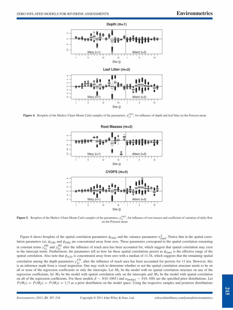
Figure 4 shows the boxplots of the MCMC samples of � .m/ij for the influence of depth (m D 1) and leaf litter (m D 2). Notice that for

many of the sites, the posterior distribution for � .m/ij is concentrated away from zero, indicating statistical significance. Furthermore, there

is considerable variation among the � .m/ij across the sites, suggesting that the relationship between depth and leaf litter to mean abundancevaries across the sites. Another important note is that the relationships seem to be more consistent in the Albert River than the Mary. Theboxplots for leaf litter for the Albert River look more similar indicating very little variation in the relationship between Leaf litter and thePoisson mean across the catchment. In contrast, the Mary river appears to have wide variation in the relationships between depth and leaflitter and the Poisson mean. Such spatial variation in these relationships could be caused by unmeasured spatial variation in site hydraulics,which may regulate leaf litter deposition.

Figure 5 shows the boxplots for the MCMC samples of � .m/ij parameters, which govern the relationship between root masses (mD 3) andCVDFS (mD 4) on the Poisson mean. Notice that most of the CVDFS coefficient boxplots contain zero, indicating that CVDFS may not besignificant at that site. Furthermore, notice that the coefficients for root masses vary across sites, however, is generally negative except forsites 7 and 12 in the Mary river. This indicates that a higher abundance of root masses is associated with a reduced abundance of H. galii.This overall negative trend may suggest that root masses are not the preferred habitat for H. galii. However, sites 7 and 12 are relativelyshallow, which may make root masses more suitable habitat. Again, the coefficients for root masses tend to be less variable and near thesame value for the Albert River than for the Mary River.

With this model, one can compare the relationships between two sites. By simply differencing the parameters of interest, one can obtainan approximation of the posterior distribution for the difference. If the difference includes zero, then the relationships at the two sites are notdifferent from each other, otherwise we can conclude they are different. In the introduction, sites 4 and 17 in the Mary river were considered

as they seemed to exhibit differing behaviour patterns with respect to depth. By creating a new variable � 0 D � .1/1;17 � �.1/1;4 the difference

in these relationships can be found. The 2.5%, 50% and 97.5% interval for � 0 is (�12.3612, �8.7805, �5.4916), which does not containzero. Hence, the influence of depth differs between sites 4 and 17 in the Mary river.

Table 2 shows the posterior quantiles of the MCMC samples and OR for the !.u/i.m/

parameters, which show how reach area influences thelower level variables depth, leaf litter, root masses and CVDFS by river. Intervals that are in bold do not contain zero suggesting that theparameters are statistically significant from zero. This shows that reach area influences both the model intercept and how root masses effectabundance in both rivers. The influence of reach area on the intercept corresponds to the direct effect of this variable on abundance andshows that, as expected, abundance increases with reach area. Furthermore, notice that the influence of reach area on root masses is negativeindicating that the larger the reach area, the effect of root masses on abundance is reduced.

Table 1. Posterior quantiles and OR values for the MCMC samples of the parameter ˇ,which relates ELEV and MDFLOW to presence/absence. Here, Q0:025, Q0:5 and Q0:975correspond to the 2.5%, 50% and 97.5% posterior quantiles, respectively

Log odds ratio Odds ratio

Term Q0:025 Q0:5 Q0:975 Q0:025 Q0:5 Q0:975 OR

Intercept 0.7180 1.0689 1.4630 2.0503 2.9122 4.3190 1.0007MDFLOW �1.1833 �0.6239 �0.1058 0.3062 0.5358 0.8995 1.0084ELEV 0.1260 0.6044 1.1161 1.1343 1.8301 3.0531 1.0008

MCMC, Markov Chain Monte Carlo; MDFLOW, mean daily flow; ELEV, elevation

214



Figure 4. Boxplots of the Markov Chain Monte Carlo samples of the parameters, �.m/ij

, for influence of depth and leaf litter on the Poisson mean

Figure 5. Boxplots of the Markov Chain Monte Carlo samples of the parameters, �.m/ij

, for influence of root masses and coefficient of variation of daily flowon the Poisson mean

Figure 6 shows boxplots of the spatial correlation parameters �i.m/ and the variance parameters �2i.m/

. Notice that in the spatial corre-lation parameters (a), �1.0/ and �2.0/ are concentrated away from zero. These parameters correspond to the spatial correlation remaining

in constant terms � .0/1j and � .0/2j after the influence of reach area has been accounted for, which suggest that spatial correlation may existin the intercept terms. Furthermore, the parameters tell us how far these spatial correlations persist as �i.m/ is the effective range of thespatial correlation. Also note that �1.3/ is concentrated away from zero with a median of 11.34, which suggests that the remaining spatial

correlation among the depth parameters � .3/1j , after the influence of reach area has been accounted for persists for 11 km. However, thisis an inference made from a visual inspection. One may wish to determine whether or not the spatial correlation structure needs to be onall or none of the regression coefficients or only the intercepts. Let M1 be the model with no spatial correlation structure on any of theregression coefficients, let M2 be the model with spatial correlation only on the intercepts and M3 be the model with spatial correlationon all of the regression coefficients. For these models ˇ � N.0; 100I / and a.m/.u/ � N.0; 100/ are the specified prior distributions. LetP.M1/ D P.M2/ D P.M3/ D 1=3 as a prior distribution on the model space. Using the respective samples and posterior distributions


215


Table 2. Posterior quantiles and OR values for the MCMC samples of the parameters, !i.m/, which relatehow reach area influences depth, leaf litter, root masses and CVDFS’s effect on abundance for the Maryand Albert rivers. Intervals in bold do not contain zero. Here, Q0:025, Q0:5 and Q0:975 correspond tothe 2.5%, 50% and 97.5% posterior quantiles, respectively

Variable Intercept .uD 0/ OR Reach area .uD 1/ OR

Mary Intercept (�2.4610, �0.3428, 1.7794) 1.0048 (0.0004, 0.0025, 0.0049) 1.0027Depth (�1.5608, 0.9256, 3.4497) 1.0045 (�0.0081, �0.0032, 0.0013) 1.0125Leaf litter (�1.2252, 1.2107, 3.6856) 1.0007 (�0.0064, �0.0016, 0.0023) 1.0622Root masses (�3.7554, �1.0827, 1.6307) 1.0246 (�0.0159, �0.0089, �0.0018) 1.0091CVDFS (�1.1930, 0.2203, 1.4419) 1.0401 (�0.0005, �0.0001, 0.0001) 1.0086

Albert Intercept (�2.4367, �0.2148, 1.7117) 1.0039 (0.0008, 0.0043, 0.0068) 1.0013Depth (�1.8537, 0.4869, 2.9892) 1.0002 (�0.0053, �0.0016, 0.0018) 1.0134Leaf litter (�1.2001, 1.2415, 3.6224) 1.0213 (�0.0082, �0.0047, 0.0005) 1.0012Root masses (�7.5551, �2.0178, 0.8744) 1.0214 (�0.0203, �0.0115, �0.0019) 1.013CVDFS (�1.9569, �0.1190, 1.6592) 1.0158 (�0.0005, 0.0001, 0.0006) 1.0175

MCMC, Markov Chain Monte Carlo; CVDFS, coefficient of variation of daily flow

Figure 6. Boxplots of the Markov Chain Monte Carlo samples of the (a) variance parameters �2i.m/

and (b) spatial correlation parameters �i.m/

p.DjMi /DRp.�i jMi /p.Dj�i ;Mi /d�i is approximated numerically using Monte Carlo integration. This gives P.M1/� 1, P.M2/� 0

and P.M3/� 0. Based on this model, M1 would be the clear choice because the posterior model probability is near one. This implies thatspatial correlation among the parameters after removing the effect of site area is not needed.

Once again, because there were only two rivers under consideration, the a.m/.u/ parameters, which average the regional relationships,inferences should not be made about these parameters. However, in the case of more rivers, these parameters may prove useful for makinginferences about ecological relationships.

For this dataset, using 100 hold out samples and using Equation (1), 80% of the X2 values fell above �228;0:95 D 41:33, indicating thatthe hold out samples have more variation than the model would suggest. Hence, this model should not be used for prediction. However, itmay be used to understand the relationships between the abundance of H. galii and the environmental and habitat variables.

For this dataset, one specific hypothesis of interest is whether or not CVDFS needs to be in the model. Because it is a measurementthat exists at a different time, it is debatable whether or not it should be included in the model. So, let M1 be the full model as describedearlier, and let M2 be the model with CVDFS removed. By removing this variable, it is removed for all sites and hence M2 has consider-ably fewer parameters than does the full model. Model M2 was estimated using the same procedure as described earlier. For these models,ˇ � N.0; 100I / and a.m/.u/ � N.0; 100/ are the specified prior distributions. Let P.M1/ D 1=2 and P.M2/ D 1=2. Using the respectivesamples and posterior distributions, p.DjMi / D

Rp.�i jMi /p.Dj�i ;Mi /d�i is approximated numerically using Monte Carlo integration.216



This gives P.M1/� 0 and P.M2/� 1. Based on this model, M2 would be the clear choice because the posterior model probability is nearone. This implies that CVDFS is not a significant contributor to model fit.

To determine if the model inferences were sensitive to prior distribution specification, a similar analysis was conducted using ˇ �N.0; 10I / with a.m/.u/ � N.0; 10/ and ˇ � N.0; I / with a.m/.u/ � N.0; 1/. For all of these inferences, using these prior distributionspecifications and Equation (2) and posterior model probabilities, none of the inferences were sensitive to prior distribution specification.

4. CONCLUSIONS AND DISCUSSIONIn this paper, we have presented a model that deals with three common problems in ecology in general and freshwater ecology in particular.The model incorporates the hierarchical structure that exists in riverine landscapes by allowing for site specific ecological relationships. Itaccounts for spatial autocorrelation that may exist in the relationships between a species and its environment, and it accounts for the occur-rence of a larger number of zeroes than the standard Poisson distribution can incorporate. Accounting for these three issues contributes toimproved understanding of species–environment relationships in complex ecological datasets.

It has been hypothesised that two separate mechanisms regulate the presence or absence and the abundance of a fish species at a givensite. The probability of the presence or absence of a fish species at a given location may be caused by a range of large scale factors such aselevation, climate and flow regime, whereas its abundance may be more directly affected by local level variables that vary at a finer spatialand temporal resolution (Kennard et al. 2007; Rahel 1990). The model presented provides estimates of the probability of the presence ofH. galii given two time-invariant landscape-level factors, elevation and mean daily flow. Subsequent levels of the model provide estimatesof the abundance of H. galii given local level variables that vary in time and space, thus matching the hypothesised hierarchical nature ofprocesses regulating fish populations. Although not conclusive, the results do lend support to this hypothesis. The probability of presence ofH. galii does vary along with landscape scale predictors, whereas the abundance shows a strong relationship to local scale predictors. Furtherresearch involving comparisons of this and other statistical model structures and combinations of predictor variables will help ecologistsunderstand the nature of processes regulating fish species abundance.

Structural microhabitat has been shown to be an important factor in regulating stream fish assemblages (Grossman et al. 1998). However,these relationships may be obscured where specific aspects of microhabitat also vary with landscape-level variables (Jackson et al. 2001), orwhere they are scale dependent (Angermeier and Winston 1998). The model we have developed can be used to identify species–environmentrelationships where this is the case. It also identifies when landscape scale predictors that do not vary in time may influence the local scalespecies–environment relationships. Table 2 shows the scale dependence of the relationship between H. galii abundance and local level micro-habitat variables, that is the effect of reach area on these relationships. This indicates that the apparent influence of root masses decreaseswith reach area in both rivers. Increases in reach area are generally associated with wider streams (unpublished data) where the area of rootmasses (percent lineal extent of stream bank) is smaller as a proportion of total wetted habitat. An additional feature of the model is that, itquantifies the extent of residual spatial autocorrelation that may be present in these local-scale species–environment relationships. This maybe useful where local-scale species–environment relationships are observed to vary across the landscape, and the cause of this is uncertain(e.g. Figure 3; Torgersen et al. 2006). This may also be useful in reducing bias in the site level estimates that may arise because of anyunquantified spatial correlation.

It is relatively common that models developed in one catchment are not transferable to other catchments, suggesting potentially differentspecies–environment relationships in space (Fausch et al. 1988; Leftwich et al. 1997; Kennard et al. 2007). This poses a problem whendeveloping general ecological principles that may govern species distribution particularly if these principles are used in ecological manage-ment. The model we presented in this paper provides estimates of ecological relationships at a regional level, that is across both rivers, aswell as relationships specific to each river and to each site. Figures 2 and 3 illustrate the variation in the posterior distributions for parame-ters affecting species abundance at each site. Although generally consistent across the two catchments, the relationship between abundanceand leaf litter and depth do vary from site to site. Identifying and quantifying this spatial variation in ecological relationships can help tounderstand how different mechanisms may structure local fish populations in different catchments and sub-catchments potentially leading toimproved river management decisions.

REFERENCES

Aitchison J. 1955. On the distribution of a positive random variable having a discrete probability mass at the origin. Journal of the American StatisticalAssociation 50: 901–908.

Agarwal DK, Gelfand AD, Citron-Pousty S. 2002. Zero-inflated models with application to spatial count data. Environmental and Ecological Statistics 9:341–355.

Ahmadi-Nedushan B, St. Hilaire A, Bérubé M, Robichaud É, Thiémonge N, Bobée B. 2006. A review of statistical methods for the evaluation of aquatichabitat suitability for instream flow assessment. River Research and Applications 22: 503–523.

Angermeier PL, Winston MR. 1998. Local vs. regional influences on local diversity in stream fish communities of Virginia. Ecology 79: 911–927.Ballinger A, Mac Nally R, Lake PS. 2005. Immediate and longer-term effects of managed flooding on floodplain invertebrate assemblages in south-eastern

Australia: generation and maintenance of a mosaic landscape. Freshwater Biology 50: 1190–1205.Beckmann MC, Scholl F, Matthaei CD. 2005. Effects of increased flow in the main stem of the River Rhine on the invertebrate communities of its tributaries.

Freshwater Biology 50: 10–26.Berger JO. 1993. Statistical Decision Theory and Bayesian Analysis. Springer: New York.Böhning D, Dietz E, Schlattmann P, Mendonça L, Kirchner U. 1999. The zero-inflated Poisson model and the decayed, missing and filled teeth index in dental

epidemiology. Journal of the Royal Statistical Society, Series A 162: 195–209.Boone EL, Ye K, Smith EP. 2005. Evaluating the relationship between ecological and habitat conditions using hierarchical models. Journal of Agricultural,

Biological and Environmental Statistics 10: 131–147.


217


Boyero L, Bailey RC. 2001. Organization of macroinvertebrate communities at a hierarchy of spatial scales in a tropical stream. Hydrobiologia 464: 219–225.Cressie N. 1993. Statistics for Spatial Data. Wiley-Interscience: New York.Cressie N, Calder CA, Clark JS, Ver Hoef JM, Wikle CK. 2009. Accounting for uncertainty in ecological analysis: the strengths and limitations of hierarchical

statistical modeling. Ecology Letters 19: 553–570.Dobbie MJ, Welsh AH. 2001. Modelling correlated zero-inflated count data. Australian and New Zealand Journal of Statistics 43: 431–444.Fausch KD, Hawkes CL, Parsons MG. 1988. Models that predict standing crop of stream fish habitat variables: 1950–85. USDA Forest Service, General

Technical Report PNW-GTR-213, Portland, OR.Fausch KD, Torgersen CE, Baxter CV, Li HW. 2002. Landscapes to riverscapes: bridging the gap between research and conservation of stream fishes.

Bioscience 52: 483–498.Frissell CA, Liss WJ, Warren CE, Hurley MD. 1986. A hierarchical framework for stream habitat classification: viewing streams in a watershed context.

Environmental Management 10: 199–214.Gelman A, Carlin JB, Stern HS, Rubin DB. 2005. Bayesian Data Analysis. Chapman Hall and CRC Press: Boca Raton, FL.Gelman A, Hill J. 2007. Data Analysis Using Regression and Multilevel/Hiearchical Models. Cambridge University Press: Cambridge, UK.Gilmore R. 2008. The Upper Murrumbidgee IQQM calibration report. A report to the Australian Government from the CSIRO Murray-Darling Basin

Sustainable Yields Project, CSIRO Australia, 19 pages.Gray BR, Haro RJ, Rogala JT, Sauer JS. 2005. Modelling habitat associations with fingernail clam (Family: Sphaeriidae) counts at multiple spatial scales

using hierarchical count models. Freshwater Biology 50: 715–729.Grossman GD, Ratajczak RE, Crawford M, Freeman MC. 1998. Assemblage organization in stream fishes: effects of environmental variation and interspecific

interactions. Ecological Applications 68: 395–420.Guisan A, Zimmerman NE. 2000. Predictive habitat distribution models in ecology. Ecological Modelling 135: 147–186.Hall DB. 2000. Zero-inflated Poisson and binomial regression with random effects: a case study. Biometrics 56: 1030–1039.Heino J, Louhi P, Muotka T. 2004. Identifying the scales of variability in stream macroinvertebrate abundance, functional composition and assemblage

structure. Freshwater Biology 49: 1230–1239.Jackson DA, Peres-Neto PR, Olden JD. 2001. What controls who is where in freshwater fish communities—the roles of biotic, abiotic, and spatial factors.

Canadian Journal of Fisheries and Aquatic Sciences 58: 157–170.Junk WJ, Bayley PB, Sparks RE. 1989. The flood-pulse concept in river-floodplain systems. Canadian Special Publications in Fisheries and Aquatic Science

106: 110–127.Karr JR. 1999. Defining and measuring river health. Freshwater Biology 41: 221–234.Kennard MJ, Pusey BJ, Harch BD, Dore E, Arthington AH. 2006. Estimating local stream fish assemblage attributes: sampling effort and efficiency at two

spatial scales. Marine and Freshwater Research 57: 635–653.Kennard MJ, Olden JD, Arthington AH, Pusey BJ, Poff NL. 2007. Multiscale effects of flow regime and habitat and their interaction on fish assemblage

structure in eastern Australia. Canadian Journal of Fisheries and Aquatic Sciences 64: 1346–1359.Kennard MJ, Pusey BJ, Olden JD, Mackay SJ, Stein JL, Marsh N. 2010. Classification of natural flow regimes in Australia to support environmental flow

management. Freshwater Biology 55: 171–193.Lambert D. 1992. Zero-inflated Poisson regression, with an application to defects in manufacturing. Technometrics 34: 1–14.Lee AH, Wang K, Yau KKW. 2001. Analysis of zero-inflated Poisson data incorporating extent of exposure. Biometrical Journal 43: 963–975.Leftwich KN, Angermeier PL, Dolloff CA. 1997. Factors influencing behavior and transferability of habitat models for a benthic stream fish. Transactions of

the American Fisheries Society 126: 725–734.Levin SA. 1992. The problem of pattern and scale in ecology: the Robert H. MacArthur award lecture. Ecology 73: 1943–1967.Li J, Herlihy A, Gerth W, Kaufmann P, Gregory S, Urquhart S, Larsen DP. 2001. Variability in stream macroinvertebrates at multiple spatial scales. Freshwater

Biology 46: 87–97.Lowe WH, Likens GE, Power ME. 2006. Linking scales in stream ecology. Bioscience 56: 591–597.Magalhães MF, Beja P, Canas C, Collares-Pereira MJ. 2002. Functional heterogeneity of dry-season fish refugia across a Mediterranean catchment: the role

of habitat and predation. Freshwater Biology 47: 1919–1934.Maloney KO, Dodd HR, Butler SE, Wahl DH. 2008. Changes in macroinvertebrate and fish assemblages in a medium-sized river following a breach of a

low-head dam. Freshwater Biology 53: 1055–1068.Martin TG, Wintle BA, Rhodes JR, Kuhnert PM, Field SA, Low-Choy SJ, Tyre AJ, Possingham HP. 2005. Zero tolerance ecology: improving ecological

inference by modelling the source of zero observations. Ecology Letters 8: 1235–1246.McGarvey DJ, Ward GM. 2008. Scale dependence in the species-discharge relationship for fishes of the southeastern USA. Freshwater Biology 53: 2206–2219.Olden JD, Jackson DA. 2002. A comparison of statistical approaches for modelling fish species distributions. Freshwater Biology 47: 1976–1995.Poff NL. 1997. Landscape filters and species traits: towards mechanistic understanding and prediction in stream ecology. Journal of the North American

Benthological Society 16: 391–409.Pusey BJ, Kennard MJ, Arthington AH. 2004. Freshwater Fishes of North-Eastern Australia. CSIRO Publishing: Collingwood.Rahel FJ. 1990. The hierarchical nature community persistence: a problem of scale. American Naturalist 136: 328–344.Raudenbush SW, Bryk AS. 2002. Hierarchical Linear Models: Applications and Data Analysis Methods. Sage Publications: Thousand Oaks, CA.Robson BJ, Hogan M, Forrester T. 2005. Hierarchical patterns of invertebrate assemblage structure in stony upland streams change with time and flow

permanence. Freshwater Biology 50: 944–953.Sandel B, Smith AB. 2009. Scale as a lurking factor: incorporating scale-dependence in experimental ecology. Oikos 118: 1284–1291.Santoul F, Mengin N, Céréghino R, Figuerola J, Mastrorillo S. 2005. Environmental factors influencing the regional distribution and local density of a small

benthic fish: the stoneloach (Barbatula barbatula). Hydrobiologia 544: 347–355.Simons M, Podger G, Cook R. 1996. A hydrologic modelling tool for water resources and salinity management. Environmental Software 11: 185–192.Stewart-Koster B, Kennard MJ, Harch BD, Sheldon F, Arthington AH, Pusey BJ. 2007. Partitioning the variation in stream fish assemblages within a

spatio-temporal hierarchy. Marine and Freshwater Research 58: 675–686.Torgersen CE, Baxter CV, Li HW, McIntosh BA. 2006. Landscape influences on longitudinal patterns of river fishes: spatially continuous analysis of

fish-habitat relationships. American Fisheries Society Symposium 48: 473–492.Ver Hoef JM, Jansen JK. 2007. Space–time zero-inflated count models of Harbor seals. Environmetrics 18: 697–712.Ver Hoef JM, Peterson EE. 2010. A moving average approach for spatial statistical models of stream networks. Journal of the American Statistical Association

105: 6–18.White JL, Harvey BC. 2001. Effects of an introduced piscivorous fish on native benthic fishes in a coastal river. Freshwater Biology 46: 987–995.Zuur AF, Ieno EN, Smith GM. 2007. Analysing ecological data. Springer: New York.

218


A hierarchical zero-inflated Poisson regression model for stream fish distribution and abundance

Documents

Transcript of A hierarchical zero-inflated Poisson regression model for stream fish distribution and abundance