A Spatial Filtering Zero Inflated Approach to the Estimation of the Gravity Model of Trade

A Spatial Filtering Zero-InflatedApproach to the Estimation of the

Gravity Model of Trade

Rodolfo Metulini, Roberto Patuelli, Daniel A. Griffith

ETSG 2015 - Paris

September 12, 2015

Contents

1 Introduction

2 Gravity of Trade review

3 Methodology

4 Empirical Application

5 Conclusion and future directions

6 Appendix

ETSG 2015 - Paris 1/21

Introduction

I Non-linear estimation of the gravity model with PPML/ZIPMLmethods has become popular to model the international trade flows,as it permits to better account for large amount of zero flows

I Trade flows are not independent from each other due to spatialinteraction. To overcome this problem, the eigenvector spatialfiltering variants of the Poisson/Negative binomial (among variousmethods) has been proposed in the literature and is used here.

This paper contributes to the literature in two directions:

I First, by employing a stepwise selection criteria for spatialfilters based on robust (sandwich) p-values.

I Second, by selecting a reduced set of spatial filters thatproperly account for importer-side and exporter-side specificspatial effects, at both stages of the process.

Introduction ETSG 2015 - Paris 2/21

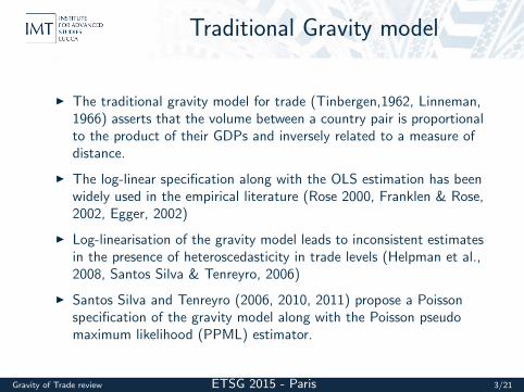
Traditional Gravity model

I The traditional gravity model for trade (Tinbergen,1962, Linneman,1966) asserts that the volume between a country pair is proportionalto the product of their GDPs and inversely related to a measure ofdistance.

I The log-linear specification along with the OLS estimation has beenwidely used in the empirical literature (Rose 2000, Franklen & Rose,2002, Egger, 2002)

I Log-linearisation of the gravity model leads to inconsistent estimatesin the presence of heteroscedasticity in trade levels (Helpman et al.,2008, Santos Silva & Tenreyro, 2006)

I Santos Silva and Tenreyro (2006, 2010, 2011) propose a Poissonspecification of the gravity model along with the Poisson pseudomaximum likelihood (PPML) estimator.

Gravity of Trade review ETSG 2015 - Paris 3/21

Recent developments

We can roughly divide the available literature on incorporating spatialdependence and heterogeneity or network autocorrelation in gravitymodels into three main streams:

I Linear spatial econometric models (Baltagi et al. 2007; Fischerand Griffith 2008; LeSage and Pace 2008; Behrens et al. 2012;Koch and LeSage 2015): these models apply and adapt traditional(linear) spatial econometric techiques to the count data case bylog-linearisation.

I Spatial generalized linear models (Lambert et al. 2010; Sellner etal. 2013): these models extend the previous approaches by allowingfor estimation based on Poisson-type models, accommodating theconcerns expressed in Santos Silva and Tenreyro (2006).

I Non-parametric (eigenvector spatial filtering) models(Chun2008; Fischer and Griffith 2008; Scherngell and Lata 2013; Krisztinand Fischer 2015; Patuelli et al. 2015): these models take anon-parametric approach, by employing eigenvector spatial filteringwithin Poisson-type models.

Gravity of Trade review ETSG 2015 - Paris 4/21

Zero inflated gravity models of trade

I The ZINB ML gravity model provides a way to model gravity whenthe data generating process results in too many zeros (Martin andPham, 2008, Burger et al., 2009, among others).

I Estimating the parameters by Poisson/Negative binomial MLmethods would only be justified statistically if we believed that thetrade flows were independent observations. Such an assumption isgenerally not valid: flows are spatially interconnected in nature.

I Several papers recently proposed to model spatial heterogeneity inthe residuals by means of the three above-mentioned econometrictechniques:

(many focused on MTR, which can be considered as a main source ofspatial heterogeneity: Behrens et al. 2012, Baier & Bergstrand 2009).

I Our approach implement eigenvector spatial filters to account forspatial heterogeneity in a ZINB ML framework, adopting ad ad-hocbackward stepwise algorithm to proper selecting the signficantspatial filters.

Methodology ETSG 2015 - Paris 5/21

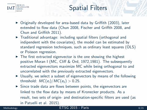
Spatial Filters

I Originally developed for area-based data by Griffith (2003), laterextended to flow data (Chun 2008, Fischer and Griffth 2008, andChun and Griffith 2011).

I Traditional advantage: including spatial filters (orthogonal andindipendent with the covariates), the model can be estimated bystandard regression techniques, such as ordinary least squares (OLS)or Poisson regression.

I The first extracted eigenvector is the one showing the highestpositive Moran I (MC, Cliff & Ord, 1972,1981). The subsequentlyextracted eigenvectors maximize MC while being orthogonal to anduncorrelated with the previously extracted eigenvectors.

I Usually, we select a subset of eigenvectors by means of the followingthreshold: MC (ei )/MC (e1) > 0.25.

I Since trade data are flows between points, the eigenvectors are

linked to the flow data by means of Kronecker products. As a

result, two sets of origin- and destination-specific filters are used (as

in Patuelli et al. 2015).Methodology ETSG 2015 - Paris 6/21

Backward stepwise algorithm

I Used to select variables in a regression model (proposed byEfroymson, 1960)

I Usually, this takes the form of a sequence of F-tests or t-tests, butother techniques are possible, such as adjusted R-square, AIC,Bayesian information criterion (BIC), or simply based on p-values.

I Backward elimination: involves starting with all candidate variables,testing the deletion of each variable, deleting the variable (if any)that improves the model the most by being deleted, and repeatingthis process until no further improvement is possible.

I Backward elimination procedure in the framework of count models

and zero inflated count models has been implemented in many

routines. In R, the be.zeroinfl (mpath, Wang et al. 2015) function

performs a backward elimination (and forward selection) stepwise

based on log likelihood.

Methodology ETSG 2015 - Paris 7/21

Model specification

I For estimation, we follow a standard specification of the gravityequation of bilateral trade.

I We employ some variables commonly mentioned in the literature(see, e.g., Frankel 1997; Raballand 2003).

I We use the following standard specification of the gravity equation

and we estimate it, after a proper over-dispersion test, by mean of a

Zero inflated negative binomial (ZINB) maximum likelihood:

Empirical Application ETSG 2015 - Paris 8/21

Data

I The trade data are from the World Trade Database compiled on thebasis of COMTRADE data by Feenstra et al. (2005).

I GDP and per capita GDP data are from the World Banks WDIdatabase.

I Distance, language, colonial history, landlocked countries, and landarea data are from the CEPII institute.

I Whether pairs of countries take part in a common regionalintegration agreement (FTA) has been determined on the basis ofOECD data about major regional integration agreements.

I Data on island status have been kindly provided by Hildegunn

Kyvik-Nordas (from Jansen and Nords 2004).


Details on Spatial Filters

I We extract n eigenvectors e1, e2, en from I−ii t

n W I−ii t

n , where W isthe nearest neighbours weight matrix.

I We only select, as candidate eigenvectors, the ones withMC (ei )/MC (e1) > 0.25.

I We link those candidate eigenvectors to the flow data by means ofKronecker products.

I We include those candidates among the covariates in the regression

model.


Details on stepwise algorithm

I We modified the be.zeroinfl function from mpath package (Wang etal. 2015.

I This function performs a backward stepwise on a zero inflatedmodel, and it uses p-values as a model choice criteria.

I In each step, the function drops the variable with the largest p-value,indifferently of whether the variable is in the count (2nd step) or inthe logit (1st step) part of the model. This stepwise process endsup when no more non significant variables are considered.

I We want to preserve all the non spatial variables as we consider

them as benchmark: we set those variables as fixed, even if their

estimated coefficient is not significant.


Estimation results - I

I Our model specification, based on different diagnostics, seems tooutperforms the benchmark models (Spat filt NB ML and ZINB MLwithout filters). We based these diagnostics on Akaike informationcriteria and on the loglikelihood.

I In terms of AIC (slide 12), our spatial filters ZINB ML model have asmaller value (47026.13), meaning it performs better than theothers (48370.13 for the ZINB, 48431.86 for the spatial filter NB).

I The same holds for the log likelihood: our model presents thesmaller value (-2.32e+04 compared to -2.42e+04 for both thebenchmark models).

I We compare the observed number of small flows with the estimated

counterpart using our selected model, the ZINB and the NB with

selected filters (slides 13 and 14): Spatial filtering ZINB predict 92

out of 484 zero flows, while Spatial Filters NB predict 19 zero flows,

and ZINB without filters only predict 2 zero flows.


Estimation results - II

Table: Estimation results (1) ZINB ML with spatial filters (2) ZINB ML(3) NB ML with spatial filters. (1st step coeffs dropped here due to lack of space)

2nd step: count (1) (2) (3)Distance -0.84*** -0.65*** -0.71***

Common language 0.46*** 0.37*** 0.44***Contiguity 0.54*** 0.71*** 0.65***

Common history 0.77*** 0.57*** 0.81***Free trade agreements 0.48*** 0.66*** 0.75***

Area exporter -0.20*** -0.25*** -0.22***Area importer 0.07*** -0.02 -0.04*

GDP per cap. exporter -0.24*** -0.26*** -0.13***GDP per cap. importer 0.16*** 0.02 -0.12***

GDP exporter 1.06*** 1.10*** 0.99***GDP importer 0.63*** 0.75*** 0.82***

Island exporter 0.43*** 0.55*** 0.30*Island importer -0.70*** -0.16 0.02

Landlocked exporter -0.21*** -0.09 -0.44***Landlocked importer 0.32*** -0.18* 0.35***

Costant -28.71 -30.93 -29.8# selected filters 1st step - exporter 11 - -# selected filters 1st step - importer 24 - -# selected filters 2nd step - exporter 11 - 8# selected filters 2nd step - importer 8 - 12

Theta 0.859 0.726 0.595AIC 47026.13 48370.13 48431.86

Log likelihood -2.32E+04 -2.42E+04 -2.42E+04Observations 4032 4032 4032


Estimation results- III

Table: Count of observed versus predicted values. Model comparison

Trade flow 0 1 2 3 4 5 6 7 8 9

Observed 484 136 112 76 64 39 42 49 35 29

Spat Filt ZINB 92 59 46 42 46 39 45 34 31 38

ZINB 2 22 23 31 31 37 32 33 26 29Spat filt NB 19 42 39 45 44 35 37 41 35 38


Estimation results- IV

Figure: Estimated probability of trade for non-zero trade flowsobservations. ZINB (red) vs. Spat Filt ZINB (black)


Estimation results- V

Figure: Mapped spatial filters (all selected filters weighted by the model coefficients).

Top-left: 2st step exporters (Moran I: 0.046. Selected filters: 11)Top-right: 2nd step importers (Moran I: 0.160**. Selected filters: 8)Bottom-left: 1st step exporters (Moran I: 0.298***. Selected filters: 11)Bottom-right: 1st step - importers (Moran I: 0.036. Selected filters: 24)


Conclusions

I We employ a backward stepwise selection criteria for spatial filteringZINB ML, based on robust p-values.

I Second, we select a reduced set of spatial filters that properlyaccount for importer-side and exporter-side specific spatial effects,both at the count and the logit process.

I Results highlighted that our specification outperforms the

benchmark models (ZINB and NB with spatial filters), in terms of

model fitting, both considering the AIC and the log likelihood, and

in predicting non zero (and small) flows.

Conclusion and future directions ETSG 2015 - Paris 17/21

Future directions

I Future research directions include comparing this model with otherZINB ML model specifications that alternatively account for SAC(Spatial generalized linear models, as in Lambert et al. 2010,Sellner et al. 2013).

I A caveat regards evaluating the contribution of the logit and thecount part of the process, in terms of the explained variance oftrade flows.

I Moreover, a similar analysis, making appropriate changes, can be

applied to a panel data framework.

Conclusion and future directions ETSG 2015 - Paris 18/21

Main references

I Patuelli R, Linders G-J, Metulini R, Griffith DA (2015) The Space ofGravity: Spatial Filtering Estimation of a Gravity Model for BilateralTrade. In: Patuelli R, Arbia G (eds) Spatial Econometric InteractionModelling. Advances in Spatial Science. Springer, Berlin, p.(forthcoming)

I Krisztin T, Fischer MM (2015) The Gravity Model for InternationalTrade: Specification and Estimation Issues. Vienna University ofEconomics and Business, Vienna

I Zhu Wang, Shuangge Ma and Ching-Yun Wang (2015) Variable

selection for zero-inflated and overdispersed data with application to

health care demand in Germany, Biometrical Journal. Article first

published online June 8, 2015

Appendix ETSG 2015 - Paris 19/21

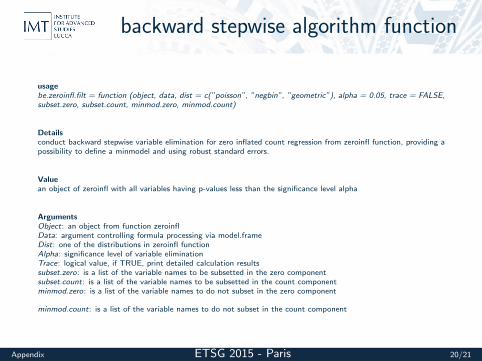
backward stepwise algorithm function

usagebe.zeroinfl.filt = function (object, data, dist = c(”poisson”, ”negbin”, ”geometric”), alpha = 0.05, trace = FALSE,subset.zero, subset.count, minmod.zero, minmod.count)

Detailsconduct backward stepwise variable elimination for zero inflated count regression from zeroinfl function, providing apossibility to define a minmodel and using robust standard errors.

Valuean object of zeroinfl with all variables having p-values less than the significance level alpha

ArgumentsObject: an object from function zeroinflData: argument controlling formula processing via model.frameDist: one of the distributions in zeroinfl functionAlpha: significance level of variable eliminationTrace: logical value, if TRUE, print detailed calculation resultssubset.zero: is a list of the variable names to be subsetted in the zero componentsubset.count: is a list of the variable names to be subsetted in the count componentminmod.zero: is a list of the variable names to do not subset in the zero component

minmod.count: is a list of the variable names to do not subset in the count component

Appendix ETSG 2015 - Paris 20/21

Thank you!

[email protected] ETSG 2015 - Paris 21/21

A Spatial Filtering Zero Inflated Approach to the Estimation of the Gravity Model of Trade

Documents

Transcript of A Spatial Filtering Zero Inflated Approach to the Estimation of the Gravity Model of Trade