A Bayesian hierarchical model for over-dispersed count data: a case study for abundance of hake...

ENVIRONMETRICS

Environmetrics 2007; 18: 27–53

Published online 12 June 2006 in Wiley InterScience (www.interscience.wiley.com). DOI: 10.1002/env.800

A Bayesian hierarchical model for over-dispersed count data:a case study for abundance of hake recruits

Jorge M. Mendes1, K. F. Turkman2*,y and Ernesto Jardim3

1Higher Institute of Statistics and Information Management, New University of Lisbon, Lisbon, Portugal2Faculty of Sciences, University of Lisbon, Lisbon, Portugal

3IPIMAR Lisbon, Portugal

SUMMARY

In this paper, we introduce a Bayesian Hierarchical model to estimate the abundance of hake recruits, as well as tostudy their spatial distributional patterns in the Portuguese territorial waters. Main objective of the paper is toimprove on traditional empirical methods based on sampling averages and variances by using probabilistic modelsthat capture spatial dependence structures. Copyright # 2006 John Wiley & Sons, Ltd.

key words: Bayesian hierarchical models; Gibbs sampling; MCMC; over-dispersed count data; hakerecruitment; abundance index

1. INTRODUCTION

In this paper, we introduce a probabilistic model to study spatial distribution patterns for over-

dispersed processes and apply it to hake recruits, estimating their abundance index in any given area.

There will be no attempt to study the time dynamics of these populations. Although, data covering the

whole Portuguese continental shelf are available, this study is restricted to the data covering the

northern shelf between Caminha and Berlengas, due to computational restrictions (data are described

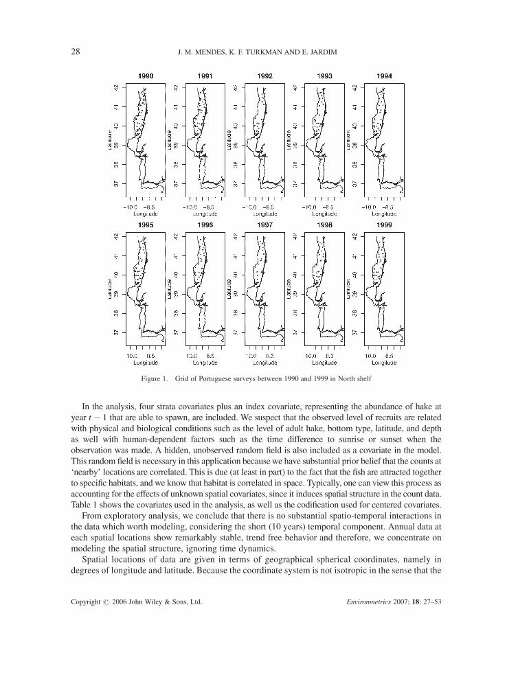
in detail in Section 2). Figure 1 shows the sampling grids used in this study.

The observed data contain an excessive number of zeros as well as some large, extreme values. For

example, the data set contains 99 zero counts out of 272 observations and the range, excluding the zero

counts, is 606. Due to the observed over-dispersion, the conventional Poisson model or its normal

approximation would not be suitable for this data set. Therefore, we explore a model specially adapted

to handle data whose over-dispersion comes from the excess of zeros as well as from heterogeneity of

the population.

*Correspondence to: K. F. Turkman, Faculty of Sciences, University of Lisbon, Lisbon, Portugal.yE-mail: [email protected]

Contract/grant sponsor: POCTI/MAT/44082/2002.

Received 13 October 2005

Copyright # 2006 John Wiley & Sons, Ltd. Accepted 16 April 2006

In the analysis, four strata covariates plus an index covariate, representing the abundance of hake at

year t � 1 that are able to spawn, are included. We suspect that the observed level of recruits are related

with physical and biological conditions such as the level of adult hake, bottom type, latitude, and depth

as well with human-dependent factors such as the time difference to sunrise or sunset when the

observation was made. A hidden, unobserved random field is also included as a covariate in the model.

This random field is necessary in this application becausewe have substantial prior belief that the counts at

‘nearby’ locations are correlated. This is due (at least in part) to the fact that the fish are attracted together

to specific habitats, and we know that habitat is correlated in space. Typically, one can view this process as

accounting for the effects of unknown spatial covariates, since it induces spatial structure in the count data.

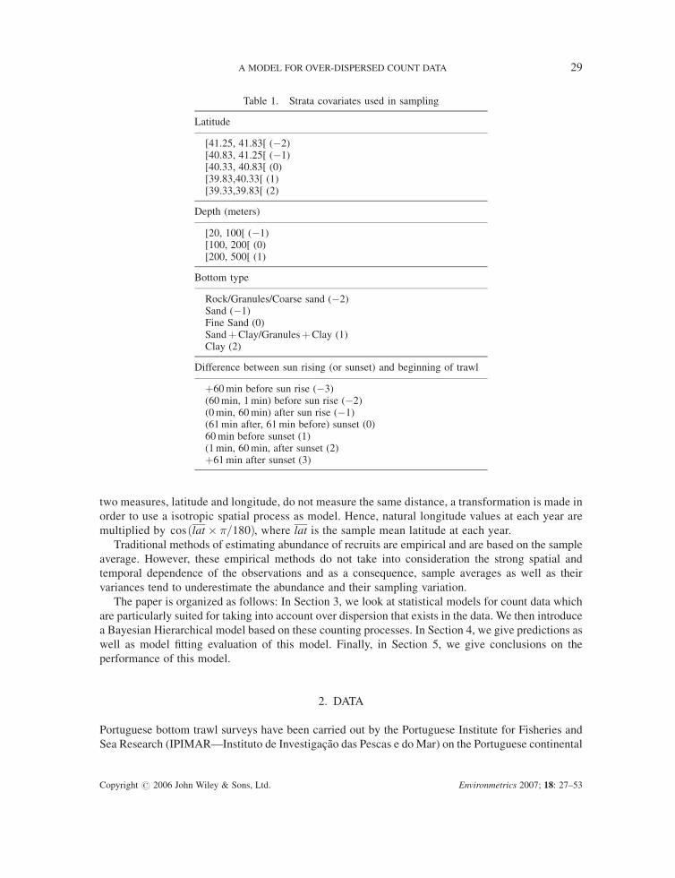
Table 1 shows the covariates used in the analysis, as well as the codification used for centered covariates.

From exploratory analysis, we conclude that there is no substantial spatio-temporal interactions in

the data which worth modeling, considering the short (10 years) temporal component. Annual data at

each spatial locations show remarkably stable, trend free behavior and therefore, we concentrate on

modeling the spatial structure, ignoring time dynamics.

Spatial locations of data are given in terms of geographical spherical coordinates, namely in

degrees of longitude and latitude. Because the coordinate system is not isotropic in the sense that the

Figure 1. Grid of Portuguese surveys between 1990 and 1999 in North shelf

28 J. M. MENDES, K. F. TURKMAN AND E. JARDIM

Copyright # 2006 John Wiley & Sons, Ltd. Environmetrics 2007; 18: 27–53

two measures, latitude and longitude, do not measure the same distance, a transformation is made in

order to use a isotropic spatial process as model. Hence, natural longitude values at each year are

multiplied by cosðlat � �=180Þ, where lat is the sample mean latitude at each year.

Traditional methods of estimating abundance of recruits are empirical and are based on the sample

average. However, these empirical methods do not take into consideration the strong spatial and

temporal dependence of the observations and as a consequence, sample averages as well as their

variances tend to underestimate the abundance and their sampling variation.

The paper is organized as follows: In Section 3, we look at statistical models for count data which

are particularly suited for taking into account over dispersion that exists in the data. We then introduce

a Bayesian Hierarchical model based on these counting processes. In Section 4, we give predictions as

well as model fitting evaluation of this model. Finally, in Section 5, we give conclusions on the

performance of this model.

2. DATA

Portuguese bottom trawl surveys have been carried out by the Portuguese Institute for Fisheries and

Sea Research (IPIMAR—Instituto de Investigacao das Pescas e do Mar) on the Portuguese continental

Table 1. Strata covariates used in sampling

Latitude

[41.25, 41.83[ (�2)[40.83, 41.25[ (�1)[40.33, 40.83[ (0)[39.83,40.33[ (1)[39.33,39.83[ (2)

Depth (meters)

[20, 100[ (�1)[100, 200[ (0)[200, 500[ (1)

Bottom type

Rock/Granules/Coarse sand (�2)Sand (�1)Fine Sand (0)SandþClay/GranulesþClay (1)Clay (2)

Difference between sun rising (or sunset) and beginning of trawl

þ60min before sun rise (�3)(60min, 1min) before sun rise (�2)(0min, 60min) after sun rise (�1)(61min after, 61min before) sunset (0)60min before sunset (1)(1min, 60min, after sunset (2)þ61min after sunset (3)

A MODEL FOR OVER-DISPERSED COUNT DATA 29


waters since June 1979 on board the R/V Noruega and R/V Capricrnio, twice a year in Summer and

Autumn. The main objectives of these surveys are: (i) to estimate indices of abundance and biomass of

the most important commercial species; (ii) to describe the spatial distribution of the most important

commercial species, (iii) to collect individual biological parameters such as maturity, sex-ratio,

weight, food habits, etc. (SESITS, 1999). The target species are hake (Merluccius merluccius), horse

mackerel (Trachurus trachurus), mackerel (Scomber scombrus), blue whiting (Micromessistius

poutassou), megrims (Lepidorhombus boscii and L. whiffiagonis), monkfish (Lophius budegassa

and L. piscatorius), and Norway lobster (Nephrops norvegicus). The gear used has been a Norwegian

Campbell Trawl 1800/96 (NCT) with a codend of 20mm mesh size, mean vertical opening of 4.8m,

and mean horizontal opening between wings of 15.6m (ICES, 2002).

The sampling design of these surveys follow a stratified random sampling design with 97

sampling locations distributed over 12 sectors. The sampling locations are fixed from year to year

and were selected based on historical records of clear tow positions and the allocation of at least

two samples by stratum. Each sector was subdivided into 4 depth ranges: 20–100, 101–200, 201–

500, and 501–750m, with a total of 48 strata. The tow duration during the period of analysis was

60min.

The data we have are the counts of recruits (individuals with age 0) in hauls of 60min

collected by the Autumn surveys from 1990 to 1999. The whole data set contains a total of 272

observations.

3. METHODS

3.1. Statistical models for count data

Typically, a Poisson model is assumed for modeling the count data. However, this model imposes

equal mean and variance to data, and fails to account for the over-dispersion that characterizes many

data sets. In many applications, the source of over-dispersion comes from the excess of zeros in the

data set. In the case of the Poisson model, one views a data set as zero inflated if there are more zeros

than the Poisson model can accommodate. If not properly modeled, the presence of excess zeros can

invalidate the distributional assumptions of the analysis, jeopardizing the integrity of the scientific

inferences (Lambert, 1992).

Over-dispersion can also be due to a heterogeneity in the population along with the excess of zeros.

In this case, the model should handle both of the problems.

Over-dispersed data can be modeled by the zero-inflated Poisson (ZIP) distribution (Johnson and

Kotz, 1962; Cohen, 1963), defined as follows:

Zi � 0; with probability piPoissonðliÞ; with probability 1� pi

�ð1Þ

so that

Zi ¼ 0; with probability pi þ ð1� piÞe�li

Zi ¼ z; with probability ð1� piÞe�li lzi

z! ; z > 0

(



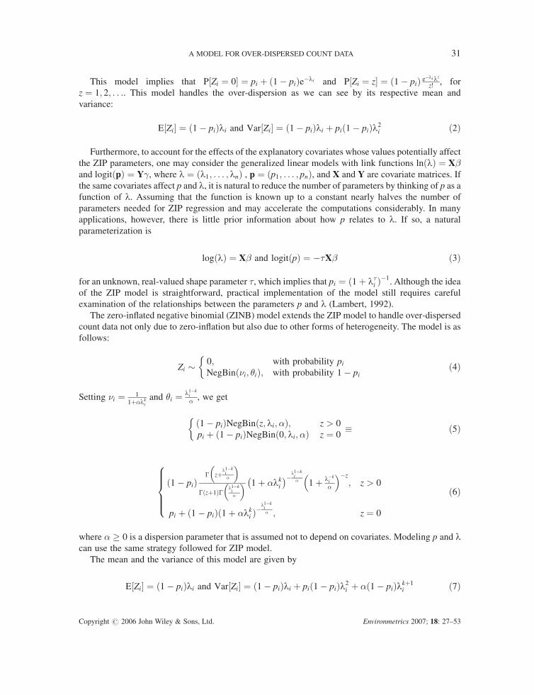
This model implies that P½Zi ¼ 0� ¼ pi þ ð1� piÞe�li and P½Zi ¼ z� ¼ ð1� piÞ e�lilz

z! , for

z ¼ 1; 2; . . .. This model handles the over-dispersion as we can see by its respective mean and

variance:

E½Zi� ¼ ð1� piÞli and Var½Zi� ¼ ð1� piÞli þ pið1� piÞl2i ð2Þ

Furthermore, to account for the effects of the explanatory covariates whose values potentially affect

the ZIP parameters, one may consider the generalized linear models with link functions lnðlÞ ¼ X�and logitðpÞ ¼ Y�, where l ¼ ðl1; . . . ; lnÞ , p ¼ ðp1; . . . ; pnÞ, and X and Y are covariate matrices. If

the same covariates affect p and l, it is natural to reduce the number of parameters by thinking of p as a

function of l. Assuming that the function is known up to a constant nearly halves the number of

parameters needed for ZIP regression and may accelerate the computations considerably. In many

applications, however, there is little prior information about how p relates to l. If so, a natural

parameterization is

logðlÞ ¼ X� and logitðpÞ ¼ ��X� ð3Þ

for an unknown, real-valued shape parameter �, which implies that pi ¼ ð1þ l�i Þ�1. Although the idea

of the ZIP model is straightforward, practical implementation of the model still requires careful

examination of the relationships between the parameters p and l (Lambert, 1992).

The zero-inflated negative binomial (ZINB) model extends the ZIP model to handle over-dispersed

count data not only due to zero-inflation but also due to other forms of heterogeneity. The model is as

follows:

Zi � 0; with probability piNegBinð�i; �iÞ; with probability 1� pi

�ð4Þ

Setting �i ¼ 11þ�lki

and �i ¼ l1�ki

� , we get

ð1� piÞNegBinðz; li; �Þ; z > 0

pi þ ð1� piÞNegBinð0; li; �Þ z ¼ 0

�� ð5Þ

ð1� piÞ� zþl1�k

i�

� ��ðzþ1Þ� l1�k

i�

� � 1þ �lki� ��l1�k

i� 1þ l�k

i

�

� ��z

; z > 0

pi þ ð1� piÞð1þ �lki Þ�l1�ki� ; z ¼ 0

8>>><>>>:

ð6Þ

where � � 0 is a dispersion parameter that is assumed not to depend on covariates. Modeling p and lcan use the same strategy followed for ZIP model.

The mean and the variance of this model are given by

E½Zi� ¼ ð1� piÞli and Var½Zi� ¼ ð1� piÞli þ pið1� piÞl2i þ �ð1� piÞlkþ1i ð7Þ



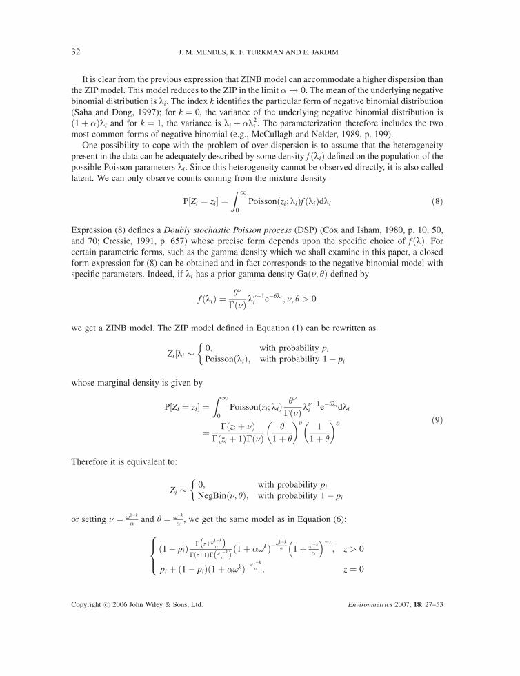
It is clear from the previous expression that ZINB model can accommodate a higher dispersion than

the ZIP model. This model reduces to the ZIP in the limit � ! 0. The mean of the underlying negative

binomial distribution is li. The index k identifies the particular form of negative binomial distribution

(Saha and Dong, 1997); for k ¼ 0, the variance of the underlying negative binomial distribution is

ð1þ �Þli and for k ¼ 1, the variance is li þ �l2i . The parameterization therefore includes the two

most common forms of negative binomial (e.g., McCullagh and Nelder, 1989, p. 199).

One possibility to cope with the problem of over-dispersion is to assume that the heterogeneity

present in the data can be adequately described by some density f ðliÞ defined on the population of thepossible Poisson parameters li. Since this heterogeneity cannot be observed directly, it is also called

latent. We can only observe counts coming from the mixture density

P½Zi ¼ zi� ¼Z 1

0

Poissonðzi; liÞf ðliÞdli ð8Þ

Expression (8) defines a Doubly stochastic Poisson process (DSP) (Cox and Isham, 1980, p. 10, 50,

and 70; Cressie, 1991, p. 657) whose precise form depends upon the specific choice of f ðlÞ. Forcertain parametric forms, such as the gamma density which we shall examine in this paper, a closed

form expression for (8) can be obtained and in fact corresponds to the negative binomial model with

specific parameters. Indeed, if li has a prior gamma density Gað�; �Þ defined by

f ðliÞ ¼ ��

�ð�Þ l��1i e��li ; �; � > 0

we get a ZINB model. The ZIP model defined in Equation (1) can be rewritten as

Zijli � 0; with probability piPoissonðliÞ; with probability 1� pi

�

whose marginal density is given by

P½Zi ¼ zi� ¼Z 1

0

Poissonðzi; liÞ ��

�ð�Þ l��1i e��lidli

¼ �ðzi þ �Þ�ðzi þ 1Þ�ð�Þ

�

1þ �

� ��1

1þ �

� �zi ð9Þ

Therefore it is equivalent to:

Zi � 0; with probability piNegBinð�; �Þ; with probability 1� pi

�

or setting � ¼ !1�k

� and � ¼ !�k

� , we get the same model as in Equation (6):

ð1� piÞ � zþ!1�k

�

� ��ðzþ1Þ� !1�k

�ð Þ ð1þ �!kÞ�!1�k

� 1þ !�k

�

� ��z

; z > 0

pi þ ð1� piÞð1þ �!kÞ�!1�k

� ; z ¼ 0

8><>:



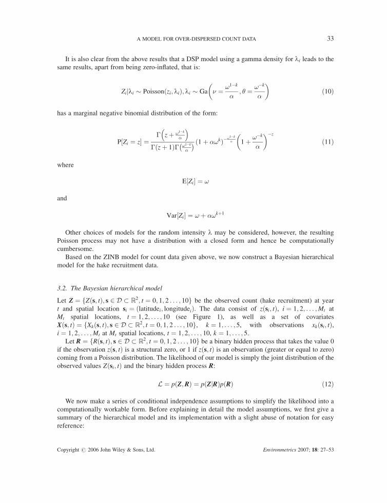
It is also clear from the above results that a DSP model using a gamma density for li leads to the

same results, apart from being zero-inflated, that is:

Zijli � Poissonðzi; liÞ; li � Ga � ¼ !1�k

�; � ¼ !�k

�

� �ð10Þ

has a marginal negative binomial distribution of the form:

P½Zi ¼ z� ¼� zþ !1�k

�

� ��ðzþ 1Þ� !1�k

�

� � ð1þ �!kÞ�!1�k

� 1þ !�k

�

� ��z

ð11Þ

where

E½Zi� ¼ !

and

Var½Zi� ¼ !þ �!kþ1

Other choices of models for the random intensity l may be considered, however, the resulting

Poisson process may not have a distribution with a closed form and hence be computationally

cumbersome.

Based on the ZINB model for count data given above, we now construct a Bayesian hierarchical

model for the hake recruitment data.

3.2. The Bayesian hierarchical model

Let Z ¼ fZðs; tÞ; s 2 D � R2; t ¼ 0; 1; 2 . . . ; 10g be the observed count (hake recruitment) at year

t and spatial location si ¼ ðlatitudei; longitudeiÞ. The data consist of zðsi; tÞ, i ¼ 1; 2; . . . ;Mt at

Mt spatial locations, t ¼ 1; 2; . . . ; 10 (see Figure 1), as well as a set of covariates

Xðs; tÞ ¼ fXkðs; tÞ; s 2 D � R2; t ¼ 0; 1; 2 . . . ; 10g, k ¼ 1; . . . ; 5, with observations xkðsi; tÞ,i ¼ 1; 2; . . . ;Mt at Mt spatial locations, t ¼ 1; 2; . . . ; 10, k ¼ 1; . . . ; 5.

Let R ¼ fRðs; tÞ; s 2 D � R2; t ¼ 0; 1; 2 . . . ; 10g be a binary hidden process that takes the value 0

if the observation zðs; tÞ is a structural zero, or 1 if zðs; tÞ is an observation (greater or equal to zero)

coming from a Poisson distribution. The likelihood of our model is simply the joint distribution of the

observed values Zðsi; tÞ and the binary hidden process R:

L ¼ pðZ;RÞ ¼ pðZjRÞpðRÞ ð12Þ

We now make a series of conditional independence assumptions to simplify the likelihood into a

computationally workable form. Before explaining in detail the model assumptions, we first give a

summary of the hierarchical model and its implementation with a slight abuse of notation for easy

reference:



* Level 1: Likelihood

zðsi; tÞjlðsi; tÞ;Rðsi; tÞ � Poissonðlðsi; tÞÞ; Rðsi; tÞ ¼ 1

0; Rðsi; tÞ ¼ 0

�ð13Þ

Rðsi; tÞj�ðsi; tÞ � Bernoullið�ðsi; tÞÞ

lðsi; tÞj�; !ðsi; tÞ � Ga1

�;

1

�!ðsi; tÞ� �

* Level 2: Link functionsLogarithm and the logit of the processes !ðsi; tÞ and �ðsi; tÞ at location si and at time t are,

respectively, linear functions of the covariates Xkðsi; tÞ, k ¼ 1; . . . ; 5 and a hidden, unobserved

Gaussian field. Specifically, let

cð!Þ ¼ �ð!Þ1 ; . . . ; �

ð!Þ5

� �

and

cð�Þ ¼ �ð�Þ1 ; . . . ; �

ð�Þ5

� �

be two sets of regression coefficients.

logð!ðsi; tÞÞ ¼ cð!ÞXðsi; tÞ þ �tðsiÞ

and

logitð�ðsi; tÞÞ ¼ cð�ÞXðsi; tÞ þ �tðsiÞ

* Level 3: Priors for parameters and hyperparameters

gt is an isotropic Gaussian random field, independent and identical in time. The priors for other

parameters are presented in Subsection 3.2.3.

We now explain in detail the assumptions leading to this model.

3.2.1. Likelihood: dependence and distributional assumptions

* Assumption 1We assume that conditional on Rðsi; tÞ, Zðsi; tÞ are Poisson random variables, independent in time

and space with mean lðsi; tÞ, so that:

pðZjRÞ ¼Y10t¼1

YMt

i¼1

pðZðsi; tÞjRðsi; tÞÞ ð14Þ



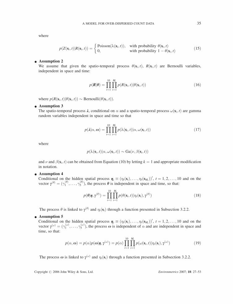
where

pðZðsi; tÞjRðsi; tÞÞ ¼ Poissonðlðsi; tÞÞ; with probability �ðsi; tÞ0; with probability 1� �ðsi; tÞ

�ð15Þ

* Assumption 2We assume that given the spatio-temporal process �ðsi; tÞ, Rðsi; tÞ are Bernoulli variables,

independent in space and time:

pðRjhÞ ¼Y10t¼1

YMt

i¼1

pðRðsi; tÞj�ðsi; tÞÞ ð16Þ

where pðRðsi; tÞj�ðsi; tÞÞ � Bernoullið�ðsi; tÞÞ.* Assumption 3

The spatio-temporal process k, conditional on � and a spatio-temporal process !ðsi; tÞ are gamma

random variables independent in space and time so that

pðkj�;xÞ ¼Y10t¼1

YMt

i¼1

pðlðsi; tÞj�; !ðsi; tÞÞ ð17Þ

where

pðlðsi; tÞj�; !ðsi; tÞÞ � Ga �; �ðsi; tÞð Þ

and � and �ðsi; tÞ can be obtained from Equation (10) by letting k ¼ 1 and appropriate modification

in notation.

* Assumption 4Conditional on the hidden spatial process gt � ð�tðsiÞ; . . . ; �tðsMt

ÞÞ0, t ¼ 1; 2; . . . ; 10 and on the

vector cð�Þ ¼ ð�ð�Þ1 ; . . . ; �ð�Þ5 Þ, the process h is independent in space and time, so that:

pðhjg; cð�ÞÞ ¼Y10t¼1

YMt

i¼1

pð�ðsi; tÞj�tðsiÞ; cð�ÞÞ ð18Þ

The process � is linked to cð�Þ and �tðsiÞ through a function presented in Subsection 3.2.2.

* Assumption 5Conditional on the hidden spatial process gt � ð�tðsiÞ; . . . ; �tðsMt

ÞÞ0, t ¼ 1; 2; . . . ; 10 and on the

vector cð!Þ ¼ ð�ð!Þ1 ; . . . ; �ð!Þ5 Þ, the process x is independent of � and are independent in space and

time, so that:

pð�;xÞ ¼ pð�Þpðxjg; cð!ÞÞ ¼ pð�ÞY10t¼1

YMt

i¼1

pð!ðsi; tÞj�tðsiÞ; cð!ÞÞ ð19Þ

The process x is linked to cð!Þ and �tðsiÞ through a function presented in Subsection 3.2.2.



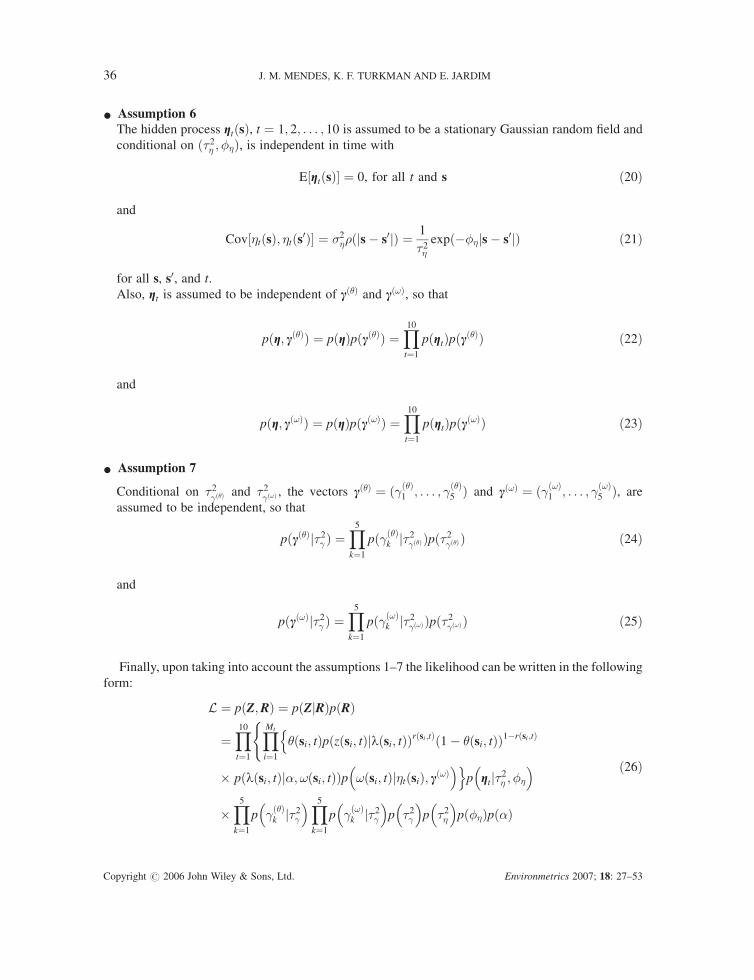
* Assumption 6The hidden process gtðsÞ, t ¼ 1; 2; . . . ; 10 is assumed to be a stationary Gaussian random field and

conditional on ð�2� ; �Þ, is independent in time with

E½gtðsÞ� ¼ 0, for all t and s ð20Þ

and

Cov½�tðsÞ; �tðs0Þ� ¼ 2��ðjs� s0jÞ ¼ 1

�2�expð��js� s0jÞ ð21Þ

for all s, s0, and t.

Also, gt is assumed to be independent of cð�Þ and cð!Þ, so that

pðg; cð�ÞÞ ¼ pðgÞpðcð�ÞÞ ¼Y10t¼1

pðgtÞpðcð�ÞÞ ð22Þ

and

pðg; cð!ÞÞ ¼ pðgÞpðcð!ÞÞ ¼Y10t¼1

pðgtÞpðcð!ÞÞ ð23Þ

* Assumption 7

Conditional on �2�ð�Þ and �2

�ð!Þ , the vectors cð�Þ ¼ ð�ð�Þ1 ; . . . ; �ð�Þ5 Þ and cð!Þ ¼ ð�ð!Þ1 ; . . . ; �

ð!Þ5 Þ, are

assumed to be independent, so that

pðcð�Þj�2� Þ ¼Y5k¼1

pð�ð�Þk j�2�ð�Þ Þpð�2�ð�Þ Þ ð24Þ

and

pðcð!Þj�2� Þ ¼Y5k¼1

pð�ð!Þk j�2�ð!Þ Þpð�2�ð!Þ Þ ð25Þ

Finally, upon taking into account the assumptions 1–7 the likelihood can be written in the following

form:

L ¼ pðZ;RÞ ¼ pðZjRÞpðRÞ

¼Y10t¼1

YMt

i¼1

�ðsi; tÞpðzðsi; tÞjlðsi; tÞÞrðsi;tÞð1� �ðsi; tÞÞ1�rðsi;tÞn(

� pðlðsi; tÞj�; !ðsi; tÞÞp !ðsi; tÞj�tðsiÞ; cð!Þ� �o

p gtj�2� ; �

� �

�Y5k¼1

p �ð�Þk j�2�

� �Y5k¼1

p �ð!Þk j�2�

� �p �2�

� �p �2�

� �pð�Þpð�Þ

ð26Þ



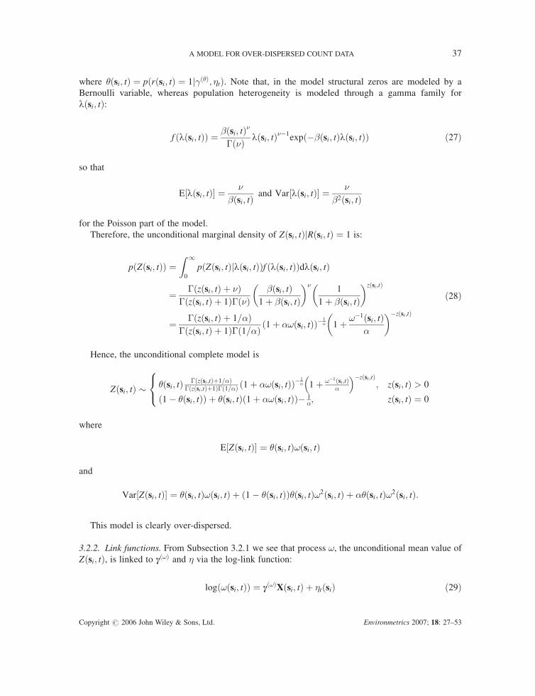
where �ðsi; tÞ ¼ pðrðsi; tÞ ¼ 1j�ð�Þ; �tÞ. Note that, in the model structural zeros are modeled by a

Bernoulli variable, whereas population heterogeneity is modeled through a gamma family for

lðsi; tÞ:

f ðlðsi; tÞÞ ¼ �ðsi; tÞ��ð�Þ lðsi; tÞ��1

expð��ðsi; tÞlðsi; tÞÞ ð27Þ

so that

E½lðsi; tÞ� ¼ �

�ðsi; tÞ and Var½lðsi; tÞ� ¼ �

�2ðsi; tÞ

for the Poisson part of the model.

Therefore, the unconditional marginal density of Zðsi; tÞjRðsi; tÞ ¼ 1 is:

pðZðsi; tÞÞ ¼Z 1

0

pðZðsi; tÞjlðsi; tÞÞf ðlðsi; tÞÞdlðsi; tÞ

¼ �ðzðsi; tÞ þ �Þ�ðzðsi; tÞ þ 1Þ�ð�Þ

�ðsi; tÞ1þ �ðsi; tÞ� ��

1

1þ �ðsi; tÞ� �zðsi;tÞ

¼ � zðsi; tÞ þ 1=�ð Þ�ðzðsi; tÞ þ 1Þ� 1=�ð Þ ð1þ �!ðsi; tÞÞ�

1� 1þ !�1ðsi; tÞ

�

� ��zðsi;tÞ

ð28Þ

Hence, the unconditional complete model is

Zðsi; tÞ � �ðsi; tÞ � zðsi;tÞþ1=�ð Þ�ðzðsi;tÞþ1Þ� 1=�ð Þ ð1þ �!ðsi; tÞÞ�

1� 1þ !�1ðsi;tÞ

�

� ��zðsi;tÞ; zðsi; tÞ > 0

ð1� �ðsi; tÞÞ þ �ðsi; tÞð1þ �!ðsi; tÞÞ� 1�; zðsi; tÞ ¼ 0

8<:

where

E½Zðsi; tÞ� ¼ �ðsi; tÞ!ðsi; tÞ

and

Var½Zðsi; tÞ� ¼ �ðsi; tÞ!ðsi; tÞ þ ð1� �ðsi; tÞÞ�ðsi; tÞ!2ðsi; tÞ þ ��ðsi; tÞ!2ðsi; tÞ:

This model is clearly over-dispersed.

3.2.2. Link functions. From Subsection 3.2.1 we see that process !, the unconditional mean value of

Zðsi; tÞ, is linked to cð!Þ and � via the log-link function:

logð!ðsi; tÞÞ ¼ cð!ÞXðsi; tÞ þ �tðsiÞ ð29Þ



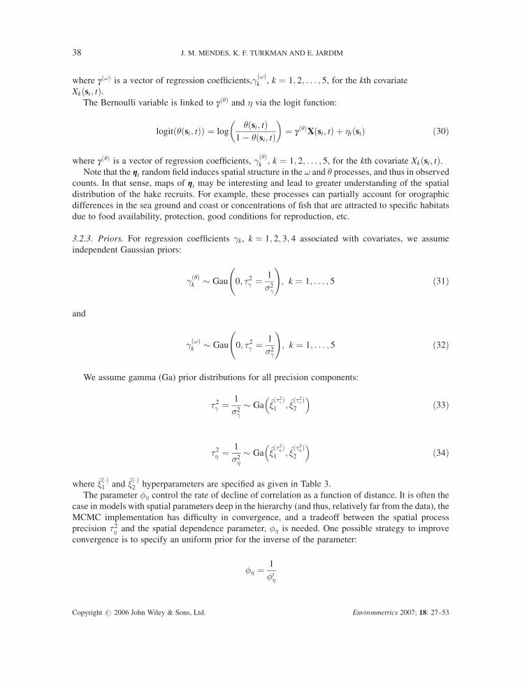
where cð!Þ is a vector of regression coefficients,�ð!Þk , k ¼ 1; 2; . . . ; 5, for the kth covariate

Xkðsi; tÞ.The Bernoulli variable is linked to cð�Þ and � via the logit function:

logitð�ðsi; tÞÞ ¼ log�ðsi; tÞ

1� �ðsi; tÞ� �

¼ cð�ÞXðsi; tÞ þ �tðsiÞ ð30Þ

where cð�Þ is a vector of regression coefficients, �ð�Þk , k ¼ 1; 2; . . . ; 5, for the kth covariate Xkðsi; tÞ.

Note that the gt random field induces spatial structure in the ! and � processes, and thus in observedcounts. In that sense, maps of gt may be interesting and lead to greater understanding of the spatial

distribution of the hake recruits. For example, these processes can partially account for orographic

differences in the sea ground and coast or concentrations of fish that are attracted to specific habitats

due to food availability, protection, good conditions for reproduction, etc.

3.2.3. Priors. For regression coefficients �k, k ¼ 1; 2; 3; 4 associated with covariates, we assume

independent Gaussian priors:

�ð�Þk � Gau 0; �2� ¼ 1

2�

!; k ¼ 1; . . . ; 5 ð31Þ

and

�ð!Þk � Gau 0; �2� ¼ 1

2�

!; k ¼ 1; . . . ; 5 ð32Þ

We assume gamma (Ga) prior distributions for all precision components:

�2� ¼ 1

2�

� Ga �ð�2� Þ1 ; �

ð�2� Þ2

� �ð33Þ

�2� ¼ 1

2�

� Ga �ð�2� Þ1 ; �

ð�2� Þ2

� �ð34Þ

where �ð�Þ1 and �

ð�Þ2 hyperparameters are specified as given in Table 3.

The parameter � control the rate of decline of correlation as a function of distance. It is often the

case in models with spatial parameters deep in the hierarchy (and thus, relatively far from the data), the

MCMC implementation has difficulty in convergence, and a tradeoff between the spatial process

precision �2� and the spatial dependence parameter, � is needed. One possible strategy to improve

convergence is to specify an uniform prior for the inverse of the parameter:

� ¼ 1

0�



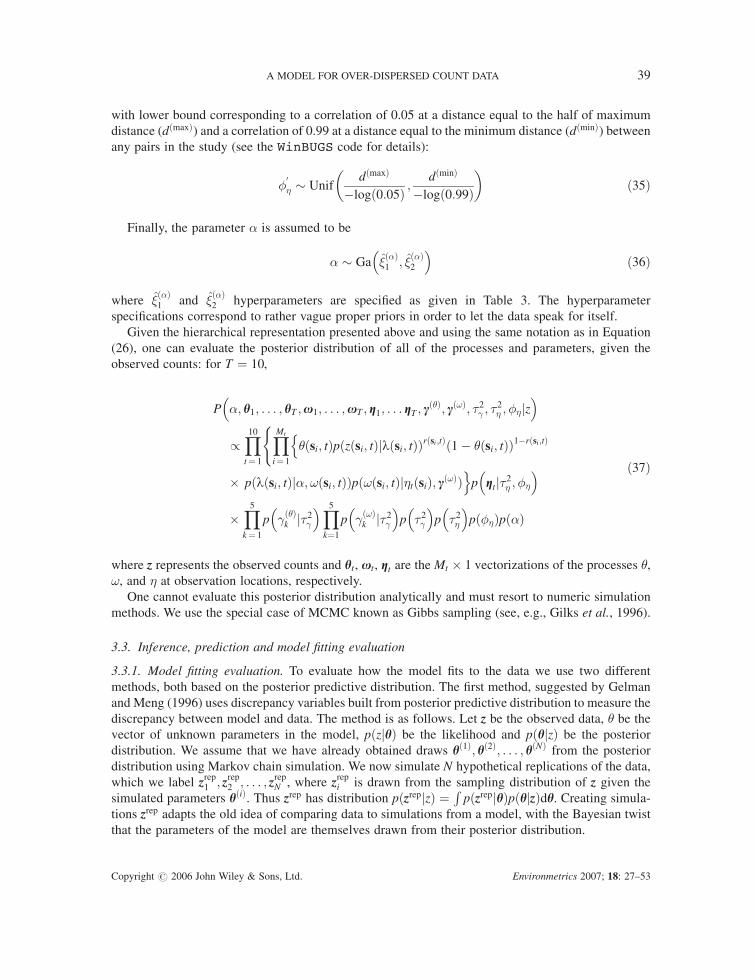
with lower bound corresponding to a correlation of 0.05 at a distance equal to the half of maximum

distance (dðmaxÞ) and a correlation of 0.99 at a distance equal to the minimum distance (dðminÞ) betweenany pairs in the study (see the WinBUGS code for details):

0� � Unif

dðmaxÞ

�logð0:05Þ ;dðminÞ

�logð0:99Þ� �

ð35Þ

Finally, the parameter � is assumed to be

� � Ga �ð�Þ1 ; �

ð�Þ2

� �ð36Þ

where �ð�Þ1 and �

ð�Þ2 hyperparameters are specified as given in Table 3. The hyperparameter

specifications correspond to rather vague proper priors in order to let the data speak for itself.

Given the hierarchical representation presented above and using the same notation as in Equation

(26), one can evaluate the posterior distribution of all of the processes and parameters, given the

observed counts: for T ¼ 10,

P �; h1; . . . ; hT ;x1; . . . ;xT ; g1; . . . gT ; cð�Þ; cð!Þ; �2� ; �

2� ; �jz

� �

/Y10t¼ 1

YMt

i¼ 1

�ðsi; tÞpðzðsi; tÞjlðsi; tÞÞrðsi;tÞð1� �ðsi; tÞÞ1�rðsi;tÞn(

� pðlðsi; tÞj�; !ðsi; tÞÞpð!ðsi; tÞj�tðsiÞ; cð!ÞÞop gtj�2� ; �

� �

�Y5k¼ 1

p �ð�Þk j�2�

� �Y5k¼1

p �ð!Þk j�2�

� �p �2�

� �p �2�

� �pð�Þpð�Þ

ð37Þ

where z represents the observed counts and ht, xt, gt are the Mt � 1 vectorizations of the processes �,!, and � at observation locations, respectively.

One cannot evaluate this posterior distribution analytically and must resort to numeric simulation

methods. We use the special case of MCMC known as Gibbs sampling (see, e.g., Gilks et al., 1996).

3.3. Inference, prediction and model fitting evaluation

3.3.1. Model fitting evaluation. To evaluate how the model fits to the data we use two different

methods, both based on the posterior predictive distribution. The first method, suggested by Gelman

and Meng (1996) uses discrepancy variables built from posterior predictive distribution to measure the

discrepancy between model and data. The method is as follows. Let z be the observed data, � be the

vector of unknown parameters in the model, pðzjhÞ be the likelihood and pðhjzÞ be the posterior

distribution. We assume that we have already obtained draws hð1Þ; hð2Þ; . . . ; hðNÞ from the posterior

distribution using Markov chain simulation. We now simulate N hypothetical replications of the data,

which we label zrep1 ; zrep2 ; . . . ; zrepN , where z

repi is drawn from the sampling distribution of z given the

simulated parameters hðiÞ. Thus zrep has distribution pðzrepjzÞ ¼ R pðzrepjhÞpðhjzÞdh. Creating simula-

tions zrep adapts the old idea of comparing data to simulations from a model, with the Bayesian twist

that the parameters of the model are themselves drawn from their posterior distribution.



If the model is reasonably accurate, the hypothetical replications should look similar to the

observed data z. Formally, one can compare the data to the predictive distribution by first choosing a

discrepancy variable Tðz; �Þ which will have an extreme value if the data z are in conflict with the

posited model. Then a p-value can be estimated by calculating the proportion of cases in which the

simulated discrepancy variable exceeds the realized value:

estimated p-value ¼ 1

N

XNi¼ 1

IðTðzrepi;hðiÞ �Tðz;hðiÞÞÞ

where Ið�Þ is the indicator function which takes the value 1 when its argument is true and 0 otherwise.

Ideally, in a well fitted model, the p-value should be close to 0.5. The model fitting evaluation can be

made graphically, as well. We can plot a scatter plot of the realized values Tðz; hðiÞÞ versus the

predictive values Tðzrepi ; hðiÞÞ on the same scale. A good fit would be indicated by about half the points

in the scatter plot falling above the 45 line and half falling below.

To evaluate the model we used as discrepancy variables:

T1ðz; hÞ ¼ffiffiffiffiffiffiffiffiffiffiffiffiffiffiffiffiffiffiffiffiffiffiffiffiffiffiffiffiffiffiffiffiffiffiffiXni¼ 1

ðzi � E½Zijh�Þ2s

ð38Þ

and

T2ðz; hÞ ¼ffiffiffiffiffiffiffiffiffiffiffiffiffiffiffiffiffiffiffiffiffiffiffiffiffiffiffiffiffiffiffiffiffiffiffiffiXni¼ 1

ðzi � E½Zijh�Þ2ffiffiffiffiffiffiffiffiffiffiffiffiffiffiffiffiffiffiVar½Zijh�

ps

ð39Þ

The second method relies on posterior predictive distribution in the way that the simulated values,

zrep, of the posterior predictive distribution are used to approximate the characteristics of that

distribution, PðzrepjzÞ ¼ R pðzrepjhÞpðhjzÞdh, namely the expected value and standard deviation.

These values can be compared with the observed data in order to assess the prediction quality of

the model.

It is of interest to know how the model predicts observations not included in the data set for

inference, as well. We present also results, based on the posterior predictive distribution, which

show the predicted values for observations not included in data set for inference, that is

pðzjzÞ ¼ R pðzjhÞpðhjzÞdh, where z* denotes the data, excluding the observation included in z.

4. RESULTS

The results presented refer only to the years of 1990 and 1997, those with the higher and lower

sampling effort, and are used as examples of the kind of analysis this method allows. Note that for

validation we randomly select 20 observations that were taken out from inference process (see

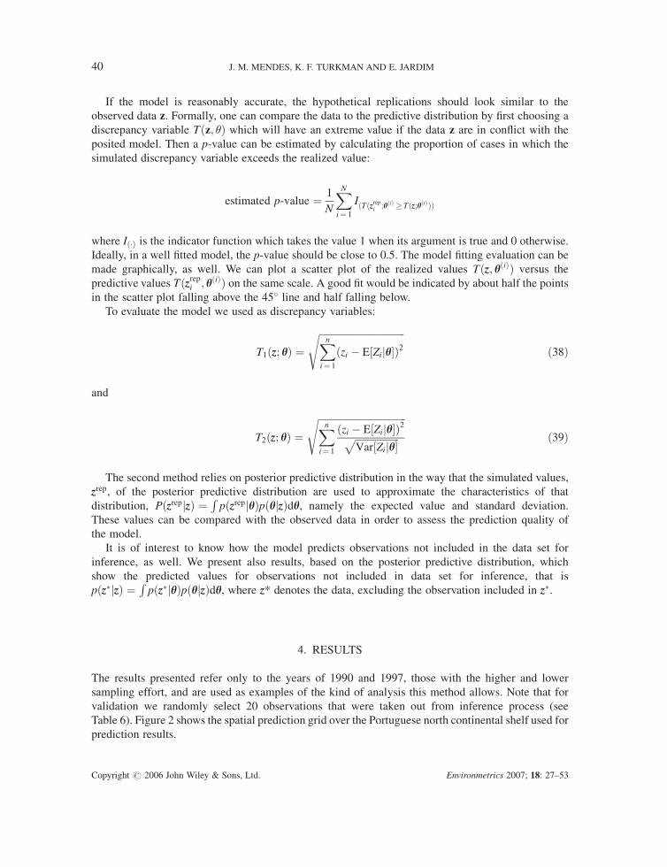
Table 6). Figure 2 shows the spatial prediction grid over the Portuguese north continental shelf used for

prediction results.



The model given in the above sections is implemented by using the software WinBugs and it’s

addin GeoBugs. It can be downloaded as well as all its documentation from:

http://www.mrc.bsu.cam.ac.uk/bugs/winbugs/contents.shtml

The computer code is given in Appendix A

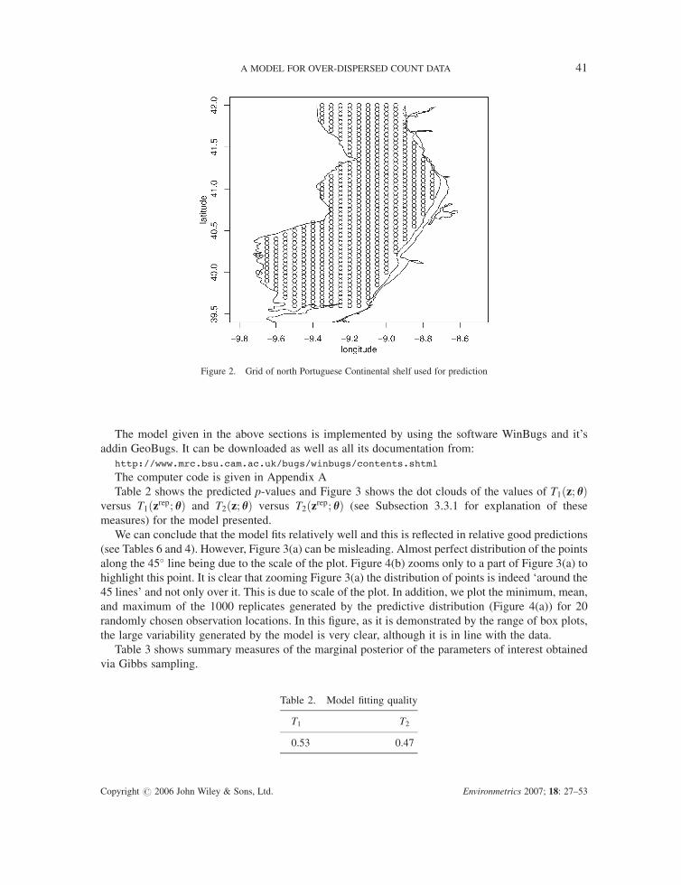
Table 2 shows the predicted p-values and Figure 3 shows the dot clouds of the values of T1ðz; hÞversus T1ðzrep; hÞ and T2ðz; hÞ versus T2ðzrep; hÞ (see Subsection 3.3.1 for explanation of these

measures) for the model presented.

We can conclude that the model fits relatively well and this is reflected in relative good predictions

(see Tables 6 and 4). However, Figure 3(a) can be misleading. Almost perfect distribution of the points

along the 45 line being due to the scale of the plot. Figure 4(b) zooms only to a part of Figure 3(a) to

highlight this point. It is clear that zooming Figure 3(a) the distribution of points is indeed ‘around the

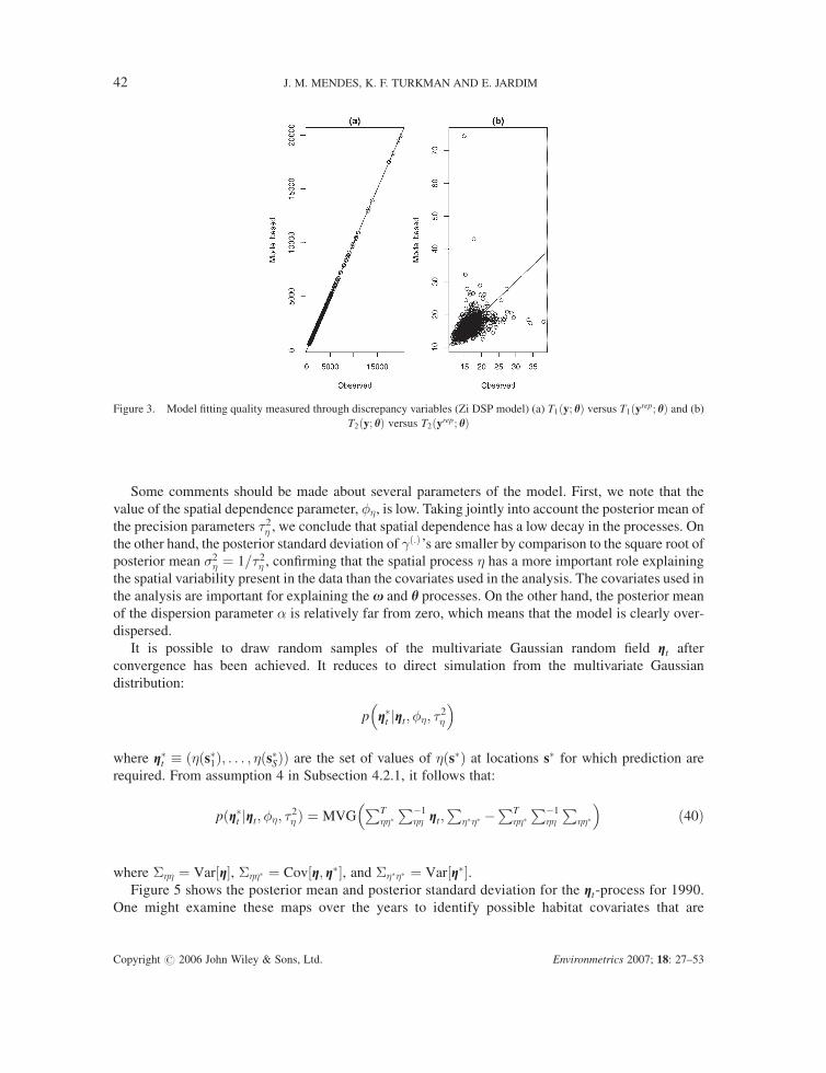
45 lines’ and not only over it. This is due to scale of the plot. In addition, we plot the minimum, mean,

and maximum of the 1000 replicates generated by the predictive distribution (Figure 4(a)) for 20

randomly chosen observation locations. In this figure, as it is demonstrated by the range of box plots,

the large variability generated by the model is very clear, although it is in line with the data.

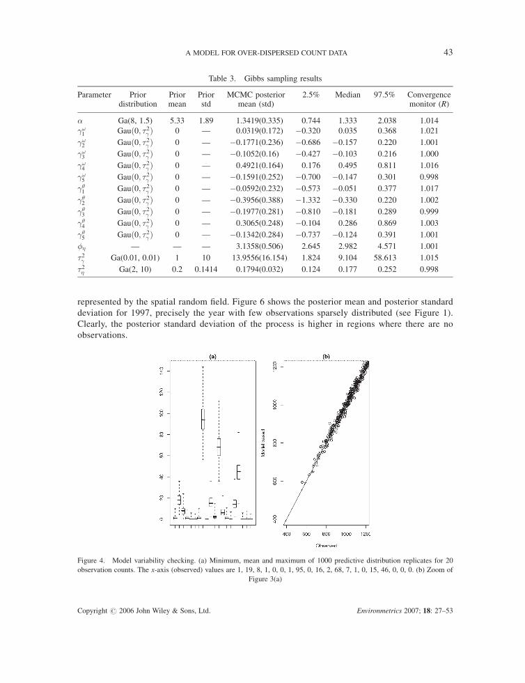
Table 3 shows summary measures of the marginal posterior of the parameters of interest obtained

via Gibbs sampling.

Figure 2. Grid of north Portuguese Continental shelf used for prediction

Table 2. Model fitting quality

T1 T2

0.53 0.47



Some comments should be made about several parameters of the model. First, we note that the

value of the spatial dependence parameter, �, is low. Taking jointly into account the posterior mean of

the precision parameters �2� , we conclude that spatial dependence has a low decay in the processes. On

the other hand, the posterior standard deviation of �ð:Þ ’s are smaller by comparison to the square root of

posterior mean 2� ¼ 1=�2� , confirming that the spatial process � has a more important role explaining

the spatial variability present in the data than the covariates used in the analysis. The covariates used in

the analysis are important for explaining the x and h processes. On the other hand, the posterior mean

of the dispersion parameter � is relatively far from zero, which means that the model is clearly over-

dispersed.

It is possible to draw random samples of the multivariate Gaussian random field gt after

convergence has been achieved. It reduces to direct simulation from the multivariate Gaussian

distribution:

p gt jgt; �; �2�

� �

where gt � ð�ðs1Þ; . . . ; �ðsSÞÞ are the set of values of �ðsÞ at locations s for which prediction are

required. From assumption 4 in Subsection 4.2.1, it follows that:

pðgt jgt; �; �2� Þ ¼ MVG

PT��P�1

�� gt;P

�� PT

��P�1

��

P��

� �ð40Þ

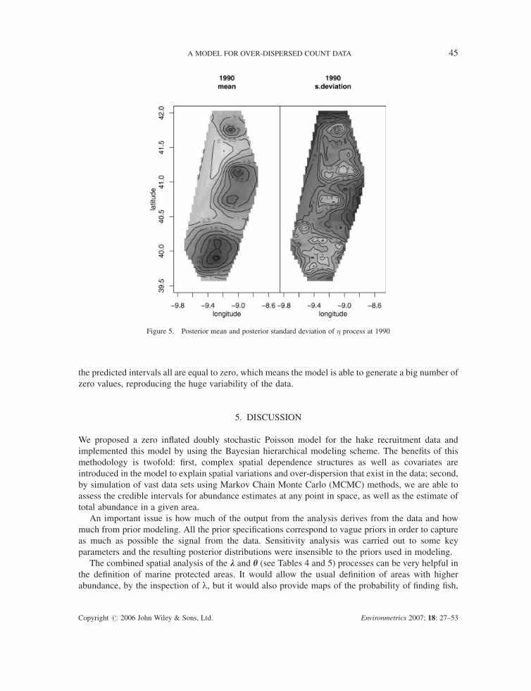
where �� ¼ Var½g�, �� ¼ Cov½g; g�, and �� ¼ Var½g�.Figure 5 shows the posterior mean and posterior standard deviation for the gt-process for 1990.

One might examine these maps over the years to identify possible habitat covariates that are

Figure 3. Model fitting quality measured through discrepancy variables (Zi DSP model) (a) T1ðy; hÞ versus T1ðyrep; hÞ and (b)T2ðy; hÞ versus T2ðyrep; hÞ



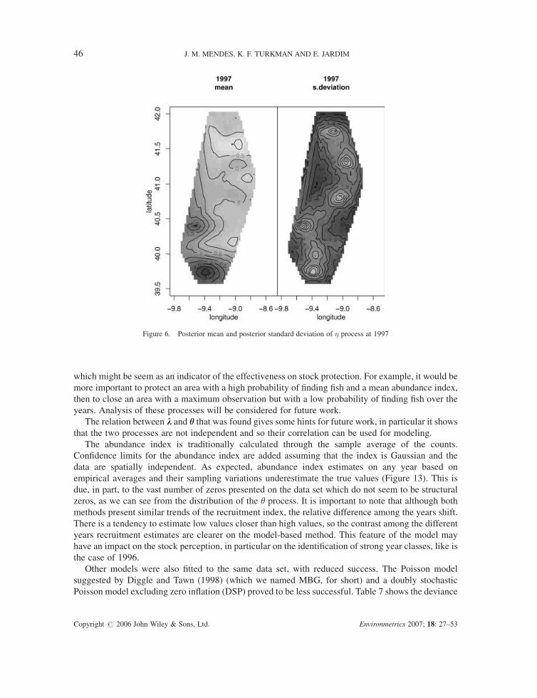
represented by the spatial random field. Figure 6 shows the posterior mean and posterior standard

deviation for 1997, precisely the year with few observations sparsely distributed (see Figure 1).

Clearly, the posterior standard deviation of the process is higher in regions where there are no

observations.

Table 3. Gibbs sampling results

Parameter Prior Prior Prior MCMC posterior 2.5% Median 97.5% Convergencedistribution mean std mean (std) monitor (R)

� Ga(8, 1.5) 5.33 1.89 1.3419(0.335) 0.744 1.333 2.038 1.014

�!1 Gauð0; �2� Þ 0 — 0.0319(0.172) �0.320 0.035 0.368 1.021

�!2 Gauð0; �2� Þ 0 — �0.1771(0.236) �0.686 �0.157 0.220 1.001

�!3 Gauð0; �2� Þ 0 — �0.1052(0.16) �0.427 �0.103 0.216 1.000

�!4 Gauð0; �2� Þ 0 — 0.4921(0.164) 0.176 0.495 0.811 1.016

�!5 Gauð0; �2� Þ 0 — �0.1591(0.252) �0.700 �0.147 0.301 0.998

��1 Gauð0; �2� Þ 0 — �0.0592(0.232) �0.573 �0.051 0.377 1.017

��2 Gauð0; �2� Þ 0 — �0.3956(0.388) �1.332 �0.330 0.220 1.002

��3 Gauð0; �2� Þ 0 — �0.1977(0.281) �0.810 �0.181 0.289 0.999

��4 Gauð0; �2� Þ 0 — 0.3065(0.248) �0.104 0.286 0.869 1.003

��5 Gauð0; �2� Þ 0 — �0.1342(0.284) �0.737 �0.124 0.391 1.001

� — — — 3.1358(0.506) 2.645 2.982 4.571 1.001

�2� Ga(0.01, 0.01) 1 10 13.9556(16.154) 1.824 9.104 58.613 1.015

�2� Ga(2, 10) 0.2 0.1414 0.1794(0.032) 0.124 0.177 0.252 0.998

Figure 4. Model variability checking. (a) Minimum, mean and maximum of 1000 predictive distribution replicates for 20

observation counts. The x-axis (observed) values are 1, 19, 8, 1, 0, 0, 1, 95, 0, 16, 2, 68, 7, 1, 0, 15, 46, 0, 0, 0. (b) Zoom of

Figure 3(a)



Although the zero-inflated probability process, h, is considered more as a ‘nuisance’ process in the

analysis, it is instructive to examine the associated parameters. First, we note from the comparison of

the posterior standard deviations of �ð�Þ and �2� (Table 3) that the spatial process is particularly

important in explaining this process. Table 5 shows the posterior mean and respective credible

intervals for � at 20 random selected observations not included in the inference. Its clear that, although

the posterior mean is well above 0.5, the credible intervals show that this process has a great degree of

variability as well, reflecting the data variability itself. A priori, it was not easy to establish a

relationship between the process � and l. Nevertheless, we can imagine that they are somehow related.

Figure 7 shows the relation between process � and process l and counts Z. It is clear that there exists a

well defined non-linear relationship which could help in future research as a mean of establishing new

models for � so we can reduce the variability and uncertainty about it.

Figures 8 and 9 show the posterior mean and standard deviation of Z for 1990 and 1997. As

expected, the variability is very high.

Figure 10 shows the posterior mean of h for 1990 and 1997. The results show clearly that the

probability of a structural zero is low.

Finally, Figures 11 and 12 show the posterior mean and posterior standard deviation of the k-

process at 1990 and 1997. These plots show clearly that the posterior standard deviation is not

proportional to the posterior mean, as expected with a simple Poisson count data model.

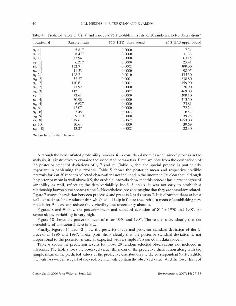
Table 6 shows the prediction results for those 20 random selected observations not included in

inference. The table shows the observed value, the mean of the predictive distribution along with the

sample mean of the predicted values of the predictive distribution and the correspondent 95% credible

intervals. As we can see, all of the credible intervals contain the observed value. And the lower limit of

Table 4. Predicted values of lðsi; tÞ and respective 95% credible intervals for 20 random selected observations*

[location, t] Sample mean 95% HPD lower bound 95% HPD upper bound

½s4; 1� 5.817 0.0000 17.31½s5; 1� 8.477 0.0000 31.33½s9; 1� 13.94 0.0000 63.15½s13; 1� 6.217 0.0000 25.41½s28; 1� 102.7 0.0002 399.90½s38; 1� 41.33 0.0000 98.95½s1; 2� 108.2 0.0010 435.30½s16; 2� 52.27 0.0001 238.80½s23; 2� 110.6 0.0002 359.90½s34; 2� 17.92 0.0000 76.90½s14; 3� 142 0.0002 469.00½s4; 4� 52.61 0.0000 209.10½s11; 4� 70.98 0.0000 213.50½s18; 4� 6.627 0.0000 23.81½s6; 6� 12.07 0.0000 72.24½s17; 6� 3.45 0.0003 16.57½s18; 9� 9.119 0.0000 39.25½s24; 9� 328.6 0.0062 1653.00½s2; 10� 10.64 0.0000 39.69½s18; 10� 23.27 0.0008 122.30

*Not included in the inference.



the predicted intervals all are equal to zero, which means the model is able to generate a big number of

zero values, reproducing the huge variability of the data.

5. DISCUSSION

We proposed a zero inflated doubly stochastic Poisson model for the hake recruitment data and

implemented this model by using the Bayesian hierarchical modeling scheme. The benefits of this

methodology is twofold: first, complex spatial dependence structures as well as covariates are

introduced in the model to explain spatial variations and over-dispersion that exist in the data; second,

by simulation of vast data sets using Markov Chain Monte Carlo (MCMC) methods, we are able to

assess the credible intervals for abundance estimates at any point in space, as well as the estimate of

total abundance in a given area.

An important issue is how much of the output from the analysis derives from the data and how

much from prior modeling. All the prior specifications correspond to vague priors in order to capture

as much as possible the signal from the data. Sensitivity analysis was carried out to some key

parameters and the resulting posterior distributions were insensible to the priors used in modeling.

The combined spatial analysis of the k and h (see Tables 4 and 5) processes can be very helpful in

the definition of marine protected areas. It would allow the usual definition of areas with higher

abundance, by the inspection of l, but it would also provide maps of the probability of finding fish,

Figure 5. Posterior mean and posterior standard deviation of � process at 1990



which might be seem as an indicator of the effectiveness on stock protection. For example, it would be

more important to protect an area with a high probability of finding fish and a mean abundance index,

then to close an area with a maximum observation but with a low probability of finding fish over the

years. Analysis of these processes will be considered for future work.

The relation between k and h that was found gives some hints for future work, in particular it shows

that the two processes are not independent and so their correlation can be used for modeling.

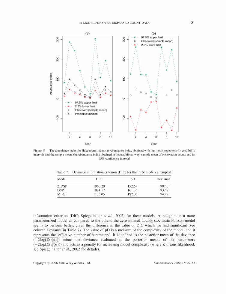
The abundance index is traditionally calculated through the sample average of the counts.

Confidence limits for the abundance index are added assuming that the index is Gaussian and the

data are spatially independent. As expected, abundance index estimates on any year based on

empirical averages and their sampling variations underestimate the true values (Figure 13). This is

due, in part, to the vast number of zeros presented on the data set which do not seem to be structural

zeros, as we can see from the distribution of the � process. It is important to note that although both

methods present similar trends of the recruitment index, the relative difference among the years shift.

There is a tendency to estimate low values closer than high values, so the contrast among the different

years recruitment estimates are clearer on the model-based method. This feature of the model may

have an impact on the stock perception, in particular on the identification of strong year classes, like is

the case of 1996.

Other models were also fitted to the same data set, with reduced success. The Poisson model

suggested by Diggle and Tawn (1998) (which we named MBG, for short) and a doubly stochastic

Poisson model excluding zero inflation (DSP) proved to be less successful. Table 7 shows the deviance

Figure 6. Posterior mean and posterior standard deviation of � process at 1997



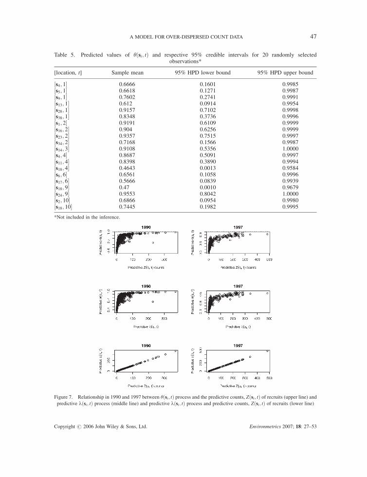
Table 5. Predicted values of �ðsi; tÞ and respective 95% credible intervals for 20 randomly selectedobservations*

[location, t] Sample mean 95% HPD lower bound 95% HPD upper bound

½s4; 1� 0.6666 0.1601 0.9985½s5; 1� 0.6618 0.1271 0.9987½s9; 1� 0.7602 0.2741 0.9991½s13; 1� 0.612 0.0914 0.9954½s28; 1� 0.9157 0.7102 0.9998½s38; 1� 0.8348 0.3736 0.9996½s1; 2� 0.9191 0.6109 0.9999½s16; 2� 0.904 0.6256 0.9999½s23; 2� 0.9357 0.7515 0.9997½s34; 2� 0.7168 0.1566 0.9987½s14; 3� 0.9108 0.5356 1.0000½s4; 4� 0.8687 0.5091 0.9997½s11; 4� 0.8398 0.3890 0.9994½s18; 4� 0.4643 0.0013 0.9584½s6; 6� 0.6561 0.1058 0.9996½s17; 6� 0.5666 0.0839 0.9939½s18; 9� 0.47 0.0010 0.9679½s24; 9� 0.9553 0.8042 1.0000½s2; 10� 0.6866 0.0954 0.9980½s18; 10� 0.7445 0.1982 0.9995

*Not included in the inference.

Figure 7. Relationship in 1990 and 1997 between �ðsi; tÞ process and the predictive counts, Zðsi; tÞ of recruits (upper line) andpredictive lðsi; tÞ process (middle line) and predictive lðsi; tÞ process and predictive counts, Zðsi; tÞ of recruits (lower line)



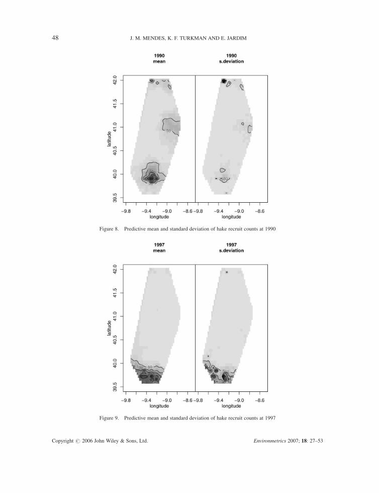
Figure 8. Predictive mean and standard deviation of hake recruit counts at 1990

Figure 9. Predictive mean and standard deviation of hake recruit counts at 1997



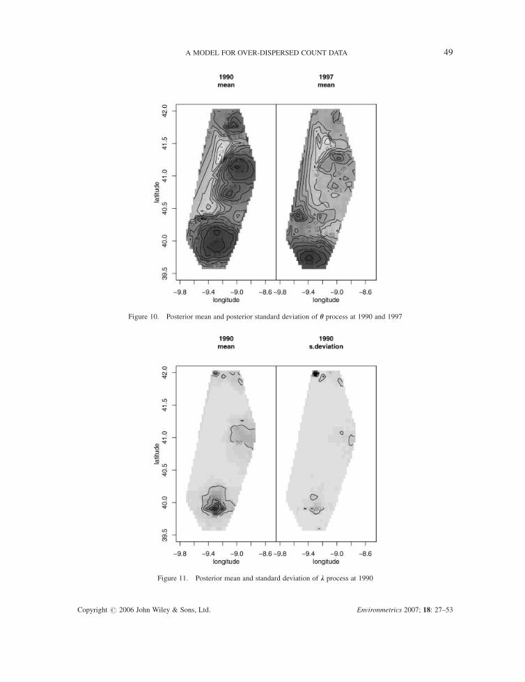
Figure 10. Posterior mean and posterior standard deviation of h process at 1990 and 1997

Figure 11. Posterior mean and standard deviation of k process at 1990



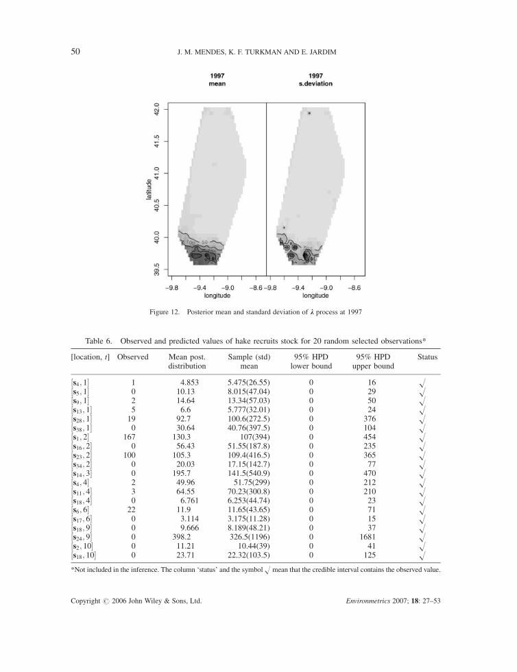
Figure 12. Posterior mean and standard deviation of k process at 1997

Table 6. Observed and predicted values of hake recruits stock for 20 random selected observations*

[location, t] Observed Mean post. Sample (std) 95% HPD 95% HPD Statusdistribution mean lower bound upper bound

½s4; 1� 1 4.853 5.475(26.55) 0 16 H½s5; 1� 0 10.13 8.015(47.04) 0 29 H½s9; 1� 2 14.64 13.34(57.03) 0 50 H½s13; 1� 5 6.6 5.777(32.01) 0 24 H½s28; 1� 19 92.7 100.6(272.5) 0 376 H½s38; 1� 0 30.64 40.76(397.5) 0 104 H½s1; 2� 167 130.3 107(394) 0 454 H½s16; 2� 0 56.43 51.55(187.8) 0 235 H½s23; 2� 100 105.3 109.4(416.5) 0 365 H½s34; 2� 0 20.03 17.15(142.7) 0 77 H½s14; 3� 0 195.7 141.5(540.9) 0 470 H½s4; 4� 2 49.96 51.75(299) 0 212 H½s11; 4� 3 64.55 70.23(300.8) 0 210 H½s18; 4� 0 6.761 6.253(44.74) 0 23 H½s6; 6� 22 11.9 11.65(43.65) 0 71 H½s17; 6� 0 3.114 3.175(11.28) 0 15 H½s18; 9� 0 9.666 8.189(48.21) 0 37 H½s24; 9� 0 398.2 326.5(1196) 0 1681 H½s2; 10� 0 11.21 10.44(39) 0 41 H½s18; 10� 0 23.71 22.32(103.5) 0 125 H

*Not included in the inference. The column ‘status’ and the symbolH mean that the credible interval contains the observed value.



information criterion (DIC; Spiegelhalter et al., 2002) for these models. Although it is a more

parameterized model as compared to the others, the zero-inflated doubly stochastic Poisson model

seems to perform better, given the difference in the value of DIC which we find significant (see

column Deviance in Table 7). The value of pD is a measure of the complexity of the model, and it

represents the ‘effective number of parameters’. It is defined as the posterior mean of the deviance

(�2logðLðzjhÞÞ) minus the deviance evaluated at the posterior means of the parameters

(�2logðLðzjf�hÞÞ) and acts as a penalty for increasing model complexity (where L means likelihood;

see Spiegelhalter et al., 2002 for details).

Figure 13. The abundance index for Hake recruitment. (a) Abundance index obtained with our model together with credibility

intervals and the sample mean. (b) Abundance index obtained in the traditional way: sample mean of observation counts and its

95% confidence interval

Table 7. Deviance information criterion (DIC) for the three models attempted

Model DIC pD Deviance

ZIDSP 1060.29 152.69 907.6DSP 1094.17 161.36 932.8MBG 1135.05 192.06 943.9



ACKNOWLEDGMENTS

The authors are grateful to Antonia Amaral Turkman for her precious help in computational aspects of MarkovChainMonte Carlo methods, and to the coordinator of IPIMAR’s surveys, Fatima Cardador and to two referees fortheir careful reading of the paper.

REFERENCES

Cohen AC. 1963. Estimation in mixtures of discrete distribution. Proceedings of International Symposium on DiscreteDistributions, Montreal; 373–378.

Cox DR, Isham V. 1980. Point Processes. Chapman & Hall: London.Cressie N. 1991. Statistics for Spatial Data. Wiley: New York.Diggle PJ, Tawn JA. 1998. Model-based geostatistics (with discussion). Journal of Royal Statistical Society 47(3): 299–350.

Gelman A, Meng X-L. 1996. Model checking and improvement. In Markov Chain Monte Carlo in Practice. InterdisciplinaryStatistics, Gilks WR, Richardson S, Spiegelhalter DJ (eds). Chapman & all: London.

Gilks WR, Richardson S, Spiegelhalter DJ (eds). 1996. Markov Chain Monte Carlo in Practice. Interdisciplinary Statistics.Chapman & Hall: London.

ICES. 2002. Report of the International Bottom Trawl Survey Working Group. ICES CM 2002/D:03.Johnson NL, Kotz S. 1962. Discrete Distributions. Wiley: New York.Lambert D. 1992. Zero-inflated poisson regression, with an application to defects in manufacturing. Technometrics 34: 1–14.McCullagh P, Nelder P. 1989. Generalized Linear Models (2nd ed). Chapman & Hall: London.Saha A, Dong D. 1997. Estimating nested count data models. Oxford Bulletin of Economics and Statistics 59: 423–430.SESITS. 1999. Evaluation of Demersal Resources of Southwestern Europe from Standardized Groundfish Surveys—Study.Final Report. DG XIV / EC, Contract 96/029.

Spiegelhalter DJ, Best NG, Carlin BP, van der Linde A. 2002. Bayesian measures of model complexity and fit (with discussion).Journal of Royal Statistics Society, Series B 64: 583–640.

APPENDIX

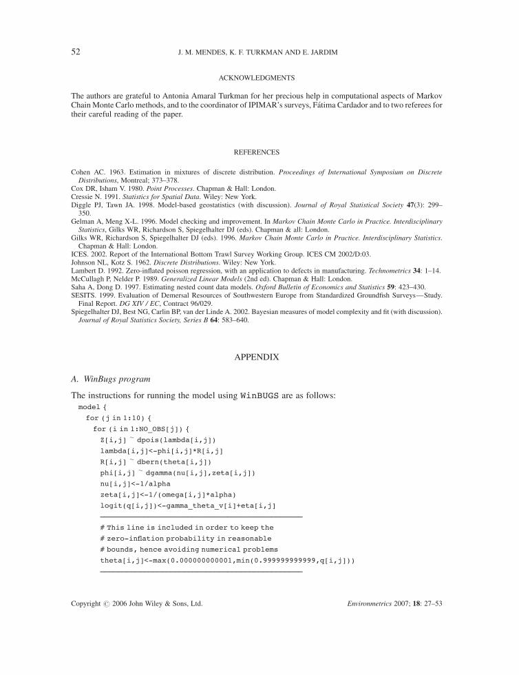
A. WinBugs program

The instructions for running the model using WinBUGS are as follows:

model {

for (j in 1:10) {

for (i in 1:NO_OBS[j]) {

Z[i,j] � dpois(lambda[i,j])

lambda[i,j]<-phi[i,j]*R[i,j]

R[i,j] � dbern(theta[i,j])

phi[i,j] � dgamma(nu[i,j],zeta[i,j])

nu[i,j]<-1/alpha

zeta[i,j]<-1/(omega[i,j]*alpha)

logit(q[i,j])<-gamma_theta_v[i]+eta[i,j]

——————————————————————————————————————————————

# This line is included in order to keep the

# zero-inflation probability in reasonable

# bounds, hence avoiding numerical problems

theta[i,j]<-max(0.000000000001,min(0.999999999999,q[i,j]))

——————————————————————————————————————————————



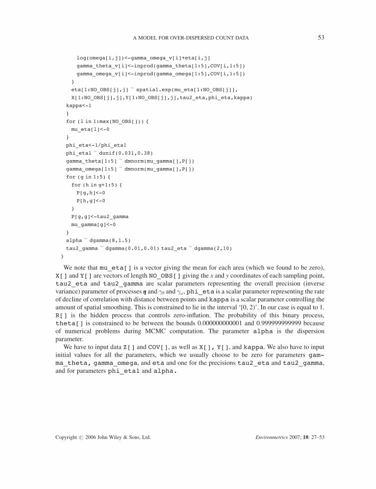
log(omega[i,j])<-gamma_omega_v[i]+eta[i,j]

gamma_theta_v[i]<-inprod(gamma_theta[1:5],COV[i,1:5])

gamma_omega_v[i]<-inprod(gamma_omega[1:5],COV[i,1:5])

}

eta[1:NO_OBS[j],j] � spatial.exp(mu_eta[1:NO_OBS[j]],

X[1:NO_OBS[j],j],Y[1:NO_OBS[j],j],tau2_eta,phi_eta,kappa)

kappa<-1

}

for (l in 1:max(NO_OBS[])) {

mu_eta[l]<-0

}

phi_eta<-1/phi_eta1

phi_eta1 � dunif(0.031,0.38)

gamma_theta[1:5] � dmnorm(mu_gamma[],P[])

gamma_omega[1:5] � dmnorm(mu_gamma[],P[])

for (g in 1:5) {

for (h in g+1:5) {

P[g,h]<-0

P[h,g]<-0

}

P[g,g]<-tau2_gamma

mu_gamma[g]<-0

}

alpha � dgamma(8,1.5)

tau2_gamma � dgamma(0.01,0.01) tau2_eta � dgamma(2,10)

}

We note that mu_eta[] is a vector giving the mean for each area (which we found to be zero),

X[] and Y[] are vectors of length NO_OBS[] giving the x and y coordinates of each sampling point,

tau2_eta and tau2_gamma are scalar parameters representing the overall precision (inverse

variance) parameter of processes g and �� and �!, phi_eta is a scalar parameter representing the rate

of decline of correlation with distance between points and kappa is a scalar parameter controlling the

amount of spatial smoothing. This is constrained to lie in the interval ‘[0, 2)’. In our case is equal to 1.

R[] is the hidden process that controls zero-inflation. The probability of this binary process,

theta[] is constrained to be between the bounds 0.000000000001 and 0.999999999999 because

of numerical problems during MCMC computation. The parameter alpha is the dispersion

parameter.

We have to input data Z[] and COV[], as well as X[], Y[], and kappa. We also have to input

initial values for all the parameters, which we usually choose to be zero for parameters gam-ma_theta, gamma_omega, and eta and one for the precisions tau2_eta and tau2_gamma,and for parameters phi_eta1 and alpha.



A Bayesian hierarchical model for over-dispersed count data: a case study for abundance of hake...

Documents

Transcript of A Bayesian hierarchical model for over-dispersed count data: a case study for abundance of hake...