Flood mitigation at watershed scale through dispersed dry dams
213
HAL Id: tel-02591342 https://hal.inrae.fr/tel-02591342 Submitted on 15 May 2020 HAL is a multi-disciplinary open access archive for the deposit and dissemination of sci- entific research documents, whether they are pub- lished or not. The documents may come from teaching and research institutions in France or abroad, or from public or private research centers. L’archive ouverte pluridisciplinaire HAL, est destinée au dépôt et à la diffusion de documents scientifiques de niveau recherche, publiés ou non, émanant des établissements d’enseignement et de recherche français ou étrangers, des laboratoires publics ou privés. Flood mitigation at watershed scale through dispersed dry dams: analysis of the impact on discharge frequency regimes S. Chennu To cite this version: S. Chennu. Flood mitigation at watershed scale through dispersed dry dams: analysis of the impact on discharge frequency regimes. Environmental Sciences. Thèse, spécialité ”Océan, Atmosphère, Hydrologie”, INPG Grenoble, 2008. English. tel-02591342
-
Upload
khangminh22 -
Category
Documents
-
view
1 -
download
0
Transcript of Flood mitigation at watershed scale through dispersed dry dams
HAL Id: tel-02591342https://hal.inrae.fr/tel-02591342
Submitted on 15 May 2020
HAL is a multi-disciplinary open accessarchive for the deposit and dissemination of sci-entific research documents, whether they are pub-lished or not. The documents may come fromteaching and research institutions in France orabroad, or from public or private research centers.
L’archive ouverte pluridisciplinaire HAL, estdestinée au dépôt et à la diffusion de documentsscientifiques de niveau recherche, publiés ou non,émanant des établissements d’enseignement et derecherche français ou étrangers, des laboratoirespublics ou privés.
Flood mitigation at watershed scale through disperseddry dams: analysis of the impact on discharge frequency
regimesS. Chennu
To cite this version:S. Chennu. Flood mitigation at watershed scale through dispersed dry dams: analysis of the impacton discharge frequency regimes. Environmental Sciences. Thèse, spécialité ”Océan, Atmosphère,Hydrologie”, INPG Grenoble, 2008. English. �tel-02591342�
INSTITUT POLYTECHNIQUE DE GRENOBLE
N° attribué par la bibliothèque
|__|__|__|__|__|__|__|__|__|__|
T H E S E
pour obtenir le grade de
DOCTEUR DE L’Institut polytechnique de Grenoble
Spécialité : Océan, Atmosphère, Hydrologie
préparée au sein de l'Unité de Recherche Hydrologie-Hydraulique du Cemagref de Lyon
dans le cadre de l’Ecole Doctorale “Terre, Univers, Environnement”
présentée et soutenue publiquement par
Sandhya Mandyam Chennu
Le 12 Décembre 2008
Flood mitigation at watershed scale through dispersed dry dams:
Analysis of the impact on discharge-frequency regimes
DIRECTEURS DE THESEJean-Michel GRESILLON et Denis DARTUS
JURY
M. Charles OBLED Prof. L.T.H.E/INP, Grenoble PrésidentM. Roger MOUSSA DR INRA, Montpellier RapporteurM. Hervé ANDRIEU DR LCPC, Nantes RapporteurM. Jean-Michel GRESILLON DR Emérite Cemagref, Lyon Directeur de thèseM. Denis DARTUS Prof. INP, Toulouse Co-Directeur de thèseM. Hans-Peter NACHTNEBEL Prof. IWMHH, Vienne ExaminateurM. Marco BORGA Assitant Prof. Univ., Padova ExaminateurM. Arnaud de BONVILLER Ingénieur. ISL, Angers Examinateur
Cem
OA
: ar
chiv
e ou
verte
d'Ir
stea
/ C
emag
ref
FLOOD MITIGATION AT WATERSHED SCALE
THROUGH DISPERSED DRY DAMS:
ANALYSIS OF THE IMPACT ON
DISCHARGE-FREQUENCY REGIMES
Cem
OA
: ar
chiv
e ou
verte
d'Ir
stea
/ C
emag
ref

Acknowledgements
I would like to first of all thank Jean-Michel Grésillon for guiding the present work, whose
experience and advice were irreplaceable. He taught me perseverance and tenacity necessary to
carry out a project to its fruitful finish. His insight helped me document and compile my PhD work.
I would also like to thank Denis Dartus for having confidence and recommend me for the present
thesis.
The funding for the present project was provided by the “Cluster de recherche Rhône-Alpes
Environnement”.
I specially thank Samuel Abiven, Elodie Renouf, Bernard Chastan, Maria-Hélène Ramos, Eric
Sauquet, Flora Branger, Benoit Camenen and Jean-Michel Grésillon for their inputs and critics in
helping me write my PhD thesis. I am grateful to Otmane Souhar, Mathieu Ribatet, Eric Sauquet
and Jean-Baptiste Faure for their help and guidance in programming and technical assistance. Along
the same lines, I express my gratitude towards Guillaume Dramais, Fabien Thollet and Mickaël
Lagouy for their help with the database.
I take this opportunity to thank Adeline Dubost, Anne Eichloz and Hélène Faurant who were the
embodiment of efficiency for administrative matters and with out whom the different administrative
tasks would have been undoubtedly endless.
Special thanks to my office room colleagues: Otmane Souhar, Flora Branger and Maria-Hélène
Ramos for having supported me and my habits during three years.
I am grateful to Françoise Bohain, Christine Poulard and Guillaume Dramais for their aid in helping
me to settle down in Lyon. Thanks to Christine for her generous nature, the train tickets and the
chocolates among many other things.
And it would be difficult not to mention the nice ambiance of Cemagref created by: Elodie with her
perspicacity, Anne-Laure with her understanding and gentle nature - whom all new comers would
inevitably assume to belong to HH and Jean-Marie, Flora, Eric, Mathieu, Judicaël, Benjamin,
Aurélien, Yan, Olivier, Jérôme, Benoit, Jan, Sébastien, Christine, Anne, Hélène. Thank you all for
Cem
OA
: ar
chiv
e ou
verte
d'Ir
stea
/ C
emag
ref

initiating me to the french culture of language, culture, food (with some very delicious recipes),
sports: soccer (a game at which I need to work), badminton and frisbee. I had the opportunity to
work and rub shoulders with some very nice people during my stay at Cemagref, Lyon.
The badminton gang of Cemagref helped me unwind during the easy and hard times of a PhD:
Elodie an adversary with whom I discovered the different facets of the game, Arnaud and Alex who
were both formidable adversaries along with Aurélien and Eric who made sure I worked for my
bread. And last but not least Olivier, Guillaume and Stephan who brought charm to the game.
Special thanks to Elodie who was a good sounding board and gave me moral support and
encouragement while writing my thesis ......... thank you for the lunches, talks, advices and
understanding which helped me through my PhD.
Thanks to Anne-Laure, Aurélien, Elodie, Eric, Flora, Stephani and Yan for preparing delicious
dishes for the party after the PhD dissertation. Thank you all for the efficient execution of a
memorable PhD party.
Above all special thanks to Samuel who put up with me and for having always been there for me
during the last three years. His support and encouragement helped me reach my goal and his efforts
are but difficult to describe in words. I am very grateful for my family: Amma, Ayya, Rajani and
Usha for trusting and encouraging me to pursue my PhD course....... and thanks to Megha who
always brought in charm and humour in her conversations.
I am sure to have forgotten lots of name, but I would like to express my sincere gratitude to all
those who made this a memorable experience.
7
Cem
OA
: ar
chiv
e ou
verte
d'Ir
stea
/ C
emag
ref

Abstract
Increase in losses of lives and properties due to flooding in recent decades has driven the search for
efficient flood management strategies. At the watershed scale, zones of interest are found dispersed
and intensified due to development pressures. Protection against flooding for the entire watershed is
thus necessary. Appropriate mitigation strategies at watershed scale through dispersed dry dams are
explored presently. Dry dams are flood mitigation structures, which reduce flood peaks while
respecting the normal river regime. During flooding, the dam holds back excess flood volume and
depreciates them to manageable levels for downstream areas. A chain of models are employed to
test potential mitigation strategies at watershed scale, on a French basin. The chain is constituted by
a rainfall generator for the simulation of space-time variable rainfall fields (TBM), a distributed
rainfall-run-off model to simulate surface run-off (MARINE) and a hydraulic model (MAGE) to
route the surface run-off to the watershed outlet. The aim is to simulate representative instantaneous
discharge-frequency regimes of the watershed, at points of interest and then introduce dry dams
along the drainage network, to simulate mitigated instantaneous discharge-frequency regimes. An
attenuation factor is defined to measure the domain of achievable mitigation efficiency. Using this
approach, it is possible to gauge the flood frequencies which can be mitigated given the parameters
of available storage volume, location and dimensions of the dry dams. Thus the efficiency and
performance limit of dry dam mitigation projects is illustrated. The importance of working at
watershed scale and discharge-frequency regime scale is shown in the present work.C
emO
A :
arch
ive
ouve
rte d
'Irst
ea /
Cem
agre
f

Résumé
En raison de l'extension des zones vulnérables ou d'une possible aggravation de l'aléa, le risque
d'inondation pourrait continuer de s'accroitre dans les années à venir. Des stratégies d'atténuation,
capables de respecter les rivières et prenant en compte l'ensemble des bassins versants s'avèrent
indispensables. Le travail présenté ici cherche à caractériser l'effet d'un ensemble de « barrages
secs » sur le régime d'une rivière. Il s'agit de barrages disposant d'un orifice tel que la rivière s'y
écoule en régime normal; à l'occasion d'une crue l'excès de débit est retenu par le barrage et restitué
ensuite. Sur un bassin versant réel de la région de Lyon (France) une chaîne de modélisation est
mise en place de façon à reconstruire par simulation un régime de débit instantané-fréquence
semblable à celui qui est observé. La chaine comprend un modèle générateur de pluies spatialement
variables (TBM), un modèle spatialisé de transformation de la pluie en débit (MARINE) et un
modèle d'écoulement en rivière (MAGE). Elle permet de modéliser les crues puis d'introduire les
barrage secs dispersés pour construire une régime instantané « naturel » puis atténué par les
barrages. Un indicateur d'efficacité est défini pour mesurer l'atténuation des crues sur l'ensemble des
fréquences. L'influence des paramètres définissant les barrages, leurs volumes, leurs emplacements,
leurs dimensions, est explorée. L'importance de travailler à l'échelle du bassin versant et à l'échelle
du régime débit-fréquence est démontrée dans ce travail.
Cem
OA
: ar
chiv
e ou
verte
d'Ir
stea
/ C
emag
ref

Table of Contents
1 Preview of flood management practices and proposed methodology...............................................1
1.1 Definition of flooding and chronicle of past decades and future trends of flood events...........2
1.1.1 Definition...........................................................................................................................2
1.1.2 Chronicle of past decades...................................................................................................2
1.1.3 Future trends of floods.......................................................................................................5
1.2 Paradigm change from flood control to flood risk management...............................................7
1.2.1 Shortcomings of flood control management......................................................................7
1.2.2 Shift to flood risk management..........................................................................................8
1.2.3 Structural and non-structural mitigation measures..........................................................10
1.3 Methodology towards an integrated assessment of flood risk management ..........................13
1.3.1 Efficiency of flood risk management measures through discharge-frequency regimes. .14
1.3.2 Protection to entire region................................................................................................17
A Dispersed mitigation strategy...........................................................................................17
B Dry dams...........................................................................................................................19
1.3.3 Accounting of spatial rainfall variability..........................................................................21
1.4 Thesis introduction...................................................................................................................24
1.4.1 Method.............................................................................................................................24
1.4.2 Attenuation factor.............................................................................................................26
1.4.3 Impact of Mitigation Measure Efficiency on Regime Scale: IMMERS..........................26
1.5 Thesis outline...........................................................................................................................28
2 Study area........................................................................................................................................31
2.1 Introduction..............................................................................................................................32
2.2 Presentation of the study area..................................................................................................32
2.3 Spatial data set of the watershed .............................................................................................34
2.3.1 Topography.......................................................................................................................34
2.3.2 Soil texture and soil depth................................................................................................36
2.3.3 Land-use...........................................................................................................................37
2.4 Hydrological data set...............................................................................................................38
2.4.1 Rainfall data.....................................................................................................................38
2.4.2 Discharge data..................................................................................................................39
2.5 Analysis of observed rainfall and discharge data set...............................................................40
2.6 Conclusions about the study area.............................................................................................47
Cem
OA
: ar
chiv
e ou
verte
d'Ir
stea
/ C
emag
ref
3 Space-time stochastic rainfall modelling for flood mitigation analysis..........................................49
3.1 Introduction..............................................................................................................................50
3.2 Rainfall generator and the simulated rainfall fields.................................................................51
3.2.1 Basic concept behind the rainfall generator.....................................................................51
A Properties of stationary random functions........................................................................52
B Theory of Turning Bands Method....................................................................................53
3.2.2 Parametrisation of the rainfall simulator..........................................................................55
A Observed rainfall data input into the TBM model............................................................57
B Point distribution and variogram of non-null rainfall values............................................59
C Rainfall zone indicator......................................................................................................61
D Point distribution and variogram of Yzeron watershed in comparison with Grand Lyon
district...................................................................................................................................62
3.2.3 Output of the TBM model and verification of the spatial and temporal variogram of the
simulated output........................................................................................................................64
A Output of TBM model......................................................................................................64
B Verification of the spatial and temporal variogram of the simulated output....................66
3.3 Analysis of the space-time variable rainfall simulated by TBM rainfall simulator.................67
3.3.1 Rainfall intensity-duration-frequency analysis................................................................68
3.3.2 Analysis of simulated hyetographs..................................................................................70
3.3.3 Analysis of the spatial correlation of simulated rainfall ..................................................73
3.4 Conclusions of the simulated space-time rainfall data furnished by the TBM model ............77
4 Simulation of rainfall-run-off process at watershed scale and design of dry dams.........................79
4.1 Introduction..............................................................................................................................80
4.2 Presentation of the hydrological and hydraulic models...........................................................81
4.2.1 Presentation of the distributed hydrological model MARINE.........................................81
4.2.2 Presentation of the 1-D hydraulic model MAGE.............................................................87
4.3 Calibration of MARINE and MAGE model parameters to simulate observed discharge under
uniform distribution of observed rainfall.......................................................................................89
4.3.1 Sensitivity analysis of MARINE......................................................................................89
4.3.2 Calibration and evaluation of MARINE..........................................................................90
4.3.3 Coupling of the models MARINE and MAGE for the routing of lateral surface run-off
...................................................................................................................................................95
A Segmentation of Yzeron drainage network......................................................................95
B Insertion of measured cross-section profiles into the extracted DEM profiles................98
C Validation of coupling of MARINE and MAGE models...............................................102
Cem
OA
: ar
chiv
e ou
verte
d'Ir
stea
/ C
emag
ref
4.3.4 Conclusions about the simulation of surface run-off process at watershed scale..........104
4.4 Simulation of observed discharge-frequency curve under space-time variable rainfall via the
MARINE and MAGE models......................................................................................................105
4.4.1 Need for selection of a set of simulated rainfall events.................................................105
4.4.2 Selection of rainfall events from the output of rainfall simulator..................................106
4.4.3 Construction of instantaneous discharges-frequency regime at Taffignon....................110
4.4.4 Construction of discharge-frequency regimes at the control points...............................115
4.5 Dry dam mitigation measures................................................................................................117
4.5.1 Dry dam design..............................................................................................................117
4.5.2 Dry dam locations and configurations...........................................................................118
4.5.3 Dry dam dimensioning...................................................................................................119
4.5.4 Designed dry dams for flood mitigation........................................................................122
4.6 Conclusions about the simulated reference discharge-frequency regimes and dimensioning of
dry dams.......................................................................................................................................125
5 Dry dam mitigation analysis..........................................................................................................127
5.1 Introduction............................................................................................................................128
5.2 Influence of rainfall distribution on hydrographs..................................................................129
5.2.1 Mitigation analysis of individual events........................................................................131
A Mitigation assured by dry dams for an example event...................................................131
B Mitigation analysis of all events.....................................................................................134
5.3 Mitigation analysis at regime scale through instantaneous discharge-frequency regime......138
5.3.1 Influence of storage volume on flood mitigation...........................................................138
5.3.2 Influence of dry dam location........................................................................................142
A Intermediate zone of interest: Charbonnières aval and Craponne..................................142
B Downstream zone of interest: Taffignon.........................................................................145
5.3.3 Influence of dry dam bottom outlet................................................................................148
A Upstream zone of interest: Charbonnières amont...........................................................148
B Intermediate zones of interest: Charbonnières aval and Craponne................................150
C Downstream zone of interest: Taffignon.........................................................................152
5.4 Conclusions about dry dam mitigation analysis....................................................................154
6 Conclusions, Discussions and Perspectives..................................................................................157
6.1 Conclusions............................................................................................................................158
6.2 Discussions............................................................................................................................159
6.2.1 Uncertainties and approximation of the developed methodology..................................159
6.2.2 Model uncertainties........................................................................................................160
Cem
OA
: ar
chiv
e ou
verte
d'Ir
stea
/ C
emag
ref

6.2.3 Choice of the study area.................................................................................................162
6.3 Perspectives...........................................................................................................................163
7 References.....................................................................................................................................167
8 Appendix........................................................................................................................................183
Cem
OA
: ar
chiv
e ou
verte
d'Ir
stea
/ C
emag
ref
Index of Figures
Figure 1.1: Evolution of the flood disaster since 1970 to 2005. Source: EM-DAT, International
Disaster Database.................................................................................................................................4
Figure 1.2: Theoretical discharge - frequency curve without the presence of mitigation measures (in
blue) and in the presence of mitigation measures (in red). Source: European Environment Agency,
2001....................................................................................................................................................16
Figure 1.3: Illustration of the dispersed dry dam mitigation measures employed in (a) Miami
watershed composed of 5 dry dams - A, B, C, D and E (constructed between 1916 – 1920). Web
source: Communication of J. David Rogers (b) Muskingum river basin flood control system in
1930's, with dry dams encircled in red. Source: Muskingum River Basin Systems Operations Study,
US Army Corps of Engineers, Huntington district and Muskingum river basin initiative, 2006......18
Figure 1.4: Illustration of dry dam functioning during normal flow and high flow...........................20
Figure 1.5: Illustration of the procedure adopted in the thesis study. The simulation of a discharge-
frequency regime in the absence and presence of dry dams...............................................................25
Figure 1.6: Graphical illustration of the Impact of Mitigation Measure Efficiency in Regime Scale
(IMMERS)..........................................................................................................................................27
Figure 2.1: Watershed layout showing the discharge stations, rain gauges and drainage network of
Yzeron................................................................................................................................................33
Figure 2.2: Generated digital elevation model of Yzeron..................................................................34
Figure 2.3: Map showing the locations of the measured river cross-section profile by Navratil, 2005.
............................................................................................................................................................35
Figure 2.4: Soil texture map of the Yzeron watershed.......................................................................36
Figure 2.5: Grouped soil depth map of the Yzeron watershed from the study of Regional
agricultural chamber of Rhone-Alpes................................................................................................37
Figure 2.6: Land-use layout of the watershed Yzeron........................................................................38
Figure 2.7: Observed mean monthly discharge and rainfall values of the Yzeron watershed deduced
from the available dataset...................................................................................................................41
Figure 2.8: Instantaneous discharge-frequency curve at Chaudanne calculated from observed
discharge records of 17 years. Left hand side: Exponential fit; Right hand side: Pareto distribution
fit.........................................................................................................................................................42
Figure 2.9: Instantaneous discharge-frequency curve at Mercier calculated from observed discharge
records of 10 years. Left hand side: Exponential fit; Right hand side: Pareto distribution fit...........43
Figure 2.10: Instantaneous discharge-frequency curve at Craponne calculated from observed
Cem
OA
: ar
chiv
e ou
verte
d'Ir
stea
/ C
emag
ref
discharge of 36 years. Left hand side: Exponential fit; Right hand side: Pareto distribution fit.
Source: Sauquet and Ribatet, 2004.....................................................................................................43
Figure 2.11: Discharge-frequency curve at Taffignon calculated from observed discharge of 17
years. Exponential fit..........................................................................................................................44
Figure 3.1: Schematic representation of the field and the turning bands lines. Adapted from:
Mantoglou and Wilson, 1982.............................................................................................................54
Figure 3.2: Illustration of the decomposed rainfall fields for the generation of spatially variable
rainfall fields. The top left illustration shows the non-null rainfall field, the top right illustration
shows the rainfall zone indicator. Both these fields are generated separately by the TBM model. The
product of these two fields gives the final output rainfall field. The black colour in the top right
illustration represents the absence of rainfall and the white colour the rainfall zone. Adapted from:
Ramos, 2002.......................................................................................................................................57
Figure 3.3: Q-Q plot of the inverse Gaussian distribution of non-null rainfall values for 3-hour
rainfall of Yzeron watershed. Source: Leblois, 2008.........................................................................59
Figure 3.4: Variogram of 3-hour rainfall. Plus sign: empirical rainfall values; Thick line: spherical
adjustment. Source: Leblois, 2008.....................................................................................................60
Figure 3.5: Comparison of 3-hour non-null rainfall value variogram of the Yzeron watershed and
the Grand Lyon district. Plus: Empirical rainfall data of Yzeron; Cross: Empirical rainfall data of
Grand Lyon, Thick lines: Spherical adjustment. Source: Leblois, 2008............................................63
Figure 3.6: Example of a rainfall event simulated by the TBM model with 3-hour time step and a
500 m × 500 m of space resolution. Each image is simulated at a 3-hour time step and constitutes a
total duration of 24 hours. The evolution of rainfall reads from left to right.....................................65
Figure 3.7: Spatial variogram structure of 3-hour non-null simulated rainfall (left hand side) and
rainfall zone indicator (right hand side). Source: Leblois, 2008........................................................66
Figure 3.8: Temporal variogram structure of 3-hour non-null simulated rainfall (left hand side) and
rainfall zone indicator (right hand side). Source: Leblois, 2008........................................................67
Figure 3.9: Comparison of fitted intensity-duration-frequency curves of the observed (thick lines)
and the randomly chosen 900 simulated rainfall events (dotted lines) at the P18 rain gauge............69
Figure 3.10: Comparison of the 12-hour normalised hyetograph between the observed and
simulated events at the P18 rain gauge. The red line represents the interval: [mean - standard
deviation; mean + standard deviation] of the observed events at each time step...............................72
Figure 3.11: Comparison of the 24-hour normalised hyetograph between the observed and simulated
events at the P18 rain gauge. The red line represents the interval: [mean - standard deviation; mean
+ standard deviation] of the observed event at each time step...........................................................72
Figure 3.12: Comparison of the 48-hour normalised hyetograph between the observed and
Cem
OA
: ar
chiv
e ou
verte
d'Ir
stea
/ C
emag
ref

simulated events at the P18 rain gauge. The red line represents the interval: [mean - standard
deviation; mean + standard deviation] of the observed event at each time step................................73
Figure 3.13: Illustration of cumulated rainfall events simulated by the TBM simulator for 3 rainfall
durations (a) 12 hours with mean cumulative rainfall of 35 mm (b) 24 hours with mean cumulative
rainfall of 43 mm(c) 48 hours with mean cumulative rainfall of 43 mm, along with approximate
positioning of the 5 rain gauges..........................................................................................................74
Figure 4.1: Distinction of the drainage network into drains and river reaches in a watershed by
MARINE model.................................................................................................................................83
Figure 4.2: Map showing the consideration of drainage network as drains and a small river reach
(encircled) during the calibration of the model MARINE to the Yzeron watershed..........................91
Figure 4.3: Graph showing the observed and simulated hydrograph by MARINE (QM).................93
Figure 4.4: Distinction of the watershed slope, river and drains in MARINE. Also shown is the 1
km² threshold draining area from which a given pixel in the DEM is treated as a drain in MARINE.
The encircled drainage network constitutes 2 river segments in MARINE.......................................96
Figure 4.5: Representation of the drainage network of Yzeron in MAGE with respect to the
segmentation done in MARINE. The encircled river reach houses two river segments of MARINE
and introduces the two resulting lateral surface run-ff hydrographs of MARINE into respective river
segments. Only the river reaches are reproduced in the MAGE model.............................................97
Figure 4.6: The measured and extracted cross-section profiles of the river and flood plain along the
drainage network................................................................................................................................98
Figure 4.7: Example of a new cross-section profile detailing the flood plain and the inserted river
geometry.............................................................................................................................................99
Figure 4.8: Generated cross-section profile input into the model MAGE for the construction of the
drainage network of Yzeron watershed. The progression of the cross-section profile is given by the
grey, black and green lines in the figure at a distance of 635 m and 165 m respectively.................101
Figure 4.9: Comparison of the simulated November 1990 event by MARINE alone (QM) and by
the coupling of MARINE + MAGE (QM+M) at Taffignon. The Nash-Sutcliff efficiency for the
simulation alone by MARINE is 96.5% and by the coupling of MARINE + MAGE is 91.6%.....102
Figure 4.10: Comparison of the simulated November 1990 event by MARINE alone (QM)and by
the coupling of MARINE + MAGE (QM+M) at Craponne.............................................................104
Figure 4.11: Moving mean cumulated rainfall of simulated 900 rainfall events classed according to
a theoretical frequency given by equation 3.11, on the left hand side. On the right hand side, moving
mean cumulated rainfall after applying the threshold limits of 20, 25 and 30 mm for the 12 hours,
24 hours and 48 hours durations respectively...................................................................................107
Figure 4.12: Graph showing the placement of chosen simulated output of the TBM rainfall
Cem
OA
: ar
chiv
e ou
verte
d'Ir
stea
/ C
emag
ref
simulator compared to the mean observed events, for the representative rainfall durations of 12, 24
and 48 hours rainfall duration...........................................................................................................110
Figure 4.13: Watershed outlay, showing the four chosen control points: Charbonnières amont
represent the upstream zone of interest. Charbonnières aval and Craponne represents the
intermediate zones of interest and Taffignon represents the downstream zone of interest...............111
Figure 4.14: Observed and simulated instantaneous discharge-frequency curve at Taffignon
(watershed outlet).............................................................................................................................112
Figure 4.15: Comparison of simulated discharge-frequency curve resulted after the modification of
the simulated rainfall structures for alpha equal to 0.75 and 0.5......................................................113
Figure 4.16: Simulated instantaneous discharge-frequency curve for 2 sets of simulated rainfall
fields. The dots represent the observed peak discharge values, the triangle and square represent the
simulated peak discharge value from the 1st and 2nd set of simulated space-time variable rainfall
fields by TBM model........................................................................................................................114
Figure 4.17: Reference discharge frequency regime constructed from spatially variable rainfall at
the four control points.......................................................................................................................116
Figure 4.18: Design of dry dam adapted in the present study..........................................................118
Figure 4.19: Localisation of dry dams inside the Yzeron watershed................................................119
Figure 4.20: Estimated discharge-area envelope curve for the four discharge stations of the Yzeron
watershed..........................................................................................................................................120
Figure 5.1: Yzeron watershed layout, showing the control points and dry dam locations along the
main drainage network.....................................................................................................................129
Figure 5.2: Example of a cumulated (114 mm) 72 hours rainfall event simulated by TBM model.130
Figure 5.3: Simulated hydrograph at Taffignon from a spatially variable rainfall (QSR) and a
homogeneous distribution (QUR) of the same event. The dotted and dash-dot lines show the
potential mitigation in the presence of 10 and 11 downstream dry dams due to the two rainfall
distributions......................................................................................................................................131
Figure 5.4: Illustration of the spatial variability of rainfall for a simulated event, with a mean
cumulative volume of 43 mm in 24 hours duration. Also indicated are the 4 control points...........132
Figure 5.5: Hydrographs at Charbonnières amont (top left), Charbonnières aval (top right),
Craponne (bottom left) and Taffignon (bottom right), showing the attenuation effect of dry dams.
..........................................................................................................................................................133
Figure 5.6: Individual peak discharge mitigated by the upstream dry dams is shown in the left hand
graph, without any reorganisation of the peak discharge value in the ascending order at Taffignon.
The corresponding attenuation factor when calculated without any reorganisation is shown in the
right hand graph................................................................................................................................135
Cem
OA
: ar
chiv
e ou
verte
d'Ir
stea
/ C
emag
ref

Figure 5.7: The mitigated peak discharge values when classed in ascending order and represented as
IMMERS is shown in the left and right hand graphs respectively...................................................136
Figure 5.8: Peak ratio expressed in return periods at Taffignon on the left hand side in the presence
of 6 upstream dams. The right hand side graph presents the aggravation of the particular rainfall
event, which exceeds the peak ratio of 1 in the presence of upstream and intermediate dry dams. 137
Figure 5.9: Left hand graph display the discharge-frequency curve in the absence and presence of
small and large (1 and 2) dams at Charbonnières amont. In the right hand graph, the increase of
mitigation efficiency due to storage volume increase is demonstrated via the IMMERS graph.....139
Figure 5.10: Discharge-frequency curve in the absence and presence of dams at Taffignon. The
IMMERS curve on the right hand side presents the influence of increasing storage volume on
mitigation efficiency.........................................................................................................................142
Figure 5.11: Left hand graph display the discharge-frequency curve in the presence and absence of
dry dams at Charbonnières aval. The right hand graph illustrates the respective IMMERS graph for
the upstream and intermediated dry dams configurations................................................................143
Figure 5.12: Left hand graph display the discharge-frequency mitigation curve in the absence and
presence of upstream and intermediate dry dams at Craponne. The right hand graph illustrates the
respective IMMERS graph for the upstream and intermediated dry dams configurations..............145
Figure 5.13: Left hand graph display the discharge-frequency curve in the absence and presence of
upstream, downstream and intermediate dry dams at Taffignon. The right hand graph illustrates the
respective IMMERS graph deduced for the location of dry dams...................................................146
Figure 5.14: Dimensionless attenuation factor expressed in volume ratio at Charbonnières aval (left)
in the presence of upstream dams (1 to 4) and intermediate dams (7 to 6). The same, is represented
for Taffignon (right) in the presence of upstream (1 to 6), intermediate (7 to 9) and downstream
dams (10 to 11).................................................................................................................................147
Figure 5.15: Left hand graph display the discharge-frequency curve in the absence and presence of
Q2 and Q10 bottom outlet dry dams at Charbonnières amont. The right hand IMPRESS graph
presents the mitigation efficiency assured by the two dry dam designs...........................................149
Figure 5.16: Attenuation factor deduced for Charbonnières aval (left hand side) and Craponne (right
hand side) for Q2 and Q10 bottom outlet dimensions......................................................................151
Figure 5.17: IMMERS graph at Taffignon showing the mitigation efficiency due to Q2 and Q10
bottom outlet dimensions.................................................................................................................153
Figure 8.1: Hydrograph obtained for varying rainfall intensities during sensitivity analysis of
MARINE model...............................................................................................................................187
Figure 8.2: Sensitivity of Manning roughess coefficient in MARINE model for the Yzeron
watershed. ........................................................................................................................................188
Cem
OA
: ar
chiv
e ou
verte
d'Ir
stea
/ C
emag
ref
Figure 8.3: Sensitivity analysis of the MARINE model to the initial soil humidity condition........189
Figure 8.4: Sensitivity analysis of MARINE model to soil depth parameter...................................190
Figure 8.5: Sensitivity of time step analysis of MARINE model to observed events of the Yzeron
watershed..........................................................................................................................................191
Figure 8.6: Observed and simulated November 2002 event by MARINE. Nash = 44.79%............192
Figure 8.7: Observed and simulated December 2003 event by MARINE. Nash = 41.19%............192
Figure 8.8: Observed and simulated November 1996 event by MARINE. Nash = 86.27%............192
Figure 8.9: Observed and simulated March 1991 event by MARINE. Nash = 86.3%....................192
Figure 8.10: Observed and simulated April 2005 event by MARINE. Nash = 74.55%..................193
Figure 8.11: Outlay of the Yzeron watershed, showing the location of the extracted profiles from the
DEM model. Also shown are the slopes of the originating drainage network of various tributaries
..........................................................................................................................................................194
Figure 8.12: Example of an extracted cross-section profile of the drainage network from the DEM
..........................................................................................................................................................194
Figure 8.13: Example of a measured cross-section profile of river to be inserted into the extracted
profile from DEM.............................................................................................................................195
Figure 8.14: Graph showing the new cross-section profile with the integrated minor bed upstream.
..........................................................................................................................................................196
Figure 8.15: An attempt to stratify a 12-hour (Top) and a 48-hour (bottom) simulated rainfall fields
with stratification factor α, of 0.75 and 0.5 respectively..................................................................197
Cem
OA
: ar
chiv
e ou
verte
d'Ir
stea
/ C
emag
ref
Index of Tables
Table 1.1.1: Examples of major floods reported in the last decade around the world. Source: ISDR,
1999 and web. B = Billion ; M = Million ; NA = Information not available. .....................................5
Table 1.2.1: Potential strategies of flood risk management at watershed scale..................................11
Table 1.3.1: Review of articles on the importance and influence of accounting rainfall variability..23
Table 2.4.1: Rain gauge database of the Yzeron watershed...............................................................39
Table 2.4.2: Discharge database of the Yzeron watershed.................................................................39
Table 2.5.1: Analysis of the peak discharge events exceeding 30 m3s-1 at Taffignon (watershed
outlet) with corresponding rainfall data.............................................................................................46
Table 3.2.1: Comparison of the mean and standard deviation values of the Yzeron watershed with
the Grand Lyon district rainfall data. µ = mean rainfall value, σ = standard deviation.....................62
Table 3.3.1: Distance (km) between the 5 rain gauges used as input to the rainfall simulator..........75
Table 3.3.2: 12-hour correlation coefficients calculated for 28 observed events and 15 simulated
events..................................................................................................................................................75
Table 3.3.3: 24-hour correlation coefficients calculated for 19 observed events and 15 simulated
events..................................................................................................................................................76
Table 3.3.4: 48-hour correlation coefficients calculated for 11 observed events and 15 simulated
events..................................................................................................................................................76
Table 4.3.1: Experimental soil characteristic values deduced from literature and the imposed soil
depth values associating with the soil texture information. Source: Maidment, 1992.......................92
Table 4.3.2: Initial experimental and calibrated Manning or roughness coefficients in MARINE.
Source: Maidment, 1992....................................................................................................................92
Table 4.3.3: Simulated discharge events at Taffignon by MARINE and the Nash-Sutcliffe efficiency
criterion obtained for the respective simulated hydrographs..............................................................94
Table 4.4.1: Recapitulation of the 45 simulated events extracted from the output of the rainfall
simulator TBM.................................................................................................................................109
Table 4.5.1: Peak discharge values recorded at the four discharge station, along with the draining
surface area by each station. The peak flow-basin area envelope relationship calculated with a
power function..................................................................................................................................120
Table 4.5.2: Design dimensions of the 11 small dry dams with a Q2 bottom outlet and a spillway
design flood of Q100. Storage volume is expressed in million (M) m3..........................................123
Table 4.5.3: Design dimensions of the 11 small dry dams with a Q10 bottom outlet and a spillway
design flood of Q100. Storage volume is expressed in million (M) m3..........................................123
Cem
OA
: ar
chiv
e ou
verte
d'Ir
stea
/ C
emag
ref
Table 4.5.4: Design dimensions of the 11 large dry dams with a Q2 bottom outlet and a spillway
design flood of Q100. Storage volume is expressed in million (M) m3..........................................124
Table 4.5.5: Design dimensions of the 11 large dry dams with a Q10 bottom outlet and a spillway
design flood of Q100. Storage volume is expressed in million (M) m3..........................................124
Table 5.3.1: Mean dimensionless attenuation factor calculated for small dry dams 1 and 2 with
bottom outlets designed to constraint the outflow discharge to Q2 flood at Charbonnières amont.
* Not a mean value, but the result of additional event included explicitly.......................................140
Table 5.3.2: Mean dimensionless attenuation factor calculated for increase in storage volume at
Taffignon.* Not a mean value, but the result of additional event included explicitly......................142
Table 5.3.3: Mean dimensionless attenuation factor calculated for upstream and intermediate dry
dam configuration with Q2 bottom outlet at Charbonnières aval.* Not a mean value, but the result
of additional event included explicitly..............................................................................................144
Table 5.3.4: Mean dimensionless attenuation factor calculated for upstream and intermediate dry
dam configuration with Q2 bottom outlets at Craponne..................................................................145
Table 5.3.5: Mean dimensionless attenuation factor calculated for different dry dam configurations
with Q2 bottom outlet, at Taffignon.* Not a mean value, but the result of additional event included
explicitly...........................................................................................................................................146
Table 5.3.6: Mean dimensionless attenuation factor calculated for dry dams 1 and 2 with bottom
outlets designed to constraint the outflow discharge to Q2 and Q10 flows at Charbonnières amont.
* Not a mean value, but the result of additional event included explicitly.......................................150
Table 5.3.7: Dimensionless attenuation factor calculated for upstream and intermediate dry dam
configuration with Q2 and Q10 bottom outlet dimensions at Charbonnières aval. * Not a mean
value, but the result of additional event included explicitly.............................................................152
Table 5.3.8: Dimensionless attenuation factor calculated for upstream and intermediate dry dam
configuration with Q2 and Q10 bottom outlet dimensions at Craponne. * Not a mean value, but the
result of additional event included explicitly....................................................................................152
Table 5.3.9: Dimensionless attenuation factor calculated for upstream, intermediate and downstream
dry dam configurations with bottom outlets designed to constrain the outflow to Q2 at Taffignon. *
Not a mean value, but the result of additional event included explicitly..........................................153
Table 5.3.10: Dimensionless attenuation factor calculated for upstream, intermediate and
downstream dry dam configurations with bottom outlets designed to constrain the outflow to Q10 at
Taffignon. * Not a mean value, but the result of additional event included explicitly.....................154
Table 8.I: Non spatial parameters imposed on Yzeron during the sensitivity analysis....................187
Table 8.II: Recapitulation of the model simulation for change in rainfall intensity.........................188
Table 8.III: Results of the sensitivity analysis of MARINE for Manning or roughness coefficient of
Cem
OA
: ar
chiv
e ou
verte
d'Ir
stea
/ C
emag
ref

watershed slopes...............................................................................................................................188
Table 8.IV: Results of the sensitivity analysis of MARINE for the initial humidity condition.......189
Table 8.V: Results of the sensitivity analysis of MARINE for variation in soil depth.....................190
Table 8.VI: Results of the sensitivity analysis of MARINE for variation in time-step of an observed.
..........................................................................................................................................................191
Cem
OA
: ar
chiv
e ou
verte
d'Ir
stea
/ C
emag
ref

1 PREVIEW OF FLOOD MANAGEMENT PRACTICES AND
PROPOSED METHODOLOGY
Cem
OA
: ar
chiv
e ou
verte
d'Ir
stea
/ C
emag
ref
1.1 Definition of flooding and chronicle of past decades and
future trends of flood events
1.1.1 Definition
A flood is defined as the irruption of water over otherwise dry land (The international Federation of
Red Cross and Red Crescent Societies, 1999). The lexical definition of flooding brings attention to
the resulting significant adverse effects to the vicinity, due to the high stream flow overtopping the
natural or artificial banks in any reach of a stream. These adverse effects are caused by two broadly
categorised types of floods, i.e. river floods or coastal floods. The river floods could be a result of
long and intense periods of rainfall and/or combined with ice and snow melt. Coastal floods could
result from storm surges, driven by ocean winds or tides. They can also result due to tsunami, which
is a seismic sea wave set off by a submarine earthquake. These two categories of floods inundate
large areas of land and destroy lives and properties.
The proximity of livelihood near rivers, which contains one of the basic element of life, encloses
not just advantages but also negative consequences such as flooding. The vulnerability of lives and
properties in proximity to flood plains can not be ignored and needs careful analysis. The present
study focuses on river floods and mitigation of the same.
1.1.2 Chronicle of past decades
Flooding is a natural phenomena and has existed since centuries, provoking disasters to different
habitats. Narrations of floods being one of the reasons for the downfall of ancient urban
civilizations like Mesopotamia, Indus valley (3000 – 1000 BCE) have been corroborated by
archaeologists. Historically, human settlements have always been in close relationship with the
rivers. Water being a basic element of life has attracted human settlements due to potable water,
2
Cem
OA
: ar
chiv
e ou
verte
d'Ir
stea
/ C
emag
ref

fertile lands and transportation. These incentives over the periods has encouraged settlements in
floodplains, where the natural flood hazard exists. Many lives have been taken and affected due to
this natural hazard through out the world. An understanding about the cause and effect of this
process is thus necessary to find much needed solutions (Blöschl et al., 2007) for sustainable
developments.
Awareness towards this natural disaster has increased lately due to the latest communication
technologies. Amongst the different types of natural disasters recorded since 1900, the Emergency
Events Database (EM-DAT) reported a worldwide increase of hydro-meteorological disasters since
the 1960's. The EM-DAT document any event as disastrous if one of the following criteria is
fulfilled:
● Ten or more people reported killed.
● Hundred people reported affected.
● Declaration of a state of emergency.
● Call for international assistance.
With the above criteria, EM-DAT reported a marked increase of flood impact (Figure 1.1), which
represented 30% distribution (the highest), amidst the natural disasters since 1970 to date (ISDR,
2003). In the regional distribution of disasters by type from 1991 – 2005, flooding represented 40%
of total world disaster distribution in Europe, 20% in Oceania, while 30% in America, Africa and
Asia (ISDR, 2003).
The perception that there are more natural disasters, in this case floods, could be fostered by the
worldwide instant information society, with regular and methodological documentation of events
compared to earlier times. It could also be linked to the intensification of human activities in flood
prone areas, which in turn increases the vulnerability of population to floods. Thus a precipitated
conclusion of an increase in the number of floods, in the recent years should be avoided. One needs
3
Cem
OA
: ar
chiv
e ou
verte
d'Ir
stea
/ C
emag
ref
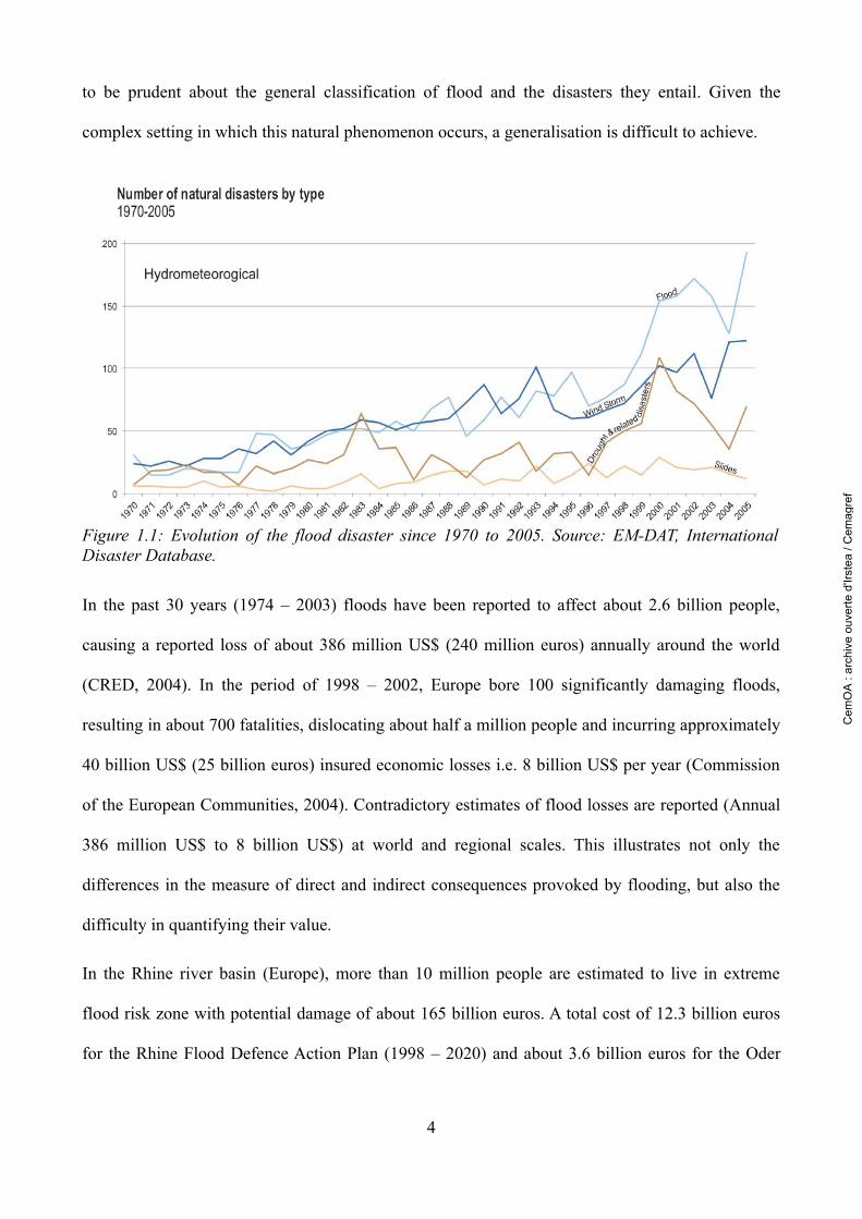
to be prudent about the general classification of flood and the disasters they entail. Given the
complex setting in which this natural phenomenon occurs, a generalisation is difficult to achieve.
In the past 30 years (1974 – 2003) floods have been reported to affect about 2.6 billion people,
causing a reported loss of about 386 million US$ (240 million euros) annually around the world
(CRED, 2004). In the period of 1998 – 2002, Europe bore 100 significantly damaging floods,
resulting in about 700 fatalities, dislocating about half a million people and incurring approximately
40 billion US$ (25 billion euros) insured economic losses i.e. 8 billion US$ per year (Commission
of the European Communities, 2004). Contradictory estimates of flood losses are reported (Annual
386 million US$ to 8 billion US$) at world and regional scales. This illustrates not only the
differences in the measure of direct and indirect consequences provoked by flooding, but also the
difficulty in quantifying their value.
In the Rhine river basin (Europe), more than 10 million people are estimated to live in extreme
flood risk zone with potential damage of about 165 billion euros. A total cost of 12.3 billion euros
for the Rhine Flood Defence Action Plan (1998 – 2020) and about 3.6 billion euros for the Oder
4
Figure 1.1: Evolution of the flood disaster since 1970 to 2005. Source: EM-DAT, International Disaster Database.
Cem
OA
: ar
chiv
e ou
verte
d'Ir
stea
/ C
emag
ref

Basin Flood Action Programme (2004 – 2029) is estimated. The investment for the Oder Basin
mitigation plan, represents a sum equal to the direct damage caused by the 1997 flood disaster alone
(Commission of the European Communities, 2004).
Some examples of floods occurred around the world in the last decade is recapitulated in Table
1.1.1. We see that the occurrence of floods is not just limited to developed countries, but affects
developing countries at a greater scale. The population in developing countries are more vulnerable
to flooding due to lack of supporting infrastructure. The impact of disasters is thus felt stronger in
the developing countries (Hansson et al., 2008).
1.1.3 Future trends of floods
Floods are threatening and the risk due to flooding is estimated to increase in the future due to two
principle trends. Firstly, due to population explosion, development pressure, land-use change and
transgression onto flood risk zones (Robert et al., 2003) and secondly due to anticipated climate
change (Guo et al., 2008; Wang et al., 2008).
Increase in flood peak values has lead to record breaking events (Arnell, 2002; Llasat et al., 2005;
5
Region River basin Year Killed Affected Economic loss (US$)
United States of America Mississippi/Missouri 1993 40 31,000 16 B
Europe Rhine, Meuse 1993-1995 0 NA 6.5 B
Europe Oder, Vistula and Niesse 1997 100 210,000 5 B
Canada Red 1997 NA 23,000 NAChina Yangtze 1998 4,150 180,000,000 30 B
Bangladesh Brahmaputra 1998;2004 918;800 900,000;360,0000 NAEurope Danube, Elbe 2002 80 600,000 15 BIndia Maharashtra 2005 1000 NA 100 M
Table 1.1.1: Examples of major floods reported in the last decade around the world. Source: ISDR, 1999 and web. B = Billion ; M = Million ; NA = Information not available.
Cem
OA
: ar
chiv
e ou
verte
d'Ir
stea
/ C
emag
ref

Pokrovsky, 2007). This trend was attributed to land-use change, (Hewlett and Helvey, 1970, Smith
and Bedient, 1981, UNESCO, 2001, Hundecha and Bardossy, 2004, Ecosystems and human well-
being: Policy responses, 2005) giving an impression of increase in flooding pattern (Kundzewicz
and Takeuchi, 1999). In Europe, the population growth steadily increased from 315 million in 1960
to 375 million by 1999, with the urban populations having increased at twice the overall growth rate
(European Environment Agency, 2002). Over the last 20 years the built-up area has increased up to
20% of growth rate compared to a population growth of only 6% in western and eastern European
countries. This rapid increase in urban infrastructure exerts enormous pressure on rural and natural
environments (European Environmental Agency, 1995). According to recent estimates, 2% of the
agricultural land in Europe is encroached by urbanisation every 10 years (European Environment
Agency, 2002). The concurrence of flood prone areas to demographic development advocates the
influence of land-use changes on the inducement, intensification and impact of flooding (Smith and
Bedient, 1981; European Environment Agency, 2001; Hundecha and Bardossy, 2004; Hall et al.,
2003; Petrow et al., 2006).
Among the numerous consequences of climate change under contemplation (Lang, 2006; Renard,
2008), some authors predict aggravation of flooding scene (International Federation of Red Cross
and Red Crescent, 1999; Chen et al., 2007; Zhang et al., 2008). The change in observed
temperature, precipitation, patterns in atmospheric and oceanic circulation, extreme weather and
climate events, i.e. overall features of the climate variability has been studied by the
Intergovernmental Panel on Climate Change (IPCC, 2001). And the potentiality of extreme events
and its consequences on flooding due to climate change can not be ignored (Zhang et al., 2008; Guo
et al., 2008; Commission of the European Communities, 2006).
The need to protect human habitat against flood disaster is acknowledged. Adapted mitigation
frameworks to protect oneself against this disaster is necessary. The evolution of the past flood
mitigation strategies and its adaptation to the current and future situation needs to be understood
6
Cem
OA
: ar
chiv
e ou
verte
d'Ir
stea
/ C
emag
ref

and is addressed in the next section.
1.2 Paradigm change from flood control to flood risk
management
1.2.1 Shortcomings of flood control management
Traditionally flood management was essentially problem driven, where usually after a severe flood,
immediate alleviation project would be quickly implemented without studying in detail the impacts
on upstream and downstream areas (WMO/GWP, 2004a; Water Directors of the European Union,
2004; Knight and Shamseldin, 2006; Hutter, 2006). The protection measures thus were composed of
aliquot solutions to alleviate the immediate danger. The problem and its solution seeming self-
evident were not preoccupied for the impacts it would have on the ecosystem, landscape and on
other regions within the catchment basin.
Various mitigation measures were employed to reduce flooding and susceptibility to flood damage.
Despite large investments, works and efforts put into these mitigation measures, the number of
people affected, economical damage and the occurrence of flood have not decreased (Kundzewicz,
1999; ISDR, 2003; ISDR, 2005, CRED, 2007). Isolated structural measures were noted to shift the
problem rather than attenuate flooding (Pinter et al., 2005; Pinter et al., 2006). Repercussion on
riparian ecosystem (example: flora and fauna), environmental issues (Falconer, 2002), wetlands and
natural settings due to conception of mitigation measures were not accounted for while planning the
mitigation project (Hughes and Rood, 2004; Braatne et al., 2008; Jonkman et al., 2008, Dijkman,
2008). These solutions were also confronted with diverse ill favoured consequences like hydraulic
structural failures (1889 South Fork dam, USA, 1958 Kaddam Project Dam, India, 1972 Canyon
Dam, USA, 1995 Banqiao and Shimantan dams, Beijing), modification of the river morphology
(Downs and Thorne, 2000, Wang and Plate, 2002), loss of active storage due to sedimentation
7
Cem
OA
: ar
chiv
e ou
verte
d'Ir
stea
/ C
emag
ref

(Wang and Plate, 2002) and establishment of a false sense of security downstream of mitigation
measures (Hansson et al., 2008).
With increase in population and standard of living, pressure on land development also increased
with intensification of land development on floodplains over the years (European Environment
Agency, 2002). Unplanned and unaccounted land development only rendered a complex situation
more intricate.
Under the described circumstances there was a growing realization of adopted flood mitigation
strategies falling short of expectations, which instigated a need to find new efficient mitigation
approaches (Kolla, 1987; Plate, 2002, Wang and Plate, 2002).
1.2.2 Shift to flood risk management
To address the continuing and existing problem of flooding, the change in approach for the present
day setting was addressed in the 1992 Dublin and Rio de Janeiro conferences (WMO/GWP, 2004a).
The new approach advocated a paradigm shift from defensive actions to risk management and
living with floods (UNDRO, 1991), where uncertainty and risk management would be the defining
attributes rather than incommodity.
Flood risk can be defined as the exposure of a society to the chance of a flood hazard (WMO/GWP,
2004a). Since complete elimination of flood risk is neither technically feasible or economically
viable, the management of the threatening risk is the best policy to be adopted.
A risk based approach to flood management would address the hazard magnitude reduction, while
downgrading the vulnerability due to floods (Dotson and Davis, 1995; Schanze, 2006; WMO/GWP,
2004a; Hutter, 2006). Risk management is thus a necessary component, essential for achieving
future sustainable development in hue of societal advancement (Plate, 2002; Hutter, 2006; Knight
and Shamseldin, 2006).
8
Cem
OA
: ar
chiv
e ou
verte
d'Ir
stea
/ C
emag
ref

A river basin is a dynamic system with complex interactions between land and water environment
and the functioning of the river basin as a whole is governed by the nature and the extent of these
interactions (WMO/GWP, 2004a; Schanze, 2006; Hutter, 2006; Knight and Shamseldin, 2006). A
holistic approach of risk based flood management is thus necessary, since any intervention be it
positive or negative in nature, would have undeniable consequences on the river dynamics and
systems associated to the river network (Falconer and Harpin, 2002; Water Directors of the
European Union, 2004; Knight and Shamseldin, 2006; Hall et al., 2003). For a sustainable future
development, land-use planning needs to be in tandem with water and ecosystem management to
establish a single synthesized integrated plan. This co-ordination is crucial for the establishment of
a stabilised and integrated existence of living beings in a river basin.
Integrated flood risk management integrates land and water resources development in a river basin
within the context of integrated water resources management, with a view to maximize the efficient
use of flood plains and minimize loss of life (WMO/GWP, 2004a). The integrated water resources
management is defined (GWP, 2000) as “a process which promotes the co-ordinated development
and management of water, land and related resources, in order to maximize the resultant economic
and social welfare in an equitable manner without compromising the sustainability of vital
ecosystems”. An integrated flood strategy covering the entire river basin area promoting and
coordinating development and management of water, land and related resources is discussed to
meet the present day requirements (Falconer and Harpin, 2002; Hall et al., 2003; Plate, 2002;
Schanze, 2006; Hutter, 2006; Hansson et al., 2008).
The following main principles for an integrated flood risk management to maximize the net benefits
from floodplain while aiming to reduce loss of life as a result of flooding, flood vulnerability and
risks are extracted from: WMO/GWP, 2004a; Falconer and Harpin, 2002; Hall et al., 2003; Plate,
2002; Schanze, 2006; Hutter, 2006 and regrouped here:
● Shift from flood control to flood management, considering the future trends. Also
9
Cem
OA
: ar
chiv
e ou
verte
d'Ir
stea
/ C
emag
ref

acknowledge that complete elimination of flood is impossible.
● Plan flood mitigation strategies at basin/watershed scale, since treating floods in isolation
results in a piecemeal, localised approach.
● Device holistic flood mitigation schemes with respect to the natural ecosystem, landscape
management and water management.
● Analyse the impact of any mitigation strategy on the environmental, economical and social
aspect of the region.
Before analysing the impact of mitigation strategies on different aspects of a region, the first step
would be to identify potential mitigation strategies meeting the requirements of a given region. The
thesis takes a step towards the first three points cited above towards an integrated flood risk
management:
1. Flood risk management, without aiming to eliminate floods completely;
2. Identify potential mitigation measures for the entire region;
3. Devise mitigation measures which respect the natural ecosystems;
A technical assessment with hydrological tools is launched to obtain concise answers to a complex
problem. The environmental impact, economical and social aspects of flooding and flood related
issues are beyond the scope of the present study and thus not undertaken.
1.2.3 Structural and non-structural mitigation measures
An appropriate mitigation strategy covering the entire watershed would be to retain rainfall on the
spot, store the resulting excess flood volume temporarily and only then eventually drain the
discharge into the water course (Water Directors of the European Union, 2004; Knight and
Shamseldin, 2006).
10
Cem
OA
: ar
chiv
e ou
verte
d'Ir
stea
/ C
emag
ref

Mitigation of floods and their effects are managed through broadly classified strategies of structural,
non-structural and a combination of structural and non-structural measures. Strictly speaking,
structural measures are physical entities built and integrated into a river system, which intervene
into the river regime directly. Non-structural measures are means which are not physical, in the
sense that no structures are constructed or explicitly involved in flood mitigation process.
International Federation of Red Cross and Red Crescent (1999) defines, strategies which keep
floods away from people as structural measures and strategies keeping people away from floods as
non-structural measures. Table 1.2.1 details the frequently used types of mitigation strategies for
flood management with varying objectives.
Objective SolutionReduce flooding Structural measure:
Dams, dikes, levees, reservoirs, detention basins , re-naturalisation and deep-loosening.Structural/Non-structural measures:floodplain management: retention (storage without outlet) and detention (storage with controlled water release) basins
References Kundzewicz and Takeuchi, 1999;Liu et al., 2004; Hansson et al., 2008
Reduce susceptibility to damage
Non-structural measures:Land-use planning, relocation, flood mapping, flood proofing, polders, flood forecasting, warning, evacuation, zoning.
References Seeger et al., 2007; Petrow et al., 2006; Irimescu et al., 2007; Correia et al., 1998; Correia et al., 1999; Environmental Agency, 2000; FEMA, 1986; Simonovic, 2002; WMO/GWP, 2004b; UNESCO, 2001; Förster et al., 2005; Beven et al., 1984; Montaldo et al., 2007; Georgakakos, 2006; Kundzewicz and Takeuchi, 1999; Hansson et al., 2008
Mitigate the impact of flooding
Non-structural measures:Diffusion of information and education, Disaster preparedness, Post flood recovery and Flood insurance
References Schanze, 2006
Preserve the natural resources of flood plains
Structural measure:Dry damsNon-structural measures:Flood plain zoning and regulation
References Simonovic, 2002; Petrow, 2006
Table 1.2.1: Potential strategies of flood risk management at watershed scale.
11
Cem
OA
: ar
chiv
e ou
verte
d'Ir
stea
/ C
emag
ref

The distinction between structural and non-structural measures is not always clear cut. For example,
the classification of flood plains as structural or non-structural mitigation measure is not easy.
Though the natural topography of a flood plain is used to its maximum advantage (non-structural
measure), modification to some extent the surroundings of flood plain to retain the excess flood
volume is not avoidable (structural measure). The structural and non-structural measures thus have
the same goal of flood mitigation, but vary in the level of assured protection.
Traditionally structural measures were erected along the river network to store the excess surface
water, modify the flood characteristics like flood peaks, time to peak and volume and render it
harmless for downstream areas (Querner and Rakhorst, 2006). Structural measures such as dams are
constructed for multi-purpose utility such as irrigation, hydro-electricity, domestic water supply and
rarely for the sole purpose of flood mitigation (World Commission on Dams, 2000). Dikes or flood
embankments are appropriate for flood plains that are already intensely used, like in Rhine basin
(Pinter et al., 2006; Apel et al., 2006) of Germany, Loire and Rhone basin in France, in New
Orleans, USA and Netherlands (Dijkman, 2008). They are employed to constrain the river to their
banks.
Traditional notion of keeping floods away from people with multiplication of structural measures
was criticised due to the negative repercussion's like failure, water pollution and landscape
management (Carluer and Marsily, 2004). Increasing the carrying capacity of the rivers for fast
evacuation of flood volume disturbs the natural morphology (Downs and Thorne, 2000; Liu et al.,
2004; Carluer and Marsily, 2004; Pinter et al., 2006) and ground water regimes. In the 1993
Mississippi flood, 800 out of 1,400 affected levees failed. Out of approximately 20,000 large dams
of the world, over 100 dams were reported to breach between 1950 to 1999 by the International
Federation of Red Cross and Red Crescent Societies (1999) (A mean 2 dam breach per year).
Non-structural measures are considered eco-friendly since there is no direct intervention into the
natural system (Water Directors of the European Union, 2004). But they alone can not assure
12
Cem
OA
: ar
chiv
e ou
verte
d'Ir
stea
/ C
emag
ref

adequate mitigation of damaging floods and have to be employed in complement with structural
measures (Kundzewicz and Takeuchi, 1999, Water Directors of the European Union, 2004;
WMO/GWP, 2004a, Schüler, 2007, Bölscher and Schulte, 2007). Also, the impact of non-structural
measures are difficult to model (Downs and Thorne, 2000) and can not be easily measured on site
(Wahren et al., 2007). The notion of using non-structural measures to the best of its advantage is
gaining grounds and is the subject of discussion lately (WaReLa, 2007; ERA-NET, 2008)
Although structural measures modify the natural regime of water and land systems, they prove to be
efficient in attenuating rare frequency flood risk (Water Directors of the European Union, 2004;
Dutta et al., 2006; Braatne et al., 2008). Though structural approach is not entirely forsaken due to
their negative repercussions, it being the absolute solution is contested. Once recommended
expensive huge concrete blocks of flood control structures are discouraged in favour of several
smaller retentions which respect the natural balance of the environment (International Federation of
Red Cross and Red Crescent Societies, 1999).
Thus a trade-off between strict structural and non-structural measures mitigation strategies must be
sought after for a desired integrated mitigation project (Kundzewicz and Takeuchi, 1999; Ganoulis,
2003; Water Directors of the European Union, 2004; Schüler, 2007).
1.3 Methodology towards an integrated assessment of flood risk
management
To construed an integrated flood risk management, the means to achieve this objective, the strategy
to be adopted and the assessment of these strategies for efficiency is requisite. As detailed in the
“Shift to flood risk management” section, mitigation strategies in the present work aim to manage
and reduce flood hazard to the best of ability within the framework of integrated flood risk
management:
13
Cem
OA
: ar
chiv
e ou
verte
d'Ir
stea
/ C
emag
ref

1. To manage floods and not eliminate them: potential mitigation strategies are tested via
hydrological regimes, i.e. discharge-frequency regimes at different points of a watershed.
2. To protect the entire region:
i. Disperse mitigation strategies, to ensure protection to the entire region.
ii. Device pertinent mitigation measures which respect the ecosystem; via dry dams.
3. Pre-requisites spatial characteristic knowledge of the region such as soil texture, soil depth
and land-use is necessary. More importantly the accounting of space-time variability of
rainfall is important, since this characteristic conditions the generation of flood run-offs and
as a consequence influences the localisation of mitigation strategies.
These points are explored further and elaborated in the following sub-sections.
1.3.1 Efficiency of flood risk management measures through
discharge-frequency regimes
In the risk based approach of flood management, learning to live with flood occurrence is promoted.
Complete abolishment is not sought after. With this basis, an efficient mitigation strategy which
aims to reduce flood hazard, which in turn reduces flood risk is required. One also needs to address
the extent and level of reduction possible with chosen strategies.
Flood damage reduction strategies are formulated for a safe, effective and efficient protection after
analysing the damage potential and prevention performance. The technical task is to balance design
exceedance risk with prevented flood damage and provide a safe and predictable performance with
mitigation strategies. But the technical task is hindered by economics, which dictates the acceptance
of less than complete protection projects. The integrated flood management on the other hand
demands protection against not only rare floods but also frequent floods (WMO/GWP, 2004a; Water
directors of the European Union, 2004). Thus a flood risk reduction measure against varying flood
14
Cem
OA
: ar
chiv
e ou
verte
d'Ir
stea
/ C
emag
ref

frequencies is necessary.
A watershed is subject to varying flood frequencies. The objective is not just to attenuate rare and
extreme catastrophic floods, but mitigate frequent floods which have damage potential inside the
watershed. Construction of unreasonably large concrete structures against the rarest of imaginable
floods is not practical and frequent floods though not necessarily fatal, could have high potential of
economic loss.
The stratagem would thus lie in choosing an appropriate strategy, knowing that a chosen flood will
be surpassed by another flood of higher amplitude and frequency. Since uncertainties are associated
with flood characteristic like return period, flood peak, time to peak and volume (Beven and
Hornberger, 1982; Arnaud et al., 2002), an analysis of sequence of events for various
meteorological and basin conditions for associated probabilities should be carried out.
The production of a flood event depends on the antecedent basin condition (Ravazzani et al., 2007),
the rainfall intensity, the storm's localisation and its movement (Woods and Sivapalan, 1999).
Resulting flood peak, time to peak and volume is also linked to the spatial rainfall variability. Thus
two events with the same flood magnitude could result from a combination of these parameters
(Taylor and Pearce, 1982; Troutman, 1983; Arnaud et al., 2002). Hence reasoning the behaviour of
mitigation strategies for one design flood should be guarded against and efforts should be focused
on studying the characteristic regime of the basin area. By testing and analysing the behaviour of
mitigation strategies for different range of floods, the efficiency and the limitation of a mitigation
strategy can be known.
This approach satisfies the prerequisite of suitable action, which aims to reduce risks from not only
frequent damaging floods, but also enfold rare events which threaten human lives (Plate, 2002;
Water Directors of the European Union, 2004; Hall, 2003).
The best means to test this approach is via the analysis of discharge-frequency regimes. A
15
Cem
OA
: ar
chiv
e ou
verte
d'Ir
stea
/ C
emag
ref
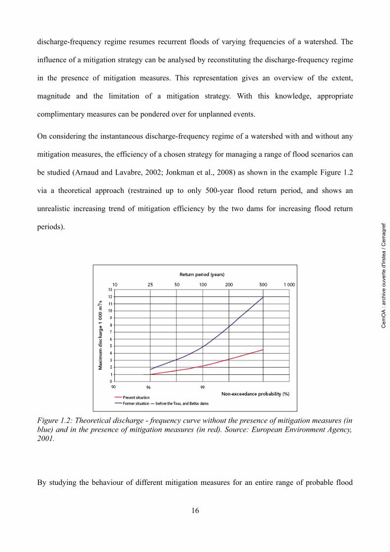
discharge-frequency regime resumes recurrent floods of varying frequencies of a watershed. The
influence of a mitigation strategy can be analysed by reconstituting the discharge-frequency regime
in the presence of mitigation measures. This representation gives an overview of the extent,
magnitude and the limitation of a mitigation strategy. With this knowledge, appropriate
complimentary measures can be pondered over for unplanned events.
On considering the instantaneous discharge-frequency regime of a watershed with and without any
mitigation measures, the efficiency of a chosen strategy for managing a range of flood scenarios can
be studied (Arnaud and Lavabre, 2002; Jonkman et al., 2008) as shown in the example Figure 1.2
via a theoretical approach (restrained up to only 500-year flood return period, and shows an
unrealistic increasing trend of mitigation efficiency by the two dams for increasing flood return
periods).
By studying the behaviour of different mitigation measures for an entire range of probable flood
16
Figure 1.2: Theoretical discharge - frequency curve without the presence of mitigation measures (in blue) and in the presence of mitigation measures (in red). Source: European Environment Agency, 2001.
Cem
OA
: ar
chiv
e ou
verte
d'Ir
stea
/ C
emag
ref

scenarios, a befitting mitigation strategy meeting the requirements of a region can be isolated (Dutta
et al., 2006). This type of analysis would put forth the extent and the limit of a given strategy, thus
giving an opportunity to plan ahead. For example identify areas that could be sacrificed for flood
storage in case of an extreme event or an event surpassing the design limit in order to protect critical
areas. Quite different strategies are likely to be appropriate in different situations and different
regions, because of the local meteorological, topographical and land-use conditions. The differences
in the performance of different strategies can be quantified and the investment for each strategy can
be compared to choose the best of strategy for a study basin (Dotson and Davis, 1995., Jonkman et
al., 2008). By seeking a resilient response that is flexible and adaptable to changing conditions, a
good management of risk can be foreseen.
1.3.2 Protection to entire region
A Dispersed mitigation strategy
A watershed is constituted of dispersed land-use practices like residential, industrial, agricultural
and forests zones. If these zones of interest have to be protected without aggravating the flood risk
of one zone while protecting another zone, corresponding strategy is required to reduce the flood
risks for the whole area. Thus a dispersed mitigation strategy is conceptualised, to ensure flood
mitigation for the entire watershed.
The study of dispersed flood mitigation measures to is not very developed in literature and a global
view of mitigation strategies on the entire watershed is still budding and the consequence of the
same has not been explored in detail. The application of dispersed structural measures for flood
mitigation is in practice (Wang and Plate, 2002; US Army Corps of Engineers, 2006) for quite
sometime now though. The use of dispersed flood mitigation strategies is reported in the Miami
watershed (Rogers, J.D) and Muskingum (US Army Corps of Engineers, 2006) river basins. An
17
Cem
OA
: ar
chiv
e ou
verte
d'Ir
stea
/ C
emag
ref
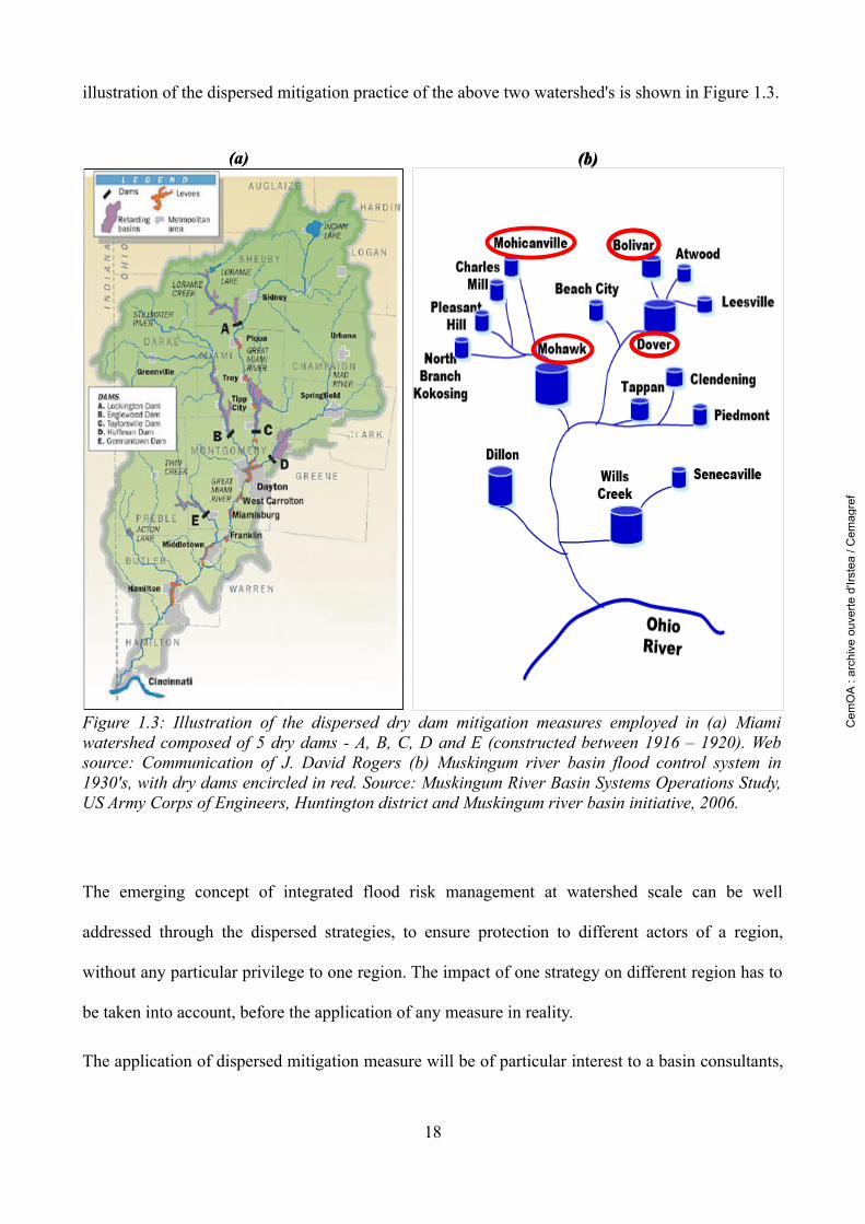
illustration of the dispersed mitigation practice of the above two watershed's is shown in Figure 1.3.
The emerging concept of integrated flood risk management at watershed scale can be well
addressed through the dispersed strategies, to ensure protection to different actors of a region,
without any particular privilege to one region. The impact of one strategy on different region has to
be taken into account, before the application of any measure in reality.
The application of dispersed mitigation measure will be of particular interest to a basin consultants,
18
Figure 1.3: Illustration of the dispersed dry dam mitigation measures employed in (a) Miami watershed composed of 5 dry dams - A, B, C, D and E (constructed between 1916 – 1920). Web source: Communication of J. David Rogers (b) Muskingum river basin flood control system in 1930's, with dry dams encircled in red. Source: Muskingum River Basin Systems Operations Study, US Army Corps of Engineers, Huntington district and Muskingum river basin initiative, 2006.
(b)(a)(a) (b)
Cem
OA
: ar
chiv
e ou
verte
d'Ir
stea
/ C
emag
ref
who can appreciate the different means to quantify the influence of different regions. Projects such
as PAPI in France have began reasoning along these lines and are conceiving projects which meets
the objectives at watershed scale.
Among the different types of structural mitigation measures possible, dry dams represent one
potential alternative within the framework of integrated flood risk management. The term
“integrated” in the present study refers to integrated protection against flooding for the entire region
and does not concern studies regarding sociology, economics and ecology. The definition of dry
dams and their functioning is detailed in the next section.
B Dry dams
Dispersed mitigation strategy can be achieved via various mitigation measures, as elaborated in the
previous section on structural and non-structural measures (Section 1.2.3). The chosen measures
should be in accord with the principles of integrated management i.e. the mitigation measure should
attenuate potential disaster provoking floods, but at the same time not perturb the water regime. One
such measure explored in the present study is dry dams. Dry dams are structural measures which
agree with the principles of integrated flood risk management.
Dry dams are structures which attenuate flood peaks without rupturing the normal river flow
regime. During times of normal flow, the river passes through the dam unimpeded through a bottom
outlet (Figure 1.4), without any permanent pools of water behind the dams (Precht et al., 2006).
Thus a dry dam has no permanent pools of water stored behind the dam walls and hence is coined
as "dry dam". During high or damaging flows, the excess water is impounded behind the dam
structure, with a controlled outflow. The bottom outlet is dimensioned so as to constrain the outflow
to safe levels for downstream zones.
19
Cem
OA
: ar
chiv
e ou
verte
d'Ir
stea
/ C
emag
ref
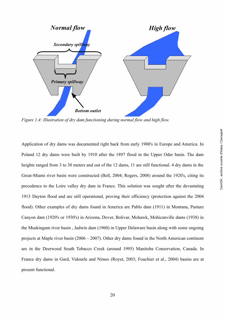
Application of dry dams was documented right back from early 1900's in Europe and America. In
Poland 12 dry dams were built by 1910 after the 1897 flood in the Upper Oder basin. The dam
heights ranged from 3 to 30 meters and out of the 12 dams, 11 are still functional. 4 dry dams in the
Great-Miami river basin were constructed (Bell, 2004; Rogers, 2008) around the 1920's, citing its
precedence to the Loire valley dry dam in France. This solution was sought after the devastating
1913 Dayton flood and are still operational, proving their efficiency (protection against the 2004
flood). Other examples of dry dams found in America are Pablo dam (1911) in Montana, Pasture
Canyon dam (1920's or 1930's) in Arizona, Dover, Bolivar, Mohawk, Mohicanville dams (1938) in
the Muskingum river basin , Jadwin dam (1960) in Upper Delaware basin along with some ongoing
projects at Maple river basin (2006 – 2007). Other dry dams found in the North American continent
are in the Deerwood South Tobacco Creek (around 1995) Manitoba Conservation, Canada. In
France dry dams in Gard, Vidourle and Nimes (Royet, 2003; Fouchier et al., 2004) basins are at
present functional.
20
Figure 1.4: Illustration of dry dam functioning during normal flow and high flow.
Normal flow High flow
Bottom outlet
Primary spillway
Secondary spillway
Cem
OA
: ar
chiv
e ou
verte
d'Ir
stea
/ C
emag
ref
1.3.3 Accounting of spatial rainfall variability
The integrated management promotes the study of flooding at watershed scale. Thus one needs to
survey the physical processes on the entire region. Flooding, are the aftermath of intense and
persistent rainfall episodes (International Federation of Red Cross and Red Crescent Societies,
1999). Based on the meteorological, topographical, land-use and soil conditions, the extent, the
impact and the type of floods vary from region to region. The meteorological and topographical
environments condition the rainfall pattern of a given area, because of their complex interactions.
Thus eventuating rainfall patterns vary in structural and temporal resolutions.
By numerous earlier studies and radar measurements undertaken, the variability of rainfall in space
and time is confirmed. Depending upon the variability of rainfall in space-time over regions with
variability in land-use, soil and the basin's antecedent conditions, the run-off volumes generated are
not identical. Conditioned by the space-time rainfall characteristic of a region, mitigation measures
are located strategically to intercept and attenuate the resulting excess run-off volumes.
A good estimation of resulting run-offs is important, to ideate amenable mitigation strategy. Since
mitigation structures are dimensioned based on the resulting run-off characteristics, the importance
of accounting realistic rainfall variability pattern is reinforced.
The importance of space-time rainfall distribution on run-off production has been under
contemplation since 1970 to date (Dawdy and Bergmann, 1969; Segond et al., 2007). A review of
articles on the influence of rainfall variability is presented in Table 1.3.1. The review details the
studies where the distributed hydrological models are used to test the influence of rainfall
distribution on flood hydrographs. And also the modelling errors which could be brought in by the
distribution of rainfall.
This review emphasised the consideration of rainfall variability as an important factor for the
analysis of flood hydrograph and at the same time the errors it could entail. Flood peak, flood
21
Cem
OA
: ar
chiv
e ou
verte
d'Ir
stea
/ C
emag
ref
volume and time to peak, are some of the key factors of mitigation guided by the space-time rainfall
distribution (Segond et al., 2007; Arnaud et al., 2002;). A good knowledge of spatial, temporal and
dynamic resolution of rainfall characteristics, of a given region would result in better estimation of
surface run-off and thus aid in the perception of appropriate mitigation strategy.
Tabulation of the literature review on rainfall distributionA deterministic rainfall-run-off (deterministic) model was used to simulate flood hydrographs to
test the influence of observed/radar rainfall records. The principle conclusions are resumed below:
1) Peak flow (up to 20%) and flood volume are influenced by type of rainfall distribution:
uniform distribution in time or space-time distribution of observed rainfall from rain gauges
(Dawdy and Bergmann, 1969).
2) Flood events with return periods ranging from 2- to 5-year were overestimated by nearly 30%
from subareal rainfall deduced from simple stochastic transformed rainfall model (Kuczera
and Williams, 1992; Arnaud et al., 2002).
3) Rare and extreme events are generally overestimated by spatial rainfall variability (Troutman,
1983; Arnaud et al., 2002). While some studies stated moderate influence of rainfall variability
patterns on extreme events (Krajewski et al., 1991).
4) Spatial variability has a high effect on peak timing along with small peak errors (Beven and
Hornberger, 1982).
5) Spatial rainfall resolution has to be defined at the same scale as the watershed modelling
resolution (Michaud and Sorooshian, 1994).
6) The derivation of areal rainfall from point estimates using the Thiessen method may be quite
accurate at the catchment scale, but the method does not estimate satisfactorily the spatial
rainfall distribution at the scale of a computational element required as input to a distributed
catchment model (Lopes, 1996).
Continued in next page
22
Cem
OA
: ar
chiv
e ou
verte
d'Ir
stea
/ C
emag
ref

Tabulation of the literature review on rainfall distribution7) The spatial variability of rainfall has a marked influence on hydrograph volume, time to peak
and peak value (Wilson et al., 1979).
8) Urban catchments and mesoscale basins are sensitive to spatial distribution of rainfall (Segond
et al., 2007).
The stochastic rainfall model was used to test the behaviour of rainfall distribution via distributed
rainfall-run-off/ lumped model to predict flood run-off. The main findings of this method is listed
below:
1) 9% to 76% errors in peak value linked to rainfall distribution pattern (Faurès et al., 1995).
2) 2% to 65% error in flood volume linked to rainfall distribution pattern (Faurès et al., 1995).
3) Spatial resolution linked to storm scale than watershed scale (Michaud and Sorooshian, 1994).
4) 2 km rainfall resolution for watersheds between 50-500 km² (Michaud and Sorooshian, 1994).
And small basins are sensitive to rainfall distribution (Faurès et al., 1995; Tetzlaff and
Uhlenbrook, 2005).
5) The basin response is more sensitive to temporal resolution of rainfall than spatial resolution
(Krajewski et al., 1991).
6) Assumption of homogeneous rainfall distribution tends to over and under estimate large and
small events respectively (Troutman, 1983).
7) Design hydrographs for the more frequent events are subject to relatively greater uncertainty
than hydrographs for rare events due rainfall input uncertainty (Kuczera and Williams, 1992).
8) Frequency analysis of flood peaks resulted from stochastic rainfall, is severely underestimated
by lumped model, which could impede the designing of hydraulic structures (Krajewski et al.,
1991).
Table 1.3.1: Review of articles on the importance and influence of accounting rainfall variability.
23
Cem
OA
: ar
chiv
e ou
verte
d'Ir
stea
/ C
emag
ref
1.4 Thesis introduction
From the above context of flooding the current work tries to propose appropriate mitigation
strategies using dry dams at watershed/catchment scale. The work also analyses the mitigation
efficiency of dry dams and defines an attenuation criteria for mitigation measures, to help choose
appropriate solutions meeting the objectives of the watershed. The thesis undertakes a technical
assessment of flooding i.e. under hydrology and hydraulics domains.
Appropriate models are employed to simulate the hydrological and hydraulic processes at watershed
scale to the best of ability. A dispersed mitigation strategy via dry dams to reduce flood risk in zones
of interest is explored and adopted for an existing watershed. The study being technical in nature,
does not undertake any social, economical or ecological aspects.
The following section presents the method adopted for analysing a dispersed flood mitigation
measure on an example watershed.
1.4.1 Method
The first step for a technical study is to simulate event scale flood process observed at the study
watershed from observed data set. And then introduce dry dams along the drainage network of the
watershed. Dry dams are then dispersed along the drainage network, to reduce flood risk for the
entire watershed.
To simulate hydrological processes at watershed scale, we require a rainfall generator capable of
simulating space and time variable rainfall fields as observed in reality, a hydrological model which
can transform the rainfall to run-off and thus simulate representative lateral surface run-offs along
the slope of the catchment. These lateral surface run-offs are then routed along the drainage network
of the watershed via a hydraulic model to the outlet of the catchment. The hydraulic model thus can
simulate surplus flood volume overflowing the river banks.
24
Cem
OA
: ar
chiv
e ou
verte
d'Ir
stea
/ C
emag
ref
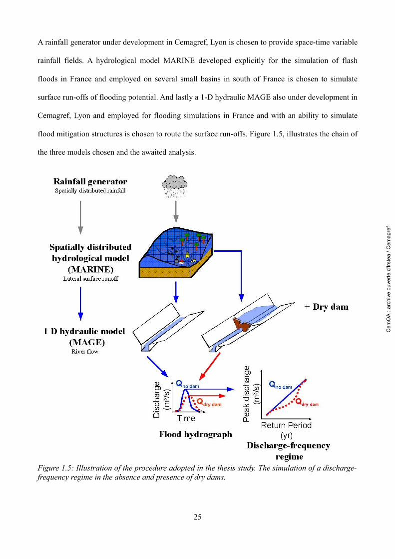
A rainfall generator under development in Cemagref, Lyon is chosen to provide space-time variable
rainfall fields. A hydrological model MARINE developed explicitly for the simulation of flash
floods in France and employed on several small basins in south of France is chosen to simulate
surface run-offs of flooding potential. And lastly a 1-D hydraulic MAGE also under development in
Cemagref, Lyon and employed for flooding simulations in France and with an ability to simulate
flood mitigation structures is chosen to route the surface run-offs. Figure 1.5, illustrates the chain of
the three models chosen and the awaited analysis.
25
Figure 1.5: Illustration of the procedure adopted in the thesis study. The simulation of a discharge-frequency regime in the absence and presence of dry dams.
Cem
OA
: ar
chiv
e ou
verte
d'Ir
stea
/ C
emag
ref
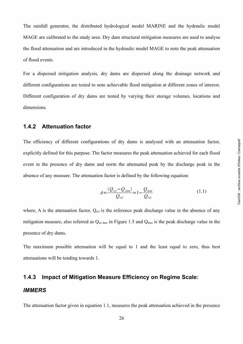
The rainfall generator, the distributed hydrological model MARINE and the hydraulic model
MAGE are calibrated to the study area. Dry dam structural mitigation measures are used to analyse
the flood attenuation and are introduced in the hydraulic model MAGE to note the peak attenuation
of flood events.
For a dispersed mitigation analysis, dry dams are dispersed along the drainage network and
different configurations are tested to note achievable flood mitigation at different zones of interest.
Different configuration of dry dams are tested by varying their storage volumes, locations and
dimensions.
1.4.2 Attenuation factor
The efficiency of different configurations of dry dams is analysed with an attenuation factor,
explicitly defined for this purpose. The factor measures the peak attenuation achieved for each flood
event in the presence of dry dams and norm the attenuated peak by the discharge peak in the
absence of any measure. The attenuation factor is defined by the following equation:
A=Qref−Q dam
Qref=1−
Qdam
Qref
(1.1)
where, A is the attenuation factor, Qref is the reference peak discharge value in the absence of any
mitigation measure, also referred as Qno dam in Figure 1.5 and Qdam is the peak discharge value in the
presence of dry dams.
The maximum possible attenuation will be equal to 1 and the least equal to zero, thus best
attenuations will be tending towards 1.
1.4.3 Impact of Mitigation Measure Efficiency on Regime Scale:
IMMERS
The attenuation factor given in equation 1.1, measures the peak attenuation achieved in the presence
26
Cem
OA
: ar
chiv
e ou
verte
d'Ir
stea
/ C
emag
ref
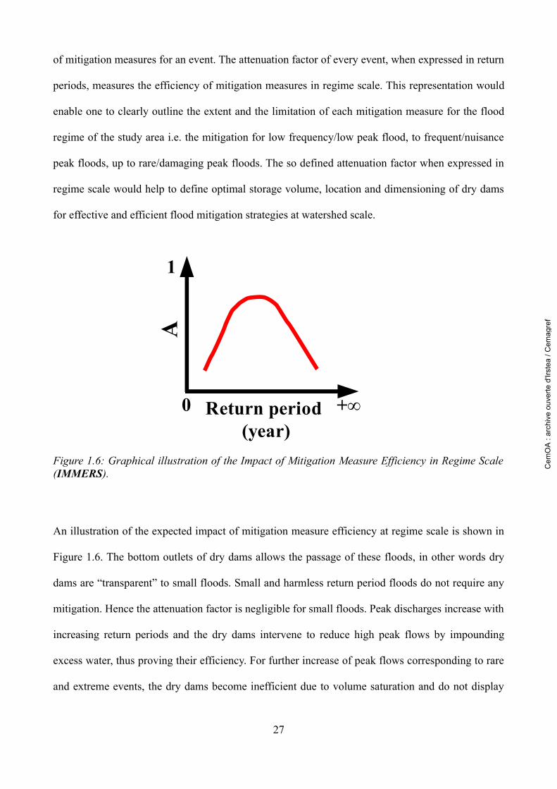
of mitigation measures for an event. The attenuation factor of every event, when expressed in return
periods, measures the efficiency of mitigation measures in regime scale. This representation would
enable one to clearly outline the extent and the limitation of each mitigation measure for the flood
regime of the study area i.e. the mitigation for low frequency/low peak flood, to frequent/nuisance
peak floods, up to rare/damaging peak floods. The so defined attenuation factor when expressed in
regime scale would help to define optimal storage volume, location and dimensioning of dry dams
for effective and efficient flood mitigation strategies at watershed scale.
An illustration of the expected impact of mitigation measure efficiency at regime scale is shown in
Figure 1.6. The bottom outlets of dry dams allows the passage of these floods, in other words dry
dams are “transparent” to small floods. Small and harmless return period floods do not require any
mitigation. Hence the attenuation factor is negligible for small floods. Peak discharges increase with
increasing return periods and the dry dams intervene to reduce high peak flows by impounding
excess water, thus proving their efficiency. For further increase of peak flows corresponding to rare
and extreme events, the dry dams become inefficient due to volume saturation and do not display
27
Figure 1.6: Graphical illustration of the Impact of Mitigation Measure Efficiency in Regime Scale (IMMERS).
+∞
1
0 Return period (year)
A
Cem
OA
: ar
chiv
e ou
verte
d'Ir
stea
/ C
emag
ref
any mitigation efficiency. This trend explains the fall of the attenuation indicator for rare and
extreme flood events. This evolution of attenuation factor will have a concave form as shown in
Figure 1.6.
The IMMERS graphical representation is used in the present work, as the main means to analyse
potential mitigation strategies and measure their efficiency for flood mitigation. This representation
is presented as a means to characterise any flood mitigation measure.
1.5 Thesis outline
The thesis is organised in 6 chapters. In the present chapter the background and the need for new
flood mitigation strategies were discussed. This discussion led to the currently researched
methodology. The developed methodology is tested on an existing watershed, which is detailed in
the second chapter where the location, characteristics and the data available for the watershed
undertaken for study is presented. The construction of the methodology with models is then
developed. The space-time stochastic rainfall modelling employed to obtain rainfall variable in
space and time is presented in chapter three, where the theory and calibration of the chosen rainfall
generator to the study area is elaborated. The resulting space-time variable rainfall field is input to
coupled hydrological and hydraulic models. Chapter four presents how the surface run-off of a
watershed is simulated with the aid of a hydrological and a hydraulic model. Chapter four entitled
“Simulation of rainfall-run-off process at watershed scale” presents the models employed and their
calibration to the studied watershed and introduces dry dam structural mitigation measures. The
resulting simulation of the developed methodology with the help of three models employed is
presented in chapter five “Dry dam mitigation analysis”. The thesis finally concludes with the main
conclusions and discussion in chapter six “Conclusion, Discussion and Perspectives”, where
perspectives of interest to take the flood mitigation analysis to the next step is explained. The
references used to construct the present study is detailed in “References” and additional information
28
Cem
OA
: ar
chiv
e ou
verte
d'Ir
stea
/ C
emag
ref

to complement the thesis is given in “Appendix”.
29
Cem
OA
: ar
chiv
e ou
verte
d'Ir
stea
/ C
emag
ref

2 STUDY AREA
Cem
OA
: ar
chiv
e ou
verte
d'Ir
stea
/ C
emag
ref
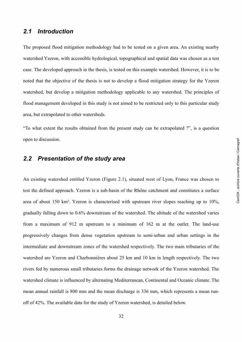
2.1 Introduction
The proposed flood mitigation methodology had to be tested on a given area. An existing nearby
watershed Yzeron, with accessible hydrological, topographical and spatial data was chosen as a test
case. The developed approach in the thesis, is tested on this example watershed. However, it is to be
noted that the objective of the thesis is not to develop a flood mitigation strategy for the Yzeron
watershed, but develop a mitigation methodology applicable to any watershed. The principles of
flood management developed in this study is not aimed to be restricted only to this particular study
area, but extrapolated to other watersheds.
“To what extent the results obtained from the present study can be extrapolated ?”, is a question
open to discussion.
2.2 Presentation of the study area
An existing watershed entitled Yzeron (Figure 2.1), situated west of Lyon, France was chosen to
test the defined approach. Yzeron is a sub-basin of the Rhône catchment and constitutes a surface
area of about 150 km². Yzeron is characterised with upstream river slopes reaching up to 10%,
gradually falling down to 0.6% downstream of the watershed. The altitude of the watershed varies
from a maximum of 912 m upstream to a minimum of 162 m at the outlet. The land-use
progressively changes from dense vegetation upstream to semi-urban and urban settings in the
intermediate and downstream zones of the watershed respectively. The two main tributaries of the
watershed are Yzeron and Charbonnières about 25 km and 10 km in length respectively. The two
rivers fed by numerous small tributaries forms the drainage network of the Yzeron watershed. The
watershed climate is influenced by alternating Mediterranean, Continental and Oceanic climate. The
mean annual rainfall is 800 mm and the mean discharge is 336 mm, which represents a mean run-
off of 42%. The available data for the study of Yzeron watershed, is detailed below.
32
Cem
OA
: ar
chiv
e ou
verte
d'Ir
stea
/ C
emag
ref
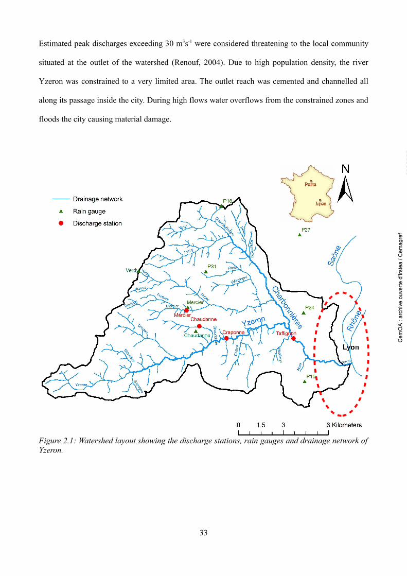
Estimated peak discharges exceeding 30 m3s-1 were considered threatening to the local community
situated at the outlet of the watershed (Renouf, 2004). Due to high population density, the river
Yzeron was constrained to a very limited area. The outlet reach was cemented and channelled all
along its passage inside the city. During high flows water overflows from the constrained zones and
floods the city causing material damage.
33
Figure 2.1: Watershed layout showing the discharge stations, rain gauges and drainage network of Yzeron.
Cem
OA
: ar
chiv
e ou
verte
d'Ir
stea
/ C
emag
ref
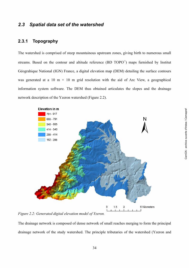
2.3 Spatial data set of the watershed
2.3.1 Topography
The watershed is comprised of steep mountainous upstream zones, giving birth to numerous small
streams. Based on the contour and altitude reference (BD TOPO) maps furnished by Institut
Géograhique National (IGN) France, a digital elevation map (DEM) detailing the surface contours
was generated at a 10 m × 10 m grid resolution with the aid of Arc View, a geographical
information system software. The DEM thus obtained articulates the slopes and the drainage
network description of the Yzeron watershed (Figure 2.2).
The drainage network is composed of dense network of small reaches merging to form the principal
drainage network of the study watershed. The principle tributaries of the watershed (Yzeron and
34
Figure 2.2: Generated digital elevation model of Yzeron.
Cem
OA
: ar
chiv
e ou
verte
d'Ir
stea
/ C
emag
ref
Charonnières) are fed by minor tributaries such as Chaudanne, Ratier, Larny, Dronau, etc.
A field survey carried out for a PhD project (Navratil, 2005) furnished cross-section profiles of the
minor bed of the drainage network at specified locations (Figure 2.3). The survey showed upstream
river reaches of a minimum width of 1.8 m enlarging up to 13 m downstream. The measured cross-
sectional profiles of the minor beds are used in the present study to represent the geometry of
drainage network.
35
Figure 2.3: Map showing the locations of the measured river cross-section profile by Navratil, 2005.
-1.4
-1.2
-1
-0.8
-0.6
-0.4
-0.2
00 0.5 1 1.5 2 2.5 3 3.5
Abscisse (m)
Altit
ude (
m) Left bank
Datum
Right bank
Cem
OA
: ar
chiv
e ou
verte
d'Ir
stea
/ C
emag
ref
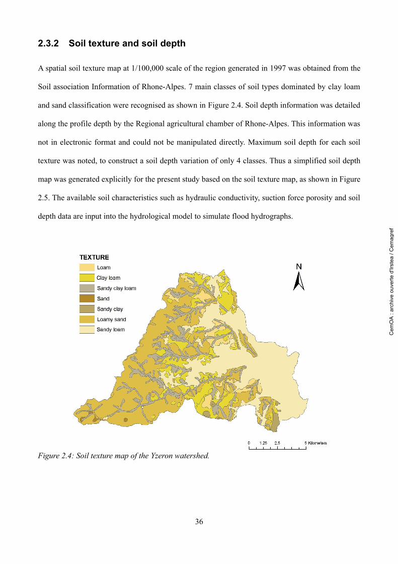
2.3.2 Soil texture and soil depth
A spatial soil texture map at 1/100,000 scale of the region generated in 1997 was obtained from the
Soil association Information of Rhone-Alpes. 7 main classes of soil types dominated by clay loam
and sand classification were recognised as shown in Figure 2.4. Soil depth information was detailed
along the profile depth by the Regional agricultural chamber of Rhone-Alpes. This information was
not in electronic format and could not be manipulated directly. Maximum soil depth for each soil
texture was noted, to construct a soil depth variation of only 4 classes. Thus a simplified soil depth
map was generated explicitly for the present study based on the soil texture map, as shown in Figure
2.5. The available soil characteristics such as hydraulic conductivity, suction force porosity and soil
depth data are input into the hydrological model to simulate flood hydrographs.
36
Figure 2.4: Soil texture map of the Yzeron watershed.
Cem
OA
: ar
chiv
e ou
verte
d'Ir
stea
/ C
emag
ref
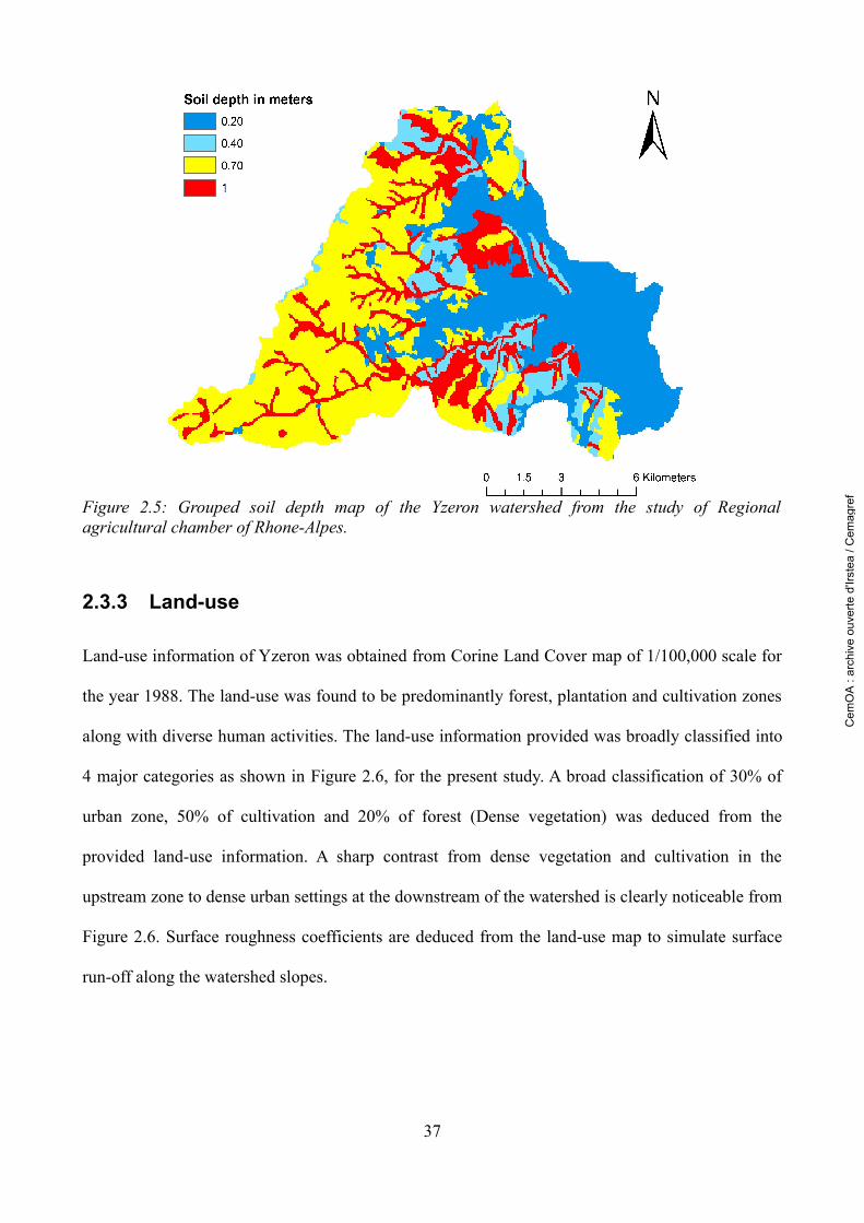
Figure 2.5: Grouped soil depth map of the Yzeron watershed from the study of Regional agricultural chamber of Rhone-Alpes.
2.3.3 Land-use
Land-use information of Yzeron was obtained from Corine Land Cover map of 1/100,000 scale for
the year 1988. The land-use was found to be predominantly forest, plantation and cultivation zones
along with diverse human activities. The land-use information provided was broadly classified into
4 major categories as shown in Figure 2.6, for the present study. A broad classification of 30% of
urban zone, 50% of cultivation and 20% of forest (Dense vegetation) was deduced from the
provided land-use information. A sharp contrast from dense vegetation and cultivation in the
upstream zone to dense urban settings at the downstream of the watershed is clearly noticeable from
Figure 2.6. Surface roughness coefficients are deduced from the land-use map to simulate surface
run-off along the watershed slopes.
37
Cem
OA
: ar
chiv
e ou
verte
d'Ir
stea
/ C
emag
ref
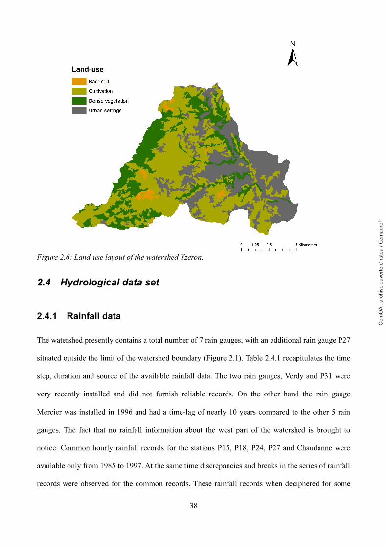
2.4 Hydrological data set
2.4.1 Rainfall data
The watershed presently contains a total number of 7 rain gauges, with an additional rain gauge P27
situated outside the limit of the watershed boundary (Figure 2.1). Table 2.4.1 recapitulates the time
step, duration and source of the available rainfall data. The two rain gauges, Verdy and P31 were
very recently installed and did not furnish reliable records. On the other hand the rain gauge
Mercier was installed in 1996 and had a time-lag of nearly 10 years compared to the other 5 rain
gauges. The fact that no rainfall information about the west part of the watershed is brought to
notice. Common hourly rainfall records for the stations P15, P18, P24, P27 and Chaudanne were
available only from 1985 to 1997. At the same time discrepancies and breaks in the series of rainfall
records were observed for the common records. These rainfall records when deciphered for some
38
Figure 2.6: Land-use layout of the watershed Yzeron.
Cem
OA
: ar
chiv
e ou
verte
d'Ir
stea
/ C
emag
ref
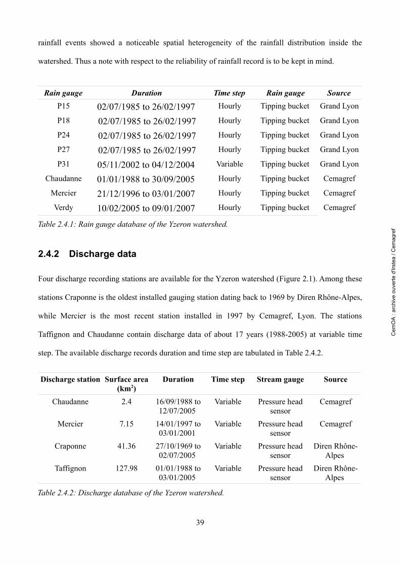
rainfall events showed a noticeable spatial heterogeneity of the rainfall distribution inside the
watershed. Thus a note with respect to the reliability of rainfall record is to be kept in mind.
2.4.2 Discharge data
Four discharge recording stations are available for the Yzeron watershed (Figure 2.1). Among these
stations Craponne is the oldest installed gauging station dating back to 1969 by Diren Rhône-Alpes,
while Mercier is the most recent station installed in 1997 by Cemagref, Lyon. The stations
Taffignon and Chaudanne contain discharge data of about 17 years (1988-2005) at variable time
step. The available discharge records duration and time step are tabulated in Table 2.4.2.
39
Rain gauge Duration Time step Rain gauge SourceP15 02/07/1985 to 26/02/1997 Hourly Tipping bucket Grand Lyon
P18 02/07/1985 to 26/02/1997 Hourly Tipping bucket Grand Lyon
P24 02/07/1985 to 26/02/1997 Hourly Tipping bucket Grand Lyon
P27 02/07/1985 to 26/02/1997 Hourly Tipping bucket Grand Lyon
P31 05/11/2002 to 04/12/2004 Variable Tipping bucket Grand Lyon
Chaudanne 01/01/1988 to 30/09/2005 Hourly Tipping bucket Cemagref
Mercier 21/12/1996 to 03/01/2007 Hourly Tipping bucket Cemagref
Verdy 10/02/2005 to 09/01/2007 Hourly Tipping bucket Cemagref
Table 2.4.1: Rain gauge database of the Yzeron watershed.
Discharge station Surface area (km2)
Duration Time step Stream gauge Source
Chaudanne 2.4 16/09/1988 to 12/07/2005
Variable Pressure head sensor
Cemagref
Mercier 7.15 14/01/1997 to 03/01/2001
Variable Pressure head sensor
Cemagref
Craponne 41.36 27/10/1969 to 02/07/2005
Variable Pressure head sensor
Diren Rhône-Alpes
Taffignon 127.98 01/01/1988 to 03/01/2005
Variable Pressure head sensor
Diren Rhône-Alpes
Table 2.4.2: Discharge database of the Yzeron watershed.
Cem
OA
: ar
chiv
e ou
verte
d'Ir
stea
/ C
emag
ref
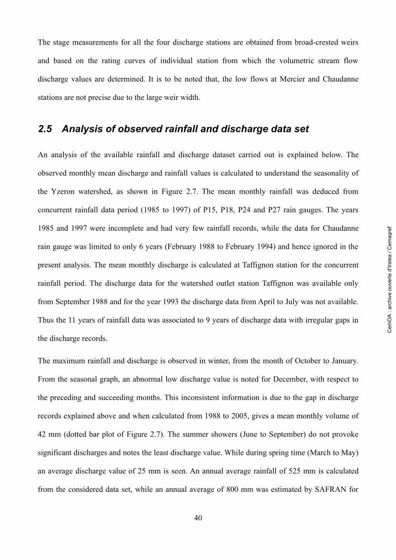
The stage measurements for all the four discharge stations are obtained from broad-crested weirs
and based on the rating curves of individual station from which the volumetric stream flow
discharge values are determined. It is to be noted that, the low flows at Mercier and Chaudanne
stations are not precise due to the large weir width.
2.5 Analysis of observed rainfall and discharge data set
An analysis of the available rainfall and discharge dataset carried out is explained below. The
observed monthly mean discharge and rainfall values is calculated to understand the seasonality of
the Yzeron watershed, as shown in Figure 2.7. The mean monthly rainfall was deduced from
concurrent rainfall data period (1985 to 1997) of P15, P18, P24 and P27 rain gauges. The years
1985 and 1997 were incomplete and had very few rainfall records, while the data for Chaudanne
rain gauge was limited to only 6 years (February 1988 to February 1994) and hence ignored in the
present analysis. The mean monthly discharge is calculated at Taffignon station for the concurrent
rainfall period. The discharge data for the watershed outlet station Taffignon was available only
from September 1988 and for the year 1993 the discharge data from April to July was not available.
Thus the 11 years of rainfall data was associated to 9 years of discharge data with irregular gaps in
the discharge records.
The maximum rainfall and discharge is observed in winter, from the month of October to January.
From the seasonal graph, an abnormal low discharge value is noted for December, with respect to
the preceding and succeeding months. This inconsistent information is due to the gap in discharge
records explained above and when calculated from 1988 to 2005, gives a mean monthly volume of
42 mm (dotted bar plot of Figure 2.7). The summer showers (June to September) do not provoke
significant discharges and notes the least discharge value. While during spring time (March to May)
an average discharge value of 25 mm is seen. An annual average rainfall of 525 mm is calculated
from the considered data set, while an annual average of 800 mm was estimated by SAFRAN for
40
Cem
OA
: ar
chiv
e ou
verte
d'Ir
stea
/ C
emag
ref
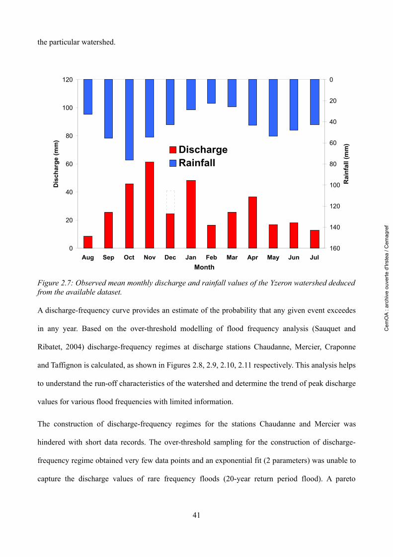
the particular watershed.
A discharge-frequency curve provides an estimate of the probability that any given event exceedes
in any year. Based on the over-threshold modelling of flood frequency analysis (Sauquet and
Ribatet, 2004) discharge-frequency regimes at discharge stations Chaudanne, Mercier, Craponne
and Taffignon is calculated, as shown in Figures 2.8, 2.9, 2.10, 2.11 respectively. This analysis helps
to understand the run-off characteristics of the watershed and determine the trend of peak discharge
values for various flood frequencies with limited information.
The construction of discharge-frequency regimes for the stations Chaudanne and Mercier was
hindered with short data records. The over-threshold sampling for the construction of discharge-
frequency regime obtained very few data points and an exponential fit (2 parameters) was unable to
capture the discharge values of rare frequency floods (20-year return period flood). A pareto
41
Figure 2.7: Observed mean monthly discharge and rainfall values of the Yzeron watershed deduced from the available dataset.
0
20
40
60
80
100
120
Aug Sep Oct Nov Dec Jan Feb Mar Apr May Jun JulMonth
Dis
char
ge (m
m)
0
20
40
60
80
100
120
140
160
Rai
nfal
l (m
m)
DischargeRainfall
Cem
OA
: ar
chiv
e ou
verte
d'Ir
stea
/ C
emag
ref

distribution fit is found to be more adaptable for the discharge stations Chaudanne, Mercier and
Craponne, as seen from Figure 2.8, 2.9 and 2.10. Different durations of discharge-frequency are not
deducible from the available data set for the above three discharge stations. The variable time step
values is not detailed enough in the discharge data base and only instantaneous peak discharge is
noticeable for the above stations except at Taffignon. For the Taffignon discharge however, an
exponential 2 parameters law gives satisfactory fit as shown in Figure 2.11 and is adapted through
out the analysis of the present study.
42
Figure 2.8: Instantaneous discharge-frequency curve at Chaudanne calculated from observed discharge records of 17 years. Left hand side: Exponential fit; Right hand side: Pareto distribution fit.
Cem
OA
: ar
chiv
e ou
verte
d'Ir
stea
/ C
emag
ref
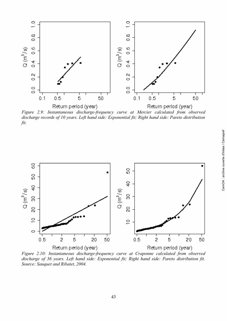
43
Figure 2.10: Instantaneous discharge-frequency curve at Craponne calculated from observed discharge of 36 years. Left hand side: Exponential fit; Right hand side: Pareto distribution fit. Source: Sauquet and Ribatet, 2004.
Figure 2.9: Instantaneous discharge-frequency curve at Mercier calculated from observed discharge records of 10 years. Left hand side: Exponential fit; Right hand side: Pareto distribution fit.
Cem
OA
: ar
chiv
e ou
verte
d'Ir
stea
/ C
emag
ref
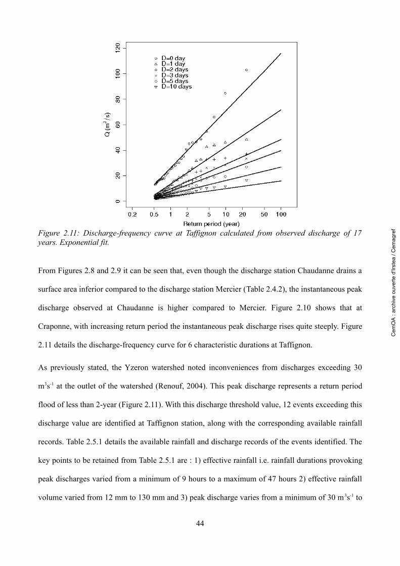
From Figures 2.8 and 2.9 it can be seen that, even though the discharge station Chaudanne drains a
surface area inferior compared to the discharge station Mercier (Table 2.4.2), the instantaneous peak
discharge observed at Chaudanne is higher compared to Mercier. Figure 2.10 shows that at
Craponne, with increasing return period the instantaneous peak discharge rises quite steeply. Figure
2.11 details the discharge-frequency curve for 6 characteristic durations at Taffignon.
As previously stated, the Yzeron watershed noted inconveniences from discharges exceeding 30
m3s-1 at the outlet of the watershed (Renouf, 2004). This peak discharge represents a return period
flood of less than 2-year (Figure 2.11). With this discharge threshold value, 12 events exceeding this
discharge value are identified at Taffignon station, along with the corresponding available rainfall
records. Table 2.5.1 details the available rainfall and discharge records of the events identified. The
key points to be retained from Table 2.5.1 are : 1) effective rainfall i.e. rainfall durations provoking
peak discharges varied from a minimum of 9 hours to a maximum of 47 hours 2) effective rainfall
volume varied from 12 mm to 130 mm and 3) peak discharge varies from a minimum of 30 m3s-1 to
44
Figure 2.11: Discharge-frequency curve at Taffignon calculated from observed discharge of 17 years. Exponential fit.
Cem
OA
: ar
chiv
e ou
verte
d'Ir
stea
/ C
emag
ref
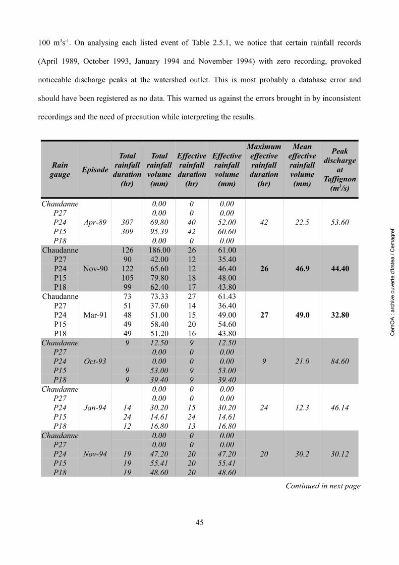
100 m3s-1. On analysing each listed event of Table 2.5.1, we notice that certain rainfall records
(April 1989, October 1993, January 1994 and November 1994) with zero recording, provoked
noticeable discharge peaks at the watershed outlet. This is most probably a database error and
should have been registered as no data. This warned us against the errors brought in by inconsistent
recordings and the need of precaution while interpreting the results.
45
Rain gauge Episode
Total rainfall duration
(hr)
Total rainfall volume(mm)
Effective rainfall duration
(hr)
Effective rainfall volume(mm)
Maximum effective rainfall duration
(hr)
Mean effective rainfall volume(mm)
Peak discharge
at Taffignon
(m3/s)
ChaudanneP27P24P15P18
Apr-89
0.00 0 0.000.00 0 0.00
307 69.80 40 52.00309 95.39 42 60.60
0.00 0 0.00
42 22.5 53.60
ChaudanneP27P24P15P18
Nov-90
126 186.00 26 61.0090 42.00 12 35.40122 65.60 12 46.40105 79.80 18 48.0099 62.40 17 43.80
26 46.9 44.40
ChaudanneP27P24P15P18
Mar-91
73 73.33 27 61.4351 37.60 14 36.4048 51.00 15 49.0049 58.40 20 54.6049 51.20 16 43.80
27 49.0 32.80
ChaudanneP27P24P15P18
Oct-93
9 12.50 9 12.500.00 0 0.000.00 0 0.00
9 53.00 9 53.009 39.40 9 39.40
9 21.0 84.60
ChaudanneP27P24P15P18
Jan-94
0.00 0 0.000.00 0 0.00
14 30.20 15 30.2024 14.61 24 14.6112 16.80 13 16.80
24 12.3 46.14
ChaudanneP27P24P15P18
Nov-94
0.00 0 0.000.00 0 0.00
19 47.20 20 47.2019 55.41 20 55.4119 48.60 20 48.60
20 30.2 30.12
Continued in next page
Cem
OA
: ar
chiv
e ou
verte
d'Ir
stea
/ C
emag
ref
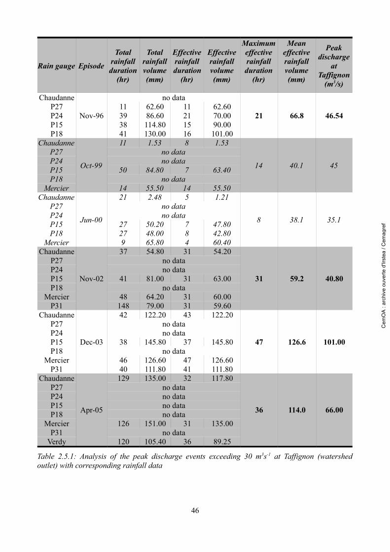
46
Rain gauge Episode
Total rainfall duration
(hr)
Total rainfall volume(mm)
Effective rainfall duration
(hr)
Effective rainfall volume(mm)
Maximum effective rainfall duration
(hr)
Mean effective rainfall volume(mm)
Peak discharge
at Taffignon
(m3/s)
ChaudanneP27P24P15P18
Nov-96
no data11 62.60 11 62.6039 86.60 21 70.0038 114.80 15 90.0041 130.00 16 101.00
21 66.8 46.54
ChaudanneP27P24P15P18
Mercier
Oct-99
11 1.53 8 1.53no datano data
50 84.80 7 63.40no data
14 55.50 14 55.50
14 40.1 45
ChaudanneP27P24P15P18
Mercier
Jun-00
21 2.48 5 1.21no datano data
27 50.20 7 47.8027 48.00 8 42.809 65.80 4 60.40
8 38.1 35.1
ChaudanneP27P24P15P18
MercierP31
Nov-02
37 54.80 31 54.20no datano data
41 81.00 31 63.00no data
48 64.20 31 60.00148 79.00 31 59.60
31 59.2 40.80
ChaudanneP27P24P15P18
MercierP31
Dec-03
42 122.20 43 122.20no datano data
38 145.80 37 145.80no data
46 126.60 47 126.6040 111.80 41 111.80
47 126.6 101.00
ChaudanneP27P24P15P18
MercierP31
Verdy
Apr-05
129 135.00 32 117.80no datano datano datano data
126 151.00 31 135.00no data
120 105.40 36 89.25
36 114.0 66.00
Table 2.5.1: Analysis of the peak discharge events exceeding 30 m3s-1 at Taffignon (watershed outlet) with corresponding rainfall data
Cem
OA
: ar
chiv
e ou
verte
d'Ir
stea
/ C
emag
ref
2.6 Conclusions about the study area
The key points to be retained about the Yzeron watershed during the present study are:
1. The Yzeron watershed is under survey by Grand Lyon district, DIREN and Cemagref from a
long time. Thus adequate topographical and hydrological database were available to
envision this watershed as a potential candidate to carry out flood mitigation study.
2. Yzeron watershed is also facing flooding issues due to the extension of urban zones in the
recent years, like many other watersheds. Thus it was of interest to test potential flood
mitigation strategies.
3. The Yzeron watershed is characterised with mountainous region in the north-western part
and eventually transforms into flat lands in the south-east region (watershed outlet) within
150 km². Thus the watershed houses steep, sharp valleys and flat plains in just 150 km²
surface area. The climatic condition are probably influenced with this characteristic of the
watershed. The topographical data has a resolution of up to 10 m × 10 m, meaning that any
precision below this resolution is not possible.
4. Spatial watershed characteristics, such as soil texture information is grouped into 7
categories for computational purposes. The soil depth map conceived especially for the
present study has a global representation and not very precise. The land-use information is
categorised into 4 groups for easy computation during subsequent modelling analysis.
5. Knowledge of the rainfall distribution over the entire watershed zone is provided
principally by 7 rain gauges and covers only the right half of the watershed. Long series of
complete rainfall records are absent and at times inconsistent.
6. Discharge records of the watershed is provided from 4 stream gauges. Long series of
discharge records are absent and estimation of rare frequency floods can bring in some
47
Cem
OA
: ar
chiv
e ou
verte
d'Ir
stea
/ C
emag
ref

uncertainties. The quality of the data for the Chaudanne and Mercier stations is not very
good and hence limited only to instantaneous discharge-frequency analysis.
7. Consistent and common rainfall and discharge records are constrained to about only 10
years. The gap in rainfall records during high river flow renders the hydrological analysis of
the Yzeron watershed delicate.
The above described data are input into the hydrological models to simulate hydrographs at
watershed scale. The description of the models employed and the procedure adapted for the
reproduction of observed hydrograph is elaborated in chapters 3 and 4.
48
Cem
OA
: ar
chiv
e ou
verte
d'Ir
stea
/ C
emag
ref
3 SPACE-TIME STOCHASTIC RAINFALL MODELLING
FOR FLOOD MITIGATION ANALYSIS
Cem
OA
: ar
chiv
e ou
verte
d'Ir
stea
/ C
emag
ref
3.1 Introduction
As detailed in section 1.3.3 “Accounting of spatial rainfall variability” of chapter 1, the
consideration of space-time variable rainfall patterns is important and under consideration for some
time now. Though the conclusions from different authors from Table 1.3.1 vary, they all agree upon
the importance of considering a space-time variable rainfall pattern for hydrological studies. Space-
time variability of rainfall patterns over a region has a direct impact on the flood run-off production.
For an integrated flood risk management, a prerequisite knowledge about the spatial characteristic
of a region is important and more importantly should account for the spatial variability of rainfall.
Depending on the space-time variability of rainfall, the resulting run-off provoked in combination
with other spatial characteristics (Land-use, soil texture, soil depth, antecedent condition) varies in
space and time. For example, the rainfall storm centre might occur downstream of the mitigation
structure and hence would not participate in any attenuation. Strategic localisation of flood
mitigation measures to counter the resulting damaging flood run-offs is important. Also, to design
efficient mitigation measures, good and adequate estimation of the flow volumes provoked by the
rainfall distribution, variable in time and space is important.
Effective flood mitigation strategies, forbids the ignorance of these spatial characteristic of a region,
which would otherwise entail miscalculations in mitigation process. The accounting of space-time
variability of rainfall is thus important in the proposed flood mitigation methodology via discharge-
frequency regime.
The aim of this chapter, is thus to possess a large number of possible potential rainfall patterns
variable in time and space for the Yzeron watershed. Observed punctual data from existing rain
gauges are analysed, to capture the characteristics of observed Yzeron rainfall. These characteristics
are used to parametrize and simulate rainfall fields variable in time and space.
Further below, the simulated variable rainfall will be used as input to a distributed rainfall-run-off
50
Cem
OA
: ar
chiv
e ou
verte
d'Ir
stea
/ C
emag
ref
model, to analyse their impact on flood mitigation strategies. First, the spatially variable rainfall
will be used to construct a discharge-frequency regime of the Yzeron watershed and the impact of
flood mitigation measures on the constructed regime will be later tested.
First, this chapter presents the chosen rainfall model to obtain a large number of spatially variable
rainfall fields and its calibration to the Yzeron watershed. This is followed by the presentation of the
analysis of the simulated events with respect to the observed rain gauge data set. Finally, the chapter
concludes with the principal characteristics of the simulated rainfall.
3.2 Rainfall generator and the simulated rainfall fields
To obtain a large number of rainfall patterns varying in time and space, a rainfall generator is
needed. A rainfall generator under development in Cemagref, Lyon (Leblois, 2004) was chosen for
this purpose. The rainfall model is based on the geostatistical Turning Bands Method (TBM) and
employs parameters deduced from the observed rainfall records of the study area, to simulate space-
time variable rainfall. The turning bands method was first presented by Matheron (1973) and was
made known mainly by the works of Journel (1978) and Mantoglou and Wilson (1982).
The TBM-based rainfall generator under development at Cemagref, Lyon, was first applied to study
long-term series of independent spatially distributed rain fields used to build intensity-duration-
area-frequency curves for urban hydrologic design and to estimate diagnosis of regional frequency
of a rainfall event (Ramos, 2002; Ramos et al., 2006). The choice of using this generator in this
study is not only supported by its availability but also by the fact that it is favourable to use this
rainfall model for its rapidity in simulation of unconditional rainfall fields.
3.2.1 Basic concept behind the rainfall generator
TBM is a technique of multidimensional simulation based on the theory of random fields. Its basic
concept is to transform a multidimensional simulation into the sum of a series of equivalent
51
Cem
OA
: ar
chiv
e ou
verte
d'Ir
stea
/ C
emag
ref
unidimensional simulations, while preserving the statistics of the true field (Mantoglou and Wilson,
1982). The concept of random fields and its application in TBM detailed here are resumed from two
main sources: Mantoglou and Wilson, 1982; Bras and Rodríguez-Iturbe, 1993. A brief description
of the properties of stationary random functions is first presented, followed by the main features of
the TBM simulation technique.
A Properties of stationary random functions
If x=x1, x2, .... xn represents a point in the n dimensional space Rn and Z(x) is a random variable
corresponding to point the x, then we define a random function as the set {[ x , Z x ] / x∈Rn} . If
the dimension of the space Rn, is n=2 or n=3, then the random function is usually called a random
field. When n=1, it is called a line process or unidimensional process. The mean function of a
stochastic process is defined as:
m x=E [Z x ] (3.1)
where E [ ] is the expectation operator. If E [Z² x ] is finite for all x, we can define the
covariance function as
C x1, x2=E [Z x1Z x2]−m x1mx2 (3.2)
where x1, x2∈Rn .
A stochastic process is called a 'second order stationary process' if the following two conditions are
satisfied:
1. The mean is independent of the position of each point in the space Rn :
E [Z x]=mx =m∀ x∈Rn (3.3)
2. The covariance function depends only on the vector difference x1−x2 and not on each
particular vector x1 , x2 :
52
Cem
OA
: ar
chiv
e ou
verte
d'Ir
stea
/ C
emag
ref
C x1, x2=C x1−x2=C h (3.4)
where h=x1− x2
A second-order stationary process is called isotropic if the covariance function does not depend on
the direction h= x1−x2 of the distance vector, but only on the vector length ∣h∣ .
B Theory of Turning Bands Method
In the TBM, the following assumptions for a field to be simulated are undertaken:
1) the field to be simulated is second-order stationary and isotropic in nature;
2) the random field is normally distributed and has zero mean (in practice, when this is not the
case, as in rainfall fields, a transformation must be applied);
3) the covariance Cs of the multidimensional field to be preserved during simulation is known;
Instead of synthesizing the multidimensional field directly, the TBM performs simulations along
several lines in space, using a unidimensional covariance function that corresponds to the given 2-D
or 3-D field. Then, a weighted sum of values of the line process are assigned to each point in the
region Rn. The example in Figure 3.1 shows the multiple lines generated to simulate an example 2-
D field.
Let P be the 2-D field one needs to simulate. Random lines (L) from an arbitrary origin O are drawn
with a random variable angle θ with the horizontal, ranging from 0 to 2π. A unidimensional process
with a mean and covariance function C1(ζ) along each line is generated discretely. The
unidimensional process Zi(ζ) generated at discrete points along the line i is nothing but the
projections along that line of points on the 2-D field (where one wants to generate random field
values).
53
Cem
OA
: ar
chiv
e ou
verte
d'Ir
stea
/ C
emag
ref
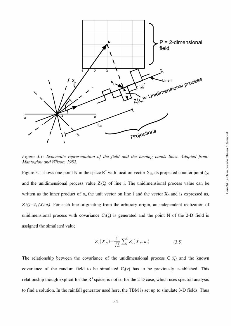
Figure 3.1 shows one point N in the space R2 with location vector XN, its projected counter point ζNi
and the unidimensional process value Zi(ζ) of line i. The unidimensional process value can be
written as the inner product of ui, the unit vector on line i and the vector XN and is expressed as,
Zi(ζ)=Zi (XN.ui). For each line originating from the arbitrary origin, an independent realization of
unidimensional process with covariance C1(ζ) is generated and the point N of the 2-D field is
assigned the simulated value
Z s X N =1L ∑i
LZ i X N .u i (3.5)
The relationship between the covariance of the unidimensional process C1(ζ) and the known
covariance of the random field to be simulated Cs(v) has to be previously established. This
relationship though explicit for the R3 space, is not so for the 2-D case, which uses spectral analysis
to find a solution. In the rainfall generator used here, the TBM is set up to simulate 3-D fields. Thus
54
Figure 3.1: Schematic representation of the field and the turning bands lines. Adapted from: Mantoglou and Wilson, 1982.
P = 2-dimensional field
Projections
x xO
XN
ui
1 2 3
Line iNi
N
ζ i
Z i(ζ Ni
)= Unidimensional processΔζ
ζ Ni
Cem
OA
: ar
chiv
e ou
verte
d'Ir
stea
/ C
emag
ref

the relationship between C1 and Cs for a 3-D field is given by the equation:
C1v =d
dζζC sζ (3.6)
where ζ is the unit sphere. Equation 3.6 relates the known 3-D covariance function Cs to the
unidimensional covariance function C1 to be simulated along the lines. The 3-D covariance function
is determined from the observed rainfall data.
The application of TBM for the modelling of rainfall implies that the rainfall at a given point is
independent with respect to its localisation and the rainfall occurrence has no privileged direction,
implying that it has the potential to occur at anywhere inside a rainfall field.
3.2.2 Parametrisation of the rainfall simulator
The rainfall generator is henceforth entitled “TBM model” in the present work. A brief description
of the procedure adopted to simulate the spatially and temporally variable rainfall fields for the
Yzeron watershed is detailed below.
The rainfall generator is based on the geostatiscal analysis of rainfall data and is used for
parametrisation and generation of space-time rainfall fields. The practice of segmenting the rainfall
phenomenon into: 1) Distribution of rainfall values in space and/or time, Fs (Non-null rainfall field)
and 2) Indicator of presence/absence of rainfall in time and/or space Is, (Rainfall zone indicator), is
well known and has been applied in previous studies (Ramos, 2002). An illustration of the
decomposition of the rainfall field in these two independent components is shown in Figure 3.2.
Based on this hypothesis the model output is given as a product of non-null rainfall fields
(containing rainfall variability) and the contour of the rainfall zone. First, each of these aspects is
simulated independently by the TBM model. Then, an anamorphosis is applied on the non-null
rainfall field. Anamorphosis is basically a process which transforms the Gaussian law of probability
distribution obtained from the application of the TBM technique (normally distributed values as
55
Cem
OA
: ar
chiv
e ou
verte
d'Ir
stea
/ C
emag
ref

described in section 3.2.1 B) to the actual probability distribution of rainfall intensity as estimated
from observed values. This transformation is necessary since Gaussian distribution is not adapted to
represent the distribution of rainfall values, better described by positive asymmetric laws. For the
rainfall zone indicator, a threshold based on the percentage of null rainfall values is imposed.
The modelling of the rainfall fields is carried out in two steps:
1) To fit a statistical distribution to the observed rainfall values at all rain gauges and for whole
length of the time series (Probability model) and
2) A structural and temporal analysis of rainfall to obtain an empirical variogram and its
theoretical model
The above two steps are applied for the simulation of non-null rainfall values and rainfall zone
indicator of the simulated space-time rainfall.
The application of the two steps on the Yzeron watershed is described briefly in the following
sections. The data used for the parametrisation of the rainfall simulator is first presented.
56
Cem
OA
: ar
chiv
e ou
verte
d'Ir
stea
/ C
emag
ref
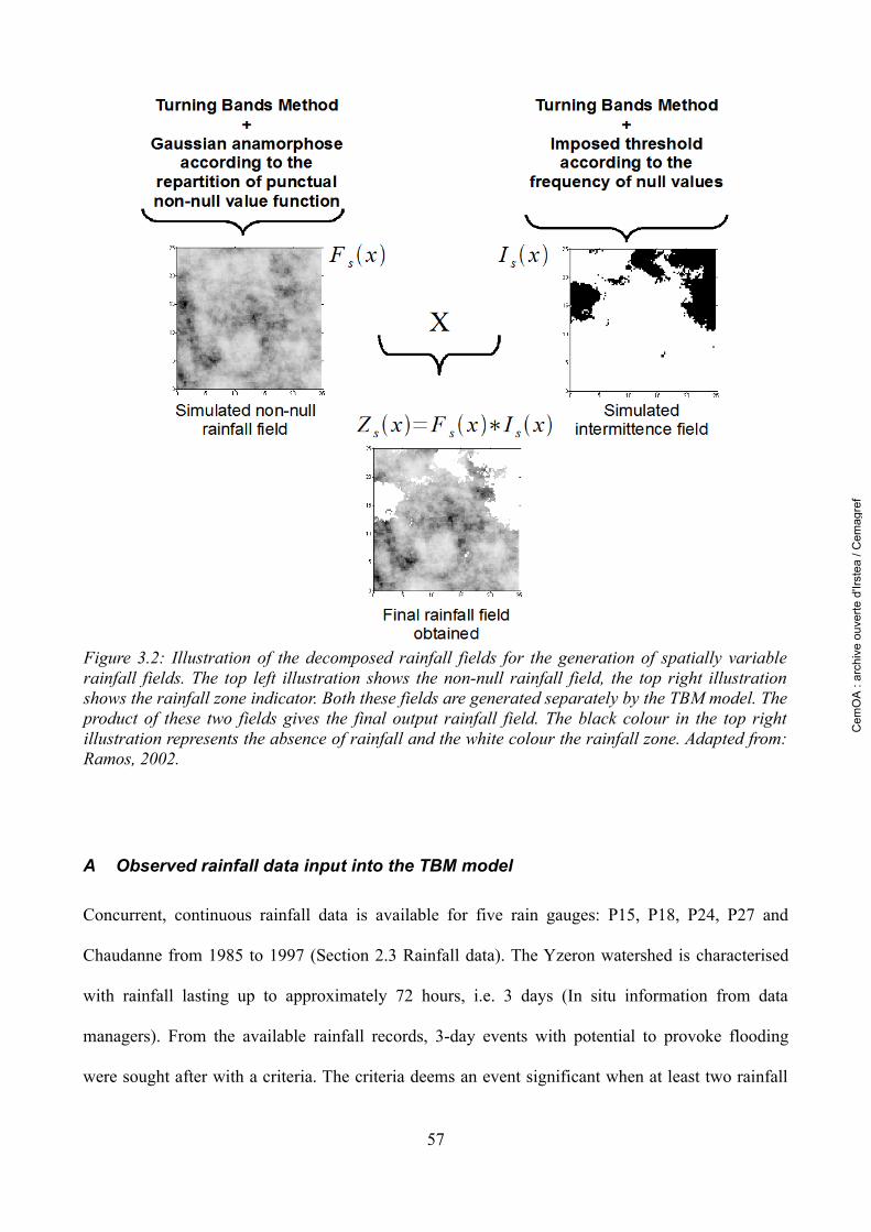
A Observed rainfall data input into the TBM model
Concurrent, continuous rainfall data is available for five rain gauges: P15, P18, P24, P27 and
Chaudanne from 1985 to 1997 (Section 2.3 Rainfall data). The Yzeron watershed is characterised
with rainfall lasting up to approximately 72 hours, i.e. 3 days (In situ information from data
managers). From the available rainfall records, 3-day events with potential to provoke flooding
were sought after with a criteria. The criteria deems an event significant when at least two rainfall
57
Figure 3.2: Illustration of the decomposed rainfall fields for the generation of spatially variable rainfall fields. The top left illustration shows the non-null rainfall field, the top right illustration shows the rainfall zone indicator. Both these fields are generated separately by the TBM model. The product of these two fields gives the final output rainfall field. The black colour in the top right illustration represents the absence of rainfall and the white colour the rainfall zone. Adapted from: Ramos, 2002.
Cem
OA
: ar
chiv
e ou
verte
d'Ir
stea
/ C
emag
ref
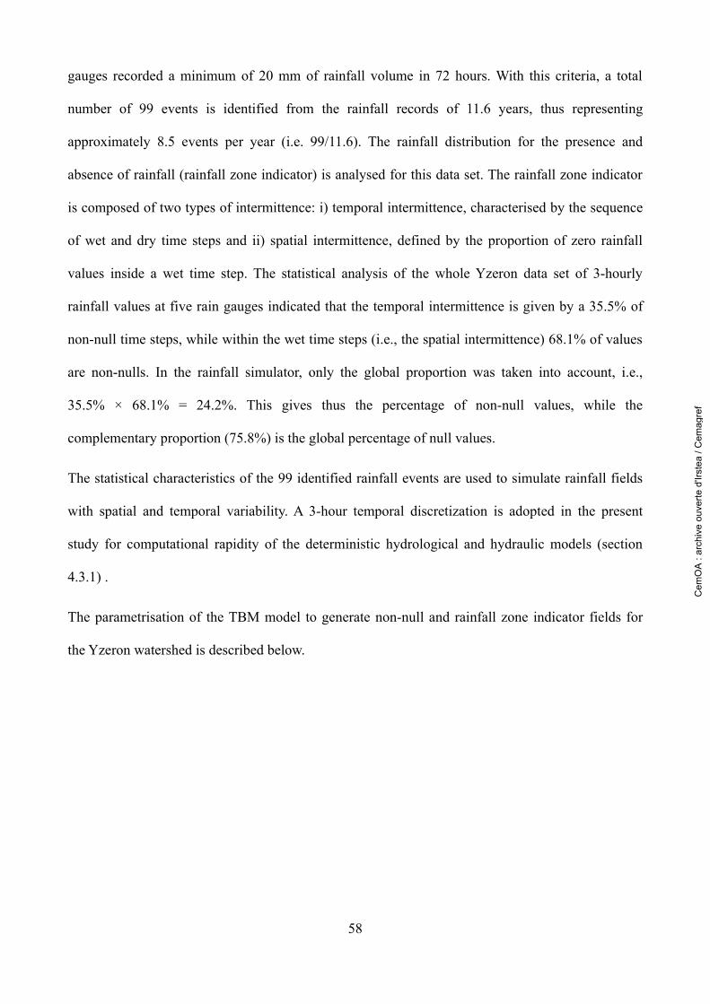
gauges recorded a minimum of 20 mm of rainfall volume in 72 hours. With this criteria, a total
number of 99 events is identified from the rainfall records of 11.6 years, thus representing
approximately 8.5 events per year (i.e. 99/11.6). The rainfall distribution for the presence and
absence of rainfall (rainfall zone indicator) is analysed for this data set. The rainfall zone indicator
is composed of two types of intermittence: i) temporal intermittence, characterised by the sequence
of wet and dry time steps and ii) spatial intermittence, defined by the proportion of zero rainfall
values inside a wet time step. The statistical analysis of the whole Yzeron data set of 3-hourly
rainfall values at five rain gauges indicated that the temporal intermittence is given by a 35.5% of
non-null time steps, while within the wet time steps (i.e., the spatial intermittence) 68.1% of values
are non-nulls. In the rainfall simulator, only the global proportion was taken into account, i.e.,
35.5% × 68.1% = 24.2%. This gives thus the percentage of non-null values, while the
complementary proportion (75.8%) is the global percentage of null values.
The statistical characteristics of the 99 identified rainfall events are used to simulate rainfall fields
with spatial and temporal variability. A 3-hour temporal discretization is adopted in the present
study for computational rapidity of the deterministic hydrological and hydraulic models (section
4.3.1) .
The parametrisation of the TBM model to generate non-null and rainfall zone indicator fields for
the Yzeron watershed is described below.
58
Cem
OA
: ar
chiv
e ou
verte
d'Ir
stea
/ C
emag
ref
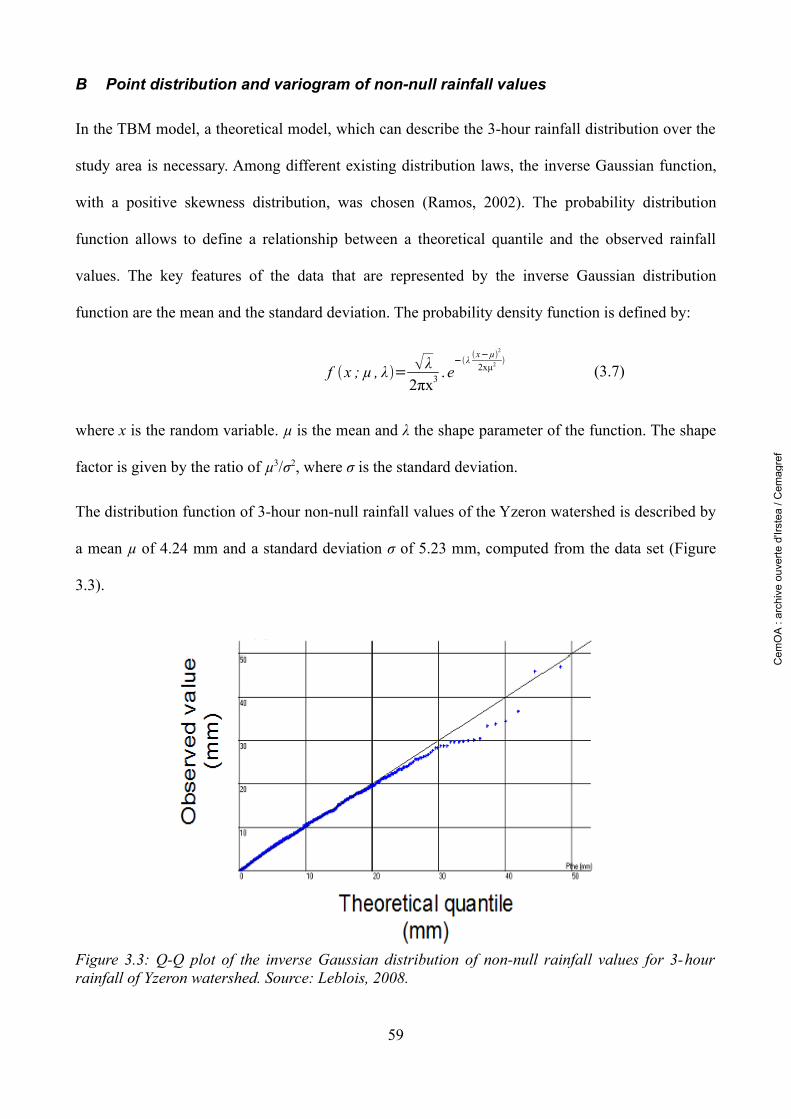
B Point distribution and variogram of non-null rainfall values
In the TBM model, a theoretical model, which can describe the 3-hour rainfall distribution over the
study area is necessary. Among different existing distribution laws, the inverse Gaussian function,
with a positive skewness distribution, was chosen (Ramos, 2002). The probability distribution
function allows to define a relationship between a theoretical quantile and the observed rainfall
values. The key features of the data that are represented by the inverse Gaussian distribution
function are the mean and the standard deviation. The probability density function is defined by:
f x ; µ , λ= λ2πx3 . e
−λ x−µ2
2xµ2 (3.7)
where x is the random variable. µ is the mean and λ the shape parameter of the function. The shape
factor is given by the ratio of µ3/σ2, where σ is the standard deviation.
The distribution function of 3-hour non-null rainfall values of the Yzeron watershed is described by
a mean µ of 4.24 mm and a standard deviation σ of 5.23 mm, computed from the data set (Figure
3.3).
59
Figure 3.3: Q-Q plot of the inverse Gaussian distribution of non-null rainfall values for 3-hour rainfall of Yzeron watershed. Source: Leblois, 2008.
Cem
OA
: ar
chiv
e ou
verte
d'Ir
stea
/ C
emag
ref
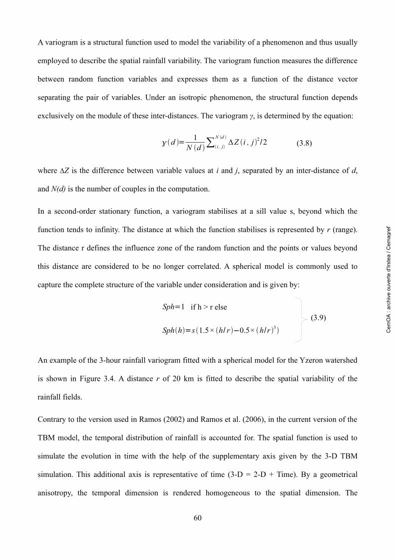
A variogram is a structural function used to model the variability of a phenomenon and thus usually
employed to describe the spatial rainfall variability. The variogram function measures the difference
between random function variables and expresses them as a function of the distance vector
separating the pair of variables. Under an isotropic phenomenon, the structural function depends
exclusively on the module of these inter-distances. The variogram γ, is determined by the equation:
d = 1N d ∑ i , j
N d ∆ Z i , j 2/2 (3.8)
where ∆Z is the difference between variable values at i and j, separated by an inter-distance of d,
and N(d) is the number of couples in the computation.
In a second-order stationary function, a variogram stabilises at a sill value s, beyond which the
function tends to infinity. The distance at which the function stabilises is represented by r (range).
The distance r defines the influence zone of the random function and the points or values beyond
this distance are considered to be no longer correlated. A spherical model is commonly used to
capture the complete structure of the variable under consideration and is given by:
Sph=1 if h > r else
Sphh=s 1.5×h/ r −0.5×h/r 3
An example of the 3-hour rainfall variogram fitted with a spherical model for the Yzeron watershed
is shown in Figure 3.4. A distance r of 20 km is fitted to describe the spatial variability of the
rainfall fields.
Contrary to the version used in Ramos (2002) and Ramos et al. (2006), in the current version of the
TBM model, the temporal distribution of rainfall is accounted for. The spatial function is used to
simulate the evolution in time with the help of the supplementary axis given by the 3-D TBM
simulation. This additional axis is representative of time (3-D = 2-D + Time). By a geometrical
anisotropy, the temporal dimension is rendered homogeneous to the spatial dimension. The
60
(3.9)
Cem
OA
: ar
chiv
e ou
verte
d'Ir
stea
/ C
emag
ref
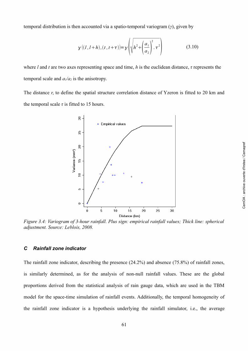
temporal distribution is then accounted via a spatio-temporal variogram (γ), given by
l , lh ,t , t=h2a1
a2 2
.2 (3.10)
where l and t are two axes representing space and time, h is the euclidean distance, τ represents the
temporal scale and a1/a2 is the anisotropy.
The distance r, to define the spatial structure correlation distance of Yzeron is fitted to 20 km and
the temporal scale τ is fitted to 15 hours.
Figure 3.4: Variogram of 3-hour rainfall. Plus sign: empirical rainfall values; Thick line: spherical adjustment. Source: Leblois, 2008.
C Rainfall zone indicator
The rainfall zone indicator, describing the presence (24.2%) and absence (75.8%) of rainfall zones,
is similarly determined, as for the analysis of non-null rainfall values. These are the global
proportions derived from the statistical analysis of rain gauge data, which are used in the TBM
model for the space-time simulation of rainfall events. Additionally, the temporal homogeneity of
the rainfall zone indicator is a hypothesis underlying the rainfall simulator, i.e., the average
61
Cem
OA
: ar
chiv
e ou
verte
d'Ir
stea
/ C
emag
ref

proportion of null values is applied at each time step (Leblois, 2008).
The space and temporal correlation ranges are 10 km and 7.5 hours, respectively, for the rainfall
zone indicator.
D Point distribution and variogram of Yzeron watershed in comparison with Grand
Lyon district
The lack of an adequate number of rain gauges covering the Yzeron watershed area for a better
assessment of rainfall space-time patterns is acknowledged. The information about the rainfall
distribution over the area is further handicapped by the lack of consistent, reliable and long rainfall
records. To assess these limitations and get a better perspective of the nature of the rainfall
distribution in the Yzeron watershed, the available data records are compared with recently obtained
(June 2008) rainfall data of the Grand Lyon district rain gauge network. The Yzeron watershed
belongs to the Grand Lyon district and a global view of the whole region might help to better
understand the rainfall patterns detected over the Yzeron watershed. A preliminary comparative
analysis of the characteristic point distribution and the variogram used to define the distribution and
the structure of rainfalls in the Yzeron watershed and in the Grand Lyon district is communicated
below.
The observed rainfall statistical properties of non-null values of Yzeron were compared with those
of the Grand Lyon district data. The mean and standard deviation of each observed rainfall data set
are resumed in Table 3.2.1. We notice that the mean rainfall intensity of the Yzeron watershed is
more intense compared to the Grand Lyon district, and that the standard deviation is higher for the
Yzeron watershed, implying a higher variability of the rainfall.
62
Cem
OA
: ar
chiv
e ou
verte
d'Ir
stea
/ C
emag
ref
The variogram of Grand Lyon district for non-null rainfall values is compared with the one obtained
for the Yzeron watershed as shown in Figure 3.5, for a 3-hour rainfall duration. For the Grand Lyon
district data, the distance r defining the correlation distance does not stabilise even at 35 km. For the
same duration, the correlation distance of non-null rainfall data for the Yzeron data is only about 20
km.
Further in-depth analyses are necessary to better explain the differences observed, which may come
from several sources, such as a strong spatial heterogeneity of rainfalls over the area or a lack of
enough data at the Yzeron watershed for capturing correctly all space-time rainfall variability. These
63
Watershed3 hours 72 hours
µ σ µ σ
Yzeron 4.24 5.23 31.34 20.29Grand Lyon 2.01 3.39 25.35 17.71
Table 3.2.1: Comparison of the mean and standard deviation values of the Yzeron watershed with the Grand Lyon district rainfall data. µ = mean rainfall value, σ = standard deviation.
Figure 3.5: Comparison of 3-hour non-null rainfall value variogram of the Yzeron watershed and the Grand Lyon district. Plus: Empirical rainfall data of Yzeron; Cross: Empirical rainfall data of Grand Lyon, Thick lines: Spherical adjustment. Source: Leblois, 2008.
Cem
OA
: ar
chiv
e ou
verte
d'Ir
stea
/ C
emag
ref
analyses are out of the scope of this study.
3.2.3 Output of the TBM model and verification of the spatial and
temporal variogram of the simulated output
A Output of TBM model
The estimated rainfall statistics of the Yzeron watershed were used as input to the TBM model. The
TBM model then generated an output of 9400 rainfall events, representing 1105.88 years of rainfall
data, based on the assumption of an average occurrence of 8.5 events per year. Each event had a
total duration of 72 hours, with a 3-hour time step and a 500 m × 500 m space resolution. This space
resolution is used to capture well the spatial and temporal rainfall variability over the 150 km²
watershed (Michaud and Soroosshian, 1994; Ogden and Julien, 1994). The choice of working at a
3-hour time step was made due to computation simplicity and respect of the observed hydrograph
precision by the coupled hydrological and hydraulic models (Section 4.3.1). An example of 24
hours of a simulated event, with a 3-hour time step is shown in Figure 3.6, which has a total mean
rainfall volume of 43 mm. From Figure 3.6, one can see the birth of storm cells in the south-east
and the north-west part of the watershed at 3-hour time step. With the evolution of time, storm cells
move and cumulate on the north-western part of the watershed. This produces a noticeable increase
in the rainfall intensity at time steps of 6 hours and 9 hours in the north-western region. A maximum
intensity of 101 mm in 3 hours is seen in the 9th hour, while the average intensity in 3 hours was 5
mm. The persistence of the storm event up to 18 hours and the slow decay of the storm event after
this duration can also be observed.
64
Cem
OA
: ar
chiv
e ou
verte
d'Ir
stea
/ C
emag
ref
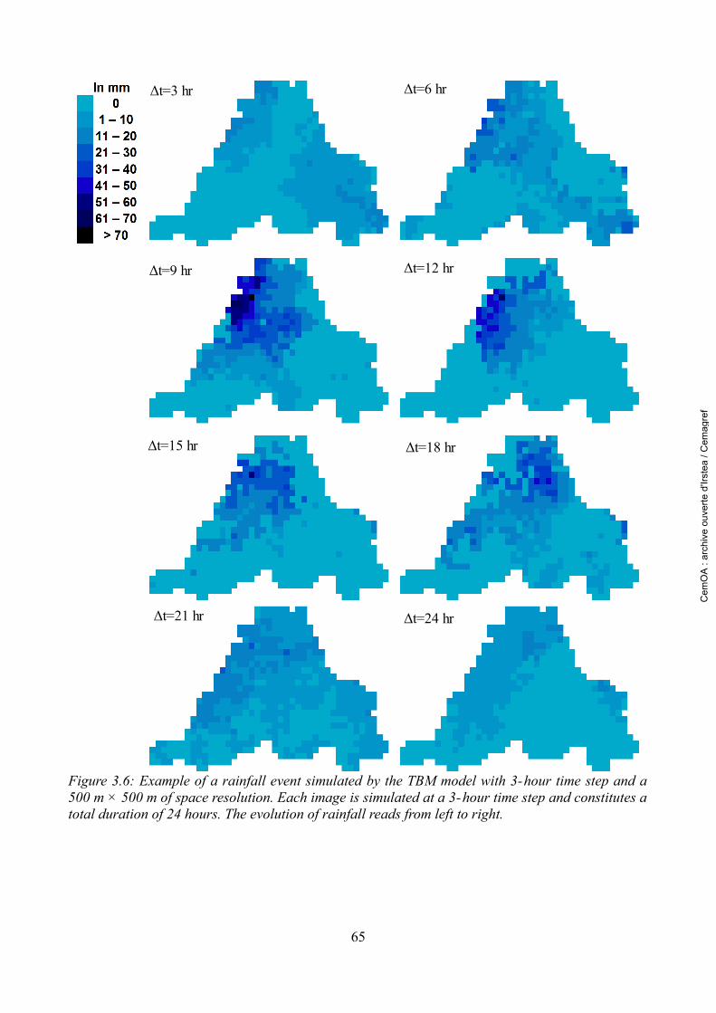
65
Figure 3.6: Example of a rainfall event simulated by the TBM model with 3-hour time step and a 500 m × 500 m of space resolution. Each image is simulated at a 3-hour time step and constitutes a total duration of 24 hours. The evolution of rainfall reads from left to right.
Δt=6 hrΔt=3 hr
Δt=9 hr
Δt=18 hr
Δt=12 hr
Δt=21 hr Δt=24 hr
Δt=15 hr
Cem
OA
: ar
chiv
e ou
verte
d'Ir
stea
/ C
emag
ref
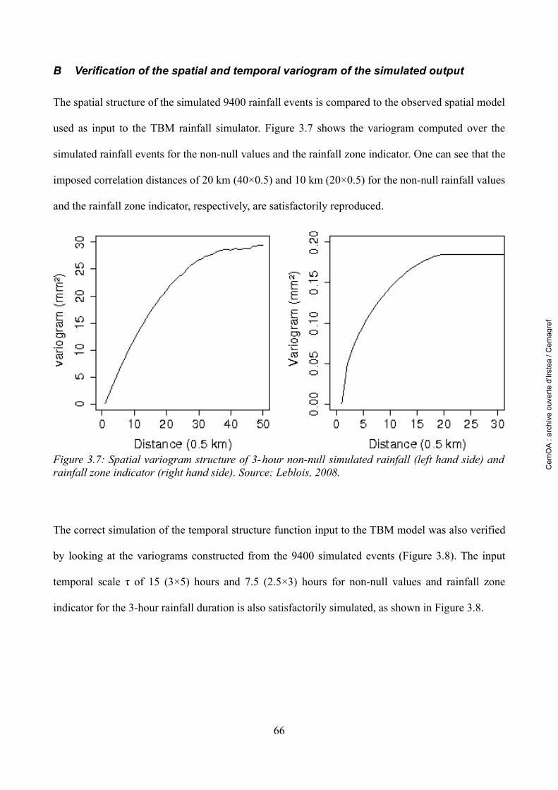
B Verification of the spatial and temporal variogram of the simulated output
The spatial structure of the simulated 9400 rainfall events is compared to the observed spatial model
used as input to the TBM rainfall simulator. Figure 3.7 shows the variogram computed over the
simulated rainfall events for the non-null values and the rainfall zone indicator. One can see that the
imposed correlation distances of 20 km (40×0.5) and 10 km (20×0.5) for the non-null rainfall values
and the rainfall zone indicator, respectively, are satisfactorily reproduced.
The correct simulation of the temporal structure function input to the TBM model was also verified
by looking at the variograms constructed from the 9400 simulated events (Figure 3.8). The input
temporal scale τ of 15 (3×5) hours and 7.5 (2.5×3) hours for non-null values and rainfall zone
indicator for the 3-hour rainfall duration is also satisfactorily simulated, as shown in Figure 3.8.
66
Figure 3.7: Spatial variogram structure of 3-hour non-null simulated rainfall (left hand side) and rainfall zone indicator (right hand side). Source: Leblois, 2008. C
emO
A :
arch
ive
ouve
rte d
'Irst
ea /
Cem
agre
f
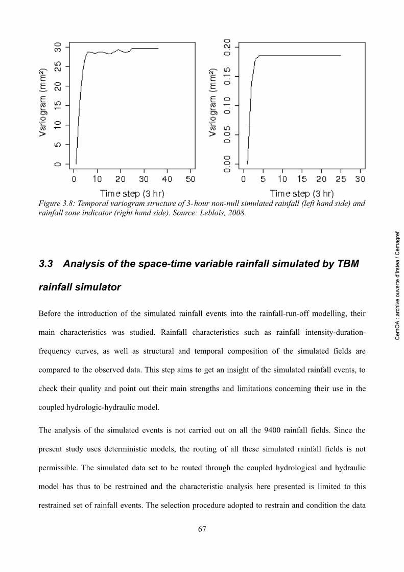
3.3 Analysis of the space-time variable rainfall simulated by TBM
rainfall simulator
Before the introduction of the simulated rainfall events into the rainfall-run-off modelling, their
main characteristics was studied. Rainfall characteristics such as rainfall intensity-duration-
frequency curves, as well as structural and temporal composition of the simulated fields are
compared to the observed data. This step aims to get an insight of the simulated rainfall events, to
check their quality and point out their main strengths and limitations concerning their use in the
coupled hydrologic-hydraulic model.
The analysis of the simulated events is not carried out on all the 9400 rainfall fields. Since the
present study uses deterministic models, the routing of all these simulated rainfall fields is not
permissible. The simulated data set to be routed through the coupled hydrological and hydraulic
model has thus to be restrained and the characteristic analysis here presented is limited to this
restrained set of rainfall events. The selection procedure adopted to restrain and condition the data
67
Figure 3.8: Temporal variogram structure of 3-hour non-null simulated rainfall (left hand side) and rainfall zone indicator (right hand side). Source: Leblois, 2008.
Cem
OA
: ar
chiv
e ou
verte
d'Ir
stea
/ C
emag
ref
set to the study area is presented in chapter 4, section 4.4.2.
The analysis of the simulated rainfall was carried out on 2 sets of rainfall events:
1) A set of 900 rainfall fields: This data set is studied to ensure that the isolation of a random
subset of simulated rainfall events does not influence the properties of the simulated rainfall
events when compared to the observed data set.
2) A set of 45 rainfall fields: Since the routing of 900 fields is still not feasible with
deterministic models, the above mentioned data subset was further restrained to 45 events.
This 45- event data set is then conditioned to represent up to approximately the same 100
years of the 900 rainfall set, by employing the equations 3.11 and 3.12 given below.
3.3.1 Rainfall intensity-duration-frequency analysis
The rainfall intensity-duration-frequency (IDF) analysis allows the calculation of the average
rainfall intensity for given exceedance probabilities and over a range of rainfall durations.
First, a set of 900 events is arbitrarily extracted from the simulated 9400 rainfall fields. Considering
the rate of 8.5 events per year, these 900 events thus represent approximately 100 years of rainfall
data. In addition to the 3-hour original duration of the set, these events are also analysed for three
representative rainfall durations of the Yzeron watershed, 12, 24 and 48 hours to calculate the
intensity-duration-frequency curves. This analysis was carried out for the rain gauge P18, which has
the longest and the most complete observed time series. The durations of 3, 12, 24 and 48 hours are
considered since they represent the effective rainfall durations, provoking significant discharges in
the watershed (Table 2.5.1).
Maximum mean moving averages of rainfall intensities for12, 24 and 48 hours are calculated from
the 900 data set. An empirical frequency value “F” is attributed to each event with the aid of
equation 3.11. It is then transformed to return period (Lang and Lavabre, 2007) with the equation
68
Cem
OA
: ar
chiv
e ou
verte
d'Ir
stea
/ C
emag
ref
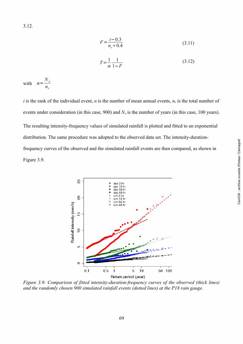
3.12.
F= i−0.3ne0.4 (3.11)
T= 1
11−F
(3.12)
with =N a
ne
i is the rank of the individual event, α is the number of mean annual events, ne is the total number of
events under consideration (in this case, 900) and Na is the number of years (in this case, 100 years).
The resulting intensity-frequency values of simulated rainfall is plotted and fitted to an exponential
distribution. The same procedure was adopted to the observed data set. The intensity-duration-
frequency curves of the observed and the simulated rainfall events are then compared, as shown in
Figure 3.9.
69
Figure 3.9: Comparison of fitted intensity-duration-frequency curves of the observed (thick lines) and the randomly chosen 900 simulated rainfall events (dotted lines) at the P18 rain gauge.
Cem
OA
: ar
chiv
e ou
verte
d'Ir
stea
/ C
emag
ref
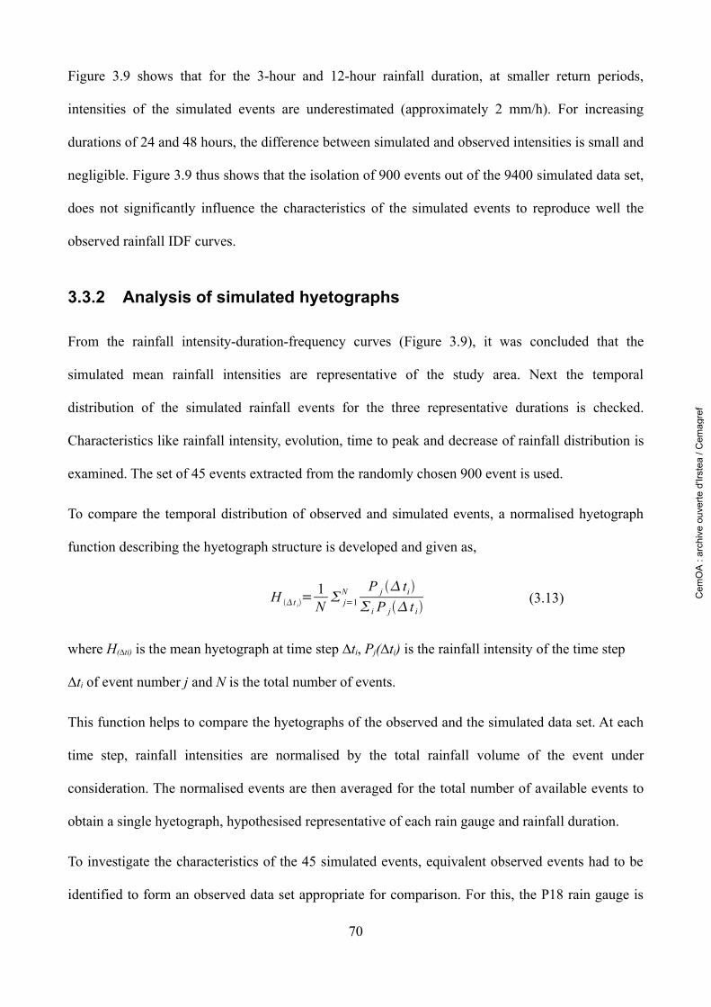
Figure 3.9 shows that for the 3-hour and 12-hour rainfall duration, at smaller return periods,
intensities of the simulated events are underestimated (approximately 2 mm/h). For increasing
durations of 24 and 48 hours, the difference between simulated and observed intensities is small and
negligible. Figure 3.9 thus shows that the isolation of 900 events out of the 9400 simulated data set,
does not significantly influence the characteristics of the simulated events to reproduce well the
observed rainfall IDF curves.
3.3.2 Analysis of simulated hyetographs
From the rainfall intensity-duration-frequency curves (Figure 3.9), it was concluded that the
simulated mean rainfall intensities are representative of the study area. Next the temporal
distribution of the simulated rainfall events for the three representative durations is checked.
Characteristics like rainfall intensity, evolution, time to peak and decrease of rainfall distribution is
examined. The set of 45 events extracted from the randomly chosen 900 event is used.
To compare the temporal distribution of observed and simulated events, a normalised hyetograph
function describing the hyetograph structure is developed and given as,
H t i= 1
N j=1
N P j ti i P j t i
(3.13)
where H(∆ti) is the mean hyetograph at time step ∆ti, Pj(∆ti) is the rainfall intensity of the time step
∆ti of event number j and N is the total number of events.
This function helps to compare the hyetographs of the observed and the simulated data set. At each
time step, rainfall intensities are normalised by the total rainfall volume of the event under
consideration. The normalised events are then averaged for the total number of available events to
obtain a single hyetograph, hypothesised representative of each rain gauge and rainfall duration.
To investigate the characteristics of the 45 simulated events, equivalent observed events had to be
identified to form an observed data set appropriate for comparison. For this, the P18 rain gauge is
70
Cem
OA
: ar
chiv
e ou
verte
d'Ir
stea
/ C
emag
ref
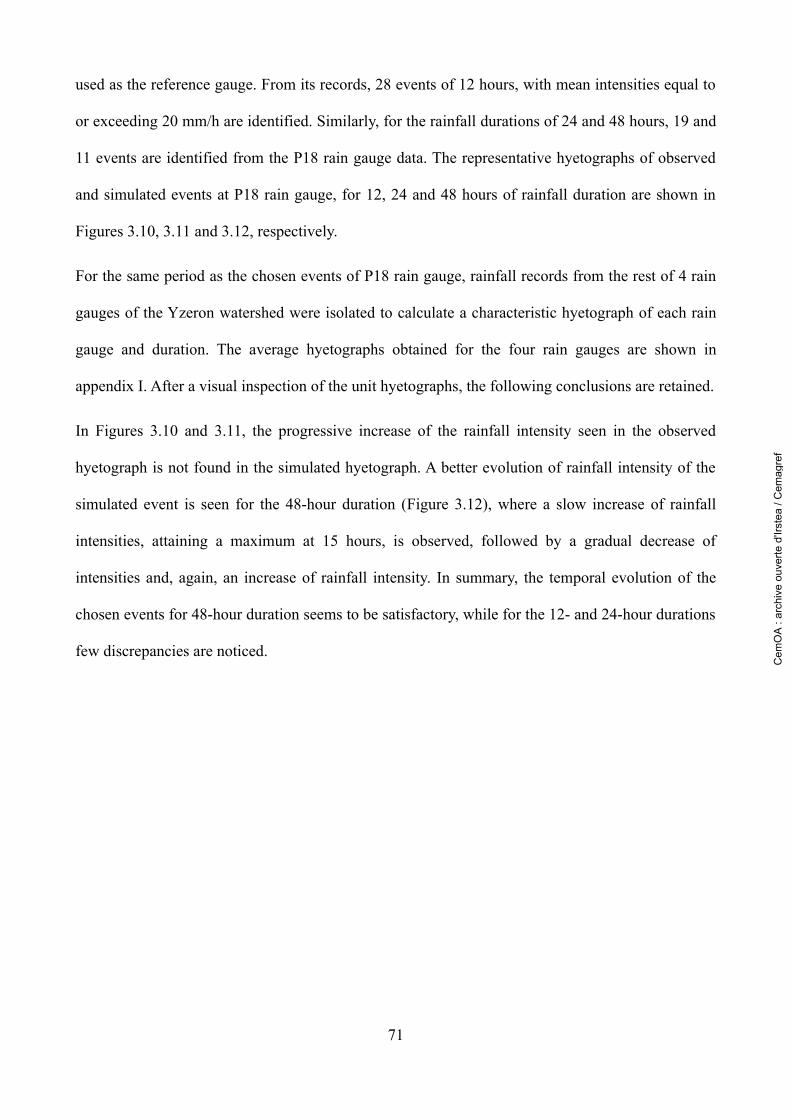
used as the reference gauge. From its records, 28 events of 12 hours, with mean intensities equal to
or exceeding 20 mm/h are identified. Similarly, for the rainfall durations of 24 and 48 hours, 19 and
11 events are identified from the P18 rain gauge data. The representative hyetographs of observed
and simulated events at P18 rain gauge, for 12, 24 and 48 hours of rainfall duration are shown in
Figures 3.10, 3.11 and 3.12, respectively.
For the same period as the chosen events of P18 rain gauge, rainfall records from the rest of 4 rain
gauges of the Yzeron watershed were isolated to calculate a characteristic hyetograph of each rain
gauge and duration. The average hyetographs obtained for the four rain gauges are shown in
appendix I. After a visual inspection of the unit hyetographs, the following conclusions are retained.
In Figures 3.10 and 3.11, the progressive increase of the rainfall intensity seen in the observed
hyetograph is not found in the simulated hyetograph. A better evolution of rainfall intensity of the
simulated event is seen for the 48-hour duration (Figure 3.12), where a slow increase of rainfall
intensities, attaining a maximum at 15 hours, is observed, followed by a gradual decrease of
intensities and, again, an increase of rainfall intensity. In summary, the temporal evolution of the
chosen events for 48-hour duration seems to be satisfactory, while for the 12- and 24-hour durations
few discrepancies are noticed.
71
Cem
OA
: ar
chiv
e ou
verte
d'Ir
stea
/ C
emag
ref
72
Figure 3.10: Comparison of the 12-hour normalised hyetograph between the observed and simulated events at the P18 rain gauge. The red line represents the interval: [mean - standard deviation; mean + standard deviation] of the observed events at each time step.
Figure 3.11: Comparison of the 24-hour normalised hyetograph between the observed and simulated events at the P18 rain gauge. The red line represents the interval: [mean - standard deviation; mean + standard deviation] of the observed event at each time step.
Cem
OA
: ar
chiv
e ou
verte
d'Ir
stea
/ C
emag
ref
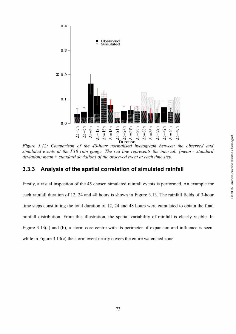
3.3.3 Analysis of the spatial correlation of simulated rainfall
Firstly, a visual inspection of the 45 chosen simulated rainfall events is performed. An example for
each rainfall duration of 12, 24 and 48 hours is shown in Figure 3.13. The rainfall fields of 3-hour
time steps constituting the total duration of 12, 24 and 48 hours were cumulated to obtain the final
rainfall distribution. From this illustration, the spatial variability of rainfall is clearly visible. In
Figure 3.13(a) and (b), a storm core centre with its perimeter of expansion and influence is seen,
while in Figure 3.13(c) the storm event nearly covers the entire watershed zone.
73
Figure 3.12: Comparison of the 48-hour normalised hyetograph between the observed and simulated events at the P18 rain gauge. The red line represents the interval: [mean - standard deviation; mean + standard deviation] of the observed event at each time step.
Cem
OA
: ar
chiv
e ou
verte
d'Ir
stea
/ C
emag
ref
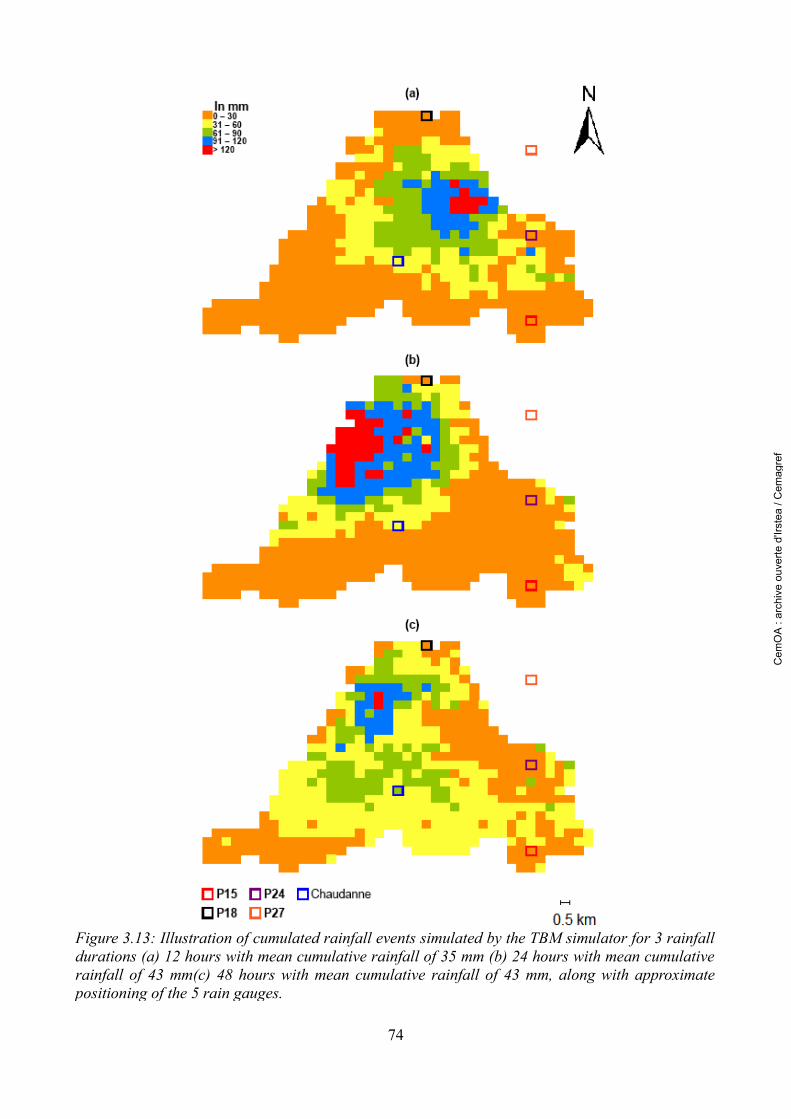
74
Figure 3.13: Illustration of cumulated rainfall events simulated by the TBM simulator for 3 rainfall durations (a) 12 hours with mean cumulative rainfall of 35 mm (b) 24 hours with mean cumulative rainfall of 43 mm(c) 48 hours with mean cumulative rainfall of 43 mm, along with approximate positioning of the 5 rain gauges.
Cem
OA
: ar
chiv
e ou
verte
d'Ir
stea
/ C
emag
ref
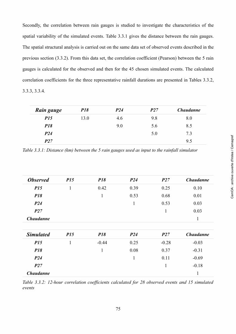
Secondly, the correlation between rain gauges is studied to investigate the characteristics of the
spatial variability of the simulated events. Table 3.3.1 gives the distance between the rain gauges.
The spatial structural analysis is carried out on the same data set of observed events described in the
previous section (3.3.2). From this data set, the correlation coefficient (Pearson) between the 5 rain
gauges is calculated for the observed and then for the 45 chosen simulated events. The calculated
correlation coefficients for the three representative rainfall durations are presented in Tables 3.3.2,
3.3.3, 3.3.4.
75
Rain gauge P18 P24 P27 Chaudanne
P15 13.0 4.6 9.8 8.0P18 9.0 5.6 8.5P24 5.0 7.3P27 9.5
Table 3.3.1: Distance (km) between the 5 rain gauges used as input to the rainfall simulator
Observed P15 P18 P24 P27 Chaudanne
P15 1 0.42 0.39 0.25 0.10P18 1 0.53 0.68 0.01P24 1 0.53 0.03P27 1 0.03
Chaudanne 1
Simulated P15 P18 P24 P27 Chaudanne
P15 1 -0.44 0.25 -0.28 -0.03P18 1 0.08 0.37 -0.31P24 1 0.11 -0.69P27 1 -0.18
Chaudanne 1
Table 3.3.2: 12-hour correlation coefficients calculated for 28 observed events and 15 simulated events
Cem
OA
: ar
chiv
e ou
verte
d'Ir
stea
/ C
emag
ref
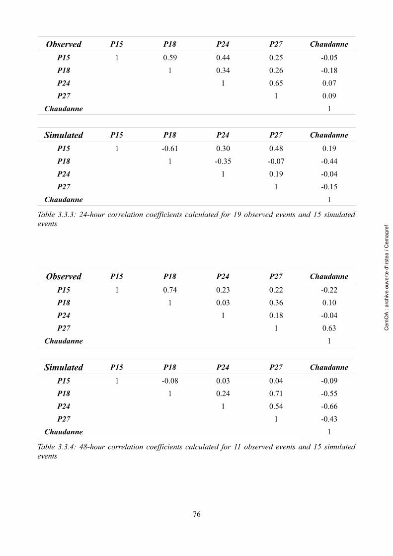
76
Observed P15 P18 P24 P27 Chaudanne
P15 1 0.74 0.23 0.22 -0.22P18 1 0.03 0.36 0.10P24 1 0.18 -0.04P27 1 0.63
Chaudanne 1
Simulated P15 P18 P24 P27 Chaudanne
P15 1 -0.08 0.03 0.04 -0.09P18 1 0.24 0.71 -0.55P24 1 0.54 -0.66P27 1 -0.43
Chaudanne 1
Table 3.3.4: 48-hour correlation coefficients calculated for 11 observed events and 15 simulated events
Observed P15 P18 P24 P27 Chaudanne
P15 1 0.59 0.44 0.25 -0.05P18 1 0.34 0.26 -0.18P24 1 0.65 0.07P27 1 0.09
Chaudanne 1
Simulated P15 P18 P24 P27 Chaudanne
P15 1 -0.61 0.30 0.48 0.19P18 1 -0.35 -0.07 -0.44P24 1 0.19 -0.04P27 1 -0.15
Chaudanne 1
Table 3.3.3: 24-hour correlation coefficients calculated for 19 observed events and 15 simulated events
Cem
OA
: ar
chiv
e ou
verte
d'Ir
stea
/ C
emag
ref
The correlation coefficients of each rain gauge should be read along the rows in association to the
respective rain gauge mentioned in columns. Contrasting results of the Pearson correlation
coefficient for the three rainfall durations is seen from the observed rainfall data set. The
correlation coefficients of Chaudanne with respect to the other rain gauges are nearly zero and even
negative at times for the observed data set. This confirmed the reservations concerning the rainfall
records from this rain gauge. From the correlation coefficients of the observed data, we conclude
that the watershed is characterised with convective (localised), as well as advective (dispersed)
rainfall patterns.
For the simulated events, the maximum correlation coefficients of different durations are quite low:
we observe negative values for more than 50% of the cases (Table 3.3.2, 3.3.3, 3.3.4). The
correlation coefficients of the chosen simulated rainfall events, representing a measure of spatial
rainfall variance between the rain gauges of the network, is disjunct and the simulated data set is
thus concluded to be composed of mainly highly localised storms (Figure 3.13(a) and (b)).
3.4 Conclusions of the simulated space-time rainfall data
furnished by the TBM model
The conclusions drawn from the analysis of the simulated space-time rainfall data provided by the
TBM model for input to the flood mitigation analysis are:
1) 9400 space-time variable rainfall fields (representing 1106 years of rainfall data) of 72
hours, with 3-hour time step were simulated by the TBM model. This output will be input to
the distributed hydrological and 1-D hydraulic model for flood mitigation analysis via
discharge-frequency regime analysis.
2) The 900 simulated events, showed that average rainfall intensity of short durations were
underestimated for frequent return periods, while increasing rainfall durations were well
77
Cem
OA
: ar
chiv
e ou
verte
d'Ir
stea
/ C
emag
ref
represented. But the reason for this underestimation is uncertain, meaning is it linked to the
sub-selection of a set of 900 events or a bias of the TBM model itself ? However, a subset of
simulated events is however inevitable since it is computationally infeasible to input all
9400 events in the coupled hydrological-hydraulic model employed in this study.
3) The available rainfall data for the Yzeron watershed alone seems too sparse to generate
realistic rainfall fields variable in space and time. The available data is not only sparse in
length, but also in space. For instance, there is a significant lack of rainfall knowledge in the
north-eastern and south-eastern parts of the watershed.
4) In the 45 subset rainfall events, the temporal distribution of the simulated rainfall is
moderately satisfactory for long rainfall durations. However, for shorter durations, it is not
so. The poor representation of the spatial and temporal rainfall distributions might entail
some errors in the flood mitigation analysis to be performed using these simulated rainfall
fields.
5) Due to the insufficient amount of rainfall data in the watershed, the range of the structural
correlation used to simulate the rainfall events was probably underestimated. Thus
reinforcing the prevailing idea that the simulated data set of rainfall events are basically
providing a set of possible scenarios of convective-type storms (strong and localized
intensities).
By comparing simulated fields to observed ones, it appeared that the assumption of equal
occurrence of null rainfall zones in each 3-hour time step within the total 72 hours of rainfall
duration is not justified and could explain the highly “convective” features (strong and localized
intensities) of the simulated events (Leblois, 2008).
Keeping in mind these features associated to the spatially variable rainfall events simulated by the
TBM model, the flood mitigation analysis is taken to the next step.
78
Cem
OA
: ar
chiv
e ou
verte
d'Ir
stea
/ C
emag
ref
4 SIMULATION OF RAINFALL-RUN-OFF PROCESS AT
WATERSHED SCALE AND DESIGN OF DRY DAMS
Cem
OA
: ar
chiv
e ou
verte
d'Ir
stea
/ C
emag
ref
4.1 Introduction
After the acquisition of space-time variable rainfall fields, the next step is to transform the
simulated rainfall to run-off process at watershed scale. The goal of this chapter is thus to model the
run-off process, to obtain peak discharge values for the construction of reference (without dams)
instantaneous discharge-frequency regimes of the watershed. And, subsequently introduce dry dams
to simulate mitigated peak discharges, to construct modified instantaneous discharge-frequency
regimes of the watershed.
Hydrological models have been used to simulate run-off processes at watershed scale. Among the
various types of models, distributed hydrological models such as TOPMODEL, MIKESHE, SWAT,
etc. are used to account for the spatial heterogeneity of a region. The heterogeneous characteristics
of a region, like land-use, soil texture, soil depth and rainfall influence the run-off production of a
watershed as previously explained. It is of interest to use distributed hydrological models, especially
in cases where the changes in spatial characteristics need to be considered. Also, in the present
study discharge information all along the drainage network necessary for mitigation analysis can be
furnished by distributed models only. Robust lumped models are very useful because of the few
parameters they require, but when enough data is available distributed hydrological models can be
employed (Refsgaard and Knudsen, 1996; Refsgaard and Henriksen, 2004) and are used in the
context of flood simulation (Correia et al., 1998a; Correia et al., 1998b; Montaldo et al., 2004;
Montaldo et al., 2007; Ravazzani et al., 2007).
In compliment to the above modelling of the run-off processes, appropriate models which can
simulate the flow along river network is considered. In the context of flooding they simulate the
flow and excess flow, overspilling from the riverbed on to the flood plain to cause flooding (Werner
et al., 2005). They also simulate flows in the presence of hydraulic structures which influence the
run-off. Thus, to conduct a technical study at watershed scale, appropriate distributed hydrological
80
Cem
OA
: ar
chiv
e ou
verte
d'Ir
stea
/ C
emag
ref
and hydraulic models are necessary.
To study flooding at watershed scale, two appropriate models: a distributed hydrological model and
a 1-D hydraulic model, adapted for flooding study were chosen. The distributed hydrological model
coined MARINE (Modélisation de l’Anticipation du Ruissellement et des Inondations pour des
évèNements Extrêmes) and a 1-D hydraulic model MAGE (MAillé GEnéralisé) are employed to
simulate hydrological and hydraulic processes of Yzeron watershed. The first step is to calibrate
these two models, so as to produce to the best of ability, the observed hydrological process of
Yzeron. The calibration is done by parametrising the model variables to simulate observed
discharge, from observed rainfall in the first step.
The inputs of the space-time variable rainfall from the stochastic rainfall generator are then input to
simulate the observed instantaneous discharge-frequency curve. Thus a discharge-frequency regime
without any mitigation measures is established. Then, the dry dams are introduced in the hydraulic
model, to simulate the discharge-frequency curve in the presence of mitigating measures.
The description of the two models, their coupling, followed by the initial calibration with observed
rainfall is first presented. The input of the simulated rainfall by the rainfall simulator for the
construction of a discharge-frequency is then elaborated. This is then followed by the description of
dry dams in the 1-D MAGE model, their localisation, configuration and dimensioning, to establish a
mitigated discharge-frequency regime.
4.2 Presentation of the hydrological and hydraulic models
4.2.1 Presentation of the distributed hydrological model MARINE
MARINE (Estupina-Borrell et al., 2004) is a distributed raster and event based, hydrological model
employing the kinematic wave approximation for overland flow and channel flow simulation
(Anderson and Burt, 1990). It was developed at Institut de Mécanique des Fluides de Toulouse
81
Cem
OA
: ar
chiv
e ou
verte
d'Ir
stea
/ C
emag
ref

(IMFT) for operational flash flood forecasting under a PhD program (Estupina Borrell, 2004) and
tested on small scale watersheds of south of France (Thoré watershed in Tarn district, Lèze
watershed of Ariège and Haute-Garonne district, Gard district). The model assures the
transformation of rainfall into dynamic surface run-off. The modelling of different hydrological
processes such as infiltration and excess run-off is applied on grid scale. The rainfall can be input at
desired time-step for the simulation of individual flood events. The simulation of run-off is
accounted from watershed slopes and drainage network. The composition of these two parts in
MARINE is explained below.
MARINE distinguishes two parts of a watershed, i.e. watershed slope and drainage network:
1) The watershed slopes from which surface run-offs arise and are routed to the banks of
drainage network. The estimated surface run-offs are also referred to as lateral run-offs in
this study.
2) The drainage network is further distinguished as drains and river reaches as shown in Figure
4.1:
i. Drains are originating source of drainage network and route the estimated lateral run-
offs using the kinematic wave equation. They are defined from a minimum threshold
surface area and are trapezoidal in shape and have associating roughness coefficients for
major and minor beds. This notion of drains helps to simulate fast contributions of
drainage network compared to watershed slopes which offer higher resistance to surface
flow. The drained threshold surface area is user defined for optimal estimation of run-off
routing.
ii. Rivers are defined in MARINE to distinguish sub-basin with their zone of influence. But
MARINE does not take up the routing of flows along the river and the task is given to
the 1-D hydraulic model to rout the lateral surface run-offs towards the watershed outlet.
82
Cem
OA
: ar
chiv
e ou
verte
d'Ir
stea
/ C
emag
ref
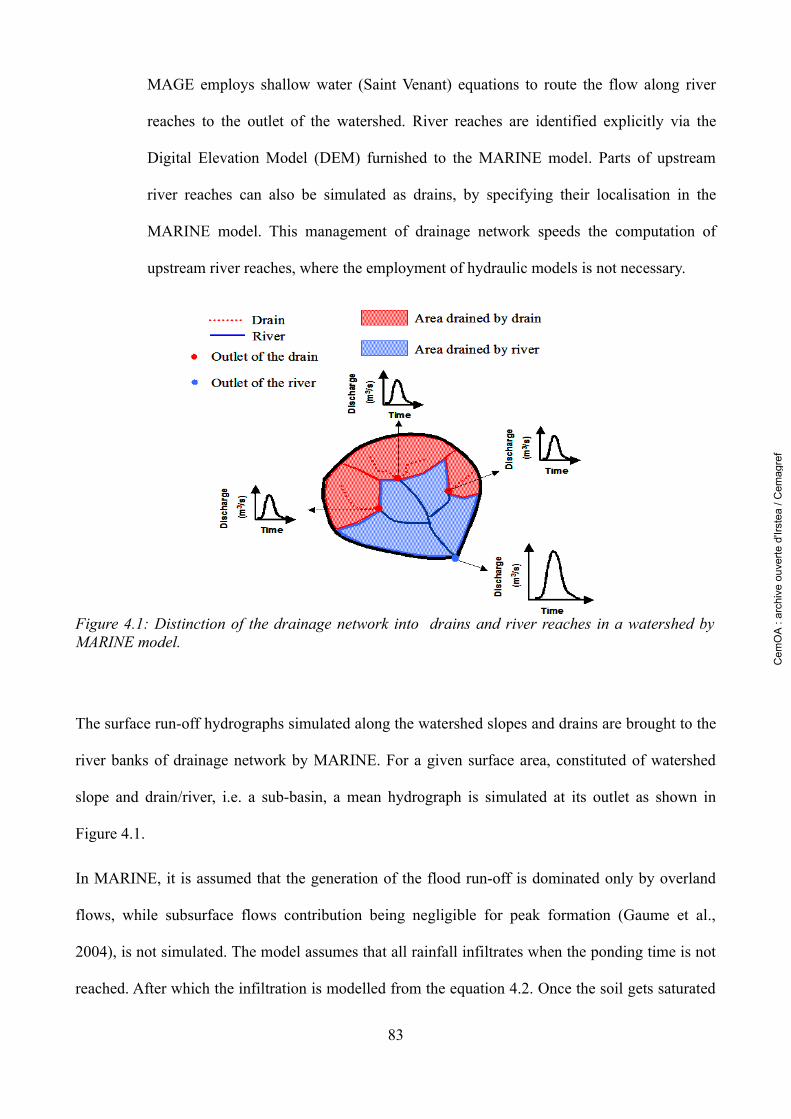
MAGE employs shallow water (Saint Venant) equations to route the flow along river
reaches to the outlet of the watershed. River reaches are identified explicitly via the
Digital Elevation Model (DEM) furnished to the MARINE model. Parts of upstream
river reaches can also be simulated as drains, by specifying their localisation in the
MARINE model. This management of drainage network speeds the computation of
upstream river reaches, where the employment of hydraulic models is not necessary.
The surface run-off hydrographs simulated along the watershed slopes and drains are brought to the
river banks of drainage network by MARINE. For a given surface area, constituted of watershed
slope and drain/river, i.e. a sub-basin, a mean hydrograph is simulated at its outlet as shown in
Figure 4.1.
In MARINE, it is assumed that the generation of the flood run-off is dominated only by overland
flows, while subsurface flows contribution being negligible for peak formation (Gaume et al.,
2004), is not simulated. The model assumes that all rainfall infiltrates when the ponding time is not
reached. After which the infiltration is modelled from the equation 4.2. Once the soil gets saturated
83
Figure 4.1: Distinction of the drainage network into drains and river reaches in a watershed by MARINE model.
Cem
OA
: ar
chiv
e ou
verte
d'Ir
stea
/ C
emag
ref

run-off is generated along the watershed slopes respecting the theory of saturated contributive areas.
The antecedent soil moisture of soil depth is pre-set to define the infiltration capacity.
MARINE takes into account the following spatial parameters of the watershed, for the production
and transfer of lateral surface run-offs to the banks of drainage network:
1) Topography and drainage network from the Digital Elevation Model.
2) The spatial soil texture distribution from soil texture map: porosity, conductivity and soil
suction force of different soil textures.
3) The soil depth and initial soil moisture content distribution from soil depth map and soil
moisture content from measurements or evalutions.
4) The spatial land-use informations from soil occupation map: Manning roughness coefficient
of watershed slopes.
5) Manning roughness coefficients for the major and minor drain beds.
In the MARINE model, an event based run-off is generated by infiltration excess flow. The
accumulated infiltration and the infiltration rate is calculated by Green-Ampt infiltration method
(Green and Ampt, 1911). The Green-Ampt infiltration is based on the Darcy's equation and reasons
on the basis of hydraulic conductivity, suction force and soil porosity parameters of soil texture.
Green-Ampt infiltration functions on the hypothesis that irrespective of the depth, soil is considered
vertically homogeneous. The wetting front is assumed to be uniformly saturated and horizontal on a
grid scale. The infiltration advances vertically, resulting in a sharply defined wetting front, which
separates the wet and dry zones. When the rainfall intensity exceeds the infiltration rate, the excess
water accumulates over the soil surface and transforms to Hortonian overland flow. The saturated
hydraulic conductivity during a rainfall event upon the ponding is maintained constant.
The infiltration rate (f) calculated, neglecting the depth of ponding at the surface, during a steady
rainfall event using the Green-Ampt equation (Maidment, 1992) is given by:
84
Cem
OA
: ar
chiv
e ou
verte
d'Ir
stea
/ C
emag
ref
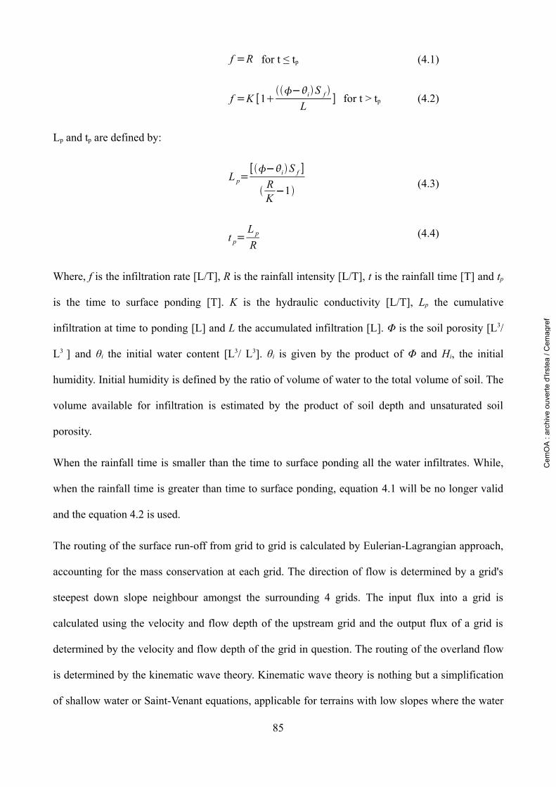
f =R for t ≤ tp (4.1)
f =K [1−iS f
L] for t > tp (4.2)
Lp and tp are defined by:
L p=[−iS f ]
RK−1 (4.3)
t p=L p
R(4.4)
Where, f is the infiltration rate [L/T], R is the rainfall intensity [L/T], t is the rainfall time [T] and tp
is the time to surface ponding [T]. K is the hydraulic conductivity [L/T], Lp the cumulative
infiltration at time to ponding [L] and L the accumulated infiltration [L]. Φ is the soil porosity [L3/
L3 ] and θi the initial water content [L3/ L3]. θi is given by the product of Φ and Hi, the initial
humidity. Initial humidity is defined by the ratio of volume of water to the total volume of soil. The
volume available for infiltration is estimated by the product of soil depth and unsaturated soil
porosity.
When the rainfall time is smaller than the time to surface ponding all the water infiltrates. While,
when the rainfall time is greater than time to surface ponding, equation 4.1 will be no longer valid
and the equation 4.2 is used.
The routing of the surface run-off from grid to grid is calculated by Eulerian-Lagrangian approach,
accounting for the mass conservation at each grid. The direction of flow is determined by a grid's
steepest down slope neighbour amongst the surrounding 4 grids. The input flux into a grid is
calculated using the velocity and flow depth of the upstream grid and the output flux of a grid is
determined by the velocity and flow depth of the grid in question. The routing of the overland flow
is determined by the kinematic wave theory. Kinematic wave theory is nothing but a simplification
of shallow water or Saint-Venant equations, applicable for terrains with low slopes where the water
85
Cem
OA
: ar
chiv
e ou
verte
d'Ir
stea
/ C
emag
ref
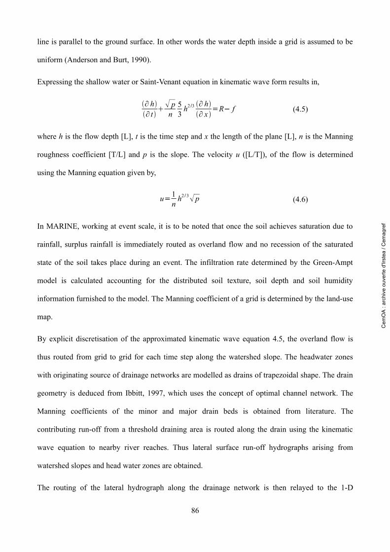
line is parallel to the ground surface. In other words the water depth inside a grid is assumed to be
uniform (Anderson and Burt, 1990).
Expressing the shallow water or Saint-Venant equation in kinematic wave form results in,
∂ h∂ t
pn
53
h2 /3 ∂ h∂ x
=R− f (4.5)
where h is the flow depth [L], t is the time step and x the length of the plane [L], n is the Manning
roughness coefficient [T/L] and p is the slope. The velocity u ([L/T]), of the flow is determined
using the Manning equation given by,
u=1n
h2 /3 p (4.6)
In MARINE, working at event scale, it is to be noted that once the soil achieves saturation due to
rainfall, surplus rainfall is immediately routed as overland flow and no recession of the saturated
state of the soil takes place during an event. The infiltration rate determined by the Green-Ampt
model is calculated accounting for the distributed soil texture, soil depth and soil humidity
information furnished to the model. The Manning coefficient of a grid is determined by the land-use
map.
By explicit discretisation of the approximated kinematic wave equation 4.5, the overland flow is
thus routed from grid to grid for each time step along the watershed slope. The headwater zones
with originating source of drainage networks are modelled as drains of trapezoidal shape. The drain
geometry is deduced from Ibbitt, 1997, which uses the concept of optimal channel network. The
Manning coefficients of the minor and major drain beds is obtained from literature. The
contributing run-off from a threshold draining area is routed along the drain using the kinematic
wave equation to nearby river reaches. Thus lateral surface run-off hydrographs arising from
watershed slopes and head water zones are obtained.
The routing of the lateral hydrograph along the drainage network is then relayed to the 1-D
86
Cem
OA
: ar
chiv
e ou
verte
d'Ir
stea
/ C
emag
ref
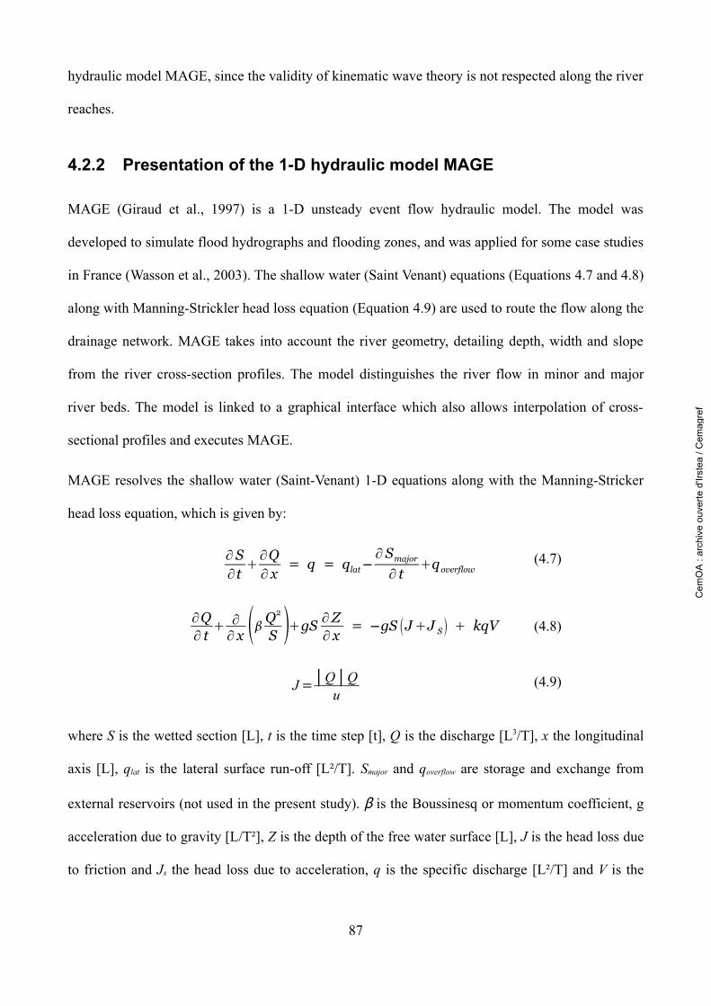
hydraulic model MAGE, since the validity of kinematic wave theory is not respected along the river
reaches.
4.2.2 Presentation of the 1-D hydraulic model MAGE
MAGE (Giraud et al., 1997) is a 1-D unsteady event flow hydraulic model. The model was
developed to simulate flood hydrographs and flooding zones, and was applied for some case studies
in France (Wasson et al., 2003). The shallow water (Saint Venant) equations (Equations 4.7 and 4.8)
along with Manning-Strickler head loss equation (Equation 4.9) are used to route the flow along the
drainage network. MAGE takes into account the river geometry, detailing depth, width and slope
from the river cross-section profiles. The model distinguishes the river flow in minor and major
river beds. The model is linked to a graphical interface which also allows interpolation of cross-
sectional profiles and executes MAGE.
MAGE resolves the shallow water (Saint-Venant) 1-D equations along with the Manning-Stricker
head loss equation, which is given by:
∂S∂t
∂Q∂ x
= q = qlat−∂Smajor∂ t
qoverflow(4.7)
∂Q∂ t
∂∂ x Q
2
S gS ∂Z∂ x = −gS JJ S kqV (4.8)
J=│Q │Qu
(4.9)
where S is the wetted section [L], t is the time step [t], Q is the discharge [L3/T], x the longitudinal
axis [L], qlat is the lateral surface run-off [L²/T]. Smajor and qoverflow are storage and exchange from
external reservoirs (not used in the present study). β is the Boussinesq or momentum coefficient, g
acceleration due to gravity [L/T²], Z is the depth of the free water surface [L], J is the head loss due
to friction and Js the head loss due to acceleration, q is the specific discharge [L²/T] and V is the
87
Cem
OA
: ar
chiv
e ou
verte
d'Ir
stea
/ C
emag
ref

mean velocity [L²/T]. k is the dimensionless momentum coefficient, where k =1 if q<0 , else k = 0.
The above equations represent the continuity equation (4.7), momentum equation (4.8) and
Manning-Strickler equation (4.9) respectively. An initial and boundary conditions of the drainage
network is input to establish an unsteady event flow model.
The head loss is deduced from Manning-Strickler equation taking into account the roughness
coefficients of drainage network and flood plain. The lateral surface run-off input into the model
MAGE are distributed homogeneously along the river reaches of the drainage network. The lateral
flows are consequently routed along the drainage network to the outlet.
The boundary conditions of the drainage network can either be input as a hydrograph or a punctual
yield at the upstream nodes. The downstream boundary condition on the other hand can either be a
limnigraph or a stage-discharge relationship.
The flow velocity in the minor and major river beds is simulated based on the Debord formulation
(Nicolet and Uan, 1979), which estimates the momentum coefficient. Head loss estimation of
various stage-discharge conditions in the presence of hydraulic structures which interrupt the
normal flow regime of the river is accounted for based on Bernoulli's and continuity equations.
The imposed initial flow condition can be in the form of permanent water level or transitory water
level simulation. Different forms of hydraulic structures such as weir-orifice, gates, pumps and
dams can be easily introduced in the model (Doussière, 2007).
The drainage network in MAGE is constituted of river reaches. The drainage network originates
from upstream nodes and is continued via river reach length to represent a river segment. The
confluence of the drainage network are linked together by intermediate nodes. The head loss in the
intermediate nodes are assumed to be zero, while always respecting the equation of conversation of
mass. The outlet of the drainage network is represented by a downstream node.
88
Cem
OA
: ar
chiv
e ou
verte
d'Ir
stea
/ C
emag
ref
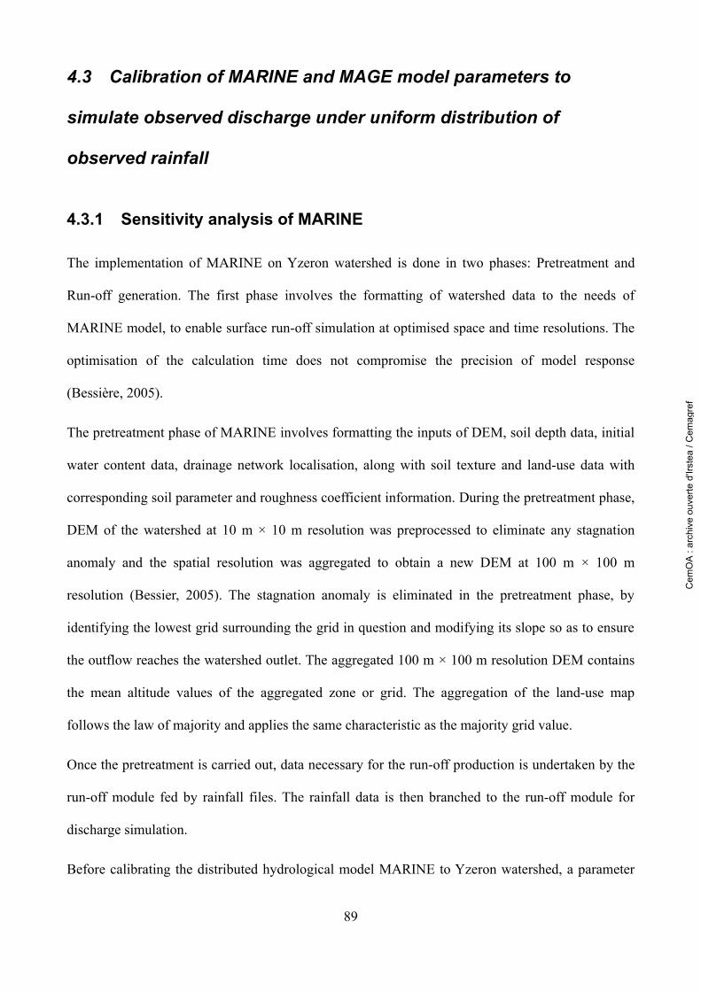
4.3 Calibration of MARINE and MAGE model parameters to
simulate observed discharge under uniform distribution of
observed rainfall
4.3.1 Sensitivity analysis of MARINE
The implementation of MARINE on Yzeron watershed is done in two phases: Pretreatment and
Run-off generation. The first phase involves the formatting of watershed data to the needs of
MARINE model, to enable surface run-off simulation at optimised space and time resolutions. The
optimisation of the calculation time does not compromise the precision of model response
(Bessière, 2005).
The pretreatment phase of MARINE involves formatting the inputs of DEM, soil depth data, initial
water content data, drainage network localisation, along with soil texture and land-use data with
corresponding soil parameter and roughness coefficient information. During the pretreatment phase,
DEM of the watershed at 10 m × 10 m resolution was preprocessed to eliminate any stagnation
anomaly and the spatial resolution was aggregated to obtain a new DEM at 100 m × 100 m
resolution (Bessier, 2005). The stagnation anomaly is eliminated in the pretreatment phase, by
identifying the lowest grid surrounding the grid in question and modifying its slope so as to ensure
the outflow reaches the watershed outlet. The aggregated 100 m × 100 m resolution DEM contains
the mean altitude values of the aggregated zone or grid. The aggregation of the land-use map
follows the law of majority and applies the same characteristic as the majority grid value.
Once the pretreatment is carried out, data necessary for the run-off production is undertaken by the
run-off module fed by rainfall files. The rainfall data is then branched to the run-off module for
discharge simulation.
Before calibrating the distributed hydrological model MARINE to Yzeron watershed, a parameter
89
Cem
OA
: ar
chiv
e ou
verte
d'Ir
stea
/ C
emag
ref

sensitivity analysis was carried out to understand the functioning of the model. For this
homogeneous distribution of soil characteristics such as soil porosity, conductivity, suction force,
depth and the roughness coefficient of soil surface was accounted. The soil characteristics values
are deduced from literature (Maidment, 1992). The tested parameter values, along with the resulting
hydrographs can be consulted in the appendix II.
The sensitivity of the model parameters in MARINE showed that :
1. The model was particularly sensitive to initial water content, soil porosity and soil depth
variation.
2. The amplitude of discharge peak was sensitive to Manning/roughness coefficient.
3. The soil parameters such as hydraulic conductivity and suction force did not show
significant influence on the output hydrograph.
4. The model and the watershed were not sensitive to the variation in time step up to 3 hours.
This incited the use of 3-hour time step for computational rapidity in the present study.
4.3.2 Calibration and evaluation of MARINE
The calibration of the MARINE model alone is first undertaken. The spatial watershed parameters
are input for model calibration. The experimental values of soil and surface characteristics
employed are tabulated in Tables 4.3.1 and 4.3.2. The distributed initial humidity information for
the watershed was not available and thus a homogeneous distribution is assumed. Hence the
distributed model MARINE is used as a semi-distributed model in the present study. The lateral
surface run-off is simulated by MARINE alone. The lateral surface run-off is simulated along the
watershed slopes and by considering the whole drainage network of the Yzeron watershed as drains,
as shown in Figure 4.2. A small stretch of river reach is considered to obtain a mean hydrograph for
the entire watershed surface area.
90
Cem
OA
: ar
chiv
e ou
verte
d'Ir
stea
/ C
emag
ref
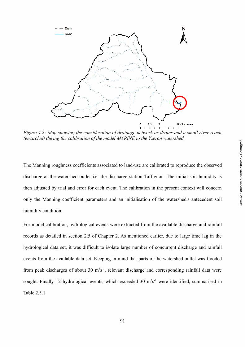
The Manning roughness coefficients associated to land-use are calibrated to reproduce the observed
discharge at the watershed outlet i.e. the discharge station Taffignon. The initial soil humidity is
then adjusted by trial and error for each event. The calibration in the present context will concern
only the Manning coefficient parameters and an initialisation of the watershed's antecedent soil
humidity condition.
For model calibration, hydrological events were extracted from the available discharge and rainfall
records as detailed in section 2.5 of Chapter 2. As mentioned earlier, due to large time lag in the
hydrological data set, it was difficult to isolate large number of concurrent discharge and rainfall
events from the available data set. Keeping in mind that parts of the watershed outlet was flooded
from peak discharges of about 30 m3s-1, relevant discharge and corresponding rainfall data were
sought. Finally 12 hydrological events, which exceeded 30 m3s-1 were identified, summarised in
Table 2.5.1.
91
Figure 4.2: Map showing the consideration of drainage network as drains and a small river reach (encircled) during the calibration of the model MARINE to the Yzeron watershed.
Cem
OA
: ar
chiv
e ou
verte
d'Ir
stea
/ C
emag
ref
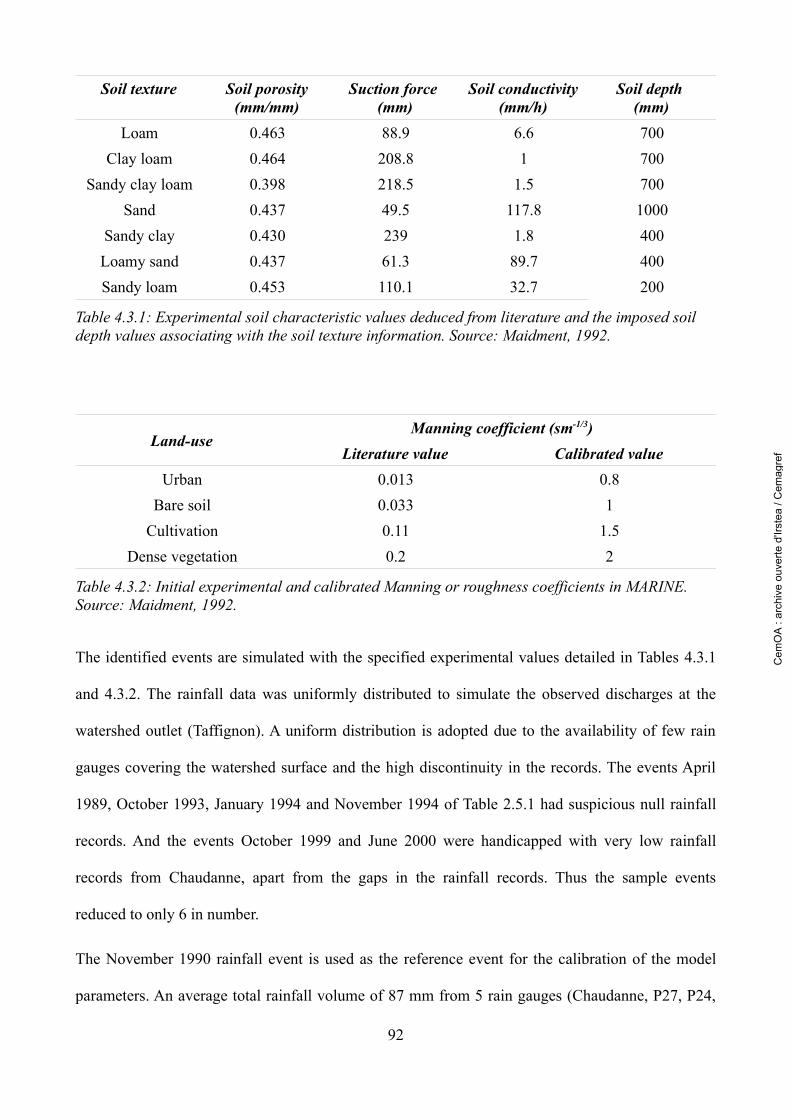
Land-useManning coefficient (sm-1/3)
Literature value Calibrated valueUrban 0.013 0.8
Bare soil 0.033 1Cultivation 0.11 1.5
Dense vegetation 0.2 2
Table 4.3.2: Initial experimental and calibrated Manning or roughness coefficients in MARINE. Source: Maidment, 1992.
The identified events are simulated with the specified experimental values detailed in Tables 4.3.1
and 4.3.2. The rainfall data was uniformly distributed to simulate the observed discharges at the
watershed outlet (Taffignon). A uniform distribution is adopted due to the availability of few rain
gauges covering the watershed surface and the high discontinuity in the records. The events April
1989, October 1993, January 1994 and November 1994 of Table 2.5.1 had suspicious null rainfall
records. And the events October 1999 and June 2000 were handicapped with very low rainfall
records from Chaudanne, apart from the gaps in the rainfall records. Thus the sample events
reduced to only 6 in number.
The November 1990 rainfall event is used as the reference event for the calibration of the model
parameters. An average total rainfall volume of 87 mm from 5 rain gauges (Chaudanne, P27, P24,
92
Soil texture Soil porosity (mm/mm)
Suction force (mm)
Soil conductivity (mm/h)
Soil depth (mm)
Loam 0.463 88.9 6.6 700Clay loam 0.464 208.8 1 700
Sandy clay loam 0.398 218.5 1.5 700Sand 0.437 49.5 117.8 1000
Sandy clay 0.430 239 1.8 400Loamy sand 0.437 61.3 89.7 400Sandy loam 0.453 110.1 32.7 200
Table 4.3.1: Experimental soil characteristic values deduced from literature and the imposed soil depth values associating with the soil texture information. Source: Maidment, 1992.
Cem
OA
: ar
chiv
e ou
verte
d'Ir
stea
/ C
emag
ref
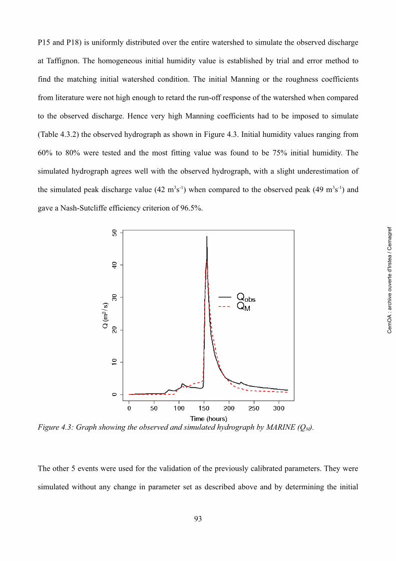
P15 and P18) is uniformly distributed over the entire watershed to simulate the observed discharge
at Taffignon. The homogeneous initial humidity value is established by trial and error method to
find the matching initial watershed condition. The initial Manning or the roughness coefficients
from literature were not high enough to retard the run-off response of the watershed when compared
to the observed discharge. Hence very high Manning coefficients had to be imposed to simulate
(Table 4.3.2) the observed hydrograph as shown in Figure 4.3. Initial humidity values ranging from
60% to 80% were tested and the most fitting value was found to be 75% initial humidity. The
simulated hydrograph agrees well with the observed hydrograph, with a slight underestimation of
the simulated peak discharge value (42 m3s-1) when compared to the observed peak (49 m3s-1) and
gave a Nash-Sutcliffe efficiency criterion of 96.5%.
The other 5 events were used for the validation of the previously calibrated parameters. They were
simulated without any change in parameter set as described above and by determining the initial
93
Figure 4.3: Graph showing the observed and simulated hydrograph by MARINE (QM).
Cem
OA
: ar
chiv
e ou
verte
d'Ir
stea
/ C
emag
ref
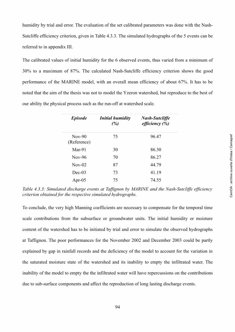
humidity by trial and error. The evaluation of the set calibrated parameters was done with the Nash-
Sutcliffe efficiency criterion, given in Table 4.3.3. The simulated hydrographs of the 5 events can be
referred to in appendix III.
The calibrated values of initial humidity for the 6 observed events, thus varied from a minimum of
30% to a maximum of 87%. The calculated Nash-Sutcliffe efficiency criterion shows the good
performance of the MARINE model, with an overall mean efficiency of about 67%. It has to be
noted that the aim of the thesis was not to model the Yzeron watershed, but reproduce to the best of
our ability the physical process such as the run-off at watershed scale.
To conclude, the very high Manning coefficients are necessary to compensate for the temporal time
scale contributions from the subsurface or groundwater units. The initial humidity or moisture
content of the watershed has to be initiated by trial and error to simulate the observed hydrographs
at Taffignon. The poor performances for the November 2002 and December 2003 could be partly
explained by gap in rainfall records and the deficiency of the model to account for the variation in
the saturated moisture state of the watershed and its inability to empty the infiltrated water. The
inability of the model to empty the the infiltrated water will have repercussions on the contributions
due to sub-surface components and affect the reproduction of long lasting discharge events.
94
Episode Initial humidity (%)
Nash-Sutcliffe efficiency (%)
Nov-90 (Reference)
75 96.47
Mar-91 30 86.30Nov-96 70 86.27Nov-02 87 44.79Dec-03 73 41.19Apr-05 75 74.55
Table 4.3.3: Simulated discharge events at Taffignon by MARINE and the Nash-Sutcliffe efficiency criterion obtained for the respective simulated hydrographs. C
emO
A :
arch
ive
ouve
rte d
'Irst
ea /
Cem
agre
f

The next step involved is to couple the hydrological model MARINE to the 1-D hydraulic model
MAGE to correctly route the lateral surface run-off along the drainage network to the outlet of the
watershed.
4.3.3 Coupling of the models MARINE and MAGE for the routing of
lateral surface run-off
A Segmentation of Yzeron drainage network
The two deterministic physical models: MARINE and MAGE, with their respective characteristics
are coupled together to simulate the dynamics of the watershed. MARINE the distributed physical
based model simulates the overland lateral surface run-offs originating from the watershed's slopes
and accompanies them to the river bank of the drainage network based on the principle explained
above (4.2.1). MAGE in turn routes the input overland lateral surface run-off along the drainage
network to the outlet of the watershed. To simulate to the best of ability the watershed dynamics, the
main river reaches of the watershed's drainage network are highlighted in MARINE, for which
representative lateral surface run-off hydrographs are simulated. The representation of the river
reaches in MARINE is replicated in MAGE, into which the lateral surface run-offs are fed. MAGE
in turn distributes homogeneously the input hydrograph along the associated river reachs of the
drainage network and routes the ensemble of simulated hydrographs to the watershed outlet.
Hydraulic structures if any are introduced in MAGE at desired locations and mitigated hydrographs
in their presence is simulated and routed along the drainage network.
To couple MARINE and MAGE, the first step is to define the segmentation of Yzeron drainage
network in MARINE so as to associate the resulting lateral surface run-offs to corresponding river
reaches in MAGE. Then the corresponding drainage network is represented in MAGE. The drainage
network in MARINE is segmented into drains (with a threshold draining area of 1 km²) and 33 river
95
Cem
OA
: ar
chiv
e ou
verte
d'Ir
stea
/ C
emag
ref
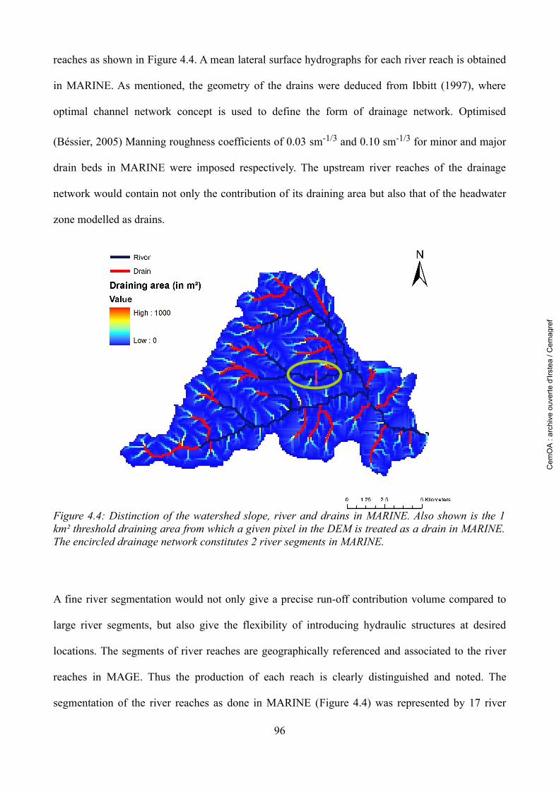
reaches as shown in Figure 4.4. A mean lateral surface hydrographs for each river reach is obtained
in MARINE. As mentioned, the geometry of the drains were deduced from Ibbitt (1997), where
optimal channel network concept is used to define the form of drainage network. Optimised
(Béssier, 2005) Manning roughness coefficients of 0.03 sm-1/3 and 0.10 sm-1/3 for minor and major
drain beds in MARINE were imposed respectively. The upstream river reaches of the drainage
network would contain not only the contribution of its draining area but also that of the headwater
zone modelled as drains.
A fine river segmentation would not only give a precise run-off contribution volume compared to
large river segments, but also give the flexibility of introducing hydraulic structures at desired
locations. The segments of river reaches are geographically referenced and associated to the river
reaches in MAGE. Thus the production of each reach is clearly distinguished and noted. The
segmentation of the river reaches as done in MARINE (Figure 4.4) was represented by 17 river
96
Figure 4.4: Distinction of the watershed slope, river and drains in MARINE. Also shown is the 1 km² threshold draining area from which a given pixel in the DEM is treated as a drain in MARINE. The encircled drainage network constitutes 2 river segments in MARINE.
Cem
OA
: ar
chiv
e ou
verte
d'Ir
stea
/ C
emag
ref
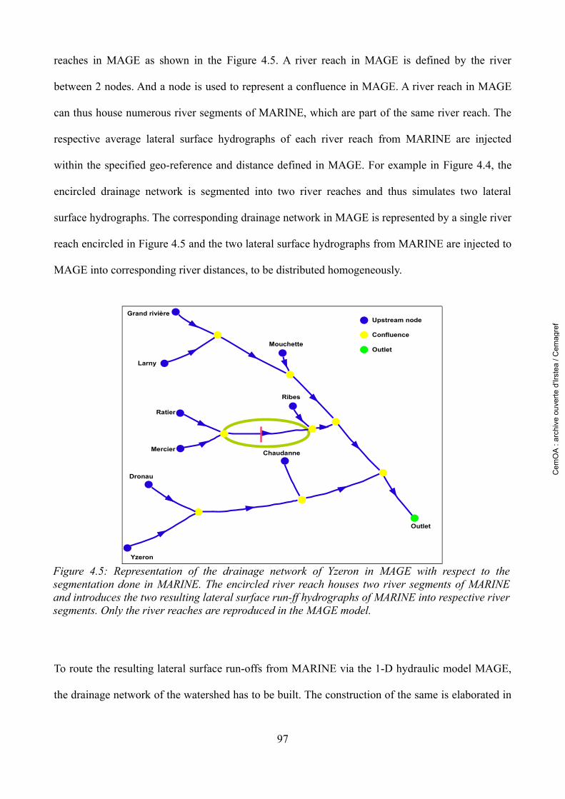
reaches in MAGE as shown in the Figure 4.5. A river reach in MAGE is defined by the river
between 2 nodes. And a node is used to represent a confluence in MAGE. A river reach in MAGE
can thus house numerous river segments of MARINE, which are part of the same river reach. The
respective average lateral surface hydrographs of each river reach from MARINE are injected
within the specified geo-reference and distance defined in MAGE. For example in Figure 4.4, the
encircled drainage network is segmented into two river reaches and thus simulates two lateral
surface hydrographs. The corresponding drainage network in MAGE is represented by a single river
reach encircled in Figure 4.5 and the two lateral surface hydrographs from MARINE are injected to
MAGE into corresponding river distances, to be distributed homogeneously.
To route the resulting lateral surface run-offs from MARINE via the 1-D hydraulic model MAGE,
the drainage network of the watershed has to be built. The construction of the same is elaborated in
97
Figure 4.5: Representation of the drainage network of Yzeron in MAGE with respect to the segmentation done in MARINE. The encircled river reach houses two river segments of MARINE and introduces the two resulting lateral surface run-ff hydrographs of MARINE into respective river segments. Only the river reaches are reproduced in the MAGE model.
Grand rivière
Larny
Mouchette
Ratier
Mercier
Dronau
Yzeron
Chaudanne
Ribes
Outlet
Outlet
Confluence
Upstream node
Cem
OA
: ar
chiv
e ou
verte
d'Ir
stea
/ C
emag
ref
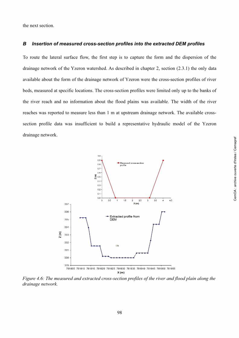
the next section.
B Insertion of measured cross-section profiles into the extracted DEM profiles
To route the lateral surface flow, the first step is to capture the form and the dispersion of the
drainage network of the Yzeron watershed. As described in chapter 2, section (2.3.1) the only data
available about the form of the drainage network of Yzeron were the cross-section profiles of river
beds, measured at specific locations. The cross-section profiles were limited only up to the banks of
the river reach and no information about the flood plains was available. The width of the river
reaches was reported to measure less than 1 m at upstream drainage network. The available cross-
section profile data was insufficient to build a representative hydraulic model of the Yzeron
drainage network.
98
Figure 4.6: The measured and extracted cross-section profiles of the river and flood plain along the drainage network.
Cem
OA
: ar
chiv
e ou
verte
d'Ir
stea
/ C
emag
ref
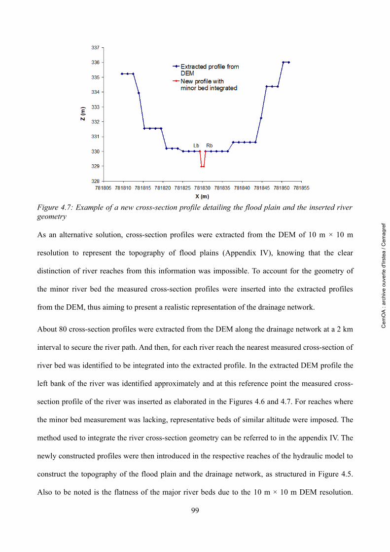
As an alternative solution, cross-section profiles were extracted from the DEM of 10 m × 10 m
resolution to represent the topography of flood plains (Appendix IV), knowing that the clear
distinction of river reaches from this information was impossible. To account for the geometry of
the minor river bed the measured cross-section profiles were inserted into the extracted profiles
from the DEM, thus aiming to present a realistic representation of the drainage network.
About 80 cross-section profiles were extracted from the DEM along the drainage network at a 2 km
interval to secure the river path. And then, for each river reach the nearest measured cross-section of
river bed was identified to be integrated into the extracted profile. In the extracted DEM profile the
left bank of the river was identified approximately and at this reference point the measured cross-
section profile of the river was inserted as elaborated in the Figures 4.6 and 4.7. For reaches where
the minor bed measurement was lacking, representative beds of similar altitude were imposed. The
method used to integrate the river cross-section geometry can be referred to in the appendix IV. The
newly constructed profiles were then introduced in the respective reaches of the hydraulic model to
construct the topography of the flood plain and the drainage network, as structured in Figure 4.5.
Also to be noted is the flatness of the major river beds due to the 10 m × 10 m DEM resolution.
99
Figure 4.7: Example of a new cross-section profile detailing the flood plain and the inserted river geometry
Cem
OA
: ar
chiv
e ou
verte
d'Ir
stea
/ C
emag
ref
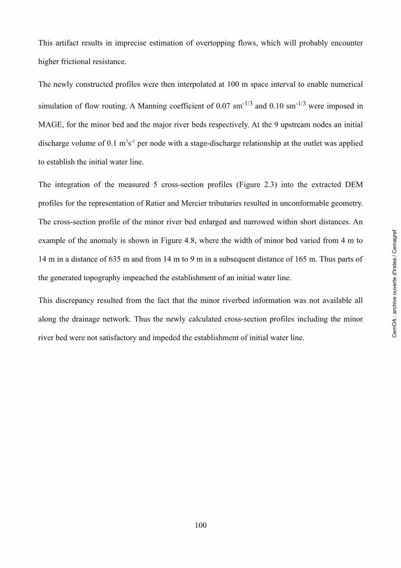
This artifact results in imprecise estimation of overtopping flows, which will probably encounter
higher frictional resistance.
The newly constructed profiles were then interpolated at 100 m space interval to enable numerical
simulation of flow routing. A Manning coefficient of 0.07 sm-1/3 and 0.10 sm-1/3 were imposed in
MAGE, for the minor bed and the major river beds respectively. At the 9 upstream nodes an initial
discharge volume of 0.1 m3s-1 per node with a stage-discharge relationship at the outlet was applied
to establish the initial water line.
The integration of the measured 5 cross-section profiles (Figure 2.3) into the extracted DEM
profiles for the representation of Ratier and Mercier tributaries resulted in unconformable geometry.
The cross-section profile of the minor river bed enlarged and narrowed within short distances. An
example of the anomaly is shown in Figure 4.8, where the width of minor bed varied from 4 m to
14 m in a distance of 635 m and from 14 m to 9 m in a subsequent distance of 165 m. Thus parts of
the generated topography impeached the establishment of an initial water line.
This discrepancy resulted from the fact that the minor riverbed information was not available all
along the drainage network. Thus the newly calculated cross-section profiles including the minor
river bed were not satisfactory and impeded the establishment of initial water line.
100
Cem
OA
: ar
chiv
e ou
verte
d'Ir
stea
/ C
emag
ref
To treat the above problem, a simplification of the geometry was assumed to model the watershed.
Firstly, to have numerically stable geometry, two profiles, i.e. an upstream and a downstream profile
of each reach were retained. The in-between geometry was reconstituted by interpolation. With this
method, the meandering characteristics of the drainage network was simplified and short-circuited.
Another hindrance came from the major riverbeds of the Yzeron and Charbonnières confluence.
The Yzeron and Charbonnières rivers shared the major riverbed, i.e. right bank and left bank of
Yzeron and Charbonnières river respectively. Due to this natural characteristic, it was difficult to
respect the conservation of mass at the outlet. Artificial extreme points were imposed to limit the
major river bed region, to establish mass conservation whenever flooding zones extended beyond
the limits of floodplain.
The flow along drainage networks with very steep slopes of river reaches up to 8% (Upstream of
Ratier, Mercier and Yzeron rivers) was assured by MARINE as drains. The hydraulic model was
thus prepared to simulate the watershed hydraulics of drainage network for slopes ranging from a
101
Figure 4.8: Generated cross-section profile input into the model MAGE for the construction of the drainage network of Yzeron watershed. The progression of the cross-section profile is given by the grey, black and green lines in the figure at a distance of 635 m and 165 m respectively.
Cem
OA
: ar
chiv
e ou
verte
d'Ir
stea
/ C
emag
ref
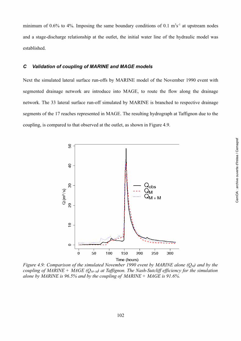
minimum of 0.6% to 4%. Imposing the same boundary conditions of 0.1 m3s-1 at upstream nodes
and a stage-discharge relationship at the outlet, the initial water line of the hydraulic model was
established.
C Validation of coupling of MARINE and MAGE models
Next the simulated lateral surface run-offs by MARINE model of the November 1990 event with
segmented drainage network are introduce into MAGE, to route the flow along the drainage
network. The 33 lateral surface run-off simulated by MARINE is branched to respective drainage
segments of the 17 reaches represented in MAGE. The resulting hydrograph at Taffignon due to the
coupling, is compared to that observed at the outlet, as shown in Figure 4.9.
102
Figure 4.9: Comparison of the simulated November 1990 event by MARINE alone (QM) and by the coupling of MARINE + MAGE (QM+M) at Taffignon. The Nash-Sutcliff efficiency for the simulation alone by MARINE is 96.5% and by the coupling of MARINE + MAGE is 91.6%.
Cem
OA
: ar
chiv
e ou
verte
d'Ir
stea
/ C
emag
ref

By comparing the simulation of the 1990 hydrograph by MARINE alone and by the coupling of
MARINE+MAGE in Figure 4.9, we see that the MARINE alone simulates relatively better fit of the
resultant hydrograph at Taffignon. The introduction of MAGE does not modify the resulting
hydrograph to a large extent. But the use of a hydraulic model, adapted to route just river flow along
the drainage network using shallow water equation is rational and the use of MAGE model is
imperative for the simulation of hydraulics structures, which the hydrological model MARINE is
not capable of doing.
The quality of the calibrated model parameters is also checked at Craponne discharge station for
the same (November 1990) event. A similar comparison as above, of simulated hydrographs at
Craponne only by MARINE and by the coupling of MAGE is done in Figure 4.10. The Figure 4.10
shows a clear underestimation of the simulated discharge values by the models. However, the form
of the observed hydrograph is well respected by MARINE and the coupling of MARINE and
MAGE. This underestimation could be explained by the lack of adequate rainfall information on the
left hand side of the watershed, as mentioned before. Also, an approximative information of soil
depth could have played a major role in the underestimation of the run-off volume. In the chosen
soil depth information, the depth of the soil were perhaps overestimated on this part of the
watershed. At the same time a homogeneous distribution of initial soil humidity value was imposed,
which could have been below that observed for this part of the watershed again.
The simulated hydrographs at Taffignon (Figure 4.9) and Craponne (Figure 4.10) show that the
observed form of the hydrographs are well reproduced by the calibrated model parameters and is
reproducing the dynamics of the Yzeron watershed satisfactorily.
103
Cem
OA
: ar
chiv
e ou
verte
d'Ir
stea
/ C
emag
ref

Thus a sequence of models representing the event scale dynamics of a watershed is built. This step
enabled us to represent satisfactorily realistic run-off hydrographs, by taking into consideration the
complex nature of topography and drainage network of a watershed. But the present modelling
though accounted for the soil spatial characteristics of the watershed, did not include the spatial
repartition of the rainfall distribution as noted in reality.
The next step is to introduce space-time variable rainfall into the coupled MARINE and MAGE
models.
4.3.4 Conclusions about the simulation of surface run-off process at
watershed scale
The main conclusions noted from the simulations of the observed discharge are:
104
Figure 4.10: Comparison of the simulated November 1990 event by MARINE alone (QM)and by the coupling of MARINE + MAGE (QM+M) at Craponne
Cem
OA
: ar
chiv
e ou
verte
d'Ir
stea
/ C
emag
ref

1) Despite the simplicity of the MARINE model, satisfactory characteristic of hydrographs at
the watershed outlet is simulated by accounting for the observed spatially distributed soil
characteristics. The low performances of some observed events could be a result of poor
rainfall knowledge.
2) Unrealistic Manning coefficient values were necessary to retard contribution of land
surfaces to simulate observed hydrographs. This is probably due to the inability of the model
to account for the sub-surface run-off contributions, which are relatively slow compared to
surface run-off contributions.
3) Though MARINE alone simulated satisfactory output hydrographs, a hydraulic model was
indispensable for the simulation of hydraulic structures.
4) Simplified representative topography of the minor and major river beds had to be used to
carry out hydraulic modelling via MAGE. The resolution of the available DEM does not
allow a precise interpretation of flow in the major river beds.
4.4 Simulation of observed discharge-frequency curve under
space-time variable rainfall via the MARINE and MAGE models
4.4.1 Need for selection of a set of simulated rainfall events
From the coupled MARINE and MAGE models, a discharge-frequency curve resembling that
observed at watershed outlet (Taffignon) using the output of the TBM model has to be reconstituted.
To resume the output provided by the TBM model (rainfall generator), nearly 9400 space-time
variable rainfall events were simulated. Each of these event had a total rainfall duration of 72 hours
with a 3-hour time step, with a space resolution of 500 m × 500 m. The simulated rainfall events are
assumed representative of the spatial and temporal characteristics of the Yzeron watershed.
105
Cem
OA
: ar
chiv
e ou
verte
d'Ir
stea
/ C
emag
ref
In order to reconstitute the observed discharge-frequency curve, a set of representative Yzeron
watershed rainfall events are needed. A selection of simulated rainfall events was necessary,
because the transformation of all the 9400 simulated rainfall events would have been a highly time
consuming process. The two main conditions to be satisfied for the selection of simulated rainfall
events are:
1) The spatial distribution of the rainfall pattern had to be homogeneous over the entire
watershed.
2) The effective rainfall events should have representative characteristics as observed in the
watershed.
The procedure carried out to identify events of interest is described as below.
4.4.2 Selection of rainfall events from the output of rainfall simulator
From the simulated rainfall events, a set of rainfall events with characteristic durations similar to
those observed was sought for. Thus representative effective rainfall durations of 12 hours, 24 hours
and 48 hours were necessary.
To obtain an unbiased set of rainfall events, firstly 900 events representing approximately 100 years
of rainfall data were arbitrarily chosen from the 9400 simulated rainfall events. To ensure that the
spatial distribution of these events over the watershed was homogeneous, the 900 rainfall events
were cumulated. The cumulative mean rainfall value for each of the 900 events of 72 hours, varied
between 25 mm to 28 mm on each grid of 500 m × 500 m resolution, thus ensuring an
homogeneous rainfall distribution of the selection. To be precise, a homogeneous distribution of a
selected rainfall events was sought for and not a homogeneous distribution of individual event.
Next representative rainfall events of 12, 24 and 48 hours duration had to be extracted from the
chosen set of 900 events. For this a cumulative moving average of rainfall, inside the watershed
106
Cem
OA
: ar
chiv
e ou
verte
d'Ir
stea
/ C
emag
ref
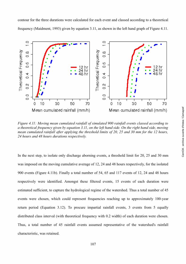
contour for the three durations were calculated for each event and classed according to a theoretical
frequency (Maidment, 1993) given by equation 3.11, as shown in the left hand graph of Figure 4.11.
In the next step, to isolate only discharge aborning events, a threshold limit for 20, 25 and 30 mm
was imposed on the moving cumulative average of 12, 24 and 48 hours respectively, for the isolated
900 events (Figure 4.11b). Finally a total number of 54, 65 and 117 events of 12, 24 and 48 hours
respectively were identified. Amongst these filtered events, 15 events of each duration were
estimated sufficient, to capture the hydrological regime of the watershed. Thus a total number of 45
events were chosen, which could represent frequencies reaching up to approximately 100-year
return period (Equation 3.12). To procure impartial rainfall events, 3 events from 5 equally
distributed class interval (with theoretical frequency with 0.2 width) of each duration were chosen.
Thus, a total number of 45 rainfall events assumed representative of the watershed's rainfall
characteristic, was retained.
107
Figure 4.11: Moving mean cumulated rainfall of simulated 900 rainfall events classed according to a theoretical frequency given by equation 3.11, on the left hand side. On the right hand side, moving mean cumulated rainfall after applying the threshold limits of 20, 25 and 30 mm for the 12 hours, 24 hours and 48 hours durations respectively.
Cem
OA
: ar
chiv
e ou
verte
d'Ir
stea
/ C
emag
ref

The selected events were assured to be independent of each other. In other words, once an
individual event was chosen for one duration it was ensured that the same event did not repeat itself
in the other two duration. Table 4.4.1 recapitulates the chosen 45 events with the mean cumulated
rainfall volume of each duration. The cumulative rainfall volumes of the selected events varied
from a minimum of 20 mm to 37 mm for 12 hours duration, while for the 24 hours duration it varied
from a minimum of 26 mm to 43 mm and for the 48 hours duration it varied from 31 mm to 54 mm.
The chosen events enumerated in Table 4.4.1 were compared with the observed events cited in
Table 2.5.1, as shown in Figure 4.12. From the Figure 4.12, the cumulative mean values of a large
part of the simulated events are found to be inferior to the mean observed rainfall durations. The
mean values of the observed events were deduced from only 3 values for the 12 and 24 hours
duration and only 2 values for the 48 hours duration. The lack of data and the uncertainty associated
with the observed data can not be ignored (Table 2.5.1).
108
Cem
OA
: ar
chiv
e ou
verte
d'Ir
stea
/ C
emag
ref
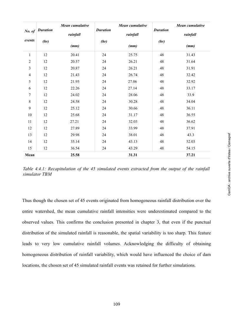
Thus though the chosen set of 45 events originated from homogeneous rainfall distribution over the
entire watershed, the mean cumulative rainfall intensities were underestimated compared to the
observed values. This confirms the conclusion presented in chapter 3, that even if the punctual
distribution of the simulated rainfall is reasonable, the spatial variability is too sharp. This feature
leads to very low cumulative rainfall volumes. Acknowledging the difficulty of obtaining
homogeneous distribution of rainfall variability, which would have influenced the choice of dam
locations, the chosen set of 45 simulated rainfall events was retained for further simulations.
109
No. of
events
Duration
(hr)
Mean cumulative
rainfall
(mm)
Duration
(hr)
Mean cumulative
rainfall
(mm)
Duration
(hr)
Mean cumulative
rainfall
(mm)
1 12 20.41 24 25.75 48 31.43
2 12 20.57 24 26.21 48 31.64
3 12 20.87 24 26.21 48 31.91
4 12 21.43 24 26.74 48 32.42
5 12 21.95 24 27.06 48 32.92
6 12 22.26 24 27.14 48 33.17
7 12 24.02 24 28.06 48 33.9
8 12 24.58 24 30.28 48 34.04
9 12 25.12 24 30.66 48 36.11
10 12 25.68 24 31.17 48 36.55
11 12 27.21 24 32.03 48 36.62
12 12 27.89 24 33.99 48 37.91
13 12 29.98 24 38.01 48 43.3
14 12 35.14 24 43.13 48 52.03
15 12 36.54 24 43.29 48 54.15
Mean 25.58 31.31 37.21
Table 4.4.1: Recapitulation of the 45 simulated events extracted from the output of the rainfall simulator TBM
Cem
OA
: ar
chiv
e ou
verte
d'Ir
stea
/ C
emag
ref
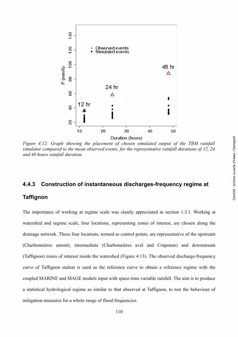
4.4.3 Construction of instantaneous discharges-frequency regime at
Taffignon
The importance of working at regime scale was clearly appreciated in section 1.3.1. Working at
watershed and regime scale, four locations, representing zones of interest, are chosen along the
drainage network. These four locations, termed as control points, are representative of the upstream
(Charbonnières amont), intermediate (Charbonnières aval and Craponne) and downstream
(Taffignon) zones of interest inside the watershed (Figure 4.13). The observed discharge-frequency
curve of Taffignon station is used as the reference curve to obtain a reference regime with the
coupled MARINE and MAGE models input with space-time variable rainfall. The aim is to produce
a statistical hydrological regime as similar to that observed at Taffignon, to test the behaviour of
mitigation measures for a whole range of flood frequencies.
110
Figure 4.12: Graph showing the placement of chosen simulated output of the TBM rainfall simulator compared to the mean observed events, for the representative rainfall durations of 12, 24 and 48 hours rainfall duration.
Cem
OA
: ar
chiv
e ou
verte
d'Ir
stea
/ C
emag
ref
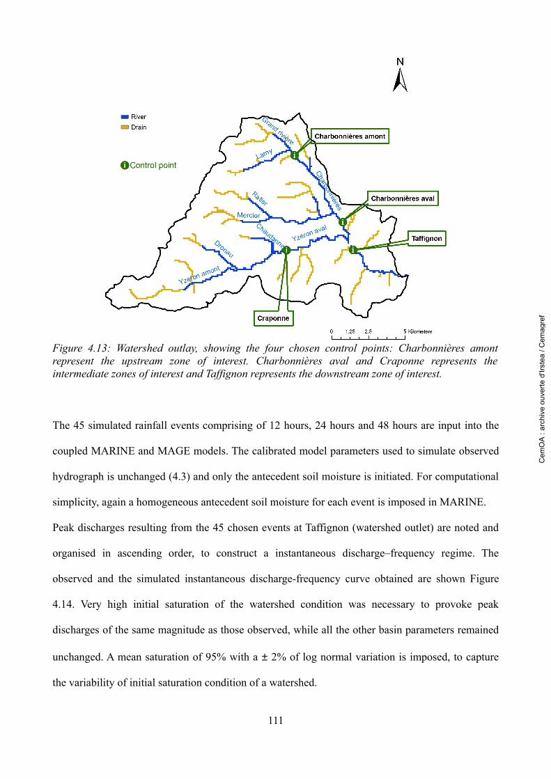
The 45 simulated rainfall events comprising of 12 hours, 24 hours and 48 hours are input into the
coupled MARINE and MAGE models. The calibrated model parameters used to simulate observed
hydrograph is unchanged (4.3) and only the antecedent soil moisture is initiated. For computational
simplicity, again a homogeneous antecedent soil moisture for each event is imposed in MARINE.
Peak discharges resulting from the 45 chosen events at Taffignon (watershed outlet) are noted and
organised in ascending order, to construct a instantaneous discharge–frequency regime. The
observed and the simulated instantaneous discharge-frequency curve obtained are shown Figure
4.14. Very high initial saturation of the watershed condition was necessary to provoke peak
discharges of the same magnitude as those observed, while all the other basin parameters remained
unchanged. A mean saturation of 95% with a ± 2% of log normal variation is imposed, to capture
the variability of initial saturation condition of a watershed.
111
Figure 4.13: Watershed outlay, showing the four chosen control points: Charbonnières amont represent the upstream zone of interest. Charbonnières aval and Craponne represents the intermediate zones of interest and Taffignon represents the downstream zone of interest.
Cem
OA
: ar
chiv
e ou
verte
d'Ir
stea
/ C
emag
ref
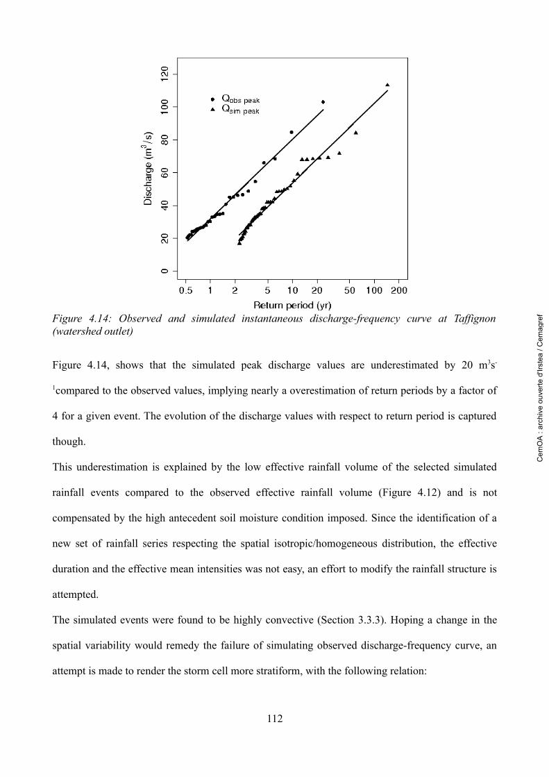
Figure 4.14, shows that the simulated peak discharge values are underestimated by 20 m3s-
1compared to the observed values, implying nearly a overestimation of return periods by a factor of
4 for a given event. The evolution of the discharge values with respect to return period is captured
though.
This underestimation is explained by the low effective rainfall volume of the selected simulated
rainfall events compared to the observed effective rainfall volume (Figure 4.12) and is not
compensated by the high antecedent soil moisture condition imposed. Since the identification of a
new set of rainfall series respecting the spatial isotropic/homogeneous distribution, the effective
duration and the effective mean intensities was not easy, an effort to modify the rainfall structure is
attempted.
The simulated events were found to be highly convective (Section 3.3.3). Hoping a change in the
spatial variability would remedy the failure of simulating observed discharge-frequency curve, an
attempt is made to render the storm cell more stratiform, with the following relation:
112
Figure 4.14: Observed and simulated instantaneous discharge-frequency curve at Taffignon (watershed outlet)
Cem
OA
: ar
chiv
e ou
verte
d'Ir
stea
/ C
emag
ref
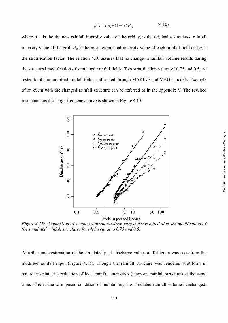
p´ i= p i1−Pm(4.10)
where p´i is the the new rainfall intensity value of the grid, pi is the originally simulated rainfall
intensity value of the grid, Pm is the mean cumulated intensity value of each rainfall field and α is
the stratification factor. The relation 4.10 assures that no change in rainfall volume results during
the structural modification of simulated rainfall fields. Two stratification values of 0.75 and 0.5 are
tested to obtain modified rainfall fields and routed through MARINE and MAGE models. Example
of an event with the changed rainfall structure can be referred to in the appendix V. The resulted
instantaneous discharge-frequency curve is shown in Figure 4.15.
A further underestimation of the simulated peak discharge values at Taffignon was seen from the
modified rainfall input (Figure 4.15). Though the rainfall structure was rendered stratiform in
nature, it entailed a reduction of local rainfall intensities (temporal rainfall structure) at the same
time. This is due to imposed condition of maintaining the simulated rainfall volumes unchanged.
113
Figure 4.15: Comparison of simulated discharge-frequency curve resulted after the modification of the simulated rainfall structures for alpha equal to 0.75 and 0.5.
Cem
OA
: ar
chiv
e ou
verte
d'Ir
stea
/ C
emag
ref
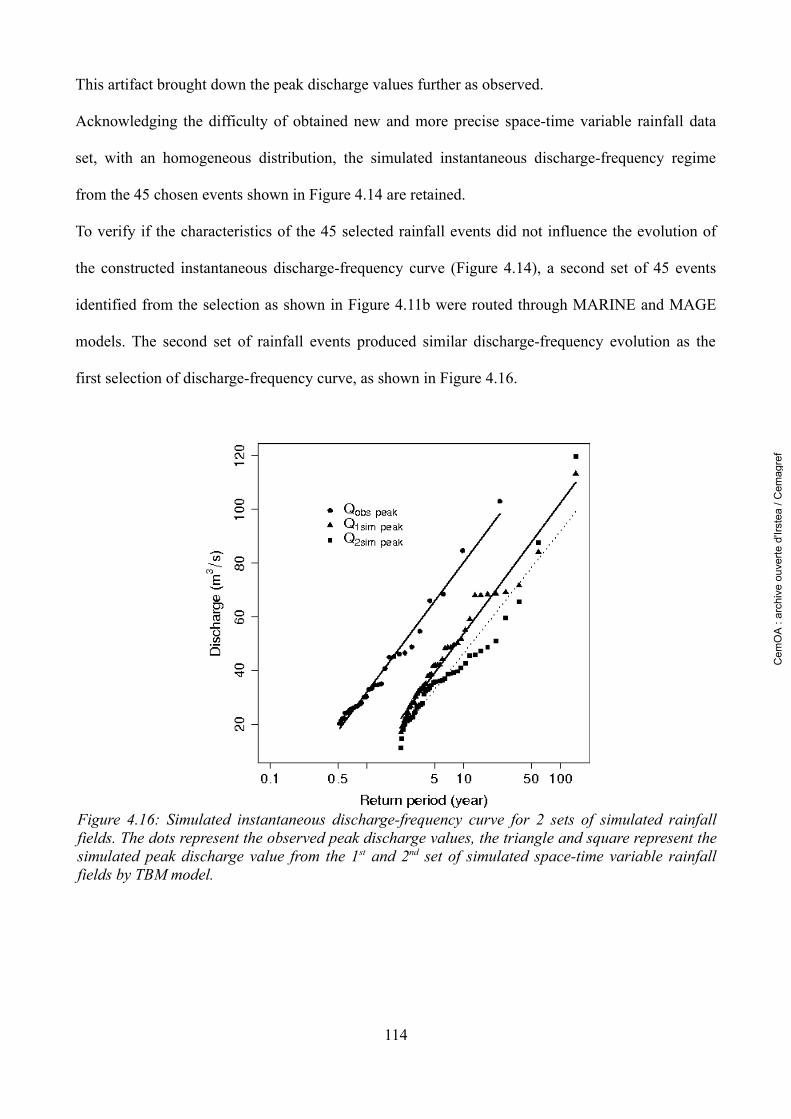
This artifact brought down the peak discharge values further as observed.
Acknowledging the difficulty of obtained new and more precise space-time variable rainfall data
set, with an homogeneous distribution, the simulated instantaneous discharge-frequency regime
from the 45 chosen events shown in Figure 4.14 are retained.
To verify if the characteristics of the 45 selected rainfall events did not influence the evolution of
the constructed instantaneous discharge-frequency curve (Figure 4.14), a second set of 45 events
identified from the selection as shown in Figure 4.11b were routed through MARINE and MAGE
models. The second set of rainfall events produced similar discharge-frequency evolution as the
first selection of discharge-frequency curve, as shown in Figure 4.16.
114
Figure 4.16: Simulated instantaneous discharge-frequency curve for 2 sets of simulated rainfall fields. The dots represent the observed peak discharge values, the triangle and square represent the simulated peak discharge value from the 1st and 2nd set of simulated space-time variable rainfall fields by TBM model.
Cem
OA
: ar
chiv
e ou
verte
d'Ir
stea
/ C
emag
ref
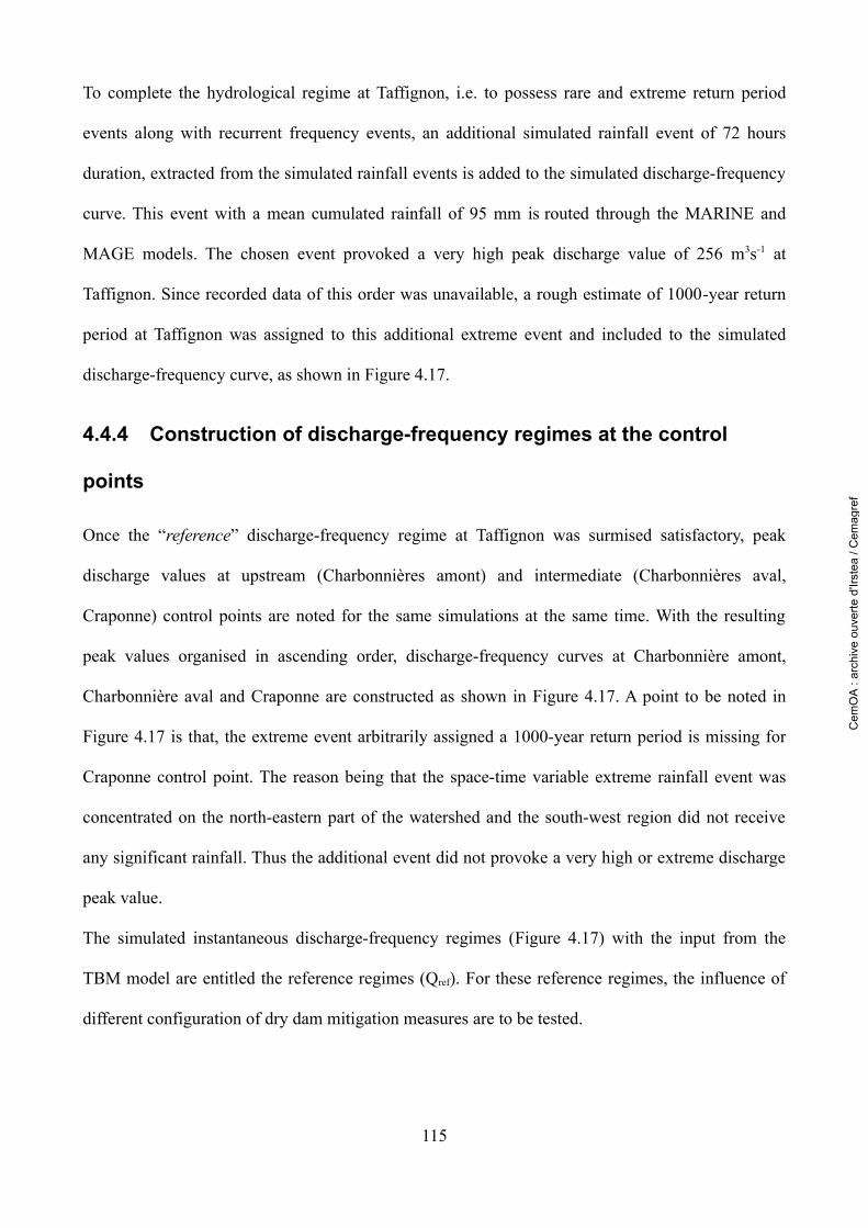
To complete the hydrological regime at Taffignon, i.e. to possess rare and extreme return period
events along with recurrent frequency events, an additional simulated rainfall event of 72 hours
duration, extracted from the simulated rainfall events is added to the simulated discharge-frequency
curve. This event with a mean cumulated rainfall of 95 mm is routed through the MARINE and
MAGE models. The chosen event provoked a very high peak discharge value of 256 m3s-1 at
Taffignon. Since recorded data of this order was unavailable, a rough estimate of 1000-year return
period at Taffignon was assigned to this additional extreme event and included to the simulated
discharge-frequency curve, as shown in Figure 4.17.
4.4.4 Construction of discharge-frequency regimes at the control
points
Once the “reference” discharge-frequency regime at Taffignon was surmised satisfactory, peak
discharge values at upstream (Charbonnières amont) and intermediate (Charbonnières aval,
Craponne) control points are noted for the same simulations at the same time. With the resulting
peak values organised in ascending order, discharge-frequency curves at Charbonnière amont,
Charbonnière aval and Craponne are constructed as shown in Figure 4.17. A point to be noted in
Figure 4.17 is that, the extreme event arbitrarily assigned a 1000-year return period is missing for
Craponne control point. The reason being that the space-time variable extreme rainfall event was
concentrated on the north-eastern part of the watershed and the south-west region did not receive
any significant rainfall. Thus the additional event did not provoke a very high or extreme discharge
peak value.
The simulated instantaneous discharge-frequency regimes (Figure 4.17) with the input from the
TBM model are entitled the reference regimes (Qref). For these reference regimes, the influence of
different configuration of dry dam mitigation measures are to be tested.
115
Cem
OA
: ar
chiv
e ou
verte
d'Ir
stea
/ C
emag
ref
Thus the 3 models: TBM, MARINE, MAGE are employed to generate dynamic flood events
corresponding to different return periods so that the mitigation schemes can be tested for realistic
events of known probability. To conclude, the spatially variable rainfall events chosen for the
simulated output had mean volumes inferior to that observed. The inferior rainfall volumes had to
be compensated with a near 100% initial saturation of the watershed. Despite this artifact, the
construction of a discharge-frequency regime though underestimated, respected the evolution of
observed data at Taffignon (watershed outlet).
116
Figure 4.17: Reference discharge frequency regime constructed from spatially variable rainfall at the four control points.
Cem
OA
: ar
chiv
e ou
verte
d'Ir
stea
/ C
emag
ref
4.5 Dry dam mitigation measures
Once the reference discharge-frequency regime curve of the watershed at control points was
simulated, the impact of dry dam mitigation measures on the discharge regime is to be tested. For
this effect, dry dams were introduced in MAGE to calculate the attenuated peak discharge, referred
as Qdam. The simulation, localisation and the dimensioning of dry dams along the drainage network
is elaborated below.
4.5.1 Dry dam design
Dry dams as shown in Figure 4.18, are adopted in the present study. The dam constitutes a
rectangular, uncontrolled bottom outlet and two levels of spillway, i.e. a primary spillway and a
secondary spillway. Firstly a design discharge required to dimension the spillway is defined. A
design discharge is the largest flood peak value, measured in cubic meter per second, that a given
mitigation project is designed to pass safely. In the present study a 100-year return period flood is
used as the design discharge to dimension the dry dam primary spillway.
The inflow-discharge hydrograph is used to estimate the spillway discharge capacity requirements
and corresponding maximum surcharge elevation in the impoundment. The primary spillway width
b1, is dimensioned to evacuate the 100-year discharge value for which the dam is dimensioned, with
a free board of 0.6 m. The secondary spillway L is designed at 1 m above the primary spillway,
which could evacuate excess flood volumes higher than the 100-year flood. The width of the
secondary spillway is conditioned by the local topography profile. The height H of dry dam is
defined based the flood volume desired to be impounded and is once again conditioned by the
topography of the watershed. The bottom outlet b2 × w2 is so dimensioned, so as to restraint the
outflow discharge to manageable levels for the downstream end when the dam impoundment is full.
117
Cem
OA
: ar
chiv
e ou
verte
d'Ir
stea
/ C
emag
ref
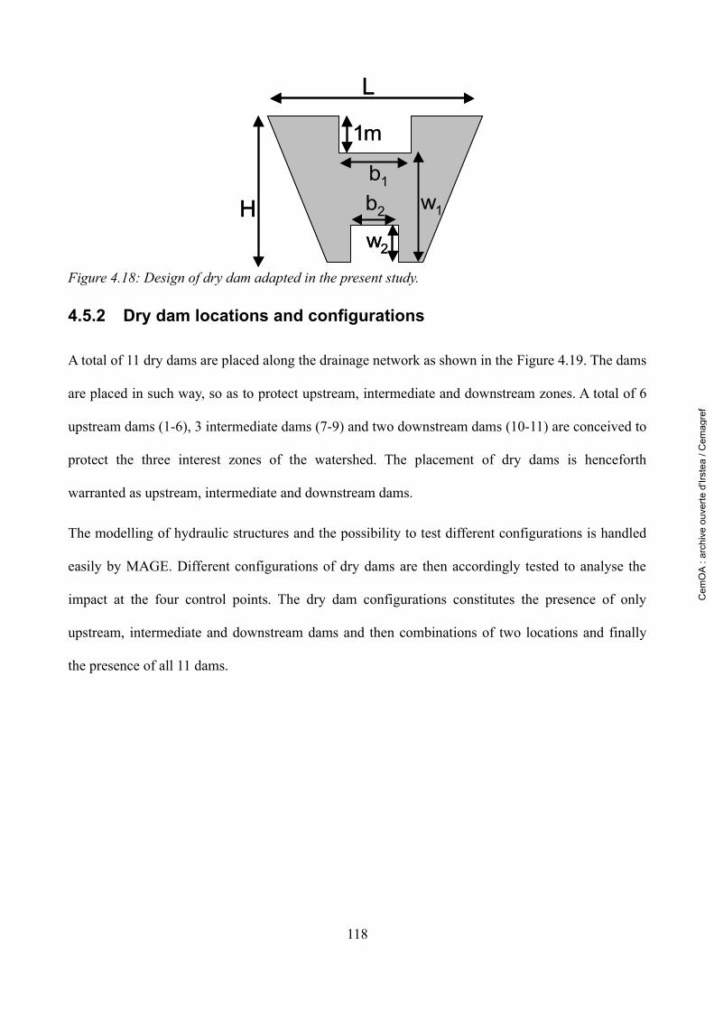
4.5.2 Dry dam locations and configurations
A total of 11 dry dams are placed along the drainage network as shown in the Figure 4.19. The dams
are placed in such way, so as to protect upstream, intermediate and downstream zones. A total of 6
upstream dams (1-6), 3 intermediate dams (7-9) and two downstream dams (10-11) are conceived to
protect the three interest zones of the watershed. The placement of dry dams is henceforth
warranted as upstream, intermediate and downstream dams.
The modelling of hydraulic structures and the possibility to test different configurations is handled
easily by MAGE. Different configurations of dry dams are then accordingly tested to analyse the
impact at the four control points. The dry dam configurations constitutes the presence of only
upstream, intermediate and downstream dams and then combinations of two locations and finally
the presence of all 11 dams.
118
Figure 4.18: Design of dry dam adapted in the present study.
L
H
1m
b1
b2
w2
w1
L
H
1m
b1
b2
w2
w1
Cem
OA
: ar
chiv
e ou
verte
d'Ir
stea
/ C
emag
ref
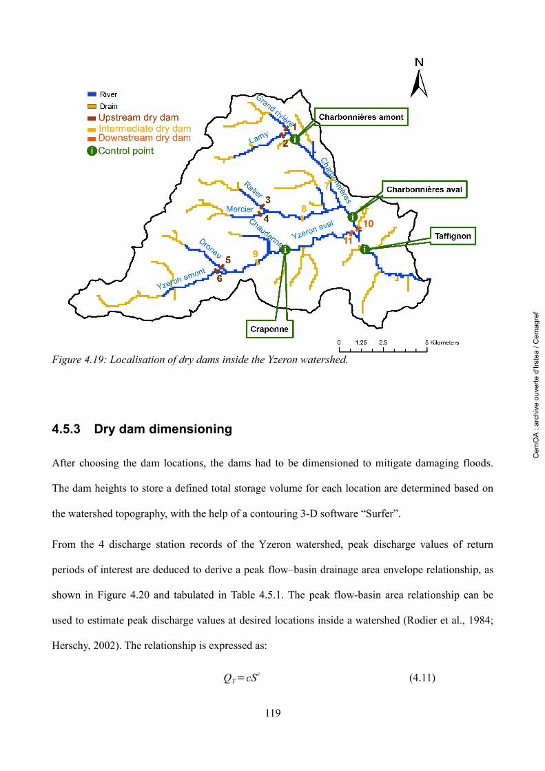
4.5.3 Dry dam dimensioning
After choosing the dam locations, the dams had to be dimensioned to mitigate damaging floods.
The dam heights to store a defined total storage volume for each location are determined based on
the watershed topography, with the help of a contouring 3-D software “Surfer”.
From the 4 discharge station records of the Yzeron watershed, peak discharge values of return
periods of interest are deduced to derive a peak flow–basin drainage area envelope relationship, as
shown in Figure 4.20 and tabulated in Table 4.5.1. The peak flow-basin area relationship can be
used to estimate peak discharge values at desired locations inside a watershed (Rodier et al., 1984;
Herschy, 2002). The relationship is expressed as:
QT=cSε (4.11)
119
Figure 4.19: Localisation of dry dams inside the Yzeron watershed.
Cem
OA
: ar
chiv
e ou
verte
d'Ir
stea
/ C
emag
ref
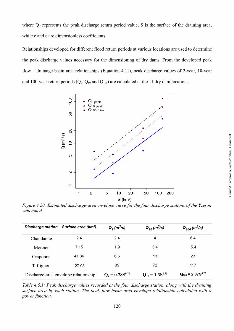
where QT represents the peak discharge return period value, S is the surface of the draining area,
while c and ε are dimensionless coefficients.
Relationships developed for different flood return periods at various locations are used to determine
the peak discharge values necessary for the dimensioning of dry dams. From the developed peak
flow – drainage basin area relationships (Equation 4.11), peak discharge values of 2-year, 10-year
and 100-year return periods (Q2, Q10 and Q100) are calculated at the 11 dry dam locations.
120
Figure 4.20: Estimated discharge-area envelope curve for the four discharge stations of the Yzeron watershed.
Discharge station Surface area (km²) Q2 (m3/s) Q10 (m
3/s) Q100 (m3/s)
Chaudanne 2.4 2.4 4 6.4
Mercier 7.15 1.9 3.4 5.4
Craponne 41.36 6.6 13 23
Taffignon 127.98 39 72 117
Discharge-area envelope relationship Q2 = 0.78S0.70 Q10 = 1.3S0.73 Q100 = 2.07S0.75
Table 4.5.1: Peak discharge values recorded at the four discharge station, along with the draining surface area by each station. The peak flow-basin area envelope relationship calculated with a power function.
Cem
OA
: ar
chiv
e ou
verte
d'Ir
stea
/ C
emag
ref

The outflow discharge from the bottom outlet (QT) is tested for peak flows of two return periods: a
2-year return period value represented by Q2 and a 10-year return period value Q10 henceforth
referred. Knowing the dam height and the outflow discharge, the surface area of the bottom outlet
cross-section is calculated by the application of continuity and energy equations between the
approach section and downstream section (Chow, 1985) for different types of flow, defined by:
Q=cs2gy (4.12)
where c is the coefficient of discharge, s is the surface area of the bottom outlet and is given by the
product of b2 and w2, the bottom outlet width and height respectively, while g is the flow
acceleration due to gravity and y is the upstream flow depth. The Q2 and Q10 values are reached
when the water depth reaches the level of the primary spillway.
The primary spillway is dimensioned to handle the 100-year inflow discharge safely with a free
board of 0.60 m. Since a QT flood is evacuated from the bottom outlet, the width of the primary
spillway is dimensioned to handle a flood QS, defined by:
QS=Q100−QT (4.13)
where QS is the spillway design discharge, Q100 the 100-year discharge return period value. The
width of the primary spillway is determined by:
QS=c× b1× h2gh (4.14)
where h is the overflow depth. The width of the secondary spillway is adapted to the local terrain
conditions, while the bottom outlet is designed to restrain the discharge outflow flow to its banks.
Note: The dimensioning of the bottom outlets and spillways of dry dams is based on observed
discharge-frequency curve, while the simulated discharge at Taffignon is underestimated by nearly
20 m3s-1. Thus over designing the bottom outlet and spillway of the dry dams.
121
Cem
OA
: ar
chiv
e ou
verte
d'Ir
stea
/ C
emag
ref
4.5.4 Designed dry dams for flood mitigation
The influence of storage volume, location and dimensions parameters of dry dams on flood
mitigation is tested for different configurations.
The promoted, good practice of using small structures for flood mitigation is first tested. According
to the world commission on dams (World Commission on Dams, 2000), a dam is considered as
large if its height is equal to 15 m or if the dam heights are between 5 to 15 m and have a reservoir
volume of more than 3 million m3. Based on this definition the following conditions were imposed
to design small dam structures.
1. Restrict the dry dam heights to about 10 m
2. Impound a minimum of 1 million m3 of flood volume and
3. Establish an approximate equal storage volume in the upstream, intermediate and
downstream dry dam locations ( ∑1
6vi≈∑7
9vi≈∑10
11vi , where vi is the individual storage
volume).
The dimensions calculated with the above criteria in mind are shown in Table 4.5.2 and Table 4.5.3
for the two bottom outlet dimensions of Q2 and Q10 and primary spillway dimension of Q100. The
number 2 dry dam exceeded the desired 10 m height, because the storage volume available below
this height was insignificant. The dry dams 10 and 11 had to be raised up to 13 m so as to maintain
a constant total storage volume for the individual dam locations of upstream, intermediate and
downstream dry dams.
Then to test the influence of increased storage volume, the dry dam heights are increased without
any modification to the topography of the study area. The formulated “large” dry dams dimensions
for a Q2 and Q10 bottom outlet dimensions, with the primary spillway dimensioned for Q100 are
recapitulated in Table 4.5.4 and Table 4.5.5 respectively.
122
Cem
OA
: ar
chiv
e ou
verte
d'Ir
stea
/ C
emag
ref

The dry dam locations are tested with different combinations of individual dam locations. The
influence of dry dam dimension on flood mitigation is tested for small (Q2) and large (Q10) bottom
outlets. The dry dam dimensions: H, L, b1, b2, w1 and w2 (Figure 4.18) defined in local
topographical unit, are input into the 1-D MAGE model.
123
Dry dam no.
Discharge Bottom outlet Primary spillway
Secondary spillway
Individual dam
storagevolume
Total storage volume
Q2
(m3/s)Q100
(m3/s)b2 (m) w2 (m) w1 (m) b1(m) H (m) L (m) (M m3) (M m3)
1 3.52 10.19 0.74 0.37 9 11.5 10 66.2 0.162 3.56 10.29 0.62 0.35 14 11.6 15 106.6 0.123 3.11 8.94 0.63 0.38 9 10.0 10 134.3 0.164 3.64 10.53 0.47 0.60 9 11.8 10 44.3 0.095 3.55 10.28 0.55 0.49 9 11.6 10 256.1 0.086 3.56 10.30 0.55 0.49 9 11.6 10 256.1 0.08
0.71
7 7.74 23.51 0.84 0.70 9 27.1 10 151.4 0.258 6.24 18.69 0.80 0.60 9 21.4 10 149.9 0.269 9.66 29.72 0.93 0.80 9 34.5 10 99.3 0.23
0.74
10 14.10 44.42 1.0 0.93 12 52.1 13 121.6 0.3211 13.59 42.71 1.1 0.81 12 50.0 13 123.3 0.37 0.69
Table 4.5.2: Design dimensions of the 11 small dry dams with a Q2 bottom outlet and a spillway design flood of Q100. Storage volume is expressed in million (M) m3.
Dry dam no.
Discharge Bottom outlet Primary spillway
Secondary spillway
Individual dam
storagevolume
Total storage volume
Q10
(m3/s)Q100
(m3/s)b2 (m) w2 (m) w1 (m) b1(m) H (m) L (m) (M m3) (M m3)
1 5.47 10.19 0.68 0.5 9 8.1 10 69.5 0.162 5.52 10.29 0.69 0.5 14 8.2 15 109.6 0.123 4.81 8.94 0.72 0.4 9 7.1 10 137.35 0.164 5.65 10.53 0.68 0.5 9 8.4 10 47.8 0.095 5.52 10.28 0.68 0.5 9 8.2 10 259.5 0.086 5.53 10.30 0.72 0.4 9 8.2 10 259.5 0.08
0.71
7 12.43 23.51 0.85 0.85 9 19.0 10 159.5 0.258 9.92 18.69 0.88 0.66 9 15.1 10 156.2 0.269 15.65 29.72 0.99 0.9 9 24.2 10 109.6 0.23
0.74
10 23.23 44.42 1.13 0.99 12 36.4 13 137.2 0.3211 22.35 42.71 1.2 0.99 12 35.0 13 138.3 0.37 0.69
Table 4.5.3: Design dimensions of the 11 small dry dams with a Q10 bottom outlet and a spillway design flood of Q100. Storage volume is expressed in million (M) m3.
Cem
OA
: ar
chiv
e ou
verte
d'Ir
stea
/ C
emag
ref
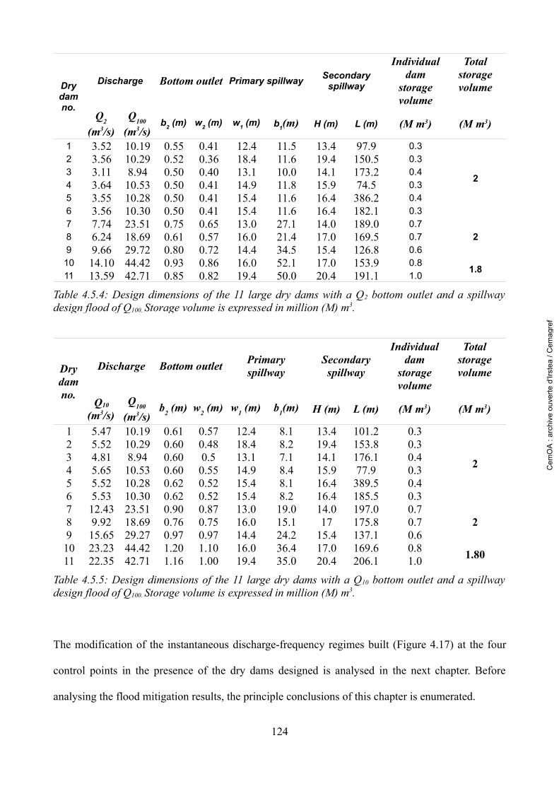
The modification of the instantaneous discharge-frequency regimes built (Figure 4.17) at the four
control points in the presence of the dry dams designed is analysed in the next chapter. Before
analysing the flood mitigation results, the principle conclusions of this chapter is enumerated.
124
Dry dam no.
Discharge Bottom outlet Primary spillway Secondary spillway
Individual dam
storagevolume
Total storage volume
Q2
(m3/s)Q100
(m3/s)b2 (m) w2 (m) w1 (m) b1(m) H (m) L (m) (M m3) (M m3)
1 3.52 10.19 0.55 0.41 12.4 11.5 13.4 97.9 0.32 3.56 10.29 0.52 0.36 18.4 11.6 19.4 150.5 0.33 3.11 8.94 0.50 0.40 13.1 10.0 14.1 173.2 0.44 3.64 10.53 0.50 0.41 14.9 11.8 15.9 74.5 0.35 3.55 10.28 0.50 0.41 15.4 11.6 16.4 386.2 0.46 3.56 10.30 0.50 0.41 15.4 11.6 16.4 182.1 0.3
2
7 7.74 23.51 0.75 0.65 13.0 27.1 14.0 189.0 0.78 6.24 18.69 0.61 0.57 16.0 21.4 17.0 169.5 0.79 9.66 29.72 0.80 0.72 14.4 34.5 15.4 126.8 0.6
2
10 14.10 44.42 0.93 0.86 16.0 52.1 17.0 153.9 0.811 13.59 42.71 0.85 0.82 19.4 50.0 20.4 191.1 1.0
1.8
Table 4.5.4: Design dimensions of the 11 large dry dams with a Q2 bottom outlet and a spillway design flood of Q100. Storage volume is expressed in million (M) m3.
Dry dam no.
Discharge Bottom outlet Primary spillway
Secondary spillway
Individual dam
storagevolume
Total storage volume
Q10
(m3/s)Q100
(m3/s)b2 (m) w2 (m) w1 (m) b1(m) H (m) L (m) (M m3) (M m3)
1 5.47 10.19 0.61 0.57 12.4 8.1 13.4 101.2 0.32 5.52 10.29 0.60 0.48 18.4 8.2 19.4 153.8 0.33 4.81 8.94 0.60 0.5 13.1 7.1 14.1 176.1 0.44 5.65 10.53 0.60 0.55 14.9 8.4 15.9 77.9 0.35 5.52 10.28 0.62 0.52 15.4 8.1 16.4 389.5 0.46 5.53 10.30 0.62 0.52 15.4 8.2 16.4 185.5 0.3
2
7 12.43 23.51 0.90 0.87 13.0 19.0 14.0 197.0 0.78 9.92 18.69 0.76 0.75 16.0 15.1 17 175.8 0.79 15.65 29.27 0.97 0.97 14.4 24.2 15.4 137.1 0.6
2
10 23.23 44.42 1.20 1.10 16.0 36.4 17.0 169.6 0.811 22.35 42.71 1.16 1.00 19.4 35.0 20.4 206.1 1.0 1.80
Table 4.5.5: Design dimensions of the 11 large dry dams with a Q10 bottom outlet and a spillway design flood of Q100. Storage volume is expressed in million (M) m3.
Cem
OA
: ar
chiv
e ou
verte
d'Ir
stea
/ C
emag
ref
4.6 Conclusions about the simulated reference discharge-
frequency regimes and dimensioning of dry dams
The principal conclusions to be retained from the construction of reference discharge-frequency
regime and dimensioning of dry dams are:
1. MARINE distributed model simulates satisfactory flood hydrographs, but ignores any sub-
surface contributions. High Manning coefficients were imposed on the watershed slopes to
retard the surface hydrograph, so as to match those observed. This increase might add errors
to the simulated peak resulting from space-time variable rainfall fields. Also the
uncertainties brought in by an approximate knowledge of soil depth and the distribution of
homogeneous initial humidity is not know.
2. The form of the drainage network in the 1-D hydraulic model MAGE is highly approximate
and might interfere with the routing of lateral hydrographs simulated by MARINE. MAGE
is imperative to simulate hydraulic structures, otherwise impossible to imitate in distributed
hydrological model. Also, the routing of river flow using kinematic wave theory is beyond
the validity of the kinematic wave theory.
3. The simulated instantaneous discharge-frequency regime at Taffignon is underestimated
compared to the observed instantaneous discharge-frequency regime by nearly 20 m3s-1 and
thus underestimates the return period by nearly a factor of 4.
4. The dry dams were dimensioned from observed peak-discharge data. Thus when positioned
for the mitigation of reference discharge-frequency regime, are over designed, in other
words the bottom outlets and spillway dimensions are bigger and larger.
5. The above two items, would imply that the intervention of the dry dams for frequent floods
might be delayed due to big bottom outlets. The efficiency of flood attenuation via dry dams
125
Cem
OA
: ar
chiv
e ou
verte
d'Ir
stea
/ C
emag
ref

may thus have a shift towards low return periods.
6. Large dams are necessary to evaluate efficient mitigation strategies. But at the same time,
they can be quite expensive and when breached could escalate the hazard to a large extent.
126
Cem
OA
: ar
chiv
e ou
verte
d'Ir
stea
/ C
emag
ref
5 DRY DAM MITIGATION ANALYSIS
Cem
OA
: ar
chiv
e ou
verte
d'Ir
stea
/ C
emag
ref
5.1 Introduction
In this chapter the mitigation achieved due to dry dam measures, dispersed inside the watershed is
analysed. The four control points, representing the upstream (Charbonnières amont), intermediate
(Charbonnières aval and Craponne) and downstream (Taffignon) zones of interest are scrutinized.
The mitigation of flood hydrographs by dry dams is first presented for a simulated rainfall event at
the four control points. The flood peak reduction and the shift of time-to-peak is analysed from this
representation.
Secondly the flood mitigation due to storage volume, different dry dam configurations and
dimensions of dry dams bottom outlets (Q2 and Q10) parameters are analysed individually and the
corresponding attenuation factor via “IMMERS” graph are presented. To facilitate the interpretation
the watershed layout indicating the zones of interest along with the dam locations is presented once
again in Figure 5.1.
Initially attenuated peak discharges are evaluated individually with respect to the same event in the
absence of dry dams to analyse the influence of spatially variable rainfall pattern on the mitigation
extent.
A second representation, in which the attenuated peak discharge are arranged each time in the
ascending order, will allow to interpret the discharge-frequency regime via the IMMERS graph.
128
Cem
OA
: ar
chiv
e ou
verte
d'Ir
stea
/ C
emag
ref
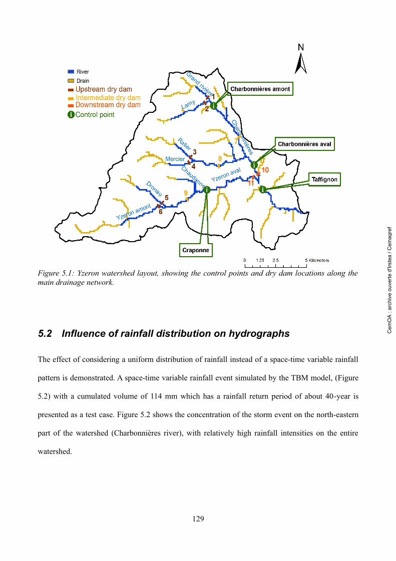
5.2 Influence of rainfall distribution on hydrographs
The effect of considering a uniform distribution of rainfall instead of a space-time variable rainfall
pattern is demonstrated. A space-time variable rainfall event simulated by the TBM model, (Figure
5.2) with a cumulated volume of 114 mm which has a rainfall return period of about 40-year is
presented as a test case. Figure 5.2 shows the concentration of the storm event on the north-eastern
part of the watershed (Charbonnières river), with relatively high rainfall intensities on the entire
watershed.
129
Figure 5.1: Yzeron watershed layout, showing the control points and dry dam locations along the main drainage network.
Cem
OA
: ar
chiv
e ou
verte
d'Ir
stea
/ C
emag
ref
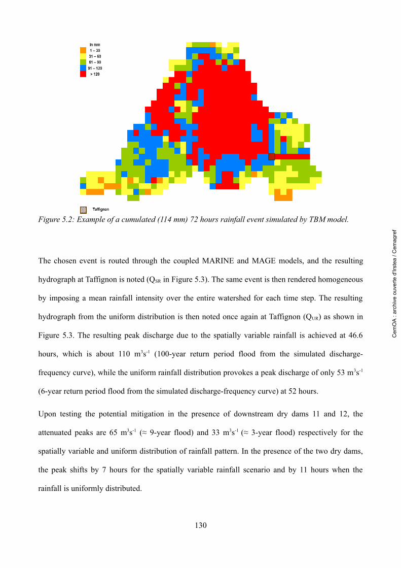
The chosen event is routed through the coupled MARINE and MAGE models, and the resulting
hydrograph at Taffignon is noted (QSR in Figure 5.3). The same event is then rendered homogeneous
by imposing a mean rainfall intensity over the entire watershed for each time step. The resulting
hydrograph from the uniform distribution is then noted once again at Taffignon (QUR) as shown in
Figure 5.3. The resulting peak discharge due to the spatially variable rainfall is achieved at 46.6
hours, which is about 110 m3s-1 (100-year return period flood from the simulated discharge-
frequency curve), while the uniform rainfall distribution provokes a peak discharge of only 53 m3s-1
(6-year return period flood from the simulated discharge-frequency curve) at 52 hours.
Upon testing the potential mitigation in the presence of downstream dry dams 11 and 12, the
attenuated peaks are 65 m3s-1 (≈ 9-year flood) and 33 m3s-1 (≈ 3-year flood) respectively for the
spatially variable and uniform distribution of rainfall pattern. In the presence of the two dry dams,
the peak shifts by 7 hours for the spatially variable rainfall scenario and by 11 hours when the
rainfall is uniformly distributed.
130
Figure 5.2: Example of a cumulated (114 mm) 72 hours rainfall event simulated by TBM model.
Cem
OA
: ar
chiv
e ou
verte
d'Ir
stea
/ C
emag
ref
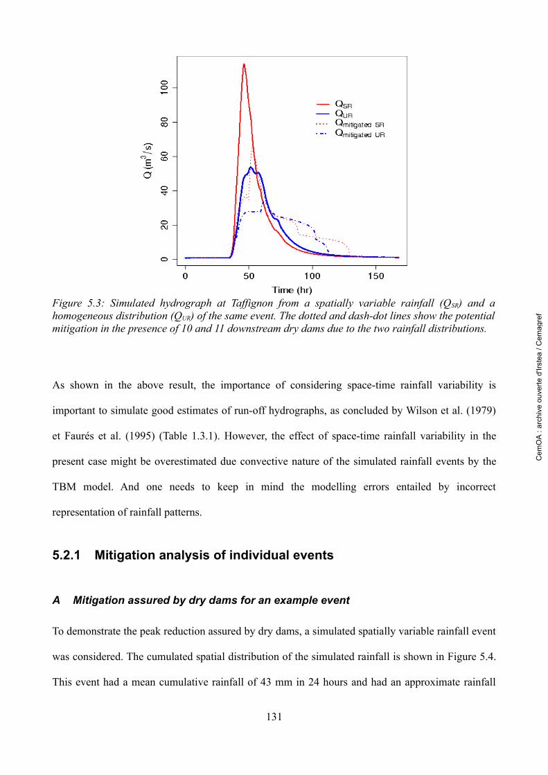
As shown in the above result, the importance of considering space-time rainfall variability is
important to simulate good estimates of run-off hydrographs, as concluded by Wilson et al. (1979)
et Faurés et al. (1995) (Table 1.3.1). However, the effect of space-time rainfall variability in the
present case might be overestimated due convective nature of the simulated rainfall events by the
TBM model. And one needs to keep in mind the modelling errors entailed by incorrect
representation of rainfall patterns.
5.2.1 Mitigation analysis of individual events
A Mitigation assured by dry dams for an example event
To demonstrate the peak reduction assured by dry dams, a simulated spatially variable rainfall event
was considered. The cumulated spatial distribution of the simulated rainfall is shown in Figure 5.4.
This event had a mean cumulative rainfall of 43 mm in 24 hours and had an approximate rainfall
131
Figure 5.3: Simulated hydrograph at Taffignon from a spatially variable rainfall (QSR) and a homogeneous distribution (QUR) of the same event. The dotted and dash-dot lines show the potential mitigation in the presence of 10 and 11 downstream dry dams due to the two rainfall distributions.
Cem
OA
: ar
chiv
e ou
verte
d'Ir
stea
/ C
emag
ref
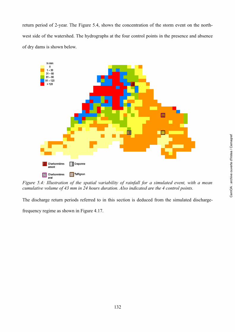
return period of 2-year. The Figure 5.4, shows the concentration of the storm event on the north-
west side of the watershed. The hydrographs at the four control points in the presence and absence
of dry dams is shown below.
The discharge return periods referred to in this section is deduced from the simulated discharge-
frequency regime as shown in Figure 4.17.
132
Figure 5.4: Illustration of the spatial variability of rainfall for a simulated event, with a mean cumulative volume of 43 mm in 24 hours duration. Also indicated are the 4 control points.
Cem
OA
: ar
chiv
e ou
verte
d'Ir
stea
/ C
emag
ref
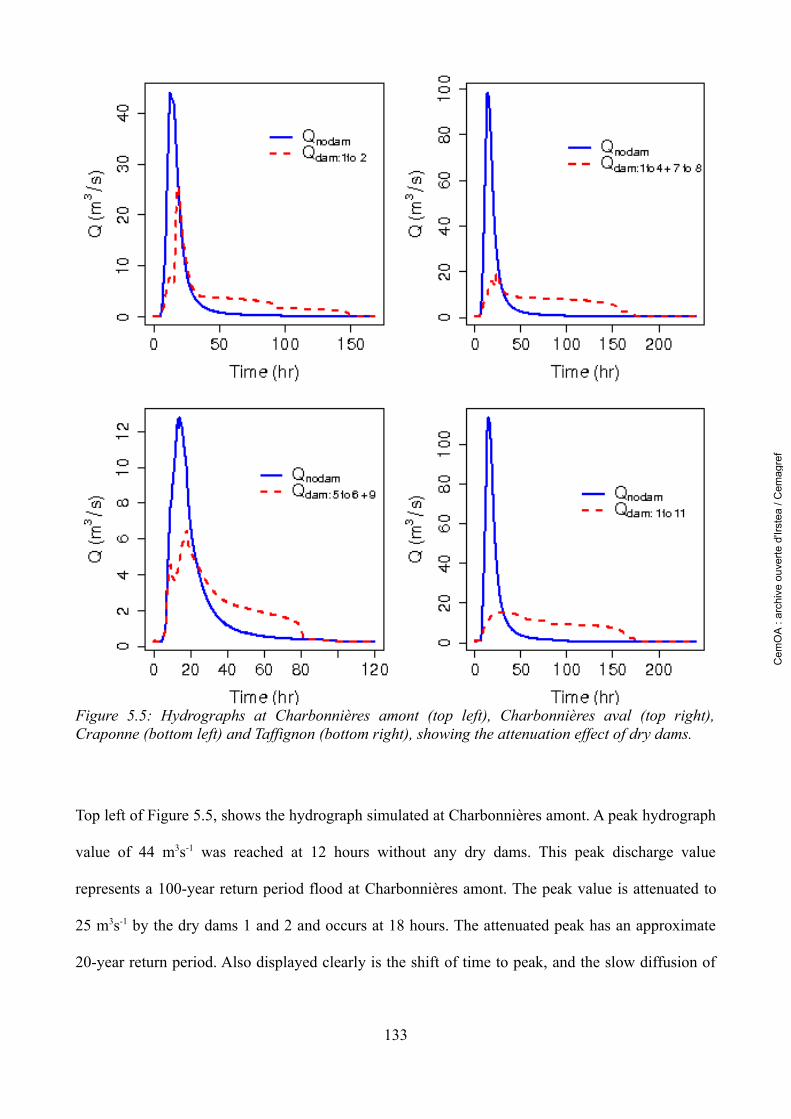
Top left of Figure 5.5, shows the hydrograph simulated at Charbonnières amont. A peak hydrograph
value of 44 m3s-1 was reached at 12 hours without any dry dams. This peak discharge value
represents a 100-year return period flood at Charbonnières amont. The peak value is attenuated to
25 m3s-1 by the dry dams 1 and 2 and occurs at 18 hours. The attenuated peak has an approximate
20-year return period. Also displayed clearly is the shift of time to peak, and the slow diffusion of
133
Figure 5.5: Hydrographs at Charbonnières amont (top left), Charbonnières aval (top right), Craponne (bottom left) and Taffignon (bottom right), showing the attenuation effect of dry dams.
Cem
OA
: ar
chiv
e ou
verte
d'Ir
stea
/ C
emag
ref
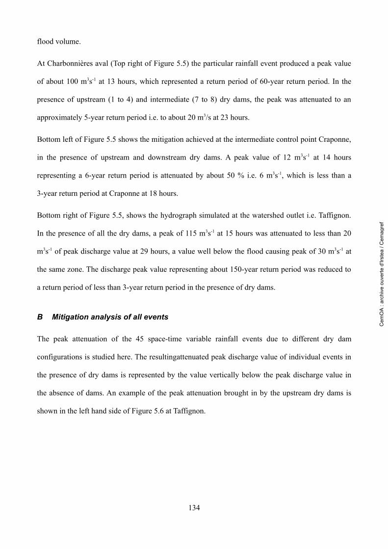
flood volume.
At Charbonnières aval (Top right of Figure 5.5) the particular rainfall event produced a peak value
of about 100 m3s-1 at 13 hours, which represented a return period of 60-year return period. In the
presence of upstream (1 to 4) and intermediate (7 to 8) dry dams, the peak was attenuated to an
approximately 5-year return period i.e. to about 20 m3/s at 23 hours.
Bottom left of Figure 5.5 shows the mitigation achieved at the intermediate control point Craponne,
in the presence of upstream and downstream dry dams. A peak value of 12 m3s-1 at 14 hours
representing a 6-year return period is attenuated by about 50 % i.e. 6 m3s-1, which is less than a
3-year return period at Craponne at 18 hours.
Bottom right of Figure 5.5, shows the hydrograph simulated at the watershed outlet i.e. Taffignon.
In the presence of all the dry dams, a peak of 115 m3s-1 at 15 hours was attenuated to less than 20
m3s-1 of peak discharge value at 29 hours, a value well below the flood causing peak of 30 m3s-1 at
the same zone. The discharge peak value representing about 150-year return period was reduced to
a return period of less than 3-year return period in the presence of dry dams.
B Mitigation analysis of all events
The peak attenuation of the 45 space-time variable rainfall events due to different dry dam
configurations is studied here. The resultingattenuated peak discharge value of individual events in
the presence of dry dams is represented by the value vertically below the peak discharge value in
the absence of dams. An example of the peak attenuation brought in by the upstream dry dams is
shown in the left hand side of Figure 5.6 at Taffignon.
134
Cem
OA
: ar
chiv
e ou
verte
d'Ir
stea
/ C
emag
ref
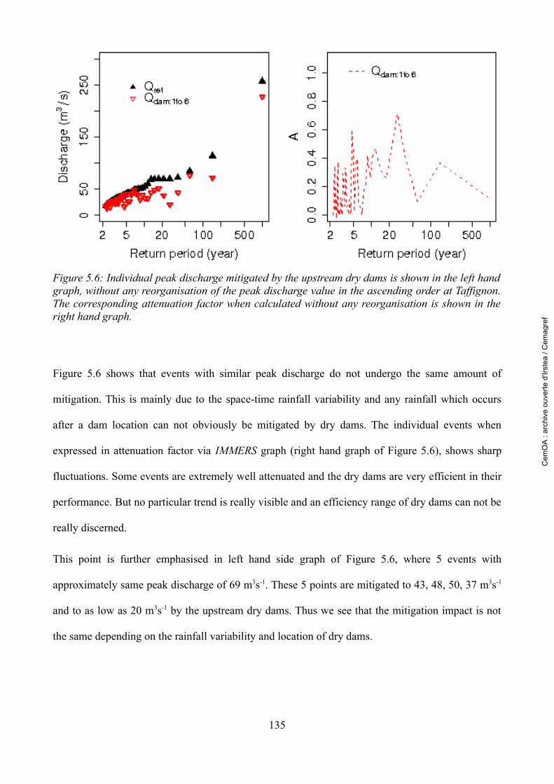
Figure 5.6 shows that events with similar peak discharge do not undergo the same amount of
mitigation. This is mainly due to the space-time rainfall variability and any rainfall which occurs
after a dam location can not obviously be mitigated by dry dams. The individual events when
expressed in attenuation factor via IMMERS graph (right hand graph of Figure 5.6), shows sharp
fluctuations. Some events are extremely well attenuated and the dry dams are very efficient in their
performance. But no particular trend is really visible and an efficiency range of dry dams can not be
really discerned.
This point is further emphasised in left hand side graph of Figure 5.6, where 5 events with
approximately same peak discharge of 69 m3s-1. These 5 points are mitigated to 43, 48, 50, 37 m3s-1
and to as low as 20 m3s-1 by the upstream dry dams. Thus we see that the mitigation impact is not
the same depending on the rainfall variability and location of dry dams.
135
Figure 5.6: Individual peak discharge mitigated by the upstream dry dams is shown in the left hand graph, without any reorganisation of the peak discharge value in the ascending order at Taffignon. The corresponding attenuation factor when calculated without any reorganisation is shown in the right hand graph.
Cem
OA
: ar
chiv
e ou
verte
d'Ir
stea
/ C
emag
ref
Next the attenuated peak discharge values are arranged each time in the ascending order for each
dry dam configuration. This second presentation implies that the attenuated peak discharge of a
given event does not necessarily correspond to the same event of a given discharge return period.
The same events when organised in ascending order (left hand graph of Figure 5.7) and when
represented via IMMERS graph (right hand graph of Figure 5.7), display a clear trend and show the
efficiency of dry dams in mitigating floods of varying frequencies.
The IMMERS graphical representation is thus better represented, when the mitigated regime in the
presence of dry dams are reorganised and the attenuation factor is calculated between the classed
peaks and not respective peaks of individual events.
The individual attenuated events, as shown in left hand graph of Figure 5.7 were next evaluated
with respect to peak ratio of attenuated peak discharge by 6 upstream dams to reference peak
discharge in return periods (Figure 5.8). We see better mitigation effect for increasing flood return
periods at times as explained just before. Figure 5.8, thus clearly demonstrates the role of spatial
variability of rainfall on the flood mitigation.
136
Figure 5.7: The mitigated peak discharge values when classed in ascending order and represented as IMMERS is shown in the left and right hand graphs respectively.
Cem
OA
: ar
chiv
e ou
verte
d'Ir
stea
/ C
emag
ref
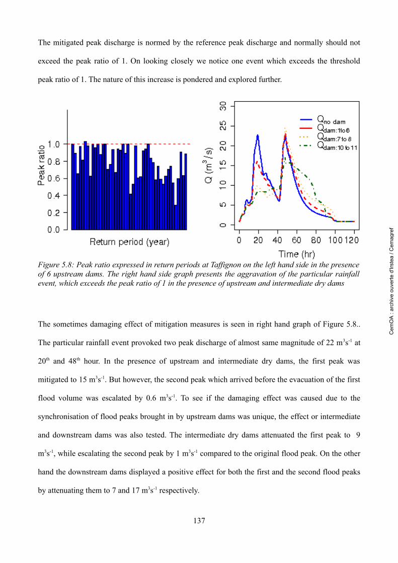
The mitigated peak discharge is normed by the reference peak discharge and normally should not
exceed the peak ratio of 1. On looking closely we notice one event which exceeds the threshold
peak ratio of 1. The nature of this increase is pondered and explored further.
The sometimes damaging effect of mitigation measures is seen in right hand graph of Figure 5.8..
The particular rainfall event provoked two peak discharge of almost same magnitude of 22 m3s-1 at
20th and 48th hour. In the presence of upstream and intermediate dry dams, the first peak was
mitigated to 15 m3s-1. But however, the second peak which arrived before the evacuation of the first
flood volume was escalated by 0.6 m3s-1. To see if the damaging effect was caused due to the
synchronisation of flood peaks brought in by upstream dams was unique, the effect or intermediate
and downstream dams was also tested. The intermediate dry dams attenuated the first peak to 9
m3s-1, while escalating the second peak by 1 m3s-1 compared to the original flood peak. On the other
hand the downstream dams displayed a positive effect for both the first and the second flood peaks
by attenuating them to 7 and 17 m3s-1 respectively.
137
Figure 5.8: Peak ratio expressed in return periods at Taffignon on the left hand side in the presence of 6 upstream dams. The right hand side graph presents the aggravation of the particular rainfall event, which exceeds the peak ratio of 1 in the presence of upstream and intermediate dry dams
Cem
OA
: ar
chiv
e ou
verte
d'Ir
stea
/ C
emag
ref
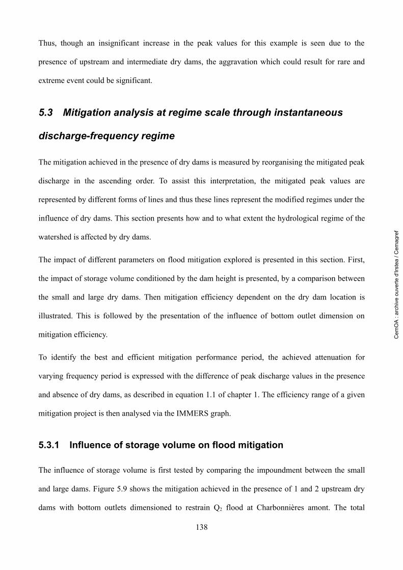
Thus, though an insignificant increase in the peak values for this example is seen due to the
presence of upstream and intermediate dry dams, the aggravation which could result for rare and
extreme event could be significant.
5.3 Mitigation analysis at regime scale through instantaneous
discharge-frequency regime
The mitigation achieved in the presence of dry dams is measured by reorganising the mitigated peak
discharge in the ascending order. To assist this interpretation, the mitigated peak values are
represented by different forms of lines and thus these lines represent the modified regimes under the
influence of dry dams. This section presents how and to what extent the hydrological regime of the
watershed is affected by dry dams.
The impact of different parameters on flood mitigation explored is presented in this section. First,
the impact of storage volume conditioned by the dam height is presented, by a comparison between
the small and large dry dams. Then mitigation efficiency dependent on the dry dam location is
illustrated. This is followed by the presentation of the influence of bottom outlet dimension on
mitigation efficiency.
To identify the best and efficient mitigation performance period, the achieved attenuation for
varying frequency period is expressed with the difference of peak discharge values in the presence
and absence of dry dams, as described in equation 1.1 of chapter 1. The efficiency range of a given
mitigation project is then analysed via the IMMERS graph.
5.3.1 Influence of storage volume on flood mitigation
The influence of storage volume is first tested by comparing the impoundment between the small
and large dams. Figure 5.9 shows the mitigation achieved in the presence of 1 and 2 upstream dry
dams with bottom outlets dimensioned to restrain Q2 flood at Charbonnières amont. The total
138
Cem
OA
: ar
chiv
e ou
verte
d'Ir
stea
/ C
emag
ref
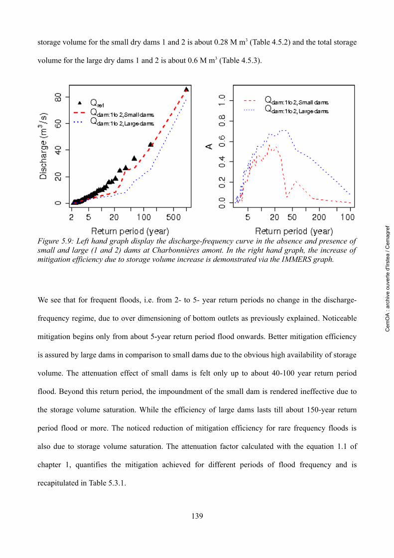
storage volume for the small dry dams 1 and 2 is about 0.28 M m3 (Table 4.5.2) and the total storage
volume for the large dry dams 1 and 2 is about 0.6 M m3 (Table 4.5.3).
We see that for frequent floods, i.e. from 2- to 5- year return periods no change in the discharge-
frequency regime, due to over dimensioning of bottom outlets as previously explained. Noticeable
mitigation begins only from about 5-year return period flood onwards. Better mitigation efficiency
is assured by large dams in comparison to small dams due to the obvious high availability of storage
volume. The attenuation effect of small dams is felt only up to about 40-100 year return period
flood. Beyond this return period, the impoundment of the small dam is rendered ineffective due to
the storage volume saturation. While the efficiency of large dams lasts till about 150-year return
period flood or more. The noticed reduction of mitigation efficiency for rare frequency floods is
also due to storage volume saturation. The attenuation factor calculated with the equation 1.1 of
chapter 1, quantifies the mitigation achieved for different periods of flood frequency and is
recapitulated in Table 5.3.1.
139
Figure 5.9: Left hand graph display the discharge-frequency curve in the absence and presence of small and large (1 and 2) dams at Charbonnières amont. In the right hand graph, the increase of mitigation efficiency due to storage volume increase is demonstrated via the IMMERS graph.
Cem
OA
: ar
chiv
e ou
verte
d'Ir
stea
/ C
emag
ref
To analyse the performance of dry dams for various flood frequencies the flood return periods were
divided into four ranges: high frequency (2- to 5-year), intermediate frequency (6- to 40-year), low
frequency (41- to 100-year) and rare frequency (> 100-year) floods. These ranges of flood
frequencies is represented by 28 events for the 2- to 5-year frequency range, 15 events for the 6- to
40-year frequency range, 2 events for the 41- to 100-year frequency range. And 1 event for return
periods above 100-year.
With small dry dams, a maximum efficiency of only 0.42 is achieved, for the return period range of
6-year to 40-year with the Q2 bottom outlet dry dams. For 2- to 5-year flood return period range, the
attenuation factor does not exceed 0.20 by small dams. The attenuation factor then increases to 0.42
for the 6-year to 40-year return period range, before dropping to 0.13 for the 41-year to 100-year
return period range. Finally, for the extreme event with an approximately 1000-year return period
no mitigation is seen. The two, small upstream dry dams 1 and 2 have a storage volume of about
only 0.28 M m3 in comparison to the average flood volume of the simulated events (≈ 0.47 M m3).
Thus the attenuation factor begins with nearly no efficiency to maximum efficiency, before
dropping back to zero efficiency. Similar trend is observed in the case of the large dams, except for
a higher period of efficiency range compared to the small dams between the 6-year to 100-year
return period range.
140
Range of return period (year)
N° of events A of small dams 1 and 2 A of large dams 1 and 2
2 to 5 28 0.19 0.13
6 to 40 15 0.42 0.58
41 to 100 2 0.13 0.47
>> 100* 1 0.00* 0.08*
Table 5.3.1: Mean dimensionless attenuation factor calculated for small dry dams 1 and 2 with bottom outlets designed to constraint the outflow discharge to Q2 flood at Charbonnières amont. * Not a mean value, but the result of additional event included explicitly.
Cem
OA
: ar
chiv
e ou
verte
d'Ir
stea
/ C
emag
ref
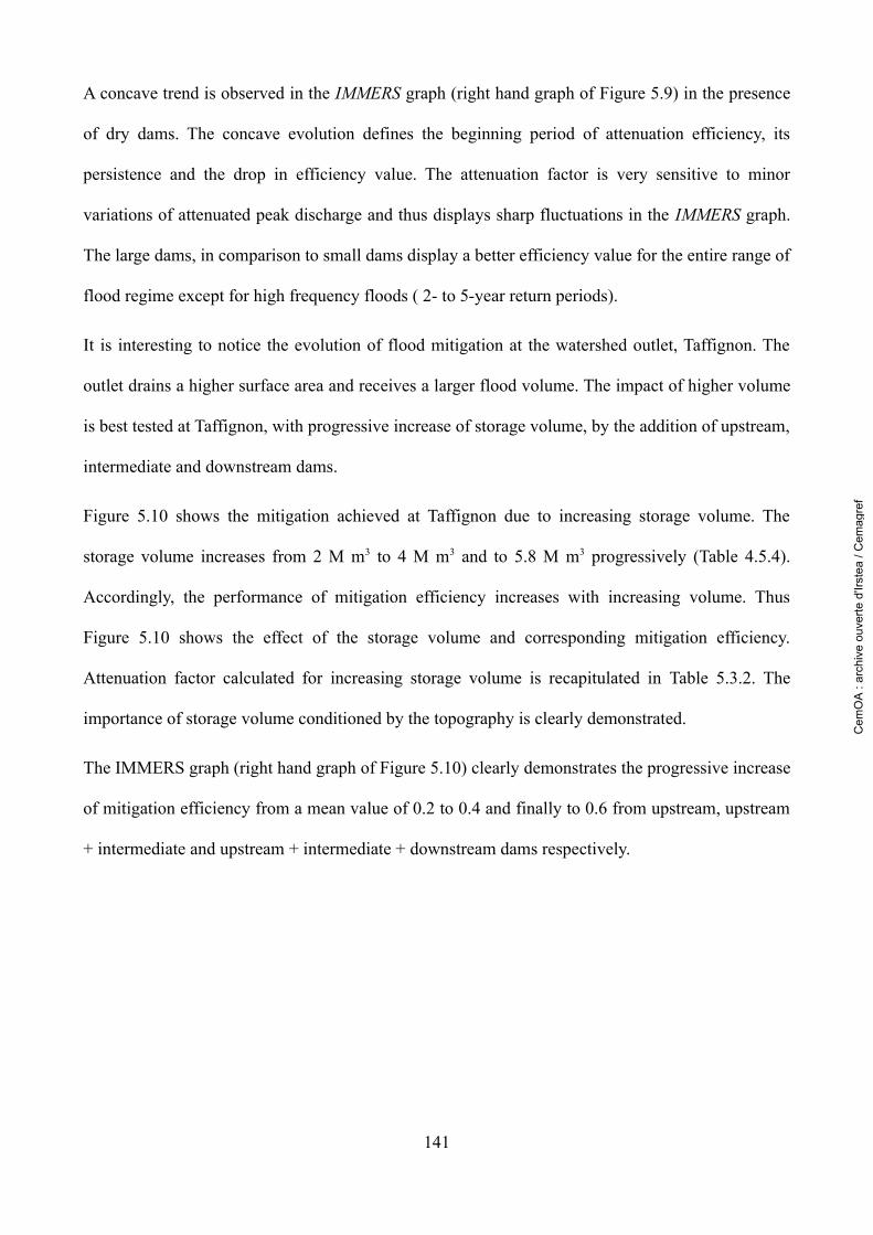
A concave trend is observed in the IMMERS graph (right hand graph of Figure 5.9) in the presence
of dry dams. The concave evolution defines the beginning period of attenuation efficiency, its
persistence and the drop in efficiency value. The attenuation factor is very sensitive to minor
variations of attenuated peak discharge and thus displays sharp fluctuations in the IMMERS graph.
The large dams, in comparison to small dams display a better efficiency value for the entire range of
flood regime except for high frequency floods ( 2- to 5-year return periods).
It is interesting to notice the evolution of flood mitigation at the watershed outlet, Taffignon. The
outlet drains a higher surface area and receives a larger flood volume. The impact of higher volume
is best tested at Taffignon, with progressive increase of storage volume, by the addition of upstream,
intermediate and downstream dams.
Figure 5.10 shows the mitigation achieved at Taffignon due to increasing storage volume. The
storage volume increases from 2 M m3 to 4 M m3 and to 5.8 M m3 progressively (Table 4.5.4).
Accordingly, the performance of mitigation efficiency increases with increasing volume. Thus
Figure 5.10 shows the effect of the storage volume and corresponding mitigation efficiency.
Attenuation factor calculated for increasing storage volume is recapitulated in Table 5.3.2. The
importance of storage volume conditioned by the topography is clearly demonstrated.
The IMMERS graph (right hand graph of Figure 5.10) clearly demonstrates the progressive increase
of mitigation efficiency from a mean value of 0.2 to 0.4 and finally to 0.6 from upstream, upstream
+ intermediate and upstream + intermediate + downstream dams respectively.
141
Cem
OA
: ar
chiv
e ou
verte
d'Ir
stea
/ C
emag
ref
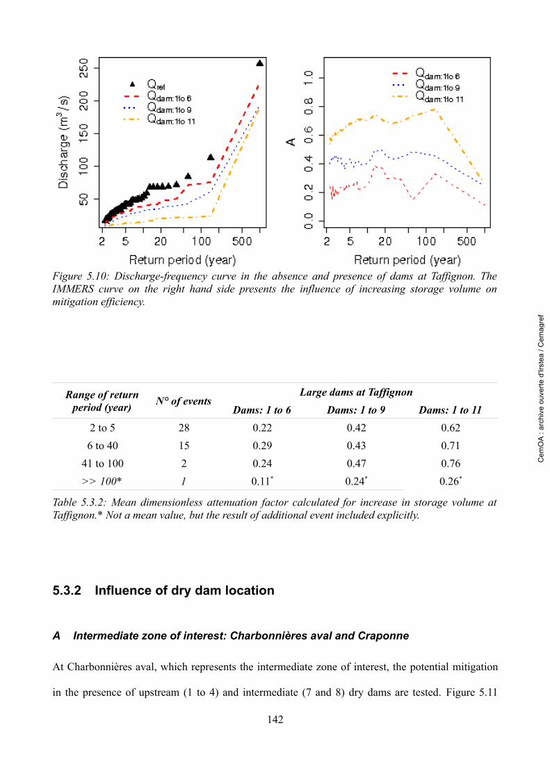
5.3.2 Influence of dry dam location
A Intermediate zone of interest: Charbonnières aval and Craponne
At Charbonnières aval, which represents the intermediate zone of interest, the potential mitigation
in the presence of upstream (1 to 4) and intermediate (7 and 8) dry dams are tested. Figure 5.11
142
Figure 5.10: Discharge-frequency curve in the absence and presence of dams at Taffignon. The IMMERS curve on the right hand side presents the influence of increasing storage volume on mitigation efficiency.
Range of return period (year) N° of events
Large dams at TaffignonDams: 1 to 6 Dams: 1 to 9 Dams: 1 to 11
2 to 5 28 0.22 0.42 0.626 to 40 15 0.29 0.43 0.71
41 to 100 2 0.24 0.47 0.76>> 100* 1 0.11* 0.24* 0.26*
Table 5.3.2: Mean dimensionless attenuation factor calculated for increase in storage volume at Taffignon.* Not a mean value, but the result of additional event included explicitly.
Cem
OA
: ar
chiv
e ou
verte
d'Ir
stea
/ C
emag
ref
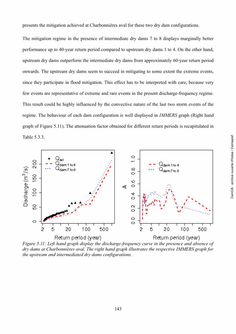
presents the mitigation achieved at Charbonnières aval for these two dry dam configurations.
The mitigation regime in the presence of intermediate dry dams 7 to 8 displays marginally better
performance up to 40-year return period compared to upstream dry dams 1 to 4. On the other hand,
upstream dry dams outperform the intermediate dry dams from approximately 60-year return period
onwards. The upstream dry dams seem to succeed in mitigating to some extent the extreme events,
since they participate in flood mitigation. This effect has to be interpreted with care, because very
few events are representative of extreme and rare events in the present discharge-frequency regime.
This result could be highly influenced by the convective nature of the last two storm events of the
regime. The behaviour of each dam configuration is well displayed in IMMERS graph (Right hand
graph of Figure 5.11). The attenuation factor obtained for different return periods is recapitulated in
Table 5.3.3.
143
Figure 5.11: Left hand graph display the discharge-frequency curve in the presence and absence of dry dams at Charbonnières aval. The right hand graph illustrates the respective IMMERS graph for the upstream and intermediated dry dams configurations.
Cem
OA
: ar
chiv
e ou
verte
d'Ir
stea
/ C
emag
ref

The mitigation efficiency at Craponne zone of interest is presented in Figure 5.12. Up to nearly 5-
year return period, the upstream (5 and 6) and the intermediate (9) dams show nearly the same
mitigation efficiency. From 5- to 20-year return period onwards the intermediate dry dams display a
slightly better efficiency compared to upstream dry dams. As already explained due to the space-
time variability of rainfall, the extreme event added at an approximate return period of 1000-year is
not seen, since the particular event did not produce an significant discharge peak
From 20-year return period to extreme event, the upstream dry dams display a higher efficiency.
Once again, the upstream dry dams contribute to the flood mitigation to some extent, compared to
the intermediate dry dam 9, which does not participate in the mitigation extent due to space-time
variability of rainfall.
Table 5.3.4 recapitulates the attenuation factor obtained for the segmented range of return periods.
Upon comparing attenuation factor due to the upstream and intermediate dry dam location, we find
that the upstream dams assures a better mitigation for frequencies ranging from 2- to 5- and 40- to
100-year return periods. The intermediate dry dam 9 assures a slightly better mitigation from 6- to
40-year return period range compared to the upstream dry dams. Once again, the dams just
upstream of zone to be protected intercepts all the run-off volume and prove efficient. While the
extreme and rare events saturates the storage volume of these dams and overflows, thus proving
144
Range of return period
(year)N° of events
Charbonnières aval control point1 to 4 7 to 8
2 to 5 28 0.28 0.376 to 40 15 0.32 0.44
41 to 100 2 0.26 0.21>> 100* 1 0.16* 0.10*
Table 5.3.3: Mean dimensionless attenuation factor calculated for upstream and intermediate dry dam configuration with Q2 bottom outlet at Charbonnières aval.* Not a mean value, but the result of additional event included explicitly.
Cem
OA
: ar
chiv
e ou
verte
d'Ir
stea
/ C
emag
ref
inefficient.
B Downstream zone of interest: Taffignon
At the control point Taffignon different configurations of dry dams are tested. The influence of only
upstream, intermediate and downstream dam locations on the discharge-frequency curve is
illustrated in Figure 5.13
145
Figure 5.12: Left hand graph display the discharge-frequency mitigation curve in the absence and presence of upstream and intermediate dry dams at Craponne. The right hand graph illustrates the respective IMMERS graph for the upstream and intermediated dry dams configurations.
Range of return period
(year)
Craponne control pointN° of events 5 to 6 9
2 to 5 28 0.15 0.13
6 to 40 15 0.39 0.42
41 to 100 2 0.27 0.14
>> 100 1 - -
Table 5.3.4: Mean dimensionless attenuation factor calculated for upstream and intermediate dry dam configuration with Q2 bottom outlets at Craponne.
Cem
OA
: ar
chiv
e ou
verte
d'Ir
stea
/ C
emag
ref
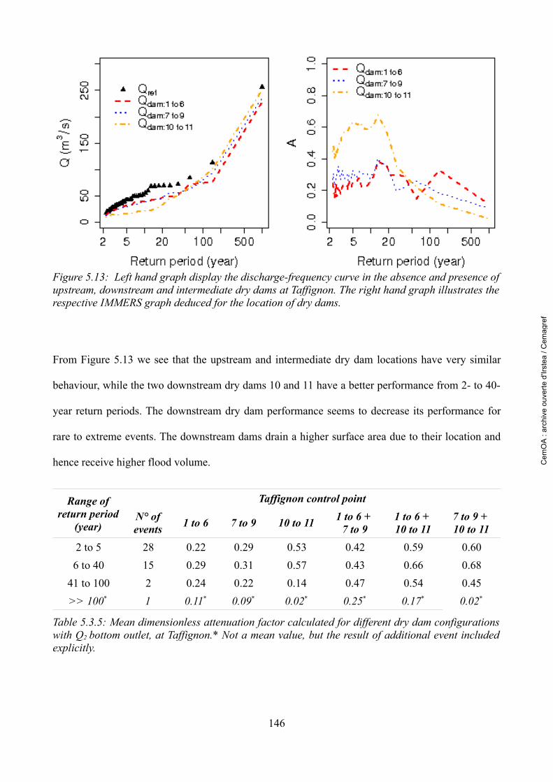
From Figure 5.13 we see that the upstream and intermediate dry dam locations have very similar
behaviour, while the two downstream dry dams 10 and 11 have a better performance from 2- to 40-
year return periods. The downstream dry dam performance seems to decrease its performance for
rare to extreme events. The downstream dams drain a higher surface area due to their location and
hence receive higher flood volume.
146
Figure 5.13: Left hand graph display the discharge-frequency curve in the absence and presence of upstream, downstream and intermediate dry dams at Taffignon. The right hand graph illustrates the respective IMMERS graph deduced for the location of dry dams.
Range of return period
(year)
Taffignon control pointN° of events 1 to 6 7 to 9 10 to 11 1 to 6 +
7 to 91 to 6 + 10 to 11
7 to 9 + 10 to 11
2 to 5 28 0.22 0.29 0.53 0.42 0.59 0.606 to 40 15 0.29 0.31 0.57 0.43 0.66 0.68
41 to 100 2 0.24 0.22 0.14 0.47 0.54 0.45>> 100* 1 0.11* 0.09* 0.02* 0.25* 0.17* 0.02*
Table 5.3.5: Mean dimensionless attenuation factor calculated for different dry dam configurations with Q2 bottom outlet, at Taffignon.* Not a mean value, but the result of additional event included explicitly.
Cem
OA
: ar
chiv
e ou
verte
d'Ir
stea
/ C
emag
ref
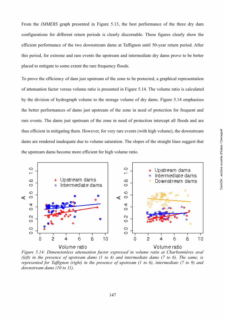
From the IMMERS graph presented in Figure 5.13, the best performance of the three dry dam
configurations for different return periods is clearly discernable. These figures clearly show the
efficient performance of the two downstream dams at Taffignon until 50-year return period. After
this period, for extreme and rare events the upstream and intermediate dry dams prove to be better
placed to mitigate to some extent the rare frequency floods.
To prove the efficiency of dam just upstream of the zone to be protected, a graphical representation
of attenuation factor versus volume ratio is presented in Figure 5.14. The volume ratio is calculated
by the division of hydrograph volume to the storage volume of dry dams. Figure 5.14 emphasises
the better performances of dams just upstream of the zone in need of protection for frequent and
rare events. The dams just upstream of the zone in need of protection intercept all floods and are
thus efficient in mitigating them. However, for very rare events (with high volume), the downstream
dams are rendered inadequate due to volume saturation. The slopes of the straight lines suggest that
the upstream dams become more efficient for high volume ratio.
147
Figure 5.14: Dimensionless attenuation factor expressed in volume ratio at Charbonnières aval (left) in the presence of upstream dams (1 to 4) and intermediate dams (7 to 6). The same, is represented for Taffignon (right) in the presence of upstream (1 to 6), intermediate (7 to 9) and downstream dams (10 to 11).
Cem
OA
: ar
chiv
e ou
verte
d'Ir
stea
/ C
emag
ref
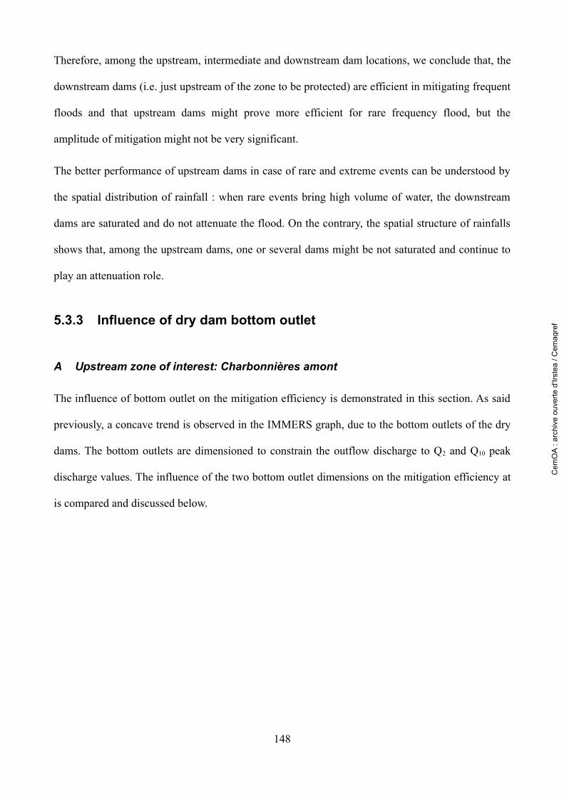
Therefore, among the upstream, intermediate and downstream dam locations, we conclude that, the
downstream dams (i.e. just upstream of the zone to be protected) are efficient in mitigating frequent
floods and that upstream dams might prove more efficient for rare frequency flood, but the
amplitude of mitigation might not be very significant.
The better performance of upstream dams in case of rare and extreme events can be understood by
the spatial distribution of rainfall : when rare events bring high volume of water, the downstream
dams are saturated and do not attenuate the flood. On the contrary, the spatial structure of rainfalls
shows that, among the upstream dams, one or several dams might be not saturated and continue to
play an attenuation role.
5.3.3 Influence of dry dam bottom outlet
A Upstream zone of interest: Charbonnières amont
The influence of bottom outlet on the mitigation efficiency is demonstrated in this section. As said
previously, a concave trend is observed in the IMMERS graph, due to the bottom outlets of the dry
dams. The bottom outlets are dimensioned to constrain the outflow discharge to Q2 and Q10 peak
discharge values. The influence of the two bottom outlet dimensions on the mitigation efficiency at
is compared and discussed below.
148
Cem
OA
: ar
chiv
e ou
verte
d'Ir
stea
/ C
emag
ref
From Figure 5.15 we see that the dry dams with Q2 bottom outlet, mitigate small frequency floods
better than the dry dams with Q10 bottom outlet dimension. Both the dry dam designs display
maximum efficiency between 20- to 50-year flood return period. A better efficiency of dry dams
with Q2 bottom outlet is assured until the 20- to 50-year flood return period, after which the dry dam
with Q10 bottom outlet displays higher efficiency. For extreme and rare frequency floods due to
storage volume saturation no or nearly null attenuation is seen. To know the extent of potential
mitigation for very frequent, frequent, rare and extreme discharge-return periods, the attenuation
factor is calculated. The attenuation factor obtained for these range of frequency floods is
recapitulated in Table 5.3.6.
149
Figure 5.15: Left hand graph display the discharge-frequency curve in the absence and presence of Q2 and Q10 bottom outlet dry dams at Charbonnières amont. The right hand IMPRESS graph presents the mitigation efficiency assured by the two dry dam designs.
Cem
OA
: ar
chiv
e ou
verte
d'Ir
stea
/ C
emag
ref
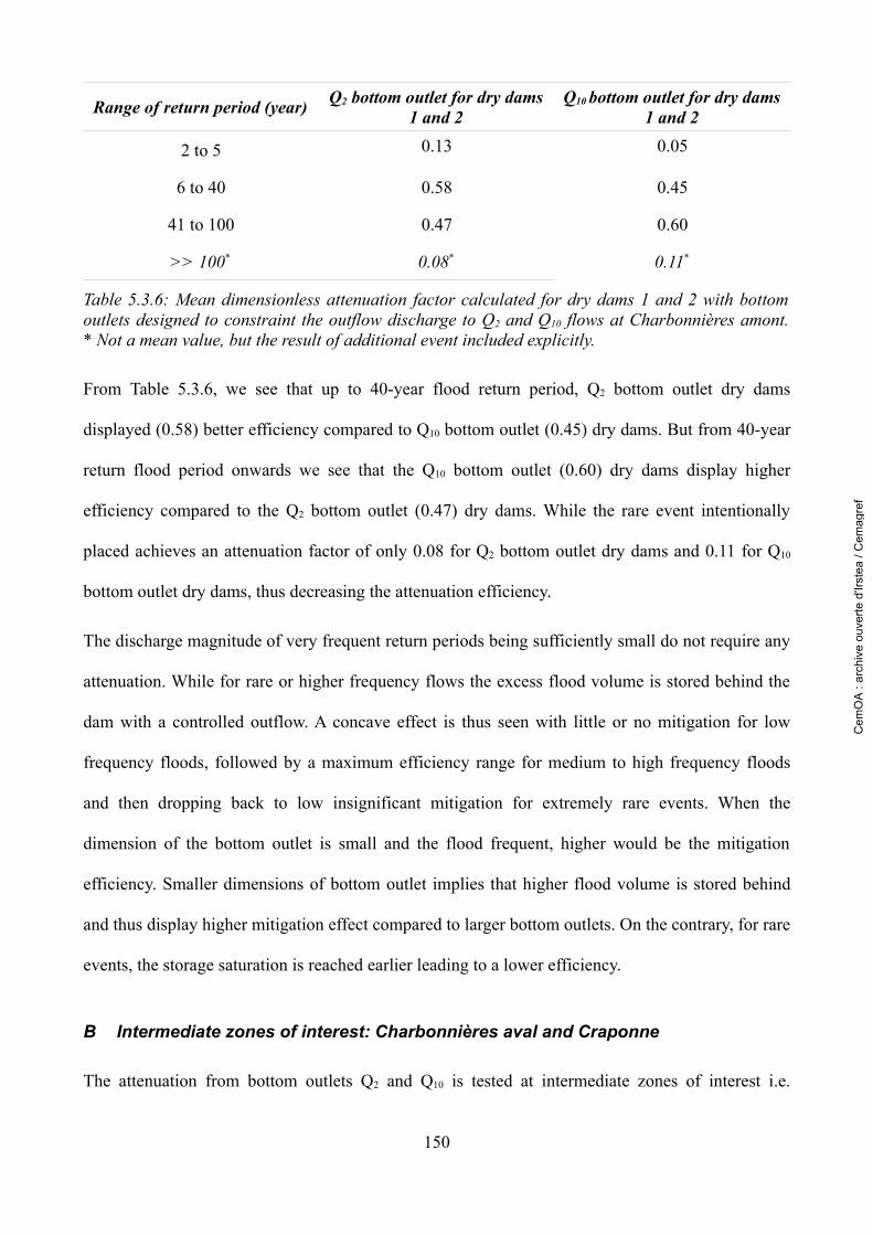
From Table 5.3.6, we see that up to 40-year flood return period, Q2 bottom outlet dry dams
displayed (0.58) better efficiency compared to Q10 bottom outlet (0.45) dry dams. But from 40-year
return flood period onwards we see that the Q10 bottom outlet (0.60) dry dams display higher
efficiency compared to the Q2 bottom outlet (0.47) dry dams. While the rare event intentionally
placed achieves an attenuation factor of only 0.08 for Q2 bottom outlet dry dams and 0.11 for Q10
bottom outlet dry dams, thus decreasing the attenuation efficiency.
The discharge magnitude of very frequent return periods being sufficiently small do not require any
attenuation. While for rare or higher frequency flows the excess flood volume is stored behind the
dam with a controlled outflow. A concave effect is thus seen with little or no mitigation for low
frequency floods, followed by a maximum efficiency range for medium to high frequency floods
and then dropping back to low insignificant mitigation for extremely rare events. When the
dimension of the bottom outlet is small and the flood frequent, higher would be the mitigation
efficiency. Smaller dimensions of bottom outlet implies that higher flood volume is stored behind
and thus display higher mitigation effect compared to larger bottom outlets. On the contrary, for rare
events, the storage saturation is reached earlier leading to a lower efficiency.
B Intermediate zones of interest: Charbonnières aval and Craponne
The attenuation from bottom outlets Q2 and Q10 is tested at intermediate zones of interest i.e.
150
Range of return period (year) Q2 bottom outlet for dry dams 1 and 2
Q10 bottom outlet for dry dams 1 and 2
2 to 5 0.13 0.05
6 to 40 0.58 0.45
41 to 100 0.47 0.60
>> 100* 0.08* 0.11*
Table 5.3.6: Mean dimensionless attenuation factor calculated for dry dams 1 and 2 with bottom outlets designed to constraint the outflow discharge to Q2 and Q10 flows at Charbonnières amont. * Not a mean value, but the result of additional event included explicitly.
Cem
OA
: ar
chiv
e ou
verte
d'Ir
stea
/ C
emag
ref
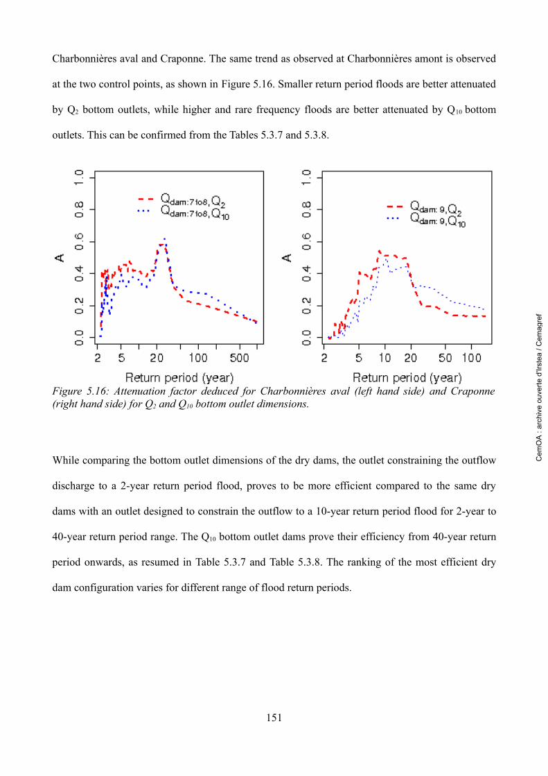
Charbonnières aval and Craponne. The same trend as observed at Charbonnières amont is observed
at the two control points, as shown in Figure 5.16. Smaller return period floods are better attenuated
by Q2 bottom outlets, while higher and rare frequency floods are better attenuated by Q10 bottom
outlets. This can be confirmed from the Tables 5.3.7 and 5.3.8.
While comparing the bottom outlet dimensions of the dry dams, the outlet constraining the outflow
discharge to a 2-year return period flood, proves to be more efficient compared to the same dry
dams with an outlet designed to constrain the outflow to a 10-year return period flood for 2-year to
40-year return period range. The Q10 bottom outlet dams prove their efficiency from 40-year return
period onwards, as resumed in Table 5.3.7 and Table 5.3.8. The ranking of the most efficient dry
dam configuration varies for different range of flood return periods.
151
Figure 5.16: Attenuation factor deduced for Charbonnières aval (left hand side) and Craponne (right hand side) for Q2 and Q10 bottom outlet dimensions.
Cem
OA
: ar
chiv
e ou
verte
d'Ir
stea
/ C
emag
ref
C Downstream zone of interest: Taffignon
The comparison of the Q2 and Q10 bottom outlet dimension is shown in Figure 5.17 only for the
downstream dam location. The influence of upstream, intermediate and combination of different
dam locations not being very different, can be referred to from Table 5.3.9 and Table 5.3.10. A
significant mitigation is seen for the 2- to 20-year return period range. After the 20-year return
period, the achieved mitigation due to the two bottom outlet dimensions are identical. No
significant difference between the two bottom outlet dimensions is seen. Saturation of the dams is
reached due to the large area drained by this point, which receives a high flood volume. Due to
152
Range of return period
(year)
Q2 bottom outlet Q10 bottom outlet1 to 4 7 to 8 1 to 4 7 to 8
2 to 5 0.28 0.37 0.18 0.246 to 40 0.32 0.44 0.27 0.38
41 to 100 0.26 0.21 0.32 0.28>> 100* 0.16* 0.10* 0.15* 0.09*
Table 5.3.7: Dimensionless attenuation factor calculated for upstream and intermediate dry dam configuration with Q2 and Q10 bottom outlet dimensions at Charbonnières aval. * Not a mean value, but the result of additional event included explicitly.
Range of return period
(year)
Q2 bottom outlet Q10 bottom outlet
5 to 6 9 5 to 6 9
2 to 5 0.15 0.13 0.08 0.06
6 to 40 0.39 0.42 0.35 0.36
41 to 100 0.27 0.14 0.31 0.20
>> 100* - - - -
Table 5.3.8: Dimensionless attenuation factor calculated for upstream and intermediate dry dam configuration with Q2 and Q10 bottom outlet dimensions at Craponne. * Not a mean value, but the result of additional event included explicitly.
Cem
OA
: ar
chiv
e ou
verte
d'Ir
stea
/ C
emag
ref
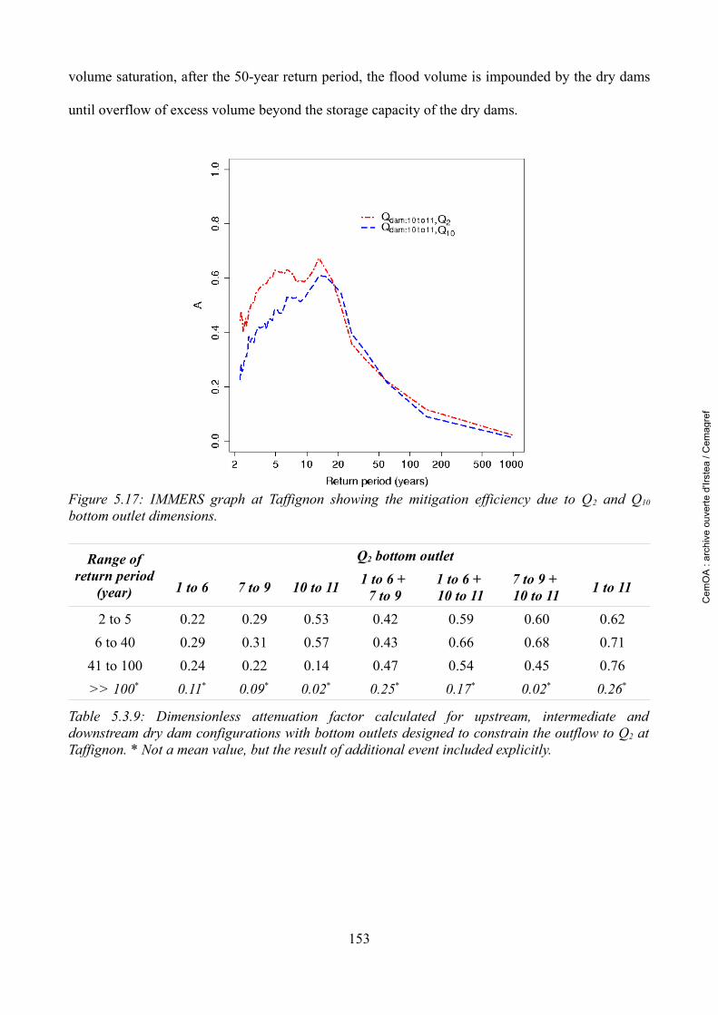
volume saturation, after the 50-year return period, the flood volume is impounded by the dry dams
until overflow of excess volume beyond the storage capacity of the dry dams.
153
Figure 5.17: IMMERS graph at Taffignon showing the mitigation efficiency due to Q2 and Q10
bottom outlet dimensions.
Range of return period
(year)
Q2 bottom outlet
1 to 6 7 to 9 10 to 11 1 to 6 + 7 to 9
1 to 6 + 10 to 11
7 to 9 + 10 to 11 1 to 11
2 to 5 0.22 0.29 0.53 0.42 0.59 0.60 0.626 to 40 0.29 0.31 0.57 0.43 0.66 0.68 0.71
41 to 100 0.24 0.22 0.14 0.47 0.54 0.45 0.76>> 100* 0.11* 0.09* 0.02* 0.25* 0.17* 0.02* 0.26*
Table 5.3.9: Dimensionless attenuation factor calculated for upstream, intermediate and downstream dry dam configurations with bottom outlets designed to constrain the outflow to Q2 at Taffignon. * Not a mean value, but the result of additional event included explicitly.
Cem
OA
: ar
chiv
e ou
verte
d'Ir
stea
/ C
emag
ref
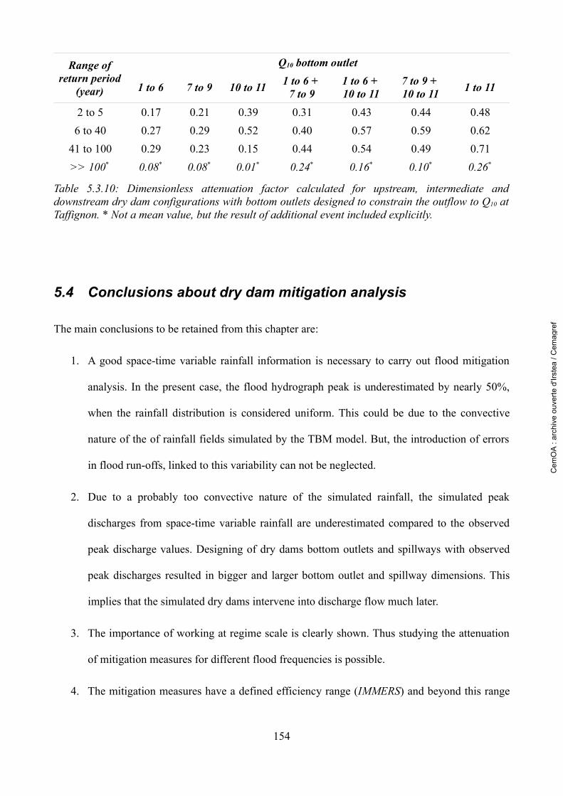
5.4 Conclusions about dry dam mitigation analysis
The main conclusions to be retained from this chapter are:
1. A good space-time variable rainfall information is necessary to carry out flood mitigation
analysis. In the present case, the flood hydrograph peak is underestimated by nearly 50%,
when the rainfall distribution is considered uniform. This could be due to the convective
nature of the of rainfall fields simulated by the TBM model. But, the introduction of errors
in flood run-offs, linked to this variability can not be neglected.
2. Due to a probably too convective nature of the simulated rainfall, the simulated peak
discharges from space-time variable rainfall are underestimated compared to the observed
peak discharge values. Designing of dry dams bottom outlets and spillways with observed
peak discharges resulted in bigger and larger bottom outlet and spillway dimensions. This
implies that the simulated dry dams intervene into discharge flow much later.
3. The importance of working at regime scale is clearly shown. Thus studying the attenuation
of mitigation measures for different flood frequencies is possible.
4. The mitigation measures have a defined efficiency range (IMMERS) and beyond this range
154
Range of return period
(year)
Q10 bottom outlet
1 to 6 7 to 9 10 to 11 1 to 6 + 7 to 9
1 to 6 + 10 to 11
7 to 9 + 10 to 11 1 to 11
2 to 5 0.17 0.21 0.39 0.31 0.43 0.44 0.486 to 40 0.27 0.29 0.52 0.40 0.57 0.59 0.62
41 to 100 0.29 0.23 0.15 0.44 0.54 0.49 0.71>> 100* 0.08* 0.08* 0.01* 0.24* 0.16* 0.10* 0.26*
Table 5.3.10: Dimensionless attenuation factor calculated for upstream, intermediate and downstream dry dam configurations with bottom outlets designed to constrain the outflow to Q10 at Taffignon. * Not a mean value, but the result of additional event included explicitly.
Cem
OA
: ar
chiv
e ou
verte
d'Ir
stea
/ C
emag
ref

i.e. for extreme and very rare frequency events, no mitigation can be expected.
5. Increasing storage volume increases the efficiency range of mitigation measures.
6. Downstream dams i.e. dams just upstream of the zone to be protected are very efficient for
frequent floods. Rare and extreme floods can not be mitigated, due to volume saturation of
mitigation measures. The upstream dam might mitigate to a very small extent, the rare and
extreme floods, but the attenuation assured by them could be weak.
7. Small bottom outlet dams are efficient in mitigation frequent floods, since they intervene
into the discharge regime earlier compared to larger bottom outlets. But on the other hand,
the small bottom outlets, saturate earlier compared to large bottom outlets and thus are
relatively less efficient for rare and extreme flood frequencies.
155
Cem
OA
: ar
chiv
e ou
verte
d'Ir
stea
/ C
emag
ref

6 CONCLUSIONS, DISCUSSIONS AND PERSPECTIVES
Cem
OA
: ar
chiv
e ou
verte
d'Ir
stea
/ C
emag
ref
6.1 Conclusions
The main results obtained is summarised below. The influence of storage volume, location and
bottom outlet dimension of dry dams is understood from the analysis of the IMMERS graph. The
IMMERS graph shows the efficiency range of the mitigation measure in question, with its concave
form. The efficiency of mitigation measures rises progressively with increasing flood return periods
initially, until reaching a maximum platform. For extreme events, the mitigation measures become
ineffective due to the amplitude of the flood wave which has volumes beyond the storage capacity
of the mitigation measures. Thus IMMERS graph defines an efficiency range, within which the
mitigation measures display their best performance and also give an idea of the behaviour of the
mitigation measures for small and extreme flood events. This representation enables an
understanding of the efficiency range of mitigation measures for different flood frequencies. This
knowledge empowers a region to plan mitigation strategies best suited and their limits. The
IMMERS graph clearly demonstrates that one can not protect oneself against all floods, especially
extreme and rare events.
The obvious increase of mitigation efficiency with increase in storage volume was demonstrated in
the section 5.3.1. When high storage volume is available for a mitigation measure, more would be
the space available for retaining the excess flood volume and thus the mitigation measures will be
efficient in mitigation function, but within the evident defined limit. This point was proved by
increasing the dam heights, which evidently increased the storage volume and also by increasing the
number of dry dams, thus adding to the total storage volume.
The best location for achieving maximum mitigation efficiency was also tested. The maximum
efficiency was assured by the dry dams just upstream of the zone to be protected for frequent to
moderately frequent floods (2-year to ≈ 50-year return period). While for extreme floods, the dams
just upstream of the zone to be protected drain a higher surface and achieve storage volume
158
Cem
OA
: ar
chiv
e ou
verte
d'Ir
stea
/ C
emag
ref
saturation. Dams situated further above from the zone of interest though not very significant in
reducing the flood peak, participated to some extent in mitigating the rare frequency floods.
From the demonstration in section 5.3.2, the conclusion that upstream dry dams are efficient in
mitigation extreme and rare return period floods has to be accepted with reservations. This result is
based on one single rainfall event, which was highly convective in nature. Thus among the 6
upstream dams, storage volume of some dams were not completely saturated, due to relatively small
surface run-off provoked by less rainfall volume.
The outlet dimensions of dry dams impose an efficient mitigation range. Dry dams designed for
small amplitude floods while mitigating low peak flows become relatively inefficient for large flood
return periods because of early storage saturation. On the other hand if the dry dams are designed
for rare and high amplitude floods they do not mitigate frequent low flows and affect only high
flows until storage depletion. In general, smaller the bottom outlet, higher will be the mitigation
efficiency, since the excess flood volume is retained from early on. This is clearly visible, especially
for the downstream zone of interest. But smaller the dimension of the bottom outlet, higher will be
the perturbation to the river flow. Thus the acceptable limit of the modification of the river regime
and its consequences have to be clearly understood.
6.2 Discussions
6.2.1 Uncertainties and approximation of the developed methodology
The major draw back in the present study, is the inability to produce a discharge-frequency curve
from space-time variable rainfall, similar to that observed. This inability undoubtedly influences the
instantaneous peak discharge values and associating flood return period values. The peak discharges
at Taffignon were underestimated by nearly 20 m3s-1 and thus undermining the return period by a
factor of 4. However, it is not clear weather the IMMERS graph deduced from these underestimated
159
Cem
OA
: ar
chiv
e ou
verte
d'Ir
stea
/ C
emag
ref
peak values overestimate the mitigation efficiency. Though a shift in the concave nature of the
attenuation curve is expected, due to the dimension of bottom outlet. In the present study the bottom
outlets were dimensioned from the observed peak discharges values, implying that the size of
bottom outlets were in reality overestimated, i.e. larger rectangular openings. A large opening would
mean no attenuation of small flood return periods, since the small peak flows pass through the
bottom opening unimpeded.
Another drawback of the present work, is the small number of spatial rainfall events chosen to
represent the return periods, especially the rare and extreme event floods. Equation 3.13 used to
define return period values, allowed only a maximum return period value of 144-year flood, with
the next highest return period value of 59-year flood. An event which provoked very high peak
discharge was arbitrarily assigned a 1000-year return period flood to possess representative extreme
floods. The deduction of mitigation measures for the rare and extreme frequency floods was thus
based on these three events. The interpretation of the behaviour of mitigation measures for rare and
extreme events, is based on very little data set. Therefore care should be taken while accepting the
tendency displayed in the present study.
6.2.2 Model uncertainties
The dispersed mitigation strategy was tested in the present study with the aid of specific tools. The
uncertainties and errors brought in by these tools should also be acknowledged.
The space-time variable rainfall data was furnished by a stochastic model under development in an
ongoing thesis project (Lepioufle, 2008). The anomalies of the furnished rainfall fields, regarding
the spatial and temporal structure was uncovered during the present study. The structural
distribution of the rainfall fields were found highly convective and due to this characteristic the
influence of spatial variability might be over exaggerated in the present results. Next, though the
intensity-duration-frequency analysis of the simulated fields could be considered in agreement with
160
Cem
OA
: ar
chiv
e ou
verte
d'Ir
stea
/ C
emag
ref

the observed data, the mean volume of the rainfall fields furnished to the distributed hydrological
model was underestimated to a large extent. This is probably due to the fact that the correlation
distance of the rainfall was underestimated. Also, the hypothesis of equal distribution of null values,
in other words the absence of dry periods might have biased the temporal dynamic of the rainfall
events according to the TBM model conceptor. The above characteristics of the rainfall data, thus
influenced the formation of peak discharge values. The feedback from the present study and the
information from the Grand Lyon district will help in the simulation of more realistic and better
quality rainfall fields in the future.
The MARINE model is based on the hypothesis that the sub-surface run-offs do not participate in
the production of flood hydrographs. But in watersheds where the contribution by the sub-surface
module is not negligible, this reasoning could entail important errors in flood volume and in the
hydrograph dynamics. During the study of the Yzeron watershed by Gnouma (2006), piezometers
installed in the Mercier sub-basin registered a quick increase and decrease in the water depth for
2006 February event. Thus implying some contribution of the sub-surface flow to the flood
hydrograph. The necessity of imposing very high Manning roughness coefficients to retard the flow
could be linked to inability of MARINE to simulate such sub-surface flows. This point is further
emphasised by the fast descent of the hydrograph tail, simulated by the model compared to the
observed hydrographs. The model is unable to retard the flow to representative time delay of sub-
surface flows.
The sensitivity of the model to the soil characteristics such as variable soil humidity, detailed soil
depth information was not explored to the maximum extent due to lack of spatial data set. The
location of dry dams was not chosen based on realistic information of land-use information,
geology, etc contrary to the reality where the choice of site, for the construction of mitigation
measure is complex.
The MAGE 1-D model was efficient in the routing of the river flow. Based on the quality and
161
Cem
OA
: ar
chiv
e ou
verte
d'Ir
stea
/ C
emag
ref
quantity of the available data set, the simplification of the geometry would not have added major
uncertainties in the flood wave propagation. The Manning roughness coefficient remained the same
for the minor river bed and the major river bed respectively all along the drainage network
distribution. A 1-D model seemed largely sufficient to meet the objectives of the present study.
The coupling of the MARINE and MAGE models helped simulate correctly the flow along the
watershed slope and the drainage network. Uncertainties related to modelling parameters and
modelling procedures were probably not too high to have largely influenced the flood mitigation
results.
6.2.3 Choice of the study area
The results obtained in this study is undoubtedly conditioned by the characteristics of the Yzeron
watershed. The watershed topography, i.e. slope, altitude, contours and drainage network,
influences the mitigation measure dimension and location. The currently promoted motto of “small
is good” is contradicted in the present case. A dispersed strategy to protect the entire watershed with
small mitigation measures proved inefficient. The small dams quite simply lacked enough storage
volume, to register any mitigation of the discharge regime. Thus, the application of large dams to
mitigate floods was necessary for the Yzeron watershed. The best strategy to protect the zone in
question by relatively large dams is particular to the configuration of the Yzeron watershed, which
has very steep slopes.
An interesting question which rises from the above result, would be to know if the developed
methodology is applicable and adaptable to other watersheds. The choice of best design and
location would not necessarily be the same, because of the singularity of each watershed in its
topography, structure and land-use. On the other hand, the IMMERS graph can and should be
adapted for the analysis of any mitigation strategy. This representation helps to understand the
behaviour of mitigation strategies for different flood frequencies confronted by any watershed. The
162
Cem
OA
: ar
chiv
e ou
verte
d'Ir
stea
/ C
emag
ref
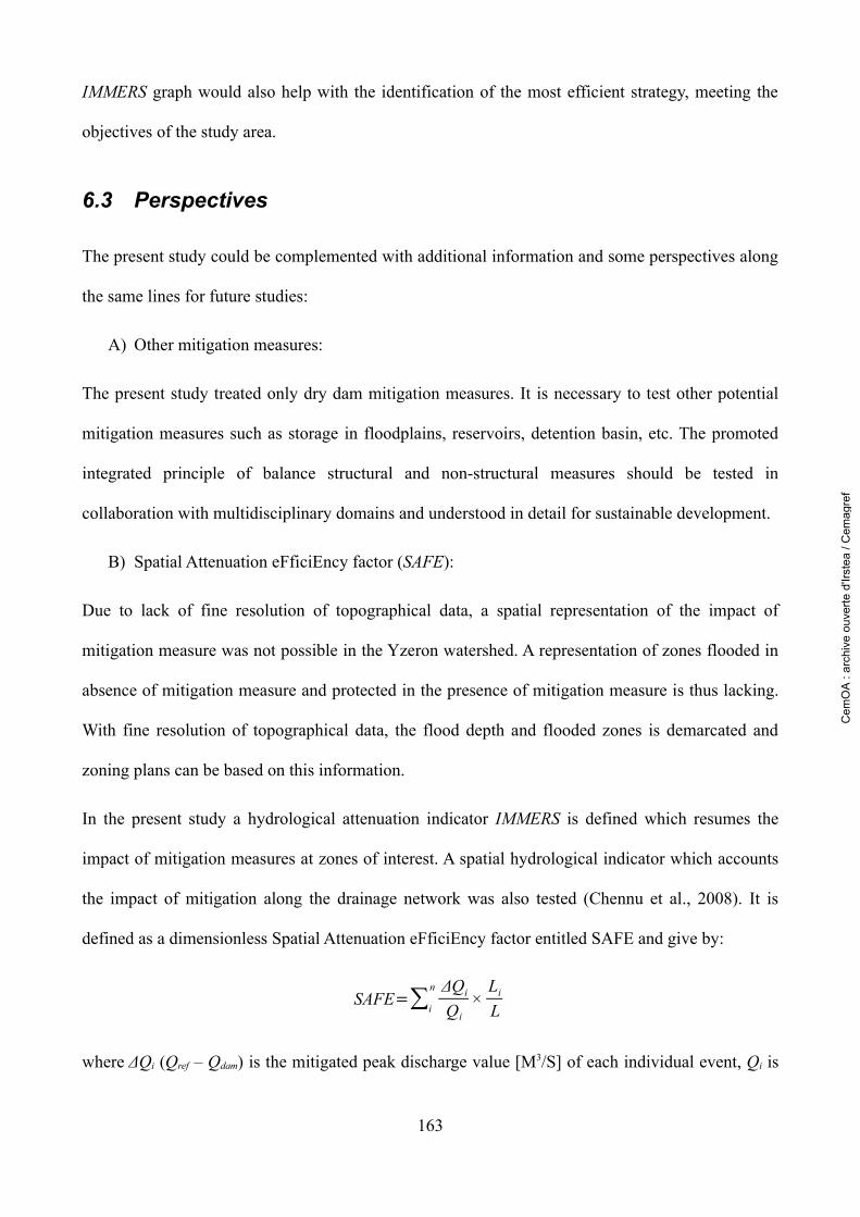
IMMERS graph would also help with the identification of the most efficient strategy, meeting the
objectives of the study area.
6.3 Perspectives
The present study could be complemented with additional information and some perspectives along
the same lines for future studies:
A) Other mitigation measures:
The present study treated only dry dam mitigation measures. It is necessary to test other potential
mitigation measures such as storage in floodplains, reservoirs, detention basin, etc. The promoted
integrated principle of balance structural and non-structural measures should be tested in
collaboration with multidisciplinary domains and understood in detail for sustainable development.
B) Spatial Attenuation eFficiEncy factor (SAFE):
Due to lack of fine resolution of topographical data, a spatial representation of the impact of
mitigation measure was not possible in the Yzeron watershed. A representation of zones flooded in
absence of mitigation measure and protected in the presence of mitigation measure is thus lacking.
With fine resolution of topographical data, the flood depth and flooded zones is demarcated and
zoning plans can be based on this information.
In the present study a hydrological attenuation indicator IMMERS is defined which resumes the
impact of mitigation measures at zones of interest. A spatial hydrological indicator which accounts
the impact of mitigation along the drainage network was also tested (Chennu et al., 2008). It is
defined as a dimensionless Spatial Attenuation eFficiEncy factor entitled SAFE and give by:
SAFE=∑i
n ΔQi
Qi×
Li
L
where ΔQi (Qref – Qdam) is the mitigated peak discharge value [M3/S] of each individual event, Qi is
163
Cem
OA
: ar
chiv
e ou
verte
d'Ir
stea
/ C
emag
ref

the peak value in the absence of mitigation measures [M3/S] in each individual river reach, Li is the
individual river reach length and L the total length of the river reaches.
With the application of SAFE, the upstream dry dams mitigation influence was felt all along the
drainage network of the watershed and proved to be more efficient compared to the intermediate
and downstream dry dams. Though, due to the rough resolution of the DEM, a finer result was not
achievable.
C) Realistic space-time rainfall fields:
The mitigation analysis tested in the present work should be redone, once more realistic and just
rainfall fields are available. The present work concentrated only on the modification and mitigation
of instantaneous discharge-frequency regime curve. It would be useful to carry out the same
analysis for different durations of discharge-frequency curve from space-time variable rainfall data,
to see how the mitigation efficiency behaviour evolves for different discharge durations.
D) Other test cases of study areas:
It would be of interesting to see how the developed methodology could be applicable to other
watersheds. Each watershed is unique in its structural and climatic composition. The form of the
attenuation indicator and the presentation via IMMERS graph will be unique. By testing the
methodology on numerous watersheds, potentially efficient strategies to reduce flood risk could be
confirmed.
E) Dam breaches:
The structural measures are vulnerable to breaches when confronted with floods beyond their
design capacity. When the dams breach, the wanted mitigation effect can turn to disaster and
aggravate the flood risk. It is thus important to understand the influence of dam breaches on the
flood regimes. Simulations where dam breach probability is accounted could be performed with
suitable models which undertake flood wave propagation.
164
Cem
OA
: ar
chiv
e ou
verte
d'Ir
stea
/ C
emag
ref

The developed method should be complemented with the vulnerability analysis, to understand the
consequences of various mitigation projects.
165
Cem
OA
: ar
chiv
e ou
verte
d'Ir
stea
/ C
emag
ref

7 REFERENCES
Cem
OA
: ar
chiv
e ou
verte
d'Ir
stea
/ C
emag
ref
Anderson, M.G. and Burt, T.P., 1990. Process studies in hillslope hydrology. Chapter 7. John Wiley
and Sons Ltd.
Apel, H., Thieken, A.H., Merz, B., Blöschl, G., 2006. A Probabilistic modelling system for
assessing flood risks. Natura Hazards 38, 79-100.
Apel, H., Merz, B., Thieken, A.H., accepted for publication. Influence of dike breaches on flood
frequency estimation. Computers and Geosciences.
Arnaud, P., Bouvier, B., Cisneros, L., Dominguez. R., 2002. Influence of rainfall spatial variability
on flood prediction. Journal of Hydrology 260 (1-4), 216-230.
Arnaud, P. and Lavabre, J., 2002. Coupled rainfall model and discharge model for flood frequency
estimation. Water Resources Research 38 (6).
Arnell, N.W., 2002. Relative effects of multi-decadal climatic variability and changes in the mean
and variability of climate due to global warming: future streamflows in Britain. Journal of
Hydrology 270 (3-4), 195-213.
Bell, T.E. (2004). “Taking engineering by storm.” The Bent of Tau Beta Pi, Winter 2004.
Engineering honor society, United States.
Beven, K. and Hornberger, G.M., 1982. Assessing the effect of spatial pattern of precipitation in
modelling stream flow hydrology. Water Resources Bulletin 18(5), 823-829.
Beven, K., Kirkby, M.J., Schofield, N., Tagg, A.F., 1984. Testing a physically-based flood
forecasting model (TOPMODEL) for three U.K. Catchments. Journal of hydrology 69, 119-
143.
Bessier, H., 2005. Intégration du reseau de drainage et changement d'échelle dans MARINE.
Master's thesis. IMFT, CNRS – INP/ENSEEIHT.
Blöschl,G., Ardoin-Bardin, S., Bonell, M., Dorninger, M., Goodrich, D., Gutknecht, D., Matamoros,
168
Cem
OA
: ar
chiv
e ou
verte
d'Ir
stea
/ C
emag
ref
D., Merz, B., Shand, P., Szolgay, J., 2007. At what scales do climate variability and land cover
change impact on flooding and low flows. Hydrological Processes 21(9), 1241-1247.
Bölscher, J. and Schulte, A., 2007. Hydrological modelling of decentralised flood protection
measures in transitional headwater areas of the Natzschung catchment/Mittleres Erzgebirge.
Proceedings of Integrated catchment management for hazard mitigation. WaReLa, Trier, 24-26
September, 2007.
Braatne, J, Rood, S.B., Goater, L.A., Charles, B.L, 2008. Analyzing the Impacts of Dams on
Riparian Ecosystems: A Review of Research Strategies and Their Relevance to the Snake River
Through Hells Canyon. Environmental Management 41 (2), 267-281.
Bras, R.L. and Rodríguez-Iturbe, I.,1993. Random functions and hydrology. Dover publication Inc,
New York.
Chen, H., Guo, S., Xu, C-Y., Singh, V.P., 2007. Historical temporal trends of hydro-climatic
variables and runoff response to climate variability and their relevance in water resource
management in the Hanjiang basin. Journal of Hydrology 344 (3-4), 171-184.
Chennu, S., Grésillon, J.-M., Faure, J.-B., Leblois, E., Poulard, C., Dartus, D., 2008. Flood
mitigation strategies at watershed scale through dispersed structural measures. Proceedings of
the 4th International Symposium on Flood Defence: Managing Flood Risk, Reliability and
Vulnerability, Toronto, Ontario, Canada, May 6-8, 2008. Institute for Catastrophic Loss
Reduction.
Chow, V., 1973. Open-Channel Hydraulics. McGraw-Hill International Editions, 109-113.
Commission of the European Communities, 2004. Communication from the commission to the
council, The European Parliament, The European economic and social committee and The
committee of the regions. Flood risk management: Flood prevention, protection and mitigation.
Commission of the European Communities, 2006. Commission staff working document. Annex to
169
Cem
OA
: ar
chiv
e ou
verte
d'Ir
stea
/ C
emag
ref
the proposal for a directive of the European Parliament and of the council on the assessment
and management of floods.
Correia, F.N., Rego, F.C., Saraiva, M.G, Ramos, I., 1998a. Coupling GIS with hydrologic and
hydraulic flood moedlling. Water Resource Management 12, 229-249.
Correia, F.N., Saraiva, M.G., Silva, , Ramos, I., 1999. Floodplain management in urban developing
areas. Part II. GIS-based flood analysis and urban growth modelling. Water Resource
Management 13, 23-37.
Carluer, N. and Marsily, G., 2004. Assessment and modelling of the influence of man-made
networks on the hydrology of a small watershed: implications for fast flow components, water
quality and landscape management. Journal of hydrology 285, 76-95.
CRED, 2004. Thirty Years of Nautral Disaster 1974 - 2003: The Numbers.
http://www.preventionweb.net/english/professional/publications/v.php?id=1080
CRED, 2007. Annual disaster statistics review: Number and trends 2006.
Dawdy, D.R. and Bergmann, J.M, 1969. Effect of rainfall variability on stream flow simulation.
Water Resources Research 5(5), 958-966.
Dijkman, 2008. A Dutch perspective on coastal Louisianan flood risk reduction and landscape
stabilization. Plenary presentation of 4th International Symposium on Flood defence, 2008,
Toronto Canada.
Dotson H.W. and Davis, D.W., 1995. Case study: Risk-based analysis of flood reduction measures.
J. Gardiner et al. (eds.), Defence from Floods and Floodplain Management, 479-485.
Doussière, F., 2007. Projet de recherche sur la prévision des inondations - Étude de la rivière
Ardèche. Project Report, Cemagref.
Downs, P.W. and Thorne, C.R., 2000. Rehabilitation of a lowland river: Reconciling flood defence
170
Cem
OA
: ar
chiv
e ou
verte
d'Ir
stea
/ C
emag
ref

with habitat diversity and geomorphological sustainability. Journal of Environmental
Management 58 (4), 249-268.
Dutta, D., Herath, S., Musiake, K., 2006. An application of a flood risk analysis system for impact
analysis of a flood control plan in a river basin. Hydrological Processes 20, 1365-1384.
Environmental Agency, 2000. Floodline – Am I at risk of flooding ? Websource :
http://www.environment-agency.gov.uk/yourenv/eff/1190084/natural_forces/flooding/
Ecosystems and human well-being: Policy responses, 2005. Websource:
http://www.millenniumassessment.org/documents/document.48.aspx.pdf. Consulted on the
28/05/2008.
EM-DAT the OFDA/CRED, International Disaster Database. Websource:
http://www.emdat.be/ExplanatoryNotes/explanotes.html. Consulted on 29/05/2008.
ERA-NET. Weblink: www.crue-eranet.net
Estupina-Borrell, V., 2004. Vers une Modélisation Hydrologique adaptée à la Prévision
Opérationnelle des Crues Eclair - Application à des Petits Bassins du Sud de la France. PhD
Thesis. Institut national polytechnique de Toulouse (INPT).
Estupina-Borrell, V., Chorda, J., Dartus, D., 2004. Flash flood anticipation/Prévision des crues
éclaire. Geoscience report 337 (13), 1109-1119.
European Environmental Agency, 1995. Europe's environment: The Dobris assessment.
European Environmental Agency, 2001. Sustainable water use in Europe. Part 3: Extreme
hydrological events: floods and droughts.
European Environment Agency, 2002. Environmental signals 2002, Benchmarking the millennium.
Falconer R.A. and Harpin R., 2002. Catchment flood management: a U.K. Perspective and
experience. Flood defence Wu et al. (eds), Science Press, New York Ltd.
171
Cem
OA
: ar
chiv
e ou
verte
d'Ir
stea
/ C
emag
ref
Faurès, J.M., Goodrich, D.C., Woolhiser, D.A., Sorooshian, S., 1995. Impact of small-scale spatial
rainfall variability on runoff modelling. Journal Hydrology 173 (1-4), 309-326.
FEMA, 1986. Floodproofing non-residential structures. Technical bulletin 3-93.
Förster, S., Kneis, D., Gocht, M., Bronstert, A., 2005. Flood risk reduction by the use of retention
areas at the Elbe River. International J.River Basin Management 3(1), 21-29.
Fouchier, C., Lavabre, J., Royet, P., Félix, H., 2004. Inondations de septembre 2002 dans le sud de
France : analyse hydrologique et hydraulique au niveau des barrages écrêteurs du Vidourle.
Report. Ingénieries 37, 23-35.
Ganoulis, J., 2003. Risk-based floodplain management: A case study from Greece. International
Journal River Basin Management 1, 41-47.
Gaume, E., Livet, M., Desbordes, M., Villeneuve, J.-P., 2004. Hydrological analysis of the river
Aude, France, flash flood on 12 and 13 November 1999; Journal of Hydrology 286 (1-4), 135-
154.
Georgakakos, K.P., 2006. Analytical results for operational flash flood guidance. Journal of
Hydrology 317, 81-103.
Giraud, F.M., Faure, J.B., Zimmer, D., Lefeuvre, J.C., Skaggs, R.W., 1997. Hydrologic modeling of
a complex wetland. Journal of Irrigation Drain Engingeering 123 (5), 344-353.
Global Water Partnership (GWP), 2000. Integrated Water resources Management. Technical
Advisory Committee.
Gnouma, R., 2002. Aide à la calibration d'un modèle hydrologique distribué au moyen d'une
analyse des processus hydrologiques : application au bassin versant de l'Yzeron. INSA de
Lyon.
Green, W.H. and Ampt, G.A., 1911. Studies on Soil Physics: 1.Flow of Air and Water through Soils.
172
Cem
OA
: ar
chiv
e ou
verte
d'Ir
stea
/ C
emag
ref

J.Agric.Sci 4, 1- 24.
Guo, H., Hu, Q., Jiang, T., 2008. Annual and seasonal streamflow responses to climate and land-
cover changes in the Poyang Lake basin, China. Journal of Hydrology 35 (1-4), 106-122.
Hall, J.W., Meadowcroft, I.C., Sayers, P.B., Bramley, M.E., 2003. Integrated flood risk management
in England and Wales. Natural Hazard Review ASCE 4(3), 126-135.
Hansson, K., Danielson, M., Ekenberg, L., 2008. A framework for evaluation of flood management
strategies. Journal of Environmental Management 86(2008) 465-480.
Hewlett, J.D. and Helvey, J.D., 1970. Effects of Forest Clear-Felling on the Storm Hydro graph.
Water Resources Research 6(3), 768-782.
Herschy, R.W., 2002. The world's maximum observed floods. Flow Measurement and
Instrumentation 13(5-6), 231-235.
Hughes, F.M.R. and Rood, S.B., 2003. Allocation of River Flows for Restoration of Floodplain
Forest Ecosystems: A Review of Approaches and Their Applicability in Europe. Environmental
Management 32 (1), 12-33.
Hundecha, Y., and Bardossy, A., 2004. Modeling of the effect of land use changes on the runoff
generation of a river basin through parameter regionalization of a watershed model. Journal of
hydrology 292, 281-295.
Hutter, G., 2006. Strategies for Flood Risk Mangaement- A Process Perspective. Flood Risk
Management Hazard, Vulnerability and Mitigation Measures 67, NATO Science Series IV.
Earth and Environmental Sciences, 229-246.
Ibbitt, K., 1997. Evaluation of optimal channel network and river basin heterogeneity concepts
using measured flow and channel properties. Journal of Hydrology 196, 119-138.
International Federation of Red Cross and Red Crescent, 1999. World Disasters Report 1999.
173
Cem
OA
: ar
chiv
e ou
verte
d'Ir
stea
/ C
emag
ref
Oxford Press.
IPCC, 2001. Climate change 2001: The scientific basis. Contribution of Working Group I to the
Third Assessment Report of the Intergovernmental Panel on Climate Change. Cambridge
University Press.
Irimescu, A., Stancalie, Gh., Catana, S., Craciunescu, Flueraru, C., 2007. Updating of land
cover/land use for post crisis analyses of flooded area using satellite images. Proceedings of
Integrated catchment management for hazard mitigation. WaReLa, Trier, 24-26 September,
2007.
ISDR, 2003. Disaster statistics occurrence: trends-century. Websource:
http://www.unisdr.org/disaster-statistics/pdf/isdr-disaster-statistics-occurrence.pdf. Consulted
on 29/05/2008.
ISDR, 2005. Disasters in numbers. Websource: http://www.unisdr.org/disaster-statistics/pdf/2005-
disaster-in-numbers.pdf. Consulted on 29/05/2008.
Jonkman, S.N., Kok, M., Van Ledden, M., Vrijling, J.K., 2008. Risk based design of flood defence
systems: A preliminary analysis for the New Orleans metropolitan area. Proceeding of the 4th
International Symposium of flood defence, Toronto, Canada.6-8 May, 2008.
Journel, A.G. and Huijbregts, Ch.J. (1978). “Mining Geostatistics.” Academic Press.
Knight, W.D. and Shamseldin, A.Y., 2006. River Basin Modelling for Flood Risk Mitigation. Taylor
and Francis, 1-19.
Kolla, E., 1987. Estimating flood peaks from small rural catchments in Switzerland. Journal of
Hydrology 95, 203-225.
Krajewski,W.F., Lakshmi, V., Georgakakos, K.P., Jain, S.C., 1991. A Monte Carlo Study of Rainfall
Sampling Effect on a Distributed Catchment Model. Water Resouces Resarch 27 (1), 119-128.
174
Cem
OA
: ar
chiv
e ou
verte
d'Ir
stea
/ C
emag
ref
Kuczera, G. and Williams, B.J., 1992. Effect of rainfall errors on accuracy of design flood
estimates. Water Resources Research 28(4), 1145-1153.
Kundzewicz, Z.W. and Takeuchi, K., 1999. Flood protection and management: quo vadimus?.
Hydrological Sciences 44 (3), 417-432.
Lang, M., Renard, B., Sauquet, E., Bois, P., Dupeyrat, C., Laurent, O., Mestre, H., Niel, H., Neppel,
L., Gailhard, J., 2006. A national study on trends and variations on French floods and droughts.
Climate Variability and Change-Hydrological impacts. Proceedings of the Fifth FRIEND
World Conference held at Havana, Cuba, November 2006.
Lang, M. and Lavabre, J., 2007. Estimation de la crue centennale pour les plans de prévention des
risques d'inondations, Quae.
Leblois, E., 2004. Variabilité des pluies fortes à Marseille/ Variability of strong rainfalls at
Marseilles. Internal Report, Cemagref, Lyon, 1-54.
Leblois, E., 2008. Eléments prescrits au simulateur de Pluie, Retour Critique et Yzeron & Grand
Lyon. Personal communication. Internal document, Cemagref, Lyon, 1-43.
Lepioufle, J-M., 2008. Simulation spatio-temporelle de champ de pluie : application sur le Bassin
Versant de la Loire. Ongoing thesis at Cemagref, Lyon.
Liu, Y.B., Gebremeskle, S., De Smedt, F., Hoffmann, L., Pfister, L., 2004. Simulation of flood
reduction by natural river rehabilitation using a distributed hydrological model. Hydrology and
Earth System Sciences 8(6), 1129-1140.
Llasat, M-G., Barriendos, M., Barrera, A., Rigo, T., 2005. Floods in Catalonia (NE Spain) since the
14th century. Climatological and meteorological aspects from historical documentary sources
and old instrumental records. Journal of Hydrology 313 (1-2), 32-47.
Lopes, V.L., 1996. On the effect of uncertainty in spatial distribution of rainfall on catchment
175
Cem
OA
: ar
chiv
e ou
verte
d'Ir
stea
/ C
emag
ref
modelling. CATENA 28 (1-2), 107-119.
Maidment, D.R., 199. Handbook of hydrology. Mc-Graw Hill, Inc.
Mantoglou, A., Wilson, J.L., 1982. The Turning Bands Method for Simulation of Random Fields
Using Line Generation by a Spectral Method. Water ressources Research 18 (5), 1379-1394.
Matheron, G., 1973. The instrinsic random functions and their applications. Advanced Applied
Probabilities 5, 439-468.
Mantoglou, A. and Wilson, J.L., 1982. The Turning Bands Method for Simulation of Random Fields
Using Line Generation by a Spectral Method. Water Resources Research 18 (5), 1379-1394.
Michaud, J.D. and Sorooshian, S., 1994. Effect of rainfall-sampling errors on simulations of desert
flash floods. Water Resourources Resarch 30 (10), 2765–2775.
Montaldo, N., Mancini, M., Rosso, R., 2004. Flood hydrograph attenuation induced by a reservoir
system: analysis with a distributed rainfall-runoff model. Hydrological Processes 18, 545-563.
Montaldo, N., Ravazzani, G., Mancini, M., 2007. On the prediction of the Toce alpine basin floods
with distributed hydrologic models. Hydrological Processes 21, 608-621.
Navratil, O, 2005. Débit de pleins bords et géométrie hydraulique : une description synthétique de
la morphologie des cours d'eau pour relier le bassin versant et les habitats aquatiques. PhD
thesis.
Nicolet, G. and Uan, M., 1979. Ecoulements permanents à surface libre en lits composés. La houille
blanche, 1.
Ogden, F.L. and Julien, P.Y., 1994. Runoff model sensitivity to radar rainfall resolution. Journal of
Hydrology 158 (1-2), 1-18.
Plate, E.J., 2002. Flood risk and flood management. Journal of Hydrology 267 (1-2), 2-11.
Petrow, T., Thieken, A.H., Kreibich, H., Merz, B., Bahlburg, C.H., 2006. Improvements on Flood
176
Cem
OA
: ar
chiv
e ou
verte
d'Ir
stea
/ C
emag
ref

Alleviation in Germany: Lessons Learned from the Elbe Flood in August 2002. Environmental
Management 38 (5), 717-732.
Pinter, N. and Heine, R.A., 2005. Hydrodynamic and morphodynamic response to river engineering
documented by fixed-discharge analysis, Lower Missouri River, USA. Journal of Hydrology
302 (1-4), 70-91.
Pinter, N., Ickes, B.S., Wlosinski, J.H., van der Ploeg, R.R., 2006. Trends in flood stages:
Contrasting results from the Mississippi and Rhine River systems. Journal of Hydrology 331
(3-4) 554-566.
Pokrovsky, O.M., 2007. European rain rate modulation enhanced by changes in the NAO and
atmospheric circulation regimes. Computers & Geosciences.
Precht, E., Ammentorp, H.A., Larsen, O., 2006. Management strategies for flash floods in Saxony,
Germany. Flood risk management: Hazards, Vulnerability and Mitigation measures, J.Schanze
et al.(eds), 199-205. Springer.
Querner, E. and Rakhorst, M., 2006. Impact assessment of measures in the upstream part of Dutch
basins to reduce flooding. Climate Variability and Change – Hydrological Impacts.
Proceedings of the fifth FRIEND World Conference, Havana, Cuba. IAHS, 308.
Ravazzani, G., Mancini, M, Giudici, I., Amadio, P., 2007. Effects of soil moisture parameterization
on a real-time flood forecasting system based on rainfall threshold. Proceedings of Symposium
HS2004, IUGG, Perugia. IAHS Publ. 313.
Ramos, M.H., 2002. Analyse de la Pluviometrie sous des Systemes Nuageux Convectifs: Etude de
cas sur des données de la ville de Marseille et de la méthode ISIS de Météo-France. PhD
Thesis. Université Joseph Fourier (UJF), Grenoble, France.
Ramos, M.H., Leblois, E., Creutin, J., 2006. From point to areal rainfall: linking the different
approaches for the frequency characterisation of rainfalls in urban areas. Water Science
177
Cem
OA
: ar
chiv
e ou
verte
d'Ir
stea
/ C
emag
ref
Technology, 54 (6-7), 33-40.
Ravazzani, G., Mancini, M, Giudici, I., Amadio, P., 2007. Effects of soil moisture parameterization
on a real-time flood forecasting system based on rainfall threshold. Proceedings of Symposium
HS2004, IUGG, Perugia. IAHS Publ. 313.
Refsgaard, J.C. and Knudsen, J., 1996. Operational validation and intercomparison of different
types of hydrological models. Waters Resources Research, 32 (7), 2189-2202.
Refsgaard, J.C. and Henriksen, H.J., 2004. Modelling guidelines-terminology and guiding
principles. Advances in Water Resources 27, 71-82.
Renouf, E., 2004. Modélisation couplée du modèle hydraulique de surface et du réseau
d’assainissement dans le cas de la ville d’Oullins (69). Master’s thesis. Institut National
Polytechnique de Grenoble (INPG), France.
Renard, B., Lang, M., Bois, P., Dupeyrat, A., Mestre, O., Niel, H., Sauquet, E., Prudhomme, C.,
Parey, S., Paquet, E., Neppel, L., Gailhard, J., 2008. Regional methods for trend detection:
Assessing field significance and regional consistency. Water Resources Research 44, 17 pages.
Robert B., Forget, S., Rousselle, J., 2003. The Effectiveness of Flood Damage Reduction Measures
in the Montreal Region. Natural Hazards 28 (2), 367-385.
Roider, J.A. and Roche, M. (1984). “World Catalogue of Maximum observed floods.” IAHS press,
Wallingford, UK Pub. No. 271.
Rogers, D. Cours material: The 1913 Dayton Flood and the Birth of Modern Flood the Birth of
Modern Flood Control Engineering in the Control Engineering in the United States.
(http://web.mst.edu/~rogersda/)
Royet, P., Fouchier, C., Lavabre, J., Félix, H. (2003). “Analyse de l’événement des 8 et 9 septembre
2002 sur les barrages Vidourle.” Report, Cemagref Aix en Provence, France.
178
Cem
OA
: ar
chiv
e ou
verte
d'Ir
stea
/ C
emag
ref
Sauquet, E. and Ribatet, M., 2004. Caractérisation du régime des hautes eaux en débit-durée-
fréquence. Application en région Rhône-Alpes. Cemagref, Lyon.
Schanze, J., Zeman, E., Marsalek, J., 2006. Flood risk management – A basic framework. Flood
Risk Management Hazard, Vulnerability and Mitigation Measures, NATO Science Series, 67,
199-205.
Schüler, G., 2007. Precautionary land-use – Sufficient for flood damage mitigation ? Proceedings of
Integrated catchment management for hazard mitigation. WaReLa, Trier, 24-26 September,
2007.
Seeger, M., Müller, Ch., Sauer, T., Johst, M., Schneider, R., Casper, M., 2007. Experimental
evaluation of Process variability after soil management and land-use changes. Proceedings of
Integrated catchment management for hazard mitigation. WaReLa, Trier, 24-26 September,
2007.
Segond, M-L., Wheater, H.S., Onof, C., 2007. The significance of spatial rainfall representation for
flood runoff estimation: A numerical evaluation based on the Lee catchment, UK. Journal of
Hydrology 347 (1-2), 116-131.
Simonovic, S.P., 2002. Two new non-structural measures for sustainable management of floods.
International Water Resources Association 27(1), 38-46.
Smith, D.P. and Bedient, P.B., 1981. Preliminary model of an urban floodplain under changing land
use. Journal of hydrology 51, 179-185.
Taylor, C.H. and Pearce, A.J., 1982. Storm runoff processes and subcatchment characteristics in a
New Zealand hill country catchment. Earth Surface Processes and Landforms 7, 439-447.
Tetzlaff, D. and Uhlenbrook, S., 2005. Significance of spatial variability in precipitation for
process-oriented modelling: results from two nested catchments using radar and ground station
data. Hydrological Earth System Science (9), 29-41.
179
Cem
OA
: ar
chiv
e ou
verte
d'Ir
stea
/ C
emag
ref
Troutman, B.M., 1983. Runoff prediction errors and bias in parameter estimation induced by spatial
variability of precipitation. Water Resources Research 19(3), 791-810.
UNDRO, 1991. Mitigating Natural Disasters. A manual for policy makers and planners. United
Nations.
UNESCO, 2001. Guide lines on non-structural measures in urban flood management. IHP-V,
Technical Documents in Hydrology, No. 50, Paris.
US Army Corps of Engineers, 2006. Muskingum River Basin Systems Operations Study,
Huntington district and Muskingum river basin initiative.Natural Hazards Mitigation Institute
Natural Hazards Mitigation Institute University of Missouri University of Missouri-Rolla.
Wahren, A, Feger, K.H., Schwärzel, K., 2007. Flood formation based on contrasting socio-
economically founded land-use scenarios. Proceedings of Integrated catchment management
for hazard mitigation. WaReLa, Trier, 24-26 September, 2007.
Wang, C-H., Lina, W-Z., Pengb, T-R., Tsaic, H-S. Temperature and hydrological variations of the
urban environment in the Taipei metropolitan area, Taiwan. Science of The Total Environment
In Press. Corrected Proof.
Wang, Z.-Y. and Plate, E.J., 2002. Recent flood disaster in China. Water and Maitime Engineering,
154 (3), 177-188.
WaReLa, 2007. Water Retention by Land use. An INTERREG III b NWE project. Weblink:
http://www.warela.eu/servlet/is/905/
Wasson, J.G., Tusseau-Vuillemin, M.H., Andréassian, V., Perrin, C., Faure, J.B., Barreteau, O.,
2003. What kind of water models are needed for the implementation of the European Water
Framework Directive? Examples from France. International Journal of River Basin
Management 1 (2), 125-135.
180
Cem
OA
: ar
chiv
e ou
verte
d'Ir
stea
/ C
emag
ref
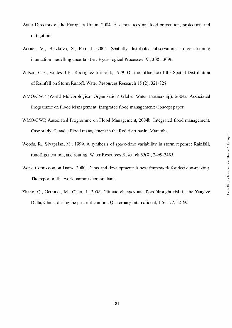
Water Directors of the European Union, 2004. Best practices on flood prevention, protection and
mitigation.
Werner, M., Blazkova, S., Petr, J., 2005. Spatially distributed observations in constraining
inundation modelling uncertainties. Hydrological Processes 19 , 3081-3096.
Wilson, C.B., Valdes, J.B., Rodriguez-Iturbe, I., 1979. On the influence of the Spatial Distribution
of Rainfall on Storm Runoff. Water Resources Research 15 (2), 321-328.
WMO/GWP (World Meteorological Organisation/ Global Water Partnership), 2004a. Associated
Programme on Flood Management. Integrated flood management: Concept paper.
WMO/GWP, Associated Programme on Flood Management, 2004b. Integrated flood management.
Case study, Canada: Flood management in the Red river basin, Manitoba.
Woods, R., Sivapalan, M., 1999. A synthesis of space-time variability in storm reponse: Rainfall,
runoff generation, and routing. Water Resources Research 35(8), 2469-2485.
World Comission on Dams, 2000. Dams and development: A new framework for decision-making.
The report of the world commission on dams
Zhang, Q., Gemmer, M., Chen, J., 2008. Climate changes and flood/drought risk in the Yangtze
Delta, China, during the past millennium. Quaternary International, 176-177, 62-69.
181
Cem
OA
: ar
chiv
e ou
verte
d'Ir
stea
/ C
emag
ref

8 APPENDIX
Cem
OA
: ar
chiv
e ou
verte
d'Ir
stea
/ C
emag
ref
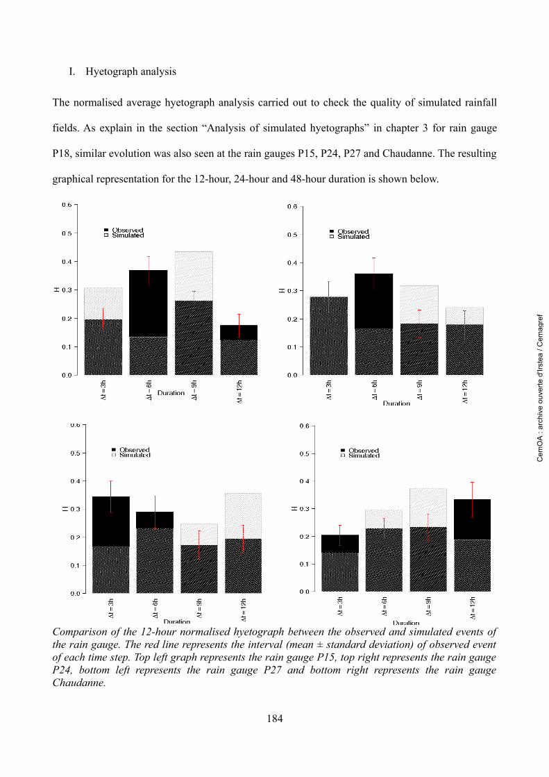
I. Hyetograph analysis
The normalised average hyetograph analysis carried out to check the quality of simulated rainfall
fields. As explain in the section “Analysis of simulated hyetographs” in chapter 3 for rain gauge
P18, similar evolution was also seen at the rain gauges P15, P24, P27 and Chaudanne. The resulting
graphical representation for the 12-hour, 24-hour and 48-hour duration is shown below.
Comparison of the 12-hour normalised hyetograph between the observed and simulated events of the rain gauge. The red line represents the interval (mean ± standard deviation) of observed event of each time step. Top left graph represents the rain gauge P15, top right represents the rain gauge P24, bottom left represents the rain gauge P27 and bottom right represents the rain gauge Chaudanne.
184
Cem
OA
: ar
chiv
e ou
verte
d'Ir
stea
/ C
emag
ref
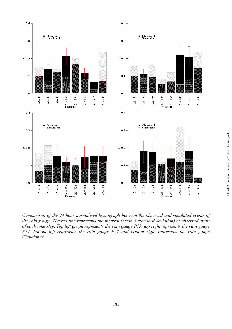
Comparison of the 24-hour normalised hyetograph between the observed and simulated events of the rain gauge. The red line represents the interval (mean ± standard deviation) of observed event of each time step. Top left graph represents the rain gauge P15, top right represents the rain gauge P24, bottom left represents the rain gauge P27 and bottom right represents the rain gauge Chaudanne.
185
Cem
OA
: ar
chiv
e ou
verte
d'Ir
stea
/ C
emag
ref
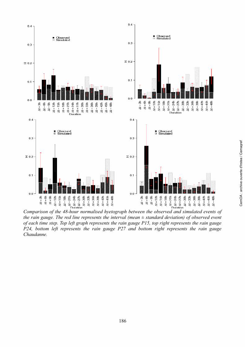
Comparison of the 48-hour normalised hyetograph between the observed and simulated events of the rain gauge. The red line represents the interval (mean ± standard deviation) of observed event of each time step. Top left graph represents the rain gauge P15, top right represents the rain gauge P24, bottom left represents the rain gauge P27 and bottom right represents the rain gauge Chaudanne.
186
Cem
OA
: ar
chiv
e ou
verte
d'Ir
stea
/ C
emag
ref
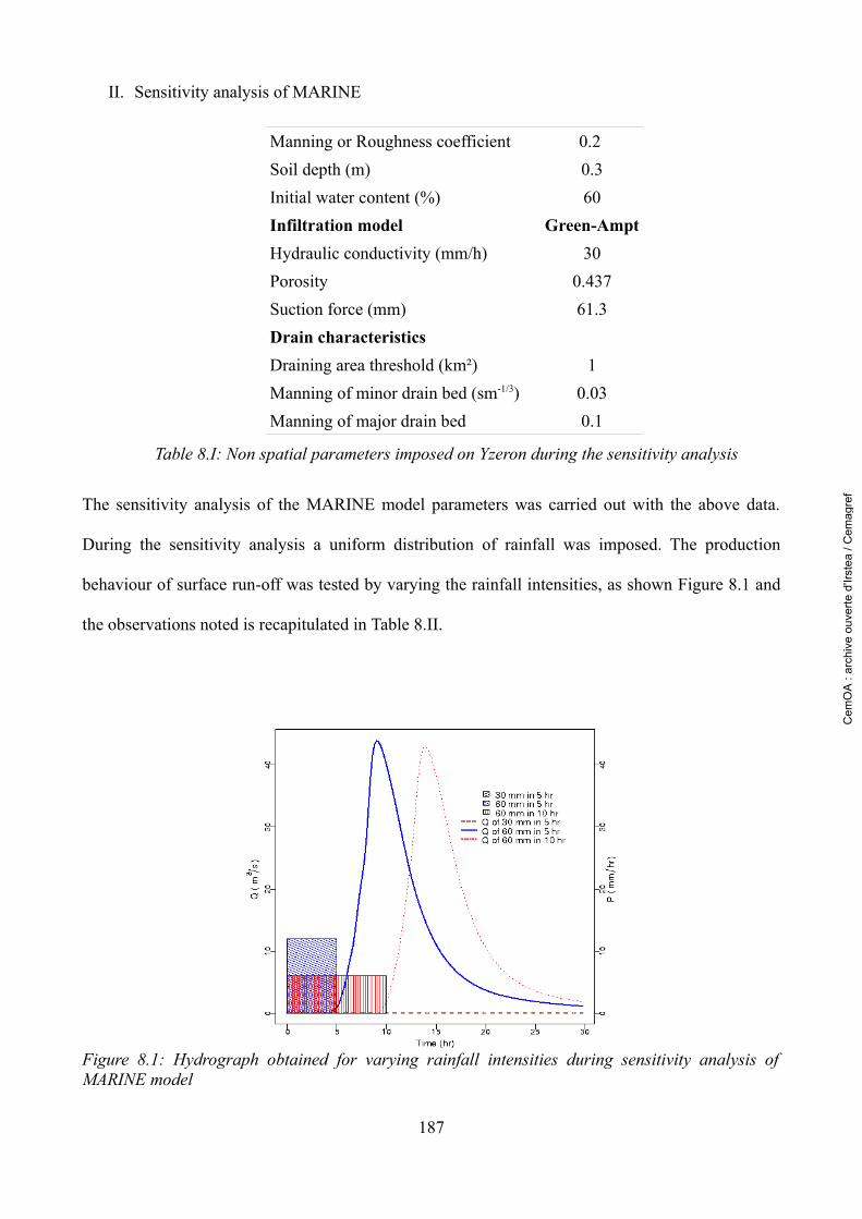
II. Sensitivity analysis of MARINE
The sensitivity analysis of the MARINE model parameters was carried out with the above data.
During the sensitivity analysis a uniform distribution of rainfall was imposed. The production
behaviour of surface run-off was tested by varying the rainfall intensities, as shown Figure 8.1 and
the observations noted is recapitulated in Table 8.II.
187
Manning or Roughness coefficient 0.2 Soil depth (m) 0.3Initial water content (%) 60Infiltration model Green-AmptHydraulic conductivity (mm/h) 30Porosity 0.437Suction force (mm) 61.3Drain characteristicsDraining area threshold (km²) 1Manning of minor drain bed (sm-1/3) 0.03Manning of major drain bed 0.1
Table 8.I: Non spatial parameters imposed on Yzeron during the sensitivity analysis
Figure 8.1: Hydrograph obtained for varying rainfall intensities during sensitivity analysis of MARINE model
Cem
OA
: ar
chiv
e ou
verte
d'Ir
stea
/ C
emag
ref
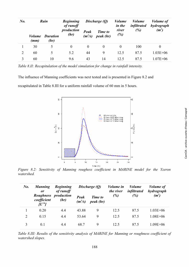
The influence of Manning coefficients was next tested and is presented in Figure 8.2 and
recapitulated in Table 8.III for a uniform rainfall volume of 60 mm in 5 hours.
188
No. Rain
Volume (mm)
Duration (hr)
Beginning of runoff
production (hr)
Discharge (Q)
Peak (m3/s)
Time to peak (hr)
Volume in the river(%)
Volume infiltrated
(%)
Volume of hydrograph
(m3)
1 30 5 0 0 0 0 100 02 60 5 5.2 44 9 12.5 87.5 1.03E+063 60 10 9.6 43 14 12.5 87.5 1.07E+06
Table 8.II: Recapitulation of the model simulation for change in rainfall intensity.
No. Manning or
Roughness coefficient
[L1/6]
Beginning of runoff
production (hr)
Discharge (Q)
Peak (m3/s)
Time to peak (hr)
Volume in the river
(%)
Volume infiltrated
(%)
Volume of hydrograph
(m3)
1 0.20 4.4 43.88 9 12.5 87.5 1.03E+062 0.15 4.4 53.64 9 12.5 87.5 1.08E+06
3 0.1 4.4 68.7 9 12.5 87.5 1.09E+06
Table 8.III: Results of the sensitivity analysis of MARINE for Manning or roughness coefficient of watershed slopes.
Figure 8.2: Sensitivity of Manning roughess coefficient in MARINE model for the Yzeron watershed.
Cem
OA
: ar
chiv
e ou
verte
d'Ir
stea
/ C
emag
ref
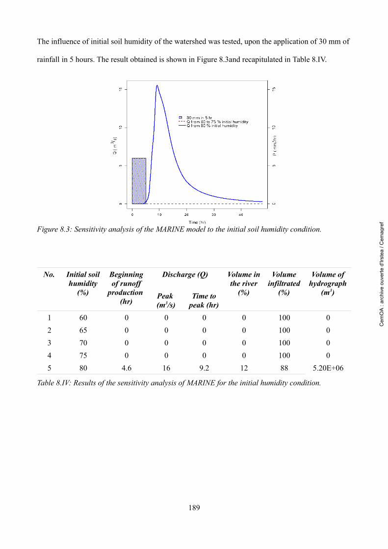
The influence of initial soil humidity of the watershed was tested, upon the application of 30 mm of
rainfall in 5 hours. The result obtained is shown in Figure 8.3and recapitulated in Table 8.IV.
189
No. Initial soil humidity
(%)
Beginning of runoff
production (hr)
Discharge (Q)
Peak (m3/s)
Time to peak (hr)
Volume in the river
(%)
Volume infiltrated
(%)
Volume of hydrograph
(m3)
1 60 0 0 0 0 100 02 65 0 0 0 0 100 03 70 0 0 0 0 100 04 75 0 0 0 0 100 05 80 4.6 16 9.2 12 88 5.20E+06
Table 8.IV: Results of the sensitivity analysis of MARINE for the initial humidity condition.
Figure 8.3: Sensitivity analysis of the MARINE model to the initial soil humidity condition.
Cem
OA
: ar
chiv
e ou
verte
d'Ir
stea
/ C
emag
ref
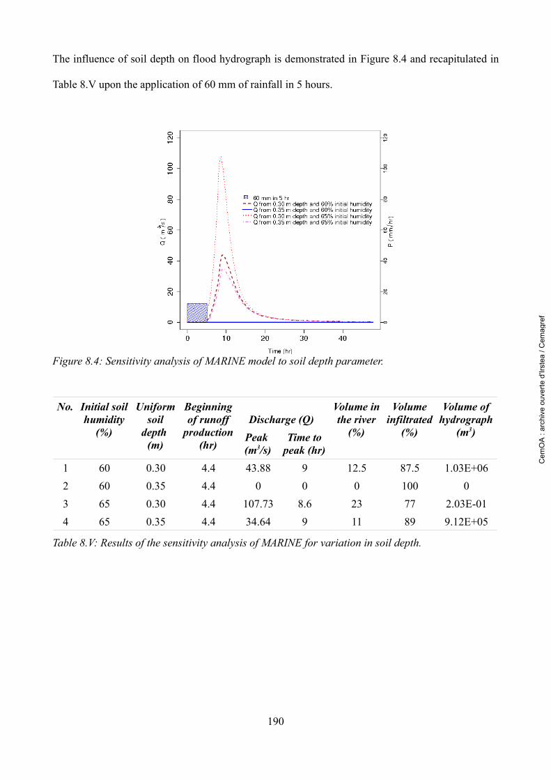
The influence of soil depth on flood hydrograph is demonstrated in Figure 8.4 and recapitulated in
Table 8.V upon the application of 60 mm of rainfall in 5 hours.
190
Figure 8.4: Sensitivity analysis of MARINE model to soil depth parameter.
No. Initial soil humidity
(%)
Uniform soil
depth (m)
Beginning of runoff
production (hr)
Discharge (Q) Peak (m3/s)
Time to peak (hr)
Volume in the river
(%)
Volume infiltrated
(%)
Volume of hydrograph
(m3)
1 60 0.30 4.4 43.88 9 12.5 87.5 1.03E+062 60 0.35 4.4 0 0 0 100 03 65 0.30 4.4 107.73 8.6 23 77 2.03E-014 65 0.35 4.4 34.64 9 11 89 9.12E+05
Table 8.V: Results of the sensitivity analysis of MARINE for variation in soil depth.C
emO
A :
arch
ive
ouve
rte d
'Irst
ea /
Cem
agre
f
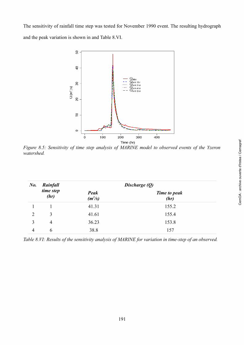
The sensitivity of rainfall time step was tested for November 1990 event. The resulting hydrograph
and the peak variation is shown in and Table 8.VI.
191
No. Rainfall time step
(hr)
Discharge (Q) Peak (m3/s)
Time to peak (hr)
1 1 41.31 155.22 3 41.61 155.43 4 36.23 153.84 6 38.8 157
Table 8.VI: Results of the sensitivity analysis of MARINE for variation in time-step of an observed.
Figure 8.5: Sensitivity of time step analysis of MARINE model to observed events of the Yzeron watershed.
Cem
OA
: ar
chiv
e ou
verte
d'Ir
stea
/ C
emag
ref
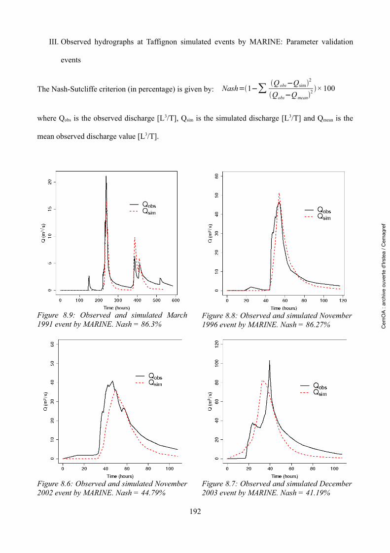
III. Observed hydrographs at Taffignon simulated events by MARINE: Parameter validation
events
The Nash-Sutcliffe criterion (in percentage) is given by: Nash=1−∑ Qobs−Qsim2
Qobs−Qmean2 ×100
where Qobs is the observed discharge [L3/T], Qsim is the simulated discharge [L3/T] and Qmean is the
mean observed discharge value [L3/T].
192
Figure 8.7: Observed and simulated December 2003 event by MARINE. Nash = 41.19%
Figure 8.8: Observed and simulated November 1996 event by MARINE. Nash = 86.27%
Figure 8.9: Observed and simulated March 1991 event by MARINE. Nash = 86.3%
Figure 8.6: Observed and simulated November 2002 event by MARINE. Nash = 44.79%
Cem
OA
: ar
chiv
e ou
verte
d'Ir
stea
/ C
emag
ref
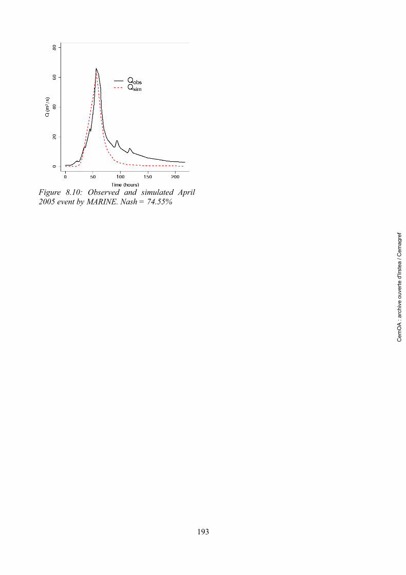
193
Figure 8.10: Observed and simulated April 2005 event by MARINE. Nash = 74.55%
Cem
OA
: ar
chiv
e ou
verte
d'Ir
stea
/ C
emag
ref
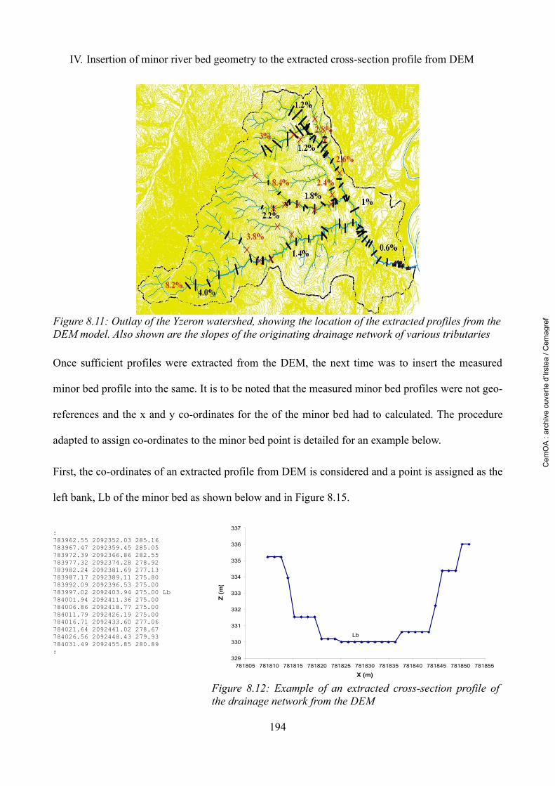
IV. Insertion of minor river bed geometry to the extracted cross-section profile from DEM
Once sufficient profiles were extracted from the DEM, the next time was to insert the measured
minor bed profile into the same. It is to be noted that the measured minor bed profiles were not geo-
references and the x and y co-ordinates for the of the minor bed had to calculated. The procedure
adapted to assign co-ordinates to the minor bed point is detailed for an example below.
First, the co-ordinates of an extracted profile from DEM is considered and a point is assigned as the
left bank, Lb of the minor bed as shown below and in Figure 8.15.
: 783962.55 2092352.03 285.16 783967.47 2092359.45 285.05 783972.39 2092366.86 282.55 783977.32 2092374.28 278.92 783982.24 2092381.69 277.13 783987.17 2092389.11 275.80 783992.09 2092396.53 275.00 783997.02 2092403.94 275.00 Lb 784001.94 2092411.36 275.00 784006.86 2092418.77 275.00 784011.79 2092426.19 275.00 784016.71 2092433.60 277.06 784021.64 2092441.02 278.67 784026.56 2092448.43 279.93 784031.49 2092455.85 280.89 :
194
Figure 8.12: Example of an extracted cross-section profile of the drainage network from the DEM
Figure 8.11: Outlay of the Yzeron watershed, showing the location of the extracted profiles from the DEM model. Also shown are the slopes of the originating drainage network of various tributaries
329
330
331
332
333
334
335
336
337
781805 781810 781815 781820 781825 781830 781835 781840 781845 781850 781855
X (m)
Z (m
)
Lb
Cem
OA
: ar
chiv
e ou
verte
d'Ir
stea
/ C
emag
ref
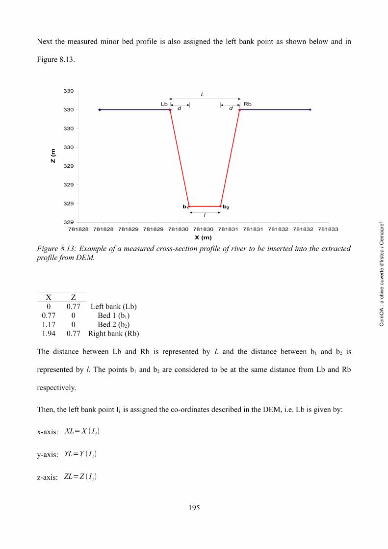
Next the measured minor bed profile is also assigned the left bank point as shown below and in
Figure 8.13.
X Z0 0.77 Left bank (Lb)
0.77 0 Bed 1 (b1)1.17 0 Bed 2 (b2)1.94 0.77 Right bank (Rb)
The distance between Lb and Rb is represented by L and the distance between b1 and b2 is
represented by l. The points b1 and b2 are considered to be at the same distance from Lb and Rb
respectively.
Then, the left bank point Ii is assigned the co-ordinates described in the DEM, i.e. Lb is given by:
x-axis: XL=X I i
y-axis: YL=Y I i
z-axis: ZL=Z I i
195
Figure 8.13: Example of a measured cross-section profile of river to be inserted into the extracted profile from DEM.
329
329
329
329
330
330
330
330
781828 781828 781829 781829 781830 781830 781831 781831 781832 781832 781833
X (m)
Z (
m)
Lb Rb
b1 b2
L
l
d d
Cem
OA
: ar
chiv
e ou
verte
d'Ir
stea
/ C
emag
ref
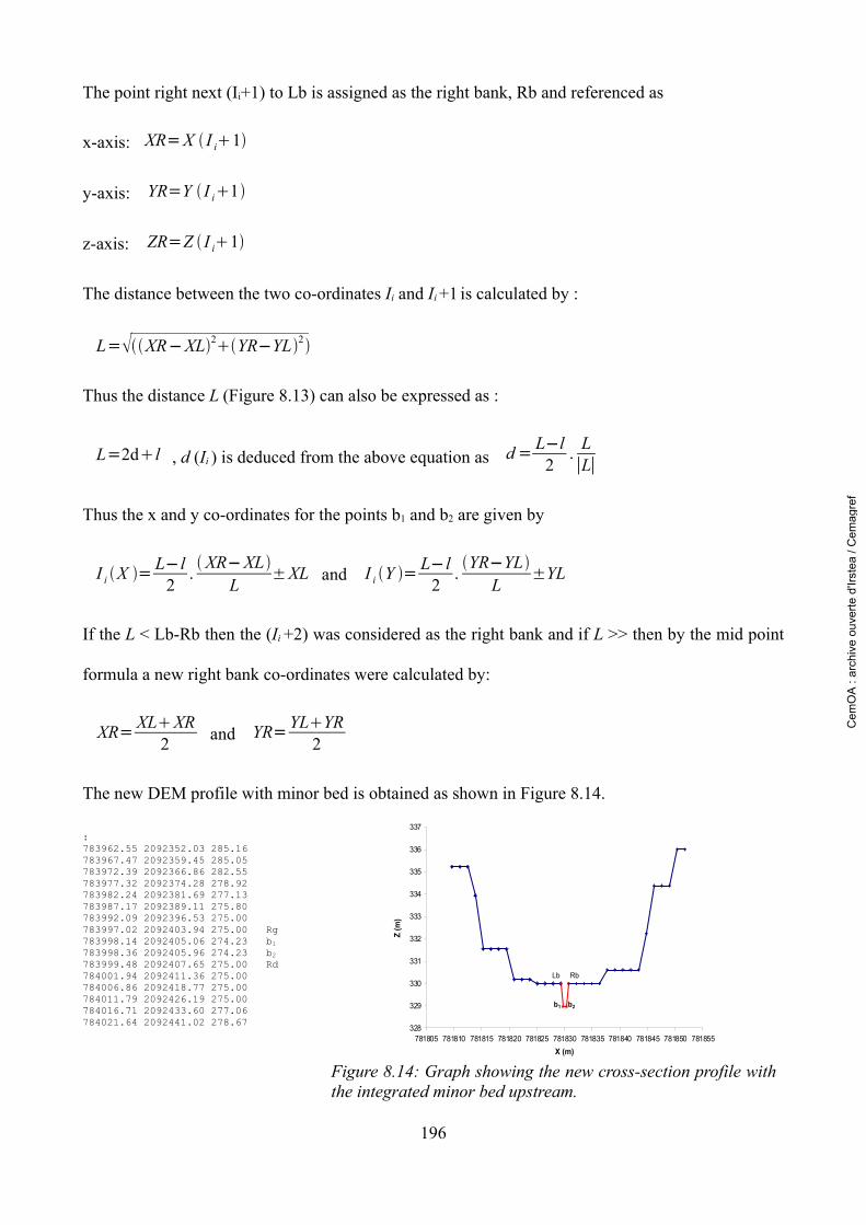
The point right next (Ii+1) to Lb is assigned as the right bank, Rb and referenced as
x-axis: XR=X I i1
y-axis: YR=Y I i1
z-axis: ZR=Z I i1
The distance between the two co-ordinates Ii and Ii +1 is calculated by :
L=XR−XL2YR−YL2
Thus the distance L (Figure 8.13) can also be expressed as :
L=2dl , d (Ii ) is deduced from the above equation as d = L−l2
. L∣L∣
Thus the x and y co-ordinates for the points b1 and b2 are given by
I i X = L−l2
. XR−XLL
±XL and I i Y = L−l2
. YR−YLL
±YL
If the L < Lb-Rb then the (Ii +2) was considered as the right bank and if L >> then by the mid point
formula a new right bank co-ordinates were calculated by:
XR= XLXR2 and YR=YLYR
2
The new DEM profile with minor bed is obtained as shown in Figure 8.14.
: 783962.55 2092352.03 285.16 783967.47 2092359.45 285.05 783972.39 2092366.86 282.55 783977.32 2092374.28 278.92 783982.24 2092381.69 277.13 783987.17 2092389.11 275.80 783992.09 2092396.53 275.00 783997.02 2092403.94 275.00 Rg 783998.14 2092405.06 274.23 b1 783998.36 2092405.96 274.23 b2 783999.48 2092407.65 275.00 Rd 784001.94 2092411.36 275.00 784006.86 2092418.77 275.00 784011.79 2092426.19 275.00 784016.71 2092433.60 277.06 784021.64 2092441.02 278.67
196
Figure 8.14: Graph showing the new cross-section profile with the integrated minor bed upstream.
328
329
330
331
332
333
334
335
336
337
781805 781810 781815 781820 781825 781830 781835 781840 781845 781850 781855X (m)
Z (m
)
Lb Rb
b1 b2
Cem
OA
: ar
chiv
e ou
verte
d'Ir
stea
/ C
emag
ref

V. Example of smoothening effect tested on the simulated rainfall fields
Illustration of two rainfall events of 12-hour and 48-hour duration rendered stratified with the
defined in equation 4.11.
197
Figure 8.15: An attempt to stratify a 12-hour (Top) and a 48-hour (bottom) simulated rainfall fields with stratification factor α, of 0.75 and 0.5 respectively.
Cem
OA
: ar
chiv
e ou
verte
d'Ir
stea
/ C
emag
ref