finding the most suitable irrigation dams for hydropower ...

FINDING THE MOST SUITABLE IRRIGATION DAMS FOR

HYDROPOWER DEVELOPMENT BY USING GIS TOOLS

A THESIS SUBMITTED TO

THE GRADUATE SCHOOL OF NATURAL AND APPLIED

SCIENCES OF ÇANKAYA UNIVERSITY

BY

OMAR AL BAYATI

IN PARTIAL FULFILLMENT OF THE REQUIREMENTS

FOR

THE DEGREE OF MASTER OF SCIENCE

IN

INFORMATION TECHNOLOGY

JANUARY 2020

iv

ABSTRACT

FINDING THE MOST SUITABLE IRRIGATION DAMS FOR

HYDROPOWER DEVELOPMENT BY USING GIS TOOLS

Al BAYATI, Omar

M.Sc., Department of Computer Engineering

Supervisor: Assoc.Prof. Dr. H. Hakan MARAŞ

Co-Supervisor: Prof. Dr. Serhat KÜÇÜKALİ

January 2020, 136 pages

This thesis aims to find the most suitable irrigation dams for hydropower development in

Turkey to provide clean energy from an available resource by assessing on technical, spatial,

and environmental criteria. The selected dams are arranged based on their suitability scores

into three categories (high, medium and low) using a multi-criteria fuzzy logic tool that

calculates the score separately for each criterion and then aggregates them into an overall

suitability score. Six criteria are assessed: normal water level, reservoir storage capacity,

dam purpose, years in operation, nearest substation distance and environment impact

assessment requirement. The criterion of nearest substation distance was used to ensure that

the benefits of potential power are consistent with the cost of grid connection. A

methodology for finding best grid connection path is presented based on a multi-criteria

geographic information system (GIS) spatial analyst to achieve the least cost, lowest power

losses and lowest environmental impact. Two dams are chosen as case studies, Karadere and

Karaçomak. For these dams, technical and spatial criteria are evaluated and the potential

power and economic benefits are estimated. A least cost path methodology is applied to find

the best grid connection path for each of those dams to their nearest substations.

Keywords: Hydropower, Grid Connection, Fuzzy logic, GIS.

v

ÖZ

HİDROELEKTRİK ENERJİ ÜRETİMİ İÇİN EN UYGUN TARIMSAL

SULAMA BARAJLARININ CBS YÖNTEMİ İLE BULUNMASI

Al BAYATI, Omar

Yüksek Lisans, Bilgisayar Mühendisliği Bölümü

Tez Yöneticisi: Doç. Dr. H. Hakan MARAŞ

Ortak Tez Yôneticisi: Prof. Dr. Serhat KÜÇÜKALİ

Ocak 2020, 136 sayfa

Bu tezde, Türkiye'de hidroelektrik gelişimi için en uygun sulama barajların bulunması

hedeflenmiştir. Teknik, mekansal ve çevresel kriterleri değerlendirerek mevcut sulama

barajlarından temiz enerji temin edilmesi amaçlanmıştır. Seçilen barajlar daha sonra

uygunluk endekslerine göre üç kategoriye ayrılmıştır: yüksek, orta ve düşük. Her kriterinin

uygunluğunun ayrı ayrı hesaplayan ve daha sonra bunları Genel Uygunluk Endeksine göre

bir araya getiren bulanık mantık aracı kullanılmıştır. Altı kriter değerlendirilmiştir: rezervuar

ortalama su düşüm yüksekliği, rezervuar hacmi, barajın amacı, baraj yaşı, en yakın trafo

merkezine mesafesi ve çevre etki değerlendirme için enerji nakil hattı mesafesi. En iyi

şebeke bağlantı yolunu bulmak için en düşük maliyet, en düşük güç kaybı ve en az çevresel

etkisini elde etmek için çok kriterli CBS mekansal analiz yöntemi sunulmuştur. Örnek

çalışma için iki baraj seçildi: Karadere ve Karaçomak. Bu barajlar için teknik ve mekansal

kriterler değerlendirilmiş, ayrıca potansiyel güç ve ekonomik faydalar tahmin edilmiştir. Ek

olarak, bu barajların her biri için en yakın trafo merkezine en iyi şebeke bağlantı yolunu

bulmak için en uygun güzergah metodolojisi uygulanmıştır.

Anahtar Kelimeleri: Hidroelektrik, Şebeke bağlantısı, Bulanık mantık, CBS.

vi

ACKNOWLEDGEMENTS

The author wishes to express his deepest gratitude to his supervisor Assoc.Prof. Dr. H.

Hakan MARAŞ and co-supervisor Prof. Dr. Serhat KÜÇÜKALİ for their guidance, advice,

criticism, encouragements and insight throughout the research.

It is a pleasure to express my special thanks to my family, friends and Çankaya university

staff for their valuable support.

vii

TABLE OF CONTENTS

STATEMENT OF NON PLAGIARISM …………………………………………………. iii

ABSTRACT…………………………… ……………………………………………….… iv

ÖZ…………………………………………………………………………………………. v

ACKNOWLEDGMENTS………………………………………………………………… vi

TABLE OF CONTENTS…………………………………………………………………. vii

LIST OF FIGURES……………………………………………………………………….. x

LIST OF TABLES………………………………………………………………………... xv

LIST OF ABBREVIATIONS…………………………………………………………….. xvi

CHAPTERS:

1. INTRODUCTION.………………………………...…………………………………… 1

1.1. Background……………………………………………………………… 2

1.2. Objectives.……………………………………………………………….. 4

1.3. Organization of the Thesis.......................................................................... 4

2. TECHNICAL AND SPATIAL CRITERIA USED TO SELECT THE MOST SUITABLE

DAMS AND POWER SUBSTATIONS.............................................................................. 6

2.1. Building the Geographical Database.......................................................... 6

2.2. Determination of criteria…………………………………………………. 8

2.2.1. Dams Criteria for Best Hydropower Generation (Technical

Criteria)............................................................................ 8

2.2.2. Substations Criteria for Electrical Power Transmission

(Technical Criteria) ......................................................... 12

2.2.3. Maximum Distance to Nearest Substation (Spatial Criteria)

.......................................................................................... 14

2.3. Geodatabase Filtering of Criteria and Spatial Analyst Results…………... 16

viii

3. USE OF MULTI-CRITERIA FUZZY LOGIC FOR DAMS SUITABILITY

SCORING...............................................................................................................................25

3.1. Introduction...................................................................................................25

3.2. Multi-Criteria Decision Making with Fuzzy Logic......................................25

3.2.1. Determination of Criteria....................................................26

3.2.2. Fuzzy Logic Methodology for Suitability Scoring.............33

3.3. Results of Suitability Scoring.......................................................................34

4. METHODOLOGY FOR FINDING BEST GRID CONNECTION PATH USING GIS

MULTI-CRITERIA SPATIAL ANALYST TOOLS.............................................................36

4.1. Introduction...................................................................................................36

4.2. Multi-Criteria Spatial Analyst.......................................................................36

4.3. Methodology for Finding Best Grid Connection Path..................................37

4.3.1. Evaluation of Shortest Distance Criterion..........................38

4.3.2. Evaluation of Elevation and Slope Criteria........................39

4.3.3. Evaluation of Near to Roads and Current Power Lines

Criteria................................................................................41

4.3.4. Evaluation of Land Use Criterion.......................................44

4.3.5. Combining the Reclassified Raster Layers of the Criteria

(Creating a Cost Layer)..................................................... .50

4.3.6. Creating the Layers of Least Cost Distance and Least Cost

Direction.............................................................................51

4.3.7. Creating the Least Cost Path Raster Layer (Best Path)..... .52

4.3.8. Converting Best Path Raster to Vector Feature Class........54

4.3.9. Projecting the Best Path Line Vector onto a 3D Surface....54

4.4. Multi-Criteria Spatial Analyst Modeling Using Model Builder...................55

5. CASE STUDIES.................................................................................................................57

5.1. Karadere Dam...............................................................................................58

5.1.1. Karadere Dam's Technical Criteria.....................................60

5.1.2. Nearest Substation to Karadere Dam..................................62

5.1.3. Suitability Score of Karadere Dam.....................................63

5.1.4. Best Grid Connection Path (Least Cost Path) from Karadere

Dam to its Nearest Substation.............................................69

5.2. Karaçomak Dam...........................................................................................82

ix

5.2.1. Karaçomak Dam's Technical Criteria.................................84

5.2.2. Nearest Substation to Karaçomak Dam..............................85

5.2.3. Suitability Score of Karaçomak Dam.................................86

5.2.4. Best Grid Connection Path (Least Cost Path) from

Karaçomak Dam to its Nearest Substation.........................91

6. CONCLUSION.................................................................................................................106

6.1. Conclusion...................................................................................................106

6.2. Discussion...................................................................................................110

6.3. Recommendations.......................................................................................111

REFERENCES......................................................................................................................112

APPENDICES:

A. MULTI-CRITERIA HIGH SUITABILITY SCORE DAMS.............................118

B. MULTI-CRITERIA MEDIUM SUITABILITY SCORE DAMS.......................121

C. MULTI-CRITERIA LOW SUITABILITY SCORE DAMS..............................130

CURRICULUM VITAE.......................................................................................................137

x

LIST OF FIGURES

FIGURES

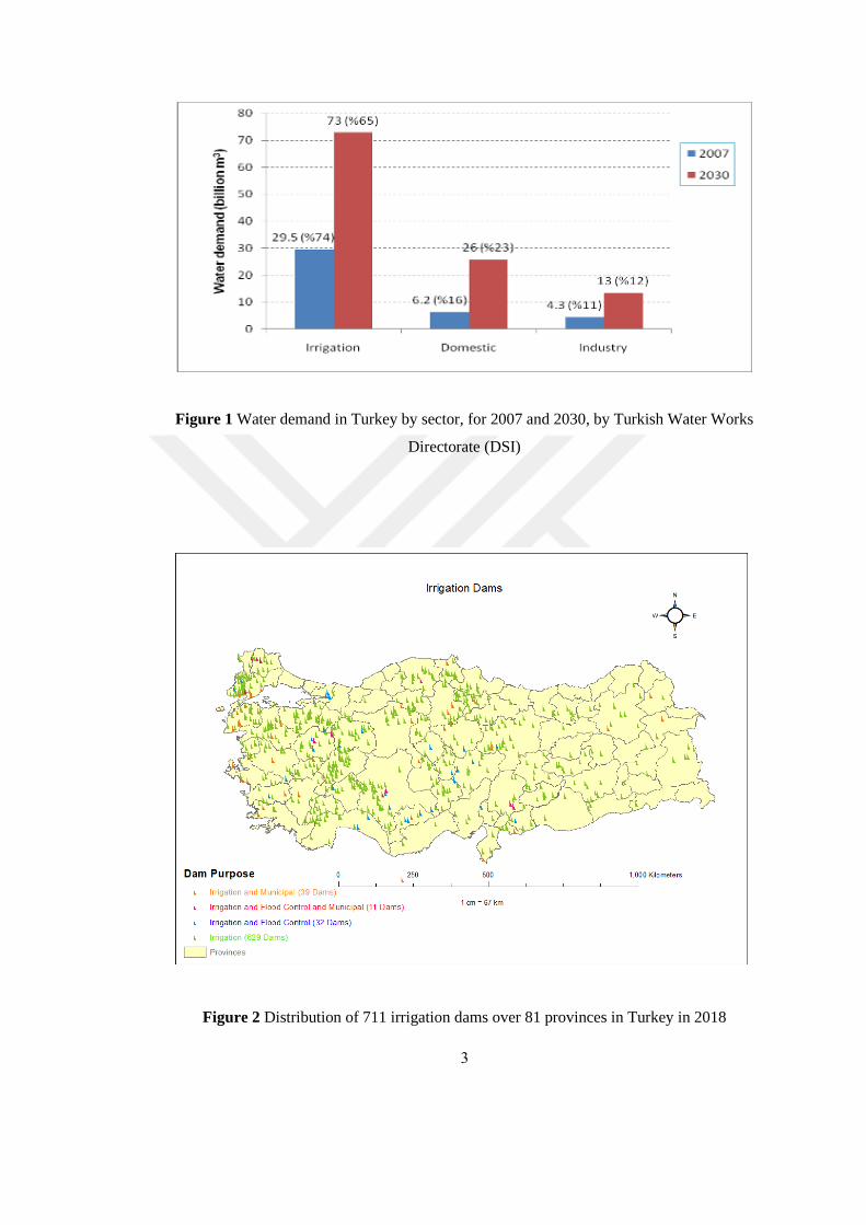
Figure 1 Water demand in Turkey by sector, for 2007 and 2030.............................................3

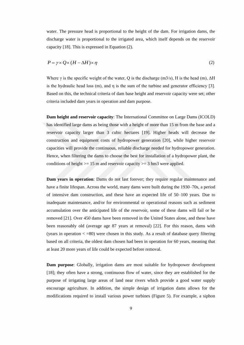
Figure 2 Distribution of 711 irrigation dams over 81 provinces in Turkey in 2018................3

Figure 3 Distribution of 692 substations over 81 provinces in Turkey in 2018 ................4

Figure 4 Calculation of normal water level from thalweg (head) for Karadere Dam..............7

Figure 5 Simple design of an irrigation dam (Koyunbaba Dam)...........................................10

Figure 6 Siphon Intake turbine...............................................................................................11

Figure 7 Base intake turbine...................................................................................................11

Figure 8 Generation, transmission and distribution grid........................................................13

Figure 9 Percentage of losses from hydropower (100–10000 kW) via 154 kV

transmission lines over distance of 10, 20, 30 and 40 km.......................................16

Figure 10 The selected 265 dams and nearest 183 substations (within 40 km).....................17

Figure 11 Statistics for the criterion of base height for the selected 265 dams......................18

Figure 12 Statistics for the criterion of reservoir capacity for the selected 265 dams...........19

Figure 13 Statistics for the nearest substation distance criterion for the selected 265 dams..20

Figure 14 Statistics for the criterion of years in operation for the selected 265 dams...........21

Figure 15 Statistics for the irrigated area criterion for the selected 265 dams.......................22

Figure 16 Statistics for the normal water level criterion for the selected 265 dams..............23

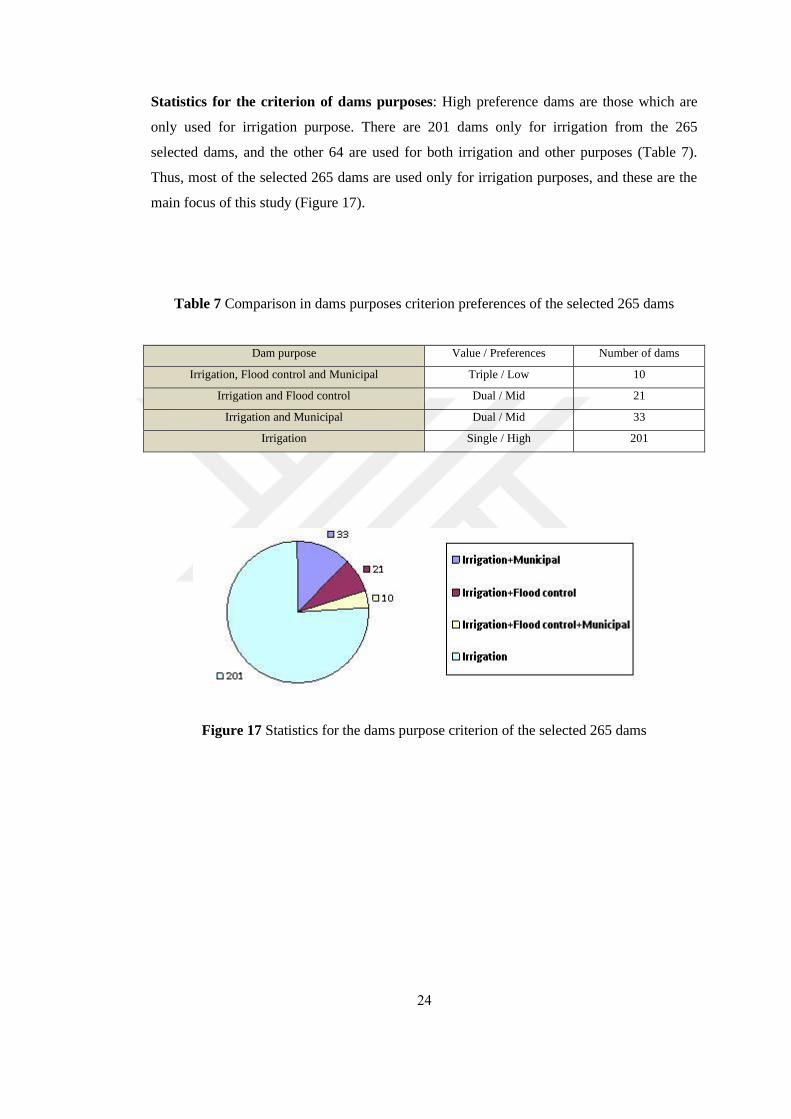
Figure 17 Statistics for the dams purpose criterion of the selected 265 dams.......................24

Figure 18 Evaluation criteria for scoring the suitability of dams...........................................26

Figure 19 Suitability function for nearest substation distance criterion.................................28

Figure 20 Suitability function for EIA requirement criterion................................................29

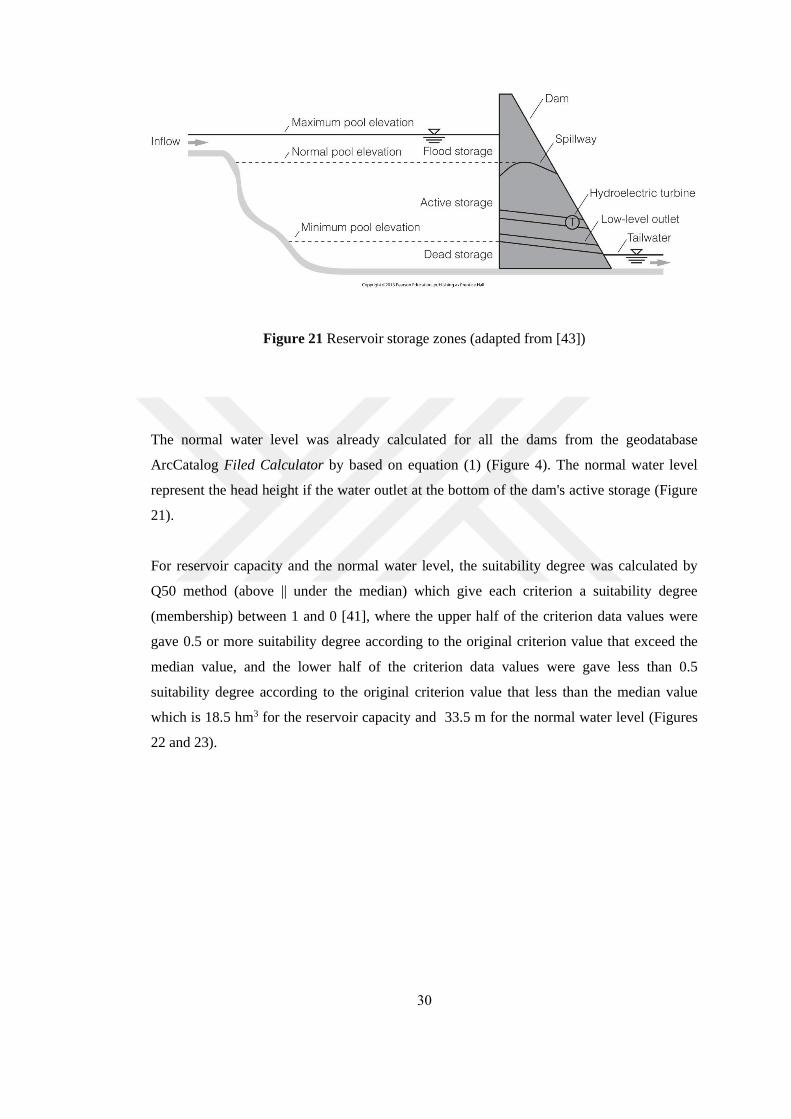
Figure 21 Reservoir storage zones.........................................................................................30

Figure 22 Suitability function for the reservoir capacity criterion.........................................31

Figure 23 Suitability function for the normal water level (head) criterion............................31

Figure 24 Suitability function for dams purpose criterion.....................................................32

xi

Figure 25 Suitability function for the years in operation criterion.........................................33

Figure 26 Distribution of the 265 dams with their suitability class and their

183 nearest substations..........................................................................................34

Figure 27 Reclassification of the criteria and cost raster layers.............................................38

Figure 28 Elevation map of Turkey........................................................................................39

Figure 29 Detailed map of roads in Turkey...........................................................................42

Figure 30 Map of power transmission lines in Turkey..........................................................42

Figure 31 Map of land cover in Turkey.................................................................................45

Figure 32 Statistics for land cover in Turkey and suitability for power lines routing...........50

Figure 33 Creation of the cost layer.......................................................................................51

Figure 34 Generation of cost distance layer and back link layer...........................................52

Figure 35 Derivation of the shortest least cost path...............................................................53

Figure 36 Shortest least cost path over the cost (suitability) layer.........................................53

Figure 37 Converting the least cost path to a vector and visualizing it in 3D format..........54

Figure 38 Virtual view of the best path, dropped onto a 3D satellite imagery scene.............55

Figure 39 Flowchart for processes of finding the cost path using the

Model Builder tool................................................................................................56

Figure 40 Top view of Karadere Dam and its lake, in Kastamonu Province.........................59

Figure 41 Karadere Dam, body and spillway.........................................................................59

Figure 42 Hydropower calculator at power-calculation.com: data for Karadere Dam..........61

Figure 43 Top view of Taşköprü Substation..........................................................................63

Figure 44 Suitability function for reservoir capacity, Karadere Dam....................................64

Figure 45 Suitability function for normal water level, Karadere Dam...................................65

Figure 46 Suitability function for dam purpose, Karadere Dam............................................66

Figure 47 Suitability function for years in operation, Karedere Dam....................................67

Figure 48 Suitability function for nearest substation distance, Karadere Dam......................67

Figure 49 Suitability function for EIA requirement, Karedere Dam......................................68

Figure 50 Karadere Dam and its nearest substation (Taşköprü) on a map of Turkey............69

Figure 51 Straight-line distance (12.07 km) between Karadere Dam and

Taşköprü Substation..............................................................................................70

Figure 52 Extent of spatial reference satellite imagery for Karadere Dam and

Taşköprü Substation feature classes.......................................................................71

Figure 53 Elevation raster layer for the extent between Karadere Dam and


xii

Figure 54 Slope raster layer for the extent between Karadere Dam and


Figure 55 Reclassified slope raster layer for the extent between Karadere Dam and

Taşköprü Substation.............................................................................................73

Figure 56 Feature classes for roads and power lines, for the extent between Karadere

Dam and Taşköprü Substation..............................................................................74

Figure 57 Raster layer representing near to roads for the extent between Karadere Dam

and Taşköprü Substation.......................................................................................75

Figure 58 Raster layer representing near to existing power lines for the extent

between Karadere Dam and Taşköprü Substation................................................75

Figure 59 Reclassified raster layer for near to roads for the extent between Karadere

Dam and Taşköprü Substation.............................................................................76

Figure 60 Reclassified raster layer for near to power lines for the extent between

Karadere Dam and Taşköprü Substation...............................................................76

Figure 61 Land use feature class map for the extent between Karadere Dam and


Figure 62 Land use raster layer for the Extent between Karadere Dam and


Figure 63 Reclassified land use raster layer for the extent between Karadere Dam

and Taşköprü Substation......................................................................................78

Figure 64 Cost raster (suitability layer) for the extent between Karadere Dam and

Taşköprü Substation.............................................................................................79

Figure 65 Cost distance raster layer for the extent between Karadere Dam and


Figure 66 Back link raster layer for the extent between Karadere Dam and


Figure 67 Least cost path (best Path) for grid connection between Karadere and

Taşköprü Substation (12.789 km).........................................................................81

Figure 68 3D view of the best path between Karadere Dam and Taşköprü

Substation.............................................................................................................82

Figure 69 Top view of Karaçomak Dam and its lake in Kastamonu province......................83

Figure 70 Karaçomak Dam and its lake.................................................................................83

Figure 71 Top view of Kastamonu Substation.......................................................................85

Figure 72 Suitability function for reservoir capacity, Karaçomak Dam................................87

Figure 73 Suitability function for normal water level, Karaçomak Dam...............................87

xiii

Figure 74 Suitability function for dam purpose, Karaçomak Dam........................................88

Figure 75 Suitability function for years in operation, Karaçomak Dam................................89

Figure 76 Suitability function for nearest substation distance, Karaçomak Dam..................89

Figure 77 Suitability function for EIA requirement, Karaçomak Dam..................................90

Figure 78 Karaçomak Dam and its nearest substation (Kastamonu) on a map

of Turkey...............................................................................................................92

Figure 79 Straight line distance (8.56 km) between Karaçomak Dam and

Kastamonu Substation...........................................................................................92

Figure 80 Extent of spatial reference satellite imagery for Karaçomak Dam and

Kastamonu Substation feature classes..................................................................93

Figure 81 Elevation raster layer for the extent between Karaçomak Dam and

Kastamonu Substation..........................................................................................94

Figure 82 Slope raster layer for the extent between Karaçomak Dam and


Figure 83 Reclassified slope raster layer for the extent between Karaçomak Dam

and Kastamonu Substation...................................................................................96

Figure 84 Roads feature class for the extent between Karaçomak Dam and


Figure 85 Raster layer representing near to roads for the extent between Karaçomak Dam

and Kastamonu Substation....................................................................................98

Figure 86 Reclassified raster layer for near to roads for the Extent between

Karaçomak Dam and Kastamonu Substation.......................................................99

Figure 87 Land use raster for the extent between Karaçomak Dam and

Kastamonu Substation.........................................................................................100

Figure 88 Reclassified land use raster for the extent between Karaçomak Dam

and Kastamonu Substation..................................................................................101

Figure 89 Cost raster (suitability layer) for the extent between Karaçomak Dam

and Kastamonu Substation...................................................................................102

Figure 90 Cost distance raster layer for the extent between Karaçomak Dam and


Figure 91 Back link raster layer for the extent between Karaçomak Dam and


Figure 92 Least cost path (best path) for grid connection between Karaçomak Dam

and Kastamonu Substation (8.607 km)..................................... .........................104

xiv

Figure 93 3D view of the best path between Karaçomak Dam and

Kastamonu Substation........................................................................................105

Figure 94 Conclusions and structure of the thesis................................................................109

Figure 95 High suitability 21 dams......................................................................................120

Figure 96 Medium suitability 149 dams...............................................................................129

Figure 97 Low suitability 95 dams.......................................................................................136

xv

LIST OF TABLES

TABLES

Table 1 Comparison in base height preference criterion of the selected 265 dams with

their other criteria statistical indicators.....................................................................18

Table 2 Comparison in reservoir capacity criterion of the selected 265 dams with their

other criteria statistical indicators.............................................................................19

Table 3 Comparison in nearest substation distance of the selected 265 dams with their


Table 4 Comparison in years in operation criterion of the selected 265 dams with their


Table 5 Comparison in irrigated area criterion of the selected 265 dams with their other

criteria statistical indicators.......................................................................................22

Table 6 Comparison in reservoir capacity criterion of the selected 265 dams with their


Table 7 Comparison in dams purposes criterion preferences of the selected 265 dams........24

Table 8 Recognition of linear features....................................................................................43

Table 9 Recognition for land use classes................................................................................48

Table 10 2018 and 2019 Reservoir status of several dams in Turkey....................................60

Table 11 Stream flow in m3/s for calculation of hydropower................................................61

Table 12 High suitability class: 21 dams had a suitability score

of between 75% and 87%......................................................................................................118

Table 13 Medium suitability class: 149 dams had a suitability score

of between 50% and 74.99%................................................................................121

Table 14 Low suitability class: 95 dams had a suitability score

of between 27% and 49.9%...................................................................................130

xvi

LIST OF ABBREVIATIONS

GIS Geographic Information System

Mha Million Hectares

DSI General Directorate of State Hydraulic Works of Turkey (Devlet Su İşleri)

ESRI Environmental Systems Research Institute

WGS World Geodetic System

NWL Normal Water Level (Head)

PDF Portable Document Format

KMZ Keyhole Markup language Zipped

TEİAŞ Turkey Electricity Transmission Corporation (Türkiye Elektrik İletim

Anonim Şirketi)

ICOLD International Committee on Large Dams

EIA Environmental Impact Assessment

Q50 (above || under the median)

TCX Garmin's Training Center for XML (Extended Markup Language) Data

IDW Inverse Distance Weighted

DNA Deoxyribonucleic Acid

MENR Ministry of Energy and Natural Resources of Turkey

OECD Organization for Economic Co-operation and Development

ESHA European Small Hydropower Association

IFC International Financial Corporation

FAO Food and Agriculture Organization

I Irrigation Purpose Dam

IM Irrigation and Municipal Purpose Dam

IF Irrigation and Flood Control Purpose Dam

IFM Irrigation, Flood Control and Municipal Purpose Dam

CCS Clay Core Sand-Gravel Fill

CCR Clay Core Rock Fill

RCC Roller Compacted Concrete

xvii

CFR Concrete Faced Rock Fill

HE Homogeneous Earth Fill

CFS Concrete Faced Sand-Gravel

CG Concrete Gravity

1

CHAPTER 1

INTRODUCTION

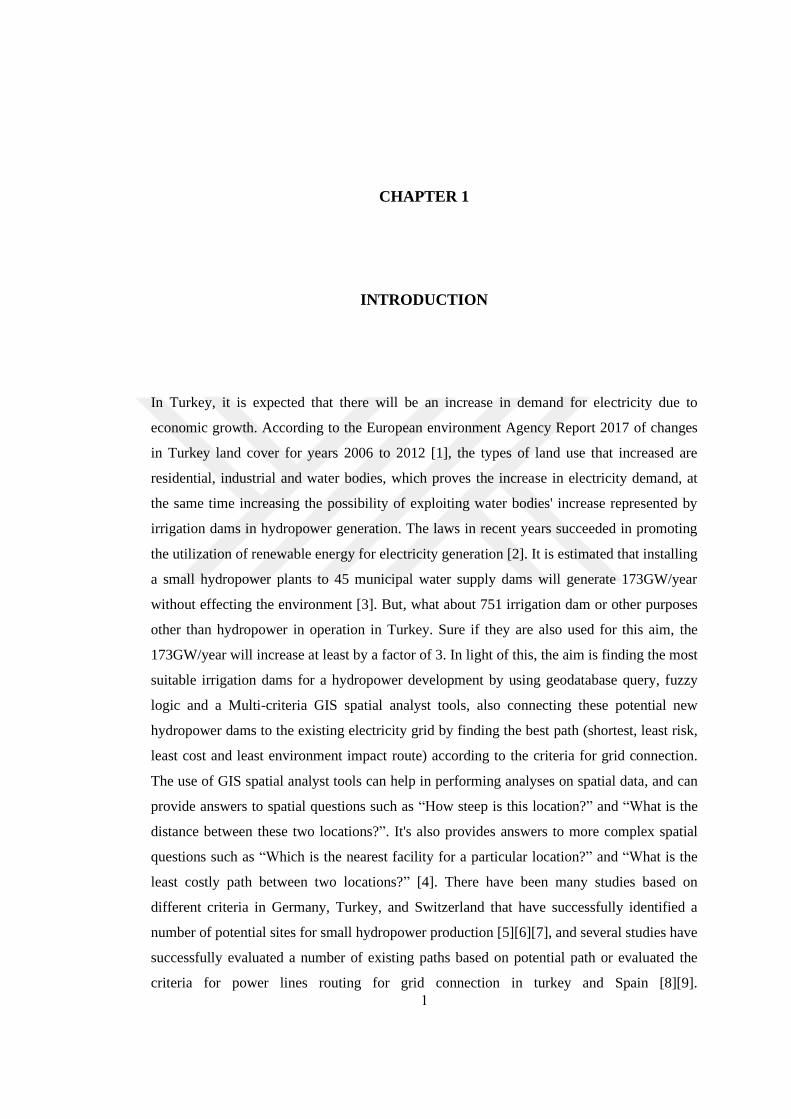
In Turkey, it is expected that there will be an increase in demand for electricity due to

economic growth. According to the European environment Agency Report 2017 of changes

in Turkey land cover for years 2006 to 2012 [1], the types of land use that increased are

residential, industrial and water bodies, which proves the increase in electricity demand, at

the same time increasing the possibility of exploiting water bodies' increase represented by

irrigation dams in hydropower generation. The laws in recent years succeeded in promoting

the utilization of renewable energy for electricity generation [2]. It is estimated that installing

a small hydropower plants to 45 municipal water supply dams will generate 173GW/year

without effecting the environment [3]. But, what about 751 irrigation dam or other purposes

other than hydropower in operation in Turkey. Sure if they are also used for this aim, the

173GW/year will increase at least by a factor of 3. In light of this, the aim is finding the most

suitable irrigation dams for a hydropower development by using geodatabase query, fuzzy

logic and a Multi-criteria GIS spatial analyst tools, also connecting these potential new

hydropower dams to the existing electricity grid by finding the best path (shortest, least risk,

least cost and least environment impact route) according to the criteria for grid connection.

The use of GIS spatial analyst tools can help in performing analyses on spatial data, and can

provide answers to spatial questions such as “How steep is this location?” and “What is the

distance between these two locations?”. It's also provides answers to more complex spatial

questions such as “Which is the nearest facility for a particular location?” and “What is the

least costly path between two locations?” [4]. There have been many studies based on

different criteria in Germany, Turkey, and Switzerland that have successfully identified a

number of potential sites for small hydropower production [5][6][7], and several studies have

successfully evaluated a number of existing paths based on potential path or evaluated the

criteria for power lines routing for grid connection in turkey and Spain [8][9].

2

Unlike these studies, this study is an integrated solution; a holistic strategy within the

modern GIS tools was created to achieve the study goals by combining spatial criteria and

technical criteria and then applied spatial analysis tools to find the best irrigation dams to

develop hydropower and ranked them according to the degree of suitableness using the fuzzy

scoring logic for the multi-criteria which include technical, spatial, environment and risk

criteria. A second phase of spatial analysis was applied by finding the best path to link the

energy produced from those dams to the existing electricity grid also for the same multi-

criteria to ensure the compatibility of the potential generated power with all these criteria and

to avoid unbalanced results as in some energy projects where the cost of grid connection

exceeded the benefits of generated power [10]. Siphon turbines have been proposed for

hydropower development without tampering the irrigation dams' body.

1.1. Background

In Turkey economic growth and an increase in population bring more electricity and

irrigation water demand. The population expected reach 91 million in 2030 with an annual

growth rate of 1% [11]. As seen from Figure 1 most of the water is consumed through

irrigation. Turkey has 25.85 Mha (million hectares) irrigable area (4.3 Mha is currently being

irrigated) and 106.6 km3 per year total available water resources, most of the irrigation

systems (96%) are depend on dams [12]. According to that and by the fact of 711 existing

dams irrigation and multipurpose dams in Turkey until 2018 (Figure 2), which could be used

to install hydropower plants and collect the highest amount of energy from these dams to

avoid the cost of constructing new hydroelectric dams [13] or thermal power plants, which

have a negative impact on the environment [6]. Previous researches in Germany [5], Turkey

[6], and Switzerland [7] were succeeded in finding appropriate dams for the development of

hydropower. Prior research has shown that hydropower can be produced from 43 domestic

water dams in Turkey, where the expected power is 173 GW/year [3]. Based on values of

106.6 km3/year of water resources for irrigation and by using a hydropower calculator to

estimate the potential power [14], it should be possible to collect around 500 GW/year of

power by choosing the best from existing 711 irrigation dams for hydropower development

with the lowest investment cost by finding the best connection path to the current power grid

in accordance with the same technical criteria that succeeded to achieve the highest energy in

addition to spatial criteria of best grid connection to about 692 existing power substation in

Turkey (Figure 3).

3

Figure 1 Water demand in Turkey by sector, for 2007 and 2030, by Turkish Water Works

Directorate (DSI)

Figure 2 Distribution of 711 irrigation dams over 81 provinces in Turkey in 2018

4

Figure 3 Distribution of 692 substations over 81 provinces in Turkey in 2018

1.2. Objectives

This thesis aims to assemble a large power capacity from several of the most suitable

irrigation or multipurpose dams to gain the maximum benefits by investigation on the best

dams for hydropower development with best grid connection to nearest substations based on

least cost, least power losses, lowest risks and lowest environmental impact.

1.3. Organization of the Thesis

This thesis contains six chapters, in which the steps and the methodology used to reach the

objective of the thesis are explained and discussed.

Chapter 1 highlights the objectives of the thesis and describes previous studies. An

introduction is given to the availability of potential hydroelectric resources in Turkey, as

5

represented by the presence of irrigation dams and the availability of substations for the

electricity transmission grid.

Chapter 2 describes the preparation of the geographical database, the determination of spatial

and technical criteria for both dams and substations, and the use of database queries to filter

the dams and substations and to choose the best of them, based on the specified criteria.

Chapter 3 explains the use of multi-criteria fuzzy logic to classify the selected dams

according to their suitability, in terms of meeting the specified technical and spatial criteria.

Chapter 4 presents the steps and methodology involved in the multi-criteria GIS spatial

analyst use to find the best grid connection paths between dams and their nearest substations,

within a maximum distance of 40 km.

Chapter 5 discusses the selection of two dams with high and medium suitability scores as

case studies: Karadere and Karaçomak. The technical and spatial aspects of these dams are

discussed, the potential power is calculated and the methodology used to find the best path to

their nearest substations for grid connection is explained.

Finally, Chapter 6 presents the conclusion of the thesis, a discussion, and recommendations

for future studies.

6

CHAPTER 2

TECHNICAL AND SPATIAL CRITERIA USED TO SELECT THE MOST

SUITABLE DAMS AND POWER SUBSTATIONS

2.1. Building the Geographical Database

In order to reach the goal of finding the best irrigation dams for hydropower development

with best grid connection, it must be dealt with the data and locations of 751 dams (which

are not already used as hydropower dams) as well as the data and locations of 692

substations (power transmission and distribution substations), in addition to the general data

of Turkey map and its 81 provinces, also the spatial reference images of the areas between

the selected dams and nearest power substations and their components for finding the best

grid connection path. For this reason, a geodatabase was first build using Environmental

Systems Research Institute (ESRI) ArcGIS-ArcCataloge softwear to apply a database query

and a multi-criteria spatial analyst and to save the resulting data. In this geodatabase the

following initial objects have been created:

Dams table (point feature class): The data table of 751 dams (which are already not

hydropower dams). For each dam in this table the following fields were included; dam name,

start operation year, river, province, purpose, dam body type, reservoir capacity in cubic

hectare, base height (dam height from the base) in meter, dam height from the thalweg (river

bed) in meter, normal water elevation above the sea level in meter, dam crest elevation above

sea level in meter, full spillway in m3/s, dam (longitude X, latitude Y and elevation Z)

geographic coordinates, normal water level in meter (head or normal water height from

thalweg) and irrigated area in squire hectare.

7

Equation (1) was derived to calculate normal water level (NWL) field values (Figure 4),

using Add Field and Field Calculator tools, where:

NWL = [dam height – [crest elevation at sea level – normal water elevation at sea level]] (1)

Figure 4 Calculation of normal water level from thalweg (head) for Karadere Dam

The dams table data were obtained from the Dams of Turkey guide provided by the Turkish

Water Works Directorate (DSI) [15], the coordinates of the dams were included by the dam

information available through Barajlar Uygulaması v1.4 online application provided by DSI

[16]. Information and data on the status of some of the dams were also updated via the

verification and matching of information from various news and informatics resources,

including the Hurriyet website, DSI website and Google Earth.

8

Substations table (point feature class): The data table of 692 substations. For each

substation in this table, the following fields were included; substation name, substation

region directorate, substation institute, operational status, voltage level in kV and substation

(longitude X, latitude Y and elevation Z) geographic coordinates.

The substations table data and coordinates (Trafo Merkezleri ve Tarife Bölgeleri Listesi)

[17], were downloaded in form of portable document format (PDF) and keyhole markup

language zipped (KMZ) files from the website of the Directorate of Environmental

Protection of Turkish Electricity Works Corporation (TEİAŞ).

Turkey provinces map (polygons feature class): The map of provinces in Turkey using the

World Geodetic System (WGS) 1984 Lambert Conformal Conic geographical coordinate

system.

The coordinates for the dams and substations were also verified and corrected by dropping

them onto the satellite image and map in the Google Earth Pro application and Google Maps.

The locations of the dams and substations on the spatial reference satellite image and map

were viewed and corrected if any deviation was detected.

2.2. Determination of Criteria

After the creation of the geodatabase to allow query filtering, the technical and spatial

criteria were defined. These criteria were used to find suitable dams and substations and to

exclude those that did not completely meet the criteria. An integrated strategy based on GIS

tools was created to achieve the goals of the study by combining geographical (spatial) and

non-geographical (technical) criteria. Spatial analysis tools were then applied to find the best

irrigation dams for hydropower development and the best power substations to connect with

them. Based on this, the following criteria were set.

2.2.1. Dams Criteria for Best Hydropower Generation (Technical Criteria)

Modern hydropower turbines can turn most of the available energy into electricity, while the

best fuel power plants are less effective. Water turbines convert water pressure into

mechanical energy, which is used to operate an electricity generator. The electrical power

available from the water pressure depends on the product of the pressure head and discharge

9

water. The pressure head is proportional to the height of the dam. For irrigation dams, the

discharge water is proportional to the irrigated area, which itself depends on the reservoir

capacity [18]. This is expressed in Equation (2).

(2)

Where γ is the specific weight of the water, Q is the discharge (m3/s), H is the head (m), ΔH

is the hydraulic head loss (m), and η is the sum of the turbine and generator efficiency [3].

Based on this, the technical criteria of dam base height and reservoir capacity were set; other

criteria included dam years in operation and dam purpose.

Dam height and reservoir capacity: The International Committee on Large Dams (ICOLD)

has identified large dams as being those with a height of more than 15 m from the base and a

reservoir capacity larger than 3 cubic hectares [19]. Higher heads will decrease the

construction and equipment costs of hydropower generation [20], while higher reservoir

capacities will provide the continuous, reliable discharge needed for hydropower generation.

Hence, when filtering the dams to choose the best for installation of a hydropower plant, the

conditions of height >= 15 m and reservoir capacity >= 3 hm3 were applied.

Dam years in operation: Dams do not last forever; they require regular maintenance and

have a finite lifespan. Across the world, many dams were built during the 1930–70s, a period

of intensive dam construction, and these have an expected life of 50–100 years. Due to

inadequate maintenance, and/or for environmental or operational reasons such as sediment

accumulation over the anticipated life of the reservoir, some of these dams will fail or be

removed [21]. Over 450 dams have been removed in the United States alone, and these have

been reasonably old (average age 87 years at removal) [22]. For this reason, dams with

(years in operation < =80) were chosen in this study. As a result of database query filtering

based on all criteria, the oldest dam chosen had been in operation for 60 years, meaning that

at least 20 more years of life could be expected before removal.

Dam purpose: Globally, irrigation dams are most suitable for hydropower development

[18]; they often have a strong, continuous flow of water, since they are established for the

purpose of irrigating large areas of land near rivers which provide a good water supply

encourage agriculture. In addition, the simple design of irrigation dams allows for the

modifications required to install various power turbines (Figure 5). For example, a siphon

−= )( HHQP

10

intake turbine can be installed; this is an elegant solution that does not need to pierce the dam

body, and the design of the crests of irrigation dams near the water surface makes it easy to

install with a generating efficiency of about 95%. There are examples of such turbines with

installed power of up to 11 MW and heads of up to 30.5 meters, and they can be located

either at the top of the dam or on the downstream side (Figure 6). If the dam already has a

bottom outlet, this will offer the possibility of installing another type of power turbine

(Figure 7) [18].

Figure 5 Simple design of an irrigation dam (Koyunbaba Dam)

11

Figure 6 Siphon Intake turbine

Figure 7 Base intake turbine

In addition, it can be observed from Figure 1 that the largest demand for water is from

irrigation dams. Approximately 96% of the irrigation systems in Turkey are based on dams

[12]. Most other types of dams are already used for hydropower or are planned for

12

hydropower development [3], or do not have a large, stable water discharge like irrigation

dams [18]. Thus, in the database query related to the purpose of the dam, only irrigation

dams or irrigation dams with other purposes I (irrigation), IM (irrigation and municipal), IF

(irrigation and flood control) and IFM (irrigation, flood control and municipal ) were

selected, meaning that municipal or flood control dams that were not used for irrigation were

excluded.

Result: As a result of applying database query filtering to all 751 dams based on the above

criteria, using the Select by Attributes tool in ArcMap, the number of dams was reduced to

273. This means that 478 dams did not meet the criteria (height >=15 m, reservoir capacity

>= 3 hm3, dam years in operation <= 80 and irrigation purposes) and were excluded.

2.2.2. Substations Criteria for Electrical Power Transmission (Technical

Criteria)

Consumers receive electrical energy after the processes of generation, transmission, and

distribution. Before the generated energy is transmitted via the grid, step-up transformers are

used to increase the voltage, in order to reduce energy losses in the lines. The generated

electricity is transmitted to a grid connection point (step-up substation), where electricity is

converted to the voltage of the transmission network (Figure 8) [23]. Step-up substations are

used for long-distance electricity transmission, and the voltages for long distance

transmission range from 155 to 765 kV [24].

Typically, renewable energy projects use step-up transformers to collect the output from

turbines and route it to a transmission substation, where the voltage can be stepped up again

to enable the efficient onward transmission of power via a land-based transmission system. It

has been shown that by increasing the array system voltage, it is possible to transport a

greater amount of power along a cable with the same cross-sectional area. The most

significant benefit in transferring to a higher voltage is that less array cabling is required, and

this can result in substantial capital costs savings, in terms of both the purchase and

installation of cables [25].

Power plant transformers are used to step up the power produced by the hydroelectric

generator, which is generally at between 0.415 and 11 kV, to a level which matches the

substation transmission system voltage, typically between 12 and 420 kV. Transformers for

13

micro hydro applications are normally 12 kV class, while those for small hydropower

projects of approximately 3 to 5 MW are generally 36 kV class. A generator transformer for

large units may be up to 420 kV class. From 145 kV class and upwards, transformers are

available with two or more values of basic insulation. The choice of the lower value of

insulation is made on the assumption that the equipment is adequately protected against

surges. Power plant step-up transformers for small hydropower applications are liable to be

subjected to high temporary overvoltage due to load rejection, and a higher voltage must

therefore be used [26].

In Turkey, electricity generated by thermal, hydro and natural gas power plants is injected to

the interconnected system via 154 kV or 380 kV power transmission lines, and is transferred

to the closest substations through auto transformers at a voltage level of 154 kV. It is then

reduced to 34.5 kV, 31.5 kV and 15 kV at substations and transmitted to the consumption

points. Distribution transformers are used to decrease the voltage level from 34.5 kV to 400

V, and the final consumers such as factories, offices, commercial institutions and homes can

use this electrical energy at this voltage level (Figure 8) [27].

Figure 8 Generation, transmission and distribution grid

14

Result: Based on the above, step-up transmission substations of 154 kV and higher were

selected, while substations that were under construction were excluded. As a result of

applying database query filtering to all 692 substations using the Select by Attributes tool in

ArcMap, the number of substations was reduced to 658, meaning that 34 substations which

did not meet the criteria of voltage >= 154 kV and in-operation status were excluded.

2.2.3. Maximum Distance to Nearest Substation (Spatial Criteria)

Turkey consider as medium-area country with a population density proportional to the total

area. It has 81 provinces that are approximately similar in area and a large number of cities

and villages that are close to each other. Most residential communities are therefore close

together and connected to the national electricity grid, meaning that the grid covers the entire

country and there is no location that is very far from the grid. This can be seen from the map

of grid transmission and distribution substations, which show 692 substations, distributed

over 81 provinces (Figure 3). With a total area of 783,562 km², this means an average of one

substation for each 34 km², as calculated using Equation (3).

Average distance between substations = √ [Total area / Number of substations] (3)

Based on this, connecting the potential hydropower produced from the selected dams of this

study to the transmission grid is a good option. In remote areas, the construction of new

transmission lines can incur considerable planning hurdles and costs, and it is easier and

more economical to locate a hydropower scheme that is closer to the loads or existing

transmission lines [23]. In this case, the grid will transfer the power and then distribute it

optimally, rather than direct distribution via an isolated grid that can create cost or instability

problems related to capacity and demand [28]. The issue of grid connection distance is one

of the most important issues that must be considered when planning power generation [29].

Many projects have encountered problems from power production that is disproportionate to

the distance to the grid or cost of the grid [10].

The grid connection distance mainly depends on the amount of power produced and the load

voltage of the transmission lines. For example, a 160 km distance at 345 kV carrying 1000

MW of power may experience losses of 4.2% [30], where when the power produced is

greater, the economic feasibility of sending them to long distance will be greater. Also when

the qualitative resistance of the transmission wire is smaller, the loss of power during the

15

distance will be smaller, and then the possible distance will be greater. At the same time the

qualitative resistance increases, when the power transferred increases then losses during the

unit of distance increases. And the qualitative resistance decreases when the load voltage

capacity increases then losses during the unit of distance decreases.

Based on this, there is a term known as (break-even distance), which is the distance that if

exceeded, the grid connection becomes economically inefficient either because of the

increased cost of grid connection above the value of power produced or because of the loss

of power due to the qualitative resistance of the transmission wire [31]. Mainly for small

hydropower the maximum transmission loss should not exceed 4.5 percent of the received

energy [10]. For short distances lines (less than about 80 km) the capacitance and leakage

resistance to the earth are usually neglected [32]. Studies determined the break-even grid

connection distance (nearest substation) for a small hydropower and or micro renewable

energy at 45 km to 50 km [33] [34]. The resources also indicate that hydropower projects

with a capacity of more than 100 kW can be connected to the grid [28].

Since the criteria for substations and power transmission were set to ensure the best transfer

of produced power with lowest loss within the distance unit, as well as through the selection

of technical criteria for irrigation dams which can achieve the highest production of

hydropower including the dam height and reservoir capacity with considering the irrigated

areas and compared with the dams of other studies whose potential power has been already

calculated, the estimated potential power that can be produced from the selected dams in this

study ranges from 100 kW to 10 MW or above. Such estimates can be attributed to small and

medium hydroelectric power according to most hydropower definitions [28], which can be

generated from small or medium-flow rivers. Such energy is economically feasible to

connect to the grid.

The maximum grid connection distance (break-even distance) between the selected dams and

their nearest substations was therefore set to 40 km, in order to avoid exceeding power losses

of 4.5% (Figure 9) and to take into account the average distance of 35 km between

substations in Turkey, as indicated in Equation (3).

16

Figure 9 Losses Percentage of losses from hydropower (100–10000 kW) via 154 kV

transmission lines over distance of 10, 20, 30 and 40 km

Result: After applying spatial analyst to the geodatabase of dams and substations using

ArcMap Select by Location tool, all dams without a substation within a distance of 40 km

were excluded. Thus, the number of dams was reduced to 265, as eight dams without a

substation within 40 km were excluded.

A 'near table' was then created using the spatial analyst tool Create Near Table. This table

identifies the nearest substation for each dam and calculates the straight-line distance to that

substation. As a result, 265 dams with 183 nearest substations within 40 km were obtained; it

should be noted that some substations were near to more than one dam.

2.3. Geodatabase Filtering of Criteria and Spatial Analyst Results

By applying geodatabase queries based on the technical criteria for the dams and substations

and the spatial criterion of nearest substation distance using ArcGIS spatial analyst tools

Select by Attribute, Select by Location and Create Near Table, and joining the records of

nearest substations from the substations table to the selected dams table using Join and

Relate tool in ArcMap, the following results were obtained (Figure 10):

17

- The most suitable 265 irrigation dams for hydropower development were identified.

- A total of 183 nearest substations located within 40 km of the selected 265 dams were

selected by assigning the nearest substation to each candidate dam, some of these substations

were near to more than one dam.

- The straight-line distance was calculated from each candidate dam to its nearest substation.

Figure 10 The selected 265 dams and nearest 183 substations (within 40 km)

For the selected 265 dams, in order to recognizing the differences between criteria data

preferences, statistical indicators were calculated.

18

Statistics for the criterion of dams base height: The dam which has the maximum base

height of the selected dams is (Burgaz Zeyti) has 115 m base height which considered a high

preference for hydropower development. Burgaz Zeyti Dam has good values in its

preferences of the other criteria. It should be noted that there is no clear relationship between

the base height of the dams and their other criteria, except for the normal water level, since

this depends on the height of the dams (Table 1). The average base height for the selected

dams was 48 m, and most of the selected 265 dams had base heights of between 20 and 70 m

(Figure 11).

Table 1 Comparison in base height criterion preference of the selected 265 dams with their

other criteria statistical indicators

Dam base

height (m)

Value /

Preferences

Reservoir

capacity (hm3)

Years in

operation

Irrigated

Area (hm2)

Normal Water

Level (m)

Near substation

distance (km)

15 Min / Low 55.2 2 77 10 26.8

46 Median / Mid 18.9 11 5128 28 20.1

115 Max / High 33 5 3009 81.5 11.9

Figure 11 Statistics for the criterion of base height for the selected 265 dams

19

Statistics for the criterion of dams reservoir capacity: The dam which has the maximum

reservoir capacity of the selected dams is (Kartalkaya) has 717.7 hm3 reservoir capacity

which considered a high preference for hydropower development. Kartalkaya Dam has a

medium values in its preferences of the other criteria. It should be noted that there is a

relationship between the dams reservoir capacity and their other criteria, except the near

substation distance because it's a spatial criterion which is not related with dams technical

criteria (Table 2). The average reservoir capacity for the selected dams is 43 hm3 and most

of the selected 265 dams have a reservoir capacity between 3 to 90 hm3 as shown in Figure

12.

Table 2 Comparison in reservoir capacity criterion preference of the selected 265 dams with

their other criteria statistical indicators

Reservoir

capacity (hm3)

Value /

Preferences

Dam base

height (m)

Years in

operation

Irrigated

Area (hm2)

Normal Water

Level (m)

Near substation

distance (km)

3 Min / Low 25.5 31 450 15 7.2

18.5 Median / Mid 44 5 2045 26.5 15.4

717.7 Max / High 57 38 20000 49 12.5

Figure 12 Statistics for the criterion of reservoir capacity for the selected 265 dams

20

Statistics for the criterion of dams nearest substation distance: The shortest grid

connection distance between the selected dams and nearest substations is (Kocadere) has 720

m nearest substations distance which considered a high preference for grid connection.

However Kocadere Dam has low values for its other technical criteria preferences. There is

no relation between the nearest substation distance of the selected dams and their other

criteria, since this is a spatial criterion that is not related to the technical aspects of the dams

(Table 3). The average distance to the nearest substation for the selected dams was 17.29 km,

and the selected 265 dams had a normal distribution around the average value (mean) for this

criterion (Figure 13).

Table 3 Comparison in nearest substation distance criterion preference of the selected 265

dams with their other criteria statistical indicators

Near substation

distance (km)

Value /

Preferences

Dam base

height (m)

Years in

operation

Irrigated

Area (hm2)

Normal

Water Level

(m)

Reservoir

capacity

(hm3)

0.72 Min / High 23.75 37 381 13.7 3.71

16.55 Median / Mid 89 22 3123 68 31.4

38.20 Max / Low 36 60 5438 31 30.9

Figure 13 Statistics for the nearest substation distance criterion for the selected 265 dams

21

Statistics for the criterion of dams years in operation: The dam which has the minimum

years in operation of the selected dams is (Ardıl) has one year in operation, which is

considered a high preference factor in encouraging hydropower development, as it indicates

that around 79 more years of operation are possible. Ardıl Dam has normal values for its

other technical criteria and a good value for the nearest substation distance. There is no

relationship between years in operation for the dams and their other criteria (Table 4).The

average value for the years in operation of the selected dams was 22 years, and most of the

selected 265 dams were built after 1980 (Figure 14).

Table 4 Comparison in years in operation criterion preference of the selected 265 dams with


Years in

operation

Value /

Preferences

Dam base

height (m)

Reservoir

capacity (hm3)

Irrigated

Area (hm2)

Normal Water

Level (m)

Near substation

distance (km)

1 Min / High 54 10.97 2126 44 12.73

20 Median / Mid 97 79.4 7872 84 13.82

60 Max / Low 36 30.9 5438 31 38.2

Figure 14 Statistics for the criterion of years in operation for the selected 265 dams

22

Statistics for the criterion of dams irrigated areas: The dam which has the maximum

irrigated area of the selected dams is (Apa) has 97015 hm2 irrigated area which considered a

high preference for providing water supply for hydropower development. Apa Dam has low

values for its other criteria preferences although it has a high value for reservoir capacity.

The irrigated area is strongly related to reservoir capacity, since a high reservoir capacity

means good availability of water for irrigation (Table 5). The average value for the irrigated

area for the selected dams was 4913 hm2, and around 200 of the selected 265 dams had

irrigated areas of less than 10,000 hm2 (Figure 15).

Table 5 Comparison in dams irrigated areas criterion preference of the selected 265 dams

with their other criteria statistical indicators

Irrigated

Area (hm2)

Value /

Preferences

Dam base

height (m)

Years in

operation

Reservoir

capacity (hm3)

Normal

Water Level

(m)

Near substation

distance (km)

53 Min / Low 34.5 26 4.96 22 19.64

2062 Median / Mid 35.5 45 8.56 36.5 25.78

97015 Max / High 30.8 56 171.6 26.8 19.76

Figure 15 Statistics for the irrigated area criterion for the selected 265 dams

23

Statistics for the criterion of dams normal water level (Head): The dam which has the

maximum normal water level of the selected dams is (Aktaş) has 98 m normal water level

which considered a high preference for providing water pressure for hydropower generation.

Aktaş Dam has good values for its other criteria preferences. There is no clear relationship

between the dams normal water level and their other criteria, (except for the base height,

since the water level depends on the height of the dam) (Table 6). The average value of the

normal water level for the selected dams was 36 m, and most of the selected 265 dams had a

normal water level of between 10 and 60 m (Figure 16).

Table 6 Comparison in reservoir capacity criterion preference of the selected 265 dams with


Normal Water

Level (m)

Value /

Preferences

Dam base

height (m)

Years in

operation

Irrigated

Area (hm2)

Reservoir

capacity (hm3)

Near substation

distance (km)

10 Min / Low 15 2 77 55.2 26.87

33.5 Median / Mid 49 5 2313 23.67 13.02

98 Max / High 105.5 1 1580 43.79 9.92

Figure 16 Statistics for the normal water level criterion for the selected 265 dams

24

Statistics for the criterion of dams purposes: High preference dams are those which are

only used for irrigation purpose. There are 201 dams only for irrigation from the 265

selected dams, and the other 64 are used for both irrigation and other purposes (Table 7).

Thus, most of the selected 265 dams are used only for irrigation purposes, and these are the

main focus of this study (Figure 17).

Table 7 Comparison in dams purposes criterion preferences of the selected 265 dams

Dam purpose Value / Preferences Number of dams

Irrigation, Flood control and Municipal Triple / Low 10

Irrigation and Flood control Dual / Mid 21

Irrigation and Municipal Dual / Mid 33

Irrigation Single / High 201

Figure 17 Statistics for the dams purpose criterion of the selected 265 dams

25

CHAPTER 3

USE OF MULTI-CRITERIA FUZZY LOGIC FOR DAMS SUITABILITY

SCORING

3.1. Introduction

After the technical and spatial criteria were applied, 265 irrigation dams were identified that

were suitable for hydropower development, within the maximum of 40 km distance from the

nearest substation for connection to the power grid. Although all of these dams are suitable

for hydropower development, it is important to determine which are most suitable. The

implementing agencies and beneficiaries aim to choose dams that meet the criteria to the

fullest extent (i.e. highest power production, least cost and environmental damage, and

shortest grid connection), especially in view of the variation in the preference of the criteria

for the selected dams, as shown by the results for the of the statistical indicators for the

selected dams criteria. The degree of suitability of each dam in terms of meeting all the

required criteria needs to be calculated, and the dams should then be sorted according to their

suitability score, allowing for classification within suitability ranges which allowes the

selection of the most suitable dams for the on-site tests for hydropower development or using

spatial analyst for best grid connection.

3.2. Multi-Criteria Decision Making with Fuzzy Logic

Multi-criteria fuzzy logic is one of the most important ways to evaluate options to achieve

objectives based on a set of compatible or conflicting criteria [35]. There have been many

studies evaluated options using fuzzy logic, such as evaluating the risk of hydropower run of

river type projects based on multiple environmental criteria in Turkey [36], or finding the

26

best sites for developing solar energy in Vietnam [37], or using fuzzy logic tools to evaluate

low-head hydropower technologies at the outlet of wastewater treatment plants [38].

Multi-criteria fuzzy logic depends on calculating the impact of each criterion to serve the

desired objective within available options. For example, if there is a decision maker which

wants to find a job to achieve the goals of making money and fun at the same time and there

were two job options, the first job profitable but boring and the second profitable and

enjoyable. Therefore, the choice will be on the second job because it meets the criteria of

profit and pleasure. In this study research, options are dams and the objective is the ability of

these dams to achieve the highest proportion of all criteria. Fuzzy logic translates each

criterion into a continuous variable that takes a value between zero and one (0<=x<=1)

called suitability degree or membership degree, which reflux the actual values within the

maximum and minimum values of the original criterion [39].

3.2.1. Determination of Criteria

The criteria chosen to calculate the suitability of each dam are spatial criterion which is the

distance to the nearest substation and the environmental criterion which is environmental

impact assessment (EIA) requirements and technical criteria such as the capacity of the

reservoir, the normal water level, the purpose of the dam and the number of years in

operation (Figure 18).

27

Figure 18 Evaluation criteria for scoring the suitability of dams

Nearest substation distance criterion: This is the distance from the body of the dam to the

nearest substation. Construction of a new transmission line is costly and may be complicated,

since it involves obtaining appropriate permits and may also require the acquisition of land

[40]. The distance to the nearest substation and the suitability degree have an inverse linear

relationship [41]; when the distance to the nearest substation decreases, the suitability degree

increases, due to the decrease in costs and increase in power efficiency. The minimum and

maximum distances between the selected dams and their nearest substations are 0.7 and 38.2

km, respectively (Figure 19).

28

Figure 19 Suitability function for nearest substation distance criterion

Environmental impact assessment requirement criterion: According to the EIA

regulations in Turkey, which were enacted in the official gazette on November 25th, 2014,

any grid connection distance greater than 15 km is considered to have a negative

environmental impact, and EIA regulations must applied; if the grid connection is less than

15 km, an EIA assessment is not required. There will therefore be a threshold point at a

distance of 15 km, where any distance less than this will give a suitability degree of one (i.e.

a low environmental impact), and a distance equal to or greater than this will give a value of

zero (i.e. a negative environmental impact) [42] (Figure 20).

29

Figure 20 Suitability function for EIA requirement criterion

Reservoir capacity criterion: It includes the active storage (full with water) and dead

storage (sedimentation part) capacity of reservoir [43]. Higher reservoir capacities will

provide continuous reliable discharge for hydropower generation. Where the maximum

reservoir capacity of the selected dams is 717.7 hm3 (high suitability) and the minimum

reservoir capacity is 3 hm3 (low suitability).

Normal water level (Head) criterion: Is the water height from the thalweg (river bed), or it

is the diffirence between the normal pool elevation (water surface level) at the top of active

storage and the minimum pool elevation at top of the dead storage (thalweg) (Figure 21).

Higher heads will decrease the construction and equipment costs of hydropower generation

[20]. In this respect, higher heads represent preferable site conditions and they have higher

scores.

30

Figure 21 Reservoir storage zones (adapted from [43])

The normal water level was already calculated for all the dams from the geodatabase

ArcCatalog Filed Calculator by based on equation (1) (Figure 4). The normal water level

represent the head height if the water outlet at the bottom of the dam's active storage (Figure

21).

For reservoir capacity and the normal water level, the suitability degree was calculated by

Q50 method (above || under the median) which give each criterion a suitability degree

(membership) between 1 and 0 [41], where the upper half of the criterion data values were

gave 0.5 or more suitability degree according to the original criterion value that exceed the

median value, and the lower half of the criterion data values were gave less than 0.5

suitability degree according to the original criterion value that less than the median value

which is 18.5 hm3 for the reservoir capacity and 33.5 m for the normal water level (Figures

22 and 23).

31

Figure 22 Suitability function for the reservoir capacity criterion

Figure 23 Suitability function for the normal water level (head) criterion

Dam purpose criterion: Under the scope of this study, purposes of dams cover (irrigation),

(irrigation and municipal), (irrigation and flood control) and (irrigation, flood control and

municipal). If the dam has a single purpose, it has the highest score. Because single purpose

dams have fewer constraints compared to multipurpose dams. The suitability degree was

determined as follows (Figure 24):

32

- If the dam is used for irrigation purpose only (single purpose), then the suitability degree of

this criterion is 1.

- If the dam is used for irrigation and municipal or irrigation and flood control purposes (dual

purposes), then the suitability degree of this criterion is 0.66.

- If the dam is used for irrigation, municipal and flood control purposes (triple purposes),

then the suitability degree of this criterion is 0.33.

Figure 24 Suitability function for dams purpose criterion

Dam years in operation criterion: This reflects the age of the dam, and is an especially

important parameter in regard to the sedimentation status of the reservoir. It also has

an inverse linear relationship with the suitability degree, since as the age of the dam

(years in operation) increases, the number of possible future years of operation

decreases and the suitability degree decreases within the range of the selected dams

ages which is from 1 to 60 years (Figure 25).

33

Figure 25 Suitability function for the years in operation criterion

3.2.2. Fuzzy Logic Methodology for Suitability Scoring

Fuzzy logic assumes that a weight is given to each criterion according to its importance. This

is done by mathematical methods or based on expert opinion [45]. It is also possible to give

the same weight to all participating criteria, if the aim is to offset the weakness of one

criterion with the strengths of the other criteria, or when all criteria are equally important

[45]. The criteria have been given equal weights in order to achieve the highest suitability

from all criteria equally; it is then easy to change these weights and obtain other results in the

future [46]. Weight control is considered a variable option that is influenced by temporal

conditions, spatial conditions, restrictions and instruction.

The suitability degree was computed for each dam based on all the criteria. The suitability

degree (score) for each dam could be aggregated in many different ways, such as a linear

method of aggregation based on multiplication of the set of weights by the degrees of

suitability memberships [45], as shown in Equation (4).

S (D𝑖) = ∑𝑊𝑗∗𝐶𝑖𝑗 𝑖=1,2,...,n 𝑗=1,2,…,r (4)

Where 𝑖 is the dam number, 𝑗 is the criterion number, n=265 is the total selected dams, r=6 is

the total number of the criteria, 𝑊𝑗 is the weight of the criterion 𝑗, 𝐶𝑖𝑗 is the suitability degree

of the criterion 𝑗 for the dam 𝑖 and S (D𝑖) is the suitability score of the dam 𝑖.

34

3.3. Results of Suitability Scoring

When the suitability scores for all of the dams were obtained, they were arranged in a table,

where the lowest suitability score is 0.27 (27%), and the highest suitability score which is

Aktaş Dam was obtained 0.87 (87%) suitability score, so the dams have been classified

according to theirs suitability score as follows (Figure 26):

- High suitability class: 21 dams had a suitability score of between 75% and 87%, and these

are listed and shown in Appendix A.

- Medium suitability class: 149 dams had a suitability score of between 50% and 74.99%,

and these are listed and shown in Appendix B.

- Low suitability class: 95 dams had a suitability score of between 27% and 49.99%, and

these are listed shown in Appendix C.

Figure 26 Distribution of the 265 dams with their suitability class and their 183 nearest

substations

35

As explained before, all the selected dams are suitable to develop a hydropower because

these dams have been selected according to criteria that ensure reaching the suitable

hydropower generation condition, although the low level class has a low suitability score, it's

can be used to develop a hydropower, where some dams in this class reach a 454 hm3

reservoir capacity or 55.1 m normal water level or 79015 hm2 irrigated area or 14.5 km near

substation distance, which consider a suitable condition for hydropower development.

The medium suitability class is good for hydropower development, it's has not a very much

low level of its criteria values, also some dams in this class reach a 717 hm3 reservoir

capacity or 84 m water level or 73690 hm2 irrigated area or 0.7 km nearest substation

distance, so it’s has good dams to select from them for installing a hydropower plant.

The most suitable dams for hydropower development are those in the high suitability class

they have a (10.9–220.5 hm3) reservoir capacity, (36–98 m) water level, (1580–31918 hm2)

irrigated area and a (2.1–14 km) nearest substation distance. All the dams in this level are

good and benefit able for hydropower generation with suitable grid connection distance.

36

CHAPTER 4

METHODOLOGY FOR FINDING BEST GRID CONNECTION PATH

USING GIS MULTI-CRITERIA SPATIAL ANALYST TOOLS

4.1. Introduction

It is possible now to select any dam from the suitability scoring table of best 265 irrigation

dams for hydropower development to find the best grid connection path to its nearest power

transmission substation using the multi-criteria GIS spatial analyst tools or to make the

manual technical tests at the dam location. For integrated solution, first the technical and

spatial criteria that ensure finding the most suitable irrigation dams and power substations for

generating and transmission electric power have been selected, then the dams were sorted

according to their suitability of meeting all the criteria. In this section how to find the best

grid connection path for power lines between the selected dams and theirs nearest power

transmission substations were discussed, again according to multi-criteria which ensure the

shortest path with least cost, least environment impact, avoids obstacles and in a suitable

land use. The dams and substations have been selected before based on the criterion of 40

km nearest substation distance as maximum, so the distance of the derived best grid

connection path between any dam and its nearest substation will be in the range of (0.7–38.2

km), which ensured the compatibility between the generated power and grid connection

distance.

4.2. Multi-Criteria Spatial Analyst

GIS has good capabilities to deal with spatial problems, it can therefore be used to support

spatial decision-making. Solving problem of spatial multiple complex criteria without GIS

37

analysis and its spatial perception tools would be arithmetically difficult, if not impossible

[47]. GIS multi-criteria spatial analyst is the most modern effective way to evaluate spatial

options to achieve objectives within a set of compatible or conflicting spatial criteria [48]. It

can be noted here that there were researches that have been able to evaluate spatial options

using multi-criteria GIS spatial analyst, such as a GIS-assisted optimal Baghdad metro route

selection based on multi-criteria decision making [49], or multi-criteria spatial analysis of

land accessibility for seismic operations [50].

Multi-criteria GIS spatial analysis depends on calculating the impact of each spatial criterion

in order to reach the desired objectives based on the available spatial options. In this study,

the options are the potential routes for power line in the area between a dam and its nearest

substation, and the objective is to find the best path in order to maximize the acceptance

based on all the spatial criteria. Prior studies have used multi-criteria GIS spatial analysis to

evaluate the paths of existing power lines in Turkey [8], and to optimize the routing of power

lines in Spain [9].

The criteria which were chosen to find the best grid connection path are the measurable

continues phenomenon spatial criteria's including (shortest distance, suitable elevation, least

slope, near to roads, near to existing power lines) which related to the cost of establish and

maintenance of new power lines, and the attributed spatial criteria's which are land cover

criteria including (avoids or exclude some public and private property, avoid natural

reserves, avoid large water surfaces, land use preferences) which related to the lands

deduction costs, EIA requirement, and natural and artificial obstacles.

4.3. Methodology for Finding Best Grid Connection Path

To find the path with the least cost (the best path) [51], GIS multi-criteria spatial analysis

starts by translating each spatial criterion from the extent of the study area (in this case, a

rectangular area including the dam and the nearest substation) into a visible raster layer,

where each cell in this layer represents a variable with a spatial value proportional to its

criterion compatibility degree [48], [52]. This raster layer is then reclassified using a

common scale for all the other criteria layers [53]. This reflects their actual spatial values

and provided the ability to combine with the other criteria layers and enable weights to be

given for each criterion by the decision maker or mathematical methods [54]. This will

produce a new visual layer called the suitability layer or cost layer [55]. The value at any

38

location (one raster cell) in this layer represents the cumulative cost or the suitability degree

of that location, based on all the spatial criteria (Figure 27).

Figure 27 Reclassification of the criteria and cost raster layers

4.3.1. Evaluation of Shortest Distance Criterion

The GIS spatial analyzer is always seeks to approximate the best path to the Euclidean direct

distance, this is basis on the fact of costs are always related to distance. But the spatial nature

of some regulations related with directing power lines leads to a compromise between a

straight line (Euclidean distance) from one point to another and the deviation of the path

(least cost path) to avoid costly terrain, obstacles or other regulations criteria. In a study [56],

the power line path was determined using Euclidean distance and spatial distance between

the starting and the destination points, multiple layers were examined using the weighted

criteria method to reach the optimal path selection, the path was compared with the

Euclidean distance and showed that the spatial distance was better than the Euclidean

distance method.

In this study case, when the grid connection distance decreases, the distance criterion

suitability degree increases by decreasing the costs of establishing new power lines and

increasing the efficiency of power transmission within the maximum and minimum grid

connection distances range which are between (0.7–38.2 km) between the selected dams and

their nearest substations, also the negative environmental impact decreases.

39

4.3.2. Evaluation of Elevation and Slope Criteria

For the criteria of suitable elevation and the least slope, Turkey consider as a varied terrain

country, with plains, undulating areas and steep mountainous areas, elevations ranging from

zero meters in coastal areas to 5200 meters elevations in mountain peaks (Figure 28). The

slope directly affects the suitability and cost of installation and maintenance of the power

transmission lines. Naturally, the power lines in the flat terrain are less expensive and more

suitable.

Figure 28 Elevation map of Turkey

In a study [8], there are different decision makers who have different professional

backgrounds on the power transmission line, one of them is an expert engineer in power

lines design, where gave attention to the importance of terrain in the design of power

transmission lines. For power towers, there are some technical regulations on the degree of

slope because it is difficult to build transmission line towers on a high sloping surface.

According to regulation of the power transmission line of the Turkish Electricity Company

TEİAŞ (2004), the degree of slope, which is more than 30%, is unsuitable for design. Also

40

areas with a slope greater than 40 % are prone to landslides, where landslides is a problem

for power transmission towers because power tower locations must have a stable base

because the landslides of the towers causes huge losses on the line.

There are also terrain-based costs including accessibility, where it requires additional costs

for the transportation, installation and maintenance of equipment to cross rough terrain. Non-

flat terrain also requires higher towers and more tower units. high elevation increases the

likelihood of ice where it requires more expensive towers to support the mechanical stress

and additional costs of electrical protection equipment, such as lightning arresters, because

the increases of lightning probability. Also, the threat of wind speed on the towers is partly

linked to the elevation [9].

Thus, the criterion of terrain slope is very important. In GIS, the quality of the results

depends on the accuracy of the data; remote sensing techniques have played an important

role in giving easy access to high-resolution data. In this study, to fit the extent of the area

between any dam and its nearest substation, satellite imagery with spatial references was

downloaded using the SASPlanet application and Google Earth Pro. The latter is the world's

most famous satellite imagery viewer, and offers instant access to a tremendous amount of

high-resolution satellite imagery. Most of this high-resolution database is filled with

QuickBird images provided by DigitalGlobe. This application also enables users not only to

preview satellite images, but also to obtain brief information about the scene, such as the

date of acquisition, an elevation histogram, the cloud cover, nadir angle and target azimuth.

Satellite imagery was used as a basis for determining the work extent and cell size for all

other layers of criteria used to generate the best grid connection path, where GIS is usually

use a base map or a base layer for serialized spatial analyses [57]. The elevation data for the

coordinates of the work extent for each selected dam area were downloaded in Excel format,

using the cells coordinates of the satellite imagery base map and the software TCX

Convertor (Garmin's Training Center for Data).

In ArcCatalog for each selected dam to find the best path, a new subgeodatabase was created

and it was gave the same name of the dam. In this subgeodatabase, the elevation data table of

the area between the dam and its nearest substation and the satellite imagery of this extent

area were imported, the feature classes of selected dam and its nearest substation were also

imported from the original geodatabase of all dams and substations, all those subgeodatabase

41

components have been projected on the polygons of turkey map feature class using WGS

1984 Lambert Conformal Conic coordinate system.

From the new subgeodatabase of the selected dam, the Excel spreadsheet of elevation data

was imported into ArcMap to create the elevation raster layer using the inverse distance

weighted (IDW) interpolation tool in spatial analyst tools box, where IDW interpolation

calculates a value for each cell in the output raster layer from the values of the data points,

with closer points given more influence and distant points less influence [58], IDW can be

used to estimate elevation, precipitation, temperature, chemical dispersion, or other spatial

persistence phenomena. So users can create surfaces from sample sites without having to

visit each site in the study area, saving time and effort [59].

Then by using the Slope tool in the surface spatial analyst tools box the slope raster layer was

created, where each cell in this layer represents the slope of its position. By using the surface

spatial analyst in ArcGIS users can create many surface layers like hill shade, slope, contour,

and aspect [59]. Then by reclassified the slope layer in a common scale from 1 to 9 with the

other reclassified criteria's by giving the low values to the low slope cells (low cost), the

slope suitability degree of that position to create a power line was represented.

4.3.3. Evaluation of Near to Roads and Current Power Lines Criteria

For the criteria of near to roads and near to existing power lines, Turkey covered by a wide

roads network (Figure 29), and also large power grid connections (Figure 30), reach 68203

km of power transmission lines (as reported by TEİAŞ in 2019). Distance to roads and

existing power lines directly affects the suitability and cost of installation and maintenance

of the power transmission lines.


backgrounds in power transmission line, one of them is an expert technician in power lines

works in the maintenance service, where attaches importance to the criterion of access to the

new power transmission lines, according to his preferences near to current power lines

makes the new power lines maintenance easier.

42

Figure 29 Detailed map of roads in Turkey

Figure 30 Map of power transmission lines in Turkey

The accessibility requires additional costs for the transportation, installation and maintenance

of equipment to cross areas far from roads. Accessibility costs analysis is important in urban

43

planning and land use management [60]. There are also land use based costs related with

near to existing power lines, where it requires additional costs for the confiscation or rent

lands for new power lines, while the passage of the new line along with the current lines

does not require these additional costs.

In view of this, it's important to calculate the distance from roads and the distance from

existing power lines. Note that any type of roads (highways, main roads or sub-roads) meets

the criterion of accessibility, as well as power lines where if the new power line passes near

any type of existing over-head power transmission lines will meets the criterion of

accessibility and there is no need for new land expropriation. To help recognize the linear

features of roads and power transmission lines from satellite images and to minimize the

possibility of human error, a table containing patterns has been organized to be used to

recognize the linear features of roads and power lines that can be seen in any of grid

connection extent area between a dam and substation (Table 8). In GIS, Calculating the

accrued cost of travel (distance analysis) provides the user additional data to make decisions.

ArcGIS Spatial Analyst provides many distance mapping tools to measure both linear and

Euclidean distance in terms of spatial parameters such as distance from the current

infrastructure of all types of linear parameters (networks) such as roads [59].

Table 8 Recognition of linear features

Linear Feature

Type Description Pattern 1 Pattern 2 Pattern 3

Sub roads Zigzagging, narrow, single-track lines.

Main roads Single, dual-track lines.

Highways Double, wide, triple-track and direct

lines.

Power

transmission lines

Towers, shadow of towers, removal of

trees or buildings along lines.

44

In the extent of the area between any selected dam and its nearest substation, by using the

spatial reference satellite imagery in the selected dam subgeodatabase and by comparison

with the available features classes data for roads and power lines or available topography

maps and Google Maps, the roads and existing power lines were digitized and have been

saved as a line feature classes in the subgeodatabase of selected dam. The ability to integrate

data from different resources is one of the most important functions of GIS, where GIS

usually use a base map or a base layer for creating new other criteria's layers or to do

serialize spatial analyzes like satellite imagery or digital elevation model [57].

In ArcMap by using one of the spatial analyst tools which is Euclidean distance [51], the

raster layer of the distance from the new feature classes of roads and existing power lines

was created which were saved before in the subgeodatabase for the selected dam, where the

value of each cell in this layers represents the distance of its position from the roads or

existing power lines. By reclassified distance from roads and distance from existing power

lines layers in a common scale with reclassified slope by giving the low values to the low

cost cells (less distances),Where the zero value will be along the roads or power lines and the

values (distances) will be increased as moving away from the road or power lines. By doing

this, the suitability degree of that position to create a power line according to criteria of near

to roads and existing power lines has been represented.

It is possible to combine the criteria of the near to roads and current power lines in one layer

while digitizing the feature classes of these two criteria as both are linear features, where

when there are many attributes within the criterion, the uniform reclassified criterion

becomes smoother because the lower attributes within the criterion give a more surprising

measure and a more biased value for each attribute [57]. However, in this study this was not

done, to allow these criteria to be controlled separately.

4.3.4. Evaluation of Land Use Criterion

Turkey has variety forms of natural land cover as well as all types of land uses, which are

constantly changing as a result of growth and climate change factors, [1] (Figure 31). All

specialists agree on the importance and impact of the nature of land cover and the type of

land use in the process of directing power lines.

45

Figure 31 Map of land cover in Turkey (produced by the European Environment Agency)


backgrounds on the power transmission lines. One of them is an expert engineer in power

lines design, where gave attention to the importance of land use. The other is an

environmental engineer working on the environmental impact assessment of power

transmission lines, who pays attention to minimizing the environmental impact of the new

power lines during construction and operation periods, therefore land use, protected areas,

water resources and urban layers have a greater important than other layers on his

perspective, where the main aim of the environmental engineer is to pass the power line from

the open areas, barren land, far from the habitat and settlement.

46

Therefore it is necessary to evaluate land cover and land use according to their suitability for

directing power transmission lines before starting any new power line project, where the

following considerations must take in account:

Costs of preparing the potential land: Which includes the confiscation or rent of lands to

erect power towers, as well as the costs of removing trees and constructing support towers at

the slopes and the crossing of linear obstacles like rivers, roads or other power lines, for

example there are some restrictions on crossing rivers with wide more than 500 meter [8].

Environmental impact requirement: Where power transmission lines can have a

significant impact on human body. Although the electromagnetic field effects of power lines

are still not well defined in the long term, there are many studies on the negative effects on

protein synthesis, Deoxyribonucleic Acid (DNA) synthesis, enzyme activity, neuronal and

muscle cells, dysfunction and heart possible neurological effects [61], so directing of power

lines in densely populated areas represents a real problem. The passage of power lines in

forest areas requires 100% deforestation of tree around power towers and under power lines

for the rights-of-way [62], which could lead to depletion of tree-based wildlife. Also in

agricultural land, power lines could harm the agricultural products and can hamper the work

of agricultural machinery [8].

Threats to power lines: There are many types of areas which pose a risk to the continued

operation of power lines. Landslides areas can cause major problems for power lines as well

as flood-prone areas that could cause problems and impede accessibility during construction

or maintenance. Growing trees in the vicinity of power lines could cause an additional threat,

so forest areas contain a potential hazard.

Obstacles: In addition for what has been mentioned above, there are some areas that are

taboo for constructing power lines such as nature reserves, public places of entertainment,

private property, military zones, airports, urban areas, archaeological sites, cemeteries, as

well as natural obstacles including coastal areas, bays, lakes, wetlands and salt lakes. where

the spatial nature of land cover associated with directing power lines cause to a compromise

between a straight line from one point to another and a deviation of the path to avoid

obstacles.

47

For the selected dams to find the best grid connection path, the areas of land cover were

evaluated according to the above considerations. The high suitability classes have been given

to land cover that has low cost, low environmental impact and low threats to power lines.

Also some potential lands obstacles were excluded from the analysis and have been given

"no data" value.

One of the most difficult and time-consuming parts of data acquisition is the digitization of

the land use layer, and data availability is a vital component for any type of spatial analysis.

Remote sensing can provide these data, and GIS can play a role when analyzing the obtained

data. Since ArcGIS is flexible and can accept different data sets and identify different types

of land use, the polygons of the land use layer were digitized by manual and digital

classification, preceded by visual interpretation of satellite images which had previously

been used as a base map for the extent of the study area to produce criteria maps. Additional

data from Google Earth were also compared for cultural heritage sites, archaeological sites,

nature reserves, and others. An online geo-information application created by the Heidelberg

Institute for Technology (https://osmlanduse.org) also provided access to global land use

maps [63]. The digitized land use polygons were then saved as a new polygon feature class

in the subgeodatabase for each dam, for use in finding the best grid connection to its nearest

substation.

In order to facilitate the process of distinguishing land use types, to reduce the risk of poor

classification due to human error, and to regulate the reclassification of land use using a

common scale with the other criteria, a table of typical land use patterns in Turkey was used

as a comparison for the visual classification process. Each record in the table contains

several images representing the types of standard land use that can be observed in any

selected area, together with the value field of the suitability degree for this land use type on a

scale from 1 to 9, as used for the other criteria (Table 9).

48

Table 9 Recognition of land use classes

Reclassified

Value Land use Type Description Pattern 1 Pattern 2 Pattern 3

1

(very good) Barren

Free of features

deserts or large

uninhabited and

uncultivated

areas.

3

(good) Agriculture

Arable multi-

green mosaics

areas, pastures,

semi natural

vegetation.

5

(acceptable) Forest

Wide dark green

trees areas.

7

(poor) Rural settlement

A few isolated

buildings and

settlements.

9

(very poor) Public Parks

Organized green

areas with toys

fields and small

lakes.

-1 no data

(obstacles) Airports

Flat rectangle

areas with single

or multi airplanes

runway.

-1 no data

(obstacles)

Urban

settlement

Wide dense group

of different sizes

squares

represents

building types.

-1 no data

(obstacles) Lakes

Large irregular

blue or green

areas also rivers

wider than 500

meters.

-1 no data

(obstacles) Salt Lakes

Large irregular

white or light

blue areas.

-1 no data

(obstacles) Wetlands

Large irregular

green and light

green areas.

-1 no data

(obstacles) Military fields

Rectangle

training fields,

aircrafts or tanks

barracks military

air bases.

49

Table 9 (continued)

-1 no data

(obstacles)

Natural

Reserves

Surrounded with

green irregular

polygon border in

Google Earth.

-1 no data

(obstacles)

Archeological

Areas

Large area of

castles, walls and

archeological

sites.

-1 no data

(obstacles) Gulfs

The extension of

the sea into the

land in the shape

of large grooves.

-1 no data

(obstacles) Beaches

The boundary

between sea and

land is either

sandy or rocky.

-1 no data

(obstacles) Cemetery

Large areas of

regular sectors

interspersed with

some trees.

In order to reclassify the land use into categories using a common scale with the rest of the

criteria, and to identify obstacles with a value of "no data" that are prohibited areas for the

other criteria, the polygon feature class of land use was converted from a vector data layer to

a raster data layer, with the extent and sizes of the cells the same as in the elevation layer and

satellite image layer. The raster data model allows the extent and the cover of analysis to be

set and enables us to avoid the more common topological errors within vector layers [57].

The Feature to Raster tool from the spatial analysis toolbox of ArcMap was used.

Based on the considerations discussed above, the land use classes values were reclassified to

be comparable with the reclassified of other criteria's layers as follow, where the higher

value indicates that it is costly to create a power lines path on that particular land use:

- Obstacles which are Lakes, salt lakes, wetlands, urban settlements, natural reserves,

archeological areas, cemeteries, airports and military bases are given a value of –1,

indicating "no data" to exclude them from evaluation for all the criteria, any of these land

uses are considered obstacles if their area diameter exceed 500 meters, which is the standard

maximum distance between power towers.

50

- Public parks are given 9 (very poor), rural settlements are given 7 (poor), forests are given

5 (acceptable), agriculture lands are given 3 (good), and barren lands are given 1 (very good)

which is the favorite lands to establish power lines. It is also possible to add a new land class

to the reclassification in any time or reordered the importance of the land use classes

according to different perspectives.

According to above reclassification and the European Environment Agency Report 2017 of

Turkey land cover for 2012 year [1], 70% of land use in turkey are between (very good, good

and acceptable) for power lines routing, and 5% considered as obstacles and excluded from

power lines routing (Figure 31 and 32).

Figure 32 Statistics for land cover in Turkey and suitability for power lines routing

4.3.5. Combining the Reclassified Raster Layers of the criteria (Creating a Cost

Layer)

After getting the reclassified raster layers in a common scale for all criteria layers and by

using the Map Algebra-Raster Calculator spatial analyst tool in ArcMap tool box, all the

reclassified raster layers were combined together with the possibility of giving weights for

each criterion by asking the decision makers or using mathematical methods to determine

weights, the cost layer was produced, where any place (one cell) on this raster layer

51

represent's the cumulative cost value of power line routing on that place or the suitability

degree of that place according to all the spatial criteria (Figure 33).

Figure 33 Creation of the cost layer

4.3.6. Creating the Layers of Least Cost Distance and Least Cost Direction

The least cost path algorithm uses the cost layer generated in the previous step with the path

starting point layer (dam position), which is a temporary single-cell raster layer (created

from the dam point feature class in the dam subgeodatabase) with the same extent as the cost

layer, i.e. the rectangular area between the dam and the nearest substation. In this way, we

produced two new visible layers: the least cost distance layer (cost distance raster) and the

least cost direction layer (back link raster). These new raster layers were obtained using the

Cost Distance and Cost Back Link spatial analysis tools in ArcMap (Figure 34).

52

Figure 34 Generation of cost distance layer and back link layer

Each cell in the least cost distance layer in Figure 34 represents the lowest cumulative cost of

traveling from that cell to the source point cell (dam position), while each cell in the back

link layer represents the direction code for the lowest cost of movement to one of the eight

neighbor cells back to the source point cell (dam position).

4.3.7. Creating the Least Cost Path Raster Layer (Best Path)

The destination layer was created by determining the destination point (the nearest

substation). This is also a temporary one-cell raster layer (created from the substation point

feature class in the dam subgeodatabase) which has the same extent as the cost layer, i.e. a

rectangular area between the dam and its nearest substation. The GIS analyzer uses the least

cost distance layer, the back link layer and the destination layer to calculate the least cost

path raster layer (best path). This is a visible layer representing the path with the lowest

possible cost from the dam to its nearest substation, based on all criteria and weights, or the

most suitable path between the dam and its nearest substation i.e. with the highest suitability

degree based on all the criteria. In this study, we aim to identify the best grid connection path

with the shortest distance, lowest cost, most suitable land use and lowest environment

impact. The least cost path raster layer (best path) was obtained using the Cost Path distance

tool from the spatial analysis tool box in ArcMap (Figure 35).

53

Figure 35 Derivation of the shortest least cost path

The output least cost path layer (best path) represents the shortest least costly path from the

dam site to its nearest substation (Figure 36). The path avoids steep slopes and certain types

of lands that are considered costlier for constructing the power line; the path also seeks to be

near to roads and existing power lines and in a preferable land use.

Figure 36 Shortest least cost path over the cost (suitability) layer

54

4.3.8. Converting Best Path Raster to Vector Feature Class

As an additional step, the raster path was converted to polyline (vector feature class) to

enable control over the design of the route and placement of the pylons, also to visualize the

path measurements and to create a database table for the path and apply the topology rules of

power network design. This was done using the using the Raster to Polyline conversion tools

in ArcMap [51] (Figure 37).

Figure 37 Converting the least cost path to a vector and visualizing it in 3D format

4.3.9. Projecting the Best Path Line Vector onto a 3D Surface

As a last step in the best path model by using ArcScene Base Height 3D analyst tools, the

best path line vector was projected on the 3D surface of satellite imagery for the area of the

path where the elevation raster layer was used as a base height to create the 3D surface for

the satellite imagery in order to allow the realization of the path and the possibility of

55

modification as well as determination of towers places by giving a realistic perception of the

path on the real surface of the terrain and land cover (Figure 38).

Figure 38 Virtual view of the best path, dropped onto a 3D satellite imagery scene

4.4. Multi-Criteria Spatial Analyst Modeling Using Model Builder

Using the Model Builder tool, ArcMap allows spatial analysis to be carried out by drawing

flowcharts for the inputs and processes, exporting them in a graphical format or via a Python

script. In this way, the spatial analysis processes used to find the best path can be

summarized by drawing a flowchart and linking the input data to the spatial analysis tools in

the chart. This capability is useful to speed up and facilitate the procedures involved in

calculating the best path for any of the selected dams (Figure 39).

56

Figure 39 Flowchart for processes of finding the cost path using the Model Builder tool

57

CHAPTER 5

CASE STUDIES

In general, the potential hydropower from the development of irrigation dams may not be

very large. However, if appropriate criteria are available, the irrigation dams are considered

the best for the development of hydropower and preferred on municipal or flood control

dams for the following reasons:

- There may not be a good flow of water throughout the year, but in the flow seasons they

often have a good flow and continue of water because they are established for the purpose of

irrigating large areas near rivers which provide good water supplies that encourage

agriculture [18][64].

- The simple design of irrigation dams allows modifications to install various power turbines.

Unlike other types of dams, the body of the irrigation dams is free from hydraulic machines

and gates, where it depends on the spillway corridor to discharge the flooded water as shown

in Figure 5. Irrigation is done by channels from the dam's lake or pumps located on the dam's

lake and not on the dam's body [65]. For example, a siphon intake turbine can be installed,

which is an elegant solution, it does not need to pierce the dam body, the design of irrigation

dams crests near the water surface makes it easy to install, with generating efficiency of

about 95%, there are examples with installed power up to 11 MW and heads up to 30.5

meters, it can be located either on top of the dam or on the downstream side (Figure 6).

Another choice if the dam already has a bottom outlet; it will be a possible solution for

install power turbine (Figure 7) [18].

58

- For hydropower development, the irrigation dams considered the best in light of connecting

the generated power to the grid from other types of dams, as it does not contain operational

installations at the body of the dam that consume the generated power, while the generated

power from municipal dams is often exploited to run a water filtration plant [3], or to operate

the gates and the observation station in case of flood control dams.

Based on multiple criteria related to spatial, technical, risk and environmental factors, the

best irrigation dams for hydropower generation have been selected in terms of the best grid

connection of the generated power. Most previous studies have separately examined factors

such as the best sites for hydropower development, criteria for hydropower generation,

lowest risk or environmental impact, grid connection, existing sites and power lines.

However, some of these projects have not been able to be implemented, since advantages in

one aspect are offset by drawbacks in others; some hydroelectric projects have suffered from

inefficient power production due to the cost of grid connection [10].

From the 265 dam’s suitability scoring table, 2 dams were selected from the medium and

high suitability classes as a case study to evaluate the criteria of the dam and its nearest

substation and the potential power also finding the best grid connection path to the nearest

substation to translating the potential generated hydropower from it to the electricity grid.

5.1. Karadere Dam

Karadere is an irrigation dam located between Kastamonu and Taşköprü District (Figure 40).

It was built on clay core sand land fill type, and is situated on the Karadere river. The length

of the dam body is 309 m, and the height from the foundation is 90 m, with a reservoir

capacity of 26.08 hm3. The area irrigated by the dam is 6852 hm2, and the full spillway is

1220 m3/s. Construction of the dam began on October 20th, 1993, and it was completed on

May 31st, 2007 (Figure 41). According to the DSI, the reservoir was filled at a level of 89.2%

in 2018 and 100% in 2019 (Table 10).

59

Figure 40 Top view of Karadere Dam and its lake, in Kastamonu Province

Figure 41 Karadere Dam, body and spillway

60

Table 10 2018 and 2019 Reservoir status of several dams in Turkey (data from DSI)

5.1.1. Karadere Dam's Technical Criteria

Based on the technical criteria, Karadere dam is suitable for hydropower generation and has

the following specifications:

- 11 years in operation, which less than the years in operation criterion in (80–11 = 69 years),

69 more possible years in operation.

- The purpose of the dam is only irrigation.

- The height from the foundation (base height) is 90 meter, which is more than the criterion

of dam height in (90–15 = 75 m).

- The reservoir capacity is 26.08 hm3, which is more than the criterion of reservoir capacity

in (26.08–3 = 23.08 hm3).

The potential power can be calculated from equation (2) previously referred to, this equation

needs dam height and a discharge flow rate to calculate the potential installed capacity. Flow

rate can be estimated by reservoir size, dam height and river type [66] (Table 11).

61

In general, the rivers of irrigation dams have a good flow [18]. The

(https://power-calculation.com/hydroelectricity-energy-calculator) site [14]; allows

calculation of potential power parameters by inserting the needed equation values in

equation (2) which represent the dam hydro resources values (Figure 42).

Table 11 Stream flow in m3/s for calculation of hydropower (as given by power-

calculation.com)

Figure 42 Hydropower calculator at power-calculation.com: data for Karadere Dam

62

Using Equation (1) above, we can calculate the waterfall height (normal water level, NWL)

in m, which represents the head height of the water outlet at the bottom of the active storage

of the dam. This value was calculated for all the dams in the geodatabase using the Filed

Calculator in ArcCatalog. For the Karadere dam (Figure 4),

NWL = [dam Height – [crest elevation at sea level – normal water elevation at the sea level]]

NWL (head) = [70 – [811– 805]] = 64 meter

Using the Hydropower Calculator by power-calculation.com for Karadere dam values, the

following parameters were got:

- Real active power available (in kW): 1587 kW.

With 150 days average number of working days per year:

- Average annual energy in the output of hydro generator: 5713.2 MWh/year.

- Annual electricity bill: €457056/year.

5.1.2. Nearest Substation to Karadere Dam

The nearest substation to this dam is Taşköprü, at a distance of 12.07 km. The substation is

in operation and belongs to TEİAŞ Institute. It is a power transmission step-up substation

with a capacity of 154 kV (Figure 43).

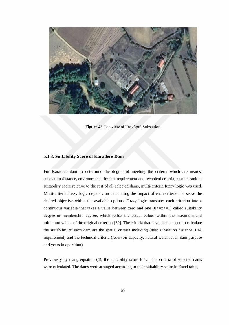
63

Figure 43 Top view of Taşköprü Substation

5.1.3. Suitability Score of Karadere Dam

For Karadere dam to determine the degree of meeting the criteria which are nearest

substation distance, environmental impact requirement and technical criteria, also its rank of

suitability score relative to the rest of all selected dams, multi-criteria fuzzy logic was used.

Multi-criteria fuzzy logic depends on calculating the impact of each criterion to serve the

desired objective within the available options. Fuzzy logic translates each criterion into a

continuous variable that takes a value between zero and one (0<=x<=1) called suitability

degree or membership degree, which reflux the actual values within the maximum and

minimum values of the original criterion [39]. The criteria that have been chosen to calculate

the suitability of each dam are the spatial criteria including (near substation distance, EIA

requirement) and the technical criteria (reservoir capacity, natural water level, dam purpose

and years in operation).

Previously by using equation (4), the suitability score for all the criteria of selected dams

were calculated. The dams were arranged according to their suitability score in Excel table,

64

then the suitability score field was exported from this table to the selected dams table in the

geodatabase. However, the calculation of suitability score for Karadere dam was as

following:

S (D𝑖) = ∑𝑊𝑗∗𝐶𝑖𝑗 𝑖=1,2,...,n 𝑗=1,2,…,r




𝐶𝑖𝑗 for Karadere dam are:

Suitability degree for reservoir capacity:

Selected 265 dams reservoir capacity median = 18.5 hm3

Minimum Selected 265 dams reservoir capacity = 3 hm3

Maximum Selected 265 dams reservoir capacity = 717.7 hm3

Karadere dam reservoir capacity = 23.08 hm3

Since reservoir capacity = 23.08 hm3 is greater than the median = 18.5 hm3 then..

Karadere reservoir capacity suitability degree = [(23.08–18.5)/(717.7–18.5)]*(1– 0.5) + 0.5

Karadere reservoir capacity suitability degree = 0.505453506 (Figure 44).

Figure 44 Suitability function for reservoir capacity, Karadere Dam

65

Suitability degree for normal water level (head):

Selected 265 dams normal water level median = 33.5 m

Minimum Selected 265 dams normal water level = 9 m

Maximum Selected 265 dams normal water level = 98 m

Karadere dam normal water level = 64 m

Since normal water level = 64 is greater than the median = 33.5 then..

Karadere normal water level suitability degree = [(64–33.5)/(98–33.5)]*(1–0.5) + 0.5

Karadere normal water level suitability degree = 0.736434109 (Figure 45).

Figure 45 Suitability function for normal water level, Karadere Dam

66

Suitability degree for purpose:

Purpose = Irrigation = 1

Since Karadere is a single purpose dam then..

Karadere purpose suitability degree = 1 (Figure 46).

Figure 46 Suitability function for dam purpose, Karadere Dam

Suitability degree for dam years in operation:

Minimum Selected 265 years in operation = 1 year

Maximum Selected 265 dams years in operation = 60 years

Karadere dam years in operation = 11 years

Karadere years in operation suitability degree = 1– (11/60)

Karadere years in operation suitability degree = 0.819672131 (Figure 47).

67

Figure 47 Suitability function for years in operation, Karedere Dam

Suitability degree for distance to nearest substation:

Minimum Selected 265 dams nearest substation distance = 0.7 km

Maximum Selected 265 dams nearest substation distance = 38.2 km

Karadere dam nearest substation distance = 12.07 km

Karadere nearest substation distance suitability degree = 1– (12.07/38.2)

Karadere nearest substation distance suitability degree = 0.6904013 (Figure 48).

Figure 48 Suitability function for nearest substation distance, Karadere Dam

68

Suitability degree for EIA requirement:

Since Karadere nearest substation distance = 12.07 km lees than 15 km then..

Karadere EIA requirement suitability degree = 1 (Figure 49)

Figure 49 Suitability function for EIA requirement, Karedere Dam

Then the suitability score for Karadere dam S (D𝑖) is:

S (D𝑖) = 0.505453506 (0.16) + 0.736434109 (0.16) + 1 (0.16) + 0.819672131 (0.16) +

0.690401261 (0.16) + 1 (0.16)

S (D𝑖) = 0.788825527 = 78%

78% is the suitability score of Karadere dam according to all the criteria, which put Karadere

dam in the high suitability class, which are 21 dams had a suitability score of between 75%

and 87%, where Karadere Dam was ranked the ninth in its the suitability score from the

selected 265 dams.

69

5.1.4. Best Grid Connection Path (Least Cost Path) from Karadere Dam to its

Nearest Substation

Both Karadere Dam and its nearest substation (Taşköprü) are located in Kastamonu

province. At first in ArcMap, the feature classes of Karadere Dam and Taşköprü substation

were selected from geodatabase tables, then they have been added them over the layer of

Turkey provinces map (Figure 50).

Figure 50 Karadere Dam and its nearest substation (Taşköprü) on a map of Turkey

We found the straight distance between them while generating the Near Table of nearest

substation for each dam in the geodatabase, where the straight distance between Karadere

dam and Taşköprü substation is 12.07 km (Figure 51).

70

Figure 51 Straight-line distance (12.07 km) between Karadere Dam and Taşköprü

Substation

The multi-criteria GIS spatial analyst depends on calculating the impact of each spatial

criterion to serve the desired objective within the available spatial options. The criteria that

have been chosen to find the best grid connection path are the measurable continues

phenomenon spatial criteria's including (shortest distance, suitable elevation, least slope, near

to roads, near to existing power lines) which related to the cost of establish and maintenance

of new power lines, and the attributed spatial criteria's which are land cover criteria including

(avoids or exclude some public and private property, avoid natural reserves, avoid large

water surfaces, land use preferences) which related to the lands costs, EIA requirement, and

natural and artificial obstacles.

Multi-criteria GIS spatial analyst starts by translating each spatial criterion from the extent of

the study area (a rectangular area between the dam and the nearest substation) into a visible

raster layer, where each cell in this layer represents a variable that has a value compatible

with the spatial value of its criterion.

71

A reference satellite image was used to calculate the extent of the area between the Karadere

Dam and Taşköprü substation in order to generate the criteria layers. The satellite imagery

and spatial references were downloaded via the SASPlanet application and Google Earth

Pro.

In the ArcCatalog, a new subgeodatabase was created and gave Karadere name. In this

subgeodatabase the satellite imagery of the area extent was imported, also the feature classes

of Karadere dam and Taşköprü substation were imported from the original geodatabase of all

the selected dams and substations, in ArcMap all those subgeodatabase components were

projected on the satellite imagery using the coordinate system of Turkey provinces feature

class polygons WGS 1984 Lambert Conformal Conic (Figure 52).

Figure 52 Extent of spatial reference satellite imagery for Karadere Dam and Taşköprü

Substation feature classes

To create the layers for the criteria of suitable elevation and least slope, using the cells

coordinates of the satellite imagery base map and the TCX Convertor application the

elevation points data were downloaded for the coordinates of the area extent of Karadere

dam and Taşköprü substation in an excel format table. In ArcMap and from the new

72

subgeodatabase of Karadere dam, the elevation data excel table was imported to create the

elevation raster layer using the inverse distance weighted IDW interpolation tool in spatial

analyst tools box (Figure 53).

Figure 53 Elevation raster layer for the extent between Karadere Dam and Taşköprü

Substation

Then by using the ArcMap Slope tool in the surface spatial analyst tools box the slope raster

layer was created, where each cell in this raster layer represents the slope of its position

(Figure 54). According to TEİAŞ, the degree of slope, which is more than 30%, is unsuitable

for design. Also areas with a slope greater than 40% are prone to landslides.

73

Figure 54 Slope raster layer for the extent between Karadere Dam and Taşköprü Substation

Then by reclassified the slope layer in a common scale range from 1 to 9 with the other

reclassified criteria's, by giving the low values to the low slope cells (low cost) the slope

suitability degree of that position to create a power line will represented. The high values

represent the areas not good for power lines routing (Figure 55).

Figure 55 Reclassified slope raster layer for the extent between Karadere Dam and Taşköprü

Substation

74

For the criteria of near to roads and near to existing power lines, where near to current power

lines and roads makes the installation and maintenance of the new power lines easier.

To calculate the distance from roads and the distance from existing power lines. In the extent

of the area between Karadere dam and Taşköprü substation, the roads and existing power

lines were digitized and saved them as line feature classes in the selected dam

subgeodatabase (Figure 56).

Figure 56 Feature classes for roads and power lines, for the extent between Karadere Dam

and Taşköprü Substation

In ArcMap by using one of the spatial analyst tools which is Euclidean Distance, the raster

layer of the distance from feature classes of roads and existing power lines was created

which was saved before in the subgeodatabase of Karadere dam, each cell's value in this

layers represents the distance in meters from its position to the roads or existing power lines

(Figure 57 and 58).

75

Figure 57 Raster layer representing near to roads for the extent between Karadere Dam and

Taşköprü Substation

Figure 58 Raster layer representing near to existing power lines for the extent between

Karadere Dam and Taşköprü Substation

By reclassified distance from roads and distance from existing power lines layers in a

common scale with reclassified slope from 1 to 9 by giving the low values to the low cost

cells (short distances), where the zero value will be along the roads or power lines and values

(distances) will be increased by moving away from the roads or existing power lines. By

doing this, the suitability degree of any position to create a new power line according to

criteria of near to roads and existing power lines was represented (Figure 59 and 60).

76

Figure 59 Reclassified raster layer for near to roads for the extent between Karadere Dam

and Taşköprü Substation

Figure 60 Reclassified raster layer for near to power lines for the extent between Karadere

Dam and Taşköprü Substation

For the criterion of land use, all specialists agree on the importance and impact of the nature

of land cover and the type of land use in the process of directing power lines, where the main

purpose is to passing the power line through open areas, barren lands, far from the habitat

and settlements. The high suitability classes were given to land uses that have low cost, low

environmental impact and low threats to power lines. Also some potential lands obstacles

were excluded from the analysis and have been given "no data" value.

77

The polygons of land use layer feature class were digitized by manual recognition and digital

classification preceded by visual interpretation of satellite images that used before as a base

map over the extent area to produce criteria's maps. Also the additional data that Google

Earth provides were compared, such as cultural heritage sites, archaeological sites, nature

reserves, and others. As well as (https://osmlanduse.org) where provides access to global

land use maps [63]. Then the digitized polygons of land use were saved as a new polygon

feature class in the Karadere dam subgeodatabase (Figure 61).

Figure 61 Land use feature class map for the extent between Karadere Dam and Taşköprü

Substation

For the purpose of the possibility of reclassification by categories of land use within a

common scale with the rest of other criteria and for the purpose of giving the obstacles value

"no data", which will be considered as prohibited areas for all other criteria, the polygon

feature class of the land use was converted from vector data layer to raster data layer (Figure

62). The Feature to Raster tool was used from the conversion tools in the spatial analysis

toolbox of ArcMap.

78

Figure 62 Land use raster layer for the Extent between Karadere Dam and Taşköprü

Substation

The land use class values were reclassified to be comparable with the reclassified of other

criteria's layers, where the higher value indicates that it is costly to create a power lines path

on that particular land use (Figure 63).

Figure 63 Reclassified land use raster layer for the extent between Karadere Dam and

Taşköprü Substation

79

After getting the reclassified raster layers in a common scale for all the criteria layers and by

using the Map Algebra-Raster Calculator spatial analyst tool in ArcMap tool box, all the

reclassified raster layers together were combined, the cost layer was produced where any

place (one cell) on this raster layer represent's the cumulative cost value or the suitability

degree of that place for power lines routing according to all spatial criteria (Figure 64).

Figure 64 Cost raster (suitability layer) for the extent between Karadere Dam and Taşköprü

Substation

The least cost path algorithm use the cost layer that was got in the previous step and the path

starting point layer (Karadere dam position) to produce two new visible layers, which are the

least cost distance layer (cost distance raster) (Figure 65), and the least cost direction layer

(back link raster) (Figure 66), where those new raster layers were got using the spatial

analyst Cost Distance and Cost Back Link distance tools in ArcMap spatial analyst tools box.

80

Figure 65 Cost distance raster layer for the extent between Karadere Dam and Taşköprü

Substation

Figure 66 Back link raster layer for the extent between Karadere Dam and Taşköprü

Substation

Each cell in the cost distance layer in Figure 65 represents the least cumulative cost of

traveling from that cell to the source point cell (Karadere dam). While each cell in the back

link layer in Figure 66 represents the direction code of the least cost movement to one of the

eight neighbor cells back to the source point cell (Karadere dam).

81

By determination of the destination point which is Taşköprü substation, the destination layer

is created. The analyzer of the GIS use the cost distance layer, the back link layer and the

destination layer to calculate the least cost path raster layer (best path). The output cost path

layer (best path) represents the shortest least costly path from Karadere dam to Taşköprü

substation. The path avoids steep slopes and certain types of lands that are considered

costlier for constructing of power line; the path also seeks to be near to roads and existing

power lines and in a favorite land use. The least cost path raster layer (best path) was got

using the spatial analyst Cost Path distance tools in ArcMap spatial analyst tools box. As an

additional step, the raster path was converted to polyline (vector feature class) to give the

possibility for controlling the design of the power line path and placing the towers (Figure

67). This was done using the from raster Raster to Polyline conversions tools in the ArcMap

tools box.

Figure 67 Least cost path (best Path) for grid connection between Karadere and Taşköprü

Substation (12.789 km)

The difference between the cost path for power line grid connection and straight line

between Karadere dam and Taşköprü substation is:

12789–12074 = 715 meter.

82

As a last step in the best path's model using ArcScene Base Height 3D analyst tools, the best

path line vector was projected on the 3D surface of satellite imagery for the area of the path

using the elevation raster layer as a base height to create the 3D surface for the satellite

imagery and the path in order to allow the realization of the path and the possibility of

modification as well as determination of towers places by giving a realistic perception of the

path on the real surface of the terrain and land cover (Figure 68).

Figure 68 3D view of the best path between Karadere Dam and Taşköprü Substation

5.2. Karaçomak Dam

Karaçomak Dam is a multi-purpose dam that is used for irrigation, flood control and

municipal supply, and is located in Kastamonu province (Figure 69). It was built on clay

core sand fill type, and is located on the Karaçomak stream. The volume of the dam body is

1100 m3, and the height from the foundation is 70 m, with a reservoir capacity of 23 hm3.

The area irrigated by the dam is 2596 hm2 and the full spillway is 900m3/s. It began

operation in 1976 (Figure 70). According to the DSI, the reservoir was filled at 92.9%

capacity in 2018 and 100% in 2019 (Table 10).

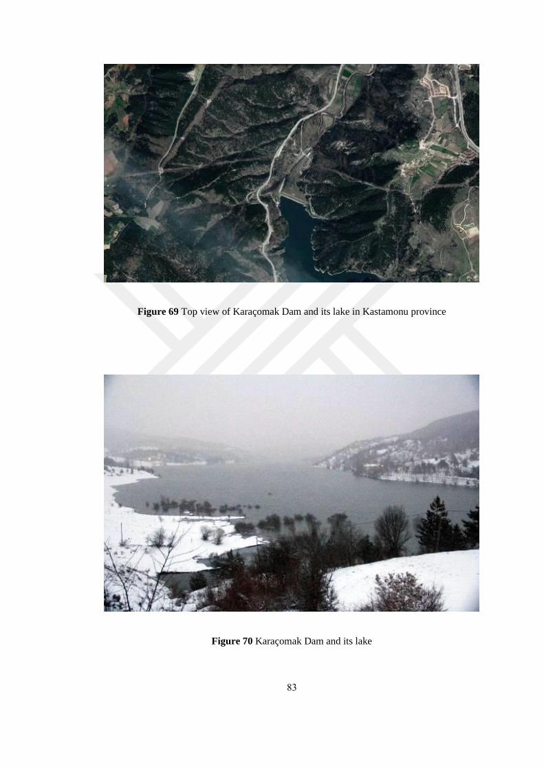
83

Figure 69 Top view of Karaçomak Dam and its lake in Kastamonu province

Figure 70 Karaçomak Dam and its lake

84

5.2.1. Karaçomak Dam's Technical Criteria

Karaçomak Dam is suitable for hydropower development since it has the following technical

specifications:

- 42 years in operation, which less than the years in operation criterion in (80–42 = 38 years),

38 more possible years in operation.

- The Dam is a multipurpose of irrigation, flood control and municipal.

- The height from the foundation (base height) is 70 meter, which is more than the criterion

of dam height in (70–15 = 55 m).

- The reservoir capacity is 23 hm3, which is more than the criterion of reservoir capacity in

(23–3 = 20 hm3).

The waterfall height (NWL) (head) was previously calculated in m for all the dams in the

geodatabase using the ArcCatalog-Filed Calculator tool based in Equation (1) (Figure 4).

The NWL represents the head height of the water if the outlet at the bottom of the active

storage of the dam. For Karaçomak Dam:

NWL = [dam height – [crest elevation at sea level – normal water elevation at sea level]]

NWL (head) = [49 – [895–889]] = 43 meter

The potential power can be calculated from equation (2) previously referred to, this equation

needs dam height and discharge flow rate to calculate the potential installed capacity. Flow

rate can be estimated by reservoir capacity, dam height and river type [66] (Table 11). It is

known that multipurpose dams have a good flow of water discharge because they always

have many water recourses. The (https://power-calculation.com/hydroelectricity-energy-

calculator) site [14]; allows calculation of potential power parameters by inserting the values

of equation (2) which represent the dam hydro resources values (Figure 42).

85

Using the Hydropower Calculator by (power-calculation.com) for Karaçomak dam values,

the following parameters were got:

- Real active power available: 799 kW.

With 150 days average number of working days per year:

- Average annual energy in output of hydro generator: 2876.4 MWh/year.

- Annual electricity bill: €230112/year.

5.2.2. Nearest Substation to Karaçomak Dam

The nearest substation to this dam is Kastamonu, at a distance of 8.56 km. The substation is

in operation and belongs to the TEİAŞ Institute. This is a power transmission step-up class

substation with a capacity of 154 kV (Figure 71).

Figure 71 Top view of Kastamonu Substation

86

5.2.3. Suitability Score of Karaçomak Dam

Multi-criteria fuzzy logic was used to determine the suitability degree to which the

Karaçomak dam meets all the criteria of distance, environmental impact and technical

criteria, and to calculate its overall suitability score relative to the rest of the selected dams.

This approach depends on calculating the impact of each criterion on reaching the desired

objective. Fuzzy logic translates each criterion into a continuous variable that takes a value

between zero and one (0<=x<=1); this is called the suitability degree or membership degree,

and reflects the actual values as a proportion of the maximum and minimum original values

of the criteria [39]. The criteria chosen to calculate the suitability of each dam are spatial

criteria (such as nearest substation distance, EIA requirements) and technical criteria (such as

reservoir capacity, natural water level, dam purpose and years in operation).

Using equation (4), the suitability score of all the criteria for selected dams were calculated.

The dams were arranged according to the suitability score in Excel table then the suitability

score field was exported from this table to our selected dams table in the geodatabase.

However, the calculation of suitability score for Karaçomak dam was as following:

S (D𝑖) = ∑𝑊𝑗∗𝐶𝑖𝑗 𝑖=1,2,...,n 𝑗=1,2,…,r




𝐶𝑖𝑗 for Karaçomak dam are:

Suitability degree for reservoir capacity:

Selected 265 dams reservoir capacity median = 18.5 hm3

Minimum Selected 265 dams reservoir capacity = 3 hm3

Maximum Selected 265 dams reservoir capacity = 717.7 hm3

Karaçomak dam reservoir capacity = 23 hm3

Since reservoir capacity = 23 hm3 is greater than the median = 18.5 hm3 then..

Karaçomak reservoir capacity suitability degree = [(23–18.5)/(717.7–18.5)*(1–0.5)] + 0.5

Karaçomak reservoir capacity suitability degree = 0.503252091 (Figure 72).

87

Figure 72 Suitability function for reservoir capacity, Karaçomak Dam

Suitability degree for normal water level (head):

Selected 265 dams normal water level median = 33.5 m

Minimum Selected 265 dams normal water level = 9 m

Maximum Selected 265 dams normal water level = 98 m

Since Karaçomak dam normal water level = 43 is greater than the median = 33.5 then..

Karaçomak normal water level suitability degree = [(43–33.5)/(98–33.5)*(1–0.5)] + 0.5

Karaçomak normal water level suitability degree = 0.573643411 (Figure 73).

Figure 73 Suitability function for normal water level, Karaçomak Dam

88

Suitability degree for dam purpose:

Purpose = Irrigation + Flood control + Municipal = 3 (triple-purpose)

Since Karaçomak is a multipurpose dam then..

Karaçomak purpose suitability degree = 0.33 (Figure 74).

Figure 74 Suitability function for dam purpose, Karaçomak Dam

Suitability degree for dam years in operation:

Minimum Selected 265 years in operation = 1 year

Maximum Selected 265 dams years in operation = 60 years

Karaçomak dam years in operation = 42 years

Karaçomak years in operation suitability degree = 1– (42/60)

Karaçomak years in operation suitability degree = 0.31147541 (Figure 75).

89

Figure 75 Suitability function for years in operation, Karaçomak Dam

Suitability degree for nearest substation distance:

Minimum nearest substation distance for the Selected 265 dams = 0.7 km

Maximum nearest substation distance for the Selected 265 dams = 38.2 km

Karaçomak dam nearest substation distance = 8.56 km

Karaçomak nearest substation distance suitability degree = 1– (8.56/38.2)

Karaçomak nearest substation distance suitability degree = 0.780445748 (Figure 76).

Figure 76 Suitability function for nearest substation distance, Karaçomak Dam

90

Suitability degree for EIA requirement:

Since Karaçomak nearest substation distance = 8.56 km lees than 15 km then..

Karaçomak EIA requirement suitability degree = 1 (Figure 77).

Figure 77 Suitability function for EIA requirement, Karaçomak Dam

Then the suitability score for Karaçomak dam S (D𝑖) is:

S (D𝑖) = 0.503252091 (0.16) + 0.573643411 (0.16) + 0.33 (0.16) + 0.31147541 (0.16) +

0.780445748 (0.16) + 1 (0.16)

S (D𝑖) = 0.580803565 = 58%

58% is the suitability score of Karaçomak dam according to all the criteria, which put

Karaçomak dam in the medium suitability class, which are 149 dams had a suitability score

of between 50% and 75%, where Karaçomak dam was ranked 112th in its suitability score

from the selected 265 dams.

91

5.2.4. Best Grid Connection Path (Least Cost Path) from Karaçomak Dam to its

Nearest Substation

Both the Karaçomak dam and its nearest substation Kastamonu are located in Kastamonu

province. Using ArcMap, the feature classes for the Karaçomak dam and Kastamonu

substation were selected from their geodatabase. Then they were added over the layer of

Turkey provinces map (Figure 78). The straight distance between them was found while

generating the Near Table of nearest substation for each dam in the geodatabase, where the

straight distance between Karaçomak dam and Kastamonu substation is 8.56 km (Figure 79).

The multi-criteria GIS spatial analyst depends on calculating the impact of each spatial

criterion to serve the desired objective within the available spatial options. The criteria that

have been chosen to find the best grid connection path are the measurable continues

phenomenon spatial criteria's including (shortest distance, suitable elevation, least slope and

near to roads) which related to the cost of establish and maintenance of new power lines, and

the attributed spatial criteria's which are land cover criteria including (avoids or exclude

some public and private property, avoid natural reserves, avoid large water surfaces and land

use preferences) which related to the lands costs, EIA requirement, and natural and artificial

obstacles.

92

Figure 78 Karaçomak Dam and its nearest substation (Kastamonu) on a map of Turkey

Figure 79 Straight line distance (8.56 km) between Karaçomak Dam and Kastamonu

Substation

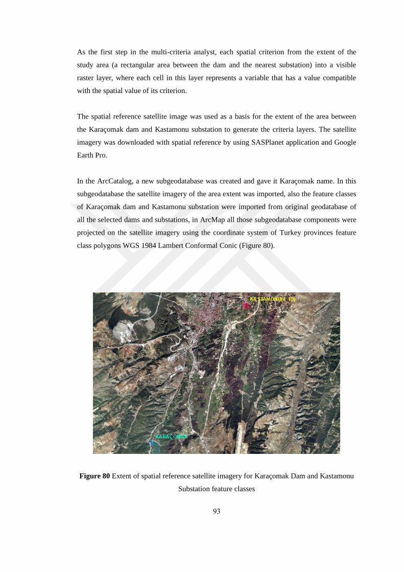
93

As the first step in the multi-criteria analyst, each spatial criterion from the extent of the

study area (a rectangular area between the dam and the nearest substation) into a visible

raster layer, where each cell in this layer represents a variable that has a value compatible

with the spatial value of its criterion.

The spatial reference satellite image was used as a basis for the extent of the area between

the Karaçomak dam and Kastamonu substation to generate the criteria layers. The satellite

imagery was downloaded with spatial reference by using SASPlanet application and Google

Earth Pro.

In the ArcCatalog, a new subgeodatabase was created and gave it Karaçomak name. In this

subgeodatabase the satellite imagery of the area extent was imported, also the feature classes

of Karaçomak dam and Kastamonu substation were imported from original geodatabase of

all the selected dams and substations, in ArcMap all those subgeodatabase components were

projected on the satellite imagery using the coordinate system of Turkey provinces feature

class polygons WGS 1984 Lambert Conformal Conic (Figure 80).

Figure 80 Extent of spatial reference satellite imagery for Karaçomak Dam and Kastamonu

Substation feature classes

94

To create the layers for the criteria of suitable elevation and the least slope, using the cells

coordinates of the satellite imagery base map and the TCX Convertor application the

elevation points data were downloaded for the coordinates of area extent of Karaçomak dam

and Kastamonu substation in an excel format table. In ArcMap and from the new

subgeodatabase of Karaçomak dam, the elevation data excel table was imported to create the

elevation raster layer using the inverse distance weighted IDW interpolation tool in spatial

analyst tools box (Figure 81).

Figure 81 Elevation raster layer for the extent between Karaçomak Dam and Kastamonu

Substation

Then by using the ArcMap Slope tool in the surface spatial analyst tool box the slope raster

layer was created, where each cell in this layer represents the slope of its position (Figure

82). According to TEİAŞ, the degree of slope, which is more than 30%, is unsuitable for

design. Also areas with a slope greater than 40% are prone to landslides.

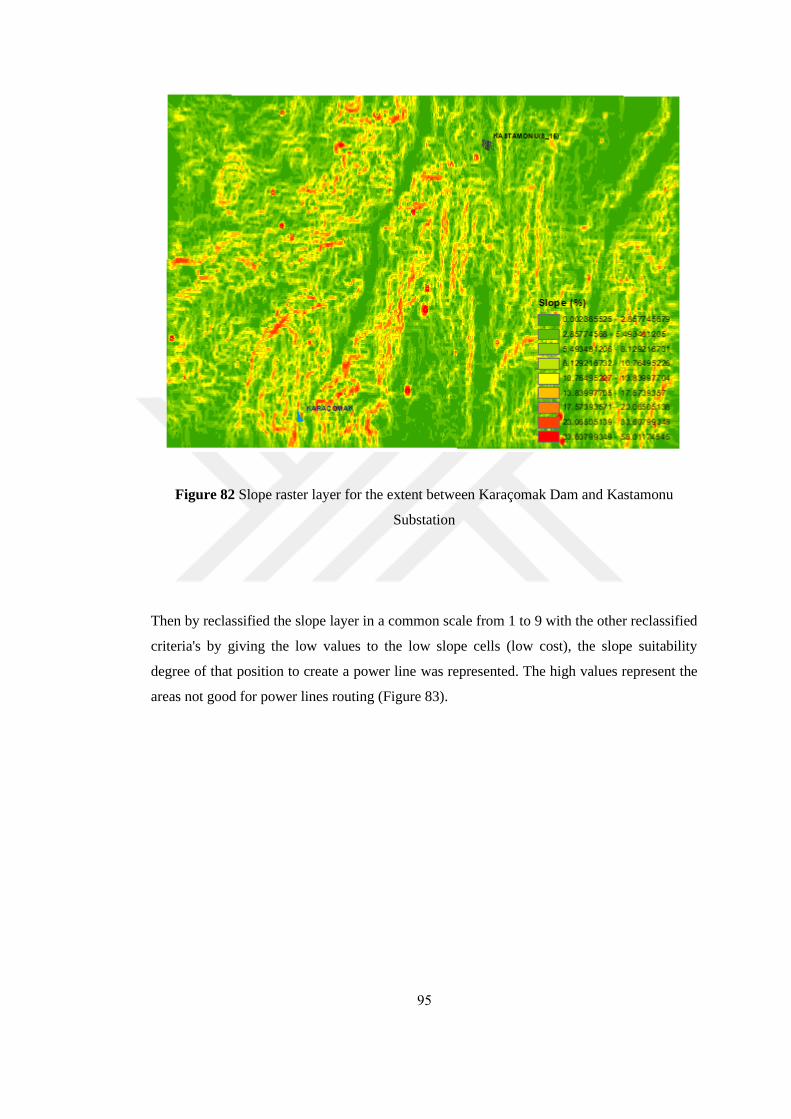
95

Figure 82 Slope raster layer for the extent between Karaçomak Dam and Kastamonu

Substation

Then by reclassified the slope layer in a common scale from 1 to 9 with the other reclassified

criteria's by giving the low values to the low slope cells (low cost), the slope suitability

degree of that position to create a power line was represented. The high values represent the

areas not good for power lines routing (Figure 83).

96

Figure 83 Reclassified slope raster layer for the extent between Karaçomak Dam and

Kastamonu Substation

To calculate the distance from roads, in the extent of the area between Karaçomak dam and

Kastamonu substation, the roads were digitized and saved as a line feature class in the

selected dam subgeodatabase (Figure 84).

97

Figure 84 Roads feature class for the extent between Karaçomak Dam and Kastamonu

Substation

In ArcMap using one of the spatial analyst tools which is Euclidean Distance, the raster

layer of the distance from the feature class of roads which is saved before in the

subgeodatabase of Karaçomak dam was created, each cell's value in this layer represents the

distance in meters from its position to the roads (Figure 85).

98

Figure 85 Raster layer representing near to roads for the extent between Karaçomak Dam

and Kastamonu Substation

By reclassified distance from roads layer in a common scale with reclassified slope from 1 to

9 by giving the low values to the low cost cells (short distances), where the zero value will

be along the roads and the values (distances) will be increased by moving away from the

road. By doing this, the suitability degree of that position to create a power line according to

criterion of near to roads was represented in Figure 86.

99

Figure 86 Reclassified raster layer for near to roads for the Extent between Karaçomak Dam

and Kastamonu Substation

For the criterion of land use, all specialists agree on the importance and impact of the nature

of land cover and the type of land use in the process of directing power lines, where the main

purpose is to passing the power line from the open areas, barren land, far from the habitat

and settlement. The high suitability classes were given to land uses that have low cost, low

environmental impact and low threats to power lines. Also some potential lands obstacles

were excluded from the analysis and have been given "no data" value.

The polygons of land use layer feature class were digitized by manual recognition and digital

classification preceded by visual interpretation of satellite images which was used before as a

base map for the extent area to produce several criteria's maps. Also the additional data that

Google Earth provides were compared, such as cultural heritage sites, archaeological sites,

nature reserves, and others. As well as (https://osmlanduse.org) which provides an access to

global land use maps [63]. Then the digitized polygons of land use were saved as a new

polygon feature class in the Karaçomak dam's subgeodatabase.

100

For the purpose of reclassification by categories of land use within a common scale with the

rest of other criteria and for the purpose of giving the obstacles "no data" value, which will

be considered as prohibited areas for all other criteria, the polygons feature class of land use

were converted from vector data layer to raster data layer. The Feature to Raster tool was

used from the conversion tools in the spatial analysis toolbox of ArcMap (Figure 87).

Figure 87 Land use raster for the extent between Karaçomak Dam and Kastamonu

Substation

The land use feature class values were reclassified to be comparable with the reclassified of

other criteria's layers, where the higher value indicates that it is costly to create a power lines

path on that particular land use (Figure 88).

101

Figure 88 Reclassified land use raster for the extent between Karaçomak Dam and


After getting the reclassified raster layers in a common scale for all criteria layers and by

using Map Algebra-Raster Calculator spatial analyst tool in ArcMap tool box, all the

reclassified raster layers were combined together, the cost layer was produced. Any place

(one cell) on this raster layer represent's the cumulative cost value or the suitability degree of

that place according to all spatial criteria (Figure 89).

102

Figure 89 Cost raster (suitability layer) for the extent between Karaçomak Dam and


The least cost path algorithm use the cost layer that was got in the previous step and the path

starting point layer (Karaçomak dam position) to produce two new visible layers, which is

the least cost distance layer (cost distance raster) (Figure 90), and the least cost direction

layer (back link raster) (Figure 91). Those new raster layers were got using the spatial

analyst Cost Distance and Cost Back Link distance tools in ArcMap spatial analyst tools box.

103

Figure 90 Cost distance raster layer for the extent between Karaçomak Dam and


Figure 91 Back link raster layer for the extent between Karaçomak Dam and Kastamonu

Substation

104

Each cell in the cost distance layer in Figure 90 represents the least cumulative cost of

traveling from that cell to the source point cell (Karaçomak dam). While each cell in the

back link layer in Figure 91 represents the direction code of the least cost movement to one

of the eight neighbor cells back to the source point cell (Karaçomak dam).

By determination of the destination point which is Kastamonu substation, the destination

layer is created. The analyzer of the GIS use the cost distance layer, the back link layer and

the destination layer to calculate the least cost path raster layer (best path). The output cost

path layer (best path) represents the shortest least costly path from Karaçomak dam to

Kastamonu substation. The path avoids steep slopes and certain of types of lands that are

considered costlier for constructing power line; the path also seeks to be near to roads and

existing power lines and in a favorite land use. The least cost path raster layer (best path)

was got using the spatial analyst Cost Path distance tools in ArcMap spatial analyst tools

box. As an additional step, the path raster was converted to polyline (vector feature class) to

give the possibility of controlling the design of the path and placing the towers (Figure 92).

This was done using the from raster Raster to Polyline conversions tools in the ArcMap tools

box.

Figure 92 Least cost path (best path) for grid connection between Karaçomak Dam and

Kastamonu Substation (8.607 km)

105

The difference between the cost path for power line grid connection and straight line

between Karaçomak dam and Kastamonu substation is:

8607–8560 = 47 meter.

As a last step in best path model by using ArcScenen Base Height 3D analyst tools, the best

path line vector was projected on the 3D surface of satellite imagery for the area of the path

were used the elevation raster layer as a base height to create the 3D surface for the satellite

imagery and the path in order to allow the realization of the path and the possibility of

modification as well as determination of pylons locations by giving a realistic perception of

the path on the real surface of the terrain and land cover (Figure 93).

Figure 93 3D view of the best path between Karaçomak Dam and Kastamonu Substation

106

CHAPTER 6

CONCLUSION

6.1. Conclusion

This study investigated on 751 operated dams in Turkey in terms of their potential for

hydropower development. A total of 265 of 711 irrigation dams were found to be most

suitable for hydropower development, and 183 substations were found within a maximum

distance of 40 km from these 265 dams for the purpose of grid connection. These were found

by assessing a set of spatial and technical criteria for both the dams and the substations, and

applying a geodatabase query to filter the dams and substations and to choose the most

suitable options based on the specified criteria.

Using Equation (3), an average distance of 35 km was calculated between substations in

Turkey, meaning that each dam should have a substation within approximately 40 km. Some

of the selected 183 substations based on the technical and spatial criteria were close to more

than one dam, and eight of the selected 273 dams based on the technical criteria were found

not to have a substation within 40 km, therefore they excluded and the number of the

selected dams becomes 265.

A variation was observed in the preferences of the criteria for any selected dam through the

results of statistical indicators of the criteria. For example, the dam with the highest

preference for the criterion of shortest distance to the nearest substation, which is 720

meters, had low preferences in relation to its other criteria where the reservoir capacity was

3.7 hm3. Therefore, the selected dams were arranged according to their suitability using

multi-criteria fuzzy logic, which was assessed in terms of meeting the specified technical and

107

spatial criteria. Three categories were identified: 21 dams with high suitability i.e. a

suitability score greater than 75%; 149 dams with medium suitability, i.e. a suitability score

of between 50% and 74.9%; and 95 dams with low suitability, i.e. a suitability score of less

than 50%.

The first case study was Karadere Dam, with an overall suitability score of 78%. This dam

was therefore from the high suitability class. The potential power was calculated at 1587

kW, and the annual benefit was estimated at €457,056/year. By applying the methodology

for finding the best path for grid connection to the nearest substation, which was within a

distance of 12.07 km, the best grid connection path was found with a length of 12.789 km,

i.e. a difference from the straight-line distance of 719 m. In addition, although the criterion

of near to rivers was not one of the criteria examined in this study, the proposed path was

close to the Karadere river (Figure 67). This can be attributed to the criterion of land use,

which takes into account the important factors that affect the cost of grid connection such as

land confiscation and slope, which always have low values near rivers. This result can be

considered a good indicator of the accuracy of the method.

The second case study was Karaçomak Dam, with an overall suitability score of 58%, which

places it in the medium suitability class. The potential power was calculated at 799 kW, and

the annual benefit was estimated at €230,112/year. By applying the methodology for finding

the best path for grid connection to the nearest substation, which was within a distance of

8.56 km, the best grid connection path was found with a length of 8.607 km, which differed

from the straight-line distance by 47 m. In the case of Karaçomak Dam, the criterion of near

to existing power lines was deliberately not taken into account, due to the presence of an

existing power line between the dam and the nearby Kastamonu substation (Figure 92). This

was in order that the proposed line could be evaluated and compared with the existing line.

The proposed best path almost matched the existing line, thus demonstrating the accuracy of

the methodology and criteria used to find the best route.

By comparing the two case studies, it can be observed how the differences in potential power

affect the suitability score for each dam. It can also be noted that the length of the proposed

grid connection route is related to the distance of the dam from the nearest substation; this

length is close to the straight-line distance when the nearest substation is close to the dam, as

in the Karaçomak dam case study, and is more different from the straight-line distance when

108

the substation is further from the dam, due to the effect of taking the various spatial criteria

into account and avoiding obstacles in wide areas, as in the Karadere case study.

The methodology used in the study and its results, main findings and conclusions are

summarized in Figure 94.

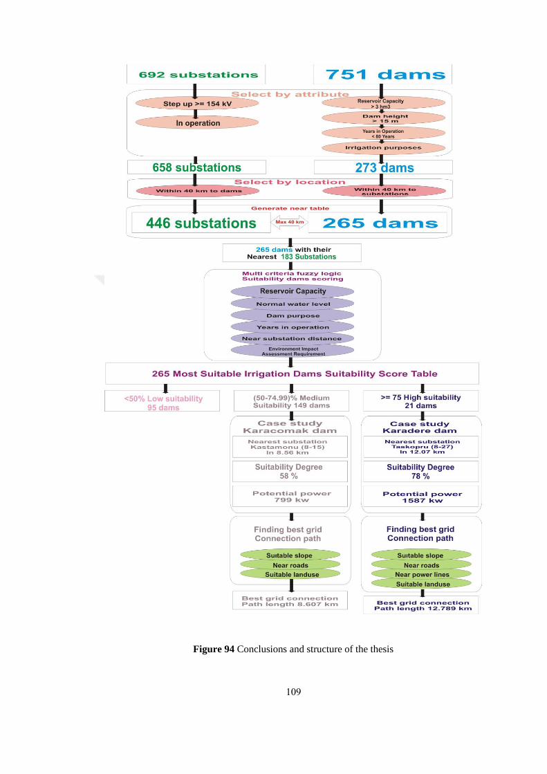
109

Figure 94 Conclusions and structure of the thesis

110

6.2. Discussion

The study has succeeded in proving the availability and capability of irrigation dams in

Turkey; these are distinguished from other types of dams due to their characteristics, which

allow them to generate hydropower with high quality, low cost, low environment impact and

ease of implementation, this done by verifying the (technical, spatial, grid connection, risk

and environmental impact) criteria's. By applying these criteria the best dams have been

selected for the possibility of hydropower development.

One of the most important criteria that often overlooked in hydropower projects is the grid

connection distance. In this study, the criterion of distance to the nearest substation was

considered in order to ensure that the potential power quantity is consistent with the cost and

distance of the grid connection. Considering an average of 35 km between substations in

turkey found using equation (3), the maximum grid connection distance (break-even

distance) between the selected dams and their nearest substations was therefore set to 40 km,

in order to avoid exceeding power losses of 4.5% and to ensure consistency between the

potential benefits and the grid connection cost.

Although all the selected dams are suitable for hydropower development, knowing the best

or start on the best was certainly wanted. Implementing agencies and beneficiaries aim to

choose dams that meet the highest criteria (i.e. highest power production, lowest cost and

environmental impact, and shortest grid connection), especially after the variation which

observed in the preference of the criteria for any selected dam through results of statistical

indicators of the criteria. Using multi-criteria fuzzy logic, the overall suitability score of each

dam was calculated based on all the required criteria and the dams were then sorted

according to their suitability score and classified into suitability ranges to allow the best to be

selected for grid connection spatial analysis and other tests. The selected dams were arranged

based on their overall suitability scores into three classes: high, medium and low suitability.

A methodology for finding the best grid connection route was presented using multi-criteria

GIS spatial analysis to find the option with lowest risk, least loss, least cost and lowest

environmental impact of the power line. The criteria were short distance to nearst substation,

least slope, near from roads and existing power lines, which were related to the risks and

costs of establishing and maintaining new power lines. Other criteria included avoiding or

excluding certain types of public and private property, avoiding natural reserves and large

111

water surfaces, and crossing some types of land, which were related to land costs, lands

confiscation, EIA requirements, and natural and artificial obstacles.

Two dams were selected as case studies: Karadere, a dam from the high suitability class, and

Karaçomak, from the medium suitability class. For each of these dams, the technical and

spatial criteria were discussed and the potential power and economic benefits were

estimated. In addition, multi-criteria GIS spatial analysis was applied to find the best routes

for grid connection for each of the two dams to their nearest substations.

6.3. Recommendations

The study propose investment in hydropower development for the best 265 irrigation dams,

which were identified in this study according to their overall suitability scores, based on

several technical, spatial and environmental criteria. The study also proposes the use of

siphon turbines for hydropower development, since it does not need to tamper the irrigation

dam's body.

In terms of grid connection, it is possible to control the weights of the criteria according to

different perspectives, removing or adding criteria to give new results. Where this study

provides a methodology for identifying the nearest substation for each dam and finding the

best grid connection path to it, based on the common criteria for the routing of power lines

and the amount of power that can be potentially generated.

For the dams with good values of their technical criteria for hydropower development but

not have substations within 40 km for grid connection, the proposed methodology can be

used to find the best grid connection route within isolated grids to the nearest potential

energy investment site, which may be the nearest small village, factory or other.

The proposed methodology can also be applied to other types of dams or renewable energy

resources, or to irrigation dams in other countries.

112

REFERENCES

1. European Environmental Agency, (2017), “Turkey Land Cover 2012”, Country fact

sheet.

2. MENR - Ministry of Energy and Natural Resources of Turkey, (2009), “The Strategic

document of Electricity Energy Market and Security of Supply”.

3. Kucukali S., (2010), “Hydropower potential of municipal water supply dams in Turkey: A

case study in Ulutan Dam”, Zonguldak Karaelmas University, Zonguldak, Turkey.

4. ESRI - Environmental Systems Research Institute, (2005), “Using ArcGIS Spatial

Analyst”.

5. P. Schaefer, P. Thapa, J. Schlüter, S. Palt, P. Vennemann, (2011), “Identification of

potential pumped-storage sites in large areas based on a multi-criteria GIS-model”.

6. Kucukali S., (2014), “Finding the most suitable existing hydropower reservoirs for the

development of pumped-storage schemes: An integrated approach”.

7. Cecile Bousquet, Irene Samora, Pedro Manso, Luca Rossi, Philippe Heller, Anton J.

Schleiss, (2017), “Assessment of hydropower potential in wastewater systems andapplication

to Switzerland”.

8. Yiğit Dedemen, (2013), “A Multi-Criteria Decision Analysis Approach to Gis-Based

Route Selection for over head Power Transmission Lines”, Middle East Technical

University, Ankara, Turkey.

9. Cláudio Monteiro, and others, (2005), “Gis Spatial Analysis Applied To Electric Line

Routing Optimization”, IEEE Transactions On Power Delivery, Vol. 20, No. 2, April 2005.

10. The World Bank Group, (2015), “Nepal: Scaling Up Electricity Access through Mini

and Micro Hydropower Applications”.

113

11. OECD - Organization for Economic Co-operation and Development, (2009), OECD

Fact book ISBN 92-64-05604-1, http://oberon.spourceoecd.org.

12. Erol H. Cakmak, “Irrigation systems performance: Turkey country report” TED Univ.,

Accessed March 27, 2019, https://www.researchgate.net/publication/228651156.

13. Niall Fitzgerald, Roberto Lacal Arántegui, Eamon McKeogh, Paul Leahy, (2012),

“A GIS-based model to calculate the potential for transforming conventional hydropower

schemes and non hydro reservoirs to pumped hydropower schemes”.

14. Hydroelectricity and energy calculator, Accessed March 27, 2019, https://power-

calculation.com/hydroelectricity-energy-calculator.php.

15. DSI, TRCOLD - International Commission on Large Dams Turkish National

Committee, (2014), “Dams of Turkey”.

16. Barajlar Uygulaması v1.4, Accessed March 31, 2018, https://barajlar.dsi.gov.tr.

17. TEİAŞ - Türkiye Elektrik İletim Anonim Şirketi, (2018), “Trafo Merkezleri ve Tarife

Bölgeleri Listesi”.

18. ESHA - European Small Hydropower Association, (2004), “Guide on How to Develop

a Small Hydropower Plant”.

19. ICOLD - International Committee on Large Dams, (2011), “CONSTITUTION”

page3.

20. IRENA - International Renewable Energy Agency, (2012), “Renewable Energy

Technoliges: Cost Analysis Series-Hydropower”.

21. Are Dams Forever? Teach Engineering Digital Library, Accessed March 4, 2019,

https://www.teachengineering.org/lessons/view/cub_dams_lesson08.

22. Decommissioning dams - costs and trends, International water power & dam

construction, Accessed March 4, 2019,

https://www.waterpowermagazine.com/features/featuredecommissioning-dams-costs-and-

trends.

23. IFC- International Financial Corporation, (2015), “Hydroelectric Power a Guide for

Developers and Investors”, page30.

http://oberon.spourceoecd.org/

https://www.researchgate.net/publication/228651156

https://power-calculation.com/hydroelectricity-energy-calculator.php

https://power-calculation.com/hydroelectricity-energy-calculator.php

https://barajlar.dsi.gov.tr/

https://www.teachengineering.org/lessons/view/cub_dams_lesson08

https://www.waterpowermagazine.com/features/featuredecommissioning-dams-costs-and-trends

https://www.waterpowermagazine.com/features/featuredecommissioning-dams-costs-and-trends

114

24. AVO, Training Institute Marketing Manager, (2017), “Basic Substation

Configurations and the Components” page22.

25. Tino Schlemmer, Lyndon Greedy, (2015), “A 66 kV systems for wind offshore”, DNV

GL Energy, page2.

26. Step Up Substation - Generator Transformer and Insulation Co-Ordination,

Accessed April 7, 2019, https://studylib.net/doc/18041411/generator--transformer-and-

insulation-coordination.

27. Turan ÇAKIL, H. Feza CARLAK, Şükrü ÖZEN, (2015), “Modeling of Power

Network System of the High Voltage Substation: a simulation study”, International Journal of

Engineering & Applied Sciences (IJEAS) Vol.7, Issue 3(2015)39-57.

28. Hydro Power Basics – Energypedia, Accessed April 10, 2019,

https://energypedia.info/wiki/Hydro_Power_Basics.

29. Kucukali S., (2015), “Risk scorecard concept in wind energy projects: An integrated

approach”, Çankaya University, Ankara, Turkey.

30. Yuri Y., Franz W., (2017), “The Future of Wind, Security in Electric Energy Supply and

HV Grid Development”.

31. Omar H., Kankar B., (2012), “Optimal planning and design of a renewable energy

based supply system for microgrids”, Department of Electrical and Computer Engineering,

University of Waterloo, Waterloo, Ontario, Canada N2L 3G12017, Renewable Energy 45

(2012) 7-15.

32. Houssem R., (2010), “Transmission and Distribution of Electrical Power” Department

of Electrical Engineering, Umm Al-Qura University, Saudi Arabia.

33. O. M. Longe, and others, (2017), “A Case Study on Off-grid Microgrid for Universal

Electricity Access in the Eastern Cape of South Africa”, Electrical and Electronics

Engineering Science, University of Johannesburg, International Journal of Energy

Engineering 2017, 7(2): 55-63 DOI: 10.5923/j.ijee.20170702.03.

34. Guedes C., (2015), “Renewable Energy Offshore”, Taylor and Frances Group, London,

ISBN: 978-1-1-38-02871-5, page 158.

35. Christer Carlsson, Robert Full´er, (1996), “Fuzzy multiple criteria decision making:

Recent developments” Volume 78, Issue 2, Pages 139-241 (11 March 1996).

https://studylib.net/doc/18041411/generator--transformer-and-insulation-coordination

https://studylib.net/doc/18041411/generator--transformer-and-insulation-coordination

https://energypedia.info/wiki/Hydro_Power_Basics

115

36. Kucukali S., (2011), “Risk assessment of river-type hydropower plants by using fuzzy

logic approach”, world renewable energy congress 2011, Sweden 8-13 May.

37. Chia - NanWang, and others, (2018), “Multi-Criteria Decision Making Approaches for

Solar Power Plant Location Selection in Viet Nam” Published: 8 June 2018.

38. Mümtaz Ak, Elçin Kentel, Kucukali S., (2017), “A fuzzy logic tool to evaluate low-

head hydropower technologies at the outlet of wastewater treatment plants”, Renewable and

Sustainable Energy Reviews 68 (2017) 727–737.

39. Zadeh L. A., (1965), “Fuzzy Sets. Information and Control”, 338-353.

40. Turgeon M, Claisse M, Landry G., (2010), “Development of the first pumped storage

project with an underground lower reservoir”, Proc., HYDRO 2010 Conference, Lisbon.

41. Gary L. Raines, and others, (2010), “New ArcGIS 10 in fuzzy logic tools”, ArcUser.

42. Lazim Abdullah, Nurnadiah Zamri, (2012), “Road Accident Models with Two

Threshold Levels of Fuzzy Linear Regression”, Journal of Emerging Trends in Computing

and Information Sciences, VOL. 3, NO. 2, February 2012.

43. Chin, D.A., (2012), “Water Resources Engineering”, Pearson, 3rd Edition.

44. Caissie D., El-Jabi N., Hebert C., (2007), “Comparison of Hydrologically Based

Instream Flow Methods Using A Resampling Techniqe”, Can. J. Civil Eng. , 34, 66-74, 2007.

45. Pelin Temel, (2015), “Evaluation of Potential Run-of River Hydropower Plant Sites

Using Multi-Criteria Decision Making in Terms of Environmental and Social Aspects”,

Middle East Technical University, February 2015.

46. Velasquez M., Hester P. T., (2013), “An Analysis of Multi-Criteria Decision Making

Methods”, International Journal of Operations Research, 10 (2), 56-66, 2013.

47. Jones Ch. B., (1997), “Geographical information systems and computer cartography”,

Longman, England.

48. Malczewski J., (1999), “GIS and Multicriteria Decision Analysis”, New York: Wiley

and Sons.

116

49. Namir N. A., Noor M. A., (2015), “A GIS-Assisted Optimal Baghdad Metro Route

Selection Based On Multi Criteria Decision Making”, Journal of Engineering and

Development Vol. 19, No. 06, November 2015.

50. Jan Burdziej, (2009), “Multi-criteria spatial analysis of land accessibility for seismic

operations”, Jagiellonian University, Krakow, Poland.

51. ESRI - Environmental Systems Research Institute, (2010), “Spatial Analyst Tutorial”.

52. Huber D., Church R., (1985), “Transmission Corridor Location Modeling”, Journal of

Transportation Engineering.

53. Saaty T. L., (1990), “How to make a decision: the analytic hierarchy process”,

European journal of operational research, 48(1), 9 26, 1990.

54. Gwo - Hshiung T., Tzeng G. H., Huang J. J., (2011), “Multiple attribute decision

making Methods and applications”, Chapman & Hall.

55. Miller, H. J., S.L. Shaw, (2001), “Geographic Information System for Transportation

Principles and applications”, Oxford University Press.

56. Öztürk T., (2007), “Finding the Optimum Route for Transmission Lines within GIS”,

Ms. Thesis, METU.

57. Kamila Małgorzata Belka, (2005), “Multicriteria analysis and GIS application in the

selection of sustainable motorway corridor”, Ms. Thesis, Institutionen för datavetenskap,

Linköpings universitet.

58. ESRI - Environmental Systems Research Institute, (2005), “Using ArcGIS 3D

Analyst”.

59. ESRI - Environmental Systems Research Institute, (2006), “Advanced Raster Spatial

Analysis”.

60. Zhu X., Liu S., Yeow Mun-Ching, (2006), “Accessibility analysis for housing

development in Singapore with GIS and multi-criteria analysis methods”, Applied GIS 2 (2):

pp. 13.1–13.12. DOI: 10.2104/ag060013. 2006.

61. Ahmed Hossam-Eldin, and others, (2012), “Effect of Electromagnetic Fields from

Power Lines on Metallic Objects and Human Bodies”, International Journal of

Electromagnetics and Applications, 2(6): 151-158. 2012.

117

62. Söderman T., (2006), “Treatment of biodiversity issues in impact assessment of

electricity power transmission lines: A Finnish case review”, Environmental impact

assessment review, 26(4), 319-338. 2006.

63. HeiGIT - Heidelberg Institute for Geoinformation Technolog, (2019), Accessed

March 27, 2019, https://data.osmlanduse.org.

64. ICID - International Commission on Irrigation and Drainage, (2000), “Role of Dams

for Irrigation, Drainage and flood control”, position paper.

65. FAO - Food and Agriculture Organization, (2019), “Water Sources and Water

Availability”, Accessed, 30 May 2019, http://www.fao.org/3/U5835E/u5835e03.htm.

66. Recep Bakiş, and other, (2018), “Investigation Of Hydropower Generation From

Irrigation Dams”, Anadolu University, Journal of Science and Technology, DOI:

10.18038/aubtda.368219. 2018.

http://www.geog.uni-heidelberg.de/gis/heigit_en.html

https://data.osmlanduse.org./

http://www.fao.org/3/U5835E/u5835e03.htm

118

APPENDIX A

MULTI-CRITERIA HIGH SUITABILITY SCORE DAMS

Table 12 High Suitability Class: 21 Dams had a Suitability Score of between 75% and 87%

Rank Dam NameStart

OperationRiver Province Purpose

Body

Type*

Reservoir

Capacity

Height from

Base (m)

Height from

Thalweg (m)

Normal Water

Level or Head

Full Spill

Way (m3/s)

Irrigated

Area (hm2)

Near

Substation (km)Substation Name

Suitability

Score

1 Aktaş 2017 Aktaş Izmir I CCS 43.79 105.5 100 98 1580 9.921 Ödemiş 0.871

2 Burgaz Zeytinova 2013 Falaka Çayi Izmir I CCS 33 115 84.5 81.5 3009 11.906 Tire 0.829

3 Çayirdere 2017 Kocadere Kirklareli I CFR 28.25 63 58.5 57.5 232.73 2583 10.597 Pinarhisar 0.814

4 Taşoluk 2009 Çinarcikdere Çanakkale I CCR 79.4 75 65 63 1352 9606 8.948 Biga 0.813

5 Yenidere 2010 Yenidere Çayi Denizli I CCS 65.37 46 43 40 1432 3304 5.087 Tavaş 0.801

6 Havran 2010 Havran Balikesir I CCR 66.5 79.5 63.5 60.5 1406 3330 12.836 Edremit 0.794

7 Vezirköprü 2005 Istavloz Çayi Samsun I CCR 51.47 75 73.5 67.5 887.75 10994 11.444 Vezirköprü 0.794

8 Madra 1998 Madra Balikesir I CCR 79.4 97 87 84 7872 13.822 Ayvalik 0.789

9 Karadere 2007 Karadere Çayi Kastamonu I CCS 26.08 90 70 64 1220 6852 12.074 Tasköprü 0.789

10 Derinöz 2002 Derinöz Amasya I CCR 18.9 77 74 70 158 4990 10.970 Ladik 0.787

119

Table 12 (continued)

Rank Dam NameStart

OperationRiver Province Purpose

Body

Type*

Reservoir

Capacity

Height from

Base (m)

Height from

Thalweg (m)

Normal Water

Level or Head

Full Spill

Way (m3/s)

Irrigated

Area (hm2)

Near


Suitability

Score

11 Beşkariş 2012 Muratçay Kütahya I CCS 75.6 62.85 52.35 48.35 314 9093 12.971 Altintaş Tm 0.784

12 Yazici 2008 Altinçayir Ağri IM CCS 220.55 90 83.5 78.5 257 31918 11.440 Ağri Tm 0.780

13 Saraydüzü 2011 Asarcik Sinop I CCS 36.28 73.5 58.5 50.5 558.98 4109 14.294 Boyabat 0.774

14 Kestel 1989 Kestel Çayi Izmir I CCS 37.4 65 58 53 4077 2.103 Bergama 0.769

15 Çamgazi 1998 Deyran Adiyaman I CCS 53.12 45 39 36 77.86 8000 3.462 Adicim 0.768

16 Kalecik 1985 Kalecik Deresi Osamniye I CCR 31.25 80 77 75 1690 4395 7.659 Bahce 0.763

17 Kalecik 2016 Uludere Ankara IM CCS 16.25 55 53 50 2455 4.018 Kalecik 0.762

18 Ibrala 2012 Ibrala Karaman IM CCR 134 58 49 45 728.3 8700 6.407 Karaman_Osb 0.758

19 Naras 2016 Manavgat Antalya IF RCC 36.18 78 68 56 915 7142 9.903 (Yavrudogan)Gundogdu 0.757

20 Erzincan 1997 Göğne Erzincan I CCS 11.54 81 74.5 73.5 5406 8.564 Erzincan_Osb 0.757

21 Ardil 2017 Ardil Gaziantep I RCC 10.97 54 49 44 507 2126 12.736 Ps5 Tm 0.753

*CCS: Clay Core Sand-Gravel, CCR: Clay Core Rock, RCC: Roller Compacted Concrete, CFR: Concrete Faced Rock Fill, HE: Homogeneous Earth, CFS: Concrete Faced Sand-Gravel, CG: Concrete Gravity

121

APPENDIX B

MULTI-CRITERIA MEDIUM SUITABILITY SCORE DAMS

Table 13 Medium suitability class: 149 dams had a suitability score of between 50% and 74.99%

Rank Dam NameStart

OperationRiver Province Perpose

Body

Type*

Reservoir

Volume (hm3)

Height from

Base (m)

Height from

Thalweg (m)

Normal Water

Level or Head

Full Spill

Way (m3/s)

Irrigated

Area (hm2)

Near


Suitability

Score

1 Babasultan 2009 Karadere Bursa I CCR 12.098 53 46 44 305.39 4006 9.551 Inegöl 0.7498

2 Sultansuyu 1994 Sultansuyu Çayi Malatya I CCS 53.3 60 53 50 1050 8596 9.797 Malorsa 0.7484

3 Akgedik 2008 Sariçay Muğla IM CCS 29.032 55 48 45 403 1642 4.786 Milas 0.7420

4 Kizildamlar 2003 Söğüt Bilecik I CCR 10.7 46.7 40 35 296 1974 4.003 Söğüt Tm 0.7392

5 Hancağiz 1990 Nizip Çayi Gaziantep I CCS 100 48 45 42 2430 6945 8.517 Belkis Tm 0.7382

6 Musabeyli 2012 Bişeközü Yozgat IM CCS 48.6 67 61 57 238 1850 13.922 Yozgat 0.7318

7 Güzelhisar 1982 Güzelhisar Çayi Izmir IM CCR 158 89 86 84 9230 6.776 Alosb I 0.7283

8 Hasanlar 2012 Kabaklar Kütahya I CFR 7.9 57.85 48 47 863 13.511 Emet Tm 0.7261

9 Seferihisar 1994 Yassiçay Izmir I CCS 29.1 59 54 49 113.63 1277 14.602 Urla 0.7237

10 Sevişler 1982 Yağcili Çayi Manisa I CCS 122.4 65 59.5 51.5 7063 10.288 Soma Santr. A 0.7237

122


Rank Dam NameStart


Body

Type*

Reservoir

Volume (hm3)

Height from

Base (m)

Height from

Thalweg (m)

Normal Water

Level or Head

Full Spill

Way (m3/s)

Irrigated

Area (hm2)

Near


Suitability

Score

11 Seve 2005 Sinnep Kilis IM CCR 20.9 41 34 31 513 196 2.309 Kilis Tm 0.7225

12 Kovali 1987 Dündar Kayseri I CCS 25.1 48.5 42 40 416 2850 7.981 Yeşilhisar 0.7208

13 Korkuteli 1976 Korkuteli Antalya I CCS 42.74 70.2 50.2 46.2 815 5985 3.316 Korkuteli 0.7208

14 Deliçay 2010 Kurt Deresi Karaman IF HE 25.6 45 35 30 339 3690 5.647 Karaman 0.7199

15 Yeşilburç 2013 Kaynardere Niğde I CCR 3.24 40.5 35.5 32.5 37.4 450 6.133 Nigde2 0.7194

16 Kiliçli 2007 Kapali Deresi Adana I HE 9.5 38 27 23 156.1 677 4.267 Clhadlye 0.7156

17 Bayir 2007 Sirainler Muğla I CCR 7.21 52.5 47 43 311.87 373 11.230 Muğla 0.7139

18 Koçhisar 2011 Büyükköz Çorum IM HE 161.7 57.4 37.4 32.4 442 12427 13.181 Alaca 0.7127

19 Çiçeközü 2013 Boğazdere Bursa I CCS 4.9 53 48.5 45.5 1730 13.895 Yenişehir1 0.7117

20 Demirtaş 1983 Ballikaya Dere Bursa I CCS 14.457 54 46 41 362 1710 3.507 Bdgkçs 0.7115

21 Gökpinar 2001 Gökpinar Denizli IM CCS 27.72 50 43 41 819 6522 6.613 Denizli2 0.7099

22 Onaç 2 1998 Onaç Burdur I HE 16.58 32.5 23.5 18.5 564 1953 4.803 Bucak 0.7096

23 Türkmenli 2001 Kumdere Tekirdağ I HE 15.29 29.8 26.8 22.8 355.88 515 7.884 Botaş 0.7095

24 Karamanli 1987 Değirmendere Burdur I CCS 24.813 53.75 47.25 42.25 631 3747 11.563 Tefenni 0.7084

25 Şarkişla Kanak 2013 Kanak Sivas IM CCS 23.67 49 37.5 33.5 275 2313 13.026 Sarkisla 0.7051

26 Gödet 1988 Gödet Akarsuyu Karaman IF CCR 158 93 64.7 62.7 972 16000 10.598 Karaman 0.7009

27 Ikizcetpeler 1991 Kille Balikesir IM CCR 164.58 52 47 45 2776 4688 7.936 Balikesir_Seka 0.6984

28 Topçam 1984 Madran Aydin IF CCS 106.2 61.65 56.15 54.15 4983 5.608 Çine 0.6942

29 Peçenek 2010 Peçenek Ankara IM HE 75.5 33 32 29 412 1410 13.323 Sereflikochisar 0.6907

30 Günyurde 2005 Bakraş Bilecik I CCR 8.79 46 37 32 122 805 13.570 Karaköy(Tcdd) Tm 0.6897

123


Rank Dam NameStart


Body

Type*

Reservoir

Volume (hm3)

Height from

Base (m)

Height from

Thalweg (m)

Normal Water

Level or Head

Full Spill

Way (m3/s)

Irrigated

Area (hm2)

Near


Suitability

Score

31 Şehitler 2003 Çukur Isparta I CCR 5 46 42.9 40.9 1.8 884 11.422 Sarkikaraağaç 0.6896

32 Alaca 1984 Suludere Akarsuyu Çorum I CCR 12.6 57 44.3 40.3 344 1546 7.327 Alaca 0.6887

33 Kunduzlar 1984 Yönek A. Eskişehir I CCS 22 42.5 28 26 804 5014 8.000 Kirka Tm 0.6853

34 Ariklar 2003 Karaağaç Kocaeli I HE 11.75 27 21 18 1832 9.100 Kaynarca 0.6819

35 Kayapa 1998 Değirmendere Bursa I HE 3.85 48.85 36.85 34.15 185.2 1418 7.193 Görükle 0.6801

36 Hacihidir 1989 Şehir Çayi Şanliurfa I CCR 62.6 42 36.4 27.4 2080 14.448 Siverek Tm 0.6797

37 Keskin 75Yil 1998 Karaöz Eskişehir I HE 8.4 28.6 24.6 22.6 80 1112 5.763 Eskişehir Iii Tm 0.6788

38 Karaidemir 1980 Poğaça Deresi Tekirdağ I HE 111.6 34 29.8 24.8 1154 7720 9.057 Malkara 0.6775

39 Kirklareli 1999 Şeytandere Kirklareli IFM CCR 113.31 70.5 67.5 61.5 1835 13679 8.821 Kirklareli 0.6768

40 Asar 2008 Değirmendere Kastamonu I CCS 5.68 36.7 32.15 28.15 145.08 1010 13.885 Tasköprü 0.6730

41 Hacidede 2000 Allahu Amasya I CCR 4.267 44 40 36 135 520 11.654 Merzifon 0.6708

42 Çatören 1987 Harami Eskişehir IF CCS 47.1 45 35 33 1150 10500 5.785 Kirka Tm 0.6667

43 Sarsap 2012 Üçpinar Kahramanmaraş I CCR 4.23 26 20 18 27.38 557 10.663 Doğanköy Tm 0.6659

44 Hatap 2008 Hatap Çayi Çorum IM CCR 11.6 63 42 38 249 780 13.229 Corum2 0.6650

45 Değirmendere 2012 Değirmendere Amasya IM CCS 5.52 52.7 49.6 45.6 260 277 12.726 Amasya 0.6605

46 Devegeçidi 1972 Furatakşa Diyarbakir I CCR 202 34.8 32.8 30.8 2580 5800 14.157 Diyarbakir_Iii 0.6597

47 Hidirbeyli 1998 Çamurluca Aydin I CCS 3.24 29.5 26.5 22.5 125 292 5.038 Germencik 0.6585

48 Uluağaç 1998 Kargasekmez Niğde I CCS 3.82 48 37.5 33.5 219.4 552 12.146 Nigde2 0.6581

49 Kizilcakişla 2009 Sofular Sivas I CCS 3 31.75 22.25 20.25 81.1 504 10.611 Sarkisla 0.6580

50 Taşbasan Depolamasi 2013 Firat Şanliurfa I HE 5.355 22.5 17.5 14.5 73690 12.959 Suruç Tm 0.6552

124


Rank Dam NameStart


Body

Type*

Reservoir

Volume (hm3)

Height from

Base (m)

Height from

Thalweg (m)

Normal Water

Level or Head

Full Spill

Way (m3/s)

Irrigated

Area (hm2)

Near


Suitability

Score

51 Kazan 1995 Kazan Deresi Muğla I CCS 3 41.5 38.5 34.5 518 10.752 Yatağan 0.6534

52 Yapialtin 1977 Çayilak Deresi Sivas I HE 14.6 36.5 30 27 205 2600 7.989 Sarkisla 0.6510

53 Germeçtepe 1986 Şadibey Deresi Kastamonu I CCR 7.3 50.5 41.7 37.7 436 2495 11.967 Kastamonu Osb 0.6472

54 Artova 1990 Karasu Çayi Tokat I HE 3.5 26 25.5 22.5 42.5 917 2.966 Adocim 0.6467

55 Ivriz 1984 Ivriz Çayi Konya IF HE 83 65 44 41 1760 37000 12.147 Eregli 0.6466

56 Dedeyolu 2008 Kumardi Elaziğ I HE 3.758 35.5 25.7 22.7 44.5 408 14.930 Hazar1 0.6464

57 Cihanbeyli 1989 Insuyu Konya I HE 8.5 18 15 13 60 1137 2.554 Cihanbeyli 0.6447

58 Gölcük 1995 Kayran Bursa I HE 4.3 28 23 20 88.56 820 6.881 Turanköy 0.6410

59 Kartalkaya 1970 Aksu Çayi Kahramanmaraş IFM CCS 717.7 57 56 49 1760 20000 12.520 Narli Tcdd Tm 0.6378

60 Gölköy 1970 Büyüksu Mudurnu Bolu I HE 24.073 24.5 21.5 18.5 60 8545 6.569 Bolu1 0.6349

61 Kapikaya 2012 Mamikan Malatya I CCR 71.14 89.5 81 78 302.3 3662 18.328 Malatya2 0.6332

62 Onaç 1967 Onaç Burdur I CCR 13.2 30 28 25 1854 3.270 Bucak 0.6326

63 Kayaliköy 1986 Teke Deresi Kirklareli IFM CCR 149.9 72 68.7 60.7 2165 15957 12.319 Kirklareli 0.6299

64 Kiziliniş 1995 Imali Çayi Kahramanmaraş I CCS 3.95 31.9 24.9 21.9 107.49 304 11.158 Kilili Tm 0.6259

65 Afşar 1979 Alaşehir Deresi Manisa IF CCS 69 45.5 43.5 34.5 13270 11.637 Alaşehir 0.6252

66 Kesiksuyu 1971 Kesiksuyu Deresi Adana IF CCS 59.1 66.4 57.4 53.4 915 8764 12.310 Kalealti Hes 0.6237

67 Hasanağa 1985 Hasanağa Deresi Bursa I CCS 3.71 37 30 26 174 742 7.486 Görükle 0.6234

68 Hakkibeyli 1994 Handeresi Adana I CCS 5 24.2 22.2 19.2 115 1091 10.808 Adana 0.6227

69 Yayladağ 2000 Kureyşi Hatay IM CCR 7.55 47.4 44.4 40.4 346 719 14.751 Sebenovares Tm 0.6216

70 Bozkir 1981 Höşür Aksaray I CCR 6.1 52.1 47 42 378 971 14.872 Ağaçören 0.6214

125


Rank Dam NameStart


Body

Type*

Reservoir

Volume (hm3)

Height from

Base (m)

Height from

Thalweg (m)

Normal Water

Level or Head

Full Spill

Way (m3/s)

Irrigated

Area (hm2)

Near


Suitability

Score

71 Gülbahar 2014 Koçan Bingöl I CCS 21.162 66.25 60.25 58.25 362.2 1572 15.894 Bingöl 0.6176

72 Çorum 1977 Çomar Akarsuyu Çorum IM HE 6.5 48.5 47.5 44.5 125 1589 1.214 Corum1 0.6172

73 Karahöyük 1998 Halya Derivasyonu Adiyaman I HE 3 25.5 22.5 20.5 31.6 304 13.876 Adiyaman 0.6148

74 Sarimsakli 1968 Sarimsakli Kayseri IF CCS 31.9 48 38 35 500 5000 6.441 Kayseri_Kap 0.6136

75 Kocadere 1981 Kocadere Edirne I HE 3.71 23.75 16.75 13.75 125 381 0.725 Kesan 0.6110

76 Çaltikoru 2011 Ilyas Çayi Izmir I RCC 41.6 66 61 56 4251 17.330 Bergama 0.6029

77 Kelkit Köse 2011 Köse Gümüşhane I CCR 15.73 93 82 78 105 5079 20.503 Gümüşhane 0.6027

78 Biyikali 1987 Değirmenler Deresi Tekirdağ I HE 3.59 23.2 21.7 19.7 27 302 10.437 Tekirdağ 0.6002

79 Atikhisar 1973 Sariçay Çanakkale IM CCS 52.52 43.7 33.7 26.7 2220 3069 9.014 Çanakkale1 0.5999

80 Değirmenci 1979 Doprali Deresi Edirne I HE 7.48 20.7 15.8 13.8 54 476 6.356 Uzunköprü 0.5987

81 Yortanli 2011 Yortanli Izmir I CCS 67.25 52.5 45.5 41.5 6990 15.598 Bergama 0.5946

82 Akkaya 1974 Tabakhane Deresi Niğde I CCS 5.8 19 18 15 600 2277 3.248 Nişde_Osb 0.5937

83 Derince 2014 Derince Muğla I CFS 20.6 64 54 51 1470 20.043 Milas 0.5906

84 Harmancik 1994 Kanliirmak Sivas I HE 3.4 22 16 13 165 520 13.249 Deceko 0.5898

85 Ürkmez 1991 Ürkmez Deresi Izmir IM CCS 7.92 44.5 32 29 370 12.251 Tahtali 0.5894

86 Umurbey 2008 Umurbey Çanakkale I CCR 52.694 80.6 61.1 59.1 1582 3661 20.354 Gelibolu 0.5872

87 Bydağ 2009 Küçük Menderesi Izmir I RCC 248.27 95 51 47 19650 23.015 Nazilli 0.5862

88 Gümüşler 1967 Gümüşler Çayi Niğde I CCS 4 30.6 25.6 23.6 56 400 4.386 Nigde2 0.5830

89 Gördes 2010 Gördes Çayi Manisa IM CFR 448.46 94.9 82.9 80.9 14890 27.004 Demirköprü 0.5829

90 Koyunbaba 2014 Terme Çankiri I CFS 210 51.85 49 47 9600 26.085 Kalecik 0.5822

126


Rank Dam NameStart


Body

Type*

Reservoir

Volume (hm3)

Height from

Base (m)

Height from

Thalweg (m)

Normal Water

Level or Head

Full Spill

Way (m3/s)

Irrigated

Area (hm2)

Near


Suitability

Score

91 Karaçomak 1976 Karaçomak Deresi Kastamonu IFM CCS 23 70 49 43 900 2596 8.563 Kastamonu 0.5808

92 Yaylakavak 1996 Kocaçay Aydin I CCS 31.4 89 71 68 880 3123 16.554 Çine 0.5796

93 Bezirgan 2013 Koldan Kastamonu I CCR 17.5 60 50 45 286.5 2312 20.785 Araç Tm 0.5724

94 Maksutlu 1977 Maksutlu Deresi Sivas I HE 3 25.5 19 15 235 450 7.246 Sarkisla 0.5722

95 Cip 1965 Cip Çayi Elaziğ I CCS 8.269 24 23 19 690 1100 7.746 Hankendi 0.5711

96 Hamzadere 2011 Hamzadere Edirne I CCR 207 47.7 26.5 24.5 15 33564 17.578 Enez Tm 0.5702

97 Beylikova Dep 2010 Porsuk Çayi Eskişehir I CCS 71.37 37.14 34.14 33.14 11760 18.536 Alpu(Tcddy) Tm 0.5687

98 Kaynarca 2013 Kaynarca Çanakkale I HE 18.51 44 31.5 26.5 392.4 2045 15.422 Biga 0.5674

99 Güzelce 2012 Finize Tokat I CCS 37.59 57.5 48.5 45.5 278.44 4737 23.080 Adocim 0.5671

100 Çat 2005 Abdülharap Malatya I CCS 288.3 78 65 60 333 14481 31.377 Malatya2 0.5612

101 Pusat Özen 2009 Pusat Sivas I CCR 95.4 85.5 72 68 662 10599 31.733 Zara 0.5580

102 Bakacak 1998 Kocaçay Çanakkale I CCR 139 65 50 47 501 9000 19.944 Çan 0.5564

103 Belkaya 2008 Guluman Burdur I CCS 8.076 69 61 58 464.25 2682 16.245 Tefenni 0.5525

104 Ulaş Karacalar 2007 Karacalar Irmaği Sivas I CCS 43.6 51 33 30 770 4100 18.134 Deceko 0.5512

105 Ayhanalr 2003 Kizilöz Nevşehir I HE 21.87 42.5 35.36 31.36 447.93 1773 16.005 Avanos 0.5502

106 Kayacik 2006 Aynifar Gaziantep I CCS 116.76 49.5 45 42 612 20000 24.814 Gaziantep4 Tm 0.5483

107 Akhasan 2010 Elma Deresi Çankiri I CCS 16.49 48 35.8 31.8 166 2253 19.499 Ismetpaşa 0.5462

108 Siddikli 2002 Körpeli Boğaz Kirşehir I CCR 28.5 53 50.2 45.2 675 4945 21.452 Kirşehir 0.5454

109 Beyramdere 2011 Karanlikdere Çanakkale IM CCR 18.45 60 56 51 376.6 1050 15.582 Gelibolu 0.5447

110 May 1960 May Nehri Konya IF HE 42.7 19.6 19 16 535 1200 7.369 Alibeyhüyüğü 0.5439

127


Rank Dam NameStart


Body

Type*

Reservoir

Volume (hm3)

Height from

Base (m)

Height from

Thalweg (m)

Normal Water

Level or Head

Full Spill

Way (m3/s)

Irrigated

Area (hm2)

Near


Suitability

Score

111 Karaçal 2009 Bozçayi Burdur I CCS 63.5 70 59.5 57.5 1176.6 5006 31.189 Burdur 0.5430

112 Nevruz 2017 Pöhrekli Sivas I CCR 22.12 54 41.3 38.3 70.7 4829 29.654 Sivas 0.5417

113 Uluborlu 2010 Pupa Çayi Isparta IF HE 19.9 75 56.46 49.46 286 1808 15.253 Keciborlu 0.5416

114 Kavakdere 2006 Kavakdere Çayi Izmir I CCS 13.8 42 36.5 32.5 560 15.708 Tahtali 0.5411

115 Sihke 1958 Akköprü Dersi Van I HE 9.2 18.2 11.2 10.2 1200 6.395 Van Tm 0.5402

116 Sulakyurt 2015 Taretözü Kirikkale I CFS 43.8 51 46 41 307 2569 30.278 Kalecik 0.5396

117 Çayboğazi 2002 Sancikisik Antalya I CCS 54.95 78.7 67.7 64.7 96 13593 29.702 Elmali 0.5385

118 Durağan 2010 Çarşak Çayi Sinop I CCR 8.44 76 51 46 431.52 624 17.701 Boyabat 0.5379

119 Çokal 2012 Kabakçayi Çanakkale IM CFR 204 80.5 57 51 1500 12757 23.007 Malkara 0.5378

120 Damsa 1971 Damsa Nevşehir IF CCS 7.12 33.5 31.5 27.5 350 1390 10.031 Urgup 0.5371

121 Akköy 1967 Asarcik Kayseri IF CCR 7.5 43.5 41.5 36.5 744 946 12.296 Yeşilhisar 0.5370

122 Damlapinar 2013 Damla Çayi Konya I CFR 10.13 57.5 54.5 51.5 339 1070 23.591 Beyşehir 0.5357

123 Pamukçay 2012 Pamukçay Diyarbakir I CCS 44.82 37.5 31.5 28.5 310.64 5100 24.190 Bismil 0.5355

124 Kulaksizlar 2007 Bük Kastamonu I CCR 18.72 46 33 28 543 5128 20.143 Kastamonu Osb 0.5347

125 Naipköy 2016 Kocadere Tekirdağ IM HE 21.59 58.5 36.5 33.5 393 100 16.930 Tekirdağ 0.5304

126 A.Kuzfindik 2007 Kocadere Eskişehir I CCS 20.95 46.5 30 25 341 2496 19.652 Seyitömer Tm 0.5297

127 Erfelek 2001 Karasu Çayi Sinop IM CCS 25.23 87.2 67 63 602.5 2873 17.004 Ayancik 0.5277

128 Çavdir 2005 Bayir Burdur I CCR 32.216 60 44 39 317 1157 25.765 Tefenni 0.5277

129 Kurtbey 1975 Karacacrman Deresi Edirne I HE 3.26 17.65 14.15 11.15 28.1 234 14.546 Uzunköprü 0.5274

130 Selim Bayburt 2012 Bozkuş Kars IM CCS 52.43 57 52 48 5237 20.514 Kars2 0.5266

128


Rank Dam NameStart


Body

Type*

Reservoir

Volume (hm3)

Height from

Base (m)

Height from

Thalweg (m)

Normal Water

Level or Head

Full Spill

Way (m3/s)

Irrigated

Area (hm2)

Near


Suitability

Score

131 Bedirkale 1995 Kala Deresi Tokat I CCS 17.87 45.56 34.66 30.66 292.13 2813 15.359 Adocim 0.5264

132 Bademli 2013 Pirinç Çayi Izmir I CCS 4.96 56.5 51 47 1048 19.069 Ödemiş 0.5259

133 Gelingüllü 1993 Kanak Yozgat I HE 270 54 44.4 38.4 1890 24806 25.269 Sorgun 0.5246

134 Doğanözü 2011 Kirmir Çayi Ankara I CCS 35.64 52 33.5 30.5 2777 27.288 Kazan 0.5234

135 Yarseli 1991 Beyazçay Hatay I CCS 55.4 43.5 36.5 34.5 888 7300 17.127 Antakya I 0.5233

136 Köprüköy 2010 Köprüköy D. Isparta I CCR 5.48 50.78 40.78 38.78 137.18 1508 16.109 Sarkikaraağaç 0.5221

137 Akçin 2012 Kocadere Çanakkale I CCS 10.3 40 34 30 226.3 820 19.153 Ezine 0.5208

138 Beyler 1994 Incesu Kastamonu I CCR 26 40 31 27 313 6121 15.139 Kure 0.5190

139 Göksu 1995 Göksu Diyarbakir I CCR 56.5 53 46 44 2215 3582 24.035 Mazidaği(Etifosfat) 0.5171

140 Dereköy 2003 Dereycan Samsun I CCR 9.603 51.2 48.2 44.2 261 1183 18.891 Vezirköprü 0.5167

141 Armağan 1998 Kocadere Kirklareli I CCR 51.5 60.5 57.5 52.5 665 590 28.967 Pinarhisar 0.5146

142 Kurusaray 2009 Dereköy Sinop I CCR 4.5 50 45 41 154 765 17.332 Boyabat 0.5126

143 Demirözü 2013 Lori Bayburt I CCR 61.8 44.5 32.5 27.5 409.75 11260 30.097 Bayburt 0.5126

144 Boztepe 2002 Kuruçay Malatya I CCS 116.1 82 71 65 1270 11560 37.706 Malorsa 0.5121

145 Sille 1960 Sille Çayi Konya IF CCR 3.1 40 39 36 235 220 9.429 Konya1 0.5098

146 Beylerli 2005 Değirmendere Denizli I CCS 3.25 52 48 45 256 828 15.933 Bozkurt 0.5072

147 Ayvacik 2008 Tuzlaçayi Çanakkale IM CCR 39 53 49 47 1190 3368 21.889 Ezine 0.5070

148 Ayvali 2007 Erkenez Çayi Kahramanmaraş IFM CCS 85.11 103 75.5 71.5 500 1680 17.245 Kahramanmaraş 2 0.5063

149 Gayt 1997 Gayt Çayi Bingöl I CCS 40.762 36 31.5 25.5 2610 4420 19.997 Bingöl 0.5046

*CCS: Clay Core Sand-Gravel, CCR: Clay Core Rock, RCC: Roller Compacted Concrete, CFR: Concrete Faced Rock Fill, HE: Homogeneous Earth, CFS: Concrete Faced Sand-Gravel, CG: Concrete Gravity

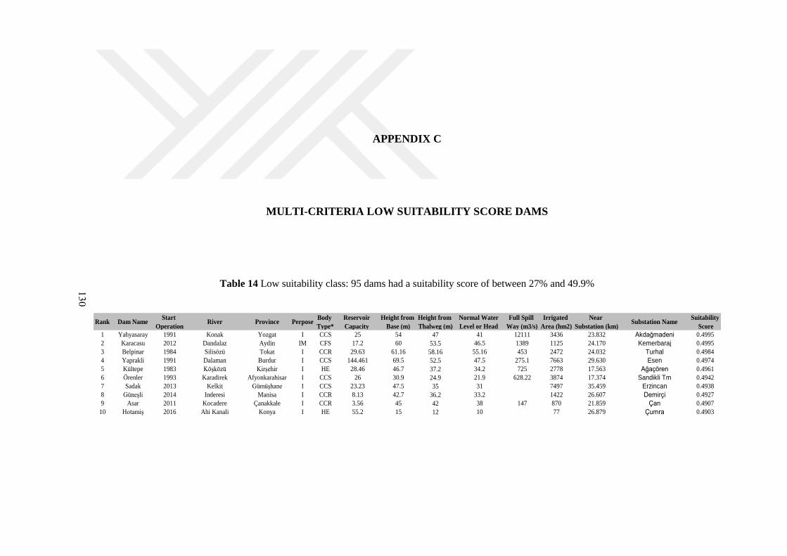
130

APPENDIX C

MULTI-CRITERIA LOW SUITABILITY SCORE DAMS

Table 14 Low suitability class: 95 dams had a suitability score of between 27% and 49.9%

Rank Dam NameStart


Body

Type*

Reservoir

Capacity

Height from

Base (m)

Height from

Thalweg (m)

Normal Water

Level or Head

Full Spill

Way (m3/s)

Irrigated

Area (hm2)

Near


Suitability

Score

1 Yahyasaray 1991 Konak Yozgat I CCS 25 54 47 41 12111 3436 23.832 Akdağmadeni 0.4995

2 Karacasu 2012 Dandalaz Aydin IM CFS 17.2 60 53.5 46.5 1389 1125 24.170 Kemerbaraj 0.4995

3 Belpinar 1984 Silisözü Tokat I CCR 29.63 61.16 58.16 55.16 453 2472 24.032 Turhal 0.4984

4 Yaprakli 1991 Dalaman Burdur I CCS 144.461 69.5 52.5 47.5 275.1 7663 29.630 Esen 0.4974

5 Kültepe 1983 Köşközü Kirşehir I HE 28.46 46.7 37.2 34.2 725 2778 17.563 Ağaçören 0.4961

6 Örenler 1993 Karadirek Afyonkarahisar I CCS 26 30.9 24.9 21.9 628.22 3874 17.374 Sandikli Tm 0.4942

7 Sadak 2013 Kelkit Gümüşhane I CCS 23.23 47.5 35 31 7497 35.459 Erzincan 0.4938

8 Güneşli 2014 Inderesi Manisa I CCR 8.13 42.7 36.2 33.2 1422 26.607 Demirçi 0.4927

9 Asar 2011 Kocadere Çanakkale I CCR 3.56 45 42 38 147 870 21.859 Çan 0.4907

10 Hotamiş 2016 Ahi Kanali Konya I HE 55.2 15 12 10 77 26.879 Çumra 0.4903

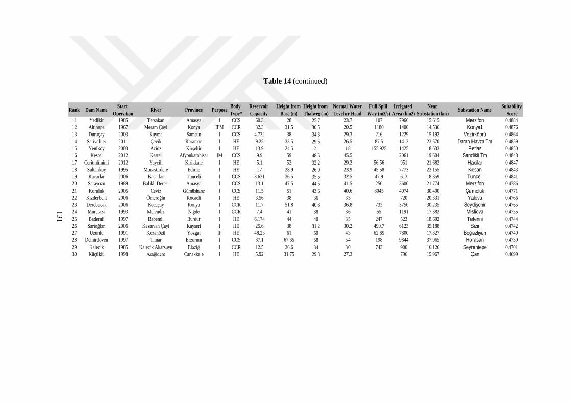
131


Rank Dam NameStart


Body

Type*

Reservoir

Capacity

Height from

Base (m)

Height from

Thalweg (m)

Normal Water

Level or Head

Full Spill

Way (m3/s)

Irrigated

Area (hm2)

Near


Suitability

Score

11 Yedikir 1985 Tersakan Amasya I CCS 60.3 28 25.7 23.7 107 7966 15.615 Merzifon 0.4884

12 Altinapa 1967 Meram Çayi Konya IFM CCR 32.3 31.5 30.5 20.5 1180 1400 14.536 Konya1 0.4876

13 Duruçay 2003 Kuyma Samsun I CCS 4.732 38 34.3 29.3 216 1229 15.192 Vezirköprü 0.4864

14 Sariveliler 2011 Çevik Karaman I HE 9.25 33.5 29.5 26.5 87.5 1412 23.570 Daran Havza Tm 0.4859

15 Yeniköy 2003 Aciöz Kirşehir I HE 13.9 24.5 21 18 155.925 1425 18.633 Petlas 0.4850

16 Kestel 2012 Kestel Afyonkarahisar IM CCS 9.9 59 48.5 45.5 2061 19.604 Sandikli Tm 0.4848

17 Ceritmüminli 2012 Yaycili Kirikkale I HE 5.1 52 32.2 29.2 56.56 951 21.682 Hacilar 0.4847

18 Sultanköy 1995 Manastirdere Edirne I HE 27 28.9 26.9 23.9 45.58 7773 22.155 Kesan 0.4843

19 Kacarlar 2006 Kacarlar Tunceli I CCS 3.631 36.5 35.5 32.5 47.9 613 18.359 Tunceli 0.4841

20 Sarayözü 1989 Balikli Deresi Amasya I CCS 13.1 47.5 44.5 41.5 250 3600 21.774 Merzifon 0.4786

21 Koruluk 2005 Ceviz Gümüşhane I CCS 11.5 51 43.6 40.6 8045 4074 30.400 Çamoluk 0.4771

22 Kizderbent 2006 Ömeroğlu Kocaeli I HE 3.56 38 36 33 720 20.331 Yalova 0.4766

23 Derebucak 2006 Kocaçay Konya I CCR 11.7 51.8 40.8 36.8 732 3750 30.235 Seydişehir 0.4765

24 Murataza 1993 Melendiz Niğde I CCR 7.4 41 38 36 55 1191 17.382 Misliova 0.4755

25 Bademli 1997 Babemli Burdur I HE 6.174 44 40 35 247 523 18.602 Tefenni 0.4744

26 Sarioğlan 2006 Kestuvan Çayi Kayseri I HE 25.6 38 31.2 30.2 490.7 6123 35.188 Sizir 0.4742

27 Uzunlu 1991 Kozanözü Yozgat IF HE 48.23 61 50 43 62.85 7800 17.827 Boğazliyan 0.4740

28 Demirdöven 1997 Timar Erzurum I CCS 37.1 67.35 58 54 198 9844 37.965 Horasan 0.4739

29 Kalecik 1985 Kalecik Akarsuyu Elaziğ I CCR 12.5 36.6 34 30 743 900 16.126 Seyrantepe 0.4701

30 Küçüklü 1998 Aşağidere Çanakkale I HE 5.92 31.75 29.3 27.3 796 15.967 Çan 0.4699

132


Rank Dam NameStart


Body

Type*

Reservoir

Capacity

Height from

Base (m)

Height from

Thalweg (m)

Normal Water

Level or Head

Full Spill

Way (m3/s)

Irrigated

Area (hm2)

Near


Suitability

Score

31 Palandöken 2005 Lezgi Erzurum IM CCS 157 49 44.45 39.45 392.67 12038 30.901 Erzurum3 0.4648

32 Ayitdere 2012 Çinardere Çanakkale I HE 6.78 20 15 13 500 1157 18.751 Biga 0.4646

33 Pazaryolu 2014 Değirmendere Erzurum I CCR 3.02 69.5 57.5 53.5 98.5 605 34.652 Kuzgun 0.4619

34 Asartepe 1980 Ilhan Çayi Ankara I HE 20 50 36.5 31.5 2850 22.224 Kazan 0.4612

35 Işiktepe 1999 Zugur Elaziğ I CCS 4.47 52.6 25.6 23.6 51 313 15.314 Maden 0.4597

36 Üçöz 2007 Üçöz Sivas I HE 13.74 28.4 23.4 19.4 85.6 989 27.863 Kangal 0.4593

37 Mamasin 1962 Uluirmax Aksaray I CCR 165.8 48.4 44.9 35.9 570 23640 17.262 Aksaray 0.4587

38 Dumluca 1992 Buğur Mardin I HE 22.5 29.5 24 20 356 1860 23.882 Ps_4_A Tm 0.4586

39 Medik 1975 Tohma Çayi Malatya I CCR 22 43 42 34 3850 15842 21.079 Malorsa 0.4583

40 Ağcaşar 1987 Yahyali Kayseri I CCS 61.7 27 24 22 16 15035 23.871 Yeşilhisar 0.4547

41 Osmankalfalar 2003 Sevindirik Antalya I CCS 8.19 30.7 25.7 22.7 266.11 842 22.874 Tefenni 0.4529

42 Tahtaköprü 1975 Karasu Deresi Hatay I CCS 200 46.5 35.5 33.5 2480 11900 27.462 Fevzipasa Tm 0.4516

43 Kizik 2003 Miçöz Tokat I CCR 7.108 45.7 26.25 22.25 248 1800 22.387 Adocim 0.4490

44 Bayrmiç 1997 Karamenderesi Çanakkale IM CCS 86.5 55.5 45.5 39.5 880 16694 27.741 Ezine 0.4481

45 Akşahan 2013 Kavakdere Konya I CFR 4.6 42 38 35 170 716 33.539 Konya1 0.4473

46 Kayapinar 2013 Özdere Kayseri I HE 3.795 41 32 28 100.95 637 29.451 Kayseri_Kap 0.4455

47 Gazibey 1992 Osugülüç Sivas IF CCR 16 58.3 45.5 40.5 358 2537 22.520 Sarkisla 0.4389

48 Çavdarhisar 1990 Bedir Kütahya IF CCS 38.8 50.5 45.5 41.5 555 5242 25.175 Gediz Tm 0.4369

49 Selevir 1964 Gali Afyonkarahisar I CCS 65 32 31.4 27.4 560 8310 16.769 Seka Tm 0.4361

50 Mumcular 1989 Kocadere Muğla IM CCS 19.4 34 32 30 598 1266 19.809 Yeniköy 0.4358

133


Rank Dam NameStart


Body

Type*

Reservoir

Capacity

Height from

Base (m)

Height from

Thalweg (m)

Normal Water

Level or Head

Full Spill

Way (m3/s)

Irrigated

Area (hm2)

Near


Suitability

Score

51 Küçükler 2005 Gavural Uşak IM CCS 10.92 41 36.3 32.3 1608 23.608 Gediz Tm 0.4348

52 Doyduk 2013 Kalaycik Nevşehir I HE 13.7 24 22 19 163 1452 37.272 Kalaba 0.4345

53 Ceffan 1995 Ceffan Batman I HE 6.845 30 26.56 23.56 192 400 21.184 Kurtalan 0.4344

54 Büyükorhan 1992 Cuma Dere Bursa I HE 6.93 36 23 21 535 707 18.032 Orhaneli 0.4337

55 Postalli 2004 Postalli Niğde I CCS 3.26 31.2 29.2 26.2 97.4 620 25.297 Bor 0.4318

56 Saribeyler 1985 Savaştepe Balikesir I CCS 15.6 37.5 35 30 304 2065 28.973 Balikesir1 0.4294

57 Apa 1962 Çarşamba Akarsuyu Konya I CCS 171.6 30.8 29.8 26.8 500 97015 19.761 Alibeyhüyüğü 0.4291

58 Kozçeşme 1998 Kocadere Çanakkale I HE 4.24 27.6 23.6 21.6 504 20.550 Biga 0.4287

59 Fehimli 1988 Fehimli Yozgat I HE 11 23 17.4 13.4 350 1000 17.058 Kalaba 0.4264

60 Serban 1994 Serban Afyonkarahisar I HE 3.35 28 26.5 23.5 199 922 20.101 Afyon I Tm 0.4204

61 Çağlayan 2013 Yayla Konya I CCS 3.85 33 31 27 75.5 713 35.774 Akseki 0.4163

62 Çayhan 1994 Çayhan Konya I HE 3.71 36 23.5 20.5 138.53 721 20.191 Eregli 0.4142

63 Seyitler 1964 Seydiler Afyonkarahisar I CCS 40.47 27 26 22 450 3222 18.291 Afyon Ii Tm (Salt) 0.4133

64 Bozarmut 2004 Devrent Sivas I HE 4.3 29 21 18 203 1010 25.984 Kangal 0.4132

65 Porsuk 1972 Porsuk Çayi Eskişehir IFM CG 454 64.7 49.7 45.7 792 24850 19.400 Karagözler (Tcddy) Tm 0.4124

66 Sürgü 1969 Sürgü Nehri Malatya I CCS 70.06 57 55 49 535 11968 34.302 Golbaşi 0.4107

67 Boztepe 1983 Boztepe Akarsuyu Tokat I HE 14.2 35.5 27.3 25.3 240 4872 27.926 Turhal 0.4105

68 Üçpinar 2007 Deliçay Kilis I HE 4.57 28 23 19 148 370 29.535 Kilis Tm 0.4100

69 Çiftliközü 2001 Karakaya Konya I HE 3.36 43 36.5 33.5 64 475 33.198 Ilgin 0.4085

70 Çataldağ 2008 Biçkidere Balikesir IM CCR 4.96 34.5 26 22 234 53 19.641 M.Kemal_Paşa 0.4076

134


Rank Dam NameStart


Body

Type*

Reservoir

Capacity

Height from

Base (m)

Height from

Thalweg (m)

Normal Water

Level or Head

Full Spill

Way (m3/s)

Irrigated

Area (hm2)

Near


Suitability

Score

71 Dutluca 1992 Sapoğlu Tokat I HE 5 37 27.5 23.5 32.55 662 23.969 Adocim 0.4059

72 Uluköy 1983 Derebey Deresi Amasya I HE 3.65 28 23 20 52.5 1190 16.007 Erbaa 0.4006

73 Mercan 1987 Sazliüvet Deresi Edirne I HE 3.52 23.3 19.8 15.8 77.61 61 16.039 Kesan 0.4004

74 Daridere 1977 Sarisu Bilecik IF CCS 19.21 33.4 27 21 220 3105 15.879 Bozüyük Tm 0.3975

75 Çatmapinar 1994 A.Dereboyu Eskişehir I HE 4.154 26.9 15.9 12.9 196.9 838 20.303 Çifteler Tm 0.3969

76 Kirkat 1985 Nehir Deresi Batman I HE 3.156 23.8 21 18 345 17.346 Midyat 0.3932

77 Yalvaç 1973 Sücüllü D. Isparta I HE 8.567 35.5 41.57 36.57 360 2062 25.786 Akşehir 0.3913

78 Çoğun 1975 Kizilözü Kirşehir IF CCR 21.77 46 29.5 23.5 790 3762 18.116 Kirşehir 0.3891

79 Balikli 1999 Deliçay Kilis I HE 3.94 30.2 25.7 22.7 113 348 31.013 Kilis Tm 0.3883

80 Süloğlu 1981 Süloğlu Deresi Edirne IFM CCR 50 53.41 50 43 960 4009 18.898 Ediçim 0.3876

81 Üçpinar 1992 Kurbağali Dere Uşak I CCS 5.3 26.5 25.5 22.5 447.4 205 28.040 Akenerji Osb. Dgçs 0.3875

82 Aydoğmuş 1988 Boğaz Konya I HE 4.7 27 21 19 88 450 23.591 Alibeyhüyüğü 0.3842

83 Çitli 1992 Gömük Amasya I HE 3.25 26 19.2 16.2 105 382 23.008 Merzifon 0.3841

84 Dokuzdere 1976 Dokuzdere Edirne I HE 4.02 30.2 24.2 21.2 208 510 16.525 Kesan 0.3840

85 Yalintaş 1994 Alaçoraközü Nevşehir I HE 10 23.5 14.5 11.5 148.9 1212 30.735 Nevşehir2 0.3753

86 Yildiz 1997 Kayaligöl Sivas I CCS 8.24 33 23.5 20.5 138 1723 36.372 Sivas_Osb 0.3739

87 Halilan 1981 Çoruk Diyarbakir I HE 7.452 26.8 21 18 409.22 670 24.441 Ergani 0.3714

88 Kuzayca 1997 Kuzayca Yozgat I HE 7.68 19.8 16.6 14.6 134 1008 35.230 Boğazliyan 0.3616

89 Gökçeada 1983 Büyükdere Çanakkale IM CCS 16.6 51 33 29 163 700 32.353 Kumlimani 0.3551

90 Deliilyas 1993 Ulusuluk Sivas I HE 3.6 26 25 22 155 398 34.222 Sarkisla 0.3550

135


Rank Dam NameStart


Body

Type*

Reservoir

Capacity

Height from

Base (m)

Height from

Thalweg (m)

Normal Water

Level or Head

Full Spill

Way (m3/s)

Irrigated

Area (hm2)

Near


Suitability

Score

91 Kayaboğazi 1988 Kocasu Kütahya IFM CCS 37.84 45 38 31 1780 6103 26.493 Tunçbilek Ts(Tutes) 0.3545

92 Kadiköy 1973 Doğanca Dervent D. Edirne IFM HE 56.5 37.8 34 30 46.3 4451 17.021 Kesan 0.3537

93 Altinyazi 1967 Basamaklar Deresi Edirne IF HE 36.764 27.1 23.5 20.5 170 7524 22.869 Kesan 0.3414

94 Takmak 1984 Değirmendere Uşak I HE 3.06 24.5 19.5 16.5 237 35.044 Akenerji Osb. Dgçs 0.3110

95 Ayranci 1958 Kocadere Çayi Karaman IF HE 30.9 36 34 31 500 5438 38.204 Karaman_Osb 0.2770

*CCS: Clay Core Sand-Gravel, CCR: Clay Core Rock, RCC: Roller Compacted Concrete, CFR: Concrete Faced Rock Fill, HE: Homogeneous Earth, CFS: Concrete Faced Sand-Gravel, CG: Concrete Grav

371

CURRICULUM VITAE

PERSONAL INFORMATION

Surname, Name: Omar Al BAYATI

Nationality: Iraqi (IQ)

Date and Place of Birth: 9 June 1975, Baghdad

Marital Status: Marred

Phone: +90 5312673966

Phone: +964 7702754583 (Whatsapp)

email: [email protected]

EDUCATION

Higher Diploma of Information

Technology (2012)

Multimedia Technique University of Information

Technology and

Communication

Bachelor of Science (2001) Statistics University of Baghdad

EXPERIENCE

Quality Management System

ISO9001:2008 (2015)

Training Course University of Information

Technology and

Communication

Computing Fundamentals, Key

Applications, Living Online

(2010)

IC3 Certification (Internet Core

Competency)

Certiport IC3

ArcGis Level 2 (2008) Training Course University of Baghdad/

Computer Center

Geographic Information System

(2007)

Training Course AL Quds School for Computers

WORK

Computer Researcher (2004–2016)

Department of Applications

Packages/ ICCI

Ministry of Higher Education

and Scientific Research/ Iraq

FOREIGN LANGUAGES

Good English, Fair Turkish, Very Good Arabic

finding the most suitable irrigation dams for hydropower ...

Documents

Transcript of finding the most suitable irrigation dams for hydropower ...